R News 2007/1 PDF Rnews 2007 1

PDF Rnews_2007-1 CRAN: R News

User Manual: PDF CRAN - Contents of R News

Open the PDF directly: View PDF .
Page Count: 58

Editorial
Viewing Binary Files with the hexView Package
FlexMix: An R Package for Finite Mixture Modelling
Using R to Perform the AMMI Analysis on Agriculture Variety Trials
- Results
Inferences for Ratios of Normal Means
Working with Unknown Values
A New Package for Fitting Random Effect Models
- The function =-1 allvc
- Summary
Augmenting R with Unix Tools
POT: Modelling Peaks Over a Threshold
Backtests
Review of John Verzani's Book Using R for Introductory Statistics
DSC 2007
New Journal: Annals of Applied Statistics
Forthcoming Events: useR! 2007
Changes in R 2.5.0
Changes on CRAN
- New contributed packages
- Other changes
R Foundation News
- Donations and new members
R News Referees 2006

News

The Newsletter of the R Project Volume 7/1, April 2007

Editorial

by Torsten Hothorn

Welcome to the ﬁrst issue of R News for 2007, which

follows the release of Rversion 2.5.0. This major revi-

sion, in addition to many other features, brings bet-

ter support of JAVA and Objective C to our desks.

Moreover, there is a new recommended package,

codetools, which includes functions that automagi-

cally check Rcode for possible problems.

Just before the release of R2.5.0 the ﬁfth devel-

oper conference on “Directions in Statistical Com-

puting” was held in Auckland, NZ, the birthplace of

R. Hadley Wickham reports on the highlights of this

meeting. The Ruser community is not only active in

conferences. Volume 7, like the preceding volumes

of R News since 2001, wouldn’t be what it is without

the outstanding support of our referees. The editorial

board would like to say “Thank you!” to all who con-

tributed criticism and encouragement during the last

year—the complete list of referees in 2006 is given at

the end of this issue.

The scientiﬁc part of Volume 7 starts with an

article by Paul Murrell, our former editor-in-chief,

on handling binary ﬁles with tools provided by the

hexView package. Andrew Robinson teaches how

Rusers can make use of standard Unix tools, for

example mail for auto-generating large amounts of

email (not spam!). Many of us are regularly con-

fronted with data lacking a unique deﬁnition of miss-

ing values–the gdata package can help in this situa-

tion, as Gregor Gorjanc explains.

Bettina Grün and Fritz Leisch give an introduc-

tion to the ﬂexmix package for ﬁnite mixture mod-

eling, analyzing a dataset on 21 different whiskey

brands. The analysis of ﬁeld agricultural experi-

ments by means of additive main effect multiplica-

tive interactions is discussed by Andrea Onofri and

Egidio Ciriciofolo. Tests and conﬁdence intervals for

ratios of means, such as ratios of regression coefﬁ-

cients, implemented in package mratio are described

by Gemechis Dilba and colleagues. The npmlreg

package for ﬁtting random effect models is intro-

duced by Jochen Einbeck and his co-workers. Math-

ieu Ribatet models peaks over a threshold by POT,

and ﬁnancial instruments like stocks or options are

(back-)tested by Kyle Campbell and colleagues.

Finally, I would like to remind everyone that the

next “useR!” conference is taking place in Ames,

Iowa, August 8–10. I hope to see you there!

Torsten Hothorn

Ludwig–Maximilians–Universität München

Germany

Torsten.Hothorn@R-project.org

Contents of this issue:

Editorial ...................... 1

Viewing Binary Files with the hexView Package 2

FlexMix: An R Package for Finite Mixture

Modelling .................... 8

Using R to Perform the AMMI Analysis on

Agriculture Variety Trials . . . . . . . . . . . 14

Inferences for Ratios of Normal Means . . . . . 20

Working with Unknown Values . . . . . . . . . 24

A New Package for Fitting Random Effect

Models...................... 26

Augmenting R with Unix Tools . . . . . . . . . 30

POT: Modelling Peaks Over a Threshold . . . . 34

Backtests ...................... 36

Review of John Verzani’s Book

Using R for Introductory Statistics . . . . . . 41

DSC2007...................... 42

New Journal: Annals of Applied Statistics . . . 43

Forthcoming Events: useR!2007......... 43

Changes in R 2.5.0 . . . . . . . . . . . . . . . . . 43

ChangesonCRAN ................ 51

R Foundation News . . . . . . . . . . . . . . . . 56

R News Referees 2006 . . . . . . . . . . . . . . . 56

Vol. 7/1, April 2007 2

Viewing Binary Files with the hexView

Package

by Paul Murrell

I really like plain text ﬁles.

I like them because I can see exactly what is in

them. I can even easily modify the ﬁle if I’m feeling

dangerous. This makes me feel like I understand the

ﬁle.

I am not so fond of binary ﬁles. I always have to

use speciﬁc software to access the contents and that

software only shows me an interpretation of the ba-

sic content of the ﬁle. The raw content is hidden from

me.

Sometimes I want to know more about a real bi-

nary ﬁle, for example when I need to read data in a

binary format that no existing R function will read.

When things go wrong, like when an R workspace

ﬁle becomes “corrupt”, I may have a strong need to

know more.

Hex editors are wonderful tools that provide a

view of the raw contents of a binary (or text) ﬁle,

whether just to aid in understanding the ﬁle or to in-

spect or recover a ﬁle. The hexView package is an

attempt to bring this sort of facility to R.

Viewing raw text ﬁles

The viewRaw() function reads and displays the raw

content of a ﬁle. The content is displayed in three

columns: the left column provides a byte offset

within the ﬁle, the middle column shows the raw

bytes, and the right column displays each byte as an

ASCII character. If the byte does not correspond to

a printable ASCII character then a full stop is dis-

played.

As a simple example, we will look at a plain text

ﬁle, "rawTest.txt", that contains a single line of

text. This ﬁle was created using the following code

(on a Linux system).

> writeLines("test pattern", "rawTest.txt")

A number of small example ﬁles are included as

part of the hexView package and the hexViewFile()

function is provided to make it convenient to refer

to these ﬁles. The readLines() function from the

base package reads in the lines of a plain text ﬁle as

a vector of strings, so the plain text content of the ﬁle

"rawTest.txt" can be retrieved as follows.

> readLines(hexViewFile("rawTest.txt"))

[1] "test pattern"

The following code uses the viewRaw() function

from hexView to display the raw contents of this ﬁle.

> viewRaw(hexViewFile("rawTest.txt"))

0 : 74 65 73 74 20 70 61 74 | test pat

8 : 74 65 72 6e 0a | tern.

As this example shows, by default, the raw bytes

are printed in hexadecimal format. The ﬁrst byte

in this ﬁle is 74, which is 7 ∗16 +4=116 in dec-

imal notation—the ASCII code for the character t.

This byte pattern can be seen several times in the ﬁle,

wherever there is a tcharacter.

The machine argument to the viewRaw() function

controls how the raw bytes are displayed. It defaults

to "hex" for hexadecimal output, but also accepts the

value "binary", which means that the raw bytes are

printed in binary format, as shown below.

> viewRaw(hexViewFile("rawTest.txt"),

machine="binary")

0 : 01110100 01100101 01110011 | tes

3 : 01110100 00100000 01110000 | t p

6 : 01100001 01110100 01110100 | att

9 : 01100101 01110010 01101110 | ern

12 : 00001010 | .

One noteworthy feature of this simple ﬁle is the

last byte, which has the hexadecimal value 0a (or

00001010 in binary; the decimal value 10) and no

printable ASCII interpretation. This is the ASCII

code for the newline or line feed (LF) special char-

acter that indicates the end of a line in text ﬁles. This

is a simple demonstration that even plain text ﬁles

have details that are hidden from the user by stan-

dard viewing software; viewers will show text on

separate lines, but do not usually show the “charac-

ter” representing the start of a new line.

The next example provides a more dramatic

demonstration of hidden details in text ﬁles. The ﬁle

we will look at contains the same text as the previous

example, but was created on a Windows XP system

with Notepad using “Save As...” and selecting “Uni-

code” as the “Encoding”. The readLines() function

just needs the ﬁle to be opened with the appropriate

encoding, then it produces the same result as before.

> readLines(

file(hexViewFile("rawTest.unicode"),

encoding="UCS-2LE"))

[1] "test pattern"

However, the raw content of the ﬁle is now very dif-

ferent.

> viewRaw(hexViewFile("rawTest.unicode"))

R News ISSN 1609-3631

Vol. 7/1, April 2007 3

0 : ff fe 74 00 65 00 73 00 | ..t.e.s.

8 : 74 00 20 00 70 00 61 00 | t. .p.a.

16 : 74 00 74 00 65 00 72 00 | t.t.e.r.

24 : 6e 00 0d 00 0a 00 | n.....

It is fairly straightforward to identify some parts of

this ﬁle. The ASCII codes from the previous example

are there again, but there is an extra 00 byte after each

one. This reﬂects the fact that, on Windows, Unicode

text is stored using two bytes per character1.

Instead of the 13 bytes in the original ﬁle, we

might expect 26 bytes in this ﬁle, but there are actu-

ally 30 bytes. Where did the extra bytes come from?

The ﬁrst two bytes at the start of the ﬁle are a

byte order mark (BOM). With two bytes to store for

each character, there are two possible orderings of

the bytes; for example, the two bytes for the charac-

ter tcould be stored as 74 00 (called little endian) or

as 00 74 (big endian). The BOM tells software which

order has been used. Another difference occurs at the

end of the ﬁle. The newline character is there again

(with an extra 00), but just before it there is a 0d char-

acter (with an extra 00). This is the carriage return

(CR) character. On Windows, a new line in a text ﬁle

is signalled by the combination CR+LF, but on UNIX

a new line is just indicated by a single LF.

As this example makes clear, software sometimes

does a lot of work behind the scenes in order to dis-

play even “plain text”.

Viewing raw binary ﬁles

An example of a binary ﬁle is the native binary for-

mat used by R to store information via the save()

function. The following code was used to create the

ﬁle "rawTest.bin".

> save(rnorm(50), file="rawTest.bin")

We can view this ﬁle with the following code; the

nbytes argument is used to show the raw data for

only the ﬁrst 80 bytes.

> viewRaw(hexViewFile("rawTest.bin"),

nbytes=80)

0 : 1f 8b 08 00 00 00 00 00 | ........

8 : 00 03 01 c0 01 3f fe 52 | .....?.R

16 : 44 58 32 0a 58 0a 00 00 | DX2.X...

24 : 00 02 00 02 05 00 00 02 | ........

32 : 03 00 00 00 04 02 00 00 | ........

40 : 00 01 00 00 10 09 00 00 | ........

48 : 00 01 7a 00 00 00 0e 00 | ..z.....

56 : 00 00 32 3f e7 60 e6 49 | ..2?. .I

64 : c6 fe 0d 3f e1 3b c5 2f | ...?.;./

72 : bb 4e 18 bf c4 9e 0f 1a | .N......

This is a good example of a binary ﬁle that is in-

triguing to view, but there is little hope of retriev-

ing any useful information because the data has been

compressed (encoded). In other cases, things are a

not so hopeless, and it is not only possible to view the

raw bytes, but also to see useful patterns and struc-

tures.

The next example looks at a binary ﬁle with a

much simpler structure. The ﬁle "rawTest.int" only

contains (uncompressed) integer values and was cre-

ated by the following code.

> writeBin(1:50, "rawTest.int", size=4)

This ﬁle only contains the integers from 1 to 50,

with four bytes used for each integer. The raw con-

tents are shown below; this time the nbytes argu-

ment has been used to show only the raw data for

the ﬁrst 10 integers (the ﬁrst 40 bytes).

> viewRaw(hexViewFile("rawTest.int"),

nbytes=40)

0 : 01 00 00 00 02 00 00 00 | ........

8 : 03 00 00 00 04 00 00 00 | ........

16 : 05 00 00 00 06 00 00 00 | ........

24 : 07 00 00 00 08 00 00 00 | ........

32 : 09 00 00 00 0a 00 00 00 | ........

None of the bytes correspond to printable ASCII

characters in this case, so the right column of out-

put is not terribly interesting. The viewRaw() func-

tion has two arguments, human and size, which con-

trol the way that the raw bytes are interpreted and

displayed. In this case, rather than interpreting each

byte as an ASCII character, it makes sense to interpret

each block of four bytes as an integer. This is done in

the following code using human="int" and size=4.

> viewRaw(hexViewFile("rawTest.int"),

nbytes=40, human="int", size=4)

0 : 01 00 00 00 02 00 00 00 | 1 2

8 : 03 00 00 00 04 00 00 00 | 3 4

16 : 05 00 00 00 06 00 00 00 | 5 6

24 : 07 00 00 00 08 00 00 00 | 7 8

32 : 09 00 00 00 0a 00 00 00 | 9 10

With this simple binary format, we can see how

the individual integers are being stored. The integer

1is stored as the four bytes 01 00 00 00, the integer

2as 02 00 00 00, and so on. This clearly demon-

strates the idea of little endian byte order; the least-

signiﬁcant byte, the value 1, is stored ﬁrst. In big en-

dian byte order, the integer 1would be 00 00 00 01

(as we shall see later).

The other option for interpreting bytes is "real"

which means that each block of size bytes is inter-

preted as a ﬂoating-point value. A simple example

1Over-simpliﬁcation alert! Windows used to use the UCS-2 encoding, which has two bytes per character, but now it uses UTF-16, which

has two or four bytes per character. There are only two bytes per character in this case because these are common english characters.

R News ISSN 1609-3631

Vol. 7/1, April 2007 4

is provided by the ﬁle "rawTest.real", which was

generated by the following code. I have deliberately

used big endian byte order because it will make it

easier to see the structure in the resulting bytes.

> writeBin(1:50/50, "rawTest.real", size=8,

endian="big")

Here is an example of reading this ﬁle and inter-

preting each block of 8 bytes as a ﬂoating-point num-

ber. This also demonstrates the use of the width ar-

gument to explicitly control how many bytes are dis-

played per line of output.

> viewRaw(hexViewFile("rawTest.real"),

nbytes=40, human="real", width=8,

endian="big")

0 : 3f 94 7a e1 47 ae 14 7b | 0.02

8 : 3f a4 7a e1 47 ae 14 7b | 0.04

16 : 3f ae b8 51 eb 85 1e b8 | 0.06

24 : 3f b4 7a e1 47 ae 14 7b | 0.08

32 : 3f b9 99 99 99 99 99 9a | 0.10

Again, we are able to see how individual ﬂoating-

point values are stored. The following code takes this

a little further and allows us to inspect the bit repre-

sentation of the ﬂoating point numbers. The output

is shown in Figure 1.

> viewRaw(hexViewFile("rawTest.real"),

nbytes=40, human="real",

machine="binary", width=8,

endian="big")

The bit representation adheres to the IEEE Stan-

dard for Binary Floating-Point Arithmetic (IEEE,

1985;Wikipedia, 2006). Each value is stored in the

form sign ×mantissa ×2exponent. The ﬁrst (left-most)

bit indicates the sign of the number, the next 11 bits

describe the exponent and the remaining 52 bits de-

scribe the mantissa. The mantissa is a binary frac-

tion, with bit icorresponding to 2−i.

For the ﬁrst value in "rawTest.real", the ﬁrst bit

has value 0indicating a positive number, the expo-

nent bits are 0111111 1001 = 1017, from which we

subtract 1023 to get −6, and the mantissa is an im-

plicit 1 plus 0 ×2−1+1×2−2+0×2−3+0×2−4+

0×2−5+1×2−6... =1.28.2So we have the value

1.28 ×2−6=0.02.

Viewing a Binary File in Blocks

As the examples so far have hopefully demonstrated,

being able to see the raw contents of a ﬁle can be a

very good way to teach concepts such as endianness,

character encodings, and ﬂoating-point representa-

tions of real numbers. Plus, it is just good fun to poke

around in a ﬁle and see what is going on.

In this section, we will look at some more ad-

vanced functions from the hexView package, which

will allow us to take a more detailed look at more

complex binary formats and will allow us to perform

some more practical tasks.

We will start by looking again at R’s native bi-

nary format. The ﬁle "rawTest.XDRint" contains

the integers 1 to 50 saved as a binary R object

and was produced using the following code. The

compress=FALSE is important to allow us to see the

structure of the ﬁle.

> save(1:50, file="rawTest.XDRint",

compress=FALSE)

We can view (the ﬁrst 80 bytes of) the raw ﬁle us-

ing viewRaw() as before and this does show us some

interesting features. For example, we can see the text

RDX2 at the start of the ﬁle (it is common for ﬁles to

have identifying markers at the start of the ﬁle). If

we look a little harder, we can also see the ﬁrst few

integers (1 to 9); the data is stored in an XDR format

(Wikipedia,2006a), which uses big endian byte or-

der, so the integers are in consecutive blocks of four

bytes that look like this: 00 00 00 01, then 00 00 00

02, and so on.

> viewRaw(hexViewFile("rawTest.XDRint"),

width=8, nbytes=80)

0 : 52 44 58 32 0a 58 0a 00 | RDX2.X..

8 : 00 00 02 00 02 04 00 00 | ........

16 : 02 03 00 00 00 04 02 00 | ........

24 : 00 00 01 00 00 10 09 00 | ........

32 : 00 00 01 78 00 00 00 0d | ...x....

40 : 00 00 00 32 00 00 00 01 | ...2....

48 : 00 00 00 02 00 00 00 03 | ........

56 : 00 00 00 04 00 00 00 05 | ........

64 : 00 00 00 06 00 00 00 07 | ........

72 : 00 00 00 08 00 00 00 09 | ........

It is clear that there is some text in the ﬁle and that

there are some integers in the ﬁle, so neither viewing

the whole ﬁle as characters nor viewing the whole

ﬁle as integers is satisfactory. What we need to be

able to do is view the text sections as characters and

the integer sections as integers. This is what the func-

tions memFormat(),memBlock(), and friends are for.

The memBlock() function creates a description of

a block of memory, specifying how many bytes are

in the block; the block is interpreted as ASCII char-

acters. The atomicBlock() function creates a de-

scription of a memory block that contains a single

value of a speciﬁed type (e.g., a four-byte integer),

and the vectorBlock() function creates a descrip-

tion of a memory block consisting of 1 or more mem-

ory blocks.

A number of standard memory blocks are prede-

ﬁned: integer4 (a four-byte integer) and integer1,

2At least, as close as it is possible to get to 1.28 with a ﬁnite number of bits. Another useful thing about viewing raw values is that it

makes explicit the fact that most decimal values do not have an exact ﬂoating-point representation.

R News ISSN 1609-3631

Vol. 7/1, April 2007 5

0 : 00111111 10010100 01111010 11100001 01000111 10101110 00010100 01111011 | 0.02

8 : 00111111 10100100 01111010 11100001 01000111 10101110 00010100 01111011 | 0.04

16 : 00111111 10101110 10111000 01010001 11101011 10000101 00011110 10111000 | 0.06

24 : 00111111 10110100 01111010 11100001 01000111 10101110 00010100 01111011 | 0.08

32 : 00111111 10111001 10011001 10011001 10011001 10011001 10011001 10011010 | 0.10

Figure 1: The ﬂoating point representation of the numbers 0.02 to 0.10 following IEEE 754 in big endian byte

order.

integer2, and integer8;real8 (an eight-byte

ﬂoating-point number, or double) and real4; and

ASCIIchar (a single-byte character). There is also

a special ASCIIline memory block for a series of

single-byte characters terminated by a newline.

The memFormat() function collects a num-

ber of memory block descriptions together and

viewFormat() reads the memory blocks and displays

them.

As an example, the following code reads in the

"RDX2" header line of the ﬁle "rawTest.XDRint",

treats the next 39 bytes as just raw binary, ignoring

any structure, then reads the ﬁrst nine integers (as in-

tegers). A new memory block description is needed

for the integers because the XDR format is big endian

(the predeﬁned integer4 is little endian). The names

of the memory blocks within the format are used to

separate the blocks of output.

> XDRint <- atomicBlock("int", endian="big")

> viewFormat(hexViewFile("rawTest.XDRint"),

memFormat(saveFormat=ASCIIline,

rawBlock=memBlock(39),

integers=vectorBlock(XDRint,

9)))

========saveFormat

0 : 52 44 58 32 0a | RDX2.

========rawBlock

5 : 58 0a 00 00 00 02 00 | X......

12 : 02 04 00 00 02 03 00 | .......

19 : 00 00 04 02 00 00 00 | .......

26 : 01 00 00 10 09 00 00 | .......

33 : 00 01 78 00 00 00 0d | ..x....

40 : 00 00 00 32 | ...2

========integers

44 : 00 00 00 01 00 00 00 02 | 1 2

52 : 00 00 00 03 00 00 00 04 | 3 4

60 : 00 00 00 05 00 00 00 06 | 5 6

68 : 00 00 00 07 00 00 00 08 | 7 8

76 : 00 00 00 09 | 9

The raw 39 bytes can be further broken down—

see the description of R’s native binary format on

pages 11 and 12 of the “R Internals” manual (R De-

velopment Core Team,2006) that is distributed with

R—but that is beyond the scope of this article.

Extracting Blocks from a Binary

File

As well as viewing different blocks of a binary

ﬁle, we may want to extract the values from each

block. For this purpose, the readFormat() function

is provided to read a binary format, as produced

by memFormat(), and generate a "rawFormat" object

(but not explicitly print it3). A "rawFormat" object is

a list with a component "blocks" that is itself a list

of "rawBlock" objects, one for each memory block

deﬁned in the memory format. A "rawBlock" object

contains the raw bytes read from a ﬁle.

The blockValue() function extracts the inter-

preted value from a "rawBlock" object. The

blockString() function is provided speciﬁcally

for extracting a null-terminated string from a

"rawBlock" object.

The following code reads in the ﬁle

"rawTest.XDRint" and just extracts the 50 integer

values.

> XDRfile <-

readFormat(hexViewFile("rawTest.XDRint"),

memFormat(saveFormat=ASCIIline,

rawBlock=memBlock(39),

integers=vectorBlock(XDRint,

50)))

> blockValue(XDRfile$blocks$integers)

[1] 1 2 3 4 5 6 7 8 9 10 11 12 13

[14] 14 15 16 17 18 19 20 21 22 23 24 25 26

[27] 27 28 29 30 31 32 33 34 35 36 37 38 39

[40] 40 41 42 43 44 45 46 47 48 49 50

A Caution

On a typical 32-bit platform, R uses 4 bytes for rep-

resenting integer values in memory and 8 bytes for

ﬂoating-point values. This means that there may be

limits on what sort of values can be interpreted cor-

rectly by hexView.

For example, if a ﬁle contains 8-byte integers, it is

possible to view each set of 8 bytes as an integer, but

on my system R can only represent an integer using

4 bytes, so 4 of the bytes are (silently) dropped. The

following code demonstrates this effect by reading

3There is a readRaw() function too.

R News ISSN 1609-3631

Vol. 7/1, April 2007 6

the ﬁle "testRaw.int" and interpreting its contents

as 8-byte integers.

> viewRaw(hexViewFile("rawTest.int"),

nbytes=40, human="int", size=8)

0 : 01 00 00 00 02 00 00 00 | 1

8 : 03 00 00 00 04 00 00 00 | 3

16 : 05 00 00 00 06 00 00 00 | 5

24 : 07 00 00 00 08 00 00 00 | 7

32 : 09 00 00 00 0a 00 00 00 | 9

An extended example:

Reading EViews Files

On November 18 2006, Dietrich Trenkler sent a mes-

sage to the R-help mailing list asking for a func-

tion to read ﬁles in the native binary format used

by Eviews, an econometrics software package (http:

//www.eviews.com/). No such function exists, but

John C Frain helpfully pointed out that an unofﬁ-

cial description of the basic structure of Eviews ﬁles

had been made available by Allin Cottrell (creator of

gretl, the Gnu Regression, Econometrics and Time-

series Library). The details of Allin Cottrell’s reverse-

engineering efforts are available on the web (http:

//www.ecn.wfu.edu/~cottrell/eviews_format/).

In this section, we will use the hexView package

to explore an Eviews ﬁle and produce a new function

for reading ﬁles in this format. The example data ﬁle

we will use is from Ramu Ramanathan’s Introduc-

tory Econometrics text (Ramanathan,2002). The data

consists of four variables measured on single family

homes in University City, San Diego, in 1990:

price: sale price in thousands of dollars.

sqft: square feet of living area.

bedrms: number of bedrooms.

baths: number of bath rooms.

The data are included in both plain text for-

mat, as "data4-1.txt", and Eviews format, as

"data4-1.wf1", as part of the hexViews package.4

For later comparison, the data from the plain text for-

mat are shown below, having been read in with the

read.table() function.

> read.table(hexViewFile("data4-1.txt"),

col.names=c("price", "sqft",

"bedrms", "baths"))

price sqft bedrms baths

1 199.9 1065 3 1.75

2 228.0 1254 3 2.00

3 235.0 1300 3 2.00

4 285.0 1577 4 2.50

5 239.0 1600 3 2.00

6 293.0 1750 4 2.00

7 285.0 1800 4 2.75

8 365.0 1870 4 2.00

9 295.0 1935 4 2.50

10 290.0 1948 4 2.00

11 385.0 2254 4 3.00

12 505.0 2600 3 2.50

13 425.0 2800 4 3.00

14 415.0 3000 4 3.00

An Eviews ﬁle begins with a header, starting with

the text “New MicroTSP Workﬁle” and including im-

portant information about the size of the header and

the number of variables and the number of observa-

tions in the ﬁle. The following code deﬁnes an ap-

propriate "memFormat" object for this header infor-

mation.

> EViewsHeader <-

memFormat(firstline=memBlock(80),

headersize=integer8,

unknown=memBlock(26),

numvblesplusone=integer4,

date=vectorBlock(ASCIIchar, 4),

unkown=memBlock(2),

datafreq=integer2,

startperiod=integer2,

startobs=integer4,

unkown=memBlock(8),

numobs=integer4)

We can use readFormat() to read this header from

the ﬁle as follows. The number of variables reported

is one greater than the actual number of variables

and also includes two “boiler plate” variables that

are always included in Eviews ﬁles (hence 7 instead

of the expected 4).

> data4.1.header <-

readFormat(hexViewFile("data4-1.wf1"),

EViewsHeader)

> data4.1.header

=========firstline

0 : 4e 65 77 20 4d 69 | New Mi

6 : 63 72 6f 54 53 50 | croTSP

12 : 20 57 6f 72 6b 66 | Workf

18 : 69 6c 65 00 00 00 | ile...

24 : d8 5e 0e 01 00 00 | .^....

30 : 00 00 00 00 08 00 | ......

36 : 15 00 00 00 00 00 | ......

42 : ff ff ff ff 21 00 | ....!.

48 : 00 00 00 00 00 00 | ......

54 : 00 00 06 00 00 00 | ......

60 : 0f 00 00 00 06 00 | ......

66 : 00 00 01 00 01 00 | ......

72 : 66 03 00 00 00 00 | f.....

78 : 00 00 | ..

=========headersize

80 : 90 00 00 00 00 00 00 00 | 144

=========unknown

88 : 01 00 00 00 01 00 | ......

4The original source of the ﬁles was: http://ricardo.ecn.wfu.edu/pub/gretl_cdrom/data/

R News ISSN 1609-3631

Vol. 7/1, April 2007 7

94 : 00 00 01 00 00 00 | ......

100 : 00 00 00 00 00 00 | ......

106 : 00 00 00 00 00 00 | ......

112 : 00 00 | ..

=========numvblesplusone

114 : 07 00 00 00 | 7

=========date

118 : d5 b7 0d 3a | ...:

=========unkown

122 : 06 00 | ..

=========datafreq

124 : 01 00 | 1

=========startperiod

126 : 00 00 | 0

=========startobs

128 : 01 00 00 00 | 1

=========unkown

132 : 00 5d 67 0e 01 59 | .]g..Y

138 : 8b 41 | .A

=========numobs

140 : 0e 00 00 00 | 14

We can extract some pieces of information from

this header and use them to look at later parts of the

ﬁle.

> headerSize <-

blockValue(

data4.1.header$blocks$headersize)

> numObs <-

blockValue(

data4.1.header$blocks$numobs)

At a location 26 bytes beyond the header size,

there are several blocks describing each variable in

the Eviews ﬁle. Each of these blocks is 70 bytes long

and contains information on the variable name and

the location within the ﬁle where the data values re-

side for that variable. The following code creates a

description of a block containing variable informa-

tion, then uses readFormat() to read the information

for the ﬁrst variable (the number of bath rooms); the

offset argument is used to start reading the block

at the appropriate location within the ﬁle. We also

extract the location of the data for this variable.

> EViewsVbleInfo <-

memFormat(unknown=memBlock(6),

recsize=integer4,

memsize=integer4,

ptrtodata=integer8,

vblename=vectorBlock(ASCIIchar,

32),

ptrtohistory=integer8,

vbletype=integer2,

unknown=memBlock(6))

> data4.1.vinfo <-

readFormat(hexViewFile("data4-1.wf1"),

EViewsVbleInfo,

offset=headerSize + 26)

> data4.1.vinfo

=========unknown

170 : 00 00 00 00 0b 00 | ......

=========recsize

176 : 86 00 00 00 | 134

=========memsize

180 : 70 00 00 00 | 112

=========ptrtodata

184 : f6 03 00 00 00 00 00 00 | 1014

=========vblename

192 : 42 41 54 48 53 00 00 00 00 00 | BATHS.....

202 : 00 00 00 00 00 00 00 00 00 00 | ..........

212 : 00 00 00 00 00 00 00 00 00 00 | ..........

222 : 00 00 | ..

=========ptrtohistory

224 : 00 00 00 00 d5 b7 0d 3a | 0

=========vbletype

232 : 2c 00 | 44

=========unknown

234 : 60 02 10 00 01 00 | .....

> firstVbleLoc <-

blockValue(data4.1.vinfo$blocks$ptrtodata)

The data for each variable is stored in a block

containing some preliminary information followed

by the data values stored as eight-byte ﬂoating-point

numbers. The code below creates a description of a

block of variable data and then reads the data block

for the ﬁrst variable.

> EViewsVbleData <- function(numObs) {

memFormat(numobs=integer4,

startobs=integer4,

unknown=memBlock(8),

endobs=integer4,

unknown=memBlock(2),

values=vectorBlock(real8,

numObs))

}

> viewFormat(hexViewFile("data4-1.wf1"),

EViewsVbleData(numObs),

offset=firstVbleLoc)

=========numobs

1014 : 0e 00 00 00 | 14

=========startobs

1018 : 01 00 00 00 | 1

=========unknown

1022 : 00 00 00 00 00 00 | ......

1028 : 00 00 | ..

=========endobs

1030 : 0e 00 00 00 | 14

=========unknown

1034 : 00 00 | ..

=========values

1036 : 00 00 00 00 00 00 fc 3f | 1.75

1044 : 00 00 00 00 00 00 00 40 | 2.00

1052 : 00 00 00 00 00 00 00 40 | 2.00

1060 : 00 00 00 00 00 00 04 40 | 2.50

1068 : 00 00 00 00 00 00 00 40 | 2.00

1076 : 00 00 00 00 00 00 00 40 | 2.00

1084 : 00 00 00 00 00 00 06 40 | 2.75

1092 : 00 00 00 00 00 00 00 40 | 2.00

1100 : 00 00 00 00 00 00 04 40 | 2.50

1108 : 00 00 00 00 00 00 00 40 | 2.00

1116 : 00 00 00 00 00 00 08 40 | 3.00

1124 : 00 00 00 00 00 00 04 40 | 2.50

1132 : 00 00 00 00 00 00 08 40 | 3.00

1140 : 00 00 00 00 00 00 08 40 | 3.00

This manual process of exploring the ﬁle struc-

ture can easily be automated within a function. The

hexView package includes such a function under the

R News ISSN 1609-3631

Vol. 7/1, April 2007 8

name readEViews(). With this function, we can read

in the data set from the Eviews ﬁle as follows.

> readEViews(hexViewFile("data4-1.wf1"))

Skipping boilerplate variable

BATHS BEDRMS PRICE SQFT

1 1.75 3 199.9 1065

2 2.00 3 228.0 1254

3 2.00 3 235.0 1300

4 2.50 4 285.0 1577

5 2.00 3 239.0 1600

6 2.00 4 293.0 1750

7 2.75 4 285.0 1800

8 2.00 4 365.0 1870

9 2.50 4 295.0 1935

10 2.00 4 290.0 1948

11 3.00 4 385.0 2254

12 2.50 3 505.0 2600

13 3.00 4 425.0 2800

14 3.00 4 415.0 3000

This solution is not the most efﬁcient way to read

Eviews ﬁles, but the hexView package does make it

easy to gradually build up a solution, it makes it easy

to view the results, and it does provide a way to solve

the problem without having to resort to C code.

Summary

The hexView package provides functions for view-

ing the raw byte contents of ﬁles. This is useful for

exploring a ﬁle structure and for demonstrating how

information is stored on a computer. More advanced

functions make it possible to read quite complex bi-

nary formats using only R code.

Acknowledgements

At the heart of the hexView package is the

readBin() function and the core facilities for work-

ing with "raw" binary objects in R code (e.g.,

rawToChar()); thanks to the R-core member(s) who

were responsible for developing those features.

I would also like to thank the anonymous re-

viewer for useful comments on early drafts of this

article.

Bibliography

IEEE Standard 754 for Binary Floating-Point Arithmetic.

IEEE computer society, 1985. 4

R Development Core Team. R Internals. R Foun-

dation for Statistical Computing, Vienna, Austria,

2006. URL http://www.R-project.org. ISBN 3-

900051-14-3. 5

R. Ramanathan. INTRODUCTORY ECONOMET-

RICS WITH APPLICATIONS. Harcourt College, 5

edition, 2002. ISBN 0-03-034342-9. 6

Wikipedia. External data representation —

wikipedia, the free encyclopedia, 2006a. URL

http://en.wikipedia.org/w/index.php?

title=External_Data_Representation&oldid=

91734878. [Online; accessed 3-December-2006]. 4

Wikipedia. IEEE ﬂoating-point standard —

wikipedia, the free encyclopedia, 2006b. URL

http://en.wikipedia.org/w/index.php?

title=IEEE_floating-point_standard&oldid=

89734307. [Online; accessed 3-December-2006]. 4

Paul Murrell

Department of Statistics

The University of Auckland

New Zealand

paul@stat.auckland.ac.nz

FlexMix: An R Package for Finite Mixture

Modelling

by Bettina Grün and Friedrich Leisch

Introduction

Finite mixture models are a popular method for

modelling unobserved heterogeneity or for approx-

imating general distribution functions. They are ap-

plied in a lot of different areas such as astronomy, bi-

ology, medicine or marketing. An overview on these

models with many examples for applications is given

in the recent monographs McLachlan and Peel (2000)

and Frühwirth-Schnatter (2006).

Due to this popularity there exist many (stand-

alone) software packages for ﬁnite mixture mod-

elling (see McLachlan and Peel,2000;Wedel and Ka-

makura,2001). Furthermore, there are several dif-

ferent R packages for ﬁtting ﬁnite mixture models

available on CRAN. Packages which use the EM algo-

R News ISSN 1609-3631

Vol. 7/1, April 2007 9

rithm for model estimation are ﬂexmix,fpc,mclust,

mixreg,mixtools, and mmlcr. Packages with other

model estimation methods are bayesmix,depmix,

moc,vabayelMix and wle. A short description

of these packages can be found in the CRAN task

view on clustering (http://cran.at.r-project.

org/src/contrib/Views/Cluster.html).

Finite mixture models

A ﬁnite mixture model is given by a convex combina-

tion of Kdifferent components, i.e. the weights of the

components are non-negative and sum to one. For

each component it is assumed that it follows a para-

metric distribution or is given by a more complex

model, such as a generalized linear model (GLM).

In the following we consider ﬁnite mixture den-

sities h(·|·)with Kcomponents, dependent variables

yand (optional) independent variables x:

h(y|x,w,Θ) =

∑

k=1

πk(w,α)f(y|x,ϑk)

where ∀w,α:

πk(w,α)≥0∀k∧

∑

k=1

πk(w,α) = 1

and

ϑk6=ϑl∀k6=l.

We assume that the component distributions f(·|·)

are from the same distributional family with compo-

nent speciﬁc parameters ϑk. The component weights

or prior class probabilities πkoptionally depend on

the concomitant variables wand the parameters α

and are modelled through multinomial logit models

as suggested for example in Dayton and Macready

(1988). A similar model class is also described in

McLachlan and Peel (2000, p. 145). The model can

be estimated using the EM algorithm (see Dempster

et al.,1977;McLachlan and Peel,2000) for ML estima-

tion or using MCMC methods for Bayesian analysis

(see for example Frühwirth-Schnatter,2006).

A possible extension of this model class is to

either have mixtures with components where the

parameters of one component are ﬁxed a-priori

(e.g. zero-inﬂated models; Grün and Leisch,2007b)

or to even allow different component speciﬁc mod-

els (e.g. for modelling noise in the data; Dasgupta

and Raftery,1998).

Design principles of FlexMix

The main reason for the implementation of the pack-

age was to allow easy extensibility and to have the

possibility for rapid prototyping in order to be able

to try out new mixture models. The package was im-

plemented using S4 classes and methods.

The EM algorithm provides a common basis for

estimation of a general class of ﬁnite mixture mod-

els and the package ﬂexmix tries to enable the user

to exploit this commonness. ﬂexmix provides the E-

step and takes care of all data handling while the user

is supposed to supply the M-step via model drivers

for the component-speciﬁc model and the concomi-

tant variable model. For the M-step available func-

tions for weighted maximum likelihood estimation

can be used as for example glm() for ﬁtting GLMs or

multinom() in MASS for multinomial logit models.

Currently model drivers are available for

model-based clustering of multivariate Gaus-

sian distributions with diagonal or unrestricted

variance-covariance matrices (FLXMCmvnorm()) and

multivariate Bernoulli and Poisson distributions

(FLXMCmvbinary() and FLXMCmvpois()) where the

dimensions are mutually independent. ﬂexmix does

not provide functionality for estimating mixtures

of Gaussian distributions with special variance-

covariance structures, as this functionality has al-

ready been implemented in the R package mclust

(Fraley and Raftery,2006).

For mixtures of regressions the Gaussian, bino-

mial, Poisson and gamma distribution can be speci-

ﬁed (FLXMRglm()). If some parameters are restricted

to be equal over the components the model driver

FLXMRglmfix() can be used. Zero-inﬂated Poisson

and binomial regression models can be ﬁtted us-

ing FLXMRziglm(). For an example of zero-inﬂated

models see example("FLXMRziglm"). For the con-

comitant variable models either constant component

weights (default) can be used or multinomial logit

models (FLXPmultinom()) can be ﬁtted.

Estimation problems can occur if the components

become too small during the EM algorithm. In or-

der to avoid these problems a minimum size can be

speciﬁed for each component. This is especially im-

portant for ﬁnite mixtures of multivariate Gaussian

distributions where full variance-covariance matri-

ces are estimated for each component.

Further details on the implementation and the de-

sign principles as well as exemplary applications of

the package can be found in the accompanying vi-

gnettes "flexmix-intro" which is an updated ver-

sion of Leisch (2004) and "regression-examples"

and in Grün and Leisch (2007a). Note that this article

uses the new version 2.0 of the package, where the

names of some driver functions have changed com-

pared with older versions of ﬂexmix.

Exemplary applications

In the following we present two examples for using

the package. The ﬁrst example demonstrates model-

based clustering, i.e., mixtures without independent

variables, and the second example gives an applica-

tion for ﬁtting mixtures of generalized linear regres-

R News ISSN 1609-3631

Vol. 7/1, April 2007 10

sion models.

Model-based clustering

The following dataset is taken from Edwards and Al-

lenby (2003) who refer to the Simmons Study of Me-

dia and Markets. It contains all households which

used any whiskey brand during the last year and

provides a binary incidence matrix on their brand

use for 21 whiskey brands during this year. This

means only the information on the different brands

used in a household is available.

We ﬁrst load the package and the dataset. The

whiskey dataset contains observations from 2218

households. The relative frequency of usage for each

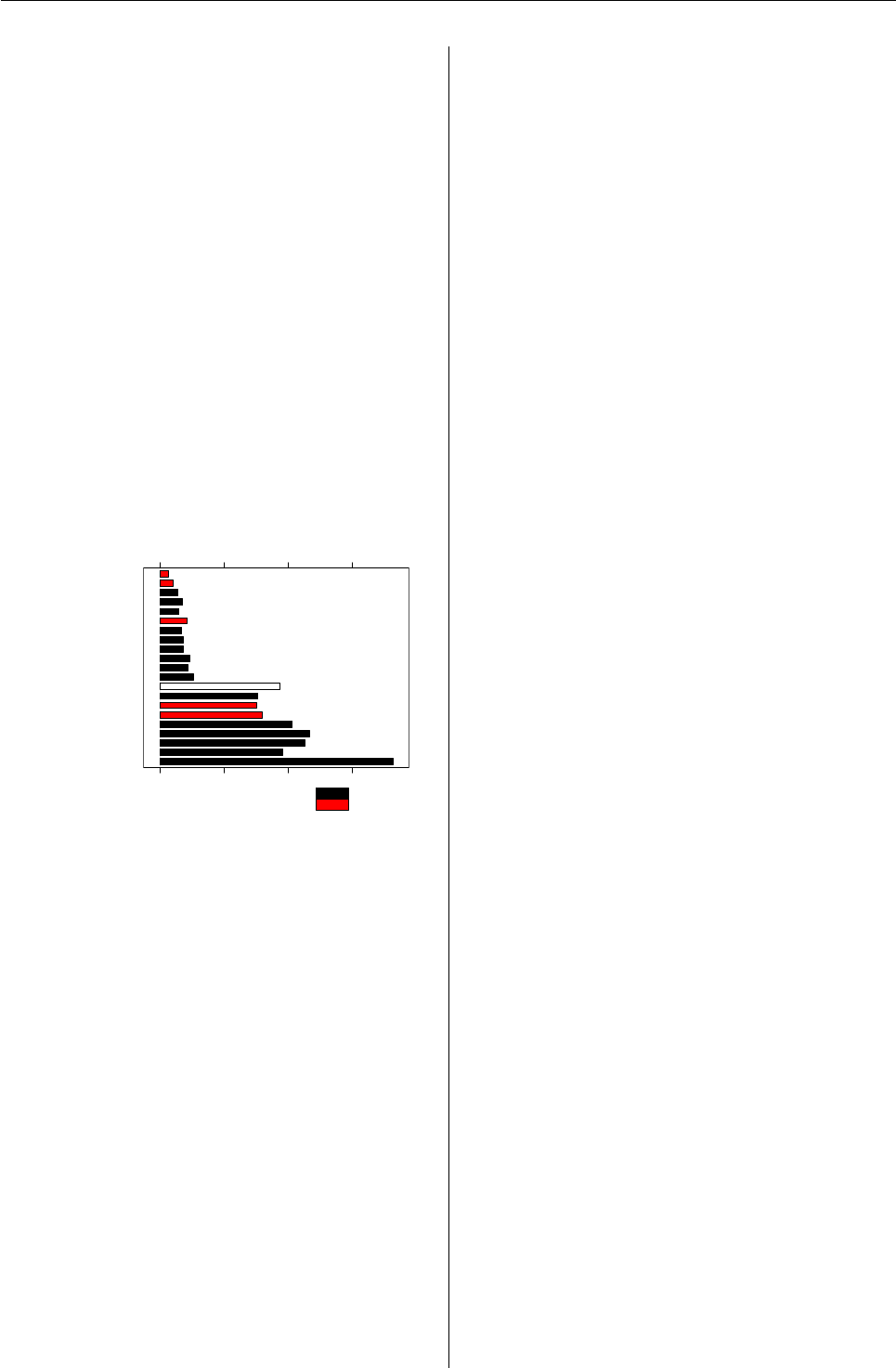
brand is given in Figure 1. Additional information

is available for the brands indicating the type of

whiskey: blend or single malt.

R> library("flexmix")

R> data("whiskey")

R> set.seed(1802)

Probability

Chivas Regal

Johnnie Walker Red Label

Johnnie Walker Black Label

Dewar's White Label

J&B

Glenlivet

Glenfiddich

Cutty Sark

Other brands

Pinch (Haig)

Ballantine

Clan MacGregor

Black & White

Passport

Grant's

Macallan

Ushers

Scoresby Rare

White Horse

Knockando

Singleton

0.0 0.1 0.2 0.3 Blend

Single Malt

Figure 1: Relative frequency of the whiskey brands.

We ﬁt a mixture of binomial distributions to the

dataset where the variables in each component spe-

ciﬁc models are assumed to be independent. The

EM algorithm is repeated nrep = 3 times using ran-

dom initialization, i.e. each observation is assigned

to one component with an a-posteriori probability of

0.9 and 0.1 otherwise and the component is selected

with equal probability.

R> wh_mix <- stepFlexmix(Incidence ~ 1,

+ weights = ~ Freq, data = whiskey,

+ model = FLXMCmvbinary(truncated = TRUE),

+ control = list(minprior = 0.005),

+ k = 1:7, nrep = 3)

Model-based clustering uses no explanatory vari-

ables, hence the right hand side of the formula

Incidence ~ 1 is constant. The model driver

is FLXMCmvbinary() with argument truncated =

TRUE, as the number of non-users is not available and

a truncated likelihood is maximized in each M-step

again using the EM-algorithm. We vary the number

of components for k = 1:7. The best solution with

respect to the log-likelihood for each of the differ-

ent numbers of components is returned in an object

of class "stepFlexmix". The control argument can

be used to control the ﬁtting with the EM algorithm.

With minprior the minimum relative size of the com-

ponents is speciﬁed, components falling below this

threshold are removed during the EM algorithm.

The dataset contains only the unique binary pat-

terns observed with the corresponding frequency.

We use these frequencies for the weights argument

instead of transforming the dataset to have one row

for each observation. The use of a weights argument

allows to use only the number of unique observa-

tions for ﬁtting, which can substantially reduce the

size of the model matrix and hence speed up the es-

timation process. For this dataset this means that the

model matrix has 484 instead of 2218 rows.

Model selection can be made using information

criteria, as for example the BIC (see Fraley and

Raftery,1998). For this example the BIC suggests a

mixture with 5 components:

R> BIC(wh_mix)

1234

27705.1 26327.6 25987.7 25683.2

567

25647.0 25670.3 25718.6

R> wh_best <- getModel(wh_mix, "BIC")

R> wh_best

Call:

stepFlexmix(Incidence ~ 1,

weights = ~Freq, data = whiskey,

model = FLXMCmvbinary(truncated = TRUE),

control = list(minprior = 0.005),

k = 5, nrep = 3)

Cluster sizes:

12345

283 791 953 25 166

convergence after 180 iterations

The estimated parameters can be inspected using

accessor functions such as prior() or parameters().

R> prior(wh_best)

[1] 0.1421343 0.3303822

[3] 0.4311072 0.0112559

[5] 0.0851203

R> parameters(wh_best, component=4:5)[1:2,]

Comp.4

center.Singleton 0.643431

center.Knockando 0.601124

Comp.5

center.Singleton 2.75013e-02

center.Knockando 1.13519e-32

R News ISSN 1609-3631

Vol. 7/1, April 2007 11

Probability

Chivas Regal

Johnnie Walker Red Label

Johnnie Walker Black Label

Dewar's White Label

J&B

Glenlivet

Glenfiddich

Cutty Sark

Other brands

Pinch (Haig)

Ballantine

Clan MacGregor

Black & White

Passport

Grant's

Macallan

Ushers

Scoresby Rare

White Horse

Knockando

Singleton

0.0 0.2 0.4 0.6 0.8 1.0

Comp. 1

0.0 0.2 0.4 0.6 0.8 1.0

Comp. 2

0.0 0.2 0.4 0.6 0.8 1.0

Comp. 3

0.0 0.2 0.4 0.6 0.8 1.0

Comp. 4

0.0 0.2 0.4 0.6 0.8 1.0

Comp. 5

Blend

Single Malt

Figure 2: Estimated probability of usage for the whiskey brands for each component.

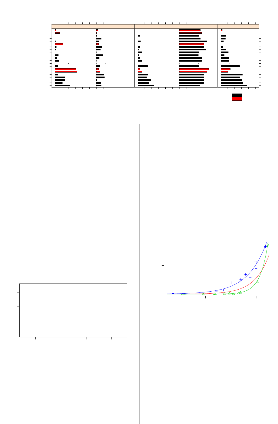
The ﬁtted parameters of the mixture for each

component are given in Figure 2. It can be seen

that component 4 (1.1% of the households) contains

the households which bought the greatest number

of different brands and all brands to a similar ex-

tent. Households from component 5 (8.5%) also buy

a wide range of whiskey brands, but tend to avoid

single malts. Component 3 (43.1%) has a similar us-

age pattern as component 5 but buys less brands in

general. Component 1 (14.2%) seems to favour sin-

gle malt whiskeys and component 2 (33%) is espe-

cially fond of other brands and tends to avoid John-

nie Walker Black Label.

Mixtures of regressions

The patent data given in Wang et al. (1998) includes

70 observations on patent applications, R&D spend-

ing and sales in millions of dollar from pharmaceuti-

cal and biomedical companies in 1976 taken from the

National Bureau of Economic Research R&D Master-

ﬁle. The data is given in Figure 3.

●

●●●

●

●●

●

●●

●

●●

● ●

●●

●

●●

●

● ●

●

●●● ●

●

● ●

●

● ● ●

●

●●

●

−2 0 2 4

0 50 100 150

lgRD

Patents

Figure 3: Patent dataset.

The model which is chosen as the best in Wang

et al. (1998) is a ﬁnite mixture of three Poisson regres-

sion models with Patents as dependent variable, the

logarithmized R&D spending lgRD as independent

variable and the R&D spending per sales RDS as con-

comitant variable. This model can be ﬁtted in R with

the component-speciﬁc model driver FLXMRglm()

which allows ﬁtting of ﬁnite mixtures of GLMs. As

concomitant variable model driver FLXPmultinom()

is used for a multinomial logit model where the pos-

terior probabilities are the dependent variables.

R> data("patent")

R> pat_mix <- flexmix(Patents ~ lgRD,

+ k = 3, data = patent,

+ model = FLXMRglm(family = "poisson"),

+ concomitant = FLXPmultinom(~RDS))

The observed values together with the ﬁtted val-

ues for each component are given in Figure 4. The

coloring and characters used for plotting the ob-

servations are according to the component assign-

ment using the maximum a-posteriori probabili-

ties, which are obtained using cluster(pat_mix).

●● ●

●

●●

●

●●

● ●

●

●●

●

● ●

●

●●

●

−2 0 2 4

0 50 100 150

lgRD

Patents

Figure 4: Patent data with ﬁtted values for each com-

ponent.

In Figure 5a rootogram of the posterior proba-

bilities of the observations is given. This is the de-

fault plot of the "flexmix" objects returned by the

ﬁtting function. It can be used for arbitrary mix-

ture models and indicates how well the observations

are clustered by the mixture. For ease of interpre-

tation the observations with a-posteriori probability

less than eps=10−4are omitted as otherwise the peak

at zero would dominate the plot. The observations

where the a-posteriori probability is largest for the

third component are colored differently. The plot is

generated using the following command.

R News ISSN 1609-3631

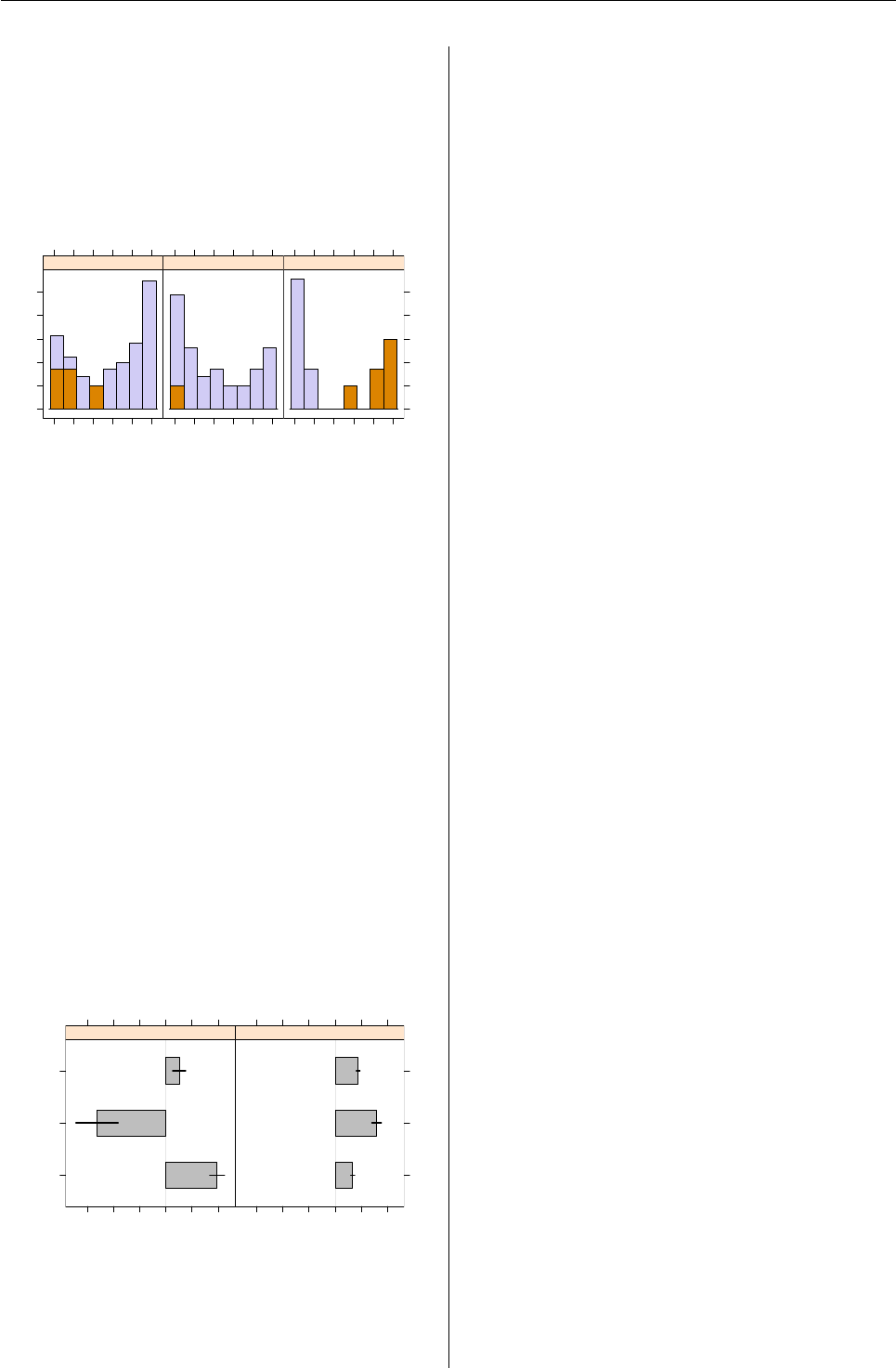
Vol. 7/1, April 2007 12

R> plot(pat_mix, mark = 3)

The posteriors of all three components have modes

at 0 and 1, indicating well-separated clusters (Leisch,

2004). Note that the object returned by the plot func-

tion is of class "trellis", and that the plot itself

is produced by the corresponding show() method

(Sarkar,2002).

Rootogram of posterior probabilities > 1e−04

0.0 0.2 0.4 0.6 0.8 1.0

Comp. 1

0.0 0.2 0.4 0.6 0.8 1.0

Comp. 2

0.0 0.2 0.4 0.6 0.8 1.0

Comp. 3

Figure 5: Rootogram of the posterior probabilities.

Further details of the ﬁtted mixture can be ob-

tained with refit() which returns the ﬁtted values

together with approximate standard deviations and

signiﬁcance tests, see Figure 6. The standard devi-

ations are only approximative because they are de-

termined separately for each component and it is not

taken into account that the components have been

estimated simultaneously. In the future functionality

to determine the standard deviations using either the

full Hesse matrix or the parametric bootstrap shall be

provided.

The estimated coefﬁcients are given in Figure 7.

The black lines indicate the (approximative) 95%

conﬁdence intervals. This is the default plot for the

objects returned by refit() and is obtained with the

following command.

R> plot(refit(pat_mix), bycluster = FALSE)

The argument bycluster indicates if the clus-

ters/components or the different variables are

used as conditioning variables for the panels.

Comp. 3

Comp. 2

Comp. 1

−3 −2 −1 0 1 2

(Intercept)

−3 −2 −1 0 1 2

lgRD

Figure 7: Estimated coefﬁcients of the component

speciﬁc models with corresponding 95% conﬁdence

intervals.

The plot indicates that the estimated coefﬁcients

vary between all components even though the co-

efﬁcients for lgRD are similar for the ﬁrst and third

component. A smaller model where these coefﬁ-

cients are restricted to be equal can be ﬁtted using

the model driver FLXMRglmfix(). The EM algorithm

can be initialized in the original solution using the

estimated posterior probabilities for the cluster ar-

gument. As in this case the ﬁrst and third component

are restricted to have the same coefﬁcient for lgRD,

the posteriors of the ﬁtted mixture are used for ini-

tialization after reordering the components to have

these two components next to each other. The mod-

iﬁed model is compared to the original model using

the BIC.

R> Model_2 <- FLXMRglmfix(family = "poisson",

+ nested = list(k = c(1,2),

+ formula = ~lgRD))

R> Post_1 <- posterior(pat_mix)[,c(2,1,3)]

R> pat_mix2 <- flexmix(Patents ~ 1,

+ concomitant = FLXPmultinom(~RDS),

+ data = patent, cluster = Post_1,

+ model = Model_2)

R> c(M_1 = BIC(pat_mix), M_2 = BIC(pat_mix2))

M_1 M_2

437.836 445.243

In this example, the original model is preferred

by the BIC.

Summary

ﬂexmix provides infrastructure for ﬁtting ﬁnite mix-

ture models with the EM algorithm and tools for

model selection and model diagnostics. We have

shown the application of the package for model-

based clustering as well as for ﬁtting ﬁnite mixtures

of regressions.

In the future we want to implement new model

drivers, e.g., for generalized additive models with

smooth terms, as well as to extend the tools for

model selection, diagnostics and model validation.

Additional functionality will be added which allows

to ﬁt mixture models with different component spe-

ciﬁc models. The implementation of zero-inﬂated

models has been a ﬁrst step in this direction.

Acknowledgments

This research was supported by the Austrian Science

Foundation (FWF) under grant P17382.

Bibliography

A. Dasgupta and A. E. Raftery. Detecting features

in spatial point processes with clutter via model-

based clustering. Journal of the American Statistical

Association, 93(441):294–302, March 1998. 9

R News ISSN 1609-3631

Vol. 7/1, April 2007 13

R> refit(pat_mix)

Call:

refit(pat_mix)

Number of components: 3

$Comp.1

Estimate Std. Error z value Pr(>|z|)

(Intercept) 0.50819 0.12366 4.11 3.96e-05 ***

lgRD 0.87976 0.03328 26.43 < 2e-16 ***

---

Signif. codes: 0 *** 0.001 ** 0.01 * 0.05 . 0.1 1

$Comp.2

Estimate Std. Error z value Pr(>|z|)

(Intercept) -2.6368 0.4043 -6.522 6.95e-11 ***

lgRD 1.5866 0.0899 17.648 < 2e-16 ***

---

Signif. codes: 0 *** 0.001 ** 0.01 * 0.05 . 0.1 1

$Comp.3

Estimate Std. Error z value Pr(>|z|)

(Intercept) 1.96217 0.13968 14.05 <2e-16 ***

lgRD 0.67190 0.03572 18.81 <2e-16 ***

---

Signif. codes: 0 *** 0.001 ** 0.01 * 0.05 . 0.1 1

Figure 6: Details of the ﬁtted mixture model for the patent data.

C. M. Dayton and G. B. Macready. Concomitant-

variable latent-class models. Journal of the American

Statistical Association, 83(401):173–178, March 1988.

A. P. Dempster, N. M. Laird, and D. B. Rubin. Maxi-

mum likelihood from incomplete data via the EM-

algorithm. Journal of the Royal Statistical Society B,

39:1–38, 1977. 9

Y. D. Edwards and G. M. Allenby. Multivariate anal-

ysis of multiple response data. Journal of Marketing

Research, 40:321–334, August 2003. 10

C. Fraley and A. E. Raftery. How many clusters?

which clustering method? answers via model-

based cluster analysis. The Computer Journal, 41(8):

578–588, 1998. 10

C. Fraley and A. E. Raftery. MCLUST version 3 for R:

Normal mixture modeling and model-based clus-

tering. Technical Report 504, University of Wash-

ington, Department of Statistics, September 2006.

S. Frühwirth-Schnatter. Finite Mixture and Markov

Switching Models. Springer Series in Statistics.

Springer, New York, 2006. ISBN 0-387-32909-9. 8,

B. Grün and F. Leisch. Fitting ﬁnite mixtures of

generalized linear regressions in R.Computational

Statistics & Data Analysis, 2007a. Accepted for pub-

lication. 9

B. Grün and F. Leisch. Flexmix 2.0: Finite mixtures

with concomitant variables and varying and ﬁxed

effects. Submitted for publication, 2007b. 9

F. Leisch. FlexMix: A general framework for ﬁ-

nite mixture models and latent class regression in

R. Journal of Statistical Software, 11(8), 2004. URL

http://www.jstatsoft.org/v11/i08/.9,12

G. J. McLachlan and D. Peel. Finite Mixture Models.

Wiley, 2000. 8,9

D. Sarkar. Lattice. R News, 2(2):19–23, June 2002. URL

http://CRAN.R-project.org/doc/Rnews/.12

P. Wang, I. M. Cockburn, and M. L. Puterman. Anal-

ysis of patent data — A mixed-Poisson-regression-

model approach. Journal of Business & Economic

Statistics, 16(1):27–41, 1998. 11

M. Wedel and W. A. Kamakura. Market Segmen-

tation — Conceptual and Methodological Founda-

tions. Kluwer Academic Publishers, second edi-

tion, 2001. ISBN 0-7923-8635-3. 8

Bettina Grün

Technische Universität Wien, Austria

Bettina.Gruen@ci.tuwien.ac.at

Friedrich Leisch

Ludwig-Maximilians-Universität München, Germany

Friedrich.Leisch@R-project.org

R News ISSN 1609-3631

Vol. 7/1, April 2007 14

Using R to Perform the AMMI Analysis

on Agriculture Variety Trials

by Andrea Onofri & Egidio Ciriciofolo

Introduction

Field agricultural experiments are generally planned

to evaluate the actual effect produced by man-

made chemical substances or human activities on

crop yield and quality, environmental health, farm-

ers’ income and so on. Field experiments include

the testing of new and traditional varieties (geno-

types), fertilizers (types and doses), pesticides (types

and doses) and cultural practices. With respect to

greenhouse or laboratory experiments, ﬁeld trials

are much more strongly subjected to environmental

variability that forces researchers into repeating ex-

periments across seasons and/or locations. A sig-

niﬁcant ’treatment x environment’ interaction may

introduce some difﬁculties in exploring the dataset,

summarizing results and determining which treat-

ment (genotype, herbicide, pesticide...) was the best.

In such conditions, the AMMI (Additive Main ef-

fect Multiplicative Interaction) analysis has been pro-

posed as an aid to visualize the dataset and explore

graphically its pattern and structure (Gollob,1968;

Zobel et al.,1988); this technique has received a par-

ticular attention from plant breeders (see for example

Abamu and Alluri,1998;Annichiarico et al.,1995;

Annichiarico,1997;Ariyo,1998) and recently it has

been stated as superior to other similar techniques,

such as the GGE (Gauch,2006). Unfortunately, such

technique is not yet very well exploited by agri-

cultural scientists, who often prefer a more tradi-

tional approach to data analysis, based on ANOVA

and multiple comparison testing. Without disre-

garding the importance of such an approach, one

cannot deny that sometimes this does not help un-

veil the underlying structure of experimental data,

which may be more important than hypothesis test-

ing, especially at the beginning of data analyses (Ex-

ploratory Data Analysis; NIST/SEMATECH,2004)

or at the very end, when graphs have to be drawn

for publication purposes.

To make more widespread the acceptance and the

use of such powerful tool within agronomists, it is

necessary to increase the availability of both practi-

cal information on how to perform and interpret an

AMMI analysis and simple software tools that give

an easily understandable output, aimed at people

with no speciﬁc and deep statistical training, such as

students and ﬁeld technicians.

The aim of this paper was to show how R can be

easily used to perform an AMMI analysis and pro-

duce ’biplots’, as well as to show how these tools can

be very useful within variety trials in agriculture.

Some basic statistical aspects

The AMMI analysis combines the ANalysis OF VAri-

ance (ANOVA) and the Singular Value Decomposi-

tion (SVD) and it has been explained in detail by Gol-

lob (1968). If we speciﬁcally refer to a variety trial,

aimed at comparing the yield of several genotypes

in several environments (years and/or locations), the

ANOVA partitions the total sum of squares into two

main effects (genotypes and environments) plus the

interaction effect (genotypes x environments). This

latter effect may be obtained by taking the observed

averages for each ’genotype x environment’ combi-

nation and doubly-centering them (i.e., subtracting

to each data the appropriate genotype and environ-

ment means and adding back the grand mean). The

interaction effect is arranged on a two-way matrix γ

(one row for each genotype and one column for each

environment) and submitted to SVD, as follows:

γ=

∑

i=1

λi·gik ·ei j (1)

where ris the rank of γ,λiis the singular value

for principal component i,gik is the eigenvector score

for genotype kand Principal Component (PC) i(left

singular vector), while ei j is the eigenvector score for

environment jand PC i(right singular vector). If PC

scores are multiplied by the square root of the singu-

lar value, equation 1is transformed into:

γ=

∑

i=1λ0.5

i·gik λ0.5

i·ei j=

∑

i=1

Gik ·Ei j (2)

In this way the additive interaction in the

ANOVA model is obtained by multiplication of

genotype PC scores by environment PC scores, ap-

propriately scaled. If a reduced number of PCs is

used (r= 1 or 2, typically) a dimensionality reduction

is achieved with just a small loss in the descriptive

ability of the model. This makes it possible to plot

the interaction effect, via the PC scores for genotypes

and environments. Such graphs are called biplots, as

they contain two kinds of data; typically, a AMMI1

and a AMMI2 biplots are used: the AMMI1 biplot

has main effects (average yields for genotypes and

environments) on the x-axis and PC1 scores on the y-

axis, while the AMMI2 biplot has PC1 scores on the

x-axis and PC2 scores on the y-axis.

R News ISSN 1609-3631

Vol. 7/1, April 2007 15

Table 1: Field averages (three replicates) for six genotypes compared in seven years.

Genotype 1996 1997 1998 1999 2000 2001 2002 Average

COLOSSEO 6.35 6.46 6.70 6.98 6.44 7.07 4.90 6.41

CRESO 5.60 6.09 6.13 7.13 6.08 6.45 4.33 5.97

DUILIO 5.64 8.06 7.15 7.99 5.18 7.88 4.24 6.59

GRAZIA 6.26 6.74 6.35 6.84 4.75 7.30 4.34 6.08

IRIDE 6.04 7.72 6.39 7.99 6.05 7.71 4.96 6.70

SANCARLO 5.70 6.77 6.81 7.41 5.66 6.67 4.50 6.22

SIMETO 5.08 7.19 6.44 7.07 4.82 7.55 3.34 5.93

SOLEX 6.14 6.39 6.44 6.87 5.45 7.52 4.79 6.23

Average 5.85 6.93 6.55 7.29 5.55 7.27 4.42 6.27

The dataset

To show how the AMMI analysis can be easily per-

formed with R, we will use a dataset obtained from

a seven-years ﬁeld trial on durum wheat, carried out

from 1996 to 2003 in central Italy, on a randomised

block design with three replicates. For the present

analysis, eight genotypes were chosen, as they were

constantly present throughout the years (Colosseo,

Creso, Duilio, Grazia, Iride, Sancarlo, Simeto, Solex).

Yield data referred to the standard humidity content

of 13% (Tab. 1) have been previously published in

Belocchi et al. (2003), Ciriciofolo et al. (2002); Ciri-

ciofolo et al. (2001); Desiderio et al. (2000), Desiderio

et al. (1999), Desiderio et al. (1998), Desiderio et al.

(1997). The interaction matrix (which is submitted to

SVD) is given in table 2.

The AMMI with R

To perform the AMMI analysis, an R function was

deﬁned, as shown on page 17.

The AMMI() function requires as inputs a vector

of genotype codes (factor), a vector of environment

codes (factor), a vector of block codes (factor) and a

vector of yields (numerical). PC is the number of PCs

to be considered (set to 2 by default) and biplot is the

type of biplot to be drown (1 for AMM1 and 2 for

AMMI2). It should be noted that the script is very el-

ementary and that it does not use any difﬁcult func-

tion or programming construct. It was simply coded

by translating the algebraic procedure proposed by

Gollob (1968) into R statements, which is a very easy

task, even without a speciﬁc programming training.

Wherever possible, built-in R functions were used, to

simplify the coding process and to facilitate the adap-

tation of the script to other kinds of AMMI models.

The ﬁrst part uses the function tapply() to cal-

culate some descriptive statistics, such as genotype

means, environment means and ’genotype x envi-

ronment’ means, which are all included in the ﬁnal

output.

The second part uses the function aov() to per-

form the ANOVA by using a randomised block de-

sign repeated in different environments with a dif-

ferent randomisation in each environment (LeClerg

et al.,1962). The interaction matrix γis calculated

by using the function model.tables() applied to the

output of the function aov(); the way the R script

is coded, the interaction matrix is actually the trans-

pose of the matrix shown in table 2, but this does not

change much in terms of the results. The interaction

matrix is then submitted to SVD, by using the built-

in R function svd().

The signiﬁcant PCs are assessed by a series of F

tests as shown by Zobel et al. (1988) and PC scores,

genotype means and environment means are used to

produce biplots, by way of the functions plot() and

points().

Table 2: Interaction effects for the dataset in table 1.

Genotype 1996 1997 1998 1999 2000 2001 2002

COLOSSEO 0.35 -0.62 0.00 -0.45 0.74 -0.34 0.33

CRESO 0.04 -0.54 -0.13 0.14 0.82 -0.52 0.20

DUILIO -0.54 0.80 0.28 0.38 -0.70 0.29 -0.51

GRAZIA 0.60 -0.01 -0.02 -0.27 -0.62 0.21 0.10

IRIDE -0.24 0.37 -0.59 0.28 0.07 0.01 0.11

SANCARLO -0.10 -0.11 0.31 0.17 0.16 -0.55 0.12

SIMETO -0.43 0.60 0.23 0.13 -0.40 0.62 -0.75

SOLEX 0.33 -0.50 -0.07 -0.38 -0.07 0.29 0.40

R News ISSN 1609-3631

Vol. 7/1, April 2007 16

$Additive_ANOVA

Df Sum Sq Mean Sq F value Pr(>F)

Environments 6 159.279 26.547 178.3996 < 2.2e-16 ***

Genotypes 7 11.544 1.649 11.0824 2.978e-10 ***

Blocks(Environments) 14 3.922 0.280 1.8826 0.03738 *

Environments x Genotypes 42 27.713 0.660 4.4342 6.779e-10 ***

Residuals 98 14.583 0.149

---

Signif. codes: 0 *** 0.001 ** 0.01 * 0.05 . 0.1 1

$Mult_Interaction

Effect SS DF MS F Prob.

1 PC1 18.398624 12 1.5332187 10.303612 7.958058e-13

2 PC2 5.475627 10 0.5475627 3.679758 3.339881e-04

3 PC3 1.961049 8 0.2451311 1.647342 1.212529e-01

4 Residuals 1.877427 12 0.1564522 1.051398 4.094193e-01

$Environment_scores

PC1 PC2 PC3

1996 0.4685599 -0.62599974 0.01665148

1997 -0.8859669 0.21085535 -0.19553672

1998 -0.1572887 -0.00567589 0.80162642

1999 -0.3139136 0.51881710 -0.13286326

2000 0.8229290 0.59868592 -0.03330554

2001 -0.5456613 -0.49726356 -0.18138908

2002 0.6113417 -0.19941917 -0.27518331

$Genotype_scores

PC1 PC2 PC3

COLOSSEO 0.74335025 -0.02451524 0.1651197989

CRESO 0.63115567 0.47768803 -0.0001969871

DUILIO -0.87632103 0.17923645 0.1445152042

GRAZIA -0.07625519 -0.74659598 -0.0108977060

IRIDE -0.12683903 0.28634343 -0.7627600696

SANCARLO 0.18186612 0.35076556 0.3753706117

SIMETO -0.78109997 0.04751457 0.1740113396

SOLEX 0.30414317 -0.57043681 -0.0851621918

Figure 1: Results from ANOVA and AMMI analyses.

Results

Results (Fig. 1) show a highly signiﬁcant ’genotypes

x environments’ interaction (GE) on the ANOVA,

that does not permit to deﬁne an overall ranking of

varieties across environments.

The SVD decomposition of the interaction matrix

was performed by extracting three PCs, though only

the ﬁrst two are signiﬁcant. It is possible to observe

that the ﬁrst PC accounts for 66% of the interaction

sum of squares, while the second one accounts for an

additional 20%.

The AMMI1 biplot shows contemporarily main

effects (genotypes and environments average yields)

and interaction, as PC1 scores (Fig. 2). This graph is

relevant as it accounts for 87% of total data variabil-

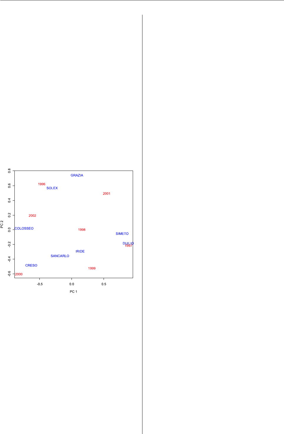
ity. Figure 2: AMMI1 biplot.

R News ISSN 1609-3631

Vol. 7/1, April 2007 17

AMMI <- function(variety, envir, block, yield, PC = 2, biplot = 1) {

## 1 - Descriptive statistics

overall.mean <- mean(yield)

envir.mean <- tapply(yield, envir, mean)

var.mean <- tapply(yield, variety, mean)

int.mean <- tapply(yield, list(variety,envir), mean)

envir.num <- length(envir.mean)

var.num <- length(var.mean)

## 2 - ANOVA (additive model)

variety <- factor(variety)

envir <- factor(envir)

block <- factor(block)

add.anova <- aov(yield ~ envir + block %in% envir + variety + envir:variety)

modelTables <- model.tables(add.anova, type = "effects", cterms = "envir:variety")

int.eff <- modelTables$tables$"envir:variety"

add.anova.residual.SS <- deviance(add.anova)

add.anova.residual.DF <- add.anova$df.residual

add.anova.residual.MS <- add.anova.residual.SS/add.anova.residual.DF

anova.table <- summary(add.anova)

row.names(anova.table[[1]]) <- c("Environments", "Genotypes", "Blocks(Environments)",

"Environments x Genotypes", "Residuals")

## 3 - SVD

dec <- svd(int.eff, nu = PC, nv = PC)

if (PC > 1) {

D <- diag(dec$d[1:PC])

} else {

D <- dec$d[1:PC]

}

E <- dec$u %*% sqrt(D)

G <- dec$v %*% sqrt(D)

Ecolnumb <- c(1:PC)

Ecolnames <- paste("PC", Ecolnumb, sep = "")

dimnames(E) <- list(levels(envir), Ecolnames)

dimnames(G) <- list(levels(variety), Ecolnames)

## 4 - Significance of PCs

numblock <- length(levels(block))

int.SS <- (t(as.vector(int.eff)) %*% as.vector(int.eff))*numblock

PC.SS <- (dec$d[1:PC]^2)*numblock

PC.DF <- var.num + envir.num - 1 - 2*Ecolnumb

residual.SS <- int.SS - sum(PC.SS)

residual.DF <- ((var.num - 1)*(envir.num - 1)) - sum(PC.DF)

PC.SS[PC + 1] <- residual.SS

PC.DF[PC + 1] <- residual.DF

MS <- PC.SS/PC.DF

F <- MS/add.anova.residual.MS

probab <- pf(F, PC.DF, add.anova.residual.DF, lower.tail = FALSE)

percSS <- PC.SS/int.SS

rowlab <- c(Ecolnames, "Residuals")

mult.anova <- data.frame(Effect = rowlab, SS = PC.SS, DF = PC.DF, MS = MS, F = F, Prob. = probab)

## 5 - Biplots

if (biplot == 1) {

plot(1, type = n , xlim = range(c(envir.mean, var.mean)), ylim = range(c(E[,1], G[,1])), xlab = "Yield",

ylab = "PC 1")

points(envir.mean, E[,1], col = "red", lwd = 5)

plot(1, type = n , xlim = range(c(envir.mean, var.mean)), ylim = range(c(E[,1], G[,1])), xlab = "Yield",

ylab = "PC 1")

points(envir.mean, E[,1], "n", col = "red", lwd = 5)

text(envir.mean, E[,1], labels = row.names(envir.mean), adj = c(0.5, 0.5), col = "red")

points(var.mean, G[,1], "n", col = "blue", lwd = 5)

text(var.mean, G[,1], labels = row.names(var.mean), adj = c(0.5, 0.5), col = "blue")

abline(h = 0, v = overall.mean, lty = 5)

} else {

plot(1, type = n , xlim = range(c(E[,1], G[,1])), ylim = range(c(E[,2], G[,2])), xlab = "PC 1",

ylab = "PC 2")

points(E[,1], E[,2], "n",col = "red", lwd = 5)

text(E[,1], E[,2], labels = row.names(E),adj = c(0.5,0.5),col = "red")

points(G[,1],G[,2], "n", col = "blue", lwd = 5)

text(G[,1], G[,2], labels = row.names(G),adj = c(0.5, 0.5), col = "blue")

}

## 6 - Other results

list(Genotype_means = var.mean, Environment_means = envir.mean, Interaction_means = int.mean,

Additive_ANOVA = anova.table, Mult_Interaction = mult.anova, Environment_scores = E,

Genotype_scores = G)

}

R News ISSN 1609-3631

Vol. 7/1, April 2007 18

To read this biplot, it is necessary to remember

that genotypes and environments on the right side

of the graph shows yield levels above the average.

Besides, genotypes and environments laying close

to the x-axis (PC 1 score close to 0) did not interact

with each other, while data with positive/negative

score on y-axis interacted positively with environ-

ments characterised by a score of same sign.

Indeed, environmental variability was much

higher than genotype variability (Fig. 2, see also the

ANOVA in Fig. 1). Iride showed the highest aver-

age yield and did not interact much with the envi-

ronment (PC1 score close to 0). Duilo ranked over-

all second, but showed a high interaction with the

environment, i.e., its yield was above the average

in 1997 (ﬁrst ranking), 2001 (ﬁrst ranking) and 1999

(second ranking), while it was below the average in

1996, 2000 and 2002. Colosseo gave also a good av-

erage yield, but its performances were very positive

in 1996, 2000 and 2002, while they were below the

average in 1997, 2000 and 2002.

Figure 3: AMMI2 biplot.

The AMMI2 biplot (Fig. 3) is more informative on

the GE interaction as it accounts for 86% of the sum

of squares of this latter effect. Remember that geno-

types and environments in the center of the graph

did not show a relevant interaction, while genotypes

and environment lying close on the external parts of

the graph interacted positively. Duilio and Simeto

were particularly brilliant in 1997 (compared to their

average performances; notice in tab. 1that Simeto

was the third in this year, which is very good com-

pared to its seventh position on the ranking based

on average yield). Solex and Grazia were brilliant

in 1997 (they were third and second respectively, in

spite of the eighth and ﬁfth ranking based on aver-

age yield). Likewise, Creso and Colosseo were the

best in 2000 and 2002, while Iride and Sancarlo inter-

acted positively with 1999.

Discussion and conclusions

The above example should be discussed with refer-

ence to two main aspects: the AMMI analysis and

the use of R. Concerning the ﬁrst aspect, the example

conﬁrms the graphical power of the biplots; indeed,

all the above comments are just an excerpt of what

can be easily grasped at ﬁrst sight from the AMMI1

and AMMI2 biplots. It is worth to notice that obtain-

ing such information from table 1is not as immediate

and quick. Of course, the AMMI analysis should be

followed by other procedures to explore the relation-

ship between the behaviour of each variety and the

environmental conditions of each year.

It is also necessary to mention that in the present

example the analyses were aimed only at graphically

exploring the underlying structure of the dataset. In

other cases, whenever hypothesis testing is more im-

portant, the F procedure employed on the script may

be too liberal and other techniques may be better

suited to evaluate the signiﬁcance of PCs (Cornelius,

1993).

Concerning R, the above example conﬁrms that

this environment can be easily used to perform sta-

tistical analyses in the agricultural ﬁeld. Thanks to

its ability to deal with linear models and to the fa-

cilities for matrix manipulation, it is very easy to ac-

complish also rather complex statistical tasks, such

as the AMMI analysis. Indeed, calculations can be

performed having in mind the usual algebraic nota-

tion, as one can ﬁnd in statistical literature, without

a deep knowledge of programming constructs. In-

deed, this script has been coded in an elementary

fashion, following the calculation pattern proposed

by Gollob (1968) and including some built-in R func-

tions when possible.

Of course, it is necessary to mention that this

elementary coding style may be useful for simple

scripts, but should not be regarded as optimal, es-

pecially for more advanced applications. Indeed, in

such cases an object-oriented approach is much more

advisable to exploit the statistical power of R. In any

case, elementary scripts such this one may be always

used as the starting point to perform other types of

statistical analyses. In particular, with slight mod-

iﬁcations, this script (available on: www.unipg.it/

~onofri/software.htm) could be used to draw the

GGE biplot, that has received a certain attention in

the last years (Yan and Tinker,2005).

However, when re-using this script, one should

bear in mind some limitations. Indeed, it is impor-

tant to notice that this script has been aimed at a spe-

ciﬁc experimental design (completely randomised

block experiment repeated across years or environ-

ments), as commonly found in ﬁeld variety trials.

Other designs will require some adaptations into

the code and unbalanced designs (especially those

with missing combinations of genotypes and envi-

ronments) should not be analysed with this script.

R News ISSN 1609-3631

Vol. 7/1, April 2007 19

Furthermore, the ’environment’ effect has been con-

sidered as ’ﬁxed’ and changes to the code should be

made in case it should be considered as ’random’.

In spite of the the above limitations, it is clear that

also users with a limited background in computer

programming (which is often the case in agriculture)

can beneﬁt from the use of R: an elementary knowl-

edge of R statements and functions is already enough

to perform also the ’less traditional’ statistical analy-

sis, with a very slight effort.

Bibliography

F. J. Abamu and K. Alluri. Ammi analysis of rainfed

lowland rice (oryza sativa) trials in nigeria. Plant

Breeding, 117(4):395–397, 1998. 14

P. Annichiarico. Addittive main effects and multi-

plicative interaction (ammi) analysis of genotype-

location interaction in variety trials repeated over

years. Theorethycal applied genetics, 94:1072–1077,

1997. 14

P. Annichiarico, F. Bozzo, G. Parente, F. Gusmeroli,

V. Mair, O. Marguerettaz, and D. Orlandi. Analysis

of adaptation of grass/legume mixtures to italian

alpine and subalpine zones through an addittive

main effects and multiplicative interaction model.

Grass and Forage Science, 50:405–413, 1995. 14

O. J. Ariyo. Use of additive main effects and mul-

tiplicative interaction model to analyse multiloca-

tion soybean varietal trials. J.Genet. Breed, (53):129–

134, 1998. 14

A. Belocchi, M. Fornara, E. Ciriciofolo, E. Bianco-

latte, S. D. Puglia, G. Olimpieri, V. Vecchiarelli,

E. Gosparini, C. Piccioni, and E. Desiderio. Scelta

delle varietà di frumento duro: risultati delle

prove varietali 2002-2003 in Lazio ed Umbria.

L’Informatore Agrario, supplemento 1, 2003. 15

E. Ciriciofolo, A. Belocchi, E. Biancolatte, S. D.

Puglia, M. Fornara, G. Olimpieri, C. Piccioni, and

E. Desiderio. Scelta delle varietà di frumento duro:

risultati delle prove varietali 2000-2001 in Lazio ed

Umbria. L’Informatore Agrario, supplemento 1, 2001.

E. Ciriciofolo, A. Belocchi, E. Biancolatte, S. D.

Puglia, M. Fornara, G. Olimpieri, C. Piccioni, and

E. Desiderio. Scelta delle varietà di frumento duro:

risultati delle prove varietali 2001-2002 in Lazio ed

Umbria. L’Informatore Agrario, supplemento 1, 2002.

P. L. Cornelius. Statistical tests and retention of terms

in the Addittive Main Effects and Multiplicative

interaction model for cultivar trials. Crop Science,

33:1186–1193, 1993. 18

E. Desiderio, A. Belocchi, E. Biancolatte, E. Ciricio-

folo, S. D. Puglia, G. Olimpieri, C. Piccioni, and

M. Fornara. Scelta delle varietà di frumento duro:

risultati delle prove varietali 1996-1997 in Lazio ed

Umbria. L’Informatore Agrario, supplemento 1, 1997.

E. Desiderio, E. Ciriciofolo, A. Belocchi, E. Bian-

colatte, S. D. Puglia, G. Olimpieri, C. Piccioni,

M. Fornara, and M. Magini. Scelta delle varietà di

frumento duro: risultati delle prove varietali 1997-

1998 in Lazio ed Umbria. L’Informatore Agrario,

supplemento 1, 1998. 15

E. Desiderio, E. Ciriciofolo, A. Belocchi, E. Bian-

colatte, S. D. Puglia, G. Olimpieri, C. Piccioni,

M. Fornara, and M. Magini. Scelta delle varietà di

frumento duro: risultati delle prove varietali 1998-

1999 in Lazio ed Umbria. L’Informatore Agrario,

supplemento 1, 1999. 15

E. Desiderio, E. Biancolatte, E. Ciriciofolo, S. D.

Puglia, M. Fornara, G. Olimpieri, C. Piccioni, and

L. Frongia. Scelta delle varietà di frumento duro:

risultati delle prove varietali 1999-2000 in Lazio ed

Umbria. L’Informatore Agrario, supplemento 1, 35:

52–55, 2000. 15

H. F. Gollob. A statistical model which combines

features of factor analytic and analysis of variance

techniques. Psychometrika, 33(1):73–114, 1968. 14,

15,18

H. G. Gauch. Statistical analysis of yield trials by

AMMI and GGE. Crop Science, 46(4):1488–1500,

2006. 14

E. L. LeClerg, W. H. Leonard, and A. G. Clark. Field

Plot Technique. Burgess Publishing Company, Min-

neapolis, Minnesota, 1962. 15

NIST/SEMATECH. E-Handbook of Statistical Meth-

ods. 1: Exploratory Data Analysis.http://www.itl.

nist.gov/div898/handbook/, 2004. 14

W. Yan and N. A. Tinker. An integrated biplot analy-

sis system for displaying, interpreting, and explor-

ing genotype ×environment interaction. Crop Sci-

ence, 45(3):1004–1016, 2005. 18

R. W. Zobel, M. J. Wright, and H. G. Gauch. Statis-

tical analysis of a yield trial. Agronomy Journal, 80:

388–393, 1988. 14,15

Andrea Onofri & Egidio Ciriciofolo

Department of Agricultural and Environmental Science

University of Perugia

onofri@unipg.it

egicir@unipg.it

R News ISSN 1609-3631

Vol. 7/1, April 2007 20

Inferences for Ratios of Normal Means

by Gemechis Dilba, Frank Schaarschmidt, Ludwig A.

Hothorn

Introduction

Inferences concerning ratios of means of normally

distributed random variables or ratios of regression

coefﬁcients arise in a variety of problems in biomedi-

cal research. For example, in tests for non-inferiority

of one or more experimental treatments against a

positive control, it is often easier to deﬁne and also

to interpret the non-inferiority margin as percent-

age changes (or fraction retained compared to the

mean of the control group). In bioassay problems,

one is also interested in ratios of regression coef-

ﬁcients, for instance in parallel line or slope ratio

assays. Our aim here is to introduce an R exten-

sion package called mratios which can perform infer-

ences about one or more such ratio parameters in the

general linear model. For two-sample problems, the

package is capable of constructing Fieller conﬁdence

intervals and performing the related tests when the

group variances are assumed homogeneous or het-

erogeneous. In simultaneous inferences for multiple

ratios, the package can (i) perform multiple tests, (ii)

construct simultaneous conﬁdence intervals using a

variety of techniques, and (iii) calculate the sample

sizes required for many-to-one comparisons in si-

multaneous tests for non-inferiority (or superiority)

based on relative margins. We demonstrate the func-

tionality of the package by using several data exam-

ples.

Two-sample Problem

The two-sample problem is one of the standard

methods routinely used in practice. Here the interest

is in comparing the means of two independent nor-

mally distributed random variables in terms of the

ratio of their means. This can be accomplished by

using the t.test.ratio function. If the variances are

homogeneous, this function performs a ratio format-

ted t-test (also known as Sasabuchi test) and com-

putes Fieller’s conﬁdence interval. If variance homo-

geneity is not tenable (the default), the test proposed

by Tamhane and Logan (2004) is performed using

Satterthwaite adjusted degrees of freedom. For con-

ﬁdence interval estimation under variance hetero-

geneity, Satterthwaite degrees of freedom depends

on the unknown ratio. To circumvent this problem,

we plug in the maximum likelihood estimate of the

ratio (i.e., ratio of sample means) in the approximate

expression for the number of degrees of freedom.

Example 1. Consider the mutagenicity assay data

described in the mratios package. A ﬁrst step in

the analysis of the data could be to test whether the

active control (cyclophosphamide at dose 25mg/kg)

results in a signiﬁcantly higher number of mutations

than the vehicle control. The data appear to be het-

eroscedastic, and therefore we use the unequal vari-

ances option (the default) to compare the two treat-

ments.

> library("mratios")

> data("Mutagenicity")

> muta2 <- subset(Mutagenicity, Treatment ==

+ "Vehicle" | Treatment == "Cyclo25")

> t.test.ratio(MN ~ Treatment, data = muta2,

+ alternative = "greater")

Ratio t-test for unequal variances

data: Cyclo25 and Vehicle

t = 5.0071, df = 3.07, p-value = 0.0073

alternative hypothesis: true ratio of means

is greater than 1

95 percent confidence interval:

5.110079 Inf

sample estimates:

mean Cyclo25 mean Vehicle

25.000000 2.571429

Cyclo25/Vehicle

9.722222

Note that when testing a ratio of means against

1, the p-value computed by the t.test.ratio func-

tion is exactly the same as that computed by t.test

when testing the difference of means against 0.

Simultaneous Inferences

In this section we consider inferential problems in-

volving one or more ratio parameters. The basic dis-

tribution underlying the analyses is the multivariate

t-distribution. Under the assumption of normality

and homogeneous variance for the error terms, the

joint distribution of the test statistics associated with

the various contrasts of interest follows a multivari-

ate t-distribution. For the computation of the related

multivariate tprobabilities and equi-coordinate crit-

ical points, we refer to Hothorn et al. (2001).

Multiple Tests

Assume a normal one-way ANOVA model with ho-

mogeneous variances. The interest is in simultane-

ous tests for several ratios of linear combinations of

the treatment means. Such tests for ratio hypothe-

ses (ratios of normal means) appear, for example,

in tests for non-inferiority (or superiority) of sev-

eral experimental treatments compared to a control

R News ISSN 1609-3631

Vol. 7/1, April 2007 21

(placebo). These are so called many-to-one compar-

isons. In the R-function simtest.ratio, most of the

routinely used multiple comparison procedures [e.g.,

many-to-one (Dunnett type), all pairs (Tukey type),

sequence (successive comparisons of ordered treat-

ment effects)] are implemented in the context of ratio

hypotheses. In general, the function also allows for

any user-deﬁned contrast matrices.

Let γj=c0

jµ/d0

jµ,j=1, . . . , rdenote the ra-

tios of interest, where µ= (µ1,...,µk)0is a vector

of the treatment means, cjand djare known vectors

of real constants each of dimension k×1, and ris the

number of ratios. To specify the ratios, we deﬁne two

contrast matrices, namely, numerator and denomina-

tor contrast matrices. The numerator contrast matrix

is a matrix whose row vectors are c0

1,...,c0

r, and the

denominator contrast matrix is a matrix whose row

vectors are d0

1,...,d0

r. Therefore, the dimensions of

both the numerator and denominator contrast ma-

trices are each r×k. Further, let (ψ1,...,ψr)0de-

note the set of margins against which we test the r

ratios. Then, for example, for one-sided upper-tailed

alternative hypotheses, the hypotheses of interest are

H0j:γj≤ψjversus H1j:γj>ψj,j=1, . . . , r.

Given a data frame containing the observa-

tions, the contrast matrices, the vector of margins,

and the family-wise type I error rate, the func-

tion simtest.ratio calculates the point estimates of

the ratios, the test statistics, the raw p-values and

the multiplicity adjusted p-values. The adjusted p-

values are computed by adapting the results of West-

fall et al. (1999) for ratio hypotheses and general con-

trasts.

In general, note that the function simtest.ratio

allows for varying margins for the set of compar-

isons. This can be quite appealing, for example, in

test problems involving a mixture of non-inferiority

and superiority hypotheses.

Example 2. Bauer et al. (1998) analyzed data

from a multi-dose experiment including a positive

control and placebo. In the experiment, patients

with chronic stable angina pectoris were random-

ized to ﬁve treatment arms (placebo, three doses of

a new compound, and an active control). The re-

sponse variable is the difference in the duration of

an exercise test before and after treatment. Now,

due to the unavailability of the original data val-

ues, we randomly generated independent samples

(from a normal distribution) that satisfy the sum-

mary statistics given in Table II of Bauer et al.

(1998). This data set is available in the mratios pack-

age. The interest is in simultaneous tests for non-

inferiority of the three doses versus the active con-

trol by including the placebo. Following Pigeot et

al. (2003), the hypotheses can succinctly be formu-

lated as H0i:(µj−µ2)/(µ1−µ2)≤0.9 versus

H1i:(µj−µ2)/(µ1−µ2)>0.9, j=3, 4, 5, where

µi,i=1, ..., 5 denote the means for the active con-

trol, placebo, dose 50, dose 100 and dose 150, consec-

utively. In this example, the non-inferiority margins

are all set to 0.9.

> data("AP")

> NC <- rbind(N1 = c(0, -1, 1, 0, 0),

+ N2 = c(0, -1, 0, 1, 0),

+ N3 = c(0, -1, 0, 0, 1))

> DC <- rbind(D1 = c(1, -1, 0, 0, 0),

+ D2 = c(1, -1, 0, 0, 0),

+ D3 = c(1, -1, 0, 0, 0))

> ap.test <- simtest.ratio(pre_post ~

+ treatment, data = AP, Num.Contrast = NC,

+ Den.Contrast = DC, Margin.vec = 0.9,

+ alternative = "greater")

> ap.test

Alternative hypotheses: Ratios greater

than margins

margin estimate statistic

N1/D1 0.9 5.306 2.9812

N2/D2 0.9 4.878 2.7152

N3/D3 0.9 1.969 0.7236

p.value.raw p.value.adj

N1/D1 0.001554 0.004429

N2/D2 0.003505 0.009799

N3/D3 0.234952 0.451045

By using the command summary(ap.test), one

can get further information — for example, the corre-

lation matrix under the null hypotheses and the crit-

ical point (equi-coordinate percentage point of the

multivariate t-distribution).

Simultaneous Conﬁdence Intervals

Unlike in multiple testing, in simultaneous estima-

tion of the ratios γj=c0

jµ/d0

jµ,j=1, . . . , r, the joint

distribution of the associated t-statistics follows a

multivariate t-distribution with a correlation matrix

that depends on the unknown ratios. This means that

the critical points that are required for conﬁdence in-

terval construction depend on these unknown pa-

rameters. There are various methods of dealing with

this problem. They are (i) using the unadjusted in-

tervals (Fieller conﬁdence intervals without multi-

plicity adjustments); (ii) Bonferroni (Fieller intervals

with simple Bonferroni adjustments); (iii) a method

called MtI which consists of replacing the unknown

correlation matrix of the multivariate t-distribution

by an identity matrix of the same dimension accord-

ing to Sidak and Slepian inequalities (Hochberg and

Tamhane,1987) for two- and one-sided conﬁdence

intervals, respectively; and (iv) plug-in (plugging the

maximum likelihood estimates of the ratios into the

unknown correlation matrix). The latter method is

known to have good simultaneous coverage proba-

bilities and hence it is set as a default method in the

R functions to be introduced. For details regarding

these methodologies, we refer to Dilba et al. (2006a).

R News ISSN 1609-3631

Vol. 7/1, April 2007 22

The sci.ratio function is used to construct si-

multaneous CIs for ratios of linear combinations of

treatment means in a one-way ANOVA model. Sev-

eral standard contrast types (e.g., Dunnett, Tukey, se-

quence, and many others) are implemented in this

function. The default contrast is many-to-one com-

parisons (Dunnett type) with the mean of the ﬁrst

level of the factor (in alpha-numeric order) taken as

the denominator of the ratios. In addition, this func-

tion has an option for user-deﬁned contrast matrices.

Example 3. Recall the data from the multi-dose

experiment in Example 2 above. Now, suppose that

the interest is to calculate simultaneous lower 95%

conﬁdence limits for the ratios of the three doses and

the active control to the placebo. Noting that placebo

is the second level in the alpha-numeric order of the

treatments, we use the following R code to calculate

the limits.

> ap.sci <- sci.ratio(pre_post ~

+ treatment, data = AP, type = "Dunnett",

+ base = 2, alternative = "greater",

+ method = "MtI")

The graph of the conﬁdence intervals can be obtained

by applying the plot function to the object in which

the conﬁdence interval estimates are stored, see Fig-

ure 1.

> plot(ap.sci)

●

Lower 95 % simultaneous CI for ratios (method: Slepian)

AC/D0

D100/D0

D150/D0

D50/D0

0.5 1.0 1.5 2.0

Figure 1: Graphical visualization of the ap.sci ob-

ject.

The sci.ratio.gen function is a more general

function that can construct simultaneous conﬁdence

intervals for ratios of linear combinations of coefﬁ-

cients in the general linear model. For this function,

it is necessary to specify the vector of responses, the

design matrix, and the numerator and denominator

contrast matrices.

Example 4. Consider the problem of simulta-

neously estimating relative potencies in a multiple

slope ratio assay. Jensen (1989) describes an exper-

iment in which three preparations are compared to

a control. The response variable (Y) is pantothenic

acid content of plant tissues. The model is Yi j =

α+βiXi j +i j,i=0, 1, 2, 3; j=1, . . . , ni, where

the Xi js are the dose levels and i=0 refers to the

control group. The vector of regression coefﬁcients

is (α,β0,β1,β2,β3)0. Now using the data in Table 5

of Jensen (1989), the interest is to construct simul-

taneous CIs for βi/β0,i=1, 2, 3. The function

sci.ratio.gen needs the response vector Yand the

design matrix X as an input.

> data(SRAssay)

> Y <- SRAssay[, "Response"]

> X <- model.matrix(Response ~ Treatment:Dose,

+ data = SRAssay)

> NC <- matrix(c(0, 0, 1, 0, 0,

+ 0, 0, 0, 1, 0,

+ 0, 0, 0, 0, 1),

+ nrow = 3, byrow = TRUE)

> DC <- matrix(c(0, 1, 0, 0, 0,

+ 0, 1, 0, 0, 0,

+ 0, 1, 0, 0, 0),

+ nrow = 3, byrow = TRUE)

> s.ratio <- sci.ratio.gen(Y, X,

+ Num.Contrast = NC, Den.Contrast = DC)

> s.ratio

Two-sided 95 % simultaneous confidence

intervals for ratios:

estimate lower upper

C1 1.1217 1.0526 1.1964

C2 0.7193 0.6603 0.7805

C3 0.7537 0.6942 0.8157

Using the command summary(s.ratio), one can

also get further details regarding the ﬁtted regres-

sion model, the contrast matrices and an estimate of

the correlation matrix (when the plug-in method is

used). The estimate of the correlation matrix used

for critical point calculation can also be obtained as

> s.ratio[["CorrMat.est"]]

[,1] [,2] [,3]

[1,] 1.0000000 0.4083451 0.4260802

[2,] 0.4083451 1.0000000 0.3767098

[3,] 0.4260802 0.3767098 1.0000000

Note that by choosing the option for method

as ’Sidak’, one gets the results reported by Jensen

(1989).

Before closing this section, we give two important

remarks.

i) According to the Slepian inequality (Hochberg

and Tamhane,1987), it is appropriate to use the MtI

method for estimating one-sided simultaneous conﬁ-

dence limits only when all the elements of the corre-

lation matrix are non-negative. Therefore, if some of

the (estimated) correlations are negative, sci.ratio

and sci.ratio.gen functions report a warning mes-

sage about the inappropriateness of the MtI method.

ii) In simultaneous CI estimation (using either

sci.ratio or simtest.ratio.gen), one may en-

counter the case where some of the contrasts in the

R News ISSN 1609-3631

Vol. 7/1, April 2007 23

denominators of the ratios are not signiﬁcantly dif-

ferent from zero. In this situation, NSD (standing for

“non-signiﬁcant denominator”) will be printed. For

instance, in Example 2 above, since there is no signif-

icant difference between the placebo and the active

control, one gets NSD in constructing the related si-

multaneous CIs for the three ratios.

Sample Size Calculation

Consider the design of a special problem in simulta-

neous comparison of m≥2 treatments with a control

for non-inferiority (or superiority), where the mar-

gins are expressed as a percentage of the mean of

the control group. For sample size calculation, we

implement a method based on normal approxima-

tion to the exact method which involves inversion of

a univariate (multivariate) non-central t-distribution

(see Dilba et al. (2006b) for details on the exact

method). Given the number of comparisons (m), the

non-inferiority (superiority) margin (rho), the power

(Power), the coefﬁcient of variation of the control

group (CV0), the percentage (of the mean of the con-

trol group) to be detected (rho.star), the family-

wise type-I error rate (alpha), and the kind of power

to be controlled (by default minimal power), the

function n.ratio calculates the sample size required

in a balanced design.

Example 5. Suppose that we have a response

variable where large response values indicate better

treatment beneﬁts. The following R code calculates

the sample size required per treatment in designing

a non-inferiority trial with four treatment arms (in-

cluding the control).

> n.ratio(m = 3, rho = 0.7, Power = 0.8,

+ CV0 = 0.5, rho.star = 0.95,

+ alpha = 0.05, Min.power = TRUE)

Number of observations per treatment = 52

Total number of observations = 208

If the aim is to control the complete power, we set

Min.power to FALSE.

For the two-sample design (m=1), the sample

sizes required in the non-inferiority trials discussed

by Laster and Johnson (2003) can be calculated as a

special case.

Remarks

We conclude by giving some general remarks regard-

ing the four basic functions in the mratios package.

• In two-sample ratio problems with homoge-

neous variances, t.test.ratio is a special case

of simtest.ratio and sci.ratio.

• The simtest.ratio function with all the el-

ements of the vector of margins equal to 1

gives the same result as the analysis based on

the difference of treatment means. Thus, the

difference-based test is a special case of the

ratio-based test with the thresholds set to 1.

• The sci.ratio function is a special case of

sci.ratio.gen for the one-way layout.

Bibliography

P. Bauer, J. Röhmel, W. Maurer and L.A. Hothorn.

Testing strategies in multi-dose experiments in-

cluding active control. Statistics in Medicine, 17:

2133-2146, 1998. 21

G. Dilba, F. Bretz and V. Guiard. Simultaneous con-

ﬁdence sets and conﬁdence intervals for multiple

ratios. Journal of Statistical Planning and Inference,

136:2640–2658, 2006a. 21

G. Dilba, F. Bretz, L.A. Hothorn and V. Guiard.

Power and sample size computations in simul-

taneous tests for non-inferiority based on rela-

tive margins. Statistics in Medicine, 25:1131–1147,

2006b. 23

J. Hochberg and A. Tamhane. Multiple comparison

procedures. Wiley, New York, 1987, p366. 21,22

T. Hothorn, F. Bretz and A. Genz. On Multivariate t

and Gauss Probabilities. R News, 1(2):27–29, 2001.

G. R. Jensen. Joint conﬁdence sets in multiple dilu-

tion assays. Biometrical Journal, 31:841–853, 1989.

L. L. Laster and M. F. Johnson. Non-inferiority tri-

als: the ‘at least as good as’ criterion. Statistics in

Medicine, 22:187–200, 2003.

I. Pigeot, J. Schäfer, J. Röhmel and D. Hauschke.

Assessing non-inferiority of a new treatment in a

three-arm clinical trial including a placebo. Statis-

tics in Medicine, 22:883–899, 2003. 21

A. C. Tamhane and B. R. Logan. Finding the maxi-

mum safe dose level for heteroscedastic data. Jour-

nal of Biopharmaceutical Statistics, 14:843–856, 2004.

P. H. Westfall, R. D. Tobias, D. Rom, R. D. Wolﬁnger

and Y. Hochberg. Multiple comparisons and mul-

tiple tests using the SAS system. Cary, NC, SAS In-

stitute Inc,1999, 65–81.

G. Dilba, F. Schaarschmidt, L. A. Hothorn

Institute of Biostatistics

Faculty of Natural Sciences

Leibniz University of Hannover, Germany

dilba@biostat.uni-hannover.de

schaarschmidt@biostat.uni-hannover.de

hothorn@biostat.uni-hannover.de

R News ISSN 1609-3631

Vol. 7/1, April 2007 24

Working with Unknown Values

The gdata package

by Gregor Gorjanc

Introduction

Unknown or missing values can be represented in

various ways. For example SAS uses .(dot), while

R uses NA, which we can read as Not Available.

When we import data into R, say via read.table

or its derivatives, conversion of blank ﬁelds to NA

(according to read.table help) is done for logical,

integer,numeric and complex classes. Addition-

ally, the na.strings argument can be used to spec-

ify values that should also be converted to NA. In-

versely, there is an argument na in write.table and

its derivatives to deﬁne value that will replace NA

in exported data. There are also other ways to im-

port/export data into R as described in the RData

Import/Export manual (R Development Core Team,

2006). However, all approaches lack the possibility

to deﬁne unknown value(s) for some particular col-

umn. It is possible that an unknown value in one

column is a valid value in another column. For ex-

ample, I have seen many datasets where values such

as 0, -9, 999 and speciﬁc dates are used as column

speciﬁc unknown values.

This note describes a set of functions in package

gdata1(Warnes ,2006): isUnknown,unknownToNA and

NAToUnknown, which can help with testing for un-

known values and conversions between unknown

values and NA. All three functions are generic (S3)

and were tested (at the time of writing) to work

with: integer,numeric,character,factor,Date,

POSIXct,POSIXlt,list,data.frame and matrix

classes.

Description with examples

The following examples show simple usage of these

functions on numeric and factor classes, where

value 0(beside NA) should be treated as an unknown

value:

> library("gdata")

> xNum <- c(0, 6, 0, 7, 8, 9, NA)

> isUnknown(x=xNum)

[1] FALSE FALSE FALSE FALSE FALSE FALSE

TRUE

The default unknown value in isUnknown is NA,

which means that output is the same as is.na — at

least for atomic classes. However, we can pass the

argument unknown to deﬁne which values should be

treated as unknown:

> isUnknown(x=xNum, unknown=0)

[1] TRUE FALSE TRUE FALSE FALSE FALSE

FALSE

This skipped NA, but we can get the expected an-

swer after appropriately adding NA into the argu-

ment unknown:

> isUnknown(x=xNum, unknown=c(0, NA))

[1] TRUE FALSE TRUE FALSE FALSE FALSE

TRUE

Now, we can change all unknown values to NA

with unknownToNA. There is clearly no need to add

NA here. This step is very handy after importing

data from an external source, where many differ-

ent unknown values might be used. Argument

warning=TRUE can be used, if there is a need to be

warned about “original” NAs:

> xNum2 <- unknownToNA(x=xNum, unknown=0)

[1] NA 6 NA 7 8 9 NA

Prior to export from R, we might want to change

unknown values (NA in R) to some other value. Func-

tion NAToUnknown can be used for this:

> NAToUnknown(x=xNum2, unknown=999)

[1] 999 6 999 7 8 9 999

Converting NA to a value that already exists in x

issues an error, but force=TRUE can be used to over-

come this if needed. But be warned that there is no

way back from this step:

> NAToUnknown(x=xNum2, unknown=7,

force=TRUE)

[1]7677897

Examples below show all peculiarities with class

factor.unknownToNA removes unknown value from

levels and inversely NAToUnknown adds it with a

warning. Additionally, "NA" is properly distin-

guished from NA. It can also be seen that the

argument unknown in functions isUnknown and

unknownToNA need not match the class of x(other-

wise factor should be used) as the test is internally

done with %in%, which nicely resolves coercing is-

sues.

> xFac <- factor(c(0, "BA", "RA", "BA",

NA, "NA"))

[1] 0 BA RA BA <NA> NA

Levels: 0 BA NA RA

> isUnknown(x=xFac)

[1] FALSE FALSE FALSE FALSE TRUE FALSE

> isUnknown(x=xFac, unknown=0)

[1] TRUE FALSE FALSE FALSE FALSE FALSE

> isUnknown(x=xFac, unknown=c(0, NA))

[1] TRUE FALSE FALSE FALSE TRUE FALSE

1package version 2.3.1

R News ISSN 1609-3631

Vol. 7/1, April 2007 25

> isUnknown(x=xFac, unknown=c(0, "NA"))

[1] TRUE FALSE FALSE FALSE FALSE TRUE

> isUnknown(x=xFac, unknown=c(0, "NA", NA))

[1] TRUE FALSE FALSE FALSE TRUE TRUE

> xFac <- unknownToNA(x=xFac, unknown=0)

[1] <NA> BA RA BA <NA> NA

Levels: BA NA RA

> xFac <- NAToUnknown(x=xFac, unknown=0)

[1] 0 BA RA BA 0 NA

Levels: 0 BA NA RA

Warning message:

new level is introduced: 0

These two examples with classes numeric and

factor are fairly simple and we could get the same

results with one or two lines of R code. The real ben-

eﬁt of the set of functions presented here is in list

and data.frame methods, where data.frame meth-

ods are merely wrappers for list methods.

We need additional ﬂexibility for list/data.frame

methods, due to possibly having multiple unknown

values that can be different among list components

or data.frame columns. For these two methods, the

argument unknown can be either a vector or list,

both possibly named. Of course, greater ﬂexibil-

ity (deﬁning multiple unknown values per compo-

nent/column) can be achieved with a list.

When a vector/list object passed to the

argument unknown is not named, the ﬁrst

value/component of a vector/list matches the ﬁrst

component/column of a list/data.frame. This

can be quite error prone, especially with vectors.

Therefore, I encourage the use of a list. In case

vector/list passed to argument unknown is named,

names are matched to names of list or data.frame.

If lengths of unknown and list or data.frame do not

match, recycling occurs.

The example below illustrates the application of

the described functions to a list which is composed

of previously deﬁned and modiﬁed numeric (xNum)

and factor (xFac) classes. First, function isUnknown

is used with 0as an unknown value. Note that we

get FALSE for NAs as has been the case in the ﬁrst ex-

ample.

> xList <- list(a=xNum, b=xFac)

[1]060789NA

[1] 0 BA RA BA 0 NA

Levels: 0 BA NA RA

> isUnknown(x=xList, unknown=0)

[1] TRUE FALSE TRUE FALSE FALSE FALSE

FALSE

[1] TRUE FALSE FALSE FALSE TRUE FALSE

We need to add NA as an unknown value. How-

ever, we do not get the expected result this way!

> isUnknown(x=xList, unknown=c(0, NA))

[1] TRUE FALSE TRUE FALSE FALSE FALSE

FALSE

[1] FALSE FALSE FALSE FALSE FALSE FALSE

This is due to matching of values in the argument

unknown and components in a list; i.e., 0is used for

component aand NA for component b. Therefore, it

is less error prone and more ﬂexible to pass a list

(preferably a named list) to the argument unknown,

as shown below.

> xList1 <- unknownToNA(x=xList,

+ unknown=list(b=c(0, "NA"), a=0))

[1] NA 6 NA 7 8 9 NA

[1] <NA> BA RA BA <NA> <NA>

Levels: BA RA

Changing NAs to some other value (only one per

component/column) can be accomplished as fol-

lows:

> NAToUnknown(x=xList1,

+ unknown=list(b="no", a=0))

[1]0607890

[1] no BA RA BA no no

Levels: BA no RA

Warning message:

new level is introduced: no

A named component .default of a list passed

to argument unknown has a special meaning as it will

match a component/column with that name and any

other not deﬁned in unknown. As such it is very use-

ful if the number of components/columns with the

same unknown value(s) is large. Consider a wide

data.frame named df. Now .default can be used

to deﬁne unknown value for several columns:

> df <- unknownToNA(x=df,

+ unknown=(.default=0,

+ col1=999,

+ col2="unknown"))

If there is a need to work only on some com-

ponents/columns you can of course “skip” columns

with standard R mechanisms, i.e., by subsetting list

or data.frame objects:

> cols <- c("col1", "col2")

> df[, cols] <- unknownToNA(x=df[, cols],

+ unknown=(col1=999,

+ col2="unknown"))

R News ISSN 1609-3631

Vol. 7/1, April 2007 26

Summary

Functions isUnknown,unknownToNA and NAToUnknown

provide a useful interface to work with various rep-

resentations of unknown/missing values. Their use

is meant primarily for shaping the data after import-

ing to or before exporting from R. I welcome any

comments or suggestions.

Bibliography

R Development Core Team. R Data Import/Export,

2006. URL http://cran.r-project.org/

manuals.html. ISBN 3-900051-10-0. 24

G. R. Warnes. gdata: Various R program-

ming tools for data manipulation, 2006. URL

http://cran.r-project.org/src/contrib/

Descriptions/gdata.html. R package version

2.3.1. Includes R source code and/or documenta-

tion contributed by Ben Bolker, Gregor Gorjanc

and Thomas Lumley. 24

Gregor Gorjanc

University of Ljubljana, Slovenia

gregor.gorjanc@bfro.uni-lj.si

A New Package for Fitting Random Effect

Models

The npmlreg package

by Jochen Einbeck, John Hinde, and Ross Darnell

Introduction

Random effects have become a standard concept in

statistical modelling over the last decades. They

enter a wide range of applications by providing a

simple tool to account for such problems as model

misspeciﬁcation, unobserved (latent) variables, un-

observed heterogeneity, and the like. One of the most

important model classes for the use of random effects

is the generalized linear model. Aitkin (1999) noted

that “the literature on random effects in generalized

linear models is now extensive,” and this is certainly

even more true today.

However, most of the literature and the imple-

mented software on generalized linear mixed mod-

els concentrates on a normal random effect distri-

bution. An approach that avoids specifying this

distribution parametrically was provided by Aitkin

(1996a), using the idea of ’Nonparametric Maximum

Likelihood’ (NPML) estimation (Laird,1978). The

random effect distribution can be considered as an

unknown mixing distribution and the NPML esti-

mate of this is a ﬁnite discrete distribution. This can

be determined by ﬁtting ﬁnite mixture distributions

with varying numbers of support points, where each

model is conveniently ﬁtted using a straightforward

EM algorithm.

This approach is implemented in GLIM4 (Aitkin

and Francis,1995). Despite being a quite pow-

erful tool, the current GLIM-based software is

computationally limited and the GLIM system is

no longer widely used. Though the alternatives

C.A.MAN (Böhning et al.,1992) and the Stata pro-

gram gllamm (Skrondal and Rabe-Hesketh,2004)

cover parts of GLIMs capacities (in the latter case

based on Newton-Raphson instead of EM), no R im-

plementation of NPML estimation existed. The pack-

age npmlreg (Einbeck et al.,2006), which we wish to

introduce to the R community in this article, is de-

signed to ﬁll this gap.

NPML estimation

Assume there is given a set of explanatory vec-

tors x1,...,xnand a set of observations y1,...,yn

sampled from an exponential family distribution1

f(yi|β,φi)with dispersion2parameter φi. In a gen-

eralized linear model, predictors and response are

assumed to be related through a link function h,

µi≡E(yi|β,φi) = h(ηi)≡h(x0

iβ),

and the variance Var(yi|β,φi) = φiv(µi)depends on

a function v(µi)which is entirely determined by the

choice of the particular exponential family. However,

often the actual variance in the data is larger than the

variance according to this strict mean-variance rela-

tionship. This effect is commonly called overdisper-

sion, reasons for which might be, e.g., correlation in

the data or important explanatory variables not in-

cluded in the model. In order to account for addi-

tional unexplained variability of the individual ob-

servations, a random effect ziwith density g(z)is in-

1In the present implementation, Gaussian, Poisson, Binomial, and Gamma distributed responses are supported

2For binomial and Poisson models, φi≡1. For Gaussian and Gamma models, the dispersion may be speciﬁed as constant, i.e., φi≡φ,

or as depending on the observation i. The theory in this section is provided for the most general case, i.e., variable dispersion.

R News ISSN 1609-3631

Vol. 7/1, April 2007 27

cluded into the linear predictor

ηi=x0

iβ+zi.

The likelihood can be approximated by a ﬁnite mix-

ture

∏

i=1Zf(yi|zi,β,φi)g(zi)dzi≈

∏

i=1(K

∑

k=1

fik πk),

where fik =f(yi|zk,β,φk),zkare the mass points

and πktheir masses. The score equations, obtained

by setting the partial derivatives of the log-likelihood

`=log Lequal to zero,

∂`

∂zk

=0, ∂`

∂β=0, ∂`

∂φk

=0,

turn out to be weighted versions of the single-

distribution score equations, with weights wik =

πkfik /∑lπlfil .

The weights wik can be interpreted as posterior

probabilities that the observation yicomes from com-

ponent k. The score equation for the mixture propor-

tions,

∂`−λ(∑πk−1)

∂πk

=0,

gives the ML estimate ˆπk=1

n∑iwik, which can be

nicely interpreted as the average posterior probabil-

ity for component k. The parameters β,zkand πkcan

now be simultaneously estimated by the EM algo-

rithm, whereby the missing information is the com-

ponent membership of the observations:

E-Step Adjust weights wik =P(obs. icomes from

comp. k)

M-Step Update parameter estimates ﬁtting a

weighted GLM with weights wik.

As starting values for the EM algorithm one uses

Gauss-Hermite integration points and masses. The

location of these starting points can be scaled in-

wards or outwards by means of a tuning parameter

tol, which is by default set to 0.5.

This procedure, and its straightforward extension

to random coefﬁcient models, is implemented in the

function alldist, while variance component models

can be ﬁtted with allvc; see Aitkin et al. (2005), pp

474ff and 485ff for details.

The function alldist

The main functions of this package are alldist and

allvc, the names of which were adapted from the

homonymous macros in GLIM4. The functions can

be used in a similar manner to the R function glm.

As an example for alldist, we consider data

from a study on lung cancer mortality presented in

Tsutakawa (1985). The data were recorded in the 84

largest Missouri cities from 1972-1981 and give the

number of lung cancer deaths of males aged 45-54 as

well as the city sizes3. The data were analyzed by

Tsutakawa (1985) and Aitkin (1996b), both authors

considering logit models of type

log pi

1−pi

=zi,

where ziis a random effect associated with the i−th

city and piis its associated mortality rate. While Tsu-

takawa ﬁtted a Poisson model with a normal ran-

dom effect, Aitkin opted for a binomial model with

an unspeciﬁed random effect distribution. We follow

Aitkin and will leave the random effect unspeciﬁed,

but as lung cancer death is a rather rare event (the

crude rate does not exceed 0.03 in any of the cities), it

seems natural to work with Poisson models. Hence,

one can write log(pi) = zi, or equivalently, in terms

of the means µi=nipi,

log(µi) = log(ni) + zi,

where the logarithm of the city sizes niappears as

an offset. The two-point solution is then obtained

via the function alldist, using the same notation

as for a usual glm ﬁt, except that the random term

and the number of mass points k=2 have also to be

speciﬁed. The resulting object (which we name, say,

missouri.np2) is of class ‘glmmNPML’ and its printed

output is given by

> print(missouri.np2)

Call: alldist(formula = Deaths ~1, random =

~1, family = poisson(link = "log"), data =

missouri, k = 2, offset = log(Size))

Coefficients:

MASS1 MASS2

-4.844 -4.232

Mixture proportions:

MASS1 MASS2

0.8461624 0.1538376

-2 log L: 355.3

One minor difference to a glm output is that the

disparity (−2 log L) is displayed instead of the de-

viance, but the latter one is immediately obtained via

> missouri.np2$dev

[1] 92.49207,

which is slightly better than the deviance 93.10 re-

ported in Aitkin (1996b) for the corresponding two-

mass point binomial logit model ﬁtted with GLIM4.

As also observed by Aitkin, the disparity does not

3The data set missouri is part of this R package

R News ISSN 1609-3631

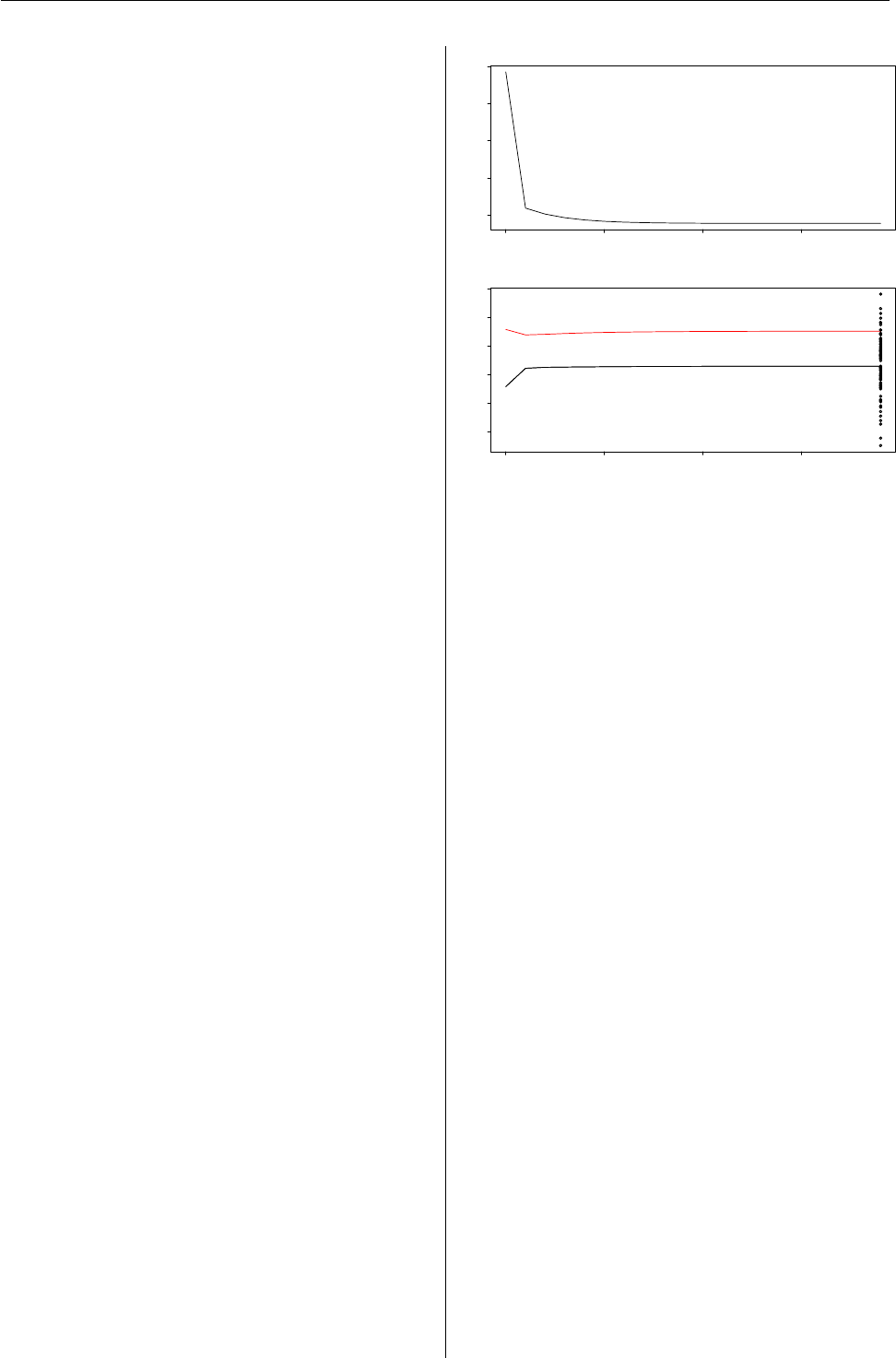
Vol. 7/1, April 2007 28

fall signiﬁcantly when increasing the number of

mass points further.

Empirical Bayes predictions (generally, h(x0

iˆ

β+

zi)for the number of deaths per city can be obtained

by the use of fitted(missouri.np2), or equiv-

alently, missouri.np2$fitted.values, or equiva-

lently, predict(missouri.np2, type="response").

Dividing this quantity by missouri$Size, one ob-

tains estimated or ‘shrunken’ rates which can be

compared to the 6th column in Table 4, Aitkin

(1996b). The shrunken rates are less variable than

the crude rates and hence are useful for small area

estimation problems. The posterior probabilities wik

can be obtained from the ﬁtted model (in analogy to

the 8th and 9th column of Table 4, Aitkin,1996b), via

the component $post.prob. Further, ’posterior in-

tercepts’ for the construction of ’league tables’ are

stored in component $post.int — see Sofroniou

et al. (2006) for an example of their application.

Methods for most generic functions that

are applied to ﬁtted model objects, such

as update(), coefficients(), residuals(),

fitted(), summary(), predict() and plot(),

have been deﬁned for the glmmNPML class. In some

cases (the ﬁrst four generic functions listed above)

the default method is used; in other cases (the last

three generics) explicit methods are provided. The

plot() function offers four different plots: (i) dis-

parity vs. EM iterations; (ii) EM trajectories; (iii)

Empirical Bayes predictions vs. true response; and

(iv) posterior probabilities against the residuals of

the ﬁxed part of the GLM ﬁt in the last EM itera-

tion. Plots (i) and (ii) are generated by default when

running alldist and are depicted in Fig. 1for the

model ﬁtted above.

One observes that the EM trajectories converge

essentially to the ﬁxed part residuals of cities no. 4

and 84 (in Tsutakawa’s list), which have populations

of 54155 and 22514, respectively, being much larger

than the majority of the other cities with only several

hundreds of inhabitants (For the very interested, the

numerical values associated with the disparity plot

and the EM trajectories, as well as the residuals plot-

ted vertically in the latter plot, are available in com-

ponent $Misc).

This was a simple example without any covari-

ates. In general an arbitrary number of ﬁxed effects

can be speciﬁed, and the random component can be

an intercept (∼1) or a single variable giving a model

with a random slope and random intercept.

0 5 10 15

360 380 400 420 440

EM iterations

−2logL

0 5 10 15

−6.0 −5.5 −5.0 −4.5 −4.0 −3.5

EM iterations

mass points

Figure 1: Top: Disparity (−2 log L) trend; bottom:

EM trajectories. The vertical dots in the latter plot are

the residuals of the ﬁxed part of the ﬁtted random

effect model (Note that these residuals are not cen-

tered around 0, in contrast to the residuals of a simple

ﬁxed effect model. The plotted residuals, generally

h−1(yi)−x0

iˆ

β, represent the random effect distribu-

tion and are on the same scale as the mass points).

The function allvc

The function alldist is designed to ﬁt simple

overdispersion models (i.e., one has a random effect

on the individual observations). However, often one

wishes to introduces shared random effects, e.g. for

students from the same class or school, for the same

individual observed repeatedly over time (longitudi-

nal data), or in small area estimation problems. This

leads to variance component models, which can be

ﬁtted in npmlreg using the function allvc. As an

example, let us consider the Oxford boys data from

Brush and Harrison (1990), which were analyzed

with NPML using GLIM4 by Aitkin et al. (2005).

The data set is part of the R package nlme (Pin-

heiro et al.,2005) and contains the heights of 26

boys, measured in Oxford on nine occasions over

two years. The boys, indexed by the factor Subject,

represent the upper level (primary sampling units,

PSU), and the particular measurements at different

time points correspond to the lower-level units (sec-

ondary sampling units, SSU).

As suggested by (Aitkin et al.,2005, p. 495), we

ﬁt a Gaussian model with unspeciﬁed random effect

distribution and K=7 mass points,

(Oxboys.np7 <- allvc(height ~ age, random =

~1|Subject, data = Oxboys, k=7))$disparity

[1] 1017.269

R News ISSN 1609-3631

Vol. 7/1, April 2007 29

which conﬁrms the GLIM4 result. Aitkin et al. state

that for all models using K>7 the ﬁtted mass

points ‘are duplicated with the same total mass as

in lower-dimension models’, and hence consider this

7- mass point model as ‘sufﬁciently complex’. How-

ever, ﬁtting for comparison a simple linear mixed

model with function lmer in package lme4 (Bates

and Sarkar,2006)

(fm1 <- lmer(height ~ age + (1|Subject),

data = Oxboys, method = "ML"))

gives the MLdeviance, i.e., disparity, of 940.569. As

this model is based on a normal random effect distri-

bution, NPML should be superior to this, or at least

competitive with it. Therefore, we went on ﬁtting

models with K=8 and K=9 mass points, yielding

(Oxboys.np8 <- allvc(height ~ age, random =

~1|Subject, data = Oxboys, k=8))$disparity

[1] 931.3752

(Oxboys.np9 <- allvc(height ~ age, random =

~1|Subject, data = Oxboys, k=9,

tol=0.3))$disparity

[1] 916.0921

For both models, all mass points are indeed distinct.

For instance, for the 9-mass point model one has

Estimate Std. Error

age 6.523719 0.05094195

MASS1 130.200174 0.16795344

MASS2 138.416628 0.09697325

MASS3 143.382397 0.09697225

MASS4 147.350113 0.07511877

MASS5 150.954327 0.06857400

MASS6 153.869256 0.11915344

MASS7 156.178153 0.09676418

MASS8 159.521550 0.16795354

MASS9 164.883640 0.11876372

This increased performance compared to the

GLIM code is due to the installation of a ‘damping’

mechanism in the ﬁrst cycles of the EM algorithm;

see Einbeck and Hinde (2006) for details.

Further increase of Kdoes not yield major drops

in disparity, so we continue to work with nine mass

points, and extend the model by allowing the lin-

ear trend to vary across boys. The function call then

takes the form

(Oxboys.np9s <- allvc(height ~ age, random =

~age|Subject, data = Oxboys, k = 9,

tol=0.3))

The difference in disparities is

> Oxboys.np9$disparity - Oxboys.np9s$disparity

[1] 102.1071

> Oxboys.np9$df.res - Oxboys.np9s$df.res

[1] 8

degrees of freedom, showing clear heterogeneity in

the slope.

Summary

We have introduced the R package npmlreg, which

is in some parts a simple translation from the corre-

sponding GLIM4 code, but, in other parts, contains

substantial extensions and methodological improve-

ments. In particular, we mention the possibility to

ﬁt Gamma models and to work with dispersion pa-

rameters varying smoothly over components, and, as

already noted, the installation of a damping proce-

dure. We note ﬁnally that for the sake of compara-

bility all implemented features are also available for

Gaussian Quadrature instead of NPML (leaving the

zkand πkﬁxed and equal to Gauss-Hermite integra-

tion points and masses). The R package is available

on CRAN. Future developments will include 3-level

models and multicategory responses.

Acknowledgements

The work on this R package was supported by

Science Foundation Ireland Basic Research Grant

04/BR/M0051. We are grateful to N. Sofroniou for

sharing his GLIM code for the Missouri data and two

anonymous referees for pointing at the comparison

with package lme4.

Bibliography

M. Aitkin. A general maximum likelihood analy-

sis of overdispersion in generalized linear models.

Statistics and Computing, 6:251–262, 1996a. 26

M. Aitkin. Empirical Bayes shrinkage using posterior

random effect means from nonparametric maxi-

mum likelihood estimation in general random ef-

fect models. In IWSM 1996: Proceedings of the 11th

International Workshop on Statistical Modelling, Orvi-

eto, pages 87–94, 1996b. 27,28

M. Aitkin. A general maximum likelihood analysis

of variance components in generalized linear mod-

els. Biometrics, 55:218–234, 1999. 26

M. Aitkin and B. Francis. Fitting overdispersed

generalized linear models by nonparametric max-

imum likelihood. The GLIM Newsletter, 25:37–45,

1995. 26

M. Aitkin, B. Francis, and J. Hinde. Statistical Mod-

elling in GLIM 4. Oxford Statistical Science Series,

Oxford, UK., 2005. 27,28

R News ISSN 1609-3631

Vol. 7/1, April 2007 30

D. Bates and D. Sarkar. lme4: Linear mixed-effects mod-

els using S4 classes, 2006. R package version 0.995-2.

D. Böhning, P. Schlattmann, and B. Lind-

sey. Computer-assisted analysis of mixtures

(C.A.MAN): statistical algorithms. Biometrics, 48:

283–303, 1992. 26

G. Brush and G. A. Harrison. Components of growth

variation in human stature. Mathematical Medicine

and Biology, 7:77–92, 1990. 28

J. Einbeck and J. Hinde. A note on NPML estimation

for exponential family regression models with un-

speciﬁed dispersion parameter. Austrian Journal of

Statistics, 35:233–243, 2006. 29

J. Einbeck, R. Darnell, and J. Hinde. npmlreg: Non-

parametric maximum likelihood estimation for random

effect models, 2006. R package version 0.40. 26

N.M. Laird. Nonparametric maximum likelihood es-

timation of a mixing distribution. Journal of the

American Statistical Association, 73:805–811, 1978.

J. Pinheiro, D. Bates, S. DebRoy, and D. Sarkar. nlme:

Linear and nonlinear mixed effects models, 2005. R

package version 3.1-66. 28

A. Skrondal and S. Rabe-Hesketh. Generalized Latent

Variable Modelling. Chapman & Hall/CRC, Boca

Raton, 2004. 26

N. Sofroniou, J. Einbeck, and J. Hinde. Analyzing

Irish suicide rates with mixture models. In IWSM

2006: Proceedings of the 21th International Work-

shop on Statistical Modelling, Galway, pages 474–481,

2006. 28

R. Tsutakawa. Estimation of cancer mortality rates: a

Bayesian analysis of small frequencies. Biometrics,

41:69–79, 1985. 27

Jochen Einbeck

Durham University, UK

jochen.einbeck@durham.ac.uk

John Hinde

National University of Ireland, Galway, Rep. of Ireland

john.hinde@nuigalway.ie

Ross Darnell

The University of Queensland, Australia

r.darnell@uq.edu.au

Augmenting R with Unix Tools

Andrew Robinson

This article describes a small collection of Unix

command-line tools that can be used to augment R. I

introduce:

make which after judicious preparation will allow

one-word execution of large-scale simulations,

all the way from compilation of source code to

construction of a PDF report;

screen which will permit remote monitoring of pro-

gram execution progress with automatic pro-

tection against disconnection; and

mail which will allow automatic alerting under er-

ror conditions or script completion.

These programs will be part of the default instal-

lations of many ﬂavours of Unix-like operating sys-

tems. Although these tools have many different ap-

plications, each is very useful for running R remotely

on a Unix-like operating system, which is the focus of

their usage in this article.

Regardless of what kind of computer is on your

own desk, you may ﬁnd these tools useful; they do

not require you to be running a BSD or GNU/Linux

on your own machine.

R and screen

It is sometimes necessary to run R code that executes

for long periods of time upon remote machines. This

requirement may be because the local computing re-

sources are too slow, too unstable, or have insufﬁ-

cient memory.

For example, I have recently completed some

simulations that took more than a month on a rea-

sonably fast cluster of Linux computers. I devel-

oped, trialed, and proﬁled my code on my local, not-

particularly-fast, computer. I then copied the scripts

and data to a more powerful machine provided by

my employer and ran the simulations on R remotely

on that machine. To get easy access to the simula-

tions whilst they ran, I used screen.

screen is a so-called terminal multiplexor, which

allows us to create, shufﬂe, share, and suspend com-

mand line sessions within one window. It provides

protection against disconnections and the ﬂexibility

to retrieve command line sessions remotely. screen

is particularly useful for R sessions that are running

on a remote machine.

We might use the following steps to invoke R

within screen:

1. log in remotely via secure shell,

R News ISSN 1609-3631

Vol. 7/1, April 2007 31

2. start screen,

3. start R,

4. source our script with echo=TRUE,

5. detach the screen session, using Ctrl-a d, and

6. log out.

The R session continues working in the background,

contained within the screen session. If we want to

revisit the session to check its progress, then we

1. log in remotely via secure shell,

2. start screen -r, which recalls the unattached

session,

3. examine the saved buffer; scrolling around,

copying and pasting as necessary,

4. detach the screen session, using Ctrl-a d, and

5. log out.

This approach works best if examining the buffer

is informative, which requires that the R script

be written to provide readable output or ﬂag its

progress every so often. I ﬁnd that the modest de-

crease in speed of looping is more than compensated

by a cheerful periodic reminder, say every 1000th

iteration, that everything is still working and that

there are only niterations left to run. I have also

been experimenting with various algorithms for R to

use the elapsed time, the elapsed number of simula-

tions, and the number of simulations remaining, to

estimate the amount of time left until the run is com-

plete.

screen offers other advantages. You can manage

several screens in one window, so editing a script re-

motely using, say, emacs, and then sourcing the script

in the remote R session in another screen, is quick

and easy. If you lose your connection, the session is

kept alive in the background, and can be re-attached,

using screen -r as above. If you have forgotten

to detach your session you can do so forcibly from

another login session, using screen -dr. You can

change the default history/scrollback buffer length,

and navigate the buffer using intuitive keystrokes.

Finally, you can share a screen session with other

people who are logged in to the same machine. That

is, each user can type and see what the other is typ-

ing, so a primitive form of online collaboration is

possible.

So, running an R session in screen provides a

simple and robust way to allow repeated access to

a simulation or a process.

More information about screen can be found

from http://www.gnu.org/software/screen/, or

man screen.

R and mail

It is very useful to be able to monitor an R session

that is running remotely. However, it would also be

useful if the session could alert us when the script has

completed, or when it has stopped for some reason,

including some pre-determined error conditions. We

can use mail for this purpose, if the computer is run-

ning an appropriate mail server, such as sendmail.

mail is an old email program, small enough to

be included by default on most Unix-like systems,

and featureless enough to be almost universally ig-

nored by users in favour of other programs, such as

mutt, or those with shiny graphical user interfaces.

However, mail does allow us to send email from the

command line. And, R can do pretty much anything

that can be done from the command line1. Of course,

a small amount of ﬁddling is necessary to make it

work. A simple function will help2. This function

will fail if any of the arguments contain single or

double quotes. So, craft your message carefully.

mail <- function(address, subject, message) {

system(paste("echo ", message,

" | mail -s ", subject,

" ", address, sep=""))

}

We can now send mail from R via, for example,

mail("andrewr", "Test", "Hello world!")

You can place calls to this function in strategic loca-

tions within your script. I call it at the end of the

script to let me know that the simulations are ﬁn-

ished, and I can collect the results at my leisure. In

order to have R let us know when it has stopped, we

can use a function like this:

alert <- function() {

mail("andrewr", "Stopped", "Problem")

browser()

}

then in our script we call

options(error = alert)

Now in case of an error, R will send an email and

drop into the browser, to allow detailed follow-up. If

you have more than one machine running, then call-

ing hostname via system, and pasting that into the

subject line, can be helpful.

Alternatively, you can use mutt with exactly the

same command line structure as mail, if mutt is in-

stalled on your system. An advantage of mutt is

that it uses the MIME protocol for binary attachments.

That would enable you to, say, attach to your email

the PDF that your script has just created with Sweave

and pdflatex, or the cvs ﬁle that your script creates,

1In theory, it can do everything, I suppose. I haven’t tried.

2Caveat: this function is written to work on bash version 3.1.17. Your mileage may vary.

R News ISSN 1609-3631

Vol. 7/1, April 2007 32

or even the relevant objects saved from the session,

neatly packaged and compressed in a *.RData object.

Different ﬂavours of Unix mail are available. You

can ﬁnd out more about yours by man mail.

R and make

I have recently been working on bootstrap tests of

a model-ﬁtting program that uses maximum likeli-

hood to ﬁt models with multivariate normal and t

distributions. The program is distributed in FOR-

TRAN, and it has to be compiled every time that it is

run with a new model. I wanted to use a studentized

bootstrap for interval estimates, gather up all the out-

put, and construct some useful tables and graphics.

So, I need to juggle FORTRAN ﬁles, FORTRAN

executables, R source ﬁles, Sweave ﬁles, PDFs, and

so on. R does a great job preparing the input ﬁles,

calling the executable (using system()), and scoop-

ing up the output ﬁles. However, to keep everything

in sync, I use make.

Although it is commonly associated with build-

ing executable programs, make can control the con-

version of pretty much any ﬁle type into pretty much

any other kind of ﬁle type. For example, make can be

told how to convert a FORTRAN source ﬁle to an ex-

ecutable, and it will do so if and when the source ﬁle

changes. It can be told how and when to run an R

source ﬁle, and then how and when to call Sweave

upon an existing ﬁle, and then how and when to cre-

ate a PDF from the resulting L

EX ﬁle.

The other advantage that make offers is splitting

large projects into chunks. I use Sweave to bind my

documentation and analysis tightly together. How-

ever, maintaining the link between documentation

and analysis can be time-consuming. For example,

when documenting a large-scale simulation, I would

rather not run the simulation every time I correct a

spelling mistake.

One option is to tweak the number of runs. make

provides a ﬂexible infrastructure for testing code, as

we can pass parameters, such as the number of runs

to perform, to R. For example, with an appropriate

Makeﬁle, typing make test at the operating system

prompt will run the entire project with only 20 simu-

lations, whereas typing make will run the project with

2000 simulations.

Another option is to split the project into two

parts: the simulation, and the analysis, and run only

the second, unless important elements change in the

ﬁrst. Again, this sort of arrangement can be con-

structed quite easily using make.

For example, I have an R source ﬁle called sim.r

that controls the simulations and produces a .RData

object called output.RData. The content is:

randoms <- runif(reps)

save.image("output.RData")

I also have a Sweave ﬁle called report.rnw which

provides summary statistics (and graphics, not in-

cluded here) for the runs. The content is:

\documentclass{article}

\begin{document}

<<>>=

load("output.RData")

We performed \Sexpr{reps} simulations.

\end{document}

The latter ﬁle often requires tweaking, depending

on the output. So, I want to separate the simulations

and the report writing, and only run the simulations

if I absolutely have to. Figure 1is an example Make-

ﬁle that takes advantage of both options noted above.

All the ﬁles referenced here are assumed to be held in

the same directory as the Makeﬁle, but of course they

could be contained in subdirectories, which is gener-

ally a neater strategy.

I do not actually need make to do these tasks, but

it does simplify the operation a great deal. One ad-

vantage is that make provides conditional execution

without me needing to ﬁddle around to see what has

and has not changed. If I now edit report.rnw, and

type make, it won’t rerun the simulation, it will just

recompile report.rnw. On the other hand, if I make

a change to sim.r, or even run sim.r again (thus

updating the .RData object), make will rerun every-

thing. That doesn’t seem very signiﬁcant here, but it

can be when you’re working on a report with numer-

ous different branches of analysis.

The other advantage (which my Makeﬁle doesn’t

currently use) is that it provides wildcard match-

ing. So, if I have a bunch of Sweave ﬁles (one for

each chapter, say) and I change only one of them,

then make will identify which one has changed and

which ones depend on that change, and recompile

only those that are needed. But I don’t have to pro-

duce a separate line in the Makeﬁle for each ﬁle.

Also, the Makeﬁle provides implicit documenta-

tion for the ﬂow of operations, so if I need to pass the

project on to someone else, all they need to do is call

make to get going.

More information on make can be found from

http://www.gnu.org/software/make/.

Andrew Robinson

Department of Mathematics and Statistics

University of Melbourne

Australia

A.Robinson@ms.unimelb.edu.au

R News ISSN 1609-3631

Vol. 7/1, April 2007 33

## Hashes indicate comments. Use these for documentation.

## Makefiles are most easily read from the bottom up, the first time!

# make is automatically interpreted as make report.pdf .

# Update report.pdf whenever report.tex changes, by running this code.

report.pdf : report.tex

( \

\pdflatex report.tex; \

while \grep -q "Rerun to get cross-references right." report.log;\

do \

\pdflatex report.tex; \

done \

)

# Update report.tex whenever report.rnw *or* output.RData changes,

# by running this code.

report.tex : report.rnw output.RData

echo "Sweave(\"report.rnw\")" | R --no-save --no-restore

# Update output.RData whenever sim.r changes, by running this code.

output.RData : sim.r

echo "reps <- 2000; source(\"sim.r\")" | R --no-save --no-restore

########################################################################

## The following section tells make how to respond to specific keywords.

.PHONY: test full neat clean

# make test cleans up, runs a small number of simulations,

# and then constructs a report

test:

make clean;

echo "reps <- 10; source(\"sim.r\")" | R --no-save --no-restore;

make

# make full cleans up and runs the whole project from scratch

full :

make clean;

make

# make neat cleans up temporary files - useful for archiving

neat :

rm -fr *.txt *.core fort.3 *~ *.aux *.log *.ps *.out

# make clean cleans up all created files.

clean :

rm -fr *.core fort.3 *~ *.exe *.tex *.txt *.lof *.lot *.tex \

*.RData *.ps *.pdf *.aux *.log *.out *.toc *.eps

Figure 1: The contents of a Makeﬁle. Note that all the indenting is done by means of tab characters, not spaces.

This Makeﬁle has been tested for both GNU make and BSD make.

R News ISSN 1609-3631

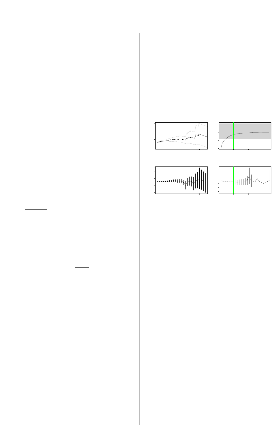
Vol. 7/1, April 2007 34

POT: Modelling Peaks Over a Threshold

by Mathieu Ribatet

The Generalised Pareto Distribution (GPD) is the

limiting distribution of normalised excesses over a

threshold, as the threshold approaches the endpoint

of the variable (Pickands,1975). The POT package

contains useful tools to perform statistical analysis

for peaks over a threshold using the GPD approxi-

mation.

There is many packages devoted to the extreme

value theory (evd,ismev,evir, . . . ); however, the

POT package is specialised in peaks over thresh-

old analysis. Moreover, this is currently the only

one which proposes many estimators for the GPD. A

user’s guide (as a package vignette) and two demos

are also included in the package.

Asymptotic Approximation

Let X1,...,Xnbe a series of i.id. random variables

with common distribution function F. Let Mn=

max {X1,...,Xn}. Suppose there exists constants

an>0 and bnsuch that:

IP Mn−bn

≤z−→ G(z),n→+∞

for z∈Rand where Gis a non degenerate distribu-

tion function. Then, for i=1, . . . , n, we have:

IP [Xi≤z|Xi>u]−→ H(z),u→uend (1)

with

H(y) = 1−1+ξy−µ

σ−1/ξ

where (µ,σ,ξ)are the location, scale and shape pa-

rameters respectively, σ>0 and z+=max(z, 0)and

uend is the right end-point of the variable Xi.

It is usual to ﬁt the GPD to excesses over a

(high enough) threshold. Thus we suppose that the

asymptotic result given by equation (1) is (approxi-

mately) true for the threshold of interest.

Application:

Ardières River at Beaujeu

The ardieres data frame containing ﬂood dis-

charges (in m3·s−1) over a period of 33 years of

the Ardières river at Beaujeau (FRANCE) is included

in the package. There are NA values in year 1994 as

a ﬂood event damaged record instrumentation. We

use this dataset as an example for a typical univari-

ate analysis. First, we have to “extract” indepen-

dent events from the time series and select a suit-

able threshold such that asymptotic approximation

in equation (1) is good enough.

library("POT")

data("ardieres")

tmp <- clust(ardieres, 0.85, tim.cond = 7/365,

clust.max = TRUE)

par(mfrow=c(2,2))

mrlplot(tmp[,"obs"], xlim = c(0.85, 17))

diplot(tmp, u.range = c(0.85, 17))

tcplot(tmp[,"obs"], u.range = c(0.85, 17))

5 10 15

0 5 10 15 20

Mean Residual Life Plot

Threshold

Mean Excess

5 10 15

0.0 0.5 1.0 1.5

Dispersion Index Plot

Threshold

Dispersion Index

5 10 15

−30 −10 10 30

Threshold

Modified Scale

5 10 15

−1.0 0.0 1.0 2.0

Threshold

Shape

Figure 1: Tools for the threshold selection

The threshold selection stage is a compromise be-

tween bias and variance. On one hand, if a too

high threshold is selected, the bias decreases as the

asymptotic approximation in equation (1) is good

enough while the variance increases as there is not

enough data above this threshold. On the other

hand, by taking a lower threshold, the variance de-

creases as the number of observations is larger and

the bias increases as the asymptotic approximation

becomes poorer.

According to Fig. 1, a threshold around ﬁve

m3·s−1should be a “good compromise”. Indeed,

the mean residual life plot is “linear” on the range

(5, 7); for thresholds greater than 5, the dispersion

index estimates are “near” the theoretical value 1;

and both modiﬁed scale and shape estimates seem to

be constant on the range (5, 9). Thus, we select only

independent values above this threshold by invok-

ing:

events <- clust(ardieres, u = 5,

tim.cond = 7/365, clust.max = TRUE)

We can ﬁt the GPD to those excesses accord-

ing several estimators by setting the method option.

There is currently 7 estimators: Moments "moments",

Unbiased and Biased Probability Weighted Moments

"pwmu", "pwmb", Minimum Density Power Diver-

gence "mdpd", medians "med", Pickands "pickands"

R News ISSN 1609-3631

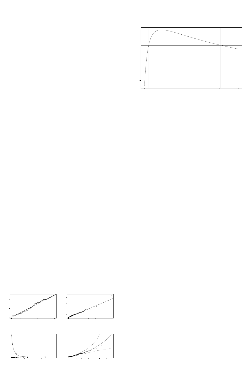
Vol. 7/1, April 2007 35

and Maximum Likelihood (the default) "mle" esti-

mators. References for these estimators can be found

in (Pickands,1975;Hosking and Wallis,1987;Coles,

2001;Peng and Welsh,2001) and (Juárez and Schu-

cany,2004). For example, if we want to ﬁt the GPD

using the unbiased probability weighted moment es-

timator:

obs <- events[,"obs"]

pwmu <- fitgpd(obs, thresh = 5, "pwmu")

Here is the scale and shape parameter estimates

of the GPD for the 7 estimators implemented.

scale shape

mle 2.735991 0.2779359

mom 2.840792 0.2465661

pwmu 2.668368 0.2922964

pwmb 2.704665 0.2826697

mdpd 2.709254 0.2915759

med 2.135882 0.8939585

pick 2.328240 0.6648158

By invoking:

par(mfrow=c(2,2))

plot(pwmu, npy=2.63)

we obtain Fig. 2which depicts graphic tools for

model diagnostic. Proﬁle likelihood conﬁdence in-

tervals can also be computed, even for return levels

see Fig. 3, with:

gpd.pfrl(mle, 0.995, range = c(20, 120),

conf = 0.95)

0.0 0.2 0.4 0.6 0.8 1.0

0.0 0.4 0.8

Probability plot

Empirical

Model

−

5 10 15 20 25 30 35

10 20 30 40

QQ−plot

Model

Empirical

−

−−−−−−−−

−

−−−−−−

−

10 20 30 40 50

0.0 0.1 0.2 0.3

Density Plot

Quantile

Density

0.5 1.0 2.0 5.0 20.0 50.0

10 20 30 40

Return Level Plot

Return Period (Years)

Return Level

Figure 2: Graphic tools for model diagnostic.

20 40 60 80 100 120

−205 −204 −203 −202 −201 −200 −199

Return Level

Profile Log−likelihood

Figure 3: 95% proﬁle conﬁdence interval for the re-

turn level associated to non exceedance probability

0.995.

Miscellaneous Features

The POT package can also:

• simulate and compute density, quantile and

distribution functions for the GPD;

• ﬁt the GPD with a varying threshold using

MLE;

• ﬁt the GPD with held ﬁxed parameters using

MLE;

• perform analysis of variance for two nested

models;

• estimate the extremal index using two estima-

tors;

• display a L-Moment plot (Hosking and Wallis,

1997);

• compute sample L-moments;

• convert non exceedance probabilities to return

periods and vice-versa;

• compute “averaged” time series using an aver-

age mobile window.

Currently, most of the package developments are

devoted to bivariate peaks over threshold. For this

purpose, the POT package can also:

• ﬁt a bivariate GPD using 6 parametric depen-

dence functions;

• ﬁt a ﬁrst order Markov chain with a ﬁxed ex-

treme value dependence structure to all thresh-

old exceedances;

• simulate ﬁrst order Markov chains with a ﬁxed

extreme value dependence structure;

• plot the Pickands’ dependence and the spectral

density functions.

R News ISSN 1609-3631

Vol. 7/1, April 2007 36

Bibliography

S. Coles. An Introduction to Statistical Modelling of Ex-

treme Values. Springer Series in Statistics. London,

2001. 35

J. Hosking and J. Wallis. Parameter and quantile

estimation for the generalised Pareto distribution.

Technometrics, 29(3):339–349, 1987. 35

J. Hosking and J. Wallis. Regional Frequency Analysis.

Cambridge University Press, 1997. 35

S. Juárez and W. Schucany. Robust and efﬁcient esti-

mation for the generalised Pareto distribution. Ex-

tremes, 7(3):237–251, 2004. ISSN 13861999. 35

L. Peng and A. Welsh. Robust estimation of the gen-

eralised Pareto distribution. Extremes, 4(1):53–65,

2001. 35

J. Pickands. Statistical inference using extreme order

statistics. Annals of Statistics, 3:119–131, 1975.

34,35

Mathieu Ribatet

Cemagref Unité de Recherche HH Lyon, France

ribatet@lyon.cemagref.fr

Backtests

by Kyle Campbell, Jeff Enos, Daniel Gerlanc and David

Kane

Introduction

The backtest package provides facilities for explor-

ing portfolio-based conjectures about ﬁnancial in-

struments (stocks, bonds, swaps, options, et cetera).

For example, consider a claim that stocks for which

analysts are raising their earnings estimates perform

better than stocks for which analysts are lowering es-

timates. We want to examine if, on average, stocks

with raised estimates have higher future returns than

stocks with lowered estimates and whether this is

true over various time horizons and across different

categories of stocks. Colloquially, “backtest” is the

term used in ﬁnance for such tests.

Background

To demonstrate the capabilities of the backtest pack-

age we will consider a series of examples based on a

single real-world data set. StarMine1is a San Fran-

sisco research company which creates quantitative

equity models for stock selection. According to the

company:

StarMine Indicator is a 1-100 percentile rank-

ing of stocks that is predictive of future an-

alyst revisions. StarMine Indicator improves

upon basic earnings revisions models by:

• Explicitly considering management

guidance.

• Incorporating SmartEstimates,

StarMine’s superior estimates con-

structed by putting more weight on the

most accurate analysts.

• Using a longer-term (forward 12-month)

forecast horizon (in addition to the cur-

rent quarter).

StarMine Indicator is positively correlated to

future stock price movements. Top-decile

stocks have annually outperformed bottom-

decile stocks by 27 percentage points over the

past ten years across all global regions.

These ranks and other attributes of stocks are in

the starmine data frame, available as part of the

backtest package.

> data("starmine")

> names(starmine)

[1] "date" "id" "name"

[4] "country" "sector" "cap.usd"

[7] "size" "smi" "fwd.ret.1m"

[10] "fwd.ret.6m"

starmine contains selected attributes such as sec-

tor, market capitalisation, country, and various mea-

sures of return for a universe of approximately 6,000

securities. The data is on a monthly frequency from

January, 1995 through November, 1995. The number

of observations varies over time from a low of 4,528

in February to a high of 5,194 in November.

date count

1995-01-31 4593

1995-02-28 4528

1995-03-31 4569

1995-04-30 4708

1995-05-31 4724

1995-06-30 4748

1995-07-31 4878

1995-08-31 5092

1995-09-30 5185

1995-10-31 5109

1995-11-30 5194

1See www.starmine.com for details.

R News ISSN 1609-3631

Vol. 7/1, April 2007 37

The smi column contains the StarMine Indicator

score for each security and date if available. Here is

a sample of rows and columns from the data frame:

date name fwd.ret.1m fwd.ret.6m smi

1995-01-31 Lojack Corp 0.09 0.8 96

1995-02-28 Raymond Corp 0.05 0.1 85

1995-02-28 Lojack Corp 0.08 0.7 90

1995-03-31 Lojack Corp 0.15 1.0 49

1995-08-31 Supercuts Inc -0.11 -0.5 57

1995-10-31 Lojack Corp -0.40 -0.2 22

1995-11-30 Lojack Corp 0.20 0.4 51

Most securities (like LoJack above) have multiple

entries in the data frame, each for a different date.

The row for Supercuts indicates that, as of the close of

business on August 31, 1995, its smi was 57. During

the month of September, its return (i.e., fwd.ret.1m)

was -11%.

A simple backtest

Backtests are run by calling the function backtest to

produce an object of class backtest.

> bt <- backtest(starmine, in.var = "smi",

+ ret.var = "fwd.ret.1m")

starmine is a data frame containing all the infor-

mation necessary to conduct the backtest. in.var

and ret.var identify the columns containing the

input and return variables, respectively. backtest

splits observations into 5 (the default) quantiles, or

“buckets,” based on the value of in.var. Lower

(higher) buckets contain smaller (larger) values of

in.var. Each quantile contains an approximately

equal number of observations. This backtest creates

quantiles according to values in the smi column of

starmine.

[1,21] (21,40] (40,59] (59,82] (82,100]

6765 6885 6642 6600 6496

backtest calculates the average return within

each bucket. From these averages we calculate the

spread, or the difference between the average return

of the highest and lowest buckets.

Calling summary on the resulting object of class

backtest reports the in.var,ret.var, and by.var

used. We will use a by.var in later backtests.

> summary(bt)

Backtest conducted with:

1 in.var: smi;

1 ret.var: fwd.ret.1m;

and no by.var.

low 2 3 4 high spread

pooled 0.011 0.013 0.016 0.02 0.032 0.021

This backtest is an example of a pooled backtest. In

such a backtest, we assume that all observations are

exchangeable. This means that a quantile may con-

tain observations for any stock and from any date.

Quantiles may contain multiple observations for the

same stock.

The backtest summary shows that the average re-

turn for the highest bucket was 3.2%. This value is

the mean one month forward return of stocks with

smi values in the highest quantile. As the obser-

vations are exchangeable, we use every observation

in the starmine data frame with a non-missing smi

value. This means that the returns for LoJack from

both 1995-01-31 and 1995-02-28 would contribute to

the 3.2% mean of the high bucket.

The backtest suggests that StarMine’s model pre-

dicted performance reasonably well. On average,

stocks in the highest quantile returned 3.2% while

stocks in the lowest quantile returned 1.1%. The

spread of 2.1% suggests that stocks with high ratings

perform better than stocks with low ratings.

Natural backtests

Anatural backtest requires that the frequency of re-

turns and observations be the same.

A natural backtest approximates the following

implementation methodology: in the ﬁrst period

form an equal weighted portfolio with long posi-

tions in the stocks in the highest quantile and short

positions in the stocks in the lowest quantile. Each

stock has an equal weight in the portfolio; if there

are 5 stocks on the long side, each stock has a weight

of 20%. Subsequently rebalance the portfolio every

time the in.var values change. If the observations

have a monthly frequency, the in.var values change

monthly and the portfolio must be rebalanced ac-

cordingly. When the in.var values change, rebalanc-

ing has the effect of exiting positions that have left

the top and bottom quantiles and entering positions

that have entered the top and bottom quantiles. If the

data contains monthly observations, we will form 12

portfolios per year.

To create a simple natural backtest, we again call

backtest using fwd.ret.1m. This is the only return

value in starmine for which we can construct a nat-

ural backtest of smi.

> bt <- backtest(starmine, id.var = "id",

+ date.var = "date", in.var = "smi",

+ ret.var = "fwd.ret.1m", natural = TRUE)

Natural backtests require a date.var and id.var,

the names of the columns in the data frame contain-

ing the dates of the observations and unique security

identiﬁers, respectively. Calling summary displays

the results of the backtest:

> summary(bt)

R News ISSN 1609-3631

Vol. 7/1, April 2007 38

Backtest conducted with:

1 in.var: smi;

1 ret.var: fwd.ret.1m;

and no by.var.

low 2 3 4 high spread

1995-01-31 0.003 0.011 0.003 -0.0001 0.019 0.016

1995-02-28 -0.008 -0.003 0.003 0.0072 0.013 0.021

1995-03-31 0.029 0.017 0.013 0.0225 0.037 0.008

1995-04-30 -0.002 -0.003 0.002 -0.0054 0.005 0.007

1995-05-31 0.010 0.013 0.019 0.0228 0.044 0.034

1995-06-30 0.072 0.059 0.057 0.0708 0.101 0.030

1995-07-31 0.033 0.030 0.034 0.0323 0.052 0.018

1995-08-31 -0.004 0.006 0.017 0.0119 0.024 0.028

1995-09-30 -0.055 -0.030 -0.031 -0.0219 -0.014 0.041

1995-10-31 0.030 0.032 0.040 0.0430 0.038 0.008

1995-11-30 0.013 0.016 0.021 0.0294 0.037 0.024

MEAN 0.011 0.014 0.016 0.0193 0.032 0.021

average turnover: 0.5

mean spread: 0.02

sd spread: 0.01

raw sharpe ratio: 2

Focus on the mean return of the highest quan-

tile for 1995-02-28 of 1.3%. backtest calculated this

value by ﬁrst computing the 5 quantiles of the in-

put variable smi over all observations in starmine.

Among the observations that fall into the highest

quantile, those with date 1995-02-28 contribute to the

mean return of 1.3%. It is important to note that

the input variable quantiles are computed over the

whole dataset, as opposed to within each category

that may be deﬁned by a date.var or by.var.

The bottom row of the table contains the mean

quantile return over all dates. On account of the

way we calculate quantile means, a single stock will

have more effect on the quantile mean if during that

month there are fewer stocks in the quantile. Sup-

pose that during January there are only 2 stocks in

the low quantile. The return of a single stock in Jan-

uary will account for 1

22 of the quantile mean. This

is different than a pooled backtest where every ob-

servation within a quantile has the same weight. In

a natural backtest, the weight of a single observation

depends on the number of observations for that pe-

riod.

Calling summary yields information beyond that

offered by the summary method of a pooled back-

test. The ﬁrst piece of extra information is average

turnover. Turnover is the percentage of the portfolio

we would have to change each month if we imple-

mented the backtest as a trading strategy. For exam-

ple, covering all the shorts and shorting new stocks

would yield a turnover of 50% because we changed

half the portfolio. We trade stocks when they enter

or exit the extreme quantiles due to in.var changes.

On average, we would turn over 50% of this portfolio

each month.

The second piece of extra information is mean

spread. The spread was positive each month, so on

average the stocks with the highest smi values out-

performed the stocks with the lowest smi values.

On average, stocks in the highest quantile outper-

formed stocks in the lowest quantile by 2%. The

third piece of extra information, the standard devia-

tion of spread, is 1%. The spread varied from month

to month, ranging from a low of close to 0% to a high

of over 4%.

We deﬁne the fourth piece of extra information,

raw (non-annualized) Sharpe ratio, as return

risk . We set

return equal to mean spread return and use the stan-

dard deviation of spread return as a measure of risk.

More than one in.var

backtest allows for more than one in.var to be

tested simultaneously. Besides using smi, we will

test market capitalisation in dollars, cap.usd. This

is largely a nonsense variable since we do not expect

large cap stocks to outperform small cap stocks — if

anything, the reverse is true historically.

> bt <- backtest(starmine, id.var = "id",

+ date.var = "date", in.var = c("smi",

+ "cap.usd"), ret.var = "fwd.ret.1m",

+ natural = TRUE)

Because more than one in.var was speciﬁed,

only the spread returns for each in.var are dis-

played, along with the summary statistics for each

variable.

> summary(bt)

Backtest conducted with:

2 in.vars: smi, cap.usd;

1 ret.var: fwd.ret.1m;

and no by.var.

smi cap.usd

1995-01-31 0.016 -0.0138

1995-02-28 0.021 0.0017

1995-03-31 0.008 -0.0023

1995-04-30 0.007 -0.0052

1995-05-31 0.034 -0.0568

1995-06-30 0.030 -0.0143

1995-07-31 0.018 -0.0008

1995-08-31 0.028 0.0051

1995-09-30 0.041 0.0321

1995-10-31 0.008 0.0127

1995-11-30 0.024 0.0029

summary stats for in.var = smi:

average turnover: 0.5

mean spread: 0.02

sd spread: 0.01

raw sharpe ratio: 2

summary stats for in.var = cap.usd:

average turnover: 0.1

mean spread: -0.004

sd spread: 0.02

raw sharpe ratio: -0.2

R News ISSN 1609-3631

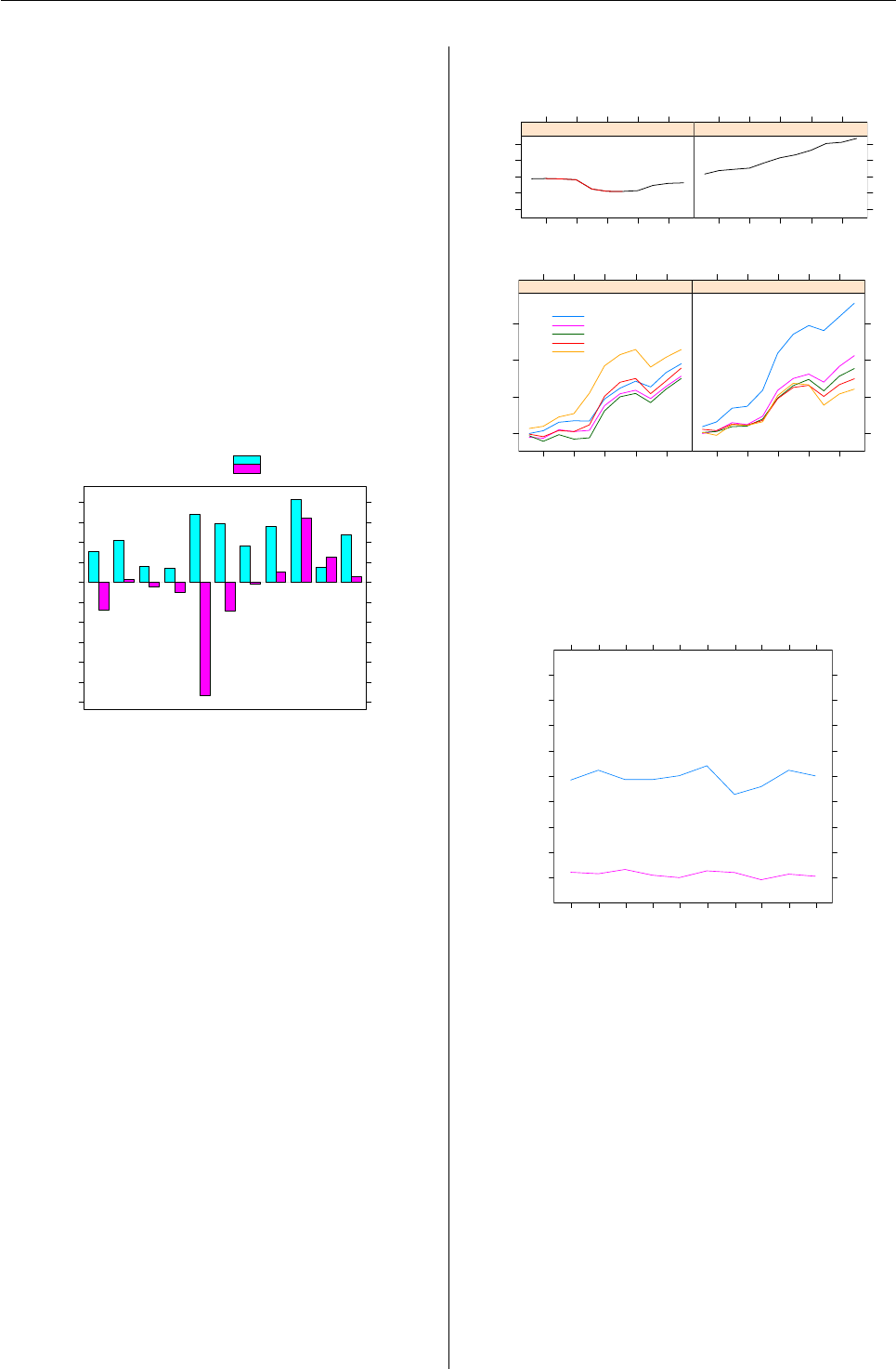
Vol. 7/1, April 2007 39

Viewing the results for the two input variables

side-by-side allows us to compare their performance

easily. As we expected, cap.usd as an input variable

did not perform as well as smi over our backtest pe-

riod. While smi had a positive return during each

month, cap.usd had a negative return in 6 months

and a negative mean spread. In addition, the spread

returns for cap.usd were twice as volatile as those of

smi.

There are several plotting facilities available in

backtest that can help illustrate the difference in

performance between these two signals. These plots

can be made from a natural backtest with any num-

ber of input variables. Below is a bar chart of the

monthly returns of the two signals together:

> plot(bt, type = "return")

Spread Return

Date

Return (%)

−6

−5

−4

−3

−2

−1

1995−01−31

1995−02−28

1995−03−31

1995−04−30

1995−05−31

1995−06−30

1995−07−31

1995−08−31

1995−09−30

1995−10−31

1995−11−30

smi

cap.usd

Figure 1: Monthly return spreads.

Returns for smi were consistently positive. Re-

turns for cap.usd were of low quality, but improved

later in the period. cap.usd had a particularly poor

return in June. We can also plot cumulative returns

for each input variable as shown in Figure 2.

The top region in this plot shows the cumulative

return of each signal on the same return scale, and

displays the total return and worst drawdown of the

entire backtest period. The bottom region shows the

cumulative return of the individual quantiles over

time. We can see that smi’s top quantile performed

best and lowest quantile performed worst. In con-

trast, cap.usd’s lowest quantile was its best perform-

ing.

Though it is clear from the summary above that

smi generated about 5 times as much turnover as

cap.usd, a plot is available to show the month-by-

month turnover of each signal, see Figure 3. This

chart shows that the turnover of smi was consistently

around 50% with lower turnover in September and

October, while the turnover of cap.usd was consis-

tently around 10%.

> plot(bt.save, type = "cumreturn.split")

Cumulative Spread Return

Return (%)

−20

−10

Mar May Jul Sep Nov

Total return: −3.9

Worst drawdown: −8

cap.usd

Mar May Jul Sep Nov

Total return: 23

Worst drawdown: −−

smi

Cumulative Quantile Return

Date

Return (%)

Mar May Jul Sep Nov

cap.usd

Mar May Jul Sep Nov

smi

quantile

high

low

Figure 2: Cumulative spread and quantile returns.

> plot(bt, type = "turnover")

Turnover

Date

Turnover (%)

Mar Apr May Jun Jul Aug Sep Oct Nov Dec

●

●●●

●

●●●

●●

●

●●

smi

cap.usd

●

Figure 3: Monthly turnover.

Using by.var

In another type of backtest we can look at quan-

tile spread returns by another variable. Specifying

by.var breaks up quantile returns into categories de-

ﬁned by the levels of the by.var column in the input

data frame. Consider a backtest of smi by sector:

> bt <- backtest(starmine, in.var = "smi",

+ ret.var = "fwd.ret.1m",

+ by.var = "sector")

> summary(bt)

Backtest conducted with:

R News ISSN 1609-3631

Vol. 7/1, April 2007 40

1 in.var: smi;

1 ret.var: fwd.ret.1m;

and by.var: sector.

low 2 3 4 high spread

Durbl 0.0063 0.007 0.009 0.007 0.01 0.004

Enrgy 0.0152 0.014 0.017 0.019 0.04 0.024

HiTec 0.0237 0.016 0.026 0.029 0.05 0.024

Hlth 0.0395 0.036 0.021 0.038 0.05 0.006

Manuf 0.0005 0.005 0.014 0.009 0.02 0.022

Money 0.0190 0.024 0.021 0.026 0.04 0.017

NoDur 0.0036 0.010 0.010 0.019 0.03 0.025

Other 0.0045 0.006 0.015 0.017 0.02 0.017

Shops 0.0020 0.004 0.005 0.017 0.03 0.026

Telcm 0.0277 0.014 0.022 0.023 0.03 0.005

Utils 0.0128 0.021 0.013 0.016 0.02 0.007

This backtest categorises observations by the

quantiles of smi and the levels of sector. The high-

est spread return of 2.6% occurs in Shops. Since

smi quantiles were computed before the observa-

tions were split into groups by sector, however, we

can not be sure how much conﬁdence to place in

this result. There could be very few observations in

this sector or one of the top and bottom quantiles

could have a disproportionate number of observa-

tions, thereby making the return calculation suspect.

counts provides a simple check.

> counts(bt)

$smi

low 2 3 4 high

Durbl 348 349 261 231 223

Enrgy 246 250 158 130 64

HiTec 647 660 824 1004 1432

Hlth 380 377 410 464 424

Manuf 1246 1265 1279 1395 1576

Money 959 1265 1244 1095 875

NoDur 615 563 528 441 371

Other 1034 940 784 760 710

Shops 870 714 710 697 548

Telcm 186 177 140 129 95

Utils 152 245 252 198 130

While there seems to be an adequate number of

observations in Shops, it is important to note that

there are approximately 60% more observations con-

tributing to the mean return of the lowest quantile

than to the mean return of the highest quantile, 870

versus 548. Overall, we should be more conﬁdent in

results for Manuf and Money due to their larger sam-

ple sizes. We might want to examine the result for

HiTec more closely, however, since there are more

than twice the number of observations in the high-

est quantile than the lowest.

by.var can also be numeric, as in this backtest us-

ing cap.usd:

> bt <- backtest(starmine,

+ in.var = "smi", ret.var = "fwd.ret.1m",

+ by.var = "cap.usd",

+ buckets = c(5, 10))

> summary(bt)

Backtest conducted with:

1 in.var: smi;

1 ret.var: fwd.ret.1m;

and by.var: cap.usd.

low 2 3 4 high spread

low 0.0105 0.0139 0.0236 0.028 0.038 0.028

2 0.0078 0.0093 0.0216 0.025 0.046 0.038

3 0.0186 0.0072 0.0167 0.031 0.034 0.016

4 0.0124 0.0142 0.0139 0.013 0.038 0.026

5 0.0080 0.0124 0.0087 0.010 0.025 0.017

6 0.0126 0.0121 0.0191 0.021 0.026 0.013

7 0.0080 0.0070 0.0160 0.019 0.034 0.026

8 0.0050 0.0181 0.0101 0.014 0.027 0.022

9 0.0104 0.0153 0.0167 0.014 0.028 0.018

high 0.0156 0.0207 0.0133 0.023 0.026 0.011

Since cap.usd is numeric, the observations are

now split by two sets of quantiles. Those listed

across the top are, as before, the input variable quan-

tiles of smi. The row names are the quantiles of

cap.usd. The buckets parameter of backtest con-

trols the number of quantiles. The higher returns

in the lower quantiles of cap.usd suggests that smi

performs better in small cap stocks than in large cap

stocks.

Multiple return horizons

Using backtest we can also analyse the performance

of a signal relative to multiple return horizons. Be-

low is a backtest that considers one month and six

month forward returns together:

> bt <- backtest(starmine, in.var = "smi",

+ buckets = 4, ret.var = c("fwd.ret.1m",

+ "fwd.ret.6m"))

> summary(bt)

Backtest conducted with:

1 in.var: smi;

2 ret.vars: fwd.ret.1m, fwd.ret.6m;

and no by.var.

low 2 3 high spread

fwd.ret.1m 0.011 0.015 0.018 0.03 0.019

fwd.ret.6m 0.112 0.121 0.142 0.17 0.059

The performance of smi over these two return

horizons tells us that the power of the signal de-

grades after the ﬁrst month. Using six month for-

ward return, fwd.ret.6m, the spread is 6%. This

is only 3 times larger than the 2% spread return in

the ﬁrst month despite covering a period which is 6

times longer. In other words, the model produces 2%

spread returns in the ﬁrst month but only 4% in the 5

months which follow.

R News ISSN 1609-3631

Vol. 7/1, April 2007 41

Conclusion

The backtest package provides a simple collection of

tools for performing portfolio-based tests of ﬁnancial

conjectures. A much more complex package, port-

folioSim, provides facilities for historical portfolio

performance analysis using more realistic assump-

tions. Built on the framework of the portfolio2pack-

age, portfolioSim tackles the issues of risk exposures

and liquidity constraints, as well as arbitrary port-

folio construction and trading rules. Above all, the

ﬂexibility of R itself allows users to extend and mod-

ify these packages to suit their own needs. Before

reaching that level of complexity, however, backtest

provides a good starting point for testing a new con-

jecture.

Bibliography

J. Enos and D. Kane. Analysing equity portfolios

in R. R News, 6(2):13–19, MAY 2006. URL http:

//CRAN.R-project.org/doc/Rnews.41

Kyle Campbell, Jeff Enos, Daniel Gerlanc and David Kane

Kane Capital Management

Cambridge, Massachusetts, USA

Kyle.W.Campbell@williams.edu,jeff@kanecap.com,

dgerlanc@gmail.com and david@kanecap.com

Review of John Verzani’s Book

Using R for Introductory Statistics

Andy Liaw

To the best of my knowledge, this

book is the ﬁrst of its kind: a stan-

dalone introductory statistics text-

book that integrates R throughout.

The advantages should be obvi-

ous: Students would not need to

purchase a supplement that cov-

ers the software, in addition to the

main textbook (although the au-

thor states in the Preface that the

book should also be useful as an accompaniment for

a standard introductory text). That the software is

freely available is a big bonus. Moreover, the book

covers basic descriptive statistics before any proba-

bility models are mentioned. For students that are

less mathematically inclined, this should make mate-

rials easier to absorb. (The author states in the Pref-

ace that the book aims at classes that are based on

pre-calculus skills.)

The book contains 12 chapters. The ﬁrst four

chapters of the book cover descriptive statistics, both

numerical and graphical, from general introduction

(Chapter 1), through univariate and bivariate data

(Chapters 2 and 3) to multivariate data (Chapter 4).

Each chapter covers both categorical and numeri-

cal data. The author chose to treat two indepen-

dent samples as bivariate data and several indepen-

dent samples as multivariate data, which I think is

a bit unusual. Chapter 5 covers probability models.

Chapter 6 covers simulations, setting up for the top-

ics on inference in the chapters that follow. Chap-

ters 7 and 8 cover conﬁdence intervals and signif-

icance tests, respectively. Chapter 9 discusses the

χ2tests for the multinomial distribution, the test

for independence, and goodness-of-ﬁt tests such as

Kolmogorov-Smirnov and Shapiro-Wilk. Chapter 10

covers both simple and multiple linear regression.

Chapter 11 covers one- and two-way ANOVA as well

as ANCOVA. Chapter 12 covers logistic and nonlin-

ear regression. There are also ﬁve appendices that

cover various aspects of R (installation, GUI, teach-

ing with R, graphics, programming). Throughout the

book, examples of R usage are interspersed among

the main text, and some sections devoted to R top-

ics are introduced as the need arises (e.g., in Chap-

ter 6, Simulations, Section 6.2 covers for() loops).

Data used as examples were drawn from a wide va-

riety of areas. Exercises are given at the end of sec-

tions (rather than chapters). The book also has an

accompanying add-on package, UsingR (available on

CRAN), which contains data sets and some functions

used in the book. The book also has a web site that

contains answers to selected problems, the UsingR

package for various platforms (including one for S-

PLUS), as well as errata.

Several ideas presented in the book deserve acco-

lades (e.g., covering EDA before introducing proba-

bility models, coverage of robust/resistant methods,

thorough integration of R into the materials). How-

ever, there are also drawbacks. The most glaring one

is the fact that many rather technical terms are used

before they are introduced or explained, and some

are not sufﬁciently elaborated. (E.g., “density” is ﬁrst

used to show how a kernel density estimate can be

added to a histogram, but no explanation was given

for what a density is or what it means.) In my teach-

ing experience, one of the most difﬁcult (but abso-

lutely essential) concepts for students to grasp is the

2See Enos and Kane (2006) for an introduction to the portfolio package.

R News ISSN 1609-3631

Vol. 7/1, April 2007 42

idea of the sampling distribution of a statistic, yet

this did not receive nearly the attention I believe it

deserves. The discussion of scatterplot smoothing

(Section 3.4.7, “Trend lines”) gave a minimal descrip-

tion of what smoothers are available in base R, such

as smoothing splines, loess, and Friedman’s super-

smoother. I would be surprised if students in intro

stat courses are not completely bewildered by such

a minimal description. This will make it harder for

some students to follow the text along on their own.

Some people might be interested in learning how

to do basic data analysis using R. As these people

are not among the intended audience, this book may

not serve them as nicely as others, because the R-

speciﬁc topics are scattered throughout the book in

bits and pieces, each making its entrance as the sta-

tistical topic being covered requires it.

Now, some real nit-picking on more esoteRic

things: The author seems to use “library” and “pack-

age” interchangeably, which could make some R

users cringe. Also, on page 8, the virtue of using <-

is touted, but the author still decides to use =for the

book, without explanation. I also found the mention

of the (evil?) <<- wholely unnecessary: The author

said that it may be useful in programming R, yet per-

sonally I have not used it in the years I have been

programming R. At the level the book is intended,

I believe the students would be better served by its

exclusion.

In summary, I like the structure of the book very

much. However, the various problems mentioned

above keep me from giving it a whole-hearted rec-

ommendation as a standalone text. It may serve well

as a supplementary text for a more standard intro-

ductory Statistics textbook (a la Peter Dalgaard’s “In-

troductory Statistics with R”).

Andy Liaw

Merck Research Laboratories

andy_liaw@merck.com

DSC 2007

by Hadley Wickham

The ﬁfth “Directions in Statistical Computing” con-

ference was held in sunny Auckland, New Zealand,

8–10 February 2007. Despite the distant location,

over 80 attendees from around the world made it to

the conference, to enjoy the interesting talks, fabu-

lous weather and the great food and drink of Auck-

land, including a fantastic ocean-side conference din-

ner.

The ﬁve key note speakers presented ﬁve quite

different looks at the future of statistical computing:

• Ross Ihaka (re-)explored the use of LISP as a

computational backend to R. He said, repeat-

edly, that this was just for fun, and will not be

the next R(Q?)

• L. Fraser Jackson demonstrated the use of J(an

open source grand child of APL) for statistics.

A very concise and powerful language.

• Patrick Wessa gave an interesting talk about

costs of the current scientiﬁc publishing frame-

work and how we can do better.

• Olivia Lau discussed zelig, a modeling frame-

work for R, which provides a common struc-

ture for modeling functions, making it easier

for users and developers.

• Duncan Temple Lang talked how about a more

composable object orientated Rcore (the code,

not the people) would make it easier to exper-

iment and explore new ideas, and continue to

keep Rrelevant for the future.

A complete programme and abstracts are avail-

able on the conference website, http://www.stat.

auckland.ac.nz/dsc-2007/. Conference papers

will be published in a special issue of Computational

Statistics.

A big round of thanks goes to the organizing

committee, Paul Murrell, Ross Ihaka, David Scott

and Thomas Yee, for such a great conference, as well

as to Sharon Walker and Suryashobha Herle for feed-

ing the hungry attendees.

Hadley Wickham

Department of Statistics

Iowa State University

Ames, Iowa, U.S.A.

h.wickham@gmail.org

R News ISSN 1609-3631

Vol. 7/1, April 2007 43

New Journal: Annals of Applied Statistics

Bradley Efron, Stanford University, USA

The Annals of Applied Statistics, newest journal

from the Institute of Mathematical Statistics, began

accepting papers on November 1, 2006. Computa-

tional statistics is an area of particular interest. Please

visit the journal website at http://www.imstat.org/

aoas for further information.

Forthcoming Events: useR! 2007

by Dianne Cook

The ﬁrst North American useR! will be held at Iowa

State University, Ames, Iowa, August 8–10, 2007,

which will be a week after JSM’07.

This follows successful meetings in Vienna, Aus-

tria, in 2006 and 2004, and also Directions in Sta-

tistical Computing (DSC) meetings in Auckland,

NZ (Feb 2007), Seattle (2005), and Vienna (1999,

2001, 2003). Information about the meeting can be

found at http://www.useR2007.org/ or by emailing

useR2007@iastate.edu.

The important dates to remember are:

• April 23, 2007: Deadline for paper submission,

with referees comments returned by April 30.

• May 1, 2007: Early registration ends

• June 30: Poster abstract submission ends

• August 8, 2007: useR! 2007 begins!

We look forward to meet you in Ames!

On behalf of the organizing committee:

Diane Cook

Department of Statistics

Iowa State University

Ames, Iowa, U.S.A.

dicook@iastate.edu

Changes in R 2.5.0

by the R Core Team

User-visible changes

•apropos(x) and find(x) now both only work

for character x, and hence drop all non-

standard evaluation behaviour.

• Data frames can have ‘automatic’ row names

which are not converted to dimnames by

as.matrix(). (Consequently, e.g., t() for such

data frames has NULL column names.) This

change leads to memory reductions in several

places, but can break code which assumes char-

acter dimnames for data frames derived from

matrices.

No existing R object is regarded as having ‘au-

tomatic’ row names, and it may be beneﬁcial

to recreate such objects via read.table() or

data.frame().

• Using $on an atomic vector now raises a warn-

ing, as does use on an S4 class for which a

method has not been deﬁned.

• The Unix-alike readline terminal interface now

does command-completion for R objects, incor-

porating the functionality formerly in package

rcompletion by Deepayan Sarkar. This can be

disabled by setting the environment variable

R_COMPLETION to FALSE when starting R (e.g.,

in ‘∼/.Renviron’).

New features

•abbreviate() no longer has an 8191 byte limit

on the size of strings it can handle.

•abs(x) now returns integer for integer or logi-

cal arguments.

•apropos() has a new argument ignore.case

which defaults to TRUE, potentially matching

more than previously, thanks to a suggestion

by Seth Falcon.

•args(),str() and print() now give the argu-

ment lists of primitive functions.

•as.matrix() gains the ... argument that sev-

eral packages have assumed it always had (and

S-PLUS has).

• Manipulation of integers as roman numerals

via as.roman() in package utils.

R News ISSN 1609-3631

Vol. 7/1, April 2007 44

•attr() no longer treats name = NA_character_

as meaning name = "NA".

•binom.test() now allows a ‘fuzz’ for calcu-

lated integer values in its xand narguments.

•boxplot(*, notch = TRUE) now warns when

notches are outside hinges; related to PR#7690.

• New function callCC() providing a

downward-only version of Scheme’s call with

current continuation.

•capabilities() now has a profmem entry in-

dicating whether R has been compiled with

memory proﬁling.

•colnames<-() and rownames<-() now handle

data frames explicitly, so calling colnames<- on

a data frame no longer alters the representation

of the row names.

•commandArgs() has a new trailingOnly argu-

ment to be used in conjunction with ‘--args’.

•contour() now passes graphical parameters in

... to axis() and box().

• New data set crimtab on Student (1908)’s 3000

criminals.

•cut.default() has a new argument

ordered_result.

•.deparseOpts() has two new options: keepNA

to ensure that different types (logical, integer,

double, character and complex) of NAs are dis-

tinguished, and S_compatible to suppress the

use of R-speciﬁc features such as 123L and to

deparse integer values of a double vector with

a trailing decimal point.

The keepInteger option now uses the sufﬁx L

rather than as.integer() where possible (un-

less all entries are NA or S_compatible is also

set).

Other deparse options can now be added to all

(which has not for some time actually switched

on all options).

Integer sequences m:n are now deparsed in that

form.

•deparse() and dput() now include

keepInteger and keepNA in their defaults for

the control argument.

•detach() now takes another argument,

unload, which indicates whether or not to un-

load the package and then only cleans up the S4

methods if the package successfully unloads.

• There are new constants NA_integer_,

NA_real_,NA_complex_ and NA_character_

to denote NAs of those types, and they

will be used in deparsing in place of

as.integer(NA) etc unless .deparseOpts()

includes S_compatible.

•dev.print() now recognizes screen devices

as all those with an enabled display list, rather

than a hard-coded set.

• Objects of class difftime are now handled

more ﬂexibly. The units of such objects can

now be accessed via a units() function, which

also has a replacement form, and there are con-

version methods to and from numeric, which

also allow the speciﬁcation of units. Objects of

this class can also be stored in data frames now.

Aformat() method has been added, and the

print method was revised.

• New function environmentName() to give

the print name of environments such as

‘namespace:base’. This is now used by str().

• New function env.profile() provides R level

access to summary statistics on environments.

In a related patch, new.env() now allows the

user to specify an initial size for a hashed envi-

ronment.

•file() can read the X11 clipboard selection

as "X11_clipboard" on suitable X11-using sys-

tems.

•file("stdin") is now recognized, and refers

to the process’s stdin ﬁle stream whereas

stdin() refers to the console. These may dif-

fer, for example for a GUI console, an embed-

ded application of R or if ‘--file=’ has been

used.

•file_test() is now also available in package

utils. (It is now private in package tools.)

•file.show() gains an encoding argument.

• New functions formatUL() and formatOL()

in package utils for formatting unordered

(itemize) and ordered (enumerate) lists.

• The statistics reported when gcinfo(TRUE) are

now of the amounts used (in Mb) and not of

the amounts free (which are not really relevant

when there are no hard limits, only gc trigger

points).

• New function get_all_vars() to retrieve all

the (untransformed) variables that the default

method of model.frame() would use to create

the model frame.

•interaction() has a new argument

lex.order.

R News ISSN 1609-3631

Vol. 7/1, April 2007 45

•initialize() (in methods) now tries to be

smarter about updating the new instance in

place, thereby reducing copying.

•install.packages(dependencies = NA) is a

new default, which is to install essential de-

pendencies when installing from repositories

to a single library. As a result of this change,

update.packages() will install any new de-

pendencies of the packages it is updating

(alongside the package in the same library

tree).

If lib is not speciﬁed or is speciﬁed of length

one and the chosen location is not a writable

directory, install.packages() offers to create

a personal library directory for you if one does

not already exist, and to install there.

•is.atomic,is.call,is.character,

is.complex,is.double (= is.real),

is.environment,is.expression,is.function,

is.integer,is.list,is.logical,is.null,

is.object,is.pairlist,is.recursive,

is.single and is.symbol (= is.name) are no

longer internally S3 generic, nor can S4 meth-

ods be written for them.

The factor methods of is.integer and

is.numeric have been replaced by internal

code.

• Added is.raw() for completeness.

•l10n_info() also reports if the current locale is

Latin-1.

•levels<-(),names() and names<-() now dis-

patch internally for efﬁciency and so no longer

have S3 default methods.

•.libPaths() now does both tilde and glob ex-

pansion.

• Functions lm(),glm() loess(),xtabs() and

the default method of model.frame() coerce

their formula argument (if supplied) to a for-

mula.

•max(),min() and range() now work with

character vectors.

•message() has a new argument appendLF

to handle messages with and without new-

lines. There is a new message class

packageStartupMessage that can be sup-

pressed separately.

• A new function, method.skeleton() writes a

skeleton version of a call to setMethod() to a

ﬁle, with correct arguments and format, given

the name of the function and the method sig-

nature.

•mode<- and storage.mode<- do slightly less

copying.

•nls.control(* , printEval = FALSE,

warnOnly = FALSE) are two new options

to help better analyze (non-)convergence of

nls(), thanks to Kate Mullen.

nls() and summary(nls()) now contain more

information and also print information about

convergence.

•options(device = ) now accepts a function

object as well as the name of a function.

•pdf() supports new values for paper of ‘"US"’

(same as ‘"letter"’), ‘"a4r"’ and ‘"USr"’

(the latter two meaning rotated to landscape).

postscript() also accepts paper = "US".

•persp() now respects the graphical pars

cex.axis,cex.lab,font.axis and font.lab.

• New faster internal functions pmax.int() and

pmin.int() for inputs which are atomic vec-

tors without classes (called by pmax/pmin

where applicable).

pmin/pmax are now more likely to work with

classed objects: they work with POSIXlt date-

times, for example.

•postscript() now by default writes grey col-

ors (including black and white) via setgray,

which gives more widely acceptable output.

There are options to write pure RGB, CMYK or

gray via the new argument colormodel.

•rbind.data.frame() now ignores all zero-row

inputs, as well as zero-column inputs (which

it used to do, undocumented). This is because

read.table() can create zero-row data frames

with NULL columns, and those cannot be ex-

tended.

•readChar() and writeChar() can now work

with a raw vector.

•read.table(),write.table() and allies have

been moved to package utils.

•rgb() now accepts the red, green and blue

components in a single matrix or data frame.

• New utility function RShowDoc() in package

utils to ﬁnd and display manuals and other

documentation ﬁles.

• New .row_names_info() utility function ﬁnds

the number of rows efﬁciently for data frames;

consequently, dim.data.frame() has become

very fast for large data frames with ‘automatic’

row names.

•RSiteSearch() now also allows to search post-

ings of the ‘R-devel’ mailing list.

R News ISSN 1609-3631

Vol. 7/1, April 2007 46

•screeplot() is now (S3) generic with a default

method, thanks to a patch from Gavin Simp-

son.

• Experimental verbose argument for

selectMethod(). Might be replaced later by

a better interface for method selection inspec-

tion.

• Added links to source ﬁles to the parsing rou-

tines, so that source() can now echo the orig-

inal source and comments (rather than depars-

ing). This affects example() and Sweave() as

well.

•stack() and unstack() have been moved to

package utils.

•strptime() now sets the ‘tzone’ attribute on

the result if tz != "".

•str.default() typically prints fewer entries of

logical vectors.

• The RweaveLatex driver for Sweave() now

supports two new options: expand=FALSE, to

show chunk references in the output, and

concordance=TRUE, to output the concordance

between input and output lines.

•system() now takes the same set of arguments

on all platforms, with those which are not ap-

plicable being ignored with a warning. Unix-

alikes gain input and wait, and Windows

gains ignore.stderr.

•system.time() and proc.time() now return

an object of class proc_time with a print()

method that returns a POSIX-like format with

names.

•Sys.getenv() has a new argument unset to al-

low unset and set to "" to be distinguished (if

the OS does). The results of Sys.getenv() are

now sorted (by name).

• New function Sys.glob(), a wrapper for the

POSIX.2 function glob(3) to do wildcard ex-

pansion (on systems which have it, plus an em-

ulation on Windows).

•Sys.setenv() is a new (and preferred) syn-

onym for Sys.putenv(). The internal C code

uses the POSIX-preferred setenv rather than

putenv where the former is available.

• New function Sys.unsetenv() to remove envi-

ronment variables (on systems where unsetenv

is implemented or putenv can remove vari-

ables, such as on Windows).

•text(),mtext(),strheight(),strwidth(),

legend(),axis(),title(),pie(),

grid.text() and textGrob() all attempt to

coerce non-language annotation objects (in the

sense of is.object) to character vectors. This

is principally intended to cover factors and

POSIXt and Date objects, and is done via the

new utility function as.graphicsAnnot() in

package grDevices.

•tk_select.list() in package tcltk now

chooses the width to ﬁt the widest item.

•retracemem() and untracemem() are now

primitives for efﬁciency and so migrate from

utils to base.

•union(),intersect(),setdiff() and

setequal() now coerce their arguments to be

vectors (and they were documented only to

apply to vectors).

•uniroot() now works if the zero occurs at one

of the ends of the interval (suggestion of Tamas

Papp).

• There is a new function View() for viewing

matrix-like objects in a spreadsheet, which can

be left up whilst R is running.

• New function withVisible() allows R level

access to the visibility ﬂag.

•zip.file.extract() has been moved to pack-

age utils.

• A few more cases of subassignment work,

e.g., raw[] <- list and vector[] <- expres-

sion, with suitable coercion of the LHS.

• There is a warning if a ‘\’ is used unnecessarily

in a string when being parsed., e.g., ‘\.’ where

probably ‘\\.’ was intended. (‘\.’ is valid, but

the same as ‘.’.) Thanks to Bill Dunlap for the

suggestion.

• Introduced the sufﬁx Lfor integer literals to

create integer rather than numeric values, e.g.,

100L,0x10L,1e2L.

• Set the parser to give verbose error messages in

case of syntax errors.

• The class LinearMethodsList has been ex-

tended and will be used to create list ver-

sions of methods, derived from the methods

tables (environments). The older recursive

MethodsList class will be deprecated (by the

release of 2.5.0 if possible).

• There are more ﬂexible ways to specify

the default library search path. In ad-

dition to R_LIBS and .Library, there are

.Library.site (defaults to ‘R HOME/site-

library’) and R_LIBS_USER (defaults to a

platform- and version-speciﬁc directory in

‘∼/R’). See ?.libPaths for details.

R News ISSN 1609-3631

Vol. 7/1, April 2007 47

• LAPACK has been updated to version 3.1.0.

This should cause only small changes to the

output, but do remember that the sign of eigen-

vectors (and principal components) is indeter-

minate.

• PCRE has been updated to version 7.0.

• Several functions handle row names more efﬁ-

ciently:

–read.table() and read.DIF() make use

of integer row names where appropriate,

and avoid at least one copy in assigning

them.

–data.frame() and the standard

as.data.frame() methods avoid gener-

ating long dummy row names and then

discarding them.

–expand.grid() and merge() generate

compact ‘automatic’ row names.

–data.matrix() and

as.matrix.data.frame() have a new ar-

gument ‘rownames.force’ that by default

drops ‘automatic’ row names.

•data_frame[i, j] is substantially more

memory-efﬁcient when only a small part of the

data frame is selected, especially when (part

of) a single column is selected.

• Command-line R (and ‘Rterm.exe’ under Win-

dows) accepts the options ‘-f ﬁlename’,

‘--file=ﬁlename’ and ‘-e expression’ to fol-

low other script interpreters. These imply

‘--no-save’ unless ‘--save’ is speciﬁed.

• Invalid bytes in character strings in an

MBCS now deparse/print in the form ‘\xc1’

rather than ‘<c1>’, which means they can be

parsed/scanned.

• Printing functions (without source attributes)

and expressions now preserves integers (using

the Lsufﬁx) and NAs (using NA_real_ etc where

necessary).

• The ‘internal’ objects .helpForCall,.tryHelp

and topicName are no longer exported from

utils.

• The internal regex code has been upgraded to

glibc 2.5 (from 2.3.6).

• Text help now attempts to display ﬁles which

have an encoding section in the speciﬁed en-

coding via file.show().

• R now attempts to keep track of character

strings which are known to be in Latin-1 or

UTF-8 and print or plot them appropriately in

other locales. This is primarily intended to

make it possible to use data in Western Eu-

ropean languages in both Latin-1 and UTF-

8 locales. Currently scan(),read.table(),

readLines(),parse() and source() allow en-

codings to be declared, and console input in

suitable locales is also recognized.

New function Encoding() can read or set the

declared encodings for a character vector.

• There have been numerous performance im-

provements to the data editor on both Win-

dows and X11. In particular, resizing the win-

dow works much better on X11.

Deprecated & defunct

•symbol.C() and symbol.For() are defunct,

and have been replaced by wrappers that give

a warning.

• Calling a builtin function with an empty argu-

ment is now always an error.

• The autoloading of ts() is defunct.

• The undocumented reserved word GLOBAL.ENV

has been removed. (It was yet another way to

get the value of the symbol .GlobalEnv.)

• The deprecated behaviour of structure() in

adding a class when specifying with tsp or

levels attributes is now defunct.

•unix() is now ﬁnally defunct, having been

deprecated for at least seven years.

•Sys.putenv() is now deprecated in favour

of Sys.setenv(), following the POSIX recom-

mendation.

• Building R with ‘--without-iconv’ is depre-

cated.

• Using $on an atomic vector is deprecated (it

was previously valid and documented to re-

turn NULL).

• The use of storage.mode<- for other than

standard types (and in particular for value

"single") is deprecated: use mode<- instead.

Installation

• A suitable iconv (e.g., from glibc or GNU

libiconv) is required. For 2.5.x only you

can build R without it by conﬁguring using

‘--without-iconv’.

• There is support again for building on AIX

(tested on 5.2 and 5.3) thanks to Ei-ji Nakama.

R News ISSN 1609-3631

Vol. 7/1, April 2007 48

• Autoconf 2.60 or later is used to create

configure. This makes a number of small

changes, and incorporates the changes to the

detection of a C99-compliant C compiler back-

ported for 2.4.1.

• Detection of a Java development environment

was added such that packages don’t need to

provide their own Java detection.

R CMD javareconf was updated to look for the

corresponding Java tools as well.

• Added workaround for reported non-POSIX

sh on OSF1. (PR#9375)

•make install-strip now works, stripping the

executables and also the shared libraries and

modules on platforms where libtool knows

how to do so.

• Building R as a shared library and standalone

nmath now installs pkg-conﬁg ﬁles ‘libR.pc’

and ‘libRmath.pc’ respectively.

• Added test for insufﬁciently complete imple-

mentation of sigaction.

C-level facilities

• Functions str2type,type2char and type2str

are now available in ‘Rinternals.h’.

• Added support for Objective C in R and pack-

ages (if available).

•R_ParseVector() has a new 4th argument

SEXP srcfile allowing source references to be

attached to the returned expression list.

• Added ptr_R_WriteConsoleEx callback which

allows consoles to distinguish between reg-

ular output and errors/warnings. To en-

sure backward compatibility it is only used if

ptr_R_WriteConsole is set to NULL.

Utilities

• Additional Sweave() internal functions are

exported to help writing new drivers, and

RweaveLatexRuncode() is now created using a

helper function (all from a patch submitted by

Seth Falcon).

• The following additional ﬂags are accessible

from R CMD config:OBJC,OBJCFLAGS,JAR,

JAVA,JAVAC,JAVAH,JAVA_HOME,JAVA_LIBS

•R CMD build now takes the package name

from the ‘DESCRIPTION’ ﬁle and not from the

directory. (PR#9266)

•checkS3methods() (and hence R CMD check)

now checks agreement with primitive internal

generics, and checks for additional arguments

in methods where the generic does not have a

... argument.

codoc() now knows the argument lists of

primitive functions.

•R CMD INSTALL and R CMD REMOVE now use as

the default library (if ‘-l’ is not speciﬁed) the

ﬁrst library that would be used if R were run

in the current environment (and they run R to

ﬁnd it).

• There is a new front-end ‘Rscript’ which can

be used for #! scripts and similar tasks. See

help("Rscript") and ‘An Introduction to R’

for further details.

•R CMD BATCH (not Windows) no longer

prepends ’invisible(options(echo =

TRUE))’ to the input script. This was the de-

fault unless ‘--slave’ is speciﬁed and the latter

is no longer overridden.

On all OSes it makes use of the ‘-f’ argument

to R, so file("stdin") can be used from BATCH

scripts.

On all OSes it reports proc.time() at the end

of the script unless q() is called with options to

inhibit this.

•R CMD INSTALL now prepends the installation

directory (if speciﬁed) to the library search

path.

• Package installation now re-encodes R ﬁles and

the ‘NAMESPACE’ ﬁle if the ‘DESCRIPTION’

ﬁle speciﬁes an encoding, and sets the en-

coding used for reading ﬁles in preparing for

LazyData. This will help if a package needs to

be used in (say) both Latin-1 and UTF-8 locales

on different systems.

•R CMD check now reports on non-ASCII strings

in datasets. (These are a portability issue,

which can be alleviated by marking their en-

coding: see ‘Writing R Extensions’.)

•Rdiff now converts CRLF endings in the target

ﬁle, and converts UTF-8 single quotes in either

to ASCII quotes.

• New recommended package codetools by

Luke Tierney provides code-analysis tools.

This can optionally be used by R CMD check to

detect problems, especially symbols which are

not visible.

•R CMD config now knows about LIBnn .

R News ISSN 1609-3631

Vol. 7/1, April 2007 49

• New recommended package rcompgen

by Deepayan Sarkar provides support for

command-line completion under the Unix ter-

minal interface (provided readline is enabled)

and the Windows Rgui and Rterm front ends.

Bug ﬁxes

•gc() can now report quantities of ‘Vcells’ in ex-

cess of 16Gb on 64-bit systems (rather than re-

porting NA).

• Assigning class factor to an object now re-

quires it has integer (and not say double) codes.

•structure() ensures that objects with added

class factor have integer codes.

• The formula and outer attributes of datasets

ChickWeight,CO2,DNase,Indometh,Loblolly,

Orange and Theoph now have an empty en-

vironment and not the environment used to

dump the datasets in the package.

• Dataset Seatbelts now correctly has class

c("mts", "ts").

•str() now labels classes on data frames more

coherently.

• Several ‘special’ primitives and .Internals could

return invisibly if the evaluation of an argu-

ment led to the visibility ﬂag being turned off.

These included as.character(),as.vector(),

call(),dim(),dimnames(),lapply(),rep(),

seq() and seq_along(). Others (e.g., dput()

and print.default()) could return visibly

when this was not intended.

• Several primitives such as dim() were not

checking the number of arguments supplied

before method dispatch.

• Tracing of primitive functions has been cor-

rected. It should now be the case that tracing

either works or is not allowed for all primi-

tive functions. (Problems remain if you make a

primitive into a generic when it is being traced.

To be ﬁxed later.)

•max.col() now omits inﬁnite values in deter-

mining the relative tolerance.

•R CMD Sweave and R CMD Stangle now re-

spond to ‘--help’ and ‘--version’ like other

utilities.

•.libPaths() adds only existing directories (as

it was documented to, but could add non-

directories).

•setIs() and setClassUnion() failed to ﬁnd

some existing subclasses and produced spuri-

ous warnings, now ﬁxed.

•data.frame() ignored row.names for 0-column

data frames, and no longer treats an explicit

row.names=NULL differently from the default

value.

•identical() looked at the internal structure of

the row.names attribute, and not the value visi-

ble at R level.

•abline(reg) now also correctly works with

intercept-only lm models, and abline() warns

more when it’s called illogically.

•warning() was truncating messages at

getOption("warning.length") - 1 (not as doc-

umented), with no indication. It now appends

[... truncated].

• Stangle/Sweave were throwing spurious

warnings if options result or strip.white

were unset.

•all.equal() was ignoring check.attributes

for list and expression targets, and checking

only attributes on raw vectors. Logical vectors

were being compared as if they were numeric,

(with a mean difference being quoted).

• Calculating the number of signiﬁcant digits in

a number was itself subject to rounding er-

rors for digits ≥16. The calculation has

been changed to err on the side of slightly

too few signiﬁcant digits (but still at least 15)

rather than far too many. (An example is

print(1.001, digits=16).)

•unlink() on Unix-alikes failed for paths con-

taining spaces.

•substr() and friends treated NA start or stop

incorrectly.

•merge(x, y, all.y = TRUE) would some-

times incorrectly return logical columns for

columns only in ywhen there were no com-

mon rows.

•read.table(fn, col.names=) on an empty

ﬁle returned NULL columns, rather than

logical(0) columns (which is what results

from reading a ﬁle with just a header).

•grid.[xy]axis(label=logical(0)) failed.

•expression() was unnecessarily duplicating

arguments.

•as.expression(list)returned a single-

element expression vector, which was not com-

patible with S: it now copies lists element-by-

element.

R News ISSN 1609-3631

Vol. 7/1, April 2007 50

•supsmu(periodic = TRUE) could segfault.

(PR#9502, detection and patch by Bill Dunlap.)

•pmax/pmin called with only logical arguments

did not coerce to numeric, although they were

documented to do so (as max/min do).

•methods() did not know that cbind() and

rbind() are internally generic.

•dim(x) <- NULL removed the names of x, but

this was always undocumented. It is not clear

that it is desirable but it is S-compatible and re-

lied on, so is now documented.

•which(x, arr.ind = TRUE) did not return a

matrix (as documented) if xwas an array of

length 0.

• C-level duplicate() truncated CHARSXPs with

embedded nuls.

• Partial matching of attributes was not work-

ing as documented in some cases if there were

more than two partial matches or if ‘names’

was involved.

•data(package=character(0)) was not looking

in ‘./data’ as documented.

•summary.mlm() failed if some response names

were "" (as can easily happen if cbind() is

used).

• The postscript() and pdf() drivers shared

an encoding list but used slightly different for-

mats. This caused problems if both were used

with the same non-default encoding in the

same session. (PR#9517)

• The data editor was not allowing Inf,NA and

NaN to be entered in numerical columns. It was

intended to differentiate between empty cells

and NAs, but did not do so: it now does so for

strings.

•supsmu() could segfault if all cases had non-

ﬁnite values. (PR#9519)

•plnorm(x, lower.tail=FALSE) was returning

the wrong tail for x≤0. (PR#9520)

•which.min() would not report a minimum

of +Inf, and analogously for which.max().

(PR#9522)

•R CMD check could fail with an unhelpful er-

ror when checking Rd ﬁles for errors if there

was only one ﬁle and that had a serious error.

(PR#9459)

•try() has been reimplemented using

tryCatch() to solve two problems with the

original implementation: (i) try() would run

non-NULL options("error") expressions for

errors within a try, and (ii) try() would catch

user interrupts.

•str(obj) could fail when obj contained a den-

drogram.

• Using data_frame[, last_column] <- NULL

failed (PR#9565).

•choose(n, k) could return non-integer values

for integer nand small kon some platforms.

•nclass.scott(x) and nclass.FD(x) no longer

return NaN when var(x) or IQR(x) (respec-

tively) is zero.

hist() now allows breaks = 1 (which the

above patch will return), but not breaks = Inf

(which gave an obscure error).

•strptime("%j") now also works for the ﬁrst

days of Feb-Dec. (PR#9577)

•write.table() now recovers better if file is

an unopened connection. (It used to open it for

both the column names and the data.)

• Fixed bug in mosaicplot(sort=) introduced

by undocumented change in R 2.4.1 (changeset

r39655).

•contr.treatment(n=0) failed with a spurious

error message. (It remains an error.)

•as.numeric() was incorrectly documented: it

is identical to as.double().

•jitter(rep(-1, 3)) gave NaNs. (PR#9580)

•max.col() was not random for a row of zeroes.

(PR#9542)

•ansari.test(conf.int=TRUE, exact=FALSE)

failed.

•trace() now works on S3 registered methods,

by modifying the version in the S3 methods ta-

ble.

•rep(length=1, each=0) segfaulted.

•postscript() could overﬂow a buffer if used

with a long command argument.

• The internal computations to copy complete at-

tribute lists did not copy the ﬂag marking S4

objects, so the copies no longer behaved like S4

objects.

• The C code of nlminb() was altering a vari-

able without duplicating it. (This did not af-

fect nlminb() but would have if the code was

called from a different wrapper.)

•smooth(kind = "3RS3R") (the current default)

used .C(DUP = FALSE) but altered its input ar-

gument. (This was masked by duplication in

as.double().)

R News ISSN 1609-3631

Vol. 7/1, April 2007 51

• The signature for the predeﬁned S4 method for

as.character() was missing ... .

•readBin(raw_vector)could read beyond the

end of the vector when size-changing was in-

volved.

• The C entry point PrintValue (designed to em-

ulate auto-printing) would not ﬁnd show() for

use on S4 objects, and did not have the same

search path (for show(),print() and print()

methods) as auto-printing. Also, auto-printing

and print() of S4 objects would fail to ﬁnd

show if the methods namespace was loaded but

the package was not attached (or otherwise not

in the search path).

•print() (and auto-printing) now recognize S4

objects even when methods is not loaded, and

print a short summary rather than dump the

internal structure.

Changes on CRAN

by Kurt Hornik

New contributed packages

ARES Allelic richness estimation, with extrapola-

tion beyond the sample size. Generates an al-

lelic richness accumulation curve. This curve

shows the expected number of unique alleles

in a population when taking a sample of indi-

viduals. The function aresCalc takes a binary

data matrix as input, showing the presence of

alleles per individual, and gives an accumula-

tion curve (mean with 95% conﬁdence bounds)

back. The function aresPlot can be used to

plot the output from aresCalc. By Emiel van

Loon and Scott Davis.

BayHaz Bayesian Hazard Rate Estimation: a suite of

R functions for Bayesian estimation of smooth

hazard rates via Compound Poisson Process

(CPP) priors. By Luca La Rocca.

BiasedUrn Biased Urn model distributions. Statis-

tical models of biased sampling in the form

of univariate and multivariate non-central hy-

pergeometric distributions, including those of

Wallenius and Fisher (also called extended hy-

pergeometric distribution). By Agner Fog.

BootCL Bootstrapping test for chromosomal local-

ization. By Eun-Kyung Lee, Samsun Sung, and

Heebal Kim.

Brobdingnag Very large numbers in R. Real num-

bers are held using their natural logarithms,

plus a logical ﬂag indicating sign. The package

includes a vignette that gives a step-by-step in-

troduction to using S4 methods. By Robin K. S.

Hankin.

CCA Canonical correlation analysis. Provides a set

of functions that extend the cancor function

with new numerical and graphical outputs.

It also include a regularized extension of the

canonical correlation analysis to deal with data

sets with more variables than observations. By

Ignacio González and Sébastien Déjean.

CreditMetrics Functions for calculating the Credit-

Metrics risk model. By Andreas Wittmann.

DAAGxtras Data sets and functions additional to

DAAG, used in additional exercises for the

book “Data Analysis and Graphics Using R”

by J. H. Maindonald and W. J. Brain (2007, 2nd

edn.), and for laboratory exercises prepared for

a ‘Data Mining’ course. By John Maindonald.

GenABEL genome-wide association analysis be-

tween quantitative or binary traits and SNPs.

By Yurii Aulchenko.

GeoXp Interactive exploratory spatial data analy-

sis. A tool for researchers in spatial statis-

tics, spatial econometrics, geography, ecol-

ogy etc., allowing to link dynamically statis-

tical plots with elementary maps. By Chris-

tine Thomas-Agnan, Yves Aragon, Anne Ruiz-

Gazen, Thibault Laurent, and Laurianne Ro-

bidou.

HydroMe Estimation of the parameters in inﬁltra-

tion and water retention models by curve-

ﬁtting method. The models considered are

those that are commonly used in soil science.

By Christian Thine Omuto.

IPSUR Data sets and functions accompanying the

book “Introduction to Probability and Statistics

Using R” by G. Andy Chang and G. Jay Kerns

(in progress). By G. Jay Kerns with contribu-

tions by Theophilius Boye, adapted from the

work of John Fox et al.

InfNet Simulation of epidemics in a network of con-

tacts. The simulations consider SIR epidemics

with events in continuous time (exponential

inter-event times). It can consider a structure

of local networks and has an option to visual-

ize it with the animator called SoNIA (http:

//www.stanford.edu/group/sonia/). By Lilia

Ramirez Ramirez and Mary Thompson.

R News ISSN 1609-3631

Vol. 7/1, April 2007 52

JointModeling Joint modeling of mean and disper-

sion through two interlinked GLMs or GAMs.

By Mathieu Ribatet and Bertrand Iooss.

NMMAPSlite NMMAPS Data Lite. Provides re-

mote access to daily mortality, weather, and

air pollution data from the National Morbid-

ity, Mortality, and Air Pollution Study for 108

U.S. cities (1987–2000); data are obtained from

the Internet-based Health and Air Pollution

Surveillance System (iHAPSS). By Roger D.

Peng.

NRAIA Data sets from the book “Nonlinear Regres-

sion Analysis and Its Applications” by D. M.

Bates and D. G. Watts (1998), John Wiley and

Sons. By Douglas Bates.

PKtools Uniﬁed computational interfaces for pop

PK. By M. Suzette Blanchard.

PhySim Phylogenetic tree simulation based on a

virth death model. Functions are provided to

model a lag-time to speciation and extract sister

species ages. By Jason T. Weir, Dolph Schluter.

PresenceAbsence Presence-absence model evalua-

tion. Includes functions for calculating thresh-

old dependent measures such as confusion ma-

trices, pcc, sensitivity, speciﬁcity, and Kappa,

and produces plots of each measure as the

threshold is varied. Can also optimize thresh-

old choice, and plot the threshold independent

ROC curves along with the associated AUC By

Elizabeth Freeman.

RJDBC Provides access to databases through the

JDBC interface, implementing R’s DBI interface

using JDBC as a back-end. This allows R to con-

nect to any DBMS that has a JDBC driver. By

Simon Urbanek.

RLadyBug Analysis of small scale infectious disease

data using stochastic Susceptible-Exposed-

Infectious-Recovered (SEIR) models. By

Michael Hoehle and Ulrike Feldmann.

RaschSampler A Rasch sampler for sampling bi-

nary matrices with ﬁxed margins. By Reinhold

Hatzinger, Patrick Mair, and Norman Verhelst.

Rcmdr.HH Rcmdr support for the introductory

course at Temple University, which spends

time on several topics that are not yet in the

R Commander. By Richard M. Heiberger, with

contributions from Burt Holland.

Rserve A binary R server which acts as a socket

server (TCP/IP or local sockets) allowing bi-

nary requests to be sent to R. Every connection

has a separate workspace and working direc-

tory. Client-side implementations are available

for popular languages such as C/C++ and Java,

allowing any application to use facilities of R

without the need of linking to R code. Supports

remote connection, user authentication and ﬁle

transfer. A simple R client is included as well.

By Simon Urbanek.

SLmisc Miscellaneous functions for analysis of

gene expression data at SIRS-Lab GmbH. By

Matthias Kohl.

SMPracticals Data sets and a few functions for use

with the practicals outlined in Appendix A

of the book “Statistical Models” by A. Davi-

son (2003), Cambridge University Press. The

practicals themselves can be found at http://

statwww.epfl.ch/davison/SM/. By Anthony

Davison.

SNPmaxsel Asymptotic methods related to maxi-

mally selected statistics, with applications to

SNP data. By Anne-Laure Boulesteix.

Snowball Snowball stemmers. By Kurt Hornik.

SpherWave Spherical wavelets and SW-based spa-

tially adaptive methods. Carries out spherical

wavelet transform developed Li (1999) and Oh

(1999), and implements wavelet thresholding

approaches proposed by Oh and Li (2004). By

Hee-Seok Oh and Donghoh Kim.

Synth Causal inference using the synthetic con-

trol group method of Abadie and Gardeaza-

bal (2003) and Abadie, Diamond, Hainmueller

(2007). By Alexis Diamond and Jens Hain-

mueller.

TRAMPR Matching of terminal restriction frag-

ment length polymorphism (TRFLP) proﬁles

between unknown samples and a database of

knowns. Facilitates the analysis of many un-

known proﬁles at once, and provides tools for

working directly with electrophoresis output

through to generating summaries suitable for

community analyses with R’s rich set of statisti-

cal functions. Also resolves the issues of multi-

ple TRFLP proﬁles within a species, and shared

TRFLP proﬁles across species. By Rich FitzJohn

and Ian Dickie.

VGAM Vector generalized linear and additive mod-

els, and associated models (Reduced-Rank

VGLMs, Quadratic RR-VGLMs, Reduced-Rank

VGAMs). Fits many models and distribution

by maximum likelihood estimation (MLE) or

penalized MLE. Also ﬁts constrained ordina-

tion models in ecology. By Thomas W. Yee.

WWGbook Functions and data sets for the book

“Linear Mixed Models: A Practical Guide Us-

ing Statistical Software” by B. T. West, K. B.

Welch, and A. T. Galecki (2006), Chapman

R News ISSN 1609-3631

Vol. 7/1, April 2007 53

Hall / CRC Press. By Shu Chen and Andrzej

Galecki.

WeedMap Map of weed intensity. Compute spatial

predictions from exact count and a covariate.

By Gilles Guillot.

ZIGP Adapt and analyze Zero Inﬂated Generalized

Poisson (ZIGP) regression models. By Vinzenz

Erhardt.

adimpro Adaptive smoothing of digital images

via the Propagation Separation approach by

Polzehl and Spokoiny (2006). By Karsten Tabe-

low and Joerg Polzehl.

agricolae Statistical Procedures for Agricultural Re-

search. These functions are currently utilized

by the International Potato Center Research

(CIP), the Statistics and Informatics Instruc-

tors and the Students of the Universidad Na-

cional Agraria La Molina Peru, and the Special-

ized Master in “Bosques y Gestión de Recur-

sos Forestales” (Forest Resource Management).

Contains functionality for the statistical anal-

ysis of experimental designs applied specially

for ﬁeld experiments in agriculture and plant

breeding. By Felipe de Mendiburu.

analogue Analogue methods for palaeoecology. Fits

modern analogue technique transfer function

models for prediction of environmental data

from species data. Also performs analogue

matching, a related technique used in palaeoe-

cological restoration. By Gavin L. Simpson.

arm Data analysis using regression and multi-

level/hierarchical models. By Andrew Gel-

man, Yu-Sung Su, Jennifer Hill, Maria Grazia

Pittau, Jouni Kerman, and Tian Zheng.

arrayMissPattern Exploratory analysis of missing

patterns for microarray data. By Eun-kyung

Lee and Taesung Park.

bbmle Modiﬁcations and extensions of the stats4

mle code. By Ben Bolker, modifying code by

Peter Dalgaard and other R-core members.

bcp Bayesian Change Point. An implementation of

the Barry and Hartigan (1993) product parti-

tion model for the standard change point prob-

lem using Markov Chain Monte Carlo. By

Chandra Erdman.

binGroup Evaluation and experimental design

for binomial group testing. By Frank

Schaarschmidt.

cgh Analysis of microarray comparative genome

hybridization data using the Smith-Waterman

algorithm. By Tom Price.

classiﬂy Exploration of classiﬁcation models in high

dimensions, implementing methods for under-

standing the division of space between groups.

See http://had.co.nz/classifly for more

details. By Hadley Wickham.

clustTool GUI for clustering data with spatial infor-

mation. By Matthias Templ.

clusterGeneration Random cluster generation (with

speciﬁed degree of separation). By Weiliang

Qiu and Harry Joe.

clusterSim Searching for optimal clustering proce-

dure for a data set. By Marek Walesiak Andrzej

Dudek.

cobs99 Constrained B-splines – outdated 1999 ver-

sion. By Pin T. Ng and Xuming He; R port by

Martin Maechler.

corrgram Plot correlograms. By Kevin Wright.

distrDoc Documentation for packages distr,dis-

trEx,distrSim, and distrTEst. By Florian Cam-

phausen, Matthias Kohl, Peter Ruckdeschel,

and Thomas Stabla.

drm Likelihood-based marginal regression and as-

sociation modeling for repeated, or otherwise

clustered, categorical responses using depen-

dence ratio as a measure of the association. By

Jukka Jokinen.

elrm Exact Logistic Regression via MCMC. By

David Zamar, Jinko Graham, and Brad Mc-

Neney.

emdbook Data sets and auxiliary functions for the

book “Ecological Models and Data” by B.

Bolker (in progress). By Ben Bolker.

epicalc Epidemiological calculator. By Virasakdi

Chongsuvivatwong.

fEcoﬁn Selected economic and ﬁnancial data for

teaching ﬁnancial engineering and computa-

tional ﬁnance. By Diethelm Wuertz and many

others.

fame Interface for the FAME time series database.

Includes FAME storage and retrieval function,

as well as functions and S3 classes for time in-

dexes and time indexed series, which are com-

patible with FAME frequencies. By Jeff Hall-

man.

ﬁlehashSQLite Simple key-value database using

SQLite as the backend. By Roger D. Peng.

gamlss.dist Extra distributions for GAMLSS mod-

eling. By Mikis Stasinopoulos and Bob Rigby

with contributions from Calliope Akantziliotou

and Raydonal Ospina.

R News ISSN 1609-3631

Vol. 7/1, April 2007 54

glmc Fits generalized linear models where the pa-

rameters are subject to linear constraints. The

model is speciﬁed by giving a symbolic de-

scription of the linear predictor, a description

of the error distribution, and a matrix of con-

straints on the parameters. By Sanjay Chaud-

huri, Mark S. Handcock, and Michael S. Ren-

dall.

heplots Visualizing Tests in Multivariate Linear

Models. Represents sums-of-squares-and-

products matrices for linear hypotheses and for

error using ellipses (in two dimensions) and el-

lipsoids (in three dimensions). By John Fox,

Michael Friendly, and Georges Monette.

homtest A collection of homogeneity tests and other

stuff for hydrological applications. By Alberto

Viglione.

ibdreg A method to test genetic linkage with covari-

ates by regression methods with response IBD

sharing for relative pairs. Accounts for correla-

tions of IBD statistics and covariates for relative

pairs within the same pedigree. By Jason P. Sin-

nwell and Daniel J. Schaid.

kernelPop Spatially explicit population genetic sim-

ulations. Creates an individual-based popula-

tion genetic simulation in discrete time, where

individuals have spatial coordinates, with dis-

persal governed by mixtures of Weibull and

normal pdfs. Simulates diploid and haploid

inheritance. Allows the development of null

distributions of genotypes for complex demo-

graphic scenarios. By Allan Strand and James

Niehaus.

klin Implements efﬁcient ways to evaluate and

solve equations of the form Ax =b, where Ais

a Kronecker product of matrices. Also includes

functions to solve least squares problems of this

type. By Tamas K Papp.

knnﬂex A more ﬂexible KNN implementation

which allows the speciﬁcation of the distance

used to calculate nearest neighbors (euclidean,

binary, etc.), the aggregation method used

to summarize response (majority class, mean,

etc.) and the method of handling ties (all,

random selection, etc.). Additionally, continu-

ous responses are handled. By Atina Dunlap

Brooks.

languageR Data sets and functions for the book

“Analyzing Linguistic Data: A practical intro-

duction to Statistics” by R. H. Baayen (2006),

Cambridge University Press. By R. H. Baayen.

lss Accelerated failure time model to right censored

data based on least-squares principle. By Lin

Huang and Zhezhen Jin.

mFilter Several time series ﬁlters useful for smooth-

ing and extracting trend and cyclical compo-

nents of a time series. Currently, Christiano-

Fitzgerald, Baxter-King, Hodrick-Prescott, But-

terworth, and trigonometric regression ﬁlters

are included in the package. By Mehmet Bal-

cilar.

meboot Maximum entropy density based depen-

dent data bootstrap for time series. An algo-

rithm is provided to create a population of time

series (ensemble) without assuming stationar-

ity. By Hrishikesh D. Vinod and Javier López-

de-Lacalle.

memisc Miscellaneous tools for data management,

including tools for preparing (especially so-

cial science) survey data, conducting simula-

tion studies, and presentation of results of sta-

tistical analyses. By Martin Elff.

mixstock Functions for mixed stock analysis. By

Ben Bolker.

mixtools Tools for analyzing mixture models. By

Ryan Elmore, Tom Hettmansperger, David

Hunter, Hoben Thomas, Fengjuan Xuan, and

Derek Young.

mlCopulaSelection Use numerical maximum likeli-

hood to choose and ﬁt a bivariate copula model

(from a library of 40 models) to the data. By Je-

sus Garcia and Veronica Gonzalez-Lopez.

msgcop Semiparametric Bayesian Gaussian copula

estimation, treating the univariate marginal

distributions as nuisance parameters in Hoff

(2006). Also provides a semiparametric impu-

tation procedure for missing multivariate data.

By Peter Hoff.

muS2RC S-PLUS to R compatibility for package

muStat. By Knut M. Wittkowski and Tingting

Song.

muStat Prentice Rank Sum Test and McNemar Test.

Performs Wilcox rank sum test, Kruskal rank

sum test, Friedman rank sum test and McNe-

mar test. By Knut M. Wittkowski and Tingting

Song.

muUtil A collection of utility functions for package

muStat. By Knut M. Wittkowski and Tingting

Song.

np Nonparametric kernel smoothing methods for

mixed data types. By Tristen Hayﬁeld and Jef-

frey S. Racine.

nsRFA Tools for objective (non-supervised) applica-

tions of the Regional Frequency Analysis meth-

ods in hydrology. By Alberto Viglione.

R News ISSN 1609-3631

Vol. 7/1, April 2007 55

pARtial (Partial) attributable risk estimates, corre-

sponding variance estimates and conﬁdence

intervals. By Andrea Lehnert-Batar.

pmml Generate PMML for various models. The

Predictive Modeling Markup Language

(PMML) is a language for representing mod-

els, in an application independent way. Such

models can then be loaded into other appli-

cations supporting PMML, such as Teradata

Warehouse Miner and IBM’s DB2. By Graham

Williams.

popbio Construct and analyze projection matrix

models from a demography study of marked

individuals classiﬁed by age or stage. Covers

methods described in the books “Matrix Popu-

lation Models” by Caswell (2001) and “Quan-

titative Conservation Biology” by Morris and

Doak (2002). By Chris Stubben and Brook Mil-

ligan.

portfolioSim Framework for simulating equity

portfolio strategies. By Jeff Enos and David

Kane, with contributions from Kyle Campbell.

prim Patient Rule Induction Method (PRIM) for

estimating highest density regions in high-

dimensional data. By Tarn Duong.

qgen Analysis of quantitative genetic data, espe-

cially helpful to perform parametric resam-

pling of quantitative genetic data sets. By

Thomas Fabbro.

rcdk Interface to the CDK libraries, a Java frame-

work for cheminformatics. Allows to load

molecules, evaluate ﬁngerprints, calculate

molecular descriptors and so on. By Rajarshi

Guha.

rcompgen Generates potential completions for a

given command snippet based on circumstan-

tial evidence. By Deepayan Sarkar.

rcompletion Pseudo-intelligent TAB completion for

R when run from a terminal, using the GNU

Readline library. By Deepayan Sarkar.

relaxo Relaxed Lasso, a generalization of the Lasso

shrinkage technique for linear regression. Both

variable selection and parameter estimation is

achieved by regular Lasso, yet both steps do

not necessarily use the same penalty parame-

ter. By Nicolai Meinshausen.

rggm Fitting Gaussian Graphical Models with ro-

bustiﬁed methods. By Masashi Miyamura.

rjacobi Compute Jacobi polynomials and Gauss-

Jacobi quadrature related operations. By Paulo

Jabardo.

sciplot Scientiﬁc graphs with error bars for data col-

lected from one-way or higher factorial de-

signs. By Manuel Morales.

signal A set of generally Matlab/Octave-compatible

signal processing functions. Includes ﬁlter gen-

eration utilities, ﬁltering functions, resampling

routines, and visualization of ﬁlter models. By

Tom Short.

smoothtail Smooth Estimation of the Generalized

Pareto distribution shape parameter. By Kas-

par Ruﬁbach and Samuel Mueller.

snp.plotter Creates plots of p-values using single

SNP and/or haplotype data, with options to

display a linkage disequilibrium (LD) plot and

the ability to plot multiple data sets simulta-

neously. By Augustin Luna and Kristin K.

Nicodemus.

spsurvey Algorithms required for design and anal-

ysis of probability surveys such as those uti-

lized by the U.S. Environmental Protection

Agency’s Environmental Monitoring and As-

sessment Program (EMAP). By Tom Kincaid

and Tony Olsen, with contributions from Don

Stevens, Christian Platt, Denis White, and

Richard Remington.

staRt Inferenza classica con TI-83 Plus. Una libre-

ria per utilizzare con semplicità le tecniche di

statistica inferenziale presenti sulla calcolatrice

scientiﬁca graﬁca TI-83 Plus. By Fabio Frascati.

stashR A set of tools for administering shared repos-

itories. By Sandy Eckel, and Roger D. Peng.

stochmod Stochastic Modeling: learning and infer-

ence algorithms for a variety of probabilistic

models. By Artem Sokolov.

stream.net Functions with example data for creat-

ing, importing, attributing, analyzing, and dis-

playing stream networks represented as bi-

nary trees. Capabilities include upstream

and downstream distance matrices, stochastic

network generation, segmentation of network

into reaches, adding attributes to reaches with

speciﬁed statistical distributions, interpolating

reach attributes from sparse data, analyzing

auto-correlation of reach attributes, and creat-

ing maps with legends of attribute data. Tar-

get applications include dynamic ﬁsh model-

ing. By Denis White.

svcm Fir 2-d and 3-d space-varying coefﬁcient mod-

els to regular grid data using either a full B-

spline tensor product approach or a sequen-

tial approximation. By Susanne Heim, with

support from Paul Eilers, Thomas Kneib, and

Michael Kobl.

R News ISSN 1609-3631

Vol. 7/1, April 2007 56

tdm A tool for therapeutic drug monitoring. Can es-

timate individual pharmacokinetic parameters

with one or more drug serum/plasma concen-

trations obtained from a single subject or mul-

tiple subjects, calculate a suggested dose with

the target drug concentration or calculate a pre-

dicted drug concentration with a given dose.

By Miou-Ting Chen, Yung-Jin Lee.

titan GUI to analyze mass spectrometric data on the

relative abundance of two substances from a

titration series. By Tom Price.

tkrgl TK widget tools for package rgl. By Duncan

Murdoch and Ming Chen.

tm A framework for text mining applications within

R. By Ingo Feinerer.

trip Access and manipulate spatial data for animal

tracking. By Michael D. Sumner.

wombsoft Wombling Computation. Analyses indi-

vidually geo-referenced multilocus genotypes

for the inferences of genetic boundaries be-

tween populations. Based on the wombling

method which estimates the systemic function

by looking for the local variation of the allele

frequencies. By Ameline Crida.

yaImpute Perform k-NN imputation. By Nicholas

L. Crookston and Andrew O. Finley.

Other changes

• Package micEcdat was moved from the main

CRAN section to the Archive.

• Package SAGx was removed from CRAN.

Kurt Hornik

Wirtschaftsuniversität Wien, Austria

Kurt.Hornik@R-project.org

R Foundation News

by Kurt Hornik

Donations and new members

Donations

Peter M Maksymuk (USA)

New benefactors

Schröder Investment Management Ltd., London,

Prediction Company, Santa Fe, New Mexico, USA

New supporting institutions

Ef-prime Inc., Tokyo, Japan

New supporting members

David Vonka (CZ)

Olivier Celhay (France)

Katarzyna Kopczewska (Poland)

Kurt Hornik

Wirtschaftsuniversität Wien, Austria

Kurt.Hornik@R-project.org

R News Referees 2006

by Torsten Hothorn

R News articles are peer-reviewed by external and

independent experts. The editorial board mem-

bers would like to take the opportunity to thank

all referees who read and commented on submitted

manuscripts during the last year. Much of the qual-

ity of R News publications is due to their invaluable

and timely service. Thank you!

• Murray Aitkin

• Doug Bates

• Axel Benner

• Adrian Bowman

• Patrick Burns

• Philip Dixon

• Romain Francois

• Thomas Gerds

• Jos Hageman

• Frank Harrell

• David James

• Sigbert Klinke

R News ISSN 1609-3631

Vol. 7/1, April 2007 57

• Eric Lecoutre

• Fritz Leisch

• Martin Maechler

• Andrew Martin

• Georges Monette

• Martyn Plummer

• Matt Pocernich

• Christina Rabe

• Tony Rossini

• Peter Ruckdeschl

• Alec Stephenson

• Simon Urbanek

• Bill Venables

• Ron Wehrens

• Keith Worsley

• Achim Zeileis

Torsten Hothorn

Friedrich–Alexander–Universität Erlangen–Nürnberg

Germany

Torsten.Hothorn@R-project.org

R News ISSN 1609-3631

Vol. 7/1, April 2007 58

Editor-in-Chief:

Torsten Hothorn

Institut für Statistik

Ludwigs–Maximilians–Universität München

Ludwigstraße 33, D-80539 München

Germany

Editorial Board:

John Fox and Vincent Carey.

Editor Programmer’s Niche:

Bill Venables

Editor Help Desk:

Uwe Ligges

Email of editors and editorial board:

firstname.lastname @R-project.org

R News is a publication of the R Foundation for Sta-

tistical Computing. Communications regarding this

publication should be addressed to the editors. All

articles are copyrighted by the respective authors.

Please send submissions to regular columns to the

respective column editor and all other submissions

to the editor-in-chief or another member of the edi-

torial board. More detailed submission instructions

can be found on the R homepage.

R Project Homepage:

http://www.R-project.org/

This newsletter is available online at

http://CRAN.R-project.org/doc/Rnews/

R News ISSN 1609-3631

R News 2007/1 PDF Rnews 2007 1

PDF Rnews_2007-1 CRAN: R News

Navigation menu

Versions of this User Manual:

Views

Navigation