R News 2007/3 PDF Rnews 2007 3
PDF Rnews_2007-3 CRAN - Contents of R News
User Manual: PDF CRAN: R News
Open the PDF directly: View PDF ![]() .
.
Page Count: 62
- Editorial
- SpherWave: An R Package for Analyzing Scattered Spherical Data by Spherical Wavelets
- Diving Behaviour Analysis in R
- Very Large Numbers in R: Introducing Package Brobdingnag
- Applied Bayesian Non- and Semi-parametric Inference using DPpackage
- An Introduction to gWidgets
- Financial Journalism with R
- Need A Hint?
- Psychometrics Task View
- meta: An R Package for Meta-Analysis
- Extending the R Commander by ``Plug-In'' Packages
- Improvements to the Multiple Testing Package multtest
- Changes in R 2.6.1
- Changes on CRAN

News
The Newsletter of the R Project Volume 7/3, December 2007
Editorial
by Torsten Hothorn
Shortly before the end of 2007 it’s a great pleasure for
me to welcome you to the third and Christmas issue
of R News. Also, it is the last issue for me as edi-
torial board member and before John Fox takes over
as editor-in-chief, I would like to thank Doug Bates,
Paul Murrell, John Fox and Vince Carey whom I had
the pleasure to work with during the last three years.
It is amazing to see how many new packages
have been submitted to CRAN since October when
Kurt Hornik previously provided us with the latest
CRAN news. Kurt’s new list starts at page 57. Most
of us have already installed the first patch release in
the 2.6.0 series. The most important facts about R
2.6.1 are given on page 56.
The contributed papers in the present issue may
be divided into two groups. The first group fo-
cuses on applications and the second group reports
on tools that may help to interact with R. Sanford
Weisberg and Hadley Wickham give us some hints
when our brain fails to remember the name of some
important R function. Patrick Mair and Reinhold
Hatzinger started a CRAN Psychometrics Task View
and give us a snapshot of current developments.
Robin Hankin deals with very large numbers in R
using his Brobdingnag package. Two papers focus
on graphical user interfaces. From a high-level point
of view, John Fox shows how the functionality of his
R Commander can be extended by plug-in packages.
John Verzani gives an introduction to low-level GUI
programming using the gWidgets package.
Applications presented here include a study on
the performance of financial advices given in the
Mad Money television show on CNBC, as investi-
gated by Bill Alpert. Hee-Seok Oh and Donghoh
Kim present a package for the analysis of scattered
spherical data, such as certain environmental condi-
tions measured over some area. Sebastián Luque fol-
lows aquatic animals into the depth of the sea and
analyzes their diving behavior. Three packages con-
centrate on bringing modern statistical methodology
to our computers: Parametric and semi-parametric
Bayesian inference is implemented in the DPpackage
by Alejandro Jara, Guido Schwarzer reports on the
meta package for meta-analysis and, finally, a new
version of the well-known multtest package is de-
scribed by Sandra L. Taylor and her colleagues.
The editorial board wants to thank all authors
and referees who worked with us in 2007 and wishes
all of you a Merry Christmas and a Happy New Year
2008!
Torsten Hothorn
Ludwig–Maximilians–Universität München, Germany
Torsten.Hothorn@R-project.org
Contents of this issue:
Editorial ...................... 1
SpherWave: An R Package for Analyzing Scat-
tered Spherical Data by Spherical Wavelets . 2
Diving Behaviour Analysis in R . . . . . . . . . 8
Very Large Numbers in R: Introducing Pack-
age Brobdingnag ................ 15
Applied Bayesian Non- and Semi-parametric
Inference using DPpackage .......... 17
An Introduction to gWidgets .......... 26
Financial Journalism with R . . . . . . . . . . . 34
NeedAHint? ................... 36
Psychometrics Task View . . . . . . . . . . . . . 38
meta: An R Package for Meta-Analysis . . . . . 40
Extending the R Commander by “Plug-In”
Packages..................... 46
Improvements to the Multiple Testing Package
multtest ..................... 52
Changes in R 2.6.1 . . . . . . . . . . . . . . . . . 56
ChangesonCRAN ................ 57
Vol. 7/3, December 2007 2
SpherWave: An R Package for Analyzing
Scattered Spherical Data by Spherical
Wavelets
by Hee-Seok Oh and Donghoh Kim
Introduction
Given scattered surface air temperatures observed
on the globe, we would like to estimate the temper-
ature field for every location on the globe. Since the
temperature data have inherent multiscale character-
istics, spherical wavelets with localization properties
are particularly effective in representing multiscale
structures. Spherical wavelets have been introduced
in Narcowich and Ward (1996) and Li (1999). A suc-
cessful statistical application has been demonstrated
in Oh and Li (2004).
SpherWave is an R package implementing the
spherical wavelets (SWs) introduced by Li (1999) and
the SW-based spatially adaptive methods proposed
by Oh and Li (2004). This article provides a general
description of SWs and their statistical applications,
and it explains the use of the SpherWave package
through an example using real data.
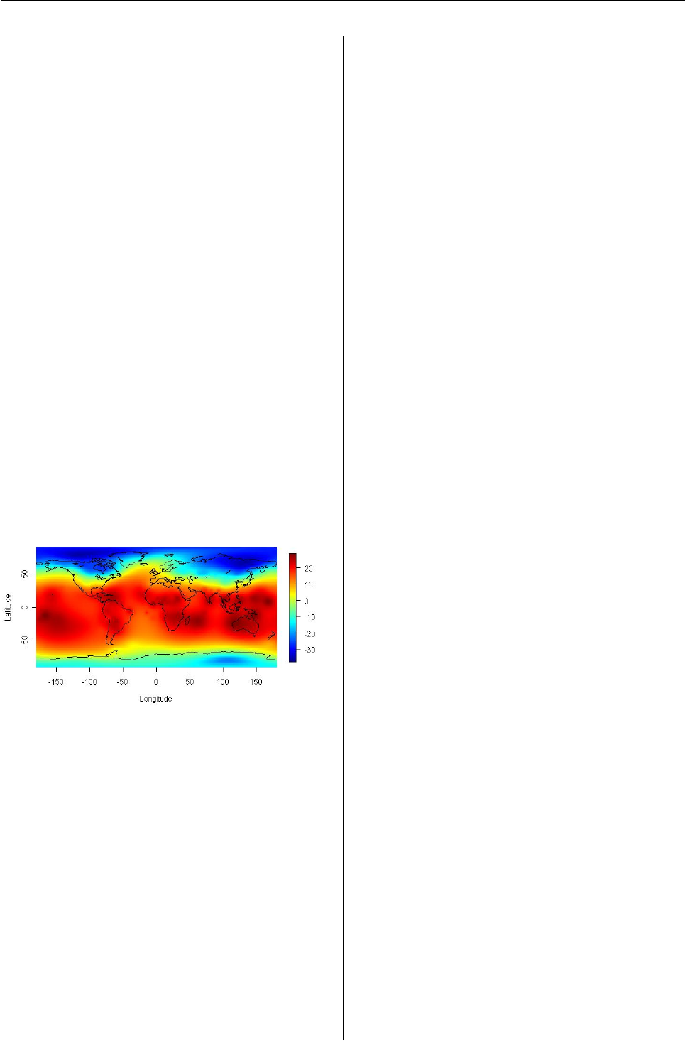
Before explaining the algorithm in detail, we
first consider the average surface air tempera-
tures (in degrees Celsius) during the period from
December 1967 to February 1968 observed at
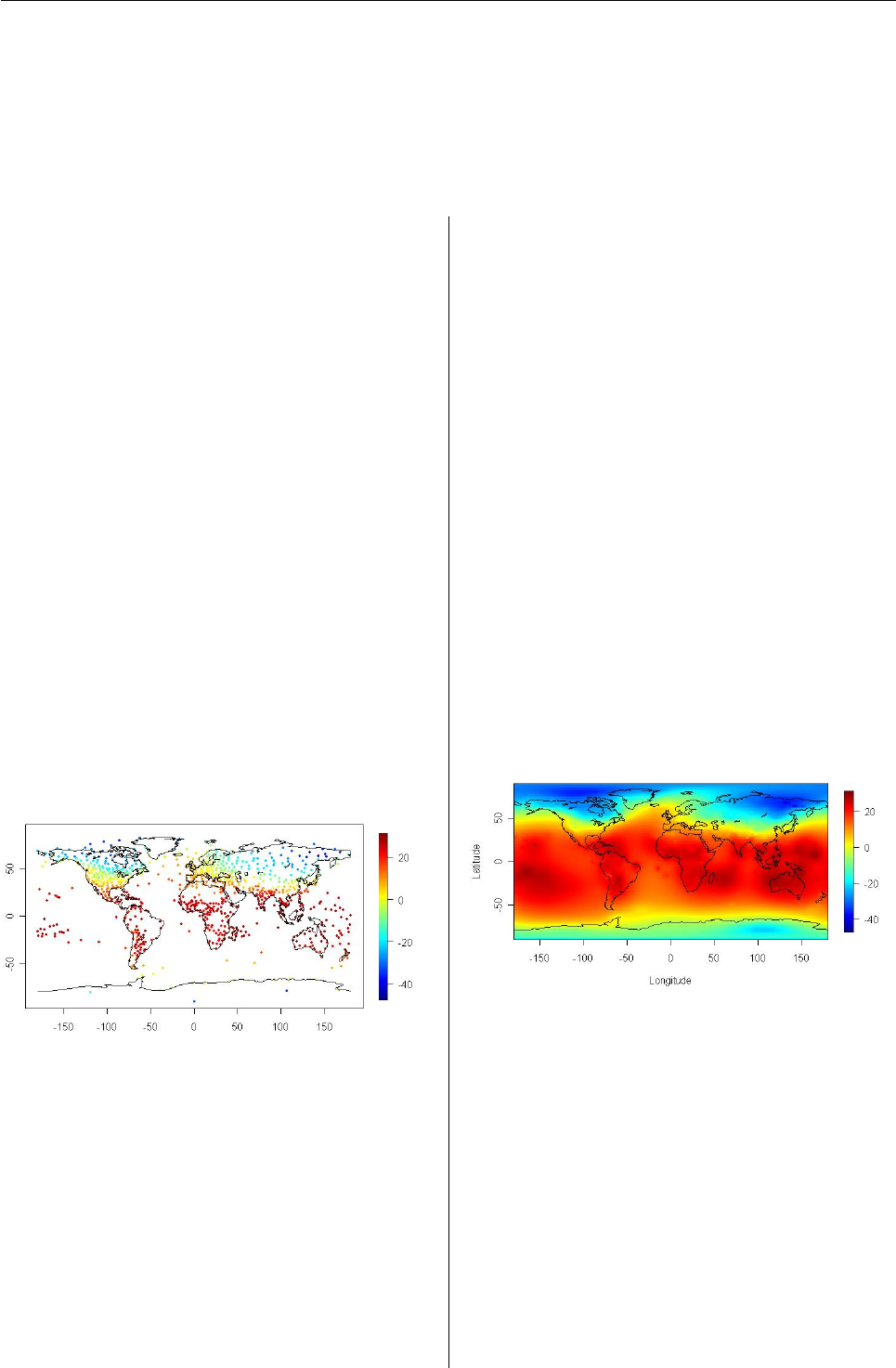
939 weather stations, as illustrated in Figure 1.
Figure 1: Average surface air temperatures observed
at 939 weather stations during the years 1967-1968.
In the SpherWave package, the data are obtained
by
> library("SpherWave")
> ### Temperature data from year 1961 to 1990
> ### list of year, grid, observation
> data("temperature")
> temp67 <- temperature$obs[temperature$year==1967]
> latlon <-
+ temperature$latlon[temperature$year==1967, ]
and Figure 1is plotted by the following code.
> sw.plot(z=temp67, latlon=latlon, type="obs",
+ xlab="", ylab="")
Similarly, various signals such as meteorological
or geophysical signal in nature can be measured at
scattered and unevenly distributed locations. How-
ever, inferring the substantial effect of such signals
at an arbitrary location on the globe is a crucial task.
The first objective of using SWs is to estimate the sig-
nal at an arbitrary location on the globe by extrap-
olating the scattered observations. An example is
the representation in Figure 2, which is obtained by
extrapolating the observations in Figure 1. This re-
sult can be obtained by simply executing the function
sbf(). The details of its arguments will be presented
later.
> netlab <- network.design(latlon=latlon,
+ method="ModifyGottlemann", type="regular", x=5)
> eta <- eta.comp(netlab)$eta
> out.pls <- sbf(obs=temp67, latlon=latlon,
+ netlab=netlab, eta=eta, method="pls",
+ grid.size=c(100, 200), lambda=0.8)
> sw.plot(out.pls, type="field", xlab="Longitude",
+ ylab="Latitude")
Figure 2: An extrapolation for the observations in
Figure 1.
Note that the representation in Figure 2has inher-
ent multiscale characteristics, which originate from
the observations in Figure 1. For example, observe
the global cold patterns near the north pole with lo-
cal anomalies of the extreme cold in the central Cana-
dian shield. Thus, classical methods such as spheri-
cal harmonics or smoothing splines are not very effi-
cient in representing temperature data since they do
not capture local properties. It is important to de-
tect and explain local activities and variabilities as
well as global trends. The second objective of using
SWs is to decompose the signal properly according
to spatial scales so as to capture the various activities
R News ISSN 1609-3631

Vol. 7/3, December 2007 3
of fields. Finally, SWs can be employed in develop-
ing a procedure to denoise the observations that are
corrupted by noise. This article illustrates these pro-
cedures through an analysis of temperature data. In
summary, the aim of this article is to explain how the
SpherWave package is used in the following:
1) estimating the temperature field T(x)for an ar-
bitrary location xon the globe, given the scat-
tered observations yi,i=1, . . . , n, from the
model
yi=T(xi) + i,i=1, 2, . . . , n, (1)
where xidenote the locations of observations
on the globe and iare the measurement errors;
2) decomposing the signal by the multiresolution
analysis; and
3) obtaining a SW estimator using a thresholding
approach.
As will be described in detail later, the multiresolu-
tion analysis and SW estimators of the temperature
field can be derived from the procedure termed mul-
tiscale spherical basis function (SBF) representation.
Theory
In this section, we summarize the SWs proposed
by Li (1999) and its statistical applications proposed
by Oh and Li (2004) for an understanding of the
methodology and promoting the usage of the Spher-
Wave package.
Narcowich and Ward (1996) proposed a method
to construct SWs for scattered data on a sphere. They
proposed an SBF representation, which is a linear
combination of localized SBFs centered at the loca-
tions of the observations. However, the Narcowich-
Ward method suffers from a serious problem: the
SWs have a constant spatial scale regardless of the
intended multiscale decomposition. Li (1999) in-
troduced a new multiscale SW method that over-
comes the single-scale problem of the Narcowich-
Ward method and truly represents spherical fields
with multiscale structure.
When a network of nobservation stations N1:=
{xi}n
i=1is given, we can construct nested networks
N1⊃ N2⊃ ··· ⊃ NLfor some L. We re-index
the subscript of the location xiso that xli belongs to
Nl\ Nl+1={xli}Ml
i=1(l=1, ··· ,L;NL+1:=∅),
and use the convention that the scale moves from the
finest to the smoothest as the resolution level index
lincreases. The general principle of the multiscale
SBF representation proposed by Li (1999) is to em-
ploy linear combinations of SBFs with various scale
parameters to approximate the underlying field T(x)
of the model in equation (1). That is, for some L
T1(x) =
L
∑
l=1
Ml
∑
i=1
βliφηl(θ(x,xli)), (2)
where φηldenotes SBFs with a scale parameter ηl
and θ(x,xi)is the cosine of the angle between two
location xand xirepresented by the spherical co-
ordinate system. Thus geodetic distance is used for
spherical wavelets, which is desirable for the data on
the globe. An SBF φ(θ(x,xi)) for a given spherical
location xiis a spherical function of xthat peaks at
x=xiand decays in magnitude as xmoves away
from xi. A typical example is the Poisson kernel used
by Narcowich and Ward (1996) and Li (1999).
Now, let us describe a multiresolution analy-
sis procedure that decomposes the SBF representa-
tion (2) into global and local components. As will be
seen later, the networks Nlcan be arranged in such a
manner that the sparseness of stations in Nlincreases
as the index lincreases, and the bandwidth of φcan
also be chosen to increase with lto compensate for
the sparseness of stations in Nl. By this construction,
the index lbecomes a true scale parameter. Suppose
Tl,l=1, . . . , L, belongs to the linear subspace of all
SBFs that have scales greater than or equal to l. Then
Tlcan be decomposed as
Tl(x) = Tl+1(x) + Dl(x),
where Tl+1is the projection of Tlonto the linear sub-
space of SBFs on the networks Nl+1, and Dlis the or-
thogonal complement of Tl. Note that the field Dlcan
be interpreted as the field containing the local infor-
mation. This local information cannot be explained
by the field Tl+1which only contains the global trend
extrapolated from the coarser network Nl+1. There-
fore, Tl+1is called the global component of scale l+1
and Dlis called the local component of scale l. Thus,
the field T1in its SBF representation (equation (2))
can be successively decomposed as
T1(x) = TL(x) +
L−1
∑
l=1
Dl(x). (3)
In general wavelet terminology, the coefficients of TL
and Dlof the SW representation in equation (3) can
be considered as the smooth coefficients and detailed
coefficients of scale l, respectively.
The extrapolated field may not be a stable esti-
mator of the underlying field Tbecause of the noise
in the data. To overcome this problem, Oh and Li
(2004) propose the use of thresholding approach pi-
oneered by Donoho and Johnstone (1994). Typical
thresholding types are hard and soft thresholding.
By hard thresholding, small SW coefficients, consid-
ered as originating from the zero-mean noise, are set
to zero while the other coefficients, considered as
originating from the signal, are left unchanged. In
soft thresholding, not only are the small coefficients
set to zero but the large coefficients are also shrunk
toward zero, based on the assumption that they are
corrupted by additive noise. A reconstruction from
these coefficients yields the SW estimators.
R News ISSN 1609-3631
Vol. 7/3, December 2007 4
Network design and bandwidth se-
lection
As mentioned previously, a judiciously designed net-
work Nland properly chosen bandwidths for the
SBFs are required for a stable multiscale SBF repre-
sentation.
In the SpherWave package, we design a network
for the observations in Figure 1as
> netlab <- network.design(latlon=latlon,
+ method="ModifyGottlemann", type="regular", x=5)
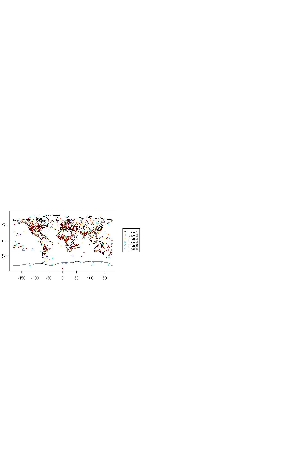
> sw.plot(z=netlab, latlon=latlon, type="network",
+ xlab="", ylab="", cex=0.6)
We then obtain the network in Figure 3, which con-
sists of 6 subnetworks.
> table(netlab)
netlab
123456
686 104 72 44 25 8
Note that the number of stations at each level de-
creases as the resolution level increases. The most
detailed subnetwork 1 consists of 686 stations while
the coarsest subnetwork 6 consists of 8 stations.
Figure 3: Network Design
The network design in the SpherWave package
depends only on the location of the data and the tem-
plate grid, which is predetermined without consid-
ering geophysical information. To be specific, given
a template grid and a radius for the spherical cap,
we can design a network satisfying two conditions
for stations: 1) choose the stations closest to the tem-
plate grid so that the stations could be distributed as
uniformly as possible over the sphere, and 2) select
stations between consecutive resolution levels so that
the resulting stations between two levels are not too
close for the minimum radius of the spherical cap.
This scheme ensures that the density of Nldecreases
as the resolution level index lincreases. The func-
tion network.design() is performed by the follow-
ing parameters: latlon denotes the matrix of grid
points (latitude, longitude) of the observation loca-
tions. The SpherWave package uses the following
convention. Latitude is the angular distance in de-
grees of a point north or south of the equator and
North and South are represented by "+" and "–" signs,
respectively. Longitude is the angular distance in de-
grees of a point east or west of the prime (Green-
wich) meridian, and East and West are represented
by "+" and "–" signs, respectively. method has four
options for making a template grid – "Gottlemann",
"ModifyGottlemann","Oh", and "cover". For de-
tails of the first three methods, see Oh and Kim
(2007). "cover" is the option for utilizing the func-
tion cover.design() in the package fields. Only
when using the method "cover", provide nlevel,
which denotes a vector of the number of observa-
tions in each level, starting from the resolution level
1. type denotes the type of template grid; it is spec-
ified as either "regular" or "reduce". The option
"reduce" is designed to overcome the problem of a
regular grid, which produces a strong concentration
of points near the poles. The parameter xis the min-
imum radius of the spherical cap.
Since the index lis a scale index in the result-
ing multiscale analysis, as lincreases, the density
of Nldecreases and the bandwidth of φηlincreases.
The bandwidths can be supplied by the user. Alter-
natively, the SpherWave package provides its own
function for the automatic choosing of the band-
widths. For example, the bandwidths for the net-
work design using "ModifyGottlemann" can be cho-
sen by the following procedure.
> eta <- eta.comp(netlab)$eta
Note that ηcan be considered as a spatial parame-
ter of the SBF induced by the Poisson kernel: the SBF
has a large bandwidth when ηis small, while a large
ηproduces an SBF with a small bandwidth. netlab
denotes the index vector of the subnetwork level. As-
suming that the stations are distributed equally over
the sphere, we can easily find how many stations are
required in order to cover the entire sphere with a
fixed spatial parameter ηand, conversely, how large
a bandwidth for the SBFs is required to cover the en-
tire sphere when the number of stations are given.
The function eta.comp() utilizes this observation.
Multiscale SBF representation
Once the network and bandwidths are decided, the
multiscale SBF representation of equation (2) can be
implemented by the function sbf(). This function is
controlled by the following arguments.
•obs : the vector of observations
•latlon : the matrix of the grid points of obser-
vation sites in degree
•netlab : the index vector of the subnetwork
level
•eta : the vector of spatial parameters according
to the resolution level
R News ISSN 1609-3631
Vol. 7/3, December 2007 5
•method : the method for the calculation of coef-
ficients of equation (2), "ls" or "pls"
•approx :approx = TRUE will use the approxi-
mation matrix
•grid.size : the size of the grid (latitude, longi-
tude) of the extrapolation site
•lambda : smoothing parameter for method =
"pls".
method has two options – "ls" and "pls".method =
"ls" calculates the coefficients by the least squares
method, and method = "pls" uses the penalized
least squares method. Thus, the smoothing param-
eter lambda is required only when using method =
"pls".approx = TRUE implies that we obtain the co-
efficients using m(<n)selected sites from among the
nobservation sites, while the interpolation method
(approx = FALSE) uses all the observation sites. The
function sbf() returns an object of class "sbf". See
Oh and Kim (2006) for details. The following code
performs the approximate multiscale SBF represen-
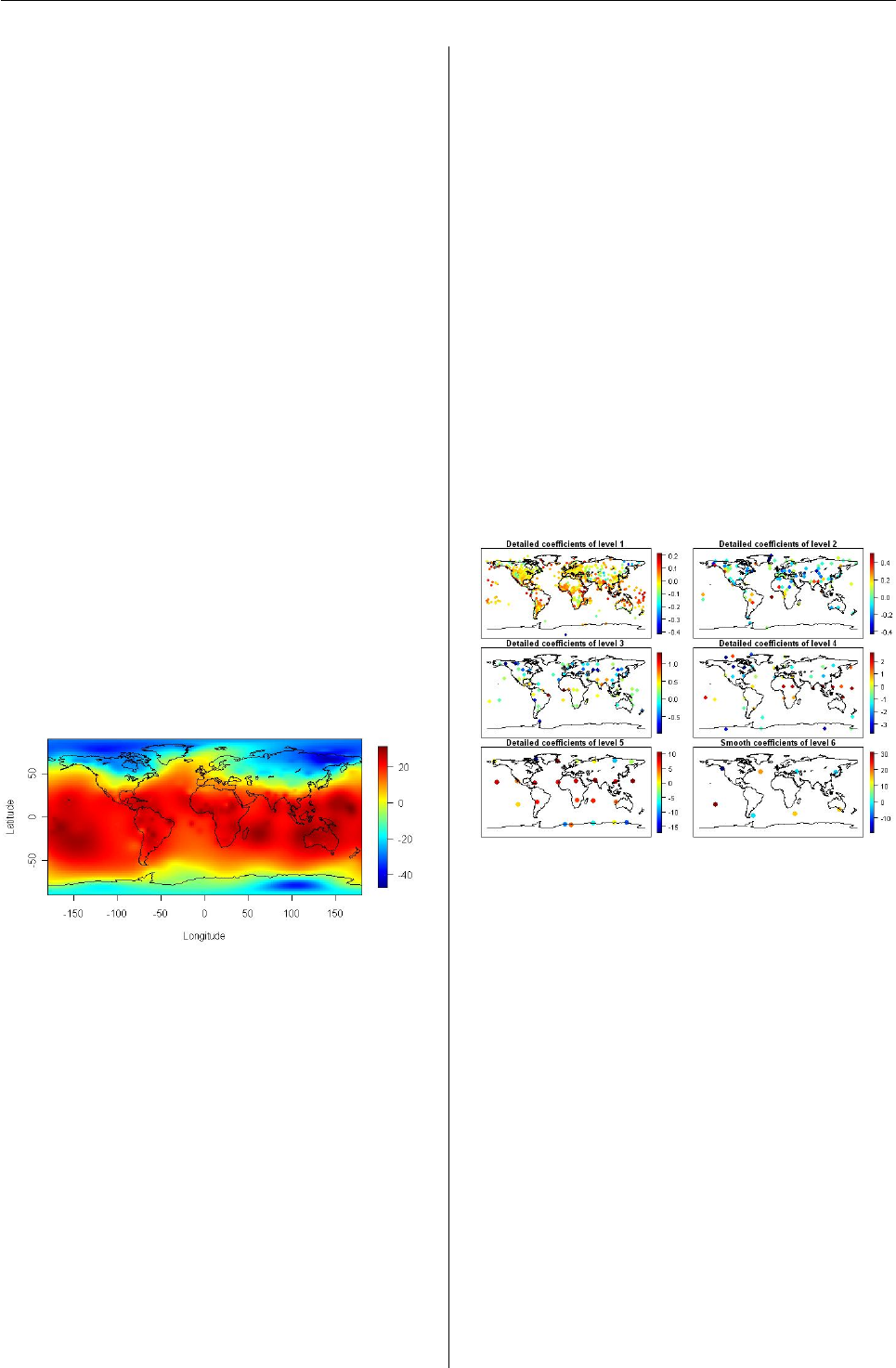
tation by the least squares method, and Figure 4il-
lustrates results.
> out.ls <- sbf(obs=temp67, latlon=latlon,
+ netlab=netlab, eta=eta,
+ method="ls", approx=TRUE, grid.size=c(100, 200))
> sw.plot(out.ls, type="field",
+ xlab="Longitude", ylab="Latitude")
Figure 4: An approximate multiscale SBF representa-
tion for the observations in Figure 1.
As can be observed, the result in Figure 4is differ-
ent from that in Figure 2, which is performed by the
penalized least squares interpolation method. Note
that the value of the smoothing parameter lambda
used in Figure 2is chosen by generalized cross-
validation. For the implementation, run the follow-
ing procedure.
> lam <- seq(0.1, 0.9, length=9)
> gcv <- NULL
> for(i in 1:length(lam))
+ gcv <- c(gcv, gcv.lambda(obs=temp67,
+ latlon=latlon, netlab=netlab, eta=eta,
+ lambda=lam[i])$gcv)
> lam[gcv == min(gcv)]
[1] 0.8
Multiresolution analysis
Here, we explain how to decompose the multiscale
SBF representation into the global field of scale l+1,
Tl+1(x), and the local field of scale l,Dl(x). Use the
function swd() for this operation.
> out.dpls <- swd(out.pls)
The function swd() takes an object of class "sbf",
performs decomposition with multiscale SWs, and
returns an object of class "swd" (spherical wavelet
decomposition). Refer to Oh and Kim (2006) for
the detailed list of an object of class "swd". Among
the components in the list are the smooth coeffi-
cients and detailed coefficients of the SW representa-
tion. The computed coefficients and decomposition
results can be displayed by the function sw.plot()
as shown in Figure 5and Figure 6.
> sw.plot(out.dpls, type="swcoeff", pch=19,
+ cex=1.1)
> sw.plot(out.dpls, type="decom")
Figure 5: Plot of SW smooth coefficients and detailed
coefficients at different levels l=1, 2, 3, 4, 5.
Spherical wavelet estimators
We now discuss the statistical techniques of smooth-
ing based on SWs. The theoretical background is
based on the works of Donoho and Johnstone (1994)
and Oh and Li (2004). The thresholding function
swthresh() for SW estimators is
> swthresh(swd, policy, by.level, type, nthresh,
+ value=0.1, Q=0.05)
This function swthresh() thresholds or shrinks
detailed coefficients stored in an swd object, and
returns the thresholded detailed coefficients in a
modified swd object. The thresh.info list of an
swd object has the thresholding information. The
available policies are "universal","sure","fdr",
"probability", and "Lorentz". For the first three
thresholding policies, see Donoho and Johnstone
(1994,1995) and Abramovich and Benjamini (1996).
R News ISSN 1609-3631
Vol. 7/3, December 2007 6
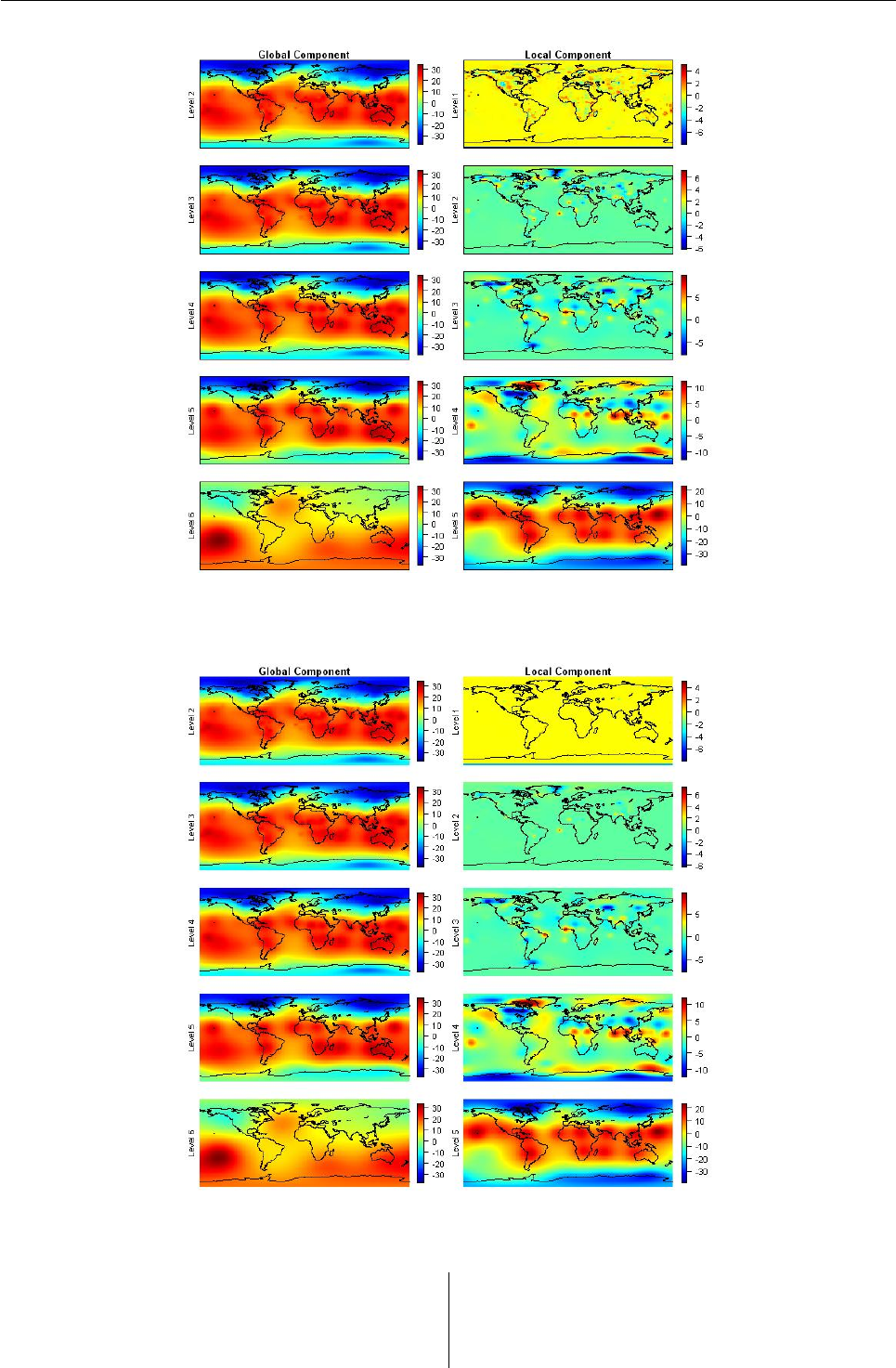
Figure 6: Multiresolution analysis of the multiscale SBF representation T1(x)in Figure 2. Note that the field
T1(x)is decomposed as T1(x) = T6(x) + D1(x) + D2(x) + D3(x) + D4(x) + D5(x).
Figure 7: Thresholding result obtained by using the FDR policy
Qspecifies the false discovery rate (FDR) of the FDR
policy. policy = "probability" performs thresh-
olding using the user supplied threshold represented
by a quantile value. In this case, the quantile value
is supplied by value. The Lorentz policy takes
the thresholding parameter λas the mean sum of
squares of the detailed coefficients.
R News ISSN 1609-3631
Vol. 7/3, December 2007 7
by.level controls the methods estimating noise
variance. In practice, we assume that the noise
variances are globally the same or level-dependent.
by.level = TRUE estimates the noise variance at
each level l. Only for the universal, Lorentz, and
FDR policies, a level-dependent thresholding is pro-
vided. The two approaches, hard and soft threshold-
ing can be specified by type. In addition, the Lorentz
type q(t,λ):=sign(t)√t2−λ2I(|t|>λ)is supplied.
Note that only soft type thresholding is appropriate
for the SURE policy. By providing the number of res-
olution levels to be thresholded by nthresh, we can
also specify the truncation parameter.
The following procedures perform thresholding
using the FDR policy and the reconstruction. Com-
paring Figure 6with Figure 7, we can observe that
the local components of resolution level 1, 2, and 3
of Figure 7are shrunk so that its reconstruction (Fig-
ure 8) illustrates a smoothed temperature field. For
the reconstruction, the function swr() is used on an
object of class "swd".
> ### Thresholding
> out.fdr <- swthresh(out.dpls, policy="fdr",
+ by.level=FALSE, type="soft", nthresh=3, Q=0.05)
> sw.plot(out.fdr, type = "decom")
> ### Reconstruction
> out.reconfdr <- swr(out.fdr)
> sw.plot(z=out.reconfdr, type="recon",
+ xlab="Longitude", ylab="Latitude")
Figure 8: Reconstruction
We repeatedly use sw.plot() for display. To
summarize its usage, the function sw.plot() dis-
plays the observation, network design, SBF rep-
resentation, SW coefficients, decomposition result
or reconstruction result, as specified by type =
"obs","network","field","swcoeff","decom" or
"recon", respectively. Either argument sw or zspec-
ifies the object to be plotted. zis used for obser-
vations, subnetwork labels and reconstruction result
and sw is used for an sbf or swd object.
Conclusion remarks
We introduce SpherWave, an R package implement-
ing SWs. In this article, we analyze surface air tem-
perature data using SpherWave and obtain mean-
ingful and promising results; furthermore provide a
step-by-step tutorial introduction for wide potential
applicability of SWs. Our hope is that SpherWave
makes SW methodology practical, and encourages
interested readers to apply the SWs for real world
applications.
Acknowledgements
This work was supported by the SRC/ERC program
of MOST/KOSEF (R11-2000-073-00000).
Bibliography
F. Abramovich and Y. Benjamini. Adaptive thresh-
olding of wavelet coefficients. Computational Statis-
tics & Data Analysis, 22(4):351–361, 1996.
D. L. Donoho and I. M. Johnstone. Ideal spatial adap-
tation by wavelet shrinkage. Biometrika, 81(3):425–
455, 1994.
D. L. Donoho and I. M. Johnstone. Adapting to un-
known smoothness via wavelet shrinkage Journal
of the American Statistical Association, 90(432):1200–
1224, 1995.
T-H. Li. Multiscale representation and analysis of
spherical data by spherical wavelets. SIAM Jour-
nal of Scientific Computing, 21(3):924–953, 1999.
F. J. Narcowich and J. D. Ward. Nonstationary
wavelets on the m-sphere for scattered data. Ap-
plied and Computational Harmonic Analysis, 3(4):
324–336, 1996.
H-S. Oh and D. Kim. SpherWave: Spherical
wavelets and SW-based spatially adaptive meth-
ods, 2006. URL http://CRAN.R-project.org/
src/contrib/Descriptions/SpherWave.html.
H-S. Oh and D. Kim. Network design and pre-
processing for multi-Scale spherical basis function
representation. Joournal of the Korean Statistical So-
ciety, 36(2):209–228, 2007.
H-S. Oh and T-H. Li. Estimation of global
temperature fields from scattered observations
by a spherical-wavelet-based spatially adaptive
method. Journal of the Royal Statistical Society B, 66
(1):221–238, 2004.
Hee-Seok Oh
Seoul National University, Korea
heeseok@stats.snu.ac.kr
Donghoh Kim
Sejong University, Korea
donghohkim@sejong.ac.kr
R News ISSN 1609-3631

Vol. 7/3, December 2007 8
Diving Behaviour Analysis in R
An Introduction to the diveMove Package
by Sebastián P. Luque
Introduction
Remarkable developments in technology for elec-
tronic data collection and archival have increased re-
searchers’ ability to study the behaviour of aquatic
animals while reducing the effort involved and im-
pact on study animals. For example, interest in the
study of diving behaviour led to the development of
minute time-depth recorders (TDRs) that can collect
more than 15 MB of data on depth, velocity, light lev-
els, and other parameters as animals move through
their habitat. Consequently, extracting useful infor-
mation from TDRs has become a time-consuming and
tedious task. Therefore, there is an increasing need
for efficient software to automate these tasks, with-
out compromising the freedom to control critical as-
pects of the procedure.
There are currently several programs available
for analyzing TDR data to study diving behaviour.
The large volume of peer-reviewed literature based
on results from these programs attests to their use-
fulness. However, none of them are in the free soft-
ware domain, to the best of my knowledge, with all
the disadvantages it entails. Therefore, the main mo-
tivation for writing diveMove was to provide an R
package for diving behaviour analysis allowing for
more flexibility and access to intermediate calcula-
tions. The advantage of this approach is that re-
searchers have all the elements they need at their dis-
posal to take the analyses beyond the standard infor-
mation returned by the program.
The purpose of this article is to outline the func-
tionality of diveMove, demonstrating its most useful
features through an example of a typical diving be-
haviour analysis session. Further information can be
obtained by reading the vignette that is included in
the package (vignette("diveMove")) which is cur-
rently under development, but already shows ba-
sic usage of its main functions. diveMove is avail-
able from CRAN, so it can easily be installed using
install.packages().
The diveMove Package
diveMove offers functions to perform the following
tasks:
• Identification of wet vs. dry periods, defined
by consecutive readings with or without depth
measurements, respectively, lasting more than
a user-defined threshold. Depending on the
sampling protocol programmed in the instru-
ment, these correspond to wet vs. dry periods,
respectively. Each period is individually iden-
tified for later retrieval.
• Calibration of depth readings, which is needed
to correct for shifts in the pressure transducer.
This can be done using a tcltk graphical user in-
terface (GUI) for chosen periods in the record,
or by providing a value determined a priori for
shifting all depth readings.
• Identification of individual dives, with their
different phases (descent, bottom, and ascent),
using various criteria provided by the user.
Again, each individual dive and dive phase is
uniquely identified for future retrieval.
• Calibration of speed readings using the
method described by Blackwell et al. (1999),
providing a unique calibration for each animal
and deployment. Arguments are provided to
control the calibration based on given criteria.
Diagnostic plots can be produced to assess the
quality of the calibration.
• Summary of time budgets for wet vs. dry peri-
ods.
• Dive statistics for each dive, including maxi-
mum depth, dive duration, bottom time, post-
dive duration, and summaries for each dive
phases, among other standard dive statistics.
•tcltk plots to conveniently visualize the entire
dive record, allowing for zooming and panning
across the record. Methods are provided to in-
clude the information obtained in the points
above, allowing the user to quickly identify
what part of the record is being displayed (pe-
riod, dive, dive phase).
Additional features are included to aid in analy-
sis of movement and location data, which are often
collected concurrently with TDR data. They include
calculation of distance and speed between successive
locations, and filtering of erroneous locations using
various methods. However, diveMove is primarily a
diving behaviour analysis package, and other pack-
ages are available which provide more extensive an-
imal movement analysis features (e.g. trip).
The tasks described above are possible thanks to
the implementation of three formal S4 classes to rep-
resent TDR data. Classes TDR and TDRspeed are used
to represent data from TDRs with and without speed
sensor readings, respectively. The latter class inher-
its from the former, and other concurrent data can
be included with either of these objects. A third for-
mal class (TDRcalibrate) is used to represent data
R News ISSN 1609-3631
Vol. 7/3, December 2007 9
obtained during the various intermediate steps de-
scribed above. This structure greatly facilitates the
retrieval of useful information during analyses.
Data Preparation
TDR data are essentially a time-series of depth read-
ings, possibly with other concurrent parameters, typ-
ically taken regularly at a user-defined interval. De-
pending on the instrument and manufacturer, how-
ever, the files obtained may contain various errors,
such as repeated lines, missing sampling intervals,
and invalid data. These errors are better dealt with
using tools other than R, such as awk and its variants,
because such stream editors use much less memory
than R for this type of problems, especially with the
typically large files obtained from TDRs. Therefore,
diveMove currently makes no attempt to fix these
errors. Validity checks for the TDR classes, however,
do test for time series being in increasing order.
Most TDR manufacturers provide tools for down-
loading the data from their TDRs, but often in a pro-
prietary format. Fortunately, some of these man-
ufacturers also offer software to convert the files
from their proprietary format into a portable for-
mat, such as comma-separated-values (csv). At least
one of these formats can easily be understood by R,
using standard functions, such as read.table() or
read.csv().diveMove provides constructors for its
two main formal classes to read data from files in one
of these formats, or from simple data frames.
How to Represent TDR Data?
TDR is the simplest class of objects used to represent
TDR data in diveMove. This class, and its TDRspeed
subclass, stores information on the source file for the
data, the sampling interval, the time and depth read-
ings, and an optional data frame containing addi-
tional parameters measured concurrently. The only
difference between TDR and TDRspeed objects is that
the latter ensures the presence of a speed vector
in the data frame with concurrent measurements.
These classes have the following slots:
file: character,
dtime: numeric,
time: POSIXct,
depth: numeric,
concurrentData: data.frame
Once the TDR data files are free of errors and in a
portable format, they can be read into a data frame,
using e.g.:
R> ff <- system.file(file.path("data",
+ "dives.csv"), package = "diveMove")
R> tdrXcsv <- read.csv(ff)
and then put into one of the TDR classes using the
function createTDR(). Note, however, that this ap-
proach requires knowledge of the sampling interval
and making sure that the data for each slot are valid:
R> library("diveMove")
R> ddtt.str <- paste(tdrXcsv$date,
+ tdrXcsv$time)
R> ddtt <- strptime(ddtt.str,
+ format = "%d/%m/%Y %H:%M:%S")
R> time.posixct <- as.POSIXct(ddtt,
+ tz = "GMT")
R> tdrX <- createTDR(time = time.posixct,
+ depth = tdrXcsv$depth,
+ concurrentData = tdrXcsv[,
+ -c(1:3)], dtime = 5,
+ file = ff)
R> tdrX <- createTDR(time = time.posixct,
+ depth = tdrXcsv$depth,
+ concurrentData = tdrXcsv[,
+ -c(1:3)], dtime = 5,
+ file = ff, speed = TRUE)
If the files are in *.csv format, these steps can be
automated using the readTDR() function to create an
object of one of the formal classes representing TDR
data (TDRspeed in this case), and immediately begin
using the methods provided:
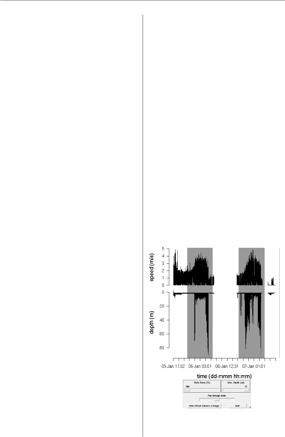
R> tdrX <- readTDR(ff, speed = TRUE)
R> plotTDR(tdrX)
Figure 1: The plotTDR() method for TDR objects pro-
duces an interactive plot of the data, allowing for
zooming and panning.
R News ISSN 1609-3631

Vol. 7/3, December 2007 10
Several arguments for readTDR() allow mapping
of data from the source file to the different slots in
diveMove’s classes, the time format in the input and
the time zone attribute to use for the time readings.
Various methods are available for displaying
TDR objects, including show(), which provides an
informative summary of the data in the object, ex-
tractors and replacement methods for all the slots.
There is a plotTDR() method (Figure 1) for both TDR
and TDRspeed objects. The interact argument al-
lows for suppression of the tcltk interface. Informa-
tion on these methods is available from methods?TDR.
TDR objects can easily be coerced to data frame
(as.data.frame() method), without losing informa-
tion from any of the slots. TDR objects can addition-
ally be coerced to TDRspeed, whenever it makes sense
to do so, using an as.TDRspeed() method.
Identification of Activities at Various
Scales
One the first steps of dive analysis involves correct-
ing depth for shifts in the pressure transducer, so
that surface readings correspond to zero. Such shifts
are usually constant for an entire deployment period,
but there are cases where the shifts vary within a par-
ticular deployment, so shifts remain difficult to de-
tect and dives are often missed. Therefore, a visual
examination of the data is often the only way to de-
tect the location and magnitude of the shifts. Visual
adjustment for shifts in depth readings is tedious,
but has many advantages which may save time dur-
ing later stages of analysis. These advantages in-
clude increased understanding of the data, and early
detection of obvious problems in the records, such
as instrument malfunction during certain intervals,
which should be excluded from analysis.
Zero-offset correction (ZOC) is done using the
function zoc(). However, a more efficient method of
doing this is with function calibrateDepth(), which
takes a TDR object to perform three basic tasks. The
first is to ZOC the data, optionally using the tcltk
package to be able to do it interactively:
R> dcalib <- calibrateDepth(tdrX)
This command brings up a plot with tcltk con-
trols allowing to zoom in and out, as well as pan
across the data, and adjust the depth scale. Thus,
an appropriate time window with a unique surface
depth value can be displayed. This allows the user
to select a depth scale that is small enough to resolve
the surface value using the mouse. Clicking on the
ZOC button waits for two clicks: i) the coordinates of
the first click define the starting time for the window
to be ZOC’ed, and the depth corresponding to the
surface, ii) the second click defines the end time for
the window (i.e. only the x coordinate has any mean-
ing). This procedure can be repeated as many times
as needed. If there is any overlap between time win-
dows, then the last one prevails. However, if the off-
set is known a priori, there is no need to go through
all this procedure, and the value can be provided as
the argument offset to calibrateDepth(). For ex-
ample, preliminary inspection of object tdrX would
have revealed a 3 m offset, and we could have simply
called (without plotting):
R> dcalib <- calibrateDepth(tdrX,
+ offset = 3)
Once depth has been ZOC’ed, the second step
calibrateDepth() will perform is identify dry and
wet periods in the record. Wet periods are those
with depth readings, dry periods are those without
them. However, records may have aberrant miss-
ing depth that should not define dry periods, as they
are usually of very short duration1. Likewise, there
may be periods of wet activity that are too short to
be compared with other wet periods, and need to be
excluded from further analyses. These aspects can
be controlled by setting the arguments dry.thr and
wet.thr to appropriate values.
Finally, calibrateDepth() identifies all dives in
the record, according to a minimum depth criterion
given as its dive.thr argument. The value for this
criterion is typically determined by the resolution of
the instrument and the level of noise close to the sur-
face. Thus, dives are defined as departures from the
surface to maximal depths below dive.thr and the
subsequent return to the surface. Each dive may sub-
sequently be referred to by an integer number indi-
cating its position in the time series.
Dive phases are also identified at this last stage.
Detection of dive phases is controlled by three ar-
guments: a critical quantile for rates of vertical de-
scent (descent.crit.q), a critical quantile for rates
of ascent (ascent.crit.q), and a proportion of max-
imum depth (wiggle.tol). The first two arguments
are used to define the rate of descent below which the
descent phase is deemed to have ended, and the rate
of ascent above which the ascent phases is deemed
to have started, respectively. The rates are obtained
from all successive rates of vertical movement from
the surface to the first (descent) and last (ascent) max-
imum dive depth. Only positive rates are considered
for the descent, and only negative rates are consid-
ered for the ascent. The purpose of this restriction is
to avoid having any reversals of direction or histere-
sis events resulting in phases determined exclusively
by those events. The wiggle.tol argument deter-
mines the proportion of maximum dive depth above
which wiggles are not allowed to terminate descent,
or below which they should be considered as part of
the bottom phase.
1They may result from animals resting at the surface of the water long enough to dry the sensors.
R News ISSN 1609-3631
Vol. 7/3, December 2007 11
A more refined call to calibrateDepth() for ob-
ject tdrX may be:
R> dcalib <- calibrateDepth(tdrX,
+ offset = 3, wet.thr = 70,
+ dry.thr = 3610, dive.thr = 4,
+ descent.crit.q = 0.1,
+ ascent.crit.q = 0.1, wiggle.tol = 0.8)
The result (value) of this function is an object of
class TDRcalibrate, where all the information ob-
tained during the tasks described above are stored.
How to Represent Calibrated TDR Data?
Objects of class TDRcalibrate contain the following
slots, which store information during the major pro-
cedures performed by calibrateDepth():
tdr: TDR. The object which was calibrated.
gross.activity: list. This list contains four com-
ponents with details on wet/dry activities de-
tected, such as start and end times, durations,
and identifiers and labels for each activity pe-
riod. Five activity categories are used for la-
belling each reading, indicating dry (L), wet
(W), underwater (U), diving (D), and brief wet
(Z) periods. However, underwater and diving
periods are collapsed into wet activity at this
stage (see below).
dive.activity: data.frame. This data frame contains
three components with details on the diving ac-
tivities detected, such as numeric vectors iden-
tifiying to which dive and post-dive interval
each reading belongs to, and a factor labelling
the activity each reading represents. Compared
to the gross.activity slot, the underwater
and diving periods are discerned here.
dive.phases: factor. This identifies each reading
with a particular dive phase. Thus, each read-
ing belongs to one of descent, descent/bottom,
bottom, bottom/ascent, and ascent phases. The
descent/bottom and bottom/ascent levels are
useful for readings which could not unambigu-
ously be assigned to one of the other levels.
dry.thr: numeric.
wet.thr: numeric.
dive.thr: numeric. These last three slots
store information given as arguments to
calibrateDepth(), documenting criteria used
during calibration.
speed.calib.coefs: numeric. If the object calibrated
was of class TDRspeed, then this is a vector of
length 2, with the intercept and the slope of the
speed calibration line (see below).
All the information contained in each of these
slots is easily accessible through extractor methods
for objects of this class (see class?TDRcalibrate). An
appropriate show() method is available to display a
short summary of such objects, including the number
of dry and wet periods identified, and the number of
dives detected.
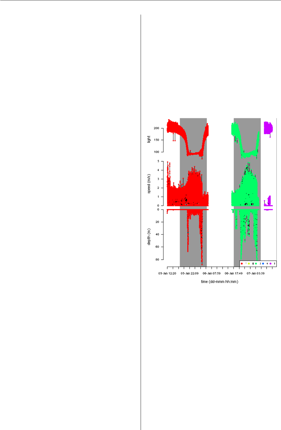
The TDRcalibrate plotTDR() method for these
objects allows visualizing the major wet/dry activ-
ities throughout the record (Figure 2):
R> plotTDR(dcalib, concurVars = "light",
+ concurVarTitles = c("speed (m/s)",
+ "light"), surface = TRUE)
Figure 2: The plotTDR() method for TDRcalibrate
objects displays information on the major activities
identified throughout the record (wet/dry periods
here).
The dcalib object contains a TDRspeed object in
its tdr slot, and speed is plotted by default in this
case. Additional measurements obtained concur-
rently can also be plotted using the concurVars ar-
gument. Titles for the depth axis and the concurrent
parameters use separate arguments; the former uses
ylab.depth, while the latter uses concurVarTitles.
Convenient default values for these are provided.
The surface argument controls whether post-dive
readings should be plotted; it is FALSE by default,
causing only dive readings to be plotted which saves
time plotting and re-plotting the data. All plot meth-
ods use the underlying plotTD() function, which has
other useful arguments that can be passed from these
methods.
R News ISSN 1609-3631
Vol. 7/3, December 2007 12
A more detailed view of the record can be ob-
tained by using a combination of the diveNo and the
labels arguments to this plotTDR() method. This
is useful if, for instance, closer inspection of certain
dives is needed. The following call displays a plot of
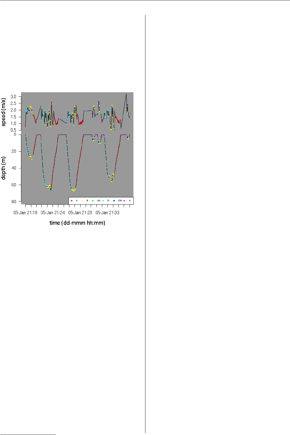
dives 2 through 8 (Figure 3):
R> plotTDR(dcalib, diveNo = 2:8,
+ labels = "dive.phase")
Figure 3: The plotTDR() method for TDRcalibrate
objects can also display information on the differ-
ent activities during each dive record (descent=D,
descent/bottom=DB, bottom=B, bottom/ascent=BA,
ascent=A, X=surface).
The labels argument allows the visualization
of the identified dive phases for all dives selected.
The same information can also be obtained with the
extractDive() method for TDRcalibrate objects:
R> extractDive(dcalib, diveNo = 2:8)
Other useful extractors include: getGAct() and
getDAct(). These methods extract the whole
gross.activity and dive.activity, respectively, if
given only the TDRcalibrate object, or a particu-
lar component of these slots, if supplied a string
with the name of the component. For example:
getGAct(dcalib, "trip.act") would retrieve the
factor identifying each reading with a wet/dry activ-
ity and getDAct(dcalib, "dive.activity") would
retrieve a more detailed factor with information on
whether the reading belongs to a dive or a brief
aquatic period.
With the information obtained during this cal-
ibration procedure, it is possible to calculate dive
statistics for each dive in the record.
Dive Summaries
A table providing summary statistics for each dive
can be obtained with the function diveStats() (Fig-
ure 4).
diveStats() returns a data frame with the final
summaries for each dive (Figure 4), providing the
following information:
• The time of start of the dive, the end of descent,
and the time when ascent began.
• The total duration of the dive, and that of the
descent, bottom, and ascent phases.
• The vertical distance covered during the de-
scent, the bottom (a measure of the level of
“wiggling”, i.e. up and down movement per-
formed during the bottom phase), and the ver-
tical distance covered during the ascent.
• The maximum depth attained.
• The duration of the post-dive interval.
A summary of time budgets of wet vs. dry pe-
riods can be obtained with timeBudget(), which
returns a data frame with the beginning and end-
ing times for each consecutive period (Figure 4).
It takes a TDRcalibrate object and another argu-
ment (ignoreZ) controlling whether aquatic periods
that were briefer than the user-specified threshold2
should be collapsed within the enclosing period of
dry activity.
These summaries are the primary goal of dive-
Move, but they form the basis from which more elab-
orate and customized analyses are possible, depend-
ing on the particular research problem. These in-
clude investigation of descent/ascent rates based on
the depth profiles, and bout structure analysis. Some
of these will be implemented in the future.
In the particular case of TDRspeed objects, how-
ever, it may be necessary to calibrate the speed read-
ings before calculating these statistics.
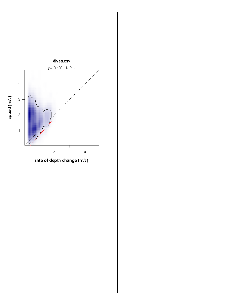
Calibrating Speed Sensor Readings
Calibration of speed sensor readings is performed
using the procedure described by Blackwell et al.
(1999). Briefly the method rests on the principle that
for any given rate of depth change, the lowest mea-
sured speeds correspond to the steepest descent an-
gles, i.e. vertical descent/ascent. In this case, mea-
sured speed and rate of depth change are expected to
be equal. Therefore, a line drawn through the bottom
edge of the distribution of observations in a plot of
measured speed vs. rate of depth change would pro-
vide a calibration line. The calibrated speeds, there-
fore, can be calculated by reverse estimation of rate
of depth change from the regression line.
2This corresponds to the value given as the wet.thr argument to calibrateDepth().
R News ISSN 1609-3631

Vol. 7/3, December 2007 13
R> tdrXSumm1 <- diveStats(dcalib)
R> names(tdrXSumm1)
[1] "begdesc" "enddesc" "begasc" "desctim"
[5] "botttim" "asctim" "descdist" "bottdist"
[9] "ascdist" "desc.tdist" "desc.mean.speed" "desc.angle"
[13] "bott.tdist" "bott.mean.speed" "asc.tdist" "asc.mean.speed"
[17] "asc.angle" "divetim" "maxdep" "postdive.dur"
[21] "postdive.tdist" "postdive.mean.speed"
R> tbudget <- timeBudget(dcalib, ignoreZ = TRUE)
R> head(tbudget, 4)
phaseno activity beg end
1 1 W 2002-01-05 11:32:00 2002-01-06 06:30:00
2 2 L 2002-01-06 06:30:05 2002-01-06 17:01:10
3 3 W 2002-01-06 17:01:15 2002-01-07 05:00:30
4 4 L 2002-01-07 05:00:35 2002-01-07 07:34:00
R> trip.labs <- stampDive(dcalib, ignoreZ = TRUE)
R> tdrXSumm2 <- data.frame(trip.labs, tdrXSumm1)
R> names(tdrXSumm2)
[1] "trip.no" "trip.type" "beg" "end"
[5] "begdesc" "enddesc" "begasc" "desctim"
[9] "botttim" "asctim" "descdist" "bottdist"
[13] "ascdist" "desc.tdist" "desc.mean.speed" "desc.angle"
[17] "bott.tdist" "bott.mean.speed" "asc.tdist" "asc.mean.speed"
[21] "asc.angle" "divetim" "maxdep" "postdive.dur"
[25] "postdive.tdist" "postdive.mean.speed"
Figure 4: Per-dive summaries can be obtained with functions diveStats(), and a summary of time budgets
with timeBudget().diveStats() takes a TDRcalibrate object as a single argument (object dcalib above, see
text for how it was created).
diveMove implements this procedure with func-
tion calibrateSpeed(). This function performs the
following tasks:
1. Subset the necessary data from the record.
By default only data corresponding to depth
changes >0 are included in the analysis, but
higher constraints can be imposed using the
zargument. A further argument limiting the
data to be used for calibration is bad, which is a
vector with the minimum rate of depth change
and minimum speed readings to include in the
calibration. By default, values >0 for both pa-
rameters are used.
2. Calculate the binned bivariate kernel den-
sity and extract the desired contour. Once
the proper data were obtained, a bivari-
ate normal kernel density grid is calculated
from the relationship between measured speed
and rate of depth change (using the KernS-
mooth package). The choice of bandwidths
for the binned kernel density is made us-
ing bw.nrd. The contour.level argument to
calibrateSpeed() controls which particular
contour should be extracted from the density
grid. Since the interest is in defining a regres-
sion line passing through the lower densities of
the grid, this value should be relatively low (it
is set to 0.1 by default).
3. Define the regression line passing through the
lower edge of the chosen contour. A quantile
regression through a chosen quantile is used
for this purpose. The quantile can be specified
using the tau argument, which is passed to the
rq() function in package quantreg.tau is set to
0.1 by default.
4. Finally, the speed readings in the TDR object are
calibrated.
As recognized by Blackwell et al. (1999), the ad-
vantage of this method is that it calibrates the instru-
ment based on the particular deployment conditions
(i.e. controls for effects of position of the instrument
on the animal, and size and shape of the instrument,
relative to the animal’s morphometry, among oth-
ers). However, it is possible to supply the coefficients
of this regression if they were estimated separately;
for instance, from an experiment. The argument
coefs can be used for this purpose, which is then as-
sumed to contain the intercept and the slope of the
line. calibrateSpeed() returns a TDRcalibrate ob-
ject, with calibrated speed readings included in its
tdr slot, and the coefficients used for calibration.
For instance, to calibrate speed readings using the
0.1 quantile regression of measured speed vs. rate
of depth change, based on the 0.1 contour of the bi-
variate kernel densities, and including only changes
in depth >1, measured speeds and rates of depth
R News ISSN 1609-3631
Vol. 7/3, December 2007 14
change >0:
R> vcalib <- calibrateSpeed(dcalib,
+ tau = 0.1, contour.level = 0.1,
+ z = 1, bad = c(0, 0),
+ cex.pts = 0.2)
Figure 5: The relationship between measured speed
and rate of depth change can be used to calibrate
speed readings. The line defining the calibration
for speed measurements passes through the bottom
edge of a chosen contour, extracted from a bivariate
kernel density grid.
This call produces the plot shown in Figure 5,
which can be suppressed by the use of the logical ar-
gument plot. Calibrating speed readings allows for
the meaningful interpretation of further parameters
calculated by diveStats(), whenever a TDRspeed
object was found in the TDRcalibrate object:
• The total distance travelled, mean speed, and
diving angle during the descent and ascent
phases of the dive.
• The total distance travelled and mean speed
during the bottom phase of the dive, and the
post-dive interval.
Summary
The diveMove package provides tools for analyz-
ing diving behaviour, including convenient methods
for the visualization of the typically large amounts
of data collected by TDRs. The package’s main
strengths are its ability to:
1. identify wet vs. dry periods,
2. calibrate depth readings,
3. identify individual dives and their phases,
4. summarize time budgets,
5. calibrate speed sensor readings, and
6. provide basic summaries for each dive identi-
fied in TDR records.
Formal S4 classes are supplied to efficiently store
TDR data and results from intermediate analysis,
making the retrieval of intermediate results readily
available for customized analysis. Development of
the package is ongoing, and feedback, bug reports,
or other comments from users are very welcome.
Acknowledgements
Many of the ideas implemented in this package de-
veloped over fruitful discussions with my mentors
John P.Y. Arnould, Christophe Guinet, and Edward
H. Miller. I would like to thank Laurent Dubroca
who wrote draft code for some of diveMove’s func-
tions. I am also greatly endebted to the regular con-
tributors to the R-help newsgroup who helped me
solve many problems during development.
Bibliography
S. Blackwell, C. Haverl, B. Le Boeuf, and D. Costa. A
method for calibrating swim-speed recorders. Ma-
rine Mammal Science, 15(3):894–905, 1999.
Sebastián P. Luque
Department of Biology, Memorial University
St. John’s, NL, Canada
sluque@mun.ca
R News ISSN 1609-3631

Vol. 7/3, December 2007 15
Very Large Numbers in R: Introducing
Package Brobdingnag
Logarithmic representation for floating-point
numbers
Robin K. S. Hankin
Introduction
The largest floating point number representable in
standard double precision arithmetic is a little un-
der 21024, or about 1.79 ×10308. This is too small for
some applications.
The R package Brobdingnag (Swift,1726) over-
comes this limit by representing a real number xus-
ing a double precision variable with value log |x|,
and a logical corresponding to x≥0; the S4 class
of such objects is brob. Complex numbers with large
absolute values (class glub) may be represented us-
ing a pair of brobs to represent the real and imagi-
nary components.
The package allows user-transparent access to
the large numbers allowed by Brobdingnagian arith-
metic. The package also includes a vignette—brob—
which documents the S4 methods used and includes
a step-by-step tutorial. The vignette also functions as
a “Hello, World!” example of S4 methods as used in
a simple package. It also includes a full description
of the glub class.
Package Brobdingnag in use
Most readers will be aware of a googol which is equal
to 10100:
> require(Brobdingnag)
> googol <- as.brob(10)^100
[1] +exp(230.26)
Note the coercion of double value 10 to an ob-
ject of class brob using function as.brob(): raising
this to the power 100 (also double) results in another
brob. The result is printed using exponential nota-
tion, which is convenient for very large numbers.
A googol is well within the capabilities of stan-
dard double precision arithmetic. Now, however,
suppose we wish to compute its factorial. Taking the
first term of Stirling’s series gives
> stirling <- function(n) {
+ n^n * exp(-n) * sqrt(2 * pi * n)
+ }
which then yields
> stirling(googol)
[1] +exp(2.2926e+102)
Note the transparent coercion to brob form
within function stirling().
It is also possible to represent numbers very close
to 1. Thus
> 2^(1/googol)
[1] +exp(6.9315e-101)
It is worth noting that if xhas an exact repre-
sentation in double precision, then exis exactly rep-
resentable using the system described here. Thus e
and e1000 are represented exactly.
Accuracy
For small numbers (that is, representable using stan-
dard double precision floating point arithmetic),
Brobdingnag suffers a slight loss of precision com-
pared to normal representation. Consider the follow-
ing function, whose return value for nonzero argu-
ments is algebraically zero:
f <- function(x){
as.numeric( (pi*x -3*x -(pi-3)*x)/x)
}
This function combines multiplication and addi-
tion; one might expect a logarithmic system such as
described here to have difficulty with it.
> f(1/7)
[1] 1.700029e-16
> f(as.brob(1/7))
[1] -1.886393e-16
This typical example shows that Brobdingnagian
numbers suffer a slight loss of precision for numbers
of moderate magnitude. This degradation increases
with the magnitude of the argument:
> f(1e+100)
[1] -2.185503e-16
> f(as.brob(1e+100))
[1] -3.219444e-14
Here, the brob’s accuracy is about two orders of
magnitude worse than double precision arithmetic:
this would be expected, as the number of bits re-
quired to specify the exponent goes as log log x.
Compare
R News ISSN 1609-3631

Vol. 7/3, December 2007 16
> f(as.brob(10)^1000)
[1] 1.931667e-13
showing a further degradation of precision. How-
ever, observe that conventional double precision
arithmetic cannot deal with numbers this big, and
the package returns about 12 correct significant fig-
ures.
A practical example
In the field of population dynamics, and espe-
cially the modelling of biodiversity (Hankin,2007b;
Hubbell,2001), complicated combinatorial formulae
often arise.
Etienne (2005), for example, considers a sample
of Nindividual organisms taken from some natural
population; the sample includes Sdistinct species,
and each individual is assigned a label in the range 1
to S. The sample comprises nimembers of species i,
with 1 ≤i≤Sand ∑ni=N. For a given sam-
ple D, Etienne defines, amongst other terms, K(D,A)
for 1 ≤A≤N−S+1 as
∑
{a1,...,aS|∑S
i=1ai=A}
S
∏
i=1
s(ni,ai)s(ai, 1)
s(ni, 1)(1)
where s(n,a)is the Stirling number of the second
kind (Abramowitz and Stegun,1965). The summa-
tion is over ai=1, . . . , niwith the restriction that
the aisum to A, as carried out by blockparts() of
the partitions package (Hankin,2006,2007a).
Taking an intermediate-sized dataset due to
Saunders1of only 5903 individuals—a relatively
small dataset in this context—the maximal element
of K(D,A)is about 1.435 ×101165. The accu-
racy of package Brobdingnag in this context may
be assessed by comparing it with that computed
by PARI/GP (Batut et al.,2000) with a work-
ing precision of 100 decimal places; the natural
logs of the two values are 2682.8725605988689
and 2682.87256059887 respectively: identical to 14
significant figures.
Conclusions
The Brobdingnag package allows representation
and manipulation of numbers larger than those cov-
ered by standard double precision arithmetic, al-
though accuracy is eroded for very large numbers.
This facility is useful in several contexts, including
combinatorial computations such as encountered in
theoretical modelling of biodiversity.
Acknowledgments
I would like to acknowledge the many stimulating
and helpful comments made by the R-help list over
the years.
Bibliography
M. Abramowitz and I. A. Stegun. Handbook of Mathe-
matical Functions. New York: Dover, 1965.
C. Batut, K. Belabas, D. Bernardi, H. Cohen,
and M. Olivier. User’s guide to pari/gp.
Technical Reference Manual, 2000. url:
http://www.parigp-home.de/.
R. S. Etienne. A new sampling formula for neutral
biodiversity. Ecology Letters, 8:253–260, 2005. doi:
10.111/j.1461-0248.2004.00717.x.
R. K. S. Hankin. Additive integer partitions in R.
Journal of Statistical Software, 16(Code Snippet 1),
May 2006.
R. K. S. Hankin. Urn sampling without replacement:
Enumerative combinatorics in R. Journal of Statisti-
cal Software, 17(Code Snippet 1), January 2007a.
R. K. S. Hankin. Introducing untb, an R package for
simulating ecological drift under the Unified Neu-
tral Theory of Biodiversity, 2007b. Under review at
the Journal of Statistical Software.
S. P. Hubbell. The Unified Neutral Theory of Biodiversity
and Biogeography. Princeton University Press, 2001.
J. Swift. Gulliver’s Travels. Benjamin Motte, 1726.
W. N. Venables and B. D. Ripley. Modern Applied
Statistics with S-PLUS. Springer, 1997.
Robin K. S. Hankin
Southampton Oceanography Centre
Southampton, United Kingdom
r.hankin@noc.soton.ac.uk
1The dataset comprises species counts on kelp holdfasts; here saunders.exposed.tot of package untb (Hankin,2007b), is used.
R News ISSN 1609-3631

Vol. 7/3, December 2007 17
Applied Bayesian Non- and
Semi-parametric Inference using
DPpackage
by Alejandro Jara
Introduction
In many practical situations, a parametric model can-
not be expected to describe in an appropriate man-
ner the chance mechanism generating an observed
dataset, and unrealistic features of some common
models could lead to unsatisfactory inferences. In
these cases, we would like to relax parametric as-
sumptions to allow greater modeling flexibility and
robustness against misspecification of a parametric
statistical model. In the Bayesian context such flex-
ible inference is typically achieved by models with
infinitely many parameters. These models are usu-
ally referred to as Bayesian Nonparametric (BNP) or
Semiparametric (BSP) models depending on whether
all or at least one of the parameters is infinity dimen-
sional (Müller & Quintana,2004).
While BSP and BNP methods are extremely pow-
erful and have a wide range of applicability within
several prominent domains of statistics, they are not
as widely used as one might guess. At least part
of the reason for this is the gap between the type of
software that many applied users would like to have
for fitting models and the software that is currently
available. The most popular programs for Bayesian
analysis, such as BUGS (Gilks et al.,1992), are gener-
ally unable to cope with nonparametric models. The
variety of different BSP and BNP models is huge;
thus, building for all of them a general software
package which is easy to use, flexible, and efficient
may be close to impossible in the near future.
This article is intended to introduce an R pack-
age, DPpackage, designed to help bridge the pre-
viously mentioned gap. Although its name is mo-
tivated by the most widely used prior on the space
of the probability distributions, the Dirichlet Process
(DP) (Ferguson,1973), the package considers and
will consider in the future other priors on functional
spaces. Currently, DPpackage (version 1.0-5) allows
the user to perform Bayesian inference via simula-
tion from the posterior distributions for models con-
sidering DP, Dirichlet Process Mixtures (DPM), Polya
Trees (PT), Mixtures of Triangular distributions, and
Random Bernstein Polynomials priors. The package
also includes generalized additive models consider-
ing penalized B-Splines. The rest of the article is or-
ganized as follows. We first discuss the general syn-
tax and design philosophy of the package. Next, the
main features of the package and some illustrative
examples are presented. Comments on future devel-
opments conclude the article.
Design philosophy and general
syntax
The design philosophy behind DPpackage is quite
different from that of a general purpose language.
The most important design goal has been the imple-
mentation of model-specific MCMC algorithms. A
direct benefit of this approach is that the sampling
algorithms can be made dramatically more efficient.
Fitting a model in DPpackage begins with a call
to an R function that can be called, for instance,
DPmodel or PTmodel. Here “model" denotes a de-
scriptive name for the model being fitted. Typically,
the model function will take a number of arguments
that govern the behavior of the MCMC sampling al-
gorithm. In addition, the model(s) formula(s), data,
and prior parameters are passed to the model func-
tion as arguments. The common elements in any
model function are:
i) prior: an object list which includes the values
of the prior hyperparameters.
ii) mcmc: an object list which must include the
integers nburn giving the number of burn-
in scans, nskip giving the thinning interval,
nsave giving the total number of scans to be
saved, and ndisplay giving the number of
saved scans to be displayed on screen: the func-
tion reports on the screen when every ndisplay
scans have been carried out and returns the
process’s runtime in seconds. For some spe-
cific models, one or more tuning parameters for
Metropolis steps may be needed and must be
included in this list. The names of these tun-
ing parameters are explained in each specific
model description in the associated help files.
iii) state: an object list giving the current values
of the parameters, when the analysis is the con-
tinuation of a previous analysis, or giving the
starting values for a new Markov chain, which
is useful for running multiple chains starting
from different points.
iv) status: a logical variable indicating whether
it is a new run (TRUE) or the continuation of a
previous analysis (FALSE). In the latter case the
R News ISSN 1609-3631

Vol. 7/3, December 2007 18
current values of the parameters must be spec-
ified in the object state.
Inside the R model function the inputs to the
model function are organized in a more useable
form, the MCMC sampling is performed by call-
ing a shared library written in a compiled language,
and the posterior sample is summarized, labeled, as-
signed into an output list, and returned. The output
list includes:
i) state: a list of objects containing the current
values of the parameters.
ii) save.state: a list of objects containing the
MCMC samples for the parameters. This
list contains two matrices randsave and
thetasave which contain the MCMC samples
of the variables with random distribution (er-
rors, random effects, etc.) and the parametric
part of the model, respectively.
In order to exemplify the extraction of the output
elements, consider the abstract model fit:
fit <- DPmodel(..., prior, mcmc,
state, status, ....)
The lists can be extracted using the following code:
fit$state
fit$save.state$randsave
fit$save.state$thetasave
Based on these output objects, it is possible to
use, for instance, the boa (Smith,2007) or the coda
(Plummer et al.,2006) R packages to perform con-
vergence diagnostics. For illustration, we consider
the coda package here. It requires a matrix of pos-
terior draws for relevant parameters to be saved as
an mcmc object. As an illustration, let us assume that
we have obtained fit1,fit2, and fit3, by indepen-
dently running a model function three times, speci-
fying different starting values each time. To compute
the Gelman-Rubin convergence diagnostic statistic
for the first parameter stored in the thetasave object,
the following commands may be used,
library("coda")
chain1 <- mcmc(fit1$save.state$thetasave[,1])
chain2 <- mcmc(fit2$save.state$thetasave[,1])
chain3 <- mcmc(fit3$save.state$thetasave[,1])
coda.obj <- mcmc.list(chain1 = chain1,
chain2 = chain2,
chain3 = chain3)
gelman.diag(coda.obj, transform = TRUE)
where the fifth command saves the results as an ob-
ject of class mcmc.list, and the sixth command com-
putes the Gelman-Rubin statistic from these three
chains.
Generic R functions such as print,plot,
summary, and anova have methods to display the re-
sults of the DPpackage model fit. The function print
displays the posterior means of the parameters in
the model, and summary displays posterior summary
statistics (mean, median, standard deviation, naive
standard errors, and credibility intervals). By de-
fault, the function summary computes the 95% HPD
intervals using the Monte Carlo method proposed by
Chen & Shao (1999). Note that this approximation is
valid when the true posterior distribution is symmet-
ric. The user can display the order statistic estimator
of the 95% credible interval by using the following
code,
summary(fit, hpd=FALSE)
The plot function displays the trace plots and a
kernel-based estimate of the posterior distribution
for the model parameters. Similarly to summary, the
plot function displays the 95% HPD regions in the
density plot and the posterior mean. The same plot
but considering the 95% credible region can be ob-
tained by using,
plot(fit, hpd=FALSE)
The anova function computes simultaneous cred-
ible regions for a vector of parameters from the
MCMC sample using the method described by Be-
sag et al. (1995). The output of the anova function is
an ANOVA-like table containing the pseudo-contour
probabilities for each of the factors included in the
linear part of the model.
Implemented Models
Currently DPpackage (version 1.0-5) contains func-
tions to fit the following models:
i) Density estimation: DPdensity,PTdensity,
TDPdensity, and BDPdensity using DPM of
normals, Mixtures of Polya Trees (MPT),
Triangular-Dirichlet, and Bernstein-Dirichlet
priors, respectively. The first two functions al-
low uni- and multi-variate analysis.
ii) Nonparametric random effects distributions in
mixed effects models: DPlmm and DPMlmm, us-
ing a DP/Mixtures of DP (MDP) and DPM
of normals prior, respectively, for the linear
mixed effects model. DPglmm and DPMglmm, us-
ing a DP/MDP and DPM of normals prior,
respectively, for generalized linear mixed ef-
fects models. The families (links) implemented
by these functions are binomial (logit, probit),
poisson (log) and gamma (log). DPolmm and
DPMolmm, using a DP/MDP and DPM of nor-
mals prior, respectively, for the ordinal-probit
mixed effects model.
iii) Semiparametric IRT-type models: DPrasch
and FPTrasch, using a DP/MDP and fi-
nite PT (FPT)/MFPT prior for the Rasch
R News ISSN 1609-3631

Vol. 7/3, December 2007 19
model with a binary distribution, respectively.
DPraschpoisson and FPTraschpoisson, em-
ploying a Poisson distribution.
iv) Semiparametric meta-analysis models: DPmeta
and DPMmeta for the random (mixed) effects
meta-analysis models, using a DP/MDP and
DPM of normals prior, respectively.
v) Binary regression with nonparametric link:
CSDPbinary, using Newton et al. (1996)’s cen-
trally standardized DP prior. DPbinary and
FPTbinary, using a DP and a finite PT prior for
the inverse of the link function, respectively.
vi) AFT model for interval-censored data:
DPsurvint, using a MDP prior for the error
distribution.
vii) ROC curve estimation: DProc, using DPM of
normals.
viii) Median regression model: PTlm, using a
median-0 MPT prior for the error distribution.
ix) Generalized additive models: PSgam, using pe-
nalized B-Splines.
Additional tools included in the package are
DPelicit, to elicit the DP prior using the exact and
approximated formulas for the mean and variance of
the number of clusters given the total mass parame-
ter and the number of subjects (see, Jara et al. 2007);
and PsBF, to compute the Pseudo-Bayes factors for
model comparison.
Examples
Bivariate Density Estimation
As an illustration of bivariate density estimation
using DPM normals (DPdensity) and MPT models
(PTdensity), part of the dataset in Chambers et al.
(1983) is considered. Here, n=111 bivariate obser-
vations yi= (yi1,yi2)Ton radiation yi1and the cube
root of ozone concentration yi2are modeled. The
original dataset has the additional variables wind
speed and temperature. These were analyzed by
Müller et al. (1996) and Hanson (2006).
The DPdensity function considers the multivari-
ate extension of the univariate Dirichlet Process Mix-
ture of Normals model discussed in Escobar & West
(1995),
yi|Giid
∼ZNk(µ,Σ)G(dµ,dΣ)
G|M,G0∼DP (αG0)
G0≡Nk(µ|m1,κ−1
0Σ)IWk(Σ|ν1,Ψ1)
α∼Γ(a0,b0)
m1|m2,S2∼Nk(m2,S2)
κ0|τ1,τ2∼Γ(τ1/2, τ2/2)
Ψ1|ν2,Ψ2∼IWk(ν2,Ψ2)
where Nk(µ,Σ)refers to a k-variate normal distri-
bution with mean and covariance matrix µand Σ,
respectively, IWk(ν,Ψ)refers to an inverted-Wishart
distribution with shape and scale parameter νand Ψ,
respectively, and Γ(a,b)refers to a gamma distribu-
tion with shape and rate parameter, aand b, respec-
tively. Note that the inverted-Wishart prior is param-
eterized such that its mean is given by 1
ν−k−1Ψ−1.
The PTdensity function considers a Mixture of
multivariate Polya Trees model discussed in Hanson
(2006),
yi|Giid
∼G, (1)
G|α,µ,Σ,M∼PTM(Πµ,Σ,Aα), (2)
p(µ,Σ)∝ |Σ|−(d+1)/2, (3)
α|a0,b0∼Γ(a0,b0), (4)
where the PT prior is centered around a Nk(µ,Σ)
distribution. To fit these models we used the follow-
ing commands:
# Data
data("airquality")
attach(airquality)
ozone <- Ozone**(1/3)
radiation <- Solar.R
# Prior information
priorDPM <- list(a0 = 1, b0 = 1/5,
nu1 = 4, nu2 = 4,
s2 = matrix(c(10000,0,0,1),ncol = 2),
m2 = c(180,3),
psiinv2 = matrix(c(1/10000,0,0,1),ncol = 2),
tau1 = 0.01, tau2 = 0.01)
priorMPT <- list(a0 = 5, b0 = 1, M = 4)
# MCMC parameters
mcmcDPM <- list(nburn = 5000, nsave = 20000,
nskip = 20, ndisplay = 1000)
mcmcMPT <- list(nburn = 5000, nsave = 20000,
nskip = 20, ndisplay = 1000,
tune1 = 0.025, tune2 = 1.1,
tune3 = 2.1)
# Fitting the models
fitDPM <- DPdensity(y = cbind(radiation,ozone),
prior = priorDPM,mcmc = mcmcDPM,
state = NULL,status = TRUE,
na.action = na.omit)
R News ISSN 1609-3631
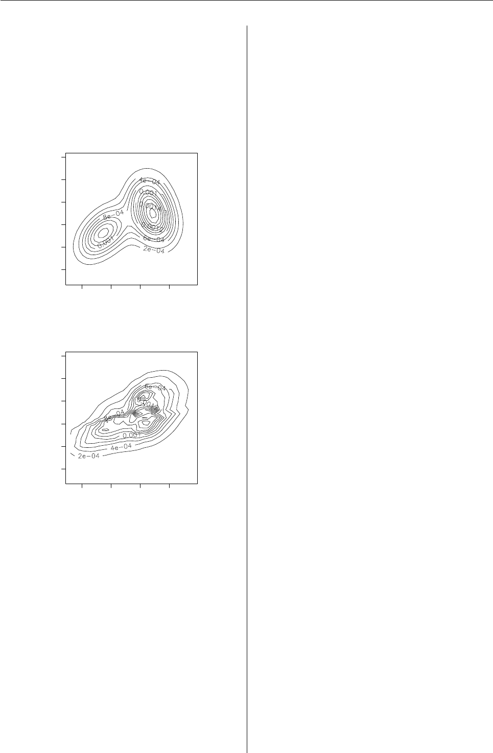
Vol. 7/3, December 2007 20
fitMPT <- PTdensity(
y = cbind(radiation,ozone),
prior = priorMPT,mcmc = mcmcMPT,
state = NULL,status = TRUE,
na.action = na.omit)
We illustrate the results from these analyses in
Figure 1. This figure shows the contour plots of
the posterior predictive density for each model.
radiation
ozone
0 100 200 300
123456
●
●
●
●
●
●
●
●
●
●
●
●
●
●
●
●
●
●
●
●
●
●
●
●
●
●
●
●●
●
●
●●
●
●
●
●
●
●
●●
●
●
●
●
●
●
●
●
●
●
●
●
●
●
●
●
●
●
●
●
●
●
●
●
●
●
●
●
●
●
●
●
●
●
●
●
●
●
●
●
●
●
●
●
●
●
●
●
●●
●
●
●
●
●
●
●
●
●
●
●
●
●
●
●
●
●
●
●●
(a)
radiation
ozone
0 100 200 300
123456
●
●
●
●
●
●
●
●
●
●
●
●
●
●
●
●
●
●
●
●
●
●
●
●
●
●
●
●●
●
●
●●
●
●
●
●
●
●
●●
●
●
●
●
●
●
●
●
●
●
●
●
●
●
●
●
●
●
●
●
●
●
●
●
●
●
●
●
●
●
●
●
●
●
●
●
●
●
●
●
●
●
●
●
●
●
●
●
●●
●
●
●
●
●
●
●
●
●
●
●
●
●
●
●
●
●
●
●●
(b)
Figure 1: Density estimate for the New York Air
Quality Measurements dataset, using (a) DPdensity
and (b) PTdensity, respectively.
Figure 1clearly shows a departure from the nor-
mality assumption for these data. The results indi-
cate the existence of at least two clusters of data. We
refer to Hanson (2006) for more details and compar-
isons between these models.
Interval-Censored Data
The DPsurvint function implements the algorithm
described by Hanson & Johnson (2004) for semipara-
metric accelerated failure time (AFT) models. We il-
lustrate the function on a dataset involving time to
cosmetic deterioration of the breast for women with
stage 1 breast cancer who have undergone a lumpec-
tomy, for two treatments, these being radiation, and
radiation coupled with chemotherapy. Radiation is
known to cause retraction of the breast, and there is
some evidence that chemotherapy worsens this ef-
fect. There is interest in the cosmetic impact of the
treatments because both are considered very effec-
tive in preventing recurrence of this early stage can-
cer.
The data come from a retrospective study of 46
patients who received radiation only and 48 who re-
ceived radiation plus chemotherapy. Patients were
observed typically every four to six months and at
each observation a clinician recorded the level of
breast retraction that had taken place since the last
visit: none, moderate, or severe. The time-to-event
considered was the time until moderate or severe
breast retraction, and this time is interval censored
between patient visits or right censored if no breast
retraction was detected over the study period of 48
months. As the observed intervals were the result
of pre-scheduled visits, an independent noninforma-
tive censoring process can be assumed. The data
were analyzed by Hanson & Johnson (2004) and also
given in Klein & Moeschberger (1997).
In the analysis of survival data with covari-
ates, the semiparametric proportional hazards (PH)
model is the most popular choice. It is flexible and
easily fitted using standard software, at least for
right-censored data. However, the assumption of
proportional hazard functions may be violated and
we may seek a proper alternative semiparametric
model. One such model is the AFT model. Whereas
the PH model assumes the covariates act multiplica-
tively on a baseline hazard function, the AFT model
assumes that the covariates act multiplicatively on
the argument of the baseline survival distribution, G,
P(T>t|x) = G(texp{xT
iβ},+∞), thus provid-
ing a model with a simple interpretation of the re-
gression coefficients for practitioners.
Classical treatments of the semiparametric AFT
model with interval-censored data were presented,
for instance, in Lin & Zhang (1998). Note, how-
ever, that for semiparametric AFT models there is
nothing comparable to a partial likelihood function.
Therefore, the vector of regression coefficients and
the baseline survival distribution must be estimated
simultaneously, complicating matters enormously in
the interval-censored case. The more recent classical
approaches only provide inferences about the regres-
sion coefficients and not for the survival function.
In the Bayesian semiparametric context, Chris-
tensen & Johnson (1998) assigned a simple DP prior,
centered in a single distribution, to baseline survival
for nested interval-censored data. A marginal like-
lihood for the vector of regression coefficients βis
maximized to provide a point estimate and resulting
survival curves. However, this approach does not
allow the computation of credible intervals for the
R News ISSN 1609-3631

Vol. 7/3, December 2007 21
parameters. Moreover, it may be difficult in prac-
tice to specify a single centering distribution for the
DP prior and, once specified, a single centering dis-
tribution may affect inferences. To overcome these
difficulties, a MDP prior can be considered. Under
this approach, it is not very difficult to demonstrated
that the computations involved for a full Bayesian
solution are horrendous at best, even for the non-
censored data problem. The analytic intractability
of the Bayesian semiparametric AFT model has been
overcome using MCMC methods by Hanson & John-
son (2004).
To test whether chemotherapy in addition to ra-
diotherapy has an effect on time to breast retraction,
an AFT model Ti=exp(−xT
iβ)Vi,i=1, . . . , n, was
considered. We model the baseline distribution in
the AFT model using a MDP prior centered in a stan-
dard parametric family, the lognormal distribution,
V1,...,Vn|Giid
∼G,
G|α,µ,σ2∼DP (αG0),G0≡LN(µ,σ2),
µ|m0,s0∼N(m0,s0),
σ−2|τ1,τ2∼Γ(τ1/2, τ2/2),
β|β0,Sβ0∼Npβ0,Sβ0,
where LN m,s2and Nm,s2refer to a log-normal
and normal distribution, respectively, with location
mand scale parameter s2. The precision parameter
of the MDP prior was chosen to be α=10, allowing
for moderate deviations from the log-normal family.
We allow the parametric family to hold only approx-
imately, and the resulting model is robust against
mis-specification of the baseline survival distribu-
tion. The covariate of interest is trti=0 if the ith
patient had radiotherapy only and trti=1 if the
ith patient had radiotherapy and chemotherapy. The
following commands were used to fit the model,
# Data
data("deterioration")
attach(deterioration)
y <- cbind(left,right)
# MCMC parameters
mcmc <- list(nburn = 20000, nsave = 10000,
nskip = 20, ndisplay = 1000,
tune = 0.25)
# Prior information
prior <- list(alpha = 10, beta0 = rep(0,1),
Sbeta0 = diag(100,1), m0 = 0,
s0 = 1, tau1 = 0.01, tau2 = 0.01)
# Fitting the model
fit <- DPsurvint(y ~ trt, prior = prior,
mcmc = mcmc, state = NULL,
status = TRUE)
In our analysis, the posterior mean and 95% HPD
associated with trt was 0.50 (0.12, 0.82), indicating
that including chemotherapy significantly reduces
the time to deterioration. Figure 2(page 22) displays
posterior summary statistics for the parameters of in-
terest. In this case, the output includes the log of the
Conditional Predictive Ordinate (CPO) (see, Geisser
& Eddy 1979) for each data point, the AFT regression
coefficients, the parameters of the DP centering dis-
tribution, and the number of clusters.
Inferences about the survival curves can be ob-
tained from the MCMC output. Indeed, given
a sample of the parameters of size J, a sam-
ple of the survival curve for a given xcan be
drawn as follows: for the MCMC scan jof the
posterior distribution, with j=1, . . . , J, we
sample from S(j)(t|x, data)∼Beta(a(j)(t),b(j)(t))
where a(j)(t) = α(j)G(j)
0(texp(xTβ(j)),+∞)
+∑n
i=1δV(j)
i(texp(xTβ(j)),+∞), and b(j)(t) =
α(j)+N−a(j)(t). This approach is implemented in
the function predict.DPsurvint. For user-specified
values of the covariates, xnew, and the grid where the
survival function is evaluated, grid, posterior infor-
mation for the survival curves can be obtained using
the following commands,
xnew <- matrix(c(0,1), nrow=2, ncol=1)
grid <- seq(0.01,70,1)
pred <- predict(fit, xnew=xnew, grid=grid)
plot(pred, all=FALSE, band=TRUE)
The resulting survival curves and point-wise 95%
HPD intervals are given in Figure 3(page 23).
Semiparametric Generalized Linear Mixed
Model
Lesaffre & Spiessens (2001) analyzed data from a
multicentre randomized comparison of two oral
treatments for toe-nail infection (dermatophyte ony-
chomycosis) involving two groups of 189 patients
evaluated at seven visits; on week 0, 4, 8, 12, 24, 36,
and 48. Onychomycosis, known popularly as toe-
nail fungus, is a fairly common condition that not
only can disfigure and sometimes destroy the nail
but that also can lead to social and self-image is-
sues for sufferers. Onychomycosis can be caused by
several types of fungi known as dermatophytes, as
well as by non-dermatophytic yeasts or molds. Der-
matophyte onychomycosis corresponds to the type
caused by dermatophytes. Here we are interested
in the degree of onycholysis which expresses the de-
gree of separation of the nail plate from the nail-bed
and which was scored in four categories (0, absent;
1, mild; 2, moderate; 3, severe). These data were
analyzed by Lesaffre & Spiessens (2001) using gen-
eralized estimating equations (GEE) and generalized
linear mixed models (GLMM).
R News ISSN 1609-3631

Vol. 7/3, December 2007 22
> summary(fit)
Bayesian Semiparametric AFT Regression Model
Call:
DPsurvint.default(formula = y ~ trt, prior = prior, mcmc = mcmc,
state = state, status = TRUE)
Posterior Predictive Distributions (log):
Min. 1st Qu. Median Mean 3rd Qu. Max.
-4.5920 -2.3570 -1.4600 -1.6240 -0.7121 -0.1991
Regression coefficients:
Mean Median Std. Dev. Naive Std.Error 95%HPD-Low 95%HPD-Upp
trt 0.502282 0.513219 0.195521 0.001955 0.120880 0.820614
Baseline distribution:
Mean Median Std. Dev. Naive Std.Error 95%HPD-Low 95%HPD-Upp
mu 3.255374 3.255518 0.173132 0.001731 2.917770 3.589759
sigma2 1.021945 0.921764 0.469061 0.004691 0.366900 1.908676
Precision parameter:
Mean Median Std. Dev. Naive Std.Error 95%HPD-Low 95%HPD-Upp
ncluster 27.58880 28.00000 3.39630 0.03396 20.00000 33.00000
Acceptance Rate for Metropolis Step = 0.2637435
Number of Observations: 94
Figure 2: Posterior summary for the Breast Cancer Data fit using DPsurvint.
GLMM provide a popular framework for the
analysis of longitudinal measures and clustered data.
The models account for correlation among clustered
observations by including random effects in the lin-
ear predictor component of the model. Although
GLMM fitting is typically complex, standard ran-
dom intercept and random intercept/slope models
with normally distributed random effects can now
be routinely fitted in standard software. Such mod-
els are quite flexible in accommodating heterogenous
behavior, but they suffer from the same lack of ro-
bustness against departures from distributional as-
sumptions as other statistical models based on Gaus-
sian distributions.
A common strategy for guarding against such
mis-specification is to build more flexible distribu-
tional assumptions for the random effects into the
model. Following Lesaffre & Spiessens (2001), we
consider a logistic mixed effects model to examine
the probability of moderate or severe toenail separa-
tion Y=1 versus the probability of absent or mild
Y=0, including as covariates treatment (trt) (0 or
1), time (t) (continuous), and time×treatment inter-
action,
logit nPYi j =1|β,θio =θi+β1Trti+β2Timei j +
β3Trti×Timei j .
However, we replace the normality assumption of
the random intercepts by using a DPM of normals
prior (see, e.g., Müller et al. 2007),
θi|Giid
∼G,
G|P,Σk∼ZN(m,Σk)P(dm),
P|α,µ,Σ∼DP (αN(µ,Σ)),
β∼Npβ0,Sβ0,
Σk|ν0,T∼IWk(ν0,T),
µ|mb,Sb∼Nq(mb,Sb),
Σ|ν0,Tb∼IWk(νb,Tb),
α|a0,b0∼Γ(a0,b0).
The semiparametric GLMM using DPM of normals
model can be fitted using function DPMglmm and the
following code,
# MCMC parameters
mcmc <- list(nburn = 20000, nsave = 20000,
nskip = 50, ndisplay = 1000)
# Prior information
prior <- list(a0 = 2.01, b0 = 0.01,
nu0 = 2.05, tinv = diag(0.02,1),
nub = 2.05, tbinv = diag(0.02,1),
mb = rep(0,1), Sb = diag(100,1),
beta0 = rep(0,3),
R News ISSN 1609-3631
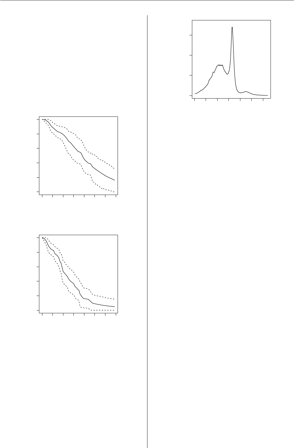
Vol. 7/3, December 2007 23
Sbeta0 = diag(100,3))
# Fitting the model
fitDPM <- DPMglmm(fixed = infect~trt+
time*trt, random = ~ 1|idnr,
family = binomial(logit),
prior = prior, mcmc = mcmc,
state = NULL, status = TRUE)
0 10 20 30 40 50 60 70
0.0 0.2 0.4 0.6 0.8 1.0
Time
Survival
(a)
0 10 20 30 40 50 60 70
0.0 0.2 0.4 0.6 0.8 1.0
Time
Survival
(b)
Figure 3: Breast cancer data: Posterior probability
of no evidence of breast retraction for (a) radiother-
apy only and (b) radiotherapy plus chemotherapy,
respectively.
Figure 4shows the posterior estimate of the
random effects distribution. The predictive den-
sity is overlaid on a plot of the posterior means
of the random effects. The results clearly in-
dicate departure from the normality assumption,
suggesting the existence of groups of patients
with respect to the resistance against the infection.
−15 −10 −5 0 5 10 15
0.00 0.05 0.10 0.15
values
density
●●●● ●●●● ●●●●● ●●●● ●●●●● ●●●● ●● ●● ●●● ●●● ●●● ●●●●●● ●●●●●●● ●●●●●●●●●● ●●●● ● ● ●●● ●●●●● ●● ●● ● ●●● ●●● ●● ●● ●●●● ●● ●●●●● ●●●●●●●●●●●● ●●●● ●● ●● ● ●●● ● ●● ●●● ●●● ●●● ●● ●●● ●●●● ●●● ●● ●●● ●●●●● ●● ●●●● ●●●● ●●●●●● ●●●●● ●● ●●● ●●● ●● ● ●●●●● ● ●● ●●●●●● ●●● ●●● ● ●● ●●●● ● ●● ●● ●● ●●●●●●● ●● ●●● ●● ●●● ●●●●●●●● ●●● ●● ●● ●●●●●● ●●● ●●● ● ● ●●● ●● ●●●●●●●●●● ●● ●●●●●
Figure 4: Toe-nail data: Random effects distribution
and posterior means estimated using DPMglmm.
Figure 5(page 24) reports summary statistics for
the posterior distribution of the parameters of in-
terest. It includes posterior means and 95% HPD
intervals for the parameters along with two model
performance measures: DIC and LPML. DIC is the
deviance information criterion of Spiegelhalter et al.
(2002). LPML is the log pseudo marginal likelihood
of Geisser & Eddy (1979), which is a leave-one-out
cross validatory measure based on predictive densi-
ties. A parametric analysis of these data (not shown),
considering equivalent prior distributions, gave a
DIC and LPML of 964.2 and -484.0, respectively. The
results, therefore, indicate that the DPM version of
the model outperforms the normal model using ei-
ther the LPML or DIC statistic, suggesting that the
semiparametric model is better both for explaining
the observed data and from a predictive point of
view.
Figure 5(page 24) and the Pseudo Contour prob-
abilities of the covariates in the model (see below)
suggest a significant effect of time on the degree of
toe-nail infection. As expected because of random-
ization of the patients to the treatment groups, no sig-
nificant difference between the two treatment groups
at baseline was observed. The results also suggest
a non-significant difference in the evolution in time
between the treatment groups, contradicting the re-
sults under the parametric normal model. The pos-
terior mean (95% HPD interval) for β3(Trt ×Time)
under the normal assumption for the random effects
was −0.138 (−0.271; −0.005). These results illus-
trate the consequences of the incorrect use of tradi-
tional model assumptions in the GLMM context.
> anova(fitDPM)
Table of Pseudo Contour Probabilities
Response: infect
Df PsCP
trt 1 0.512
time 1 <0.01 ***
R News ISSN 1609-3631

Vol. 7/3, December 2007 24
> summary(fitDPM)
Bayesian semiparametric generalized linear mixed effect model
Call:
DPMglmm.default(fixed = infect ~ trt + time * trt, random = ~1 |
idnr, family = binomial(logit), prior = prior, mcmc = mcmc,
state = state, status = TRUE)
Posterior Predictive Distributions (log):
Min. 1st Qu. Median Mean 3rd Qu. Max.
-9.644e+00 -2.335e-01 -4.190e-02 -2.442e-01 -8.629e-03 -4.249e-05
Model s performance:
Dbar Dhat pD DIC LPML
753.0 603.6 149.4 902.5 -466.0
Regression coefficients:
Mean Median Std. Dev. Naive Std.Error 95%HPD-Low 95%HPD-Upp
(Intercept) -2.508419 -2.440589 0.762218 0.005390 -4.122867 -1.091684
trt 0.300309 0.304453 0.478100 0.003381 -0.669604 1.242553
time -0.392343 -0.390384 0.046101 0.000326 -0.482329 -0.302442
trt:time -0.128891 -0.128570 0.072272 0.000511 -0.265813 0.018636
Kernel variance:
Mean Median Std. Dev. Naive Std.Error 95%HPD-Low 95%HPD-Upp
sigma-(Intercept) 0.0318682 0.0130737 0.0966504 0.0006834 0.0009878 0.1069456
Baseline distribution:
Mean Median Std. Dev. Naive Std.Error 95%HPD-Low 95%HPD-Upp
mub-(Intercept) -2.624227 -2.558427 1.405269 0.009937 -5.621183 0.008855
sigmab-(Intercept) 26.579978 23.579114 13.640300 0.096451 7.714973 52.754246
Precision parameter:
Mean Median Std. Dev. Naive Std.Error 95%HPD-Low 95%HPD-Upp
ncluster 70.6021 64.0000 36.7421 0.2598 11.0000 143.0000
alpha 38.4925 25.7503 44.1123 0.3119 1.1589 112.1120
Acceptance Rate for Metropolis Steps = 0.8893615 0.9995698
Number of Observations: 1908
Number of Groups: 294
Figure 5: Posterior summary for the Toe-nail Data fit using DPMglmm.
trt:time 1 0.075 .
---
Signif. codes: 0 *** 0.001 ** 0.01
* 0.05 . 0.1 1
Finally, information about the posterior distribution
of the subject-specific effects can be obtained by us-
ing the DPMrandom function as follows,
> DPMrandom(fitDPM)
Random effect information for the DP object:
Call:
DPMglmm.default(fixed = infect ~ trt +
time * trt, random = ~1 |idnr,
family = binomial(logit),
prior = prior, mcmc = mcmc,
state = state, status = TRUE)
Posterior mean of subject-specific components:
(Intercept)
1 1.6239
.
.
383 2.0178
R News ISSN 1609-3631

Vol. 7/3, December 2007 25
Summary and Future Develop-
ments
As the main obstacle for the practical use of BSP
and BNP methods has been the lack of estimation
tools, we presented an R package for fitting some fre-
quently used models. Until the release of DPpack-
age, the two options for researchers who wished to
fit a BSP or BNP model were to write their own code
or to rely heavily on particular parametric approxi-
mations to some specific processes using the BUGS
code given in Peter Congdon’s books (see, e.g., Con-
gdon 2001). DPpackage is geared primarily towards
users who are not willing to bear the costs associated
with both of these options.
Many improvements to the current status of the
package can be made. For example, all DPpackage
modeling functions compute CPOs for model com-
parison. However, only some of them compute the
effective number of parameters pD and the deviance
information criterion (DIC), as presented by Spiegel-
halter et al. (2002). These and other model compar-
ison criteria will be included for all the functions in
future versions of DPpackage.
The implementation of more models, the devel-
opment of general-purpose sampling functions, and
the ability to run several Markov chains at once and
to handle large dataset problems through the use of
sparse matrix techniques, are areas of further im-
provement.
Acknowledgments
I wish to thank (in alphabetical order) Timothy Han-
son, George Karabatsos, Emmanuel Lesaffre, Peter
Müller, and Fernando Quintana for many valuable
discussions, comments, and suggestions during the
development of the package. Timothy Hanson and
Fernando Quintana are also co-authors of the func-
tions PTdensity and FPTbinary, and BDPdensity, re-
spectively. I gratefully acknowledge the partial sup-
port of the KUL-PUC bilateral (Belgium-Chile) grant
No BIL05/03 and of the IAP research network grant
No P6/03 of the Belgian government (Belgian Sci-
ence Policy). The author thanks Novartis, Belgium,
for permission to use their dermatological data for
statistical research.
Bibliography
J. Besag, P. Green, D. Higdon, and K. Mengersen.
Bayesian computation and stochastic systems
(with Discussion). Statistical Science, 10:3–66, 1995.
J. M. Chambers, S. Cleveland, and A. P. Tukey.
Graphical Methods for Data Analysis. Boston,
USA: Duxbury, 1983.
M. H. Chen and Q. M. Shao. Monte Carlo estimation
of Bayesian credible and HPD intervals. Journal
of Computational and Graphical Statistics, 8(1):69–92,
1999.
R. Christensen and W. O. Johnson. Modeling Ac-
celerated Failure Time With a Dirichlet Process.
Biometrika, 75:693–704, 1998.
P. Congdon. Bayesian Statistical Modelling. New York,
USA: John Wiley and Sons, 2001.
M. D. Escobar and M. West. Bayesian density esti-
mation and inference using mixtures. Journal of the
American Statistical Association, 90:577–588, 1995.
T. S. Ferguson. A Bayesian analysis of some nonpara-
metric problems. The Annals of Statistics, 1:209–230,
1973.
S. Geisser and W. Eddy. A predictive approach to
model selection. Journal of the American Statistical
Association, 74:153–160, 1979.
W. R. Gilks, A. Thomas, and D. J. Spiegelhalter. Soft-
ware for Gibbs sampler Computing Science and
Statistics 24:439–448, 1992.
T. Hanson. Inference for Mixtures of Finite Polya Tree
Models. Journal of the American Statistical Associa-
tion, 101:1548–1565, 2006.
T. Hanson and W. O. Johnson. A Bayesian Semipara-
metric AFT Model for Interval-Censored Data.
Journal of Computational and Graphical Statistics
13(2):341–361, 2004.
A. Jara, M. J. Garcia-Zattera, and E. Lesaffre. A
Dirichlet Process Mixture model for the analysis of
correlated binary responses. Computational Statis-
tics and Data Analysis, 51:5402–5415, 2007.
J. Klein and M. Moeschberger. Survival Analysis. New
York, USA: Springer-Verlag, 1997.
E. Lesaffre and B. Spiessens. On the effect of the
number of quadrature points in a logistic random-
effects model: an example. Applied Statistics 50:
325–335, 2001.
G. Lin and C. Zhang. Linear Regression With Inter-
val Censored Data. The Annals of Statistics 26:1306–
1327, 1998.
P. Müller and F.A. Quintana. Nonparametric
Bayesian Data Analysis. Statistical Science 19(1):95–
110, 2004.
P. Müller, A. Erkanli, and M. West. Bayesian
Curve Fitting Using Multivariate Normal Mix-
tures. Biometrika, 83:67–79, 1996.
P. Müller, F. A. Quintana, and G. Rosner. Semi-
parametric Bayesian Inference for Multilevel Re-
peated Measurement Data. Biometrics, 63(1):280–
289, 2007.
R News ISSN 1609-3631
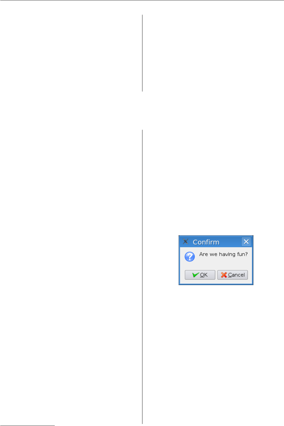
Vol. 7/3, December 2007 26
M. A. Newton, C. Czado, and R. Chappell. Bayesian
inference for semiparametric binary regression.
Journal of the American Statistical Association 91:142–
153, 1996.
M. Plummer, N. Best, K. Cowles, and K. Vines.
CODA: Output analysis and diagnostics for
MCMC. R package version 0.12-1, 2007.
B. J. Smith. boa: Bayesian Output Analysis Program
(BOA) for MCMC. R package version 1.1.6-1, 2007.
S. D. Spiegelhalter, N. G.Best, B. P. Carlin, and
A. Van der Linde. Bayesian measures of model
complexity and fit. Journal of the Royal Statistical
Society: Series B 64:583–639, 2002.
Alejandro Jara
Biostatistical Centre
Catholic University of Leuven
Leuven, Belgium
Alejandro.JaraVallejos@med.kuleuven.be
An Introduction to gWidgets
by John Verzani
Introduction
CRAN has several different packages that interface
R with toolkits for making graphical user inter-
faces (GUIs). For example, among others, there are
RGtk2 (Lawrence and Temple Lang,2006), rJava,
and tcltk (Dalgaard,2001). These primarily provide
a mapping between library calls for the toolkits and
similarly named R functions. To use them effectively
to create a GUI, one needs to learn quite a bit about
the underlying toolkit. Not only does this add com-
plication for many R users, it can also be tedious,
as there are often several steps required to set up a
basic widget. The gWidgets package adds another
layer between the R user and these packages provid-
ing an abstract, simplified interface that tries to be
as familiar to the R user as possible. By abstracting
the toolkit it is possible to use the gWidgets inter-
face with many different toolkits. Although, open to
the criticism that such an approach can only provide
a least-common-denominator user experience, we’ll
see that gWidgets, despite not being as feature-rich
as any underlying toolkit, can be used to produce
fairly complicated GUIs without having as steep a
learning curve as the toolkits themselves.
As of this writing there are implementations for
three toolkits, RGtk2,tcltk, and rJava (with progress
on a port to RwxWidgets). The gWidgetsRGtk2
package was the first and is the most complete.
Whereas gWidgetstcltk package is not as complete,
due to limitations of the base libraries, but it has
many useful widgets implemented. Installation of
these packages requires the base toolkit libraries be
installed. For gWidgetstcltk these are bundled with
the windows distribution, for others they may re-
quire a separate download.
Dialogs
We begin by loading the package. Both the package
and at least one toolkit implementation must be in-
stalled prior to this. If more than one toolkit imple-
mentation has been installed, you will be queried as
to which one to use.
library("gWidgets")
The easiest GUI elements to create are the basic
dialogs (Figure 1). These are useful for sending out
quick messages, such as: 1
gconfirm("Are we having fun?")
Figure 1: Simple dialog created by gconfirm using
the RGtk2 toolkit.
A basic dialog could be used to show error mes-
sages
options(error = function() {
err = geterrmessage()
gmessage(err, icon="error")
})
or, be an alternative to file.choose
source(gfile())
In gWidgets, these basic dialogs are modal,
meaning the user must take some action before con-
trol of R is returned. The return value is a logical or
string, as appropriate, and can be used as input to a
further command. Modal dialogs can be confusing
1The code for these examples is available from http://www.math.csi.cuny.edu/pmg/gWidgets/rnews.R
R News ISSN 1609-3631
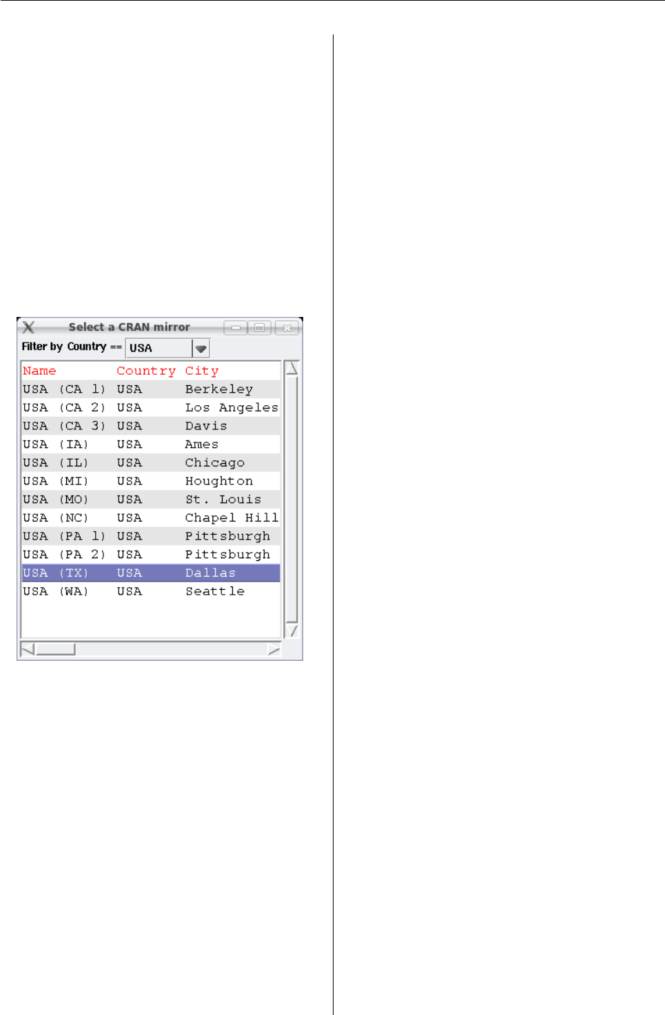
Vol. 7/3, December 2007 27
if the dialog gets hidden by another window. Addi-
tionally, modal dialogs disrupt a user’s flow. A more
typical GUI will allow the R session to continue and
will only act when a user initiates some action with
the GUI by mouse click, text entry, etc. The GUI de-
signer adds handlers to respond to these events. The
gWidgets programming interface is based around fa-
cilitating the following basic tasks in building a GUI:
constructing widgets that a user can control to af-
fect the state of the GUI, using generic functions to
programmatically manipulate these widgets, simpli-
fying the layout of widgets within containers, and fa-
cilitating the assigning of handlers to events initiated
by the user of the GUI.
Selecting a CRAN site
Figure 2: GUI to select a CRAN mirror shown using
gWidgetstcltk. The filter feature of gtable has been
used to narrow the selection to USA sites. Double
clicking a row causes the CRAN repository to be set.
Selecting an item from a list of items or a table
of items is a very common task in GUIs. Our next
example presents a GUI that allows a user to se-
lect with the mouse a CRAN repository from a ta-
ble. The idea comes from a tcltk GUI created by the
chooseCRANmirror function. This example shows
how the widget constructors allow specification of
both containers and event handlers.
We will use this function to set the CRAN reposi-
tory from a URL.
setCRAN <- function(URL) {
repos = getOption("repos")
repos["CRAN"] <- gsub("/$", "", URL)
options(repos=repos)
}
To begin our GUI we first create a top-level win-
dow to contain our table widget.
win <- gwindow("Select a CRAN mirror")
A call to gwindow will pop-up a new window on the
screen and return an object which can be manipu-
lated later. The argument sets the window title.
The widget we create will show the possible
CRAN values in a tabular format for easy selection
by a mouse. Selection occurs when a row is clicked.
We will assign this function to respond to a double
click event:
handler = function(h,...) {
URL <- svalue(tbl) # get value of widget
setCRAN(URL) # set URL
dispose(win) # close window
}
The svalue function is a new generic function which
retrieves the selected value for a widget, in this case
one called tbl constructed below. The dispose func-
tion is a new generic which for windows causes them
to be destroyed. So this handler will set the chosen
URL and then destroy the top-level window.
The gtable function constructs a widget allow-
ing the user to select a value from a data frame and
returns an object for which generic functions are de-
fined. The row of the value is selected with a mouse
click, whereas, the selected column is specified at the
time the widget is constructed using the chosencol
argument. Additionally, this function allows the
specification of a column whose unique values can
be used to filter the display of possible values to se-
lect from.
tbl <- gtable(
items=utils:::getCRANmirrors(),
chosencol=4,
filter.column=2,
container=win,
handler=handler
)
Figure 2shows the final widget using the tcltk
toolkit.
Using gWidgets
We now go through the basic steps of building a GUI
using gWidgets a little more systematically.
Containers
As illustrated previously a top-level window is cre-
ated using gwindow. The gWidgets package only al-
lows one widget to be packed into a top-level win-
dow. As such, typically a container that can hold
more than one object is packed into the top-level win-
dow. There are several types of containers available.
R News ISSN 1609-3631
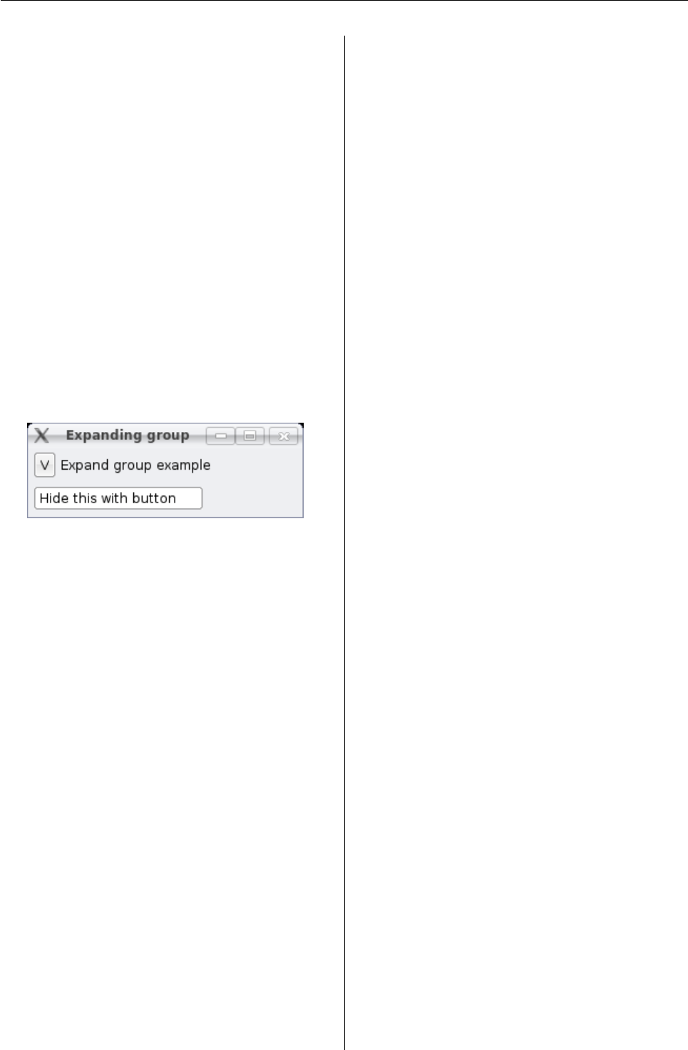
Vol. 7/3, December 2007 28
The ggroup function produces a container that
may be visualized as a box that allows new wid-
gets to be packed in from left to right (the default)
or from top to bottom (horizontal=FALSE). Nesting
such containers gives a wide range of flexibility.
Widgets are added to containers through the
container argument at the time of construction
(which hereafter we shorten to cont) or using the add
method for containers. However, gWidgetstcltk re-
quires one to use the container argument when a
widget is constructed. That is, except with gWidget-
stcltk
win <- gwindow("test")
b <- gbutton("click me", cont=win)
is equivalent to
win <- gwindow("test")
add(win, gbutton("click me"))
The latter is a bit more convenient as it allows one to
keep separate the widget’s construction and its lay-
out, but the former allows more portability of code.
Figure 3: Expanding group example after resizing
window. The button, label and text widgets use
nested ggroup containers for their layout.
To illustrate nested ggroup containers and the add
and delete generics for containers, the following ex-
ample shows how to create a widget that can hide
or show its contents when a button is clicked. This
is more fully implemented in the gexpandgroup con-
tainer.
We begin by defining a top-level window and im-
mediately add a ggroup instance which packs in its
widgets from top to bottom.
win <- gwindow("Expanding group")
g <- ggroup(horizontal=FALSE, cont=win)
Inside of gwe add a nested group which will con-
tain a button and a label.
g1 <- ggroup(horizontal=TRUE, cont=g)
button <- gbutton("V",cont=g1)
label <- glabel("Expand group example",
cont=g1)
Finally, we add a ggroup instance to the gcon-
tainer to hold the widgets that we wish to hide and
put a widget into the new container.
g2 <- ggroup(cont=g, expand=TRUE)
e <- gedit("Hide this with button",
cont=g2)
That finishes the layout. Figure 3shows the
GUI in the expanded state. To make this example
do something interesting, we define functions to re-
spond to clicking on the button or the label. These
functions toggle whether or not the g2 container is
packed into the gcontainer using the add and delete
generics for containers.
expandGroup = function()
add(g,g2, expand=TRUE)
hideGroup = function() delete(g,g2)
The add generic is used to add a widget (or con-
tainer) to a container. In this case, the argument
expand=TRUE is given to force the added widget to
take up as much space as possible. The delete
generic removes a widget from a container. The wid-
get is not destroyed, as with dispose, just removed
from its container.
Next, we define a handler to be called when the
button or label is clicked. This involves arranging a
means to toggle between states and to adjust the but-
ton text accordingly.
state <- TRUE # a global
changeState <- function(h,...) {
if(state) {
hideGroup()
svalue(button) <- ">"
} else {
expandGroup()
svalue(button) <- "V"
}
state <<- !state
}
We used the <<- operator so that the value of state
is updated in the global environment, rather than the
environment of the handler.
Finally, we bind this handler to both the but-
ton and the label, so that it is called when they are
clicked.
ID <- addHandlerClicked(button,
handler=changeState)
ID <- addHandlerClicked(label,
handler=changeState)
There are just a few options for the layout of wid-
gets within a ggroup container, compared to those
available in the various toolkits. We illustrated the
expand argument. With rJava and tcltk there is also
an anchor argument which takes a value of the form
c(x,y) where xor yare −1, 0, or 1. These are used
to specify which corner of the space allocated by the
container the widget should add itself in.
Additionally, the ggroup instances have methods
addSpace to add a fixed amount of blank space and
addSpring to add a “spring” which forces the re-
maining widgets to be pushed to the right (or the bot-
tom) of the containers. This simple example shows
how these can be used to put buttons on the right
R News ISSN 1609-3631
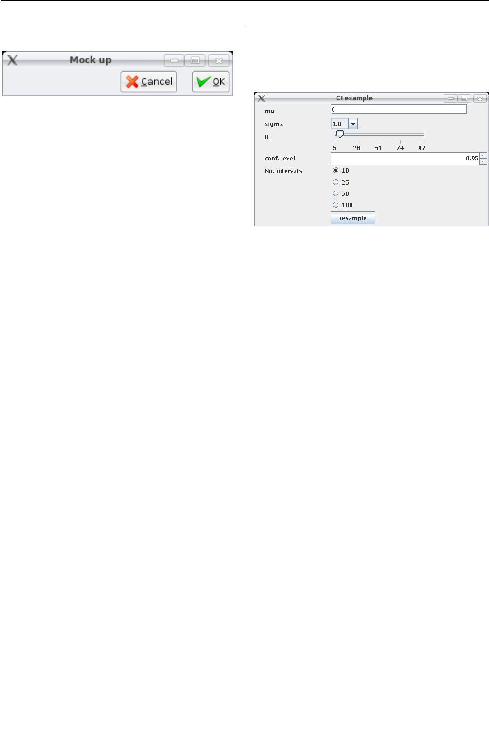
Vol. 7/3, December 2007 29
side of a dialog. First we pack a ggroup instance into
a top-level container.
Figure 4: Illustration of addSpace and addSpring
methods of ggroup using the gWidgetsRGTk2 pack-
age after resizing main window. The buttons are
pushed to the right side by addSpring.
win <- gwindow("Mock up")
bg <- ggroup(cont=win, expand=TRUE)
addSpring(bg) # push to right
Now we add two buttons and a bit of space, 10
pixels, between them. By default, packing is done
from left to right, starting on the left. The use of
addSpring pushes the packed in containers and wid-
gets to the right side of the container.
b1 <- gbutton("cancel", cont=bg)
addSpace(bg,10) # add some space
b2 <- gbutton("ok", cont=bg)
The expand=TRUE value for bg ensures that that
container expands to fill the space it can, otherwise
the button widgets would push to the boundary of
the button group and not the outside container win.
Figure 4shows the widget.
Other containers are illustrated in the examples
below. These include glayout for laying out widgets
in a grid, gnotebook for holding multiple widgets at
once with tabs used to select between the widgets,
and gpanedgroup which uses a movable pane to al-
locate space between widgets. Additionally, gframe
is similar to ggroup, but with an external frame and
area for a label.
Basic widgets
A GUI is composed of widgets packed into con-
tainers. In gWidgets there are a number of famil-
iar widgets. We’ve illustrated labels and buttons
(glabel and gbutton). Additionally there are wid-
gets to select from a list of items (gradio,gdroplist,
and gcheckboxgroup); widgets to select from a ta-
ble of values (gtable); widgets to select files or
dates (gfile,gcalendar); widgets to edit text (gedit,
gtext); a widget to edit a data frame (gdf); a widget
to display graphic files (gimage); and others. Not all
are available for each toolkit.
The following example, modified from a recent R
News article on the rpanel package (Bowman et al.,
2006), illustrates how many of these widgets can be
combined to create a GUI to demonstrate confidence
intervals. This example uses the glayout container
to lay out its widgets in a grid.
First we pack the container into a top level win-
dow.
win <- gwindow("CI example")
tbl <- glayout(cont=win)
The glayout container uses matrix-like notation to
specify where the widgets are placed. When the as-
signed value is a string, a glabel is used.
Figure 5: GUI for a confidence interval demonstra-
tion, using gWidgetsrJava, illustrating several dif-
ferent widgets: gedit for single-line editing; and
gdroplist,gslider,gspinbox, and gradio for selec-
tion from a fixed set of items.
tbl[1,1] <- "mu"
tbl[1,2] <-
(mu <- gedit("0", cont=tbl,
coerce.with=as.numeric))
tbl[2,1] <- "sigma"
tbl[2,2] <-
(sigma <- gdroplist(c(1,5,10),
cont=tbl))
tbl[3,1] <- "n"
tbl[3,2] <- (
n <- gslider(from=5,to=100, by=1,
value = 10, cont=tbl))
tbl[4,1] <- "conf. level"
tbl[4,2, expand=TRUE] <-
(confLevel <- gspinbutton(
from=0.5, to=0.99, by=0.01,
value=0.95, cont=tbl))
tbl[5,1] <- "No. intervals"
tbl[5,2] <-
(noIntervals <- gradio(c(10,25,
50,100), cont=tbl))
tbl[6,2] <-
(resample <- gbutton("resample",
cont=tbl))
visible(tbl) <- TRUE
The last line with visible is necessary for gWidget-
sRGtk2 to produce the layout.
The matrix-notation refers to where the widget is
placed. An assignment like
tbl[1:2,2:3] <- "testing"
would place a label within the area for the first and
second rows and second and third columns. Unlike
matrices, the notation is not used to vectorize the
placement of several widgets, extract widgets, or re-
place a widget. The above code completes the widget
R News ISSN 1609-3631

Vol. 7/3, December 2007 30
construction and layout. Figure 5shows a realization
using rJava.
The widgets have various arguments to specify
their values that depend on what the widget does.
For example, the slider and spinbutton select a value
from a sequence, so the arguments mirror those of
seq. Some widgets have a coerce.with argument
which allows a text-based widget, like gedit, to re-
turn numeric values through svalue. The gdroplist
widget is used above to pop up its possible values
for selection. Additionally, if the editable=TRUE ar-
gument is given, it becomes a combo-box allowing a
user to input a different value.
In Figure 5we see in the slider widget one of the
limitations of the gWidgets approach – it is not as
feature rich as any individual toolkit. Although the
underlying JSlider widget has some means to adjust
the labels on the slider, gWidgets provides none in its
API, which in this case is slightly annoying, as Java’s
chosen values of 5, 28, 51, 74, and 97 just don’t seem
right.
The values specified by these widgets are to be
fed into the function makeCIs, which is not shown
here, but uses matplot to construct a graphic dis-
playing simulated confidence intervals. To make this
GUI interactive, the following handler will be used
to respond to changes in the GUI. We need to call
svalue on each of the widgets and then pass these
results to the makeCIs function. This task is stream-
lined by using lapply and do.call:
allWidgets <- list(mu,sigma,noIntervals,
n, confLevel, resample)
plotCI <- function(h, ...) {
lst <- lapply(allWidgets,svalue)
do.call(makeCIs,lst)
}
Again we use lapply to add the handler to re-
spond to the different widget default events all at
once.
invisible(sapply(allWidgets,function(i)
addHandlerChanged(i,handler=plotCI))
)
Interacting with widgets programmati-
cally
In gWidgets, the widget and container constructors
return S4 objects of various classes. These objects are
accessed programmatically with generic functions.
As was sensible, generic methods familiar to R users
were used, and when not possible, new generics
were added. For example, for widgets which store
values to select from, the generics [and [<- are used
to refer to the possible values. For other widgets, as
appropriate, the generics dim,names,length, etc., are
defined. To get and set a widget’s “selected” value,
the new generic functions svalue and svalue<- were
defined. The term “selected” is loosely defined, e.g.,
applying to a button’s text when clicked.
This simple example shows how selecting values
in a checkbox group can be used to set the possible
values in a drop list. First we create a container to
hold the two widgets.
win <- gwindow("methods example")
g <- ggroup(cont=win)
The construction of the two widgets is straight-
forward: simply specify the available values using
items.
cb <- gcheckboxgroup(items=letters[1:5],
cont=g)
dl <- gdroplist(items="", cont=g)
To finish, the following adds a handler to cb
which will update the possible values of dl when the
user changes the value of the checkbox group.
ID <- addHandlerChanged(cb,
function(h,...) {
dl[] <- svalue(cb)
})
A few other new generics are defined in gWid-
gets for the basic widgets such as font<- for setting
font properties, size<- to adjust the size in pixels for
a widget, enabled<- to adjust if the widget can ac-
cept input, and the pair tag and tag<-, which is like
attr only its values are stored with the widget. This
latter function is useful as its values can be updated
within a function call, such as a handler, as this next
example shows. The expanding group example with
the state variable would have been a good place to
use this feature.
> x = gbutton("test", cont=gwindow())
> tag(x,"ex") <- attr(x,"ex") <- "a"
> f = function(y)
+ tag(y,"ex") <- attr(y,"ex") <- "b"
> c(tag(x,"ex"),attr(x,"ex"))
[1] "a" "a"
> f(x)
> c(tag(x,"ex"),attr(x,"ex"))
[1] "b" "a"
Handlers
A GUI user initiates an event to happen when a but-
ton is clicked, or a key is pressed, or a drag and drop
is initiated, etc. The gWidgets package allows one to
specify a handler, or callback, to be called when an
event occurs. These handlers may be specified when
a widget is constructed using the handler argument,
or added at a later time. To add the default handler,
use the addHandlerChanged generic. Most, but not
all, widgets have just one type of event for which
a handler may be given. For instance, the gedit
R News ISSN 1609-3631
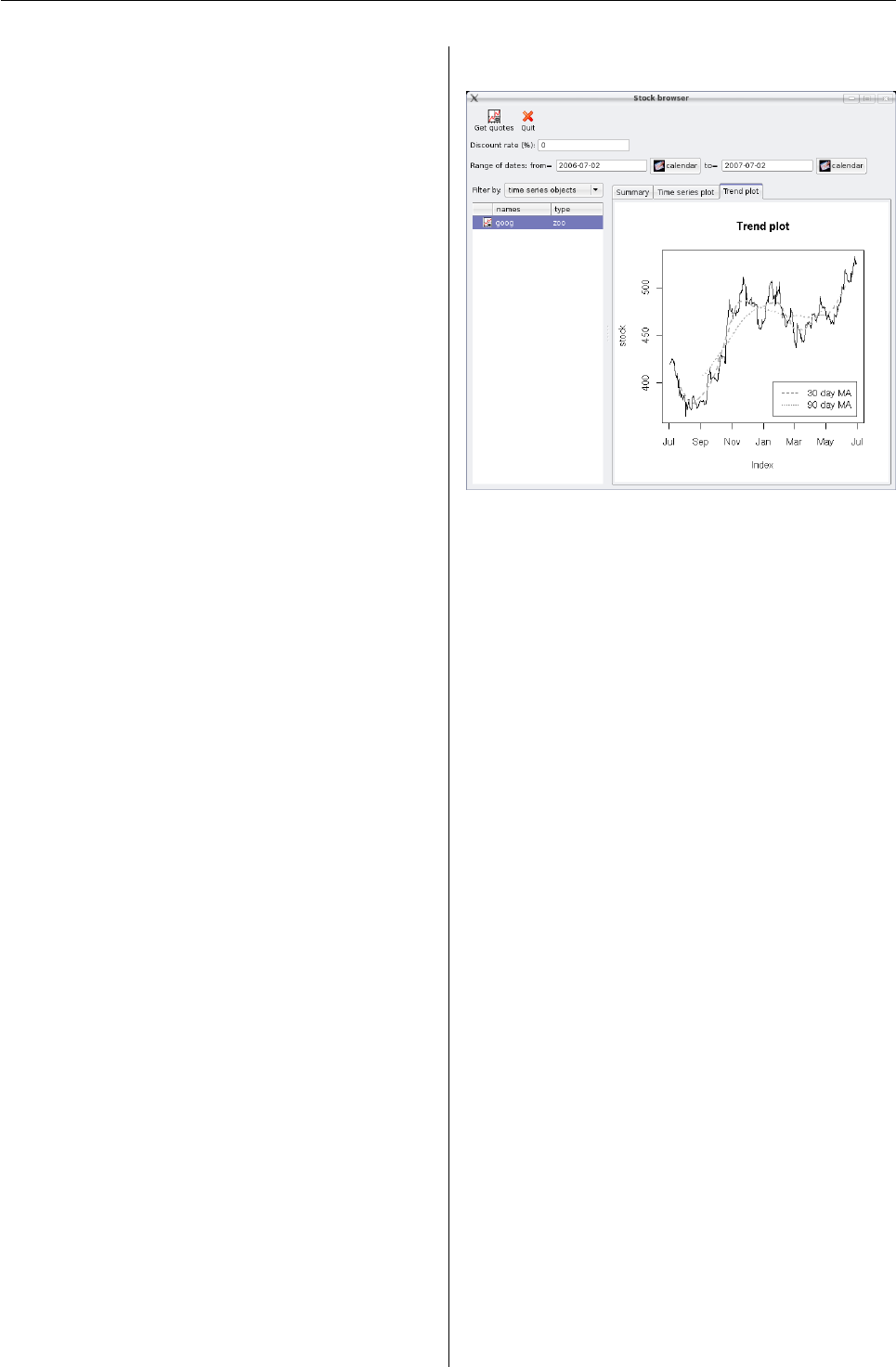
Vol. 7/3, December 2007 31
widget has the default handler respond to the event
of a user pressing the ENTER key. Whereas, the
addHandlerKeystroke method can be used to add a
handler that responds to any keystroke. Officially,
only one handler can be assigned per event, although
some toolkits allow more.
Handlers return an ID which can be used with
removeHandler to remove the response to the event.
The signature of a handler function has a first ar-
gument, h, to which is passed a list containing com-
ponents obj,action and perhaps others. The obj
component refers to the underlying widget. In the
examples above we found this widget after storing
it to a variable name, this provides an alternative.
The action component may be used to passed along
an arbitrary value to the handler. The other compo-
nents depend on the widget. For the ggraphics wid-
get (currently just gWidgetsRGtk2), the components
xand yreport the coordinates of a mouse click for
addHandlerClicked. Whereas, for addDropTarget
the dropdata component contains a string specifying
the value being dragged.
To illustrate the drag-and-drop handlers the fol-
lowing creates two buttons. The drop source needs a
handler which returns the value passed along to the
dropdata component of the drop target handler. In
this example, clicking on the first button and drag-
ging its value onto the label will change the text dis-
played on the label.
g = ggroup(cont=gwindow("DnD example"))
l1 <- gbutton("drag me", cont=g)
l2 <- glabel("drop here", cont=g)
ID <- addDropSource(l1, handler=
function(h,...) svalue(h$obj))
ID <- addDropTarget(l2, handler =
function(h,...)
svalue(h$obj) <- h$dropdata)
Drag and drop works with all the toolkits except
gWidgetsrJava where only what is provided natively
through the Java libraries is working.
An application
This last example shows how to make a more am-
bitious GUI for a task; in this case, an interface to
download and visualize stock prices. New widgets
and containers shown are the toolbar widget; the
notebook container, which is used to present dif-
ferent simultaneous summaries of a stock; the vari-
able selector widget, for selecting variables from
the workspace; and the generic widget constructor,
which creates a simple GUI based on a function’s ar-
guments, as found by formal. Although more in-
volved than the examples above, it is meant to show
how specialized GUIs can be formed relatively eas-
ily by gluing together the pieces available through
gWidgets. Figure 6shows the result of running the
following code, then downloading data for Google
into the session.
Figure 6: Stock browser widget using gWidget-
sRGtk2. This illustrates a toolbar, the variable selec-
tor, and a notebook container.
We begin by loading the tseries package which
contains the get.hist.quote() function for retriev-
ing stock data from www.yahoo.com and calls in the
handy zoo package by Achim Zeileis and Gabor
Grothendieck or use for later use.
invisible(require("tseries"))
In previous examples we used the global environ-
ment to store our variables. This works well for a
single GUI, but can quickly lead to problems with
colliding variable names with multiple GUIs. Setting
up a separate environment for each GUI is one way
around this potential conflict. Similarly, the proto
package can be used effectively to provide an envi-
ronment and more. Other possible methods are to
use namespaces or the environment within a func-
tion body. In this example, we create a new environ-
ment to store our global variables.
e <- new.env()
The environment eis accessed using list-like syntax.
To download stock information we use
get.hist.quote. We define this function to reduce
the number of arguments so that ggenericwidget
produces a simpler GUI (Figure 7).
getQuotes = function(
inst = "GOOG",
quote = c("Open","High","Low","Close"),
start, end)
get.hist.quote(inst, start=start,
end=end, quote=quote)
R News ISSN 1609-3631
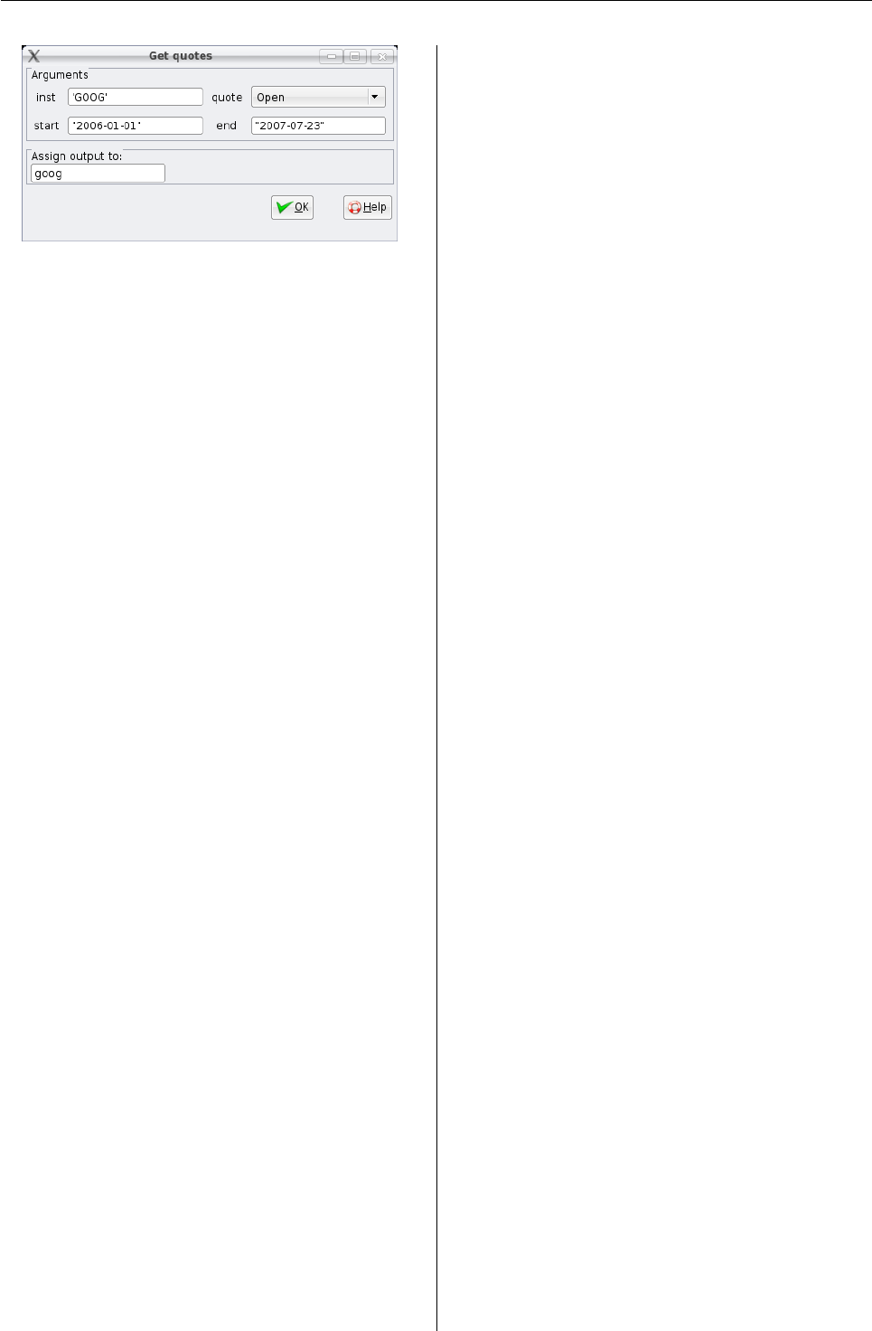
Vol. 7/3, December 2007 32
Figure 7: The GUI for getQuotes created by
ggenericwidget using the RGtk2 toolkit.
We define two functions to display graphical
summaries of the stock, using the zoo package to
produce the plots. Rather than use a plot device (as
only gWidgetsRGtk2 implements an embeddable
one through ggraphics), we choose instead to make
a file containing the plot as a graphic and display
this using the gimage widget. In gWidgetstcltk the
number of graphic formats that can be displayed is
limited, so we use an external program, convert, to
create a gif file. This is not needed if using RGtk2 or
rJava.
showTrend <- function(stock) {
trendPlotFile <- e$trendPlotFile
png(trendPlotFile)
plot(stock, main="Trend plot")
lines(rollmean(stock, k = 30), lwd=2,
lty=2, col=gray(.7))
lines(rollmean(stock, k = 90), lwd=2,
lty=3, col=gray(.7))
legend(index(stock)[length(stock)],
min(stock),
legend=c("30 day MA","90 day MA"),
lty=2:3,xjust=1, yjust=0)
dev.off()
## create a gif file
system(paste("convert ",
trendPlotFile," ",
trendPlotFile,".gif",sep=""))
svalue(e$trendPlot) = paste(
trendPlotFile,".gif",sep="")
}
The function showDiscount is similarly defined
but not shown.
The main function below is used to update the
notebook pages when a new stock is selected, or
the graphing parameters are changed. This func-
tion refers to widgets defined in a subsequent code
chunk.
updateNB <- function(h,...) {
## update data set
ifelse(e$curDSName != "",
e$curDS <- get(e$curDSName),
return())
## get data within specified range
start <- svalue(e$startD)
if(start == "") start=NULL
end <- svalue(e$endD)
if(end == "") end = NULL
dataSet = window(e$curDS,
start=start,end=end)
## update summaries
svalue(e$noSum) =
capture.output(summary(dataSet))
showDiscount(dataSet,
svalue(e$discRate))
showTrend(dataSet)
}
Now the main application is defined. First some
variables.
e$curDSName <- ""
e$curDS <- NA
e$tsPlotFile <- tempfile()
e$trendPlotFile <- tempfile()
Next we define the main window and a container
to hold the subsequent widgets.
## layout
e$win <- gwindow("Stock browser")
e$gp <- ggroup(horizontal=FALSE,
cont=e$win)
The first widget will be a toolbar. This basic one
has two actions, one to open a dialog allowing a user
to download stock information from the internet, the
other a quit button. To be more friendly to R users,
The gtoolbar() constructor uses a list to specify the
toolbar structure, rather than, say, XML. Basically,
each named component of this list should be a list
with a handler component and optionally an icon
component. Menubars are similarly defined, only
nesting is allowed.
## Set up simple toolbar
tb <- list()
tb$"Get quotes"$handler <- function(...)
ggenericwidget("getQuotes",
container=gwindow("Get quotes"))
tb$"Get quotes"$icon <- "ts"
tb$Quit$handler <- function(...)
dispose(e$win)
tb$Quit$icon <- "cancel"
theTB <- gtoolbar(tb, cont=e$gp)
This application has widgets to adjust the interest
rate (used as a discounting factor), and the start and
end dates. The date widgets use the gcalendar()
constructor for easier date selection.
## Now add parameters
e$pg <- ggroup(horizontal=TRUE,
cont = e$gp)
## the widgets
l <- glabel("Discount rate (%):",
cont=e$pg)
e$discRate <- gedit(0, cont=e$pg,
R News ISSN 1609-3631

Vol. 7/3, December 2007 33
coerce.with=as.numeric,
handler=updateNB)
e$pg <- ggroup(horizontal=TRUE,
cont = e$gp)
l <- glabel("Range of dates:",
cont=e$pg)
curDate <- Sys.Date()
l <- glabel("from=", cont=e$pg)
e$startD <-
gcalendar(as.character(curDate-365),
handler=updateNB, cont=e$pg)
l <- glabel("to=", cont=e$pg)
e$endD <-
gcalendar(as.character(curDate),
handler=updateNB, cont=e$pg)
A paned group is used for the final layout, alllow-
ing the user to adjust the amount of room for each
major part of the GUI. One part is a variable selection
widget provided by gvarbrowser(). Double clicking
a row calls the updateNB handler to update the note-
book pages.
e$gpg <- gpanedgroup(cont=e$gp,
expand=TRUE)
e$varSel <- gvarbrowser(
cont= e$gpg,
handler = function(h,...) {
e$curDSName <- svalue(e$varSel)
updateNB()
})
The other major part of the GUI is a notebook con-
tainer to hold the three different summaries of the
stock.
e$nb <- gnotebook(cont=e$gpg)
Finally, we add pages to the notebook container
below. The additional label argument sets the text
for the tab. (These can be adjusted later using
names<-.)
## A numeric summary of the data set
e$noSum <- gtext("Numeric summary",
cont=e$nb, label="Summary")
## First graphic summary
e$tsPlot <- gimage(e$tsPlotFile,
cont=e$nb, label="Time series plot")
size(e$tsPlot) <- c(480,480)
## secondGraphicSummary
e$trendPlot <- gimage(e$trendPlotFile,
cont=e$nb, label="Trend plot")
Acknowledgments
The gWidgets package was designed as an extension
of the iWidgets package (Urbanek,2007) of Simon
Urbanek for Michael Lawrence’s RGtk2 package (an
extension of Duncan Temple Lang’s RGtk package).
Michael had done an initial port. Philippe Grosjean
suggested to the author to abstract the code to make
it independent of toolkit and Simon Urbanek con-
tributed several key ideas for this. The author would
like to thank all of the above for helpful comments,
and the thoughtful and thorough report of an anony-
mous referee of an initial version of this article.
Bibliography
A. Bowman, E. Crawford, and R. Bowman. rpanel:
Making graphs move with tcltk.R News, 6(5):12–
17, October 2006.
P. Dalgaard. The R-Tcl/Tk interface. In F. Leisch and
K. Hornik, editors, Proceedings of the 2nd Interna-
tional Workshop on Distributed Statistical Computing
(DSC 2001), March 2001. ISSN: 1609-395X.
M. Lawrence and D. Temple Lang. RGTK2–
A GUI Toolkit for R. Statistical Computing
and Graphics, 17(1), 2006. Pusblished at
http://www.amstat-online.org/sections/
graphics/newsletter/newsletter.html.
S. Urbanek. iWidgets. http://www.rforge.net/
iWidgets/.
John Verzani
The College of Staten Island
City University of New York
verzani@math.csi.cuny.edu
R News ISSN 1609-3631
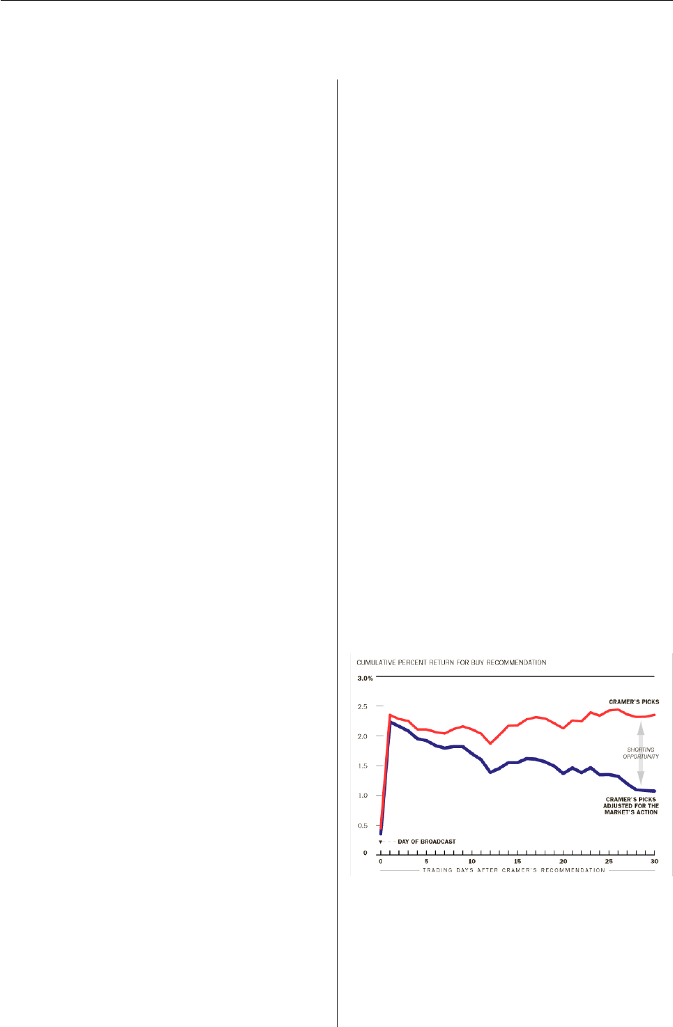
Vol. 7/3, December 2007 34
Financial Journalism with R
Bill Alpert
R proved itself a sharp tool in testing the stock picks
of Jim Cramer, a popular US financial journalist.
We examined Cramer’s advice for a recent cover
story in Barron’s, the Dow Jones & Co. stock market
weekly, where I am a reporter and floundering R user
(Alpert,2007). The August 20, 2007 story should be
accessible without subscription at the Barron’s web-
site (http://www.barrons.com).
The 52-year-old Cramer once ran a hedge fund
which racked up 24% annualized returns over about
a dozen years. His current celebrity comes from the
Mad Money television show on the cable network
CNBC, in which he makes Buy and Sell recommen-
dations to the accompaniment of wacky sound ef-
fects and clownish antics. A few have attempted
to measure the performance of modest samples of
Cramer’s picks (Engelberg et al.,2007;Nayda,2006).
Yet Cramer makes almost 7,000 recommendations
a year, according to the count of a database at his
Mad Money website (http://madmoney.thestreet.
com/). He has never reported the performance of all
those stock picks. I figured I’d try.
As in most projects, data collection was the hard
part. I called Cramer and asked for any records of his
Mad Money picks. After ripping into me and all jour-
nalists who’ve reviewed his show, he stopped tak-
ing my calls. Meanwhile, I found a website main-
tained by a retired stock analyst, who had tallied
about 1,300 of Cramer’s Mad Money recommenda-
tions over two years. I also found the abovemen-
tioned database at Cramer’s official website, which
recorded over 3,400 recommendations from the pre-
ceding six months. This Cramer site classified his
picks in ways useful for subsetting in R, but con-
spicuously lacked any performance summaries. I
turned these Web records of his stock picks into Ex-
cel spreadsheets. Then I downloaded stock price his-
tories from Edgar Online’s I-Metrix service (http:
//I-Metrix.Edgar-Online.com), using some Excel
macros. None of this was trivial work, because I
wanted a year’s worth of stock prices around each
recommendation and the date ranges varied over the
thousands of stocks. Financial data suppliers can de-
liver a wealth of information for a single, common
date range, but an "event study" like mine involved
hundreds of date ranges for thousands of stocks.
Most finance researchers deal with this hassle by us-
ing SAS and a third-party add-on called Eventus that
eases data collection. But I wanted to use R.
I reached out to quantitative finance program-
mer Pat Burns and Pat wrote some R code for our
event study style analysis. Pat has posted his own
working paper on our study at his website (http:
//www.burns-stat.com). R’s flexibility was useful
because we needed a novel data structure for the
Cramer analysis. In most analyses, the data for prices
(or for returns) are in a matrix where each column is a
different stock and each row is a specific date. In our
case, each stock recommendation had the same num-
ber of data points, so a matrix was a logical choice.
However, instead of each row being a specific date, it
was a specific offset from the recommendation date.
We still needed the actual date, though, in order to
get the difference in return between the stocks and
the S&P 500 on each day – to see if Cramer’s picks
"beat the market." Pat’s solution was to have a ma-
trix of dates as a companion to the matrix of prices.
It was then a trivial subscripting exercise to get a ma-
trix of S&P returns that matched the matrix of returns
for the recommendations. Many stocks were recom-
mended multiple times, so the column names of the
matrices were not unique.
Once the data were in R, it was fairly easy
to test various investment strategies, such as buy-
ing the day after Cramer’s 6 pm show or, instead,
waiting two days before buying. Any investment
strategy that actively picks stocks should at least
beat the returns you’d get from a passive market-
mimicking portfolio with comparable risk (that is,
similar return variance) – and it should beat the
market by enough to cover trading costs. Oth-
erwise you ought to keep your money in an in-
dex fund. You can see the importance of market-
adjusting Cramer’s returns by comparing the red
and blue lines in Figure 1. The Nasdaq Compos-
ite Index is arguably a better match to the riski-
ness of Cramer’s widely-varying returns. We made
his performance look better when we used the S&P.
Figure 1: Average cumulative percentage log return
from the day of broadcast for approx. 1,100 Mad
Money recommendations recorded at http://www.
yourmoneywatch.com. Blue line shows return rela-
tive to S&P 500 Index.
The red line shows his average pick’s unad-
justed log return, while the blue shows the log re-
R News ISSN 1609-3631
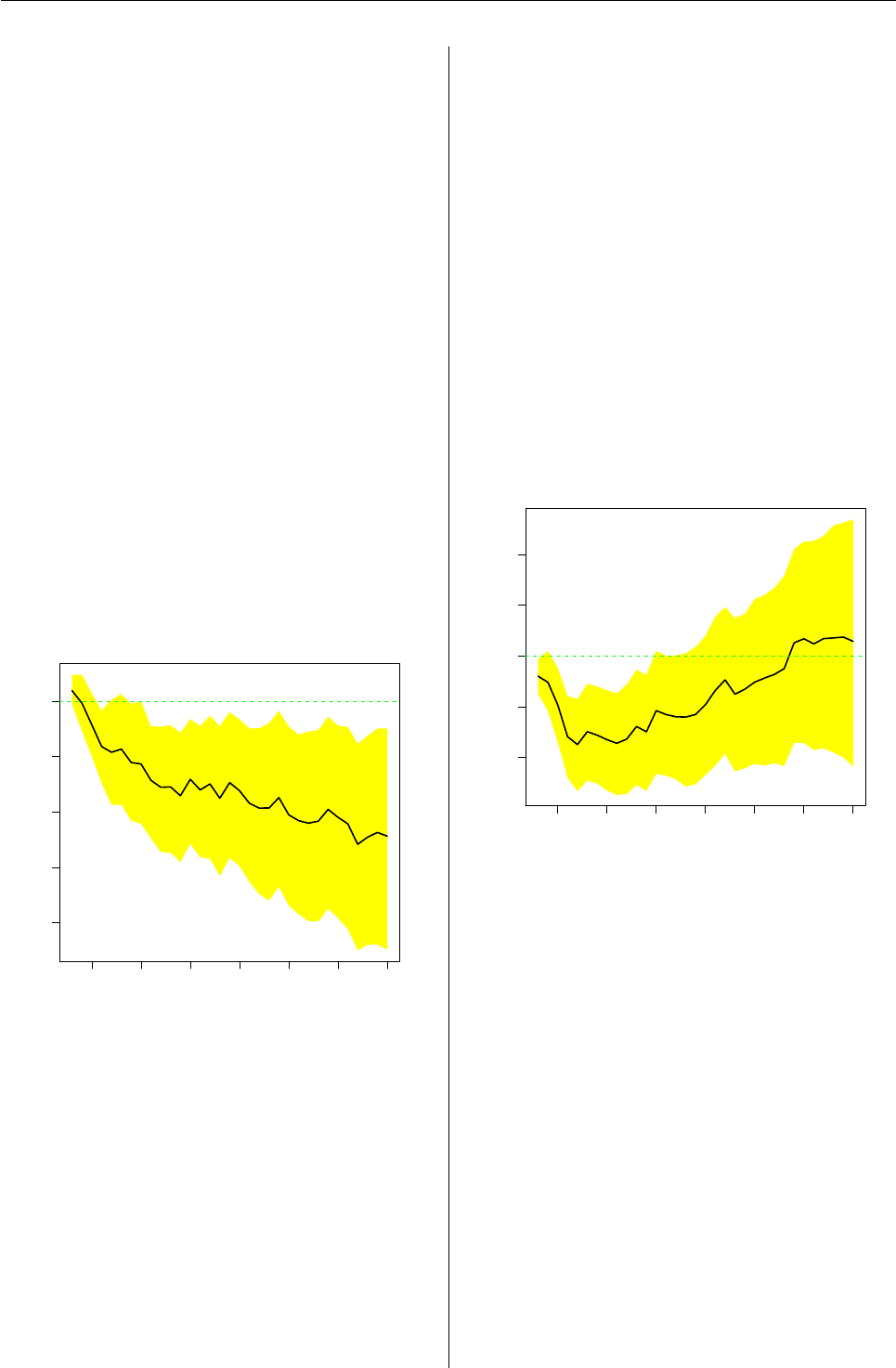
Vol. 7/3, December 2007 35
turn relative to the Standard & Poors 500 Index.
The data were roughly 1,100 Buy recommendations
over the period from July 2005 to July 2007. The
lines’ lefthand peaks mark the trading day after each
evening broadcast, when enthusiastic fans have bid
up Cramer’s pick. We ultimately tested several
dozen investment strategies.
The results were disappointing for someone who
wants to follow Cramer’s advice. You could not
beat the market by a statistically significant amount if
you followed his recommendations in any way read-
ily available to a viewer. But we did find that you
might make an interesting return if you went against
Cramer’s recommendations – shorting his Buys the
morning after his shows, while putting on offset-
ting S&P 500 positions. This shorting opportunity
appears in Figure 1, as the widening difference be-
tween the red and blue lines. If a viewer shorted only
Cramer’s recommendations that jumped 2% or more
on the day after his broadcasts, that difference could
earn the viewer an annualized 12% on average (less
trading costs). The bootstrapped 95% confidence in-
tervals of this difference ranged from 3% to 21%. (For
background on bootstrap techniques, see Efron and
Tibshirani,1993)
0 5 10 15 20 25 30
−4 −3 −2 −1 0
Negative lightning
Days
Cumulative abnormal return
Figure 2: Cumulative log return relative to S&P
500 on about 480 of Cramer’s off-the-cuff Lightning
Round Sell recommendations, as recorded at mad-
money.thestreet.com. The yellow band is a boot-
strapped 95% confidence interval, showing that the
negative return – desirable for Sell recommendations
– is clearly different from zero
One reason we tested so many different strate-
gies is that when I finally started getting responses
from Cramer and CNBC, they kept changing their
story. They argued about selection. Neither of my
databases were reliable records of Cramer’s picks,
CNBC said, not even the database endorsed by
Cramer at his website. Instead of giving me a record
of his two-years’ of stock picks, they suggested that
I watch tapes of all his shows, which they’d gladly
provide me. It reminded me of the endless tasks as-
signed in fairy tales – separating peas from the ash
pile.
They also argued that certain subsets of Cramer’s
recommendations were the only proper ones to
count . . . as if viewers would somehow know which
of his screaming "Buys" he meant them to ignore.
As it happened, the segment of his show that
Cramer argued most shrilly for us to deselect (the
"Lightning Round" with his impromptu responses to
phoned-in questions) was the only segment with any
statistically-significant marketbeating returns – in
this case, on the Sell recommendations (see Figure 2).
Embarrassingly, the Sell recommendations that
Cramer prepared in advance went up (see Figure 3).
0 5 10 15 20 25 30
−2 −1 0 1 2
Negative featured or discussed
Days
Cumulative abnormal return
Figure 3: Cumulative log return relative to S&P 500
on about 160 of Cramer’s Prepared Sell recommen-
dations as recorded at madmoney.thestreet.com
CNBC and Cramer also kept shifting their claim
about when Cramer advises his audience to act on
his picks. After I told Cramer that viewers got
market-lagging returns if they bought the day after
his recommendations (when most viewers clearly do
their buying), he angrily said that he "always" ad-
vises waiting until the second day. When I came
back with evidence that a second-day purchase also
lagged the market (as is clear in Figure 1), CNBC
said that Cramer’s advice had "always" been to wait
a week or two after each show. Later still, they said
that a good test should wait exactly five days.
Such data dredging and methodological de-
bates are probably not unfamiliar to readers of this
newsletter who use R for high stakes evaluations
of pharmaceuticals or government interventions, but
journalism may be extreme in its extensive interac-
R News ISSN 1609-3631

Vol. 7/3, December 2007 36
tion with the subjects of its analyses. Academics
rarely contact authors they critique – indeed, post-
publication data repositories aim to make it easy to
replicate a study without questioning the authors.
Good journalists do the opposite: we contact the sub-
jects of our investigations early and often.
And of course, R let us flexibly change our anal-
ysis every time CNBC and Cramer changed their
story. When they argued for a different selection,
R made it easy to create a new data subset. When
they argued for a different holding strategy, R’s in-
dexing facility let us start and stop our analysis on
different dates. In fact, when I begged CNBC for
their own analysis of Cramer’s performance, they
said something that should warm the hearts of all
you folks who’ve made R the powerful environment
it is. CNBC told me not to expect a timely response
from them because it was obvious that Pat and I had
spent months on our analysis. In truth, Pat put in less
than a week’s work.
Acknowledgments
Essential services for this project included: R cod-
ing by Pat Burns, of Burns Statistics in London; Excel
macros by Edgar Online analyst Elias-John Kies and
from Tufts University undergraduate Madison Mc-
gaffin; wise statistical pointers from Tim Hesterberg,
of Insightful Corp. in Seattle . . . none of whom bear
responsibility for any woebegone errors.
Bibliography
B. Alpert. Shorting Cramer. Barron’s, 2007.
B. Efron and R. Tibshirani. Introduction to the Boot-
strap. Chapman and Hall, 1993.
J. Engelberg, C. Sasseville, and J. Williams. Attention
and Asset Prices: the Case of Mad Money. Tech-
nical report, Kellogg School of Management, 2007.
http://papers.ssrn.com.
N. Nayda. You! Me! Let’s Get Ready to Make Mad
Money!!! Technical report, Elmont Virginia Ele-
mentary School, 2006. Science fair project.
Bill Alpert
Barron’s, Dow Jones & Co., U.S.A.
william.alpert@barrons.com
Need A Hint?
Sanford Weisberg and Hadley Wickham
Suppose you have created an object in R, for example
from a regression fit using lm or loess. You know
that auxiliary functions exist that do useful compu-
tations on the object, but you can’t remember their
names. You need a hint on what to do next.
The hints function in the hints package does just
this, finding a list of appropriate functions to jog
your memory. For example, Figure 1shows a list of
hints for a lm object.
The output lists methods for generic functions
like print specific to the class you specify, as well
as searching the documentation to find all mentions
of the class. You can then use the usual help mecha-
nism to learn more about each of these methods and
functions.
The hints function has three arguments:
hints(x, class=class(x), all.packages=FALSE)
If specified, the argument xcan be any R object. For
example, xmight have been created by x <- lm(y
z).hints determines the S3 class of the object, and
then looks for functions that operate on that class.
The S3 class of an object is a character vector, and
may consist of multiple strings, as, for example, a
generalized linear model which has class c("glm",
"lm"). If xis not given, then you can specify the
class you want hints about as character vector.
The hints function will look for methods and
functions in all currently loaded packages. For ex-
ample, the hints for lm would be different if either the
car or the alr3 packages have been loaded, since both
of these add methods and functions for lm objects.
Similarly, hints(class="lda") would return meth-
ods only if the package MASS were loaded, since all
the relevant methods and functions are in that pack-
age. You can get hints for all your packages by set-
ting all.packages=TRUE, but note that this works by
require’ing all available packages so may be time
consuming.
The hints package also includes an xtable
method so, for example, xtable(hints(m1)) would
have produced a version of Figure 1, but in L
A
T
EX for-
mat.
The function isn’t foolproof, as it depends on
the quality of documentation written by others. It
may find irrelevant functions if the name of the
class appears in the documentation for the irrele-
vant function. It can miss functions, too. For ex-
ample, the function coeftest in the lmtest package
can be used with lm objects by applying the function
coeftest.default.
R News ISSN 1609-3631

Vol. 7/3, December 2007 37
> hints(class = "lm")
Functions for lm in package base
kappa Estimate the Condition Number
base-defunct Defunct Functions in Base Package
Functions for lm in package methods
setOldClass Specify Names for Old-Style Classes
Functions for lm in package stats
add1 Add or Drop All Possible Single Terms to a Model
alias Find Aliases (Dependencies) in a Model
anova.lm ANOVA for Linear Model Fits
case.names.lm Case and Variable Names of Fitted Models
cooks.distance.lm Regression Deletion Diagnostics
dfbeta.lm Regression Deletion Diagnostics
dfbetas.lm Regression Deletion Diagnostics
drop1.lm Add or Drop All Possible Single Terms to a Model
dummy.coef.lm Extract Coefficients in Original Coding
effects Effects from Fitted Model
family.lm Accessing Linear Model Fits
formula.lm Accessing Linear Model Fits
hatvalues.lm Regression Deletion Diagnostics
influence.lm Regression Diagnostics
labels.lm Accessing Linear Model Fits
logLik Extract Log-Likelihood
model.frame.lm Extracting the "Environment" of a Model Formula
model.matrix.lm Construct Design Matrices
plot.lm Plot Diagnostics for an lm Object
predict.lm Predict method for Linear Model Fits
print.lm Fitting Linear Models
proj Projections of Models
residuals.lm Accessing Linear Model Fits
rstandard.lm Regression Deletion Diagnostics
rstudent.lm Regression Deletion Diagnostics
summary.lm Summarizing Linear Model Fits
variable.names.lm Case and Variable Names of Fitted Models
vcov Calculate Variance-Covariance Matrix for a Fitted Model
Object
case.names Case and Variable Names of Fitted Models
dummy.coef Extract Coefficients in Original Coding
influence.measures Regression Deletion Diagnostics
lm Fitting Linear Models
lm.influence Regression Diagnostics
lm.fit Fitter Functions for Linear Models
model.frame Extracting the "Environment" of a Model Formula
model.matrix Construct Design Matrices
stats-defunct Defunct Functions in Package stats
Functions for lm in package unknown
confint.lm NA
deviance.lm NA
extractAIC.lm NA
simulate.lm NA
Figure 1: Hints for the lm class.
R News ISSN 1609-3631

Vol. 7/3, December 2007 38
Hints can’t figure this out because there is no ex-
plicit mention of lm in the function or the documen-
tation, and so it misses the function. If the regres-
sion had been done using glm rather than lm,hints
would have found coeftest.glm.
The explanations of what the methods and func-
tions do may be more generic than one might want, if
the title of the help page is too generic. In some cases,
no explanation is found. For example, simulate.lm
is shown in Figure 1, but its description is missing.
The help page for simulate mentions the lm class,
but no page is available for simulate.lm, and so the
hints function doesn’t know where to get documen-
tation. Finally, the hints function can only find hints
for S3 objects, not for S4. Nevertheless, this simple
function can be a useful tool, if you are willing to
take a hint.
Sanford Weisberg
University of Minnesota
sandy@stat.umn.edu
Hadley Wickham
Iowa State University
h.wickham@gmail.com
Psychometrics Task View
Patrick Mair, Reinhold Hatzinger
Psychometrics is concerned with the design and
analysis of research and the measurement of human
characteristics. Psychometricians have also worked
collaboratively with those in the field of statistics and
quantitative methods to develop improved ways to
organize and analyze data. In our task view we sub-
divide “Psychometrics" into the following method-
ological areas: Item Response Theory (IRT), Corre-
spondence Analysis (CA), Structural Equation Mod-
els (SEM) and related methods such as Factor Anal-
ysis (FA) and Principal Component Analysis (PCA),
Multidimensional Scaling (MDS), Classical Test The-
ory (CTT), and other approaches related to psycho-
metrics.
Since much functionality is already contained in
base R and there is considerable overlap between
tools for psychometry and tools described in other
views, particularly in SocialSciences, we only give
a brief overview of packages that are closely related
to psychometric methodology. Recently, Journal
of Statistical Software (JSS) published a spe-
cial volume on Psychometrics in R in which some
new R packages were published. For an overview
see de Leeuw and Mair (2007).
Item Response Theory (IRT)
The eRm package fits extended Rasch models, i.e.
the ordinary Rasch model for dichotomous data
(RM), the linear logistic test model (LLTM), the rating
scale model (RSM) and its linear extension (LRSM),
the partial credit model (PCM) and its linear exten-
sion (LPCM) using conditional ML estimation.
The package ltm also fits the simple RM. Addi-
tionally, functions for estimating Birnbaum’s 2- and
3-parameter models based on a marginal ML ap-
proach are implemented as well as the graded re-
sponse model for polytomous data, and the linear
multidimensional logistic model.
Item and ability parameters can be calibrated us-
ing the package plink. It provides various functions
for conducting separate calibration of IRT single-
format or mixed-format item parameters for multiple
groups using the Mean/Mean, Mean/Sigma, Hae-
bara, and Stocking-Lord methods. It includes sym-
metric and non-symmetric optimization and chain-
linked rescaling of item and ability parameters.
The package plRasch computes maximum like-
lihood estimates and pseudo-likelihood estimates
of parameters of Rasch models for polytomous (or
dichotomous) items and multiple (or single) la-
tent traits. Robust standard errors for the pseudo-
likelihood estimates are also computed.
A multilevel Rasch model can be estimated using
the package lme4 with functions for mixed-effects
models with crossed or partially crossed random ef-
fects.
Other packages of interest are: mokken in the
JSS special issue as a package to compute non-
parametric item analysis, the RaschSampler allow-
ing for the construction of exact Rasch model tests
by generating random zero-one matrices with given
marginals, mprobit fitting the multivariate binary
probit model, and irtoys providing a simple interface
to the estimation and plotting of IRT models. Simple
Rasch computations such a simulating data and joint
maximum likelihood are included in the MiscPsycho
package.
Gaussian ordination, related to logistic IRT and
also approximated as maximum likelihood esti-
mation through canonical correspondence analysis
is implemented in various forms in the package
VGAM.
Two additional IRT packages (for Microsoft Win-
dows only) are available and documented on the
JSS site. The package mlirt computes multilevel IRT
models, and cirt uses a joint hierarchically built up
likelihood for estimating a two-parameter normal
ogive model for responses and a log-normal model
for response times.
R News ISSN 1609-3631

Vol. 7/3, December 2007 39
Bayesian approaches for estimating item and per-
son parameters by means of Gibbs-Sampling are in-
cluded in MCMCpack.
Correspondence Analysis (CA)
Simple and multiple correspondence analysis can be
performed using corresp() and mca() in package
MASS (and in the corresponding bundle VR). The
package ca comprises two parts, one for simple cor-
respondence analysis and one for multiple and joint
correspondence analysis. Within each part, func-
tions for computation, summaries and visualization
in two and three dimensions are provided, includ-
ing options to display supplementary points and
perform subset analyses. Other features are visual-
ization functions that offer features such as differ-
ent scaling options for biplots and three-dimensional
maps using the rgl package. Graphical options in-
clude shading and sizing plot symbols for the points
according to their contributions to the map and
masses respectively.
The package ade4 contains an extensive set of
functions covering, e.g., principal components, sim-
ple and multiple, fuzzy, non symmetric, and decen-
tered correspondence analysis. Additional function-
ality is provided at Bioconductor in the package
made4.
The PTAk package provides a multiway method
to decompose a tensor (array) of any order, as a gen-
eralisation of SVD also supporting non-identity met-
rics and penalisations. 2-way SVD with these ex-
tensions is also available. Additionally, the pack-
age includes some other multiway methods: PCAn
(Tucker-n) and PARAFAC/CANDECOMP with ex-
tensions.
The package cocorresp fits predictive and sym-
metric co-correspondence analysis (CoCA) models to
relate one data matrix to another data matrix.
Apart from several factor analytic methods Fac-
toMineR performs CA including supplementary
row and/or column points and multiple correspon-
dence analysis (MCA) with supplementary individ-
uals, supplementary quantitative variables and sup-
plementary qualitative variables.
Package vegan supports all basic ordination
methods, including non-metric multidimensional
scaling. The constrained ordination methods in-
clude constrained analysis of proximities, redun-
dancy analysis, and constrained (canonical) and par-
tially constrained correspondence analysis.
Other extensions of CA and MCA which also gen-
eralize many common IRT models can be found on
the PsychoR page.
Structural Equation Models (SEM)
and related methods
Ordinary factor analysis (FA) and principal compo-
nent analysis (PCA) are in the package stats as func-
tions factanal() and princomp(). Additional rota-
tion methods for FA based on gradient projection al-
gorithms can be found in the package GPArotation.
The package nFactors produces a non-graphical so-
lution to the Cattell scree test. Some graphical PCA
representations can be found in the psy package.
The sem package fits general (i.e., latent-
variable) SEMs by FIML, and structural equations in
observed-variable models by 2SLS. Categorical vari-
ables in SEMs can be accommodated via the polycor
package. The systemfit package implements a wider
variety of estimators for observed-variables models,
including nonlinear simultaneous-equations models.
See also the pls package, for partial least-squares es-
timation, the gR task view for graphical models and
the SocialSciences task view for other related pack-
ages.
FA and PCA with supplementary individuals
and supplementary quantitative/qualitative vari-
ables can be performed using the FactoMineR pack-
age. The homals package can do various forms of
mixed data PCA whereas MCMCpack has some op-
tions for sampling from the posterior for ordinal and
mixed factor models.
Independent component analysis (ICA) can be
computed using the packages mlica and fastICA.
Independent factor analysis (IFA) with independent
non-Gaussian factors can be performed with the ifa
package. A desired number of robust principal com-
ponents can be computed with the pcaPP package.
The package psych includes functions such as
fa.parallel() and VSS() for estimating the ap-
propriate number of factors/components as well as
ICLUST() for item clustering.
Multidimensional Scaling (MDS)
MASS (and the corresponding bundle VR) as well
as stats provide functionalities for computing clas-
sical MDS using the cmdscale() function. Sammon
mapping sammon() and non-metric MDS isoMDS()
are other relevant functions. Non-metric MDS can
additionally be performed with metaMDS() in vegan.
Furthermore, labdsv and ecodist provide the func-
tion nmds() and other relevant routines can be found
in xgobi.
Principal coordinate analysis can be computed
with capscale() in vegan; in labdsv and ecodist us-
ing pco() and with dudi.pco() in ade4.
Individual differences in multidimensional scal-
ing can be computed with indscal() in the Sen-
soMineR package. The package MLDS allows for
R News ISSN 1609-3631

Vol. 7/3, December 2007 40
the computation of maximum likelihood difference
scaling (MLDS).
Classical Test Theory (CTT)
The package psychometric contains functions use-
ful for correlation theory, meta-analysis (validity-
generalization), reliability, item analysis, inter-rater
reliability, and classical utility. Cronbach alpha,
kappa coefficients, and intra-class correlation coeffi-
cients (ICC) can be found in the psy package.
A number of routines for scale construction and
reliability analysis useful for personality and exper-
imental psychology are contained in the packages
psych and MiscPsycho. Additional measures for re-
liability and concordance can be computed with the
concord package.
Other related packages
Latent class analysis can be performed using the
function lca() from package e1071. Further pack-
ages are mmlcr and poLCA. They compute mixed-
mode latent class regression and polytomous vari-
able latent class analysis, respectively.
The cfa package allows for the computation of
simple, more-sample, and stepwise configural fre-
quency analysis (CFA).
Coefficients for interrater reliability and agree-
ments can be computed with the irr package. Psy-
chophysical data can be analyzed with the psyphy
package. Bradley-Terry models for paired compar-
isons are implemented in the package BradleyTerry
and in eba. The latter allowes also for the compu-
tation of elimination-by-aspects models. Confidence
intervals for standardized effect sizes can be found
in MBESS.
Bibliography
J. de Leeuw and P. Mair. An Introduction to the
Special Volume on Psychometrics in R Journal
of Statistical Software, 20(1):1-5, 2007. URL http:
//www.jstatsoft.org/v20/i01/
Patrick Mair, Reinhold Hatzinger
Department of Statistics and Mathematics
Wirtschaftsuniversität Wien
patrick.mair@wu-wien.ac.at
reinhold.hatzinger@wu-wien.ac.at
meta: An R Package for Meta-Analysis
by G. Schwarzer
Introduction
The statistical method of meta-analysis can be used
to combine two or more individual study results.
More specificly, an overall effect is estimated by cal-
culating a weighted average of estimates in individ-
ual studies. Various methods of meta-analysis exist
that differ mainly in the weighting scheme utilised.
Meta-analysis provides a statistical method to evalu-
ate the direction and size of the effect as well as the
question whether the effect is consistent across dif-
ferent studies.
The package meta is a comprehensive set of func-
tions for meta-analysis. Initially, the package was
intended to provide statistical methods for meta-
analysis available in Review Manager, Version 4
(RevMan 4), the Cochrane Collaboration’s program
for preparing and maintaining Cochrane reviews
(see http://www.cc-ims.net/RevMan/). The statisti-
cal capabilities of RevMan 4 have been extended over
time.
The package provides methods for meta-analysis
of studies comparing two groups with either bi-
nary or continuous outcome (function metabin()
and metacont(), respectively). Furthermore, the
package can be used in a more general way by us-
ing the function metagen(), e.g., to combine hazard
ratios for survival outcomes.
Statistical methods for fixed effect and random
effects models (Fleiss,1993) are available as well as
functions to draw the most commonly used graph-
ical displays (forest plots, funnel plots, and radial
plots). Various statistical tests for funnel plot asym-
metry, which is often taken as an indication of publi-
cation bias, are implemented. Some additional func-
tions are available which will not be described in de-
tail in this article, e.g. the function trimfill() for
the trim-and-fill method, which can be used to cor-
rect for funnel plot asymmetry (Duval and Tweedie,
2000), and the function read.mtv() to read data anal-
ysis files exported from RevMan 4.
Another package for meta-analysis exists, called
rmeta, which also provides functions for fixed ef-
fect and random effects models. As compared to
the package meta, functions implementing statistical
methods for funnel plot asymmetry, specific meth-
ods for continuous outcomes, the Peto method for
pooling as well as the additional functions men-
tioned in the last paragraph are not available in the
package rmeta.
R News ISSN 1609-3631

Vol. 7/3, December 2007 41
Meta-analysis of binary outcomes
The function metabin() provides methods for the
meta-analysis of studies comparing two groups with
binary outcomes. Output from metabin() is an ob-
ject with classes "metabin" and "meta".
The summary measure to compare the two
groups (parameter sm) can be
• the relative risk (RR, default): pE
pC
• the odds ratio (OR): pE/(1−pE)
pC/(1−pC)
• the risk difference (RD): pE−pC
• the arcsine difference (AS):
arcsin(√pE)−arcsin(√pC)
with pEand pCdenoting the event probabilities for
experimental and control group, respectively.
At a minimum, the number of events (event.e,
event.c) and the sample size in both groups (n.e,
n.c) are needed as input to metabin(). Further pa-
rameters could be set, e.g., the type of fixed effect
method to be utilised (parameter method):
• Inverse variance method, available for all effect
measures (Fleiss,1993),
• Mantel-Haenszel method, available for RR,
OR, and RD (Greenland and Robins,1985;
Robins et al.,1986),
• Peto method, only available for OR (Yusuf
et al.,1985).
In any case, results of a random effects meta-analysis
based on the inverse variance method and a method
of moments estimator for the between-study vari-
ance are also calculated (DerSimonian and Laird,
1986).
Zero cell frequencies
Several parameters of metabin() are concerned with
the handling of studies with zero cell frequencies.
The estimated event probability b
pEor b
pCis zero
if either the number of events in the experimental
or control group is zero; accordingly, the estimated
odds ratio and risk ratio are either 0 or infinite. If
both event numbers are zero, odds ratio and relative
risk are undefined (see below). Furthermore, vari-
ance estimates of log odds ratio and log relative risk
are infinite due to division by zero. For the risk dif-
ference, the estimated effect is always finite, but the
variance estimate can be zero. Thus, an adjustment
for zero cell frequencies is necessary for odds ratio,
relative risk, and risk difference. On the other hand,
no adjustment for zero cell frequencies is necessary
for the arcsine difference as summary measure.
It is common practice to add a small constant,
typically 0.5, to each cell count in the case of zero cell
frequencies (Gart and Zweifel,1967;Pettigrew et al.,
1986); a different value for this increment can be cho-
sen (parameter incr). This modification can be used
in general, but it is typically only applied if any of
the cell counts is zero.
Three meta-analytic strategies are implemented
in metabin() to adjust for zero cell frequencies:
• add 0.5 only to cell counts of two-by-two tables
with zero cell counts (default),
• add 0.5 to all two-by-two tables in the case of
zero cell counts in one or more studies (param-
eter allincr=TRUE),
• add 0.5 to all two-by-two tables (parameter
addincr=TRUE).
To calculate the Mantel-Haenszel and the Peto
estimate, there is no need to adjust for zero cell
frequencies. However, an adjustment is utilised
for the Mantel-Haenszel method in commonly used
software for meta-analysis like RevMan 4 or the
Stata procedure metan (http://www.stata.com/).
Accordingly, an adjustment is also used by de-
fault for the Mantel-Haenszel method in metabin();
the exact Mantel-Haenszel estimate without adjust-
ment can be calculated by setting the parameter
MH.exact=TRUE.
For odds ratio and relative risk, studies with zero
events in both groups are typically excluded from
the meta-analysis, which is the default behaviour in
metabin(). However, it is possible to include these
studies in the meta-analysis by setting the parameter
allstudies=TRUE.
Example: aspirin in myocardial infarction
A dataset of seven randomised controlled trials of the
effectiveness of aspirin versus placebo in preventing
death after myocardial infarction (Fleiss,1993) is in-
cluded in the package meta.
The result of conducting a meta-analysis of these
trials using the odds ratio as measure of treatment
effect is given in Figure 1. The assignment
> m1 <- metabin(...)
results in an object of classes "metabin" and "meta".
Accordingly, the command
> m1
utilises the generic function print.meta() to print
individual results of the seven trials as well as sum-
maries for the fixed effect and random effects model.
The columns %W(fixed) and %W(random) give the
percentage weights of individual trials in the fixed
effect and random effects model, respectively.
R News ISSN 1609-3631
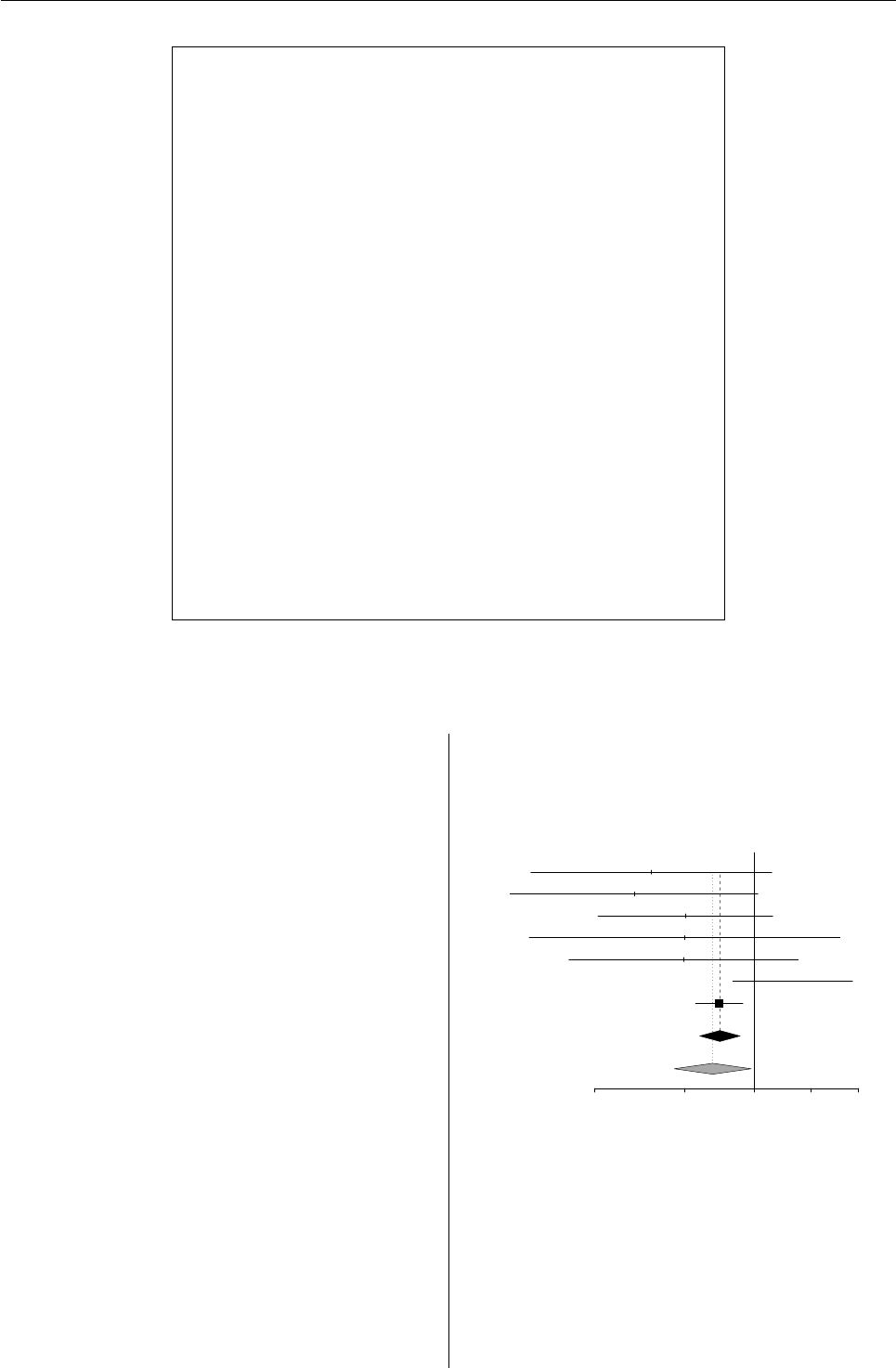
Vol. 7/3, December 2007 42
> data("Fleiss93")
> m1 <- metabin(event.e, n.e, event.c, n.c,
+ data=Fleiss93, studlab=paste(study, year),
+ sm="OR")
> m1
OR 95%-CI %W(fixed) %W(random)
MRC-1 1974 0.7197 [0.4890; 1.0593] 3.18 8.21
CDP 1976 0.6808 [0.4574; 1.0132] 3.10 7.85
MRC-2 1979 0.8029 [0.6065; 1.0629] 5.68 13.23
GASP 1979 0.8007 [0.4863; 1.3186] 1.80 5.36
PARIS 1980 0.7981 [0.5526; 1.1529] 3.22 8.89
AMIS 1980 1.1327 [0.9347; 1.3728] 10.15 20.70
ISIS-2 1988 0.8950 [0.8294; 0.9657] 72.88 35.77
Number of trials combined: 7
OR 95%-CI z p.value
Fixed effects model 0.8969 [0.8405; 0.9570] -3.2876 0.001
Random effects model 0.8763 [0.7743; 0.9917] -2.0918 0.0365
Quantifying heterogeneity:
tau^2 = 0.0096; H = 1.29 [1; 1.99]; I^2 = 39.7% [0%; 74.6%]
Test of heterogeneity:
Q d.f. p.value
9.95 6 0.1269
Method: Mantel-Haenszel method
Figure 1: Meta-analysis with binary outcome – myocardial infarction trials (Fleiss,1993); output of function
metabin().
Summary and forest plot
The command
> summary(m1)
results in the same output as given in Figure 1
but omitting results for individual studies; actu-
ally, the function summary.meta() is called inside
print.meta(). The function summary.meta() re-
sults in an object of class "summary.meta" with cor-
responding function print.summary.meta().
An object of class "summary.meta" contains infor-
mation on several summary statistics. For example,
the command
> summary(m1)$fixed
gives a list of elements with results for the fixed effect
meta-analysis.
The function summary.meta() can also be used to
conduct a sub-group analysis. For example, the fol-
lowing command results in a sub-group analysis of
the myocardial infarction trials based on the year of
publication:
> summary(m1, byvar=Fleiss93$year<1980,
+ bylab="year<1980")
The result of a meta-analysis can be shown graph-
ically by using the function plot.meta(). Figure 2
was generated by the command
> plot(m1, comb.f=TRUE, comb.r=TRUE)
MRC−1 1974
CDP 1976
MRC−2 1979
GASP 1979
PARIS 1980
AMIS 1980
ISIS−2 1988
Fixed effect model
Random effects model
0.6 0.8 1.0 1.2 1.4
Odds Ratio
Figure 2: Forest plot of the myocardial infarction tri-
als (Fleiss,1993); output of function plot.meta().
This type of figure is usually called a forest plot.
For individual trials, the estimated odds ratio with
95% confidence interval is plotted. Fixed effect and
random effects estimate and 95% confidence interval
are depicted by the diamonds.
R News ISSN 1609-3631
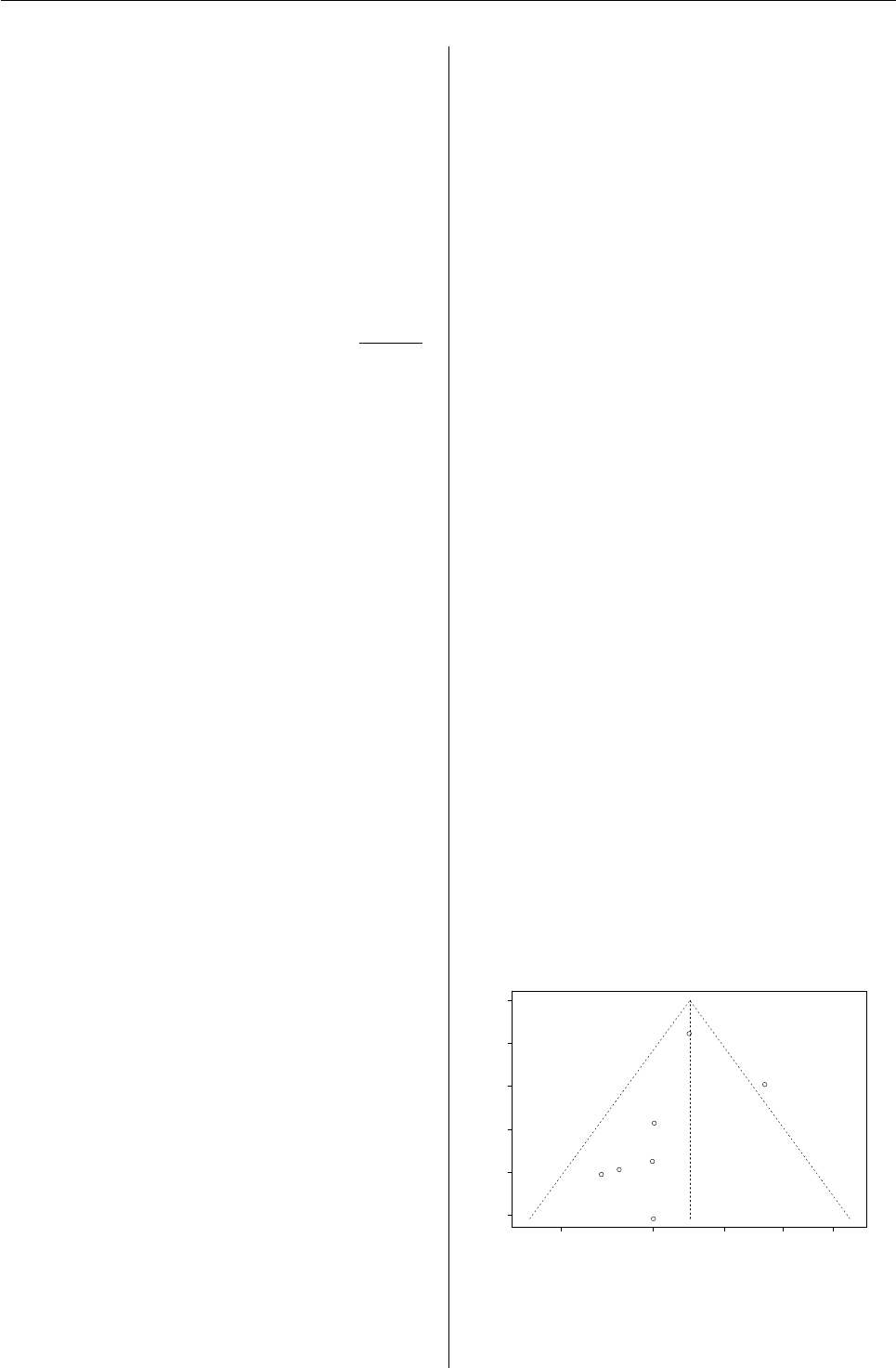
Vol. 7/3, December 2007 43
Meta-analysis of continuous out-
comes
The function metacont() provides methods for the
meta-analysis of continuous outcomes; an object of
classes "metacont" and "meta" is generated. The fol-
lowing summary measures (parameter sm) are avail-
able:
• weighted mean difference (WMD, default):
¯
xE−¯
xC
• standardised mean difference (SMD): ¯
xE−¯
xC
SD
with ¯
xEand ¯
xCdenoting the mean values in the two
groups and SD denoting the average standard devia-
tion. Hedges’ adjusted g (Cooper and Hedges,1994)
is utilised for the standardised mean difference.
At a minimum, sample sizes (n.e,n.c), mean val-
ues (mean.e,mean.c), and standard deviations (sd.e,
sd.c) are needed as input to metacont(). Both fixed
effect and random effects summary estimates are cal-
culated based on the inverse variance method (Fleiss,
1993).
The generic functions print(),summary(), and
plot() described in the last section are also available
for meta-analyses with continuous outcomes.
Meta-analysis based on generic in-
verse variance method
The function metagen() provides methods for the
meta-analysis of any outcome. At a minimum, the
estimated effect (TE) and its standard error (seTE)
are needed as input to metagen(). Both fixed ef-
fect and random effects summary estimates are cal-
culated based on the inverse variance method (Fleiss,
1993).
For example, the function metagen() can be
utilised to summarise
• adjusted estimates (e.g. from logistic regres-
sion),
• log hazard ratios for survival outcomes (Par-
mar et al.,1998),
• estimates from cross-over trials (Curtin et al.,
2002),
• estimates from both direct and indirect com-
parisons (Bucher et al.,1997).
The generic functions print(),summary(), and
plot() described in the section on meta-analyses of
binary outcomes can be utilised for objects generated
by metagen().
Statistical methods to detect small-
study effects
In meta-analyses it sometimes happens that smaller
studies show different, often larger, treatment ef-
fects. One possible reason for such “small study ef-
fects” is publication bias. This is said to occur when
the chance of a smaller study being published is in-
creased if it shows a stronger effect. If this occurs, it
in turn biases the result of the meta-analysis. A com-
prehensive review of these issues is given in Roth-
stein et al. (2005).
Funnel plot
A natural way of visualising the evidence for pos-
sible small study effects/publication bias is the fun-
nel plot (Light and Pillemer,1984), which plots each
study’s treatment effect (x-axis) against a measure of
its variability (y-axis); usually this is the standard er-
ror, although other options are preferable in different
situations (Sterne and Egger,2001). The funnel plot
gives an idea of whether there is any dependence of
treatment effect on precision.
In principal, at least two sources of asymmetry in
funnel plots exist. Publication bias, the first of them,
is well known. The second reason is heterogeneity,
for example, smaller studies may select patients who
are more likely to benefit from the intervention. Ef-
fects like these have been referred to as “small study
effects” (Sterne et al.,2000).
A funnel plot of the myocardial infarction trials
generated by the command
> funnel(m1, level=0.95)
is plotted in Figure 3. In this figure, a gap in the lower
right part is somewhat suggestive of asymmetry in
the funnel plot.
0.6 0.8 1.0 1.2 1.4
0.25 0.20 0.15 0.10 0.05 0.00
Odds Ratio
Standard error
Figure 3: Funnel plot of the myocardial infarction
trials (Fleiss,1993); output of function funnel().
R News ISSN 1609-3631

Vol. 7/3, December 2007 44
Tests for funnel plot asymmetry
A number of tests for small study effects/publication
bias have been developed and are available in the
function metabias(). Output of this command is
an object of class "htest" which utilises the default
print() function available with basic R.
Tests for small study effects/publication bias fall
into two classes:
• non-parametric tests using rank-correlation
methods, going back to Begg and Mazumdar
(1994),
• regression tests, represented by the so-called
Egger test (Egger et al.,1997).
The tests assume that under the null hypothesis of
no “publication bias” among studies included in a
meta-analysis, there is no association between treat-
ment effect and precision.
While this assumption is plausible when the out-
come is quantitative, as assuming normality the sam-
ple mean is statistically independent of the sample
variance, it is not generally true for binary data.
Specifically, suppose the outcome is binary and the
effect is summarised by the log relative risk (logRR)
or log odds ratio (logOR). The variance estimators of
both the logRR and logOR are statistically dependent
on the estimated logRR and logOR. Even in the ab-
sence of small study effects, this dependence induces
asymmetry in the funnel plot (Macaskill et al.,2001;
Schwarzer et al.,2002).
This observation has motivated recent proposals
to modify existing tests for binary outcomes (Har-
bord et al.,2006;Peters et al.,2006;Schwarzer et al.,
2007;Rücker et al.,2007). These tests are available in
the function metabias() (parameter method).
In Figure 4, results for two different tests on fun-
nel plot asymmetry (Begg and Mazumdar,1994;Har-
bord et al.,2006) are given for the meta-analysis of
the myocardial infarction trials. Both tests are non-
significant (p-value ≥0.1); thus, there is no clear in-
dication of funnel plot asymmetry.
Summary
The package meta is a comprehensive set of func-
tions for meta-analysis and provides functions for
the most commonly used outcomes, i.e., metabin()
for binary and metacont() for continuous outcomes.
Furthermore, the package can be used in a more gen-
eral way by using the function metagen(). Generic
functions to print and plot the results of a meta-
analysis and to conduct sub-group analyses are
available. Various statistical tests for funnel plot
asymmetry which is often taken as an indication of
publication bias are implemented.
Acknowledgments
This research was supported by the Deutsche
Forschungsgemeinschaft (German Research Founda-
tion) under grants Schu 756/6-1 and FOR 534.
Bibliography
C. B. Begg and M. Mazumdar. Operating character-
istics of a rank correlation test for publication bias.
Biometrics, 50:1088–1101, 1994.
H. C. Bucher, G. H. Guyatt, L. E. Griffith, and S. D.
Walter. The results of direct and indirect treatment
comparisons in meta-analysis of randomized con-
trolled trials. Journal of Clinical Epidemiology, 50:
683–91, 1997.
H. Cooper and L. V. Hedges, editors. The Handbook of
Research Synthesis. Russell Sage Foundation, New-
bury Park, CA, 1994.
F. Curtin, D. G. Altman, and D. Elbourne. Meta-
analysis combining parallel and cross-over clin-
ical trials. I: Continuous outcomes. Statistics in
Medicine, 21:2131–2144, 2002.
R. DerSimonian and N. Laird. Meta-analysis in clini-
cal trials. Controlled Clinical Trials, 7:177–188, 1986.
S. Duval and R. Tweedie. A nonparametric “Trim
and Fill” method of accounting for publication
bias in meta-analysis. Journal of the American Sta-
tistical Association, 95:89–98, 2000.
M. Egger, G. D. Smith, M. Schneider, and C. Minder.
Bias in meta-analysis detected by a simple, graph-
ical test. British Medical Journal, 315:629–634, 1997.
J. L. Fleiss. The statistical basis of meta-analysis. Sta-
tistical Methods in Medical Research, 2:121–145, 1993.
J. J. Gart and J. R. Zweifel. On the bias of various
estimators of the logit and its variance with appli-
cation to quantal bioassay. Biometrika, 54:181–187,
1967.
S. Greenland and J. M. Robins. Estimation of a com-
mon effect parameter from sparse follow-up data.
Biometrics, 41:55–68, 1985. (C/R: V45 p1323–1324).
R. M. Harbord, M. Egger, and J. A. Sterne. A modi-
fied test for small-study effects in meta-analyses of
controlled trials with binary endpoints. Statistics
in Medicine, 25(20):3443–3457, 2006.
R. J. Light and D. B. Pillemer. Summing up. The sci-
ence of reviewing research. Harvard University Press,
Cambridge, Massachusetts, 1984.
P. Macaskill, S. D. Walter, and L. Irwig. A compari-
son of methods to detect publication bias in meta-
analysis. Statistics in Medicine, 20:641–654, 2001.
R News ISSN 1609-3631

Vol. 7/3, December 2007 45
> metabias(m1, meth="rank")
Rank correlation test of funnel plot asymmetry
data: m1
z = -1.3517, p-value = 0.1765
alternative hypothesis: true is 0
sample estimates:
ks se.ks
-9.000000 6.658328
> metabias(m1, meth="score")
Linear regression test of funnel plot asymmetry (efficient score)
data: m1
t = -0.9214, df = 5, p-value = 0.3991
alternative hypothesis: true is 0
sample estimates:
bias se.bias slope
-0.72587833 0.78775820 -0.05932016
Figure 4: Statistical tests for funnel plot asymmetry – myocardial infarction trials (Fleiss,1993); output of
function metabias().
M. K. B. Parmar, V. Torri, and L. Stewart. Extract-
ing summary statistics to perform meta-analyses
of the published literature for survival endpoints.
Statistics in Medicine, 17:2815–2834, 1998.
J. L. Peters, A. J. Sutton, D. R. Jones, K. R. Abrams,
and L. Rushton. Comparison of two methods to
detect publication bias in meta-analysis. Journal of
the American Medical Association, 295:676–680, 2006.
H. M. Pettigrew, J. J. Gart, and D. G. Thomas. The
bias and higher cumulants of the logarithm of a bi-
nomial variate. Biometrika, 73:425–435, 1986.
J. Robins, N. E. Breslow, and S. Greenland. Estima-
tors of the Mantel-Haenszel variance consistent in
both sparse data and large-strata limiting models.
Biometrics, 42:311–323, 1986.
H. R. Rothstein, A. J. Sutton, and M. Borenstein. Pub-
lication bias in meta analysis: prevention, assessment
and adjustments. Wiley, Chichester, 2005.
G. Rücker, G. Schwarzer, and J. R. Carpenter. Arc-
sine test for publication bias in meta-analyses with
binary outcomes. Statistics in Medicine, 2007. Ac-
cepted.
G. Schwarzer, G. Antes, and M. Schumacher. Infla-
tion of type I error rate in two statistical tests for
the detection of publication bias in meta-analyses
with binary outcomes. Statistics in Medicine, 21:
2465–2477, 2002.
G. Schwarzer, G. Antes, and M. Schumacher. A test
for publication bias in meta-analysis with sparse
binary data. Statistics in Medicine, 26(4):721–733,
2007.
J. A. C. Sterne and M. Egger. Funnel plots for detect-
ing bias in meta-analysis: Guideline on choice of
axis. Journal of Clinical Epidemiology, 54:1046–1055,
2001.
J. A. C. Sterne, D. Gavaghan, and M. Egger. Pub-
lication and related bias in meta-analysis: Power
of statistical tests and prevalence in the literature.
Journal of Clinical Epidemiology, 53:1119–1129, 2000.
S. Yusuf, R. Peto, J. Lewis, R. Collins, and P. Sleight.
Beta blockade during and after myocardial in-
farction: An overview of the randomized tri-
als. Progress in Cardiovascular Diseases, 27:335–371,
1985.
Guido Schwarzer
Institute of Medical Biometry and Medical Informatics
University Medical Center Freiburg, Germany
sc@imbi.uni-freiburg.de
R News ISSN 1609-3631

Vol. 7/3, December 2007 46
Extending the R Commander by “Plug-In”
Packages
by John Fox
This article describes how the Rcmdr package can be
extended by suitably designed “plug-in” packages.
Embodied in the Rcmdr package, the R Commander
was originally conceived as a basic-statistics graph-
ical user interface (“GUI”) to R. The R Comman-
der’s capabilities have since been extended substan-
tially beyond this original purpose, although it still
accesses only a small fraction of the statistical and
data-management capabilities of the standard Rdis-
tribution, not to mention those of the more than 1000
contributed packages now on CRAN.
In addition to enhancing the usefulness of the R
Commander as a teaching tool, the plug-in package
mechanism allows interested package developers to
add graphical interfaces to their Rsoftware, with the
R Commander providing most of the necessary in-
trastructure, and without — as was previously the
case — requiring the developer to maintain an in-
dependent version of the Rcmdr package [e.g., Dusa
(2007)].
The Rcmdr package is based on the tcltk package
(Dalgaard,2001,2002), which provides an Rinterface
to the Tcl/Tk GUI builder. Because Tcl/Tk and the
tcltk package are available for all of the computing
platforms on which Ris commonly run, the R Com-
mander GUI runs on all of these platforms as well.
The main R Commander window is shown in
Figure 1. Along the top are the R Commander
menus: File,Edit,Data,Statistics, and so on. Below
the menus is a tool bar, containing buttons for se-
lecting, editing, and viewing the “active” data set,
and for selecting the “active” statistical model. Be-
low the toolbar are script, output, and messages win-
dows: Commands generated by the R Commander
appear in the script window; these commands can be
edited and re-executed. Printed output is displayed
in the output window, while error messages, warn-
ings, and notes appear in the messages window. A
more detailed description of the R Commander in-
terface may be found in Fox (2005).
Workflow in the R Commander is straightfor-
ward, and is based on a single rectangular (i.e., case-
by-variable) data set being “active” at any given
time. Users can import, select, or modify the active
data set via the R Commander’s Data menu. Various
statistical methods are provided by the Statistics and
Graphs menus. The R Commander recognizes certain
classes of objects as statistical models. There can be
an active statistical model that is manipulated via the
Models menu. As long as a package conforms to this
simple design (and does not, for example, require ac-
cess to several data frames simultaneously), it should
be possible to integrate it with the R Commander.
From a very early stage in its development, the
R Commander was designed to be extensible: The
menus for the R Commander interface are not hard-
coded in the package sources, but rather are de-
fined in a plain-text configuration file that installs
into the Rcmdr package’s etc subdirectory. Simi-
larly, when it starts up, the R Commander will auto-
matically source files with .R extensions that reside
in the Rcmdr etc subdirectory; such files can con-
tain Rcode to build R Commander dialog boxes, for
example. Nevertheless, extending the R Comman-
der has been relatively inconvenient, requiring either
that users modify the installed package (e.g., by edit-
ing the R Commander menu-configuration file), or
that they modify and recompile the Rcmdr source
package.1
Starting with version 1.3-0, the Rcmdr makes
alternative provision for extension by “plug-in”
packages — standard Rpackages that are devel-
oped, maintained, distributed, and installed inde-
pendently of the Rcmdr package. Plug-in packages
can augment the R Commander menus, and can
provide additional dialog boxes and statistical func-
tionality. Once installed on the user’s system, plug-
in packages are automatically detected when the R
Commander starts up and can be loaded from the R
Commander’s Tools menu. Plug-in packages can al-
ternatively be loaded independently via R’s library
command; in this event, the Rcmdr package will also
be loaded with the plug-in’s menus installed in the R
Commander menu bar. Finally, plug-in packages can
be loaded automatically along with the Rcmdr pack-
age by setting the Rcmdr plugins option; for exam-
ple, the command
options(Rcmdr=list(plugins=
"RcmdrPlugin.TeachingDemos"))
causes the RcmdrPlugin.TeachingDemos plug-in
package (described below) to load when the R Com-
mander starts up.
The remainder of this article explains in some
detail how to design R Commander plug-in pack-
ages. I begin with a description of the R Comman-
der menu-definition file, because the format of this
file is shared by R Commander plug-in packages. I
then very briefly explain how to write functions for
constructing R Commander dialog boxes. Finally, I
1In at least one instance, this inconvenience led to the distribution of a complete, alternative version of the Rcmdr package, Richard
Heiberger and Burt Holland’s Rcmdr.HH package. Exploiting the new facilities for extending the Rcmdr described in this article, Professor
Heiberger has redesigned Rcmdr.HH as an R Commander plug-in package (Heiberger with Holland, 2007).
R News ISSN 1609-3631
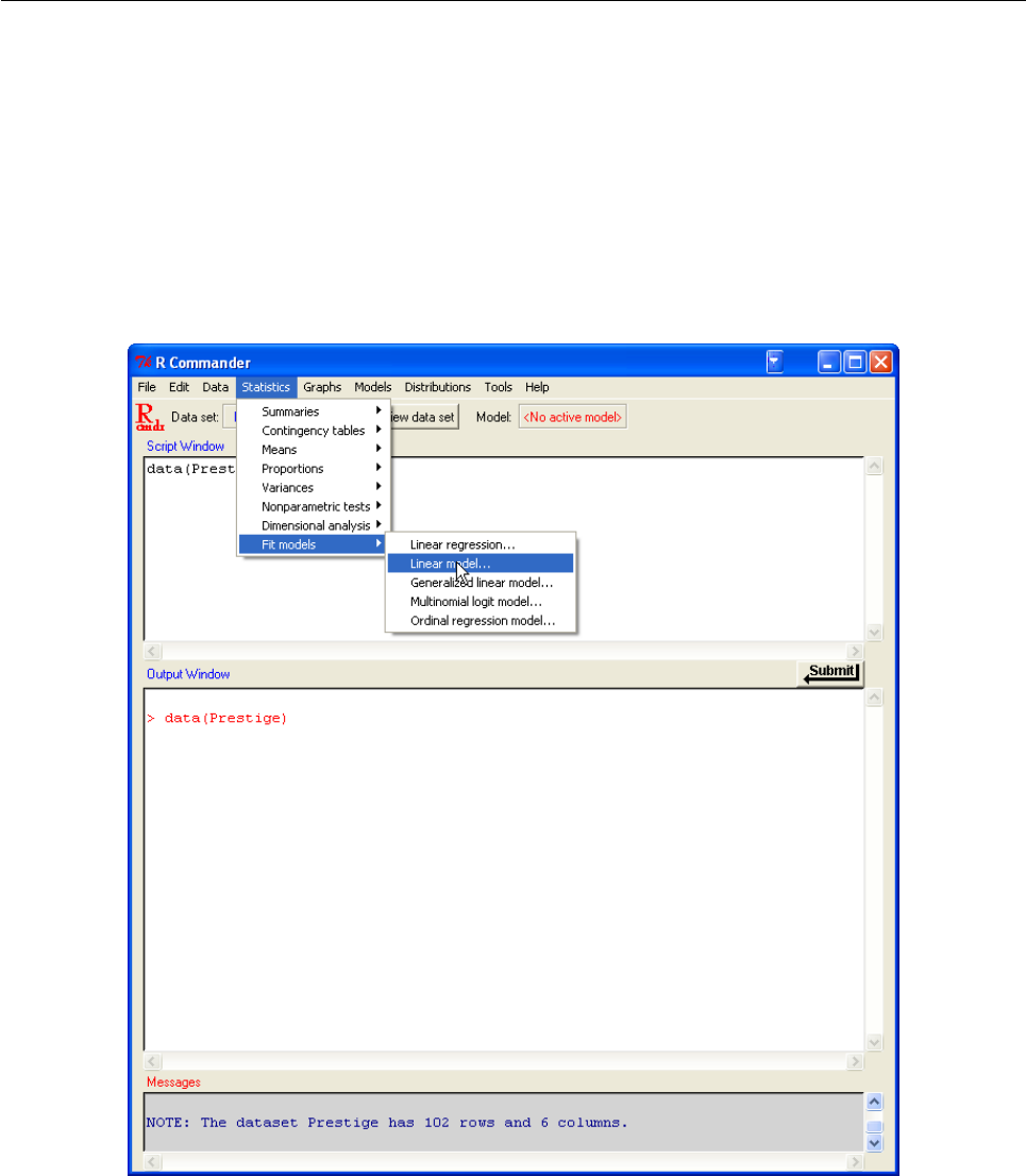
Vol. 7/3, December 2007 47
Figure 1: The R Commander interface (under Windows XP), showing menus, script, output, and messages
windows.
R News ISSN 1609-3631
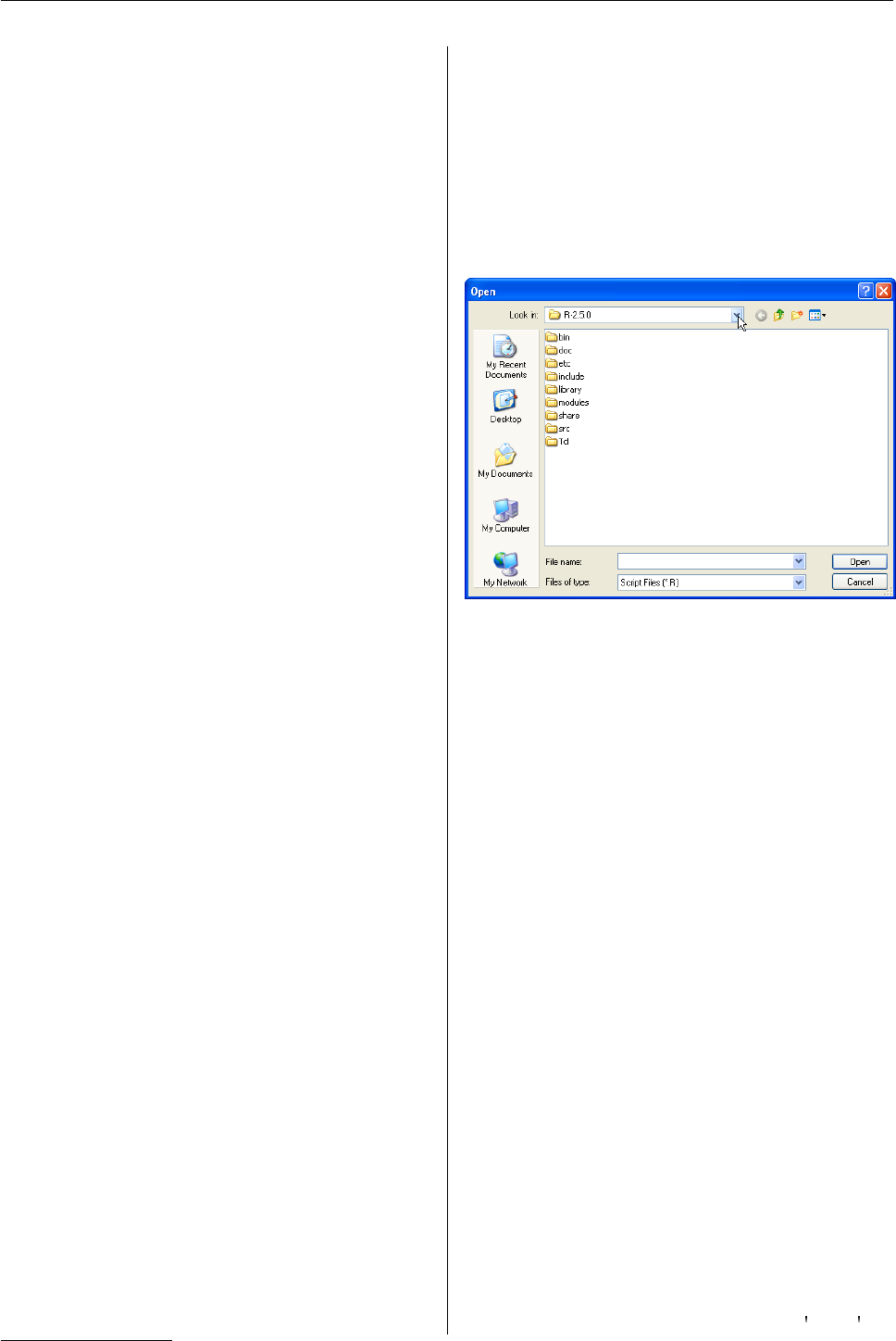
Vol. 7/3, December 2007 48
describe the structure of plug-in packages.
The Menu-Definition File
The standard R Commander menus are defined in
the file Rcmdr-menus.txt, which resides in the in-
stalled Rcmdr package’s etc subdirectory. Each line
in the file comprises seven text fields, separated by
white space. Fields with embedded blanks must be
enclosed in single or double-quotes; unused fields
are specified by an empty character string, "".
The Rcmdr-menus.txt file is quite large, and so
I will not reproduce it here (though you may want
to look at it in a text editor as you read the fol-
lowing description). Let us instead examine some
representative lines in the file. The first line in
Rcmdr-menus.txt defines the top-level File menu:
menu fileMenu topMenu "" "" "" ""
• The first, or “operation type”, field — menu —
indicates that we are defining a menu; it is also
possible to define a menu item, in which case
the operation type is item (see below).
• The second field — fileMenu — gives an arbi-
trary name to the new menu; any valid Rname
can be employed.
• The third field — topMenu — specifies the “par-
ent” of the menu, in this case signifying that
fileMenu is a top-level menu, to be installed di-
rectly in the R Commander menu bar. It is also
possible to define a submenu of another menu
(see below).
• The remaining four fields are empty.
The second line in Rcmdr-menus.txt defines a
menu item under fileMenu:2
item fileMenu command "Open script file..."
loadLog "" ""
• As explained previously, the first field indicates
the definition of a menu item.
• The second field indicates that the menu item
belongs to fileMenu.
• The third field specifies that the menu item in-
vokes a command.
• The fourth field gives the text corresponding
to the menu item that will be displayed when
a user opens the File menu; the ellipses (...)
are a conventional indication that selecting this
menu item leads to a dialog box (see Figure 2).
• The fifth field specifies the name of the function
(loadLog) to be called when the menu item is
selected. This function is defined in the Rcmdr
package, but any Rfunction that has no re-
quired arguments can serve as a menu-item
call-back function.
• In this case, the sixth and seventh fields are
empty; I will explain their purpose presently.
Figure 2: The dialog box produced by the R Com-
mander loadLog function.
A little later in Rcmdr-menus.txt, the following
line appears:
menu exitMenu fileMenu "" "" "" ""
This line defines a submenu, named exitMenu, under
fileMenu. Subsequent lines (not shown here) define
menu items belonging to exitMenu.
Still later, we encounter the lines
item fileMenu cascade "Exit" exitMenu "" ""
item topMenu cascade "File" fileMenu "" ""
Each of these lines installs a menu and the items that
belong to it, “cascading” the menu under its parent:
exitMenu is cascaded under fileMenu, and will ap-
pear with the label Exit, while fileMenu is installed
as a top-level menu with the label File. Again, the last
two fields are not used.
Fields six and seven control, respectively, the con-
ditional activation and conditional installation of the
corresponding item. Each of these fields contains
an Rexpression enclosed in quotes that evaluates
either to TRUE or FALSE. Here is an example from
Rcmdr-menus.txt:
item tablesMenu command "Multi-way table..."
multiWayTable
"factorsP(3)" "packageAvailable( abind )"
2I have broken this — and other — menu lines for purposes of display because they are too long to show on a single line.
R News ISSN 1609-3631
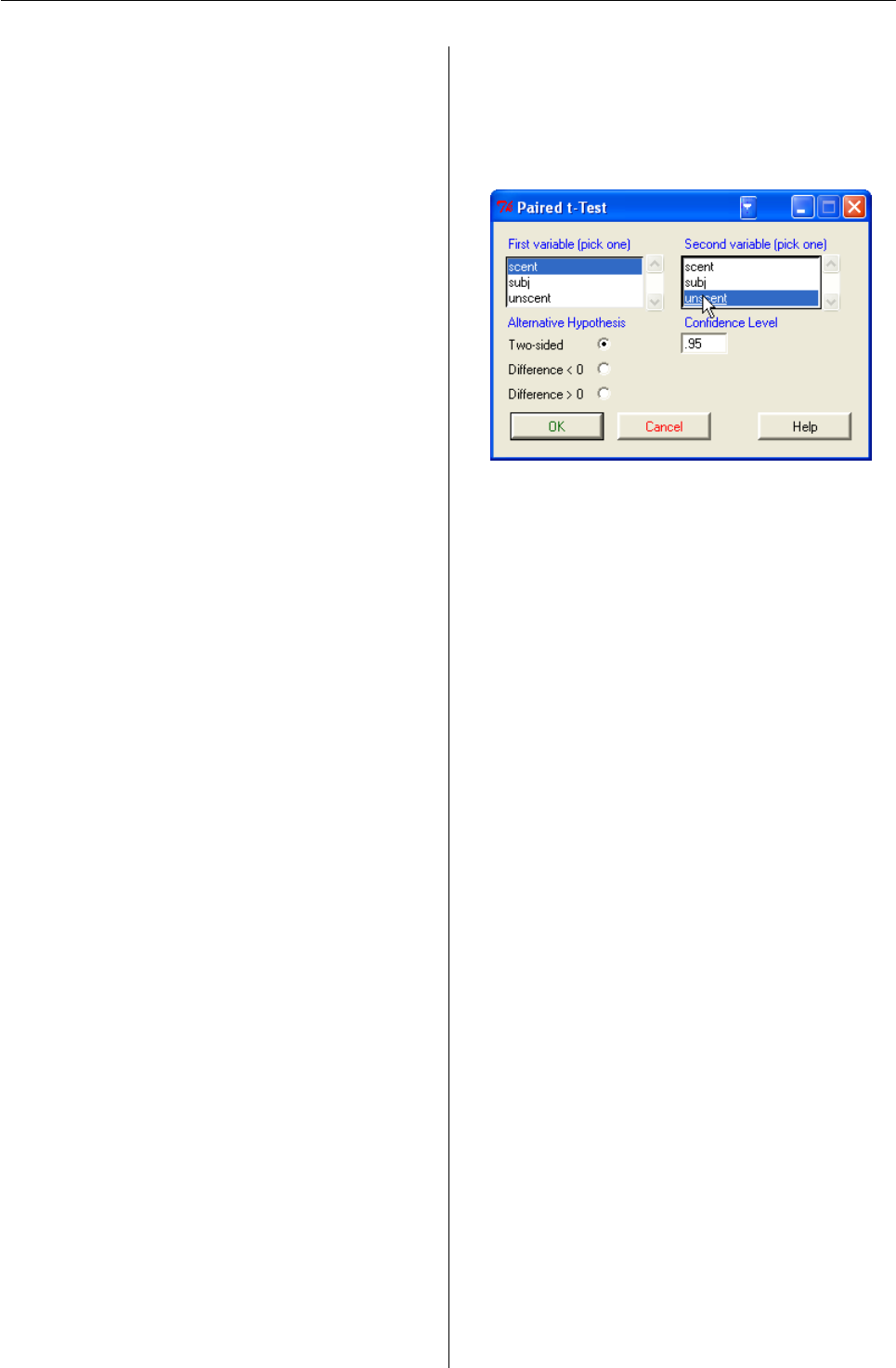
Vol. 7/3, December 2007 49
This line defines an item under tablesMenu (which
is a submenu of the Statistics menu); the item leads
to a dialog box, produced by the call-back function
multiWayTable, for constructing multi-way contin-
gency tables.
The activation field, "factorsP(3)", returns TRUE
if the active dataset contains at least three factors
— it is, of course, not possible to construct a multi-
way table from fewer than three factors. When
factorsP(3) is TRUE, the menu item is activated; oth-
erwise, it is inactive and “grayed out.”
The function that constructs multi-way con-
tingency tables requires the abind package, both
in the sense that it needs this package to oper-
ate and in the literal sense that it executes the
command require(abind). If the abind package
is available on the user’s system, the command
packageAvailable(’abind’) returns TRUE. Under
these circumstances, the menu item will be installed
when the R Commander starts up; otherwise, it will
not be installed.
Through judicious use of the activation and in-
stallation fields, a menu designer, therefore, is able to
prevent the user from trying to do some things that
are inappropriate in the current context, and even
from seeing menu items that cannot work.
R Commander Dialogs
Most R Commander menu items lead to dialog
boxes. A call-back function producing a dialog can
make use of any appropriate tcltk commands, and
indeed in writing such functions it helps to know
something about Tcl/Tk. The articles by Dalgaard
(2001,2002) mentioned previously include basic ori-
enting information, and there is a helpful web site
of R tcltk examples compiled by James Wetten-
hall, at http://bioinf.wehi.edu.au/~wettenhall/
RTclTkExamples/.Welch et al. (2003) provide a thor-
ough introduction to Tcl/Tk.
In addition, however, the Rcmdr package exports
a number of functions meant to facilitate the con-
struction of R Commander dialogs, and to help in-
sure that these dialogs have a uniform appearance.
For example, the Rcmdr radioButtons function con-
structs a related set of radio buttons (for selecting one
of several choices) in a single simple command (see
below). One relatively painless way to proceed, if
it is applicable, is to find an existing R Commander
dialog box that is similar to what you intend to con-
struct and to adapt it.
A reasonably typical, if simple, Rcmdr dialog
box, for computing a paired t-test, is shown in Fig-
ure 3. This dialog box is produced by the call-back
function pairedTTest shown in Figure 4, which il-
lustrates the use of a number of functions exported
by the Rcmdr package, such as initializeDialog,
variableListBox, and radioButtons, as well as
some tlctk functions that are called directly, such
as tclvalue,tkentry, and tkgrid. Additional
information about the functions provided by the
Rcmdr package may be found in Fox (2005) and via
?Rcmdr.Utilities.
Figure 3: R Commander dialog produced by the
function pairedTTest.
Writing Plug-In Packages
I have contributed an illustrative plug-in package to
CRAN, RcmdrPlugin.TeachingDemos. The name
was selected so that this package will sort alphabet-
ically after the Rcmdr package on CRAN; I suggest
that other writers of Rcmdr plug-ins adopt this nam-
ing convention. The RcmdrPlugin.TeachingDemos
package adds menus to the R Commander for some
of the demonstrations in Greg Snow’s intriguing
TeachingDemos package (Snow,2005). In particular,
aVisualize distributions sub-menu with several items
is cascaded under the standard R Commander top-
level Distributions menu, and a new Demos top-level
menu, also with several menu items, is installed in
the R Commander menu bar.
An R Commander plug-in package is, in the first
instance, an ordinary Rpackage. Detailed instruc-
tions for creating packages are available in the man-
ual Writing R Extensions (R Development Core Team,
2007), which ships with R.
The DESCRIPTION file for the RcmdrPlugin.-
TeachingDemos package is given in Figure 5. All of
the fields in this DESCRIPTION file are entirely stan-
dard, with the exception of the last, Models:. Certain
classes of objects are recognized by the R Comman-
der as statistical models, including objects of class lm,
glm,multinom, and polr. You can add to this list
here, separating the entries by commas, if there are
more than one. The RcmdrPlugin.TeachingDemos
package specifies no additional models; it is, there-
fore, not necessary to include the Models: field in the
DESCRIPTION file — I have done so simply to indicate
its format.
Figure 6shows the .First.lib function for the
RcmdrPlugin.TeachingDemos package. As is stan-
R News ISSN 1609-3631

Vol. 7/3, December 2007 50
pairedTTest <- function(){
initializeDialog(title=gettextRcmdr("Paired t-Test"))
.numeric <- Numeric()
xBox <- variableListBox(top, .numeric,
title=gettextRcmdr("First variable (pick one)"))
yBox <- variableListBox(top, .numeric,
title=gettextRcmdr("Second variable (pick one)"))
onOK <- function(){
x <- getSelection(xBox)
y <- getSelection(yBox)
if (length(x) == 0 | length(y) == 0){
errorCondition(recall=pairedTTest,
message=gettextRcmdr("You must select two variables."))
return()
}
if (x == y){
errorCondition(recall=pairedTTest,
message=gettextRcmdr("Variables must be different."))
return()
}
alternative <- as.character(tclvalue(alternativeVariable))
level <- tclvalue(confidenceLevel)
closeDialog()
.activeDataSet <- ActiveDataSet()
doItAndPrint(paste("t.test(", .activeDataSet, "$", x, ", ",
.activeDataSet, "$", y,
", alternative= ", alternative, " , conf.level=", level,
", paired=TRUE)", sep=""))
tkfocus(CommanderWindow())
}
OKCancelHelp(helpSubject="t.test")
radioButtons(top, name="alternative",
buttons=c("twosided", "less", "greater"),
values=c("two.sided", "less", "greater"),
labels=gettextRcmdr(c("Two-sided", "Difference < 0",
"Difference > 0")),
title=gettextRcmdr("Alternative Hypothesis"))
confidenceFrame <- tkframe(top)
confidenceLevel <- tclVar(".95")
confidenceField <- tkentry(confidenceFrame, width="6",
textvariable=confidenceLevel)
tkgrid(getFrame(xBox), getFrame(yBox), sticky="nw")
tkgrid(tklabel(confidenceFrame,
text=gettextRcmdr("Confidence Level"), fg="blue"))
tkgrid(confidenceField, sticky="w")
tkgrid(alternativeFrame, confidenceFrame, sticky="nw")
tkgrid(buttonsFrame, columnspan=2, sticky="w")
dialogSuffix(rows=3, columns=2)
}
Figure 4: The pairedTTest function.
R News ISSN 1609-3631

Vol. 7/3, December 2007 51
Package: RcmdrPlugin.TeachingDemos
Type: Package
Title: Rcmdr Teaching Demos Plug-In
Version: 1.0-3
Date: 2007-11-02
Author: John Fox <jfox@mcmaster.ca>
Maintainer: John Fox <jfox@mcmaster.ca>
Depends: Rcmdr (>= 1.3-0), rgl, TeachingDemos
Description: This package provides an Rcmdr "plug-in" based on the
TeachingDemos package, and is primarily for illustrative purposes.
License: GPL (>= 2)
Models:
Figure 5: The DESCRIPTION file from the RcmdrPlugin.TeachingDemos package.
dard in R, this function executes when the package is
loaded, and serves to load the Rcmdr package, with
the plug-in activated, if the Rcmdr is not already
loaded. .First.lib is written so that it can (and
should) be included in every R Commander plug-in
package.3
Every R Commander plug-in package must in-
clude a file named menus.txt, residing in the
installed package’s etc subdirectory. This file,
therefore, should be located in the source pack-
age’s inst/etc subdirectory. A plug-in pack-
age’s menus.txt file has the same structure as
Rcmdr-menus.txt, described previously. For exam-
ple, the line
menu demosMenu topMenu "" "" "" ""
in the menus.txt file for the RcmdrPlugin.-
TeachingDemos package creates a new top-level
menu, demosMenu;
item demosMenu command
"Central limit theorem..."
centralLimitTheorem
"" "packageAvailable( TeachingDemos )"
creates an item under this menu; and
item topMenu cascade "Demos" demosMenu
"" "packageAvailable( TeachingDemos )"
installs the new menu, and its items, in the menu bar
(see Figure 7).
Figure 7: The Demos menu provided by the
RcmdrPlugin.TeachingDemos package.
The R Commander takes care of reconciling the
menus.txt files for plug-in packages with the mas-
ter Rcmdr-menus.txt file: New top-level menus ap-
pear to the left of the standard Tools and Help menus;
when new sub-menus or items are inserted into exist-
ing menus, they appear at the end. The RcmdrPlug-
in.TeachingDemos package also includes Rcode,
for example for the centralLimitTheorem call-back
function, which creates a dialog box.
Concluding Remarks
It is my hope that the ability to define plug-in pack-
ages will extend the utility of the R Commander in-
terface. The availability of a variety of specialized
plug-ins, and the possibility of writing one’s own
plug-in package, should allow instructors to tailor
the R Commander more closely to the specific needs
of their classes. Similarly Rdevelopers wishing to
add a GUI to their packages have a convenient means
of doing so. An added benefit of having a vari-
ety of optionally loaded plug-ins is that unnecessary
menus and menu items need not be installed: After
all, one of the disadvantages of an extensive GUI is
that users can easily become lost in a maze of menus
and dialogs.
Bibliography
P. Dalgaard. A primer on the R-Tcl/Tk package.
R News, 1(3):27–31, September 2001. URL http:
//CRAN.R-project.org/doc/Rnews/.
P. Dalgaard. Changes to the R-Tcl/Tk package. R
News, 2(3):25–27, December 2002. URL http://
CRAN.R-project.org/doc/Rnews/.
A. Dusa. QCAGUI: QCA Graphical User Interface,
2007. R package version 1.3-0.
3I am grateful to Richard Heiberger for help in writing this function, and, more generally, for his suggestions for the design of the
Rcmdr plug-in facility.
R News ISSN 1609-3631

Vol. 7/3, December 2007 52
.First.lib <- function(libname, pkgname){
if (!interactive()) return()
Rcmdr <- options()$Rcmdr
plugins <- Rcmdr$plugins
if ((!pkgname %in% plugins) && !getRcmdr("autoRestart")) {
Rcmdr$plugins <- c(plugins, pkgname)
options(Rcmdr=Rcmdr)
closeCommander(ask=FALSE, ask.save=TRUE)
Commander()
}
}
Figure 6: The .First.lib function from the RcmdrPlugin.TeachingDemos package.
J. Fox. The R Commander: A basic-statistics
graphical user interface to R. Journal of Statisti-
cal Software, 14(9):1–42, Aug. 2005. ISSN 1548-
7660. URL http://www.jstatsoft.org/counter.
php?id=134&url=v14/i09/v14i09.pdf&ct=1.
R. M. Heiberger and with contributions from
Burt Holland. RcmdrPlugin.HH: Rcmdr support for
the HH package, 2007. R package version 1.1-4.
R Development Core Team. Writing R Extensions.
2007.
G. Snow. TeachingDemos: Demonstrations for teaching
and learning, 2005. R package version 1.5.
B. B. Welch, K. Jones, and J. Hobbs. Practical Program-
ming in Tcl/Tk, Fourth Edition. Prentice Hall, Upper
Saddle River NJ, 2003.
John Fox
Department of Sociology
McMaster University
Hamilton, Ontario, Canada
jfox@mcmaster.ca
Improvements to the Multiple Testing
Package multtest
by Sandra L. Taylor, Duncan Temple Lang, and Katherine
S. Pollard
Introduction
The R package multtest (Dudoit and Ge,2005) con-
tains multiple testing procedures for analyses of
high-dimensional data, such as microarray studies
of gene expression. These methods include var-
ious marginal p-value adjustment procedures (the
mt.rawp2adjp function) as well as joint testing pro-
cedures. A key component of the joint testing meth-
ods is estimation of a null distribution for the vector
of test statistics, which is accomplished via permu-
tations (Westfall and Young,1993;Ge et al.,2003) or
the non-parametric bootstrap (Pollard and van der
Laan,2003;Dudoit et al.,2004). Statistical analyses
of high-dimensional data often are computationally
intensive. Application of resampling-based statisti-
cal methods such as bootstrap or permutation meth-
ods to these large data sets further increases compu-
tational demands. Here we report on improvements
incorporated into multtest version 1.16.1 available
via both Bioconductor and CRAN. These updates have
significantly increased the computational speed of
using the bootstrap procedures.
The multtest package implements multiple test-
ing procedures with a bootstrap null distribution
through the main user function MTP. Eight test
statistic functions (meanX,diffmeanX,FX,blockFX,
twowayFX,lmX,lmY,coxY) are used to conduct one
and two sample t-tests, one and two-way ANOVAs,
simple linear regressions and survival analyses, re-
spectively. To generate a bootstrap null distribution,
the MTP function calls the function boot.null. This
function then calls boot.resample to generate boot-
strap samples. Thus, the call stack for the bootstrap is
MTP -> boot.null -> boot.resample. Finally, the
test statistic function is applied to each sample, and
boot.null returns a matrix of centered and scaled
bootstrap test statistics.
We increased the computational speed of gener-
ating this bootstrap null distribution through three
main modifications:
1. optimizing the R code of the test statistics;
2. implementing two frequently used tests (two
sample t-test and F-test) in C; and
R News ISSN 1609-3631

Vol. 7/3, December 2007 53
3. integrating an option to run the bootstrap in
parallel on a computer cluster.
Changes to Test Statistic Functions
Since the test statistic functions are applied to each
bootstrap sample, even small increases in the speed
of these functions yielded noticeable improvements
to the overall bootstrap procedure. Through pro-
filing the R code of the test statistic functions, we
identified several ways to increase the speed of these
functions. First, the function ifelse was com-
monly used in the test statistic functions. Chang-
ing ifelse to an if...else construct yielded the
largest speed improvements. The ifelse function is
designed to evaluate vectors quickly but is less effi-
cient at evaluating single values. Small gains were
achieved with changing unique to unique.default,
mean to mean.default, and sort to sort.init.
These changes eliminated the need to assess the ob-
ject class before selecting the appropriate method
when each function was called. The functions
lmX and lmY benefitted from using rowSums (i.e.,
rowSums(is.na(covar))) rather than using apply
(i.e., apply(is.na(covar),1,sum)).
The greatest improvements were achieved for the
one-sample t-test (meanX) and the regression tests
(lmX and lmY). We conducted a simulation to eval-
uate the speed improvements. For the one-sample
t-test, we randomly generated 100 and 1,000 Nor-
mal(0,1) variables for sample sizes of 50 and 100. We
tested the null hypotheses that the means for each
of the 100 or 1,000 variables were 0. For the two-
sample t-test, we randomly generated 100 and 1,000
Normal(0,1) variables for two groups consisting of 50
and 100 samples each. For the F-test, we used three
groups of 50 and 100 samples each. We tested the
null hypotheses of equal group means for each of the
variables. We evaluated the speed of 1,000 and 10,000
iterations when computing the bootstrap null distri-
butions.
We reduced computational times for the one-
sample t-test by nearly 60% when the sample size
was 50 and from 40% to 46% when the sample
size was 100. The number of variables tested and
the number of bootstrap iterations did not influence
the relative improvement of the revised functions.
Changes in R code yielded more modest improve-
ments for the two-sample t-test and F-test. Compu-
tational times were reduced by 25% to 28%, and by
about 10%, respectively. As with the one-sample t-
test, the speed improvements were not affected by
the number of variables tested or the number of boot-
strap iterations. Sample size had a very small effect
for the two-sample test, but did not influence com-
putation speed for the F-test.
Because two-sample t-tests and F-tests are some
of the most commonly used tests in multtest and
only modest improvements were achieved through
changes in the R code, we implemented these statis-
tics in C to further increase speed. These modifica-
tions took advantage of C code for calculating test
statistics in permutation tests that was already in
the package. While moving computations into C in-
creases the complexity of the code, the availability of
a reference implementation in R allowed us to easily
test the new code, easing the transition.
We evaluated the speed improvements of our
C implementation with the same approach used to
evaluate the R code modifications. By executing the
two-sample t-test in C, computational time was re-
duced by about one-half ranging from 46% when the
sample size was 100 to 52% for a sample size of 50.
The results were more dramatic for the F-test; time
was reduced by 79% to 82% with the C code imple-
mentation. Relative improvements did not vary with
the number of bootstrap iterations or variables eval-
uated. Some further optimization could be done by
profiling the C code.
Integration of Parallel Processing
Although we increased the computational speed of
generating bootstrap null distributions considerably
through improvements to the test statistics code,
some analyses still require a long time to complete
using a single CPU. Many institutions have com-
puter clusters that can greatly increase computa-
tional speed through parallel processing. Bootstrap-
ping is a straightforward technique to conduct in
parallel, since each resampled data set is indepen-
dently generated with no communication needed
between individual iterations (Tierney et al.,2007).
Thus, synchronizing cluster nodes only entails dis-
patching tasks to each node and combining the re-
sults.
Running the bootstrap on a cluster requires the R
package snow (Tierney et al.,2007). Through func-
tions in this package, the user can create a cluster
object using makeCluster and then dispatch jobs to
nodes of the cluster through several apply functions
designed for use with a cluster. We integrated use of
a cluster for generating a bootstrap null distribution
by adding an argument to the main user interface
function (MTP) called cluster. When this argument
is 1 (the default value), the bootstrap is executed on
a single CPU. To implement the bootstrap in parallel,
the user either supplies a cluster object created using
the function makeCluster in snow or identifies the
number of nodes to use in a cluster which MTP then
uses to create a cluster. In this case, the type of inter-
face system to use must be specified in the type ar-
gument. MPI and PVM interfaces require Rmpi and
rpvm packages, respectively. MTP will check if these
packages are installed and load them if necessary.
To use a cluster, multtest and Biobase (required
R News ISSN 1609-3631
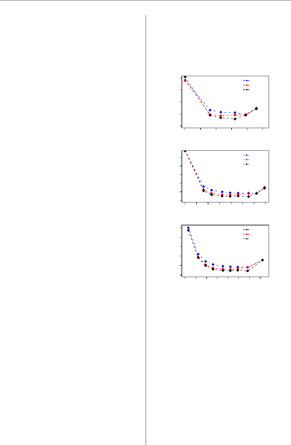
Vol. 7/3, December 2007 54
by multtest) must be loaded on each node in the
cluster. MTP checks if these packages are installed and
loads them on each node. However, if these packages
are not installed in a directory in R’s library search
path, the user will need to create a cluster, load the
packages on each node and supply the cluster object
as the argument to cluster as shown in the following
example code. This code loads the snow package,
makes a cluster consisting of two nodes and loads
Biobase and multtest onto each node of the cluster
using clusterEvalQ.
library("snow")
cl <- makeCluster(2, "MPI")
clusterEvalQ(cl, {library("Biobase");
library("multtest")})
Use of the cluster for the bootstrap is then accom-
plished by specifying the cluster object as the argu-
ment to cluster in the MTP function.
diffMeanData <- matrix(rnorm(100*100),100)
group <- gl(2, 100)
MTP(X=diffMeanData, Y=group,
test="t.twosamp.unequalvar",
alternative="two.sided", B=1000,
method="sd.minP", cluster=cl)
In multtest, we use the snow package function
clusterApplyLB to dispatch bootstrap iterations to
cluster nodes. This function automatically balances
tasks among available nodes. The user can specify
the number or percentage of bootstrap samples to
dispatch at a time to each node via the dispatch ar-
gument. We set the default value for the dispatch
argument to 5% based on simulation results. We con-
sidered bootstraps with 100, 1,000 and 10,000 itera-
tions and evaluated dispatching between 1 and 2,500
samples at a time with cluster sizes ranging from 2 to
4 nodes. Dispatching small numbers of iterations to
each node took the longest (Figure 1); in these cases
the I/O time became substantial. Processing times
initially declined as the number of iterations trans-
mitted at one time increased but then leveled off at
10 to 25 iterations for 100 iterations, 25 to 50 for 1,000
iterations and 250 to 500 for 10,000 iterations. Based
on these results, we chose to dispatch 5% of the boot-
strap iterations at a time as the default value.
Overall Speed Improvements
To assess the overall speed improvements achieved,
we compared the speed of the original user inter-
face function MTP and supporting test statistic func-
tions with the new interface function and support-
ing functions. We compared the speed of 10,000,
25,000 and 50,000 bootstrap iterations for one-sample
t-tests, two-sample t-tests and F-tests with 100 and
1,000 variables and group sample sizes of 50 and 100.
To assess the effect of a cluster, we used a Linux clus-
ter consisting of 3 nodes. Each node was a Dual Core
AMD Opteron 2411.127 MHz Processor with 4 GB of
memory.
0 0.5 1 1.5 2
012345
B=100
Total Time (sec)
2 Nodes
3 Nodes
4 Nodes
0 1 2 3 4 5 6 7
0 5 10 15 20 25
B=1,000
Total Time (sec)
2 Nodes
3 Nodes
4 Nodes
2 3 4 5 6 7 8 9
0 50 100 150 200 250
B=10,000
Total Time (sec)
Log Number of Iterations Dispatched
2 Nodes
3 Nodes
4 Nodes
Figure 1: Time to execute 100, 1, 000, and 10, 000
bootstrap iterations for 2, 3, and 4 nodes and varying
numbers of samples dispatched at a time.
Computational speed increased substantially
with the new methods. For the one-sample t-test,
computation times were reduced by about 75% for a
sample size of 50 and 49% to 69% for a sample size of
100 (Figure 2). Evaluating 1,000 variables in a sample
of 50 based on 10,000 bootstrap iterations required 26
minutes with the original functions but only 6.5 min-
utes with the new functions. The two-sample t-test
showed the greatest improvement for 50,000 boot-
strap iterations, with speed increasing by up to 96%.
At 10,000 bootstrap iterations, the new methods were
64% to 90% faster. For 1,000 variables, two groups of
50 and 10,000 bootstrap iterations, computation time
was reduced from over an hour to 20 minutes. Speed
increases for the F-test were more consistent ranging
R News ISSN 1609-3631
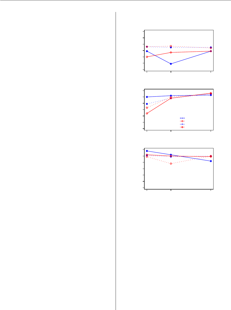
Vol. 7/3, December 2007 55
from 78% to 98%. The new methods reduced com-
putation time for 1,000 variables in 3 groups of 50
and based on 10,000 bootstrap iterations from over 3
hours to about 20 minutes. The non-monotone pat-
tern of improvement versus number of bootstrap it-
erations for the one-sample t-test with 100 variables
and a sample size of 100 and the F-test for 1,000 vari-
ables and a sample size of 50 reflects sampling vari-
ability of a single observation for each combination.
Summary
Substantial increases in computational speed for
implementing the bootstrap null distribution were
achieved through optimizing the R code, executing
calculations of test statistics in C code, and using a
cluster. Through these changes, computational times
typically were reduced by more than 75% and up to
96%. Computations that previously required several
hours to complete can now be accomplished in half
an hour.
Bibliography
S. Dudoit and Y. Ge. Multiple testing procedures, R
package, 2005.
S. Dudoit, M. van der Laan, and K. Pollard. Multi-
ple testing. Part I. Single-step procedures for con-
trol of general type I error rates. Statistical Ap-
plications in Genetics and Molecular Biology, 3(1):1–
69, 2004. URL http://www.bepress.com/sagmb/
vol3/iss1/art13.
Y. Ge, S. Dudoit, and T. Speed. Resampling-
based multiple testing for microarray data
analysis. TEST, 12(1):1–44, 2003. URL
http://www.stat.berkeley.edu/users/
sandrine/Docs/Papers/Test_spe.pdf.
K. Pollard and M. van der Laan. Resampling-based
multiple testing: Asymptotic control of type I er-
ror and applications to gene expression data. Tech-
nical Report 121, Division of Biostatistics, University
of California, Berkeley, pages 1–37, 2003. URL http:
//www.bepress.com/ucbbiostat/paper121.
L. Tierney, A. Rossini, N. Li, and H. Sevcikova. Sim-
ple network of workstations, R package, 2007.
P. Westfall and S. Young. Resampling-based Multiple
Testing: Examples and Methods for p-value Adjust-
ment. John Wiley and Sons, 1993.
40 50 60 70 80 90 100
10,000 25,000 50,000
One−sample t−test
Percent Improvement
40 50 60 70 80 90 100
10,000 25,000 50,000
Two−sample t−test
Percent Improvement
n=50, No. Vars=100
n=50, No. vars=1,000
n=100, No. Vars=100
n=100, No. Vars=1,000
40 50 60 70 80 90 100
10,000 25,000 50,000
F test
Percent Improvement
Number of Bootstrap Iterations
Figure 2: Percent improvement in time to generate
bootstrap null distributions based on 10,000, 25,000,
and 50,000 iterations for one-sample t-tests, two-
sample t-tests, and F-tests. For the simulations, sam-
ple sizes within groups for each test were 50 (dot-
ted lines) or 100 (solid lines). Mean differences were
tested for 100 (blue lines) and 1,000 variables (red
lines) at each sample size.
Sandra L. Taylor, Duncan Temple Lang,
and Katherine S. Pollard
Department of Statistics, University of California, Davis.
staylor@wald.ucdavis.edu
duncan@wald.ucdavis.edu
kpollard@wald.ucdavis.edu
R News ISSN 1609-3631

Vol. 7/3, December 2007 56
Changes in R 2.6.1
by the R Core Team
New features
• The data.frame and factor methods for [[
now support the exact argument introduced in
2.6.0.
•plot.lm() gains a new argument cex.caption
to allow the size of the captions to be con-
trolled.
• A series of changes make the CHARSXP cache
introduced in 2.6.0 faster (and in some cases
many times faster) in sessions with a large
number (e.g., a million) of unique character
strings, and also if there are many empty
strings.
•embedFonts(),bitmap() and dev2bitmap()
explicitly turn off auto-rotation in Ghostscript
when generating PDF.
• The canonical architecture is no longer checked
when loading packages using a non-empty
sub-architecture, since it is possible to (e.g.)
build packages for i386-pc-linux-gnu on both
that architecture and on x86_64-unknown-
linux-gnu.
• Deparsing will (if option warnIncomplete is
set) warn on strings longer than the parser limit
(8192 bytes).
•url() now uses the UserAgent header
in http transactions in the same way as
download.file() (making use of option
"HTTPUserAgent").
Bug fixes
•iconv() is again able to translate character
strings with embedded nuls (such as those in
UCS-2).
•new.packages() and update.packages()
failed when called on an empty library,
since old.packages() threw an error.
old.packages() now returns NULL (as docu-
mented) in that case.
• Builds on Mac OS X 10.4 or higher now allocate
enough space in the binary headers to relocate
dependent libraries into the framework.
•R CMD build now computes the exclusion list
on the copy it makes: this avoids problems
if the original sources contain symbolic links
(which are resolved in the copy). Thanks to
Michael Lawrence for diagnosis and patch.
•object.size() had slightly too low a size for
objects of type "S4".
•symbol() in plotmath expressions was only ac-
cepting valid character strings, which made it
impossible to specify symbols such as aleph
(obtained by symbol("300")) in a UTF-8 locale.
• An event handling issue caused autorepeat
functions to misbehave with tcltk (notably
scrollbars).
•plot(sin, -5, 5) gives ylab "sin(x)" again,
where it resulted in "x(x)" in 2.6.0. Further,
plot(sin) again plots from [0,1] also in cases
where a previously used coordinate system dif-
fers.
•curve() with unspecified from,to and xlim
now reuses the previous xlimits, and not
slightly larger ones.
• It was intended that R code filenames in pack-
ages should start with an ASCII letter or dig-
its (and R CMD INSTALL uses that), but the
test used in R CMD build ([A-Za-z0-9]) was
locale-specific (and excluded tto yin Estonian,
for example). (PR#10351)
•R CMD build could misbehave when faced
with files with CRLF line endings and no line
ending on the final line of the file, removing the
last byte of the file.
•DF[i, j] failed in 2.6.0 if jwas a logical vector
selecting a single column.
• Unix x11() would fail if a valid display was
specified but DISPLAY was unset. (PR#10379)
•postscript() was not always ignoring
.Postscript.Options in the workspace
(where it should not have occurred).
•help.search() would give an error if it found
a badly installed package, even if package was
not specified.
•tclServiceMode() (package tcltk) now works
under Unix-alikes. (Although documented, it
used only to work under Windows.)
• As Mac OS X 10.5.0 comes with incompati-
ble /bin/sh shell, we force SHELL=/bin/bash
(which is ok) in that case. [Only for 2.6.x: an-
other solution is used in 2.7.0.]
• Deliberately using malformed source attributes
no longer causes deparsing/printing of func-
tions to crash R. (PR#10437)
R News ISSN 1609-3631

Vol. 7/3, December 2007 57
•R CMD check and R CMD INSTALL now work
with (some) directory names containing
spaces.
•choose(n, k) gave incorrect values for nega-
tive nand small k.
•plot.ts(x,y) could use wrong default labels;
fixed thanks to Antonio Fabio di Narzo.
•reshape() got column names out of sync with
contents in some cases; found by Antonio Fabio
Di Narzo.
•ar(x) for short x(i.e., length ≤10) could
fail because the default order.max was ≥
length(x) which is non-sensical.
• Keyboard events in getGraphicsEvent()
could cause stack imbalance errors (PR#10453)
Changes on CRAN
by Kurt Hornik
New contributed packages
BARD Better Automated ReDistricting and heuris-
tic exploration of redistricter revealed prefer-
ence. By Micah Altman.
CellularAutomaton An object-oriented implemen-
tation of one-dimensional cellular automata.
Supports many of the features offered by
Mathematica, including elementary rules, user-
defined rules, radii, user-defined seeding, and
plotting. By John Hughes.
ComPairWise Compare phylogenetic or population
genetic data alignments. By Trina E. Roberts.
EDR Estimation of the effective dimension reduc-
tion (EDR) space in multi-index regression
models. By Joerg Polzehl.
FGN Fractional Gaussian Noise (FGN) model fit-
ting, including MLEs for the Hparameter and
regression with FGN errors, and simulation of
FGN. By A. I. McLeod.
FKBL Fuzzy Knowledge Base Learning, an R/C im-
plementation of a fuzzy inference engine sup-
porting several inference methods. By Alvaro
Gonzalez Alvarez.
FieldSim Routines to simulate random fields.
By Alexandre Brouste and Sophie Lambert-
Lacroix.
GLDEX Fitting single and mixture of Generalized
Lambda Distributions (RS and FMKL) using
Discretized and Maximum Likelihood meth-
ods. The fitting algorithms considered have
two major objectives. One is to provide a
smoothing device to fit distributions to data
using the weight and unweighted discretized
approach based on the bin width of the his-
togram. The other is to provide a definitive fit
to the data set using the maximum likelihood
estimation. Diagnostics on goodness of fit can
be done via QQ-plots, KS-resample tests and
comparing mean, variance, skewness and kur-
tosis of the data with the fitted distribution. By
Steve Su.
GillespieSSA Gillespie’s Stochastic Simulation Al-
gorithm (SSA). Provides a simple to use, in-
tuitive, and extensible interface to several
stochastic simulation algorithms for generat-
ing simulated trajectories of finite population
continuous-time models. Currently it imple-
ments Gillespie’s exact stochastic simulation
algorithm (Direct method) and several ap-
proximate methods (Explicit tau-leap, Bino-
mial tau-leap, and Optimized tau-leap). Also
contains a library of template models that
can be run as demo models and can eas-
ily be customized and extended. Currently
the following models are included: decaying-
dimerization reaction set, linear chain sys-
tem, logistic growth model, Lotka predator-
prey model, Rosenzweig-MacArthur predator-
prey model, Kermack-McKendrick SIR model,
and a meta-population SIRS model. By Mario
Pineda-Krch.
HardyWeinberg Exploration of bi-allelic marker
data. Focuses on the graphical representation
of the results of tests for Hardy-Weinberg equi-
librium in a ternary plot. Routines for several
tests for Hardy-Weinberg equilibrium are in-
cluded. By Jan Graffelman.
HiddenMarkov Hidden Markov Models. Contains
functions for the analysis of Discrete Time
Hidden Markov Models, Markov Modulated
GLMs and the Markov Modulated Poisson Pro-
cess. Includes functions for simulation, param-
eter estimation, and the Viterbi algorithm. The
algorithms are based of those of Walter Zuc-
chini. By David Harte.
JADE JADE and ICA performance criteria. The
R News ISSN 1609-3631

Vol. 7/3, December 2007 58
package ports J.-F. Cardoso’s JADE algorithm
as well as his function for joint diagonaliza-
tion. There are also several criteria for perfor-
mance evaluation of ICA algorithms. By Klaus
Nordhausen, Jean-Francois Cardoso, Hannu
Oja, and Esa Ollila.
JudgeIt Calculates bias, responsiveness, and other
characteristics of two-party electoral systems,
with district-level electoral and other data. By
Andrew Gelman, Gary King, and Andrew C.
Thomas.
NestedCohort Estimate hazard ratios, standardized
survival and attributable risks for cohorts with
missing covariates, for Cox models or Kaplan-
Meier. By Hormuzd A. Katki.
ProfessR Grades setting and exam maker. Programs
to determine student grades and create exam-
inations from question banks. Programs will
create numerous multiple choice exams, ran-
domly shuffled, for different versions of same
question list. By Jonathan M. Lees.
RFOC Graphics for statistics on a sphere, as ap-
plied to geological fault data, crystallogra-
phy, earthquake focal mechanisms, radia-
tion patterns, ternary plots and geographi-
cal/geological maps. By Jonathan M. Lees.
RHmm Discrete, univariate or multivariate Gaus-
sian, mixture of univariate or multivariate
Gaussian HMM functions for simulation and
estimation. By Ollivier Taramasco.
RPMG R Poor Man’s Gui: create interactive R anal-
ysis sessions. By Jonathan M. Lees.
RPyGeo ArcGIS Geoprocessing in R via Python.
Provides access to (virtually any) ArcGIS Geo-
processing tool from within R by running
Python geoprocessing scripts without writing
Python code or touching ArcGIS. Requires Ar-
cGIS ≥9.2, a suitable version of Python (cur-
rently 2.4), and Windows. By Alexander Bren-
ning.
RSAGA SAGA Geoprocessing and Terrain Analysis
in R. Provides access to geocomputing and ter-
rain analysis functions of SAGA (http://www.
saga-gis.org/) from within R by running the
command line version of SAGA. In addition,
several R functions for handling and manip-
ulating ASCII grids are provided, including a
flexible framework for applying local or focal
functions to grids. By Alexander Brenning.
RcmdrPlugin.FactoMineR Rcmdr plugin for pack-
age FactoMineR. By Francois Husson, Julie
Josse, and Sebastien Le.
Rsundials SUite of Nonlinear DIfferential ALge-
braic equations Solvers in R. Provides an inter-
face for the package of nonlinear differential al-
gebraic equation solvers that comprise SUNDI-
ALS. ODEs are expressed as R functions or as
compiled code. By Selwyn-Lloyd McPherson.
Rvelslant Code for interactively analyzing down-
hole seismic data and interpreting layered ve-
locity models of constant velocity layers ac-
counting for refractions across layer bound-
aries. Original method by Dave Boore, R port
and some additions by Eric M. Thompson.
SASxport Functions for reading, listing the contents
of, and writing SAS XPORT format files. The
functions support reading and writing of either
individual data frames or sets of data frames.
Further, a mechanism has been provided for
customizing how variables of different data
types are stored. By Gregory R. Warnes.
SoDA Utilities and examples from the book “Soft-
ware for Data Analysis: Programming with R”.
By John M Chambers.
StatDA Offers different possibilities to make statis-
tical analysis for environmental data. By Peter
Filzmoser and Barbara Steiger.
TSMySQL Time Series Database Interface exten-
sions for MySQL. By Paul Gilbert.
TSSQLite Time Series Database Interface extensions
for SQLite. By Paul Gilbert.
TSdbi Time Series Database Interface. By Paul
Gilbert.
TSpadi TSdbi Interface to PADI Time Series Server
(for e.g. Fame). Provides methods for generics
in the TSdbi package to connect through a pro-
tocol for application database interface (PADI)
to a time series database (e.g., Fame). By Paul
Gilbert.
TTR Functions and data to construct Technical Trad-
ing Rules. By Josh Ulrich.
animation Various functions for animations in
statistics, covering many areas such as prob-
ability theory, mathematical statistics, multi-
variate statistics, nonparamatric statistics, sam-
pling survey, linear models, time series, com-
putational statistics, data mining and machine
learning. These functions might be of help in
teaching statistics and data analysis. By Yihui
Xie.
bnlearn Bayesian network structure learning via
constraint-based (also known as “conditional
independence”) algorithms. This package im-
plements the Grow-Shrink (GS) algorithm, the
R News ISSN 1609-3631

Vol. 7/3, December 2007 59
Incremental Association (IAMB) algorithm, the
Interleaved-IAMB (Inter-IAMB) algorithm and
the Fast-IAMB (Fast-IAMB) algorithm for both
discrete and Gaussian networks. Simulation
and some score functions are implemented for
discrete networks. By Marco Scutari.
bs A collection of utilities for the Birnbaum-
Saunders distribution (BSD). By Víctor Leiva,
Hugo Hernández, and Marco Riquelme.
cacher Tools for caching statistical analyses in key-
value databases which can subsequently be
distributed over the web. By Roger D. Peng.
calib Statistical tool for calibration of plate based
bioassays. By Dan Samarov and Perry Haa-
land.
caret Classification And REgression Training: func-
tions for training and plotting classification and
regression models. By Max Kuhn, Jed Wing,
Steve Weston, and Andre Williams.
caretLSF Classification And REgression Training
LSF style. By Max Kuhn.
caretNWS Classification And REgression Training
in parallel Using NetworkSpaces. By Max
Kuhn and Steve Weston.
cggd Continuous Generalized Gradient Descent. Ef-
ficient procedures for fitting an entire regres-
sion sequences with different model types. By
Cun-Hui Zhang and Ofer Melnik.
demogR Construction and analysis of matrix popu-
lation models in R. By James Holland Jones.
dice Calculate probabilities of various dice-rolling
events. By Dylan Arena.
dtw Implementation of Dynamic Time Warp (DTW)
and its generalizations. DTW finds the optimal
mapping (local time stretch) between a given
query into a given template time series. Im-
plements symmetric, asymmetric, and custom
step patterns with weights. Supports window-
ing (none, Itakura, Sakoe-Chiba, custom). Out-
puts minimum cumulative distance, warping
paths, etc. By Toni Giorgino, with contribu-
tions from Paolo Tormene.
ecespa Some wrappers, functions and data sets
for for spatial point pattern analysis, used in
the book “Introduccion al Analisis Espacial
de Datos en Ecologia y Ciencias Ambientales:
Metodos y Aplicaciones”. By Marcelino de
la Cruz Rot, with contributions of Philip M.
Dixon.
fAsianOptions Rmetrics: EBM and Asian option
valuation. By Diethelm Wuertz and many oth-
ers.
fAssets Rmetrics: Assets selection and modeling.
By Diethelm Wuertz and many others.
fBonds Rmetrics: Bonds and interest rate models.
By Diethelm Wuertz and many others.
fExoticOptions Rmetrics: Exotic option valuation.
By Diethelm Wuertz and many others.
fGarch Rmetrics: Autoregressive conditional het-
eroskedastic modeling. By Diethelm Wuertz
and many others.
fImport Rmetrics: Economic and financial data im-
port. By Diethelm Wuertz and many others.
fNonlinear Rmetrics: Nonlinear and chaotic time
series modeling. By Diethelm Wuertz and
many others.
fRegression Rmetrics: Regression based decision
and prediction. By Diethelm Wuertz and many
others.
fTrading Rmetrics: Technical trading analysis. By
Diethelm Wuertz and many others.
fUnitRoots Rmetrics: Trends and unit roots. By Di-
ethelm Wuertz and many others.
fUtilities Rmetrics utilities. By Diethelm Wuertz
and many others.
ff Flat file database designed for large vectors and
multi-dimensional arrays. By Daniel Adler,
Oleg Nenadic, Walter Zucchini, and Christian
Glaeser.
fuzzyFDR Exact calculation of fuzzy decision rules
for multiple testing. Choose to control FDR
(false discovery rate) using the Benjamini and
Hochberg method, or FWER (family wise er-
ror rate) using the Bonferroni method. By Alex
Lewin.
gamlss.cens An add on package to GAMLSS
for fitting interval response variables us-
ing gamlss.family distributions. By Mikis
Stasinopoulos, Bob Rigby, and Nicoleta Mor-
tan.
glasso Graphical lasso. By Jerome Friedman and R.
Tibshirani.
hbim Hill/Bliss Independence Model for combina-
tion vaccines. Calculate expected relative risk
and proportion protected assuming normally
distributed log10 transformed antibody dose
for several component vaccine. Uses Hill mod-
els for each component which are combined
under Bliss independence. By M. P. Fay.
hints Gives hints on what functions you might want
to apply to an object you have created. By
Hadley Wickham and Sanford Weisberg.
R News ISSN 1609-3631

Vol. 7/3, December 2007 60
ig A collection of utilities for robust and classical
versions of the inverse Gaussian distribution
known as inverse Gaussian type distribution
(IGTD). By Víctor Leiva, Hugo Hernández, and
Antonio Sanhueza.
lga Tools for linear grouping analysis (LGA). By
Justin Harrington.
logilasso Analysis of sparse contingency tables with
penalization approaches. By Corinne Dahin-
den.
ltsa Linear time series analysis. Methods are given
for loglikelihood computation, forecasting and
simulation. By A. I. McLeod, Hao Yu, and Zi-
novi Krougly.
matrixcalc A collection of functions to support ma-
trix differential calculus as presented in Mag-
nus and Neudecker (1999) “Matrix Differen-
tial Calculus with Applications in Statistics and
Econometrics”, Second Edition, John Wiley,
New York. Some of the functions are compa-
rable to APL and J functions which are useful
for actuarial models and calculations. By Fred-
erick Novomestky.
mefa Faunistic count data handling and report-
ing. The name “mefa” stands for the term
“metafaunistics” indicating that handling of
basic data is only the first, but the most criti-
cal and sometimes most time consuming part
of data analysis. It contains functions to cre-
ate and manage objects combining basic faunis-
tic (sample/species/count or crosstabulated)
count data and sample/species attribute tables.
Segments within the count data and samples
with zero count can be indicated and used in
subsequent operations. Reports can be gener-
ated in plain text or L
A
T
EX format. By Peter Soly-
mos.
mlegp Maximum Likelihood Estimates of Gaussian
Processes for univariate and multi-dimensional
outputs with diagnostic plots and sensitivity
analysis. By Garrett M. Dancik.
mra Analysis of mark-recapture (capture-recapture)
data using individual, time, and individual-
time varying covariates. Contains functions
to estimate live-capture Cormack-Jolly-Seber
open population models. By Trent McDonald.
nnls An R interface to the Lawson-Hanson NNLS
algorithm for non-negative least squares that
solves the least squares problem Ax =bwith
the constraint x>=0. By Katharine M.
Mullen.
nonbinROC ROC-type analysis for non-binary gold
standards. Estimate and compare the accura-
cies of diagnostic tests in situations where the
gold standard is continuous, ordinal or nomi-
nal. By Paul Nguyen.
paleoTSalt Modeling evolution in paleontological
time-series (alternate parametrization). Facili-
tates the analysis of paleontological sequences
of trait values from an evolving lineage. Func-
tions are provided to fit, using maximum likeli-
hood, evolutionary models including unbiased
random walks, directional evolution, stasis and
Ornstein-Uhlenbeck (OU) models. Performs
many of the same functions as package pale-
oTS, but does so using a different parametriza-
tion of the evolutionary models. By Gene Hunt.
playwith A GUI for interactive plots using GTK+.
Tries to work out the structure of a plot, in or-
der to interact with it. The built-in features in-
clude: navigating the data space, identifying
data points, editing and annotating the plot,
and saving to a file. New tools can be defined.
Note: the interaction features do not work with
multiple-plot layouts. Based on RGtk2, and
so requires the GTK+ libraries, and still very
much under development.
ppls Linear and nonlinear regression methods
based on Partial Least Squares and Penaliza-
tion Techniques. By Nicole Kraemer and Anne-
Laure Boulesteix.
predbayescor Classification rule based on naive
Bayes models with feature selection bias cor-
rected. By Longhai Li.
predmixcor Classification rule based on Bayesian
mixture models with feature selection bias cor-
rected. By Longhai Li.
pseudo Various functions for computing pseudo-
observations for censored data regression. By
Mette Gerster and Maja Pohar Perme.
ramps Bayesian geostatistical modeling of Gaus-
sian processes using a reparametrized and
marginalized posterior sampling (RAMPS) al-
gorithm designed to lower autocorrelation in
MCMC samples. Package performance is
tuned for large spatial datasets. By Brian J.
Smith, Jun Yan, and Mary Kathryn Cowles.
realized Realized Variance Toolkit. By Scott Pay-
seur.
regsubseq Detect and test regular sequences and
subsequences. For a sequence of event occur-
rence times, we are interested in finding subse-
quences in it that are too “regular” (in the sense
of being significantly different from a homoge-
neous Poisson process). By Yanming Di.
sendplot A tool for sending interactive plots. By
Daniel P Gaile, Lori A. Shepherd, Lara Suche-
ston, Andrew Bruno, and Kenneth F. Manly.
R News ISSN 1609-3631

Vol. 7/3, December 2007 61
sets Data structures and basic operations for ordi-
nary sets, and generalizations such as fuzzy
sets, multisets, and fuzzy multisets. By David
Meyer and Kurt Hornik.
surv2sample Two-sample tests for survival analy-
sis. Provides tests for comparing two sur-
vival distributions, testing equality of two cu-
mulative incidence functions under competing
risks and checking goodness of fit of propor-
tional rate models (proportional hazards, pro-
portional odds) for two samples. By David
Kraus.
zoeppritz Zoeppritz equations: calculate and plot
scattering matrix coefficients for plane waves
at interface. By Jonathan M. Lees.
Other changes
• Packages FLCore,FLEDA,FortranCallsR,
GammaTest,InfNet,RcppTemplate,edci,
limma,rcompletion, and roblm were moved
to the Archive.
• Packages StoppingRules and pwt were re-
moved from CRAN.
Kurt Hornik
Wirtschaftsuniversität Wien, Austria
Kurt.Hornik@R-project.org
R News ISSN 1609-3631

Vol. 7/3, December 2007 62
Editor-in-Chief:
Torsten Hothorn
Institut für Statistik
Ludwigs–Maximilians–Universität München
Ludwigstraße 33, D-80539 München
Germany
Editorial Board:
John Fox and Vincent Carey.
Editor Programmer’s Niche:
Bill Venables
Editor Help Desk:
Uwe Ligges
Email of editors and editorial board:
firstname.lastname @R-project.org
R News is a publication of the R Foundation for Sta-
tistical Computing. Communications regarding this
publication should be addressed to the editors. All
articles are copyrighted by the respective authors.
Please send submissions to regular columns to the
respective column editor and all other submissions
to the editor-in-chief or another member of the edi-
torial board. More detailed submission instructions
can be found on the R homepage.
R Project Homepage:
http://www.R-project.org/
This newsletter is available online at
http://CRAN.R-project.org/doc/Rnews/
R News ISSN 1609-3631
