Print Preview C:\TEMP\Apdf_2541_3068\home\AppData\Local\PTC\Arbortext\Editor\.aptcache\ae1yswts/tf1ysdeu Robust Control Toolbox Getting Started Guide
User Manual:
Open the PDF directly: View PDF ![]() .
.
Page Count: 371 [warning: Documents this large are best viewed by clicking the View PDF Link!]
- toc
- Introduction
- Product Description
- Product Requirements
- Modeling Uncertainty
- System with Uncertain Parameters
- Worst-Case Performance
- Worst-Case Performance of Uncertain System
- Synthesis of Robust MIMO Controllers
- Loop-Shaping Controller Design
- Model Reduction and Approximation
- Reduce Order of Synthesized Controller
- LMI Solvers
- Extends Control System Toolbox Capabilities
- Acknowledgments
- Bibliography
- Multivariable Loop Shaping
- Tradeoff Between Performance and Robustness
- Norms and Singular Values
- Typical Loop Shapes, S and T Design
- Using LOOPSYN to Do H-Infinity Loop Shaping
- Loop-Shaping Control Design of Aircraft Model
- Fine-Tuning the LOOPSYN Target Loop Shape Gd to Meet Design Goal
- Mixed-Sensitivity Loop Shaping
- Mixed-Sensitivity Loop-Shaping Controller Design
- Loop-Shaping Commands
- Model Reduction for Robust Control
- Robustness Analysis
- H-Infinity and Mu Synthesis
- Tuning Fixed Control Architectures
- What Is a Fixed-Structure Control System?
- Choosing an Approach to Fixed Control Structure Tuning
- Difference Between Fixed-Structure Tuning and Traditional H-Infi
- How looptune Sees a Control System
- Set Up Your Control System for Tuning with looptune
- Performance and Robustness Specifications for looptune
- Related Examples
- Tune a MIMO Control System for a Specified Bandwidth
- What Is hinfstruct?
- Formulating Design Requirements as H-Infinity Constraints
- Structured H-Infinity Synthesis Workflow
- Build Tunable Closed-Loop Model for Tuning with hinfstruct
- Tune the Controller Parameters
- Interpret the Outputs of hinfstruct
- Validate the Controller Design
- Set Up Your Control System for Tuning with systune
- Specifying Design Requirements for systune
- Tune Controller Against Set of Plant Models
- Supported Blocks for Tuning in Simulink
- Speed Up Tuning with Parallel Computing Toolbox Software
- Tuning Control Systems with SYSTUNE
- Head-Disk Assembly Control
- Specifying the Tunable Elements
- Building a Tunable Closed-Loop Model
- Specifying the Design Requirements
- Tuning the Controller Parameters
- Validating Results
- Tuning Feedback Loops with LOOPTUNE
- Engine Speed Control
- Specifying the Tunable Elements
- Building a Tunable Model of the Feedback Loop
- Tuning the Controller Parameters
- Validating Results
- Tuning Control Systems in Simulink
- Engine Speed Control
- Controller Tuning with SYSTUNE
- Controller Tuning with LOOPTUNE
- Validation in Simulink
- Comparison of PI and PID Controllers
- Building Tunable Models
- Background
- Using Pre-Defined Tunable Elements
- Interacting with the Tunable Parameters
- Creating Custom Tunable Elements
- Enabling Open-Loop Requirements
- Using Design Requirement Objects
- Background
- Tracking Requirement
- Gain Requirement
- Variance Requirement
- Weighted Gain and Weighted Variance Requirements
- Loop Shape Requirement
- Stability Margins Requirement
- Closed-Loop Pole Requirement
- Stable Controller Requirement
- Configuring Requirements
- Validating Results
- Background
- Controller Tuning with SYSTUNE
- Interpreting Results
- Verifying Requirements
- Evaluating Requirements
- Analyzing System Responses
- Soft vs Hard Requirements
- Tuning Multi-Loop Control Systems
- Cascaded PID Loops
- Plant Models and Bandwidth Requirements
- Tuning the PID Controllers with SYSTUNE
- Validating the Design
- Equivalent Workflow in MATLAB
- Using Parallel Computing to Accelerate Tuning
- Background
- Autopilot Tuning
- Parallel Tuning with LOOPTUNE
- Decoupling Controller for a Distillation Column
- Distillation Column Model
- Control Architecture
- Controller Tuning in Simulink with LOOPTUNE
- Equivalent Workflow in MATLAB
- Tuning of a Digital Motion Control System
- Motion Control System
- Compensator Tuning
- Design Validation
- Tuning an Additional Notch Filter
- Discretizing the Notch Filter
- Control of a Linear Electric Actuator
- Linear Electric Actuator Model
- Design Specifications
- Control System Tuning
- Preventing Saturations
- Active Vibration Control in Three-Story Building
- Background
- Model of Earthquake Acceleration
- Open-Loop Characteristics
- Control Structure and Design Requirements
- Controller Tuning
- Validation
- Tuning of a Two-Loop Autopilot
- Model of Airframe Autopilot
- Frequency-Domain Tuning with LOOPTUNE
- Adding a Tracking Requirement
- MIMO Design with SYSTUNE
- Control of a UAV Formation
- Background
- Model and Control Structure
- Design Requirements
- Tuning of Decentralized Controller
- Closed-Loop Simulation
- Multi-Loop Controller for the Westland Lynx Helicopter
- Helicopter Model
- Control Architecture
- Controller Tuning
- Benefit of the Inner Loop
- Fixed-Structure Autopilot for a Passenger Jet
- Aircraft Model and Autopilot Configuration
- Tuning Setup
- Design Requirements
- Autopilot Tuning
- Closed-Loop Simulations
- Reliable Control of a Fighter Jet
- Background
- Aircraft Model
- Actuator Failures
- Design Requirements
- Controller Tuning for Nominal Flight
- Controller Tuning for Reliable Flight
- Fixed-Structure H-infinity Synthesis with HINFSTRUCT
- Introduction
- Plant Model
- Tunable Elements
- Loop Shaping Design
- Specifying the Control Structure in MATLAB
- Tuning the Controller Gains
- Tuning the Controller Gains from Simulink
- Examples
- Index
- Introduction
- tables

Robust Control Toolbox™
Getting Started Guide
R2012b
Gary Balas
Richard Chiang
Andy Packard
Michael Safonov

How to Contact MathWorks
www.mathworks.com Web
comp.soft-sys.matlab Newsgroup
www.mathworks.com/contact_TS.html Technical Support
suggest@mathworks.com Product enhancement suggestions
bugs@mathworks.com Bug reports
doc@mathworks.com Documentation error reports
service@mathworks.com Order status, license renewals, passcodes
info@mathworks.com Sales, pricing, and general information
508-647-7000 (Phone)
508-647-7001 (Fax)
The MathWorks, Inc.
3 Apple Hill Drive
Natick, MA 01760-2098
For contact information about worldwide offices, see the MathWorks Web site.
Robust Control Toolbox™ Getting Started Guide
© COPYRIGHT 2005–2012 by The MathWorks, Inc.
The software described in this document is furnished under a license agreement. The software may be used
or copied only under the terms of the license agreement. No part of this manual may be photocopied or
reproduced in any form without prior written consent from The MathWorks, Inc.
FEDERAL ACQUISITION: This provision applies to all acquisitions of the Program and Documentation
by, for, or through the federal government of the United States. By accepting delivery of the Program
or Documentation, the government hereby agrees that this software or documentation qualifies as
commercial computer software or commercial computer software documentation as such terms are used
or defined in FAR 12.212, DFARS Part 227.72, and DFARS 252.227-7014. Accordingly, the terms and
conditions of this Agreement and only those rights specified in this Agreement, shall pertain to and govern
theuse,modification,reproduction,release,performance,display,anddisclosureoftheProgramand
Documentation by the federal government (or other entity acquiring for or through the federal government)
and shall supersede any conflicting contractual terms or conditions. If this License fails to meet the
government’s needs or is inconsistent in any respect with federal procurement law, the government agrees
to return the Program and Documentation, unused, to The MathWorks, Inc.
Trademarks
MATLAB and Simulink are registered trademarks of The MathWorks, Inc. See
www.mathworks.com/trademarks for a list of additional trademarks. Other product or brand
names may be trademarks or registered trademarks of their respective holders.
Patents
MathWorks products are protected by one or more U.S. patents. Please see
www.mathworks.com/patents for more information.
Revision History
September 2005 First printing New for Version 3.0.2 (Release 14SP3)
March 2006 Online only Revised for Version 3.1 (Release 2006a)
September 2006 Online only Revised for Version 3.1.1 (Release 2006b)
March 2007 Online only Revised for Version 3.2 (Release 2007a)
September 2007 Online only Revised for Version 3.3 (Release 2007b)
March 2008 Online only Revised for Version 3.3.1 (Release 2008a)
October 2008 Online only Revised for Version 3.3.2 (Release 2008b)
March 2009 Online only Revised for Version 3.3.3 (Release 2009a)
September 2009 Online only Revised for Version 3.4 (Release 2009b)
March 2010 Online only Revised for Version 3.4.1 (Release 2010a)
September 2010 Online only Revised for Version 3.5 (Release 2010b)
April 2011 Online only Revised for Version 3.6 (Release 2011a)
September 2011 Online only Revised for Version 4.0 (Release 2011b)
March 2012 Online only Revised for Version 4.1 (Release 2012a)
September 2012 Online only Revised for Version 4.2 (Release 2012b)

Contents
Introduction
1
Product Description ............................... 1-2
Key Features ..................................... 1-2
Product Requirements ............................. 1-3
Modeling Uncertainty .............................. 1-4
System with Uncertain Parameters ................. 1-5
Worst-Case Performance ........................... 1-9
Worst-Case Performance of Uncertain System ........ 1-10
Synthesis of Robust MIMO Controllers .............. 1-12
Loop-Shaping Controller Design .................... 1-13
Model Reduction and Approximation ................ 1-17
Reduce Order of Synthesized Controller ............. 1-18
LMI Solvers ....................................... 1-22
Extends Control System Toolbox Capabilities ........ 1-23
Acknowledgments ................................. 1-24
Bibliography ...................................... 1-26
v

Multivariable Loop Shaping
2
Tradeoff Between Performance and Robustness ...... 2-2
Norms and Singular Values ......................... 2-4
Properties of Singular Values ........................ 2-4
Typical Loop Shapes, S and T Design ................ 2-6
Robustness in Terms of Singular Values ............... 2-7
Guaranteed Gain/Phase Margins in MIMO Systems ..... 2-12
UsingLOOPSYNtoDoH-InfinityLoopShaping ...... 2-15
Loop-Shaping Control Design of Aircraft Model ...... 2-16
Design Specifications .............................. 2-18
MATLAB Commands for a LOOPSYN Design .......... 2-18
Fine-Tuning the LOOPSYN Target Loop Shape Gd to
Meet Design Goals ............................... 2-21
Mixed-Sensitivity Loop Shaping .................... 2-22
Mixed-Sensitivity Loop-Shaping Controller Design ... 2-24
Loop-Shaping Commands .......................... 2-26
Model Reduction for Robust Control
3
Why Reduce Model Order? ......................... 3-2
Hankel Singular Values ............................ 3-3
Model Reduction Techniques ....................... 3-5
vi Contents

Approximate Plant Model by Additive Error
Methods ........................................ 3-7
Approximate Plant Model by Multiplicative Error
Method ......................................... 3-9
Using Modal Algorithms ............................ 3-11
Rigid Body Dynamics .............................. 3-11
Reducing Large-Scale Models ....................... 3-14
Normalized Coprime Factor Reduction .............. 3-15
Bibliography ...................................... 3-16
Robustness Analysis
4
Create Models of Uncertain Systems ................ 4-2
Creating Uncertain Models of Dynamic Systems ........ 4-2
Creating Uncertain Parameters ...................... 4-3
Quantifying Unmodeled Dynamics ................... 4-6
Robust Controller Design .......................... 4-9
MIMO Robustness Analysis ......................... 4-14
Adding Independent Input Uncertainty to Each
Channel ....................................... 4-15
Closed-Loop Robustness Analysis .................... 4-17
Nominal Stability Margins .......................... 4-19
Robustness of Stability Model Uncertainty ............. 4-21
Worst-Case Gain Analysis .......................... 4-22
Summary of Robustness Analysis Tools .............. 4-25
vii

H-Infinity and Mu Synthesis
5
Interpretation of H-Infinity Norm ................... 5-2
Norms of Signals and Systems ....................... 5-2
Using Weighted Norms to Characterize Performance .... 5-3
H-Infinity Performance ............................ 5-9
Performance as Generalized Disturbance Rejection ...... 5-9
Robustness in the H-Infinity Framework .............. 5-15
Functions for Control Design ....................... 5-17
H-Infinity and Mu Synthesis for Active Suspension
Control ......................................... 5-19
Quarter Car Suspension Model ...................... 5-19
Linear H-Infinity Controller Design .................. 5-21
H-Infinity Control Design 1 ......................... 5-22
H-Infinity Control Design 2 ......................... 5-24
Control Design via Mu Synthesis ..................... 5-28
Bibliography ...................................... 5-35
Tuning Fixed Control Architectures
6
What Is a Fixed-Structure Control System? .......... 6-3
Choosing an Approach to Fixed Control Structure
Tuning ......................................... 6-4
Difference Between Fixed-Structure Tuning and
Traditional H-Infinity Synthesis .................. 6-5
Bibliography ..................................... 6-5
How looptune Sees a Control System ................ 6-6
viii Contents
Set Up Your Control System for Tuning with
looptune ........................................ 6-8
Set Up Your Control System for looptunein MATLAB .... 6-8
Set Up Your Control System for looptune in Simulink .... 6-8
Performance and Robustness Specifications for
looptune ........................................ 6-10
Tune a MIMO Control System for a Specified
Bandwidth ...................................... 6-12
What Is hinfstruct? ................................ 6-18
Formulating Design Requirements as H-Infinity
Constraints ..................................... 6-19
Structured H-Infinity Synthesis Workflow ........... 6-20
Build Tunable Closed-Loop Model for Tuning with
hinfstruct ....................................... 6-21
Constructing the Closed-Loop System Using Control
System Toolbox Commands ....................... 6-21
Constructing the Closed-Loop System Using Simulink
Control Design Commands ........................ 6-25
Tune the Controller Parameters .................... 6-28
Interpret the Outputs of hinfstruct .................. 6-29
Output Model is Tuned Version of Input Model ......... 6-29
Interpreting gamma ............................... 6-29
Validate the Controller Design ...................... 6-30
Validating the Design in MATLAB ................... 6-30
Validating the Design in Simulink ................... 6-31
Set Up Your Control System for Tuning with systune .. 6-34
Set Up Your Control System for systune in MATLAB .... 6-34
Set Up Your Control System for systune in Simulink .... 6-34
ix
Specifying Design Requirements for systune ......... 6-36
Tune Controller Against Set of Plant Models ......... 6-38
Supported Blocks for Tuning in Simulink ............ 6-40
Tuning Other Blocks ............................... 6-40
Speed Up Tuning with Parallel Computing Toolbox
Software ........................................ 6-42
Tuning Control Systems with SYSTUNE ............. 6-43
Tuning Feedback Loops with LOOPTUNE ........... 6-51
Tuning Control Systems in Simulink ................ 6-57
Building Tunable Models ........................... 6-66
Using Design Requirement Objects .................. 6-74
Validating Results ................................. 6-86
Tuning Multi-Loop Control Systems ................. 6-94
Using Parallel Computing to Accelerate Tuning ...... 6-105
Decoupling Controller for a Distillation Column ..... 6-110
Tuning of a Digital Motion Control System ........... 6-121
Control of a Linear Electric Actuator ................ 6-134
Active Vibration Control in Three-Story Building .... 6-143
Tuning of a Two-Loop Autopilot .................... 6-155
xContents

Control of a UAV Formation ........................ 6-169
Multi-Loop Controller for the Westland Lynx
Helicopter ...................................... 6-177
Fixed-Structure Autopilot for a Passenger Jet ....... 6-186
Reliable Control of a Fighter Jet .................... 6-200
Fixed-Structure H-infinity Synthesis with
HINFSTRUCT ................................... 6-211
Examples
A
Getting Started .................................... A-2
Index
xi
xii Contents

1
Introduction
•“Product Description” on page 1-2
•“Product Requirements” on page 1-3
•“Modeling Uncertainty” on page 1-4
•“System with Uncertain Parameters” on page 1-5
•“Worst-Case Performance” on page 1-9
•“Worst-Case Performance of Uncertain System” on page 1-10
•“Synthesis of Robust MIMO Controllers” on page 1-12
•“Loop-Shaping Controller Design” on page 1-13
•“Model Reduction and Approximation” on page 1-17
•“Reduce Order of Synthesized Controller” on page 1-18
•“LMI Solvers” on page 1-22
•“Extends Control System Toolbox Capabilities” on page 1-23
•“Acknowledgments” on page 1-24
•“Bibliography” on page 1-26

1Introduction
Product Description
Design robust controllers for uncertain plants
Robust Control Toolbox™ provides tools for analyzing and automatically
tuning control systems for performance and robustness. You can create
uncertain models by combining nominal dynamics with uncertain elements,
such as an uncertain parameter or unmodeled dynamics. You can analyze
the impact of plant model uncertainty on control system performance and
identify worst-case combinations of uncertain elements. Using H-infinity or
mu-synthesis techniques, you can design controllers that maximize robust
stability and performance. The toolbox can automatically tune both SISO
and MIMO robust controllers, including decentralized control architectures
modeled in Simulink®. You can validate your design by calculating worst-case
gain and phase margins and worst-case sensitivity to disturbances.
Key Features
•Modeling of systems with uncertain parameters or neglected dynamics
•Worst-case stability and performance analysis of uncertain systems
•Automatic tuning of centralized and decentralized control systems
•Robustness analysis and controller tuning in Simulink
•H-infinity and mu-synthesis algorithms
•General-purpose LMI solvers for feasibility, minimization of linear
objectives, and generalized eigenvalue minimization
•Model reduction algorithms based on Hankel singular values
1-2

Product Requirements
Product Requirements
Robust Control Toolbox software requires that you have installed Control
System Toolbox™ software.
1-3

1Introduction
Modeling Uncertainty
At the heart of robust control is the concept of an uncertain LTI system.
Model uncertainty arises when system gains or other parameters are not
precisely known, or can vary over a given range. Examples of real parameter
uncertainties include uncertain pole and zero locations and uncertain gains.
You can also have unstructured uncertainties, by which is meant complex
parameter variations satisfying given magnitude bounds.
With Robust Control Toolbox software you can create uncertain LTI models
as MATLAB®objects specifically designed for robust control applications. You
can build models of complex systems by combining models of subsystems
using addition, multiplication, and division, as well as with Control System
Toolbox commands like feedback and lft.
For information about LTI model types, see “Linear System Representation”.
1-4

System with Uncertain Parameters
System with Uncertain Parameters
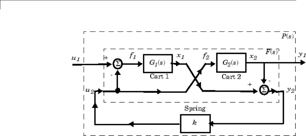
For instance, consider the two-cart "ACC Benchmark" system [13] consisting
of two frictionless carts connected by a spring shown as follows.
ACC Benchmark Problem
The system has the block diagram model shown below, where the individual
carts have the respective transfer functions.
Gs
ms
Gs
ms
1
12
2
22
1
1
()
=
()
=.
The parameters m1,m2,andkare uncertain, equal to one plus or minus 20%:
m1=1–0.2
m2= 1 – 0.2
k=1–0.2
1-5
1Introduction
"ACC Benchmark" Two-Cart System Block Diagram y1=P(s)u1
The upper dashed-line block has transfer function matrix F(s):
Fs Gs Gs
()
=
()
⎡
⎣
⎢⎤
⎦
⎥−
[]
+−
⎡
⎣
⎢⎤
⎦
⎥
()
⎡
⎣⎤
⎦
011 1
10
12.
This code builds the uncertain system model Pshown above:
% Create the uncertain real parameters m1, m2, & k
m1 = ureal('m1',1,'percent',20);
m2 = ureal('m2',1,'percent',20);
k = ureal('k',1,'percent',20);
s = zpk('s'); % create the Laplace variable s
G1 = ss(1/s^2)/m1; % Cart 1
G2 = ss(1/s^2)/m2; % Cart 2
%Nowbuild F and P
F=[
0;G1]*[1 -1]+[1;-1]*[0,G2];
P=l
ft(F,k) % close the loop with the spring k
1-6
System with Uncertain Parameters
The variable Pis a SISO uncertain state-space (USS) object with four states
and three uncertain parameters, m1,m2,andk. You can recover the nominal
plant with the command
zpk(P.nominal)
which returns
Zero/pole/gain:
1
--------------
s^2 (s^2 + 2)
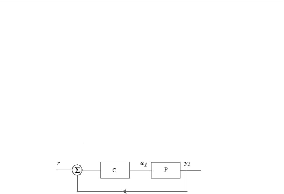
If the uncertain model P(s) has LTI negative feedback controller
Cs s
s
()
=+
()
+
()
100 1
0 001 1
3
3
.
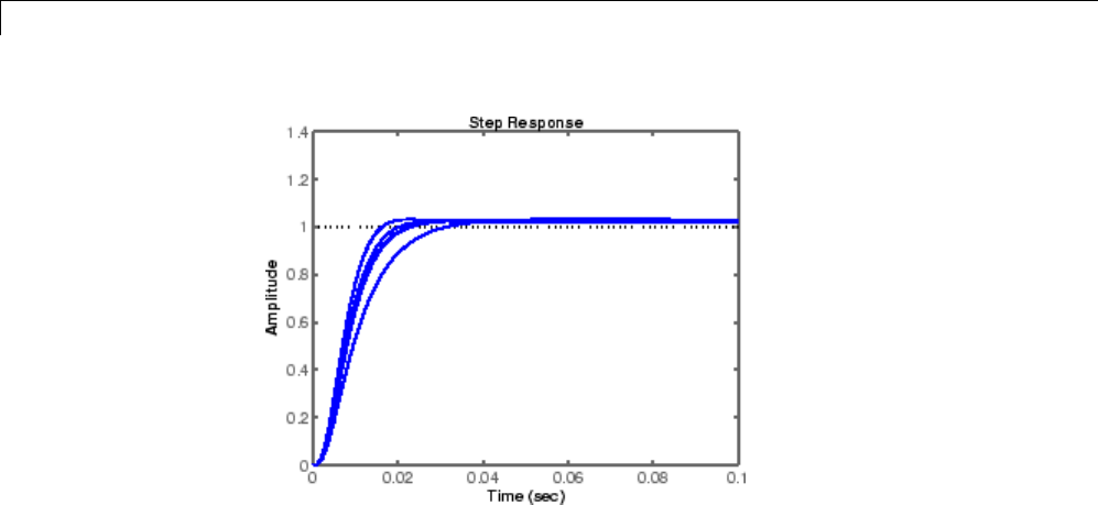
then you can form the controller and the closed-loop system y1=T(s)u1and
view the closed-loop system’s step response on the time interval from t=0 to
t=0.1 for a Monte Carlo random sample of five combinations of the three
uncertain parameters k,m1,andm2 using this code:
C=100*ss((s+1)/(.001*s+1))^3 % LTI controller
T=feedback(P*C,1); % closed-loop uncertain system
step(usample(T,5),.1);
The resulting plot is shown below.
1-7
1Introduction
Monte Carlo Sampling of Uncertain System’s Step Response
1-8

Worst-Case Performance
Worst-Case Performance
To be robust, your control system should meet your stability and performance
requirements for all possible values of uncertain parameters. Monte Carlo
parameter sampling via usample can be used for this purpose as shown in
Monte Carlo Sampling of Uncertain System’s Step Response on page 1-8, but
Monte Carlo methods are inherently hit or miss. With Monte Carlo methods,
you might need to take an impossibly large number of samples before you hit
upon or near a worst-case parameter combination.
Robust Control Toolbox software gives you a powerful assortment of
robustness analysis commands that let you directly calculate upper and lower
bounds on worst-case performance without random sampling.
Worst-Case Robustness Analysis Commands
loopmargin Comprehensive analysis of feedback loop
loopsens Sensitivity functions of feedback loop
ncfmargin Normalized coprime stability margin of feedback
loop
robustperf Robust performance of uncertain systems
robuststab Stability margins of uncertain systems
wcgain Worst-case gain of an uncertain system
wcmargin Worst-case gain/phase margins for feedback loop
wcsens Worst-case sensitivity functions of feedback loop
1-9

1Introduction
Worst-Case Performance of Uncertain System
Returning to the “System with Uncertain Parameters” on page 1-5, the closed
loop system is:
T=feedback(P*C,1); % Closed-loop uncertain system
This uncertain state-space model Thas three uncertain parameters, k,m1,
and m2, each equal to 1±20% uncertain variation. To analyze whether the
closed-loop system Tis robustly stable for all combinations of values for these
three parameters, you can execute the commands:
[StabilityMargin,Udestab,REPORT] = robuststab(T);
REPORT
This displays the REPORT:
Uncertain System is robustly stable to modeled uncertainty.
-- It can tolerate up to 311% of modeled uncertainty.
-- A destabilizing combination of 500% the modeled uncertainty exists,
causing an instability at 44.3 rad/s.
The report tells you that the control system is robust for all parameter
variations in the ±20% range, and that the smallest destabilizing combination
of real variations in the values k,m1,andm2 has sizes somewhere between
311% and 500% greater than ±20%, i.e., between ±62.2% and ±100%. The
value Udestab returns an estimate of the 500% destabilizing parameter
variation combination:
Udestab =
k: 1.2174e-005
m1: 1.2174e-005
m2: 2.0000.
1-10
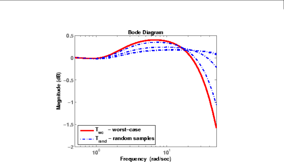
Worst-Case Performance of Uncertain System
Uncertain System Closed-Loop Bode Plots
You have a comfortable safety margin of between 311% to 500% larger
than the anticipated ±20% parameter variations before the closed loop
goes unstable. But how much can closed-loop performance deteriorate for
parameter variations constrained to lie strictly within the anticipated ±20%
range? The following code computes worst-case peak gain of T,andestimates
the frequency and parameter values at which the peak gain occurs:
[PeakGain,Uwc] = wcgain(T);
Twc=usubs(T,Uwc);
% Worst case closed-loop system T
Trand=usample(T,4);
% 4 random samples of uncertain system T
bodemag(Twc,'r',Trand,'b-.',{.5,50}); % Do bode plot
legend('T_{wc} - worst-case',...
'T_{rand} - random samples',3);
The resulting plot is shown in Uncertain System Closed-Loop Bode Plots
on page 1-11.
1-11

1Introduction
Synthesis of Robust MIMO Controllers
You can design controllers for multiinput-multioutput (MIMO) LTI models
with your Robust Control Toolbox software using the following command.
Robust Control Synthesis Commands
h2hinfsyn Mixed H2/H∞controller synthesis
h2syn H2controller synthesis
hinfsyn H∞controller synthesis
loopsyn H∞loop-shaping controller synthesis
ltrsyn Loop-transfer recovery controller synthesis
mixsyn H∞mixed-sensitivity controller synthesis
ncfsyn H∞normalized coprime factor controller synthesis
sdhinfsyn Sampled-data H∞controller synthesis
1-12

Loop-Shaping Controller Design
Loop-Shaping Controller Design
One of the most powerful yet simple controller synthesis tools is loopsyn.
Given an LTI plant, you specify the shape of the open-loop systems frequency
response plot that you want, then loopsyn computes a stabilizing controller
that best approximates your specified loop shape.
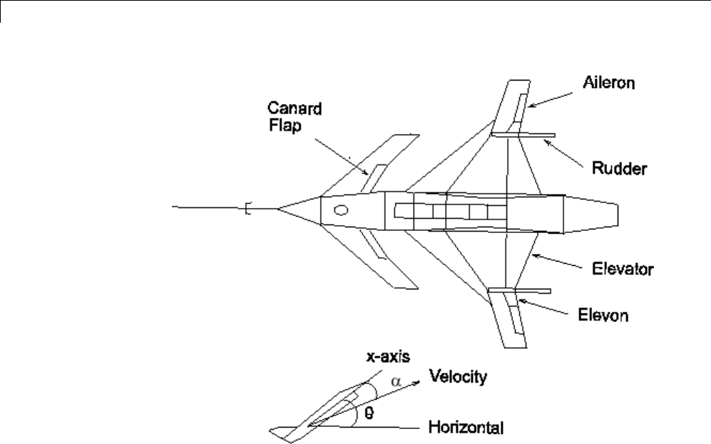
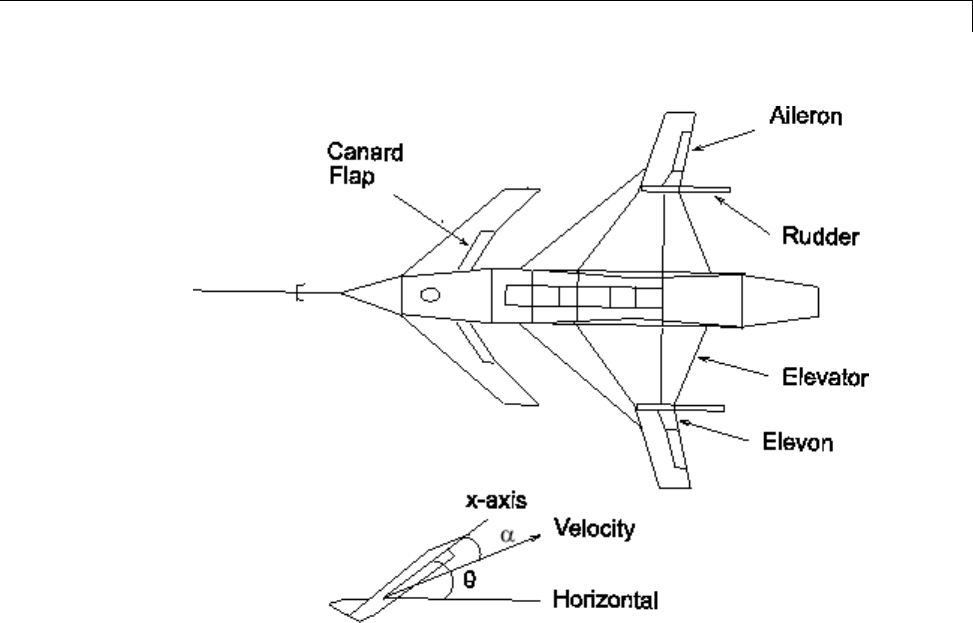
For example, consider the 2-by-2 NASA HiMAT aircraft model (Safonov,
Laub, and Hartmann [8]) depicted in the following figure. The control
variables are elevon and canard actuators (δeand δc). The output variables
are angle of attack (α) and attitude angle (θ). The model has six states:
x
x
x
x
x
x
x
x
x
e
=
⎡
⎣
⎢
⎢
⎢
⎢
⎢
⎢
⎢
⎢
⎤
⎦
⎥
⎥
⎥
⎥
⎥
⎥
⎥
⎥
=
⎡
⎣
⎢
⎢
⎢
⎢
⎢
⎢
⎢
⎢
⎤
⎦
⎥
1
2
3
4
5
6
⎥⎥
⎥
⎥
⎥
⎥
⎥
⎥
where xeand xδare elevator and canard actuator states.
1-13
1Introduction
Aircraft Configuration and Vertical Plane Geometry
You can enter the state-space matrices for this model with the following code:
% NASA HiMAT model G(s)
ag =[ -2.2567e-02 -3.6617e+01 -1.8897e+01 -3.2090e+01 3.2509e+00 -7.6257e-01;
9.2572e-05 -1.8997e+00 9.8312e-01 -7.2562e-04 -1.7080e-01 -4.9652e-03;
1.2338e-02 1.1720e+01 -2.6316e+00 8.7582e-04 -3.1604e+01 2.2396e+01;
0 0 1.0000e+00 0 0 0;
0000-
3.0000e+01 0;
00000 -3.0000e+01];
bg=[00;
00;
00;
00;
30 0;
030
];
cg = [010000;
1-14

Loop-Shaping Controller Design
000100];
dg=[0 0;
0 0];
G=ss(ag,bg,cg,dg);
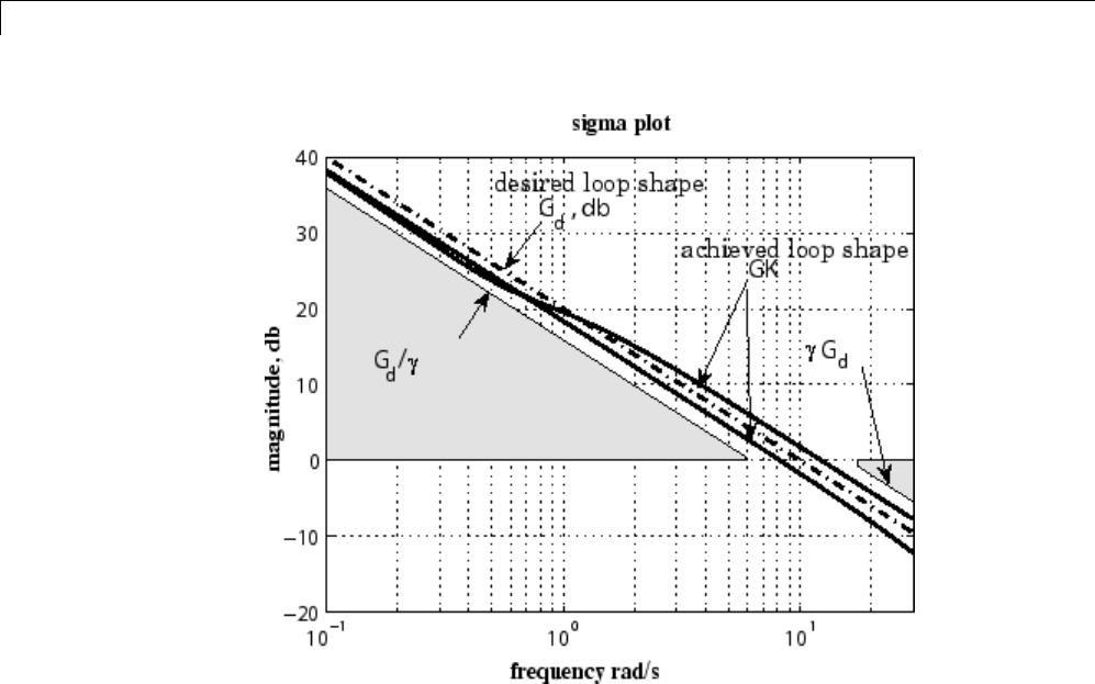
To design a controller to shape the frequency response (sigma)plotsothatthe
system has approximately a bandwidth of 10 rad/s, you can set as your target
desiredloopshapeGd(s)=10/s, then use loopsyn(G,Gd) to find a loop-shaping
controller for Gthat optimally matches the desired loop shape Gd by typing:
s=zpk('s'); w0=10; Gd=w0/(s+.001);
[K,CL,GAM]=loopsyn(G,Gd); % Design a loop-shaping controller K
% Plot the results
sigma(G*K,'r',Gd,'k-.',Gd/GAM,'k:',Gd*GAM,'k:',{.1,30})
figure ;T=feedback(G*K,eye(2));
sigma(T,ss(GAM),'k:',{.1,30});grid
The value of γ=GAM returned is an indicator of the accuracy to which
the optimal loop shape matches your desired loop shape and is an upper
bound on the resonant peak magnitude of the closed-loop transfer function
T=feedback(G*K,eye(2)).Inthiscase,γ= 1.6024 = 4 dB — see the next
figure.
1-15
1Introduction
MIMO Robust Loop Shaping with loopsyn(G,Gd)
Theachievedloopshapematches the desired target Gd to within about γdB.
1-16

Model Reduction and Approximation
Model Reduction and Approximation
Complex models are not always required for good control. Unfortunately,
however, optimization methods (including methods based on H∞,H2,and
µ-synthesis optimal control theory) generally tend to produce controllers
with at least as many states as the plant model. For this reason, Robust
Control Toolbox software offers you an assortment of model-order reduction
commands that help you to find less complex low-order approximations to
plant and controller models.
Model Reduction Commands
reduce Main interface to model approximation algorithms
balancmr Balanced truncation model reduction
bstmr Balanced stochastic truncation model reduction
hankelmrOptimal Hankel norm model approximations
modreal State-space modal truncation/realization
ncfmr Balanced normalized coprime factor model reduction
schurmr Schur balanced truncation model reduction
slowfast State-space slow-fast decomposition
stabsep State-space stable/antistable decomposition
imp2ss Impulseresponsetostate-spaceapproximation
Among the most important types of model reduction methods are minimize
bounds methods on additive, multiplicative, and normalized coprime factor
(NCF) model error. You can access all three of these methods using the
command reduce.
1-17

1Introduction
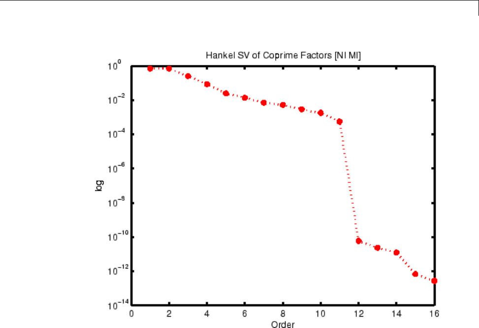
Reduce Order of Synthesized Controller
For instance, the NASA HiMAT model considered in “Loop-Shaping Controller
Design” on page 1-13 has eight states, and the optimal loop-shaping controller
turns out to have 16 states. Using model reduction, you can remove at least
some of the states without appreciably affecting stability or closed-loop
performance. For controller order reduction, the NCF model reduction is
particularly useful, and it works equally well with controllers that have poles
anywhere in the complex plane.
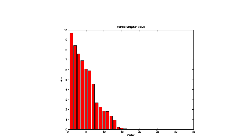
For the NASA HiMAT design in the last section, you can type
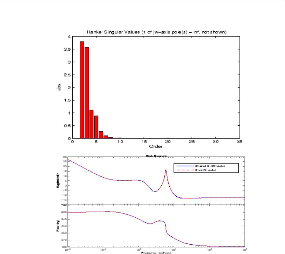
hankelsv(K,'ncf','log');
which displays a logarithmic plot of the NCF Hankel singular values — see
the following figure.
1-18
Reduce Order of Synthesized Controller
Hankel Singular Values of Coprime Factorization of K
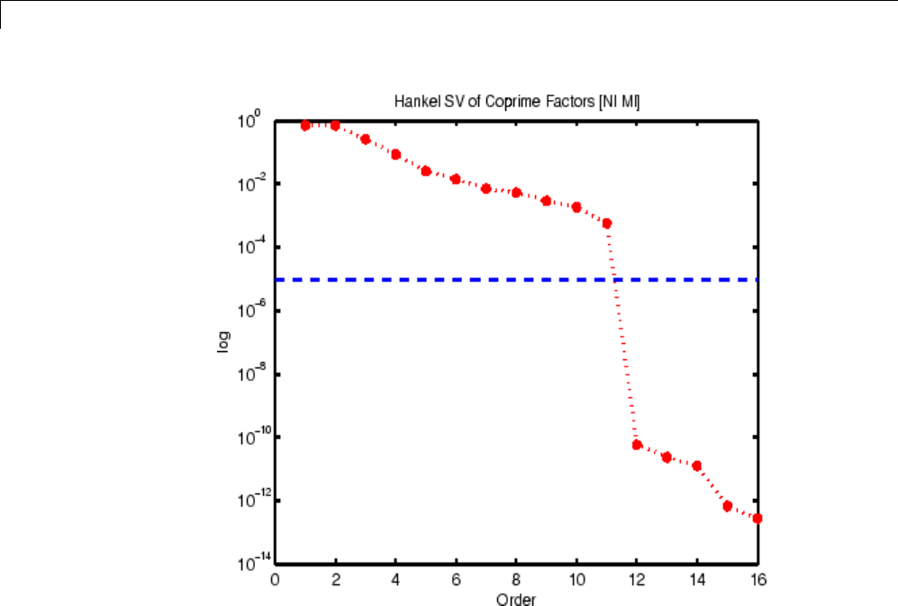
Theory says that, without danger of inducing instability, you can confidently
discard at least those controller states that have NCF Hankel singular values
that are much smaller than ncfmargin(G,K).
Compute ncfmargin(G,K) and add it to your Hankel singular values plot.
hankelsv(K,'ncf','log');v=axis;
hold on; plot(v(1:2), ncfmargin(G,K)*[1 1],'--'); hold off
1-19
1Introduction
Five of the 16 NCF Hankel Singular Values of HiMAT Controller K Are Small
Compared to ncfmargin(G,K)
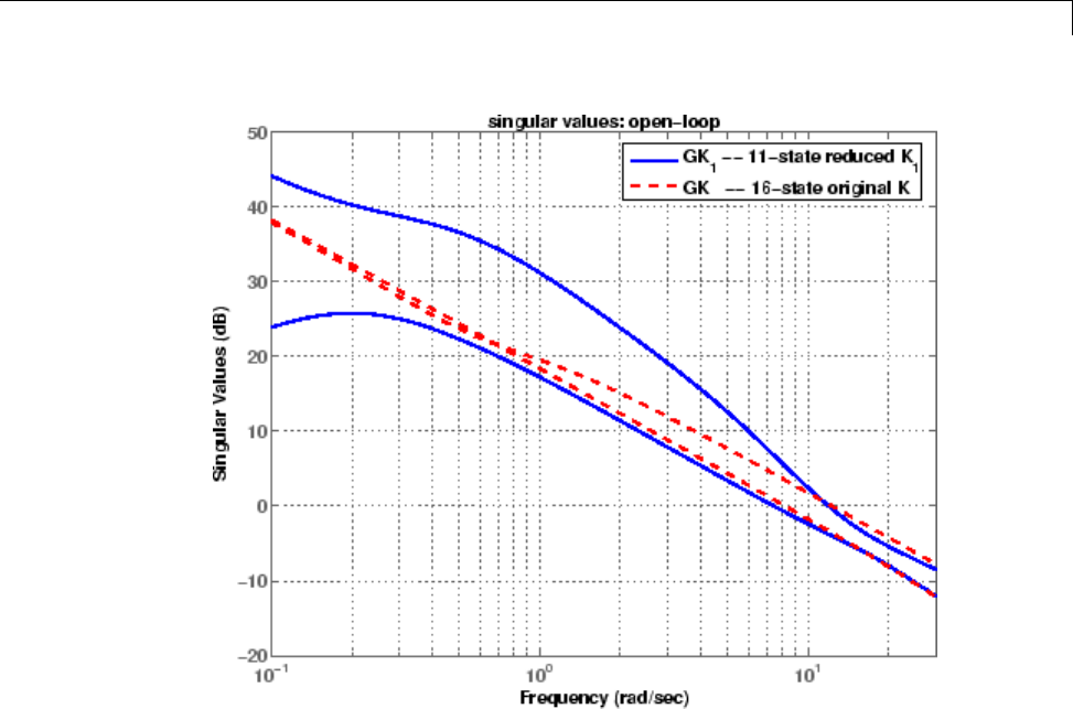
In this case, you can safely discard 5 of the 16 states of Kand compute an
11-state reduced controller by typing:
K1=reduce(K,11,'errortype','ncf');
The result is plotted in the following figure.
sigma(G*K1,'b',G*K,'r--',{.1,30});
1-20
Reduce Order of Synthesized Controller
HiMAT with 11-State Controller K1 vs. Original 16-State Controller K
The picture above shows that low-frequency gain is decreased considerably for
inputs in one vector direction. Although this does not affect stability, it affects
performance. If you wanted to better preserve low-frequency performance,
you would discard fewer than five of the 16 states of K.
1-21

1Introduction
LMI Solvers
At the core of many emergent robust control analysis and synthesis routines
are powerful general-purpose functions for solving a class of convex nonlinear
programming problems known as linear matrix inequalities. The LMI
capabilities are invoked by Robust Control Toolbox software functions
that evaluate worst-case performance, as well as functions like hinfsyn
and h2hinfsyn. Some of the main functions that help you access the LMI
capabilities of the toolbox are shown in the following table.
Specification of LMIs
lmiedit GUI for LMI specification
setlmis Initialize the LMI description
lmivar Define a new matrix variable
lmiterm Specify the term content of an LMI
newlmi Attach an identifying tag to new LMIs
getlmis Get the internal description of the LMI system
LMI Solvers
feasp Test feasibility of a system of LMIs
gevp Minimize generalized eigenvalue with LMI constraints
mincx Minimize a linear objective with LMI constraints
dec2mat Convert output of the solvers to values of matrix
variables
Evaluation of LMIs/Validation of Results
evallmi Evaluate for given values of the decision variables
showlmi Return the left and right sides of an evaluated LMI
1-22

Extends Control System Toolbox™ Capabilities
Extends Control System Toolbox Capabilities
Robust Control Toolbox software is designed to work with Control System
Toolbox software. Robust Control Toolbox software extends the capabilities
of Control System Toolbox software and leverages the LTI and plotting
capabilities of Control System Toolbox software. The major analysis and
synthesis commands in Robust Control Toolbox software accept LTI object
inputs, e.g., LTI state-space systems produced by commands such as:
G=tf(1,[1 2 3])
G=ss([-1 0; 0 -1], [1;1],[1 1],3)
The uncertain system (USS) objects in Robust Control Toolbox software
generalize the Control System Toolbox LTI SS objects and help ease the
task of analyzing and plotting uncertain systems. You can do many of
the same algebraic operations on uncertain systems that are possible for
LTI objects (multiply, add, invert), and Robust Control Toolbox software
provides USS uncertain system extensions of Control System Toolbox software
interconnection and plotting functions like feedback,lft,andbode.
1-23

1Introduction
Acknowledgments
Professor Andy Packard is with the Faculty of Mechanical Engineering
at the University of California, Berkeley. His research interests include
robustness issues in control analysis and design, linear algebra and numerical
algorithms in control problems, applications of system theory to aerospace
problems, flight control, and control of fluid flow.
Professor Gary Balas is with the Faculty of Aerospace Engineering &
Mechanics at the University of Minnesota and is president of MUSYN Inc.
His research interests include aerospace control systems, both experimental
and theoretical.
Dr. Michael Safonov is with the Faculty of Electrical Engineering at the
University of Southern California. His research interests include control
and decision theory.
Dr. Richard Chiang is employed by Boeing Satellite Systems, El Segundo,
CA. He is a Boeing Technical Fellow and has been working in the aerospace
industry over 25 years. In his career, Richard has designed 3 flight control
laws, 12 spacecraft attitude control laws, and 3 large space structure vibration
controllers, using modern robust control theory and the tools he built in this
toolbox. His research interests include robust control theory, model reduction,
and in-flight system identification. Working in industry instead of academia,
Richard serves a unique role in our team, bridging the gap between theory
and reality.
The linear matrix inequality (LMI) portion of Robust Control Toolbox software
was developed by these two authors:
Dr. Pascal Gahinet is employed by MathWorks. His research interests
include robust control theory, linear matrix inequalities, numerical linear
algebra, and numerical software for control.
Professor Arkadi Nemirovski is with the Faculty of Industrial Engineering
and Management at Technion, Haifa, Israel. His research interests include
convex optimization, complexity theory, and nonparametric statistics.
1-24

Acknowledgments
The structured H∞synthesis (hinfstruct) portion of Robust Control Toolbox
software was developed by the following author in collaboration with Pascal
Gahinet:
Professor Pierre Apkarian is with ONERA (The French Aerospace Lab)
and the Institut de Mathématiques at Paul Sabatier University, Toulouse,
France. His research interests include robust control, LMIs, mathematical
programming, and nonsmooth optimization techniques for control.
1-25

1Introduction
Bibliography
[1] Boyd, S.P., El Ghaoui, L., Feron, E., and Balakrishnan, V., Linear Matrix
Inequalities in Systems and Control Theory, Philadelphia, PA, SIAM, 1994.
[2] Dorato, P. (editor), Robust Control, New York, IEEE Press, 1987.
[3] Dorato, P., and Yedavalli, R.K. (editors), Recent Advances in Robust
Control, New York, IEEE Press, 1990.
[4] Doyle, J.C., and Stein, G., “Multivariable Feedback Design: Concepts
for a Classical/Modern Synthesis,” IEEE Trans. on Automat. Contr., 1981,
AC-26(1), pp. 4-16.
[5] El Ghaoui, L., and Niculescu, S., Recent Advances in LMI Theory for
Control, Philadelphia, PA, SIAM, 2000.
[6] Lehtomaki, N.A., Sandell, Jr., N.R., and Athans, M., “Robustness Results
in Linear-Quadratic Gaussian Based Multivariable Control Designs,” IEEE
Trans. on Automat. Contr., Vol. AC-26, No. 1, Feb. 1981, pp. 75-92.
[7] Safonov,M.G., Stability and Robustness of Multivariable Feedback
Systems, Cambridge, MA, MIT Press, 1980.
[8] Safonov, M.G., Laub, A.J., and Hartmann, G., “Feedback Properties of
Multivariable Systems: The Role and Use of Return Difference Matrix,” IEEE
Trans. of Automat. Contr., 1981, AC-26(1), pp. 47-65.
[9] Safonov, M.G., Chiang, R.Y., and Flashner, H., “H∞Control Synthesis
for a Large Space Structure,” Proc. of American Contr. Conf., Atlanta, GA,
June 15-17, 1988.
[10] Safonov, M.G., and Chiang, R.Y., “CACSD Using the State-Space L∞
Theory — A Design Example,” IEEE Trans. on Automatic Control, 1988,
AC-33(5), pp. 477-479.
[11] Sanchez-Pena, R.S., and Sznaier, M., Robust Systems Theory and
Applications, New York, Wiley, 1998.
1-26

Bibliography
[12] Skogestad, S., and Postlethwaite, I., Multivariable Feedback Control,
New York, Wiley, 1996.
[13] Wie, B., and Bernstein, D.S., “A Benchmark Problem for Robust
Controller Design,” Proc. American Control Conf., San Diego, CA, May 23-25,
1990; also Boston, MA, June 26-28, 1991.
[14] Zhou, K., Doyle, J.C., and Glover, K., Robust and Optimal Control,
Englewood Cliffs, NJ, Prentice Hall, 1996.
1-27

1Introduction
1-28

2
Multivariable Loop Shaping
•“Tradeoff Between Performance and Robustness” on page 2-2
•“Norms and Singular Values” on page 2-4
•“Typical Loop Shapes, S and T Design” on page 2-6
•“Using LOOPSYN to Do H-Infinity Loop Shaping” on page 2-15
•“Loop-Shaping Control Design of Aircraft Model” on page 2-16
•“Fine-Tuning the LOOPSYN Target Loop Shape Gd to Meet Design Goals”
on page 2-21
•“Mixed-Sensitivity Loop Shaping” on page 2-22
•“Mixed-Sensitivity Loop-Shaping Controller Design” on page 2-24
•“Loop-Shaping Commands” on page 2-26

2Multivariable Loop Shaping
Tradeoff Between Performance and Robustness
When the plant modeling uncertainty is not too big, you can design high-gain,
high-performance feedback controllers. High loop gains significantly larger
than 1 in magnitude can attenuate the effects of plant model uncertainty
and reduce the overall sensitivity of the system to plant noise. But if your
plant model uncertainty is so large that you do not even know the sign of
your plant gain, then you cannot use large feedback gains without the risk
that the system will become unstable. Thus, plant model uncertainty can
be a fundamental limiting factor in determining what can be achieved with
feedback.
Multiplicative Uncertainty: Given an approximate model of the plant G0
of a plant G,themultiplicative uncertainty ΔMof the model G0is defined
as ΔMGGG=−
()
−
010
or, equivalently,
GI G
M
=+
()
Δ0.
Plant model uncertainty arises from many sources. There might be
small unmodeled time delays or stray electrical capacitance. Imprecisely
understood actuator time constants or, in mechanical systems, high-frequency
torsional bending modes and similar effects can be responsible for plant
model uncertainty. These types of uncertainty are relatively small at lower
frequencies and typically increase at higher frequencies.
In the case of single-input/single-output (SISO) plants, the frequency at
which there are uncertain variations in your plant of size |ΔM|=2 marks
a critical threshold beyond which there is insufficient information about
the plant to reliably design a feedback controller. With such a 200% model
uncertainty, the model provides no indication of the phase angle of the true
plant, which means that the only way you can reliably stabilize your plant is
to ensure that the loop gain is less than 1. Allowing for an additional factor
of 2 margin for error, your control system bandwidth is essentially limited
2-2

Tradeoff Between Performance and Robustness
to the frequency range over which your multiplicative plant uncertainty ΔM
has gain magnitude |ΔM|<1.
2-3

2Multivariable Loop Shaping
Norms and Singular Values
For MIMO systems the transfer functions are matrices, and relevant
measures of gain are determined by singular values, H∞,andH
2norms, which
are defined as follows:
H2and H•Norms The H2-norm is the energy of the impulse response
of plant G.TheH
∞-norm is the peak gain of Gacross all frequencies and all
input directions.
Another important concept is the notion of singular values.
Singular Values: The singular values of a rank rmatrix AC
mn
∈×, denoted
σi, are the nonnegative square roots of the eigenvalues of AA
*ordered such
that σ1≥σ2≥... ≥σp>0,p≤min{m,n}.
If r<pthen there are p–rzero singular values, i.e., σr+1 =σr+2 = ... =σp=0.
The greatest singular value σ1is sometimes denoted
A
()
=1.
When Ais a square n-by-nmatrix, then the nth singular value (i.e., the least
singular value) is denoted
An
()
.
Properties of Singular Values
Some useful properties of singular values are:
2-4

Norms and Singular Values
AAx
x
AAx
x
xC
xC
h
h
()
=
()
=
∈
∈
max
min
These properties are especially important because they establish that the
greatest and least singular values of a matrix Aare the maximal and minimal
"gains" of the matrix as the input vector xvaries over all possible directions.
For stable continuous-time LTI systems G(s), the H2-norm and the H∞-norms
are defined terms of the frequency-dependent singular values of G(jω):
H2-norm:
GGjd
i
i
p
2
2
1
1
2
⎡
⎣
⎢⎤
⎦
⎥
()
()
()
=
−∞
∞∑
∫
H∞-norm:
GGj
2sup
()
()
where sup denotes the least upper bound.
2-5
2Multivariable Loop Shaping
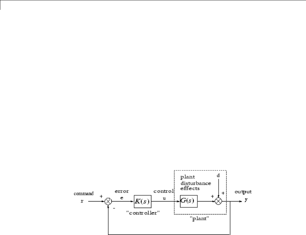
Typical Loop Shapes, S and T Design
Consider the multivariable feedback control system shown in the following
figure. In order to quantify the multivariable stability margins and
performance of such systems, you can use the singular values of the closed-loop
transfer function matrices from rto each of the three outputs e,u,andy,viz.
Ss I Ls
Rs Ks I Ls
Ts Ls I Ls
def
def
def
()
=+
()
()
()
=
()
+
()
()
()
=
()
+
()
−
−
1
1
(()
=−
()
−1ISs
where the L(s) is the loop transfer function matrix
Ls GsK s
()
=
() ()
.(2-1)
Block Diagram of the Multivariable Feedback Control System
The two matrices S(s)andT(s)areknownasthesensitivity function and
complementary sensitivity function, respectively. The matrix R(s)hasno
common name. The singular value Bode plots of each of the three transfer
function matrices S(s), R(s), and T(s) play an important role in robust
multivariable control system design. The singular values of the loop transfer
function matrix L(s) are important because L(s) determines the matrices
S(s)andT(s).
2-6

Typical Loop Shapes, S and T Design
Robustness in Terms of Singular Values
The singular values of S(jω) determine the disturbance attenuation, because
S(s) is in fact the closed-loop transfer function from disturbance dto plant
output y— see Block Diagram of the Multivariable Feedback Control System
on page 2-6. Thus a disturbance attenuation performance specification can
be written as
Sj W j
()
()
≤
()
−
11
(2-2)
where Wj
11−
()
is the desired disturbance attenuation factor. Allowing
Wj
1
()
to depend on frequency ωenables you to specify a different
attenuation factor for each frequency ω.
The singular value Bode plots of R(s)andofT(s) are used to measure
the stability margins of multivariable feedback designs in the face of
additive plant perturbations ΔAand multiplicative plant perturbations ΔM,
respectively. See the following figure.
Consider how the singular value Bode plot of complementary sensitivity T(s)
determines the stability margin for multiplicative perturbations ΔM.The
multiplicative stability margin is, by definition, the "size" of the smallest
stable ΔM(s) that destabilizes the system in the figure below when ΔA=0.
2-7
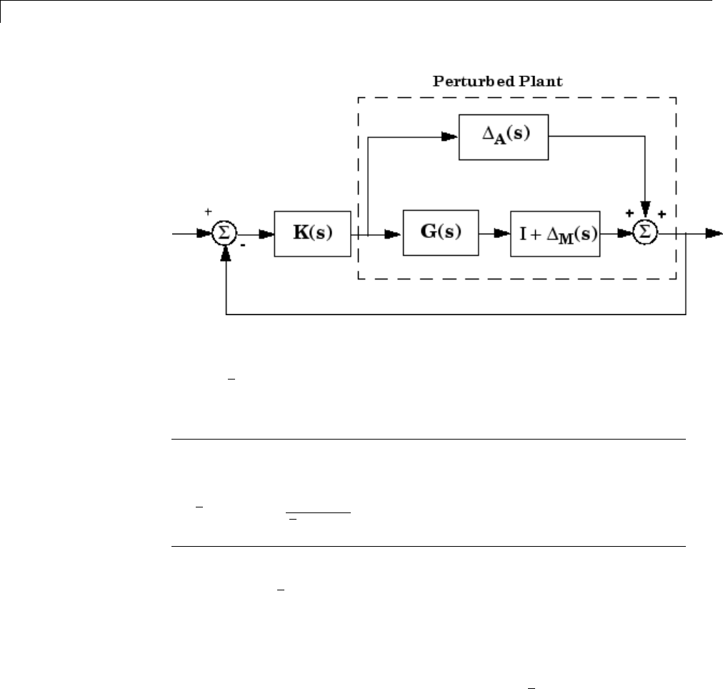
2Multivariable Loop Shaping
Additive/Multiplicative Uncertainty
Taking
ΔMj
()
()
to be the definition of the "size" of ΔM(jω), you have the
following useful characterization of "multiplicative" stability robustness:
Multiplicative Robustness: The size of the smallest destabilizing
multiplicative uncertainty ΔM(s)is:
ΔMjTj
()
()
=
()
()
1.
The smaller is
Tj
()
()
, the greater will be the size of the smallest
destabilizing multiplicative perturbation, and hence the greater will be the
stability margin.
A similar result is available for relating the stability margin in the face of
additive plant perturbations ΔA(s)toR(s)ifyoutake
ΔAj
()
()
to be the
definition of the "size" of ΔA(jω) at frequency ω.
2-8

Typical Loop Shapes, S and T Design
Additive Robustness: The size of the smallest destabilizing additive
uncertainty ΔAis:
ΔAjRj
()
()
=
()
()
1.
As a consequence of robustness theorems 1 and 2, it is common to specify the
stability margins of control systems via singular value inequalities such as
Rj W j
{}
()
≤
()
−
21
(2-3)
Tj W j
{}
()
≤
()
−
31
(2-4)
where |W2(jω)| and |W3(jω)| are the respective sizes of the largest
anticipated additive and multiplicative plant perturbations.
It is common practice to lump the effects of all plant uncertainty into a
single fictitious multiplicative perturbation ΔM, so that the control design
requirements can be written
1
13
1
i
i
Sj Wj Tj W j
()
()
≥
()
[]
()
≤
()
−
;
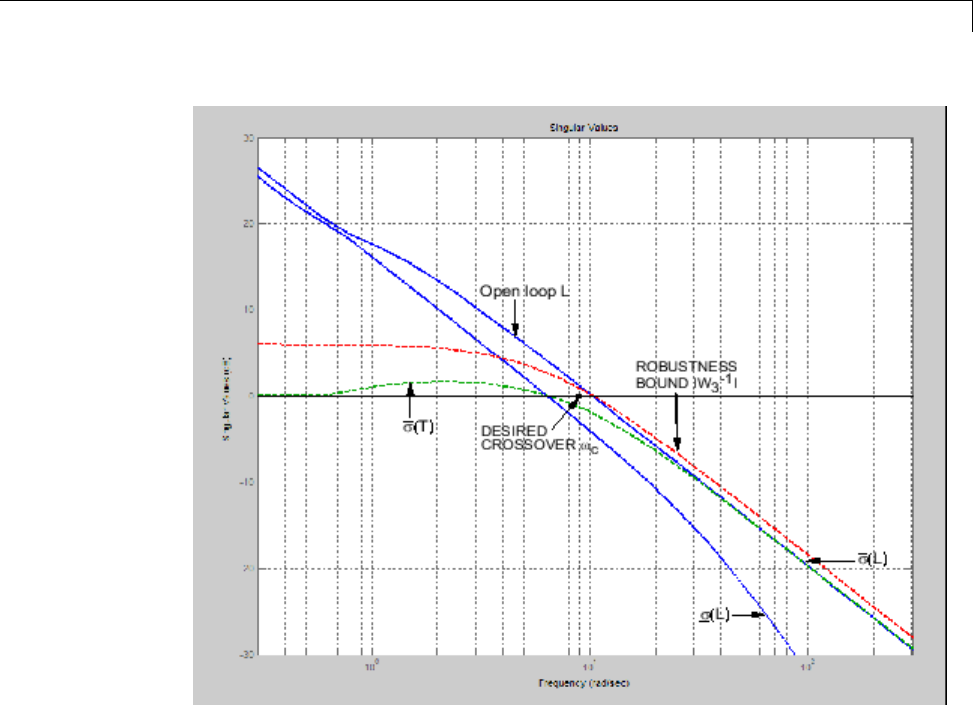
as shown in Singular Value Specifications on L, S, and T on page 2-12.
It is interesting to note that in the upper half of the figure (above the 0 dB
line),
Lj Sj
()
()
≈
()
()
1
while in the lower half of Singular Value Specifications on L, S, and T on page
2-12 (below the 0 dB line),
2-9

2Multivariable Loop Shaping
Lj Tj
()
()
≈
()
()
.
This results from the fact that
Ss I Ls Ls
def
()
=+
()
()
≈
()
−−
11
if
Ls
()
()
1,and
Ts Ls I Ls Ls
def
()
=
()
+
()
()
≈
()
−1
if
Ls
()
()
1.
2-10
Typical Loop Shapes, S and T Design
2-11
2Multivariable Loop Shaping
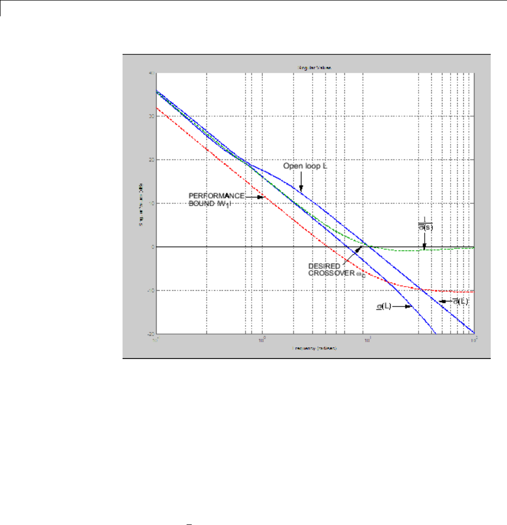
Singular Value Specifications on L, S, and T
Thus, it is not uncommon to see specifications on disturbance attenuation
and multiplicative stability margin expressed directly in terms of forbidden
regions for the Bode plots of σi(L(jω)) as "singular value loop shaping"
requirements, either as specified upper/lower bounds or as a target desired
loop shape — see the preceding figure.
Guaranteed Gain/Phase Margins in MIMO Systems
For those who are more comfortable with classical single-loop concepts, there
are the important connections between the multiplicative stability margins
predicted by
T
()
and those predicted by classical M-circles, as found on the
Nichols chart. Indeed in the single-input/single-output case,
2-12

Typical Loop Shapes, S and T Design
Tj Lj
Lj
()
()
=
()
+
()
1
which is precisely the quantity you obtain from Nichols chart M-circles. Thus,
T∞is a multiloop generalization of the closed-loop resonant peak magnitude
which, as classical control experts will recognize, is closely related to the
damping ratio of the dominant closed-loop poles. Also, it turns out that you
can relate T∞,S∞to the classical gain margin GMand phase margin θMin
each feedback loop of the multivariable feedback system of Block Diagram of
the Multivariable Feedback Control System on page 2-6 via the formulas:
GT
G
S
T
T
M
M
M
M
≥+
≥+
−
≥⎛
⎝
⎜
⎜
⎞
⎠
⎟
⎟
≥⎛
⎝
⎜
⎜
⎞
∞
∞
−
∞
−
∞
11
11
11
21
2
21
2
1
1
sin
sin
⎠⎠
⎟
⎟.
(See [6].) These formulas are valid provided S∞and T∞are larger than 1,
as is normally the case. The margins apply even when the gain perturbations
or phase perturbations occur simultaneously in several feedback channels.
The infinity norms of Sand Talso yield gain reduction tolerances. The gain
reduction tolerance gmis defined to be the minimal amount by which the gains
in each loop would have to be decreased in order to destabilize the system.
Upper bounds on gmare as follows:
2-13

2Multivariable Loop Shaping
gT
g
S
M
M
≤−
≤
+
∞
∞
11
1
11.
2-14

Using LOOPSYN to Do H-Infinity Loop Shaping
Using LOOPSYN to Do H-Infinity Loop Shaping
The command loopsyn lets you design a stabilizing feedback controller to
optimally shape the open loop frequency response of a MIMO feedback control
system to match as closely as possible a desired loop shape Gd — see the
preceding figure. The basic syntax of the loopsyn loop-shaping controller
synthesis command is:
K = loopsyn(G,Gd)
Here Gis the LTI transfer function matrix of a MIMO plant model, Gd is
the target desired loop shape for the loop transfer function L=G*K,andKis
the optimal loop-shaping controller. The LTI controller Khas the property
that it shapes the loop L=G*K so that it matches the frequency response of Gd
as closely as possible, subject to the constraint that the compensator must
stabilize the plant model G.
2-15

2Multivariable Loop Shaping
Loop-Shaping Control Design of Aircraft Model
To see how the loopsyn command works in practice to address robustness
and performance tradeoffs, consider again the NASA HiMAT aircraft model
taken from the paper of Safonov, Laub, and Hartmann [8]. The longitudinal
dynamics of the HiMAT aircraft trimmed at 25000 ft and 0.9 Mach are
unstable and have two right-half-plane phugoid modes. The linear model
has state-space realization G(s)=C(Is –A)–1Bwith six states, with the first
four states representing angle of attack (α) and attitude angle (θ)andtheir
rates of change, and the last two representing elevon and canard control
actuator dynamics — see Aircraft Configuration and Vertical Plane Geometry
on page 2-17.
ag =[
-2.2567e-02 -3.6617e+01 -1.8897e+01 -3.2090e+01 3.2509e+00 -7.6257e-01;
9.2572e-05 -1.8997e+00 9.8312e-01 -7.2562e-04 -1.7080e-01 -4.9652e-03;
1.2338e-02 1.1720e+01 -2.6316e+00 8.7582e-04 -3.1604e+01 2.2396e+01;
0 0 1.0000e+00 0 0 0;
0 0 0 0 -3.0000e+01 0;
0 0 0 0 0 -3.0000e+01];
bg=[0 0;
00;
00;
00;
30 0;
0 30];
cg=[010000;
000100];
dg=[0 0;
0 0];
G=ss(ag,bg,cg,dg);
The control variables are elevon and canard actuators (δeand δc). The output
variables are angle of attack (α) and attitude angle (θ).
2-16
Loop-Shaping Control Design of Aircraft Model
Aircraft Configuration and Vertical Plane Geometry
This model is good at frequencies below 100 rad/s with less than 30%
variation between the true aircraft and the model in this frequency range.
However as noted in [8], it does not reliably capture very high-frequency
behaviors, because it was derived by treating the aircraft as a rigid body and
neglecting lightly damped fuselage bending modes that occur at somewhere
between 100 and 300 rad/s. These unmodeled bending modes might cause as
much as 20 dB deviation (i.e., 1000%) between the frequency response of
the model and the actual aircraft for frequency ω>100rad/s. Othereffects
like control actuator time delays and fuel sloshing also contribute to model
inaccuracy at even higher frequencies, but the dominant unmodeled effects
are the fuselage bending modes. You can think of these unmodeled bending
modes as multiplicative uncertainty of size 20 dB, and design your controller
using loopsyn, by making sure that the loop has gain less than –20 dB at, and
beyond, the frequency ω>100rad/s.
2-17

2Multivariable Loop Shaping
Design Specifications
The singular value design specifications are
•Robustness Spec.: –20 dB/decade roll-off slope and –20 dB loop gain
at 100 rad/s
•Performance Spec.: Minimize the sensitivity function as much as
possible.
Bothspecscanbeaccommodatedbytakingasthedesiredloopshape
Gd(s)=8/s
MATLAB Commands for a LOOPSYN Design
%% Enter the desired loop shape Gd
s=zpk('s'); % Laplace variable s
Gd=8/s; % desired loop shape
%% Compute the optimal loop shaping controller K
[K,CL,GAM]=loopsyn(G,Gd);
%% Compute the loop L, sensitivity S and
%% complementary sensitivity T:
L=G*K;
I=eye(size(L));
S=feedback(I,L); % S=inv(I+L);
T=I-S;
%% Plot the results:
% step response plots
step(T);title('\alpha and \theta command step responses');
% frequency response plots
figure;
sigma(I+L,'--',T,':',L,'r--',Gd,'k-.',Gd/GAM,'k:',...
Gd*GAM,'k:',{.1,100});grid
legend('1/\sigma(S) performance',...
'\sigma(T) robustness',...
'\sigma(L) loopshape',...
'\sigma(Gd) desired loop',...
'\sigma(Gd) \pm GAM, dB');
2-18
Loop-Shaping Control Design of Aircraft Model
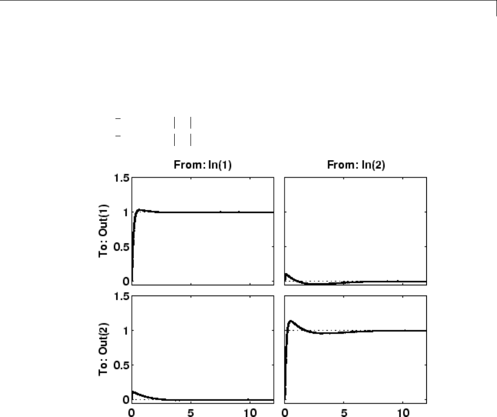
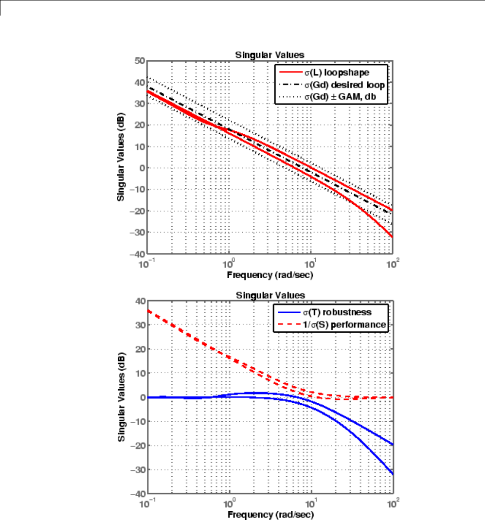
The plots of the resulting step and frequency response for the NASA HiMAT
loopsyn loop-shaping controller design are shown in the following figure. The
number ±GAM, dB (i.e., 20log10(GAM)) tells you the accuracy with which
your loopsyn control design matches the target desired loop:
GK
GK
c
c
()
≥− <
()
≥+ >
,, ,()
,, ,().
db G db GAM db
db G db GAM db
d
d
HiMAT Closed Loop Step Responses
2-19
2Multivariable Loop Shaping
LOOPSYN Design Results for NASA HiMAT
2-20

Fine-Tuning the LOOPSYN Target Loop Shape Gd to Meet Design Goals
Fine-Tuning the LOOPSYN Target Loop Shape Gd to Meet
Design Goals
If your first attempt at loopsyn design does not achieve everything you
wanted, you will need to readjust your target desired loop shape Gd.Hereare
some basic design tradeoffs to consider:
•Stability Robustness. Your target loop Gd should have low gain (as small
as possible) at high frequencies where typically your plant model is so poor
that its phase angle is completely inaccurate, with errors approaching
±180° or more.
•Performance. Your Gd loop should have high gain (as great as possible)
at frequencies where your model is good, in order to ensure good control
accuracy and good disturbance attenuation.
•Crossover and Roll-Off. YourdesiredloopshapeGd should have its 0 dB
crossover frequency (denoted ωc) between the above two frequency ranges,
and below the crossover frequency ωcit should roll off with a negative slope
of between –20 and –40 dB/decade, which helps to keep phase lag to less
than –180° inside the control loop bandwidth (0 < ω<ωc).
Other considerations that might affect your choice of Gd are the
right-half-plane poles and zeros of the plant G, which impose ffundamental
limits on your 0 dB crossover frequency ωc[12]. For instance, your 0 dB
crossover ωcmust be greater than the magnitude of any plant right-half-plane
poles and less than the magnitude of any right-half-plane zeros.
max min .
Re Re
pic zi
ii
pz
()
>
()
>
<<
00
If you do not take care to choose a target loop shape Gd that conforms to
these fundamental constraints, then loopsyn will still compute the optimal
loop-shaping controller Kfor your Gd, but you should expect that the optimal
loop L=G*K will have a poor fit to the target loop shape Gd, and consequently it
mightbeimpossibletomeetyourperformancegoals.
2-21

2Multivariable Loop Shaping
Mixed-Sensitivity Loop Shaping
A popular alternative approach to loopsyn loop shaping is H∞mixed-sensitivity
loop shaping, which is implemented by the Robust Control Toolbox software
command:
K=mixsyn(G,W1,[],W3)
With mixsyn controller synthesis, your performance and stability robustness
specifications equations (2-2) and (2-4) are combined into a single infinity
norm specification of the form
Tyu
11 1
∞≤
where (see MIXSYN H∞Mixed-Sensitivity Loop Shaping Ty1 u1 on page 2-23):
TWS
WT
yu
def
11
1
3
=⎡
⎣
⎢⎤
⎦
⎥.
The term Tyu
11 ∞is called a mixed-sensitivity cost function because it
penalizes both sensitivity S(s) and complementary sensitivity T(s). Loop
shaping is achieved when you choose W1to have the target loop shape for
frequencies ω<ωc, and you choose 1/W3to be the target for ω>ωc. In choosing
design specifications W1and W3for a mixsyn controller design, you need to
ensure that your 0 dB crossover frequency for the Bode plot of W1is below the
0dBcr
ossover frequency of 1/W3, as shown in Singular Value Specifications
on L, S, and T on page 2-12, so that there is a gap for the desired loop shape
Gd to pass between the performance bound W1and your robustness bound
W31−. Otherwise, your performance and robustness requirements will not
be achievable.
2-22

Mixed-Sensitivity Loop Shaping
MIXSYN H•Mixed-Sensitivity Loop Shaping Ty1 u1
2-23

2Multivariable Loop Shaping
Mixed-Sensitivity Loop-Shaping Controller Design
To do a mixsyn H∞mixed-sensitivity synthesis design on the HiMAT model,
start with the plant model Gcreated in “Mixed-Sensitivity Loop-Shaping
Controller Design” on page 2-24 and type the following commands:
% Set up the performance and robustness bounds W1 & W3
s=zpk('s'); % Laplace variable s
MS=2;AS=.03;WS=5;
W1=(s/MS+WS)/(s+AS*WS);
MT=2;AT=.05;WT=20;
W3=(s+WT/MT)/(AT*s+WT);
% Compute the H-infinity mixed-sensitivity optimal sontroller K1
[K1,CL1,GAM1]=mixsyn(G,W1,[],W3);
% Next compute and plot the closed-loop system.
% Compute the loop L1, sensitivity S1, and comp sensitivity T1:
L1=G*K1;
I=eye(size(L1));
S1=feedback(I,L1); % S=inv(I+L1);
T1=I-S1;
% Plot the results:
% step response plots
step(T1,1.5);
title('\alpha and \theta command step responses');
% frequency response plots
figure;
sigma(I+L1,'--',T1,':',L1,'r--',... W1/GAM1,'k--',GAM1/W3,'k-.',{.1,100});grid
legend('1/\sigma(S) performance',...
'\sigma(T) robustness',...
'\sigma(L) loopshape',...
'\sigma(W1) performance bound',...
'\sigma(1/W3) robustness bound');
The resulting mixsyn singular value plots for the NASA HiMAT model are
shown below.
2-24
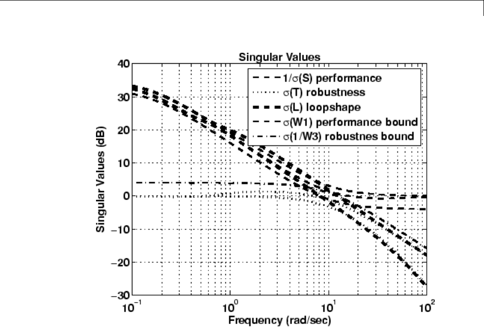
Mixed-Sensitivity Loop-Shaping Controller Design
MIXSYN Design Results for NASA HiMAT
2-25

2Multivariable Loop Shaping
Loop-Shaping Commands
Robust Control Toolbox software gives you several choices for shaping the
frequency response properties of multiinput/multioutput (MIMO) feedback
control loops. Some of the main commands that you are likely to use for
loop-shaping design, and associated utility functions, are listed below:
MIMO Loop-Shaping Commands
loopsyn H∞loop-shaping controller synthesis
ltrsyn LQG loop-transfer recovery
mixsyn H∞mixed-sensitivity controller synthesis
ncfsyn Glover-McFarlane H∞normalized coprime factor loop-
shaping controller synthesis
MIMO Loop-Shaping Utility Functions
augw Augmented plant for weighted H2and H∞mixed-
sensitivity control synthesis
makeweight WeightsforH∞mixed sensitivity (mixsyn,augw)
sigma Singular value plots of LTI feedback loops
2-26

3
Model Reduction for Robust
Control
•“Why Reduce Model Order?” on page 3-2
•“Hankel Singular Values” on page 3-3
•“Model Reduction Techniques” on page 3-5
•“Approximate Plant Model by Additive Error Methods” on page 3-7
•“Approximate Plant Model by Multiplicative Error Method” on page 3-9
•“Using Modal Algorithms” on page 3-11
•“Reducing Large-Scale Models” on page 3-14
•“Normalized Coprime Factor Reduction” on page 3-15
•“Bibliography” on page 3-16

3Model Reduction for Robust Control
Why Reduce Model Order?
In the design of robust controllers for complicated systems, model reduction
fits several goals:
1To simplify the best available model in light of the purpose for which the
model is to be used—namely, to design a control system to meet certain
specifications.
2To speed up the simulation process in the design validation stage, using a
smaller size model with most of the important system dynamics preserved.
3Finally, if a modern control method such as LQG or H∞is used for which
the complexity of the control law is not explicitly constrained, the order of
the resultant controller is likely to be considerably greater than is truly
needed. A good model reduction algorithm applied to the control law can
sometimes significantly reduce control law complexitywithlittlechangein
control system performance.
Model reduction routines in this toolbox can be put into two categories:
•Additiveerrormethod— The reduced-order model has an additive error
bounded by an error criterion.
•Multiplicative error method — The reduced-order model has a
multiplicative or relative error bounded by an error criterion.
The error is measured in terms of peak gain across frequency (H∞norm), and
the error bounds are a function of the neglected Hankel singular values.
3-2

Hankel Singular Values
Hankel Singular Values
In control theory, eigenvalues define a system stability, whereas Hankel
singular values define the “energy” of each state in the system. Keeping
larger energy states of a system preserves most of its characteristics in terms
of stability, frequency, and time responses. Model reduction techniques
presented here are all based on the Hankel singular values of a system.
They can achieve a reduced-order model that preserves the majority of the
system characteristics.
Mathematically, given a stable state-space system (A,B,C,D), its Hankel
singular values are defined as [1]
-
Hi
PQ=
()
where Pand Qare controllability and observability grammians satisfying
AP PA BB
AQ QA CC
TT
TT
+=−
+=−.
For example,
rand('state',1234); randn('state',5678);
G = rss(30,4,3);
hankelsv(G)
returns a Hankel singular value plot as follows:
3-3
3Model Reduction for Robust Control
which shows that system Ghas most of its “energy” stored in states 1 through
15 or so. Later, you will see how to use model reduction routines to keep a
15-state reduced model that preserves most of its dynamic response.
3-4

Model Reduction Techniques
Model Reduction Techniques
Robust Control Toolbox software offers several algorithms for model
approximation and order reduction. These algorithms let you control the
absolute or relative approximation error, and are all based on the Hankel
singular values of the system.
Robust control theory quantifies a system uncertainty as either additive or
multiplicative types. These model reduction routines are also categorized
into two groups: additive error and multiplicative error types. In other
words, some model reduction routines produce a reduced-order model Gred
of the original model Gwith a bound on the error G Gred−∞,thepeakgain
across frequency. Others produce a reduced-order model with a bound on
the relative error G G Gred
−
∞
−
()
1.
These theoretical bounds are based on the “tails” of the Hankel singular
values of the model, i.e.,
Additive Error Bound
G Gred i
k
n
−≤
∞+
∑
2
1
(3-1)
where σiare denoted the ith Hankel singular value of the original system G.
Multiplicative (Relative) Error Bound
G G Gred iii
k
n
−
∞+
−
()
≤+ ++
()
⎛
⎝
⎜⎞
⎠
⎟−
∏
12
1
12 1 1
(3-2)
where σiare denoted the ith Hankel singular value of the phase matrix of the
model G(see the bstmr reference page).
3-5
3Model Reduction for Robust Control
Top-Level Model Reduction Command
Method Description
reduce Main interface to model approximation algorithms
Normalized Coprime Balanced Model Reduction Command
Method Description
ncfmr Normalized coprime balanced truncation
Additive Error Model Reduction Commands
Method Description
balancmr Square-root balanced model truncation
schurmr Schur balanced model truncation
hankelmr Hankel minimum degree approximation
Multiplicative Error Model Reduction Command
Method Description
bstmr Balanced stochastic truncation
Additional Model Reduction Tools
Method Description
modreal Modal realization and truncation
slowfast Slow and fast state decomposition
stabsep Stable and antistable state projection
3-6
Approximate Plant Model by Additive Error Methods
Approximate Plant Model by Additive Error Methods
Given a system in LTI form, the following commands reduce the system to
any desired order you specify. The judgment call is based on its Hankel
singular values as shown in the previous paragraph.
rand('state',1234); randn('state',5678);
G = rss(30,4,3);
% balanced truncation to models with sizes 12:16
[g1,info1] = balancmr(G,12:16); % or use reduce
% Schur balanced truncation by specifying `MaxError'
[g2,info2] = schurmr(G,'MaxError',[1,0.8,0.5,0.2]);
sigma(G,'b-',g1,'r--',g2,'g-.')
shows a comparison plot of the original model Gand reduced models g1 and g2.
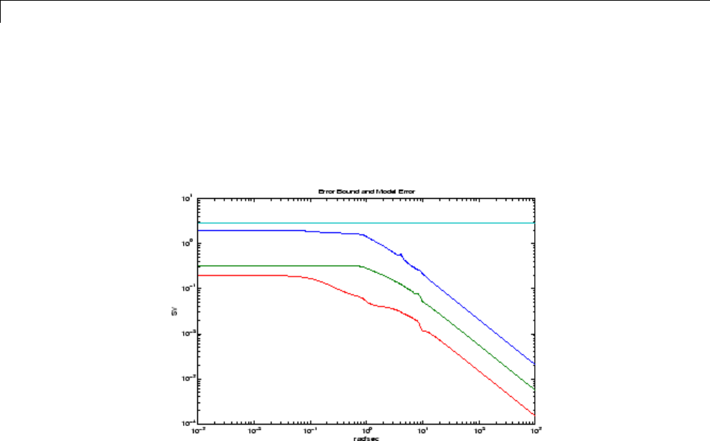
To determine whether the theoretical error bound is satisfied,
norm(G-g1(:,:,1),'inf') % 2.0123
info1.ErrorBound(1) % 2.8529
3-7
3Model Reduction for Robust Control
or plot the model error vs. error bound via the following commands:
[sv,w] = sigma(G-g1(:,:,1));
loglog(w,sv,w,info1.ErrorBound(1)*ones(size(w)))
xlabel('rad/sec');ylabel('SV');
title('Error Bound and Model Error')
3-8
Approximate Plant Model by Multiplicative Error Method
Approximate Plant Model by Multiplicative Error Method
In most cases, multiplicative error model reduction method bstmr tends to
bound the relative error between the original and reduced-order models
across the frequency range of interest, hence producing a more accurate
reduced-order model than the additive error methods. This characteristic is
obvious in system models with low damped poles.
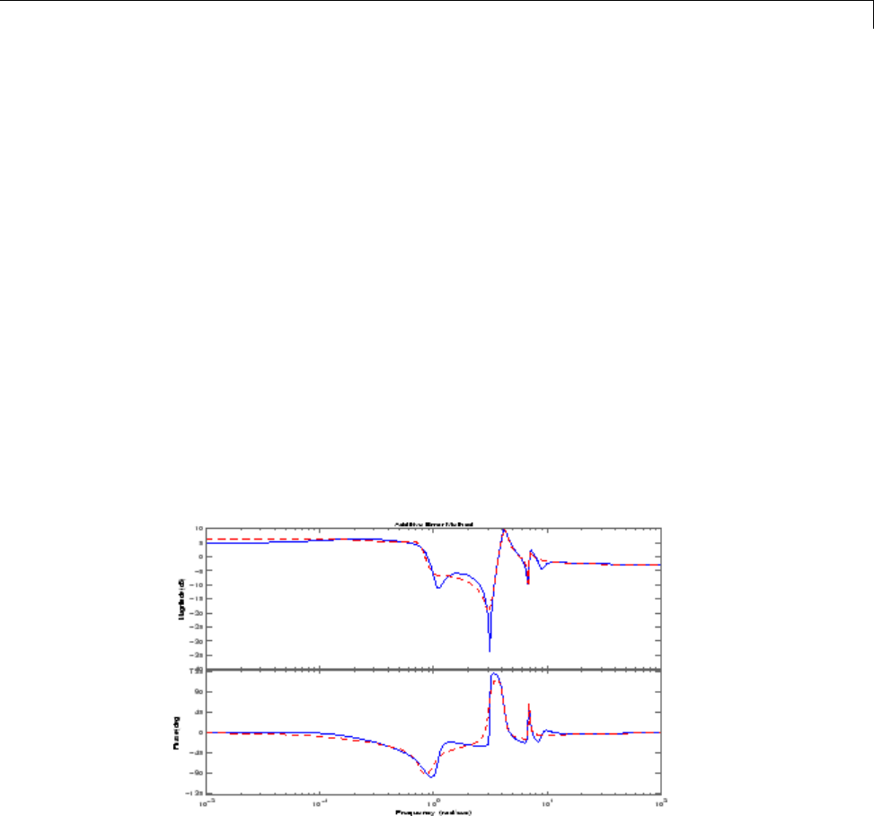
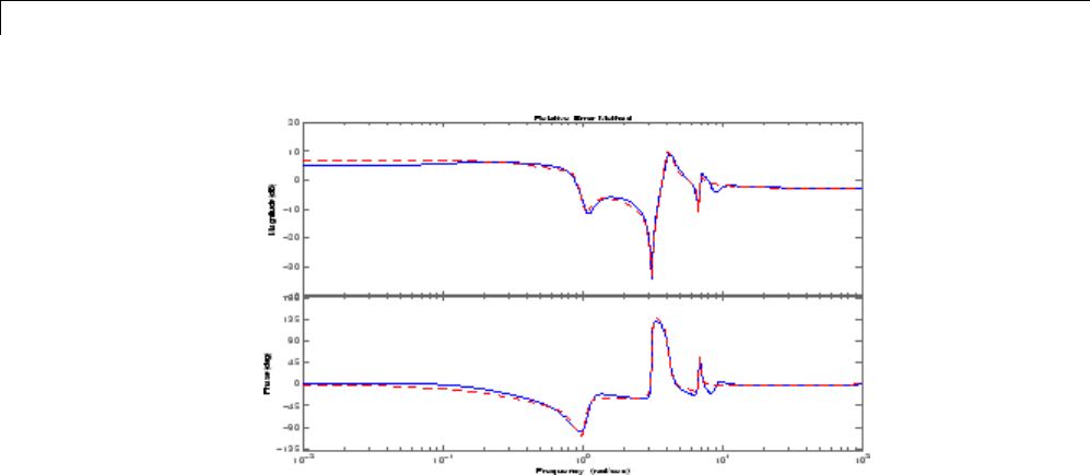
The following commands illustrate the significance of a multiplicative error
model reduction method as compared to any additive error type. Clearly, the
phase-matching algorithm using bstmr provides a better fit in the Bode plot.
rand('state',1234); randn('state',5678); G = rss(30,1,1);
[gr,infor] = reduce(G,'algo','balance','order',7);
[gs,infos] = reduce(G,'algo','bst','order',7);
figure(1);bode(G,'b-',gr,'r--');
title('Additive Error Method')
figure(2);bode(G,'b-',gs,'r--');
title('Relative Error Method')
3-9
3Model Reduction for Robust Control
Therefore, for some systems with low damped poles/zeros, the balanced
stochasticmethod(
bstmr) produces a better reduced-order model fit in those
frequency ranges to make multiplicative error small. Whereas additive error
methods such as balancmr,schurmr,orhankelmr only care about minimizing
the overall “absolute” peak error, they can produce a reduced-order model
missing those low damped poles/zeros frequency regions.
3-10

Using Modal Algorithms
Using Modal Algorithms
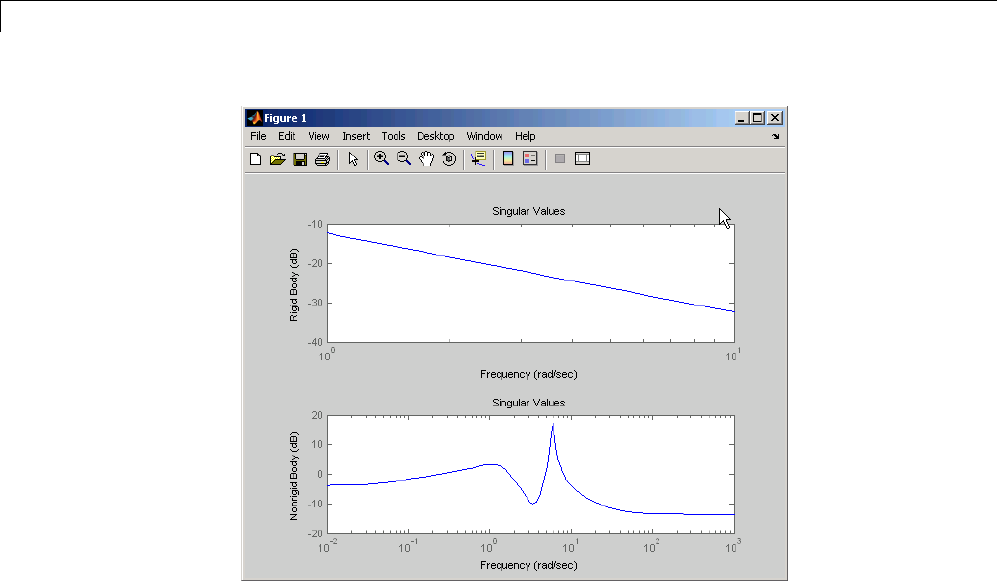
Rigid Body Dynamics
In many cases, a model’s jω-axis poles are important to keep after model
reduction, e.g., rigid body dynamics of a flexible structure plant or integrators
of a controller. A unique routine, modreal, serves the purpose nicely.
modreal puts a system into its modal form, with eigenvalues appearing on
the diagonal of its A-matrix. Real eigenvalues appear in 1-by-1 blocks, and
complex eigenvalues appear in 2-by-2 real blocks. All the blocks are ordered
in ascending order, based on their eigenvalue magnitudes, by default, or
descending order, based on their real parts. Therefore, specifying the number
of jω-axis poles splits the model into two systems with one containing only
jω-axis dynamics, the other containing the non-jωaxis dynamics.
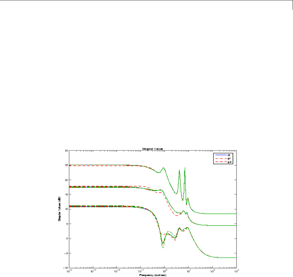
rand('state',5678); randn('state',1234); G = rss(30,1,1);
[Gjw,G2] = modreal(G,1); % only one rigid body dynamics
G2.d = Gjw.d; Gjw.d = 0; % put DC gain of G into G2
subplot(211);sigma(Gjw);ylabel('Rigid Body')
subplot(212);sigma(G2);ylabel('Nonrigid Body')
3-11
3Model Reduction for Robust Control
Further model reduction can be done on G2 without any numerical difficulty.
After G2 is further reduced to Gred, the final approximation of the model is
simply Gjw+Gred.
This process of splitting jω-axis poles has been built in and automated in
all the model reduction routines (balancmr,schurmr,hankelmr,bstmr,
hankelsv) so that users need not worry about splitting the model.
The following single command creates a size 8 reduced-order model from
its original 30-state model:
rand('state',5678); randn('state',1234); G = rss(30,1,1);
[gr,info] = reduce(G); % choose a size of 8 at prompt
bode(G,'b-',gr,'r--')
Without specifying the size of the reduced-order model, a Hankel singular
value plot is shown below.
3-12
Using Modal Algorithms
The default algorithm balancmr of reduce has done a great job of
approximating a 30-state model with just eight states. Again, the rigid body
dynamics are preserved for further controller design.
3-13

3Model Reduction for Robust Control
Reducing Large-Scale Models
For some really large size problems (states > 200), modreal turns out
to be the only way to start the model reduction process. Because of the
size and numerical properties associated with those large size, and low
damped dynamics, most Hankel based routines can fail to produce a good
reduced-order model.
modreal puts the large size dynamics into the modal form, then truncates the
dynamic model to an intermediate stage model with a comfortable size of 50
or so states. From this point on, those more sophisticated Hankel singular
value based routines can further reduce this intermediate stage model, in a
much more accurate fashion, to a smaller size for final controller design.
For a typical 240-state flexible spacecraft model in the spacecraft industry,
applying modreal and bstmr (or any other additive routines) in sequence can
reduce the original 240-state plant dynamics to a seven-state three-axis model
including rigid body dynamics. Any modern robust control design technique
mentioned in this toolbox can then be easily applied to this smaller size plant
for a controller design.
3-14
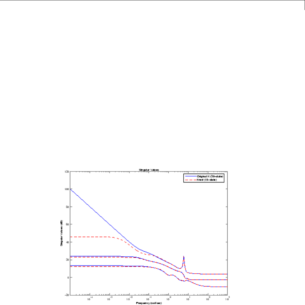
Normalized Coprime Factor Reduction
Normalized Coprime Factor Reduction
A special model reduction routine ncfmr produces a reduced-order model
by truncating a balanced coprime set of a given model. It can directly
simplify a modern controller with integrators to a smaller size by balanced
truncation of the normalized coprime factors. It does not need modreal for
pre-/postprocessing as the other routines do. However, the integrators will
not be preserved.
rand('state',5678); randn('state',1234);
K= rss(30,4,3); % The same model G used in the 1st example
[Kred,info2] = ncfmr(K);
sigma(K,Kred)
Again, without specifying the size of the reduced-order model, any model
reduction routine presented here will plot a Hankel singular value bar chart
and prompt you for a reduced model size. In this case, enter 15.
If integral control is important, previously mentioned methods (except ncfmr)
can nicely preserve the original integrator(s) in the model.
3-15

3Model Reduction for Robust Control
Bibliography
[1] Glover, K., “All Optimal Hankel Norm Approximation of Linear
Multivariable Systems, and Their L∝- Error Bounds,” Int. J. Control,Vol.39,
No. 6, 1984, pp. 1145-1193.
[2]Zhou,K.,Doyle,J.C.,andGlover,K.,Robust and Optimal Control,
Englewood Cliffs, NJ, Prentice Hall, 1996.
[3] Safonov, M.G., and Chiang, R.Y., “A Schur Method for Balanced Model
Reduction,” IEEE Trans. on Automat. Contr., Vol. 34, No. 7, July 1989,
pp. 729-733.
[4] Safonov, M.G., Chiang, R.Y., and Limebeer, D.J.N., “Optimal Hankel
Model Reduction for Nonminimal Systems,” IEEE Trans. on Automat. Contr.,
Vol. 35, No. 4, April 1990, pp. 496-502.
[5] Safonov, M.G., and Chiang, R.Y., “Model Reduction for Robust Control:
A Schur Relative Error Method,” International J. of Adaptive Control and
Signal Processing, Vol. 2, 1988, pp. 259-272.
[6] Obinata, G., and Anderson, B.D.O., Model Reduction for Control System
Design, London, Springer-Verlag, 2001.
3-16


4Robustness Analysis
Create Models of Uncertain Systems
Dealing with and understanding the effects of uncertainty are important tasks
for the control engineer. Reducing the effects of some forms of uncertainty
(initial conditions, low-frequency disturbances) without catastrophically
increasing the effects of other dominant forms (sensor noise, model
uncertainty) is the primary job of the feedback control system.
Closed-loop stability is the way to deal with the (always present) uncertainty
in initial conditions or arbitrarily small disturbances.
High-gain feedback in low-frequency ranges is a way to deal with the effects
of unknown biases and disturbances acting on the process output. In this
case, you are forced to use roll-off filters in high-frequency ranges to deal with
high-frequency sensor noise in a feedback system.
Finally, notions such as gain and phase margins (and their generalizations)
help quantify the sensitivity of stability and performance in the face of model
uncertainty, which is the imprecise knowledgeofhowthecontrolinput
directly affects the feedback variables.
Robust Control Toolbox software has built-in features allowing you to specify
model uncertainty simply and naturally. The primary building blocks, called
uncertain elements (or uncertain Control Design Blocks) are uncertain real
parameters and uncertain linear, time-invariant objects. These can be used to
create coarse and simple or detailed and complex descriptions of the model
uncertainty present within your process models.
Once formulated, high-level system robustness tools can help you analyze the
potential degradation of stability and performance of the closed-loop system
brought on by the system model uncertainty.
Creating Uncertain Models of Dynamic Systems
The two dominant forms of model uncertainty are as follows:
•Uncertainty in parameters of the underlying differential equation models
4-2

Create Models of Uncertain Systems
•Frequency-domain uncertainty, which often quantifies model uncertainty
by describing absolute or relative uncertainty in the process’s frequency
response
Using these two basic building blocks, along with conventional system
creation commands (such as ss and tf), you can easily create uncertain
system models.
Creating Uncertain Parameters
An uncertain parameter has a name (used to identify it within an uncertain
system with many uncertain parameters) and a nominal value. Being
uncertain, it also has variability, described in one of the following ways:
•An additive deviation from the nominal
•A range about the nominal
•A percentage deviation from the nominal
Create a real parameter, with name ’bw’, nominal value 5, and a percentage
uncertainty of 10%.
bw = ureal('bw',5,'Percentage',10)
This creates a ureal object. View its properties using the get command.
Uncertain Real Parameter: Name bw, NominalValue 5, variability = [-10 10]%
get(bw)
Name: 'bw'
NominalValue: 5
Mode: 'Percentage'
Range: [4.5000 5.5000]
PlusMinus: [-0.5000 0.5000]
Percentage: [-10 10]
AutoSimplify: 'basic'
Note that the range of variation (Range property) and the additive deviation
from nominal (the PlusMinus property) are consistent with the Percentage
property value.
4-3

4Robustness Analysis
You can create state-space and transfer function models with uncertain
real coefficients using ureal objects. The result is an uncertain state-space
object,oruss. As an example, use the uncertain real parameter bw to model a
first-order system whose bandwidth is between 4.5 and 5.5 rad/s.
H = tf(1,[1/bw 1])
USS: 1 State, 1 Output, 1 Input, Continuous System
bw: real, nominal = 5, variability = [-10 10]%, 1 occurrence
Note that the result His an uncertain system, called a uss object. The nominal
value of His a state-space object. Verify that the pole is at –5.
pole(H.NominalValue)
ans =
-5
Next, use bode and step to examine the behavior of H.
bode(H,{1e-1 1e2});
4-4
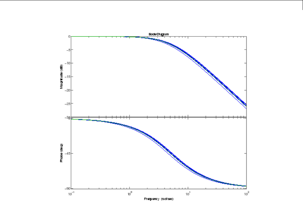
Create Models of Uncertain Systems
step(H)
4-5
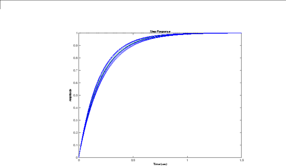
4Robustness Analysis
While there are variations in the bandwidth and time constant of H,the
high-frequency rolls off at 20 dB/decade regardless of the value of bw.Youcan
capture the more complicated uncertain behavior that typically occurs at high
frequencies using the ultidyn uncertain element, which is described next.
Quantifying Unmodeled Dynamics
An informal way to describe the difference between the model of a process and
the actual process behavior is in terms of bandwidth. It is common to hear
“The model is good out to 8 radians/second.” The precise meaning is not clear,
but it is reasonable to believe that for frequencies lower than, say, 5 rad/s,
the model is accurate, and for frequencies beyond, say, 30 rad/s, the model is
not necessarily representative of the process behavior. In the frequency range
between 5 and 30, the guaranteed accuracy of the model degrades.
The uncertain linear, time-invariant dynamics object ultidyn can be used
to model this type of knowledge. An ultidyn object represents an unknown
linear system whose only known attribute is a uniform magnitude bound
on its frequency response. When coupled with a nominal model and a
4-6

Create Models of Uncertain Systems
frequency-shaping filter, ultidyn objects can be used to capture uncertainty
associated with the model dynamics.
Suppose that the behavior of the system modeled by Hsignificantly deviates
from its first-order behavior beyond 9 rad/s, for example, about 5% potential
relative error at low frequency, increasing to 1000% at high frequency where
Hrolls off. In order to model frequency domain uncertainty as described above
using ultidyn objects, follow these steps:
1Create the nominal system Gnom,usingtf,ss,orzpk.Gnom itself might
already have parameter uncertainty. In this case Gnom is H,thefirst-order
system with an uncertain time constant.
2Create a filter W, called the “weight,” whose magnitude represents the
relative uncertainty at each frequency. The utility makeweight is useful for
creating first-order weights with specific low- and high-frequency gains,
and specified gain crossover frequency.
3Create an ultidyn object Delta with magnitude bound equal to 1.
The uncertain model Gis formed by G = Gnom*(1+W*Delta).
If the magnitude of Wrepresents an absolute (rather than relative)
uncertainty, use the formula G = Gnom + W*Delta instead.
The following commands carry out these steps:
Gnom = H;
W = makeweight(.05,9,10);
Delta = ultidyn('Delta',[1 1]);
G = Gnom*(1+W*Delta)
USS: 2 States, 1 Output, 1 Input, Continuous System
Delta: 1x1 LTI, max. gain = 1, 1 occurrence
bw: real, nominal = 5, variability = [-10 10]%, 1 occurrence
Note that the result Gis also an uncertain system, with dependence on both
Delta and bw.Youcanusebode tomakeaBodeplotof20randomsamplesof
G's behavior over the frequency range [0.1 100] rad/s.
bode(G,{1e-1 1e2},25)
4-7
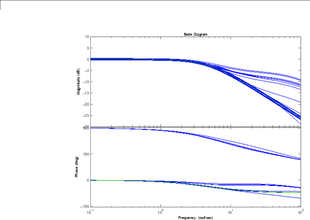
4Robustness Analysis
In the next section, you design and compare two feedback controllers for G.
4-8

Robust Controller Design
Robust Controller Design
In this tutorial, design a feedback controller for G, the uncertain model
created in “Create Models of Uncertain Systems” on page 4-2. The goals of
this design are the usual ones: good steady-state tracking and disturbance
rejection properties. Because the plant model is nominally a first-order lag,
choose a PI control architecture. Given the desired closed-loop damping ratio
ξand natural frequency ωn, the design equations for KIand KP(based on the
nominal open-loop time constant of 0.2) are
KK
InPn
==−
2
5
2
51,.
Follow these steps to design the controller:
1In order to study how the uncertain behavior of Gaffects the achievable
closed-loop bandwidth, design two controllers, both achieving ξ=0.707, with
differentωn:3and7.5respectively.
xi = 0.707;
wn = 3;
K1 = tf([(2*xi*wn/5-1) wn*wn/5],[1 0]);
wn = 7.5;
K2 = tf([(2*xi*wn/5-1) wn*wn/5],[1 0]);
Note that the nominal closed-loop bandwidth achieved by K2 is in a region
where Ghas significant model uncertainty. It will not be surprising if
the model variations lead to significant degradations in the closed-loop
performance.
2Form the closed-loop systems using feedback.
T1 = feedback(G*K1,1);
T2 = feedback(G*K2,1);
3Plot the step responses of 20 samples of each closed-loop system.
tfinal = 3;
step(T1,'b',T2,'r',tfinal,20)
4-9

4Robustness Analysis
The step responses for T2 exhibit a faster rise time because K2 sets a higher
closed loop bandwidth. However, the model variations have a greater effect.
You can use robuststab to check the robustness of stability to the model
variations.
[stabmarg1,destabu1,report1] = robuststab(T1);
stabmarg1
stabmarg1 =
ubound: 4.0241
lbound: 4.0241
destabfreq: 3.4959
[stabmarg2,destabu2,report2] = robuststab(T2);
stabmarg2
stabmarg2 =
ubound: 1.2545
lbound: 1.2544
destabfreq: 10.5249
4-10

Robust Controller Design
The stabmarg variable gives lower and upper bounds on the stability margin.
A stability margin greater than 1 means the system is stable for all values
of the modeled uncertainty. A stability margin less than 1 means there are
allowable values of the uncertain elements that make the system unstable.
The report variable briefly summarizes the analysis.
report1
report1 =
Uncertain System is robustly stable to modeled uncertainty.
-- It can tolerate up to 402% of modeled uncertainty.
-- A destabilizing combination of 402% the modeled uncertainty exists, causing an instability at
3.5 rad/s.
report2
report2 =
Uncertain System is robustly stable to modeled uncertainty.
-- It can tolerate up to 125% of modeled uncertainty.
-- A destabilizing combination of 125% the modeled uncertainty exists, causing an instability at
10.5 rad/s.
While both systems are stable for all variations, their performance is clearly
affected to different degrees. To determine how the uncertainty affects
closed-loop performance, you can use wcgain to compute the worst-case
effect of the uncertainty on the peak magnitude of the closed-loop sensitivity
(S=1/(1+GK)) function. This peak gain is typically correlated with the amount
of overshoot in a step response.
To do this, form the closed-loop sensitivity functions and call wcgain.
S1 = feedback(1,G*K1);
S2 = feedback(1,G*K2);
[maxgain1,wcu1] = wcgain(S1);
maxgain1
maxgain1 =
lbound: 1.8684
ubound: 1.9025
critfreq: 3.5152
[maxgain2,wcu2] = wcgain(S2);
maxgain2
maxgain2 =
lbound: 4.6031
4-11
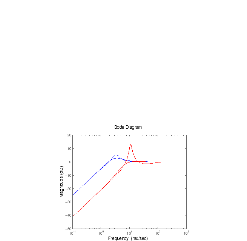
4Robustness Analysis
ubound: 4.6671
critfreq: 11.0231
The maxgain variable gives lower and upper bounds on the worst-case peak
gain of the sensitivity transfer function, as well as the specific frequency
where the maximum gain occurs. The wcu variable contains specific values of
the uncertain elements that achieve this worst-case behavior.
You can use usubs to substitute these worst-case values for uncertain
elements, and compare the nominal and worst-case behavior. Use bodemag
and step to make the comparison.
bodemag(S1.NominalValue,'b',usubs(S1,wcu1),'b');
hold on
bodemag(S2.NominalValue,'r',usubs(S2,wcu2),'r');
hold off
Clearly, while K2 achieves better nominal sensitivity than K1, the nominal
closed-loop bandwidth extends too far into the frequency range where the
4-12

Robust Controller Design
process uncertainty is very large. Hence the worst-case performance of K2 is
inferior to K1 for this particular uncertain model.
The next section explores these robustness analysis tools further on a
multiinput, multioutput system.
4-13

4Robustness Analysis
MIMO Robustness Analysis
The previous sections focused on simple uncertainty models of single-input
and single-output systems, predominantly from a transfer function
perspective. You can also create uncertain state-space models made up of
uncertain state-space matrices. Moreover, all the analysis tools covered thus
far can be applied to these systems as well.
Consider, for example, a two-input, two-output, two-state system whose
model has parametric uncertainty in the state-space matrices. First create
an uncertain parameter p. Using the parameter, make uncertain Aand C
matrices. The B matrix happens to be not-uncertain, although you will add
frequency domain input uncertainty to the model in “Adding Independent
Input Uncertainty to Each Channel” on page 4-15.
p = ureal('p',10,'Percentage',10);
A = [0 p;-p 0];
B = eye(2);
C = [1 p;-p 1];
H = ss(A,B,C,[0 0;0 0]);
You can view the properties of the uncertain system Husing the get command.
get(H)
a: [2x2 umat]
b: [2x2 double]
c: [2x2 umat]
d: [2x2 double]
e: []
StateName: {2x1 cell}
StateUnit: {2x1 cell}
NominalValue: [2x2 ss]
Uncertainty: [1x1 struct]
InternalDelay: [0x1 double]
InputDelay: [2x1 double]
OutputDelay: [2x1 double]
Ts: 0
TimeUnit: 'seconds'
InputName: {2x1 cell}
InputUnit: {2x1 cell}
4-14

MIMO Robustness Analysis
InputGroup: [1x1 struct]
OutputName: {2x1 cell}
OutputUnit: {2x1 cell}
OutputGroup: [1x1 struct]
Name: ''
Notes: {}
UserData: []
The properties a,b,c,d,andStateName behave in exactly the same manner
as ss objects. The properties InputName,OutputName,InputGroup,and
OutputGroup behave in exactly the same manner as all the system objects
(ss,zpk,tf,andfrd). The NominalValue is an ss object.
Adding Independent Input Uncertainty
to Each Channel
The model for Hdoes not include actuator dynamics. Said differently, the
actuator models are unity-gain for all frequencies.
Nevertheless, the behavior of the actuator for channel 1 is modestly uncertain
(say 10%) at low frequencies, and the high-frequency behavior beyond 20
rad/s is not accurately modeled. Similar statements hold for the actuator in
channel 2, with larger modest uncertainty at low frequency (say 20%) but
accuracy out to 45 rad/s.
Use ultidyn objects Delta1 and Delta2 along with shaping filters W1 and W2
to add this form of frequency domain uncertainty to the model.
W1 = makeweight(.1,20,50);
W2 = makeweight(.2,45,50);
Delta1 = ultidyn('Delta1',[1 1]);
Delta2 = ultidyn('Delta2',[1 1]);
G = H*blkdiag(1+W1*Delta1,1+W2*Delta2)
USS: 4 States, 2 Outputs, 2 Inputs, Continuous System
Delta1: 1x1 LTI, max. gain = 1, 1 occurrence
Delta2: 1x1 LTI, max. gain = 1, 1 occurrence
p: real, nominal = 10, variability = [-10 10]%, 2 occurrences
4-15
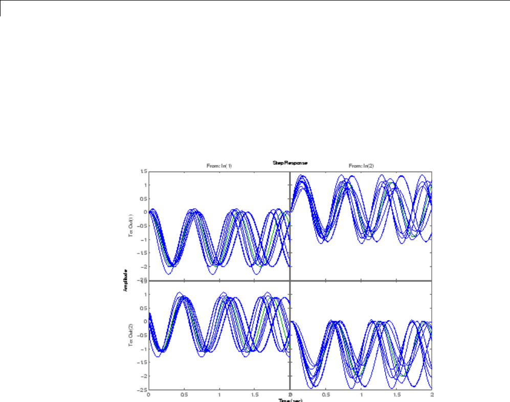
4Robustness Analysis
Note that Gis a two-input, two-output uncertain system, with dependence on
three uncertain elements, Delta1,Delta2,andp. It has four states, two from
Hand one each from the shaping filters W1 and W2, which are embedded in G.
You can plot a 2-second step response of several samples of G.The10%
uncertainty in the natural frequency is obvious.
step(G,2)
You can create a Bode plot of 50 samples of G. The high-frequency uncertainty
in the model is also obvious. For clarity, start the Bode plot beyond the
resonance.
bode(G,{13 100},50)
4-16
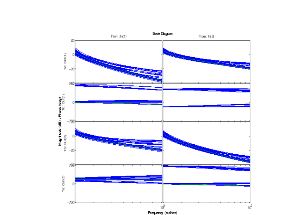
MIMO Robustness Analysis
Closed-Loop Robustness Analysis
You need to load the controller and verify that it is two-input and two-output.
load mimoKexample
size(K)
State-space model with 2 outputs, 2 inputs, and 9 states.
You can use the command loopsens to form all the standard plant/controller
feedback configurations, including sensitivity and complementary sensitivity
at both the input and output. Because Gis uncertain, all the closed-loop
systems are uncertain as well.
F = loopsens(G,K)
4-17

4Robustness Analysis
F=
Poles: [13x1 double]
Stable: 1
Si: [2x2 uss]
Ti: [2x2 uss]
Li: [2x2 uss]
So: [2x2 uss]
To: [2x2 uss]
Lo: [2x2 uss]
PSi: [2x2 uss]
CSo: [2x2 uss]
Fis a structure with many fields. The poles of the nominal closed-loop system
are in F.Poles,andF.Stable is 1 if the nominal closed-loop system is stable.
In the remaining 10 fields, Sstands for sensitivity, Tfor complementary
sensitivity, and Lfor open-loop gain. The suffixes iand orefer to the input and
output of the plant (G).Finally,Pand Crefer to the “plant” and “controller.”
Hence Ti is mathematically the same as
K(I+GK)–1G
while Lo is G*K,andCSo is mathematically the same as
K(I+GK)–1
You can examine the transmission of disturbances at the plant input to the
plant output using bodemag on F.PSi. Graph 50 samples along with the
nominal.
bodemag(F.PSi,':/-',{1e-1 100},50)
4-18
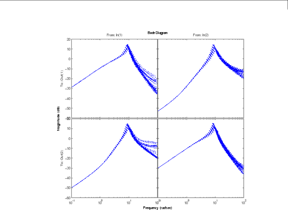
MIMO Robustness Analysis
Nominal Stability Margins
You can use loopmargin to investigate loop-at-a-time gain and phase margins,
loop-at-a-time disk margins, and simultaneous multivariable margins. They
are computed for the nominal system and do not reflect the uncertainty
models within G.
Explore the simultaneous margins individually at the plant input,
individually at the plant output, and simultaneously at both input and output.
[I,DI,SimI,O,DO,SimO,Sim] = loopmargin(G,K);
The third output argument is the simultaneous gain and phase variations
allowed in all input channels to the plant.
4-19

4Robustness Analysis
SimI
SimI =
GainMargin: [0.1180 8.4769]
PhaseMargin: [-76.5441 76.5441]
Frequency: 6.2287
This information implies that the gain at the plant input can vary in both
channels independently by factors between (approximately) 1/8 and 8,as well
as phase variations up to 76 degrees.
The sixth output argument is the simultaneous gain and phase variations
allowed in all output channels to the plant.
SimO
SimO =
GainMargin: [0.1193 8.3836]
PhaseMargin: [-76.3957 76.3957]
Frequency: 18.3522
Note that the simultaneous margins at the plant output are similar to those
at the input. This is not always the case in multiloop feedback systems.
The last output argument is the simultaneous gain and phase variations
allowed in all input and output channels to the plant. As expected, when
you consider all such variations simultaneously, the margins are somewhat
smaller than those at the input or output alone.
Sim
Sim =
GainMargin: [0.5671 1.7635]
PhaseMargin: [-30.8882 30.8882]
Frequency: 18.3522
Nevertheless, these numbers indicate a generally robust closed-loop system,
able to tolerate significant gain (more than +/-50% in each channel) and 30
degree phase variations simultaneously in all input and output channels
of the plant.
4-20

MIMO Robustness Analysis
Robustness of Stability Model Uncertainty
With loopmargin, you determined various margins of the nominal, multiloop
system. These margins are computed only for the nominal system, and do
not reflect the uncertainty explicitly modeled by the ureal and ultidyn
objects. When you work with detailed, complex uncertain system models,
the conventional margins computed by loopmargin might not always be
indicative of the actual stability margins associated with the uncertain
elements. You can use robuststab to check the stability margin of the system
to these specific modeled variations.
In this example, use robuststab to compute the stability margin of the
closed-loop system represented by Delta1,Delta2,andp.
Use any of the closed-loop systems within F = loopsens(G,K).Allofthem,
F.Si, F.To, etc., have the same internal dynamics, and hence the stability
properties are the same.
[stabmarg,desgtabu,report] = robuststab(F.So);
stabmarg
stabmarg =
ubound: 2.2175
lbound: 2.2175
destabfreq: 13.7576
report
report =
Uncertain System is robustly stable to modeled uncertainty.
-- It can tolerate up to 222% of modeled uncertainty.
-- A destabilizing combination of 222% the modeled uncertainty exists,causing an instability at
13.8 rad/s.
This analysis confirms what the loopmargin analysis suggested. The
closed-loop system is quite robust, in terms of stability, to the variations
modeled by the uncertain parameters Delta1,Delta2,andp.Infact,the
system can tolerate more than twice the modeled uncertainty without losing
closed-loop stability.
The next section studies the effects of these variations on the closed-loop
output sensitivity function.
4-21
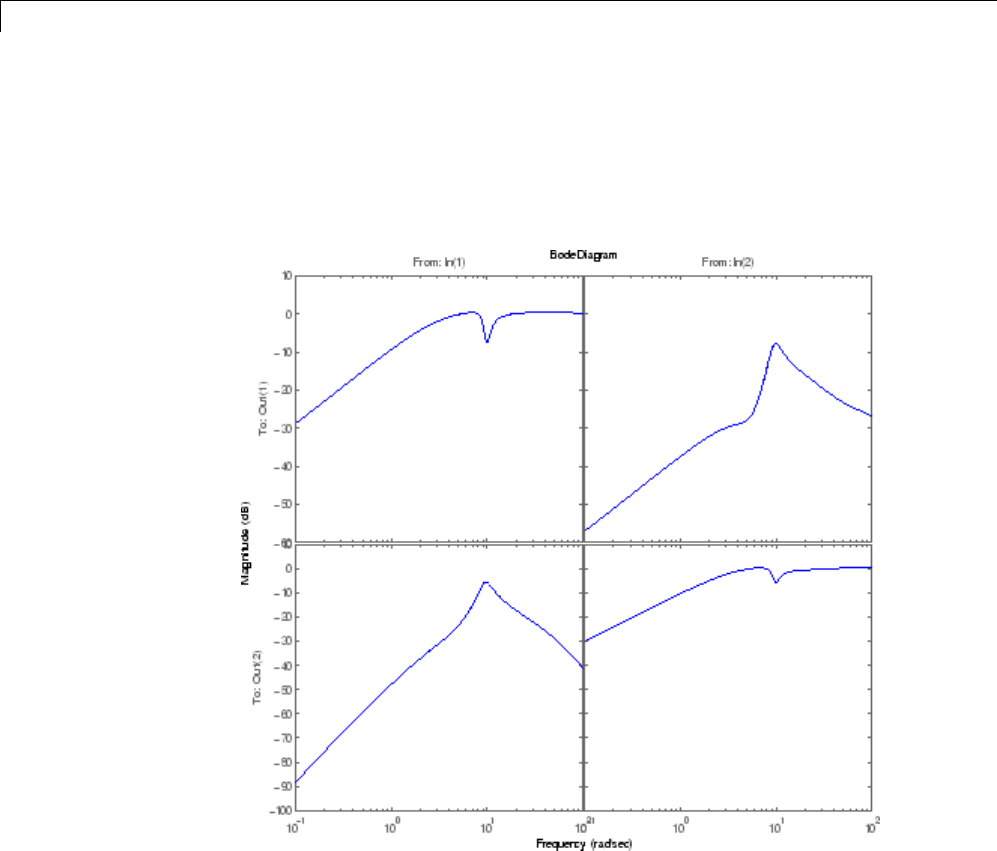
4Robustness Analysis
Worst-Case Gain Analysis
You can plot the Bode magnitude of the nominal output sensitivity function.
It clearly shows decent disturbance rejection in all channels at low frequency.
bodemag(F.So.NominalValue,{1e-1 100})
You can compute the peak value of the maximum singular value of the
frequency response matrix using norm.
[PeakNom,freq] = norm(F.So.NominalValue,'inf')
PeakNom =
1.1317
freq =
7.0483
4-22

MIMO Robustness Analysis
The peak is about 1.13, occurring at a frequency of 36 rad/s.
What is the maximum output sensitivity gain that is achieved when the
uncertain elements Delta1,Delta2,and pvary over their ranges? You can
use wcgain to answer this.
[maxgain,wcu] = wcgain(F.So);
maxgain
maxgain =
lbound: 2.1017
ubound: 2.1835
critfreq: 8.5546
The analysis indicates that the worst-case gain is somewhere between 2.1 and
2.2. The frequency where the peak is achieved is about 8.5.
You can replace the values for Delta1,Delta2,andpthat achieve the gain
of 2.1, using usubs. Make the substitution in the output complementary
sensitivity, and do a step response.
step(F.To.NominalValue,usubs(F.To,wcu),5)
4-23
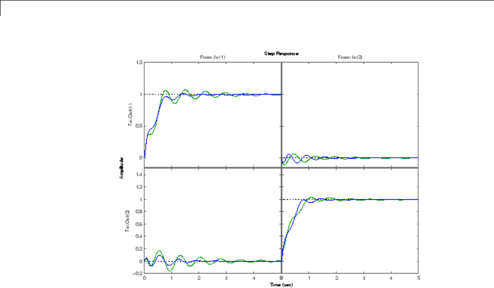
4Robustness Analysis
The perturbed response, which is the worst combination of uncertain values
in terms of output sensitivity amplification, does not show significant
degradation of the command response. The settling time is increased by about
50%, from 2 to 4, and the off-diagonal coupling is increased by about a factor
of about 2, but is still quite small.
4-24

Summary of Robustness Analysis Tools
Summary of Robustness Analysis Tools
Function Description
ureal Create uncertain real parameter.
ultidyn Create uncertain, linear, time-invariant dynamics.
uss Create uncertain state-space object from uncertain
state-space matrices.
ufrd Create uncertain frequency response object.
loopsens Compute all relevant open and closed-loop
quantities for a MIMO feedback connection.
loopmargin Compute loop-at-a-time as well as MIMO gain and
phase margins for a multiloop system, including
the simultaneous gain/phase margins.
robustperf Robustness performance of uncertain systems.
robuststab Compute the robust stability margin of a nominally
stable uncertain system.
wcgain Compute the worst-case gain of a nominally stable
uncertain system.
wcmargin Compute worst-case (over uncertainty)
loop-at-a-time disk-based gain and phase margins.
wcsens Compute worst-case (over uncertainty) sensitivity
of plant-controller feedback loop.
4-25

4Robustness Analysis
4-26


5H-Infinity and Mu Synthesis
Interpretation of H-Infinity Norm
Norms of Signals and Systems
There are several ways of defining norms of a scalar signal e(t)inthe
time domain. We will often use the 2-norm, (L2-norm), for mathematical
convenience, which is defined as
eetdt
2
2
1
2
:.=
()
⎛
⎝
⎜⎞
⎠
⎟
−∞
∞
∫
If this integral is finite, then the signal eis square integrable, denoted as e
L2.Forvector-valuedsignals
et
et
et
et
n
()
=
()
()
()
⎡
⎣
⎢
⎢
⎢
⎢
⎢
⎤
⎦
⎥
⎥
⎥
⎥
⎥
1
2
,
the 2-norm is defined as
eetdt
etetdt
T
22
2
1
2
1
2
:
.
=
()
⎛
⎝
⎜⎞
⎠
⎟
=
() ()
⎛
⎝
⎜⎞
⎠
⎟
−∞
∞
−∞
∞
∫
∫
In µ-tools the dynamic systems we deal with are exclusively linear, with
state-space model
x
e
AB
CD
x
d
⎡
⎣
⎢⎤
⎦
⎥=⎡
⎣
⎢⎤
⎦
⎥⎡
⎣
⎢⎤
⎦
⎥,
or, in the transfer function form,
5-2

Interpretation of H-Infinity Norm
e(s)=T(s)d(s),T(s):= C(sI – A)–1B+D
Two mathematically convenient measures of the transfer matrix T(s)inthe
frequency domain are the matrix H2and H∞norms,
TTjd
TTj
F
R
2
2
1
2
1
2
:
:max ,
=
()
⎡
⎣
⎢⎤
⎦
⎥
=
()
⎡
⎣⎤
⎦
−∞
∞
∞∈
∫
where the Frobenius norm (see the MATLAB norm command)ofacomplex
matrix Mis
MMM
F:.
*
=
()
Trace
Both of these transfer function norms have input/output time-domain
interpretations. If, starting from initial condition x(0) = 0, two signals dand
eare related by
x
e
AB
CD
x
d
⎡
⎣
⎢⎤
⎦
⎥=⎡
⎣
⎢⎤
⎦
⎥⎡
⎣
⎢⎤
⎦
⎥,
then
•For d,aunitintensity,whitenoiseprocess,thesteady-statevarianceofe
is T2.
•The L2(or RMS) gain from d→e,
max
d
e
d
≠0
2
2
is equal to T∞. This is discussed in greater detail in the next section.
Using Weighted Norms to Characterize Performance
Any performance criterion must also account for
5-3
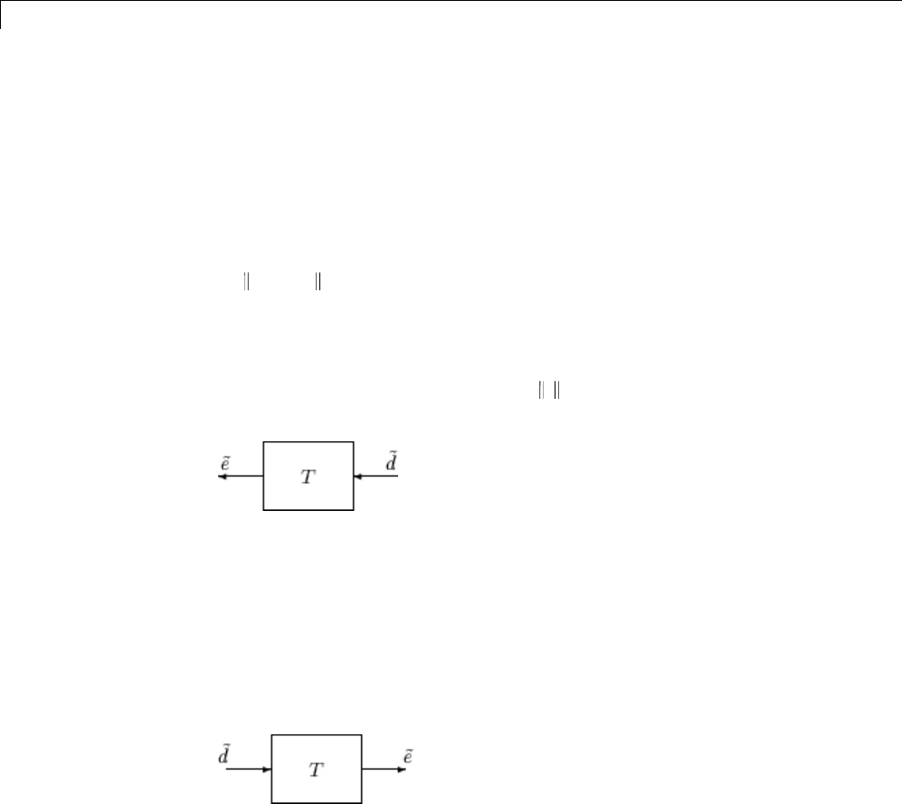
5H-Infinity and Mu Synthesis
•Relative magnitude of outside influences
•Frequency dependence of signals
•Relative importance of the magnitudes of regulated variables
So, if the performance objective is in the form of a matrix norm, it should
actually be a weighted norm
WLTWR
where the weighting function matrices WLand WRare frequency dependent,
to account for bandwidth constraints and spectral content of exogenous
signals. The most natural (mathematical) manner to characterize acceptable
performance is in terms of the MIMO ·∞(H∞) norm. For this reason, this
section now discusses some interpretations of the H∞norm.
Unweighted MIMO System
Suppose Tis a MIMO stable linear system, with transfer function matrix T(s).
For a given driving signal
dt
()
,define
eas the output, as shown below.
Note that it is more traditional to write the diagram in Unweighted MIMO
System: Vectors from Left to Right on page 5-4 with the arrows going from
left to right as in Weighted MIMO System on page 5-6.
Unweighted MIMO System: Vectors from Left to Right
The two diagrams shown above represent the exact same system. We prefer to
write these block diagrams with the arrows going right to left to be consistent
with matrix and operator composition.
Assume that the dimensions of Tare ne×nd.Letβ>0bedefinedas
5-4

Interpretation of H-Infinity Norm
::max .==
()
⎡
⎣⎤
⎦
∞∈
TTj
R
Now consider a response, starting from initial condition equal to 0. In that
case, Parseval’s theorem gives that
e
d
etetdt
dtdtdt
T
T
2
2
0
1
2
0
1
2
=
() ()
⎡
⎣
⎢⎤
⎦
⎥
() ()
⎡
⎣
⎢⎤
⎦
⎥
≤
∞
∞
∫
∫
.
Moreover, there are specific disturbances dthat result in the ratio
ed
22
arbitrarily close to β. Because of this, T∞is referred to as the L2(or RMS)
gain of the system.
As you would expect, a sinusoidal, steady-state interpretation of T∞is also
possible: For any frequency
∈R, any vector of amplitudes aR
nd
∈,and
any vector of phases
∈Rnd,with a2≤1, define a time signal
dt
at
at
nn
dd
()
=
+
()
+
()
⎡
⎣
⎢
⎢
⎢
⎢
⎤
⎦
⎥
⎥
⎥
⎥
11
sin
sin
.
Applying this input to the system Tresults in a steady-state response
ess of
the form
et
bt
bt
ss
nn
ee
()
=
+
()
+
()
⎡
⎣
⎢
⎢
⎢
⎢
⎤
⎦
⎥
⎥
⎥
⎥
11
sin
sin
.
5-5
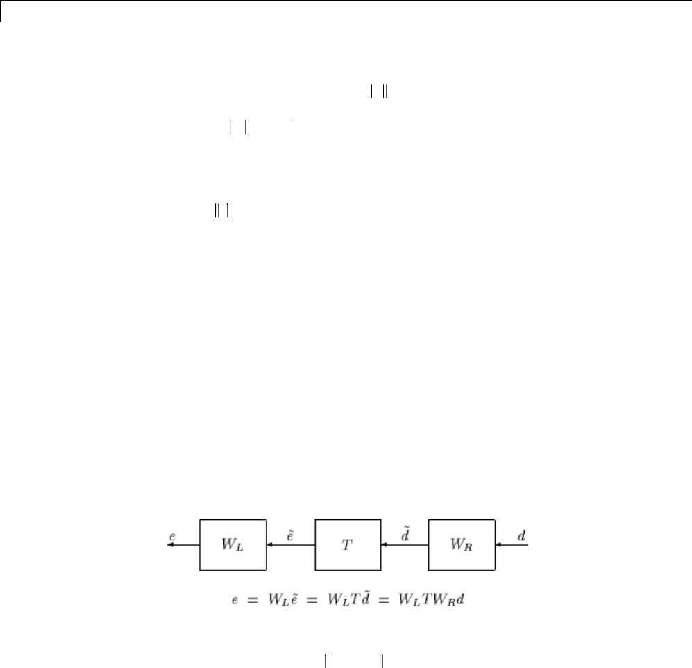
5H-Infinity and Mu Synthesis
The vector bR
ne
∈will satisfy b2≤β. Moreover, β, as defined in Weighted
MIMO System on page 5-6, is the smallest number such that this is true
for every a2≤1,
,and
ϕ
.
Note that in this interpretation, the vectors of the sinusoidal magnitude
responses are unweighted, and measured in Euclidean norm. If realistic
multivariableperformanceobjectivesaretoberepresentedbyasingle
MIMO ·∞objective on a closed-loop transfer function, additional scalings
are necessary. Because many different objectives are being lumped into one
matrix and the associated cost is the norm of the matrix, it is important to
use frequency-dependent weighting functions, so that different requirements
can be meaningfully combined into a single cost function. Diagonal weights
are most easily interpreted.
Consider the diagram of Weighted MIMO System on page 5-6, along with
Unweighted MIMO System: Vectors from Left to Right on page 5-4.
Assume that WLand WRare diagonal, stable transfer function matrices, with
diagonal entries denoted Liand Ri.
W
L
L
L
W
R
R
L
n
R
e
=
⎡
⎣
⎢
⎢
⎢
⎢
⎢
⎤
⎦
⎥
⎥
⎥
⎥
⎥
=
1
2
1
2
00
00
00
00
00
00
,
RRnd
⎡
⎣
⎢
⎢
⎢
⎢
⎢
⎤
⎦
⎥
⎥
⎥
⎥
⎥
.
Weighted MIMO System
Bounds on the quantity WLTWR∞will imply bounds about the sinusoidal
steady-state behavior of the signals
dand
eTd=
()
in the diagram of
Unweighted MIMO System: Vectors from Left to Right on page 5-4.
Specifically, for sinusoidal signal
d, the steady-state relationship between
5-6

Interpretation of H-Infinity Norm
eTd=
()
,
dand WLTWR∞is as follows. The steady-state solution
ess ,
denoted as
et
et
et
ss
nn
ed
()
=
+
()
+
()
⎡
⎣
⎢
⎢
⎢
⎢
⎤
⎦
⎥
⎥
⎥
⎥
11
sin
sin
(5-1)
satisfies
Wje
Li
i
n
i
e
()
≤
=
∑2
1
1
for all sinusoidal input signals
dof the form
dt
dt
dt
nn
ed
()
=
+
()
+
()
⎡
⎣
⎢
⎢
⎢
⎢
⎤
⎦
⎥
⎥
⎥
⎥
11
sin
sin
(5-2)
satisfying
d
Wj
i
R
i
n
i
d
2
2
1
1
()
≤
=
∑
if and only if WLTWR∞≤1.
This approximately (very approximately — the next statement is not actually
correct) implies that WLTWR∞≤1 if and only if for every fixed frequency
,
and all sinusoidal disturbances
dof the form Equation 5-2 satisfying
dWj
iR
i
≤
()
5-7

5H-Infinity and Mu Synthesis
the steady-state error components will satisfy
eWj
i
Li
≤
()
1
.
This shows how one could pick performance weights to reflect the desired
frequency-dependent performance objective. Use WRto represent the relative
magnitude of sinusoids disturbances that might be present, and use 1/WLto
represent the desired upper bound on the subsequent errors that are produced.
Remember, however, that the weighted H∞norm does not actually
give element-by-element bounds on the components of
ebased on
element-by-element bounds on the components of
d. The precise bound it
gives is in terms of Euclidean norms of the components of
eand
d(weighted
appropriately by WL(j
)andWR(j
)).
5-8

H-Infinity Performance
H-Infinity Performance
Performance as Generalized Disturbance Rejection
The modern approach to characterizing closed-loop performance objectives
is to measure the size of certain closed-loop transfer function matrices using
various matrix norms. Matrix norms provide a measure of how large output
signals can get for certain classes of input signals. Optimizing these types
of performance objectives over the set of stabilizing controllers is the main
thrust of recent optimal control theory, such as L1,H2,H∞,andoptimal
control. Hence, it is important to understand how many types of control
objectives can be posed as a minimization of closed-loop transfer functions.
Consider a tracking problem, with disturbance rejection, measurement noise,
and control input signal limitations, as shown in Generalized and Weighted
Performance Block Diagram on page 5-11. Kis some controller to be designed
and Gis the system you want to control.
Typical Closed-Loop Performance Objective
A reasonable, though not precise, design objective would be to design K
to keep tracking errors and control input signal small for all reasonable
reference commands, sensor noises, and external force disturbances.
Hence, a natural performance objective is the closed-loop gain from
exogenous influences (reference commands, sensor noise, and external force
disturbances) to regulated variables (tracking errors and control input signal).
Specifically, let Tdenote the closed-loop mapping from the outside influences
to the regulated variables:
5-9
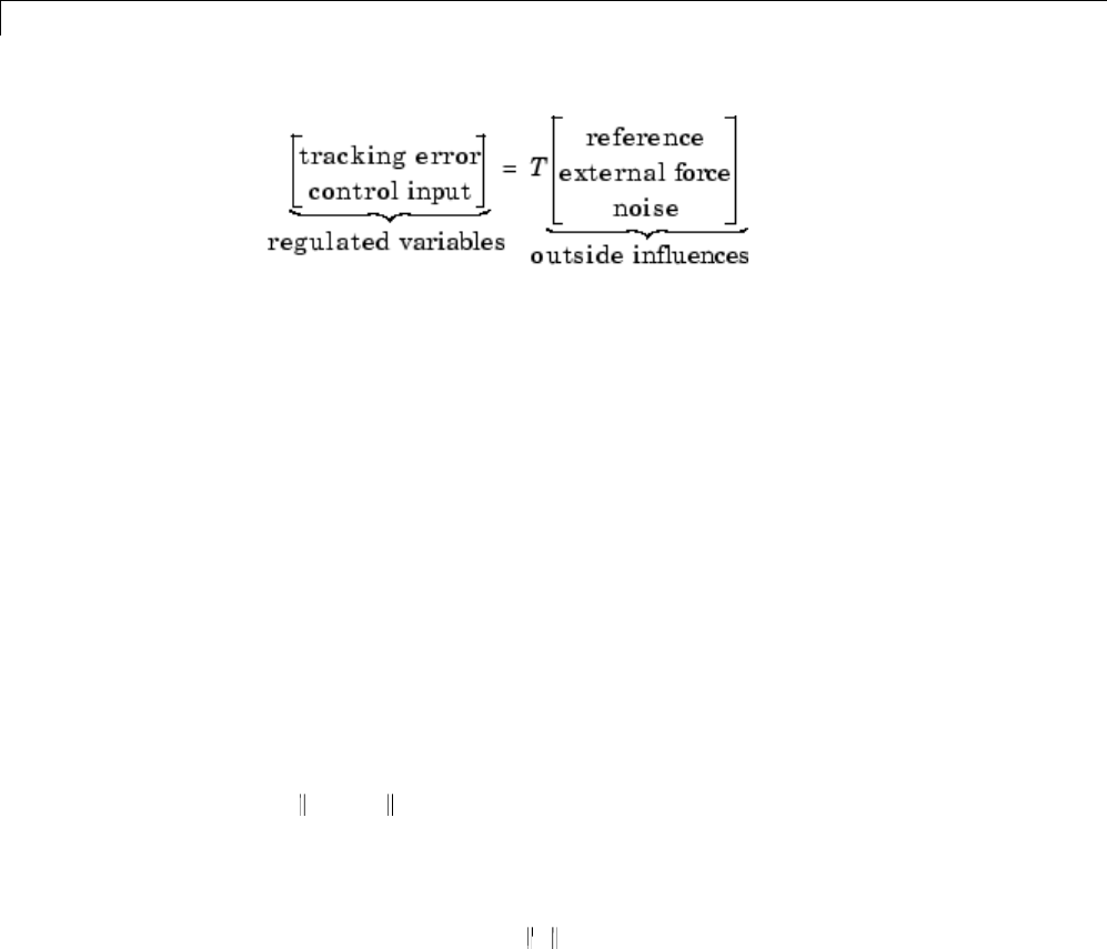
5H-Infinity and Mu Synthesis
You can assess performance by measuring the gain from outside influences
to regulated variables. In other words, good performance is associated with
Tbeing small. Because the closed-loop system is a multiinput, multioutput
(MIMO) dynamic system, there are two different aspects to the gain of T:
•Spatial (vector disturbances and vector errors)
•Temporal (dynamic relationship between input/output signals)
Hence the performance criterion must account for
•Relative magnitude of outside influences
•Frequency dependence of signals
•Relative importance of the magnitudes of regulated variables
So if the performance objective is in the form of a matrix norm, it should
actually be a weighted norm
WLTWR
where the weighting function matrices WLand WRare frequency dependent, to
account for bandwidth constraints and spectral content of exogenous signals.
A natural (mathematical) manner to characterize acceptable performance
is in terms of the MIMO ·∞(H∞) norm. See “Interpretation of H-Infinity
Norm” on page 5-2 for an interpretation of the H∞norm and signals.
Interconnection with Typical MIMO Performance Objectives
The closed-loop performance objectives are formulated as weighted closed-loop
transfer functions that are to be made small through feedback. A generic
example, which includes many relevant terms, is shown in block diagram
form in Generalized and Weighted Performance Block Diagram on page 5-11.
In the diagram, Gdenotes the plant model and Kis the feedback controller.
5-10
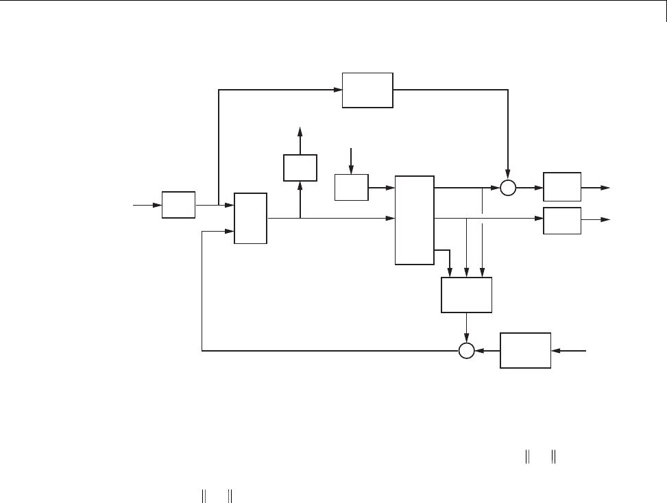
H-Infinity Performance
Wcmd
K
Wmodel
Wact
Wsnois
Hsens
G
Wdist Wperf1
Wperf2
-
d1d1
~
d2
d2
~
d3
d3
~
e1
e1
~
e2
e2
~
e3
e3
~
Generalized and Weighted Performance Block Diagram
The blocks in this figure might be scalar (SISO) and/or multivariable (MIMO),
depending on the specific example. The mathematical objective of H∞control
is to make the closed-loop MIMO transfer function Ted satisfy Ted ∞<1.The
weighting functions are used to scale the input/output transfer functions such
that when Ted ∞< 1, the relationship between
dand
eis suitable.
Performance requirements on the closed-loop system are transformed into
the H∞framework with the help of weighting or scaling functions. Weights
are selected to account for the relative magnitude of signals, their frequency
dependence, and their relative importance. This is captured in the figure
above, where the weights or scalings [Wcmd,Wdist,Wsnois] are used to transform
and scale the normalized input signals [d1,d2,d3] into physical units defined
as [d1,d2,d3]. Similarly weights or scalings [Wact,Wperf1,Wperf2] transform
and scale physical units into normalized output signals [e1,e2,e3]. An
interpretation of the signals, weighting functions, and models follows.
5-11

5H-Infinity and Mu Synthesis
Signal Meaning
d1
d1
Normalized reference command
Typical reference command in physical units
d2
d2
Normalized exogenous disturbances
Typical exogenous disturbances in physical units
d3
d3
Normalized sensor noise
Typical sensor noise in physical units
e1
e1
Weighted control signals
Actual control signals in physical units
e2
e2
Weighted tracking errors
Actual tracking errors in physical units
e3
e3
Weighted plant errors
Actual plant errors in physical units
Wcmd
Wcmd is included in H∞control problems that require tracking of a reference
command. Wcmd shapes the normalized reference command signals
(magnitude and frequency) into the actual (or typical) reference signals that
you expect to occur. It describes the magnitude and the frequency dependence
of the reference commands generated by the normalized reference signal.
Normally Wcmd is flat at low frequency and rolls off at high frequency. For
example, in a flight control problem, fighter pilots generate stick input
reference commands up to a bandwidth of about 2 Hz. Suppose that the stick
has a maximum travel of three inches. Pilot commands could be modeled as
normalized signals passed through a first-order filter:
W
s
cmd =
⋅+
3
1
22 1
.
5-12

H-Infinity Performance
Wmodel
Wmodel represents a desired ideal model for the closed-looped system and is
often included in problem formulations with tracking requirements. Inclusion
of an ideal model for tracking is often called a model matching problem, i.e.,
the objective of the closed-loop system is to match the defined model. For
good command tracking response, you might want the closed-loop system to
respond like a well-damped second-order system. The ideal model would
then be
W
s
model =++
2
22
2
for specific desired natural frequency ωand desired damping ratio ζ.Unit
conversions might be necessary to ensure exact correlation between the ideal
model and the closed-loop system. In the fighter pilot example, suppose that
roll-rate is being commanded and 10º/second response is desired for each inch
of stick motion. Then, in these units, the appropriate model is:
W
s
model =++
10 2
2
22
.
Wdist
Wdist shapes the frequency content and magnitude of the exogenous
disturbances affecting the plant. For example, consider an electron microscope
as the plant. The dominant performance objective is to mechanically isolate
the microscope from outside mechanical disturbances, such as ground
excitations, sound (pressure) waves, and air currents. You can capture the
spectrum and relative magnitudes of these disturbances with the transfer
function weighting matrix Wdist.
Wperf1
Wperf1 weights the difference between the response of the closed-loop system
and the ideal model Wmodel. Often you might want accurate matching of the
ideal model at low frequency and require less accurate matching at higher
frequency, in which case Wperf1 is flat at low frequency, rolls off at first or
5-13

5H-Infinity and Mu Synthesis
second order, and flattens out at a small, nonzero value at high frequency.
The inverse of the weight is related to the allowable size of tracking errors,
when dealing with the reference commands and disturbances described by
Wcmd and Wdist.
Wperf2
Wperf2 penalizes variables internal to the process G, such as actuator states
that are internal to Gor other variables that are not part of the tracking
objective.
Wact
Wact is used to shape the penalty on control signal use. Wact is a frequency
varying weighting function used to penalize limits on the deflection/position,
deflection rate/velocity, etc., response of the control signals, when dealing
with the tracking and disturbance rejection objectives defined above. Each
control signal is usually penalized independently.
Wsnois
Wsnois represents frequency domain models of sensor noise. Each sensor
measurement feedback to the controller has some noise, which is often
higher in one frequency range than another. The Wsnois weight tries to
capture this information, derived from laboratory experiments or based on
manufacturer measurements, in the control problem. For example, medium
grade accelerometers have substantial noise at low frequency and high
frequency. Therefore the corresponding Wsnois weight would be larger at low
and high frequency and have a smaller magnitude in the mid-frequency
range. Displacement or rotation measurement is often quite accurate at low
frequency and in steady state, but responds poorly as frequency increases.
The weighting function for this sensor would be small at low frequency,
gradually increase in magnitude as a first- or second-order system, and level
outathighfrequency.
Hsens
Hsens represents a model of the sensor dynamics or an external antialiasing
filter. The transfer functions used to describe Hsens are based on physical
5-14
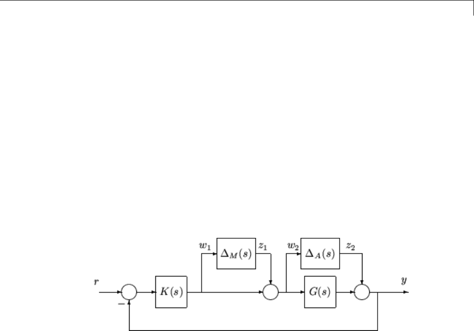
H-Infinity Performance
characteristics of the individual components. These models might also be
lumped into the plant model G.
This generic block diagram has tremendous flexibility and many control
performance objectives can be formulated in the H∞framework using this
block diagram description.
Robustness in the H-Infinity Framework
Performance and robustness tradeoffs in control design were discussed in the
context of multivariable loop shaping in “Tradeoff Between Performance and
Robustness” on page 2-2. In the H∞control design framework, you can include
robustness objectives as additional disturbance to error transfer functions —
disturbances to be kept small. Consider the following figure of a closed-loop
feedback system with additive and multiplicative uncertainty models.
The transfer function matrices are defined as:
TF s T s KG I GK
TF s KS s K I GK
zw I
zw O
()
=
()
=+
()
()
=
()
=+
()
→−
→−
11
22
1
1
where TI(s) denotes the input complementary sensitivity function and SO(s)
denotes the output sensitivity function. Bounds on the size of the transfer
function matrices from z1to w1and z2to w2ensure that the closed-loop
system is robust to multiplicative uncertainty, ΔM(s), at the plant input, and
additive uncertainty, ΔA(s), around the plant G(s). In the H∞control problem
formulation, the robustness objectives enter the synthesis procedure as
additional input/output signals to be kept small. The interconnection with the
uncertainty blocks removed follows.
5-15
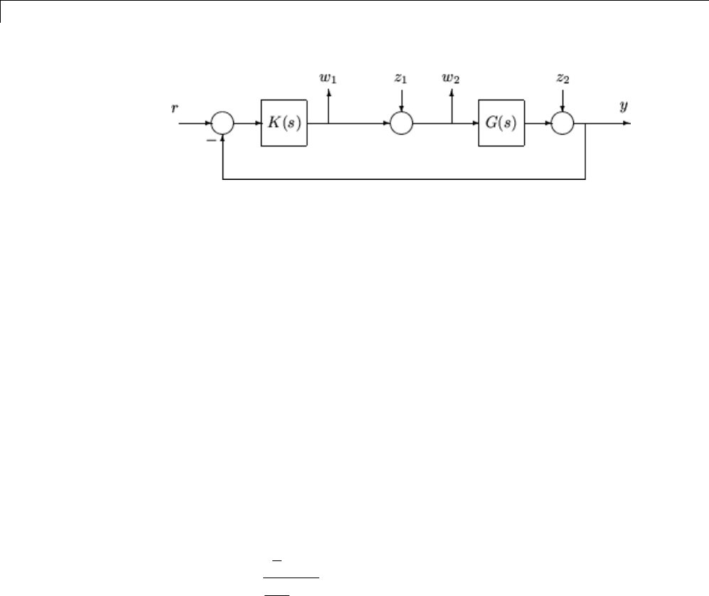
5H-Infinity and Mu Synthesis
The H∞control robustness objective is now in the same format as the
performanceobjectives,thatis,tominimizetheH∞norm of the transfer
matrix from z,[z1,z2], to w,[w1,w2].
Weighting or scaling matrices are often introduced to shape the frequency and
magnitude content of the sensitivity and complementary sensitivity transfer
function matrices. Let WMcorrespond to the multiplicative uncertainty and
WAcorrespond to the additive uncertainty model. ΔM(s)andΔA(s) are assumed
to be a norm bounded by 1, i.e., |ΔM(s)|<1 and |ΔA(s)|<1. Hence as a function
of frequency, |WM(jω)| and |WA(jω)| are the respective sizes of the largest
anticipated additive and multiplicative plant perturbations.
The multiplicative weighting or scaling WMrepresents a percentage error in
the model and is often small in magnitude at low frequency, between 0.05 and
0.20 (5% to 20% modeling error), and growing larger in magnitude at high
frequency, 2 to 5 ((200% to 500% modeling error). The weight will transition
by crossing a magnitude value of 1, which corresponds to 100% uncertainty
in the model, at a frequency at least twice the bandwidth of the closed-loop
system. A typical multiplicative weight is
W
s
s
M=+
+
010
1
51
1
200 1
..
By contrast, the additive weight or scaling WArepresents an absolute error
that is often small at low frequency and large in magnitude at high frequency.
The magnitude of this weight depends directly on the magnitude of the plant
model, G(s).
5-16

Functions for Control Design
Functions for Control Design
The term control system design refers to the process of synthesizing a
feedback control law that meets design specifications in a closed-loop control
system. The design methods are iterative, combining parameter selection
with analysis, simulation, and insight into the dynamics of the plant. Robust
Control Toolbox software provides a set of commands that you can use for a
broad range of multivariable control applications, including
•H2control design
•H∞standard and loop-shaping control design
•H∞tuning of controllers with fixed structure
•H∞normalized coprime factor control design
•Mixed H2/H∞control design
•µ-synthesis via D-Kand D-G-K iteration
•Sampled-data H∞control design
These functions cover both continuous and discrete-time problems. The
following table summarizes the H2and H∞control design commands.
Function Description
augw Augments plant weights for mixed-sensitivity
control design
h2hinfsyn Mixed Η2/Η∞controller synthesis
h2syn Η2controller synthesis
hinfsyn Η∞controller synthesis
hinfstruct Η∞tuning of fixed control structures
loopsyn Η∞loop-shaping controller synthesis
ltrsyn Loop-transfer recovery controller synthesis
mixsyn Η∞mixed-sensitivity controller synthesis
ncfsyn Η∞normalized coprime factor controller synthesis
sdhinfsyn Sample-data Η∞controller synthesis
5-17

5H-Infinity and Mu Synthesis
The following table summarizes µ-synthesis control design commands.
Function Description
dksyn Synthesis of a robust controller via µ-synthesis
dkitopt Create a dksyn options object
drawmag Interactive mouse-based sketching and fitting tool
fitfrd Fit scaling frequency response data with LTI model
fitmagfrd Fit scaling magnitude data with stable,
minimum-phase model
5-18
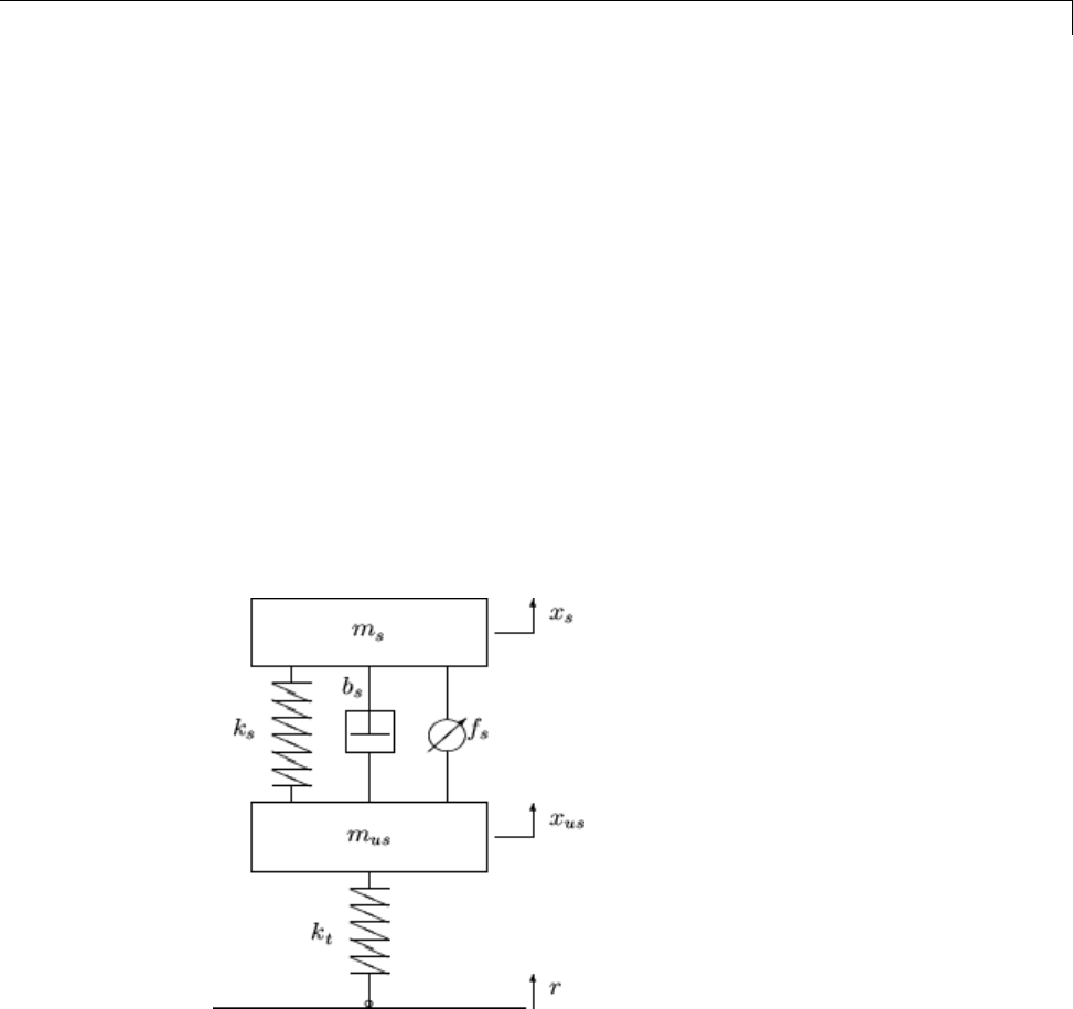
H-Infinity and Mu Synthesis for Active Suspension Control
H-Infinity and Mu Synthesis for Active Suspension Control
Conventional passive suspensions employ a spring and damper between the
car body and wheel assembly, representing a tradeoff between conflicting
performance metrics such as passenger comfort, road holding, and suspension
deflection. Active suspensions allow the designer to balance these objectives
using a hydraulic actuator, controlled by feedback, between the chassis and
wheel assembly.
In this section, you design an active suspension system for a quarter car body
and wheel assembly model using the H∞control design technique. You will
see the tradeoff between passenger comfort, i.e., minimizing car body travel,
versus suspension travel as the performance objective.
Quarter Car Suspension Model
The quarter car model shown is used to design active suspension control laws.
The sprung mass msrepresents the car chassis, while the unsprung mass mus
represents the wheel assembly. The spring, ks,anddamper,bs,representa
passive spring and shock absorber that are placed between the car body and
the wheel assembly, while the spring ktserves to model the compressibility of
the pneumatic tire. The variables xs,xus,andrare the car body travel, the
5-19

5H-Infinity and Mu Synthesis
wheel travel, and the road disturbance, respectively. The force fs,kN,applied
between the sprung and unsprung masses, is controlled by feedback and
represents the active component of the suspension system. The dynamics of
the actuator are ignored in this example, and assume that the control signal
is the force fs.Definingx1:= xs,xx
s2:=,x3:= xus,and xx
us4:=, the following
is the state-space description of the quarter car dynamics.
xx
xmkx x bx x f
xx
xmkx
s
sss
us
s
12
21324
34
11
1
1
=
=− −
()
+−
()
−
⎡
⎣⎤
⎦
=
=−−
()
+−
()
−−
()
−
⎡
⎣⎤
⎦
xbxxkxrf
sts3243 .
The following component values are taken from reference [9].
ms = 290; % kg
mus = 59; % kg
bs = 1000; % N/m/s
ks = 16182 ; % N/m
kt = 190000; % N/m
A linear, time-invariant model of the quarter car model, qcar, is constructed
from the equations of motion and parameter values. The inputs to the model
are the road disturbance and actuator force, respectively, and the outputs are
the car body deflection, acceleration, and suspension deflection.
A12 = [ 0 1 0 0; [-ks -bs ks bs]/ms ];
A34 = [ 0 0 0 1; [ks bs -ks-kt -bs]/mus];
B12 = [0 0; 0 10000/ms];
B34 = [0 0; [kt -10000]/mus];
C = [1 0 0 0; A12(2,:); 1 0 -1 0; 0 0 0 0];
D = [0 0; B12(2,:); 0 0; 0 1];
qcar = ss([A12; A34],[B12; B34],C,D);
It is well known [8] that the acceleration transfer function has an invariant
pointatthetirehop frequency, 56.7 rad/s. Similarly, the suspension deflection
transfer function has an invariant point at the rattlespace frequency, 23.3
5-20
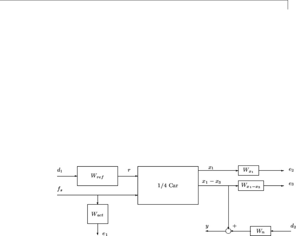
H-Infinity and Mu Synthesis for Active Suspension Control
rad/s. The tradeoff between passenger comfort and suspension deflection is
because it is not possible to simultaneously keep both transfer functions small
around the tirehop frequency and in the low frequency range.
Linear H-Infinity Controller Design
The design of linear suspension controllers that emphasize either passenger
comfort or suspension deflection. The controllers in this section are designed
using linear H∞synthesis [5]. As is standard in the H∞framework, the
performance objectives are achieved via minimizing weighted transfer
function norms.
Weighting functions serve two purposes in the H∞framework: They allow
the direct comparison of different performance objectives with the same
norm, and they allow for frequency information to be incorporated into the
analysis. For more details on H∞controldesign,referto[4],[6],[7],[11],and
[13]. A block diagram of the H∞control design interconnection for the active
suspension problem is shown below.
The measured output or feedback signal yis the suspension deflection
x1–x3. The controller acts on this signal to produce the control input, the
hydraulic actuator force fs.TheblockWnserves to model sensor noise in the
measurement channel. Wnis set to a sensor noise value of 0.01 m.
Wn = 0.01;
In a more realistic design, Wnwould be frequency dependent and would serve
to model the noise associated with the displacement sensor. The weight Wref
5-21

5H-Infinity and Mu Synthesis
is used to scale the magnitude of the road disturbances. Assume that the
maximum road disturbance is 7 cm and hence choose Wref = 0.07.
Wref = 0.07;
The magnitude and frequency content of the control force fsare limited by
the weighting function Wact.Choose
Ws
s
act =+
+
100
13
50
500 .
The magnitude of the weight increases above 50 rad/s in order to limit the
closed-loop bandwidth.
Wact = (100/13)*tf([1 50],[1 500]);
H-Infinity Control Design 1
The purpose of the weighting functions Wx1and Wxx
13
−is to keep the car
deflection and the suspension deflection small over the desired frequency
ranges. In the first design, you are designing the controller for passenger
comfort, and hence the car body deflection x1is penalized.
Wx1 = 8*tf(2*pi*5,[1 2*pi*5]);
The weight magnitude rolls off above 5×2πrad/s to respect a well-known H∞
design rule of thumb that requires the performance weights to roll off before
an open-loop zero (56.7 rad/s in this case). The suspension deflection weight
Wxx
13
−is not included in this control problem formulation.
You can construct the weighted H∞plant model for control design, denoted
qcaric1,usingthesysic command. The control signal corresponds to the
last input to qcaric1,fs. The car body acceleration, which is noisy, is the
measured signal and corresponds to the last output of qcaric1.
systemnames = 'qcar Wn Wref Wact Wx1';
inputvar = '[ d1; d2; fs ]';
outputvar = '[ Wact; Wx1; qcar(3)+Wn ]';
input_to_qcar = '[ Wref; fs]';
input_to_Wn = '[ d2 ]';
5-22

H-Infinity and Mu Synthesis for Active Suspension Control
input_to_Wref = '[ d1 ]';
input_to_Wact = '[ fs ]';
input_to_Wx1 = '[ qcar(1) ]';
qcaric1 = sysic;
An H∞controller is synthesized with the hinfsyn command. There is one
control input, the hydraulic actuator force, and one measurement signal, the
car body acceleration.
ncont = 1;
nmeas = 1;
[K1,Scl1,gam1] = hinfsyn(qcaric1,nmeas,ncont);
CL1 = lft(qcar([1:4 3],1:2),K1);
sprintf('H-infinity controller K1 achieved a norm of %2.5g',gam1)
ans =
H-infinity controller K1 achieved a norm of 0.60887
You can analyze the H∞controller by constructing the closed-loop feedback
system CL1. Bode magnitude plots of the passive suspension and active
suspension are shown in the following figure.
bodemag(qcar(3,1),'k-.',CL1(3,1),'r-',logspace(0,2.3,140))
legend('Passive','Active (K1)','Location','SouthEast')
5-23
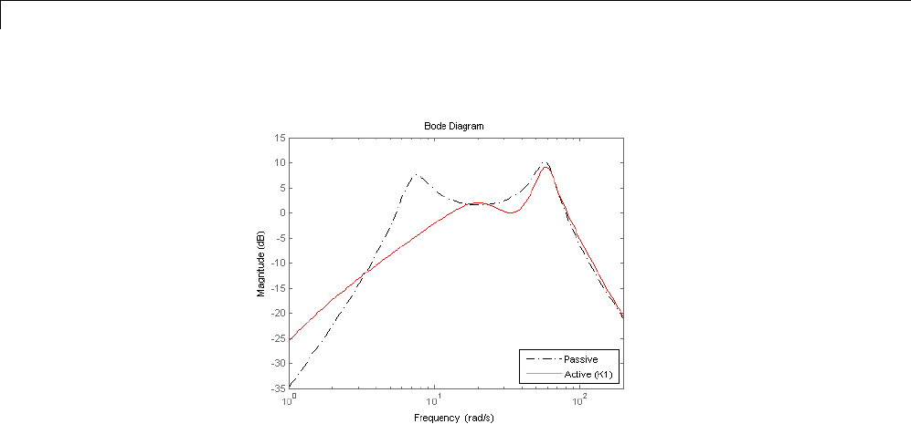
5H-Infinity and Mu Synthesis
H-Infinity Control Design 2
In the second design, you are designing the controller to keep the suspension
deflection transfer function small. Hence the road disturbance to suspension
deflection x1–x3is penalized via the weighting function Wx1x3.TheWx1x3
weight magnitude rolls off above 10 rad/s to roll off before an open-loop zero
(23.3 rad/s) in the design.
Wx1x3 = 25*tf(1,[1/10 1]);
The car deflection weight Wx1is not included in this control problem
formulation. You can construct the weighted H∞plant model for control
design, denoted qcaric2,usingthesysic command. As an alternative,
you can create qcaric2 using iconnect objects. The same control and
measurements are used as in the first design.
M = iconnect;
d = icsignal(2);
fs = icsignal(1);
ycar = icsignal(size(qcar,1));
M.Equation{1} = equate(ycar,qcar*[Wref*d(1); fs]);
M.Input = [d;fs];
M.Output = [Wact*fs;Wx1x3*ycar(1);ycar(2)+Wn*d(2)];
qcaric2 = M.System;
5-24
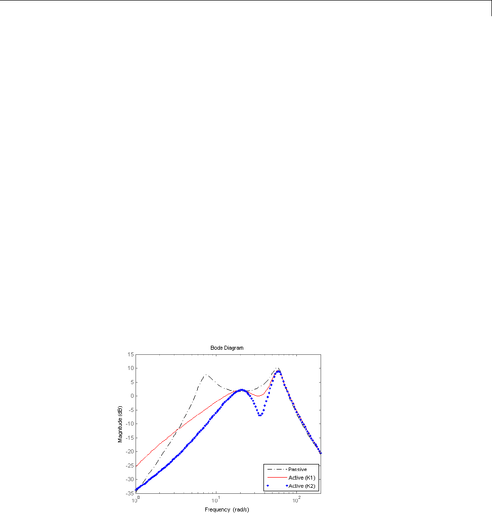
H-Infinity and Mu Synthesis for Active Suspension Control
The second H∞controller is synthesized with the hinfsyn command.
[K2,Scl2,gam2] = hinfsyn(qcaric2,nmeas,ncont);
CL2 = lft(qcar([1:4 2],1:2),K2);
sprintf('H-infinity controller K2 achieved a norm of %2.5g',gam2)
ans =
H-infinity controller K2 achieved a norm of 1.7519
Recall that this H∞control design emphasizes minimization of suspension
deflection over passenger comfort, whereas the first H∞design focused on
passenger comfort.
You can analyze the H∞controller by constructing the closed-loop feedback
system CL2. Bode magnitude plots of the transfer function from road
disturbance to suspension deflection for both controllers and the passive
suspension system are shown in the following figure.
bodemag(qcar(3,1),'k-.',CL1(3,1),'r-',CL2(3,1),'b.',logspace(0,2.3,140))
legend('Passive','Active (K1)','Active (K2)','Location','SouthEast')
5-25
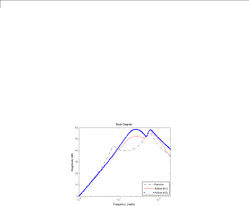
5H-Infinity and Mu Synthesis
The dotted and solid lines in the figure are the closed-loop frequency responses
that result from the different performance weighting functions selected.
Observe the reduction in suspension deflection in the vicinity of the tirehop
frequency, ω1= 56.7 rad/s, and the corresponding increase in the acceleration
frequency response in this vicinity. Also, compared to design 1, a reduction in
suspension deflection has been achieved for frequencies below the rattlespace
frequency, ω2= 23.3 rad/s.
The second H∞control design attenuates both resonance modes, whereas the
first controller focused its efforts on the first mode, the rattlespace frequency
at 23.3 rad/s.
bodemag(qcar(2,1),'k-.',CL1(2,1),'r-',CL2(2,1),'b.',logspace(0,2.3,140))
legend('Passive','Active (K1)','Active (K2)','Location','SouthEast')
All the analysis till now has been in the frequency domain. Time-domain
performance characteristics are criticaltothesuccessoftheactivesuspension
system on the car. Time response plots of the two H∞controllers are shown
in following figures. The dashed, solid, and dotted lines correspond to
the passive suspension, H∞controller 1, and controller 2 respectively. All
responses correspond to the road disturbance r(t):
r(t)=a(1–cos8πt)for0≤t≤0.25s
5-26

H-Infinity and Mu Synthesis for Active Suspension Control
r(t)=0otherwise.
where a=0.025 corresponds to a road bump of peak magnitude 5 cm. In the
following plots, observe that the acceleration response of design 1 to the 5
cm bump is very good; however the suspension deflection is larger than for
design 2. This is because suspension deflection was not penalized in this
design. The suspension deflection response of design 2 to a 5 cm bump is good.
However, the acceleration response to the 5 cm bump is much inferior to
design 1. Once again this is because car body displacement and acceleration
were not penalized in design 2.
time = 0:0.005:1;
roaddist = 0*time;
roaddist(1:51) = 0.025*(1-cos(8*pi*time(1:51)));
[p1,t] = lsim(qcar(1:4,1),roaddist,time);
[y1,t] = lsim(CL1(1:4,1),roaddist,time);
[y2,t] = lsim(CL2(1:4,1),roaddist,time);
subplot(221)
plot(t,y1(:,1),'b-',t,y2(:,1),'r.',t,p1(:,1),'k--',t,...
roaddist,'g-.')
title('Body Travel')
ylabel('x_1 (m)')
subplot(222)
plot(t,y1(:,2),'b-',t,y2(:,2),'r.',t,p1(:,2),'k--')
title('Body Acceleration')
ylabel('Accel (m/s/s)')
subplot(223)
plot(t,y1(:,3),'b-',t,y2(:,3),'r.',t,p1(:,3),'k--')
title('Suspension Deflection')
xlabel('Time (sec)')
ylabel('x_1 - x_3 (m)')
subplot(224)
plot(t,y1(:,4),'b-',t,y2(:,4),'r.',t,p1(:,4),'k--')
title('Control Force')
xlabel('Time (sec)')
ylabel('fs (10kN)')
5-27
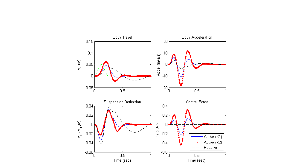
5H-Infinity and Mu Synthesis
Designs 1 and 2 represent extreme ends of the performance tradeoff spectrum.
This section described synthesis of H∞to achieve the performance objectives
ontheactivesuspensionsystem.Equally, if not more important, is the design
of controllers robust to model error or uncertainty.
The goal of every control design is to achieve the desired performance
specifications on the nominal model as well as other plants that are close to
the nominal model. In other words, you want to achieve the performance
objectives in the presence of model error or uncertainty. This is called robust
performance. In the next section, you will design a controller that achieves
robust performance using the µ-synthesis control design methodology. The
active suspension system again serves as the example. Instead of assuming a
perfect actuator, a nominal actuator model with modeling error is introduced
into the control problem.
Control Design via Mu Synthesis
The active suspension H∞controllers designed in the previous section ignored
the hydraulic actuator dynamics. In this section, you will include a first-order
modelofthehydraulicactuatordynamicsaswellasanuncertaintymodelto
5-28

H-Infinity and Mu Synthesis for Active Suspension Control
account for differences between the actuator model and the actual actuator
dynamics.
The nominal model for the hydraulic actuator is
actnom = tf(1,[1/60 1]);
The actuator model itself is uncertain. You can describe the actuator model
error as a set of possible models using a weighting function. At low frequency,
below 4 rad/s, it can vary up to 10% from its nominal value. Around 4 rad/s the
percentage variation starts to increase and reaches 400% at approximately
800 rad/s. The model uncertainty is represented by the weight Wunc,which
corresponds to the frequency variation of the model uncertainty and the
uncertain LTI dynamic object Δunc defined as unc.
Wunc = 0.10*tf([1/4 1],[1/800 1]);
unc = ultidyn('unc',[1 1]);
actmod = actnom*(1+ Wunc*unc)
actmod =
Uncertain continuous-time state-space model with 1 outputs, 1 inputs, 2
s
The model uncertainty consists of the following blocks:
unc: Uncertain 1x1 LTI, peak gain = 1, 1 occurrences
Type "actmod.NominalValue" to see the nominal value, "get(actmod)" to see
a
The actuator model actmod is an uncertain state-space system. The following
Bode plot shows the nominal actuator model, actnom, denoted with a '+'
symbol, and 20 random actuator models described by actmod.(Because
bodeplot computes random samples of the uss model actmod,yourplot
might not be identical.)
bodeplot(actnom,'r+',actmod,'b',logspace(-1,3,120))
5-29
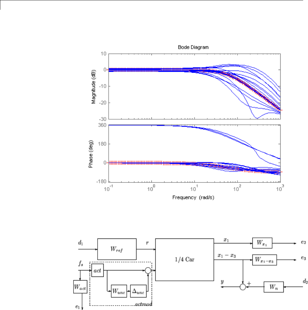
5H-Infinity and Mu Synthesis
The uncertain actuator model actmod represents the model of the hydraulic
actuator used for control. The revised control design interconnection diagram
is
5-30

H-Infinity and Mu Synthesis for Active Suspension Control
You are designing the controller for passenger comfort, as in the first H∞
control design, hence the car body deflection x1is penalized with Wx1.The
uncertain weighted H∞plant model for control design, denoted qcaricunc,
is using the sysic command. As previously described, the control signal
corresponds to the last input to qcaric1,fs. The car body acceleration,
which is noisy, is the measured signal and corresponds to the last output of
qcaricunc.
systemnames = 'qcar Wn Wref Wact Wx1 actmod';
inputvar = '[ d1; d2; fs ]';
outputvar = '[ Wact; Wx1; qcar(2)+Wn ]';
input_to_actmod = '[ fs ]';
input_to_qcar = '[ Wref; fs]';
input_to_Wn = '[ d2 ]';
input_to_Wref = '[ d1 ]';
input_to_Wact = '[ fs ]';
input_to_Wx1 = '[ qcar(1) ]';
qcaricunc = sysic;
A µ-synthesis controller is synthesized using D-K iteration with the dksyn
command. The D-Kiteration procedure is an approximation to µ-synthesis
that attempts to synthesize a controller that achieves robust performance [1],
[10], [11], [12]. There is one control input, the hydraulic actuator force, and
one measurement signal, the car body acceleration.
[Kdk,CLdk,gdk] = dksyn(qcaricunc,nmeas,ncont);
CLdkunc = lft(qcar([1:4 2],1:2)*blkdiag(1,actmod),Kdk);
sprintf('mu-synthesis controller Kdk achieved a norm of %2.5g',gdk)
ans =
mu-synthesis controller Kdk achieved a norm of 0.56712
You can analyze the performance of the µ-synthesis controller by constructing
the closed-loop feedback system CLdkunc. Bode magnitude plots of the
passive suspension and active suspension systems on the nominal actuator
model with H∞design 1 and the µ-synthesis controller are shown in the
following figure. Note that the µ-synthesis controller better attenuates the
first resonant mode at the expense of decreased performance below 3 rad/s.
bodemag(qcar(3,1),'k-.',CL1(3,1),'r-',CLdkunc.Nominal(3,1),'b.',...
5-31

5H-Infinity and Mu Synthesis
logspace(0,2.3,140))
legend('Passive','Active (K1)','Active (Kmu)','Location','SouthEast')
It is important to understand how robust both controllers are in the presence
of model error. You can simulate the active suspension system with the H∞
design 2 and the µ-synthesis controller. The uncertain closed-loop systems,
CL2unc and CLdkunc, are formed with K2 and Kdk,respectively. Foreach
uncertain system, 40 random plant models in the model set are simulated. As
you can see, both controllers are robust and perform well in the presence of
actuator model error. The µ-synthesis controller Kdk achieves slightly better
performance than H∞design 1.
CL2unc = lft(qcar([1:4 2],1:2)*blkdiag(1,actmod),K2);
[CLdkunc40,dksamples] = usample(CLdkunc,40);
CL2unc40 = usubs(CL2unc,dksamples);
nsamp = 40;
5-32
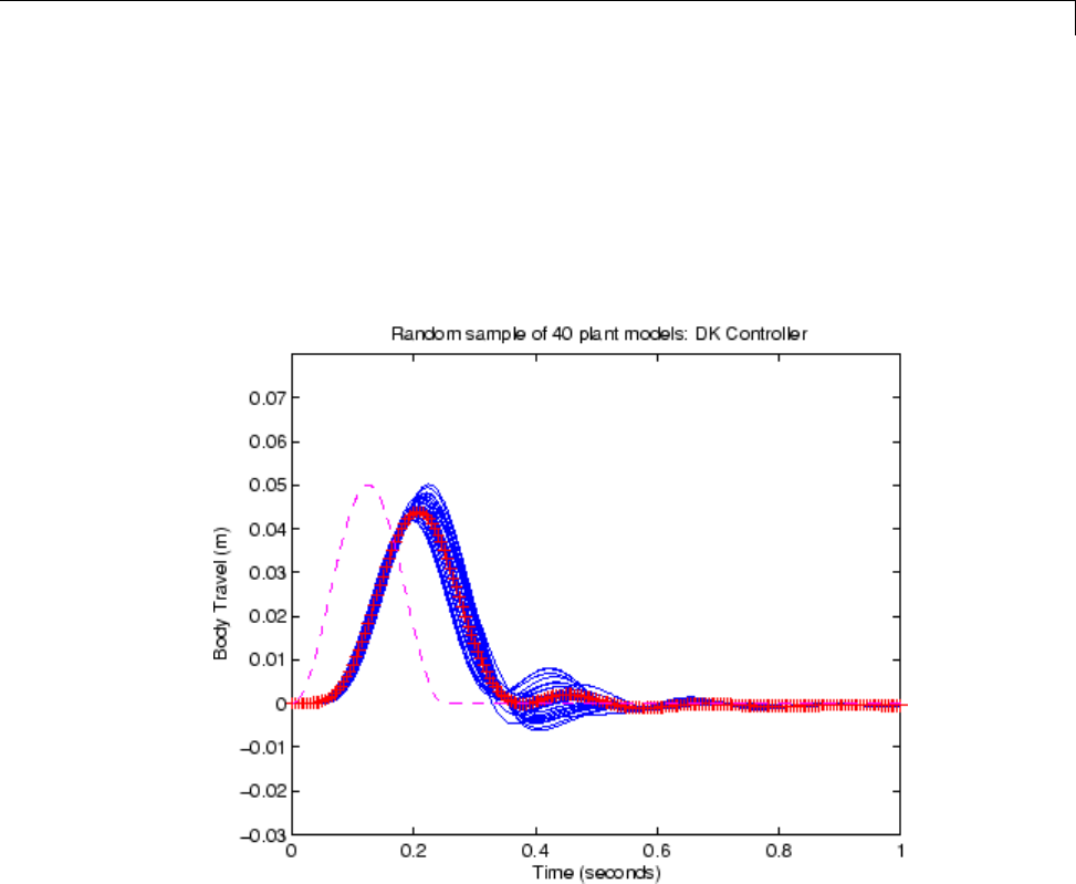
H-Infinity and Mu Synthesis for Active Suspension Control
for i=1:nsamp
[ymusamp,t] = lsim(CLdkunc40(1:4,1,i),roaddist,time);
plot(t,ymusamp(:,1),'b')
hold on
end
[ymusamp,t] = lsim(CLdkunc.Nominal(1:4,1),roaddist,time);
plot(t,ymusamp(:,1),'r+',t,roaddist,'m--')
for i=1:nsamp
[y1samp,t] = lsim(CL2unc40(1:4,1,i),roaddist,time);
plot(t,y1samp(:,1),'b')
hold on
end
[y1samp,t] = lsim(CL2unc.Nominal(1:4,1),roaddist,time);
plot(t,y1samp(:,1),'r+',t,roaddist,'m--')
5-33
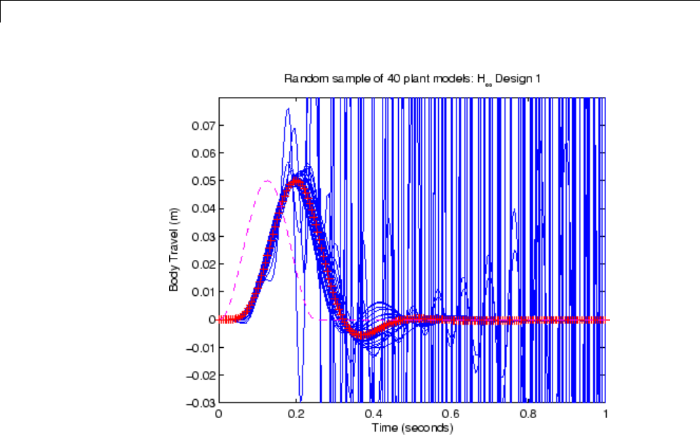
5H-Infinity and Mu Synthesis
5-34

Bibliography
Bibliography
[1] Balas, G.J., and A.K. Packard, “The structured singular value
µ-framework,” CRC Controls Handbook, Section 2.3.6, January, 1996, pp.
671-688.
[2] Ball, J.A., and N. Cohen, “Sensitivity minimization in an H∞norm:
Parametrization of all suboptimal solutions,” International Journal of Control,
Vol. 46, 1987, pp. 785-816.
[3] Bamieh, B.A., and Pearson, J.B., “A general framework for linear periodic
systems with applications to H∞sampled-data control,” IEEE Transactions on
Automatic Control, Vol. AC-37, 1992, pp. 418-435.
[4] Doyle, J.C., Glover, K., Khargonekar, P., and Francis, B., “State-space
solutions to standard H2and H∞control problems,” IEEE Transactions on
Automatic Control, Vol. AC-34, No. 8, August 1989, pp. 831-847.
[5] Fialho, I., and Balas, G.J., “Design of nonlinear controllers for active
vehicle suspensions using parameter-varying control synthesis,” Vehicle
Systems Dynamics, Vol. 33, No. 5, May 2000, pp. 351-370.
[6] Francis, B.A., A course in H∞control theory, Lecture Notes in Control and
Information Sciences, Vol. 88, Springer-Verlag, Berlin, 1987.
[7] Glover, K., and Doyle, J.C., “State-space formulae for all stabilizing
controllers that satisfy an H∞norm bound and relations to risk sensitivity,”
Systems and Control Letters, Vol. 11, pp. 167-172, August 1989. International
Journal of Control, Vol. 39, 1984, pp. 1115-1193.
[8] Hedrick, J.K., and Batsuen, T., “Invariant Properties of Automotive
Suspensions,” Proceedings of The Institution of Mechanical Engineers,204
(1990), pp. 21-27.
[9] Lin, J., and Kanellakopoulos, I., “Road Adaptive Nonlinear Design of
Active Suspensions,” Proceedings of the American Control Conference, (1997),
pp. 714-718.
5-35

5H-Infinity and Mu Synthesis
[10] Packard, A.K., Doyle, J.C., and Balas, G.J., “Linear, multivariable robust
control with a µ perspective,” ASME Journal of Dynamics, Measurements and
Control: Special Edition on Control, Vol. 115, No. 2b, June, 1993, pp. 426-438.
[11] Skogestad, S., and Postlethwaite, I., Multivariable Feedback Control:
Analysis & Design, John Wiley & Sons, 1996.
[12] Stein, G., and Doyle, J., “Beyond singular values and loopshapes,” AIAA
Journal of Guidance and Control, Vol. 14, Num. 1, January, 1991, pp. 5-16.
[13] Zames, G., “Feedback and optimal sensitivity: model reference
transformations, multiplicative seminorms, and approximate inverses,” IEEE
Transactions on Automatic Control, Vol. AC-26, 1981, pp. 301-320.
5-36

6
Tuning Fixed Control
Architectures
•“What Is a Fixed-Structure Control System?” on page 6-3
•“Choosing an Approach to Fixed Control Structure Tuning” on page 6-4
•“Difference Between Fixed-Structure Tuning and Traditional H-Infinity
Synthesis” on page 6-5
•“How looptune Sees a Control System” on page 6-6
•“Set Up Your Control System for Tuning with looptune” on page 6-8
•“Performance and Robustness Specifications for looptune” on page 6-10
•“Tune a MIMO Control System for a Specified Bandwidth” on page 6-12
•“What Is hinfstruct?” on page 6-18
•“Formulating Design Requirements as H-Infinity Constraints” on page 6-19
•“Structured H-Infinity Synthesis Workflow” on page 6-20
•“Build Tunable Closed-Loop Model for Tuning with hinfstruct” on page 6-21
•“Tune the Controller Parameters” on page 6-28
•“Interpret the Outputs of hinfstruct” on page 6-29
•“Validate the Controller Design” on page 6-30
•“Set Up Your Control System for Tuning with systune” on page 6-34
•“Specifying Design Requirements for systune” on page 6-36
•“Tune Controller Against Set of Plant Models” on page 6-38
•“Supported Blocks for Tuning in Simulink” on page 6-40

6Tuning Fixed Control Architectures
•“Speed Up Tuning with Parallel Computing Toolbox Software” on page 6-42
•“Tuning Control Systems with SYSTUNE” on page 6-43
•“Tuning Feedback Loops with LOOPTUNE” on page 6-51
•“Tuning Control Systems in Simulink” on page 6-57
•“Building Tunable Models” on page 6-66
•“Using Design Requirement Objects” on page 6-74
•“Validating Results” on page 6-86
•“Tuning Multi-Loop Control Systems” on page 6-94
•“Using Parallel Computing to Accelerate Tuning” on page 6-105
•“Decoupling Controller for a Distillation Column” on page 6-110
•“Tuning of a Digital Motion Control System” on page 6-121
•“Control of a Linear Electric Actuator” on page 6-134
•“Active Vibration Control in Three-Story Building” on page 6-143
•“Tuning of a Two-Loop Autopilot” on page 6-155
•“Control of a UAV Formation” on page 6-169
•“Multi-Loop Controller for the Westland Lynx Helicopter” on page 6-177
•“Fixed-Structure Autopilot for a Passenger Jet” on page 6-186
•“Reliable Control of a Fighter Jet” on page 6-200
•“Fixed-Structure H-infinity Synthesis with HINFSTRUCT” on page 6-211
6-2

What Is a Fixed-Structure Control System?
What Is a Fixed-Structure Control System?
Fixed-structure control systems are control systems that have predefined
architectures and controller structures. For example,
•A single-loop SISO control architecture where the controller is a fixed-order
transfer function, a PID controller, or a PID controller plus a filter.
•A MIMO control architecture where the controller has fixed order and
structure. For example, a 2-by-2 decoupling matrix plus two PI controllers
is a MIMO controller of fixed order and structure.
•A multiple-loop SISO or MIMO control architecture, including nested or
cascaded loops, with multiple gains and dynamic components to tune.
You can use systune,looptune or hinfstruct for frequency-domain tuning
of virtually any SISO or MIMO feedback architecture to meet your design
requirements. You can use both approaches to tune fixed structure control
systems in either MATLAB or Simulink (requires Simulink Control Design™).
6-3

6Tuning Fixed Control Architectures
Choosing an Approach to Fixed Control Structure Tuning
Robust Control Toolbox includes several commands for frequency-domain
tuning of control systems with fixed control structure.
•systune (or slTunable.systune) — Automatically tunes control systems
from high-level design requirements you specify, such as reference tracking,
disturbance rejection, and stability margins. systune jointly tunes all the
free parameters of your control system regardless of its architecture and
the number of feedback loops it contains.
systune can also robustly tune control systems for multiple plant models
or multiple operating conditions of the plant.
For more information, see “Set Up Your Control System for Tuning with
systune” on page 6-34.
•looptune (or slTunable.looptune) — Automatic tuning of SISO or MIMO
feedback loops. looptune tunes the a SISO or MIMO feedback loop to
high-level design requirements such as loop bandwidth, reference tracking,
or stability margins. For more information, see “Set Up Your Control
System for Tuning with looptune” on page 6-8.
•hinfstruct —H∞synthesis with fixed-structure controllers. Using
hinfstruct requires you to formulate the H∞synthesis problem and
choose weighting functions yourself. For more information, see “What Is
hinfstruct?” on page 6-18.
6-4

Difference Between Fixed-Structure Tuning and Traditional H-Infinity Synthesis
Difference Between Fixed-Structure Tuning and Traditional
H-Infinity Synthesis
All of the tuning commands systune,looptune,andhinfstruct tune the
controller parameters by optimizing the H∞norm across a closed-loop system
(see [1]). However, these functions differ in important ways from traditional
H∞methods.
Traditional H∞synthesis (performed using the hinfsyn or loopsyn
commands) designs a full-order, centralized controller. Traditional H∞
synthesis provides no way to impose structure on the controller and often
results in a controller that has high-order dynamics. Thus, the results can be
difficult to map to your specific real-world control architecture. Additionally,
traditional H∞synthesis requires you to express all design requirements in
terms of a single weighted MIMO transfer function.
In contrast, structured H∞synthesis allows you to describe and tune the
specific control system with which you are working. You can specify your
control architecture, including the number and configuration of feedback
loops. You can also specify the complexity, structure, and parametrization
of each tunable component in your control system, such as PID controllers,
gains, and fixed-order transfer functions. Additionally, you can easily combine
requirements on separate closed-loop transfer functions.
Bibliography
[1] P. Apkarian and D. Noll, "Nonsmooth H-infinity Synthesis," IEEE
Transactions on Automatic Control, Vol. 51, Number 1, 2006, pp. 71-86.
6-5
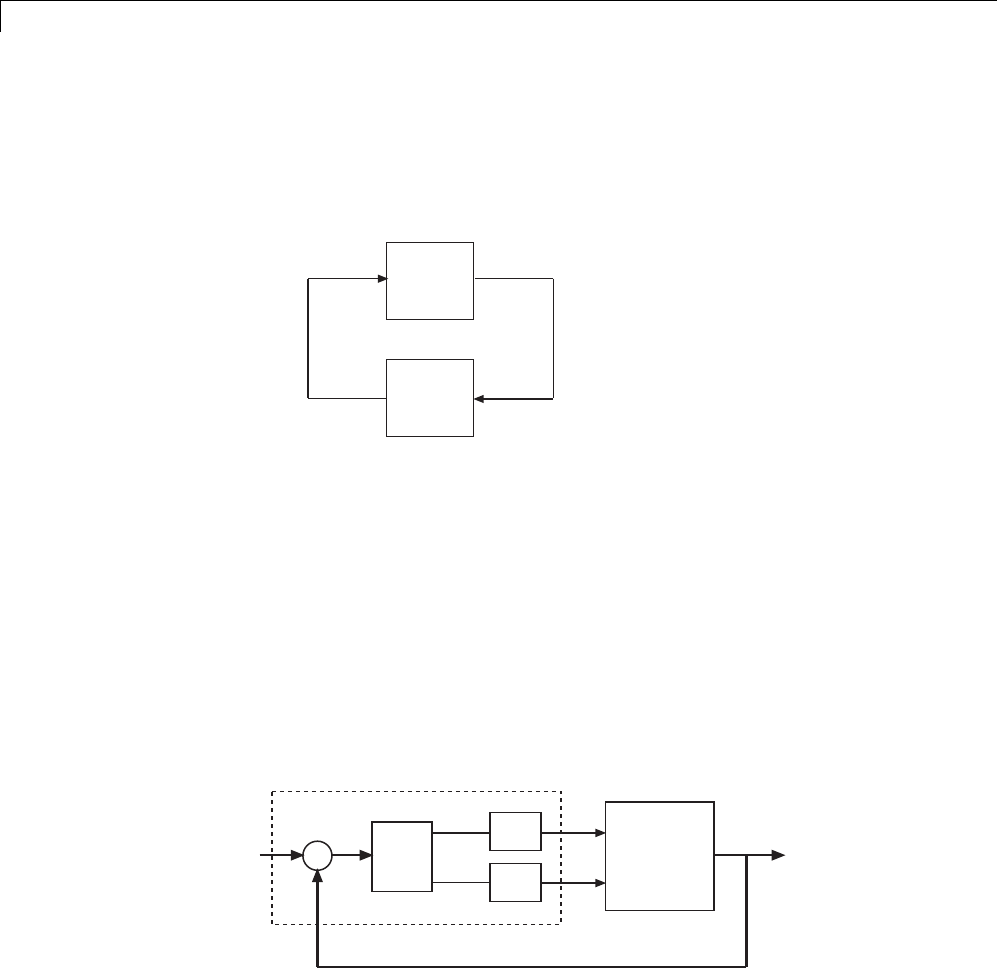
6Tuning Fixed Control Architectures
How looptune Sees a Control System
looptune tunes the feedback loop illustrated below to meet default
requirements or requirements that you specify.
G
C
uy
Crepresents the controller and Grepresents the plant. The sensor outputsy
(measurements) and actuator outputs u(controls) define the boundary
between plant and controller. The controller is the portion of your control
system whose inputs are measurements, and whose outputs are control
signals. Conversely, the plant is the remainder—the portion of your control
system that receives control signals as inputs, and produces measurements as
outputs.
For example, in the control system of the following illustration, the controller
Creceives the measurement y, and the reference signal r. The controller
produces the controls qL and qV as outputs.
PIL
PIV
Dy
r+
-
G
qL
qV
pL
pV
e
C
The controller Chas a fixed internal structure. Cincludes a gain matrix D,
the PI controllers PI_L and PI_V, and a summing junction. The looptune
command tunes free parameters of Csuch as the gains in Dand the
6-6

How looptune Sees a Control System
proportional and integral gains of PI_L and PI_V.Youcanalsouselooptune
to co-tune free parameters in both Cand G.
6-7

6Tuning Fixed Control Architectures
Set Up Your Control System for Tuning with looptune
In this section...
“Set Up Your Control System for looptunein MATLAB” on page 6-8
“Set Up Your Control System for looptune in Simulink” on page 6-8
Set Up Your Control System for looptunein MATLAB
To set up your control system in MATLAB for tuning with looptune:
1Parameterize the tunable elements of your controller. You can use
predefined structures such as ltiblock.pid,ltiblock.gain,and
ltiblock.tf. Or, you can create your own structure from elementary
tunable parameters (realp).
2Use model interconnection commands such as series and connect to build
a tunable genss model representing the controller C0.
3Create a Numeric LTI model representing the plant G. For co-tuning the
plant and controller, represent the plant as a tunable genss model.
Set Up Your Control System for looptune in Simulink
To set up your control system in Simulink for tuning with
slTunable.looptune (requires Simulink Control Design software):
1Use slTunable to create an interface to the Simulink model of your control
system. When you create the interface, youspecifywhichblockstotunein
your model.
2Use slTunable.addControl and slTunable.addMeasurement to specify
the control and measurement signals that define the boundaries between
plant and controller. Use slTunable.addSwitch to mark optional
loop-opening or signal injection sites for specifying and assessing open-loop
requirements.
The slTunable interface automatically linearizes your Simulink model. The
slTunable interface also automatically parametrizes the blocks that you
6-8

Set Up Your Control System for Tuning with looptune
specify as tunable blocks. For more information, see the slTunable reference
page and “Supported Blocks for Tuning in Simulink” on page 6-40.
Related
Examples
•“Tune a MIMO Control System for a Specified Bandwidth” on page 6-12
•“Tuning Feedback Loops with LOOPTUNE” on page 6-51
Concepts •“How looptune Sees a Control System” on page 6-6
6-9

6Tuning Fixed Control Architectures
Performance and Robustness Specifications for looptune
When you use looptune, you specify a target control bandwidth as a target
open-loop gain crossover, the wc input to looptune.Bydefault,looptune
automatically tunes your control system to a loop shape of wc/s to enforce
the following requirements:
•Performance—integral action at low frequency
•Roll-off—gain roll-off at frequencies above the crossover frequency
•Stability margins—adequate robustness at frequencies above the crossover
frequency. You can override the default stability margins using the
looptuneOptions command to create an options set to pass to looptune.
looptune is a wrapper for the systune command. looptune simplifies the
setup for less complex problems by automatically tuning your feedback loop to
meet the default performance requirements. You can specify addition design
requirements using TuningGoal requirements objects. The following table
summarizes the types of design requirements you can specify.
Design
Requirement
Description How To Specify
Reference
Tracking
Requirementthataspecified
output track a specified input
TuningGoal.Tracking
Stability margins Gain and phase margins, defined
as multi-loop disk margins for
MIMO systems (see loopmargin)
TuningGoal.Margins
6-10

Performance and Robustness Specifications for looptune
Design
Requirement
Description How To Specify
Gain Limits Limit on the maximum gain and
the gain profile across specified
I/Os. For example:
•Disturbance rejection
•Custom roll-off specification
•Frequency-weighted peak gain
limit
•Noise amplification limit
•TuningGoal.Gain
•TuningGoal.WeightedGain
•TuningGoal.Variance
•TuningGoal.WeightedVariance
Custom Loop
Shape
Constraints on the open-loop
gain profile of a specified SISO or
MIMO feedback loop
TuningGoal.LoopShape
Pole Placement Constraints on location of tunable
closed-loop system poles and
controller poles
•TuningGoal.Poles
•TuningGoal.StableController
Related Examples
•“Using Design Requirement Objects” on page 6-74
6-11
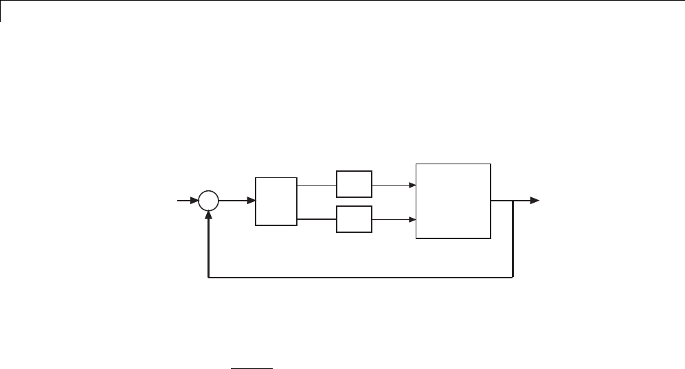
6Tuning Fixed Control Architectures
Tune a MIMO Control System for a Specified Bandwidth
This example shows how to tune the control system of the following
illustration to achieve crossover between 0.1 and 1 rad/min, using looptune.
PIL
PIV
Dy
r+
-
G
qL
qV
pL
pV
e
The setpoint signal r, the error signal e, and the output signal yare
vector-valued signals of dimension 2. The 2-by-2 plant Gis represented by:
Gs s
1
75 1
87 8 86 4
108 2 109 6
..
..
.
Create a Numeric LTI model representing the plant.
s = tf('s');
G = 1/(75*s+1)*[87.8 -86.4; 108.2 -109.6];
G.InputName = {'qL','qV'};
G.OutputName = 'y';
Name the inputs and outputs of your model using the InputName and
OutputName properties. Doing so tells looptune how to interconnect your
plant and controller.
The controller, C, has a fixed structure that includes three tunable
components: the 2-by-2 decoupling matrix, D, and the two PI controllers, PI_L
and PI_V. (For more information about this control system, see Decoupling
Controller for a Distillation Column.)
6-12
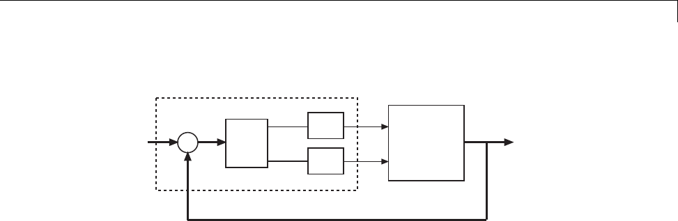
Tune a MIMO Control System for a Specified Bandwidth
PIL
PIV
Dy
r+
-
G
qL
qV
pL
pV
e
C
Creceives the measurement signal yand the reference ras inputs. Cproduces
the control signals qL and qV.
Use Control Design Blocks to represent the tunable components of the
controller.
D = ltiblock.gain('Decoupler',eye(2));
D.InputName = 'e';
D.OutputName = {'pL','pV'};
PI_L = ltiblock.pid('PI_L','pi');
PI_L.InputName = 'pL';
PI_L.OutputName = 'qL';
PI_V = ltiblock.pid('PI_V','pi');
PI_V.InputName = 'pV';
PI_V.OutputName = 'qV';
Create the summing junction using sumblk.
sum1 = sumblk('e = r - y',2);
Connect the components using model interconnection commands.
C0 = connect(PI_L,PI_V,D,sum1,{'r','y'},{'qL','qV'});
The genss model C0 represents the controller structure. C0 specifies which
controller parameters are tunable, and contains the initial values of those
parameters.
6-13

6Tuning Fixed Control Architectures
Tune the control system.
wc = [0.1,1];
options = looptuneOptions('RandomStart',5);
[G,C,gam,Info] = looptune(G,C0,wc,options);
Final: Peak gain = 0.949, Iterations = 27
The looptune algorithm uses the input and output names of C0 and Gto form
the closed loop system for tuning. The input wc specifies that the crossover
frequency of each loop in the system falls between 0.1 and 1 rad/min.
Setting RandomStart to 5 causes looptune to perform five additional
optimization runs, beginning from parameter values it chooses randomly.
Most runs return 0.949 as optimal gain value, suggesting that this local
minimum has a wide region of attraction and is likely to be the global
optimum.
The output gam is a normalized parameter indicating the degree of success
meeting the tuning requirements. gam is the best value of the peak gain over
all optimization runs. gam <=1 indicates that all requirements are satisfied. A
gam value much greater than one indicates failure to meet some requirement.
In this example, the best value of gam = 0.949 indicates success meeting
the specified crossover requirement.
looptune also returns C, the tuned version of C0 that yields the best peak gain
value. Examine the tuned values of all components using showTunable.
showTunable(C)
Decoupler =
d=
u1 u2
y1 1.075 -0.8273
y2 -1.581 1.328
Name: Decoupler
Static gain.
-----------------------------------
PI_L =
6-14

Tune a MIMO Control System for a Specified Bandwidth
1
Kp + Ki * ---
s
with Kp = 2.82, Ki = 0.0398
Name: PI_L
Continuous-time PI controller in parallel form.
-----------------------------------
PI_V =
1
Kp + Ki * ---
s
with Kp = -1.94, Ki = -0.0303
Name: PI_V
Continuous-time PI controller in parallel form.
Validate the frequency domain response of the tuned result using loopview.
loopview(G,C,Info)
6-15
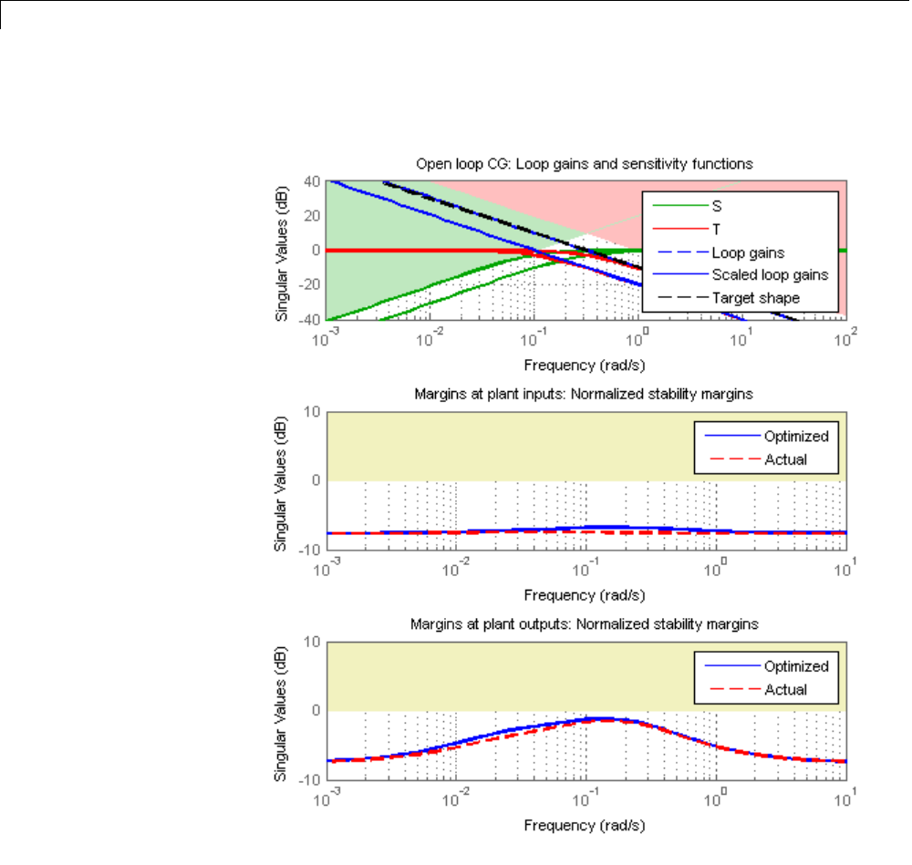
6Tuning Fixed Control Architectures
The firstplotshowsthattheopen-loopgain crossovers fall within the specified
interval [0.1,1]. This plot also includes the maximum and tuned values of
the sensitivity function S=(I–GC)–1 and complementary sensitivity T=I–S.
6-16
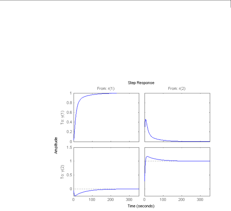
Tune a MIMO Control System for a Specified Bandwidth
The second and third plots show that the MIMO stability margins of the
tuned system (blue curve) do not exceed the upper limit (yellow curve).
Validate the time domain response using Control System Toolbox analysis
commands such as step.
T = connect(G,C,'r','y');
step(T)
The tuned controller provides good setpoint tracking with reasonably small
crosstalk between channels. To impose further constraints on crosstalk, use
the TuningGoal.Gain requirements object.
6-17

6Tuning Fixed Control Architectures
What Is hinfstruct?
hinfstruct lets you use the frequency-domain methods of H∞synthesis
to tune control systems that have predefined architectures and controller
structures.
To use hinfstruct, you describe your control system as a Generalized LTI
model that keeps track of the tunable components of your system. hinfstruct
tunes those parameters by minimizing the closed-loop gain from the system
inputs to the system outputs (the H∞norm).
hinfstruct is the counterpart of hinfsyn for fixed-structure controllers. The
methodology and algorithm behind hinfstruct are described in [1].
6-18

Formulating Design Requirements as H-Infinity Constraints
Formulating Design Requirements as H-Infinity Constraints
Control design requirements are typically performance measures such as
response speed, control bandwidth, roll-off, and steady-state error. To use
hinfstruct, first express the design requirements as constraints on the
closed-loop gain.
You can formulate design requirements in terms of the closed-loop gain using
loop shaping. Loop shaping is a common systematic technique for defining
control design requirements for H∞synthesis. In loop shaping, you first
express design requirements as open-loop gain requirements.
For example, a requirement of good reference tracking and disturbance
rejection is equivalent to high (>1) open-loop gain at low frequency. A
requirement of insensitivity to measurement noise or modeling error is
equivalent to a low (<1) open-loop gain at high frequency. You can then
convert these open-loop requirements toconstraintsontheclosed-loopgain
using weighting functions.
This formulation of design requirements results in a H∞constraint of the form:
Hs
1,
where H(s) is a closed-loop transfer function that aggregates and normalizes
the various requirements.
For an example of how to formulate design requirements for H∞synthesis
using loop shaping, see “Fixed-Structure H-infinity Synthesis with
HINFSTRUCT” on page 6-211.
For more information about constructing weighting functions from design
requirements, see “H-Infinity Performance” on page 5-9.
6-19

6Tuning Fixed Control Architectures
Structured H-Infinity Synthesis Workflow
Performing structured H∞synthesis requires the following steps:
1Formulate your design requirements as H∞constraints, which are
constraints on the closed-loop gains from specific system inputs to specific
system outputs.
2Build tunable models of the closed-loop transfer functions of Step 1.
3Tune the control system using hinfstruct.
4Validate the tuned control system.
6-20

Build Tunable Closed-Loop Model for Tuning with hinfstruct
Build Tunable Closed-Loop Model for Tuning with hinfstruct
In the previous step you expressed your design requirements as a constraint
on the H∞norm of a closed-loop transfer function H(s).
ThenextstepistocreateaGeneralizedLTImodelofH(s) that includes all of
the fixed and tunable elements of the control system. The model also includes
any weighting functions that represent your design requirements. There are
two ways to obtain this tunable model of your control system:
•Construct the model using Control System Toolbox commands.
•Obtain the model from a Simulink model using Simulink Control Design
commands.
Constructing the Closed-Loop System Using Control
System Toolbox Commands
To construct the tunable generalized linear model of your closed-loop control
system in MATLAB:
1Use commands such as tf,zpk,andss to create numeric linear models
that represent the fixed elements of your control system and any weighting
functions that represent your design requirements.
2Use tunable models (either Control Design Blocks or Generalized LTI
models) to model the tunable elements of your control system. For more
information about tunable models, see “Models with Tunable Coefficients”
in the Control System Toolbox User’s Guide.
3Use model-interconnection commands such as series,parallel,and
connect to construct your closed-loop system from the numeric and tunable
models.
Example: Modeling a Control System With a Tunable PI
Controller and Tunable Filter
This example shows how to construct a tunable generalized linear model of
the following control system for tuning with hinfstruct.
6-21
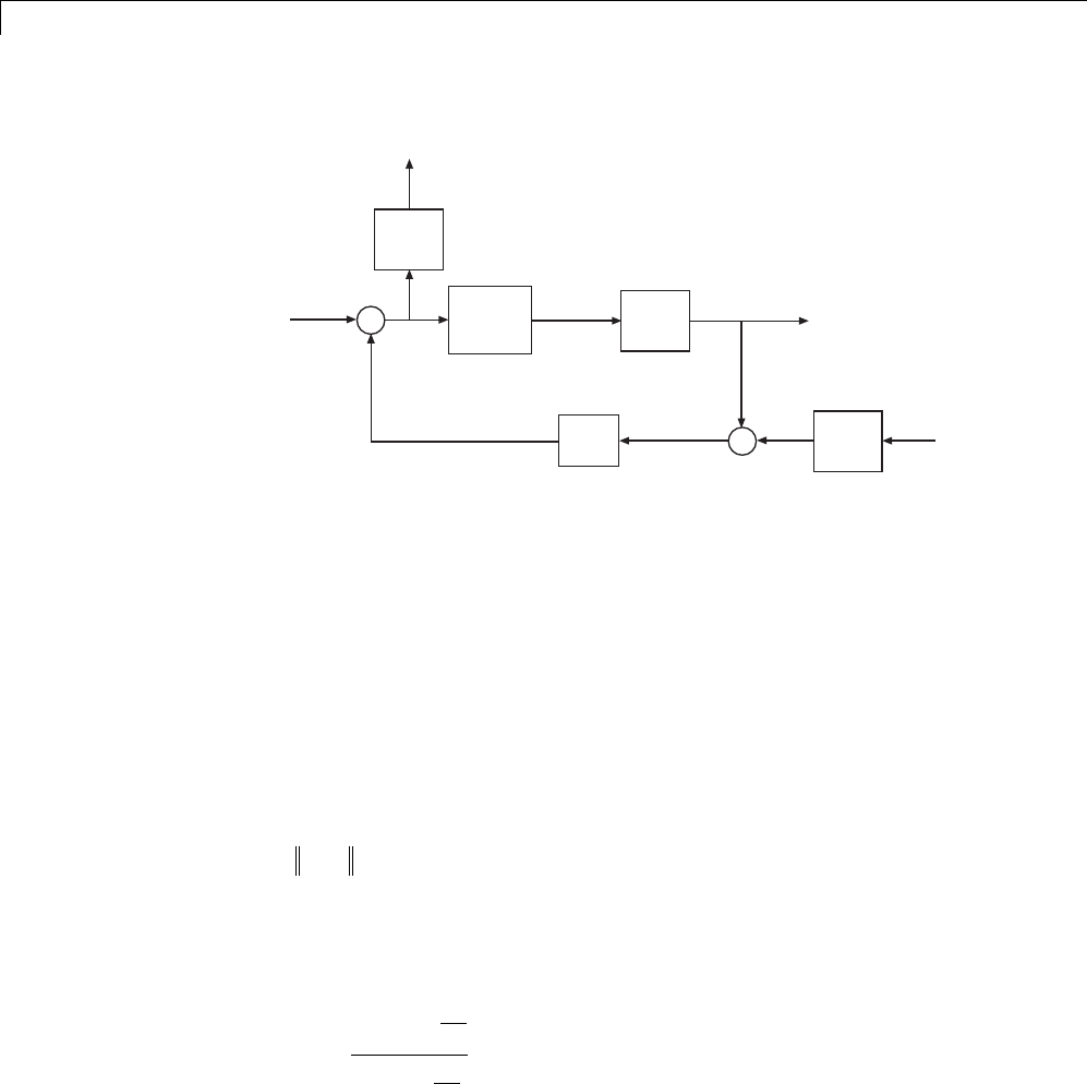
6Tuning Fixed Control Architectures
-
G
r+uy
C
e
y
fF
+
yn
+
1/LS
nnw
LS
ew
This block diagram represents a head-disk assembly (HDA) in a hard disk
drive. The architecture includes the plant Gin a feedback loop with a PI
controller Cand a low-pass filter, F = a/(s+a). The tunable parameters are
the PI gains of Cand the filter parameter a.
The block diagram also includes the weighting functions LS and 1/LS,which
express the loop-shaping requirements. Let T(s) denote the closed-loop
transfer function from inputs (r,nw)tooutputs(y,ew). Then, the H∞constraint:
Ts
1
approximately enforces the target open-loop response shape LS.Forthis
example, the target loop shape is
LS
s
s
c
c
1 0 001
0 001
.
.
.
6-22
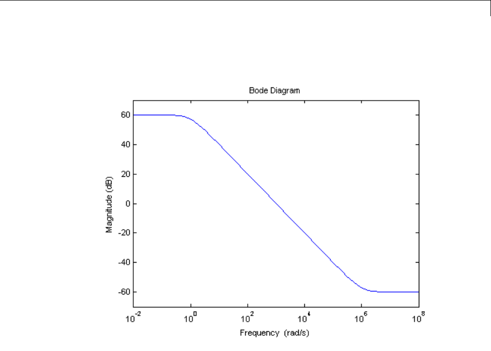
Build Tunable Closed-Loop Model for Tuning with hinfstruct
This value of LS corresponds to the following open-loop response shape.
To tune the HDA control system with hinfstruct, construct a tunable model
of the closed-loop system T(s), including the weighting functions, as follows.
1Load the plant Gfrom a saved file.
load hinfstruct_demo G
Gis a 9th-order SISO state-space (ss) model.
2Create a tunable model of the PI controller.
You can use the predefined Control Design Block ltiblock.pid to
represent a tunable PI controller.
C=ltiblock.pid('C','pi');
6-23

6Tuning Fixed Control Architectures
3Create a tunable model of the low-pass filter.
Because there is no predefined Control Design Block for the filter F=
a/(s+a),userealp to represent the tunable filter parameter a.Then
create a tunable genss model representing the filter.
a = realp('a',1);
F = tf(a,[1 a]);
4Specify the target loop shape LC.
wc = 1000;
s = tf('s');
LS = (1+0.001*s/wc)/(0.001+s/wc);
5Label the inputs and outputs of all the components of the control system.
Labeling the I/Os allows you to connect theelementstobuildtheclosed-loop
system T(s).
Wn = 1/LS; Wn.InputName = 'nw'; Wn.OutputName = 'n';
We = LS; We.InputName = 'e'; We.OutputName = 'ew';
C.InputName = 'e'; C.OutputName = 'u';
F.InputName = 'yn'; F.OutputName = 'yf';
6Specify the summing junctions in terms of the I/O labels of the other
components of the control system.
Sum1 = sumblk('e = r - yf');
Sum2 = sumblk('yn = y + n');
7Use connect to combine all the elements into a complete model of the
closed-loop system T(s).
T0 = connect(G,Wn,We,C,F,Sum1,Sum2,{'r','nw'},{'y','ew'});
T0 is a genss object, which is a Generalized LTI model representing the
closed-loop control system with weighting functions. The Blocks property of
T0 contains the tunable blocks Cand a.
T0.Blocks
ans =
6-24
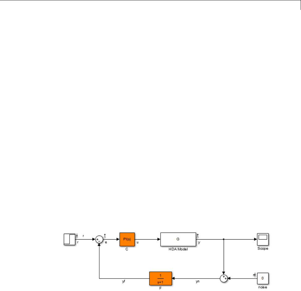
Build Tunable Closed-Loop Model for Tuning with hinfstruct
C: [1x1 ltiblock.pid]
a: [1x1 realp]
For more information about generalized models of control systems that
include both numeric and tunable components, see “Models with Tunable
Coefficients” in the Control System Toolbox documentation.
You can now use hinfstruct to tune the parameters of this control system.
See “Tune the Controller Parameters” on page 6-28.
Constructing the Closed-Loop System Using Simulink
Control Design Commands
If you have a Simulink model of your control system and Simulink Control
Design software, use slTunable to create an interface to the Simulink model
of your control system. When you create the interface, you specify which
blocks to tune in your model. The slTunable interface allows you to extract
a closed-loop model for tuning with hinfstruct.
Example: Creating a Weighted Tunable Model of Control
System Starting From a Simulink Model
This example shows how to construct a tunable generalized linear model of
the control system in the Simulink model rct_diskdrive.
To create a generalized linear model of this control system (including
loop-shaping weighting functions):
1Open the model.
6-25

6Tuning Fixed Control Architectures
open('rct_diskdrive');
2Create an slTunable interfacetothemodel. Theinterfaceallowsyouto
specify the tunable blocks and extract linearized open-loop and closed-loop
responses. (For more information about the interface, see the slTunable
reference page.)
ST0 = slTunable('rct_diskdrive',{'C','F'});
This command specifies that Cand Fare the tunable blocks in the model.
The slTunable interface automatically parametrizes these blocks. The
default parametrization of the transfer function block Fis a transfer
function with two free parameters. Because Fis a low-pass filter, you must
constrain its coefficients. To do so, specify a custom parameterization of F.
a = realp('a',1); % filter coefficient
setBlockParam(ST0,'F',tf(a,[1 a]));
3Extract a tunable model of the closed-loop transfer function you want to
tune.
T0 = getIOTransfer(ST0,{'r','n'},{'y','e'});
This command returns a genss model of the linearized closed-loop transfer
function from the reference and noise inputs r,n to the measurement
and error outputs y,e. The error output is needed for the loop-shaping
weighting function.
4Define the loop-shaping weighting functions and append them to T0.
wc = 1000;
s = tf('s');
LS = (1+0.001*s/wc)/(0.001+s/wc);
T0 = blkdiag(1,LS) * T0 * blkdiag(1,1/LS);
The generalized linear model T0 is a tunable model of the closed-loop transfer
function T(s), discussed in “Example: Modeling a Control System With a
Tunable PI Controller and Tunable Filter” on page 6-21. T(s)isaweighted
closed-loop model of the control system of rct_diskdrive. Tuning T0 to
enforce the H∞constraint
6-26


6Tuning Fixed Control Architectures
Tune the Controller Parameters
After you obtain the genss model representing your control system, use
hinfstruct to tune the tunable parameters in the genss model .
hinfstruct takes a tunable linear model as its input.
For example, you can tune controller parameters for the example discussed
in “Build Tunable Closed-Loop Model for Tuning with hinfstruct” on page
6-21 using the following command:
[T,gamma,info] = hinfstruct(T0);
This command returns the following outputs:
•T,agenss model object containing the tuned values of Cand a.
•gamma, the minimum peak closed-loop gain of Tachieved by hinfstruct.
•info, a structure containing additional information about the minimization
runs.
6-28

Interpret the Outputs of hinfstruct
Interpret the Outputs of hinfstruct
Output Model is Tuned Version of Input Model
Tcontains the same tunable components as the input closed-loop model T0.
However, the parameter values of TarenowtunedtominimizetheH∞norm
of this transfer function.
Interpreting gamma
gamma is the smallest H∞norm achieved by the optimizer. Examine gamma to
determine how close the tuned system is to meeting your design constraints.
If you normalize your H∞constraints, a final gamma value of 1 or less indicates
that the constraints are met. A final gamma value exceeding 1 by a small
amount indicates that the constraints are nearly met.
The value of gamma that hinfstruct returns is a local minimum of the gain
minimization problem. For best results, use the RandomStart option to
hinfstruct to obtain several minimization runs. Setting RandomStart to an
integer N>0causes hinfstruct to run the optimization Nadditional times,
beginning from parameter values it chooses randomly. For example:
opts = hinfstructOptions('RandomStart',5);
[T,gamma,info] = hinfstruct(T0,opts);
You can examine gamma for each run to identify an optimization result that
meets your design requirements.
For more details about hinfstruct, its options, and its outputs, see the
hinfstruct and hinfstructOptions reference pages.
6-29

6Tuning Fixed Control Architectures
Validate the Controller Design
To validate the hinfstruct control design, analyze the tuned output models
described in “Interpret the Outputs of hinfstruct” on page 6-29. Use these
tuned models to examine the performance of the tuned system.
Validating the Design in MATLAB
This example shows how to obtain the closed-loop step response of a system
tuned with hinfstruct in MATLAB.
You can use the tuned versions of the tunable components of your system
to build closed-loop or open-loop numeric LTI models of the tuned control
system. You can then analyze open-loop or closed-loop performance using
other Control System Toolbox tools.
In this example, create and analyze a closed-loop model of the HDA system
tuned in “Tune the Controller Parameters” on page 6-28. To do so, extract the
tuned controller values from the tuned closed-loop model. Use getBlockValue
to get the tuned value of a tunable Control Design Block. Use getValue to
evaluate a genss model using parameter values from another genss model.
Ctuned = getBlockValue(T,'C');
Ftuned = getValue(F,T);
Then construct the tuned closed-loop response of the control system from r
to y.
Try = connect(G,Ctuned,Ftuned,Sum1,Sum2,'r','y');
step(Try)
6-30

Validate the Controller Design
Validating the Design in Simulink
This example shows how to write tuned values to your Simulink model for
validation.
The slTunable interface linearizes your Simulink model. As a best practice,
validate the tuned parameters in your nonlinear model. You can use the
slTunable interfacetodoso.
In this example, write tuned parameters to the rct_diskdrive system tuned
in “Tune the Controller Parameters” on page 6-28.
Make a copy of the slTunable description of the control system, to preserve
the original parameter values. Then propagate the tuned parameter values
to the copy.
6-31
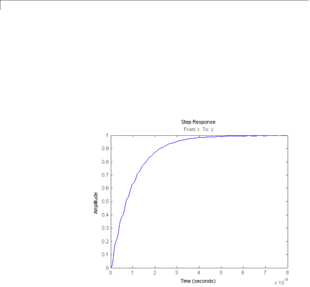
6Tuning Fixed Control Architectures
ST = copy(ST0);
setBlockValue(ST,T);
This command writes the parameter values from the tuned, weighted
closed-loop model Tto the corresponding parameters in the interface ST.
You can examine the closed-loop responses of the linearized version of the
control system represented by ST. For example:
Try = getIOTransfer(ST,'r','y');
Since hinfstruct tunes a linearized version of your system, you should also
validate the tuned controller in the full nonlinear Simulink model. To do so,
write the parameter values from the slTunable interfacetotheSimulink
model.
6-32

Validate the Controller Design
writeBlockValue(ST)
You can now simulate the model using the tuned parameter values to validate
the controller design.
6-33

6Tuning Fixed Control Architectures
Set Up Your Control System for Tuning with systune
systune tunes the free parameters of your control system to meet tuning
requirements that you specify. To use systune, you create a tunable model of
your control system in either MATLAB or Simulink.
Set Up Your Control System for systune in MATLAB
To set up your control system in MATLAB for tuning with systune:
1Parameterize the tunable elements of your control system. You can
use predefined structures such as ltiblock.pid,ltiblock.gain,and
ltiblock.tf. Or, you can create your own structure from elementary
tunable parameters (realp).
2Use model interconnection commands such as feedback and connect to
build a closed-loop model of the overall control system as an interconnection
of fixed and tunable components. Use loopswitch blocks to mark optional
loop-opening or signal injection sites for specifying and assessing open-loop
requirements. systune tunes the resulting genss model of the control
system.
Set Up Your Control System for systune in Simulink
To set up your control system in Simulink for tuning with slTunable.systune
(requires Simulink Control Design software):
1Use slTunable to create an interface to the Simulink model of your control
system. When you create the interface, youspecifywhichblockstotunein
your model.
2Use slTunable.addIO,slTunable.addControl,and
slTunable.addMeasurement to mark the input and output
signals you need to specify and assess closed-loop requirements.
3Use slTunable.addSwitch,slTunable.addControl,and
slTunable.addMeasurement to mark optional loop-opening sites for
specifying and assessing open-loop requirements.
The slTunable interface automatically linearizes your Simulink model. The
slTunable interface also automatically parametrizes the blocks that you
6-34

Set Up Your Control System for Tuning with systune
specify as tunable blocks. For more information, see the slTunable reference
page and “Supported Blocks for Tuning in Simulink” on page 6-40.
After setting up your control system, define your design requirements using
TuningGoal objects as described in “Specifying Design Requirements for
systune” on page 6-36
.
Related
Examples
•“Using Design Requirement Objects” on page 6-74
•“Tuning Control Systems with SYSTUNE” on page 6-43
6-35

6Tuning Fixed Control Architectures
Specifying Design Requirements for systune
When you tune a control system with systune, you specify tuning
requirements such as reference tracking, maximum gain from specified
inputs to specified outputs, or stability margins. You can designate tuning
requirements as either soft constraints or hard constraints. systune tunes
the free parameters of your control system to come as close as possible to
satisfying the soft constraints, subject to satisfying the hard constraints.
Specify your tuning requirements using TuningGoal requirements objects.
The following table summarizes the types of design requirements you can
specify for systune.
Design
Requirement
Description How To Specify
Reference
Tracking
Requirementthataspecified
output track a specified input
TuningGoal.Tracking
Stability margins Gain and phase margins, defined
as multi-loop disk margins for
MIMO systems (see loopmargin)
TuningGoal.Margins
Gain Limits Limit on the maximum gain and
the gain profile across specified
I/Os. For example:
•Disturbance rejection
•Custom roll-off specification
•Frequency-weighted peak gain
limit
•Noise amplification limit
•TuningGoal.Gain
•TuningGoal.WeightedGain
•TuningGoal.Variance
•TuningGoal.WeightedVariance
6-36

Specifying Design Requirements for systune
Design
Requirement
Description How To Specify
Custom Loop
Shape
Constraints on the open-loop
gain profile of a specified SISO or
MIMO feedback loop
TuningGoal.LoopShape
Pole Placement Constraints on location of tunable
closed-loop system poles and
controller poles
•TuningGoal.Poles
•TuningGoal.StableController
Related
Examples
•“Using Design Requirement Objects” on page 6-74
•“Tuning Control Systems with SYSTUNE” on page 6-43
6-37

6Tuning Fixed Control Architectures
Tune Controller Against Set of Plant Models
systune can simultaneously tune the parameters of multiple models or
control configurations. For example you can:
•Tune a single controller against a range of plant models, to help ensure
that the tuned control system is robust against parameter variations
•Tune for reliable control by simultaneously to multiple plant configurations
that represent different failure modes of a system
In either case, systune finds values for tunable parameters that best satisfy
the specified tuning objectives for all models.
To tune a controller parameters against a set of plant models:
1Create an array of genss models that represent the control systems or
configurations to tune against.
2Specify your tuning objectives using TuningGoal requirements objects such
as TuningGoal.Tracking,TuningGoal.Gain,orTuningGoal.Margins.If
you want to limit a tuning requirement to a subset of the models in the
model array, set the Models property of the TuningGoal requirement.
For example, suppose you have a model array whose first entry represents
your control system under normal operating conditions, and whose second
entry represents the system in a failure mode. Suppose further that Req
is a TuningGoal.Tracking requirement that only applies to the normally
operating system. To enforce the requirement only on the first entry, use
the following command:
Req.Models = [1];
3Provide the model array and tuning requirements as input argument to
systune.
systune jointly tunes the tunable parameters for all models in the array to
best meet the tuning requirements as you specify them. systune returns an
array containing the corresponding tuned models. You can use getBlockValue
or showBlockValue to access the tuned values of the control elements.
6-38


6Tuning Fixed Control Architectures
Supported Blocks for Tuning in Simulink
slTunable automatically assigns a parameterization to certain Simulink
blocks. You can write tuned parameter values back to the Simulink model
using slTunable.writeBlockValue.
Supported blocks include the following:
Automatically Parametrized
Blocks
Simulink Library
Gain Math Operations
LTI System Control System Toolbox
Discrete Filter Discrete
PID Controller
(one-degree-of-freedom only)
•Continuous
•Discrete
State-Space blocks •Continuous
•Discrete
•Simulink Extras Additional
Linear
Zero-pole blocks •Continuous
•Discrete
Transfer function blocks •Continuous
•Discrete
LTI blocks, state-space blocks, transfer function blocks, and zero-pole blocks
discretized using the Model Discretizer are also supported.
Tuning Other Blocks
You can specify tuned blocks in the slTunable interface other than the
automatically parametrized blocks. slTunable assigns a state-space
parametrization to such blocks based upon the block linearization. Use
6-40

Supported Blocks for Tuning in Simulink®
slTunable.getBlockParam to examine the parametrization of a block. Use
slTunable.setBlockParam to override the default parametrization.
For blocks that are not automatically parametrized, you cannot write
parameter values back to the block using slTunable.writeBlockValue.
6-41

6Tuning Fixed Control Architectures
Speed Up Tuning with Parallel Computing Toolbox
Software
If you have the Parallel Computing Toolbox™ software installed, you can use
parallel computing to speed up tuning of fixed-structure control systems.
When you run multiple randomized optimization starts, parallel computing
speeds up tuning by distributing the optimization runs among MATLAB
workers.
To distribute randomized optimization runs among workers:
Start a worker pool of MATLAB sessions using the Parallel Computing
Toolbox command matlabpool. For example:
matlabpool('open')
Create a systuneOptions,looptuneOptions,orhinfstructOptions set
that specifies multiple random starts. For example, the following options set
specifies20randomrestartstoruninparallel for tuning with looptune:
options = systuneOptions('RandomStart',20,'UseParallel',true);
Setting UseParallel to true enables parallel processing by distributing the
randomized starts among available MATLAB workers in the pool.
Use the options set when you call systune,looptune or hinfstruct.For
example, if you have already created a tunable control system model, CL0,and
tunable controller, and tuning requirement vectors SoftReqs and HardReqs,
the following command uses parallel computing to tune the control system
of CL0 with systune.
[CL,fSoft,gHard,info] = systune(CL0,SoftReq,Hardreq,options);
For an example of using parallel computing to tune a Simulink model, see
“Using Parallel Computing to Accelerate Tuning” on page 6-105.
To learn more about configuring a worker pool of MATLAB sessions, see the
Parallel Computing Toolbox documentation.
6-42
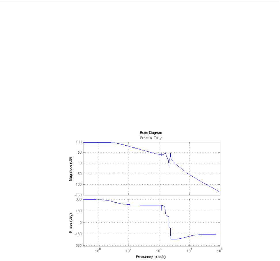
Tuning Control Systems with SYSTUNE
Tuning Control Systems with SYSTUNE
The systune command can jointly tune the gains of your control system
regardless of its architecture and number of feedback loops. This example
outlines the systune workflow on a simple application.
Head-Disk Assembly Control
This example uses a 9th-order model of the head-disk assembly (HDA) in a
hard-disk drive. This model captures the first few flexible modes in the HDA.
load rctExamples G
bode(G), grid
We use the feedback loop shown below to position the head on the correct
track. This control structure consists of a PI controller and a low-pass filter
in the return path. The head position yshould track a step change rwith
a response time of about one millisecond, little or no overshoot, and no
steady-state error.
6-43
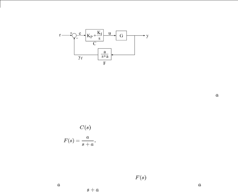
6Tuning Fixed Control Architectures
Figure 1: Control Structure
You can use systune to directly tune the PI gains and filter coefficient
subject to a variety of time- and frequency-domain requirements.
Specifying the Tunable Elements
There are two tunable elements in the control structure of Figure 1: the PI
controller and the low-pass filter
You can use the ltiblock.pid class to parameterize the PI block:
C0 = ltiblock.pid('C','pi'); % tunable PI
To parameterize the lowpass filter , create a tunable real parameter
and construct a first-order transfer function with numerator and
denominator :
a = realp('a',1); % filter coefficient
F0 = tf(a,[1 a]); % filter parameterized by a
See the "Building Tunable Models" example for an overview of available
tunable elements.
Building a Tunable Closed-Loop Model
6-44
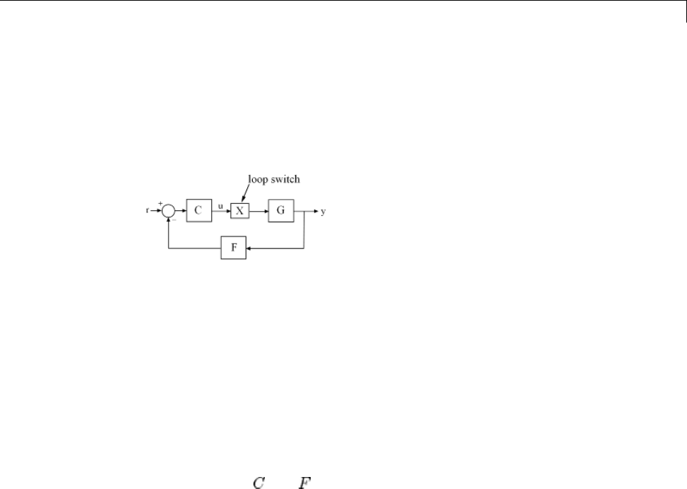
Tuning Control Systems with SYSTUNE
Next build a closed-loop model of the feedback loop in Figure 1. To facilitate
open-loop analysis and specify open-loop requirements such as desired
stability margins, add a loop opening switch at the plant input u:
LSU = loopswitch('u');
Figure 2: Loop Switch Block
Use feedback to build a model of the closed-loop transfer from reference
rto head position y:
T0 = feedback(G*LSU*C0,F0); % closed-loop transfer from r to y
T0.InputName = 'r';
T0.OutputName = 'y';
The result T0 is a generalized state-space model (genss) that depends on the
tunable elements and .
Specifying the Design Requirements
The TuningGoal package contains a variety of control design requirements
for specifying the desired behavior of the control system. These include
requirements on the response time, deterministic and stochastic gains, loop
shape, stability margins, and pole locations. Here we use two requirements to
capture the control objectives:
•Tracking requirement :Theposition
yshould track the reference r
with a 1 millisecond response time
•Stability margin requirement : The feedback loop should have 6dB of
gain margin and 45 degrees of phase margin
6-45

6Tuning Fixed Control Architectures
Use the TuningGoal.Tracking and TuningGoal.Margins objects to capture
these requirements. Note that the margins requirement applies to the
open-loop response measured at the plant input u(location marked by the
loopswitch block LSU).
Req1 = TuningGoal.Tracking('r','y',0.001);
Req2 = TuningGoal.Margins('u',6,45);
Tuning the Controller Parameters
You can now use systune to tune the PI gain and filter coefficient .This
function takes the tunable closed-loop model T0 and the requirements
Req1,Req2. Use a few randomized starting points to improve the chances
of getting a globally optimal design.
rng('default')
Options = systuneOptions('RandomStart',3);
[T,fSoft,~,Info] = systune(T0,[Req1,Req2],Options);
Final: Soft = 1.35, Hard = -Inf, Iterations = 157
Final: Soft = 2.61, Hard = -Inf, Iterations = 104
Final: Soft = 2.78e+03, Hard = -Inf, Iterations = 180
Min decay rate 1e-07 is close to lower bound 1e-07
Final: Soft = 1.35, Hard = -Inf, Iterations = 51
All requirements are normalized so a requirement is satisfied when its value
is less than 1. Here the final value is slightly greater than 1, indicating that
the requirements are nearly satisfied. Use the output fSoft to see the tuned
valueofeachrequirement. Hereweseethatthefirstrequirement(tracking)
is slightly violated while the second requirement (margins) is satisfied.
fSoft
fSoft =
1.3461 0.6326
6-46

Tuning Control Systems with SYSTUNE
The first output Tof systune is the "tuned" closed-loop model. Use
showTunable or getBlockValue to access the tuned values of the PI gains
and filter coefficient:
getBlockValue(T,'C') % tuned value of PI controller
ans =
1
Kp + Ki * ---
s
with Kp = 0.00104, Ki = 0.0122
Name: C
Continuous-time PI controller in parallel form.
showTunable(T) % tuned values of all tunable elements
C=
1
Kp + Ki * ---
s
with Kp = 0.00104, Ki = 0.0122
Name: C
Continuous-time PI controller in parallel form.
-----------------------------------
a = 3.19e+03
Validating Results
First use viewSpec to inspect how the tuned system does against each
requirement. The first plot shows the tracking error as a function of frequency,
and the second plot shows the normalized disk margins as a function of
6-47
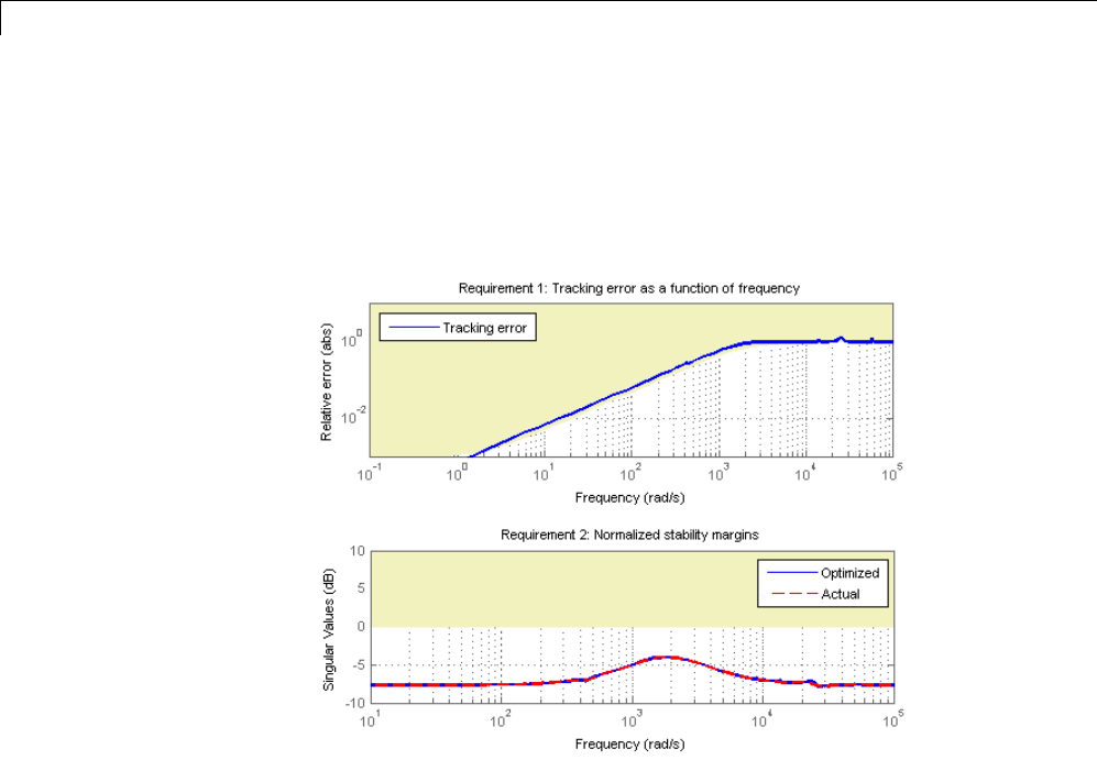
6Tuning Fixed Control Architectures
frequency (see loopmargin). See the "Creating Design Requirements" example
for details.
clf, viewSpec([Req1 Req2],T,Info)
Next plot the closed-loop step response from reference rto head position y.
The response has no overshoot but wobbles a little.
clf, step(T)
6-48
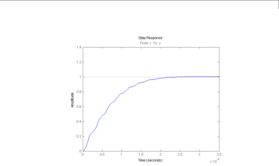
Tuning Control Systems with SYSTUNE
To investigate further, use getLoopTransfer to get the open-loop response at
the plant input.
L = getLoopTransfer(T,'u');
bode(L,{1e3,1e6}), grid
title('Open-loop response')
6-49
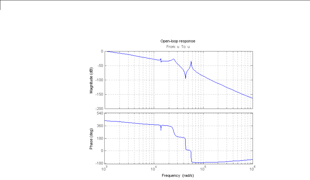
6Tuning Fixed Control Architectures
Thewobbleisduetothefirstresonanceafterthegaincrossover.Toeliminate
it, you could add a notch filter to the feedback loop and tune its coefficients
along with the lowpass coefficient and PI gains using systune.
6-50
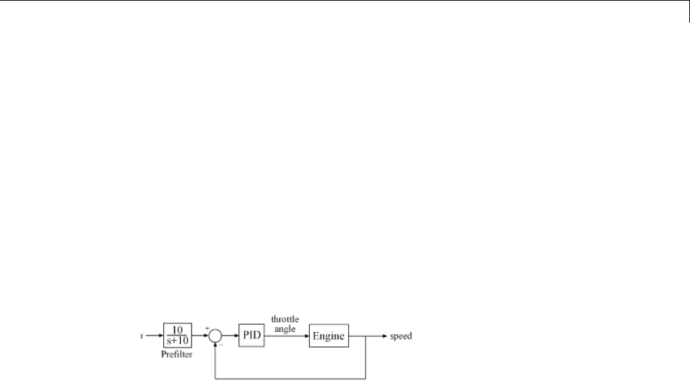
Tuning Feedback Loops with LOOPTUNE
Tuning Feedback Loops with LOOPTUNE
This example shows the basic workflow of tuning feedback loops with the
looptune command. looptune is similar to systune and meant to facilitate
loop shaping design by automatically generating the tuning requirements.
Engine Speed Control
This example uses a simple engine speed control application as illustration.
The control system consists of a single PID loop and the PID controller gains
must be tuned to adequately respond to step changes in the desired speed.
Specifically, we want the response to settle in less than 5 seconds with little
or no overshoot.
Figure 1: Engine Speed Control Loop
We use the following fourth-order model of the engine dynamics.
load rctExamples Engine
bode(Engine), grid
6-51
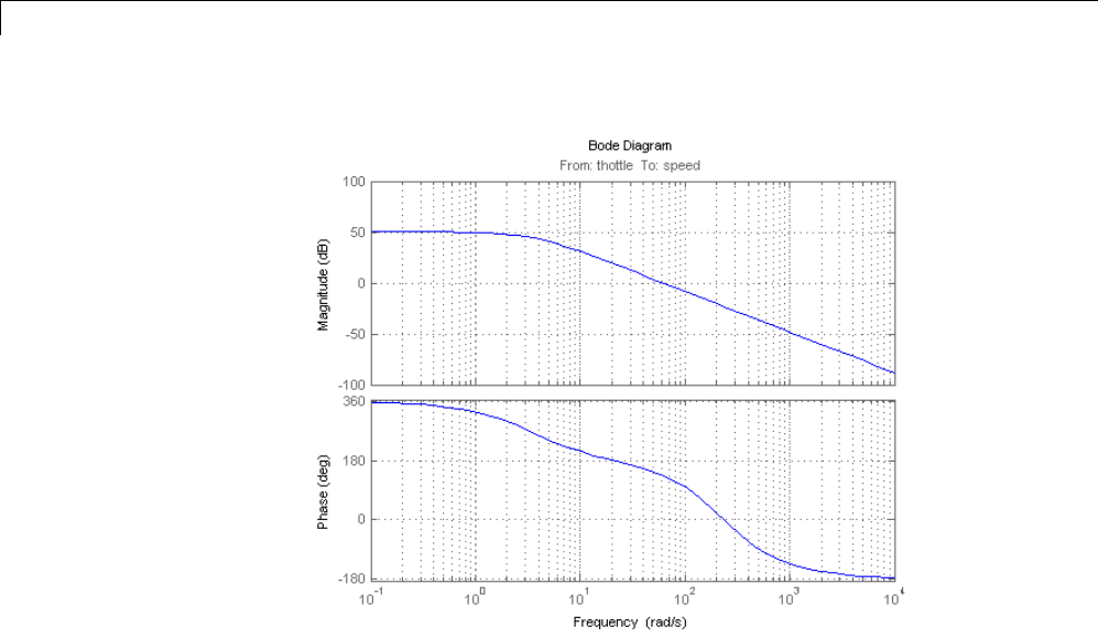
6Tuning Fixed Control Architectures
Specifying the Tunable Elements
We need to tune the four PID gains to achieve the desired performance. Use
the ltiblock.pid class to parameterize the PID controller.
PID0 = ltiblock.pid('SpeedController','pid')
PID0 =
Parametric continuous-time PID controller "SpeedController" with formula:
1s
Kp + Ki * --- + Kd * --------
s Tf*s+1
and tunable parameters Kp, Ki, Kd, Tf.
Type "pid(PID0)" to see the current value and "get(PID0)" to see all prope
r
6-52
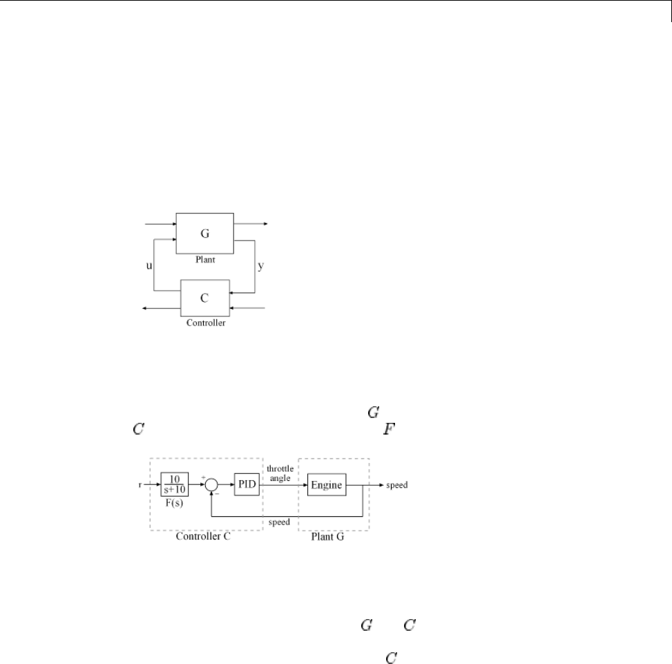
Tuning Feedback Loops with LOOPTUNE
Building a Tunable Model of the Feedback Loop
looptune tunes the generic SISO or MIMO feedback loop of Figure 2. This
feedback loop models the interaction between the plant and the controller.
Note that this is a positive feedback interconnection.
Figure 2: Generic Feedback Loop
For the speed control loop, the plant is the engine model and the controller
consists of the PID and the prefilter .
Figure 3: Feedback Loop for Engine Speed Control
To use looptune, create models for and in Figure 3. Assign names to the
inputs and outputs of each model to specify the feedback paths between plant
and controller. Note that the controller has two inputs: the speed reference
"r" and the speed measurement "speed".
F = tf(10,[1 10]); % prefilter
6-53

6Tuning Fixed Control Architectures
G = Engine;
G.InputName = 'throttle';
G.OutputName = 'speed';
C0 = PID0 * [F , -1];
C0.InputName = {'r','speed'};
C0.OutputName = 'throttle';
Here C0 is a generalized state-space model (genss) that depends on the
tunable PID block PID0.
Tuning the Controller Parameters
You can now use looptune to tune the PID gains subject to a simple control
bandwidth requirement. To achieve the 5-second settling time, the gain
crossover frequency of the open-loop response should be approximately
1 rad/s. Given this basic requirement, looptune automatically shapes
the open-loop response to provide integral action, high-frequency roll-off,
and adequate stability margins. Note that you could specify additional
requirements to further constrain the design, see "Decoupling Controller for a
Distillation Column" for an example.
wc = 1; % target gain crossover frequency
[~,C,~,Info] = looptune(G,C0,wc);
Final: Peak gain = 0.92, Iterations = 3
The final value is less than 1, indicating that the desired bandwidth was
achieved with adequate roll-off and stability margins. looptune returns the
tuned controller C.UsegetBlockValue to retrieve the tuned value of the
PID block.
PIDT = getBlockValue(C,'SpeedController')
PIDT =
1s
Kp + Ki * --- + Kd * --------
6-54
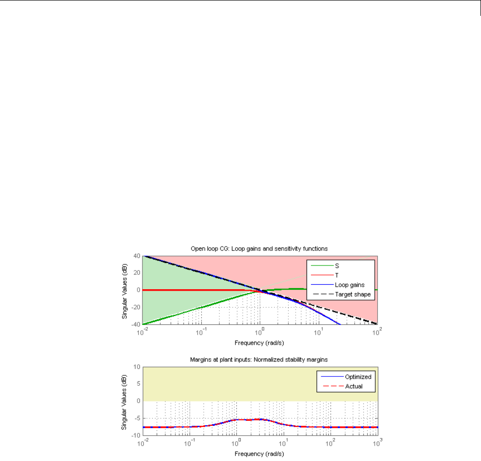
Tuning Feedback Loops with LOOPTUNE
s Tf*s+1
with Kp = 0.000484, Ki = 0.00324, Kd = 0.000835, Tf = 1
Name: SpeedController
Continuous-time PIDF controller in parallel form.
Validating Results
Use loopview to validate the design and visualize the loop shaping
requirements implicitly enforced by looptune.
clf, loopview(G,C,Info)
Next plot the closed-loop response to a step command in engine speed. The
tuned response satisfies our requirements.
T = connect(G,C,'r','speed'); % closed-loop transfer from r to speed
clf, step(T)
6-55
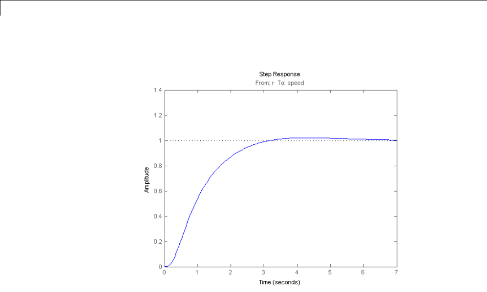
6Tuning Fixed Control Architectures
6-56
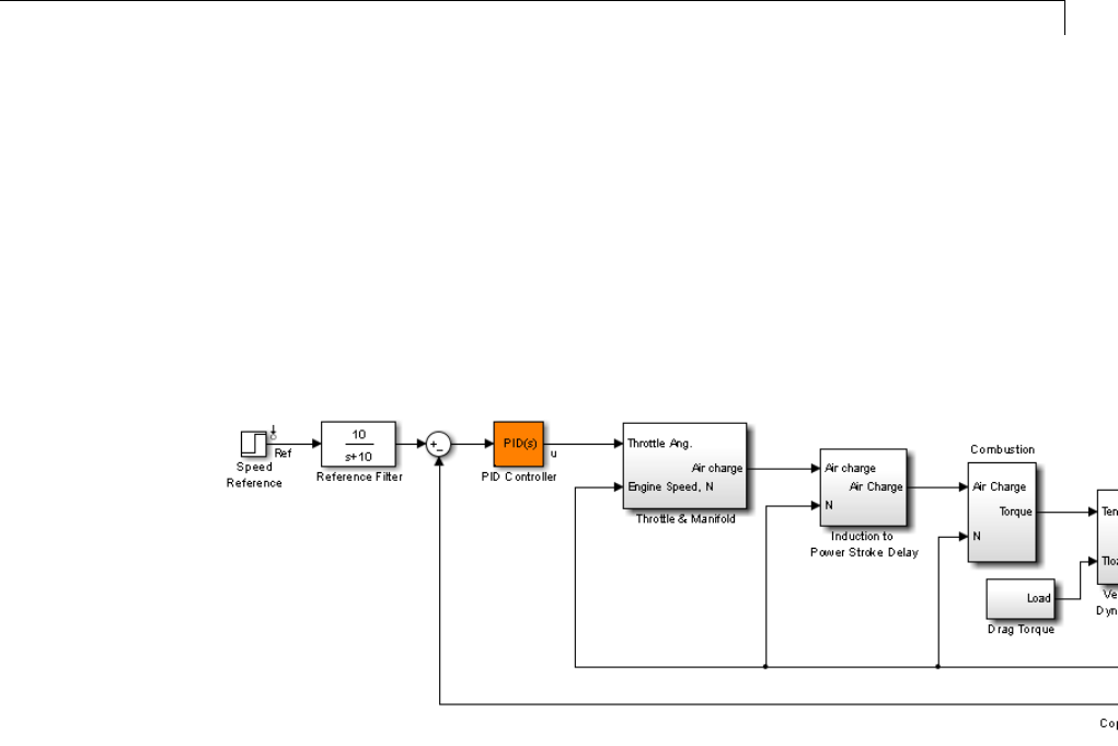
Tuning Control Systems in Simulink
Tuning Control Systems in Simulink
This example shows how to use systune or looptune to automatically tune
control systems modeled in Simulink.
Engine Speed Control
For this example we use the following model of an engine speed control system:
open_system('rct_engine_speed')
The control system consists of a single PID loop and the PID controller gains
must be tuned to adequately respond to step changes in the desired speed.
Specifically, we want the response to settle in less than 5 seconds with little
or no overshoot. While pidtune is a faster alternative for tuning a single
PID controller, this simple example is well suited for an introduction to the
systune and looptune workflows in Simulink.
Controller Tuning with SYSTUNE
The slTunable interface provides a convenient gateway to systune for
control systems modeled in Simulink. This interface lets you specify which
blocks in the Simulink model are tunable and what signals are of interest
for open- or closed-loop validation. Create an slTunable instance for the
rct_engine_speed model and list the "PID Controller" block (highlighted in
6-57

6Tuning Fixed Control Architectures
orange) as tunable. Note that all linearization points in the model (signals
"Ref" and "Speed" here) are automatically available as analysis I/Os.
ST0 = slTunable('rct_engine_speed','PID Controller');
The PID block is initialized with its value in the Simulink model, which you
can access using getBlockValue. Note that the proportional and derivative
gains are initialized to zero.
ST0.getBlockValue('PID Controller')
ans =
1
Ki * ---
s
with Ki = 0.01
Name: PID_Controller
Continuous-time I-only controller.
Next create a reference tracking requirement to capture the target settling
time. Use the signal names in the Simulink model to refer to the reference
and output signals, and use a two-second response time target to ensure
settling in less than 5 seconds.
TrackReq = TuningGoal.Tracking('Ref','Speed',2);
You can now tune the control system ST0 subject to the requirement TrackReq.
ST1 = systune(ST0,TrackReq);
Final: Soft = 1.07, Hard = -Inf, Iterations = 99
The final value is close to 1 indicating that the tracking requirement is met.
systune returns a "tuned" version ST1 of the control system described by ST0.
Again use getBlockValue to access the tuned values of the PID gains:
6-58

Tuning Control Systems in Simulink
ST1.getBlockValue('PID Controller')
ans =
1s
Kp + Ki * --- + Kd * --------
s Tf*s+1
with Kp = 0.00189, Ki = 0.00357, Kd = 0.000473, Tf = 0.00176
Name: PID_Controller
Continuous-time PIDF controller in parallel form.
To simulate the closed-loop response to a step command in speed, get the
initial and tuned transfer functions from speed command "Ref" to "Speed"
output and plot their step responses:
T0 = ST0.getIOTransfer('Ref','Speed');
T1 = ST1.getIOTransfer('Ref','Speed');
step(T0,T1)
legend('Initial','Tuned')
6-59
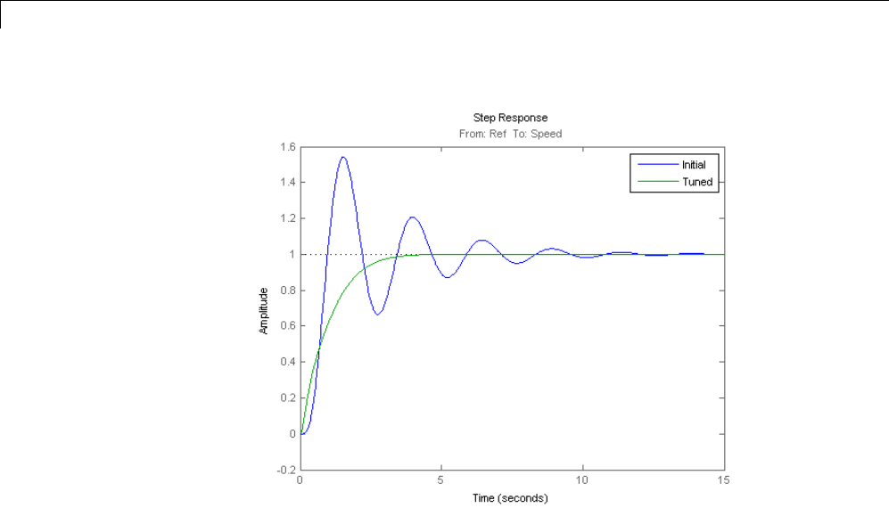
6Tuning Fixed Control Architectures
Controller Tuning with LOOPTUNE
You can also use looptune to tune control systems modeled in Simulink. The
looptune workflow is very similar to the systune workflow. One difference is
that looptune needs to know the boundary between the plant and controller,
which is specified in terms of controls and measurements signals.
ST0 = slTunable('rct_engine_speed','PID Controller');
% Specify plant/controller boundary
ST0.addControl('u');
ST0.addMeasurement('Speed');
% Add the "Ref" signal to the list of analysis I/Os
ST0.addIO('Ref','in')
For a single loop the performance is essentially captured by the response
time, or equivalently by the open-loop crossover frequency. Based on
first-order characteristics the crossover frequency should exceed 1 rad/s for
6-60

Tuning Control Systems in Simulink
the closed-loop response to settle in less than 5 seconds. You can therefore
tune the PID loop using 1 rad/s as target 0-dB crossover frequency.
wc = 1;
ST1 = ST0.looptune(wc);
Final: Peak gain = 0.961, Iterations = 10
Again the final value is close to 1, indicating that the target control bandwidth
was achieved. As with systune,usegetIOTransfer to compute and plot the
closed-loop response from speed command to actual speed. The result is very
similar to that obtained with systune.
T0 = ST0.getIOTransfer('Ref','Speed');
T1 = ST1.getIOTransfer('Ref','Speed');
step(T0,T1)
legend('Initial','Tuned')
6-61
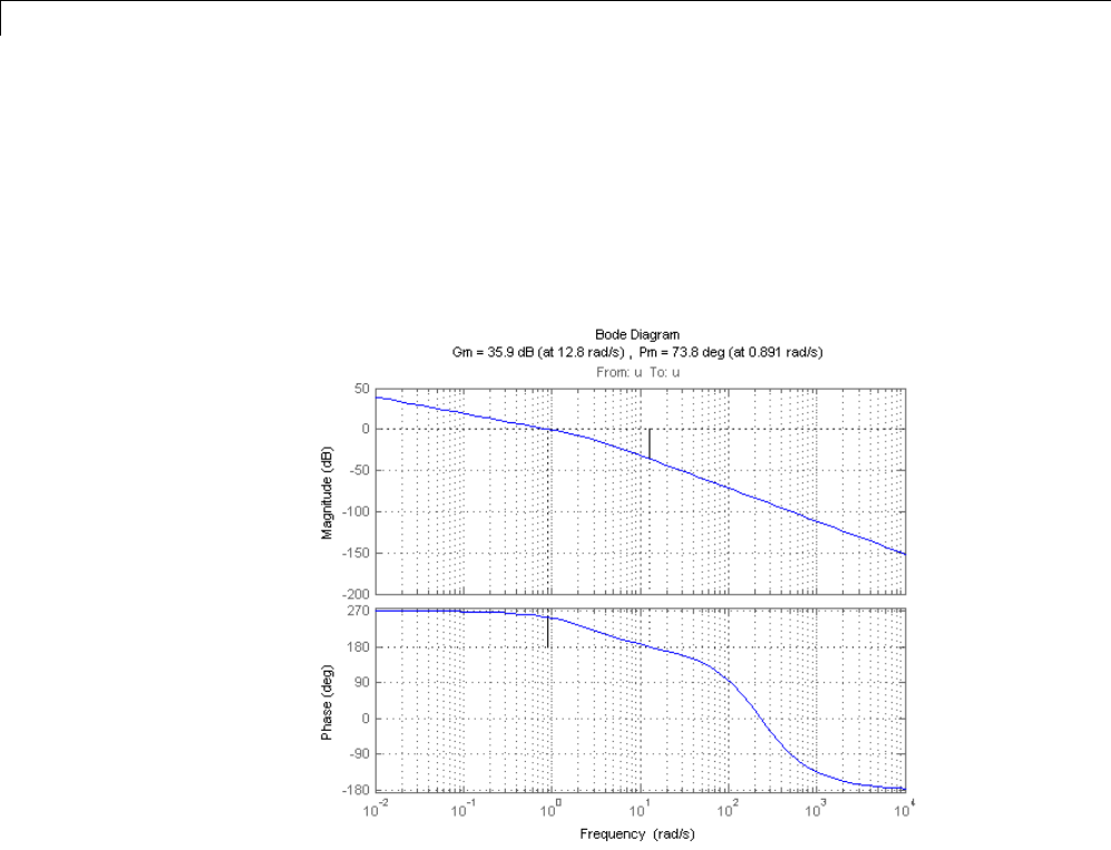
6Tuning Fixed Control Architectures
You can also perform open-loop analysis, for example, compute the gain and
phase margins at the plant input u.
% Note: -1 because |margin| expects the negative-feedback loop transfer
L = ST1.getLoopTransfer('u',-1);
margin(L), grid
Validation in Simulink
Once you are satisfied with the systune or looptune results, you can upload
the tuned controller parameters to Simulink for further validation with the
nonlinear model.
ST1.writeBlockValue()
You can now simulate the engine response with the tuned PID controller.
6-62
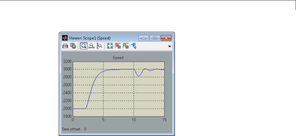
Tuning Control Systems in Simulink
The nonlinear simulation results closely match the linear responses obtained
in MATLAB.
Comparison of PI and PID Controllers
Closer inspection of the tuned PID gains suggests that the derivative term
contributes little because of the large value of the Tf coefficient.
ST1.showTunable()
Block "rct_engine_speed/PID Controller" =
Value =
1s
Kp + Ki * --- + Kd * --------
s Tf*s+1
with Kp = 0.000653, Ki = 0.00282, Kd = 0.0021, Tf = 46.7
Name: PID_Controller
Continuous-time PIDF controller in parallel form.
6-63

6Tuning Fixed Control Architectures
This suggests using a simpler PI controller instead. To do this, you need to
override the default parameterization for the "PID Controller" block:
ST0.setBlockParam('PID Controller',ltiblock.pid('C','pi'))
This specifies that the "PID Controller" block should now be parameterized
as a mere PI controller. Next re-tune the control system for this simpler
controller:
ST2 = ST0.looptune(wc);
Final: Peak gain = 0.915, Iterations = 5
Again the final value is less than one indicating success. Compare the
closed-loop response with the previous ones:
T2 = ST2.getIOTransfer('Ref','Speed');
step(T0,T1,T2,'r--')
legend('Initial','PID','PI')
6-64

Tuning Control Systems in Simulink
Clearly a PI controller is sufficient for this application.
6-65
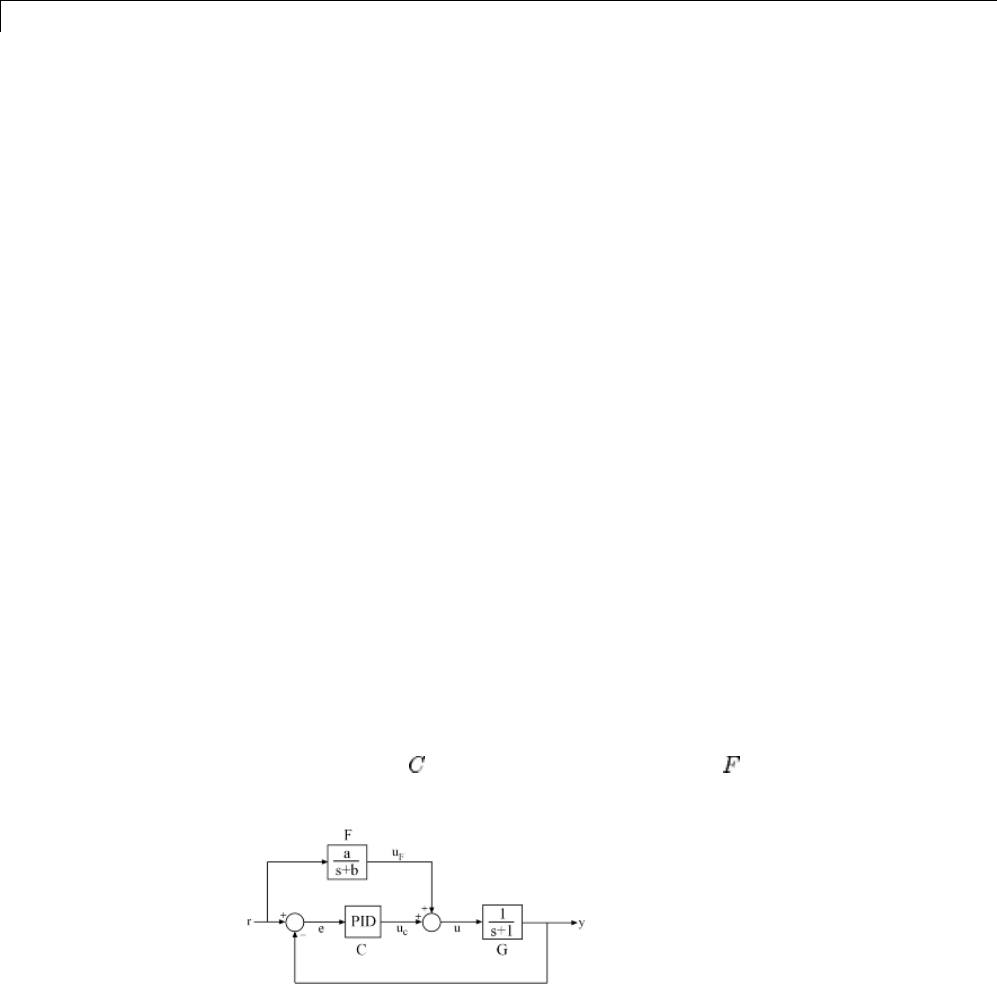
6Tuning Fixed Control Architectures
Building Tunable Models
This example shows how to create tunable models of control systems for use
with systune or looptune.
Background
You can tune the gains and parameters of your control system with systune
or looptune. Tousethesecommands,youneedtoconstructatunablemodel
of the control system that identifies and parameterizes its tunable elements.
This is done by combining numeric LTI models of the fixed elements with
parametric models of the tunable elements.
Using Pre-Defined Tunable Elements
You can use one of the following "parametric" blocks to model commonly
encountered tunable elements:
•ltiblock.gain: Tunable gain
•ltiblock.pid: Tunable PID controller
•ltiblock.pid2: Tunable two-degree-of-freedom PID controller
•ltiblock.tf: Tunable transfer function
•ltiblock.ss: Tunable state-space model.
For example, create a tunable model of the feedforward/feedback configuration
of Figure 1 where is a tunable PID controller and is a tunable first-order
transfer function.
6-66

Building Tunable Models
Figure 1: Control System with Feedforward and Feedback Paths
First model each block in the block diagram, using suitable parametric blocks
for and .
G = tf(1,[1 1]);
C = ltiblock.pid('C','pid'); % tunable PID block
F = ltiblock.tf('F',0,1); % tunable first-order transfer function
Then use connect to build a model of the overall block diagram. To specify
how the blocks are connected, label the inputs and outputs of each block and
model the summing junctions using sumblk.
G.u = 'u'; G.y = 'y';
C.u = 'e'; C.y = 'uC';
F.u = 'r'; F.y = 'uF';
% Summing junctions
S1 = sumblk('e = r-y');
S2 = sumblk('u = uF + uC');
T = connect(G,C,F,S1,S2,'r','y')
T=
Generalized continuous-time state-space model with 1 outputs, 1 inputs,
3
C: Parametric PID controller, 1 occurrences.
F: Parametric SISO transfer function, 0 zeros, 1 poles, 1 occurrences.
Type "ss(T)" to see the current value, "get(T)" to see all properties, and
This creates a generalized state-space model Tof the closed-loop transfer
function from rto y. This model depends on the tunable blocks Cand Fand
you can use systune to automatically tune the PID gains and feedforward
coefficients a,b subject to your performance requirements. Use showTunable
to see the current value of the tunable blocks.
showTunable(T)
6-67

6Tuning Fixed Control Architectures
C=
1
Ki * ---
s
with Ki = 0.001
Name: C
Continuous-time I-only controller.
-----------------------------------
F=
10
------
s+10
Name: F
Continuous-time transfer function.
Interacting with the Tunable Parameters
You can adjust the parameterization of the tunable elements and by
interacting with the objects Cand F.Useget to see their list of properties.
get(C)
Kp: [1x1 param.Continuous]
Ki: [1x1 param.Continuous]
Kd: [1x1 param.Continuous]
Tf: [1x1 param.Continuous]
IFormula: ''
DFormula: ''
Ts: 0
TimeUnit: 'seconds'
InputName: {'e'}
InputUnit: {''}
InputGroup: [1x1 struct]
OutputName: {'uC'}
6-68

Building Tunable Models
OutputUnit: {''}
OutputGroup: [1x1 struct]
Name: 'C'
Notes: {}
UserData: []
A PID controller has four tunable parameters Kp,Ki,Kd,Tf,andCcontains a
description of each of these parameters. Parameter attributes include current
value, minimum and maximum values, and whether the parameter is free
or fixed.
C.Kp
ans =
Name: 'Kp'
Value: 0
Minimum: -Inf
Maximum: Inf
Free: 1
Scale: 1
Info: [1x1 struct]
1x1 param.Continuous
Set the corresponding attributes to override defaults. For example, you can
fix the time constant Tf to the value 0.1 by
C.Tf.Value = 0.1;
C.Tf.Free = false;
Creating Custom Tunable Elements
For tunable elements not covered by the pre-definedblockslistedabove,you
can create your own parameterization in terms of elementary real parameters
(realp). Consider the low-pass filter
6-69
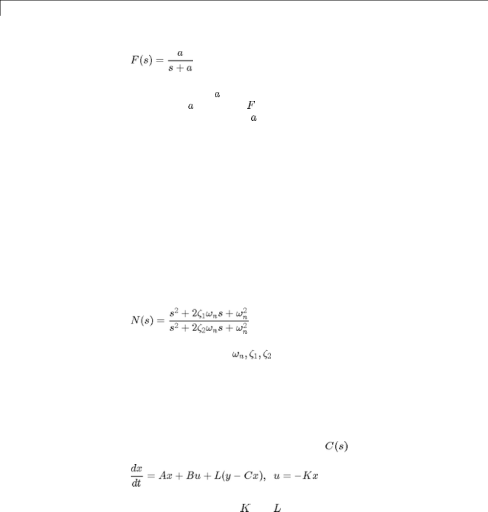
6Tuning Fixed Control Architectures
where the coefficient is tunable. To model this tunable element, create a
real parameter and define as a transfer function whose numerator and
denominator are functions of . This creates a generalized state-space model
Fof the low-pass filter parameterized by the tunable scalar a.
a = realp('a',1); % real tunable parameter, initial value 1
F = tf(a,[1 a])
F=
Generalized continuous-time state-space model with 1 outputs, 1 inputs, 1
a: Scalar parameter, 2 occurrences.
Type "ss(F)" to see the current value, "get(F)" to see all properties, and
Similarly, you can use real parameters to model the notch filter
with tunable coefficients .
wn = realp('wn',100);
zeta1 = realp('zeta1',1); zeta1.Maximum = 1; % zeta1 <= 1
zeta2 = realp('zeta2',1); zeta2.Maximum = 1; % zeta2 <= 1
N = tf([1 2*zeta1*wn wn^2],[1 2*zeta2*wn wn^2]); % tunable notch filter
You can also create tunable elements with matrix-valued parameters. For
example, model the observer-based controller with equations
and tunable gain matrices and .
6-70

Building Tunable Models
% Plant with 6 states, 2 controls, 3 measurements
[A,B,C] = ssdata(rss(6,3,2));
K = realp('K',zeros(2,6));
L = realp('L',zeros(6,3));
C = ss(A-B*K-L*C,L,-K,0)
C=
Generalized continuous-time state-space model with 2 outputs, 3 inputs,
6
K: Parametric 2x6 matrix, 2 occurrences.
L: Parametric 6x3 matrix, 2 occurrences.
Type "ss(C)" to see the current value, "get(C)" to see all properties, and
Enabling Open-Loop Requirements
The systune command takes a closed-loop model of the overall control system,
like the tunable model Tbuilt at the beginning of this example. Such models
do not readily support open-loop analysis or open-loop specifications such as
loop shapes and stability margins. To gain access to open-loop responses,
insert a loopswitch block as shown in Figure 2.
Figure 2: Loop Switch Block
The loopswitch block is an open/closed switch that can be used to open
feedback loops or to measure open-loop responses. For example, construct a
closed-loop model Tof the feedback loop of Figure 2 where is a tunable PID.
G = tf(1,[1 1]);
6-71
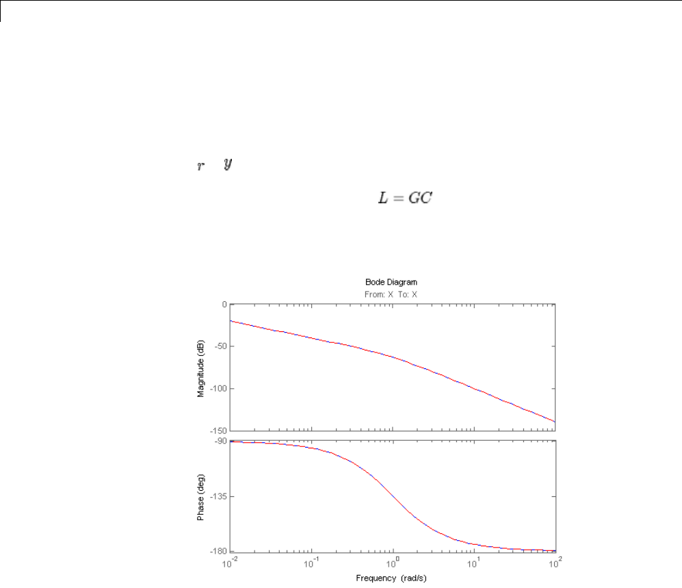
6Tuning Fixed Control Architectures
C = ltiblock.pid('C','pid');
LS = loopswitch('X');
T = feedback(G*C,LS);
By default the loop switch "X" is closed and Tmodels the closed-loop transfer
from to . However, you can now use getLoopTransfer to compute the
(negative-feedback) loop transfer function measured at the location "X". Note
that this loop transfer function is for the feedback loop of Figure 2.
L = getLoopTransfer(T,'X',-1); % loop transfer at "X"
clf, bode(L,'b',G*C,'r--')
You can also refer to the location "X" when specifying target loop shapes or
stability margins for systune. The requirement then applies to the loop
transfer measured at this location.
% Target loop shape for loop transfer at "X"
Req1 = TuningGoal.LoopShape('X',tf(5,[1 0]));
% Target stability margins for loop transfer at "X"
6-72

Building Tunable Models
Req2 = TuningGoal.Margins('X',6,40);
In general, the loop identifiers (names of the loop opening sites marked by a
loopswitch block) are specified in the LoopID property of loopswitch blocks.
For single-loop switches, the loop identifier defaults to the block name. For
multi-loop switches, the default identifiers are the block name followed by
an index.
LS = loopswitch('Y',2); % two-channel switch
LS.LoopID
ans =
'Y(1)'
'Y(2)'
You can override these default names by modifying the LoopID property.
% Relabel feedback channels to "Inner" and "Outer".
LS.LoopID = {'Inner' ; 'Outer'};
LS.LoopID
ans =
'Inner'
'Outer'
6-73

6Tuning Fixed Control Architectures
Using Design Requirement Objects
This example gives a tour of available design requirements for control system
tuning with systune or looptune.
Background
The systune and looptune commands let you tune the parameters
of fixed-structure control systems subject to a variety of time- and
frequency-domain requirements. The TuningGoal package is the repository
for such design requirements.
Tracking Requirement
The TuningGoal.Tracking requirement enforces setpoint tracking and loop
decouplingobjectives. Forexample
R1 = TuningGoal.Tracking('r','y',2);
specifies that the output yshould track the reference rwith a two-second
response time. Similarly
R2 = TuningGoal.Tracking({'Vsp','wsp'},{'V','w'},2);
specifies that Vshould track Vsp and wshould track wsp with minimum
cross-coupling between the two responses. Tracking requirements are
converted into frequency-domain constraints on the tracking error as a
function of frequency. For the first requirement R1, for example, the gain from
rto the tracking error e=r-yshould be small at low frequency and approach
1 (100%) at frequencies greater than 1 rad/s (bandwidth for a two-second
response time). You can use viewSpec to visualize this frequency-domain
constraint.
viewSpec(R1)
6-74
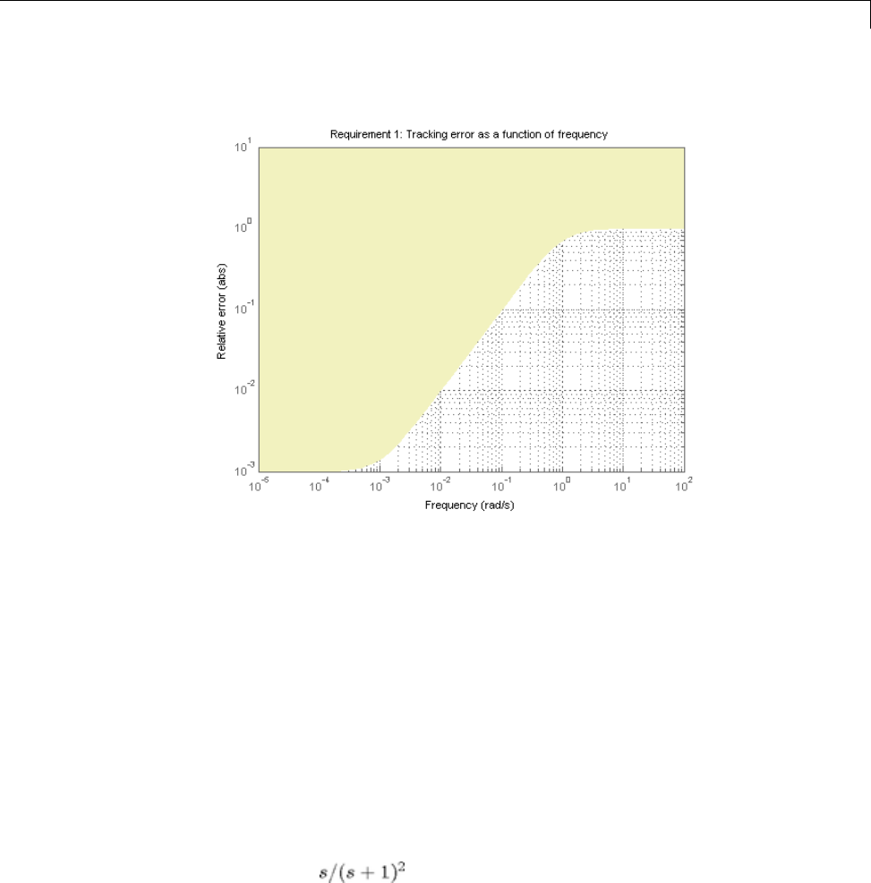
Using Design Requirement Objects
Note that the yellow region indicates where the requirement is violated.
Gain Requirement
The TuningGoal.Gain requirement enforces gain limits on SISO or MIMO
closed-loop transfer functions. This requirement is useful to enforce adequate
disturbance rejection and roll off, limit sensitivity and control effort, and
prevent saturation. For MIMO transfer functions, "gain" refers to the largest
singular value of the frequency response matrix. The gain limit can be
frequency dependent. For example
s = tf('s');
R1 = TuningGoal.Gain('d','y',s/(s+1)^2);
specifies that the gain from dto yshould not exceed the magnitude of the
transfer function .
viewSpec(R1)
6-75
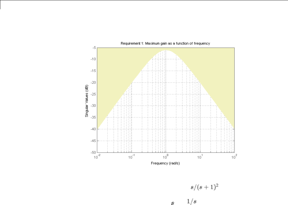
6Tuning Fixed Control Architectures
It is often convenient to just sketch the asymptotes of the desired gain profile.
For example, instead of the transfer function , we could just specify
gain values of 0.01,1,0.01 at the frequencies 0.01,1,100, the point (1,1) being
the breakpoint of the two asymptotes and .
Asymptotes = frd([0.01,1,0.01],[0.01,1,100]);
R2 = TuningGoal.Gain('d','y',Asymptotes);
The requirement object automatically turns this discrete gain profile into a
gain limit defined at all frequencies.
bodemag(Asymptotes,R2.MaxGain)
legend('Specified','Interpolated')
6-76

Using Design Requirement Objects
Variance Requirement
The TuningGoal.Variance requirement limits the noise variance
amplification from specified inputs to specified outputs. In technical terms,
this requirement constrains the norm of a closed-loop transfer function.
This requirement is preferable to TuningGoal.Gain when the input signals
are random processes and the average gain matters more than the peak gain.
For example,
R = TuningGoal.Variance('n','y',0.1);
limits the output variance of yto for a unit-variance white-noise input n.
Weighted Gain and Weighted Variance Requirements
The TuningGoal.WeightedGain and TuningGoal.WeightedVariance
requirements are generalizations of the TuningGoal.Gain and
TuningGoal.Variance requirements. These requirements constrain the
or norm of a frequency-weighted closed-loop transfer function
6-77
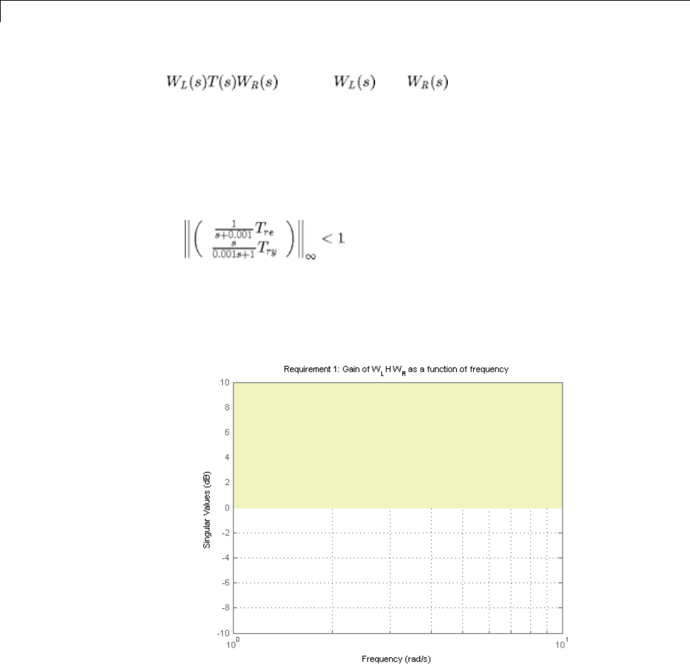
6Tuning Fixed Control Architectures
,where and are user-defined weighting
functions. For example
WL = blkdiag(1/(s+0.001),s/(0.001*s+1));
WR = [];
R = TuningGoal.WeightedGain('r',{'e','y'},WL,[]);
specifies the constraint
Note that this is a normalized gain constraint (unit bound across frequency).
viewSpec(R)
The TuningGoal.WeightedVariance requirement is useful to specify
LQG-like performance objectives. For example, the LQG cost
6-78
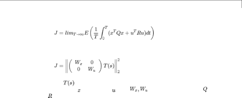
Using Design Requirement Objects
can be expressed as
where is the closed-loop transfer from process and measurement noise
to the states and controls ,and are Cholesky factors of and
(see chol).
Loop Shape Requirement
The TuningGoal.LoopShape requirement is used to shape the open-loop
response gain(s), a design approach known as loop shaping. For example,
R1 = TuningGoal.LoopShape('u',1/s);
specifies that the open-loop response measured at the location "u" should
look like a pure integrator (as far as its gain is concerned). In MATLAB, the
location "u" should be marked using a loopswitch block, see the "Building
Tunable Models" example for details. In Simulink, this location should
be registered as control, measurement, or switch using the addControl,
addMeasurement,addSwitch methods of the slTunable tuning interface.
As with other gain specifications, you can just specify the asymptotes of the
desired loop shape using a few frequency points. For example, to specify a loop
shape with gain crossover at 1 rad/s, -20 dB/decade slope before 1 rad/s, and
-40 dB/decade slope after 1 rad/s, just specify that the gain at the frequencies
0.1,1,10 should be 10,1,0.01, respectively.
LS = frd([10,1,0.01],[0.1,1,10]);
R2 = TuningGoal.LoopShape('u',LS);
bodemag(LS,R2.LoopGain)
legend('Specified','Interpolated')
6-79
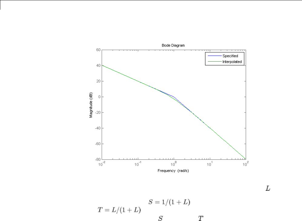
6Tuning Fixed Control Architectures
Loop shape requirements are constraints on the open-loop response .
For tuning purposes, they are converted into closed-loop gain constraints
on the sensitivity function and complementary sensitivity
function .UseviewSpec to visualize the target loop shape and
corresponding gain bounds on (green) and (red).
viewSpec(R2)
6-80
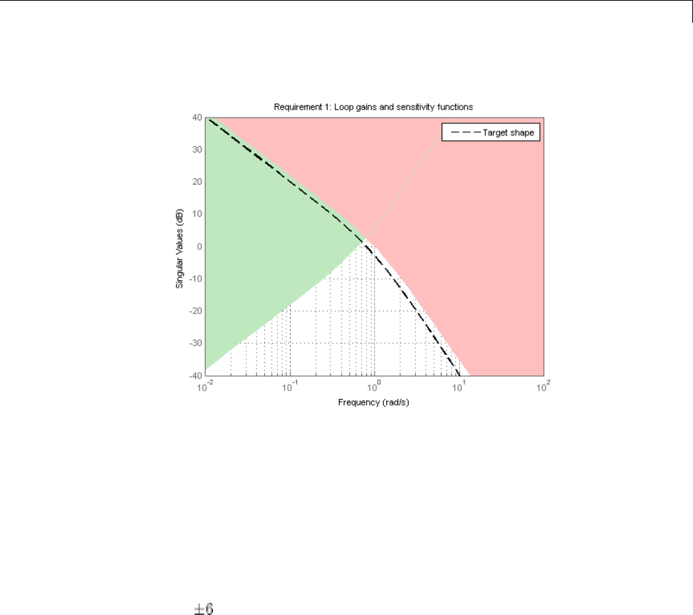
Using Design Requirement Objects
Stability Margins Requirement
The TuningGoal.Margins requirement enforces minimum amounts of gain
and phase margins at the specified loop opening site(s). For MIMO feedback
loops, this requirement uses the notion of disk margins,whichguarantee
stability for concurrent gain and phase variations of the specified amount in
all feedback channels (see loopmargin for details). For example,
R = TuningGoal.Margins('u',6,45);
enforces dB of gain margin and 45 degrees of phase margin at the location
"u". In MATLAB, this location should be marked with a loopswitch block in
the overall model of the control system. In Simulink, it should be registered
as control, measurement, or switch using the addControl,addMeasurement,
addSwitch methods of the slTunable tuning interface. Stability margins are
typically measured at the plant inputs or plant outputs or both.
6-81
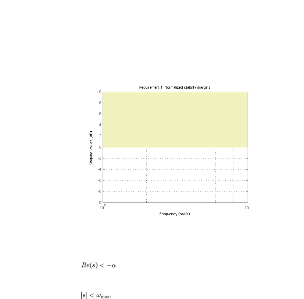
6Tuning Fixed Control Architectures
The target gain and phase margin values are converted into a normalized gain
constraint on some appropriate closed-loop transfer function. The desired
margins are achieved at frequencies where the gain is less than 1.
viewSpec(R)
Closed-Loop Pole Requirement
The TuningGoal.Poles requirement constrains the location of the closed-loop
poles. You can enforce some minimum decay rate
or constrain the pole magnitude to
For example
R = TuningGoal.Poles();
6-82
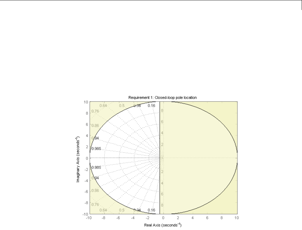
Using Design Requirement Objects
R.MinDecay = 0.5;
R.MaxFrequency = 10;
constrains the closed-loop poles to lie in the white region below.
viewSpec(R)
Increasing the MinDecay value results in better damping and faster
transients. Decreasing the MaxFrequency value prevents fast dynamics and
high-frequency oscillations.
Stable Controller Requirement
The TuningGoal.StableController requirement enforces stability of a given
control element (compensator). The tuning algorithm may produce unstable
compensators for unstable plants. You can prevent this by constraining
the location of the compensator poles. For example, if your compensator is
parameterized as a second-order transfer function,
C = ltiblock.tf('C',1,2);
6-83
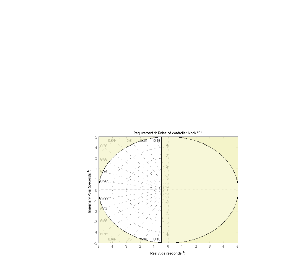
6Tuning Fixed Control Architectures
you can force it to have stable dynamics by adding the requirement
R = TuningGoal.StableController('C');
You can further constrain the minimum decay rate and maximum natural
frequency of its poles, for example,
R.MinDecay = 0.5;
R.MaxFrequency = 5;
viewSpec(R)
Configuring Requirements
All requirements discussed above are objects that can be further configured
by modifying their default attributes. The display shows the list of such
attributes. For example
R = TuningGoal.Gain('d','y',1)
6-84

Using Design Requirement Objects
R=
TuningGoal.Gain
Package: TuningGoal
Properties:
Input: {'d'}
Output: {'y'}
MaxGain: [1x1 zpk]
Focus: [0 Inf]
Models: NaN
Openings: {0x1 cell}
Name: ''
Three attributes are shared by multiple requirements. The Focus property
specifies the frequency band in which the requirement is active. For example,
R.Focus = [1 20];
limits the gain from dto yin the frequency interval [1,20] only. The Models
property specifies which models the requirement applies to (in the context of
tuning for multiple plant models). For example,
R.Models = [2 3 5];
indicates that the requirement only applies to the second, third, and fifth
model in the model array supplied to systune.Finally,theOpenings property
lets you specify additional loop openings. For example
R = TuningGoal.Margins('Inner',6,45);
R.Openings = 'Outer';
specifies stability margins for the inner loop with the outer loop open. All loop
opening sites should be registered with loopswitch blocks in MATLAB and
with the addControl,addMeasurement,addSwitch methods of the slTunable
tuning interface in Simulink.
6-85
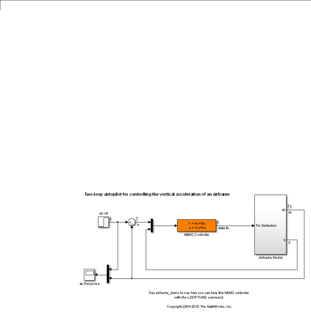
6Tuning Fixed Control Architectures
Validating Results
This example shows how to interpret and validate tuning results from
systune.
Background
You can tune the parameters of your control system with systune or
looptune. The design specifications are captured using TuningGoal
requirement objects. This example shows how to interpret the results from
systune, graphically verify the design requirements, and perform additional
open- and closed-loop analysis.
Controller Tuning with SYSTUNE
We use an autopilot tuning application as illustration, see the "Tuning of
aTwo-LoopAutopilot" example for details. The tuned compensator is the
"MIMO Controller" block highlighted in orange in the model below.
open_system('rct_airframe2')
The setup and tuning steps are repeated below for completeness.
6-86

Validating Results
ST0 = slTunable('rct_airframe2','MIMO Controller');
ST0.addControl('delta fin');
% Compensator parameterization
C0 = ltiblock.ss('C',2,1,2);
C0.d.Value(1) = 0; C0.d.Free(1) = false;
ST0.setBlockParam('MIMO Controller',C0)
% Requirements
Req1 = TuningGoal.Tracking('az ref','az',1); % tracking
Req2 = TuningGoal.Gain('delta fin','delta fin',tf(25,[1 0])); % roll-off
Req3 = TuningGoal.Margins('delta fin',7,45); % margins
MaxGain = frd([2 200 200],[0.02 2 200]);
Req4 = TuningGoal.Gain('delta fin','az',MaxGain); % disturbance rejection
% Tuning
Opt = systuneOptions('RandomStart',3);
rng('default')
[ST1,fSoft,~,Info] = ST0.systune([Req1,Req2,Req3,Req4],Opt);
Final: Soft = 1.5, Hard = -Inf, Iterations = 57
Final: Soft = 1.49, Hard = -Inf, Iterations = 93
Final: Soft = 1.15, Hard = -Inf, Iterations = 57
Final: Soft = 1.15, Hard = -Inf, Iterations = 82
Interpreting Results
systune run three optimizations from three different starting points and
returned the best overall result. The first output ST is an slTunable interface
representing the tuned control system. The second output fSoft contains the
final values of the four requirements for the best design.
fSoft
fSoft =
1.1477 1.1477 0.5458 1.1477
6-87
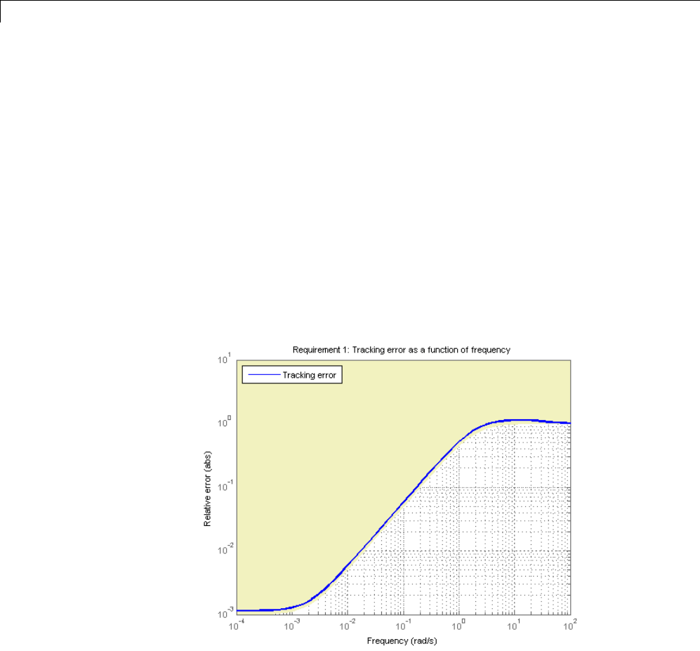
6Tuning Fixed Control Architectures
Requirements are normalized so a requirement is satisfied if and only if its
valueislessthan1. InspectionoffSoft reveals that Requirements 1,2,4
are active and slightly violated while Requirement 3 (stability margins)
is satisfied.
Verifying Requirements
Use viewSpec to graphically inspect each requirement. This is useful to
understand whether small violations are acceptable or what causes large
violations. MakesuretoprovidethestructureInfo returned by systune
to properly account for scalings and other parameters computed by the
optimization algorithms. First verify the tracking requirement.
viewSpec(Req1,ST1,Info)
We observe a slight violation across frequency, suggesting that setpoint
tracking will perform close to expectations. Similarly, verify the disturbance
rejection requirement.
viewSpec(Req4,ST1,Info)
6-88
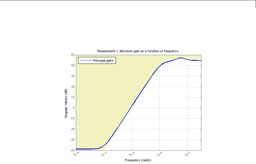
Validating Results
legend('location','NorthWest')
Most of the violation is at low frequency with a small bump near 35 rad/s,
suggesting possible damped oscillations at this frequency. Finally, verify the
stability margin requirement.
viewSpec(Req3,ST1,Info)
6-89
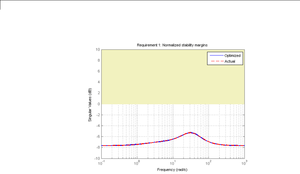
6Tuning Fixed Control Architectures
This requirement is satisfied at all frequencies, with the smallest margins
achieved near the crossover frequency as expected. To see the actual margin
values at a given frequency, click on the red curve and read the values from
the data tip.
Evaluating Requirements
You can also use evalSpec to evaluate each requirement, that is, compute its
contribution to the soft and hard constraints. For example
[H1,f1] = evalSpec(Req1,ST1,Info);
returns the value f1 of the requirement and the underlying
frequency-weighted transfer function H1 used to computed it. You can verify
that f1 matches the first entry of fSoft and coincides with the peak gain of H1.
[f1 fSoft(1) getPeakGain(H1,1e-6)]
ans =
6-90
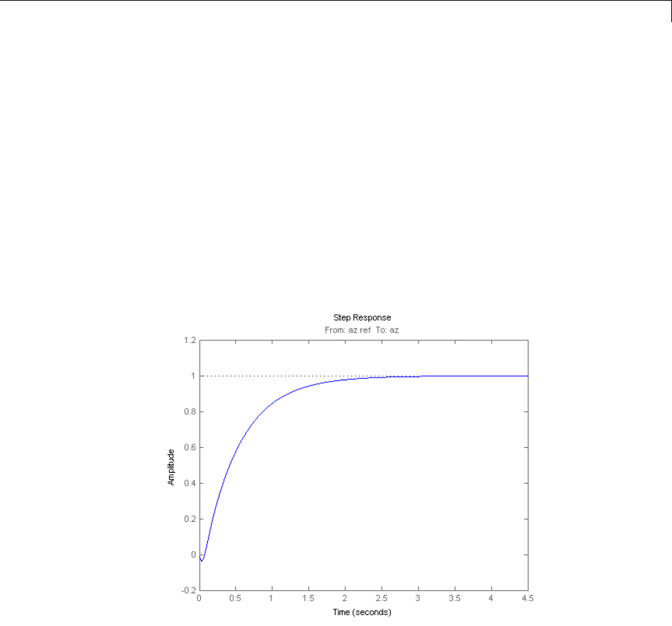
Validating Results
1.1477 1.1477 1.1477
Analyzing System Responses
In addition to verifying requirements, you can perform basic open- and
closed-loop analysis using getIOTransfer and getLoopTransfer.For
example, verify tracking performance in the time domain by plotting the
response az to a step command azref for the tuned system ST1.
T = ST1.getIOTransfer('az ref','az');
step(T)
Also plot the open-loop response measured at the plant input delta fin.
You can use this plot to assess the classical gain and phase margins at the
plant input.
L = ST1.getLoopTransfer('delta fin',-1); % negative-feedback loop transfe
r
margin(L), grid
6-91

6Tuning Fixed Control Architectures
Soft vs Hard Requirements
So far we have treated all four requirements equally in the objective function.
Alternatively, you can use a mix of soft and hard constraints to differentiate
between must-have and nice-to-have requirements. For example, you could
treat Requirements 3,4 as hard constraints and optimize the first two
requirements subject to these constraints. For best results, do this only after
obtaining a reasonable design with all requirements treated equally.
[ST2,fSoft,gHard,Info] = ST1.systune([Req1 Req2],[Req3 Req4]);
Final: Soft = 1.31, Hard = 0.99979, Iterations = 137
fSoft
fSoft =
6-92

Validating Results
1.3072 1.3120
gHard
gHard =
0.4756 0.9998
Here fSoft contains the final values of the first two requirements (soft
constraints) and gHard contains the the final values of the last two
requirements (hard constraints). The hard constraints are satisfied since all
entries of gHard are less than 1. As expected, the best value of the first two
requirements went up as the optimizer strived to strictly enforce the fourth
requirement.
6-93
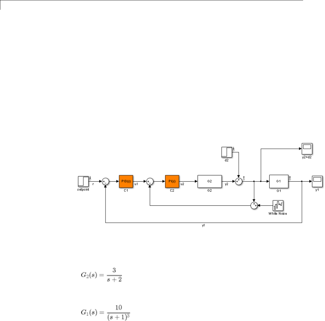
6Tuning Fixed Control Architectures
Tuning Multi-Loop Control Systems
This example shows how to jointly tune the inner and outer loops of a cascade
architecture with the systune command.
Cascaded PID Loops
Cascade control is often used to achieve smooth tracking with fast disturbance
rejection. The simplest cascade architecture involves two control loops (inner
and outer) as shown in the block diagram below. The inner loop is typically
faster than the outer loop to reject disturbances before they propagate to
the outer loop.
open_system('rct_cascade')
Plant Models and Bandwidth Requirements
In this example, the inner loop plant G2 is
and the outer loop plant G1 is
6-94

Tuning Multi-Loop Control Systems
G2 = zpk([],-2,3);
G1 = zpk([],[-1 -1 -1],10);
We use a PI controller in the inner loop and a PID controller in the outer loop.
The outer loop must have a bandwidth of at least 0.2 rad/s and the inner loop
bandwidth should be ten times larger for adequate disturbance rejection.
Tuning the PID Controllers with SYSTUNE
When the control system is modeled in Simulink, use the slTunable interface
in Simulink Control Design™ to set up the tuning task. List the tunable
blocks and mark the signals y1 and y2 as loop opening locations where to
measure open-loop transfers and specify loop shapes.
ST0 = slTunable('rct_cascade',{'C1','C2'});
ST0.addSwitch({'y1','y2'})
You can query the current values of C1 and C2 in the Simulink model using
showTunable. The control system is unstable for these initial values as
confirmed by simulating the Simulink model.
ST0.showTunable()
Block "rct_cascade/C1" =
Value =
1
Kp + Ki * ---
s
with Kp = 0.1, Ki = 0.1
Name: C1
Continuous-time PI controller in parallel form.
-----------------------------------
Block "rct_cascade/C2" =
6-95

6Tuning Fixed Control Architectures
Value =
1
Kp + Ki * ---
s
with Kp = 0.1, Ki = 0.1
Name: C2
Continuous-time PI controller in parallel form.
Next use "LoopShape" requirements to specify the desired bandwidths for the
the inner and outer loops. Use as target loop shape for the outer loop to
enforce integral action with a gain crossover frequency at 0.2 rad/s:
% Outer loop bandwidth = 0.2
s = tf('s');
Req1 = TuningGoal.LoopShape('y1',0.2/s); % loop transfer measured at y1
Req1.Name = 'Outer Loop';
Use for the inner loop to make it ten times faster (higher bandwidth) than
theouterloop. Toconstraintheinnerlooptransfer,makesuretoopenthe
outer loop by specifying y1 as a loop opening:
% Inner loop bandwidth = 2
Req2 = TuningGoal.LoopShape('y2',2/s); % loop transfer measured at y2
Req2.Openings = 'y1'; % with outer loop opened at y1
Req2.Name = 'Inner Loop';
You can now tune the PID gains in C1 and C2 with systune:
[ST,fSoft,~,Info] = ST0.systune([Req1,Req2]);
Final: Soft = 0.86, Hard = -Inf, Iterations = 96
Use showTunable to see the tuned PID gains.
ST.showTunable()
6-96

Tuning Multi-Loop Control Systems
Block "rct_cascade/C1" =
Value =
1s
Kp + Ki * --- + Kd * --------
s Tf*s+1
with Kp = 0.0493, Ki = 0.0186, Kd = 0.042, Tf = 0.022
Name: C1
Continuous-time PIDF controller in parallel form.
-----------------------------------
Block "rct_cascade/C2" =
Value =
1
Kp + Ki * ---
s
with Kp = 0.697, Ki = 1.64
Name: C2
Continuous-time PI controller in parallel form.
Validating the Design
Thefinalvalueislessthan1whichmeansthatsystune successfully met
both loop shape requirements. Confirm this by inspecting the tuned control
system ST with viewSpec
viewSpec([Req1,Req2],ST,Info)
6-97

6Tuning Fixed Control Architectures
Note that the inner and outer loops have the desired gain crossover
frequencies. To further validate the design, plot the tuned responses to a step
command r and step disturbance d2:
% Response to a step command
H = ST.getIOTransfer('r','y1');
clf, step(H,30), title('Step command')
6-98

Tuning Multi-Loop Control Systems
% Response to a step disturbance
H = ST.getIOTransfer('d2','y1');
step(H,30), title('Step disturbance')
6-99

6Tuning Fixed Control Architectures
Once you are satisfied with the linear analysis results, use writeBlockValue
to write the tuned PID gains back to the Simulink blocks. You can then
conduct a more thorough validation in Simulink.
ST.writeBlockValue
Equivalent Workflow in MATLAB
If you do not have a Simulink model of the control system, you can perform
the same steps using LTI models of the plant and Control Design blocks to
model the tunable elements.
6-100

Tuning Multi-Loop Control Systems
Figure 1: Cascade Architecture
First create parametric models of the tunable PI and PID controllers.
C1 = ltiblock.pid('C1','pid');
C2 = ltiblock.pid('C2','pi');
Then use loopswitch blocks to mark the loop opening locations y1 and y2.
LS1 = loopswitch('y1');
LS2 = loopswitch('y2');
Finally, create a closed-loop model T0 of the overall control system by closing
each feedback loop. The result is a generalized state-space model depending
on the tunable elements C1 and C2.
InnerCL = feedback(LS2*G2*C2,1);
T0 = feedback(G1*InnerCL*C1,LS1);
T0.InputName = 'r';
T0.OutputName = 'y1';
You can now tune the PID gains in C1 and C2 with systune.
[T,fSoft,~,Info] = systune(T0,[Req1,Req2]);
Final: Soft = 0.861, Hard = -Inf, Iterations = 64
As before, use getIOTransfer to compute and plot the tuned responses to a
step command r and step disturbance entering at the location y2:
% Response to a step command
6-101
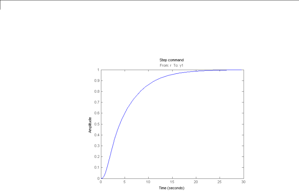
6Tuning Fixed Control Architectures
H = getIOTransfer(T,'r','y1');
clf, step(H,30), title('Step command')
% Response to a step disturbance
H = getIOTransfer(T,'y2','y1');
step(H,30), title('Step disturbance')
6-102
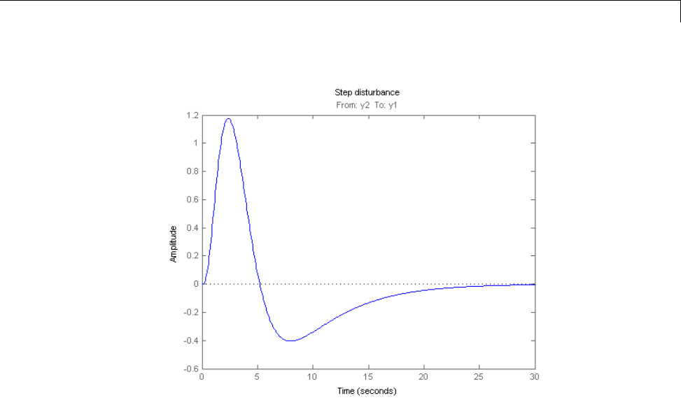
Tuning Multi-Loop Control Systems
You can also plot the open-loop gains for the inner and outer loops to
validate the bandwitdth requirements. Note the -1 sign to compute the
negative-feedback open-loop transfer:
L1 = getLoopTransfer(T,'y1',-1); % crossover should be at .2
L2 = getLoopTransfer(T,'y2',-1,'y1'); % crossover should be at 2
bodemag(L2,L1,{1e-2,1e2}), grid
legend('Inner Loop','Outer Loop')
6-103
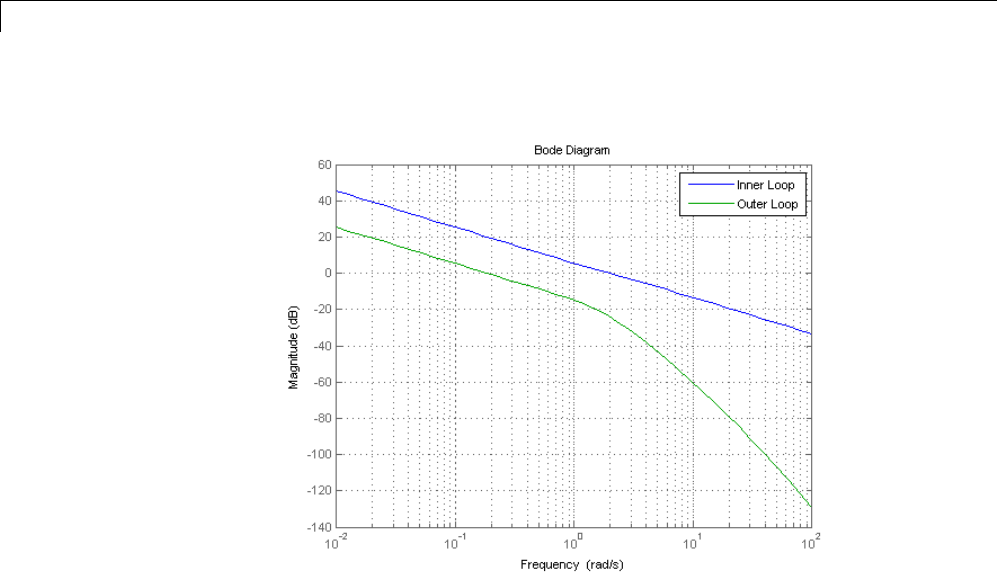
6Tuning Fixed Control Architectures
6-104

Using Parallel Computing to Accelerate Tuning
Using Parallel Computing to Accelerate Tuning
This example shows how to leverage the Parallel Computing Toolbox™ to
accelerate multi-start strategies for tuning fixed-structure control systems.
Background
Both systune and looptune use local optimization methods for tuning
the control architecture at hand. To mitigate the risk of ending up with a
locally optimal but globally poor design, it is recommended to run several
optimizations starting from different randomly generated initial points. If you
have a multi-core machine or have access to distributed computing resources,
you can significantly speed up this process using the Parallel Computing
Toolbox.
This example shows how to parallelize the tuning of an airframe autopilot
with looptune. See the example "Tuning of a Two-Loop Autopilot" for more
details about this application of looptune.
AutopilotTuning
The airframe dynamics and autopilot are modeled in Simulink.
open_system('rct_airframe1')
6-105
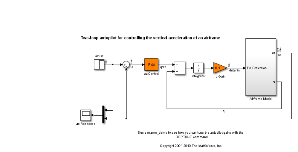
6Tuning Fixed Control Architectures
The autopilot consists of two cascaded loops whose tunable elements include
two PI controller gains ("az Control" block) and one gain in the pitch-rate
loop ("q Gain" block). The vertical acceleration az should track the command
azref with a 1 second response time. Use slTunable to configure this tuning
task (see "Tuning of a Two-Loop Autopilot" example for details):
ST0 = slTunable('rct_airframe1',{'az Control','q Gain'});
ST0.addControl('delta fin');
ST0.addMeasurement({'az','q'});
% Design requirements
wc = [3,12]; % bandwidth
TrackReq = TuningGoal.Tracking('az ref','az',1); % tracking
Parallel Tuning with LOOPTUNE
We are ready to tune the autopilot gains with looptune. To minimize the risk
of getting a poor-quality local minimum, run 20 optimizations starting from 20
randomly generated values of the three gains. To enable parallel processing
of these 20 runs, open the MATLAB pool and configure the looptune options
to enable parallel processing:
6-106

Using Parallel Computing to Accelerate Tuning
rng('default')
matlabpool open
Options = looptuneOptions('RandomStart',20,'UseParallel',true);
Starting matlabpool using the 'local' profile ... connected to 8 workers.
Next call looptune to launch the tuning algorithm. The 20 runs are
automatically distributed across available computing resources:
[ST,gam,Info] = ST0.looptune(wc,TrackReq,Options);
Final: Failed to enforce closed-loop stability (spectral abscissa = 0.0405)
Final: Failed to enforce closed-loop stability (spectral abscissa = 0.0405)
Final: Failed to enforce closed-loop stability (spectral abscissa = 0.0405)
Final: Failed to enforce closed-loop stability (spectral abscissa = 0.067)
Final: Failed to enforce closed-loop stability (spectral abscissa = 0.0406)
Final: Failed to enforce closed-loop stability (spectral abscissa = 0.0405)
Final: Failed to enforce closed-loop stability (spectral abscissa = 0.0405)
Final: Failed to enforce closed-loop stability (spectral abscissa = 0.0405)
Final: Failed to enforce closed-loop stability (spectral abscissa = 0.0405)
Final: Failed to enforce closed-loop stability (spectral abscissa = 0.0406)
Final: Failed to enforce closed-loop stability (spectral abscissa = 0.0406)
Final: Failed to enforce closed-loop stability (spectral abscissa = 0.0392)
Final: Failed to enforce closed-loop stability (spectral abscissa = 0.081)
Final: Failed to enforce closed-loop stability (spectral abscissa = 0.0405)
Final: Failed to enforce closed-loop stability (spectral abscissa = 0.0405)
Final: Failed to enforce closed-loop stability (spectral abscissa = 0.0405)
Final: Failed to enforce closed-loop stability (spectral abscissa = 0.0406)
Final: Failed to enforce closed-loop stability (spectral abscissa = 0.0406)
Final: Peak gain = 1.23, Iterations = 39
Final: Peak gain = 62.1, Iterations = 38
Min decay rate 2.1e-07 is close to lower bound 1e-07
Final: Peak gain = 1.23, Iterations = 112
Most runs return 1.23 as optimal gain value, suggesting that this local
minimum has a wide region of attraction and is likely to be the global
optimum. Use showBlockValue to see the corresponding gain values:
showBlockValue(ST)
6-107

6Tuning Fixed Control Architectures
Block "rct_airframe1/az Control" =
Value =
1
Kp + Ki * ---
s
with Kp = 0.00165, Ki = 0.00166
Name: az_Control
Continuous-time PI controller in parallel form.
-----------------------------------
Block "rct_airframe1/q Gain" =
Value =
d=
u1
y1 1.985
Name: q_Gain
Static gain.
Plot the closed-loop response for this set of gains:
T = ST.getIOTransfer('az ref','az');
step(T,5)
6-108
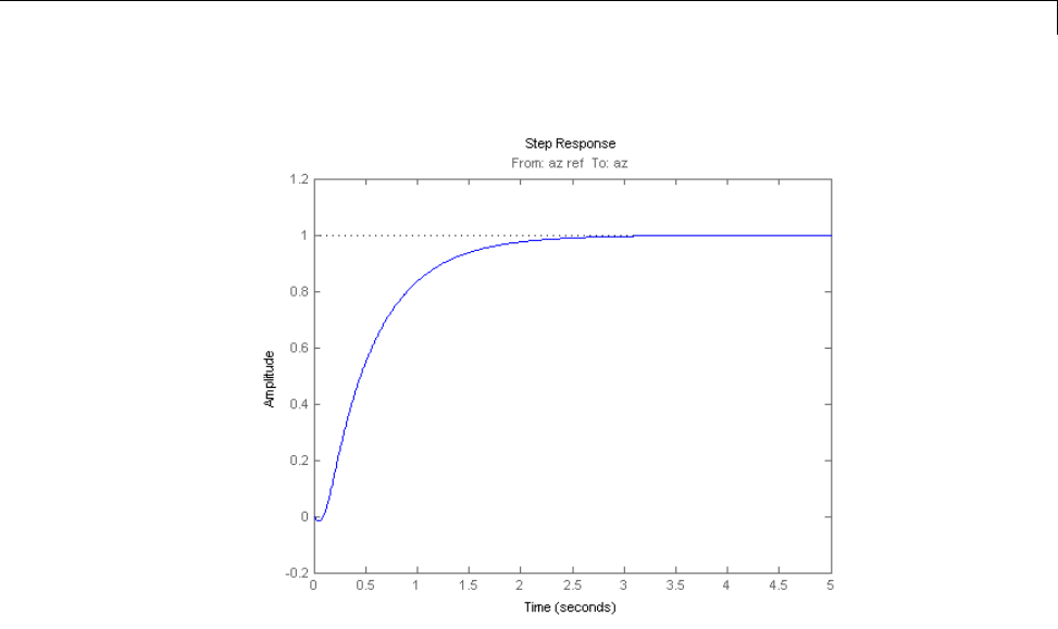
Using Parallel Computing to Accelerate Tuning
YoucannowclosetheMATLABpooltoreleasethedistributedcomputing
resources used by looptune.
matlabpool close
Sending a stop signal to all the workers ... stopped.
6-109
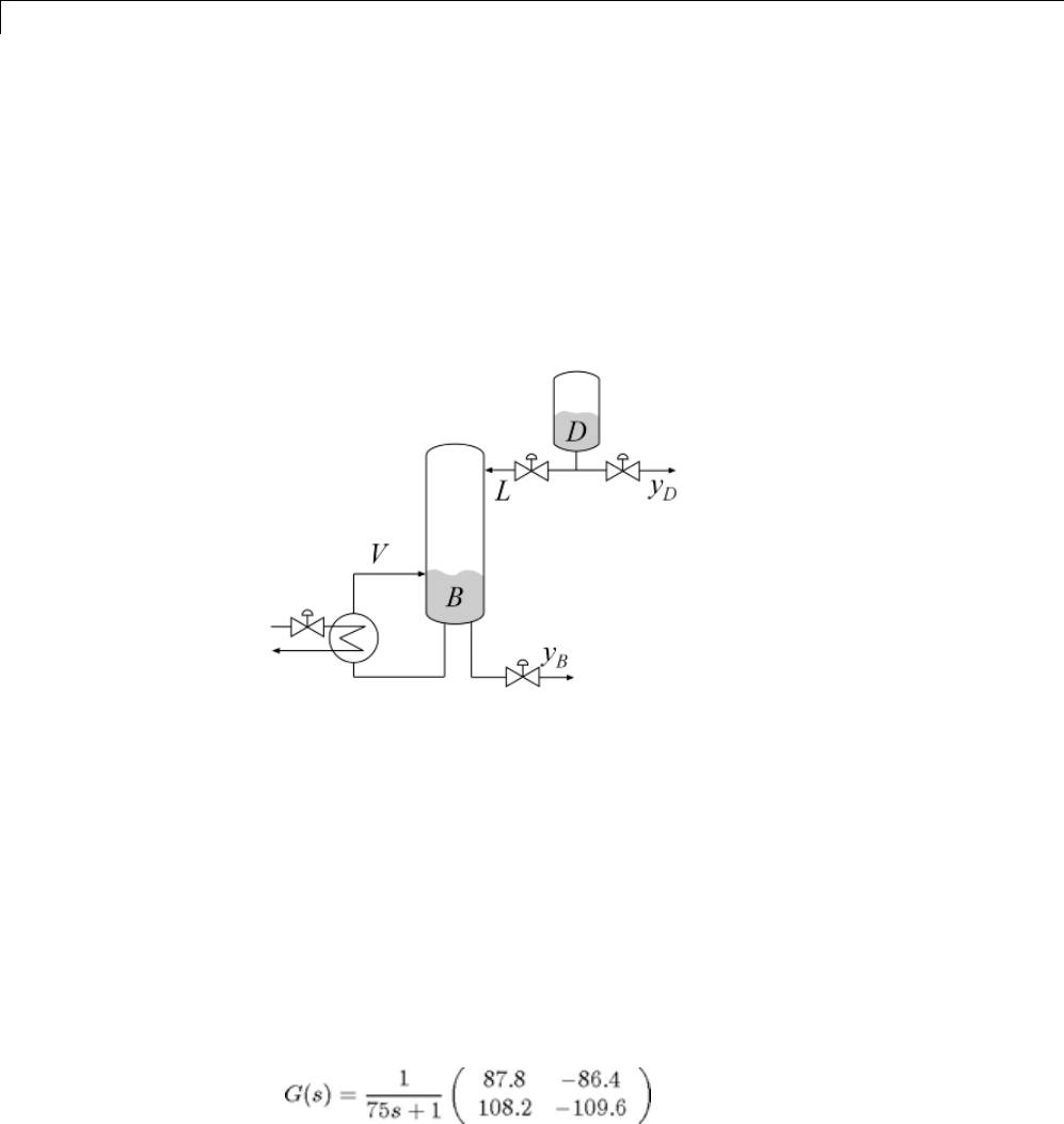
6Tuning Fixed Control Architectures
Decoupling Controller for a Distillation Column
ThisexampleshowshowtouseRobustControlToolbox™todecouplethetwo
main feedback loops in a distillation column.
Distillation Column Model
This example uses a simple model of the distillation column shown below.
Figure 1: Distillation Column
In the so-called LV configuration, the controlled variables are the
concentrations yD and yB of the chemicals D(tops) and B(bottoms), and
the manipulated variables are the reflux Land boilup V. This process
exhibits strong coupling and large variations in steady-state gain for some
combinations of L and V. For more details, see Skogestad and Postlethwaite,
Multivariable Feedback Control.
The plant is modeled as a first-order transfer function with inputs L,V and
outputs yD,yB:
6-110
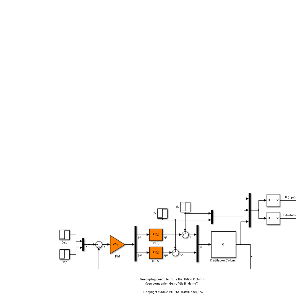
Decoupling Controller for a Distillation Column
s = tf('s','TimeUnit','minutes');
G = [87.8 -86.4 ; 108.2 -109.6]/(75*s+1);
G.InputName = {'L','V'};
G.OutputName = {'yD','yB'};
Control Architecture
The control objectives are as follows:
•Independent control of the tops and bottoms concentrations by ensuring
that a change in the tops setpoint Dsp has little impact on the bottoms
concentration Band vice versa
•Response time of about 15 minutes
•Fast rejection of input disturbances affecting the effective reflux Land
boilup V
To achieve these objectives we use the control architecture shown below. This
architecture consists of a static decoupling matrix DM in series with two PI
controllers for the reflux Land boilup V.
open_system('rct_distillation')
6-111

6Tuning Fixed Control Architectures
Controller Tuning in Simulink with LOOPTUNE
The looptune command provides a quick way to tune MIMO feedback loops.
When the control system is modeled in Simulink, you just specify the tuned
blocks, the control and measurement signals, and the desired bandwidth,
and looptune automatically sets up the problem and tunes the controller
parameters. looptune shapes the open-loop response to provide integral
action, roll-off, and adequate MIMO stability margins.
Use the slTunable interfacetospecifythetunedblocks,plant/controller
boundary, and signals for closed-loop validation.
% Tuned blocks (specified by their name in the model)
ST0 = slTunable('rct_distillation',{'PI_L','PI_V','DM'});
% Control and measurement signals
ST0.addControl({'L','V'})
ST0.addMeasurement('y')
% Analysis I/Os
ST0.addIO('r','in') % reference inputs
ST0.addIO({'dL','dV'},'in') % disturbances
Use TuningGoal objects to express the design requirements. Specify that each
loop should respond to a step command in about 15 minutes with minimum
cross-coupling.
TR = TuningGoal.Tracking('r','y',15);
Set the control bandwidth by using [0.1,0.5] as gain crossover band for the
open-loop response.
wc = [0.1,0.5];
To enforce fast disturbance rejection, limit the gain from disturbance inputs
to yD,yB as shown in the plot below. This seeks to reject disturbances at low
frequency and attenuate their effect up to the control bandwidth wc.The
desired gain profile is sketched with a few frequency points.
MaxGain = frd([0.05 5 5],[0.001 0.1 10],'TimeUnit','min');
DR = TuningGoal.MaxGain({'dL','dV'},'y',MaxGain);
6-112
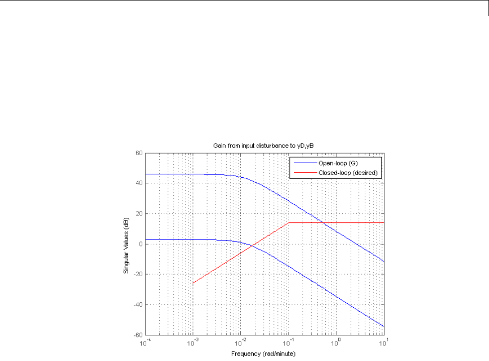
Decoupling Controller for a Distillation Column
% Plot gain limit and compare with open-loop gain
sigma(G,'b',MaxGain,'r'), grid
title('Gain from input disturbance to yD,yB')
legend('Open-loop (G)','Closed-loop (desired)')
Next use looptune to tune the controller blocks PI_L,PI_V,andDM subject to
these requirements.
[ST,gam,Info] = ST0.looptune(wc,TR,DR);
Final: Peak gain = 1.03, Iterations = 92
The final value is near 1 which indicates that all requirements were met. Use
loopview to check the resulting design. The responses should stay outside
the shaded areas.
ST.loopview(Info)
6-113
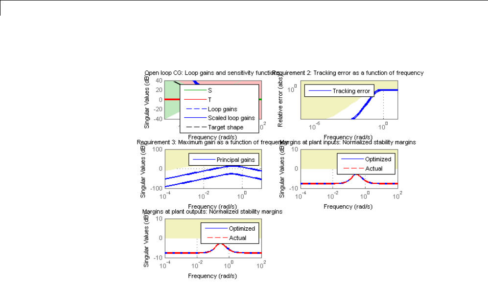
6Tuning Fixed Control Architectures
Finally, use getIOTransfer to access and plot the closed-loop responses
from reference and disturbance to the tops and bottoms concentrations. The
tuned responses show a good compromise between tracking and disturbance
rejection.
clf
Ttrack = ST.getIOTransfer('r','y');
step(Ttrack,50), grid, title('Setpoint tracking')
6-114
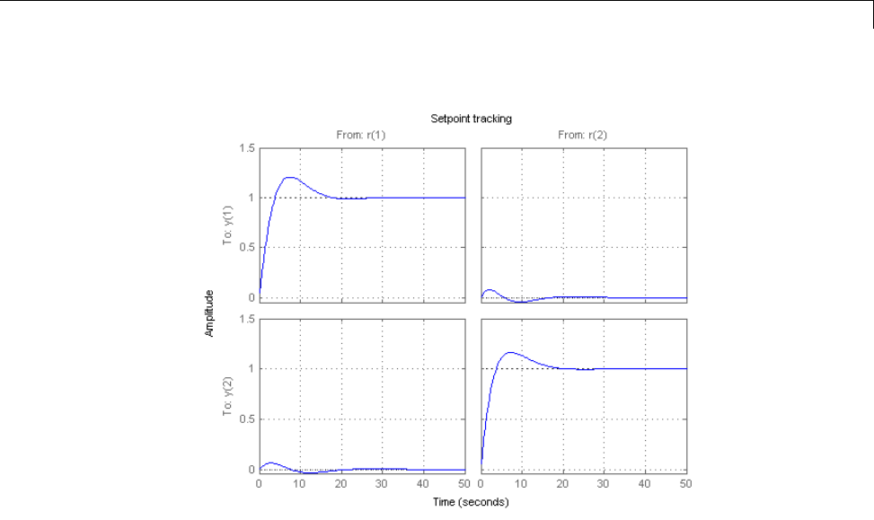
Decoupling Controller for a Distillation Column
Treject = ST.getIOTransfer({'dV','dL'},'y');
step(Treject,50), grid, title('Disturbance rejection')
6-115
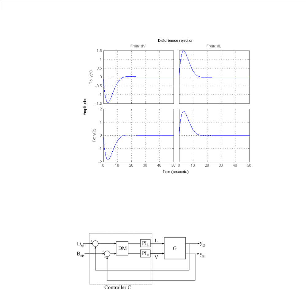
6Tuning Fixed Control Architectures
Equivalent Workflow in MATLAB
If you do not have a Simulink model of the control system, you can use LTI
objects and Control Design blocks to create a MATLAB representation of
the following block diagram.
Figure 2: Block Diagram of Control System
6-116

Decoupling Controller for a Distillation Column
First parameterize the tunable elements using Control Design blocks. Use
the ltiblock.gain block to parameterize DM:
DM = ltiblock.gain('Decoupler',eye(2));
This creates a 2x2 static gain with four tunable parameters. Similarly, use
the ltiblock.pid block to parameterize the two PI controllers:
PI_L = ltiblock.pid('PI_L','pi'); PI_L.TimeUnit = 'minutes';
PI_V = ltiblock.pid('PI_V','pi'); PI_V.TimeUnit = 'minutes';
At this point, the tunable elements are over-parameterized because
multiplying DM by two and dividing the PI coefficients by two does not change
the overall controller. To eliminate redundant parameters, normalize the PI
controllers by fixing their proportional gain Kp to 1:
PI_L.Kp.Value = 1; PI_L.Kp.Free = false;
PI_V.Kp.Value = 1; PI_V.Kp.Free = false;
Next construct a model C0 of the controller in Figure 2.
C0 = blkdiag(PI_L,PI_V) * DM * [eye(2) -eye(2)];
% Note: I/O names should be consistent with those of G
C0.InputName = {'Dsp','Bsp','yD','yB'};
C0.OutputName = {'L','V'};
Now tune the controller parameters with looptune as done previously.
% Tracking requirement
TR = TuningGoal.Tracking({'Dsp','Bsp'},{'yD','yB'},15);
% Disturbance rejection requirement
DR = TuningGoal.MaxGain({'L','V'},{'yD','yB'},MaxGain);
% Crossover band
wc = [0.1,0.5];
[~,C] = looptune(G,C0,wc,TR,DR);
Final: Peak gain = 1.04, Iterations = 77
6-117

6Tuning Fixed Control Architectures
To validate the design, close the loop with the tuned compensator Cand
simulate the step responses for setpoint tracking and disturbance rejection.
Also compare the open- and closed-loop disturbance rejection characteristics
in the frequency domain.
Tcl = connect(G,C,{'Dsp','Bsp','L','V'},{'yD','yB'});
Ttrack = Tcl(:,[1 2]);
step(Ttrack,50), grid, title('Setpoint tracking')
Treject = Tcl(:,[3 4]);
Treject.InputName = {'dL','dV'};
step(Treject,50), grid, title('Disturbance rejection')
6-118
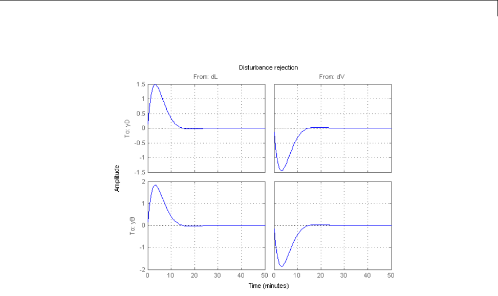
Decoupling Controller for a Distillation Column
clf, sigma(G,Treject), grid
title('Rejection of input disturbances')
legend('Open-loop','Closed-loop')
6-119
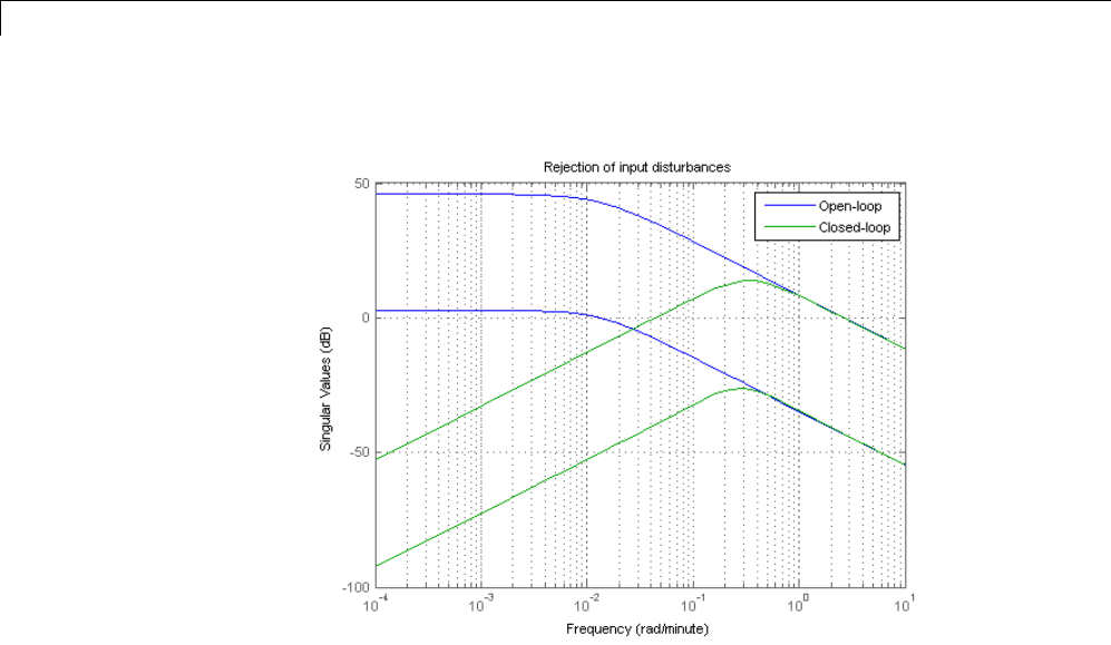
6Tuning Fixed Control Architectures
The results are similar to those obtained in Simulink.
6-120
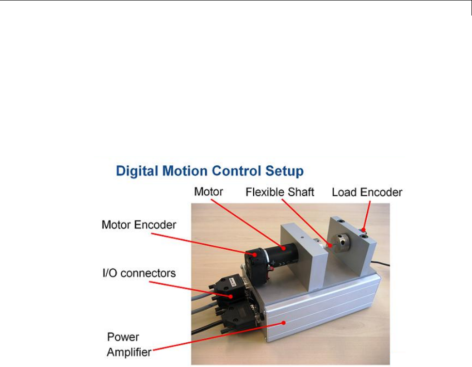
Tuning of a Digital Motion Control System
Tuning of a Digital Motion Control System
This example shows how to use Robust Control Toolbox™ to tune a digital
motion control system.
Motion Control System
The motion system under consideration is shown below.
Figure 1: Digital Motion Control Hardware
This device could be part of some production machine and is intended to move
some load (a gripper, a tool, a nozzle, or anything else that you can imagine)
from one angular position to another and back again. This task is part of the
"production cycle" that has to be completed to create each product or batch
of products.
The digital controller must be tuned to maximize the production speed of the
machine without compromising accuracy and product quality. To do this,
6-121
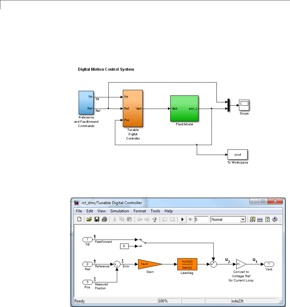
6Tuning Fixed Control Architectures
we first model the control system in Simulink using a 4th-order model of
the inertia and flexible shaft:
open_system('rct_dmc')
The "Tunable Digital Controller" consists of a gain in series with a lead/lag
controller.
6-122
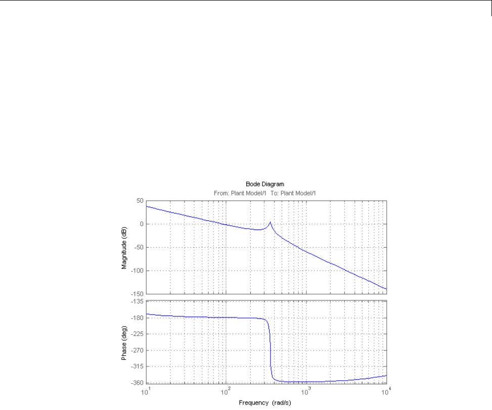
Tuning of a Digital Motion Control System
Figure 2: Digital Controller
Tuning is complicated by the presence of a flexible mode near 350 rad/s
in the plant:
G = linearize('rct_dmc','rct_dmc/Plant Model');
bode(G,{10,1e4}), grid
Compensator Tuning
We are seeking a 0.5 second response time to a step command in angular
position with minimum overshoot. This corresponds to a target bandwidth
of approximately 5 rad/s. The looptune command offers a convenient way
to tune fixed-structure compensators like the one in this application. To use
looptune, first instantiate the slTunable interface to automatically acquire
the control structure from Simulink. This requires specifying the tuned blocks
and the control and measurement signals (to delimit the controller).
6-123

6Tuning Fixed Control Architectures
ST0 = slTunable('rct_dmc',{'Gain','Leadlag'});
ST0.addControl('Leadlag');
ST0.addMeasurement('Measured Position');
Next use looptune to tune the compensator parameters for the target gain
crossover frequency of 5 rad/s:
ST1 = ST0.looptune(5);
Final: Peak gain = 0.975, Iterations = 21
A final value below or near 1 indicates success. Inspect the tuned values of
the gain and lead/lag filter:
ST1.showBlockValue
Block "rct_dmc/Tunable Digital Controller/Gain" =
Value =
d=
u1
y1 2.757e-06
Name: Gain
Static gain.
-----------------------------------
Block "rct_dmc/Tunable Digital Controller/Leadlag" =
Value =
30.53 s + 59.01
---------------
s + 18.97
Name: Leadlag
Continuous-time transfer function.
6-124
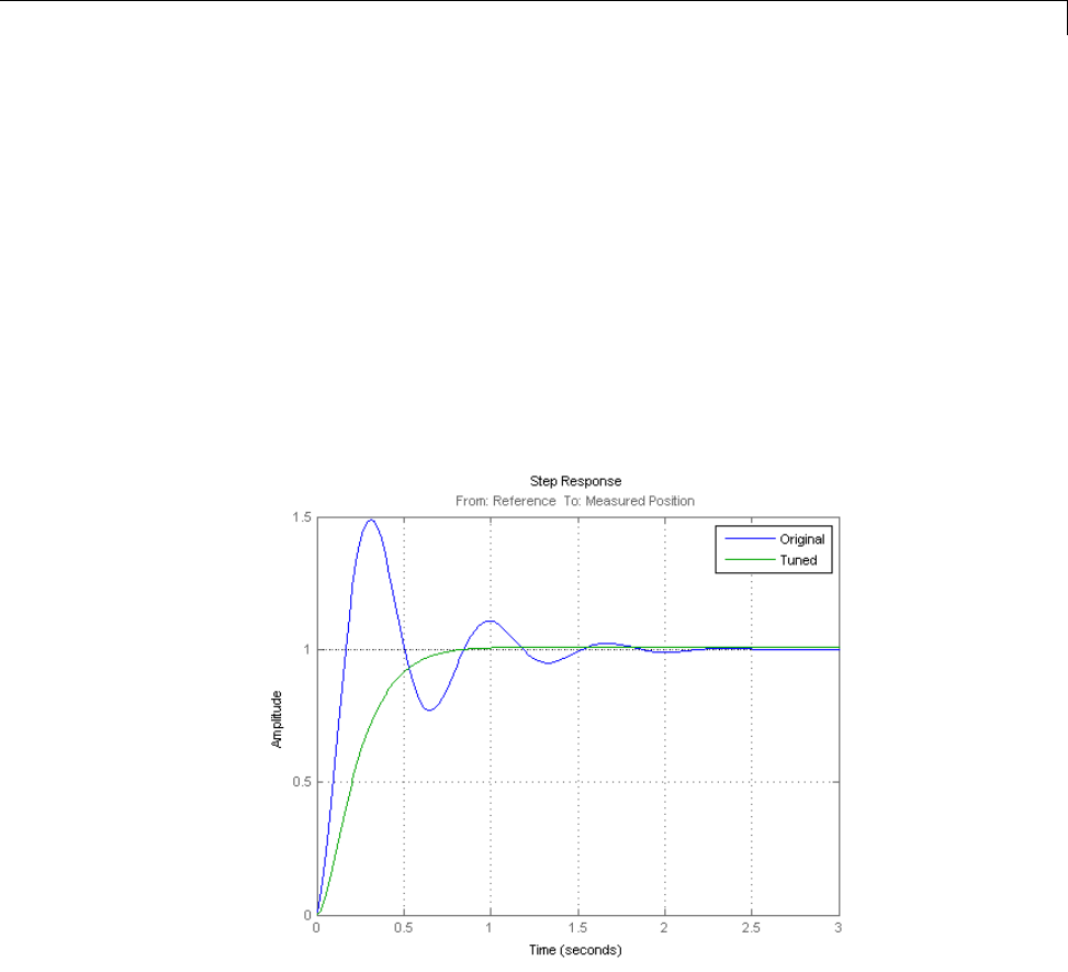
Tuning of a Digital Motion Control System
Design Validation
To validate the design, use the slTunable interface to quickly access the
closed-loop transfer functions of interest and compare the responses before
and after tuning.
T0 = ST0.getIOTransfer('Reference','Measured Position');
T1 = ST1.getIOTransfer('Reference','Measured Position');
step(T0,T1), grid
legend('Original','Tuned')
The tuned response has significantly less overshoot and satisfies the
response time requirement. However these simulations are obtained using
a continuous-time lead/lag compensator (looptune operates in continuous
time)soweneedtofurthervalidatethedesigninSimulinkusingadigital
implementation of the lead/lag compensator. Use writeBlockValue to apply
6-125
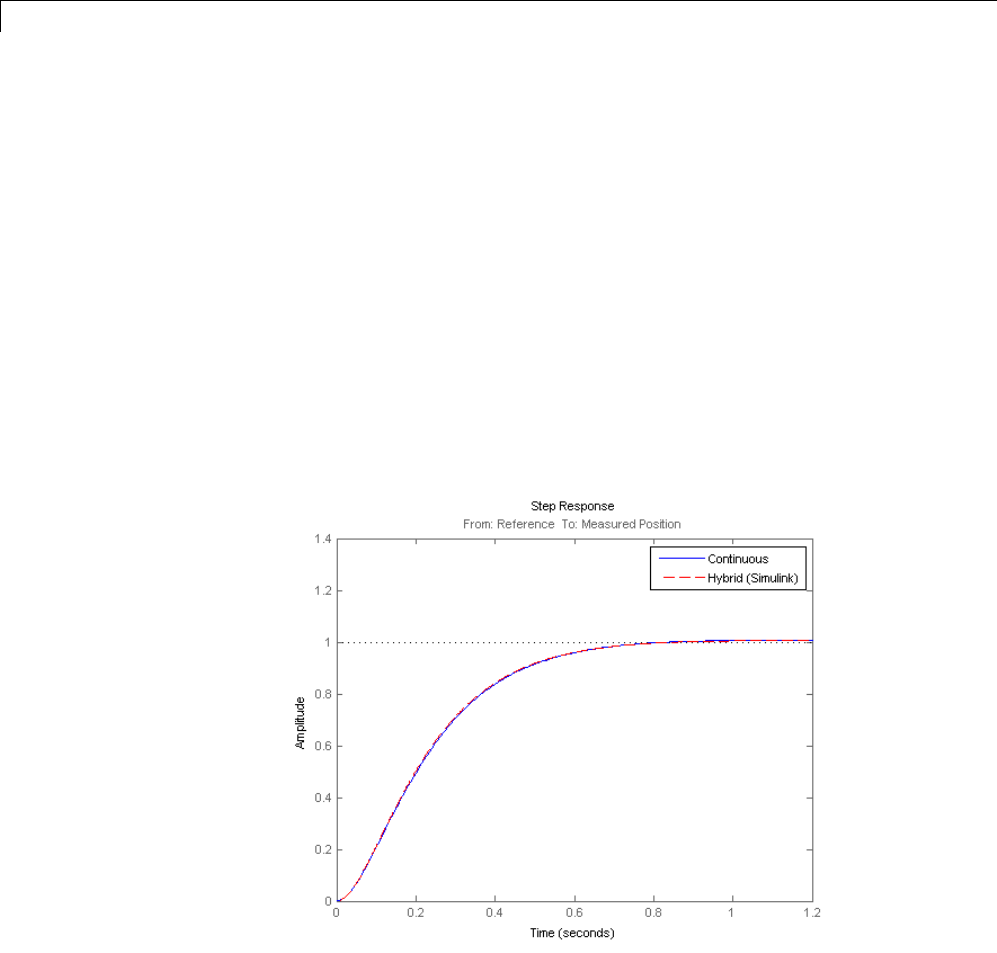
6Tuning Fixed Control Architectures
the tuned values to the Simulink model and automatically discretize the
lead/lag compensator to the rate specified in Simulink.
ST1.writeBlockValue
You can now simulate the response of the continuous-time plant with the
digital controller:
sim('rct_dmc'); % angular position logged in "yout" variable
t = yout.time;
y = yout.signals.values;
step(T1), hold, plot(t,y,'r--')
legend('Continuous','Hybrid (Simulink)')
Current plot held
The simulations closely match and the coefficients of the digital lead/lag can
be read from the "Leadlag" block in Simulink.
Tuning an Additional Notch Filter
6-126

Tuning of a Digital Motion Control System
Next try to increase the control bandwidth from 5 to 50 rad/s. Because of
the plant resonance near 350 rad/s, the lead/lag compensator is no longer
sufficient to get adequate stability margins and small overshoot. One remedy
is to add a notch filter as shown in Figure 3.
Figure 3: Digital Controller with Notch Filter
To tune this modified control architecture, specify the tunable blocks and
controller I/Os as before:
ST0 = slTunable('rct_dmcNotch',{'Gain','Leadlag','Notch'});
ST0.addControl('Notch');
ST0.addMeasurement('Measured Position');
By default the "Notch" block is parameterized as any second-order transfer
function. To retain the notch structure
specify the coefficients as real parameters and create a parametric
model Nof the transfer function shown above:
6-127

6Tuning Fixed Control Architectures
wn = realp('wn',300);
zeta1 = realp('zeta1',1); zeta1.Maximum = 1; % zeta1 <= 1
zeta2 = realp('zeta2',1); zeta2.Maximum = 1; % zeta2 <= 1
N = tf([1 2*zeta1*wn wn^2],[1 2*zeta2*wn wn^2]); % tunable notch filter
Then associate this parametric notch model with the "Notch" block in the
Simulink model. Because the control system is tuned in the continuous time,
you can use a continuous-time parameterization of the notch filter even
though the "Notch" block itself is discrete.
ST0.setBlockParam('Notch',N);
Next use looptune to jointly tune the "Gain", "Leadlag", and "Notch" blocks
with a 50 rad/s target crossover frequency. To eliminate residual oscillations
from the plant resonance, specify a target loop shape with a -40 dB/decade
roll-off past 50 rad/s.
% Specify target loop shape with a few frequency points
Freqs = [5 50 500];
Gains = [10 1 0.01];
TLS = TuningGoal.LoopShape('Notch',frd(Gains,Freqs));
ST2 = ST0.looptune(TLS);
Final: Peak gain = 1.05, Iterations = 66
The final gain is close to 1, indicating that all requirements are met. Compare
the closed-loop step response with the previous designs.
T2 = ST2.getIOTransfer('Reference','Measured Position');
clf
step(T0,T1,T2,1.5), grid
legend('Original','Lead/lag','Lead/lag + notch')
6-128
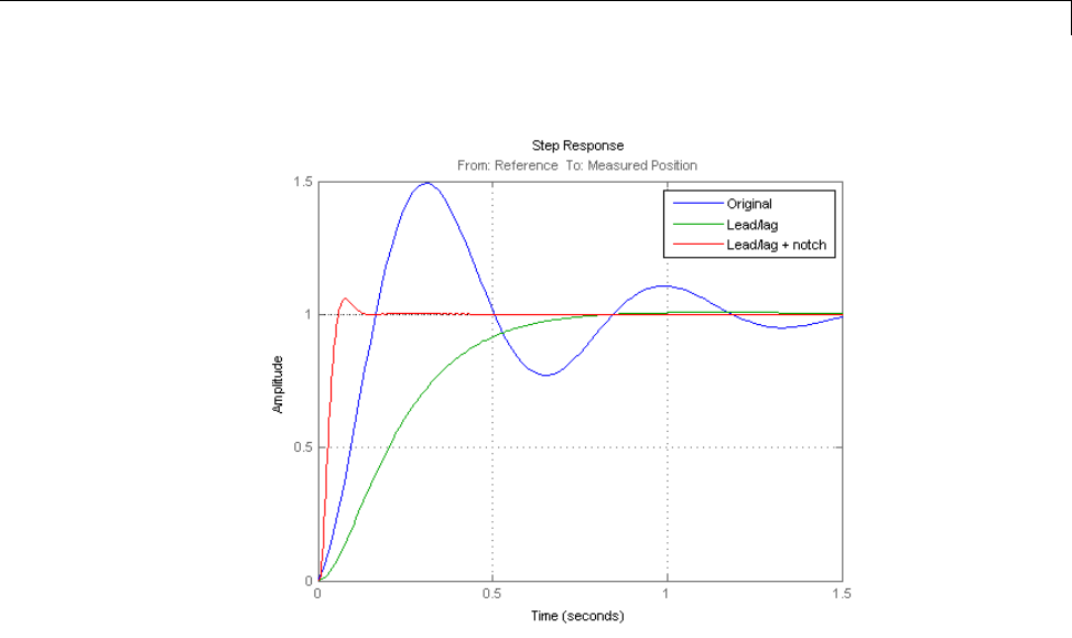
Tuning of a Digital Motion Control System
To verify that the notch filter performs as expected, evaluate the total
compensator Cand the open-loop response Land compare the Bode responses
of G,C,L:
% Get tuned block values (in the order blocks are listed in ST2.TunedBlock
s
[g,LL,N] = ST2.getBlockValue();
C=N*LL*g;
L = ST2.getLoopTransfer('Notch',-1);
bode(G,C,L,{1e1,1e3}), grid
legend('G','C','L')
6-129
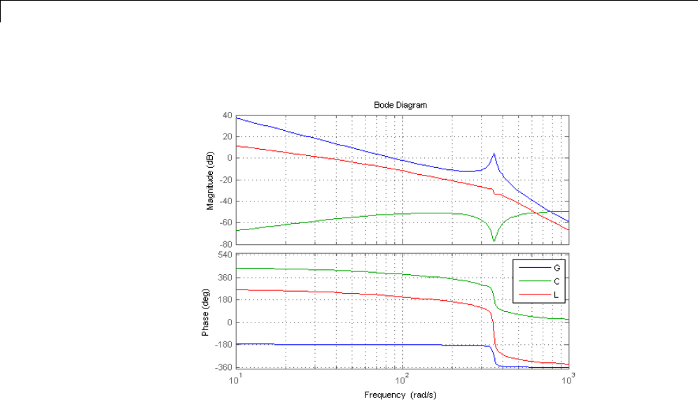
6Tuning Fixed Control Architectures
This Bode plot confirms that the plant resonance has been correctly "notched
out."
Discretizing the Notch Filter
Again use writeBlockValue to discretize the tuned lead/lag and notch
filters and write their values back to Simulink. Compare the MATLAB and
Simulink responses:
ST2.writeBlockValue
sim('rct_dmcNotch');
t = yout.time;
y = yout.signals.values;
step(T2), hold, plot(t,y,'r--')
legend('Continuous','Hybrid (Simulink)')
Current plot held
6-130
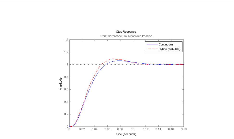
Tuning of a Digital Motion Control System
The Simulink response exhibits small residual oscillations. The notch filter
discretization is the likely culprit because the notch frequency is close to the
Nyquist frequency pi/0.002=1570 rad/s. By default the notch is discretized
using the ZOH method. Compare this with the Tustin method prewarped at
the notch frequency:
wn = damp(N); % natural frequency of the notch filter
Ts = 0.002; % sample time of discrete notch filter
Nd1 = c2d(N,Ts,'zoh');
Nd2 = c2d(N,Ts,'tustin',c2dOptions('PrewarpFrequency',wn(1)));
clf, bode(N,Nd1,Nd2)
legend('Continuous','Discretized with ZOH','Discretized with Tustin',...
'Location','NorthWest')
6-131
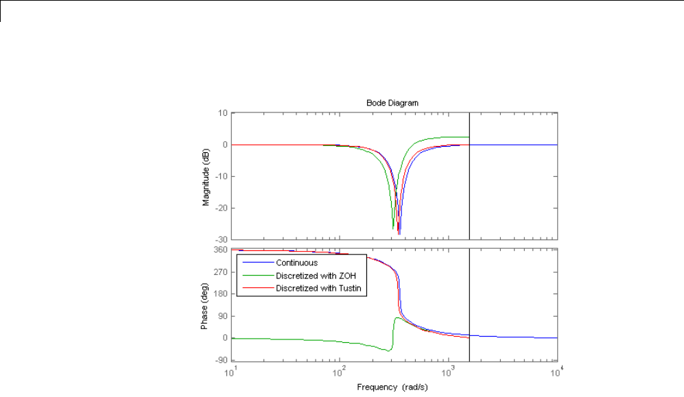
6Tuning Fixed Control Architectures
The ZOH method has significant distortion and prewarped Tustin should
be used instead. To do this, specify the desired rate conversion method for
the notch filter block:
ST2.setBlockRateConversion('Notch','tustin',wn(1))
ST2.writeBlockValue
writeBlockValue now uses Tustin prewarped at the notch frequency to
discretize the notch filter and write it back to Simulink. Verify that this gets
rid of the oscillations.
sim('rct_dmcNotch');
t = yout.time;
y = yout.signals.values;
step(T2), hold, plot(t,y,'r--')
legend('Continuous','Hybrid (Simulink)')
Current plot held
6-132
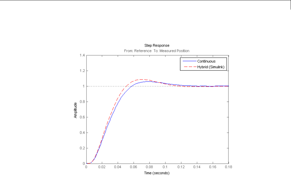
Tuning of a Digital Motion Control System
6-133
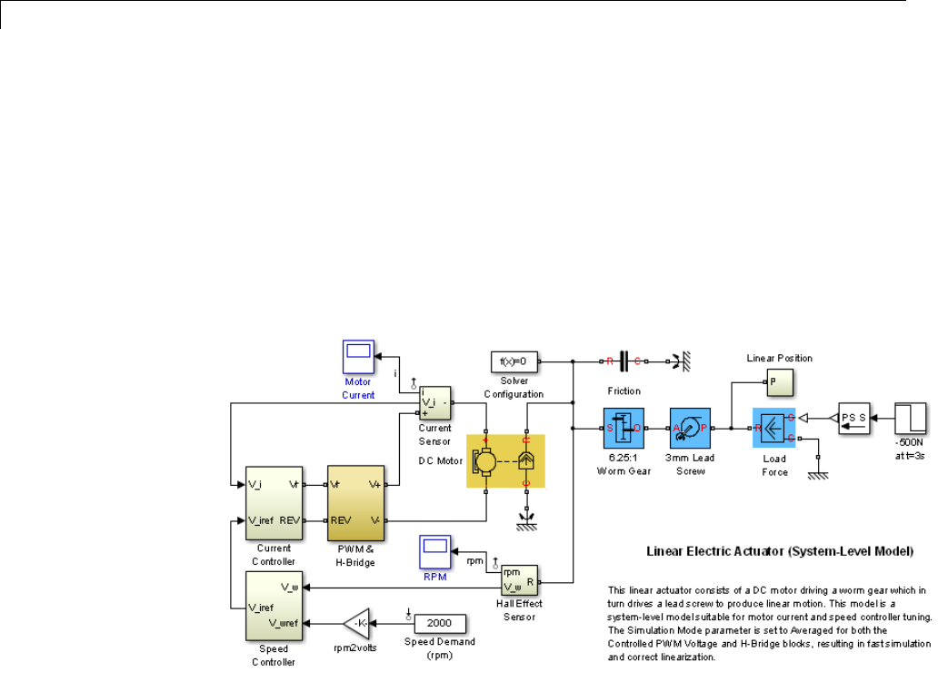
6Tuning Fixed Control Architectures
Control of a Linear Electric Actuator
This example shows how to use Robust Control Toolbox™ to tune the current
and velocity loops in a linear electric actuator with saturation limits.
Linear Electric Actuator Model
Open the Simulink model of the linear electric actuator:
open_system('rct_linact')
The electrical and mechanical components are modeled using SimElectronics
and SimMechanics. The control system consists of two cascaded feedback
loops controlling the driving current and angular speed of the DC motor.
6-134
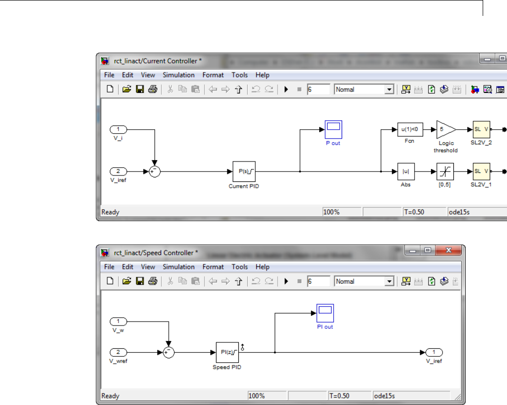
Control of a Linear Electric Actuator
Figure 1: Current and Speed Controllers.
Note that the inner-loop (current) controller is a proportional gain while the
outer-loop (speed) controller has proportional and integral actions. The output
of both controllers is limited to plus/minus 5.
Design Specifications
6-135
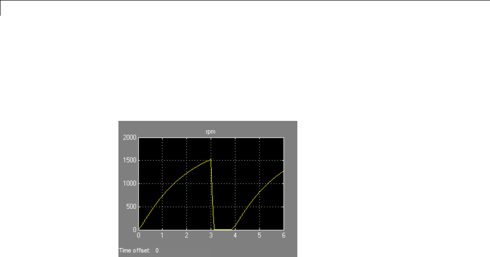
6Tuning Fixed Control Architectures
We need to tune the proportional and integral gains to respond to a 2000 rpm
speed demand in about 0.1 seconds with minimum overshoot. The initial gain
settings in the model are P=50 and PI(s)=0.2+0.1/s and the corresponding
response is shown in Figure 2. This response is too slow and too sensitive
to load disturbances.
Figure 2: Untuned Response.
Control System Tuning
You can use systune to jointly tune both feedback loops. To set up the design,
create an instance of the slTunable interface with the list of tuned blocks. All
blocks and signals are specified by their names in the model. The model is
linearized at t=0.5 to avoid discontinuities in some derivatives at t=0.
TunedBlocks = {'Current PID','Speed PID'};
op = findop('rct_linact',0.5); % linearize at t=0.5
% Create tuning interface
ST0 = slTunable('rct_linact',TunedBlocks,op);
The data structure ST0 contains a description of the control system and its
tunable elements. Next specify that the DC motor should follow a 2000 rpm
speed demand in 0.1 seconds:
TR = TuningGoal.Tracking('Speed Demand (rpm)','rpm',0.1);
6-136
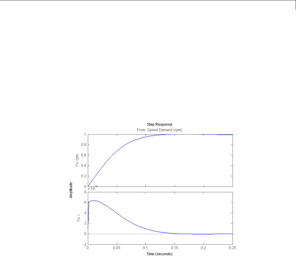
Control of a Linear Electric Actuator
You can now tune the proportional and integral gains with looptune:
ST1 = systune(ST0,TR);
Final: Soft = 1.12, Hard = -Inf, Iterations = 25
This returns an updated description ST1 containing the tuned gain values. To
validate this design, plot the closed-loop response from speed demand to speed:
T1 = ST1.getIOTransfer('Speed Demand (rpm)',{'rpm','i'});
step(T1)
The response looks good in the linear domain so push the tuned gain values to
Simulink and further validate the design in the nonlinear model.
ST1.writeBlockValue()
The nonlinear simulation results appear in Figure 3. The nonlinear behavior
isfarworsethanthelinearapproximation, a discrepancy that can be traced
to saturations in the inner loop (see Figure 4).
6-137
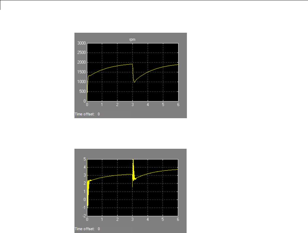
6Tuning Fixed Control Architectures
Figure 3: Nonlinear Simulation of Tuned Controller.
Figure 4: Current Controller Output (limited to plus/minus 5).
% Close model to discard this first set of tuned gains
close_system('rct_linact',0)
Preventing Saturations
So far we have only specified a desired response time for the outer (speed)
loop. This leaves systune free to allocate the control effort between the inner
and outer loops. Saturations in the inner loop suggest that the proportional
gain is too high and that some rebalancing is needed. One possible remedy is
6-138

Control of a Linear Electric Actuator
to explicitly limit the gain from the speed command to the outputs of the P
and PI controllers. For a speed reference of 2000 rpm and saturation limits
of plus/minus 5, the average gain should not exceed 5/2000 = 0.0025. To be
conservative, we can try to keep the gain from speed reference to controller
outputs below 0.001. To do this, add two gain requirements and retune the
controller gains with all three requirements in place.
% Mark the outputs of the "Current PID" and "Speed PID" blocks as control
% signals so that they can be referenced in the gain requirements
ST0 = slTunable('rct_linact',TunedBlocks,op);
ST0.addControl({'Current PID','Speed PID'})
% Limit gain from speed demand to control signals to avoid saturation
MG1 = TuningGoal.Gain('Speed Demand (rpm)','Speed PID',0.001);
MG2 = TuningGoal.Gain('Speed Demand (rpm)','Current PID',0.001);
% Retune with these additional requirements
[ST2,~,~,info] = systune(ST0,[TR,MG1,MG2]);
Final: Soft = 1.39, Hard = -Inf, Iterations = 34
The final gain 1.39 indicates that the requirements are nearly but not exactly
met (all requirements are met when the final gain is less than 1). Use
viewSpec to inspect how the tuned controllers fare against each requirement.
viewSpec([TR,MG1,MG2],ST2,info)
6-139
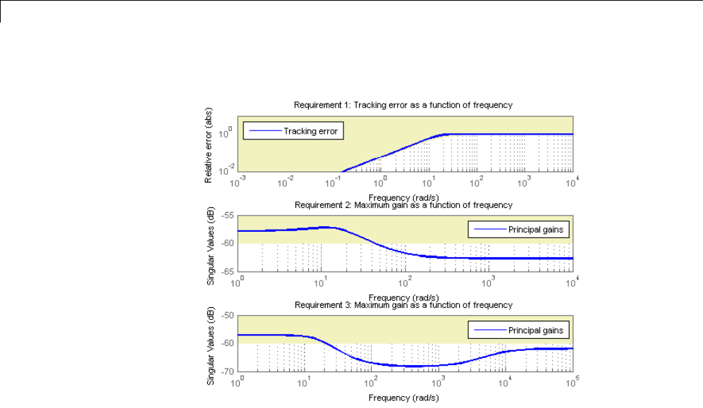
6Tuning Fixed Control Architectures
Nextcomparethetwodesignsinthelineardomain.
T2 = ST2.getIOTransfer('Speed Demand (rpm)',{'rpm','i'});
clf, step(T1,'b',T2,'g--')
legend('Initial tuning','Tuning with Gain Constraints')
6-140
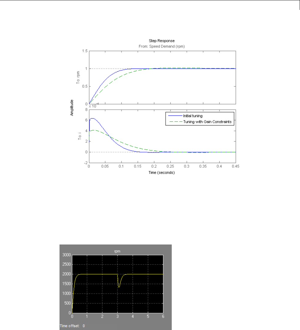
Control of a Linear Electric Actuator
The second design is less aggressive but still meets the response time
requirement. Finally, push the new tuned gain values to the Simulink model
and simulate the response to a 2000 rpm speed demand and 500 N load
disturbance. The simulation results appear in Figure 5 and the current
controller output is shown in Figure 6.
ST2.writeBlockValue()
6-141
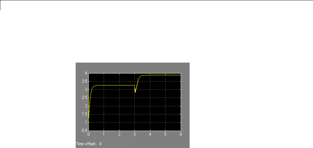
6Tuning Fixed Control Architectures
Figure 5: Nonlinear Response of Tuning with Gain Constraints.
Figure 6: Current Controller Output.
The nonlinear responses are now satisfactory and the current loop is no
longer saturating. The additional gain constraints have forced systune to
re-distribute the control effort between the inner and outer loops so as to
avoid saturation.
6-142

Active Vibration Control in Three-Story Building
Active Vibration Control in Three-Story Building
This example uses systune to control seismic vibrations in a three-story
building.
Background
This example considers an Active Mass Driver (AMD) control system for
vibration isolation in a three-story experimental structure. This setup is used
to assess control design techniques for increasing safety of civil engineering
structures during earthquakes. The structure consists of three stories with
an active mass driver on the top floor which is used to attenuate ground
disturbances. This application is borrowed from "Benchmark Problems in
Structural Control: Part I - Active Mass Driver System," B.F. Spencer Jr., S.J.
Dyke, and H.S. Deoskar, Earthquake Engineering and Structural Dynamics,
27(11), 1998, pp. 1127-1139.
6-143
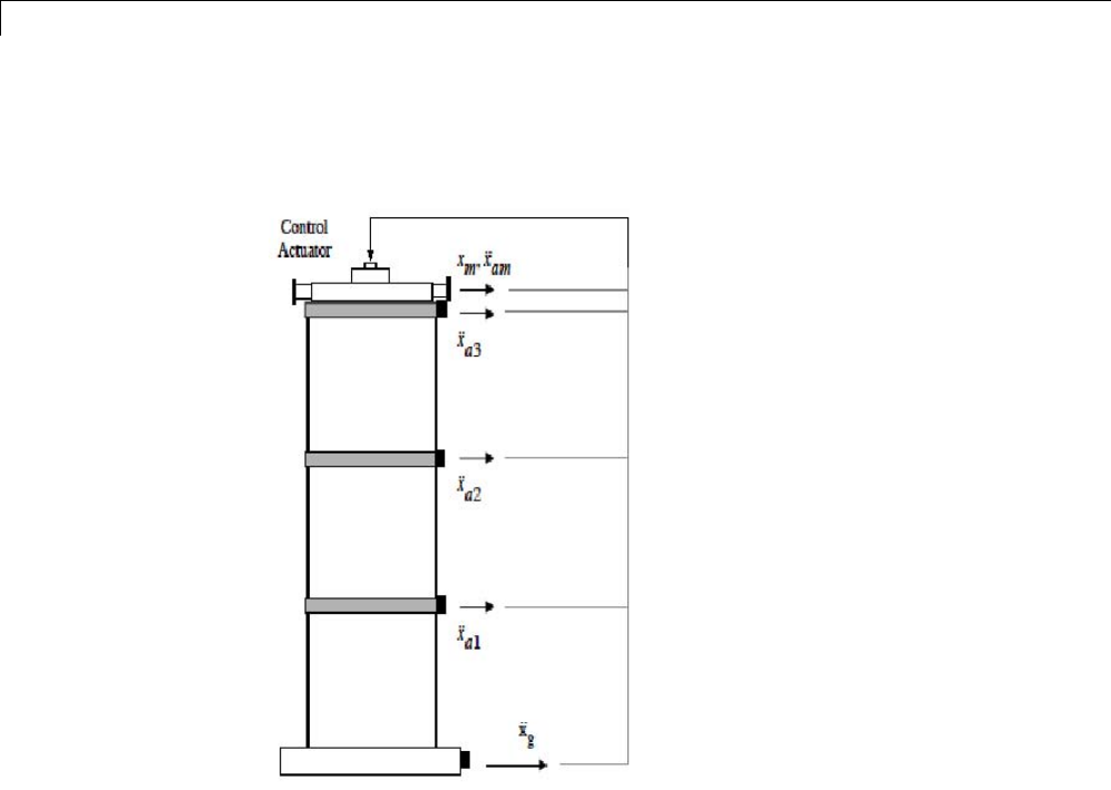
6Tuning Fixed Control Architectures
Figure 1: Active Mass Driver Control System
The plant Pis a 28-state model with the following state variables:
•x(i): displacement of i-th floor relative to the ground (cm)
•xm: displacement of AMD relative to 3rd floor (cm)
•xv(i): velocity of i-th floor relative to the ground (cm/s)
•xvm: velocity of AMD relative to the ground (cm/s)
•xa(i): acceleration of i-th floor relative to the ground (g)
•xam: acceleration of AMD relative to the ground (g)
6-144

Active Vibration Control in Three-Story Building
•d(1)=x(1),d(2)=x(2)-x(1),d(3)=x(3)-x(2): inter-story drifts
The inputs are the ground acceleration xag (in g) and the control signal u.We
use 1 g = 981 cm/s^2.
load ThreeStoryData
size(P)
State-space model with 20 outputs, 2 inputs, and 28 states.
Model of Earthquake Acceleration
The earthquake acceleration is modeled as a white noise process filtered
through a Kanai-Tajimi filter.
zg = 0.3; wg = 37.3;
S0 = 0.03*zg/(pi*wg*(4*zg^2+1));
num = sqrt(S0)*[2*zg*wg wg^2];
den = [1 2*zg*wg wg^2];
F = sqrt(2*pi)*tf(num,den);
F.InputName = 'n'; % white noise input
bodemag(F), grid, title('Kanai-Tajimi filter')
6-145
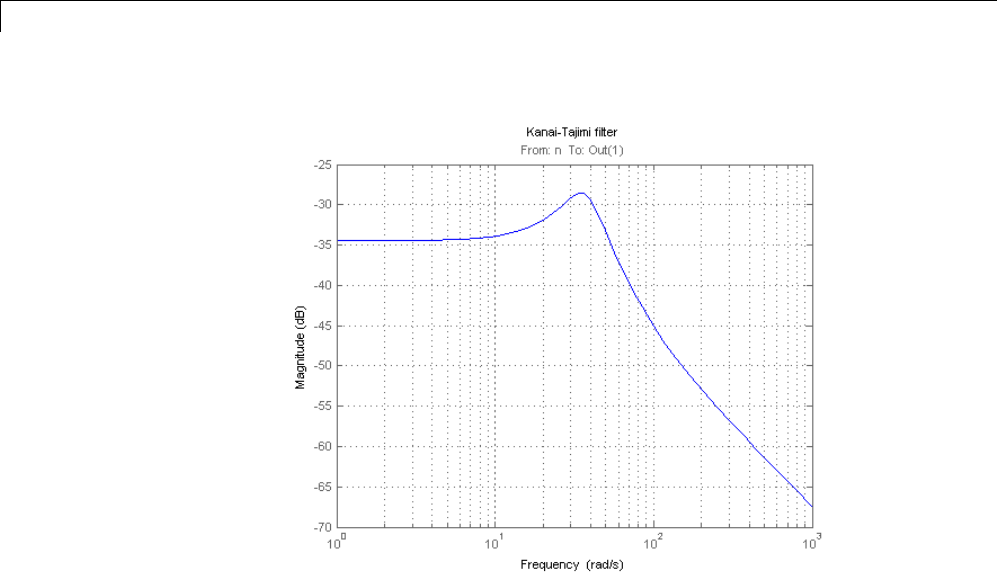
6Tuning Fixed Control Architectures
Open-Loop Characteristics
The effect of an earthquake on the uncontrolled structure can be simulated
by injecting a white noise input ninto the plant-filter combination. You can
also use covar to directly compute the standard deviations of the resulting
inter-story drifts and accelerations.
% Add Kanai-Tajimi filter to the plant
PF = P*append(F , 1);
% Standard deviations of open-loop drifts
CV = covar(PF('d','n'),1);
d0 = sqrt(diag(CV));
% Standard deviations of open-loop acceleration
CV = covar(PF('xa','n'),1);
xa0 = sqrt(diag(CV));
% Plot open-loop RMS values
6-146
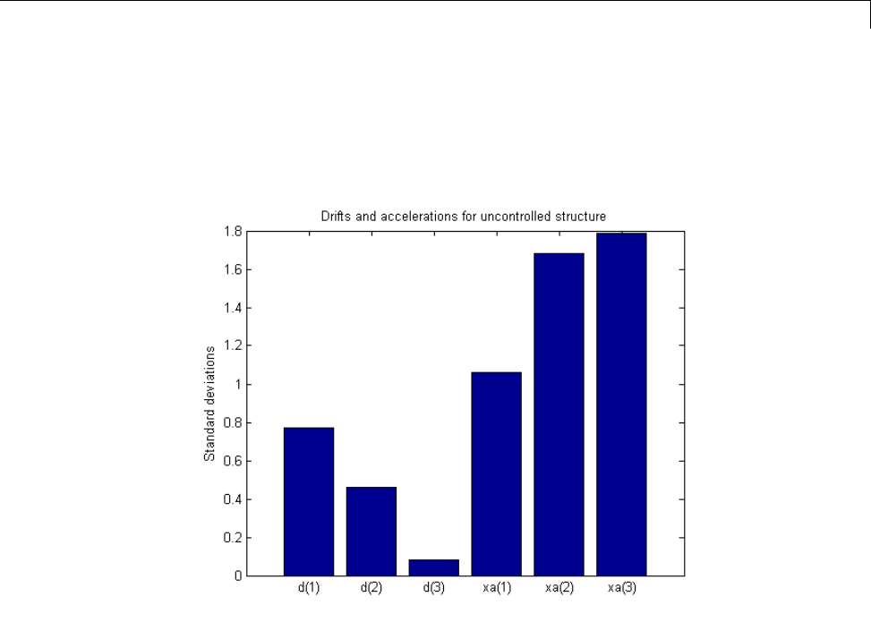
Active Vibration Control in Three-Story Building
clf, bar([d0 ; xa0])
title('Drifts and accelerations for uncontrolled structure')
ylabel('Standard deviations')
set(gca,'XTickLabel',{'d(1)','d(2)','d(3)','xa(1)','xa(2)','xa(3)'})
Control Structure and Design Requirements
The control structure is depicted in Figure 2.
6-147
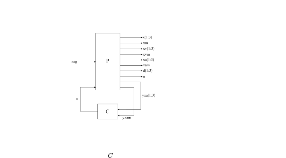
6Tuning Fixed Control Architectures
Figure 2: Control Structure
The controller uses measurements yxa and yxam of xa and xam to generate
the control signal u. Physically, the control uis an electrical current driving
an hydraulic actuator that moves the masses of the AMD. The design
requirements involve:
•Minimization of the inter-story drifts d(i) and accelerations xa(i)
•Hard constraints on control effort in terms of mass displacement xm,mass
acceleration xam, and control effort u
All design requirements are assessed in terms of standard deviations of
the corresponding signals. Use TuningGoal.Variance to express these
requirements and scale each variable by its open-loop standard deviation to
seek uniform relative improvement in all variables.
% Soft requirements on drifts and accelerations
Soft = [...
TuningGoal.Variance('n','d(1)', d0(1)) ; ...
TuningGoal.Variance('n','d(2)', d0(2)) ; ...
TuningGoal.Variance('n','d(3)', d0(3)) ; ...
TuningGoal.Variance('n','xa(1)', xa0(1)) ; ...
TuningGoal.Variance('n','xa(2)', xa0(2)) ; ...
TuningGoal.Variance('n','xa(3)', xa0(3))];
6-148

Active Vibration Control in Three-Story Building
% Hard requirements on control effort
Hard = [...
TuningGoal.Variance('n','xm', 3) ; ...
TuningGoal.Variance('n','xam', 2) ; ...
TuningGoal.Variance('n','u', 1)];
Controller Tuning
systune lets you tune virtually any controller structure subject to these
requirements. The controller complexity can be adjusted by trial-and-error,
starting with sufficiently high order to gauge the limits of performance, then
reducing the order until you observe a noticeable performance degradation.
For this example, start with a 5th-order controller with no feedthrough term.
C = ltiblock.ss('C',5,1,4);
C.d.Value = 0;
C.d.Free = false; % Fix feedthrough to zero
Construct a tunable model T0 of the closed-loop system of Figure 2 and tune
the controller parameters with systune.
% Build tunable closed-loop model
T0 = lft(PF,C);
% Tune controller parameters
[T,fSoft,gHard] = systune(T0,Soft,Hard);
Final: Soft = 0.601, Hard = 0.99898, Iterations = 138
The summary indicates that we achieved an overall reduction of 40% in
standard deviations (Soft = 0.6) while meeting all hard constraints (Hard
<1
).
Validation
Compute the standard deviations of the drifts and accelerations for the
controlled structure and compare with the uncontrolled results. The AMD
control system yields significant reduction of both drift and acceleration.
% Standard deviations of closed-loop drifts
6-149
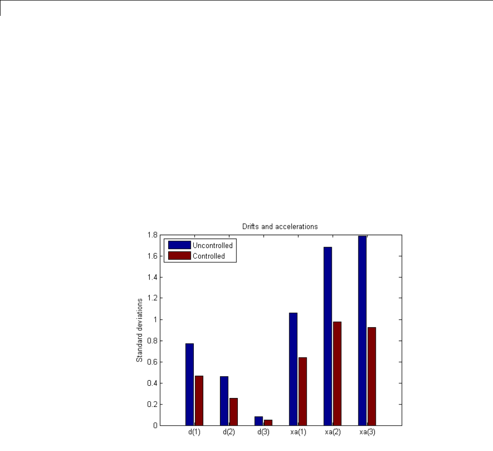
6Tuning Fixed Control Architectures
CV = covar(T('d','n'),1);
d = sqrt(diag(CV));
% Standard deviations of closed-loop acceleration
CV = covar(T('xa','n'),1);
xa = sqrt(diag(CV));
% Compare open- and closed-loop values
clf, bar([d0 d; xa0 xa])
title('Drifts and accelerations')
ylabel('Standard deviations')
set(gca,'XTickLabel',{'d(1)','d(2)','d(3)','xa(1)','xa(2)','xa(3)'})
legend('Uncontrolled','Controlled','location','NorthWest')
Simulate the response of the 3-story structure to an earthquake-like excitation
in both open and closed loop. The earthquake acceleration is modeled as a
white noise process colored by the Kanai-Tajimi filter.
% Sampled white noise process
6-150
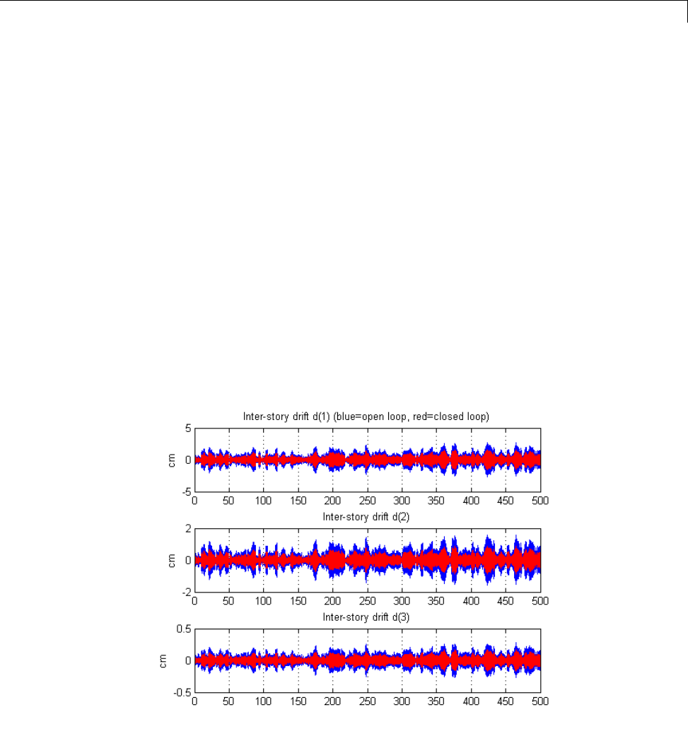
Active Vibration Control in Three-Story Building
rng('default')
dt = 1e-3;
t = 0:dt:500;
n = randn(1,length(t))/sqrt(dt); % white noise signal
% Open-loop simulation
ysimOL = lsim(PF(:,1), n , t);
% Closed-loop simulation
ysimCL = lsim(T, n , t);
% Drifts
clf, subplot(311); plot(t,ysimOL(:,13),'b',t,ysimCL(:,13),'r'); grid;
title('Inter-story drift d(1) (blue=open loop, red=closed loop)'); ylabel(
subplot(312); plot(t,ysimOL(:,14),'b',t,ysimCL(:,14),'r'); grid;
title('Inter-story drift d(2)'); ylabel('cm');
subplot(313); plot(t,ysimOL(:,15),'b',t,ysimCL(:,15),'r'); grid;
title('Inter-story drift d(3)'); ylabel('cm');
6-151
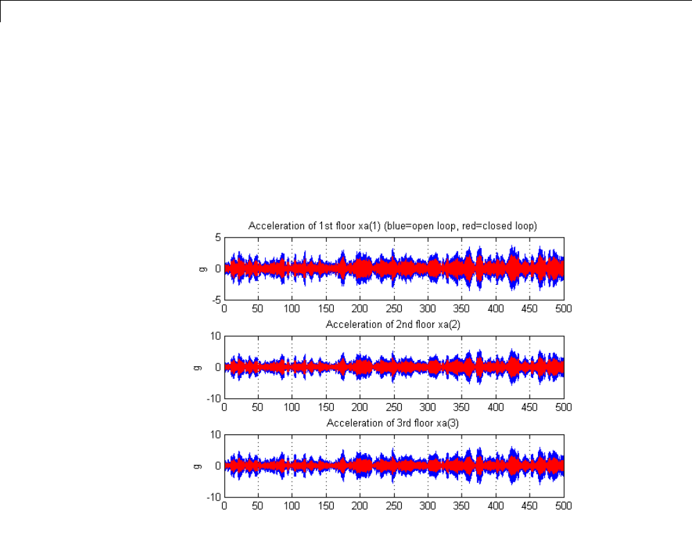
6Tuning Fixed Control Architectures
% Accelerations
clf, subplot(311); plot(t,ysimOL(:,9),'b',t,ysimCL(:,9),'r'); grid;
title('Acceleration of 1st floor xa(1) (blue=open loop, red=closed loop)');
subplot(312); plot(t,ysimOL(:,10),'b',t,ysimCL(:,10),'r'); grid;
title('Acceleration of 2nd floor xa(2)'); ylabel('g');
subplot(313); plot(t,ysimOL(:,11),'b',t,ysimCL(:,11),'r'); grid;
title('Acceleration of 3rd floor xa(3)'); ylabel('g');
% Control variables
clf, subplot(311); plot(t,ysimCL(:,4),'r'); grid;
title('AMD position xm'); ylabel('cm');
subplot(312); plot(t,ysimCL(:,12),'r'); grid;
title('AMD acceleration xam'); ylabel('g');
subplot(313); plot(t,ysimCL(:,16),'r'); grid;
title('Control signal u');
6-152
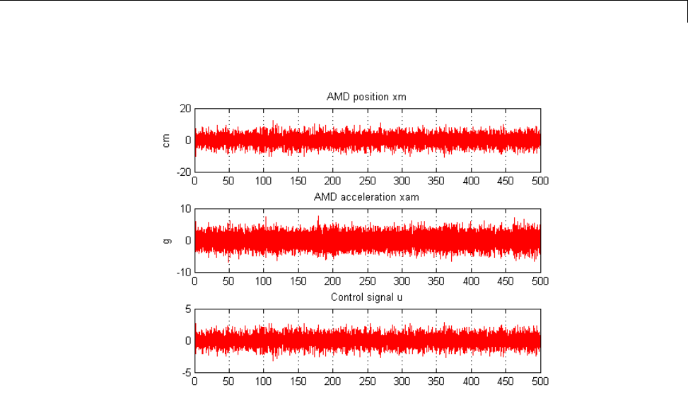
Active Vibration Control in Three-Story Building
Plot the root-mean-square (RMS) of the simulated signals for both the
controlled and uncontrolled scenarios. Assuming ergodicity, the RMS
performance can be estimated from a single sufficiently long simulation of the
process and coincides with the standard deviations computed earlier. Indeed
the RMS plot closely matches the standard deviation plot obtained earlier.
clf, bar([std(ysimOL(:,13:15)) std(ysimOL(:,9:11)) ; ...
std(ysimCL(:,13:15)) std(ysimCL(:,9:11))]')
title('Drifts and accelerations')
ylabel('Simulated RMS values')
set(gca,'XTickLabel',{'d(1)','d(2)','d(3)','xa(1)','xa(2)','xa(3)'})
legend('Uncontrolled','Controlled','location','NorthWest')
6-153
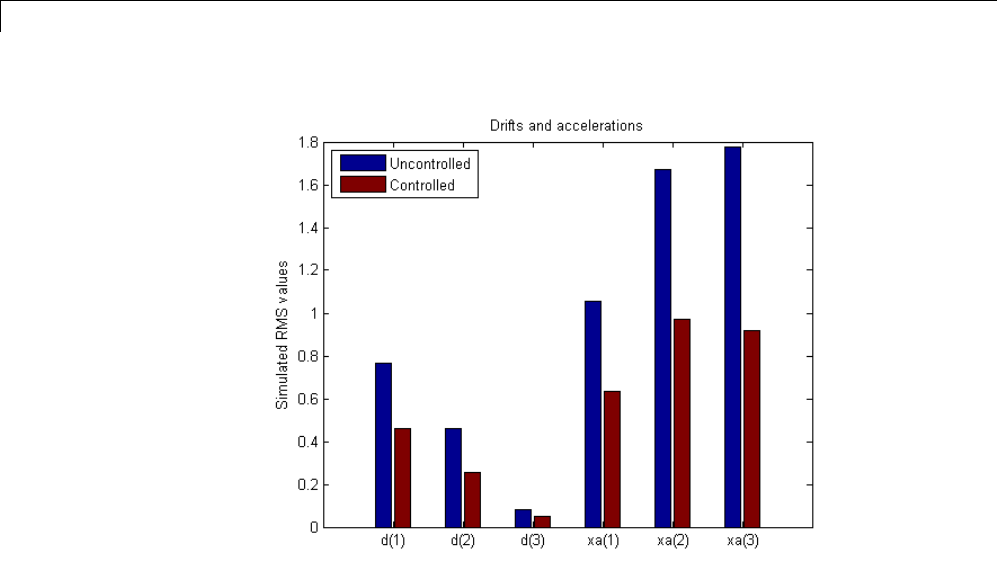
6Tuning Fixed Control Architectures
Overall, the controller achieves significant reduction of ground vibration
both in terms of drift and acceleration for all stories while meeting the hard
constraints on control effort and mass displacement.
6-154
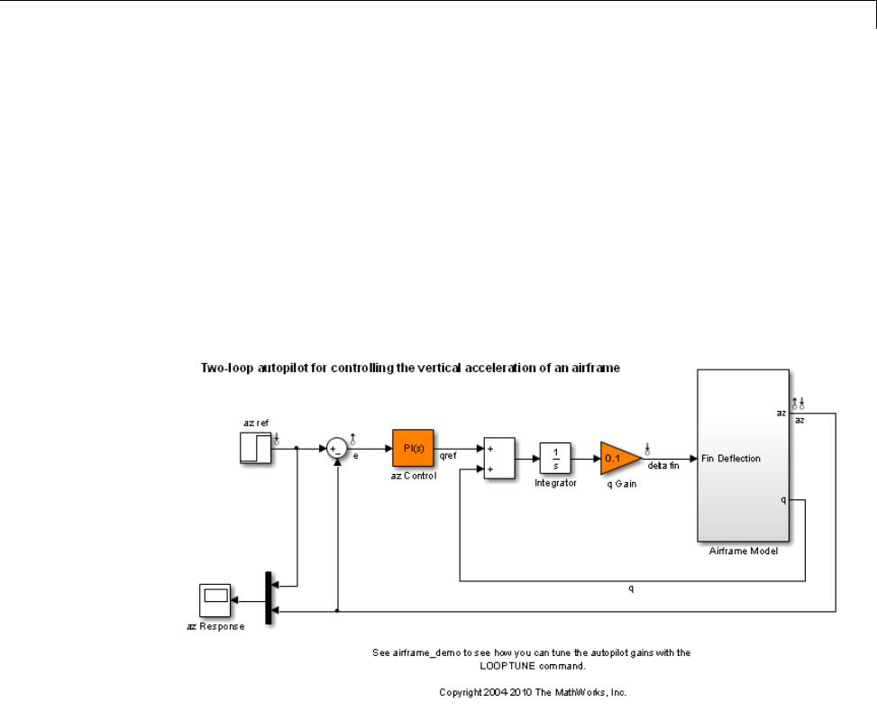
Tuning of a Two-Loop Autopilot
Tuning of a Two-Loop Autopilot
This example shows how to use Robust Control Toolbox™ to tune a two-loop
autopilot controlling the pitch rate and vertical acceleration of an airframe.
Model of Airframe Autopilot
TheairframedynamicsandtheautopilotaremodeledinSimulink. Toopen
the model, type
open_system('rct_airframe1')
The autopilot consists of two cascaded loops. The inner loop controls the pitch
rate q, and the outer loop controls the vertical acceleration az in response to
the pilot stick command azref. In this architecture, the tunable elements
include the PI controller gains ("az Control" block) and the pitch-rate gain ("q
Gain" block). The autopilot must be tuned to respond to a step command
azref in about 1 second with minimal overshoot.
To analyze the airframe dynamics, linearize the "Airframe Model" block and
plot the gains from the fin deflection delta to az and q:
6-155
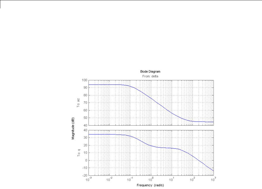
6Tuning Fixed Control Architectures
G = linearize('rct_airframe1','rct_airframe1/Airframe Model');
G.InputName = 'delta';
G.OutputName = {'az','q'};
bodemag(G), grid
Note that the airframe model has an unstable pole:
pole(G)
ans =
0.1213
-29.4685
Frequency-Domain Tuning with LOOPTUNE
6-156

Tuning of a Two-Loop Autopilot
You can use the looptune function to automatically tune multi-loop control
systems subject to basic requirements such as integral action, adequate
stability margins, and desired bandwidth. To apply looptune to the autopilot
model, create an instance of the slTunable interface and designate the
Simulink blocks az Control and qGainas tunable:
ST0 = slTunable('rct_airframe1',{'az Control','q Gain'});
Next outline the plant/controller boundary by specifying the control and
measurement signals:
ST0.addControl('delta fin');
ST0.addMeasurement({'az','q'});
Finally, tune the control system parameters to meet the 1 second response
time requirement. In the frequency domain, this roughly corresponds to a gain
crossover frequency wc = 5 rad/s for the open-loop response at the plant input
"delta fin". Run a few optimizations from random starting points to increase
the likelihood of finding a stabilizing controller for this unstable plant:
rng('default')
Options = looptuneOptions('RandomStart',10);
wc = 5;
[ST,gam,Info] = ST0.looptune(wc,Options);
gam
Final: Peak gain = 1, Iterations = 32
Final: Failed to enforce closed-loop stability (spectral abscissa = 0.0405)
Final: Peak gain = 1, Iterations = 42
Final: Failed to enforce closed-loop stability (spectral abscissa = 0.0405)
Final: Failed to enforce closed-loop stability (spectral abscissa = 0.0405)
Final: Peak gain = 1, Iterations = 34
Final: Failed to enforce closed-loop stability (spectral abscissa = 0.0317)
Final: Failed to enforce closed-loop stability (spectral abscissa = 0.0405)
Final: Failed to enforce closed-loop stability (spectral abscissa = 0.0405)
Final: Failed to enforce closed-loop stability (spectral abscissa = 0.0406)
Final: Failed to enforce closed-loop stability (spectral abscissa = 0.0405)
gam =
6-157
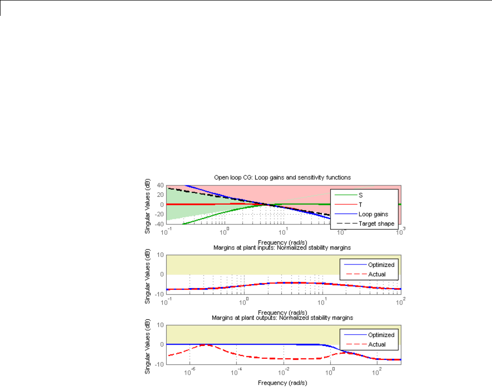
6Tuning Fixed Control Architectures
1.0002
The final value of the success gauge gam is less than one, which means that all
requirements were met. Confirm this by graphically validating the design.
ST.loopview(Info)
The first plot confirms that the open-loop response has integral action and
the desired gain crossover frequency while the second plot shows that the
MIMO stability margins are satisfactory (the blue curve should remain below
the yellow bound). Next check the response from the step command azref to
the vertical acceleration az:
T = ST.getIOTransfer('az ref','az');
clf
step(T,5)
6-158
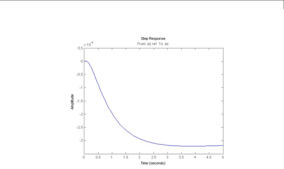
Tuning of a Two-Loop Autopilot
The acceleration az does not track azref despite the presence of an integrator
in the loop. This is because the feedback loop acts on the two variables az and
qand we have not specified which one should track azref.
Adding a Tracking Requirement
To remedy this issue, add an explicit requirement that az should follow
the step command azref with a 1 second response time. Also relax the
gain crossover requirement to the interval [3,12] to let the tuner find the
appropriate gain crossover frequency.
rng(0)
TrackReq = TuningGoal.Tracking('az ref','az',1);
ST = ST0.looptune([3,12],TrackReq,Options);
Final: Peak gain = 62.1, Iterations = 38
Min decay rate 2.1e-07 is close to lower bound 1e-07
Final: Failed to enforce closed-loop stability (spectral abscissa = 0.0405)
Final: Peak gain = 1.23, Iterations = 122
6-159
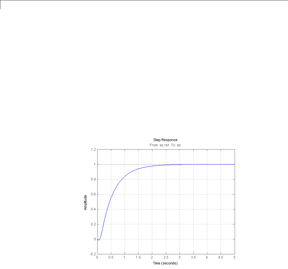
6Tuning Fixed Control Architectures
Final: Failed to enforce closed-loop stability (spectral abscissa = 0.0405)
Final: Failed to enforce closed-loop stability (spectral abscissa = 0.0405)
Final: Peak gain = 62.1, Iterations = 59
Min decay rate 2.68e-07 is close to lower bound 1e-07
Final: Failed to enforce closed-loop stability (spectral abscissa = 0.0317)
Final: Failed to enforce closed-loop stability (spectral abscissa = 0.0405)
Final: Failed to enforce closed-loop stability (spectral abscissa = 0.0405)
Final: Failed to enforce closed-loop stability (spectral abscissa = 0.0406)
Final: Failed to enforce closed-loop stability (spectral abscissa = 0.0405)
Thestepresponsefromazref to az is now satisfactory:
Tr1 = ST.getIOTransfer('az ref','az');
step(Tr1,5), grid
Also check the disturbance rejection characteristics by looking at the
responses from a disturbance entering at the plant input
Td1 = ST.getIOTransfer('delta fin','az');
bodemag(Td1), grid
6-160
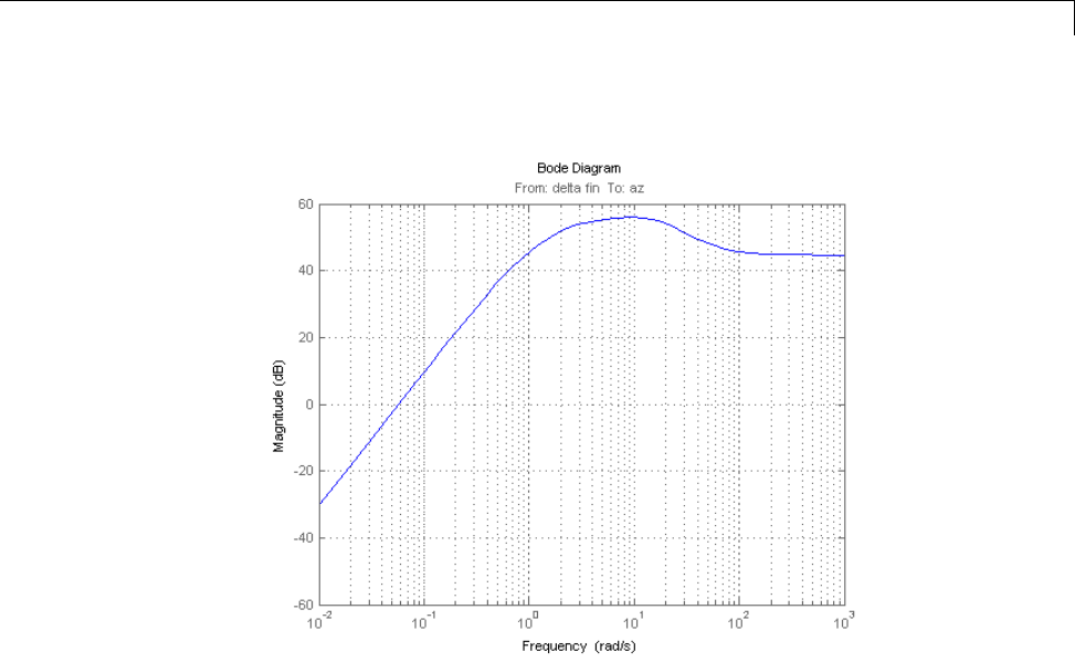
Tuning of a Two-Loop Autopilot
step(Td1,5), grid, title('Disturbance rejection')
6-161
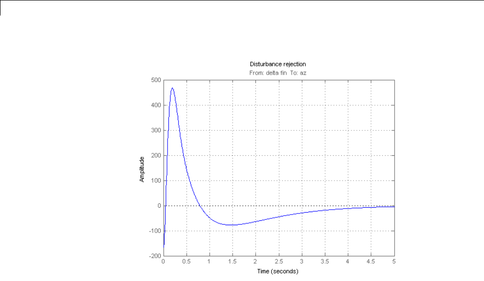
6Tuning Fixed Control Architectures
Use showBlockValue to see the tuned values of the PI controller and
inner-loop gain
ST.showBlockValue()
Block "rct_airframe1/az Control" =
Value =
1
Kp + Ki * ---
s
with Kp = 0.00165, Ki = 0.00166
Name: az_Control
Continuous-time PI controller in parallel form.
6-162

Tuning of a Two-Loop Autopilot
-----------------------------------
Block "rct_airframe1/q Gain" =
Value =
d=
u1
y1 1.985
Name: q_Gain
Static gain.
If this design is satisfactory, use writeBlockValue to apply the tuned values
to the Simulink model and simulate the tuned controller in Simulink.
ST.writeBlockValue()
MIMO Design with SYSTUNE
Cascaded loops are commonly used for autopilots. Yet one may wonder how
a single MIMO controller that uses both az and qto generate the actuator
command delta fin would compare with the two-loop architecture. Trying
new control architectures is easy with systune or looptune. For variety, we
now use systune to tune the following MIMO architecture.
open_system('rct_airframe2')
6-163
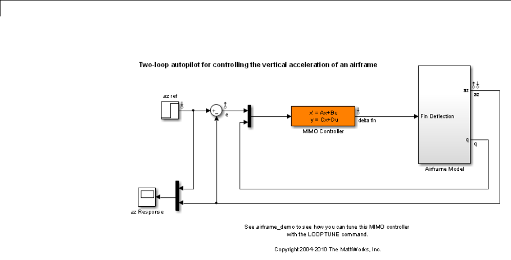
6Tuning Fixed Control Architectures
As with looptune, first create an slTunable interface to facilitate tuning
in Simulink.
ST0 = slTunable('rct_airframe2','MIMO Controller');
ST0.addControl('delta fin');
Try a second-order MIMO controller with zero feedthrough from eto delta
fin. To do this, create the desired controller parameterization and associate
it with the "MIMO Controller" block using setBlockParam:
C0 = ltiblock.ss('C',2,1,2); % Second-order controller
C0.d.Value(1) = 0; C0.d.Free(1) = false; % Fix D(1) to zero
ST0.setBlockParam('MIMO Controller',C0)
Nextcreateadequatetuningrequirements. Hereweusethefollowingfour
requirements:
1Tracking:az should respond in about 1 second to the azref command
2Bandwidth and roll-off: The loop gain at delta fin should roll off after
25 rad/s with a -20 dB/decade slope
6-164

Tuning of a Two-Loop Autopilot
3Stability margins:Themarginsatdelta fin should exceed 7 dB and 45
degrees
4Disturbance rejection:Limitthegainfromdelta fin to az to ensure
good disturbance rejection at low frequencies.
% Tracking
Req1 = TuningGoal.Tracking('az ref','az',1);
% Bandwidth and roll-off
Req2 = TuningGoal.Gain('delta fin','delta fin',tf(25,[1 0])); % roll-off
% Margins
Req3 = TuningGoal.Margins('delta fin',7,45);
% Disturbance rejection
% Use an FRD model to sketch the desired gain profile with a few points
Freqs = [0.02 2 200];
MaxGain = [2 200 200];
GainLimit = frd(MaxGain,Freqs);
Req4 = TuningGoal.Gain('delta fin','az',GainLimit);
You can now use systune to tune the controller parameters subject to these
requirements.
AllReqs = [Req1,Req2,Req3 Req4];
Opt = systuneOptions('RandomStart',3);
rng('default')
[ST,fSoft,~,Info] = ST0.systune(AllReqs,Opt);
Final: Soft = 1.5, Hard = -Inf, Iterations = 57
Final: Soft = 1.49, Hard = -Inf, Iterations = 93
Final: Soft = 1.15, Hard = -Inf, Iterations = 57
Final: Soft = 1.15, Hard = -Inf, Iterations = 82
The best design has an overall objective value close to 1, indicating that all
four requirements are nearly met. Use viewSpec to inspect each requirement
for the best design.
6-165
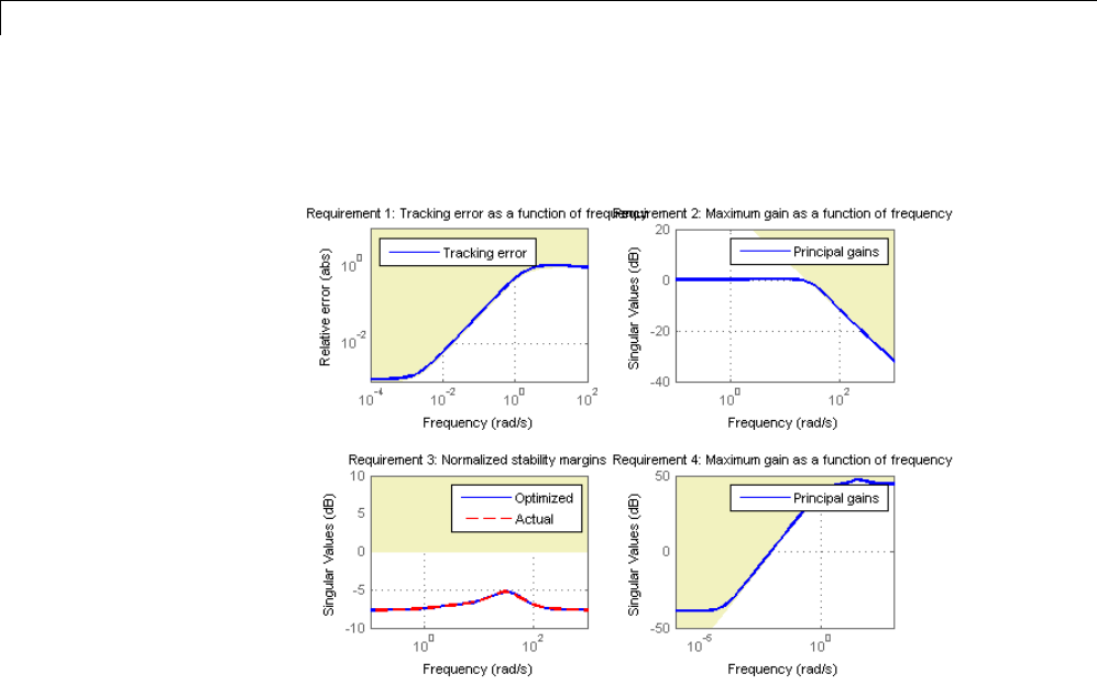
6Tuning Fixed Control Architectures
viewSpec(AllReqs,ST,Info)
Compute the closed-loop responses and compare with the two-loop design.
T = ST.getIOTransfer({'az ref','delta fin'},'az');
clf
step(Tr1,'b',T(1),'r',5)
title('Tracking'), legend('Cascade','2 dof')
6-166
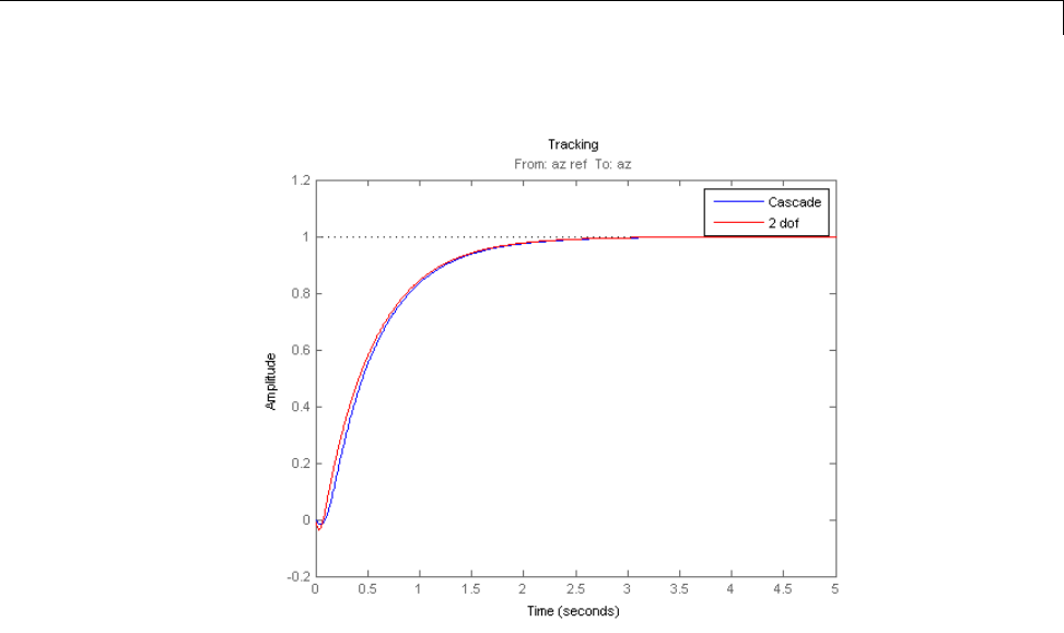
Tuning of a Two-Loop Autopilot
step(Td1,'b',T(2),'r',5)
title('Disturbance rejection'), legend('Cascade','2 dof')
6-167
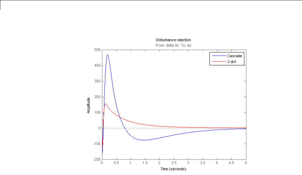
6Tuning Fixed Control Architectures
The tracking performance is similar but the second design has better
disturbance rejection properties.
6-168

Control of a UAV Formation
Control of a UAV Formation
This example uses systune to optimize a decentralized control law for a
UAV formation. For more details, see "A Model-Predictive Decentralized
Control Scheme With Reduced Communication Requirement for Spacecraft
Formation", J. Lavaei et al., IEEE Transactions of Control Systems
Technology, 16(2), 2008.
Background
This example deals with the guidance of a leader-follower formation of 3
UAVs. The leader is UAV 1 and the followers are UAVs 2 and 3. The objective
is to maintain prescribed velocities for all UAVs and prescribed distances
along the x and y axes between UAVs 1 and 2, and UAVs 2 and 3. Each UAV
has only access to partial information which leads to a decentralized control
problem.
Model and Control Structure
6-169
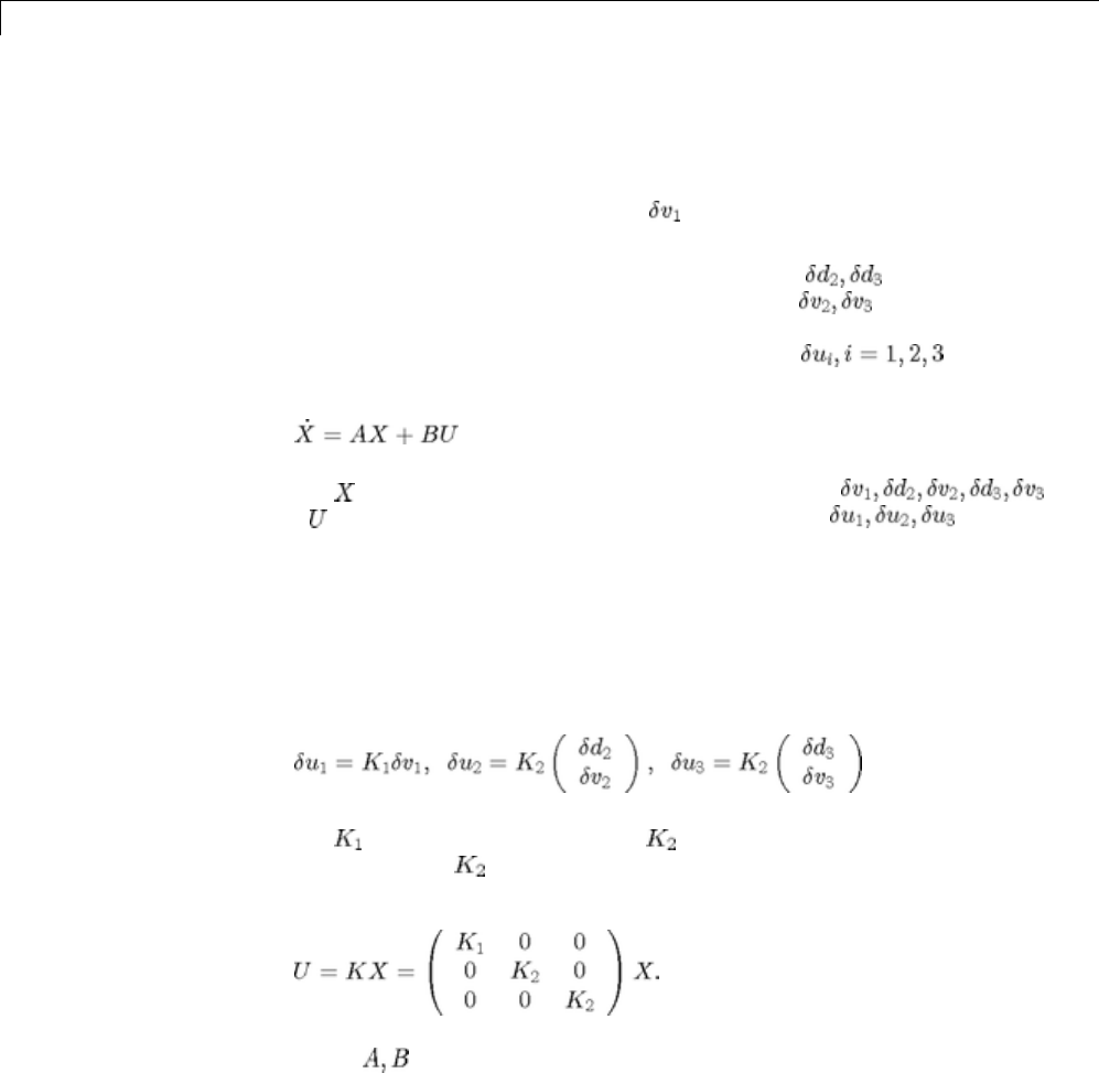
6Tuning Fixed Control Architectures
We consider the motion of the formation in the horizontal (x,y) plane. The
state of each UAV is described by:
•Leader (UAV 1): Two-entry vector of speed errors of leader in x and
ydirections
•Followers (UAV 2 and UAV 3): Two-entry vectors of errors in x,y
distances with predecessor and two-entry vectors of speed errors
Each UAV is controlled by a two-entry thrust vector (thrusts in
x and y directions). The linearized dynamics for the entire formation are:
where is the overall state vector obtained by stacking
and is the overall thrust vector obtained by stacking .Units
are ft, ft/s, and ft/s^2.
The leader sets the target velocity for the entire formation and only worries
about achieving this target velocity. Meanwhile, the followers must control
both their velocity and their distance to their predecessor. Each follower
only knows its own speed and its position relative to its predecessor, which
leads to the decentralized control law:
where is a 2-by-2 gain matrix and is a 2-by-4 gain matrix. Note that we
use the same gain for both followers since they are interchangeable UAVs.
Overall, this amounts to state-feedback control with the diagonal structure:
Load the matrices of the linearized dynamics and parameterized the
controller gains.
load FormationFlightData
6-170
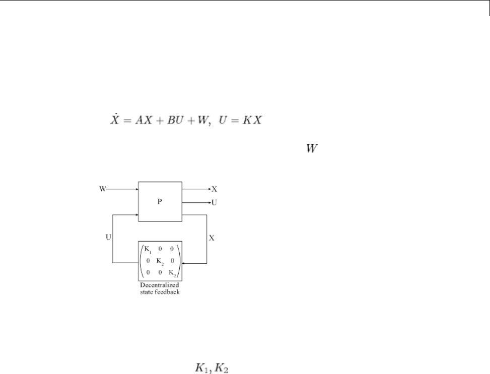
Control of a UAV Formation
K1 = ltiblock.gain('K1', 2,2);
K2 = ltiblock.gain('K2', 2,4);
The closed-loop system has equations
and is depicted in Figure 1. The input vector models the speed and velocity
disturbances.
Figure 1: Closed-Loop System
Construct a tunable model T0 of the closed-loop system. This model depends
on the tunable gains .Addaloopswitch blockattheplantinputUso
that you can specify and analyze the gain and phase margins of the feedback
loop.
% Plant P
nx = size(A,1); % number of states
nu = size(B,2); % number of controls
BP = [eye(nx) , B];
CP = [eye(nx) ; zeros(nu,nx) ; eye(nx)];
DP = [zeros(nx,nx+nu) ; zeros(nu,nx) eye(nu) ; zeros(nx,nx+nu)];
P = ss(A, BP, CP, DP);
% Loop switch for open-loop analysis/requirement
LSU = loopswitch('U',nu);
6-171
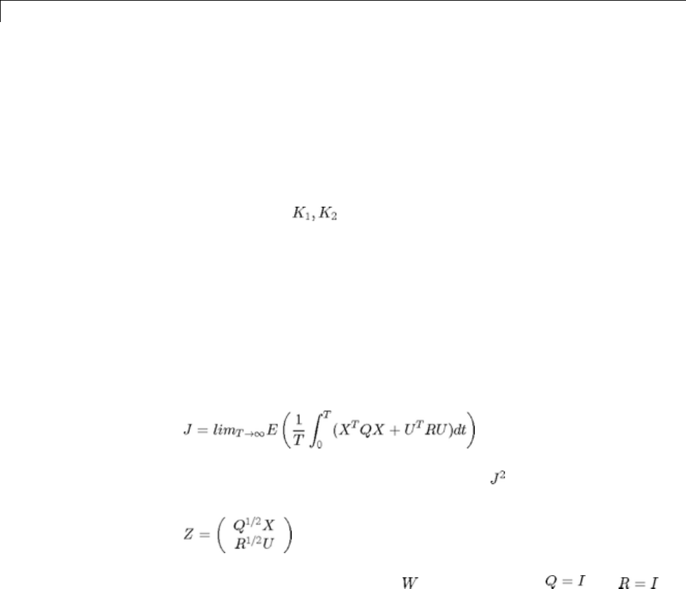
6Tuning Fixed Control Architectures
% Tunable closed-loop model
T0 = lft( P , LSU * blkdiag(K1,K2,K2) );
T0.InputName = 'W';
T0.OutputName = {'X(1)' 'X(2)' 'X(3)' 'X(4)' 'X(5)' 'X(6)' 'X(7)'...
'X(8)' 'X(9)' 'X(10)' 'U(1)' 'U(2)' 'U(3)' 'U(4)' 'U(5)' 'U(6)'};
Design Requirements
The feedback gains must be tuned to ensure:
1Stability of the formation flight
2Appropriate decay of the distances and speeds to their desired values. The
reference is zero here since we are working with error dynamics.
3Reasonable thrust levels
4Adequate gain and phase margins at the plant inputs.
UseaquadraticLQG-likecostoftheform
to capture the first three requirements. The value is just the variance of
the weighted output signal
for a unit-variance white noise input (see Figure 1). Use and
for the initial tuning.
Q=ey
e(nx);
R=ey
e(nu);
Req1 = TuningGoal.WeightedVariance('W',T0.OutputName,...
blkdiag(sqrtm(Q),sqrtm(R)),[]);
For the last requirement, specify a minimum of 10 dB and 45 degrees of gain
and phase margins at the plant inputs.
6-172
Control of a UAV Formation
Req2 = TuningGoal.Margins('U',10,45);
Tuning of Decentralized Controller
Use systune to tune the gains subject to the two requirements defined
above.
rng('default')
T = systune(T0,Req1,Req2,systuneOptions('RandomStart',2));
Final: Failed to enforce closed-loop stability (spectral abscissa = 0)
Final: Soft = 4.42, Hard = 0.84135, Iterations = 63
Final: Soft = 4.42, Hard = 0.77999, Iterations = 48
The stability margins requirement (hard constraint) is satisfied since its value
is less than 1. The optimized value of is about 4.4. Confirm the stability
margins by computing the negative-feedback open-loop response Lat the plant
inputs and using loopmargin to compute the corresponding disk margins.
L = getLoopTransfer(T,'U',-1); % negative-feedback loop transfer
[~,~,MM] = loopmargin(L);
% Gain margins
mag2db(MM.GainMargin)
ans =
-14.6551 14.6551
% Phase margins
MM.PhaseMargin
ans =
-69.0341 69.0341
6-173

6Tuning Fixed Control Architectures
The loopmargin results indicate that the tuned control system can sustain
concurrent gain and phase variations in excess of dB and degrees in
all feedback channels U without going unstable.
Closed-Loop Simulation
Simulate how the UAV formation responds to initial errors of 100 ft/s in
x-speed, 150 ft/s in y-speed, 400 ft in x-distance, and 300 ft in y-distance.
X0 = -[100 150 400 300 100 150 400 300 100 150]'; % initial errors
[X,t] = initial(T(1:nx,:),X0);
% Plot speed errors for leader and followers
clf
subplot(311), plot(t, X(:,1), 'b', t, X(:,2), 'r'), grid
title('Speed errors for UAV 1'); legend('X','Y')
subplot(312), plot(t, X(:,5), 'b', t, X(:,6), 'r'), grid
title('Speed errors for UAV 2 (following UAV 1)'); legend('X','Y')
subplot(313), plot(t, X(:,9), 'b', t, X(:,10), 'r'), grid
title('Speed errors for UAV 3 (following UAV 2)'); legend('X','Y')
6-174
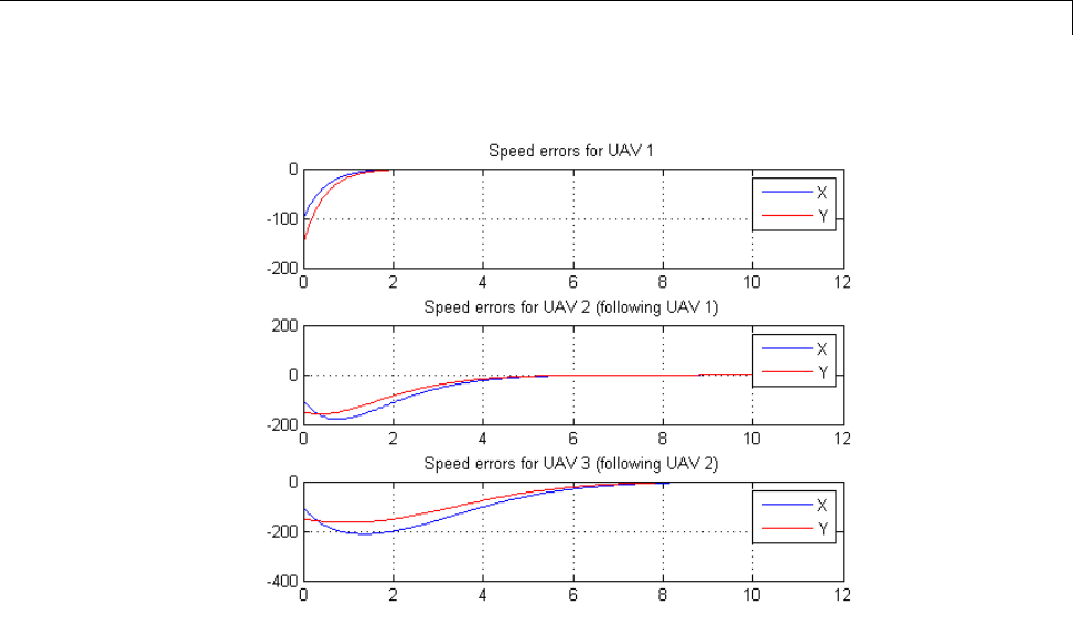
Control of a UAV Formation
% Plot distance errors
clf
subplot(211), plot(t, X(:,3), 'b', t, X(:,4), 'r'), grid
title('Distance errors between UAV 1 and UAV 2'); legend('X','Y')
subplot(212), plot(t, X(:,7), 'b', t, X(:,8), 'r'), grid
title('Distance errors between UAV 2 and UAV 3'); legend('X','Y')
6-175
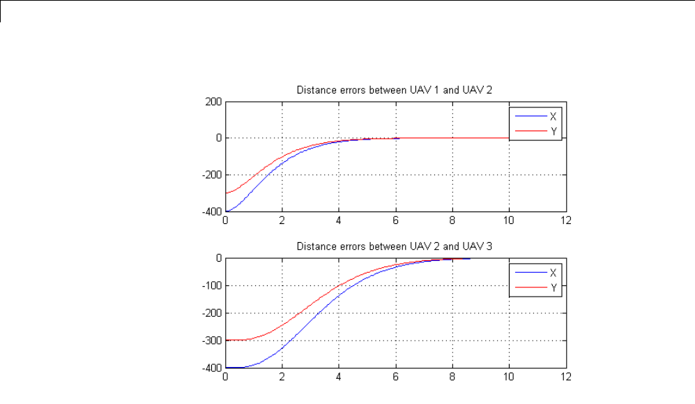
6Tuning Fixed Control Architectures
Note how the follower UAVs initially accelerate to reduce the distance errors
andthenslowdowntokeepaconstantdistancewiththeirpredecessor.
6-176

Multi-Loop Controller for the Westland Lynx Helicopter
Multi-Loop Controller for the Westland Lynx Helicopter
This example shows how to use Robust Control Toolbox™ to tune a multi-loop
controller for a rotorcraft. We thank Professor Pierre Apkarian from ONERA
for providing the example material.
Helicopter Model
This example uses an 8-state model of the Westland Lynx helicopter at the
hovering trim condition. The state vector x = [u,w,q,theta,v,p,phi,r]
consists of
•Longitudinal velocity u(m/s)
•Lateral velocity v(m/s)
•Normal velocity w(m/s)
•Pitch angle theta (deg)
•Roll angle phi (deg)
•Roll rate p(deg/s)
•Pitch rate q(deg/s)
•Yaw rate r(deg/s).
The controller generates commands ds,dc,dT in degrees for the longitudinal
cyclic, lateral cyclic, and tail rotor collective using measurements of theta,
phi,p,q,andr. For a detailed description of the model, see "Helicopter
Control Design with Robust Flying Quality," Aerospace Science & Technology,
7 (2003), pp 159-169.
Control Architecture
The following Simulink model depicts the control architecture:
open_system('rct_helico')
6-177
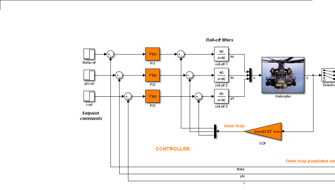
6Tuning Fixed Control Architectures
The control system consists of two feedback loops. The inner loop (static
output feedback) provides stability augmentation and decoupling. The outer
loop (PI controllers) provides the desired setpoint tracking performance. The
main control objectives are as follows:
•Track setpoint changes in theta,phi,andrwith zero steady-state
error, settling times of about 2 seconds, minimal overshoot, and minimal
cross-coupling
•Limit the control bandwidth to guard against neglected high-frequency
rotor dynamics and measurement noise
•Provide strong multivariable gain and phase margins (robustness to
simultaneous gain/phase variations at the plant inputs and outputs, see
loopmargin for details).
We use lowpass filters with cutoff at 40 rad/s to partially enforce the second
objective.
6-178
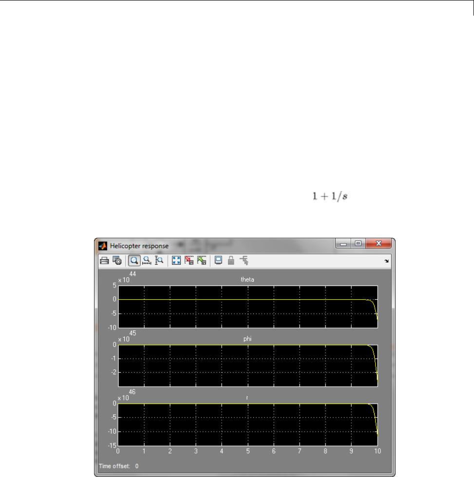
Multi-Loop Controller for the Westland Lynx Helicopter
Controller Tuning
You can jointly tune the inner and outer loops with the looptune command.
This command only requires models of the plant and controller along with the
desired bandwidth (which is function of the desired response time). When the
control system is modeled in Simulink, you can use the slTunable interface
to quickly set up the tuning task. Create an instance of this interface with
thelistofblockstobetuned.
ST0 = slTunable('rct_helico',{'PI1','PI2','PI3','SOF'});
Each tunable block is automatically parameterized according to its type and
initialized with its value in the Simulink model ( for the PI controllers
and zero for the static output-feedback gain). Simulating the model shows
that the control system is unstable for these initial values:
Specify the I/O signals of interest for setpoint tracking.
6-179

6Tuning Fixed Control Architectures
ST0.addIO({'theta-ref','phi-ref','r-ref'},'in') % setpoint commands
ST0.addIO({'theta','phi','r'},'out') % corresponding outputs
Also identify the plant inputs and outputs (control and measurement signals)
where the stability margin are measured.
ST0.addControl('u');
ST0.addMeasurement('y');
Finally, capture the design requirements using TuningGoal objects. We use
the following requirements for this example:
•Tracking requirement: The outputs theta,phi,rmust track the
commands theta_ref,phi_ref,r_ref with a 2-second response time
•Stability margins: The multivariable gain and phase margins at the
plant inputs uand plant outputs ymust be at least 5 dB and 40 degrees
•Fast dynamics: The magnitude of the closed-loop poles must not exceed
20 to prevent fast dynamics and jerky transients
% Tracking
TrackReq = TuningGoal.Tracking({'theta-ref','phi-ref','r-ref'},...
{'theta','phi','r'},2,1e-2);
% Gain and phase margins at plant inputs and outputs
MarginReq1 = TuningGoal.Margins('u',5,40);
MarginReq2 = TuningGoal.Margins('y',5,40);
% Limit on fast dynamics
PoleReq = TuningGoal.Poles();
PoleReq.MaxFrequency = 20;
You can now use systune to jointly tune all controller parameters. This
returns the tuned version ST1 of the control system ST0.
AllReqs = [TrackReq,MarginReq1,MarginReq2,PoleReq];
[ST1,fSoft,~,Info] = ST0.systune(AllReqs);
Final: Soft = 1.15, Hard = -Inf, Iterations = 49
6-180

Multi-Loop Controller for the Westland Lynx Helicopter
Thefinalvalueiscloseto1sotherequirementsarenearlymet. Plotthe
tuned responses to step commands in theta, phi, r:
T1 = ST1.getIOTransfer({'theta-ref','phi-ref','r-ref'},{'theta','phi','r'})
step(T1,5)
The response time is about two seconds with no overshoot and little
cross-coupling. You can use viewSpec for a more thorough validation of each
requirement, including a visual assessment of the multivariable stability
margins (see loopmargin for details):
viewSpec(AllReqs,ST1,Info)
6-181
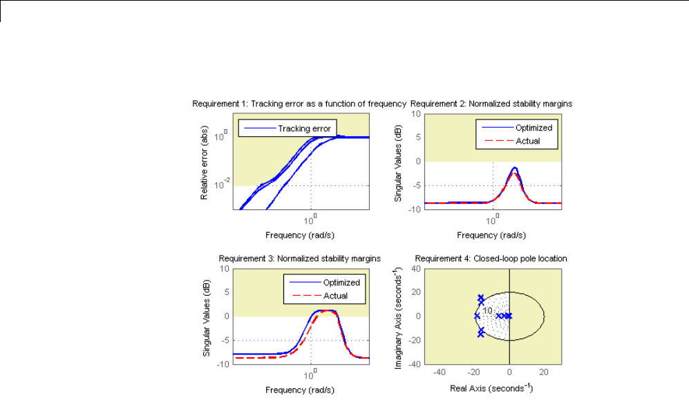
6Tuning Fixed Control Architectures
Inspect the tuned values of the PI controllers and static output-feedback gain.
ST1.showTunable()
Block "rct_helico/PI1" =
Value =
1
Kp + Ki * ---
s
with Kp = 0.504, Ki = 1.92
Name: PI1
Continuous-time PI controller in parallel form.
-----------------------------------
6-182

Multi-Loop Controller for the Westland Lynx Helicopter
Block "rct_helico/PI2" =
Value =
1
Kp + Ki * ---
s
with Kp = -0.0557, Ki = -1.88
Name: PI2
Continuous-time PI controller in parallel form.
-----------------------------------
Block "rct_helico/PI3" =
Value =
1
Kp + Ki * ---
s
with Kp = -0.515, Ki = -4.69
Name: PI3
Continuous-time PI controller in parallel form.
-----------------------------------
Block "rct_helico/SOF" =
Value =
d=
u1 u2 u3 u4 u5
y1 2.1 -0.2376 -0.09408 0.5177 0.003496
y2 -0.4855 -1.514 0.008369 -0.07761 -0.1078
y3 -0.9372 0.48 -0.9289 -0.07711 0.2312
6-183

6Tuning Fixed Control Architectures
Name: SOF
Static gain.
Benefit of the Inner Loop
You may wonder whether the static output feedback is necessary and whether
PID controllers aren’t enough to control the helicopter. This question is easily
answered by re-tuning the controller with the inner loop open. First break the
inner loop by adding a loop opening after the SOF block:
ST0.addOpening('SOF')
Then remove the SOF block from the tunable block list and re-parameterize
thePIblocksasfull-blownPIDswiththe correct loop signs (as inferred from
the first design).
PID = pid(0,0.001,0.001,.01); % initial guess for PID controllers
ST0.TunedBlocks = ST0.TunedBlocks(1:3);
ST0.setBlockParam('PI1',ltiblock.pid('C1',PID));
ST0.setBlockParam('PI2',ltiblock.pid('C2',-PID));
ST0.setBlockParam('PI3',ltiblock.pid('C3',-PID));
Re-tune the three PID controllers and plot the closed-loop step responses.
[ST2,fSoft,~,Info] = ST0.systune(AllReqs);
Final: Soft = 2.07, Hard = -Inf, Iterations = 95
T2 = ST2.getIOTransfer({'theta-ref','phi-ref','r-ref'},{'theta','phi','r'})
clf, step(T2,5)
6-184
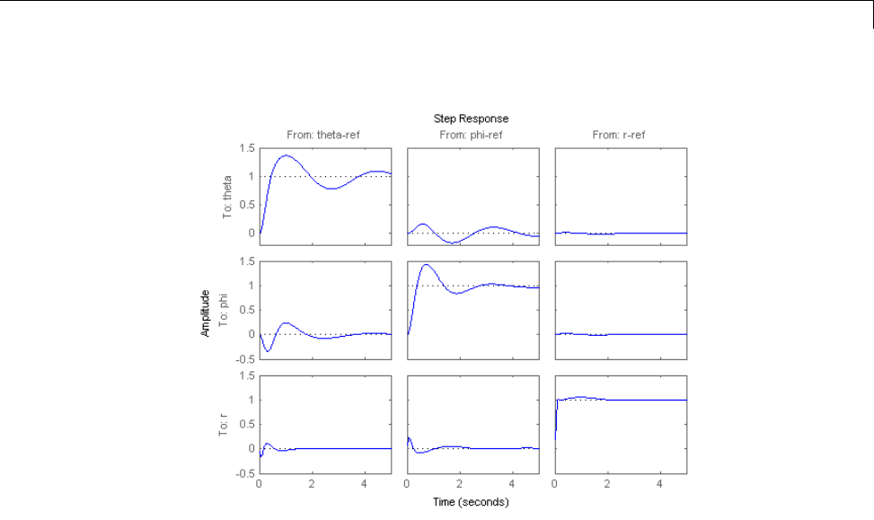
Multi-Loop Controller for the Westland Lynx Helicopter
Thefinalvalueisnolongercloseto1and the step responses confirm some
performance degradation with regard to settling time, overshoot, and
decoupling. This suggests that the inner loop has an important stabilizing
effect that should be preserved.
6-185
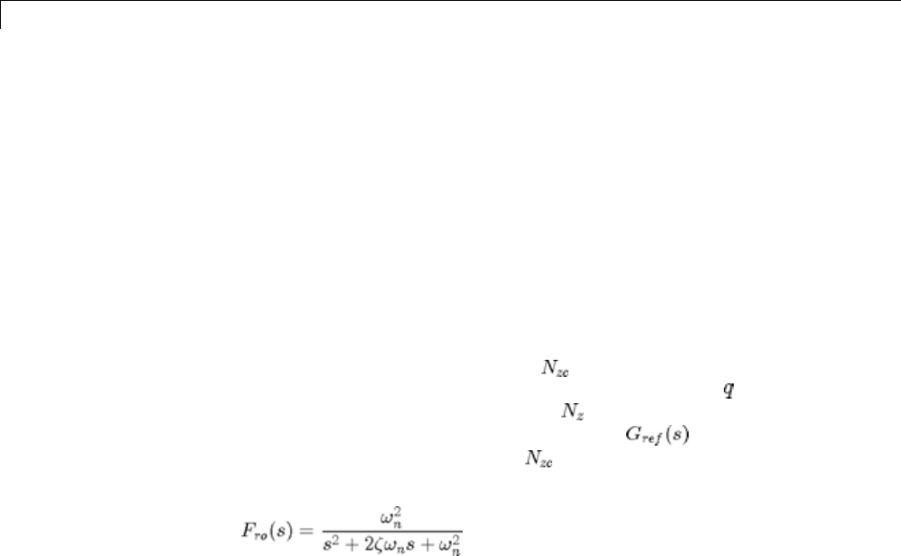
6Tuning Fixed Control Architectures
Fixed-Structure Autopilot for a Passenger Jet
This example shows how to use Robust Control Toolbox™ to tune the standard
configuration of a longitudinal autopilot. We thank Professor D. Alazard
from Institut Superieur de l’Aeronautique et de l’Espace for providing the
aircraft model and Professor Pierre Apkarian from ONERA for developing
the example.
Aircraft Model and Autopilot Configuration
The longitudinal autopilot for a supersonic passenger jet flying at Mach
0.7 and 5000 ft is depicted in Figure 1. The autopilot main purpose is to
follow vertical acceleration commands issued by the pilot. The feedback
structure consists of an inner loop controlling the pitch rate and an outer
loop controlling the vertical acceleration . The autopilot also includes
a feedforward component and a reference model that specifies the
desiredresponsetoastepcommand .Finally,thesecond-order roll-off
filter
is used to attenuate noise and limit the control bandwidth as a safeguard
against unmodeled dynamics. The tunable components are highlighted in
orange.
6-186
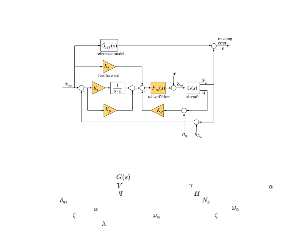
Fixed-Structure Autopilot for a Passenger Jet
Figure 1: Longitudinal Autopilot Configuration.
The aircraft model is a 5-state model, the state variables being the
aerodynamic speed (m/s), the climb angle (rad), the angle of attack
(rad), the pitch rate (rad/s), and the altitude (m). The elevator deflection
(rad) is used to control the vertical load factor . The open-loop dynamics
include the oscillation with frequency and damping ratio = 1.7 (rad/s)
and = 0.33, the phugoid mode =0.64(rad/s)and =0.06,andtheslow
altitude mode = -0.0026.
load ConcordeData G
bode(G,{1e-3,1e2}), grid
title('Aircraft Model')
6-187
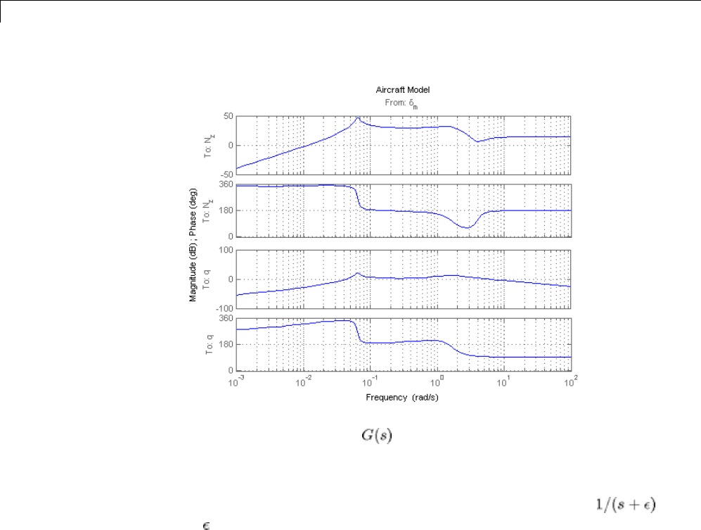
6Tuning Fixed Control Architectures
Note the zero at the origin in . Because of this zero, we cannot achieve
zero steady-state error and must instead focus on the transient response
to acceleration commands. Note that acceleration commands are transient
in nature so steady-state behavior is not a concern. This zero at the origin
also precludes pure integral action so we use a pseudo-integrator
with =0.001.
TuningSetup
When the control system is modeled in Simulink, you can use the slTunable
interface to quickly set up the tuning task. Open the Simulink model of the
autopilot.
open_system('rct_concorde')
6-188
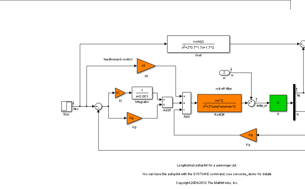
Fixed-Structure Autopilot for a Passenger Jet
Configure the slTunable interface by listing the tuned blocks in the Simulink
model (highlighted in orange).
ST0 = slTunable('rct_concorde',{'Ki','Kp','Kq','Kf','RollOff'});
This automatically picks all linearization points in the model as analysis I/Os.
ST0.IOs
ans =
'rct_concorde/Nzc/1[Nzc]' 'in'
'rct_concorde/noise/1[n]' 'in'
'rct_concorde/w/1[w]' 'in'
'rct_concorde/Demux/1[Nz]' 'out'
'rct_concorde/Sum2/1[e]' 'out'
6-189
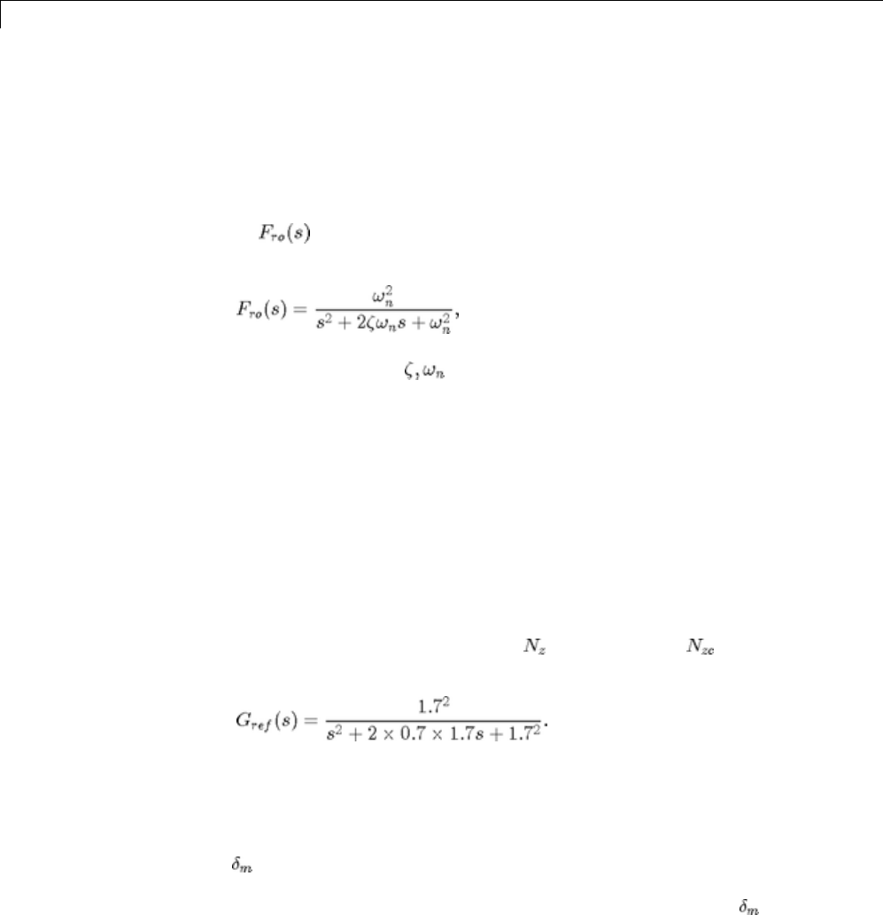
6Tuning Fixed Control Architectures
'rct_concorde/Sum5/1[delta_m]' 'out'
This also parameterizes each tuned block and initializes the block parameters
based on their values in the Simulink model. Note that the four gains
Ki,Kp,Kq,Kf are initialized to zero in this example. By default the roll-off
filter is parameterized as a generic second-order transfer function.
To parameterize it as
create real parameters , build the transfer function shown above, and
associate it with the RollOff block.
wn = realp('wn', 3); % natural frequency
zeta = realp('zeta',0.8); % damping
Fro = tf(wn^2,[1 2*zeta*wn wn^2]); % parametric transfer function
ST0.setBlockParam('RollOff',Fro) % use Fro to parameterize "RollOff" blo
c
Design Requirements
Theautopilotmustbetunedtosatisfythreemaindesignrequirements:
1. Setpoint tracking: The response to the command should closely
match the response of the reference model:
This reference model specifies a well-damped response with a 2 second
settling time.
2. High-frequency roll-off: The closed-loop response from the noise signals
to should roll off past 8 rad/s with a slope of at least -40 dB/decade.
3. Stability margins: The stability margins at the plant input should be
at least 7 dB and 45 degrees.
6-190
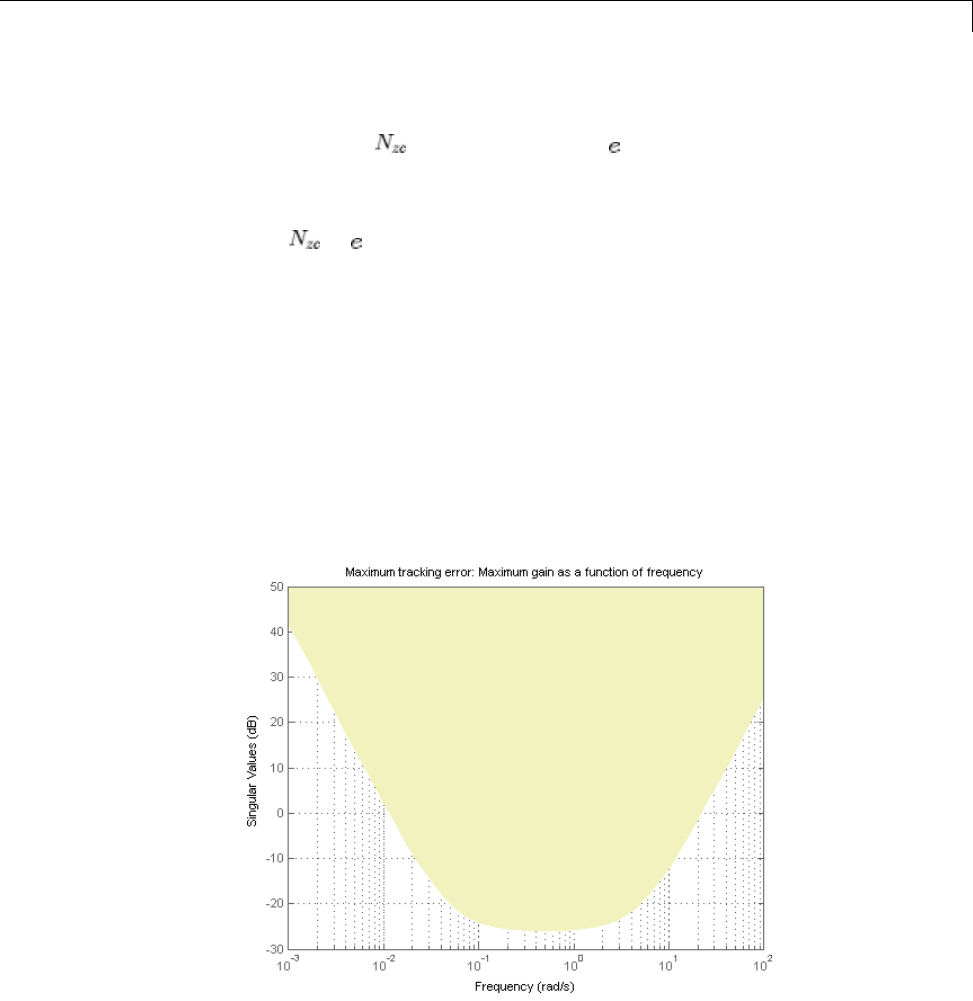
Fixed-Structure Autopilot for a Passenger Jet
For setpoint tracking, we require that the gain of the closed-loop transfer
from the command to the tracking error be small in the frequency
band [0.05,5] rad/s (recall that we cannot drive the steady-state error to zero
because of the plant zero at s=0). Using a few frequency points, sketch the
maximum tracking error as a function of frequency and use it to limit the
gain from to .
Freqs = [0.005 0.05 5 50];
Gains = [5 0.05 0.05 5];
Req1 = TuningGoal.Gain('Nzc','e',frd(Gains,Freqs));
Req1.Name = 'Maximum tracking error';
The TuningGoal.Gain constructor automatically turns the maximum error
sketch into a smooth weighting function. Use viewSpec to graphically verify
the desired error profile.
viewSpec(Req1)
6-191

6Tuning Fixed Control Architectures
Repeat the same process to limit the high-frequency gain from the noise
inputs to and enforce a -40 dB/decade slope in the frequency band from 8
to 800 rad/s
Freqs = [0.8 8 800];
Gains = [10 1 1e-4];
Req2 = TuningGoal.Gain('n','delta_m',frd(Gains,Freqs));
Req2.Name = 'Roll-off requirement';
viewSpec(Req2)
Finally, register the plant input as a site for open-loop analysis and use
TuningGoal.Margins to capture the stability margin requirement.
ST0.addSwitch('delta_m')
Req3 = TuningGoal.Margins('delta_m',7,45);
Autopilot Tuning
6-192

Fixed-Structure Autopilot for a Passenger Jet
Wearenowreadytotunetheautopilotparameterswithsystune.This
command takes the untuned configuration ST0 and the three design
requirements and returns the tuned version ST of ST0. All requirements are
satisfied when the final value is less than one.
[ST,fSoft,~,Info] = systune(ST0,[Req1 Req2 Req3]);
Final: Soft = 0.965, Hard = -Inf, Iterations = 49
Use showTunable to see the tuned block values.
ST.showTunable()
Block "rct_concorde/Ki" =
Value =
d=
u1
y1 -0.03008
Name: Ki
Static gain.
-----------------------------------
Block "rct_concorde/Kp" =
Value =
d=
u1
y1 -0.009661
Name: Kp
Static gain.
-----------------------------------
6-193

6Tuning Fixed Control Architectures
Block "rct_concorde/Kq" =
Value =
d=
u1
y1 -0.2889
Name: Kq
Static gain.
-----------------------------------
Block "rct_concorde/Kf" =
Value =
d=
u1
y1 -0.02291
Name: Kf
Static gain.
-----------------------------------
Block "rct_concorde/RollOff" =
Value =
a=
x1 x2
x1 -4.996 -23.31
x210
b=
u1
x1 1
x2 0
6-194

Fixed-Structure Autopilot for a Passenger Jet
c=
x1 x2
y1 0 23.31
d=
u1
y1 0
Continuous-time state-space model.
To get the tuned value of ,usegetBlockValue to evaluate Fro for
the tuned parameter values in ST:
Fro = ST.getBlockValue('RollOff');
tf(Fro)
ans =
23.31
---------------------
s^2 + 4.996 s + 23.31
Continuous-time transfer function.
Finally, use viewSpec to graphically verify that all requirements are satisfied.
viewSpec([Req1 Req2 Req3],ST)
6-195
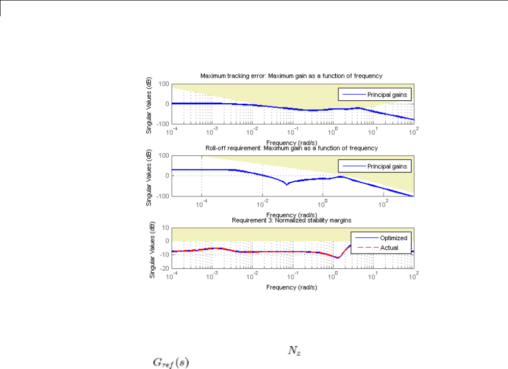
6Tuning Fixed Control Architectures
Closed-Loop Simulations
We now verify that the tuned autopilot satisfies the design requirements.
First compare the step response of with the step response of the reference
model .Again use getIOTransfer to compute the tuned closed-loop
transfer from Nzc to Nz:
Gref = tf(1.7^2,[1 2*0.7*1.7 1.7^2]); % reference model
T = ST.getIOTransfer('Nzc','Nz'); % transfer Nzc -> Nz
clf, step(T,'b',Gref,'b--',6), grid,
ylabel('N_z'), legend('Actual response','Reference model')
6-196
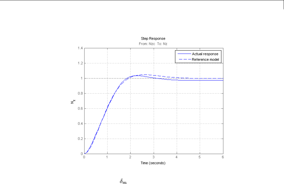
Fixed-Structure Autopilot for a Passenger Jet
Also plot the deflection and the respective contributions of the feedforward
and feedback paths:
T = ST.getIOTransfer('Nzc','delta_m'); % transfer Nzc -> delta_m
Kf = ST.getBlockValue('Kf'); % tuned value of Kf
Tff = Fro*Kf; % feedforward contribution to delta_m
step(T,'b',Tff,'g--',T-Tff,'r-.',6), grid
ylabel('\delta_m'), legend('Total','Feedforward','Feedback')
6-197
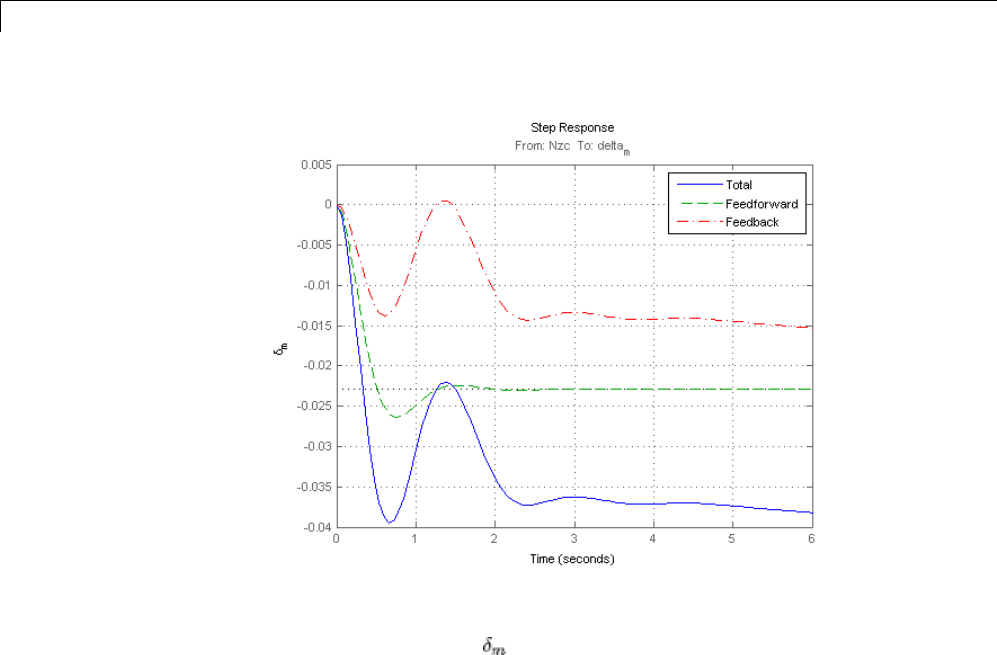
6Tuning Fixed Control Architectures
Finally, check the roll-off and stability margin requirements by computing
the open-loop response at .
OL = ST.getLoopTransfer('delta_m',-1); % negative-feedback loop transfer
margin(OL); grid; set(gca,'XLim',[1e-3,1e2])
6-198
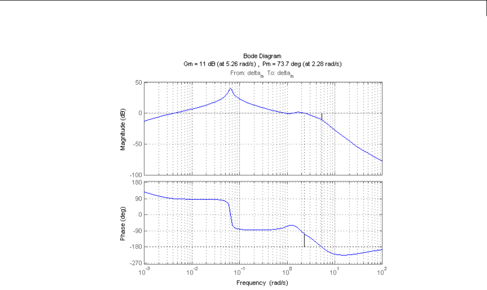
Fixed-Structure Autopilot for a Passenger Jet
The Bode plot confirms a roll-off of -40 dB/decade past 8 rad/s and indicates
gain and phase margins in excess of 10 dB and 70 degrees.
6-199

6Tuning Fixed Control Architectures
Reliable Control of a Fighter Jet
This example shows how to tune a fixed-structure controller for multiple
operating modes of the plant.
Background
This example deals with reliable flight control of an F16 aircraft undergoing
outages in the elevator and aileron actuators. The flight control system is
required to maintain stability and adequate performance in both nominal
operationanddegradedconditionswheresomeactuatorsarenolonger
effective due to control surface impairment. Wind gusts must be alleviated
in all conditions. This application is often called reliable control as aircraft
safety must be maintained in extreme flight conditions.
Aircraft Model
The control system is modeled in Simulink.
open_system('rct_reliableF16')
6-200
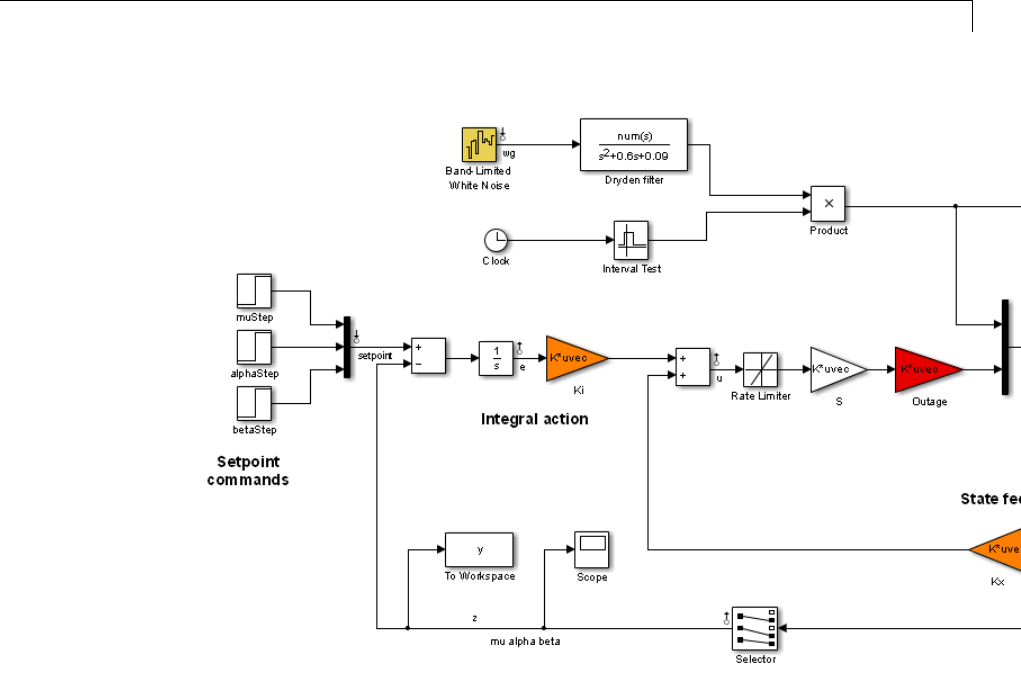
Reliable Control of a Fighter Jet
The aircraft is modeled as a 6th-order state-space system with the following
state variables (units are m/s for velocities and deg/s for angular rates):
•u: x-body axis velocity
•w: z-body axis velocity
•q: pitch rate
•v: y-body axis velocity
•p: roll rate
•r: yaw rate
The state vector is available for control as well as the flight-path bank angle
rate mu (deg/s), the angle of attack alpha (deg), and the sideslip angle beta
6-201

6Tuning Fixed Control Architectures
(deg). The control inputs are the deflections of the right elevator, left elevator,
right aileron, left aileron, and rudder. All deflections are in degrees. Elevators
are grouped symmetrically to generate the angle of attack. Ailerons are
grouped anti-symmetrically to generate roll motion. This leads to 3 control
actionsasshownintheSimulinkmodel.
The controller consists of state-feedback control in the inner loop and MIMO
integral action in the outer loop. The gain matrices Ki and Kx are 3-by-3 and
3-by-6, respectively, so the controller has 27 tunable parameters.
Actuator Failures
We use a 9x5 matrix to encode the nominal mode and various actuator failure
modes. Each row corresponds to one flight condition, a zero indicating outage
of the corresponding deflection surface.
OutageCases = [...
1 1 1 1 1; ... % nominal operational mode
0 1 1 1 1; ... % right elevator outage
1 0 1 1 1; ... % left elevator outage
1 1 0 1 1; ... % right aileron outage
1 1 1 0 1; ... % left aileron outage
1 0 0 1 1; ... % left elevator and right aileron outage
0 1 0 1 1; ... % right elevator and right aileron outage
0 1 1 0 1; ... % right elevator and left aileron outage
1 0 1 0 1; ... % left elevator and left aileron outage
];
Design Requirements
The controller should:
1Provide good tracking performance in mu, alpha, and beta in nominal
operating mode with adequate decoupling of the three axes
2Maintain performance in the presence of wind gust of 5 m/s
3Limit stability and performance degradation in the face of actuator outage.
To express the first requirement, you can use an LQG-like cost function that
penalizes the integrated tracking error eand the control effort u:
6-202
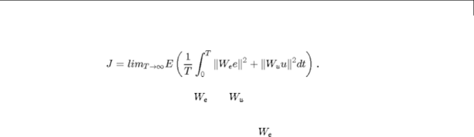
Reliable Control of a Fighter Jet
The diagonal weights and are the main tuning knobs for trading
responsiveness and control effort and emphasizing some channels over others.
Use the WeightedVariance requirement to express this cost function, and use
a less stringent performance weight for the outage scenarios.
% Nominal tracking requirement
We = diag([20 30 20]); Wu = eye(3);
SoftNom = TuningGoal.WeightedVariance('setpoint',{'e','u'}, blkdiag(We,Wu),
SoftNom.Models = 1; % nominal model
% Tracking requirement for outage conditions
We = diag([8 12 8]); Wu = eye(3);
SoftOut = TuningGoal.WeightedVariance('setpoint',{'e','u'}, blkdiag(We,Wu),
SoftOut.Models = 2:9; % outage scenarios
For wind gust alleviation, limit the variance of the error signal edue to
the white noise wg driving the wind gust model. Again use a less stringent
requirement for the outage scenarios.
% Nominal gust alleviation requirement
HardNom = TuningGoal.Variance('wg','e',0.01);
HardNom.Models = 1;
% Gust alleviation requirement for outage conditions
HardOut = TuningGoal.Variance('wg','e',0.03);
HardOut.Models = 2:9;
Controller Tuning for Nominal Flight
Set the wind gust speed to 5 m/s and initialize the tunable state-feedback and
integrators gains of the controller.
GustSpeed = 5;
Ki = eye(3);
Kx = zeros(3,6);
6-203

6Tuning Fixed Control Architectures
Use the slTunable interface to acquire a closed-loop model for each of the
nine flight conditions. The resulting generalized state-space array T0 contains
nine tunable models parameterized by the gains Ki,Kx.
clear T0
for k = 9:-1:1
outage = OutageCases(k,:) ;
ST = slTunable('rct_reliableF16',{'Ki','Kx'}) ;
T0(:,:,k) = ST.getIOTransfer({'setpoint';'wg'},{'e';'u'}) ;
end
T0
T0 =
9x1 array of generalized continuous-time state-space models.
Each model has 6 outputs, 4 inputs, 11 states, and the following blocks:
Ki: Parametric 3x3 gain, 1 occurrences.
Kx: Parametric 3x6 gain, 1 occurrences.
Type "ss(T0)" to see the current value, "get(T0)" to see all properties, a
n
Use systune to tune the controller gains for the first model (nominal
flight condition) subject to the nominal requirements. Treat the wind gust
alleviation as a hard constraint.
[T,fSoft,gHard] = systune(T0(:,:,1),SoftNom,HardNom);
Final: Soft = 23.2, Hard = 0.99652, Iterations = 250
Retrieve the gain values and simulate the responses to step commands in mu,
alpha, beta for the nominal and degraded flight conditions. All simulations
include wind gust effects, and the red curve is the nominal response.
Ki = getBlockValue(T, 'Ki'); Ki = Ki.d;
Kx = getBlockValue(T, 'Kx'); Kx = Kx.d;
% Bank-angle setpoint simulation
6-204
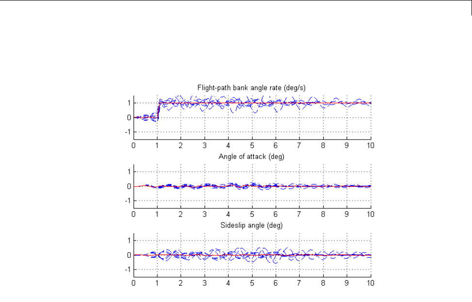
Reliable Control of a Fighter Jet
plotResponses(OutageCases,1,0,0);
% Angle-of-attack setpoint simulation
plotResponses(OutageCases,0,1,0);
6-205
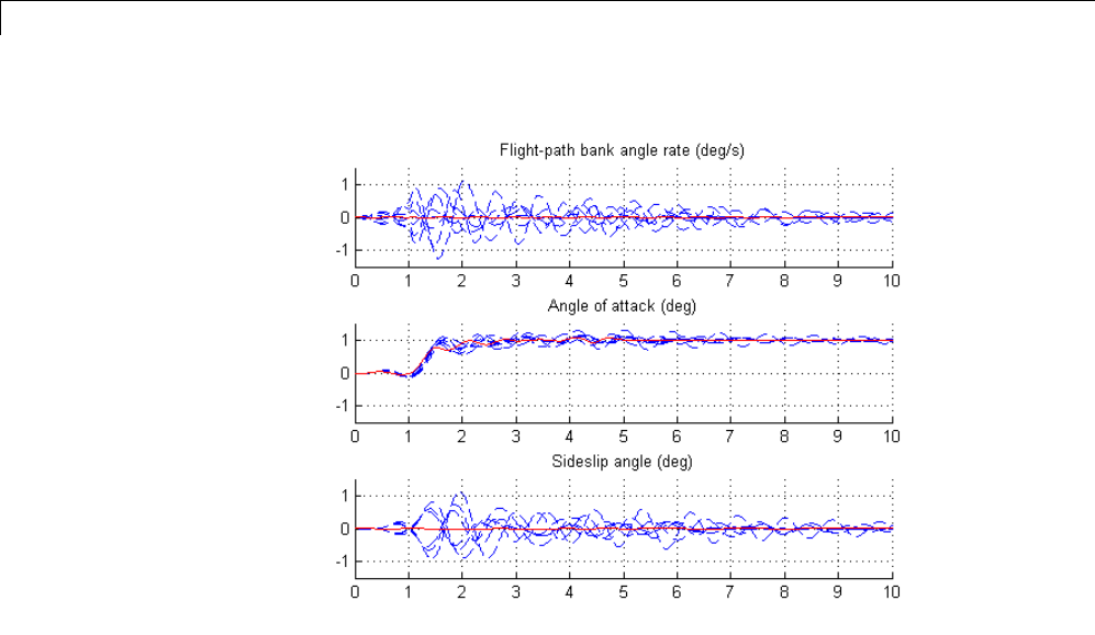
6Tuning Fixed Control Architectures
% Sideslip-angle setpoint simulation
plotResponses(OutageCases,0,0,1);
6-206
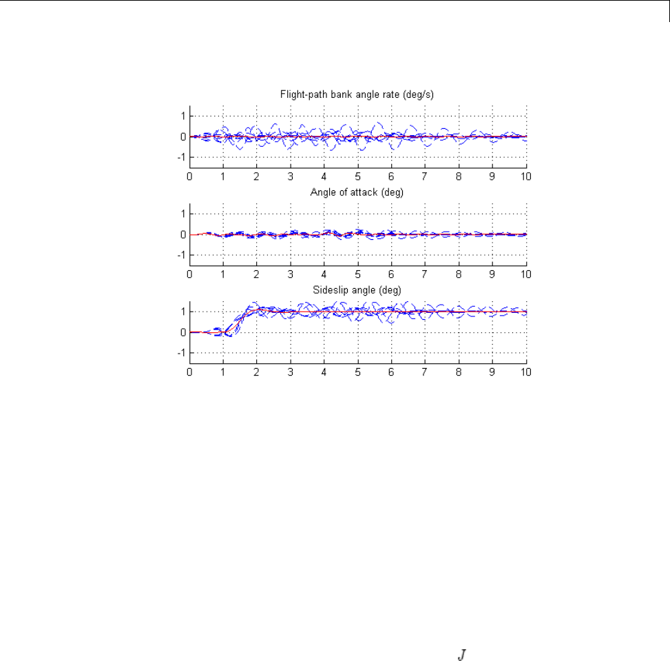
Reliable Control of a Fighter Jet
The nominal responses are good but the deterioration in performance is
unacceptable when faced with actuator outage.
Controller Tuning for Reliable Flight
To improve reliability, retune the controller gains to meet the nominal
requirement for the nominal plant (first model) as well as the relaxed
requirements for all eight outage scenarios. Note that systune now takes an
array of tunable models and tunes the gains against this set of plant models.
[T,fSoft,gHard] = systune(T0,[SoftNom;SoftOut],[HardNom;HardOut]);
Final: Soft = 25.9, Hard = 0.99758, Iterations = 358
The optimal performance (square root of LQG cost )isonlyslightlyworse
than for the nominal tuning (26 vs. 23). Retrieve the gain values and rerun
the simulations (red curve is the nominal response).
Ki = getBlockValue(T, 'Ki'); Ki = Ki.d;
Kx = getBlockValue(T, 'Kx'); Kx = Kx.d;
6-207
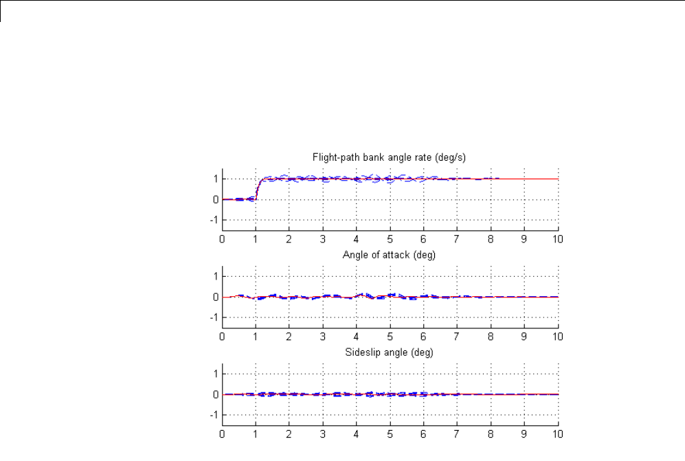
6Tuning Fixed Control Architectures
% Bank-angle setpoint simulation
plotResponses(OutageCases,1,0,0);
% Angle-of-attack setpoint simulation
plotResponses(OutageCases,0,1,0);
6-208
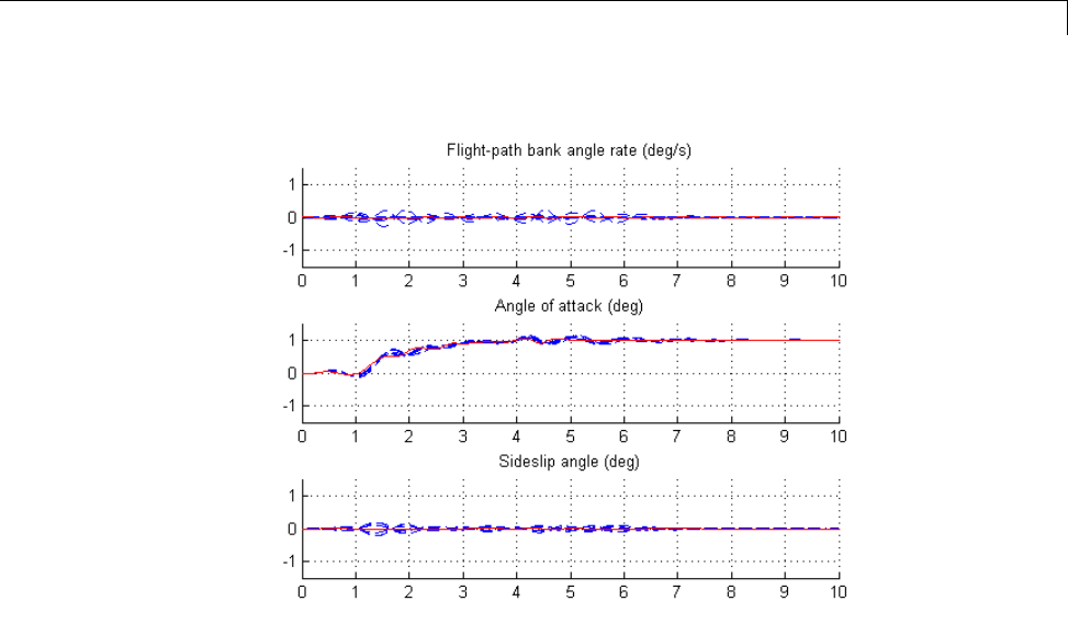
Reliable Control of a Fighter Jet
% Sideslip-angle setpoint simulation
plotResponses(OutageCases,0,0,1);
6-209

6Tuning Fixed Control Architectures
The controller now provides reliable performance in all flight conditions. The
design could be further refined by adding specifications such as minimum
stability margins and gain limits to avoid actuator rate saturation.
6-210
Fixed-Structure H-infinity Synthesis with HINFSTRUCT
Fixed-Structure H-infinity Synthesis with HINFSTRUCT
This example uses the hinfstruct command to tune a fixed-structure
controller subject to constraints.
Introduction
The hinfstruct command extends classical synthesis (see hinfsyn)to
fixed-structure control systems. This command is meant for users already
comfortable with the hinfsyn workflow. If you are unfamiliar with
synthesis or find augmented plants and weighting functions intimidating,
use systune and looptune instead. See "Tuning Control Systems with
SYSTUNE" for the systune counterpart of this example.
Plant Model
This example uses a 9th-order model of the head-disk assembly (HDA) in a
hard-disk drive. This model captures the first few flexible modes in the HDA.
load hinfstruct_demo G
bode(G), grid
6-211
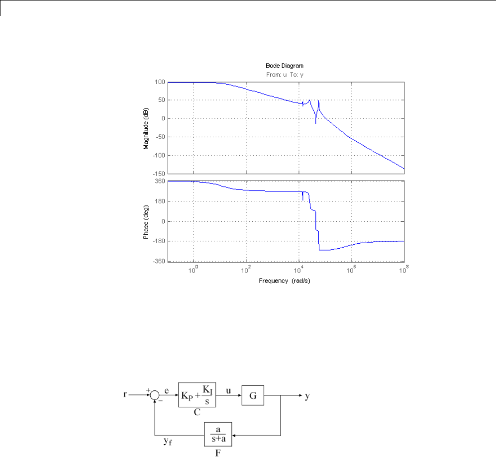
6Tuning Fixed Control Architectures
We use the feedback loop shown below to position the head on the correct
track. This control structure consists of a PI controller and a low-pass filter
in the return path. The head position yshould track a step change rwith
a response time of about one millisecond, little or no overshoot, and no
steady-state error.
Figure 1: Control Structure
Tunable Elements
6-212
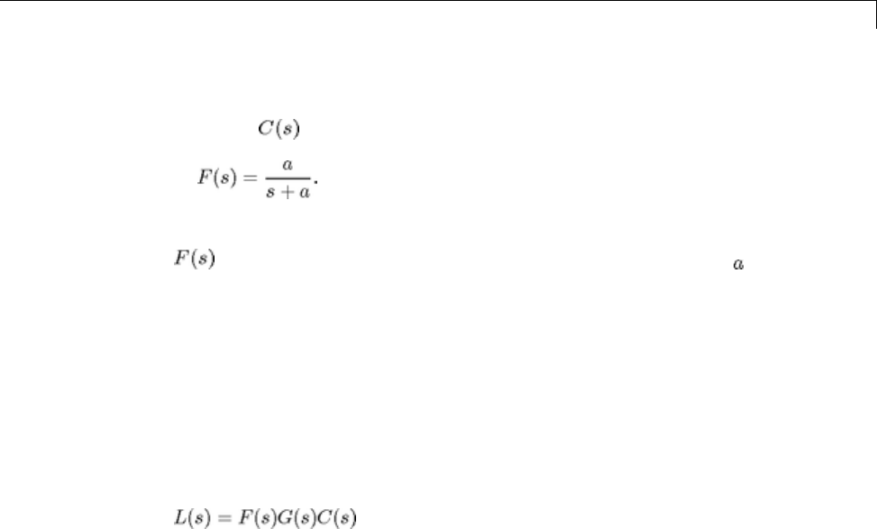
Fixed-Structure H-infinity Synthesis with HINFSTRUCT
There are two tunable elements in the control structure of Figure 1: the PI
controller and the low-pass filter
Use the ltiblock.pid class to parameterize the PI block and specify the filter
as a transfer function depending on a tunable real parameter .
C0 = ltiblock.pid('C','pi'); % tunable PI
a = realp('a',1); % filter coefficient
F0 = tf(a,[1 a]); % filter parameterized by a
Loop Shaping Design
Loop shaping is a frequency-domain technique for enforcing requirements on
response speed, control bandwidth, roll-off, and steady state error. The idea
is to specify a target gain profile or "loop shape" for the open-loop response
. A reasonable loop shape for this application should
have integral action and a crossover frequency of about 1000 rad/s (the
reciprocal of the desired response time of 0.001 seconds). This suggests the
following loop shape:
wc = 1000; % target crossover
s = tf('s');
LS = (1+0.001*s/wc)/(0.001+s/wc);
bodemag(LS,{1e1,1e5}), grid, title('Target loop shape')
6-213

6Tuning Fixed Control Architectures
Note that we chose a bi-proper, bi-stable realization to avoid technical
difficulties with marginally stable poles and improper inverses. In order to
tune and with hinfstruct, we must turn this target loop shape
into constraints on the closed-loop gains. A systematic way to go about this is
to instrument the feedback loop as follows:
•Add a measurement noise signal n
•Use the target loop shape LS and its reciprocal to filter the error signal e
and the white noise source nw.
6-214
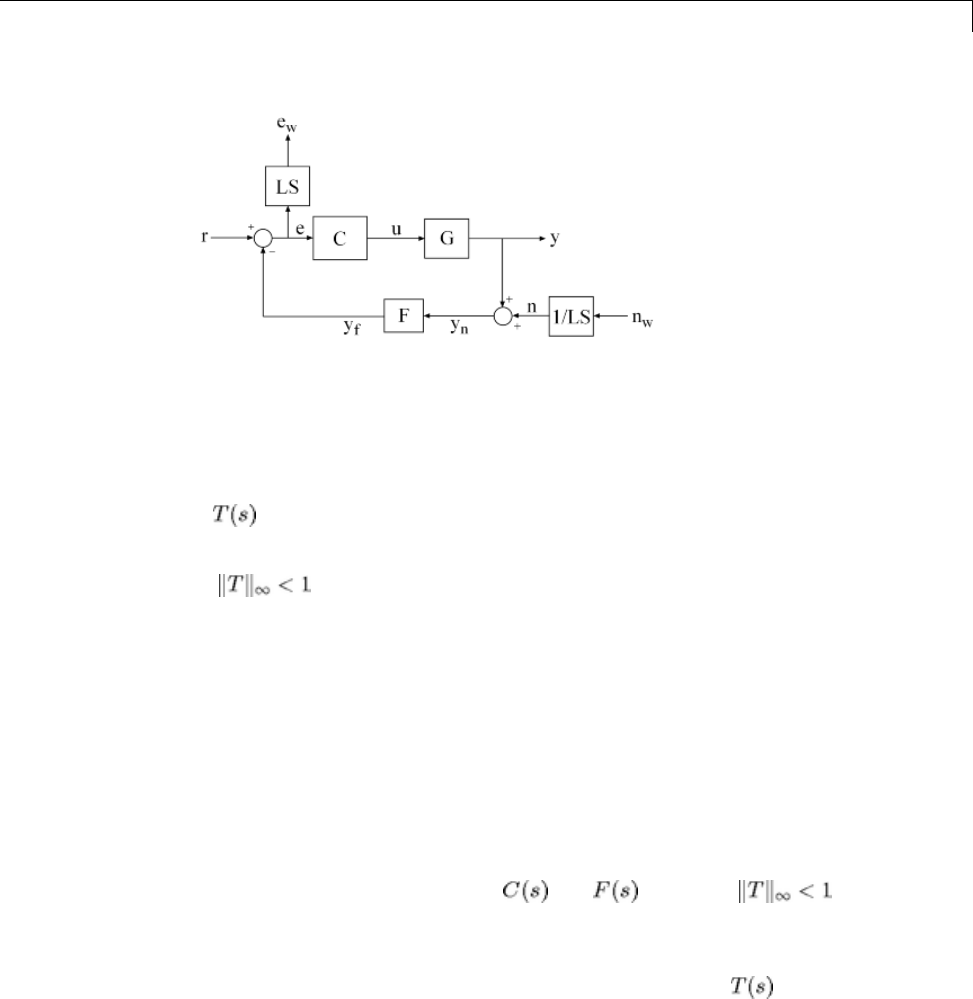
Fixed-Structure H-infinity Synthesis with HINFSTRUCT
Figure 2: Closed-Loop Formulation
If denotes the closed-loop transfer function from (r,nw) to (y,ew),the
gain constraint
secures the following desirable properties:
•At low frequency (w<wc), the open-loop gain stays above the gain specified
by the target loop shape LS
•At high frequency (w>wc), the open-loop gain stays below the gain specified
by LS
•The closed-loop system has adequate stability margins
•The closed-loop step response has small overshoot.
We can therefore focus on tuning and to enforce .
Specifying the Control Structure in MATLAB
In MATLAB, you can use the connect command to model by connecting
the fixed and tunable components according to the block diagram of Figure 2:
% Label the block I/Os
6-215
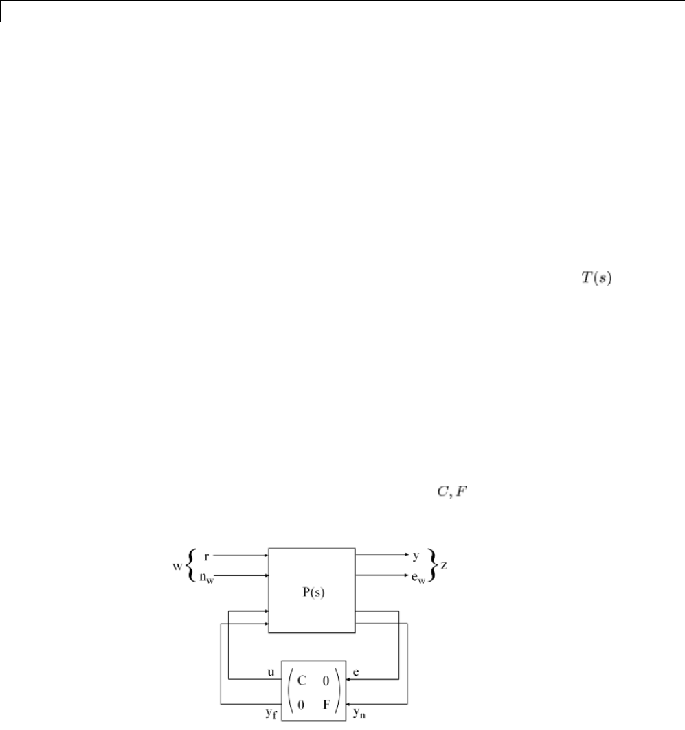
6Tuning Fixed Control Architectures
Wn = 1/LS; Wn.u = 'nw'; Wn.y = 'n';
We = LS; We.u = 'e'; We.y = 'ew';
C0.u = 'e'; C0.y = 'u';
F0.u = 'yn'; F0.y = 'yf';
% Specify summing junctions
Sum1 = sumblk('e = r - yf');
Sum2 = sumblk('yn = y + n');
% Connect the blocks together
T0 = connect(G,Wn,We,C0,F0,Sum1,Sum2,{'r','nw'},{'y','ew'});
These commands construct a generalized state-space model T0 of .This
model depends on the tunable blocks Cand a:
T0.Blocks
ans =
C: [1x1 ltiblock.pid]
a: [1x1 realp]
Note that T0 captures the following "Standard Form" of the block diagram
of Figure 2 where the tunable components are separated from the fixed
dynamics.
6-216
Fixed-Structure H-infinity Synthesis with HINFSTRUCT
Figure 3: Standard Form for Disk-Drive Loop Shaping
Tuning the Controller Gains
We are now ready to use hinfstruct to tune the PI controller and filter
for the control architecture of Figure 1. To mitigate the risk of local minima,
run three optimizations, two of which are started from randomized initial
values for C0 and F0:
rng('default')
opt = hinfstructOptions('Display','final','RandomStart',4);
T = hinfstruct(T0,opt);
Final: Peak gain = 1.56, Iterations = 123
Final: Peak gain = 597, Iterations = 199
Min decay rate 1e-07 is close to lower bound 1e-07
Final: Peak gain = 1.56, Iterations = 131
Final: Peak gain = 1.56, Iterations = 129
Final: Peak gain = 1.56, Iterations = 113
The best closed-loop gain is 1.56, so the constraint is nearly
satisfied. The hinfstruct command returns the tuned closed-loop transfer
.UseshowTunable to see the tuned values of and the filter coefficient
:
showTunable(T)
C=
1
Kp + Ki * ---
s
with Kp = 0.000846, Ki = 0.0103
Name: C
Continuous-time PI controller in parallel form.
-----------------------------------
6-217

6Tuning Fixed Control Architectures
a = 5.49e+03
Use getBlockValue to get the tuned value of and use getValue to
evaluate the filter for the tuned value of :
C = getBlockValue(T,'C');
F = getValue(F0,T.Blocks); % propagate tuned parameters from T to F
tf(F)
ans =
From input "yn" to output "yf":
5486
--------
s + 5486
Continuous-time transfer function.
To validate the design, plot the open-loop response L=F*G*C and compare
with the target loop shape LS:
bode(LS,'r--',G*C*F,'b',{1e1,1e6}), grid,
title('Open-loop response'), legend('Target','Actual')
6-218
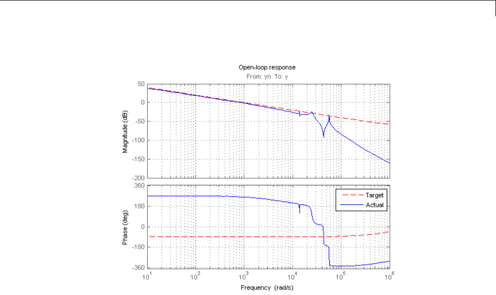
Fixed-Structure H-infinity Synthesis with HINFSTRUCT
The 0dB crossover frequency and overall loop shape are as expected. The
stability margins can be read off the plot by right-clicking and selecting the
Characteristics menu. This design has 24dB gain margin and 81 degrees
phase margin. Plot the closed-loop step response from reference rto position y:
step(feedback(G*C,F)), grid, title('Closed-loop response')
6-219
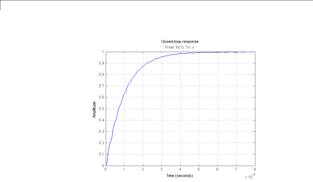
6Tuning Fixed Control Architectures
While the response has no overshoot, there is some residual wobble due to
the first resonant peaks in G. You might consider adding a notch filter in the
forward path to remove the influence of these modes.
Tuning the Controller Gains from Simulink
Suppose you used this Simulink model to represent the control structure.
If you have Simulink Control Design installed, you can tune the controller
gains from this Simulink model as follows. First mark the signals r,e,y,n
as linearization I/Os:
6-220
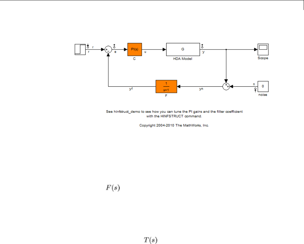
Fixed-Structure H-infinity Synthesis with HINFSTRUCT
Then create an instance of the slTunable interface and mark the Simulink
blocks Cand Fas tunable:
ST = slTunable('rct_diskdrive',{'C','F'});
Since the filter has a special structure, explicitly specify how to
parameterize the Fblock:
a = realp('a',1); % filter coefficient
ST.setBlockParam('F',tf(a,[1 a]));
Finally, use the getIOTransfer method to derive a tunable model of the
closed-loop transfer function (see Figure 2)
% Tunable model of closed-loop transfer (r,n) -> (y,e)
slT0 = ST.getIOTransfer({'r','n'},{'y','e'});
% Add weighting functions in n and e channels
slT0 = blkdiag(1,LS) * slT0 * blkdiag(1,1/LS);
You are now ready to tune the controller gains with hinfstruct:
rng(0)
opt = hinfstructOptions('Display','final','RandomStart',4);
slT = hinfstruct(slT0,opt);
6-221

6Tuning Fixed Control Architectures
Final: Peak gain = 3.89, Iterations = 124
Final: Peak gain = 597, Iterations = 184
Min decay rate 1.01e-07 is close to lower bound 1e-07
Final: Peak gain = 1.56, Iterations = 125
Final: Peak gain = 1.56, Iterations = 93
Final: Peak gain = 1.56, Iterations = 92
Verify that you obtain the same tuned values as with the MATLAB approach:
showTunable(slT)
C=
1
Kp + Ki * ---
s
with Kp = 0.000846, Ki = 0.0103
Name: C
Continuous-time PI controller in parallel form.
-----------------------------------
a = 5.49e+03
6-222

A
Examples
Use this list to find examples in the documentation.


Index
IndexSymbols and Numerics
μ-synthesis control design 5-28
2-norm
definition 5-2
A
actmod actuator model 5-29
actnom nominal actuator model 5-29
additive error bound 3-5
B
block diagrams
direction of arrows 5-4
bstmr 3-10
C
complementary sensitivity 2-6
crossover frequency wc2-21
D
Delta1 object 4-15
Delta2 object 4-15
design goals
crossover 2-21
performance 2-21
roll-off 2-21
stability robustness 2-21
disturbance attenuation 2-7
dksyn 5-31
E
Euclidean norms 5-8
F
feedback 4-9
forbidden regions 2-12
frequency domain uncertainty
adding to the model 4-15
fundamental limits
right-half-plane poles 2-21
right-half-plane zeros 2-21
G
gain reduction tolerance 2-13
gain/phase margins
MIMO system 2-12
get
viewing the properties of the uncertain
system 4-14
H
H∞
loop shaping 1-12
mixed-sensitivity 1-12
mixsyn 2-22
norm 2-5
sampled-data 1-12
H∞control
performance objectives 5-10
H2
norm 2-5
H2and H∞control design commands
summary 5-17
Hankel singular value
NCF 1-19
HiMAT aircraft model 1-13
hinfsyn 5-23
I
InputGroup property 4-15
InputName property 4-15
Index-1

Index
L
L2-norm 5-2
linear matrix inequalities
LMI solvers 1-22
LMI solvers 1-22
loop shaping 1-12
loopsyn 2-6
loop transfer function matrix 2-6
loopmargin 4-19
loopsens 4-17
M
makeweight utility 4-7
maxgain variable 4-12
mixed H∞/H2
controller synthesis 1-12
mixed-sensitivity cost function 2-22
mixed-sensitivity loop shaping 2-22
model reduction 1-17
additive error methods 3-7
balanced stochastic method 3-10
large-scale models 3-14
multiplicative error method 3-9
normalized coprime factor truncation 3-15
model reduction routines 3-5
models
with uncertain real coefficients 4-4
modreal 3-14
Monte Carlo random sample 1-7
multiplicative (relative) error bound 3-5
multiplicative uncertainty 2-2
N
ncfmr 3-15
NominalValue property 4-15
norm 4-22
norms 5-2
H∞2-4
H22-4
performance 5-3
O
OutputGroup property 4-15
OutputName property 4-15
P
Percentage property 4-3
performance weights 5-8
perturbation
additive 2-7
multiplicative 2-7
PlusMinus property 4-3
R
Range property 4-3
reduce 3-7
report variable 4-11
robust performance
defined 5-28
robustness
of stability 2-21
robustness analysis
Monte Carlo 1-9
worst case 1-9
robustperf 4-25
robuststab 4-10
roll-off 2-21
S
schurmr 3-7
sensitivity 2-6
singular values 2-4
properties of 2-4
stabmarg variable 4-11
sysic 5-22
Index-2

Index
U
ultidyn 4-6
uncertain elements 4-2
uncertain LTI system 1-4
uncertain parameters 4-3
uncertain state-space object.SeeUSS object
uncertainty
capturing 4-7
ureal 4-3
USS object 1-7
usubs
substituting worst-case values for uncertain
elements 4-12
W
W1 and W2 shaping filters 4-15
wcgain
computing worst-case peak gain 4-11
wcsens 4-25
wcu variable 4-12
weighted norms 5-4
worst-case
peak gain 1-11
Index-3
