R User Guide

User Manual:

Open the PDF directly: View PDF .
Page Count: 26

AC-PCA: simultaneous dimension reduction and

adjustment for confounding variation

User’s Guide

Zhixiang Lin

October 31, 2016

If you use AC-PCA in published research, please cite:

Z. Lin, C. Yang, Y. Zhu, J. C. Duchi, Y. Fu, Y. Wang, B. Jiang, M. Zamanighomi,

X. Xu, M. Li, N. Sestan, H. Zhao, W. H. Wong:

AC-PCA: simultaneous dimension reduction and adjustment for confounding variation

bioRxiv, http://dx.doi.org/10.1101/040485

Contents

1 Introduction 2

1.1 Scope ................................. 2

1.2 How to get help . . . . . . . . . . . . . . . . . . . . . . . . . . . . 2

1.3 Input for AC-PCA . . . . . . . . . . . . . . . . . . . . . . . . . . 2

2 Theory behind AC-PCA 2

2.1 AC-PCA in a general form . . . . . . . . . . . . . . . . . . . . . . 2

2.2 AC-PCA with sparse loading . . . . . . . . . . . . . . . . . . . . 3

3 Speciﬁc experimental designs and case studies 3

3.1 Categorical confounding factors . . . . . . . . . . . . . . . . . . . 3

3.2 Continuous confounding factors . . . . . . . . . . . . . . . . . . . 7

3.3 Experiments with replicates . . . . . . . . . . . . . . . . . . . . . 10

3.4 Application to a human brain exon array dataset . . . . . . . . . 12

3.5 Application to a model organism ENCODE (modENCODE) RNA-

Seqdataset .............................. 16

3.6 AC-PCA with sparsity . . . . . . . . . . . . . . . . . . . . . . . . 23

1 Introduction

1.1 Scope

Dimension reduction methods are commonly applied to visualize datapoints in a

lower dimensional space and identify dominant patterns in the data. Confound-

ing variation, technically and biologically originated, may aﬀect the performance

of these methods, and hence the visualization and interpretation of the results.

AC-PCA simultaneously performs dimension reduction and adjustment for con-

founding variation. The intuition of AC-PCA is that it captures the variations

that are invariant to the confounding factors. One major application area for

AC-PCA is the transcriptome data, and it can be implemented to other data

types as well.

1.2 How to get help

This user’s guide addresses many scenarios for confounding factors. Additional

questions about AC-PCA can be sent to linzx06@gmail.com. Comments on

possible improvements are very welcome.

1.3 Input for AC-PCA

AC-PCA requires two inputs: the data matrix Xand the confounder matrix Y.

Xis of dimension n×p, where nis the number of samples and pis the number

of variables (genes). Yis of dimension n×q, where nis the number of samples

and qis the number of confounding factors. Missing data is allowed in both X

and Y. The columns in Xand Yare assumed to be centered.

Confounding factors depend on the experimental design and can also depend

on the scientiﬁc question: confounding factors can be diﬀerent for the same

experiment. As an example, consider a transcriptome experiment where gene

expression levels were measured in multiple tissues from multiple species. If

one wants to capture the variation across tissues that is shared among species,

then the species labels are the confounding factors. In constrast, if the variation

across species but shared among tissues are desirable, the tissue labels are the

confounding factors. AC-PCA is suitable for experiments with complex designs.

In the following sections, we implement AC-PCA and provide details on how

to design Yfor various types of confounders and various experimental designs.

2 Theory behind AC-PCA

2.1 AC-PCA in a general form

Let Xbe the N×pdata matrix and Ybe the N×lmatrix for lconfounding

factors. Let K=Y Y T. We propose the following objective function to adjust

for confounding variation:

maximize

v∈RpvTXTXv −λvTXTKXv

subject to ||v||2

2≤1,

(1)

We can choose Yso that vTXTKXv represents the confounding variation in

the projected data. Formula 1 can be generalized to other kernels on Y. In the

R package, we provide options for linear kernel(i.e. Y Y T) and Gaussian kernel.

2.2 AC-PCA with sparse loading

A sparse solution for vcan be achieved by adding `1constraint:

maximize

v∈RpvTXTXv subject to vTXTKXv ≤c1,||v||1≤c2,||v||2

2≤1.(2)

3 Speciﬁc experimental designs and case studies

3.1 Categorical confounding factors

Categorical confounding factors are commonly observed in biological data, it

can be technical (diﬀerent experimental batches, etc.) and biological (donor

labels, diﬀerent races, species, etc.). we treat samples with the same confounder

label as a group. Here are the group labels for simulated example 1:

> library(acPCA)

> data(data_example1)

> data_example1$group ### the group labels

[1]111111111122222222223333333333

> X <- data_example1$X ### the data matrix

we perform regular PCA and compare the result with the true simulated

pattern:

> pca <- prcomp(X, center=T) ###regular PCA

> par(mfrow=c(1,2), pin=c(2.5,2.5), mar=c(4.1, 3.9, 3.2, 1.1))

> plot(pca$x[,1], pca$x[,2], xlab="PC 1", ylab="PC 2", col="black", type="n", main="PCA")

> text(pca$x[,1], pca$x[,2], labels = data_example1$lab, col=data_example1$group+1)

> plot(data_example1$true_pattern[1,], data_example1$true_pattern[2,],

+ xlab="Factor 1", ylab="Factor 2", col="black", type="n", main="True pattern",

+ xlim=c(min(data_example1$true_pattern[1,])-0.3,

+ max(data_example1$true_pattern[1,])+0.3) )

> text(data_example1$true_pattern[1,], data_example1$true_pattern[2,], labels = 1:10)

−20 0 20 40

−20 −10 0 10 20 30 40

PCA

PC 1

PC 2

10 1

−1.5 −0.5 0.5 1.5

0.0 0.5 1.0 1.5

True pattern

Factor 1

Factor 2

In the PCA plot, each color represents a group of samples with the same

confounder label. The confounding variation dominates variation of the true

pattern.

To adjust for the confounding variation, the Ymatrix is desiged such that

the penalty term equals the between groups sum of squares:

> Y <- data_example1$Y ### the confounder matrix

> Y

[,1] [,2] [,3]

[1,] 0.6666667 -0.3333333 -0.3333333

[2,] 0.6666667 -0.3333333 -0.3333333

[3,] 0.6666667 -0.3333333 -0.3333333

[4,] 0.6666667 -0.3333333 -0.3333333

[5,] 0.6666667 -0.3333333 -0.3333333

[6,] 0.6666667 -0.3333333 -0.3333333

[7,] 0.6666667 -0.3333333 -0.3333333

[8,] 0.6666667 -0.3333333 -0.3333333

[9,] 0.6666667 -0.3333333 -0.3333333

[10,] 0.6666667 -0.3333333 -0.3333333

[11,] -0.3333333 0.6666667 -0.3333333

[12,] -0.3333333 0.6666667 -0.3333333

[13,] -0.3333333 0.6666667 -0.3333333

[14,] -0.3333333 0.6666667 -0.3333333

[15,] -0.3333333 0.6666667 -0.3333333

[16,] -0.3333333 0.6666667 -0.3333333

[17,] -0.3333333 0.6666667 -0.3333333

[18,] -0.3333333 0.6666667 -0.3333333

[19,] -0.3333333 0.6666667 -0.3333333

[20,] -0.3333333 0.6666667 -0.3333333

[21,] -0.3333333 -0.3333333 0.6666667

[22,] -0.3333333 -0.3333333 0.6666667

[23,] -0.3333333 -0.3333333 0.6666667

[24,] -0.3333333 -0.3333333 0.6666667

[25,] -0.3333333 -0.3333333 0.6666667

[26,] -0.3333333 -0.3333333 0.6666667

[27,] -0.3333333 -0.3333333 0.6666667

[28,] -0.3333333 -0.3333333 0.6666667

[29,] -0.3333333 -0.3333333 0.6666667

[30,] -0.3333333 -0.3333333 0.6666667

Here are the results when we implement AC-PCA:

> par(mfrow=c(1,1))

> ### first tune lambda

> result_tune <- acPCAtuneLambda(X=X, Y=Y, nPC=2, lambdas=seq(0, 10, 0.05),

+ anov=T, kernel = "linear", quiet=T)

> ###run with the best lambda

> result <- acPCA(X=X, Y=Y, lambda=result_tune$best_lambda,

+ kernel="linear", nPC=2)

> ###the signs of the PCs are meaningless

> plot(result$Xv[,1], -result$Xv[,2], xlab="PC 1", ylab="PC 2",

+ type="n", main="AC-PCA")

> text(result$Xv[,1], -result$Xv[,2], labels = data_example1$lab,

+ col=data_example1$group+1)

−30 −20 −10 0 10 20 30

−10 −5 0 5

AC−PCA

PC 1

PC 2

456

We set anov =Tas the penalty term has the ANOVA interpretation. AC-

PCA is able to recover the true latent structure. We can also implement AC-

PCA with Gaussian kernel (bandwidth h= 0.5):

> h <- 0.5

> result_tune <- acPCAtuneLambda(X=X, Y=Y, nPC=2, lambdas=seq(0, 10, 0.05),

+ anov=F, kernel = "gaussian",

+ bandwidth=h, quiet=T)

> result <- acPCA(X=X, Y=Y, lambda=result_tune$best_lambda,

+ kernel="gaussian", bandwidth=h, nPC=2)

> ###the signs of the PCs are meaningless

> plot(result$Xv[,1], -result$Xv[,2], xlab="PC 1", ylab="PC 2",

+ col="black", type="n", main="Gaussian kernel, h=0.5")

> text(result$Xv[,1], -result$Xv[,2], labels = data_example1$lab,

+ col=data_example1$group+1)

−30 −20 −10 0 10 20 30

−10 −5 0 5

Gaussian kernel, h=0.5

PC 1

PC 2

456

We set anov =Fas the penalty term does not have the ANOVA interpre-

tation. Gaussian kernel also works well. For detailed discussion on bandwidth

selection, please refer to Chapter 3 in [4].

3.2 Continuous confounding factors

Continuous confounding factors may be present in biological data, for example,

age.

Simulated example 2: the confounder is assumed to be continuous and it con-

tributes a global trend to the data.

We ﬁrst perform regular PCA:

> data(data_example2)

> X <- data_example2$X ###the data matrix

> Y <- data_example2$Y ###the confounder matrix

> Y

[,1]

[1,] 2.5

[2,] -0.5

[3,] -3.5

[4,] 4.5

[5,] 0.5

[6,] -4.5

[7,] -1.5

[8,] 3.5

[9,] 1.5

[10,] -2.5

> pca <- prcomp(X, center=T) ###regular PCA

> par(mfrow=c(2,2), pin=c(2.5,2.5), mar=c(4.1, 3.9, 3.2, 1.1))

> plot(pca$x[,1], pca$x[,2], xlab="PC 1", ylab="PC 2", col="black", type="n", main="PCA")

> text(pca$x[,1], pca$x[,2], labels = data_example2$lab)

> plot(data_example2$true_pattern[1,], data_example2$true_pattern[2,],

+ xlab="Factor 1", ylab="Factor 2", col="black", type="n", main="True pattern",

+ xlim=c(min(data_example2$true_pattern[1,])-0.3,

+ max(data_example2$true_pattern[1,])+0.3) )

> text(data_example2$true_pattern[1,], data_example2$true_pattern[2,],

+ labels = data_example2$lab)

> plot(data_example2$confound_pattern[1,], data_example2$confound_pattern[2,],

+ xlab="", ylab="", col="black", type="n", main="Confounding pattern",

+ xlim=c(min(data_example2$confound_pattern[1,])-0.3,

+ max(data_example2$confound_pattern[1,])+0.3) )

> text(data_example2$confound_pattern[1,], data_example2$confound_pattern[2,], labels =

+ paste(data_example2$lab, '(',data_example2$Y, ')', sep=""), cex=0.5 )

−40 −20 0 20 40

−20 0 10 20 30

PCA

PC 1

PC 2

abc

def

hij

−1.5 −0.5 0.5 1.5

0.0 0.5 1.0 1.5

True pattern

Factor 1

Factor 2

def

−1.5 −0.5 0.5 1.5

0.2 0.4 0.6 0.8

Confounding pattern

a(2.5)

b(−0.5)

c(−3.5)

d(4.5)

e(0.5)

f(−4.5)

g(−1.5)

h(3.5)

i(1.5)

j(−2.5)

Next, we implement AC-PCA with linear and Gaussian kernels:

> ### linear kernel

> result_tune <- acPCAtuneLambda(X=X, Y=Y, nPC=2, lambdas=seq(0, 10, 0.05),

+ anov=F, kernel = "linear", quiet=T)

> result <- acPCA(X=X, Y=Y, lambda=result_tune$best_lambda,

+ kernel="linear", nPC=2)

> par(mfrow=c(1,2), pin=c(2.5,2.5), mar=c(4.1, 3.9, 3.2, 1.1))

> plot(result$Xv[,1], result$Xv[,2], xlab="PC 1", ylab="PC 2",

+ col="black", type="n", main="Linear kernel")

> text(result$Xv[,1], result$Xv[,2], labels = data_example2$lab)

> ### Gaussian kernel

> result_tune <- acPCAtuneLambda(X=X, Y=Y, nPC=2, lambdas=seq(0, 10, 0.05),

+ anov=F, kernel = "gaussian",

+ bandwidth=mean(abs(Y)), quiet=T)

> result <- acPCA(X=X, Y=Y, lambda=result_tune$best_lambda,

+ kernel = "gaussian", bandwidth=mean(abs(Y)), nPC=2)

> plot(result$Xv[,1], result$Xv[,2], xlab="PC 1", ylab="PC 2",

+ col="black", type="n", main=paste("Gaussian kernel, h=", mean(abs(Y)), sep="") )

> text(result$Xv[,1], result$Xv[,2], labels = data_example2$lab)

−20 0 10 20 30

−10 −5 0 5

Linear kernel

PC 1

PC 2

−30 −10 0 10 20

−5 0 5 10

Gaussian kernel, h=2.5

PC 1

PC 2

The results of linear and Gaussian kernels are comparable.

3.3 Experiments with replicates

Consider an experiment where the gene expression levels are measured under

multiple biological conditions with several replicates. It may be desirable to

capture the variation across biological conditions but shared among replicates.

Simulated example 3: there are 10 biological conditions, each with n= 3 repli-

cates. The variation is shared among replicates for half of the genes and not

shared for the other genes. Suppose we want to capture the variation shared

among replicates, the confounder matrix can be chosen such that samples within

the same biological condition are “pushed” together:

> data(data_example3)

> X <- data_example3$X ### the data matrix

> data_example3$lab ### the biological conditions

[1]1112223334445556667778889

[26] 9 9 10 10 10

> Y <- data_example3$Y ### the confounder matrix

> dim(Y)

[1] 30 30

> Y[,1]

[1] 0.5773503 -0.5773503 0.0000000 0.0000000 0.0000000 0.0000000

[7] 0.0000000 0.0000000 0.0000000 0.0000000 0.0000000 0.0000000

[13] 0.0000000 0.0000000 0.0000000 0.0000000 0.0000000 0.0000000

[19] 0.0000000 0.0000000 0.0000000 0.0000000 0.0000000 0.0000000

[25] 0.0000000 0.0000000 0.0000000 0.0000000 0.0000000 0.0000000

In each column of Y, there is one 1/√nand one −1/√ncorresponding to a

pair of samples from the same biological condition. So the number of columns

in Yis 10 ×3×2/2. For a biological condition, treating the 3 replicates as

3 groups, it can be shown that the penalty term vTXTY Y TXv equals the

summation of the between groups sum of squares over the biological conditions.

When the number of replicates across the biological conditions is not the same, to

maintain the ANOVA interpretation, we can change the corresponding entries in

Yto 1/√niand 1/√ni, where niis the number of replicates in the ith biological

condition. We ﬁrst implement PCA and compare it with the true pattern:

> pca <- prcomp(X, center=T) ###regular PCA

> par(mfrow=c(1,2), pin=c(2.5,2.5), mar=c(4.1, 3.9, 3.2, 1.1))

> plot(pca$x[,1], pca$x[,2], xlab="PC 1", ylab="PC 2", col="black", type="n", main="PCA")

> text(pca$x[,1], pca$x[,2], labels = data_example3$lab)

> plot(data_example3$true_pattern[1,], data_example3$true_pattern[2,],

+ xlab="Factor 1", ylab="Factor 2", col="black", type="n", main="True pattern",

+ xlim=c(min(data_example3$true_pattern[1,])-0.3,

+ max(data_example3$true_pattern[1,])+0.3) )

> text(data_example3$true_pattern[1,], data_example3$true_pattern[2,],

+ labels = 1:10)

−40 0 20 40 60

−40 −30 −20 −10 0 10 20 30

PCA

PC 1

PC 2

−1.5 −0.5 0.5 1.5

0.0 0.5 1.0 1.5

True pattern

Factor 1

Factor 2

Next we implement AC-PCA:

> result_tune <- acPCAtuneLambda(X=X, Y=Y, nPC=2, lambdas=seq(0, 10, 0.05),

+ anov=T, kernel = "linear", quiet=T)

> result <- acPCA(X=X, Y=Y, lambda=result_tune$best_lambda,

+ kernel="linear", nPC=2)

> par(mfrow=c(1,1))

> plot(-result$Xv[,1], result$Xv[,2], xlab="PC 1", ylab="PC 2",

+ col="black", type="n", main="Linear kernel")

> text(-result$Xv[,1], result$Xv[,2], labels = data_example3$lab)

−20 −10 0 10 20

−10 −5 0 5

Linear kernel

PC 1

PC 2

3.4 Application to a human brain exon array dataset

We analyze the human brain exon array dataset [3]. The dataset was down-

loaded from the Gene Expression Omnibus (GEO) database under the acces-

sion number GSE25219. The dataset was generated from 1,340 tissue samples

collected from 57 developing and adult post-mortem brains. In the dataset,

gene expression levels were measured in diﬀerent brain regions in multiple time

windows. We use a subset of 1,000 genes for demonstration purpose. For time

window 5, we ﬁrst perform PCA to visualize the brain regions:

> data(data_brain_w5)

> X <- data_brain_w5$X;

> table(data_brain_w5$hemispheres) ###1: left hemisphere, 3: right hemisphere

1 3

45 29

> pca <- prcomp(X, center=T) ###regular PCA

> plot(pca$x[,1], pca$x[,2], xlab="PC 1", ylab="PC 2",

+ col="black", type="n", main="PCA, window 5, brain data")

> text(pca$x[,1], pca$x[,2], labels = data_brain_w5$regions,

+ col=data_brain_w5$donor_labs, font=data_brain_w5$hemispheres)

−20 −10 0 10

−10 −5 0 5 10

PCA, window 5, brain data

PC 1

PC 2

MFC

VFC

DFC

STC

ITC

A1C

IPC

S1C

M1C MFC

OFC

VFC

DFC STC

ITC

A1C

IPC

S1C

M1C

MFC

OFC VFC

DFC

STC

ITC

A1C

IPC

S1C

M1C

MFC

OFC

VFC

DFC

STC

ITC

A1C

IPC

S1C

M1C

MFC

OFC

VFC

DFC

STC

ITC

A1C

IPC

S1C

M1C

MFC

OFC

VFC

DFC

STC

ITC

IPC S1C

MFC

OFC

VFC

DFC

STC

ITC

A1C

IPC

S1C M1C

VFC

STC

ITC

A1C

IPC

S1CM1C

In window 5, samples from the same donor tend to form a cluster. To adjust

for the donor’s eﬀect, we selected Yso that the penalty term vTXTY Y TXv

equals the donor to donor variation in the projected data.

> Y <- data_brain_w5$Y

We ﬁrst tune λ:

> result_tune <- acPCAtuneLambda(X=X, Y=Y, nPC=2, lambdas=seq(0, 20, 0.1),

+ anov=T, kernel = "linear", quiet=T)

> result_tune$best_lambda

[1] 2.9

We set anov =Tas the penalty term has the ANOVA interpretation. Next

we use the tuned λ:

> result1 <- acPCA(X=X, Y=Y, lambda=result_tune$best_lambda,

+ kernel="linear", nPC=2)

> Xv1 <- result1$Xv

> plot(Xv1[,1], Xv1[,2], xlab="PC 1", ylab="PC 2",

+ col="black", type="n", main=paste("AC-PCA, window 5, lambda=",

+ result_tune$best_lambda, sep="") )

> text(Xv1[,1], Xv1[,2], labels = data_brain_w5$regions,

+ col=data_brain_w5$donor_labs, font=data_brain_w5$hemispheres)

−4 −2 0 2 4

−3 −2 −1 0 1 2 3 4

AC−PCA, window 5, lambda=2.9

PC 1

PC 2

MFC

VFC

DFC

STC ITC

A1C

IPC

S1C

M1C

MFC

OFC

VFC

DFC

STC ITC

A1C

IPC

S1C

M1C

MFC

OFC

VFC

DFC

STC

ITC

A1C

IPC

S1C

M1C

MFC

OFC

VFC

DFC

STC ITC

A1C

IPC

S1C

M1C

MFC

OFC

VFC DFC

STC ITC

A1C

IPC

S1C

M1C

MFC

OFC

VFC

DFC

STC ITC

IPC

S1C

MFC

OFC

VFC

DFC

STC ITC

A1C

IPC

S1C

M1C

VFC

STC ITC

A1C

IPC

S1C

M1C

In the manuscript, we used λ= 5:

> result2 <- acPCA(X=X, Y=Y, lambda=5, kernel="linear", nPC=2)

> Xv2 <- result2$Xv

> plot(-Xv2[,1], Xv2[,2], xlab="PC 1", ylab="PC 2",

+ col="black", type="n", main="AC-PCA, window 5, lambda=5")

> text(-Xv2[,1], Xv2[,2], labels = data_brain_w5$regions,

+ col=data_brain_w5$donor_labs, font=data_brain_w5$hemispheres)

Figure 1: Representative fetal human brain, lateral surface of hemisphere [3]

−2 0 2 4

−2 −1 0 1 2 3

AC−PCA, window 5, lambda=5

PC 1

PC 2

MFC

VFC

DFC

STC ITC

A1C

IPC

S1C

M1C

MFC

OFC

VFC

DFC

STC ITC

A1C

IPC

S1C

M1C

MFC

OFC

VFC

DFC

STC ITC

A1C

IPC

S1C

M1C

MFC

OFC

VFC

DFC

STC ITC

A1C

IPC

S1C

M1C

MFC

OFC

VFC DFC

STC ITC

A1C

IPC

S1C

M1C

MFC

OFC

VFC

DFC

STC ITC

IPC

S1C

MFC

OFC

VFC

DFC

STC ITC

A1C

IPC

S1C

M1C VFC

STC ITC

A1C

IPC

S1C

M1C

The overall patterns for the two λs are similar. The pattern is in consistent

with the anatomical structure of neocortex (Figure 1).

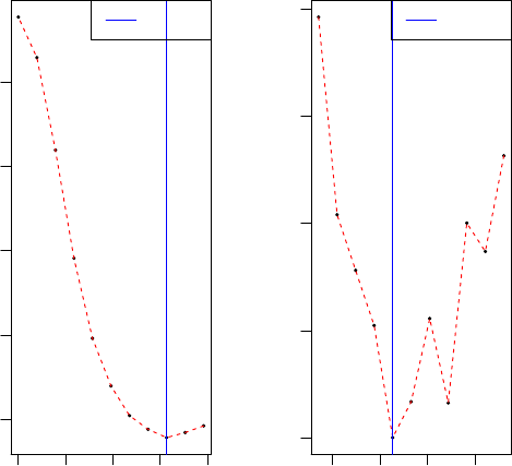
We can use permutation to evaluate the signiﬁcance of the ﬁrst 8 PCs:

> result <- acPCA(X=X, Y=Y, lambda=5, kernel="linear", nPC=8, eval=T)

> result$sigPC

[1] 3

1 3 5 7

100 150 200 250

Eigenvalue

1 3 5 7

1.0 1.5 2.0 2.5 3.0 3.5 4.0

Variance

Data: red cross; Permutation: boxplot

The ﬁrst 3 PCs are signiﬁcant.

3.5 Application to a model organism ENCODE (modEN-

CODE) RNA-Seq dataset

The modENCODE project generates the transcriptional landscapes for model

organisms during development[1, 2]. In the analysis, we used the time-course

RNA-Seq data for ﬂy and worm embryonic development. The modENCODE

RNA-Seq dataset was downloaded from https://www.encodeproject.org/comparative/transcriptome/.

For the orthologs in ﬂy that map to multiple orthologs in worm, we took median

to get a one to one match, resulting in 4831 ortholog paris. We ﬁrst perform

some exploratory analysis:

> library(acPCA)

> data(data_fly_worm)

> data_fly <- data_fly_worm$data_fly ###the data matrix for fly

> data_worm <- data_fly_worm$data_worm ###the data matrix for fly

> dim(data_fly)

[1] 12 4831

> dim(data_worm)

[1] 24 4831

> par(mfrow=c(2,1), pin=c(2.5,2.5), mar=c(4.1, 3.9, 3.2, 1.1))

> boxplot(t(rbind(data_fly, data_worm)),las = 2, names =

+ c(rep('fly', 12), rep('worm', 24)), ylab="expression level")

> boxplot(log2(t(rbind(data_fly, data_worm))+1),las = 2,

+ names = c(rep('fly', 12), rep('worm', 24)), ylab="log2(expression+1)")

fly

worm

5000

10000

15000

20000

expression level

fly

worm

log2(expression+1)

We can clearly see that the expression levels in worm samples tend to be

higher. Next we perform PCA on ﬂy and worm separately on the log2 scale:

> pca_fly <- prcomp(log2(data_fly+1), center=T)

> pca_worm <- prcomp(log2(data_worm+1), center=T)

> par(mfrow=c(1,1), pin=c(3, 3))

> plot(pca_fly$x[,1], -pca_fly$x[,2], xlab="PC 1", ylab="PC 2",

+ col="red", type="n", main="fly PCA",

+ xlim=c(-(max(abs(pca_fly$x[,1]))+13), max(abs(pca_fly$x[,1]))+13),

+ ylim=c(-(max(abs(pca_fly$x[,2]))+13), max(abs(pca_fly$x[,2]))+13))

> text(pca_fly$x[,1], -pca_fly$x[,2], labels =

+ data_fly_worm$fly_time, col="red")

−60 −20 0 20 40 60

−60 −40 −20 0 20 40 60

fly PCA

PC 1

PC 2

0−2

2−4

4−6

6−8

8−10

10−12

12−14

14−16

16−18

18−20

20−22

22−24

> par(mfrow=c(1,1), pin=c(3, 3))

> plot(pca_worm$x[,1], pca_worm$x[,2], xlab="PC 1", ylab="PC 2",

+ col="red", type="n", main="worm PCA",

+ xlim=c(-(max(abs(pca_worm$x[,1]))+13), max(abs(pca_worm$x[,1]))+13),

+ ylim=c(-(max(abs(pca_worm$x[,2]))+13), max(abs(pca_worm$x[,2]))+13))

> text(pca_worm$x[,1], pca_worm$x[,2], labels =

+ data_fly_worm$worm_time, col="blue")

−100 −50 0 50 100

−50 0 50

worm PCA

PC 1

PC 2

0.5

11.5

2.5

33.5

55.5

66.5

77.5

8.5

9.5

10.5

11.5

In the PCA plots, each data point represents a time window (ﬂy) or a time

point (worm), in the unit of hours(h). For ﬂy, there is a smooth temporal

pattern. For worm, there seems to be three clusters, which may originate from

the dominated eﬀect of a small subset of highly expressed genes. To adjust for

the highly expressed genes, we used the rank across samples within the same

species. The rank matrix was then scaled to have unit variance. Another beneﬁt

of using rank is that we simultaneously make adjustment for the observation that

worm genes tend to have higher expression levels. For ties in the expression

level, we used ’average’ option in the R’s rank function. Here is PCA on the

rank matrix:

> X <- data_fly_worm$X ###this is the scaled rank matrix. Fly and worm are combined.

> pca_fly_rank <- prcomp(X[1:12,], center=T)

> pca_worm_rank <- prcomp(X[13:36,], center=T)

> par(mfrow=c(1,1), pin=c(3, 3))

> plot(pca_fly_rank$x[,1], -pca_fly_rank$x[,2], xlab="PC 1", ylab="PC 2",

+ col="red", type="n", main="fly PCA, rank",

+ xlim=c(-(max(abs(pca_fly_rank$x[,1]))+13), max(abs(pca_fly_rank$x[,1]))+13),

+ ylim=c(-(max(abs(pca_fly_rank$x[,2]))+13), max(abs(pca_fly_rank$x[,2]))+13))

> text(pca_fly_rank$x[,1], -pca_fly_rank$x[,2], labels =

+ data_fly_worm$fly_time, col="red")

−50 0 50

−40 −20 0 20 40

fly PCA, rank

PC 1

PC 2

0−2

2−4

4−6

6−8

8−10

10−12

12−14

14−16

16−18

18−20

20−22

22−24

> par(mfrow=c(1,1), pin=c(3, 3))

> plot(pca_worm_rank$x[,1], pca_worm_rank$x[,2], xlab="PC 1", ylab="PC 2",

+ col="red", type="n", main="worm PCA, rank",

+ xlim=c(-(max(abs(pca_worm_rank$x[,1]))+13), max(abs(pca_worm_rank$x[,1]))+13),

+ ylim=c(-(max(abs(pca_worm_rank$x[,2]))+13), max(abs(pca_worm_rank$x[,2]))+13))

> text(pca_worm_rank$x[,1], pca_worm_rank$x[,2], labels =

+ data_fly_worm$worm_time, col="blue")

−50 0 50

worm PCA, rank

PC 1

PC 2

0.5

11.5

22.5

3.5

55.5

6.5

77.5

8.5

99.5

10.5

11.5

Using rank gives a better visualization, as the data points are more spread

out. Next we implement PCA on ﬂy and worm jointly, using the rank matrix:

> pca_rank <- prcomp(X, center=T)

> par(mfrow=c(1,1), pin=c(3, 3))

> plot(pca_rank$x[,1], pca_rank$x[,2], xlab="PC 1", ylab="PC 2",

+ col="red", type="n", main="fly+worm, PCA, rank",

+ xlim=c(-(max(abs(pca_rank$x[,1]))+13), max(abs(pca_rank$x[,1]))+13),

+ ylim=c(-(max(abs(pca_rank$x[,2]))+13), max(abs(pca_rank$x[,2]))+13))

> text(pca_rank$x[,1], pca_rank$x[,2],

+ labels=data_fly_worm$X_time,

+ col=c(rep("red", 12), rep("blue", 24)) )

> legend("topright", legend = c("fly", "worm"), lty=1,

+ col=c("red","blue"),lwd=1.5,seg.len=1)

−50 0 50

−60 −20 0 20 40 60

fly+worm, PCA, rank

PC 1

PC 2

0−2

2−4

4−6

6−8

8−10

10−12

12−14

14−16

16−18

18−20

20−22

22−24

0.5

11.5

22.5

3.5

55.5

6.5

77.5

8.5

99.5

10.5

11.5

fly

worm

The variation of species confounds the PCA result, as we observed that

samples from the same species tend to be close.

Next we implement AC-PCA. Without prior knowledge on the alignment

of the developmental stages in ﬂy and worm, we shrink the data points in ﬂy

towards the mean of the data points in worm: for example, time window 0-2h

in ﬂy is shrunk to the mean of time points 0h, 0.5h and 1h in worm, as the

embryonic stage for ﬂy is 24h, and for worm it is 12h. Time window 8-10h in

ﬂy is shrunk to the mean of 4h and 5h in worm, as the worm sample 4.5h is

missing.

> Y <- data_fly_worm$Y

> Y[,1]

[1] 1.0000000 0.0000000 0.0000000 0.0000000 0.0000000 0.0000000

[7] 0.0000000 0.0000000 0.0000000 0.0000000 0.0000000 0.0000000

[13] -0.3333333 -0.3333333 -0.3333333 0.0000000 0.0000000 0.0000000

[19] 0.0000000 0.0000000 0.0000000 0.0000000 0.0000000 0.0000000

[25] 0.0000000 0.0000000 0.0000000 0.0000000 0.0000000 0.0000000

[31] 0.0000000 0.0000000 0.0000000 0.0000000 0.0000000 0.0000000

> result_tune <- acPCAtuneLambda(X=X, Y=Y, nPC=2, lambdas=seq(0, 10, 0.05),

+ anov=F, kernel = "linear", quiet=T)

> result <- acPCA(X=X, Y=Y, lambda=result_tune$best_lambda,

+ kernel="linear", nPC=2)

> par(mfrow=c(1,1), pin=c(3, 3))

> plot(-result$Xv[,1], result$Xv[,2], xlab="PC 1", ylab="PC 2",

+ col="red", type="n", main="fly+worm, AC-PCA, rank",

+ xlim=c(-(max(abs(result$Xv[,1]))+13), max(abs(result$Xv[,1]))+13),

+ ylim=c(-(max(abs(result$Xv[,2]))+13), max(abs(result$Xv[,2]))+13))

> text(-result$Xv[,1], result$Xv[,2],

+ labels=data_fly_worm$X_time,

+ col=c(rep("red", 12), rep("blue", 24)) )

> legend("topright", legend = c("fly", "worm"),

+ lty=1, col=c("red","blue"),lwd=1.5,seg.len=1)

−60 −20 0 20 40 60

−60 −40 −20 0 20 40 60

fly+worm, AC−PCA, rank

PC 1

PC 2

0−2

2−4

4−6

6−8

8−10

10−12

12−14

14−16

16−18

18−20

20−22

22−24

0.5

11.5

2.5

3.5

5.5

6.5

77.5

8.5

99.5

10.5

11.5

fly

worm

We set anov =Fas the penalty term does not have the ANOVA inter-

pretation. The variation of diﬀerent species is adjusted. The genes with top

loadings in AC-PCA tend to have consistent temporal pattern in ﬂy and worm

(see manuscript).

3.6 AC-PCA with sparsity

For AC-PCA with sparsity constrains, there are two tuning parameters, c1and

c2:c1controls the strength of the penalty, and c2controls the sparsity of v. The

parameters are tuned sequentially: c1is tuned without the sparsity constrain,

and then c2is tuned with c1ﬁxed. We implement the procedure on the brain

exon array data, time window 2:

> set.seed(10)

> data(data_brain_w2)

> X <- data_brain_w2$X ###the data matrix

> Y <- data_brain_w2$Y

> result1cv <- acPCAtuneLambda(X=X, Y=Y, nPC=2, lambdas=seq(0, 20, 0.1),

+ anov=T, kernel = "linear", quiet=T)

> result1 <- acPCA(X=X, Y=Y, lambda=result1cv$best_lambda, kernel="linear", nPC=2)

> v_ini <- as.matrix(result1$v[,1])

> par(mfrow=c(1,2), pin=c(2.5,2.5), mar=c(4.1, 3.9, 3.2, 1.1))

> c2s <- seq(1, 0, -0.1)*sum(abs(v_ini))

> resultcv_spc1_coarse <- acSPCcv( X=X, Y=Y, c2s=c2s, v_ini=v_ini,

+ kernel="linear", quiet=T, fold=10)

> c2s <- seq(0.9, 0.7, -0.02)*sum(abs(v_ini))

> resultcv_spc1_fine <- acSPCcv( X=X, Y=Y, c2s=c2s, v_ini=v_ini,

+ kernel="linear", quiet=T, fold=10)

> result_spc1 <- acSPC( X=X, Y=Y, c2=resultcv_spc1_fine$best_c2,

+ v_ini=v_ini, kernel="linear")

> v1 <- result_spc1$v

> sum(v1!=0)

[1] 736

0 5 10 15 20

2650 2700 2750 2800 2850

Cross−validation

Sparsity parameter c2

mean squared error(MSE)

Best c2

14 15 16 17

2641 2642 2643 2644 2645

Cross−validation

Sparsity parameter c2

mean squared error(MSE)

Best c2

To speed-up the computational time, a coarse search for c2was performed

ﬁrst, followed by a ﬁner grid.

Multiple sparse principal components can be obtained by substracting the

ﬁrst several principal components, and then implement the algorithm:

> v_substract <- as.matrix(result1$v[,1])

> v_ini <- as.matrix(result1$v[,2])

> par(mfrow=c(1,2), pin=c(2.5,2.5), mar=c(4.1, 3.9, 3.2, 1.1))

> c2s <- seq(1, 0, -0.1)*sum(abs(v_ini))

> resultcv_spc2_coarse <- acSPCcv(X=X, Y=Y, c2s=c2s, v_ini=v_ini,

+ v_substract=v_substract, kernel="linear",

+ quiet=T, fold=10)

> c2s <- seq(0.5, 0.2, -0.02)*sum(abs(v_ini))

> resultcv_spc2_fine <- acSPCcv(X=X, Y=Y, c2s=c2s, v_ini=v_ini,

+ v_substract=v_substract, kernel="linear",

+ quiet=T, fold=10)

> result_spc2 <- acSPC(X=X, Y=Y, c2=resultcv_spc2_fine$best_c2,

+ v_ini=v_ini, v_substract=v_substract, kernel="linear")

> v2 <- result_spc2$v

> sum(v2!=0)

[1] 68

0 5 10 15 20

2880 2885 2890

Cross−validation

Sparsity parameter c2

mean squared error(MSE)

Best c2

5 6 7 8 9 10

2874 2876 2878 2880 2882 2884

Cross−validation

Sparsity parameter c2

mean squared error(MSE)

Best c2

In the example, the non-sparse ﬁrst PC was substracted. We can also sub-

stract the sparse PC:

> v_substract <- v1

References

[1] Susan E Celniker, Laura AL Dillon, Mark B Gerstein, Kristin C Gunsalus,

Steven Henikoﬀ, Gary H Karpen, Manolis Kellis, Eric C Lai, Jason D Lieb,

David M MacAlpine, et al. Unlocking the secrets of the genome. Nature,

459(7249):927–930, 2009.

[2] Mark B Gerstein, Joel Rozowsky, Koon-Kiu Yan, Daifeng Wang, Chao

Cheng, James B Brown, Carrie A Davis, LaDeana Hillier, Cristina Sisu,

Jingyi Jessica Li, et al. Comparative analysis of the transcriptome across

distant species. Nature, 512(7515):445–448, 2014.

[3] Hyo Jung Kang, Yuka Imamura Kawasawa, Feng Cheng, Ying Zhu, Xuming

Xu, Mingfeng Li, Andr´e MM Sousa, Mihovil Pletikos, Kyle A Meyer, Goran

Sedmak, et al. Spatio-temporal transcriptome of the human brain. Nature,

478(7370):483–489, 2011.

[4] Matt P Wand and M Chris Jones. Kernel smoothing. Crc Press, 1994.

R User Guide

Navigation menu

Versions of this User Manual:

Views

Navigation