S06 Instructions
User Manual:
Open the PDF directly: View PDF ![]() .
.
Page Count: 25
2019-02-27, 11:23 AMSTAT540-UBC.github.io/sm06_clustering-pca.md at master · STAT540-UBC/STAT540-UBC.github.io
Page 1 of 25https://github.com/STAT540-UBC/STAT540-UBC.github.io/blob/master/seminars/seminars_winter_2019/seminar6/sm06_clustering-pca.md
STAT540-UBC.github.io / seminars / seminars_winter_2019 / seminar6 / sm06_clustering-pca.md
STAT540-UBC /STAT540-UBC.github.io
master
Branch:
Find file Copy path
Jwong684 Updated guideline !"#$%## on Jan 9
2 contributors
&''()*+,-(.!/#(-)012( (3&4#(56
Seminar 6: Dimensionality reduction and Cluster Analysis-
Hierarchical Clustering
Contributors: Gabriela Cohen Freue, Jasleen Grewal, Alice Zhu.
Learning objectives
By the end of this tutorial, you should be able to
Differentiate between sample-wise clustering and gene-wise clustering, and identify when either may be appropriate.
Differentiate between agglomerative hierarchical clustering and partition clustering methods like K-means.
Outline the methods used to determine an optimal number of clusters in K-means clustering.
Undertake dimensionality reduction using PCA.
Appreciate the differences between PCA and t-SNE.
Recognize that the t-SNE approach is an intricate process requiring parametrization.
Add cluster annotations to t-SNE visualizations of their datasets.
Understand the limitations of the clustering methods, PCA, and t-SNE, as discussed in this seminar.
Introduction
In this seminar we'll explore clustering genes and samples using the Affymetrix microarray data on characterizing the gene
expression profile of nebulin knockout mice. This data was made available by Li F et al., with the GEO accession number
GSE70213. There are two genotypes - the wildtype mice, and the knockout mice. We will compare the results of different
clustering algorithms on the data, evaluate the effect of filtering/feature selection on the clusters, and lastly, try to assess
if different attributes help explain the clusters we see.
Load data and packages
Install required libraries Install required packages if you haven't done so before. This seminar will require 789:;,<= ,
>?1);-@ , A@B%), , )*CCB , 1);-@,< , DE0)0<6<,F,< , and >)=< .
Remember you may need to edit the file paths below, to reflect your working directory and local file storage choices.

2019-02-27, 11:23 AMSTAT540-UBC.github.io/sm06_clustering-pca.md at master · STAT540-UBC/STAT540-UBC.github.io
Page 2 of 25https://github.com/STAT540-UBC/STAT540-UBC.github.io/blob/master/seminars/seminars_winter_2019/seminar6/sm06_clustering-pca.md
)*%<B<=.DE0)0<6<,F,<2
)*%<B<=.1);-@,<2
)*%<B<=.>?1);-@2
)*%<B<=.A@B%),2
)*%<B<=.)*CCB2
)*%<B<=.>)=<2
)*%<B<=.)B@@*1,2
)*%<B<=.DE;<)2
0>@*0+-."0F+)0B"4G*),4C,@H0"(I(J1;<)J2
)*%<B<=.789:;,<=2
)*%<B<=.K+*@<2
)*%<B<=.>H,B@CB>2
If you don't have 789:;,<= installed, you will need to get it using biocLite ( *+-@B))4>B1KBL,- won't work!).
-0;<1,.JH@@>MNN%*010+";1@0<40<LN%*01O*@,4DJ2
%*01O*@,.J789:;,<=J2
Read the data into R > We will be reading in the data using the GEOquery library. This lets us read in the expression data
and phenotypic data for a particular analysis, using its GEO accession ID.
*G(.G*),4,A*-@-.J7P8$Q'/34D"B@BJ22(R
((((S(*G(><,?*0;-)=("0F+)0B","
(((()0B".J7P8$Q'/34D"B@BJ2
T(,)-,(R
((((S(7,@(L,0(0%U,1@(@HB@(10+@B*+-(0;<("B@B(B+"(>H,+0@=>,(*+G0<CB@*0+
((((L,0V0%U(WX(L,@789.J7P8$Q'/3JY(7P8ZB@<*A(I([D\82
((((L,0V0%U(WX(L,0V0%U]]/^^
((((-B?,.L,0V0%UY(G*),(I(J7P8$Q'/34D"B@BJ2
T
S(7,@(,A><,--*0+("B@B
"B@B(WX(,A><-.L,0V0%U2
S(7,@(10?B<*B@,("B@B
><_,-(WX(>_B@B.L,0V0%U2]Y(1.J0<LB+*-CV1H/JY(J@*@),JY(10)+BC,-.>_B@B.L,0V0%U22]L<,>.J1HB<B1@,<*-@*1-JY(
((((10)+BC,-.>_B@B.L,0V0%U222^2^
SS(E),B+(;>(10?B<*B@,("B@B
10)+BC,-.><_,-2(I(1.J0<LB+*-CJY(J-BC>),V+BC,JY(J@*--;,JY(JL,+0@=>,JY(J-,AJY(JBL,J2
><_,-`@*--;,(I(B-4GB1@0<.L-;%.J@*--;,M(JY(JJY(><_,-`@*--;,22
><_,-`L,+0@=>,(I(B-4GB1@0<.L-;%.JL,+0@=>,M(JY(JJY(><_,-`L,+0@=>,22
><_,-`-,A(I(B-4GB1@0<.L-;%.JP,AM(JY(JJY(><_,-`-,A22
><_,-`BL,(I(L-;%.JBL,M(JY(JJY(><_,-`BL,2
You might get an error like 8<<0<(*+("0F+)0B"4G*),441B++0@("0F+)0B"(B))(G*),- . This happens when R cannot
connect to the NCBI ftp servers from linux systems. We will need to set the 'curl' option to fix this.
0>@*0+-."0F+)0B"4G*),4C,@H0"(I(J1;<)J2
Exploratory analysis
Let us take a look at our data.

2019-02-27, 11:23 AMSTAT540-UBC.github.io/sm06_clustering-pca.md at master · STAT540-UBC/STAT540-UBC.github.io
Page 3 of 25https://github.com/STAT540-UBC/STAT540-UBC.github.io/blob/master/seminars/seminars_winter_2019/seminar6/sm06_clustering-pca.md
KB%),.H,B"."B@B]Y(/Ma^22
GSM1720833 GSM1720834 GSM1720835 GSM1720836 GSM1720837
10338001 2041.408000 2200.861000 2323.760000 3216.263000 2362.775000
10338002 63.780590 65.084380 58.308200 75.861450 66.956050
10338003 635.390400 687.393600 756.004000 1181.929000 759.099800
10338004 251.566800 316.997300 320.513200 592.806000 359.152500
10338005 2.808835 2.966376 2.985357 3.352954 3.155735
10338006 3.573085 3.816430 3.815323 4.690040 3.862684
"*C."B@B2
SS(]/^(3aaa$(((('#
We have 24 samples (columns) and 35,557 genes (rows) in our dataset. If we look in our covars object (called prDes), we
should have 24 rows, each corresponding to each sample.
KB%),.H,B".><_,-22
organism sample_name tissue genotype sex age
GSM1720833 Mus musculus quad-control-1 quadriceps control male 41 days old
GSM1720834 Mus musculus quad-control-2 quadriceps control male 41 days old
GSM1720835 Mus musculus quad-control-3 quadriceps control male 41 days old
GSM1720836 Mus musculus quad-control-4 quadriceps control male 41 days old
GSM1720837 Mus musculus quad-control-5 quadriceps control male 42 days old
GSM1720838 Mus musculus quad-control-6 quadriceps control male 40 days old
"*C.><_,-2
SS(]/^('#((!
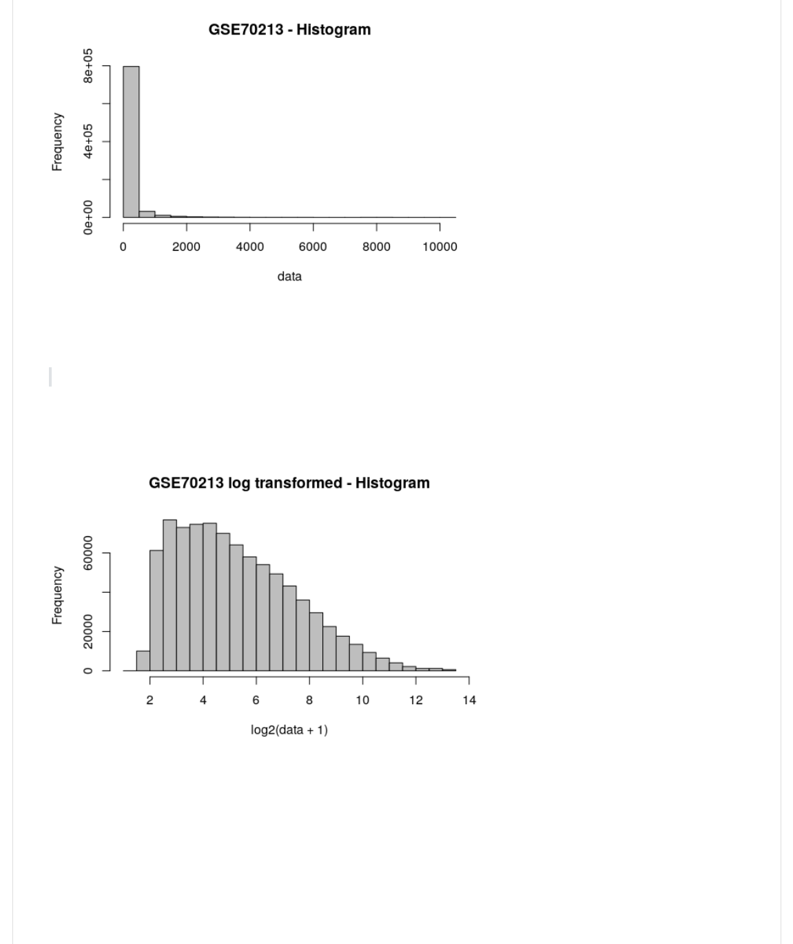
Now let us see how the gene values are spread across our dataset, with a frequency histogram (using base R).
H*-@."B@BY(10)(I(JL<B=JY(CB*+(I(J7P8$Q'/3(X(b*-@0L<BCJ2
2019-02-27, 11:23 AMSTAT540-UBC.github.io/sm06_clustering-pca.md at master · STAT540-UBC/STAT540-UBC.github.io
Page 4 of 25https://github.com/STAT540-UBC/STAT540-UBC.github.io/blob/master/seminars/seminars_winter_2019/seminar6/sm06_clustering-pca.md
It appears a lot of genes have values < 1000. What happens if we plot the frequency distribution after Log2
transformation?
Why might it be useful to log transform the data, prior to making any comparisons?
H*-@.)0L'."B@B(c(/2Y(10)(I(JL<B=JY(CB*+(I(J7P8$Q'/3()0L(@<B+-G0<C,"(X(b*-@0L<BCJ2
Finally, as an additional step to make visualization easier later, we'll rescale the rows in our data object, since we're not
interested in absolute differences in expression between genes at the moment. Note that although one can do this step
within the >H,B@CB>.2 function, it will not be available for other functions we will use. We can always go back to the
original data if we need to.
-><_B@(WX(@.-1B),.@."B@B222
-@<.-><_B@Y(CBA4),?,)(I(QY(L*?,4B@@<(I(deOP82

2019-02-27, 11:23 AMSTAT540-UBC.github.io/sm06_clustering-pca.md at master · STAT540-UBC/STAT540-UBC.github.io
Page 5 of 25https://github.com/STAT540-UBC/STAT540-UBC.github.io/blob/master/seminars/seminars_winter_2019/seminar6/sm06_clustering-pca.md
SS((+;C(]/M3aaa$Y(/M'#^(XQ4'Q#'(Q4f!f3(XQ4Q!f3(XQ433'f(XQ4$!$/(444
<0;+"."B@B4G<BC,.B?L6,G0<,(I(<0FZ,B+-.H,B"."B@B22Y(B?LeG@,<(I(<0FZ,B+-.H,B".-><_B@22Y(
((((?B<6,G0<,(I(B>>)=.H,B"."B@B2Y(/Y(?B<2Y(?B<eG@,<(I(B>>)=.H,B".-><_B@2Y(/Y(?B<22Y(
(((('2
SS((((((((((B?L6,G0<,(B?LeG@,<(?B<6,G0<,(?B<eG@,<
SS(/Q33&QQ/((('/Qf4#'((((((((Q(//Qf##4'&((((((((/
SS(/Q33&QQ'(((((aa4!'((((((((Q((((($Q4&'((((((((/
SS(/Q33&QQ3((((!#a4$!((((((((Q((''3&!4f'((((((((/
SS(/Q33&QQ#(((('&Q4#3((((((((Q((($a/34#&((((((((/
SS(/Q33&QQa(((((('4f'((((((((Q((((((Q4Q'((((((((/
SS(/Q33&QQ!((((((34!#((((((((Q((((((Q4Q$((((((((/
The data for each row -- which is for one probeset -- now has mean 0 and variance 1.
Now, let us try and consider how the various samples cluster across all our genes. We will then try and do some feature
selection, and see the effect it has on the clustering of the samples. We will use the covars object to annotate our clusters
and identify interesting clusters. The second part of our analysis will focus on clustering the genes across all our samples.
Sample Clustering
In this part, we will use samples as objects to be clustered using gene attributes (i.e., vector variables of dimension ~35K).
First we will cluster the data using agglomerative hierarchical clustering. Here, the partitions can be visualized using a
dendrogram at various levels of granularity. We do not need to input the number of clusters, in this approach. Then, we
will find various clustering solutions using partitional clustering methods, specifically K-means and partition around
medoids (PAM). Here, the partitions are independent of each other, and the number of clusters is given as an input. As
part of your take-home exercise, you will pick a specific number of clusters, and compare the sample memberships in
these clusters across the various clustering methods. ## Part I: Hierarchical Clustering ### Hierarchical clustering for
mice knockout data
In this section we will illustrate different hierarchical clustering methods. These plots were included in Lecture 16.
However, for most expression data applications, we suggest you should standardize the data; use Euclidean as the
"distance" (so it's just like Pearson correlation) and use "average linkage".
"B@BV@0V>)0@(I(-><_B@
S(10C>;@,(>B*<F*-,("*-@B+1,-
><4"*-(WX("*-@.@."B@BV@0V>)0@2Y(C,@H0"(I(J,;1)*",B+J2
S(1<,B@,(B(+,F(GB1@0<(<,><,-,+@*+L(@H,(*+@,<B1@*0+(0G(@*--;,(@=>,(B+"(L,+0@=>,
><_,-`L<>(WX(F*@H.><_,-Y(*+@,<B1@*0+.@*--;,Y(L,+0@=>,22
-;CCB<=.><_,-`L<>2
SS((((:;B"<*1,>-410+@<0)((((((((-0),;-410+@<0)(:;B"<*1,>-4+,%;)*+(59(
SS(((((((((((((((((((((!(((((((((((((((((((((!(((((((((((((((((((((!(
SS(((((-0),;-4+,%;)*+(59(
SS(((((((((((((((((((((!

2019-02-27, 11:23 AMSTAT540-UBC.github.io/sm06_clustering-pca.md at master · STAT540-UBC/STAT540-UBC.github.io
Page 6 of 25https://github.com/STAT540-UBC/STAT540-UBC.github.io/blob/master/seminars/seminars_winter_2019/seminar6/sm06_clustering-pca.md
S(10C>;@,(H*,<B<1H*1B)(1);-@,<*+L(;-*+L("*GG,<,+@()*+KBL,(@=>,-
><4H14-(WX(H1);-@.><4"*-Y(C,@H0"(I(J-*+L),J2
><4H141(WX(H1);-@.><4"*-Y(C,@H0"(I(J10C>),@,J2
><4H14B(WX(H1);-@.><4"*-Y(C,@H0"(I(JB?,<BL,J2
><4H14F(WX(H1);-@.><4"*-Y(C,@H0"(I(JFB<"4_J2
S(>)0@(@H,C
0>(WX(>B<.CB<(I(1.QY(#Y(#Y('2Y(CG<0F(I(1.'Y('22
>)0@.><4H14-Y()B%,)-(I(deOP8Y(CB*+(I(JP*+L),JY(A)B%(I(JJ2
>)0@.><4H141Y()B%,)-(I(deOP8Y(CB*+(I(JE0C>),@,JY(A)B%(I(JJ2
>)0@.><4H14BY()B%,)-(I(deOP8Y(CB*+(I(Je?,<BL,JY(A)B%(I(JJ2
>)0@.><4H14FY()B%,)-(I(deOP8Y(CB*+(I(JgB<"JY(A)B%(I(JJ2
>B<.0>2
We can look at the trees that are output from different clustering algorithms. However, it can also be visually helpful to
identify what sorts of trends in the data are associated with these clusters. We can look at this output using heatmaps. We
will be using the pheatmap package for is purpose.
When you call >H,B@CB>.2 , it automatically performs hierarchical clustering for you and it reorders the rows and/or
columns of the data accordingly. Both the reordering and the dendrograms can be suppressed with 1);-@,<V<0F-(I(deOP8
and/or 1);-@,<V10)-(I(deOP8 .
Note that when you have a lot of genes, the tree is pretty ugly. Thus, the row clustering was suppressed for now.
By default, >H,B@CB>.2 uses the H1);-@.2 function, which takes a distance matrix, calculated by the "*-@.2 function
(with ",GB;)@(I(h,;1)*",B+h ). However, you can also write your own clustering and distance functions. In the examples
below, I used H1);-@.2 with FB<" linkage method and the ,;1)*",B+ distance.
Note that the dendrogram in the top margin of the heatmap is the same as that of the H1);-@.2 function.
2019-02-27, 11:23 AMSTAT540-UBC.github.io/sm06_clustering-pca.md at master · STAT540-UBC/STAT540-UBC.github.io
Page 7 of 25https://github.com/STAT540-UBC/STAT540-UBC.github.io/blob/master/seminars/seminars_winter_2019/seminar6/sm06_clustering-pca.md
Exercise: Play with the options of the pheatmap function and compare the different heatmaps. Note that one can also use
the original data "B@B and set the option -1B),(I(J<0FJ . You will get the same heatmaps although the columns may be
ordered differently (use 1);-@,<V10)-(I(deOP8 to suppress reordering).
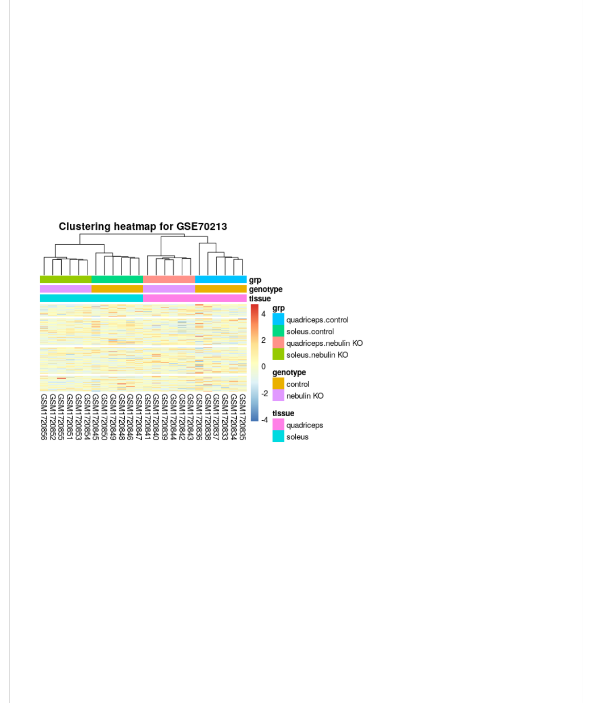
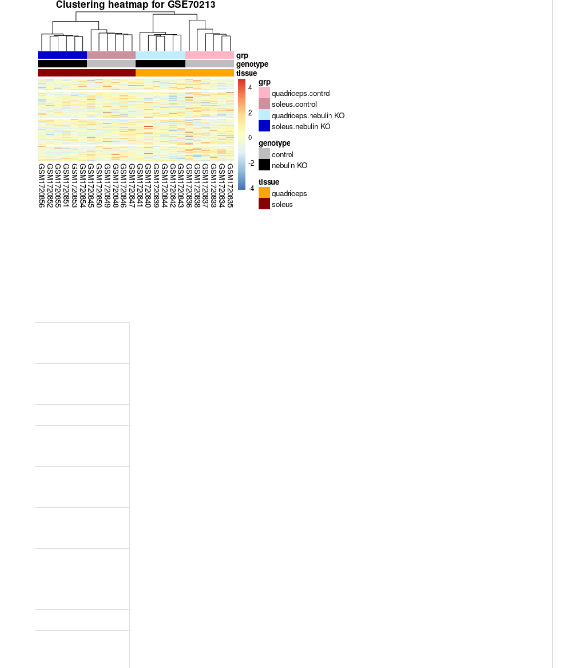
We can also change the colours of the different covariates. As you see, this can help differentiate important variables and
the clustering trends.
SS(g,(1B+(1HB+L,(@H,(10)0;<-(0G(@H,(10?B<*B@,-
?B</(I(1.J0<B+L,/JY(J"B<K<,"J2
+BC,-.?B</2(I(),?,)-.><_,-`@*--;,2
?B<'(I(1.JL<,=JY(J%)B1KJ2
+BC,-.?B<'2(I(),?,)-.><_,-`L,+0@=>,2
?B<3(I(1.J>*+K/JY(J>*+K3JY(J)*LH@%);,/JY(J%);,3J2
+BC,-.?B<32(I(),?,)-.B-4GB1@0<.><_,-`L<>22
10?B<V10)0<(I()*-@.@*--;,(I(?B</Y(L,+0@=>,(I(?B<'Y(L<>(I(?B<32
C=VH,B@CB>V0%U(I(>H,B@CB>."B@BV@0V>)0@Y(1);-@,<V<0F-(I(deOP8Y(-1B),(I(1);-@V-1B),Y(
((((1);-@,<*+LVC,@H0"(I(1);-@VC,@H0"Y(1);-@,<*+LV"*-@B+1,V10)-(I(1);-@V"*-@V10)Y(
((((-H0FV<0F+BC,-(I(deOP8Y(CB*+(I(JE);-@,<*+L(H,B@CB>(G0<(7P8$Q'/3JY(B++0@B@*0+(I(><_,-]Y(
((((((((1.J@*--;,JY(JL,+0@=>,JY(JL<>J2^Y(B++0@B@*0+V10)0<-(I(10?B<V10)0<2
S(-,@(>H,B@CB>(1);-@,<*+L(>B<BC,@,<-
1);-@V"*-@V10)(I(J,;1)*",B+J((Sih10<<,)B@*0+hj(G0<(k,B<-0+(10<<,)B@*0+Y(ih,;1)*",B+hjY(ihCBA*C;ChjY(ihCB+HB@@B+hjY(ih1B+%,<<BhjY(ih%*+B<=hj(0<(ihC*+K0F-K*hj
1);-@VC,@H0"(I(JFB<"4_'J((SihFB<"4_hjY(ihFB<"4_'hjYih-*+L),hjY(ih10C>),@,hjY(ihB?,<BL,hj(.I(\k7Ze2Y(ihC1:;*@@=hj(.I(gk7Ze2Y(ihC,"*B+hj(.I(gk7ZE2(0<(ih1,+@<0*"hj(.I(\k7ZE2
1);-@V-1B),(I(J+0+,J((Sh10);C+hY(h+0+,hY(h<0Fh
SS(@H,(B++0@B@*0+(0>@*0+(;-,-(@H,(10?B<*B@,(0%U,1@(.><_,-2(F,(",G*+,"4(l@(-H0;)"
SS(HB?,(@H,(-BC,(<0F+BC,-Y(B-(@H,(10)+BC,-(*+(0;<("B@B(0%U,1@(."B@BV@0V>)0@24
>H,B@CB>."B@BV@0V>)0@Y(1);-@,<V<0F-(I(deOP8Y(-1B),(I(1);-@V-1B),Y(1);-@,<*+LVC,@H0"(I(1);-@VC,@H0"Y(
((((1);-@,<*+LV"*-@B+1,V10)-(I(1);-@V"*-@V10)Y(Y(-H0FV10)+BC,-(I([Y(-H0FV<0F+BC,-(I(deOP8Y(
((((CB*+(I(JE);-@,<*+L(H,B@CB>(G0<(7P8$Q'/3JY(B++0@B@*0+(I(><_,-]Y(1.J@*--;,JY(JL,+0@=>,JY(
((((((((JL<>J2^2
2019-02-27, 11:23 AMSTAT540-UBC.github.io/sm06_clustering-pca.md at master · STAT540-UBC/STAT540-UBC.github.io
Page 8 of 25https://github.com/STAT540-UBC/STAT540-UBC.github.io/blob/master/seminars/seminars_winter_2019/seminar6/sm06_clustering-pca.md
We can also get clusters from our pheatmap object. We will use the 1;@<,, function to extract the clusters. Note that we
can do this for samples (look at the @<,,V10) ) or for genes (look at the @<,,V<0F ).
1);-@,<V-BC>),-(I(1;@<,,.C=VH,B@CB>V0%U`@<,,V10)Y(K(I(/Q2
S(1);-@,<VL,+,-(I(1;@<,,.C=VH,B@CB>V0%U`@<,,V<0FY(KI/QQ2
KB%),.1);-@,<V-BC>),-2
x
GSM1720833 1
GSM1720834 1
GSM1720835 1
GSM1720836 2
GSM1720837 1
GSM1720838 3
GSM1720839 4
GSM1720840 4
GSM1720841 5
GSM1720842 4
GSM1720843 4
GSM1720844 4
GSM1720845 6
GSM1720846 7
GSM1720847 7
GSM1720848 7
2019-02-27, 11:23 AMSTAT540-UBC.github.io/sm06_clustering-pca.md at master · STAT540-UBC/STAT540-UBC.github.io
Page 9 of 25https://github.com/STAT540-UBC/STAT540-UBC.github.io/blob/master/seminars/seminars_winter_2019/seminar6/sm06_clustering-pca.md
GSM1720849 8
GSM1720850 9
GSM1720851 10
GSM1720852 10
GSM1720853 10
GSM1720854 10
GSM1720855 10
GSM1720856 10
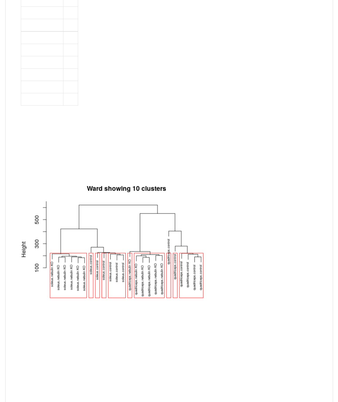
Note you can do this with the base H1);-@ method too, as shown here. We are using one of the hclust objects we defined
earlier in this document.
S(*",+@*G=(/Q(1);-@,<-
0>(WX(>B<.CB<(I(1./Y(#Y(#Y(/22
>)0@.><4H14FY()B%,)-(I(><_,-`L<>Y(1,A(I(Q4!Y(CB*+(I(JgB<"(-H0F*+L(/Q(1);-@,<-J2
<,1@4H1);-@.><4H14FY(K(I(/Q2
>B<.0>2
We can save the heatmap we made, to a PDF file for reference. Remember to define the filename properly as the file will be
saved relative to where you are running the script in your directory structure.
S(PB?,(@H,(H,B@CB>(@0(B(k_d(G*),
>"G.J7P8$Q'/3Vb,B@CB>4>"GJ2
>H,B@CB>."B@BV@0V>)0@Y(1);-@,<V<0F-(I(dY(-1B),(I(1);-@V-1B),Y(1);-@,<*+LVC,@H0"(I(1);-@VC,@H0"Y(
((((1);-@,<*+LV"*-@B+1,V10)-(I(1);-@V"*-@V10)Y(B++0@B@*0+(I(><_,-]Y(1.J@*--;,JY(JL,+0@=>,JY(
((((((((JL<>J2^Y(B++0@B@*0+V10)0<-(I(10?B<V10)0<2
",?40GG.2

2019-02-27, 11:23 AMSTAT540-UBC.github.io/sm06_clustering-pca.md at master · STAT540-UBC/STAT540-UBC.github.io
Page 10 of 25https://github.com/STAT540-UBC/STAT540-UBC.github.io/blob/master/seminars/seminars_winter_2019/seminar6/sm06_clustering-pca.md
Part II: Parametric and Alternative Non-Parametric Clustering with PCA and t-
SNE
Partitioning methods for mice knockout data
We can build clusters bottom-up from our data, via agglomerative hierarchical clustering. This method produces a
dendrogram. As a different algorithmic approach, we can pre-determine the number of clusters (k), iteratively pick
different 'cluster representatives', called centroids, and assign the closest remaining samples to it, until the solution
converges to stable clusters. This way, we can find the best way to divide the data into the k clusters in this top-down
clustering approach.
The centroids can be determined by different means, as covered in lecture already. We will be covering two approaches, k-
means (implemented in kmeans function), and k-medoids (implemented in the pam function).
Note that the results depend on the initial values (randomly generated) to create the first k clusters. In order to get
the same results, you need to set many initial points (see the parameter +-@B<@ ).
K-means clustering
Keep in mind that k-means makes certain assumptions about the data that may not always hold:
Variance of distribution of each variable (in our case, genes) is spherical
All variables have the same variance
A prior probability that all k clusters have the same number of members
Often, we have to try different 'k' values before we identify the most suitable k-means decomposition. We can look at the
mutual information loss as clusters increase in count, to determine the number of clusters to use.
Here we'll just do a k-means clustering of samples using all genes (~35K).
S(9%U,1@-(*+(10);C+-
-,@4-,,".3/2
K(WX(a
><4KC(WX(KC,B+-.@."B@BV@0V>)0@2Y(1,+@,<-(I(KY(+-@B<@(I(aQ2
S(g,(1B+()00K(B@(@H,(F*@H*+(-;C(0G(-:;B<,-(0G(,B1H(1);-@,<
><4KC`F*@H*+--
SS(]/^(/3/#'a((fa''!4''(/Q$'334!/(/Q3Q&343#((((((Q4QQ
S(g,(1B+()00K(B@(@H,(10C>0-*@*0+(0G(,B1H(1);-@,<
><4KC[B%),(WX("B@B4G<BC,.,A>@P@BL,(I(><_,-`L<>Y(1);-@,<(I(><4KC`1);-@,<2
KB%),.><4KC[B%),2
exptStage cluster
GSM1720833 quadriceps.control 4
GSM1720834 quadriceps.control 4

2019-02-27, 11:23 AMSTAT540-UBC.github.io/sm06_clustering-pca.md at master · STAT540-UBC/STAT540-UBC.github.io
Page 11 of 25https://github.com/STAT540-UBC/STAT540-UBC.github.io/blob/master/seminars/seminars_winter_2019/seminar6/sm06_clustering-pca.md
GSM1720835 quadriceps.control 4
GSM1720836 quadriceps.control 5
GSM1720837 quadriceps.control 4
GSM1720838 quadriceps.control 4
GSM1720839 quadriceps.nebulin KO 3
GSM1720840 quadriceps.nebulin KO 3
GSM1720841 quadriceps.nebulin KO 3
GSM1720842 quadriceps.nebulin KO 3
GSM1720843 quadriceps.nebulin KO 3
GSM1720844 quadriceps.nebulin KO 3
GSM1720845 soleus.control 1
GSM1720846 soleus.control 1
GSM1720847 soleus.control 1
GSM1720848 soleus.control 1
GSM1720849 soleus.control 1
GSM1720850 soleus.control 1
GSM1720851 soleus.nebulin KO 2
GSM1720852 soleus.nebulin KO 2
GSM1720853 soleus.nebulin KO 2
GSM1720854 soleus.nebulin KO 2
GSM1720855 soleus.nebulin KO 2
GSM1720856 soleus.nebulin KO 2
Repeat the analysis using a different seed and check if you get the same clusters.
Helpful info and tips:
An aside on -,@4-,,".2 : Normally you might not need to set this; R will pick one. But if you are doing a "real"
experiment and using methods that require random number generation, you should consider it when finalizing an
analysis. The reason is that your results might come out slightly different each time you run it. To ensure that you can
exactly reproduce the results later, you should set the seed (and record what you set it to). Of course if your results
are highly sensitive to the choice of seed, that indicates a problem. In the case above, we're just choosing genes for
an exercise so it doesn't matter, but setting the seed makes sure all students are looking at the same genes.
PAM algorithm

2019-02-27, 11:23 AMSTAT540-UBC.github.io/sm06_clustering-pca.md at master · STAT540-UBC/STAT540-UBC.github.io
Page 12 of 25https://github.com/STAT540-UBC/STAT540-UBC.github.io/blob/master/seminars/seminars_winter_2019/seminar6/sm06_clustering-pca.md
In K-medoids clustering, K representative objects (= medoids) are chosen as cluster centers and objects are assigned to
the center (= medoid = cluster) with which they have minimum dissimilarity (Kaufman and Rousseeuw, 1990). Nice
features of partitioning around medoids (PAM) are: (a) it accepts a dissimilarity matrix (use "*--(I([D\8 ). (b) it is more
robust to outliers as the centroids of the clusters are data objects, unlike k-means.
We will determine the optimal number of clusters in this experiment, by looking at the average silhouette value. This is a
stastistic introduced in the PAM algorithm, which lets us identify a suitable k.
><4>BC(WX(>BC.><4"*-Y(K(I(K2
><4>BC[B%),(WX("B@B4G<BC,.,A>@P@BL,(I(><_,-`L<>Y(1);-@,<(I(><4>BC`1);-@,<*+L2
KB%),.><4>BC[B%),2
exptStage cluster
GSM1720833 quadriceps.control 1
GSM1720834 quadriceps.control 1
GSM1720835 quadriceps.control 1
GSM1720836 quadriceps.control 2
GSM1720837 quadriceps.control 1
GSM1720838 quadriceps.control 3
GSM1720839 quadriceps.nebulin KO 3
GSM1720840 quadriceps.nebulin KO 3
GSM1720841 quadriceps.nebulin KO 3
GSM1720842 quadriceps.nebulin KO 3
GSM1720843 quadriceps.nebulin KO 3
GSM1720844 quadriceps.nebulin KO 3
GSM1720845 soleus.control 4
GSM1720846 soleus.control 5
GSM1720847 soleus.control 5
GSM1720848 soleus.control 5
GSM1720849 soleus.control 5
GSM1720850 soleus.control 4
GSM1720851 soleus.nebulin KO 4
GSM1720852 soleus.nebulin KO 4
GSM1720853 soleus.nebulin KO 4
GSM1720854 soleus.nebulin KO 4
GSM1720855 soleus.nebulin KO 4
GSM1720856 soleus.nebulin KO 4
2019-02-27, 11:23 AMSTAT540-UBC.github.io/sm06_clustering-pca.md at master · STAT540-UBC/STAT540-UBC.github.io
Page 13 of 25https://github.com/STAT540-UBC/STAT540-UBC.github.io/blob/master/seminars/seminars_winter_2019/seminar6/sm06_clustering-pca.md
Additional information on the PAM result is available through -;CCB<=.><4>BC2
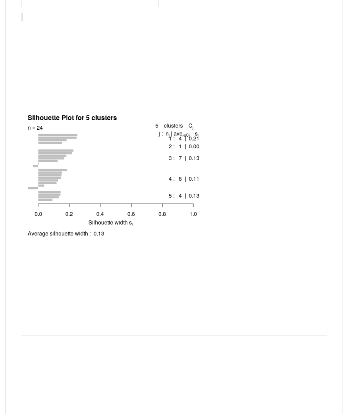
The silhouette plot The 1);-@,< package contains the function -*)H0;,@@,.2 that compares the minimum average
dissimilarity of each object to other clusters with the average dissimilarity to objects in its own cluster. The resulting
measure is called the "width of each object's silhouette". A value close to 1 indicates that the object is similar to objects in
its cluster compared to those in other clusters. Thus, the average of all objects silhouette widths gives an indication of how
well the clusters are defined.
0>(WX(>B<.CB<(I(1.aY(/Y(#Y(#22
>)0@.><4>BCY(CB*+(I(JP*)H0;,@@,(k)0@(G0<(a(1);-@,<-J2
>B<.0>2
Take-home problem (1)draw a plot with number of clusters in the x-axis and the average silhouette widths in the y-axis.
Use the information obtained to determine if 5 was the best choice for the number of clusters.
(2)For a common choice of k, compare the clustering across different methods, e.g. hierarchical (pruned to specific k,
obviously), k-means, PAM. You will re-discover the "label switching problem" for yourself. How does that manifest itself?
How concordant are the clusterings for different methods?
Gene clustering
A different view at the data can be obtained from clustering genes instead of samples. Since clustering genes is slow when
you have a lot of genes, for the sake of time we will work with a smaller subset of genes.
In many cases, analysts use cluster analysis to illustrate the results of a differential expression analysis. Sample clustering
following a differential expression (DE) analysis will probably show the separation of the groups identified by the DE
analysis. Thus, as it was mentioned in lectures, we need to be careful in over-interpreting these kind of results. However,
note that it is valid to perform a gene clustering to see if differential expressed genes cluster according to their function,
subcellular localizations, pathways, etc.

2019-02-27, 11:23 AMSTAT540-UBC.github.io/sm06_clustering-pca.md at master · STAT540-UBC/STAT540-UBC.github.io
Page 14 of 25https://github.com/STAT540-UBC/STAT540-UBC.github.io/blob/master/seminars/seminars_winter_2019/seminar6/sm06_clustering-pca.md
A smaller dataset
In Seminar 4: Differential Expression Analysis, you've learned how to use )*CCB to fit a common linear model to a very
large number of genes and thus identify genes that show differential expression over the course of development.
1;@0GG(WX(/,XQa
_,-ZB@(WX(C0",)4CB@<*A.mL<>Y(><_,-2
"-d*@(WX()Cd*@.-><_B@Y(_,-ZB@2
"-8%d*@(WX(,6B=,-."-d*@2
"-b*@-(WX(@0>[B%),."-8%d*@Y(10,G(I(L<,>.JL<>JY(10)+BC,-.10,G."-8%d*@222Y(>4?B);,(I(1;@0GGY(
((((+(I(l+G2
+;C6bH*@-(WX(+<0F."-b*@-2
@0>7,+,-(WX(<0F+BC,-."-b*@-2
S(P1B),"("B@B(0G(@0>7,+,-
@0>_B@(WX(-><_B@]@0>7,+,-Y(^
We start by using different clustering algorithms to cluster the top 897 genes that showed differential expression across
the different developmental stage (BH adjusted p value < 10^{-5}).
Agglomerative Hierarchical Clustering
We can plot the heatmap using the >H,B@CB> function....
>H,B@CB>.@0>_B@Y(1);-@,<V<0F-(I([D\8Y(-1B),(I(J+0+,JY(1);-@,<*+LVC,@H0"(I(JB?,<BL,JY(
((((1);-@,<*+LV"*-@B+1,V10)-(I(J,;1)*",B+JY(1);-@,<*+LV"*-@B+1,V<0F-(I(J,;1)*",B+JY(
((((B++0@B@*0+(I(><_,-]Y(1.J@*--;,JY(JL,+0@=>,JY(JL<>J2^Y(-H0FV<0F+BC,-(I(deOP8Y(
((((B++0@B@*0+V10)0<-(I(10?B<V10)0<2
Or we can plot the heatmap using the >)0@ function, after we have made the hclust object....
L,+,E4"*-(WX("*-@.@0>_B@Y(C,@H0"(I(J,;1)*",B+J2
L,+,E4H14B(WX(H1);-@.L,+,E4"*-Y(C,@H0"(I(JB?,<BL,J2

2019-02-27, 11:23 AMSTAT540-UBC.github.io/sm06_clustering-pca.md at master · STAT540-UBC/STAT540-UBC.github.io
Page 15 of 25https://github.com/STAT540-UBC/STAT540-UBC.github.io/blob/master/seminars/seminars_winter_2019/seminar6/sm06_clustering-pca.md
>)0@.L,+,E4H14BY()B%,)-(I(deOP8Y(CB*+(I(Jb*,<B<1H*1B)(F*@H(e?,<BL,(O*+KBL,JY(A)B%(I(JJ2
As you can see, when there are lots of objects to cluster, the dendrograms are in general not very informative as it is
difficult to identify any interesting pattern in the data.
Partitioning Methods
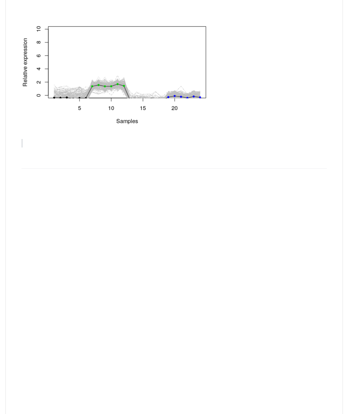
The most interesting thing to look at is the cluster centers (basically the "prototype" for the cluster) and membership sizes.
Then we can try to visualize the genes that are in each cluster.
Let's visualize a cluster (remember the data were rescaled) using line plots. This makes sense since we also want to be
able to see the cluster center.
-,@4-,,"./'3#2
K(WX(a
KC,B+-4L,+,-(WX(KC,B+-.@0>_B@Y(1,+@,<-(I(K2
S(1H00-,(FH*1H(1);-@,<(F,(FB+@
1);-@,<n;C(WX('
S(P,@(;>(@H,(BA,-(F*@H0;@(>)0@@*+Lo(=)*C(-,@(%B-,"(0+(@<*B)(<;+4
>)0@.KC,B+-4L,+,-`1,+@,<-]1);-@,<n;CY(^Y(=)*C(I(1.QY(/Q2Y(@=>,(I(J+JY(A)B%(I(JPBC>),-JY(
((((=)B%(I(JD,)B@*?,(,A><,--*0+J2
S(k)0@(@H,(,A><,--*0+(0G(B))(@H,(L,+,-(*+(@H,(-,),1@,"(1);-@,<(*+(L<,=4
CB@)*+,-.=(I(@.@0>_B@]KC,B+-4L,+,-`1);-@,<(II(1);-@,<n;CY(^2Y(10)(I(JL<,=J2
S(e""(@H,(1);-@,<(1,+@,<4([H*-(*-()B-@(-0(*@(*-+h@(;+",<+,B@H(@H,(C,C%,<-
>0*+@-.KC,B+-4L,+,-`1,+@,<-]1);-@,<n;CY(^Y(@=>,(I(J)J2
S(9>@*0+B)M(10)0<,"(>0*+@-(@0(-H0F(FH*1H(-@BL,(@H,(-BC>),-(B<,(G<0C4
>0*+@-.KC,B+-4L,+,-`1,+@,<-]1);-@,<n;CY(^Y(10)(I(><_,-`L<>Y(>1H(I('Q2
2019-02-27, 11:23 AMSTAT540-UBC.github.io/sm06_clustering-pca.md at master · STAT540-UBC/STAT540-UBC.github.io
Page 16 of 25https://github.com/STAT540-UBC/STAT540-UBC.github.io/blob/master/seminars/seminars_winter_2019/seminar6/sm06_clustering-pca.md
Improve the plot above adding sample names to the x-axis (e.g., wt_E16_1)
Evaluating clusters
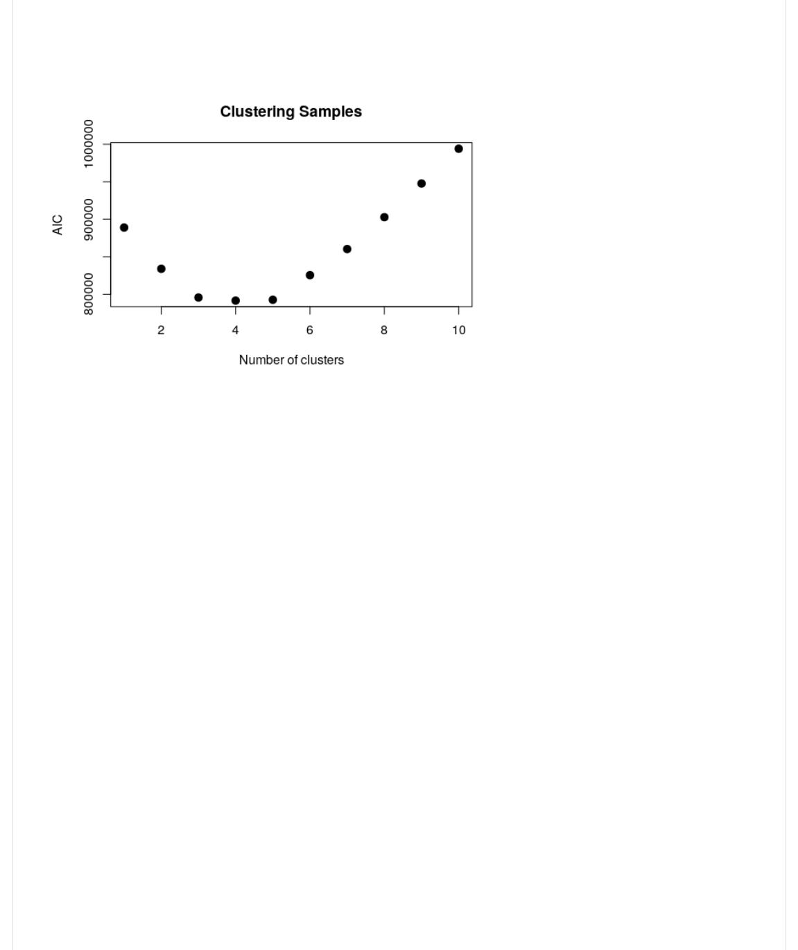
Choosing the right k
As mentioned in Lecture 12, we need to find a balance between accurately grouping similar data into one representative
cluster and the “cost” of adding additional clusters. Sometimes we don't have any prior knowledge to tell us how many
clusters there are supposed to be in our data. In this case, we can use Akaike information criterion (AIC) and Bayesian
information criterion (BIC) to help us to choose a proper k.
First, we calculate the AIC for each choice of k. We are clustering the samples in this example:
-,@4-,,".3/2
KVCBA(WX(/Q((S(@H,(CBA(+;C%,<(0G(1);-@,<-(@0(,A>)0<,(1);-@,<*+L(F*@H(
KCVG*@(WX()*-@.2((S(1<,B@,(,C>@=()*-@(@0(-@0<,(@H,(KC,B+-(0%U,1@
G0<(.*(*+(/MKVCBA2(R
((((KV1);-@,<(WX(KC,B+-.@.-><_B@2Y(1,+@,<-(I(*Y(+-@B<@(I(aQ2
((((KCVG*@]]*^^(WX(KV1);-@,<
T
S(1B)1;)B@,(elE
KCVelE(WX(G;+1@*0+.KCV1);-@,<2(R
((((C(WX(+10).KCV1);-@,<`1,+@,<-2
((((+(WX(),+L@H.KCV1);-@,<`1);-@,<2
((((K(WX(+<0F.KCV1);-@,<`1,+@,<-2
((((_(WX(KCV1);-@,<`@0@4F*@H*+--
((((<,@;<+._(c('(p(C(p(K2
T
Then, we plot the AIC vs. the number of clusters. We want to choose the k value that corresponds to the elbow point on
the AIC/BIC curve.
2019-02-27, 11:23 AMSTAT540-UBC.github.io/sm06_clustering-pca.md at master · STAT540-UBC/STAT540-UBC.github.io
Page 17 of 25https://github.com/STAT540-UBC/STAT540-UBC.github.io/blob/master/seminars/seminars_winter_2019/seminar6/sm06_clustering-pca.md
B*1(WX(-B>>)=.KCVG*@Y(KCVelE2
>)0@.-,:./Y(KVCBA2Y(B*1Y(A)B%(I(Jn;C%,<(0G(1);-@,<-JY(=)B%(I(JelEJY(>1H(I('QY(1,A(I('Y(
((((CB*+(I(JE);-@,<*+L(PBC>),-J2
Same for BIC
S(1B)1;)B@,(6lE
KCV6lE(WX(G;+1@*0+.KCV1);-@,<2(R
((((C(WX(+10).KCV1);-@,<`1,+@,<-2
((((+(WX(),+L@H.KCV1);-@,<`1);-@,<2
((((K(WX(+<0F.KCV1);-@,<`1,+@,<-2
((((_(WX(KCV1);-@,<`@0@4F*@H*+--
((((<,@;<+._(c()0L.+2(p(C(p(K2
T
%*1(WX(-B>>)=.KCVG*@Y(KCV6lE2
>)0@.-,:./Y(KVCBA2Y(%*1Y(A)B%(I(Jn;C%,<(0G(1);-@,<-JY(=)B%(I(J6lEJY(>1H(I('QY(1,A(I('Y(
((((CB*+(I(JE);-@,<*+L(PBC>),-J2

2019-02-27, 11:23 AMSTAT540-UBC.github.io/sm06_clustering-pca.md at master · STAT540-UBC/STAT540-UBC.github.io
Page 18 of 25https://github.com/STAT540-UBC/STAT540-UBC.github.io/blob/master/seminars/seminars_winter_2019/seminar6/sm06_clustering-pca.md
Can you eyeball the optimal 'k' by looking at these plots?
The code for the section "Choosing the right k" is based on Towers' blog and this thread
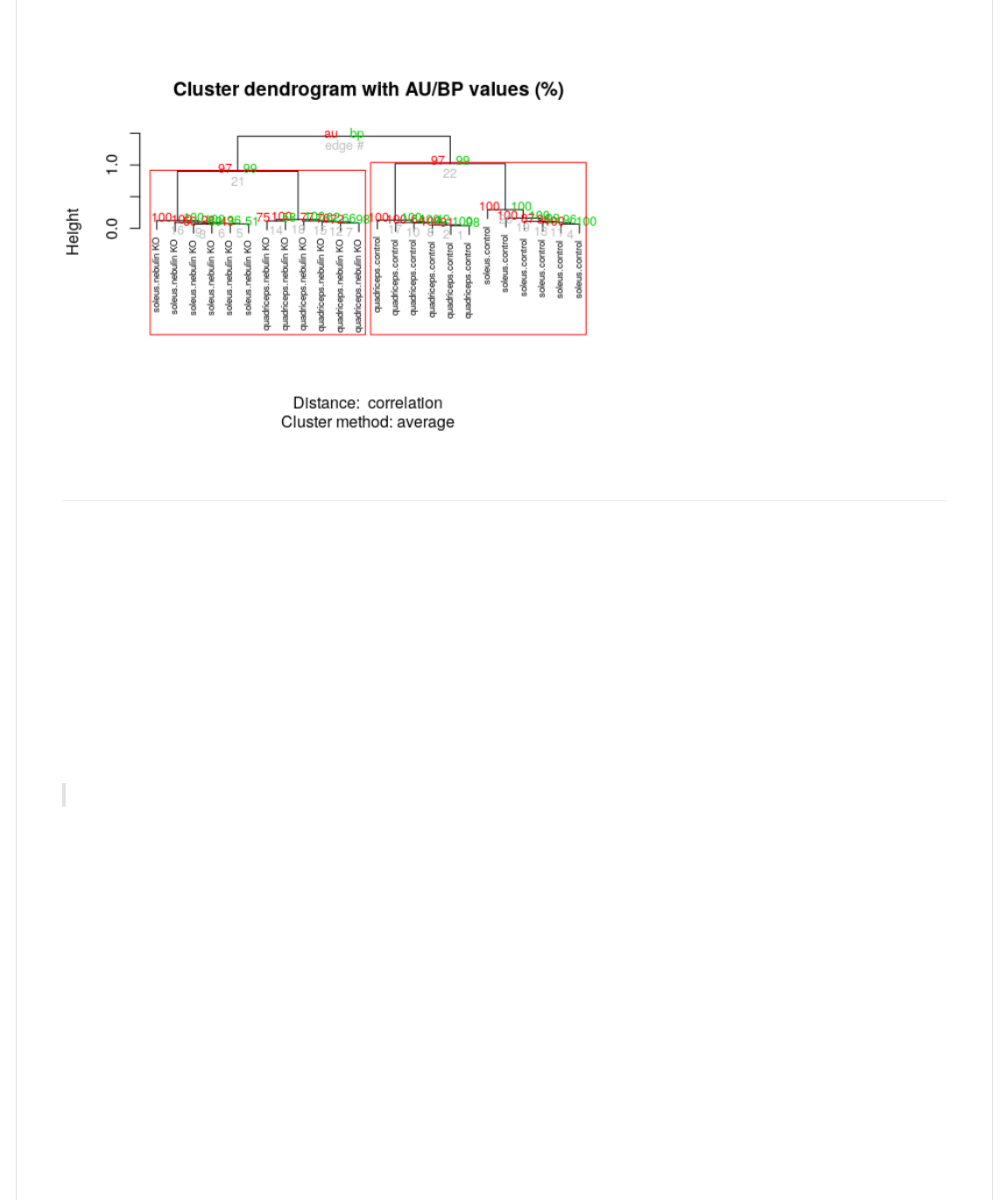
Statistical methods
An important issue for clustering is the question of certainty of the cluster membership. Clustering always gives you an
answer, even if there aren't really any underlying clusters. There are many ways to address this. Here we introduce an
approachable one offered in R, >?1);-@ , which you can read about at (http://www.sigmath.es.osaka-u.ac.jp/shimo-
lab/prog/pvclust/).
Important: >?1);-@ clusters the columns. I don't recommend doing this for genes! The computation will take a very
long time. Even the following example with all 30K genes will take some time to run.
You control how many bootstrap iterations >?1);-@ does with the +%00@ parameter. We've also noted that >?1);-@
causes problems on some machines, so if you have trouble with it, it's not critical.
Unlike picking the right clusters in the partition based methods (like k-means and PAM), here we are identifying the most
stable clustering arising from hierarchichal clustering.
>?1(WX(>?1);-@.@0>_B@Y(+%00@(I(/QQ2
SS(600@-@<B>(.<(I(Q4a2444(_0+,4
SS(600@-@<B>(.<(I(Q4!2444(_0+,4
SS(600@-@<B>(.<(I(Q4$2444(_0+,4
SS(600@-@<B>(.<(I(Q4&2444(_0+,4
SS(600@-@<B>(.<(I(Q4f2444(_0+,4
SS(600@-@<B>(.<(I(/4Q2444(_0+,4
SS(600@-@<B>(.<(I(/4/2444(_0+,4
SS(600@-@<B>(.<(I(/4'2444(_0+,4
SS(600@-@<B>(.<(I(/432444(_0+,4
SS(600@-@<B>(.<(I(/4#2444(_0+,4
>)0@.>?1Y()B%,)-(I(><_,-`L<>Y(1,A(I(Q4!2
2019-02-27, 11:23 AMSTAT540-UBC.github.io/sm06_clustering-pca.md at master · STAT540-UBC/STAT540-UBC.github.io
Page 19 of 25https://github.com/STAT540-UBC/STAT540-UBC.github.io/blob/master/seminars/seminars_winter_2019/seminar6/sm06_clustering-pca.md
>?<,1@.>?1Y(B)>HB(I(Q4fa2
Feature reduction
There are various ways to reduce the number of features (variables) being used in our clustering analyses. We have
already shown how to subset the number of variables (genes) based on variance, calculated using the limma package.
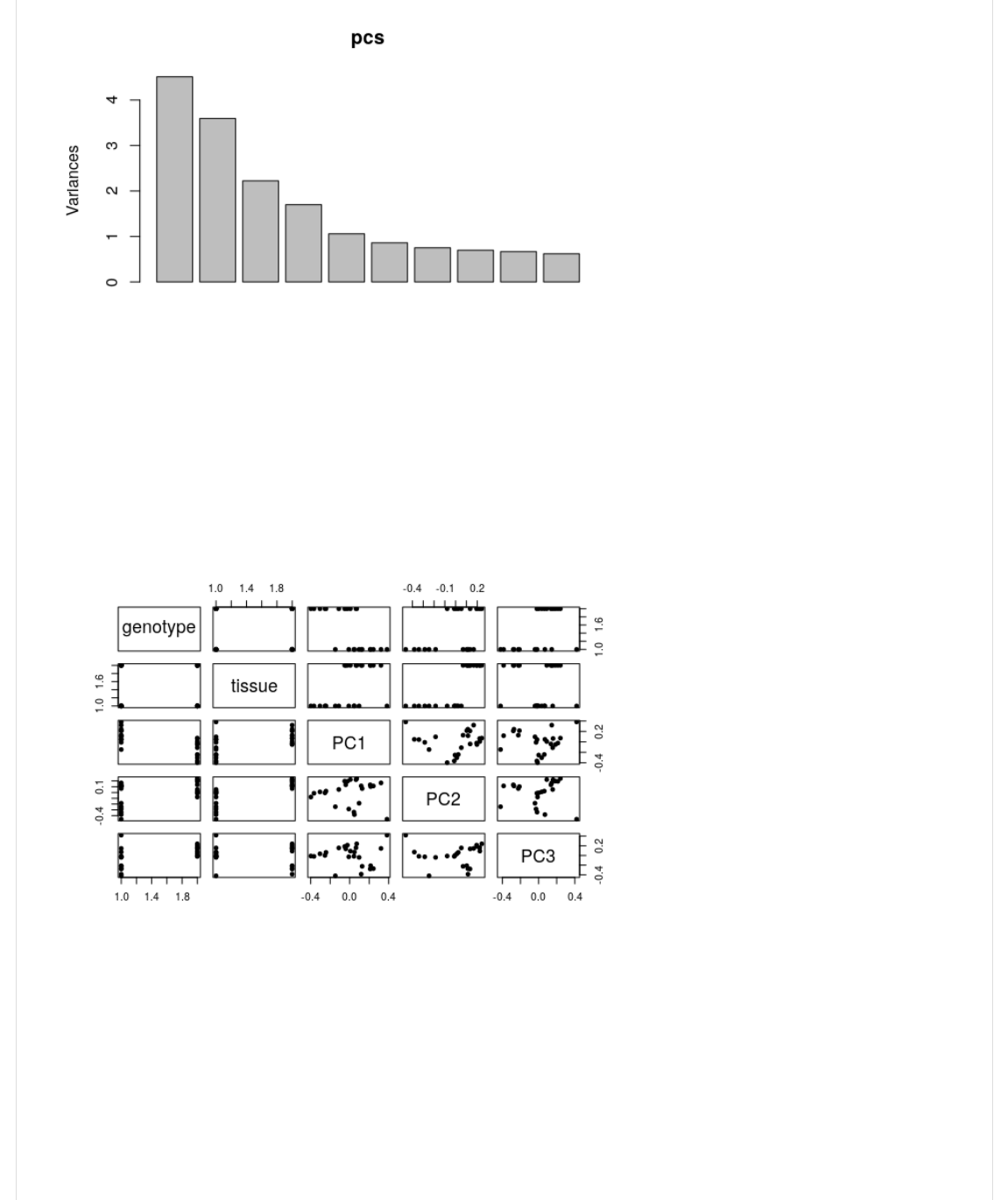
PCA plots
The other way we can do this is using PCA (principal components analysis). PCA assumes that the most important
characteristics of our data are the ones with the largest variance. Furthermore, it takes our data and organizes it in such a
way that redundancy is removed as the most important variables are listed first. The new variables will be linear
combinations of the original variables, with different weights.
In R, we can use ><10C>.2 to do PCA. You can also use -?".2 .
Scaling is suppressed because we already scaled the rows. You can experiment with this to see what happens.
>1-(WX(><10C>.-><_B@Y(1,+@,<(I(deOP8Y(-1B),(I(deOP82
S(-1<,,(>)0@
>)0@.>1-2
2019-02-27, 11:23 AMSTAT540-UBC.github.io/sm06_clustering-pca.md at master · STAT540-UBC/STAT540-UBC.github.io
Page 20 of 25https://github.com/STAT540-UBC/STAT540-UBC.github.io/blob/master/seminars/seminars_winter_2019/seminar6/sm06_clustering-pca.md
S(B>>,+"(@H,(<0@B@*0+-(G0<(@H,(G*<-@(/Q(kE-(@0(@H,(>H,+0"B@B
><*+E0C>(WX(1%*+".><_,-Y(>1-`<0@B@*0+]<0F+BC,-.><_,-2Y(/M/Q^2
S(-1B@@,<(>)0@(-H0F*+L(;-(H0F(@H,(G*<-@(G,F(kE-(<,)B@,(@0(10?B<*B@,-
>)0@.><*+E0C>]Y(1.JL,+0@=>,JY(J@*--;,JY(JkE/JY(JkE'JY(JkE3J2^Y(>1H(I(/fY(1,A(I(Q4&2
What does the samples spread look like, as explained by their first 2 principal components?
>)0@.><*+E0C>]Y(1.JkE/JY(JkE'J2^Y(>1H(I('/Y(1,A(I(/4a2

2019-02-27, 11:23 AMSTAT540-UBC.github.io/sm06_clustering-pca.md at master · STAT540-UBC/STAT540-UBC.github.io
Page 21 of 25https://github.com/STAT540-UBC/STAT540-UBC.github.io/blob/master/seminars/seminars_winter_2019/seminar6/sm06_clustering-pca.md
Is the covariate @*--;, localized in the different clusters we see?
>)0@.><*+E0C>]Y(1.JkE/JY(JkE'J2^Y(%L(I(><_,-`@*--;,Y(>1H(I('/Y(1,A(I(/4a2
),L,+".)*-@.A(I(Q4'Y(=(I(Q432Y(B-41HB<B1@,<.),?,)-.><_,-`@*--;,22Y(>1H(I('/Y(>@4%L(I(1./Y(
(((('Y(3Y(#Y(a22
Is the covariate L,+0@=>, localized in the different clusters we see?
>)0@.><*+E0C>]Y(1.JkE/JY(JkE'J2^Y(%L(I(><_,-`L,+0@=>,Y(>1H(I('/Y(1,A(I(/4a2
),L,+".)*-@.A(I(Q4'Y(=(I(Q432Y(B-41HB<B1@,<.),?,)-.><_,-`L,+0@=>,22Y(>1H(I('/Y(>@4%L(I(1./Y(
(((('Y(3Y(#Y(a22

2019-02-27, 11:23 AMSTAT540-UBC.github.io/sm06_clustering-pca.md at master · STAT540-UBC/STAT540-UBC.github.io
Page 22 of 25https://github.com/STAT540-UBC/STAT540-UBC.github.io/blob/master/seminars/seminars_winter_2019/seminar6/sm06_clustering-pca.md
PCA is a useful initial means of analysing any hidden structures in your data. We can also use it to determine how many
sources of variance are important, and how the different features interact to produce these sources.
First, let us first assess how much of the total variance is captured by each principal component.
S(7,@(@H,(-;%-,@(0G(kE-(@HB@(1B>@;<,(@H,(C0-@(?B<*B+1,(*+(=0;<(><,"*1@0<-
-;CCB<=.>1-2
SS(lC>0<@B+1,(0G(10C>0+,+@-M
SS(((((((((((((((((((((((((((kE/((((kE'(((((kE3(((((kE#(((((kEa(((((kE!
SS(P@B+"B<"(",?*B@*0+((((('4/'3a(/4&fa$(/4#fQ!$(/43Q33!(/4Q'&$&(Q4f'$fa
SS(k<0>0<@*0+(0G(qB<*B+1,(Q4/f!/(Q4/a!'(Q4Qf!!/(Q4Q$3&!(Q4Q#!Q'(Q4Q3$##
SS(E;C;)B@*?,(k<0>0<@*0+((Q4/f!/(Q43a'3(Q4##&fQ(Q4a''$!(Q4a!&$$(Q4!Q!'/
SS((((((((((((((((((((((((((((kE$(((((kE&(((((kEf((((kE/Q((((kE//((((kE/'
SS(P@B+"B<"(",?*B@*0+(((((Q4&!!$#(Q4&3a3#(Q4&/!'/(Q4$&!$&(Q4$$'#3(Q4$!/#3
SS(k<0>0<@*0+(0G(qB<*B+1,(Q4Q3'!!(Q4Q3Q3#(Q4Q'&f!(Q4Q'!f/(Q4Q'af#(Q4Q'a'/
SS(E;C;)B@*?,(k<0>0<@*0+((Q4!3&&$(Q4!!f'/(Q4!f&/$(Q4$'aQf(Q4$a/Q3(Q4$$!'3
SS((((((((((((((((((((((((((kE/3((((kE/#((((kE/a((((kE/!((((kE/$((((kE/&
SS(P@B+"B<"(",?*B@*0+(((((Q4$#$$(Q4$3/3f(Q4$'/'$(Q4$Q&$'(Q4!f#Q!(Q4!$a/f
SS(k<0>0<@*0+(0G(qB<*B+1,(Q4Q'#3(Q4Q'3'!(Q4Q''!'(Q4Q'/&#(Q4Q'Qf#(Q4Q/f&'
SS(E;C;)B@*?,(k<0>0<@*0+((Q4&QQa(Q4&'3$f(Q4&#!#/(Q4&!&'a(Q4&&f/f(Q4fQfQ/
SS(((((((((((((((((((((((((((kE/f((((kE'Q((((kE'/((((kE''((((kE'3((((((kE'#
SS(P@B+"B<"(",?*B@*0+(((((Q4!$#'3(Q4!a$#Q(Q4!#f33(Q4!'&/'(Q4!'#33(/4!&$,X/a
SS(k<0>0<@*0+(0G(qB<*B+1,(Q4Q/f$!(Q4Q/&$f(Q4Q/&33(Q4Q/$/a(Q4Q/!fa(Q4QQQ,cQQ
SS(E;C;)B@*?,(k<0>0<@*0+((Q4f'&$&(Q4f#$a$(Q4f!afQ(Q4f&3Qa(/4QQQQQ(/4QQQ,cQQ
We see that the first two principal components capture 35% of the total variance. If we include the first 11 principal
components, we capture 75% of the total variance. Depending on which of these subsets you want to keep, we will select
the rotated data from the first n components. We can use the @0) parameter in ><10C> to remove trailing PCs.
>1-V'"*C(I(><10C>.-><_B@Y(1,+@,<(I(deOP8Y(-1B),(I(deOP8Y(@0)(I(Q4&2
It is commonly seen a cluster analysis on the first 3 principal components to illustrate and explore the data.

2019-02-27, 11:23 AMSTAT540-UBC.github.io/sm06_clustering-pca.md at master · STAT540-UBC/STAT540-UBC.github.io
Page 23 of 25https://github.com/STAT540-UBC/STAT540-UBC.github.io/blob/master/seminars/seminars_winter_2019/seminar6/sm06_clustering-pca.md
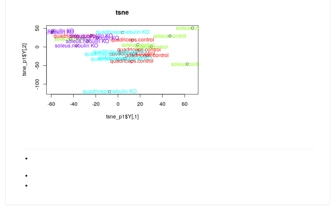
t-SNE plots
WHen we are dealing with datasets that have thousands of variables, and we want to have an initial pass at identifying
hidden patterns in the data, another method we can use as an alterative to PCA is t-SNE. This method allows for non-linear
interactions between our features.
Importantly, there are certain caveats with using t-SNE.
1. Solutions are not deterministic: While in PCA the correct solution to a question is guaranteed, t-SNE can have many
multiple minima, and might give many different optimal solutions. It is hence non-deterministic. This may make it
challenging to generate reproducible results.
2. Clusters are not intuitive: t-SNE collapses similar points in high dimensional space, on top of each other in lower
dimensions. This means it maps features that are proximal to each other in a way that global trends may be warped.
On the other hand, PCA always rotates our features in specific ways that can be extracted by considering the
covariance matrix of our initial dataset and the eigenvectors in the new coordinate space.
3. Applying our fit to new data: t-SNE embedding is generated by moving all our data to a lower dimensional state. It
does not give us eigenvectors (like PCA does) that can map new/unseen data to this lower dimensional state.
The computational costs of t-SNE are also quite expensive, and finding an embedding in lower space that makes sense
may often require extensive fientuning of several hyperparameters.
We will be using the D@-+, package to visualize our data using t-SNE. In this plot we are changing the perplexity
parameter for the two different plots. As you see, the outputs are remarkably different.
S(*+-@B))4>B1KBL,-.hD@-+,h2
)*%<B<=.D@-+,2
10)0<-(I(<B*+%0F.),+L@H.;+*:;,.><_,-`L<>222
+BC,-.10)0<-2(I(;+*:;,.><_,-`L<>2
@-+,(WX(D@-+,.;+*:;,.@.-><_B@22Y("*C-(I('Y(>,<>),A*@=(I(Q4/Y(?,<%0-,(I([D\8Y(CBAV*@,<(I(/QQ2
SS(k,<G0<C*+L(kEe
SS(D,B"(@H,('#(A('#("B@B(CB@<*A(-;11,--G;))=r
SS(9>,+Zk(*-(F0<K*+L4(/(@H<,B"-4
SS(\-*+L(+0V"*C-(I('Y(>,<>),A*@=(I(Q4/QQQQQY(B+"(@H,@B(I(Q4aQQQQQ
SS(E0C>;@*+L(*+>;@(-*C*)B<*@*,-444
SS(k,<>),A*@=(-H0;)"(%,()0F,<(@HB+(5r
SS(6;*)"*+L(@<,,444
SS(_0+,(*+(Q4QQ(-,10+"-(.->B<-*@=(I(Q4QQQQQQ2r
SS(O,B<+*+L(,C%,""*+L444
SS(l@,<B@*0+(aQM(,<<0<(*-(Q4QQQQQQ(.aQ(*@,<B@*0+-(*+(Q4QQ(-,10+"-2
SS(l@,<B@*0+(/QQM(,<<0<(*-(Q4QQQQQQ(.aQ(*@,<B@*0+-(*+(Q4QQ(-,10+"-2
SS(d*@@*+L(>,<G0<C,"(*+(Q4Q/(-,10+"-4
>)0@.@-+,`sY(CB*+(I(J@-+,J2
@,A@.@-+,`sY()B%,)-(I(><_,-`L<>Y(10)(I(10)0<-]><_,-`L<>^2

2019-02-27, 11:23 AMSTAT540-UBC.github.io/sm06_clustering-pca.md at master · STAT540-UBC/STAT540-UBC.github.io
Page 24 of 25https://github.com/STAT540-UBC/STAT540-UBC.github.io/blob/master/seminars/seminars_winter_2019/seminar6/sm06_clustering-pca.md
@-+,V>/(WX(D@-+,.;+*:;,.@.-><_B@22Y("*C-(I('Y(>,<>),A*@=(I(/Y(?,<%0-,(I([D\8Y(CBAV*@,<(I(/QQ2
SS(k,<G0<C*+L(kEe
SS(D,B"(@H,('#(A('#("B@B(CB@<*A(-;11,--G;))=r
SS(9>,+Zk(*-(F0<K*+L4(/(@H<,B"-4
SS(\-*+L(+0V"*C-(I('Y(>,<>),A*@=(I(/4QQQQQQY(B+"(@H,@B(I(Q4aQQQQQ
SS(E0C>;@*+L(*+>;@(-*C*)B<*@*,-444
SS(6;*)"*+L(@<,,444
SS(_0+,(*+(Q4QQ(-,10+"-(.->B<-*@=(I(Q4/!3/f#2r
SS(O,B<+*+L(,C%,""*+L444
SS(l@,<B@*0+(aQM(,<<0<(*-(a!4Q$!$!a(.aQ(*@,<B@*0+-(*+(Q4QQ(-,10+"-2
SS(l@,<B@*0+(/QQM(,<<0<(*-(a$4f!/&#a(.aQ(*@,<B@*0+-(*+(Q4QQ(-,10+"-2
SS(d*@@*+L(>,<G0<C,"(*+(Q4Q/(-,10+"-4
>)0@.@-+,V>/`sY(CB*+(I(J@-+,J2
@,A@.@-+,V>/`sY()B%,)-(I(><_,-`L<>Y(10)(I(10)0<-]><_,-`L<>^2
2019-02-27, 11:23 AMSTAT540-UBC.github.io/sm06_clustering-pca.md at master · STAT540-UBC/STAT540-UBC.github.io
Page 25 of 25https://github.com/STAT540-UBC/STAT540-UBC.github.io/blob/master/seminars/seminars_winter_2019/seminar6/sm06_clustering-pca.md
Deliverables
Regenerate the pheatmap clustering plot for the top genes, selected from limma, using clustering distance:
correlation, and clustering method: mcquitty.
Regenerate the dendrogram on the samples of this heatmap using the H1);-@ and "*-@ functions.
Plot the data for this analyses along PCs 1 and 2 using LL>)0@ instead base plotting. Color the points by tissue
