Step By Programming With Base SAS Software Manual
SAS_programming_manual
User Manual:
Open the PDF directly: View PDF ![]() .
.
Page Count: 788 [warning: Documents this large are best viewed by clicking the View PDF Link!]
- Table of Contents
- Introduction to the SAS System
- What Is the SAS System?
- Getting Your Data into Shape
- Introduction to DATA Step Processing
- Introduction to DATA Step Processing
- The SAS Data Set: Your Key to the SAS System
- How the DATA Step Works: A Basic Introduction
- Supplying Information to Create a SAS Data Set
- Overview of Creating a SAS Data Set
- Telling SAS How to Read the Data: Styles of Input
- Reading Dates with Two-Digit and Four-Digit Year Values
- Defining Variables in SAS
- Indicating the Location of Your Data
- Using External Files in Your SAS Job
- Identifying an External File Directly
- Referencing an External File with a Fileref
- Review of SAS Tools
- Learning More
- Starting with Raw Data: The Basics
- Starting with Raw Data: Beyond the Basics
- Introduction to Beyond the Basics with Raw Data
- Testing a Condition before Creating an Observation
- Creating Multiple Observations from a Single Record
- Reading Multiple Records to Create a Single Observation
- Problem Solving: When an Input Record Unexpectedly Does Not Have Enough Values
- Review of SAS Tools
- Learning More
- Starting with SAS Data Sets
- Basic Programming
- Understanding DATA Step Processing
- Working with Numeric Variables
- Working with Character Variables
- Introduction to Working with Character Variables
- Input SAS Data Set for Examples
- Identifying Character Variables and Expressing Character Values
- Setting the Length of Character Variables
- Handling Missing Values
- Creating New Character Values
- Saving Storage Space by Treating Numbers as Characters
- Review of SAS Tools
- Learning More
- Acting on Selected Observations
- Creating Subsets of Observations
- Working with Grouped or Sorted Observations
- Using More Than One Observation in a Calculation
- Finding Shortcuts in Programming
- Working with Dates in the SAS System
- Combining SAS Data Sets
- Methods of Combining SAS Data Sets
- Concatenating SAS Data Sets
- Interleaving SAS Data Sets
- Merging SAS Data Sets
- Updating SAS Data Sets
- Modifying SAS Data Sets
- Conditionally Processing Observations from Multiple SAS Data Sets
- Understanding Your SAS Session
- Analyzing Your SAS Session with the SAS Log
- Directing SAS Output and the SAS Log
- Introduction to Directing SAS Output and the SAS Log
- Input File and SAS Data Set for Examples
- Routing the Output and the SAS Log with PROC PRINTTO
- Storing the Output and the SAS Log in the SAS Windowing Environment
- Redefining the Default Destination in a Batch or Noninteractive Environment
- Review of SAS Tools
- Learning More
- Diagnosing and Avoiding Errors
- Producing Reports
- Producing Detail Reports with the PRINT Procedure
- Creating Summary Tables with the TABULATE Procedure
- Introduction to Creating Summary Tables with the TABULATE Procedure
- Understanding Summary Table Design
- Understanding the Basics of the TABULATE Procedure
- Input File and SAS Data Set for Examples
- Creating Simple Summary Tables
- Creating More Sophisticated Summary Tables
- Creating Hierarchical Tables to Report on Subgroups
- Formatting Output
- Calculating Descriptive Statistics
- Reporting on Multiple Statistics
- Reducing Code and Applying a Single Label to Multiple Elements
- Getting Summaries for All Variables
- Defining Labels
- Using Styles and the Output Delivery System
- Ordering Class Variables
- Review of SAS Tools
- Learning More
- Creating Detail and Summary Reports with the REPORT Procedure
- Producing Plots and Charts
- Plotting the Relationship between Variables
- Producing Charts to Summarize Variables
- Designing Your Own Output
- Writing Lines to the SAS Log or to an Output File
- Understanding and Customizing SAS Output: The Basics
- Understanding and Customizing SAS Output: The Output Delivery System ( ODS)
- Introduction to Customizing SAS Output by Using the Output Delivery System
- Input Data Set for Examples
- Understanding ODS Output Formats and Destinations
- Selecting an Output Format
- Creating Formatted Output
- Selecting the Output That You Want to Format
- Customizing ODS Output
- Storing Links to ODS Output
- Review of SAS Tools
- Learning More
- Storing and Managing Data in SAS Files
- Understanding SAS Data Libraries
- Managing SAS Data Libraries
- Getting Information about Your SAS Data Sets
- Modifying SAS Data Set Names and Variable Attributes
- Copying, Moving, and Deleting SAS Data Sets
- Understanding Your SAS Environment
- Introducing the SAS Environment
- Using the SAS Windowing Environment
- Customizing the SAS Environment
- Appendix
- Additional Data Sets
- Introduction
- Data Set CITY
- Raw Data Used for “Understanding Your SAS Session” Section
- Data Set SAT_SCORES
- Data Set YEAR_SALES
- Data Set HIGHLOW
- Data Set GRADES
- Data Sets for “Storing and Managing Data in SAS Files” Section
- DATA Step to Create the Data Set USCLIM.HIGHTEMP
- DATA Step to Create the Data Set USCLIM.HURRICANE
- DATA Step to Create the Data Set USCLIM.LOWTEMP
- DATA Step to Create the Data Set USCLIM.TEMPCHNG
- Note on Catalogs USCLIM.BASETEMP and USCLIM.REPORT
- DATA Step to Create the Data Set CLIMATE.HIGHTEMP
- DATA Step to Create the Data Set CLIMATE.LOWTEMP
- DATA Step to Create the Data Set PRECIP.RAIN
- DATA Step to Create the Data Set PRECIP.SNOW
- DATA Step to Create the Data Set STORM.TORNADO
- Glossary
- Index

Step-by-Step Programming with
Base SAS®Software
The correct bibliographic citation for this manual is as follows: SAS Institute Inc.
2001. Step-by-Step Programming with Base SAS ®Software. Cary, NC: SAS Institute Inc.
Step-by-Step Programming with Base SAS®Software
Copyright © 2001 by SAS Institute Inc., Cary, NC, USA.
ISBN 978-1-58025-791-6
All rights reserved. Produced in the United States of America.
For a hard-copy book: No part of this publication may be reproduced, stored in a
retrieval system, or transmitted, in any form or by any means, electronic, mechanical,
photocopying, or otherwise, without the prior written permission of the publisher, SAS
Institute Inc.
For a Web download or e-book: Your use of this publication shall be governed by the
terms established by the vendor at the time you acquire this publication.
U.S. Government Restricted Rights Notice. Use, duplication, or disclosure of this
software and related documentation by the U.S. government is subject to the Agreement
with SAS Institute and the restrictions set forth in FAR 52.227-19 Commercial Computer
Software-Restricted Rights (June 1987).
SAS Institute Inc., SAS Campus Drive, Cary, North Carolina 27513.
February 2007
SAS®Publishing provides a complete selection of books and electronic products to help
customers use SAS software to its fullest potential. For more information about our
e-books, e-learning products, CDs, and hard-copy books, visit the SAS Publishing Web site
at support.sas.com/pubs or call 1-800-727-3228.
SAS®and all other SAS Institute Inc. product or service names are registered trademarks
or trademarks of SAS Institute Inc. in the USA and other countries. ®indicates USA
registration.
Other brand and product names are registered trademarks or trademarks of their
respective companies.
Contents
PART1Introduction to the SAS System 1
Chapter 1 What Is the SAS System? 3
Introduction to the SAS System 3
Components of Base SAS Software 4
Output Produced by the SAS System 8
Ways to Run SAS Programs 11
Running Programs in the SAS Windowing Environment 13
Review of SAS Tools 15
Learning More 16
PART2Getting Your Data into Shape 17
Chapter 2 Introduction to DATA Step Processing 19
Introduction to DATA Step Processing 20
The SAS Data Set: Your Key to the SAS System 20
How the DATA Step Works: A Basic Introduction 26
Supplying Information to Create a SAS Data Set 33
Review of SAS Tools 41
Learning More 41
Chapter 3 Starting with Raw Data: The Basics 43
Introduction to Raw Data 44
Examine the Structure of the Raw Data: Factors to Consider 44
Reading Unaligned Data 44
Reading Data That Is Aligned in Columns 47
Reading Data That Requires Special Instructions 50
Reading Unaligned Data with More Flexibility 53
Mixing Styles of Input 55
Review of SAS Tools 58
Learning More 59
Chapter 4 Starting with Raw Data: Beyond the Basics 61
Introduction to Beyond the Basics with Raw Data 61
Testing a Condition before Creating an Observation 62
Creating Multiple Observations from a Single Record 63
Reading Multiple Records to Create a Single Observation 67
Problem Solving: When an Input Record Unexpectedly Does Not Have Enough
Values 74
Review of SAS Tools 77
Learning More 79

iv
Chapter 5 Starting with SAS Data Sets 81
Introduction to Starting with SAS Data Sets 81
Understanding the Basics 82
Input SAS Data Set for Examples 82
Reading Selected Observations 84
Reading Selected Variables 85
Creating More Than One Data Set in a Single DATA Step 89
Using the DROP= and KEEP= Data Set Options for Efficiency 91
Review of SAS Tools 92
Learning More 93
PART3Basic Programming 95
Chapter 6 Understanding DATA Step Processing 97
Introduction to DATA Step Processing 97
Input SAS Data Set for Examples 97
Adding Information to a SAS Data Set 98
Defining Enough Storage Space for Variables 103
Conditionally Deleting an Observation 104
Review of SAS Tools 105
Learning More 105
Chapter 7 Working with Numeric Variables 107
Introduction to Working with Numeric Variables 107
About Numeric Variables in SAS 108
Input SAS Data Set for Examples 108
Calculating with Numeric Variables 109
Comparing Numeric Variables 113
Storing Numeric Variables Efficiently 115
Review of SAS Tools 116
Learning More 117
Chapter 8 Working with Character Variables 119
Introduction to Working with Character Variables 119
Input SAS Data Set for Examples 120
Identifying Character Variables and Expressing Character Values 121
Setting the Length of Character Variables 122
Handling Missing Values 124
Creating New Character Values 127
Saving Storage Space by Treating Numbers as Characters 134
Review of SAS Tools 135
Learning More 136
Chapter 9 Acting on Selected Observations 139
Introduction to Acting on Selected Observations 139
Input SAS Data Set for Examples 140

v
Selecting Observations 141
Constructing Conditions 145
Comparing Characters 152
Review of SAS Tools 156
Learning More 157
Chapter 10 Creating Subsets of Observations 159
Introduction to Creating Subsets of Observations 159
Input SAS Data Set for Examples 160
Selecting Observations for a New SAS Data Set 161
Conditionally Writing Observations to One or More SAS Data Sets 164
Review of SAS Tools 170
Learning More 170
Chapter 11 Working with Grouped or Sorted Observations 173
Introduction to Working with Grouped or Sorted Observations 173
Input SAS Data Set for Examples 174
Working with Grouped Data 175
Working with Sorted Data 181
Review of SAS Tools 185
Learning More 186
Chapter 12 Using More Than One Observation in a Calculation 187
Introduction to Using More Than One Observation in a Calculation 187
Input File and SAS Data Set for Examples 188
Accumulating a Total for an Entire Data Set 189
Obtaining a Total for Each BY Group 191
Writing to Separate Data Sets 193
Using a Value in a Later Observation 196
Review of SAS Tools 199
Learning More 200
Chapter 13 Finding Shortcuts in Programming 201
Introduction to Shortcuts 201
Input File and SAS Data Set 201
Performing More Than One Action in an IF-THEN Statement 202
Performing the Same Action for a Series of Variables 204
Review of SAS Tools 207
Learning More 209
Chapter 14 Working with Dates in the SAS System 211
Introduction to Working with Dates 211
Understanding How SAS Handles Dates 212
Input File and SAS Data Set for Examples 213
Entering Dates 214
Displaying Dates 217
Using Dates in Calculations 221

vi
Using SAS Date Functions 223
Comparing Durations and SAS Date Values 225
Review of SAS Tools 227
Learning More 228
PART4Combining SAS Data Sets 231
Chapter 15 Methods of Combining SAS Data Sets 233
Introduction to Combining SAS Data Sets 233
Definition of Concatenating 234
Definition of Interleaving 234
Definition of Merging 235
Definition of Updating 236
Definition of Modifying 237
Comparing Modifying, Merging, and Updating Data Sets 238
Learning More 239
Chapter 16 Concatenating SAS Data Sets 241
Introduction to Concatenating SAS Data Sets 241
Concatenating Data Sets with the SET Statement 242
Concatenating Data Sets Using the APPEND Procedure 255
Choosing between the SET Statement and the APPEND Procedure 259
Review of SAS Tools 260
Learning More 260
Chapter 17 Interleaving SAS Data Sets 263
Introduction to Interleaving SAS Data Sets 263
Understanding BY-Group Processing Concepts 263
Interleaving Data Sets 264
Review of SAS Tools 267
Learning More 267
Chapter 18 Merging SAS Data Sets 269
Introduction to Merging SAS Data Sets 270
Understanding the MERGE Statement 270
One-to-One Merging 270
Match-Merging 276
Choosing between One-to-One Merging and Match-Merging 286
Review of SAS Tools 290
Learning More 290
Chapter 19 Updating SAS Data Sets 293
Introduction to Updating SAS Data Sets 293
Understanding the UPDATE Statement 294
Understanding How to Select BY Variables 294
Updating a Data Set 295

vii
Updating with Incremental Values 300
Understanding the Differences between Updating and Merging 302
Handling Missing Values 305
Review of SAS Tools 308
Learning More 309
Chapter 20 Modifying SAS Data Sets 311
Introduction 311
Input SAS Data Set for Examples 312
Modifying a SAS Data Set: The Simplest Case 313
Modifying a Master Data Set with Observations from a Transaction Data Set 314
Understanding How Duplicate BY Variables Affect File Update 317
Handling Missing Values 319
Review of SAS Tools 320
Learning More 321
Chapter 21 Conditionally Processing Observations from Multiple SAS Data Sets 323
Introduction to Conditional Processing from Multiple SAS Data Sets 323
Input SAS Data Sets for Examples 324
Determining Which Data Set Contributed the Observation 326
Combining Selected Observations from Multiple Data Sets 328
Performing a Calculation Based on the Last Observation 330
Review of SAS Tools 332
Learning More 332
PART5Understanding Your SAS Session 333
Chapter 22 Analyzing Your SAS Session with the SAS Log 335
Introduction to Analyzing Your SAS Session with the SAS Log 335
Understanding the SAS Log 336
Locating the SAS Log 337
Understanding the Log Structure 337
Writing to the SAS Log 339
Suppressing Information to the SAS Log 341
Changing the Log’s Appearance 344
Review of SAS Tools 346
Learning More 346
Chapter 23 Directing SAS Output and the SAS Log 349
Introduction to Directing SAS Output and the SAS Log 349
Input File and SAS Data Set for Examples 350
Routing the Output and the SAS Log with PROC PRINTTO 351
Storing the Output and the SAS Log in the SAS Windowing Environment 353
Redefining the Default Destination in a Batch or Noninteractive Environment 354
Review of SAS Tools 355
Learning More 356

viii
Chapter 24 Diagnosing and Avoiding Errors 357
Introduction to Diagnosing and Avoiding Errors 357
Understanding How the SAS Supervisor Checks a Job 357
Understanding How SAS Processes Errors 358
Distinguishing Types of Errors 358
Diagnosing Errors 359
Using a Quality Control Checklist 366
Learning More 366
PART6Producing Reports 369
Chapter 25 Producing Detail Reports with the PRINT Procedure 371
Introduction to Producing Detail Reports with the PRINT Procedure 372
Input File and SAS Data Sets for Examples 372
Creating Simple Reports 373
Creating Enhanced Reports 381
Creating Customized Reports 391
Making Your Reports Easy to Change 399
Review of SAS Tools 402
Learning More 405
Chapter 26 Creating Summary Tables with the TABULATE Procedure 407
Introduction to Creating Summary Tables with the TABULATE Procedure 408
Understanding Summary Table Design 408
Understanding the Basics of the TABULATE Procedure 410
Input File and SAS Data Set for Examples 412
Creating Simple Summary Tables 413
Creating More Sophisticated Summary Tables 419
Review of SAS Tools 431
Learning More 433
Chapter 27 Creating Detail and Summary Reports with the REPORT Procedure 435
Introduction to Creating Detail and Summary Reports with the REPORT
Procedure 436
Understanding How to Construct a Report 436
Input File and SAS Data Set for Examples 438
Creating Simple Reports 439
Creating More Sophisticated Reports 446
Review of SAS Tools 454
Learning More 458
PART7Producing Plots and Charts 461
Chapter 28 Plotting the Relationship between Variables 463
Introduction to Plotting the Relationship between Variables 463
Input File and SAS Data Set for Examples 464

ix
Plotting One Set of Variables 466
Enhancing the Plot 468
Plotting Multiple Sets of Variables 473
Review of SAS Tools 480
Learning More 481
Chapter 29 Producing Charts to Summarize Variables 483
Introduction to Producing Charts to Summarize Variables 484
Understanding the Charting Tools 484
Input File and SAS Data Set for Examples 485
Charting Frequencies with the CHART Procedure 487
Customizing Frequency Charts 494
Creating High-Resolution Histograms 503
Review of SAS Tools 514
Learning More 518
PART8Designing Your Own Output 519
Chapter 30 Writing Lines to the SAS Log or to an Output File 521
Introduction to Writing Lines to the SAS Log or to an Output File 521
Understanding the PUT Statement 522
Writing Output without Creating a Data Set 522
Writing Simple Text 523
Writing a Report 528
Review of SAS Tools 535
Learning More 536
Chapter 31 Understanding and Customizing SAS Output: The Basics 537
Introduction to the Basics of Understanding and Customizing SAS Output 538
Understanding Output 538
Input SAS Data Set for Examples 540
Locating Procedure Output 541
Making Output Informative 542
Controlling Output Appearance 548
Controlling the Appearance of Pages 550
Representing Missing Values 561
Review of SAS Tools 563
Learning More 564
Chapter 32 Understanding and Customizing SAS Output: The Output Delivery System
(ODS) 565
Introduction to Customizing SAS Output by Using the Output Delivery System 565
Input Data Set for Examples 566
Understanding ODS Output Formats and Destinations 567
Selecting an Output Format 568
Creating Formatted Output 569

x
Selecting the Output That You Want to Format 577
Customizing ODS Output 585
Storing Links to ODS Output 589
Review of SAS Tools 590
Learning More 592
PART9Storing and Managing Data in SAS Files 593
Chapter 33 Understanding SAS Data Libraries 595
Introduction to Understanding SAS Data Libraries 595
What Is a SAS Data Library? 596
Accessing a SAS Data Library 596
Storing Files in a SAS Data Library 598
Referencing SAS Data Sets in a SAS Data Library 599
Review of SAS Tools 601
Learning More 601
Chapter 34 Managing SAS Data Libraries 603
Introduction 603
Choosing Your Tools 603
Understanding the DATASETS Procedure 604
Looking at a PROC DATASETS Session 605
Review of SAS Tools 606
Learning More 606
Chapter 35 Getting Information about Your SAS Data Sets 607
Introduction to Getting Information about Your SAS Data Sets 607
Input Data Library for Examples 608
Requesting a Directory Listing for a SAS Data Library 608
Requesting Contents Information about SAS Data Sets 610
Requesting Contents Information in Different Formats 613
Review of SAS Tools 615
Learning More 615
Chapter 36 Modifying SAS Data Set Names and Variable Attributes 617
Introduction to Modifying SAS Data Set Names and Variable Attributes 617
Input Data Library for Examples 618
Renaming SAS Data Sets 618
Modifying Variable Attributes 619
Review of SAS Tools 626
Learning More 627
Chapter 37 Copying, Moving, and Deleting SAS Data Sets 629
Introduction to Copying, Moving, and Deleting SAS Data Sets 629
Input Data Libraries for Examples 630
Copying SAS Data Sets 630

xi
Copying Specific SAS Data Sets 634
Moving SAS Data Libraries and SAS Data Sets 635
Deleting SAS Data Sets 637
Deleting All Files in a SAS Data Library 639
Review of SAS Tools 640
Learning More 640
PART10 Understanding Your SAS Environment 641
Chapter 38 Introducing the SAS Environment 643
Introduction to the SAS Environment 644
Starting a SAS Session 645
Selecting a SAS Processing Mode 645
Review of SAS Tools 652
Learning More 654
Chapter 39 Using the SAS Windowing Environment 655
Introduction to Using the SAS Windowing Environment 657
Getting Organized 657
Finding Online Help 660
Using SAS Windowing Environment Command Types 660
Working with SAS Windows 663
Working with Text 667
Working with Files 671
Working with SAS Programs 676
Working with Output 682
Review of SAS Tools 690
Learning More 692
Chapter 40 Customizing the SAS Environment 693
Introduction to Customizing the SAS Environment 694
Customizing Your Current Session 695
Customizing Session-to-Session Settings 698
Customizing the SAS Windowing Environment 702
Review of SAS Tools 707
Learning More 708
PART11 Appendix 709
Appendix 1 Additional Data Sets 711
Introduction 711
Data Set CITY 712
Raw Data Used for “Understanding Your SAS Session” Section 713
Data Set SAT_SCORES 714
Data Set YEAR_SALES 715
Data Set HIGHLOW 716

1
PART
1
Introduction to the SAS System
Chapter 1..........
What Is the SAS System? 3
2
3
CHAPTER
1
What Is the SAS System?
Introduction to the SAS System 3
Components of Base SAS Software 4
Overview of Base SAS Software 4
Data Management Facility 4
Programming Language 5
Elements of the SAS Language 5
Rules for SAS Statements 6
Rules for Most SAS Names 6
Special Rules for Variable Names 6
Data Analysis and Reporting Utilities 6
Output Produced by the SAS System 8
Traditional Output 8
Output from the Output Delivery System (ODS) 9
Ways to Run SAS Programs 11
Selecting an Approach 11
SAS Windowing Environment 11
SAS/ASSIST Software 12
Noninteractive Mode 12
Batch Mode 12
Interactive Line Mode 13
Running Programs in the SAS Windowing Environment 13
Review of SAS Tools 15
Statements 15
Procedures 15
Learning More 16
Introduction to the SAS System
SAS is an integrated system of software solutions that enables you to perform the
following tasks:
data entry, retrieval, and management
report writing and graphics design
statistical and mathematical analysis
business forecasting and decision support
operations research and project management
applications development
How you use SAS depends on what you want to accomplish. Some people use many of
the capabilities of the SAS System, and others use only a few.
4 Components of Base SAS Software Chapter 1
At the core of the SAS System is Base SAS software which is the software product
that you will learn to use in this documentation. This section presents an overview of
Base SAS. It introduces the capabilities of Base SAS, addresses methods of running
SAS, and outlines various types of output.
Components of Base SAS Software
Overview of Base SAS Software
Base SAS software contains the following:
a data management facility
a programming language
data analysis and reporting utilities
Learning to use Base SAS enables you to work with these features of SAS. It also
prepares you to learn other SAS products, because all SAS products follow the same
basic rules.
Data Management Facility
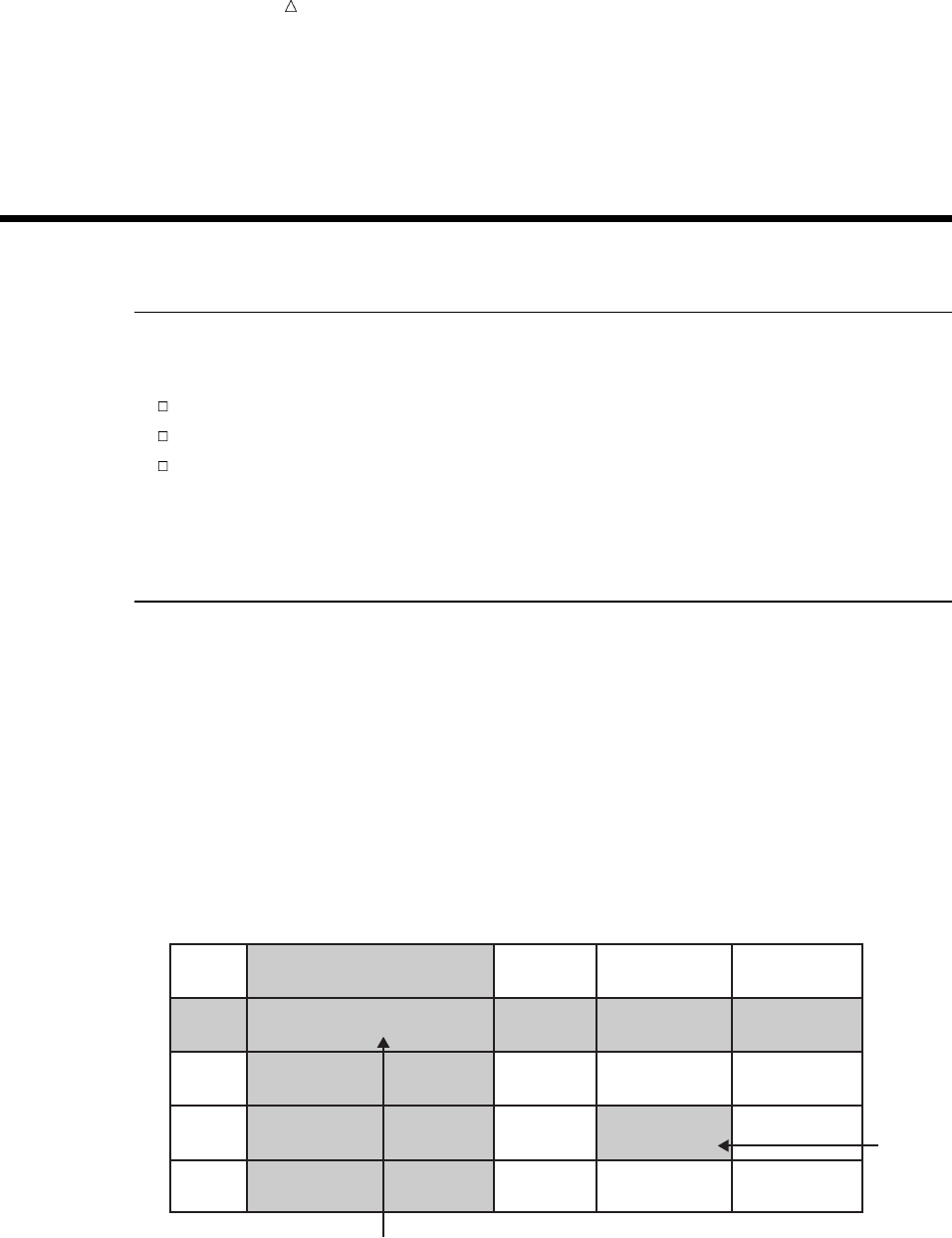
SAS organizes data into a rectangular form or table that is called a SAS data set.
The following figure shows a SAS data set. The data describes participants in a
16-week weight program at a health and fitness club. The data for each participant
includes an identification number, name, team name, and weight (in U.S. pounds) at
the beginning and end of the program.
Figure 1.1 Rectangular Form of a SAS Data Set
IdNumber
1023
1049
1219
1246
1078
1
2
3
4
5
StartWeightTeamName
variable
data value
EndWeight
David Shaw
Amelia Serrano
Alan Nance
Ravi Sinha
Ashley McKnight
red
yellow
red
yellow
red
189
145
210
194
127
165
124
192
177
118
data value
observation
In a SAS data set, each row represents information about an individual entity and is
called an observation. Each column represents the same type of information and is
called a variable. Each separate piece of information is a data value. In a SAS data set,

What Is the SAS System? Programming Language 5
an observation contains all the data values for an entity; a variable contains the same
type of data value for all entities.
To build a SAS data set with Base SAS, you write a program that uses statements in
the SAS programming language. A SAS program that begins with a DATA statement
and typically creates a SAS data set or a report is called a DATA step.
The following SAS program creates a SAS data set named WEIGHT_CLUB from the
health club data:
data weight_club; u
input IdNumber 1-4 Name $ 6-24 Team $ StartWeight EndWeight; v
Loss=StartWeight-EndWeight; w
datalines; x
1023 David Shaw red 189 165 y
1049 Amelia Serrano yellow 145 124 y
1219 Alan Nance red 210 192 y
1246 Ravi Sinha yellow 194 177 y
1078 Ashley McKnight red 127 118 y
;U
run;
The following list corresponds to the numbered items in the preceding program:
uThe DATA statement tells SAS to begin building a SAS data set named
WEIGHT_CLUB.
vThe INPUT statement identifies the fields to be read from the input data and
names the SAS variables to be created from them (IdNumber, Name, Team,
StartWeight, and EndWeight).
wThe third statement is an assignment statement. It calculates the weight each
person lost and assigns the result to a new variable, Loss.
xThe DATALINES statement indicates that data lines follow.
yThe data lines follow the DATALINES statement. This approach to processing
raw data is useful when you have only a few lines of data. (Later sections show
ways to access larger amounts of data that are stored in files.)
UThe semicolon signals the end of the raw data, and is a step boundary. It tells
SAS that the preceding statements are ready for execution.
Note: By default, the data set WEIGHT_CLUB is temporary; that is, it exists only
for the current job or session. For information about how to create a permanent SAS
data set, see Chapter 2, “Introduction to DATA Step Processing,” on page 19.
Programming Language
Elements of the SAS Language
The statements that created the data set WEIGHT_CLUB are part of the SAS
programming language. The SAS language contains statements, expressions, functions
and CALL routines, options, formats, and informats – elements that many
programming languages share. However, the way you use the elements of the SAS
language depends on certain programming rules. The most important rules are listed in
the next two sections.

6 Data Analysis and Reporting Utilities Chapter 1
Rules for SAS Statements
The conventions that are shown in the programs in this documentation, such as
indenting of subordinate statements, extra spacing, and blank lines, are for the purpose
of clarity and ease of use. They are not required by SAS. There are only a few rules for
writing SAS statements:
SAS statements end with a semicolon.
You can enter SAS statements in lowercase, uppercase, or a mixture of the two.
You can begin SAS statements in any column of a line and write several
statements on the same line.
You can begin a statement on one line and continue it on another line, but you
cannot split a word between two lines.
Words in SAS statements are separated by blanks or by special characters (such
as the equal sign and the minus sign in the calculation of the Loss variable in the
WEIGHT_CLUB example).
Rules for Most SAS Names
SAS names are used for SAS data set names, variable names, and other items. The
following rules apply:
A SAS name can contain from one to 32 characters.
The first character must be a letter or an underscore (_).
Subsequent characters must be letters, numbers, or underscores.
Blanks cannot appear in SAS names.
Special Rules for Variable Names
For variable names only, SAS remembers the combination of uppercase and
lowercase letters that you use when you create the variable name. Internally, the case
of letters does not matter. “CAT,” “cat,” and “Cat” all represent the same variable. But
for presentation purposes, SAS remembers the initial case of each letter and uses it to
represent the variable name when printing it.
Data Analysis and Reporting Utilities
The SAS programming language is both powerful and flexible. You can program any
number of analyses and reports with it. SAS can also simplify programming for you
with its library of built-in programs known as SAS procedures. SAS procedures use
data values from SAS data sets to produce preprogrammed reports, requiring minimal
effort from you.
For example, the following SAS program produces a report that displays the values
of the variables in the SAS data set WEIGHT_CLUB. Weight values are presented in
U.S. pounds.
options linesize=80 pagesize=60 pageno=1 nodate;
proc print data=weight_club;
title ’Health Club Data’;
run;
This procedure, known as the PRINT procedure, displays the variables in a simple,
organized form. The following output shows the results:

What Is the SAS System? Data Analysis and Reporting Utilities 7
Output 1.1 Displaying the Values in a SAS Data Set
Health Club Data 1
Id Start End
Obs Number Name Team Weight Weight Loss
1 1023 David Shaw red 189 165 24
2 1049 Amelia Serrano yellow 145 124 21
3 1219 Alan Nance red 210 192 18
4 1246 Ravi Sinha yellow 194 177 17
5 1078 Ashley McKnight red 127 118 9
To produce a table showing mean starting weight, ending weight, and weight loss for
each team, use the TABULATE procedure.
options linesize=80 pagesize=60 pageno=1 nodate;
proc tabulate data=weight_club;
class team;
var StartWeight EndWeight Loss;
table team, mean*(StartWeight EndWeight Loss);
title ’Mean Starting Weight, Ending Weight,’;
title2 ’and Weight Loss’;
run;
The following output shows the results:
Output 1.2 Table of Mean Values for Each Team
Mean Starting Weight, Ending Weight, 1
and Weight Loss
-----------------------------------------------------------
| | Mean |
| |--------------------------------------|
| |StartWeight | EndWeight | Loss |
|------------------+------------+------------+------------|
|Team | | | |
|------------------| | | |
|red | 175.33| 158.33| 17.00|
|------------------+------------+------------+------------|
|yellow | 169.50| 150.50| 19.00|
-----------------------------------------------------------
A portion of a SAS program that begins with a PROC (procedure) statement and ends
with a RUN statement (or is ended by another PROC or DATA statement) is called a
PROC step. Both of the PROC steps that create the previous two outputs comprise the
following elements:
a PROC statement, which includes the word PROC, the name of the procedure you
want to use, and the name of the SAS data set that contains the values. (If you
omit the DATA= option and data set name, the procedure uses the SAS data set
that was most recently created in the program.)
additional statements that give SAS more information about what you want to do,
for example, the CLASS, VAR, TABLE, and TITLE statements.

8 Output Produced by the SAS System Chapter 1
a RUN statement, which indicates that the preceding group of statements is ready
to be executed.
Output Produced by the SAS System
Traditional Output
A SAS program can produce some or all of the following kinds of output:
a SAS data set
contains data values that are stored as a table of observations and variables. It
also stores descriptive information about the data set, such as the names and
arrangement of variables, the number of observations, and the creation date of the
data set. A SAS data set can be temporary or permanent. The examples in this
section create the temporary data set WEIGHT_CLUB.
the SAS log
is a record of the SAS statements that you entered and of messages from SAS
about the execution of your program. It can appear as a file on disk, a display on
your monitor, or a hardcopy listing. The exact appearance of the SAS log varies
according to your operating environment and your site. The output in Output 1.3
shows a typical SAS log for the program in this section.
a report or simple listing
ranges from a simple listing of data values to a subset of a large data set or a
complex summary report that groups and summarizes data and displays statistics.
The appearance of procedure output varies according to your site and the options
that you specify in the program, but the output in Output 1.1 and Output 1.2
illustrate typical procedure output. You can also use a DATA step to produce a
completely customized report (see “Creating Customized Reports” on page 391).
other SAS files such as catalogs
contain information that cannot be represented as tables of data values. Examples
of items that can be stored in SAS catalogs include function key settings, letters
that are produced by SAS/FSP software, and displays that are produced by
SAS/GRAPH software.
external files or entries in other databases
can be created and updated by SAS programs. SAS/ACCESS software enables you
to create and update files that are stored in databases such as Oracle.

What Is the SAS System? Output from the Output Delivery System (ODS) 9
Output 1.3 Traditional Output: A SAS Log
NOTE: PROCEDURE PRINTTO used:
real time 0.02 seconds
cpu time 0.01 seconds
22
23 options pagesize=60 linesize=80 pageno=1 nodate;
24
25 data weight_club;
26 input IdNumber 1-4 Name $ 6-24 Team $ StartWeight EndWeight;
27 Loss=StartWeight-EndWeight;
28 datalines;
NOTE: The data set WORK.WEIGHT_CLUB has 5 observations and 6 variables.
NOTE: DATA statement used:
real time 0.14 seconds
cpu time 0.07 seconds
34 ;
35
36
37 proc tabulate data=weight_club;
38 class team;
39 var StartWeight EndWeight Loss;
40 table team, mean*(StartWeight EndWeight Loss);
41 title ’Mean Starting Weight, Ending Weight,’;
42 title2 ’and Weight Loss’;
43 run;
NOTE: There were 5 observations read from the data set WORK.WEIGHT_CLUB.
NOTE: PROCEDURE TABULATE used:
real time 0.18 seconds
cpu time 0.09 seconds
44 proc printto; run;
Output from the Output Delivery System (ODS)
The Output Delivery System (ODS) enables you to produce output in a variety of
formats, such as
an HTML file
a traditional SAS Listing (monospace)
a PostScript file
an RTF file (for use with Microsoft Word)
an output data set
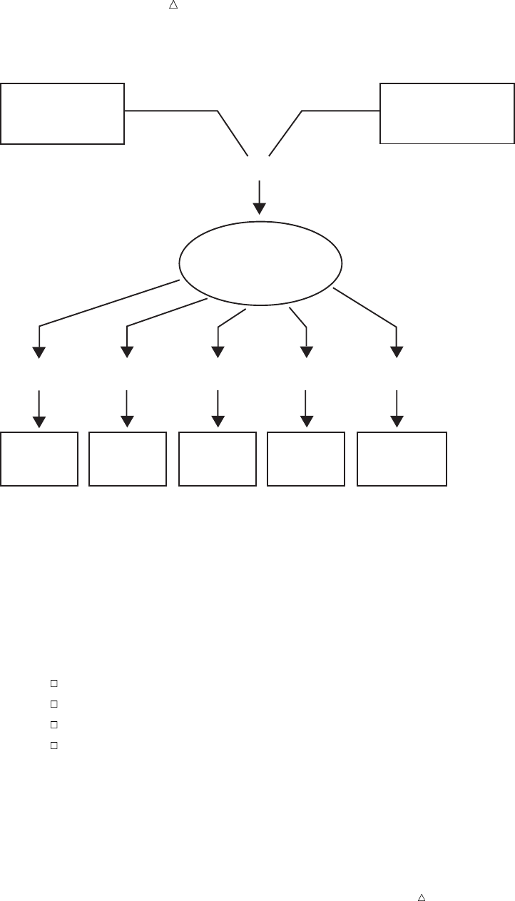
The following figure illustrates the concept of output for SAS Version 8.
10 Output from the Output Delivery System (ODS) Chapter 1
Figure 1.2 Model of the Production of ODS Output
Data Table Definition
(formatting instructions)
Output
Object
RTF
Output
SAS
Data
Sets
Listing
Output
HTML
Output
High-resolution
Printer
Output
ODS
Output
}
+
RTF
Destination
Output
Destination
Listing
Destination
HTML
Destination
Printer
Destination
ODS
Destination
}
The following definitions describe the terms in the preceding figure:
data
Each procedure that supports ODS and each DATA step produces data, which
contains the results (numbers and characters) of the step in a form similar to a
SAS data set.
table definition
The table definition is a set of instructions that describes how to format the data.
This description includes but is not limited to
the order of the columns
text and order of column headings
formats for data
font sizes and font faces
output object
ODS combines formatting instructions with the data to produce an output object.
The output object, therefore, contains both the results of the procedure or DATA
step and information about how to format the results. An output object has a
name, a label, and a path.
Note: Although many output objects include formatting instructions, not all do.
In some cases the output object consists of only the data.
ODS destinations
An ODS destination specifies a specific type of output. ODS supports a number of
destinations, which include the following:
RTF

What Is the SAS System? SAS Windowing Environment 11
produces output that is formatted for use with Microsoft Word.
Output
produces a SAS data set.
Listing
produces traditional SAS output (monospace format).
HTML
produces output that is formatted in Hyper Text Markup Language (HTML).
You can access the output on the web with your web browser.
Printer
produces output that is formatted for a high-resolution printer. An example
of this type of output is a PostScript file.
ODS output
ODS output consists of formatted output from any of the ODS destinations.
For more information about ODS output, see Chapter 23, “Directing SAS Output and
the SAS Log,” on page 349 and Chapter 32, “Understanding and Customizing SAS
Output: The Output Delivery System (ODS),” on page 565.
For complete information about ODS, see SAS Output Delivery System: User’s Guide.
Ways to Run SAS Programs
Selecting an Approach
There are several ways to run SAS programs. They differ in the speed with which
they run, the amount of computer resources that are required, and the amount of
interaction that you have with the program (that is, the kinds of changes you can make
while the program is running).
The examples in this documentation produce the same results, regardless of the way
you run the programs. However, in a few cases, the way that you run a program
determines the appearance of output. The following sections briefly introduce different
ways to run SAS programs.
SAS Windowing Environment
The SAS windowing environment enables you to interact with SAS directly through a
series of windows. You can use these windows to perform common tasks, such as
locating and organizing files, entering and editing programs, reviewing log information,
viewing procedure output, setting options, and more. If needed, you can issue operating
system commands from within this environment. Or, you can suspend the current SAS
windowing environment session, enter operating system commands, and then resume
the SAS windowing environment session at a later time.
Using the SAS windowing environment is a quick and convenient way to program in
SAS. It is especially useful for learning SAS and developing programs on small test
files. Although it uses more computer resources than other techniques, using the SAS
windowing environment can save a lot of program development time.
For more information about the SAS windowing environment, see Chapter 39, “Using
the SAS Windowing Environment,” on page 655.

12 SAS/ASSIST Software Chapter 1
SAS/ASSIST Software
One important feature of SAS is the availability of SAS/ASSIST software.
SAS/ASSIST provides a point-and-click interface that enables you to select the tasks
that you want to perform. SAS then submits the SAS statements to accomplish those
tasks. You do not need to know how to program in the SAS language in order to use
SAS/ASSIST.
SAS/ASSIST works by submitting SAS statements just like the ones shown earlier in
this section. In that way, it provides a number of features, but it does not represent the
total functionality of SAS software. If you want to perform tasks other than those that
are available in SAS/ASSIST, you need to learn to program in SAS as described in this
documentation.
Noninteractive Mode
In noninteractive mode, you prepare a file that contains SAS statements and any
system statements that are required by your operating environment, and submit the
program. The program runs immediately and occupies your current workstation
session. You cannot continue to work in that session while the program is running,*
and you usually cannot interact with the program.** The log and procedure output go
to prespecified destinations, and you usually do not see them until the program ends.
To modify the program or correct errors, you must edit and resubmit the program.
Noninteractive execution may be faster than batch execution because the computer
system runs the program immediately rather than waiting to schedule your program
among other programs.
Batch Mode
To run a program in batch mode, you prepare a file that contains SAS statements
and any system statements that are required by your operating environment, and then
you submit the program.
You can then work on another task at your workstation. While you are working, the
operating environment schedules your job for execution (along with jobs submitted by
other people) and runs it. When execution is complete, you can look at the log and the
procedure output.
The central feature of batch execution is that it is completely separate from other
activities at your workstation. You do not see the program while it is running, and you
cannot correct errors at the time they occur. The log and procedure output go to
prespecified destinations; you can look at them only after the program has finished
running. To modify the SAS program, you edit the program with the editor that is
supported by your operating environment and submit a new batch job.
When sites charge for computer resources, batch processing is a relatively
inexpensive way to execute programs. It is particularly useful for large programs or
when you need to use your workstation for other tasks while the program is executing.
However, for learning SAS or developing and testing new programs, using batch mode
might not be efficient.
*In a workstation environment, you can switch to another window and continue working.
** Limited ways of interaction are available. You can, for example, use the asterisk (*) option in a %INCLUDE statement in
your program.
What Is the SAS System? Running Programs in the SAS Windowing Environment 13
Interactive Line Mode
In an interactive line-mode session, you enter one line of a SAS program at a time,
and SAS executes each DATA or PROC step automatically as soon as it recognizes the
end of the step. You usually see procedure output immediately on your display monitor.
Depending on your site’s computer system and on your workstation, you may be able to
scroll backward and forward to see different parts of your log and procedure output, or
you may lose them when they scroll off the top of your screen. There are limited
facilities for modifying programs and correcting errors.
Interactive line-mode sessions use fewer computer resources than a windowing
environment. If you use line mode, you should familiarize yourself with the
%INCLUDE, %LIST, and RUN statements in SAS Language Reference: Dictionary.
Running Programs in the SAS Windowing Environment
You can run most programs in this documentation by using any of the methods that
are described in the previous sections. This documentation uses the SAS windowing
environment (as it appears on Windows and UNIX operating environments) when it is
necessary to show programming within a SAS session. The SAS windowing
environment appears differently depending on the operating environment that you use.
For more information about the SAS windowing environment, see Chapter 39, “Using
the SAS Windowing Environment,” on page 655.
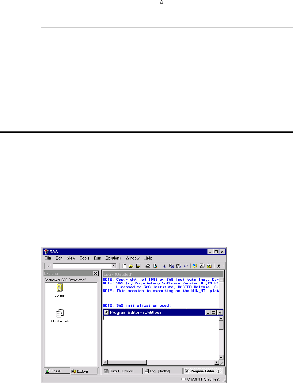
The following example gives a brief overview of a SAS session that uses the SAS
windowing environment. When you invoke SAS, the following windows appear.
Display 1.1 SAS Windowing Environment
The specific window placement, display colors, messages, and some other details vary
according to your site, your monitor, and your operating environment. The window on
the left side of the display is the SAS Explorer window, which you can use to assign and
locate SAS libraries, files, and other items. The window at the top right is the Log
14 Running Programs in the SAS Windowing Environment Chapter 1
window; it contains the SAS log for the session. The window at the bottom right is the
Program Editor window. This window provides an editor in which you edit your SAS
programs.
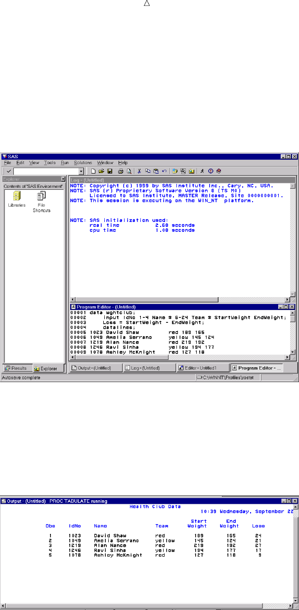
To create the program for the health and fitness club, type the statements in the
Program Editor window. You can turn line numbers on or off to facilitate program
creation. The following display shows the beginning of the program.
Display 1.2 Editing a Program in the Program Editor Window
When you fill the Program Editor window, scroll down to continue typing the
program. When you finish editing the program, submit it to SAS and view the output.
(If SAS does not create output, check the SAS log for error messages.)
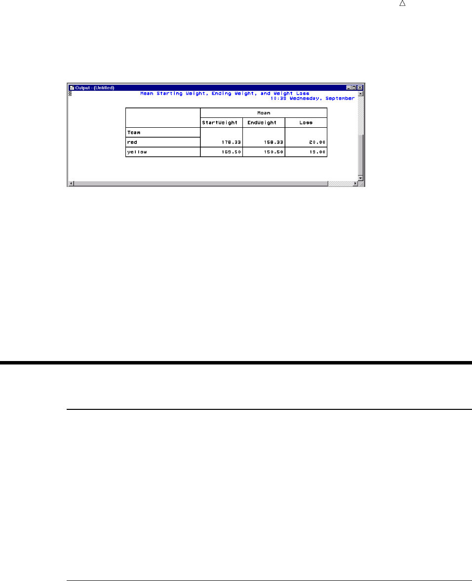
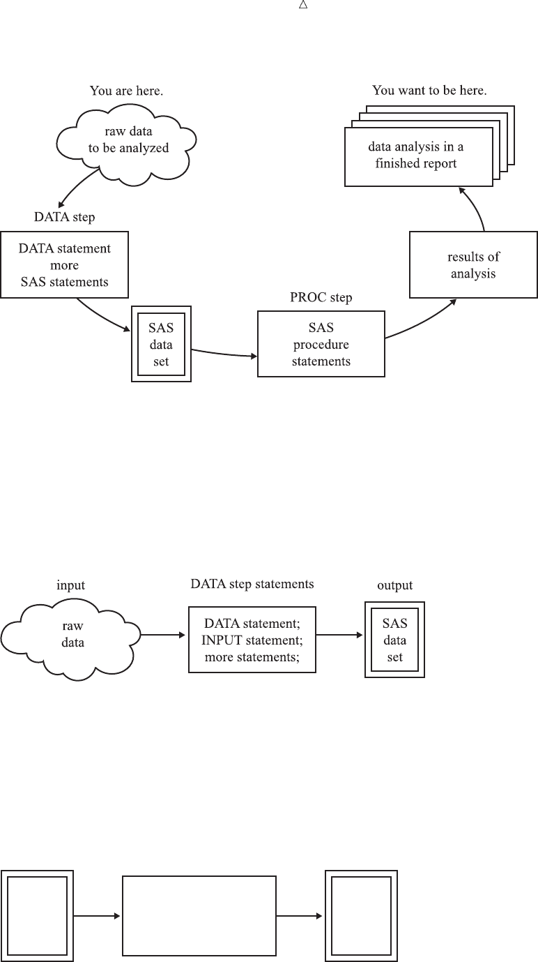
The following displays show the first and second pages of the Output window.
Display 1.3 The First Page of Output in the Output Window
What Is the SAS System? Procedures 15
Display 1.4 The Second Page of Output in the Output Window
After you finish viewing the output, you can return to the Program Editor window to
begin creating a new program.
By default, the output from all submissions remains in the Output window, and all
statements that you submit remain in memory until the end of your session. You can
view the output at any time, and you can recall previously submitted statements for
editing and resubmitting. You can also clear a window of its contents.
All the commands that you use to move through the SAS windowing environment can
be executed as words or as function keys. You can also customize the SAS windowing
environment by determining which windows appear, as well as by assigning commands
to function keys. For more information about customizing the SAS windowing
environment, see Chapter 40, “Customizing the SAS Environment,” on page 693.
Review of SAS Tools
Statements
DATA SAS-data-set;
begins a DATA step and tells SAS to begin creating a SAS data set. SAS-data-set
names the data set that is being created.
%INCLUDE source(s) </<SOURCE2> <S2=length><host-options>>;
brings SAS programming statements, data lines, or both into a current SAS
program.
RUN;
tells SAS to begin executing the preceding group of SAS statements.
For more information, see Statements in SAS Language Reference: Dictionary.
Procedures
PROC procedure <DATA=SAS-data-set>;
begins a PROC step and tells SAS to invoke a particular SAS procedure to process
the SAS data set that is specified in the DATA= option. If you omit the DATA=
option, then the procedure processes the most recently created SAS data set in the
program.

16 Learning More Chapter 1
For more information about using procedures, see the Base SAS Procedures Guide.
Learning More
Basic SAS usage
For an entry-level introduction to basic SAS programming language, see The Little
SAS Book: A Primer, Second Edition.
DATA step
For more information about how to create SAS data sets, see Chapter 2,
“Introduction to DATA Step Processing,” on page 19.
DATA step processing
For more information about DATA step processing, see Chapter 6, “Understanding
DATA Step Processing,” on page 97.
For information about how to easily use the SAS environment, see Getting Started
with the SAS System.

17
PART
2
Getting Your Data into Shape
Chapter 2..........
Introduction to DATA Step Processing 19
Chapter 3..........
Starting with Raw Data: The Basics 43
Chapter 4..........
Starting with Raw Data: Beyond the Basics 61
Chapter 5..........
Starting with SAS Data Sets 81
18

19
CHAPTER
2
Introduction to DATA Step
Processing
Introduction to DATA Step Processing 20
Purpose 20
Prerequisites 20
The SAS Data Set: Your Key to the SAS System 20
Understanding the Function of the SAS Data Set 20
Understanding the Structure of the SAS Data Set 22
Temporary versus Permanent SAS Data Sets 24
Creating and Using Temporary SAS Data Sets 24
Creating and Using Permanent SAS Data Sets 24
Conventions That Are Used in This Documentation 25
How the DATA Step Works: A Basic Introduction 26
Overview of the DATA Step 26
During the Compile Phase 28
During the Execution Phase 28
Example of a DATA Step 29
The DATA Step 29
The Statements 29
The Process 30
Supplying Information to Create a SAS Data Set 33
Overview of Creating a SAS Data Set 33
Telling SAS How to Read the Data: Styles of Input 34
Reading Dates with Two-Digit and Four-Digit Year Values 35
Defining Variables in SAS 35
Indicating the Location of Your Data 36
Data Locations 36
Raw Data in the Job Stream 37
Data in an External File 37
Data in a SAS Data Set 37
Data in a DBMS File 38
Using External Files in Your SAS Job 38
Identifying an External File Directly 38
Referencing an External File with a Fileref 39
Review of SAS Tools 41
Statements 41
Learning More 41

20 Introduction to DATA Step Processing Chapter 2
Introduction to DATA Step Processing
Purpose
The DATA step is one of the basic building blocks of SAS programming. It creates
the data sets that are used in a SAS program’s analysis and reporting procedures.
Understanding the basic structure, functioning, and components of the DATA step is
fundamental to learning how to create your own SAS data sets. In this section, you will
learn the following:
what a SAS data set is and why it is needed
how the DATA step works
what information you have to supply to SAS so that it can construct a SAS data
set for you
Prerequisites
You should understand the concepts introduced in Chapter 1, “What Is the SAS
System?,” on page 3 before continuing.
The SAS Data Set: Your Key to the SAS System
Understanding the Function of the SAS Data Set
SAS enables you to solve problems by providing methods to analyze or to process
your data in some way. You need to first get the data into a form that SAS can
recognize and process. After the data is in that form, you can analyze it and generate
reports. The following figure shows this process in the simplest case.
Introduction to DATA Step Processing Understanding the Function of the SAS Data Set 21
Figure 2.1 From Raw Data to Final Analysis
You begin with raw data, that is, a collection of data that has not yet been processed
by SAS. You use a set of statements known as a DATA step to get your data into a SAS
data set. Then you can further process your data with additional DATA step
programming or with SAS procedures.
In its simplest form, the DATA step can be represented by the three components that
are shown in the following figure.
Figure 2.2 From Raw Data to a SAS Data Set
SAS processes input in the form of raw data and creates a SAS data set.
When you have a SAS data set, you can use it as input to other DATA steps. The
following figure shows the SAS statements that you can use to create a new SAS data
set.
Figure 2.3 Using One SAS Data Set to Create Another
input output
DATA step statements
DATA statement;
SET, MERGE,
MODIFY, or UPDATE;
more statements;
existing
SAS
data set
new
SAS
data
set
22 Understanding the Structure of the SAS Data Set Chapter 2
Understanding the Structure of the SAS Data Set
Think of a SAS data set as a rectangular structure that identifies and stores data.
When your data is in a SAS data set, you can use additional DATA steps for further
processing, or perform many types of analyses with SAS procedures.
The rectangular structure of a SAS data set consists of rows and columns in which
data values are stored. The rows in a SAS data set are called observations, and the
columns are called variables. In a raw data file, the rows are called records and the
columns are called fields. Variables contain the data values for all of the items in an
observation.
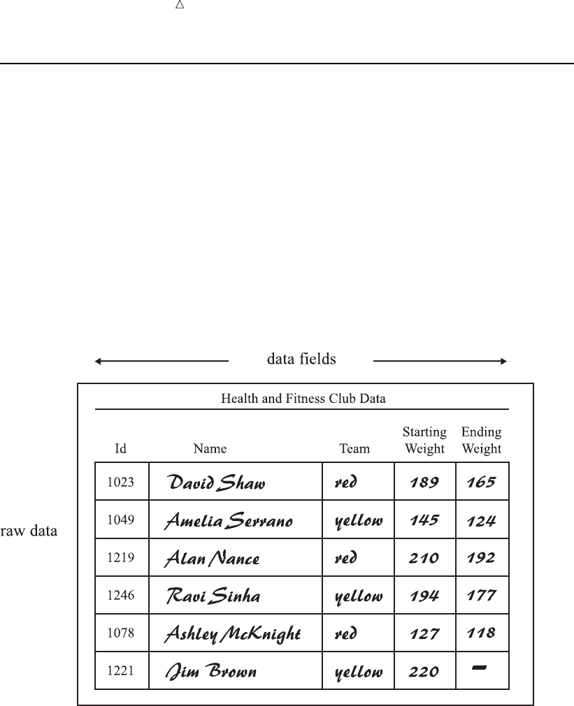
For example, the following figure shows a collection of raw data about participants in
a health and fitness club. Each record contains information about one participant.
Figure 2.4 Raw Data from the Health and Fitness Club
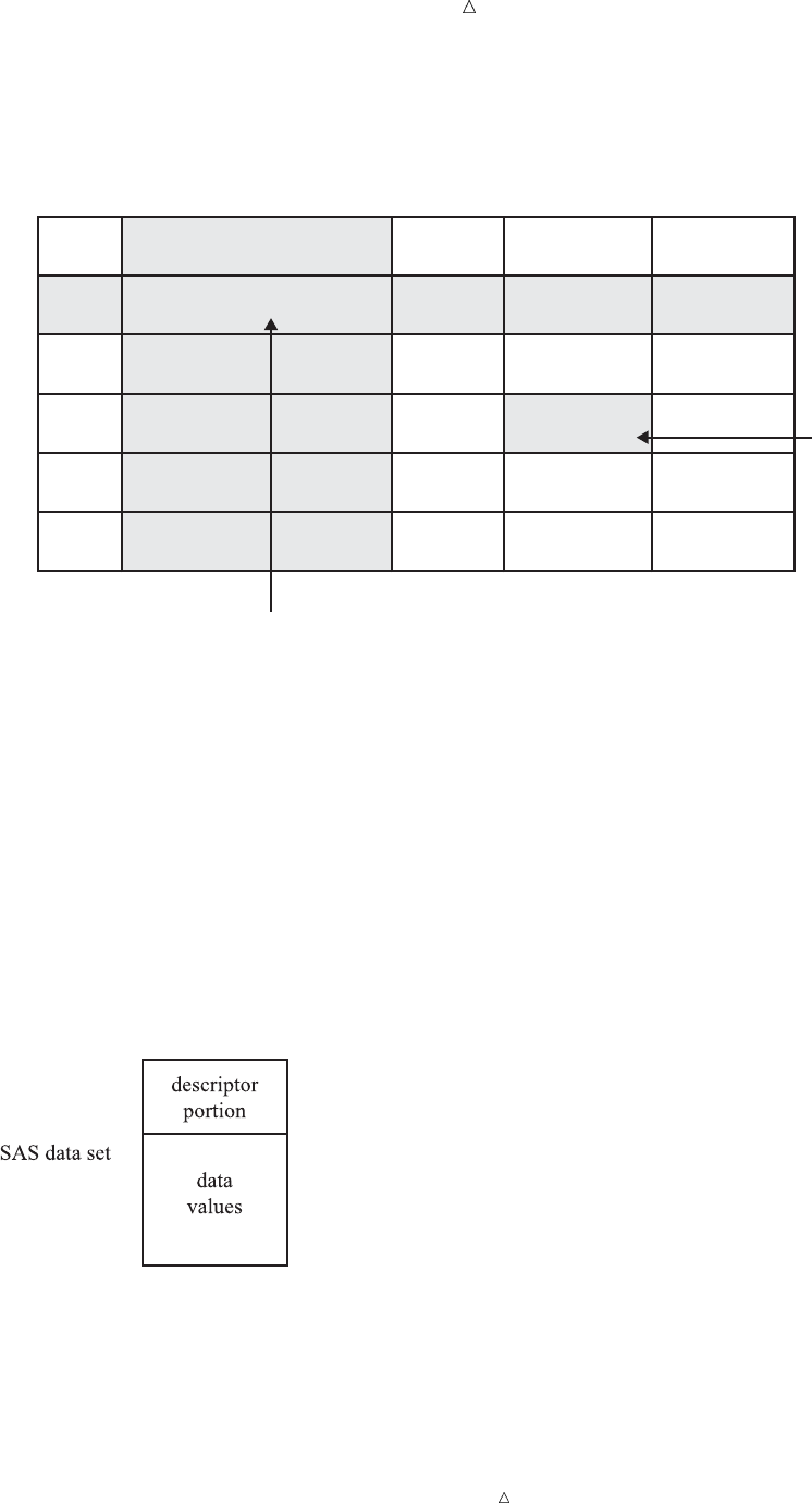
The following figure shows how easily the health club records can be translated into
parts of a SAS data set. Each record becomes an observation. In this case, each
observation represents a participant in the program. Each field in the record becomes a
variable. The variables represent each participant’s identification number, name, team
name, and weight at the beginning and end of a 16-week program.
Introduction to DATA Step Processing Understanding the Structure of the SAS Data Set 23
Figure 2.5 How Data Fits into a SAS Data Set
IdNumber
1023
1049
1219
1246
1078
1221
1
2
3
4
5
6
StartWeightTeamName
variable
data value
EndWeight
David Shaw
Amelia Serrano
Alan Nance
Ravi Sinha
Ashley McKnight
Jim Brown
red
yellow
red
yellow
red
yellow
189
145
210
194
127
220
165
124
192
177
118
.
data value
observation
missing value
In a SAS data set, every variable exists for every observation. What if you do not
have all the data for each observation? If the raw data is incomplete because a value for
the numeric variable EndWeight was not recorded for one observation, then this missing
value is represented by a period that serves as a placeholder, as shown in observation 6
in the previous figure. (Missing values for character variables are represented by
blanks. Character and numeric variables are discussed later in this section.) By coding
a value as missing, you can add an observation to the data set for which the data is
incomplete and still retain the rectangular shape necessary for a SAS data set.
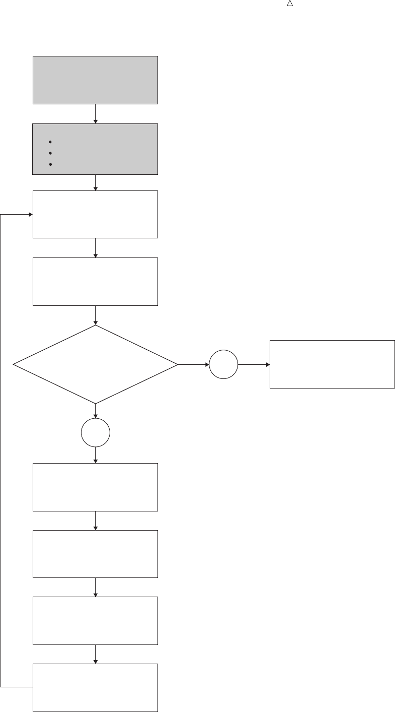
Along with data values, each SAS data set contains a descriptor portion, as
illustrated in the following figure:
Figure 2.6 Parts of a SAS Data Set
The descriptor portion consists of details that SAS records about a data set, such as
the names and attributes of all the variables, the number of observations in the data
set, and the date and time that the data set was created and updated.
Operating Environment Information: Depending on your operating environment and
the engine used to write the SAS data set, SAS may store additional information about
a SAS data set in its descriptor portion. For more information, refer to the SAS
documentation for your operating environment.

24 Temporary versus Permanent SAS Data Sets Chapter 2
Temporary versus Permanent SAS Data Sets
Creating and Using Temporary SAS Data Sets
When you use a DATA step to create a SAS data set with a one-level name, you
normally create a temporary SAS data set, one that exists only for the duration of your
current session. SAS places this data set in a SAS data library referred to as WORK.
In most operating environments, all files that SAS stores in the WORK library are
deleted at the end of a session.
The following is an example of a DATA step that creates the temporary data set
WEIGHT_CLUB.
data weight_club;
input IdNumber Name $ 6--20 Team $ 22--27 StartWeight EndWeight;
datalines;
1023 David Shaw red 189 165
1049 Amelia Serrano yellow 145 124
1219 Alan Nance red 210 192
1246 Ravi Sinha yellow 194 177
1078 Ashley McKnight red 127 118
1221 Jim Brown yellow 220 .
;
run;
The preceding program code refers to the temporary data set as WEIGHT_CLUB.
SAS. However, it assigns the first-level name WORK to all temporary data sets, and
refers to the WEIGHT_CLUB data set with its two-level name, WORK.WEIGHT_CLUB.
The following output from the SAS log shows the name of the temporary data set.
Output 2.1 SAS Log: The WORK.WEIGHT_CLUB Temporary Data Set
162 data weight_club;
163 input IdNumber Name $ 6-20 Team $ 22-27 StartWeight EndWeight;
164 datalines;
NOTE: The data set WORK.WEIGHT_CLUB has 6 observations and 5 variables.
Because SAS assigns the first-level name WORK to all SAS data sets that have only
a one-level name, you do not need to use WORK. You can refer to these temporary data
sets with a one-level name, such as WEIGHT_CLUB.
To reference this SAS data set in a later DATA step or in a PROC step, you can use a
one-level name:
proc print data = weight_club;
run;
Creating and Using Permanent SAS Data Sets
To create a permanent SAS data set, you must indicate a SAS data library other than
WORK. (WORK is a reserved libref that SAS automatically assigns to a temporary SAS
data library.) Use a LIBNAME statement to assign a libref to a SAS data library on

Introduction to DATA Step Processing Temporary versus Permanent SAS Data Sets 25
your operating environment’s file system. The libref functions as a shorthand way of
referring to a SAS data library. Here is the form of the LIBNAME statement:
LIBNAME libref ’your-data-library’;
where
libref
is a shortcut name to where your SAS files are stored. libref must be a valid SAS
name. It must begin with a letter or an underscore, and it can contain uppercase
and lowercase letters, numbers, or underscores. A libref has a maximum length of
8 characters.
’your-data-library’
must be the physical name for your SAS data library. The physical name is the
name that is recognized by the operating environment.
Operating Environment Information: Additional restrictions can apply to librefs and
physical file names under some operating environments. For more information, refer to
the SAS documentation for your operating environment.
The following is an example of the LIBNAME statement that is used with a DATA
step:
libname saveit ’your-data-library’; u
data saveit.weight_club; v
...more SAS statements...
;
proc print data = saveit.weight_club; w
run;
The following list corresponds to the numbered items:
uThe LIBNAME statement associates the libref SAVEIT with your-data-library,
where your-data-library is your operating environment’s name for a SAS data
library.
vTo create a new permanent SAS data set and store it in this SAS data library, you
must use the two-level name SAVEIT.WEIGHT_CLUB in the DATA statement.
wTo reference this SAS data set in a later DATA step or in a PROC step, you must
use the two-level name SAVEIT.WEIGHT_CLUB in the PROC step.
For more information, see Chapter 33, “Understanding SAS Data Libraries,” on page
595.
Conventions That Are Used in This Documentation
Data sets that are used in examples are usually shown as temporary data sets
specified with a one-level name:
data fitness;
In rare cases in this documentation, data sets are created as permanent SAS data
sets. These data sets are specified with a two-level name, and a LIBNAME statement
precedes each DATA step in which a permanent SAS data set is created:
libname saveit ’your-data-library’;
data saveit.weight_club;

26 How the DATA Step Works: A Basic Introduction Chapter 2
How the DATA Step Works: A Basic Introduction
Overview of the DATA Step
The DATA step consists of a group of SAS statements that begins with a DATA
statement. The DATA statement begins the process of building a SAS data set and
names the data set. The statements that make up the DATA step are compiled, and the
syntax is checked. If the syntax is correct, then the statements are executed. In its
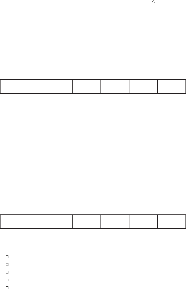
simplest form, the DATA step is a loop with an automatic output and return action.
The following figure illustrates the flow of action in a typical DATA step.
Introduction to DATA Step Processing Overview of the DATA Step 27
Figure 2.7 Flow of Action in a Typical DATA Step
data-reading
statement:
is there a
record to read?
reads
an input record
executes additional
executable statements
writesan observation to
the SAS data set
returns
to the beginning of
the DATA step
compiles
SAS statements
(includes syntax checking)
creates
an input buffer
a program data vector
descriptor information
begins
with a DATA statement
(counts iterations)
sets variable values
to missing in the
program data vector
closes data set;
goes on to the next
DATA or PROC step
NO
YES
Compile Phase
Execution Phase

28 During the Compile Phase Chapter 2
During the Compile Phase
When you submit a DATA step for execution, SAS checks the syntax of the SAS
statements and compiles them, that is, automatically translates the statements into
machine code. SAS further processes the code, and creates the following three items:
input buffer is a logical area in memory into which SAS reads each record of data
from a raw data file when the program executes. (When SAS reads
from a SAS data set, however, the data is written directly to the
program data vector.)
program data
vector
is a logical area of memory where SAS builds a data set, one
observation at a time. When a program executes, SAS reads data
values from the input buffer or creates them by executing SAS
language statements. SAS assigns the values to the appropriate
variables in the program data vector. From here, SAS writes the
values to a SAS data set as a single observation.
The program data vector also contains two automatic variables,
_N_ and _ERROR_. The _N_ variable counts the number of times
the DATA step begins to iterate. The _ERROR_ variable signals the
occurrence of an error caused by the data during execution. These
automatic variables are not written to the output data set.
descriptor
information
is information about each SAS data set, including data set attributes
and variable attributes. SAS creates and maintains the descriptor
information.
During the Execution Phase
All executable statements in the DATA step are executed once for each iteration. If
your input file contains raw data, then SAS reads a record into the input buffer. SAS
then reads the values in the input buffer and assigns the values to the appropriate
variables in the program data vector. SAS also calculates values for variables created
by program statements, and writes these values to the program data vector. When the
program reaches the end of the DATA step, three actions occur by default that make
using the SAS language different from using most other programming languages:
1SAS writes the current observation from the program data vector to the data set.
2The program loops back to the top of the DATA step.
3Variables in the program data vector are reset to missing values.
Note: The following exceptions apply:
Variables that you specify in a RETAIN statement are not reset to missing
values.
The automatic variables _N_ and _ERROR_ are not reset to missing.
For information about the RETAIN statement, see “Using a Value in a Later
Observation” on page 196.
If there is another record to read, then the program executes again. SAS builds the
second observation, and continues until there are no more records to read. The data set
is then closed, and SAS goes on to the next DATA or PROC step.

Introduction to DATA Step Processing Example of a DATA Step 29
Example of a DATA Step
The DATA Step
The following simple DATA step produces a SAS data set from the data collected for
a health and fitness club. As discussed earlier, the input data contains each
participant’s identification number, name, team name, and weight at the beginning and
end of a 16-week weight program:
data weight_club; u
input IdNumber 1-4 Name $ 6-24 Team $ StartWeight EndWeight; v
Loss = StartWeight - EndWeight; w
datalines; x
1023 David Shaw red 189 165
1049 Amelia Serrano yellow 145 124
1219 Alan Nance red 210 192
1246 Ravi Sinha yellow 194 177
1078 Ashley McKnight red 127 118
1221 Jim Brown yellow 220 .
1095 Susan Stewart blue 135 127
1157 Rosa Gomez green 155 141
1331 Jason Schock blue 187 172
1067 Kanoko Nagasaka green 135 122
1251 Richard Rose blue 181 166
1333 Li-Hwa Lee green 141 129
1192 Charlene Armstrong yellow 152 139
1352 Bette Long green 156 137
1262 Yao Chen blue 196 180
1087 Kim Sikorski red 148 135
1124 Adrienne Fink green 156 142
1197 Lynne Overby red 138 125
1133 John VanMeter blue 180 167
1036 Becky Redding green 135 123
1057 Margie Vanhoy yellow 146 132
1328 Hisashi Ito red 155 142
1243 Deanna Hicks blue 134 122
1177 Holly Choate red 141 130
1259 Raoul Sanchez green 189 172
1017 Jennifer Brooks blue 138 127
1099 Asha Garg yellow 148 132
1329 Larry Goss yellow 188 174
;x
The Statements
The following list corresponds to the numbered items in the preceding program:
uThe DATA statement begins the DATA step and names the data set that is being
created.

30 Example of a DATA Step Chapter 2
vThe INPUT statement creates five variables, indicates how SAS reads the values
from the input buffer, and assigns the values to variables in the program data
vector.
wThe assignment statement creates an additional variable called Loss, calculates
the value of Loss during each iteration of the DATA step, and writes the value to
the program data vector.
xThe DATALINES statement marks the beginning of the input data. The single
semicolon marks the end of the input data and the DATA step.
Note: A DATA step that does not contain a DATALINES statement must end
with a RUN statement.
The Process
When you submit a DATA step for execution, SAS automatically compiles the DATA
step and then executes it. At compile time, SAS creates the input buffer, program data
vector, and descriptor information for the data set WEIGHT_CLUB. As the following
figure shows, the program data vector contains the variables that are named in the
INPUT statement, as well as the variable Loss. The values of the _N_ and the
_ERROR_ variables are automatically generated for every DATA step. The _N_
automatic variable represents the number of times that the DATA step has iterated.
The _ERROR_ automatic variable acts like a binary switch whose value is 0 if no errors
exist in the DATA step, or 1 if one or more errors exist. These automatic variables are
not written to the output data set.
All variable values, except _N_ and _ERROR_, are initially set to missing. Note that
missing numeric values are represented by a period, and missing character values are
represented by a blank.
Figure 2.8 Variable Values Initially Set to Missing
Input Buffer
Program Data Vector
IdNumber Name StartWeight EndWeight LossTeam
----+----1----+----2----+----3----+----4----+----5----+----6----+----7
....
The syntax is correct, so the DATA step executes. As the following figure illustrates,
the INPUT statement causes SAS to read the first record of raw data into the input
buffer. Then, according to the instructions in the INPUT statement, SAS reads the data
values in the input buffer and assigns them to variables in the program data vector.
Introduction to DATA Step Processing Example of a DATA Step 31
Figure 2.9 Values Assigned to Variables by the INPUT Statement
Input Buffer
Program Data Vector
IdNumber Name StartWeight EndWeight LossTeam
----+----1----+----2----+----3----+----4----+----5----+----6----+----7
1023 David Shaw red 189 165
1023 David Shaw red 189 165 .
When SAS assigns values to all variables that are listed in the INPUT statement,
SAS executes the next statement in the program:
Loss = StartWeight - EndWeight;
This assignment statement calculates the value for the variable Loss and writes that
value to the program data vector, as the following figure shows.
Figure 2.10 Value Computed and Assigned to the Variable Loss
Input Buffer
Program Data Vector
IdNumber Name StartWeight EndWeight LossTeam
----+----1----+----2----+----3----+----4----+----5----+----6----+----7
1023 David Shaw red 189 165
1023 David Shaw red 189 165 24
SAS has now reached the end of the DATA step, and the program automatically does
the following:
writes the first observation to the data set
loops back to the top of the DATA step to begin the next iteration
increments the _N_ automatic variable by 1
resets the _ERROR_ automatic variable to 0
except for _N_ and _ERROR_, sets variable values in the program data vector to
missing values, as the following figure shows
32 Example of a DATA Step Chapter 2
Figure 2.11 Values Set to Missing
Input Buffer
Program Data Vector
IdNumber Name StartWeight EndWeight LossTeam
----+----1----+----2----+----3----+----4----+----5----+----6----+----7
1023 David Shaw red 189 165
....
Execution continues. The INPUT statement looks for another record to read. If there
are no more records, then SAS closes the data set and the system goes on to the next
DATA or PROC step. In this example, however, more records exist and the INPUT
statement reads the second record into the input buffer, as the following figure shows.
Figure 2.12 Second Record Is Read into the Input Buffer
Input Buffer
Program Data Vector
IdNumber Name StartWeight EndWeight LossTeam
----+----1----+----2----+----3----+----4----+----5----+----6----+----7
1049 Amelia Serrano yellow 145 124
....
The following figure shows that SAS assigned values to the variables in the program
data vector and calculated the value for the variable Loss, building the second
observation just as it did the first one.
Figure 2.13 Results of Second Iteration of the DATA Step
Input Buffer
Program Data Vector
IdNumber Name StartWeight EndWeight LossTeam
----+----1----+----2----+----3----+----4----+----5----+----6----+----7
1049 Amelia Serrano yellow 145 124
1049 Amelia Serrano yellow 145 124 21
This entire process continues until SAS detects the end of the file. The DATA step
iterates as many times as there are records to read. Then SAS closes the data set
WEIGHT_CLUB, and SAS looks for the beginning of the next DATA or PROC step.

Introduction to DATA Step Processing Overview of Creating a SAS Data Set 33
Now that SAS has transformed the collected data from raw data into a SAS data set,
it can be processed by a SAS procedure. The following output, produced with the
PRINT procedure, shows the data set that has just been created.
proc print data=weight_club;
title ’Fitness Center Weight Club’;
run;
Output 2.2 PROC PRINT Output of the WEIGHT_CLUB Data Set
Fitness Center Weight Club 1
Id Start End
Obs Number Name Team Weight Weight Loss
1 1023 David Shaw red 189 165 24
2 1049 Amelia Serrano yellow 145 124 21
3 1219 Alan Nance red 210 192 18
4 1246 Ravi Sinha yellow 194 177 17
5 1078 Ashley McKnight red 127 118 9
6 1221 Jim Brown yellow 220 . .
7 1095 Susan Stewart blue 135 127 8
8 1157 Rosa Gomez green 155 141 14
9 1331 Jason Schock blue 187 172 15
10 1067 Kanoko Nagasaka green 135 122 13
11 1251 Richard Rose blue 181 166 15
12 1333 Li-Hwa Lee green 141 129 12
13 1192 Charlene Armstrong yellow 152 139 13
14 1352 Bette Long green 156 137 19
15 1262 Yao Chen blue 196 180 16
16 1087 Kim Sikorski red 148 135 13
17 1124 Adrienne Fink green 156 142 14
18 1197 Lynne Overby red 138 125 13
19 1133 John VanMeter blue 180 167 13
20 1036 Becky Redding green 135 123 12
21 1057 Margie Vanhoy yellow 146 132 14
22 1328 Hisashi Ito red 155 142 13
23 1243 Deanna Hicks blue 134 122 12
24 1177 Holly Choate red 141 130 11
25 1259 Raoul Sanchez green 189 172 17
26 1017 Jennifer Brooks blue 138 127 11
27 1099 Asha Garg yellow 148 132 16
28 1329 Larry Goss yellow 188 174 14
Supplying Information to Create a SAS Data Set
Overview of Creating a SAS Data Set
You supply SAS with specific information for reading raw data so that you can create
a SAS data set from the raw data. You can use the data set for further processing, data
analysis, or report writing. To process raw data in a DATA step, you must
use an INPUT statement to tell SAS how to read the data
define the variables and indicate whether they are character or numeric
specify the location of the raw data

34 Telling SAS How to Read the Data: Styles of Input Chapter 2
Telling SAS How to Read the Data: Styles of Input
SAS provides many tools for reading raw data into a SAS data set. These tools
include three basic input styles as well as various format modifiers and pointer controls.
List input is used when each field in the raw data is separated by at least one space
and does not contain embedded spaces. The INPUT statement simply contains a list of
the variable names. List input, however, places numerous restrictions on your data.
These restrictions are discussed in detail in Chapter 3, “Starting with Raw Data: The
Basics,” on page 43. The following example shows list input. Note that there is at least
one blank space between each data value.
data scores;
input Name $ Test_1 Test_2 Test_3;
datalines;
Bill 187 97 103
Carlos 156 76 74
Monique 99 102 129
;
Column input enables you to read the same data if it is located in fixed columns:
data scores;
input Name $ 1-7 Test_1 9-11 Test_2 13-15 Test_3 17-19;
datalines;
Bill 187 97 103
Carlos 156 76 74
Monique 99 102 129
;
Formatted input enables you to supply special instructions in the INPUT statement
for reading data. For example, to read numeric data that contains special symbols, you
need to supply SAS with special instructions so that it can read the data correctly.
These instructions, called informats, are discussed in more detail in Chapter 3,
“Starting with Raw Data: The Basics,” on page 43. In the INPUT statement, you can
specify an informat to be used to read a data value, as in the example that follows:
data total_sales;
input Date mmddyy10. +2 Amount comma5.;
datalines;
09/05/2000 1,382
10/19/2000 1,235
11/30/2000 2,391
;
In this example, the MMDDYY10. informat for the variable Date tells SAS to
interpret the raw data as a month, day, and year, ignoring the slashes. The COMMA5.
informat for the variable Amount tells SAS to interpret the raw data as a number,
ignoring the comma. The +2 is a pointer control that tells SAS where to look for the
next item. For more information about pointer controls, see Chapter 3, “Starting with
Raw Data: The Basics,” on page 43.
SAS also enables you to mix these styles of input as required by the way values are
arranged in the data records. Chapter 3, “Starting with Raw Data: The Basics,” on
page 43 discusses in detail input styles (including their rules and restrictions), as well
as additional data-reading tools.
Introduction to DATA Step Processing Defining Variables in SAS 35
Reading Dates with Two-Digit and Four-Digit Year Values
In the previous example, the year values in the dates in the raw data had four digits:
09/05/2000
10/19/2000
11/30/2000
However, SAS is also capable of reading two-digit year values (for example, 09/05/99).
In this example, use the MMDDYY8. informat for the variable Date.
How does SAS know to which century a two-digit year belongs? SAS uses the value
of the YEARCUTOFF= SAS system option. In Version 7 and later of SAS, the default
value of the YEARCUTOFF= option is 1920. This means that two-digit years from 00 to
19 are assumed to be in the twenty-first century, that is, 2000 to 2019. Two-digit years
from 20 to 99 are assumed to be in the twentieth century, that is, 1920 to 1999.
Note: The YEARCUTOFF= option and the default setting may be different at your
site.
To avoid confusion, you should use four-digit year values in your raw data wherever
possible. For more information, see the Dates, Times, and Intervals section of SAS
Language Reference: Concepts.
Defining Variables in SAS
So far you have seen that the INPUT statement instructs SAS on how to read raw
data lines. At the same time that the INPUT statement provides instructions for
reading data, it defines the variables for the data set that come from the raw data. By
assuming default values for variable attributes, the INPUT statement does much of the
work for you. Later in this documentation, you will learn other statements that enable
you to define variables and assign attributes to variables, but this section and Chapter
3, “Starting with Raw Data: The Basics,” on page 43 concentrate on the use of the
INPUT statement.
SAS variables can have these attributes:
name
type
length
informat
format
label
position in observation
index type
See the SAS Variables section of SAS Language Reference: Concepts for more
information about variable attributes.
In an INPUT statement, you must supply each variable name. Unless you also
supply an informat, the type is assumed to be numeric, and its length is assumed to be
eight bytes. The following INPUT statement creates four numeric variables, each with
a length of eight bytes, without requiring you to specify either type or length. The table
summarizes this information.
input IdNumber Test_1 Test_2 Test_3;

36 Indicating the Location of Your Data Chapter 2
Variable name Type Length
IdNumber numeric 8
Test_1 numeric 8
Test_2 numeric 8
Test_3 numeric 8
The values of numeric variables can contain only numbers. To store values that contain
alphabetic or special characters, you must create a character variable. By following a
variable name in an INPUT statement with a dollar sign ($), you create a character
variable. The default length of a character variable is also eight bytes. The following
statement creates a data set that contains one character variable and four numeric
variables, all with a default length of eight bytes. The table summarizes this
information.
input IdNumber Name $ Test_1 Test_2 Test_3;
Variable name Type Length
IdNumber numeric 8
Name character 8
Test_1 numeric 8
Test_2 numeric 8
Test_3 numeric 8
In addition to specifying the types of variables in the INPUT statement, you can also
specify the lengths of character variables. Character variables can be up to 32,767 bytes
in length. To specify the length of a character variable in an INPUT statement, you
need to supply an informat or use column numbers. For example, following a variable
name in the INPUT statement with the informat $20., or with column specifications
such as 1-20, creates a character variable that is 20 bytes long.
Note that the length of numeric variables is not affected by informats or column
specifications in an INPUT statement. See SAS Language Reference: Concepts for more
information about numeric variables and lengths.
Two other variable attributes, format and label, affect how variable values and
names are represented when they are printed or displayed. These attributes are
assigned with different statements that you will learn about later.
Indicating the Location of Your Data
Data Locations
To create a SAS data set, you can read data from one of four locations:
raw data in the data (job) stream, that is, following a DATALINES statement
raw data in a file that you specify with an INFILE statement

Introduction to DATA Step Processing Indicating the Location of Your Data 37
data from an existing SAS data set
data in a database management system (DBMS) file
Raw Data in the Job Stream
You can place data directly in the job stream with the programming statements that
make up the DATA step. The DATALINES statement tells SAS that raw data follows.
The single semicolon that follows the last line of data marks the end of the data. The
DATALINES statement and data lines must occur last in the DATA step statements:
data weight_club;
input IdNumber 1-4 Name $ 6-24 Team $ StartWeight EndWeight;
Loss = StartWeight - EndWeight;
datalines;
1023 David Shaw red 189 165
1049 Amelia Serrano yellow 145 124
1219 Alan Nance red 210 192
1246 Ravi Sinha yellow 194 177
1078 Ashley McKnight red 127 118
;
Data in an External File
If your raw data is already stored in a file, then you do not have to bring that file into
the data stream. Use an INFILE statement to specify the file containing the raw data.
(See “Using External Files in Your SAS Job” on page 38 for details about INFILE, FILE,
and FILENAME statements.) The statements in the code that follows demonstrate the
same example, this time showing that the raw data is stored in an external file:
data weight_club;
infile ’your-input-file’;
input IdNumber $ 1-4 Name $ 6-23 StartWeight 24-26
EndWeight 28-30;
Loss=StartWeight-EndWeight;
run;
Data in a SAS Data Set
You can also use data that is already stored in a SAS data set as input to a new data
set. To read data from an existing SAS data set, you must specify the existing data set’s
name in one of these statements:
SET statement
MERGE statement
MODIFY statement
UPDATE statement
For example, the statements that follow create a new SAS data set named RED that
adds the variable LossPercent:
data red;
set weight_club;
LossPercent = Loss / StartWeight * 100;
run;
38 Using External Files in Your SAS Job Chapter 2
The SET statement indicates that the input data is already in the structure of a SAS
data set and gives the name of the SAS data set to be read. In this example, the SET
statement tells SAS to read the WEIGHT_CLUB data set in the WORK library.
Data in a DBMS File
If you have data that is stored in another vendor’s database management system
(DBMS) files, then you can use SAS/ACCESS software to bring this data into a SAS
data set. SAS/ACCESS software enables you to assign a libref to a library containing
the DBMS file. In this example, a libref is declared, and points to a library containing
Oracle data. SAS reads data from an Oracle file into a SAS data set:
libname dblib oracle user=scott password=tiger path=’hrdept_002’;
data employees;
set dblib.employees;
run;
See SAS/ACCESS for Relational Databases: Reference for more information about
using SAS/ACCESS software to access DBMS files.
Using External Files in Your SAS Job
Your SAS programs often need to read raw data from a file, or write data or reports
to a file that is not a SAS data set. To use a file that is not a SAS data set in a SAS
program, you need to tell SAS where to find it. You can do the following:
Identify the file directly in the INFILE, FILE, or other SAS statement that uses
the file.
Set up a fileref for the file by using the FILENAME statement, and then use the
fileref in the INFILE, FILE, or other SAS statement.
Use operating environment commands to set up a fileref, and then use the fileref
in the INFILE, FILE, or other SAS statement.
The first two methods are described here. The third method depends on the
operating environment that you use.
Operating Environment Information: For more information, refer to the SAS
documentation for your operating environment.
Identifying an External File Directly
The simplest method for referring to an external file is to use the name of the file in
the INFILE, FILE, or other SAS statement that needs to refer to the file. For example,
if your raw data is stored in a file in your operating environment, and you want to read
the data using a SAS DATA step, you can tell SAS where to find the raw data by
putting the name of the file in the INFILE statement:
data temp;
infile ’your-input-file’;
input IdNumber $ 1-4 Name $ 6-23 StartWeight 24-26
EndWeight 28-30;
run;
The INFILE statement for this example may appear as follows for various operating
environments:

Introduction to DATA Step Processing Referencing an External File with a Fileref 39
Table 2.1 Example INFILE Statements for Various Operating Environments
Operating
environment
INFILE statement example
z/OS infile ’fitness.weight.rawdata(club1)’;
CMS infile ’club1 weight a’;
OpenVMS infile ’[fitness.weight.rawdata]club1.dat’;
UNIX infile ’/usr/local/fitness/club1.dat’;
Windows infile ’c:\fitness\club1.dat’;
Operating Environment Information: For more information, refer to the SAS
documentation for your operating environment.
Referencing an External File with a Fileref
An alternate method for referencing an external file is to use the FILENAME
statement to set up a fileref for a file. The fileref functions as a shorthand way of
referring to an external file. You then use the fileref in later SAS statements that
reference the file, such as the FILE or INFILE statement. The advantage of this
method is that if the program contains many references to the same external file and
the external filename changes, then the program needs to be modified in only one place,
rather than in every place where the file is referenced.
Here is the form of the FILENAME statement:
FILENAME fileref ’your-input-or-output-file’;
The fileref must be a valid SAS name, that is, it must
begin with a letter or an underscore
contain only letters, numbers, or underscores
have no more than 8 characters.
Operating Environment Information: Additional restrictions may apply under some
operating environments. For more information, refer to the SAS documentation for your
operating environment.
For example, you can reference the raw data that is stored in a file in your operating
environment by first using the FILENAME statement to specify the name of the file
and its fileref, and then using the INFILE statement with the same fileref to reference
the file.
filename fitclub ’your-input-file’;
data temp;
infile fitclub;
input IdNumber $ 1-4 Name $ 6-23 StartWeight 24-26 EndWeight 28-30;
run;
In this example, the INFILE statement stays the same for all operating
environments. The FILENAME statement, however, can appear differently in different
operating environments, as the following table shows:

40 Referencing an External File with a Fileref Chapter 2
Table 2.2 Example FILENAME Statements for Various Operating Environments
Operating
environment
FILENAME statement example
z/OS filename fitclub ’fitness.weight.rawdata(club1)’;
CMS filename fitclub ’club1 weight a’;
OpenVMS filename fitclub ’[fitness.weight.rawdata]club1.dat’;
UNIX filename fitclub ’/usr/local/fitness/club1.dat’;
Windows filename fitclub ’c:\fitness\club1.dat’;
If you need to use several files or members from the same directory, partitioned data
set (PDS), or MACLIB, then you can use the FILENAME statement to create a fileref
that identifies the name of the directory, PDS, or MACLIB. Then you can use the fileref
in the INFILE statement and enclose the name of the file, PDS member, or MACLIB
member in parentheses immediately after the fileref, as in this example:
filename fitclub ’directory-or-PDS-or-MACLIB’;
data temp;
infile fitclub(club1);
input IdNumber $ 1-4 Name $ 6-23 StartWeight 24-26 EndWeight 28-30;
run;
data temp2;
infile fitclub(club2);
input IdNumber $ 1-4 Name $ 6-23 StartWeight 24-26 EndWeight 28-30;
run;
In this case, the INFILE statements stay the same for all operating environments.
The FILENAME statement, however, can appear differently for different operating
environments, as the following table shows:
Table 2.3 Referencing Directories, PDSs, and MACLIBs in Various Operating
Environments
Operating
environment
FILENAME statement example
z/OS filename fitclub ’fitness.weight.rawdata’;
CMS filename fitclub ’use1 maclib’;1
OpenVMS filename fitclub ’[fitness.weight.rawdata]’;
UNIX filename fitclub ’/usr/local/fitness’;
Windows filename fitclub ’c:\fitness’;
1Under CMS, the external file must be a CMS MACLIB, a CMS TXTLIB, or a z/OS PDS.
Introduction to DATA Step Processing Learning More 41
Review of SAS Tools
Statements
DATA <libref.>SAS-data-set;
tells SAS to begin creating a SAS data set. If you omit the libref, then SAS creates
a temporary SAS data set. (SAS attaches the libref WORK for its internal
processing.) If you give a previously defined libref as the first level of the name,
then SAS stores the data set permanently in the library referenced by the libref. A
SAS program or a portion of a program that begins with a DATA statement and
ends with a RUN statement, another DATA statement, or a PROC statement is
called a DATA step.
FILENAME fileref ’your-input-or-output-file’;
associates a fileref with an external file. Enclose the name of the external file in
quotation marks.
INFILE fileref|’your-input-file’;
identifies an external file to be read by an INPUT statement. Specify a fileref that
has been assigned with a FILENAME statement or with an appropriate operating
environment command, or specify the actual name of the external file.
INPUT variable <$>;
reads raw data using list input. At least one blank must occur between any two
data values. The $denotes a character variable.
INPUT variable<$>column-range;
reads raw data that is aligned in columns. The $denotes a character variable.
INPUT variable informat;
reads raw data using formatted input. An informat supplies special instructions
for reading the data.
LIBNAME libref ’your-SAS-data-library’;
associates a libref with a SAS data library. Enclose the name of the library in
quotation marks. SAS locates a permanent SAS data set by matching the libref in
a two-level SAS data set name with the library associated with that libref in a
LIBNAME statement. The rules for creating a SAS data library depend on your
operating environment.
Learning More
ATTRIBUTE statement
For information about how the ATTRIBUTE statement enables you to assign
attributes to variables, see SAS Language Reference: Dictionary.
DBMS access
This documentation explains how to use SAS for reading files of raw data and SAS
data sets and writing to SAS data sets. However, SAS documentation for
SAS/ACCESS provides complete information about using SAS to read and write
information stored in several types of database management system (DBMS) files.
Informats

42 Learning More Chapter 2
For a discussion about informats that you use with dates, see Chapter 14,
“Working with Dates in the SAS System,” on page 211.
Length of variables
For more information about how a variable’s length affects the values you can
store in the variable, see Chapter 7, “Working with Numeric Variables,” on page
107 and Chapter 8, “Working with Character Variables,” on page 119.
LINESIZE= option
For information about how to use the LINESIZE= option in an INPUT statement
to limit how much of each data line the INPUT statement reads, see SAS
Language Reference: Dictionary.
MERGE, MODIFY, or UPDATE statements
In addition to the SET statement, you can read a SAS data set with the MERGE,
MODIFY, or UPDATE statements. For more information, see Chapter 18,
“Merging SAS Data Sets,” on page 269 and Chapter 19, “Updating SAS Data
Sets,” on page 293.
SET statement
For information about the SET statement, see Chapter 5, “Starting with SAS Data
Sets,” on page 81.
USER= SAS system option
You can specify the USER= SAS system option to use one-level names to point to
permanent SAS files. (If you specify USER=WORK, then SAS assumes that files
referenced with one-level names refer to temporary work files.) See the SAS
System Options section in SAS Language Reference: Dictionary for details.

43
CHAPTER
3
Starting with Raw Data: The
Basics
Introduction to Raw Data 44
Purpose 44
Prerequisites 44
Examine the Structure of the Raw Data: Factors to Consider 44
Reading Unaligned Data 44
Understanding List Input 44
Program: Basic List Input 45
Program: When the Data Is Delimited by Characters, Not Blanks 46
List Input: Points to Remember 46
Reading Data That Is Aligned in Columns 47
Understanding Column Input 47
Program: Reading Data Aligned in Columns 47
Understanding Some Advantages of Column Input over Simple List Input 48
Reading Embedded Blanks and Creating Longer Variables 48
Program: Skipping Fields When Reading Data Records 49
Column Input: Points to Remember 50
Reading Data That Requires Special Instructions 50
Understanding Formatted Input 50
Program: Reading Data That Requires Special Instructions 50
Understanding How to Control the Position of the Pointer 52
Formatted Input: Points to Remember 53
Reading Unaligned Data with More Flexibility 53
Understanding How to Make List Input More Flexible 53
Creating Longer Variables and Reading Numeric Data That Contains Special Characters 53
Reading Character Data That Contains Embedded Blanks 54
Mixing Styles of Input 55
An Example of Mixed Input 55
Understanding the Effect of Input Style on Pointer Location 56
Why You Can Get into Trouble by Mixing Input Styles 56
Pointer Location with Column and Formatted Input 56
Pointer Location with List Input 57
Review of SAS Tools 58
Statements 58
Column-Pointer Controls 59
Learning More 59
44 Introduction to Raw Data Chapter 3
Introduction to Raw Data
Purpose
To create a SAS data set from raw data, you must examine the data records first to
determine how the data values that you want to read are arranged. Then you can look
at the styles of reading input that are available in the INPUT statement. SAS provides
three basic input styles:
list
column
formatted
You can use these styles individually, in combination with each other, or in conjunction
with various line-hold specifiers, line-pointer controls, and column-pointer controls.
This section demonstrates various ways of using the INPUT statement to turn your raw
data into SAS data sets.
You can enter the data directly in a DATA step or use an existing file of raw data. If
your data is machine readable, then you need to learn how to use those tools that
enable SAS to read them. If your data is not yet entered, then you can choose the input
style that enables you to enter the data most easily.
Prerequisites
You should understand the concepts presented in Chapter 1, “What Is the SAS
System?,” on page 3 and Chapter 2, “Introduction to DATA Step Processing,” on page 19
before continuing.
Examine the Structure of the Raw Data: Factors to Consider
Before you can select the appropriate style of input, examine the structure of the raw
data that you want to read. Consider some of the following factors:
how the data is arranged in the input records (For example, are data fields aligned
in columns or unaligned? Are they separated by blanks or by other characters?)
whether character values contain embedded blanks
whether numeric values contain non-numeric characters such as commas
whether the data contains time or date values
whether each input record contains data for more than one observation
whether data for a single observation is spread over multiple input records
Reading Unaligned Data
Understanding List Input
The simplest form of the INPUT statement uses list input. List input is used to read
data values that are separated by a delimiter character (by default, a blank space). With
list input, SAS reads a data value until it encounters a blank space. SAS assumes the

Starting with Raw Data: The Basics Program: Basic List Input 45
value has ended and assigns the data to the appropriate variable in the program data
vector. SAS continues to scan the record until it reaches a nonblank character again.
SAS reads a data value until it encounters a blank space or the end of the input record.
Program: Basic List Input
This program uses the health and fitness club data from Chapter 2, “Introduction to
DATA Step Processing,” on page 19 to illustrate a DATA step that uses list input in an
INPUT statement.
data club1;
input IdNumber Name $ Team $ StartWeight EndWeight;w
datalines;u
1023 David red 189 165 v
1049 Amelia yellow 145 124
1219 Alan red 210 192
1246 Ravi yellow 194 177
1078 Ashley red 127 118
1221 Jim yellow 220 . v
;u
proc print data=club1;
title ’Weight of Club Members’;
run;
The following list corresponds to the numbered items in the preceding program:
uThe DATALINES statement marks the beginning of the data lines. The semicolon
that follows the data lines marks the end of the data lines and the end of the
DATA step.
vEach data value in the raw data record is separated from the next by at least one
blank space. The last record contains a missing value, represented by a period, for
the value of EndWeight.
wThe variable names in the INPUT statement are specified in exactly the same
order as the fields in the raw data records.
The output that follows shows the resulting data set. The PROC PRINT statement
that follows the DATA step produces this listing.
Output 3.1 Data Set Created with List Input
Weight of Club Members 1
Id Start End
Obs Number Name Team Weight Weight
1 1023 David red 189 165
2 1049 Amelia yellow 145 124
3 1219 Alan red 210 192
4 1246 Ravi yellow 194 177
5 1078 Ashley red 127 118
6 1221 Jim yellow 220 .

46 Program: When the Data Is Delimited by Characters, Not Blanks Chapter 3
Program: When the Data Is Delimited by Characters, Not Blanks
This program also uses the health and fitness club data but notice that here the data
is delimited by a comma instead of a blank space, the default delimiter.
options pagesize=60 linesize=80 pageno=1 nodate;
data club1;
infile datalinesvdlm=’,’w;
input IdNumber Name $ Team $ StartWeight EndWeight;
datalines;
1023,David,red,189,165u
1049,Amelia,yellow,145,124
1219,Alan,red,210,192
1246,Ravi,yellow,194,177
1078,Ashley,red,127,118
1221,Jim,yellow,220,.
;
proc print data=club1;
title ’Weight of Club Members’;
run;
The following list corresponds to the numbered items in the preceding output:
uThese data values are separated by commas instead of blanks.
vList input, by default, scans the input records, looking for blank spaces to delimit
each data value. The DLM= option enables list input to recognize a character, here
a comma, as the delimiter.
wThis example required the DLM= option, which is available only in the INFILE
statement. Usually this statement is used only when the input data resides in an
external file. The DATALINES specification, however, enables you to take
advantage of INFILE statement options, when you are reading data records from
the job stream.
Output 3.2 Reading Data Delimited by Commas
Weight of Club Members 1
Id Start End
Obs Number Name Team Weight Weight
1 1023 David red 189 165
2 1049 Amelia yellow 145 124
3 1219 Alan red 210 192
4 1246 Ravi yellow 194 177
5 1078 Ashley red 127 118
6 1221 Jim yellow 220 .
List Input: Points to Remember
The points to remember when you use list input are:
Use list input when each field is separated by at least one blank space or delimiter.
Specify each field in the order that they appear in the records of raw data.

Starting with Raw Data: The Basics Program: Reading Data Aligned in Columns 47
Represent missing values by a placeholder such as a period. (Under the default
behavior, a blank field causes the variable names and values to become
mismatched.)
Character values cannot contain embedded blanks.
The default length of character variables is eight bytes. SAS truncates a longer
value when it writes the value to the program data vector. (To read a character
variable that contains more than eight characters with list input, use a LENGTH
statement. See “Defining Enough Storage Space for Variables” on page 103.)
Data must be in standard character or numeric format (that is, it can be read
without an informat).
Note: List input requires the fewest specifications in the INPUT statement.
However, the restrictions that are placed on the data may require that you learn to use
other styles of input to read your data. For example, column input, which is discussed
in the next section, is less restrictive. This section has introduced only simple list input.
See “Understanding How to Make List Input More Flexible” on page 53 to learn about
modified list input.
Reading Data That Is Aligned in Columns
Understanding Column Input
With column input, data values occupy the same fields within each data record.
When you use column input in the INPUT statement, list the variable names and
specify column positions that identify the location of the corresponding data fields. You
can use column input when your raw data is in fixed columns and does not require the
use of informats to be read.
Program: Reading Data Aligned in Columns
The following program also uses the health and fitness club data, but now two more
data values are missing. The data is aligned in columns and SAS reads the data with
column input:
data club1;
input IdNumber 1-4 Name $ 6-11 Team $ 13-18 StartWeight 20-22
EndWeight 24-26;
datalines;
1023 David red 189 165
1049 Amelia yellow 145
1219 Alan red 210 192
1246 Ravi yellow 177
1078 Ashley red 127 118
1221 Jim yellow 220
;
proc print data=club1;
title ’Weight Club Members’;
run;

48 Understanding Some Advantages of Column Input over Simple List Input Chapter 3
The specification that follows each variable name indicates the beginning and ending
columns in which the variable value will be found. Note that with column input you are
not required to indicate missing values with a placeholder such as a period.
The following output shows the resulting data set. Missing numeric values occur
three times in the data set, and are indicated by periods.
Output 3.3 Data Set Created with Column Input
Weight Club Members 1
Id Start End
Obs Number Name Team Weight Weight
1 1023 David red 189 165
2 1049 Amelia yellow 145 .
3 1219 Alan red 210 192
4 1246 Ravi yellow . 177
5 1078 Ashley red 127 118
6 1221 Jim yellow 220 .
Understanding Some Advantages of Column Input over Simple List
Input
Here are several advantages of using column input:
With column input, character variables can contain embedded blanks.
Column input also enables the creation of variables that are longer than eight
bytes. In the preceding example, the variable Name in the data set CLUB1
contains only the members’ first names. By using column input, you can read the
first and last names as a single value. These differences between input styles are
possible for two reasons:
Column input uses the columns that you specify to determine the length of
character variables.
Column input, unlike list input, reads data until it reaches the last specified
column, not until it reaches a blank space.
Column input enables you to skip some data fields when reading records of raw
data. It also enables you to read the data fields in any order and reread some
fields or parts of fields.
Reading Embedded Blanks and Creating Longer Variables
This DATA step uses column input to create a new data set named CLUB2. The
program still uses the health and fitness club weight data. However, the data has been
modified to include members’ first and last names. Now the second data field in each
record or raw data contains an embedded blank and is 18 bytes long.
data club2;
input IdNumber 1-4 Name $ 6-23 Team $ 25-30 StartWeight 32-34
EndWeight 36-38;
datalines;
1023 David Shaw red 189 165

Starting with Raw Data: The Basics Program: Skipping Fields When Reading Data Records 49
1049 Amelia Serrano yellow 145 124
1219 Alan Nance red 210 192
1246 Ravi Sinha yellow 194 177
1078 Ashley McKnight red 127 118
1221 Jim Brown yellow 220
;
proc print data=club2;
title ’Weight Club Members’;
run;
The following output shows the resulting data set.
Output 3.4 Data Set Created with Column Input (Embedded Blanks)
Weight Club Members 1
Id Start End
Obs Number Name Team Weight Weight
1 1023 David Shaw red 189 165
2 1049 Amelia Serrano yellow 145 124
3 1219 Alan Nance red 210 192
4 1246 Ravi Sinha yellow 194 177
5 1078 Ashley McKnight red 127 118
6 1221 Jim Brown yellow 220 .
Program: Skipping Fields When Reading Data Records
Column input also enables you to skip over fields or to read the fields in any order.
This example uses column input to read the same health and fitness club data, but it
reads the value for the variable Team first and omits the variable IdNumber altogether.
You can read or reread part of a value when using column input. For example,
because the team names begin with different letters, this program saves storage space
by reading only the first character in the field that contains the team name. Note the
INPUT statement:
data club2;
input Team $ 25 Name $ 6-23 StartWeight 32-34 EndWeight 36-38;
datalines;
1023 David Shaw red 189 165
1049 Amelia Serrano yellow 145 124
1219 Alan Nance red 210 192
1246 Ravi Sinha yellow 194 177
1078 Ashley McKnight red 127 118
1221 Jim Brown yellow 220
;
proc print data=club2;
title ’Weight Club Members’;
run;
The following output shows the resulting data set. The variable that contains the
identification number is no longer in the data set. Instead, Team is the first variable in
the new data set, and it contains only one character to represent the team value.
50 Column Input: Points to Remember Chapter 3
Output 3.5 Data Set Created with Column Input (Skipping Fields)
Weight Club Members 1
Start End
Obs Team Name Weight Weight
1 r David Shaw 189 165
2 y Amelia Serrano 145 124
3 r Alan Nance 210 192
4 y Ravi Sinha 194 177
5 r Ashley McKnight 127 118
6 y Jim Brown 220 .
Column Input: Points to Remember
Remember the following rules when you use column input:
Character variables can be up to 32,767 bytes (32KB) in length and are not limited
to the default length of eight bytes.
Character variables can contain embedded blanks.
You can read fields in any order.
A placeholder is not required to indicate a missing data value. A blank field is
read as missing and does not cause other values to be read incorrectly.
You can skip over part of the data in the data record.
You can reread fields or parts of fields.
You can read standard character and numeric data only. Informats are ignored.
Reading Data That Requires Special Instructions
Understanding Formatted Input
Sometimes the INPUT statement requires special instructions to read the data
correctly. For example, SAS can read numeric data that is in special formats such as
binary, packed decimal, or date/time. SAS can also read numeric values that contain
special characters such as commas and currency symbols. In these situations, use
formatted input. Formatted input combines the features of column input with the
ability to read nonstandard numeric or character values. The following data shows
formatted input:
1,262
$55.64
02JAN2003
Program: Reading Data That Requires Special Instructions
The data in this program includes numeric values that contain a comma, which is an
invalid character for a numeric variable:
data january_sales;
input Item $ 1-16 Amount comma5.;
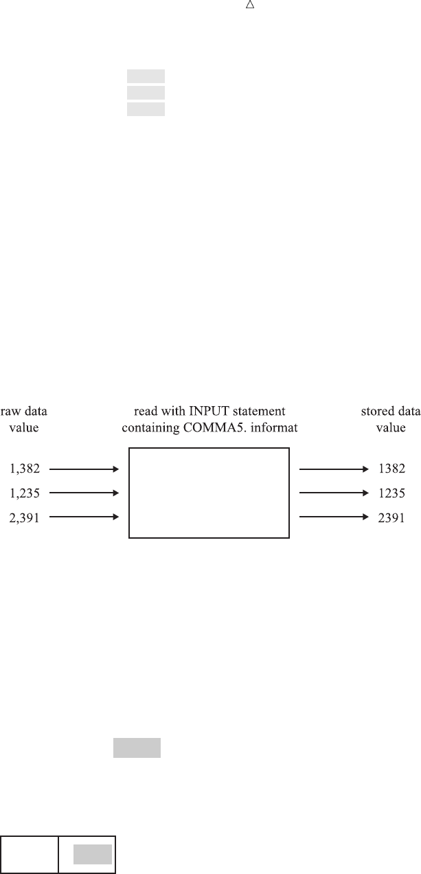
Starting with Raw Data: The Basics Program: Reading Data That Requires Special Instructions 51
datalines;
trucks 1,382
vans 1,235
sedans 2,391
;
proc print data=january_sales;
title ’January Sales in Thousands’;
run;
The INPUT statement cannot read the values for the variable Amount as valid
numeric values without the additional instructions provided by an informat. The
informat COMMA5. enables the INPUT statement to read and store this data as a
valid numeric value.
The following figure shows that the informat COMMA5. instructs the program to
read five characters of data (the comma counts as part of the length of the data), to
remove the comma from the data, and to write the resulting numeric value to the
program data vector. Note that the name of an informat always ends in a period (.).
Figure 3.1 Reading a Value with an Informat
COMMA5. informat
The following figure shows that the data values are read into the input buffer exactly
as they occur in the raw data records, but they are written to the program data vector
(and then to the data set as an observation) as valid numeric values without any special
characters.
Figure 3.2 Input Value Compared to Variable Value
Input Buffer
Program Data Vector
Item Amount
----+----1----+----2----+----3
trucks 1,382
1382trucks
The following output shows the resulting data set. The values for Amount contain
only numbers. Note that the commas are removed.

52 Understanding How to Control the Position of the Pointer Chapter 3
Output 3.6 Data Set Created with Column and Formatted Input
January Sales in Thousands 1
Obs Item Amount
1 trucks 1382
2 vans 1235
3 sedans 2391
In a report, you might want to include the comma in numeric values to improve
readability. Just as the informat gives instructions on how to read a value and to remove
the comma, a format gives instructions to add characters to variable values in the
output. See “Writing Output without Creating a Data Set” on page 522 for an example.
Understanding How to Control the Position of the Pointer
As the INPUT statement reads data values, it uses an input pointer to keep track of
the position of the data in the input buffer. Column-pointer controls provide additional
control over pointer movement and are especially useful with formatted input.
Column-pointer controls tell how far to advance the pointer before SAS reads the next
value. In this example, SAS reads data lines with a combination of column and
formatted input:
data january_sales;
input Item $ 1-16 Amount comma5.;
datalines;
trucks 1,382
vans 1,235
sedans 2,391
;
In the next example, SAS reads data lines by using formatted input with a
column-pointer control:
data january_sales;
input Item $10. @17 Amount comma5.;
datalines;
trucks 1,382
vans 1,235
sedans 2,391
;
After SAS reads the first value for the variable Item, the pointer is left in the next
position, column 11. The absolute column-pointer control, @17, then directs the pointer
to move to column 17 in the input buffer. Now, it is in the correct position to read a
value for the variable Amount.
In the following program, the relative column-pointer control, +6, instructs the
pointer to move six columns to the right before SAS reads the next data value.
data january_sales;
input Item $10. +6 Amount comma5.;
datalines;
trucks 1,382
Starting with Raw Data: The Basics Creating Longer Variables and Reading Numeric Data That Contains Special Characters 53
vans 1,235
sedans 2,391
;
The data in these two programs is aligned in columns. As with column input, you
instruct the pointer to move from field to field. With column input you use column
specifications; with formatted input you use the length that is specified in the informat
together with pointer controls.
Formatted Input: Points to Remember
Remember the following rules when you use formatted input:
SAS reads formatted input data until it has read the number of columns that the
informat indicates. This method of reading the data is different from list input,
which reads until a blank space (or other defined delimiter character) is reached.
You can position the pointer to read the next value by using pointer controls.
You can read data stored in nonstandard form such as packed decimal, or data
that contains commas.
You have the flexibility of using informats with all the features of column input, as
described in “Column Input: Points to Remember” on page 50.
Reading Unaligned Data with More Flexibility
Understanding How to Make List Input More Flexible
While list input is the simplest to code, remember that it places restrictions on your
data. By using format modifiers, you can take advantage of the simplicity of list input
without the inconvenience of the usual restrictions. For example, you can use modified
list input to do the following:
Create character variables that are longer than the default length of eight bytes.
Read numeric data with special characters like commas, dashes, and currency
symbols.
Read character data that contains embedded blanks.
Read data values that can be stored as SAS date variables.
Creating Longer Variables and Reading Numeric Data That Contains
Special Characters
By simply modifying list input with the colon format modifier (:) you can read
character data that contains more than eight characters
numeric data that contains special characters.
To use the colon format modifier with list input, place the colon between the variable
name and the informat. As in simple list input, at least one blank (or other defined
delimiter character) must separate each value from the next, and character values
cannot contain embedded blanks (or other defined delimiter characters). Consider this
DATA step:
data january_sales;
input Item : $12. Amount : comma5.;

54 Reading Character Data That Contains Embedded Blanks Chapter 3
datalines;
Trucks 1,382
Vans 1,235
Sedans 2,391
SportUtility 987
;
proc print data=january_sales;
title ’January Sales in Thousands’;
run;
The variable Item has a length of 12, and the variable Amount requires an informat (in
this case, COMMA5.) that removes commas from numbers so that they are read as
valid numeric values. The data values are not aligned in columns as was required in
the last example, which used formatted input to read the data.
The following output shows the resulting data set.
Output 3.7 Data Set Created with Modified List Input (: comma5.)
January Sales in Thousands 1
Obs Item Amount
1 Trucks 1382
2 Vans 1235
3 Sedans 2391
4 SportUtility 987
Reading Character Data That Contains Embedded Blanks
Because list input uses a blank space to determine where one value ends and the
next one begins, values normally cannot contain blanks. However, with the ampersand
format modifier (&) you can use list input to read data that contains single embedded
blanks. The only restriction is that at least two blanks must divide each value from the
next data value in the record.
To use the ampersand format modifier with list input, place the ampersand between
the variable name and the informat. The following DATA step uses the ampersand
format modifier with list input to create the data set CLUB2. Note that the data is not
in fixed columns; therefore, column input is not appropriate.
data club2;
input IdNumber Name & $18. Team $ StartWeight EndWeight;
datalines;
1023 David Shaw red 189 165
1049 Amelia Serrano yellow 145 124
1219 Alan Nance red 210 192
1246 Ravi Sinha yellow 194 177
1078 Ashley McKnight red 127 118
1221 Jim Brown yellow 220 .
;
proc print data=club2;
title ’Weight Club Members’;
run;

Starting with Raw Data: The Basics An Example of Mixed Input 55
The character variable Name, with a length of 18, contains members’ first and last
names separated by one blank space. The data lines must have two blank spaces
between the values for the variable Name and the variable Team for the INPUT
statement to correctly read the data.
The following output shows the resulting data set.
Output 3.8 Data Set Created with Modified List Input (& $18.)
Weight Club Members 1
Id Start End
Obs Number Name Team Weight Weight
1 1023 David Shaw red 189 165
2 1049 Amelia Serrano yellow 145 124
3 1219 Alan Nance red 210 192
4 1246 Ravi Sinha yellow 194 177
5 1078 Ashley McKnight red 127 118
6 1221 Jim Brown yellow 220 .
Mixing Styles of Input
An Example of Mixed Input
When you begin an INPUT statement in a particular style (list, column, or
formatted), you are not restricted to using that style alone. You can mix input styles in
a single INPUT statement as long as you mix them in a way that appropriately
describes the raw data records. For example, this DATA step uses all three input styles:
data club1;
input IdNumber u
Name $18. v
Team $ 25-30 w
StartWeight EndWeight; u
datalines;
1023 David Shaw red 189 165
1049 Amelia Serrano yellow 145 124
1219 Alan Nance red 210 192
1246 Ravi Sinha yellow 194 177
1078 Ashley McKnight red 127 118
1221 Jim Brown yellow 220 .
;
proc print data=club1;
title ’Weight Club Members’;
run;
The following list corresponds to the numbered items in the preceding program:
uThe variables IdNumber, StartWeight, and EndWeight are read with list input.
vThe variable Name is read with formatted input.
wThe variable Team is read with column input.
The following output demonstrates that the data is read correctly.

56 Understanding the Effect of Input Style on Pointer Location Chapter 3
Output 3.9 Data Set Created with Mixed Styles of Input
Weight Club Members 1
Id Start End
Obs Number Name Team Weight Weight
1 1023 David Shaw red 189 165
2 1049 Amelia Serrano yellow 145 124
3 1219 Alan Nance red 210 192
4 1246 Ravi Sinha yellow 194 177
5 1078 Ashley McKnight red 127 118
6 1221 Jim Brown yellow 220 .
Understanding the Effect of Input Style on Pointer Location
Why You Can Get into Trouble by Mixing Input Styles
CAUTION:
When you mix styles of input in a single INPUT statement, you can get unexpected results
if you do not understand where the input pointer is positioned after SAS reads a value in
the input buffer. As the INPUT statement reads data values from the record in the
input buffer, it uses a pointer to keep track of its position. Read the following
sections so that you understand how the pointer movement differs between input
styles before mixing multiple input styles in a single INPUT statement
Pointer Location with Column and Formatted Input
With column and formatted input, you supply the instructions that determine the
exact pointer location. With column input, SAS reads the columns that you specify in
the INPUT statement. With formatted input, SAS reads the exact length that you
specify with the informat. In both cases, the pointer moves as far as you instruct it and
stops. The pointer is left in the column that immediately follows the last column that is
read.
Here are two examples of input followed by an explanation of the pointer location.
The first DATA step shows column input:
data scores;
input Team $ 1-6 Score 12-13;
datalines;
red 59
blue 95
yellow 63
green 76
;
The second DATA step uses the same data to show formatted input:
data scores;
input Team $6. +5 Score 2.;
datalines;
red 59
blue 95
yellow 63
green 76

Starting with Raw Data: The Basics Understanding the Effect of Input Style on Pointer Location 57
;
The following figure shows that the pointer is located in column 7 after the first
value is read with either of the two previous INPUT statements.
Figure 3.3 Pointer Position: Column and Formatted Input
----+----1----+----2
red 59
Unlike list input, column and formatted input rely totally on your instructions to
move the pointer and read the value for the second variable, Score. Column input uses
column specifications to move the pointer to each data field. Formatted input uses
informats and pointer controls to control the position of the pointer.
This INPUT statement uses column input with the column specifications 12-13 to
move the pointer to column 12 and read the value for the variable Score:
input Team $ 1-6 Score 12-13;
This INPUT statement uses formatted input with the +5 column-pointer control to
move the pointer to column 12. Then the value for the variable Score is read with the 2.
numeric informat.
input Team $6. +5 Score 2.;
Without the use of a pointer control, which moves the pointer to the column where the
value begins, this INPUT statement would attempt to read the value for Score in
columns 7 and 8, which are blank.
Pointer Location with List Input
List input, on the other hand, uses a scanning method to determine the pointer
location. With list input, the pointer reads until a blank is reached and then stops in
the next column. To read the next variable value, the pointer moves automatically to
the first nonblank column, discarding any leading blanks it encounters. Here is the
same data that is read with list input:
data scores;
input Team $ Score;
datalines;
red 59
blue 95
yellow 63
green 76
;
The following figure shows that the pointer is located in column 5 after the value red
is read. Because Score, the next variable, is read with list input, the pointer scans for
the next nonblank space before it begins to read a value for Score. Unlike column and
formatted input, you do not have to explicitly move the pointer to the beginning of the
next field in list input.
58 Review of SAS Tools Chapter 3
Figure 3.4 Pointer Position: List Input
----+----1----+----2
red 59
Review of SAS Tools
Statements
DATALINES;
indicates that data lines immediately follow the DATALINES statement. A
semicolon in the line that immediately follows the last data line indicates the end
of the data and causes the DATA step to compile and execute.
INFILE DATALINES DLM=’character’;
identifies the source of the input records as data lines in the job stream rather
than as an external file. When your program contains the input data, the data
lines directly follow the DATALINES statement. Because you can specify
DATALINES in the INFILE statement, you can take advantage of many
data-reading options that are available only through the INFILE statement.
The DLM= option specifies the character that is used to separate data values in
the input records. By default, a blank space denotes the end of a data value. This
option is useful when you want to use list input to read data records in which a
character other than a blank separates data values.
INPUT variable <&> <$>;
reads the input data record using list input. The & (ampersand format modifier)
enables character values to contain embedded blanks. When you use the
ampersand format modifier, two blanks are required to signal the end of a data
value. The $ indicates a character variable.
INPUT variable start-column <– end-column>;
reads the input data record using column input. You can omit end-column if the
data is only 1 byte long. This style of input enables you to skip columns of data
that you want to omit.
INPUT variable :informat;
INPUT variable &informat;
read the input data record using modified list input. The : (colon format modifier)
instructs SAS to use the informat that follows to read the data value. The &
(ampersand format modifier) instructs SAS to use the informat that follows to read
the data value. When you use the ampersand format modifier, two blanks are
required to signal the end of a data value.
INPUT <pointer-control> variable informat;
reads raw data using formatted input. The informat supplies special instructions
to read the data. You can also use a pointer-control to direct SAS to start reading
at a particular column.
The syntax given above for the three styles of input shows only one variable.
Subsequent variables in the INPUT statement may or may not be described in the

Starting with Raw Data: The Basics Learning More 59
same input style as the first one. You may use any of the three styles of input (list,
column, and formatted) in a single INPUT statement.
Column-Pointer Controls
@n
moves the pointer to the nth column in the input buffer.
+n
moves the pointer forward ncolumns in the input buffer.
/
moves the pointer to the next line in the input buffer.
#n
moves the pointer to the nth line in the input buffer.
Learning More
Advanced features
For some more advanced data-reading features, see Chapter 4, “Starting with Raw
Data: Beyond the Basics,” on page 61.
Character-delimited data
For more information about reading data that is delimited by a character other
than a blank space, see the DELIMITER= option in the INFILE statement in SAS
Language Reference: Dictionary .
Pointer controls
For a complete discussion and listing of column-pointer controls, line-pointer
controls, and line-hold specifiers, see SAS Language Reference: Dictionary.
Types of input
For more information about the INPUT statement, see SAS Language Reference:
Dictionary.
60
61
CHAPTER
4
Starting with Raw Data: Beyond
the Basics
Introduction to Beyond the Basics with Raw Data 61
Purpose 61
Prerequisites 62
Testing a Condition before Creating an Observation 62
Creating Multiple Observations from a Single Record 63
Using the Double Trailing @ Line-Hold Specifier 63
Understanding How the Double Trailing @ Affects DATA Step Execution 64
Reading Multiple Records to Create a Single Observation 67
How the Data Records Are Structured 67
Method 1: Using Multiple Input Statements 67
Method 2: Using the / Line-Pointer Control 69
Reading Variables from Multiple Records in Any Order 70
Understanding How the #n Line-Pointer Control Affects DATA Step Execution 71
Problem Solving: When an Input Record Unexpectedly Does Not Have Enough Values 74
Understanding the Default Behavior 74
Methods of Control: Your Options 75
Four Options: FLOWOVER, STOPOVER, MISSOVER, and TRUNCOVER 75
Understanding the MISSOVER Option 76
Understanding the TRUNCOVER Option 77
Review of SAS Tools 77
Column-Pointer Controls 77
Line-Hold Specifiers 78
Statements 78
Learning More 79
Introduction to Beyond the Basics with Raw Data
Purpose
To create a SAS data set from raw data, you often need more than the most basic
features. In this section, you will learn advanced features for reading raw data that
include the following:
how to understand and then control what happens when a value is unexpectedly
missing in an input record
how to read a record more than once so that you may test a condition before
taking action on the current record
how to create multiple observations from a single input record
how to read multiple observations to create a single record
62 Prerequisites Chapter 4
Prerequisites
You should understand the concepts presented in Chapter 1, “What Is the SAS
System?,” on page 3 and Chapter 2, “Introduction to DATA Step Processing,” on page 19
before continuing.
Testing a Condition before Creating an Observation
Sometimes you need to read a record, and hold that record in the input buffer while
you test for a specified condition before a decision can be made about further
processing. As an example, the ability to hold a record so that you can read from it
again, if necessary, is useful when you need to test for a condition before SAS creates an
observation from a data record. To do this, you can use the trailing at-sign (@).
For example, to create a SAS data set that is a subset of a larger group of records,
you might need to test for a condition to decide if a particular record will be used to
create an observation. The trailing at-sign placed before the semicolon at the end of an
INPUT statement instructs SAS to hold the current data line in the input buffer. This
makes the data line available for a subsequent INPUT statement. Otherwise, the next
INPUT statement causes SAS to read a new record into the input buffer.
You can set up the process to read each record twice by following these steps:
1Use an INPUT statement to read a portion of the record.
2Use a trailing @ at the end of the INPUT statement to hold the record in the input
buffer for the execution of the next INPUT statement.
3Use an IF statement on the portion that is read in to test for a condition.
4If the condition is met, use another INPUT statement to read the remainder of the
record to create an observation.
5If the condition is not met, the record is released and control passes back to the
top of the DATA step.
To read from a record twice, you must prevent SAS from automatically placing a new
record into the input buffer when the next INPUT statement executes. Use of a trailing
@ in the first INPUT statement serves this purpose. The trailing @ is one of two
line-hold specifiers that enable you to hold a record in the input buffer for further
processing.
For example, the health and fitness club data contains information about all
members. This DATA step creates a SAS data set that contains only members of the
red team:
data red_team;
input Team $ 13-18 @; u
if Team=’red’; v
input IdNumber 1-4 StartWeight 20-22 EndWeight 24-26; w
datalines;
1023 David red 189 165
1049 Amelia yellow 145 124
1219 Alan red 210 192
1246 Ravi yellow 194 177
1078 Ashley red 127 118
1221 Jim yellow 220 .
;x
proc print data=red_team;
Starting with Raw Data: Beyond the Basics Using the Double Trailing @ Line-Hold Specifier 63
title ’Red Team’;
run;
In this DATA step, these actions occur:
uThe INPUT statement reads a record into the input buffer, reads a data value
from columns 13 through 18, and assigns that value to the variable Team in the
program data vector. The single trailing @ holds the record in the input buffer.
vThe IF statement enables the current iteration of the DATA step to continue only
when the value for Team is red. When the value is not red, the current iteration
stops and SAS returns to the top of the DATA step, resets values in the program
data vector to missing, and releases the held record from the input buffer.
wThe INPUT statement executes only when the value of Team is red. It reads the
remaining data values from the record held in the input buffer and assigns values
to the variables IdNumber, StartWeight, and EndWeight.
xThe record is released from the input buffer when the program returns to the top
of the DATA step.
The following output shows the resulting data set:
Output 4.1 Subset Data Set Created with Trailing @
Red Team 1
Id Start End
Obs Team Number Weight Weight
1 red 1023 189 165
2 red 1219 210 192
3 red 1078 127 118
Creating Multiple Observations from a Single Record
Using the Double Trailing @ Line-Hold Specifier
Sometimes you may need to create multiple observations from a single record of raw
data. One way to tell SAS how to read such a record is to use the other line-hold
specifier, the double trailing at-sign (@@ or “double trailing @”). The double trailing @
not only prevents SAS from reading a new record into the input buffer when a new
INPUT statement is encountered, but it also prevents the record from being released
when the program returns to the top of the DATA step. (Remember that the trailing @
does not hold a record in the input buffer across iterations of the DATA step.)
For example, this DATA step uses the double trailing @ in the INPUT statement:
data body_fat;
input Gender $ PercentFat @@;
datalines;
m 13.3 f 22
m 22 f 23.2
m16 m12
;
proc print data=body_fat;
64 Understanding How the Double Trailing @ Affects DATA Step Execution Chapter 4
title ’Results of Body Fat Testing’;
run;
The following output shows the resulting data set:
Output 4.2 Data Set Created with Double Trailing @
Results of Body Fat Testing 1
Percent
Obs Gender Fat
1 m 13.3
2 f 22.0
3 m 22.0
4 f 23.2
5 m 16.0
6 m 12.0
Understanding How the Double Trailing @ Affects DATA Step Execution
To understand how the data records in the previous example were read, look at the
data lines that were used in the previous DATA step:
m 13.3 f 22
m 22 f 23.2
m16 m12
Each record contains the raw data for two observations instead of one. Consider this
example in terms of the flow of the DATA step, as explained in Chapter 2, “Introduction
to DATA Step Processing,” on page 19.
When SAS reaches the end of the DATA step, it returns to the top of the program
and begins the next iteration, executing until there are no more records to read. Each
time it returns to the top of the DATA step and executes the INPUT statement, it
automatically reads a new record into the input buffer. The second set of data values in
each record, therefore, would never be read:
m 13.3 f22
m22 f 23.2
m16 m12
To allow the second set of data values in each record to be read, the double trailing @
tells SAS to hold the record in the input buffer. Each record is held in the input buffer
until the end of the record is reached. The program does not automatically place the
next record into the input buffer each time the INPUT statement is executed, and the
current record is not automatically released when it returns to the top of the DATA
step. As a result, the pointer location is maintained on the current record which
enables the program to read each value in that record. Each time the DATA step
completes an iteration, an observation is written to the data set.
The next five figures demonstrate what happens in the input buffer when a double
trailing @ appears in the INPUT statement, as in this example:
input Gender $ PercentFat @@;
The first figure shows that all values in the program data vector are set to missing.
The INPUT statement reads the first record into the input buffer. The program begins

Starting with Raw Data: Beyond the Basics Understanding How the Double Trailing @ Affects DATA Step Execution 65
to read values from the current pointer location, which is the beginning of the input
buffer.
Figure 4.1 First Iteration: First Record Is Read
Input Buffer
Program Data Vector
Gender PercentFat
----+----1----+----2
m 13.3 f 22
.
The following figure shows that the value mis written to the program data vector.
When the pointer reaches the blank space that follows 13.3, the complete value for the
variable PercentFat has been read. The pointer stops in the next column, and the value
13.3 is written to the program data vector.
Figure 4.2 First Observation Is Created
Input Buffer
Program Data Vector
Gender PercentFat
----+----1----+----2
m 13.3 f 22
m 13.3
There are no other variables in the INPUT statement and no more statements in the
DATA step, so three actions take place:
1The first observation is written to the data set.
2The DATA step begins its next iteration.
3The values in the program data vector are set to missing.
The following figure shows the current position of the pointer. SAS is ready to read
the next piece of data in the same record.
66 Understanding How the Double Trailing @ Affects DATA Step Execution Chapter 4
Figure 4.3 Second Iteration: First Record Remains in the Input Buffer
Input Buffer
Program Data Vector
Gender PercentFat
----+----1----+----2
m 13.3 f 22
.
The following figure shows that the INPUT statement reads the next two values from
the input buffer and writes them to the program data vector.
Figure 4.4 Second Observation Is Created
Input Buffer
Program Data Vector
Gender PercentFat
----+----1----+----2
m 13.3 f 22
f22
When the DATA step completes the second iteration, the values in the program data
vector are written to the data set as the second observation. Then the DATA step
begins its third iteration. Values in the program data vector are set to missing, and the
INPUT statement executes. The pointer, which is now at column 13 (two columns to the
right of the last data value that was read), continues reading. Because this is list input,
the pointer scans for the next nonblank character to begin reading the next value.
When the pointer reaches the end of the input buffer and fails to find a nonblank
character, SAS reads a new record into the input buffer.
The final figure shows that values for the third observation are read from the
beginning of the second record.
Starting with Raw Data: Beyond the Basics Method 1: Using Multiple Input Statements 67
Figure 4.5 Third Iteration: Second Record Is Read into the Input Buffer
Input Buffer
Program Data Vector
Gender PercentFat
----+----1----+----2
m 22 f 23.2
.
The process continues until SAS reads all the records. The resulting SAS data set
contains six observations instead of three.
Note: Although this program successfully reads all of the data in the input records,
SAS writes a message to the log noting that the program had to go to a new line.
Reading Multiple Records to Create a Single Observation
How the Data Records Are Structured
An earlier example (see “Reading Character Data That Contains Embedded Blanks”
on page 54) shows data for several observations that are contained in a single record of
raw data:
1023 David Shaw red 189 165
This INPUT statement reads all the data values arranged across a single record:
input IdNumber 1-4 Name $ 6-23 Team $ StartWeight EndWeight;
Now, consider the opposite situation: when information for a single observation is not
contained in a single record of raw data but is scattered across several records. For
example, the health and fitness club data could be constructed in such a way that the
information about a single member is spread across several records instead of in a
single record:
1023 David Shaw
red
189 165
Method 1: Using Multiple Input Statements
Multiple INPUT statements, one for each record, can read each record into a single
observation, as in this example:
input IdNumber 1-4 Name $ 6-23;
input Team $ 1-6;
input StartWeight 1-3 EndWeight 5-7;
To understand how to use multiple INPUT statements, consider what happens as a
DATA step executes. Remember that one record is read into the INPUT buffer
68 Method 1: Using Multiple Input Statements Chapter 4
automatically as each INPUT statement is encountered during each iteration. SAS
reads the data values from the input buffer and writes them to the program data vector
as variable values. At the end of the DATA step, all the variable values in the program
data vector are written automatically as a single observation.
This example uses multiple INPUT statements in a DATA step to read only selected
data fields and create a data set containing only the variables IdNumber, StartWeight,
and EndWeight.
data club2;
input IdNumber 1-4; u
input; v
input StartWeight 1-3 EndWeight 5-7; w
datalines;
1023 David Shaw
red
189 165
1049 Amelia Serrano
yellow
145 124
1219 Alan Nance
red
210 192
1246 Ravi Sinha
yellow
194 177
1078 Ashley McKnight
red
127 118
1221 Jim Brown
yellow
220 .
;
proc print data=club2;
title ’Weight Club Members’;
run;
The following list corresponds to the numbered items in the preceding program:
uThe first INPUT statement reads only one data field in the first record and
assigns a value to the variable IdNumber.
vThe second INPUT statement, without arguments, is a null INPUT statement
that reads the second record into the input buffer. However, it does not assign a
value to a variable.
wThe third INPUT statement reads the third record into the input buffer and
assigns values to the variables StartWeight and EndWeight.
The following output shows the resulting data set:
Starting with Raw Data: Beyond the Basics Method 2: Using the / Line-Pointer Control 69
Output 4.3 Data Set Created with Multiple INPUT Statements
Weight Club Members 1
Id Start End
Obs Number Weight Weight
1 1023 189 165
2 1049 145 124
3 1219 210 192
4 1246 194 177
5 1078 127 118
6 1221 220 .
Method 2: Using the / Line-Pointer Control
Writing a separate INPUT statement for each record is not the only way to create a
single observation. You can write a single INPUT statement and use the slash (/)
line-pointer control. The slash line-pointer control forces a new record into the input
buffer and positions the pointer at the beginning of that record.
This example uses only one INPUT statement to read multiple records:
data club2;
input IdNumber 1-4 / / StartWeight 1-3 EndWeight 5-7;
datalines;
1023 David Shaw
red
189 165
1049 Amelia Serrano
yellow
145 124
1219 Alan Nance
red
210 192
1246 Ravi Sinha
yellow
194 177
1078 Ashley McKnight
red
127 118
1221 Jim Brown
yellow
220 .
;
proc print data=club2;
title ’Weight Club Members’;
run;
The / line-pointer control appears exactly where a new INPUT statement begins in
the previous example (see “Method 1: Using Multiple Input Statements” on page 67).
The sequence of events in the input buffer and the program data vector as this DATA
step executes is identical to the previous example in method 1. The / is the signal to
read a new record into the input buffer, which happens automatically when the DATA
step encounters a new INPUT statement. The preceding example shows two slashes

70 Reading Variables from Multiple Records in Any Order Chapter 4
(/ /), indicating that SAS skips a record. SAS reads the first record, skips the second
record, and reads the third record.
The following output shows the resulting data set:
Output 4.4 Data Set Created with the / Line-Pointer Control
Weight Club Members 1
Id Start End
Obs Number Weight Weight
1 1023 189 165
2 1049 145 124
3 1219 210 192
4 1246 194 177
5 1078 127 118
6 1221 220 .
Reading Variables from Multiple Records in Any Order
You can also read multiple records to create a single observation by pointing to a
specific record in a set of input records with the #nline-pointer control. As you saw in
the last section, the advantage of using the / line-pointer control over multiple INPUT
statements is that it requires fewer statements. However, using the #nline-pointer
control enables you to read the variables in any order, no matter which record contains
the data values. It is also useful if you want to skip data lines.
This example uses one INPUT statement to read multiple data lines in a different
order:
data club2;
input #2 Team $ 1-6 #1 Name $ 6-23 IdNumber 1-4
#3 StartWeight 1-3 EndWeight 5-7;
datalines;
1023 David Shaw
red
189 165
1049 Amelia Serrano
yellow
145 124
1219 Alan Nance
red
210 192
1246 Ravi Sinha
yellow
194 177
1078 Ashley McKnight
red
127 118
1221 Jim Brown
yellow
220 .
;
proc print data=club2;
Starting with Raw Data: Beyond the Basics Understanding How the #n Line-Pointer Control Affects DATA Step Execution 71
title ’Weight Club Members’;
run;
The following output shows the resulting data set:
Output 4.5 Data Set Created with the #nLine-Pointer Control
Weight Club Members 1
Id Start End
Obs Team Name Number Weight Weight
1 red David Shaw 1023 189 165
2 yellow Amelia Serrano 1049 145 124
3 red Alan Nance 1219 210 192
4 yellow Ravi Sinha 1246 194 177
5 red Ashley McKnight 1078 127 118
6 yellow Jim Brown 1221 220 .
The order of the observations is the same as in the raw records ( shown in the section
“Reading Variables from Multiple Records in Any Order” on page 70). However, the
order of the variables in the data set differs from the order of the variables in the raw
input data records. This occurs because the order of the variables in the INPUT
statements corresponds with their order in the resulting data sets.
Understanding How the #n Line-Pointer Control Affects DATA Step
Execution
To understand the importance of the #nline-pointer control, remember the sequence
of events in the DATA steps that demonstrate the / line-pointer control and multiple
INPUT statements. Each record is read into the input buffer sequentially. The data is
read, and then a / or a new INPUT statement causes the program to read the next
record into the input buffer. It is impossible for the program to read a value from the
first record after a value from the second record is read because the data in the first
record is no longer available in the input buffer.
To solve this problem, use the #nline-pointer control. The #nline-pointer control
signals the program to create a multiple-line input buffer so that all the data for a
single observation is available while the observation is being built in the program data
vector. The #nline-pointer control also identifies the record in which data for each
variable appears. To use the #nline-pointer control, the raw data must have the same
number of records for each observation; for example, it cannot have three records for
one observation and two for the next.
When the program compiles and builds the input buffer, it looks at the INPUT
statement and creates an input buffer with as many lines as are necessary to contain
the number of records it needs to read for a single observation. In this example, the
highest number of records specified is three, so the input buffer is built to contain three
records at one time. The following figures demonstrate the flow of the DATA step in
this example.
This figure shows that the values are set to missing in the program data vector and
that the INPUT statement reads the first three records into the input buffer.

72 Understanding How the #n Line-Pointer Control Affects DATA Step Execution Chapter 4
Figure 4.6 Three Records Are Read into the Input Buffer as a Single Observation
Input Buffer
Program Data Vector
IdNumberName StartWeight EndWeightTeam
----+----1----+----2----+----3----+----4----+----5----+----6
1023 David Shaw
----+----1----+----2----+----3----+----4----+----5----+----6
red
----+----1----+----2----+----3----+----4----+----5----+----6
189 165
...
The INPUT statement for this example is as follows:
input #2 Team $ 1-6
#1 Name $ 6-23 IdNumber 1-4
#3 StartWeight 1-3 EndWeight 5-7;
The first variable is preceded by #2 to indicate that the value in the second record is
assigned to the variable Team. The following figure shows that the pointer advances to
the second line in the input buffer, reads the value, and writes it to the program data
vector.
Figure 4.7 Reading from the Second Record First
Input Buffer
Program Data Vector
IdNumberName StartWeight EndWeightTeam
----+----1----+----2----+----3----+----4----+----5----+----6
1023 David Shaw
----+----1----+----2----+----3----+----4----+----5----+----6
red
----+----1----+----2----+----3----+----4----+----5----+----6
189 165
..red .
The following figure shows that the pointer then moves to the sixth column in the first
record, reads a value, and assigns it to the variable Name in the program data vector.
It then moves to the first column to read the ID number, and assigns it to the variable
IdNumber.
Starting with Raw Data: Beyond the Basics Understanding How the #n Line-Pointer Control Affects DATA Step Execution 73
Figure 4.8 Reading from the First Record
Input Buffer
Program Data Vector
IdNumberName StartWeight EndWeightTeam
----+----1----+----2----+----3----+----4----+----5----+----6
1023 David Shaw
----+----1----+----2----+----3----+----4----+----5----+----6
red
----+----1----+----2----+----3----+----4----+----5----+----6
189 165
.1023red David Shaw .
The following figure shows that the process continues with the pointer moving to the
third record in the first observation. Values are read and assigned to StartWeight and
EndWeight, the last variable that is listed.
Figure 4.9 Reading from the Third Record
Input Buffer
Program Data Vector
IdNumberName StartWeight EndWeightTeam
----+----1----+----2----+----3----+----4----+----5----+----6
1023 David Shaw
----+----1----+----2----+----3----+----4----+----5----+----6
red
----+----1----+----2----+----3----+----4----+----5----+----6
189 165
1891023red David Shaw 165
When the bottom of the DATA step is reached, variable values in the program data
vector are written as an observation to the data set. The DATA step returns to the top,
and values in the program data vector are set to missing. The INPUT statement
executes again. The final figure shows that the next three records are read into the
input buffer, ready to create the second observation.
74 Problem Solving: When an Input Record Unexpectedly Does Not Have Enough Values Chapter 4
Figure 4.10 Reading the Next Three Records into the Input Buffer
Input Buffer
Program Data Vector
IdNumberName StartWeight EndWeightTeam
----+----1----+----2----+----3----+----4----+----5----+----6
1049 Amelia Serrano
----+----1----+----2----+----3----+----4----+----5----+----6
yellow
----+----1----+----2----+----3----+----4----+----5----+----6
145 124
...
Problem Solving: When an Input Record Unexpectedly Does Not Have
Enough Values
Understanding the Default Behavior
When a DATA step reads raw data from an external file, problems can occur when
SAS encounters the end of an input line before reading in data for all variables
specified in the input statement. This problem can occur when reading variable-length
records and/or records containing missing values.
The following is an example of an external file that contains variable-length records:
----+-----1-----+-----2
22
333
4444
55555
This DATA step uses the numeric informat 5. to read a single field in each record of
raw data and to assign values to the variable TestNumber:
data numbers;
infile ’your-external-file’;
input TestNumber 5.;
run;
proc print data=numbers;
title ’Test DATA Step’;
run;
The DATA step reads the first value (22). Because the value is shorter than the 5
characters expected by the informat, the DATA step attempts to finish filling the value
with the next record (333). This value is entered into the PDV and becomes the value of

Starting with Raw Data: Beyond the Basics Methods of Control: Your Options 75
the TestNumber variable for the first observation. The DATA step then goes to the next
record, but encounters the same problem because the value (4444) is shorter than the
value that is expected by the informat. Again, the DATA step goes to the next record,
reads the value (55555), and assigns that value to the TestNumber variable for the
second observation.
The following output shows the results. After this program runs, the SAS log
contains a note to indicate the places where SAS went to the next record to search for
data values.
Output 4.6 Reading Raw Data Past the End of a Line: Default Behavior
Test DATA Step 1
Test
Obs Number
1 333
2 55555
Methods of Control: Your Options
Four Options: FLOWOVER, STOPOVER, MISSOVER, and TRUNCOVER
To control how SAS behaves after it attempts to read past the end of a data line, you
can use the following options in the INFILE statement:
infile ’your-external-file’ flowover;
is the default behavior. The DATA step simply reads the next record into the input
buffer, attempting to find values to assign to the rest of the variable names in the
INPUT statement.
infile ’your-external-file’ stopover;
causes the DATA step to stop processing if an INPUT statement reaches the end of
the current record without finding values for all variables in the statement. Use
this option if you expect all of the data in the external file to conform to a given
standard and if you want the DATA step to stop when it encounters a data record
that does not conform to the standard.
infile ’your-external-file’ missover;
prevents the DATA step from going to the next line if it does not find values in the
current record for all of the variables in the INPUT statement. Instead, the DATA
step assigns a missing value for all variables that do not have values.
infile ’your-external-file’ truncover;
causes the DATA step to assign the raw data value to the variable even if the
value is shorter than expected by the INPUT statement. If, when the DATA step
encounters the end of an input record, there are variables without values, the
variables are assigned missing values for that observation.
You can also use these options even when your data lines are in the program itself,
that is, when they follow the DATALINES statement. Simply use datalines instead of
a reference to an external file to indicate that the data records are in the DATA step
itself:
infile datalines flowover;
infile datalines stopover;

76 Methods of Control: Your Options Chapter 4
infile datalines missover;
infile datalines truncover;
Note: The examples in this section show the use of the MISSOVER and
TRUNCOVER options with formatted input. You can also use these options with list
input and column input.
Understanding the MISSOVER Option
The MISSOVER option prevents the DATA step from going to the next line if it does
not find values in the current record for all of the variables in the INPUT statement.
Instead, the DATA step assigns a missing value for all variables that do not have
complete values according to any specified informats. The input file contains the
following raw data:
----+-----1-----+-----2
22
333
4444
55555
The following example uses the MISSOVER option:
data numbers;
infile ’your-external-file’ missover;
input TestNumber 5.;
run;
proc print data=numbers;
title ’Test DATA Step’;
run;
Output 4.7 Output from the MISSOVER Option
Test DATA Step 1
Test
Obs Number
1.
2.
3.
4 55555
Because the fourth record is the only one whose value matches the informat, it is the
only record whose value is assigned to the TestNumber variable. The other observations
receive missing values. This result is probably not the desired outcome for this
example, but the MISSOVER option can sometimes be valuable. For an example, see
“Updating a Data Set” on page 295.
Note: If there is a blank line at the end of the last record, the DATA step attempts
to load another record into the input buffer. Because there are no more records, the
MISSOVER option instructs the DATA step to assign missing values to all variables,
and an extra observation is added to the data set. To prevent this situation from

Starting with Raw Data: Beyond the Basics Column-Pointer Controls 77
occurring, make sure that your input data does not have a blank line at the end of the
last record.
Understanding the TRUNCOVER Option
The TRUNCOVER option causes the DATA step to assign the raw data value to the
variable even if the value is shorter than the length that is expected by the INPUT
statement. If, when the DATA step encounters the end of an input record, there are
variables without values, the variables are assigned missing values for that observation.
The following example demonstrates the use of the TRUNCOVER statement:
data numbers;
infile ’your-external-file’ truncover;
input TestNumber 5.;
run;
proc print data=numbers;
title ’Test DATA Step’;
run;
Output 4.8 Output from the TRUNCOVER Option
Test DATA Step 1
Test
Obs Number
122
2 333
3 4444
4 55555
This result shows that all of the values were assigned to the TestNumber variable,
despite the fact that three of them did not match the informat. For another example
using the TRUNCOVER option, see “Input SAS Data Set for Examples” on page 140.
Review of SAS Tools
Column-Pointer Controls
@n
moves the pointer to the ncolumn in the input buffer.
+n
moves the pointer forward ncolumns in the input buffer.
/
moves the pointer to the next line in the input buffer.
#n
moves the pointer to the nth line in the input buffer.
78 Line-Hold Specifiers Chapter 4
Line-Hold Specifiers
@
(trailing @) prevents SAS from automatically reading a new data record into the
input buffer when a new INPUT statement is executed within the same iteration
of the DATA step. When used, the trailing @ must be the last item in the INPUT
statement.
@@
(double trailing @) prevents SAS from automatically reading a new data record
into the input buffer when the next INPUT statement is executed, even if the
DATA step returns to the top for another iteration. When used, the double trailing
@ must be the last item in the INPUT statement.
Statements
DATALINES;
indicates that data lines immediately follow. A semicolon in the line that
immediately follows the last data line indicates the end of the data and causes the
DATA step to compile and execute.
INFILE fileref< FLOWOVER | STOPOVER | MISSOVER | TRUNCOVER>;
INFILE ’external-file’ <FLOWOVER | STOPOVER | MISSOVER | TRUNCOVER>;
identifies an external file to be read by an INPUT statement. Specify a fileref that
has been assigned with a FILENAME statement or with an appropriate operating
environment command. Or you can specify the actual name of the external file.
These options give you control over how SAS behaves if the end of a data record
is encountered before all of the variables are assigned values. You can use these
options with list, modified list, formatted, and column input.
FLOWOVER
is the default behavior. It causes the DATA step to look in the next record if
the end of the current record is encountered before all of the variables are
assigned values
MISSOVER
causes the DATA step to assign missing values to any variables that do not
have values when the end of a data record is encountered. The DATA step
continues processing.
STOPOVER
causes the DATA step to stop execution immediately and write a note to the
SAS log.
TRUNCOVER
causes the DATA step to assign values to variables, even if the values are
shorter than expected by the INPUT statement, and to assign missing values
to any variables that do not have values when the end of a record is
encountered.
INPUT variable <&> <$>;
reads the input data record using list input. The & (ampersand format modifier)
allows character values to contain embedded blanks. When you use the
ampersand format modifier, two blanks are required to signal the end of a data
value. The $ indicates a character variable.
Starting with Raw Data: Beyond the Basics Learning More 79
INPUT variable start-column<end-column>;
reads the input data record using column input. You can omit end-column if the
data is only 1 byte long. This style of input enables you to skip columns of data
that you want to omit.
INPUT variable :informat;
INPUT variable &informat;
reads the input data record using modified list input. The : (colon format modifier)
instructs SAS to use the informat that follows to read the data value. The &
(ampersand format modifier) instructs SAS to use the informat that follows to read
the data value. When you use the ampersand format modifier, two blanks are
required to signal the end of a data value.
INPUT <pointer-control> variable informat;
reads raw data using formatted input. The informat supplies special instructions
to read the data. You can also use a pointer-control to direct SAS to start reading
at a particular column.
The syntax given above for the three styles of input shows only one variable.
Subsequent variables in the INPUT statement may or may not be described in the
same input style as the first one. You may use any of the three styles of input (list,
column, and formatted) in a single INPUT statement.
Learning More
Handling missing data values
For complete details about the FLOWOVER, STOPOVER, MISSOVER, and
TRUNCOVER options in the INFILE statement, see SAS Language Reference:
Dictionary.
Reading multiple input records
Testing a condition
For more information about performing conditional processing with the IF
statement, see Chapter 9, “Acting on Selected Observations,” on page 139 and
Chapter 10, “Creating Subsets of Observations,” on page 159.
For a complete discussion and listing of line-pointer controls and line-hold
specifiers, see SAS Language Reference: Dictionary.
80

81
CHAPTER
5
Starting with SAS Data Sets
Introduction to Starting with SAS Data Sets 81
Purpose 81
Prerequisites 81
Understanding the Basics 82
Input SAS Data Set for Examples 82
Reading Selected Observations 84
Reading Selected Variables 85
Overview of Reading Selected Variables 85
Keeping Selected Variables 86
Dropping Selected Variables 87
Choosing between Data Set Options and Statements 88
Choosing between the DROP= and KEEP= Data Set Option 88
Creating More Than One Data Set in a Single DATA Step 89
Using the DROP= and KEEP= Data Set Options for Efficiency 91
Review of SAS Tools 92
Data Set Options 92
Procedures 93
Statements 93
Learning More 93
Introduction to Starting with SAS Data Sets
Purpose
In this section, you will learn how to do the following:
display information about a SAS data set
create a new SAS data set from an existing SAS data set rather than creating it
from raw data records
Reading a SAS data set in a DATA step is simpler than reading raw data because the
work of describing the data to SAS has already been done.
Prerequisites
You should understand the concepts presented in Chapter 1, “What Is the SAS
System?,” on page 3 and Chapter 2, “Introduction to DATA Step Processing,” on page 19
before continuing with this section.
82 Understanding the Basics Chapter 5
Understanding the Basics
When you use a SAS data set as input into a DATA step, the description of the data
set is available to SAS. In your DATA step, use a SET, MERGE, MODIFY, or UPDATE
statement to read the SAS data set. Use SAS programming statements to process the
data and create an output SAS data set.
In a DATA step, you can create a new data set that is a subset of the original data
set. For example, if you have a large data set of personnel data, you might want to look
at a subset of observations that meet certain conditions, such as observations for
employees hired after a certain date. Alternatively, you might want to see all
observations but only a few variables, such as the number of years of education or years
of service to the company.
When you use existing SAS data sets, as well as with subsets created from SAS data
sets, you can make more efficient use of computer resources than if you use raw data or
if you are working with large data sets. Reading fewer variables means that SAS
creates a smaller program data vector, and reading fewer observations means that
fewer iterations of the DATA step occur. Reading data directly from a SAS data set is
more efficient than reading the raw data again, because the work of describing and
converting the data has already been done.
One way of looking at a SAS data set is to produce a listing of the data in a SAS data
set by using the PRINT procedure. Another way to look at a SAS data set is to display
information that describes its structure rather than its data values. To display
information about the structure of a data set, use the DATASETS procedure with the
CONTENTS statement. If you need to work with a SAS data set that is unfamiliar to
you, the CONTENTS statement in the DATASETS procedure displays valuable
information such as the name, type, and length of all the variables in the data set. An
example that shows the CONTENTS statement in the DATASETS procedure is shown
in “Input SAS Data Set for Examples” on page 82.
Input SAS Data Set for Examples
The examples in this section use a SAS data set named CITY, which contains
information about expenditures for a small city. It reports total city expenditures for
the years 1980 through 2000 and divides the expenses into two major categories:
services and administration. (To see the program that creates the CITY data set, see
“DATA Step to Create the Data Set CITY” on page 712.)
The following example uses the DATASETS procedure with the NOLIST option to
display the CITY data set. The NOLIST option prevents the DATASETS procedure
from listing other data sets that are also located in the WORK library:
proc datasets library=work nolist;
contents data=city;
run;

Starting with SAS Data Sets Input SAS Data Set for Examples 83
Output 5.1 The Structure of CITY as Shown by PROC DATASETS
The SAS System 1
The DATASETS Procedure
Data Set Name: WORK.CITY Observations: 21 u
Member Type: DATA Variables: 10 u
Engine: V8 Indexes: 0
Created: 9:54 Wednesday, October 6, 1999 Observation Length: 80
Last Modified: 9:54 Wednesday, October 6, 1999 Deleted Observations: 0
Protection: Compressed: NO
Data Set Type: Sorted: NO
Label:
-----Engine/Host Dependent Information----- v
Data Set Page Size: 8192
Number of Data Set Pages: 1
First Data Page: 1
Max Obs per Page: 101
Obs in First Data Page: 21
Number of Data Set Repairs: 0
File Name: /usr/tmp/code_editor_saswork/SAS_
work63ED00006E98/city.sas7bdat
Release Created: 8.0001M0
Host Created: HP-UX
Inode Number: 62403
Access Permission: rw-r--r--
Owner Name: abcdef
File Size (bytes): 16384
-----Alphabetic List of Variables and Attributes-----
w# Variable Type Len Pos xLabel
----------------------------------------------------------------------------
5 AdminLabor Num 8 32 Administration: Labor
6 AdminSupplies Num 8 40 Administration: Supplies
9 AdminTotal Num 8 64 Administration: Total
7 AdminUtilities Num 8 48 Administration: Utilities
3 ServicesFire Num 8 16 Services: Fire
2 ServicesPolice Num 8 8 Services: Police
8 ServicesTotal Num 8 56 Services: Total
4 ServicesWater_Sewer Num 8 24 Services: Water & Sewer
10 Total Num 8 72 Total Outlays
1 Year Num 8 0
The following list corresponds to the numbered items in the previous SAS output:
uThe Observations and the Variables fields identify the number of observations and
the number of variables.
vThe Engine/Host Dependent Information section lists detailed information about
the data set. This information is generated by the engine, which is the mechanism
for reading from and writing to files.
Operating Environment Information: The output in this section may differ,
depending on your operating environment. For more information, refer to the SAS
documentation for your operating environment.
wThe Alphabetic List of Variables and Attributes lists the name, type, length, and
position of each variable.
xThe Label lists the format, informat, and label for each variable, if they exist.
84 Reading Selected Observations Chapter 5
Reading Selected Observations
If you are interested in only part of a large data set, you can use data set options to
create a subset of your data. Data set options specify which observations you want the
new data set to include. In Chapter 10, “Creating Subsets of Observations,” on page
159 you learn how to use the subsetting IF statement to create a subset of a large SAS
data set. In this section, you learn how to use the FIRSTOBS= and OBS= data set
options to create subsets of a larger data set.
For example, you might not want to read the observations at the beginning of the
data set. You can use the FIRSTOBS= data set option to define which observation
should be the first one that is processed. For the data set CITY, this example creates a
data set that excludes observations that contain data prior to 1991 by specifying
FIRSTOBS=12. As a result, SAS does not read the first 11 observations, which contain
data prior to 1991. (To see the program that creates the CITY data set, see “DATA Step
to Create the Data Set CITY” on page 712.)
The following program creates the data set CITY2, which contains the same number
of variables but fewer observations than CITY.
data city2;
set city(firstobs=12);
run;
proc print;
title ’City Expenditures’;
title2 ’1991 - 2000’;
run;
The following output shows the results:

Starting with SAS Data Sets Overview of Reading Selected Variables 85
Output 5.2 Subsetting a Data Set by Observations
City Expenditures 1
1991 - 2000
S
e
r
v
i
Sc A
eeAdS
rSs dme
veW mir
i r aAinvA
c v tdnUid
e i emStcm
s c riuiei
P e _nplsn
osSLpiTTT
YlFealtooo
Oeiiwbiittt
bacreoeeaaa
sreerrsslll
1 1991 2195 1002 643 256 24 55 3840 335 4175
2 1992 2204 964 692 256 28 70 3860 354 4214
3 1993 2175 1144 735 241 19 83 4054 343 4397
4 1994 2556 1341 813 238 25 97 4710 360 5070
5 1995 2026 1380 868 226 24 97 4274 347 4621
6 1996 2526 1454 946 317 13 89 4926 419 5345
7 1997 2027 1486 1043 226 . 82 4556 . .
8 1998 2037 1667 1152 244 20 88 4856 352 5208
9 1999 2852 1834 1318 270 23 74 6004 367 6371
10 2000 2787 1701 1317 307 26 66 5805 399 6204
You can also specify the last observation you want to include in a new data set with
the OBS= data set option. For example, the next program creates a SAS data set
containing only the observations for 1989 (the 10th observation) through 1994 (the 15th
observation).
data city3;
set city (firstobs=10 obs=15);
run;
Reading Selected Variables
Overview of Reading Selected Variables
You can create a subset of a larger data set not only by excluding observations but
also by specifying which variables you want the new data set to contain. In a DATA
step you can use the SET statement and the KEEP= or DROP= data set options (or the
DROP and KEEP statements) to create a subset from a larger data set by specifying
which variables you want the new data set to include.

86 Keeping Selected Variables Chapter 5
Keeping Selected Variables
This example uses the KEEP= data set option in the SET statement to read only the
variables that represent the services-related expenditures of the data set CITY.
data services;
set city (keep=Year ServicesTotal ServicesPolice ServicesFire
ServicesWater_Sewer);
run;
proc print data=services;
title ’City Services-Related Expenditures’;
run;
The following output shows the resulting data set. Note that the data set SERVICES
contains only those variables that are specified in the KEEP= option.
Output 5.3 Selecting Variables with the KEEP= Option
City Services-Related Expenditures 1
Services
Services Services Water_ Services
Obs Year Police Fire Sewer Total
1 1980 2819 1120 422 4361
2 1981 2477 1160 500 4137
3 1982 2028 1061 510 3599
4 1983 2754 893 540 4187
5 1984 2195 963 541 3699
6 1985 1877 926 535 3338
7 1986 1727 1111 535 3373
8 1987 1532 1220 519 3271
9 1988 1448 1156 577 3181
10 1989 1500 1076 606 3182
11 1990 1934 969 646 3549
12 1991 2195 1002 643 3840
13 1992 2204 964 692 3860
14 1993 2175 1144 735 4054
15 1994 2556 1341 813 4710
16 1995 2026 1380 868 4274
17 1996 2526 1454 946 4926
18 1997 2027 1486 1043 4556
19 1998 2037 1667 1152 4856
20 1999 2852 1834 1318 6004
21 2000 2787 1701 1317 5805
The following example uses the KEEP statement instead of the KEEP= data set
option to read all of the variables from the CITY data set. The KEEP statement creates
a new data set (SERVICES) that contains only the variables listed in the KEEP
statement. The following program gives results that are identical to those in the
previous example:
data services;
set city;
keep Year ServicesTotal ServicesPolice ServicesFire
ServicesWater_Sewer;
run;

Starting with SAS Data Sets Dropping Selected Variables 87
The following example has the same effect as using the KEEP= data set option in the
DATA statement. All of the variables are read into the program data vector, but only
the specified variables are written to the SERVICES data set:
data services (keep=Year ServicesTotal ServicesPolice ServicesFire
ServicesWater_Sewer);
set city;
run;
Dropping Selected Variables
Use the DROP= option to create a subset of a larger data set when you want to
specify which variables are being excluded rather than which ones are being included.
The following DATA step reads all of the variables from the data set CITY except for
those that are specified with the DROP= option, and then creates a data set named
SERVICES2:
data services2;
set city (drop=Total AdminTotal AdminLabor AdminSupplies
AdminUtilities);
run;
proc print data=services2;
title ’City Services-Related Expenditures’;
run;
The following output shows the resulting data set:
Output 5.4 Excluding Variables with the DROP= Option
City Services-Related Expenditures 1
Services
Services Services Water_ Services
Obs Year Police Fire Sewer Total
1 1980 2819 1120 422 4361
2 1981 2477 1160 500 4137
3 1982 2028 1061 510 3599
4 1983 2754 893 540 4187
5 1984 2195 963 541 3699
6 1985 1877 926 535 3338
7 1986 1727 1111 535 3373
8 1987 1532 1220 519 3271
9 1988 1448 1156 577 3181
10 1989 1500 1076 606 3182
11 1990 1934 969 646 3549
12 1991 2195 1002 643 3840
13 1992 2204 964 692 3860
14 1993 2175 1144 735 4054
15 1994 2556 1341 813 4710
16 1995 2026 1380 868 4274
17 1996 2526 1454 946 4926
18 1997 2027 1486 1043 4556
19 1998 2037 1667 1152 4856
20 1999 2852 1834 1318 6004
21 2000 2787 1701 1317 5805
88 Choosing between Data Set Options and Statements Chapter 5
The following example uses the DROP statement instead of the DROP= data set option
to read all of the variables from the CITY data set and to exclude the variables that are
listed in the DROP statement from being written to the new data set. The results are
identical to those in the previous example:
data services2;
set city;
drop Total AdminTotal AdminLabor AdminSupplies AdminUtilities;
run;
proc print data=services2;
run;
Choosing between Data Set Options and Statements
When you create only one data set in the DATA step, the data set options to drop and
keep variables have the same effect on the output data set as the statements to drop
and keep variables. When you want to control which variables are read into the
program data vector, using the data set options in the statement (such as a SET
statement) that reads the SAS data set is generally more efficient than using the
statements. Later topics in this section show you how to use the data set options in
some cases where the statements will not work.
Choosing between the DROP= and KEEP= Data Set Option
In a simple case, you might decide to use the DROP= or KEEP= option, depending on
which method enables you to specify fewer variables. If you work with large jobs that
read data sets, and you expect that variables might be added between the times your
batch jobs run, you may want to use the KEEP= option to specify which variables are
included in the subset data set.
The following figure shows two data sets named SMALL. They have different
contents because the new variable F was added to data set BIG before the DATA step
ran on Tuesday. The DATA step uses the DROP= option to keep variables D and E from
being written to the output data set. The result is that the data sets contain different
contents: the second SMALL data set has an extra variable, F. If the DATA step used
the KEEP= option to specify A, B, and C, then both of the SMALL data sets would have
the same variables (A, B, and C). The addition of variable F to the original data set BIG
would have no effect on the creation of the SMALL data set.
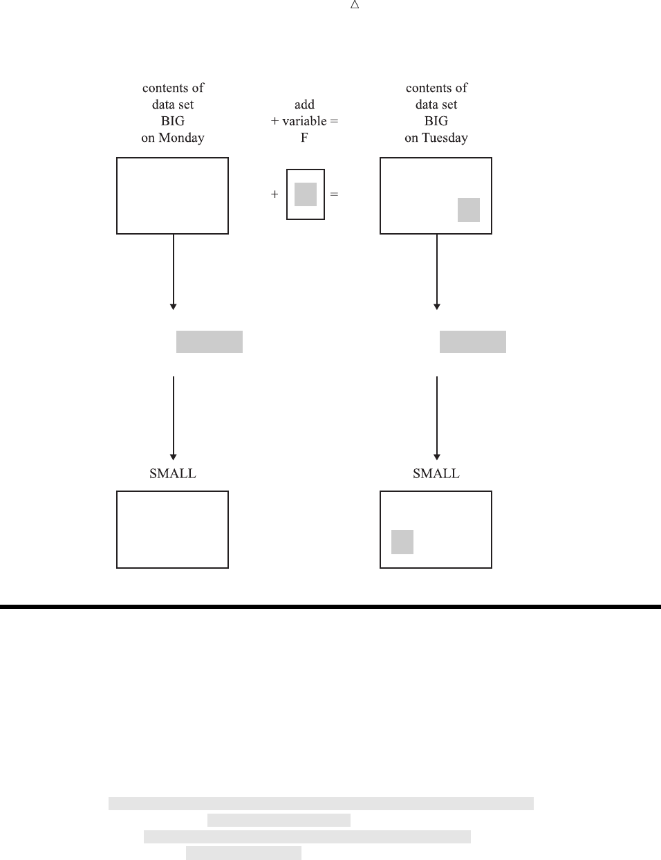
Starting with SAS Data Sets Creating More Than One Data Set in a Single DATA Step 89
Figure 5.1 Using the DROP= Option
A B C
data small;
set big(drop=d e);
run;
data small;
set big(drop=d e);
run;
A B C
D E
A B C
D E F
F
A B C
F
Creating More Than One Data Set in a Single DATA Step
You can use a single DATA step to create more than one data set at a time. You can
create data sets with different contents by using the KEEP= or DROP= data set
options. For example, the following DATA step creates two SAS data sets: SERVICES
contains variables that show services-related expenditures, and ADMIN contains
variables that represent the administration-related expenditures. Use the KEEP=
option after each data set name in the DATA statement to determine which variables
are written to each SAS data set being created.
data services(keep=ServicesTotal ServicesPolice ServicesFire
ServicesWater_Sewer)
admin(keep=AdminTotal AdminLabor AdminSupplies
AdminUtilities);
set city;
run;
proc print data=services;
title ’City Expenditures: Services’;
run;

90 Creating More Than One Data Set in a Single DATA Step Chapter 5
proc print data=admin;
title ’City Expenditures: Administration’;
run;
The following output shows both data sets. Note that each data set contains only the
variables that are specified with the KEEP= option after its name in the DATA
statement.
Output 5.5 Creating Two Data Sets in One DATA Step
City Expenditures: Services 1
Services
Services Services Water_ Services
Obs Police Fire Sewer Total
1 2819 1120 422 4361
2 2477 1160 500 4137
3 2028 1061 510 3599
4 2754 893 540 4187
5 2195 963 541 3699
6 1877 926 535 3338
7 1727 1111 535 3373
8 1532 1220 519 3271
9 1448 1156 577 3181
10 1500 1076 606 3182
11 1934 969 646 3549
12 2195 1002 643 3840
13 2204 964 692 3860
14 2175 1144 735 4054
15 2556 1341 813 4710
16 2026 1380 868 4274
17 2526 1454 946 4926
18 2027 1486 1043 4556
19 2037 1667 1152 4856
20 2852 1834 1318 6004
21 2787 1701 1317 5805
Starting with SAS Data Sets Using the DROP= and KEEP= Data Set Options for Efficiency 91
City Expenditures: Administration 2
Admin Admin Admin Admin
Obs Labor Supplies Utilities Total
1 391 63 98 552
2 172 47 70 289
3 269 29 79 377
4 227 21 67 315
5 214 21 59 294
6 198 16 80 294
7 213 27 70 310
8 195 11 69 275
9 225 12 58 295
10 235 19 62 316
11 266 11 63 340
12 256 24 55 335
13 256 28 70 354
14 241 19 83 343
15 238 25 97 360
16 226 24 97 347
17 317 13 89 419
18 226 . 82 .
19 244 20 88 352
20 270 23 74 367
21 307 26 66 399
Note: In this case, using the KEEP= data set option is necessary, because when you
use the KEEP statement, all data sets that are created in the DATA step contain the
same variables.
Using the DROP= and KEEP= Data Set Options for Efficiency
The DROP= and KEEP= data set options are valid in both the DATA statement and
the SET statement. However, you can write a more efficient DATA step if you
understand the consequences of using these options in the DATA statement rather than
the SET statement.
In the DATA statement, these options affect which variables SAS writes from the
program data vector to the resulting SAS data set. In the SET statement, these options
determine which variables SAS reads from the input SAS data set. Therefore, they
determine how the program data vector is built.
When you specify the DROP= or KEEP= option in the SET statement, SAS does not
read the excluded variables into the program data vector. If you work with a large data
set (perhaps one containing thousands or millions of observations), you can construct a
more efficient DATA step by not reading unneeded variables from the input data set.
Note also that if you use a variable from the input data set to perform a calculation,
the variable must be read into the program data vector. If you do not want that
variable to appear in the new data set, however, use the DROP= option in the DATA
statement to exclude it.
The following DATA step creates the same two data sets as the DATA step in the
previous example, but it does not read the variable Total into the program data vector.
Compare the SET statement here to the one in “Creating More Than One Data Set in a
Single DATA Step” on page 89.
data services (keep=ServicesTotal ServicesPolice ServicesFire
ServicesWater_Sewer)

92 Review of SAS Tools Chapter 5
admin (keep=AdminTotal AdminLabor AdminSupplies
AdminUtilities);
set city(drop=Total);
run;
proc print data=services;
title ’City Expenditures: Services’;
run;
proc print data=admin;
title ’City Expenditures: Administration’;
run;
In contrast with previous examples, the data set options in this example appear in
both the DATA and SET statements. In the SET statement, the DROP= option
determines which variables are omitted from the program data vector. In the DATA
statement, the KEEP= option controls which variables are written from the program
data vector to each data set being created.
Note: Using a DROP or KEEP statement is comparable to using a DROP= or
KEEP= option in the DATA statement. All variables are included in the program data
vector; they are excluded when the observation is written from the program data vector
to the new data set. When you create more than one data set in a single DATA step,
using the data set options enables you to drop or keep different variables in each of the
new data sets. A DROP or KEEP statement, on the other hand, affects all of the data
sets that are created.
Review of SAS Tools
Data Set Options
DROP=variable(s)
specifies the variables to be excluded.
Used in the SET statement, DROP= specifies the variables that are not to be
read from the existing SAS data set into the program data vector. Used in the
DATA statement, DROP= specifies the variables to be excluded from the data set
that is being created.
FIRSTOBS=n
specifies the first observation to be read from the SAS data set that you specify in
the SET statement.
KEEP=variable(s)
specifies the variables to be included.
Used in the SET statement, KEEP= specifies the variables to be read from the
existing SAS data set into the program data vector. Used in the DATA statement,
KEEP= specifies which variables in the program data vector are to be written to
the data set being created.
OBS=n
specifies the last observation to be read from the SAS data set that you specify in
the SET statement.

Starting with SAS Data Sets Learning More 93
Procedures
PROC DATASETS <LIBRARY=SAS-data-library>;
CONTENTS <DATA=SAS-data set>;
describes the structure of a SAS data set, including the name, type, and length of
all variables in the data set.
Statements
DATA SAS-data-set<(data-set-options)>;
begins a DATA step and names the SAS data set or data sets that are being
created. You can specify the DROP= or KEEP= data set options in parentheses
after each data set name to control which variables are written to the output data
set from the program data vector.
DROP variable(s);
specifies the variables to be excluded from the data set that is being created. See
also the DROP= data set option.
KEEP variable(s)
specifies the variables to be written to the data set that is being created. See also
the KEEP= data set option.
SET SAS-data-set(data-set-options);
reads observations from a SAS data set rather than records of raw data. You can
specify the DROP= or KEEP= data set options in parentheses after a data set
name to control which variables are read into the program data vector from the
input data set.
Learning More
Creating SAS data sets
For a general discussion about creating SAS data sets from other SAS data sets by
merging, concatenating, interleaving, and updating, see Chapter 15, “Methods of
Combining SAS Data Sets,” on page 233.
Data set options
See the “Data Set Options” section of SAS Language Reference: Dictionary, and
the SAS documentation for your operating environment.
DROP and KEEP statements
See the “Statements” section of SAS Language Reference: Dictionary.
Engines
see SAS Language Reference: Concepts.
Subsetting IF statement
You can use the subsetting IF statement and conditional (IF-THEN) logic when
creating a new SAS data set from an existing one. For more information, see
Chapter 9, “Acting on Selected Observations,” on page 139 and Chapter 10,
“Creating Subsets of Observations,” on page 159.
94

95
PART
3
Basic Programming
Chapter 6..........
Understanding DATA Step Processing 97
Chapter 7..........
Working with Numeric Variables 107
Chapter 8..........
Working with Character Variables 119
Chapter 9..........
Acting on Selected Observations 139
Chapter 10.........
Creating Subsets of Observations 159
Chapter 11.........
Working with Grouped or Sorted Observations 173
Chapter 12.........
Using More Than One Observation in a Calculation 187
Chapter 13.........
Finding Shortcuts in Programming 201
Chapter 14.........
Working with Dates in the SAS System 211
96
97
CHAPTER
6
Understanding DATA Step
Processing
Introduction to DATA Step Processing 97
Purpose 97
Prerequisites 97
Input SAS Data Set for Examples 97
Adding Information to a SAS Data Set 98
Understanding the Assignment Statement 98
Making Uniform Changes to Data by Creating a Variable 99
Adding Information to Some Observations but Not Others 100
Making Uniform Changes to Data Without Creating Variables 101
Using Variables Efficiently 101
Defining Enough Storage Space for Variables 103
Conditionally Deleting an Observation 104
Review of SAS Tools 105
Statements 105
Learning More 105
Introduction to DATA Step Processing
Purpose
To add, modify, and delete information in a SAS data set, you use a DATA step. In
this section, you will learn how the DATA step works, the general form of the
statements, and some programming techniques.
Prerequisites
You should understand the concepts presented in Chapter 2, “Introduction to DATA
Step Processing,” on page 19 and Chapter 3, “Starting with Raw Data: The Basics,” on
page 43 before proceeding with this section.
Input SAS Data Set for Examples
Tradewinds Travel Inc. has an external file that they use to manipulate and store
data about their tours. The external file contains the following information:
u vwxy
France 8 793 575 Major

98 Adding Information to a SAS Data Set Chapter 6
Spain 10 805 510 Hispania
India 10 . 489 Royal
Peru 7 722 590 Mundial
The numbered fields represent
uthe name of the country toured
vthe number of nights on the tour
wthe airfare in US dollars
xthe cost of the land package in US dollars
ythe name of the company that offers the tour
Notice that the cost of the airfare for the tour to India has a missing value, which is
indicated by a period.
The following DATA step creates a permanent SAS data set named
MYLIB.INTERNATIONALTOURS:
options pagesize=60 linesize=80 pageno=1 nodate;
libname mylib ’permanent-data-library’;
data mylib.internationaltours;
infile ’input-file’;
input Country $ Nights AirCost LandCost Vendor $;
proc print data = mylib.internationaltours;
title ’Data Set MYLIB.INTERNATIONALTOURS’;
run;
The PROC PRINT statement that follows the DATA step produces this display of the
MYLIB.INTERNATIONALTOURS data set:
Output 6.1 Creating a Permanent SAS Data Set
Data Set MYLIB.INTERNATIONALTOURS 1
Air Land
Obs Country Nights Cost Cost Vendor
1 France 8 793 575 Major
2 Spain 10 805 510 Hispania
3 India 10 . 489 Royal
4 Peru 7 722 590 Mundial
Adding Information to a SAS Data Set
Understanding the Assignment Statement
One of the most common reasons for using program statements in the DATA step is
to produce new information from the original information or to change the information
read by the INPUT or SET/MERGE/MODIFY/UPDATE statement. How do you add
information to observations with a DATA step?

Understanding DATA Step Processing Making Uniform Changes to Data by Creating a Variable 99
The basic method of adding information to a SAS data set is to create a new variable
in a DATA step with an assignment statement. An assignment statement has the form:
variable=expression;
The variable receives the new information; the expression creates the new
information. You specify the calculation necessary to produce the information and write
the calculation as the expression. When the expression contains character data, you
must enclose the data in quotation marks. SAS evaluates the expression and stores the
new information in the variable that you name. It is important to remember that if you
need to add the information to only one or two observations out of many, SAS creates
that variable for all observations. The SAS data set that is being created must have
information in every observation and every variable.
Making Uniform Changes to Data by Creating a Variable
Sometimes you want to make a particular change to every observation. For example,
at Tradewinds Travel the airfare must be increased for every tour by $10 because of a
new tax. One way to do this is to write an assignment statement that creates a new
variable that calculates the new airfare:
NewAirCost = AirCost+10;
This statement directs SAS to read the value of AirCost, add 10 to it, and assign the
result to the new variable, NewAirCost.
When this assignment statement is included in a DATA step, the DATA step looks
like this:
options pagesize=60 linesize=80 pageno=1 nodate;
data newair;
set mylib.internationaltours;
NewAirCost = AirCost + 10;
proc print data=newair;
var Country AirCost NewAirCost;
title ’Increasing the Air Fare by $10 for All Tours’;
run;
Note: In this example, the VAR statement in the PROC PRINT step determines
which variables are displayed in the output.
The following output shows the resulting SAS data set, NEWAIR:
Output 6.2 Adding Information to All Observations by Using a New Variable
Increasing the Air Fare by $10 for All Tours 1
New u
Air Air
Obs Country Cost Cost
1 France 793 803
2 Spain 805 815
3 India . . v
4 Peru 722 732

100 Adding Information to Some Observations but Not Others Chapter 6
Notice in this data set that
ubecause SAS carries out each statement in the DATA step for every observation,
NewAirCost is calculated during each iteration of the DATA step.
vthe observation for India contains a missing value for AirCost; SAS therefore
assigns a missing value to NewAirCost for that observation
The SAS data set has information in every observation and every variable.
Adding Information to Some Observations but Not Others
Often you need to add information to some observations but not to others. For
example, some tour operators award bonus points to travel agencies for scheduling
particular tours. Two companies, Hispania and Mundial, are offering bonus points this
year.
IF-THEN/ELSE statements can cause assignment statements to be carried out only
when a condition is met. In the following DATA step, the IF statements check the value
of the variable Vendor. If the value is either Hispania or Mundial, information about
the bonus points is added to those observations.
options pagesize=60 linesize=80 pageno=1 nodate;
data bonus;
set mylib.internationaltours;
if Vendor = ’Hispania’ then BonusPoints = ’For 10+ people’;
else if Vendor = ’Mundial’ then BonusPoints = ’Yes’;
run;
proc print data=bonus;
var Country Vendor BonusPoints;
title1 ’Adding Information to Observations for’;
title2 ’Vendors Who Award Bonus Points’;
run;
The following output displays the results:
Output 6.3 Specifying Values for Specific Observations by Using a New Variable
Adding Information to Observations for 1
Vendors Who Award Bonus Points
Obs Country Vendor BonusPoints
1 France Major u
2 Spain Hispania For 10+ people v
3 India Royal u
4 Peru Mundial Yes
The new variable BonusPoints has the following information:
uIn the two observations that are not assigned a value for BonusPoints, SAS
assigns a missing value, represented by a blank in this case, to indicate the
absence of a character value.
vThe first value that SAS encounters for BonusPoints contains 14 characters;
therefore, SAS sets aside 14 bytes of storage in each observation for BonusPoints,
regardless of the length of the value for that observation.

Understanding DATA Step Processing Using Variables Efficiently 101
Making Uniform Changes to Data Without Creating Variables
Sometimes you want to change the value of existing variables without adding new
variables. For example, in one DATA step a new variable, NewAirCost, was created to
contain the value of the airfare plus the new $10 tax:
NewAirCost = AirCost + 10;
You can also decide to change the value of an existing variable rather than create a
new variable. Following the example, AirCost is changed as follows:
AirCost = AirCost + 10;
SAS processes this statement just as it does other assignment statements. It
evaluates the expression on the right side of the equal sign and assigns the result to the
variable on the left side of the equal sign. The fact that the same variable appears on
the right and left sides of the equal sign does not matter. SAS evaluates the expression
on the right side of the equal sign before looking at the variable on the left side.
The following program contains the new assignment statement:
options pagesize=60 linesize=80 pageno=1 nodate;
data newair2;
set mylib.internationaltours;
AirCost = AirCost + 10;
proc print data=newair2;
var Country AirCost;
title ’Adding Tax to the Air Cost Without Adding a New Variable’;
run;
The following output displays the results:
Output 6.4 Changing the Information in a Variable
Adding Tax to the Air Cost Without Adding a New Variable 1
Air
Obs Country Cost
1 France 803
2 Spain 815
3 India .
4 Peru 732
When you change the kind of information that a variable contains, you change the
meaning of that variable. In this case, you are changing the meaning of AirCost from
airfare without tax to airfare with tax. If you remember the current meaning and if you
know that you do not need the original information, then changing a variable’s values is
useful. However, for many programmers, having separate variables is easier than
recalling one variable whose definition changes.
Using Variables Efficiently
Variables that contain information that applies to only one or two observations use
more storage space than necessary. When possible, create fewer variables that apply to

102 Using Variables Efficiently Chapter 6
more observations in the data set, and allow the different values in different
observations to supply the information.
For example, the Major company offers discounts, not bonus points, for groups of 30
or more people. An inefficient program would create separate variables for bonus points
and discounts, as follows:
/* inefficient use of variables */
options pagesize=60 linesize=80 pageno=1 nodate;
data tourinfo;
set mylib.internationaltours;
if Vendor = ’Hispania’ then BonusPoints = ’For 10+ people’;
else if Vendor = ’Mundial’ then BonusPoints = ’Yes’;
else if Vendor = ’Major’ then Discount = ’For 30+ people’;
run;
proc print data=tourinfo;
var Country Vendor BonusPoints Discount;
title ’Information About Vendors’;
run;
The following output displays the results:
Output 6.5 Inefficient: Using Variables That Scatter Information Across Multiple Variables
Information About Vendors 1
Obs Country Vendor BonusPoints Discount
1 France Major For 30+ people
2 Spain Hispania For 10+ people
3 India Royal
4 Peru Mundial Yes
As you can see, storage space is used inefficiently. Both BonusPoints and Discount
have a significant number of missing values.
With a little planning, you can make the SAS data set much more efficient. In the
following DATA step, the variable Remarks contains information about bonus points,
discounts, and any other special features of any tour.
/* efficient use of variables */
options pagesize=60 linesize=80 pageno=1 nodate;
data newinfo;
set mylib.internationaltours;
if Vendor = ’Hispania’ then Remarks = ’Bonus for 10+ people’;
else if Vendor = ’Mundial’ then Remarks = ’Bonus points’;
else if Vendor = ’Major’ then Remarks = ’Discount: 30+ people’;
run;
proc print data=newinfo;
var Country Vendor Remarks;
title ’Information About Vendors’;
run;
Understanding DATA Step Processing Defining Enough Storage Space for Variables 103
The following output displays a more efficient use of variables:
Output 6.6 Efficient: Using Variables to Contain Maximum Information
Information About Vendors 1
Obs Country Vendor Remarks
1 France Major Discount: 30+ people
2 Spain Hispania Bonus for 10+ people
3 India Royal
4 Peru Mundial Bonus points
Remarks has fewer missing values and contains all the information that is used by
BonusPoints and Discount in the inefficient example. Using variables efficiently can
save storage space and optimize your SAS data set.
Defining Enough Storage Space for Variables
The first time that a value is assigned to a variable, SAS enables as many bytes of
storage space for the variable as there are characters in the first value assigned to it.
At times, you may need to specify the amount of storage space that a variable requires.
For example, as shown in the preceding example, the variable Remarks contains
miscellaneous information about tours:
if Vendor = ’Hispania’ then Remarks = ’Bonus for 10+ people’;
In this assignment statement, SAS enables 20 bytes of storage space for Remarks as
there are 20 characters in the first value assigned to it. The longest value may not be
the first one assigned, so you specify a more appropriate length for the variable before
the first value is assigned to it:
length Remarks $ 30;
This statement, called a LENGTH statement, applies to the entire data set. It
defines the number of bytes of storage that is used for the variable Remarks in every
observation. SAS uses the LENGTH statement during compilation, not when it is
processing statements on individual observations. The following DATA step shows the
use of the LENGTH statement:
options pagesize=60 linesize=80 pageno=1 nodate;
data newlength;
set mylib.internationaltours;
length Remarks $ 30;
if Vendor = ’Hispania’ then Remarks = ’Bonus for 10+ people’;
else if Vendor = ’Mundial’ then Remarks = ’Bonus points’;
else if Vendor = ’Major’ then Remarks = ’Discount for 30+ people’;
run;
proc print data=newlength;
var Country Vendor Remarks;
title ’Information About Vendors’;
run;

104 Conditionally Deleting an Observation Chapter 6
The following output displays the NEWLENGTH data set:
Output 6.7 Using a LENGTH Statement
Information About Vendors 1
Obs Country Vendor Remarks
1 France Major Discount for 30+ people
2 Spain Hispania Bonus for 10+ people
3 India Royal
4 Peru Mundial Bonus points
Because the LENGTH statement affects variable storage, not the spacing of columns
in printed output, the Remarks variable appears the same in Output 6.6 and Output
6.7. To show the effect of the LENGTH statement on variable storage using the
DATASETS procedures, see Chapter 35, “Getting Information about Your SAS Data
Sets,” on page 607.
Conditionally Deleting an Observation
If you do not want the program data vector to write to a data set based on a
condition, use the DELETE statement in the DATA step. For example, if the tour to
Peru has been discontinued, it is no longer necessary to include the observation for
Peru in the data set that is being created. The following example uses the DELETE
statement to prevent SAS from writing that observation to the output data set:
options pagesize=60 linesize=80 pageno=1 nodate;
data subset;
set mylib.internationaltours;
if Country = ’Peru’ then delete;
run;
proc print data=subset;
title ’Omitting a Discontinued Tour’;
run;
The following output displays the results:
Output 6.8 Deleting an Observation
Omitting a Discontinued Tour 1
Air Land
Obs Country Nights Cost Cost Vendor
1 France 8 793 575 Major
2 Spain 10 805 510 Hispania
3 India 10 . 489 Royal
The observation for Peru has been deleted from the data set.
Understanding DATA Step Processing Learning More 105
Review of SAS Tools
Statements
DELETE;
prevents SAS from writing a particular observation to the output data set. It
usually appears as part of an IF-THEN/ELSE statement.
If condition THEN action ELSE action;
tests whether the condition is true. When the condition is true, the THEN
statement specifies the action to take. When the condition is false, the ELSE
statement provides an alternative action. The action can be one or more
statements, including assignment statements.
LENGTH variable <$> length;
assigns the number of bytes of storage (length) for a variable. Include a dollar sign
($) if the variable is character. The LENGTH statement must appear before the
first use of the variable.
variable=expression;
is an assignment statement. It causes SAS to evaluate the expression on the right
side of the equal sign and assign the result to the variable on the left. You must
select the name of the variable and create the proper expression for calculating its
value. The same variable name can appear on the left and right sides of the equal
sign because SAS evaluates the right side before assigning the result to the
variable on the left side.
Learning More
Character variables
For information about expressions involving alphabetic and special characters as
well as numbers, see Chapter 8, “Working with Character Variables,” on page 119.
DATA step
For general DATA step information, see Chapter 2, “Introduction to DATA Step
Processing,” on page 19. Complete information about the DATA step can be found
in the “DATA Step Concepts” section of SAS Language Reference: Concepts.
IF-THEN/ELSE statements
The IF-THEN/ELSE statements are discussed in Chapter 9, “Acting on Selected
Observations,” on page 139.
LENGTH statement
Additional information about the LENGTH statement can be found in Chapter 7,
“Working with Numeric Variables,” on page 107 and Chapter 8, “Working with
Character Variables,” on page 119. To show the effect of the LENGTH statement
on variable storage using the DATASETS procedures, see Chapter 35, “Getting
Information about Your SAS Data Sets,” on page 607.
Missing values
For more information about missing values, see the in Chapter 7, “Working with
Numeric Variables,” on page 107 and Chapter 8, “Working with Character
Variables,” on page 119.

106 Learning More Chapter 6
Numeric variables
Information about working with numeric variables and expressions can be found
in Chapter 7, “Working with Numeric Variables,” on page 107.
SAS statements
For complete reference information about the IF-THEN/ELSE, LENGTH,
DELETE, assignment, and comment statements, see SAS Language Reference:
Dictionary.
107
CHAPTER
7
Working with Numeric Variables
Introduction to Working with Numeric Variables 107
Purpose 107
Prerequisites 107
About Numeric Variables in SAS 108
Input SAS Data Set for Examples 108
Calculating with Numeric Variables 109
Using Arithmetic Operators in Assignment Statements 109
Understanding Numeric Expressions and Assignment Statements 111
Understanding How SAS Handles Missing Values 111
Why SAS Assigns Missing Values 111
Rules for Missing Values 111
Propagating Missing Values 112
Calculating Numbers Using SAS Functions 112
Rounding Values 112
Calculating a Cost When There Are Missing Values 112
Combining Functions 113
Comparing Numeric Variables 113
Storing Numeric Variables Efficiently 115
Review of SAS Tools 116
Functions 116
Statements 117
Learning More 117
Introduction to Working with Numeric Variables
Purpose
In this section, you will learn the following:
how to perform arithmetic calculations in SAS using arithmetic operators and the
SAS functions ROUND and SUM
how to compare numeric variables using logical operators
how to store numeric variables efficiently when disk space is limited
Prerequisites
Before proceeding with this section, you should understand the concepts presented in
the following topics:
108 About Numeric Variables in SAS Chapter 7
Part 1, “Introduction to the SAS System”
Part 2, “Getting Your Data into Shape”
Chapter 6, “Understanding DATA Step Processing,” on page 97
About Numeric Variables in SAS
Anumeric variable is a variable whose values are numbers.
Note: SAS uses double-precision floating point representation for calculations and,
by default, for storing numeric variables in SAS data sets.
SAS accepts numbers in many forms, such as scientific notation, and hexadecimal. For
more information, see the discussion on the types of numbers that SAS can read from
data lines in SAS Language Reference: Concepts. For simplicity, this documentation
concentrates on numbers in standard representation, as shown here:
1254
336.05
-243
You can use SAS to perform all kinds of mathematical operations. To perform a
calculation in a DATA step, you can write an assignment statement in which the
expression contains arithmetic operators, SAS functions, or a combination of the two.
To compare numeric variables, you can write an IF-THEN/ELSE statement using
logical operators. For more information on numeric functions, see the discussion in the
“Functions and CALL Routines” section in SAS Language Reference: Dictionary.
Input SAS Data Set for Examples
Tradewinds Travel Inc. has an external file that contains information about their
most popular tours:
u vwxy
Japan 8 982 1020 Express
Greece 12 . 748 Express
New Zealand 16 1368 1539 Southsea
Ireland 7 787 628 Express
Venezuela 9 426 505 Mundial
Italy 8 852 598 Express
Russia 14 1106 1024 A-B-C
Switzerland 9 816 834 Tour2000
Australia 12 1299 1169 Southsea
Brazil 8 682 610 Almeida
The numbered fields represent
uthe name of the country toured
vthe number of nights on the tour
wthe airfare in US dollars
xthe cost of the land package in US dollars
ythe name of the company that offers the tour
The following program creates a permanent SAS data set named
MYLIB.POPULARTOURS:
Working with Numeric Variables Using Arithmetic Operators in Assignment Statements 109
options pagesize=60 linesize=80 pageno=1 nodate;
libname mylib ’permanent-data-library’;
data mylib.populartours;
infile ’input-file’;
input Country $ 1-11 Nights AirCost LandCost Vendor $;
run;
proc print data=mylib.populartours;
title ’Data Set MYLIB.POPULARTOURS’;
run;
The following output shows the data set:
Output 7.1 Data Set MYLIB.POPULARTOURS
Data Set MYLIB.POPULARTOURS 1
Air Land
Obs Country Nights Cost Cost Vendor
1 Japan 8 982 1020 Express
2 Greece 12 . 748 Express
3 New Zealand 16 1368 1539 Southsea
4 Ireland 7 787 628 Express
5 Venezuela 9 426 505 Mundial
6 Italy 8 852 598 Express
7 Russia 14 1106 1024 A-B-C
8 Switzerland 9 816 834 Tour2000
9 Australia 12 1299 1169 Southsea
10 Brazil 8 682 610 Almeida
In MYLIB.POPULARTOURS, the variables Nights, AirCost, and LandCost contain
numbers and are stored as numeric variables. For comparison, variables Country and
Vendor contain alphabetic and special characters as well as numbers; they are stored as
character variables.
Calculating with Numeric Variables
Using Arithmetic Operators in Assignment Statements
One way to perform calculations on numeric variables is to write an assignment
statement using arithmetic operators. Arithmetic operators indicate addition,
subtraction, multiplication, division, and exponentiation (raising to a power). For more
information on arithmetic expressions, see the discussion in SAS Language Reference:
Concepts. The following table shows operators that you can use in arithmetic
expressions.
110 Using Arithmetic Operators in Assignment Statements Chapter 7
Table 7.1 Operators in Arithmetic Expressions
Operation Symbol Example
addition + x = y + z;
subtraction – x = y - z;
multiplication * x = y * z
division / x = y / z
exponentiation ** x = y ** z
The following examples show some typical calculations using the Tradewinds Travel
sample data.
Table 7.2 Examples of Using Arithmetic Operators
Action SAS Statement
Add the airfare and land cost to produce the
total cost.
TotalCost = AirCost + Landcost;
Calculate the peak season airfares by increasing
the basic fare by 10% and adding an $8
departure tax.
PeakAir = (AirCost * 1.10) + 8;
Show the cost per night of each land package. NightCost = LandCost / Nights;
In each case, the variable on the left side of the equal sign receives the calculated
value from the numeric expression on the right side of the equal sign. Including these
statements in the following DATA step produces data set NEWTOUR:
options pagesize=60 linesize=80 pageno=1 nodate;
data newtour;
set mylib.populartours;
TotalCost = AirCost + LandCost;
PeakAir = (AirCost * 1.10) + 8;
NightCost = LandCost / Nights;
run;
proc print data=newtour;
var Country Nights AirCost LandCost TotalCost PeakAir NightCost;
title ’Costs for Tours’;
run;
The VAR statement in the PROC PRINT step causes only the variables listed in the
statement to be displayed in the output.
Working with Numeric Variables Understanding How SAS Handles Missing Values 111
Output 7.2 Creating New Variables by Using Arithmetic Expressions
Costs for Tours 1
Air Land Total Peak Night
Obs Country Nights Cost Cost Cost Air Cost
1 Japan 8 982 1020 2002 1088.2 127.500
2 Greece 12 . 748 . . 62.333
3 New Zealand 16 1368 1539 2907 1512.8 96.188
4 Ireland 7 787 628 1415 873.7 89.714
5 Venezuela 9 426 505 931 476.6 56.111
6 Italy 8 852 598 1450 945.2 74.750
7 Russia 14 1106 1024 2130 1224.6 73.143
8 Switzerland 9 816 834 1650 905.6 92.667
9 Australia 12 1299 1169 2468 1436.9 97.417
10 Brazil 8 682 610 1292 758.2 76.250
Understanding Numeric Expressions and Assignment Statements
Numeric expressions in SAS share some features with mathematical expressions:
When an expression contains more than one operator, the operations have the
same order of precedence as in a mathematical expression: exponentiation is done
first, then multiplication and division, and finally addition and subtraction.
When operators of equal precedence appear, the operations are performed from left
to right (except exponentiation, which is performed right to left).
Parentheses are used to group parts of an expression; as in mathematical
expressions, operations in parentheses are performed first.
Note: The equal sign in an assignment statement does not perform the same
function as the equal sign in a mathematical equation. The sequence variable= in an
assignment statement defines the statement, and the variable must appear on the left
side of the equal sign. You cannot switch the positions of the result variable and the
expression as you can in a mathematical equation.
Understanding How SAS Handles Missing Values
Why SAS Assigns Missing Values
What if an observation lacks a value for a particular numeric variable? For example,
in the data set MYLIB.POPULARTOURS, as shown in Output 7.2, the observation for
Greece has no value for the variable AirCost. To maintain the rectangular structure of a
SAS data set, SAS assigns a missing value to the variable in that observation. A missing
value indicates that no information is present for the variable in that observation.
Rules for Missing Values
The following rules describe missing values in several situations:
In data lines, a missing numeric value is represented by a period, for example,
Greece 8 12 . 748 Express
112 Calculating Numbers Using SAS Functions Chapter 7
By default, SAS interprets a single period in a numeric field as a missing value.
(If the INPUT statement reads the value from particular columns, as in column
input, a field that contains only blanks also produces a missing value.)
In an expression, a missing numeric value is represented by a period, for example,
if AirCost= . then Status = ’Need air cost’;
In a comparison and in sorting, a missing numeric value is a lower value than any
other numeric value.
In procedure output, SAS by default represents a missing numeric value with a
period.
Some procedures eliminate missing values from their analyses; others do not.
Documentation for individual procedures describes how each procedure handles
missing values.
Propagating Missing Values
When you use a missing value in an arithmetic expression, SAS sets the result of the
expression to missing. If you use that result in another expression, the next result is
also missing. In SAS, this method of treating missing values is called propagation of
missing values. For example, Output 7.2 shows that in the data set NEWTOUR, the
values for TOTALCOST and PEAKAIR are also missing in the observation for Greece.
Note: SAS enables you to distinguish between various kinds of numeric missing
values. See “Missing Values” section of SAS Language Reference: Concepts. The SAS
language contains 27 special missing values based on the letters A–Z and the
underscore (_).
Calculating Numbers Using SAS Functions
Rounding Values
In the example data that lists costs of the different tours (Output 7.1), some of the
tours have odd prices: $748 instead of $750, $1299 instead of $1300, and so on.
Rounded numbers, created by rounding the tour prices to the nearest $10, would be
easier to work with.
Programming a rounding calculation with only the arithmetic operators is a lengthy
process. However, SAS contains around 280 built-in numeric expressions called
functions. You can use them in expressions just as you do the arithmetic operators. For
example, the following assignment statement rounds the value of AirCost to the nearest
$50:
RoundAir = round(AirCost,50);
The following statement calculates the total cost of each tour, rounded to the nearest
$100:
TotalCostR = round(AirCost + LandCost,100);
Calculating a Cost When There Are Missing Values
As another example, the travel agent can calculate a total cost for the tours based on
all nonmissing costs. Therefore, when the airfare is missing (as it is for Greece) the
total cost represents the land cost, not a missing value. (Of course, you must decide
whether skipping missing values in a particular calculation is a good idea.) The SUM

Working with Numeric Variables Comparing Numeric Variables 113
function calculates the sum of its arguments, ignoring missing values. This example
illustrates the SUM function:
SumCost = sum(AirCost,LandCost);
Combining Functions
It is possible for you to combine functions. The ROUND function rounds the quantity
given in the first argument to the nearest unit given in the second argument. The SUM
function adds any number of arguments, ignoring missing values. The calculation in
the following assignment statement rounds the sum of all nonmissing airfares and land
costs to the nearest $100 and assigns the value to RoundSum:
RoundSum = round(sum(AirCost,LandCost),100);
Using the ROUND and SUM functions in the following DATA step creates the data
set MORETOUR:
options pagesize=60 linesize=80 pageno=1 nodate;
data moretour;
set mylib.populartours;
RoundAir = round(AirCost,50);
TotalCostR = round(AirCost + LandCost,100);
CostSum = sum(AirCost,LandCost);
RoundSum = round(sum(AirCost,LandCost),100);
run;
proc print data=moretour;
var Country AirCost LandCost RoundAir TotalCostR CostSum RoundSum;
title ’Rounding and Summing Values’;
run;
The following output displays the results:
Output 7.3 Creating New Variables with ROUND and SUM Functions
Rounding and Summing Values 1
Air Land Round Total Cost Round
Obs Country Cost Cost Air CostR Sum Sum
1 Japan 982 1020 1000 2000 2002 2000
2 Greece . 748 . . 748 700
3 New Zealand 1368 1539 1350 2900 2907 2900
4 Ireland 787 628 800 1400 1415 1400
5 Venezuela 426 505 450 900 931 900
6 Italy 852 598 850 1500 1450 1500
7 Russia 1106 1024 1100 2100 2130 2100
8 Switzerland 816 834 800 1700 1650 1700
9 Australia 1299 1169 1300 2500 2468 2500
10 Brazil 682 610 700 1300 1292 1300
Comparing Numeric Variables
Often in a program you need to know if variables are equal to each other, or if they
are greater than or less than each other. To compare two numeric variables, you can

114 Comparing Numeric Variables Chapter 7
write an IF-THEN/ELSE statement using logical operators. The following table lists
some of the logical operators you can use for variable comparisons.
Table 7.3 Logical Operators
Symbol Mnemonic Equivalent Logical Operation
= eq equal
=, ^=, ~= ne not equal to ( the =, ^=, or ~=
symbol, depending on your keyboard)
> gt greater than
>= ge greater than or equal to
< lt less than
<= le less than or equal to
In this example, the total cost of each tour in the POPULARTOURS data set is
compared to 2000 using the greater-than logical operator (gt). If the total cost of the
tour is greater than 2000, the tour is excluded from the data set. The resulting data set
TOURSUNDER2K contains tours that are $2000 or less.
options pagesize=60 linesize=80 pageno=1 nodate;
data toursunder2K;
set mylib.populartours;
TotalCost = AirCost + LandCost;
if TotalCost gt 2000 then delete;
run;
proc print data=toursunder2K;
var Country Nights AirCost Landcost TotalCost Vendor;
title ’Tours $2000 or Less’;
run;
The following output shows the tours that are less than $2000 in total cost:
Output 7.4 Comparing Numeric Variables
Tours $2000 or Less 1
Air Land Total
Obs Country Nights Cost Cost Cost Vendor
1 Greece 12 . 748 . Express
2 Ireland 7 787 628 1415 Express
3 Venezuela 9 426 505 931 Mundial
4 Italy 8 852 598 1450 Express
5 Switzerland 9 816 834 1650 Tour2000
6 Brazil 8 682 610 1292 Almeida
The TotalCost value for Greece is a missing value because any calculation that
includes a missing value results in a missing value. In a comparison, missing numeric
values are lower than any other numeric value.
If you need to compare a variable to more than one value, you can include multiple
comparisons in a condition. To eliminate tours with missing values, a second
comparison is added:
Working with Numeric Variables Storing Numeric Variables Efficiently 115
options pagesize=60 linesize=80 pageno=1 nodate;
data toursunder2K2;
set mylib.populartours;
TotalCost = AirCost + LandCost;
if TotalCost gt 2000 or Totalcost = . then delete;
run;
proc print data=toursunder2K2;
var Country Nights TotalCost Vendor;
title ’Tours $2000 or Less’;
run;
The following output displays the results:
Output 7.5 Multiple Comparisons in a Condition
Tours $2000 or Less 1
Total
Obs Country Nights Cost Vendor
1 Ireland 7 1415 Express
2 Venezuela 9 931 Mundial
3 Italy 8 1450 Express
4 Switzerland 9 1650 Tour2000
5 Brazil 8 1292 Almeida
Notice that Greece is no longer included in the tours for under $2000.
Storing Numeric Variables Efficiently
The data sets shown in this section are very small, but data sets are often very large.
If you have a large data set, you may need to think about the storage space that your
data set occupies. There are ways to save space when you store numeric variables in
SAS data sets.
Note: The SAS documentation for your operating environment provides information
about storing numeric variables whose values are limited to 1 or 0 in the minimum
number of bytes used by SAS (either 2 or 3 bytes, depending on your operating
environment).
By default, SAS uses 8 bytes of storage in a data set for each numeric variable.
Therefore, storing the variables for each observation in the earlier data set
MORETOUR requires 75 bytes:
56 bytes for numeric variables
(8 bytes per variable * 7 numeric variables)
11 bytes for Country
8 bytes for Vendor
__________________________
75 bytes for all variables
When numeric variables contain only integers (whole numbers), you can often
shorten them in the data set being created. For example, a length of 4 bytes accurately
stores all integers up to at least 2,000,000.

116 Review of SAS Tools Chapter 7
Note: Under some operating environments, the maximum number of bytes is much
greater. For more information, refer to the documentation provided by the vendor for
your operating environment.
To change the number of bytes used for each variable, use a LENGTH statement.
A LENGTH statement contains the names of the variables followed by the number of
bytes to be used for their storage. For numeric variables, the LENGTH statement
affects only the data set being created; it does not affect the program data vector. The
following program changes the storage space for all numeric variables that are in the
data set SHORTER:
options pagesize=60 linesize=80 pageno=1 nodate;
data shorter;
set mylib.populartours;
length Nights AirCost LandCost RoundAir TotalCostR
Costsum RoundSum 4;
RoundAir = round(AirCost,50);
TotalCostR = round(AirCost + LandCost,100);
CostSum = sum(AirCost,LandCost);
RoundSum = round(sum(AirCost,LandCost),100);
run;
By calculating the storage space that is needed for the variables in each observation
of SHORTER, you can see how the LENGTH statement changes the amount of storage
space used:
28 bytes for numeric variables
(4 bytes per variable in the LENGTH statement X 7 numeric variables)
11 bytes for Country
8 bytes for Vendor
__________________________
47 bytes for all variables
Because of the 7 variables in SHORTER are shortened by the LENGTH statement,
the storage space for the variables in each observation is reduced by almost half.
CAUTION:
Be careful in shortening the length of numeric variables if your variable values are not
integers. Fractional numbers lose precision permanently if they are truncated. In
general, use the LENGTH statement to truncate values only when disk space is
limited. Use the default length of 8 bytes to store variables containing fractions.
Review of SAS Tools
Functions
ROUND (expression,round-off-unit)
rounds the quantity in expression to the figure given in round-off-unit. The
expression can be a numeric variable name, a numeric constant, or an arithmetic
expression. Separate round-off-unit from expression with a comma.
SUM (expression-1<,...expression-n>)
produces the sum of all expressions that you specify in the parentheses. The SUM
function ignores missing values as it calculates the sum of the expressions. Each
expression can be a numeric variable, a numeric constant, another arithmetic
expression, or another numeric function.
Working with Numeric Variables Learning More 117
Statements
LENGTH variable-list number-of-bytes;
indicates that the variables in the variable-list are to be stored in the data set
according to the number-of-bytes that you specify. Numeric variables are not
affected while they are in the program data vector. The default length for a
numeric variable is 8 bytes. In general, the minimum you should use is 4 bytes for
variables that contain integers and 8 bytes for variables that contain fractions.
You can assign lengths to both numeric and character variables (discussed in the
next section) in a single LENGTH statement.
variable=expression;
is an assignment statement. It causes SAS to calculate the value of the expression
on the right side of the equal sign and assign the result to the variable on the left.
When variable is numeric, the expression can be an arithmetic calculation, a
numeric constant, or a numeric function.
Learning More
Abbreviating lists of variables
Ways to abbreviate lists of variables in function arguments are documented in
SAS Language Reference: Concepts. Many functions, including the SUM function,
accept abbreviated lists of variables as arguments.
DEFAULT= option
Information about using the DEFAULT= option in the LENGTH statement to
assign a default storage length to all newly created numeric variables can be found
in SAS Language Reference: Dictionary.
Logical expressions
Additional information about the use of logical expressions can be found in SAS
Language Reference: Concepts.
Numeric precision
For a discussion about numeric precision, see SAS Language Reference: Concepts.
Because the computer’s hardware determines the way that a computer stores
numbers, the precision with which SAS can store numbers depends on the
hardware of the computer system on which it is installed. Specific limits for
hardware are discussed in the SAS documentation for each operating environment.
Saving space
For information about how you can save space by treating some numeric values as
character values see Chapter 8, “Working with Character Variables,” on page 119.
118

119
CHAPTER
8
Working with Character
Variables
Introduction to Working with Character Variables 119
Purpose 119
Prerequisites 120
Character Variables in SAS 120
Input SAS Data Set for Examples 120
Identifying Character Variables and Expressing Character Values 121
Setting the Length of Character Variables 122
Handling Missing Values 124
Reading Missing Values 124
Checking for Missing Character Values 125
Setting a Character Variable Value to Missing 126
Creating New Character Values 127
Extracting a Portion of a Character Value 127
Understanding the SCAN Function 127
Aligning New Values 128
Saving Storage Space When Using the SCAN Function 129
Combining Character Values: Using Concatenation 129
Understanding Concatenation of Variable Values 129
Performing a Simple Concatenation 130
Removing Interior Blanks 130
Adding Additional Characters 132
Troubleshooting: When New Variables Appear Truncated 132
Saving Storage Space by Treating Numbers as Characters 134
Review of SAS Tools 135
Functions 135
Statements 136
Learning More 136
Introduction to Working with Character Variables
Purpose
In this section, you will learn how to do the following:
identify character variables
set the length of character variables
align character values within character variables
handle missing values of character variables
120 Prerequisites Chapter 8
work with character variables, character constants, and character expressions in
SAS program statements
instruct SAS to read fields that contain numbers as character variables in order to
save space
Prerequisites
Before proceeding with this section, you should understand the concepts presented in
the following topics:
Part 1, “Introduction to SAS”
Part 2, “Getting Your Data into Shape”
Chapter 6, “Understanding DATA Step Processing,” on page 97
Character Variables in SAS
Acharacter variable is a variable whose value contains letters, numbers, and special
characters, and whose length can be from 1 to 32,767 characters long. Character
variables can be used in declarative statements, comparison statements, or assignment
statements where they can be manipulated to create new character variables.
Input SAS Data Set for Examples
Tradewinds Travel has an external file with data on flight schedules for tours.
The following DATA step reads the information and stores it in a data set named
AIR.DEPARTURES:
options pagesize=60 linesize=80 pageno=1 nodate;
libname mylib ’permanent-data-library’;
data mylib.departures;
input Country $ 1-9 CitiesInTour 11-12 USGate $ 14-26
ArrivalDepartureGates $ 28-48;
datalines;
uvw x
Japan 5 San Francisco Tokyo, Osaka
Italy 8 New York Rome, Naples
Australia 12 Honolulu Sydney, Brisbane
Venezuela 4 Miami Caracas, Maracaibo
Brazil 4 Rio de Janeiro, Belem
;
proc print data=mylib.departures;
title ’Data Set AIR.DEPARTURES’;
run;
The numbered fields represent
uthe name of the country toured
vthe number of cities in the tour
wthe city from which the tour leaves the United States (the gateway city)
xthe cities of arrival and departure in the destination country
The PROC PRINT statement that follows the DATA step produces this display of the
AIR.DEPARTURES data set:

Working with Character Variables Identifying Character Variables and Expressing Character Values 121
Output 8.1 Data Set AIR.DEPARTURES
Data Set AIR.DEPARTURES 1
Cities
Obs Country InTour USGate ArrivalDepartureGates
1 Japan 5 San Francisco Tokyo, Osaka
2 Italy 8 New York Rome, Naples
3 Australia 12 Honolulu Sydney, Brisbane
4 Venezuela 4 Miami Caracas, Maracaibo
5 Brazil 4 Rio de Janeiro, Belem
In AIR.DEPARTURES, the variables Country, USGate, and ArrivalDepartureGates
contain information other than numbers, so they must be stored as character variables.
The variable CitiesInTour contains only numbers; therefore, it can be created and
stored as either a character or numeric variable.
Identifying Character Variables and Expressing Character Values
To store character values in a SAS data set, you need to create a character value.
One way to create a character variable is to define it in an input statement. Simply
place a dollar sign after the variable name in the INPUT statement, as shown in the
DATA step that created AIR.DEPARTURES:
input Country $ 1-9 CitiesInTour 11-12 USGate $ 14-26
ArrivalDepartureGates $ 28-48;
You can also create a character variable and assign a value to it in an assignment
statement. Simply enclose the value in quotation marks:
Schedule = ’3-4 tours per season’;
Either single quotation marks (apostrophes) or double quotation marks are
acceptable. If the value itself contains a single quote, then surround the value with
double quotation marks, as in
Remarks = "See last year’s schedule";
Note: Matching quotation marks properly is important. Missing or extraneous
quotation marks cause SAS to misread both the erroneous statement and the
statements following it.
When you specify a character value in an expression, you must also enclose the value
in quotation marks. For example, the following statement compares the value of
USGate to San Francisco and, when a match occurs, assigns the airport code SFO to
the variable Airport:
if USGate = ’San Francisco’ then Airport = ’SFO’;
In character values, SAS distinguishes uppercase letters from lowercase letters. For
example, in the data set AIR.DEPARTURES, the value of USGate in the observation for
Australia is Honolulu. The following IF condition is true; therefore, SAS assigns to
Airport the value HNL:
else if USGate = ’Honolulu’ then Airport = ’HNL’;

122 Setting the Length of Character Variables Chapter 8
However, the following condition is false:
if USGate = ’HONOLULU’ then Airport = ’HNL’;
SAS does not select that observation because the characters in Honolulu and
HONOLULU are not equivalent.
The following program places these shaded statements in a DATA step:
options pagesize=60 linesize=80 pageno=1 nodate;
data charvars;
set mylib.departures;
Schedule = ’3-4 tours per season’;
Remarks = "See last year’s schedule";
if USGate = ’San Francisco’ then Airport = ’SFO’;
else if USGate = ’Honolulu’ then Airport = ’HNL’;
run;
proc print data=charvars noobsu;
var Country Schedule Remarks USGate Airport;
title ’Tours By City of Departure’;
run;
uThe NOOBS option in the PROC PRINT statement suppresses the display of
observation numbers in the output.
The following output displays the character variables in the data set CHARVARS:
Output 8.2 Examples of Character Variables
Tours By City of Departure 1
Country Schedule Remarks USGate Airport
Japan 3-4 tours per season See last year’s schedule San Francisco SFO
Italy 3-4 tours per season See last year’s schedule New York
Australia 3-4 tours per season See last year’s schedule Honolulu HNL
Venezuela 3-4 tours per season See last year’s schedule Miami
Brazil 3-4 tours per season See last year’s schedule
Setting the Length of Character Variables
This example illustrates why you may want to specify a length for a character
variable, rather than let the first assigned value determine the length. Because New
York City has two airports, both the abbreviations for John F. Kennedy International
Airport and La Guardia Airport can be assigned to the Airport variable as in the DATA
step.
Note: When you create character variables, SAS determines the length of the
variable from its first occurrence in the DATA step. Therefore, you must allow for the
longest possible value in the first statement that mentions the variable. If you do not
assign the longest value the first time the variable is assigned, then data can be
truncated.
Working with Character Variables Setting the Length of Character Variables 123
/* first attempt */
options pagesize=60 linesize=80 pageno=1 nodate;
data aircode;
set mylib.departures;
if USGate = ’San Francisco’ then Airport = ’SFO’;
else if USGate = ’Honolulu’ then Airport = ’HNL’;
else if USGate = ’New York’ then Airport = ’JFK or LGA’;
run;
proc print data=aircode;
var Country USGate Airport;
title ’Country by US Point of Departure’;
run;
The following output displays the results:
Output 8.3 Truncation of Character Values
Country by US Point of Departure 1
Obs Country USGate Airport
1 Japan San Francisco SFO
2 Italy New York JFK
3 Australia Honolulu HNL
4 Venezuela Miami
5 Brazil
Only the characters JFK appear in the observation for New York. SAS first
encounters Airport in the statement that assigns the value SFO. Therefore, SAS creates
Airport with a length of three bytes and uses only the first three characters in the New
York observation.
To allow space to write JFK or LGA, use a LENGTH statement as the first reference
to Airport. The LENGTH statement is a declarative statement and has the form
LENGTH variable-list $number-of-bytes;
where variable-list is the variable or variables to which you are assigning the length
number-of-bytes. The dollar sign ($) indicates that the variable is a character variable.
The LENGTH statement determines the length of a character variable in both the
program data vector and the data set that are being created. (In contrast, a LENGTH
statement determines the length of a numeric variable only in the data set that is being
created.) The maximum length of any character value in SAS is 32,767 bytes.
This LENGTH statement assigns a length of 10 to the character variable Airport:
length Airport $ 10;
Note: If you use a LENGTH statement to assign a length to a character variable,
then it must be the first reference to the character variables in the DATA step.
Therefore, the best position in the DATA step for a LENGTH statement is immediately
after the DATA statement.
The following DATA step includes the LENGTH statement for Airport. Remember
that you can use the DATASETS procedure to display the length of variables in a SAS
data set.
124 Handling Missing Values Chapter 8
/* correct method */
options pagesize=60 linesize=80 pageno=1 nodate;
data aircode2;
length Airport $ 10;
set mylib.departures;
if USGate = ’San Francisco’ then Airport = ’SFO’;
else if USGate = ’Honolulu’ then Airport = ’HNL’;
else if USGate = ’New York’ then Airport = ’JFK or LGA’;
else if USGate = ’Miami’ then Airport = ’MIA’;
run;
proc print data=aircode2;
var Country USGate Airport;
title ’Country by US Point of Departure’;
run;
The following output displays the results:
Output 8.4 Using a LENGTH Statement to Capture Complete Variable Information
Country by US Point of Departure 1
Obs Country USGate Airport
1 Japan San Francisco SFO
2 Italy New York JFK or LGA
3 Australia Honolulu HNL
4 Venezuela Miami MIA
5 Brazil
Handling Missing Values
Reading Missing Values
SAS uses a blank to represent a missing value of a character variable. For example,
the data line for Brazil lacks the departure city from the United States:
Japan 5 San Francisco Tokyo, Osaka
Italy 8 New York Rome, Naples
Australia 12 Honolulu Sydney, Brisbane
Venezuela 4 Miami Caracas, Maracaibo
Brazil 4 Rio de Janeiro, Belem
As Output 8.1 shows, when the INPUT statement reads the data line for Brazil and
determines that the value for USGate in columns 14-26 is missing, SAS assigns a
missing value to USGate for that observation. The missing value is represented by a
blank when printing.
One special case occurs when you read character data values with list input. In that
case, you must use a period to represent a missing value in data lines. (Blanks in list
input separate values; therefore, SAS interprets blanks as a signal to keep searching
for the value, not as a missing value.) In the following DATA step, the TourGuide
information for Venezuela is missing and is represented with a period:

Working with Character Variables Checking for Missing Character Values 125
options pagesize=60 linesize=80 pageno=1 nodate;
data missingval;
length Country $ 10 TourGuide $ 10;
input Country TourGuide;
datalines;
Japan Yamada
Italy Militello
Australia Edney
Venezuela .
Brazil Cardoso
;
proc print data=missingval;
title ’Missing Values for Character List Input Data’;
run;
The following output displays the results:
Output 8.5 Using a Period in List Input for Missing Character Data
Missing Values for Character List Data 1
Obs Country TourGuide
1 Japan Yamada
2 Italy Militello
3 Australia Edney
4 Venezuela
5 Brazil Cardoso
SAS recognized the period as a missing value in the fourth data line; therefore, it
recorded a missing value for the character variable TourGuide in the resulting data set.
Checking for Missing Character Values
When you want to check for missing character values, compare the character
variable to a blank surrounded by quotation marks:
if USGate = ’ ’ then GateInformation = ’Missing’;
The following DATA step includes this statement to check USGate for missing
information. The results are recorded in GateInformation:
options pagesize=60 linesize=80 pageno=1 nodate;
data checkgate;
length GateInformation $ 15;
set mylib.departures;
if USGate = ’ ’ then GateInformation = ’Missing’;
else GateInformation = ’Available’;
run;
proc print data=checkgate;

126 Setting a Character Variable Value to Missing Chapter 8
var Country CitiesIntour USGate ArrivalDepartureGates GateInformation;
title ’Checking For Missing Gate Information’;
run;
The following output displays the results:
Output 8.6 Checking for Missing Character Values
Checking For Missing Gate Information 1
Cities Gate
Obs Country InTour USGate ArrivalDepartureGates Information
1 Japan 5 San Francisco Tokyo, Osaka Available
2 Italy 8 New York Rome, Naples Available
3 Australia 12 Honolulu Sydney, Brisbane Available
4 Venezuela 4 Miami Caracas, Maracaibo Available
5 Brazil 4 Rio de Janeiro, Belem Missing
Setting a Character Variable Value to Missing
You can assign missing character values in assignment statements by setting the
character variable to a blank surrounded by quotation marks. For example, the
following statement sets the day of departure based on the number of days in the tour.
If the number of cities in the tour is a week or less, then the day of departure is a
Sunday. Otherwise, the day of departure is not known and is set to a missing value.
if Cities <=7 then DayOfDeparture = ’Sunday’;
else DayOfDeparture = ’ ’;
The following DATA step includes these statements:
options pagesize=60 linesize=80 pageno=1 nodate;
data departuredays;
set mylib.departures;
length DayOfDeparture $ 8;
if CitiesInTour <=7 then DayOfDeparture = ’Sunday’;
else DayOfDeparture = ’ ’;
run;
proc print data=departuredays;
var Country CitiesInTour DayOfDeparture;
title ’Departure Day is Sunday or Missing’;
run;
The following output displays the results:

Working with Character Variables Extracting a Portion of a Character Value 127
Output 8.7 Assigning Missing Character Values
Departure Day is Sunday or Missing 1
Cities DayOf
Obs Country InTour Departure
1 Japan 5 Sunday
2 Italy 8
3 Australia 12
4 Venezuela 4 Sunday
5 Brazil 4 Sunday
Creating New Character Values
Extracting a Portion of a Character Value
Understanding the SCAN Function
Some character values may contain multiple pieces of information that need to be
isolated and assigned to separate character variables. For example, the value of
ArrivalDepartureGates contains two cities: the city of arrival and the city of departure.
How can the individual values be isolated so that separate variables can be created for
the two cities?
The SCAN function returns a character string when it is given the source string, the
position of the desired character string, and a character delimiter:
SCAN (source,n<,list-of-delimiters>)
The source is the value that you want to examine. It can be any kind of character
expression, including character variables, character constants, and so on. The nis the
position of the term to be selected from the source. The list-of-delimiters can list one,
multiple, or no delimiters. If you specify more than one delimiter, then SAS uses any of
them; if you omit the delimiter, then SAS divides words according to a default list of
delimiters (including the blank and some special characters).
For example, to select the first term in the value of ArrivalDepartureGates and
assign it to a new variable named ArrivalGate, write
ArrivalGate = scan(ArrivalDepartureGates,1,’,’);
The SCAN function examines the value of ArrivalDepartureGates and selects the first
string as identified by a comma.
Although default values can be used for the delimiter, it is a good idea to specify the
delimiter to be used. If the default delimiter is used in the SCAN function when the
observation for Brazil is processed, then SAS recognizes a blank space as the delimiter
and selects Rio rather than Rio de Janeiro as the first term. Specifying the delimiter
enables you to control where the division of the term occurs.
To select the second term from ArrivalDepartureGates and assign it to a new
variable term named DEPARTUREGATE, specify the following:
DepartureGate = scan(ArrivalDepartureGates,2,’,’);
Note: The default length of a target variable where the expression contains the
SCAN function is 200 bytes.

128 Extracting a Portion of a Character Value Chapter 8
Aligning New Values
Remember that SAS maintains the existing alignment of a character value used in
an expression; it does not perform any automatic realignment. This example creates the
values for a new variable DepartureGate from the values of ArrivalDepartureGates.
The value of ArrivalDepartureGates contains a comma and a blank between the two
city names as shown in the following output:
Output 8.8 Dividing Values into Separate Words Using the SCAN Function
Data Set AIR.DEPARTURES 1
Cities
Obs Country InTour USGate ArrivalDepartureGates
1 Japan 5 San Francisco Tokyo, Osaka
2 Italy 8 New York Rome, Naples
3 Australia 12 Honolulu Sydney, Brisbane
4 Venezuela 4 Miami Caracas, Maracaibo
5 Brazil 4 Rio de Janeiro, Belem
When the SCAN function divides the names at the comma, the second term begins with
a blank; therefore, all the values that are assigned to DepartureGate begin with a blank.
To left-align the values, use the LEFT function:
LEFT (source)
The LEFT function produces a value that has all leading blanks in the source moved
to the right side of the value; therefore, the result is left aligned. The source can be any
kind of character expression, including a character variable, a character constant
enclosed in quotation marks, or another character function.
This example uses the LEFT function in the second assignment statement:
DepartureGate = scan(ArrivalDepartureGates,2,’,’);
DepartureGate = left(DepartureGate);
You can also nest the two functions:
DepartureGate = left(scan(ArrivalDepartureGates,2,’,’));
When you nest functions, SAS performs the action in the innermost function first. It
uses the result of that function as the argument of the next function, and so on.
The following DATA step creates separate variables for the arrival gates and the
departure gates:
options pagesize=60 linesize=80 pageno=1 nodate;
data gates;
set mylib.departures;
ArrivalGate = scan(ArrivalDepartureGates,1,’,’);
DepartureGate = left(scan(ArrivalDepartureGates,2,’,’));
run;
proc print data=gates;
var Country ArrivalDepartureGates ArrivalGate DepartureGate;
title ’Arrival and Departure Gates’;
run;

Working with Character Variables Combining Character Values: Using Concatenation 129
The following output displays the results:
Output 8.9 Dividing Values into Separate Words with the SCAN Function
Arrival and Departure Gates 1
Departure
Obs Country ArrivalDepartureGates ArrivalGate Gate
1 Japan Tokyo, Osaka Tokyo Osaka
2 Italy Rome, Naples Rome Naples
3 Australia Sydney, Brisbane Sydney Brisbane
4 Venezuela Caracas, Maracaibo Caracas Maracaibo
5 Brazil Rio de Janeiro, Belem Rio de Janeiro Belem
Saving Storage Space When Using the SCAN Function
The SCAN function causes SAS to assign a length of 200 bytes to the target variable
in an assignment statement. Most of the other character functions cause the target to
have the same length as the original value. In the data set GATELENGTH, the
variable ArrivalGate has a length of 200 because the SCAN function creates it. The
variable DepartureGate also has a length of 200 because the argument of the LEFT
function contains the SCAN function.
Setting the lengths of ArrivalGate and DepartureGate to the needed values rather
than to the default length saves a lot of storage space. Because SAS sets the length of a
character variable the first time SAS encounters it, the LENGTH statement must
appear before the assignment statements that create values for the variables:
data gatelength;
length ArrivalGate $ 14 DepartureGate $ 9;
set mylib.departures;
ArrivalGate = scan(ArrivalDepartureGate,1,’,’);
DepartureGate = left(scan(ArrivalDepartureGate,2,’,’));
run;
Combining Character Values: Using Concatenation
Understanding Concatenation of Variable Values
SAS enables you to combine character values into longer ones using an operation
known as concatenation. Concatenation combines character values by placing them one
after the other and assigning them to a variable. In SAS programming, the
concatenation operator is a pair of vertical bars (||). If your keyboard does not have a
solid vertical bar, use two broken vertical bars (¦¦) or two exclamation points (!!). The
length of the new variable is the sum of the lengths of the pieces or number of
characters that is specified in a LENGTH statement for the new variable.
Concatenation is illustrated in the following figure:
130 Combining Character Values: Using Concatenation Chapter 8
Display 8.1 Concatenation of Two Values
Performing a Simple Concatenation
The following statement combines all the cities named as gateways into a single
variable named AllGates:
AllGates = USGate || ArrivalDepartureGates;
SAS attaches the beginning of each value of ArrivalDepartureGates to the end of
each value of USGate and assigns the results to AllGates. The following DATA step
includes this statement:
/* first try */
options pagesize=60 linesize=80 pageno=1 nodate;
data all;
set mylib.departures;
AllGates = USGate || ArrivalDepartureGates;
run;
proc print data=all;
var Country USGate ArrivalDepartureGates AllGates;
title ’All Tour Gates’;
run;
The following output displays the results:
Output 8.10 Simple Concatenation: Interior Blanks Not Removed
All Tour Gates 1
Obs Country USGate ArrivalDepartureGates
1 Japan San Francisco Tokyo, Osaka
2 Italy New York Rome, Naples
3 Australia Honolulu Sydney, Brisbane
4 Venezuela Miami Caracas, Maracaibo
5 Brazil Rio de Janeiro, Belem
Obs AllGates
1 San FranciscoTokyo, Osaka
2 New York Rome, Naples
3 Honolulu uSydney, Brisbane
4 Miami Caracas, Maracaibo
5vRio de Janeiro, Belem
Removing Interior Blanks
Why, in the previous output, does
uthe middle of AllGates contain blanks?

Working with Character Variables Combining Character Values: Using Concatenation 131
vthe beginning of AllGates in the Brazil observation contain blanks?
When a character value is shorter than the length of the variable to which it belongs,
SAS pads the value with trailing blanks. The length of USGate is 13 bytes, but only
San Francisco uses all of them. Therefore, the other values contain blanks at the end,
and the value for Brazil is entirely blank. SAS concatenates USGate and
ArrivalDepartureGates without change; therefore, the middle of AllGates contains
blanks for most observations. Most of the values of ArrivalDepartureGates also contain
trailing blanks. If you concatenate another variable such as Country to
ArrivalDepartureGates, you will see the trailing blanks in ArrivalDepartureGates.To
eliminate trailing blanks, use the TRIM function:
TRIM (source)
The TRIM function produces a value without the trailing blanks in the source.
Note: Other rules about trailing blanks in SAS still apply. If the trimmed result is
shorter than the length of the variable to which the result is assigned, SAS pads the
result with new blanks as it makes the assignment.
To eliminate the trailing blanks in USGate from AllGates, add the TRIM function to
the expression:
AllGate2 = trim(USGate) || ArrivalDepartureGates;
The following program adds this statement to the DATA step:
/* removing interior blanks */
options pagesize=60 linesize=80 pageno=1 nodate;
data all2;
set mylib.departures;
AllGate2 = trim(USGate) || ArrivalDepartureGates;
run;
proc print data=all2;
var Country USGate ArrivalDepartureGates AllGate2;
title ’All Tour Gates’;
run;
The following output displays the results:
Output 8.11 Removing Blanks with the TRIM Function
All Tour Gates 1
Obs Country USGate ArrivalDepartureGates AllGate2
1 Japan San Francisco Tokyo, Osaka San FranciscoTokyo, Osaka
2 Italy New York Rome, Naples New YorkRome, Naples
3 Australia Honolulu Sydney, Brisbane HonoluluSydney, Brisbane
4 Venezuela Miami Caracas, Maracaibo MiamiCaracas, Maracaibo
5 Brazil Rio de Janeiro, Belem Rio de Janeiro, Belem
u
Notice at uthat the AllGate2 value for Brazil has a blank space before Rio de
Janeiro, Belem. When the TRIM function encounters a missing value in the argument,
one blank space is returned. In this observation, USGate has a missing value;
therefore, one blank space is concatenated with Rio de Janeiro, Belem.

132 Combining Character Values: Using Concatenation Chapter 8
Adding Additional Characters
Data set ALL2 shows that removing the trailing blanks from USGate causes all the
values of ArrivalDepartureGates to appear immediately after the corresponding values
of USGate. To make the result easier to read, you can concatenate a comma and blank
between the trimmed value of USGate and the value of ArrivalDepartureGates. Also, to
align the AllGate3 value for Brazil with all other values of AllGate3, use an IF-THEN
statement to equate the value of AllGate3 with the value of ArrivalDepartureGates in
that observation.
AllGate3 = trim(USGate)||’, ’||ArrivalDepartureGates;
if Country = ’Brazil’ then AllGate3 = ArrivalDepartureGates;
This DATA step includes these statements:
/* final version */
options pagesize=60 linesize=80 pageno=1 nodate;
data all3;
set mylib.departures;
AllGate3 = trim(USGate)||’, ’||ArrivalDepartureGates;
if Country = ’Brazil’ then AllGate3 = ArrivalDepartureGates;
run;
proc print data=all3;
var Country USGate ArrivalDepartureGates AllGate3;
title ’All Tour Gates’;
run;
The following output displays the results:
Output 8.12 Concatenating Additional Characters for Readability
All Tour Gates 1
Obs Country USGate ArrivalDepartureGates AllGate3
1 Japan San Francisco Tokyo, Osaka San Francisco, Tokyo, Osaka
2 Italy New York Rome, Naples New York, Rome, Naples
3 Australia Honolulu Sydney, Brisbane Honolulu, Sydney, Brisbane
4 Venezuela Miami Caracas, Maracaibo Miami, Caracas, Maracaibo
5 Brazil Rio de Janeiro, Belem Rio de Janeiro, Belem
Troubleshooting: When New Variables Appear Truncated
When you concatenate variables, you might see the apparent loss of part of a
concatenated value. Earlier in this section, ArrivalDepartureGates was divided into two
new variables, ArrivalGate and DepartureGate, each with a default length of 200 bytes.
(Remember that when a variable is created by an expression that uses the SCAN
function, the variable length is 200 bytes.) For reference, this example re-creates the
DATA step:
options pagesize=60 linesize=80 pageno=1 nodate;
data gates;
set mylib.departures;
ArrivalGate = scan(ArrivalDepartureGates,1,’,’);
DepartureGate = left(scan(ArrivalDepartureGates,2,’,’));
run;

Working with Character Variables Combining Character Values: Using Concatenation 133
If the variables ArrivalGate and DepartureGate are concatenated, as they are in the
next DATA step, then the length of the resulting concatenation is 402 bytes: 200 bytes
for each variable and 1 byte each for the comma and the blank space. This example
uses the VLENGTH function to show the length of ADGates.
/* accidentally omitting the TRIM function */
options pagesize=60 linesize=80 pageno=1 nodate;
data gates2;
set gates;
ADGates = ArrivalGate||’, ’||DepartureGate;;
ADLength = vlength(ADGates);
run;
proc print data=gates2;
var Country ArrivalDepartureGates ADGates ADLength;
title ’All Tour Gates’;
run;
The following output displays the results:
Output 8.13 Losing Part of a Concatenated Value
All Tour Gates 1
Obs Country ArrivalDepartureGates
1 Japan Tokyo, Osaka
2 Italy Rome, Naples
3 Australia Sydney, Brisbane
4 Venezuela Caracas, Maracaibo
5 Brazil Rio de Janeiro, Belem
Obs ADGates
1 Tokyo
2 Rome
3 Sydney
4 Caracas
5 Rio de Janeiro
Obs ADLength
1 402
2 402
3 402
4 402
5 402
The concatenated value from DepartureGate appears to be truncated in the output.
It has been concatenated after the trailing blanks of ArrivalGate, and it does not
appear because the output does not display 402 bytes.
There is a two-step solution to the problem:
1The TRIM function can trim the trailing blanks from ArrivalGate, as shown in the
preceding section. The significant characters from all three pieces that are
assigned to ADGates can then fit in the output.
2The length of ADGates remains 402 bytes. The LENGTH statement can assign to
the variable a length that is shorter but large enough to contain the significant
pieces.

134 Saving Storage Space by Treating Numbers as Characters Chapter 8
The following DATA step uses the TRIM function and the LENGTH statement to
remove interior blanks from the concatenation:
options pagesize=60 linesize=80 pageno=1 nodate;
data gates3;
length ADGates $ 30;
set gates;
ADGates = trim(ArrivalGate)||’, ’||DepartureGate;
run;
proc print data=gates3;
var country ArrivalDepartureGates ADGates;
title ’All Tour Gates’;
run;
The following output displays the results:
Output 8.14 Showing All of a Newly Concatenated Value
All Tour Gates 1
Obs Country ArrivalDepartureGates ADGates
1 Japan Tokyo, Osaka Tokyo, Osaka
2 Italy Rome, Naples Rome, Naples
3 Australia Sydney, Brisbane Sydney, Brisbane
4 Venezuela Caracas, Maracaibo Caracas, Maracaibo
5 Brazil Rio de Janeiro, Belem Rio de Janeiro, Belem
Saving Storage Space by Treating Numbers as Characters
Remember that SAS uses eight bytes of storage for every numeric value in the DATA
step; by default, SAS also uses eight bytes of storage for each numeric value in an
output data set. However, a character value can contain a minimum of one character;
in that case, SAS uses one byte for the character variable, both in the program data
vector and in the output data set. In addition, SAS treats the digits 0 through 9 in a
character value like any other character. When you are not going to perform
calculations on a variable, you can save storage space by treating a value that contains
digits as a character value.
For example, some tours offer various prices, depending on the quality of the hotel
room. The brochures rank the rooms as two stars, three stars, and so on. In this case
the values 2, 3, and 4 are really the names of categories, and arithmetic operations are
not expected to be performed on them. Therefore, the values can be read into a
character variable. The following DATA step reads HotelRank as a character variable
and assigns it a length of one byte:
data hotels;
input Country $ 1-9 HotelRank $ 11 LandCost;
datalines;
Italy 2 498
Italy 4 698
Australia 2 915
Australia 3 1169
Working with Character Variables Functions 135
Australia 4 1399
;
proc print data=hotels;
title ’Hotel Rankings’;
run;
In the previous example, the INPUT statement assigns HotelRank a length of one
byte because the INPUT statement reads one column to find the value (shown by the
use of column input). If you are using list input, place a LENGTH statement before the
INPUT statement to set the length to one byte.
If you read a number as a character value and then discover that you need to use it
in a numeric expression, then you can do so without making changes in your program.
SAS automatically produces a numeric value from the character value for use in the
expression; it also issues a note in the log that the conversion occurred. (Of course, the
conversion causes the DATA step to use slightly more computer resources.) The original
variable remains unchanged.
The following output displays the results:
Output 8.15 Saving Storage Space by Creating a Character Variable
Hotel Rankings 1
Hotel Land
Obs Country Rank Cost
1 Italy 2 498
2 Italy 4 698
3 Australia 2 915
4 Australia 3 1169
5 Australia 4 1399
Note: Note that the width of the column is not the default width of eight.
Review of SAS Tools
Functions
LEFT (source)
left-aligns the source by moving any leading blanks to the end of the value. The
source can be any kind of character expression, including a character variable, a
character constant enclosed in quotation marks, or another character function.
Because any blanks removed from the left are added to the right, the length of the
result matches the length of the source.
SCAN (source,n<,list-of-delimiters>)
selects the nth term from the source. The source can be any kind of character
expression, including a character variable, a character constant enclosed in
quotation marks, or another character function. To choose the character that
divides the terms, use a delimiter; if you omit the delimiter, then SAS divides the
terms using a default list of delimiters (the blank and some special characters).
136 Statements Chapter 8
TRIM (source)
trims trailing blanks from the source. The source can be any kind of character
expression, including a character variable, a character constant enclosed in
quotation marks, or another character function. The TRIM function does not affect
the way a variable is stored. If you use the TRIM function to remove trailing
blanks and assign the trimmed value to a variable that is longer than that value,
then SAS pads the value with new trailing blanks to make the value match the
length of the new variable.
Statements
LENGTH variable-list $number-of-bytes;
assigns a length that you specify in number-of-bytes to the character variable or
variables in variable-list. You can assign any number of lengths in a single
LENGTH statement, and you can assign lengths to both character and numeric
variables in the same statement. Place a dollar sign ($) before the length of any
character variable.
Learning More
Character values
This section illustrates the flexibility that SAS provides for manipulating
character values. In addition to the functions that are described in this section,
the following character functions are also frequently used:
COMPBL
removes multiple blanks from a character string.
COMPRESS
removes specified character(s) from the source.
INDEX
searches the source data for a pattern of characters.
LOWCASE
converts all letters in an argument to lowercase.
RIGHT
right-aligns the source.
SUBSTR
extracts a group of characters.
TRANSLATE
replaces specific characters in a character expression.
UPCASE
returns the source data in uppercase.
The INDEX and UPCASE functions are discussed in Chapter 9, “Acting on
Selected Observations,” on page 139. Complete descriptions of all character
functions appear in SAS Language Reference: Dictionary.
Character variables

Working with Character Variables Learning More 137
Detailed information about character variables is found SAS Language Reference:
Concepts.
Additional information about aligning character variables is explained in the
TEMPLATE procedure in SAS Output Delivery System: User’s Guide, and in the
REPORT procedure in Base SAS Procedures Guide.
Comparing uppercase and lowercase characters
How to compare uppercase and lowercase characters is shown in Chapter 9,
“Acting on Selected Observations,” on page 139.
Concatenation operator
Information about the concatenation operator can be found in SAS Language
Reference: Concepts.
DATASETS procedure
Using the DATASETS procedure to display the length of variables in a SAS data
set is explained in Chapter 35, “Getting Information about Your SAS Data Sets,”
on page 607.
IF-THEN statements
A detailed explanation of the IF-THEN statements can be found in Chapter 9,
“Acting on Selected Observations,” on page 139.
Informats and formats
Complete information about the SAS System’s numerous informats and formats
for reading and writing character variables is found in SAS Language Reference:
Dictionary.
Missing values
Detailed information about missing values is found in SAS Language Reference:
Concepts.
VLENGTH function
The VLENGTH function is explained in detail in SAS Language Reference:
Dictionary.
138

139
CHAPTER
9
Acting on Selected Observations
Introduction to Acting on Selected Observations 139
Purpose 139
Prerequisites 140
Input SAS Data Set for Examples 140
Selecting Observations 141
Understanding the Selection Process 141
Selecting Observations Based on a Simple Condition 142
Providing an Alternative Action 143
Creating a Series of Mutually Exclusive Conditions 144
Constructing Conditions 145
Understanding Construct Conditions 145
Selecting an Observation Based on Simple Conditions 146
Using More Than One Comparison in a Condition 147
Specifying Multiple Comparisons 147
Making Comparisons When All of the Conditions Must Be True 147
When Only One Condition Must Be True 148
Using Negative Operators with AND or OR 149
Using Complex Comparisons That Require AND and OR 150
Abbreviating Numeric Comparisons 151
Comparing Characters 152
Types of Character Comparisons 152
Comparing Uppercase and Lowercase Characters 152
Selecting All Values That Begin with the Same Group of Characters 153
Selecting a Range of Character Values 154
Finding a Value Anywhere within Another Character Value 155
Review of SAS Tools 156
Statements 156
Functions 156
Learning More 157
Introduction to Acting on Selected Observations
Purpose
One of the most useful features of SAS is its ability to perform an action on only the
observations that you have selected. In this section, you will learn the following:
how the selection process works
how to write statements that select observations based on a condition

140 Prerequisites Chapter 9
some special points about selecting numeric and character variables
Prerequisites
You should understand the concepts presented in all previous sections before
proceeding with this section.
Input SAS Data Set for Examples
Tradewinds Travel offers tours to art museums and galleries in various cities. The
company has decided that in order to make its process more efficient, additional
information is needed. For example, if the tour covers too many museums and galleries
within a time period, then the number of museums visited must be decreased or the
number of days for the tour needs to change. If the guide who is assigned to the tour is
not available, then another guide must be assigned. Most of the process involves
selecting observations that meet or that do not meet various criteria and then taking
the required action.
The Tradewinds Travel tour data is stored in an external file that contains the
following information:
u vwxy U V
Rome 3 750 7 4 M, 3 G D’Amico Torres
Paris 8 1680 6 5 M, 1 other Lucas Lucas
London 6 1230 5 3 M, 2 G Wilson Lucas
New York 6 . 8 5 M, 1 G, 2 other Lucas D’Amico
Madrid 3 370 5 3 M, 2 other Torres D’Amico
Amsterdam 4 580 6 3 M, 3 G Vandever
The numbered fields represent
uthe name of the city
vthe number of nights in the city
wthe cost of the land package (not airfare) in US dollars
xthe number of events the trip offers (such as visits to museums and galleries)
ya brief description of the events (where Mindicates a museum; G, a gallery; and
other, another kind of event)
Uthe name of the tour guide
Vthe name of the backup tour guide
The following DATA step creates MYLIB.ARTTOURS:
options pagesize=60 linesize=80 pageno=1 nodate;
libname mylib ’permanent-data-library’;
data mylib.arttours;
infile ’input-file’truncover;
input City $ 1-9 Nights 11 LandCost 13-16 NumberOfEvents 18
EventDescription $ 20-36 TourGuide $ 38-45
BackUpGuide $ 47-54;
run;
proc print data=mylib.arttours;
title ’Data Set MYLIB.ARTTOURS’;
run;
Acting on Selected Observations Understanding the Selection Process 141
Note: When the TRUNCOVER option is specified in the INFILE statement, and
when the record is shorter than what the INPUT statement expects, SAS will read a
variable length record.
The PROC PRINT statement that follows the DATA step produces this display of the
MYLIB.ARTTOURS data set:
Output 9.1 Data Set MYLIB.ARTTOURS
Data Set MYLIB.ARTTOURS 1
wx
Land Number uv Tour BackUp
Obs City Nights Cost OfEvents EventDescription Guide Guide
1 Rome 3 750 7 4 M, 3 G D’Amico Torres
2 Paris 8 1680 6 5 M, 1 other Lucas Lucas
3 London 6 1230 5 3 M, 2 G Wilson Lucas
4 New York 6 . 8 5 M, 1 G, 2 other Lucas D’Amico
5 Madrid 3 370 5 3 M, 2 other Torres D’Amico
6 Amsterdam 4 580 6 3 M, 3 G Vandever
The following list corresponds to the numbered items in the preceding output:
uthe variable NumberOfEvents contains the number of attractions visited during
the tour
vEventDescription lists the number of museums (M), art galleries (G), and other
attractions (other) visited
wTourGuide lists the name of the tour guide assigned to the tour
xBackUpGuide lists the alternate tour guide in case the original tour guide is
unavailable
Selecting Observations
Understanding the Selection Process
The most common way that SAS selects observations for action in a DATA step is
through the IF-THEN statement:
IF condition THEN action;
The condition is one or more comparisons, for example,
City = ’Rome’
NumberOfEvents > Nights
TourGuide = ’Lucas’ and Nights > 7
(The symbol > stands for greater than. You will see how to use symbols as
comparison operators in “Understanding Construct Conditions” on page 145.)
For a given observation, a comparison is either true or false. In the first example, the
value of City is either Rome or it is not. In the second example, the value of
NumberOfEvents in the current observation is either greater than the value of Nights
in the same observation or it is not. If the condition contains more than one

142 Selecting Observations Based on a Simple Condition Chapter 9
comparison, as in the third example, then SAS evaluates all of them according to its
rules (discussed later) and declares the entire condition to be true or false.
When the condition is true, SAS takes the action in the THEN clause. The action
must be expressed as a SAS statement that can be executed in an individual iteration
of the DATA step. Such statements are called executable statements. The most common
executable statements are assignment statements, such as
LandCost = LandCost + 30;
Calendar = ’Check schedule’;
TourGuide = ’Torres’;
This section concentrates on assignment statements in the THEN clause, but
examples in other sections show other types of statements that are used with the
THEN clause.
Statements that provide information about a data set are not executable. Such
statements are called declarative statements. For example, the LENGTH statement
affects a variable as a whole, not how the variable is treated in a particular
observation. Therefore, you cannot use a LENGTH statement in a THEN clause.
When the condition is false, SAS ignores the THEN clause and proceeds to the next
statement in the DATA step.
Selecting Observations Based on a Simple Condition
The following DATA step uses the previous example conditions and actions in
IF-THEN statements:
options pagesize=60 linesize=80 pageno=1 nodate;
data revise;
set mylib.arttours;
if City = ’Rome’ then LandCost = LandCost + 30;
if NumberOfEvents > Nights then Calendar = ’Check schedule’;
if TourGuide = ’Lucas’ and Nights > 7 then TourGuide = ’Torres’;
run;
proc print data=revise;
var City Nights LandCost NumberOfEvents TourGuide Calendar;
title ’Tour Information’;
run;
The following output displays the results:
Output 9.2 Selecting Observations with IF-THEN Statements
Tour Information 1
Land Number Tour
Obs City Nights Cost OfEvents Guide Calendar v
1 Rome 3 780 u7 D’Amico Check schedule
2 Paris 8 1680 6 Torres w
3 London 6 1230 5 Wilson
4 New York 6 . 8 Lucas Check schedule
5 Madrid 3 370 5 Torres Check schedule
6 Amsterdam 4 580 6 Check schedule

Acting on Selected Observations Providing an Alternative Action 143
You can see in the output that
uthe land cost was increased by $30 in the observation for Rome
vfour observations have a greater number of events than they do number of days in
the tour
wthe tour guide for Paris is replaced by Torres because the original tour guide is
Lucas and the number of nights in the tour is greater than 7
Providing an Alternative Action
Remember that SAS creates a variable in all observations, even if you do not assign
the variable a value in all observations. In the previous output, the value of Calendar is
blank in two observations. A second IF-THEN statement can assign a different value,
as in these examples:
if NumberOfEvents > Nights then Calendar = ’Check schedule’;
if NumberOfEvents <= Nights then Calendar = ’No problems’;
(The symbol <= means less than or equal to.) In this case, SAS compares the values
of Events and Nights twice, once in each IF condition. A more efficient way to provide
an alternative action is to use an ELSE statement:
ELSE action;
An ELSE statement names an alternative action to be taken when the IF condition is
false. It must immediately follow the corresponding IF-THEN statement, as shown here:
if NumberOfEvents > Nights then Calendar = ’Check schedule’;
else Calendar = ’No problems’;
The REVISE2 DATA step adds the preceding ELSE statement to the previous DATA
step:
options pagesize=60 linesize=80 pageno=1 nodate;
data revise2;
set mylib.arttours;
if City = ’Rome’ then LandCost = LandCost + 30;
if NumberOfEvents > Nights then Calendar = ’Check schedule’;
else Calendar = ’No problems’;
if TourGuide = ’Lucas’ and Nights > 7 then TourGuide = ’Torres’;
run;
proc print data=revise2;
var City Nights LandCost NumberOfEvents TourGuide Calendar;
title ’Tour Information’;
run;
The following output displays the results:

144 Creating a Series of Mutually Exclusive Conditions Chapter 9
Output 9.3 Providing an Alternative Action with the ELSE Statement
Tour Information 1
Land Number Tour
Obs City Nights Cost OfEvents Guide Calendar
1 Rome 3 780 7 D’Amico Check schedule
2 Paris 8 1680 6 Torres No problems
3 London 6 1230 5 Wilson No problems
4 New York 6 . 8 Lucas Check schedule
5 Madrid 3 370 5 Torres Check schedule
6 Amsterdam 4 580 6 Check schedule
Creating a Series of Mutually Exclusive Conditions
Using an ELSE statement after an IF-THEN statement provides one alternative
action when the IF condition is false. However, many cases involve a series of mutually
exclusive conditions, each of which requires a separate action. In this example, tour
prices can be classified as high, medium, or low. A series of IF-THEN and ELSE
statements classifies the tour prices appropriately:
if LandCost >= 1500 then Price = ’High ’;
else if LandCost >= 700 then Price = ’Medium’;
else Price = ’Low’;
(The symbol >= is greater than or equal to.) To see how SAS executes this series of
statements, consider two observations: Amsterdam, whose value of LandCost is 580,
and Paris, whose value is 1680.
When the value of LandCost is 580:
1SAS tests whether 580 is equal to or greater than 1500, determines that the
comparison is false, ignores the THEN clause, and proceeds to the ELSE
statement.
2The action in the ELSE statement is to evaluate another condition. SAS tests
whether 580 is equal to or greater than 700, determines that the comparison is
false, ignores the THEN clause, and proceeds to the accompanying ELSE
statement.
3SAS executes the action in the ELSE statement and assigns Price the value Low.
When the value of LandCost is 1680:
1SAS tests whether 1680 is greater than or equal to 1500, determines that the
comparison is true, and executes the action in the THEN clause. The value of
Price becomes High.
2SAS ignores the ELSE statement. Because the entire remaining series is part of
the first ELSE statement, SAS skips all remaining actions in the series.
A simple way to think of these actions is to remember that when an observation
satisfies one condition in a series of mutually exclusive IF-THEN/ELSE statements,
SAS processes that THEN action and skips the rest of the statements. (Therefore, you
can increase the efficiency of a program by ordering the IF-THEN/ELSE statements so
that the most common conditions appear first.)
The following DATA step includes the preceding series of statements:
options pagesize=60 linesize=80 pageno=1 nodate;
data prices;

Acting on Selected Observations Understanding Construct Conditions 145
set mylib.arttours;
if LandCost >= 1500 then Price = ’High ’;
else if LandCost >= 700 then Price = ’Medium’;
else Price = ’Low’;
run;
proc print data=prices;
var City LandCost Price;
title ’Tour Prices’;
run;
The following output displays the results:
Output 9.4 Assigning Mutually Exclusive Values with IF-THEN/ELSE Statements
Tour Prices 1
Land
Obs City Cost Price
1 Rome 750 Medium
2 Paris 1680 High
3 London 1230 Medium
4 New York . Low
5 Madrid 370 Low
6 Amsterdam 580 Low
Note the value of Price in the fourth observation. The Price value is Low because the
LandCost value for the New York trip is a missing value. Remember that a missing
value is the lowest possible numeric value.
Constructing Conditions
Understanding Construct Conditions
When you use an IF-THEN statement, you ask SAS to make a comparison. SAS
must determine whether a value is equal to another value, greater than another value,
and so on. SAS has six main comparison operators:
Table 9.1 Comparison Operators
Symbol Mnemonic Operator Meaning
= EQ equal to
=, ^= , ~= NE not equal to (the , ^, or ~ symbol,
depending on your keyboard)
> GT greater than
< LT less than
146 Selecting an Observation Based on Simple Conditions Chapter 9
Symbol Mnemonic Operator Meaning
>= GE greater than or equal to
<= LE less than or equal to
The symbols in the table are based on mathematical symbols; the letter
abbreviations, known as mnemonic operators, have the same effect. Use the form that
you prefer, but remember that you can use the mnemonic operators only in
comparisons. For example, the equal sign in an assignment statement must be
represented by the symbol =, not the mnemonic operator. Both of the following
statements compare the number of nights in the tour to six:
if Nights >= 6 then Stay = ’Week+’;
if Nights ge 6 then Stay = ’Week+’;
The terms on each side of the comparison operator can be variables, expressions, or
constants. The side a particular term appears on does not matter, as long as you use
the correct operator. All of the following comparisons are constructed correctly for use
in SAS statements:
Guide = ’ ’
LandCost ne .
LandCost lt 600
600 ge LandCost
NumberOfEvents / Nights > 2
2 <= NumberOfEvents / Nights
Selecting an Observation Based on Simple Conditions
The following DATA step illustrates some of these conditions:
options pagesize=60 linesize=80 pageno=1 nodate;
data changes;
set mylib.arttours;
if Nights >= 6 then Stay = ’Week+’;
else Stay = ’Days’;
if LandCost ne . then Remarks = ’OK ’;
else Remarks = ’Redo’;
if LandCost lt 600 then Budget = ’Low ’;
else Budget = ’Medium’;
if NumberOfEvents / Nights > 2 then Pace = ’Too fast’;
else Pace = ’OK’;
run;
proc print data=changes;
var City Nights LandCost NumberOfEvents Stay Remarks Budget Pace;
title ’Tour Information’;
run;
The following output displays the results:

Acting on Selected Observations Using More Than One Comparison in a Condition 147
Output 9.5 Assigning Values to Variables According to Specific Conditions
Tour Information 1
Land Number
Obs City Nights Cost OfEvents Stay Remarks Budget Pace
1 Rome 3 750 7 Days OK Medium Too fast
2 Paris 8 1680 6 Week+ OK Medium OK
3 London 6 1230 5 Week+ OK Medium OK
4 New York 6 . 8 Week+ Redo Low OK
5 Madrid 3 370 5 Days OK Low OK
6 Amsterdam 4 580 6 Days OK Low OK
Using More Than One Comparison in a Condition
Specifying Multiple Comparisons
You can specify more than one comparison in a condition with these operators:
&or AND
|or OR
A condition can contain any number of ANDs, ORs, or both.
Making Comparisons When All of the Conditions Must Be True
When comparisons are connected by AND, all of the comparisons must be true for
the condition to be true. Consider this example:
if City = ’Paris’ and TourGuide = ’Lucas’ then Remarks = ’Bilingual’;
The comparison is true for observations in which the value of City is Paris and the
value of TourGuide is Lucas.
A common comparison is to determine whether a value is between two quantities,
greater than one quantity and less than another quantity. For example, to select
observations in which the value of LandCost is greater than or equal to 1000, and less
than or equal to 1500, you can write a comparison with AND:
if LandCost >= 1000 and LandCost <= 1500 then Price = ’1000-1500’;
A simpler way to write this comparison is
if 1000 <= LandCost <= 1500 then Price = ’1000-1500’;
This comparison has the same meaning as the previous one. You can use any of the
operators <, <=, >, >=, or their mnemonic equivalents in this way.
The following DATA step includes these multiple comparison statements:
options pagesize=60 linesize=80 pageno=1 nodate;
data showand;
set mylib.arttours;
if City = ’Paris’ and TourGuide = ’Lucas’ then Remarks = ’Bilingual’;
if 1000 <= LandCost <= 1500 then Price = ’1000-1500’;
run;
proc print data=showand;
var City LandCost TourGuide Remarks Price;

148 Using More Than One Comparison in a Condition Chapter 9
title ’Tour Information’;
run;
The following output displays the results:
Output 9.6 Using AND When Making Multiple Comparisons
Tour Information 1
Land Tour
Obs City Cost Guide Remarks Price
1 Rome 750 D’Amico
2 Paris 1680 Lucas Bilingual
3 London 1230 Wilson 1000-1500
4 New York . Lucas
5 Madrid 370 Torres
6 Amsterdam 580
When Only One Condition Must Be True
When comparisons are connected by OR, only one of the comparisons needs to be
true for the condition to be true. Consider the following example:
if LandCost gt 1500 or LandCost / Nights gt 200 then Level = ’Deluxe’;
Any observation in which the land cost is over $1500, the cost per night is over $200,
or both, satisfies the condition. The following DATA step shows this condition:
options pagesize=60 linesize=80 pageno=1 nodate;
data showor;
set mylib.arttours;
if LandCost gt 1500 or LandCost / Nights gt 200 then Level = ’Deluxe’;
run;
proc print data=showor;
var City LandCost Nights Level;
title ’Tour Information’;
run;
The following output displays the results:
Output 9.7 Using OR When Making Multiple Comparisons
Tour Information 1
Land
Obs City Cost Nights Level
1 Rome 750 3 Deluxe
2 Paris 1680 8 Deluxe
3 London 1230 6 Deluxe
4 New York . 6
5 Madrid 370 3
6 Amsterdam 580 4

Acting on Selected Observations Using More Than One Comparison in a Condition 149
Using Negative Operators with AND or OR
Be careful when you combine negative operators with OR. Often, the operator that
you really need is AND. For example, the variable TourGuide contains some problems
with the data. In the observation for Paris, the tour guide and the backup tour guide
are both Lucas; in the observation for Amsterdam, the name of the tour guide is
missing. You want to label the observations that have no problems with TourGuide as
OK. Should you write the IF condition with OR or with AND?
The following DATA step shows both conditions:
options pagesize=60 linesize=80 pageno=1 nodate;
data test;
set mylib.arttours;
if TourGuide ne BackUpGuide or TourGuide ne ’ ’ then GuideCheckUsingOR = ’OK’;
else GuideCheckUsingOR = ’No’;
if TourGuide ne BackUpGuide and TourGuide ne ’ ’ then GuideCheckUsingAND = ’OK’;
else GuideCheckUsingAND = ’No’;
run;
proc print data = test;
var City TourGuide BackUpGuide GuideCheckUsingOR GuideCheckUsingAND;
title ’Negative Operators with OR and AND’;
run;
The following output displays the results:
Output 9.8 Using Negative Operators When Making Comparisons
Negative Operators with OR and AND 1
Guide Guide
Tour BackUp Check Check
Obs City Guide Guide UsingOR UsingAND
1 Rome D’Amico Torres OK OK
2 Paris Lucas Lucas OK uNo
3 London Wilson Lucas OK OK
4 New York Lucas D’Amico OK OK
5 Madrid Torres D’Amico OK OK
6 Amsterdam Vandever OK vNo
In the IF-THEN/ELSE statements that create GuideCheckUsingOR, only one
comparison needs to be true to make the condition true. Note that for the Paris and
Amsterdam observations in the data set MYLIB.ARTTOURS,
uin the observation for Paris, TourGuide does not have a missing value and the
comparison TourGuide NE ’ ’ is true.
vfor Amsterdam, the comparison TourGuide NE BackUpGuide is true.
Because one OR comparison is true in each observation, GuideCheckUsingOR is
labeled OK for all observations. The IF-THEN/ELSE statements that create
GuideCheckUsingAND achieve better results. That is, the AND operator selects the
observations in which the value of TourGuide is not the same as BackUpGuide and is
not missing.

150 Using More Than One Comparison in a Condition Chapter 9
Using Complex Comparisons That Require AND and OR
A condition can contain both ANDs and ORs. When it does, SAS evaluates the ANDs
before the ORs. The following example specifies a list of cities and a list of guides:
/* first attempt */
if City = ’Paris’ or City = ’Rome’ and TourGuide = ’Lucas’ or
TourGuide = "D’Amico" then Topic = ’Art history’;
SAS first joins the items that are connected by AND:
City = ’Rome’ and TourGuide = ’Lucas’
Then SAS makes the following OR comparisons:
City = ’Paris’
or
City = ’Rome’ and TourGuide = ’Lucas’
or
TourGuide = "D’Amico"
To group the City comparisons and the TourGuide comparisons, use parentheses:
/* correct method */
if (City = ’Paris’ or City = ’Rome’) and
(TourGuide = ’Lucas’ or TourGuide = "D’Amico") then
Topic = ’Art history’;
SAS evaluates the comparisons within parentheses first and uses the results as the
terms of the larger comparison. You can use parentheses in any condition to control the
grouping of comparisons or to make the condition easier to read.
The following DATA step illustrates these conditions:
options pagesize=60 linesize=80 pageno=1 nodate;
data combine;
set mylib.arttours;
if (City = ’Paris’ or City = ’Rome’) and
(TourGuide = ’Lucas’ or TourGuide = "D’Amico") then
Topic = ’Art history’;
run;
proc print data=combine;
var City TourGuide Topic;
title ’Tour Information’;
run;
The following output displays the results:
Output 9.9 Using Parentheses to Combine Comparisons with AND and OR
Tour Information 1
Tour
Obs City Guide Topic
1 Rome D’Amico Art history
2 Paris Lucas Art history
3 London Wilson
4 New York Lucas
5 Madrid Torres
6 Amsterdam

Acting on Selected Observations Using More Than One Comparison in a Condition 151
Abbreviating Numeric Comparisons
Two points about numeric comparisons are especially helpful to know:
An abbreviated form of comparison is possible.
Abbreviated comparisons with OR require you to use caution.
In computing terms, a value of TRUE is 1 and a value of FALSE is 0. In SAS, the
following is true
Any numeric value other than 0 or missing is true.
A value of 0 or missing is false.
Therefore, a numeric variable or expression can stand alone in a condition. If its
value is a number other than 0 or if the value is missing, then the condition is true; if
its value is 0 or missing, then the condition is false.
The following example assigns a value to the variable Remarks only if the value of
LandCost is present for a given observation:
if LandCost then Remarks = ’Ready to budget’;
This statement is equivalent to
if LandCost ne . and LandCost ne 0 then Remarks = ’Ready to budget’;
Be careful when you abbreviate comparisons with OR; it is easy to produce
unexpected results. For example, this IF-THEN statement selects tours that last six or
eight nights:
/* first try */
if Nights = 6 or 8 then Stay = ’Medium’;
SAS treats the condition as the following comparisons:
Nights=6
or
8
The second comparison does not use the values of Nights; it is simply the number 8
standing alone. Because the number 8 is neither 0 nor a missing value, it always has
the value TRUE. Because only one comparison in a series of OR comparisons needs to
be true to make the condition true, this condition is true for all observations.
The following comparisons correctly select observations that have six or eight nights:
/* correct way */
if Nights = 6 or Nights = 8 then Stay = ’Medium’;
The following DATA step includes these IF-THEN statements:
options pagesize=60 linesize=80 pageno=1 nodate;
data morecomp;
set mylib.arttours;
if LandCost then Remarks = ’Ready to budget’;
else Remarks = ’Need land cost’;
if Nights = 6 or Nights = 8 then Stay = ’Medium’;
else Stay = ’Short’;
run;
proc print data=morecomp;
var City Nights LandCost Remarks Stay;
title ’Tour Information’;
run;
The following output displays the results:
152 Comparing Characters Chapter 9
Output 9.10 Abbreviating Numeric Comparisons
Tour Information 1
Land
Obs City Nights Cost Remarks Stay
1 Rome 3 750 Ready to budget Short
2 Paris 8 1680 Ready to budget Medium
3 London 6 1230 Ready to budget Medium
4 New York 6 . Need land cost Medium
5 Madrid 3 370 Ready to budget Short
6 Amsterdam 4 580 Ready to budget Short
Comparing Characters
Types of Character Comparisons
Some special situations occur when you make character comparisons. You might
need to do the following:
Compare uppercase and lowercase characters.
Select all values beginning with a particular group of characters.
Select all values beginning with a particular range of characters.
Find a particular value anywhere within another character value.
Comparing Uppercase and Lowercase Characters
SAS distinguishes between uppercase and lowercase letters in comparisons. For
example, the values Madrid and MADRID are not equivalent. To compare values that
may occur in different cases, use the UPCASE function to produce an uppercase value;
then make the comparison between two uppercase values, as shown here:
options pagesize=60 linesize=80 pageno=1 nodate;
data newguide;
set mylib.arttours;
if upcase(City) = ’MADRID’ then TourGuide = ’Balarezo’;
run;
proc print data=newguide;
var City TourGuide;
title ’Tour Guides’;
run;
Within the comparison, SAS produces an uppercase version of the value of City and
compares it to the uppercase constant MADRID. The value of City in the observation
remains in its original case. The following output displays the results:

Acting on Selected Observations Selecting All Values That Begin with the Same Group of Characters 153
Output 9.11 Data Set Produced by an Uppercase Comparison
Tour Guides 1
Tour
Obs City Guide
1 Rome D’Amico
2 Paris Lucas
3 London Wilson
4 New York Lucas
5 Madrid Balarezo
6 Amsterdam
Now Balarezo is assigned as the tour guide for Madrid because the UPCASE function
compares the uppercase value of Madrid with the value MADRID. The UPCASE
function enables SAS to read the two values as equal.
Selecting All Values That Begin with the Same Group of Characters
Sometimes you need to select a group of character values, such as all tour guides
whose names begin with the letter D.
By default, SAS compares values of different lengths by adding blanks to the end of
the shorter value and testing the result against the longer value. In this example,
/* first attempt */
if Tourguide = ’D’ then Chosen = ’Yes’;
else Chosen = ’No’;
SAS interprets the comparison as
TourGuide = ’D ’
where Dis followed by seven blanks (because TourGuide, a character variable created
by column input, has a length of eight bytes). Because the value of TourGuide never
consists of the single letter D, the comparison is never true.
To compare a long value to a shorter standard, put a colon (:) after the operator, as in
this example:
/* correct method */
if TourGuide =: ’D’ then Chosen = ’Yes’;
else Chosen = ’No’;
The colon causes SAS to compare the same number of characters in the shorter value
and the longer value. In this case, the shorter string contains one character; therefore,
SAS tests only the first character from the longer value. All names beginning with a D
make the comparison true. (If you are not sure that all the values of TourGuide begin
with a capital letter, then use the UPCASE function.) The following DATA step selects
names beginning with D:
options pagesize=60 linesize=80 pageno=1 nodate;
data dguide;
set mylib.arttours;
if TourGuide =: ’D’ then Chosen = ’Yes’;
else Chosen = ’No’;
run;
proc print data=dguide;

154 Selecting a Range of Character Values Chapter 9
var City TourGuide Chosen;
title ’Guides Whose Names Begin with D’;
run;
The following output displays the results:
Output 9.12 Selecting All Values That Begin with a Particular String
Guides Whose Names Begin with D 1
Tour
Obs City Guide Chosen
1 Rome D’Amico Yes
2 Paris Lucas No
3 London Wilson No
4 New York Lucas No
5 Madrid Torres No
6 Amsterdam No
Selecting a Range of Character Values
You may want to select values beginning with a range of characters, such as all
names beginning with A through L or M through Z. To select a range of character
values, you need to understand the following points:
In computer processing, letters have magnitude. A is the smallest letter in the
alphabet and Z is the largest. Therefore, the comparison A<B is true; so is the
comparison D>C.*
A blank is smaller than any letter.
The following statements divide the names of the guides into two groups beginning
with A-L and M-Z by combining the comparison operator with the colon:
if TourGuide <=: ’L’ then TourGuideGroup = ’A-L’;
else TourGuideGroup = ’M-Z’;
The following DATA step creates the groups:
options pagesize=60 linesize=80 pageno=1 nodate;
data guidegrp;
set mylib.arttours;
if TourGuide <=: ’L’ then TourGuideGroup = ’A-L’;
else TourGuideGroup = ’M-Z’;
run;
proc print data=guidegrp;
var City TourGuide TourGuideGroup;
title ’Tour Guide Groups’;
run;
The following output displays the results:
*The magnitude of letters in the alphabet is true for all operating environments under which SAS runs. Other points, such as
whether uppercase or lowercase letters are larger and how to treat numbers in character values, depend on your operating
system. For more information about how character values are sorted under various operating environments, see Chapter 11,
“Working with Grouped or Sorted Observations,” on page 173.

Acting on Selected Observations Finding a Value Anywhere within Another Character Value 155
Output 9.13 Selecting All Values Beginning with a Range of Characters
Tour Guide Groups 1
Tour
Tour Guide
Obs City Guide Group
1 Rome D’Amico A-L
2 Paris Lucas A-L
3 London Wilson M-Z
4 New York Lucas A-L
5 Madrid Torres M-Z
6 Amsterdam A-L
All names beginning with A through L, as well as the missing value, go into group
A-L. The missing value goes into that group because a blank is smaller than any letter.
Finding a Value Anywhere within Another Character Value
A data set is needed that lists tours that visit other attractions in addition to
museums and galleries. In the data set MYLIB.ARTTOURS, the variable
EventDescription refers to those events as other. However, the position of the word
other varies in different observations. How can it be determined that other exists
anywhere in the value of EventDescription for a given observation?
The INDEX function determines whether a specified character string (the excerpt) is
present within a particular character value (the source):
INDEX (source,excerpt)
Both source and excerpt can be any kind of character expression, including character
strings enclosed in quotation marks, character variables, and other character functions.
If excerpt does occur within source, then the function returns the position of the first
character of excerpt, which is a positive number. If it does not, then the function returns
a 0. By testing for a value greater than 0, you can determine whether a particular
character string is present in another character value.
The following statements select observations containing the string other:
if index(EventDescription,’other’) > 0 then OtherEvents = ’Yes’;
else OtherEvents = ’No’;
You can also write the condition as
if index(EventDescription,’other’) then OtherEvents = ’Yes’;
else OtherEvents = ’No’;
The second example uses the fact that any value other than 0 or missing makes the
condition true. This statement is included in the following DATA step:
options pagesize=60 linesize=80 pageno=1 nodate;
data otherevent;
set mylib.arttours;
if index(EventDescription,’other’) then OtherEvents = ’Yes’;
else OtherEvents = ’No’;
run;
proc print data=otherevent;
var City EventDescription OtherEvents;
156 Review of SAS Tools Chapter 9
title ’Tour Events’;
run;
The following output displays the results:
Output 9.14 Finding a Character String within Another Value
Tour Events 1
Other
Obs City EventDescription Events
1 Rome 4 M, 3 G No
2 Paris 5 M, 1 other Yes
3 London 3 M, 2 G No
4 New York 5 M, 1 G, 2 other Yes
5 Madrid 3 M, 2 other Yes
6 Amsterdam 3 M, 3 G No
In the observations for Paris and Madrid, the INDEX function returns the value 8
because the string other is found in the eighth field of the variable (5 M, 1 other for
Paris and 3 M, 2 other for Madrid). For New York, it returns the value 13 because the
string other is found in the thirteenth field of the variable (5 M, 1 G, 2 other). In
the remaining observations, the function does not find the string other and returns a 0.
Review of SAS Tools
Statements
IF condition THEN action;
<ELSE action;>
tests whether the condition is true; if so, the action in the THEN clause is carried
out. If the condition is false and an ELSE statement is present, then the ELSE
action is carried out. If the condition is false and no ELSE statement is present,
then the next statement in the DATA step is processed. The condition is one or
more numeric or character comparisons. The action must be an executable
statement; that is, one that can be processed in an individual iteration of the
DATA step. (Statements that affect the entire DATA step, such as LENGTH, are
not executable.)
In SAS processing, any numeric value other than 0 or missing is true; 0 and
missing are false. Therefore, a numeric value can stand alone in a comparison. If
its value is 0 or missing, then the comparison is false; otherwise, the comparison is
true.
Functions
INDEX(source,excerpt)
searches the source for the string given in excerpt. Both the source and excerpt can
be any kind of character expression, such as character variables, character strings
enclosed in quotation marks, other character functions, and so on. When excerpt is
present in source, the function returns the position of the first character of excerpt
(a positive number). When excerpt is not present, the function returns a 0.

Acting on Selected Observations Learning More 157
UPCASE(argument)
produces an uppercase value of argument, which can be any kind of character
expression, such as character variables, character strings enclosed in quotation
marks, other character functions, and so on.
Learning More
Base SAS functions
Base SAS functions are documented in SAS Language Reference: Dictionary.
Comparison and logical operators
Complete information about comparison and logical operators is provided in SAS
Language Reference: Concepts.
Executable statements
You can issue only executable statements in IF-THEN/ELSE statements. For a
complete list of executable and nonexecutable statements, see SAS Language
Reference: Dictionary.
IF-THEN and ELSE statement and clauses
The IF-THEN and ELSE statement and clauses are documented in SAS Language
Reference: Dictionary.
IN operator
Information about the IN operator can be found in SAS Language Reference:
Concepts. You can use the IN operator to shorten a comparison when you are
comparing a value to a series of numeric or character constants (not variables or
expressions).
SELECT statement
The SELECT statement, which selects observations based on a condition, is
documented in SAS Language Reference: Dictionary. Its action is equivalent to a
series of IF-THEN/ELSE statements. If you have a long series of conditions and
actions, then the DATA step may be easier to read if you write them in a SELECT
group.
TRUNCOVER option
The TRUNCOVER option in the INFILE statement is described in Chapter 3,
“Starting with Raw Data: The Basics,” on page 43 .
158

159
CHAPTER
10
Creating Subsets of
Observations
Introduction to Creating Subsets of Observations 159
Purpose 159
Prerequisites 159
Input SAS Data Set for Examples 160
Selecting Observations for a New SAS Data Set 161
Deleting Observations Based on a Condition 161
Accepting Observations Based on a Condition 162
Comparing the DELETE and Subsetting IF Statements 163
Conditionally Writing Observations to One or More SAS Data Sets 164
Understanding the OUTPUT Statement 164
Example for Conditionally Writing Observations to Multiple Data Sets 165
A Common Mistake When Writing to Multiple Data Sets 166
Understanding Why the Placement of the OUTPUT Statement Is Important 166
Writing an Observation Multiple Times to One or More Data Sets 168
Review of SAS Tools 170
Statements 170
Learning More 170
Introduction to Creating Subsets of Observations
Purpose
In this section, you will learn to select specific observations from existing SAS data
sets in order to create tne following:
a new SAS data set that includes only some of the observations from the input
data source
several new SAS data sets by writing observations from an input data source,
using a single DATA step
Prerequisites
Before proceeding with this section, you should understand the concepts presented in
the following topics:
Part 1, “Introduction to the SAS System”
Part 2, “Getting Your Data into Shape”
Chapter 6, “Understanding DATA Step Processing,” on page 97

160 Input SAS Data Set for Examples Chapter 10
Input SAS Data Set for Examples
Tradewinds Travel has a schedule for tours to various art museums and galleries. It
would be convenient to keep different SAS data sets that contain different information
about the tours. The tour data is stored in an external file that contains the following
information:
uvwxy
Rome 3 750 Medium D’Amico
Paris 8 1680 High Lucas
London 6 1230 High Wilson
New York 6 . Lucas
Madrid 3 370 Low Torres
Amsterdam 4 580 Low
The numbered fields represent
uthe name of the destination city
vthe number of nights on the tour
wthe cost of the land package in US dollars
xa rating of the budget
ythe name of the tour guide
The following program creates a permanent SAS data set named MYLIB.ARTS:
options pagesize=60 linesize=80 pageno=1 nodate;
libname mylib ’permanent-data-library’;
data mylib.arts;
infile ’input-file’ truncover;
input City $ 1-9 Nights 11 LandCost 13-16 Budget $ 18-23
TourGuide $ 25-32;
;
proc print data=mylib.arts;
title ’Data Set MYLIB.ARTS’;
run;
The PROC PRINT statement that follows the DATA step produces this display of the
MYLIB.ARTS data set:
Output 10.1 Data Set MYLIB.ARTS
Data Set MYLIB.ARTS 1
Land Tour
Obs City Nights Cost Budget Guide
1 Rome 3 750 Medium D’Amico
2 Paris 8 1680 High Lucas
3 London 6 1230 High Wilson
4 New York 6 . Lucas
5 Madrid 3 370 Low Torres
6 Amsterdam 4 580 Low

Creating Subsets of Observations Deleting Observations Based on a Condition 161
Selecting Observations for a New SAS Data Set
Deleting Observations Based on a Condition
There are two ways to select specific observations in a SAS data set when creating a
new SAS data set:
1Delete the observations that do not meet a condition, keeping only the ones that
you want.
2Accept only the observations that meet a condition.
To delete an observation, first identify it with an IF condition; then use a DELETE
statement in the THEN clause:
IF condition THEN DELETE
Processing the DELETE statement for an observation causes SAS to return
immediately to the beginning of the DATA step for a new observation without writing
the current observation to the output DATA set. The DELETE statement does not
include the observation in the output data set, but it does not delete the observation
from the input data set. For example, the following statement deletes observations that
contain a missing value for LandCost:
if LandCost = . then delete;
The following DATA step includes this statement:
options pagesize=60 linesize=80 pageno=1 nodate;
data remove;
set mylib.arts;
if LandCost = . then delete;
;
proc print data=remove;
title ’Tours With Complete Land Costs’;
run;
The following output displays the results:
Output 10.2 Deleting Observations That Have a Particular Value
Tours With Complete Land Costs 1
Land Tour
Obs City Nights Cost Budget Guide
1 Rome 3 750 Medium D’Amico
2 Paris 8 1680 High Lucas
3 London 6 1230 High Wilson
4 Madrid 3 370 Low Torres
5 Amsterdam 4 580 Low
New York, the observation that is missing a value for LandCost, is not included in the
resulting data set, REMOVE.
You can also delete observations as you enter data from an external file. The
following DATA step produces the same SAS data set as the REMOVE data set:

162 Accepting Observations Based on a Condition Chapter 10
options pagesize=60 linesize=80 pageno=1 nodate;
data remove2;
infile ’input-file’ truncover;
input City $ 1-9 Nights 11 LandCost 13-16 Budget $ 18-23
TourGuide $ 25-32;
if LandCost = . then delete;
;
proc print data=remove2;
title ’Tours With Complete Land Costs’;
run;
The following output displays the results:
Output 10.3 Deleting Observations While Reading from an External File
Tours With Complete Land Costs 1
Land Tour
Obs City Nights Cost Budget Guide
1 Rome 3 750 Medium D’Amico
2 Paris 8 1680 High Lucas
3 London 6 1230 High Wilson
4 Madrid 3 370 Low Torres
5 Amsterdam 4 580 Low
Accepting Observations Based on a Condition
One data set that is needed by the travel agency contains observations for tours that
last only six nights. One way to make the selection is to delete observations in which
the value of Nights is not equal to 6:
if Nights ne 6 then delete;
A more straightforward way is to select only observations meeting the criterion. The
subsetting IF statement selects the observations that you specify. It contains only a
condition:
IF condition;
The implicit action in a subsetting IF statement is always the same: if the condition
is true, then continue processing the observation; if it is false, then stop processing the
observation and return to the top of the DATA step for a new observation. The
statement is called subsetting because the result is a subset of the original
observations. For example, if you want to select only observations in which the value of
Nights is equal to 6, then you specify the following statement:
if Nights = 6;
The following DATA step includes the subsetting IF:
options pagesize=60 linesize=80 pageno=1 nodate;
data subset6;
set mylib.arts;
if nights=6;
;
Creating Subsets of Observations Comparing the DELETE and Subsetting IF Statements 163
proc print data=subset6;
title ’Six-Night Tours’;
run;
The following output displays the results:
Output 10.4 Selecting Observations with a Subsetting IF Statement
Six-Night Tours 1
Land Tour
Obs City Nights Cost Budget Guide
1 London 6 1230 High Wilson
2 New York 6 . Lucas
Two observations met the criteria for a six-night tour.
Comparing the DELETE and Subsetting IF Statements
The main reasons for choosing between a DELETE statement and a subsetting IF
statement are that
it is usually easier to choose the statement that requires the fewest comparisons to
identify the condition.
it is usually easier to think in positive terms than negative ones (this favors the
subsetting IF).
One additional situation favors the subsetting IF: it is the safer method if your data
has missing or misspelled values. Consider the following situation.
Tradewinds Travel needs a SAS data set of low- to medium-priced tours. Knowing
that the values of Budget are Low,Medium, and High, a first thought would be to delete
observations with a value of High. The following program creates a SAS data set by
deleting observations that have a Budget value of HIGH:
/* first attempt */
options pagesize=60 linesize=80 pageno=1 nodate;
data lowmed;
set mylib.arts;
if upcase(Budget) = ’HIGH’ then delete;
;
proc print data=lowmed;
title ’Medium and Low Priced Tours’;
run;
The following output displays the results:
164 Conditionally Writing Observations to One or More SAS Data Sets Chapter 10
Output 10.5 Producing a Subset by Deletion
Medium and Low Priced Tours 1
Land Tour
Obs City Nights Cost Budget Guide
1 Rome 3 750 Medium D’Amico
2 New York 6 . Lucas
3 Madrid 3 370 Low Torres
4 Amsterdam 4 580 Low
The data set LOWMED contains both the tours that you want and the tour to New
York. The inclusion of the tour to New York is erroneous because the value of Budget
for the New York observation is missing. Using a subsetting IF statement ensures that
the data set contains exactly the observations you want. This DATA step creates the
subset with a subsetting IF statement:
/* a safer method */
options pagesize=60 linesize=80 pageno=1 nodate;
data lowmed2;
set mylib.arts;
if upcase(Budget) = ’MEDIUM’ or upcase(Budget) = ’LOW’;
;
proc print data=lowmed2;
title ’Medium and Low Priced Tours’;
run;
The following output displays the results:
Output 10.6 Producing an Exact Subset with Subsetting IF
Medium and Low Priced Tours 1
Land Tour
Obs City Nights Cost Budget Guide
1 Rome 3 750 Medium D’Amico
2 Madrid 3 370 Low Torres
3 Amsterdam 4 580 Low
The result is a SAS data set with no missing values for Budget.
Conditionally Writing Observations to One or More SAS Data Sets
Understanding the OUTPUT Statement
SAS enables you to create multiple SAS data sets in a single DATA step using an
OUTPUT statement:
OUTPUT <SAS-data-set(s)>;

Creating Subsets of Observations Example for Conditionally Writing Observations to Multiple Data Sets 165
When you use an OUTPUT statement without specifying a data set name, SAS
writes the current observation to all data sets named in the DATA statement. If you
want to write observations to a selected data set, then you specify that data set name
directly in the OUTPUT statement. Any data set name appearing in the OUTPUT
statement must also appear in the DATA statement.
Example for Conditionally Writing Observations to Multiple Data Sets
One of the SAS data sets contains tours that are guided by the tour guide Lucas and
the other contains tours led by other guides. Writing to multiple data sets is
accomplished by doing one of the following:
1naming both data sets in the DATA statement.
2selecting the observations using an IF condition
3using an OUTPUT statement in the THEN and ELSE clauses to output the
observations to the appropriate data sets
The following DATA step shows these steps:
options pagesize=60 linesize=80 pageno=1 nodate;
data lucastour othertours;
set mylib.arts;
if TourGuide = ’Lucas’ then output lucastour;
else output othertours;
;
proc print data=lucastour;
title "Data Set with TourGuide = ’Lucas’";
;
proc print data=othertours;
title "Data Set with Other Guides";
run;
The following output displays the results:
Output 10.7 Creating Two Data Sets wth One DATA Step
Data Set with TourGuide = ’Lucas’ 1
Land Tour
Obs City Nights Cost Budget Guide
1 Paris 8 1680 High Lucas
2 New York 6 . Lucas
Data Set with Other Guides 2
Land Tour
Obs City Nights Cost Budget Guide
1 Rome 3 750 Medium D’Amico
2 London 6 1230 High Wilson
3 Madrid 3 370 Low Torres
4 Amsterdam 4 580 Low

166 A Common Mistake When Writing to Multiple Data Sets Chapter 10
A Common Mistake When Writing to Multiple Data Sets
If you use an OUTPUT statement, then you suppress the automatic output of
observations at the end of the DATA step. Therefore, if you plan to use any OUTPUT
statements in a DATA step, then you must program all output for that step with
OUTPUT statements. For example, in the previous DATA step you sent output to both
LUCASTOUR and OTHERTOURS. For comparison, the following program shows what
would happen if you omit the ELSE statement in the DATA step:
options pagesize=60 linesize=80 pageno=1 nodate;
data lucastour2 othertour2;
set mylib.arts;
if TourGuide = ’Lucas’ then output lucastour2;
run;
proc print data=lucastour2;
title "Data Set with Guide = ’Lucas’";
run;
proc print data=othertour2;
title "Data Set with Other Guides";
run;
The following output displays the results:
Output 10.8 Failing to Direct Output to a Second Data Set
Data Set with Guide = ’Lucas’ 1
Land Tour
Obs City Nights Cost Budget Guide
1 Paris 8 1680 High Lucas
2 New York 6 . Lucas
No observations are written to OTHERTOUR2 because output was not directed to it.
Understanding Why the Placement of the OUTPUT Statement Is
Important
By default SAS writes an observation to the output data set at the end of each
iteration. When you use an OUTPUT statement, you override the automatic output
feature. Where you place the OUTPUT statement, therefore, is very important. For
example, if a variable value is calculated after the OUTPUT statement executes, then
that value is not available when the observation is written to the output data set.
For example, in the following DATA step, an assignment statement is placed after
the IF-THEN/ELSE group:
/* first attempt to combine assignment and OUTPUT statements */
options pagesize=60 linesize=80 pageno=1 nodate;
data lucasdays otherdays;
set mylib.arts;
if TourGuide = ’Lucas’ then output lucasdays;
else output otherdays;
Creating Subsets of Observations Understanding Why the Placement of the OUTPUT Statement Is Important 167
Days = Nights+1;
run;
proc print data=lucasdays;
title "Number of Days in Lucas’s Tours";
run;
proc print data=otherdays;
title "Number of Days in Other Guides’ Tours";
run;
Output 10.9 Unintended Results: Outputting Observations before Assigning Values
Number of Days in Lucas’s Tours 1
Land Tour
Obs City Nights Cost Budget Guide Days
1 Paris 8 1680 High Lucas .
2 New York 6 . Lucas .
Number of Days in Other Guides’ Tours 2
Land Tour
Obs City Nights Cost Budget Guide Days
1 Rome 3 750 Medium D’Amico .
2 London 6 1230 High Wilson .
3 Madrid 3 370 Low Torres .
4 Amsterdam 4 580 Low .
The value of DAYS is missing in all observations because the OUTPUT statement
writes the observation to the SAS data sets before the assignment statement is
processed. If you want the value of DAY to appear in the data sets, then use the
assignment statement before you use the OUTPUT statement. The following program
shows the correct position:
/* correct position of assignment statement */
options pagesize=60 linesize=80 pageno=1 nodate;
data lucasdays2 otherdays2;
set mylib.arts;
Days = Nights + 1;
if TourGuide = ’Lucas’ then output lucasdays2;
else output otherdays2;
run;
proc print data=lucasdays2;
title "Number of Days in Lucas’s Tours";
run;
proc print data=otherdays2;
168 Writing an Observation Multiple Times to One or More Data Sets Chapter 10
title "Number of Days in Other Guides’ Tours";
run;
Output 10.10 Intended Results: Assigning Values after Outputting Observations
Number of Days in Lucas’s Tours 1
Land Tour
Obs City Nights Cost Budget Guide Days
1 Paris 8 1680 High Lucas 9
2 New York 6 . Lucas 7
Number of Days in Other Guides’ Tours 2
Land Tour
Obs City Nights Cost Budget Guide Days
1 Rome 3 750 Medium D’Amico 4
2 London 6 1230 High Wilson 7
3 Madrid 3 370 Low Torres 4
4 Amsterdam 4 580 Low 5
Writing an Observation Multiple Times to One or More Data Sets
After SAS processes an OUTPUT statement, the observation remains in the program
data vector and you can continue programming with it. You can even output it again to
the same SAS data set or to a different one. The following example creates two pairs of
data sets, one pair based on the name of the tour guide and one pair based on the
number of nights.
options pagesize=60 linesize=80 pageno=1 nodate;
data lucastour othertour weektour daytour;
set mylib.arts;
if TourGuide = ’Lucas’ then output lucastour;
else output othertour;
if nights >= 6 then output weektour;
else output daytour;
run;
proc print data=lucastour;
title "Lucas’s Tours";
run;
proc print data=othertour;
title "Other Guides’ Tours";
run;
proc print data=weektour;

Creating Subsets of Observations Writing an Observation Multiple Times to One or More Data Sets 169
title ’Tours Lasting a Week or More’;
run;
proc print data=daytour;
title ’Tours Lasting Less Than a Week’;
run;
The following output displays the results:
Output 10.11 Assigning Observations to More Than One Data Set
Lucas’s Tours 1
Land Tour
Obs City Nights Cost Budget Guide
1 Paris 8 1680 High Lucas
2 New York 6 . Lucas
Other Guides’ Tours 2
Land Tour
Obs City Nights Cost Budget Guide
1 Rome 3 750 Medium D’Amico
2 London 6 1230 High Wilson
3 Madrid 3 370 Low Torres
4 Amsterdam 4 580 Low
Tours Lasting a Week or More 3
Land Tour
Obs City Nights Cost Budget Guide
1 Paris 8 1680 High Lucas
2 London 6 1230 High Wilson
3 New York 6 . Lucas
Tours Lasting Less Than a Week 4
Land Tour
Obs City Nights Cost Budget Guide
1 Rome 3 750 Medium D’Amico
2 Madrid 3 370 Low Torres
3 Amsterdam 4 580 Low
The first IF-THEN/ELSE group outputs all observations to either data set
LUCASTOUR or OTHERTOUR. The second IF-THEN/ELSE group outputs the same
observations to a different pair of data sets, WEEKTOUR and DAYTOUR. This
repetition is possible because each observation remains in the program data vector after
the first OUTPUT statement is processed and can be output again.
170 Review of SAS Tools Chapter 10
Review of SAS Tools
Statements
DATA <libref-1.>SAS-data-set-1<...<libref-n.>SAS-data-set-n>;
names the SAS data set(s) to be created in the DATA step.
DELETE;
deletes the current observation. The DELETE statement is usually used as part of
an IF-THEN/ELSE group.
IF condition;
tests whether the condition is true. If it is true, then SAS continues processing the
current observation; if it is not true, then SAS stops processing the observation,
does not add it to the SAS data set, and returns to the top of the DATA step. The
conditions used are the same as in the IF-THEN/ELSE statements. This type of
IF statement is called a subsetting IF statement because it produces a subset of
the original observations.
OUTPUT <SAS data set>;
immediately writes the current observation to the SAS data set. The observation
remains in the program data vector, and you can continue programming with it,
including outputting it again if you desire. When an OUTPUT statement appears
in a DATA step, SAS does not automatically output observations to the SAS data
set; you must specify the destination for all output in the DATA step with
OUTPUT statements. Any SAS data set that you specify in an OUTPUT
statement must also appear in the DATA statement.
Learning More
Comparison and logical operators
See Chapter 9, “Acting on Selected Observations,” on page 139 and SAS Language
Reference: Concepts.
DROP= and KEEP= data set options
Using the DROP= and KEEP= data set options to output a subset of variables to a
SAS data set are discussed in Chapter 5, “Starting with SAS Data Sets,” on page
81.
FIRSTOBS= and OBS= data set options
Using these data set options to select observations from the beginning, middle, or
end of a SAS data set are discussed in Chapter 5, “Starting with SAS Data Sets,”
on page 81. They are documented completely in SAS Language Reference:
Dictionary.
IF-THEN/ELSE, DELETE, and OUTPUT statements
The IF-THEN/ELSE, DELETE, and OUTPUT statements are completely
documented in SAS Language Reference: Dictionary.
WHERE statement
See Chapter 25, “Producing Detail Reports with the PRINT Procedure,” on page
371. The WHERE statement selects observations based on a condition. Its action
is similar to that of a subsetting IF statement. The WHERE statement is

Creating Subsets of Observations Learning More 171
extremely useful in PROC steps, and it can also be useful in some DATA steps.
The WHERE statement selects observations before they enter the program data
vector (in contrast to the subsetting IF statement, which selects observations
already in the program data vector).
Note: In some cases, the same condition in a WHERE statement in the DATA
step and in a subsetting IF statement produces different subsets. The difference is
described in the discussion of the WHERE statement in SAS Language Reference:
Dictionary. Be sure you understand the difference before you use the WHERE
statement in the DATA step. With that caution in mind, a WHERE statement can
increase the efficiency of the DATA step considerably.
172

173
CHAPTER
11
Working with Grouped or Sorted
Observations
Introduction to Working with Grouped or Sorted Observations 173
Purpose 173
Prerequisites 173
Input SAS Data Set for Examples 174
Working with Grouped Data 175
Understanding the Basics of Grouping Data 175
Grouping Observations with the SORT Procedure 175
Grouping by More Than One Variable 177
Arranging Groups in Descending Order 177
Finding the First or Last Observation in a Group 178
Working with Sorted Data 181
Understanding Sorted Data 181
Sorting Data 181
Deleting Duplicate Observations 182
Understanding Collating Sequences 184
ASCII Collating Sequence 184
EBCDIC Collating Sequence 185
Review of SAS Tools 185
Procedures 185
Statements 185
Learning More 186
Introduction to Working with Grouped or Sorted Observations
Purpose
Sometimes you need to create reports where observations are grouped according to
the values of a particular variable, or where observations are sorted alphabetically. In
this section you will learn the following:
how to group observations by variables and how to work with grouped observations
how to sort the observations and how to work with sorted observations
Prerequisites
Before proceeding with this section, you should understand the concepts presented in
the following parts:
Part 1, “Introduction to the SAS System”

174 Input SAS Data Set for Examples Chapter 11
Part 2, “Getting Your Data into Shape”
Chapter 6, “Understanding DATA Step Processing,” on page 97.
Input SAS Data Set for Examples
Tradewinds Travel has an external file that contains data about tours that emphasize
either architecture or scenery. After the data is created in a SAS data set and the
observations for those tours are grouped together, SAS can produce reports on each
group separately. In addition, if the observations need to be alphabetized by country,
SAS can sort them. The external file looks like this:
uv wxy
Spain architecture 10 510 World
Japan architecture 8 720 Express
Switzerland scenery 9 734 World
France architecture 8 575 World
Ireland scenery 7 558 Express
New Zealand scenery 16 1489 Southsea
Italy architecture 8 468 Express
Greece scenery 12 698 Express
The numbered fields represent
uthe name of the destination country
vthe tour’s area of emphasis
wthe number of nights on the tour
xthe cost of the land package in US dollars
ythe name of the tour vendor
The following DATA step creates the permanent SAS data set
MYLIB.ARCH_OR_SCEN:
options pagesize=60 linesize=80 pageno=1 nodate;
libname mylib ’permanent-data-library’;
data mylib.arch_or_scen;
infile ’input-file’ truncover;
input Country $ 1-11 TourType $ 13-24 Nights LandCost Vendor $;
run;
proc print data=mylib.arch_or_scen;
title ’Data Set MYLIB.ARCH_OR_SCEN’;
run;
The PROC PRINT statement that follows the DATA step produces this display of the
MYLIB.ARCH_OR_SCEN data set:

Working with Grouped or Sorted Observations Grouping Observations with the SORT Procedure 175
Output 11.1 Data Set MYLIB.ARCH_OR_SCEN
Data Set MYLIB.ARCH_OR_SCEN 1
Land
Obs Country TourType Nights Cost Vendor
1 Spain architecture 10 510 World
2 Japan architecture 8 720 Express
3 Switzerland scenery 9 734 World
4 France architecture 8 575 World
5 Ireland scenery 7 558 Express
6 New Zealand scenery 16 1489 Southsea
7 Italy architecture 8 468 Express
8 Greece scenery 12 698 Express
Working with Grouped Data
Understanding the Basics of Grouping Data
The basic method for grouping data is to use a BY statement:
BY list-of-variables;
The BY statement can be used in a DATA step with a SET, MERGE, MODIFY, or
UPDATE statement, or it can be used in SAS procedures.
To work with grouped data using the SET, MERGE, MODIFY, or UPDATE
statements, the data must meet these conditions:
The observations must be in a SAS data set, not an external file.
The variables that define the groups must appear in the BY statement.
All observations in the input data set must be in ascending or descending numeric
or character order, or grouped in some way, such as by calendar month or a
formatted value, according to the variables that will be specified in the BY
statement.
Note: If you use the MODIFY statement, the input data does not need to be in
any order. However, ordering the data can improve performance.
If the third condition is not met, the data are in a SAS data set but are not arranged
in the groups you want, you can order the data using the SORT procedure (discussed in
the next section).
Once the SAS data set is arranged in some order, you can use the BY statement to
group values of one or more common variables.
Grouping Observations with the SORT Procedure
All observations in the input data set must be in a particular order. To meet this
condition, the observations in MYLIB.ARCH_OR_SCEN can be ordered by the values of
TourType, architecture and scenery:
proc sort data=mylib.arch_or_scen out=tourorder;
by TourType;
run;

176 Grouping Observations with the SORT Procedure Chapter 11
The SORT procedure sorts the data set MYLIB.ARCH_OR_SCEN alphabetically
according to the values of TourType. The sorted observations go into a new data set
specified by the OUT= option. In this example, TOURORDER is the sorted data set. If
the OUT= option is omitted, the sorted version of the data set replaces the data set
MYLIB.ARCH_OR_SCEN.
The SORT procedure does not produce output other than the sorted data set. A
message in the SAS log says that the SORT procedure was executed:
Output 11.2 Message That the SORT Procedure Has Executed Successfully
2 proc sort data=mylib.arch_or_scen out=tourorder;
3 by TourType;
4 run;
NOTE: There were 8 observations read from the data set MYLIB.ARCH_OR_SCEN.
NOTE: The data set WORK.TOURORDER has 8 observations and 5 variables.
NOTE: PROCEDURE SORT used:
To see the sorted data set, add a PROC PRINT step to the program:
options pagesize=60 linesize=80 pageno=1 nodate;
proc sort data=mylib.arch_or_scen out=tourorder;
by TourType;
run;
proc print data=tourorder;
var TourType Country Nights LandCost Vendor;
title ’Tours Sorted by Architecture or Scenic Tours’;
run;
The following output displays the results:
Output 11.3 Displaying the Sorted Output
Tours Sorted by Architecture or Scenic Tours 1
Land
Obs TourType Country Nights Cost Vendor
1 architecture Spain 10 510 World
2 architecture Japan 8 720 Express
3 architecture France 8 575 World
4 architecture Italy 8 468 Express
5 scenery Switzerland 9 734 World
6 scenery Ireland 7 558 Express
7 scenery New Zealand 16 1489 Southsea
8 scenery Greece 12 698 Express
By default, SAS arranges groups in ascending order of the BY values, smallest to
largest. Sorting a data set does not change the order of the variables within it.
However, most examples in this section use a VAR statement in the PRINT procedure to
display the BY variable in the first column. (The PRINT procedure and other procedures
used in this documentation can also produce a separate report for each BY group.)

Working with Grouped or Sorted Observations Arranging Groups in Descending Order 177
Grouping by More Than One Variable
You can group observations by as many variables as you want. This example groups
observations by TourType, Vendor, and LandCost:
options pagesize=60 linesize=80 pageno=1 nodate;
proc sort data=mylib.arch_or_scen out=tourorder2;
by TourType Vendor Landcost;
run;
proc print data=tourorder2;
var TourType Vendor Landcost Country Nights;
title ’Tours Grouped by Type of Tour, Vendor, and Price’;
run;
The following output displays the results:
Output 11.4 Grouping by Several Variables
Tours Grouped by Type of Tour, Vendor, and Price 1
Land
Obs TourType Vendor Cost Country Nights
1 architecture Express 468 Italy 8
2 architecture Express 720 Japan 8
3 architecture World 510 Spain 10
4 architecture World 575 France 8
5 scenery Express 558 Ireland 7
6 scenery Express 698 Greece 12
7 scenery Southsea 1489 New Zealand 16
8 scenery World 734 Switzerland 9
As this example shows, SAS groups the observations by the first variable that is
named within those groups, by the second variable named; and so on. The groups
defined by all variables contain only one observation each. In this example, no two
variables have the same values for all observations. In other words, this example does
not have any duplicate entries.
Arranging Groups in Descending Order
In the data sets that are grouped by TourType, the group for architecture comes
before the group for scenery because architecture begins with an “a”; “a” is smaller
than “s” in computer processing. (The order of characters, known as their collating
sequence, is discussed later in this section.) To produce a descending order for a
particular variable, place the DESCENDING option before the name of the variable in
the BY statement of the SORT procedure. In the next example, the observations are
grouped in descending order by TourType, but in ascending order by Vendor and
LandCost:
options pagesize=60 linesize=80 pageno=1 nodate;
proc sort data=mylib.arch_or_scen out=tourorder3;
by descending TourType Vendor LandCost;
run;

178 Finding the First or Last Observation in a Group Chapter 11
proc print data=tourorder3;
var TourType Vendor LandCost Country Nights;
title ’Descending Order of TourType’;
run;
The following output displays the results:
Output 11.5 Combining Descending and Ascending Sorted Observations
Descending Order of TourType 1
Land
Obs TourType Vendor Cost Country Nights
1 scenery Express 558 Ireland 7
2 scenery Express 698 Greece 12
3 scenery Southsea 1489 New Zealand 16
4 scenery World 734 Switzerland 9
5 architecture Express 468 Italy 8
6 architecture Express 720 Japan 8
7 architecture World 510 Spain 10
8 architecture World 575 France 8
Finding the First or Last Observation in a Group
If you do not want to display the entire data set, how can you create a data set
containing only the least expensive tour that features architecture, and the least
expensive tour that features scenery?
First, sort the data set by TourType and LandCost:
options pagesize=60 linesize=80 pageno=1 nodate;
proc sort data=mylib.arch_or_scen out=tourorder4;
by TourType LandCost;
run;
proc print data=tourorder4;
var TourType LandCost Country Nights Vendor;
title ’Tours Arranged by TourType and LandCost’;
run;
The following output displays the results:

Working with Grouped or Sorted Observations Finding the First or Last Observation in a Group 179
Output 11.6 Sorting to Find the Least Expensive Tours
Tours Arranged by TourType and LandCost 1
Land
Obs TourType Cost Country Nights Vendor
1 architecture 468 Italy 8 Express
2 architecture 510 Spain 10 World
3 architecture 575 France 8 World
4 architecture 720 Japan 8 Express
5 scenery 558 Ireland 7 Express
6 scenery 698 Greece 12 Express
7 scenery 734 Switzerland 9 World
8 scenery 1489 New Zealand 16 Southsea
You sorted LandCost in ascending order, so the first observation in each value of
TourType has the lowest value of LandCost. If you can locate the first observation in
each BY group in a DATA step, you can use a subsetting IF statement to select that
observation. But how can you locate the first observation with each value of TourType?
When you use a BY statement in a DATA step, SAS automatically creates two
additional variables for each variable in the BY statement. One is named
FIRST.variable, where variable is the name of the BY variable, and the other is named
LAST.variable. Their values are either 1 or 0. They exist in the program data vector
and are available for DATA step programming, but SAS does not add them to the SAS
data set being created. For example, the DATA step begins with these statements:
data lowcost;
set tourorder4;
by TourType;
...more SAS statements...
run;
The BY statement causes SAS to create one variable called FIRST.TOURTYPE and
another variable called LAST.TOURTYPE. When SAS processes the first observation
with the value architecture, the value of FIRST.TOURTYPE is 1; in other
observations with the value architecture, it is 0. Similarly, when SAS processes the
last observation with the value architecture, the value of LAST.TOURTYPE is 1; in
other architecture observations, it is 0. The same result occurs in the scenery group
with the observations.
SAS does not write FIRST. and LAST. variables to the output data set, so you can not
display their values with the PRINT procedure. Therefore, the simplest method of
displaying the values of FIRST. and LAST. variables is to assign their values to other
variables. This example assigns the value of FIRST.TOURTYPE to a variable named
FirstTour and the value of LAST.TOURTYPE to a variable named LastTour:
options pagesize=60 linesize=80 pageno=1 nodate;
data temp;
set tourorder4;
by TourType;
FirstTour = first.TourType;
LastTour = last.TourType;
run;
proc print data=temp;

180 Finding the First or Last Observation in a Group Chapter 11
var Country Tourtype FirstTour LastTour;
title ’Specifying FIRST.TOURTYPE and LAST.TOURTYPE’;
run;
The following output displays the results:
Output 11.7 Demonstrating FIRST. and LAST. Values
Specifying FIRST.TOURTYPE and LAST.TOURTYPE 1
First Last
Obs Country TourType Tour Tour
1 Italy architecture 1 0
2 Spain architecture 0 0
3 France architecture 0 0
4 Japan architecture 0 1
5 Ireland scenery 1 0
6 Greece scenery 0 0
7 Switzerland scenery 0 0
8 New Zealand scenery 0 1
In this data set, Italy is the first observation with the value architecture; for that
observation, the value of FIRST.TOURTYPE is 1. Italy is not the last observation with
the value architecture, so its value of LAST.TOURTYPE is 0. The observations for
Spain and France are neither the first nor the last with the value architecture; both
FIRST.TOURTYPE and LAST.TOURTYPE are 0 for them. Japan is the last with the
value architecture; the value of LAST.TOURTYPE is 1. The same rules apply to
observations in the scenery group.
Now you’re ready to use FIRST.TOURTYPE in a subsetting IF statement. When the
data are sorted by TourType and LandCost, selecting the first observation in each type
of tour gives you the lowest price of any tour in that category:
options pagesize=60 linesize=80 pageno=1 nodate;
proc sort data=mylib.arch_or_scen out=tourorder4;
by TourType LandCost;
run;
data lowcost;
set tourorder4;
by TourType;
if first.TourType;
run;
proc print data=lowcost;
title ’Least Expensive Tour for Each Type of Tour’;
run;
The following output displays the results:
Working with Grouped or Sorted Observations Sorting Data 181
Output 11.8 Selecting One Observation from Each BY Group
Least Expensive Tour for Each Type of Tour 1
Land
Obs Country TourType Nights Cost Vendor
1 Italy architecture 8 468 Express
2 Ireland scenery 7 558 Express
Working with Sorted Data
Understanding Sorted Data
By default, groups appear in ascending order of the BY values. In some cases you
want to emphasize the order in which the observations are sorted, not the fact that they
can be grouped. For example, you may want to alphabetize the tours by country.
To sort your data in a particular order, use the SORT procedure just as you do for
grouped data. When the sorted order is more important than the grouping, you usually
want only one observation with a given BY value in the resulting data set. Therefore,
you may need to remove duplicate observations.
Operating Environment Information: The SORT procedure accesses either a sorting
utility that is supplied as part of SAS, or a sorting utility supplied by the host operating
system. All examples in this documentation use the SAS sorting utility. Some operating
system utilities do not accept particular options, including the NODUPRECS option
described later in this section. The default sorting utility is set by your site. For more
information about the utilities available to you, see the documentation for your
operating system.
Sorting Data
The following example sorts data set MYLIB.ARCH_OR_SCEN by COUNTRY:
options pagesize=60 linesize=80 pageno=1 nodate;
proc sort data=mylib.arch_or_scen out=bycountry;
by Country;
run;
proc print data=bycountry;
title ’Tours in Alphabetical Order by Country’;
run;
The following output displays the results:
182 Deleting Duplicate Observations Chapter 11
Output 11.9 Sorting Data
Tours in Alphabetical Order by Country 1
Land
Obs Country TourType Nights Cost Vendor
1 France architecture 8 575 World
2 Greece scenery 12 698 Express
3 Ireland scenery 7 558 Express
4 Italy architecture 8 468 Express
5 Japan architecture 8 720 Express
6 New Zealand scenery 16 1489 Southsea
7 Spain architecture 10 510 World
8 Switzerland scenery 9 734 World
Deleting Duplicate Observations
You can eliminate duplicate observations in a SAS data set by using the
NODUPRECS option with the SORT procedure. The following programs show you how
to create a SAS data set and then remove duplicate observations.
The external file shown below contains a duplicate observation for Switzerland:
Spain architecture 10 510 World
Japan architecture 8 720 Express
Switzerland scenery 9 734 World
France architecture 8 575 World
Switzerland scenery 9 734 World
Ireland scenery 7 558 Express
New Zealand scenery 16 1489 Southsea
Italy architecture 8 468 Express
Greece scenery 12 698 Express
The following DATA step creates a permanent SAS data set named
MYLIB.ARCH_OR_SCEN2.
options pagesize=60 linesize=80 pageno=1 nodate;
libname mylib ’SAS-data-library’;
data mylib.arch_or_scen2;
infile ’input-file’;
input Country $ 1--11 TourType $ 13--24 Nights LandCost Vendor $;
run;
proc print data=mylib.arch_or_scen2;
title ’Data Set MYLIB.ARCH_OR_SCEN2’;
run;
The following output shows that this data set contains a duplicate observation for
Switzerland:

Working with Grouped or Sorted Observations Deleting Duplicate Observations 183
Output 11.10 Data Set MYLIB.ARCH_OR_SCEN2
Data Set MYLIB.ARCH_OR_SCEN2 1
Land
Obs Country TourType Nights Cost Vendor
1 Spain architecture 10 510 World
2 Japan architecture 8 720 Express
3 Switzerland scenery 9 734 World
4 France architecture 8 575 World
5 Switzerland scenery 9 734 World
6 Ireland scenery 7 558 Express
7 New Zealand scenery 16 1489 Southsea
8 Italy architecture 8 468 Express
9 Greece scenery 12 698 Express
The following program uses the NODUPRECS option in the SORT procedure to
delete duplicate observations. The program creates a new data set called FIXED.
options pagesize=60 linesize=80 pageno=1 nodate;
proc sort data=mylib.arch_or_scen out=fixed noduprecs;
by Country;
run;
proc print data=fixed;
title ’Data Set FIXED: MYLIB.ARCH_OR_SCEN2 With Duplicates Removed’;
run;
The following output displays messages that appear in the SAS log:
Output 11.11 Partial SAS Log Indicating Duplicate Observations Deleted
311 options pagesize=60 linesize=80 pageno=1 nodate;
312 proc sort data=mylib.arch_or_scen out=fixed noduprecs;
313 by Country;
314 run;
NOTE: 1 duplicate observations were deleted.
NOTE: There were 9 observations read from the data set MYLIB.ARCH_OR_SCEN.
NOTE: The data set WORK.FIXED has 8 observations and 5 variables.
315
316 proc print data=fixed;
317 title ’Data Set FIXED: MYLIB.ARCH_OR_SCEN2 With Duplicates Removed’;
318 run;
NOTE: There were 8 observations read from the data set WORK.FIXED.
The following output shows the results of the NODUPRECS option:
184 Understanding Collating Sequences Chapter 11
Output 11.12 Data Set FIXED with No Duplicate Observations
Data Set FIXED: MYLIB.ARCH_OR_SCEN2 With Duplicates Removed 1
Land
Obs Country TourType Nights Cost Vendor
1 France architecture 8 575 World
2 Greece scenery 12 698 Express
3 Ireland scenery 7 558 Express
4 Italy architecture 8 468 Express
5 Japan architecture 8 720 Express
6 New Zealand scenery 16 1489 Southsea
7 Spain architecture 10 510 World
8 Switzerland scenery 9 734 World
Understanding Collating Sequences
Both numeric and character variables can be sorted into ascending or descending
order. For numeric variables, ascending or descending order is easy to understand, but
what about the order of characters? Character values include uppercase and lowercase
letters, special characters, and the digits 0 through 9 when they are treated as
characters rather than as numbers. How does SAS sort these characters?
The order in which characters sort is called a collating sequence. By default, SAS
sorts characters in one of two sequences: EBCDIC or ASCII, depending on the
operating environment under which SAS is running. For reference, both sequences are
displayed here.
As long as you work under a single operating system, you seldom need to think about
the details of collating sequences. However, when you transfer files from an operating
system using EBCDIC to an operating system using ASCII or vice versa, character
values that are sorted on one operating system are not necessarily in the correct order
for the other operating system. The simplest solution to the problem is to re-sort
character data (not numeric data) on the destination operating system. For detailed
information about collating sequences, see the documentation for your operating
environment.
ASCII Collating Sequence
The following operating systems use the ASCII collating sequence:
Macintosh
MS-DOS
OpenVMS
OS/2
PC DOS
UNIX and its derivatives
Windows
From the smallest to the largest displayable character, the English-language ASCII
sequence is
blank!"#$%&’()*+,−./0123456789:;<=>?@
ABCDEFGHIJKLMNOPQRSTUVWXYZ [ \ ] _ˆ
abcdefghijklmnopqrstuvwxyz{}~
Working with Grouped or Sorted Observations Statements 185
The main features of the ASCII sequence are that digits are smaller than uppercase
letters and uppercase letters are smaller than lowercase ones. The blank is the smallest
displayable character, followed by the other types of characters:
blank < digits < uppercase letters < lowercase letters
EBCDIC Collating Sequence
The following operating systems use the EBCDIC collating sequence:
CMS
z/OS
From the smallest to largest displayable character, the English-language EBCDIC
sequence is
blank.<(+|&!$*); −/,%_>?:#@’="
abcdefghijklmnopqr~stuvwxyz
{ABCDEFGHI}JKLMNOPQR\ STUVWXYZ
0123456789
The main features of the EBCDIC sequence are that lowercase letters are smaller
than uppercase letters and uppercase letters are smaller than digits. The blank is the
smallest displayable character, followed by the other types of characters:
blank < lowercase letters < uppercase letters < digits
Review of SAS Tools
Procedures
PROC SORT <DATA=SAS-data-set> <OUT=SAS-data-set> <NODUPRECS>;
sorts a SAS data set by the values of variables listed in the BY statement. If you
specify the OUT= option, the sorted data are stored in a different SAS data set
than the input data. The NODUPRECS option tells PROC SORT to eliminate
identical observations.
Statements
BY <DESCENDING> variable-1 < . . . <DESCENDING> variable-n>;
in a DATA step causes SAS to create FIRST. and LAST. variables for each variable
named in the statement. The value of FIRST.variable-1 is 1 for the first
observation with a given BY value and 0 for other observations. Similarly, the
value of LAST.variable-1 is 1 for the last observation for a given BY value and 0
for other observations. The BY statement can follow a SET, MERGE, MODIFY, or
UPDATE statement in the DATA step; it can not be used with an INPUT
statement. By default, SAS assumes that data being read with a BY statement are
in ascending order of the BY values. The DESCENDING option indicates that
values of the variable that follow are in the opposite order, that is, largest to
smallest.
186 Learning More Chapter 11
Learning More
Alternative to sorting observations
Information about an alternative to sorting observations: creating an index that
identifies the observations with particular values of a variable, can be found in the
“SAS Data Files” section of SAS Language Reference: Concepts.
BY statement and BY-group processing
See SAS Language Reference: Dictionary and SAS Language Reference: Concepts.
Interleaving, merging, and updating SAS data sets
See Chapter 17, “Interleaving SAS Data Sets,” on page 263, Chapter 18, “Merging
SAS Data Sets,” on page 269, and Chapter 19, “Updating SAS Data Sets,” on page
293. These operations depend on the BY statement in the DATA step. Interleaving
combines data sets in sorted order (Chapter 17, “Interleaving SAS Data Sets,” on
page 263); match-merging joins observations identified by the value of a BY
variable (Chapter 18, “Merging SAS Data Sets,” on page 269); and updating uses a
data set containing transactions to change values in a master file Chapter 19,
“Updating SAS Data Sets,” on page 293).
NOTSORTED option
The NOTSORTED option can be used in both DATA and PROC steps, except for
the SORT procedure. Information about the NOTSORTED option can be found in
Chapter 30, “Writing Lines to the SAS Log or to an Output File,” on page 521. The
NOTSORTED option is useful when data are grouped according to the values of a
variable, but the groups are not in ascending or descending order. Using the
NOTSORTED option in the BY statement enables SAS to process them.
SORT procedure
The SORT procedure and the role of the BY statement in it is documented in Base
SAS Procedures Guide. It also describes how to specify different sorting utilities.
When you work with large data sets, plan your work so that you sort the data
set as few times as possible. For example, if you need to sort a data set by
STATE at the beginning of a program and by CITY within STATE later, sort
the data set by STATE and CITY at the beginning of the program.
To eliminate observations whose BY values duplicate BY values in other
observations (but not necessarily values of other variables), use the
NODUPKEY option in the SORT procedure.
SAS can sort data in sequences other than English-language EBCDIC or
ASCII. Examples include the Danish-Norwegian and Finnish/Swedish
sequences.
The SAS documentation for your operating system presents operating
system-specific information about the SORT procedure. In general, many points
about sorting data depend on the operating system and other local conditions at
your site (such as whether various operating system utilities are available).
187
CHAPTER
12
Using More Than One
Observation in a Calculation
Introduction to Using More Than One Observation in a Calculation 187
Purpose 187
Prerequisites 187
Input File and SAS Data Set for Examples 188
Accumulating a Total for an Entire Data Set 189
Creating a Running Total 189
Printing Only the Total 190
Obtaining a Total for Each BY Group 191
Writing to Separate Data Sets 193
Writing Observations to Separate Data Sets 193
Writing Totals to Separate Data Sets 194
The Program 194
Using a Value in a Later Observation 196
Review of SAS Tools 199
Statements 199
Learning More 200
Introduction to Using More Than One Observation in a Calculation
Purpose
In this section you will learn about calculations that require more than one
observation. Examples of those calculations include:
accumulating a total across a data set or a BY group
saving a value from one observation in order to compare it to a value in a later
observation
Prerequisites
Before proceeding with this section, you should understand the concepts presented in
the following parts:
Chapter 6, “Understanding DATA Step Processing,” on page 97
Chapter 11, “Working with Grouped or Sorted Observations,” on page 173.
188 Input File and SAS Data Set for Examples Chapter 12
Input File and SAS Data Set for Examples
Tradewinds Travel needs to know how much business the company did with various
tour vendors during the peak season. The data that the company wants to look at is the
total number of people that are scheduled on tours with various vendors, and the total
value of the tours that are scheduled.
The following external file contains data about Tradewinds Travel tours:
uvwx
France 575 Express 10
Spain 510 World 12
Brazil 540 World 6
India 489 Express .
Japan 720 Express 10
Greece 698 Express 20
New Zealand 1489 Southsea 6
Venezuela 425 World 8
Italy 468 Express 9
USSR 924 World 6
Switzerland 734 World 20
Australia 1079 Southsea 10
Ireland 558 Express 9
The numbered fields represent
uthe destination country for the tour
vthe cost of the land package in US dollars
wthe name of the vendor
xthe number of people that were scheduled on that tour
The first step is to create a permanent SAS data set. The following program creates
the data set MYLIB.TOURREVENUE:
options pagesize=60 linesize=80 pageno=1 nodate;
libname mylib ’permanent-data-library’;
data mylib.tourrevenue;
infile ’input-file’ truncover;
input Country $ 1-11 LandCost Vendor $ NumberOfBookings;
run;
proc print data=mylib.tourrevenue;
title ’SAS Data Set MYLIB.TOURREVENUE’;
run;
The PROC PRINT statement that follows the DATA step produces this display of the
MYLIB.TOURREVENUE data set:
Using More Than One Observation in a Calculation Creating a Running Total 189
Output 12.1 Data Set MYLIB.TOURREVENUE
SAS Data Set MYLIB.TOURREVENUE 1
Number
Land Of
Obs Country Cost Vendor Bookings
1 France 575 Express 10
2 Spain 510 World 12
3 Brazil 540 World 6
4 India 489 Express .
5 Japan 720 Express 10
6 Greece 698 Express 20
7 New Zealand 1489 Southsea 6
8 Venezuela 425 World 8
9 Italy 468 Express 9
10 USSR 924 World 6
11 Switzerland 734 World 20
12 Australia 1079 Southsea 10
13 Ireland 558 Express 9
Each observation in the data set MYLIB.TOURREVENUE contains the cost of a tour
and the number of people who scheduled that tour. The tasks of Tradewinds Travel are
as follows:
to determine how much money was spent with each vendor and with all vendors
together
to store the totals in a SAS data set that is separate from the individual vendors’
records
to find the tour that produced the most revenue, which is determined by the land
cost times the number of people who scheduled the tour
Accumulating a Total for an Entire Data Set
Creating a Running Total
The first task in performing calculations on the data set MYLIB.TOURREVENUE is
to find out the total number of people who scheduled tours with Tradewinds Travel.
Therefore, a variable is needed whose value starts at 0 and increases by the number of
schedulings in each observation. The sum statement gives you that capability:
variable +expression
In a sum statement, the value of the variable on the left side of the plus sign is 0
before the statement is processed for the first time. Processing the statement adds the
value of the expression on the right side of the plus sign to the initial value; the sum
variable retains the new value until the next processing of the statement. The sum
statement ignores a missing value for the expression; the previous total remains
unchanged.
The following statement creates the total number of schedulings :
TotalBookings + NumberOfBookings;
The following DATA step includes the sum statement above:
options pagesize=60 linesize=80 pageno=1 nodate;
data total;

190 Printing Only the Total Chapter 12
set mylib.tourrevenue;
TotalBookings + NumberOfBookings;
run;
proc print data=total;
var Country NumberOfBookings TotalBookings;
title ’Total Tours Booked’;
run;
The following output displays the results:
Output 12.2 Accumulating a Total for a Data Set
Total Tours Booked 1
Number
Of Total
Obs Country Bookings Bookings
1 France 10 10
2 Spain 12 22
3 Brazil 6 28
4 India . 28
5 Japan 10 38
6 Greece 20 58
7 New Zealand 6 64
8 Venezuela 8 72
9 Italy 9 81
10 USSR 6 87
11 Switzerland 20 107
12 Australia 10 117
13 Ireland 9 126
The TotalBookings variable in the last observation of the TOTAL data set contains the
total number of schedulings for the year.
Printing Only the Total
If the total is the only information that is needed from the data set, a data set that
contains only one observation and one variable (the TotalBookings variable) can be
created by writing a DATA step that does all of the following:
specifies the END= option in the SET statement to determine if the current
observation is the last observation
uses a subsetting IF to write only the last observation to the SAS data set
specifies the KEEP= option in the DATA step to keep only the variable that totals
the schedulings.
When the END= option in the SET statement is specified, the variable that is named
in the END= option is set to 1 when the DATA step is processing the last observation;
the variable that is named in the END= option is set to 0 for other observations:
SET SAS-data-set <END=variable>;
SAS does not add the END= variable to the data set that is being created. By testing
the value of the END= variable, you can determine which observation is the last
observation.
Using More Than One Observation in a Calculation Obtaining a Total for Each BY Group 191
The following program selects the last observation with a subsetting IF statement and
uses a KEEP= data set option to keep only the variable TotalBookings in the data set:
options pagesize=60 linesize=80 pageno=1 nodate;
data total2(keep=TotalBookings);
set mylib.tourrevenue end=Lastobs;
TotalBookings + NumberOfBookings;
if Lastobs;
run;
proc print data=total2;
title ’Total Number of Tours Booked’;
run;
The following output displays the results:
Output 12.3 Selecting the Last Observation in a Data Set
Total Number of Tours Booked 1
Total
Obs Bookings
1 126
The condition in the subsetting IF statement is true when Lastobs has a value of 1.
When SAS is processing the last observation from MYLIB.TOURREVENUE, it assigns
to Lastobs the value 1. Therefore, the subsetting IF statement accepts only the last
observation from MYLIB.TOURREVENUE, and SAS writes the last observation to the
data set TOTAL2.
Obtaining a Total for Each BY Group
An additional requirement of Tradewinds Travel is to determine the number of tours
that are scheduled with each vendor. In order to accomplish this task, a program must
group the data by a variable; that is, the program must organize the data set into
groups of observations, with one group for each vendor. In this case, the program must
group the data by the Vendor variable. Each group is known generically as a BY group;
the variable that is used to determine the groupings is called a BY variable.
In order to group the data by the Vendor variable, the program must
include a PROC SORT step to group the observations by the Vendor variable
use a BY statement in the DATA step
use a sum statement to total the schedulings
reset the sum variable to 0 at the beginning of each group of observations.
The following program sorts the data set by Vendor and sums the total schedulings for
each vendor.
options pagesize=60 linesize=80 pageno=1 nodate;
proc sort data=mylib.tourrevenue out=mylib.sorttour;
by Vendor;
run;

192 Obtaining a Total for Each BY Group Chapter 12
data totalby;
set mylib.sorttour;
by Vendor;
if First.Vendor then VendorBookings = 0;
VendorBookings + NumberOfBookings;
run;
proc print data=totalby;
title ’Summary of Bookings by Vendor’;
run;
In the preceding program, the FIRST.Vendor variable is used in an IF-THEN
statement to set the sum variable (VendorBookings) to 0 in the first observation of each
BY group. (For more information on the FIRST.variable and LAST.variable temporary
variables, see “Finding the First or Last Observation in a Group” on page 178.)
The following output displays the results.
Output 12.4 Creating Totals for BY Groups
Summary of Bookings by Vendor 1
Number
Land Of Vendor
Obs Country Cost Vendor Bookings Bookings
1 France 575 Express 10 10
2 India 489 Express . 10
3 Japan 720 Express 10 20
4 Greece 698 Express 20 40
5 Italy 468 Express 9 49
6 Ireland 558 Express 9 58
7 New Zealand 1489 Southsea 6 6
8 Australia 1079 Southsea 10 16
9 Spain 510 World 12 12
10 Brazil 540 World 6 18
11 Venezuela 425 World 8 26
12 USSR 924 World 6 32
13 Switzerland 734 World 20 52
Notice that while this output does in fact include the total number of schedulings for
each vendor, it also includes a great deal of extraneous information. Reporting the total
schedulings for each vendor requires only the variables Vendor and VendorBookings
from the last observation for each vendor. Therefore, the program can
use the DROP= or KEEP= data set options to eliminate the variables Country,
LandCost, and NumberOfBookings from the output data set
use the LAST.Vendor variable in a subsetting IF statement to write only the last
observation in each group to the data set TOTALBY.
The following program creates data set TOTALBY:
options pagesize=60 linesize=80 pageno=1 nodate;
proc sort data=mylib.tourrevenue out=mylib.sorttour;
by Vendor;
run;
data totalby(drop=country landcost);

Using More Than One Observation in a Calculation Writing Observations to Separate Data Sets 193
set mylib.sorttour;
by Vendor;
if First.Vendor then VendorBookings = 0;
VendorBookings + NumberOfBookings;
if Last.Vendor;
run;
proc print data=totalby;
title ’Total Bookings by Vendor’;
run;
The following output displays the results:
Output 12.5 Putting Totals for Each BY Group in a New Data Set
Total Bookings by Vendor 1
Vendor
Obs Vendor Bookings
1 Express 58
2 Southsea 16
3 World 52
Writing to Separate Data Sets
Writing Observations to Separate Data Sets
Tradewinds Travel wants overall information about the tours that were conducted
this year. One SAS data set is needed to contain detailed information about each tour,
including the total money that was spent on that tour. Another SAS data set is needed
to contain the total number of schedulings with each vendor and the total money spent
with that vendor. Both of these data sets can be created using the techniques that you
have learned so far.
Begin the program by creating two SAS data sets from the SAS data set
MYLIB.SORTTOUR using the following DATA and SET statements:
data tourdetails vendordetails;
set mylib.sorttour;
The data set TOURDETAILS will contain the individual records, and
VENDORDETAILS will contain the information about vendors. The observations do not
need to be grouped for TOURDETAILS, but they need to be grouped by Vendor for
VENDORDETAILS.
If the data are not already grouped by Vendor, first use the SORT procedure. Add a
BY statement to the DATA step for use with VENDORDETAILS.
proc sort data=mylib.tourrevenue out=mylib.sorttour;
by Vendor;
run;
data tourdetails vendordetails;

194 Writing Totals to Separate Data Sets Chapter 12
set mylib.sorttour;
by Vendor;
run;
The only calculation that is needed for the individual tours is the amount of money
that was spent on each tour. Therefore, calculate the amount in an assignment
statement and write the record to TOURDETAILS.
Money = LandCost * NumberOfBookings;
output tourdetails;
The portion of the DATA step that builds TOURDETAILS is now complete.
Writing Totals to Separate Data Sets
Because observations remain in the program data vector after an OUTPUT
statement executes, you can continue using them in programming statements. The rest
of the DATA step creates information for the VENDORDETAILS data set.
Use the FIRST.Vendor variable to determine when SAS is processing the first
observation in each group.
Then set the sum variables VendorBookings and VendorMoney to 0 in that
observation. VendorBookings totals the schedulings for each vendor, and VendorMoney
totals the costs. Add the following statements to the DATA step:
if First.Vendor then
do;
VendorBookings = 0;
VendorMoney = 0;
end;
VendorBookings + NumberOfBookings;
VendorMoney + Money;
Note: The program uses a DO group. Using DO groups enables the program to
evaluate a condition once and take more than one action as a result. For more
information on DO groups, see “Performing More Than One Action in an IF-THEN
Statement” on page 202.
The last observation in each BY group contains the totals for that vendor; therefore,
use the following statement to output the last observation to the data set
VENDORDETAILS:
if Last.Vendor then output vendordetails;
As a final step, use KEEP= and DROP= data set options to remove extraneous
variables from the two data sets so that each data set has just the variables that are
wanted.
data tourdetails(drop=VendorBookings VendorMoney)
vendordetails(keep=Vendor VendorBookings VendorMoney);
The Program
The following is the complete program that creates the VENDORDETAILS and
TOURDETAILS data sets:
options pagesize=60 linesize=80 pageno=1 nodate;

Using More Than One Observation in a Calculation The Program 195
proc sort data=mylib.tourrevenue out=mylib.sorttour;
by Vendor;
run;
data tourdetails(drop=VendorBookings VendorMoney)
vendordetails(keep=Vendor VendorBookings VendorMoney);
set mylib.sorttour;
by Vendor;
Money = LandCost * NumberOfBookings;
output tourdetails;
if First.Vendor then
do;
VendorBookings = 0;
VendorMoney = 0;
end;
VendorBookings + NumberOfBookings;
VendorMoney + Money;
if Last.Vendor then output vendordetails;
run;
proc print data=tourdetails;
title ’Detail Records: Dollars Spent on Individual Tours’;
run;
proc print data=vendordetails;
title ’Vendor Totals: Dollars Spent and Bookings by Vendor’;
run;
The following output displays the results:
Output 12.6 Detail Tour Records in One SAS Data Set and Vendor Totals in Another
Detail Records: Dollars Spent on Individual Tours 1
Number
Land Of
Obs Country Cost Vendor Bookings Money
1 France 575 Express 10 5750
2 India 489 Express . .
3 Japan 720 Express 10 7200
4 Greece 698 Express 20 13960
5 Italy 468 Express 9 4212
6 Ireland 558 Express 9 5022
7 New Zealand 1489 Southsea 6 8934
8 Australia 1079 Southsea 10 10790
9 Spain 510 World 12 6120
10 Brazil 540 World 6 3240
11 Venezuela 425 World 8 3400
12 USSR 924 World 6 5544
13 Switzerland 734 World 20 14680
196 Using a Value in a Later Observation Chapter 12
Vendor Totals: Dollars Spent and Bookings by Vendor 2
Vendor Vendor
Obs Vendor Bookings Money
1 Express 58 36144
2 Southsea 16 19724
3 World 52 32984
Using a Value in a Later Observation
A further requirement of Tradewinds Travel is a separate SAS data set that contains
the tour that generated the most revenue. (The revenue total equals the price of the
tour multiplied by the number of schedulings.) One method of creating the new data set
might be to follow these three steps:
1Calculate the revenue in a DATA step.
2Sort the data set in descending order by the revenue.
3Use another DATA step with the OBS= data set option to write that observation.
A more efficient method compares the revenue from all observations in a single
DATA step. SAS can retain a value from the current observation to use in future
observations. When the processing of the DATA step reaches the next observation, the
held value represents information from the previous observation.
The RETAIN statement causes a variable that is created in the DATA step to retain
its value from the current observation into the next observation rather than being set to
missing at the beginning of each iteration of the DATA step. It is a declarative
statement, not an executable statement. This statement has the following form:
RETAIN variable-1 <...variable-n>;
To compare the Revenue value in one observation to the Revenue value in the next
observation, create a retained variable named HoldRevenue and assign the value of the
current Revenue variable to it. In the next observation, the HoldRevenue variable
contains the Revenue value from the previous observation, and its value can be
compared to that of Revenue in the current observation.
To see how the RETAIN statement works, look at the next example. The following
DATA step outputs observations to data set TEMP before SAS assigns the current
revenue to HoldRevenue:
options pagesize=60 linesize=80 pageno=1 nodate;
data temp;
set mylib.tourrevenue;
retain HoldRevenue;
Revenue = LandCost * NumberOfBookings;
output;
HoldRevenue = Revenue;
run;
proc print data=temp;
var Country LandCost NumberOfBookings Revenue HoldRevenue;
title ’Tour Revenue’;
run;
The following output displays the results:

Using More Than One Observation in a Calculation Using a Value in a Later Observation 197
Output 12.7 Retaining a Value By Using the Retain Statement
Tour Revenue 1
Number
Land Of Hold
Obs Country Cost Bookings Revenue Revenue
1 France 575 10 5750 .
2 Spain 510 12 6120 5750
3 Brazil 540 6 3240 6120
4 India 489 . . 3240
5 Japan 720 10 7200 .
6 Greece 698 20 13960 7200
7 New Zealand 1489 6 8934 13960
8 Venezuela 425 8 3400 8934
9 Italy 468 9 4212 3400
10 USSR 924 6 5544 4212
11 Switzerland 734 20 14680 5544
12 Australia 1079 10 10790 14680
13 Ireland 558 9 5022 10790
The value of HoldRevenue is missing at the beginning of the first observation; it is
still missing when the OUTPUT statement writes the first observation to TEMP. After
the OUTPUT statement, an assignment statement assigns the value of Revenue to
HoldRevenue. Because HoldRevenue is retained, that value is present at the beginning
of the next iteration of the DATA step. When the OUTPUT statement executes again,
the value of HoldRevenue still contains that value.
To find the largest value of Revenue, assign the value of Revenue to HoldRevenue
only when Revenue is larger than HoldRevenue, as shown in the following program:
options pagesize=60 linesize=80 pageno=1 nodate;
data mostrevenue;
set mylib.tourrevenue;
retain HoldRevenue;
Revenue = LandCost * NumberOfBookings;
if Revenue > HoldRevenue then HoldRevenue = Revenue;
run;
proc print data=mostrevenue;
var Country LandCost NumberOfBookings Revenue HoldRevenue;
title ’Tour Revenue’;
run;
The following output displays the results:

198 Using a Value in a Later Observation Chapter 12
Output 12.8 Holding the Largest Value in a Retained Variable
Tour Revenue 1
Number
Land Of Hold
Obs Country Cost Bookings Revenue Revenue
1 France 575 10 5750 5750
2 Spain 510 12 6120 6120
3 Brazil 540 6 3240 6120
4 India 489 . . 6120
5 Japan 720 10 7200 7200
6 Greece 698 20 13960 13960
7 New Zealand 1489 6 8934 13960
8 Venezuela 425 8 3400 13960
9 Italy 468 9 4212 13960
10 USSR 924 6 5544 13960
11 Switzerland 734 20 14680 14680
12 Australia 1079 10 10790 14680
13 Ireland 558 9 5022 14680
The value of HoldRevenue in the last observation represents the largest revenue that
is generated by any tour. To determine which observation the value came from, create a
variable named HoldCountry to hold the name of the country from the observations
with the largest revenue. Include HoldCountry in the RETAIN statement to retain its
value until explicitly changed. Then use the END= data set option to select the last
observation, and use the KEEP= data set option to keep only HoldRevenue and
HoldCountry in MOSTREVENUE.
options pagesize=60 linesize=80 pageno=1 nodate;
data mostrevenue (keep=HoldCountry HoldRevenue);
set mylib.tourrevenue end=LastOne;
retain HoldRevenue HoldCountry;
Revenue = LandCost * NumberOfBookings;
if Revenue > HoldRevenue then
do;
HoldRevenue = Revenue;
HoldCountry = Country;
end;
if LastOne;
run;
proc print data=mostrevenue;
title ’Country with the Largest Value of Revenue’;
run;
Note: The program uses a DO group. Using DO groups enables the program to
evaluate a condition once and take more than one action as a result. For more
information on DO groups, see “Performing More Than One Action in an IF-THEN
Statement” on page 202.
The following output displays the results:
Using More Than One Observation in a Calculation Statements 199
Output 12.9 Selecting a New Data Set Using RETAIN and Subsetting IF Statements
Country with the Largest Value of Revenue 1
Hold
Obs Revenue HoldCountry
1 14680 Switzerland
Review of SAS Tools
Statements
RETAIN variable-1 <...variable-n>;
retains the value of the variable for use in a subsequent observation. The RETAIN
statement prevents the value of the variable from being reinitialized to missing
when control returns to the top of the DATA step.
The RETAIN statement affects variables that are created in the current DATA
step (for example, variables that are created with an INPUT or assignment
statement). Variables that are read with a SET, MERGE, or UPDATE statement
are retained automatically; naming them in a RETAIN statement has no effect.
The RETAIN statement can assign an initial value to a variable. If you need a
variable to have the same value in all observations of a DATA step, it is more
efficient to put the value in a RETAIN statement rather than in an assignment
statement. SAS assigns the value in the RETAIN statement when it is compiling
the DATA step, but it carries out the assignment statement during each execution
of the DATA step.
The plus sign is required in the sum statement; to subtract successive values
from a starting value, add negative values to the sum variable.
SET SAS-data-set <END=variable>;
reads from the SAS-data-set specified. The variable specified in the END= option
has the value 0 until SAS is processing the last observation in the data set. Then
the variable has the value 1. SAS does not include the END= variable in the data
set that is being created.
variable +expression;
is called a sum statement; it adds the result of the expression on the right side of
the plus sign to the variable on the left side of the plus sign and holds the new
value of variable for use in subsequent observations. The expression can be a
numeric variable or expression. The value of variable is retained. If the expression
is a missing value, the variable maintains its previous value. Before the sum
statement is executed for the first time, the default value of the variable is 0.
The plus sign is required in the sum statement; to subtract successive values
from a starting value, add negative values to the sum variable.

200 Learning More Chapter 12
Learning More
Automatic variable _N_
The automatic variable _N_, which provides a way to count the number of times
SAS executes a DATA step, is discussed in Chapter 30, “Writing Lines to the SAS
Log or to an Output File,” on page 521. Using _N_ is more efficient than using a
sum statement. SAS creates _N_ in each DATA step. The first time SAS begins to
execute the DATA step, the value of _N_ is 1; the second time, 2; and so on. SAS
does not add _N_ to the output data set.
DO groups
information about DO groups can be found in Chapter 13, “Finding Shortcuts in
Programming,” on page 201.
END= option
Another example of using the END= option in the SET statement is presented in
Chapter 21, “Conditionally Processing Observations from Multiple SAS Data Sets,”
on page 323.
KEEP= and DROP= data set options
see Chapter 5, “Starting with SAS Data Sets,” on page 81.
LAG family of functions
See SAS Language Reference: Dictionary. LAG functions provide another way to
retain a value from one observation for use in a subsequent observation. LAG
functions can retain a value for up to 100 observations.
RETAIN, SUM, and SET statements
See SAS Language Reference: Dictionary.
SUM and SUMBY statements
The SUM and SUMBY statements in the PRINT procedure are discussed in
Chapter 25, “Producing Detail Reports with the PRINT Procedure,” on page 371.
The SUM and SUMBY statements can be used in the PRINT procedure if the only
purpose in getting a total is to display it in a report.
SUMMARY and MEANS procedures
The SUMMARY and MEANS procedures, which can also be used to compute totals
are documented in the Base SAS Procedures Guide.
201
CHAPTER
13
Finding Shortcuts in
Programming
Introduction to Shortcuts 201
Purpose 201
Prerequisites 201
Input File and SAS Data Set 201
Performing More Than One Action in an IF-THEN Statement 202
Performing the Same Action for a Series of Variables 204
Using a Series of IF-THEN statements 204
Grouping Variables into Arrays 204
Repeating the Action 205
Selecting the Current Variable 206
Review of SAS Tools 207
Statements 207
Learning More 209
Introduction to Shortcuts
Purpose
In this section you will learn two DATA step programming techniques that make the
code easier to write and read. They are the following:
using a DO group to perform more than one action after evaluating an IF condition
using arrays to perform the same action on more than one variable with a single
group of statements
Prerequisites
You should understand the topics presented in Chapter 6, “Understanding DATA
Step Processing,” on page 97 and Chapter 9, “Acting on Selected Observations,” on page
139 before proceeding with this section.
Input File and SAS Data Set
In the following example, Tradewinds Travel is making adjustments to their data
about tours to art museums and galleries. The data for the tours is as follows:
uvwxyU
Rome 4 3 . D’Amico 2

202 Performing More Than One Action in an IF-THEN Statement Chapter 13
Paris 5 . 1 Lucas 5
London 3 2 . Wilson 3
New York 5 1 2 Lucas 5
Madrid . . 5 Torres 4
Amsterdam 3 3 . .
The numbered fields represent
uthe name of the city
vthe number of museums to be visited
wthe number of art galleries in the tour
xthe number of other attractions to be toured
ythe last name of the tour guide
Uthe number of years of experience the guide has
The following program creates the permanent SAS data set MYLIB.ATTRACTIONS:
options pagesize=60 linesize=80 pageno=1 nodate;
libname mylib ’permanent-data-library’;
data mylib.attractions;
infile ’input-file’;
input City $ 1-9 Museums 11 Galleries 13
Other 15 TourGuide $ 17-24 YearsExperience 26;
run;
proc print data=mylib.attractions;
title ’Data Set MYLIB.ATTRACTIONS’;
run;
The PROC PRINT statement that follows the DATA step produces this report of the
MYLIB.ATTRACTIONS data set:
Output 13.1 Data Set MYLIB.ATTRACTIONS
Data Set MYLIB.ATTRACTIONS 1
Tour Years
Obs City Museums Galleries Other Guide Experience
1 Rome 4 3 . D’Amico 2
2 Paris 5 . 1 Lucas 5
3 London 3 2 . Wilson 3
4 New York 5 1 2 Lucas 5
5 Madrid . . 5 Torres 4
6 Amsterdam 3 3 . .
Performing More Than One Action in an IF-THEN Statement
Several changes are needed in the observations for Madrid and Amsterdam. One
way to select those observations is to evaluate an IF condition in a series of IF-THEN
statements, as follows:

Finding Shortcuts in Programming Performing More Than One Action in an IF-THEN Statement 203
/* multiple actions based on the same condition */
data updatedattractions;
set mylib.attractions;
if City = ’Madrid’ then Museums = 3;
if City = ’Madrid’ then Other = 2;
if City = ’Amsterdam’ then TourGuide = ’Vandever’;
if City = ’Amsterdam’ then YearsExperience = 4;
run;
To avoid writing the IF condition twice for each city, use a DO group in the THEN
clause, for example:
IF condition THEN
DO;
...more SAS statements...
END;
The DO statement causes all statements following it to be treated as a unit until a
matching END statement appears. A group of SAS statements that begin with DO and
end with END is called a DO group.
The following DATA step replaces the multiple IF-THEN statements with DO groups:
options pagesize=60 linesize=80 pageno=1 nodate;
/* a more efficient method */
data updatedattractions2;
set mylib.attractions;
if City = ’Madrid’ then
do;
Museums = 3;
Other = 2;
end;
else if City = ’Amsterdam’ then
do;
TourGuide = ’Vandever’;
YearsExperience = 4;
end;
run;
proc print data=updatedattractions2;
title ’Data Set MYLIB.UPDATEDATTRACTIONS’;
run;
Output 13.2 Using DO Groups to Produce a Data Set
Data Set MYLIB.UPDATEDATTRACTIONS 1
Tour Years
Obs City Museums Galleries Other Guide Experience
1 Rome 4 3 . D’Amico 2
2 Paris 5 . 1 Lucas 5
3 London 3 2 . Wilson 3
4 New York 5 1 2 Lucas 5
5 Madrid 3 . 2 Torres 4
6 Amsterdam 3 3 . Vandever 4

204 Performing the Same Action for a Series of Variables Chapter 13
Using DO groups makes the program faster to write and easier to read. It also
makes the program more efficient for SAS in two ways:
1The IF condition is evaluated fewer times. (Although there are more statements in
this DATA step than in the preceding one, the DO and END statements require
very few computer resources.)
2The conditions City = ’Madrid’ and City = ’Amsterdam’ are mutually
exclusive, as condensing the multiple IF-THEN statements into two statements
reveals. You can make the second IF-THEN statement part of an ELSE statement;
therefore, the second IF condition is not evaluated when the first IF condition is
true.
Performing the Same Action for a Series of Variables
Using a Series of IF-THEN statements
In the data set MYLIB.ATTRACTIONS, the variables Museums, Galleries, and Other
contain missing values when the tour does not feature that kind of attraction. To
change the missing values to 0, you can write a series of IF-THEN statements with
assignment statements, as the following program illustrates:
/* same action for different variables */
data changes;
set mylib.attractions;
if Museums = . then Museums = 0;
if Galleries = . then Galleries = 0;
if Other = . then Other = 0;
run;
The pattern of action is the same in the three IF-THEN statements; only the variable
name is different. To make the program easier to read, you can write SAS statements
that perform the same action several times, changing only the variable that is affected.
This technique is called array processing, and consists of the following three steps:
1grouping variables into arrays
2repeating the action
3selecting the current variable to be acted upon
Grouping Variables into Arrays
In DATA step programming you can put variables into a temporary group called an
array. To define an array, use an ARRAY statement. A simple ARRAY statement has
the following form:
ARRAY array-name{number-of-variables} variable-1 < . . . variable-n>;
The array-name is a SAS name that you choose to identify the group of variables.
The number-of-variables, enclosed in braces, tells SAS how many variables you are
grouping, and variable-1<...variable-n> lists their names.
Note: If you have worked with arrays in other programming languages, note that
arrays in SAS are different from those in many other languages. In SAS, an array is
simply a convenient way of temporarily identifying a group of variables by assigning an
Finding Shortcuts in Programming Repeating the Action 205
alias to them. It is not a permanent data structure; it exists only for the duration of the
DATA step. The array-name identifies the array and distinguishes it from any other
arrays in the same DATA step; it is not a variable.
The following ARRAY statement lists the three variables Museums, Galleries, and
Other:
array changelist{3} Museums Galleries Other;
This statement tells SAS to do the following:
make a group named CHANGELIST for the duration of this DATA step
put three variable names in CHANGELIST: Museums, Galleries, and Other
In addition, by listing a variable in an ARRAY statement, you assign the variable an
extra name with the form array-name {position}, where position is the position of the
variable in the list (1, 2, or 3 in this case). The position can be a number, or the name of
a variable whose value is the number. This additional name is called an array reference,
and the position is called the subscript. The previous ARRAY statement assigns to
Museums the array reference CHANGELIST{1}; Galleries, CHANGELIST{2}; and
Other, CHANGELIST{3}. From that point in the DATA step, you can refer to the
variable by either its original name or by its array reference. For example, the names
Museums and CHANGELIST{1} are equivalent.
Repeating the Action
To tell SAS to perform the same action several times, use an iterative DO loop of the
following form:
DO index-variable=1 TO number-of-variables-in-array;
...SAS statements...
END;
An iterative DO loop begins with an iterative DO statement, contains other SAS
statements, and ends with an END statement. The loop is processed repeatedly
(iterated) according to the directions in the iterative DO statement. The iterative DO
statement contains an index-variable whose name you choose and whose value changes
in each iteration of the loop. In array processing, you usually want the loop to execute
as many times as there are variables in the array; therefore, you specify that the values
of index-variable are 1 TO number-of-variables-in-array. By default, SAS increases the
value of index-variable by 1 before each new iteration of the loop. When the value
becomes greater than number-of-variables-in-array, SAS stops processing the loop. By
default, SAS adds the index variable to the data set that is being created.
An iterative DO loop that processes three times and has an index variable named
Count looks like this:
do Count = 1 to 3;
SAS statements
end;
The first time the loop is processed, the value of Count is 1; the second time, the
value is 2; and the third time, the value is 3. At the beginning of the fourth execution,
the value of Count is 4, exceeding the specified range of 1 TO 3. SAS stops processing
the loop.

206 Selecting the Current Variable Chapter 13
Selecting the Current Variable
Now that you have grouped the variables and you know how many times the loop
will be processed, you must tell SAS which variable in the array to use in each iteration
of the loop. Recall that variables in an array can be identified by their array references,
and that the subscript of the reference can be a variable name as well as a number.
Therefore, you can write programming statements in which the index variable of the
DO loop is the subscript of the array reference:
array-name {index-variable}
When the value of the index variable changes, the subscript of the array reference
(and, therefore, the variable that is referenced) also changes.
The following statement uses the index variable Count as the subscript of array
references:
if changelist{Count} = . then changelist{Count} = 0;
You can place this statement inside an iterative DO loop. When the value of Count is
1, SAS reads the array reference as CHANGELIST{1} and processes the IF-THEN
statement on CHANGELIST{1}, that is, Museums. When Count has the value 2 or 3,
SAS processes the statement on CHANGELIST{2}, Galleries, or CHANGELIST{3},
Other. The complete iterative DO loop with array references looks like this:
do Count = 1 to 3;
if changelist{Count} = . then changelist{Count} = 0;
end;
These statements tell SAS to do the following:
perform the actions in the loop three times
replace the array subscript Count with the current value of Count for each
iteration of the IF-THEN statement
locate the variable with that array reference and process the IF-THEN statement
on that variable
The following DATA step uses the ARRAY statement and iterative DO loop:
options pagesize=60 linesize=80 pageno=1 nodate;
data changes;
set mylib.attractions;
array changelist{3} Museums Galleries Other;
do Count = 1 to 3;
if changelist{Count} = . then changelist{Count} = 0;
end;
run;
proc print data=changes;
title ’Tour Attractions’;
run;
The following output displays the results:

Finding Shortcuts in Programming Statements 207
Output 13.3 Using an Array and an Iterative DO Loop to Produce a Data Set
Tour Attractions 1
Tour Years
Obs City Museums Galleries Other Guide Experience Count
1 Rome 4 3 0 D’Amico 2 4
2 Paris 5 0 1 Lucas 5 4
3 London 3 2 0 Wilson 3 4
4 New York 5 1 2 Lucas 5 4
5 Madrid 0 0 5 Torres 4 4
6 Amsterdam 3 3 0 . 4
The data set CHANGES shows that the missing values for the variables Museums,
Galleries, and Other are now zero. In addition, the data set contains the variable Count
with the value 4 (the value that caused processing of the loop to cease in each
observation). To exclude Count from the data set, use a DROP= data set option:
options pagesize=60 linesize=80 pageno=1 nodate;
data changes2 (drop=Count);
set mylib.attractions;
array changelist{3} Museums Galleries Other;
do Count = 1 to 3;
if changelist{Count} = . then changelist{count} = 0;
end;
run;
proc print data=changes2;
title ’Tour Attractions’;
run;
The following output displays the results:
Output 13.4 Dropping the Index Variable from a Data Set
Tour Attractions 1
Tour Years
Obs City Museums Galleries Other Guide Experience
1 Rome 4 3 0 D’Amico 2
2 Paris 5 0 1 Lucas 5
3 London 3 2 0 Wilson 3
4 New York 5 1 2 Lucas 5
5 Madrid 0 0 5 Torres 4
6 Amsterdam 3 3 0 .
Review of SAS Tools
Statements

208 Statements Chapter 13
ARRAY array-name{number-of-variables} variable-1 < . . . variable-n>;
creates a named, ordered list of variables that exists for processing of the current
DATA step. The array-name must be a valid SAS name. Each variable is the
name of a variable to be included in the array. Number-of-variables is the number
of variables listed.
When you place a variable in an array, the variable can also be accessed by
array-name {position}, where position is the position of the variable in the list (from
1tonumber-of-variables). This way of accessing the variable is called an array
reference, and the position is known as the subscript of the array reference. After
you list a variable in an ARRAY statement, programming statements in the same
DATA step can use either the original name of the variable or the array reference.
This documentation uses curly braces around the subscript. Parentheses ( ) are
also acceptable, and square brackets [ ] are acceptable on operating environments
that support those characters. Refer to the documentation provided by the vendor
for your operating environment to determine the supported characters.
DO;
...SAS statements...
END;
treats the enclosed SAS statements as a unit. A group of statements beginning
with DO and ending with END is called a DO group. DO groups usually appear in
THEN clauses or ELSE statements.
DO index-variable=1 TO number-of-variables-in-array;
... SAS statements...
END;
is known as an iterative DO loop. In each execution of the DATA step, an iterative
DO loop is processed repeatedly (is iterated) based on the value of index-variable.
To create an index variable, simply use a SAS variable name in an iterative DO
statement.
When you use iterative DO loops for array processing, the value of
index-variable usually starts at 1 and increases by 1 before each iteration of the
loop. When the value becomes greater than the number-of-variables-in-array
(usually the number of variables in the array being processed), SAS stops
processing the loop and proceeds to the next statement in the DATA step.
In array processing, the SAS statements in an iterative DO loop usually contain
array references whose subscript is the name of the index variable (as in
array-name {index-variable}). In each iteration of the loop, SAS replaces the
subscript in the reference with the index variable’s current value. Therefore,
successive iterations of the loop cause SAS to process the statements on the first
variable in the array, then on the second variable, and so on.

Finding Shortcuts in Programming Learning More 209
Learning More
Arrays
Detailed information about using arrays can be found in SAS Language Reference:
Concepts. Arrays can be single or multidimensional.
DO groups
information about DO groups and iterative DO loops can be found in SAS
Language Reference: Dictionary.
Iterative DO statements are flexible and powerful; they are useful in many
situations other than array processing. The range of the index variable can start
and stop with any number, and the increment can be any positive or negative
number. The range of the index variable can be given as starting and stopping
values; the values of the DIM, LBOUND, and HBOUND functions; a list of values
separated by commas; or a combination of these. A range can also contain a
WHILE or UNTIL clause. The index variable can also be a character variable (in
that case, the range must be given as a list of character values). The DIM,
LBOUND, and HBOUND functions are documented in SAS Language Reference:
Dictionary.
DO WHILE and DO UNTIL statements
A DO WHILE statement processes a loop as long as a condition is true; a DO
UNTIL statement processes a loop until a condition is true. (A DO UNTIL loop
always processes at least once; a DO WHILE loop is not processed at all if the
condition is initially false.) For more information, see SAS Language Reference:
Dictionary.
210

211
CHAPTER
14
Working with Dates in the SAS
System
Introduction to Working with Dates 211
Purpose 211
Prerequisites 212
Understanding How SAS Handles Dates 212
How SAS Stores Date Values 212
Determining the Century for Dates with Two-Digit Years 213
Input File and SAS Data Set for Examples 213
Entering Dates 214
Understanding Informats for Date Values 214
Reading a Date Value 214
Using Good Programming Practices to Read Dates 215
Using Dates as Constants 217
Displaying Dates 217
Understanding How SAS Displays Values 217
Formatting a Date Value 218
Assigning Permanent Date Formats to Variables 219
Changing Formats Temporarily 220
Using Dates in Calculations 221
Sorting Dates 221
Creating New Date Variables 222
Using SAS Date Functions 223
Finding the Day of the Week 223
Calculating a Date from Today 224
Comparing Durations and SAS Date Values 225
Review of SAS Tools 227
Statements 227
Formats and Informats for Dates 227
Functions 227
System Options 228
Learning More 228
Introduction to Working with Dates
Purpose
SAS stores dates as single, unique numbers so that they can be used in programs
like any other numeric variable. In this section you will learn how to do the following:
make SAS read dates in raw data files and store them as SAS date values
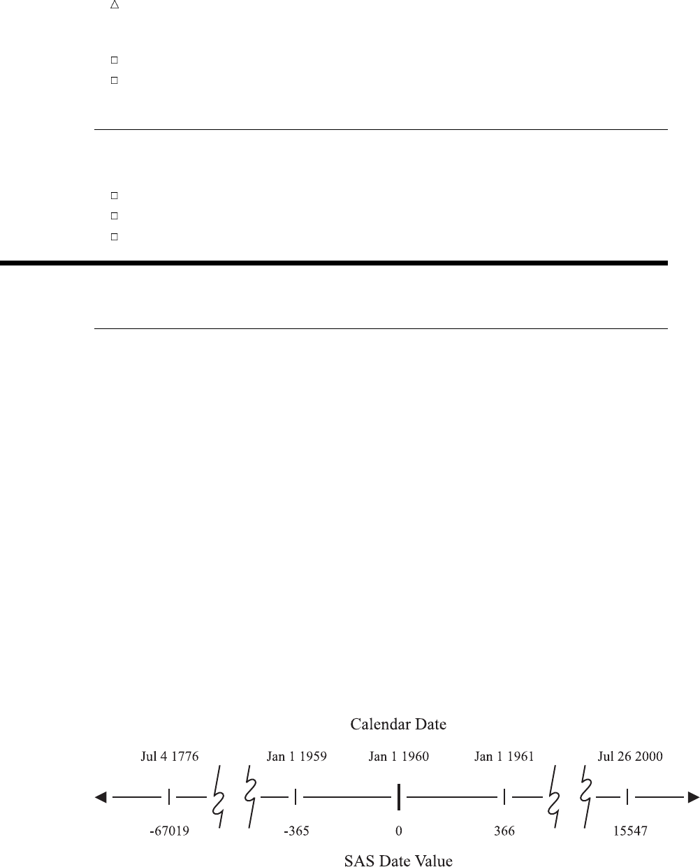
212 Prerequisites Chapter 14
indicate which calendar form SAS should use to display SAS date values
calculate with dates, that is, determine the number of days between dates, find the
day of the week on which a date falls, and use today’s date in calculations
Prerequisites
You should understand the following topics before proceeding with this section:
Chapter 6, “Understanding DATA Step Processing,” on page 97
Chapter 10, “Creating Subsets of Observations,” on page 159
Chapter 11, “Working with Grouped or Sorted Observations,” on page 173
Understanding How SAS Handles Dates
How SAS Stores Date Values
Dates are written in many different ways. Some dates contain only numbers, while
others contain various combinations of numbers, letters, and characters. For example,
all the following forms represent the date July 26, 2000:
072600 26JUL00 002607
7/26/00 26JUL2000 July 26, 2000
With so many different forms of dates, there must be some common ground, a way to
store dates and use them in calculations, regardless of how dates are entered or
displayed.
The common ground that SAS uses to represent dates is called a SAS date value.No
matter which form you use to write a date, SAS can convert and store that date as the
number of days between January 1, 1960, and the date that you enter. The following
figure shows some dates written in calendar form and as SAS date values:
Figure 14.1 Comparing Calendar Dates to SAS Date Values
In SAS, every date is a unique number on a number line. Dates before January 1,
1960, are negative numbers; those after January 1, 1960, are positive. Because SAS
date values are numeric variables, you can sort them easily, determine time intervals,
and use dates as constants, as arguments in SAS functions, or in calculations.
Working with Dates in the SAS System Input File and SAS Data Set for Examples 213
Note: SAS date values are valid for dates based on the Gregorian calendar from
A.D. 1582 through A.D. 19,900. Use caution when working with historical dates.
Although the Gregorian calendar was used throughout most of Europe from 1582, Great
Britain and the American colonies did not adopt the calendar until 1752.
Determining the Century for Dates with Two-Digit Years
If dates in your external data sources or SAS program statements contain two-digit
years, then you can determine which century prefix should be assigned to them by using
the YEARCUTOFF= system option. The YEARCUTOFF= system option specifies the
first year of the 100-year span that is used to determine the century of a two-digit year.
Before you use the YEARCUTOFF= system option, examine the dates in your data:
If the dates in your data fall within a 100-year span, then you can use the
YEARCUTOFF= system option.
If the dates in your data do not fall within a 100-year span, then you must either
convert the two-digit years to four-digit years or use a DATA step with conditional
logic to assign the proper century prefix.
After you have determined that the YEARCUTOFF= system option is appropriate for
your range of data, you can determine the setting to use. The best setting for
YEARCUTOFF= is the year before the lowest year in your data. For example, if you
have data in a range from 1921 to 2001, then set YEARCUTOFF= to 1920, if that is not
already your system default. The result of setting YEARCUTOFF= to 1920 is that
SAS interprets all two-digit dates in the range of 20 through 99 as 1920 through
1999.
SAS interprets all two-digit dates in the range of 00 through 19 as 2000 through
2019.
With YEARCUTOFF= set to 1920, a two-digit year of 10 would be interpreted as
2010 and a two-digit year of 22 would be interpreted as 1922.
Input File and SAS Data Set for Examples
In the travel industry, some of the most important data about a tour includes dates,
when the tour leaves and returns, when payments are due, when refunds are allowed,
and so on. Tradewinds Travel has data that contains dates of past and upcoming
popular tours as well as the number of nights spent on the tour. The raw data is stored
in an external file that looks like this:
uvw
Japan 13may2000 8
Greece 17oct99 12
New Zealand 03feb2001 16
Brazil 28feb2001 8
Venezuela 10nov00 9
Italy 25apr2001 8
USSR 03jun1997 14
Switzerland 14jan2001 9
Australia 24oct98 12
Ireland 27aug2000 7
The numbered fields represent
uthe name of the country toured

214 Entering Dates Chapter 14
vthe departure date
wthe number of nights on the tour
Entering Dates
Understanding Informats for Date Values
In order for SAS to read a value as a SAS date value, you must give it a set of
directions called an informat. By default, SAS reads numeric variables with a standard
numeric informat that does not include letters or special characters. When a field that
contains data does not match the standard patterns, you specify the appropriate
informat in the INPUT statement.
SAS provides many informats. Four informats that are commonly used to read date
values are:
MMDDYY8. reads dates written as mm/dd/yy.
MMDDYY10. reads dates written as mm/dd/yyyy.
DATE7. reads dates in the form ddMMMyy.
DATE9. reads dates in the form ddMMMyyyy.
Note that each informat name ends with a period and contains a width specification
that tells SAS how many columns to read.
Reading a Date Value
To create a SAS data set for the Tradewinds Travel data, the DATE9. informat is
used in the INPUT statement to read the variable DepartureDate.
input Country $ 1-11 @13 DepartureDate date9. Nights;
Using an informat in the INPUT statement is called formatted input. The formatted
input in this example contains the following items:
a pointer to indicate the column in which the value begins (@13)
the name of the variable to be read (DepartureDate)
the name of the informat to use (DATE9.)
The following DATA step creates MYLIB.TOURDATES using the DATE9. informat
to create SAS date values:
options yearcutoff=1920 pagesize=60 linesize=80 pageno=1 nodate;
libname mylib ’permanent-data-library’;
data mylib.tourdates;
infile ’input-file’;
input Country $ 1-11 @13 DepartureDate date9. Nights;
run;
proc print data=mylib.tourdates;
title ’Tour Departure Dates as SAS Date Values’;
run;
The following output displays the results:

Working with Dates in the SAS System Using Good Programming Practices to Read Dates 215
Output 14.1 Creating SAS Date Values from Calendar Dates
Tour Departure Dates as SAS Date Values 1
Departure
Obs Country Date Nights
1 Japan 14743 8
2 Greece 14534 12
3 New Zealand 15009 16
4 Brazil 15034 8
5 Venezuela 14924 9
6 Italy 15090 8
7 Russia 13668 14
8 Switzerland 14989 9
9 Australia 14176 12
10 Ireland 14849 7
Compare the SAS values of the variable DepartureDate with the values of the raw
data shown in the previous section. The data set MYLIB.TOURDATES shows that SAS
read the departure dates and created SAS date values. Now you need a way to display
the dates in a recognizable form.
Using Good Programming Practices to Read Dates
When reading dates, it is good programming practice to always use the DATE9. or
MMDDYY10. informats to be sure that the data is read correctly. If you use the
DATE7. or MMDDYY8. informat, then SAS reads only the first two digits of the year.
If the data contains four-digit years, then SAS reads the century and not the year.
Consider the Tradewinds Travel external file with both two-digit years and four-digit
years:
Japan 13may2000 8
Greece 17oct99 12
New Zealand 03feb2001 16
Brazil 28feb2001 8
Venezuela 10nov00 9
Italy 25apr2001 8
USSR 03jun1997 14
Switzerland 14jan2001 9
Australia 24oct98 12
Ireland 27aug2000 7
The following DATA step creates a SAS data set MYLIB.TOURDATES7 by using the
DATE7. informat:
options yearcutoff=1920 pagesize=60 linesize=80 pageno=1 nodate;
data mylib.tourdates7;
infile ’input-file’;
input Country $ 1-11 @13 DepartureDate date7. Nights;
run;
proc print data=mylib.tourdates7;
title ’Tour Departure Dates Using the DATE7. Informat’;

216 Using Good Programming Practices to Read Dates Chapter 14
title2 ’Displayed as Two-Digit Calendar Dates’;
format DepartureDate date7.;
run;
proc print data=mylib.tourdates7;
title ’Tour Departure Dates Using the DATE7. Informat’;
title2 ’Displayed as Four-Digit Calendar Dates’;
format DepartureDate date9.;
run;
The PRINT procedures format DepartureDate using two-digit year (DATE7.) and
four-digit year (DATE9.) calendar dates. The following output displays the results:
Output 14.2 Using the Wrong Informat Can Produce Invalid SAS Data Sets
Tour Departure Dates Using the DATE7. Informat 1
Displayed as Two-Digit Calendar Dates
Departure
Obs Country Date Nights
uv
1 Japan 13MAY20 0
2 Greece 17OCT99 12
3 New Zealand 03FEB20 1
4 Brazil 28FEB20 1
5 Venezuela 10NOV00 9
6 Italy 25APR20 1
7 Russia 03JUN19 97
8 Switzerland 14JAN20 1
9 Australia 24OCT98 12
10 Ireland 27AUG20 0
Tour Departure Dates Using the DATE7. Informat 2
Displayed as Four-Digit Calendar Dates
Departure
Obs Country Date Nights
w
1 Japan 13MAY1920 0
2 Greece 17OCT1999 12
3 New Zealand 03FEB1920 1
4 Brazil 28FEB1920 1
5 Venezuela 10NOV2000 9
6 Italy 25APR1920 1
7 Russia 03JUN2019 97
8 Switzerland 14JAN1920 1
9 Australia 24OCT1998 12
10 Ireland 27AUG1920 0
Notice that the four-digit years in the input file do not match the years in
MYLIB.TOURDATES7 for observations 1, 3, 4, 6, 7, 8, and 10:
uSAS stopped reading the date after seven characters; it read the first two digits,
the century, and not the complete four-digit year.
vTo read the data for the next variable, SAS moved the pointer one column and
read the next two numeric characters (the years 00, 01, and 97) as the value for
the variable Nights. The data for Nights in the input file was ignored.
wWhen the dates were formatted for four-digit calendar dates, SAS used the
YEARCUTOFF= 1920 system option to determine the century for the two-digit

Working with Dates in the SAS System Understanding How SAS Displays Values 217
year. What was originally 1997 in observation 7 became 2019, and what was
originally 2000 and 2001 in observations 1, 3, 4, 6, 8, and 10 became 1920.
Using Dates as Constants
If the tour of Switzerland leaves on January 21, 2001 instead of January 14, then
you can use the following assignment statement to make the update:
if Country = ’Switzerland’ then DepartureDate = ’21jan2001’d;
The value ’21jan2001’D is a SAS date constant. To write a SAS date constant, enclose
a date in quotation marks in the standard SAS form ddMMMyyyy and immediately
follow the final quotation mark with the letter D. The D suffix tells SAS to convert the
calendar date to a SAS date value. The following DATA step includes the use of the
SAS date constant:
options pagesize=60 linesize=80 pageno=1 nodate;
data correctdates;
set mylib.tourdates;
if Country = ’Switzerland’ then DepartureDate = ’21jan2001’d;
run;
proc print data=correctdates;
title ’Corrected Departure Date for Switzerland’;
format DepartureDate date9.;
run;
The following output displays the results:
Output 14.3 Changing a Date by Using a SAS Date Constant
Corrected Departure Date for Switzerland 1
Departure
Obs Country Date Nights
1 Japan 13MAY2000 8
2 Greece 17OCT1999 12
3 New Zealand 03FEB2001 16
4 Brazil 28FEB2001 8
5 Venezuela 10NOV2000 9
6 Italy 25APR2001 8
7 Russia 03JUN1997 14
8 Switzerland 21JAN2001 9
9 Australia 24OCT1998 12
10 Ireland 27AUG2000 7
Displaying Dates
Understanding How SAS Displays Values
To understand how to display the departure dates, you need to understand how SAS
displays values in general. SAS displays all data values with a set of directions called a
format. By default, SAS uses a standard numeric format with no commas, letters, or

218 Formatting a Date Value Chapter 14
other special notation to display the values of numeric variables. Output 14.1 shows
that printing SAS date values with the standard numeric format produces numbers
that are difficult to recognize. To display these numbers as calendar dates, you need to
specify a SAS date format for the variable.
SAS date formats are available for the most common ways of writing calendar dates.
The DATE9. format represents dates in the form ddMMMyyyy. If you want the month,
day, and year to be spelled out, then use the WORDDATE18. format. The
WEEKDATE29. format includes the day of the week. There are also formats available
for number representations such as the format MMDDYY8., which displays the
calendar date in the form mm/dd/yy, or the format MMDDYY10., which displays the
calendar date in the form mm/dd/yyyy. Like informat names, each format name ends
with a period and contains a width specification that tells SAS how many columns to
use when displaying the date value.
Formatting a Date Value
You tell SAS which format to use by specifying the variable and the format name in
a FORMAT statement. The following FORMAT statement assigns the MMDDYY10.
format to the variable DepartureDate:
format DepartureDate mmddyy10.;
In this example, the FORMAT statement contains the following items:
the name of the variable (DepartureDate)
the name of the format to be used (MMDDYY10.)
The following PRINT procedures format the variable DepartureDate in both the
two-digit year calendar format and the four-digit year calendar format:
options pagesize=60 linesize=80 pageno=1 nodate;
proc print data=mylib.tourdates;
title ’Departure Dates in Two-Digit Calendar Format’;
format DepartureDate mmddyy8.;
run;
proc print data=mylib.tourdates;
title ’Departure Dates in Four-Digit Calendar Format’;
format DepartureDate mmddyy10.;
run;
The following output displays the results:
Output 14.4 Displaying a Formatted Date Value
Departure Dates in Two-Digit Calendar Format 1
Departure
Obs Country Date Nights
1 Japan 05/13/00 8
2 Greece 10/17/99 12
3 New Zealand 02/03/01 16
4 Brazil 02/28/01 8
5 Venezuela 11/10/00 9
6 Italy 04/25/01 8
7 Russia 06/03/97 14
8 Switzerland 01/14/01 9
9 Australia 10/24/98 12
10 Ireland 08/27/00 7

Working with Dates in the SAS System Assigning Permanent Date Formats to Variables 219
Departure Dates in Four-Digit Calendar Format 2
Departure
Obs Country Date Nights
1 Japan 05/13/2000 8
2 Greece 10/17/1999 12
3 New Zealand 02/03/2001 16
4 Brazil 02/28/2001 8
5 Venezuela 11/10/2000 9
6 Italy 04/25/2001 8
7 Russia 06/03/1997 14
8 Switzerland 01/14/2001 9
9 Australia 10/24/1998 12
10 Ireland 08/27/2000 7
Placing a FORMAT statement in a PROC step associates the format with the
variable only for that step. To associate a format with a variable permanently, use the
FORMAT statement in a DATA step.
Assigning Permanent Date Formats to Variables
The next example creates a new permanent SAS data set and assigns the DATE9.
format in the DATA step. Now all subsequent procedures and DATA steps that use the
variable DepartureDate will use the DATE9. format by default. The PROC
CONTENTS step displays the characteristics of the data set MYLIB.TOURDATE.
options yearcutoff=1920 pagesize=60 linesize=80 pageno=1 nodate;
data mylib.fmttourdate;
set mylib.tourdates;
format DepartureDate date9.;
run;
proc contents data=mylib.fmttourdate nodetails;
run;
The following output shows that the DATE9. format is permanently associated with
DepartureDate:

220 Changing Formats Temporarily Chapter 14
Output 14.5 Assigning a Format in a DATA Step
The SAS System 1
The CONTENTS Procedure
Data Set Name: MYLIB.FMTTOURDATE Observations: 10
Member Type: DATA Variables: 3
Engine: V8 Indexes: 0
Created: 14:15 Friday, November 19, 1999 Observation Length: 32
Last Modified: 14:15 Friday, November 19, 1999 Deleted Observations: 0
Protection: Compressed: NO
Data Set Type: Sorted: NO
Label:
-----Engine/Host Dependent Information-----
Data Set Page Size: 8192
Number of Data Set Pages: 1
First Data Page: 1
Max Obs per Page: 254
Obs in First Data Page: 10
Number of Data Set Repairs: 0
filename: /SAS_DATA_LIBRARY/fmttourdate.sas7bdat
Release Created: 8.0001M0
Host Created: HP-UX
Inode Number: 1498874206
Access Permission: rw-r--r--
Owner Name: user01
File Size (bytes): 16384
-----Alphabetic List of Variables and Attributes-----
# Variable Type Len Pos Format
--------------------------------------------------
1 Country Char 11 16
2 DepartureDate Num 8 0 DATE9.
3 Nights Num 8 8
Changing Formats Temporarily
If you are preparing a report that requires the date in a different format, then you
can override the permanent format by using a FORMAT statement in a PROC step. For
example, to display the value for DepartureDate in the data set MYLIB.TOURDATES
in the form of month-name dd, yyyy, you can issue a FORMAT statement in a PROC
PRINT step. The following program specifies the WORDDATE18. format for the
variable DepartureDate:
options pagesize=60 linesize=80 pageno=1 nodate;
proc print data=mylib.tourdates;
title ’Tour Departure Dates’;
format DepartureDate worddate18.;
run;
The following output displays the results:

Working with Dates in the SAS System Sorting Dates 221
Output 14.6 Overriding a Previously Specified Format
Tour Departure Dates 1
Obs Country DepartureDate Nights
1 Japan May 13, 2000 8
2 Greece October 17, 1999 12
3 New Zealand February 3, 2001 16
4 Brazil February 28, 2001 8
5 Venezuela November 10, 2000 9
6 Italy April 25, 2001 8
7 Russia June 3, 1997 14
8 Switzerland January 14, 2001 9
9 Australia October 24, 1998 12
10 Ireland August 27, 2000 7
The format DATE9. is still permanently assigned to DepartureDate. Calendar dates
in the remaining examples are in the form ddMMMyyyy unless a FORMAT statement is
included in the PROC PRINT step.
Using Dates in Calculations
Sorting Dates
Because SAS date values are numeric variables, you can sort them and use them in
calculations. The following example uses the data set MYLIB.TOURDATES to extract
other information about the Tradewinds Travel data.
To help determine how frequently tours are scheduled, you can print a report with
the tours listed in chronological order. The first step is to specify the following BY
statement in a PROC SORT step to tell SAS to arrange the observations in ascending
order of the date variable DepartureDate:
by DepartureDate;
By using a VAR statement in the following PROC PRINT step, you can list the
departure date as the first column in the report:
options pagesize=60 linesize=80 pageno=1 nodate;
proc sort data=mylib.fmttourdate out=sortdate;
by DepartureDate;
run;
proc print data=sortdate;
var DepartureDate Country Nights;
title ’Departure Dates Listed in Chronological Order’;
run;
The following output displays the results:

222 Creating New Date Variables Chapter 14
Output 14.7 Sorting by SAS Date Values
Departure Dates Listed in Chronological Order 1
Departure
Obs Date Country Nights
1 03JUN1997 Russia 14
2 24OCT1998 Australia 12
3 17OCT1999 Greece 12
4 13MAY2000 Japan 8
5 27AUG2000 Ireland 7
6 10NOV2000 Venezuela 9
7 14JAN2001 Switzerland 9
8 03FEB2001 New Zealand 16
9 28FEB2001 Brazil 8
10 25APR2001 Italy 8
The observations in the data set SORTDATE are now arranged in chronological
order. Note that there are no FORMAT statements in this example, so the dates are
displayed in the DATE9. format you assigned to DepartureDate when you created the
data set MYLIB.FMTTOURDATE.
Creating New Date Variables
Because you know the departure date and the number of nights spent on each tour,
you can calculate the return date for each tour. To start, create a new variable by
adding the number of nights to the departure date, as follows:
Return = DepartureDate + Nights;
The result is a SAS date value for the return date that you can display by assigning
it the DATE9. format, as follows:
options yearcutoff=1920 pagesize=60 linesize=80 pageno=1 nodate;
data home;
set mylib.tourdates;
Return = DepartureDate + Nights;
format Return date9.;
run;
proc print data=home;
title ’Dates of Departure and Return’;
run;
Working with Dates in the SAS System Finding the Day of the Week 223
Output 14.8 Adding Days to a Date Value
Dates of Departure and Return 1
Departure
Obs Country Date Nights Return
1 Japan 14743 8 21MAY2000
2 Greece 14534 12 29OCT1999
3 New Zealand 15009 16 19FEB2001
4 Brazil 15034 8 08MAR2001
5 Venezuela 14924 9 19NOV2000
6 Italy 15090 8 03MAY2001
7 Russia 13668 14 17JUN1997
8 Switzerland 14989 9 23JAN2001
9 Australia 14176 12 05NOV1998
10 Ireland 14849 7 03SEP2000
Note that because the variable DepartureDate in the data set MYLIB.TOURDATES
has no permanent format, you see a numeric value instead of a readable calendar date
for that variable.
Using SAS Date Functions
Finding the Day of the Week
SAS has various functions that produce calendar dates from SAS date values. SAS
date functions enable you to do such things as derive partial date information or use
the current date in calculations.
If the final payment for a tour is due 30 days before the tour leaves, then the final
payment date can be calculated using subtraction; however, Tradewinds Travel is closed
on Sundays. If the payment is due on a Sunday, then an additional day must be
subtracted to make the payment due on Saturday. The WEEKDAY function, which
returns the day of the week as a number from 1 through 7 (Sunday through Saturday)
can be used to determine if the return day is a Sunday.
The following statements determine the final payment date by
subtracting 30 from the departure date
checking the value returned by the WEEKDAY function
subtracting an additional day if necessary
DueDate = DepartureDate - 30;
if Weekday(DueDate) = 1 then DueDate = DueDate - 1;
Constructing a data set with these statements produces a list of payment due dates.
The following program includes these statements and assigns the format
WEEKDATE29. to the new variable DueDate:
options yearcutoff=1920 pagesize=60 linesize=80 pageno=1 nodate;
data pay;
set mylib.tourdates;
DueDate = DepartureDate - 30;
if Weekday(DueDate) = 1 then DueDate = DueDate - 1;
224 Calculating a Date from Today Chapter 14
format DueDate weekdate29.;
run;
proc print data=pay;
var Country DueDate;
title ’Date and Day of Week Payment Is Due’;
run;
Output 14.9 Using the WEEKDAY Function
Date and Day of Week Payment Is Due 1
Obs Country DueDate
1 Japan Thursday, April 13, 2000
2 Greece Friday, September 17, 1999
3 New Zealand Thursday, January 4, 2001
4 Brazil Monday, January 29, 2001
5 Venezuela Wednesday, October 11, 2000
6 Italy Monday, March 26, 2001
7 Russia Saturday, May 3, 1997
8 Switzerland Friday, December 15, 2000
9 Australia Thursday, September 24, 1998
10 Ireland Friday, July 28, 2000
Calculating a Date from Today
Tradewinds Travel occasionally gets the opportunity to do special advertising
promotions. In general, tours that depart more than 90 days from today’s date, but less
than 180 days from today’s date, are advertised. The following figure illustrates the
time frame for advertising:
Figure 14.2 Optimum Interval for Advertising Tours Based on Today’s Date
A program is needed that determines which tours leave between 90 and 180 days
from the date the program is run, regardless of when you run the program.
The TODAY function produces a SAS date value that corresponds to the date when
the program is run. The following statements determine which tours depart at least 90
days from today’s date but not more than 180 days from now:
Now = today();
if Now + 90 <= DepartureDate <= Now + 180;

Working with Dates in the SAS System Comparing Durations and SAS Date Values 225
To print the value that is returned by the TODAY function, this example creates a
variable that is equal to the value returned by the TODAY function. This step is not
necessary but is used here to clarify the program. You can also use the function as part
of the program statement.
if today() + 90 <= DepartureDate <= today() + 180;
The following program uses the TODAY function to determine which tours to
advertise:
options yearcutoff=1920 pagesize=60 linesize=80 pageno=1 nodate;
data ads;
set mylib.tourdates;
Now = today();
if Now + 90 <= DepartureDate <= Now + 180;
run;
proc print data=ads;
title ’Tours Departing between 90 and 180 Days from Today’;
format DepartureDate Now date9.;
run;
The following output displays the results:
Output 14.10 Using the Current Date as a SAS Date Value
Tours Departing between 90 and 180 Days from Today 1
Departure
Obs Country Date Nights Now
1 Japan 13MAY2000 8 23NOV1999
Note that the PROC PRINT step contains a FORMAT statement that temporarily
assigns the format DATE9. to the variables DepartureDate and Now.
Comparing Durations and SAS Date Values
You can use SAS date values to find the units of time between dates. Tradewinds
Travel was founded on February 8, 1982. On November 23, 1999, you decide to find out
how old Tradewinds Travel is, and you write the following program:
options yearcutoff=1920 pagesize=60 linesize=80 pageno=1 nodate;
/* Calculating a duration in days */
data ttage;
Start = ’08feb82’d;
RightNow = today();
Age = RightNow - Start;
format Start RightNow date9.;
run;
proc print data=ttage;
title ’Age of Tradewinds Travel’;
run;

226 Comparing Durations and SAS Date Values Chapter 14
Output 14.11 Calculating a Duration in Days
Age of Tradewinds Travel 1
Obs Start RightNow Age
1 08FEB1982 23NOV1999 6497
The value of Age is 6497, a number that looks like an unformatted SAS date value.
However, Age is actually the difference between February 8, 1982, and November 23,
1999, and represents a duration in days, not a SAS date value. To make the value of
Age more understandable, divide the number of days by 365 (more precisely, 365.25) to
produce a duration in years. The following DATA step calculates the age of Tradewinds
Travel in years:
options yearcutoff=1920 pagesize=60 linesize=80 pageno=1 nodate;
/* Calculating a duration in years */
data ttage2;
Start = ’08feb82’d;
RightNow = today();
AgeInDays = RightNow - Start;
AgeInYears = AgeInDays / 365.25;
format AgeInYears 4.1 Start RightNow date9.;
run;
proc print data=ttage2;
title ’Age in Years of Tradewinds Travel’;
run;
The following output displays the results:
Output 14.12 Calculating a Duration in Years
Age in Years of Tradewinds Travel 1
Age Age
In In
Obs Start RightNow Days Years
1 08FEB1982 23NOV1999 6497 17.8
To show a portion of a year, the value for AgeInYears is assigned a numeric format of
4.1 in the FORMAT statement of the DATA step. The 4 tells SAS that the number
contains up to four characters. The 1 tells SAS that the number includes one digit after
the decimal point.

Working with Dates in the SAS System Functions 227
Review of SAS Tools
Statements
date-variable=’ddMMMyy’D;
is an assignment statement that tells SAS to convert the date in quotation marks
to a SAS date value and assign it to date-variable. The SAS date constant
’ddMMMyy’D specifies a particular date, for example, ’23NOV00’D, and can be
used in many SAS statements and expressions, not only assignment statements.
FORMAT date-variable date-format;
tells SAS to format the values of the date-variable using the date-format.A
FORMAT statement within a DATA step permanently associates a format with a
date-variable.
INPUT date-variable date-informat;
tells SAS how to read the values for the date-variable from an external file. The
date-informat is an instruction that tells SAS the form of the date in the external
file.
Formats and Informats for Dates
DATE9.
the form of the date-variable is ddMMMyyyy, for example 23NOV2000.
DATE7.
the form of the date-variable is ddMMMyy, for example 23NOV00.
MMDDYY10.
the form of the date-variable is mm/dd/yyyy, for example, 11/23/2000.
MMDDYY8.
the form of the date-variable is mm/dd/yy, for example, 11/23/00.
WORDDATE18.
the form of the date-variable is month-name dd, yyyy, for example, November 23,
2000.
WEEKDATE29.
the form of the date-variable is day-of-the-week, month-name dd, yyyy, for example,
Thursday, November 23, 2000.
Functions
WEEKDAY (SAS-date-value)
is a function that returns the day of the week on which the SAS-date-value falls as
a number 1 through 7, with Sunday assigned the value 1.
TODAY()
is a function that returns a SAS date value corresponding to the date on which the
SAS program is initiated.
228 System Options Chapter 14
System Options
YEARCUTOFF=
specifies the first year of a 100-year span that is used by informats and functions
to read two-digit years, and used by formats to display two-digit years. The value
that is specified in YEARCUTOFF= can result in a range of years that span two
centuries. If YEARCUTOFF=1950, then any two-digit value between 50 and 99
inclusive refers to the first half of the 100-year span, which is in the 1900s. Any
two-digit value between 00 and 49 inclusive refers to the second half of the
100-year span, which is in the 2000s. YEARCUTOFF= has no effect on existing
SAS dates or dates that are read from input data that include a four-digit year.
Learning More
ATTRIB statement
Information about using the ATTRIB statement to assign or change a permanent
format can be found in SAS Language Reference: Dictionary.
DATASETS procedure
To assign or change a variable to a permanent format see the DATASETS
procedure in Chapter 34, “Managing SAS Data Libraries,” on page 603.
PUT and INPUT functions
The PUT and INPUT functions can be used for correcting two common errors in
working with SAS dates: treating date values that contain letters or symbols as
character variables or storing dates written as numbers as ordinary numeric
variables. Neither method enables you to use dates in calculations. Information
about these functions can be found in SAS Language Reference: Dictionary.
SAS date values
Documentation on informats, formats, and functions for working with SAS date
values, SAS time, and SAS datetime values can be found in SAS Language
Reference: Concepts. This documentation includes the following date and time
information:
SAS stores a time as the number of seconds since midnight of the current
day. For example, 9:30 am. is 34200. A number of this type is known as a
SAS time value. A SAS time value is independent of the date; the count
begins at 0 each midnight.
When a date and a time are both present, SAS stores the value as the
number of seconds since midnight, January 1, 1960. For example, 9:30 am,
November 23, 2000, is 1290591000. This type of number is known as a SAS
datetime value.
SAS date and time informats read fields of different widths. SAS date and
time formats can display date variables in different ways according to the
widths that you specify in the format name. The number at the end of the
format or informat name indicates the number of columns that SAS can use.
For example, the DATE9. informat reads up to nine columns (as in
23NOV2000). The WEEKDATE8. format displays eight columns, as in
Thursday, and WEEKDATE27. displays 27 columns, as in Thursday,
November 23, 2000.

Working with Dates in the SAS System Learning More 229
SAS provides date, time, and datetime intervals for counting different periods
of elapsed time, such as MONTH, which represents an interval from the
beginning of one month to the next, not a period of 30 or 31 days.
International date, time, and datetime formats.
SYSDATE9
To include the current date in a title, you can use the macro variable SYSDATE9,
which is explained in Chapter 25, “Producing Detail Reports with the PRINT
Procedure,” on page 371.
230

231
PART
4
Combining SAS Data Sets
Chapter 15.........
Methods of Combining SAS Data Sets 233
Chapter 16.........
Concatenating SAS Data Sets 241
Chapter 17.........
Interleaving SAS Data Sets 263
Chapter 18.........
Merging SAS Data Sets 269
Chapter 19.........
Updating SAS Data Sets 293
Chapter 20.........
Modifying SAS Data Sets 311
Chapter 21.........
Conditionally Processing Observations from Multiple SAS
Data Sets 323
232
233
CHAPTER
15
Methods of Combining SAS Data
Sets
Introduction to Combining SAS Data Sets 233
Purpose 233
Prerequisites 233
Definition of Concatenating 234
Definition of Interleaving 234
Definition of Merging 235
Definition of Updating 236
Definition of Modifying 237
Comparing Modifying, Merging, and Updating Data Sets 238
Learning More 239
Introduction to Combining SAS Data Sets
Purpose
SAS provides several different methods for combining SAS data sets. In this section,
you will be introduced to five methods of combining data sets:
concatenating
interleaving
merging
updating
modifying
Subsequent sections teach you how to use these methods.
Prerequisites
Before continuing with this section, you should understand the concepts presented in
the following sections:
Chapter 2, “Introduction to DATA Step Processing,” on page 19
Chapter 5, “Starting with SAS Data Sets,” on page 81
Chapter 6, “Understanding DATA Step Processing,” on page 97
234 Definition of Concatenating Chapter 15
Definition of Concatenating
Concatenating combines two or more SAS data sets, one after the other, into a single
SAS data set. You concatenate data sets using either the SET statement in a DATA
step or the APPEND procedure. The following figure shows the results of concatenating
two SAS data sets, and the DATA step that produces the results.
Figure 15.1 Concatenating Two SAS Data Sets
COMBINED
Year
DATA2
1996
1997
1998
1999
2000
Year
DATA1
Year
1996
1997
1998
1999
2000
data combined;
set data1 data2;
run;
+=
1996
1997
1998
1999
2000
1996
1997
1998
1999
2000
Definition of Interleaving
Interleaving combines individual, sorted SAS data sets into one sorted SAS data set.
For each observation, the following figure shows the value of the variable by which the
data sets are sorted. (In this example, the data sets are sorted by the variable Year.)
You interleave data sets using a SET statement along with a BY statement.
Methods of Combining SAS Data Sets Definition of Merging 235
Figure 15.2 Interleaving SAS Data Sets
COMBINED
Year
DATA2
1996
1997
1998
1999
2000
Year
DATA1
Year
1995
1996
1997
1998
1999
data combined;
set data1 data2;
by Year;
run;
+=
1995
1996
1996
1997
1997
1998
1998
1999
1999
2000
Definition of Merging
Merging combines observations from two or more SAS data sets into a single
observation in a new data set.
Aone-to-one merge, shown in the following figure, combines observations based on
their position in the data sets. You use the MERGE statement for one-to-one merging.
Figure 15.3 One-to-One Merging
X1
X2
X3
X4
X5
Y1
Y2
Y3
Y4
Y5
+=
data combined;
merge data1 data2;
run;
X1
X2
X3
X4
X5
Y1
Y2
Y3
Y4
Y5
VarYVarX
DATA1 DATA2 COMBINED
VarX VarY
Amatch-merge, shown in the following figure, combines observations based on the
values of one or more common variables. If you are performing a match-merge, then
use the MERGE statement along with a BY statement. (In this example, two data sets
are match-merged by the value of the variable Year.)
236 Definition of Updating Chapter 15
Figure 15.4 Match-Merging Two SAS Data Sets
data combined;
merge data1 data2;
by Year;
run;
+=
COMBINED
1996
1996
1997
1998
1999
2000
Year
X1
X1
X2
X3
X4
X5
Y1
Y2
Y3
Y4
Y5
VarYVarX
DATA2
1996
1996
1998
1999
2000
VarYYear
Y1
Y2
Y3
Y4
Y5
DATA1
VarX
X1
X2
X3
X4
X5
Year
1996
1997
1998
1999
2000
Definition of Updating
Updating a SAS data set replaces the values of variables in one data set (the master
data set) with values from another data set (the transaction data set). If the
UPDATEMODE= option in the UPDATE statement is set to MISSINGCHECK, then
missing values in a transaction data set do not replace existing values in a master data
set. If the UPDATEMODE= option is set to NOMISSINGCHECK, then missing values
in a transaction data set replace existing values in a master data set. The default
setting is MISSINGCHECK.
You update a data set by using the UPDATE statement along with a BY statement.
Both of the input data sets must be sorted by the variable that you use in the BY
statement. The following figure shows the results of updating a SAS data set.
Methods of Combining SAS Data Sets Definition of Modifying 237
Figure 15.5 Updating a Master Data Set
data master;
update master transaction;
by Year;
run;
+=
MASTER
X1
X1
X1
X1
X1
X1
X2
X2
X2
X1
X2
1990
1991
1992
1993
1994
1995
1996
1997
1998
1999
2000
Y1
Y1
Y1
Y1
Y1
Y1
Y1
Y2
Y2
Y1
Y2
Year VarYVarX
Y1
Y1
Y1
Y1
Y1
Y1
Y1
Y1
Y1
Y1
MASTER
VarXYear VarY
X1
X1
X1
X1
X1
X1
X1
X1
X1
X1
1990
1991
1992
1993
1994
1995
1996
1997
1998
1999
TRANSACTION
1996
1997
1998
1998
2000
Y2
Y2
Y2
X2
X2
X2
X2
VarXYearear VarY
Definition of Modifying
Modifying a SAS data set replaces, deletes, or appends observations in an existing
data set. Modifying a SAS data set is similar to updating a SAS data set, but the
following differences exist:
Modifying cannot create a new data set, while updating can.
Unlike updating, modifying does not require that the master data set or the
transaction data set be sorted.
You change an existing file by using the MODIFY statement along with a BY
statement. The following figure shows the results.

238 Comparing Modifying, Merging, and Updating Data Sets Chapter 15
Figure 15.6 Modifying a Data Set
data master;
modify master transaction;
by Year;
run;
+=
MASTER
Year VarYVarX
X1
X1
X1
X1
X1
X1
X2
X2
X2
X2
1991
1992
1993
1994
1995
1996
1997
1998
1999
2000
Y1
Y1
Y1
Y1
Y1
Y1
Y1
Y2
Y2
Y2
MASTER
VarXYear VarY
Y1
Y1
Y1
Y1
Y1
Y1
Y1
Y1
Y1
Y1
X1
X1
X1
X1
X1
X1
X1
X1
X1
X1
1991
1992
1993
1994
1995
1996
1997
1998
1999
2000
TRANSACTION
VarXYearear VarY
1999
1999
1997
2000
1998
Y2
Y2
Y2
X2
X2
X2
X2
Comparing Modifying, Merging, and Updating Data Sets
The table that follows summarizes several differences among the MERGE, UPDATE,
and MODIFY statements.
Criterion MERGE UPDATE MODIFY
Data sets must be
sorted or indexed
Match-merge: Yes
One-to-one merge: No
Yes No
BY values must be
unique
No Master data set: Yes
Transaction data set: No
No
Can create or delete
variables
Yes Yes No
Methods of Combining SAS Data Sets Learning More 239
Criterion MERGE UPDATE MODIFY
Number of data sets
combined
Any number 2 2
Processing missing
values
Overwrites nonmissing
values from first data
set with missing values
from second data set
Default behavior: missing
values in the transaction
data set do not replace
values in the master data
set
Depends on the
value of the
UPDATEMODE=
option (see
“Comparing
Modifying,
Merging, and
Updating Data
Sets” on page 238)
Default:
MISSINGCHECK
Learning More
Concatenating data sets
For more information about concatenating data sets, see Chapter 16,
“Concatenating SAS Data Sets,” on page 241.
Interleaving data sets
For more information about interleaving data sets, see Chapter 17, “Interleaving
SAS Data Sets,” on page 263.
Manipulating data sets
You can manipulate data sets as you combine them. For example, you can select
certain observations from each data set and determine which data set an
observation came from. For more information, see Chapter 21, “Conditionally
Processing Observations from Multiple SAS Data Sets,” on page 323.
MERGE, MODIFY, and UPDATE statements
For more information about these statements, see the Statements section of SAS
Language Reference: Dictionary, and the Reading, Combining, and Modifying SAS
Data Sets section of SAS Language Reference: Concepts.
Merging data sets
For more information about merging data sets, see Chapter 18, “Merging SAS
Data Sets,” on page 269.
Modifying data sets
For more information about modifying data sets, see Chapter 20, “Modifying SAS
Data Sets,” on page 311, and Chapter 21, “Conditionally Processing Observations
from Multiple SAS Data Sets,” on page 323.
Updating data sets
For more information about updating data sets, see Chapter 19, “Updating SAS
Data Sets,” on page 293.
240

241
CHAPTER
16
Concatenating SAS Data Sets
Introduction to Concatenating SAS Data Sets 241
Purpose 241
Prerequisites 242
Concatenating Data Sets with the SET Statement 242
Understanding the SET Statement 242
Using the SET Statement: The Simplest Case 242
Using the SET Statement When Data Sets Contain Different Variables 244
Using the SET Statement When Variables Have Different Attributes 246
Understanding Attributes 246
Using the SET Statement When Variables Have Different Types 247
Changing the Type of a Variable 248
Using the SET Statement When Variables Have Different Formats, Informats, or
Labels 250
Using the SET Statement When Variables Have Different Lengths 253
Concatenating Data Sets Using the APPEND Procedure 255
Understanding the APPEND Procedure 255
Using the APPEND Procedure: The Simplest Case 256
Using the APPEND Procedure When Data Sets Contain Different Variables 257
Using the APPEND Procedure When Variables Have Different Attributes 258
Choosing between the SET Statement and the APPEND Procedure 259
Review of SAS Tools 260
Statements 260
Procedures 260
Learning More 260
Introduction to Concatenating SAS Data Sets
Purpose
Concatenating combines two or more SAS data sets, one after the other, into a single
data set. The number of observations in the new data set is the sum of the number of
observations in the original data sets.
You can concatenate SAS data sets by using
the SET statement in a DATA step
the APPEND procedure
If the data sets that you concatenate contain the same variables, and each variable has
the same attributes in all data sets, then the results of the SET statement and PROC
242 Prerequisites Chapter 16
APPEND are the same. In other cases, the results differ. In this section you will learn
both of these methods and their differences so that you can decide which one to use.
Prerequisites
Before continuing with this section, you should be familiar with the concepts
presented in Chapter 5, “Starting with SAS Data Sets,” on page 81 through Chapter 8,
“Working with Character Variables,” on page 119.
Concatenating Data Sets with the SET Statement
Understanding the SET Statement
The SET statement reads observations from one or more SAS data sets and uses
them to build a new data set.
The SET statement for concatenating data sets has the following form:
SET SAS-data-set(s);
where
SAS-data-set
is two or more SAS data sets to concatenate. The observations from the first data
set that you name in the SET statement appear first in the new data set. The
observations from the second data set follow those from the first data set, and so
on. The list can contain any number of data sets.
Using the SET Statement: The Simplest Case
In the simplest situation, the data sets that you concatenate contain the same
variables (variables with the same name). In addition, the type, length, informat,
format, and label of each variable match across all data sets. In this case, SAS copies
all observations from the first data set into the new data set, then copies all
observations from the second data set into the new data set, and so on. Each
observation is an exact copy of the original.
In the following example, a company that uses SAS to maintain personnel records for
six separate departments decided to combine all personnel records. Two departments,
Sales and Customer Support, store their data in the same form. Each observation in
both data sets contains values for these variables:
EmployeeID is a character variable that contains the employee’s identification
number.
Name is a character variable that contains the employee’s name in the
form last name, comma, first name.
HireDate is a numeric variable that contains the date the employee was hired.
This variable has a format of DATE9.
Salary is a numeric variable that contains the employee’s annual salary in
US dollars.
HomePhone is a character variable that contains the employee’s home telephone
number.

Concatenating SAS Data Sets Using the SET Statement: The Simplest Case 243
The following program creates the SAS data sets SALES and
CUSTOMER_SUPPORT:
options pagesize=60 linesize=80 pageno=1 nodate;
data sales;
input EmployeeID $ 1-9 Name $ 11-29 @30 HireDate date9.
Salary HomePhone $;
format HireDate date9.;
datalines;
429685482 Martin, Virginia 09aug1990 34800 493-0824
244967839 Singleton, MaryAnn 24apr1995 27900 929-2623
996740216 Leighton, Maurice 16dec1993 32600 933-6908
675443925 Freuler, Carl 15feb1998 29900 493-3993
845729308 Cage, Merce 19oct1992 39800 286-0519
;
proc print data=sales;
title ’Sales Department Employees’;
run;
data customer_support;
input EmployeeID $ 1-9 Name $ 11-29 @30 HireDate date9.
Salary HomePhone $;
format HireDate date9.;
datalines;
324987451 Sayre, Jay 15nov1994 44800 933-2998
596771321 Tolson, Andrew 18mar1998 41200 929-4800
477562122 Jensen, Helga 01feb1991 47400 286-2816
894724859 Kulenic, Marie 24jun1993 41400 493-1472
988427431 Zweerink, Anna 07jul1995 43700 929-3885
;
proc print data=customer_support;
title ’Customer Support Department Employees’;
run;
The following output shows the results of both DATA steps:
Output 16.1 The SALES and the CUSTOMER_SUPPORT Data Sets
Sales Department Employees 1
Employee Home
Obs ID Name HireDate Salary Phone
1 429685482 Martin, Virginia 09AUG1990 34800 493-0824
2 244967839 Singleton, MaryAnn 24APR1995 27900 929-2623
3 996740216 Leighton, Maurice 16DEC1993 32600 933-6908
4 675443925 Freuler, Carl 15FEB1998 29900 493-3993
5 845729308 Cage, Merce 19OCT1992 39800 286-0519

244 Using the SET Statement When Data Sets Contain Different Variables Chapter 16
Customer Support Department Employees 2
Employee Home
Obs ID Name HireDate Salary Phone
1 324987451 Sayre, Jay 15NOV1994 44800 933-2998
2 596771321 Tolson, Andrew 18MAR1998 41200 929-4800
3 477562122 Jensen, Helga 01FEB1991 47400 286-2816
4 894724859 Kulenic, Marie 24JUN1993 41400 493-1472
5 988427431 Zweerink, Anna 07JUL1995 43700 929-3885
To concatenate the two data sets, list them in the SET statement. Use the PRINT
procedure to display the resulting DEPT1_2 data set.
options pagesize=60 linesize=80 pageno=1 nodate;
data dept1_2;
set sales customer_support;
run;
proc print data=dept1_2;
title ’Employees in Sales and Customer Support Departments’;
run;
The following output shows the new DEPT1_2 data set. The data set contains all
observations from SALES followed by all observations from CUSTOMER_SUPPORT:
Output 16.2 The Concatenated DEPT1_2 Data Set
Employees in Sales and Customer Support Departments 1
Employee Home
Obs ID Name HireDate Salary Phone
1 429685482 Martin, Virginia 09AUG1990 34800 493-0824
2 244967839 Singleton, MaryAnn 24APR1995 27900 929-2623
3 996740216 Leighton, Maurice 16DEC1993 32600 933-6908
4 675443925 Freuler, Carl 15FEB1998 29900 493-3993
5 845729308 Cage, Merce 19OCT1992 39800 286-0519
6 324987451 Sayre, Jay 15NOV1994 44800 933-2998
7 596771321 Tolson, Andrew 18MAR1998 41200 929-4800
8 477562122 Jensen, Helga 01FEB1991 47400 286-2816
9 894724859 Kulenic, Marie 24JUN1993 41400 493-1472
10 988427431 Zweerink, Anna 07JUL1995 43700 929-3885
Using the SET Statement When Data Sets Contain Different Variables
The two data sets in the previous example contain the same variables, and each
variable is defined the same way in both data sets. However, you might want to
concatenate data sets when not all variables are common to the data sets that are
named in the SET statement. In this case, each observation in the new data set
includes all variables from the SAS data sets that are named in the SET statement.
The examples in this section show the SECURITY data set, and the concatenation of
this data set to the SALES and the CUSTOMER_SUPPORT data sets. Not all variables
are common to the three data sets. The personnel records for the Security department

Concatenating SAS Data Sets Using the SET Statement When Data Sets Contain Different Variables 245
do not include the variable HomePhone, and do include the new variable Gender, which
does not appear in the SALES or the CUSTOMER_SUPPORT data sets.
The following program creates the SECURITY data set:
options pagesize=60 linesize=80 pageno=1 nodate;
data security;
input EmployeeID $ 1-9 Name $ 11-29 Gender $ 30
@32 HireDate date9. Salary;
format HireDate date9.;
datalines;
744289612 Saparilas, Theresa F 09may1998 33400
824904032 Brosnihan, Dylan M 04jan1992 38200
242779184 Chao, Daeyong M 28sep1995 37500
544382887 Slifkin, Leah F 24jul1994 45000
933476520 Perry, Marguerite F 19apr1992 39900
;
proc print data=security;
title ’Security Department Employees’;
run;
The following output shows the results:
Output 16.3 The SECURITY Data Set
Security Department Employees 1
Employee
Obs ID Name Gender HireDate Salary
1 744289612 Saparilas, Theresa F 09MAY1998 33400
2 824904032 Brosnihan, Dylan M 04JAN1992 38200
3 242779184 Chao, Daeyong M 28SEP1995 37500
4 544382887 Slifkin, Leah F 24JUL1994 45000
5 933476520 Perry, Marguerite F 19APR1992 39900
The following program concatenates the SALES, CUSTOMER_SUPPORT, and
SECURITY data sets, and creates the new data set, DEPT1_3:
options pagesize=60 linesize=80 pageno=1 nodate;
data dept1_3;
set sales customer_support security;
run;
proc print data=dept1_3;
title ’Employees in Sales, Customer Support,’;
title2 ’and Security Departments’;
run;
The following output shows the results:
246 Using the SET Statement When Variables Have Different Attributes Chapter 16
Output 16.4 The Concatenated DEPT1_3 Data Set
Employees in Sales, Customer Support, 1
and Security Departments
Employee Home
Obs ID Name HireDate Salary Phone Gender
1 429685482 Martin, Virginia 09AUG1990 34800 493-0824
2 244967839 Singleton, MaryAnn 24APR1995 27900 929-2623
3 996740216 Leighton, Maurice 16DEC1993 32600 933-6908
4 675443925 Freuler, Carl 15FEB1998 29900 493-3993
5 845729308 Cage, Merce 19OCT1992 39800 286-0519
6 324987451 Sayre, Jay 15NOV1994 44800 933-2998
7 596771321 Tolson, Andrew 18MAR1998 41200 929-4800
8 477562122 Jensen, Helga 01FEB1991 47400 286-2816
9 894724859 Kulenic, Marie 24JUN1993 41400 493-1472
10 988427431 Zweerink, Anna 07JUL1995 43700 929-3885
11 744289612 Saparilas, Theresa 09MAY1998 33400 F
12 824904032 Brosnihan, Dylan 04JAN1992 38200 M
13 242779184 Chao, Daeyong 28SEP1995 37500 M
14 544382887 Slifkin, Leah 24JUL1994 45000 F
15 933476520 Perry, Marguerite 19APR1992 39900 F
All observations in the data set DEPT1_3 have values for both the variable Gender
and the variable HomePhone. Observations from data sets SALES and
CUSTOMER_SUPPORT, the data sets that do not contain the variable Gender, have
missing values for Gender (indicated by blanks under the variable name). Observations
from SECURITY, the data set that does not contain the variable HomePhone, have
missing values for HomePhone (indicated by blanks under the variable name).
Using the SET Statement When Variables Have Different Attributes
Understanding Attributes
Each variable in a SAS data set can have as many as six attributes that are
associated with it. These attributes are
name identifies a variable. That is, when SAS looks at two or more data
sets, it considers variables with the same name to be the same
variable.
type identifies a variable as character or numeric.
length refers to the number of bytes that SAS uses to store each of the
variable’s values in a SAS data set. Length is an especially
important consideration when you use character variables, because
the default length of character variables is eight bytes. If your data
values are greater than eight bytes, then you can use a LENGTH
statement to specify the number of bytes of storage that you need so
that your data is not truncated.
informat refers to the instructions that SAS uses when reading data values.
These instructions specify the form of an input value.
format refers to the instructions that SAS uses when writing data values.
These instructions specify the form of an output value.
label refers to descriptive text that is associated with a specific variable.

Concatenating SAS Data Sets Using the SET Statement When Variables Have Different Attributes 247
If the data sets that you name in the SET statement contain variables with the same
names and types, then you can concatenate the data sets without modification.
However, if variable types differ, then you must modify one or more data sets before
concatenating them. When lengths, formats, informats, or labels differ, you might want
to modify one or more data sets before proceeding.
Using the SET Statement When Variables Have Different Types
If a variable is defined as a character variable in one data set that is named in the
SET statement, and as a numeric variable in another, then SAS issues an error
message and does not concatenate the data sets.
In the following example, the Accounting department in the company treats the
employee identification number (EmployeeID) as a numeric variable, whereas all other
departments treat it as a character variable.
The following program creates the ACCOUNTING data set:
options pagesize=60 linesize=80 pageno=1 nodate;
data accounting;
input EmployeeID 1-9 Name $ 11-29 Gender $ 30
@32 HireDate date9. Salary;
format HireDate date9.;
datalines;
634875680 Gardinski, Barbara F 29may1998 49800
824576630 Robertson, Hannah F 14mar1995 52700
744826703 Gresham, Jean F 28apr1992 54000
824447605 Kruize, Ronald M 23may1994 49200
988674342 Linzer, Fritz M 23jul1992 50400
;
proc print data=accounting;
title ’Accounting Department Employees’;
run;
The following output shows the results:
Output 16.5 The ACCOUNTING Data Set
Accounting Department Employees 1
Employee
Obs ID Name Gender HireDate Salary
1 634875680 Gardinski, Barbara F 29MAY1998 49800
2 824576630 Robertson, Hannah F 14MAR1995 52700
3 744826703 Gresham, Jean F 28APR1992 54000
4 824447605 Kruize, Ronald M 23MAY1994 49200
5 988674342 Linzer, Fritz M 23JUL1992 50400
The following program attempts to concatenate the data sets for all four departments:
data dept1_4;
set sales customer_support security accounting;
run;

248 Using the SET Statement When Variables Have Different Attributes Chapter 16
The program fails because of the difference in variable type among the four
departments, and SAS writes the following error message to the log:
ERROR: Variable EmployeeID has been defined as both character
and numeric.
Changing the Type of a Variable
One way to correct the error in the previous example is to change the type of the
variable EmployeeID in ACCOUNTING from numeric to character. Because performing
calculations on employee identification numbers is unlikely, EmployeeID can be a
character variable.
To change the type of the variable EmployeeID, you can
re-create the data set, changing the INPUT statement so that it identifies
EmployeeID as a character variable
use the PUT function to create a new variable, and data set options to rename and
drop variables.
The following program uses the PUT function and data set options to change the
variable type of EmployeeID from numeric to character:
options pagesize=60 linesize=80 pageno=1 nodate;
data new_accounting (rename=(TempVar=EmployeeID)drop=EmployeeID); u
set accounting; v
TempVar=put(EmployeeID, 9.); w
run;
proc datasets library=work; x
contents data=new_accounting;
run;
The following list corresponds to the numbered items in the preceding program:
uThe RENAME= data set option renames the variable TempVar to EmployeeID
when SAS writes an observation to the output data set. The DROP= data set
option is applied before the RENAME= option. The result is a change in the
variable type for EmployeeID from numeric to character.
Note: Although this example creates a new data set called
NEW_ACCOUNTING, you can create a data set that has the same name as the
data set that is listed on the SET statement. If you do this, then the type attribute
for EmployeeID will be permanently altered in the ACCOUNTING data set.
vThe SET statement reads observations from the ACCOUNTING data set.
wThe PUT function converts a numeric value to a character value, and applies a
format to the variable EmployeeID. The assignment statement assigns the result
of the PUT function to the variable TempVar.
xThe DATASETS procedure enables you to verify the new attribute type for
EmployeeID.
The following output shows a partial listing from PROC DATASETS:

Concatenating SAS Data Sets Using the SET Statement When Variables Have Different Attributes 249
Output 16.6 PROC DATASETS Output for the NEW_ACCOUNTING Data Set
-----Alphabetic List of Variables and Attributes-----
# Variable Type Len Pos Format
-----------------------------------------------
5 EmployeeID Char 9 36
2 Gender Char 1 35
3 HireDate Num 8 0 DATE9.
1 Name Char 19 16
4 Salary Num 8 8
Now that the types of all variables match, you can easily concatenate all four data
sets using the following program:
options pagesize=60 linesize=80 pageno=1 nodate;
data dept1_4;
set sales customer_support security new_accounting;
run;
proc print data=dept1_4;
title ’Employees in Sales, Customer Support, Security,’;
title2 ’and Accounting Departments’;
run;
The following output shows the results:
Output 16.7 The Concatenated DEPT1_4 Data Set
Employees in Sales, Customer Support, Security, 1
and Accounting Departments
Employee Home
Obs ID Name HireDate Salary Phone Gender
1 429685482 Martin, Virginia 09AUG1990 34800 493-0824
2 244967839 Singleton, MaryAnn 24APR1995 27900 929-2623
3 996740216 Leighton, Maurice 16DEC1993 32600 933-6908
4 675443925 Freuler, Carl 15FEB1998 29900 493-3993
5 845729308 Cage, Merce 19OCT1992 39800 286-0519
6 324987451 Sayre, Jay 15NOV1994 44800 933-2998
7 596771321 Tolson, Andrew 18MAR1998 41200 929-4800
8 477562122 Jensen, Helga 01FEB1991 47400 286-2816
9 894724859 Kulenic, Marie 24JUN1993 41400 493-1472
10 988427431 Zweerink, Anna 07JUL1995 43700 929-3885
11 744289612 Saparilas, Theresa 09MAY1998 33400 F
12 824904032 Brosnihan, Dylan 04JAN1992 38200 M
13 242779184 Chao, Daeyong 28SEP1995 37500 M
14 544382887 Slifkin, Leah 24JUL1994 45000 F
15 933476520 Perry, Marguerite 19APR1992 39900 F
16 634875680 Gardinski, Barbara 29MAY1998 49800 F
17 824576630 Robertson, Hannah 14MAR1995 52700 F
18 744826703 Gresham, Jean 28APR1992 54000 F
19 824447605 Kruize, Ronald 23MAY1994 49200 M
20 988674342 Linzer, Fritz 23JUL1992 50400 M

250 Using the SET Statement When Variables Have Different Attributes Chapter 16
Using the SET Statement When Variables Have Different Formats,
Informats, or Labels
When you concatenate data sets with the SET statement, the following rules
determine which formats, informats, and labels are associated with variables in the
new data set.
An explicitly defined format, informat, or label overrides a default, regardless of
the position of the data sets in the SET statement.
If two or more data sets explicitly define different formats, informats, or labels for
the same variable, then the variable in the new data set assumes the attribute
from the first data set in the SET statement that explicitly defines that attribute.
Returning to the examples, you may have noticed that the DATA steps that created
the SALES, CUSTOMER_SUPPORT, SECURITY, and ACCOUNTING data sets use a
FORMAT statement to explicitly assign a format of DATE9. to the variable HireDate.
Therefore, although HireDate is a numeric variable, it appears in all displays as
DDMMMYYYY (for example, 13DEC2000). The SHIPPING data set that is created in
the following example, however, uses a format of DATE7. for HireDate. The DATE7.
format displays as DDMMMYY (for example, 13DEC00).
In addition, the SALES, CUSTOMER_SUPPORT, SECURITY, and ACCOUNTING
data sets contain a default format for Salary, whereas the SHIPPING data set contains
an explicitly defined format, COMMA6., for the same variable. The COMMA6. format
inserts a comma in the appropriate place when SAS displays the numeric variable
Salary.
The following program creates the data set for the Shipping department:
options pagesize=60 linesize=80 pageno=1 nodate;
data shipping;
input employeeID $ 1-9 Name $ 11-29 Gender $ 30
@32 HireDate date9.
@42 Salary;
format HireDate date7.
Salary comma6.;
datalines;
688774609 Carlton, Susan F 28jan1995 29200
922448328 Hoffmann, Gerald M 12oct1997 27600
544909752 DePuis, David M 23aug1994 32900
745609821 Hahn, Kenneth M 23aug1994 33300
634774295 Landau, Jennifer F 30apr1996 32900
;
proc print data=shipping;
title ’Shipping Department Employees’;
run;
The following output shows the results:
Concatenating SAS Data Sets Using the SET Statement When Variables Have Different Attributes 251
Output 16.8 The SHIPPING Data Set
Shipping Department Employees 1
employee Hire
Obs ID Name Gender Date Salary
1 688774609 Carlton, Susan F 28JAN95 29,200
2 922448328 Hoffmann, Gerald M 12OCT97 27,600
3 544909752 DePuis, David M 23AUG94 32,900
4 745609821 Hahn, Kenneth M 23AUG94 33,300
5 634774295 Landau, Jennifer F 30APR96 32,900
Now consider what happens when you concatenate SHIPPING with the previous four
data sets.
options pagesize=60 linesize=80 pageno=1 nodate;
data dept1_5;
set sales customer_support security new_accounting shipping;
run;
proc print data=dept1_5;
title ’Employees in Sales, Customer Support, Security,’;
title2 ’Accounting, and Shipping Departments’;
run;
The following output shows the results:

252 Using the SET Statement When Variables Have Different Attributes Chapter 16
Output 16.9 The DEPT1_5 Data Set: Concatenation of Five Data Sets
Employees in Sales, Customer Support, Security, 1
Accounting, and Shipping Departments
Employee Home
Obs ID Name HireDate Salary Phone Gender
1 429685482 Martin, Virginia 09AUG1990 34,800 493-0824
2 244967839 Singleton, MaryAnn 24APR1995 27,900 929-2623
3 996740216 Leighton, Maurice 16DEC1993 32,600 933-6908
4 675443925 Freuler, Carl 15FEB1998 29,900 493-3993
5 845729308 Cage, Merce 19OCT1992 39,800 286-0519
6 324987451 Sayre, Jay 15NOV1994 44,800 933-2998
7 596771321 Tolson, Andrew 18MAR1998 41,200 929-4800
8 477562122 Jensen, Helga 01FEB1991 47,400 286-2816
9 894724859 Kulenic, Marie 24JUN1993 41,400 493-1472
10 988427431 Zweerink, Anna 07JUL1995 43,700 929-3885
11 744289612 Saparilas, Theresa 09MAY1998 33,400 F
12 824904032 Brosnihan, Dylan 04JAN1992 38,200 M
13 242779184 Chao, Daeyong 28SEP1995 37,500 M
14 544382887 Slifkin, Leah 24JUL1994 45,000 F
15 933476520 Perry, Marguerite 19APR1992 39,900 F
16 634875680 Gardinski, Barbara 29MAY1998 49,800 F
17 824576630 Robertson, Hannah 14MAR1995 52,700 F
18 744826703 Gresham, Jean 28APR1992 54,000 F
19 824447605 Kruize, Ronald 23MAY1994 49,200 M
20 988674342 Linzer, Fritz 23JUL1992 50,400 M
21 688774609 Carlton, Susan 28JAN1995 29,200 F
22 922448328 Hoffmann, Gerald 12OCT1997 27,600 M
23 544909752 DePuis, David 23AUG1994 32,900 M
24 745609821 Hahn, Kenneth 23AUG1994 33,300 M
25 634774295 Landau, Jennifer 30APR1996 32,900 F
In this concatenation, the input data sets contain the variable HireDate, which was
explicitly defined using two different formats. The data sets also contain the variable
Salary, which has both a default and an explicit format. You can see from the output
that SAS creates the new data set according to the rules mentioned earlier:
In the case of HireDate, SAS uses the format that is defined in the first data set
that is named in the SET statement (DATE9. in SALES).
In the case of Salary, SAS uses the explicit format (COMMA6.) that is defined in
the SHIPPING data set. In this case, SAS does not use the default format.
Notice the difference if you perform a similar concatenation but reverse the order of
the data sets in the SET statement.
options pagesize=60 linesize=80 pageno=1 nodate;
data dept5_1;
set shipping new_accounting security customer_support sales;
run;
proc print data=dept5_1;
title ’Employees in Shipping, Accounting, Security,’;
title2 ’Customer Support, and Sales Departments’;
run;
The following output shows the results:

Concatenating SAS Data Sets Using the SET Statement When Variables Have Different Attributes 253
Output 16.10 The DEPT5_1 Data Set: Changing the Order of Concatenation
Employees in Shipping, Accounting, Security, 1
Customer Support, and Sales Departments
employee Hire Home
Obs ID Name Gender Date Salary Phone
1 688774609 Carlton, Susan F 28JAN95 29,200
2 922448328 Hoffmann, Gerald M 12OCT97 27,600
3 544909752 DePuis, David M 23AUG94 32,900
4 745609821 Hahn, Kenneth M 23AUG94 33,300
5 634774295 Landau, Jennifer F 30APR96 32,900
6 634875680 Gardinski, Barbara F 29MAY98 49,800
7 824576630 Robertson, Hannah F 14MAR95 52,700
8 744826703 Gresham, Jean F 28APR92 54,000
9 824447605 Kruize, Ronald M 23MAY94 49,200
10 988674342 Linzer, Fritz M 23JUL92 50,400
11 744289612 Saparilas, Theresa F 09MAY98 33,400
12 824904032 Brosnihan, Dylan M 04JAN92 38,200
13 242779184 Chao, Daeyong M 28SEP95 37,500
14 544382887 Slifkin, Leah F 24JUL94 45,000
15 933476520 Perry, Marguerite F 19APR92 39,900
16 324987451 Sayre, Jay 15NOV94 44,800 933-2998
17 596771321 Tolson, Andrew 18MAR98 41,200 929-4800
18 477562122 Jensen, Helga 01FEB91 47,400 286-2816
19 894724859 Kulenic, Marie 24JUN93 41,400 493-1472
20 988427431 Zweerink, Anna 07JUL95 43,700 929-3885
21 429685482 Martin, Virginia 09AUG90 34,800 493-0824
22 244967839 Singleton, MaryAnn 24APR95 27,900 929-2623
23 996740216 Leighton, Maurice 16DEC93 32,600 933-6908
24 675443925 Freuler, Carl 15FEB98 29,900 493-3993
25 845729308 Cage, Merce 19OCT92 39,800 286-0519
Compared with the output in Output 16.9, this example shows that not only does the
order of the observations change, but in the case of HireDate, the DATE7. format
specified in SHIPPING now prevails because that data set now appears first in the SET
statement. The COMMA6. format prevails for the variable Salary because SHIPPING
is the only data set that explicitly specifies a format for the variable.
Using the SET Statement When Variables Have Different Lengths
If you use the SET statement to concatenate data sets in which the same variable
has different lengths, then the outcome of the concatenation depends on whether the
variable is character or numeric. The SET statement determines the length of variables
as follows:
For a character or numeric variable, an explicitly defined length overrides a
default, regardless of the position of the data sets in the SET statement.
If two or more data sets explicitly define different lengths for the same numeric
variable, then the variable in the new data set has the same length as the variable
in the data set that appears first in the SET statement.
If the length of a character variable differs among data sets, whether or not the
differences are explicit, then the variable in the new data set has the same length
as the variable in the data set that appears first in the SET statement.
The following program creates the RESEARCH data set for the sixth department,
Research. Notice that the INPUT statement for this data set creates the variable Name
with a length of 27; in all other data sets, Name has a length of 19.
options pagesize=60 linesize=80 pageno=1 nodate;

254 Using the SET Statement When Variables Have Different Attributes Chapter 16
data research;
input EmployeeID $ 1-9 Name $ 11-37 Gender $ 38
@40 HireDate date9. Salary;
format HireDate date9.;
datalines;
922854076 Schoenberg, Marguerite F 19nov1994 39800
770434994 Addison-Hardy, Jonathon M 23feb1992 41400
242784883 McNaughton, Elizabeth F 24jul1993 45000
377882806 Tharrington, Catherine F 28sep1994 38600
292450691 Frangipani, Christopher M 12aug1990 43900
;
proc print data=research;
title ’Research Department Employees’;
run;
The following output shows the results:
Output 16.11 The RESEARCH Data Set
Research Department Employees 1
Employee
Obs ID Name Gender HireDate Salary
1 922854076 Schoenberg, Marguerite F 19NOV1994 39800
2 770434994 Addison-Hardy, Jonathon M 23FEB1992 41400
3 242784883 McNaughton, Elizabeth F 24JUL1993 45000
4 377882806 Tharrington, Catherine F 28SEP1994 38600
5 292450691 Frangipani, Christopher M 12AUG1990 43900
If you concatenate all six data sets, naming RESEARCH in any position except the
first in the SET statement, then SAS defines Name with a length of 19.
If you want your program to use the Name variable that has a length of 27, then you
have two options. You can
change the order of data sets in the SET statement
change the length of Name in the new data set.
In the first case, list the data set (RESEARCH) that uses the longer length first:
data dept6_1;
set research shipping new_accounting
security customer_support sales;
run;
In the second case, include a LENGTH statement in the DATA step that creates the
new data set. If you change the length of a numeric variable, then the LENGTH
statement can appear anywhere in the DATA step. However, if you change the length of
a character variable, then the LENGTH statement must precede the SET statement.
The following program creates the data set DEPT1_6A. The LENGTH statement
gives the character variable Name a length of 27, even though the first data set in the
SET statement (SALES) assigns it a length of 19.
options pagesize=60 linesize=80 pageno=1 nodate;

Concatenating SAS Data Sets Understanding the APPEND Procedure 255
data dept1_6a;
length Name $ 27;
set sales customer_support security
new_accounting shipping research;
run;
proc print data=dept1_6a;
title ’Employees in All Departments’;
run;
The following output shows that all values of Name are complete. Note that the
order of the variables in the new data set changes because Name is the first variable
encountered in the DATA step.
Output 16.12 The DEPT1_6A Data Set: Effects of Using a LENGTH Statement
Employees in All Departments 1
Employee Home
Obs Name ID HireDate Salary Phone Gender
1 Martin, Virginia 429685482 09AUG1990 34,800 493-0824
2 Singleton, MaryAnn 244967839 24APR1995 27,900 929-2623
3 Leighton, Maurice 996740216 16DEC1993 32,600 933-6908
4 Freuler, Carl 675443925 15FEB1998 29,900 493-3993
5 Cage, Merce 845729308 19OCT1992 39,800 286-0519
6 Sayre, Jay 324987451 15NOV1994 44,800 933-2998
7 Tolson, Andrew 596771321 18MAR1998 41,200 929-4800
8 Jensen, Helga 477562122 01FEB1991 47,400 286-2816
9 Kulenic, Marie 894724859 24JUN1993 41,400 493-1472
10 Zweerink, Anna 988427431 07JUL1995 43,700 929-3885
11 Saparilas, Theresa 744289612 09MAY1998 33,400 F
12 Brosnihan, Dylan 824904032 04JAN1992 38,200 M
13 Chao, Daeyong 242779184 28SEP1995 37,500 M
14 Slifkin, Leah 544382887 24JUL1994 45,000 F
15 Perry, Marguerite 933476520 19APR1992 39,900 F
16 Gardinski, Barbara 634875680 29MAY1998 49,800 F
17 Robertson, Hannah 824576630 14MAR1995 52,700 F
18 Gresham, Jean 744826703 28APR1992 54,000 F
19 Kruize, Ronald 824447605 23MAY1994 49,200 M
20 Linzer, Fritz 988674342 23JUL1992 50,400 M
21 Carlton, Susan 688774609 28JAN1995 29,200 F
22 Hoffmann, Gerald 922448328 12OCT1997 27,600 M
23 DePuis, David 544909752 23AUG1994 32,900 M
24 Hahn, Kenneth 745609821 23AUG1994 33,300 M
25 Landau, Jennifer 634774295 30APR1996 32,900 F
26 Schoenberg, Marguerite 922854076 19NOV1994 39,800 F
27 Addison-Hardy, Jonathon 770434994 23FEB1992 41,400 M
28 McNaughton, Elizabeth 242784883 24JUL1993 45,000 F
29 Tharrington, Catherine 377882806 28SEP1994 38,600 F
30 Frangipani, Christopher 292450691 12AUG1990 43,900 M
Concatenating Data Sets Using the APPEND Procedure
Understanding the APPEND Procedure
The APPEND procedure adds the observations from one SAS data set to the end of
another SAS data set. PROC APPEND does not process the observations in the first

256 Using the APPEND Procedure: The Simplest Case Chapter 16
data set. It adds the observations in the second data set directly to the end of the
original data set.
The APPEND procedure has the following form:
PROC APPEND BASE=base-SAS-data-set <DATA=SAS-data-set-to-append>
<FORCE>;
where
base-SAS-data-set
names the SAS data set to which you want to append the observations. If this
data set does not exist, then SAS creates it. At the completion of PROC APPEND,
the value of base-SAS-data-set becomes the current (most recently created) SAS
data set.
SAS-data-set-to-append
names the SAS data set that contains the observations to add to the end of the
base data set. If you omit this option, then PROC APPEND adds the observations
in the current SAS data set to the end of the base data set.
FORCE
forces PROC APPEND to concatenate the files in some situations in which the
procedure would normally fail.
Using the APPEND Procedure: The Simplest Case
The following program appends the data set CUSTOMER_SUPPORT to the data set
SALES. Both data sets contain the same variables and each variable has the same
attributes in both data sets.
options pagesize=60 linesize=80 pageno=1 nodate;
proc append base=sales data=customer_support;
run;
proc print data=sales;
title ’Employees in Sales and Customer Support Departments’;
run;
The following output shows the results:
Output 16.13 Output from PROC APPEND
Employees in Sales and Customer Support Departments 1
Employee Home
Obs ID Name HireDate Salary Phone
1 429685482 Martin, Virginia 09AUG1990 34800 493-0824
2 244967839 Singleton, MaryAnn 24APR1995 27900 929-2623
3 996740216 Leighton, Maurice 16DEC1993 32600 933-6908
4 675443925 Freuler, Carl 15FEB1998 29900 493-3993
5 845729308 Cage, Merce 19OCT1992 39800 286-0519
6 324987451 Sayre, Jay 15NOV1994 44800 933-2998
7 596771321 Tolson, Andrew 18MAR1998 41200 929-4800
8 477562122 Jensen, Helga 01FEB1991 47400 286-2816
9 894724859 Kulenic, Marie 24JUN1993 41400 493-1472
10 988427431 Zweerink, Anna 07JUL1995 43700 929-3885

Concatenating SAS Data Sets Using the APPEND Procedure When Data Sets Contain Different Variables 257
The resulting data set is identical to the data set that was created by naming SALES
and CUSTOMER_SUPPORT in the SET statement (see Output 16.2). It is important to
realize that PROC APPEND permanently alters the SALES data set, which is the data
set for the BASE= option. SALES now contains observations from both the Sales and
the Customer Support departments.
Using the APPEND Procedure When Data Sets Contain Different
Variables
Recall that the SECURITY data set contains the variable Gender, which is not in the
SALES data set, and lacks the variable HomePhone, which is present in the SALES
data set. What happens if you try to use PROC APPEND to concatenate data sets that
contain different variables?
If you try to append SECURITY to SALES using the following program, then the
concatenation fails:
proc append base=sales data=security;
run;
SAS writes the following messages to the log:
Output 16.14 SAS Log: PROC APPEND Error
2 proc append base=sales data=security;
3 run;
NOTE: Appending WORK.SECURITY to WORK.SALES.
WARNING: Variable Gender was not found on BASE file.
WARNING: Variable HomePhone was not found on DATA file.
ERROR: No appending done because of anomalies listed above.
Use FORCE option to append these files.
NOTE: 0 observations added.
NOTE: The data set WORK.SALES has 5 observations and 5 variables.
NOTE: Statements not processed because of errors noted above.
NOTE: The SAS System stopped processing this step because of errors.
You must use the FORCE option with PROC APPEND when the DATA= data set
contains a variable that is not in the BASE= data set. If you modify the program to
include the FORCE option, then it successfully concatenates the files.
options pagesize=60 linesize=80 pageno=1 nodate;
proc append base=sales data=security force;
run;
proc print data=sales;
title ’Employees in the Sales and the Security Departments’;
run;
The following output shows the results:
258 Using the APPEND Procedure When Variables Have Different Attributes Chapter 16
Output 16.15 The SALES Data Set: Using FORCE with PROC APPEND
Employees in the Sales and the Security Departments 1
Employee Home
Obs ID Name HireDate Salary Phone
1 429685482 Martin, Virginia 09AUG1990 34800 493-0824
2 244967839 Singleton, MaryAnn 24APR1995 27900 929-2623
3 996740216 Leighton, Maurice 16DEC1993 32600 933-6908
4 675443925 Freuler, Carl 15FEB1998 29900 493-3993
5 845729308 Cage, Merce 19OCT1992 39800 286-0519
6 744289612 Saparilas, Theresa 09MAY1998 33400
7 824904032 Brosnihan, Dylan 04JAN1992 38200
8 242779184 Chao, Daeyong 28SEP1995 37500
9 544382887 Slifkin, Leah 24JUL1994 45000
10 933476520 Perry, Marguerite 19APR1992 39900
This output illustrates two important points about using PROC APPEND to
concatenate data sets with different variables:
If the BASE= data set contains a variable that is not in the DATA= data set (for
example, HomePhone), then PROC APPEND concatenates the data sets and
assigns a missing value to that variable in the observations that are taken from
the DATA= data set.
If the DATA= data set contains a variable that is not in the BASE= data set (for
example, Gender), then the FORCE option in PROC APPEND forces the procedure
to concatenate the two data sets. But because that variable is not in the descriptor
portion of the BASE= data set, the procedure cannot include it in the concatenated
data set.
Note: In the current example, each data set contains a variable that is not in the
other. It is only the case of a variable in the DATA= data set that is not in the BASE=
data set that requires the use of the FORCE option. However, both cases display a
warning in the log.
Using the APPEND Procedure When Variables Have Different Attributes
When you use PROC APPEND with variables that have different attributes, the
following applies:
If a variable has different attributes in the BASE= data set than it does in the
DATA= data set, then the attributes in the BASE= data set prevail. In the cases of
differing formats, informats, and labels, the concatenation succeeds.
If the length of a variable is longer in the BASE= data set than in the DATA= data
set, then the concatenation succeeds.
If the length of a variable is longer in the DATA= data set than in the BASE= data
set, or if the same variable is a character variable in one data set and a numeric
variable in the other, then PROC APPEND fails to concatenate the files unless you
specify the FORCE option.
Using the FORCE option has these consequences:
The length that is specified in the BASE= data set prevails. Therefore, SAS
truncates values from the DATA= data set to fit them into the length that is
specified in the BASE= data set.
Concatenating SAS Data Sets Choosing between the SET Statement and the APPEND Procedure 259
The type that is specified in the BASE= data set prevails. The procedure replaces
values of the wrong type (all values for the variable in the DATA= data set) with
missing values.
Choosing between the SET Statement and the APPEND Procedure
If two data sets contain the same variables and the variables possess the same
attributes, then the file that results from concatenating them with the SET statement
is the same as the file that results from concatenating them with the APPEND
procedure. The APPEND procedure concatenates much faster than the SET statement,
particularly when the BASE= data set is large, because the APPEND procedure does
not process the observations from the BASE= data set. However, the two methods of
concatenating are sufficiently different when the variables or their attributes differ
between data sets. In this case, you must consider the differences in behavior before
you decide which method to use.
The following table summarizes the major differences between using the SET
statement and using the APPEND procedure to concatenate files.
Table 16.1 Differences between the SET Statement and the APPEND Procedure
Criterion SET statement APPEND procedure
Number of data sets
that you can
concatenate
Uses any number of
data sets.
Uses two data sets.
Handling of data sets
that contain different
variables
Uses all variables and
assigns missing values
where appropriate.
Uses all variables in the BASE= data set and
assigns missing values to observations from the
DATA= data set where appropriate. Requires
the FORCE option to concatenate data sets if
the DATA= data set contains variables that are
not in the BASE= data set. Cannot include
variables found only in the DATA= data set
when concatenating the data sets.
Handling of different
formats, informats, or
labels
Uses explicitly defined
formats, informats,
and labels rather than
defaults. If two or
more data sets
explicitly define the
format, informat, or
label, then SAS uses
the definition from the
data set you name first
in the SET statement.
Uses formats, informats, and labels from the
BASE= data set.
260 Review of SAS Tools Chapter 16
Criterion SET statement APPEND procedure
Handling of different
variable lengths
If the same variable
has a different length
in two or more data
sets, then SAS uses
the length from the
data set you name first
in the SET statement.
Requires the FORCE option if the length of a
variable is longer in the DATA= data set.
Truncates the values of the variable to match
the length in the BASE= data set.
Handling of different
variable types
Does not concatenate
the data sets.
Requires the FORCE option to concatenate data
sets. Uses the type attribute from the BASE=
data set and assigns missing values to the
variable in observations from the DATA= data
set.
Review of SAS Tools
Statements
LENGTH variable(s) <$> length;
specifies the number of bytes that are used for storing variables.
SET SAS-data-set(s);
reads one or more SAS data sets and creates a single SAS data set that you
specify in the DATA statement.
Procedures
PROC APPEND BASE=base-SAS-data-set <DATA=SAS-data-set-to-append>
<FORCE>;
appends the DATA= data set to the BASE= data set. base-SAS-data-set names the
SAS data set to which you want to append the observations. If this data set does
not exist, then SAS creates it. At the completion of PROC APPEND the base data
set becomes the current (most recently created) SAS data set.
SAS-data-set-to-append names the SAS data set that contains the observations to
add to the end of the base data set. If you omit this option, then PROC APPEND
adds the observations in the current SAS data set to the end of the base data set.
The FORCE option forces PROC APPEND to concatenate the files in situations in
which the procedure would otherwise fail.
Learning More
CONTENTS statement
The CONTENTS statement in the DATASETS procedure displays information
about a data set, including the names and attributes of all variables. This

Concatenating SAS Data Sets Learning More 261
information reveals any problems that you might have when you try to
concatenate data sets, and helps you decide whether to use the SET statement or
PROC APPEND. For more information about using the CONTENTS statement in
the DATASETS procedure, see Chapter 33, “Understanding SAS Data Libraries,”
on page 595.
END= statement option
enables you to determine when SAS is processing the last observation in the DATA
step. For more information about using the END= option in the SET statement,
see Chapter 21, “Conditionally Processing Observations from Multiple SAS Data
Sets,” on page 323.
IN= data set option
enables you to process observations from each data set differently. For more
information about using the IN= option in the SET statement, see Chapter 21,
“Conditionally Processing Observations from Multiple SAS Data Sets,” on page
323.
Variable attributes
For more information about variable attributes, see SAS Language Reference:
Dictionary.
262

263
CHAPTER
17
Interleaving SAS Data Sets
Introduction to Interleaving SAS Data Sets 263
Purpose 263
Prerequisites 263
Understanding BY-Group Processing Concepts 263
Interleaving Data Sets 264
Preparing to Interleave Data Sets 264
Understanding the Interleaving Process 266
Using the Interleaving Process 266
Review of SAS Tools 267
Statements 267
Learning More 267
Introduction to Interleaving SAS Data Sets
Purpose
Interleaving combines individual sorted SAS data sets into one sorted data set. You
interleave data sets using a SET statement and a BY statement in a DATA step. The
number of observations in the new data set is the sum of the number of observations in
the original data sets.
In this section, you will learn how to use the BY statement, how to sort data sets to
prepare for interleaving, and how to use the SET and BY statements together to
interleave observations.
Prerequisites
Before continuing with this section, you should be familiar with the concepts
presented in Chapter 3, “Starting with Raw Data: The Basics,” on page 43 and Chapter
5, “Starting with SAS Data Sets,” on page 81.
Understanding BY-Group Processing Concepts
The BY statement specifies the variable or variables by which you want to interleave
the data sets. In order to understand interleaving, you must understand BY variables,
BY values, and BY groups.
BY variable

264 Interleaving Data Sets Chapter 17
is a variable that is named in a BY statement and by which the data is sorted or
needs to be sorted.
BY value
is the value of a BY variable.
BY group
is the set of all observations with the same value for a BY variable (when only one
BY variable is specified). If you use more than one variable in a BY statement,
then a BY group is a group of observations with a unique combination of values for
those variables. In discussions of interleaving, BY groups commonly span more
than one data set.
Interleaving Data Sets
Preparing to Interleave Data Sets
Before you can interleave data sets, the data must be sorted by the same variable or
variables you will use with the BY statement that accompanies your SET statement.
For example, the Research and Development division and the Publications division of
a company both maintain data sets containing information about each project currently
under way. Each data set includes these variables:
Project is a unique code that identifies the project.
Department is the name of a department involved in the project.
Manager is the last name of the manager from Department.
StaffCount is the number of people working for Manager on this project.
Senior management for the company wants to combine the data sets by Project so
that the new data set shows the resources that both divisions are devoting to each
project. Both data sets must be sorted by Project before they can be interleaved.
The program that follows creates and displays the data set
RESEARCH_DEVELOPMENT. See Output 17.1. Note that the input data is already
sorted by Project.
data research_development;
length Department Manager $ 10;
input Project $ Department $ Manager $ StaffCount;
datalines;
MP971 Designing Daugherty 10
MP971 Coding Newton 8
MP971 Testing Miller 7
SL827 Designing Ramirez 8
SL827 Coding Cho 10
SL827 Testing Baker 7
WP057 Designing Hascal 11
WP057 Coding Constant 13
WP057 Testing Slivko 10
;
run;

Interleaving SAS Data Sets Preparing to Interleave Data Sets 265
proc print data=research_development;
title ’Research and Development Project Staffing’;
run;
Output 17.1 The RESEARCH_DEVELOPMENT Data Set
Research and Development Project Staffing 1
Staff
Obs Department Manager Project Count
1 Designing Daugherty MP971 10
2 Coding Newton MP971 8
3 Testing Miller MP971 7
4 Designing Ramirez SL827 8
5 Coding Cho SL827 10
6 Testing Baker SL827 7
7 Designing Hascal WP057 11
8 Coding Constant WP057 13
9 Testing Slivko WP057 10
The following program creates, sorts, and displays the second data set,
PUBLICATIONS. Output 17.2 shows the data set sorted by Project.
data publications;
length Department Manager $ 10;
input Manager $ Department $ Project $ StaffCount;
datalines;
Cook Writing WP057 5
Deakins Writing SL827 7
Franscombe Editing MP971 4
Henry Editing WP057 3
King Production SL827 5
Krysonski Production WP057 3
Lassiter Graphics SL827 3
Miedema Editing SL827 5
Morard Writing MP971 6
Posey Production MP971 4
Spackle Graphics WP057 2
;
run;
proc sort data=publications;
by Project;
run;
proc print data=publications;
title ’Publications Project Staffing’;
run;

266 Understanding the Interleaving Process Chapter 17
Output 17.2 The PUBLICATIONS Data Set
Publications Project Staffing 1
Staff
Obs Department Manager Project Count
1 Editing Franscombe MP971 4
2 Writing Morard MP971 6
3 Production Posey MP971 4
4 Writing Deakins SL827 7
5 Production King SL827 5
6 Graphics Lassiter SL827 3
7 Editing Miedema SL827 5
8 Writing Cook WP057 5
9 Editing Henry WP057 3
10 Production Krysonski WP057 3
11 Graphics Spackle WP057 2
Understanding the Interleaving Process
When interleaving, SAS creates a new data set as follows:
1Before executing the SET statement, SAS reads the descriptor portion of each data
set that you name in the SET statement. Then SAS creates a program data vector
that, by default, contains all the variables from all data sets as well as any
variables created by the DATA step. SAS sets the value of each variable to missing.
2SAS looks at the first BY group in each data set in the SET statement in order to
determine which BY group should appear first in the new data set.
3SAS copies to the new data set all observations in that BY group from each data
set that contains observations in the BY group. SAS copies from the data sets in
the same order as they appear in the SET statement.
4SAS looks at the next BY group in each data set to determine which BY group
should appear next in the new data set.
5SAS sets the value of each variable in the program data vector to missing.
6SAS repeats steps 3 through 5 until it has copied all observations to the new data
set.
Using the Interleaving Process
The following program uses the SET and BY statements to interleave the data sets
RESEARCH_DEVELOPMENT and PUBLICATIONS. “Interleaving Data Sets” on page
264 shows the new data set.
data rnd_pubs;
set research_development publications;
by Project;
run;
proc print data=rnd_pubs;
title ’Project Participation by Research and Development’;
title2 ’and Publications Departments’;
title3 ’Sorted by Project’
run;

Interleaving SAS Data Sets Learning More 267
Output 17.3 Interleaving the Data Sets
Project Participation by Research and Development 1
and Publications Departments
Sorted by Project
Staff
Obs Department Manager Project Count
1 Designing Daugherty MP971 10
2 Coding Newton MP971 8
3 Testing Miller MP971 7
4 Editing Franscombe MP971 4
5 Writing Morard MP971 6
6 Production Posey MP971 4
7 Designing Ramirez SL827 8
8 Coding Cho SL827 10
9 Testing Baker SL827 7
10 Writing Deakins SL827 7
11 Production King SL827 5
12 Graphics Lassiter SL827 3
13 Editing Miedema SL827 5
14 Designing Hascal WP057 11
15 Coding Constant WP057 13
16 Testing Slivko WP057 10
17 Writing Cook WP057 5
18 Editing Henry WP057 3
19 Production Krysonski WP057 3
20 Graphics Spackle WP057 2
The new data set RND_PUBS includes all observations from both data sets. Each BY
group in the new data set contains observations from RESEARCH_DEVELOPMENT
followed by observations from PUBLICATIONS.
Review of SAS Tools
Statements
SET SAS-data-set-list;
BY variable-list;
read multiple sorted SAS data sets and create one sorted SAS data set.
SAS-data-set-list is a list of the SAS data sets to interleave; variable-list contains
the names of one or more variables (BY variables) by which to interleave the data
sets. All of the data sets must be sorted by the same variable(s) before you can
interleave them.
Learning More
Indexes
You do not need to sort unordered data sets before interleaving them if the data
sets have an index on the variable or variables by which you want to interleave.

268 Learning More Chapter 17
For more information about indexes, see SAS Language Reference: Concepts and
the Base SAS Procedures Guide.
Interleaving data sets
For information about interleaving data sets when they contain different variables
or when the same variables have different attributes, see Chapter 16,
“Concatenating SAS Data Sets,” on page 241. The same rules apply to interleaving
data sets as to concatenating them.
SORT procedure and the BY statement
See Chapter 11, “Working with Grouped or Sorted Observations,” on page 173.

269
CHAPTER
18
Merging SAS Data Sets
Introduction to Merging SAS Data Sets 270
Purpose 270
Prerequisites 270
Understanding the MERGE Statement 270
One-to-One Merging 270
Definition of One-to-One Merging 270
Performing a Simple One-to-One Merge 271
Input SAS Data Set for Examples 271
The Program 272
Explanation 273
Performing a One-to-One Merge on Data Sets with the Same Variables 273
Input SAS Data Set for Examples 273
The Program 274
Explanation 274
Match-Merging 276
Merging with a BY Statement 276
Input SAS Data Set for Examples 276
The Program 278
Explanation 278
Match-Merging Data Sets with Multiple Observations in a BY Group 279
Input SAS Data Set for Examples 279
The Program 281
Explanation 282
Match-Merging Data Sets with Dropped Variables 284
Match-Merging Data Sets with the Same Variables 284
Match-Merging Data Sets That Lack a Common Variable 285
Choosing between One-to-One Merging and Match-Merging 286
Comparing Match-Merge Methods 286
Input SAS Data Set for Examples 287
When to Use a One-to-One Merge 288
When to Use a Match-Merge 289
Review of SAS Tools 290
Statements 290
Learning More 290
270 Introduction to Merging SAS Data Sets Chapter 18
Introduction to Merging SAS Data Sets
Purpose
Merging combines observations from two or more SAS data sets into a single
observation in a new SAS data set. The new data set contains all variables from all the
original data sets unless you specify otherwise.
In this section, you will learn about two types of merging: one-to-one merging and
match merging. In one-to-one merging, you do not use a BY statement. Observations
are combined based on their positions in the input data sets. In match merging, you use
a BY statement to combine observations from the input data sets based on common
values of the variable by which you merge the data sets.
Prerequisites
Before continuing with this section, you should be familiar with the concepts
presented in Chapter 3, “Starting with Raw Data: The Basics,” on page 43 and Chapter
5, “Starting with SAS Data Sets,” on page 81.
Understanding the MERGE Statement
You merge data sets using the MERGE statement in a DATA step. The form of the
MERGE statement that is used in this section is the following:
MERGE SAS-data-set-list;
BY variable-list;
SAS-data-set-
list
is the names of two or more SAS data sets to merge. The list may
contain any number of data sets.
variable-list is one or more variables by which to merge the data sets. If you use
a BY statement, then the data sets must be sorted by the same BY
variables before you can merge them.
One-to-One Merging
Definition of One-to-One Merging
When you use the MERGE statement without a BY statement, SAS combines the
first observation in all data sets you name in the MERGE statement into the first
observation in the new data set, the second observation in all data sets into the second
observation in the new data set, and so on. In a one-to-one merge, the number of
observations in the new data set is equal to the number of observations in the largest
data set you name in the MERGE statement.

Merging SAS Data Sets Performing a Simple One-to-One Merge 271
Performing a Simple One-to-One Merge
Input SAS Data Set for Examples
For example, the instructor of a college acting class wants to schedule a conference
with each student. One data set, CLASS, contains these variables:
Name is the student’s name.
Year is the student’s year: first, second, third, or fourth.
Major is the student’s area of specialization. This value is always missing
for first-year and second-year students, who have not selected a
major subject yet.
The following program creates and displays the data set CLASS:
data class;
input Name $ 1-25 Year $ 26-34 Major $ 36-50;
datalines;
Abbott, Jennifer first
Carter, Tom third Theater
Kirby, Elissa fourth Mathematics
Tucker, Rachel first
Uhl, Roland second
Wacenske, Maurice third Theater
;
proc print data=class;
title ’Acting Class Roster’;
run;
The following output displays the data set CLASS:
Output 18.1 The CLASS Data Set
Acting Class Roster 1
Obs Name Year Major
1 Abbott, Jennifer first
2 Carter, Tom third Theater
3 Kirby, Elissa fourth Mathematics
4 Tucker, Rachel first
5 Uhl, Roland second
6 Wacenske, Maurice third Theater
A second data set contains a list of the dates and times the instructor has scheduled
conferences and the rooms in which the conferences are to take place. The following
program creates and displays the data set TIME_SLOT. Note the use of the date format
and informat.
data time_slot;
input Date date9. @12 Time $ @19 Room $;
format date date9.;
datalines;

272 Performing a Simple One-to-One Merge Chapter 18
14sep2000 10:00 103
14sep2000 10:30 103
14sep2000 11:00 207
15sep2000 10:00 105
15sep2000 10:30 105
17sep2000 11:00 207
;
proc print data=time_slot;
title ’Dates, Times, and Locations of Conferences’;
run;
The following output displays the data set TIME_SLOT:
Output 18.2 The TIME_SLOT Data Set
Dates, Times, and Locations of Conferences 1
Obs Date Time Room
1 14SEP2000 10:00 103
2 14SEP2000 10:30 103
3 14SEP2000 11:00 207
4 15SEP2000 10:00 105
5 15SEP2000 10:30 105
6 17SEP2000 11:00 207
The Program
The following program performs a one-to-one merge of these data sets, assigning a
time slot for a conference to each student in the class.
data schedule;
merge class time_slot;
run;
proc print data=schedule;
title ’Student Conference Assignments’;
run;
The following output displays the conference schedule data set:
Output 18.3 One-to-One Merge
Student Conference Assignments 1
Obs Name Year Major Date Time Room
1 Abbott, Jennifer first 14SEP2000 10:00 103
2 Carter, Tom third Theater 14SEP2000 10:30 103
3 Kirby, Elissa fourth Mathematics 14SEP2000 11:00 207
4 Tucker, Rachel first 15SEP2000 10:00 105
5 Uhl, Roland second 15SEP2000 10:30 105
6 Wacenske, Maurice third Theater 17SEP2000 11:00 207

Merging SAS Data Sets Performing a One-to-One Merge on Data Sets with the Same Variables 273
Explanation
Output 18.3 shows that the new data set combines the first observation from CLASS
with the first observation from TIME_SLOT, the second observation from CLASS with
the second observation from TIME_SLOT, and so on.
Performing a One-to-One Merge on Data Sets with the Same Variables
Input SAS Data Set for Examples
The previous example illustrates the simplest case of a one-to-one merge: the data
sets contain the same number of observations, all variables have unique names, and
you want to keep all variables from both data sets in the new data set. This example
merges data sets that contain variables with the same names. Also, the second data set
in this example contains one more observation than the first data set. Each data set
contains data on a separate acting class.
In addition to the data set CLASS, the instructor also uses the data set CLASS2,
which contains the same variables as CLASS but one more observation. The following
program creates and displays the data set CLASS2:
data class2;
input Name $ 1-25 Year $ 26-34 Major $ 36-50;
datalines;
Hitchcock-Tyler, Erin second
Keil, Deborah third Theater
Nacewicz, Chester third Theater
Norgaard, Rolf second
Prism, Lindsay fourth Anthropology
Singh, Rajiv second
Wittich, Stefan third Physics
;
proc print data=class2;
title ’Acting Class Roster’;
title2 ’(second section)’;
run;
The following output displays the data set CLASS2:
Output 18.4 The CLASS2 Data Set
Acting Class Roster 1
(second section)
Obs Name Year Major
1 Hitchcock-Tyler, Erin second
2 Keil, Deborah third Theater
3 Nacewicz, Chester third Theater
4 Norgaard, Rolf second
5 Prism, Lindsay fourth Anthropology
6 Singh, Rajiv second
7 Wittich, Stefan third Physics

274 Performing a One-to-One Merge on Data Sets with the Same Variables Chapter 18
The Program
Instead of scheduling conferences for one class, the instructor wants to schedule
acting exercises for pairs of students, one student from each class. The instructor wants
to create a data set in which each observation contains the name of one student from
each class and the date, time, and location of the exercise. The variables Year and
Major should not be in the new data set.
This new data set can be created by merging the data sets CLASS, CLASS2, and
TIME_SLOT. Because Year and Major are not wanted in the new data set, the DROP=
data set option can be used to drop them. Notice that the data sets CLASS and
CLASS2 both contain the variable Name, but the values for Name are different in each
data set. To preserve both sets of values, the RENAME= data set option must be used
to rename the variable in one of the data sets.
The following program uses these data set options to merge the three data sets:
data exercise;
merge class (drop=Year Major)
class2 (drop=Year Major rename=(Name=Name2))
time_slot;
run;
proc print data=exercise;
title ’Acting Class Exercise Schedule’;
run;
The following output displays the new data set:
Output 18.5 Merging Three Data Sets
Acting Class Exercise Schedule 1
Obs Name Name2 Date Time Room
1 Abbott, Jennifer Hitchcock-Tyler, Erin 14SEP2000 10:00 103
2 Carter, Tom Keil, Deborah 14SEP2000 10:30 103
3 Kirby, Elissa Nacewicz, Chester 14SEP2000 11:00 207
4 Tucker, Rachel Norgaard, Rolf 15SEP2000 10:00 105
5 Uhl, Roland Prism, Lindsay 15SEP2000 10:30 105
6 Wacenske, Maurice Singh, Rajiv 17SEP2000 11:00 207
7 Wittich, Stefan .
Explanation
The following steps describe how SAS merges the data sets:
1Before executing the DATA step, SAS reads the descriptor portion of each data set
that you name in the MERGE statement. Then SAS creates a program data vector
for the new data set that, by default, contains all the variables from all data sets,
as well as variables created by the DATA step. In this case, however, the DROP=
data set option excludes the variables Year and Major from the program data
vector. The RENAME= data set option adds the variable Name2 to the program
data vector. Therefore, the program data vector contains the variables Name,
Name2, Date, Time, and Room.
2SAS sets the value of each variable in the program data vector to missing, as the
next figure illustrates.
Merging SAS Data Sets Performing a One-to-One Merge on Data Sets with the Same Variables 275
Figure 18.1 Program Data Vector before Reading from Data Sets
.
3Next, SAS reads and copies the first observation from each data set into the
program data vector (reading the data sets in the same order they appear in the
MERGE statement), as the next figure illustrates.
Figure 18.2 Program Data Vector after Reading from Each Data Set
Name Name2 Time RoomDate
Abbott, Jennifer .
Name Name2 Time RoomDate
Abbott, Jennifer Hitchcock-Tyler, Erin .
Name Name2 Time RoomDate
Abbott, Jennifer Hitchcock-Tyler, Erin 14SEP2000 10:00 103
4After processing the first observation from the last data set and executing any
other statements in the DATA step, SAS writes the contents of the program data
vector to the new data set. If the DATA step attempts to read past the end of a
data set, then the values of all variables from that data set in the program data
vector are set to missing.
This behavior has two important consequences:
If a variable exists in more than one data set, then the value from the last
data set SAS reads is the value that goes into the new data set, even if that
value is missing. If you want to keep all the values for like-named variables
from different data sets, then you must rename one or more of the variables
with the RENAME= data set option so that each variable has a unique name.
After SAS processes all observations in a data set, the program data vector
and all subsequent observations in the new data set have missing values for
the variables unique to that data set. So, as the next figure shows, the
program data vector for the last observation in the new data set contains
missing values for all variables except Name2.
Figure 18.3 Program Data Vector for the Last Observation
Wittich, Stefan .

276 Match-Merging Chapter 18
5SAS continues to merge observations until it has copied all observations from all
data sets.
Match-Merging
Merging with a BY Statement
Merging with a BY statement enables you to match observations according to the
values of the BY variables that you specify. Before you can perform a match-merge, all
data sets must be sorted by the variables that you want to use for the merge.
In order to understand match-merging, you must understand three key concepts:
BY variable is a variable named in a BY statement.
BY value is the value of a BY variable.
BY group is the set of all observations with the same value for the BY variable
(if there is only one BY variable). If you use more than one variable
in a BY statement, then a BY group is the set of observations with a
unique combination of values for those variables. In discussions of
match-merging, BY groups commonly span more than one data set.
Input SAS Data Set for Examples
For example, the director of a small repertory theater company, the Little Theater,
maintains company records in two SAS data sets, COMPANY and FINANCE.
Data Set Variable Description
Name player’s name
Age player’s age
COMPANY
Gender player’s gender
Name player’s name
IdNumber player’s employee ID number
FINANCE
Salary player’s annual salary
The following program creates, sorts, and displays COMPANY and FINANCE:
data company;
input Name $ 1-25 Age 27-28 Gender $ 30;
datalines;
Vincent, Martina 34 F
Phillipon, Marie-Odile 28 F
Gunter, Thomas 27 M
Harbinger, Nicholas 36 M
Benito, Gisela 32 F
Rudelich, Herbert 39 M

Merging SAS Data Sets Input SAS Data Set for Examples 277
Sirignano, Emily 12 F
Morrison, Michael 32 M
;
proc sort data=company;
by Name;
run;
data finance;
input IdNumber $ 1-11 Name $ 13-40 Salary;
datalines;
074-53-9892 Vincent, Martina 35000
776-84-5391 Phillipon, Marie-Odile 29750
929-75-0218 Gunter, Thomas 27500
446-93-2122 Harbinger, Nicholas 33900
228-88-9649 Benito, Gisela 28000
029-46-9261 Rudelich, Herbert 35000
442-21-8075 Sirignano, Emily 5000
;
proc sort data=finance;
by Name;
run;
proc print data=company;
title ’Little Theater Company Roster’;
run;
proc print data=finance;
title ’Little Theater Employee Information’;
run;
The following output displays the data sets. Notice that the FINANCE data set does
not contain an observation for Michael Morrison.
Output 18.6 The COMPANY and FINANCE Data Sets
Little Theater Company Roster 1
Obs Name Age Gender
1 Benito, Gisela 32 F
2 Gunter, Thomas 27 M
3 Harbinger, Nicholas 36 M
4 Morrison, Michael 32 M
5 Phillipon, Marie-Odile 28 F
6 Rudelich, Herbert 39 M
7 Sirignano, Emily 12 F
8 Vincent, Martina 34 F

278 The Program Chapter 18
Little Theater Employee Information 2
Obs IdNumber Name Salary
1 228-88-9649 Benito, Gisela 28000
2 929-75-0218 Gunter, Thomas 27500
3 446-93-2122 Harbinger, Nicholas 33900
4 776-84-5391 Phillipon, Marie-Odile 29750
5 029-46-9261 Rudelich, Herbert 35000
6 442-21-8075 Sirignano, Emily 5000
7 074-53-9892 Vincent, Martina 35000
The Program
To avoid having to maintain two separate data sets, the director wants to merge the
records for each player from both data sets into a new data set that contains all the
variables. The variable that is common to both data sets is Name. Therefore, Name is
the appropriate BY variable.
The data sets are already sorted by NAME, so no further sorting is required. The
following program merges them by NAME:
data employee_info;
merge company finance;
by name;
run;
proc print data=employee_info;
title ’Little Theater Employee Information’;
title2 ’(including personal and financial information)’;
run;
The following output displays the merged data set:
Output 18.7 Match-Merging
Little Theater Employee Information 1
(including personal and financial information)
Obs Name Age Gender IdNumber Salary
1 Benito, Gisela 32 F 228-88-9649 28000
2 Gunter, Thomas 27 M 929-75-0218 27500
3 Harbinger, Nicholas 36 M 446-93-2122 33900
4 Morrison, Michael 32 M .
5 Phillipon, Marie-Odile 28 F 776-84-5391 29750
6 Rudelich, Herbert 39 M 029-46-9261 35000
7 Sirignano, Emily 12 F 442-21-8075 5000
8 Vincent, Martina 34 F 074-53-9892 35000
Explanation
The new data set contains one observation for each player in the company. Each
observation contains all the variables from both data sets. Notice in particular the
fourth observation. The data set FINANCE does not have an observation for Michael

Merging SAS Data Sets Match-Merging Data Sets with Multiple Observations in a BY Group 279
Morrison. In this case, the values of the variables that are unique to FINANCE
(IdNumber and Salary) are missing.
Match-Merging Data Sets with Multiple Observations in a BY Group
Input SAS Data Set for Examples
The Little Theater has a third data set, REPERTORY, that tracks the casting
assignments in each of the season’s plays. REPERTORY contains these variables:
Play is the name of one of the plays in the repertory.
Role is the name of a character in Play.
IdNumber is the employee ID number of the player playing Role.
The following program creates and displays REPERTORY:
data repertory;
input Play $ 1-23 Role $ 25-48 IdNumber $ 50-60;
datalines;
No Exit Estelle 074-53-9892
No Exit Inez 776-84-5391
No Exit Valet 929-75-0218
No Exit Garcin 446-93-2122
Happy Days Winnie 074-53-9892
Happy Days Willie 446-93-2122
The Glass Menagerie Amanda Wingfield 228-88-9649
The Glass Menagerie Laura Wingfield 776-84-5391
The Glass Menagerie Tom Wingfield 929-75-0218
The Glass Menagerie Jim O’Connor 029-46-9261
The Dear Departed Mrs. Slater 228-88-9649
The Dear Departed Mrs. Jordan 074-53-9892
The Dear Departed Henry Slater 029-46-9261
The Dear Departed Ben Jordan 446-93-2122
The Dear Departed Victoria Slater 442-21-8075
The Dear Departed Abel Merryweather 929-75-0218
;
proc print data=repertory;
title ’Little Theater Season Casting Assignments’;
run;
The following output displays the REPERTORY data set:

280 Match-Merging Data Sets with Multiple Observations in a BY Group Chapter 18
Output 18.8 The REPERTORY Data Set
Little Theater Season Casting Assignments 1
Obs Play Role IdNumber
1 No Exit Estelle 074-53-9892
2 No Exit Inez 776-84-5391
3 No Exit Valet 929-75-0218
4 No Exit Garcin 446-93-2122
5 Happy Days Winnie 074-53-9892
6 Happy Days Willie 446-93-2122
7 The Glass Menagerie Amanda Wingfield 228-88-9649
8 The Glass Menagerie Laura Wingfield 776-84-5391
9 The Glass Menagerie Tom Wingfield 929-75-0218
10 The Glass Menagerie Jim O’Connor 029-46-9261
11 The Dear Departed Mrs. Slater 228-88-9649
12 The Dear Departed Mrs. Jordan 074-53-9892
13 The Dear Departed Henry Slater 029-46-9261
14 The Dear Departed Ben Jordan 446-93-2122
15 The Dear Departed Victoria Slater 442-21-8075
16 The Dear Departed Abel Merryweather 929-75-0218
To maintain confidentiality during preliminary casting, this data set identifies
players by employee ID number. However, casting decisions are now final, and the
manager wants to replace each employee ID number with the player’s name. Of course,
it is possible to re-create the data set, entering each player’s name instead of the
employee ID number in the raw data. However, it is more efficient to make use of the
data set FINANCE, which already contains the name and employee ID number of all
players (see Output 18.6). When the data sets are merged, SAS takes care of adding the
players’ names to the data set.
Of course, before you can merge the data sets, you must sort them by IdNumber.
proc sort data=finance;
by IdNumber;
run;
proc sort data=repertory;
by IdNumber;
run;
proc print data=finance;
title ’Little Theater Employee Information’;
title2 ’(sorted by employee ID number)’;
run;
proc print data=repertory;
title ’Little Theater Season Casting Assignments’;
title2 ’(sorted by employee ID number)’;
run;
The following output displays the FINANCE and REPERTORY data sets, sorted by
IdNumber:

Merging SAS Data Sets Match-Merging Data Sets with Multiple Observations in a BY Group 281
Output 18.9 Sorting the FINANCE and REPERTORY Data Sets by IdNumber
Little Theater Employee Information 1
(sorted by employee ID number)
Obs IdNumber Name Salary
1 029-46-9261 Rudelich, Herbert 35000
2 074-53-9892 Vincent, Martina 35000
3 228-88-9649 Benito, Gisela 28000
4 442-21-8075 Sirignano, Emily 5000
5 446-93-2122 Harbinger, Nicholas 33900
6 776-84-5391 Phillipon, Marie-Odile 29750
7 929-75-0218 Gunter, Thomas 27500
Little Theater Season Casting Assignments 2
(sorted by employee ID number)
Obs Play Role IdNumber
1 The Glass Menagerie Jim O’Connor 029-46-9261
2 The Dear Departed Henry Slater 029-46-9261
3 No Exit Estelle 074-53-9892
4 Happy Days Winnie 074-53-9892
5 The Dear Departed Mrs. Jordan 074-53-9892
6 The Glass Menagerie Amanda Wingfield 228-88-9649
7 The Dear Departed Mrs. Slater 228-88-9649
8 The Dear Departed Victoria Slater 442-21-8075
9 No Exit Garcin 446-93-2122
10 Happy Days Willie 446-93-2122
11 The Dear Departed Ben Jordan 446-93-2122
12 No Exit Inez 776-84-5391
13 The Glass Menagerie Laura Wingfield 776-84-5391
14 No Exit Valet 929-75-0218
15 The Glass Menagerie Tom Wingfield 929-75-0218
16 The Dear Departed Abel Merryweather 929-75-0218
These two data sets contain seven BY groups; that is, among the 23 observations are
seven different values for the BY variable, IdNumber. The first BY group has a value of
029-46-9261 for IdNumber. FINANCE has one observation in this BY group;
REPERTORY has two. The last BY group has a value of 929-75-0218 for IdNumber.
FINANCE has one observation in this BY group; REPERTORY has three.
The Program
The following program merges the data sets FINANCE and REPERTORY and
illustrates what happens when a BY group in one data set has more observations in it
than the same BY group in the other data set.
The resulting data set contains all variables from both data sets.
options linesize=120;
data repertory_name;
merge finance repertory;
by IdNumber;
run;
proc print data=repertory_name;
282 Match-Merging Data Sets with Multiple Observations in a BY Group Chapter 18
title ’Little Theater Season Casting Assignments’;
title2 ’with employee financial information’;
run;
Note: The OPTIONS statement extends the line size to 120 so that PROC PRINT
can display all variables on one line. Most output in this section is created with line
size set to 76 in the OPTIONS statement. An OPTIONS statement appears only in
examples using a different line size. When you set the LINESIZE= option, it remains in
effect until you reset it or end the SAS session.
The following output displays the merged data set:
Output 18.10 Match-Merge with Multiple Observations in a BY Group
Little Theater Season Casting Assignments 1
with employee financial information
Obs IdNumber Name Salary Play Role
1 029-46-9261 Rudelich, Herbert 35000 The Glass Menagerie Jim O’Connor
2 029-46-9261 Rudelich, Herbert 35000 The Dear Departed Henry Slater
3 074-53-9892 Vincent, Martina 35000 No Exit Estelle
4 074-53-9892 Vincent, Martina 35000 Happy Days Winnie
5 074-53-9892 Vincent, Martina 35000 The Dear Departed Mrs. Jordan
6 228-88-9649 Benito, Gisela 28000 The Glass Menagerie Amanda Wingfield
7 228-88-9649 Benito, Gisela 28000 The Dear Departed Mrs. Slater
8 442-21-8075 Sirignano, Emily 5000 The Dear Departed Victoria Slater
9 446-93-2122 Harbinger, Nicholas 33900 No Exit Garcin
10 446-93-2122 Harbinger, Nicholas 33900 Happy Days Willie
11 446-93-2122 Harbinger, Nicholas 33900 The Dear Departed Ben Jordan
12 776-84-5391 Phillipon, Marie-Odile 29750 No Exit Inez
13 776-84-5391 Phillipon, Marie-Odile 29750 The Glass Menagerie Laura Wingfield
14 929-75-0218 Gunter, Thomas 27500 No Exit Valet
15 929-75-0218 Gunter, Thomas 27500 The Glass Menagerie Tom Wingfield
16 929-75-0218 Gunter, Thomas 27500 The Dear Departed Abel Merryweather
Explanation
Carefully examine the first few observations in the new data set and consider how
SAS creates them.
1Before executing the DATA step, SAS reads the descriptor portion of the two data
sets and creates a program data vector that contains all variables from both data
sets:
IdNumber, Name, and Salary from FINANCE
Play and Role from REPERTORY.
IdNumber is already in the program data vector because it is in FINANCE. SAS
sets the values of all variables to missing, as the following figure illustrates.
Figure 18.4 Program Data Vector before Reading from Data Sets
.
Merging SAS Data Sets Match-Merging Data Sets with Multiple Observations in a BY Group 283
2SAS looks at the first BY group in each data set to determine which BY group
should appear first. In this case, the first BY group, observations with the value
029-46-9261 for IdNumber, is the same in both data sets.
3SAS reads and copies the first observation from FINANCE into the program data
vector, as the next figure illustrates.
Figure 18.5 Program Data Vector after Reading FINANCE Data Set
IdNumber Name Play RoleSalary
029-46-9261 Rudelich, Herbert 35000
4SAS reads and copies the first observation from REPERTORY into the program
data vector, as the next figure illustrates. If a data set does not have any
observations in a BY group, then the program data vector contains missing values
for the variables that are unique to that data set.
Figure 18.6 Program Data Vector after Reading REPERTORY Data Set
IdNumber Name Play RoleSalary
029-46-9261 Rudelich, Herbert 35000
5SAS writes the observation to the new data set and retains the values in the
program data vector. (If the program data vector contained variables created by the
DATA step, then SAS would set them to missing after writing to the new data set.)
6SAS looks for a second observation in the BY group in each data set. REPERTORY
has one; FINANCE does not. The MERGE statement reads the second observation
in the BY group from REPERTORY. Because FINANCE has only one observation
in the BY group, the statement uses the values of Name (Rudelich ,Herbert) and
Salary (35000) retained in the program data vector for the second observation in
the new data set. The next figure illustrates this behavior.
Figure 18.7 Program Data Vector with Second Observation in the BY Group
029-46-9261 Rudelich, Herbert 35000 The Dear Departed Henry Slater
7SAS writes the observation to the new data set. Neither data set contains any
more observations in this BY group. Therefore, as the final figure illustrates, SAS
sets all values in the program data vector to missing and begins processing the
next BY group. It continues processing observations until it exhausts all
observations in both data sets.
Figure 18.8 Program Data Vector before New BY Groups
IdNumber Name Play RoleSalary
.

284 Match-Merging Data Sets with Dropped Variables Chapter 18
Match-Merging Data Sets with Dropped Variables
Now that casting decisions are final, the director wants to post the casting list, but
does not want to include salary or employee ID information. As the next program
illustrates, Salary and IdNumber can be eliminated by using the DROP= data set
option when creating the new data set.
data newrep (drop=IdNumber);
merge finance (drop=Salary) repertory;
by IdNumber;
run;
proc print data=newrep;
title ’Final Little Theater Season Casting Assignments’;
run;
Note: The difference in placement of the two DROP= data set options is crucial.
Dropping IdNumber in the DATA statement means that the variable is available to the
MERGE and BY statements (to which it is essential) but that it does not go into the
new data set. Dropping Salary in the MERGE statement means that the MERGE
statement does not even read this variable, so Salary is unavailable to the program
statements. Because the variable Salary is not needed for processing, it is more
efficient to prevent it from being read into the PDV in the first place.
The following output displays the merged data set without the IdNumber and Salary
variables:
Output 18.11 Match-Merging Data Sets with Dropped Variables
Final Little Theater Season Casting Assignments 1
Obs Name Play Role
1 Rudelich, Herbert The Glass Menagerie Jim O’Connor
2 Rudelich, Herbert The Dear Departed Henry Slater
3 Vincent, Martina No Exit Estelle
4 Vincent, Martina Happy Days Winnie
5 Vincent, Martina The Dear Departed Mrs. Jordan
6 Benito, Gisela The Glass Menagerie Amanda Wingfield
7 Benito, Gisela The Dear Departed Mrs. Slater
8 Sirignano, Emily The Dear Departed Victoria Slater
9 Harbinger, Nicholas No Exit Garcin
10 Harbinger, Nicholas Happy Days Willie
11 Harbinger, Nicholas The Dear Departed Ben Jordan
12 Phillipon, Marie-Odile No Exit Inez
13 Phillipon, Marie-Odile The Glass Menagerie Laura Wingfield
14 Gunter, Thomas No Exit Valet
15 Gunter, Thomas The Glass Menagerie Tom Wingfield
16 Gunter, Thomas The Dear Departed Abel Merryweather
Match-Merging Data Sets with the Same Variables
You can match-merge data sets that contain the same variables (variables with the
same name) by using the RENAME= data set option, just as you would when
Merging SAS Data Sets Match-Merging Data Sets That Lack a Common Variable 285
performing a one-to-one merge (see “Performing a One-to-One Merge on Data Sets with
the Same Variables” on page 273).
If you do not use the RENAME= option and a variable exists in more than one data
set, then the value of that variable in the last data set read is the value that goes into
the new data set.
Match-Merging Data Sets That Lack a Common Variable
You can name any number of data sets in the MERGE statement. However, if you
are match-merging the data sets, then you must be sure they all have a common
variable and are sorted by that variable. If the data sets do not have a common
variable, then you might be able to use another data set that has variables common to
the original data sets to merge them.
For instance, consider the data sets that are used in the match-merge examples. The
table that follows shows the names of the data sets and the names of the variables in
each data set.
Data Set Variables
COMPANY Name, Age, Gender
FINANCE Name, IdNumber, Salary
REPERTORY Play, Role, IdNumber
These data sets do not share a common variable. However, COMPANY and
FINANCE share the variable Name. Similarly, FINANCE and REPERTORY share the
variable IdNumber. Therefore, as the next program shows, you can merge the data sets
into one with two separate DATA steps. As usual, you must sort the data sets by the
appropriate BY variable. (REPERTORY is already sorted by IdNumber.)
options linesize=120;
/* Sort FINANCE and COMPANY by Name */
proc sort data=finance;
by Name;
run;
proc sort data=company;
by Name;
run;
/* Merge COMPANY and FINANCE into a */
/* temporary data set. */
data temp;
merge company finance;
by Name;
run;
proc sort data=temp;
by IdNumber;
run;
/* Merge the temporary data set with REPERTORY */
data all;

286 Choosing between One-to-One Merging and Match-Merging Chapter 18
merge temp repertory;
by IdNumber;
run;
proc print data=all;
title ’Little Theater Complete Casting Information’;
run;
In order to merge the three data sets, this program
sorts FINANCE and COMPANY by Name
merges COMPANY and FINANCE into a temporary data set, TEMP
sorts TEMP by IdNumber
merges TEMP and REPERTORY by IdNumber.
The following output displays the resulting data set, ALL:
Output 18.12 Match-Merging Data Sets That Lack a Common Variable
Little Theater Complete Casting Information 1
Obs Name Age Gender IdNumber Salary Play Role
1 Morrison, Michael 32 M .
2 Rudelich, Herbert 39 M 029-46-9261 35000 The Glass Menagerie Jim O’Connor
3 Rudelich, Herbert 39 M 029-46-9261 35000 The Dear Departed Henry Slater
4 Vincent, Martina 34 F 074-53-9892 35000 No Exit Estelle
5 Vincent, Martina 34 F 074-53-9892 35000 Happy Days Winnie
6 Vincent, Martina 34 F 074-53-9892 35000 The Dear Departed Mrs. Jordan
7 Benito, Gisela 32 F 228-88-9649 28000 The Glass Menagerie Amanda Wingfield
8 Benito, Gisela 32 F 228-88-9649 28000 The Dear Departed Mrs. Slater
9 Sirignano, Emily 12 F 442-21-8075 5000 The Dear Departed Victoria Slater
10 Harbinger, Nicholas 36 M 446-93-2122 33900 No Exit Garcin
11 Harbinger, Nicholas 36 M 446-93-2122 33900 Happy Days Willie
12 Harbinger, Nicholas 36 M 446-93-2122 33900 The Dear Departed Ben Jordan
13 Phillipon, Marie-Odile 28 F 776-84-5391 29750 No Exit Inez
14 Phillipon, Marie-Odile 28 F 776-84-5391 29750 The Glass Menagerie Laura Wingfield
15 Gunter, Thomas 27 M 929-75-0218 27500 No Exit Valet
16 Gunter, Thomas 27 M 929-75-0218 27500 The Glass Menagerie Tom Wingfield
17 Gunter, Thomas 27 M 929-75-0218 27500 The Dear Departed Abel Merryweather
Choosing between One-to-One Merging and Match-Merging
Comparing Match-Merge Methods
Use one-to-one merging when you want to combine one observation from each data
set, but it is not important to match observations. For example, when merging an
observation that contains a student’s name, year, and major with an observation that
contains a date, time, and location for a conference, it does not matter which student
gets which time slot; therefore, a one-to-one merge is appropriate.
In cases where you must merge certain observations, use a match-merge. For
example, when merging employee information from two different data sets, it is crucial
that you merge observations that relate to the same employee. Therefore, you must use
a match-merge.
Sometimes you might want to merge by a particular variable, but your data is
arranged in such a way that you can see that a one-to-one merge will work. The next

Merging SAS Data Sets Input SAS Data Set for Examples 287
example illustrates a case when you could use a one-to-one merge for matching
observations because you are certain that your data is ordered correctly. However, as a
subsequent example shows, it is risky to use a one-to-one merge in such situations.
Input SAS Data Set for Examples
Consider the data set COMPANY2. Each observation in this data set corresponds to
an observation with the same value of Name in FINANCE. The program that follows
creates and displays COMPANY2; it also displays FINANCE for comparison.
data company2;
input name $ 1-25 age 27-28 gender $ 30;
datalines;
Benito, Gisela 32 F
Gunter, Thomas 27 M
Harbinger, Nicholas 36 M
Phillipon, Marie-Odile 28 F
Rudelich, Herbert 39 M
Sirignano, Emily 12 F
Vincent, Martina 34 F
;
proc print data=company2;
title ’Little Theater Company Roster’;
run;
proc print data=finance;
title ’Little Theater Employee Information’;
run;
The following outout displays the two data sets:
Output 18.13 The COMPANY2 and FINANCE Data Sets
Little Theater Company Roster 1
Obs name age gender
1 Benito, Gisela 32 F
2 Gunter, Thomas 27 M
3 Harbinger, Nicholas 36 M
4 Phillipon, Marie-Odile 28 F
5 Rudelich, Herbert 39 M
6 Sirignano, Emily 12 F
7 Vincent, Martina 34 F

288 When to Use a One-to-One Merge Chapter 18
Little Theater Employee Information 2
Obs IdNumber Name Salary
1 228-88-9649 Benito, Gisela 28000
2 929-75-0218 Gunter, Thomas 27500
3 446-93-2122 Harbinger, Nicholas 33900
4 776-84-5391 Phillipon, Marie-Odile 29750
5 029-46-9261 Rudelich, Herbert 35000
6 442-21-8075 Sirignano, Emily 5000
7 074-53-9892 Vincent, Martina 35000
When to Use a One-to-One Merge
The following program shows that because both data sets are sorted by NAME and
because each observation in one data set has a corresponding observation in the other
data set, a one-to-one merge has the same result as merging by Name.
/* One-to-one merge */
data one_to_one;
merge company2 finance;
run;
proc print data=one_to_one;
title ’Using a One-to-One Merge to Combine’;
title2 ’COMPANY2 and FINANCE’;
run;
/* Match-merge */
data match;
merge company2 finance;
by name;
run;
proc print data=match;
title ’Using a Match-Merge to Combine’;
title2 ’COMPANY2 and FINANCE’;
run;
The following output displays the results of the two merges. You can see that they are
identical.
Output 18.14 Comparing a One-to-One Merge with a Match-Merge When Observations Correspond
Using a One-to-One Merge to Combine 1
COMPANY2 and FINANCE
Obs name age gender IdNumber Salary
1 Benito, Gisela 32 F 228-88-9649 28000
2 Gunter, Thomas 27 M 929-75-0218 27500
3 Harbinger, Nicholas 36 M 446-93-2122 33900
4 Phillipon, Marie-Odile 28 F 776-84-5391 29750
5 Rudelich, Herbert 39 M 029-46-9261 35000
6 Sirignano, Emily 12 F 442-21-8075 5000
7 Vincent, Martina 34 F 074-53-9892 35000

Merging SAS Data Sets When to Use a Match-Merge 289
Using a Match-Merge to Combine 2
COMPANY2 and FINANCE
Obs name age gender IdNumber Salary
1 Benito, Gisela 32 F 228-88-9649 28000
2 Gunter, Thomas 27 M 929-75-0218 27500
3 Harbinger, Nicholas 36 M 446-93-2122 33900
4 Phillipon, Marie-Odile 28 F 776-84-5391 29750
5 Rudelich, Herbert 39 M 029-46-9261 35000
6 Sirignano, Emily 12 F 442-21-8075 5000
7 Vincent, Martina 34 F 074-53-9892 35000
Even though the resulting data sets are identical, it is not wise to use a one-to-one
merge when it is essential to merge a particular observation from one data set with a
particular observation from another data set.
When to Use a Match-Merge
In the previous example, you can easily determine that the data sets contain the
same values for Name and that the values appear in the same order. However, if the
data sets contained hundreds of observations, then it would be difficult to ascertain that
all the values match. If the observations do not match, then serious problems can occur.
The next example illustrates why you should not use a one-to-one merge for matching
observations.
Consider the original data set, COMPANY, which contains an observation for Michael
Morrison (see Output 18.6). FINANCE has no corresponding observation. If a
programmer did not realize this fact and tried to use the following program to perform
a one-to-one merge with FINANCE, then several problems could appear.
data badmerge;
merge company finance;
run;
proc print data=badmerge;
title ’Using a One-to-One Merge Instead of a Match-Merge’;
run;
The following output shows the potential problems:
Output 18.15 One-to-One Merge with Unequal Numbers of Observations in Each Data Set
Using a One-to-One Merge Instead of a Match-Merge 1
Obs Name Age Gender IdNumber Salary
1 Benito, Gisela 32 F 228-88-9649 28000
2 Gunter, Thomas 27 M 929-75-0218 27500
3 Harbinger, Nicholas 36 M 446-93-2122 33900
4 Phillipon, Marie-Odile 32 M 776-84-5391 29750
5 Rudelich, Herbert 28 F 029-46-9261 35000
6 Sirignano, Emily 39 M 442-21-8075 5000
7 Vincent, Martina 12 F 074-53-9892 35000
8 Vincent, Martina 34 F .
290 Review of SAS Tools Chapter 18
The first three observations merge correctly. However, FINANCE does not have an
observation for Michael Morrison. A one-to-one merge makes no attempt to match parts
of the observations from the different data sets. It simply combines observations based
on their positions in the data sets that you name in the MERGE statement. Therefore,
the fourth observation in BADMERGE combines the fourth observation in COMPANY
(Michael’s name, age, and gender) with the fourth observation in FINANCE
(Marie-Odile’s name, employee ID number, and salary). As SAS combines the
observations, Marie-Odile’s name overwrites Michael’s. After writing this observation to
the new data set, SAS processes the next observation in each data set. These
observations are similarly mismatched.
This type of mismatch continues until the seventh observation when the MERGE
statement exhausts the observations in the smaller data set, FINANCE. After writing
the seventh observation to the new data set, SAS begins the next iteration of the DATA
step. Because SAS has read all observations in FINANCE, it sets the values for
variables from that data set to missing in the program data vector. Then it reads the
values for Name, Age, and Gender from COMPANY and writes the contents of the
program data vector to the new data set. Therefore, the last observation has the same
value for NAME as the previous observation and contains missing values for IdNumber
and Salary.
These missing values and the duplication of the value for Name might make you
suspect that the observations did not merge as you intended them to. However, if
instead of being an additional observation, the observation for Michael Morrison
replaced another observation in COMPANY2, then no observations would have missing
values, and the problem would not be as easy to spot. Therefore, you are safer using a
match-merge in situations that call for it even if you think the data is arranged so that
a one-to-one merge will have the same results.
Review of SAS Tools
Statements
MERGE SAS-data-set-list;
BY variable-list;
read observations in multiple SAS data sets and combine them into one
observation in one new SAS data set. SAS-data-set-list is a list of the SAS data
sets to merge. The list may contain any number of data sets; variable-list is the
name of one or more variables by which to merge the data sets. If you use a BY
statement, then the data sets must be sorted by the same BY variables before you
can merge them. If you do not use a BY statement, then SAS merges observations
based on their positions in the original data sets.
Learning More
Indexes
If a data set has an index on the variable or variables named in the BY statement
that accompanies the MERGE statement, then you do not need to sort that data

Merging SAS Data Sets Learning More 291
set. For more information about indexes, see SAS Language Reference: Concepts
and the Base SAS Procedures Guide.
SAS date and time formats and informats
The examples in this section read Time as a character variable, and they read
Date with a SAS date informat. You could read Time using special SAS time
informats. For more information about SAS date and time formats and informats,
see SAS Language Reference: Dictionary.
292

293
CHAPTER
19
Updating SAS Data Sets
Introduction to Updating SAS Data Sets 293
Purpose 293
Prerequisites 293
Understanding the UPDATE Statement 294
Understanding How to Select BY Variables 294
Updating a Data Set 295
Updating with Incremental Values 300
Understanding the Differences between Updating and Merging 302
General Comparisons between Updating and Merging 302
How the UPDATE and MERGE Statements Process Missing Values Differently 304
How the UPDATE and MERGE Statements Process Multiple Observations in a BY Group
Differently 305
Handling Missing Values 305
Review of SAS Tools 308
Statements 308
Learning More 309
Introduction to Updating SAS Data Sets
Purpose
Updating replaces the values of variables in one data set with nonmissing values
from another data set. In this section, you will learn about the following:
master data sets and transaction data sets
using the UPDATE statement
how to choose between updating and merging
Prerequisites
Before using this section, you should be familiar with the concepts presented in
Chapter 3, “Starting with Raw Data: The Basics,” on page 43
Chapter 5, “Starting with SAS Data Sets,” on page 81
Chapter 18, “Merging SAS Data Sets,” on page 269
294 Understanding the UPDATE Statement Chapter 19
Understanding the UPDATE Statement
When you update, you work with two SAS data sets. The data set that contains the
original information is the master data set. The data set that contains the new
information is the transaction data set. Many applications, such as maintaining mailing
lists and inventories, call for periodic updates of information.
In a DATA step, the UPDATE statement reads observations from the transaction
data set and updates corresponding observations (observations with the same value of
all BY variables) from the master data set. All nonmissing values for variables in the
transaction data set replace the corresponding values that are read from the master
data set. SAS writes the modified observations to the data set that you name in the
DATA statement without modifying either the master or the transaction data set.
The general form of the UPDATE statement is
UPDATE master-SAS-data-set transaction-SAS-data-set;
BY identifier-list;
where
master-SAS-data-set
is the SAS data set containing information you want to update.
transaction-SAS-data-set
is the SAS data set containing information with which you want to update the
master data set.
identifier-list
is the list of BY variables by which you identify corresponding observations.
If the master data set contains an observation that does not correspond to an
observation in the transaction data set, the DATA step writes that observation to the
new data set without modification. An observation from the transaction data set that
does not correspond to any observation in the master data set becomes the basis for a
new observation. The new observation may be modified by other observations from the
transaction data set before it is written to the new data set.
Understanding How to Select BY Variables
The master data set and the transaction data set must be sorted by the same
variable or variables that you specify in the BY statement. Select a variable that meets
these criteria:
The value of the variable is unique for each observation in the master data set. If
you use more than one BY variable, no two observations in the master data set
should have the same values for all BY variables.
The variable or variables never need to be updated.
Some examples of variables that you can use in the BY statement include employee
or student identification numbers, stock numbers, and the names of objects in an
inventory.
If you are updating a data set, you probably do not want duplicate values of BY
variables in the master data set. For example, if you update by NAME, each
observation in the master data set should have a unique value of NAME. If you update
by NAME and AGE, two or more observations can have the same value for either
NAME or AGE but should not have the same values for both. SAS warns you if it finds

Updating SAS Data Sets Updating a Data Set 295
duplicates but proceeds with the update. It applies all transactions only to the first
observation in the BY group in the master data set.
Updating a Data Set
In this example, the circulation department of a magazine maintains a mailing list
that contains tens of thousands of names. Each issue of the magazine contains a form
for readers to fill out when they change their names or addresses. To simplify the
maintenance job, the form requests that readers send only new information. New
subscribers can start a subscription by completing the entire form. When a form is
received, a data entry operator enters the information on the form into a raw data file.
The mailing list is updated once per month from the raw data file.
The mailing list includes these variables for each subscriber:
SubscriberId is a unique number assigned to the subscriber at the time the
subscription begins. A subscriber’s SubscriberId never changes.
Name is the subscriber’s name. The last name appears first, followed by a
comma and the first name.
StreetAddress is the subscriber’s street address.
City is the subscriber’s city.
StateProv is the subscriber’s state or province. This variable is missing for
addresses outside the United States and Canada.
PostalCode is the subscriber’s postal code (zip code for addresses in the United
States).
Country is the subscriber’s country.
The following program creates and displays the first part of this data set. The raw
data are already sorted by SubscriberId.
options pagesize=60 linesize=80 pageno=1 nodate;
data mail_list;
input SubscriberId 1-8 Name $ 9-27 StreetAddress $ 28-47 City $ 48-62
StateProv $ 63-64 PostalCode $ 67-73 Country $ ;
datalines;
1001 Ericson, Jane 111 Clancey Court Chapel Hill NC 27514 USA
1002 Dix, Martin 4 Shepherd St. Vancouver BC V6C 3E8 Canada
1003 Gabrielli, Theresa Via Pisanelli, 25 Roma 00196 Italy
1004 Clayton, Aria 14 Bridge St. San Francisco CA 94124 USA
1005 Archuleta, Ruby Box 108 Milagro NM 87429 USA
1006 Misiewicz, Jeremy 43-C Lakeview Apts. Madison WI 53704 USA
1007 Ahmadi, Hafez 52 Rue Marston Paris 75019 France
1008 Jacobson, Becky 1 Lincoln St. Tallahassee FL 32312 USA
1009 An, Ing 95 Willow Dr. Toronto ON M5J 2T3 Canada
1010 Slater, Emily 1009 Cherry St. York PA 17407 USA
...more data lines...
;
proc print data=mail_list (obs=10);
title ’Magazine Master Mailing List’;

296 Updating a Data Set Chapter 19
run;
The following output shows the results:
Output 19.1 The MAIL_LIST Data Set
Magazine Master Mailing List 1
S
St
ur
be P
se So
ct ts
rA atC
id tao
bd elu
eN r C P C n
Ora e i r o t
bIm s t o d r
sde s y v e y
1 1001 Ericson, Jane 111 Clancey Court Chapel Hill NC 27514 USA
2 1002 Dix, Martin 4 Shepherd St. Vancouver BC V6C 3E8 Canada
3 1003 Gabrielli, Theresa Via Pisanelli, 25 Roma 00196 Italy
4 1004 Clayton, Aria 14 Bridge St. San Francisco CA 94124 USA
5 1005 Archuleta, Ruby Box 108 Milagro NM 87429 USA
6 1006 Misiewicz, Jeremy 43-C Lakeview Apts. Madison WI 53704 USA
7 1007 Ahmadi, Hafez 52 Rue Marston Paris 75019 France
8 1008 Jacobson, Becky 1 Lincoln St. Tallahassee FL 32312 USA
9 1009 An, Ing 95 Willow Dr. Toronto ON M5J 2T3 Canada
10 1010 Slater, Emily 1009 Cherry St. York PA 17407 USA
This month the information that follows is received for updating the mailing list:
Martin Dix changed his name to Martin Dix-Rosen.
Jane Ericson’s postal code changed.
Jeremy Misiewicz moved to a new street address. His city, state, and postal code
remain the same.
Ing An moved from Toronto, Ontario, to Calgary, Alberta.
Martin Dix-Rosen, shortly after changing his name, moved from Vancouver,
British Columbia, to Seattle, Washington.
Two new subscribers joined the list. They are given SubscriberID numbers 1011
and 1012.
Each change is entered into the raw data file as soon as it is received. In each case,
only the customer’s SubscriberId and the new information are entered. The raw data
file looks like this:
1002 Dix-Rosen, Martin
1001 27516
1006 932 Webster St.
1009 2540 Pleasant St. Calgary AB T2P 4H2
1011 Mitchell, Wayne 28 Morningside Dr. New York NY 10017 USA
1002 P.O. Box 1850 Seattle WA 98101 USA
1012 Stavros, Gloria 212 Northampton Rd. South Hadley MA 01075 USA
The data is in fixed columns, matching the INPUT statement that created
MAIL_LIST.

Updating SAS Data Sets Updating a Data Set 297
First, you must transform the raw data into a SAS data set and sort that data set by
SubscriberId so that you can use it to update the master list.
data mail_trans;
infile ’your-input-file’missover;
input SubscriberId 1-8 Name $ 9-27 StreetAddress $ 28-47 City $ 48-62
StateProv $ 63-64 PostalCode $ 67-73 Country $ 75-80;
run;
proc sort data=mail_trans;
by SubscriberId;
run;
proc print data=mail_trans;
title ’Magazine Mailing List Changes’;
title2 ’(for current month)’;
run;
Note the MISSOVER option in the INFILE statement. The MISSOVER option
prevents the INPUT statement from going to a new line to search for values for
variables which have not received values; instead, any variables that have not received
values are set to missing. For example, when the first record is read, the end of the
record is encountered before any value has been assigned to the Country variable;
instead of going to the next record to search for a value for Country, the Country
variable is assigned a missing value. For more information about the MISSOVER
option, see Chapter 4, “Starting with Raw Data: Beyond the Basics,” on page 61.
The following output shows the sorted data set MAIL_TRANS:
Output 19.2 The MAIL_TRANS Data Set
Magazine Mailing List Changes 1
(for current month)
S
St
ur
be P
seSo
ctts
rAatC
idtao
bdelu
eN rC PCn
Or a e i r o t
bI m s t o d r
sd e s y v e y
1 1001 27516
2 1002 Dix-Rosen, Martin
3 1002 P.O. Box 1850 Seattle WA 98101 USA
4 1006 932 Webster St.
5 1009 2540 Pleasant St. Calgary AB T2P 4H2
6 1011 Mitchell, Wayne 28 Morningside Dr. New York NY 10017 USA
7 1012 Stavros, Gloria 212 Northampton Rd. South Hadley MA 01075 USA
Now that the new data are in a sorted SAS data set, the following program updates
the mailing list.

298 Updating a Data Set Chapter 19
data mail_newlist;
update mail_list mail_trans;
by SubscriberId;
run;
proc print data=mail_newlist;
title ’Magazine Mailing List’;
title2 ’(updated for current month)’;
run;
The following output shows the resulting data set MAIL_NEWLIST:
Output 19.3 Updating a Data Set
Magazine Mailing List 1
(updated for current month)
S
St
ur
be P
se So
ct ts
rA atC
id tao
bd elu
eN r C P C n
Ora e i r o t
bIm s t o d r
sde s y v e y
1 1001 Ericson, Jane 111 Clancey Court Chapel Hill NC 27516 USA
2 1002 Dix-Rosen, Martin P.O. Box 1850 Seattle WA 98101 USA
3 1003 Gabrielli, Theresa Via Pisanelli, 25 Roma 00196 Italy
4 1004 Clayton, Aria 14 Bridge St. San Francisco CA 94124 USA
5 1005 Archuleta, Ruby Box 108 Milagro NM 87429 USA
6 1006 Misiewicz, Jeremy 932 Webster St. Madison WI 53704 USA
7 1007 Ahmadi, Hafez 52 Rue Marston Paris 75019 France
8 1008 Jacobson, Becky 1 Lincoln St. Tallahassee FL 32312 USA
9 1009 An, Ing 2540 Pleasant St. Calgary AB T2P 4H2 Canada
10 1010 Slater, Emily 1009 Cherry St. York PA 17407 USA
11 1011 Mitchell, Wayne 28 Morningside Dr. New York NY 10017 USA
12 1012 Stavros, Gloria 212 Northampton Rd. South Hadley MA 01075 USA
The data for subscriber 1002, who has two update transactions, is used below to
show what happens when you update an observation in the master data set with
corresponding observations from the transaction data set.
1Before executing the DATA step, SAS reads the descriptor portion of each data set
named in the UPDATE statement and, by default, creates a program data vector
that contains all the variables from all data sets. As the following figure
illustrates, SAS sets the value of each variable to missing. (Use the DROP= or
KEEP= data set option to exclude one or more variables.)
Updating SAS Data Sets Updating a Data Set 299
Figure 19.1 Program Data Vector before Execution of the DATA Step
.
2Next, SAS reads the first observation from the master data set and copies it into
the program data vector, as the following figure illustrates.
Figure 19.2 Program Data Vector after Reading the First Observation from the
Master Data Set
1002 Dix, Martin 4 Shepherd St. Vancouver BC V6C 3E8 Canada
3SAS applies the first transaction by copying all nonmissing values (the value of
Name) from the first observation in this BY group (ID=1002) into the program
data vector, as the following figure illustrates.
Figure 19.3 Program Data Vector after Applying the First Transaction
1002 Dix-Rosen, Martin 4 Shepherd St. Vancouver BC V6C 3E8 Canada
4After completing this transaction, SAS looks for another observation in the same
BY group in the transaction data set. If it finds a second observation with the
same value for ID, then it applies the second transaction too (new values for
StreetAddress, City, StateProv, PostalCode, and Country). Now the observation
contains the new values from both transactions, as the following figure illustrates.
Figure 19.4 Program Data Vector after Applying the Second Transaction
1002 Dix-Rosen, Martin P.O. Box 1850 Seattle WA 98101 USA
5After completing the second transaction, SAS looks for a third observation in the
same BY group. Because no such observation exists, it writes the observation in
its current form to the new data set and sets the values in the program data
vector to missing.
As the DATA step iterates, the UPDATE statement continues processing observations
in this way until it reaches the end of the master and transaction data sets. The two
observations in the transaction data set that describe new subscribers (and therefore
have no corresponding observation in the master data set) become observations in the
new data set.
Remember that if there are duplicate observations in the master data set, all
matching observations in the transaction data set are applied only to the first of the
duplicate observations in the master data set.

300 Updating with Incremental Values Chapter 19
Updating with Incremental Values
Some applications do not update a data set by overwriting values in the master data
set with new values from a transaction data set. Instead, they update a variable by
mathematically manipulating its value based on the value of a variable in the
transaction data set.
In this example, a bookstore uses SAS to keep track of weekly sales and year-to-date
sales. The program that follows creates, sorts by Title, and displays the data set,
YEAR_SALES, which contains the year-to-date information.
data year_sales;
input Title $ 1-25 Author $ 27-50 Sales;
datalines;
The Milagro Beanfield War Nichols, John 303
The Stranger Camus, Albert 150
Always Coming Home LeGuin, Ursula 79
Falling through Space Gilchrist, Ellen 128
Don Quixote Cervantes, Miguel de 87
The Handmaid’s Tale Atwood, Margaret 64
;
proc sort data=year_sales;
by title;
run;
proc print data=year_sales (obs=6);
title ’Bookstore Sales, Year-to-Date’;
title2 ’By Title’;
run;
The following output displays the YEAR_SALES data set:
Output 19.4 The YEAR_SALES Data Set, Sorted by Title
Bookstore Sales, Year-to-Date 1
By Title
Obs Title Author Sales
1 Always Coming Home LeGuin, Ursula 79
2 Don Quixote Cervantes, Miguel de 87
3 Falling through Space Gilchrist, Ellen 128
4 The Handmaid’s Tale Atwood, Margaret 64
5 The Milagro Beanfield War Nichols, John 303
6 The Stranger Camus, Albert 150
Every Saturday a SAS data set is created containing information about all the books
that were sold during the past week. The program following creates, sorts by Title, and
displays the data set WEEK_SALES, which contains the current week’s information.
data week_sales;
input Title $ 1-25 Author $ 27-50 Sales;
datalines;
The Milagro Beanfield War Nichols, John 32

Updating SAS Data Sets Updating with Incremental Values 301
The Stranger Camus, Albert 17
Always Coming Home LeGuin, Ursula 10
Falling through Space Gilchrist, Ellen 12
The Accidental Tourist Tyler, Anne 15
The Handmaid’s Tale Atwood, Margaret 8
;
proc sort data=week_sales;
by title;
run;
proc print data=week_sales;
title ’Bookstore Sales for Current Week’;
title2 ’By Title’;
run;
The following output shows the data set, which contains the same variables as the
year-to-date data set, but the variable Sales represents sales for only one week:
Output 19.5 The WEEK_SALES Data Set, Sorted by Title
Bookstore Sales for Current Week 1
By Title
Obs Title Author Sales
1 Always Coming Home LeGuin, Ursula 10
2 Falling through Space Gilchrist, Ellen 12
3 The Accidental Tourist Tyler, Anne 15
4 The Handmaid’s Tale Atwood, Margaret 8
5 The Milagro Beanfield War Nichols, John 32
6 The Stranger Camus, Albert 17
Note: If the transaction data set is updating only titles that are already in
YEAR_SALES, it does not need to contain the variable Author. However, because this
variable is there, the transaction data set can be used to add complete observations to
the master data set.
The program that follows uses the weekly information to update the year-to-date
data set and displays the new data set.
data total_sales;
drop NewSales; w
update year_sales week_sales (rename=(Sales=NewSales)); u
by Title;
sales=sum(Sales,NewSales); v
run;
proc print data=total_sales;
title ’Updated Year-to-Date Sales’;
run;
The following list corresponds to the numbered items in the preceding program:
uThe RENAME= data set option in the UPDATE statement changes the name of
the variable Sales in the transaction data set (WEEK_SALES) to NewSales. As a
302 Understanding the Differences between Updating and Merging Chapter 19
result, these values do not replace the value of Sales that are read from the
master data set (YEAR_SALES).
vThe Sales value that is in the updated data set (TOTAL_SALES) is the sum of the
year-to-date sales and the weekly sales.
wThe program drops the variable NewSales because it is not needed in the new
data set.
The following output shows that in addition to updating sales information for the
titles already in the master data set, the UPDATE statement has added a new title,
The Accidental Tourist.
Output 19.6 Updating Year-to-Date Sales with Weekly Sales
Updated Year-to-Date Sales 1
Obs Title Author Sales
1 Always Coming Home LeGuin, Ursula 89
2 Don Quixote Cervantes, Miguel de 87
3 Falling through Space Gilchrist, Ellen 140
4 The Accidental Tourist Tyler, Anne 15
5 The Handmaid’s Tale Atwood, Margaret 72
6 The Milagro Beanfield War Nichols, John 335
7 The Stranger Camus, Albert 167
Understanding the Differences between Updating and Merging
General Comparisons between Updating and Merging
The MERGE statement and the UPDATE statement both match observations from
two SAS data sets; however, the two statements differ significantly. It is important to
distinguish between the two processes and to choose the one that is appropriate for
your application.
The most straightforward differences are as follows:
The UPDATE statement uses only two data sets. The number of data sets that the
MERGE statement can use is limited only by machine-dependent factors such as
memory and disk space.
A BY statement must accompany an UPDATE statement. The MERGE statement
performs a one-to-one merge if no BY statement follows it.
The two statements also process observations differently when a data set contains
missing values or multiple observations in a BY group.
To illustrate the differences, compare updating the SAS data set MAIL_LIST with
the data set MAIL_TRANS to merging the two data sets. You have already seen the
results of updating in the example that created Output 19.3. That output appears again
in the following output for easy comparison.
Updating SAS Data Sets General Comparisons between Updating and Merging 303
Output 19.7 Updating a Data Set
Magazine Mailing List 1
(updated for current month)
S
St
ur
be P
se So
ct ts
rA atC
id tao
bd elu
eN r C P C n
Ora e i r o t
bIm s t o d r
sde s y v e y
1 1001 Ericson, Jane 111 Clancey Court Chapel Hill NC 27516 USA
2 1002 Dix-Rosen, Martin P.O. Box 1850 Seattle WA 98101 USA
3 1003 Gabrielli, Theresa Via Pisanelli, 25 Roma 00196 Italy
4 1004 Clayton, Aria 14 Bridge St. San Francisco CA 94124 USA
5 1005 Archuleta, Ruby Box 108 Milagro NM 87429 USA
6 1006 Misiewicz, Jeremy 932 Webster St. Madison WI 53704 USA
7 1007 Ahmadi, Hafez 52 Rue Marston Paris 75019 France
8 1008 Jacobson, Becky 1 Lincoln St. Tallahassee FL 32312 USA
9 1009 An, Ing 2540 Pleasant St. Calgary AB T2P 4H2 Canada
10 1010 Slater, Emily 1009 Cherry St. York PA 17407 USA
11 1011 Mitchell, Wayne 28 Morningside Dr. New York NY 10017 USA
12 1012 Stavros, Gloria 212 Northampton Rd. South Hadley MA 01075 USA
In contrast, the following program merges the two data sets.
data mail_merged;
merge mail_list mail_trans;
by SubscriberId;
run;
proc print data=mail_merged;
title ’Magazine Mailing List’;
run;
The following output shows the results of the merge:

304 How the UPDATE and MERGE Statements Process Missing Values Differently Chapter 19
Output 19.8 Results of Merging the Master and Transaction Data Sets
Magazine Mailing List 1
S
St
ur
be P
se So
ct ts
rA atC
id tao
bd elu
eNr C PCn
Orae i rot
bIms t odr
sdes y vey
1 1001 27516
2 1002 Dix-Rosen, Martin
3 1002 P.O. Box 1850 Seattle WA 98101 USA
4 1003 Gabrielli, Theresa Via Pisanelli, 25 Roma 00196 Italy
5 1004 Clayton, Aria 14 Bridge St. San Francisco CA 94124 USA
6 1005 Archuleta, Ruby Box 108 Milagro NM 87429 USA
7 1006 932 Webster St.
8 1007 Ahmadi, Hafez 52 Rue Marston Paris 75019 France
9 1008 Jacobson, Becky 1 Lincoln St. Tallahassee FL 32312 USA
10 1009 2540 Pleasant St. Calgary AB T2P 4H2
11 1010 Slater, Emily 1009 Cherry St. York PA 17407 USA
12 1011 Mitchell, Wayne 28 Morningside Dr. New York NY 10017 USA
13 1012 Stavros, Gloria 212 Northampton Rd. South Hadley MA 01075 USA
The MERGE statement produces a data set containing 13 observations, whereas
UPDATE produces a data set containing 12 observations. In addition, merging the data
sets results in several missing values, whereas updating does not. Obviously, using the
wrong statement may result in incorrect data. The differences between the merged and
updated data sets result from the ways the two statements handle missing values and
multiple observations in a BY group.
How the UPDATE and MERGE Statements Process Missing Values
Differently
During an update, if a value for a variable is missing in the transaction data set,
SAS uses the value from the master data set when it writes the observation to the new
data set. When merging the same observations, SAS overwrites the value in the
program data vector with the missing value. For example, the following observation
exists in data set MAILING.MASTER.
1001 ERICSON, JANE 111 CLANCEY COURT CHAPEL HILL NC 27514
The following corresponding observation exists in MAILING.TRANS.
1001 27516
Updating combines the two observations and creates the following observation:
1001 ERICSON, JANE 111 CLANCEY COURT CHAPEL HILL NC 27516
Merging combines the two observations and creates this observation:
1001 27516

Updating SAS Data Sets Handling Missing Values 305
How the UPDATE and MERGE Statements Process Multiple
Observations in a BY Group Differently
SAS does not write an updated observation to the new data set until it has applied
all the transactions in a BY group. When merging data sets, SAS writes one new
observation for each observation in the data set with the largest number of observations
in the BY group. For example, consider this observation from MAILING.MASTER:
1002 DIX, MARTIN 4 SHEPHERD ST. NORWICH VT 05055
and the corresponding observations from MAILING.TRANS:
1002 DIX-ROSEN, MARTIN
1002 R.R. 2, BOX 1850 HANOVER NH 03755
The UPDATE statement applies both transactions and combines these observations into
a single one:
1002 DIX-ROSEN, MARTIN R.R. 2, BOX 1850 HANOVER NH 03755
The MERGE statement, on the other hand, first merges the observation from
MAILING.MASTER with the first observation in the corresponding BY group in
MAILING.TRANS. All values of variables from the observation in MAILING.TRANS
are used, even if they are missing. Then SAS writes the observation to the new data set:
1002 DIX-ROSEN, MARTIN
Next, SAS looks for other observations in the same BY group in each data set.
Because more observations are in the BY group in MAILING.TRANS, all the values in
the program data vector are retained. SAS merges them with the second observation in
the BY group from MAILING.TRANS and writes the result to the new data set:
1002 R.R. 2, BOX 1850 HANOVER NH 03755
Therefore, merging creates two observations for the new data set, whereas updating
creates only one.
Handling Missing Values
If you update a master data set with a transaction data set, and the transaction data
set contains missing values, you can use the UPDATEMODE option on the UPDATE
statement to tell SAS how you want to handle the missing values. The UPDATEMODE
option specifies whether missing values in a transaction data set will replace existing
values in a master data set.
The syntax for using the UPDATEMODE option with the UPDATE statement is as
follows:
UPDATE master-SAS-data-set transaction-SAS-data-set
<UPDATEMODE=MISSINGCHECK | NOMISSINGCHECK>;
BY by-variable;
The MISSINGCHECK value in the UPDATEMODE option prevents missing values
in a transaction data set from replacing values in a master data set. This is the default.
The NOMISSINGCHECK value in the UPDATEMODE option enables missing values
in a transaction data set to replace values in a master data set by preventing the check
for missing data from being performed.

306 Handling Missing Values Chapter 19
The following examples show how SAS handles missing values when you use the
UPDATEMODE option on the UPDATE statement.
The following example creates and sorts a master data set:
options pagesize=60 linesize=80 pageno=1 nodate;
data inventory;
input PartNumber $ Description $ Stock @17
ReceivedDate date9. @27 Price;
format ReceivedDate date9.;
datalines;
K89R seal 34 27jul2004 245.00
M4J7 sander 98 20jun2004 45.88
LK43 filter 121 19may2005 10.99
MN21 brace 43 10aug2005 27.87
BC85 clamp 80 16aug2005 9.55
NCF3 valve 198 20mar2005 24.50
;
proc sort data=inventory;
by PartNumber;
run;
proc print data=inventory;
title ’Master Data Set’;
title2 ’Tool Warehouse Inventory’;
run;
The following output shows the results:
Output 19.9 The Master Data Set
Master Data Set 1
Tool Warehouse Inventory
Part Received
Obs Number Description Stock Date Price
1 BC85 clamp 80 16AUG2005 9.55
2 K89R seal 34 27JUL2004 245.00
3 LK43 filter 121 19MAY2005 10.99
4 M4J7 sander 98 20JUN2004 45.88
5 MN21 brace 43 10AUG2005 27.87
6 NCF3 valve 198 20MAR2005 24.50
The following example creates and sorts a transaction data set:
options linesize=80 pagesize=64 nodate pageno=1;
data add_inventory;
input PartNumber $ 1-4 Description $ 6-11 Stock 13-15 @17 Price;
datalines;
K89R seal 245.00
M4J7 sander 121 45.88
LK43 filter 34 10.99
MN21 brace 28.87
BC85 clamp 57 11.64

Updating SAS Data Sets Handling Missing Values 307
NCF3 valve 121 .
;
proc sort data=add_inventory;
by PartNumber;
run;
proc print data=add_inventory;
title ’Transaction Data Set’;
title2 ’Tool Warehouse Inventory’;
run;
The following output shows the results:
Output 19.10 The Transaction Data Set
Transaction Data Set 1
Tool Warehouse Inventory
Part
Obs Number Description Stock Price
1 BC85 clamp 57 11.64
2 K89R seal . 245.00
3 LK43 filter 34 10.99
4 M4J7 sander 121 45.88
5 MN21 brace . 28.87
6 NCF3 valve 121
In the following example, SAS uses the NOMISSINGCHECK value of the
UPDATEMODE option on the UPDATE statement:
options pagesize=60 linesize=80 pageno=1 nodate;
data new_inventory;
update inventory add_inventory updatemode=nomissingcheck;
by PartNumber;
ReceivedDate=today();
run;
proc print data=new_inventory;
title ’Updated Master Data Set’;
title2 ’Tool Warehouse Inventory’;
run;
The following output shows the results of using the NOMISSINGCHECK value.
Observations 2 and 5 contain missing values for STOCK because the transaction data
set contains missing values for STOCK for these items. Because checking for missing
values in the transaction data set is not done, the original value in STOCK is replaced
by missing values. In the sixth observation, the original value of PRICE is replaced by
a missing value.
308 Review of SAS Tools Chapter 19
Output 19.11 Updated Master Data Set: UPDATEMODE=NOMISSINGCHECK
Updated Master Data Set 1
Tool Warehouse Inventory
Part Received
Obs Number Description Stock Date Price
1 BC85 clamp 57 12JAN2007 11.64
2 K89R seal . 12JAN2007 245.00
3 LK43 filter 34 12JAN2007 10.99
4 M4J7 sander 121 12JAN2007 45.88
5 MN21 brace . 12JAN2007 28.87
6 NCF3 valve 121 12JAN2007 .
The following output shows the results of using the MISSINGCHECK value. Note
that no missing values are written to the updated master data set. The missing data in
observations 2, 5, and 6 of the transaction data set is ignored, and the original data
from the master data set remains.
Output 19.12 Updated Master Data Set: UPDATEMODE=MISSINGCHECK
Updated Master Data Set 1
Tool Warehouse Inventory
Part Received
Obs Number Description Stock Date Price
1 BC85 clamp 57 12JAN2007 11.64
2 K89R seal 34 12JAN2007 245.00
3 LK43 filter 34 12JAN2007 10.99
4 M4J7 sander 121 12JAN2007 45.88
5 MN21 brace 43 12JAN2007 28.87
6 NCF3 valve 121 12JAN2007 24.50
For more information about using the UPDATE statement, see SAS Language
Reference: Dictionary.
Review of SAS Tools
Statements
UPDATE master-SAS-data-set transaction-SAS-data-set;
BY identifier-list;
replace the values of variables in one SAS data set with nonmissing values from
another SAS data set. Master-SAS-data-set is the SAS data set containing
information that you want to update; transaction-SAS-data-set is the SAS data set
containing information with which you want to update the master data set;
identifier-list is the list of BY variables by which you identify corresponding
observations.

Updating SAS Data Sets Learning More 309
Learning More
DATASETS procedure
When you update a data set, you create a new data set containing the updated
information. Typically, you want to use PROC DATASETS to delete the old master
data set and rename the new one so that you can use the same program the next
time you update the information. For more information about the DATASETS
procedure, see Chapter 34, “Managing SAS Data Libraries,” on page 603.
Indexes
If a data set has an index on the variable or variables named in the BY statement
that accompanies the UPDATE statement, you do not need to sort that data set.
For more information about indexes, see the SAS Language Reference: Dictionary
and the SAS Language Reference: Concepts.
Merge statement
See Chapter 18, “Merging SAS Data Sets,” on page 269.
310

311
CHAPTER
20
Modifying SAS Data Sets
Introduction 311
Purpose 311
Prerequisites 311
Input SAS Data Set for Examples 312
Modifying a SAS Data Set: The Simplest Case 313
Modifying a Master Data Set with Observations from a Transaction Data Set 314
Understanding the MODIFY Statement 314
Adding New Observations to the Master Data Set 314
Checking for Program Errors 315
The Program 315
Understanding How Duplicate BY Variables Affect File Update 317
How the DATA Step Processes Duplicate BY Variables 317
The Program 318
Handling Missing Values 319
Review of SAS Tools 320
Statements 320
Learning More 321
Introduction
Purpose
In this section, you will learn how to use the MODIFY statement in a DATA step to
do the following:
replace values in a data set
replace values in a master data set with values from a transaction data set
append observations to an existing SAS data set
delete observations from an existing SAS data set.
The MODIFY statement modifies observations directly in the original master file. It
does not create a copy of the file.
Prerequisites
Before continuing with this section, you should be familiar with the concepts
presented in the following parts:
Chapter 3, “Starting with Raw Data: The Basics,” on page 43

312 Input SAS Data Set for Examples Chapter 20
Chapter 5, “Starting with SAS Data Sets,” on page 81
Chapter 18, “Merging SAS Data Sets,” on page 269
Chapter 19, “Updating SAS Data Sets,” on page 293.
Input SAS Data Set for Examples
In this section you will look at examples from an inventory tracking system that is
used by a tool vendor. The examples use the SAS data set INVENTORY as input. The
data set contains these variables:
PartNumber is a character variable that contains a unique value that identifies
each item.
Description is a character variable that contains the text description of each
item.
InStock is a numeric variable that contains a value that describes how many
units of each tool the warehouse has in stock.
ReceivedDate is a numeric variable that contains the SAS date value that is the
day for which InStock values are current.
Price is a numeric variable that contains the price of each item.
The following program creates and displays the INVENTORY data set:
options pagesize=60 linesize=80 pageno=1 nodate;
data inventory;
input PartNumber $ Description $ InStock @17
ReceivedDate date9. @27 Price;
format ReceivedDate date9.;
datalines;
K89R seal 34 27jul1998 245.00
M4J7 sander 98 20jun1998 45.88
LK43 filter 121 19may1999 10.99
MN21 brace 43 10aug1999 27.87
BC85 clamp 80 16aug1999 9.55
NCF3 valve 198 20mar1999 24.50
KJ66 cutter 6 18jun1999 19.77
UYN7 rod 211 09sep1999 11.55
JD03 switch 383 09jan2000 13.99
BV1E timer 26 03aug2000 34.50
;
proc print data=inventory;
title ’Tool Warehouse Inventory’;
run;
The following output shows the results:

Modifying SAS Data Sets Modifying a SAS Data Set: The Simplest Case 313
Output 20.1 The INVENTORY Data Set
Tool Warehouse Inventory 1
Part In Received
Obs Number Description Stock Date Price
1 K89R seal 34 27JUL1998 245.00
2 M4J7 sander 98 20JUN1998 45.88
3 LK43 filter 121 19MAY1999 10.99
4 MN21 brace 43 10AUG1999 27.87
5 BC85 clamp 80 16AUG1999 9.55
6 NCF3 valve 198 20MAR1999 24.50
7 KJ66 cutter 6 18JUN1999 19.77
8 UYN7 rod 211 09SEP1999 11.55
9 JD03 switch 383 09JAN2000 13.99
10 BV1E timer 26 03AUG2000 34.50
Modifying a SAS Data Set: The Simplest Case
You can use the MODIFY statement to replace all values for a specific variable or
variables in a data set. The syntax for using the MODIFY statement for this purpose is
MODIFY SAS-data-set;
In the following program, the price of each part in the inventory is increased by 15%.
The new values for PRICE replace the old values on all records in the original
INVENTORY data set. The FORMAT statement in the print procedure writes the price
of each item with two-digit decimal precision.
data inventory;
modify inventory;
price=price+(price*.15);
run;
proc print data=inventory;
title ’Tool Warehouse Inventory’;
title2 ’(Price reflects 15% increase)’;
format price 8.2;
run;
The following output shows the results:

314 Modifying a Master Data Set with Observations from a Transaction Data Set Chapter 20
Output 20.2 The INVENTORY Data Set with Updated Prices
Tool Warehouse Inventory 1
(Price reflects 15% increase)
Part In Received
Obs Number Description Stock Date Price
1 K89R seal 34 27JUL1998 281.75
2 M4J7 sander 98 20JUN1998 52.76
3 LK43 filter 121 19MAY1999 12.64
4 MN21 brace 43 10AUG1999 32.05
5 BC85 clamp 80 16AUG1999 10.98
6 NCF3 valve 198 20MAR1999 28.18
7 KJ66 cutter 6 18JUN1999 22.74
8 UYN7 rod 211 09SEP1999 13.28
9 JD03 switch 383 09JAN2000 16.09
10 BV1E timer 26 03AUG2000 39.68
Modifying a Master Data Set with Observations from a Transaction
Data Set
Understanding the MODIFY Statement
The MODIFY statement replaces data in a master data set with data from a
transaction data set, and makes the changes in the original master data set. You can
use a BY statement to match observations from the transaction data set with
observations in the master data set. The syntax for using the MODIFY statement and
the BY statement is
MODIFY master-SAS-data-set transaction-SAS-data-set;
BY by-variable;
The master-SAS-data-set specifies the SAS data set that you want to modify. The
transaction-SAS-data-set specifies the SAS data set that provides the values for
updating the master data set. The by-variable specifies one or more variables by which
you identify corresponding observations.
When you use a BY statement with the MODIFY statement, the DATA step uses
dynamic WHERE processing to find observations in the master data set. Neither the
master data set nor the transaction data set needs to be sorted. For large data sets,
however, sorting the data before you modify it can enhance performance significantly.
Adding New Observations to the Master Data Set
You can use the MODIFY statement to add observations to an existing master data
set. If the transaction data set contains an observation that does not match an
observation in the master data set, then SAS enables you to write a new observation to
the master data set if you use an explicit OUTPUT statement in your program. When
you specify an explicit OUTPUT statement, you must also specify a REPLACE
statement if you want to replace observations in place. All new observations append to
the end of the master data set.
Modifying SAS Data Sets The Program 315
Checking for Program Errors
You can use the _IORC_ automatic variable for error checking in your DATA step
program. The _IORC_ automatic variable contains the return code for each I/O
operation that the MODIFY statement attempts to perform.
The best way to test the values of _IORC_ is with the mnemonic codes that are
provided by the SYSRC autocall macro. Each mnemonic code describes one condition.
The mnemonics provide an easy method for testing problems in a DATA step program.
The following is a partial list of codes:
_DSENMR
specifies that the transaction data set observation does not exist in the master
data set (used only with MODIFY and BY statements). If consecutive observations
with different BY values do not find a match in the master data set, then both of
them return _DSENMR.
_DSEMTR
specifies that multiple transaction data set observations with a given BY value do
not exist in the master data set (used only with MODIFY and BY statements). If
consecutive observations with the same BY values do not find a match in the
master data set, then the first observation returns _DSENMR and the subsequent
observations return _DSEMTR.
_SOK
specifies that the observation was located in the master data set.
For a complete list of mnemonic codes, see the MODIFY statement in SAS Language
Reference: Dictionary.
The Program
The program in this section updates values in a master data set with values from a
transaction data set. If a transaction does not exist in the master data set, then the
program adds the transaction to the master data set.
In this example, a warehouse received a shipment of new items, and the
INVENTORY master data set must be modified to reflect the changes. The master data
set contains a complete list of the inventory items. The transaction data set contains
items that are on the master inventory as well as new inventory items.
The following program creates the ADD_INVENTORY transaction data set, which
contains items for updating the master data set. The PartNumber variable contains the
part number for the item and corresponds to PartNumber in the INVENTORY data set.
The Description variable names the item. The NewStock variable contains the number
of each item in the current shipment. The NewPrice variable contains the new price of
the item.
The program attempts to update the master data set INVENTORY (see Output 20.1)
according to the values in the transaction data set ADD_INVENTORY. The program
uses the _IORC_ automatic variable to detect errors.
data add_inventory; u
input PartNumber $ Description $ NewStock @16 NewPrice;
datalines;
K89R seal 6 247.50
AA11 hammer 55 32.26
BB22 wrench 21 17.35

316 The Program Chapter 20
KJ66 cutter 10 24.50
CC33 socket 7 22.19
BV1E timer 30 36.50
;
options pagesize=60 linesize=80 pageno=1 nodate;
data inventory;
modify inventory add_inventory; v
by PartNumber;
select (_iorc_); w
/* The observation exists in the master data set. */
when (%sysrc(_sok)) do; x
InStock=InStock+NewStock;
ReceivedDate=today();
Price=NewPrice;
replace; y
end;
/* The observation does not exist in the master data set. */
when (%sysrc(_dsenmr)) do; U
InStock=NewStock;
ReceivedDate=today();
Price=NewPrice;
output; V
_error_=0;
end;
otherwise do; W
put ’An unexpected I/O error has occurred.’/ W
’Check your data and your program.’; W
_error_=0;
stop;
end;
end;
proc print data=inventory;
title ’Tool Warehouse Inventory’;
run;
The following list corresponds to the numbered items in the preceding program:
uThe DATA statement creates the transaction data set ADD_INVENTORY.
vThe MODIFY statement loads the data from the INVENTORY and
ADD_INVENTORY data sets.
wThe _IORC_ automatic variable is used for error checking. The value of _IORC_ is
a numeric return code that indicates the status of the most recent I/O operation.
xThe SYSRC autocall macro checks to see if the value of _IORC_ is _SOK. If the
value is _SOK, then an observation in the transaction data set matches an
observation in the master data set.
yThe REPLACE statement updates the master data set INVENTORY by replacing
the observation in the master data set with the observation from the transaction
data set.
UThe SYSRC autocall macro checks to see if the value of _IORC_ is _DSENMR. If
the value is _DSENMR, then an observation in the transaction data set does not
exist in the master data set.
Modifying SAS Data Sets How the DATA Step Processes Duplicate BY Variables 317
VThe OUTPUT statement writes the current observation to the end of the master
data set.
WIf neither condition is met, the PUT statement writes a message to the log.
The following output shows the results:
Output 20.3 The Updated INVENTORY Data Set
Tool Warehouse Inventory 1
Part In Received
Obs Number Description Stock Date Price
1 K89R seal 40 19JAN2001 247.50
2 M4J7 sander 98 20JUN1998 45.88
3 LK43 filter 121 19MAY1999 10.99
4 MN21 brace 43 10AUG1999 27.87
5 BC85 clamp 80 16AUG1999 9.55
6 NCF3 valve 198 20MAR1999 24.50
7 KJ66 cutter 16 19JAN2001 24.50
8 UYN7 rod 211 09SEP1999 11.55
9 JD03 switch 383 09JAN2000 13.99
10 BV1E timer 56 19JAN2001 36.50
11 AA11 hammer 55 19JAN2001 32.26
12 BB22 wrench 21 19JAN2001 17.35
13 CC33 socket 7 19JAN2001 22.19
SAS writes the following message to the log:
NOTE: The data set WORK.INVENTORY has been updated. There were 3 observations
rewritten, 3 observations added and 0 observations deleted.
CAUTION:
If you execute your program without the OUTPUT and REPLACE statements, then your
master file might not update correctly. Using OUTPUT or REPLACE in a DATA step
overrides the default replacement of observations. If you use these statements in a
DATA step, then you must explicitly program each action that you want to take.
For more information about the MODIFY, OUTPUT, and REPLACE statements, see
the Statements section in SAS Language Reference: Dictionary.
Understanding How Duplicate BY Variables Affect File Update
How the DATA Step Processes Duplicate BY Variables
When you use a BY statement with MODIFY, both the master and the transaction
data sets can have observations with duplicate values of BY variables. Neither the
master nor the transaction data set needs to be sorted, because BY-group processing
uses dynamic WHERE processing to find an observation in the master data set.
The DATA step processes duplicate observations in the following ways:
If duplicate BY values exist in the master data set, then MODIFY applies the
current transaction to the first occurrence in the master data set.

318 The Program Chapter 20
If duplicate BY values exist in the transaction data set, then the observations are
applied one on top of another so that the values overwrite each other. The value in
the last transaction is the final value in the master data set.
If both the master and the transaction data sets contain duplicate BY values, then
MODIFY applies each transaction to the first occurrence in the group in the
master data set.
The Program
The program in this section updates the master data set INVENTORY_2 with
observations from the transaction data set ADD_INVENTORY_2. Both data sets contain
consecutive and nonconsecutive duplicate values of the BY variable PartNumber.
The following program creates the master data set INVENTORY_2. Note that the
data set contains three observations for PartNumber M4J7.
data inventory_2;
input PartNumber $ Description $ InStock @17
ReceivedDate date9. @27 Price;
format ReceivedDate date9.;
datalines;
K89R seal 34 27jul1998 245.00
M4J7 sander 98 20jun1998 45.88
M4J7 sander 98 20jun1998 45.88
LK43 filter 121 19may1999 10.99
MN21 brace 43 10aug1999 27.87
M4J7 sander 98 20jun1998 45.88
BC85 clamp 80 16aug1999 9.55
NCF3 valve 198 20mar1999 24.50
KJ66 cutter 6 18jun1999 19.77
;
The following program creates the transaction data set ADD_INVENTORY_2, and
then modifies the master data set INVENTORY_2. Note that the data set
ADD_INVENTORY_2 contains three observations for PartNumber M4J7.
options pagesize=60 linesize=80 pageno=1 nodate;
data add_inventory_2;
input PartNumber $ Description $ NewStock;
datalines;
K89R abc 17
M4J7 def 72
M4J7 ghi 66
LK43 jkl 311
M4J7 mno 43
BC85 pqr 75
;
data inventory_2;
modify inventory_2 add_inventory_2;
by PartNumber;
ReceivedDate=today();
InStock=InStock+NewStock;
run;
Modifying SAS Data Sets Handling Missing Values 319
proc print data=inventory_2;
title "Tool Warehouse Inventory";
run;
The following output shows the results:
Output 20.4 The Updated INVENTORY_2 Data Set: Duplicate BY Variables
Tool Warehouse Inventory 1
Part In Received
Obs Number Description Stock Date Price
1 K89R abc 51 22JAN2001 245.00
2 M4J7 mno 279 22JAN2001 45.88
3 M4J7 sander 98 20JUN1998 45.88
4 LK43 jkl 432 22JAN2001 10.99
5 MN21 brace 43 10AUG1999 27.87
6 M4J7 sander 98 20JUN1998 45.88
7 BC85 pqr 155 22JAN2001 9.55
8 NCF3 valve 198 20MAR1999 24.50
9 KJ66 cutter 6 18JUN1999 19.77
Handling Missing Values
By default, if the transaction data set contains missing values for a variable that is
common to both the master and the transaction data sets, then the MODIFY statement
does not replace values in the master data set with missing values.
If you want to replace values in the master data set with missing values, then you
use the UPDATEMODE= option on the MODIFY statement. UPDATEMODE specifies
whether missing values in a transaction data set will replace existing values in a
master data set.
The syntax for using the UPDATEMODE= option with the MODIFY statement is
MODIFY master-SAS-data-set transaction-SAS-data-set
<UPDATEMODE=MISSINGCHECK | NOMISSINGCHECK>;
BY by-variable;
MISSINGCHECK prevents missing values in a transaction data set from replacing
values in a master data set. This is the default. NOMISSINGCHECK enables missing
values in a transaction data set to replace values in a master data set by preventing the
check for missing data from being performed.
The following example creates the master data set Event_List, which contains the
schedule and codes for athletic events. The example then updates Event_List with the
transaction data set Event_Change, which contains new information about the
schedule. Because the MODIFY statement uses the NOMISSINGCHECK value of the
UPDATEMODE= option, values in the master data set are replaced by missing values
from the transaction data set.
The following program creates the EVENT_LIST master data set:
data Event_List;
input Event $ 1-10 Weekday $ 12-20 TimeofDay $ 22-30 Fee Code;
datalines;
Basketball Monday evening 10 58
Soccer Tuesday morning 5 33
Yoga Wednesday afternoon 15 92
320 Review of SAS Tools Chapter 20
Swimming Wednesday morning 10 63
;
The following program creates the EVENT_CHANGE transaction data set:
data Event_Change;
input Event $ 1-10 Weekday $ 12-20 Fee Code;
datalines;
Basketball Wednesday 10 .
Yoga Monday . 63
Swimming . .
;
The following program modifies and prints the master data set:
options pagesize=60 linesize=80 pageno=1 nodate;
data Event_List;
modify Event_List Event_Change updatemode=nomissingcheck;
by Event;
run;
proc print data=Event_List;
title ’Schedule of Athletic Events’;
run;
The following output shows the results:
Output 20.5 The EVENT_LIST Master Data Set: Missing Values
Schedule of Athletic Events 1
Obs Event Weekday TimeofDay Fee Code
1 Basketball Wednesday evening 10 .
2 Soccer Tuesday morning 5 33
3 Yoga Monday afternoon . 63
4 Swimming morning . .
Review of SAS Tools
Statements
BY by-variable;
specifies one or more variables to use with the BY statement. You use the BY
variable to identify corresponding observations in a master data set and a
transaction data set.
MODIFY master-SAS-data-set transaction-SAS-data-set
<UPDATEMODE=MISSINGCHECK|NOMISSINGCHECK>;
replaces the values of variables in one SAS data set with values from another SAS
data set. The master-SAS-data-set contains data that you want to update. The

Modifying SAS Data Sets Learning More 321
transaction-SAS-data-set contains observations with which to update the master
data set.
The UPDATEMODE argument determines whether missing values in the
transaction data set overwrite values in the master data set. The
MISSINGCHECK option prevents missing values in a transaction data set from
replacing values in a master data set. This is the default. The
NOMISSINGCHECK option enables missing values in a transaction data set to
replace values in a master data set by preventing the check for missing data from
being performed.
MODIFY SAS-data-set;
replaces the values of variables in a data set with values that you specify in your
program.
OUTPUT;
if a MODIFY statement is present, writes the current observation to the end of the
master data set.
REPLACE;
if a MODIFY statement is present, writes the current observation to the same
physical location from which it was read in a data set that is named in the DATA
statement.
Learning More
MERGE statement
See Chapter 18, “Merging SAS Data Sets,” on page 269.
MODIFY statement
For complete information about the various applications of the MODIFY
statement, see SAS Language Reference: Dictionary.
UPDATE statement
See Chapter 19, “Updating SAS Data Sets,” on page 293.
322

323
CHAPTER
21 Conditionally Processing
Observations from Multiple SAS
Data Sets
Introduction to Conditional Processing from Multiple SAS Data Sets 323
Purpose 323
Prerequisites 323
Input SAS Data Sets for Examples 324
Determining Which Data Set Contributed the Observation 326
Understanding the IN= Data Set Option 326
The Program 326
Combining Selected Observations from Multiple Data Sets 328
Performing a Calculation Based on the Last Observation 330
Understanding When the Last Observation Is Processed 330
The Program 330
Review of SAS Tools 332
Statements 332
Learning More 332
Introduction to Conditional Processing from Multiple SAS Data Sets
Purpose
When combining SAS data sets, you can process observations conditionally, based on
which data set contributed that observation. You can do the following:
Determine which data set contributed each observation in the combined data set.
Create a new data set that includes only selected observations from the data sets
that you combine.
Determine when SAS is processing the last observation in the DATA step so that
you can execute conditional operations, such as creating totals.
You have seen some of these concepts in earlier topics, but in this section you will apply
them to the processing of multiple data sets. The examples use the SET statement, but
you can also use all of the features that are discussed here with the MERGE, MODIFY,
and UPDATE statements.
Prerequisites
Before using this section, you should understand the concepts presented in the
following sections:
Chapter 3, “Starting with Raw Data: The Basics,” on page 43
324 Input SAS Data Sets for Examples Chapter 21
Chapter 5, “Starting with SAS Data Sets,” on page 81
Chapter 17, “Interleaving SAS Data Sets,” on page 263
Input SAS Data Sets for Examples
The following program creates two SAS data sets, SOUTHAMERICAN and
EUROPEAN. Each data set contains the following variables:
Year is the year that South American and European countries competed
in the World Cup Finals from 1954 to 1998.
Country is the name of the competing country.
Score is the final score of the game.
Result is the result of the game. The value for winners is won; the value for
losers is lost.
data southamerican;
title "South American World Cup Finalists from 1954 to 1998";
input Year $ Country $ 9-23 Score $ 25-28 Result $ 32-36;
datalines;
1998 Brazil 0-3 lost
1994 Brazil 3-2 won
1990 Argentina 0-1 lost
1986 Argentina 3-2 won
1978 Argentina 3-1 won
1970 Brazil 4-1 won
1962 Brazil 3-1 won
1958 Brazil 5-2 won
;
data european;
title "European World Cup Finalists From 1954 to 1998";
input Year $ Country $ 9-23 Score $ 25-28 Result $ 32-36;
datalines;
1998 France 3-0 won
1994 Italy 2-3 lost
1990 West Germany 1-0 won
1986 West Germany 2-3 lost
1982 Italy 3-1 won
1982 West Germany 1-3 lost
1978 Holland 1-2 lost
1974 West Germany 2-1 won
1974 Holland 1-2 lost
1970 Italy 1-4 lost
1966 England 4-2 won
1966 West Germany 2-4 lost
1962 Czechoslovakia 1-3 lost
1958 Sweden 2-5 lost
1954 West Germany 3-2 won
1954 Hungary 2-3 lost
;

Conditionally Processing Observations from Multiple SAS Data Sets Input SAS Data Sets for Examples 325
options pagesize=60 linesize=80 pageno=1 nodate;
proc sort data=southamerican;u
by year;u
run;
proc print data=southamerican;
title ’World Cup Finalists:’;
title2 ’South American Countries’;
title3 ’from 1954 to 1998’;
run;
proc sort data=european;u
by year;u
run;
proc print data=european;
title ’World Cup Finalists:’;
title2 ’European Countries’;
title3 ’from 1954 to 1998’;
run;
uThe PROC SORT statement sorts the data set in ascending order according to the
BY variable. To create the interleaved data set in the next example, the data must
be in ascending order.
Output 21.1 World Cup Finalists by Continent
World Cup Finalists: 1
South American Countries
from 1954 to 1998
Obs Year Country Score Result
1 1958 Brazil 5-2 won
2 1962 Brazil 3-1 won
3 1970 Brazil 4-1 won
4 1978 Argentina 3-1 won
5 1986 Argentina 3-2 won
6 1990 Argentina 0-1 lost
7 1994 Brazil 3-2 won
8 1998 Brazil 0-3 lost
326 Determining Which Data Set Contributed the Observation Chapter 21
World Cup Finalists: 2
European Countries
from 1954 to 1998
Obs Year Country Score Result
1 1954 West Germany 3-2 won
2 1954 Hungary 2-3 lost
3 1958 Sweden 2-5 lost
4 1962 Czechoslovakia 1-3 lost
5 1966 England 4-2 won
6 1966 West Germany 2-4 lost
7 1970 Italy 1-4 lost
8 1974 West Germany 2-1 won
9 1974 Holland 1-2 lost
10 1978 Holland 1-2 lost
11 1982 Italy 3-1 won
12 1982 West Germany 1-3 lost
13 1986 West Germany 2-3 lost
14 1990 West Germany 1-0 won
15 1994 Italy 2-3 lost
16 1998 France 3-0 won
Determining Which Data Set Contributed the Observation
Understanding the IN= Data Set Option
When you create a new data set by combining observations from two or more data
sets, knowing which data set an observation came from can be useful. For example, you
might want to perform a calculation based on which data set contributed an
observation. Otherwise, you might lose important contextual information that you need
for later processing. You can determine which data set contributed a particular
observation by using the IN= data set option.
The IN= data set option enables you to determine which data sets have contributed
to the observation that is currently in the program data vector. The syntax for this
option on the SET statement is
SET SAS-data-set-1 (IN=variable)SAS-data-set-2;
BY a-common-variable;
When you use the IN= option with a data set in a SET, MERGE, MODIFY, or
UPDATE statement, SAS creates a temporary variable associated with that data set.
The value of variable is 1 if the data set has contributed to the observation currently in
the program data vector. The value is 0 if it has not contributed. You can use the IN=
option with any or all the data sets you name in a SET, MERGE, MODIFY, or UPDATE
statement, but use a different variable name in each case.
Note: The IN= variable exists during the execution of the DATA step only; it is not
written to the output data set that is created.
The Program
The original data sets, SOUTHAMERICAN and EUROPEAN, do not need a variable
that identifies the countries’ continent because all observations in SOUTHAMERICAN
pertain to the South American continent, and all observations in EUROPEAN pertain

Conditionally Processing Observations from Multiple SAS Data Sets The Program 327
to the European continent. However, when you combine the data sets, you lose the
context, which in this case is the relevant continent for each observation. The following
example uses the SET statement with a BY statement to combine the two data sets into
one data set that contains all the observations in chronological order:
options pagesize=60 linesize=80 pageno=1 nodate;
data finalists;
set southamerican european;
by year;
run;
proc print data=finalists;
title ’World Cup Finalists’;
title2 ’from 1958 to 1998’;
run;
Output 21.2 World Cup Finalists Grouped by Year
World Cup Finalists 1
from 1958 to 1998
Obs Year Country Score Result
1 1954 West Germany 3-2 won
2 1954 Hungary 2-3 lost
3 1958 Brazil 5-2 won
4 1958 Sweden 2-5 lost
5 1962 Brazil 3-1 won
6 1962 Czechoslovakia 1-3 lost
7 1966 England 4-2 won
8 1966 West Germany 2-4 lost
9 1970 Brazil 4-1 won
10 1970 Italy 1-4 lost
11 1974 West Germany 2-1 won
12 1974 Holland 1-2 lost
13 1978 Argentina 3-1 won
14 1978 Holland 1-2 lost
15 1982 Italy 3-1 won
16 1982 West Germany 1-3 lost
17 1986 Argentina 3-2 won
18 1986 West Germany 2-3 lost
19 1990 Argentina 0-1 lost
20 1990 West Germany 1-0 won
21 1994 Brazil 3-2 won
22 1994 Italy 2-3 lost
23 1998 Brazil 0-3 lost
24 1998 France 3-0 won
Notice that this output would be more useful if it showed from which data set each
observation originated. To solve this problem, the following program uses the IN= data
set option in conjunction with IF-THEN/ELSE statements. By determining which data
set contributed an observation, the conditional statement executes and assigns the
appropriate value to the variable Continent in each observation in the new data set
FINALISTS.
options pagesize=60 linesize=80 pageno=1 nodate;
data finalists;

328 Combining Selected Observations from Multiple Data Sets Chapter 21
set southamerican (in=S) european;u
by Year;
if S then Continent=’South America’;v
else Continent=’Europe’;
run;
proc print data=finalists;
title ’World Cup Finalists’;
title2 ’from 1954 to 1998’;
run;
The following list corresponds to the numbered items in the preceding program:
uThe IN= option in the SET statement tells SAS to create a variable named S.
vWhen the current observation comes from the data set SOUTHAMERICAN, the
value of S is 1. Otherwise, the value is 0. The IF-THEN/ELSE statements execute
one of two assignment statements, depending on the value of S. If the observation
comes from the data set SOUTHAMERICAN, then the value that is assigned to
Continent is South America. If the observation comes from the data set
EUROPEAN, then the value that is assigned to Continent is Europe.
The following output shows the results:
Output 21.3 World Cup Finalists with Continent
World Cup Finalists 1
from 1954 to 1998
Obs Year Country Score Result Continent
1 1954 West Germany 3-2 won Europe
2 1954 Hungary 2-3 lost Europe
3 1958 Brazil 5-2 won South America
4 1958 Sweden 2-5 lost Europe
5 1962 Brazil 3-1 won South America
6 1962 Czechoslovakia 1-3 lost Europe
7 1966 England 4-2 won Europe
8 1966 West Germany 2-4 lost Europe
9 1970 Brazil 4-1 won South America
10 1970 Italy 1-4 lost Europe
11 1974 West Germany 2-1 won Europe
12 1974 Holland 1-2 lost Europe
13 1978 Argentina 3-1 won South America
14 1978 Holland 1-2 lost Europe
15 1982 Italy 3-1 won Europe
16 1982 West Germany 1-3 lost Europe
17 1986 Argentina 3-2 won South America
18 1986 West Germany 2-3 lost Europe
19 1990 Argentina 0-1 lost South America
20 1990 West Germany 1-0 won Europe
21 1994 Brazil 3-2 won South America
22 1994 Italy 2-3 lost Europe
23 1998 Brazil 0-3 lost South America
24 1998 France 3-0 won Europe
Combining Selected Observations from Multiple Data Sets
To create a data set that contains only the observations that are selected according to
a particular criterion, you can use the subsetting IF statement and a SET statement

Conditionally Processing Observations from Multiple SAS Data Sets Combining Selected Observations 329
that specifies multiple data sets. The following DATA step reads two input data sets to
create a combined data set that lists only the winning teams:
data champions(drop=result);u
set southamerican (in=S) european;v
by Year;
if result=’won’;w
if S then Continent=’South America’;x
else Continent=’Europe’;
run;
proc print data=champions;
title ’World Cup Champions from 1954 to 1998’;
title2 ’including Countries’’ Continent’;
run;
The following list corresponds to the numbered items in the preceding program:
uThe DROP= data set option drops the variable Result from the new data set
CHAMPIONS because all values for this variable will be the same.
vThe SET statement reads observations from two data sets: SOUTHAMERICAN
and EUROPEAN. The S= data option creates the variable S which is set to 1 each
time an observation is contributed by the SOUTHAMERICAN data set.
wA subsetting IF statement writes the observation to the output data set
CHAMPIONS only if the value of the Result variable is won.
xWhen the current observation comes from the data set SOUTHAMERICAN, the
value of S is 1. Otherwise, the value is 0. The IF-THEN/ELSE statements execute
one of two assignment statements, depending on the value of S. If the observation
comes from the data set SOUTHAMERICAN, then the value assigned to
Continent is South America. If the observation comes from the data set
EUROPEAN, then the value assigned to Continent is Europe.
The following output shows the resulting data set CHAMPIONS:
Output 21.4 Combining Selected Observations
World Cup Champions from 1954 to 1998 2
including Countries’ Continent
Obs Year Country Score Continent
1 1954 West Germany 3-2 Europe
2 1958 Brazil 5-2 South America
3 1962 Brazil 3-1 South America
4 1966 England 4-2 Europe
5 1970 Brazil 4-1 South America
6 1974 West Germany 2-1 Europe
7 1978 Argentina 3-1 South America
8 1982 Italy 3-1 Europe
9 1986 Argentina 3-2 South America
10 1990 West Germany 1-0 Europe
11 1994 Brazil 3-2 South America
12 1998 France 3-0 Europe

330 Performing a Calculation Based on the Last Observation Chapter 21
Performing a Calculation Based on the Last Observation
Understanding When the Last Observation Is Processed
Many applications require that you determine when the DATA step processes the last
observation in the input data set. For example, you might want to perform calculations
only on the last observation in a data set, or you might want to write an observation
only after the last observation has been processed. For this purpose, you can use the
END= option for the SET, MERGE, MODIFY, or UPDATE statement. The syntax for
this option is:
SET SAS-data-set-list END=variable;
The END= option defines a temporary variable whose value is 1 when the DATA step
is processing the last observation. At all other times, the value of variable is 0.
Although the DATA step can use the END= variable, SAS does not add it to the
resulting data set.
Note: Chapter 12, “Using More Than One Observation in a Calculation,” on page
187 explains how to use the END= option in the SET statement with a single data set.
The END= option works the same way with multiple data sets, but it is important to
note that END= is set to 1 only when the last observation from all input data sets is
being processed.
The Program
This example uses the data in SOUTHAMERICAN and EUROPEAN to calculate
how many years a team from each continent won the World Cup from 1954 to 1998.
To perform this calculation, this program must perform the following tasks:
1identify on which continent a country is located.
2keep a running total of how many times a team from each continent won the
World Cup.
3after processing all observations, multiply the final total for each continent by 4
(the length of time between World Cups) to determine the length of time each
continent has been a World Cup champion.
4write only the final observation to the output data set. The variables that contain
the totals do not contain the final total until the last observation is processed.
The following DATA step calculates the running totals and produces the output data
set that contains only those totals.
data timespan (keep=YearsSouthAmerican keep=YearsEuropean);x
set southamerican (in=S) european end=LastYear;uw
by Year;
if result=’won’ then
do;
if S then SouthAmericanWins+1;v
else EuropeanWins+1;v
end;
if lastyear thenw
do;
YearsSouthAmerican=SouthAmericanWins*4;

Conditionally Processing Observations from Multiple SAS Data Sets The Program 331
YearsEuropean=EuropeanWins*4;
output;x
end;
proc print data=timespan;
title ’Total Years as Reigning World Cup Champions’;
title2 ’from 1954 to 1998’;
run;
The following list corresponds to the numbered items in the preceding program:
uThe END= option creates the temporary variable LastYear. The value of LastYear
is 0 until the DATA step begins processing the last observation. At that point, the
value of LastYear is set to 1.
vTwo new variables, SouthAmericanWins and EuropeanWins, keep a running total
of the number of victories each continent achieves. For each observation in which
the value of the variable Result is won, a different sum statement executes, based
on the data set that the observation came from:
SouthAmericanWins+1;
or
EuropeanWins+1;
wWhen the DATA step begins processing the last observation, the value of
LASTYEAR changes from 0 to 1. When this change occurs, the conditional
statement IF LastYear becomes true, and the statements that follow it are
executed. The assignment statement multiplies the total number of victories for
each continent by 4 and assigns the result to the appropriate variable,
YearsSouthAmerican or YearsEuropean.
xThe OUTPUT statement writes the observation to the newly created data set.
Remember that the DATA step automatically writes an observation at the end of
each iteration. However, the OUTPUT statement turns off this automatic feature.
The DATA step writes only the last observation to TIMESPAN. When the DATA
step writes the observation from the program data vector to the output data set, it
writes only two variables, YearsSouthAmerican and YearsEuropean, as directed by
the KEEP= data set option in the DATA statement.
Output 21.5 Using the END= Option to Perform a Calculation Based on the Last Observation in the Data Sets
Total Years as Reigning World Cup Champions 3
from 1954 to 1998
Years
South Years
Obs American European
124 24

332 Review of SAS Tools Chapter 21
Review of SAS Tools
Statements
IF condition;
tests whether the condition is true. If it is true, then SAS continues processing the
current observation; if it is false, then SAS stops processing the observation and
returns to the beginning of the DATA step. This type of IF statement is called a
subsetting IF statement because it produces a subset of the original observations.
IF condition THEN action;
<ELSE action;>
tests whether the condition is true; if so, then the action in the THEN clause is
executed. If the condition is false and an ELSE statement is present, then the
ELSE action is executed. If the condition is false and no ELSE statement is
present, then execution proceeds to the next statement in the DATA step.
SET SAS-data-set (IN=variable)SAS-data-set-list;
creates a variable that is associated with a SAS data set. The value of variable is
1 if the data set has contributed to the observation currently in the program data
vector; 0 if it has not. The IN= variable exists only while the DATA step executes;
it is not written to the output data set.
You can use the option with any data set that you name in the SET, MERGE,
MODIFY, or UPDATE statement, but use a different variable name for each one.
SET SAS-data-set-list END=variable;
creates a variable whose value is 0 until the DATA step starts to process its last
observation. When processing of the last observation begins, the value of variable
changes to 1. The END= variable exists only while the DATA step executes; it is
not written to the output data set.
You can also use the END= option with the MERGE, MODIFY, and UPDATE
statements.
Learning More
DATA set options
For an introduction to data set options, see Chapter 5, “Starting with SAS Data
Sets,” on page 81.
DO statement
See Chapter 13, “Finding Shortcuts in Programming,” on page 201.
IF statements
For more information about both the subsetting and conditional IF statements, see
Chapter 9, “Acting on Selected Observations,” on page 139.
OUTPUT and subsetting IF statement
See Chapter 10, “Creating Subsets of Observations,” on page 159.
SUM statement and END= option
See Chapter 12, “Using More Than One Observation in a Calculation,” on page 187.

333
PART
5
Understanding Your SAS Session
Chapter 22.........
Analyzing Your SAS Session with the SAS Log 335
Chapter 23.........
Directing SAS Output and the SAS Log 349
Chapter 24.........
Diagnosing and Avoiding Errors 357
334

335
CHAPTER
22
Analyzing Your SAS Session with
the SAS Log
Introduction to Analyzing Your SAS Session with the SAS Log 335
Purpose 335
Prerequisites 336
Understanding the SAS Log 336
Understanding the Role of the SAS Log 336
Resolving Errors with the Log 337
Locating the SAS Log 337
Understanding the Log Structure 337
Detecting a Syntax Error 337
Examining the Components of a Log 338
Writing to the SAS Log 339
Default Output to the SAS Log 339
Using the PUT Statement 339
Using the LIST Statement 340
Suppressing Information to the SAS Log 341
Using SAS System Options to Suppress Log Output 341
Suppressing SAS Statements 341
Suppressing System Notes 342
Limiting the Number of Error Messages 342
Suppressing SAS Statements, Notes, and Error Messages 343
Changing the Log’s Appearance 344
Review of SAS Tools 346
Statements 346
System Options 346
Learning More 346
Introduction to Analyzing Your SAS Session with the SAS Log
Purpose
The SAS log is a useful tool for analyzing your SAS session and programs. In this
section, you will learn about the following:
the log in relation to output
the log structure
the log’s default destination, which depends on the method that you use to run SAS
You will also learn how to do the following:
write to the log
336 Prerequisites Chapter 22
suppress information from being written to the log
Prerequisites
You should understand the basic SAS programming concepts that are presented in
the following sections:
Chapter 1, “What Is the SAS System?,” on page 3
Chapter 2, “Introduction to DATA Step Processing,” on page 19
Chapter 3, “Starting with Raw Data: The Basics,” on page 43
Understanding the SAS Log
Understanding the Role of the SAS Log
The SAS log results from executing a SAS program, and in that sense it is output.
The SAS log provides a record of everything that you do in your SAS session or with
your SAS program, from the names of the data sets that you have created to the
number of observations and variables in those data sets. This record can tell you what
statements were executed, how much time the DATA and PROC steps required, and
whether your program contains errors.
As with SAS output, the destination of the SAS log varies depending on your method
of running SAS and on your operating environment. The content of the SAS log varies
according to the DATA and PROC steps that are executed and the options that are used.
The sample log in the following output was generated by a SAS program that
contains two PROC steps.* Another typical log is described in detail later in the section.
Output 22.1 A Sample SAS Log
NOTE: Libref OUT was successfully assigned as follows:
Engine: V8
Physical Name: YOUR-DATA-LIBRARY
57 options linesize=120;
58
59 proc sort data=out.sat_scores;
60 by test;
61 run;
62
63 proc plot data=out.sat_scores;
64 by test;
65 label SATscore=’SAT score’;
66 plot SATscore*year / haxis= 1972 1975 1978 1981 1984 1987 1990 1993 1996 1999;
67 title1 ’SAT Scores by Year, 1972-1999’;
68 title3 ’Separate statistics by Test Type’;
69 run;
NOTE: There were 108 observations read from the data set OUT.SAT_SCORES.
*The DATA step that created this data set is shown in the Appendix. The data set is stored in a SAS data library referenced
by the libref OUT throughout the rest of this section. For examples in which raw data is read, the raw data is shown in the
Appendix.
Analyzing Your SAS Session with the SAS Log Detecting a Syntax Error 337
Resolving Errors with the Log
The SAS program that generated the log in the previous example ran without errors.
If the program had contained errors, then those errors would have been reflected, as
part of the session, in the log. SAS generates messages for data errors, syntax errors,
and programming errors. You can browse those messages, make necessary changes to
your program, and then rerun it successfully.
Locating the SAS Log
The destination of your log depends on the method you are using to start, run, and
exit SAS. It also depends on your operating environment and on the setting of SAS
system options. The following table shows the default destination for each method of
operation:
Method of Operation Destination of SAS Log
SAS windowing environment (interactive
full-screen)
Log window
interactive line mode on the terminal display, as statements are
entered
noninteractive SAS programs depends on the operating environment
batch jobs line printer or disk file
Understanding the Log Structure
Detecting a Syntax Error
The following SAS program contains one DATA step and two PROC steps. However,
the DATA statement has a syntax error– that is, it does not have a semicolon.
/* omitted semicolon */
data out.sat_scores4
infile ’your-input-file’;
input test $ 1-8 gender $ 18 year 20-23
score 25-27;
run;
proc sort data = out.sat_scores4;
by test;
run;
proc print data = out.sat_scores4;
by test;
run;

338 Examining the Components of a Log Chapter 22
The following output shows the results. Although some variation occurs across
operating environments and among methods of running SAS, the SAS log is a
representative sample.
Output 22.2 Analyzing a SAS Log with Error Messages
3 /* omitted semicolon */
4 data out.sat_scores4u
5 infile ’your-input-file’;
6 input test $ 1-8 gender $ 18 year 20-23
7 scores 25-27;
8 run;
ERROR: No CARDS or INFILE statement. v
ERROR: The value YOUR-INPUT-FILE is not a valid SAS name.
NOTE: The SAS System stopped processing this step because of errors. w
WARNING: The data set OUT.SAT_SCORES4 may be incomplete. When this step was
stopped there were 0 observations and 4 variables.
WARNING: Data set OUT.SAT_SCORES4 was not replaced because this step was
stopped.
WARNING: The data set WORK.INFILE may be incomplete. When this step was
stopped there were 0 observations and 4 variables.
9
10 proc sort data=out.sat_scores4; u
11 by test;
12 run;
NOTE: Input data set is empty.w
NOTE: The data set OUT.SAT_SCORES4 has 0 observations and 4 variables. x
13
14 proc print data=out.sat_scores4; u
15 by test;
16 run;
NOTE: No observations in data set OUT.SAT_SCORES4.
Examining the Components of a Log
The SAS log provides valuable information, especially if you have questions and need
to contact your site’s SAS Support Consultant or SAS Technical Support, because the
contents of the log will help them diagnose your problem.
The following list corresponds to the numbered items in the preceding log:
uSAS statements for the DATA and PROC steps
verror messages
wnotes, which might include warning messages.
xnotes that contain the number of observations and variables for each data set that
is created.

Analyzing Your SAS Session with the SAS Log Using the PUT Statement 339
Writing to the SAS Log
Default Output to the SAS Log
The previous sample logs show the information that appears on the log by default.
You can also write to the log by using the PUT statement or the LIST statement within
a DATA step. These statements can be used to debug your SAS programs.
Using the PUT Statement
The PUT statement enables you to write information that you specify, including text
strings and variable values, to the log. Values can be written in column, list, formatted,
or named output style.* Used as a screening device, the PUT statement can also be a
useful debugging tool. For example, the following statement writes the values of all
variables, including the automatic variables _ERROR_ and _N_, that are defined in the
current DATA step:
put _all_;
The following program reads the data set OUT.SAT_SCORES and uses the PUT
statement to write to the SAS log the records for which the score is 500 points or more.
The following partial output shows that the records are written to the log
immediately after the SAS statements:
libname out ’your-data-library’;
data _null_;
set out.sat_scores;
if SATscore >= 500 then put test gender year;
run;
Output 22.3 Writing to the SAS Log with the PUT Statement
NOTE: Libref OUT was successfully assigned as follows:
Engine: V8
Physical Name: YOUR-DATA-LIBRARY
123
124 data _null_;
125 set out.sat_scores;
126 if SATscore >= 500 then put test gender year;
127 run;
Math m 1972
Math m 1973
Math m 1974
.
.
.
*Named output enables you to write a variable’s name as well as its value to the SAS log. For more information, see “PUT,
Named” in the Statements section of SAS Language Reference: Dictionary.
340 Using the LIST Statement Chapter 22
Using the LIST Statement
Use the LIST statement in the DATA step to list on the log the current input record.
The following program shows that the LIST statement, like the PUT statement, can be
very effective when combined with conditional processing to write selected information
to the log:
data out.sat_scores3;
infile ’your-input-file’;
input test $ gender $ year SATscore @@;
if SATscore < 500 then delete;
else list;
run;
When the LIST statement is executed, SAS causes the current input buffer to be
printed following the DATA step. The following partial output shows the results. Note
the presence of the columns ruler before the first line. The ruler indicates that input
data has been written to the log. It can be used to reference column positions in the
input buffer. Also notice that, because two observations are created from each input
record, the entire input record is printed whenever either value of the SATscore
variable from that input line is at least 500. Finally, note that the LIST statement
causes the record length to be printed at the end of each line (in this case, each record
has a length of 36). This feature of the LIST statement works only in operating
environments that support variable-length (as opposed to fixed-length) input records.

Analyzing Your SAS Session with the SAS Log Suppressing SAS Statements 341
Output 22.4 Writing to the SAS Log with the LIST Statement
NOTE: Libref OUT was successfully assigned as follows:
Engine: V8
Physical Name: YOUR-DATA-LIBRARY
248 data out.sat_scores3;
249 infile ’YOUR-DATA-FILE’;
250 input test $ gender $ year SATscore @@;
251 if SATscore < 500 then delete;
252 else list;
253 run;
NOTE: The infile
’YOUR-DATA-FILE’ is:
File
Name=YOUR-DATA-FILE,
Owner Name=userid,Group Name=dev,
Access Permission=rw-r--r--,
File Size (bytes)=1998
RULE: ----+----1----+----2----+----3----+----4----+----5----+----6----+----7
1 Verbal m 1972 531 Verbal f 1972 529 36
2 Verbal m 1973 523 Verbal f 1973 521 36
3 Verbal m 1974 524 Verbal f 1974 520 36
.
.
.
53 Math m 1997 530 Math f 1997 494 36
54 Math m 1998 531 Math f 1998 496 36
NOTE: 54 records were read from the infile
’YOUR-DATA-FILE’.
The minimum record length was 36.
The maximum record length was 36.
NOTE: SAS went to a new line when INPUT statement reached past the end of a
line.
NOTE: The data set OUT.SAT_SCORES3 has 69 observations and 4 variables.
Suppressing Information to the SAS Log
Using SAS System Options to Suppress Log Output
There might be times when you want to prevent some information from being
written to the SAS log. You can suppress SAS statements, system messages, and error
messages with the NOSOURCE, NONOTES, and ERRORS= SAS system options. You
can specify these options when you invoke SAS, in the OPTIONS window, or in an
OPTIONS statement. In this section, the options are specified in OPTIONS statements.
Note that all SAS system options remain in effect for the duration of your session or
until you change them.
Suppressing SAS Statements
If you regularly execute large SAS programs without making changes, then you can
use the NOSOURCE system option as follows to suppress the listing of the SAS
statements to the log:
options nosource;
The NOSOURCE option causes only source lines that contain errors to be printed.
You can return to the default by specifying the SOURCE system option as follows:

342 Suppressing System Notes Chapter 22
options source;
The SOURCE option causes all subsequent source lines to be printed.
You can also control whether secondary source statements (from files that are
included with a %INCLUDE statement) are printed on the SAS log. Specify the
following statement to suppress secondary statements:
options nosource2;
The following OPTIONS statement causes secondary source statements to print to
the log:
options source2;
Suppressing System Notes
Much of the information that is supplied by the log appears as notes, including
copyright information
licensing and site information
number of observations and variables in the data set.
SAS also issues a note to tell you that it has stopped processing a step because of
errors.
If you do not want the notes to appear on the log, then use the NONOTES system
option to suppress their printing:
options nonotes;
All messages starting with NOTE: are suppressed. You can return to the default by
specifying the NOTES system option:
options notes;
Limiting the Number of Error Messages
SAS prints messages for data input errors that appear in your SAS program; the
default number is usually 20 but might vary from site to site. Use the ERRORS=
system option to specify the maximum number of observations for which error messages
are printed.
Note that this option limits only the error messages that are produced for incorrect
data. This kind of error is caused primarily by trying to read character values for a
variable that the INPUT statement defines as numeric.
If data errors are detected in more observations than the number you specify, then
processing continues, but error messages do not print for the additional errors. For
example, the following OPTIONS statement specifies printing for a maximum of five
observations:
options errors=5;
However, as discussed in “Suppressing SAS Statements, Notes, and Error Messages”
on page 343, it might be dangerous to suppress error messages.
Note: No option is available to eliminate warning messages.

Analyzing Your SAS Session with the SAS Log Suppressing SAS Statements, Notes, and Error Messages 343
Suppressing SAS Statements, Notes, and Error Messages
The following SAS program reads the test score data as in the other examples in this
section, but in this example the character symbol for the variable GENDER is omitted.
Also, the data is not sorted before using a BY statement with PROC PRINT. At the
same time, for efficiency, SAS statements, notes, and error messages are suppressed.
libname out ’your-data-library’;
options nosource nonotes errors=0;
data out.sats5;
infile ’your-input-file’;
input test $ gender year SATscore 25-27;
run;
proc print;
by test;
run;
This program does not generate output. The SAS log that appears is shown in the
following output. Because the SAS system option ERRORS=0 is specified, the error
limit is reached immediately, and the errors that result from trying to read GENDER as
a numeric value are not printed. Also, specifying the NOSOURCE and NONOTES
system options causes the log to contain no SAS statements that can be verified and no
notes to explain what happened. The log does contain an error message that explains
that OUT.SATS5 is not sorted in ascending sequence. This error is not caused by
invalid input data, so the ERRORS=0 option has no effect on this error.
Output 22.5 Suppressing Information to the SAS Log
NOTE: Libref OUT was successfully assigned as follows:
Engine: V8
Physical Name: YOUR-DATA-LIBRARY
370 options nosource nonotes errors=0;
ERROR: Limit set by ERRORS= option reached. Further errors of this type will
not be printed.
ERROR: Data set OUT.SAT_SCORES5 is not sorted in ascending sequence. The
current by-group has test = Verbal and the next by-group has test = Math.
Note: The NOSOURCE, NONOTES, and ERRORS= system options are used to save
space. They are most useful with an already-tested program, perhaps one that is run
regularly. However, as demonstrated in this section, they are not always appropriate.
During development of a new program, the error messages in the log might be essential
for debugging, and should not be limited. Similarly, notes should not be suppressed
because they can help you pinpoint problems with a program. They are especially
important if you seek help in debugging your program from someone not already
familiar with it. In short, you should not suppress any information in the log until you
have already executed the program without errors.
The following partial output shows the results if the previous sample SAS code is
reexecuted with the SOURCE, NOTES, and ERRORS= options.

344 Changing the Log’s Appearance Chapter 22
Output 22.6 Debugging with the SAS Log
412 options source notes errors=20;
413
414 data out.sat_scores5;
415 infile ’YOUR-DATA-FILE’;
416 input test $ gender year score @@;
417 run;
NOTE: The infile
’YOUR-DATA-FILE’ is:
File Name=YOUR-DATA-FILE,
Owner Name=userid,Group Name=dev,
Access Permission=rw-r--r--,
File Size (bytes)=1998
NOTE: Invalid data for gender in line 1 8-8.
RULE: ----+----1----+----2----+----3----+----4----+----5----+----6----+----7
1 Verbal m 1972 531 Verbal f 1972 529 36
test=Verbal gender=. year=1972 score=531 _ERROR_=1 _N_=1
NOTE: Invalid data for gender in line 1 27-27.
test=Verbal gender=. year=1972 score=529 _ERROR_=1 _N_=2
NOTE: Invalid data for gender in line 2 8-8.
2 Verbal m 1973 523 Verbal f 1973 521 36
test=Verbal gender=. year=1973 score=523 _ERROR_=1 _N_=3
NOTE: Invalid data for gender in line 2 27-27.
test=Verbal gender=. year=1973 score=521 _ERROR_=1 _N_=4
.
.
.
NOTE: Invalid data for gender in line 10 8-8.
10 Verbal m 1981 508 Verbal f 1981 496 36
test=Verbal gender=. year=1981 score=508 _ERROR_=1 _N_=19
NOTE: Invalid data for gender in line 10 27-27.
ERROR: Limit set by ERRORS= option reached. Further errors of this type will
not be printed.
test=Verbal gender=. year=1981 score=496 _ERROR_=1 _N_=20
NOTE: 54 records were read from the infile
’YOUR-DATA-FILE’.
The minimum record length was 36.
The maximum record length was 36.
NOTE: SAS went to a new line when INPUT statement reached past the end of a
line.
NOTE: The data set OUT.SAT_SCORES5 has 108 observations and 4 variables.
418
419 proc print;
420 by test;
421 run;
ERROR: Data set OUT.SAT_SCORES5 is not sorted in ascending sequence. The
current by-group has test = Verbal and the next by-group has test = Math.
NOTE: The SAS System stopped processing this step because of errors.
NOTE: There were 55 observations read from the data set OUT.SAT_SCORES5.
Again, this program does not generate output, but this time the log is a more
effective problem-solving tool. The log includes all the SAS statements from the
program as well as many informative notes. Specifically, it includes enough messages
about the invalid data for the variable GENDER that the problem can be spotted. With
this information, the program can be modified and rerun successfully.
Changing the Log’s Appearance
Chapter 31, “Understanding and Customizing SAS Output: The Basics,” on page 537
shows you how to customize your output. Except in an interactive session, you can also

Analyzing Your SAS Session with the SAS Log Changing the Log’s Appearance 345
customize the log by using the PAGE and SKIP statements. Use the PAGE statement
to move to a new page on the log; use the SKIP statement to skip lines on the log. With
the SKIP statement, specify the number of lines that you want to skip; if you do not
specify a number, then one line is skipped. If the number that you specify exceeds the
number of lines remaining on the page, then SAS treats the SKIP statement like a
PAGE statement and skips to the top of the next page. The PAGE and SKIP statements
do not appear on the log.
The following output shows the result if a PAGE statement is inserted before the
PROC PRINT step in the previous example:
Output 22.7 Using the PAGE Statement
456 options source notes errors=20;
457
458 data out.sat_scores5;
459 infile
459! ’/dept/pub/doc/901/authoring/basess/miscsrc/rawdata/sat_scores.raw’;
460 input test $ gender year score @@;
461 run;
NOTE: The infile
’YOUR-DATA-FILE’ is:
File Name=YOUR-DATA-FILE,
Owner Name=userid,Group Name=dev,
Access Permission=rw-r--r--,
File Size (bytes)=1998
NOTE: Invalid data for gender in line 1 8-8.
RULE: ----+----1----+----2----+----3----+----4----+----5----+----6----+----7
1 Verbal m 1972 531 Verbal f 1972 529 36
test=Verbal gender=. year=1972 score=531 _ERROR_=1 _N_=1
NOTE: Invalid data for gender in line 1 27-27.
test=Verbal gender=. year=1972 score=529 _ERROR_=1 _N_=2
NOTE: Invalid data for gender in line 2 8-8.
2 Verbal m 1973 523 Verbal f 1973 521 36
test=Verbal gender=. year=1973 score=523 _ERROR_=1 _N_=3
NOTE: Invalid data for gender in line 2 27-27.
test=Verbal gender=. year=1973 score=521 _ERROR_=1 _N_=4
.
.
.
NOTE: Invalid data for gender in line 10 8-8.
10 Verbal m 1981 508 Verbal f 1981 496 36
test=Verbal gender=. year=1981 score=508 _ERROR_=1 _N_=19
NOTE: Invalid data for gender in line 10 27-27.
ERROR: Limit set by ERRORS= option reached. Further errors of this type will
not be printed.
test=Verbal gender=. year=1981 score=496 _ERROR_=1 _N_=20
NOTE: 54 records were read from the infile
’/dept/pub/doc/901/authoring/basess/miscsrc/rawdata/sat_scores.raw’.
The minimum record length was 36.
The maximum record length was 36.
NOTE: SAS went to a new line when INPUT statement reached past the end of a
line.
NOTE: The data set OUT.SAT_SCORES5 has 108 observations and 4 variables.
465 proc print;
466 by test;
467 run;
ERROR: Data set OUT.SAT_SCORES5 is not sorted in ascending sequence. The
current by-group has test = Verbal and the next by-group has test = Math.
NOTE: The SAS System stopped processing this step because of errors.
NOTE: There were 55 observations read from the data set OUT.SAT_SCORES5.
346 Review of SAS Tools Chapter 22
Review of SAS Tools
Statements
The following statements are used to write to the log and to change the log’s
appearance:
LIST;
lists on the SAS log the contents of the input buffer for the observation being
processed.
PAGE;
skips to a new page on the log.
PUT <variable-list> | <_ALL_>;
writes lines to the SAS log, the output file, or any file that is specified in a FILE
statement. If no FILE statement has been executed in this iteration of the DATA
step, then the PUT statement writes to the SAS log. Variable-list names the
variables whose values are to be written, and _ALL_ signifies that the values of all
variables, including _ERROR_ and _N_, are to be written to the log.
SKIP <n>;
on the SAS log, skips the number of lines that you specify with the value n. If the
number is greater than the number of lines remaining on the page, then SAS treats
the SKIP statement like a PAGE statement and skips to the top of the next page.
System Options
The following system options are used to suppress information to the log. In this
section, they are specified in OPTIONS statements.
ERRORS=n
specifies the maximum number of observations for which error messages about
data input errors are printed.
NOTES|NONOTES
controls whether notes are printed to the log.
SOURCE|NOSOURCE
controls whether SAS statements are printed to the log.
SOURCE2|NOSOURCE2
controls whether secondary SAS statements from files included by %INCLUDE
statements are printed to the log.
Learning More
Automatic variables
Chapter 24, “Diagnosing and Avoiding Errors,” on page 357 discusses the
automatic variables _N_ and _ERROR_.
FILE and PUT statements

Analyzing Your SAS Session with the SAS Log Learning More 347
Chapter 31, “Understanding and Customizing SAS Output: The Basics,” on page
537 discusses the FILE and PUT statements.
The Log window
Chapter 39, “Using the SAS Windowing Environment,” on page 655 discusses the
Log window.
Operating environment-specific information
The SAS documentation for your operating environment contains information
about the appearance and destination of the SAS log, as well as for routing output.
The SAS environment
Chapter 38, “Introducing the SAS Environment,” on page 643 provides information
about methods of operation and on specifying SAS system options when you invoke
SAS. It also discusses executing SAS statements automatically.
The SAS log
SAS Language Reference: Concepts provides complete reference information about
the SAS log.
SAS statements
SAS Language Reference: Dictionary provides complete reference information
about the SAS statements that are discussed in this section.
SAS system options
SAS Language Reference: Dictionary provides complete reference information
about SAS options that work across all operating environments. Refer to the SAS
documentation for your operating environment for information about operating
environment-specific options.
Your SAS session
Other sections provide more information about your SAS session. See especially
Chapter 24, “Diagnosing and Avoiding Errors,” on page 357, which contains more
information about error messages.
348
349
CHAPTER
23
Directing SAS Output and the
SAS Log
Introduction to Directing SAS Output and the SAS Log 349
Purpose 349
Prerequisites 350
Input File and SAS Data Set for Examples 350
Routing the Output and the SAS Log with PROC PRINTTO 351
Routing Output to an Alternate Location 351
Routing the SAS Log to an Alternate Location 352
Restoring the Default Destination 353
Storing the Output and the SAS Log in the SAS Windowing Environment 353
Understanding the Default Destination 353
Storing the Contents of the Output and Log Windows 354
Redefining the Default Destination in a Batch or Noninteractive Environment 354
Determining the Default Destination 354
Changing the Default Destination 354
Understanding the Configuration File 355
Review of SAS Tools 355
PROC PRINTTO Statement Options 355
SAS Windowing Environment Commands 356
SAS System Options 356
Learning More 356
Introduction to Directing SAS Output and the SAS Log
Purpose
The SAS provides several methods to direct SAS output and the SAS log to different
destinations. In this section, you will learn how to use the following SAS language
elements:
PRINTTO procedure from within a program or session to route DATA step output,
the SAS log, or procedure output from their default destinations to another
destination
FILE command, in the SAS windowing environment, to store the contents of the
Log and Output windows in files
PRINT= and LOG= system options when you invoke SAS to redefine the
destination of the log and output for an entire SAS session

350 Prerequisites Chapter 23
Prerequisites
Before proceeding with this section, you should be familiar with the following
features and concepts:
creating DATA step or PROC step output
locating the log and procedure output
referencing external files
Input File and SAS Data Set for Examples
The examples in this section are based on data from a university entrance exam
called the Scholastic Aptitude Test, or SAT. The data is provided in one input file that
contains the average SAT scores of entering university classes from 1972 to 1998.* The
input file has the following structure:
Verbal m 1972 531
Verbal f 1972 529
Verbal m 1973 523
Verbal f 1973 521
Verbal m 1974 524
Verbal f 1974 520
Verbal m 1975 515
Verbal f 1975 509
Verbal m 1976 511
Verbal f 1976 508
The input file contains the following values from left to right:
type of SAT exam
gender of student
year of the exam
average exam score of the first-year class
The following program creates the data set that this section uses:
data sat_scores;
input Test $ Gender $ Year SATscore @@;
datalines;
Verbal m 1972 531 Verbal f 1972 529
Verbal m 1973 523 Verbal f 1973 521
Verbal m 1974 524 Verbal f 1974 520
...more data lines...
Math m 1996 527 Math f 1996 492
Math m 1997 530 Math f 1997 494
Math m 1998 531 Math f 1998 496
;
*See Chapter 31, “Understanding and Customizing SAS Output: The Basics,” on page 537 for a complete listing of the input
data.

Directing SAS Output and the SAS Log Routing Output to an Alternate Location 351
Routing the Output and the SAS Log with PROC PRINTTO
Routing Output to an Alternate Location
You can use the PRINTTO procedure to redirect SAS procedure output from the
listing destination to an alternate location. These locations are:
a permanent file
a SAS catalog entry
a dummy file, which serves to suppress the output
After PROC PRINTTO executes, all procedure output is sent to the alternate location
until you execute another PROC PRINTTO statement or until your program or session
ends.
The default destination for the procedure output depends on how you configure SAS
to handle output. For more information, see the discussion of SAS output in Chapter
31, “Understanding and Customizing SAS Output: The Basics,” on page 537.
Note: If you used the Output Delivery System (ODS) to close the listing destination,
then PROC PRINTTO does not receive any output to redirect. However, the procedure
results still go to the destination that you specified with ODS.
You use the PRINT= option in the PROC PRINTTO statement to specify the name of
the file or SAS catalog that will contain the procedure output. If you specify a file, then
either use the complete name of the file in quotation marks or use a fileref for the file.
(See “Using External Files in Your SAS Job” on page 38 for more information about
filerefs and filenames.) You can also specify the NEW option in the PROC PRINTTO
statement so that SAS replaces the previous contents of the output file. Otherwise, SAS
appends the output to any output that is currently in the file.
To route output to an alternate file, insert a PROC PRINTTO step in the program
before the PROC step that generates the procedure output. The following program
routes the output from PROC PRINT to an external file:
proc printto print=’alternate-output-file’ new;
run;
proc print data=sat_scores;
title ’Mean SAT Scores for Entering University Classes’;
run;
proc printto;
run;
After the PROC PRINT step executes, alternate-output-file contains the procedure
output. The second PROC PRINTTO step redirects output back to its default
destination.
The PRINTTO procedure does not produce the output. Instead it tells SAS to route
the results of all subsequent procedures until another PROC PRINTTO statement
executes. Therefore, the PROC PRINTTO statement must precede the procedure whose
output you want to route.
Figure 23.1 on page 352 shows how SAS uses PROC PRINTTO to route procedure
output. You can also use PROC PRINTTO multiple times in a program so that output
from different steps of a SAS job is stored in different files.

352 Routing the SAS Log to an Alternate Location Chapter 23
Figure 23.1 Using PROC PRINTTO Route Output
proc ...;
proc ...;
proc printto
file=
alt-dest-1
;
proc ...;
proc printto
file=
alt-dest-2
;
proc ...;
Routing the SAS Log to an Alternate Location
You can use the PRINTTO procedure to redirect the SAS log to an alternate location.
The location can be one of the following:
a permanent file
a SAS catalog entry
a dummy file to suppress the log
After PROC PRINTTO executes, the log is sent either to a permanent external file or to
a SAS catalog entry until you execute another PROC PRINTTO statement, or until
your program or session ends.
You use the LOG= option in the PROC PRINTTO statement to specify the name of
the file or SAS catalog that will contain the log. If you specify a file, then either use the
complete name of the file in quotation marks or use a fileref for the file. You can also
specify the NEW option in the PROC PRINTTO statement so that SAS replaces the
previous contents of the file. Otherwise, SAS appends the log to any log that is
currently in the file.
The following program routes the SAS log to an alternate file:
proc printto log=’alternate-log-file’;
run;
After the PROC PRINT step executes, alternate-log-file contains the SAS log. The
contents of this file are shown in the following output:
Directing SAS Output and the SAS Log Understanding the Default Destination 353
Output 23.1 Using the PRINTTO Procedure to Route the SAS Log to an Alternate File
8 data sat_scores;
9 input Test $ Gender $ Year SATscore @@;
10 datalines;
NOTE: SAS went to a new line when INPUT statement reached past the end of a line.
NOTE: The data set WORK.SAT_SCORES has 108 observations and 4 variables.
65 ;
66 proc print data=sat_scores;
67 title ’Mean SAT Scores for Entering University Classes’;
68 run;
NOTE: There were 108 observations read from the dataset WORK.SAT_SCORES.
69 proc printto; run;
Restoring the Default Destination
Specify the PROC PRINTTO statement with no argument when you want to route
the log and the output back to their default destinations:
proc printto;
run;
You might want to return only the log or only the procedure output to its default
destination. The following PROC PRINTTO statement routes only the log back to the
default destination:
proc printto log=log;
run;
The following PROC PRINTTO statement routes only the procedure output to the
default destination:
proc printto print=print;
run;
Storing the Output and the SAS Log in the SAS Windowing Environment
Understanding the Default Destination
Within the SAS windowing environment, the default destination for most procedure
output is a monospace listing that appears in the Output window. However, you can use
the Output Delivery System (ODS) to change which destinations are opened and closed.
Each time you execute a procedure within a single session, SAS appends the output
to the existing output. To view the results, you can
scroll the Output window, which contains the output in the order in which you
generated it
use the Results window to select a pointer that is a link to the procedure output.
The SAS windowing environment interacts with certain aspects of the ODS to format,
control, and manage your output.
In the SAS windowing environment, the default destination for the SAS log messages
is the Log window. When you execute a procedure, SAS appends the log messages to
the existing log messages in the Log window. You can scroll the Log window to see the
results. To print your log messages, execute the PRINT command. To clear the contents
354 Storing the Contents of the Output and Log Windows Chapter 23
of the Log window, execute the CLEAR command. When your session ends, SAS
automatically clears the window.
Within the SAS windowing environment, you can use the PRINTTO procedure to
route log messages or procedure output to a location other than the default location,
just as you can in other methods of operation. For details, see “Routing the Output and
the SAS Log with PROC PRINTTO” on page 351. You can also use ODS to change the
destination of the procedure output.
For additional information about using ODS, viewing procedure output, and
changing the destination of the procedure output, see Chapter 31, “Understanding and
Customizing SAS Output: The Basics,” on page 537.
Storing the Contents of the Output and Log Windows
If you want to store a copy of the contents of the Output or Log window in a file, then
use the FILE command. On the command line, specify the FILE command followed by
the name of the file:
file ’file-to-store-contents-of-window’
SAS has a built-in safeguard that prevents you from accidentally overwriting a file.
If you inadvertently specify an existing file, then a dialog box appears. The dialog box
asks you to choose a course of action, provides you with information, and might prevent
you from overwriting the file by mistake. You are asked whether to:
replace the contents of the file
append the contents of the file
cancel the FILE command
Redefining the Default Destination in a Batch or Noninteractive
Environment
Determining the Default Destination
Usually, in a batch or noninteractive environment, SAS routes procedure output to
the listing file and routes the SAS log to a log file. These files are usually defined by
your installation and are created automatically when you invoke SAS. Contact your
SAS Support Consultant if you have questions pertaining to your site.
Changing the Default Destination
If you want to redefine the default destination for procedure output, then use the
PRINT= system option. If you want to redefine the default destination for the SAS log,
then use the LOG= system option. You specify these options only at initialization.
Operating Environment Information: The way that you specify output destinations
when you use SAS system options depends on your operating environment. For details,
see the SAS documentation for your operating environment.
Options that you must specify at initialization are called configuration options. The
configuration options affect the following:
the initialization of the SAS System
the hardware interface
Directing SAS Output and the SAS Log PROC PRINTTO Statement Options 355
the operating system interface
In contrast to other SAS system options, which affect the appearance of output, file
handling, use of system variables, or processing of observations, you cannot change
configuration options in the middle of a program. You specify configuration options
when SAS is invoked, either in the configuration file or in the SAS command.
Understanding the Configuration File
The configuration file is a special file that contains configuration options as well as
other SAS system options and their settings. Each time you invoke SAS, the settings of
the configuration file are examined. You can specify the options in the configuration file
in the same format as they are used in the SAS command for your operating
environment. For example, under UNIX this file’s contents might include the following:
WORK=WORK
SASUSER=SASUSER
EXPLORER
SAS automatically sets the options as they appear in the configuration file. If you
specify options both in the configuration file and in the SAS command, then the options
are concatenated. If you specify the same option in the SAS command and in the
configuration file, then the setting in the SAS command overrides the setting in the file.
For example, specifying the NOEXPLORER option in the SAS command overrides the
EXPLORER option in the configuration file and tells SAS to start your session without
displaying the Explorer window.
Review of SAS Tools
PROC PRINTTO Statement Options
PROC PRINTTO <PRINT=’alternate-output-file’> <LOG=’alternate-log-file’>
<NEW>;
LOG=’alternate-log-file’
identifies the location and routes the SAS log to this alternate location.
NEW
specifies that the current log or procedure output writes over the previous contents
of the file.
PRINT=’alternate-output-file’
identifies the location and routes the procedure output to this alternate location.
356 SAS Windowing Environment Commands Chapter 23
SAS Windowing Environment Commands
CLEAR
clears the contents of a window, as specified.
FILE <file-to-store-contents-of-window>
routes a copy of the contents of a window to the file that you specify; the original
contents remain in place.
PRINT
prints the contents of the window.
SAS System Options
LOG=system-filename
redefines the default destination for the SAS log to the file named system-filename.
PRINT=system-filename
redefines the default destination for procedure output to the file named
system-filename.
Learning More
Output Delivery System
For complete reference documentation about the Output Delivery System, see SAS
Output Delivery System: User’s Guide.
PROC PRINTTO
For complete reference documentation about PROC PRINTTO, see Base SAS
Procedures Guide.
SAS environment
For details about the methods of operating SAS and interactive processing in the
windowing environment, see Part 10, “Understanding Your SAS Environment.”
SAS log
For complete reference information about the SAS log and procedure output, see
SAS Language Reference: Concepts.
SAS output
For more information, see the other sections in “Understanding Your SAS Session.”
SAS system options
For details about SAS system options, including configuration options, see SAS
Language Reference: Dictionary.
For operating-specific information about routing output, the PRINT= option,
LOG= option, and other SAS system options, see the SAS documentation for your
operating environment.

357
CHAPTER
24
Diagnosing and Avoiding Errors
Introduction to Diagnosing and Avoiding Errors 357
Purpose 357
Prerequisites 357
Understanding How the SAS Supervisor Checks a Job 357
Understanding How SAS Processes Errors 358
Distinguishing Types of Errors 358
Diagnosing Errors 359
Examples in This Section 359
Diagnosing Syntax Errors 359
Diagnosing Execution-Time Errors 361
Diagnosing Data Errors 362
Using a Quality Control Checklist 366
Learning More 366
Introduction to Diagnosing and Avoiding Errors
Purpose
In this section, you will learn how to diagnose errors in your programs by learning
the following:
how the SAS Supervisor checks a program for errors
how to distinguish among the types of errors
how to interpret the notes, warning messages, and error messages in the log
what to check for as you develop a program
Prerequisites
You should understand the concepts that are presented in the following sections:
Chapter 2, “Introduction to DATA Step Processing,” on page 19
Chapter 3, “Starting with Raw Data: The Basics,” on page 43
Chapter 6, “Understanding DATA Step Processing,” on page 97
Chapter 22, “Analyzing Your SAS Session with the SAS Log,” on page 335
Understanding How the SAS Supervisor Checks a Job
To better understand the errors that you make so that you can avoid others, it is
important to understand how the SAS Supervisor checks a job. The SAS Supervisor is
358 Understanding How SAS Processes Errors Chapter 24
the part of SAS that is responsible for executing SAS programs. To check the syntax of
a SAS program, the SAS Supervisor does the following:
reads the SAS statements and data
translates the program statements into executable machine code or intermediate
code
creates data sets
calls SAS procedures, as requested
prints error messages
ends the job
The SAS Supervisor knows
the forms and types of statements that can be present in a DATA step
the types of statements and the options that can be present in a PROC step
To process a program, the SAS Supervisor scans all the SAS statements and breaks
each statement into words. Each word is processed separately; when all the words in a
step are processed, the step is executed. If the SAS Supervisor detects an error, then it
flags the error at its location and prints an explanation. The SAS Supervisor assumes
that anything it does not recognize is an error.
Understanding How SAS Processes Errors
When SAS detects an error, it usually underlines the error or underlines the point at
which it detects the error, identifying the error with a number. Each number is
uniquely associated with an error message. Then SAS enters syntax check mode. SAS
reads the remaining program statements, checks their syntax, and underlines
additional errors if necessary.
In a batch or noninteractive program, an error in a DATA step statement causes SAS
to remain in syntax check mode for the rest of the program. It does not execute any
more DATA or PROC steps that create external files or SAS data sets. Procedures that
read from SAS data sets execute with 0 observations, and procedures that do not read
SAS data sets execute normally. A syntax error in a PROC step usually affects only
that step. At the end of the step, SAS writes a message in the SAS log for each error
that is detected.
Distinguishing Types of Errors
SAS recognizes four kinds of errors:
syntax errors
execution-time errors
data errors
semantic errors
Syntax errors are errors made in the SAS statements of a program. They include
misspelled keywords, missing or invalid punctuation, and invalid statement or data set
options. SAS detects syntax errors as it compiles each DATA or PROC step.
Execution-time errors cause a program to fail when it is submitted for execution.
Most execution-time errors that are not serious produce notes in the SAS log, but the
program is allowed to run to completion. For more serious errors, however, SAS issues
error messages and stops all processing.
Diagnosing and Avoiding Errors Diagnosing Syntax Errors 359
Data errors are actually a type of execution-time error. They occur when the raw data
that you are analyzing with a SAS program contains invalid values. For example, a data
error occurs if you specify numeric variables in the INPUT statement for character data.
Data errors do not cause a program to stop but instead generate notes in the SAS log.
Semantic errors, another type of execution-time error, occur when the form of a SAS
statement is correct, but some elements are not valid in that usage. Examples include
the following:
specifying the wrong number of arguments for a function
using a numeric variable name where only character variables are valid
using a libref that has not yet been assigned
Diagnosing Errors
Examples in This Section
This section uses nationwide test results from the Scholastic Aptitude Test (SAT) for
university-bound students from 1972 through 1998* to show what happens when errors
occur.
Diagnosing Syntax Errors
The SAS Supervisor detects syntax errors as it compiles each step, and then SAS
does the following:
prints the word ERROR
identifies the error’s location
prints an explanation of the error.
In the following program, the CHART procedure is used to analyze the data. Note
that a semicolon in the DATA statement is omitted, and the keyword INFILE is
misspelled.
/* omitted semicolon and misspelled keyword */
libname out ’your-data-library’;
data out.error1
infill ’your-input-file’;
input test $ gender $ year SATscore @@;
run;
proc chart data = out.error1;
hbar test / sumvar=SATscore type=mean group=gender discrete;
run;
The following output shows the result of the two syntax errors:
*See the Appendix for a complete listing of the input data that is used to create the data sets in this section.

360 Diagnosing Syntax Errors Chapter 24
Output 24.1 Diagnosing Syntax Errors
NOTE: Libref OUT was successfully assigned as follows:
Engine: V8
Physical Name: ’YOUR-DATA-LIBRARY’
50 data out.error1
51 infill ’YOUR-INPUT-FILE’;
52 input test $ gender $ year SATscore @@;
53 run;
ERROR: No CARDS or INFILE statement.
ERROR: Memtype field is invalid.
NOTE: The SAS System stopped processing this step because of errors.
WARNING: The data set OUT.ERROR1 may be incomplete. When this step was stopped
there were 0 observations and 4 variables.
WARNING: Data set OUT.ERROR1 was not replaced because this step was stopped.
WARNING: The data set WORK.INFILL may be incomplete. When this step was
stopped there were 0 observations and 4 variables.
WARNING: Data set WORK.INFILL was not replaced because this step was stopped.
54
55 proc chart data=out.error1;
56 hbar test / sumvar=SATscore type=mean group=gender discrete;
57 run;
NOTE: No observations in data set OUT.ERROR1.
As the log indicates, SAS recognizes the keyword DATA and attempts to process the
DATA step. Because the DATA statement must end with a semicolon, SAS assumes
that INFILL is a data set name and that two data sets are being created:
OUT.ERROR1 and WORK.INFILL. Because it considers INFILL the name of a data
set, it does not recognize it as part of another statement and, therefore, does not detect
the spelling error. Because the quoted string is invalid in a DATA statement, SAS stops
processing here and creates no observations for either data set.
SAS attempts to execute the program logically based on the statements that it
contains, according to the steps outlined earlier in this section. The second syntax error,
the misspelled keyword, is never recognized because SAS considers the DATA
statement to be in effect until a semicolon ends the statement. The point to remember
is that when multiple errors are made in the same program, not all of them might be
detected the first time the program is executed, or they might be flagged differently in a
group than if they were made alone. You might find that one correction uncovers
another error or at least changes its explanation in the log.
To illustrate this point, the previous program is reexecuted with the semicolon added
to the DATA statement. An attempt to correct the misspelled keyword simply
introduces a different spelling error, as follows.
/* misspelled keyword */
libname out ’your-data-library’;
data out.error2;
unfile ’your-input-file’;
input test $ gender $ year SATscore @@;
run;
proc chart data = out.error1;
hbar test / sumvar=SATscore type=mean group=gender discrete;
run;
The following output shows the results:

Diagnosing and Avoiding Errors Diagnosing Execution-Time Errors 361
Output 24.2 Correcting Syntax and Finding Different Error Messages
NOTE: Libref OUT was successfully assigned as follows:
Engine: V8
Physical Name: YOUR-DATA-LIBRARY
70 data out.error2;
71 unfile ’YOUR-INPUT-FILE’
------
180
ERROR 180-322: Statement is not valid or it is used out of proper order.
72 input test $ gender $ year SATscore @@;
73 run;
ERROR: No CARDS or INFILE statement.
NOTE: The SAS System stopped processing this step because of errors.
WARNING: The data set OUT.ERROR2 may be incomplete. When this step was stopped
there were 0 observations and 4 variables.
74
75 proc chart data=out.error1;
76 hbar test / sumvar=SATscore type=mean group=gender discrete;
77 run;
NOTE: No observations in data set OUT.ERROR1.
With the semicolon added, SAS now attempts to create only one data set. From that
point on, SAS reads the SAS statements as it did before and issues many of the same
messages. However, this time SAS considers the UNFILE statement invalid or out of
proper order, and it creates no observations for the data set.
Diagnosing Execution-Time Errors
Several types of errors are detected at execution time. Execution-time errors include
the following:
illegal mathematical operations
observations out of order for BY-group processing
an incorrect reference in an INFILE statement (for example, misspelling or
otherwise incorrectly stating the external file)
When the SAS Supervisor encounters an execution-time error, it does the following:
prints a note, warning, or error message, depending on the seriousness of the error
in some cases, lists the values that are stored in the program data vector
continues or stops processing, depending on the seriousness of the error
If the previous program is rerun with the correct spelling for INFILE but with a
misspelling of the filename in the INFILE statement, then the error is detected at
execution time and the data is not read.
/* misspelled file in the INFILE statement */
libname out ’your-data-library’;
data out.error3;
infile ’an-incorrect-filename’;
input test $ gender $ year SATscore @@;
run;
proc chart data = out.error3;
hbar test / sumvar=SATscore type=mean group=gender discrete;
run;
362 Diagnosing Data Errors Chapter 24
As the SAS log in the following output indicates, SAS cannot find the file. SAS stops
processing because of errors and creates no observations in the data set.
Output 24.3 Diagnosing an Error in the INFILE Statement
NOTE: Libref OUT was successfully assigned as follows:
Engine: V8
Physical Name: YOUR-DATA-LIBRARY
10 data out.error3;
11 infile ’AN-INCORRECT-FILENAME’;
12 input test $ gender $ year SATscore @@;
13 run;
ERROR: Physical file does not exist, AN-INCORRECT-FILENAME
NOTE: The SAS System stopped processing this step because of errors.
WARNING: The data set OUT.ERROR3 may be incomplete. When this step was stopped
there were 0 observations and 4 variables.
14
15 proc chart data=out.error3;
16 hbar test / sumvar=SATscore type=mean group=gender discrete;
17 run;
NOTE: No observations in data set OUT.ERROR3.
Diagnosing Data Errors
When SAS detects data errors during execution, it continues processing and then
does the following:
prints a note that describes the error
lists the values that are stored in the input buffer
lists the values that are stored in the program data vector
Note that the values listed in the program data vector include two variables created
automatically by SAS:
_N_ counts the number of times the DATA step iterates.
_ERROR_ indicates the occurrence of an error during an execution of the DATA
step. The value that is assigned to the variable _ERROR_ is 0 when
no error is encountered and 1 when an error is encountered.

Diagnosing and Avoiding Errors Diagnosing Data Errors 363
These automatic variables are assigned temporarily to each observation and are not
stored with the data set.
The raw data that is shown here is read by a program that uses formats to
determine how variable values are printed:
verbal m 1967 463
verbal f 1967 468
verbal m 1970 459
verbal f 1970 461
math m 1967 514
math f 1967 467
math m 1970 509
math f 1970 509
However, the data is not aligned correctly in the columns that are described by the
INPUT statement. The sixth data line is shifted two spaces to the right, and the rest of
the data lines, except for the first, are shifted one space to the right, as shown by a
comparison of the raw data with the following program:
/* data in wrong columns */
libname out ’your-data-library’;
proc format;

364 Diagnosing Data Errors Chapter 24
value xscore . =’accurate scores unavailable’;
run;
data out.error4;
infile ’your--input-file’;
input test $ 1-8 gender $ 18 year 20-23
score 25-27;
format score xscore.;
run;
proc print data = out.error4;
title ’Viewing Incorrect Output’;
run;
The following output shows the results of the SAS program:
Output 24.4 Detecting Data Errors with Incorrect Output
Viewing Incorrect Output 1
Obs test gender year score
1 verbal m 1967 463
2 verbal 196 46
3 verbal 197 45
4 verbal 197 46
5 math 196 51
6 math . accurate scores unavailable
7 math 197 50
8 math 197 50
This program generates output, but it is not the expected output. The first
observation appears to be correct, but subsequent observations have the following
problems:
The values for the variable GENDER are missing.
Only the first three digits of the value for the variable YEAR are shown except in
the sixth observation where a missing value is indicated.
The third digit of the value for the variable SCORE is missing, again except in the
sixth observation, which does show the assigned value for the missing value.
The SAS log in the following output contains an explanation:

Diagnosing and Avoiding Errors Diagnosing Data Errors 365
Output 24.5 Diagnosing Data Errors
NOTE: Libref OUT was successfully assigned as follows:
Engine: V8
Physical Name: YOUR-DATA-LIBRARY
10 proc format;
NOTE: Format XSCORE has been output.
11 value xscore . =’accurate scores unavailable’;
12 run;
13
14 data out.error4;
15 infile ’YOUR--INPUT-FILE’;
16 input test $ 1-8 gender $ 18 year 20-23
17 score 25-27;
18 format score xscore.;
19 run;
NOTE: The infile ’YOUR-INPUT-FILE’ is:
File Name=YOUR-INPUT-FILE,
Owner Name=userid,Group Name=dev,
Access Permission=rw-r--r--,
File Size (bytes)=233
NOTE: Invalid data for year in line 6 20-23.
NOTE: Invalid data for score in line 6 25-27.
RULE: ----+----1----+----2----+----3----+----4----+----5----+----6----+----7
6 math f 1967 467 29
test=math gender= year=. score=accurate scores unavailable _ERROR_=1 _N_=6
NOTE: 9 records were read from the infile
’YOUR-INPUT-FILE’.
The minimum record length was 0.
The maximum record length was 29.
NOTE: SAS went to a new line when INPUT statement reached past the end of a
line.
NOTE: The data set OUT.ERROR4 has 8 observations and 4 variables.
20
21 proc print data=out.error4;
22 title ’Viewing Incorrect Output’;
23 run;
NOTE: There were 8 observations read from the data set OUT.ERROR4.
The errors are flagged, starting with the first message that line 6 contains invalid
data for the variable YEAR. The rule indicates that input data has been written to the
log. SAS lists on the log the values that are stored in the program data vector. The
following lines from the log indicate that SAS has encountered an error:
NOTE: Invalid data for year in line 6 20-23.
NOTE: Invalid data for score in line 6 25-27.
RULE: ----+----1----+----2----+----3----+----4----+----5----+----6----+----7
6 math f 1967 467 29
test=math gender= year=. score=accurate scores unavailable _ERROR_=1 _N_=6
Missing values are shown for the variables GENDER and YEAR. The NOTEs in the
log indicate that the sixth line of input contained the error.
To debug the program, either the raw data can be repositioned or the INPUT
statement can be rewritten, remembering that all the data lines were shifted at least
one space to the right. The variable TEST was unaffected, but the variable GENDER
was completely removed from its designated field; therefore, SAS reads the variable
GENDER as a missing value. In the sixth observation, for which the data was shifted
right an additional space, the character value for GENDER occupied part of the field for
the numeric variable YEAR. When SAS encounters invalid data, it treats the value as a
missing value but also notes on the log that the data is invalid. The important point to
366 Using a Quality Control Checklist Chapter 24
remember is that SAS can use only the information that you provide to it, not what you
intend to provide to it.
Using a Quality Control Checklist
If you follow some basic guidelines as you develop a program, then you can avoid
common errors. Use the following checklist to flag and correct common mistakes before
you submit your program.
Check the syntax of your program. In particular, check the following:
All SAS statements end with a semicolon; be sure you have not omitted any
semicolons or accidentally typed the wrong character.
Any starting and ending quotation marks must match; you can use either
single or double quotation marks.
Most SAS statements begin with a SAS keyword. (Exceptions are assignment
statements and sum statements.) Be sure you have not misspelled or omitted
any of the keywords.
Every DO and SELECT statement must be followed by an END statement.
Check the order of your program. SAS usually executes the statements in a DATA
step one by one, in the order they appear. After executing the DATA step, SAS
moves to the next step and continues in the same fashion. Be sure that all the
SAS statements appear in order so that SAS can execute them properly. For
example, an INFILE statement, if used, must precede an INPUT statement.
Also, be sure to end steps with the RUN statement. This is especially important
at the end of your program because the RUN statement causes the previous step
to be executed.
Check your INPUT statement and your data. SAS classifies all variables as either
character or numeric. The assignment in the INPUT statement as either character
or numeric must correspond to the actual values of variables in your data. Also,
SAS allows for list, column, formatted, or named input. The method of input that
you specify in the INPUT statement must correspond with the actual arrangement
of raw data.
Learning More
INFILE statement options
SAS Language Reference: Dictionary contains information about using the
MISSOVER and STOPOVER options in the INFILE statement as debugging tools.
The MISSOVER option prevents a SAS program from going past the end of a line
to read values with list input if it does not find values in the current line for all
INPUT statement variables. Then SAS assigns missing values to variables for
which no values appear on the current input line. The STOPOVER option stops
processing the DATA step when an INPUT statement using list input reaches the
end of the current record without finding values for all variables in the statement.
Then SAS sets _ERROR_ to 1, stops building the data set, and prints an
incomplete data line.
Program data vector and input buffer
Chapter 2, “Introduction to DATA Step Processing,” on page 19 and Chapter 3,
“Starting with Raw Data: The Basics,” on page 43 contain information about the
program data vector and the input buffer.

Diagnosing and Avoiding Errors Learning More 367
The SAS log
SAS Language Reference: Concepts contains complete reference information about
the SAS log.
SAS output
SAS Language Reference: Concepts contains complete reference information about
SAS output.
Your SAS session
Other sections provide more information about your SAS session. Chapter 23,
“Directing SAS Output and the SAS Log,” on page 349 discusses warnings, notes,
and error messages and presents debugging guidelines.
368

369
PART
6
Producing Reports
Chapter 25.........
Producing Detail Reports with the PRINT Procedure 371
Chapter 26.........
Creating Summary Tables with the TABULATE Procedure 407
Chapter 27.........
Creating Detail and Summary Reports with the REPORT
Procedure 435
370

371
CHAPTER
25
Producing Detail Reports with
the PRINT Procedure
Introduction to Producing Detail Reports with the PRINT Procedure 372
Purpose 372
Prerequisites 372
Input File and SAS Data Sets for Examples 372
Creating Simple Reports 373
Showing All the Variables 373
Labeling the Observation Column 374
Suppressing the Observation Column 375
Emphasizing a Key Variable 376
Understanding the ID Statement 376
Using an Unsorted Key Variable 376
Using a Sorted Key Variable 377
Reporting the Values of Selected Variables 378
Selecting Observations 379
Understanding the WHERE Statement 379
Making a Single Comparison 379
Making Multiple Comparisons 380
Creating Enhanced Reports 381
Ways to Enhance a Report 381
Specifying Formats for the Variables 382
Summing Numeric Variables 383
Grouping Observations by Variable Values 383
Computing Group Subtotals 384
Identifying Group Subtotals 385
Computing Multiple Group Subtotals 386
Computing Group Totals 389
Grouping Observations on Separate Pages 390
Creating Customized Reports 391
Ways to Customize a Report 391
Understanding Titles and Footnotes 392
Adding Titles and Footnotes 392
Defining Labels 393
Splitting Labels across Two or More Lines 394
Adding Double Spacing 395
Requesting Uniform Column Widths 396
Making Your Reports Easy to Change 399
Understanding the SAS Macro Facility 399
Using Automatic Macro Variables 399
Using Your Own Macro Variables 400
Defining Macro Variables 401
Referring to Macro Variables 401

372 Introduction to Producing Detail Reports with the PRINT Procedure Chapter 25
Review of SAS Tools 402
PROC PRINT Statements 402
PROC SORT Statements 405
SAS Macro Language 405
Learning More 405
Introduction to Producing Detail Reports with the PRINT Procedure
Purpose
Detail reports, or simple data listings, contain one row for every observation that is
selected for inclusion in the report. A detail report provides information about every
record that is processed. For example, a detail report for a sales company includes all
the information about every sale made during a particular quarter of the year. The
PRINT procedure is one of several report writing tools that you can use to create a
variety of detail reports.
In this section, you will learn how to do the following:
produce simple reports by using a few basic PROC PRINT options and statements
produce enhanced reports by adding additional statements that format values,
sum columns, group observations, and compute totals
customize the appearance of reports by adding titles, footnotes, and column labels
substitute text by using macro variables
Prerequisites
Before proceeding with this section, you should be familiar with the following
features and concepts:
the assignment statement
the OUTPUT statement
the SORT procedure
the BY statement
the location of the procedure output
Input File and SAS Data Sets for Examples
The examples in this section use one input file* and five SAS data sets. The input
file contains sales records for a company, TruBlend Coffee Makers, that distributes the
coffee machines. The file has the following structure:
01 1 Hollingsworth Deluxe 260 49.50
01 1 Garcia Standard 41 30.97
01 1 Hollingsworth Deluxe 330 49.50
01 1 Jensen Standard 1110 30.97
01 1 Garcia Standard 715 30.97
01 1 Jensen Deluxe 675 49.50
*See the “Data Set YEAR_SALES” on page 715 for a complete listing of the input data.
Producing Detail Reports with the PRINT Procedure Showing All the Variables 373
02 1 Jensen Standard 45 30.97
02 1 Garcia Deluxe 10 49.50
…more data lines…
12 4 Hollingsworth Deluxe 125 49.50
12 4 Jensen Standard 1254 30.97
12 4 Hollingsworth Deluxe 175 49.50
The input file contains the following values from left to right:
the month that a sale was made
the quarter of the year that a sale was made
the name of the sales representative
the type of coffee maker sold (standard or deluxe)
the number of units sold
the price of each unit in US dollars
The first of the five SAS data sets is named YEAR_SALES. This data set contains all
the sales data from the input file, and a new variable named AmountSold, which is
created by multiplying Units by Price.
The following program creates the five SAS data sets that this section uses:
data year_sales;
infile ’your-input-file’;
input Month $ Quarter $ SalesRep $14. Type $ Units Price;
AmountSold = Units * Price;
Creating Simple Reports
Showing All the Variables
By default, the PRINT procedure generates a simple report that shows the values of
all the variables and the observations in the data set. For example, the following PROC
PRINT step creates a report for the first sales quarter:
options linesize=80 pageno=1 nodate;
proc print data=qtr01;
title ’TruBlend Coffee Makers Quarterly Sales Report’;
run;
The following output shows the values of all the variables for all the observations in
QTR01:

374 Labeling the Observation Column Chapter 25
Output 25.1 Showing All Variables and All Observations
TruBlend Coffee Makers Quarterly Sales Reportv1
Amount
ObsuMonth Quarter SalesRep Type Units Price Sold
1 01 1 Hollingsworth Deluxe 260 49.50 12870.00
2 01 1 Garcia Standard 41 30.97 1269.77
3 01 1 Hollingsworth Standard 330 30.97 10220.10
4 01 1 Jensen Standard 110 30.97 3406.70
5 01 1 Garcia Deluxe 715 49.50 35392.50
6 01 1 Jensen Standard 675 30.97 20904.75
7 02 1 Garcia Standard 2045 30.97 63333.65
8 02 1 Garcia Deluxe 10 49.50 495.00
9 02 1 Garcia Standard 40 30.97 1238.80
10 02 1 Hollingsworth Standard 1030 30.97 31899.10
11 02 1 Jensen Standard 153 30.97 4738.41
12 02 1 Garcia Standard 98 30.97 3035.06
13 03 1 Hollingsworth Standard 125 30.97 3871.25
14 03 1 Jensen Standard 154 30.97 4769.38
15 03 1 Garcia Standard 118 30.97 3654.46
16 03 1 Hollingsworth Standard 25 30.97 774.25
17 03 1 Jensen Standard 525 30.97 16259.25
18 03 1 Garcia Standard 310 30.97 9600.70
The following list corresponds to the numbered items in the preceding output:
uThe Obs column identifies each observation by a number. By default, SAS
automatically displays the observation number at the beginning of each row.
vThe top of the report has a title and a page number.
The TITLE statement in the PROC PRINT step produces the title. “Creating
Customized Reports” on page 391 discusses the TITLE statement in more detail. For
now, be aware that all the examples include at least one TITLE statement that
produces a descriptive title similar to the one in this example.
The content of the report is very similar to the contents of the original data set
QTR01; however, the report is easy to produce and to enhance.
Labeling the Observation Column
A quick way to modify the report is to label the observation number (Obs column).
The following SAS program includes the OBS= option in the PROC PRINT statement to
change the column label for the Obs column:
options linesize=80 pageno=1 nodate;
proc print data=qtr01 obs=’Observation Number’;
title ’TruBlend Coffee Makers Quarterly Sales Report’;
run;
The following output shows the report:

Producing Detail Reports with the PRINT Procedure Suppressing the Observation Column 375
Output 25.2 Labeling the Observation Column
TruBlend Coffee Makers Quarterly Sales Report 1
Observation Amount
Number Month Quarter SalesRep Type Units Price Sold
1 01 1 Hollingsworth Deluxe 260 49.50 12870.00
2 01 1 Garcia Standard 41 30.97 1269.77
3 01 1 Hollingsworth Standard 330 30.97 10220.10
4 01 1 Jensen Standard 110 30.97 3406.70
5 01 1 Garcia Deluxe 715 49.50 35392.50
6 01 1 Jensen Standard 675 30.97 20904.75
7 02 1 Garcia Standard 2045 30.97 63333.65
8 02 1 Garcia Deluxe 10 49.50 495.00
9 02 1 Garcia Standard 40 30.97 1238.80
10 02 1 Hollingsworth Standard 1030 30.97 31899.10
11 02 1 Jensen Standard 153 30.97 4738.41
12 02 1 Garcia Standard 98 30.97 3035.06
13 03 1 Hollingsworth Standard 125 30.97 3871.25
14 03 1 Jensen Standard 154 30.97 4769.38
15 03 1 Garcia Standard 118 30.97 3654.46
16 03 1 Hollingsworth Standard 25 30.97 774.25
17 03 1 Jensen Standard 525 30.97 16259.25
18 03 1 Garcia Standard 310 30.97 9600.70
Suppressing the Observation Column
A quick way to simplify the report is to suppress the observation number (Obs
column). Usually it is unnecessary to identify each observation by number. (In some
cases, you might want to show the observation numbers.) The following SAS program
includes the NOOBS option in the PROC PRINT statement to suppress the Obs column:
options linesize=80 pageno=1 nodate;
proc print data=qtr01 noobs;
title ’TruBlend Coffee Makers Quarterly Sales Report’;
run;
The following output shows the report:

376 Emphasizing a Key Variable Chapter 25
Output 25.3 Suppressing the Observation Column
TruBlend Coffee Makers Quarterly Sales Report 1
Amount
Month Quarter SalesRep Type Units Price Sold
01 1 Hollingsworth Deluxe 260 49.50 12870.00
01 1 Garcia Standard 41 30.97 1269.77
01 1 Hollingsworth Standard 330 30.97 10220.10
01 1 Jensen Standard 110 30.97 3406.70
01 1 Garcia Deluxe 715 49.50 35392.50
01 1 Jensen Standard 675 30.97 20904.75
02 1 Garcia Standard 2045 30.97 63333.65
02 1 Garcia Deluxe 10 49.50 495.00
02 1 Garcia Standard 40 30.97 1238.80
02 1 Hollingsworth Standard 1030 30.97 31899.10
02 1 Jensen Standard 153 30.97 4738.41
02 1 Garcia Standard 98 30.97 3035.06
03 1 Hollingsworth Standard 125 30.97 3871.25
03 1 Jensen Standard 154 30.97 4769.38
03 1 Garcia Standard 118 30.97 3654.46
03 1 Hollingsworth Standard 25 30.97 774.25
03 1 Jensen Standard 525 30.97 16259.25
03 1 Garcia Standard 310 30.97 9600.70
Emphasizing a Key Variable
Understanding the ID Statement
To emphasize a key variable in a data set, you can use the ID statement in the PROC
PRINT step. When you identify a variable in the ID statement, PROC PRINT displays
the values of this variable in the first column of each row of the report. Highlighting a
key variable in this way can help answer questions about your data. For example, the
report can answer this question: “For each sales representative, what are the sales
figures for the first quarter of the year?” The following two examples demonstrate how
to answer this question quickly using data that is unsorted and sorted.
Using an Unsorted Key Variable
To produce a report that emphasizes the sales representative, the PROC PRINT step
includes an ID statement that specifies the variable SalesRep. The revised program
follows:
options linesize=80 pageno=1 nodate;
proc print data=qtr01;
id SalesRep;
title ’TruBlend Coffee Makers Quarterly Sales Report’;
run;
Because the ID statement automatically suppresses the observation numbers, the
NOOBS option is not needed in the PROC PRINT statement.
The following output shows the new report:

Producing Detail Reports with the PRINT Procedure Emphasizing a Key Variable 377
Output 25.4 Using the ID Statement with an Unsorted Key Variable
TruBlend Coffee Makers Quarterly Sales Report 1
Amount
SalesRep Month Quarter Type Units Price Sold
Hollingsworth 01 1 Deluxe 260 49.50 12870.00
Garcia 01 1 Standard 41 30.97 1269.77
Hollingsworth 01 1 Standard 330 30.97 10220.10
Jensen 01 1 Standard 110 30.97 3406.70
Garcia 01 1 Deluxe 715 49.50 35392.50
Jensen 01 1 Standard 675 30.97 20904.75
Garcia 02 1 Standard 2045 30.97 63333.65
Garcia 02 1 Deluxe 10 49.50 495.00
Garcia 02 1 Standard 40 30.97 1238.80
Hollingsworth 02 1 Standard 1030 30.97 31899.10
Jensen 02 1 Standard 153 30.97 4738.41
Garcia 02 1 Standard 98 30.97 3035.06
Hollingsworth 03 1 Standard 125 30.97 3871.25
Jensen 03 1 Standard 154 30.97 4769.38
Garcia 03 1 Standard 118 30.97 3654.46
Hollingsworth 03 1 Standard 25 30.97 774.25
Jensen 03 1 Standard 525 30.97 16259.25
Garcia 03 1 Standard 310 30.97 9600.70
Notice that the names of the sales representatives are not in any particular order. The
report will be easier to read when the observations are grouped together in alphabetical
order by sales representative.
Using a Sorted Key Variable
If your data is not already ordered by the key variable, then use PROC SORT to sort
the observations by this variable. If you do not specify an output data set, then PROC
SORT permanently changes the order of the observations in the input data set.
The following program shows how to alphabetically order the observations by sales
representative:
options linesize=80 pageno=1 nodate;
proc sort data=qtr01;u
by SalesRep;v
run;
proc print data=qtr01;
id SalesRep;w
title ’TruBlend Coffee Makers Quarterly Sales Report’;
run;
The following list corresponds to the numbered items in the preceding program:
uA PROC SORT step precedes the PROC PRINT step. PROC SORT orders the
observations in the data set alphabetically by the values of the BY variable and
overwrites the input data set.
vA BY statement sorts the observations alphabetically by SalesRep.
wAn ID statement identifies the observations with the value of SalesRep rather
than with the observation number. PROC PRINT uses the sorted order of
SalesRep to create the report.

378 Reporting the Values of Selected Variables Chapter 25
The following output shows the report:
Output 25.5 Using the ID Statement with a Sorted Key Variable
TruBlend Coffee Makers Quarterly Sales Report 1
Amount
SalesRep Month Quarter Type Units Price Sold
Garcia 01 1 Standard 41 30.97 1269.77
Garcia 01 1 Deluxe 715 49.50 35392.50
Garcia 02 1 Standard 2045 30.97 63333.65
Garcia 02 1 Deluxe 10 49.50 495.00
Garcia 02 1 Standard 40 30.97 1238.80
Garcia 02 1 Standard 98 30.97 3035.06
Garcia 03 1 Standard 118 30.97 3654.46
Garcia 03 1 Standard 310 30.97 9600.70
Hollingsworth 01 1 Deluxe 260 49.50 12870.00
Hollingsworth 01 1 Standard 330 30.97 10220.10
Hollingsworth 02 1 Standard 1030 30.97 31899.10
Hollingsworth 03 1 Standard 125 30.97 3871.25
Hollingsworth 03 1 Standard 25 30.97 774.25
Jensen 01 1 Standard 110 30.97 3406.70
Jensen 01 1 Standard 675 30.97 20904.75
Jensen 02 1 Standard 153 30.97 4738.41
Jensen 03 1 Standard 154 30.97 4769.38
Jensen 03 1 Standard 525 30.97 16259.25
Now, the report clearly shows what each sales representative sold during the first three
months of the year.
Reporting the Values of Selected Variables
By default, the PRINT procedure reports the values of all the variables in the data
set. However, to control which variables are shown and in what order, add a VAR
statement to the PROC PRINT step.
For example, the information for the variables Quarter, Type, and Price is
unnecessary. Therefore, the report needs to show only the values of the variables that
are specified in the following order:
SalesRep Month Units AmountSold
The following program adds the VAR statement to create a report that lists the
values of the four variables in a specific order:
options linesize=80 pageno=1 nodate;
proc print data=qtr01 noobs;
var SalesRep Month Units AmountSold;
title ’TruBlend Coffee Makers Quarterly Sales Report’;
run;
This program does not include the ID statement. It is unnecessary to identify the
observations because the variable SalesRep is the first variable that is specified in the
VAR statement. The NOOBS option in the PROC PRINT statement suppresses the
observation numbers so that the sales representative appears in the first column of the
report.
The following output shows the report:

Producing Detail Reports with the PRINT Procedure Selecting Observations 379
Output 25.6 Showing Selected Variables
TruBlend Coffee Makers Quarterly Sales Report 1
Amount
SalesRep Month Units Sold
Hollingsworth 01 260 12870.00
Garcia 01 41 1269.77
Hollingsworth 01 330 10220.10
Jensen 01 110 3406.70
Garcia 01 715 35392.50
Jensen 01 675 20904.75
Garcia 02 2045 63333.65
Garcia 02 10 495.00
Garcia 02 40 1238.80
Hollingsworth 02 1030 31899.10
Jensen 02 153 4738.41
Garcia 02 98 3035.06
Hollingsworth 03 125 3871.25
Jensen 03 154 4769.38
Garcia 03 118 3654.46
Hollingsworth 03 25 774.25
Jensen 03 525 16259.25
Garcia 03 310 9600.70
The report is concise because it contains only those variables that are specified in the
VAR statement. The next example revises the report to show only those observations
that satisfy a particular condition.
Selecting Observations
Understanding the WHERE Statement
To select observations that meet a particular condition from a data set, use a
WHERE statement. The WHERE statement subsets the input data by specifying
certain conditions that each observation must meet before it is available for processing.
The condition that you define in a WHERE statement is an arithmetic or logical
expression that generally consists of a sequence of operands and operators.* To compare
character values, you must enclose them in single or double quotation marks and the
values must match exactly, including capitalization. You can also specify multiple
comparisons that are joined by logical operators in the WHERE statement.
Using the WHERE statement might improve the efficiency of your SAS programs
because SAS is not required to read all the observations in the input data set.
Making a Single Comparison
You can select observations based on a single comparison by using the WHERE
statement. The following program uses a single comparison in a WHERE statement to
produce a report that shows the sales activity for a sales representative named Garcia:
options linesize=80 pageno=1 nodate;
*The construction of the WHERE statement is similar to the construction of IF and IF-THEN statements.

380 Selecting Observations Chapter 25
proc print data=qtr01 noobs;
var SalesRep Month Units AmountSold;
where SalesRep=’Garcia’;
title ’TruBlend Coffee Makers Quarterly Sales for Garcia’;
run;
In the WHERE statement, the value Garcia is enclosed in quotation marks because
SalesRep is a character variable. In addition, the letter G in the value Garcia is
uppercase so that it matches exactly the value in the data set QTR01.
The following output shows the report:
Output 25.7 Making a Single Comparison
TruBlend Coffee Makers Quarterly Sales for Garcia 1
Sales Amount
Rep Month Units Sold
Garcia 01 41 1269.77
Garcia 01 715 35392.50
Garcia 02 2045 63333.65
Garcia 02 10 495.00
Garcia 02 40 1238.80
Garcia 02 98 3035.06
Garcia 03 118 3654.46
Garcia 03 310 9600.70
Making Multiple Comparisons
You can also select observations based on two or more comparisons by using the
WHERE statement. However, when you use multiple WHERE statements in a PROC
step, then only the last statement is used. You can create a compound comparison by
using AND operator. For example, the following WHERE statement selects
observations where Garcia sold only the deluxe coffee maker:
where SalesRep = ’Garcia’ and Type=’Deluxe’
The following program uses two comparisons in a WHERE statement to produce a
report that shows sales activities for a sales representative (Garcia) during the first
month of the year:
options linesize=80 pageno=1 nodate;
proc print data=year_sales noobs;
var SalesRep Month Units AmountSold;
where SalesRep=’Garcia’ and Month=’01’;
title ’TruBlend Coffee Makers Monthly Sales for Garcia’;
run;
The WHERE statement uses the logical AND operator. Therefore, both comparisons
must be true for PROC PRINT to include an observation in the report.
The following output shows the report:

Producing Detail Reports with the PRINT Procedure Ways to Enhance a Report 381
Output 25.8 Making Two Comparisons
TruBlend Coffee Makers Monthly Sales for Garcia 1
Sales Amount
Rep Month Units Sold
Garcia 01 41 1269.77
Garcia 01 715 35392.50
You might also want to select observations that meet at least one of several
conditions. The following program uses two comparisons in the WHERE statement to
create a report that shows every sale during the first quarter of the year that was
greater than 500 units or more than $20,000:
options linesize=80 pageno=1 nodate;
proc print data=qtr01 noobs;
var SalesRep Month Units AmountSold;
where Units>500 or AmountSold>20000;
title ’Quarterly Report for Sales above 500 Units or $20,000’;
run;
Notice this WHERE statement uses the logical OR operator. Therefore, only one of the
comparisons must be true for PROC PRINT to include an observation in the report.
The following output shows the report:
Output 25.9 Making Comparisons for One Condition or Another
Quarterly Report for Sales above 500 Units or $20,000 1
Amount
SalesRep Month Units Sold
Garcia 01 715 35392.50
Jensen 01 675 20904.75
Garcia 02 2045 63333.65
Hollingsworth 02 1030 31899.10
Jensen 03 525 16259.25
Creating Enhanced Reports
Ways to Enhance a Report
With just a few PROC PRINT statements and options, you can produce a variety of
detail reports. By using additional statements and options that enhance the reports,
you can do the following:
format the columns
sum the numeric variables
group the observations based on variable values

382 Specifying Formats for the Variables Chapter 25
sum the groups of variable values
group the observations on separate pages
The examples in this section use the SAS data set QTR02, which was created in
“Input File and SAS Data Sets for Examples” on page 372.
Specifying Formats for the Variables
Specifying the formats of variables is a simple yet effective way to enhance the
readability of your reports. By adding the FORMAT statement to your program, you
can specify formats for variables. The format of a variable is a pattern that SAS uses to
write the values of the variables. For example, SAS contains formats that add commas
to numeric values, that add dollar signs to figures, or that report values as Roman
numerals.
Using a format can make the values of the variables Units and AmountSold easier to
read than in the previous reports. Specifically, Units can use a COMMA format with a
total field width of 7, which includes commas to separate every three digits and omits
decimal values. AmountSold can use a DOLLAR format with a total field width of 14,
which includes commas to separate every three digits, a decimal point, two decimal
places, and a dollar sign.
The following program illustrates how to apply these formats in a FORMAT
statement:
options linesize=80 pageno=1 nodate;
proc print data=qtr02 noobs;
var SalesRep Month Units AmountSold;
where Units>500 or AmountSold>20000;
format Units comma7. AmountSold dollar14.2;
title ’Quarterly Report for Sales above 500 Units or $20,000’;
run;
PROC PRINT applies the COMMA7. format to the values of the variable Units and the
DOLLAR14.2 format to the values of the variable AmountSold.
The following output shows the report:
Output 25.10 Formatting Numeric Variables
Quarterly Report for Sales above 500 Units or $20,000 1
SalesRep Month Units AmountSold
Hollingsworth 04 530 $16,414.10u
Jensen 04 1,110v$34,376.70
Garcia 04 1,715 $53,113.55
Jensen 04 675 $20,904.75
Hollingsworth 05 1,120 $34,686.40
Hollingsworth 05 1,030 $31,899.10
Garcia 06 512 $15,856.64
Garcia 06 1,000 $30,970.00
The following list corresponds to the numbered items in the preceding output:
uAmountSold uses the DOLLAR14.2 format. The maximum column width is 14
spaces. Two spaces are reserved for the decimal part of a value. The remaining 12
spaces include the decimal point, whole numbers, the dollar sign, commas, and a
minus sign if a value is negative.

Producing Detail Reports with the PRINT Procedure Grouping Observations by Variable Values 383
vUnits uses the COMMA7. format. The maximum column width is seven spaces.
The column width includes the numeric value, commas, and a minus sign if a
value is negative.
The formats do not affect the internal data values that are stored in the SAS data set.
The formats change only how the current PROC step displays the values in the report.
Note: Be sure to specify enough columns in the format to contain the largest value.
If the format that you specify is not wide enough to contain the largest value, including
special characters such as commas and dollar signs, then SAS applies the most
appropriate format.
Summing Numeric Variables
In addition to reporting the values in a data set, you can add the SUM statement to
compute subtotals and totals for the numeric variables. The SUM statement enables
you to request totals for one or more variables.
The following program produces a report that shows totals for the two numeric
variables Units and AmountSold:
options linesize=80 pageno=1 nodate;
proc print data=qtr02 noobs;
var SalesRep Month Units AmountSold;
where Units>500 or AmountSold>20000;
format Units comma7. AmountSold dollar14.2;
sum Units AmountSold;
title ’Quarterly Sales Total for Sales above 500 Units or $20,000’;
run;
The following output shows the report:
Output 25.11 Summing Numeric Variables
Quarterly Sales Totals for Sales above 500 Units or $20,000 1
SalesRep Month Units AmountSold
Hollingsworth 04 530 $16,414.10
Jensen 04 1,110 $34,376.70
Garcia 04 1,715 $53,113.55
Jensen 04 675 $20,904.75
Hollingsworth 05 1,120 $34,686.40
Hollingsworth 05 1,030 $31,899.10
Garcia 06 512 $15,856.64
Garcia 06 1,000 $30,970.00
======= ==============
7,692 $238,221.24
The totals for Units and AmountSold are computed by summing the values for each
sale made by all the sales representatives. As the next example shows, the PRINT
procedure can also separately compute subtotals for each sales representative.
Grouping Observations by Variable Values
The BY statement enables you to obtain separate analyses on groups of observations.
The previous example used the SUM statement to compute totals for the variables

384 Grouping Observations by Variable Values Chapter 25
Units and AmountSold. However, the totals were for all three sales representatives as
one group. The next two examples show how to use the BY and ID statements as a part
of the PROC PRINT step to separate the sales representatives into three groups with
three separate subtotals and one grand total.
Computing Group Subtotals
To obtain separate subtotals for specific numeric variables, add a BY statement to
the PROC PRINT step. When you use a BY statement, the PRINT procedure expects
that you already sorted the data set by using the BY variables. Therefore, if your data
is not sorted in the proper order, then you must add a PROC SORT step before the
PROC PRINT step.
The BY statement produces a separate section of the report for each BY group. Do
not specify in the VAR statement the variable that you use in the BY statement.
Otherwise, the values of the BY variable appear twice in the report, as a header across
the page and in columns down the page.
The following program uses the BY statement in the PROC PRINT step to obtain
separate subtotals of the variables Units and AmountSold for each sales representative:
options linesize=80 pageno=1 nodate;
proc sort data=qtr02;
by SalesRep;u
run;
proc print data=qtr02 noobs;
var Month Units AmountSold;v
where Units>500 or AmountSold>20000;
format Units comma7. AmountSold dollar14.2;
sum Units AmountSold;
by SalesRep;v
title1 ’Sales Rep Quarterly Totals for Sales Above 500 Units or $20,000’;
run;
The following list corresponds to the numbered items in the preceding program:
uThe BY statement in the PROC SORT step sorts the data.
vThe variable SalesRep becomes part of the BY statement instead of the VAR
statement.
The following output shows the report:

Producing Detail Reports with the PRINT Procedure Grouping Observations by Variable Values 385
Output 25.12 Grouping Observations with the BY Statement
Sales Rep Quarterly Totals for Sales above 500 Units or $20,000 1
------------------------------- SalesRep=Garcia --------------------------------u
Month Units AmountSold
04 1,715 $53,113.55
06 512 $15,856.64
06 1,000 $30,970.00
-------- ------- --------------
SalesRep 3,227v$99,940.19v
---------------------------- SalesRep=Hollingsworth ----------------------------
Month Units AmountSold
04 530 $16,414.10
05 1,120 $34,686.40
05 1,030 $31,899.10
-------- ------- --------------
SalesRep 2,680 $82,999.60
------------------------------- SalesRep=Jensen --------------------------------
Month Units AmountSold
04 1,110 $34,376.70
04 675 $20,904.75
-------- ------- --------------
SalesRep 1,785 $55,281.45
======= ==============
7,692w$238,221.24w
The following list corresponds to the numbered items in the preceding report:
uThe values of the BY variables appear in dashed lines, called BY lines, above the
output for the BY group.
vThe subtotal for the numeric variables is computed for each BY group (the three
sales representatives).
wA grand total is computed for the numeric variables.
Identifying Group Subtotals
You can use both the BY and ID statements in the PROC PRINT step to modify the
appearance of your report. When you specify the same variables in both the BY and ID
statements, the PRINT procedure uses the ID variable to identify the start of the BY
group.
The following example uses the data set that was sorted in the last example and
adds the ID statement to the PROC PRINT step:
options linesize=80 pageno=1 nodate;
proc print data=qtr02;
var Month Units AmountSold;
where Units>500 or AmountSold>20000;
format Units comma7. AmountSold dollar14.2;
sum Units AmountSold;
by SalesRep;

386 Grouping Observations by Variable Values Chapter 25
id SalesRep;
title1 ’Sales Rep Quarterly Totals for Sales above 500 Units or $20,000’;
run;
The following output shows the report:
Output 25.13 Grouping Observations with the BY and ID Statements
Sales Rep Quarterly Totals for Sales above 500 Units or $20,000 1
SalesRep Month Units AmountSold
Garcia 04 1,715 $53,113.55
06 512 $15,856.64
06 1,000 $30,970.00
------------- ------- --------------
Garcia 3,227 $99,940.19
Hollingsworth 04 530 $16,414.10
05 1,120 $34,686.40
05 1,030 $31,899.10
------------- ------- --------------
Hollingsworth 2,680 $82,999.60
Jensen 04 1,110 $34,376.70
04 675 $20,904.75
------------- ------- --------------
Jensen 1,785 $55,281.45
======= ==============
7,692 $238,221.24
The report has two distinct features. PROC PRINT separates the report into groups
and suppresses the repetitive values of the BY and ID variables. The dashed lines
above the BY groups do not appear because the BY and ID statements are used
together in the PROC PRINT step.
Remember these general rules about the SUM, BY, and ID statements:
You can specify a variable in the SUM statement while omitting it in the VAR
statement. PROC PRINT simply adds the variable to the list of variables in the
VAR statement.
You do not specify variables in the SUM statement that you used in the ID or BY
statement.
When you use a BY statement and you specify only one BY variable, PROC PRINT
subtotals the SUM variable for each BY group that contains more than one
observation.
When you use a BY statement and you specify multiple BY variables, PROC
PRINT shows a subtotal for a BY variable only when the value changes and when
there are multiple observations with that value.
Computing Multiple Group Subtotals
You can also use two or more variables in a BY statement to define groups and
subgroups. The following program produces a report that groups observations first by
sales representative and then by month:
options linesize=80 pageno=1 nodate;

Producing Detail Reports with the PRINT Procedure Grouping Observations by Variable Values 387
proc sort data=qtr02;
by SalesRep Month;u
run;
proc print data=qtr02 noobs n=’Sales Transactions:’v
’Total Sales Transactions:’v;
var Units AmountSold;w
where Units>500 or AmountSold>20000;
format Units comma7. AmountSold dollar14.2;
sum Units AmountSold;
by SalesRep Monthw;
title1 ’Monthly Sales Rep Totals for Sales above 500 Units or $20,000’;
run;
The following list corresponds to the numbered items in the preceding program:
uThe BY statement in the PROC SORT step sorts the data by SalesRep and Month.
vThe N= option in the PROC PRINT statement reports the number of observations
in a BY group and (because of the SUM statement) the overall total number of
observations at the end of the report. The first piece of explanatory text that N=
provides precedes the number for each BY group. The second piece of explanatory
text that N= provides precedes the number for the overall total.
wThe variables SalesRep and Month are omitted in the VAR statement because the
variables are specified in the BY statement. This prevents PROC PRINT from
reporting the values for these variables twice.
The following output shows the report:

388 Grouping Observations by Variable Values Chapter 25
Output 25.14 Grouping Observations with Multiple BY Variables
Monthly Sales Rep Totals for Sales above 500 Units or $20,000 1
--------------------------- SalesRep=Garcia Month=04 ---------------------------
Units AmountSold
1,715 $53,113.55
Sales Transactions:1u
--------------------------- SalesRep=Garcia Month=06 ---------------------------
Units AmountSold
512 $15,856.64
1,000 $30,970.00
------- --------------
1,512v$46,826.64v
3,227w$99,940.19w
Sales Transactions:2
----------------------- SalesRep=Hollingsworth Month=04 ------------------------
Units AmountSold
530 $16,414.10
Sales Transactions:1
----------------------- SalesRep=Hollingsworth Month=05 ------------------------
Units AmountSold
1,120 $34,686.40
1,030 $31,899.10
------- --------------
2,150 $66,585.50
2,680 $82,999.60
Sales Transactions:2
--------------------------- SalesRep=Jensen Month=04 ---------------------------
Units AmountSold
1,110 $34,376.70
675 $20,904.75
------- --------------
1,785 $55,281.45
1,785 $55,281.45
======= ==============
7,692x$238,221.24x
Sales Transactions:2u
Total Sales Transactions:8y
The following list corresponds to the numbered items in the preceding report:
uThe number of observations in the BY group is computed. This corresponds to the
number of sales transactions for a sales representative in the month.
Producing Detail Reports with the PRINT Procedure Computing Group Totals 389
vWhen the BY group contains two or more observations, then a subtotal is
computed for each numeric variable.
wWhen the value of the first variable in the BY group changes, then an overall
subtotal is computed for each numeric variable. The values of Units and
AmountSold are summed for every month that Garcia had sales transactions
because the sales representative changes in the next BY group.
xThe grand total is computed for the numeric variables.
yThe number of observations in the whole report is computed. This corresponds to
the total number of sales transactions for every sales representative during the
second quarter.
Computing Group Totals
When you use multiple BY variables as in the previous example, you can suppress
the subtotals every time a change occurs for the value of the BY variables. Use the
SUMBY statement to control which BY variable causes subtotals to appear.
You can specify only one SUMBY variable, and this variable must also be specified in
the BY statement. PROC PRINT computes sums when a change occurs to the following
values:
the value of the SUMBY variable
the value of any variable in the BY statement that is specified before the SUMBY
variable
For example, consider the following statements:
by Quarter SalesRep Month;
sumby SalesRep;
SalesRep is the SUMBY variable. In the BY statement, Quarter comes before SalesRep
while Month comes after SalesRep. Therefore, these statements cause PROC PRINT to
compute totals when either Quarter or SalesRep changes value, but not when Month
changes value.
The following program omits the monthly subtotals for each sales representative by
designating SALESREP as the variable to sum by:
options linesize=80 pageno=1 nodate;
proc print data=qtr02;
var Units AmountSold;
where Units>500 or AmountSold>20000;
format Units comma7. AmountSold dollar14.2;
sum Units AmountSold;
by SalesRep Month;
id SalesRep Month;
sumby SalesRep;
title1 ’Sales Rep Quarterly Totals for Sales above 500 Units or $20,000’;
run;
This program assumes that QTR02 data has been previously sorted by the variables
SalesRep and Month.
The following output shows the report:

390 Grouping Observations on Separate Pages Chapter 25
Output 25.15 Combining Subtotals for Groups of Observations
Sales Rep Quarterly Totals for Sales above 500 Units or $20,000 1
SalesRep Month Units AmountSold
Garcia 04 1,715 $53,113.55
Garcia 06 512 $15,856.64
1,000 $30,970.00
------------- ----- ------- --------------
Garcia 3,227 $99,940.19
Hollingsworth 04 530 $16,414.10
Hollingsworth 05 1,120 $34,686.40
1,030 $31,899.10
------------- ----- ------- --------------
Hollingsworth 2,680 $82,999.60
Jensen 04 1,110 $34,376.70
675 $20,904.75
------------- ----- ------- --------------
Jensen 1,785 $55,281.45
======= ==============
7,692 $238,221.24
Grouping Observations on Separate Pages
You can also create a report with multiple sections that appear on separate pages by
using the PAGEBY statement with the BY statement. The PAGEBY statement
identifies a variable in the BY statement that causes the PRINT procedure to begin the
report on a new page when a change occurs to the following values:
the value of the BY variable
the value of any BY variable that precedes it in the BY statement
The following program uses a PAGEBY statement with the BY statement to create a
report with multiple sections:
options linesize=80 pageno=1 nodate;
proc print data=qtr02 noobs;
var Units AmountSold;
where Units>500 or AmountSold>20000;
format Units comma7. AmountSold dollar14.2;
sum Units AmountSold;
by SalesRep Month;
id SalesRep Month;
sumby SalesRep;
pageby SalesRep;
title1 ’Sales Rep Quarterly Totals for Sales above 500 Units or $20,000’;
run;
This program assumes that QTR02 data has been previously sorted by the variables
SalesRep and Month.
The following output shows the report:
Producing Detail Reports with the PRINT Procedure Ways to Customize a Report 391
Output 25.16 Grouping Observations on Separate Pages
Sales Rep Quarterly Totals for Sales above 500 Units or $20,000 1
SalesRep Month Units AmountSold
Garcia 04 1,715 $53,113.55
Garcia 06 512 $15,856.64
1,000 $30,970.00
------------- ----- ------- --------------
Garcia 3,227 $99,940.19
Sales Rep Quarterly Totals for Sales above 500 Units or $20,000 2
SalesRep Month Units AmountSold
Hollingsworth 04 530 $16,414.10
Hollingsworth 05 1,120 $34,686.40
1,030 $31,899.10
------------- ----- ------- --------------
Hollingsworth 2,680 $82,999.60
Sales Rep Quarterly Totals for Sales above 500 Units or $20,000 3
SalesRep Month Units AmountSold
Jensen 04 1,110 $34,376.70
675 $20,904.75
------------- ----- ------- --------------
Jensen 1,785 $55,281.45
======= ==============
7,692 $238,221.24
A page breaks occurs in the report when the value of the variable SalesRep changes
from Garcia to Hollingsworth and from Hollingsworth to Jensen.
Creating Customized Reports
Ways to Customize a Report
As you have seen from the previous examples, the PRINT procedure produces simple
detail reports quickly and easily. With additional statements and options, you can
enhance the readability of your reports. For example, you can do the following:
Add descriptive titles and footnotes.
Define and split labels across multiple lines.
Add double spacing.
Ensure that the column widths are uniform across the pages of the report.

392 Understanding Titles and Footnotes Chapter 25
Understanding Titles and Footnotes
Adding descriptive titles and footnotes is one of the easiest and most effective ways
to improve the appearance of a report. You can use the TITLE statement to include
from 1 to 10 lines of text at the top of the report. You can use the FOOTNOTE
statement to include from 1 to 10 lines of text at the bottom of the report.
In the TITLE statement, you can specify nimmediately following the keyword
TITLE, to indicate the level of the TITLE statement. nis a number from 1 to 10 that
specifies the line number of the TITLE. You must enclose the text of each title in single
or double quotation marks.
Skipping over some values of nindicates that those lines are blank. For example, if
you specify TITLE1 and TITLE3 statements but skip TITLE2, then a blank line occurs
between the first and third lines.
When you specify a title, SAS uses that title for all subsequent output until you
cancel it or define another title for that line. A TITLE statement for a given line cancels
the previous TITLE statement for that line and for all lines below it, that is, for those
with larger nvalues.
To cancel all existing titles, specify a TITLE statement without the nvalue:
title;
To suppress the nthe title and all titles below it, use the following statement:
titlen;
Footnotes work the same way as titles. In the FOOTNOTE statement, you can
specify nimmediately following the keyword FOOTNOTE, to indicate the level of the
FOOTNOTE statement. nis a number from 1 to 10 that specifies the line number of
the FOOTNOTE. You must enclose the text of each footnote in single or double
quotation marks. As with the TITLE statement, skipping over some values of n
indicates that those lines are blank.
Remember that the footnotes are pushed up from the bottom of the report. In other
words, the FOOTNOTE statement with the largest number appears on the bottom line.
When you specify a footnote, SAS uses that footnote for all subsequent output until
you cancel it or define another footnote for that line. You cancel and suppress footnotes
in the same way that you cancel and suppress titles.
Note: The maximum title length and footnote length that is allowed depends on
your operating environment and the value of the LINESIZE= system option. Refer to
the SAS documentation for your operating environment for more information.
Adding Titles and Footnotes
The following program includes titles and footnotes in a report of second quarter
sales during the month of April:
options linesize=80 pageno=1 nodate;
proc sort data=qtr02;
by SalesRep;
run;
proc print data=qtr02 noobs;
var SalesRep Month Units AmountSold;
where Month=’04’;
format Units comma7. AmountSold dollar14.2;

Producing Detail Reports with the PRINT Procedure Defining Labels 393
sum Units AmountSold;
title1 ’TruBlend Coffee Makers, Inc.’;
title3 ’Quarterly Sales Report’;
footnote1 ’April Sales Totals’;
footnote2 ’COMPANY CONFIDENTIAL INFORMATION’;
run;
The report includes three title lines and two footnote lines. The program omits the
TITLE2 statement so that the second title line is blank.
The following output shows the report:
Output 25.17 Adding Titles and Footnotes
TruBlend Coffee Makers, Inc.u1
v
Quarterly Sales Reportu
SalesRep Month Units AmountSold
Garcia 04 150 $4,645.50
Garcia 04 1,715 $53,113.55
Hollingsworth 04 260 $8,052.20
Hollingsworth 04 530 $16,414.10
Jensen 04 1,110 $34,376.70
Jensen 04 675 $20,904.75
======= ==============
4,440 $137,506.80
April Sales Totalsw
COMPANY CONFIDENTIAL INFORMATIONw
The following list corresponds to the numbered items in the preceding report:
ua descriptive title line that is generated by a TITLE statement
va blank title line that is generated by omitting a TITLE statement for the second
line
wa descriptive footnote line that is generated by a FOOTNOTE statement.
Defining Labels
By default, SAS uses variable names for column headings. However, to improve the
appearance of a report, you can specify your own column headings.
To override the default headings, you need to do the following:
Add the LABEL option to the PROC PRINT statement.
Define the labels in the LABEL statement.
The LABEL option causes the report to display labels, instead of variable names, for
the column headings. You use the LABEL statement to assign the labels for the specific
variables. A label can be up to 256 characters long, including blanks, and must be
enclosed in single or double quotation marks. If you assign labels when you created the
SAS data set, then you can omit the LABEL statement from the PROC PRINT step.

394 Splitting Labels across Two or More Lines Chapter 25
The following program modifies the previous program and defines labels for the
variables SalesRep, Units, and AmountSold:
options linesize=80 pageno=1 nodate;
proc sort data=qtr02;
by SalesRep;
run;
proc print data=qtr02 noobs label;
var SalesRep Month Units AmountSold;
where Month=’04’;
format Units comma7. AmountSold dollar14.2;
sum Units AmountSold;
label SalesRep = ’Sales Rep.’
Units = ’Units Sold’
AmountSold = ’Amount Sold’;
title ’TruBlend Coffee Maker Sales Report for April’;
footnote;
run;
The TITLE statement redefines the first title and cancels any additional titles that
might have been previously defined. The FOOTNOTE statement cancels any footnotes
that might have been previously defined.
The following output shows the report:
Output 25.18 Defining Labels
TruBlend Coffee Maker Sales Report for April 1
Units
Sales Rep. Month Sold Amount Sold
Garcia 04 150 $4,645.50
Garcia 04 1,715 $53,113.55
Hollingsworth 04 260 $8,052.20
Hollingsworth 04 530 $16,414.10
Jensen 04 1,110 $34,376.70
Jensen 04 675 $20,904.75
======= ==============
4,440 $137,506.80
The label Units Sold is split between two lines. The PRINT procedure splits the label to
conserve space.
Splitting Labels across Two or More Lines
Sometimes labels are too long to fit on one line, or you might want to split a label
across two or more lines. By default, SAS automatically splits labels on the basis of
column width. You can use the SPLIT= option to control where the labels are separated
into multiple lines.
The SPLIT= option replaces the LABEL option in the PROC PRINT statement. (You
do not need to use both SPLIT= and LABEL because SPLIT= implies that PROC
PRINT use labels.) In the SPLIT= option, you specify an alphanumeric character that
indicates where to split labels. To use the SPLIT= option, you need to do the following:

Producing Detail Reports with the PRINT Procedure Adding Double Spacing 395
Define the split character as a part of the PROC PRINT statement.
Define the labels with a split character in the LABEL statement.
The following PROC PRINT step defines the slash (/) as the split character and
includes slashes in the LABEL statements to split the labels Sales Representative,
Units Sold, and Amount Sold into two lines each:
options linesize=80 pageno=1 nodate;
proc sort data=qtr02;
by SalesRep;
run;
proc print data=qtr02 noobs split=’/’;
var SalesRep Month Units AmountSold;
where Month=’04’;
format Units comma7. AmountSold dollar14.2;
sum Units AmountSold;
title ’TruBlend Coffee Maker Sales Report for April’;
label SalesRep = ’Sales/Representative’
Units = ’Units/Sold’
AmountSold = ’Amount/Sold’;
run;
The following output shows the report:
Output 25.19 Reporting: Splitting Labels into Two Lines
TruBlend Coffee Maker Sales Report for April 1
Sales Units Amount
Representative Month Sold Sold
Garcia 04 150 $4,645.50
Garcia 04 1,715 $53,113.55
Hollingsworth 04 260 $8,052.20
Hollingsworth 04 530 $16,414.10
Jensen 04 1,110 $34,376.70
Jensen 04 675 $20,904.75
======= ==============
4,440 $137,506.80
Adding Double Spacing
You might want to improve the appearance of a report by adding double spaces
between the rows of the report. The following program uses the DOUBLE option in the
PROC PRINT statement to double-space the report:
options linesize=80 pageno=1 nodate;
proc sort data=qtr02;
by SalesRep;
run;
proc print data=qtr02 noobs split=’/’ double;
var SalesRep Month Units AmountSold;

396 Requesting Uniform Column Widths Chapter 25
where Month=’04’;
format Units comma7. AmountSold dollar14.2;
sum Units AmountSold;
title ’TruBlend Coffee Maker Sales Report for April’;
label SalesRep = ’Sales/Representative’
Units = ’Units/Sold’
AmountSold = ’Amount/Sold’;
run;
The following output shows the report:
Output 25.20 Adding Double Spacing
TruBlend Coffee Maker Sales Report for April 1
Sales Units Amount
Representative Month Sold Sold
Garcia 04 150 $4,645.50
Garcia 04 1,715 $53,113.55
Hollingsworth 04 260 $8,052.20
Hollingsworth 04 530 $16,414.10
Jensen 04 1,110 $34,376.70
Jensen 04 675 $20,904.75
======= ==============
4,440 $137,506.80
Requesting Uniform Column Widths
By default, PROC PRINT uses the width of the formatted variable as the column
width. If you do not assign a format to the variable that explicitly specifies a field
width, then the column width is the widest value of the variable on that page. This can
cause the column widths to vary on different pages of a report.
The WIDTH=UNIFORM option ensures that the columns of data line up from one
page to the next. PROC PRINT will use a variable’s formatted width or, if no format is
assigned, the widest data value as the variable’s column width on all pages. Unless you
specify this option, PROC PRINT individually constructs each page of output. Each
page contains as many variables and observations as possible. As a result, the report
might have different numbers of variables or different column widths from one page to
the next.
If the sales records for TruBlend Coffee Makers* are sorted by the sales
representatives and a report is created without using the WIDTH=UNIFORM option in
the PROC PRINT statement, then the columns of values on the first page will not line
up with those on the next page. The column shift occurs because of differences in the
name length of the sales representatives. PROC PRINT lines up the columns on the first
*See “Input File and SAS Data Sets for Examples” on page 372 to examine the sales records.

Producing Detail Reports with the PRINT Procedure Requesting Uniform Column Widths 397
page of the report, allowing enough space for the longest name, Hollingsworth. On the
second page the longest name is Jensen, so the columns shift relative to the first page.
The following example uses the WIDTH= option in the PROC PRINT statement to
prevent the shifting of columns:
options pagesize=66 linesize=80 pageno=1 nodate;
proc sort data=qtr03;
by SalesRep;
run;
proc print data=qtr03 split=’/’ width=uniform;
var SalesRep Month Units AmountSold;
format Units comma7. AmountSold dollar14.2;
sum Units AmountSold;
title ’TruBlend Coffee Makers 3rd Quarter Sales Report’;
label SalesRep = ’Sales/Rep.’
Units = ’Units/Sold’
AmountSold = ’Amount/Sold’;
run;
The following output shows the report:

398 Requesting Uniform Column Widths Chapter 25
Output 25.21 Reporting: Using Uniform Column Widths
TruBlend Coffee Makers 3rd Quarter Sales Report 1
Sales Units Amount
Obs Rep. Month Sold Sold
1 Garcia 07 250 $7,742.50
2 Garcia 07 90 $2,787.30
3 Garcia 07 90 $2,787.30
4 Garcia 07 265 $8,207.05
5 Garcia 07 1,250 $38,712.50
6 Garcia 07 90 $2,787.30
7 Garcia 07 90 $2,787.30
8 Garcia 07 465 $14,401.05
9 Garcia 08 110 $5,445.00
10 Garcia 08 240 $7,432.80
11 Garcia 08 198 $6,132.06
12 Garcia 08 1,198 $37,102.06
13 Garcia 08 110 $5,445.00
14 Garcia 08 240 $7,432.80
15 Garcia 08 198 $6,132.06
16 Garcia 09 118 $3,654.46
17 Garcia 09 412 $12,759.64
18 Garcia 09 100 $3,097.00
19 Garcia 09 1,118 $34,624.46
20 Garcia 09 412 $12,759.64
21 Garcia 09 100 $3,097.00
22 Hollingsworth 07 60 $2,970.00
23 Hollingsworth 07 30 $1,485.00
24 Hollingsworth 07 130 $4,026.10
25 Hollingsworth 07 60 $2,970.00
26 Hollingsworth 07 330 $10,220.10
27 Hollingsworth 08 120 $3,716.40
28 Hollingsworth 08 230 $7,123.10
29 Hollingsworth 08 230 $11,385.00
30 Hollingsworth 08 290 $8,981.30
31 Hollingsworth 08 330 $10,220.10
32 Hollingsworth 08 50 $2,475.00
33 Hollingsworth 09 125 $3,871.25
34 Hollingsworth 09 1,000 $30,970.00
35 Hollingsworth 09 125 $3,871.25
36 Hollingsworth 09 175 $5,419.75
37 Jensen 07 110 $3,406.70
38 Jensen 07 110 $3,406.70
39 Jensen 07 275 $8,516.75
40 Jensen 07 110 $3,406.70
41 Jensen 07 110 $3,406.70
42 Jensen 07 675 $20,904.75
43 Jensen 08 145 $4,490.65
44 Jensen 08 453 $14,029.41
45 Jensen 08 453 $14,029.41
46 Jensen 08 45 $2,227.50
47 Jensen 08 145 $4,490.65
48 Jensen 08 453 $14,029.41
49 Jensen 08 225 $11,137.50
50 Jensen 09 254 $7,866.38
51 Jensen 09 284 $8,795.48
52 Jensen 09 275 $13,612.50
53 Jensen 09 876 $27,129.72
54 Jensen 09 254 $7,866.38
55 Jensen 09 284 $8,795.48
Producing Detail Reports with the PRINT Procedure Using Automatic Macro Variables 399
TruBlend Coffee Makers 3rd Quarter Sales Report 2
Sales Units Amount
Obs Rep. Month Sold Sold
56 Jensen 09 275 $13,612.50
57 Jensen 09 876 $27,129.72
======= ==============
17,116 $557,321.62
Making Your Reports Easy to Change
Understanding the SAS Macro Facility
Base SAS includes the macro facility as a tool to customize SAS and to reduce the
amount of text you must enter to do common tasks. The macro facility enables you to
assign a name to character strings or groups of SAS programming statements.
From that point on, you can work with the names rather than with the text itself.
When you use a macro facility name in a SAS program, the macro facility generates
SAS statements and commands as needed. The rest of SAS receives those statements
and uses them in the same way it uses the ones you enter in the standard manner.
The macro facility enables you to create macro variables to substitute text in SAS
programs. One of the major advantages of using macro variables is that it enables you
to change the value of a variable in one place in your program and then have the
change appear in multiple references throughout your program. You can substitute text
by using automatic macro variables or by using your own macro variables, which you
define and assign values to.
Using Automatic Macro Variables
The SAS macro facility includes many automatic macro variables. Some of the values
associated with the automatic macro variables depend on your operating environment.
You can use automatic macro variables to provide the time, the day of the week, and the
date based on your computer’s internal clock as well as other processing information.
To include a second title on a report that displays the text string “Produced on”
followed by today’s date, add the following TITLE statement to your program:
title2 "Produced on &SYSDATE9";
Notice the syntax for this statement. First, the ampersand that precedes SYSDATE9
tells the SAS macro facility to replace the reference with its assigned value. In this
case, the assigned value is the date the SAS session started and is expressed as
ddmmmyyyy, where
dd is a two-digit date
mmm is the first three letters of the month name
yyyy is a four-digit year
Second, the text of the TITLE statement is enclosed in double quotation marks because
the SAS macro facility resolves macro variable references in the TITLE statement and
the FOOTNOTE statement only if they are in double quotation marks.
The following program, which includes a PROC SORT step and the TITLE
statement, demonstrates how to use the SYSDATE9. automatic macro variable:

400 Using Your Own Macro Variables Chapter 25
options linesize=80 pageno=1 nodate;
proc sort data=qtr04;
by SalesRep;
run;
proc print data=qtr04 noobs split=’/’ width=uniform;
var SalesRep Month Units AmountSold;
format Units comma7. AmountSold dollar14.2;
sum Units AmountSold;
title1 ’TruBlend Coffee Maker Quarterly Sales Report’;
title2 "Produced on &SYSDATE9";
label SalesRep = ’Sales/Rep.’
Units = ’Units/Sold’
AmountSold = ’Amount/Sold’;
run;
The following output shows the report:
Output 25.22 Using Automatic Macro Variables
TruBlend Coffee Maker Quarterly Sales Report 1
Produced on 30JAN2001
Sales Units Amount
Rep. Month Sold Sold
Garcia 10 250 $7,742.50
Garcia 10 365 $11,304.05
Garcia 11 198 $6,132.06
Garcia 11 120 $3,716.40
Garcia 12 1,000 $30,970.00
Hollingsworth 10 530 $16,414.10
Hollingsworth 10 265 $8,207.05
Hollingsworth 11 1,230 $38,093.10
Hollingsworth 11 150 $7,425.00
Hollingsworth 12 125 $6,187.50
Hollingsworth 12 175 $5,419.75
Jensen 10 975 $30,195.75
Jensen 10 55 $1,703.35
Jensen 11 453 $14,029.41
Jensen 11 70 $2,167.90
Jensen 12 876 $27,129.72
Jensen 12 1,254 $38,836.38
======= ==============
8,091 $255,674.02
Using Your Own Macro Variables
In addition to using automatic macro variables, you can use the %LET statement to
define your own macro variables and refer to them with the ampersand prefix. Defining
macro variables at the beginning of your program enables you to change other parts of
the program easily. The following example shows how to define two macro variables,
Quarter and Year, and how to refer to them in a TITLE statement.

Producing Detail Reports with the PRINT Procedure Using Your Own Macro Variables 401
Defining Macro Variables
To use two macro variables that produce flexible report titles, first define the macro
variables. The following %LET statements define the two macro variables:
%let Quarter=Fourth;
%let Year=2000;
The name of the first macro variable is Quarter and it is assigned the value Fourth.
The name of the second macro variable is Year and it is assigned the value 2000.
Macro variable names such as these conform to the following rules for SAS names:
macro variable names are one to 32 characters long
macro variable names begin with a letter or an underscore
letters, numbers, and underscores follow the first character.
In these simple situations, do not assign values to macro variables that contain
unmatched quotation marks or semicolons. If the values contain leading or trailing
blanks, then SAS removes the blanks.
Referring to Macro Variables
To refer to the value of a macro variable, place an ampersand prefix in front of the
name of the variable. The following TITLE statement contains references to the values
of the macro variables Quarter and Year, which were previously defined in %LET
statements:
title3 "&Quarter Quarter &Year Sales Totals";
The complete program, which includes the two %LET statements and the TITLE3
statement, follows:
options linesize=80 pageno=1 nodate;
%let Quarter=Fourth;u
%let Year=2000;v
proc sort data=qtr04;
by SalesRep;
run;
proc print data=qtr04 noobs split=’/’ width=uniform;
var SalesRep Month Units AmountSold;
format Units comma7. AmountSold dollar14.2;
sum Units AmountSold;
title1 ’TruBlend Coffee Maker Quarterly Sales Report’;
title2 "Produced on &SYSDATE9";
title3 "&Quarter Quarter &Year Sales Totals";w
label SalesRep = ’Sales/Rep.’
Units = ’Units/Sold’
AmountSold = ’Amount/Sold’;
run;
The following list corresponds to the numbered items in the preceding program:
uThe %LET statement creates a macro variable with the sales quarter. When an
ampersand precedes Quarter, the SAS macro facility knows to replace any
reference to &Quarter with the assigned value of Fourth.
vThe %LET statement creates a macro variable with the year. When ampersand
precedes Year, the SAS macro facility knows to replace any reference to &Year
with the assigned value of 2000.

402 Review of SAS Tools Chapter 25
wThe text of the TITLE2 and TITLE3 statements are enclosed in double quotation
marks so that the SAS macro facility can resolve them.
The following output shows the report:
Output 25.23 Using Your Own Macro Variables
TruBlend Coffee Maker Quarterly Sales Report 1
Produced on 12JAN2001
Fourth Quarter 2000 Sales Totals
Sales Units Amount
Rep. Month Sold Sold
Garcia 10 250 $7,742.50
Garcia 10 365 $11,304.05
Garcia 11 198 $6,132.06
Garcia 11 120 $3,716.40
Garcia 12 1,000 $30,970.00
Hollingsworth 10 530 $16,414.10
Hollingsworth 10 265 $8,207.05
Hollingsworth 11 1,230 $38,093.10
Hollingsworth 11 150 $7,425.00
Hollingsworth 12 125 $6,187.50
Hollingsworth 12 175 $5,419.75
Jensen 10 975 $30,195.75
Jensen 10 55 $1,703.35
Jensen 11 453 $14,029.41
Jensen 11 70 $2,167.90
Jensen 12 876 $27,129.72
Jensen 12 1,254 $38,836.38
======= ==============
8,091 $255,674.02
Using macro variables can make your programs easy to modify. For example, if the
previous program contained many references to Quarter and Year, then changes in only
three places will produce an entirely different report:
the two values in the %LET statements
the data set name in the PROC PRINT statement
Review of SAS Tools
PROC PRINT Statements
PROC PRINT < DATA=SAS-data-set><option(s)>;
BY variable(s);
FOOTNOTE<n><’footnote’>;
FORMAT variable(s) format-name;
ID variable(s);
LABEL variable=’label’;
PAGEBY variable;
SUM variable(s);
SUMBY variable;

Producing Detail Reports with the PRINT Procedure PROC PRINT Statements 403
TITLE<n><’title’>;
VAR variable(s);
WHERE where-expression;
PROC PRINT <DATA=SAS-data-set><options>;
starts the procedure and, when used alone, shows all variables for all observations
in the SAS-data-set in the report. Other statements, that are listed below, enable
you to control what to report.
You can specify the following options in the PROC PRINT statement:
DATA=SAS-data-set
names the SAS data set that PROC PRINT uses. If you omit DATA=, then
PROC PRINT uses the most recently created data set.
DOUBLE|D
writes a blank line between observations.
LABEL
uses variable labels instead of variable names as column headings for any
variables that have labels defined. Variable labels appear only if you use the
LABEL option or the SPLIT= option. You can specify labels in LABEL
statements in the DATA step that creates the data set or in the PROC PRINT
step. If you do not specify the LABEL option or if there is no label for a
variable, then PROC PRINT uses the variable name.
N<=”string-1”<”string-2”>>
shows the number of observations in the data set, in BY groups, or both and
optionally specifies explanatory text to include with the number.
NOOBS
suppresses the observation numbers in the output. This option is useful when
you omit an ID statement and do not want to show the observation numbers.
SPLIT=’split-character’
specifies the split character, which controls line breaks in column headers.
PROC PRINT breaks a column heading when it reaches the split character
and continues the header on the next line. The split character is not part of
the column heading.
PROC PRINT uses variable labels only when you use the LABEL option or
the SPLIT= option. It is not necessary to use both the LABEL and SPLIT=
options because SPLIT= implies to use labels.
WIDTH=UNIFORM
uses each variable’s formatted width as its column width on all pages. If the
variable does not have a format that explicitly specifies a field width, then
PROC PRINT uses the widest data value as the column width. Without this
option, PROC PRINT fits as many variables and observations on a page as
possible. Therefore, the report might contain a different number of columns
on each page.
BY variable(s);
produces a separate section of the report for each BY group. The BY group is
made up of the variables that you specify. When you use a BY statement, the
procedure expects that the input data set is sorted by the variables.
FOOTNOTE<n><’footnote’>;
specifies a footnote. The argument nis a number from 1 to 10 that immediately
follows the word FOOTNOTE, with no intervening blank, and specifies the line

404 PROC PRINT Statements Chapter 25
number of the FOOTNOTE. The text of each footnote must be enclosed in single or
double quotation marks. The maximum footnote length that is allowed depends on
your operating environment and the value of the LINESIZE= system option. Refer
to the SAS documentation for your operating environment for more information.
FORMAT variable(s) format-name;
enables you to report the value of a variable using a special pattern that you
specify as format-name.
ID variable(s);
specifies one or more variables that PROC PRINT uses instead of observation
numbers to identify observations in the report.
LABEL variable=’label’;
specifies to use labels for column headings. Variable names the variable to label,
and label specifies a string of up to 256 characters, which includes blanks. The
label must be enclosed in single or double quotation marks.
OBS=’column-header’
specifies a column header for the column that identifies each observation by
number.
PAGEBY variable;
causes PROC PRINT to begin a new page when the variable that you specify
changes value or when any variable that you list before it in the BY statement
changes value. You must use a BY statement with the PAGEBY statement.
SUM variable(s);
identifies the numeric variables to total in the report. You can specify a variable in
the SUM statement and omit it in the VAR statement because PROC PRINT will
add the variable to the VAR list. PROC PRINT ignores requests to total the BY
and ID variables. In general, when you also use the BY statement, the SUM
statement produces subtotals each time the value of a BY variable changes.
SUMBY variable;
limits the number of sums that appear in the report. PROC PRINT reports totals
only when variable changes value or when any variable that is listed before it in
the BY statement changes value. You must use a BY statement with the SUMBY
statement.
TITLE<n><’title’>;
specifies a title. The argument nis a number from 1 to 10 that immediately
follows the word TITLE, with no intervening blank, and specifies the level of the
TITLE. The text of each title must be enclosed in single or double quotation marks.
The maximum title length that is allowed depends on your operating environment
and the value of the LINESIZE= system option. Refer to the SAS documentation
for your operating environment for more information.
VAR variable(s);
identifies one or more variables that appear in the report. The variables appear in
the order that you list them in the VAR statement. If you omit the VAR statement,
then all the variables appear in the report.
WHERE where-expression;
subsets the input data set by identifying certain conditions that each observation
must meet before an observation is available for processing. Where-expression
defines the condition. The condition is a valid arithmetic or logical expression that
generally consists of a sequence of operands and operators.

Producing Detail Reports with the PRINT Procedure Learning More 405
PROC SORT Statements
PROC SORT < DATA=SAS-data-set>;
BY variable(s);
PROC SORT DATA=SAS-data-set;
sorts a SAS data set by the values of variables that you list in the BY statement.
BY variable(s);
specifies one or more variables by which PROC SORT sorts the observations. By
default, PROC SORT arranges the data set by the values in ascending order
(smallest value to largest).
SAS Macro Language
%LET macro-variable=value;
is a macro statement that defines a macro-variable and assigns it a value. The
value that you define in the %LET statement is substituted for the macro-variable
in output. To use the macro-variable in a program, include an ampersand (&)
prefix before it.
SYSDATE9
is an automatic macro variable that contains the date that a SAS job or session
began to execute. SYSDATE9 contains a SAS date value in the DATE9 format
(ddmmmyyyy). The date displays a two-digit date, the first three letters of the
month name, and a four-digit year. To use it in a program, you include an
ampersand (&) prefix before SYSDATE9.
Learning More
Data Set Indexes
For information about indexing data sets, see SAS Language Reference:
Dictionary. You do not need to sort data sets before using a BY statement in the
PRINT procedure if the data sets have an index for the variable or variables that
are specified in the BY statement.
PROC PRINT
For complete documentation, see Base SAS Procedures Guide.
PROC SORT
For a discussion, see Chapter 11, “Working with Grouped or Sorted Observations,”
on page 173. For complete reference documentation about the SORT procedure,
see Base SAS Procedures Guide.
SAS formats
For complete documentation, see SAS Language Reference: Dictionary. Formats
that are available with SAS software include fractions, hexadecimal values, roman

406 Learning More Chapter 25
numerals, social security numbers, date and time values, and numbers written as
words.
SAS macro facility
For complete reference documentation, see SAS Macro Language: Reference.
WHERE statement
For complete reference documentation, see SAS Language Reference: Dictionary.
For a complete discussion of WHERE processing, see SAS Language Reference:
Concepts.

407
CHAPTER
26
Creating Summary Tables with
the TABULATE Procedure
Introduction to Creating Summary Tables with the TABULATE Procedure 408
Purpose 408
Prerequisites 408
Understanding Summary Table Design 408
Understanding the Basics of the TABULATE Procedure 410
Required Statements for the TABULATE Procedure 410
Begin with the PROC TABULATE Statement 410
Specify Class Variables with the CLASS Statement 410
Specify Analysis Variables with the VAR Statement 411
Define the Table Structure with the TABLE Statement 411
Syntax of a TABLE Statement 411
Restrictions on a TABLE Statement 411
Identifying Missing Values for Class Variables 411
Input File and SAS Data Set for Examples 412
Creating Simple Summary Tables 413
Creating a Basic One-Dimensional Summary Table 413
Creating a Basic Two-Dimensional Summary Table 414
Creating a Basic Three-Dimensional Summary Table 415
Producing Multiple Tables in a Single PROC TABULATE Step 417
Creating More Sophisticated Summary Tables 419
Creating Hierarchical Tables to Report on Subgroups 419
Formatting Output 420
Calculating Descriptive Statistics 421
Reporting on Multiple Statistics 422
Reducing Code and Applying a Single Label to Multiple Elements 423
Getting Summaries for All Variables 424
Defining Labels 425
Using Styles and the Output Delivery System 427
Ordering Class Variables 430
Review of SAS Tools 431
Global Statement 431
TABULATE Procedure Statements 431
Learning More 433
408 Introduction to Creating Summary Tables with the TABULATE Procedure Chapter 26
Introduction to Creating Summary Tables with the TABULATE Procedure
Purpose
Summary tables display the relationships that exist among the variables in a data
set. The variables in the data set form the columns, rows, and pages of summary
tables. The data at each intersection of a column and row (that is, each cell) shows a
relationship between the variables. The TABULATE procedure enables you to create a
variety of summary tables.
In this section, you learn how to do the following:
Produce simple summary tables by using a few basic PROC TABULATE options
and statements.
Produce enhanced summary tables by summarizing more complex relationships
between and across variables, applying formats to variables, and calculating
statistics for variables.
Add the finishing touches to tables by using labels, by specifying fonts and colors
with the Output Delivery System, and by ordering class variables.
Prerequisites
To understand the examples in this section, you should be familiar with the following
features and concepts:
summary table design (see the next section)
locating procedure output (see Chapter 31, “Understanding and Customizing SAS
Output: The Basics,” on page 537)
the TITLE statement (see Chapter 25, “Producing Detail Reports with the PRINT
Procedure,” on page 371)
Understanding Summary Table Design
If you design your summary table in advance, then you can save time and write
simpler SAS code to produce the summary table. The basic steps of summary table
design and construction are listed next. For a detailed step-by-step example of the
design process, see PROC TABULATE by Example.
Prior to designing a summary table, it is important to understand that the summary
table produces summary data wherever values for two or more variables intersect. The
point of intersection is a cell. When values for two or more variables intersect, the
variables are said to be crossed. The process of crossing variables to form intersections
is called cross-tabulation. Variables in columns, rows, and pages can be crossed to
produce summary data. The following summary table displays how two variables are
crossed by highlighting a single value for each variable:
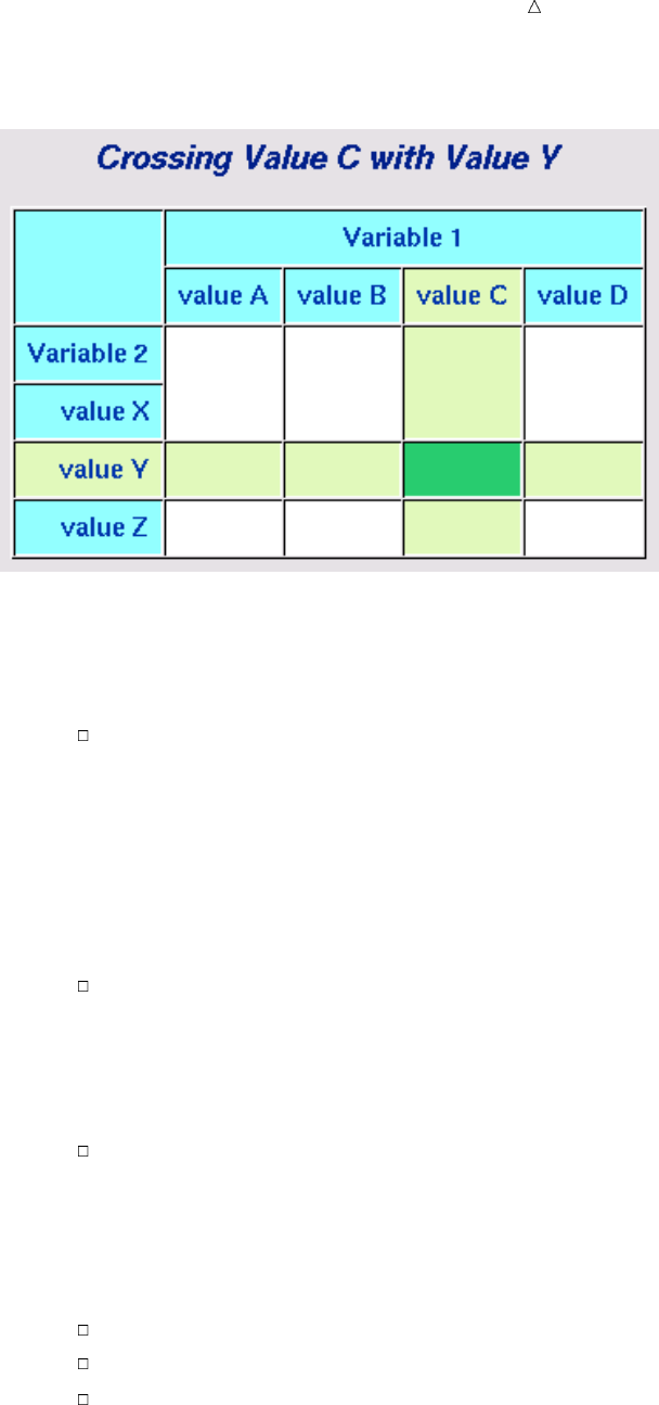
Creating Summary Tables with the TABULATE Procedure Understanding Summary Table Design 409
Display 26.1 Crossing Variables
Here are the basic steps for designing and constructing a summary table:
1Start with a question that you want to answer with a summary table.
2Identify the variables necessary to answer your question.
See if any of the data sets that you are using already use the variables that
you identified. If they do not, then you might be able to use the FORMAT
procedure to reclassify the variable values in these data sets so that they
produce the data that you need.
For example, you can apply a new format to values for a variable MONTH
so that they become values for a variable QUARTER. To do this, assign the
values representing the first three months to a value for quarter one, values
representing the second set of three months to a value for quarter two, and so
on.
If possible, use discrete variables rather than continuous variables for
categories or headings. If you must use continuous variables, then it might
be helpful to create categories. For example, you can group ages into
categories such as ages 15-19, 20-35, 36-55, and 56-higher. This creates four
categories rather than a possible 56+ categories. You can use PROC
FORMAT to categorize the data.
Choose formats for the variables and the data that you want to display in
your summary table. See if the data in your data sets is in a format that you
can use. You might need to create new formats with PROC FORMAT, or copy
the formats of variables from another data set so that the data will be
formatted in the same way.
3Review the data for anything that might cause discrepancies in your report.
Remove data that does not relate to your needs.
Identify missing data.
Make sure that the data overall seems to make logical sense.
4Choose statistics that will help answer your question. For a complete list of
statistics, see “Statistics Available in PROC TABULATE” in the Base SAS
Procedures Guide.
410 Understanding the Basics of the TABULATE Procedure Chapter 26
5Decide on the basic structure of the table. Use the variables that you have
identified to determine the headings for the columns, rows, and pages. The values
of the variables are the subheadings. Statistics are usually represented as
subheadings, but are sometimes represented as headings. Display 26.1 on page
409 is an example of a template for a very basic table.
Understanding the Basics of the TABULATE Procedure
Required Statements for the TABULATE Procedure
The TABULATE procedure requires three statements, usually in the following order:
1PROC TABULATE statement
2CLASS statements or VAR statements or both
3TABLE statements
Note that there can be multiple CLASS statements, VAR statements and TABLE
statements.
Begin with the PROC TABULATE Statement
The TABULATE procedure begins with a PROC TABULATE statement. Many
options are available with the PROC TABULATE statement; however, most of the
examples in this section use only two options, the DATA= option and the FORMAT=
option. The PROC TABULATE statement that follows is used for all of the examples in
this section:
proc tabulate data=year_sales format=comma10.;
You can direct PROC TABULATE to use a specific SAS data set with the DATA=
option. If you omit the DATA= option in the current job or session, then the
TABULATE procedure uses the SAS data set that was created most recently.
You can specify a default format for PROC TABULATE to apply to the value in each
cell in the table with the FORMAT= option. You can specify any valid SAS numeric
format or user-defined format.
Specify Class Variables with the CLASS Statement
Use the CLASS statement to specify which variables are class variables. Class
variables (that is, classification variables) contain values that are used to form
categories. In summary tables, the categories are used as the column, row, and page
headings. The categories are crossed to obtain descriptive statistics. See Display 26.1
on page 409 for an example of crossing categories (variable values).
Class variables can be either character or numeric. The default statistic for class
variables is N, which is the frequency or number of observations in the data set for
which there are nonmissing variable values.
The following CLASS statement specifies the variables SalesRep and Type as class
variables:
class SalesRep Type;
For important information about how PROC TABULATE behaves when class
variables that have missing values are listed in a CLASS statement but are not used in
a TABLE statement, see “Identifying Missing Values for Class Variables” on page 411.

Creating Summary Tables with the TABULATE Procedure Identifying Missing Values for Class Variables 411
Specify Analysis Variables with the VAR Statement
Use the VAR statement to specify which variables are analysis variables. Analysis
variables contain numeric values for which you want to compute statistics. The default
statistic for analysis variables is SUM.
The following VAR statement specifies the variable AmountSold as an analysis
variable:
var AmountSold;
Define the Table Structure with the TABLE Statement
Syntax of a TABLE Statement
Use the TABLE statement to define the structure of the table that you want PROC
TABULATE to produce. A TABLE statement consists of one to three dimension
expressions, separated by commas. Dimension expressions define the columns, rows,
and pages of a summary table. Options can follow dimension expressions. You must
specify at least one TABLE statement, because there is no default table in a PROC
TABULATE step. Here are three variations of the syntax for a basic TABLE statement:
TABLE column-expression;
TABLE row-expression, column-expression;
TABLE page-expression, row-expression, column-expression;
In this syntax
a column expression is required
a row expression is optional
a page expression is optional
the order of the expressions must be page expression, row expression, and then
column expression
Here is an example of a basic TABLE statement with three dimension expressions:
table SalesRep, Type, AmountSold;
This TABLE statement defines a three-dimensional summary table that places the
values of the variable AmountSold in the column dimension, the values of the variable
Type in the row dimension, and the values of the variable SalesRep in the page
dimension.
Restrictions on a TABLE Statement
Here are restrictions on the TABLE statement:
A TABLE statement must have a column dimension.
Every variable that is used in a dimension expression in a TABLE statement must
appear in either a CLASS statement or a VAR statement, but not both.
All analysis variables must be in the same dimension and cannot be crossed.
Therefore, only one dimension of any TABLE statement can contain analysis
variables.
Identifying Missing Values for Class Variables
You can identify missing values for class variables with the MISSING option. By
default, if an observation contains a missing value for any class variable, that
412 Input File and SAS Data Set for Examples Chapter 26
observation will be excluded from all tables even if the variable does not appear in the
TABLE statement for one or more tables. Therefore, it is helpful to run your program
at least once with the MISSING option to identify missing values.
The MISSING option creates a separate category in the summary table for missing
values. It can be used with the PROC TABULATE statement or the CLASS statement.
If you specify the MISSING option in the PROC TABULATE statement, the procedure
considers missing values as valid levels for all class variables:
proc tabulate data=year_sales format=comma10. missing;
class SalesRep;
class Month Quarter;
var AmountSold;
Because the MISSING option is in the PROC TABULATE statement in this example,
observations with missing values for SalesRep, Month, or Quarter will display in the
summary table.
If you specify the MISSING option in a CLASS statement, PROC TABULATE
considers missing values as valid levels for the class variable(s) that are specified in
that CLASS statement:
proc tabulate data=year_sales format=comma10.;
class SalesRep;
class Month Quarter / missing;
var AmountSold;
Because the MISSING option is in the second CLASS statement, observations with
missing values for Month or Quarter will display in the summary table, but
observations with a missing value for SalesRep will not display.
If you have class variables with missing values in your data set, then you must
decide whether or not the observations with the missing values should be omitted from
every table. If the observations should not be omitted, then you can fill in the missing
values where appropriate or continue to run the PROC TABULATE step with the
MISSING option. For other options for handling missing values, see “Handling Missing
Data” in PROC TABULATE by Example. For general information about missing values,
see “Missing Values” in SAS Language Reference: Concepts.
Input File and SAS Data Set for Examples
The examples in this section use one input file* and one SAS data set. The input file
contains sales records for a company, TruBlend Coffee Makers, that distributes the
coffee machines. The file has the following structure:
01 1 Hollingsworth Deluxe 260 49.50
01 1 Garcia Standard 41 30.97
01 1 Hollingsworth Deluxe 330 49.50
01 1 Jensen Standard 1110 30.97
01 1 Garcia Standard 715 30.97
01 1 Jensen Deluxe 675 49.50
02 1 Jensen Standard 45 30.97
02 1 Garcia Deluxe 10 49.50
…more data lines…
*See the “Data Set YEAR_SALES” on page 715 for a complete listing of the input data.

Creating Summary Tables with the TABULATE Procedure Creating a Basic One-Dimensional Summary Table 413
12 4 Hollingsworth Deluxe 125 49.50
12 4 Jensen Standard 1254 30.97
12 4 Hollingsworth Deluxe 175 49.50
The input file contains the following data from left to right:
the month that a sale was made
the quarter of the year that a sale was made
the name of the sales representative
the type of coffee maker sold (standard or deluxe)
the number of units sold
the price of each unit in US dollars
The SAS data set is named YEAR_SALES. This data set contains all the sales data
from the input file and data from a new variable named AmountSold, which is created
by multiplying Units by Price.
The following program creates the SAS data set that is used in this section:
data year_sales;
infile ’your-input-file’;
input Month $ Quarter $ SalesRep $14. Type $ Units Price;
AmountSold = Units * Price;
run;
Creating Simple Summary Tables
Creating a Basic One-Dimensional Summary Table
The simplest summary table contains multiple columns but only a single row. It is
called a one-dimensional summary table because it has only a column dimension. The
PROC TABULATE step that follows creates a one-dimensional summary table that
answers the question, “How many times did each sales representative make a sale?”
options linesize=84 pageno=1 nodate;
proc tabulate data=year_sales format=comma10.;
title1 ’TruBlend Coffee Makers, Inc.’;
title2 ’Number of Sales by Each Sales Representative’;
class SalesRep;u
table SalesRep;v
run;
The numbered items in the previous program correspond to the following:
uThe variable SalesRep is specified as a class variable in the CLASS statement. A
category will be created for each value of SalesRep wherever SalesRep is used in a
TABLE statement.
vThe variable SalesRep is specified in the column dimension of the TABLE
statement. A column will be created for each category of SalesRep. Each column
will show the number of times (N) that values belonging to the category appear in
the data set.

414 Creating a Basic Two-Dimensional Summary Table Chapter 26
The following summary table displays the results of this program:
Output 26.1 Basic One-Dimensional Summary Table
TruBlend Coffee Makers, Inc. 1
Number of Sales by Each Sales Representative
----------------------------------
| SalesRep |
|--------------------------------|
| |Hollingsw-| |
| Garcia | orth | Jensen |
|----------+----------+----------|
|N |N |N |
|----------+----------+----------|
| 40| 32| 38|
----------------------------------
The values 40, 32, and 38 are the frequency with which each sales representative’s
name (Garcia, Hollingsworth, and Jensen) occurs in the data set. For this data set,
each occurrence of the sales representative’s name in the data set represents a sale.
Creating a Basic Two-Dimensional Summary Table
The most commonly used form of a summary table has at least one column and
multiple rows, and is called a two-dimensional summary table. The PROC TABULATE
step that follows creates a two-dimensional summary table that answers the question,
“What was the amount that was sold by each sales representative?”
options linesize=84 pageno=1 nodate;
proc tabulate data=year_sales format=comma10.;
title1 ’TruBlend Coffee Makers, Inc.’;
title2 ’Amount Sold by Each Sales Representative’;
class SalesRep;u
var AmountSold;v
table SalesRep,w
AmountSold;x;
run;
The numbered items in the previous program correspond to the following:
uThe variable SalesRep is specified as a class variable in the CLASS statement. A
category will be created for each value of SalesRep wherever SalesRep is used in a
TABLE statement.
vThe variable AmountSold is specified as an analysis variable in the VAR
statement. The values of AmountSold will be used to compute statistics wherever
AmountSold is used in a TABLE statement.
wThe variable SalesRep is in the row dimension of the TABLE statement. A row
will be created for each value or category of SalesRep.
xThe variable AmountSold is in the column dimension of the TABLE statement.
The default statistic for analysis variables, SUM, will be used to summarize the
values of AmountSold.
The following summary table displays the results of this program:

Creating Summary Tables with the TABULATE Procedure Creating a Basic Three-Dimensional Summary Table 415
Output 26.2 Basic Two-Dimensional Summary Table
TruBlend Coffee Makers, Inc. 1
Amount Sold by Each Sales Representative
--------------------------------
| |AmountSold|
| |----------|
| | Sum |v
|-------------------+----------|
|SalesRep |u|
|-------------------| |
|Garcia | 512,071|
|-------------------+----------|
|Hollingsworth | 347,246|
|-------------------+----------|
|Jensen | 461,163|
--------------------------------
The numbered items in the previous SAS output correspond to the following:
uThe variable AmountSold has been crossed with the variable SalesRep to produce
each data cell of the summary table.
vThe column heading AmountSold includes the subheading SUM. The values that
are displayed in the column dimension are sums of the amount sold by each sales
representative.
Creating a Basic Three-Dimensional Summary Table
Three-dimensional summary tables produce the output on separate pages with rows
and columns on each page. The PROC TABULATE step that follows creates a
three-dimensional summary table that answers the question, “What was the amount
that was sold during each quarter of the year by each sales representative?”
options linesize=84 pageno=1 nodate;
proc tabulate data=year_sales format=comma10.;
title1 ’TruBlend Coffee Makers, Inc.’;
title2 ’Quarterly Sales by Each Sales Representative’;
class SalesRep Quarter;u
var AmountSold;v
table SalesRep,w
Quarter,x
AmountSold;y
run;
The numbered items in the previous program correspond to the following:
uThe variables SalesRep and Quarter are specified as class variables in the CLASS
statement. A category will be created for each value of SalesRep wherever
SalesRep is used in the TABLE statement. Similarly, a category will be created for
each value of Quarter wherever Quarter is used in a TABLE statement.
vThe variable AmountSold is specified as an analysis variable in the VAR
statement. The values of AmountSold will be used to compute statistics wherever
AmountSold is used in a TABLE statement.
wThe variable SalesRep is used in the page dimension of the TABLE statement. A
page will be created for each value or category of SalesRep.

416 Creating a Basic Three-Dimensional Summary Table Chapter 26
xThe variable Quarter is used in the row dimension of the TABLE statement. A
row will be created for each value or category of Quarter.
yThe variable AmountSold is used in the column dimension of the TABLE
statement. The default statistic for analysis variables, SUM, will be used to
summarize the values of AmountSold.
The following summary table displays the results of this program:
Output 26.3 Basic Three-Dimensional Summary Table
TruBlend Coffee Makers, Inc. 1
Quarterly Sales by Each Sales Representative
SalesRep Garcia u
--------------------------------
| |AmountSold|
| |----------|
| | Sum |w
|-------------------+----------|
|Quarter |v|
|-------------------| |
|1 | 118,020|
|-------------------+----------|
|2 | 108,860|
|-------------------+----------|
|3 | 225,326|
|-------------------+----------|
|4 | 59,865|
--------------------------------
TruBlend Coffee Makers, Inc. 2
Quarterly Sales by Each Sales Representative
SalesRep Hollingsworth u
--------------------------------
| |AmountSold|
| |----------|
| | Sum |w
|-------------------+----------|
|Quarter |v|
|-------------------| |
|1 | 59,635|
|-------------------+----------|
|2 | 96,161|
|-------------------+----------|
|3 | 109,704|
|-------------------+----------|
|4 | 81,747|
--------------------------------

Creating Summary Tables with the TABULATE Procedure Producing Multiple Tables in a Single PROC TABULATE Step 417
TruBlend Coffee Makers, Inc. 3
Quarterly Sales by Each Sales Representative
SalesRep Jensen u
--------------------------------
| |AmountSold|
| |----------|
| | Sum |w
|-------------------+----------|
|Quarter |v|
|-------------------| |
|1 | 50,078|
|-------------------+----------|
|2 | 74,731|
|-------------------+----------|
|3 | 222,291|
|-------------------+----------|
|4 | 114,063|
--------------------------------
The numbered items in the previous SAS output correspond to the following:
uThis summary table has a separate page for each sales representative.
vFor each sales representative, the amount sold is reported for each quarter.
wThe column heading AmountSold includes the subheading SUM. The values that
are displayed in this column indicate the total amount sold in US dollars for each
quarter by each sales representative.
Producing Multiple Tables in a Single PROC TABULATE Step
You can produce multiple tables in a single PROC TABULATE step. However, you
cannot change the way a variable is used or defined in the middle of the step. In other
words, the variables in the CLASS or VAR statements are defined only once for all
TABLE statements in the PROC TABULATE step. If you need to change the way a
variable is used or defined for different TABLE statements, then you must place the
TABLE statements, and define the variables, in multiple PROC TABULATE steps. The
program that follows produces three summary tables during one execution of the
TABULATE procedure:
options linesize=84 pageno=1 nodate;
proc tabulate data=year_sales format=comma10.;
title1 ’TruBlend Coffee Makers, Inc.’;
title2 ’Sales of Deluxe Model Versus Standard Model’;
class SalesRep Type;
var AmountSold Units;
table Type;u
table Type, Units;v
table SalesRep, Type, AmountSold;w
run;
The numbered items in the previous program correspond to the following:
uThe first TABLE statement produces a one-dimensional summary table with the
values for the variable Type in the column dimension.
vThe second TABLE statement produces a two-dimensional summary table with
the values for the variable Type in the row dimension and the variable Units in
the column dimension.

418 Producing Multiple Tables in a Single PROC TABULATE Step Chapter 26
wThe third TABLE statement produces a three-dimensional summary table with the
values for the variable SalesRep in the page dimension, the values for the variable
Type in the row dimension, and the variable AmountSold in the column dimension.
The following summary table displays the results of this program:
Output 26.4 Multiple Tables Produced by a Single PROC TABULATE Step
TruBlend Coffee Makers, Inc. 1
Sales of Deluxe Model Versus Standard Model
-----------------------
| Type |
|---------------------|
| Deluxe | Standard |
|----------+----------|
|N |N |
|----------+----------|
| 16| 94|
-----------------------
TruBlend Coffee Makers, Inc. 2
Sales of Deluxe Model Versus Standard Model
--------------------------------
| | Units |
| |----------|
| | Sum |
|-------------------+----------|
|Type | |
|-------------------| |
|Deluxe | 2,525|
|-------------------+----------|
|Standard | 38,464|
--------------------------------
TruBlend Coffee Makers, Inc. 3
Sales of Deluxe Model Versus Standard Model
SalesRep Garcia
--------------------------------
| |AmountSold|
| |----------|
| | Sum |
|-------------------+----------|
|Type | |
|-------------------| |
|Deluxe | 46,778|
|-------------------+----------|
|Standard | 465,293|
--------------------------------
Creating Summary Tables with the TABULATE Procedure Creating Hierarchical Tables to Report on Subgroups 419
TruBlend Coffee Makers, Inc. 4
Sales of Deluxe Model Versus Standard Model
SalesRep Hollingsworth
--------------------------------
| |AmountSold|
| |----------|
| | Sum |
|-------------------+----------|
|Type | |
|-------------------| |
|Deluxe | 37,620|
|-------------------+----------|
|Standard | 309,626|
--------------------------------
TruBlend Coffee Makers, Inc. 5
Sales of Deluxe Model Versus Standard Model
SalesRep Jensen
--------------------------------
| |AmountSold|
| |----------|
| | Sum |
|-------------------+----------|
|Type | |
|-------------------| |
|Deluxe | 40,590|
|-------------------+----------|
|Standard | 420,573|
--------------------------------
Creating More Sophisticated Summary Tables
Creating Hierarchical Tables to Report on Subgroups
You can create a hierarchical table to report on subgroups of your data by crossing
elements within a dimension. Crossing elements is the operation that combines two or
more elements, such as class variables, analysis variables, format modifiers, statistics,
or styles. Dimensions are automatically crossed. When you cross variables in a single
dimension expression, values for one variable are placed within the values for the other
variable in the same dimension. This forms a hierarchy of variables and, therefore, a
hierarchical table. The order in which variables are listed when they are crossed
determines the order of the headings in the table. In the column dimension, variables
are stacked top to bottom; in the row dimension, left to right; and in the page
dimension, front to back. You cross elements in a dimension expression by putting an
asterisk between them. Note that two analysis variables cannot be crossed. Also,
because dimensions are automatically crossed, all analysis variables must occur in one
dimension.
The PROC TABULATE step that follows creates a two-dimensional summary table
that crosses two variables and that answers the question, “What was the amount sold
of each type of coffee maker by each sales representative?”
options linesize=84 pageno=1 nodate;
proc tabulate data=year_sales format=comma10.;

420 Formatting Output Chapter 26
title1 ’TruBlend Coffee Makers, Inc.’;
title2 ’Amount Sold Per Item by Each Sales Representative’;
class SalesRep Type;
var AmountSold;
table SalesRep*Type,
AmountSold;
run;
The expression SalesRep*Type in the row dimension uses the asterisk operator to
cross the values of the variable SalesRep with the values of the variable Type. Because
SalesRep is listed before Type when crossed, and because the elements are crossed in
the row dimension, values for Type will be listed to the right of values of SalesRep.
Values for Type will be repeated for each value of SalesRep.
The following summary table displays the results:
Output 26.5 Crossing Variables
TruBlend Coffee Makers, Inc. 1
Amount Sold Per Item by Each Sales Representative
--------------------------------
| |AmountSold|
| |----------|
| | Sum |
|-------------------+----------|
|SalesRep |Type | |
|---------+---------| |
|Garcia |Deluxe | 46,778|
| |---------+----------|
| |Standard | 465,293|
|---------+---------+----------|
|Hollings-|Deluxe | 37,620|
|worth |---------+----------|
| |Standard | 309,626|
|---------+---------+----------|
|Jensen |Deluxe | 40,590|
| |---------+----------|
| |Standard | 420,573|
--------------------------------
Notice the hierarchy of values that are created when the values for Type are
repeated to the right of each value of SalesRep.
Formatting Output
You can override formats in summary table output by crossing variables with format
modifiers. You cross a variable with a format modifier by putting an asterisk between
them.
The PROC TABULATE step that follows creates a two-dimensional summary table
that crosses a variable with a format modifier and that answers the question, “What
was the amount sold of each type of coffee maker by each sales representative?”
options linesize=84 pageno=1 nodate;
proc tabulate data=year_sales format=comma10.;
title1 ’TruBlend Coffee Makers, Inc.’;
title2 ’Amount Sold Per Item by Each Sales Representative’;
class SalesRep Type;

Creating Summary Tables with the TABULATE Procedure Calculating Descriptive Statistics 421
var AmountSold;
table SalesRep*Type,
AmountSold*f=dollar16.2;
run;
The expression AmountSold*f=dollar16.2 in the column dimension uses the
asterisk operator to cross the values of the variable AmountSold with the SAS format
modifier f=dollar16.2. The values for AmountSold will now display using the
DOLLAR16.2 format. The DOLLAR16.2 format is better suited for dollar figures than
the COMMA10. format, which is specified as the default in the PROC TABULATE
statement.
The following summary table displays the results:
Output 26.6 Crossing Variables with Format Modifiers
TruBlend Coffee Makers, Inc. 1
Amount Sold Per Item by Each Sales Representative
--------------------------------------
| | AmountSold |
| |----------------|
| | Sum |
|-------------------+----------------|
|SalesRep |Type | |
|---------+---------| |
|Garcia |Deluxe | $46,777.50|
| |---------+----------------|
| |Standard | $465,293.28|
|---------+---------+----------------|
|Hollings-|Deluxe | $37,620.00|
|worth |---------+----------------|
| |Standard | $309,626.10|
|---------+---------+----------------|
|Jensen |Deluxe | $40,590.00|
| |---------+----------------|
| |Standard | $420,572.60|
--------------------------------------
Calculating Descriptive Statistics
You can request descriptive statistics for a variable by crossing that variable with the
appropriate statistic keyword. Crossing either a class variable or an analysis variable
with a statistic tells PROC TABULATE what type of calculations to perform. Note that
two statistics cannot be crossed. Also, because dimensions are automatically crossed, all
statistics must occur in one dimension.
The default statistic crossed with a class variable is the N statistic or frequency.
Class variables can only be crossed with frequency and percent frequency statistics.
The default statistic crossed with an analysis variable is the SUM statistic. Analysis
variables can be crossed with any of the many descriptive statistics that are available
with PROC TABULATE including commonly used statistics like MIN, MAX, MEAN,
STD, and MEDIAN. For a complete list of statistics available for use with analysis
variables, see “Statistics Available in PROC TABULATE” in the Base SAS Procedures
Guide.
The PROC TABULATE step that follows creates a two-dimensional summary table
that crosses elements with a statistic and that answers the question, “What was the
average amount per sale of each type of coffee maker by each sales representative?”

422 Reporting on Multiple Statistics Chapter 26
options linesize=84 pageno=1 nodate;
proc tabulate data=year_sales format=comma10.;
title1 ’TruBlend Coffee Makers, Inc.’;
title2 ’Average Amount Sold Per Item by Each Sales Representative’;
class SalesRep Type;
var AmountSold;
table SalesRep*Type,
AmountSold*mean*f=dollar16.2;
run;
In this program, the column dimension crosses the variable AmountSold with the
statistic mean and with the format modifier f=dollar16.2. The MEAN statistic
provides the arithmetic mean for AmountSold.
The following summary table displays the results:
Output 26.7 Crossing a Variable with a Statistic
TruBlend Coffee Makers, Inc. 1
Average Amount Sold Per Item by Each Sales Representative
--------------------------------------
| | AmountSold |
| |----------------|
| | Mean |
|-------------------+----------------|
|SalesRep |Type | |
|---------+---------| |
|Garcia |Deluxe | $11,694.38|
| |---------+----------------|
| |Standard | $12,924.81|
|---------+---------+----------------|
|Hollings-|Deluxe | $4,702.50|
|worth |---------+----------------|
| |Standard | $12,901.09|
|---------+---------+----------------|
|Jensen |Deluxe | $10,147.50|
| |---------+----------------|
| |Standard | $12,369.78|
--------------------------------------
Reporting on Multiple Statistics
You can create summary tables that report on two or more statistics by concatenating
variables. Concatenating is the operation that joins the information of two or more
elements, such as class variables, analysis variables, or statistics, by placing the output
of the second and subsequent elements immediately after the output of the first
element. You concatenate elements in a dimension expression by putting a blank space
between them.
The PROC TABULATE step that follows creates a two-dimensional summary table
that uses concatenation and that answers the question, “How many sales were made,
and what was the total sales figure for each type of coffee maker sold by each sales
representative?”
options linesize=84 pageno=1 nodate;
proc tabulate data=year_sales format=comma10.;

Creating Summary Tables with the TABULATE Procedure Reducing Code and Applying a Single Label to Multiple Elements 423
title1 ’TruBlend Coffee Makers, Inc.’;
title2 ’Sales Summary by Representative and Product’;
class SalesRep Type;
var AmountSold;
table SalesRep*Type,
AmountSold*n AmountSold*f=dollar16.2;
run;
In this program, because the expressions AmountSold*n and
AmountSold*f=dollar16.2 in the column dimension are separated by a blank space,
their output will be concatenated.
The following summary table displays the results:
Output 26.8 Concatenating Variables
TruBlend Coffee Makers, Inc. 1
Sales Summary by Representative and Product
uv
-------------------------------------------------
| |AmountSold| AmountSold |
| |----------+----------------|
| | N | Sum |
|-------------------+----------+----------------|
|SalesRep |Type | | |
|---------+---------| | |
|Garcia |Deluxe | 4| $46,777.50|
| |---------+----------+----------------|
| |Standard | 36| $465,293.28|
|---------+---------+----------+----------------|
|Hollings-|Deluxe | 8| $37,620.00|
|worth |---------+----------+----------------|
| |Standard | 24| $309,626.10|
|---------+---------+----------+----------------|
|Jensen |Deluxe | 4| $40,590.00|
| |---------+----------+----------------|
| |Standard | 34| $420,572.60|
-------------------------------------------------
In this summary table the frequency (N) of AmountSold uis shown in the same
table as the SUM of AmountSold v.
Reducing Code and Applying a Single Label to Multiple Elements
You can use parentheses to group concatenated elements (variables, formats,
statistics, and so on) that are concatenated or crossed with a common element. This can
reduce the amount of code used and can change how labels are displayed. The PROC
TABULATE step that follows uses parentheses to group elements that are crossed with
AmountSold and answers the question, “How many sales were made, and what was the
total sales figure for each type of coffee maker sold by each sales representative?”
options linesize=84 pageno=1 nodate;
proc tabulate data=year_sales format=comma10.;
title1 ’TruBlend Coffee Makers, Inc.’;
title2 ’Sales Summary by Representative and Product’;
class SalesRep Type;

424 Getting Summaries for All Variables Chapter 26
var AmountSold;
table SalesRep*Type,
AmountSold*(n sum*f=dollar16.2);
run;
In this program, AmountSold*(n sum*f=dollar16.2) takes the place of
AmountSold*n AmountSold*f=dollar16.2. Notice the default statistic SUM from
AmountSold*f=dollar16.2 must now be included in the expression. This is because
the format modifier must be crossed with a variable or a statistic. It cannot be in the
expression by itself.
The following summary table displays the results:
Output 26.9 Using Parentheses to Group Elements
TruBlend Coffee Makers, Inc. 1
Sales Summary by Representative and Product
-------------------------------------------------
| | AmountSold |
| |---------------------------|
| | N | Sum |
|-------------------+----------+----------------|
|SalesRep |Type | | |
|---------+---------| | |
|Garcia |Deluxe | 4| $46,777.50|
| |---------+----------+----------------|
| |Standard | 36| $465,293.28|
|---------+---------+----------+----------------|
|Hollings-|Deluxe | 8| $37,620.00|
|worth |---------+----------+----------------|
| |Standard | 24| $309,626.10|
|---------+---------+----------+----------------|
|Jensen |Deluxe | 4| $40,590.00|
| |---------+----------+----------------|
| |Standard | 34| $420,572.60|
-------------------------------------------------
Note that the label, AmountSold, spans multiple columns rather than appearing
twice in the summary table, as it does in Output 26.8.
Getting Summaries for All Variables
You can summarize all of the class variables in a dimension with the universal class
variable ALL. ALL can be concatenated with each of the three dimensions of the
TABLE statement and within groups of elements delimited by parentheses. The PROC
TABULATE step that follows creates a two-dimensional summary table with the
universal class variable ALL, and answers the question, “For each sales representative
and for all of the sales representatives as a group, how many sales were made, what
was the average amount per sale, and what was the amount sold?”
options linesize=84 pageno=1 nodate;
proc tabulate data=year_sales format=comma10.;
title1 ’TruBlend Coffee Makers, Inc.’;
title2 ’Sales Report’;
class SalesRep Type;
var AmountSold;
table SalesRep*Type all,

Creating Summary Tables with the TABULATE Procedure Defining Labels 425
AmountSold*(n (mean sum)*f=dollar16.2);
run;
In this program, the TABLE statement now includes the universal class variable
ALL in the row dimension. SalesRep and Type will be summarized.
The following summary table displays the results:
Output 26.10 Crossing with the Universal Class Variable ALL
TruBlend Coffee Makers, Inc. 1
Sales Report
------------------------------------------------------------------
| | AmountSold |
| |--------------------------------------------|
| | N | Mean | Sum |
|-------------------+----------+----------------+----------------|
|SalesRep |Type | | | |
|---------+---------| | | |
|Garcia |Deluxe | 4| $11,694.38| $46,777.50|
| |---------+----------+----------------+----------------|
| |Standard | 36| $12,924.81| $465,293.28|
|---------+---------+----------+----------------+----------------|
|Hollings-|Deluxe | 8| $4,702.50| $37,620.00|
|worth |---------+----------+----------------+----------------|
| |Standard | 24| $12,901.09| $309,626.10|
|---------+---------+----------+----------------+----------------|
|Jensen |Deluxe | 4| $10,147.50| $40,590.00|
| |---------+----------+----------------+----------------|
| |Standard | 34| $12,369.78| $420,572.60|
|-------------------+----------+----------------+----------------|
|All u| 110| $12,004.36| $1,320,479.48|
------------------------------------------------------------------
This summary table reports the frequency (N), the MEAN, and the SUM of
AmountSold for each category of SalesRep and Type. This data has been summarized
for all categories of SalesRep and Type in the row labeled All u.
Defining Labels
You can add your own labels to a summary table or remove headings from a
summary table by assigning labels to variables in the TABLE statement. Simply follow
the variable with an equal sign (=) followed by either the desired label or by a blank
space in quotation marks. A blank space in quotation marks removes the heading from
the summary table. The PROC TABULATE step that follows creates a two-dimensional
summary table that uses labels in the TABLE statement and that answers the
question, “What is the percent of total sales and average amount sold by each sales
representative of each type of coffee maker and all coffee makers?”
options linesize=84 pageno=1 nodate;
proc tabulate data=year_sales format=comma10.;
title1 ’TruBlend Coffee Makers, Inc.’;
title2 ’Sales Performance’;
class SalesRep Type;
var AmountSold;
table SalesRep=’Sales Representative’u*

426 Defining Labels Chapter 26
(Type=’Type of Coffee Maker’uall) all,
AmountSold=’ ’x*
(N=’Sales’v
SUM=’Amount’v*f=dollar16.2
colpctsum=’% Sales’w
mean=’Average Sale’v*f=dollar16.2);
run;
The numbered items in the previous program correspond to the following:
uThe variables SalesRep and Type are assigned labels.
vThe frequency statistic N, the statistic SUM, and the statistic MEAN are assigned
labels.
wThe statistic COLPCTSUM is used to calculate the percentage of the value in a
single table cell in relation to the total of the values in the column and is assigned
the label ‘% Sales’.
xThe variable AmountSold is assigned a blank label. As a result, the heading for
AmountSold does not appear in the summary table.
The following summary table displays the results:
Output 26.11 Using Labels to Customize Summary Tables
TruBlend Coffee Makers, Inc. 1
Sales Performance
u
-----------------------------------------------------------------------------
|v| Sales | Amount | % Sales | Average Sale |
|-------------------+----------+----------------+----------+----------------|
w|Sales |Type of | | | | |
|Represen-|Coffee | | | | |
|tative |Maker | | | | |
|---------+---------| | | | |
|Garcia |Deluxe | 4| $46,777.50| 4| $11,694.38|
| |---------+----------+----------------+----------+----------------|
| |Standard | 36| $465,293.28| 35| $12,924.81|
| |---------+----------+----------------+----------+----------------|
| |All | 40| $512,070.78| 39| $12,801.77|
|---------+---------+----------+----------------+----------+----------------|
|Hollings-|Type of | | | | |
|worth |Coffee | | | | |
| |Maker | | | | |
| |---------| | | | |
| |Deluxe | 8| $37,620.00| 3| $4,702.50|
| |---------+----------+----------------+----------+----------------|
| |Standard | 24| $309,626.10| 23| $12,901.09|
| |---------+----------+----------------+----------+----------------|
| |All | 32| $347,246.10| 26| $10,851.44|
|---------+---------+----------+----------------+----------+----------------|
|Jensen |Type of | | | | |
| |Coffee | | | | |
| |Maker | | | | |
| |---------| | | | |
| |Deluxe | 4| $40,590.00| 3| $10,147.50|
| |---------+----------+----------------+----------+----------------|
| |Standard | 34| $420,572.60| 32| $12,369.78|
| |---------+----------+----------------+----------+----------------|
| |All | 38| $461,162.60| 35| $12,135.86|
|-------------------+----------+----------------+----------+----------------|
|All | 110| $1,320,479.48| 100| $12,004.36|
-----------------------------------------------------------------------------
Creating Summary Tables with the TABULATE Procedure Using Styles and the Output Delivery System 427
The numbered items in the previous SAS output correspond to the following:
uNo heading for the variable AmountSold is displayed.
vThe labels ‘Sales’, ‘Amount’, ‘% Sales’, and ‘Average Sale’ replace the frequency
(N), SUM, COLPCTSUM, and MEAN respectively.
wlabels replace the variables SalesRep and Type.
Using Styles and the Output Delivery System
If you use the Output Delivery System to create output from PROC TABULATE, for
any destination other than Listing or Output destinations, you can do the following:
Set certain style elements (such as font style, font weight, and color) that the
procedure uses for various parts of the table.
Specify style elements for the labels for variables by adding the option to the
CLASS statement.
Specify style elements for cells in the summary table by crossing the STYLE=
option with an element of a dimension expression.
When it is used in a dimension expression, the STYLE= option must be enclosed
within square brackets ([ and ]) or braces ({ and }). The PROC TABULATE step that
follows creates a two-dimensional summary table that uses the STYLE= option in a
CLASS statement and in the TABLE statement and that answers the question, “What
is the percent of total sales and average amount sold by each sales representative of
each type of coffee maker and all coffee makers?”
options linesize=84 pageno=1 nodate;
ods html file=’summary-table.htm’;u
ods printer file=’summary-table.ps’;v
proc tabulate data=year_sales format=comma10.;
title1 ’TruBlend Coffee Makers, Inc.’;
title2 ’Sales Performance’;
class SalesRep;
class Type / style=[font_style=italic]w;
var AmountSold;
table SalesRep=’Sales Representative’*(Type=’Type of Coffee Maker’
all*[style=[background=yellow font_weight=bold]]x)
all*[style=[font_weight=bold]]y,
AmountSold=’ ’*(colpctsum=’% Sales’ mean=’Average Sale’*
f=dollar16.2);
run;
ods html close;U
ods printer close;V
The numbered items in the previous program correspond to the following:
uThe ODS HTML statement opens the HTML destination and creates HTML
output. FILE= identifies the file that contains the HTML output. Some browsers
require an extension of HTM or HTML on the filename.
vThe ODS PRINTER statement opens the Printer destination and creates Printer
output. FILE= identifies the file that contains the Printer output.
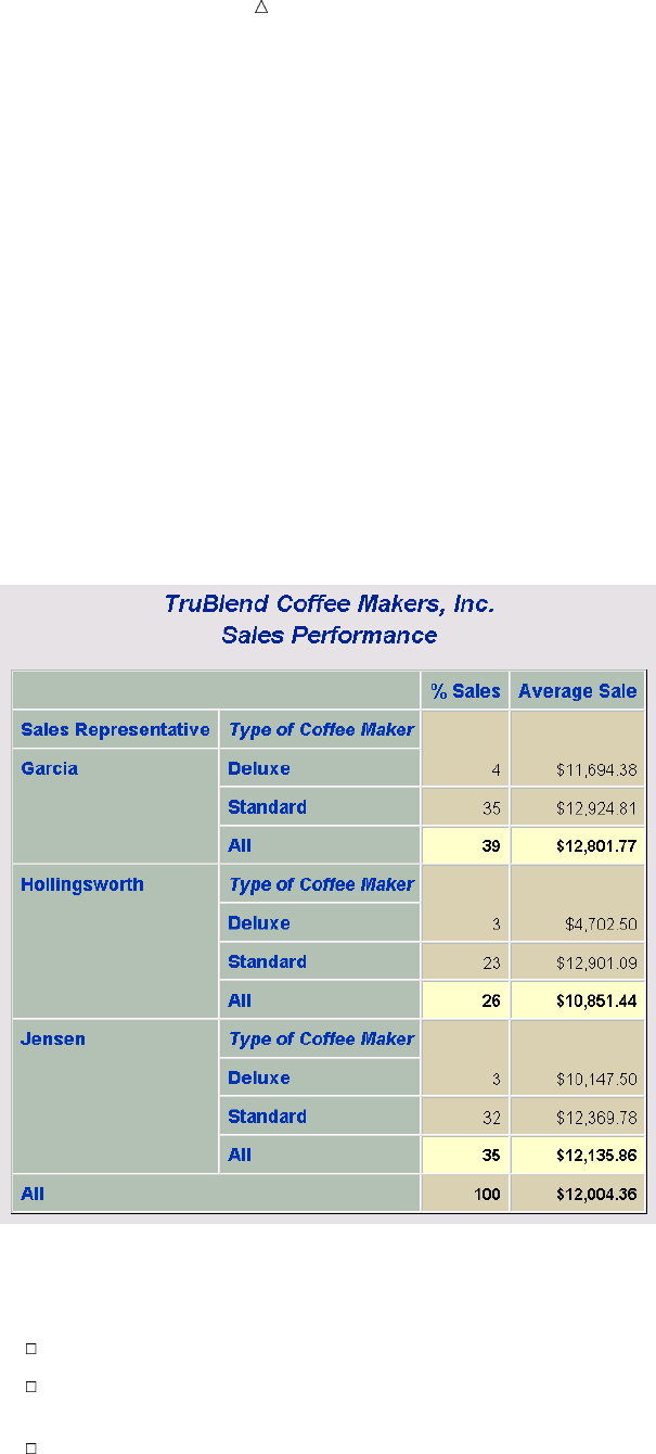
428 Using Styles and the Output Delivery System Chapter 26
wThe STYLE= option is specified in the second CLASS statement, which sets the
font style of the label for Type to italic. The label for SalesRep is not affected by
the STYLE= option because it is in a separate CLASS statement.
xThe universal class variable ALL is crossed with the STYLE= option, which sets
the background for the table cells to yellow and the font weight for these cells to
bold.
yThe universal class variable ALL is crossed with the STYLE= option, which sets
the font weight for the table cells to bold.
UThe last ODS HTML statement closes the HTML destination and all of the files
that are associated with it. You must close the HTML destination before you can
view the HTML output with a browser.
VThe last ODS PRINTER statement closes the Printer destination. You must close
the Printer destination before you can print the output on a physical printer.
The following summary table displays the results:
Display 26.2 Using Style Modifiers and the ODS HTML Statement
This summary table shows the effects of the three uses of the STYLE= option with
the ODS HTML statement in the previous SAS program:
The repeated label, Type of Coffee Maker, is in italics.
The subtotals for each value of sales representative are highlighted in a lighter
color (yellow) and are bold.
The totals for all sales representatives are bold.
The following summary table displays the results:
Creating Summary Tables with the TABULATE Procedure Using Styles and the Output Delivery System 429
Display 26.3 Using Style Modifiers and the ODS PRINTER Statement
TruBlend Coffee Makers, Inc.
Sales Performance
%
Sales
Average
Sale
Sales
Representative
Type of
Coffee
Maker
Garcia Deluxe 4 $11,694.38
Standard 35 $12,924.81
All 39 $12,801.77
Hollingsworth Type of
Coffee
Maker
Deluxe 3 $4,702.50
Standard 23 $12,901.09
All 26 $10,851.44
Jensen Type of
Coffee
Maker
Deluxe 3 $10,147.50
Standard 32 $12,369.78
All 35 $12,135.86
All 100 $12,004.36
This summary table shows the effects of the three uses of the STYLE= option with
the ODS PRINTER statement in the previous SAS program:
The repeated label, Type of Coffee Maker, is in italics.

430 Ordering Class Variables Chapter 26
The subtotals for each value of sales representative are highlighted and are bold.
The totals for all sales representatives are bold.
Ordering Class Variables
You can control the order in which class variable values and their headings display in
a summary table with the ORDER= option. You can use the ORDER= option with the
PROC TABULATE statement and with individual CLASS statements. The syntax is
ORDER=sort-order. The four possible sort orders (DATA, FORMATTED, FREQ, and
UNFORMATTED) are defined in “Review of SAS Tools” on page 431. The PROC
TABULATE step that follows creates a two-dimensional summary table that uses the
ORDER= option with the PROC TABULATE statement to order all class variables by
frequency, and that answers the question, “Which quarter produced the greatest
number of sales, and which sales representative made the most sales overall?”
options linesize=84 pageno=1 nodate;
proc tabulate data=year_sales format=comma10. order=freq;
title1 ’TruBlend Coffee Makers, Inc.’;
title2 ’Quarterly Sales and Representative Sales by Frequency’;
class SalesRep Quarter;
table SalesRep all,
Quarter all;
run;
The following summary table displays the results of this program:
Output 26.12 Ordering Class Variables
TruBlend Coffee Makers, Inc. 1
Quarterly Sales and Representative Sales by Frequency
----------------------------------------------------------------------------
| | Quarter | |
| |-------------------------------------------| |
||3u|1 |2 |4 |All|w
| |----------+----------+----------+----------+----------|
| |N|N|N|N|N|
|-------------------+----------+----------+----------+----------+----------|
|SalesRep | | | | | |
|-------------------| | | | | |
|Garcia v| 21| 8| 6| 5| 40|
|-------------------+----------+----------+----------+----------+----------|
|Jensen | 21| 5| 6| 6| 38|
|-------------------+----------+----------+----------+----------+----------|
|Hollingsworth | 15| 5| 6| 6| 32|
|-------------------+----------+----------+----------+----------+----------|
|All w| 57| 18| 18| 17| 110|
----------------------------------------------------------------------------
The numbered items in the previous SAS output correspond to the following:
uThe order of the values of the class variable Quarter shows that most sales
occurred in quarter 3 followed by quarters 1, 2, and then 4.
vThe order of the values of the class variable SalesRep shows that Garcia made the
most sales overall, followed by Jensen and then Hollingsworth.
Creating Summary Tables with the TABULATE Procedure TABULATE Procedure Statements 431
wThe universal class variable ALL is included in both dimensions of this example to
show the frequency data that SAS used to order the data when creating the
summary table.
Review of SAS Tools
Global Statement
TITLE<n><’title’>;
specifies a title. The argument nis a number from 1 to 10 that immediately follows
the word TITLE, with no intervening blank, and specifies the level of the TITLE.
The text of each title can be up to 132 characters long (256 characters long in some
operating environments) and must be enclosed in single or double quotation marks.
TABULATE Procedure Statements
PROC TABULATE <option(s)>;
CLASS variable(s)</option(s)>;
VAR analysis-variable(s);
TABLE <<page-expression,> row-expression,> column-expression;
PROC TABULATE <option(s)>;
starts the procedure.
You can specify the following options in the PROC TABULATE statement:
DATA=SAS-data-set
specifies the SAS-data-set to be used by PROC TABULATE. If you omit the
DATA= option, then the TABULATE procedure uses the SAS data set that
was created most recently in the current job or session.
FORMAT=format-name
specifies a default format for formatting the value in each cell in the table.
You can specify any valid SAS numeric format or user-defined format.
MISSING
considers missing values as valid values to create the combinations of class
variables. A heading for each missing value appears in the table.
ORDER=DATA | FORMATTED | FREQ | UNFORMATTED
specifies the sort order that is used to create the unique combinations of the
values of the class variables, which form the headings of the table. A brief
description of each sort order follows:
DATA
orders values according to their order in the input data set.
FORMATTED
orders values by their ascending formatted values. This order depends
on your operating environment.
FREQ
orders values by descending frequency count.

432 TABULATE Procedure Statements Chapter 26
UNFORMATTED
orders values by their unformatted values, which yields the same order
as PROC SORT. This order depends on your operating environment.
This sort sequence is particularly useful for displaying dates
chronologically.
ORDER= used on a CLASS statement overrides ORDER= used on the PROC
TABULATE statement.
CLASS variable(s)/option(s);
identifies class variables for the table. Class variables determine the categories
that PROC TABULATE uses to calculate statistics.
MISSING
considers missing values as valid values to create the combinations of class
variables. A heading for each missing value appears in the table. If MISSING
should apply only to a subset of the class variables, then specify MISSING in
a separate CLASS statement with the subset of the class variables.
ORDER=DATA | FORMATTED | FREQ | UNFORMATTED
specifies the sort order used to create the unique combinations of the values
of the class variables, which form the headings of the table. If ORDER=
should apply only to a subset of the class variables, then specify ORDER= in
a separate CLASS statement with the subset of the class variables. In this
way, a separate sort order can be specified for each class variable. A brief
description of each sort order follows:
DATA
orders values according to their order in the input data set.
FORMATTED
orders values by their ascending formatted values. This order depends
on your operating environment.
FREQ
orders values by descending frequency count.
UNFORMATTED
orders values by their unformatted values, which yields the same order
as PROC SORT. This order depends on your operating environment.
This sort sequence is particularly useful for displaying dates
chronologically.
ORDER= used on a CLASS statement overrides ORDER= used on the PROC
TABULATE statement.
VAR analysis-variable(s);
identifies analysis variables for the table. Analysis variables contain values for
which you want to compute statistics.
TABLE <<page-expression,>row-expression,> column-expression;
defines the table that you want PROC TABULATE to produce. You must specify at
least one TABLE statement. In the TABLE statement you specify page-expressions,
row-expressions, and column-expressions, all of which are constructed in the same
way and are referred to collectively as dimension expressions. Use commas to
separate dimension expressions from one another. You define relationships among
variables, statistics, and other elements within a dimension by combining them
with one or more operators. Operators are symbols that tell PROC TABULATE
what actions to perform on the variables, statistics, and other elements. The table
that follows lists the common operators and the actions that they symbolize:

Creating Summary Tables with the TABULATE Procedure Learning More 433
Operator Action
, comma separates dimensions of the table
* asterisk crosses elements within a dimension
blank space concatenates elements within a dimension
= equal overrides default cell format or assigns label to an
element
( )parentheses groups elements and associates an operator with each
concatenated element in the group
[ ]square brackets groups the STYLE= option for crossing, and groups
style attribute specifications within the STYLE=
option
{ } braces groups the STYLE= option for crossing, and groups
style attribute specifications within the STYLE=
option
Learning More
Locating procedure output
See Chapter 31, “Understanding and Customizing SAS Output: The Basics,” on
page 537.
Missing values
For a discussion about missing values, see SAS Language Reference: Concepts.
Information about handling missing values is also in PROC TABULATE by
Example.
ODS
For complete documentation on how to use the Output Delivery System, see SAS
Output Delivery System: User’s Guide.
PROC TABULATE
See the TABULATE procedure in the Base SAS Procedures Guide.
For a detailed discussion and comprehensive examples of the TABULATE
procedure, see PROC TABULATE by Example.
SAS formats
See SAS Language Reference: Dictionary. Many formats are available with SAS,
such as fractions, hexadecimal values, roman numerals, social security numbers,
date and time values, and numbers written as words.
Statistics
For a list of the statistics available in the TABULATE procedure, see the
discussion of concepts in the TABULATE procedure in the Base SAS Procedures
Guide. For more information about the listed statistics, see the discussion of
elementary statistics in the appendix of the Base SAS Procedures Guide.
Style attributes

434 Learning More Chapter 26
For information about style attributes that can be set for a style element by using
the Output Delivery System, see Base SAS Procedures Guide.
Summary tables
For additional examples of how to produce a variety of summary tables, see SAS
Guide to Report Writing: Examples.
For a discussion of how to use the REPORT procedure to create summary
tables, see Chapter 27, “Creating Detail and Summary Reports with the REPORT
Procedure,” on page 435.
Tabular reports
For interactive online examples and discussion, see lessons related to creating
tabular reports in SAS Online Tutor for Version 8: SAS Programming.
Title statement
See Chapter 25, “Producing Detail Reports with the PRINT Procedure,” on page
371.

435
CHAPTER
27 Creating Detail and Summary
Reports with the REPORT
Procedure
Introduction to Creating Detail and Summary Reports with the REPORT Procedure 436
Purpose 436
Prerequisites 436
Understanding How to Construct a Report 436
Using the Report Writing Tools 436
Types of Reports 437
Laying Out a Report 437
Establishing the Layout 437
Constructing the Layout 437
Input File and SAS Data Set for Examples 438
Creating Simple Reports 439
Displaying All the Variables 439
Specifying and Ordering the Columns 441
Ordering the Rows 441
Consolidating Several Observations into a Single Row 443
Changing the Default Order of the Rows 444
Creating More Sophisticated Reports 446
Adjusting the Column Layout 446
Understanding Column Width and Spacing 446
Modifying the Column Width and Spacing 446
Customizing Column Headers 447
Understanding the Structure of Column Headers 447
Modifying the Column Headers 448
Specifying Formats 448
Using SAS Formats 448
Applying Formats to Report Items 449
Using Variable Values as Column Headers 449
Creating the Column Headers 449
Creating Frequency Counts 450
Sharing a Column with Multiple Analysis Variables 451
Summarizing Groups of Observations 452
Using Group Summaries 452
Creating Group Summaries 453
Review of SAS Tools 454
PROC REPORT Statements 454
Learning More 458
436 Introduction to Creating Detail and Summary Reports with the REPORT Procedure Chapter 27
Introduction to Creating Detail and Summary Reports with the REPORT
Procedure
Purpose
SAS provides a variety of report writing tools that produce detail and summary
reports. The reports enable you to communicate information about your data in a
organized, concise manner. The REPORT procedure enables you to create detail and
summary reports in a single report writing tool.
In this section, you will learn how to use PROC REPORT to do the following:
produce simple detail reports
produce simple summary reports
produce enhanced reports by adding additional statements that order and group
observations, sum columns, and compute overall totals
customize the appearance of reports by adding column spacing, column labels, line
separators, and formats
Prerequisites
To understand the examples in this section, you should be familiar with the following
features and concepts:
data set options
the TITLE statement
the LABEL statement
WHERE processing
creating and assigning SAS formats
Understanding How to Construct a Report
Using the Report Writing Tools
The REPORT procedure combines the features of PROC MEANS, PROC PRINT, and
PROC TABULATE along with features of the DATA step report writing into a powerful
report writing tool. PROC REPORT enables you to do the following:
Create customized, presentation-quality reports.
Develop and store report definitions that control the structure and layout.
View previously defined reports.
Generate multiple reports from one report definition.
There are three different ways that you can use PROC REPORT to construct reports:
in a windowing environment with a prompting facility
in a windowing environment without a prompting facility
in a nonwindowing environment where you use PROC REPORT to submit a series
of statements
Creating Detail and Summary Reports with the REPORT Procedure Laying Out a Report 437
The windowing environment requires minimal SAS programming skills and allows
immediate, visual feedback as you develop the report. This section explains how you
use the nonwindowing environment to create summary and detail reports.
Types of Reports
The REPORT procedure enables you to construct two types of reports:
detail report
contains one row for every observation that is selected for the report (see Output
27.1). Each of these rows is a detail row.
summary report
consolidates data so that each row represents multiple observations (see Output
27.5). Each of these rows is also called a detail row.
Both detail and summary reports can contain summary lines as well as detail rows.
A summary line summarizes numerical data for a set of detail rows or for all detail
rows. You can use PROC REPORT to provide both default summaries and customized
summaries.
Laying Out a Report
Establishing the Layout
If you first decide on the layout of the report, then creating the report is easier. You
need to determine the following:
which columns to display in the report
the order of the columns and rows
how to label the rows and columns
which statistics to display
whether to display a column for each value of a particular variable
whether to display a row for every observation, or to consolidate multiple
observations in a single row
Once you establish the layout of the report, use the COLUMN statement and DEFINE
statement in the PROC REPORT step to construct the layout.
Constructing the Layout
The COLUMN statement lists the report items to include as columns of the report,
describes the arrangement of the columns, and defines headers that span multiple
columns. A report item is a data set variable, a calculated statistic, or a variable that
you compute based on other items in the report.
The DEFINE statement defines the characteristics of an item in the report. These
characteristics include how PROC REPORT uses an item in the report, the text of the
column header, and the format to display the values.
You control much of a report’s layout by the usages that you specify for variables in
the DEFINE statements. The types of variable usages are:
ACROSS
creates a column for each value of an ACROSS variable.
ANALYSIS
438 Input File and SAS Data Set for Examples Chapter 27
computes a statistic from a numeric variable for all the observations represented
by a cell of the report. The value of the variable depends on where it appears in
the report. By default, PROC REPORT treats all numeric variables as ANALYSIS
variables and computes the sum.
COMPUTED
computes a report item from variables that you define for the report. They are not
in the input data set, and PROC REPORT does not add them to the input data set.
DISPLAY
displays a row for every observation in the input data set. By default, PROC
REPORT treats all character variables as DISPLAY variables.
GROUP
consolidates into one row all of the observations from the data set that have a
unique combination of the formatted values for all GROUP variables.
ORDER
specifies to order the rows for every observation in the input data set according to
the ascending, formatted values of the ORDER variable.
The position and usage of each variable in the report determine the report’s structure
and content. For example, PROC REPORT orders the detail rows of the report
according to the values of ORDER and GROUP variables (from left to right). Similarly,
PROC REPORT orders columns for an ACROSS variable from top to bottom, according
to the values of the variable. For a complete discussion of how PROC REPORT
determines the layout of a report, see the Base SAS Procedures Guide.
Input File and SAS Data Set for Examples
The examples in this section use one input file* and one SAS data set. The input file
contains sales records for a company, TruBlend Coffee Makers, that distributes the
coffee machines. The file has the following structure:
01 1 Hollingsworth Deluxe 260 49.50
01 1 Garcia Standard 41 30.97
01 1 Hollingsworth Deluxe 330 49.50
01 1 Jensen Standard 1110 30.97
01 1 Garcia Standard 715 30.97
01 1 Jensen Deluxe 675 49.50
02 1 Jensen Standard 45 30.97
02 1 Garcia Deluxe 10 49.50
…more data lines…
12 4 Hollingsworth Deluxe 125 49.50
12 4 Jensen Standard 1254 30.97
12 4 Hollingsworth Deluxe 175 49.50
The input file contains the following values from left to right:
the month that a sale was made
the quarter of the year that a sale was made
the name of the sales representative
*See the “Data Set YEAR_SALES” on page 715 for a complete listing of the input data.
Creating Detail and Summary Reports with the REPORT Procedure Displaying All the Variables 439
the type of coffee maker sold (standard or deluxe)
the number of units sold
the price of each unit in US dollars
The SAS data set is named YEAR_SALES. This data set contains all the sales data
from the input file and a new variable named AmountSold, which is created by
multiplying Units by Price.
The following program creates the SAS data set that this section uses:
data year_sales;
infile ’your-input-file’;
input Month $ Quarter $ SalesRep $14. Type $ Units Price;
AmountSold = Units * Price;
run;
Creating Simple Reports
Displaying All the Variables
By default, PROC REPORT uses all of the variables in the data set. The layout of
the report depends on the type of variables in the data set. If the data set contains any
character variables, then PROC REPORT generates a simple detail report that lists the
values of all the variables and the observations in the data set. If the data set contains
only numeric variables, then PROC REPORT sums the value of each variable over all
observations in the data set and produces a one-line summary of the sums. To produce
a detail report for a data set with only numeric values, you have to define the columns
in the report.
By default, PROC REPORT opens the REPORT window so that you can modify a
report repeatedly and see the modifications immediately. To run PROC REPORT
without the REPORT window and send your results to the SAS procedure output, you
must use the NOWINDOWS option in the PROC REPORT statement.
The following PROC REPORT step creates the default detail report for the first
quarter sales:
options linesize=80 pageno=1 nodate;
proc report data=year_sales nowindows;
where quarter=’1’;
title1 ’TruBlend Coffee Makers, Inc.’;
title2 ’First Quarter Sales Report’;
run;
The WHERE statement specifies a condition that SAS uses to select observations from
the YEAR_SALES data set. Before PROC REPORT builds the report, SAS selectively
processes observations so that the report contains only data for the observations from
the first quarter. For additional information about WHERE processing, see “Selecting
Observations” on page 379.
The following detail report shows all the variable values for those observations in
YEAR_SALES that contains first quarter sales data:

440 Displaying All the Variables Chapter 27
Output 27.1 The Default Report When the Data Set Contains Character Values
TruBlend Coffee Makers, Inc.x1
First Quarter Sales Report
AmountSol
MonthuQuarter SalesRep Type Units Price dv
01 1 Hollingsworth Deluxe 260 49.5 12870w
01 1 Garcia Standard 41 30.97 1269.77
01 1 Hollingsworth Standard 330 30.97 10220.1
01 1 Jensen Standard 110 30.97 3406.7
01 1 Garcia Deluxe 715 49.5 35392.5
01 1 Jensen Standard 675 30.97 20904.75
02 1 Garcia Standard 2045 30.97 63333.65
02 1 Garcia Deluxe 10 49.5 495
02 1 Garcia Standard 40 30.97 1238.8
02 1 Hollingsworth Standard 1030 30.97 31899.1
02 1 Jensen Standard 153 30.97 4738.41
02 1 Garcia Standard 98 30.97 3035.06
03 1 Hollingsworth Standard 125 30.97 3871.25
03 1 Jensen Standard 154 30.97 4769.38
03 1 Garcia Standard 118 30.97 3654.46
03 1 Hollingsworth Standard 25 30.97 774.25
03 1 Jensen Standard 525 30.97 16259.25
03 1 Garcia Standard 310 30.97 9600.7
The following list corresponds to the numbered items in the preceding report:
uThe order of the columns corresponds to the position of the variables in the data
set.
vThe default column width for numeric variables is nine. Therefore, the column
label for AmountSold wraps across two lines.
wA blank line does not automatically appear between the column labels and the
data values.
xThe top of the report has a title, produced by the TITLE statement.
The following PROC REPORT step produces the default summary report when the
YEAR_SALES data set contains only numeric values:
options linesize=80 pageno=1 nodate;
proc report data=year_sales (keep=Units AmountSold)
colwidth=10 nowindows;
title1 ’TruBlend Coffee Makers, Inc.’;
title2 ’Total Yearly Sales’;
run;
The KEEP= data set option specifies to process only the numeric variables Units and
Amountsold. PROC REPORT uses these variables to create the report. The
COLWIDTH= option increases the column width so that the column label for
AmountSold displays on a single line.
The following report displays a one-line summary for the two numeric variables:
Output 27.2 The Default Report When the Data Set Contains Only Numeric Values
TruBlend Coffee Makers, Inc. 1
Total Yearly Sales
Units AmountSold
40989 1320479.48

Creating Detail and Summary Reports with the REPORT Procedure Ordering the Rows 441
PROC REPORT computed the one-line summary for Units and AmountSold by
summing the value of each variable for all the observations in the data set.
Specifying and Ordering the Columns
The first step in constructing a report is to select the columns that you want to
appear in the report. By default, the report contains a column for each variable and the
order of the columns corresponds to the order of the variables in the data set.
You use the COLUMN statement to specify the variables to use in the report and the
arrangement of the columns. In the COLUMN statement you can list data set
variables, statistics that are calculated by PROC REPORT, or variables that are
computed from other items in the report.
The following program creates a four column sales report for the first quarter:
options linesize=80 pageno=1 nodate;
proc report data=year_sales nowindows;
where Quarter=’1’;
column SalesRep Month Type Units;
title1 ’TruBlend Coffee Makers, Inc.’;
title2 ’First Quarter Sales Report’;
run;
The COLUMN statement specifies the order of the items in the report. The first column
lists the values in SalesRep, the second column lists the values in Month, and so forth.
The following output shows the report:
Output 27.3 Displaying Selected Columns
TruBlend Coffee Makers, Inc. 1
First Quarter Sales Report
SalesRep Month Type Units
Hollingsworth 01 Deluxe 260
Garcia 01 Standard 41
Hollingsworth 01 Standard 330
Jensen 01 Standard 110
Garcia 01 Deluxe 715
Jensen 01 Standard 675
Garcia 02 Standard 2045
Garcia 02 Deluxe 10
Garcia 02 Standard 40
Hollingsworth 02 Standard 1030
Jensen 02 Standard 153
Garcia 02 Standard 98
Hollingsworth 03 Standard 125
Jensen 03 Standard 154
Garcia 03 Standard 118
Hollingsworth 03 Standard 25
Jensen 03 Standard 525
Garcia 03 Standard 310
Ordering the Rows
You control much of the layout of a report by deciding how you use the variables. You
tell PROC REPORT how to use a variable by specifying a usage option in the DEFINE
statement for the variable.

442 Ordering the Rows Chapter 27
To specify the order of the rows in the report, you can use the ORDER option in one
or more DEFINE statements. PROC REPORT orders the rows of the report according
to the values of the ORDER variables. If the report contains multiple ORDER
variables, then PROC REPORT first orders rows according to the values of the first
ORDER variable in the COLUMN statement.* Within each value of the first ORDER
variable, the procedure orders rows according to the values of the second ORDER
variable in the COLUMN statement, and so forth.
The following program creates a detail report of sales for the first quarter that is
ordered by the sales representatives and month:
options linesize=80 pageno=1 nodate;
proc report data=year_sales nowindows;
where Quarter=’1’;
column SalesRep Month Type Units;
define SalesRep / order;
define Month / order;
title1 ’TruBlend Coffee Makers, Inc.’;
title2 ’First Quarter Sales Report’;
run;
The DEFINE statements specify that SalesRep and Month are the ORDER variables.
The COLUMN statement specifies the order of the columns. By default, the rows are
ordered by the ascending formatted values of SalesRep. The rows for each sales
representative are ordered by the values of Month.
The following output shows the report:
Output 27.4 Ordering the Rows
TruBlend Coffee Makers, Inc. 1
First Quarter Sales Report
SalesRep Month Type Units
Garcia 01 Standard 41
Deluxe 715
02 Standard 2045
Deluxe 10
Standard 40
Standard 98
03 Standard 118
Standard 310
Hollingsworth 01 Deluxe 260
Standard 330
02 Standard 1030
03 Standard 125
Standard 25
Jensen 01 Standard 110
Standard 675
02 Standard 153
03 Standard 154
Standard 525
PROC REPORT does not repeat the values of the ORDER variables from one row to the
next when the values are the same.
*If you omit the COLUMN statement, then PROC REPORT processes the ORDER variables according to their position in the
input data set.

Creating Detail and Summary Reports with the REPORT Procedure Consolidating Several Observations into a Single Row 443
Consolidating Several Observations into a Single Row
You can create summary reports with PROC REPORT by defining one or more
GROUP variables. A group is a set of observations that has a unique combination of
values for all GROUP variables. PROC REPORT tries to consolidate, or summarize,
each group into one row of the report.
To consolidate all columns across a row, you must define all variables in the report as
either GROUP, ANALYSIS, COMPUTED, or ACROSS. The GROUP option in one or
more DEFINE statements identifies the variables that PROC REPORT uses to form
groups. You can define more than one variable as a GROUP variable, but GROUP
variables must precede variables of the other types of usage. PROC REPORT
determines the nesting by the order of the variables in the COLUMN statement. For
more information about defining the usage of a variable, see “Constructing the Layout”
on page 437.
The value of an ANALYSIS variable for a group is the value of the statistic that
PROC REPORT computes for all observations in a group. For each ANALYSIS variable,
you can specify the statistic in the DEFINE statement. By default, PROC REPORT
uses all numeric variables as the ANALYSIS variables and computes the SUM statistic.
The statistics that you can request in the DEFINE statement are as follows:
Table 27.1 Descriptive Statistics
Descriptive statistic keywords
CSS PCTSUM
CV RANGE
MAX STD
MEAN STDERR
MIN SUM
N SUMWGT
NMISS USS
PCTN VAR
Quantile statistic keywords
MEDIAN|P50 Q3|P75
P1 P90
P5 P95
P10 P99
Q1|P25 QRANGE
Hypothesis testing keyword
PRT T
For definitions and discussion of these elementary statistics, see the Appendix in the
Base SAS Procedures Guide.
The following program creates a summary report that shows the total yearly sales for
each sales representative:
options linesize=80 pageno=1 nodate;

444 Changing the Default Order of the Rows Chapter 27
proc report data=year_sales nowindows colwidth=10;
column SalesRep Units AmountSold;
define SalesRep /group;u
define Units / analysis sum;v
define AmountSold/ analysis sum;w
title1 ’TruBlend Coffee Makers Sales Report’;
title2 ’Total Yearly Sales’;
run;
The following list corresponds to the numbered items in the preceding program:
uThe DEFINE statement specifies that SalesRep is the GROUP variable.
vThe DEFINE statement specifies that Units is an ANALYSIS variable and
specifies that PROC REPORT computes the SUM statistic.
wThe DEFINE statement specifies that AmountSold is an ANALYSIS variable and
specifies that PROC REPORT computes the SUM statistic.
The following output shows the report:
Output 27.5 Grouping Multiple Observations in a Summary Report
TruBlend Coffee Makers Sales Report 1
Total Yearly Sales
SalesRep Units AmountSold
Garcia 15969 512070.78
Hollingsworth 10620 347246.1
Jensen 14400 461162.6
Each row of the report represents one group and summarizes all observations that have
a unique value for SalesRep. PROC REPORT orders these rows in ascending order of
the GROUP variable, which in this example is the sales representative ordered
alphabetically. The values of the ANALYSIS variables are the sum of Units and
AmountSold for all observations in a group, which in this case is the total units and
amount sold by each sales representative.
Changing the Default Order of the Rows
You can modify the default ordering sequence for the rows of a report by using the
ORDER= or DESCENDING option in the DEFINE statement. The ORDER= option
specifies the sort order for a variable. You can order the rows by:
DATA the order of the data in the input data set.
FORMATTED ascending formatted values.
FREQ ascending frequency count.
INTERNAL ascending unformatted or internally stored values.
By default, PROC REPORT uses the formatted values of a variable to order the rows.
The DESCENDING option reverses the sort sequence so that PROC REPORT uses
descending values to order the rows.
The following program creates a detail report of the first quarter sales that is ordered
by number of sales:

Creating Detail and Summary Reports with the REPORT Procedure Changing the Default Order of the Rows 445
options linesize=80 pageno=1 nodate;
proc report data=year_sales nowindows;
where Quarter=’1’;
column SalesRep Type Units Month;
define SalesRep / orderuorder=freq;v
define Units / orderudescending;w
define Type / orderu;
title1 ’TruBlend Coffee Makers, Inc.’;
title2 ’First Quarter Sales Report’;
run;
The following list corresponds to the numbered items in the preceding program:
uThe DEFINE statements specify that SalesRep, Units, and Type are ORDER
variables that correspond to the number of sales each sales representative made.
vThe ORDER=FREQ option orders the rows of the report by the frequency of
SalesRep.
wThe DESCENDING option orders the rows for UNITS from the largest to the
smallest value.
.
The following output shows the report:
Output 27.6 Changing the Order Sequence of the Rows
TruBlend Coffee Makers, Inc. 1
First Quarter Sales Report
SalesRep Type Units Monthu
HollingsworthvDeluxe 260 01
Standardw1030 02
x330 01
125 03
25 03
Jensen Standard 675 01
525 03
154 03
153 02
110 01
Garcia Deluxe 715 01
10 02
Standard 2045 02
310 03
118 03
98 02
41 01
40 02
The following list corresponds to the numbered items in the preceding report:
uThe order of the columns corresponds to the order in which the variables are
specified in the COLUMN statement. The order of the DEFINE statements does
not affect the order of the columns.
vThe order of the rows is by ascending frequency of SalesRep so that the sales
representative with the least number of sales (observations) appears first while
the sales representative with the greatest number of sales appears last.
wThe order of the rows within SalesRep is by ascending formatted values of Type so
that sales information about the deluxe coffee maker occurs before the standard
coffee maker.
446 Creating More Sophisticated Reports Chapter 27
xThe order of the rows within Type is by descending formatted values of Units so
that the observation with the highest number of units sold appears first.
Creating More Sophisticated Reports
Adjusting the Column Layout
Understanding Column Width and Spacing
You can modify the column spacing and the column width by specifying options in
either the PROC REPORT statement or the DEFINE statement. To control the spacing
between columns, you can use the SPACING= option in the following statements:
PROC REPORT statement to specify the default number of blank characters
between all columns
DEFINE statement to override the default value and to specify the number of
blank characters to the left of a particular column
By default, PROC REPORT inserts two blank spaces between the columns. To remove
space between columns, specify SPACING=0. The maximum space that PROC REPORT
allows between columns depends on the number of columns in the report. The sum of
all column widths plus the blank characters to left of each column cannot exceed the
line size.
To specify the column widths, you can use the following options:
the COLWIDTH= option in the PROC REPORT statement to specify the default
number of characters for columns that contain computed variables or numeric data
set variables
the WIDTH= option in the DEFINE statement to specify the width of the column
that PROC REPORT uses to display a report item
By default, the column width is nine characters for numeric values. You can specify the
column width as small as one character and as large as the line size. PROC REPORT
sets the width of a column by first looking at the WIDTH= option in the DEFINE
statement. If you omit WIDTH=, then PROC REPORT uses a column width large
enough to accommodate the format for a report item. If you do not assign a format,
then the column width is either the length of the character variable or the value of the
COLWIDTH= option.
You can adjust the column layout by specifying how to align the formatted values of a
report item and the column header with the column width. The following options in the
DEFINE statement align the columns:
CENTER centers the column values and column header.
LEFT left-aligns the column values and column header
RIGHT right-aligns the column values and column header.
Modifying the Column Width and Spacing
The following program modifies column spacing in a summary report that shows the
total yearly sales for each sales representative:
options linesize=80 pageno=1 nodate;

Creating Detail and Summary Reports with the REPORT Procedure Customizing Column Headers 447
proc report data=year_sales nowindows spacing=3;u
column SalesRep Units AmountSold;
define SalesRep /group right;v
define Units / analysis sum width=5;w
define AmountSold/ analysis sum width=10;w
title1 ’TruBlend Coffee Makers Sales Report’;
title2 ’Total Yearly Sales’;
run;
The following list corresponds to the numbered items in the preceding program:
uThe SPACING= option in the PROC REPORT statement inserts three blank
characters between all the columns.
vThe RIGHT option in the DEFINE statement right-aligns the name of the sales
representative and the column header in the column.
wThe WIDTH= options in the DEFINE statements specify enough space to
accommodate column headers on one line.
The following output shows the report:
Output 27.7 Adjusting Column Width and Spacing
TruBlend Coffee Makers Sales Report 1
Total Yearly Sales
SalesRep Units AmountSold
Garcia 15969 512070.78
Hollingsworth 10620 347246.1
Jensen 14400 461162.6
The column width for SalesRep is 14 characters wide, which is the length of the variable.
Customizing Column Headers
Understanding the Structure of Column Headers
By default, PROC REPORT does not insert a vertical space beneath column headers
to visually separate the detail rows from the headers. To further improve the
appearance of a report, you can underline the column headers, insert a blank line
beneath column headers, and specify your own column headers. The HEADLINE and
HEADSKIP options in the PROC REPORT statement enable you to underline the
column headers and insert a blank line after the column headers, respectively.
By default, SAS uses the variable name or the variable label, if the data set variable
was previously assigned a label, for the column header. To specify a different column
header, place text between single or double quotation marks in the DEFINE statement
for the report item.
By default, PROC REPORT produces line breaks in the column header based on the
width of the column. When you use multiple sets of quotation marks in the label, each
set defines a separate line of the header. If you include split characters in the label, then
PROC REPORT breaks the header when it reaches the split character and continues the
header on the next line. By default, the split character is the slash (/). Use the SPLIT=
option in the PROC REPORT statement to specify an alternative split character.

448 Specifying Formats Chapter 27
Modifying the Column Headers
The following program creates a summary report with multiple-line column headers
for the variables SalesRep, Units, and AmountSold:
options linesize=80 pageno=1 nodate;
proc report data=year_sales nowindows spacing=3 headskip;u
column SalesRep Units AmountSold;
define SalesRep /group ’Sales/Representative’;v
define Units / analysis sum ’Units Sold’ width=5;v
define AmountSold/ analysis sum ’Amount’ ’Sold’;v
title1 ’TruBlend Coffee Makers Sales Report’;
title2 ’Total Yearly Sales’;
run;
The following list corresponds to the numbered items in the preceding program:
uThe HEADSKIP option inserts a blank line after the column headers.
vThe text in quotation marks specifies the column headers.
The SPLIT= option in the PROC REPORT statement is omitted because the label for
SalesRep uses the default split character and the label for AmountSold identifies where
to split the label by using multiple sets of quotation marks.
The following output shows the report:
Output 27.8 Modifying the Column Headers
TruBlend Coffee Makers Sales Report 1
Total Yearly Sales
Sales Units Amount
Representative Sold Sold
Garcia 15969 512070.78
Hollingsworth 10620 347246.1
Jensen 14400 461162.6
The label Units Sold is split between two lines because the column width for this report
item is 5 characters wide.
Specifying Formats
Using SAS Formats
A simple and effective way to enhance the readability of your reports is to specify a
format for the report items. To assign a format to a column, you can use the FORMAT
statement or the FORMAT= option in the DEFINE statement. The FORMAT statement
only works for data set variables. The FORMAT= option assigns a SAS format or a
user-defined format to any report item.
PROC REPORT determines how to format a report item by searching for the format
to use in these places and in this order:
1the FORMAT= option in the DEFINE statement
2the FORMAT statement
3the data set

Creating Detail and Summary Reports with the REPORT Procedure Using Variable Values as Column Headers 449
PROC REPORT uses the first format that it finds. If you have not assigned a format,
then PROC REPORT uses the BEST9. format for numeric variables and the $w. format
for character variables.
Applying Formats to Report Items
The following program illustrates how to apply formats to the columns of a summary
report of total yearly sales for each sales representative:
options linesize=80 pageno=1 nodate;
proc report data=year_sales nowindows spacing=3 headskip;
column SalesRep Units AmountSold;
define SalesRep / group ’Sales/Representative’;
define Units / analysis sum ’Units Sold’ format=comma7.;
define AmountSold / analysis sum ’Amount’ ’Sold’ format=dollar14.2;
title1 ’TruBlend Coffee Makers Sales Report’;
title2 ’Total Yearly Sales’;
run;
PROC REPORT applies the COMMA7. format to the values of the variable Units and
the DOLLAR14.2 format to the values of the variable AmountSold.
The following output shows the report:
Output 27.9 Formatting the Numeric Columns
TruBlend Coffee Makers Sales Report 1
Total Yearly Sales
Sales Units Amount
Representative Sold Sold
Garcia 15,969 $512,070.78u
Hollingsworth 10,620v$347,246.10
Jensen 14,400 $461,162.60
The following list corresponds to the numbered items in the preceding report:
uThe variable AmountSold uses the DOLLAR14.2 format for a maximum column
width of 14 spaces. Two spaces are reserved for the decimal part of a value. The
remaining 12 spaces include the decimal point, whole numbers, the dollar sign,
commas, and a minus sign if a value is negative.
vThe variable Units uses the COMMA7. format for a maximum column width of
seven spaces. The column width includes the numeric value, commas, and a minus
sign if a value is negative.
These formats do not affect the actual data values that are stored in the SAS data set.
That is, the formats only affect the way values appear in a report.
Using Variable Values as Column Headers
Creating the Column Headers
To create column headers from the values of the data set variables and produce
cross-tabulations, you can use the ACROSS option in a DEFINE statement. When you

450 Using Variable Values as Column Headers Chapter 27
define an ACROSS variable, PROC REPORT creates a column for each value of the
ACROSS variable.
Columns created by an ACROSS variable contain statistics or computed values. If
nothing is above or below an ACROSS variable, then PROC REPORT displays the
number of observations in the input data set that belong to a cell of the report (N
statistic). A cell is a single unit of a report, formed by the intersection of a row and a
column.
The examples in this section show you how to display frequency counts (the N
statistic) and statistics that are computed for ANALYSIS variables. For information
about placing computed variables in the cells of the report, see the REPORT procedure
in Base SAS Procedures Guide.
Creating Frequency Counts
The following program creates a report that tabulates the number of sales for each
sales representative:
options linesize=84 pageno=1 nodate;
proc report data=year_sales nowindows colwidth=5 headline;u
column SalesRep Type N;v
define SalesRep / group ’Sales Representative’;
define Type / across ’Coffee Maker’;w
define N / ’Total’;
title1 ’TruBlend Coffee Makers Yearly Sales Report’;
title2 ’Number of Sales’;
run;
The following list corresponds to the numbered items in the preceding program:
uThe HEADLINE option in the PROC REPORT statement underlines all column
headers and the spaces between them.
vThe COLUMN statement specifies that the report contain two data set variables
and a calculated statistic, N. The N statistic causes PROC REPORT to add a third
column that displays the number of observations for each sales representative.
wThe DEFINE statement specifies that Type is an ACROSS variable.
The following output shows the report:
Output 27.10 Showing Frequency Counts
TruBlend Coffee Makers Yearly Sales Report 1
Number of Sales
Sales Coffee Makeru
Representative Deluxe Standard Totalv
-----------------------------------------
Garcia 4 36 40
Hollingsworth 8 24 32
Jensen 4 34 38
The following list corresponds to the numbered items in the preceding report:
uType is an ACROSS variable with nothing above or below it. Therefore, the report
shows how many observations the input data set contains for each sales representative
and coffee maker type.
vThe column for N statistic is labeled Total and contains the total number of
observations for each sales representative.

Creating Detail and Summary Reports with the REPORT Procedure Using Variable Values as Column Headers 451
By default, PROC REPORT ordered the columns of the ACROSS variable according
to its formatted values. You can use the ORDER= option in the DEFINE statement to
alter the sort order for an ACROSS variable. See “Changing the Default Order of the
Rows” on page 444 for more information.
Sharing a Column with Multiple Analysis Variables
You can create sophisticated cross-tabulation by having the value of ANALYSIS
variables appear in columns that the ACROSS variable creates. When an ACROSS
variable shares columns with one or more ANALYSIS variables, PROC REPORT will
stack the columns. For example, you can share the columns of the ACROSS variable
Type with the ANALYSIS variable Units so that the each column contains the number
of units sold for a type of coffee maker.
To stack the value of an ANALYSIS variable in the columns created by the ACROSS
variable, place that variable next to the ACROSS variable in the COLUMN statement:
column SalesRep Type, Unit;
The comma separates the ACROSS variable from the ANALYSIS variable. To specify
multiple ANALYSIS variables, list their names in parentheses next to the ACROSS
variable in the COLUMN statement:
column SalesRep Type,(Unit AmountSold);
If you place the ACROSS variable before the ANALYSIS variable, then the name and
values of the ACROSS variable are above the name of the ANALYSIS variable in the
report. If you place the ACROSS variable after the ANALYSIS variable, then the name
and the values of the ACROSS variable are below the name of the ANALYSIS variable.
By default, PROC REPORT calculates the SUM statistic for the ANALYSIS
variables. To display another statistic for the column, use the DEFINE statement to
specify the statistic that you want computed for the ANALYSIS variable. See the list
Table 27.1 on page 443 for a list of the available statistics.
The following program creates a report that tabulates the number of coffee makers
sold and the average sale in dollars for each sales representative:
options linesize=84 pageno=1 nodate;
proc report data=year_sales nowindows headline;
column SalesRep Type,(Units Amountsold);u
define SalesRep / group ’Sales Representative’;
define Type / across ’’;v
define units / analysis sum ’Units Sold’ format=comma7.;w
define AmountSold /analysis mean ’Average/Sale’ format=dollar12.2;x
title1 ’TruBlend Coffee Makers Yearly Sales Report’;
run;
The following list corresponds to the numbered items in the preceding program:
uThe COLUMN statement creates columns for SalesRep and Type. The ACROSS
variable Type shares its columns with the ANALYSIS variables Units and
Amountsold.
vThe DEFINE statement uses a blank as the label of Type in the column header.
wThe DEFINE statement uses the ANALYSIS variable Units to compute a SUM
statistic.
xThe DEFINE statement uses the ANALYSIS variable AmountSold to compute a
MEAN statistic.
The following output shows the report:
452 Summarizing Groups of Observations Chapter 27
Output 27.11 Sharing a Column with Multiple Analysis Variables
TruBlend Coffee Makers Yearly Sales Report 1
Deluxe Standard
Sales Units Average Units Average
Representative Sold Sale Sold Sale
------------------------------------------------------------
Garcia 945 $11,694.38 15,024 $12,924.81
Hollingsworth 760 $4,702.50 9,860 $12,901.09
Jensen 820 $10,147.50 13,580 $12,369.78
The values in the columns for a particular type of coffee maker are the total units sold
and the average dollar sale for each sales representative.
Summarizing Groups of Observations
Using Group Summaries
For some reports, you may want to summarize information about a group of
observations and visually separate each group. To do so, you can create a break in the
report before or after each group.
To visually separate each group, you insert lines of text, called break lines,ata
break. Break lines can occur at the beginning or end of a report, at the top or bottom of
each page, and whenever the value of a group or order variable changes. The break line
can contain the following items:
text (including blanks)
summaries of statistics
report variables
computed variables
To create group summaries, use the BREAK statement. A BREAK statement must
include (in this order) the following:
the keyword BREAK
the location of the break (BEFORE or AFTER)
the name of a GROUP variable that is called the break variable
PROC REPORT creates a break each time the value of the break variable changes. If
you want summaries to appear before the first row of each group, then use the
BEFORE argument. If you want the summaries to appear after the last row of each
group, then use the AFTER argument.
To create summary information for the whole report, use the RBREAK statement.
An RBREAK statement must include (in this order) the following:
the keyword RBREAK
the location of the break (BEFORE or AFTER)
When you use the RBREAK statement, PROC REPORT inserts text, summary
statistics for the entire report, or computed variables at the beginning or end of the
detail rows of a report. If you want the summary to appear before the first row of the
report, then use the BEFORE argument. If you want the summaries to appear after the
last row of each group, then use the AFTER argument.

Creating Detail and Summary Reports with the REPORT Procedure Summarizing Groups of Observations 453
Both the BREAK and RBREAK statements support options that control the
appearance of the group and the report summaries. You can use any combination of
options in the statement in any order. For a list of the available options, see the
REPORT procedure in Base SAS Procedures Guide.
Creating Group Summaries
The following program creates a summary report that uses break lines to display
subtotals with yearly sales for each sales representative, and a yearly grand total for all
sales representatives:
options linesize=80 pageno=1 nodate linesize=84;
proc report data=year_sales nowindows headskip;
column Salesrep Quarter Units AmountSold;
define SalesRep / group ’Sales Representative’;
define Quarter / group center;u
define Units / analysis sum ’Units Sold’ format=comma7.;
define AmountSold / analysis sum ’Amount/Sold’ format=dollar14.2;
break after SalesRep / summarize skip ol suppress;v
rbreak after / summarize skip dol;w
title1 ’TruBlend Coffee Makers Sales Report’;
title2 ’Total Yearly Sales’;
run;
The following list corresponds to the numbered items in the preceding program:
uThe CENTER option in the DEFINE statement centers the values of the variable
Quarter and the label of the column header.
vThe BREAK statement adds break lines after a change in the value of the GROUP
variable SalesRep. The SUMMARIZE option writes a summary line to summarize
the statistics for each group of break lines. The SKIP option inserts a blank line
after each group of break lines. The OL option writes a line of hyphens (-) above
each value in the summary line. The SUPPRESS option suppresses printing the
value of the break variable and the overlines in the break variable column.
wThe RBREAK statement adds a break line at the end of the report. The
SUMMARIZE option writes a summary line that summarizes the SUM statistics
for the ANALYSIS variables Units and AmountSold. The SKIP option inserts a
blank line before the break line. The DOL option writes a line of equal signs (=)
above each value in the summary line.
The following output shows the report:

454 Review of SAS Tools Chapter 27
Output 27.12 Creating Group Summaries
TruBlend Coffee Makers Sales Report 1
Total Yearly Sales
Sales Units Amount
Representative Quarter Sold Sold
Garcia 1 3,377 $118,019.94
2 3,515 $108,859.55
3 7,144 $225,326.28
4 1,933 $59,865.01
------- --------------
15,969u$512,070.78u
Hollingsworth 1 1,770 $59,634.70
2 3,090 $96,160.55
3 3,285 $109,704.35
4 2,475 $81,746.50
------- --------------
10,620 $347,246.10
Jensen 1 1,617 $50,078.49
2 2,413 $74,730.61
3 6,687 $222,290.99
4 3,683 $114,062.51
------- --------------
14,400 $461,162.60
======= ==============
40,989v$1,320,479.48v
The following list corresponds to the numbered items in the preceding report:
uThe values of the ANALYSIS variables Units and AmountSold in the group
summary lines are sums for all rows in the group (subtotals).
vThe values of the ANALYSIS variables Units and AmountSold in the report
summary line are sums for all rows in the report (grand totals).
In this report, Units and AmountSold are ANALYSIS variables that are used to
calculate the SUM statistic. If these variables were defined to calculate a different
statistic, then the values in the summary lines would be the value of that statistic for
all rows in the group and all rows in the report.
Review of SAS Tools
PROC REPORT Statements
PROC REPORT <DATA=SAS-data-set><option(s)>;
BREAK location break-variable </option(s)>;
COLUMN column-specification(s);
DEFINE report-item /<usage><option(s)>;
RBREAK location</option(s)>;
TITLE<n><’title’>;

Creating Detail and Summary Reports with the REPORT Procedure PROC REPORT Statements 455
WHERE where-expression;
PROC REPORT <DATA=SAS-data-set><option(s)>;
starts the procedure. If no other statements are used, then SAS shows all
variables in the SAS-data-set in a detail report in the REPORT window. If the
data set contains only numeric data, then PROC REPORT shows all variables in a
summary report. Other statements, listed below, enable you to control the
structure of the report.
You can specify the following options in the PROC REPORT statement:
COLWIDTH=column-width
specifies the default number of characters for columns that contain computed
variables or numeric data set variables.
DATA=SAS-data-set
names the SAS data set that PROC REPORT uses. If you omit DATA=, then
PROC REPORT uses the most recently created data set.
HEADLINE
inserts a line of hyphens (-) under the column headers at the top of each page
of the report.
HEADSKIP
inserts a blank line beneath all column headers (or beneath the line that the
HEADLINE option inserts) at the top of each page of the report.
SPACING=space-between-columns
specifies the number of blank characters between columns. For each column,
the sum of its width and the blank characters between it and the column to
its left cannot exceed the line size.
SPLIT=’character’
specifies the split character. PROC REPORT breaks a column header when it
reaches that character and continues the header on the next line. The split
character itself is not part of the column header, although each occurrence of
the split character is counted toward the 256-character maximum for a label.
WINDOWS|NOWINDOWS
selects a windowing or nonwindowing environment.
When you use WINDOWS, SAS opens the REPORT window, which enables
you to modify a report repeatedly and to see the modifications immediately.
When you use NOWINDOWS, PROC REPORT runs without the REPORT
window and sends its results to the SAS procedure output.
BREAK location break-variable </option(s)>;
produces a default summary at a break (a change in the value of a GROUP or
ORDER variable). The information in a summary applies to a set of observations.
The observations share a unique combination of values for the break variable and
all other GROUP or ORDER variables to the left of the break variable in the
report.
You must specify the following arguments in the BREAK statement:
location
controls the placement of the break lines, where location is
AFTER
places the break lines immediately after the last row of each set of rows
that have the same value for the break variable.
BEFORE

456 PROC REPORT Statements Chapter 27
places the break lines immediately before the first row of each set of
rows that have the same value for the break variable.
break-variable
is a GROUP or ORDER variable. PROC REPORT writes break lines each
time the value of this variable changes.
You can specify the following options in the BREAK statement:
OL
inserts a line of hyphens (-) above each value that appears in the summary
line.
SKIP
writes a blank line for the last break line.
SUMMARIZE
writes a summary line in each group of break lines.
SUPPRESS
suppresses the printing of the value of the break variable in the summary
line, and of any underlining or overlining in the break lines.
COLUMN <column-specification(s)>;
identifies items that form columns in the report and describes the arrangement of
all columns. You can specify the following column-specification(s) in the COLUMN
statement:
report-item(s)
report-item-1,report-item-2 <...,report-item-n>
where report-item identifies items that form columns in the report. A report-item
is either the name of a data set variable, a computed variable, or a statistic.
report-item-1,report-item-2 <...,report-item-n>
identifies report items that collectively determine the contents of the column
or columns. These items are said to be stacked in the report because each
item generates a header, and the headers are stacked one above the other.
The header for the leftmost item is on top. If one of the items is an
ANALYSIS variable, then a computed variable, or a statistic, its values fill
the cells in that part of the report. Otherwise, PROC REPORT fills the cells
with frequency counts.
DEFINE report-item /<usage><option(s)>;
describes how to use and display a report item. A report item is either the name
or alias (established in the COLUMN statement) of a data set variable, a
computed variable, or a statistic. The usage of the report item is
ACROSS
ANALYSIS
COMPUTED
DISPLAY
GROUP
ORDER
You can specify the following options in the DEFINE statement:
CENTER
centers the formatted values of the report item within the column width, and
centers the column header over the values.
column-header

Creating Detail and Summary Reports with the REPORT Procedure PROC REPORT Statements 457
defines the column header for the report item. Enclose each header in single
or double quotation marks. When you specify multiple column headers,
PROC REPORT uses a separate line for each one. The split character also
splits a column header over multiple lines.
DESCENDING
reverses the order in which PROC REPORT displays rows or values of a
GROUP, ORDER, or ACROSS variable.
FORMAT=format
assigns a SAS format or a user-defined format to the report item. This format
applies to report-item as PROC REPORT displays it; the format does not alter
the format associated with a variable in the data set.
ORDER=DATA | FORMATTED | FREQ | INTERNAL
orders the values of a GROUP, ORDER, or ACROSS variable according to the
specified order, where
DATA
orders values according to their order in the input data set.
FORMATTED
orders values by their formatted (external) values. By default, the order
is ascending.
FREQ
orders values by ascending frequency count.
INTERNAL
orders values by their unformatted values, which yields the same order
that PROC SORT would yield. This order is operating environment
dependent. This sort sequence is particularly useful for displaying dates
chronologically.
RIGHT
right-justifies the formatted values of the specified report item within the
column width and right-justifies the column headers over the values. If the
format width is the same as the width of the column, then RIGHT has no
affect on the placement of values.
SPACING=horizontal-positions
defines the number of blank characters to leave between the column that is
being defined and the column immediately to its left. For each column, the
sum of its width and the blank characters between it and the column to its
left cannot exceed the line size.
statistic
associates a statistic with an ANALYSIS variable. PROC REPORT uses this
statistic to calculate values for the ANALYSIS variable for the observations
represented by each cell of the report. If you do not associate a statistic with
the variable, then PROC REPORT calculates the SUM statistic. You cannot
use statistic in the definition of any other kind of variable.
WIDTH=column-width
defines the width of the column in which PROC REPORT displays report-item.
RBREAK location </option(s)>;
produces a default summary at the beginning or end of a report.
You must specify the following argument in the RBREAK statement:
location

458 Learning More Chapter 27
controls the placement of the break lines and is either
AFTER
places the break lines at the end of the report.
BEFORE
places the break lines at the beginning of the report.
You can specify the following options in the RBREAK statement:
DOL
specifies to double overline each value that appears in the summary line.
SKIP
writes a blank line after the last break line of a break located at the
beginning of the report.
SUMMARIZE
includes a summary line as one of the break lines. A summary line at the
beginning or end of a report contains values for statistics, ANALYSIS
variables, or computed variables.
TITLE<n><’title’>;
specifies a title. The argument nis a number from 1 to 10 that immediately
follows the word TITLE, with no intervening blank, and it specifies the level of the
TITLE. The text of each title must be enclosed in single or double quotation marks.
The maximum title length depends on your operating environment and the value
of the LINESIZE= system option. Refer to the SAS documentation for your
operating environment for more information.
WHERE where-expression;
subsets the input data set by identifying certain conditions that each observation
must meet before an observation is available for processing. Where-expression
defines the condition. The condition is a valid arithmetic or logical expression that
generally consists of a sequence of operands and operators.
Learning More
KEEP= data set option
For an additional example, see “Reading Selected Variables” on page 85. For a
complete documentation about the KEEP= data set option, see the SAS Language
Reference: Dictionary.
PROC PRINT
For a discussion of how to create several types of detail reports, see Chapter 25,
“Producing Detail Reports with the PRINT Procedure,” on page 371.
PROC REPORT
For complete documentation, see Base SAS Procedures Guide.
PROC TABULATE
For a discussion of how to create several types of summary reports, see Chapter
26, “Creating Summary Tables with the TABULATE Procedure,” on page 407
Report writing examples
For step-by-step instructions for creating a variety of reports, see SAS Guide to
Report Writing: Examples.
SAS formats

Creating Detail and Summary Reports with the REPORT Procedure Learning More 459
For complete documentation, see SAS Language Reference: Dictionary. Many
formats are available with the SAS software, such as fractions, hexadecimal
values, roman numerals, social security numbers, date and time values, and
numbers written as words.
WHERE statement
For a discussion, see “Understanding the WHERE Statement” on page 379. For
complete reference documentation about the WHERE statement, see SAS
Language Reference: Dictionary. For a complete discussion of WHERE processing,
see SAS Language Reference: Concepts
460

461
PART
7
Producing Plots and Charts
Chapter 28.........
Plotting the Relationship between Variables 463
Chapter 29.........
Producing Charts to Summarize Variables 483
462

463
CHAPTER
28
Plotting the Relationship
between Variables
Introduction to Plotting the Relationship between Variables 463
Prerequisites 463
Input File and SAS Data Set for Examples 464
Plotting One Set of Variables 466
Understanding the PLOT Statement 466
Example 467
Enhancing the Plot 468
Specifying the Axes Labels 468
Specifying the Tick Marks Values 469
Specifying Plotting Symbols 470
Removing the Legend 471
Plotting Multiple Sets of Variables 473
Creating Multiple Plots on Separate Pages 473
Creating Multiple Plots on the Same Page 475
Plotting Multiple Sets of Variables on the Same Axes 478
Review of SAS Tools 480
PROC PLOT Statements 480
Learning More 481
Introduction to Plotting the Relationship between Variables
An effective way to examine the relationship between variables is to plot their values.
You can use the PLOT procedure to display relationships and patterns in the data.
In this section, you will learn how to do the following:
plot one set of variables
enhance the appearance of a plot
create multiple plots on separate pages
create multiple plots on the same page
plot multiple sets of variables on the same pair of axes
Prerequisites
To understand the examples in this section, you should be familiar with the following
features and concepts:
the LOG function
the FORMAT statement
the LABEL statement
the TITLE statement
SAS system options

464 Input File and SAS Data Set for Examples Chapter 28
Input File and SAS Data Set for Examples
The examples in this section use one input file* and one SAS data set. The input file
contains information about the high and low values of the Dow Jones Industrial
Average from 1954 to 1998. The input file has the following structure:
1954 31DEC1954 404.39 11JAN1954 279.87
1955 30DEC1955 488.40 17JAN1955 388.20
1956 06APR1956 521.05 23JAN1956 462.35
1957 12JUL1957 520.77 22OCT1957 419.79
1958 31DEC1958 583.65 25FEB1958 436.89
...more data lines...
1995 13DEC1995 5216.47 30JAN1995 3832.08
1996 27DEC1996 6560.91 10JAN1996 5032.94
1997 06AUG1997 8259.31 11APR1997 6391.69
1998 23NOV1998 9374.27 31AUG1998 7539.07
The input file contains the following values from left to right:
the year that the observation describes
the date of the yearly high for the Dow Jones Industrial Average
the yearly high value for the Dow Jones Industrial Average
the date of the yearly low for the Dow Jones Industrial Average
the yearly low value for the Dow Jones Industrial Average
The following program creates the SAS data set HIGHLOW:
options pagesize=60 linesize=80 pageno=1 nodate;
data highlow;
infile ’your-input-file’;
input Year @7 DateOfHigh date9. DowJonesHigh @28 DateOfLow date9. DowJonesLow;
format LogDowHigh LogDowLow 5.2 DateOfHigh DateOfLow date9.;
LogDowHigh=log(DowJonesHigh);
LogDowLow=log(DowJonesLow);
run;
The computed variables LogDowHigh and LogDowLow contain the log transformation
of the yearly high and low values for the Dow Jones Industrial Average.
proc print data=highlow;
title ’Dow Jones Industrial Average Yearly High and Low Values’;
run;
*Refer to Appendix 1, “Additional Data Sets,” on page 711 for a complete listing of the input data.

Plotting the Relationship between Variables Input File and SAS Data Set for Examples 465
Output 28.1 A Listing of the HIGHLOW Data Set
Dow Jones Industrial Average Yearly High and Low Values 1
Dow Log
DateOf Jones Dow Dow Log
Obs Year High High DateOfLow JonesLow High DowLow
1 1954 31DEC1954 404.39 11JAN1954 279.87 6.00 5.63
2 1955 30DEC1955 488.40 17JAN1955 388.20 6.19 5.96
3 1956 06APR1956 521.05 23JAN1956 462.35 6.26 6.14
4 1957 12JUL1957 520.77 22OCT1957 419.79 6.26 6.04
5 1958 31DEC1958 583.65 25FEB1958 436.89 6.37 6.08
6 1959 31DEC1959 679.36 09FEB1959 574.46 6.52 6.35
7 1960 05JAN1960 685.47 25OCT1960 568.05 6.53 6.34
8 1961 13DEC1961 734.91 03JAN1961 610.25 6.60 6.41
9 1962 03JAN1962 726.01 26JUN1962 535.76 6.59 6.28
10 1963 18DEC1963 767.21 02JAN1963 646.79 6.64 6.47
11 1964 18NOV1964 891.71 02JAN1964 768.08 6.79 6.64
12 1965 31DEC1965 969.26 28JUN1965 840.59 6.88 6.73
13 1966 09FEB1966 995.15 07OCT1966 744.32 6.90 6.61
14 1967 25SEP1967 943.08 03JAN1967 786.41 6.85 6.67
15 1968 03DEC1968 985.21 21MAR1968 825.13 6.89 6.72
16 1969 14MAY1969 968.85 17DEC1969 769.93 6.88 6.65
17 1970 29DEC1970 842.00 06MAY1970 631.16 6.74 6.45
18 1971 28APR1971 950.82 23NOV1971 797.97 6.86 6.68
19 1972 11DEC1972 1036.27 26JAN1972 889.15 6.94 6.79
20 1973 11JAN1973 1051.70 05DEC1973 788.31 6.96 6.67
21 1974 13MAR1974 891.66 06DEC1974 577.60 6.79 6.36
22 1975 15JUL1975 881.81 02JAN1975 632.04 6.78 6.45
23 1976 21SEP1976 1014.79 02JAN1976 858.71 6.92 6.76
24 1977 03JAN1977 999.75 02NOV1977 800.85 6.91 6.69
25 1978 08SEP1978 907.74 28FEB1978 742.12 6.81 6.61
26 1979 05OCT1979 897.61 07NOV1979 796.67 6.80 6.68
27 1980 20NOV1980 1000.17 21APR1980 759.13 6.91 6.63
28 1981 27APR1981 1024.05 25SEP1981 824.01 6.93 6.71
29 1982 27DEC1982 1070.55 12AUG1982 776.92 6.98 6.66
30 1983 29NOV1983 1287.20 03JAN1983 1027.04 7.16 6.93
31 1984 06JAN1984 1286.64 24JUL1984 1086.57 7.16 6.99
32 1985 16DEC1985 1553.10 04JAN1985 1184.96 7.35 7.08
33 1986 02DEC1986 1955.57 22JAN1986 1502.29 7.58 7.31
34 1987 25AUG1987 2722.42 19OCT1987 1738.74 7.91 7.46
35 1988 21OCT1988 2183.50 20JAN1988 1879.14 7.69 7.54
36 1989 09OCT1989 2791.41 03JAN1989 2144.64 7.93 7.67
37 1990 16JUL1990 2999.75 11OCT1990 2365.10 8.01 7.77
38 1991 31DEC1991 3168.83 09JAN1991 2470.30 8.06 7.81
39 1992 01JUN1992 3413.21 09OCT1992 3136.58 8.14 8.05
40 1993 29DEC1993 3794.33 20JAN1993 3241.95 8.24 8.08
41 1994 31JAN1994 3978.36 04APR1994 3593.35 8.29 8.19
42 1995 13DEC1995 5216.47 30JAN1995 3832.08 8.56 8.25
43 1996 27DEC1996 6560.91 10JAN1996 5032.94 8.79 8.52
44 1997 06AUG1997 8259.31 11APR1997 6391.69 9.02 8.76
45 1998 23NOV1998 9374.27 31AUG1998 7539.07 9.15 8.93
Note: All graphics output in this section uses an OPTIONS statement that specifies
PAGESIZE=40 and LINESIZE=76. When the PAGESIZE= and LINESIZE= options are
set, they remain in effect until you reset the options with another OPTIONS statement,
or you end the SAS session.
466 Plotting One Set of Variables Chapter 28
Plotting One Set of Variables
Understanding the PLOT Statement
The PLOT procedure produces two-dimensional graphs that plot one variable against
another within a set of coordinate axes. The coordinates of each point on the plot
correspond to the values of two variables. Graphs are automatically scaled to the values
of your data, although you can control the scale by specifying the coordinate axes.
You can create a simple two-dimensional plot for one set of measures by using the
following PLOT statement:
PROC PLOT < DATA=SAS-data-set>;
PLOT vertical*horizontal;
where vertical is the name of the variable to plot on the vertical axis and horizontal is
the name of the variable to plot on the horizontal axis.
By default, PROC PLOT selects plotting symbols. The data determines the labels for
the axes, the values of the axes, and the values of the tick marks. The plot displays the
following:
the name of the vertical variable that is next to the vertical axis and the name of
the horizontal variable that is beneath the horizontal axis
the axes and the tick marks that are based on evenly spaced intervals
the letter A as the plotting symbol to indicate one observation; the letter B as the
plotting symbol if two observations coincide; the letter C if three coincide, and so on
a legend with the name of the variables in the plot and meaning of the plotting
symbols
The following display shows the axes, values, and tick marks on a plot.
Display 28.1 Diagram of Axes, Values, and Tick Marks
vertical
axis
horizontal axis
value
tick marks
20
10
2 4 8 10 12
Note: PROC PLOT is an interactive procedure. After you issue the PROC PLOT
statement, you can continue to submit any statements that are valid with the procedure
without resubmitting the PROC statement. Therefore, you can easily and quickly
experiment with changing labels, values for tick marks, and so on.

Plotting the Relationship between Variables Example 467
Example
The following program uses the PLOT statement to create a simple plot that shows
the trend in high Dow Jones values from 1954 to 1998:
options pagesize=40 linesize=76 pageno=1 nodate;
proc plot data=highlow;
plot DowJonesHigh*Year;
title ’Dow Jones Industrial Average Yearly High’;
run;
The following output shows the plot:
Output 28.2 Using a Simple Plot to Show Data Trends
Dow Jones Industrial Average Yearly High 1
Plot of DowJonesHigh*Year. Legend: A = 1 obs, B = 2 obs, etc.
DowJonesHigh |
|
10000 +
|
|A
|
|A
8000 +
|
|
|
|A
6000 +
|
|A
|
|
4000 + A
|AA
|A
|AAA
|
2000 + A A
|A
| AA A AAAAA
| AAAAAAAAAAAAA AA AAA
| AAAAA
0+
|
---+---------+---------+---------+---------+---------+--
1950 1960 1970 1980 1990 2000
Year
The plot graphically depicts the exponential trend in the high value of the Dow Jones
Industrial Average over the last 50 years. The greatest growth has occurred in the last
10 years, increasing by almost 6,000 points.

468 Enhancing the Plot Chapter 28
Enhancing the Plot
Specifying the Axes Labels
Sometimes you might want to supply additional information about the axes. You can
enhance the plot by specifying the labels for the vertical and horizontal axes.
The following program plots the log transformation of DowJonesHigh for each year
and uses the LABEL statement to change the axes labels:
options pagesize=40 linesize=76 pageno=1 nodate;
proc plot data=highlow;
plot LogDowHigh*Year;
label LogDowHigh=’Log of Highest Value’
Year=’Year Occurred’;
title ’Dow Jones Industrial Average Yearly High’;
run;
The following output shows the plot:
Output 28.3 Specifying the Labels for the Axes
Dow Jones Industrial Average Yearly High 1
Plot of LogDowHigh*Year. Legend: A = 1 obs, B = 2 obs, etc.
|
10.00 +
|
|
|
L|
o|
g| A
9.00 + A
o| A
f|
|A
H|
i| AA
g| A
h 8.00 + AAA
e| A
s| A
t| A
|
V| A
a| AA
l 7.00 + AA AA
u | AAAAAA A A AAAAA
e| AA
| AAAAA
|A
|AA
|A
6.00 + A
---+---------+---------+---------+---------+---------+--
1950 1960 1970 1980 1990 2000
Year Occurred

Plotting the Relationship between Variables Specifying the Tick Marks Values 469
Plotting the log transformation of DowJonesHigh changes the exponential trend to a
linear trend. The label for each variable is centered parallel to its axis.
Specifying the Tick Marks Values
In the previous plots, the range on the horizontal axis is from 1950 to 2000. Tick
marks and labels representing the years are spaced at intervals of 10. You can control
the selection of the range and the interval on the horizontal axis with the HAXIS=
option in the PLOT statement. A corresponding PLOT statement option, VAXIS=,
controls the values of the tick mark on the vertical axis.
The forms of the HAXIS= and VAXIS= options follow. You must precede the first
option in a PLOT statement with a slash.
PLOT vertical*horizontal / HAXIS=tick-value-list;
PLOT vertical*horizontal / VAXIS=tick-value-list;
where tick-value-list is a list of all values to assign to tick marks.
For example, to specify tick marks every five years from 1950 to 2000, use the
following option:
haxis=1950 1955 1960 1965 1970 1975 1980 1985 1990 1995 2000
Or, you can abbreviate this list of tick marks:
haxis=1950 to 2000 by 5
The following program uses the HAXIS= option to specify the tick mark values for
the horizontal axis:
options pagesize=40 linesize=76 pageno=1 nodate;
proc plot data=highlow;
plot LogDowHigh*Year / haxis=1954 to 1998 by 4;
label LogDowHigh=’Log of Highest Value’
Year=’Year Occurred’;
title ’Dow Jones Industrial Average Yearly High’;
run;
The following output shows the plot:

470 Specifying Plotting Symbols Chapter 28
Output 28.4 Specifying the Range and the Intervals of the Horizontal Axis
Dow Jones Industrial Average Yearly High 1
Plot of LogDowHigh*Year. Legend: A = 1 obs, B = 2 obs, etc.
|
10.00 +
|
|
|
L|
o|
g| A
9.00 + A
o| A
f|
| A
H|
i| AA
g| A
h 8.00 + AA A
e| A
s| A
t| A
|
V| A
a| AA
l 7.00 + A A AA
u | AAAAAA A A AAAAA
e| AA
|AAAAA
|A
|AA
|A
6.00 +A
-+-----+-----+-----+-----+-----+-----+-----+-----+-----+-----+-----+
1954 1958 1962 1966 1970 1974 1978 1982 1986 1990 1994 1998
Year Occurred
The range of the horizontal axis is from 1954 to 1998, and the tick marks are now
arranged at four-year intervals.
Specifying Plotting Symbols
By default, PROC PLOT uses the letter A as the plotting symbol to indicate one
observation, the letter B as the plotting symbol if two observations coincide, the letter C
if three coincide, and so on. The letter Z represents 26 or more coinciding observations.
In many instances, particularly if you are plotting two sets of data on the same pair
of axes, then you use the following form of the PLOT statement to specify your own
plotting symbols:
PLOT vertical*horizontal=’character’;
where character is a plotting symbol to mark each point on the plot. PROC PLOT uses
this character to represent values from one or more observations.
The following program uses the plus sign (+) as the plotting symbol for the plot:
options pagesize=40 linesize=76 pageno=1 nodate;
proc plot data=highlow;
plot LogDowHigh*Year=’+’ / haxis=1954 to 1998 by 4;

Plotting the Relationship between Variables Removing the Legend 471
label LogDowHigh=’Log of Highest Value’
Year=’Year Occurred’;
title ’Dow Jones Industrial Average Yearly High’;
run;
The plotting symbol must be enclosed in either single or double quotation marks.
The following output shows the plot:
Output 28.5 Specifying a Plotting Symbol
Dow Jones Industrial Average Yearly High 1
Plot of LogDowHigh*Year. Symbol used is ’+’.
|
10.00 +
|
|
|
L|
o|
g| +
9.00 + +
o| +
f|
| +
H|
i| ++
g| +
h 8.00 + ++ +
e| +
s| +
t| +
|
V| +
a| ++
l 7.00 + + + ++
u | ++++++ + + +++++
e| ++
|+++++
|+
|++
|+
6.00 ++
-+-----+-----+-----+-----+-----+-----+-----+-----+-----+-----+-----+
1954 1958 1962 1966 1970 1974 1978 1982 1986 1990 1994 1998
Year Occurred
Note: When a plotting symbol is specified, PROC PLOT uses that symbol for all
points on the plot regardless of how many observations might coincide. If observations
coincide, then a message appears at the bottom of the plot telling how many
observations are hidden.
Removing the Legend
Often, a few simple changes to a plot will improve its appearance. You can draw a
frame around the entire plot, rather than just on the left side and bottom. This makes it
easier to determine the values that the plotting symbols represent on the left side of the

472 Removing the Legend Chapter 28
plot. Also, you can suppress the legend when the labels clearly identify the variables in
the plot or when the association between the plotting symbols and the variables is clear.
The following program uses the NOLEGEND option in the PROC PLOT statement to
suppress the legend and the BOX option in the PLOT statement to box the entire plot:
options pagesize=40 linesize=76 pageno=1 nodate;
proc plot data=highlow nolegend;
plot LogDowHigh*Year=’+’ / haxis=1954 to 1998 by 4
box;
label LogDowHigh=’Log of Highest Value’
Year=’Year Occurred’;
title ’Dow Jones Industrial Average Yearly High’;
run;
The following output shows the plot:
Output 28.6 Removing the Legend
Dow Jones Industrial Average Yearly High 1
---+----+----+----+----+----+----+----+----+----+----+----+---
| |
10.00 + +
| |
| |
| |
L| |
o| |
g| +|
9.00 + ++
o| +|
f| |
|+|
H| |
i | ++ |
g| + |
h 8.00 + +++ +
e| + |
s| + |
t| + |
| |
V| + |
a| ++ |
l 7.00 + ++ ++ +
u | ++++ ++ + + ++++ + |
e| ++ |
| + ++++ |
|+ |
|++ |
|+ |
6.00 + + +
| |
---+----+----+----+----+----+----+----+----+----+----+----+---
1954 1958 1962 1966 1970 1974 1978 1982 1986 1990 1994 1998
Year Occurred
Plotting the Relationship between Variables Creating Multiple Plots on Separate Pages 473
Plotting Multiple Sets of Variables
Creating Multiple Plots on Separate Pages
You can compare trends for different sets of measures by creating multiple plots. To
request more than one plot from the same SAS data set, simply specify additional sets
of variables in the PLOT statement. The form of the statement is
PLOT vertical-1*horizontal-1 vertical-2*horizontal-2;
All the options that you list in a PLOT statement apply to all of the plots that the
statement produces.
The following program uses the PLOT statement to produce separate plots of the
highest and lowest values of the Dow Jones Industrial Average from 1954 to 1998:
options pagesize=40 linesize=76 pageno=1 nodate;
proc plot data=highlow;
plot LogDowHigh*Year=’+’ LogDowLow*Year=’o’
/ haxis=1954 to 1998 by 4 box;
label LogDowHigh=’Log of Highest Value’
LogDowLow=’Log of Lowest Value’
Year=’Year Occurred’;
title ’Dow Jones Industrial Average Yearly High’;
run;
The following output shows the plots:

474 Creating Multiple Plots on Separate Pages Chapter 28
Output 28.7 Creating Multiple Plots on Separate Pages
Dow Jones Industrial Average Yearly High 1
Plot of LogDowHigh*Year. Symbol used is ’+’.
---+----+----+----+----+----+----+----+----+----+----+----+---
10.00 + +
| |
| |
| |
L| |
o| |
g| +|
9.00 + ++
o| +|
f| |
|+|
H| |
i | ++ |
g| + |
h 8.00 + +++ +
e| + |
s| + |
t| + |
| |
V| + |
a| ++ |
l 7.00 + ++ ++ +
u | ++++ ++ + + ++++ + |
e| ++ |
| + ++++ |
|+ |
|++ |
|+ |
6.00 + + +
---+----+----+----+----+----+----+----+----+----+----+----+---
1954 1958 1962 1966 1970 1974 1978 1982 1986 1990 1994 1998
Year Occurred

Plotting the Relationship between Variables Creating Multiple Plots on the Same Page 475
Dow Jones Industrial Average Yearly High 2
Plot of LogDowLow*Year. Symbol used is ’o’.
-+-----+-----+-----+-----+-----+-----+-----+-----+-----+-----+-----+-
9.00 + +
| o|
|o|
|o|
| |
L| o|
o| oo |
g 8.00 + o+
|o|
o | oo |
f| o |
|o|
L| o |
o| o |
w 7.00 + oo +
e| o |
s | ooooooo ooooo |
t| o oo |
|ooooo |
V | oo o |
a|oo |
l 6.00 + o o +
u| |
e| |
|o |
| |
| |
| |
5.00 + +
-+-----+-----+-----+-----+-----+-----+-----+-----+-----+-----+-----+-
1954 1958 1962 1966 1970 1974 1978 1982 1986 1990 1994 1998
Year Occurred
The plots appear on separate pages and use different vertical axes. Different plotting
symbols represent the high and low values of the Dow Jones Industrial Average.
Creating Multiple Plots on the Same Page
You can more easily compare the trends in different sets of measures when the plots
appear on the same page. PROC PLOT provides two options that display multiple plots
on the same page:
the VPERCENT= option
the HPERCENT= option
You can specify these options in the PROC PLOT statement by using one of the
following forms:
PROC PLOT < DATA=SAS-data-set> VPERCENT=number;
PROC PLOT < DATA=SAS-data-set> HPERCENT=number;
where number is the percent of the vertical or the horizontal space given to each plot.
You can substitute the aliases VPCT= and HPCT= for these options.
To fit two plots on a page, one beneath the other, as in Figure 28.1 on page 476, use
VPERCENT=50; to fit three plots, use VPERCENT=33; and so on. To fit two plots on a
page, side by side, use HPERCENT=50; to fit three plots, as in Figure 28.2 on page 476,
use HPERCENT=33; and so on. Figure 28.3 on page 477 combines both of these options
476 Creating Multiple Plots on the Same Page Chapter 28
in the same PLOT statement to create a matrix of plots. Because the VPERCENT=
option and the HPERCENT= option appear in the PROC PLOT statement, they affect
all plots that are created in the PROC PLOT step.
Figure 28.1 Plots Produced with VPERCENT=50
Plot 1
Plot 2
Figure 28.2 Plots Produced with HPERCENT=33

Plotting the Relationship between Variables Creating Multiple Plots on the Same Page 477
Figure 28.3 Plots Produced with VPERCENT=50 and HPERCENT=33
Plot 1 Plot 2 Plot 3
Plot 4 Plot 5 Plot 6
The following program uses the VPERCENT= option to display two plots on the same
page so that you can compare the trends for the high and the low Dow Jones values:
options pagesize=40 linesize=76 pageno=1 nodate;
proc plot data=highlow vpercent=50;
plot LogDowHigh*Year=’+’ LogDowLow*Year=’o’
/ haxis=1954 to 1998 by 4 box;
label LogDowHigh=’Log of High’
LogDowLow=’Log of Low’
Year=’Year Occurred’;
title ’Dow Jones Industrial Average Yearly High’;
run;
PROC PLOT will use 50% of the vertical space on the page to display each plot.
The following output shows the plots:

478 Plotting Multiple Sets of Variables on the Same Axes Chapter 28
Output 28.8 Creating Multiple Plots on the Same Page
Dow Jones Industrial Average Yearly High 1
Plot of LogDowHigh*Year. Symbol used is ’+’.
-+-----+-----+-----+-----+-----+-----+-----+-----+-----+-----+-----+-
L| |
o 9.00 + +++
g| ++ |
| ++ |
o 8.00 + + ++ ++ +
f| ++ |
|+|
H 7.00 + ++ ++ + ++ + + + + ++ ++ +
i | ++ ++ ++ + + + + + |
g | ++ ++ |
h 6.00 ++ +
-+-----+-----+-----+-----+-----+-----+-----+-----+-----+-----+-----+-
1954 1958 1962 1966 1970 1974 1978 1982 1986 1990 1994 1998
Year Occurred
Plot of LogDowLow*Year. Symbol used is ’o’.
---+----+----+----+----+----+----+----+----+----+----+----+---
L| |
o 10.00 + +
g| |
| ooo |
o 8.00 + ooo oooo +
f | ooo o |
| o oo o oooo oooo oooo oooo oooo o |
L 6.00 + o ooo o +
o|o |
w| |
4.00 + +
---+----+----+----+----+----+----+----+----+----+----+----+---
1954 1958 1962 1966 1970 1974 1978 1982 1986 1990 1994 1998
Year Occurred
The two plots appear on the same page, one beneath the other.
Plotting Multiple Sets of Variables on the Same Axes
The easiest way to compare trends in multiple sets of measures is to superimpose the
plots on one set of axes by using the OVERLAY option in the PLOT statement. The
variable names, or variable labels if they exist, from the first plot become the axes
labels. Unless you use the HAXIS= option or the VAXIS= option, PROC PLOT
automatically scales the axes to best fit all the variables.
The following program uses the OVERLAY option to plot the high and the low Dow
Jones Industrial Average values on the same pair of axes:
options pagesize=40 linesize=76 pageno=1 nodate;
proc plot data=highlow;
plot LogDowHigh*Year=’+’ LogDowLow*Year=’o’
/ haxis=1954 to 1998 by 4
overlay box;
label LogDowHigh=’Log of High or Low’

Plotting the Relationship between Variables Plotting Multiple Sets of Variables on the Same Axes 479
Year=’Year Occurred’;
title ’Dow Jones Industrial Average’;
run;
A new label for the variable LogDowHigh is specified because PROC PLOT uses only
this variable to label the vertical axis.
The following output shows the plot:
Output 28.9 Overlaying Two Plots
Dow Jones Industrial Average 1
Plot of LogDowHigh*Year. Symbol used is ’+’.
Plot of LogDowLow*Year. Symbol used is ’o’.
---+----+----+----+----+----+----+----+----+----+----+----+---
| |
10.00 + +
| |
| |
| |
L| +|
o 9.00 + +o +
g| +o |
|+o|
o| |
f | +++o |
8.00 + + +++ oo +
H | oo |
i| ++o |
g | +oo |
h| ++ |
7.00 + + ++ ++ +++o oo +
o | ++ + ++++ o ++ o ++ o |
r | + ++++ o oo o o o ooo o o |
|+oooo ooo |
L|+++o |
o 6.00 + +o oo +
w| |
|o |
| |
| |
5.00 + +
| |
---+----+----+----+----+----+----+----+----+----+----+----+---
1954 1958 1962 1966 1970 1974 1978 1982 1986 1990 1994 1998
Year Occurred
NOTE: 5 obs hidden.
The linear trends in the high and low Dow Jones values over the years from 1954 to
1998 are easily noticed.
Note: When the SAS system option OVP is in effect and overprinting is allowed, the
plots are superimposed; otherwise, when NOOVP is in effect, PROC PLOT uses the
plotting symbol from the first plot to represent points that appear in more than one
plot. In such a case, the output includes a message telling you how many observations
are hidden.

480 Review of SAS Tools Chapter 28
Review of SAS Tools
PROC PLOT Statements
PROC PLOT <DATA=SAS-data-set><options>;
LABEL variable=’label’;
PLOT request-list </option(s)>;
TITLE<n><’title’>;
PROC PLOT <DATA=SAS-data-set><option(s)>;
starts the PLOT procedure. You can specify the following option(s) in the PROC
PLOT statement:
DATA=SAS-data-set
names the SAS data set that PROC PLOT uses. If you omit DATA=, then
PROC PLOT uses the most recently created data set.
HPERCENT=percent(s)
specifies one or more percentages of the available horizontal space to use for
each plot. HPERCENT= enables you to put multiple plots on one page.
PROC PLOT tries to fit as many plots as possible on a page. After using each
of the percent(s), PROC PLOT cycles back to the beginning of the list. A zero
in the list forces PROC PLOT to go to a new page even though it could fit the
next plot on the same page.
NOLEGEND
suppresses the default legend. The legend lists the names of the variables
being plotted and the plotting symbols that are used in the plot.
VPERCENT=percent(s)
specifies one or more percentages of the available vertical space to use for
each plot. If you use a percentage greater than 100, then PROC PLOT prints
sections of the plot on successive pages.
LABEL variable=’label’;
specifies to use labels for the axes. Variable names the variable to label and label
specifies a string of up to 256 characters, which includes blanks. The label must
be enclosed in single or double quotation marks.
PLOT request-list </option(s)>;
enables you to request individual plots in the request-list in the PLOT statement.
Each element in the list has the following form:
vertical*horizontal<=’symbol’>
where vertical and horizontal are the names of the variables that appear on the
axes and symbol is the character to use for all points on the plot.
You can request any number of plot statements in one PROC PLOT step. A list
of options pertains to a single plot statement.
BOX
draws a box around the entire plot, rather than only on the left side and
bottom.
HAXIS=<tick-value-list>
specifies the tick mark values for the horizontal axis. The tick-value-list
consists of a list of values to use for tick marks.

Plotting the Relationship between Variables Learning More 481
OVERLAY
superimposes all of the plots that are requested in the PLOT statement on
one set of axes. The variable names, or variable labels if they exist, from the
first plot are used to label the axes. Unless you use the HAXIS= or the
VAXIS= option, PROC PLOT automatically scales the axes in the way that
best fits all the variables.
VAXIS=<tick-value-list>
specifies tick mark values for the vertical axis. The tick-value-list consists of
a list of values to use for tick marks.
TITLE<n><’title’>;
specifies a title. The argument nis a number from 1 to 10 that immediately
follows the word TITLE, with no intervening blank, and specifies the level of the
TITLE. The text of each title must be enclosed in single or double quotation marks.
The maximum title length that is allowed depends on your operating environment
and the value of the LINESIZE= system option. Refer to the SAS documentation
for your operating environment for more information.
Learning More
PROC CHART and PROC UNIVARIATE
When you are preparing graphics presentations, some data lends itself to charts,
while other data is better suited for plots. For a discussion about how to make a
variety of charts, see Chapter 29, “Producing Charts to Summarize Variables,” on
page 483.
PROC PLOT
In addition to the features that are described in this section, you can use PROC
PLOT to create contour plots, to draw a reference line at a particular value on a
plot, and to change the characters that are used to draw the borders of the plot.
For complete documentation, see Base SAS Procedures Guide.
SAS functions
SAS provides a wide array of numeric functions that include arithmetic and
algebraic expressions, trigonometric and hyperbolic expressions, probability
distributions, simple statistics, and random number generation. For complete
documentation, see SAS Language Reference: Dictionary.
482

483
CHAPTER
29
Producing Charts to Summarize
Variables
Introduction to Producing Charts to Summarize Variables 484
Purpose 484
Prerequisites 484
Understanding the Charting Tools 484
Input File and SAS Data Set for Examples 485
Charting Frequencies with the CHART Procedure 487
Types of Frequency Charts 487
Creating Vertical Bar Charts 487
Understanding Vertical Bar Charts 487
The Program 488
Creating a Horizontal Bar Chart 489
Understanding Horizontal Bar Charts 489
Understanding HBAR Statistics 489
The Programs 490
Creating Block Charts 491
Understanding Block Charts 491
The Program 491
Creating Pie Charts 492
Understanding Pie Charts 492
The Program 493
Customizing Frequency Charts 494
Changing the Number of Ranges 494
Specifying Midpoints for a Numeric Variable 494
Specifying the Number of Midpoints in a Chart 495
Charting Every Value 496
Charting the Frequency of a Character Variable 498
Specifying Midpoints for a Character Variable 498
Creating Subgroups within a Range 499
Charting Mean Values 501
Creating a Three-Dimensional Chart 502
Creating High-Resolution Histograms 503
Understanding How to Use the HISTOGRAM Statement 503
Understanding How to Use SAS/GRAPH to Create Histograms 504
Creating a Simple Histogram 504
Changing the Axes of a Histogram 506
Enhancing the Vertical Axis 506
Specifying the Vertical Axis Values 507
Specifying the Midpoints of a Histogram 508
Displaying Summary Statistics in a Histogram 509
Understanding How to Use the INSET Statement 509
The Program 510

484 Introduction to Producing Charts to Summarize Variables Chapter 29
Creating a Comparative Histogram 511
Understanding Comparative Histograms 511
The Program 512
Review of SAS Tools 514
PROC CHART Statements 514
PROC UNIVARIATE Statements 515
GOPTIONS Statement 517
FORMAT Statement 517
Learning More 518
Introduction to Producing Charts to Summarize Variables
Purpose
Charts, like plots, provide a technique to summarize data graphically. You can use a
chart to show the values of a single variable or several variables. A bar chart also
enables you to graphically examine the distribution of the values of a variable.
In this section, you will learn how to create the following:
vertical bar charts
horizontal bar charts
pie charts
block charts
high-resolution histograms and comparative histograms
The examples range in complexity from simple frequency bar charts to more complex
charts that group variables and include summary statistics.
Prerequisites
To understand the examples in this section, you should be familiar with the following
features and concepts:
the LABEL statement
the TITLE statement
SAS system options
creating and assigning SAS formats
Understanding the Charting Tools
Base SAS software provides two procedures that produce charts:
PROC CHART
PROC UNIVARIATE
PROC CHART produces a variety of charts for character or numeric variables. The
charts include vertical and horizontal bar charts, block charts, pie charts, and star
charts. These types of charts graphically display the values of a variable or a statistic

Producing Charts to Summarize Variables Input File and SAS Data Set for Examples 485
that are associated with those values. PROC UNIVARIATE produces histograms for
continuous numeric variables that enable you to visualize the distribution of your data.
PROC CHART is a useful tool to visualize data quickly. However, you can use PROC
GCHART* to produce high-resolution, publication-quality bar charts that include color
and various fonts when your site licenses SAS/GRAPH software. You can use PROC
UNIVARIATE to customize the histograms by adding tables with summary statistics
directly on the graphical display. PROC UNIVARIATE also enables you to overlay the
histogram with fitted density curves or kernel density estimates so that you can
examine the underlying distribution of your data.
Input File and SAS Data Set for Examples
The examples in this section use one input file** and one SAS data set. The input
file contains the enrollment and exam grades for an introductory chemistry course. The
50 students enrolled in the course attend several lectures, and a discussion section one
day a week. The input file has the following structure:
Abdallah F Mon 46 Anderson M Wed 75
Aziz F Wed 67 Bayer M Wed 77
Bhatt M Fri 79 Blair F Fri 70
Bledsoe F Mon 63 Boone M Wed 58
Burke F Mon 63 Chung M Wed 85
Cohen F Fri 89 Drew F Mon 49
Dubos M Mon 41 Elliott F Wed 85
…more data lines…
Simonson M Wed 62 Smith N M Wed 71
Smith R M Mon 79 Sullivan M Fri 77
Swift M Wed 63 Wolfson F Fri 79
Wong F Fri 89 Zabriski M Fri 89
The input file contains the following values from left to right:
the student’s last name (and first initial if necessary)
the student’s gender (F or M)
the day of the week for the student’s discussion section (Mon, Wed, or Fri)
the student’s first exam grade
The following program creates the GRADES data set that this section uses:
options pagesize=60 linesize=80 pageno=1 nodate;
data grades;
infile ’your-input-file’;
input Name & $14. Gender : $2. Section : $3. ExamGrade1 @@;
run;
proc print data=grades;
title ’Introductory Chemistry Exam Scores’;
run;
*PROC GCHART and PROC CHART produce identical charts.
** See the “Data Set YEAR_SALES” on page 715 for a complete listing of the input data.

486 Input File and SAS Data Set for Examples Chapter 29
Note: Most output in this section uses an OPTIONS statement that specifies
PAGESIZE=40 and LINESIZE=80. Other examples use an OPTIONS statement with a
different line size or page size to make a chart more readable. When the PAGESIZE=
and LINESIZE= options are set, they remain in effect until you reset the options with
another OPTIONS statement, or you end the SAS session.
Output 29.1 A Listing of the GRADES Data Set
Introductory Chemistry Exam Scores 1
Exam
Obs Name Gender Section Grade1
1 Abdallah F Mon 46
2 Anderson M Wed 75
3 Aziz F Wed 67
4 Bayer M Wed 77
5 Bhatt M Fri 79
6 Blair F Fri 70
7 Bledsoe F Mon 63
8 Boone M Wed 58
9 Burke F Mon 63
10 Chung M Wed 85
11 Cohen F Fri 89
12 Drew F Mon 49
13 Dubos M Mon 41
14 Elliott F Wed 85
15 Farmer F Wed 58
16 Franklin F Wed 59
17 Freeman F Mon 79
18 Friedman M Mon 58
19 Gabriel M Fri 75
20 Garcia M Mon 79
21 Harding M Mon 49
22 Hazelton M Mon 55
23 Hinton M Fri 85
24 Hung F Fri 98
25 Jacob F Wed 64
26 Janeway F Wed 51
27 Jones F Mon 39
28 Jorgensen M Mon 63
29 Judson F Fri 89
30 Kuhn F Mon 89
31 LeBlanc F Fri 70
32 Lee M Fri 48
33 Litowski M Fri 85
34 Malloy M Wed 79
35 Meyer F Fri 85
36 Nichols M Mon 58
37 Oliver F Mon 41
38 Park F Mon 77
39 Patel M Wed 73
40 Randleman F Wed 46
41 Robinson M Fri 64
42 Shien M Wed 55
43 Simonson M Wed 62
44 Smith N M Wed 71
45 Smith R M Mon 79
46 Sullivan M Fri 77
47 Swift M Wed 63
48 Wolfson F Fri 79
49 Wong F Fri 89
50 Zabriski M Fri 89
Producing Charts to Summarize Variables Creating Vertical Bar Charts 487
You can create bar charts with this data set to do the following:
Examine the distribution of grades.
Determine a letter grade for each student.
Compare the number of students in each section.
Compare the number of males and females in each section.
Compare the performance of the students in different sections.
Charting Frequencies with the CHART Procedure
Types of Frequency Charts
By default, PROC CHART creates a frequency chart in which each bar, section, or
block in the chart represents a range of values. By default, PROC CHART selects
ranges based on the values of the chart variable. At the center of each range is a
midpoint. A midpoint does not always correspond to an actual value of the chart
variable. The size of each bar, block, or section represents the number of observations
that fall in that range.
PROC CHART makes several different types of charts:
vertical and horizontal bar charts
display the magnitude of data with the length or height of bars.
block charts
display the relative magnitude of data with blocks of varying size.
pie charts
display data as wedge-shaped sections of a circle that represent the relative
contribution of each section to the whole circle.
star charts
display data as bars that radiate from a center point, like spokes in a wheel.
The shape of each type of chart emphasizes a certain aspect of the data. The chart that
you choose depends on the nature of your data and the aspect that you want to
emphasize.
Creating Vertical Bar Charts
Understanding Vertical Bar Charts
A vertical bar chart emphasizes individual ranges. The horizontal, or midpoint, axis
shows the values of the variable divided into ranges. By default, the vertical axis shows
the frequency of values for a given range. The differences in bar heights enables you to
quickly determine which ranges contain many observations and which contain few
observations.
The VBAR statement in a PROC CHART step produces vertical bar charts. If you
use the VBAR statement without any options, then PROC CHART automatically does
the following:
scales the vertical axis
determines the bar width

488 Creating Vertical Bar Charts Chapter 29
selects the spacing between bars
labels the axes
For continuous numeric data, PROC CHART determines the number of bars and the
midpoint for each bar from the minimum and maximum value of the chart variable.
For character variables or discrete numeric variables, PROC CHART creates a bar for
each value of the chart variable. However, you can change how PROC CHART
determines the axes by using options.
Note: If the number of characters per line (LINESIZE=) is not sufficient to display
vertical bars, then PROC CHART automatically produces a horizontal bar chart.
The Program
The following program uses the VBAR statement to create a vertical bar chart of
frequencies for the numeric variable ExamGrade1:
options pagesize=40 linesize=80 pageno=1 nodate;
proc chart data=grades;
vbar ExamGrade1;
title ’Grades for First Chemistry Exam’;
run;
The following output shows the bar chart:
Output 29.2 Using a Vertical Bar Chart to Show Frequencies
Grades for First Chemistry Exam 1
Frequency
14 + *****
| *****
13 + *****
| *****
12 + *****
| *****
11 + ***** *****
| ***** *****
10 + ***** ***** *****
| ***** ***** *****
9 + ***** ***** *****
| ***** ***** *****
8 + ***** ***** *****
| ***** ***** *****
7 + ***** ***** *****
| ***** ***** *****
6 + ***** ***** ***** *****
| ***** ***** ***** *****
5 + ***** ***** ***** ***** *****
| ***** ***** ***** ***** *****
4 + ***** ***** ***** ***** *****
| ***** ***** ***** ***** *****
3 + ***** ***** ***** ***** ***** *****
| ***** ***** ***** ***** ***** *****
2 + ***** ***** ***** ***** ***** *****
| ***** ***** ***** ***** ***** *****
1 + ***** ***** ***** ***** ***** ***** *****
| ***** ***** ***** ***** ***** ***** *****
----------------------------------------------------------------------------
40 50 60 70 80 90 100
ExamGrade1 Midpoint
Producing Charts to Summarize Variables Creating a Horizontal Bar Chart 489
The midpoint axis for the above chart ranges from 40 to 100 and is incremented in
intervals of 10. The following table shows the values and frequency of each bar:
Range Midpoint Frequency
35 to 44 40 3
45 to 54 50 6
55 to 64 60 14
65 to 74 70 5
75 to 84 80 11
85 to 94 90 10
95 to 104 10 1
Note: Because PROC CHART selects the size of the ranges and the location of their
midpoints based on all values of the numeric variable, the highest and lowest ranges
can extend beyond the values in the data. In this example the lowest grade is 39 while
the lowest range extends from 35 to 44. Similarly, the highest grade is 98 while the
highest range extends from 95 to 104.
Creating a Horizontal Bar Chart
Understanding Horizontal Bar Charts
A horizontal bar chart has essentially the same characteristics as a vertical bar
chart. Both charts emphasize individual ranges. However, a horizontal bar chart
rotates the bars so that the horizontal axis shows frequency and the vertical axis shows
the values of the chart variable. To the right of the horizontal bars, PROC CHART
displays a table of statistics that summarizes the data.
The HBAR statement in a PROC CHART step produces horizontal bar charts. By
default, the table of statistics includes frequency, cumulative frequency, percentage, and
cumulative percentage. You can request specific statistics so that the table contains
only these statistics and the frequency.
Understanding HBAR Statistics
The default horizontal bar chart uses less space than charts of other shapes. PROC
CHART takes advantage of the small size of horizontal bar charts and displays
statistics to the right of the chart. The statistics include
Frequency
is the number of observations in a given range.
Cumulative Frequency
is the number of observations in all ranges up to and including a given range. The
cumulative frequency for the last range is equal to the number of observations in
the data set.
Percent
is the percentage of observations in a given range.

490 Creating a Horizontal Bar Chart Chapter 29
Cumulative Percent
is the percentage of observations in all ranges up to and including a given range.
The cumulative percentage for the last range is always 100.
Various options enable you to control the statistics that appear in the table. You can
select the statistics by using the following options: FREQ, CFREQ, PERCENT, and
CPERCENT. To suppress the table of statistics, use the NOSTAT option.
The Programs
The following program uses the HBAR statement to create a horizontal bar chart of
the frequency for the variable ExamGrade1:
options pagesize=40 linesize=80 pageno=1 nodate;
proc chart data=grades;
hbar Examgrade1;
title ’Grades for First Chemistry Exam’;
run;
The following output shows the bar chart:
Output 29.3 Using a Horizontal Bar Chart to Show Frequencies
Grades for First Chemistry Exam 1
ExamGrade1 Cum. Cum.
Midpoint Freq Freq Percent Percent
|
40 |****** 3 3 6.00 6.00
|
50 |************ 6 9 12.00 18.00
|
60 |**************************** 14 23 28.00 46.00
|
70 |********** 5 28 10.00 56.00
|
80 |********************** 11 39 22.00 78.00
|
90 |******************** 10 49 20.00 98.00
|
100 |** 1 50 2.00 100.00
|
----+---+---+---+---+---+---+
2468101214
Frequency
The cumulative percent shows that the median grade for the exam (the grade that 50%
of observations lie above and 50% below) lies within the midpoint of 70.
The next example produces the same horizontal bar chart as above, but the program
uses the NOSTAT option to eliminate the table of statistics.
options pagesize=40 linesize=80 pageno=1 nodate;
proc chart data=grades;
hbar Examgrade1 / nostat;
title ’Grades for First Chemistry Exam’;
run;

Producing Charts to Summarize Variables Creating Block Charts 491
The following output shows the bar chart:
Output 29.4 Removing Statistics from a Horizontal Bar Chart
Grades for First Chemistry Exam 1
ExamGrade1
Midpoint
|
40 |************
|
50 |************************
|
60 |********************************************************
|
70 |********************
|
80 |********************************************
|
90 |****************************************
|
100 |****
|
----+---+---+---+---+---+---+---+---+---+---+---+---+---+
1234567891011121314
Frequency
Creating Block Charts
Understanding Block Charts
A block chart displays the relative magnitude of data by using blocks of varying
height. Each block in a square represents a category of data. A block chart is similar to
a vertical bar chart. It uses a more sophisticated presentation of the data to emphasize
the individual ranges. However, a block chart is less precise than a bar chart because
the maximum height of a block is 10 lines.
The BLOCK statement in a PROC CHART step produces a block chart. You can also
use the BLOCK statement to create three-dimensional frequency charts. For an
example, see “Creating a Three-Dimensional Chart” on page 502. If you create block
charts with a large number of charted values, then you might have to adjust the SAS
system options LINESIZE= and PAGESIZE= so that the block chart fits on one page.
Note: If the line size or page size is not sufficient to display all the bars, then PROC
CHART automatically produces a horizontal bar chart.
The Program
The following program uses the BLOCK statement to create a block frequency chart
for the numeric variable ExamGrade1:
options linesize=120 pagesize=40 pageno=1 nodate;
proc chart data=grades;
block Examgrade1;
title ’Grades for First Chemistry Exam’;
run;
492 Creating Pie Charts Chapter 29
The OPTIONS statement increases the line size to 120.
The following output shows the block chart:
Output 29.5 Using a Block Chart to Show Frequencies
Grades for First Chemistry Exam 1
Frequency of ExamGrade1
___
/_ /|w
|**| | ___
|**| | /_ /| ___
|**| | |**| | /_ /|
|**| | |**| | |**| |
___ |**| | ___ |**| | |**| |
----------------/_ /|--------|**| |---------/_ /|--------|**| |--------|**| |---------------------
/ ___ / |**| | / |**| | / |**| | / |**| | / |**| | / /
/ /_ /| / |**| | / |**| | / |**| | / |**| | / |**| | / ___ /
/ |**| | / |**| | / |**| | / |**| | / |**| | / |**| | / /_ /| /
/ |**|/ / |**|/ / |**|/ / |**|/ / |**|/ / |**|/ / |**|/ /
////////
/3/6/14v/5/11/10/1/
/-------------/-------------/-------------/-------------/-------------/-------------/-------------/
40 50 60 70 80 90 100u
ExamGrade1 Midpoint
The chart shows the effects of using the BLOCK statement.
uPROC CHART uses the same midpoints for both the bar chart and block chart.
The midpoints appear beneath the chart.
vThe number of observations represented by each block appear beneath the block.
wThe height of a block is proportional to the number of observations in a block.
Creating Pie Charts
Understanding Pie Charts
A pie chart emphasizes the relative contribution of parts (a range of values) to the
whole. Graphing the distribution of grades as a pie chart shows you the size of each
range relative to the others just as the vertical bar chart does. However, the pie chart
also enables you to visually compare the number of grades in a range to the total
number of grades.
The PIE statement in a PROC CHART step produces a pie chart. PROC CHART
determines the number of sections for the pie chart the same way it determines the
number of bars for a vertical chart, with one exception: if any slices of the pie account
for fewer than three print positions, then PROC CHART groups them into a category
called “Other.”
PROC CHART displays the values of the midpoints around the perimeter of the pie
chart. Inside each section of the chart, PROC CHART displays the number of
observations in the range and the percentage of observations that the number
represents.
The SAS system options LINESIZE= and PAGESIZE= determine the size of the pie.
If your printer does not print 6 lines per inch and 10 columns per inch, then the pie
looks elliptical. To make a circular pie chart, you must use the LPI= option in the

Producing Charts to Summarize Variables Creating Pie Charts 493
PROC CHART statement. For more information, see the CHART procedure in the Base
SAS Procedures Guide.
The Program
The following program uses the PIE statement to create a pie chart of frequencies for
the numeric variable ExamGrade1:
options pagesize=40 linesize=80 pageno=1 nodate;
proc chart data=grades;
pie ExamGrade1;
title ’Grades for First Chemistry Exam’;
run;
The following output shows the pie chart:
Output 29.6 Using a Pie Chart to Show Frequencies
Grades for First Chemistry Exam 1
Frequency of ExamGrade1
60 *************
**** ****
*** . ***
** . **
** . ** 50
*.*
*14. *
** 28.00% . 6 **
* . 12.00% *
*..*
** . . . . **
* . .. . .. . * 40
*.... ...3 *
* . . .. . .. 6.00% *
* 5 . + . . .. . .. .1.. . .*
70 * 10.00% .. . .. . ..2.00% * Other
* .. . .. *
*... . *
** ... . **
*. . 10 *
* . 20.00% *
** 11 . **
* 22.00% . *
*.*
** . ** 90
** . **
*** . ***
80 **** . ****
*************
In this pie chart the Other section represents the one grade in the range with a
midpoint of 100. The size of a section corresponds to the number of observations that
fall in its range.
494 Customizing Frequency Charts Chapter 29
Customizing Frequency Charts
Changing the Number of Ranges
You can change the appearance of the charts in the following ways:
Action Option
specify midpoints that define the range of values that each bar, block,
or section represents.
MIDPOINTS= option
specify the number of bars on the chart and let PROC CHART
compute the midpoints.
LEVELS= option
specify a variable that contains discrete numeric values. PROC
CHART will produce a bar chart with a bar for each distinct value.
DISCRETE option
Note: Most examples in this section use vertical bar charts. However, unless
documented otherwise, you can use any of the options in the PIE, BLOCK, or HBAR
statements.
Specifying Midpoints for a Numeric Variable
You can specify midpoints for a continuous numeric variable by using the
MIDPOINTS= option in the VBAR statement. The form of this option is
VBAR variable / MIDPOINTS=midpoints-list;
where midpoints-list is a list of the numbers to use as midpoints.
For example, to specify the traditional grading ranges with midpoints from 55 to 95,
use the following option:
midpoints=55 65 75 85 95
Or, you can abbreviate the list of midpoints:
midpoints=55 to 95 by 10
The corresponding ranges are as follows:
50 to 59
60 to 69
70 to 79
80 to 89
90 to 99
The following program uses the MIDPOINTS= option to create a bar chart for
ExamGrade1:
options pagesize=40 linesize=80 pageno=1 nodate;
proc chart data=grades;
vbar Examgrade1 / midpoints=55 to 95 by 10;
title ’Assigning Grades for First Chemistry Exam’;
run;

Producing Charts to Summarize Variables Changing the Number of Ranges 495
The MIDPOINTS= option forces PROC CHART to center the five bars around the
traditional midpoints for exam grades.
The following output shows the bar chart:
Output 29.7 Specifying the Midpoints for a Vertical Bar Chart
Assigning Grades for First Chemistry Exam 1
Frequency
16 + *****
| *****
15 + ***** *****
| ***** *****
14 + ***** *****
| ***** *****
13 + ***** *****
| ***** *****
12 + ***** *****
| ***** *****
11 + ***** *****
| ***** *****
10 + ***** ***** *****
| ***** ***** *****
9 + ***** ***** *****
| ***** ***** *****
8 + ***** ***** ***** *****
| ***** ***** ***** *****
7 + ***** ***** ***** *****
| ***** ***** ***** *****
6 + ***** ***** ***** *****
| ***** ***** ***** *****
5 + ***** ***** ***** *****
| ***** ***** ***** *****
4 + ***** ***** ***** *****
| ***** ***** ***** *****
3 + ***** ***** ***** *****
| ***** ***** ***** *****
2 + ***** ***** ***** *****
| ***** ***** ***** *****
1 + ***** ***** ***** ***** *****
| ***** ***** ***** ***** *****
--------------------------------------------------------------------
55 65 75 85 95
ExamGrade1 Midpoint
A traditional method to assign grades assumes the data is normally distributed.
However, the bars do not appear as a normal (bell-shaped) curve. If grades are assigned
based on these midpoints and the traditional pass/fail boundary of 60, then a
substantial portion of the class will fail the exam because more observations fall in the
bar around the midpoint of 55 than in any other bar.
Specifying the Number of Midpoints in a Chart
You can specify the number of midpoints in the chart rather than the values of the
midpoints by using the LEVELS= option. The procedure selects the midpoints.
The form of the option is
VBAR variable / LEVELS=number-of-midpoints;

496 Changing the Number of Ranges Chapter 29
where number-of-midpoints specifies the number of midpoints.
The following program uses the LEVELS= option to create a bar chart with five bars:*
options pagesize=40 linesize=80 pageno=1 nodate;
proc chart data=grades;
vbar Examgrade1 / levels=5;
title ’Assigning Grades for First Chemistry Exam’;
run;
The LEVELS= option forces PROC CHART to compute only five midpoints.
The following output shows the bar chart:
Output 29.8 Specifying Five Midpoints for a Vertical Bar Chart
Assigning Grades for First Chemistry Exam 1
Frequency
| *****
20 + *****
| *****
| *****
| *****
| *****
15 + *****
| *****
| ***** *****
| ***** ***** *****
| ***** ***** *****
10 + ***** ***** *****
| ***** ***** *****
| ***** ***** *****
| ***** ***** *****
| ***** ***** *****
5 + ***** ***** *****
| ***** ***** *****
| ***** ***** ***** *****
| ***** ***** ***** *****
| ***** ***** ***** ***** *****
--------------------------------------------------------------------
37.5 52.5 67.5 82.5 97.5
ExamGrade1 Midpoint
Assigning grades for these midpoints results in three students with exam grades in the
lowest range.
Charting Every Value
By default, PROC CHART assumes that all numeric variables are continuous and
automatically chooses intervals for them unless you use MIDPOINTS= or LEVELS=.
You can specify that a numeric variable is discrete rather than continuous by using the
DISCRETE option. PROC CHART will create a frequency chart with bars for each
distinct value of the discrete numeric variable.
The following program uses the DISCRETE option to create a bar chart with a bar
for each value of ExamGrade1:
*You can use SAS to normalize the data before the chart is created.

Producing Charts to Summarize Variables Changing the Number of Ranges 497
options pagesize=40 linesize=80 pageno=1 nodate;
proc chart data=grades;
vbar Examgrade1 / discrete;
title ’Grades for First Chemistry Exam’;
run;
The following output shows the bar chart:
Output 29.9 Specifying a Bar for Each Exam Grade
Grades for First Chemistry Exam 1
Frequency
6+ **
| **
| **
| **
| **
5+ ** ** **
| ** ** **
| ** ** **
| ** ** **
| ** ** **
4 + ** ** ** ** **
|**********
|**********
|**********
|**********
3 + ** ** ** ** ** **
| ** ** ********
| ** ** ********
| ** ** ********
| ** ** ********
2 + ** ** ** ** ** ** ** ** ** ** ** ** **
| **** ** **** **** ** **********
| **** ** **** **** ** **********
| **** ** **** **** ** **********
| **** ** **** **** ** **********
1+********************************************
|********************************************
|********************************************
|********************************************
|********************************************
--------------------------------------------------------------------
39 41 46 48 49 51 55 58 59 62 63 64 67 70 71 73 75 77 79 85 89 98
ExamGrade1
The chart shows that in most cases only one or two students earned a given grade.
However, clusters of three or more students earned grades of 58, 63, 77, 79, 85, and 89.
The mode for this exam (most frequently earned exam grade) is 79.
Note: PROC CHART does not proportionally space the values of a discrete numeric
variable on the horizontal axis.

498 Charting the Frequency of a Character Variable Chapter 29
Charting the Frequency of a Character Variable
You can create charts of a character variable as well as a numeric variable. For
instance, to compare enrollment among sections, PROC CHART creates a chart that
shows the number of students in each section.
Creating a frequency chart of a character variable is the same as creating a frequency
chart of a numeric variable. However, the main difference between charting a numeric
variable and charting a character variable is how PROC CHART selects the midpoints.
By default, PROC CHART uses each value of a character variable as a midpoint, as if
the DISCRETE option were in effect. You can limit the selection of midpoints to a
subset of the variable’s values, but if you do not define a format for the chart variable,
then a single bar, block, or section represents a single value of the variable.
Specifying Midpoints for a Character Variable
By default, the midpoints that PROC CHART uses for character variables are in
alphabetical order. However, you can easily rearrange the order of the midpoints with
the MIDPOINTS= option. When you use the MIDPOINTS= option for character
variables, you must enclose the value of each midpoint in single or double quotation
marks, and the values must correspond to values in the data set. For example,
midpoints=’Mon’ ’Wed’ ’Fri’
uses the three days the class sections meet as midpoints.
The following program uses the MIDPOINTS= option to create a bar chart that
shows the number of students enrolled in each section:
options pagesize=40 linesize=80 pageno=1 nodate;
proc chart data=grades;
vbar Section / midpoints=’Mon’ ’Wed’ ’Fri’;
title ’Enrollment for an Introductory Chemistry Course’;
run;
The MIDPOINTS= option alters the chart so that the days of the week appear in
chronological rather than alphabetical order.
The following output shows the bar chart:

Producing Charts to Summarize Variables Charting the Frequency of a Character Variable 499
Output 29.10 Ordering Character Midpoints Chronologically
Enrollment for an Introductory Chemistry Course 1
Frequency
| ***** *****
| ***** ***** *****
15 + ***** ***** *****
| ***** ***** *****
| ***** ***** *****
| ***** ***** *****
| ***** ***** *****
10 + ***** ***** *****
| ***** ***** *****
| ***** ***** *****
| ***** ***** *****
| ***** ***** *****
5 + ***** ***** *****
| ***** ***** *****
| ***** ***** *****
| ***** ***** *****
| ***** ***** *****
--------------------------------------------
Mon Wed Fri
Section
The chart shows that the Monday and Wednesday sections have the same number of
students; the Friday section has one fewer student.
Creating Subgroups within a Range
You can show how a subgroup contributes to each bar or block by using the
SUBGROUP= option in the BLOCK statement, HBAR statement, or VBAR statement.
For example, you can use the SUBGROUP= option to explore patterns within a
population (gender differences).
The SUBGROUP= option defines a variable called the subgroup variable. PROC
CHART uses the first character of each value to fill in the portion of the bar or block
that corresponds to that value, unless more than one value begins with the same first
character. In that case, PROC CHART uses the letters A, B, C, and so on to fill in the
bars or blocks.
If you assign a format to the variable, then PROC CHART uses the first character of
the formatted value. The characters that PROC CHART uses in the chart and the
values that they represent are shown in a legend at the bottom of the chart.
PROC CHART orders the subgroup symbols as A through Z, and as 0 through 9, with
the characters in ascending order. PROC CHART calculates the height of a bar or block
for each subgroup individually and rounds the percentage of the total bar up or down.
So the total height of the bar might be greater or less than the height of the same bar
without the SUBGROUP= option.
The following program uses GENDER as the subgroup variable to show how many
members in each section are male and female:
options pagesize=40 linesize=80 pageno=1 nodate;
proc chart data=grades;
vbar Section / midpoints=’Mon’ ’Wed’ ’Fri’
subgroup=Gender;
title ’Enrollment for an Introductory Chemistry Course’;

500 Charting the Frequency of a Character Variable Chapter 29
run;
The following output shows the bar chart:
Output 29.11 Using Gender to Form Subgroups
Enrollment for an Introductory Chemistry Course 1
Frequency
| MMMMM MMMMM
| MMMMM MMMMM MMMMM
15 + MMMMM MMMMM MMMMM
| MMMMM MMMMM MMMMM
| MMMMM MMMMM MMMMM
| MMMMM MMMMM MMMMM
| MMMMM MMMMM MMMMM
10 + MMMMM MMMMM MMMMM
| FFFFF MMMMM MMMMM
| FFFFF MMMMM FFFFF
| FFFFF FFFFF FFFFF
| FFFFF FFFFF FFFFF
5 + FFFFF FFFFF FFFFF
| FFFFF FFFFF FFFFF
| FFFFF FFFFF FFFFF
| FFFFF FFFFF FFFFF
| FFFFF FFFFF FFFFF
--------------------------------------------
Mon Wed Fri
Section
Symbol Gender Symbol Gender
FF MM
PROC CHART fills each bar in the chart with the characters that represent the value of
the variable GENDER. The portion of the bar that is filled with Fs represents the
number of observations that correspond to females; the portion that is filled with Ms
represents the number of observations that correspond to males. Because the value of
Gender contains a single character (F or M), the symbol that PROC CHART uses as the
fill character is identical to the value of the variable.
Producing Charts to Summarize Variables Charting Mean Values 501
Charting Mean Values
PROC CHART enables you to specify what the bars or sections in the chart
represent. By default, each bar, block, or section represents the frequency of the chart
variable. You can also identify a variable whose values determine the sizes of the bars,
blocks, or sections in the chart.
You define a variable called the sumvar variable by using the SUMVAR= option.
With the SUMVAR= option, you can also use the TYPE= option to specify whether the
sum of the Sumvar variable or the mean of the Sumvar variable determines the size of
the bars or sections. The available types are
SUM
sums the values of the Sumvar variable in each range. Then PROC CHART uses
the sums to determine the size of each bar, block, or section. SUM is the default
type.
MEAN
determines the mean value of the Sumvar variable in each range. Then PROC
CHART uses the means to determine the size of each bar, block, or section.
The following program creates a bar chart grouped by gender to compare the mean
value of all grades in each section:
options pagesize=40 linesize=80 pageno=1 nodate;
proc chart data=grades;
vbar Section / midpoints=’Mon’ ’Wed’ ’Fri’ group=Gender
sumvar=Examgrade1 type=mean;
title ’Mean Exam Grade for Introductory Chemistry Sections’;
run;
The SUMVAR= option specifies that the values of ExamGrade1 determine the size of
the bars. The TYPE=MEAN option specifies to compare the mean grade for each group.
The following output shows the bar chart:

502 Creating a Three-Dimensional Chart Chapter 29
Output 29.12 Using the SUMVAR= Option to Compare Mean Values
Mean Exam Grade for Introductory Chemistry Sections 1
ExamGrade1 Mean
| *****
80 + *****
| ***** *****
| ***** ***** *****
| ***** ***** *****
60 + ***** ***** ***** ***** ***** *****
| ***** ***** ***** ***** ***** *****
| ***** ***** ***** ***** ***** *****
| ***** ***** ***** ***** ***** *****
40 + ***** ***** ***** ***** ***** *****
| ***** ***** ***** ***** ***** *****
| ***** ***** ***** ***** ***** *****
| ***** ***** ***** ***** ***** *****
20 + ***** ***** ***** ***** ***** *****
| ***** ***** ***** ***** ***** *****
| ***** ***** ***** ***** ***** *****
| ***** ***** ***** ***** ***** *****
-----------------------------------------------------------------------------
Mon Wed Fri Mon Wed Fri Section
|---------- F ----------| |---------- M ----------| Gender
The chart shows that the females in the Friday section achieved the highest mean
grade, followed by the males in the same section.
Creating a Three-Dimensional Chart
Complicated relationships such as the ones charted with the GROUP= option might
be easier to understand if you present them as three-dimensional block charts. The
following program uses the BLOCK statement to create a block chart for the numeric
variable ExamGrade1:
options linesize=120 pagesize=40 pageno=1 nodate;
proc chart data=grades;
block Section / midpoints=’Mon’ ’Wed’ ’Fri’
sumvar=Examgrade1 type=mean
group=Gender;
format Examgrade1 4.1;
title ’Mean Exam Grade for Introductory Chemistry Sections’;
run;
The FORMAT statement specifies the number of decimals that PROC CHART uses to
report the mean value of ExamGrade1 beneath each block.
Note: If the line size or page size is not sufficient to display all the bars, then PROC
CHART produces a horizontal bar chart.
The following output shows the block chart:

Producing Charts to Summarize Variables Understanding How to Use the HISTOGRAM Statement 503
Output 29.13 Using a Block Chart to Compare Group Means
Mean Exam Grade for Introductory Chemistry Sections 1
Mean of ExamGrade1 by Section grouped by Gender
___
___ /_ /|
___ /_ /| |**| |
/_ /| |**| | |**| |
|**| | |**| | |**| |
|**| | |**| | |**| |
-|**| |--------|**| |---___ -|**| |-------
/ |**| | / |**| | /_ /| |**| | /
/ |**| | / |**| | |**| | |**| | /
M ___ |**| | ___ |**| | |**| | |**| | /
/_ /| |**|/ /_ /| |**|/ |**| | |**|/ /
|**| | |**| | |**| | /
|**| | 60.3 |**| | 69.8 |**| | 75.3 /
Gender /|**| |-------/|**| |-------/|**| |-------/
/ |**| | / |**| | / |**| | /
/ |**| | / |**| | / |**| | /
F / |**| | / |**| | / |**| | /
/ |**|/ / |**|/ / |**|/ /
////
/ 60.7 / 61.4 / 83.6 /
/-------------/-------------/-------------/
Mon Wed Fri
Section
The value that is shown beneath each block is the mean of ExamGrade1 for that
combination of Section and Gender. You can easily see that both females and males in
the Friday section earned higher grades than their counterparts in the other sections.
Creating High-Resolution Histograms
Understanding How to Use the HISTOGRAM Statement
A histogram is similar to a vertical bar chart. This type of bar chart emphasizes the
individual ranges of continuous numeric variables and enables you to examine the
distribution of your data.
The HISTOGRAM statement in a PROC UNIVARIATE step produces histograms and
comparative histograms. PROC UNIVARIATE creates a histogram by dividing the data
into intervals of equal length, counting the number of observations in each interval, and
plotting the counts as vertical bars that are centered around the midpoint of each
interval.
If you use the HISTOGRAM statement without any options, then PROC
UNIVARIATE automatically does the following:
scales the vertical axis to show the percentage of observations in an interval
determines the bar width based on the method of Terrell and Scott (1985)
labels the axes
The HISTOGRAM statement provides various options that enable you to control the
layout of the histogram and enhance the graph. You can also fit families of density

504 Understanding How to Use SAS/GRAPH to Create Histograms Chapter 29
curves and superimpose kernel density estimates on the histograms, which can be useful
in examining the data distribution. For additional information about the density curves
that SAS computes, see the UNIVARIATE procedure in the Base SAS Procedures Guide.
Understanding How to Use SAS/GRAPH to Create Histograms
If your site licenses SAS/GRAPH software, then you can use the HISTOGRAM
statement to create high-resolution graphs. When you create charts with a graphics
device, you can also use the AXIS, LEGEND, PATTERN, and SYMBOL statements to
enhance your plots.
To control the appearance of a high-resolution graph, you can specify a GOPTIONS
statement before the PROC step that creates the graph. The GOPTIONS statement
changes the values of the graphics options that SAS uses when graphics output is
created. Graphics options affect the characteristics of a graph, such as size, colors, type
fonts, fill patterns, and line thickness. In addition, they affect the settings of device
parameters such as the appearance of the display, the type of output that is produced,
and the destination of the output.
Most of the examples in this section use the following GOPTIONS statement:
goptions reset=global
gunit=pct
hsize= 5.625 in
vsize= 3.5 in
htitle=4
htext=3
vorigin=0 in
horigin= 0 in
cback=white border
ctext=black
colors=(black blue green red yellow)
ftext=swiss
lfactor=3;
For additional information about how to modify the appearance of your graphics output,
see SAS/GRAPH Software: Reference, Volumes 1 and 2.
Creating a Simple Histogram
The following program uses the HISTOGRAM statement to create a histogram for
the numeric variable ExamGrade1:
proc univariate data=grades noprint;
histogram ExamGrade1;
title ’Grades for First Chemistry Exam’;
run;
The NOPRINT option suppresses the tables of statistics that the PROC UNIVARIATE
statement creates.
The following figure shows the histogram:
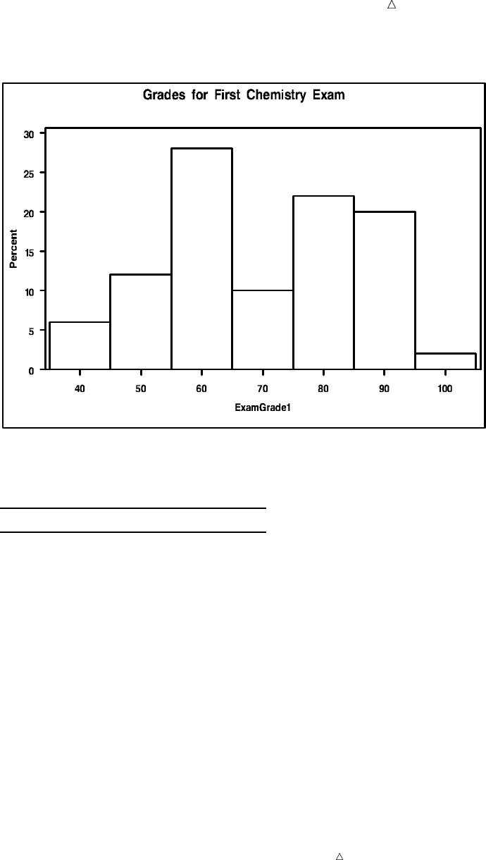
Producing Charts to Summarize Variables Creating a Simple Histogram 505
Figure 29.1 Using a Histogram to Show Percentages
The midpoint axis for the above histogram goes from 40 to 100 and is incremented in
intervals of 10. The following table shows the values:
Interval Midpoint
35 to 44 40
45 to 54 50
55 to 64 60
65 to 74 70
75 to 84 80
85 to 94 90
95 to 104 10
Note: Because PROC UNIVARIATE selects the size of the intervals and the location
of their midpoints based on all values of the numeric variable, the highest and lowest
intervals can extend beyond the values in the data. In this example the lowest grade is
39 while the lowest interval extends from 35 to 44. Similarly, the highest grade is 98
while the highest interval extends from 95 to 104.
506 Changing the Axes of a Histogram Chapter 29
Changing the Axes of a Histogram
Enhancing the Vertical Axis
The exact value of a histogram bar is sometimes difficult to determine. By default,
PROC UNIVARIATE does not provide minor tick marks between the vertical axis
values (major tick marks). You can specify the number of minor tick marks between
major tick marks with the VMINOR= option.
To make it easier to see the location of major tick marks, you can use the GRID
option to add grid lines on the histogram. Grid lines are horizontal lines that are
positioned at major tick marks on the vertical axis. PROC UNIVARIATE provides two
options to change the appearance of the grid line:
Action Option
set the color of the grid lines CGRID=
set the line type of the grid lines LGRID=
By default, PROC UNIVARIATE draws a solid line using the first color in the device
color list. For a list of the available line types, see SAS/GRAPH Software: Reference,
Volumes 1 and 2.
The following program creates a histogram that displays minor tick marks and grid
lines for the numeric variable ExamGrade1:
proc univariate data=grades noprint;
histogram Examgrade1 / vminor=4 grid lgrid=34;
title ’Grades for First Chemistry Exam’;
run;
Four minor tick marks are inserted between each major tick mark. Narrowly spaced
dots are used to draw the grid lines.
The following figure shows the histogram:
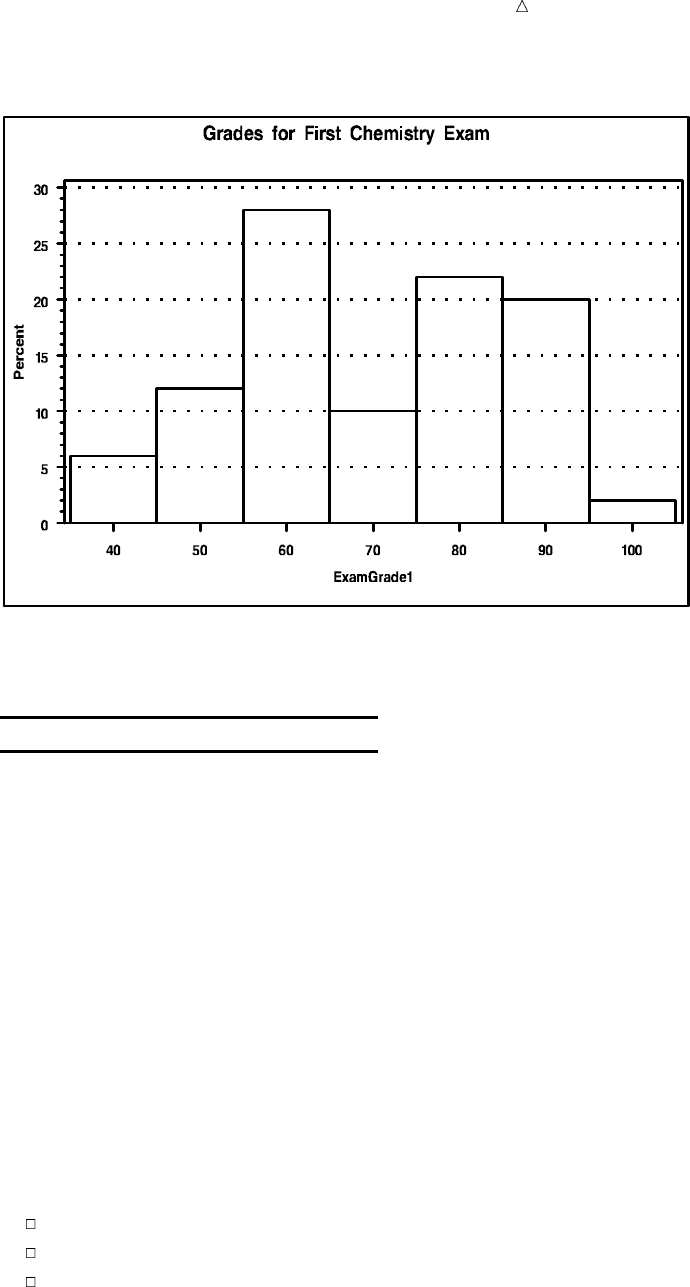
Producing Charts to Summarize Variables Changing the Axes of a Histogram 507
Figure 29.2 Specifying Grid Lines for a Histogram
Now, the height of each histogram bar is easily determined from the chart. The
following table shows the percentage each interval represents:
Interval Percent
35 to 44 6
45 to 54 12
55 to 64 28
65 to 74 10
75 to 84 22
85 to 94 20
95 to 104 2
Specifying the Vertical Axis Values
PROC UNIVARIATE enables you to specify what the bars in the histogram
represent, and the values of the vertical axis. By default, each bar represents the
percentage of observations that fall into the given interval.
The VSCALE= option enables you to specify the following scales for the vertical axis:
COUNT
PERCENT
PROPORTION
The VAXIS= option enables you to specify evenly spaced tick mark values for the
vertical axis. The form of this option is
HISTOGRAM variable / VAXIS=value-list;
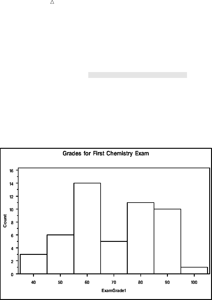
508 Changing the Axes of a Histogram Chapter 29
where value-list is a list of numbers to use as major tick mark values. The first value is
always equal to zero and the last value is always greater than or equal to the height of
the largest bar.
The following program creates a histogram that displays counts on the vertical axis
for the numeric variable ExamGrade1:
proc univariate data=grades noprint;
histogram Examgrade1 / vscale=count vaxis=0 to 16 by 2 vminor=1;
title ’Grades for First Chemistry Exam’;
run;
The values of the vertical axis range from 0 to 16 in increments of two. One minor tick
mark is inserted between each major tick mark.
The following figure shows the histogram:
Figure 29.3 Using a Histogram to Show Counts
Specifying the Midpoints of a Histogram
You can control the width of the histogram bars by using the MIDPOINTS= option.
PROC UNIVARIATE uses the value of the midpoints to determine the width of the
histogram bars. The difference between consecutive midpoints is the bar width.
To specify midpoints, use the MIDPOINTS= option in the HISTOGRAM statement.
The form of the MIDPOINTS= option is
HISTOGRAM variable / MIDPOINTS=midpoint-list;
where midpoint-list is a list of numbers to use as midpoints. You must use evenly
spaced midpoints that are listed in increasing order.
For example, to specify the traditional grading ranges with midpoints from 55 to 95,
use the following option:
midpoints=55 65 75 85 95
Or, you can abbreviate this list of midpoints:
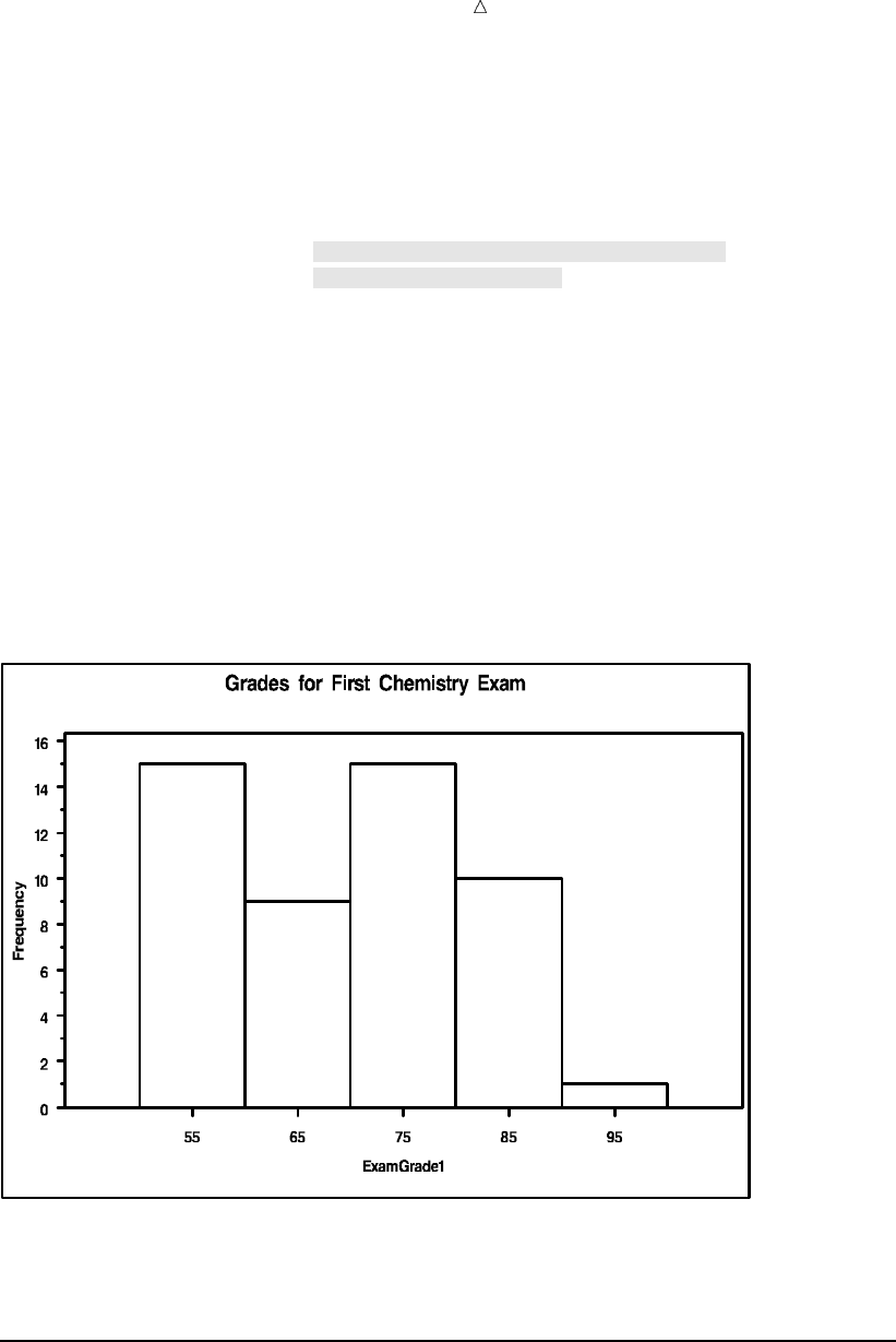
Producing Charts to Summarize Variables Displaying Summary Statistics in a Histogram 509
midpoints=55 to 95 by 10
The following program uses the MIDPOINTS= option to create a histogram for the
numeric variable ExamGrade1:
proc univariate data=grades noprint;
histogram Examgrade1 / vscale=count vaxis=0 to 16 by 2 vminor=1
midpoints=55 65 75 85 95uhoffset=10v
vaxislabel=’Frequency’w;
title ’Grades for First Chemistry Exam’;
run;
The following list corresponds to the numbered items in the preceding program:
uThe MIDPOINTS= option forces PROC UNIVARIATE to center the five bars
around the traditional midpoints for exam grades.
vThe HOFFSET= option uses a 10 percent offset at both ends of the horizontal axis.
wThe VAXISLABEL= option uses Frequency as the label for the vertical axis. The
default label is Count.
The following figure shows the histogram:
Figure 29.4 Specifying Five Midpoints for a Histogram
The midpoint axis for the above histogram goes from 55 to 95 and is incremented in
intervals of 10. The histogram excludes any exam scores that are below 50.
Displaying Summary Statistics in a Histogram
Understanding How to Use the INSET Statement
PROC UNIVARIATE enables you to add a box or table of summary statistics, called
an inset, directly in the histogram. Typically, an inset displays statistics that PROC

510 Displaying Summary Statistics in a Histogram Chapter 29
UNIVARIATE has calculated, but an inset can also display values that you provide in a
SAS data set.
To add a table of summary statistics, use the INSET statement. You can use multiple
INSET statements in the UNIVARIATE procedure to add more than one table to a
histogram. The INSET statements must follow the HISTOGRAM statement that
creates the plot that you want augmented. The inset appears in all the graphs that the
preceding HISTOGRAM statement produces.
The form of the INSET statement is as follows:
INSET<keyword(s)></option(s)>
You specify the keywords for inset statistics (such as N, MIN, MAX, MEAN, and STD)
immediately after the word INSET. You can also specify the keyword DATA= followed
by the name of a SAS data set to display customized statistics that are stored in a SAS
data set. The statistics will appear in the order in which you specify the keywords.
By default, PROC UNIVARIATE uses appropriate labels and appropriate formats to
display the statistics in the inset. To customize a label, specify the keyword followed by
an equal sign (=) and the desired label in quotation marks. To customize the format,
specify a numeric format in parentheses after the keyword. You can assign labels that
are up to 24 characters. If you specify both a label and a format for a keyword, then the
label must appear before the format. For example,
inset n=’Sample Size’ std=’Std Dev’ (5.2);
requests customized labels for two statistics (sample size and standard deviation). The
standard deviation is also assigned a format that has a field width of five and includes
two decimal places.
Various options enable you to customize the appearance of the inset. For example,
you can do the following:
Specify the position of the inset.
Specify a heading for the inset table.
Specify graphical enhancements, such as background colors, text colors, text
height, text font, and drop shadows.
For a complete list of the keywords and the options that you can use in the INSET
statement, see the Base SAS Procedures Guide.
The Program
The following program uses the INSET statement to add summary statistics for the
numeric variable ExamGrade1 to the histogram:
proc univariate data=grades noprint;
histogram Examgrade1 /vscale=count vaxis=0 to 16 by 2 vminor=1 hoffset=10
midpoints=55 65 75 85 95 vaxislabel=’Frequency’;
inset n=’No. Students’ mean=’Mean Grade’ min=’Lowest Grade’u
max=’Highest Grade’ / header=’Summary Statistics’vposition=new
format=3.x;
title ’Grade Distribution for the First Chemistry Exam’;
run;
The following list corresponds to the numbered items in the preceding program:
uThe statistical keywords N, MEAN, MIN, and MAX specify that the number of
observations, the mean exam grade, the minimum exam grade, and the maximum
exam grade appear in the inset. Each keyword is assigned a customized label to
identify the statistic in the inset.
vThe HEADER= option specifies the heading text that appears at the top of the
inset.
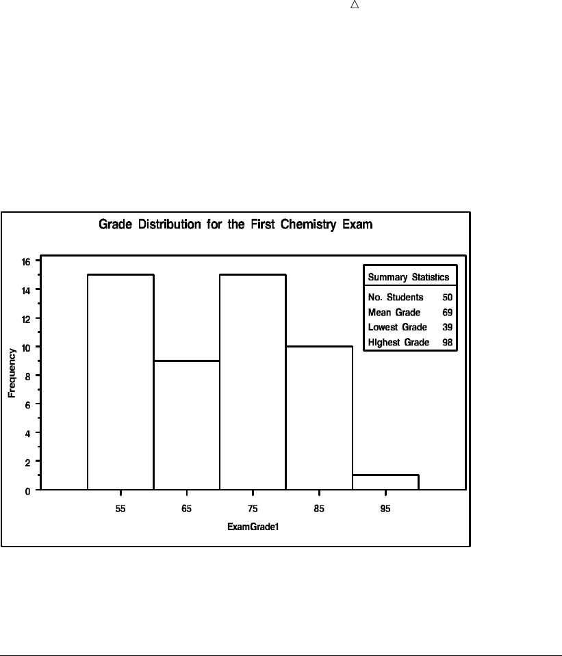
Producing Charts to Summarize Variables Creating a Comparative Histogram 511
wThe POSITION= option uses a compass point to position the inset. The table will
appear at the northeast corner of the histogram.
xThe FORMAT= option requests a format with a field width of three for all the
statistics in the inset.
The following figure shows the histogram:
Figure 29.5 Adding an Inset to a Histogram
The histogram shows the data distribution. The table of summary statistics in the
upper-right corner of the histogram provides information about the sample size, the
mean grade, the lowest value, and the highest value.
Creating a Comparative Histogram
Understanding Comparative Histograms
A comparative histogram is a series of component histograms that are arranged as
an array or a matrix. PROC UNIVARIATE uses uniform horizontal and vertical axes to
display the component histograms. This enables you to use the comparative histogram
to visually compare the distribution of a numeric variable across the levels of up to two
classification variables.
You use the CLASS statement with a HISTOGRAM statement to create either a
one-way or a two-way comparative histogram. The form of the CLASS statement is as
follows:
CLASS variable-1<(variable-option(s))> <variable-2<(variable-option(s))>></
options>;
Class variables can be numeric or character. Class variables can have continuous
values, but they typically have a few discrete values that define levels of the variable.

512 Creating a Comparative Histogram Chapter 29
You can reduce the number of classification levels by using a FORMAT statement to
combine the values of a class variable.
When you specify one class variable, PROC UNIVARIATE displays an array of
component histograms (stacked or side-by-side). To create the one-way comparative
histogram, PROC UNIVARIATE categorizes the values of the analysis variable by the
formatted values (levels) of the class variable. Each classification level generates a
separate histogram.
When you specify two class variables, PROC UNIVARIATE displays a matrix of
component plots. To create the two-way comparative histogram, PROC UNIVARIATE
categorizes the values of the analysis variable by the cross-classified values (levels) of
the class variables. Each combination of the cross-classified levels generates a separate
histogram. The levels of class variable-1 are the labels for the rows of the matrix, and
the levels of class variable-2 are the labels for the columns of the matrix.
You can specify options in the HISTOGRAM statement to customize the appearance
of the comparative histogram. For example, you can do the following:
Specify the number of rows for the comparative histogram.
Specify the number of columns for the comparative histogram.
Specify graphical enhancements, such as background colors and text colors for the
labels.
For a complete list of the keywords and the options that you can use in the
HISTOGRAM statement, see the Base SAS Procedures Guide.
The Program
The following program uses the CLASS statement to create a comparative histogram
by gender and section for the numeric variable ExamGrade1:
proc format;
value $gendfmt ’M’=’Male’
’F’=’Female’u;
run;
proc univariate data=grades noprint;
class GendervSection(order=data)w;
histogram Examgrade1 / midpoints=45 to 95 by 10 vscale=count vaxis=0 to 6 by 2
vaxislabel=’Frequency’ turnvlabelsxnrows=2 ncols=3y
cframe=ligrUcframeside=gwh cframetop=gwh cfill=gwhV;
inset mean(4.1) n / noframeWposition=(2,65)X;
format Gender $gendfmt.u;
title ’Grade Distribution for the First Chemistry Exam’;
run;
The following list corresponds to the numbered items in the preceding program:
uPROC FORMAT creates a user-written format that will label Gender with a
character string. The FORMAT statement assigns the format to Gender.
vThe CLASS statement creates a two-way comparative histogram that uses Gender
and Section as the classification variables. PROC UNIVARIATE produces a
component histogram for each level (a distinct combination of values) of these
variables.
wThe ORDER= option positions the values of Section according to their order in the
input data set. The comparative histogram displays the levels of Section according
to the days of the week (Mon, Wed, and Fri). The default order of the levels is
determined by sorting the internal values of Section (Fri, Mon, and Wed).
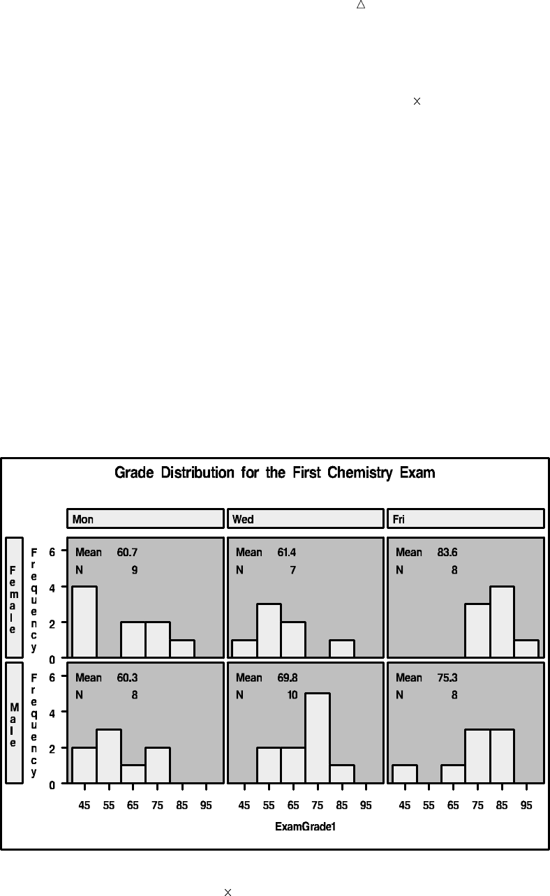
Producing Charts to Summarize Variables Creating a Comparative Histogram 513
xThe TURNVLABELS option turns the characters in the vertical axis labels so that
they display vertically instead of horizontally.
yThe NROWS= option and the NCOLS= option specify a 2 3 arrangement for the
component histograms.
UThe CFRAME= option specifies the color that fills the area of each component
histogram that is enclosed by the axes and the frame. The CFRAMESIDE= option
and the CFRAMETOP= option specify the color to fill the frame area for the
column labels and the row labels that appear down the side and across the top of
the comparative histogram. By default, these areas are not filled.
VThe CFILL= option specifies the color to fill the bars of each component histogram.
By default, the bars are not filled.
WThe NOFRAME option suppresses the frame around the inset table.
XThe POSITION= option uses axis percentage coordinates to position the inset. The
position of the bottom-left corner of the inset is 2% of the way across the
horizontal axis and 65% of the way up the vertical axis.
The following figure shows the comparative histogram:
Figure 29.6 Using a Comparative Histogram to Examine Exam Grades by Gender
and Section
The comparative histogram is a 2 3 matrix of component histograms for each
combination of Section and Gender. Each component histogram displays a table of
statistics that reports the mean of ExamGrade1 and the number of students. You can
easily see that both females and males in the Friday section earned higher grades than
their counterparts in the other sections.
514 Review of SAS Tools Chapter 29
Review of SAS Tools
PROC CHART Statements
PROC CHART < DATA=SAS-data-set ><options>;
chart-type variable(s) </options>;
PROC CHART <DATA=SAS-data-set><options>;
starts the CHART procedure. You can specify the following options in the PROC
CHART statement:
DATA=SAS-data-set
names the SAS data set that PROC CHART uses. If you omit DATA=, then
PROC CHART uses the most recently created data set.
LPI=value
specifies the proportions of PIE and STAR charts.
chart-type variable(s) </options>;
is a chart statement where
chart-type
specifies the kind of chart and can be any of the following:
BLOCK
HBAR
PIE
VBAR
You can use any number of chart statements in one PROC CHART step. A
list of options pertains to a single chart statement.
variable(s)
identifies the variables to chart (called the chart variables).
options
specifies a list of options. Not all types of chart support all options.
You can use the following options in the VBAR, HBAR, and BLOCK
statements:
GROUP=variable
produces a set of bars or blocks for each value of variable.
SUBGROUP=variable
proportionally fills each block or bar with characters that represent
different values of variable.
You can use the following options in the VBAR, HBAR, BLOCK, and PIE
statements:
DISCRETE
creates a bar, block, or section for every value of the chart variable.
LEVELS=number-of-midpoints
specifies the number-of-midpoints. The procedure selects the midpoints.
MIDPOINTS=midpoints-list
specifies the values of the midpoints.

Producing Charts to Summarize Variables PROC UNIVARIATE Statements 515
SUMVAR=variable
specifies the variable to use to determine the size of the bars, blocks, or
sections.
TYPE=SUM|MEAN
specifies the type of chart to create, where
SUM
sums the values of the Sumvar variable in each range. Then PROC
CHART uses the sums to determine the size of each bar, block, or
section.
MEAN
determines the mean value of the Sumvar variable in each range.
Then PROC CHART uses the means to determine the size of each
bar, block, or section.
You can use the following options in the HBAR statement:
NOSTAT
suppresses the printing of the statistics that accompany the chart by
default.
FREQ
requests frequency statistics.
CFREQ
requests cumulative frequency statistics.
PERCENT
requests percentage statistics.
CPERCENT
requests cumulative percentage statistics.
PROC UNIVARIATE Statements
PROC UNIVARIATE <option(s)>;
CLASS variable-1<(variable-option(s))>
<variable-2<(variable-option(s))>> </option(s)>;
HISTOGRAM <variable(s)></option(s)>;
INSET <keyword(s) ></option(s)>;
PROC UNIVARIATE option(s);
starts the UNIVARIATE procedure. You can specify the following options in the
PROC UNIVARIATE statement:
DATA=SAS-data-set
names the SAS data set that PROC UNIVARIATE uses. If you omit DATA=,
then PROC UNIVARIATE uses the most recently created data set.
NOPRINT
suppresses the descriptive statistics that the PROC UNIVARIATE statement
creates.
CLASS variable-1<(variable-option(s))> <variable-2<(variable-option(s))>>
</ option(s)>;
specifies up to two variables whose values determine the classification levels for
the component histograms. Variables in a CLASS statement are referred to as
class variables.

516 PROC UNIVARIATE Statements Chapter 29
You can specify the following option(s) in the CLASS statement:
ORDER=DATA | FORMATTED | FREQ | INTERNAL
specifies the display order for the class variable values, where
DATA
orders values according to their order in the input data set.
FORMATTED
orders values by their ascending formatted values. This order depends
on your operating environment.
FREQ
orders values by descending frequency count so that levels with the
most observations are listed first.
INTERNAL
orders values by their unformatted values, which yields the same order
as PROC SORT. This order depends on your operating environment.
HISTOGRAM <variable(s)></option(s)>;
creates histograms and comparative histograms using high-resolution graphics for
the analysis variables that are specified. If you omit variable(s) in the
HISTOGRAM statement, then the procedure creates a histogram for each variable
that you list in the VAR statement, or for each numeric variable in the DATA=
data set if you omit a VAR statement.
You can specify the following options in the PROC UNIVARIATE statement:
CGRID=color
specifies the color for grid lines when a grid displays on the histogram.
GRID
specifies to display a grid on the histogram. Grid lines are horizontal lines
that are positioned at major tick marks on the vertical axis.
HOFFSET=value
specifies the offset in percentage screen units at both ends of the horizontal
axis.
GRID
specifies to display a grid on the histogram. Grid lines are horizontal lines
that are positioned at major tick marks on the vertical axis.
LGRID=linetype
specifies the line type for the grid when a grid displays on the histogram. The
default is a solid line.
MIDPOINTS=value(s)
determines the width of the histogram bars as the difference between
consecutive midpoints. PROC UNIVARIATE uses the same value(s) for all
variables. You must use evenly spaced midpoints that are listed in increasing
order.
VAXIS=value(s)
specifies tick mark values for the vertical axis. Use evenly spaced values that
are listed in increasing order. The first value must be zero and the last value
must be greater than or equal to the height of the largest bar. You must scale
the values in the same units as the bars.
VMINOR=n
specifies the number of minor tick marks between each major tick mark on
the vertical axis. PROC UNIVARIATE does not label minor tick marks.

Producing Charts to Summarize Variables FORMAT Statement 517
VSCALE=scale
specifies the scale of the vertical axis, where scale is
COUNT
scales the data in units of the number of observations per data unit.
PERCENT
scales the data in units of percentage of observations per data unit.
PROPORTION
scales the data in units of proportion of observations per data unit.
INSET <keyword(s)></option(s)>;
places a box or table of summary statistics, called an inset, directly in the
histogram.
You can specify the following options in the PROC UNIVARIATE statement:
keyword(s)
specifies one or more keywords that identify the information to display in the
inset. PROC UNIVARIATE displays the information in the order that you
request the keywords. For a complete list of keywords, see the INSET
statement in SAS/GRAPH Software: Reference, Volumes 1 and 2.
FORMAT=format
specifies a format for all the values in the inset. If you specify a format for a
particular statistic, then this format overrides FORMAT=format.
HEADER=string
specifies the heading text where string cannot exceed 40 characters.
NOFRAME
suppresses the frame drawn around the text.
POSITION=position
determines the position of the inset. The position is a compass point keyword, a
margin keyword, or a pair of coordinates (x,y). The default position is NW, which
positions the inset in the upper-left (northwest) corner of the display.
GOPTIONS Statement
GOPTIONS options-list;
specifies values for graphics options. Graphics options control characteristics of
the graph, such as size, colors, type fonts, fill patterns, and symbols. In addition,
they affect the settings of device parameters, which are defined in the device entry.
Device parameters control such characteristics as the appearance of the display,
the type of output that is produced, and the destination of the output.
FORMAT Statement
FORMAT variable format-name;
enables you to display the value of a variable by using a special pattern that you
specify as format-name.

518 Learning More Chapter 29
Learning More
PROC CHART
For complete documentation, see the Base SAS Procedures Guide. In addition to
the features that are described in this section, you can use PROC CHART to
create star charts, to draw a reference line at a particular value on a bar chart,
and to change the symbol that is used to draw charts. You can also create charts
based, not only on frequency, sum, and mean, but also on cumulative frequency,
percent, and cumulative percent.
PROC UNIVARIATE
For complete documentation, see the Base SAS Procedures Guide.
PROC PLOT
For a discussion about how to plot the relationship between variables, see Chapter
28, “Plotting the Relationship between Variables,” on page 463. When you are
preparing graphics presentations, some data lends itself to charts, while other
data is better suited for plots.
SAS formats
For complete documentation, see SAS Language Reference: Dictionary. Many
formats are available with SAS, including fractions, hexadecimal values, roman
numerals, social security numbers, date and time values, and numbers written as
words.
PROC FORMAT
For complete documentation about how to create your own formats, see the Base
SAS Procedures Guide.
SAS/GRAPH software
For complete documentation, see SAS/GRAPH Software: Reference, Volumes 1
and 2. If your site has SAS/GRAPH software, then you can use the GCHART
procedure to take advantage of the high-resolution graphics capabilities of output
devices and produce charts that include color, different fonts, and text.
TITLE and FOOTNOTE statements
For a discussion about using titles and footnotes in a report, see “Understanding
Titles and Footnotes” on page 392.

519
PART
8
Designing Your Own Output
Chapter 30.........
Writing Lines to the SAS Log or to an Output File 521
Chapter 31.........
Understanding and Customizing SAS Output: The Basics 537
Chapter 32.........
Understanding and Customizing SAS Output: The Output
Delivery System (ODS) 565
520
521
CHAPTER
30
Writing Lines to the SAS Log or
to an Output File
Introduction to Writing Lines to the SAS Log or to an Output File 521
Purpose 521
Prerequisites 521
Understanding the PUT Statement 522
Writing Output without Creating a Data Set 522
Writing Simple Text 523
Writing a Character String 523
Writing Variable Values 524
Writing on the Same Line More than Once 525
Releasing a Held Line 526
Writing a Report 528
Writing to an Output File 528
Designing the Report 528
Writing Data Values 529
Improving the Appearance of Numeric Data Values 530
Writing a Value at the Beginning of Each BY Group 531
Calculating Totals 532
Writing Headings and Footnotes for a One-Page Report 533
Review of SAS Tools 535
Statements 535
Learning More 536
Introduction to Writing Lines to the SAS Log or to an Output File
Purpose
In previous sections you learned how to store data values in a SAS data set and to
use SAS procedures to produce a report that is based on these data values. In this
section, you will learn how to do the following:
design output by positioning data values and character strings in an output file
prevent SAS from creating a data set by using the DATA _NULL_ statement
produce reports by using the DATA step instead of using a procedure
direct data to an output file by using a FILE statement
Prerequisites
Before proceeding with this section, you should be familiar with the concepts
presented in the following sections:

522 Understanding the PUT Statement Chapter 30
Chapter 1, “What Is the SAS System?,” on page 3
Chapter 2, “Introduction to DATA Step Processing,” on page 19
Understanding the PUT Statement
When you create output using the DATA step, you can customize that output by
using the PUT statement to write text to the SAS log or to another output file. The
PUT statement has the following form:
PUT<variable<format>><’character-string’>;
where
variable
names the variable that you want to write.
format
specifies a format to use when you write variable values.
’character-string’
specifies a string of text to write. Be sure to enclose the string in quotation marks.
Writing Output without Creating a Data Set
In many cases, when you use a DATA step to write a report, you do not need to
create an additional data set. When you use the DATA _NULL_ statement, SAS
processes the DATA step without writing observations to a data set. Using the DATA
_NULL_ statement can increase program efficiency considerably.
The following is an example of a DATA _NULL_ statement:
data _null_;
The following program uses a PUT statement to write newspaper circulation values
to the SAS log. Because the program uses a DATA _NULL_ statement, SAS does not
create a data set.
data _null_;
length state $ 15;
input state $ morning_copies evening_copies year;
put state morning_copies evening_copies year;
datalines;
Massachusetts 798.4 984.7 1999
Massachusetts 834.2 793.6 1998
Massachusetts 750.3 . 1997
Alabama . 698.4 1999
Alabama 463.8 522.0 1998
Alabama 583.2 234.9 1997
Alabama . 339.6 1996
;
The following output shows the results:

Writing Lines to the SAS Log or to an Output File Writing a Character String 523
Output 30.1 Writing to the SAS Log
184 data _null_;
185 length state $ 15;
186 input state $ morning_copies evening_copies year;
187 put state morning_copies evening_copies year;
188 datalines;
Massachusetts 798.4 984.7 1999
Massachusetts 834.2 793.6 1998
Massachusetts 750.3 . 1997
Alabama . 698.4 1999
Alabama 463.8 522 1998
Alabama 583.2 234.9 1997
Alabama . 339.6 1996
196 ;
SAS indicates missing numeric values with a period. Note that the log contains three
missing values.
Writing Simple Text
Writing a Character String
In its simplest form, the PUT statement writes the character string that you specify
to the SAS log, to a procedure output file, or to an external file. If you omit the
destination (as in this example), then SAS writes the string to the log. In the following
example, SAS executes the PUT statement once during each iteration of the DATA step.
When SAS encounters missing values for MORNING_VALUES or EVENING_COPIES,
the PUT statement writes a message to the log.
data _null_;
length state $ 15;
infile ’your-input-file’;
input state $ morning_copies evening_copies year;
if morning_copies=. then put ’** Morning Circulation Figures Missing’;
else
if evening_copies=. then put ’** Evening Circulation Figures Missing’;
run;
The following output shows the results:

524 Writing Variable Values Chapter 30
Output 30.2 Writing a Character String to the SAS Log
93 data _null_;
94 length state $ 15;
95 infile ’your-input-file’;
96 input state $ morning_copies evening_copies year;
97 if morning_copies =. then put ’** Morning Circulation Figures Missing’;
98 else
99 if evening_copies =. then put ’** Evening Circulation Figures Missing’;
100 run;
NOTE: The infile ’your-input-file’ is:
File Name=file-name,
Owner Name=xxxxxx,Group Name=xxxx,
Access Permission=rw-r--r--,
File Size (bytes)=223
** Evening Circulation Figures Missing
** Morning Circulation Figures Missing
** Morning Circulation Figures Missing
NOTE: 7 records were read from the infile ’your-input-file’.
The minimum record length was 30.
The maximum record length was 31.
Writing Variable Values
Output 30.2 shows that the value for MORNING_COPIES is missing for two
observations in the data set, and the value for EVENING_COPIES is missing for one
observation. To identify which observations have the missing values, write the value of
one or more variables along with the character string. The following program writes the
value of YEAR and STATE, as well as the character string:
data _null_;
length state $ 15;
infile ’your-input-file’;
input state $ morning_copies evening_copies year;
if morning_copies =. then put
’** Morning Circulation Figures Missing: ’ year state;
else
if evening_copies =. then put
’** Evening Circulation Figures Missing: ’ year state;
run;
Notice that the last character in each of the strings is blank. This is an example of
list output. In list output, SAS automatically moves one column to the right after
writing a variable value, but not after writing a character string. The simplest way to
include the required space is to include it in the character string.
SAS keeps track of its position in the output line with a pointer. Another way to
describe the action in this PUT statement is to say that in list output, the pointer
moves one column to the right after writing a variable value, but not after writing a
character string. In later parts of this section, you will learn ways to move the pointer
to control where the next piece of text is written.
The following output shows the results:

Writing Lines to the SAS Log or to an Output File Writing on the Same Line More than Once 525
Output 30.3 Writing a Character String and Variable Values
164 data _null_;
165 length state $ 15;
166 infile ’your-input-file’;
167 input state $ morning_copies evening_copies year;
168 if morning_copies =. then put
169 ’** Morning Circulation Figures Missing: ’ year state;
170 else
171 if evening_copies =. then put
172 ’** Evening Circulation Figures Missing: ’ year state;
173 run;
NOTE: The infile ’your-file-name’ is:
File Name=file-name,
Owner Name=xxxxxx,Group Name=xxxx,
Access Permission=rw-r--r--,
File Size (bytes)=223
** Evening Circulation Figures Missing: 1997 Massachusetts
** Morning Circulation Figures Missing: 1999 Alabama
** Morning Circulation Figures Missing: 1996 Alabama
NOTE: 7 records were read from the infile ’your-input-file’.
The minimum record length was 30.
The maximum record length was 31.
Writing on the Same Line More than Once
By default, each PUT statement begins on a new line. However, you can write on the
same line if you use more than one PUT statement and at least one trailing @ (“at” sign).
The trailing @ is a type of pointer control called a line-hold specifier. Pointer controls
are one way to specify where SAS writes text. In the following example, using the
trailing @ causes SAS to write the item in the second PUT statement on the same line
rather than on a new line. The execution of either PUT statement holds the output line
for further writing because each PUT statement has a trailing @. SAS continues to
write on that line when a later PUT statement in the same iteration of the DATA step
is executed and also when a PUT statement in a later iteration is executed.
options linesize=80 pagesize=60;
data _null_;
length state $ 15;
infile ’your-input-file’;
input state $ morning_copies evening_copies year;
if morning_copies =. then put
’** Morning Tot Missing: ’ year state @;
if evening_copies =. then put
’** Evening Tot Missing: ’ year state @;
run;
The following output shows the results:
526 Releasing a Held Line Chapter 30
Output 30.4 Writing on the Same Line More than Once
157 options linesize=80 pagesize=60;
158
159 data _null_;
160 length state $ 15;
161 infile ’your-input-file’;
162 input state $ morning_copies evening_copies year;
163 if morning_copies =. then put
164 ’** Morning Tot Missing: ’ year state @;
165 if evening_copies =. then put
166 ’** Evening Tot Missing: ’ year state @;
167 run;
NOTE: The infile ’your-input-file’ is:
File Name=file-name,
Owner Name=xxxxxx,Group Name=xxxx,
Access Permission=rw-r--r--,
File Size (bytes)=223
** Evening Tot Missing: 1997 Massachusetts ** Morning Tot Missing: 1999 Alabama
** Morning Tot Missing: 1996 Alabama
NOTE: 7 records were read from the infile ’your-input-file’.
The minimum record length was 30.
The maximum record length was 31.
If the output line were long enough, then SAS would write all three messages about
missing data on a single line. Because the line is not long enough, SAS continues
writing on the next line. When it determines that an individual data value or character
string does not fit on a line, SAS brings the entire item down to the next line. SAS does
not split a data value or character string.
Releasing a Held Line
In the following example, the input file has five missing values. One record has
missing values for both the MORNING_COPIES and EVENING_COPIES variables.
Three other records have missing values for either the MORNING_COPIES or the
EVENING_COPIES variable.
To improve the appearance of your report, you can write all the missing variables for
each observation on a separate line. When values for the two variables
MORNING_COPIES and EVENING_COPIES are missing, two PUT statements write
to the same line. When either MORNING_COPIES or EVENING_COPIES is missing,
only one PUT statement writes to that line.
SAS determines where to write the output by the presence of the trailing @ sign in
the PUT statement and the presence of a null PUT statement that releases the hold on
the line. Executing a PUT statement with a trailing @ causes SAS to hold the current
output line for further writing, either in the current iteration of the DATA step or in a
future iteration. Executing a PUT statement without a trailing @ releases the held line.
To release a line without writing a message, use a null PUT statement:
put;
A null PUT statement has the same characteristics of other PUT statements: by
default, it writes output to a new line, writes what you specify in the statement
(nothing in this case), and releases the line when it finishes executing. If a trailing @ is
in effect, then the null PUT statement begins on the current line, writes nothing, and
releases the line.
The following program shows how to write one or more items to the same line:
Writing Lines to the SAS Log or to an Output File Releasing a Held Line 527
If a value for MORNING_COPIES is missing, then the first PUT statement holds
the line in case EVENING_COPIES is missing a value for that observation.
If a value for EVENING_COPIES is missing, then the next PUT statement writes
a message and releases the line.
If EVENING_COPIES does not have a missing value, but if a message has been
written for MORNING_COPIES (MORNING_COPIES=.), then the null PUT
statement releases the line.
If neither EVENING_COPIES nor MORNING_COPIES has missing values, then
the line is not released and no PUT statement is executed.
options linesize=80 pagesize=60;
data _null_;
length state $ 15;
infile ’your-input-file’;
input state $ morning_copies evening_copies year;
if morning_copies=. then put
’** Morning Tot Missing: ’ year state @;
if evening_copies=. then put
’** Evening Tot Missing: ’ year state;
else if morning_copies=. then put;
run;
The following output shows the results:
Output 30.5 Writing One or More Times to a Line and Releasing the Line
7 data _null_;
8 length state $ 15;
9 infile ’your-input-file’;
10 input state $ morning_copies evening_copies year;
11 if morning_copies=. then put
12 ’** Morning Tot Missing: ’ year state @;
13 if evening_copies=. then put
14 ’** Evening Tot Missing: ’ year state;
15 else if morning_copies=. then put;
16 run;
NOTE: The infile ’your-input-file’ is:
File Name=your-input-file,
Owner Name=xxxxxx,Group Name=xxxx,
Access Permission=rw-r--r--,
File Size (bytes)=223
** Evening Tot Missing: 1997 Massachusetts
** Morning Tot Missing: 1999 Alabama
** Morning Tot Missing: 1998 Alabama ** Evening Tot Missing: 1998 Alabama
** Morning Tot Missing: 1996 Alabama
NOTE: 7 records were read from the infile ’your-input-file’.
The minimum record length was 30.
The maximum record length was 31.

528 Writing a Report Chapter 30
Writing a Report
Writing to an Output File
The PUT statement writes lines of text to the SAS log. However, the SAS log is not
usually a good destination for a formal report because it also contains the source
statements for the program and messages from SAS.
The simplest destination for a printed report is the SAS output file, which is the
same place SAS writes output from procedures. SAS automatically defines various
characteristics such as page numbers for the procedure output file, and you can take
advantage of them instead of defining all the characteristics yourself.
To route lines to the procedure output file, use the FILE statement. The FILE
statement has the following form:
FILE PRINT <options>;
PRINT is a reserved fileref that directs output that is produced by PUT statements
to the same print file as the output that is produced by SAS procedures.
Note: Be sure that the FILE statement precedes the PUT statement in the program
code.
FILE statement options specify options that you can use to customize output. The
report that is produced in this section uses the following options:
NOTITLES
eliminates the default title line and makes that line available for writing. By
default, the procedure output file contains the title “The SAS System.” Because
the report creates another title that is descriptive, you can remove the default title
by specifying the NOTITLES option.
FOOTNOTES
controls whether currently defined footnotes are written to the report.
Note: When you use the FILE statement to include footnotes in a report, you
must use the FOOTNOTES option in the FILE statement and include a
FOOTNOTE statement in your program. The FOOTNOTE statement contains the
text of the footnote.
Note: You can also remove the default title with a null TITLE statement: title;.
In this case, SAS writes a line that contains only the date and page number in place of
the default title, and the line is not available for writing other text.
Designing the Report
After choosing a destination for your report, the next step in producing a report is to
decide how you want it to look. You create the design and determine which lines and
columns the text will occupy. Planning how you want your final report to look helps you
write the necessary PUT statements to produce the report. The rest of the examples in
this section show how to modify a program to produce a final report that resembles the
one shown here.

Writing Lines to the SAS Log or to an Output File Writing Data Values 529
----+----1----+----2----+----3----+----4----+----5----+----6----+----7--
1 Morning and Evening Newspaper Circulation
2
3 State Year Thousands of Copies
4 Morning Evening
5
6 Alabama 1984 256.3 480.5
7 1985 291.5 454.3
8 1986 303.6 454.7
9 1987 . 454.5
10 ------ --------
11 Total for each category 851.4 1844.0
12 Combined total 2695.4
13
14
15 Massachusetts 1984 . .
16 1985 . 68.0
17 1986 222.7 68.6
18 1987 224.1 66.7
19 ------ ------
20 Total for each category 446.8 203.3
21 Combined total 650.1
22
23
24
25
26
27
28
29
30 Preliminary Report
----+----1----+----2----+----3----+----4----+----5----+----6----+----7--
Writing Data Values
After you design your report, you can begin to write the program that will create it.
The following program shows how to display the data values for the YEAR,
MORNING_COPIES, and EVENING_COPIES variables in specific positions.
In a PUT statement, the @ followed by a number is a pointer control, but it is
different from the trailing @ described earlier. The @nargument is a column-pointer
control. It tells SAS to move to column n. In this example the pointer moves to the
specified locations, and the PUT statement writes values at those points using list
output. Combining list output with pointer controls is a simple but useful way of
writing data values in columns.
options pagesize=30 linesize=80 pageno=1 nodate;
data _null_;
infile ’your-input-file’;
input state $ morning_copies evening_copies year;
file print notitles;
put @26 year @53 morning_copies @66 evening_copies;
run;
530 Improving the Appearance of Numeric Data Values Chapter 30
The following output shows the results:
Output 30.6 Data Values in Specific Locations in the Output
1999 798.4 984.7
1998 834.2 793.6
1997 750.3 .
1999 . 698.4
1998 463.8 522
1997 583.2 234.9
1996 . 339.6
Improving the Appearance of Numeric Data Values
In the design for your report, all numeric values are aligned on the decimal point
(see Output 30.6). To achieve this result, you have to alter the appearance of the
numeric data values by using SAS formats. In the input data all values for
MORNING_COPIES and EVENING_COPIES contain one decimal place, except in one
case where the decimal value is 0. In list output SAS writes values in the simplest way,
that is, by omitting the 0s in the decimal portion of a value. In formatted output, you
can show one decimal place for every value by associating a format with a variable in
the PUT statement. Using a format can also align your output values.
The format that is used in the program is called the w.d format. The w.d format
specifies the number of columns to be used for writing the entire value, including the
decimal point. It also specifies the number of columns to be used for writing the
decimal portion of each value. In this example the format 5.1 causes SAS to use five
columns, including one decimal place, for writing each value. Therefore, SAS prints the
0s in the decimal portion as necessary. The format also aligns the periods that SAS
uses to indicate missing values with the decimal points.
options pagesize=30 linesize=80 pageno=1 nodate;
data _null_;
infile ’your-input-file’;
input state $ morning_copies evening_copies year;
file print notitles;
put @26 year @53 morning_copies 5.1 @66 evening_copies 5.1;
run;
The following output shows the results:
Output 30.7 Formatted Numeric Output
1999 798.4 984.7
1998 834.2 793.6
1997 750.3 .
1999 . 698.4
1998 463.8 522.0
1997 583.2 234.9
1996 . 339.6

Writing Lines to the SAS Log or to an Output File Writing a Value at the Beginning of Each BY Group 531
Writing a Value at the Beginning of Each BY Group
The next step in creating your report is to add the name of the state to your output.
If you include the name of the state in the PUT statement with other data values, then
the state will appear on every line. However, remembering what you want your final
report to look like, you need to write the name of the state only for the first observation
of a particular state. Performing a task once for a group of observations requires the use
of the BY statement for BY-group processing. The BY statement has the following form:
BY by-variable(s)<NOTSORTED>;
The by-variable names the variable by which the data set is sorted. The optional
NOTSORTED option specifies that observations with the same BY value are grouped
together but are not necessarily sorted in alphabetical or numerical order.
For BY-group processing,
ensure that observations come from a SAS data set, not an external file.
when the data is grouped in BY groups but the groups are not necessarily in
alphabetical order, use the NOTSORTED option in the BY statement. For
example, use
by state notsorted;
The following program creates a permanent SAS data set named
NEWS.CIRCULATION, and writes the name of the state on the first line of the report
for each BY group.
options pagesize=30 linesize=80 pageno=1 nodate;
libname news ’SAS-data-library’;
data news.circulation;
length state $ 15;
input state $ morning_copies evening_copies year;
datalines;
Massachusetts 798.4 984.7 1999
Massachusetts 834.2 793.6 1998
Massachusetts 750.3 . 1997
Alabama . 698.4 1999
Alabama 463.8 522.0 1998
Alabama 583.2 234.9 1997
Alabama . 339.6 1996
;
data _null_;
set news.circulation;
by state notsorted;
file print notitles;
if first.state then put / @7 state @;
put @26 year @53 morning_copies 5.1 @66 evening_copies 5.1;
run;
During the first observation for a given state, a PUT statement writes the name of
the state and holds the line for further writing (the year and circulation figures). The
next PUT statement writes the year and circulation figures and releases the held line.
In observations after the first, only the second PUT statement is processed. It writes
the year and circulation figures and releases the line as usual.
532 Calculating Totals Chapter 30
The first PUT statement contains a slash (/), a pointer control that moves the pointer
to the beginning of the next line. In this example, the PUT statement prepares to write
on a new line (the default action). Then the slash moves the pointer to the beginning of
the next line. As a result, SAS skips a line before writing the value of STATE. In the
output, a blank line separates the data for Massachusetts from the data for Alabama.
The output for Massachusetts also begins one line farther down the page than it would
have otherwise. (That blank line is used later in the development of the report.)
The following output shows the results:
Output 30.8 Effect of BY-Group Processing
Massachusetts 1999 798.4 984.7
1998 834.2 793.6
1997 750.3 .
Alabama 1999 . 698.4
1998 463.8 522.0
1997 583.2 234.9
1996 . 339.6
Calculating Totals
The next step is to calculate the total morning circulation figures, total evening
circulation figures, and total overall circulation figures for each state. Sum statements
accumulate the totals, and assignment statements start the accumulation at 0 for each
state. When the last observation for a given state is being processed, an assignment
statement calculates the overall total, and a PUT statement writes the totals and
additional descriptive text.
options pagesize=30 linesize=80 pageno=1 nodate;
libname news ’SAS-data-library’;
data _null_;
set news.circulation;
by state notsorted;
file print notitles;
/* Set values of accumulator variables to 0 */
/* at beginning of each BY group. */
if first.state then
do;
morning_total=0;
evening_total=0;
put / @7 state @;
end;
put @26 year @53 morning_copies 5.1 @66 evening_copies 5.1;
/* Accumulate separate totals for morning and */
/* evening circulations. */
morning_total+morning_copies;
evening_total+evening_copies;
/* Calculate total circulation at the end of */
Writing Lines to the SAS Log or to an Output File Writing Headings and Footnotes for a One-Page Report 533
/* each BY group. */
if last.state then
do;
all_totals=morning_total+evening_total;
put @52 ’------’ @65 ’------’ /
@26 ’Total for each category’
@52 morning_total 6.1 @65 evening_total 6.1 /
@35 ’Combined total’ @59 all_totals 6.1;
end;
run;
The following output shows the results:
Output 30.9 Calculating and Writing Totals for Each BY Group
Massachusetts 1999 798.4 984.7
1998 834.2 793.6
1997 750.3 .
------ ------
Total for each category 2382.9 1778.3
Combined total 4161.2
Alabama 1999 . 698.4
1998 463.8 522.0
1997 583.2 234.9
1996 . 339.6
------ ------
Total for each category 1047.0 1794.9
Combined total 2841.9
Notice that Sum statements ignore missing values when they accumulate totals.
Also, by default, Sum statements assign the accumulator variables (in this case,
MORNING_TOTAL and EVENING_TOTAL) an initial value of 0. Therefore, although
the assignment statements in the DO group are executed for the first observation for
both states, you need them only for the second state.
Writing Headings and Footnotes for a One-Page Report
The report is complete except for the title lines, column headings, and footnote.
Because this is a simple, one-page report, you can write the heading with a PUT
statement that is executed only during the first iteration of the DATA step. The
automatic variable _N_ counts the number of times the DATA step has iterated or
looped, and the PUT statement is executed when the value of _N_ is 1.
The FOOTNOTES option on the FILE statement and the FOOTNOTE statement
create the footnote. The following program is complete:
options pagesize=30 linesize=80 pageno=1 nodate;
libname news ’SAS-data-library’;
data _null_;
set news.circulation;
by state notsorted;
file print notitles footnotes;
if _n_=1 then put @16 ’Morning and Evening Newspaper Circulation’ //
@7 ’State’ @26 ’Year’ @51 ’Thousands of Copies’ /

534 Writing Headings and Footnotes for a One-Page Report Chapter 30
@51 ’Morning Evening’;
if first.state then
do;
morning_total=0;
evening_total=0;
put / @7 state @;
end;
put @26 year @53 morning_copies 5.1 @66 evening_copies 5.1;
morning_total+morning_copies;
evening_total+evening_copies;
if last.state then
do;
all_totals=morning_total+evening_total;
put @52 ’------’ @65 ’------’ /
@26 ’Total for each category’
@52 morning_total 6.1 @65 evening_total 6.1 /
@35 ’Combined total’ @59 all_totals 6.1;
end;
footnote ’Preliminary Report’;
run;
The following output shows the results:
Output 30.10 The Final Report
Morning and Evening Newspaper Circulation
State Year Thousands of Copies
Morning Evening
Massachusetts 1999 798.4 984.7
1998 834.2 793.6
1997 750.3 .
------ ------
Total for each category 2382.9 1778.3
Combined total 4161.2
Alabama 1999 . 698.4
1998 463.8 522.0
1997 583.2 234.9
1996 . 339.6
------ ------
Total for each category 1047.0 1794.9
Combined total 2841.9
Preliminary Report
Notice that a blank line appears between the last line of the heading and the first
data for Massachusetts although the PUT statement for the heading does not write a
blank line. The line comes from the slash (/) in the PUT statement that writes the
value of STATE in the first observation of each BY group.

Writing Lines to the SAS Log or to an Output File Statements 535
Executing a PUT statement during the first iteration of the DATA step is a simple
way to produce headings, especially when a report is only one page long.
Review of SAS Tools
Statements
BY variable-1 <. . . variable-n > <NOTSORTED>;
indicates that all observations with common values of the BY variables are
grouped together. The NOTSORTED option indicates that the variables are
grouped but that the groups are not necessarily in alphabetical or numerical order.
DATA _NULL_;
specifies that SAS will not create an output data set.
FILE PRINT <NOTITLES> <FOOTNOTES>;
directs output to the SAS procedure output file. Place the FILE statement before
the PUT statements that write to that file. The NOTITLES option suppresses
titles that are currently in effect, and makes the lines unavailable for writing
other text. The FOOTNOTES option, along with the FOOTNOTE statement,
writes a footnote to the file.
PUT;
by default, begins a new line and releases a previously held line. A PUT statement
that does not write any text is known as a null PUT statement.
PUT <variable <format>> <character string>;
writes lines to the destination that is specified in the FILE statement; if no FILE
statement is present, then the PUT statement writes to the SAS log. By default,
each PUT statement begins on a new line, writes what is specified, and releases
the line. A DATA step can contain any number of PUT statements.
By default, SAS writes a variable or character-string at the current position in
the line. SAS automatically moves the pointer one column to the right after
writing a variable value but not after writing a character string; that is, SAS
places a blank after a variable value but not after a character string. This form of
output is called list output. If you place a format after a variable name, then SAS
writes the value of the variable beginning at its current position in the line and
using the format that you specify. The position of the pointer after a formatted
value is the following column; that is, SAS does not automatically skip a column.
Using a format in a PUT statement is called formatted output. You can combine
list and formatted output in a single PUT statement.
PUT<@n><variable <format>> <character-string> </> <@>;
writes lines to the destination that is specified in the FILE statement; if no FILE
statement is present, then the PUT statement writes to the SAS log. The @n
pointer control moves the pointer to column nin the current line. The / moves the
pointer to the beginning of a new line. (You can use slashes anywhere in the PUT
statement to skip lines.) Multiple slashes skip multiple lines. The trailing @, if
present, must be the last item in the PUT statement. Executing a PUT statement
with a trailing @ holds the current line for use by a later PUT statement either in
the same iteration of the DATA step or a later iteration. Executing a PUT
statement without a trailing @ releases a held line.
TITLE;
specifies title lines for SAS output.

536 Learning More Chapter 30
Learning More
Pointer controls
For more information about pointer controls, see the PUT statement in the
Statements section of SAS Language Reference: Dictionary.
Statements
For more information about the statements that are described in this section, see
SAS Language Reference: Dictionary.

537
CHAPTER
31
Understanding and Customizing
SAS Output: The Basics
Introduction to the Basics of Understanding and Customizing SAS Output 538
Purpose 538
Prerequisites 538
Understanding Output 538
Output from Procedures 538
Output from DATA Step Applications 538
Output from the Output Delivery System (ODS) 539
Input SAS Data Set for Examples 540
Locating Procedure Output 541
Making Output Informative 542
Adding Titles 542
Adding Footnotes 543
Labeling Variables 545
Developing Descriptive Output 546
Controlling Output Appearance 548
Specifying SAS System Options 548
Numbering Pages 548
Centering Output 548
Specifying Page and Line Size 548
Writing Date and Time Values 549
Choosing Options Selectively 549
Controlling the Appearance of Pages 550
Input Data Set for Examples of Multiple-page Reports 550
Writing Centered Title and Column Headings 551
Writing Titles and Column Headings in Specific Columns 554
Changing a Portion of a Heading 556
Controlling Page Divisions 558
Representing Missing Values 561
Recognizing Default Values 561
Customizing Output of Missing Values by Using a System Option 561
Customizing Output of Missing Values by Using a Procedure 562
Review of SAS Tools 563
Statements 563
SAS System Options 564
Learning More 564

538 Introduction to the Basics of Understanding and Customizing SAS Output Chapter 31
Introduction to the Basics of Understanding and Customizing SAS
Output
Purpose
In this section you will learn to understand your output so that you can enhance its
appearance and make it more informative. It discusses DATA step and PROC step
output.
This section describes how to enhance the appearance of your output by doing the
following:
adding titles, column headings, footnotes, and labels
customizing headings
changing a portion of a heading
numbering pages and controlling page divisions
printing date and time values
representing missing numeric values with a character
Prerequisites
Before proceeding with this section, you should understand the concepts that are
presented in the following sections:
Chapter 2, “Introduction to DATA Step Processing,” on page 19
Chapter 30, “Writing Lines to the SAS Log or to an Output File,” on page 521
Understanding Output
Output from Procedures
When you invoke a SAS procedure, SAS analyzes or processes your data. You can
read a SAS data set, compute statistics, print results, or create a new data set. One of
the results of executing a SAS procedure is creating procedure output. The destination
of procedure output varies with the method of running SAS, the operating environment,
and the options that you use. The form and content of the output varies with each
procedure. Some procedures, such as the SORT procedure, do not produce printed
output.
SAS has numerous procedures that you can use to process your data. For example,
you can use the PRINT procedure to print a report that lists the values of each variable
in your SAS data set. You can use the MEANS procedure to compute descriptive
statistics for variables across all observations and within groups of observations. You
can use the UNIVARIATE procedure to produce information on the distribution of
numeric variables. For a graphic representation of your data, you can use the CHART
procedure. Many other procedures are available through SAS.
Output from DATA Step Applications
Although output is usually generated by a procedure, you can also generate output
by using a DATA step application. Using the DATA step, you can do the following:
Understanding and Customizing SAS Output: The Basics Output from the Output Delivery System (ODS) 539
create a SAS data set
write to an external file
produce a report
To generate output, you can use the FILE and PUT statements together within the
DATA step. Use the FILE statement to identify your current output file. Then use the
PUT statement to write lines that contain variable values or text strings to the output
file. You can write the values in column, list, or formatted style.
You can use the FILE and PUT statements to target a subset of data. If you have a
large data set that includes unnecessary information, this kind of DATA step processing
can save time and computer resources. Write your code so that the FILE statement
executes before a PUT statement in the current execution of a DATA step. Otherwise,
your data will be written to the SAS log.
If you have a SAS data set, you can use the FILE and PUT statements to create an
external file that another computer language can process. For example, you can create
a SAS data set that lists the test scores for high school students. You can then use this
file as input to a FORTRAN program that analyzes test scores. The following table lists
the variables and the column positions that an existing FORTRAN program expects to
find in the input SAS data set:
Variable Column location
YEAR 10-13
TEST 15-25
GENDER 30
SCORE 35-37
You can use the FILE and PUT statements in the DATA step to create the data set that
the FORTRAN program reads:
data _null_;
set out.sats1;
file ’your-output-file’;
put @10 year @15 test
@30 gender @35 score;
run;
Output from the Output Delivery System (ODS)
Beginning with Version 7, procedure output is much more flexible because of the
Output Delivery System (ODS). ODS is a method of delivering output in a variety of
formats and of making the formatted output easy to access. Important features of ODS
include the following:
ODS combines raw data with one or more table definitions to produce one or more
output objects. When you send these objects to any or all ODS destinations, your
output is formatted according to the instructions in the table definition. ODS
destinations can produce an output data set, traditional monospace output, output
that is formatted for a high-resolution printer, output that is formatted in
HyperText Markup Language (HTML), and so on.
ODS provides table definitions that define the structure of the output from
procedures and from the DATA step. You can customize the output by modifying
these definitions or by creating your own definitions.

540 Input SAS Data Set for Examples Chapter 31
ODS provides a way for you to choose individual output objects to send to ODS
destinations. For example, PROC UNIVARIATE produces five output objects. You
can easily create HTML output, an output data set, traditional Listing output, or
Printer output from any or all of these output objects. You can send different
output objects to different destinations.
ODS stores a link to each output object in the Results folder in the Results window.
In addition, ODS removes responsibility for formatting output from individual
procedures and from the DATA step. The procedure or DATA step supplies raw data
and the name of the table definition that contains the formatting instructions; then
ODS formats the output. Because formatting is now centralized in ODS, the addition of
a new ODS destination does not affect any procedures or the DATA step. As future
destinations are added to ODS, they will automatically become available to the DATA
step and to all procedures that support ODS.
For more information and examples, see Chapter 32, “Understanding and
Customizing SAS Output: The Output Delivery System (ODS),” on page 565.
Input SAS Data Set for Examples
The following program creates a SAS data set that contains Scholastic Aptitude Test
(SAT) information for university-bound high school seniors from 1972 through 1998. (To
view the entire DATA step, see “DATA Step to Create the Data Set SAT_SCORES” on
page 714.) The data set in this example is stored in a SAS data library that is
referenced by the libref ADMIN. For selected years between 1972 and 1998, the data
set shows estimated scores that are based on the total number of students nationwide
taking the test. Scores are estimated for male (m)and female (f) students, for both the
verbal and math portions of the test.
options pagesize=60 linesize=80 pageno=1 nodate;
libname admin ’your-data-library’;
data admin.sat_scores;
input Test $ Gender $ Year SATscore @@;
datalines;
Verbal m 1972 531 Verbal f 1972 529
Verbal m 1973 523 Verbal f 1973 521
Verbal m 1974 524 Verbal f 1974 520
...more SAS data lines...
Math m 1996 527 Math f 1996 492
Math m 1997 530 Math f 1997 494
Math m 1998 531 Math f 1998 496
;
proc print data=admin.sat_scores;
run;
The following output shows a partial list of the results:

Understanding and Customizing SAS Output: The Basics Locating Procedure Output 541
Output 31.1 The ADMIN.SAT_SCORES Data Set: Partial List of Output
The SAS System 1
Obs Test Gender Year SATscore
1 Verbal m 1972 531
2 Verbal f 1972 529
3 Verbal m 1973 523
4 Verbal f 1973 521
5 Verbal m 1974 524
6 Verbal f 1974 520
7 Verbal m 1975 515
8 Verbal f 1975 509
9 Verbal m 1976 511
10 Verbal f 1976 508
11 Verbal m 1977 509
12 Verbal f 1977 505
13 Verbal m 1978 511
14 Verbal f 1978 503
15 Verbal m 1979 509
16 Verbal f 1979 501
17 Verbal m 1980 506
18 Verbal f 1980 498
19 Verbal m 1981 508
20 Verbal f 1981 496
21 Verbal m 1982 509
22 Verbal f 1982 499
23 Verbal m 1983 508
24 Verbal f 1983 498
25 Verbal m 1984 511
26 Verbal f 1984 498
27 Verbal m 1985 514
28 Verbal f 1985 503
29 Verbal m 1986 515
30 Verbal f 1986 504
Locating Procedure Output
The destination of your procedure output depends on the method that you use to
start, run, and exit SAS. It also depends on your operating environment and on the
settings of SAS system options. The following table shows the default destination for
each method of operation.
Method of operation Destination of procedure output
windowing environment OUTPUT and RESULTS windows
interactive line mode on the terminal display, as each step executes
noninteractive SAS programs depends on the operating environment
batch jobs line printer or disk file

542 Making Output Informative Chapter 31
Making Output Informative
Adding Titles
At the top of each page of output, SAS automatically writes the following title:
The SAS System
You can make output more informative by using the TITLE statement to specify your
own title. A TITLE statement writes the title you specify at the top of every page. The
form of the TITLE statement is:
TITLE<n><’text’>;
where nspecifies the relative line that contains the title, and text specifies the text of
the title. The value of ncan be 1 to 10. If you omit n, SAS assumes a value of 1.
Therefore, you can specify TITLE or TITLE1 for the first title line. By default, SAS
centers a title.
To add the title ’SAT Scores by Year, 1972-1998’ to your output, use the following
TITLE statement:
title ’SAT Scores by Year, 1972-1998’;
The TITLE statement is a global statement. This means that within a SAS session,
SAS continues to use the most recently created title until you change or eliminate it,
even if you generate different output later. You can use the TITLE statement anywhere
in your program.
You can specify up to ten titles per page by numbering them in ascending order. If
you want to add a subtitle to your previous title, for example, the subtitle ’Separate
Statistics by Test Type,’ then number your titles by the order in which you want them
to appear. To add a blank line between titles, skip a number as you number your
TITLE statements. Your TITLE statements now become
title1 ’SAT Scores by Year, 1972-1998’;
title3 ’Separate Statistics by Test Type’;
To modify a title line, you change the text in the title and resubmit your program,
including all of the TITLE statements. Be aware that a TITLE statement for a given
line cancels the previous TITLE statement for that line and for all lines with
higher-numbered titles.
To eliminate all titles including the default title, specify
title;
or
title1;
The following example shows how to use multiple TITLE statements.
options linesize=80 pagesize=60 pageno=1 nodate;
libname admin ’SAS-data-library’;
data report;
set admin.sat_scores;
if year ge 1995 then output;

Understanding and Customizing SAS Output: The Basics Adding Footnotes 543
title1 ’SAT Scores by Year, 1995-1998’;
title3 ’Separate Statistics by Test Type’;
run;
proc print data=report;
run;
The following output shows the results:
Output 31.2 Report Showing Multiple TITLE Statements
SAT Scores by Year, 1995-1998 1
Separate Statistics by Test Type
Obs Test Gender Year SATscore
1 Verbal m 1995 505
2 Verbal f 1995 502
3 Verbal m 1996 507
4 Verbal f 1996 503
5 Verbal m 1997 507
6 Verbal f 1997 503
7 Verbal m 1998 509
8 Verbal f 1998 502
9 Math m 1995 525
10 Math f 1995 490
11 Math m 1996 527
12 Math f 1996 492
13 Math m 1997 530
14 Math f 1997 494
15 Math m 1998 531
16 Math f 1998 496
Although the TITLE statement can appear anywhere in your program, you can
associate the TITLE statement with a particular procedure step by positioning it in one
of the following locations:
before the step that produces the output
after the procedure statement but before the next DATA or RUN statement, or the
next procedure
Remember that the TITLE statement applies globally until you change or eliminate
it.
Adding Footnotes
The FOOTNOTE statement follows the same guidelines as the TITLE statement.
The FOOTNOTE statement is a global statement. This means that within a SAS
session, SAS continues to use the most recently created footnote until you change or
eliminate it, even if you generate different output later. You can use the FOOTNOTE
statement anywhere in your program.
A footnote writes up to ten lines of text at the bottom of the procedure output or
DATA step output. The form of the FOOTNOTE statement is:
FOOTNOTE<n><’text’>;
where nspecifies the relative line to be occupied by the footnote, and text specifies
the text of the footnote. The value of ncan be 1 to 10. If you omit n, SAS assumes a
value of 1.

544 Adding Footnotes Chapter 31
To add the footnote ’1967 and 1970 SAT scores estimated based on total number of
people taking the SAT,’ specify the following statements anywhere in your program:
footnote1 ’1967 and 1970 SAT scores estimated based on total number’;
footnote2 ’of people taking the SAT’;
You can specify up to ten lines of footnotes per page by numbering them in ascending
order. When you alter the text of one footnote in a series and execute your program
again, SAS changes the text of that footnote. However, if you execute your program
with numbered FOOTNOTE statements, SAS eliminates all higher-numbered footnotes.
footnote;
or
footnote1;
The following example shows how to use multiple FOOTNOTE statements.
options linesize=80 pagesize=30 pageno=1 nodate;
libname admin ’SAS-data-library’;
data report;
set admin.sat_scores;
if year ge 1996 then output;
title1 ’SAT Scores by Year, 1996-1998’;
title3 ’Separate Statistics by Test Type’;
footnote1 ’1996 through 1998 SAT scores estimated based on total number’;
footnote2 ’of people taking the SAT’;
run;
proc print data=report;
run;
The following output shows the results:

Understanding and Customizing SAS Output: The Basics Labeling Variables 545
Output 31.3 Report Showing a Footnote
SAT Scores by Year, 1996-1998 1
Separate Statistics by Test Type
Obs Test Gender Year SATscore
1 Verbal m 1996 507
2 Verbal f 1996 503
3 Verbal m 1997 507
4 Verbal f 1997 503
5 Verbal m 1998 509
6 Verbal f 1998 502
7 Math m 1996 527
8 Math f 1996 492
9 Math m 1997 530
10 Math f 1997 494
11 Math m 1998 531
12 Math f 1998 496
1996 through 1998 SAT scores estimated based on total number
of people taking the SAT
Although the FOOTNOTE statement can appear anywhere in your program, you can
associate the FOOTNOTE statement with a particular procedure step by positioning it
at one of the following locations:
after the RUN statement for the previous step
after the procedure statement but before the next DATA or RUN statement, or
before the next procedure
Remember that the FOOTNOTE statement applies globally until you change or
eliminate it.
Labeling Variables
In procedure output, SAS automatically writes the variables with the names that you
specify. However, you can designate a label for some or all of your variables by specifying
a LABEL statement either in the DATA step or, with some procedures, in the PROC
step of your program. Your label can be up to 256 characters long, including blanks.
For example, to describe the variable SATscore with the phrase ’SAT Score,’ specify
label SATscore =’SAT Score’;
If you specify the LABEL statement in the DATA step, the label is permanently
stored in the data set. If you specify the LABEL statement in the PROC step, the label
is associated with the variable only for the duration of the PROC step. In either case,
when a label is assigned, it is written with almost all SAS procedures. The exception is
the PRINT procedure. Whether you put the LABEL statement in the DATA step or in
the PROC step, with the PRINT procedure you must specify the LABEL option as
follows:

546 Developing Descriptive Output Chapter 31
proc print data=report label;
run;
The following example shows how to use a label statement.
options linesize=80 pagesize=30 pageno=1 nodate;
libname admin ’SAS-data-library’;
data report;
set admin.sat_scores;
if year ge 1996 then output;
label Test=’Test Type’
SATscore=’SAT Score’;
title1 ’SAT Scores by Year, 1996-1998’;
title3 ’Separate Statistics by Test Type’;
run;
proc print data=report label;
run;
The following output shows the results:
Output 31.4 Variable Labels in SAS Output
SAT Scores by Year, 1996-1998 1
Separate Statistics by Test Type
Test SAT
Obs Type Gender Year Score
1 Verbal m 1996 507
2 Verbal f 1996 503
3 Verbal m 1997 507
4 Verbal f 1997 503
5 Verbal m 1998 509
6 Verbal f 1998 502
7 Math m 1996 527
8 Math f 1996 492
9 Math m 1997 530
10 Math f 1997 494
11 Math m 1998 531
12 Math f 1998 496
Developing Descriptive Output
The following example incorporates the TITLE, LABEL, and FOOTNOTE
statements, and produces output.
options linesize=80 pagesize=40 pageno=1 nodate;
libname admin ’SAS-data-library’;
proc sort data=admin.satscores;
by gender;
run;

Understanding and Customizing SAS Output: The Basics Developing Descriptive Output 547
proc means data=admin.satscores maxdec=2 fw=8;
by gender;
label SATscore=’SAT score’;
title1 ’SAT Scores by Year, 1967-1976’;
title3 ’Separate Statistics by Test Type’;
footnote1 ’1972 and 1976 SAT scores estimated based on the’;
footnote2 ’total number of people taking the SAT’;
run;
The following output shows the results:
Output 31.5 Titles, Labels, and Footnotes in SAS Output
SAT Scores by Year, 1967-1976 1
Separate Statistics by Test Type
----------------------------------- Gender=f -----------------------------------
The MEANS Procedure
Variable Label N Mean Std Dev Minimum Maximum
--------------------------------------------------------------------------
Year 4 1975.00 2.58 1972.00 1978.00
SATscore SAT score 4 515.00 11.75 503.00 529.00
--------------------------------------------------------------------------
----------------------------------- Gender=m -----------------------------------
Variable Label N Mean Std Dev Minimum Maximum
--------------------------------------------------------------------------
Year 4 1975.00 2.58 1972.00 1978.00
SATscore SAT score 4 519.25 9.95 511.00 531.00
--------------------------------------------------------------------------
1972 and 1976 SAT scores estimated based on the
total number of people taking the SAT

548 Controlling Output Appearance Chapter 31
Controlling Output Appearance
Specifying SAS System Options
You can enhance the appearance of your output by specifying SAS system options on
the OPTIONS statement. The changes that result from specifying system options
remain in effect for the rest of the job, session, or SAS process, or until you issue
another OPTIONS statement to change the options.
You can specify SAS system options through the OPTIONS statement, through the
OPTIONS window, at SAS invocation, at the initiation of a SAS process, and in a
configuration file. Default option settings can vary among sites. To determine the
settings at your site, execute the OPTIONS procedure or browse the OPTIONS window.
The OPTIONS statement has the following form:
OPTIONS option(s);
where option specifies one or more SAS options that you want to change.
Note: An OPTIONS statement can appear at any place in a SAS program, except
within data lines.
Numbering Pages
By default, SAS numbers pages of output starting with page 1. However, you can
suppress page numbers with the NONUMBER system option. To suppress page
numbers, specify the following OPTIONS statement:
options nonumber;
This option, like all SAS system options, remains in effect for the duration of your
session or until you change it. Change the option by specifying
options number;
You can use the PAGENO= system option to specify a beginning page number for the
next page of output that SAS writes. The PAGENO= option enables you to reset page
numbering in the middle of a SAS session. For example, the following OPTIONS
statement resets the next output page number to 5:
options pageno=5;
Centering Output
By default, SAS centers both the output and output titles. However, you can
left-align your output by specifying the following OPTIONS statement:
options nocenter;
The NOCENTER option remains in effect for the duration of your SAS session or
until you change it. Change the option by specifying
options center;
Specifying Page and Line Size
Procedure output is scaled automatically to fit the size of the page and line. The
number of lines per page and the number of characters per line of printed output are

Understanding and Customizing SAS Output: The Basics Choosing Options Selectively 549
determined by the settings of the PAGESIZE= and LINESIZE= system options. The
default settings vary from site to site and are further affected by the machine,
operating environment, and method of running SAS. For example, when SAS runs in
interactive mode, the PAGESIZE= option by default assumes the size of the device that
you specify. You can adjust both your page size and line size by resetting the
PAGESIZE= and LINESIZE= options.
For example, you can specify the following OPTIONS statement:
options pagesize=40 linesize=64;
The PAGESIZE= and LINESIZE= options remain in effect for the duration of your
SAS session or until you change them.
Writing Date and Time Values
By default, SAS writes at the top of your output the beginning date and time of the
SAS session during which your job executed. This automatic record is especially useful
when you execute a program many times. However, you can use the NODATE system
option to specify that these values not appear. To do this, specify the following
OPTIONS statement:
options nodate;
The NODATE option remains in effect for the duration of your SAS session or until
you change it.
Choosing Options Selectively
Choose the system options that you need to meet your specifications. The following
program, which uses the conditional IF-THEN/ELSE statement to subset the data set,
includes a number of SAS options. The OPTIONS statement specifies a line size of 64,
left-aligns the output, numbers the output pages and supplies the date that the SAS
session was started.
options linesize=64 nocenter number date;
libname admin ’/u/lirezn/saslearnV8’;
data high_scores;
set admin.sat_scores;
if SATscore < 525 then delete;
run;
proc print data=high_scores;
title ’SAT Scores: 525 and Above’;
run;
The following output shows the results:
550 Controlling the Appearance of Pages Chapter 31
Output 31.6 Effect of System Options on SAS Output
SAT Scores: 525 and Above 1
10:59 Wednesday, October 11, 2000
Obs Test Gender Year SATscore
1 Verbal m 1972 531
2 Verbal f 1972 529
3 Math m 1972 527
4 Math m 1973 525
5 Math m 1995 525
6 Math m 1996 527
7 Math m 1997 530
8 Math m 1998 531
Controlling the Appearance of Pages
Input Data Set for Examples of Multiple-page Reports
In the sections that follow, you learn how to customize multiple-page reports.
The following program creates and prints a SAS data set that contains newspaper
circulation figures for morning and evening editions. Each record lists the state,
morning circulation figures (in thousands), evening circulation figures (in thousands),
and year that the data represents.
data circulation_figures;
length state $ 15;
input state $ morning_copies evening_copies year;
datalines;
Colorado 738.6 210.2 1984
Colorado 742.2 212.3 1985
Colorado 731.7 209.7 1986
Colorado 789.2 155.9 1987
Vermont 623.4 566.1 1984
Vermont 533.1 455.9 1985
Vermont 544.2 566.7 1986
Vermont 322.3 423.8 1987
Alaska 51.0 80.7 1984
Alaska 58.7 78.3 1985
Alaska 59.8 70.9 1986
Alaska 64.3 64.6 1987
Alabama 256.3 480.5 1984
Alabama 291.5 454.3 1985
Alabama 303.6 454.7 1986
Alabama . 454.5 1987
Maine . . 1984
Maine . 68.0 1985
Maine 222.7 68.6 1986
Maine 224.1 66.7 1987
Hawaii 433.5 122.3 1984
Hawaii 455.6 245.1 1985
Hawaii 499.3 355.2 1986

Understanding and Customizing SAS Output: The Basics Writing Centered Title and Column Headings 551
Hawaii 503.2 488.6 1987
;
proc print data=circulation_figures;
run;
The following output shows the results:
Output 31.7 SAS Data Set CIRCULATION_FIGURES
The SAS System 1
morning_ evening_
Obs state copies copies year
1 Colorado 738.6 210.2 1984
2 Colorado 742.2 212.3 1985
3 Colorado 731.7 209.7 1986
4 Colorado 789.2 155.9 1987
5 Vermont 623.4 566.1 1984
6 Vermont 533.1 455.9 1985
7 Vermont 544.2 566.7 1986
8 Vermont 322.3 423.8 1987
9 Alaska 51.0 80.7 1984
10 Alaska 58.7 78.3 1985
11 Alaska 59.8 70.9 1986
12 Alaska 64.3 64.6 1987
13 Alabama 256.3 480.5 1984
14 Alabama 291.5 454.3 1985
15 Alabama 303.6 454.7 1986
The SAS System 2
morning_ evening_
Obs state copies copies year
16 Alabama . 454.5 1987
17 Maine . . 1984
18 Maine . 68.0 1985
19 Maine 222.7 68.6 1986
20 Maine 224.1 66.7 1987
21 Hawaii 433.5 122.3 1984
22 Hawaii 455.6 245.1 1985
23 Hawaii 499.3 355.2 1986
24 Hawaii 503.2 488.6 1987
Writing Centered Title and Column Headings
Producing centered titles with TITLE statements is easy, because centering is the
default for the TITLE statement. Producing column headings is not so easy. You must
insert the correct number of blanks in the TITLE statements so that the entire title,
when centered, causes the text to fall in the correct columns. The following example
shows how to write centered lines and column headings. The titles and column
headings appear at the top of every page of output.

552 Writing Centered Title and Column Headings Chapter 31
options linesize=80 pagesize=20 nodate;
data report1;
infile ’your-data-file’;
input state $ morning_copies evening_copies year;
run;
title ’Morning and Evening Newspaper Circulation’;
title2;
title3 ’State Year Thousands of Copies’;
title4 ’ Morning Evening’;
data _null_;
set report1;
by state notsorted;
file print;
if first.state then
do;
morning_total=0;
evening_total=0;
put / @7 state @;
end;
put @26 year @53 morning_copies 5.1 @66 evening_copies 5.1;
morning_total+morning_copies;
evening_total+evening_copies;
if last.state then
do;
all_totals=morning_total+evening_total;
put @52 ’------’ @65 ’------’ /
@26 ’Total for each category’
@52 morning_total 6.1 @65 evening_total 6.1 /
@35 ’Combined total’ @59 all_totals 6.1;
end;
run;
The following output shows the results:

Understanding and Customizing SAS Output: The Basics Writing Centered Title and Column Headings 553
Output 31.8 Centered Lines and Column Headings in SAS Output
Morning and Evening Newspaper Circulation 1
State Year Thousands of Copies
Morning Evening
Colorado 1984 738.6 210.2
1985 742.2 212.3
1986 731.7 209.7
1987 789.2 155.9
------ ------
Total for each category 3001.7 788.1
Combined total 3789.8
Vermont 1984 623.4 566.1
1985 533.1 455.9
1986 544.2 566.7
1987 322.3 423.8
------ ------
Total for each category 2023.0 2012.5
Combined total 4035.5
Morning and Evening Newspaper Circulation 2
State Year Thousands of Copies
Morning Evening
Alaska 1984 51.0 80.7
1985 58.7 78.3
1986 59.8 70.9
1987 64.3 64.6
------ ------
Total for each category 233.8 294.5
Combined total 528.3
Alabama 1984 256.3 480.5
1985 291.5 454.3
1986 303.6 454.7
1987 . 454.5
------ ------
Total for each category 851.4 1844.0
Combined total 2695.4

554 Writing Titles and Column Headings in Specific Columns Chapter 31
Morning and Evening Newspaper Circulation 3
State Year Thousands of Copies
Morning Evening
Maine 1984 . .
1985 . 68.0
1986 222.7 68.6
1987 224.1 66.7
------ ------
Total for each category 446.8 203.3
Combined total 650.1
Hawaii 1984 433.5 122.3
1985 455.6 245.1
1986 499.3 355.2
1987 503.2 488.6
------ ------
Total for each category 1891.6 1211.2
Combined total 3102.8
When you create titles and column headings with TITLE statements, consider the
following:
SAS writes page numbers on title lines by default. Therefore, page numbers
appear in this report. If you do not want page numbers, specify the NONUMBER
system option.
The PUT statement pointer begins on the first line after the last TITLE
statement. SAS does not skip a line before beginning the text as it does with
procedure output. In this example, the blank line between the TITLE4 statement
and the first line of data for each state is produced by the slash (/) in the PUT
statement in the FIRST.STATE group.
Writing Titles and Column Headings in Specific Columns
The easiest way to program headings in specific columns is to use a PUT statement.
Instead of calculating the exact number of blanks that are required to make text fall in
particular columns, you move the pointer to the appropriate column with pointer
controls and write the text. To write headings with a PUT statement, you must execute
the PUT statement at the beginning of each page, regardless of the observation that is
being processed or the iteration of the DATA step. The FILE statement with the
HEADER= option specifies the headings you want to write.
Use the following form of the FILE statement to specify column headings.
FILE PRINT HEADER=label;
PRINT is a reserved fileref that directs output that is produced by any PUT
statements to the same print file as the output that is produced by SAS procedures.
The label variable defines a statement label that identifies a group of SAS statements
that execute each time SAS begins a new output page.
The following program uses the HEADER= option of the FILE statement to add a
header routine to the DATA step. The routine uses pointer controls in the PUT
statement to write the title, skip two lines, and then write column headings in specific
locations.
options linesize=80 pagesize=24;

Understanding and Customizing SAS Output: The Basics Writing Titles and Column Headings in Specific Columns 555
data _null_;
set circulation_figures;
by state notsorted;
file print notitles header=pagetop; u
if first.state then
do;
morning_total=0;
evening_total=0;
put / @7 state @;
end;
put @26 year @53 morning_copies 5.1 @66 evening_copies 5.1;
morning_total+morning_copies;
evening_total+evening_copies;
if last.state then
do;
all_totals=morning_total+evening_total;
put @52 ’------’ @65 ’------’ /
@26 ’Total for each category’
@52 morning_total 6.1 @65 evening_total 6.1 /
@35 ’Combined total’ @59 all_totals 6.1;
end;
return; v
pagetop: w
put @16 ’Morning and Evening Newspaper Circulation’ //
@7 ’State’ @26 ’Year’ @51 ’Thousands of Copies’/
@51 ’Morning Evening’;
return; x
run;
The following list corresponds to the numbered items in the preceding program:
uThe PRINT fileref in the FILE statement creates Listing output. The NOTITLES
option eliminates title lines so that the lines can be used by the PUT statement.
The HEADER= option defines a statement label that points to a group of SAS
statements that executes each time SAS begins a new output page. (You can use
the HEADER= option only for creating print files.)
vThe RETURN statement that is located before the header routine marks the end
of the main part of the DATA step. It causes execution to return to the beginning
of the step for another iteration. Without this return statement, the statements in
the header routine would be executed during each iteration of the DATA step, as
well as at the beginning of each page.
wThe pagetop: label identifies the header routine. Each time SAS begins a new
page, execution moves from its current position to the label pagetop: and
continues until SAS encounters the RETURN statement. When execution reaches
the RETURN statement at the end of the header routine, execution returns to the
statement that was being executed when SAS began a new page.
xThe RETURN statement ends the header routine. Execution returns to the
statement that was being executed when SAS began a new page.
The following output shows the results:

556 Changing a Portion of a Heading Chapter 31
Output 31.9 Title and Column Headings in Specific Locations
Morning and Evening Newspaper Circulation
State Year Thousands of Copies
Morning Evening
Colorado 1984 738.6 210.2
1985 742.2 212.3
1986 731.7 209.7
1987 789.2 155.9
------ ------
Total for each category 3001.7 788.1
Combined total 3789.8
Vermont 1984 623.4 566.1
1985 533.1 455.9
1986 544.2 566.7
1987 322.3 423.8
------ ------
Total for each category 2023.0 2012.5
Combined total 4035.5
Alaska 1984 51.0 80.7
1985 58.7 78.3
1986 59.8 70.9
Morning and Evening Newspaper Circulation
State Year Thousands of Copies
Morning Evening
1987 64.3 64.6
------ ------
Total for each category 233.8 294.5
Combined total 528.3
Alabama 1984 256.3 480.5
1985 291.5 454.3
1986 303.6 454.7
1987 . 454.5
------ ------
Total for each category 851.4 1844.0
Combined total 2695.4
Maine 1984 . .
1985 . 68.0
1986 222.7 68.6
1987 224.1 66.7
------ ------
Total for each category 446.8 203.3
Combined total 650.1
Changing a Portion of a Heading
You can use variable values to create headings that change on every page. For
example, if you eliminate the default page numbers in the procedure output file, you can
create your own page numbers as part of the heading. You can also write the numbers
differently from the default method. For example, you can write “Page 1” rather than
“1.” Page numbers are an example of a heading that changes with each new page.
The following program creates page numbers using a Sum statement and writes the
numbers as part of the header routine.

Understanding and Customizing SAS Output: The Basics Changing a Portion of a Heading 557
options linesize=80 pagesize=24;
data _null_;
set circulation_figures;
by state notsorted;
file print notitles header=pagetop;
if first.state then
do;
morning_total=0;
evening_total=0;
put / @7 state @;
end;
put @26 year @53 morning_copies 5.1 @66 evening_copies 5.1;
morning_total+morning_copies;
evening_total+evening_copies;
if last.state then
do;
all_totals=morning_total+evening_total;
put @52 ’------’ @65 ’------’ /
@26 ’Total for each category’
@52 morning_total 6.1 @65 evening_total 6.1 /
@35 ’Combined total’ @59 all_totals 6.1;
end;
return;
pagetop:
pagenum+1; u
put @16 ’Morning and Evening Newspaper Circulation’
@67 ’Page ’ pagenum // v
@7 ’State’ @26 ’Year’ @51 ’Thousands of Copies’/
@51 ’Morning Evening’;
return;
run;
The following list corresponds to the numbered items in the preceding program:
uIn this Sum statement, SAS adds the value 1 to the accumulator variable
PAGENUM each time a new page begins.
vThe literal Page and the current page number print at the top of each new page.
The following output shows the results:

558 Controlling Page Divisions Chapter 31
Output 31.10 Changing a Portion of a Heading
Morning and Evening Newspaper Circulation Page 1
State Year Thousands of Copies
Morning Evening
Colorado 1984 738.6 210.2
1985 742.2 212.3
1986 731.7 209.7
1987 789.2 155.9
------ ------
Total for each category 3001.7 788.1
Combined total 3789.8
Vermont 1984 623.4 566.1
1985 533.1 455.9
1986 544.2 566.7
1987 322.3 423.8
------ ------
Total for each category 2023.0 2012.5
Combined total 4035.5
Alaska 1984 51.0 80.7
1985 58.7 78.3
1986 59.8 70.9
Morning and Evening Newspaper Circulation Page 2
State Year Thousands of Copies
Morning Evening
1987 64.3 64.6
------ ------
Total for each category 233.8 294.5
Combined total 528.3
Alabama 1984 256.3 480.5
1985 291.5 454.3
1986 303.6 454.7
1987 . 454.5
------ ------
Total for each category 851.4 1844.0
Combined total 2695.4
Maine 1984 . .
1985 . 68.0
1986 222.7 68.6
1987 224.1 66.7
------ ------
Total for each category 446.8 203.3
Combined total 650.1
Controlling Page Divisions
The report in Output 31.10 automatically split the data for Alaska over two pages.
To make attractive page divisions, you need to know that there is sufficient space on a
page to print all the data for a particular state before you print any data for it.
First, you must know how many lines are needed to print a group of data. Then you
use the LINESLEFT= option in the FILE statement to create a variable whose value is
the number of lines remaining on the current page. Before you begin writing a group of
data, compare the number of lines that you need to the value of that variable. If more

Understanding and Customizing SAS Output: The Basics Controlling Page Divisions 559
lines are required than are available, use the _PAGE_ pointer control to advance the
pointer to the first line of a new page.
In your report, the maximum number of lines that you need for any state is eight
(four years of circulation data for each state plus four lines for the underline, the totals,
and the blank line between states). The following program creates a variable named
CKLINES and compares its value to eight at the beginning of each BY group. If the
value is less than eight, SAS begins a new page before writing that state.
options pagesize=24;
data _null_;
set circulation_figures;
by state notsorted;
file print notitles header=pagetop linesleft=cklines;
if first.state then
do;
morning_total=0;
evening_total=0;
if cklines<8 then put _page_;
put / @7 state @;
end;
put @26 year @53 morning_copies 5.1 @66 evening_copies 5.1;
morning_total+morning_copies;
evening_total+evening_copies;
if last.state then
do;
all_totals=morning_total+evening_total;
put @52 ’------’ @65 ’------’ /
@26 ’Total for each category’
@52 morning_total 6.1 @65 evening_total 6.1 /
@35 ’Combined total’ @59 all_totals 6.1;
end;
return;
pagetop:
pagenum+1;
put @16 ’Morning and Evening Newspaper Circulation’
@67 ’Page ’ pagenum //
@7 ’State’ @26 ’Year’ @51 ’Thousands of Copies’/
@51 ’Morning Evening’;
return;
run;
The following output shows the results:

560 Controlling Page Divisions Chapter 31
Output 31.11 Output with Specific Page Divisions
Morning and Evening Newspaper Circulation Page 1
State Year Thousands of Copies
Morning Evening
Colorado 1984 738.6 210.2
1985 742.2 212.3
1986 731.7 209.7
1987 789.2 155.9
------ ------
Total for each category 3001.7 788.1
Combined total 3789.8
Vermont 1984 623.4 566.1
1985 533.1 455.9
1986 544.2 566.7
1987 322.3 423.8
------ ------
Total for each category 2023.0 2012.5
Combined total 4035.5
Morning and Evening Newspaper Circulation Page 2
State Year Thousands of Copies
Morning Evening
Alaska 1984 51.0 80.7
1985 58.7 78.3
1986 59.8 70.9
1987 64.3 64.6
------ ------
Total for each category 233.8 294.5
Combined total 528.3
Alabama 1984 256.3 480.5
1985 291.5 454.3
1986 303.6 454.7
1987 . 454.5
------ ------
Total for each category 851.4 1844.0
Combined total 2695.4
Morning and Evening Newspaper Circulation Page 3
State Year Thousands of Copies
Morning Evening
Maine 1984 . .
1985 . 68.0
1986 222.7 68.6
1987 224.1 66.7
------ ------
Total for each category 446.8 203.3
Combined total 650.1

Understanding and Customizing SAS Output: The Basics Customizing Output of Missing Values by Using a System Option 561
Representing Missing Values
Recognizing Default Values
In the following example, numeric data for male verbal and math scores is missing
for 1972. Character data for gender is missing for math scores in 1975. By default, SAS
replaces a missing numeric value with a period, and a missing character value with a
blank when it creates the data set.
options pagesize=60 linesize=80 pageno=1 nodate;
libname admin ’SAS-data-library’;
data admin.sat_scores2;
input Test $ 1-8 Gender $ 10 Year 12-15 SATscore 17-19;
datalines;
verbal m 1972 .
verbal f 1972 529
verbal m 1975 515
verbal f 1975 509
math m 1972 .
math f 1972 489
math 1975 518
math 1975 479
;
run;
proc print data=admin.sat_scores2;
title ’SAT Scores for Years 1972 and 1975’;
run;
The following output shows the results:
Output 31.12 Default Display of Missing Values
SAT Scores for Years 1972 and 1975 1
Obs Test Gender Year SATscore
1 verbal m 1972 .
2 verbal f 1972 529
3 verbal m 1975 515
4 verbal f 1975 509
5 math m 1972 .
6 math f 1972 489
7 math 1975 518
8 math 1975 479
Customizing Output of Missing Values by Using a System Option
If your data set contains missing numeric values, you can use the MISSING= system
option to display the missing values as a single character rather than as the default

562 Customizing Output of Missing Values by Using a Procedure Chapter 31
period. You specify the character you want to use as the value of the MISSING= option.
You can specify any single character.
In the following program, the MISSING= option in the OPTIONS statement causes
the PRINT procedure to display the letter M, rather than a period, for each numeric
missing value.
options missing=’M’ pageno=1;
libname admin ’SAS-data-library’;
data admin.sat_scores2;
input Test $ 1-8 Gender $ 10 Year 12-15 SATscore 17-19;
datalines;
verbal m 1972
verbal f 1972 529
verbal m 1975 515
verbal f 1975 509
math m 1972
math f 1972 489
math 1975 518
math 1975 479
;
proc print data=admin.sat_scores2;
title ’SAT Scores for Years 1972 and 1975’;
run;
The following output shows the results:
Output 31.13 Customized Output of Missing Numeric Values
SAT Scores for Years 1972 and 1975 1
Obs Test Gender Year SATscore
1 verbal m 1972 M
2 verbal f 1972 529
3 verbal m 1975 515
4 verbal f 1975 509
5 math m 1972 M
6 math f 1972 489
7 math 1975 518
8 math 1975 479
Customizing Output of Missing Values by Using a Procedure
Using the FORMAT procedure is another way to represent missing numeric values.
It enables you to customize missing values by formatting them. You first use the
FORMAT procedure to define a format, and then use a FORMAT statement in a PROC
or DATA step to associate the format with a variable.
The following program uses the FORMAT procedure to define a format, and then
uses a FORMAT statement in the PROC step to associate the format with the variable
SCORE. Note that you do not follow the format name with a period in the VALUE
statement but a period always accompanies the format when you use it in a FORMAT
statement.

Understanding and Customizing SAS Output: The Basics Statements 563
options pageno=1;
libname admin ’SAS-data-library’;
proc format;
value xscore .=’score unavailable’;
run;
proc print data=admin.sat_scores2;
format SATscore xscore.;
title ’SAT Scores for Years 1972 and 1975’;
run;
The following output shows the results:
Output 31.14 Numeric Missing Values Replaced by a Format
SAT Scores for Years 1972 and 1975 1
Obs Test Gender Year SATscore
1 verbal m 1972 score unavailable
2 verbal f 1972 529
3 verbal m 1975 515
4 verbal f 1975 509
5 math m 1972 score unavailable
6 math f 1972 489
7 math 1975 518
8 math 1975 479
Review of SAS Tools
Statements
FILE file-specification;
identifies an external file that the DATA step uses to write output from a PUT
statement.
FILE PRINT <HEADER=label> <LINESLEFT=number-of-lines>;
directs the output that is produced by any PUT statements to the same print file
as the output that is produced by SAS procedures. The HEADER option defines a
statement label that identifies a group of SAS statements that you want to execute
each time SAS begins a new output page. The LINESLEFT= option defines a
variable whose value is the number of lines left on the current page.
FOOTNOTE <n><’text’>;
specifies up to ten footnote lines to be printed at the bottom of a page of output.
The variable nspecifies the relative line to be occupied by the footnote, and text
specifies the text of the footnote.
LABEL variable=’label’;
associates the variable that you specify with the descriptive text that you specify
as the label. Your label can be up to 256 characters long, including blanks. You
can use the LABEL statement in either the DATA step or the PROC step.
564 SAS System Options Chapter 31
OPTIONS option(s);
changes the value of one or more SAS system options.
TITLE <n><’text’>;
specifies up to ten title lines to be printed on each page of the procedure output file
and other SAS output. The variable nspecifies the relative line that contains the
title line, and text specifies the text of the title.
SAS System Options
NUMBER|NONUMBER
controls whether the page number prints on the first title line of each page of
output.
PAGENO=n
resets the page number for the next page of output.
CENTER|NOCENTER
controls whether SAS procedure output is centered.
PAGESIZE=n
specifies the number of lines that can be printed per page of output.
LINESIZE=n
specifies the printer line width for the SAS log and the standard procedure output
file used by the DATA step and procedures.
DATE|NODATE
controls whether the date and time are printed at the top of each page of the SAS
log, the standard print file, or any file with the PRINT attribute.
MISSING=’character’
specifies the character to be printed for missing numeric variable values.
Learning More
SAS output
Chapter 30, “Writing Lines to the SAS Log or to an Output File,” on page 521
Chapter 32, “Understanding and Customizing SAS Output: The Output
Delivery System (ODS),” on page 565

565
CHAPTER
32 Understanding and Customizing
SAS Output: The Output Delivery
System (ODS)
Introduction to Customizing SAS Output by Using the Output Delivery System 565
Purpose 565
Prerequisites 566
Input Data Set for Examples 566
Understanding ODS Output Formats and Destinations 567
Selecting an Output Format 568
Creating Formatted Output 569
Creating HTML Output for a Web Browser 569
Understanding the Four Types of HTML Output Files 569
Creating HTML Output: The Simplest Case 569
Creating HTML Output: Linking Results with a Table of Contents 571
Creating PostScript Output for a High-Resolution Printer 573
Creating RTF Output for Microsoft Word 574
Selecting the Output That You Want to Format 577
Identifying Output 577
Selecting and Excluding Program Output 579
Creating a SAS Data Set 584
Customizing ODS Output 585
Customizing ODS Output at the Level of a SAS Job 585
Customizing ODS Output by Using a Template 585
Storing Links to ODS Output 589
Review of SAS Tools 590
ODS Statements 590
Procedures 592
Learning More 592
Introduction to Customizing SAS Output by Using the Output Delivery
System
Purpose
The Output Delivery System (ODS) enables you to produce output in a variety of
formats, such as:
an HTML file
a traditional SAS Listing
a PostScript file
an RTF file (for use with Microsoft Word)
566 Prerequisites Chapter 32
an output data set
In this chapter, you will learn how to create ODS output for the formats that are
listed above.
Prerequisites
Before using this chapter, you should be familiar with the concepts presented in:
Chapter 1, “What Is the SAS System?,” on page 3
Chapter 23, “Directing SAS Output and the SAS Log,” on page 349
You should also be familiar with DATA step processing, and creating procedure
output.
Input Data Set for Examples
The examples in this chapter are based on data from a college entrance exam called
the Scholastic Aptitude Test, or SAT. The data is provided in one input file that contains
the average SAT scores of students that are entering the university from 1972 to 1998.
The input file has the following structure:
Verbal m 1972 531
Verbal f 1972 529
Verbal m 1973 523
Verbal f 1973 521
Math m 1972 527
Math f 1972 489
Math m 1973 525
Math f 1973 489
The input file contains the following kinds of values:
type of SAT test
gender of the student
year the test was given
average test score of the entering first-year college class
The following program creates the data set that this chapter uses. (For a complete
listing of the input data, see “Data Set SAT_SCORES” on page 714.)
data sat_scores;
input Test $ Gender $ Year SATscore @@;
datalines;
Verbal m 1972 531 Verbal f 1972 529
Verbal m 1973 523 Verbal f 1973 521
Verbal m 1974 524 Verbal f 1974 520
...more data lines...
Math m 1996 527 Math f 1996 492
Math m 1997 530 Math f 1997 494
Math m 1998 531 Math f 1998 496
;
Note: The examples use file names that may not be valid in all operating
environments. For information about how your operating environment uses file
specifications, see the documentation for your operating environment.
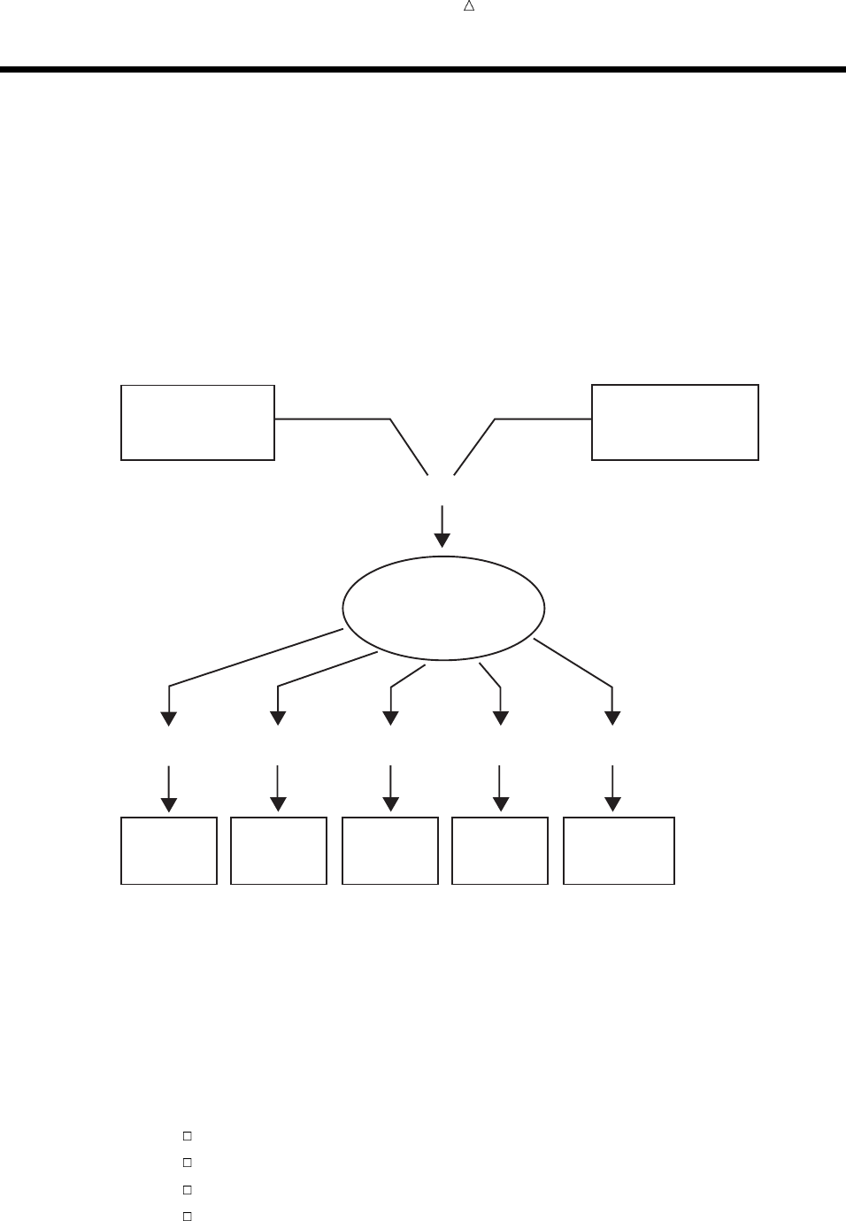
Customizing SAS Output: The Output Delivery System (ODS) Understanding ODS Output Formats and Destinations 567
Understanding ODS Output Formats and Destinations
The Output Delivery System (ODS) enables you to produce output in a variety of
formats that you can easily access. ODS removes responsibility for formatting output
from individual procedures and from the DATA step. The procedure or DATA step
supplies the data and the table definition, which contains formatting instructions for
the output.
The following figure illustrates the concept of output for SAS Version 8. The data and
the table definition form an output object, which creates the type of ODS output that
you specified in the table definition.
Figure 32.1 Model of the Production of ODS Output
Data Table Definition
(formatting instructions)
Output
Object
RTF
Output
SAS
Data
Sets
Listing
Output
HTML
Output
High-resolution
Printer
Output
ODS
Output
}
+
RTF
Destination
Output
Destination
Listing
Destination
HTML
Destination
Printer
Destination
ODS
Destination
}
The following definitions describe the terms in the preceding figure:
data
Each procedure that supports ODS and each DATA step produces data, which
contains the results (numbers and characters) of the step in a form similar to a
SAS data set.
table definition
The table definition is a set of instructions that describes how to format the data.
This description includes but is not limited to the following items:
the order of the columns
text and order of column headings
formats for data
font sizes and font faces

568 Selecting an Output Format Chapter 32
output object
ODS combines formatting instructions with the data to produce an output object.
The output object, therefore, contains both the results of the procedure or DATA
step and information about how to format the results. An output object has a
name, a label, and a path.
Note: Although many output objects include formatting instructions, not all of
them do. In some cases the output object consists of only the data.
ODS destinations
An ODS destination specifies a specific type of output. ODS supports a number of
destinations, including the following:
RTF
produces output that is formatted for use with Microsoft-Word.
Output
produces a SAS data set.
Listing
produces traditional SAS output (monospace format).
HTML
produces output that is formatted in Hyper Text Markup Language (HTML).
You can access the output on the web with your web browser.
Printer
produces output that is formatted for a high-resolution printer. An example
of this type of output is a PostScript file.
ODS output
ODS output consists of formatted output from any of the ODS destinations.
For detailed information about ODS, see SAS Output Delivery System: User’s Guide.
Selecting an Output Format
You select the format for your output by opening and closing ODS destinations in
your program. When one or more destinations are open, ODS can send output objects to
them and produce formatted output. When a destination is closed, ODS does not send
an output object to it and no output is produced.
By default, all programs automatically produce Listing output along with output for
other destinations that you specifically open. Therefore, by default, the Listing
destination is open, and all other destinations are closed.
To create formatted output, open one or more destinations by using the following
ODS statements:
ODS HTML file-specification(s);
ODS OUTPUT data-set-definition;
ODS PRINTER file-specification;
ODS RTF file-specification;
The argument file-specification opens the destination and specifies one or more files
to write to. The argument data-set-definition opens the Output destination and enables
SAS to create a data set from an output object.
To view or print the ODS output that you have selected, you need to close all the
destinations that you opened, except for the Listing destination. You can use separate
Customizing SAS Output: The Output Delivery System (ODS) Creating HTML Output for a Web Browser 569
statements to close individual destinations, or use one statement to close all
destinations (including the Listing destination). To close ODS destinations, use the
following statements:
ODS HTML CLOSE;
ODS OUTPUT CLOSE;
ODS PRINTER CLOSE;
ODS RTF CLOSE;
ODS _ALL_ CLOSE;
Note: The ODS _ALL_ CLOSE statement, which closes all open destinations, is
available with SAS Release 8.2 and higher.
In some cases you might not want to create Listing output. Use the
ODS LISTING CLOSE; statement at the beginning of your program to close the Listing
destination and prevent SAS from producing Listing output. Closing unnecessary
destinations conserves system resources.
Note: Because ODS statements are global statements, it is good practice to open the
Listing destination at the end of your program. If you execute other programs in your
current SAS session, Listing output is then available. To open the Listing destination,
use the ODS LISTING; statement at the end of your program.
Creating Formatted Output
Creating HTML Output for a Web Browser
Understanding the Four Types of HTML Output Files
When you use the ODS HTML statement, you can create output that is formatted in
HTML. You can browse the output files with Internet Explorer, Netscape, or any other
browser that fully supports the HTML 3.2 tag set.
The ODS HTML statement can create four types of HTML files:
a body file that contains the results of the DATA step or procedure
a table of contents that links to items in the body file
a table of pages that links to items in the body file
a frame file that displays the results of the procedure or DATA step, the table of
contents, and the table of pages
The body file is required with all ODS HTML output. If you do not want to link to
your output, then creating a table of contents, a table of pages, and a frame file is not
necessary.
Creating HTML Output: The Simplest Case
To produce the simplest kind of HTML output, the only file you need to create is a
body file.
The following example executes the MEANS procedure and creates an HTML body
file and the default Listing file. These files contain summary statistics for the average
SAT scores of entering first-year college students. The output is grouped by the CLASS
variables Test and Gender.
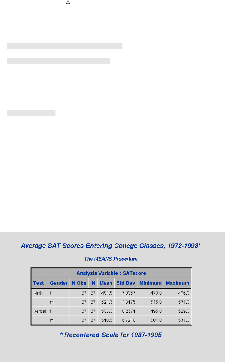
570 Creating HTML Output for a Web Browser Chapter 32
options pageno=1 nodate pagesize=30 linesize=78;
ods html file=’summary-results.htm’; u
proc means data=sat_scores fw=8; v
var SATscore;
class Test Gender;
title1 ’Average SAT Scores Entering College Classes, 1972-1998*’;
footnote1 ’* Recentered Scale for 1987-1995’;
run;
ods html close; w
The following list corresponds to the numbered items in the preceding program:
uThe ODS HTML statement opens the HTML destination and creates the body file
SUMMARY-RESULTS.HTM.
vThe MEANS procedure produces summary statistics for the average SAT scores of
entering first-year college students. The output is grouped by the CLASS variables
Test and Gender.
wThe ODS HTML CLOSE statement closes the HTML destination to make output
available for viewing.
The following output shows the results in HTML format:
Display 32.1 ODS Output: HTML Format
The following output shows the results in the Listing format:

Customizing SAS Output: The Output Delivery System (ODS) Creating HTML Output for a Web Browser 571
Output 32.1 ODS Output: Listing Format
Average SAT Scores Entering College Classes, 1972-1998* 1
The MEANS Procedure
Analysis Variable : SATscore
N
Test Gender Obs N Mean Std Dev Minimum Maximum
---------------------------------------------------------------------------
Math f 27 27 481.8 7.0057 473.0 496.0
m 27 27 521.6 4.3175 515.0 531.0
Verbal f 27 27 503.0 8.2671 495.0 529.0
m 27 27 510.5 6.7218 501.0 531.0
---------------------------------------------------------------------------
* Recentered Scale for 1987-1995
Creating HTML Output: Linking Results with a Table of Contents
The ODS HTML destination enables you to link to your results from a table of
contents and a table of pages. To do this, you need to create the following HTML files: a
body file, a frame file, a table of contents, and a table of pages (see “Understanding the
Four Types of HTML Output Files” on page 569). When you view the frame file and
select a link in the table of contents or the table of pages, the HTML table that contains
the selected part of the procedure results appears at the top of your browser.
The following example creates multiple pages of output from the UNIVARIATE
procedure. You can access specific output results (tables) from links in the table of
contents or the table of pages. The results contain statistics for the average SAT scores
of entering first-year college classes. The output is grouped by the value of Gender in
the CLASS statement and by the value of Test in the BY statement.
proc sort data=sat_scores out=sorted_scores;
by Test;
run;
options pageno=1 nodate;
ods listing close; u
ods html file=’odshtml-body.htm’ v
contents=’odshtml-contents.htm’
page=’odshtml-page.htm’
frame=’odshtml-frame.htm’;
572 Creating HTML Output for a Web Browser Chapter 32
proc univariate data=sorted_scores; w
var SATscore;
class Gender;
by Test;
title1 ’Average SAT Scores Entering College Classes, 1972-1998*’;
footnote1 ’* Recentered Scale for 1987-1995’;
run;
ods html close; x
ods listing; y
The following list corresponds to the numbered items in the preceding program:
uBy default, the Listing destination is open. To conserve resources, the ODS
LISTING CLOSE statement closes this destination.
vThe ODS HTML statement opens the HTML destination and creates four types of
files:
the body file (created with the FILE= option), which contains the formatted
data
the contents file, which is a table of contents with links to items in the body
file
the page file, which is a table of pages with links to items in the body file
the frame file, which displays the table of contents, the table of pages, and
the body file
wThe UNIVARIATE procedure produces statistics for the average SAT scores of
entering first-year college students. The output is grouped by the value of Gender
in the CLASS statement and the value of Test in the BY statement.
xThe ODS HTML CLOSE statement closes the HTML destination to make output
available for viewing.
yThe ODS LISTING statement reopens the Listing destination so that the next
program that you run can produce Listing output.
The following SAS log shows that four HTML files are created with the ODS HTML
statement:
Output 32.2 Partial SAS Log: HTML File Creation
489 ods listing close;
490 ods html file=’odshtml-body.htm’
491 contents=’odshtml-contents.htm’
492 page=’odshtml-page.htm’
493 frame=’odshtml-frame.htm’;
NOTE: Writing HTML Body file: odshtml-body.htm
NOTE: Writing HTML Contents file: odshtml-contents.htm
NOTE: Writing HTML Pages file: odshtml-page.htm
NOTE: Writing HTML Frames file: odshtml-frame.htm
494
495 proc univariate data=sorted_scores;
496 var SATscore;
497 class Gender;
498 by Test;
499 title1 ’Average SAT Scores Entering College Classes, 1972-1998*’;
500 footnote1 ’* Recentered Scale for 1987-1995’;
501 run;
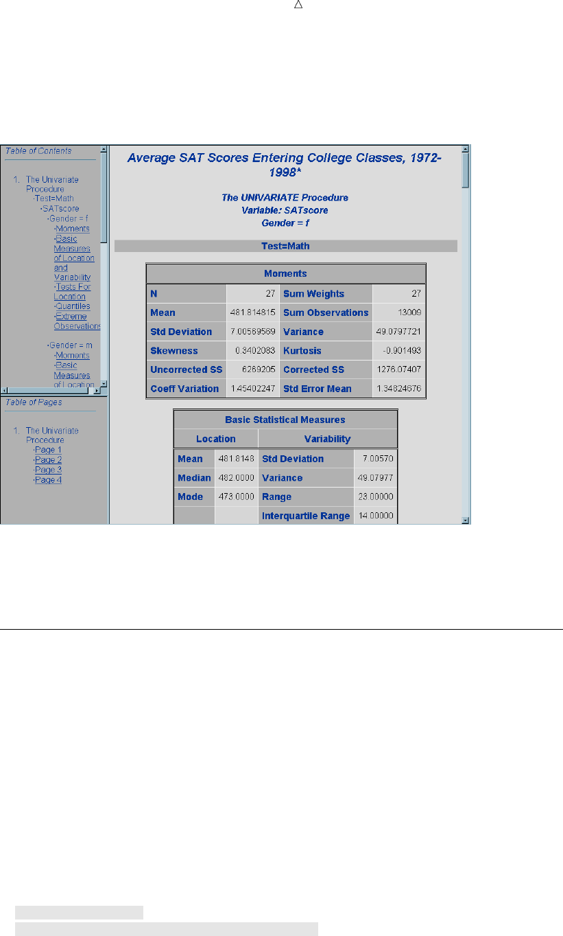
Customizing SAS Output: The Output Delivery System (ODS) PostScript Output for a High-Resolution Printer 573
The following output shows the frame file, which displays the table of contents
(upper left side), the table of pages (lower left side), and the body file (right side).
Display 32.2 View of the HTML Frame File
Both the Table of Contents and the Table of Pages contain links to the results in the
body file. If you click on a link in the Table of Contents or the Table of Pages, SAS
displays the corresponding results at the top of the browser.
Creating PostScript Output for a High-Resolution Printer
You can create output that is formatted for a high-resolution printer if you open the
Printer destination. Before you can access the file, however, you must close the Printer
destination.
The following example executes the MEANS procedure and creates a PostScript file
which contains summary statistics for the average SAT scores of entering first-year
college students. The output is grouped by the value of Gender in the CLASS statement
and the value of Test in the BY statement.
proc sort data=sat_scores out=sorted_scores;
by Test;
run;
options pageno=1 nodate;
ods listing close; u
ods printer ps file=’odsprinter_output.ps’; v

574 Creating RTF Output for Microsoft Word Chapter 32
proc means data=sorted_scores fw=8; w
var SATscore;
class Gender ;
by Test;
title1 ’Average SAT Scores Entering College Classes, 1972-1998*’;
footnote1 ’* Recentered Scale for 1987-1995’;
run;
ods printer close; x
ods listing; y
The following list corresponds to the numbered items in the preceding program:
uBy default, the Listing destination is open. To conserve resources, the program
uses the ODS LISTING CLOSE statement to close this destination.
vThe ODS PRINTER statement opens the Printer destination and specifies the file
to write to. The PS (PostScript) option ensures that you create a generic
PostScript file. If this option is missing, ODS produces output for your current
printer, if possible.
wThe MEANS procedure produces summary statistics for the average SAT scores of
entering first-year college students. The output is grouped by the value of Gender
in the CLASS statement and the value of Test in the BY statement.
xThe ODS PRINTER CLOSE statement closes the Printer destination to make
output available for printing.
yThe ODS LISTING statement reopens the Listing destination so that the next
program that you run can produce Listing output.
The following output shows the results:
Display 32.3 ODS Output: PostScript Format
Creating RTF Output for Microsoft Word
You can create output that is formatted for use with Microsoft Word if you open the
RTF destination. Before you can access the file, you must close the RTF destination.
The following example executes the UNIVARIATE procedure and creates an RTF file
that contains summary statistics for the average SAT scores of entering first-year
college students. The output is grouped by the CLASS variable Gender.
ods listing close; u
ods rtf file=’odsrtf_output.rtf’; v
proc univariate data=sat_scores; w
var SATscore;
class Gender;
title1 ’Average SAT Scores Entering College Classes, 1972-1998*’;
footnote1 ’* Recentered Scale for 1987-1995’;
run;
ods rtf close; x
ods listing; y

Customizing SAS Output: The Output Delivery System (ODS) Creating RTF Output for Microsoft Word 575
The following list corresponds to the numbered items in the preceding program:
uBy default, the Listing destination is open. To conserve resources, the ODS
LISTING CLOSE statement closes this destination.
vThe ODS RTF statement opens the RTF destination and specifies the file to write
to.
wThe UNIVARIATE procedure produces summary statistics for the average SAT
scores of entering first-year college students. The output is grouped by the CLASS
variable Gender.
xThe ODS RTF CLOSE statement closes the RTF destination to make output
available.
yThe ODS LISTING statement reopens the Listing destination so that the next
program that you run can produce Listing output.
The following output shows the first page of the RTF output:
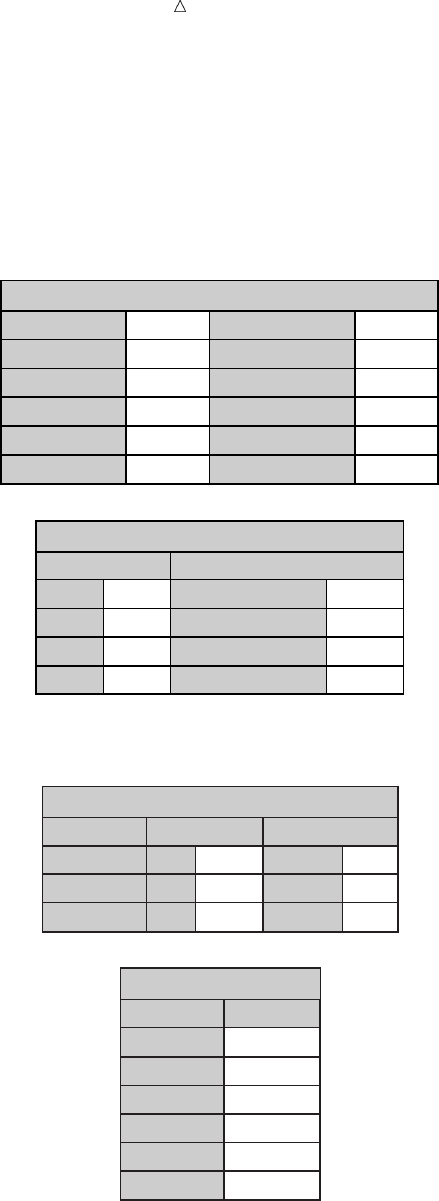
576 Creating RTF Output for Microsoft Word Chapter 32
Display 32.4 ODS Output: RTF Format
Average SAT Scores Entering College Classes, 1972–1998*
* Recentered Scale for 1987–1995
1
The UNIVARIATE Procedure
Variable: SATscore
Gender=f
NOTE: The mode displayed is the smallest of 4 modes with a count of 4.
N
Mean
Std Deviation
Skewness
Uncorrected SS
Coeff Variation
Moments
Sum Weights
Sum Observations
Varience
Kurtosis
Corrected SS
Std Error Mean
54
492.425926
13.1272464
0.38649931
13103231
2.66588169
54
26591
172.324598
0.03082111
9133.2037
1.78639197
Mean
Median
Mode
Std Deviation
Variance
Range
Interquartile Range
Basic Statistical Measures
Location Variability
492.4259
495.5000
473.0000
13.12725
172.32460
56.00000
20.00000
Test
Student's t
Sign
Signed Rank
Statistic
Tests for Location: Mu0=0
t
M
S
Pr > |t|
Pr >= |M|
Pr >= |S|
p Value
275.6539
27
7425
<.0001
<.0001
<.0001
Quantile
100% Max
99%
95%
90%
75% Q3
50% Median
Estimate
Quantiles (Definition 5)
529.0
529.0
520.0
505.0
502.0
495.5

Customizing SAS Output: The Output Delivery System (ODS) Identifying Output 577
Selecting the Output That You Want to Format
Identifying Output
Program output, in the form of output objects, contain both the results of a procedure
or DATA step and information about how to format the results. To select an output
object for formatting, you need to know which output objects your program creates. To
identify the output objects, use the ODS TRACE statement. The simplest form of the
ODS TRACE statement is as follows:
ODS TRACE ON|OFF;
ODS TRACE determines whether to write to the SAS log a record of each output
object that a program creates. The ON option writes the trace record to the log, and the
OFF option suppresses the writing of the trace record.
The trace record has the following components:
Name is the name of the output object.
Label is the label that briefly describes the contents of the output object.
Template is the name of the table definition that ODS used to format the
output object.
Path shows the location of the output object.
In the ODS SELECT statement in your program, you can refer to an output object by
name, label, or path.
The following program executes the UNIVARIATE procedure and writes a trace
record to the SAS log.
ods trace on;
proc univariate data=sat_scores;
var SATscore;
class Gender;
title1 ’Average SAT Scores Entering College Classes, 1972-1998*’;
footnote1 ’* Recentered Scale for 1987-1995’;
run;
ods trace off;
The following output shows the results of ODS TRACE. Two sets of output objects
are listed because the program uses the class variable Gender to separate male and
female results. The path component of the output objects identifies the female (f) and
male (m) objects.

578 Identifying Output Chapter 32
Output 32.3 ODS TRACE Output in the Log
403 ods trace on;
404
405 proc univariate data=sat_scores;
406 var SATscore;
407 class Gender;
408 title1 ’Average SAT Scores Entering College Classes, 1972-1998*’;
409 footnote1 ’* Recentered Scale for 1987-1995’;
410 run;
Output Added:
-------------
Name: Moments
Label: Moments
Template: base.univariate.Moments
Path: Univariate.SATscore.f.Moments
Output Added:
-------------
Name: BasicMeasures
Label: Basic Measures of Location and Variability
Template: base.univariate.Measures
Path: Univariate.SATscore.f.BasicMeasures
-------------
Output Added:
-------------
Name: TestsForLocation
Label: Tests For Location
Template: base.univariate.Location
Path: Univariate.SATscore.f.TestsForLocation
-------------
Output Added:
-------------
Name: Quantiles
Label: Quantiles
Template: base.univariate.Quantiles
Path: Univariate.SATscore.f.Quantiles
-------------
Output Added:
-------------
Name: ExtremeObs
Label: Extreme Observations
Template: base.univariate.ExtObs
Path: Univariate.SATscore.f.ExtremeObs
-------------
Output Added:
-------------
Name: Moments
Label: Moments
Template: base.univariate.Moments
Path: Univariate.SATscore.m.Moments
-------------
Output Added:
-------------
Name: BasicMeasures
Label: Basic Measures of Location and Variability
Template: base.univariate.Measures
Path: Univariate.SATscore.m.BasicMeasures
-------------
Customizing SAS Output: The Output Delivery System (ODS) Selecting and Excluding Program Output 579
Output Added:
-------------
Name: TestsForLocation
Label: Tests For Location
Template: base.univariate.Location
Path: Univariate.SATscore.m.TestsForLocation
-------------
Output Added:
-------------
Name: Quantiles
Label: Quantiles
Template: base.univariate.Quantiles
Path: Univariate.SATscore.m.Quantiles
-------------
Output Added:
-------------
Name: ExtremeObs
Label: Extreme Observations
Template: base.univariate.ExtObs
Path: Univariate.SATscore.m.ExtremeObs
-------------
411
412 ods trace off;
Selecting and Excluding Program Output
For each destination, ODS maintains a selection list or an exclusion list. The
selection list is a list of output objects that produce formatted output. The exclusion list
is a list of output objects for which no output is produced.
You can select and exclude output objects by specifying the destination in an ODS
SELECT or ODS EXCLUDE statement. If you do not specify a destination, ODS sends
output to all open destinations.
Selection and exclusion lists can be modified and reset at different points in a SAS
session, such as at procedure boundaries. If you end each procedure with an explicit
QUIT statement, rather than waiting for the next PROC or DATA step to end it for you,
the QUIT statement resets the selection list.
To choose one or more output objects and send them to open ODS destinations, use
the ODS SELECT statement. The simplest form of the ODS SELECT statement is as
follows:
ODS SELECT <ODS-destination>output-object(s);
The argument ODS-destination identifies the output format, and output-object
specifies one or more output objects to add to a selection list.
To exclude one or more output objects from being sent to open destinations, use the
ODS EXCLUDE statement. The simplest form of the ODS EXCLUDE statement is as
follows:
ODS EXCLUDE <ODS-destination>output-object(s);
The argument ODS-destination identifies the output format, and output-object
specifies one or more output objects to add to an exclusion list.
The following example executes the UNIVARIATE procedure and creates 10 output
objects. The ODS SELECT statement uses the name component in the trace records to
select only the BasicMeasures and the TestsForLocation output objects. Because the
HTML and Printer destinations are open, ODS creates HTML and Printer output from
the output objects.
580 Selecting and Excluding Program Output Chapter 32
options nodate pageno=1;
ods listing close;
ods html file=’odsselect-body.htm’
contents=’odsselect-contents.htm’
page=’odsselect-page.htm’
frame=’odsselect-frame.htm’;
ods printer file=’odsprinter-select.ps’;
ods select BasicMeasures TestsForLocation;
proc univariate data=sat_scores;
var SATscore;
class Gender;
title1 ’Average SAT Scores Entering College Classes, 1972-1998*’;
footnote1 ’* Recentered Scale for 1987-1995’;
run;
ods html close;
ods printer close;
ods listing;
The following two displays show the results in Printer format. They show the Basic
Statistical Measures and Tests for Location tables based on gender.
Customizing SAS Output: The Output Delivery System (ODS) Selecting and Excluding Program Output 581
Display 32.5 ODS SELECT Statement: Printer Format (females)
Average SAT Scores Entering College Classes, 1972–1998*
The UNIVARIATE Procedure
Variable: SATscore
Gender = f
Basic Statistical Measures
Tests for Location: Mu0=0
Location Variability
Mean
Median
Mode
Std Deviation
Variance
Range
Interquartile Range
NOTE: The mode displayed is the smallest of 4 modes with a count of 4.
492.4259
495.5000
473.0000
13.12725
172.32460
56.00000
20.00000
Test
Student's t
Sign
Signed Rank
t
M
S
275.6539
27
742.5
< .0001
< .0001
< .0001
Pr > |t|
Pr > = |M|
Pr >= |S|
Statistic p Value
* Recentered Scale for 1987–1995
1
582 Selecting and Excluding Program Output Chapter 32
Display 32.6 ODS SELECT Statement: Printer Format (males)
Average SAT Scores Entering College Classes, 1972–1998*
The UNIVARIATE Procedure
Variable: SATscore
Gender = m
Basic Statistical Measures
Tests for Location: Mu0=0
Location Variability
Mean
Median
Mode
Std Deviation
Variance
Range
Interquartile Range
516.0185
516.0000
523.0000
7.90865
62.54682
30.00000
14.00000
Test
Student's t
Sign
Signed Rank
t
M
S
479.4679
27
742.5
< .0001
< .0001
< .0001
Pr > |t|
Pr > = |M|
Pr >= |S|
Statistic p Value
* Recentered Scale for 1987–1995
2
The following two displays show the results in HTML format. They, too, show the
Basic Statistical Measures and Tests for Location tables based on gender.
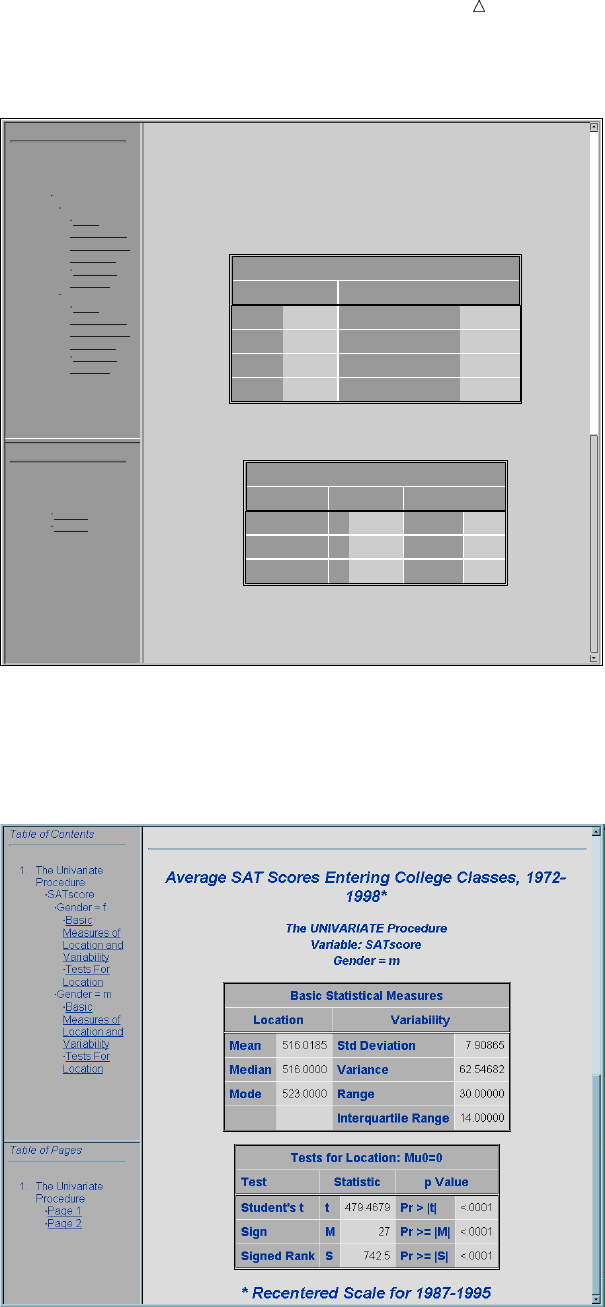
Customizing SAS Output: The Output Delivery System (ODS) Selecting and Excluding Program Output 583
Display 32.7 ODS SELECT Statement: HTML Format (females)
1. The Univariate
Procedure
Page 1
Page 2
Table of Pages
1. The Univariate
Procedure
SATscore
Gender= f
Basic
Measures of
Location and
Variability
Tests For
Location
Gender = m
Basic
Measures of
Location and
Variability
Tests For
Location
Table of Contents
Average SAT Scores Entering College Classes, 1972-
1998*
The UNIVARIATE Procedure
Variable: SATscore
Gender = f
Basic Statistical Measures
Tests for Location: Mu0=0
Location Variability
Mean
Median
Mode
Std Deviation
Variance
Range
Interquartile Range
NOTE: The mode displayed is the smallest of 4 modes with a count of 4.
492.4259
495.5000
473.0000
13.12725
172.32460
56.00000
20.00000
Test
Student's t
Sign
Signed Rank
t
M
S
275.6539
27
742.5
< .0001
< .0001
< .0001
Pr > |t|
Pr > = |M|
Pr >= |S|
Statistic p Value
* Recentered Scale for 1987–1995
Display 32.8 ODS SELECT Statement: HTML Format (males)

584 Creating a SAS Data Set Chapter 32
Creating a SAS Data Set
ODS enables you to create a SAS data set from an output object. To create a single
output data set, use the following form of the ODS OUTPUT statement:
ODS OUTPUT output-object(s)=SAS-data-set;
The argument output-object specifies one or more output objects to turn into a SAS
data set, and SAS-data-set specifies the data set that you want to create.
In the following program, ODS opens the Output destination and creates the SAS
data set MYFILE.MEASURES from the output object BasicMeasures. ODS then closes
the Output destination.
libname myfile ’SAS-data-library’;
ods listing close; u
ods output BasicMeasures=myfile.measures; v
proc univariate data=sat_scores; w
var SATscore;
class Gender;
run;
ods output close; x
ods listing; y
The following list corresponds to the numbered items in the preceding program:
uBy default, the Listing destination is open. To conserve resources, the ODS
LISTING CLOSE statement closes this destination.
vThe ODS OUTPUT statement opens the Output destination and specifies the
permanent data set to create from the output object BasicMeasures.
wThe UNIVARIATE procedure produces summary statistics for the average SAT
scores of entering first-year college students. The output is grouped by the CLASS
variable Gender.
xThe ODS OUTPUT CLOSE statement closes the Output destination.
yThe ODS LISTING statement reopens the default Listing destination so that the
next program that you run can produce Listing output.
The following SAS log shows that the MYFILE.MEASURES data set was created
with the ODS OUTPUT statement:
Output 32.4 Partial SAS Log: SAS Data Set Creation
404 libname myfile ’SAS-data-library’;
NOTE: Libref MYFILE was successfully assigned as follows:
Engine: V8
Physical Name: path-name
405 ods listing close;
406 ods output BasicMeasures=myfile.measures;
407
408 proc univariate data=sat_scores;
409 var SATscore;
410 class Gender;
411 run;
NOTE: The data set MYFILE.MEASURES has 8 observations and 6 variables.

Customizing SAS Output: The Output Delivery System (ODS) Customizing ODS Output by Using a Template 585
Customizing ODS Output
Customizing ODS Output at the Level of a SAS Job
ODS provides a way for you to customize output at the level of the SAS job. To do
this, you use a style definition, which describes how to show such items as color, font
face, font size, and so on. The style definition determines the appearance of the output.
The fancyprinter style definition is one of several that is available with SAS.
The following example uses the fancyprinter style definition to customize program
output. The output consists of two output objects, Moments and BasicMeasures, that
the UNIVARIATE procedure creates. The STYLE= option on the ODS PRINTER
statement specifies that the program use the fancyprinter style.
options nodate pageno=1;
ods listing close;
ods printer ps file=’style_job.ps’ style=fancyprinter;
ods select Moments BasicMeasures;
proc univariate data=sat_scores;
var SATscore;
title ’Average SAT Scores for Entering College Classes, 1972-1982*’;
footnote1 ’* Recentered Scale for 1987-1995’;
run;
ods printer close;
ods listing;
The following output shows the results:
Display 32.9 Printer Output: Titles, Footnote, and Variables Printed in Italics
For detailed information about style and table definitions, as well as the TEMPLATE
procedure, see SAS Output Delivery System: User’s Guide.
Customizing ODS Output by Using a Template
Another way to customize ODS output is by using a template. In ODS, templates are
called table definitions. A table definition describes how to format the output. It can
determine the order of table headings and footnotes, the order of columns, and the
appearance of the output. A table definition can contain one or more columns, headings,
or footnotes.
Many procedures that fully support ODS provide table definitions that you can
customize. You can also create your own table definition by using the TEMPLATE
procedure. The following is a simplified form of the TEMPLATE procedure:
PROC TEMPLATE;
DEFINE table-definition;
HEADER header(s);
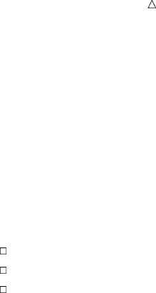
586 Customizing ODS Output by Using a Template Chapter 32
COLUMN column(s);
END;
The DEFINE statement creates the table definition that serves as the template for
writing the output. The HEADER statement specifies the order of the headings, and
the COLUMN statement specifies the order of the columns. The arguments in each of
these statements point to routines in the program that format the output. The END
statement ends the table definition.
The following example shows how to use PROC TEMPLATE to create customized
HTML and printer output. In the example, the SAS program creates a customized table
definition for the Basic Measures output table from PROC UNIVARIATE. The following
customized version shows that
the “Measures of Variability” section precedes the “Measures of Location” section
column headings are modified
statistics are displayed in a bold, italic font with a 7.3 format.
options nodate nonumber linesize=80 pagesize=60; u
proc template; v
define table base.univariate.Measures; w
header h1 h2 h3; x
column VarMeasure VarValue LocMeasure LocValue; y
define h1; U
text "Basic Statistical Measures";
spill_margin=on;
space=1;
end;
define h2; U
text "Measures of Variability";
start=VarMeasure;
end=VarValue;
end;
define h3; U
text "Measures of Location";
start=LocMeasure;
end=LocValue;
end;
define LocMeasure; V
print_headers=off;
glue=2;
space=3;
style=rowheader;
end;
define LocValue; V
print_headers=off;
space=5;
format=7.3;
style=data{font_style=italic font_weight=bold};
end;
define VarMeasure; V
print_headers=off;
glue=2;

Customizing SAS Output: The Output Delivery System (ODS) Customizing ODS Output by Using a Template 587
space=3;
style=rowheader;
end;
define VarValue; V
print_headers=off;
format=7.3;
style=data{font_style=italic font_weight=bold};
end;
end; W
run; X
ods listing close;
ods html file=’scores-body.htm’ at
contents=’scores-contents.htm’
page=’scores-page.htm’
frame=’scores-frame.htm’;
ods printer file=’scores.ps’; ak
ods select BasicMeasures; al
title;
proc univariate data=sorted_scores mu0=3.5; am
var SATscore;
run;
ods html close; an
ods printer close; an
ods listing; ao
The following list corresponds to the numbered items in the preceding program:
uAll four options affect the Listing output. The NODATE and NONUMBER options
affect the Printer output. None of the options affects the HTML output.
vPROC TEMPLATE begins the procedure for creating a table.
wThe DEFINE statement creates the table definition base.univariate.Measures in
SASUSER.
xThe HEADER statement determines the order in which the table definition uses
the headings, which are defined later in the program.
yThe COLUMN statement determines the order in which the variables appear.
PROC UNIVARIATE names the variables.
UThese DEFINE blocks define the three headings and specify the text to use for
each heading. By default, a heading spans all columns. This is the case for H1.
H2 spans the variables VarMeasure and VarValue. H3 spans LocMeasure and
LocValue.
VThese DEFINE blocks specify characteristics for each of the four variables. They
use FORMAT= to specify a format of 7.3 for LocValue and VarValue. They also use
STYLE= to specify a bold, italic font for these two variables. The STYLE= option
does not affect the Listing output.
WThe END statement ends the table definition.
XThe RUN statement executes the procedure.
at The ODS HTML statement begins the program that uses the customized table
definition. It opens the HTML destination and identifies the files to write to.
ak The ODS PRINTER statement opens the Printer destination and identifies the file
to write to.
588 Customizing ODS Output by Using a Template Chapter 32
al The ODS SELECT statement selects the output object that contains the basic
measures.
am PROC UNIVARIATE produces one object for each variable. It uses the customized
table definition to format the data.
an The ODS statements close the HTML and the PRINTER destinations.
ao The ODS LISTING statement opens the listing destination for output.
The following display shows the printer output:
Display 32.10 Customized Printer Output from the TEMPLATE Procedure
The UNIVARIATE Procedure
Variable: SATscore
Basic Statistical Measures
Measures of Variability
Measures of
Location
Std Deviation 16.025 Mean 504.222
Variance 256.791 Median 505.000
Range 58.000 Mode 503.000
Interquartile Range 22.000 _
NOTE: The mode displayed is the smallest of 3 modes with a count of 5.
The following display shows the HTML output:
Display 32.11 Customized HTML Output from the TEMPLATE Procedure

Customizing SAS Output: The Output Delivery System (ODS) Storing Links to ODS Output 589
Storing Links to ODS Output
When you run a procedure that supports ODS, SAS automatically stores a link to
each piece of ODS output in the Results folder in the Results window. It marks the link
with an icon that identifies the output destination that created the output.
In the following example, SAS executes the UNIVARIATE procedure and generates
Listing, HTML, Printer, and Rich Text Format (RTF) output as well as a SAS data set
(Output output). The output contains statistics for the average SAT scores of entering
first-year college students. The output is grouped by the CLASS variable Gender.
ods listing close;
ods html file=’store-links.htm’;
ods printer file=’store-links.ps’;
ods rtf file=’store-links.rtf’;
ods output basicmeasures=measures;
proc univariate data=sat_scores;
var SATscore;
class Gender;
title;
run;
ods _all_ close;
ods listing;
PROC UNIVARIATE generates a folder called Univariate in the Results folder.
Within this folder is another folder (SAT score) for the variable in the VAR statement.
This folder contains two folders (Gender=f and Gender=m), one for each variable in the
CLASS statement. The Gender=f and Gender=m folders each contain a folder for each
output object. Within the folder for each output object is a link to each piece of output.
The icon next to the link indicates which ODS destination created the output. In this
example, the Moments output was sent to the Listing, HTML, Printer, and RTF
destinations. The Basic Measures of Location and Variability output was sent to the
Listing, HTML, Printer, RTF, and Output destinations.
The Results folder in the display that follows shows the folders and output objects
that the UNIVARIATE procedure creates.
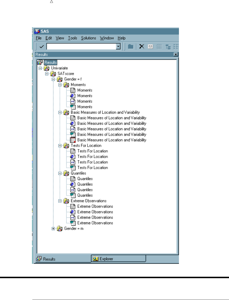
590 Review of SAS Tools Chapter 32
Display 32.12 View of the Results Folder
Review of SAS Tools
ODS Statements
ODS EXCLUDE <ODS-destination>output-object(s);
specifies one or more output objects to add to an exclusion list.

Customizing SAS Output: The Output Delivery System (ODS) ODS Statements 591
ODS HTMLHTML-file-specification(s) <STYLE=’style-definition’>;
opens the HTML destination and specifies the HTML file or files to write to. After
the destination is open, you can create output that is written in Hyper Text
Markup Language (HTML).
You can specify up to four HTML files to write to. The specifications for these
files have the following form:
BODY=’body-file-name’
identifies the file that contains the HTML output.
Alias: FILE=
CONTENTS=’contents-file-name’
identifies the file that contains a table of contents for the HTML output. The
contents file has links to the body file.
FRAME=’frame-file-name’
identifies the file that integrates the table of contents, the page contents, and
the body file. If you open the frame file, you see a table of contents, a table of
pages, or both, as well as the body file. If you specify FRAME=, you must also
specify CONTENTS= or PAGE= or both.
PAGE=’page-file-name’
identifies the file that contains a description of each page of the body file and
links to the body file. ODS produces a new page of output whenever a
procedure explicitly asks for a new page. The SAS system option PAGESIZE=
has no effect on pages in HTML output.
The STYLE= option enables you to choose HTML presentation styles.
ODS LISTING;
opens the Listing destination.
Note: The Listing destination is open by default.
ODS LISTING CLOSE;
closes the Listing destination so that no Listing output is created.
ODS OUTPUT output-object(s)=SAS-data-set;
opens the Output destination and converts one or more output objects to a SAS
data set.
ODS PRINTER PS file-specification;
opens the Printer destination and specifies the file to write to. The PS (PostScript)
option ensures that you create a generic PostScript file. If this option is missing,
ODS produces output for your current printer.
ODS RTF file-specification;
opens the RTF destination and specifies the file to write to. After the destination
is open, you can create RTF output.
ODS HTML CLOSE;
ODS OUTPUT CLOSE;
ODS PRINTER CLOSE;
ODS RTF CLOSE;
closes the specific destination and enables you to view the output.
ODS _ALL_ CLOSE;
closes all open destinations.
ODS SELECT <ODS-destination>output-object(s);
specifies one or more output objects to add to a selection list.
ODS TRACE ON |OFF;

592 Procedures Chapter 32
turns the writing of the trace record on or off. Turning trace on is useful because
the results list the output objects that your program creates.
Procedures
PROC MEANS DATA=SAS-data-set <FW=>;
CLASS variable(s);
VAR variable(s);
provides data summarization tools to compute descriptive statistics for variables
across all observations and within groups of observations. The DATA= option
specifies the input SAS data set, and FW= specifies the field width for statistics.
The CLASS statement specifies the variables whose values define the subgroup
combinations for the analysis.
The VAR statement identifies the analysis variables and determines their order
in the output.
PROC TEMPLATE;
DEFINE table-definition;
COLUMN header(s);
HEADER column(s);
END;
creates an ODS table definition. The DEFINE statement uses the COLUMN and
HEADER statements to create column and table headings.
PROC UNIVARIATE DATA=SAS-data-set;
VAR variable(s);
CLASS variable(s);
BY variable(s);
provides data summarization tools and information about the distribution of
numeric variables. The DATA= option specifies the input SAS data set.
The VAR statement identifies the analysis variables and determines their order
in the output.
The CLASS statement specifies up to two variables whose values define the
classification levels for the analysis.
The BY statement calculates separate statistics for each BY group.
Learning More
ODS output
For detailed information about the Output Delivery System, see SAS Output
Delivery System: User’s Guide.
SAS procedures
For information about procedures, see the Base SAS Procedures Guide.

593
PART
9
Storing and Managing Data in SAS Files
Chapter 33.........
Understanding SAS Data Libraries 595
Chapter 34.........
Managing SAS Data Libraries 603
Chapter 35.........
Getting Information about Your SAS Data Sets 607
Chapter 36.........
Modifying SAS Data Set Names and Variable Attributes 617
Chapter 37.........
Copying, Moving, and Deleting SAS Data Sets 629
594
595
CHAPTER
33
Understanding SAS Data
Libraries
Introduction to Understanding SAS Data Libraries 595
Purpose 595
Prerequisites 595
What Is a SAS Data Library? 596
Accessing a SAS Data Library 596
Telling SAS Where the SAS Data Library Is Located 596
Assigning a Libref 596
Using Librefs for Temporary and Permanent Libraries 597
Storing Files in a SAS Data Library 598
What Is a SAS File? 598
Understanding SAS Data Sets 598
Understanding Other SAS Files 598
Referencing SAS Data Sets in a SAS Data Library 599
Understanding Data Set Names 599
Using a One-Level Name 599
Using a Two-Level Name 601
Review of SAS Tools 601
Statements 601
SAS Data Set Reference 601
Learning More 601
Introduction to Understanding SAS Data Libraries
Purpose
The way in which SAS handles data libraries is different from one operating
environment to another. In this section, you will learn basic concepts about the SAS
data library and how to use libraries in SAS programs. For more detailed information,
see the SAS documentation for your operating environment.
Prerequisites
Before proceeding with this section, you should understand the concepts presented in
the following sections:
Chapter 1, “What Is the SAS System?,” on page 3
Chapter 2, “Introduction to DATA Step Processing,” on page 19
596 What Is a SAS Data Library? Chapter 33
What Is a SAS Data Library?
ASAS data library is a collection of one or more SAS files that are recognized by
SAS and can be referenced and stored as a unit. Each file is a member of the library.
SAS data libraries help to organize your work. For example, if a SAS program uses
more than one SAS file, then you can keep all the files in the same library. Organizing
files in libraries makes it easier to locate the files and reference them in a program.
Under most operating environments, a SAS data library roughly corresponds to the
level of organization that the operating environment uses to organize files. For
example, in directory-based operating environments, a SAS data library is a group of
SAS files in the same directory. The directory might contain other files, but only the
SAS files are part of the SAS data library.
Operating Environment Information: Under the CMS operating environment, a SAS
data library is a group of SAS files with the same filetype. Under the z/OS operating
environment, a SAS data library is a specially formatted z/OS data set. This kind of
data set can contain only SAS files.
Accessing a SAS Data Library
Telling SAS Where the SAS Data Library Is Located
No matter which operating environment you are using, to access a SAS data library,
you must tell SAS where it is. To do so, you can do one of the following:
directly specify the operating environment’s physical name for the location of the
SAS data library. The physical name must conform to the naming conventions of
your operating environment, and it must be in single quotation marks. For
example, in the SAS windowing environment, the following DATA statement
creates a data set named MYFILE:
data ’c:\my documents\sasfiles\myfile’;
assign a SAS libref (library reference), which is a SAS name that is temporarily
associated with the physical location name of the SAS data library.
Assigning a Libref
After you assign a libref to the location of a SAS data library, then in your SAS
program you can reference files in the library by using the libref instead of using the
long physical name that the operating environment uses. The libref is a SAS name that
is temporarily associated with the physical location of the SAS data library. There are
several ways to assign a libref:
use the LIBNAME statement
use the LIBNAME function
use the New Library window from the SAS Explorer window
for some operating environments, use operating environment commands
A common method for assigning a libref is to use the LIBNAME statement to
associate a name with a SAS data library. Here is the simplest form of the LIBNAME
statement:

Understanding SAS Data Libraries Using Librefs for Temporary and Permanent Libraries 597
LIBNAME libref ’SAS-data-library’;
where
libref is a shortcut name to associate with the SAS data library. This
name must conform to the rules for SAS names. A libref cannot
exceed eight characters.
Operating Environment Information: Under the z/OS operating
environment, the libref must also conform to the rules for operating
environment names.
Think of the libref as an abbreviation for the operating
environment’s name for the library. Because the libref endures only
for the duration of the SAS session, you do not have to use the same
libref for a particular SAS data library each time you use SAS.
Operating Environment Information: Under the CMS operating
environment, the libref typically specifies the filetype of all files in
the library. In this case, you must always use the same libref for a
SAS data library because the filetype does not change.
SAS-data-
library
is the physical name for the SAS data library. The physical name is
the name that is recognized by your operating environment. Enclose
the physical name in single or double quotation marks.
Operating Environment Information: Here are examples of the LIBNAME statement
for different operating environments. For more examples, see the SAS documentation
for your operating environment.
Windows libname mydata ’c:\my documents\sasfiles’;
UNIX libname mydata ’/u/myid/sasfiles’;
z/OS libname mydata ’edc.company.sasfiles’;
When you assign a libref with the LIBNAME statement, SAS writes a note to the
SAS log confirming the assignment. This note also includes the operating
environment’s physical name for the SAS data library.
Using Librefs for Temporary and Permanent Libraries
When a libref is assigned to a SAS data library, you can use the libref throughout the
SAS session to access the SAS files that are stored in that library or to create new files.
When you start a SAS session, SAS automatically assigns the libref WORK to a
special SAS data library. Normally, the files in the WORK library are temporary files;
that is, usually SAS initializes the WORK library when you begin a SAS session, and
deletes all files in the WORK library when you end the session. Therefore, the WORK
library is a useful place to store SAS files that you do not need to save for a subsequent
SAS session. The automatic deletion of the WORK library files at the end of the session
prevents you from wasting disk space.
Files that are stored in any SAS data library other than the WORK library are
usually permanent files; that is, they endure from one SAS session to the next. Store
SAS files in a permanent library if you plan to use them in multiple SAS sessions.
598 Storing Files in a SAS Data Library Chapter 33
Storing Files in a SAS Data Library
What Is a SAS File?
You store all SAS files in a SAS data library. A SAS file is a specially structured file
that is created, organized, and maintained by SAS. The files reside in SAS data
libraries as members with specific types. Examples of SAS files are as follows:
SAS data sets (which can be SAS data files or SAS data views)
SAS catalogs
SAS/ACCESS descriptor files
stored compiled DATA step programs
Note: A file that contains SAS statements, even one that is created during a SAS
session, is usually not considered a SAS file. For example, in directory-based operating
environments, a .sas file is a text file that typically contains a program and is not
considered a SAS file.
Understanding SAS Data Sets
ASAS data set is a SAS file that is stored in a SAS data library that consists of
descriptor information. Descriptor information identifies the attributes of a SAS data
set and its contents, and data values that are organized as a table of observations
(rows) and variables (columns). A SAS data set can be either a SAS data file or a SAS
data view.
If the descriptor information and the observations are in the same physical location,
then the data set is a SAS data file, which has a member type DATA. A SAS data file
can have an index associated with it. One purpose of an index is to optimize the
performance of WHERE processing. Basically, an index contains values in ascending
order for a specific variable or variables. The index also includes information about the
location of those values within observations in the SAS data file.
If the descriptor and the observations are stored separately, then they form a SAS
data view, which has a member type VIEW. The observations in a SAS data view might
be stored in a SAS data file, an external database, or an external file. The descriptor
contains information about where the data is located and which observations and
variables to process. You use a view like a SAS data file. You might use a view when
you need only a subset of a large amount of data. In addition to saving storage space,
views simplify maintenance because they automatically reflect any changes to the data.
There are three types of SAS data views:
DATA step views
SAS/ACCESS views
PROC SQL views
Note: SAS data views usually behave like SAS data files. Other topics in this
documentation do not distinguish between the two types of SAS data sets.
Understanding Other SAS Files
In addition to SAS data sets, a SAS data library can contain the following types of
SAS files:
Understanding SAS Data Libraries Using a One-Level Name 599
SAS catalog is a SAS file that stores many kinds of information, in separate
units called catalog entries. Each entry is distinguished by an entry
name and an entry type. Some catalog entries contain system
information such as key definitions. Other catalog entries contain
application information about window definitions, help windows,
formats, informats, macros, or graphics output. A SAS catalog has a
member type CATALOG.
SAS/ACCESS
descriptor
is a SAS file that contains information about the layout of an
external database. SAS uses this information in order to build a
SAS data view in which the observations are stored in an external
database. An access descriptor has a member type ACCESS.
stored compiled
DATA step
program
is a SAS file that contains a DATA step, which has been compiled
and stored in a SAS data library. A stored compiled DATA step
program has a member type PROGRAM.
Complete discussion of all SAS files, except SAS data sets, is beyond the scope of this
section. For more information about SAS files, see SAS Language Reference: Concepts.
Referencing SAS Data Sets in a SAS Data Library
Understanding Data Set Names
Every SAS data set has a two-level name of the form libref.filename. You can always
reference a file with its two-level name. However, you can also use a one-level name
(just filename) to reference a file. By default, a one-level name references a file that
uses the libref WORK for the temporary SAS data library.
Note: This section separates the issues of permanent versus temporary files and
one-level versus two-level names. Other topics in this documentation and most SAS
documentation assume typical use of the WORK libref and refer to files that are
referenced with a one-level name as temporary and to files that are referenced with a
two-level name as permanent.
Operating Environment Information: The documentation that is provided by the
vendor for your operating environment provides information about how to create
temporary and permanent files. From the point of view of SAS, files in the WORK
library are temporary unless you specify the NOWORKINIT and NOWORKTERM
options and the files in all other SAS data libraries are permanent. However, your
operating environment’s point of view might be different. For example, the operating
environment might enable you to create a temporary directory or a z/OS data set, that
is, one that is deleted when you log off. Because all files in a SAS data library are
deleted if the underlying operating environment structure is deleted, the way the
operating environment views the SAS data library determines whether the library
endures from one session to the next.
Using a One-Level Name
Typically, when you reference a SAS data set with a one-level name, SAS by default
uses the libref WORK for the temporary library. For example, the following program
creates a temporary SAS data set named WORK.GRADES:

600 Using a One-Level Name Chapter 33
data grades;
infile ’file-specification’;
input Name $ 1-14 Gender $ 15-20 Section $ 22-24 Grade;
run;
However, if you want to use a one-level name to reference a permanent SAS data set,
you can assign the reserved libref USER. When USER is assigned and you reference a
SAS data set with a one-level name, SAS by default uses the libref USER for a
permanent SAS data library. For example, the following program creates a permanent
SAS data set named USER.GRADES. Note that you assign the libref USER as you do
any other libref.
libname user ’SAS-data-library’;
data grades;
infile ’file-specification’;
input Name $ 1-14 Gender $ 15-20 Section $ 22-24 Grade;
run;
Therefore, when you reference a SAS data set with a one-level name, SAS
1looks for the libref USER. If it is assigned to a SAS data library, then USER
becomes the default libref for one-level names.
2uses WORK as the default libref for one-level names if the libref USER has not
been assigned.
If USER is assigned, then you must use a two-level name (for example,
WORK.TEST) to access a temporary data set in the WORK library. For example, if
USER is assigned, then to print the data set WORK.GRADES requires a two-level
name in the PROC PRINT statement:
proc print data=work.grades;
run;
If USER is assigned, then you need to make only one change in order to use the
same program with files of the same name in different SAS data libraries. Instead of
specifying two-level names, simply assign USER differently in each case. For example,
the following program concatenates five SAS data sets in SAS-data-library-1 and puts
them in a new SAS data set, WEEK, in the same library:
libname user ’SAS-data-library-1’;
data week;
set mon tues wed thurs fri;
run;
By changing just the name of the library in the LIBNAME statement, you can
combine files with the same names in another library, SAS-data-library-2:
libname user ’SAS-data-library-2’;
data week;
set mon tues wed thurs fri;
run;
Note: At your site, the libref USER might be assigned for you when you start a SAS
session. Your SAS Support Consultant will know whether the libref is assigned.

Understanding SAS Data Libraries Learning More 601
Using a Two-Level Name
You can always reference a SAS data set with a two-level name, whether the libref
you use is WORK, USER, or some other libref that you have assigned. Usually, any
two-level name with a libref other than WORK references a permanent SAS data set.
In the following program, the LIBNAME statement establishes a connection between
the SAS name INTRCHEM and SAS-data-library, which is the physical name for the
location of an existing z/OS data set or a directory, for example. The DATA step creates
the SAS data set GRADES in the SAS data library INTRCHEM. SAS uses the INPUT
statement to construct the data set from the raw data in file-specification.
libname intrchem ’SAS-data-library’;
data intrchem.grades;
infile ’file-specification’;
input Name $ 1-14 Gender $ 15-20 Section $ 22-24 Grade;
run;
When the SAS data set INTRCHEM.GRADES is created, you can read from it by
using its two-level name. The following program reads the file INTRCHEM.GRADES
and creates a new SAS data set named INTRCHEM.FRIDAY, which is a subset of the
original data set:
data intrchem.friday;
set intrchem.grades;
if Section=’Fri’;
run;
The following program displays the SAS data set INTRCHEM.FRIDAY:
proc print data=intrchem.friday;
run;
Review of SAS Tools
Statements
LIBNAME libref ’SAS-data-library’;
on most operating environments, associates a libref with a SAS data library.
Enclose the name of the SAS data library in single or double quotation marks.
SAS Data Set Reference
You can reference any SAS data set with a two-level name of the form libref.filename.
By default, if you use a one-level name to reference a SAS data set, then SAS uses the
libref USER if it is assigned. If USER is not assigned, then SAS uses the libref WORK.
Learning More
LIBNAME statement

602 Learning More Chapter 33
For more information about the LIBNAME statement, including options for the
statement and information about specifying an engine other than the default
engine, see “Statements” in SAS Language Reference: Dictionary.
Operating environment
For operating environment specifics, see the SAS documentation for your
operating environment.
SAS files
Detailed information about SAS files can be found in Part 3, “SAS Files Concepts,”
in SAS Language Reference: Concepts.
For detailed information about PROC SQL views, see the Base SAS Procedures
Guide.
SAS tools
To learn about the tools that are available for managing SAS data libraries,
including the DATASETS procedure, see Chapter 34, “Managing SAS Data
Libraries,” on page 603.
USER libref
For information about the USER= system option, which you can use instead of the
LIBNAME statement to assign the USER libref, see “SAS System Options” in SAS
Language Reference: Dictionary. Note that if you assign the libref both ways or if
you assign it more than once with either method, then the last definition holds.
WORK library
For more information about the WORKINIT and NOWORKINIT and the
WORKTERM and NOWORKTERM system options, which control when SAS
initializes the WORK library, see “SAS System Options” in SAS Language
Reference: Dictionary.
Operating Environment Information: These options are implemented slightly
differently on the VMS operating environment. For details, see the SAS
Companion for the OpenVMS Operating Environment.

603
CHAPTER
34
Managing SAS Data Libraries
Introduction 603
Purpose 603
Prerequisites 603
Choosing Your Tools 603
Understanding the DATASETS Procedure 604
Looking at a PROC DATASETS Session 605
Review of SAS Tools 606
Procedures 606
Statements 606
Learning More 606
Introduction
Purpose
In this section, you will learn about the tools that are available for managing SAS
data libraries, including the DATASETS procedure. Subsequent sections describe how
to use the DATASETS procedure.
Prerequisites
Before using this section, you should understand the concepts presented in Chapter
33, “Understanding SAS Data Libraries,” on page 595.
Choosing Your Tools
As you accumulate more SAS files, you will need to manage the SAS data libraries.
Managing libraries generally involves using SAS procedures or operating environment
commands to perform routine tasks such as
getting information about the contents of libraries and individual SAS files
renaming, deleting, and moving files
renaming variables
copying libraries and files.
You can use operating environment commands to manage SAS files, but for the most
part, their use is restricted to the library level. To delete or copy individual SAS files,
such as a SAS data set, it is necessary to use SAS utility procedures.
604 Understanding the DATASETS Procedure Chapter 34
Operating Environment Information: For SAS files that are stored on directory-based
computers or in the CMS operating environment and that do not have auxiliary files
(such as a SAS data set without an index or audit trail file), you can use operating
environment utilities at both the library and file level. If a SAS data set has either an
index file or an audit trail file, then you must use SAS utility procedures to delete the
file.
One advantage of SAS utility procedures is that you can use them in any operating
environment at any level. If you learn SAS procedures, then you can handle any file
management task for your SAS data libraries without knowing the corresponding
operating environment commands.
There are several SAS tools that are available for basic file management. You can
use these features alone or in combination.
SAS Explorer includes windows that enable you to perform most file management
tasks without submitting SAS program statements. For example,
you can create new libraries and SAS files, open existing SAS files,
and perform most file management tasks such as moving, copying,
and deleting files. To use SAS Explorer windows, type libname,
catalog,ordir in the command bar, or select the Explorer icon
from the Toolbar menu.
CATALOG
procedure
provides catalog management utilities with the COPY and
CONTENTS statements.
COPY procedure copies all members of a library or individual files within the library.
CONTENTS
procedure
lists the contents of libraries and provides general information about
characteristics of library members.
DATASETS
procedure
combines all library management functions into one procedure. If
you do not use SAS Explorer or if SAS executes in a batch or
interactive line mode, then using this procedure can save you time
and resources.
Understanding the DATASETS Procedure
The DATASETS procedure is an interactive procedure; that is, the procedure remains
active after a RUN statement is executed. After you start the procedure, you can
continue to manipulate files within a SAS data library until you have finished all the
tasks that you have planned. This capability can save time and resources when you
have a number of tasks for one session.
Here are some important features to know about the DATASETS procedure:
You can specify the input library in the PROC DATASETS statement.
When you start the DATASETS procedure, you can also specify the input
library, which is referred to as the procedure input library. If you do not specify a
library as the source of files, then SAS uses the default library, which could be the
temporary library WORK or the USER library. To specify a different input library,
you must start the procedure again.
Statements execute in the order in which they are written.
For example, to see the contents of a SAS data set, to copy a data set from
another library, and then to see the contents of the second data set so that you can
visually compare with the first data set, the SAS statements that perform those
tasks must be specified in that order so that they execute correctly.
Groups of statements can execute without a RUN statement.
Managing SAS Data Libraries Looking at a PROC DATASETS Session 605
For the DATASETS procedure only, SAS recognizes these statements as implied
RUN statements and therefore executes them immediately when you submit them:
APPEND statement
CONTENTS statement
MODIFY statement
COPY statement
PROC DATASETS statement.
SAS reads the statements that are associated with one task until it reaches one
of the above statements. SAS executes all of the preceding statements immediately
and then continues reading until it reaches another of the above statements. To
cause the last task to execute, you must submit a RUN or QUIT statement.
Note: If you are running in interactive line mode, then this feature enables you
to receive messages that statements have already executed before you submit a
RUN statement.
The RUN statement does not stop a PROC DATASETS step.
You must submit a QUIT statement, a new PROC statement, or a DATA step.
Submitting a QUIT statement executes any statements that have not executed
and ends the procedure.
Looking at a PROC DATASETS Session
The following example illustrates how PROC DATASETS behaves in a typical
session. In the example, a file from one SAS data library is used to create a test file in
another SAS data library. A data set is copied and its contents are described so that the
output can be visually checked in order to be sure that the variables are compatible
with an existing file in the test library.
The following program is arranged in groups to show which statements are executed
as one task. The tasks and the action by SAS are numbered in the order in which they
occur in the program.
proc datasets library=test89; u
copy in=realdata out=test89; v
select income88;
contents data=income88; w
run;
modify income88; x
rename Sales=Sales88;
quit; y
The following list corresponds to the numbered items in the preceding program:
uStarts the DATASETS procedure and specifies the procedure input library TEST89.
vCopies the data set INCOME88 from the SAS data library REALDATA. SAS
recognizes these statements as one task. When SAS reads the CONTENTS
statement, it immediately copies INCOME88 into the library TEST89. The
CONTENTS statement acts as an implied RUN statement, which causes the
606 Review of SAS Tools Chapter 34
COPY statement to execute. This action is more noticeable if you are running SAS
in the windowing environment.
wDescribes the contents of the data set. Visually checking the output can verify that
the variables are compatible with an existing SAS data set. When SAS receives
the RUN statement, it describes the contents of INCOME88. Because the previous
task has executed, it finds the data set in the procedure input library TEST89.
After visually checking the contents, you determine that it is necessary to
rename the variable Sales. Because the DATASETS procedure is still active, you
can submit more statements.
xRenames the variable Sales to Sales88.
yStops the DATASETS procedure. SAS executes the last two statements and ends
the DATASETS procedure.
Review of SAS Tools
Procedures
PROC DATASETS <LIBRARY=libref>;
starts the procedure and specifies the library that the procedure processes, that is,
the procedure input library. If you do not specify the LIBRARY= option, then the
default is the WORK or USER library. PROC DATASETS automatically sends a
directory listing to the SAS log when it is submitted.
Statements
QUIT;
executes any preceding statements that have not run and stops the procedure.
RUN;
executes the preceding group of statements that have not run without ending the
procedure.
Learning More
DATASETS procedure
To learn about using the DATASETS procedure to manage SAS data libraries
whose members are primarily data sets, see
Chapter 35, “Getting Information about Your SAS Data Sets,” on page 607
Chapter 36, “Modifying SAS Data Set Names and Variable Attributes,” on
page 617
Chapter 37, “Copying, Moving, and Deleting SAS Data Sets,” on page 629.
SAS windowing environment
For information about managing SAS files through the SAS windowing
environment, see Chapter 39, “Using the SAS Windowing Environment,” on page
655.
Operating environment commands
For information about managing SAS files using operating environment
commands, see the SAS documentation for your operating environment.

607
CHAPTER
35
Getting Information about Your
SAS Data Sets
Introduction to Getting Information about Your SAS Data Sets 607
Purpose 607
Prerequisites 607
Input Data Library for Examples 608
Requesting a Directory Listing for a SAS Data Library 608
Understanding a Directory Listing 608
Listing All Files in a Library 608
Listing Files That Have the Same Member Type 609
Requesting Contents Information about SAS Data Sets 610
Using the DATASETS Procedure for SAS Data Sets 610
Listing the Contents of One Data Set 610
Listing the Contents of All Data Sets in a Library 613
Requesting Contents Information in Different Formats 613
Review of SAS Tools 615
Procedures 615
DATASETS Procedure Statements 615
Learning More 615
Introduction to Getting Information about Your SAS Data Sets
Purpose
As you create libraries of SAS data sets, SAS generates and maintains information
about where the library is stored in your operating environment, how and when the
data sets were created, and how their contents are defined. Using the DATASETS
procedure, you can view this information without displaying the contents of the data set
or referring to additional documentation.
In this section, you will learn how to get the following information about SAS data
libraries and SAS data sets:
names and types of SAS files that are included in a SAS data library
names and attributes for variables in SAS data sets
summary information about storage parameters for the operating environment
summary information about the history and structure of SAS data sets
Prerequisites
Before using this section, you should understand the concepts presented in the
following sections:
608 Input Data Library for Examples Chapter 35
Chapter 33, “Understanding SAS Data Libraries,” on page 595
Chapter 34, “Managing SAS Data Libraries,” on page 603
Input Data Library for Examples
The examples in this section use a SAS data library that contains information about
the climate of the United States. The DATA steps that create the data sets are shown
in “Data Sets for “Storing and Managing Data in SAS Files” Section” on page 718.
Requesting a Directory Listing for a SAS Data Library
Understanding a Directory Listing
Adirectory listing is a list of files in a SAS data library. Each file is called a member,
and each member has a member type that is assigned to it by SAS. The member type
indicates the type of SAS file, such as DATA or CATALOG. When SAS processes
statements, SAS not only looks for the specified file, it verifies that the file has a
member type that can be processed by the statement.
The directory listing contains two parts:
heading
list of library member names and their member types
Listing All Files in a Library
To obtain a directory listing of all members in a library, you need only the PROC
DATASETS statement and the LIBRARY= option. For example, the following
statements send a directory listing to the SAS log for a library that contains climate
information. The LIBNAME statement assigns the libref USCLIM to this library.
options pagesize=60 linesize=80 nonumber nodate;
libname usclim ’SAS-data-library’;
proc datasets library=usclim;
The following output shows the resulting SAS log, which contains the directory
listing:

Getting Information about Your SAS Data Sets Listing Files That Have the Same Member Type 609
Output 35.1 Directory Listing for the Library USCLIM
22 options pagesize=60 linesize=80 nonumber nodate;
23 libname usclim ’SAS-data-library’;
NOTE: Libref USCLIM was successfully assigned as follows:
Engine: V8
Physical Name: external-file
24
25 proc datasets library=usclim;
-----Directory----- u
Libref: USCLIM
Engine: V8
Physical Name: external-file
File Name: external-file
Inode Number: 1864992
Access Permission: rwxr-xr-x
Owner Name: userid
File Size (bytes): 4096
File
# Name vMemtype wSize Last Modified
--------------------------------------------------
1 BASETEMP CATALOG 20480 15NOV2000:14:38:35
2 HIGHTEMP DATA 16384 15NOV2000:14:26:48
3 HURRICANE DATA 16384 15NOV2000:14:29:11
4 LOWTEMP DATA 16384 15NOV2000:14:30:08
5 REPORT CATALOG 20480 15NOV2000:14:39:02
6 TEMPCHNG DATA 16384 15NOV2000:14:30:41
The following list corresponds to the numbered items in the preceding output:
uHeading gives the physical name as well as the libref for the library. Note
that some operating environments provide additional and different
information. For example, not all operating environments have an
inode number.
vName contains the second-level SAS member name that is assigned to the
file. If the files are different member types, then you can have two
files of the same name in one library.
wMemtype indicates the SAS file member type. The most common member
types are DATA and CATALOG. For example, the library USCLIM
contains two catalogs of type CATALOG and four data sets of type
DATA.
Listing Files That Have the Same Member Type
To show only certain types of SAS files in the directory listing, use the MEMTYPE=
option in the PROC DATASETS statement. The following statement produces a listing
for USCLIM that contains only the information about data sets:
proc datasets library=usclim memtype=data;
The following output shows the SAS log, which lists only the data sets that are
stored in USCLIM:
610 Requesting Contents Information about SAS Data Sets Chapter 35
Output 35.2 Directory Listing of Data Sets Only for the Library USCLIM
7 options pagesize=60 linesize=80 nonumber nodate;
8 libname usclim ’SAS-data-library’;
NOTE: Libref USCLIM was successfully assigned as follows:
Engine: V8
Physical Name: external-file
9
10 proc datasets library=usclim memtype=data;
-----Directory-----
Libref: USCLIM
Engine: V8
Physical Name: external-file
File Name: external-file
Inode Number: 1864992
Access Permission: rwxr-xr-x
Owner Name: userid
File Size (bytes): 4096
File
# Name Memtype Size Last Modified
--------------------------------------------------
1 HIGHTEMP DATA 16384 15NOV2000:14:26:48
2 HURRICANE DATA 16384 15NOV2000:14:29:11
3 LOWTEMP DATA 16384 15NOV2000:14:30:08
4 TEMPCHNG DATA 16384 15NOV2000:14:30:41
Note: Examples in this documentation focus on using PROC DATASETS to manage
only SAS data sets; you can also list other member types by specifying MEMTYPE=.
For example, MEMTYPE=CATALOG lists only SAS catalogs.
Requesting Contents Information about SAS Data Sets
Using the DATASETS Procedure for SAS Data Sets
To look at the contents of a SAS data set without displaying the observations, use the
CONTENTS statement in the DATASETS procedure. The CONTENTS statement and
its options provide descriptive information about data sets and a list of variables and
their attributes.
Listing the Contents of One Data Set
The SAS data library USCLIM contains four data sets, with the data set
TEMPCHNG containing data for extreme changes in temperature. The following
program displays the variables in the data set TEMPCHNG:
proc datasets library=usclim memtype=data;
contents data=tempchng;
run;
The CONTENTS statement produces a contents listing, and the DATA= option
specifies the name of the data set. The following output shows the results from the

Getting Information about Your SAS Data Sets Listing the Contents of One Data Set 611
CONTENTS statement, which are sent to SAS output rather than to the SAS log. Note
that output from the CONTENTS statement varies for different operating environments.
Output 35.3 Contents Listing for the Data Set TEMPCHNG
The SAS System
The DATASETS Procedure u
Data Set Name: USCLIM.TEMPCHNG Observations: 5
Member Type: DATA Variables: 6
Engine: V8 Indexes: 0
Created: 14:32 Wednesday, November 15, 2000 Observation Length: 56
Last Modified: 14:32 Wednesday, November 15, 2000 Deleted Observations: 0
Protection: Compressed: NO
Data Set Type: Sorted: NO
Label:
-----Engine/Host Dependent Information----- v
Data Set Page Size: 8192
Number of Data Set Pages: 1
First Data Page: 1
Max Obs per Page: 145
Obs in First Data Page: 5
Number of Data Set Repairs: 0
File Name: /u/userid/usclim/tempchng.sas7bdat
Release Created: 8.0202M0
Host Created: HP-UX
Inode Number: 14595
Access Permission: rw-r--r--
Owner Name: userid
File Size (bytes): 16384
-----Alphabetic List of Variables and Attributes----- w
# Variable Type Len Pos Format Informat
---------------------------------------------------------
2 Date Num 8 0 DATE9. DATE7.
6 Diff Num 8 32
4 End_f Num 8 16
5 Minutes Num 8 24
3 Start_f Num 8 8
1 State Char 13 40 $CHAR13.
The following list describes information that you might find in contents listing and
corresponds to the numbered items in the preceding output:
uHeading contains field names. Fields are empty if they do not apply to the
data set. Field names are listed below:
Data Set Name is the two-level name that is assigned to the data
set.
Member Type is the type of library member.
Engine is the access method that SAS uses to read from
or write to the data set.
Created is the date that the data set was created.
Last Modified is the last date that the data set was modified.

612 Listing the Contents of One Data Set Chapter 35
Protection indicates whether the data set is password
protected for READ, WRITE, or ALTER
operations.
Data Set Type applies only to files with the member type DATA.
Information in this field indicates that the data
set contains special observations and variables
for use with SAS statistical procedures.
Label is the descriptive information that you supply in
a LABEL= data set option to identify the data
set.
Observations is the total number of observations currently in
the data set.
Variables is the number of variables in the data set.
Indexes is the number of indexes for the data set.
Observation
Length
is the length of each observation in bytes.
Deleted
Observations
is the number of observations marked for
deletion, if applicable.
Compressed indicates whether the data is in fixed-length or
variable-length records. If the data set is
compressed, then additional fields indicate
whether new observations are added to the end
of the data set or written to unused space within
the data set and whether the data set can be
randomly accessed by observation number rather
than sequential access only.
Sorted indicates whether the data set has been sorted.
vEngine/Host
Dependent
Information
lists information about the engine, which is the mechanism for
reading from and writing to files, and about how the data set is
stored by the operating environment. Depending on the engine, the
output in this section might differ. For more information, see the
SAS documentation for your operating environment.
wAlphabetical
List of Variables
and Attributes
lists all the variable names in the data set in alphabetical order and
describes the attributes that are assigned to the variable when it is
defined. The attributes are described below:
# is the logical position of the variable in the
observation. This is the number that is assigned
to the variable when it is defined.
Variable is the name of the variable.
Type indicates whether the variable is character or
numeric.
Len is the length of the variable in bytes.
Pos is the physical position in the observation buffer
of the first byte of the variable’s associated value.
Format is the format of the variable.
Informat is the informat of the variable.
Getting Information about Your SAS Data Sets Requesting Contents Information in Different Formats 613
In addition, if applicable, the output also displays a table that describes the following
information:
indexes for indexed variable(s)
any defined integrity constraints
sort information
Listing the Contents of All Data Sets in a Library
You can list the contents of all the data sets in a library by specifying the keyword
_ALL_ with the DATA= option. The following statements produce a directory listing in
SAS output for the library and a contents listing for each data set in the directory:
contents data=_all_;
run;
To send only a directory listing to SAS output, add the NODS option. The following
statements produce a directory listing but suppress a contents listing for individual
data sets. Use this form if you want the directory listing for the procedure input library:
contents data=_all_ nods;
run;
Include the libref if you want the directory listing for another library. This example
specifies the library STORM:
contents data=storm._all_ nods;
run;
Requesting Contents Information in Different Formats
For a variation of the contents listing, use the VARNUM option or the SHORT option
in the CONTENTS statement. For example, the following statements produce a list of
variable names in the order in which they were defined, which is their logical position
in the data set:
contents data=tempchng varnum;
run;
The CONTENTS statement specifies the data set TEMPCHNG and includes the
VARNUM option to list variables in order of their logical position. (By default, the
CONTENTS statement lists variables alphabetically.)
The following output shows the contents in variable number order:

614 Requesting Contents Information in Different Formats Chapter 35
Output 35.4 Listing Contents of the Data Set TEMPCHNG in Variable Number Order
The SAS System
The DATASETS Procedure
Data Set Name: USCLIM.TEMPCHNG Observations: 5
Member Type: DATA Variables: 6
Engine: V8 Indexes: 0
Created: 14:32 Wednesday, November 15, 2000 Observation Length: 56
Last Modified: 14:32 Wednesday, November 15, 2000 Deleted Observations: 0
Protection: Compressed: NO
Data Set Type: Sorted: NO
Label:
-----Engine/Host Dependent Information-----
Data Set Page Size: 8192
Number of Data Set Pages: 1
First Data Page: 1
Max Obs per Page: 145
Obs in First Data Page: 5
Number of Data Set Repairs: 0
File Name: /u/userid/usclim/tempchng.sas7bdat
Release Created: 8.0202M0
Host Created: HP-UX
Inode Number: 14595
Access Permission: rw-r--r--
Owner Name: userid
File Size (bytes): 16384
-----Variables Ordered by Position-----
# Variable Type Len Format Informat
--------------------------------------------------
1 State Char 13 $CHAR13.
2 Date Num 8 DATE9. DATE7.
3 Start_f Num 8
4 End_f Num 8
5 Minutes Num 8
6 Diff Num 8
If you do not need all of the information in the contents listing, then you can request
an abbreviated version by using the SHORT option in the CONTENTS statement. The
following statements request an abbreviated version and then end the DATASETS
procedure by issuing the QUIT statement:
contents data=tempchng short;
run;
quit;
The following output lists the variable names for the TEMPCHNG data set:
Getting Information about Your SAS Data Sets Learning More 615
Output 35.5 Listing Variable Names Only for the Data Set TEMPCHNG
The SAS System
The DATASETS Procedure
-----Alphabetic List of Variables for USCLIM.TEMPCHNG-----
Date Diff End_f Minutes Start_f State
Review of SAS Tools
Procedures
PROC DATASETS <LIBRARY=libref <MEMTYPE=mtype(s)>>;
The MEMTYPE= option restricts processing to a certain type or types of SAS files
and restricts the library directory listing to SAS files of the specified member types.
DATASETS Procedure Statements
CONTENTS <DATA=<libref>.SAS-data-set> <NODS> <SHORT> <VARNUM> ;
describes the contents of a specific SAS data set in the library. The default data
set is the most recently created data set for the job or session. For the
CONTENTS statement in PROC DATASETS, when you specify DATA=, the
default libref is the procedure input library. However, for the CONTENTS
procedure, the default libref is either WORK or USER.
Use the NODS option with the keyword _ALL_ in the DATA= option to produce
only the directory listing of the library in SAS output. That is, the NODS option
suppresses the contents of individual files. You cannot use the NODS option when
you specify only one SAS data set in the DATA= option.
The SHORT option produces only an alphabetical list of variable names, index
information, integrity constraint information, and sort information for the SAS
data set.
The VARNUM option produces a list of variable names in the order in which
they were defined, which is their logical position in the data set. By default, the
CONTENTS statement lists variables alphabetically.
Learning More
CATALOG procedure
You can use the CATALOG procedure to obtain contents information about
catalogs. For more information, see the Base SAS Procedures Guide.
DATASETS procedure
For more information about the DATASETS procedure and the CONTENTS
statement as well as the CONTENTS procedure, see the Base SAS Procedures
Guide.

616 Learning More Chapter 35
Windowing environment
For information about using the windowing environment in order to obtain
information about SAS data sets, see Chapter 39, “Using the SAS Windowing
Environment,” on page 655.

617
CHAPTER
36
Modifying SAS Data Set Names
and Variable Attributes
Introduction to Modifying SAS Data Set Names and Variable Attributes 617
Purpose 617
Prerequisites 617
Input Data Library for Examples 618
Renaming SAS Data Sets 618
Modifying Variable Attributes 619
Understanding How to Modify Variable Attributes 619
Renaming Variables 620
Assigning, Changing, or Removing Formats 620
Assigning, Changing, or Removing Labels 623
Review of SAS Tools 626
DATASETS Procedure Statements 626
Learning More 627
Introduction to Modifying SAS Data Set Names and Variable Attributes
Purpose
SAS enables you to modify data set names and variable attributes without creating
new data sets. In this section, you will learn how to use statements in the DATASETS
procedure to do the following:
rename data sets
rename variables
modify variable formats
modify variable labels
This section focuses on using the DATASETS procedure to modify data sets.
However, you can also use some of the illustrated statements and options to modify
other types of SAS files.
Note: You cannot use the DATASETS procedure to change the values of
observations, to create or delete variables, or to change the type or length of variables.
These modifications are done with DATA step statements and functions.
Prerequisites
Before using this section, you should understand the concepts presented in the
following sections:
618 Input Data Library for Examples Chapter 36
Chapter 33, “Understanding SAS Data Libraries,” on page 595
Chapter 34, “Managing SAS Data Libraries,” on page 603
Chapter 35, “Getting Information about Your SAS Data Sets,” on page 607
Input Data Library for Examples
The examples in this section use a SAS data library that contains information about
the climate of the United States. The DATA steps that create the data sets in the SAS
data library are shown in “Data Sets for “Storing and Managing Data in SAS Files”
Section” on page 718.
Renaming SAS Data Sets
Renaming data sets is often required for effective library management. For example,
you might rename a data set when you archive it or when you add new data values.
Use the CHANGE statement in the DATASETS procedure to rename one or more
data sets in the same library. Here is the syntax for the CHANGE statement:
CHANGE old-name=new-name;
where
old-name is the current name of the SAS data set.
new-name is the name that you want to give the data set.
This example renames two data sets in the SAS data library USCLIM, which
contains information about the climate of the United States. The following program
starts the DATASETS procedure, then changes the name of the data set HIGHTEMP to
USHIGH and the name of the data set LOWTEMP to USLOW:
options pagesize=60 linesize=80 nonumber nodate;
libname usclim ’SAS-data-library’;
proc datasets library=usclim;
change hightemp=ushigh lowtemp=uslow;
run;
As it processes these statements, SAS sends messages to the SAS log, as shown in
the following output. The messages verify that the data sets are renamed.
Modifying SAS Data Set Names and Variable Attributes Understanding How to Modify Variable Attributes 619
Output 36.1 Renaming Data Sets in the Library USCLIM
7 options pagesize=60 linesize=80 nonumber nodate;
8 libname usclim ’SAS-data-library’;
NOTE: Libref USCLIM was successfully assigned as follows:
Engine: V8
Physical Name: external-file
9
10 proc datasets library=usclim;
-----Directory-----
Libref: USCLIM
Engine: V8
Physical Name: external-file
File Name: external-file
Inode Number: 1864992
Access Permission: rwxr-xr-x
Owner Name: userid
File Size (bytes): 4096
File
# Name Memtype Size Last Modified
--------------------------------------------------
1 BASETEMP CATALOG 20480 15NOV2000:14:38:35
2 HIGHTEMP DATA 16384 15NOV2000:14:26:48
3 HURRICANE DATA 16384 15NOV2000:14:29:11
4 LOWTEMP DATA 16384 15NOV2000:14:30:08
5 REPORT CATALOG 20480 15NOV2000:14:39:02
6 TEMPCHNG DATA 16384 15NOV2000:14:30:41
11 change hightemp=ushigh lowtemp=uslow;
12 run;
NOTE: Changing the name USCLIM.HIGHTEMP to USCLIM.USHIGH (memtype=DATA).
NOTE: Changing the name USCLIM.LOWTEMP to USCLIM.USLOW (memtype=DATA).
Modifying Variable Attributes
Understanding How to Modify Variable Attributes
Each variable in a SAS data set has attributes such as name, type, length, format,
informat, label, and so on. These attributes enable you to identify a variable as well as
define to SAS how the variable can be used.
By using the DATASETS procedure, you can assign, change, or remove certain
attributes with the MODIFY statement and subordinate statements. For example,
using MODIFY and subordinate statements enables you to
rename variables
assign, change, or remove a format, which changes the way the values are printed
or displayed
assign, change, or remove labels.
Note: You cannot use the MODIFY statement to modify fixed attributes such as the
type or length of a variable.

620 Renaming Variables Chapter 36
Renaming Variables
You might need to rename variables, for example, before combining data sets that
have one or more matching variable names. The DATASETS procedure enables you to
rename one or more variables by using the MODIFY statement and its subordinate
RENAME statement. Here is the syntax for the statements:
MODIFY SAS-data-set;
RENAME old-name=new-name;
where
SAS-data-set is the name of the SAS data set that contains the variable that you
want to rename.
old-name is the current name of the variable.
new-name is the name that you want to give the variable.
This example renames two variables in the data set HURRICANE, which is in the
SAS data library USCLIM. The following statements change the variable name State to
Place and the variable name Deaths to USDeaths. The DATASETS procedure is
already active, so the PROC DATASETS statement is not necessary.
modify hurricane;
rename State=Place Deaths=USDeaths;
run;
The SAS log messages verify that the variables are renamed to Place and USDeaths
as shown in the following output. All other attributes that are assigned to these
variables remain unchanged.
Output 36.2 Renaming Variables in the Data Set HURRICANE
38 modify hurricane;
39 rename State=Place Deaths=USDeaths;
NOTE: Renaming variable State to Place.
NOTE: Renaming variable Deaths to USDeaths.
40 run;
Assigning, Changing, or Removing Formats
SAS enables you to assign and store formats, which are used by many SAS
procedures for output. Assigning, changing, or removing a format changes the way the
values are printed or displayed. By using the DATASETS procedure, you can change a
variable’s format with the MODIFY statement and its subordinate FORMAT statement.
You can change a variable’s format either to a SAS format or to a format that you have
defined and stored, or you can remove a format. Here is the syntax for these statements:
MODIFY SAS-data-set;
FORMAT variable(s) <format>;
where
SAS-data-set is the name of the SAS data set that contains the variable whose
format you want to modify.

Modifying SAS Data Set Names and Variable Attributes Assigning, Changing, or Removing Formats 621
variable(s) is the name of one or more variables whose format you want to
assign, change, or remove.
format is the format that you want to give the variable(s). If you do not
specify a format, then SAS removes any format that is associated
with the specified variable(s).
When you assign or change a format, follow these rules:
List the variable name before the format.
List multiple variable names or use an abbreviated variable list if you want to
assign the format to more than one variable.
Do not use punctuation to separate items in the list.
The following FORMAT statement illustrates ways to include many variables and
formats in the same FORMAT statement:
format Date1-Date5 date9. Cost1 Cost2 dollar4.2 Place $char25.;
The variables Date1 through Date5 are written in abbreviated list form, and the
format DATE9. is assigned to all five variables. The variables Cost1 and Cost2 are
listed individually before their format. The format $CHAR25. is assigned to the
variable Place.
There are two rules when you are removing formats from variables:
List the variable names only.
Place the variable names last in the list if you are using the same FORMAT
statement to assign or change formats.
For example, by using the SAS data set HURRICANE, the following statements
change the format for the variable Date from a full spelling of the month, date, and
year to an abbreviation of the month and year, remove the format for the variable
Millions, and display the contents of the data set HURRICANE before and after the
changes. Note that because the FORMAT statement does not send messages to the SAS
log, you must use the CONTENTS statement if you want to make sure that the changes
were made.
contents data=hurricane;
modify hurricane;
format Date monyy7. Millions;
contents data=hurricane;
run;
The following output from the two CONTENTS statements displays the contents of
the data set before and after the changes. The format for the variable Date is changed
from WORDDATE18. to MONYY7., and the format for the variable Millions is removed.

622 Assigning, Changing, or Removing Formats Chapter 36
Output 36.3 Modifying Variable Formats in the Data Set HURRICANE
The SAS System
The DATASETS Procedure
Data Set Name: USCLIM.HURRICANE Observations: 5
Member Type: DATA Variables: 5
Engine: V8 Indexes: 0
Created: 14:31 Wednesday, November 15, 2000 Observation Length: 48
Last Modified: 9:19 Thursday, November 16, 2000 Deleted Observations: 0
Protection: Compressed: NO
Data Set Type: Sorted: NO
Label:
-----Engine/Host Dependent Information-----
Data Set Page Size: 8192
Number of Data Set Pages: 1
First Data Page: 1
Max Obs per Page: 169
Obs in First Data Page: 5
Number of Data Set Repairs: 0
File Name: /u/userid/usclim/hurricane.sas7bdat
Release Created: 8.0202M0
Host Created: HP-UX
Inode Number: 14593
Access Permission: rw-r--r--
Owner Name: userid
File Size (bytes): 16384
-----Alphabetic List of Variables and Attributes-----
# Variable Type Len Pos Format Informat Label
------------------------------------------------------------------------
2 Date Num 8 0 WORDDATE18. DATE9.
4 Millions Num 8 16 DOLLAR6. Damage
5 Name Char 8 35
1 Place Char 11 24 $CHAR11.
3 USDeaths Num 8 8

Modifying SAS Data Set Names and Variable Attributes Assigning, Changing, or Removing Labels 623
The SAS System
The DATASETS Procedure
Data Set Name: USCLIM.HURRICANE Observations: 5
Member Type: DATA Variables: 5
Engine: V8 Indexes: 0
Created: 14:31 Wednesday, November 15, 2000 Observation Length: 48
Last Modified: 9:23 Thursday, November 16, 2000 Deleted Observations: 0
Protection: Compressed: NO
Data Set Type: Sorted: NO
Label:
-----Engine/Host Dependent Information-----
Data Set Page Size: 8192
Number of Data Set Pages: 1
First Data Page: 1
Max Obs per Page: 169
Obs in First Data Page: 5
Number of Data Set Repairs: 0
File Name: /u/userid/usclim/hurricane.sas7bdat
Release Created: 8.0202M0
Host Created: HP-UX
Inode Number: 14593
Access Permission: rw-r--r--
Owner Name: userid
File Size (bytes): 16384
-----Alphabetic List of Variables and Attributes-----
# Variable Type Len Pos Format Informat Label
--------------------------------------------------------------------
2 Date Num 8 0 MONYY7. DATE9.
4 Millions Num 8 16 Damage
5 Name Char 8 35
1 Place Char 11 24 $CHAR11.
3 USDeaths Num 8 8
Assigning, Changing, or Removing Labels
A label is the descriptive information that identifies variables in tables, plots, and
graphs. You usually assign labels when you create a variable. If you do not assign a
label, then SAS uses the variable name as the label. However, in CONTENTS output, if
a label is not assigned, then the field is blank. By using the MODIFY statement and its
subordinate LABEL statement, you can assign, change, or remove a label. Here is the
syntax for these statements:
MODIFY SAS-data-set;
LABEL variable=<’label’>;
where
SAS-data-set is the name of the SAS data set that contains the variable whose
label you want to modify.
variable is the name of the variable whose label you want to assign, change,
or remove.
label is the label, which can be from 1 to 256 characters, that you want to
give the variable. If you do not specify a label and one exists, then
SAS removes the current label.

624 Assigning, Changing, or Removing Labels Chapter 36
When you use the LABEL statement, follow these rules:
Enclose the text of the label in single or double quotation marks. If a single
quotation mark appears in the label (for example, an apostrophe), then enclose the
text with double quotation marks.
Limit the label to no more than 256 characters, including blanks.
To remove a label, use a blank as the text of the label, that is, variable=’ ’.
For example, by using the SAS data set HURRICANE, the following statements
change the label for the variable Millions and assign a label for the variable Place.
Because the LABEL statement does not send messages to the SAS log, the CONTENTS
statement is specified to verify that the changes were made. The QUIT statement stops
the DATASETS procedure.
contents data=hurricane;
modify hurricane;
label Millions=’Damage in Millions’ Place=’State Hardest Hit’;
contents data=hurricane;
run;
quit;
The following output from the two CONTENTS statements displays the contents of
the data set before and after the changes:

Modifying SAS Data Set Names and Variable Attributes Assigning, Changing, or Removing Labels 625
Output 36.4 Modifying Variable Labels in the Data Set HURRICANE
The SAS System
The DATASETS Procedure
Data Set Name: USCLIM.HURRICANE Observations: 5
Member Type: DATA Variables: 5
Engine: V8 Indexes: 0
Created: 14:31 Wednesday, November 15, 2000 Observation Length: 48
Last Modified: 9:23 Thursday, November 16, 2000 Deleted Observations: 0
Protection: Compressed: NO
Data Set Type: Sorted: NO
Label:
-----Engine/Host Dependent Information-----
Data Set Page Size: 8192
Number of Data Set Pages: 1
First Data Page: 1
Max Obs per Page: 169
Obs in First Data Page: 5
Number of Data Set Repairs: 0
File Name: /u/userid/usclim/hurricane.sas7bdat
Release Created: 8.0202M0
Host Created: HP-UX
Inode Number: 14593
Access Permission: rw-r--r--
Owner Name: userid
File Size (bytes): 16384
-----Alphabetic List of Variables and Attributes-----
# Variable Type Len Pos Format Informat Label
--------------------------------------------------------------------
2 Date Num 8 0 MONYY7. DATE9.
4 Millions Num 8 16 Damage
5 Name Char 8 35
1 Place Char 11 24 $CHAR11.
3 USDeaths Num 8 8

626 Review of SAS Tools Chapter 36
The SAS System
The DATASETS Procedure
Data Set Name: USCLIM.HURRICANE Observations: 5
Member Type: DATA Variables: 5
Engine: V8 Indexes: 0
Created: 14:31 Wednesday, November 15, 2000 Observation Length: 48
Last Modified: 9:28 Thursday, November 16, 2000 Deleted Observations: 0
Protection: Compressed: NO
Data Set Type: Sorted: NO
Label:
-----Engine/Host Dependent Information-----
Data Set Page Size: 8192
Number of Data Set Pages: 2
First Data Page: 1
Max Obs per Page: 169
Obs in First Data Page: 5
Number of Data Set Repairs: 0
File Name: /u/userid/usclim/hurricane.sas7bdat
Release Created: 8.0202M0
Host Created: HP-UX
Inode Number: 14593
Access Permission: rw-r--r--
Owner Name: userid
File Size (bytes): 24576
-----Alphabetic List of Variables and Attributes-----
# Variable Type Len Pos Format Informat Label
--------------------------------------------------------------------------------
2 Date Num 8 0 MONYY7. DATE9.
4 Millions Num 8 16 Damage in Millions
5 Name Char 8 35
1 Place Char 11 24 $CHAR11. State Hardest Hit
3 USDeaths Num 8 8
Review of SAS Tools
DATASETS Procedure Statements
CHANGE old-name=new-name;
renames the SAS data set that you specify with old-name to the name that you
specify with new-name. You can rename more than one data set in the same library
by using one CHANGE statement. All new names must be valid SAS names.
MODIFY SAS-data-set;
identifies the SAS data set that you want to modify. These are some of the
subordinate statements that you can use with the MODIFY statement:
FORMAT variable(s) <format>;
assigns, changes, or removes the format for the variable(s) that you specify
with variable(s) by using the format that you specify with format. You can

Modifying SAS Data Set Names and Variable Attributes Learning More 627
give more than one variable the same format by listing more than one
variable before the format. Do not specify format if you want to remove a
format.
LABEL variable=<’label’>;
assigns, changes, or removes the label for the variable that you specify with
variable. To remove a label, place a blank space inside the quotation marks.
RENAME old-name=new-name;
changes the name of the variable(s) that you specify with old-name to the
name that you specify with new-name. You can rename more than one
variable in the same data set by using one RENAME statement. All names
must be valid SAS names.
Learning More
Informats and formats
For more information about informats and formats available for reading and
displaying data, see SAS Language Reference: Dictionary.
LABEL statement
For information about the LABEL statement that is used in the DATA step, see
SAS Language Reference: Dictionary.
MODIFY statement
The MODIFY statement in the DATASETS procedure has additional statements
that change informats and that create and delete indexes for variables. See the
Base SAS Procedures Guide.
Renaming variables
You can use the RENAME= data set option and the RENAME statement in the
DATA step to rename variables. See SAS Language Reference: Dictionary.
Variables
To learn how to create and delete variables in the DATA step, see Chapter 5,
“Starting with SAS Data Sets,” on page 81.
628
629
CHAPTER
37
Copying, Moving, and Deleting
SAS Data Sets
Introduction to Copying, Moving, and Deleting SAS Data Sets 629
Purpose 629
Prerequisites 630
Input Data Libraries for Examples 630
Copying SAS Data Sets 630
Copying from the Procedure Input Library 630
Copying from Other Libraries 632
Copying Specific SAS Data Sets 634
Selecting Data Sets to Copy 634
Excluding Data Sets from Copying 634
Moving SAS Data Libraries and SAS Data Sets 635
Moving Libraries 635
Moving Specific Data Sets 636
Deleting SAS Data Sets 637
Specifying Data Sets to Delete 637
Specifying Data Sets to Save 638
Deleting All Files in a SAS Data Library 639
Review of SAS Tools 640
Procedures 640
DATASETS Procedure Statements 640
Learning More 640
Introduction to Copying, Moving, and Deleting SAS Data Sets
Purpose
Copying, moving, and deleting SAS data sets are the library management tasks that
you will perform most frequently. For example, you perform these tasks to create test
files, make backups, archive files, and remove unused files. The DATASETS procedure
enables you to work with all the files in a SAS data library or with specific files in the
library.
In this section, you will learn how to use the DATASETS procedure to do the
following:
copy an entire library
copy specific SAS data sets
move specific SAS data sets
delete specific SAS data sets
delete all files in a library
630 Prerequisites Chapter 37
This section focuses on using the DATASETS procedure to copy, move, and delete
data sets. You can also use the illustrated statements and options to copy, move, and
delete other types of SAS files.
Prerequisites
Before using this section, you should understand the concepts presented in the
following sections:
Chapter 33, “Understanding SAS Data Libraries,” on page 595
Chapter 34, “Managing SAS Data Libraries,” on page 603
Chapter 36, “Modifying SAS Data Set Names and Variable Attributes,” on page 617
Input Data Libraries for Examples
The examples in this section use five SAS data libraries that contain sample data
sets that are used to collect and store weather statistics for the United States and other
countries. The libraries have the librefs PRECIP, USCLIM, CLIMATE, WEATHER, and
STORM. The following LIBNAME statements assign the librefs:
libname precip ’SAS-data-library-1’;
libname usclim ’SAS-data-library-2’;
libname climate ’SAS-data-library-3’;
libname weather ’SAS-data-library-4’;
libname storm ’SAS-data-library-5’;
Note: For each LIBNAME statement, SAS-data-library is a different physical name
for the location of the SAS data library. In order to copy all or some SAS data sets from
one library to another, the input and output libraries must be in different physical
locations.
The DATA steps that create the data sets in the SAS data libraries CLIMATE,
PRECIP, and STORM are shown in the Appendix. The DATA steps that create the data
sets in the SAS data library USCLIM are shown in Appendix.
Copying SAS Data Sets
Copying from the Procedure Input Library
You can use the COPY statement in the DATASETS procedure to copy all or some
SAS data sets from one library to another. When copying data sets, SAS duplicates the
contents of each file, including the descriptor information, and updates information in
the directory for each library.
CAUTION:
During processing, SAS automatically writes the data from the input library into an output
data set of the same name. If there are duplicate data set names, then you do not receive
a warning message before copying starts. Before you make changes to libraries, it is
important to obtain directory listings of the input and output libraries in order to
visually check for duplicate data set names.

Copying, Moving, and Deleting SAS Data Sets Copying from the Procedure Input Library 631
To copy files from the procedure input library (specified in the PROC DATASETS
statement), use the COPY statement. Here is the syntax of the COPY statement:
COPY OUT=libref <options>;
where
libref is the libref for the SAS data library to which you want to copy the
files. You must specify an output library.
For example, the library PRECIP contains data sets for snowfall and rainfall
amounts, and the library CLIMATE contains data sets for temperature. The following
program lists the contents so that they can be visually compared before any action is
taken:
options pagesize=60 linesize=80 nonumber nodate;
proc datasets library=precip;
contents data=_all_ nods;
contents data=climate._all_ nods;
run;
The PROC DATASETS statement starts the procedure and specifies the procedure
input library PRECIP. The first CONTENTS statement produces a directory listing of
the library PRECIP. Then, the second CONTENTS statement produces a directory
listing of the library CLIMATE.
The following SAS output shows the two directory listings:
Output 37.1 Checking Directories of PRECIP and CLIMATE before Copying
The SAS System
The DATASETS Procedure
-----Directory-----
Libref: PRECIP
Engine: V8
Physical Name: external-file
File Name: external-file
Inode Number: 1864994
Access Permission: rwxr-xr-x
Owner Name: userid
File Size (bytes): 4096
File
# Name Memtype Size Last Modified
---------------------------------------------
1 RAIN DATA 16384 15NOV2000:14:32:09
2 SNOW DATA 16384 15NOV2000:14:32:35

632 Copying from Other Libraries Chapter 37
The SAS System
The DATASETS Procedure
-----Directory-----
Libref: CLIMATE
Engine: V8
Physical Name: external-file
File Name: external-file
Inode Number: 1864993
Access Permission: rwxr-xr-x
Owner Name: userid
File Size (bytes): 4096
File
# Name Memtype Size Last Modified
-------------------------------------------------
1 HIGHTEMP DATA 16384 15NOV2000:14:31:17
2 LOWTEMP DATA 16384 15NOV2000:14:31:39
There are no duplicate names in the directories, so the COPY statement can be
issued to achieve the desired results.
copy out=climate;
run;
The following SAS log shows the messages as the data sets in the library PRECIP
are copied to the library CLIMATE. There are now two copies of the data sets RAIN
and SNOW: one in the PRECIP library and one in the CLIMATE library.
Output 37.2 Messages Sent to the SAS Log during Copying
35 copy out=climate;
36 run;
NOTE: Copying PRECIP.RAIN to CLIMATE.RAIN (memtype=DATA).
NOTE: There were 5 observations read from the data set PRECIP.RAIN.
NOTE: The data set CLIMATE.RAIN has 5 observations and 4 variables.
NOTE: Copying PRECIP.SNOW to CLIMATE.SNOW (memtype=DATA).
NOTE: There were 3 observations read from the data set PRECIP.SNOW.
NOTE: The data set CLIMATE.SNOW has 3 observations and 4 variables.
Copying from Other Libraries
You can copy from a library other than the procedure input library without using
another PROC DATASETS statement. To do so, use the IN= option in the COPY
statement to override the procedure input library. Here is the syntax for the option:
COPY OUT=libref-1 IN=libref-2;
where
libref-1 is the libref for the SAS data library to which you want to copy files.
libref-2 is the libref for the SAS data library from which you want to copy
files.

Copying, Moving, and Deleting SAS Data Sets Copying from Other Libraries 633
The IN= option is a useful tool when you want to copy more than one library into the
output library. You can use one COPY statement for each input library without
repeating the PROC DATASETS statement.
For example, the following statements copy the libraries PRECIP, STORM,
CLIMATE, and USCLIM to the library WEATHER. The procedure input library is
PRECIP, which was specified in the previous PROC DATASETS statement.
copy out=weather;
copy in=storm out=weather;
copy in=climate out=weather;
copy in=usclim out=weather;
run;
The following SAS log shows that the data sets from these libraries have been
consolidated in the library WEATHER:
Output 37.3 Copying Four Libraries into the Library WEATHER
54 copy out=weather;
NOTE: Copying PRECIP.RAIN to WEATHER.RAIN (memtype=DATA).
NOTE: There were 5 observations read from the data set PRECIP.RAIN.
NOTE: The data set WEATHER.RAIN has 5 observations and 4 variables.
NOTE: Copying PRECIP.SNOW to WEATHER.SNOW (memtype=DATA).
NOTE: There were 3 observations read from the data set PRECIP.SNOW.
NOTE: The data set WEATHER.SNOW has 3 observations and 4 variables.
55 copy in=storm out=weather;
NOTE: Copying STORM.TORNADO to WEATHER.TORNADO (memtype=DATA).
NOTE: There were 5 observations read from the data set STORM.TORNADO.
NOTE: The data set WEATHER.TORNADO has 5 observations and 4 variables.
56 copy in=climate out=weather;
NOTE: Copying CLIMATE.HIGHTEMP to WEATHER.HIGHTEMP (memtype=DATA).
NOTE: There were 5 observations read from the data set CLIMATE.HIGHTEMP.
NOTE: The data set WEATHER.HIGHTEMP has 5 observations and 4 variables.
NOTE: Copying CLIMATE.LOWTEMP to WEATHER.LOWTEMP (memtype=DATA).
NOTE: There were 5 observations read from the data set CLIMATE.LOWTEMP.
NOTE: The data set WEATHER.LOWTEMP has 5 observations and 4 variables.
NOTE: Copying CLIMATE.RAIN to WEATHER.RAIN (memtype=DATA).
NOTE: There were 5 observations read from the data set CLIMATE.RAIN.
NOTE: The data set WEATHER.RAIN has 5 observations and 4 variables.
NOTE: Copying CLIMATE.SNOW to WEATHER.SNOW (memtype=DATA).
NOTE: There were 3 observations read from the data set CLIMATE.SNOW.
NOTE: The data set WEATHER.SNOW has 3 observations and 4 variables.
57 copy in=usclim out=weather;
58 run;
NOTE: Copying USCLIM.BASETEMP to WEATHER.BASETEMP (memtype=CATALOG).
NOTE: Copying USCLIM.HURRICANE to WEATHER.HURRICANE (memtype=DATA).
NOTE: There were 5 observations read from the data set USCLIM.HURRICANE.
NOTE: The data set WEATHER.HURRICANE has 5 observations and 5 variables.
NOTE: Copying USCLIM.REPORT to WEATHER.REPORT (memtype=CATALOG).
NOTE: Copying USCLIM.TEMPCHNG to WEATHER.TEMPCHNG (memtype=DATA).
NOTE: There were 5 observations read from the data set USCLIM.TEMPCHNG.
NOTE: The data set WEATHER.TEMPCHNG has 5 observations and 6 variables.
NOTE: Copying USCLIM.USHIGH to WEATHER.USHIGH (memtype=DATA).
NOTE: There were 6 observations read from the data set USCLIM.USHIGH.
NOTE: The data set WEATHER.USHIGH has 6 observations and 5 variables.
NOTE: Copying USCLIM.USLOW to WEATHER.USLOW (memtype=DATA).
NOTE: There were 7 observations read from the data set USCLIM.USLOW.
NOTE: The data set WEATHER.USLOW has 7 observations and 5 variables.
634 Copying Specific SAS Data Sets Chapter 37
Copying Specific SAS Data Sets
Selecting Data Sets to Copy
To copy only a few data sets from a large SAS data library, use the SELECT
statement with the COPY statement. After the keyword SELECT, list the data set
name(s) with a blank space between the names, or use an abbreviated member list
(such as YRDATA1-YRDATA5) if applicable.
For example, the following statements copy the data set HURRICANE from the
library USCLIM to the library STORM. The input procedure library is PRECIP, so the
COPY statement includes the IN= option in order to specify the USCLIM input library.
copy in=usclim out=storm;
select hurricane;
run;
The following SAS log shows that only the data set HURRICANE was copied to the
library STORM:
Output 37.4 Copying the Data Set HURRICANE to the Library STORM
76 copy in=usclim out=storm;
77 select hurricane;
78 run;
NOTE: Copying USCLIM.HURRICANE to STORM.HURRICANE (memtype=DATA).
NOTE: There were 5 observations read from the data set USCLIM.HURRICANE.
NOTE: The data set STORM.HURRICANE has 5 observations and 5 variables.
Excluding Data Sets from Copying
To copy an entire library except for a few data sets, use the EXCLUDE statement
with the COPY statement. After the keyword EXCLUDE, simply list the data set
name(s) that you want to exclude with a blank space between the names, or use an
abbreviated member list (such as YRDATA1-YRDATA5) if applicable.
The following statements copy the files in the library PRECIP to USCLIM except for
the data set SNOW. The procedure input library is PRECIP, so the IN= option is not
needed.
copy out=usclim;
exclude snow;
run;
The following SAS log shows that the data set RAIN was copied to USCLIM and that
the data set SNOW remains only in the library PRECIP:

Copying, Moving, and Deleting SAS Data Sets Moving Libraries 635
Output 37.5 Excluding the Data Set SNOW from Copying to the Library USCLIM
96 copy out=usclim;
97 exclude snow;
98 run;
NOTE: Copying PRECIP.RAIN to USCLIM.RAIN (memtype=DATA).
NOTE: There were 5 observations read from the data set PRECIP.RAIN.
NOTE: The data set USCLIM.RAIN has 5 observations and 4 variables.
Moving SAS Data Libraries and SAS Data Sets
Moving Libraries
The COPY statement provides the MOVE option to move SAS data sets from the
input library (either the procedure input library or the input library named with the
IN= option) to the output library (named with the OUT= option). Note that with the
MOVE option, SAS first copies the files to the output library, then deletes them from
the input library.
The following statements move all the data sets in the library PRECIP to the library
CLIMATE:
copy out=climate move;
run;
The following SAS log shows that the data sets in PRECIP were moved to CLIMATE:
Output 37.6 Moving Data Sets in the Library PRECIP to the Library CLIMATE
116 copy out=climate move;
117 run;
NOTE: Moving PRECIP.RAIN to CLIMATE.RAIN (memtype=DATA).
NOTE: There were 5 observations read from the data set PRECIP.RAIN.
NOTE: The data set CLIMATE.RAIN has 5 observations and 4 variables.
NOTE: Moving PRECIP.SNOW to CLIMATE.SNOW (memtype=DATA).
NOTE: There were 3 observations read from the data set PRECIP.SNOW.
NOTE: The data set CLIMATE.SNOW has 3 observations and 4 variables.
After moving files with the MOVE option, a directory listing of PRECIP from the
CONTENTS statement confirms that there are no members in the library. As the
output from the following statements illustrates, the library PRECIP no longer contains
any data sets; therefore, the library CLIMATE contains the only copy of the data sets
RAIN and SNOW.
contents data=_all_ nods;
run;
The following outputs show the SAS log, then the directory listing for the library
PRECIP:
636 Moving Specific Data Sets Chapter 37
Output 37.7 SAS Log from the CONTENTS Statement
135 contents data=_all_ nods;
136 run;
WARNING: No matching members in directory.
Output 37.8 Directory Listing of the Library PRECIP Showing No Data Sets
The SAS System
The DATASETS Procedure
-----Directory-----
Libref: PRECIP
Engine: V8
Physical Name: external-file
File Name: external-file
Inode Number: 1864994
Access Permission: rwxr-xr-x
Owner Name: userid
File Size (bytes): 4096
Note: The data sets are deleted from the SAS data library PRECIP, but the libref is
still assigned. The name that is assigned to the library in your operating environment
is not removed when you move all files from one library to another.
Moving Specific Data Sets
You can use the SELECT and EXCLUDE statements to move one or more SAS data
sets. For example, the following statements move the data set HURRICANE from the
library USCLIM to the library STORM:
copy in=usclim out=storm move;
select hurricane;
run;
Output 37.9 Moving the Data Set HURRICANE from the Library USCLIM to the Library STORM
173 copy in=usclim out=storm move;
174 select hurricane;
175 run;
NOTE: Moving USCLIM.HURRICANE to STORM.HURRICANE (memtype=DATA).
NOTE: There were 5 observations read from the data set USCLIM.HURRICANE.
NOTE: The data set STORM.HURRICANE has 5 observations and 5 variables.
Similarly, the following code uses the EXCLUDE statement to move all files except
the data set SNOW from the library CLIMATE to the library USCLIM:
copy in=climate out=usclim move;
exclude snow;
run;
Copying, Moving, and Deleting SAS Data Sets Specifying Data Sets to Delete 637
Output 37.10 Moving All Data Sets Except SNOW from the Library CLIMATE to the Library USCLIM
193 copy in=climate out=usclim move;
194 exclude snow;
195 run;
NOTE: Moving CLIMATE.HIGHTEMP to USCLIM.HIGHTEMP (memtype=DATA).
NOTE: There were 5 observations read from the data set CLIMATE.HIGHTEMP.
NOTE: The data set USCLIM.HIGHTEMP has 5 observations and 4 variables.
NOTE: Moving CLIMATE.LOWTEMP to USCLIM.LOWTEMP (memtype=DATA).
NOTE: There were 5 observations read from the data set CLIMATE.LOWTEMP.
NOTE: The data set USCLIM.LOWTEMP has 5 observations and 4 variables.
NOTE: Moving CLIMATE.RAIN to USCLIM.RAIN (memtype=DATA).
NOTE: There were 5 observations read from the data set CLIMATE.RAIN.
Deleting SAS Data Sets
Specifying Data Sets to Delete
Use the DELETE statement to delete one or more data sets from a SAS data library.
If you want to delete more than one data set, then simply list the names after the
DELETE keyword with a blank space between the names, or use an abbreviated
member list if applicable (such as YRDATA1-YRDATA5).
CAUTION:
SAS immediately deletes the files in a SAS data library when the program statements are
submitted. You are not asked to verify the delete operation before it begins, so be
sure that you intend to delete the files before submitting the program.
For example, the following program specifies USCLIM as the procedure input library,
then deletes the data set RAIN from the library:
proc datasets library=usclim;
delete rain;
run;
The following output shows that SAS sends messages to the SAS log when it
processes the DELETE statement:
638 Specifying Data Sets to Save Chapter 37
Output 37.11 Deleting the Data Set RAIN from the Library USCLIM
212 proc datasets library=usclim;
-----Directory-----
Libref: USCLIM
Engine: V8
Physical Name: external-file
File Name: external-file
Inode Number: 1864992
Access Permission: rwxr-xr-x
Owner Name: userid
File Size (bytes): 4096
File
# Name Memtype Size Last Modified
-------------------------------------------------
1 BASETEMP CATALOG 20480 15NOV2000:14:38:35
2 HIGHTEMP DATA 16384 16NOV2000:12:14:50
3 LOWTEMP DATA 16384 16NOV2000:12:14:54
4 RAIN DATA 16384 16NOV2000:12:14:59
5 REPORT CATALOG 20480 15NOV2000:14:39:02
6 TEMPCHNG DATA 16384 15NOV2000:14:30:41
7 USHIGH DATA 16384 15NOV2000:14:26:48
8 USLOW DATA 16384 15NOV2000:14:30:08
213 delete rain;
214 run;
NOTE: Deleting USCLIM.RAIN (memtype=DATA).
Specifying Data Sets to Save
To delete all data sets but a few, you can use the SAVE statement to list the names of
the data sets that you want to keep. List the data set names with a blank space
between the names, or use an abbreviated member list (such as YRDATA1-YRDATA5) if
applicable.
The following statements delete all the data sets except TEMPCHNG from the
library USCLIM:
save tempchng;
run;
The following output shows the SAS log from the delete operation. SAS sends
messages to the SAS log, verifying that it has kept the data sets that you specified in
the SAVE statement and deleted all other members of the library.
Output 37.12 Deleting All Members of the Library USCLIM Except the Data Set TEMPCHNG
232 save tempchng;
233 run;
NOTE: Saving USCLIM.TEMPCHNG (memtype=DATA).
NOTE: Deleting USCLIM.BASETEMP (memtype=CATALOG).
NOTE: Deleting USCLIM.HIGHTEMP (memtype=DATA).
NOTE: Deleting USCLIM.LOWTEMP (memtype=DATA).
NOTE: Deleting USCLIM.REPORT (memtype=CATALOG).
NOTE: Deleting USCLIM.USHIGH (memtype=DATA).
NOTE: Deleting USCLIM.USLOW (memtype=DATA).

Copying, Moving, and Deleting SAS Data Sets Deleting All Files in a SAS Data Library 639
Deleting All Files in a SAS Data Library
To delete all files in a SAS data library at one time, use the KILL option in the
PROC DATASETS statement.
CAUTION:
The KILL option deletes all members of the library immediately after the statement is
submitted. You are not asked to verify the delete operation, so be sure that you intend
to delete the files before submitting the program.
For example, the following program deletes all data sets in the library WEATHER
and stops the DATASETS procedure:
proc datasets library=weather kill;
run;
quit;
The following output shows the SAS log:
Output 37.13 Deleting All Members of the Library WEATHER
250 proc datasets library=weather kill;
-----Directory-----
Libref: WEATHER
Engine: V8
Physical Name: external-file
File Name: external-file
Inode Number: 1864996
Access Permission: rwxr-xr-x
Owner Name: userid
File Size (bytes): 4096
File
# Name Memtype Size Last Modified
---------------------------------------------------
1 BASETEMP CATALOG 20480 16NOV2000:11:15:14
2 HIGHTEMP DATA 16384 16NOV2000:11:14:50
3 HURRICANE DATA 16384 16NOV2000:11:15:19
4 LOWTEMP DATA 16384 16NOV2000:11:14:53
5 RAIN DATA 16384 16NOV2000:11:15:00
6 REPORT CATALOG 20480 16NOV2000:11:15:30
7 SNOW DATA 16384 16NOV2000:11:15:06
8 TEMPCHNG DATA 16384 16NOV2000:11:15:36
9 TORNADO DATA 16384 16NOV2000:11:14:46
10 USHIGH DATA 16384 16NOV2000:11:15:40
11 USLOW DATA 16384 16NOV2000:11:15:46
NOTE: Deleting WEATHER.BASETEMP (memtype=CATALOG).
NOTE: Deleting WEATHER.HIGHTEMP (memtype=DATA).
NOTE: Deleting WEATHER.HURRICANE (memtype=DATA).
NOTE: Deleting WEATHER.LOWTEMP (memtype=DATA).
NOTE: Deleting WEATHER.RAIN (memtype=DATA).
NOTE: Deleting WEATHER.REPORT (memtype=CATALOG).
NOTE: Deleting WEATHER.SNOW (memtype=DATA).
NOTE: Deleting WEATHER.TEMPCHNG (memtype=DATA).
NOTE: Deleting WEATHER.TORNADO (memtype=DATA).
NOTE: Deleting WEATHER.USHIGH (memtype=DATA).
NOTE: Deleting WEATHER.USLOW (memtype=DATA).
251 run;
252 quit;
640 Review of SAS Tools Chapter 37
Note: All data sets and catalogs are deleted from the SAS data library, but the libref
is still assigned for the session. The name that is assigned to the library in your
operating environment is not removed when you delete the files that are included in the
library.
Review of SAS Tools
Procedures
PROC DATASETS LIBRARY=libref <KILL>;
starts the procedure and specifies the procedure input library for subsequent
statements. The KILL option deletes all members and member types from the
library.
DATASETS Procedure Statements
COPY OUT=libref <IN=libref> <MOVE>;
copies files from the procedure input library that is specified in the PROC
DATASETS statement to the output library that is specified in the OUT= option.
The IN= option specifies a different input library. The MOVE option deletes files
from the input library after copying them to the output library.
You can use the following statements with the COPY statement:
EXCLUDE SAS-data-set;
specifies a SAS data set that you want to exclude from the copy process. Files
that you do not list in this statement are copied to the output library.
SELECT SAS-data-set;
specifies a SAS data set that you want to copy to the output library.
DELETE SAS-data-set;
deletes only the SAS data set that you specify in this statement.
SAVE SAS-data-set;
deletes all members of the library except those that you specify in this statement.
Learning More
CATALOG procedure
You can use the CATALOG procedure to copy, move, and delete entries in SAS
catalogs. See the Base SAS Procedures Guide.
DATASETS procedure
For more information about the DATASETS procedure, which you use to copy,
move, and delete other member types, see the Base SAS Procedures Guide.

641
PART
10
Understanding Your SAS Environment
Chapter 38.........
Introducing the SAS Environment 643
Chapter 39.........
Using the SAS Windowing Environment 655
Chapter 40.........
Customizing the SAS Environment 693
642

643
CHAPTER
38
Introducing the SAS Environment
Introduction to the SAS Environment 644
Purpose 644
Prerequisites 644
Operating Environment Differences 644
Starting a SAS Session 645
Selecting a SAS Processing Mode 645
Processing Modes and Categories 645
Understanding Foreground Processing 646
Understanding Background Processing 646
Processing in the SAS Windowing Environment 647
Overview of Processing in the SAS Windowing Environment 647
General Characteristics 647
Invoking the SAS Windowing Environment 648
Ending a SAS Windowing Environment Session 649
Interrupting a SAS Windowing Environment Session 649
Processing Interactively in Line Mode 650
General Characteristics 650
Invoking SAS in Line Mode 650
Using the Run Statement to Execute a Program in Line Mode 650
Ending a Line Mode SAS Session 650
Interrupting a Line Mode SAS Session 651
Processing in Batch Mode 651
Processing Noninteractively 651
General Characteristics 651
Executing a Program in Noninteractive Mode 652
Browsing the Log and Output 652
Review of SAS Tools 652
Command 652
Options 653
System Options 653
Statements 653
Commands 653
Learning More 654
Operating environment information 654
Windowing environment commands 654
Documentation 654
644 Introduction to the SAS Environment Chapter 38
Introduction to the SAS Environment
Purpose
In this section you will learn about the various ways that you can run SAS programs.
More importantly, it explains the different modes that SAS can run in, and which
modes are best, depending on the types of jobs you are doing.
This section introduces the SAS windowing environment, which is the default
processing mode.
Even though SAS has a different appearance for each operating environment, most of
the actions that are available from the menus are the same.
One of the biggest differences between operating environments is the way that you
select menu items. If your workstation is not equipped with a mouse, then here are the
keyboard equivalents to mouse actions:
Mouse Action Keyboard Equivalent
double-click type an sor an xin the space next to the item,
then press the ENTER or RETURN key.
right-click instead of right-clicking an item, type ?in the
space next to the item, then press the ENTER or
RETURN key.
Examples in this documentation show SAS windows as they appear in the Microsoft
Windows environment. For the most part, corresponding windows in other operating
environments show similar results. If you do not see the drop-down menus in your
operating environment, then enter the global command PMENU at a command prompt.
Prerequisites
To understand the discussions in this section, you should be familiar with the basics
of DATA step programming that are presented in Chapter 6, “Understanding DATA
Step Processing,” on page 97.
Operating Environment Differences
Even though SAS has a different appearance for each operating environment, most of
the actions that are available from the menus are the same.
One of the biggest differences between operating environments is the way that you
select menu items. If your workstation is not equipped with a mouse, then here are the
keyboard equivalents to mouse actions:
Introducing the SAS Environment Processing Modes and Categories 645
Mouse Action Keyboard Equivalent
double-click the item type an sor an xin the space next to the item,
then press the ENTER or RETURN key
right-click the item type ?in the space next to the item, then press
the ENTER or RETURN key
Examples in this documentation show SAS windows as they appear in the Microsoft
Windows environment. For the most part, corresponding windows in other operating
environments show similar results. If you do not see the drop-down menus in your
operating environment, then enter the global command PMENU at a command prompt.
Starting a SAS Session
To start a SAS session, you must invoke SAS. At the operating environment prompt,
execute the SAS command. In most cases, the SAS command is
sas
Note: The SAS command may vary from site to site. Consult your SAS Software
Representative if you need more information.
You can customize your SAS session when it starts by specifying SAS system options,
which then remain in effect throughout a session. For example, you can use the
LINESIZE= system option to specify a line size for the SAS log and print file. Some
system options can be specified only at initialization, and other system options can be
specified during a SAS session. For details, see “Customizing SAS Sessions and
Programs at Startup” on page 695.
Selecting a SAS Processing Mode
Processing Modes and Categories
All four modes that you can use to run SAS belong to one of two categories:
foreground processing
background processing.
The following figure shows the four different modes and the processing types they
belong to. As your processing requirements change, you might find it helpful to change
from one processing mode to another.
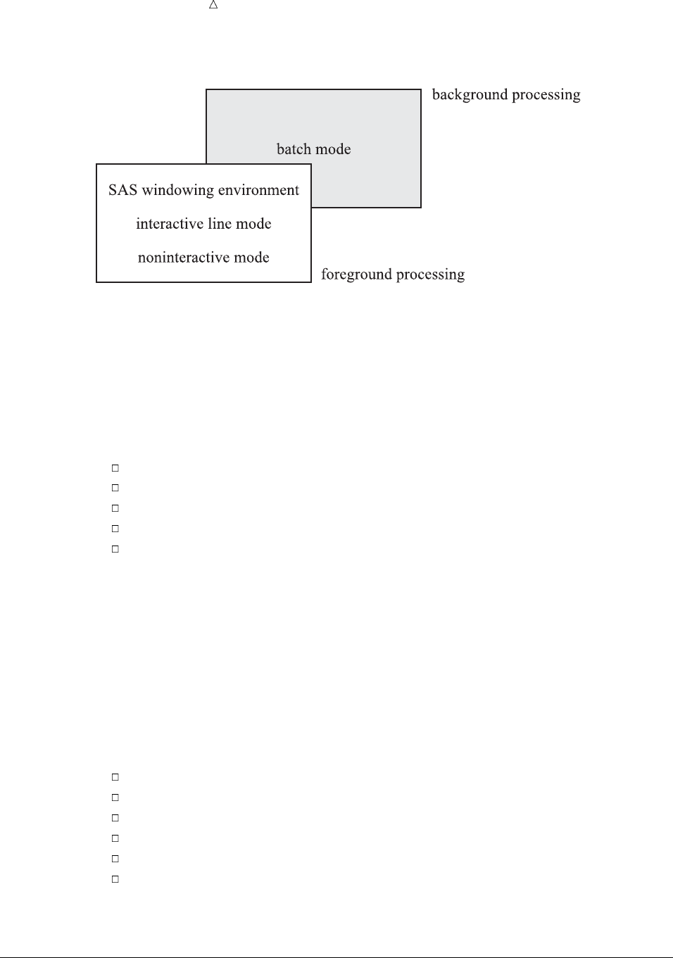
646 Processing Modes and Categories Chapter 38
Figure 38.1 Modes of Running SAS during Foreground or Background Processing
Understanding Foreground Processing
Foreground processing includes all the ways that you can run SAS in except batch
mode. Foreground processing begins immediately, but as your program runs, your
current workstation session is occupied, so you can not use it to do anything else.* With
foreground processing, you can route your output to the workstation display, to a file, to
a printer, or to tape.
If you can answer yes to one or more of the following questions, then you might want
to consider foreground processing:
Are you learning SAS programming?
Are you testing a program to see if it works?
Do you need fast turnaround?
Are you processing a fairly small data file?
Are you using an interactive application?
Understanding Background Processing
Batch processing is the only way to run SAS in the background. Your operating
environment coordinates all the work, so you can use your workstation session to do
other work at the same time that your program runs. However, because the operating
environment also schedules your program for execution and assigns it a priority, the
program may have to wait in the input queue (the operating environment’s list of jobs
to be run) before it is executed. When your program runs to completion, you can
browse, delete, or print your output.
Background processing may be required at your site. In addition, consider the
following questions:
Are you an experienced SAS user, likely to make fewer errors than a novice?
Are you running a program that has already been tested and refined?
Is fast turnaround less important than minimizing the use of computer resources?
Are you processing a large data file?
Will your program run for a long time?
Are you using a tape?
If you answer yes to one or more of these questions, then you might want to choose
background processing.
*In a workstation environment, you can switch to another window and continue working.
Introducing the SAS Environment Processing in the SAS Windowing Environment 647
Processing in the SAS Windowing Environment
Overview of Processing in the SAS Windowing Environment
The SAS windowing environment is a graphical user interface (GUI) that consists of
a series of windows with which you can organize files and folders, edit and execute
programs, view program output, and view messages about your programs and your SAS
session.
Because it is an interactive and graphical facility, you can use a single session to
prepare and submit a program and, if necessary, to modify and resubmit the program
after browsing the output and messages. You can move from window to window and
even interrupt and return to a session at the same point you left it.
General Characteristics
The SAS windowing environment is the default environment for a SAS session
(unless your environment is customized at your site).
Note: Because it is the default environment, many topics in this documentation
describe tasks as you would perform them in the SAS windowing environment.
The five most commonly used windows in the SAS windowing environment are
Explorer, Results, Editor, Log, and Output.
Explorer
is a hierarchical system of folders, subfolders, and individual items. It provides a
primary graphical interface to SAS from which you can do the following:
access and work with data, such as catalogs, tables, libraries, and operating
environment files
open SAS programming windows
access the Output Delivery System (ODS)
create and define customized folders
You can use Explorer to view or set libraries and file shortcuts, view or set library
members and catalog entries, or open and edit SAS files.
Note that when you start the SAS windowing environment, the Explorer might
appear as a single-paned window that lists libraries that are currently available.
You can add a navigational tree to the Explorer window by selecting View Show
Tree or by issuing the TREE command.
Editor or Program Editor
provides an area to enter, edit, and submit SAS statements and to save SAS
source files.
Log
enables you to browse and scroll the SAS log. The SAS log provides messages
about what is happening in your SAS session.
Output
enables you to browse and scroll procedure output.
Results
enables you to browse and manipulate an index of your procedure output.
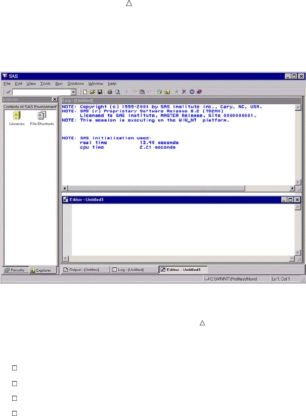
648 Processing in the SAS Windowing Environment Chapter 38
Display 38.1 SAS Windowing Environment: SAS Explorer, Log and Editor Windows, (Windows Operating
System)
Note: Together, the Program Editor, Log, and Output windows are sometimes
referred to as the programming windows.
Additional windows are also available in the SAS windowing environment that
enable you to do the following:
access online help
view and change some SAS system options
view and change function key settings
create and store text information
For more information about these windows and about performing tasks in the
windowing environment, see Chapter 39, “Using the SAS Windowing Environment,” on
page 655.
Invoking the SAS Windowing Environment
To invoke the SAS windowing environment, execute the SAS command followed by
any system options that you want to put into effect. The SAS windowing environment
is set as the default method of operation for SAS, but it may not be the default setting
at your work site.
If the SAS windowing environment is not the default method of operation, you can
specify the DMSEXP option in the SAS command. Or, you can include the DMSEXP
option in the configuration file, which contains settings for system options. For more
information about the configuration file, see “Customizing SAS Sessions and Programs
at Startup” on page 695.
You specify options in the SAS command as you do any other command options on
your system. The following table shows how you would start the SAS windowing
environment and specify the DMSEXP option under various operating environments:
Introducing the SAS Environment Processing in the SAS Windowing Environment 649
Operating Environment Command
z/OS sas options (’dmsexp’)
Windows sas -dmsexp
UNIX sas -dmsexp
OpenVMS sas /dmsexp
CMS sas (dmsexp
For details about how to specify command options on other systems, see the SAS
documentation for your operating environment.
Ending a SAS Windowing Environment Session
You can end your SAS windowing environment session with the BYE or ENDSAS
command. Specify BYE or ENDSAS on the SAS command line, and then execute the
command by pressing ENTER or RETURN (depending on which operating environment
you use).
You can also end your session with the ENDSAS statement in the Program Editor
window. Type the following statement on a data line and submit it for execution:
endsas;
Interrupting a SAS Windowing Environment Session
You might occasionally find it necessary to return to your operating environment
from a SAS session. If you do not want to end your SAS session, then you can escape to
the operating environment by issuing the X command. Simply execute the following
command on the command line:
x
From your operating environment, you can then return to the same SAS session as
you left it, by executing the appropriate operating environment command. For example,
under the z/OS operating environment, the operating environment command is
RETURN or END; under the OpenVMS operating environment, the command is
LOGOFF.
Use this form of the X command to execute a single operating environment command:
Xoperating-environment-command
or, if the command contains embedded blanks,
X’operating-environment-command’
For example, on many systems you can display the current time by specifying
x time
After the command executes, you can take the appropriate action to return to your
SAS session.
For information about interrupting a SAS session in other operating environments,
see the SAS documentation for your operating environment.

650 Processing Interactively in Line Mode Chapter 38
Processing Interactively in Line Mode
General Characteristics
With line mode processing, you enter programming statements one line at a time;
DATA and PROC steps are executed after you enter a RUN statement, or after another
step boundary. Program messages and output appear on the monitor.
You can modify program statements only when you first enter them, before you press
ENTER or RETURN, which means that you must type your entries carefully.
Invoking SAS in Line Mode
To invoke SAS in line mode, execute the SAS command followed by any system
options that you want to put into effect. The NODMS system option activates an
interactive line mode session. If NODMS is not the default system option at your site,
you can either specify the option with the SAS command or include the NODMS
specification in the configuration file, the file that contains settings for system options
that are put into effect at invocation. The following table shows you how to specify the
NODMS system option with the SAS command under various operating environments.
Operating environment Command
z/OS sas options (’nodms’)
Windows sas -nodms
UNIX sas -nodms
OpenVMS sas /nodms
CMS sas (nodms
Using the Run Statement to Execute a Program in Line Mode
In line mode, DATA steps are executed only when a new step boundary is
encountered. This occurs after you enter a RUN DATA or PROC statement. In other
words, if you submit DATA X; X=1; in the windowing environment, then you will not
see execution until the next RUN DATA or PROC statement is submitted.
At the beginning of each line, SAS prompts you with a number and a question mark
to enter more statements. If you use a DATALINES statement, then a greater-than
symbol (>) replaces the question mark, indicating that data lines are expected.
When you are using line mode, the log will be easier to read if you follow this
programming tip: cause each DATA or PROC step to execute before you begin entering
programming statements for the next step. Either an END statement or a semicolon
that marks the end of datalines causes a step to execute immediately.
Ending a Line Mode SAS Session
To end your session, type endsas; at the SAS prompt, then press ENTER or
RETURN. Your session ends, and you are returned to your operating environment.
Introducing the SAS Environment Processing Noninteractively 651
Interrupting a Line Mode SAS Session
In line mode, you can escape to the operating environment by executing the following
statement:
x;
You can return to your SAS session by executing the appropriate operating
environment command. Use this form of the X statement to execute a single operating
environment command:
Xoperating-environment-command;
or, if the command contains embedded blanks,
X’operating-environment-command’;
For example, on many systems you can display the current time by specifying
x time;
When you use this form of the X command, the command executes, and you are
returned to your SAS session.
Processing in Batch Mode
The first step in executing a program in batch mode is to prepare files that include:
any control language statements that are required by the operating environment
that you are using to manage the program
the SAS statements necessary to execute the program
Then you submit your file to the operating environment, and your workstation
session is free for other work while the operating environment executes the program.
This is called background processing because you cannot view or change the program in
any way until after it executes. The log and output are routed to the destination that
you specify in the operating environment control language; without a specification, they
are routed to the default. For examples of batch processing, see the SAS documentation
for your operating environment.
Processing Noninteractively
General Characteristics
Noninteractive processing has some characteristics of interactive processing and
some of batch processing. When you process noninteractively, you execute SAS program
statements that are stored in an external file. You use a SAS command to submit the
program statements to your operating environment.
Note: The SAS command is implemented differently under each operating
environment. For example, under z/OS the command is typically a CLIST, and under
CMS it is an EXEC.
As in interactive processing, processing begins immediately, and your current
workstation session is occupied. However, as with batch processing, you cannot interact
with your program.
Note: For some exceptions to this, see the SAS documentation for your operating
environment.
652 Review of SAS Tools Chapter 38
You can see the log or procedure output immediately after the program has run. Log
and listing output are routed to the workstation, unlike the SAS windowing
environment, where you must explicitly save output to a file. If you decide that you
must correct or modify your program, then you must use an editor to make necessary
changes and then resubmit your program.
Executing a Program in Noninteractive Mode
When you run a program in noninteractive mode, you do not enter a SAS session as
you do in interactive mode; instead of starting a SAS session, you are executing a SAS
program. The first step is to enter the SAS statements in a file, just as you would for a
batch job. Then, at the system prompt, you specify the SAS command followed by the
complete name of the file and any system options that you want to specify.
The following example executes the SAS statements in the member TEMP in the
partitioned data set your-userid.UGWRITE.TEXT in the z/OS operating environment:
sas input(ugwrite.text(temp))
Note that the INPUT operand points to the file that contains the SAS statements for
a noninteractive session.
The next example executes the SAS statements that are stored in the subdirectory
[USERID.UGWRITE.TEXT] on the OpenVMS operating environment in the file
TEMP.SAS:
$ sas [userid.ugwrite.text] temp
SAS looks for the file on the current disk.
The following example executes the SAS statements in the CMS file TEMP SAS A:
sas temp
Note: Note that in CMS, SAS looks for filetype SAS on any accessed disk. CMS
executes the first file called temp that it finds on any accessible mini disk. If TEMP
SAS lives on disk ’G’, then it will still be executed.
For details about how to use noninteractive mode on other operating environments, see
the SAS documentation for your operating environment. Consult your SAS Site
Representative for information specific to your site.
Browsing the Log and Output
Log and output information either appears in your workstation display or it is sent to
a file. The default action is dependent on your operating environment. In either case,
you can browse the information within your display or by opening the appropriate file.
See your operating environment documentation for more information.
Review of SAS Tools
Command
OPTIONS
view the option settings when you use the windowing environment.
Introducing the SAS Environment Commands 653
Options
PROC OPTIONS options;
lists the current values of all SAS system options.
System Options
DMS | NODMS
at invocation, specifies whether the SAS Programming windows are to be active in
a SAS session.
LINESIZE=n
specifies the line width for SAS output.
VERBOSE
at invocation, displays a listing of all options in the configuration file and on the
command line.
Statements
DATALINES;
signals to SAS that the data follows immediately.
ENDSAS
causes a SAS job or session to terminate at the end of the current DATA or PROC
step.
OPTIONS option;
changes one or more system options from the default value set at a site.
RUN
causes the previously entered SAS step to be executed.
X’operating-environment-command’;
is used to issue an operating environment command from within a SAS session.
Operating-environment-command specifies the command. Omitting the command
puts you into the operating environment’s submode.
Commands
BYE
ends a SAS session.
ENDSAS
ends a SAS session.
EXPLORER
invokes the Explorer window.
PMENU
turns on drop-down menus in windows.
X<’operating-environment-command’>
executes the operating environment command and then prompts you to take the
appropriate action to return to SAS. Omitting the command puts you into the
operating environment’s submode.
654 Learning More Chapter 38
Learning More
Operating environment information
For information about specific customization options and preferences, see the
documentation for your operating environment.
Windowing environment commands
For a list of all the commands that you can use in the SAS windowing environment,
see SAS online Help.
Help SAS System HelpSelect
Base SAS software
. The help topic is called Command Reference.
Documentation
For more examples of using the SAS windowing environment, see Getting Started
with the SAS System.

655
CHAPTER
39
Using the SAS Windowing
Environment
Introduction to Using the SAS Windowing Environment 657
Purpose 657
Prerequisites 657
Operating Environment Differences 657
Getting Organized 657
Overview of Data Organization 657
Exploring Libraries and Library Members 658
Assigning a Library Reference 658
Managing Library Assignment Problems 659
Finding Online Help 660
Accessing SAS Online Help System 660
Accessing Window Help 660
Accessing SAS OnlineDoc and SAS OnlineTutor 660
Using SAS Windowing Environment Command Types 660
Overview of SAS Windowing Environment Command Types 660
Using Command Line Commands 661
Using Pull-Down Menus 661
Using Line Commands 662
Using Function Keys 662
Working with SAS Windows 663
Opening Windows 663
Managing Windows 664
Scrolling Windows 665
Example: Scrolling Windows 665
Changing Colors and Highlighting in Windows 666
Finding and Changing Text 666
Cutting, Pasting, and Storing Text 667
Working with Text 667
The SAS Text Editor 667
Moving and Rearranging Text 668
Displaying Columns and Line Numbers 669
Making Text Uppercase and Lowercase 669
Overview 669
Changing the Default 670
Changing the Case of Existing Text 670
Combining and Separating Text 671
Working with Files 671
Ways to Find a File 672
Using Explorer to Find a File 672
Using the Find Window to Find a File 672
Example: Finding Files with the Find Window 673

656 Contents Chapter 39
Issuing File-Specific Commands 673
Opening Files 673
Assigning a File Shortcut 674
Modifying an Existing File Shortcut 675
Printing Files 675
Working with SAS Programs 676
Editor Window 676
Command Line Commands and the Editor 676
Line Commands and the Editor 677
Output Window 678
Log Window 679
Using Other Editors 679
NOTEPAD Window 679
Creating and Submitting a Program 680
Storing a Program 680
Debugging a Program 681
Opening a Program 681
Editing a Program 681
Assigning a Program to a File Shortcut 682
Working with Output 682
Overview of Working with Output 682
Setting Output Format 682
Setting Output Type with the Preferences Window 682
Setting Output Type with the SAS Registry Editor 683
Assigning a Default Viewer to a SAS Output Type 683
Working with Output in the Results Window 684
Customizing the Results Window View 685
Using Results Pointers to Navigate Output 685
Navigating the Results Window in Tree View 685
Navigating the Results Window in Contents Only View 686
Navigating the Results Window in Explorer View 686
Deleting Results Pointers 686
Renaming Results Pointers 686
Saving Listing Output to Other Formats 687
Viewing the First Output Pointer Item 687
Viewing Results Properties 687
Working with Output Templates 687
Overview of Working with Output Templates 687
Customizing the Templates Window View 688
Navigating the Templates Window in Explorer View 688
Navigating the Templates Window in Tree View 689
Navigating the Templates Window in Contents Only View 689
Browsing PROC TEMPLATE Source Code 689
Editing PROC TEMPLATE Source Code 689
Viewing Template Properties 690
Printing Output 690
Review of SAS Tools 690
Statements 690
Windows 690
Commands 691
Procedures 692
Learning More 692
Using the SAS Windowing Environment Overview of Data Organization 657
Introduction to Using the SAS Windowing Environment
Purpose
In this section you will learn about the SAS windowing environment, including how
to get organized, how to access help, and how to find and use appropriate commands.
In addition, you will learn how to use the SAS windowing environment to work with
files, SAS programs, and SAS output.
Prerequisites
Before proceeding with this section, you should understand the concepts presented in
Chapter 38, “Introducing the SAS Environment,” on page 643.
Operating Environment Differences
Even though SAS has a different appearance for each operating environment, most of
the actions that are available from the menus are the same.
One of the biggest differences between operating environments is the way that you
select menu items. If your workstation is not equipped with a mouse, then here are the
keyboard equivalents to mouse actions:
Mouse action Keyboard equivalent
double-click the item type an sor an xin the space next to the item,
then press the ENTER or RETURN key
right-click the item type ?in the space next to the item, then press
the ENTER or RETURN key
Examples in this documentation show SAS windows as they appear in the Microsoft
Windows environment. For the most part, corresponding windows in other operating
environments will yield similar results. If you do not see the drop-down menus in your
operating environment, then enter the global command PMENU at a command prompt.
Getting Organized
Overview of Data Organization
The SAS windowing environment helps you to organize your data, and to locate and
access your files easily. In this section, you learn how to use windows to do the following:
explore libraries and library members
assign a library reference
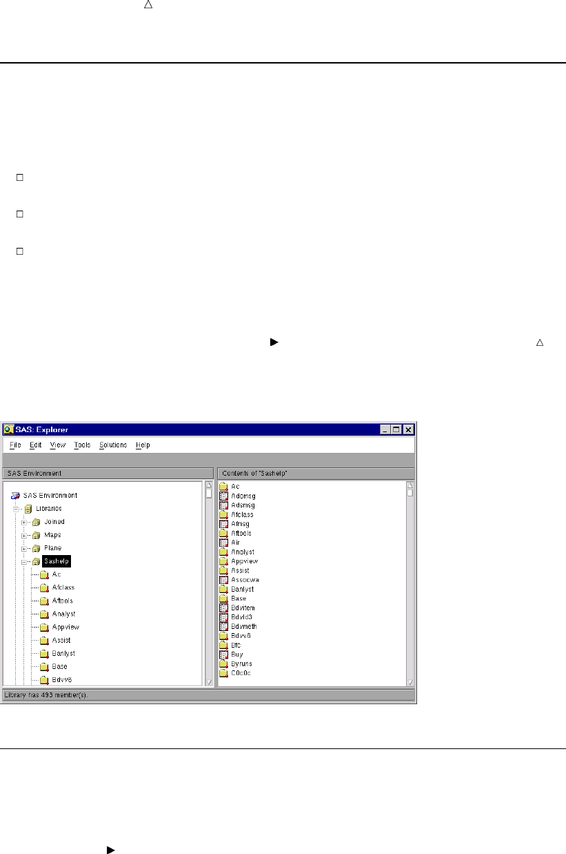
658 Exploring Libraries and Library Members Chapter 39
Exploring Libraries and Library Members
The SAS windowing environment opens to the Explorer window by default on many
hosts. You can issue the EXPLORER command to invoke this window if it does not
appear by default. You can use Explorer to view the libraries that are currently
available, as well as to explore their contents.
To list available libraries, select the Libraries folder, and then select Open from the
pop-up menu.
To explore the contents of a library, select a specific library, and then select
Explore from Here from the pop-up menu.
To explore the contents of a library member, select a specific library member, and
then select Open from the pop-up menu.
Note: If the Explorer Tree view is on, then you can explore libraries and library
members by expanding and collapsing tree nodes. You can expand or collapse Tree
nodes by selecting their expansion icons, which look like + and - symbols. You can toggle
the Explorer Tree view by selecting View Show Tree from the Explorer window.
Display 39.1 SAS Explorer Window with Tree View On
Assigning a Library Reference
Assign a library reference before continuing your work in a SAS session, so that you
can have a permanent storage location for your working SAS files:
1From the Explorer window, select the Libraries folder.
2Select File New
The New Library window appears.
3Enter a name for the library.
4Select an engine type.
5Enter an operating environment directory pathname or browse to select the
directory.
Using the SAS Windowing Environment Managing Library Assignment Problems 659
6Fill in any other fields as necessary for the engine, and enter any options that you
want to specify.
If you are not sure which engine to choose, then use the Default engine (which
is selected automatically).
The Default engine enables SAS to choose which engine to use for any data sets
that exist at the given path of your new library. If no data sets exist, then the
Base SAS engine is assigned.
7Select OK. The new library will appear under the Libraries folder in the Explorer
window.
Note: If you want SAS to assign the new library automatically at startup, then
select the Enable at Startup check box in the New Library window.
You can use the following ways to assign a library, depending on your operating
environment:
Menu File New
(from the Explorer window only)
Command DMLIBASSIGN (from any window)
Pop-up New (from the Explorer window only)
Toolbar New Library (from any window)
Managing Library Assignment Problems
If any permanent library assignment that is stored in the SAS Registry fails at
startup, then the following note appears in the SAS Log:
NOTE: One or more library startup assignments were not restored.
The following errors are common causes of library assignment problems:
library dependencies are missing
required field values for library assignment in the SAS Registry are missing
required field values for library assignment in the SAS Registry are invalid
For example, library names are limited to eight characters, and engine values
must match actual engine names.
encrypted password data for a library reference has changed in the SAS Registry
CAUTION:
You can correct many library assignment errors in the SAS Registry Editor. If you are
unfamiliar with library references or the SAS Registry Editor, ask for assistance. Errors can
be made easily in the SAS Registry Editor, and can prevent your libraries from being
assigned at startup.
To correct a library assignment error in the SAS Registry Editor:
1Select Solutions Accessories Registry Editor or issue the REGEDIT
command.
2Select one of the following paths, depending on your operating system, and then
make modifications to keys and key values as needed:
CORE\OPTIONS\LIBNAMES
or
CORE\OPTIONS\LIBNAMES\CONCATENATED
660 Finding Online Help Chapter 39
or
CORE\LIBNAMES
For example, if you determine that a key for a permanent concatenated library has
been renamed to something other than a positive whole number, then you can rename
that key again so that it is in compliance. Select the key, and then select Rename from
the pop-up menu to begin the process.
Finding Online Help
Accessing SAS Online Help System
To access the SAS online Help, select Help SAS System Help
Accessing Window Help
You can access help on an individual window in any of the following ways:
Issue the HELP command from the command line of the window.
Select the window’s help button, if one exists.
Select the Help icon on the toolbar.
From the window for which you want help, select Help Using This Window
Accessing SAS OnlineDoc and SAS OnlineTutor
SAS OnlineDoc is a CD that provides reference information about SAS. The SAS
OnlineDoc has a table of contents, index, and a search engine that enables you to find
information quickly. For some operating systems, you can access it by selecting Help
Books and Training OnlineDoc
SAS OnlineTutor is an interactive online training application that enables you to
learn about the SAS environment, SAS programming, and specific SAS products. SAS
OnlineTutor is available on CD and must be licensed. If your site has licensed and
installed SAS OnlineTutor, then you can access this product by selecting Help Books
and Training OnlineTutor
For more information about configuring the SAS OnlineDoc CD or installing SAS
OnlineTutor at your site, contact your SAS Installation Representative.
Using SAS Windowing Environment Command Types
Overview of SAS Windowing Environment Command Types
There are specific types of SAS windowing environment commands. The type of
commands that you use might depend on the task that you need to complete, or on your
personal preferences. These commands can be in the form of:
command line commands
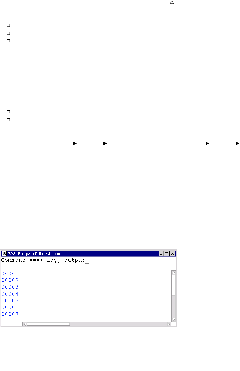
Using the SAS Windowing Environment Using Pull-Down Menus 661
pull-down menu commands
line commands (in text editing windows)
keyboard function keys
For information about specific commands that can be issued in the SAS windowing
environment, see “Working with SAS Windows” on page 663. For information about
specific commands that can be used in the SAS text editor, see “Working with Text” on
page 667.
Using Command Line Commands
Command line commands can be entered in two places:
on the command line (if it is turned on)
in the Command window (if it is available)
If the command line is turned on, then you can place your cursor on the command
line and type commands. You can toggle the command line on or off for a specific
window by selecting Tools Options Turn Command Line On or Tools Options
Turn Command Line Off.
The Command window (if it is available in your operating environment) includes a
text area. You can place your cursor in this area and then issue commands.
To execute a command, type the command on the command line and then press the
ENTER or RETURN key, depending on which operating environment you are using.
You can specify a simple one-word command, multiple commands separated by
semicolons, or a command followed by an option.
For example, if you want to move from the Editor window and open both the Log and
the Output windows, on the command line of the Editor window, specify
log; output
Display 39.2 Entering Commands on the Command Line
Next, press ENTER or RETURN to execute both commands. The Log and Output
windows appear. The Output window is the active window because the command to
open this window was executed last.
Using Pull-Down Menus
SAS windowing environment windows can display pull-down menus instead of a
command line. You can then make menu selections to do things that you would usually
accomplish by typing commands.
662 Using Line Commands Chapter 39
If your operating environment does not default to using drop-down menus, then issue
the PMENU command at a command line to turn on menus for all windows that
support them.
You can point and click menus and menu items with a mouse to make your
selections. In some operating environments, you can also make menu selections by
moving your cursor over the menu items and then pressing ENTER or RETURN.
Depending on the item that you select, one of three things happens:
a command executes
a pull-down menu appears
a dialog box appears
In many cases, double-clicking on items and right-clicking on items will cause different
menus to appear. Sometimes you might want to try one or the other when selecting an
item does not give you the expected result.
In other operating environments with workstations that are not equipped with a
mouse, here are the keyboard equivalents to mouse actions:
Mouse action Keyboard equivalent
double-click type an sor an xin the space next to the item,
then press the ENTER or RETURN key.
right-click instead of right-clicking an item, type ?in the
space next to the item, then press the ENTER or
RETURN key.
Using Line Commands
Line commands are one or more letters that copy, move, delete, and otherwise edit
text. You can execute line commands by typing them in the numbered part of a text
editing window (such as the Editor or the SAS NOTEPAD).
Although line commands are usually executed in the numbered part of the display or
with function keys, they can also be executed from the command line if preceded by a
colon.
Note: Issue the NUMBERS command to toggle line numbers on or off in text editing
windows.
For more information about line commands, see “Working with Text” on page 667.
Using Function Keys
Your keyboard includes function keys to which default values have already been
assigned. You can browse or alter those values in the Keys window. To open the Keys
window, select Tools Options Keys or issue the KEYS command.
To change the setting of a key in the Keys window, type the new value over the old
value. The new setting takes effect immediately and is saved permanently when you
execute the END command to close the Keys window.
Function keys enable you to tailor your key settings to meet your needs in a
particular SAS session. For example, If you might need to submit a number of
programs and need to move between the Editor window and the Output window. Then
each time you finish viewing your output, you must type the PGM and ZOOM
Using the SAS Windowing Environment Opening Windows 663
commands on the command line and press ENTER or RETURN. As a shortcut, define
one of your function keys to perform this action by typing the following commands over
an unwanted value or where no value existed before:
pgm; zoom
Then, each time you press that function key, the commands are executed, saving you
time. You can also use function keys to execute line commands. Simply precede the line
command with a colon as you would if you were issuing the line command from the
command line.
Working with SAS Windows
Opening Windows
The SAS windowing environment has numerous windows that you can use to
complete tasks. You can enter commands to open windows. For more information about
how to execute commands, see “Using SAS Windowing Environment Command Types”
on page 660.
You can use the following commands to open a window and make it active.
Window command Window name
AF C=library.catalog.entry.type Build
DMFILEASSIGN File Shortcut Assignment
DMLIBASSIGN New Library
EDOP Editor Options
EXPFIND Find
EXPLORER Explorer
FOOTNOTES Footnotes
FSBROWSE FSBrowse
FSEDIT FSEdit
FSFORM formname FSForm
FSVIEW FSView
HELP Help
KEYS Keys
LOG Log
NOTEPAD, NOTE Notepad
ODSRESULTS Results
ODSTEMPLATES Templates
OPTIONS Options
OUTPUT, LISTING, LIST, LST Output
PROGRAM, PGM, PROG Program Editor
REGEDIT Registry Editor
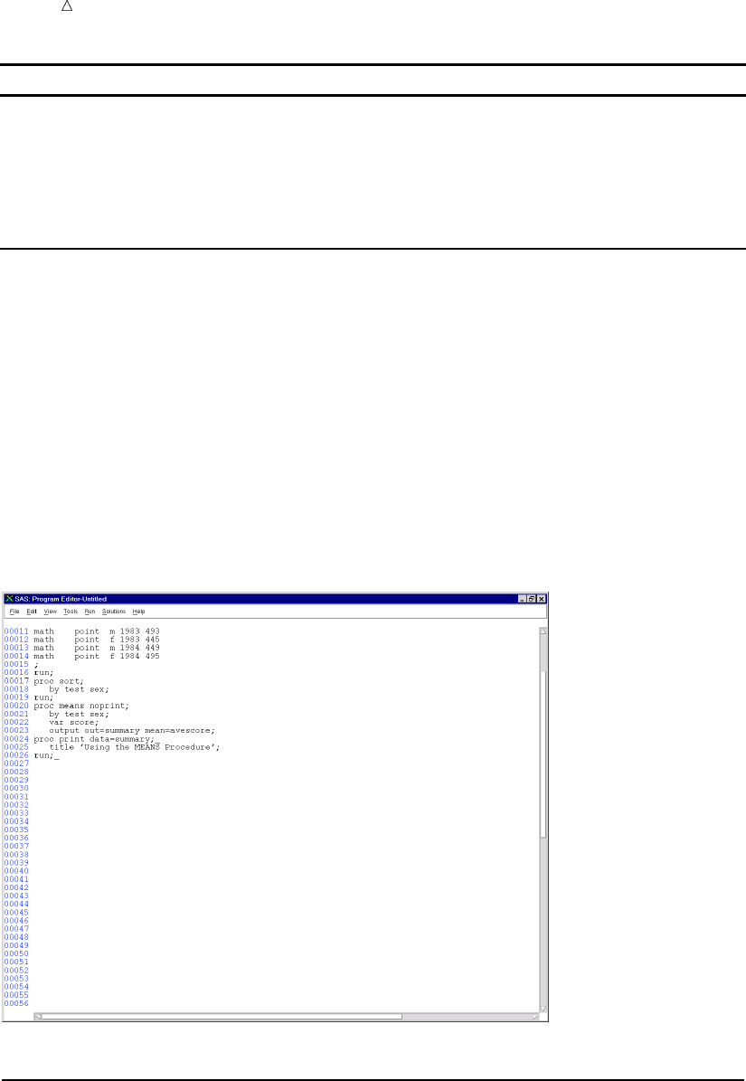
664 Managing Windows Chapter 39
Window command Window name
REPOSMGR Repository Manager
SASENV Explorer (Contents Only view)
SETPASSWORD Password
TITLES Titles
VAR Properties
You can use window commands at any command prompt. You might find it helpful to
use multiple window commands together.
For example, from the Log window, the following string of commands changes the
active window, maximizes it, and changes the word paint to print:
pgm; zoom; change paint print
The following display shows that the cursor immediately moves to the Editor, which
has been maximized to fill the entire display (due to the ZOOM command). The word
paint has been changed to print, and the cursor rests after the last character of that
text string.
Display 39.3 Executing a Window-Call Command in a Series
Managing Windows
Window management commands enable you to access and use windows more
efficiently. The following list includes the commands that you might use most often
when managing windows:
BYE ends a SAS session.
CLEAR removes all text from an active window.

Using the SAS Windowing Environment Example: Scrolling Windows 665
END closes a window. In the Editor, this command acts like the SUBMIT
command.
NEXT moves the cursor to the next open window and makes it active.
PREVWIND moves the cursor to the previous open window and makes it active.
RECALL returns statements that are submitted from a text editor window
(such as the Editor or SAS NOTEPAD) to the text editor.
ZOOM enlarges a window to occupy the entire display. Execute it again to
return a window to its previous size. This command is not available
in all operating environments.
Scrolling Windows
Scrolling commands enable you to maneuver within text, and the command names
indicate what they do. They include the following:
BACKWARD moves the contents of a window backward.
FORWARD moves the contents of a window forward.
LEFT moves the contents of a window to the left.
RIGHT moves the contents of a window to the right.
TOP moves the cursor to the first character of the first line in a window.
BOTTOM displays the last line of text.
HSCROLL,
VSCROLL
HSCROLL determines the amount that you move to the left or right
when using the LEFT or RIGHT commands. VSCROLL determines
the amount that you move forward or backward when using the
FORWARD or BACKWARD commands.
Use the following options with the HSCROLL and VSCROLL
commands as needed. HALF is the default scroll amount.
PAGE is the entire amount that shows in the window.
HALF is half the amount that shows in the window.
MAX is the maximum portion to the left or right or to
the top or bottom that shows in the window.
nis nlines or columns, where nis the number that
you specify.
CURSOR When used with HSCROLL, the cursor moves to
the left or right of the display, when the LEFT or
RIGHT command is executed.
Note: This option is valid only in windows
that allow editing.
When used with VSCROLL, the cursor moves
up and down when the FORWARD and
BACKWARD command is executed.
Example: Scrolling Windows
To set the automatic horizontal scrolling value to five character spaces, then specify
666 Changing Colors and Highlighting in Windows Chapter 39
hscroll 5
Now, when you execute the LEFT or RIGHT command, you move five character
spaces in the appropriate direction. If you want to set the automatic vertical scrolling
value to half a page, then specify
vscroll half
Then, when you execute the FORWARD command, half of the previous page remains
on the display and half of a new page is scrolled into view.
If you need to scroll a specific number of lines forward or backward, then use the
scroll amount on the FORWARD command to temporarily override the default scrolling
value. You can specify scrolling values with the BACKWARD and FORWARD
commands and the LEFT and RIGHT commands.
Changing Colors and Highlighting in Windows
SAS gives you a simple way to customize your environment if your display supports
color. You can change SAS windowing environment colors with the COLOR command.
You can also change SAS code color schemes by using the SYNCONFIG command. To
change windowing environment colors, simply specify the COLOR command followed by
the field or window element that you want changed, and the desired color. You might
also be able to change highlighting attributes, such as blinking and reverse video.
For example, to change the border of a window to red, specify
color border red
This changes the border to red.
Other available colors are blue, green, cyan, pink, yellow, white, black, magenta,
gray, brown, and orange. If the color that you specify is not available, then SAS
attempts to match the color to its closest counterpart.
Some color selections are valid only for certain windows.
For more information, see the online help for the SASColor window. You can access
the SASColor window with the SASCOLOR command.
You can also change the color scheme of text in the windows in which you enter code,
such as the Editor window and NOTEPAD. This is useful, because you can make
different elements of the SAS language appear in different colors, which makes it easier
to parse code. To change the color scheme for code, use the SYNCONFIG command.
The SYNCOLOR command toggles color coding off and on in these windows.
For more information about changing the color schemes for windows in which you
create and edit code, see the online help that is available when you issue the
SYNCONFIG command.
Finding and Changing Text
Often, you might want to search for a character string and change it. You can locate
the character string by specifying the FIND command and then the character string.
Then the cursor moves to the first occurrence of the string that you want to locate.
Remember to enclose a string in quotation marks if CAPS ON is in effect.
You can change a string by specifying the CHANGE command, then a space and the
current character string, and then a space and the new character string. Remember to
enclose in quotation marks any string that contains an embedded blank or special
characters. For both the FIND and CHANGE commands, the character string can be
any length.
With both the FIND and CHANGE commands, you can specify the following options
to locate or change a particular occurrence of a string:

Using the SAS Windowing Environment The SAS Text Editor 667
ALL
FIRST
ICASE
LAST
NEXT
PREFIX
PREV
SUFFIX
WORD
For details about which options you can use together, see the SAS Language
Reference: Dictionary. Note that the option ALL finds or changes all occurrences of the
specified string. In the following example, all occurrences of host are changed to
operating environment:
change host ’operating environment’ all
To resume the search for a string that was previously specified with the FIND
command, specify the RFIND command. To continue changing a string that was
previously specified with the CHANGE command, specify the RCHANGE command. To
find the previous occurrence of a string, specify the BFIND or FIND PREV command;
you can use the PREFIX, SUFFIX, and WORD options with the BFIND command.
Cutting, Pasting, and Storing Text
With the cut and paste facility, you can do the following:
Identify the text that you want to manipulate.
Store a copy of the text in a temporary storage place called a paste buffer.
Insert text.
List the names of all current paste buffers or delete them.
You can manipulate and store text by using the following commands:
MARK identifies the text that you want to cut or paste.
CUT removes the marked text from the display and stores it in the paste
buffer.
STORE copies the marked text and stores it in the paste buffer.
PASTE inserts the text that you have stored in the paste buffer at the
cursor location.
Working with Text
The SAS Text Editor
The SAS text editor is an editing facility that is available in the Editor and SAS
NOTEPAD windows of Base SAS, SAS/FSP, and SAS/AF software. You can edit text
from the command line and from any line on which code appears in an edit window.

668 Moving and Rearranging Text Chapter 39
This section provides information about commands that you can use to perform
common text editing tasks by using the SAS text editor. For more information about all
SAS windowing environment commands, see “Using SAS Windowing Environment
Command Types” on page 660.
Moving and Rearranging Text
Some of the basics of moving, deleting, inserting, and copying single lines of text
have already been reviewed. The rules are similar for working with a block of text;
simply use double letters on the beginning and ending lines that you want to edit.
For example, alphabetizing the following list requires that you move a block of text.
Note the MM (move) block command on lines 5 and 6 and the B line command on line 1
of the example.
b 001 c signifies the line command copy
00002 d signifies the line command delete
00003 i signifies the line command insert
00004 m signifies the line command move
mm 05 a signifies the line command after
mm 06 b signifies the line command before
00007 r signifies the line command repeat
Press the ENTER or RETURN key to execute the changes. Here are the results:
00001 a signifies the line command after
00002 b signifies the line command before
00003 c signifies the line command copy
00004 d signifies the line command delete
00005 i signifies the line command insert
00006 m signifies the line command move
00007 r signifies the line command repeat
Mastering a few more commands greatly increases the complexity of what you can do
within the text editor. Several commands enable you to justify text. Specify the JL
(justify left) command to left justify, the JR (justify right) command to right justify, and
the JC (justify center) command to center text. To justify blocks of text, use the JJL,
JJR, and JJC commands. For example, if you want to center the following text,
00001 Study of Advertising Responses
00002 Topnotch Hotel Website
00003 Conducted by Global Information, Inc.
then simply add the JJC block command on the first and last lines and press ENTER
or RETURN.
You can also shift text right or left the number of spaces that you choose by executing
the following set of line commands:
>[n] shifts text to the right the number of spaces that you specify; the
default is one space.
<[n] shifts text to the left the number of spaces that you specify; the
default is one space.
To shift a block of text left, specify the following command on the beginning and
ending line numbers of the block:
<<[n]
Specify the following command to shift a block of text to the right:
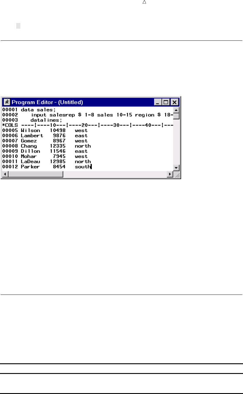
Using the SAS Windowing Environment Making Text Uppercase and Lowercase 669
>>[n]
Displaying Columns and Line Numbers
To display column numbers in the text editor, specify the COLS line command. This
command is especially useful if you are writing an INPUT statement in column mode,
as shown in the following figure:
Display 39.4 Executing the COLS Command
To remove the COLS line command or any other pending line command, execute the
RESET command on the command line. You can also execute the D (delete) line
command on the line where you have specified the COLS command to achieve the same
results.
The NUMBERS command numbers the data lines in the Editor and SAS NOTEPAD
windows. Specify the following command to add numbers to the data lines:
numbers on
To remove the numbers, specify
numbers off
You can also use the NUMBERS command without an argument, executing the
command once to turn numbers on, and again to turn them off.
Making Text Uppercase and Lowercase
Overview
Making text uppercase and lowercase involves two sets of commands to accomplish
two kinds of tasks:
Command Action
CAPS changes the default
CU, CL line commands change the case of existing text
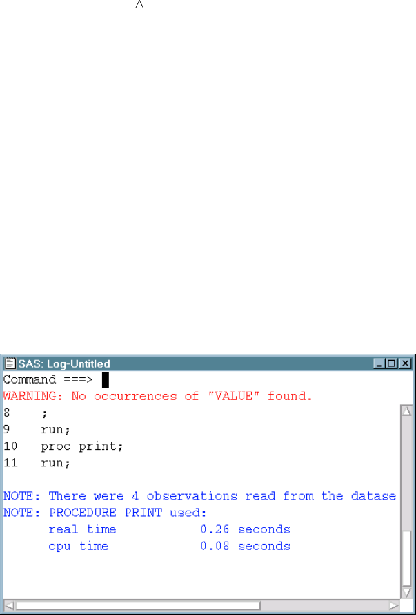
670 Making Text Uppercase and Lowercase Chapter 39
Changing the Default
To change the default case of text as you enter it, use the CAPS command. After you
execute the CAPS command, the text that you enter is converted to uppercase as soon
as you press ENTER or RETURN. Under some operating environments, with CAPS
ON, characters that are entered or modified are translated into uppercase when you
move the cursor from the line. Character strings that you specify with a FIND, RFIND,
or BFIND command are interpreted as having been entered in uppercase unless you
enclose the character strings in quotation marks.
For example, if you want to find the word value in the Log window, then on the
command line, specify
find value
If the CAPS command has already been specified, then SAS searches for the word
VALUE instead of value. You receive a message indicating that no occurrences of
VALUE have been found, as shown in the following display:
Display 39.5 The Results of the FIND Command with CAPS ON
However, specify the following command and SAS searches for the word value, and
finds it:
find ’value’
Setting CAPS ON remains in effect until the end of your session or until you turn it
off. You can execute the CAPS command by specifying
caps on
To discontinue the automatic uppercasing of text, specify
caps off
You can also use the CAPS command like a toggle switch, executing it once to turn
the command on, and again to turn it off.
Changing the Case of Existing Text
To uppercase or lowercase text that has already been entered, use the line commands
CU and CL. Execute the CU (case upper) command to uppercase a line of text and the
CL (case lower) command to lowercase a line of text.

Using the SAS Windowing Environment Working with Files 671
In the following example, the CU and CL line commands each mark a line of text
that will be converted to uppercase and lowercase, respectively.
00001 Study of Gifted Seventh Graders
cu002 Burns County Schools, North Carolina
cl003 Conducted by Educomp, Inc.
Press ENTER or RETURN to execute the commands. The lines of text are converted
as follows:
00001 Study of Gifted Seventh Graders
00002 BURNS COUNTY SCHOOLS, NORTH CAROLINA
00003 conducted by educomp, inc.
For a block of text, you have two choices. First, you can execute the CCU block
command to uppercase a block of text and the CCL block command to lowercase a block
of text. Position the block command on both the first and last lines of text that you
want to convert. Second, you can designate a number of lines that you want to
uppercase or lowercase by specifying a numeric argument, as shown below:
cu3 1 Study of Gifted Seventh Graders
00002 Burns County Schools, North Carolina
00003 Conducted by Educomp, Inc.
Press ENTER or RETURN to execute the command. The three lines of text are
converted to uppercase, as shown below:
00001 STUDY OF GIFTED SEVENTH GRADERS
00002 BURNS COUNTY SCHOOLS, NORTH CAROLINA
00003 CONDUCTED BY EDUCOMP, INC.
Combining and Separating Text
You can combine and separate pieces of text with a number of line commands. With
the TC (text connect) command, you can connect two lines of text. For example, if you
want to join the following lines, then type the TC line command as shown below. Note
that the second line is deliberately started in column 2 to create a space between the
last word of the first line and the first word of the second line.
tc001 This study was conducted by
00002 Educomp, Inc., of Annapolis, Md.
Press ENTER or RETURN to execute the command. The lines appear as shown
below:
00001 This study was conducted by Educomp, Inc., of Annapolis, Md.
Conversely, the TS (text split) command shifts text after the cursor’s current position
to the beginning of a new line.
Remember that you can also use a function key to execute the TC line command, the
TS line command, or any other line command as long as you precede it with a colon.
Working with Files
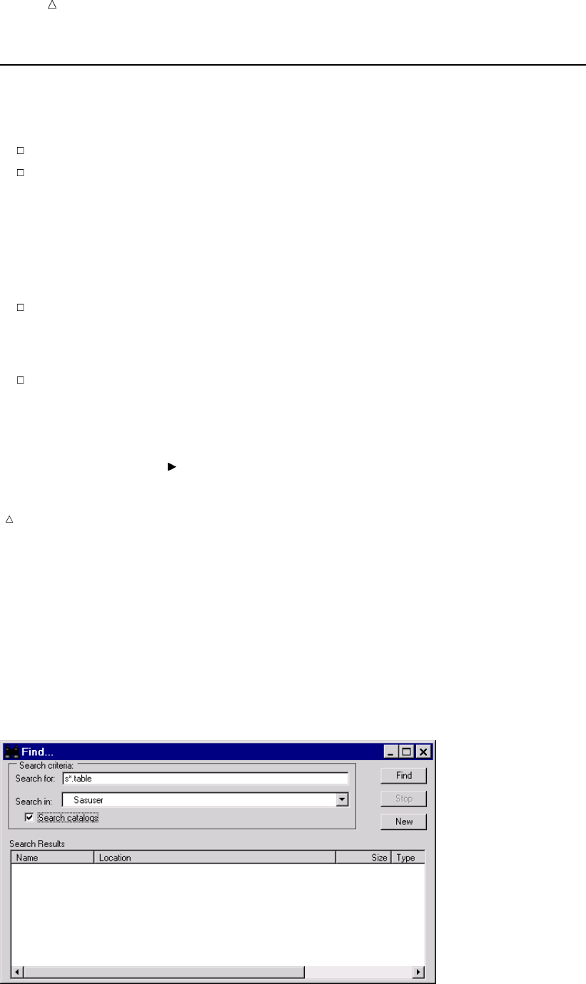
672 Ways to Find a File Chapter 39
Ways to Find a File
There are a number of ways in which you can find a file or library member in the
SAS windowing environment, including the following:
using the Explorer window
using the Find window
Using Explorer to Find a File
When the SAS windowing environment opens, the Explorer window also opens by
default in many operating environments. You can issue the EXPLORER command to
open the Explorer window if it does not open by default.
To find a file in the Contents Only view of the Explorer window, select the
Libraries folder or the File Shortcuts folder, and then select Open from the
pop-up menu. You can continue this process with subfolders until you locate the
appropriate file.
To find a file in the Tree view of the Explorer window, use the expansion icons (+
and – icons) located in the tree until the appropriate file appears in the window.
Note: You might find it useful to use specific navigational tools to move through the
different levels of the Explorer window:
Menu View Up One Level
Command UPLEVEL
For more information about selecting an Explorer window view, see “Customizing the
Explorer Window” on page 702.
Using the Find Window to Find a File
The Find window enables you to search for an expression (such as a text string or a
library member) that exists in a SAS library. The default search looks at everything in
the library, except catalogs, but you can click the check box for the search to include the
catalogs in the library as well.
Display 39.6 The Find Window
Using the SAS Windowing Environment Opening Files 673
To search for a file:
1Select Tools Find from the Explorer window to open the Find window.
Alternatively, issue the EXPFIND or EXPFIND <library-name> command. If
you issue the EXPFIND command, then SASUSER is the default library. If you
issue the EXPFIND WORK command, then WORK is the default library.
2In the Search For field, enter the expression that you want to find. Wildcard
characters are acceptable.
3From the Search In drop-down list, select the library in which you want to search.
4Click Search Catalogs to expand the search to include the catalogs of the library
that you have selected.
Searching catalogs can lengthen search time considerably depending on the size
and number of catalogs in the library.
5Click Find.
Example: Finding Files with the Find Window
You can find TABLE files that begin with a specific letter and exist in a specific
library. For a file that starts with the letter Sand which exists in the SASHELP library
1Select Tools Find to open the Find window.
2Type s*.table in the Search For field.
3Select SASHELP from the Search In drop-down list.
4Click Find.
Issuing File-Specific Commands
There are a number of commands that you can issue against a file after you find the
file in the SAS windowing environment. The commands that are available are
determined by the type of file with which you are working.
1Find the file with which you want to work. For more information, see “Ways to
Find a File” on page 672.
2Select the file, and then right-click the file. A list of file-specific commands appears
from which you can make a selection.
Operating Environment Information: If you are using the z/OS or CMS operating
environment, then you can open a pop-up menu by typing ?in the selection field next
to an item. Alternatively you can type an type ansor xin the selection field next to an
item.
Opening Files
There are a number of ways in which you can open files in the SAS windowing
environment.
To open a SAS file from Explorer:
1Open a library and appropriate library members until you see the file that you
want to open.
2Select the file, then select Open from the pop-up menu.
Depending on the file type, you might also be able to select Open in Editor.

674 Assigning a File Shortcut Chapter 39
Note: In some cases, the pop-up menu also enables you to select Browse in SAS
Notepad, which enables you to open a file in the SAS NOTEPAD window.
To open a file that has a file shortcut:
1Open the File Shortcuts folder.
2Select a file shortcut, and then select Open from the pop-up menu.
Assigning a File Shortcut
File shortcut references provide aliases to external files (such as a .sas program file
or a .dat text file). A file shortcut is the same as a file reference or fileref. In operating
environments that support drag and drop functionality, you can drag file shortcuts from
the Explorer window to the Editor window to display their contents.
To assign a file shortcut
1From the Explorer window, select the File Shortcuts folder.
2Select File New.
3In the Name field of the File Shortcut Assignment window, enter a name for the
file shortcut.
4Select the method or device that you want to use for the file shortcut.
The methods or devices that are available from the Method drop-down list
depend on your operating environment. The DISK method is the default method
(if it is available for your operating environment).
5Select the Enable at Startup check box if you want SAS to automatically assign
the file shortcut each time SAS starts. This option is not available for all the file
shortcut methods.
If you want to stop a file shortcut from being enabled at startup, then select the
file shortcut in the SAS Explorer window, and then select Delete from the pop-up
menu.
6Fill in the fields of the Method Information area, including the name and location
of the file for which you want to create a file shortcut. You can select Browse to
locate the actual file. The fields that are available in this area depend on the type
of method or device that you select.
Note: Selecting a new method type erases any entries that you might have made
in the Method Information fields.
7Select OK to create the new file shortcut. The file shortcut appears in the File
Shortcut folder of the SAS Explorer window.
You can use the following ways to create a file shortcut, depending on your operating
environment:
Menus
File Newwhile your mouse is positioned on File Shortcuts in the Explorer
window.
Command
DMFILEASSIGN<file-shortcut-name><METHOD=><AUTO=>
file-shortcut-
name
specifies an existing file shortcut reference.
METHOD=
method-name
specifies which method to use when the File Shortcut
Assignment window opens.
Using the SAS Windowing Environment Printing Files 675
AUTO= Yes|No sets the state of the File Shortcut Assignment window’s Enable
at Startup check box when the window opens.
Pop-up
New File Shortcut if you have opened the File Shortcut folder in the Explorer
window.
Toolbar
New (while your mouse is positioned on File Shortcuts in the Explorer window.)
Modifying an Existing File Shortcut
You can modify existing file shortcut references, if needed.
From the command line:
1Issue the following command:
DMFILEASSIGN file-shortcut-name
The File Shortcut Assignment window appears. Its fields include information
that is specific to the chosen file shortcut.
2Edit the fields of the File Shortcut Assignment window as needed.
From the SAS Explorer:
1Right-click the File Shortcuts folder and select Open. Alternatively, you can
double-click the folder to open it.
2Right-click the file shortcut reference that you want to change, and then select
Modify.
3Edit the fields of the File Shortcut Assignment window as needed.
Operating Environment Information: If you are using the z/OS or CMS operating
environment, then you can open a pop-up menu by typing ?in the selection field next
to an item. Alternatively you can type an type an sor xin the selection field next to an
item.
Printing Files
There are a number of ways in which you can print files. Often, printing capabilities
depend on the type of file with which you are working, as well as your operating
environment.
Nonetheless, the following lists common ways in which you might be able to print a
file.
Printing from
Explorer
Find the appropriate file in the SAS Explorer window. Right-click
over the file, and then select Print.
Printing from a
Text Editor
Open your file into a text editor such as the Editor or the SAS
NOTEPAD. Use the text editor’s printing commands.
Refer to your operating environment documentation for information about printing
files.

676 Working with SAS Programs Chapter 39
Working with SAS Programs
Editor Window
When you work with SAS programs, you typically use the SAS programming
windows (the Editor, Log, and Output windows). Of these programming windows, the
Editor is the window that you might use most often. It enables you to do the following:
Enter and submit the program statements that define a SAS program.
Edit text.
Store your program in a file.
Copy contents from an already-created file.
Copy contents into another file.
Display 39.7 The Editor Window with Line Numbers Turned On
Note: The Editor window shown here includes line numbers. You might find line
numbers helpful when creating or editing programs. To toggle line numbers on or off,
issue the NUMBERS command.
Command Line Commands and the Editor
There are a number of commands that you might find useful while working on
programs in the Editor. You can execute these commands from the command line:
TOP scrolls to the beginning of the Editor.
BOTTOM scrolls to the last line of text.
BACKWARD scrolls back toward the beginning of the text.
FORWARD scrolls forward toward the end of the text.
LEFT scrolls to the left of the window.
RIGHT scrolls to the right of the window.
Using the SAS Windowing Environment Editor Window 677
ZOOM increases the size of the window. You can issue this command again
to return the window to its previous size.
UNDO cancels the effect of the most recently submitted text editing
command. Continuing to execute the UNDO command undoes
previous commands, starting with the most recent and moving
backward.
SUBMIT submits the block of statements in your current SAS windowing
environment session.
RECALL returns to the Editor window the most recently submitted block of
statements in your current SAS windowing environment session.
Continuing to execute the RECALL command recalls previous
statements, starting with the most recent and moving backward.
CLEAR clears a window as specified. You can clear the Editor, Log, or Output
windows from another window by executing the CLEAR command
with the appropriate option as shown in the following examples:
clear pgm
clear log
clear output
CAPS converts everything that you type to uppercase.
FIND searches for a specified string of characters. Enclose the string in
quotation marks if it contains embedded blanks or special characters.
CHANGE changes a specified string of characters to another. Follow the
command keyword with the first string, a space, and then the second
string. The rules for embedded blanks and special characters apply.
For example, you might specify
change ’operating system’ platform
This CHANGE command replaces the first occurrence of operating
system with the word platform. Note that the first string must be
enclosed in quotation marks because it contains an embedded blank.
Note: Some of the more useful command line commands have been listed here.
Almost all SAS commands are valid in the Editor window. For more information about
other command line commands, see “Working with SAS Windows” on page 663.
Line Commands and the Editor
The left-most portion of the Editor window includes a numbered field. This field is
where you enter line commands. These commands are denoted by one or more letters,
and can move, copy, delete, justify, or insert lines.
Some common line commands include
M — moves a line of text
C — copies a line of text
D — deletes a line of text
I — inserts a line of text.
When you use some line commands, you also need to specify a location. For example,
if you type an Min the numbered field for a line in the Editor, then you must specify
where you want the line of text to be moved. You can use the A(after) and B(before)
line commands to specify a location.
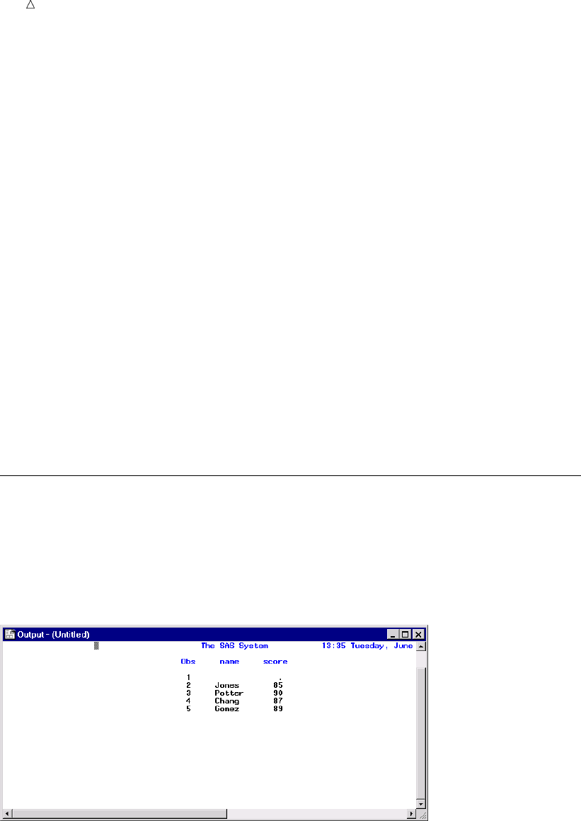
678 Output Window Chapter 39
If you type an Ain the numbered field for a line, then the line of text that you want
to move will be placed after the line marked with an A after you press the ENTER or
RETURN key. If you type a Bin the numbered field for a line, then the line of text that
you want to move will be placed before the line marked with a B after you press the
ENTER or RETURN key.
The following examples show how to use line commands to move a line of text in the
Editor window to a new location. To make the following lines alphabetical, place the
first line after the last line. To do this, use the M and A line commands:
m 001 Lincoln f Wake Ligon 135
00002 Andrews f Wake Martin 140
00003 Black m Wake Martin 149
a 004 Jones m Wake Ligon 142
After pressing the ENTER or RETURN key, your Editor window lines appear as
follows:
00001 Andrews f Wake Martin 140
00002 Black m Wake Martin 149
00003 Jones m Wake Ligon 142
00004 Lincoln f Wake Martin 135
There are many other line commands and combinations of line commands that you
can use to edit the statements of a program in the Editor window. For more
information, see “Working with Text” on page 667.
Output Window
You can browse and scroll procedure output from your current SAS session with the
Output window. The results of submitting a program, if it contains a PROC step that
produces output, are usually displayed in the Output window.
Display 39.8 The Output Window Showing the Results of a Submitted Procedure
Most of the command line commands described earlier for the Editor window can be
used in the Output window. The CLEAR command is particularly useful in the Output
window because all output is appended to the previous output within a SAS session. If
you want to avoid accumulating output, then execute the CLEAR command before you
submit your next program. From any other window, you can clear the Output window
by specifying
clear output
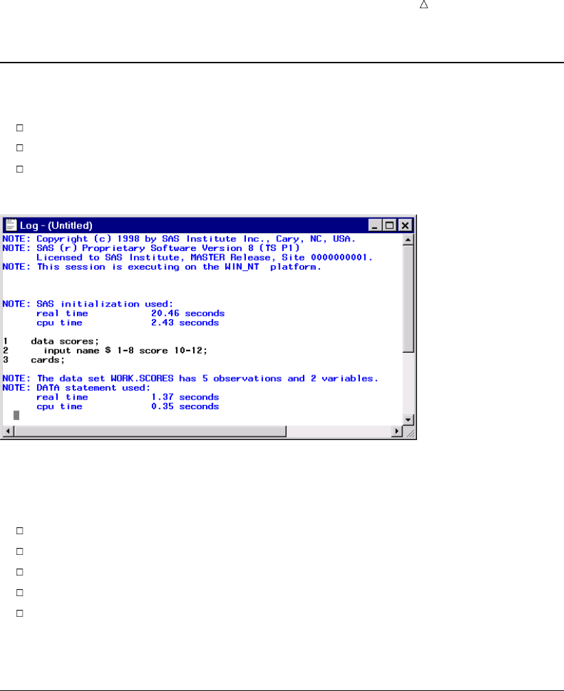
Using the SAS Windowing Environment Using Other Editors 679
Log Window
The Log window enables you to:
recognize when you have made programming errors
understand what is necessary to correct those errors
receive feedback on the steps that you take to correct errors
Display 39.9 The Log Window Showing Information about a SAS Session
The Log window shows the SAS statements that you have submitted as well as
messages from SAS concerning your program. Under most operating environments, the
Log window tells you:
when the program was executed
the release of SAS under which the program was run
details about the computer installation and its site number
the number of observations and variables for a given output data set
the computer resources that each step used
You can use command line commands in the Log window, just as you can in the
Editor and Output windows. For more information, see “ Editor Window” on page 676.
Using Other Editors
NOTEPAD Window
Although the Editor was designed for writing SAS programs, you can also use the
NOTEPAD window to create and edit SAS programs. The NOTEPAD is a text editor
that you can use to create, edit, save, and submit SAS programs. You might find
NOTEPAD useful as a separate place to work on code. To open NOTEPAD, issue the
NOTEPAD or NOTES command.
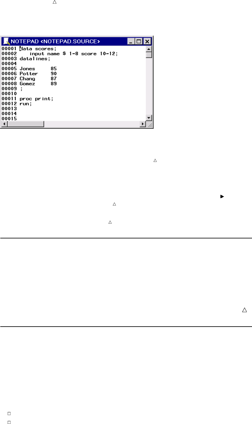
680 Creating and Submitting a Program Chapter 39
Display 39.10 The SAS NOTEPAD Window with Line Numbers Turned On
Note: The SAS NOTEPAD window shown here includes line numbers. You might
find line numbers helpful when you create or edit programs. To toggle line numbers on
or off in NOTEPAD, issue the NUMBERS command.
If you open multiple NOTEPADS, then you can cut, copy, and paste text between
NOTEPAD windows and the Editor window, multiple SAS sessions, and other
applications.
Note: To submit a program from NOTEPAD, you must either select Run Submit
or issue the NOTESUBMIT command.
Note: The program information that is presented in this documentation uses the
Editor windows as the default editor.
Creating and Submitting a Program
To create and submit a SAS program:
1Type the text of your program in the Editor.
2Type submit on the command line, and then press ENTER or RETURN.
You can also use the function key, menu command, or toolbar item that is
assigned to submit programs in your environment.
Note: If you are submitting a program from the SAS NOTEPAD window, then
you must use the NOTESUBMIT command instead of the SUBMIT command.
Storing a Program
To store a program:
1In the Editor window, create or edit a program.
2On the command line, issue the FILE command followed by a fileref or an actual
filename. If you use an actual filename, then enclose it in quotation marks.
The FILE command does not clear the contents of the Editor window. You can store
one copy of a program and then continue working in the Editor window.
If you try to store a program with a fileref or filename that already exists, then SAS
displays a dialog box. The dialog box enables you to choose to
overwrite the contents of the existing file with the new file
append the new file to the existing file
Using the SAS Windowing Environment Editing a Program 681
cancel the FILE command
Often you will want to replace a file with an updated version. To suppress the dialog
box, add the REPLACE option to the FILE command after the fileref or complete
filename. To add the text in the Editor window to the end of an existing file, specify the
APPEND option with the FILE command after the fileref or complete filename.
Note: You can also store a program as a SAS object or as a file that is specific to
your operating environment. After you have created or edited a program, select File
Save As Object or File Save As respectively.
Debugging a Program
You or someone in your organization might be able to help debug a program with the
information that appears in the Log window after a program is submitted. If you are
having problems with your program, save the contents of the Log window to an external
file, if you need to study it after your SAS session has ended.
To save the contents of the Log window to an external file:
1Open the Log window if it is not already open.
2From the command line, execute the FILE command followed by a fileref or an
actual filename. If you use a filename, then enclose the name in quotation marks.
The FILE command stores a copy of the information in the Log window without
removing what is currently displayed. If you specify the name of an existing fileref or
file, then a dialog box appears and offers you three choices: overwriting the contents of
the existing file with the new file, appending the new file to the existing file, or
canceling the command.
Opening a Program
There is more than one way to open a SAS program. Two of the most popular
methods are listed in this section.
To open a SAS program from the Editor window:
1Select:File Open.
2Use the Open window to locate the appropriate SAS program file.
To open a SAS program with commands:
1Open the Editor window if it is not already open.
2On the command line, specify the INCLUDE command followed by an assigned
fileref or an actual filename. Remember to enclose an actual filename in single or
double quotation marks.
By default, a program is appended to the end of any existing program
statements.
Note: If program statements already exist in the Editor, then you can determine
where your program is appended by using the B (before) or A (after) line commands.
For more information about line commands, see Line Commands“Using Line
Commands” on page 662.
If you want to replace the text that is already in the Editor window with the program
that you open, then specify the REPLACE option with the INCLUDE command after
the fileref or filename.
Editing a Program
To edit a program:
682 Assigning a Program to a File Shortcut Chapter 39
1Open an existing program in the Editor window.
2Edit existing program statements or append new statements to the program.
Use command line commands and line commands as needed.
3Store the program.
Assigning a Program to a File Shortcut
You can assign a program to a file shortcut to make it easier to find and work with
the file in the future. For more information about file shortcuts, see “Assigning a File
Shortcut” on page 674.
Working with Output
Overview of Working with Output
You can manage your SAS procedure output with the SAS Output Delivery System
(ODS). Procedures that fully support ODS can do the following:
combine the raw data that they produce with one or more table definitions to
produce one or more output objects that contain formatted results
store a link to each output object in the Results folder in the Results window
can generate various types of file output, such as HTML, Listing, and in some
cases, SAS/Graph output
can generate output data sets from procedure output
provide a way for you to customize the procedure output by creating table
definitions that you can use whenever you run the procedure
The SAS windowing environment enables you to use many features of ODS through
the Results, Templates, Preferences, and SAS Registry Editor windows. The Results
window provides pointers to the procedure output that is produced by SAS. The
Templates window provides a way to manage all the table, column header, and style
definitions (sometimes called templates) that can be associated with procedure output.
Finally, the Preferences window and the SAS Registry Editor can be used to set the
type(s) of procedure output that you want SAS to produce.
This section details only those portions of ODS that are related to the SAS windowing
environment. For more information about ODS, see Chapter 23, “Directing SAS Output
and the SAS Log,” on page 349 and SAS Output Delivery System: User’s Guide.
Setting Output Format
Depending on your operating environment, SAS output can be produced in one or
more formats (or types). Listing output is the default type. Other output types include
HTML, Output Data Sets, and PostScript. Pointers to procedure output appear in the
Results window.
To set your output type, use either the Preferences window (if available in your
operating environment), the SAS Registry Editor, or both.
Setting Output Type with the Preferences Window
If your operating environment supports the Preferences window, you can set output
type as follows:
Using the SAS Windowing Environment Assigning a Default Viewer to a SAS Output Type 683
1Select Tools Options Preferences or issue the DLGPREF command to open
the Preferences window.
2Select the Results tab.
3Select or deselect the check boxes that match the output types that you want to
produce.
If you choose to produce HTML output, then you can further define the output
by selecting:
an HTML style
Click the Style box and highlight a style. Styles among other things,
define output colors and fonts.
the folder to which the output is saved
Select Use WORK folder to save HTML output only for the duration of
the current session. Your output is deleted when your current SAS session
ends.
Enter a path in the Folder text box to save HTML output to a folder
that is not deleted when your SAS session ends.
the View Results as they are Generated check box
If selected, then each time HTML output is produced, your browser
automatically opens and loads the output.
Setting Output Type with the SAS Registry Editor
To set output type with the SAS Registry Editor:
1Select Solutions Accessories Registry Editor or issue the REGEDIT
command to open the SAS Registry Editor.
2From the tree on the left side, expand the ODS folder.
3Expand the Preferences folder.
4Select the appropriate output type.
5On the right side, select the Value key, and then select Modify from the pop-up
menu.
6In the dialog box that appears, edit the Value Data field as needed.
If this field is set to 1, then the output type is produced. If this field is set to 0,
then the output type is not produced.
Assigning a Default Viewer to a SAS Output Type
When you produce output in SAS, output pointers appear in the Results window. You
can assign a default viewer for each of the types of output that you produce. After a
default viewer is assigned, you can double-click an output pointer in the Results
window to open output in its default viewer. For example, double-clicking on a
PostScript output pointer could open Ghostview with your PostScript output loaded.
Operating Environment Information: In the Windows operating environment, default
viewers are established automatically with information from your Windows Registry.
To assign a default viewer to a SAS Output Type:
1From the Explorer window, select Tools Options Explorer.
2Select Host Files from the drop-down menu at the top of the Explorer Options
window.
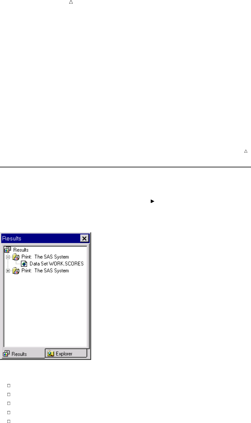
684 Working with Output in the Results Window Chapter 39
3Scroll through the registered file types until you find the file type with which you
want to work.
4Select the appropriate file type, and then select Edit.
5Select Add, and then enter an action name and action command for the file type in
the Edit Action window.
For example, add the following action name and action command to set
Ghostview as the default viewer for PostScript file types:
Action Name &Edit
Action
Command
x ghostview ’%s’ &
6Select OK from the Edit Action window.
7Select the action that you just specified, and then select Set Default.
Operating Environment Information: In the Windows operating environment, default
viewers are established automatically with information from your Windows Registry.
Working with Output in the Results Window
The Results window provides pointers to the procedure or DATA step output that
SAS produces. This window might open by default when you start a SAS session. You
can also open the Results window by selecting View Results or by issuing the
ODSRESULTS command.
Display 39.11 The Results Window in Tree View
You can use the Results window to do the following:
Navigate pointers to output.
Delete results pointers.
Rename results pointers.
Save listing output to other formats.
Quickly view the first output pointer item.
Using the SAS Windowing Environment Working with Output in the Results Window 685
View results properties.
Customizing the Results Window View
You can have the Results window display in one of three views:
Tree
Contents Only
Explorer
In Tree view (the default), only a navigational tree is present. In Contents Only view,
the tree is turned off, and contents appear as folders. In Explorer view, the Results
window appears with two panes: one for the tree and one for the contents.
To toggle the Tree view pane, issue the TREE command from the Results window. To
toggle the Contents pane, issue the CHILD command from the Results window. You can
also select commands from the View menu of the Results window to perform the same
actions, such as Show Tree,Show Contents, and others.
Note: By default, output pointers are listed by label rather than by name in the
Tree pane. Labels are typically more descriptive than output names. You can use the
following SAS system option to change this setting: LABEL.
Using Results Pointers to Navigate Output
When SAS runs a procedure or a DATA step, pointers to the output are placed in the
Results window. To use the pointers in the Results window, see “Navigating the Results
Window in Tree View” on page 685, “Navigating the Results Window in Contents Only
View” on page 686, or “Navigating the Results Window in Explorer View” on page 686.
Navigating the Results Window in Tree View
In Tree view, output pointers appear in a procedural hierarchy. To work with your
SAS output:
1Locate the folder that matches the procedure output that you want to view.
2Use the expansion icons (+ or – icons) next to the folder to open or hide its contents.
You can also:
Double-click a folder to make it expand or collapse.
Select a folder, and then select Open from the pop-up menu.
3When you locate the appropriate pointer, double-click the pointer or select the
pointer and then select Open from the pop-up menu.
The appropriate output appears.
Operating Environment Information: If you are using the z/OS or CMS operating
environment, then you can open a pop-up menu by typing ?in the selection field next
to an item. Alternatively you can type an type ansor xin the selection field next to an
item.
You can also use the following ways to navigate in the Tree view:
Menu View Up One Level
Command UPLEVEL
Toolbar Up One Level icon

686 Working with Output in the Results Window Chapter 39
Key Depending on your operating environment, you might also use arrow
and backspace keys to navigate.
Navigating the Results Window in Contents Only View
In Contents Only view, output pointers appear in a procedural hierarchy, beginning
with the top level of the hierarchy. You can drill down or roll up within the hierarchy to
find the appropriate output.
When you open a folder, the current window contents are replaced with the contents
of the selected folder. To work with your SAS output:
1Locate the folder that matches the procedure output that you want to view.
2Select the folder, and then select Open from the pop-up menu.
You can also double-click a folder to open it.
3When you locate the appropriate pointer, double-click the pointer or select the
pointer, and then select Open from the pop-up menu.
The appropriate output appears.
Operating Environment Information: If you are using the z/OS or CMS operating
environment, then you can open a pop-up menu by typing ?in the selection field next
to an item. Alternatively you can type an type ansor xin the selection field next to an
item.
Navigating the Results Window in Explorer View
In Explorer view, two window panes exist. The left pane includes a hierarchical view
(the Tree view) of the procedure output that you can view. The right pane shows the
contents (the Contents view) of the item that is currently in focus.
Deleting Results Pointers
You can delete results pointers by deleting the procedure folder in which the pointers
exist. When you delete a procedure folder in the Results window, any output pointer
that exists in that folder is removed.
Note: When you delete a procedure folder that contains a listing output pointer, the
actual listing output is removed from the Output window. If other output pointers exist
in the folder (such as HTML), then only the pointer is removed; the actual output
remains available.
To delete procedure output:
1In the Results window, select the procedure folder that matches the procedure that
you want to delete.
2Select Delete from the pop-up menu.
3Select Yes to confirm the deletion.
Tip
You can also delete output pointers by selecting the procedure folder that you want to
delete, and then selecting Edit Delete.
Renaming Results Pointers
To rename results pointers:
1Select the pointer that you want to rename.

Using the SAS Windowing Environment Working with Output Templates 687
2Select Rename from the pop-up menu.
3Type in a new name and/or a description, and then select OK.
Tip
You can also rename results pointers by selecting the pointer that you want to
rename, and then selecting Edit Rename.
Saving Listing Output to Other Formats
To save listing output to a file from the Results window:
1Expand the Results window tree until you find the appropriate listing output
pointer.
2Select the listing output pointer, and then select Save As from the pop-up menu.
To save listing output to a file from the Output window:
1Access the Output window.
2On the command line, specify the FILE command followed by a fileref or an actual
filename. If you use a filename, then surround the filename with quotation marks.
Note: The FILE command stores a copy of the information in the Output window
without removing what is currently displayed.
To save listing output as a catalog object:
1Expand the Results window tree until you find the appropriate listing output item.
2Select the listing output item, and then select Save As Object from the pop-up
menu.
Viewing the First Output Pointer Item
To view the first output pointer item:
1Select the appropriate results pointer.
2Select View from the pop-up menu.
The first output pointer item listed for the results pointer that you selected
appears. For example, if you produced listing and HTML output for a procedure
and the listing output was created first, then the listing output would appear.
Viewing Results Properties
You can view the properties of a Results window folder, an output pointer, or an
output pointer item (such as listing or HTML output).
1In the Results window, select the appropriate folder, output pointer, or output
pointer item.
2Select Properties from the pop-up menu.
Working with Output Templates
Overview of Working with Output Templates
Templates contain descriptive information that enables the Output Delivery System
(ODS) to determine the desired layout of a procedure’s results.
The Templates window provides a way to manage all the templates that are currently
available to SAS. Specifically, you can use the Templates window to do the following:
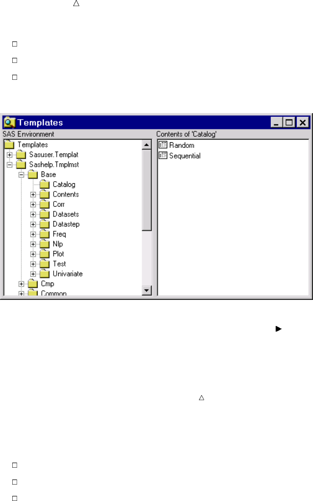
688 Working with Output Templates Chapter 39
Browse PROC TEMPLATE source code.
Edit PROC TEMPLATE source code.
View template properties.
Display 39.12 The Templates Window in Explorer View
You can open the Templates window by selecting View Templates from the Results
window, or by issuing the ODSTEMPLATES command.
You can create or modify templates with PROC TEMPLATE.
Note: Templates that are supplied by SAS are stored in SASHELP. Templates that
are created with PROC TEMPLATE are stored in SASUSER or whatever library that
you specify in the ODS PATH statement.
Customizing the Templates Window View
The Templates window appears in one of three views:
Explorer
Tree
Contents Only
In Explorer view (the default), the Templates window appears with two panes: one
for the tree and one for the contents. In Tree view, only a navigational tree is present.
In Contents Only view, the tree is turned off.
To toggle the Contents pane, issue the CHILD command from the Templates window.
To toggle the Tree pane, issue the TREE command from the Templates window.
For more information, see “Navigating the Templates Window in Explorer View” on
page 688, “Navigating the Templates Window in Tree View” on page 689, or “Navigating
the Templates Window in Contents Only View” on page 689.
Navigating the Templates Window in Explorer View
In Explorer view, two window panes exist. The left pane includes a hierarchical view
(the Tree view) of the templates that you can view. The right pane shows the contents
(the Contents view) of the template currently in focus.
You can open additional template windows from the Explorer view by selecting a
template, and then selecting Explore from Here from the pop-up menu.
Using the SAS Windowing Environment Working with Output Templates 689
Navigating the Templates Window in Tree View
In Tree view, templates appear in a hierarchy. To work with a template:
1Locate the folder that includes the template that you want to view.
2Use the expansion icons (+ or – icons) next to the folder to open or hide its contents.
You can also do the following:
Double-click a folder to make it expand or collapse.
Select a folder, and then select Open from the pop-up menu.
3Double-click the template that you want to see, or select the template, and then
select Open from the pop-up menu.
The template code appears in a browser window.
Operating Environment Information: If you are using the z/OS or CMS operating
environments, then you can open a pop-up menu by typing ?in the selection field next
to an item. Alternatively, you can double-click by typing an sor xin the selection field
next to an item.
Navigating the Templates Window in Contents Only View
In Contents Only view, templates appear as folders. When you open a folder, the
current window contents are replaced with the contents of the selected folder. To work
with your templates in this view:
1Locate the folder that includes the template that you want to view.
2Select the folder, and then select Open from the pop-up menu.
You can also double-click on a folder to open it.
3Double-click on the template that you want to see, or select the template, and then
select Open from the pop-up menu.
The template code appears in a browser window.
Operating Environment Information: If you are using the z/OS or CMS operating
environments, then you can open a pop-up menu by typing ?in the selection field next
to an item. alternatively, you can double-click by typing an sor xin the selection field
next to an item.
Browsing PROC TEMPLATE Source Code
To browse the PROC TEMPLATE source code:
1Locate the appropriate template in the Templates window.
2Select the template, and then select Open from the pop-up menu.
Template code appears in a browser window.
Editing PROC TEMPLATE Source Code
To edit the PROC TEMPLATE source code:
1Locate the appropriate template in the Templates window.
2Select the template, and then select Edit from the pop-up menu. Template code
appears in an editor window.
3Modify the template code as needed.
4Select Run Submit to submit your modified template code.
Note: If syntax errors occur when the code for an edited template is submitted, then
the errors appear in the Log window.
690 Printing Output Chapter 39
Note: Additional information for PROC TEMPLATE is available in the Base SAS
Procedures Guide.
Viewing Template Properties
To view template properties:
1Locate the appropriate template in the Templates window.
2Select the template, and then select Properties from the pop-up menu.
The Properties dialog box lists the type, path, size, description, and modification date
for the template. You can also view this information by selecting View Details when
the Templates window is active.
Printing Output
The method that you use to print output depends on the type of output that you
produce, as well as your operating environment. SAS windowing environment windows
have menus with print options that enable you to print the contents of that particular
window. This feature varies from operating system to operating system, but is available
in all operating environments.
If you produce HTML output, then you can open the output in a Web browser, and
then print the output from the Web browser with the Web browser’s printing command.
For more information about printing, refer to your SAS operating environment
companion documentation and your operating environment documentation.
Review of SAS Tools
Statements
ODS PATH location(s)
specifies which locations to search for definitions that were created by PROC
TEMPLATE, as well as the order in which to search for them.
<libname.>item-store <(READ | UPDATE | WRITE)>
item-store
identifies an item store that contains style definitions, table definitions, or both.
Windows
File Shortcut Assignment
enables you to create or edit file shortcut references. To open this window, issue
the DMFILEASSIGN command.
Find
enables you to search for an expression that exists in a SAS library. To open this
window, select Tools Find from Explorer or issue the EXPFIND command.
Log
enables you to review information about the programs that you have run. To open
this window, select View Log or issue the LOG command.
Using the SAS Windowing Environment Commands 691
Output
enables you to see listing output. To open this window, select View Output or
issue the OUTPUT command.
Editor
enables you to enter, edit, submit, and save SAS program statements. To open this
window, select View Editor or issue the PGM command.
Results
provides pointers to the procedure output that you produce with SAS. To open this
window, select View Results or issue the ODSRESULTS command.
SAS NOTEPAD
enables you to enter, edit, submit, and save SAS program statements. To open this
window, issue the NOTEPAD or NOTES command.
SAS Registry Editor
enables you to edit the SAS Registry and to customize aspects of the SAS
windowing environment. To access this window, issue the REGEDIT command.
Templates
provides a way to manage the output templates that are currently available. To
access this window, select View Templates from within the Results window.
Commands
AUTOEXPAND automatically expands the tree hierarchy when you select a tree
node or when procedure output is produced.
AUTOSYNC enables you to automatically navigate to the first available output in
the Output window by means of a single click.
CHILD toggles the Contents pane on and off.
CLEAR removes all the SAS output pointers.
DELETESELS removes the item currently in focus.
Note: If the output pointer is associated with listing output, then
the listing output is also removed.
DESELECT_ALL deselects any items that are selected while the Contents pane is
viewable.
DETAILS toggles the item details on and off while the Contents pane is
viewable.
DMOPTLOAD recalls system option settings saved by DMOPTSAVE.
DMOPTSAVE saves all system option settings for recall in later SAS sessions
FIND searches for a match to the string that you provide.
LARGEVIEW displays large icons (on some operating environments) while the
Contents pane is viewable.
PMENU turns on menus in windows.
PRINT prints the desired SAS listing output.
REFRESH refreshes the window’s contents.
RENAMESELS enables you to rename the output pointer that currently has focus.
SELECT_ALL selects all items while the Contents pane is viewable.
692 Procedures Chapter 39
SMALLVIEW displays small icons (on some operating environments) in a
horizontal fashion while the Contents pane is viewable.
TREE toggles the Tree view (hierarchical view) on and off.
UPLEVEL moves focus up one level in the hierarchy.
Procedures
Use PROC TEMPLATE to set template information.
Learning More
To learn more about SAS language elements, see
SAS Language Reference: Dictionary.
To learn more about printing and the SAS Output Delivery System, see
SAS Output Delivery System: User’s Guide.
To find examples that will help you get started, see
Getting Started with the SAS System.

693
CHAPTER
40
Customizing the SAS
Environment
Introduction to Customizing the SAS Environment 694
Purpose 694
Prerequisites 694
Operating Environment Differences 694
Customizing Your Current Session 695
Ways to Customize 695
Customizing SAS Sessions and Programs at Startup 695
Setting Invocation-Only Options Automatically 695
Executing SAS Statements Automatically 696
Customizing with SAS System Options 696
Using the OPTIONS Statement and the Options Window 696
Finding Options in the SAS Options Window 697
Setting Options in the SAS Options Window 697
Customizing Session-to-Session Settings 698
Overview of Customizing Session-to-Session Settings 698
Customizing SAS Sessions and Applications with the SAS Registry Editor 698
Understanding the SAS Registry 698
Opening the SAS Registry Editor 699
Finding Information in the SAS Registry Editor 699
Setting Keys in the SAS Registry Editor 699
Setting New Key Values in the SAS Registry Editor 700
Editing Existing Key Values in the SAS Registry Editor 700
Importing Registry Files 700
Exporting Registry Files 700
Uninstalling an Imported Registry File 701
Setting Registry Editor Options 701
Customizing SAS Sessions with the Preferences Window 702
Saving System Option Settings with the DMOPTSAVE and DMOPTLOAD Commands 702
Customizing the SAS Windowing Environment 702
Customizing the Explorer Window 702
Ways to Customize the Explorer Window 702
Selecting Contents Only View or Explorer View 703
Changing How Items Appear in the Contents View 704
Adding and Removing Folders 704
Enabling Member, Entry, and Operating Environment File Types to Appear 705
Adding a Pop-Up Menu Action to a Member, Entry, or Operating Environment File
Type 705
Hiding Member, Entry, and Host File Types 706
Customizing an Editor 706
Customizing Fonts 706
Customizing Colors 706
694 Introduction to Customizing the SAS Environment Chapter 40
Setting SAS Windowing Environment Preferences 706
Review of SAS Tools 707
Commands 707
Procedures 707
Statements 707
System Options 707
Windows 708
Learning More 708
Introduction to Customizing the SAS Environment
Purpose
In this section, you will learn how to make the following types of customizations in
SAS:
those that remain in effect for the current session only
those that remain in effect from session to session
those that you can apply to the SAS windowing environment, which is the default
SAS environment
Prerequisites
To use this section, you should be familiar with the SAS windowing environment.
For more information about the SAS windowing environment, see Chapter 39, “Using
the SAS Windowing Environment,” on page 655.
Operating Environment Differences
Even though SAS has a different appearance for each operating environment, most of
the actions that are available from the menus are the same.
One of the biggest differences between operating environments is the way that you
select menu items. If your workstation is not equipped with a mouse, then here are the
keyboard equivalents to mouse actions:
Mouse action Keyboard equivalent
double-click the item type an sor an xin the space next to the item,
then press the ENTER or RETURN key
right-click the item type ?in the space next to the item, then press
the ENTER or RETURN key
Examples in this documentation show SAS windows as they appear in the Microsoft
Windows environment. For the most part, corresponding windows in other operating
environments will yield similar results. If you do not see the drop-down menus in your
operating environment, then enter the global command PMENU at a command prompt.
Customizing the SAS Environment Customizing SAS Sessions and Programs at Startup 695
Customizing Your Current Session
Ways to Customize
As you become familiar with SAS, you will probably develop preferences for how you
want SAS configured. Many options are available to you to make SAS conform to your
preferred working style. Some of the things that you can change are the following:
window color and font attributes
library and file shortcuts
output appearance
file-handling capabilities
the use of system variables
You can customize your current SAS session in the following ways:
at the startup of a SAS session or program
through SAS system options
with drop-down menu options
Customizing SAS Sessions and Programs at Startup
Setting Invocation-Only Options Automatically
You can specify some system options only when you invoke SAS. These system
options affect the following:
the way SAS interacts with your operating system
the hardware that you are using
the way in which your session or program is configured
Note: There are other system options that you can specify at any time. For more
information, see “Customizing with SAS System Options” on page 696.
Usually, any invocation-only options are set by default when SAS is installed at your
site. However, you can specify invocation-only options on the command line each time
you invoke SAS.
To avoid having to specify options that you use every time you run SAS, set the
options in a configuration file. Each time you invoke SAS, SAS looks for that file and
uses the customized settings it contains. Be sure to examine the default configuration
file before creating your own.
Note: If you specify options both in the configuration file and in the SAS command,
then the options are concatenated. If you specify an option in the SAS command that
also appears in the configuration file, then the setting from the SAS command overrides
the setting in the configuration file.
To display the current settings for all options that are listed in the configuration file
and on your command line as you invoke the system, use the VERBOSE system option
in the SAS command.
696 Customizing with SAS System Options Chapter 40
Executing SAS Statements Automatically
Just as you can set SAS system options automatically when you invoke SAS, you can
also execute statements automatically when you invoke SAS by creating a special
autoexec file. Each time you invoke SAS, it looks for this special file and executes any
of the statements it contains.
You can save time by using this file to execute statements that you use routinely. For
example, you might add the following statements:
OPTIONS statements that include system options that you use regularly
FILENAME and LIBNAME statements to define the file shortcuts and libraries
that you use regularly
Operating Environment Information: In order to execute SAS statements
automatically in the CMS operating environment, you must have a file shortcut defined
as SASEXEC.
Customizing with SAS System Options
Using the OPTIONS Statement and the Options Window
SAS system options determine global SAS settings. For example, the global options
can affect the following:
how your SAS output appears
how files are handled by SAS
how observations from SAS data sets are processed
how system variables are used
The previous section discusses some invocation-only options that must be set at
startup. However, there are many system options that can be set at any time. These
system options can be set in an OPTIONS statement as well as in the SAS Options
window.
It is important to note that system option settings remain in effect until you change
them again, or until your current session ends.
There are several ways to view your system option settings. The two most common
methods are the following:
the SAS Options window (type OPTIONS at a command line)
the OPTIONS procedure
To obtain a complete list of system option settings using the OPTIONS procedure,
submit the following statements:
proc options;
run;
The SAS Options window groups options by function. The left side of the window
includes a tree that lists the available option groups. You can expand option groups to
see subgroups.
Operating Environment Information: Mainframe users can expand groups and
subgroups by using the mouse or by typing an Sor an Xbefore the group or subgroup
name. When you select a subgroup, the individual options of that subgroup appear on
the right side of the window.
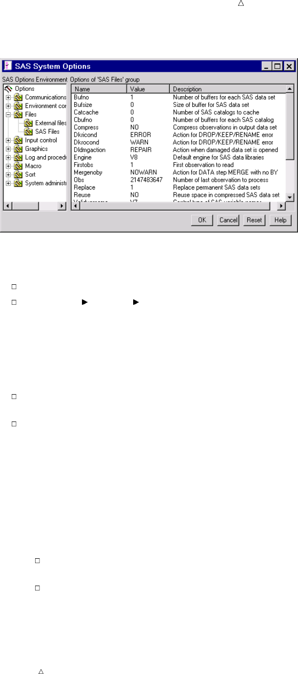
Customizing the SAS Environment Customizing with SAS System Options 697
Display 40.1 SAS Options Window
To open the SAS Options window, do one of the following tasks:
Issue the OPTIONS command.
Select Tools Options System.
The options in each group or subgroup are listed alphabetically, followed by options
that are specific to your operating environment (which are also listed alphabetically).
Finding Options in the SAS Options Window
You can find options in a number of ways.
Expand the option groups and subgroups on the left side of the window until the
appropriate option appears on the right side of the window.
Select an option group or subgroup, then select Find Option from the pop-up
menu. In the Find Option window, enter the name of the option that you want to
locate, and then select OK.
Setting Options in the SAS Options Window
1In the SAS Options window, find the option that you want to set.
2Select the option from the right side of the SAS Options window.
3Select Modify Value or Set to Default from the pop-up menu. Mainframe
users can type an Sor an Xbefore the option name to access the pop-up menu.
If you choose Modify Value, then a dialog box appears that enables you to
edit the option value.
If you choose Set to Default, then the option value is reset to the default
SAS System value.
4Select OK to save your changes. Select Reset to return all edited options to their
previous values.
Note: If all the items on the pop-up menu are grayed out (that is, unavailable), then
the options are invocation-only options and can be set only when a SAS session is
started.
698 Customizing Session-to-Session Settings Chapter 40
Customizing Session-to-Session Settings
Overview of Customizing Session-to-Session Settings
The previous section discusses making customizations that stay in effect for the
duration of the current SAS session only. This section provides information about
making customizations that remain from SAS session to SAS session.
You can make customizations that remain from session to session by using one of the
following windows:
SAS Registry Editor
Preferences window
Options window
Customizing SAS Sessions and Applications with the SAS Registry
Editor
Understanding the SAS Registry
The SAS Registry stores information about specific SAS sessions and applications.
Unlike system options, customizations to the SAS Registry remain in effect for more
than one SAS session. You can make SAS Registry customizations by using either
PROC REGISTRY or the SAS Registry Editor.
This section shows you how to use the SAS Registry Editor, which is a graphical
alternative to PROC REGISTRY. For more information about PROC REGISTRY, see the
Base SAS Procedures Guide.
CAUTION:
Changes to SAS Registry should be well planned. In many cases, it is appropriate to have
a designated person in charge of SAS Registry edits. Inappropriate SAS Registry edits can
adversely affect your SAS session performance.
SAS Registry Editor values, which store data, exist in keys and subkeys. Keys and
subkeys, which look like folders, appear in a tree on the left side of the SAS Registry
Editor. If a key has subkeys, then you can expand or collapse it with the + and – icons
that are found in the tree. If a key or subkey has values, then the values appear on the
right side of the window.
Operating Environment Information: In the z/OS and CMS operating environments,
you can select a + or – icon by positioning your cursor on it and then pressing the
ENTER key.
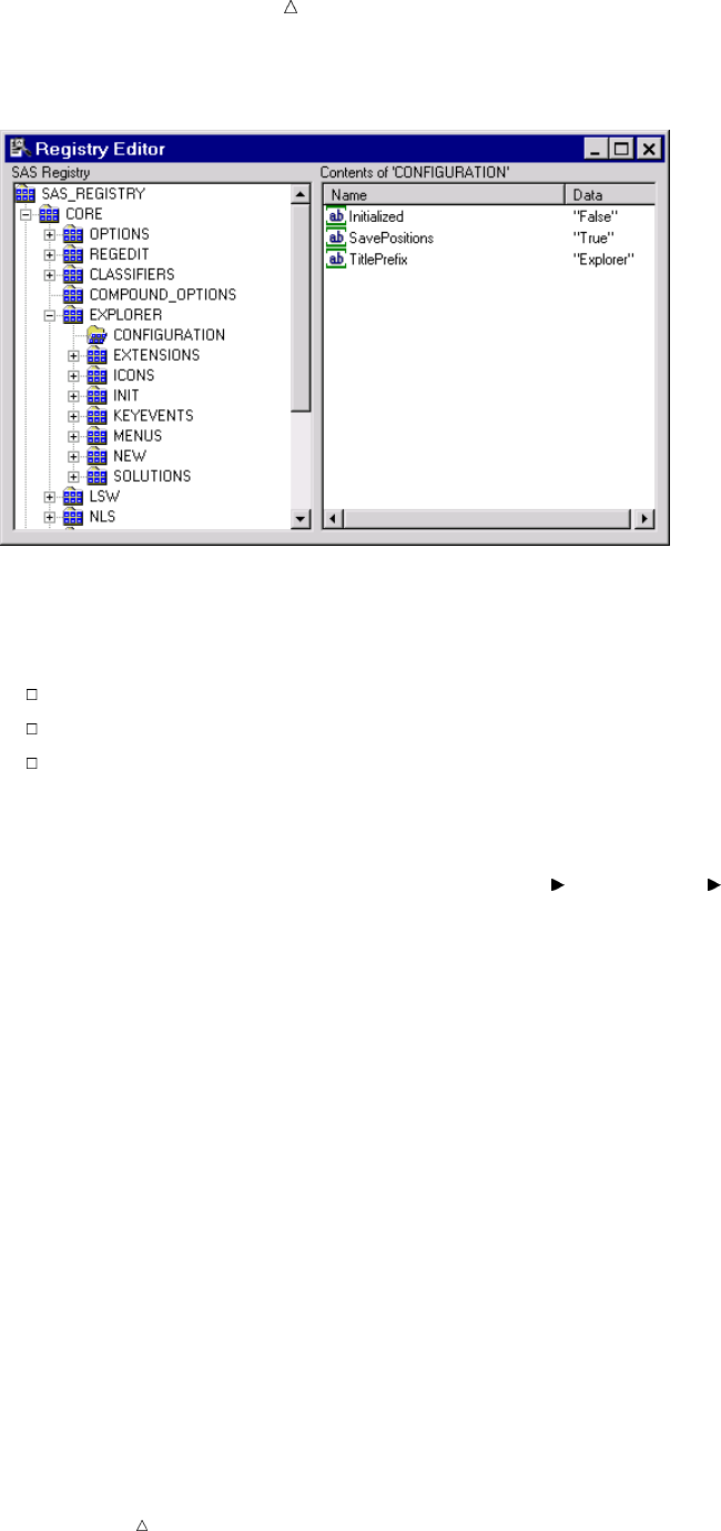
Customizing the SAS Environment Customizing SAS Sessions and Applications with the SAS Registry Editor 699
Display 40.2 The SAS Registry Editor
To customize SAS sessions and applications, use the SAS Registry Editor to add,
modify, rename, and delete keys and key values.
You can also use the SAS Registry Editor to the following:
import registry files (starting at any key)
export the contents of the registry (starting at any key)
unregister a registry file
Opening the SAS Registry Editor
To open the SAS Registry Editor, select Solutions Accessories Registry Editor,
or issue the REGEDIT command.
Finding Information in the SAS Registry Editor
You can search for specific information in the SAS Registry Editor, including specific
keys, key value names, and key value data:
1Select the key from which you want to start a search.
2Open the drop-down menu and select Find.
3In the Registry Editor Find window, type your search string in the Find What field.
4Check one or more of the Keys,Value Name,orValue Data check boxes,
depending on where you want to perform your search.
5Select Find to begin the search.
Setting Keys in the SAS Registry Editor
You can add, modify, rename, or delete keys in the SAS Registry Editor. For example,
you might want SAS to be able to work with a new paper type when printing output.
Therefore, you might need to create a new key that represents the paper type.
Additionally, you would have to create and set key values for this new paper type. For
more information, see “Setting New Key Values in the SAS Registry Editor” on page 700.
Note: When you add a key, the new key becomes a subkey of the most recently
selected key.

700 Customizing SAS Sessions and Applications with the SAS Registry Editor Chapter 40
To set a key in the SAS Registry Editor:
1Expand or collapse the keys on the left side of the SAS Registry Editor (using the
+ and – icons) until you find the appropriate key.
2With a key selected, select an action from the drop-down menu (such as New Key,
Rename,orDelete). A dialog box appears that enables you to enter additional
information or confirm an action.
CAUTION:
Delete removes all subkeys and values (if any) under the key that you are deleting.
Setting New Key Values in the SAS Registry Editor
If you create a new key, then you might want to add values to that key. Adding
values includes assigning a value name as well as the value data.
Note: If your new key is similar to an existing key, then you might want to review
that key’s subkeys and key values. The review process might help you determine which
subkeys and key values you should have for the new key.
To add a new key value, do the following:
1Select the new key on the left side of the SAS Registry Editor.
2Select an action from the pop-up menu (such as New String Value,New Binary
Value,orNew Double Value).
3in the dialog box, enter a name and a value for the new key value
4select OK to complete the process
Editing Existing Key Values in the SAS Registry Editor
1Select a key on the left side of the SAS Registry Editor.
2If the key contains subkeys, then continue to expand the key by selecting the +
icon.
3Select the key value that you want to edit on the right side of the SAS Registry
Editor.
4Select the appropriate action from the pop-up menu (such as Modify,Rename,or
Delete). A dialog box appears that enables you to enter additional information or
confirm an action.
Importing Registry Files
You can import a registry file to populate and modify the SAS Registry quickly.
Registry files are text files that you create with a text editor. For information about
registry file syntax, see PROC REGISTRY in the Base SAS Procedures Guide.
1Select File Import Registry File.
2Select the file that you want to import, and then select OK.
If errors occur during the import, then a message appears in the status bar and the
errors are reported in the Log window. All registry changes can be sent to the log if you
use the SAS Registry Editor option Output full status to Log. For more
information, see “Setting Registry Editor Options” on page 701.
Exporting Registry Files
You can export (or copy) all or a portion of the SAS Registry to a file:
Customizing the SAS Environment Customizing SAS Sessions and Applications with the SAS Registry Editor 701
1Select the key in the existing registry from where you want to begin exporting the
file. Selecting a root key exports the entire tree, beginning at the root key that you
select.
2Select File Export Registry File.
3Enter the full path to the file or browse to select the file to which you want to save
the existing registry, and then select OK.
If errors occur during the export, then a message appears in the status bar and the
errors are reported in the Log window. All registry changes can be sent to the log if you
use the Output full status to Log SAS Registry Editor option.
Uninstalling an Imported Registry File
The uninstall function reads an imported registry file and removes the keys found in
the file from the registry. If any errors occur during this process, then a message
appears in the status bar and errors are reported in the Log window.
Note: SAS ships with a set of ROOT keys. Root keys are not removed during an
uninstall process.
1Select File Uninstall Registry File.
2Select the external registry file that you want to uninstall from the SAS Registry,
and then select OK. A message appears in the message line when the uninstall is
complete.
Setting Registry Editor Options
1Open the SAS Registry Editor if it is not already open.
2From the Registry Editor window, select Tools Options Registry Editor.
3In the Select Registry View group box, choose a view for the Registry Editor.
View Overlay mode enables you to modify data anywhere in the registry. The
HKEY_USER_ROOT overlays the HKEY_SYSTEM_ROOT. The parent root for
overlay view mode is shown as SAS REGISTRY.
In View All mode, the Registry Editor shows all the entries that are contained
in the two main entry points into the registry: HKEY_SYSTEM_ROOT and
HKEY_USER_ROOT. Typically, the HKEY_SYSTEM_ROOT tree is stored in
the SASHELP library and the HKEY_USER_ROOT is stored in the SASUSER
library.
4Select or deselect appropriate check boxes:
Open
HKEY_SYSTEM
_ROOT for write
access
enables you to open the registry for write access if you have
write access to SASHELP.
Output full
status to Log
writes to the log all changes that were made when the registry
file was imported or uninstalled. Usually, only errors appear in
the Log window.
View unsigned
integers in
hexadecimal
format
enables you to view unsigned integers in the value list in HEX
or DECIMAL format.
You can select Reset all options to return all Registry Editor Options window
settings to the default values.
702 Customizing SAS Sessions with the Preferences Window Chapter 40
Customizing SAS Sessions with the Preferences Window
The Preferences window includes a series of tabs that you can access to set SAS
preferences. Preferences enable you to customize and control your SAS environment.
For example, you might use the General tab to select a startup logo, or the Results
tab to control your output preferences, or even the Editing tab to set editor
preferences, if, for example, your cursor inserts or overtypes text in an editor.
Preference window settings remain in effect from one SAS session to the next.
To access the Preferences window, select Tools Options Preferences or issue the
DLGPREF command.
Operating Environment Information: The Preferences window is unavailable in some
operating environments. Additionally, some preference settings are specific to your
operating environment. Refer to the SAS documentation for your operating
environment for more information about setting preferences.
Saving System Option Settings with the DMOPTSAVE and DMOPTLOAD
Commands
Perhaps the easiest way to save your system option settings from one SAS session to
another is to use the global commands DMOPTSAVE and DMOPTLOAD. After you set
up your system options in a way that best suits your working style, type DMOPTSAVE at
the command line and press ENTER. This saves the current system option settings for
later use. Later, when you have started another SAS session and would like to retrieve
your saved settings, type DMOPTLOAD at the command line and press ENTER. This
changes your system option settings back to the system option settings in effect when
you issued the DMOPTSAVE command.
The DMOPTSAVE and DMOPTLOAD commands have other useful features:
You can issue parameters to name different sets of system option settings and
control where they are saved.
You can view the saved system option settings by using SAS Explorer, because
they are saved by default as a data set.
You can also issue parameters to save the system option settings to a registry key.
When you issue a DMOPTSAVE command without parameters, SAS saves a data set
(myopts) that contains the system option settings to the default library. The default
library is usually the library where the current user profile is. In most cases, this is the
SASUSER library.
See SAS online Help for more details about using these commands.
Customizing the SAS Windowing Environment
Customizing the Explorer Window
Ways to Customize the Explorer Window
You can customize the Explorer window in these ways:
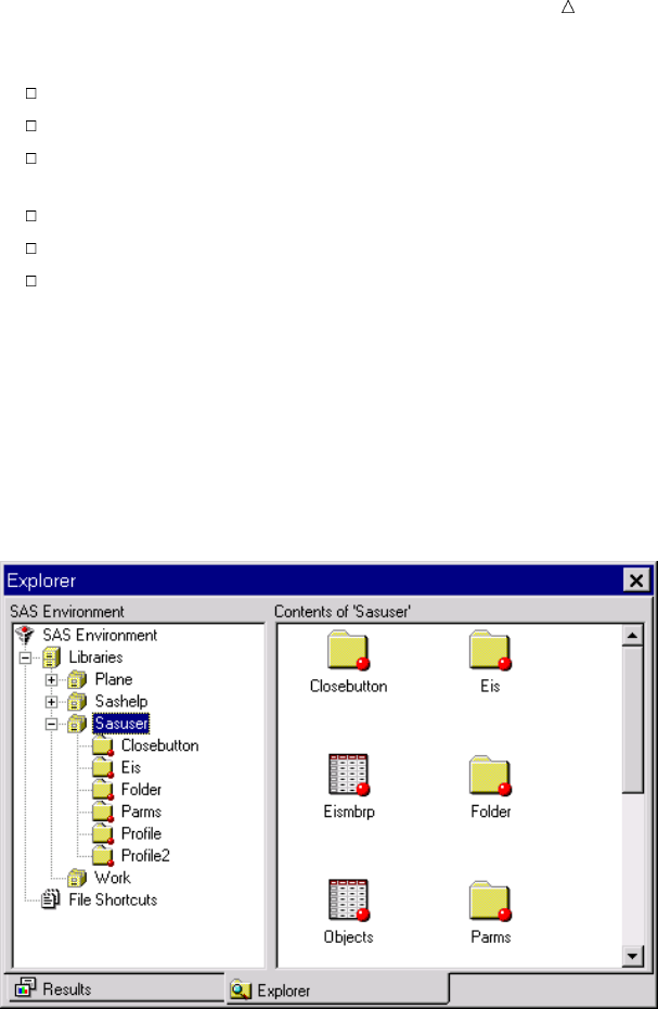
Customizing the SAS Environment Customizing the Explorer Window 703
Select Contents Only view or Explorer view.
Change how items appear in the contents view.
Add and remove folders (including one that adds access to files in your operating
environment).
Enable member, entry, and operating environment file types to appear.
Add a pop-up menu action.
Hide member, entry, and operating environment file types.
Selecting Contents Only View or Explorer View
The Explorer window can appear in either Explorer view or Contents Only view.In
Explorer view, the Explorer window includes two sides: a tree view on the left that lists
folders, and a contents view on the right that shows the contents of the folder that is
selected in the tree view.
Display 40.3 The Explorer Window with Explorer View Enabled
In Contents Only view, the Explorer window is a single-paned window that shows the
contents of your SAS environment. As you open folders, the folder contents replace the
previous contents in the same window. In Contents Only view, you navigate the
Explorer window using pull-down and pop-up menu actions, and toolbar items (if a
toolbar is available).
704 Customizing the Explorer Window Chapter 40
Display 40.4 The Explorer Window with Contents Only View Enabled
Operating Environment Information: In most operating environments, the Explorer
appears in Contents Only view by default.
Depending on your operating environment, you can toggle between the two views in
these ways:
Menu: View Show Tree
Command: TREE
Toolbar Toggle the Tree tool button
Changing How Items Appear in the Contents View
You can make selections from the View menu to determine how files appear in the
Contents view of the Explorer window. All possible selections follow, although not all
the selections may be available in your operating environment:
Large Icons displays a large icon for each file.
Small Icons displays a small icon for each file (only available on PC hosts).
List displays a left-justified list of files.
Details lists files along with columns of descriptive information (such as file
size, type, and so on).
You might also be able to use the following commands in your operating environment
instead of making selections from the View menu:
DETAILS lists files along with columns of descriptive information (such as file
size, type, and so on).
LARGEVIEW displays a large icon for each file.
SMALLVIEW depending on your operating environment, this command displays
either a list of files or a small icon for each file.
Adding and Removing Folders
The Explorer window shows the Libraries and File Shortcuts folders by default in
many operating environments. You can turn off these folders, or turn on other folders,
including Extensions, My Favorite Folders, and Results.

Customizing the SAS Environment Customizing the Explorer Window 705
1From the Explorer window, select Tools Options Explorer.
2From the drop-down list at the top of the window, select Initialization.
3Select the folder that you want to add or remove, and then select Add or Remove.
The Description field changes to On or Off to reflect your change.
Operating Environment Information: The My Favorite Folders window enables you to
access operating environment-specific files from the Explorer. This feature is not
available in CMS and z/OS operating environments.
Enabling Member, Entry, and Operating Environment File Types to Appear
Commonly used members, catalog entries, and operating environment files are
registered and appear in the Explorer window. Registered types must have at least an
icon defined and might also have pop-up menu actions defined. Undefined types do not
appear in the Explorer window and have no actions associated with them.
To add (register) an undefined type:
1From the Explorer window, select Tools Options Explorer.
2From the drop-down list at the top of the window, select a category (such as
Members, Catalog Entries, or Host Files). The registered types are displayed in
the window.
3Select the View Undefined Types check box to see the undefined types for the
category.
4Select a type and then select Edit.
5Select Select Icon.
6In the Select Icon dialog box, choose a category from the drop-down list at the top,
select an icon, and then select OK to close the dialog box.
7Add actions for the type (if desired) and then select OK. For more information
about adding actions to a type, see “Adding a Pop-Up Menu Action to a Member,
Entry, or Operating Environment File Type” on page 705. The type is added to the
Registered Types list.
Adding a Pop-Up Menu Action to a Member, Entry, or Operating
Environment File Type
You can add a pop-up menu action to any catalog entry, member, or operating
environment file type.
1From the Explorer window, select Tools Options Explorer.
2From the drop-down list at the top of the window, select a category (such as
Members, Catalog Entries, or Host Files). The registered types are displayed in
the window.
3Select the registered type that you want to edit.
4Select Edit.
5In the Options dialog box for that entry, select Add.
6Enter a name for the action (this is the action that will appear on the pop-up
menu for the item), and an action command. To see examples of action commands,
look at the commands for registered types.
7Select OK.
Note: The letter immediately after the ampersand (&) in the Action section denotes
the shortcut key that can be used to perform that action.
706 Customizing an Editor Chapter 40
Hiding Member, Entry, and Host File Types
You can hide members, catalog entries, and host files so that they do not appear in
the Explorer window:
1From the Explorer window, select Tools Options Explorer.
2From the drop-down list at the top of the window, select a category (such as
Members, Catalog Entries, or Host Files). The registered types are displayed in
the window.
3Select the registered type that you want to remove from view.
4Select Remove. Confirm the removal by selecting OK when prompted.
When you remove a registered type, it is moved to the View Undefined Types view.
To add the registered type back, you must redefine its icon.
Customizing an Editor
You can customize general and text editing options for your editor. For example, if
you use line commands when you edit programs, then you might always want the
Program Editor to appear with line numbers.
To customize your editor, do the following:
1Select a SAS programming window (such as the Program Editor, Log, Output, or
SAS Notepad window).
2Select Tools Options Editor.
3From the drop-down list, select the category of options that you want to edit.
4In the Options group box, select an option, and then select Modify from the pop-up
menu.
5In the dialog box that appears, edit the option name, value, or both.
Customizing Fonts
You can set default font information for the SAS windowing environment with the
Font window. To access the Font window, issue the DLGFONT command, or select
Tools Options Fonts.
The Font window is host-specific. Refer to your host documentation for more
information.
Customizing Colors
Note: Changes made with the SASColor window are visible only after affected SAS
windows are closed and then reopened.
You can also change the default colors in edit windows, such as the Notepad and the
Program Editor by using the SYNCONFIG command. This command controls the color
of SAS language and programming elements, which makes it easier to parse through a
SAS program and understand how it works. SYNCONFIG opens the Edit Scheme
window, which gives you several different color schemes to select. You can also modify
the provided color schemes.
Setting SAS Windowing Environment Preferences
You can use the Preferences window to customize portions of the SAS windowing
environment to your liking. For more information, see “Customizing SAS Sessions with
the Preferences Window” on page 702.

Customizing the SAS Environment System Options 707
Review of SAS Tools
Commands
DLGFONT
opens the Font window, which is used to control the fonts in the SAS windowing
environment.
DLGPREF
opens the Preferences window, in some operating environments.
OPTIONS
opens the SAS System Options window.
PMENU
turns on the menu bar in the windowing environment.
REGEDIT
opens the Registry Editor window.
SASCOLOR
opens the SASCOLOR window, which is used to change the color of window
elements, such as backgrounds and borders.
SYNCONFIG
opens the Edit Scheme window, which is used to edit color schemes in the Editor,
NOTEPAD, or Program Editor windows.
Procedures
PROC OPTIONS < SHORT|LONG>;
lists the current values of all SAS system options. The SHORT and LONG options
determine the format in which you want SAS system options listed.
Note: You can also use the SAS Options window to see the current values of all
SAS system options.
PROC REGISTRY <options>;
maintains the SAS Registry.
Note: You can also use the SAS Registry Editor to maintain the SAS Registry.
Statements
OPTIONS option-1<... option-n>;
changes the value of one or more SAS system options.
System Options
VERBOSE|NOVERBOSE

708 Windows Chapter 40
controls whether SAS writes the settings of all the system options that are
specified in the configuration file to either the workstation or batch log.
Windows
Editor Options window
enables you to set options for specific SAS windowing environment windows, such
as the Program Editor. To open the Editor Options window, go to the window that
you want to change, and then select Tools Options Editor or issue the
EDOPT command.
Explorer Options window
enables you to set Explorer window options. To open this window, select Tools
Options Explorer Options or issue the EXPOPTS command.
Fonts window
enables you to select the default font that you want to use in the SAS windowing
environment. To access this window, issue the DLGFONT command.
Note: This window is specific to your operating environment.
Preferences window
enables you to set SAS system preferences. To access this window, issue the
DLGPREF command.
Note: This window is specific to your operating environment.
SASColor window
enables you to change the default colors for the different window elements in your
SAS windows. To access this window, issue the SASCOLOR command.
SAS Registry Editor
enables you to edit the SAS Registry and to customize aspects of the SAS
windowing environment. To access this window, issue the REGEDIT command.
SAS System Options window
enables you to view or change current SAS system options. To access this window,
issue the OPTIONS command.
Learning More
For information about operating environment-specific customization options and
preferences, refer to the SAS documentation for your operating environment.
For more information about SAS procedures, see the Base SAS Procedures Guide.
For more information about the statements and options that are discussed in this
section, see SAS Language Reference: Dictionary.
For more tips and examples on using the SAS windowing environment, see Getting
Started with the SAS System.

709
PART
11
Appendix
Appendix 1.........
Additional Data Sets 711
710

711
APPENDIX
1
Additional Data Sets
Introduction 711
Data Set CITY 712
DATA Step to Create the Data Set CITY 712
Raw Data Used for “Understanding Your SAS Session” Section 713
Raw Data for OUT.SAT_SCORES3, OUT.SAT_SCORES4, OUT.SAT_SCORES5, OUT.ERROR1,
OUT.ERROR2, OUT.ERROR3 713
Data Set SAT_SCORES 714
DATA Step to Create the Data Set SAT_SCORES 714
Data Set YEAR_SALES 715
DATA Step to Create the Data Set YEAR_SALES 715
Data Set HIGHLOW 716
DATA Step to Create the Data Set HIGHLOW 716
Data Set GRADES 717
DATA Step to Create the Data Set GRADES 717
Data Sets for “Storing and Managing Data in SAS Files” Section 718
DATA Step to Create the Data Set USCLIM.HIGHTEMP 718
DATA Step to Create the Data Set USCLIM.HURRICANE 719
DATA Step to Create the Data Set USCLIM.LOWTEMP 719
DATA Step to Create the Data Set USCLIM.TEMPCHNG 719
Note on Catalogs USCLIM.BASETEMP and USCLIM.REPORT 720
DATA Step to Create the Data Set CLIMATE.HIGHTEMP 720
DATA Step to Create the Data Set CLIMATE.LOWTEMP 720
DATA Step to Create the Data Set PRECIP.RAIN 720
DATA Step to Create the Data Set PRECIP.SNOW 721
DATA Step to Create the Data Set STORM.TORNADO 721
Introduction
This documentation shows how to create the data sets that are used in each section.
However, when the input data are lengthy or the actual contents of the data set are not
crucial to the section, the DATA steps or raw data to create data sets are listed in this
appendix instead of within the section.
Only the raw data, or DATA steps that are not provided in detail in the section, are
included here.

712 Data Set CITY Appendix 1
Data Set CITY
DATA Step to Create the Data Set CITY
data city;
input Year 4. @7 ServicesPolice comma6.
@15 ServicesFire comma6. @22 ServicesWater_Sewer comma6.
@30 AdminLabor comma6. @39 AdminSupplies comma6.
@45 AdminUtilities comma6.;
ServicesTotal=ServicesPolice+ServicesFire+ServicesWater_Sewer;
AdminTotal=AdminLabor+AdminSupplies+AdminUtilities;
Total=ServicesTotal+AdminTotal;
label Total=’Total Outlays’
ServicesTotal=’Services: Total’
ServicesPolice=’Services: Police’
ServicesFire=’Services: Fire’
ServicesWater_Sewer=’Services: Water & Sewer’
AdminTotal=’Administration: Total’
AdminLabor=’Administration: Labor’
AdminSupplies=’Administration: Supplies’
AdminUtilities=’Administration: Utilities’ ;
datalines;
1980 2,819 1,120 422 391 63 98
1981 2,477 1,160 500 172 47 70
1982 2,028 1,061 510 269 29 79
1983 2,754 893 540 227 21 67
1984 2,195 963 541 214 21 59
1985 1,877 926 535 198 16 80
1986 1,727 1,111 535 213 27 70
1987 1,532 1,220 519 195 11 69
1988 1,448 1,156 577 225 12 58
1989 1,500 1,076 606 235 19 62
1990 1,934 969 646 266 11 63
1991 2,195 1,002 643 256 24 55
1992 2,204 964 692 256 28 70
1993 2,175 1,144 735 241 19 83
1994 2,556 1,341 813 238 25 97
1995 2,026 1,380 868 226 24 97
1996 2,526 1,454 946 317 13 89
1997 2,027 1,486 1,043 226 . 82
1998 2,037 1,667 1,152 244 20 88
1999 2,852 1,834 1,318 270 23 74
2000 2,787 1,701 1,317 307 26 66
;

Additional Data Sets Raw Data for OUT.SAT_SCORES3, OUT.SAT_SCORES4, OUT.SAT_SCORES5, OUT.ERROR1, OUT.ERROR2,
OUT.ERROR3 713
Raw Data Used for “Understanding Your SAS Session” Section
Raw Data for OUT.SAT_SCORES3, OUT.SAT_SCORES4,
OUT.SAT_SCORES5, OUT.ERROR1, OUT.ERROR2, OUT.ERROR3
Verbal m 1972 531 Verbal f 1972 529
Verbal m 1973 523 Verbal f 1973 521
Verbal m 1974 524 Verbal f 1974 520
Verbal m 1975 515 Verbal f 1975 509
Verbal m 1976 511 Verbal f 1976 508
Verbal m 1977 509 Verbal f 1977 505
Verbal m 1978 511 Verbal f 1978 503
Verbal m 1979 509 Verbal f 1979 501
Verbal m 1980 506 Verbal f 1980 498
Verbal m 1981 508 Verbal f 1981 496
Verbal m 1982 509 Verbal f 1982 499
Verbal m 1983 508 Verbal f 1983 498
Verbal m 1984 511 Verbal f 1984 498
Verbal m 1985 514 Verbal f 1985 503
Verbal m 1986 515 Verbal f 1986 504
Verbal m 1987 512 Verbal f 1987 502
Verbal m 1988 512 Verbal f 1988 499
Verbal m 1989 510 Verbal f 1989 498
Verbal m 1990 505 Verbal f 1990 496
Verbal m 1991 503 Verbal f 1991 495
Verbal m 1992 504 Verbal f 1992 496
Verbal m 1993 504 Verbal f 1993 497
Verbal m 1994 501 Verbal f 1994 497
Verbal m 1995 505 Verbal f 1995 502
Verbal m 1996 507 Verbal f 1996 503
Verbal m 1997 507 Verbal f 1997 503
Verbal m 1998 509 Verbal f 1998 502
Math m 1972 527 Math f 1972 489
Math m 1973 525 Math f 1973 489
Math m 1974 524 Math f 1974 488
Math m 1975 518 Math f 1975 479
Math m 1976 520 Math f 1976 475
Math m 1977 520 Math f 1977 474
Math m 1978 517 Math f 1978 474
Math m 1979 516 Math f 1979 473
Math m 1980 515 Math f 1980 473
Math m 1981 516 Math f 1981 473
Math m 1982 516 Math f 1982 473
Math m 1983 516 Math f 1983 474
Math m 1984 518 Math f 1984 478
Math m 1985 522 Math f 1985 480
Math m 1986 523 Math f 1986 479
Math m 1987 523 Math f 1987 481
Math m 1988 521 Math f 1988 483
Math m 1989 523 Math f 1989 482
Math m 1990 521 Math f 1990 483
714 Data Set SAT_SCORES Appendix 1
Math m 1991 520 Math f 1991 482
Math m 1992 521 Math f 1992 484
Math m 1993 524 Math f 1993 484
Math m 1994 523 Math f 1994 487
Math m 1995 525 Math f 1995 490
Math m 1996 527 Math f 1996 492
Math m 1997 530 Math f 1997 494
Math m 1998 531 Math f 1998 496
Data Set SAT_SCORES
DATA Step to Create the Data Set SAT_SCORES
data sat_scores;
input Test $ Gender $ Year SATscore @@;
datalines;
Verbal m 1972 531 Verbal f 1972 529
Verbal m 1973 523 Verbal f 1973 521
Verbal m 1974 524 Verbal f 1974 520
Verbal m 1975 515 Verbal f 1975 509
Verbal m 1976 511 Verbal f 1976 508
Verbal m 1977 509 Verbal f 1977 505
Verbal m 1978 511 Verbal f 1978 503
Verbal m 1979 509 Verbal f 1979 501
Verbal m 1980 506 Verbal f 1980 498
Verbal m 1981 508 Verbal f 1981 496
Verbal m 1982 509 Verbal f 1982 499
Verbal m 1983 508 Verbal f 1983 498
Verbal m 1984 511 Verbal f 1984 498
Verbal m 1985 514 Verbal f 1985 503
Verbal m 1986 515 Verbal f 1986 504
Verbal m 1987 512 Verbal f 1987 502
Verbal m 1988 512 Verbal f 1988 499
Verbal m 1989 510 Verbal f 1989 498
Verbal m 1990 505 Verbal f 1990 496
Verbal m 1991 503 Verbal f 1991 495
Verbal m 1992 504 Verbal f 1992 496
Verbal m 1993 504 Verbal f 1993 497
Verbal m 1994 501 Verbal f 1994 497
Verbal m 1995 505 Verbal f 1995 502
Verbal m 1996 507 Verbal f 1996 503
Verbal m 1997 507 Verbal f 1997 503
Verbal m 1998 509 Verbal f 1998 502
Math m 1972 527 Math f 1972 489
Math m 1973 525 Math f 1973 489
Math m 1974 524 Math f 1974 488
Math m 1975 518 Math f 1975 479
Math m 1976 520 Math f 1976 475
Math m 1977 520 Math f 1977 474
Math m 1978 517 Math f 1978 474
Additional Data Sets DATA Step to Create the Data Set YEAR_SALES 715
Math m 1979 516 Math f 1979 473
Math m 1980 515 Math f 1980 473
Math m 1981 516 Math f 1981 473
Math m 1982 516 Math f 1982 473
Math m 1983 516 Math f 1983 474
Math m 1984 518 Math f 1984 478
Math m 1985 522 Math f 1985 480
Math m 1986 523 Math f 1986 479
Math m 1987 523 Math f 1987 481
Math m 1988 521 Math f 1988 483
Math m 1989 523 Math f 1989 482
Math m 1990 521 Math f 1990 483
Math m 1991 520 Math f 1991 482
Math m 1992 521 Math f 1992 484
Math m 1993 524 Math f 1993 484
Math m 1994 523 Math f 1994 487
Math m 1995 525 Math f 1995 490
Math m 1996 527 Math f 1996 492
Math m 1997 530 Math f 1997 494
Math m 1998 531 Math f 1998 496
;
Data Set YEAR_SALES
DATA Step to Create the Data Set YEAR_SALES
data year_sales;
input Month $ Quarter $ SalesRep $14. Type $ Units Price @@;
AmountSold=Units*price;
datalines;
01 1 Hollingsworth Deluxe 260 49.50 01 1 Garcia Standard 41 30.97
01 1 Hollingsworth Standard 330 30.97 01 1 Jensen Standard 110 30.97
01 1 Garcia Deluxe 715 49.50 01 1 Jensen Standard 675 30.97
02 1 Garcia Standard 2045 30.97 02 1 Garcia Deluxe 10 49.50
02 1 Garcia Standard 40 30.97 02 1 Hollingsworth Standard 1030 30.97
02 1 Jensen Standard 153 30.97 02 1 Garcia Standard 98 30.97
03 1 Hollingsworth Standard 125 30.97 03 1 Jensen Standard 154 30.97
03 1 Garcia Standard 118 30.97 03 1 Hollingsworth Standard 25 30.97
03 1 Jensen Standard 525 30.97 03 1 Garcia Standard 310 30.97
04 2 Garcia Standard 150 30.97 04 2 Hollingsworth Standard 260 30.97
04 2 Hollingsworth Standard 530 30.97 04 2 Jensen Standard 1110 30.97
04 2 Garcia Standard 1715 30.97 04 2 Jensen Standard 675 30.97
05 2 Jensen Standard 45 30.97 05 2 Hollingsworth Standard 1120 30.97
05 2 Garcia Standard 40 30.97 05 2 Hollingsworth Standard 1030 30.97
05 2 Jensen Standard 153 30.97 05 2 Garcia Standard 98 30.97
06 2 Jensen Standard 154 30.97 06 2 Hollingsworth Deluxe 25 49.50
06 2 Jensen Standard 276 30.97 06 2 Hollingsworth Standard 125 30.97
06 2 Garcia Standard 512 30.97 06 2 Garcia Standard 1000 30.97
07 3 Garcia Standard 250 30.97 07 3 Hollingsworth Deluxe 60 49.50
07 3 Garcia Standard 90 30.97 07 3 Hollingsworth Deluxe 30 49.50
716 Data Set HIGHLOW Appendix 1
07 3 Jensen Standard 110 30.97 07 3 Garcia Standard 90 30.97
07 3 Hollingsworth Standard 130 30.97 07 3 Jensen Standard 110 30.97
07 3 Garcia Standard 265 30.97 07 3 Jensen Standard 275 30.97
07 3 Garcia Standard 1250 30.97 07 3 Hollingsworth Deluxe 60 49.50
07 3 Garcia Standard 90 30.97 07 3 Jensen Standard 110 30.97
07 3 Garcia Standard 90 30.97 07 3 Hollingsworth Standard 330 30.97
07 3 Jensen Standard 110 30.97 07 3 Garcia Standard 465 30.97
07 3 Jensen Standard 675 30.97 08 3 Jensen Standard 145 30.97
08 3 Garcia Deluxe 110 49.50 08 3 Hollingsworth Standard 120 30.97
08 3 Hollingsworth Standard 230 30.97 08 3 Jensen Standard 453 30.97
08 3 Garcia Standard 240 30.97 08 3 Hollingsworth Standard 230 49.50
08 3 Jensen Standard 453 30.97 08 3 Garcia Standard 198 30.97
08 3 Hollingsworth Standard 290 30.97 08 3 Garcia Standard 1198 30.97
08 3 Jensen Deluxe 45 49.50 08 3 Jensen Standard 145 30.97
08 3 Garcia Deluxe 110 49.50 08 3 Hollingsworth Standard 330 30.97
08 3 Garcia Standard 240 30.97 08 3 Hollingsworth Deluxe 50 49.50
08 3 Jensen Standard 453 30.97 08 3 Garcia Standard 198 30.97
08 3 Jensen Deluxe 225 49.50 09 3 Hollingsworth Standard 125 30.97
09 3 Jensen Standard 254 30.97 09 3 Garcia Standard 118 30.97
09 3 Hollingsworth Standard 1000 30.97 09 3 Jensen Standard 284 30.97
09 3 Garcia Standard 412 30.97 09 3 Jensen Deluxe 275 49.50
09 3 Garcia Standard 100 30.97 09 3 Jensen Standard 876 30.97
09 3 Hollingsworth Standard 125 30.97 09 3 Jensen Standard 254 30.97
09 3 Garcia Standard 1118 30.97 09 3 Hollingsworth Standard 175 30.97
09 3 Jensen Standard 284 30.97 09 3 Garcia Standard 412 30.97
09 3 Jensen Deluxe 275 49.50 09 3 Garcia Standard 100 30.97
09 3 Jensen Standard 876 30.97 10 4 Garcia Standard 250 30.97
10 4 Hollingsworth Standard 530 30.97 10 4 Jensen Standard 975 30.97
10 4 Hollingsworth Standard 265 30.97 10 4 Jensen Standard 55 30.97
10 4 Garcia Standard 365 30.97 11 4 Hollingsworth Standard 1230 30.97
11 4 Jensen Standard 453 30.97 11 4 Garcia Standard 198 30.97
11 4 Jensen Standard 70 30.97 11 4 Garcia Standard 120 30.97
11 4 Hollingsworth Deluxe 150 49.50 12 4 Garcia Standard 1000 30.97
12 4 Jensen Standard 876 30.97 12 4 Hollingsworth Deluxe 125 49.50
12 4 Jensen Standard 1254 30.97 12 4 Hollingsworth Standard 175 30.97
;
Data Set HIGHLOW
DATA Step to Create the Data Set HIGHLOW
data highlow;
input Year @7 DateOfHigh:date9. DowJonesHigh @26 DateOfLow:date9. DowJonesLow;
format LogDowHigh LogDowLow 5.2 DateOfHigh DateOfLow date9.;
LogDowHigh=log(DowJonesHigh);
LogDowLow=log(DowJonesLow);
datalines;
1954 31DEC1954 404.39 11JAN1954 279.87
1955 30DEC1955 488.40 17JAN1955 388.20
1956 06APR1956 521.05 23JAN1956 462.35
Additional Data Sets DATA Step to Create the Data Set GRADES 717
1957 12JUL1957 520.77 22OCT1957 419.79
1958 31DEC1958 583.65 25FEB1958 436.89
1959 31DEC1959 679.36 09FEB1959 574.46
1960 05JAN1960 685.47 25OCT1960 568.05
1961 13DEC1961 734.91 03JAN1961 610.25
1962 03JAN1962 726.01 26JUN1962 535.76
1963 18DEC1963 767.21 02JAN1963 646.79
1964 18NOV1964 891.71 02JAN1964 768.08
1965 31DEC1965 969.26 28JUN1965 840.59
1966 09FEB1966 995.15 07OCT1966 744.32
1967 25SEP1967 943.08 03JAN1967 786.41
1968 03DEC1968 985.21 21MAR1968 825.13
1969 14MAY1969 968.85 17DEC1969 769.93
1970 29DEC1970 842.00 06MAY1970 631.16
1971 28APR1971 950.82 23NOV1971 797.97
1972 11DEC1972 1036.27 26JAN1972 889.15
1973 11JAN1973 1051.70 05DEC1973 788.31
1974 13MAR1974 891.66 06DEC1974 577.60
1975 15JUL1975 881.81 02JAN1975 632.04
1976 21SEP1976 1014.79 02JAN1976 858.71
1977 03JAN1977 999.75 02NOV1977 800.85
1978 08SEP1978 907.74 28FEB1978 742.12
1979 05OCT1979 897.61 07NOV1979 796.67
1980 20NOV1980 1000.17 21APR1980 759.13
1981 27APR1981 1024.05 25SEP1981 824.01
1982 27DEC1982 1070.55 12AUG1982 776.92
1983 29NOV1983 1287.20 03JAN1983 1027.04
1984 06JAN1984 1286.64 24JUL1984 1086.57
1985 16DEC1985 1553.10 04JAN1985 1184.96
1986 02DEC1986 1955.57 22JAN1986 1502.29
1987 25AUG1987 2722.42 19OCT1987 1738.74
1988 21OCT1988 2183.50 20JAN1988 1879.14
1989 09OCT1989 2791.41 03JAN1989 2144.64
1990 16JUL1990 2999.75 11OCT1990 2365.10
1991 31DEC1991 3168.83 09JAN1991 2470.30
1992 01JUN1992 3413.21 09OCT1992 3136.58
1993 29DEC1993 3794.33 20JAN1993 3241.95
1994 31JAN1994 3978.36 04APR1994 3593.35
1995 13DEC1995 5216.47 30JAN1995 3832.08
1996 27DEC1996 6560.91 10JAN1996 5032.94
1997 06AUG1997 8259.31 11APR1997 6391.69
1998 23NOV1998 9374.27 31AUG1998 7539.07
;
Data Set GRADES
DATA Step to Create the Data Set GRADES
data grades;
input Name &$14. Gender :$2. Section :$3. ExamGrade1 @@;
718 Data Sets for “Storing and Managing Data in SAS Files” Section Appendix 1
datalines;
Abdallah F Mon 46 Anderson M Wed 75
Aziz F Wed 67 Bayer M Wed 77
Bhatt M Fri 79 Blair F Fri 70
Bledsoe F Mon 63 Boone M Wed 58
Burke F Mon 63 Chung M Wed 85
Cohen F Fri 89 Drew F Mon 49
Dubos M Mon 41 Elliott F Wed 85
Farmer F Wed 58 Franklin F Wed 59
Freeman F Mon 79 Friedman M Mon 58
Gabriel M Fri 75 Garcia M Mon 79
Harding M Mon 49 Hazelton M Mon 55
Hinton M Fri 85 Hung F Fri 98
Jacob F Wed 64 Janeway F Wed 51
Jones F Mon 39 Jorgensen M Mon 63
Judson F Fri 89 Kuhn F Mon 89
LeBlanc F Fri 70 Lee M Fri 48
Litowski M Fri 85 Malloy M Wed 79
Meyer F Fri 85 Nichols M Mon 58
Oliver F Mon 41 Park F Mon 77
Patel M Wed 73 Randleman F Wed 46
Robinson M Fri 64 Shien M Wed 55
Simonson M Wed 62 Smith N M Wed 71
Smith R M Mon 79 Sullivan M Fri 77
Swift M Wed 63 Wolfson F Fri 79
Wong F Fri 89 Zabriski M Fri 89
;
Data Sets for “Storing and Managing Data in SAS Files” Section
DATA Step to Create the Data Set USCLIM.HIGHTEMP
libname usclim ’SAS-data-library’;
data usclim.hightemp;
input State $char14. City $char14. Temp_f Date $ Elevation;
datalines;
Arizona Parker 127 07jul05 345
Kansas Alton 121 25jul36 1651
Nevada Overton 122 23jun54 1240
North Dakota Steele 121 06jul36 1857
Oklahoma Tishomingo 120 26jul43 6709
Texas Seymour 120 12aug36 1291
;

Additional Data Sets DATA Step to Create the Data Set USCLIM.TEMPCHNG 719
DATA Step to Create the Data Set USCLIM.HURRICANE
libname usclim ’SAS-data-library’;
data usclim.hurricane;
input @1 State $char11. @13 Date date7. Deaths Millions Name $;
format Date worddate18. Millions dollar6.;
informat State $char11. Date date9.;
label Millions=’Damage’;
datalines;
Mississippi 14aug69 256 1420 Camille
Florida 14jun72 117 2100 Agnes
Alabama 29aug79 5 2300 Frederick
Texas 15aug83 21 2000 Alicia
Texas 03aug80 28 300 Allen
;
DATA Step to Create the Data Set USCLIM.LOWTEMP
libname usclim ’SAS-data-library’;
data usclim.lowtemp;
input State $char14. City $char14. Temp_f Date $ Elevation;
datalines;
Alaska Prospect Creek -80 23jan71 1100
Colorado Maybell -60 01jan79 5920
Idaho Island Prk Dam -60 18jan43 6285
Minnesota Pokegama Dam -59 16feb03 1280
North Dakota Parshall -60 15feb36 1929
South Dakota McIntosh -58 17feb36 2277
Wyoming Moran -63 09feb33 6770
;
DATA Step to Create the Data Set USCLIM.TEMPCHNG
libname usclim ’SAS-data-library’;
data usclim.tempchng;
input @1 State $char13. @15 Date date7. Start_f End_f Minutes;
Diff=End_f-Start_f;
informat State $char13. Date date7.;
format Date date9.;
datalines;
North Dakota 21feb18 -33 50 720
South Dakota 22jan43 -4 45 2
South Dakota 12jan11 49 -13 120
South Dakota 22jan43 54 -4 27
South Dakota 10jan11 55 8 15

720 Note on Catalogs USCLIM.BASETEMP and USCLIM.REPORT Appendix 1
;
Note on Catalogs USCLIM.BASETEMP and USCLIM.REPORT
The catalogs USCLIM.BASETEMP and USCLIM.REPORT are used to show how the
DATASETS procedure processes both SAS data sets and catalogs. The contents of these
catalogs are not important in the context of this book. In most cases, you would use
SAS/AF, SAS/FSP, or other SAS products to create catalog entries. You can test the
examples in this section without having these catalogs.
DATA Step to Create the Data Set CLIMATE.HIGHTEMP
libname climate ’SAS-data-library’;
data climate.hightemp;
input Place $ 1-13 Date $ Degree_f Degree_c;
datalines;
Libya 13sep22 136 58
California 10jul13 134 57
Israel 21jun42 129 54
Argentina 11dec05 120 49
Saskatchewan 05jul37 113 45
;
DATA Step to Create the Data Set CLIMATE.LOWTEMP
libname climate ’SAS-data-library’;
data climate.lowtemp;
input Place $ 1-13 Date $ Degree_f Degree_c;
datalines;
Antarctica 21jul83 -129 -89
Siberia 06feb33 -90 -68
Greenland 09jan54 -87 -66
Yukon 03feb47 -81 -63
Alaska 23jan71 -80 -67
;
DATA Step to Create the Data Set PRECIP.RAIN
libname precip ’SAS-data-library’;
data precip.rain;
input Place $ 1-12 @13 Date date7. Inches Cms;
format Date date9.;
datalines;
La Reunion 15mar52 74 188
Additional Data Sets DATA Step to Create the Data Set STORM.TORNADO 721
Taiwan 10sep63 49 125
Australia 04jan79 44 114
Texas 25jul79 43 109
Canada 06oct64 19 49
;
DATA Step to Create the Data Set PRECIP.SNOW
libname precip ’SAS-data-library’;
data precip.snow;
input Place $ 1-12 @13 Date date7. Inches Cms;
format Date date9.;
datalines;
Colorado 14apr21 76 193
Alaska 29dec55 62 158
France 05apr69 68 173
;
DATA Step to Create the Data Set STORM.TORNADO
libname storm ’SAS-data-library’;
data storm.tornado;
input State $ 1-12 @13 Date date7. Deaths Millions;
format Date date9. Millions dollar6.;
label Millions=’Damage in Millions’;
datalines;
Iowa 11apr65 257 200
Texas 11may70 26 135
Nebraska 06may75 3 400
Connecticut 03oct79 3 200
Georgia 31mar73 9 115
;
722

723
Glossary
across variable
in the REPORT procedure, a variable used so that each formatted value of the
variable forms a column in the report. If the variable does not have a format, each
value forms a column.
active data set
the SAS data set specified in the current analysis.
active window
a window that is open, displayed, and to which keyboard input is directed. Only one
window can be active at a time.
alphanumeric characters
a string of characters that can include alphabetic letters, numerals, and special
characters or blanks. Most computer systems store strictly numeric data differently
from alphanumeric or textual data.
analysis variable
1(1) a numeric variable used to calculate statistics. Usually an analysis variable
contains quantitative or continuous values, but this is not required.
2in the REPORT procedure, you must associate a statistic with an analysis
variable. By default, the REPORT procedure treats a numeric variable as an
analysis variable that is used to calculate the SUM statistic.
argument
1in a SAS function or CALL routine, the values or expressions a user supplies
within parentheses on which the function or CALL routine performs the
indicated operation.
2in syntax descriptions, any word that follows the keyword in a SAS statement.
arithmetic expression
see SAS expression.
arithmetic operators
the symbols (+, -, /, *, and **) used to perform addition, subtraction, division,
multiplication, and exponentiation in SAS expressions.
array
a group of variables of the same type available for processing under a single name.
724 Glossary
array name
a name selected to identify a group of variables or temporary data objects. It must be
a valid SAS name that is not the name of a variable in the same DATA step. See also
array.
array reference
a reference to the object to be processed in an array. See also array.
ASCII
an acronym for the American Standard Code for Information Interchange. ASCII is a
7-bit character coding scheme (8 bits when a parity check bit is included) including
graphic (printable) and control (nonprintable) codes.
ASCII collating sequence
an ordering of characters that follows the order of the characters in the American
Standard Code for Information Interchange (ASCII) character coding scheme. SAS
uses the same collating sequence as its host operating environment. See also
EBCDIC collating sequence.
assignment statement
a DATA step statement that evaluates an expression and stores the result in a
variable. An assignment statement has the following form: variable=expression;
attributes
See variable attributes.
autocall facility
a feature of SAS that enables you to store the source statements that define a macro
and invoke the macro as needed, without having to include the definition in your
program.
autoexec file
a file containing SAS statements that are executed automatically when SAS is
invoked. The autoexec file can be used to specify some SAS system options, as well
as librefs and filerefs that are commonly used.
automatic macro variable
a macro variable defined by SAS rather than by the user.
automatic variable
a variable that is created automatically by the DATA step, some DATA step
statements, some SAS procedures, and the SAS macro facility.
background processing
processing in which you cannot interact with the computer. Background sessions
may run somewhat slower than foreground sessions because this type of session
executes as processor time becomes available. See also foreground processing.
Base SAS
software that includes a programming language that manages your data, procedures
for data analysis and reporting, procedures for managing SAS files, a macro facility,
help menus, and a windowing environment for text editing and file management.
batch job
a job submitted to the operating environment for batch processing.
batch mode
a method of executing SAS programs in which you prepare a file containing SAS
statements and any necessary operating environment commands and submit the
program to the computer’s batch queue. While the program executes, control returns
to your terminal or workstation environment where you can perform other tasks.
Glossary 725
Batch mode is sometimes referred to as running in the background. The job output
can be written to files or printed on an output device.
Boolean operator
See logical operator.
break
in the REPORT procedure, a section of the report that does one or more of the
following: visually separates parts of the report; summarizes statistics and computed
variables; displays text, values calculated for a set of rows of the report, or both;
executes DATA step statements. You can create breaks when the value of a selected
variable changes or at the beginning or end of a report. See also break variable.
break line
in the REPORT procedure, a line of a report that contains one of the following:
characters that visually separate parts of the report; summaries of statistics and
computed variables (called a summary line); text, values calculated for a set of rows
of the report, or both.
break variable
in the REPORT procedure, a group or order variable you select to determine the
location of break lines. The REPORT procedure performs the actions you specify for
the break each time the value of this variable changes.
BY group
all observations with the same values for all BY variables.
BY value
the value of a BY variable.
BY variable
a variable named in a BY statement whose values define groups of observations to
process.
BY-group processing
the process of using the BY statement to process observations that are ordered,
grouped, or indexed according to the values of one or more variables. Many SAS
procedures and the DATA step support BY-group processing. For example, you can
use BY-group processing with the PRINT procedure to print separate reports for
different groups of observations in a single SAS data set.
CALL routine
a program that can be called in a DATA step by issuing a CALL statement. A CALL
routine may change the value of some of the arguments passed to it, but it does not
return a value as a function does.
calling a macro
See macro invocation.
carriage-control character
a specific symbol that tells the printer how many lines to advance the paper, when to
begin a new page, when to skip a line, and when to hold the current line for overprint.
catalog
See SAS catalog.
catalog directory
in SAS, a part of a SAS catalog that stores and maintains information about the
name, type, description, and update status of each member of the catalog.
catalog entry
See entry type and SAS catalog entry.
726 Glossary
category
in the TABULATE procedure, the combination of unique values of class variables.
The TABULATE procedure creates a separate category for each unique combination
of values that exists in the observations of the data set. Each category created by
PROC TABULATE is represented by one or more cells in the table where the pages,
rows, and columns that describe the category intersect.
cell
a single unit of a table produced by a SAS procedure, such as the TABULATE or
FREQ procedure. The value contained in the cell is a summary statistic for the input
data set. The contents of the cell are described by the page, row, and column that
contain the cell.
character constant
one or more characters enclosed in quotes in a SAS statement (sometimes called a
character literal). The maximum number of characters allowed is 200. See also
character string.
character format
instructions to SAS to write character data values using a specific pattern.
character function
a function that enables you to perform character string manipulations, comparisons,
evaluations, or analyses.
character informat
instructions to SAS to read character data values into character variables using a
specific pattern.
character literal
See character constant.
character string
one or more alphanumeric or other keyboard characters or both. See also character
constant.
character value
a value that can contain alphabetic characters, numeric characters 0 through 9, and
other special characters. See also character variable.
character variable
a variable whose values can consist of alphabetic and special characters as well as
numeric characters.
chart
a graph in which graphics objects (bars, pie slices, and so on) show the magnitude of a
statistic. The graphics objects can represent one data value or a range of data values.
chart statistic
the statistical value calculated for the chart variable: frequency, cumulative
frequency, percentage, cumulative percentage, sum, or mean.
chart variable
a variable in the input data set whose values are categories of data represented by
bars, blocks, slices, or spines.
check box
an item in a window that you can select without affecting any other items. You can
deactivate a check box by selecting it again.
class variable
Glossary 727
in some SAS procedures, a variable used to group, or classify, data. Class variables
can be character or numeric. Class variables can have continuous values, but they
typically have a few discrete values that define the classifications of the variable.
collating sequence
See ASCII collating sequence and EBCDIC collating sequence.
column concatenation
in TABULATE procedure output, two or more tables produced by one TABLE
statement and placed side by side.
column input
in the DATA step, a style of input that gives column specifications in the INPUT
statement for reading data in fixed columns.
command
a keyword that gives directions to the host operating environment or to the SAS
windowing environment.
command bar
a row of push buttons at the bottom of a window. The push buttons represent actions
or classes of actions that can be executed in that window.
comment
text that provides additional information in a SAS program. SAS ignores comments
during processing but writes them to the SAS log. Comments have two forms. A
comment can appear as a statement that begins with an asterisk and ends with a
semicolon:* message; A comment can also appear as text that begins with a forward
slash and an asterisk and ends with an asterisk and a forward slash:/* message */
comment statement
See comment.
comparison operator
a symbolic or mnemonic instruction that tests for a particular relationship between
two values. If the comparison is true, the result of executing the instruction is the
value 1; if the comparison is false, the result is the value 0.
compilation
the process of checking syntax and translating a portion of a program into a form
that the computer can execute.
composite index
an index that locates observations in a SAS data set by the values of two or more key
variables. See also index and simple index.
compound expression
an expression containing more than one operator.
computed variable
in the REPORT procedure, a variable whose value is calculated by statements
entered in the COMPUTE window.
concatenating
1for character values, a process in which SAS combines two or more character
values, one after the other, into a single character value.
2for SAS data sets, a process in which SAS combines two or more SAS data sets,
one after the other, into a single data set.
3for external files, the process that enables SAS to access two or more files as if
they were one by specifying the filenames one after another in the same SAS
statement.
728 Glossary
4in the TABULATE procedure, the operation that instructs the procedure to join
information for two or more table objects by placing the output for the second
object immediately after the output for the first object. Concatenated objects
produce tables consisting of two or more subtables. See also column
concatenation.
condition
in a SAS program, one or more numeric or character expressions that result in a
value upon which some decision depends.
configuration file
an external file containing SAS system options that are put into effect when SAS is
invoked.
configuration option
a SAS option that can be specified in the SAS command or in a configuration file.
Configuration options affect how SAS interfaces with the computer hardware and
operating environment.
constant
a number or a character string that indicates a fixed value. Character constants
must be enclosed in quotation marks.
constant text
in the SAS macro facility, the strings stored as part of a macro or as a macro
variable’s value in open code, from which the macro processor generates text to be
used as SAS statements, display manager commands, or other macro program
statements. Constant text is also called model text.
crossing
in the TABULATE procedure, the process that combines the effects of two or more
objects.
data error
a type of execution error that occurs when a SAS program analyzes data containing
invalid values. For example, a data error occurs if you specify numeric variables in
the INPUT statement for character data. By default, data errors do not cause a
program to stop but, instead, to generate notes in the SAS log. See also programming
error and syntax error.
data file
See SAS data file.
data lines
lines of unprocessed (raw) data. In a SAS program, data lines follow a CARDS or
DATALINES statement.
data set label
in a SAS data set, a user-defined attribute of up to 40 characters used for
documenting the SAS data set.
data set option
See SAS data set option.
data set reference
a SAS argument that specifies a SAS data set similar to DATA= libref.member or
OUT=libref.member.
DATA step
a group of statements in a SAS program that begins with a DATA statement and ends
with either a RUN statement, another DATA statement, a PROC statement, the end
Glossary 729
of the job, or the semicolon that immediately follows instream data lines. The DATA
step enables you to read raw data or other SAS data sets and use programming logic
to create a SAS data set, write a report, or write to an external file.
data value
1in SAS, a unit of character or numeric information in a SAS data set. A data
value represents one variable in an observation.
2in the rectangular structure of a SAS data set, intersection of a row and a
column.
date and time format
the instructions that tell SAS how to write numeric values as dates, times, and
datetimes.
date and time informat
the instructions that tell SAS how to read numeric values represented as dates,
times, and datetimes.
date value
See SAS date value.
declarative statement
a statement that supplies information to SAS and that takes effect when SAS
compiles program statements, rather than when it executes them. See also
executable statement.
default directory
the directory you are working in at any given time. When you log in, your default
directory is usually your home directory.
delimiter
a character that serves as a boundary separating the objects of a character string,
programming statement, data line, or list of arguments.
descriptor information
the information SAS creates and maintains identifying the attributes of a SAS data
set and its contents.
destination
a specific type of output from the Output Delivery System. Types of output include
HTML, Listing, PostScript, RTF, and SAS data sets.
detail row
in the REPORT procedure, a row of a report that either contains information from a
single observation in the data set or consolidates the information for a group of
observations that have a unique combination of values for all group variables.
dialog box
a type of window that opens to prompt you for additional information, provide
additional information, or ask you to confirm a request.
dialog window
a window that prompts a user for additional information in order to perform a
specified action.
dimension
in the TABULATE procedure, the page, row, or column portion of a table. PROC
TABULATE can produce tables that have one, two, or three dimensions.
dimension expression
in the TABULATE procedure, the portion of the TABLE statement that defines what
variables and statistics make up a single dimension of the table. The format of a
730 Glossary
dimension expression is the same for any of the three dimensions page, row, and
column.
DO group
a sequence of statements headed by a simple DO statement and ended by a
corresponding END statement. See also DO loop.
DO loop
a sequence of statements headed by an iterative DO, DO WHILE, or DO UNTIL
statement; ended by a corresponding END statement; and executed (usually
repeatedly) according to directions in the DO statement. See also DO group.
double trailing at sign (@@)
a special symbol used to hold a line in the input buffer across iterations of the DATA
step. See also trailing at sign (@).
EBCDIC
an acronym for Extended Binary Coded Decimal Interchange Code. EBCDIC is an
8-bit character coding scheme including graphic (printable) and control
(nonprintable) codes.
EBCDIC collating sequence
an ordering of characters that follows the order in the Extended Binary Coded
Decimal Interchange Code (EBCDIC) character coding scheme. SAS uses the same
collating sequence as its host operating environment. See also ASCII collating
sequence.
entry
a unit of information stored in a SAS catalog. Catalog entries differ widely in content
and purpose. See also entry type.
entry type
a characteristic of a SAS catalog entry that identifies its structure and attributes to
SAS. When you create an entry, SAS automatically assigns the entry type as part of
the name.
error message
a message in the SAS log or Message window that indicates that SAS was not able to
continue processing the program
executable statement
in the DATA step, a SAS statement that causes some action to occur while the DATA
step executes rather than when SAS compiles the DATA step. See also declarative
statement.
execution
1in the DATA step, the process in which SAS carries out statements for each
observation or record in the file. See also compilation.
2in contexts other than the DATA step, such as SAS macros, procedures, and
global statements, the process in which SAS performs the actions indicated
explicit array
an array that consists of a valid SAS name, reference to the number of variables or
temporary data elements, and an optional list of the array elements. In an explicit
array, you must explicitly specify the subscript in the reference when referring to an
element. See also explicit array reference.
explicit array reference
a description of the element to be processed in an explicit array. See also explicit
array.
Glossary 731
exponent
in a mathematical expression, the number or expression that indicates the power to
which you raise a base number or expression.
expression
See SAS expression.
external file
1a file maintained by the host operating environment that SAS can read data
from and route output to. External files can contain raw data, SAS
programming statements, procedure output, or output created by the PUT
statement. An external file is not a SAS data set. See also fileref.
2in a DATA step, a file that SAS can use the INFILE and INPUT statements to
read or a file that SAS can use the FILE and PUT statements to write.
field
1in a hierarchical database, the smallest unit of data storage.
2in an external file, the smallest logical unit of data. See also file and record.
3in windowing environments, a window area that is defined to contain a value
that users usually can view, enter, or modify.
file
1a collection of related records treated as a unit. SAS files are processed and
controlled through the SAS System and are stored in a SAS data library.
2A Prime INFORMATION file is made up of two parts, a data part and a
dictionary part.
3An ADABAS file can contain from 0 to 16,777,215 records. The records are
physically stored in compressed form in Data Storage. File control information,
field definitions, and inverted list entries are contained in the Associator.
4In CA-DATACOM/DB, each database contains one or more FILE entity-
occurrences that comprise specific records, fields, and elements. Each FILE
entity-occurrence requires a unique name and specific attributes in the
CA-DATADICTIONARY database.
5In SYSTEM 2000 software, each database contains six database files, which
together hold the definition, the indexes, the values, and the hierarchical
structure of the database. Database files 7 and 8 are optional files for the
Update Log and Rollback Log.
file pathname
a pathname that identifies a specific file. A file pathname includes a filename,
filename extension, and whatever partition and directory specification is necessary.
file reference
See fileref.
file specification
1the name of an external file. This name is the name by which the host
operating environment recognizes the file. On directory-based systems, the file
specification can be either the complete pathname or the relative pathname
from the current working directory.
2the pathname or fileref required to identify a file in a SAS command or
statement. See also file pathname and fileref.
fileref
a name temporarily assigned to an external file or to an aggregate storage location
that identifies it to SAS. You assign a fileref with a FILENAME statement or with an
732 Glossary
operating environment command. Do not confuse filerefs with librefs. Filerefs are
used for external files; librefs are used for SAS data libraries. See also libref.
first-level name
See libref.
FIRST.variable
a temporary variable that SAS creates to identify the first observation of each BY
group. The variable is not added to the SAS data set. See also LAST.variable.
foreground processing
a type of processing in which you interact with the computer while the process is
executing. See also background processing.
format
an instruction SAS uses to display or write each value of a variable. Some formats
are supplied by SAS software. Other formats can be written by the user with the
FORMAT procedure in Base SAS. See also user-written format.
format modifier
1a special symbol used in the INPUT and PUT statements that enables you to
control the way SAS reads input data and writes output data
2in the TABULATE procedure, an element of the form F=format that can be
crossed in a dimension expression to indicate how the values in cells should be
formatted.
format, variable
See format.
formatted input
a style of input that uses special instructions called informats in the INPUT
statement to determine how values entered in data fields should be interpreted. See
also informat.
formatted output
a style of output that uses special instructions called formats in the PUT statement
to determine how to write variable values. See also format.
function
in Base SAS, a routine that can accept arguments, perform an operation, and return
a value. For example, the ABS function returns the absolute value of a numeric
argument. Functions can return either numeric or character results. Some functions
are included with SAS.
global command
a command valid in all windows for a given SAS software product.
global macro variable
a macro variable that, once created, can be referenced in any referencing
environment in a SAS program, except where blocked by a local macro variable of the
same name. A global macro variable exists until the end of the session or program.
See also macro variable.
global option
See system option.
group
in Program Manager, a collection of applications, such as Main or Accessories. You
can run SAS by adding it to a group.
group variable
Glossary 733
1in the REPORT procedure, a variable that orders the detail rows in a report
according to their formatted values and consolidates multiple observations that
have a unique combination of values for all group variables into one row.
2a variable in the input data set that is used to categorize chart variable values
into groups
header
in the REPORT procedure, a string of characters that spans the top of one or more
columns in the report. A header can occupy multiple lines. See also heading and
split character.
header routine
a group of DATA step statements that produces page headers in print files. You
identify with the HEADER= option in the FILE statement. A header routine begins
with a statement label and ends with a RETURN statement.
heading
1in reporting procedures, a label that describes the contents of some portion of
the table. This includes page, row, and column headings in the TABULATE
procedure and column headings in many other procedures. See also header.
2in SAS output, the text located near the beginning of each page of output. This
includes text produced by a HEADER= option in a FILE statement, titles
written with a TITLE statement, and default information such as date and page
numbers.
host
the operating environment that provides facilities, computer services, and the
environment for software applications.
identification variable
in Proc GMAP, a variable common to both the map data set and the response data
set that the procedure uses to associate each pair of map coordinates and each
response value with a unique map area.
index
1a component of a SAS data set that enables SAS to access observations in the
SAS data set quickly and efficiently. The purpose of SAS indexes is to optimize
WHERE-clause processing and facilitate BY-group processing.
2a component of a SAS data set that contains the data values of a key variable or
variables paired with a location identifier for the observation containing the
value. The value/identifier pairs are ordered in a structure that enables SAS to
search by a value of a variable. See also composite index and simple index.
informat
an instruction that SAS uses to read raw data values to create variable values. Some
informats are supplied by SAS software. Other informats can be written by the user
with the FORMAT procedure in Base SAS. See also user-written informat.
informat, variable
See informat.
input buffer
the temporary area of memory into which each record of data is read when the
INPUT statement executes. Note that the input buffer is a logical concept
independent of physical implementation.
interactive line mode
a method of running SAS programs in which you enter one line of a SAS program at
a time at the SAS session prompt. SAS processes each line immediately after you
734 Glossary
press the ENTER or RETURN key. Procedure output and informative messages are
returned directly to the display monitor.
interleaving
a process in which SAS combines two or more sorted SAS data sets into one sorted
SAS data set based on the values of the BY variables. See also merging and
concatenating.
item
in the REPORT procedure, a data set variable, a statistic, or a computed variable.
An item can occupy one or more columns in a report. Under some circumstances,
multiple items can share a column.
label
in Base SAS, data set label, statement label, label, and variable.
label assignment
in the TABULATE procedure, a method of changing the default heading for a page,
row, or column by assigning the new heading in the TABLE statement. A label
assignment can change the name of a class or analysis variable or the name of a
statistic, but it cannot change the values of a class variable. You use the LABEL
statement to assign labels.
label, variable
a descriptive label of up to 40 characters that can be printed in the output by certain
procedures instead of, or in addition to, the variable name.
LAST. variable
a temporary variable that SAS creates to identify the last observation of each BY
group. This variable is not added to the SAS data set. See also FIRST.variable.
length, variable
the number of bytes used to store each of a variable’s values in a SAS data set.
library reference
See libref.
libref
the name temporarily associated with a SAS data library. For example, in the name
SASUSERS.ACCOUNTS, the name SASUSER is the libref. You assign a libref with
a LIBNAME statement or with operating environment control language. See also
first-level name.
line mode
See interactive line mode.
line-hold specifier
a special symbol used in INPUT and PUT statements that enables you to hold a
record in the input or output buffer for further processing. Line-hold specifiers
include the trailing at sign (@) and the double trailing at sign (@@).
list input
a style that supplies variable names, not column locations, in the INPUT statement to
scan input records for data values separated by at least one blank or other delimiter.
list input, modified
a style that uses special instructions called informats and format modifiers in the
INPUT statement to scan input records for data values that are separated by at least
one blank or other delimiter, and in some cases, by two blanks.
list input, simple
Glossary 735
a style that gives only variable names and dollar signs ($) in the INPUT statement to
scan input records for data values that are separated by at least one blank or other
delimiter.
list output
a style in which a character string or variable is specified in a PUT statement
without explicit directions that specify where SAS should place the string or value.
literal
any character or numeric value in a SAS program that is not the value of a variable,
but the literal value of numbers or characters representing it. Character literals are
usually enclosed in quotes. See also numeric constant.
logical operator
an operator used in expressions to link sequences of comparisons. The logical
operators are AND, OR, and NOT.
macro facility
a portion of Base SAS that you can use for extending and customizing your SAS
programs and for reducing the amount of text that must be entered to do common
tasks. It consists of the macro processor and the macro language.
macro invocation
an instruction to the macro processor to execute a macro; it is also known as a macro
call. A macro invocation can be either name-style (%name) or statement-style (name;
)depending on how the macro was defined.
macro language
the programming language used to communicate with the macro processor.
macro variable
a variable belonging to the macro language whose value is a string that remains
constant until you change it. A macro variable is also called a symbolic variable.
macro variable reference
the name of a macro variable preceded by an ampersand (&) that the macro
processor replaces with the value of the macro variable named.
master data set
in an update operation, the data set containing the information you want to update.
See also transaction data set.
match-merging
a process in which SAS joins observations from two or more SAS data sets according
to the values of the BY variables. See also one-to-one merging.
member
a SAS file in a SAS library.
member type
a name assigned by SAS that identifies the type of information stored in a SAS file.
Member types include ACCESS, DATA, CATALOG, PROGRAM, and VIEW.
merging
the process of combining observations from two or more SAS data sets into a single
observation in a new SAS data set. See also match-merging and one-to-one merging.
methods of running the SAS System
standard methods of operation used to run SAS System programs. These methods
are the SAS windowing environment, SAS/ASSIST software, interactive line mode,
noninteractive mode, and batch mode.
missing value
736 Glossary
a value that indicates that no data are stored for the variable in the current
observation. By default, SAS prints a missing numeric value as a single period (.)
and a missing character value as a blank space.
mnemonic operator
an arithmetic or logical (Boolean) operator composed of letters rather than symbols
(for example, EQ rather than =).
multi-panel report
output that uses sets of columns on a page to display the values of variables. For
example, telephone books are usually arranged in multi-panels of names, addresses,
and phone numbers on a single page.
name, variable
the identifying attribute of a variable. A variable name must conform to SAS naming
rules.
named input
a style in which equal signs appear in the INPUT statement to read data values in
the for variable=data-value.
named output
a style in which equal signs appear in the PUT statement to write variable values in
the form variable=data-value.
noninteractive mode
a method of running SAS programs in which you prepare a file of SAS statements
and submit the program to the operating environment. The program runs
immediately and occupies your current session.
nonstandard data
data that SAS can read or write only with the aid of informats or formats. Examples
of nonstandard data are hexadecimal or binary values.
null statement
a statement consisting of a single semicolon or four semicolons, most commonly used
to designate the end of instream data in a DATA step.
null value
1a special value that means absence of information. It is analogous to a SAS
missing value.
2in the SAS macro language, a value consisting of zero characters.
numeric constant
a number that appears in a SAS expression. See also literal.
numeric format
an instruction to SAS to write numeric variable values using a specific pattern.
numeric informat
an instruction to SAS to read numeric data values using a specific pattern.
numeric value
a value that usually contains only numbers, including numbers in E-notation and
hexadecimal notation. A numeric value can sometimes contain a decimal point, plus
sign, or minus sign. Numeric values are stored in numeric variables.
numeric variable
a variable that can contain only numeric values. By default, SAS stores all numeric
variables in floating-point representation.
observation
Glossary 737
1a row in a SAS data set. An observation is a collection of data values associated
with a single entity, such as a customer or state. Each observation contains one
data value for each variable.
2the horizontal component of a SAS data file. An observation is a collection of
data values associated with a single entity, such as a customer or state. Each
observation contains one data value for each variable in the data file.
observation number
a number indicating the relative position of an observation in a SAS data set when
you read the entire data set sequentially. This number is not stored internally. See
also record ID.
ODS
See Output Delivery System.
one-to-one matching
the process of combining observations from two or more data sets into one
observation using two or more SET statements to read observations independently
from each data set. See also match-merging.
one-to-one merging
the process of using the MERGE statement (without a BY statement) to combine
observations from two or more data sets based on the observations’ positions in the
data sets. See also match-merging.
output buffer
in the DATA step, the area of memory to which a PUT statement writes before
writing to a designated file or output device.
Output Delivery System (ODS)
a system that can produce output in a variety of formats such as HTML, PDF,
Listing, PostScript, and a SAS data set.
output object
a combination of procedure or DATA step output and a table definition. An output
object tells the Output Delivery System how to format the output.
padding a value with blanks
in SAS, a process in which the software adds blanks to the end of a character value
that is shorter than the length of the variable.
period
the default character that SAS uses to print or display a missing value for a numeric
variable.
permanent SAS data library
a library that is not deleted when the SAS session terminates; it is available for
subsequent SAS sessions. Unless the USER libref is defined, you use a two-level
name to access a file in a permanent library. The first-level name is the libref, and
the second-level name is the member name.
permanent SAS data set
a data set that remains after the current program or interactive SAS session
terminates. Permanent SAS data sets are available for future SAS sessions.
permanent SAS file
a file in a SAS data library that is not deleted when the SAS session or job
terminates.
physical filename
the name that the operating environment uses to identify a file.
738 Glossary
pointer
in the DATA step, a programming tool that SAS uses to keep track of its position in
the input or output buffer.
pointer control
the process of instructing SAS to move the pointer before reading or writing data.
print file
an external file containing carriage-control (printer-control) information. See also
carriage-control character and external file.
PROC step
a group of SAS statements that call and execute a procedure, usually with a SAS
data set as input.
procedure
See SAS procedure.
PROFILE catalog
a SAS catalog in a special SAS data library that contains information used by the
SAS System to control various aspects of your display manager session. See also
SASUSER library.
program data vector
the temporary area of memory, or storage area, where SAS builds a SAS data set,
one observation at a time. Note that the program data vector is a logical concept that
is independent of physical implementation.
programming error
a flaw in the logic of a SAS program that can cause it to fail or to perform differently
than the programmer intended. See also syntax error.
propagation of missing values
a consequence of using missing values in which a missing value in an arithmetic
expression causes SAS to set the result of the expression to missing. Using that
result in another expression causes the next result to be missing, and so on.
raw data
data that have not been read into a SAS data set. See also data lines and raw data
file.
raw data file
an external file whose records contain data values in fields. A DATA step can read a
raw data file by using the INFILE and INPUT statements.
record
a logical unit of information consisting of fields of related data. A collection of records
makes up a file. A record is analogous to a SAS observation or a row in a SAS data
set.
SAS catalog
a SAS file that stores many different kinds of information in smaller units called
catalog entries. A single SAS catalog can contain several different types of catalog
entries.
SAS catalog entry
a separate storage unit within a SAS catalog. Each entry has an entry type that
identifies its purpose to SAS. Some catalog entries contain system information such
as key definitions. Other catalog entries contain application information such as
window definitions, help windows, formats, informats, macros, or graphics output.See
also entry type.
Glossary 739
SAS command
a command that invokes SAS software. This command may vary depending on
operating environment and site. See also SAS invocation.
SAS compilation
the process of converting statements in the SAS language from the form in which you
enter them into a form ready for SAS software to use.
SAS data file
a SAS data set that contains both data values and descriptor information associated
with the data, such as the variable attributes. SAS data files have the type DATA.
See also SAS data set and SAS data view.
SAS data library
a collection of one or more SAS files that are recognized by SAS software and that
are referenced and stored as a unit. Each file is a member of the library.
SAS data set
descriptor information and its related data values organized as a table of
observations and variables that can be processed by SAS. A SAS data set can be
either a SAS data file or a SAS data view.
SAS data set option
an option that appears in parentheses after a SAS data set name. Data set options
specify actions that apply only to the processing of that SAS data set. See also SAS
system option.
SAS data view
a SAS data set in which the descriptor information and the observations are obtained
from other files. A SAS data view contains only the descriptor and other information
required to retrieve the data values from other SAS files. Both PROC SQL views and
SAS/ACCESS views are considered SAS data views. SAS data views are of member
type VIEW. See also SAS data set and SAS data file.
SAS date constant
a string in the form ’ddMMMyy’d or ’ddMMMyyyy’d representing a date in a SAS
statement. The string should be enclosed in quotes and followed by the character d
(for example ’06JUL2001’d).
SAS date value
an integer representing a date in SAS software. The integer represents the number
of days between January 1, 1960, and another specified date. (For example, the SAS
date value 366 represents the calendar date January 1, 2001.)
SAS datetime constant
a string in the form ’ddMMMyy:hh:mm:ss’dt or or ’ddMMMyyyy :hh :mm :ss’dt
representing a date and time in SAS. The string should be enclosed in quotes and
followed by the characters dt (for example, ’06JUL2001:09:53:22’dt).
SAS datetime value
an integer representing a date and time in SAS. The integer represents the number
of seconds between midnight, January 1, 1960, and another specified date and time.
(For example, the SAS datetime value for 9:30 a.m., June 5, 2000, is 928661400.)
SAS Display Manager System
an interactive, windowing interface to SAS System software. Display manager
commands can be issued by typing them on the command line, pressing function
keys, or selecting items from the PMENU facility. Within one session, many different
tasks can be accomplished, including preparing and submitting programs, viewing
and printing results, and debugging and resubmitting programs.
740 Glossary
SAS Editor
a text-editing facility available in some windows of the SAS windowing environment,
as well as in windows of SAS/AF, SAS/FSP, and SAS/GRAPH software.
SAS expression
a sequence of operands and operators forming a set of instructions that SAS performs
to produce a result value. A single variable name, constant, or function is also a SAS
expression.
SAS file
a specially structured file that is created, organized, and, optionally, maintained by
SAS. A SAS file can be a SAS data set, a catalog, a stored program, or an access
descriptor.
SAS initialization
the setting of global characteristics that must be in place at start-up for a SAS
programming environment. SAS performs initialization by setting certain SAS
system options called initialization options. Invoking SAS software initiates SAS
initialization. See also SAS invocation.
SAS invocation
the process of calling or starting up SAS software by an individual user through
execution of the SAS command. Invoking SAS initiates SAS initialization. See also
SAS initialization.
SAS keyword
a literal that is a primary part of the SAS language. Keywords are statement names,
function names, command names, macro statement names, and macro function
names.
SAS language
1a programming language used to manage data.
2as a grouping in SAS documentation, all parts of Base SAS except procedures
and the windowing environment.
SAS log
a file that contains the SAS statements you have submitted, messages about the
execution of your program, and in some cases, output from the DATA step and from
certain procedures.
SAS name
a name whose construction follows certain rules and that can appear in a SAS
statement (for example, names of variables and SAS data sets).
SAS print file
an obsolete term that refers to an external file to which a DATA step or a SAS
procedure writes output that contains, by default, carriage-control characters, titles,
footnotes, and page numbers. Do not use this term. It blurs the distinction between
SAS files and external files. Instead, use the term "procedure output file."
SAS procedure
a program accessed with a PROC statement that produces reports, manages files, or
analyzes data. Many procedures are included in SAS software.
SAS procedure output file
an obsolete term that makes an external file sound like a SAS file. Use the term
"procedure output file" when you need to refer to the destination instead of to the
procedure output itself.
SAS program
Glossary 741
a group of SAS statements that guide SAS through a process or series of processes.
SAS session
an environment created by invoking SAS in which you can give commands, submit
SAS statements, receive responses to the commands, and receive results of the SAS
statements until you exit the environment or until the environment is terminated.
SAS Software Consultant
an individual at your computing installation who is designated as a support person
for SAS software users at the installation. The consultant can help you with
questions about using SAS software.
SAS Software Representative
an individual at your computing installation who is designated as SAS Institute’s
contact for information on new and existing software. The representative receives
any distribution package of software from SAS.
SAS statement
a string of SAS keywords, SAS names, and special characters and operators ending
in a semicolon that instructs SAS to perform an operation or that gives information
to SAS.
SAS system option
an option that affects processing the entire SAS program or interactive SAS session
from the time the option is specified until it is changed. Examples of items controlled
by SAS system options include appearance of SAS output, handling of some files used
by SAS, use of system variables, processing observations in SAS data sets, features of
SAS System initialization, and the way SAS interacts with your computer hardware
and with the host operating environment.
SAS time constant
a string in the form ’hh:mm :ss’t representing a time in a SAS statement. The string
should be enclosed in quotes and followed by the character t (for example, ’09:53:22’t).
SAS time value
an integer representing a time in SAS software. The integer represents the number
of seconds between midnight of the current day and another specified time value.
(For example, the SAS time value for 9:30 a.m. is 34200.)
SAS windowing environment
See SAS Display Manager System.
SASUSER library
a default permanent SAS data library that is created at the beginning of your first
SAS session. It contains a PROFILE catalog that stores the tailoring features you
specify for SAS. You can also store other SAS files in this library. See also PROFILE
catalog and SAS data library.
selection field
the portion of a window (shown on the display as an underscore) where you can enter
a short command to perform an action, such as B for browse.
selection-field command
a command that enables you to perform actions from a selection field in a SAS
windowing environment. For example, entering D in the selection field beside the
name of a SAS data set in the DIRECTORY window enables you to delete that SAS
data set.
simple expression
a SAS expression that uses only one operator.
simple index
742 Glossary
an index that locates observations by the values of one variable. See also composite
index and index.
site number
the number used by SAS to identify the site to which SAS software is licensed. The
site number appears near the top of the log in every SAS session.
split character
in some SAS procedures, a character that splits headers across multiple lines. If you
use the split character in a column header, the procedure breaks the header when it
reaches that character and continues the header on the next line. The split character
itself is not part of the column header.
standard data
data that are stored with one digit or character per byte.
statement label
a SAS name followed by a colon that prefixes a statement in a DATA step so that
other statements can direct execution to that statement as necessary, bypassing
other statements in the step.
statement option
a word you specify in a given SAS statement that affects only the processing that
statement performs.
step boundary
a point in a SAS program when SAS recognizes that a DATA step or PROC step is
complete.
sum statement
a DATA step statement that adds the result of the expression on the right side of the
plus sign to the accumulator variable on the left side of the plus sign. A sum
statement has the following form: variable +expression;
summary table
output that provides a concise overview of the information in a data set.
syntax checking
the process by which SAS checks each SAS statement for proper usage, correct
spelling, proper SAS naming conventions, and so on.
syntax error
an error in the spelling or grammar of a SAS statement. SAS finds syntax errors as
it compiles each SAS step before execution.
system option
See SAS system option.
table definition
a set of instructions that describes how to format output in the Output Delivery
System.
temporary SAS data library
a library that exists only for the current SAS session or job. The most common
temporary library is the WORK library. See also WORK library.
temporary SAS data set
a data set that exists only for the duration of the current program or interactive SAS
session. Temporary SAS data sets are not available for future SAS sessions.
temporary SAS file
a SAS file in a SAS data library (usually the WORK library) that is deleted at the
end of the SAS session or job.
Glossary 743
text-editing command
a command specific to the text editor.
title
in SAS, a heading printed at the top of each page of SAS output or of the SAS log.
toggle
an option, parameter, or other mechanism that enables you to turn on or turn off a
processing feature.
trailing at sign (@)
a special symbol used to hold a line so that you can read from it or write to it with
another INPUT or PUT statement.
transaction data set
in an update operation, the data set containing the information needed to update the
master data set. See also master data set.
type, variable
See variable type.
updating
a process in which SAS replaces the values of variables in the master data set with
values from observations in the transaction data set.
user-written format
a format you define with the FORMAT procedure. See also format.
user-written informat
an informat you define with the FORMAT procedure. See also informat.
variable
a column in a SAS data set. A variable is a set of data values that describe a given
characteristic across all observations. See also macro variable.
variable attributes
the name, label, format, informat, type, and length associated with a particular
variable.
variable list
a list of variables. You can use abbreviated variable lists in many SAS statements
instead of listing all the variable names.
variable type
the classification of a variable as either numeric or character. Type is an attribute of
SAS variables.
WHERE expression
a type of SAS expression used to specify a condition for selecting observations for
processing by a DATA or PROC step. WHERE expressions can contain special
operators not available in other SAS expressions. WHERE expressions can appear in
a WHERE statement, a WHERE= data set option, a WHERE clause, or a WHERE
command. See also SAS expression and WHERE processing.
WHERE processing
a method of conditionally selecting observations for processing in a DATA or PROC
step. WHERE processing involves using a WHERE expression in a WHERE
statement, a WHERE= data set option, a WHERE clause, or a WHERE command.
See also WHERE expression.
WORK library
the SAS data library automatically defined by SAS at the beginning of each SAS
session or SAS job. It contains SAS files that are temporary by default. When the
744 Glossary
libref USER is not defined, SAS uses WORK as the default library for SAS files
created with one-level names.
WORK library
See WORK library.

745
Index
{ } (braces), in STYLE= option 427
[ ] (square brackets), in STYLE= option 427
: (colon)
character comparisons 153
format modifier 53
, (comma), in input data 50
$ (dollar sign)
defining character variables 35
in input data 50
in variable names 121
@@ (double trailing @)
DATA step execution and 64
definition 63
description 78
= (equal sign)
defining summary table labels 425
drawing lines with 453
!! (exclamation points), concatenation operator 129
. (period)
as missing value 23, 124
in informat names 51
in input data 50
’ (quotation mark)
as literal character 121
variable indicator 121
; (semicolon)
end-of-data indicator 37
in statements 6
/ (slash), column-pointer control
description 59, 77
forcing pointer to next line 69
/ (slash), splitting column headers 447
@ (trailing @)
description 78
reading raw data records 62
releasing held output lines 526
writing output lines 525, 535
_ (underscore), in SAS names 6
|| (vertical bars), concatenation operator 129
A
A (after) command 677
absolute column-pointer control 52
ACCESS member type 598
ACROSS variable 437, 449, 451
adding numbers
See numeric variables, calculations on
See observations, calculations on
See summing numbers
aliases for files 39
aliases for libraries
See librefs
aligned raw data
See column input
aligning values 128
ampersand
format modifier 54
in macro variable names 401
ANALYSIS variable 437, 443
analysis variables, specifying 411
apostrophe
See quotation mark (’)
APPEND procedure 260
concatenating SAS data sets 255
description 260
versus SET statement 259
applications, customizing 698
arithmetic operations
See numeric variables, calculations on
See observations, calculations on
array processing 204
See also DO groups
defining arrays 204
iterative DO loops 205
selecting current variable 206
ARRAY statement
defining arrays 204
description 208
arrays, definition 204
ASCII collating sequence 184
assignment statements
arithmetic operators and 109
description 105, 117
in DATA step 98
numeric expressions and 111
overview 98
attributes, variables 246
AUTOEXPAND command 691
See TREE command
AUTOSYNC command 691
B
B (before) command 668, 677
background processing 646
BACKWARD command 665, 676
746 Index
bar charts
horizontal 489
vertical, creating 487
vertical, midpoint values 494
vertical, number of midpoints 495
batch mode 12, 651
BFIND command 93
blanks
as missing values 23, 124
in SAS names 6
leading, removing 128
list input delimiter 44
blanks, embedded
See embedded blanks
block charts 491
BLOCK statement, CHART procedure 514
block charts 491
three-dimensional charts 502
BODY= option 591
BOTTOM command 665, 676
BOX option
box borders around plots 471
PLOT statement 480
braces, in STYLE= option 427
break lines in reports 452
BREAK statement, REPORT procedure 455
break lines 452
BY groups
counting observations 387
definition 264
totaling 191
BY statement
computing group subtotals 384, 386
finding first or last observation 179
FIRST. and LAST. variables 185
grouping observations 175, 390
identifying group subtotals 385
in detail reports 383
interleaving SAS data sets 266, 267
match-merging SAS data sets 276
merging SAS data sets 290
modifying SAS data sets 320
PRINT procedure 403
printing values by group 531
SORT procedure 405
UNIVARIATE procedure 592
updating SAS data sets 308, 314
writing to output files 535
writing to SAS log 535
BY values 264
BY variables
definition 263
duplicates 317
selecting for SAS data set update 294
BYE command
description 653
ending SAS sessions 649
managing windows 664
C
C (copy) command 677
calendar dates
See also date functions
See also date values
converting to SAS date values 217, 227
versus SAS date values 212
calling windows 663
CAPS command 670, 677
case, changing 669
CAPS command 670, 677
CCL (case lower) command 670
CCU (case upper) command 670
CL (case lower) command 670
CU (case upper) command 670
UPCASE function 152, 157
case, setting default for 670
case sensitivity
character comparisons 152
character variables 121
converting characters to uppercase 152
SAS language 6
sorting observations 184
statements 6
variable names 6
catalog management 604
CATALOG member type 598
CATALOG procedure 604
CCL (case lower) command 670
CCU (case upper) command 670
cells, report 449
CENTER option 564
column alignment 446
DEFINE statement 456
century cutoff
See YEARCUTOFF= system option
CFILL= option 513
CFRAME= option 513
CFREQ option
HBAR statement 515
horizontal bar charts 489
CGRID= option
HISTOGRAM statement 516
histograms 506
CHANGE command 666, 677
CHANGE statement 626
character comparisons
case sensitivity 152
types of 152
character groups, selecting 153, 154, 155
character strings, scanning for 127
character variables 119
aligning values 128
blanks, removing leading 128
case sensitivity 121
contents of 35
creating 35, 127
definition 120
dollar sign ($), in variable names 121
extracting portions of 127
identifying 121
length, default 35
length, determining 122
length, displaying 123
length, maximum 123
length, setting 123
longer than eight bytes 53
missing values, blanks as 124
missing values, checking for 125
missing values, periods as 124
missing values, setting 126
numbers as characters 134
Index 747
quotation mark (’), as literal character 121
quotation mark (’), variable indicator 121
scanning for character strings 127
truncation of 122
character variables, combining
See character variables, concatenating
character variables, concatenating 129
adding characters 132
blanks, removing interior 130
blanks, removing trailing 131
exclamation points (!!), concatenation operator 129
simple concatenation 130
vertical bars (||), concatenation operator 129
CHART procedure 484
BLOCK statement, block charts 491
BLOCK statement, description 514
BLOCK statement, three-dimensional charts 502
charting frequencies 487
HBAR statement, description 514
HBAR statement, horizontal bar charts 489
PIE statement, description 514
PIE statement, pie charts 492
PROC CHART statement 514
VBAR statement, description 514
VBAR statement, vertical bar charts 487
charts 484
See also CHART procedure
See also frequency charts
See also histograms
See also PLOT procedure
See also plots
See also UNIVARIATE procedure
See also vertical bar charts
block charts 491
charting every value 496
charting means 501
discrete versus continuous values 496
horizontal bar charts 489
pie charts 492
subgroups within ranges 499
tables of statistics, suppressing 490, 504
three-dimensional 502
tools for 484
charts, midpoints for
character variables, values of 498
histograms 508
numeric variables, number of 495
numeric variables, values of 494
CHILD command
description 691
toggling Contents pane on and off 685
CITY data set 82, 712
CL (case lower) command 670
CLASS statement
comparative histograms 511
MEANS procedure 592
specifying summary table class variables 410
TABULATE procedure 432
UNIVARIATE procedure 515, 592
class variables
missing values 411
ordering 430
specifying 410
CLEAR command
clearing windows 353, 664, 677
description 691
CLIMATE.HIGHTEMP data set 618, 630, 720
CLIMATE.LOWTEMP data set 618, 630, 720
collating sequences 184
ASCII 184
EBCDIC 185
magnitude of letters 154
colon (:)
character comparisons 153
format modifier 53
COLOR command 666
colors
SASCOLOR command 666
SASCOLOR statement 707
SYNCOLOR command 666
windows 666
COLS command 669
column headings, reports
centering 551
customizing 447
in specific columns 554
variables as 449
column input 47
See also formatted input
See also list input
See also reading raw data records
creating SAS data sets 34
definition 47
embedded blanks 48
input pointers 56
mixing input styles 54
rules for 50
sample program for 47
skipping fields 49, 70
versus list input 48
column-pointer controls 52
See also line-pointer controls
See also pointer controls
/ (slash), forcing pointer to next line 69
absolute 52
definition 52
description of 59, 77
formatted input 52, 59
+n 59, 77
@n 59, 77
#n, description 59, 77
relative 52
slash (/), description 59, 77
COLUMN statement
customizing ODS output 586
laying out reports 58, 441
REPORT procedure 456
TEMPLATE procedure 586, 592
columns, report
layout 441
ordering 441
spacing 446
width 446
columns, SAS data sets
See variables
columns (raw data) 22
COLWIDTH= option
column width 446
description 455
combining SAS data sets
See SAS data sets, concatenating
See SAS data sets, interleaving
748 Index
See SAS data sets, merging
See SAS data sets, modifying
See SAS data sets, updating
combining summary table elements 419, 422
command line commands 676
Command window 661
commands
command line commands 676
file-specific 673
line commands 677
operating environment, issuing from SAS sessions 649,
650
SAS Windowing Environment 660
commas, in input data 50
comparison operators 145
COMPUTED variable 438
concatenating character variables
See character variables, concatenating
concatenating SAS data sets
See SAS data sets, concatenating
concatenating summary table elements 422
concatenation operators
exclamation points (!!) 129
vertical bars (||) 129
CONTENTS= option 591
Contents pane, toggling on and off 691
CONTENTS procedure 604
CONTENTS statement 615
describing SAS data set contents 82
description 93, 615
listing SAS data sets 610
COPY procedure 604
COPY statement
copying SAS data sets 630
description 640
moving SAS data sets 635
copying files or members 604, 605
copying from SAS data sets
See SAS data sets, copying
CPERCENT option
HBAR statement 515
horizontal bar charts 489
cross-tabulation 408, 419, 451
crossing summary table elements 408, 419
CU (case upper) command 670
CURSOR command 665
customizing
See also Explorer window, customizing
See also ODS output, customizing
See also output, customizing
See also plots, customizing
See also SAS sessions, customizing
See also SAS sessions, customizing session-to-session
applications 698
column headers in reports 447
detail reports 391, 399
frequency charts 494
missing values output, with a procedure 562
missing values output, with a system option 561
Results window 685
SAS log 344
SAS Registry Editor 701
SAS Windowing Environment 702
SAS windows 666
Templates window 688
CUT command 667
D
D (delete) command 669, 677
D suffix for date values 217
data, ODS 10, 567
data, raw
See raw data
data analysis utilities 6
data errors
definition 359
diagnosing 362
data listings
See detail reports
data management facility 4
DATA member type 598
DATA= option 15
creating summary tables 410
description 15
PRINT procedure 403
PROC CHART statement 514
PROC PLOT statement 480
PROC REPORT statement 455
PROC TABULATE statement 431
PROC UNIVARIATE statement 515
data set names
See SAS names
data sets
See SAS data sets
DATA statement 15
description 15, 41
dropping/keeping variables 93
versus SET statement 91
DATA step 5
assignment statements 98
compile phase 28
compiled program files 598
definition 5
descriptor information 28
duplicate BY variables 317
example 29
execution phase 28
generating reports 522
input buffers 28
observations, changing globally 99
observations, changing selectively 100
output from 538
process overview 30
program data vectors 28
variables, changing 101
variables, creating 99
variables, defining length of 103
variables, efficient use of 101
variables, storage space for 103
data values 4
database entries, output to
See also ODS
traditional output 8
DATALINES statement
creating SAS data sets 37
description 437
running SAS programs in interactive line mode 650
DATA_NULL statement
description 535
writing reports from DATA step 522
DATASETS procedure 606
CHANGE statement 626
CONTENTS statement, description 615
Index 749
CONTENTS statement, listing SAS data sets 610
COPY statement, copying SAS data sets 630
COPY statement, description 640
COPY statement, moving SAS data sets 635
definition 604
DELETE statement, deleting SAS data sets 637
DELETE statement, description 640
EXCLUDE statement, copying SAS data sets 634
EXCLUDE statement, description 640
EXCLUDE statement, moving SAS data sets 636
FORMAT statement, description 626
FORMAT statement, reformatting SAS data set variable
attributes 620
LABEL statement, assigning SAS data set labels 623
LABEL statement, description 627
LABEL statement, modifying SAS data set labels 623
LABEL statement, removing SAS data set labels 623
listing SAS data sets 610
managing SAS data libraries 604
MODIFY statement, assigning SAS data set labels 623
MODIFY statement, description 626
MODIFY statement, modifying SAS data set labels 623
MODIFY statement, modifying SAS data set variable at-
tributes 619
MODIFY statement, reformatting SAS data set variable
attributes 620
MODIFY statement, removing SAS data set labels 623
MODIFY statement, renaming SAS data set variable at-
tributes 620
PROC DATASETS statement, description 93, 606, 615
PROC DATASETS statement, directory listings 608
PROC DATASETS statement, KILL option 640
PROC DATASETS statement, managing SAS data li-
braries 605
RENAME statement, description 627
RENAME statement, renaming SAS data set variable at-
tributes 620
RENAME statement, renaming SAS data sets 618
SAVE statement, deleting SAS data sets 638
SAVE statement, description 640
SELECT statement, copying SAS data sets 634
SELECT statement, description 640
SELECT statement, moving SAS data sets 636
date functions 223
See also date values
TODAY(), calculations from today’s date 224
TODAY(), description 227
WEEKDAY, description 227
WEEKDAY, returning day of the week 223
DATE option 564
date values 211
as constants 217
as input data 50
calculations on 221
calendar dates, converting to SAS date values 217, 227
calendar dates, versus SAS date values 212
century cutoff, determining 35, 213
creating 222
D suffix 217
DATE7. informat, description 214, 227
DATE7. informat, length of year 215
DATE9. informat, description 214, 227
DATE9. informat, length of year 215
displaying 217
entering 214
FORMAT statement, description 227
FORMAT statement, permanent date formats 218
formats for 217
in reports 399, 549
informats for 214
MMDDYY10. informat, description 214, 227
MMDDYY10. informat, length of year 215
MMDDYY8. informat, description 214, 227
MMDDYY8. informat, length of year 215
programming practices 215
reading 214, 215
SAS storage format 212
sorting 221
two-digit years versus four-digit 35, 213, 215
WEEKDATE29. format, description 227
WEEKDATE29. format, displaying dates 217
WORDDATE18. format, description 227
WORDDATE18. format, displaying dates 217
YEARCUTOFF= system option, description 228
YEARCUTOFF= system option, determining cen-
tury 35, 213
date values, calculations
comparing durations 225
day of week, finding 223
from today’s date 224
date values, formatting
for input 214
for output 217
permanently 219
temporarily 220
DATE7. informat
description 214, 227
length of year 215
DATE9. informat
description 214, 227
length of year 215
day of week, finding 223
DBMS files, creating SAS data sets 38
debugging 357
See also Log window
See also SAS log
library assignment problems 659
programs, Log window 679
programs, Program Editor 681
quality control checklist 366
truncation of concatenated variables 132
debugging, with SAS Supervisor 359
data errors, definition 359
data errors, diagnosing 362
error types 358
_ERROR_ variable 362
execution-time errors, definition 358
execution-time errors, diagnosing 361
_N_ variable 362
SAS error processing 358
semantic errors 359
syntax checking 357
syntax errors, definition 358
syntax errors, diagnosing 359
DEFINE statement
column width and spacing 446
customizing ODS output 586
defining GROUP variables 443
formatting report items 448
laying out reports 58, 441, 444
REPORT procedure 456
TEMPLATE procedure 586, 592
750 Index
DELETE statement 105
See also observations, subsetting
deleting observations 104, 161
deleting SAS data sets 637
description 105, 170, 640
versus IF statement 163
DELETESELS command 691
DESCENDING option
description 457
report layout 444
descriptive statistics, calculating for summary tables 421
DESELECT_ALL command 691
detail reports 372, 436
See also printing
See also reports
column labels, defining 374, 393
column labels, multi-line 394
column widths, uniform 396
creating enhanced reports 381
creating simple reports 373
customizing 391, 399
date, including automatically 399
definition 437
double spacing 395
footnotes 392
formatting 382
group subtotals, computing for multiple variables 386
group subtotals, computing for single variables 384
group subtotals, identifying 385
group totals, computing 389
key variables, emphasizing 376
macro facility and 399
observation columns, suppressing 375
observations, grouping by page 390
observations, grouping by variable values 383
observations, selecting 379
observations, selecting (multiple comparisons) 380
observations, selecting (single comparison) 379
page breaks 390
reporting selected variables 378
showing all variables 373
sorted key variables 377
summing numeric variables 383
time, including automatically 399
titles 392, 399
unsorted key variables 376
DETAILS command
customizing Explorer window 704
description 691
diagnosing errors
See debugging
See debugging, with SAS Supervisor
dimension expressions 411
directory listings
all files 608
by member type 609
definition 608
formatting contents listings 613
DISCRETE option
BLOCK statement 514
discrete versus continuous values 496
HBAR statement 514
PIE statement 514
VBAR statement 514
DISPLAY variable 438
DLGFONT command
description 707
opening Fonts window 706, 708
DLGPREF command
customizing SAS sessions 702
description 707
opening Preferences window 708
setting output formats 682
DLM= option 437
DMFILEASSIGN command
description 690
modifying file shortcuts 675
DMOPTLOAD command
description 691
retrieving system options 702
DMOPTSAVE command
description 691
saving system options 702
DMS option 653
DMSEXP option 648
DO groups 202
See also array processing
iterative DO loops 205
DO loops 205
See array processing
DO statement
description 208
DO groups 202
iterative DO loops 205
DOL option
equal sign (=), drawing lines with 453
RBREAK statement 458
dollar sign ($)
defining character variables 35
in input data 50
in variable names 121
double-clicking, keyboard equivalent 657
DOUBLE option
description 403
double spacing detail reports 395
double trailing @ (@@)
DATA step execution and 64
definition 63
description 78
DROP= option 92
DATA statement versus SET statement 91
description 92
dropping selected variables 87
efficiency 91
versus KEEP= option 88
DROP statement 93
description 93
dropping variables 87
dropping variables
See DATA statement
See DROP= option
See DROP statement
See SET statement
_DSEMTR code 315
_DSENMR code 315
E
EBCDIC collating sequence 185
Editor Options window
description 708
Index 751
opening 708
Editor window
See Program Editor
editors
See also NOTEPAD window
See also Program Editor
See also SAS text editor
customizing 706
EDOPT command 708
ELSE statement
description 156
selecting observations 143
embedded blanks 48
in column input 48
in list input 54
embedded special characters, reading
See informats
END command 665
END= option
description 199, 332
determining last observation 190, 330
END statement
description 208
DO groups 202
iterative DO loops 205
TEMPLATE procedure 586, 592
ENDSAS command
description 653
ending interactive line mode 650
ending SAS sessions 649
ENDSAS statement
description 653
ending SAS sessions 649
equal sign (=)
defining summary table labels 425
drawing lines with 453
error diagnosis
See debugging
See debugging, with SAS Supervisor
error messages, suppressing logging of 342, 343
error processing 358
See debugging
See debugging, with SAS Supervisor
error types 358
_ERROR_ variable 362
ERRORS= option
description 346
suppressing error messages 342, 343
exclamation points (!!), concatenation operator 129
EXCLUDE statement
copying SAS data sets 634
description 640
moving SAS data sets 636
execution-time errors
definition 358
diagnosing 361
EXOPTS command 708
EXPFIND command
description 690
finding files 673
EXPLORER command
description 653
opening Explorer window 658
Explorer Options window
description 708
opening 708
Explorer window 647
See also SAS Windowing Environment, windows
definition 647
finding files 672
opening 658
Explorer window, customizing 702
Contents Only view versus Explorer view 703
Contents view 704
editing options 706
file types, enabling display of 705
file types, hiding 706
folders, adding and removing 704
fonts 706
icon size 704
pop-up menu actions, adding 705
external files 39
assigning filerefs to 39
creating SAS data sets 37, 38
specifying as input 38, 39
external files, output to
See also ODS
traditional output 8
F
fields (raw data) 22
FILE command 354
storing Log window 354
storing Output window 354
storing Program Editor 680
storing Results window 687
file contents, listing 613
See also CONTENTS statement
all files in a library 613
CONTENTS procedure 604
formatting contents listings 613
one file 610
file management
See SAS Windowing Environment, file management
File Shortcut Assignment window
assigning file shortcuts 674
description 690
file shortcuts 674
assigning 674, 682
modifying 675
FILE statement
description 535
writing reports to SAS output files 528
FILENAME statement
description 41
filerefs for external files 39
filerefs, external files 39
files
See also external files
See also SAS files
See also SAS Windowing Environment, file management
copying 604, 605
finding 672
finding, with Explorer 672
finding, with Find window 672
issuing file-specific commands 673
opening 673
overwriting 354
printing 675
SAS data files 598
working with 672
752 Index
files, writing to
See output routing, procedures
See reports, SAS output files
See SAS log, routing output to
See SAS log, writing to
FIND command
description 691
finding and changing text 666, 677
Find window
description 690
finding files 672
FIRST. variable
description 185
finding first observation 179
FIRSTOBS= option 92
description 92
pointing to first observation 84
FLOWOVER option 78
description 78
unexpected end of record 75
fonts, SAS Windowing Environment 706
Fonts window 708
customizing fonts 706
description 708
opening 706, 708
FOOTNOTE statement
description 403, 563
footnotes in detail reports 392
footnotes in procedure output 543, 546
footnotes
procedure output 543, 546
reports 392, 543, 546
reports in SAS output files 528, 533
FOOTNOTES option
FILE statement 535
writing reports to SAS output files 528, 533
foreground processing 646
format attribute 246
FORMAT= option
DEFINE statement 457
formatting report items 448
formatting summary tables 410
histograms 509
INSET statement 517
PROC TABULATE statement 431
FORMAT procedure 562
FORMAT statement
formatting charts 502, 511, 517
formatting dates 227
formatting detail reports 382, 404
formatting report items 448
formatting variables 626
permanent date formats 218
reformatting SAS data set variable attributes 620
reformatting variable attributes 620
formats, date values
WEEKDATE29. 227
WORDDATE18. 227
formatted input 50
See also column input
See also list input
See also reading raw data records
absolute column-pointer control 52
column-pointer controls 52, 59
creating SAS data sets 34
definition 50
input pointers 52, 56, 59
mixing input styles 54
pointer positioning 52, 59
relative column-pointer control 52
rules for 53
sample program for 50
formatting report items 448
FORWARD command 665, 676
fractions, loss of precision 116
FRAME= option 591
FREQ option
HBAR statement 515
horizontal bar charts 489
frequency charts 487
character variables 498
creating 487
customizing 494
midpoints for numeric variables 494
numeric variables 487
frequency counts 450
functions 113
See also date functions
See also date values
combining 113
INDEX 156
LEFT 135
ROUND 116
SCAN 135
SUM 116
TRIM 136
UPCASE 157
G
GOPTIONS statement
description 517
histograms 504
GRADES data set 485, 717
graphs
See charts
See plots
greater-than sign, with DATALINES statement 650
grid lines, histograms 506
GRID option
HISTOGRAM statement 516
histograms 506
GROUP= option
BLOCK statement 514
HBAR statement 514
VBAR statement 514
GROUP variable 438, 443
grouping observations
See observations, grouping
H
HAXIS= option
PLOT statement 480
tick mark values 469
HBAR statement
CHART procedure 514
horizontal bar charts 489
HEADER= option 517
FILE statement 563
headings in specific columns 554
histograms 509
Index 753
INSET statement 517
HEADER statement, TEMPLATE procedure 586, 592
customizing ODS output 586
headings, reports 447
See also titles, reports
centering 551
customizing 447
in SAS output files 533
in specific columns 554
variables as 449
HEADLINE option 455
column headers 447
PROC REPORT statement 455
HEADSKIP option 455
column headers 447
PROC REPORT statement 455
help, SAS Windowing Environment
See SAS Windowing Environment, help
HELP command 660
hierarchical tables 419
hierarchical view
See Tree view
HIGHLOW data set 464, 716
HISTOGRAM statement, UNIVARIATE procedure 516
histograms 503
histograms 503
changing axes of 506
comparative histograms 511
grid lines 506
HISTOGRAM statement 503
midpoints 508
SAS/GRAPH software 504
simple histograms 504
summary statistics 509
tick marks 506
HOFFSET= option
HISTOGRAM statement 516
histograms 508
horizontal bar charts 489
statistics 489
HPCT= option
multiple plots on same page 475
PROC PLOT statement 480
HPERCENT= option
multiple plots on same page 475
PROC PLOT statement 480
HSCROLL command 665
HTML output 569
I
I (insert) command 677
ID statement
description 404
emphasizing key variables 376
in detail reports 385
IF statement 170
See also observations, subsetting
accepting observations 162
combining observations 328
deleting observations 161
description 170, 332
versus DELETE statement 163
IF-THEN/ELSE statements
changing observations selectively 100
description 105, 332
IF-THEN statements
description 156
selecting observations 141
IN= option 332
COPY statement 640
description 332
moving SAS data sets and libraries 635
observations from multiple SAS data sets 326
INCLUDE command 681
%INCLUDE statement
description 15
interactive line mode 13
INDEX function
description 156
finding character strings 155
INFILE DATALINES statement 437
INFILE statement
creating SAS data sets 37
description 41, 78
unexpected end of record 75
informat attribute 246
informats 50
ampersand format modifier 54
colon (:) format modifier 53
creating long character variables 53
naming conventions 51
reading embedded blanks in list input 54
reading special characters 50
informats, date values
DATE7. 214, 227
DATE9. 214, 215, 227
MMDDYY10. 214, 227
MMDDYY8. 214, 227
input buffers, DATA step 28
input pointers 52, 56, 59
INPUT statement
column input 34, 47
defining variables 35
description 41
forcing a new record 69
formatted input 34, 50
holding records 63
list input 34, 44
mixed input styles 55
multiple records per observation 67
multiple statements 67
reading date variables 214, 227
reading records twice 62
skipping data lines 70
input styles
See also column input
See also formatted input
See also list input
See also reading raw data records
effects on line pointers 56
mixing 54
INSET statement, UNIVARIATE procedure 517
summary statistics in histograms 509
interactive line mode 13, 650
See also line mode
interrupting SAS sessions 651
interleaving SAS data sets
See SAS data sets, interleaving
invoking SAS
in line mode 650
_IORC_ automatic variable 315
754 Index
item-store statement 690
iterative DO loops 205
See array processing
See DO groups
J
JC (justify center) command 668
JJC (justify center) command 668
JJL (justify center) command 668
JJR (justify center) command 668
JL (justify left) command 668
JR (justify right) command 668
K
KEEP= option 92
DATA statement versus SET statement 91
description 92
efficiency 91
keeping selected variables 86
versus DROP= option 88
KEEP statement 93
description 93
keeping variables 86
keeping variables
See DATA statement
See KEEP= option
See KEEP statement
See SET statement
keys, SAS Registry
definition 698
deleting 699
setting 699
values, editing 700
values, setting 700
KEYS command 662
Keys window 662
KILL option
deleting SAS data library members 639
PROC DATASETS statement 640
L
label attribute 246
LABEL option 403
column labels in detail reports 393
description 403
LABEL statement 404
assigning SAS data set labels 623
column headings in detail reports 393, 404
modifying SAS data set labels 623, 627
plot axes labels 468, 480
PLOT procedure 480
PRINT procedure 404
removing SAS data set labels 623
variable labels in procedure output 545, 546, 563
labels, SAS data sets
See SAS data sets, labels
labels, summary table
defining 425
single for multiple elements 423
LARGEVIEW command
description 691
setting icon size 704
LAST. variable
description 185
finding last observation 179
LEFT command 665, 676
LEFT function
aligning character values 128
description 135
LEFT option 446
length attribute 246
LENGTH statement
concatenating SAS data sets 253
defining length of variables 103, 105, 136
description 117
length of character variables 123
length of numeric variables 103
loss of precision 116
positioning 123
%LET statement 405
LEVELS= option
BLOCK statement 514
HBAR statement 514
number of midpoints 495
PIE statement 514
VBAR statement 514
LGRID= option
HISTOGRAM statement 516
histograms 506
LIBNAME statement
assigning librefs to SAS data libraries 596
description 41
library contents, listing 604, 605
library information, listing 604, 605
LIBRARY= option
directory listings 608
syntax 615
librefs 596
assigning with LIBNAME statement 596
assigning with SAS Windowing Environment 658
USER, reserved name 599
line commands 677
line-hold specifiers
holding lines 525, 535
reading raw data 62, 63, 78
writing output lines 525, 535
line mode 650
line-pointer controls 70
See also column-pointer controls
See also pointer controls
#n, and DATA step execution 71
#n, skipping input variables 70
line size, output reports 548
LINESIZE= option
description 564, 653
output line size 548, 645
LINESLEFT= option
FILE statement 563
page breaks 558
links to ODS, storing 568
list input 44
See also column input
See also formatted input
See also reading raw data records
ampersand format modifier 54
blank delimiters 44
character delimiters 46
colon (:) format modifier 53
Index 755
creating long character variables 53
creating SAS data sets 34
definition 44
delimiter character 437
embedded blanks 53
embedded special characters 53
input pointers 57
mixing input styles 54
modified list input 53
rules for 46
versus column input 48
LIST statement 340, 346
%LIST statement 13
listings
See reports
log
See SAS log
LOG command 690
LOG= option
description 355
routing SAS log 352
Log window 690
See also SAS Windowing Environment, windows
browsing 652
clearing 353
debugging programs 679
definition 647
description 690
SAS log output 353
saving contents of 354
logical operators 113
loops
See array processing
See DO groups
See iterative DO loops
lowercasing
See case, changing
LPI= option
pie charts 492
PROC CHART statement 514
M
M (move) command 677
macro facility
See SAS macro facility
macro variables
ampersand, in names 401
automatic 399
customizing detail reports 399
referring to 401
user-defined 400
MARK command 667
master data sets
definition 294
modifying, adding observations 314
modifying, from a transaction data set 314
update errors 317
updating 294
match-merging SAS data sets
See SAS data sets, merging (match-merge)
MAX command 665
means, charting 501
MEANS procedure 592
CLASS statement 592
PROC MEANS statement 592
VAR statement 592
members
copying 604, 605
deleting 639
members, listing contents of
See CONTENTS procedure
See CONTENTS statement
See file contents, listing
MEMTYPE= option
directory listings, by member type 609
PROC DATASETS statement 615
menus, displaying 645
MERGE statement
creating SAS data sets 37
description 290
merging SAS data sets 270
missing values 304
multiple observations in a BY group 305
versus MODIFY and UPDATE statements 238
versus UPDATE statement 302
merging SAS data sets
See SAS data sets, merging
midpoints
character variables, values of 498
histograms 508
numeric variables, number of 495
numeric variables, values of 494
MIDPOINTS= option
BLOCK statement 514
HBAR statement 514
HISTOGRAM statement 516
midpoints for character variables 498
midpoints for numeric variables 494
midpoints in histograms 508
PIE statement 514
VBAR statement 514
MISSING option
CLASS statement 432
missing values in summary tables 411
PROC TABULATE statement 431
description 564
missing values in output reports 561
MISSING= system option 561
missing values
customizing, with a procedure 562
customizing, with a system option 561
MERGE statement 304
MODIFY statement 305
numeric variables 111, 112
output reports 561
reading raw records 74
SAS data sets 236
summary tables 411
UPDATE statement 304, 305
updating SAS data sets 304, 305
missing values, in character variables
blanks as 124
checking for 125
periods as 124
setting 126
MISSOVER option 78
description 78
unexpected end of record 75, 76
MM (move) command 668
MMDDYY10. informat
description 227
756 Index
length of year 215
MMDDYY8. informat
description 227
length of year 215
MODIFY statement 320
assigning SAS data set labels 623
creating SAS data sets 37
description 320, 626
missing values 305, 319
modifying SAS data set labels 623
modifying SAS data set variable attributes 619
reformatting SAS data set variable attributes 620
removing SAS data set labels 623
renaming SAS data set variable attributes 620
versus MERGE and UPDATE statements 238
mouse, keyboard equivalents 657
MOVE option
COPY statement 640
moving SAS data sets and libraries 635
N
#n, column-pointer control 59, 77
+n, column-pointer control 59, 77
@n, column-pointer control 59, 77
#n, line-pointer control
DATA step execution and 71
skipping input variables 70
@n, pointer control 529
See column-pointer controls
N= option
counting observations in BY groups 387
description 403
_N_ variable 362
name attribute 246
names, data set
See SAS names
naming conventions
informats 51
SAS language 6
SAS names 6
variables 6
negative operators 149
NEW option
description 355
routing SAS log 352
NEXT command 665
NOCENTER option
centering output 548
description 564
NODATE option
date values 549
description 564
NODMS option
description 653
running SAS programs 650
NODS option
CONTENTS statement 615
directory listings 613
NOFRAME option
INSET statement 517
suppressing frame on inset tables 513
NOLEGEND option
PROC PLOT statement 480
removing plot legends 471
noninteractive mode 12, 651
NONOTES option
description 346
suppressing system notes 342, 343
NONUMBER option
description 564
page numbering 548
NOOBS option
description 403
suppressing observation columns 375
NOPRINT option
PROC UNIVARIATE statement 515
suppressing statistics tables 504
NOSOURCE option
description 346
suppressing SAS statements 341, 343
NOSTAT option
HBAR statement 515
horizontal bar charts 489
NOTEPAD command
description 691
opening NOTEPAD window 679
NOTEPAD editor 679
NOTEPAD window 691
description 691
opening 679
notes, suppressing logging of 342, 343
NOTES command
description 691
opening NOTEPAD window 679
NOTES option
description 346
suppressing system notes 342
NOTESUBMIT command 679
NOTITLES option
FILE statement 535
writing reports to SAS output files 528
NOVERBOSE option 707
NOWINDOWS option
bypassing REPORT window 439
description 455
NROWS= option 513
NUMBER option 564
numbers, formatting in reports 448
NUMBERS command 590, 662, 669
numeric comparisons, abbreviating 151
numeric variables 107
contents of 35
definition 108
embedded special characters 53
fractions, loss of precision 116
shortening 115
storing efficiently 115
numeric variables, calculations on 109
See also functions
assignment statements, and arithmetic operators 109
assignment statements, and numeric expressions 111
comparing variables 113
logical operators 113
missing values 111, 112
O
OBS= option 92
description 92, 404
labeling observation columns 374
pointing to last observation 85
Index 757
observations 22
See also SAS data sets
See also variables
assignment statements 98
changing globally 99
changing selectively 100
conditional processing 323
counting in BY groups 387
definition 22
deleting conditionally 104, 161
deleting duplicates 182
variables, changing 101
variables, creating 99
variables, efficient use of 101
variables, storage space for 103
observations, calculations on 189
END= option, description 199
END= option, determining last observation 190
printing only totals 190
RETAIN statement, description 199
RETAIN statement, retaining values 196
retaining values for later observations 196
running totals 189
sum statement, running totals 189
totals for each BY group 191
writing observations to separate data sets 193
writing totals to separate data sets 194
observations, creating
multiple from single DATA step 89
multiple from single record 63
single from multiple records 67
testing raw data records 62
observations, from multiple SAS data sets
See also IN= option
calculations on last observation 330
combining selected observations 328
determining source data set 326
example program 326, 330
observations, grouping 175
See also observations, sorting
See also observations, subsetting
by multiple variables 177
BY statement, basic groups 175
BY statement, description 185
BY statement, finding first or last observation 179
finding first or last observation 178
FIRST. variable, description 185
FIRST. variable, finding first observation 179
in descending order 177
LAST. variable, description 185
LAST. variable, finding last observation 179
SORT procedure, description 185
SORT procedure, grouping observations 175
observations, selecting
See observations, subsetting
observations, sorting 181
See also observations, grouping
case sensitivity 184
collating sequences, ASCII 184
collating sequences, EBCDIC 185
collating sequences, magnitude of letters 154
deleting duplicates 182
example 181
NODUPRECS option, deleting duplicate records 182
NODUPRECS option, description 185
SORT procedure, description 185
SORT procedure, sorting observations 181
observations, subsetting 159, 175
See also DATA statement
See also DELETE statement
See also DROP= option
See also DROP statement
See also FIRSTOBS= option
See also IF statement
See also KEEP= option
See also KEEP statement
See also OBS= option
See also observations, sorting
See also SET statement
all conditions true (AND) 147
alternative actions 143
character comparisons, case sensitivity 152
character comparisons, types of 152
character groups, selecting 153, 154, 155
comparison operators 145
complex comparisons 150
construct conditions 145
deleting conditionally 104, 161
efficiency 91
ELSE statement 143
IF-THEN statement 141
multiple comparisons 147
mutually exclusive conditions 144
negative operators 149
numeric comparisons, abbreviating 151
one condition true (OR) 148
options versus statements 88
pointing to first record 84, 92
pointing to last record 85, 92
simple conditions 142, 146, 162
to SAS data sets 164
observations, writing to SAS data sets 164
See also OUTPUT statement
multiple times to one or more data sets 168
to multiple data sets, common mistake 166
to multiple data sets, example 165
to separate data sets 193, 194
ODS 565
data, definition 10, 567
features of 539
table definitions 567
ODS _ALL_ CLOSE statement 591
ODS destinations
definition 10, 568
opening 568
ODS destinations, closing 568
ODS _ALL_ CLOSE statement 591
ODS HTML CLOSE statement 591
ODS LISTING CLOSE statement 591
ODS OUTPUT CLOSE statement 591
ODS PRINTER CLOSE statement 591
ODS RTF CLOSE statement 591
ODS EXCLUDE statement
description 590
excluding ODS output objects 579
ODS HTML CLOSE statement 591
ODS HTML statement 591
ODS LISTING CLOSE statement 591
ODS LISTING statement 591
ODS output 568
definition 11, 568
formats, list of 9
758 Index
formats, selecting 589
HTML, for Web browsers 569
PostScript output, high-resolution printers 573
RTF output, for Microsoft Word 574
SAS data sets, creating 584
storing links to 568
ODS output, customizing 585
See also output, customizing
at SAS job level 585
style definitions 585
with table definitions 585
ODS OUTPUT CLOSE statement 591
ODS output objects 568
definition 10, 568
excluding 579
identifying 577
selecting 579
ODS OUTPUT statement
creating SAS data sets 584
description 591
ODS PATH statement 690
ODS PRINTER CLOSE statement 591
ODS PRINTER statement 591
ODS RTF CLOSE statement 591
ODS RTF statement 591
ODS SELECT statement
description 591
selecting ODS output objects 579
ODS table definitions
customizing ODS output 585
definition 10
ODS TRACE statement
description 591
identifying ODS output objects 577
ODSRESULTS command
description 691
opening Results window 684
ODSTEMPLATE command 688
OL option 456
one-dimensional summary tables 413
one-level names 599
one-to-one merging SAS data sets
See SAS data sets, merging
See SAS data sets, merging (one-to-one)
online help, SAS Windowing Environment
See SAS Windowing Environment, help
OnlineDoc 660
OnlineTutor 660
operating environment
keyboard equivalents for mouse 694
OPTIONS command
definition 652
description 707
opening SAS Options window 696
opening SAS System Options window 708
OPTIONS procedure 707
description 707
listing SAS system options 653
listing system options 696
OPTIONS statement
customizing output 548
customizing SAS sessions 696
description 564, 653
ORDER= option
CLASS statement 432, 516
DEFINE statement 457
ordering class variables 430, 512
PROC TABULATE statement 431
report layouts 441, 444
ORDER variable 438
OUT= option
COPY statement 640
moving SAS data sets and libraries 635
OUT.ERROR1 data set 359, 713
OUT.ERROR2 data set 359, 713
OUT.ERROR3 data set 359, 713
output 8
See also ODS
See also reports
See also SAS log, routing output to
See also SAS log, writing to
See also SAS Windowing Environment, output
browsing 652
from DATA step 538
navigating with pointers 685
printing 690
setting format 682
setting format, with Preferences window 682
setting format, with Registry Editor 683
output, customizing 542
See also ODS output, customizing
centering output 548, 551
column headings, centering 551
column headings, in specific columns 554
date values 549
footnotes 543, 546
line size 548
missing values 561
missing values, with a procedure 562
missing values, with a system option 561
page breaks 558
page numbering 548, 556
page size 548
report headings, symbolic values in 556
SAS system options for 548, 549, 564
time values 549
titles, adding 542
titles, centering 551
titles, in specific columns 554
variable labels 545, 546
output, SAS output files
See reports, SAS output files
output, traditional
database entries 8
external files 8
reports 8
SAS data sets 8
SAS files 8
SAS log, definition 8
SAS log, example 8
OUTPUT command 691
Output Delivery System
See ODS
output objects
See ODS output objects
output routing, procedures 538
default destinations 541
default location, SAS Windowing Environment 353
overview 538
PRINT= option 351
PRINTTO procedure 351
suppressing output 351
Index 759
to dummy file 351
to permanent file 351
to SAS catalog entry 351
to SAS Windowing Environment 353
output routing, summary tables 427
OUTPUT statement 164
See also SAS data sets, writing observations to
description 164, 170
MODIFY statement and 321
placement 166
output templates
See Templates window
Output window 647
See also SAS Windowing Environment, windows
browsing 652
clearing 678
definition 647
description 691
example 14
procedure output 353
saving contents of 354
OUT.SAT_SCORES3 data set 350, 713
OUT.SAT_SCORES4 data set 350, 713
OUT.SAT_SCORES5 data set 350, 713
OVERLAY option
multiple sets of variables on same axes 478
PLOT statement 481
P
page breaks
detail reports 390
output reports 558
SAS log 344
page numbering
NONUMBER option 548
NUMBER option 548
output reports 548, 556
PAGENO= option 548
PAGE= option 591
page size, output reports 548
PAGE statement
description 346
new SAS log page 344
PAGEBY statement
description 404
grouping observations in detail reports 390
PAGENO= option
description 564
page numbering 548
PAGESIZE= option
description 564
page size 548
PASTE command 667
PERCENT option
HBAR statement 515
horizontal bar charts 489
period (.)
as missing value 23, 124
in informat names 51
in input data 50
permanent SAS data sets 24, 601
PGM command 691
pie charts 492
PIE statement, CHART procedure 514
pie charts 492
PLOT procedure 463
See also plots
LABEL statement, description 480
LABEL statement, plot axes labels 468
PLOT statement, description 480
PLOT statement, plotting multiple sets of variables 473
PLOT statement, plotting one set of variables 480
PLOT statement, plotting symbols 470
PROC PLOT statement, description 480
PROC PLOT statement, multiple plots on same page 475
TITLE statement 481
PLOT statement, PLOT procedure
description 480
plotting multiple sets of variables 473
plotting one set of variables 480
plotting symbols 470
plots 463
See charts
See PLOT procedure
plots, customizing 468
axes labels, specifying 468
box borders 468
legends, removing 471
plotting symbols 470
tick mark values 469
titling 481
plots, multiple sets of variables
multiple plots on same page 475
multiple plots on separate pages 473
multiple sets on same axes 478
plots, one set of variables
example 467
PLOT statement 466
two-dimensional plots 467
PMENU command
description 653, 691
displaying menus 645, 661
pointer controls 529
See also column-pointer controls
See also line-pointer controls
@n 529
pointer positioning 52, 59
pointers
deleting Results pointers 686
navigating output with 685
renaming Results pointers 686
POSITION= option 513
histograms 509
INSET statement 517
PostScript output 573
PRECIP.RAIN data set 618, 630, 720
PRECIP.SNOW data set 618, 630, 721
Preferences window 708
customizing Explorer window 706
customizing SAS sessions 702
description 708
opening 708
setting output format 682
PREVWIND command 665
PRINT command 353, 691
PRINT= option
description 355
routing SAS log 354
PRINT procedure 402
See detail reports
printing 675
760 Index
See also output
See also PRINT procedure
See also REPORT procedure
See also reports
from SAS Windowing Environment 675, 690
output 690
PRINTTO procedure 355
description 355
routing procedure output 351
routing SAS log output 352
PROC CHART statement 514
PROC DATASETS statement
description 93, 606, 615
directory listings 608
KILL option 640
managing SAS data libraries 605
PROC MEANS statement 592
PROC PLOT statement
description 480
multiple plots on same page 475
PROC PRINT statement 402
PROC REPORT statement
column width and spacing 446
description 455
PROC SORT statement
description 185, 405
sorting detail reports 377
PROC TABULATE statement 431
PROC TEMPLATE statement 592
PROC UNIVARIATE statement
description 515
ODS output 592
procedures 6
customizing missing values output 562
procedures, description and usage
APPEND 260
CATALOG 604
CHART 484
CONTENTS 604
COPY 604
DATASETS 606, 615
FORMAT 562
MEANS 592
OPTIONS 707
PLOT 463
PRINT 402
PRINTTO 355
REGISTRY 707
REPORT 455
SORT 185
TABULATE 427
TEMPLATE 592
UNIVARIATE 484
program data vectors 28
Program Editor 676
See also SAS Windowing Environment, windows
command line commands 676
creating programs 680
debugging programs 681
definition 647
description 691
editing programs 681
example 14
file shortcuts, assigning 682
line commands 677
opening programs 681
overview 676
storing programs 680
submitting programs 680
PROGRAM member type 598
programming language
See SAS language
programming windows 648
programs, running
See Program Editor
See SAS programs, running
PUT statement 346
description 346, 535
reports to SAS output files 522
Q
quality control checklist 366
QUIT statement 606
quotation mark (’) 121
as literal character 121
variable indicator 121
R
raw data 21
See also SAS data sets
creating SAS data sets 37
definition 21
fields 22
records 22
raw data, aligned
See column input
raw data, reading
See reading raw data records
raw data, unaligned
See list input
RBREAK statement, REPORT procedure 457
break lines 452
RCHANGE command 93
reading raw data records 61
See also column input
See also formatted input
See also list input
double trailing @ (@@) 63
holding after reading 62
line-hold specifiers 62, 63, 78
missing values 74
reading twice 62
testing for conditions 62
trailing @ (@) 62
unexpected end of record 74
variable-length records 74
RECALL command 665, 677
records, raw data 22
records, SAS data sets
See observations
REFRESH command 691
REGEDIT command 691
See also SAS Registry, editing
See also SAS Registry Editor
description 691
editing the SAS Registry 659
opening SAS Registry Editor window 708
setting output formats 683
REGEDIT statement 707
Registry, editing
Index 761
See SAS Registry, editing
registry files
exporting 700
importing 700
uninstalling 701
REGISTRY procedure 707
description 707
editing SAS Registry 698
relative column-pointer control 52
RENAME= option 284
RENAME statement
description 627
renaming SAS data set variable attributes 620
renaming SAS data sets 618
RENAMESELS command 691
renaming
MODIFY statement 620
output pointers 691
RENAME= option 284
RENAME statement 618, 620
results pointers 686
SAS data set variable attributes 620
SAS data sets 618
REPLACE statement 321
REPORT procedure 455
BREAK statement 455
COLUMN statement 456
DEFINE statement 456
PROC REPORT statement 455
RBREAK statement 457
report writing tools 436
reports 436
See also detail reports
See also ODS
See also output
See also output, customizing
See also PRINT procedure
See also REPORT procedure
See also summary reports
ACROSS variable 437, 449, 451
ANALYSIS variable 437, 443
break lines 452
cells 449
column alignment 446
column headers, customizing 447
column headers, variables as 449
column layout 441
column spacing 446
column width 446
columns, ordering 441
COMPUTED variable 438
constructing 436
cross-tabulation 451
DISPLAY variable 438
displaying all variables 439
formatting report items 448
frequency counts 450
from DATA step 522
group summaries 453
GROUP variable 438, 443
headings, symbolic values in 556
layout, adjusting 446
layout, constructing 437
log messages, printing 353
numbers, formatting 448
observations, consolidating 443
observations, summarizing 452
ORDER variable 438
row layout 441, 444
rows, ordering 441, 444
traditional output 8
types of 437
reports, SAS output files 522
calculating totals 532
character strings 523
data values 529
designing report layout 528
footnotes 533
headings 533
line size 645
numeric data values, formatting 530
printing values by group 531
PUT statement 522
releasing held lines 526
rewriting on same line 525
routing lines to 528
variable values 524
RESET command 669
Results window 691
Contents Only view 686
customizing 685
definition 647
description 691
Explorer view 686
navigating output 685
opening 684
output pointer items, viewing 687
results pointers, deleting 686
results pointers, renaming 686
saving to other formats 687
Tree view 685
window properties, viewing 687
working with output 684
RETAIN statement
description 199
retaining values 196
RFIND command 93
right-clicking, keyboard equivalent 657
RIGHT command 665, 676
RIGHT option
column alignment 446
DEFINE statement 457
ROUND function
description 116
rounding numbers 112
rounding numbers 112, 116
routing output, SAS log
See SAS log, routing output to
rows, raw data 22
rows, reports
layout 441, 444
ordering 441, 444
rows, SAS data sets
See observations
RTF output 574
RUN statement
description 15, 653
interactive line mode 13
S
SAS/ASSIST software 12
762 Index
SAS catalogs
definition 598
SAS/ACCESS files 598
SAS command
starting noninteractive mode 651
starting SAS sessions 645
SAS data files 598
See also SAS files
definition 598
examples 598
SAS data libraries 596
See also SAS data sets
accessing 596
catalog management 604
copying files or members 604, 605
definition 596
directory listings, all files 608
directory listings, by member type 609
directory listings, definition 608
exploring with SAS Windowing Environment 658
file contents listing, all data sets 613
file contents listing, one data set 610
file management 604
finding expressions in 690
formatting contents listings 613
library assignment problems 659
library contents, listing 604, 605
library information, listing 604, 605
locating 596
managing 603
referencing SAS data sets 599
SAS Explorer 604
storing files in 598
storing SAS data sets 598
WORK 24
SAS data libraries, assigning librefs with
LIBNAME statement 596
SAS Windowing Environment 658
SAS data libraries, moving 635
selected data sets 636
whole libraries 635
SAS data set columns
See variables
SAS data set names
See SAS names
SAS data set rows
See observations
SAS data sets 81
See also observations
See also raw data
See also SAS data libraries
See also variables
bypassing 522
data values 4
definition 4, 598
function of 20
permanent 24, 601
raw data, definition 21
referencing in SAS data libraries 599
renaming 618
storing in SAS data libraries 598
structure of 22
temporary 24, 599
SAS data sets, combining
See SAS data sets, concatenating
See SAS data sets, interleaving
See SAS data sets, merging
See SAS data sets, modifying
See SAS data sets, updating
SAS data sets, concatenating 241
See also SAS data sets, interleaving
See also SAS data sets, merging
See also SAS data sets, modifying
See also SAS data sets, updating
definition 234
SAS data sets, concatenating with APPEND procedure
APPEND procedure, description 255, 260
APPEND procedure, versus SET statement 259
variable attributes are different 258
variables and attributes are the same 256
variables are different 257
SAS data sets, concatenating with SET statement
SET statement, description 242, 260
SET statement, versus APPEND procedure 259
variable attributes are different 246
variable formats are different 250
variable informats are different 250
variable labels are different 250
variable lengths are different 253
variable types, changing 248
variable types are different 247
variables are different 244
variables are the same 242
SAS data sets, contents information
DATASETS procedure 610
formatting contents listings 613
listing all data sets 613
listing one data set 610
SAS data sets, copying 630
duplicate names 630
from other libraries 632
from procedure input library 630
selecting data sets for 634
SAS data sets, creating
column input 34
data locations 36
formatted input 34
from DBMS files 38
from external files 37, 38
from other SAS data sets 37
from raw data in the job stream 37
input styles 34
list input 34
variables, defining 35
with ODS 584
year values, two-digit versus four-digit 35
SAS data sets, deleting 637
confirmation of deletion 637
specific files 637
whole libraries 639
SAS data sets, interleaving 263
See also SAS data sets, concatenating
See also SAS data sets, merging
See also SAS data sets, modifying
See also SAS data sets, updating
BY-group processing 263
BY statement 266
definition 234
process overview 266
SET statement 266
sorting data for 264
Index 763
SAS data sets, labels 623
assigning 623
modifying 623
removing 623
SAS data sets, merging 270
See also SAS data sets, concatenating
See also SAS data sets, interleaving
See also SAS data sets, modifying
See also SAS data sets, updating
definition 235
MERGE statement 270
versus updating and modifying 238
SAS data sets, merging (match-merge) 235
BY statement with 276
definition 235
example program 274
multiple observations in a BY group 279
versus one-to-one merge 286
when to use 289
with common variables 284
with dropped variables 284
without common variables 285
SAS data sets, merging (one-to-one) 235
definition 235
different number of observations 270
different variables 270
example program 272
same number of observations 270
same variables 273
versus match-merge 286
when to use 288
SAS data sets, modifying 311
See also MODIFY statement
See also SAS data sets, concatenating
See also SAS data sets, interleaving
See also SAS data sets, merging
See also SAS data sets, updating
checking for program errors 315
definition 237
duplicate BY variables 317
example program 315, 318
master data sets, from transaction data sets 314
master data sets, update errors 317
master data sets, with network observations 314
missing values 319
versus updating and merging 238
SAS data sets, moving 635
selected data sets 636
whole libraries 635
SAS data sets, output to
See also ODS
traditional output 8
SAS data sets, specifying for input
See DATA= option
SAS data sets, subsetting
See observations, subsetting
SAS data sets, updating 293
See also SAS data sets, concatenating
See also SAS data sets, interleaving
See also SAS data sets, merging
See also SAS data sets, modifying
definition 235
example 295
master data sets 294
missing values 236, 304, 305
selecting BY variables 294
transaction data sets 294
UPDATE statement, description 294
versus merging 238, 302
versus modifying 238
with incremental values 300
SAS data sets, used in this book
CITY 712
CLIMATE.HIGHTEMP 720
CLIMATE.LOWTEMP 720
GRADES 717
HIGHLOW 716
OUT.ERROR1 713
OUT.ERROR2 713
OUT.ERROR3 713
OUT.SAT_SCORES3 713
OUT.SAT_SCORES4 713
OUT.SAT_SCORES5 713
PRECIP.RAIN 720
PRECIP.SNOW 721
SAT_SCORES 714
STORM.TORNADO 721
USCLIM.BASETEMP 720
USCLIM.HIGHTEMP 718
USCLIM.HURRICANE 719
USCLIM.LOWTEMP 719
USCLIM.REPORT 720
USCLIM.TEMPCHNG 719
YEAR_SALES 412, 715
SAS data sets, used in this documentation
CITY 82
CLIMATE.HIGHTEMP 618, 630
CLIMATE.LOWTEMP 618, 630
GRADES 485
HIGHLOW 464
OUT.ERROR1 359
OUT.ERROR2 359
OUT.ERROR3 359
OUT.SAT_SCORES3 350
OUT.SAT_SCORES4 350
OUT.SAT_SCORES5 350
PRECIP.RAIN 618, 630
PRECIP.SNOW 618, 630
SAT_SCORES 336
STORM.TORNADO 618, 630
USCLIM.BASETEMP 608, 618, 630
USCLIM.HIGHTEMP 608, 618, 630
USCLIM.HURRICANE 608, 618, 630
USCLIM.LOWTEMP 608, 618, 630
USCLIM.REPORT 608, 618, 630
USCLIM.TEMPCHNG 608, 618, 630
YEAR_SALES 372, 438
SAS data sets, variable attributes
assigning 620
modifying 619
reformatting 620
removing 620
renaming 620
SAS data sets, writing observations to
See observations, writing to SAS data sets
SAS data views 598
SAS date constants
See date functions
See date values
SAS date values
See date functions
See date values
764 Index
SAS Explorer 604
SAS files 598
definition 598
in SAS data libraries 598
SAS data files 598
SAS files, output to
See ODS output
See output
See SAS Windowing Environment, output
SAS functions
See functions
SAS language 5
case sensitivity 6
elements of 5
naming conventions 6
SAS log 335
See also debugging
See also debugging, with SAS Supervisor
browsing 652
customizing 344
detecting syntax errors 337
examining components of 338
line size 645
locating 337
printing 353
printing from SAS Windowing Environment 353
resolving errors with 337
role of 336
skip lines 344
skip to new page 344
structure of 337
SAS log, routing output to 352
See also SAS log, writing to
configuration file 355
default location, batch environment 354
default location, changing 354
default location, restoring 353
default location, SAS Windowing Environment 353
LOG= option 352
LOG= system option 354
NEW option 352
PRINT= system option 354
PRINTTO procedure 352
to alternate location 352
to SAS Windowing Environment 353
SAS log, suppressing
error messages 342, 343
ERRORS= option 342, 343
example program for 343
NONOTES option 342, 343
NOSOURCE option 341, 343
NOTES option 342
SAS statements 341, 343
SAS system options for 341
SOURCE option 341
system notes 342, 343
SAS log, writing to 521
See also ODS
See also SAS log, routing output to
bypassing the SAS data set 522
default output 339
LIST statement 340
PUT statement 339, 522
traditional output, definition 8
traditional output, example 8
SAS macro facility 399
definition 399
macro variables, automatic 399
macro variables, referring to 401
macro variables, user-defined 400
SAS macro language 405
SAS names 6
blanks in 6
naming conventions 6
underscore (_) in 6
SAS OnlineDoc 660
SAS OnlineTutor 660
SAS Options window
customizing system options 696
finding system options 697
opening 696, 697
setting system options 697
SAS output files
See reports, SAS output files
SAS procedures
See procedures
SAS programs, running 11
See also Program Editor
See also SAS Windowing Environment
background processing 646
batch mode 12, 651
foreground processing 646
from NOTEPAD 679
in SAS Windowing Environment 647
interactive line mode 13, 650
noninteractive mode 12, 652
one line at a time 13
SAS/ASSIST software 12
selecting an approach 11, 645
SAS Registry, editing 698
See also REGEDIT command
See also SAS Registry Editor
key values, editing 700
key values, setting 700
keys, definition 698
keys, deleting 699
keys, setting 699
overview 698
registry files, exporting 700
registry files, importing 700
registry files, uninstalling 701
subkeys 698
SAS Registry Editor 698
See also REGEDIT command
See also SAS Registry, editing
customizing 701
description 691, 708
editing the SAS Registry 659
finding information in 699
opening 699, 708
SAS sessions 645
See also SAS Windowing Environment, SAS sessions
interrupting, in line mode 651
starting in host operating environment 645
SAS sessions, customizing 695
at startup 695
executing SAS statements automatically 696
invocation-only options 695
OPTIONS statement 696
setting system options 696
viewing system options 696
Index 765
with Preferences window 702
with system options 696
SAS sessions, customizing session-to-session 698
saving/retrieving system options 702
with SAS Registry Editor 698
SAS statements
See statements
SAS Supervisor
See debugging, with SAS Supervisor
SAS System
base software components 4
data analysis utilities 6
data management facility 4
definition 3
invoking in line mode 650
SAS system options
customizing missing values output 561
finding 697
listing 696
logging 707
retrieving 702
saving 702
setting 696, 697
viewing 696, 707
SAS System Options window
description 708
opening 708
SAS text editor 667
case, changing 670
case, setting default for 670
column numbers, displaying 669
combining text 671
cutting, pasting, and copying 667
finding and changing text 666
justifying text 668
line numbers, displaying 669
moving text 668
rearranging text 668
separating text 671
SAS Windowing Environment 11
See also SAS sessions
See also Templates window
command line commands 661
command types 660
definition 11
deselecting items 691
function keys, assigning commands to 662
icons, large 691
icons, small 692
invoking 648
item details, toggling on and off 691
keyboard equivalents to mouse actions 657
library assignment problems 659
line commands 662
line numbers, toggling on and off 662
listing output, deleting 691
moving up one level 692
output pointers, renaming 691
printing listings 691
printing log messages 353
pull-down menus 661
refreshing contents 691
running programs 647
SAS windows, customizing 666
SAS windows, managing 664
SAS windows, opening 663
SAS windows, scrolling 665
selecting items 691
system option settings, loading 691
system option settings, saving 691
Tree view, expanding 691
Tree view, toggling on and off 647, 692
SAS Windowing Environment, customizing 702
See also Explorer window, customizing
editors 706
fonts 706
setting preferences 706
SAS Windowing Environment, editing programs
See Program Editor
SAS Windowing Environment, editing SAS Registry
See SAS Registry Editor
SAS Windowing Environment, editing text
See SAS text editor
SAS Windowing Environment, file management 672
file shortcuts, assigning 674
file shortcuts, modifying 675
file-specific commands, issuing 673
finding files 672
opening files 673
printing files 675
SAS Windowing Environment, help 660
online help system 660
SAS OnlineDoc 660
SAS OnlineTutor 660
window help 660
SAS Windowing Environment, output 682
See also Log window
See also Results window
See also Templates window
default viewers, assigning 683
format, setting with Preferences window 682
format, setting with SAS Registry Editor 683
overview 682
SAS Windowing Environment, SAS sessions 648
ending 649
example 13
interrupting 649
issuing host commands from 649
starting 648
SAS Windowing Environment, windows 663
See also Explorer window
See also Fonts window
See also Log window
See also Output window
See also Preferences window
See also Program Editor
See also Results window
See also SAS Registry Editor
calling windows 663
Command window, executing commands from 661
Contents pane, toggling on and off 691
Editor Options window, description 708
Editor window 676
Explorer Options window, description 708
File Shortcut Assignment window 674, 690
Find window, description 690
Find window, finding files 672
Keys window, keyboard assignments 662
navigating to first available output 691
NOTEPAD window, description 691
NOTEPAD window, opening 679
programming windows 648
766 Index
SAS Options window, customizing system options 696
SAS Options window, opening 696
SAS System Options window, description 708
SAS System Options window, opening 708
SASColor window, description 708
SASColor window, opening 708
Templates window, description 691
SAS windows 663
customizing 666
managing 664
opening 663
scrolling 676
SASCOLOR command
customizing windows 666
opening SASColor window 708
SASCOLOR statement 707
SASColor window
description 708
opening 708
SAT_SCORES data set 336, 714
SAVE statement 640
SCAN function
description 135
saving storage space 129
scanning for character strings 127
scrolling windows 676
BACKWARD command 665, 676
BOTTOM command 665, 676
CURSOR command 665
FORWARD command 665, 676
HSCROLL command 665
LEFT command 665, 676
MAX command 665
RIGHT command 665, 676
TOP command 665, 676
VSCROLL command 665
search and replace 677
SELECT statement
copying SAS data sets 634
description 640
moving SAS data sets 636
SELECT_ALL command 691
selecting observations
See observations, subsetting
semantic errors 359
semicolon (;)
end-of-data indicator 37
in statements 6
SET statement 199
combining observations 328
concatenating SAS data sets 242
creating SAS data sets 37
description 199, 242, 332
determining last observation 190, 330
determining source of observations 326
interleaving SAS data sets 266
keeping selected variables 86
versus APPEND procedure 259
versus DATA statement 91
shift left command 668
shift right command 668
SHORT option
CONTENTS statement 615
formatting contents listings 613
shortcuts
See file shortcuts
SKIP option
blank lines, inserting 453
BREAK statement 456
RBREAK statement 458
SKIP statement
description 346
skipping SAS log lines 344
skipping input variables 49, 70
slash (/), column-pointer control
description 59, 77
forcing pointer to next line 69
slash (/), splitting column headers 447
SMALLVIEW command
description 692
setting icon size 704
_SOK code 315
SORT procedure 185
description 185, 405
grouping observations 175
sorting detail reports 377
sorting observations 181
sorting date values 221
sorting observations
See observations, sorting
sorting sequences
See collating sequences
SOURCE option
description 346
suppressing SAS statements 341
SPACING= option
column spacing 446
DEFINE statement 457
PROC REPORT statement 455
special characters, reading
See informats
SPLIT= option
multi-line column labels 394
PROC PRINT statement 403
PROC REPORT statement 455
square brackets, in STYLE= option 427
statements 5
case sensitivity 6
executing automatically at startup 696
line continuation 6
rules for writing 5
semicolon (;) in 6
suppressing logging of 341, 343
statements, submitting
See SAS programs, running
STOPOVER option 78
description 78
unexpected end of record 75
storage space, defining for variables 103
storage space, saving
SCAN function 129
treating numbers as variables 134
STORE command 667
STORM.TORNADO data set 618, 630, 721
style definitions 585
STYLE= option
in dimension expressions 427
ODS PRINTER statement 585
styles, summary table 427
SUBGROUP= option
BLOCK statement 514
HBAR statement 514
Index 767
subgroups within ranges 499
VBAR statement 514
subkeys, SAS Registry 698
SUBMIT command 677
subsetting observations
See observations, subsetting
subtraction 199
SUM function
description 116
summing numbers 112
sum statement
description 199
running totals 189
SUM statement
description 404
totals in detail reports 383
SUMBY statement
computing group totals 389
description 404
SUMMARIZE option
BREAK statement 456
RBREAK statement 458
summary lines 453
summary reports 436
See also reports
creating 443, 453
definition 437
summary tables 408
analysis variables, specifying 411
class variables, missing values 411
class variables, ordering 430
class variables, specifying 410
combining elements 419, 422
concatenating elements 422
cross-tabulation 408, 419
crossing elements 408, 419
defining structure of 411
definition 408
descriptive statistics, calculating 421
dimension expressions 411
formatting output 420
input data sets, specifying 410
labels, defining 425
labels, single for multiple elements 423
missing values 411
output destination 427
reducing code 423
reporting on subgroups 419
styles 427
summaries for all variables 424
summary tables, creating
hierarchical tables 419
multiple tables per PROC TABULATE step 417
one-dimensional 413
three-dimensional 415
two-dimensional 414
summing numbers 112, 116
See numeric variables, calculations on
See observations, calculations on
summing numeric variables 383
SUMVAR= option
BLOCK statement 515
charting means 501
HBAR statement 515
PIE statement 515
VBAR statement 515
SUPPRESS option 456
SYNCOLOR command 666
SYNCONFIG command 666
SYNCONFIG statement 707
syntax checking 357
syntax errors
definition 358
diagnosing 359
SYSDATE9 automatic macro variable
dates in detail reports 399
description 405
system notes, suppressing logging of 342, 343
T
table definitions (ODS) 585
See also Templates window
customizing ODS output 585
definition 10, 567
TABLE statement, TABULATE procedure 432
defining summary table structure 411
restrictions 411
tables
See summary tables
TABULATE procedure 431
CLASS statement 410, 432
PROC TABULATE statement 431
required statements 410
TABLE statement 411, 432
VAR statement 411, 432
TC (text connect) command 671
TEMPLATE procedure 592
COLUMN statement, customizing ODS output 586
COLUMN statement, description 592
DEFINE statement, customizing ODS output 586
DEFINE statement, description 592
END statement, customizing ODS output 586
END statement, description 592
HEADER statement, customizing ODS output 586
HEADER statement, description 592
PROC TEMPLATE statement 592
setting template information 692
source code, browsing 689
source code, editing 689
Templates window 687
See also SAS Windowing Environment, windows
See also table definitions (ODS)
Contents Only view 689
Contents pane 688
customizing 688
description 691
Explorer view 688
opening 687
overview 687
printing output 690
source code, browsing 689
source code, editing 689
Tree view 688, 689
window properties, viewing 690
temporary SAS data sets 599
text 667
changing case 669
combining and separating 671
moving and rearranging 668
SAS text editor 667
search and replace 677
768 Index
text editing
See NOTEPAD editor
See SAS text editor
three-dimensional charts 502
three-dimensional summary tables 415
tick marks, histograms 506
time values, in reports 399, 549
TITLE statement
as global statement 431
centering output titles 551
description 404, 564
output titles 542, 546
plot titles 481
REPORT procedure 458
report titles 392, 399, 440
titling plots 481
titles, plots 481
titles, reports 392
See also headings, reports
centering 551
creating 392, 542, 546
in specific columns 554
overview 392
symbolic values in 399
TODAY() function
calculations from today’s date 224
description 227
today’s date, calculations from 224
TOP command 665, 676
totaling variables
See observations, calculations on
See summing numbers
trailing @
description 78
reading raw data records 62
releasing held output lines 526
writing output lines 525, 535
transaction data sets 294
TREE command 692
See also AUTOEXPAND command
description 692
Tree view, toggling on and off 647
Tree view 647, 685
expanding 691
toggling on and off 647, 692
TRIM function
description 136
trimming trailing blanks 131
troubleshooting
See debugging
See debugging, with SAS Supervisor
truncation
See also FLOWOVER option
See also MISSOVER option
See also STOPOVER option
See also TRUNCOVER option
character variables 122
concatenated variables 132
controlling 75
TRUNCOVER option 78
description 78
unexpected end of record 75, 77
TS (text split) command 671
TURNVLABELS option 513
two-dimensional summary tables 414
two-level names 599, 601
type attribute 246
TYPE= option
BLOCK statement 515
charting means 501
HBAR statement 515
PIE statement 515
VBAR statement 515
U
unaligned raw data
See list input
underscore, in SAS names 6
UNDO command 677
UNIVARIATE procedure 484
BY statement 592
CLASS statement, comparative histograms 511
CLASS statement, description 515, 592
HISTOGRAM statement, description 516
HISTOGRAM statement, histograms 503
INSET statement, description 517
INSET statement, summary statistics in histograms 509
PROC UNIVARIATE statement 515, 592
RTF output, for Microsoft Word 574
VAR statement 592
UPCASE function
converting characters to uppercase 152
description 157
UPDATE statement
creating SAS data sets 37
description 294, 308
missing values 304, 305
multiple observations in a BY group 305
versus MERGE and MODIFY statements 238
versus MERGE statement 302
UPDATEMODE= option
description 320
modifying SAS data sets 319
updating SAS data sets 305
updating SAS data sets 235
See SAS data sets, updating
UPLEVEL command
description 692
navigating Explorer window 672
navigating Results window 686
navigating Templates window 689
uppercasing
See case, changing
USCLIM.BASETEMP data set 608, 618, 630, 720
USCLIM.HIGHTEMP data set 608, 618, 630, 718
USCLIM.HURRICANE data set 608, 618, 630, 719
USCLIM.LOWTEMP data set 608, 618, 630, 719
USCLIM.REPORT data set 608, 618, 630, 720
USCLIM.TEMPCHNG data set 608, 618, 630, 719
V
VAR statement
description 404
MEANS procedure 592
reporting selected variables 378
specifying summary table analysis variables 411
TABULATE procedure 432
UNIVARIATE procedure 592
variable attributes 246
variable-length records, reading 74
Index 769
variables 22
See also character variables
See also numeric variables
See also observations
See also SAS data sets
attributes 246
changing 101
comparing 113
creating 99
defining 35
defining length of 103
definition 22
efficient use of 101
naming conventions 6
storage space for 103
VARNUM option
CONTENTS statement 615
formatting contents listings 613
VAXIS= option
HISTOGRAM statement 516
histograms 507
PLOT statement 481
tick mark values 469
VAXISLABEL= option 508
VBAR statement, CHART procedure 514
vertical bar charts 487
VERBOSE option
customizing SAS sessions 695
description 653, 707
vertical bar charts 487
creating 487
midpoint values 494
number of midpoints 495
vertical bars, concatenation operator 129
VIEW member type 598
views 598
VMINOR= option
HISTOGRAM statement 516
histograms 506
VPCT= option
multiple plots on same page 475
PROC PLOT statement 480
VPERCENT= option
multiple plots on same page 475
PROC PLOT statement 480
VSCALE= option
HISTOGRAM statement 517
histograms 507
VSCROLL command 665
W
WEEKDATE29. format
description 227
displaying dates 217
WEEKDAY function
description 227
returning day of the week 223
WHERE statement
case sensitivity 379
description 404
printing detail reports 379
REPORT procedure 458
selecting report data 439
WIDTH= option
column width 396, 446
DEFINE statement 457
PROC PRINT statement 403
window help 660
windows, SAS
See SAS windows
windows, SAS Windowing Environment
See SAS Windowing Environment, windows
WINDOWS option 455
WORDDATE18. format
description 227
displaying dates 217
WORK library 24
writing
See ODS
See output
writing reports
See PRINT procedure
See REPORT procedure
See reports
writing to output files
See DATA step
See PUT statement
See reports, SAS output files
writing to SAS log
See PUT statement
See SAS log, writing to
X
X command
description 653
interrupting interactive line mode 650
interrupting SAS sessions 649
issuing commands from host environment 649
X statement
description 653
interrupting interactive line mode 650
Y
year values, two-digit versus four-digit 35, 213, 215
See date functions
See date values
YEARCUTOFF= system option 228
description 228
determining century 35, 213
YEAR_SALES data set 372
creating 715
using 412, 438
Z
ZOOM command 665, 677

Your Turn
If you have comments or suggestions about Step-by-Step Programming with Base SAS ®
Software, please send them to us on a photocopy of this page or send us electronic mail.
Send comments about this book to
SAS Publishing
Publications Division
SAS Campus Drive
Cary, NC 27513
E-mail: yourturn@unx.sas.com
Send suggestions about the software to
SAS Institute Inc.
Technical Support Division
SAS Campus Drive
Cary, NC 27513
E-mail: suggest@unx.sas.com

SAS and all other SAS Institute Inc. product or service names are registered trademarks or trademarks of SAS Institute Inc. in the USA and other countries. ® indicates USA registration.
Other brand and product names are trademarks of their respective companies. © 2006 SAS Institute Inc. All rights reserved. 403726US.0806
SAS® Publishing gives you the tools to
flourish in any environment with SAS®!
Whether you are new to the workforce or an experienced professional, you need to distinguish yourself
in this rapidly changing and competitive job market. SAS® Publishing provides you with a wide range of
resources — including publications, online training, and software — to help you set yourself apart.
Expand Your Knowledge with Books from SAS® Publishing
SAS® Press offers user-friendly books for all skill levels, covering such topics as univariate and multivariate
statistics, linear models, mixed models, fixed effects regression, and more. View our complete catalog and get
free access to the latest reference documentation by visiting us online.
support.sas.com/pubs
SAS® Self-Paced e-Learning Puts Training at Your Fingertips
You are in complete control of your learning environment with SAS Self-Paced e-Learning! Gain immediate
24/7 access to SAS training directly from your desktop, using only a standard Web browser. If you do not have
SAS installed, you can use SAS® Learning Edition for all Base SAS e-learning.
support.sas.com/selfpaced
Build Your SAS Skills with SAS® Learning Edition
SAS skills are in demand, and hands-on knowledge is vital. SAS users at all levels, from novice to advanced,
will appreciate this inexpensive, intuitive, and easy-to-use personal learning version of SAS. With SAS Learning
Edition, you have a unique opportunity to gain SAS software experience and propel your career in new and
exciting directions.
support.sas.com/LE