Toc SEAWAT Manual
User Manual:
Open the PDF directly: View PDF ![]() .
.
- Cover
- Title Page
- Contents
- Conversion Factors
- Abstract
- Chapter 1--Introduction
- Chapter 2--Mathematical Description of Variable-Density Ground-Water Flow
- Chapter 3--Finite-Difference Approximation for the Variable-Density Ground-Water Flow Equation
- Chapter 4--Design & Structure of the SEAWAT Program
- Chapter 5--Modifications of MODFLOW and MT3DMS
- Chapter 6--Instructions for Using SEAWAT
- Chapter 7--Benchmark Problems
- References Cited
Techniques of Water-Resources Investigations
of the U.S. Geological Survey
BOOK 6
Chapter A7
A Computer Program For Simulation of
Three-Dimensional Variable-Density
Ground-Water Flow
User’s Guide to SEAWAT:

User’s Guide to SEAWAT: A Computer
Program for Simulation of Three-Dimensional
Variable-Density Ground-Water Flow
By Weixing Guo1
an d Christian D. Langevin2
U.S. Geological Survey
Techniques of Water-Resources Investigations 6-A7
Tallahassee, Florida
2002
1CDM Missimer, Fort Myers, Fla.
2U.S. Geological Survey, Miami, Fla.

Contents III
PREFACE
This report describes the SEAWAT program, which can be used to simulate three-
dimensional, variable-density, ground-water flow. The performance of the program has
been tested in a variety of applications. Future applications, however, might reveal errors
that were not detected in the test simulations. Users are encouraged to notify the U.S.
Geological Survey of any errors found in this User Guide for the computer program by
using the address on the back of the report title page. Updates might occasionally be made
to both the User Guide and SEAWAT program. Users can check for updates on the Internet
at URL http://water.usgs.gov/software/ground_water.html/.

IV Contents

Contents V
CONTENTS
Abstract .................................................................................................................................................................................. 1
Chapter 1: Introduction.......................................................................................................................................................... 3
Purpose and Scope ....................................................................................................................................................... 4
Development of SEAWAT ........................................................................................................................................... 4
Acknowledgments........................................................................................................................................................ 5
Chapter 2: Mathematical Description of Variable-Density Ground-Water Flow .................................................................. 7
Basic Assumptions....................................................................................................................................................... 7
Concept of Equivalent Freshwater Head ..................................................................................................................... 7
Governing Equation for Ground-Water Flow .............................................................................................................. 9
Darcy’s Law for Variable-Density Ground-Water Flow..............................................................................................11
General Form of Darcy’s Law ...........................................................................................................................11
Assumption of Axes Alignment with Principal Permeability Directions..........................................................12
Darcy’s Law in Terms of Equivalent Freshwater Head .....................................................................................12
Governing Equation for Flow in Terms of Freshwater Head ......................................................................................14
Governing Equation for Solute Transport....................................................................................................................15
Boundary and Initial Conditions..................................................................................................................................15
Dirichlet Boundary.............................................................................................................................................16
Neumann Boundary ...........................................................................................................................................16
Cauchy Boundary...............................................................................................................................................16
Initial Conditions ...............................................................................................................................................17
Sink and Source Terms ................................................................................................................................................17
Concentration and Density...........................................................................................................................................18
Chapter 3: Finite-Difference Approximation for the Variable-Density Ground-Water Flow Equation ................................19
Finite-Difference Approximation for the Flow Equation ............................................................................................19
Construction of System Equations...............................................................................................................................25
Chapter 4: Design and Structure of the SEAWAT Program...................................................................................................27
Temporal Discretization...............................................................................................................................................28
Explicit Coupling of Flow and Transport ....................................................................................................................29
Implicit Coupling of Flow and Transport ....................................................................................................................30
Structure of the SEAWAT Program .............................................................................................................................31
Packages.............................................................................................................................................................33
Array Structure and Memory Allocation ...........................................................................................................33
Chapter 5: Modifications of MODFLOW and MT3DMS.....................................................................................................35
Matrix and Vector Accumulators .................................................................................................................................35
Modifications of the Basic Flow Equation ..................................................................................................................36
Addition of Relative Density-Difference Term .................................................................................................36
Addition of Solute Mass Accumulation Term ...................................................................................................36
Conversion from Volume Conservation to Mass Conservation.........................................................................37
Conversion from Fluid Volume Storage to Fluid Mass Storage ........................................................................37
Conversion between Confined and Unconfined Conditions..............................................................................38
Vertical Flow Calculation for Dewatered Conditions........................................................................................38
Variable-Density Flow for Water-Table Case ....................................................................................................41
Modifications of MODFLOW Stress Packages...........................................................................................................43
Well (WEL) Package .........................................................................................................................................43
River (RIV) Package..........................................................................................................................................44
Drain (DRN) Package ........................................................................................................................................48
Recharge (RCH) Package ..................................................................................................................................50
Evapotranspiration (EVT) Package ...................................................................................................................51
General-Head Boundary (GHB) Package..........................................................................................................53
Time-Varying Constant Head (CHD) Package ..................................................................................................54
Modification of MODFLOW Solver Packages ...........................................................................................................54
MODFLOW-MT3DMS Link Package and Modifications to MT3DMS ....................................................................54

VI Contents
Chapter 6: Instructions for Using SEAWAT.......................................................................................................................... 55
Preparation of MODFLOW Input Packages for SEAWAT ......................................................................................... 55
Basic (BAS) Package ........................................................................................................................................ 55
Output Control (OC) Option ............................................................................................................................. 56
Block-Centered Flow (BCF) Package............................................................................................................... 56
Well (WEL) Package......................................................................................................................................... 57
Drain (DRN) Package ....................................................................................................................................... 57
River (RIV) Package ......................................................................................................................................... 58
Evapotranspiration (EVT) Package................................................................................................................... 58
General-Head Boundary (GHB) Package ......................................................................................................... 59
Recharge (RCH) Package.................................................................................................................................. 59
Time-Varying Constant Head (CHD) Package.................................................................................................. 59
Solver (SIP, SOR, PCG) Packages .................................................................................................................... 60
Preparation of MT3DMS Input Packages for SEAWAT ............................................................................................. 60
Basic Transport (BTN) Package........................................................................................................................ 60
Advection (ADV) Package................................................................................................................................ 62
Source/Sink Mixing (SSM) Package................................................................................................................. 62
Running SEAWAT....................................................................................................................................................... 63
Output Files and Post Processing ................................................................................................................................ 65
Calculation of Equivalent Freshwater Head................................................................................................................ 65
Tips for Designing SEAWAT Models ......................................................................................................................... 66
Chapter 7: Benchmark Problems........................................................................................................................................... 69
Box Problems .............................................................................................................................................................. 69
Case 1 ................................................................................................................................................................ 69
Case 2 ................................................................................................................................................................ 70
Henry Problem ............................................................................................................................................................ 70
Elder Problem.............................................................................................................................................................. 72
HYDROCOIN Problem .............................................................................................................................................. 73
References Cited.................................................................................................................................................................... 76
FIGURES
1. Schematic showing two piezometers, one filled with freshwater and the other with saline aquifer water,
open to the same point in the aquifer.......................................................................................................................... 8
2. Diagram showing representative elementary volume in a porous medium................................................................ 9
3. Schematic showing relation between a coordinate system aligned with the principal axes of permeability
and the upward z-axis ................................................................................................................................................. 12
4. Generalized flow chart of the SEAWAT program ...................................................................................................... 27
5. Schematic showing example of the explicit scheme used to couple the flow and transport equations...................... 29
6. Schematic showing example of the implicit scheme used to couple the flow and transport equations ..................... 31
7. Flow chart showing step-by-step procedures of the SEAWAT program .................................................................... 32
8. Schematic showing cell indices and variable definitions for the case of a partially dewatered cell underlying
an active model cell .................................................................................................................................................... 39
9. Schematic showing conceptual representation of flow between two cells for the water-table case .......................... 41
10. Diagram showing conceptual model and variable description for river leakage in MODFLOW and SEAWAT ...... 45
11. Diagram showing conceptual model and variable description for drain leakage in MODFLOW and SEAWAT...... 49
12. Grid showing boundary conditions and model parameters for the Henry problem ................................................... 70
13. Graphs showing comparison between SEAWAT and SUTRA for the Henry problem.............................................. 71
14. Grid showing boundary conditions and model parameters for the Elder problem..................................................... 72
15. Finite-difference grid used to simulate the Elder problem ......................................................................................... 73
16. Schematics showing comparison between SEAWAT, SUTRA, and Elder’s solution for the Elder problem
over time..................................................................................................................................................................... 74
17. Grid showing boundary conditions and model parameters for the HYDROCOIN problem ..................................... 75
18. Graph showing comparison between SEAWAT and MOCDENSE for the HYDROCOIN problem......................... 75
TABLE
1. MODFLOW and MT3DMS packages used in SEAWAT........................................................................................... 33

Contents VII
CONVERSION FACTORS AND VERTICAL DATUM
Sea level: In this report, “sea level” refers to the National Geodetic Vertical Datum of 1929
(NGVD of 1929)−a geodetic datum derived from a general adjustment of the first-order
levels nets of the United States and Canada, formerly called Sea Level Datum of 1929.
Multiply By To obtain
gram (g) 0.03527 ounce
liter (L) 0.2642 gallon
meter (m) 3.281 foot
meter per day (m/d) 3.281 foot per day
kilogram (kg) 2.205 pound
kilogram per day (kg/d) 2.205 pound per day
kilogram per cubic meter (kg/m3) 0.06243 pound per cubic foot
square meter per day (m2/d) 10.76 square foot per day
cubic meter per day (m3/d) 35.31 cubic foot per day

VIII Contents

Abstract 1
User’s Guide to SEAWAT: A Computer
Program for Simulation of Three-Dimensional
Variable-Density Ground-Water Flow
By Weixing Guo1and Christian D. Langevin2
Abstract
The SEAWAT program was developed to simulate three-dimensional, variable-density,
transient ground-water flow in porous media. The source code for SEAWAT was developed by
combining MODFLOW and MT3DMS into a single program that solves the coupled flow and
solute-transport equations. The SEAWAT code follows a modular structure, and thus, new
capabilities can be added with only minor modifications to the main program. SEAWAT reads
and writes standard MODFLOW and MT3DMS data sets, although some extra input may be
required for some SEAWAT simulations. This means that many of the existing pre- and post-
processors can be used to create input data sets and analyze simulation results. Users familiar
with MODFLOW and MT3DMS should have little difficulty applying SEAWAT to problems
of variable-density ground-water flow.
MODFLOW was modified to solve the variable-density flow equation by reformulating
the matrix equations in terms of fluid mass rather than fluid volume and by including the appro-
priate density terms. Fluid density is assumed to be solely a function of the concentration of
dissolved constituents; the effects of temperature on fluid density are not considered. Tempo-
rally and spatially varying salt concentrations are simulated in SEAWAT using routines from
the MT3DMS program. SEAWAT uses either an explicit or implicit procedure to couple the
ground-water flow equation with the solute-transport equation. With the explicit procedure, the
flow equation is solved first for each timestep, and the resulting advective velocity field is then
1CDM Missimer, Fort Myers, Fla.
2U.S. Geological Survey, Miami, Fla.
2 User’s Guide to SEAWAT: A Computer Program for Simulation of Three-Dimensional Variable-Density Ground-Water Flow
used in the solution to the solute-transport equation. This procedure for alternately solving the
flow and transport equations is repeated until the stress periods and simulation are complete.
With the implicit procedure for coupling, the flow and transport equations are solved multiple
times for the same timestep until the maximum difference in fluid density between consecutive
iterations is less than a user-specified tolerance.
The SEAWAT code was tested by simulating five benchmark problems involving vari-
able-density ground-water flow. These problems include two box problems, the Henry prob-
lem, Elder problem, and HYDROCOIN problem. The purpose of the box problems is to verify
that fluid velocities are properly calculated by SEAWAT. For each of the box problems,
SEAWAT calculates the appropriate velocity distribution. SEAWAT also accurately simulates
the Henry problem, and SEAWAT results compare well with those of SUTRA. The Elder prob-
lem is a complex flow system in which fluid flow is driven solely by density variations. Results
from SEAWAT, for six different times, compare well with results from Elder’s original solution
and results from SUTRA. The HYDROCOIN problem consists of fresh ground water flowing
over a salt dome. Simulated contours of salinity compare well for SEAWAT and MOCDENSE.
CHAPTER 1--Introduction 3
CHAPTER 1
INTRODUCTION
Ground water contains dissolved constituents, such as the salts commonly found in seawater.
At relatively low concentrations, dissolved constituents do not substantially affect fluid density. As solute
concentrations increase, however, the mass of the dissolved constituents can substantially affect the fluid
density. If the spatial variations in fluid density are minimal, regardless of the actual density value, field and
mathematical methods for quantifying rates and patterns of ground-water flow are relatively straightfor-
ward. Where spatial variations in fluid density are present, such as in coastal aquifers, investigations of
ground-water flow are more complicated because the density variations can substantially affect rates and
patterns of fluid flow. In many of these hydrogeologic settings, an accurate representation of variable-
density ground-water flow is necessary to characterize and predict ground-water flow rates, travel paths,
and residence times.
Spatial variations in fluid density that affect ground-water flow have been observed in a wide range
of hydrogeologic settings. For example, in coastal aquifers, an interface exists between fresh ground water
flowing toward the ocean and saline ground water. Across the interface, the fluid density may increase from
that of freshwater (about 1,000 kg/m3) to that of seawater (about 1,025 kg/m3), an increase of about 2.5
percent. Field observations and mathematical analyses have shown that this relatively minor variation in
ground-water density has a substantial effect on ground-water flow rates and patterns. An understanding of
variable-density ground-water flow, therefore, can be important in many types of studies of coastal aquifers,
such as studies of saltwater intrusion, contaminated site remediation, and fresh ground-water discharge into
oceanic water bodies.
Characterization of variable-density ground-water flow also can be important for studies of aquifer
storage and recovery (ASR). ASR projects typically involve the injection of surface water into an aquifer
during times of surplus and retrieval of this same water during times of demand. If the native water quality
of the aquifer selected for ASR is brackish or saline, the storage times and recovery efficiencies can be
affected by the density differences between the injected water and the native aquifer water. In some situa-
tions, the freshwater “bubble” can migrate upward in response to the differences in fluid density.
The theory of variable-density ground-water flow has been studied for many years, beginning with
the early work of Ghyben (1888) and Herzberg (1901). Later, Hubbert (1940) presented a simple equation
relating the elevation of a sharp interface to freshwater heads measured on the interface and to the densities
of saltwater and freshwater. Henry (1964) used a semianalytical solution to define the location and shape of
the interface under the condition of a constant seaward flux of freshwater toward an oceanic boundary.
Several other analytical and numerical solutions since then have been developed for the original Henry
problem, including Pinder and Cooper (1970), Lee and Cheng (1974), Huyakorn and others (1987), Voss
and Souza (1987), and Croucher and O’Sullivan (1995).
There is a wide range of private and public domain computer codes that can be used to simulate vari-
able-density ground-water flow. For example, the U.S. Geological Survey (USGS) offers the finite-element
SUTRA code (Voss, 1984) and the finite-difference HST3D (Kipp, 1997) and MOCDENSE (Sanford and
Konikow, 1985) codes. These codes contain powerful options for simulating a wide range of complex prob-
lems. Although many hydrogeologists are familiar with the constant-density MODFLOW (McDonald and
Harbaugh, 1988) code, there are fewer hydrogeologists familiar with the complex variable-density codes.This
manual describes the SEAWAT code, which is based on the 1988 version of the MODFLOW code, and
demonstrates how those familiar with MODFLOW and the solute-transport code, MT3DMS (Zheng and
Wang, 1998), should have little difficulty developing variable-density models of ground-water flow.
4 User’s Guide to SEAWAT: A Computer Program for Simulation of Three-Dimensional Variable-Density Ground-Water Flow
Purpose and Scope
The purpose of this report is to document a computer program (SEAWAT) that simulates
variable-density, transient, ground-water flow in three dimensions. Two popular computer programs,
MODFLOW and MT3DMS, were used in the development of SEAWAT. This report is divided into seven
chapters. Chapter 1 is an introduction to the development of SEAWAT. Chapter 2 contains a mathematical
development of variable-density ground-water flow in terms of freshwater head and includes a discussion
of Darcy’s law for variable-density flow. The finite-difference equation for flow of variable-density water,
using a block-centered scheme, is presented in Chapter 3. The design and structure of the SEAWAT program
are presented in Chapter 4. Additionally, this chapter discusses the solution procedures implemented in
MODFLOW and MT3DMS and describes how the timestep calculated by MT3DMS (based on stability
criteria) is used as the timestep in SEAWAT. The major modifications made to the block-centered flow
(BCF) package and the stress packages (RIV, DRN, WEL, RCH, EVT, CHD, and GHB) of MODFLOW are
discussed in Chapter 5. Instructions for preparing input files for individual MODFLOW and MT3DMS
packages for use in SEAWAT are explained in Chapter 6. Several benchmark problems solved using
SEAWAT are presented in Chapter 7.
This report should be used to supplement the documentations of MODFLOW and MT3DMS, which
are available in the public domain. The documentation for MODFLOW and MT3DMS can be obtained from
the USGS and the Hydrogeology Group at the University of Alabama, respectively.
Development of SEAWAT
The original SEAWAT concept of combining MODFLOW and MT3D into a single program to
simulate three-dimensional variable-density ground-water flow was first documented by Guo and Bennett
(1998). Later, as part of a U.S. Geological Survey project to quantify submarine ground-water discharge to
Biscayne Bay, Fla. (Langevin, 2001), the SEAWAT program was improved, updated, and verified against a
number of benchmark test problems (Langevin and Guo, 1999; Guo and others, 2001). This user’s manual
presents the concept behind the original SEAWAT code (Guo and Bennett, 1998) and documents the recent
changes and improvements that extend the applicability of the SEAWAT code to a wide range of variable-
density ground-water flow problems.
The source code for SEAWAT was developed by combining MODFLOW and MT3DMS into a single
program that solves the coupled flow and solute-transport equations. The SEAWAT code follows a modular
structure, so new capabilities can be added with only minor modifications to the source code. MODFLOW
was modified to conserve fluid mass rather than fluid volume and uses equivalent freshwater head as the
principal dependent variable. In the revised form of MODFLOW, the cell-by-cell flow is calculated from
freshwater head gradients and relative density-difference terms. The resulting flow field is passed to
MT3DMS for transport of solute; an updated density field is then calculated from the new solute concentra-
tions and incorporated back into MODFLOW as relative density-difference terms.
For the convenience of hydrologists and modelers familiar with MODFLOW and MT3DMS, the
changes in input files for MODFLOW and MT3DMS were kept to a minimum. Thus, existing input files for
the standard versions of MODFLOW and MT3DMS can be revised for SEAWAT with minor modifications.
Because no additional data files are needed to run SEAWAT, individuals familiar with MODFLOW and
MT3DMS should be able to use SEAWAT with few difficulties. SEAWAT reads and writes standard
MODFLOW and MT3DMS data sets, which are easily manipulated with the commercially available pre-
and post-processors. These processors substantially reduce the length of time it takes to create input data
sets and evaluate model results.
CHAPTER 1--Introduction 5
Acknowledgments
The authors would like to express great appreciation to Gordon D. Bennett of S.S. Papadopulos &
Associates, Inc., for his significant and generous contributions to the development of SEAWAT in the past
years. Gordon provided numerous comments and suggestions that substantially improved the quality of this
user’s documentation and the SEAWAT program.
The authors also would like to extend appreciation to other individuals who helped with the
development of the SEAWAT code, particularly Chunmiao Zheng from the University of Alabama;
Charlie Andrews from S.S. Papadopulos and Associates, Inc; Tom Missimer from CDM Missimer; and
Arlen Harbaugh, Leonard Konikow, Ward Sanford, Barclay Shoemaker, Eric Swain, and Clifford Voss from
the USGS. The authors also would like to thank Barbara Howie, Rhonda Howard, Michael Deacon,
Stephen Garabedian, and Arlen Harbaugh for providing insightful reviews of the SEAWAT documentation.
Beta testing of the SEAWAT program was performed by Trayle Kulshan at Stanford University;
Amy Johnson and Jeff Weaver from Water Management Consultants; James Schneider from the University
of South Florida; Mike Riley from S.S. Papadopulos & Associates, Inc; and Barclay Shoemaker,
Alyssa Dausman, Melinda Wolfert, Raul Patterson, David Garces, and David Kirby from the USGS. Appre-
ciation also is extended to Jim Tomberlin, Haymeli Castillo, and Taina Camacho for help with report prep-
aration.
6 User’s Guide to SEAWAT: A Computer Program for Simulation of Three-Dimensional Variable-Density Ground-Water Flow
CHAPTER 2--Mathematical Description of Variable-Density Ground-Water Flow 7
CHAPTER 2
MATHEMATICAL DESCRIPTION OF VARIABLE-DENSITY
GROUND-WATER FLOW
This chapter develops the governing equations that describe variable-density ground-water flow and
solute transport in porous media. The theory of variable-density ground-water flow is usually developed and
presented in terms of fluid pressure and fluid density. In this chapter, however, the variable-density ground-
water flow equation is developed in terms of equivalent freshwater head and fluid density. The purpose for
developing the flow equation in terms of equivalent freshwater head, rather than pressure, is discussed in
this chapter and later in Chapter 5 where modifications to the MODFLOW computer program are presented.
Basic Assumptions
The development presented here is based on the usual assumptions that Darcy’s law is valid (laminar
flow); the standard expression for specific storage in a confined aquifer is applicable; the diffusive approach
to dispersive transport based on Fick’s law can be applied; and isothermal conditions prevail. The porous
medium is assumed to be fully saturated with water. A single, fully miscible liquid phase of very small
compressibility also is assumed.
Concept of Equivalent Freshwater Head
SEAWAT is based on the concept of freshwater head, or equivalent freshwater head, in a saline
ground-water environment. A thorough understanding of this concept is required in developing the equa-
tions of variable-density ground-water flow as used in the SEAWAT program and in interpreting calculated
results. The subsequent discussion is intended to provide readers with an understanding of equivalent fresh-
water head and its relation to head.
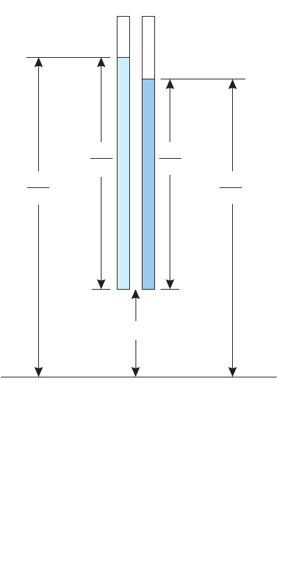
Twopiezometersopentoagivenpoint,N, in an aquifer containing saline water are shown in figure 1.
Piezometer A contains freshwater and is equipped with a mechanism that prevents saline water in the aqui-
fer from mixing with freshwater in the piezometer, while still allowing the piezometer to respond accurately
to the pressure at point N. Piezometer B contains water identical to that present in the saline aquifer at point
N. The height of the water level in piezometer A above point Nis . The freshwater head at point N
is the elevation of the water level in piezometer A above datum, and thus is given by:
,(1)
where:
hfis equivalent freshwater head [L],
PNis pressure at point N[ML-1
T-2],
ρfis density of freshwater [ML-3]
gis acceleration due to gravity [LT-2], and
ZNis elevation of point Nabove datum [L].
Piezometers filled with freshwater would seldom if ever be used in field studies of a saline aquifer
(although pressure transducers calibrated to read values of freshwater head could certainly be implemented
without difficulty). However, the point here is not that field measurements would ever be made in terms of
freshwater head, but rather that because pressure and elevation are defined at all points in any aquifer,
PNρf
⁄g
hf
PN
ρfg
--------ZN
+=
8 User’s Guide to SEAWAT: A Computer Program for Simulation of Three-Dimensional Variable-Density Ground-Water Flow
AB
Piezometer filled
with freshwater
Piezometer filled
with saline
aquifer water
h= +Z
fN
PN
ρfgh= +ZN
PN
ρg
PN
ρg
PN
ρ
f
g
ZN
Equivalent freshwater head [L]
Head [L]
Pressure [ML T ]
Density of freshwater [ML ]
Density of saline aquifer water [ML ]
Acceleration due to gravity [LT ]
Elevation [L]
-1 -2
-3
-3
-2
h
h
P
g
Z
f
N
f
N
ρ
ρ
NOTE: L = length, M = mass, T = time
EXPLANATION
freshwater head also can be defined as a function at all
points in any aquifer; in certain cases, this leads to
convenience in calculation or software application.
The elevation of the water level in piezometer
B above point Nis . The head expressed in
terms of the saline aquifer is the level in piezometer B
above datum and is given by:
,(2)
where:
his head [L], and
ρis density of saline ground water at point N
[ML-3].
Head in terms of the aquifer water, h, varies not only
as do pressure and elevation, but also as the water
density, ρ, varies. Thus, at two points having equal
pressures and the same elevation but different water
densities, different values of hwill be recorded. The
equation of ground-water flow can be formulated in
terms of h, but the result includes cumbersome
expressions involving density and its derivatives, and
no computational advantage is gained. On the other
hand, formulation of the flow equation in terms of
freshwater head causes no increase in complexity and
allows the use of software, such as MODFLOW, with
relatively little modification.
The values calculated by the SEAWAT program
in a variable-density simulation are freshwater head
values corresponding to the level in piezometer A
(fig. 1). They can be used in a variable-density form
of Darcy’s law to calculate volumetric ground-water
flows. However, the calculated value of freshwater
head at a given point in the aquifer does not represent
the level to which ambient saline ground water will
PNρg⁄
hPN
ρg
------ ZN
+=
rise in a piezometer open to that point. As discussed above and shown in figure 1, native ground water will
rise to the level hin a tightly cased piezometer. Conversion between head as measured by the native aquifer
water and equivalent freshwater head is, therefore, necessary in converting model results or field data, and
in model calibration or in the interpretation of calculated results. These conversions can be made using the
following relations:
(3)
and:
(4)
hf
ρ
ρf
---- hρρ–f
ρf
--------------Z–=
hρf
ρ
---- hf
ρρ–f
ρ
--------------Z+=
Figure 1. Two piezometers, one filled with
freshwater and the other with saline aquifer
water, open to the same point in the aquifer.
CHAPTER 2--Mathematical Description of Variable-Density Ground-Water Flow 9
ρqxρqx+ x∆
∆x
Fluid density [ML ]
Specific discharge at [LT ]
Specific discharge at [LT ]
Distance along the axis [L]
-3
-1
-1
x
xx
x
+∆
ρ
∆
q
q
x
x
x+ x∆
NOTE: L = length, M = mass, T = time
EXPLANATION
where Zis elevation [L]. Equations 3 and 4 are obtained by eliminating pressure between equations 1 and
2, and solving for the respective head value.
Governing Equation for Ground-Water Flow
A representative elementary volume (REV) in a porous medium is shown in figure 2. Based on the
principle of mass conservation for fluid and solute, the rate of accumulation of mass stored in the REV is
equal to the algebraic sum of the mass fluxes across the faces of the element and the mass exchange due to
sinks or sources. The mathematical expression for the conservation of mass is:
,(5)
where:
∇is the gradient operator ,
ρis the fluid density [ML-3],
is the specific discharge vector [LT-1],
ρis the density of water entering from a
source or leaving through a sink
[ML-3],
qsis the volumetric flow rate per unit
volume of aquifer representing
sources and sinks [T-1],
θis porosity [dimensionless], and
tis time [T].
∇ρq()ρqs
+⋅–∂ρθ()
∂t
--------------
=
∂
∂x
----- ∂
∂y
----- ∂
∂x
-----
++
q
The left-hand side of equation 5 is the net flux of mass through the faces of the REV, plus
therate(ρqs) at which mass enters from sources or leaves through sinks located in the REV. The right-hand
side of equation 5 is the time rate of change in the mass stored in the REV over a given period and can be
expanded with the chain rule as:
.(6)
The changes of porosity considered here are restricted to those associated with the change of fluid
pressure; therefore, the change of porosity with time is mathematically represented as:
.(7)
Under isothermal conditions, fluid density is a function of fluid pore pressure and solute concentration;
therefore, the equation of the state for fluid density is:
,(8)
∇ρq()⋅
∂ρθ()
∂t
-------------- ρ∂θ
∂t
------θ∂ρ
∂t
------
+=
∂θ
∂t
------∂θ
∂P
------ ∂P
∂t
------
=
ρfPC,()=
Figure 2. Representative elementary
volume in a porous medium.
10 User’s Guide to SEAWAT: A Computer Program for Simulation of Three-Dimensional Variable-Density Ground-Water Flow
where:
Pis fluid pore pressure [ML-1
T-2], and
Cis solute concentration [ML-3].
Differentiating equation 8 with respect to time gives:
.(9)
Substituting equations 7 and 9 into equation 6 gives:
. (10)
The first two terms in the right-hand side of equation 10 represent the rate of fluid mass accumulation
due to ground-water storage effects (for example, due to the compressibility of the bulk porous material and
fluid compressibility). The third term on the right-hand side of equation 10 represents the rate of fluid mass
accumulation due to the change of solute concentration.
The relation between porosity, pressure, and the compressibility of a bulk porous material is given by
Bear (1979) as:
,(11)
where ξis the compressibility of the bulk porous material [M-1LT2]. The coefficient of water compressibility
is defined as (Bear, 1979):
, (12)
where ζis the coefficient of water compressibility [M-1LT2]. Using equations 11 and 12, equation 10 can be
rewritten as:
. (13)
The term, , represents the volume of water released from storage in a unit volume of a
confined elastic aquifer per unit change in pressure:
, (14)
where Spis the specific storage in terms of pressure [M-1LT2]. Substitution of equation 14 into 13 gives:
.(15)
A more thorough discussion of storativity is presented by Bear (1979).
∂ρ
∂t
------ ∂ρ
∂P
------ ∂P
∂t
------ ∂ρ
∂C
-------∂C
∂t
-------
+=
∂ρθ()
∂t
-------------- ρ∂θ
∂t
------θ∂ρ
∂t
------ ρ∂θ
∂P
------ ∂P
∂t
------ θ∂ρ
∂P
------ ∂P
∂t
------ θ∂ρ
∂C
-------∂C
∂t
-------
++=+=
ξ1
1(θ)–
----------------- ∂θ
∂P
------
=
ζ1
ρ
---∂ρ
∂P
------
=
∂ρθ()
∂t
-------------- ρξ1θ–[]ζθ+()
∂P
∂t
------ θ∂ρ
∂C
-------∂C
∂t
-------
+=
ρξ1θ–[]ζθ+()
Spξ1θ–[]ζθ+()=
∂ρθ()
∂t
-------------- ρSp
∂P
∂t
------ θ∂ρ
∂C
-------∂C
∂t
-------
+=
CHAPTER 2--Mathematical Description of Variable-Density Ground-Water Flow 11
The first term in the right-hand side of equation 15 is the rate of fluid mass accumulation due to fluid
pore pressure change, and the second term is the rate of fluid mass accumulation due to the change of solute
concentration. Further discussion of the second term in the right-hand side of equation 15 is presented later.
Substituting equation 15 into equation 5, the flow equation becomes:
. (16)
Equation 16 is the general form of the partial differential equation for variable-density ground-water flow
in porous media.
If density is constant, the term in equation 16 is zero, and the remaining density terms cancel.
The resulting equation would conserve fluid mass and fluid volume for a constant density system, but would
conserve only fluid volume for a variable-density system. The flow equation based on fluid volume conser-
vation is often cited for the case of uniform density (for example, de Marsily, 1986). As Bear (1972) points
out, however, the use of an equation based on volume balance is inappropriate when substantial density or
temperature gradients are present. Evans and Raffensperger (1992) compared the mass- and volume-based
stream functions for variable-density ground-water flow and found that the differences between the stream
functions, calculated using the mass-based stream function and volume-based stream function, could reach
9.55 percent for their particular test problem after a calculation period of 600 years. They concluded that
mass fluxes rather than volumetric fluxes must be used to describe the flow of ground water if the variation
in fluid density is substantial.
Darcy’s Law for Variable-Density Ground-Water Flow
The governing equation for variable-density ground-water flow includes a term for specific
discharge, which is calculated with Darcy’s law. In this section, the variable-density form of Darcy’s law is
presented.
General Form of Darcy’s Law
Mass fluxes are defined as the product of fluid density and the specific discharge, or volumetric flow
per unit cross-sectional area of bulk porous medium. Darcy’s law for a fluid of variable density can be
expressed by the equations:
, (17)
, (18)
and:
, (19)
where:
qx,qy,qzare the individual components of specific discharge,
µis the dynamic viscosity [ML-1
T-1],
kx,ky,kzrepresent intrinsic permeabilities [L2] in the three coordinate directions, and
gis the gravitational constant [LT-2] and treated here as a positive scalar quantity.
∇ρq()⋅–ρqsρSp
∂P
∂t
------ θ∂ρ
∂C
-------∂C
∂t
-------
+=+
∂ρ ∂C⁄
qx
kx
µ
----
–∂P
∂x
------
=
qy
ky
µ
----
–∂P
∂y
------
=
qz
kz
µ
---- ∂P
∂z
------ ρg+–=
12 User’s Guide to SEAWAT: A Computer Program for Simulation of Three-Dimensional Variable-Density Ground-Water Flow
In this formulation, it is assumed that the three principal directions of permeability are aligned with the
orthogonal x-,y-,andz-coordinate system. The z-coordinate axis, representing the vertical, is positive
upward.
Note that in equation 19, the density, ρ, is that of the fluid at the calculation point (and time) for
which specific discharge is to be determined. The density term reflects the direct action of gravity on a fluid
element at the calculation point and only affects the component of specific discharge in the vertical direction.
It should be kept in mind, however, that the overall pressure distribution in a porous medium is controlled,
in part, by the overall fluid density distribution, and thus, horizontal components of specific discharge also
are affected by density variations in the system.
Assumption of Axes Alignment with Principal Permeability Directions
The assumption that the principal axes of permeability are horizontal and vertical is usually accept-
able for an aquifer with horizontal bedding. A more general form of Darcy’s law is required when the prin-
cipal directions of permeability do not coincide with the horizontal and vertical x-,y-,andz-coordinate
system. The simplest approach is to abandon the x-,y-,andz-coordinate system, and instead use a coordinate
system aligned with the principal directions of permeability as shown in figure 3. If γrepresents the direction
normal to the bedding and αand βrepresent the principal directions of permeability parallel to the bedding,
the pressure gradients acting in the α,β,andγdirections can be formulated independently. Because none of
the coordinate directions are horizontal, although they are orthogonal to one another, a component of the
gravitational force applies in each coordinate direction. This leads to the following expression of Darcy's law:
, (20)
, (21)
and:
, (22)
where:
qα,qβ,qγrepresent the specific discharge components in the
coordinate axes aligned with permeability directions [LT-1],
kα,kβ,kγare the permeabilities in these directions [L2], and
δα,δβ,δγare the angles between the respective coordinate axes and
the upward vertical direction.
Darcy’s Law in Terms of Equivalent Freshwater Head
Darcy's law can also be expressed in terms of the freshwater head
or elevation above an arbitrary datum of the water surface in a piezom-
eter filled with freshwater. Note that it is not assumed that the aquifer
itself contains freshwater of uniform density, but rather that piezometers
open to the aquifer have been filled with freshwater, and a mechanism
prevents the dissolved salts in the aquifer water from mixing with the
water in the piezometers. As shown in figure 1, the elevation of the
qα
kα
µ
----- ∂P
∂α
-------ρgδα
cos+
–=
qβ
kβ
µ
-----∂P
∂β
------ ρgδβ
cos+
–=
qγ
kγ
µ
---- ∂P
∂γ
------ ρgδγ
cos+
–=
δ
β
δ
γ
α
β
γ
z
δ
α
Figure 3. Relation between a
coordinate system aligned with
the principal axes of permeabil-
ity and the upward z-axis.
CHAPTER 2--Mathematical Description of Variable-Density Ground-Water Flow 13
water surface in a piezometer has two components: the elevation of the point of measurement above some
datum, z, and the height of the fluid column in the piezometer itself. Because the piezometer is assumed to
contain freshwater having a fixed density, ρf, the height of the water column within the piezometer is
P/ρfg,wherePis the pressure at the piezometer opening. Thus, the freshwater head, hf, at this point is equal
to (P/ρfg,) + zand the pressure is given by:
. (23)
For the dipping-aquifer problem (fig. 3), equation 23 is first differentiated with respect to the coordi-
nate direction α, which yields:
. (24)
Substituting this expression into equation 20 and noting that , the following relation is
obtained:
. (25)
It is important to note that both ρf, the density of freshwater in the piezometers and ρ, the density of water
in the formation at the point of velocity calculation, appear in equation 25. These two density terms should
not be confused.
The freshwater hydraulic conductivity, Kf,intheαdirection is defined as:
,(26)
where µf[ML-1
T-1] represents the viscosity of freshwater under standard conditions (for example, 20 degrees
Celsius and 1 atmospheric pressure). Using this term for freshwater hydraulic conductivity, equation 20 can
be written as:
. (27)
Similarly, equation 21 can be written as:
, (28)
and equation 22 as:
. (29)
Note that for a horizontally stratified aquifer, equations 27 to 29 would reduce to:
, (30)
Pρfgh
fz–()=
∂P
∂α
-------ρfg∂hf
∂α
------- ρfg∂z
∂α
-------
–=
δcos α
∂z
∂α
-------
=
qα
kα
–
µ
-------- ρfg∂hf
∂α
------- ρfg∂z
∂α
-------
–ρg∂z
∂α
-------
+=
Kfα
kαρfg
µf
--------------
=
qαKfα
–µf
µ
---- ∂hf
∂α
------- ρρ
f
–
ρf
--------------
∂z
∂α
-------
+=
qβKfβ
–µf
µ
---- ∂hf
∂β
------- ρρ
f
–
ρf
--------------
∂z
∂β
------
+=
qγKfγ
–µf
µ
---- ∂hf
∂γ
------- ρρ
f
–
ρf
--------------
∂z
∂γ
-----
+=
qxKfx
–µf
µ
---- ∂hf
∂x
-------
=
14 User’s Guide to SEAWAT: A Computer Program for Simulation of Three-Dimensional Variable-Density Ground-Water Flow
, (31)
and:
. (32)
For many practical applications, the term µf/µin equations 27 to 32 can be considered equal to one;
it can be assumed that the viscosity of water in the formation is essentially the same as that of freshwater,
even though differences in density are present. Variations in fluid viscosity arise primarily because of vari-
ations in water temperature. Where substantial temperature variations are absent and where hydraulic
conductivity has been measured at the same water temperature for which velocity is to be calculated, the
viscosity correction usually can be neglected.
Governing Equation for Flow in Terms of Freshwater Head
With the definition of freshwater head and Darcy’s law in terms of freshwater head, the governing
equation for ground-water flow (eq. 16) can be written in terms of equivalent freshwater head. Expanding
the left-hand side of equation 16 and rearranging yield:
. (33)
Differentiation of equation 23 with respect to time shows that can be expanded as
. Using this form and substituting Darcy’s law as given in equations 27 to 29 for the components
of specific discharge yield:
(34)
The specific storage in terms of pressure, Sp(eq. 14), includes the compressibility of the water, which
in turn, depends on the water density, ρ, at the point of calculation (eq. 12). The assumption is made here
that the difference between the compressibility coefficients of saltwater and freshwater can be neglected in
that:
, (35)
where ζfis the compressibility coefficient for freshwater. The specific storage, in terms of freshwater head,
Sf[L-1], or the volume of water released from storage in a unit volume of aquifer per unit decline in
freshwater head is given by Bear (1979) as:
. (36)
qyKfy
–µf
µ
---- ∂hf
∂y
-------
=
qzKfz
–µf
µ
---- ∂hf
∂z
------- ρρ
f
–
ρf
--------------
+=
∂
∂α
-------ρqα
()–∂
∂β
------ ρqβ
()–∂
∂γ
----- ρqγ
()ρSP
∂P
∂t
------ θ∂ρ
∂C
-------∂C
∂t
-------ρqs
–+=–
∂P∂t⁄
ρfg∂hf∂t⁄
∂
∂α
-------ρKfα
∂hf
∂α
------- ρρ
f
–
ρf
--------------∂Z
∂α
-------
+
∂
∂β
------ ρKfβ
∂hf
∂β
------- ρρ
f
–
ρf
--------------∂Z
∂β
------
+
+
∂
∂γ
-----
+ρKfγ
∂hf
∂γ
------- ρρ
f
–
ρf
--------------∂Z
∂γ
------
+
ρSpgρf
∂hf
∂t
------- θ∂ρ
∂C
-------∂C
∂t
-------ρqs.–+=
ζ1
ρ
---∂ρ
∂P
------ ζf
1
ρf
---- ∂ρ
∂P
------
=≈=
Sfgρfξ1θ)–ζfθ]+([=
CHAPTER 2--Mathematical Description of Variable-Density Ground-Water Flow 15
By using equations 14 and 35, the term Spgρfinequation34canbereplacedbythetermSf, which yields:
(37)
Equation 37 is the governing equation for variable-density flow in terms of freshwater head as used in
SEAWAT.
Governing Equation for Solute Transport
In addition to the flow equation that was developed (eq. 37), a second partial differential equation is
required to describe solute transport in the aquifer. Ground-water flow causes the redistribution of solute
concentration, and the redistribution of solute concentration alters the density field, thus, affecting ground-
water movement. Therefore, the movement of ground water and the transport of solutes in the aquifer are
coupled processes, and the two equations must be solved jointly.
Solute mass is transported in porous media by the flow of ground water (advection), molecular diffu-
sion, and mechanical dispersion. The transport of solute mass in ground water can be described by the
following partial differential equation (Zheng and Bennett, 1995):
, (38)
where:
Dis the hydrodynamic dispersion coefficient [L2T-1],
is the fluid velocity [LT-1],
Csis the solute concentration of water entering from sources or sinks [ML-3], and
Rk(k=1, …, N) is the rate of solute production or decay in reaction kof Ndifferent reactions [ML-3T-1].
When fluid density varies, the concentration gradient, , should actually be formulated as ρ∇(C/ρ)
(de Marsily, 1986, p. 239). This is only necessary for brines of high density; however for fluid densities in
the seawater range, the change introduced by this expression is negligible, and the transport equation as
formulated in equation 38 may be used.
Boundary and Initial Conditions
Boundary and initial conditions must be specified to solve the differential equations for flow (eq. 37)
and transport (eq. 38) in a particular problem. Mathematical boundaries are commonly defined in three cate-
gories: Dirichlet (constant head or concentration), Neumann (specific flux), and Cauchy (head-dependent
flux or mixed boundary condition). The physical features and processes, which impose boundary conditions
on ground-water regimes, normally include streams and other surface-water bodies, drains, low-permeabil-
ity boundaries, seepage faces, evapotranspiration, discharging wells, injection wells and recharge. In simu-
lation theory, many of the boundary conditions are commonly implemented through the sink/source term in
equations 37 and 38; that approach is followed in this model. There is a separate section that further
describes sink and source terms.
∂
∂α
-------ρKfα
∂hf
∂α
------- ρρ
f
–
ρf
--------------∂Z
∂α
-------
+
∂
∂β
------ ρKfβ
∂hf
∂β
------- ρρ
f
–
ρf
--------------∂Z
∂β
------
+
+
∂
∂γ
----- ρKfγ
∂hf
∂γ
------- ρρ
f
–
ρf
--------------∂Z
∂γ
------
+
ρSf
∂hf
∂t
------- θ∂ρ
∂C
-------∂C
∂t
-------ρqs.–+=+
∂C
∂t
-------∇D∇C⋅()⋅=∇vC()⋅qs
θ
---- CsRk
k1=
N
∑
+––
v
∇C
16 User’s Guide to SEAWAT: A Computer Program for Simulation of Three-Dimensional Variable-Density Ground-Water Flow
Dirichlet Boundary
A Dirichlet boundary (also referred to as Type I) is one in which the value of head or concentration is
specified at all points along the boundary. The head or concentration value may vary from point to point or
as a function of time and is treated as a known quantity in the solution of the equation. In terms of flow simu-
lation, a specified head implies that flow toward or away from the boundary occurs in proportion to the
difference between the specified head at the boundary and the calculated head at points directly adjacent to
the boundary. This is simulated by not solving a flow equation at the specified-head cell. In terms of solute
transport, a specified concentration implies that the dispersive flux toward or away from the boundary
occurs in response to the difference between the specified boundary concentration and the calculated
concentration at points directly adjacent to the boundary. Advective solute flux into the modeled area from
a specified concentration boundary depends on the flow from the boundary and the specified concentration
value. Advective solute flux toward any type of boundary depends on the calculated concentration of the
water at points adjacent to the boundary and on the flow toward the boundary.
A physical example of an external Dirichlet boundary might be a fully penetrating stream or other
surface-water body on the boundary of the model domain along which head or concentration is specified.
An example of an internal Dirichlet boundary might be a drain operating at a specified water level in the
interior of the model domain.
Neumann Boundary
The Neumann boundary (also referred to as Type II) represents the condition in which the gradient of
the dependent variable is specified normal to the boundary. For ground-water flow, this boundary condition
results in a specified flux of water into or out of the modeled area. For solute transport, the concentration
gradient is specified normal to the boundary. This results in a specified dispersive flux of solute across the
Neumann boundary. Although the Neumann boundary for solute transport ensures a specified dispersive
flux, the advective solute flux depends on the ground-water flow velocity normal to the boundary and the
calculated concentration on the boundary. Thus, the total solute flux across a Neumann boundary cannot be
specified prior to simulation.
An impermeable boundary represents a special case of the Neumann condition for flow and transport,
where the gradients of head and concentration are zero such that neither flow nor dispersive solute flux may
occur, and advective solute flux is precluded by the absence of flow. An impermeable boundary (commonly
called a no-flow boundary) is simulated by specifying cells for which a flow equation is not solved. Addi-
tionally, the flow between a no-flow cell and an adjacent cell is zero. A nonzero Neumann boundary is simu-
lated using sink/source terms. An example of a nonzero Neumann boundary in flow simulation might be a
surface-water body from which seepage occurs at a prescribed rate.
Cauchy Boundary
A head-dependent flow condition represents a Cauchy boundary (also referred to as Type III) for the
simulation of flow (Anderson and Woessner, 1992). The Cauchy boundary for solute transport, however, is
not analogous because boundary conditions for solute transport may contain both advective and dispersive
components, whereas boundary conditions for flow contain only the flow component. With the Cauchy
boundary for flow, a control head is specified, but this control head prevails at some hydraulic separation
from the boundary. The head on the boundary itself is calculated in the simulation, but is linked to the control
head through a conductance term, which may represent, for example, the semipermeable material on the bed
of a stream or the local head loss through convergent flow into a drain. The flow, Qb, into or from a head-
dependent flow boundary is calculated as:
CHAPTER 2--Mathematical Description of Variable-Density Ground-Water Flow 17
, (39)
where:
COND is the conductance term,
hcis the specified control head, and
hi,j,k is the calculated head at the boundary cell, which is linked through the conductance term.
Examples of the head-dependent condition are provided by the River (RIV), Drain (DRN),
Evapotranspiration (EVT), and General-Head Boundary (GHB) packages of MODFLOW; the first three of
these nonlinear variations involve limiting values of head beyond which the flow value, Qb, takes on a fixed
value, making these nonlinear variations of the head-dependent flux boundary condition.
The Cauchy boundary for solute transport represents a boundary on which both concentration and
concentration gradient are specified (Zheng and Bennett, 1995). This implies that the dispersive flux across
the boundary is specified and that the advective flux across the boundary will vary only to the extent that
the flow across the boundary in the transport simulation varies. A Cauchy boundary condition in the trans-
port model, which coincides with a Neumann boundary condition in the flow regime, will result in a spec-
ified total flux of solute mass across the boundary.
Initial Conditions
Initial conditions represent starting values for the dependent variable, such as freshwater head for
ground-water flow and concentration for solute transport, at some starting time. Initial conditions for both
flow and transport must be specified for transient simulations.
Sink and Source Terms
The third term on the right-hand side of equation 37 and the third term on the left-hand side of equa-
tion 38 are the sink/source terms for water and solute, respectively. These terms quantify the exchange of
water and solute mass between the aquifer and such features as discharging wells, injection wells, and
recharge. Sinks and sources may be areally distributed or localized. Areally distributed sinks or sources
include recharge and evapotranspiration; localized sinks and sources may include wells, drains, and rivers.
In the case of sources, which provide a mechanism for bringing solute mass into the flow systems, solute
concentration of the source water must be specified. The concentration of water removed at a sink generally
is the simulated value for the cell containing the sink and may represent information useful in model cali-
bration. Evapotranspiration, which is typically thought to remove only freshwater from the flow system, is
an exception.
The strength (that is, the mass of solute per unit time) of a source or sink component in the transport
equation depends on the volumetric flow rate and solute concentration of the water entering the sink or leav-
ing through the source. For a transport source, the concentration is specified; for a sink, the calculated
concentration of the water in the aquifer as it enters the sink is used. The flow terms are identical to those
used for the corresponding source or sink in the flow equation. Solutes entering the flow field by dissolution
of minerals from the aquifer generally would not be treated as part of the source term, but rather as part of
the chemical reaction term, Rk, in equation 38.
QbCOND hchijk,, )–(=
18 User’s Guide to SEAWAT: A Computer Program for Simulation of Three-Dimensional Variable-Density Ground-Water Flow
Concentration and Density
The second term on the right-hand side of equation 37 represents the change of fluid mass in the REV
due to the change in solute concentration. To evaluate this term, the relation between solute concentration
and fluid density is required. For isothermal conditions, fluid density is predominantly affected by the solute
concentration and fluid pore pressure. The effects of pore pressure on fluid density are included in the stor-
age term (eq. 9). An empirical relation between the density of saltwater and concentration was developed
by Baxter and Wallace (1916):
, (40)
where:
Eis a dimensionless constant having an approximate value of 0.7143 for salt concentrations ranging
from zero to that of seawater, and
Cis the salt concentration [ML-3].
The derivative of equation 40 with respect to salt concentration is:
. (41)
Substituting this relation into equation 37, the governing equation is rewritten as:
(42)
Sometimes salt concentration is measured as salinity and expressed as mass/mass (for example, grams
per kilogram or parts per thousand). Salinity is defined as the total amount of solid material in grams
contained in 1 kg of seawater when all the carbonate is converted to oxide, the bromine and iodine are
replaced by chloride, and all organic matter is completely oxidized (Chow, 1964). The value of salinity is
often close to the dissolved-solids concentration; however, the salinity cannot be used directly in equation
40, but must rather be converted to concentration in units of mass/volume. The conversion for a dilute solu-
tion is relatively simple; for example, parts per million can approximately be treated as milligrams per liter
(Freeze and Cherry, 1979). For a solution with higher concentrations of solute, such as seawater, the conver-
sion is more complicated because of the change in volume of the solution, which accompanies a change in
salt concentration. For example, the solution volume increases about 1 percent when 35 g of salt are added
to 1 L of water. The volume change of a solution with high concentration depends on many factors, and the
conversion from units of mass/mass to units of mass/volume must, therefore, generally be based on empir-
ical relations.
Equations 40 to 42 are applied only for typical seawaters for which the relation between fluid density
and solute concentration can be expressed as a linear function as in equation 40. If the fluid has a different
composition from typical seawater or the salt concentration in the fluid is much higher than normal seawater
concentration, then these equations may not be valid. In that case, a different empirical relation between salt
concentration and fluid density (similar to eq. 40) should be developed for that particular application.
ρρ
fEC+=
∂ρ
∂C
-------E=
∂
∂α
-------ρKfα
∂hf
∂α
------- ρρ
f
–
ρf
--------------∂Z
∂α
-------
+
∂
∂β
------ ρKfβ
∂hf
∂β
------- ρρ
f
–
ρf
--------------∂Z
∂β
------
+
+
∂
∂γ
----- ρKfγ
∂hf
∂γ
------- ρρ
f
–
ρf
--------------∂Z
∂γ
------
+
ρSf
∂hf
∂t
------- θE∂C
∂t
-------ρqs.–+=+
CHAPTER 3--Finite-Difference Approximation for the Variable-Density Ground-Water Flow Equation 19
CHAPTER 3
FINITE-DIFFERENCE APPROXIMATION FOR THE
VARIABLE-DENSITY GROUND-WATER FLOW EQUATION
For variable-density ground-water conditions, flow and solute transport are linked processes. This
means that a fully coupled solution to the flow and transport equations is required to properly represent
dynamic ground-water flow. For most problems, it is difficult, if not impossible, to develop analytical solu-
tions for these coupled governing equations; therefore, numerical methods generally are required.
This chapter contains the development of the finite-difference approximation for the variable-density
flow equation that is used in SEAWAT. The finite-difference equation for variable-density ground-water
flow is developed using sign conventions and nomenclature similar to those used by McDonald and
Harbaugh (1988) in the documentation of MODFLOW. As a result, the similarities and differences between
the flow equation in MODFLOW and the flow equation in SEAWAT are readily apparent.
The numerical methods used by the MT3DMS program to simulate solute transport in a constant-
density flow field are directly used in SEAWAT to simulate solute transport in a variable-density flow field.
Because the solute-transport equation is applicable for both constant and variable-density flow conditions,
it was not necessary to make substantial changes to the MT3DMS program prior to the incorporation into
SEAWAT. For this reason, the finite-difference and other methods used to solve the solute-transport equa-
tion are not presented. Instead, interested users are referred to the MT3DMS documentation (Zheng and
Wang, 1998) for a detailed description of the equations and methods used to solve the solute-transport
equation.
Finite-Difference Approximation for the Flow Equation
The finite-difference method is commonly used to solve partial differential equations, wherein a grid
is overlain on the area of interest, dividing the domain into individual model cells. The finite-difference
approximation to the partial differential equation is then applied to the discretized model domain. The
assumption is then made that the concept of an REV can be applied to each model cell. Both MODFLOW
and MT3DMS use cell-centered grids. In this formulation, the dependent variables obtained in the finite-
difference solution represent average values (assumed to exist at the cell center) for the respective cells.
SEAWAT also uses a block-centered grid because it is used for both MODFLOW and MT3DMS. The subse-
quent discussion of the finite-difference approximation of the variable-density ground-water flow equation,
therefore, is based on the concept of a cell-centered grid, although the general approach could easily be
appliedtoothergriddesigns.
The terms on the left-hand side of the governing equation for variable-density ground-water flow
(eq. 42) account for the difference between inflow and outflow of mass per unit volume of aquifer across
the faces of a differential element of aquifer (for example, a model cell). The first term on the right-hand
side of equation 42 represents the time rate of change of liquid mass (which includes both water and solute)
per unit volume of aquifer due to pressure changes in the system. The second term on the right-hand side of
equation 42 represents the time rate of change of fluid mass per unit volume of aquifer due to the change in
solute concentration. This second term is calculated from the concentrations obtained in the solution of the
solute-transport equation. As the concentrations reach dynamic equilibrium, this term becomes negligible.
Thus, the flow field does not reach steady state until the solute concentrations remain constant in time.
The third term on the right-hand side represents the mass flux due to sources and sinks.
20 User’s Guide to SEAWAT: A Computer Program for Simulation of Three-Dimensional Variable-Density Ground-Water Flow
With a central finite-difference scheme in space and a backward finite-difference scheme in time, the
finite-difference approximation for the partial differential equation of ground-water flow is:
(43)
where:
i,j,kare row, column, and layer indices, respectively.
Aj,kis the area of the finite-difference cell normal to the αaxis [L2]suchthatAj,k =∆βj⋅∆γ
k,and
similarly for other coordinate directions,
Zi,j,kis the cell center elevation [L],
nis the timestep number,
Vi,j,k is the volume of the cell [L3]suchthatVi,j,k =∆αi∆βj∆γk,and
Qsis the volumetric flow rate of the sink/source term [L3T-1].
The subscripts i+1/2,i-1/2,j+1/2,j-1/2,k+1/2 and k-1/2 refer to the value of a property or variable between
two neighboring cells (for example, the harmonic mean for hydraulic conductivity). In equation 43, the f
subscript is dropped for convenience from the freshwater-equivalent hydraulic conductivity terms, and this
simplified notation is used throughout the rest of this section. The equivalent freshwater head values on the
left-hand side of equation 43 refer to the n+1 timestep. If the timestep superscript is not listed with the
variable, as is the case with the freshwater head values on the left-hand side of equation 43, the variable is
evaluated at the n+1 timestep.
In equation 43, there are two types of density terms calculated at boundaries between model cells. The
density term, , converts the volumetric flow rate to a mass flux. In SEAWAT, this density term is calculated
before each iteration of the flow equation using an upstream weighting algorithm. For example, if flow is
from cell i,j,k to cell i,j,k+1, then the term would be assigned a density value equal to . If,
however, the flow direction were reversed (from i,j,k+1 to i,j,k), then would be assigned a value
equal to . The other density term calculated at cell boundaries in equation 43 is denoted by ρand is
simply the arithmetic average of fluid density between neighboring cells. These density values are used in
ρ
ˆi12⁄jk,,+
Kαi12jk,,⁄+,
∆αi12jk,,⁄+
-----------------------------Ajk,hfi 1jk,,+,hfijk,,,
–ρi12jk,,⁄+ρ–f
ρf
-------------------------------- Zi1jk,,+Zijk,,
–()+
ρ
ˆi12⁄–jk,,
–Kαi12jk,,⁄–,
∆αi12jk,,⁄–
---------------------------- Ajk,hfijk,,, hfi 1– jk,,,
–ρi12jk,,⁄–ρ–f
ρf
--------------------------------Zijk,, Zi1– jk,,
–()+
ρ
ˆij 12k,⁄+,
+Kβij,12k,⁄+,
∆βij,12k,⁄+
---------------------------- Aik,hfij 1+ k,,, hfijk,,,
–ρij 12⁄k,+, ρf
–
ρf
---------------------------------Zij 1k,+, Zijk,,
–()+
ρ
ˆij12⁄–k,,
–Kβij,12k,⁄–,
∆βij12k,⁄–,
----------------------------Aik,hfijk,,, hfij,1– k,,
–ρij,12k,⁄–ρ–f
ρf
--------------------------------Zijk,, Zij 1– k,,
–()+
ρ
ˆijk,12⁄+,
+Kγijk 12⁄+,,,
∆γijk 12⁄+,,
---------------------------Aij,hfijk,1+,, hfijk,,,
–ρij k,12⁄+, ρf
–
ρf
----------------------------------Zij k,1+, Zijk,,
–()+
ρ
ˆijk12⁄–,,
–Kγijk,, 12⁄–,
∆γijk 12⁄–,,
--------------------------- Aij,hfijk,,, hfijk 1–,,,
–ρijk 12⁄–,, ρ–f
ρf
--------------------------------Zijk,, Zijk 1–,,
–()+
ρijk,, Sfijk,,,
hfijk,,,
n1+ hfijk,,,
n
–
tn1+ tn
–
----------------------------------θE∂C
∂t
-------
+
Vijk,, ρQs
()
ijk,, ,–=
ρ
ˆ
ρ
ˆ
ijk 12⁄+,, ρijk,,
ρ
ˆ
ijk 12⁄+,,
ρijk 1+,,
CHAPTER 3--Finite-Difference Approximation for the Variable-Density Ground-Water Flow Equation 21
the density-difference terms within the brackets on the left side of equation 43; as discussed previously, the
density-difference terms are required in Darcy’s Law when gradients of freshwater head are used in a saline
environment.
Following the concepts of McDonald and Harbaugh (1988), several of the coefficients in equation 43
can be grouped together to form the conductance term, COND [L2T-1]:
, (44)
where:
Arepresents the area normal to flow [L2], and
Lrepresents the distance along the flow path [L].
Following this convention, equation 43 can be rewritten as:
(45)
COND AK
L
--------
=
ρ
ˆi12jk,,⁄+CCi12jk,,⁄+hfi 1+ jk,,,
hfijk,,,
–ρi12jk,,⁄+ρf
–
ρf
---------------------------------Zi1jk,,+ Zijk,,
–()+
ρ
ˆi12jk,,⁄–CCi12jk,,⁄–hfijk,,, hfi 1– jk,,,
–ρi12jk,,⁄–ρf
–
ρf
---------------------------------Zijk,, Zi1– jk,,
–()+–
ρ
ˆij 12k,⁄+,CRij,12k,⁄+hfij 1+ k,,, hfijk,,,
–ρij,12k,⁄+ρf
–
ρf
----------------------------------Zij 1k,+, Zijk,,
–()++
ρ
ˆij 12k,⁄–,CRij,12k,⁄–hfijk,,, hfij,1– k,,
–ρij,12k,⁄–ρf
–
ρf
--------------------------------- Zijk,, Zij,1– k,
–()+–
ρ
ˆijk 12⁄+,, CVijk,,12⁄+hf ijk,,1+,hfijk,,,
–ρijk,,12⁄+ρf
–
ρf
----------------------------------- Zijk,,1+Zijk,,
–()++
ρ
ˆijk 12⁄–,, CVijk,,12⁄–
–hfijk,,,hfijk 1–,,,
–ρijk,,12⁄–ρf
–
ρf
----------------------------------- Zijk,, Zijk 1–,,
–()+
ρijk,, Sfijk,,,
hfijk,,,
n1+ hfijk,,,
n
–
tn1+ tn
–
------------------------------------ θE∂C
∂t
-------
+
=Vijk,, ρQs
()
ijk,, ,–
22 User’s Guide to SEAWAT: A Computer Program for Simulation of Three-Dimensional Variable-Density Ground-Water Flow
where CC,CR,andCV refer to the conductance factors along columns, rows, and normal to layers,
respectively [L2T-1]. Equation 45 can be rewritten as:
(46)
ρ
ˆ
i12jk,,⁄+CCi12jk,,⁄+hfi 1+ jk,,,
hfijk,,,
–[]
ρ
ˆi12jk,,⁄+CCi12jk,,⁄+
ρi12jk,,⁄+ρf
–
ρf
---------------------------------------- Zi1jk,,+ Zijk,,
–()+
ρ
ˆi12jk,,⁄–CCi12jk,,⁄–
–hfijk,,, hfi 1– jk,,,
–[]
ρ
ˆi12jk,,⁄–CCi12jk,,⁄–
ρi12jk,,⁄–ρf
–
ρf
---------------------------------------- Zijk,, Zi1– jk,,
–()–
ρ
ˆij 12k,⁄+,
+CRij,12k,⁄+hfij 1+ k,, , hfijk,,,
–[]
ρ
ˆij 12k,⁄+,CRij,12k,⁄+
ρij,12k,⁄+ρf
–
ρf
----------------------------------------- Zij 1k,+, Zijk,,
–()+
ρ
ˆij 12k,⁄–,CR–ij,12k,⁄–hfijk,,, hfij,1– k,,
–[]
ρ
ˆij 12k,⁄–,CR–ij,12k,⁄–
ρij,12k,⁄–ρf
–
ρf
----------------------------------------- Zijk,, Zij,1– k,
–()
ρ
ˆijk 12⁄+,, CV+ijk,,12⁄+hfijk,,1+,hfijk,,,
–[]
ρ
ˆijk 12⁄+,, CVijk,,12⁄+
ρijk,,12⁄+ρf
–
ρf
--------------------------------------------Zijk,,1+Zijk,,
–()+
ρ
ˆijk 12⁄–,, CV–ijk,,12⁄–hf ijk,,,hfijk 1–,,,
–[]
ρ
ˆijk 12⁄–,, CV–ijk,,12⁄–
ρijk,,12⁄–ρf
–
ρf
------------------------------------------- Zijk,, Zijk 1–,,
–()
ρijk,, Sfijk,,,
hfijk,,,
n1+ hfijk,,,
n
–
tn1+ tn
–
--------------------------------------------- θE∂C
∂t
-------
+
=Vijk,, ρQs
()
ijk,, .–
CHAPTER 3--Finite-Difference Approximation for the Variable-Density Ground-Water Flow Equation 23
The signs in equation 46 can be rearranged to give:
(47)
Equation 47 is the finite-difference equation for three-dimensional flow of variable-density ground water as
implemented in SEAWAT. Using the following expression for the relative density-difference terms:
, (48)
where:
, (49a)
, (49b)
, (49c)
ρ
ˆ
i12jk,,⁄+CCi12jk,,⁄+hfi 1+ jk,,,
hfijk,,,
–[]
ρ
ˆi12jk,,⁄+CCi12jk,,⁄+
ρi12jk,,⁄+ρf
–
ρf
---------------------------------------- Zi1jk,,+ Zijk,,
–()+
ρ
ˆi12jk,,⁄–CCi12jk,,⁄–
+hfi 1– jk,,,
hfijk,,,
–[]
ρ
ˆi12jk,,⁄–CCi12jk,,⁄–
ρi12jk,,⁄–ρf
–
ρf
----------------------------------------Zi1jk,,–Zijk,,
–()+
ρ
ˆij 12k,⁄+,
+CRij,12k,⁄+hfij 1+ k,, , hfijk,,,
–[]
ρ
ˆij 12k,⁄+,CRij,12k,⁄+
ρij,12k,⁄+ρf
–
ρf
----------------------------------------- Zij 1k,+, Zijk,,
–()+
ρ
ˆij 12k,⁄–,
+CRij,12k,⁄–hfij 1– k,, , hfij,k,,
–[]
ρ
ˆij,12jk,,⁄–CRij12k,⁄–,
ρij,12k,⁄–ρf
–
ρf
----------------------------------------- Zij 1k,–,Zij,k,
–()+
ρ
ˆijk 12⁄+,, CV+ijk,,12⁄+hf ijk,,1+,hfijk,,,
–[]
ρ
ˆijk 12⁄+,, CVijk,,12⁄+
ρijk,,12⁄+ρf
–
ρf
--------------------------------------------Zijk,,1+Zijk,,
–()+
ρ
ˆijk 12⁄–,, CV+ijk,,12⁄–hf ijk,,1–,hfijk,,,
–[]
ρ
ˆijk 12⁄–,, CVijk,,12⁄–
ρijk,,12⁄–ρf
–
ρf
------------------------------------------- Zijk 1–,, Zijk,,
–()+
ρijk,, Sfijk,,,
hfijk,,,
n1+ hfijk,,,
n
–
tn1+ tn
–
--------------------------------------------- θE∂C
∂t
-------
+
=Vijk,, ρQs
()
ijk,, .–
Dijk,, Di12jk,,⁄+Di12jk,,⁄–Dij 12k,⁄+,Dij 12k,⁄–,Dijk 12⁄+,, Dijk 12⁄–,,
+++++=
Di12⁄+jk,, ρ
ˆi12jk,,⁄+CCi12jk,,⁄+
ρi12jk,,⁄+ρf
–
ρf
---------------------------------Zi1jk,,+ Zijk,,
–()=
Di12jk,,⁄–ρ
ˆi12jk,,⁄–CCi12jk,,⁄–
ρi12jk,,⁄–ρf
–
ρf
---------------------------------Zi1jk,,– Zijk,,
–()=
Dij,12k,⁄+ρ
ˆij,12k,⁄+CRij,12k,⁄+
ρij,12k,⁄+ρf
–
ρf
----------------------------------Zij 1k,+, Zijk,,
–()=

24 User’s Guide to SEAWAT: A Computer Program for Simulation of Three-Dimensional Variable-Density Ground-Water Flow
, (49d)
,(49e)
and:
.(49f)
Equation 47 becomes:
(50)
Equation 50 implies that model layers can be either horizontal or tilted. When model layers are tilted,
Di+1/2,j,k,Di-1/2,j,k,Di,j+1/2,k,Di,j-1/2,k contribute to the mass flux across the four faces normal to model layers.
When the model layers are horizontal, Di+1/2,j,k,Di-1/2,j,k,Di,j+1/2,k,Di,j-1/2,k become zero. For this case,
equation 50 reduces to:
(51)
Dij,12k,⁄–ρ
ˆij,12k,⁄–CRij,12k,⁄–
ρij,12k,⁄–ρf
–
ρf
--------------------------------- Zij 1k,–, Zij,k,
–()=
Dijk,,12⁄+ρ
ˆijk,,12⁄+CVijk,,12⁄+
ρijk,,12⁄+ρf
–
ρf
----------------------------------- Zijk,,1+Zijk,,
–()=
Dijk,,12⁄–ρ
ˆijk,,12⁄–CVijk,,12⁄–
ρijk,,12⁄–ρf
–
ρf
----------------------------------- Zijk 1–,, Zijk,,
–()=
ρ
ˆi12jk,,⁄+CCi12jk,,⁄+hfi 1+ jk,,,
hfijk,,,
–[]ρ
ˆi12jk,,⁄–CCi12jk,,⁄–hfi 1– jk,,,hfijk,,,
–[]+
ρ
ˆij,12k,⁄+CR+ij,12k,⁄+hfij 1+ k,, , hfijk,,,
–[]ρ
ˆij,12k,⁄–CRij,12k,⁄–hfij 1– k,, , hfij,k,,
–[]+
ρ
ˆijk,,12⁄+CV+ijk,,12⁄+hfijk,,1+,hfijk,,,
–[]ρ
ˆijk,,12⁄–CVijk,,12⁄–hfijk 1–,,,hfijk,,,
–[]Dijk,,
++
ρfijk,,, Sfijk,,,
hfijk,,,
n1+ hfijk,,,
n
–
tn1+ tn
–
------------------------------------ θE∂C
∂t
-------
+
=Vijk,, ρQs
()
ijk,, .–
ρ
ˆ
i12jk,,⁄+CCi12jk,,⁄+hfi 1+ jk,,,
hfijk,,,
–[]ρ
ˆ
i12jk,,⁄–CCi12jk,,⁄–hfi 1– jk,,,
hfijk,,,
–[]+
ρ
ˆ
+ij 12k,⁄+,CRij,12k,⁄+hfij 1+ k,, , hfijk,,,
–[]ρ
ˆij 12k,⁄–,CRij,12k,⁄–hfij 1– k,, , hfij,k,,
–[]++
ρ
ˆijk 12⁄+,, CVijk,,12⁄+
+hfijk,,1+,hfijk,,,
–ρijk,,12⁄+ρf
–
ρf
---------------------------------Zijk,,1+Zijk,,
–()+
ρ
ˆijk 12⁄–,, CVijk,,12⁄–
+hfijk,,1–,hfijk,,,
–ρijk,,12⁄–ρf
–
ρf
---------------------------------Zijk,,1–Zijk,,
–()+
ρfijk,,, Sfijk,,,
hfijk,,,
n1+ hfijk,,,
n
–
tn1+ tn
–
------------------------------------ θE∂C
∂t
-------
+
=Vijk,, ρQs
()
ijk,, .–

CHAPTER 3--Finite-Difference Approximation for the Variable-Density Ground-Water Flow Equation 25
If variations in fluid density are not considered, equation 51 reduces to:
(52)
Equation 52 is the finite-difference equation solved in a conventional MODFLOW application (McDonald
and Harbaugh, 1988).
Construction of System Equations
At timestep n+1, equation 50 can be rearranged so that all terms containing the dependent variable,
hfat time n+1, are on the left-hand side and all terms that do not contain the unknown are on the right-hand-
side. The equation becomes:
(53)
As noted in Chapter 2, the strength of the source/sink terms may be head dependent. Thus, the flux
between a sink/source and an aquifer can be proportional to the head difference between the aquifer and
sink/source feature, such as drains and rivers. For other cases, the flux between a sink/source and an aquifer
may not depend on the head in the aquifer (for example, wells and recharge). Formulation of sink/source
terms will be presented in Chapter 5, which discusses the modification of individual packages required in
SEAWAT.
All the terms, except for the relative density-difference term Di,j,k in the left-hand side of equation 53,
explicitly contain the dependent variable, hf,attimeleveln+1. The terms in the right-hand side of equation
53 do not contain the dependent variable at time level n+1.
All density values, except for the freshwater density, should correspond to the same time level as the
freshwater heads. In SEAWAT, the density terms are treated as “constants” when the flow equation is formu-
lated and solved for freshwater head. This simplification is acceptable for most cases as long as the timestep
is sufficiently short or the change of fluid density is relatively slow compared to the change of freshwater
head. Because the relative density-difference term, Di,j,k, is evaluated using the solute concentration from
CCi12jk,,⁄+hfi 1+ jk,,,
hijk,,
–[]CCi12jk,,⁄–hi1– jk,, hijk,,
–[]+
CRij,12k,⁄+hij 1+ k,,hijk,,
–[]CRij,12k,⁄–hij 1– k,,hij,k,
–[]++
C+Vijk,,12⁄+hijk,,1+hijk,,
–[]CVijk,,12⁄–hijk 1–,, hijk,,
–[]+
Sfijk,,,
hijk,,
n1+ hijk,,
n
–
tn1+ tn
–
------------------------------
=Vijk,, Qsijk,,, .–
ρ
ˆi12jk,,⁄+CCi12jk,,⁄+hfi 1+ jk,,,
n1+ ρ
ˆi12jk,,⁄+CCi12jk,,⁄+hfijk,,,
n1+
–
ρ
ˆi12jk,,⁄–CCi12jk,,⁄–hfi 1– jk,,,
n1+ ρ
ˆi12jk,,⁄–CCi12jk,,⁄–hfijk,,,
n1+
–+
ρ
ˆij,12k,⁄+CR+ij,12k,⁄+hfij 1+ k,, ,
n1+ ρ
ˆij,12k,⁄+CRij,12k,⁄+hfijk,,,
n1+
–
ρ
ˆij,12k,⁄–CRij,12k,⁄–hfij,1– k,,
n1+ ρ
ˆij,12k,⁄–CRij,12k,⁄–hfij,k,,
n1+
–+
ρ
ˆijk,, 12⁄+CV+ijk,, 12⁄+hfijk,, 1+,
n1+ ρ
ˆijk,, 12⁄+CVijk,, 12⁄+hfijk,,,
n1+
–
ρ
ˆijk,, 12⁄–CV+ijk,, 12⁄–hfijk,, 1–,
n1+ ρ
ˆijk,, 12⁄–CVijk,, 12⁄–hfijk,,,
n1+
–
D+ijk,, ρijk,, Sfijk,,,
Vijk,,
tn1+ tn
–
---------------------hfijk,,,
n1+ ρijk,, Sfijk,,,
h–fijk,,,
n
tn1+ tn
–
---------------------θE∂C
∂t
-------
+
Vijk,, ρQs
()
ijk,, .–=–

26 User’s Guide to SEAWAT: A Computer Program for Simulation of Three-Dimensional Variable-Density Ground-Water Flow
the previous timestep (or previous iteration of the same timestep if the flow and transport equations are
implicitly coupled), Di,j,k in equation 53 represents a “constant” value for each cell, in the sense that it is not
affected by the heads at the new time level n+1. It follows that the relative density-difference term can be
treated as a constant when the flow equation is solved iteratively. Thus, the relative density-difference term,
Di,j,k, can be moved to the right-hand side of equation 53. Then equation 53 becomes:
(54)
Because none of the terms in the right-hand side of equation 54 explicitly contain the dependent variable, hf
at time level n+1, they can be lumped together and treated as one constant in the solution procedure.
Equation 54 is the finite-difference approximation of flow for cell (i,j,k). As previously mentioned, a
similar equation can be written for each cell inside the model domain. If Nactive cells are inside the model
domain, there are Nequations similar to equation 54 for the Nactive cells. Following the general matrix
notation:
, (55)
where:
[A] is the coefficient matrix with size Nby N(a sparse matrix where most entries are zero except for
those falling on the seven diagonals for a three-dimensional model),
{hf} is the unknown vector of size N(the freshwater head at each cell) at the new time level, and
{B} is a vector of size N, which accumulates all known or constant terms appearing on the right-hand
side of equation 55.
For this reason, the vector Bis sometimes referred to as the RHS (right-hand side) accumulator in
MODFLOW. In SEAWAT, the RHS accumulator is different compared with MODFLOW because each term
is multiplied by fluid density. Thus, the RHS accumulator in SEAWAT has dimensions of [MT-1] compared
with the RHS accumulator in MODFLOW, which has dimensions of [L3T-1].
Equation 55 can be solved using standard methods applicable to a system of linear equations and is
identical to the system of equations solved by MODFLOW. Readers should refer to the MODFLOW docu-
mentation (McDonald and Harbaugh, 1988) for further information.
ρ
ˆi12jk,,⁄+CCi12jk,,⁄+hfi 1+ jk,,,
n1+ ρ
ˆi12jk,,⁄+CCi12jk,,⁄+hfijk,,,
n1+
–
ρ
ˆi12jk,,⁄–CCi12jk,,⁄–hfi 1– jk,,,
n1+ ρ
ˆi12jk,,⁄–CCi12jk,,⁄–hfijk,,,
n1+
–+
ρ
ˆij,12k,⁄+CR+ij,12k,⁄+hfij,1+ k,,
n1+ ρ
ˆij,12k,⁄+CRij,12k,⁄+hfijk,,,
n1+
–
ρ
ˆij,12k,⁄–CRij,12k,⁄–hfij,1– k,,
n1+ ρ
ˆij,12k,⁄–CRij,12k,⁄–hfijk,,,
n1+
–+
ρ
ˆijk,, 12⁄+CV+ijk,, 12⁄+hfijk,, 1+,
n1+ ρ
ˆijk,, 12⁄+CVijk,, 12⁄+hfijk,,,
n1+
–
ρ
ˆijk,, 12⁄–CV+ijk,, 12⁄–hfijk,, 1–,
n1+ ρ
ˆijk,, 12⁄–CVijk,, 12⁄–hfijk,,,
n1+
–
ρijk,, Sfijk,,,
Vijk,,
tn1+ tn
–
-------------------------hfijk,,,
n1+
–
ρijk,, Sfijk,,,
h
–fijk,,,
n
tn1+ tn
–
-------------------------θE∂C
∂t
-------
+
Vijk,, ρQs
()
ijk,, D–ijk,, .–=
A[]hf
{} B{}=
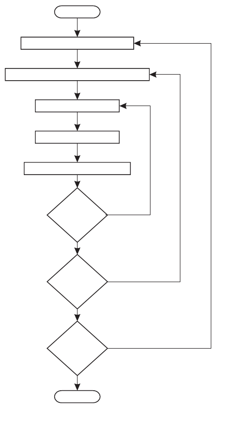
CHAPTER 4--Design and Structure of the SEAWAT Program 27
CHAPTER 4
DESIGN AND STRUCTURE OF THE SEAWAT PROGRAM
The SEAWAT code is MODFLOW and MT3DMS combined into a single program that solves the
coupled flow and solute-transport equations. Parts of the original MODFLOW code were modified to
include the relative density-difference terms and the term that quantifies the rate of mass accumulation due
to changes in solute concentration, and the entire flow equation was reformulated to conserve mass rather
than fluid volume. The coupling between flow and transport is performed through a synchronous timestep-
ping approach that cycles between MODFLOW solutions of the flow equation and MT3DMS solutions of
the transport equation (fig. 4).
SEAWAT includes both explicit and implicit methods for coupling the flow and solute-transport equa-
tions. With the explicit method, a lagged approach is used for assigning fluid densities in the flow equation.
This means that fluid densities are calculated with solute concentrations from the previous timestep. Advec-
tive fluxes from the flow solution for the current timestep are then used in the current solution to the trans-
port equation. This cycling mechanism results in an explicit coupling of the flow and transport equations.
With the implicit coupling method, solutions to the
flow and transport equations are repeated, and
concentrations and densities are updated within each
timestep until the maximum difference in fluid
density at a single cell for consecutive iterations is
less than a user-specified value.
The present version of SEAWAT is written
with MODFLOW-88 and MT3DMS. In linking
these two codes, the SEAWAT program was coded
and designed to meet the following three objectives
in order of importance:
1. Simulations provide an accurate solution to the
variable-density ground-water flow equation;
2. The program maintains a modular structure,
which makes it easy to modify and improve; and
3. Modifications to the original MODFLOW and
MT3DMS subroutines and input files are kept to
a minimum to allow users of these programs to
gain rapid familiarity with SEAWAT and to allow
newer versions of MODFLOW and MT3DMS to
be easily incorporated into SEAWAT.
The third objective was only partially achieved
because many of the MODFLOW procedures
required modification to accommodate the variable-
density form of the ground-water flow equation.
This chapter presents the overall design and
structure of the SEAWAT program and provides the
framework for Chapter 5, which provides details of
the modifications of MODFLOW and MT3DMS.
MODFLOW and MT3DMS are lengthy programs
that do much more than simply solve equations.
Both programs perform read and write operations,
track volumetric and mass budgets, and so forth. For
START
INITIALIZE STRESS PERIOD
CALCULATE LENGTH OF TIMESTEP
SOLVE FLOW
SOLVE TRANSPORT
UPDATE FLUID DENSITIES
LARGE
DENSITY
CHANGE
YES
NO
END OF
STRESS
PERIOD
NO
YES
NO
END OF
SIMULATION
YES
END
IMPLICIT COUPLING LOOP
(OPTIONAL)
TIMESTEP LOOP
STRESS PERIOD LOOP
Figure 4. Generalized flow chart of the SEAWAT
program.

28 User’s Guide to SEAWAT: A Computer Program for Simulation of Three-Dimensional Variable-Density Ground-Water Flow
this reason, the phrases “solve the flow equation” or “solve the transport equation” are used herein to refer
to only those parts of MODFLOW or MT3DMS, respectively, which are actually required to solve the
particular equation.
Temporal Discretization
The temporal discretization scheme implemented in the SEAWAT code is a combination of the
schemes used by MODFLOW and MT3DMS. This section reviews the temporal discretization schemes
implemented in the conventional versions of MODFLOW and MT3DMS and presents the approach
implemented in SEAWAT.
For a conventional MODFLOW application, the total simulation period is divided into one or more
stress periods. During a single stress period, flow rates and boundary heads−with the exception of the Time-
Varying Constant Head (CHD) package−remain constant. Each stress period is further divided into one or
more timesteps to produce results that are more accurate or to allow output from the model to be saved for
selected times. During each timestep, MODFLOW solves the flow equation for the period from tnto tn+1.
MT3DMS was originally designed to work with MODFLOW. In a conventional MODFLOW-
MT3DMS application, spatial and temporal variations in fluid density are assumed to be so small as to have
no measurable effect on the flow field. Thus, a practical procedure was developed in which the flow simu-
lation is first performed with MODFLOW, and during the simulation, flow information (saturated thickness,
cell-by-cell discharge rates, and boundary flows) required by MT3DMS to solve the solute-transport equa-
tion is stored in a MODFLOW-MT3DMS link file. This link file is then used in a subsequent MT3DMS run
in which only solute transport is simulated.
MT3DMS further divides each MODFLOW timestep into transport steps. The term, transport step,
was introduced to avoid confusion with a MODFLOW timestep. A transport step, however, is the timestep
or time increment used by MT3DMS to solve the transport equation (eq. 38), and thus, is conceptually
analogous to a MODFLOW timestep. MODFLOW timesteps are further divided into transport steps in
MT3DMS because of stability requirements with the explicit solution schemes implemented in MT3DMS.
For example, Zheng and Wang (1998) list the stability constraints and accuracy requirements for the
transport of conservative species with the explicit finite-difference scheme as:
advection, ,
(56a)
dispersion, , (56b)
and:
sink/source, , (56c)
where:
∆tis the length of the timestep, and
∆x,∆y,∆z are the dimensions of the model cell.
MT3DMS uses the stability constraints and accuracy requirements in equation 56a-c to calculate the
maximum permissible length of transport steps; therefore, the lengths of transport steps are not specified by
the user, but rather calculated by the program. The stability constraint for advection requires flow velocities
∆t1
vx
∆x
------ vy
∆y
------ vz
∆z
------
++
---------------------------------
≤
∆t0.5
Dxx
∆x2
---------Dyy
∆y2
---------Dzz
∆z2
--------
++
----------------------------------------
≤
∆tθ
qs
-------
≤
CHAPTER 4--Design and Structure of the SEAWAT Program 29
to calculate transport step lengths. For a given MODFLOW timestep, extending from tnto tn+1,MT3DMS
uses the velocities calculated for the end of the timestep, tn+1, in equation 56a-c to calculate the length and
number of transport steps required over the interval tnto tn+1.
In addition to the explicit solvers for the transport equation, MT3DMS also has an implicit iterative
procedure called the generalized conjugate gradient (GCG) solver (Zheng and Wang, 1998). With the
implicit solver, the user is allowed to specify the lengths of transport steps. In many cases, the implicit solver
may reduce the number of transport steps required for a simulation. The lengths of transport steps, however,
may be limited by accuracy requirements, and convergence issues may arise if the specified transport
lengths are too long.
The above procedure involves the calculation of the full sequence of head and flow values prior to
the start of transport calculation and cannot be used in a variable-density program because of the interde-
pendence of the flow and transport equations. In SEAWAT, stress periods are divided into timesteps. If an
explicit solver is used for transport, the timestep lengths are calculated during the simulation by SEAWAT
to satisfy the stability constraints and accuracy requirements (eq. 56a-c), and thus, the number of timesteps
is not known prior to execution. Both the flow and transport equations are solved during a SEAWAT
timestep. For the coupling of the flow and the transport equations, the SEAWAT program contains two
approaches, explicit and implicit. The explicit approach requires less computer time but may not be as accu-
rate as the implicit approach. Additionally, smaller timesteps may be required for the explicit approach
compared to those needed for the implicit approach. Descriptions of these coupling options are presented in
the subsequent sections.
Explicit Coupling of Flow and Transport
The following sequence is used in SEAWAT to advance the simulation through time if the user specifies
an explicit coupling between flow and transport (fig. 5).
Figure 5. Example of the explicit scheme used to couple the flow and
transport equations.
∆t1∆t2∆t3
∂t
∂C
ρ00
=( ); =0fC
∂∆tt
2
∂CC-C
21
ρ22
= ( ); =fC
∂∆
t
t1
∂CC-C
10
ρ11
= ( ); =fC
TIME
1
2
3
TIMESTEP
Distribution of fluid density at end of timestep [ML ]
Distribution of solute concentration at end of timestep [ML ]
Field of specific discharge at end of timestep [LT ]
n
n
n
-3
-3
-1
C
q
ρn
n
n
C1
q1
C2
q2
C3
q3
FLOW
TRANSPORT
FLOW
TRANSPORT
FLOW
TRANSPORT
t0t1t2t3
1. The flow equation is solved
iteratively using the modified
MODFLOW routines to calculate
heads at a time t1,representingthe
end of the initial timestep. This
iterative solution procedure is
performed with fluid densities
from the previous stress period, or
with densities calculated from the
initial solute concentrations if it is
the first stress period. The length
of the initial timestep, ∆t1,is
specified by the user through the
input variable INITIALDT or is
assigned a default value if no
input is specified. The default
value currently used in SEAWAT
is 0.01 time units; the default
value would be 0.01 day, for
example, if the units selected for
time are days.
30 User’s Guide to SEAWAT: A Computer Program for Simulation of Three-Dimensional Variable-Density Ground-Water Flow
2. Values of specific discharge for time t1at model boundaries and within the model domain are
calculated from the results of the flow simulation and passed to the transport routines to represent
flow over the time interval ∆t1.
3. Solute concentrations for time t1are determined by solving the transport equation over the time
interval ∆t1.
4. Fluid densities for t1, which are used in solving the flow equation for the second timestep, are
calculated from the t1solute concentrations.
5. The length of ∆t2is calculated according to the stability constraints and accuracy requirements,
using velocities calculated for the beginning of that time period. This calculated timestep length
for ∆t2should always be greater than the length of the initial timestep length, ∆t1. A calculated
value for ∆t2less than ∆t1indicates rapidly changing concentration and density fields at the
beginning of the stress period. If ∆t1, which has a default value of 0.01 time units unless
otherwise specified by the user, is greater than ∆t2, SEAWAT displays a warning message. At this
point, the user needs to go back to step 1 and shorten the value of INITIALDT, and rerun
SEAWAT.
6. The flow equation is solved to calculate heads and flows for the end of the second step, t2,using
the fluid densities that were calculated in the first timestep.
7. Solute concentrations for time t2are determined by solving the transport equation over the time
interval ∆t2. These concentrations are then used to calculate fluid densities for t2.
8. The stability constraints and accuracy requirements are used to calculate the maximum timestep
length for ∆t3, and the sequence is repeated.
When the explicit coupling approach is used in SEAWAT, three criteria should be considered: (1)
instability problems may occur during solution of the flow equation because densities are calculated using
the previous timestep concentrations; (2) the lengths of timesteps, which are calculated to satisfy the stabil-
ity constraints and accuracy requirements of the transport equation, are based on velocities calculated for
the end of the preceding timestep; and thus (3) there is a lag of one timestep in the application of the stability
constraints and accuracy requirements. The constraints that should be applied to timestep nare actually
appliedtotimestepn+1. Because this coupling approach is explicit, additional simulations with reduced
timestep lengths should be performed to verify that consistent results are obtained.
Implicit Coupling of Flow and Transport
The implicit approach involves the solution of the flow and transport equations in an iterative
sequence for each timestep until the consecutive differences in the calculated fluid densities are less than a
user-specified value (fig. 6). Referring to the explicit approach outlined previously, the implicit coupling
approach will repeat steps 2, 3, and 4 within each timestep until the consecutive change in fluid density is
less than a user-specified convergence value. The implicit coupling approach results in heads, concentra-
tions, densities, and flows that pertain to the end of the timestep.
The implicit coupling approach in the current version of SEAWAT only works when a MT3DMS
finite-difference method (as opposed to a particle-tracking-based method) is used to solve the solute-trans-
port equation. The implicit coupling approach was not programmed for the particle-based solution methods
because of the computer memory that would be required to store particle information. As the implicit
coupling approach may solve the transport equation more than one time for each timestep, the same starting
particle distribution would have to be used for each solution.
CHAPTER 4--Design and Structure of the SEAWAT Program 31
TRANSPORT
FLOW
FLOW
FLOW
1,1
1,2
1,3
2,1
2,2
3,1
3,2
∆t2∆t3
TIME
TIMESTEP, IMPLICIT COUPLING ITERATION
Distribution of fluid density at end of timestep and end of coupling iteration [ML ]
Distribution of solute concentration at end of timestep and end of coupling iteration [ML ]
Field of specific discharge at end of timestep and end of coupling iteration [LT ]
n ncpl
n ncpl
n ncpl
-3
-3
1
-
C
q
ρn,ncpl
n,ncpl
n,ncpl
ρ
1 0 1,0
,=fC()
ρ11 11
,,
=fC()
ρ1,2 1,2
=fC()
ρ1,3 1,3
=fC()
ρ2,1 2,1
=fC()
ρ2,2 2,2
=fC()
ρ3,1=fC()
3,1
TRANSPORT
TRANSPORT
C1,2
C1,1
C13
,
q1,1
q1,2
q1,3
FLOW
q2,1
C22
,
C2,1
q2,2
TRANSPORT
TRANSPORT
FLOW
q3,2
C3,2
q3,1
C3,1
TRANSPORT
FLOW
TRANSPORT
FLOW
t1t2t3
∆t1
t0
With the implicit coupling approach, the user may specify the lengths of the timesteps. In a conven-
tional application of MT3DMS, the implicit GCG solver can increase the lengths of transport steps, reduce
the number of transport steps, and substantially reduce the amount of time required for a computer to
perform the simulation. While the GCG solver may be used in SEAWAT to increase the lengths of timesteps,
the advantages may not be as large as with conventional applications of MT3DMS because of the interde-
pendence between flow and transport. As with the explicit coupling approach, repeated simulations with
shorter timesteps can help verify the numerical accuracy of results.
Structure of the SEAWAT Program
The structure of the original MODFLOW and MT3DMS programs is a main program that performs
calls to subroutines. This is the general approach used by SEAWAT, whereby the main SEAWAT program
makes calls to MODFLOW, MT3DMS, and SEAWAT subroutines. The main SEAWAT program was writ-
ten by adding appropriate MT3DMS and SEAWAT subroutine calls to the main MODFLOW program and
synchronizing the timesteps.
The original MODFLOW and MT3DMS main programs are divided into “procedures,” which are
categories of tasks that fall under the same general purpose. Because SEAWAT primarily consists of
MODFLOW and MT3DMS, the main SEAWAT program also is divided into procedures. The flow chart
for SEAWAT procedures is presented in figure 7.
Figure 6. Example of the implicit scheme used to couple the flow and transport equations.
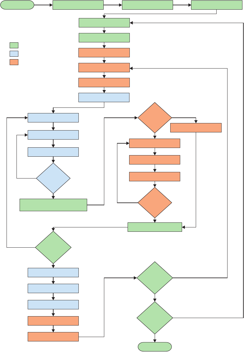
32 User’s Guide to SEAWAT: A Computer Program for Simulation of Three-Dimensional Variable-Density Ground-Water Flow
EXPLANATION
START DEFINE ALLOCATE READ AND PREPARE
STRESS
READ AND PREPARE
READ AND PREPARE
COEFFICIENT
ADVANCE
ADVANCE
FORMULATE
FORMULATE
APPROXIMATE
DONE
ITERATING
NO
YES
SAVE ADVECTIVE FLUXES
IMPLICIT
SOLVER
FORMULATE
APPROXIMATE
COEFFICIENT
NO
YES
YES
NO
YES
NO
YES
NO
YES
NO
DONE
ITERATING
CALCULATE DENSITY
SOLVE
LARGE
DENSITY
CHANGE
OUTPUT CONTROL
BUDGET
OUTPUT
BUDGET
OUTPUT
MORE
TIMESTEPS
MORE
STRESS
PERIODS
END
IMPLICIT COUPLING LOOP (OPTIONAL)
TIMESTEP LOOP
STRESS PERIOD LOOP
SEAWAT procedure
Flow procedure
Transport procedure
Figure 7. Step-by-step procedures of the SEAWAT program.

CHAPTER 4--Design and Structure of the SEAWAT Program 33
Packages
The 1988 version of MODFLOW and the MT3DMS version of MT3D are used in SEAWAT. Both of
these codes utilize the “package” approach in which features and options may be turned on or off by users
depending on the requirements of the specific problem. Table 1 lists the packages that are available in the
current version of SEAWAT. Several additional MODFLOW packages, introduced after the 1988 version of
MODFLOW was released, also are included in SEAWAT to extend the applicability of the program to a
wide range of problems. These additional or updated packages include the BCF2 package (McDonald and
others, 1992), EVT package that allows evapotranspiration to be withdrawn from the highest active cell
(Swain and others, 1996), CHD package (Leake and Prudic, 1988), PCG2 package (Hill, 1990), and
LKMT3D package (Zheng and Wang, 1998).
Array Structure and Memory Allocation
Both MODFLOW and MT3DMS utilize the same general approach for allocating computer memory.
In the original versions of MODFLOW and MT3DMS, a single array, called the X array, is used to store
most of the information for a simulation. In the SEAWAT code, four main arrays are used: X array
(for MODFLOW information), Y array (for real MT3DMS information), IY array (for integer MT3DMS
information), and Z array (for SEAWAT-specific information). Computer memory for each of these arrays
is allocated during run time using the FORTRAN 90 statements—ALLOCATABLE and ALLOCATE.
Table 1. MODFLOW and MT3DMS packages used in SEAWAT
Package Acronym Program Reference
Basic BAS MODFLOW McDonald and Harbaugh (1988)
Block-Centered Flow BCF2 MODFLOW McDonald and others (1992)
Well WEL MODFLOW McDonald and Harbaugh (1988)
Drain DRN MODFLOW McDonald and Harbaugh (1988)
River RIV MODFLOW McDonald and Harbaugh (1988)
Evapotranspiration EVT MODFLOW Swain and others (1996)
General-Head Boundary GHB MODFLOW McDonald and Harbaugh (1988)
Recharge RCH MODFLOW McDonald and Harbaugh (1988)
Strongly Implicit Procedure SIP MODFLOW McDonald and Harbaugh (1988)
Successive Over-Relaxation SOR MODFLOW McDonald and Harbaugh (1988)
Preconditioned Conjugate Gradient Solver PCG2 MODFLOW Hill (1990)
Output Control OC MODFLOW McDonald and Harbaugh (1988)
Time-Variant Constant Head CHD MODFLOW Leake and Prudic (1988)
LinkMT3D LKMT3D MODFLOW Zheng and Wang (1998)
Basic Transport BTN MT3DMS Zheng and Wang (1998)
Advection ADV MT3DMS Zheng and Wang (1998)
Dispersion DSP MT3DMS Zheng and Wang (1998)
Source/Sink Mixing SSM MT3DMS Zheng and Wang (1998)
Reaction RCT MT3DMS Zheng and Wang (1998)
Generalized Conjugate Gradient Solver GCG MT3DMS Zheng and Wang (1998)
34 User’s Guide to SEAWAT: A Computer Program for Simulation of Three-Dimensional Variable-Density Ground-Water Flow
CHAPTER 5--Modifications of MODFLOW and MT3DMS 35
CHAPTER 5
MODIFICATIONS OF MODFLOW AND MT3DMS
Under the SEAWAT approach, two separate computer programs, MODFLOW and MT3DMS, were
modified and combined into one program. Among these modifications are the conversion of volumetric
fluxes to mass fluxes and the addition of relative density-difference terms and solute-mass accumulation
terms to the basic finite-difference equation solved by MODFLOW. Additionally, modifications were made
to each of the stress packages of MODFLOW because mass fluxes and freshwater heads are used in
SEAWAT. Modifications of MT3DMS are relatively minor and mainly affect internal data transfer and
manipulation. This chapter focuses on the modifications made to the block-centered flow (BCF) package
and the following stress packages implemented in MODFLOW:
• Well (WEL) package
• River (RIV) package
• Drain (DRN) package
• Recharge (RCH) package
• Evapotranspiration (EVT) package
• General-Head Boundary (GHB) package
• Time-Varying Constant Head (CHD) package
This chapter shows how the equations, as originally formulated in MODFLOW, were modified to
represent variable-density ground-water flow. To simplify this documentation, presentation of the
FORTRAN source code is excluded because much of the SEAWAT program is unmodified MODFLOW
and MT3DMS code. Modifications to the original MODFLOW and MT3DMS programs are marked in the
source code where the changes were made.
Matrix and Vector Accumulators
SEAWAT uses the same approach as MODFLOW for constructing the matrix equations that describe
ground-water flow. Equation 55 shows the general form of the matrix equation solved by SEAWAT and is
identical in form to the one solved by MODFLOW. The [A] matrix represents coefficients of equivalent
freshwater head, of which a portion is stored in a three-dimensional array called the HCOF accumulator.
The {B} vector represents constant terms on the right-hand side of equation 55 and is stored in a three-
dimensional array called the RHS accumulator. MODFLOW and SEAWAT pass these accumulators and
other terms into subroutines that solve for head or equivalent freshwater head, respectively.
As part of the solution procedure, a series of subroutines assemble the RHS and HCOF accumulators.
Prior to assembly, the RHS and HCOF accumulators are initialized with values of zero. During the assem-
bly, consecutive calls to various subroutines add to or subtract from the accumulators in order to include
storage effects, sources, sinks, and other components. In the following sections, the RHS accumulator is
referred to in mathematical expressions as and . represents the value of RHS
for cell (i,j,k) up to that point in the series of assembly subroutines. The term represents the new
value of RHS at cell (i,j,k) after the mathematical expression from that subroutine has been applied. Note,
however, that the final value of passed into the solver cannot be determined until the entire
sequence of assembly routines has been called.
RHSijk,,
old RHSijk,,
new RHSijk,,
old
RHSijk,,
new
RHSijk,,
new
36 User’s Guide to SEAWAT: A Computer Program for Simulation of Three-Dimensional Variable-Density Ground-Water Flow
Modifications of the Basic Flow Equation
In Chapter 3, the finite-difference equation for freshwater head in cell (i,j,k) was developed with the
simplification that relative density-difference terms are kept constant within each timestep (or within each
solution of the flow equation if the implicit coupling approach is utilized). Inspection of the flow equation
solved by SEAWAT (eq. 50) suggests that it is similar in mathematical form to the equation solved by
MODFLOW (eq. 52). Thus, the solution techniques implemented in the original version of MODFLOW
also can be used to solve the variable-density flow equation if the code is appropriately modified to include
the density terms.
Addition of Relative Density-Difference Term
The relative density-difference term for a model cell, as defined in equation 48 (and in more detail in
eq. 49a-f), is treated as constant during solution of the flow equation. With the explicit approach for coupling
flow and transport, the density values are calculated from solute concentrations from the previous timestep
(or initial concentrations for the first timestep). With the implicit approach for coupling flow and transport,
the density values are calculated from solute concentrations from the previous iteration of that timestep.
SEAWAT adds the relative density-difference term to the RHS accumulator using the following
expression:
. (57)
Note that one or more of the six components of the relative density-difference term (eq. 49a-f) may equal
zero if the fluid density is the same as the density of freshwater, or if the elevations of two adjacent cell
centers are the same.
Weiss (1982) developed a similar approach for the steady-state situation when fluid density does not
change with time. With that approach, “pseudo sources” are calculated for each model cell prior to simula-
tion. The “pseudo sources,” which represent the relative density-difference terms, are then treated as
constants during a simulation with a constant density ground-water flow model.
Addition of Solute Mass Accumulation Term
A similar approach to that used for the density-difference terms also can be used to include the term
for solute mass accumulation. The term for solute mass accumulation can be added to the RHS accumulator
because the term does not contain the principal variable, freshwater head. With the explicit coupling
approach, the partial derivative for solute concentration, , is evaluated using concentrations from the
previous timestep. With the implicit coupling approach, is evaluated using concentrations from the
previous coupling iteration. With either approach, is zero for the first timestep of a simulation.
For the explicit coupling approach, SEAWAT uses the following expression to include the term for
solute mass accumulation in the RHS accumulator:
. (58)
For the implicit coupling approach, a similar equation is used to update the RHS accumulatorexceptthatthe
concentrations from a previous coupling iteration are used rather than concentrations from a previous
timestep.
RHSijk,,
new RHSijk,,
old Dijk,,
–=
∂C∂t⁄
∂C∂t⁄
∂C∂t⁄
RHSijk,,
new RHSijk,,
old θECijk,,
n1– Cijk,,
n2–
–
tn1–
∆
------------------------------- Vijk,,
+=
CHAPTER 5--Modifications of MODFLOW and MT3DMS 37
Conversion from Volume Conservation to Mass Conservation
Volumetric fluxes are converted to mass fluxes by multiplying by fluid density. This is accomplished
by multiplying the conductance terms by fluid density. In MODFLOW, three-dimensional arrays called CC,
CR and CV contain values of conductance in each direction. The conductance values stored in these three
arrays are calculated as the harmonic mean of the transmissivity between two adjacent nodes. For example,
the conductance along a column is calculated with the following equation:
, (59)
where:
DELR is the grid width along the row [L],
TC is the transmissivity for each cell in the column direction [L2T-1], and
DELC is the grid width along the column [L].
These conductance arrays may or may not be updated during simulations depending on the aquifer type
(LAYCON) specified by the user.
In SEAWAT, three new arrays (RHOCR, RHOCC, and RHOCV) are used to hold the mass conduc-
tances, which are the conductance values multiplied by fluid density. The original conductance arrays (CR,
CC,andCV) are still used to hold the values of conductance in each direction. The new arrays are calculated
as the product of the conductance terms and the fluid density in the upstream direction. An example of the
expression is:
. (60)
Whether or not the conductance terms are updated, these three new arrays are recalculated within each
iteration of the flow equation. The three mass conductance arrays are passed into the solver, rather than the
original conductance arrays, because the system of equations is conserving fluid mass, not fluid volume.
Conversion from Fluid Volume Storage to Fluid Mass Storage
For a layer in which the storage coefficient remains constant during the simulation, the storage
formulation is based on a direct application of the storage expression that applies to an individual cell, (i,j,k).
In MODFLOW, the storage expression has the form:
, (61)
where:
∆V/∆tis the volumetric rate of accumulation of water in the cell;
SSi,j,k is the specific storage of the material in cell i,j,k;and
∆rj,∆ci,∆vkare the cell dimensions.
In SEAWAT, the storage formulation has the form:
, (62)
CCi12jk,,⁄+2DELR TCijk,, TCi1jk,,+
TCijk,, DELCi1+ TCi1jk,,+DELCi
+
-----------------------------------------------------------------------------------------
=
RHOCCi12jk,,⁄+ρ
ˆ
i12jk,,⁄+CCi12jk,,⁄+
=
∆V
∆t
------- SSijk,, ∆rj∆ci∆vk
()
hijk,,
nhijk,,
n1–
–
tntn1–
–
-----------------------------
=
∆m
∆t
--------ρijk,, SSijk,, ∆rj∆ci∆vk
()
hfijk,,,
nhfijk,,,
n1–
–
tntn1–
–
------------------------------------
=
38 User’s Guide to SEAWAT: A Computer Program for Simulation of Three-Dimensional Variable-Density Ground-Water Flow
where ∆m/∆tis the rate of mass accumulation of water in the cell. Using the storage concept defined in
MODFLOW, mass storage capacity, SC1i,j,k, can be defined as:
. (63)
Equation 62 then can be rewritten as:
. (64)
Conversion Between Confined and Unconfined Conditions
The primary value for specific storage is only adequate if the water level in each individual cell
remains above the top of the cell during an entire simulation or below the top of the cell during an entire
simulation. If the water level in a cell crosses the top of the cell during a simulation, the aquifer “converts”
from confined to water-table (unconfined) conditions, or vice versa. When these conditions are likely, the
user may invoke a storage term conversion by specifying the appropriate layer-type flag (LAYCON).
In SEAWAT, a check is made after each iteration of the flow equation to determine if the head in a cell
is above the top of the cell. This check is only performed if the layer is specified as “convertible”
(for example, LAYCON = 2 or 3). Because the check depends on the elevation of the water table, the head
is used rather than the freshwater head. The expression for calculating head at cell (i,j,k)is:
, (65)
where hi,j,k is the head value [L]. The head value (as opposed to the value of freshwater head) is used to
determine if the water table is above the top of the cell. The storage conversion mechanism is invoked only
when the head crosses the top of the cell during the simulation. When the storage conversion is necessary,
the rate of fluid mass accumulation in storage in cell (i,j,k) is formulated as follows:
, (66)
where:
SCB is the “current” storage capacity during the iteration in progress,
TOP is the elevation of the top of the model cell, and
SCA is the storage capacity in effect in cell (i,j,k) at the start of the timestep.
Note that the freshwater head value is used in the storage calculation, but the actual head is used to check
for the onset of storage conversion. This is because the change in freshwater head serves as an indicator of
pressure change, which is ultimately responsible for storage accumulation, whereas the actual head is
required to measure water-level movement.
Vertical Flow Calculation for Dewatered Conditions
MODFLOW accounts for the special case of downward vertical flow into a dewatering cell by adding
correction terms to the RHS accumulator (fig. 8). Similar conditions might be encountered in a SEAWAT
simulation; therefore, correction terms based on the variable-density form of Darcy’s law are used to
account for downward flow into a dewatering cell.
SC1ijk,, ρijk,, SSijk,, ∆rj∆ci∆vk
()=
∆m
∆t
--------SC1ijk,,
hfijk,,,
nhfijk,,,
n1–
–
tntn1–
–
------------------------------------
=
hijk,,
ρf
ρijk,,
------------hfijk,,,
ρijk,, ρf
–
ρijk,,
-----------------------Zijk,,
+=
∆m
∆t
--------SCB hfijk,,,
nTOPijk,,
–()SCA TOPijk,, hfijk,,,
n1–
–()+
tntn1–
–
----------------------------------------------------------------------------------------------------------------------------
=
CHAPTER 5--Modifications of MODFLOW and MT3DMS 39
ρ
i,j,k
Z
i,j,k
Z
i,j,k+1
ρ
i,j,k+1
i,j,k
Q
i,j,k+1/2
i,j,k+1
i,j,k
NOTE: L = length, M = mass, T = time
EXPLANATION
Indices that refer to row, column, and layer,
respectively, of a finite-difference model grid
Equivalent freshwater head [L]
Head [L]
Flow rate [L T ]
3-1
Fluid density [ML ]
-3
Elevation of cell center [L]
Top elevation of model cell [L]
h
f
h
Q
ρ
Z
TOP
h
i,j,k+1
TOP
i,j,k+1
ρ
i,j,k-1
Z
i,j,k-1
Z
i,j,k
ρ
i,j,k
i,j,k-1
Q
i,j,k-1/2
i,j,k
h
i,j,k
TOP
i,j,k
CORRECTION TO
OVERLYING CELL
CORRECTION TO
UNDERLYING CELL
Q
C
Q
C
Flow correction [L T ]
3-1
Qc
Noting that MODFLOW layers are numbered from top downward, the downward vertical flow from
upper cell (i,j,k) to lower cell (i,j,k+1) is normally computed with the following equation:
, (67)
where is the mass flux of fluid between the two cells [MT-1].
Equation 67 is based on the assumption that cell (i,j,k+1) is fully saturated, which means that the
water level in cell (i,j,k+1) is higher than the top of the cell. There are, however, situations in which cell
(i,j,k+1) could become partially unsaturated while the overlying cell remains saturated. In this case, flow
between cell (i,j,k)andcell(i,j,k+1) does not depend on the head in cell (i,j,k+1). In this case, the “actual”
mass flux, , between cell (i,j,k) and cell (i,j,k+1), which is partially dewatered, is:
Qijk 12⁄+,,
mρ
ˆijk 12⁄+,, CVijk 12⁄+,, hfijk,1+,, hfijk,,,
–ρijk 12⁄+,, ρf
–
ρf
---------------------------------- Zijk,1+,Zijk,, )–(+=
Qijk 12⁄+,,
m
Qa
m
Figure 8. Cell indices and
variable definitions for the
case of a partially dewatered cell
underlying an active model cell.
A correction term is added to the
overlying cell and subtracted
from the underlying cell to
account for the inaccurate flow
rate that would be calculated
with the uncorrected finite-differ-
ence equation. Note that in each
case, cell indices are rewritten
so that the correction is applied
to cell i,j,k.
40 User’s Guide to SEAWAT: A Computer Program for Simulation of Three-Dimensional Variable-Density Ground-Water Flow
. (68)
Although equation 68 may not seem intuitive, it was derived from the variable-density form of Darcy’s law.
The correction term, , is calculated by subtracting equation 68 from equation 67 to give:
. (69)
The RHS accumulator is updated with the following equation to include this correction:
(70)
To overcome the problem of having the principal variable within the correction term, the value for hf,i,j,k+1
is taken from the preceding iteration of the flow equation, rather than from the current iteration.
In a similar manner, a correction term must also be applied to the cell that is being dewatered. In this
case, the cell (i,j,k) is being dewatered and is receiving flow from the overlying cell (i,j,k-1). In the standard
finite-difference equations shown in Chapter 3, the mass flux computed for this situation would erroneously
be calculated according to the following equation:
, (71)
but the “actual” mass flux is:
. (72)
The correction term, which is calculated by subtracting equation 72 from 71, is:
. (73)
This correction for the dewatering cell is handled by modifying the RHS accumulator according to the
following expression:
. (74)
As before, to overcome the problem of having the principal variable within the correction term, the value
for hf,i,j,k is taken from the preceding iteration of the flow equation, rather than from the current iteration.
Qa
mρ
ˆijk 12⁄+,, CVijk 12⁄+,, Zijk,, hfijk,,,
–ρijk 12⁄+,,
ρf
------------------------TOPijk,1+,Zijk,, )–(+=
Qc
m
Qc
mρ
ˆijk 12⁄+,, CVijk 12⁄+,, hfijk,1+,, Zijk 1+,,
–ρijk 12⁄+,,
ρf
------------------------Zijk,1+,TOPijk 1+,, )–(+=
RHSijk,,
new RHSijk,,
old
=
ρ
ˆijk 12⁄+,, CVijk 12⁄+,, hfijk,1+,, Zijk 1+,,
–
ρijk 12⁄+,,
ρf
------------------------------- Zijk,1+,TOPijk 1+,, )–(+.+
Qijk 12⁄–,,
mρ
ˆijk 12⁄–,, CVijk 12⁄–,, hfijk,1–,, hfijk,,,
–ρijk 12⁄–,, ρf
–
ρf
---------------------------------- Zijk,1–,Zijk,, )–(+=
Qa
mρ
ˆijk 12⁄–,, CVijk 12⁄–,, hfijk 1–,,, Zijk 1–,,
–ρijk 12⁄–,,
ρf
----------------------- Zijk 1–,, TOPijk,, )–(+=
Qc
mρ
ˆijk 12⁄–,, CVijk 12⁄–,, Zijk,, hfijk,,,
–ρijk 12⁄–,,
ρf
----------------------- TOPijk,, Zijk,, )–(+=
RHSijk,,
new RHSijk,,
old ρ
ˆijk 12⁄–,, CVijk 12⁄–,, Zijk,, hfijk,,,
–
ρijk 12⁄–,,
ρf
------------------------------- TOPijk,, Zijk,, )–(++=
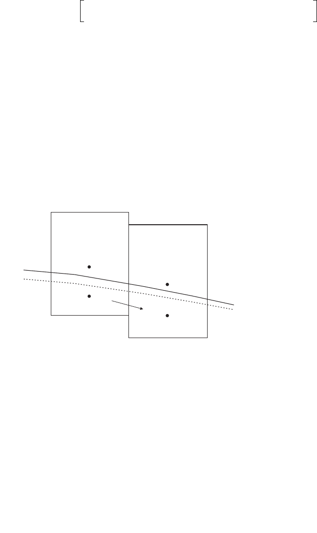
CHAPTER 5--Modifications of MODFLOW and MT3DMS 41
BOTi,j,k
hf
h
ZWT/2,i,j,k
ρi,j,k
Zi,j,k
Zi+1,j,k
ZWT/2,i+1,j,k
BOTi+1,j,k
ρi+1,j,k
i,j,k
Qi+1/2,j,k
i+1,j,k
i,j,k
NOTE: L = len
g
th, M = mass, T = time
EXPLANATION
Indices that refer to row, column, and layer,
respectively, of a finite-difference model grid
low rate [L T
Elevation of cell water [L]
Elevation of vertical midpoint between the water
table and the bottom of the model cell [L]
3-1
]
Equivalent freshwater head [L]
Head [L]
F
Fluid density [ML-3]
h
h
Q
Z
Z
f
WT/2
ρ
BOT
Variable-Density Flow for Water-Table Case
As previously shown, the general form of Darcy’s law used by SEAWAT to calculate the mass flux
between cell (i,j,k)and(i+1, j, k)is:
. (75)
For the water-table case (fig. 9), however, equation 75 cannot accurately represent the mass flux between
cell (i,j,k)and(i+1, j, k) for two reasons. First, the concept of equivalent freshwater head does not apply
when the evaluation point is above the water table. For example, when the center elevation of a model cell
is above the water table, the equivalent freshwater head will decrease as fluid density increases (if the water
table were to remain at the same elevation). This would suggest that for a fixed water-table elevation, if ρi,j,k
were to increase, then Qi+1/2,j,k would decrease, resulting in an inaccurate flow rate. The second reason that
equation 75 is not appropriate for the water-table case relates to the elevation for which the equivalent
freshwater head is evaluated. To accurately calculate flow between two cells, the equivalent freshwater head
should be calculated halfway between the water-table elevation, h, and the bottom of the cell, BOT.This
elevation is designated by ZWT/2 and corresponds to the vertical midpoint between the water table and the
bottom of the cell (fig. 9).
Qi12jk,,⁄+
mρ
ˆi12jk,,⁄+CCi12jk,,⁄+hfi 1jk,,+,hfijk,,,
–ρi12jk,,⁄+ρf
–
ρf
---------------------------------- Zi1jk,,+Zijk,,
–()+=
Figure 9. Conceptual representation of flow between two cells for
the water-table case.
42 User’s Guide to SEAWAT: A Computer Program for Simulation of Three-Dimensional Variable-Density Ground-Water Flow
Based on this conceptual model for the water-table case, a better expression for the mass flux between
cell (i,j,k)and(i+1,j,k)is:
Qm
i+1/2,j,k =i+1/2,j,kCCi+1/2,j,k [hf,WT/2,i +1,j,k
-hf,WT /2,i,j,k]+(ZWT / 2,i +1,j,k -ZWT / 2,i,j,k), (76)
where hf,WT/2,i,j,k and hf,WT/2,i+1,j,k are the equivalent freshwater heads at ZWT/2,i,j,k and ZWT/2,i+1,j,k, respectively.
These equivalent freshwater heads can be calculated from the equivalent freshwater heads at the cell centers
by assuming hydrostatic conditions within the model cell:
, (77)
and:
. (78)
By substituting equations 77 and 78 into equation 76, the expression for flow between cell (i,j,k)and
(i+1,j,k) in terms of the equivalent freshwater head at the cell centers is:
(79)
In SEAWAT, the method for using equation 79 to solve for the water-table case is similar to the correction
method used by MODFLOW and SEAWAT for the dewatered case. If equation 75 represents the flow
calculated by SEAWAT without any adjustments for the water-table case, a correction term can be calculated
by subtracting the actual flow (eq. 79) from equation 75. The correction term can then be incorporated into
the RHS accumulator to adjust for error that would result from using equation 75. Through algebraic
manipulation, the water-table correction term for flow between cell (i,j,k)and(i+1, j, k)is:
(80)
The correction term is a function of ZWT/2,whichis:
. (81)
The addition of the correction term for the water-table case adds nonlinearity to the flow equation because
head is a function of equivalent freshwater head. This problem is partially treated by using the equivalent
ρ
ˆ
ρi12jk,,⁄+ρf
–
ρf
-------------------------------------------
hfWT 2ijk,,,⁄, hfijk,,,
ρijk,, ρf
–
ρf
-----------------------Zijk,, Z–WT 2ijk,,,⁄
()+=
hfWT 2i1+ jk,,,⁄, hfi 1+ jk,,,
ρi1+ jk,, ρf
–
ρf
----------------------------- Zi1jk,,+Z–WT 2i1+ jk,,,⁄
()+=
Qi12jk,,⁄+
mρ
ˆi12jk,,⁄+CCi12⁄+jk,, hfi 1jk,,+,
ρi1jk,,+ρf
–
ρf
----------------------------- Zi1jk,,+ZWT 2i1jk,,+,⁄
–()+=
hfijk,,,
–ρ–ijk,, ρf
–
ρf
--------------------------Zijk,, ZWT 2ijk,,,⁄
–()
ρi12⁄+jk,, ρf
–
ρf
---------------------------------- ZWT 2i1jk,,+,⁄ ZWT 2ijk,,,⁄
–()++ .
Qc
mρ
ˆi12jk,,⁄+CCijk,,
ρi12jk,,⁄+ρf
–
ρf
---------------------------------- Zi1jk,,+Zijk,,
–ZWT 2ijk,,,⁄ZWT 2i1jk,,+,⁄
–+()=
ρi1+ jk,, ρf
–
ρf
----------------------------- ZWT 2i,⁄ 1+ jk,, Zi1jk,,+
–()
ρijk,, ρf
–
ρf
-----------------------Zijk,, ZWT 2ijk,,,⁄
–()++.
ZWT 2⁄
hBOT+
2
---------------------
=
CHAPTER 5--Modifications of MODFLOW and MT3DMS 43
freshwater head from the previous iteration of the flow equation to solve for the ZWT/2 terms prior to
calculating the correction term.
This development of the correction term for the water-table case was presented for flow between cell
(i,j,k)and(i+1,j,k). For a two-dimensional water-table layer, there may be up to four correction terms, one
for each horizontally adjacent cell. These correction terms are used to update the RHS accumulator accord-
ing to the following expression:
(82)
Modifications of MODFLOW Stress Packages
Modifications to the original package subroutines in MODFLOW were required because the flow
equation in SEAWAT conserves mass, which means that all terms added to the RHS accumulator must be
written as mass fluxes. Additionally, all terms added to the HCOF accumulator must be coefficients of
freshwater head. Modifications to each of the stress packages in MODFLOW are described in the subse-
quent sections.
Well (WEL) Package
The WEL package is used to represent specified source or sink boundaries within the model domain.
These specified flux boundaries may be injection wells or extraction wells. Original MODFLOW subrou-
tines were modified to include the effects of injection and extraction wells. The RHS accumulator is updated
by adding or subtracting the mass flux of the well. The mass flux is equal to the flow rate of the well, QWELL,
multiplied by the appropriate fluid density, ρWELL. Conditional statements are used within the SEAWAT
program to determine the density of the well fluid. If the well is an extraction well, the fluid density is equal
to the density in the model cell. If the well is an injection well, the fluid density is calculated from the
concentration of the well injection fluid. The concentration of injected fluid, CWELL, is specified in the
Source/Sink Mixing (SSM) package of MT3DMS. These steps are summarized with the following mathe-
matical expressions:
RHSijk,,
new RHSijk,,
old ρ
ˆi12jk,,⁄+CRi12jk,,⁄+
ρi12jk,,⁄+ρf
–
ρf
-------------------------------------------Zi1jk,,+Zijk,,
–ZWT 2ijk,,,⁄Z–WT 2i1jk,,+,⁄
+()+=
ρi1jk,,+ρf
–
ρf
----------------------------- ZWT 2i1jk,,+,⁄ Zi1jk,,+
–()
ρijk,, ρf
–
ρf
-----------------------Zijk,, ZWT 2ijk,,,⁄
–()++
ρ
ˆi12jk,,⁄–CRi12jk,,⁄–
ρi12jk,,⁄–ρf
–
ρf
------------------------------------------ Zi1– jk,, Zijk,,
–ZWT 2ijk,,,⁄Z–WT 2i1– jk,,,⁄
+
()+
ρi1jk,,–ρf
–
ρf
----------------------------- ZWT 2i1– jk,,,⁄ Zi1jk,,–
–()
ρijk,, ρf
–
ρf
-----------------------Zijk,, ZWT 2ijk,,,⁄
–()++
ρ
ˆij,12k,⁄+CCij,12k,⁄+
ρij,12k,⁄+ρf
–
ρf
-------------------------------------------Zij 1k,+,Zijk,,
–ZWT 2ijk,,,⁄Z–WT 2ij 1k,+,,⁄
+
()+
ρij 1k,+,ρf
–
ρf
----------------------------- ZWT 2ij 1k,+,,⁄Zij 1k,+,
–()
ρijk,, ρf
–
ρf
-----------------------Zijk,, ZWT 2ijk,,,⁄
–()++
ρ
ˆij,12k,⁄–CCij,12k,⁄–
ρij,12k,⁄–ρf
–
ρf
------------------------------------------ Zij1– k,, Zijk,,
–ZWT 2ijk,,,⁄Z–WT 2ij 1– k,,,⁄
+
()+
ρij 1– k,, ρf
–
ρf
--------------------------- ZWT 2ij 1k,–,,⁄Zij 1– k,,
–()
ρijk,, ρf
–
ρf
-----------------------Zijk,, ZWT 2ijk,,,⁄
–().++
44 User’s Guide to SEAWAT: A Computer Program for Simulation of Three-Dimensional Variable-Density Ground-Water Flow
For an extraction well (Qwell <0):
. (83)
For an injection well (Qwell >0):
. (84)
Accordingly, the RHS accumulator is updated with the following expression:
. (85)
River (RIV) Package
TheRIVpackageinMODFLOWiscommonlyusedtoapproximateleakagetoorfromastreamor
river. The conceptual model is based on the vertical leakage of water across river bottom sediments (fig. 10).
The cross section of the river is assumed to be rectangular with impermeable vertical sides. Leakage into or
out of the model cell is dependent on the stage in the river (hRIV), the value of head in the model cell (hi,j,k),
and a conductance value. The conductance of the river is mathematically defined as:
, (86)
where:
CONDRIV is the conductance of the riverbed [L2T-1],
Lis the length of the river segment in the model cell [L],
wis the width of the river [L],
Kseds is the hydraulic conductivity of the river bottom sediments [LT-1], and
bseds is the thickness of the river bottom sediments [L].
The elevation of the base of the river bottom sediments is specified as RBOT, an input parameter for
the RIV package. When the head in the model cell is above RBOT, river leakage (QRIV) is calculated using
the following form of Darcy’s law:
. (87)
The sign convention used by MODFLOW treats ground-water sources as positive and sinks as negative.
QRIV
, therefore, is positive if the aquifer is receiving river leakage and negative if the aquifer is providing
baseflow to the river. If hi,j,k falls below RBOT, the RIV package uses a slightly different equation for
leakage:
. (88)
This approach restricts the maximum leakage rate and is a reasonable approximation for leakage when the
water table falls below the base of a saturated river bottom deposit.
To incorporate river leakage into the system of MODFLOW equations, the RHS and HCOF accumu-
lators are updated using the following conditions and expressions:
For hi,j,k >RBOT:
ρwell ρijk,,
=
ρwell ρfCwell E⋅+=
RHSijk,,
new RHSijk,,
old ρwell Qwell
⋅–=
CONDRIV
LwK
seds
⋅⋅
bseds
-----------------------------
=
QRIV CONDRIV hRIV hijk,, )–(⋅=
QRIV CONDRIV hRIV RBOT)–(⋅=
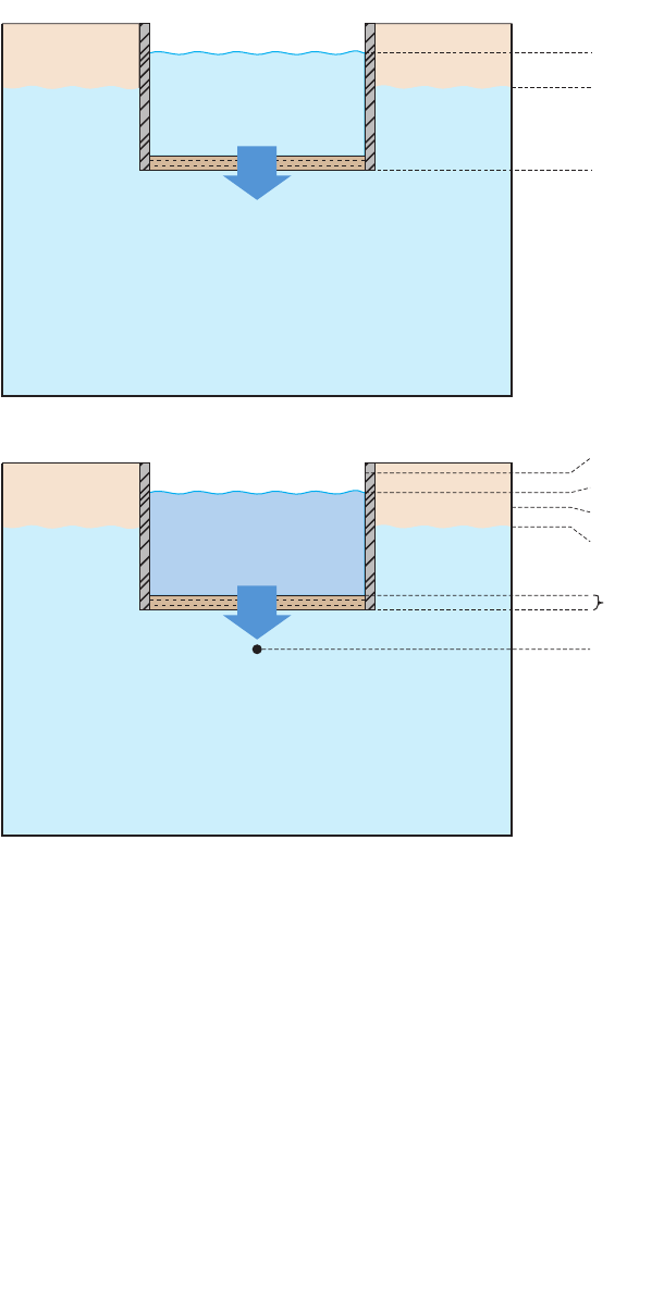
CHAPTER 5--Modifications of MODFLOW and MT3DMS 45
bseds
NOTE: L = length, M = mass, T = time
EXPLANATION
ρi,j,k
hRIV
QRIV
hi,j,k
RBOT
MODFLOW
QRIV
SEAWAT
ρRIV
hRIV
hi,j,k
hf,i,j,k
hf,RIV
RBOT
Zi,j,k
h
h
RBOT
h
h
b
Z
RIV
i,j,k
f,RIV
f,i,j,k
seds
i,j,k
ρ
ρ
RIV
i,j,k
RIV
Q
Head in the river [L]
Head in the model cell [L]
Bottom elevation of the river bed sediments [L]
Equivalent freshwater head in the river relative to the
top of the river bed [L]
Equivalent freshwater head in the model cell [L]
Thickness of river bed sediments [L]
Elevation of the center of the model cell [L]
Density of the river water [ML ]
Density of the water in the model cell [ML ]
Flux of water from the river to the aquifer [L T ]
-3
-3
3-1
Figure 10. Conceptual model and variable description for river leakage in
MODFLOW and SEAWAT.
46 User’s Guide to SEAWAT: A Computer Program for Simulation of Three-Dimensional Variable-Density Ground-Water Flow
, (89)
and:
. (90)
For hi,j,k <= RBOT:
. (91)
In SEAWAT, the mathematical treatment of river leakage is more complicated because a variable-
density form of Darcy’s law is required. Additionally, the river leakage must be converted from a volumetric
flux to a mass flux using the appropriate fluid density. The conceptual model of variable-density river leak-
age is shown in figure 10. To provide the reader with an understanding of how to incorporate a head-depen-
dent, variable-density package into SEAWAT, the development of the river leakage equations is presented
in detail.
The conceptual model for variable-density river leakage is based on vertical flow across river bottom
sediments. The general form of Darcy’s law for variable-density vertical flow is:
. (92)
In this form, positive flow is in the positive z direction (upward).
The objective of the following steps is to rewrite equation 92 into a form that can be added to the RHS
and HCOF accumulators in SEAWAT. This means that pressure will be replaced with freshwater head, the
conceptual model for river leakage will be used to reformulate the equation, and leakage will be converted
from volumetric flux to mass flux.
The equation for pressure (eq. 23) is substituted into equation 92, which is then rearranged to give:
. (93)
The equivalent freshwater hydraulic conductivity, Kf, is defined as:
. (94)
Substituting equation 94 into equation 93 gives:
. (95)
As previously discussed, the dynamic viscosity of water is slightly dependent on the concentration of
dissolved constituents, but for many applications it can be assumed that is one. With this
simplification, equation 95 reduces to:
. (96)
HCOFijk,,
new HCOFijk,,
old CONDRIV
–=
RHSijk,,
new RHSijk,,
old CONDRIV hRIV
⋅–=
RHSijk,,
new RHSijk,,
old CONDRIV hRIV RBOT)–(–=
QzA–k
µ
---dP
dz
-------ρg+=
QzAkρfg
µ
-----------dhf
dz
------- ρρ
f
–
ρf
--------------
+–=
Kf
kρfg
µf
-----------
=
QzAKf
µf
µ
---- dhf
dz
------- ρρ
f
–
ρf
--------------
+–=
µfµ⁄
Qz
AKf
dz
---------dhf
ρρ
f
–
ρf
--------------dz+–=
CHAPTER 5--Modifications of MODFLOW and MT3DMS 47
Equation 96 is one form of the equation for vertical, variable-density ground-water flow. In applying
this equation to the RIV package in SEAWAT, it was assumed that energy (pressure and elevation) losses
associated with the vertical flow occur primarily across the river bottom materials, and that losses across
the upper part of the model cell underlying the river are small by comparison. It was further assumed that
fluid density is essentially uniform within the cell. Under these assumptions the head, expressed in terms of
the cell fluid, does not vary with vertical distance through the cell; thus, the value for head is the same at
RBOT and the cell center. However, the values of freshwater head at RBOT and at the cell center must differ
under these conditions and are related by:
, (97)
and the equation for river leakage is:
, (98)
where ρis the average fluid density of the river and the model cell. By substituting equation 97 into equation
98, and introducing a new term called the equivalent freshwater river conductance, CONDf,RIV
,where:
, (99)
the equation for river leakage (changing the sign to the MODFLOW sign convention of positive into the
model cell) becomes:
. (100)
The volumetric river leakage, QRIV
, is converted to a mass river leakage by multiplying QRIV by the upstream
fluid density , where is equal to ρi,j,k if flow is out of the cell or ρRIV if flow is into the model cell.
The following expressions are used to add the river leakage to the RHS and HCOF accumulators.
Note that the actual head in the model cell hi,j,k is used in the conditional statements rather than the equiva-
lent freshwater head hf,i,j,k.
For hi,j,k >RBOT:
, (101)
and:
. (102)
For hi,j,k RBOT:
. (103)
hf RBOT,hfijk,,,
ρijk,, ρf
–
ρf
-----------------------Zijk,, RBOT–()+=
QRIV
AKfseds,
bseds
--------------------hfRIV,hf RBOT,
–ρρ
f
–
ρf
--------------bseds
+–=
CONDfRIV,
AKfseds,
bseds
--------------------
=
QRIV C–ONDfRIV,hfijk,,, CONDfRIV,hfRIV,
ρijk,, ρf
–
ρf
--------------------------
–Zijk,, RBOT–()
ρρ
f
–
ρf
--------------bseds
++⋅=
ρ
ˆ
ρ
ˆ
HCOFijk,,
new HCOFijk,,
old ρ
ˆCONDfRIV,
⋅–=
RHSijk,,
new RHSijk,,
old ρ
ˆCONDRIV hfRIV,
ρijk,, ρf
–
ρf
-----------------------
–Zijk,, RBOT–()
ρρ
f
–
ρf
--------------bseds
+⋅–=
≤
RHSijk,,
new RHSijk,,
old ρRIV CONDfR,IV hfRIV,RBOT–ρRIV ρf
–
ρf
--------------------- bseds
+⋅–=
48 User’s Guide to SEAWAT: A Computer Program for Simulation of Three-Dimensional Variable-Density Ground-Water Flow
For the constant-density case simulated by MODFLOW, the thickness of the river bottom sediments
is lumped into the conductance term. In the variable-density equations for river leakage, however, bseds is in
the conductance term (CONDf,RIV) and the leakage equation. This means that bseds must be specified by the
user for SEAWAT to appropriately include the effects of variable-density river leakage.
Drain (DRN) Package
The DRN package in MODFLOW uses a head-dependent flux condition to withdraw water from a
model cell if the head in the model cell is higher than the drain elevation (fig. 11). The equations used by
MODFLOW are as follows:
For hi,j,k >hDRN:
. (104)
For hi,j,k <hDRN:
, (105)
where:
QDRN is the volumetric flux to the drain [L3T-1],
CONDDRN is the conductance of the drain [L2T-1], and
hDRN is the control stage of the drain [L].
With the above formulation, the RHS and HCOF accumulators are updated according to the following
condition and expressions:
For hi,j,k >hDRN:
, (106)
and:
. (107)
In adapting the DRN package to SEAWAT, it was assumed that the density of water in the drain would
be equal at all times to that in the model cell (i,j,k) to which the drain is connected, and that the level of water
in the drain would remain fixed by engineered or natural controls at a head level, hDRN (fig. 11). Under these
assumptions, the volumetric flow from the cell into the drain is given by the equations used by MODFLOW
(eqs. 104 and 105), where CONDDRN is the drain conductance for water of density, ρi,j,k, which is the density
of the water present in the cell. The drain conductance term, CONDDRN, is related to the drain conductance
for freshwater, CONDf,DRN, by:
. (108)
QDRN CONDDRN hDRN hijk,,
–()⋅=
QDRN 0=
HCOFijk,,
new HCOFijk,,
old CONDDRN
–=
RHSijk,,
new RHSijk,,
old CONDDRN hDRN
⋅–=
CONDfDRN,CONDDRN
ρf
ρijk,,
------------
=
CHAPTER 5--Modifications of MODFLOW and MT3DMS 49
NOTE: L = length, M = mass, T = time
EXPLANATION
Head in the model cell [L]
Head in the drain [L]
Equivalent freshwater head in the model cell [L]
Equivalent freshwater head in the drain [L]
Elevation of the drain bottom [L]
Elevation of the center of the model cell [L]
Density of the water in the model cell [ML ]
Flux of water from the aquifer to the drain [L T ]
-3
3-1
h
h
Z
i,j,k
f,i,j,k
DRN
h
h
Z
DRN
f,DRN
i,j,k
ρi,j,k
DRN
Q
ρi,j,k
hDRN
QDRN
hi,j,k
MODFLOW
QDRN
SEAWAT
ρi,j,k hDRN
hi,j,k
hf,i,j,k
hf,DRN
Zi,j,k
ZDRN
Figure 11. Conceptual model and variable description for drain leakage in
MODFLOW and SEAWAT.
50 User’s Guide to SEAWAT: A Computer Program for Simulation of Three-Dimensional Variable-Density Ground-Water Flow
Applying equation 4 to the drain, where again the density of water in the drain is the same as that in the
model cell, ρi,j,k,gives:
, (109)
where, as shown in figure 11, ZDRN is the elevation of the bottom of the drain. Substituting equations 65,
108, and 109 into 104 yields:
. (110)
Equation 110 is multiplied by ρi,j,k to obtain an expression for mass flux into the drain.
To incorporate the effects of the drain into SEAWAT, the HCOF and RHS accumulators are updated
according to the following expressions:
For hi,j,k >hDRN:
,(111)
and:
. (112)
In the constant-density case simulated by MODFLOW, the user need only specify the stage within the
drain and the conductance. Because the drain formulation in SEAWAT is written for the variable-density
case, the user also needs to specify the elevation of the drain bottom, ZDRN.
Recharge (RCH) Package
The RCH package in MODFLOW is used to add aerial recharge to a model. If the recharge rates are
negative, the RCH package also can be used to withdraw ground water from a model. In the input data sets,
therechargerate(RECH) is entered in dimensions of [LT-1], but is converted to a volumetric flux (QRCH)by
multiplying by the cell area. A positive value for RECH adds water to a model cell; a negative value for
RECH withdraws ground water from a model cell. The recharge quantity is included in the MODFLOW
system of equations by subtracting the volumetric flux from the RHS accumulator. The expression is:
. (113)
SEAWAT uses this same approach, except the volumetric flux is converted to a mass flux. If QRCH is
positive, the recharge density is calculated from the concentration of the recharge fluid specified in the
MT3DMS data sets. If QRCH is negative, the recharge density is set equal to the fluid density of that model
cell, which is the approach used by MT3DMS for negative recharge. Therefore, the expressions for deter-
mining the appropriate recharge density, ρRCH, are as follows:
hDRN
ρf
ρijk,,
------------hfDRN,
ρijk,, ρf
–
ρijk,,
-----------------------ZDRN
+=
QDRN CONDfDRN,hfDRN,hfijk,,,
–ρijk,, ρf
–
ρf
-----------------------
–Zijk,, ZDRN
–()⋅=
HCOFijk,,
new HCOFijk,,
old CONDfDRN,ρijk,,
⋅–=
RHSijk,,
new RHSijk,,
old ρijk,, CONDfDRN,hfDRN,
ρijk,, ρf
–
ρf
-----------------------
–Zijk,, ZDRN
–()⋅–=
RHSijk,,
new RHSijk,,
old QRCH
–=
CHAPTER 5--Modifications of MODFLOW and MT3DMS 51
For RECH >0:
. (114)
For RECH <0:
, (115)
where CRCH is the concentration of the recharge fluid [ML-3]. Accordingly, the RHS accumulator is updated
with the following expression:
. (116)
Evapotranspiration (EVT) Package
The EVT package in MODFLOW is used to simulate ground-water withdrawals from an aquifer. The
rate of ground-water withdrawal (QEVT) is dependent on the depth from a user-specified surface, SURF,to
the position of the water table. When the water table is below the extinction depth, EXTD, the evapotrans-
piration rate is equal to zero. When the water table is above SURF,QEVT is equal to the maximum evapo-
transpiration rate (QMAX). Values of QMAX are positive in the input data sets, but the values of QEVT that result
from the equations are negative. In the input data sets, QMAX is expressed as [LT-1] but is multiplied by the
area of the model cell to convert to a volumetric flux. When the water table is between SURF and EXTD,
QEVT is linearly interpolated between QMAX and zero, depending on the depth to the water table.
Mathematically, the conceptual model for evapotranspiration is written with the following conditions
and expressions:
For hi,j,k >SURF:
. (117)
For hi,j,k <(SURF –EXTD):
. (118)
For (SURF –EXTD)<hi,j,k <SURF:
. (119)
MODFLOW incorporates these conditions into the RHS and HCOF accumulators with the following
equations:
For hi,j,k >SURF:
. (120)
For hi,j,k <(SURF –EXTD):
No change in RHS or HCOF.
For (SURF –EXTD)<hi,j,k <SURF:
, (121)
and:
ρRCH ρfCRCH E⋅+=
ρRCH ρijk,,
=
RHSijk,,
new RHSijk,,
old ρRCH QRCH
⋅–=
QEVT Q–MAX
=
QEVT 0=
QEVT
Q–MAX
EXTD
-----------------hijk,, QMAX
–QMAX SURF⋅
EXTD
----------------------------------
+=
RHSijk,,
new RHSijk,,
old QMAX
+=
HCOFijk,,
new HCOFijk,,
old QMAX
EXTD
----------------
–=

52 User’s Guide to SEAWAT: A Computer Program for Simulation of Three-Dimensional Variable-Density Ground-Water Flow
. (122)
In SEAWAT, the ground-water flow equation is written in terms of freshwater head, hf,i,j,k. The concep-
tual model for evapotranspiration, however, poses QEVT as a function of the water-table position (hi,j,k). This
means that the MODFLOW equations for QEVT are not appropriate for variable-density cases. Accordingly,
the equations for QEVT in SEAWAT are adjusted by substituting an expression for the actual head hi,j,k into
the original MODFLOW equations and rewriting in terms of freshwater head hf,i,j,k.
When equation 65 is substituted into equation 119, the following equation results for QEVT:
. (123)
In SEAWAT, the RHS and HCOF accumulators are updated using the following conditions and equa-
tions. The conditional statements use the actual head hi,j,k rather than the freshwater head hf,i,j,k, and evapo-
transpiration is expressed as a mass flux rather than volumetric flux by multiplying by the density of the
evapotranspiration fluid ρEVT. The expressions are:
For hi,j,k >SURF:
. (124)
For hi,j,k <(SURF –EXTD):
No change in RHS or HCOF.
For (SURF –EXTD)<h
i,j,k <SURF:
, (125)
and
. (126)
With MT3DMS, users are allowed to specify the concentration of the evapotranspiration fluid with-
drawn from a cell. The conversion from volumetric to mass flux uses ρEVT, which is calculated from the
concentration of the evapotranspiration water, CEVT, using the following equation:
. (127)
If the concentration of the evapotranspiration fluid is not specified, the density of freshwater is used to
convert the volumetric evapotranspiration rate to a mass flux.
RHSijk,,
new RHSijk,,
old QMAX
QMAX SURF⋅
EXTD
----------------------------------
–+=
QEVT
Q–MAX
EXTD
-----------------ρf
ρijk,,
------------hijk,,
QMAX
EXTD
----------------Zijk,,
–ρijk,, ρf
–
ρijk,,
-----------------------QMAX
QMAX SURF⋅
EXTD
----------------------------------
+–=
RHSijk,,
new RHSijk,,
old ρEVT QMAX
⋅+=
HCOFijk,,
new HCOFijk,,
old ρEVT
QMAX
EXTD
----------------ρf
ρijk,,
------------
⋅–=
RHSijk,,
new RHSijk,,
old ρEVT
QMAX
EXTD
----------------Zijk,,
ρijk,, ρf
–
ρijk,,
-----------------------QMAX
QMAX SURF⋅
EXTD
----------------------------------
–++=
ρEVT ρfCEVT E⋅+=
CHAPTER 5--Modifications of MODFLOW and MT3DMS 53
General-Head Boundary (GHB) Package
The GHB package in MODFLOW is one of the more robust packages available for simulating a wide
range of boundary conditions. General-head boundaries are head-dependent boundaries where the volumetric
flux, QGHB, is proportional to the head difference. The form of Darcy’s law used to characterize the flux is:
, (128)
where:
CONDGHB is the conductance of the GHB [L2T-1], and
hGHB is the head value for the GHB.
MODFLOW incorporates this type of boundary condition into the system of equations by updating the RHS
and HCOF accumulators with the following expressions:
, (129)
and:
. (130)
For constant-density simulations, equation 128 is valid for horizontal or vertical flow between the
model domain and the general-head boundary. In SEAWAT simulations, however, the variable-density form
of Darcy’s law is dependent on elevation as well as the head difference, which means that the elevation of
the general-head boundary reservoir is important. The GHB package in SEAWAT was designed so that
reservoirs for the general-head boundaries could be located anywhere around the cell. Accordingly, the
following equation is used to quantify the volumetric flux between a general-head boundary and a model
cell:
, (131)
where:
CONDf,GHB is the equivalent freshwater conductance of the general-head boundary [L2T-1],
hf,GHB is the equivalent freshwater head of the general-head boundary [L],
ρis the average fluid density of the general-head boundary reservoir and the model cell [ML-3],
and
ZGHB is the elevation of the base of the general-head boundary reservoir [L].
SEAWAT incorporates the effects of the general-head boundary into the system of equations by
updating the HCOF and RHS accumulators with the appropriate mass flux:
, (132)
and:
, (133)
QGHB CONDGHB hGHB hijk,,
–()⋅=
HCOFijk,,
new HCOFijk,,
old CONDGHB
–=
RHSijk,,
new RHSijk,,
old CONDGHB hGHB
⋅–=
QGHB CONDf GHB,hf GHB,hfijk,,,
–ρρ
f
–
ρf
--------------ZGHB Zijk,,
–()+⋅=
HCOFijk,,
new HCOFijk,,
old ρ
ˆCONDf GHB,
⋅–=
RHSijk,,
new RHSijk,,
old ρ
ˆCONDfGHB,hf GHB,
ρρ
f
–
ρf
--------------ZGHB Zijk,,
–()+⋅⋅–=
54 User’s Guide to SEAWAT: A Computer Program for Simulation of Three-Dimensional Variable-Density Ground-Water Flow
where: is the upstream-weighted fluid density with a value of ρGHB if flow is into the model cell, and ρi,j,k
if flow is out of the model cell. The value for ρGHB is calculated from the concentration of the general-head
boundary specified in the MT3DMS input data set.
The elevation of the general-head boundary (ZGHB) is not standard input for the general-head bound-
ary package. If this information is omitted from the GHB package, SEAWAT assumes the reservoir for the
general-head boundary is at the same elevation as the center elevation for the model cell.
Time-Varying Constant Head (CHD) Package
The CHD package allows the values for constant head cells to change during a stress period. Users
enter a starting and ending head value for each constant head cell, and the program linearly interpolates a
head value at the appropriate times based on the elapsed time within the stress period. The CHD package
was modified to allow SEAWAT users the option to enter either equivalent freshwater heads or heads. If the
user enters equivalent freshwater heads, SEAWAT linearly interpolates an equivalent freshwater head value
for the end of the timestep. If the user enters heads, however, SEAWAT converts the head value that was
linearly interpolated to an equivalent freshwater head using equation 3 and the fluid density calculated for
that cell. Therefore, if the solute concentration in the CHD cell changes during the simulation, the user has
the option to specify the head (or stage if the CHD cell represents a surface-water feature) rather than equiv-
alent freshwater head.
Modification of MODFLOW Solver Packages
There are no modifications to the source code of the solver packages, but there are changes in the main
program where the statements call the solvers. SEAWAT passes the arrays RHOCC,RHOCR,andRHOCV
into the solvers, which are the conductance arrays multiplied by the upstream-weighted fluid density. The
RHOCC,RHOCR,andRHOCV arrays are updated during each iteration of the flow equation with the
current upstream-weighted fluid density. These mass conductances are passed to the solvers because all
terms in the HCOF and RHS accumulators are written as mass terms rather than as volumetric terms.
MODFLOW-MT3DMS Link Package and Modifications to MT3DMS
The link package passes advective fluxes for the model domain and boundaries, along with saturated
cell thicknesses, from the flow model component to the transport model component. The link subroutines,
which include one subroutine for each stress package, were updated with the appropriate variable-density
flow equations for the different boundary conditions so that the link package is consistent with the variable-
density equations previously discussed.
There are only minor modifications to MT3DMS. These modifications do not change the way the
transport equation is solved, but only facilitate the mechanics of running MODFLOW and MT3DMS within
a single code. For this reason, a description of the relatively minor changes to MT3DMS is not presented in
this document.
ρ
ˆ
CHAPTER 6--Instructions for Using SEAWAT 55
CHAPTER 6
INSTRUCTIONS FOR USING SEAWAT
A principal advantage in using SEAWAT is that the program reads and writes standard MODFLOW
and MT3DMS data sets. Users of MODFLOW and MT3DMS can easily apply SEAWAT to problems
involving variable-density ground-water flow; however, users not familiar with MODFLOW and MT3DMS
should accustom themselves with these programs before using SEAWAT. The MODFLOW and MT3DMS
manuals provide detailed instructions for selecting simulation options, creating input files, and processing
model results. This chapter assumes that SEAWAT users have access to these manuals and are familiar with
the concepts and limitations of the programs. Users should also recognize that solute-transport modeling
presents additional considerations and requirements in addition to those for flow modeling (Zheng and
Bennett, 1995). For example, the quasi three-dimensional approach should not be used with SEAWAT.
Instead, a true three-dimensional approach with an increased level of vertical discretization may be required
to accurately simulate solute-transport and variable-density flow patterns.
In the next sections, instructions for preparing input files for individual MODFLOW and MT3DMS
packages for use in SEAWAT are explained. Input files for the packages are divided into records. In most
cases, records used for SEAWAT are the same as records for MODFLOW and MT3DMS. Information for
these identical records is not included in this chapter. If, however, a record contains additional information
that is specific to SEAWAT, then this information is included in this chapter. An input variable within a
record that is highlighted in bold indicates that the variable is specific to SEAWAT or that a change has been
made to facilitate data entry for SEAWAT.
Preparation of MODFLOW Input Packages for SEAWAT
The MODFLOW input packages for SEAWAT are:
• Basic (BAS) package
• Output Control (OC) option
• Block-Centered Flow (BCF) package
• Well (WEL) package
• Drain (DRN) package
• River (RIV) package
• Evapotranspiration (EVT) package
• General-Head Boundary (GHB) package
• Recharge (RCH) package
• Time-Varying Constant Head (CHD) package
• Solver packages, including Strongly Implicit Procedure (SIP), Successive Over-Relaxation (SOR), and
Preconditioned Conjugate Gradient (PCG)
Basic (BAS) Package
For a SEAWAT simulation, the user is required to develop an input file for the BAS package.
Record 4 Data: IUNIT(24)
Format: 24I3
SEAWAT uses the IUNIT array (like MODFLOW) to determine which stress pack-
ages and solver are used for the flow portion of the variable-density simulation. Packages are
activated by entering a positive integer into the appropriate position in the IUNIT array.
56 User’s Guide to SEAWAT: A Computer Program for Simulation of Three-Dimensional Variable-Density Ground-Water Flow
The value of the integer is the FORTRAN unit number that will be used to open the input file
for that package. The list below shows the location of the particular packages within the IUNIT
array.
IMPORTANT: FORTRAN unit numbers 1, 6, and 35 to 49 are reserved for SEA-
WAT files. These numbers should not be used by the user for MODFLOW input or output files.
Record 8 Data: SHEAD(NCOL,NROW)
Module: U2DREL (one array for each layer in grid)
The starting heads entered in this record should represent equivalent freshwater
heads.
Record 9 Data: PERLEN, NSTP, TSMULT
Format: F10.0, I10, F10.0
Information in record 9 is required for the BAS package, but SEAWAT does not use
this information. These same parameters are also required for the MT3DMS Basic Transport
(BTN) package. SEAWAT uses the time parameters from the BTN package to determine stress
period information.
Output Control (OC) Option
The output control (OC) option is used to control the results that are saved from the flow portion of
the variable-density simulation. Results pertaining to flow include heads, drawdowns, cell-by-cell flow
terms, and budget information. Concentrations and other solute-transport results are saved according to the
standard MT3DMS instructions.
Block-Centered Flow (BCF) Package
The user is required to develop an input file for the BCF package. This file contains information about
spatially distributed input parameters such as hydraulic conductivity, aquifer tops and bottoms, and storage
coefficients.
Record 1 Data: ISS, IBCFCB, HDRY, IWDFLG, WETFCT, IWETIT, IHDWET,
IWTABLE
Format: 2I10, F10.0, I10, F10.0, 2I10, I10
ISS is the steady-state flag. When ISS is set to one, SEAWAT will solve the steady-
state form of the flow equation. This does not mean that the solute-transport part of the model
will automatically run to steady state. For most applications, the user should specify transient
flow conditions (ISS equal to zero) because the redistribution of salt in the aquifer may affect
flow patterns.
The input variable, IWTABLE, determines if the corrections for the variable-den-
sity water-table case will be included in the solution to the flow equation. If IWTABLE is zero
(or not specified), SEAWAT will not use equation 82 to correct for variable-density flow under
12345 6 789101112
BCF WEL DRN RIV EVT XXX GHB RCH SIP XXX SOR OC
13 14 15 16 17 18 19 20 21 22 23 24
PCG XXX XXX XXX XXX XXX XXX CHD XXX LKMT XXX XXX
CHAPTER 6--Instructions for Using SEAWAT 57
water-table conditions. If IWTABLE isgreaterthanzero,SEAWATwilluseequation82tocor-
rect for variable-density flow. Because equation 82 adds nonlinearity to the flow equation, the
solvers may not converge for complicated water-table conditions. The user, therefore, has the
option to run SEAWAT with or without the corrections.
Record 6 Data: SF1(NCOL,NROW)
Format: U2DREL
SF1 is the primary storage coefficient. Values for SF1 should be entered as equiv-
alent freshwater storage coefficients.
Record 7 Data: TRAN(NCOL,NROW)
Format: U2DREL
TRAN is the transmissivity along rows. Values for TRAN should be entered as
equivalent freshwater transmissivity values.
Record 8 Data: HY(NCOL,NROW)
Format: U2DREL
HY is the hydraulic conductivity along rows and should be entered as equivalent
freshwater hydraulic conductivity.
Record 10 Data: VCONT(NCOL,NROW)
Format: U2DREL
VCONT is the vertical hydraulic conductance and should be entered in equivalent
freshwater terms.
Record 11 Data: SF2(NCOL,NROW)
Format: U2DREL
SF2 is the secondary storage coefficient. Values for SF2 should be entered as equiv-
alent freshwater storage coefficients.
Well (WEL) Package
As in a standard MODFLOW simulation, an input file for the WEL package is required for a
SEAWAT simulation if a nonzero integer is entered in position 2 of the IUNIT array in the BAS package.
Record 3 Data: K,I,J,Qwell
Format: 3I10, F10.0
For extraction wells, the pumping rate (Qwell) is less than zero, and the concentra-
tion of the fluid withdrawn from the aquifer is equal to the concentration of the model cell that
contains the extraction well. For injection wells, Qwell is greater than zero. If the concentration
of the injection fluid is greater than zero, the user specifies this information in the MT3DMS
source/sink mixing (SSM) package. The user cannot specify different concentrations for two
injection wells in the same model cell. This limitation is described in more detail later.
Drain (DRN) Package
An input file for the DRN package is required for a SEAWAT simulation if a nonzero integer is entered
in location 3 of the IUNIT array in the BAS package.
Record 1 Data: MXDRN, IDRNCB, IDRNELEV
Format: 3I10
58 User’s Guide to SEAWAT: A Computer Program for Simulation of Three-Dimensional Variable-Density Ground-Water Flow
To accurately simulate the flow of variable-density ground water to a drain, the
elevation of the drain bottom also is required. A positive value for the flag, IDRNELEV,indi-
cates that drain bottom elevations are included in record 3 for each drain. If IDRNELEV is
equal to zero, SEAWAT sets the elevation of the drain bottom to the elevation of the center
of the model cell.
Record 3 Data: K,I,J,hf,DRN,CONDf,DRN,ZDRN
Format: 3I10, 3F10.0
The variable hf,DRN represents the equivalent freshwater stage within the drain.
The variable CONDf,DRN is the equivalent freshwater conductance of the drain sediments.
The variable ZDRN is the bottom elevation of the drain.
River (RIV) Package
An input file for the RIV package is required for a SEAWAT simulation if a nonzero integer is entered
in location 4 of the IUNIT array in the BAS package.
Record 1 Data: MXRIVR, IRIVCB, IRBDTHK
Format: 3I10
To accurately simulate the flow of variable-density ground water to a river, the
thickness of the river bottom sediments is required. A positive value for the flag, IRBDTHK,
indicates that river bottom thicknesses are included in record 3 for each river. If IRBDTHK is
equal to zero, SEAWAT sets the thickness of the river bottom sediments (bseds) equal to the
distance between the river bottom (RBOT)andtheverticalcenterofthecell(Zi,j,k).
Record 3 Data: K,I,J,hf,RIV
,CONDf,RIV
,RBOT,bseds
Format: 3I10, 3F10.0
The variable hf,RIV is the equivalent freshwater head of the river. The variable
CONDf,RIV is the equivalent freshwater conductance of the river bottom sediments. The variable
RBOT is the elevation of the river bottom. The variable bseds is the thickness of the river bottom
sediments (distance over which the resistance to flow occurs).
The concentration of river water is specified in the MT3DMS SSM package.
The user cannot specify different concentrations for two river boundaries in the same model
cell. This limitation is described in more detail later.
Evapotranspiration (EVT) Package
An input file for the EVT package is required for a SEAWAT simulation if a nonzero integer is entered
in location 5 of the IUNIT array in the BAS package.
Record 1 Data: NEVTOP, IEVTCB
Format: 2I10
Another evapotranspiration option, originally developed by Swain and others
(1996), was added to the SEAWAT code. If NEVTOP is equal to 3, evapotranspiration is with-
drawn from the highest active cell in the model. This option is not included in the standard
version of MODFLOW.
SEAWAT allows a nonzero concentration for the evapotranspiration fluid with-
drawn from the model. The concentration value is specified in the MT3DMS SSM package.
CHAPTER 6--Instructions for Using SEAWAT 59
General-Head Boundary (GHB) Package
An input file for the GHB package is required for a SEAWAT simulation if a nonzero integer is
entered in location 17 of the IUNIT array in the BAS package.
Record 1 Data: MXGHB, IGHBCB, IGHBELEV
Format: 3I10
To accurately simulate the flow of variable-density ground water to general-head
boundaries, the elevation of the general-head boundary is required. A nonzero value for the
flag, IGHBELEV, indicates that elevations for the general-head boundaries are included in
record 3 for each boundary. If IGHBELEV is equal to zero, SEAWAT sets the elevation of the
general-head boundary (ZGHB)tothecenterelevationofthemodelcell(Zi,j,k). In this case, flow
between the general-head boundary and the model cell is calculated with the equation for hor-
izontal ground-water flow.
Record 3 Data: K,I,J,hf,GHB,CONDf,GHB,ZGHB
Format: 3I10, 3F10.0
The variable hf,GHB is the equivalent freshwater head within the general-head
boundary. The variable CONDf,GHB is the equivalent freshwater conductance of the general-
head boundary. The variable ZGHB is the elevation of the general-head boundary from which
the equivalent freshwater head (hf,GHB) is calculated.
The concentration of source water is specified in the MT3DMS SSM package. The
user cannot specify different concentrations for two general-head boundaries in the same model
cell. This limitation is described in more detail in the description of the MT3DMS SSM input
instructions.
Recharge (RCH) Package
There are no special considerations, in terms of data input, for using the RCH package in SEAWAT.
Recharge rates can be positive or negative. If a positive recharge value is specified, the concentration of the
recharge fluid can be specified in the MT3DMS SSM package. If a negative value is specified for recharge,
fluid is withdrawn from the model at the concentration and density of the model cell.
Time-Varying Constant Head (CHD) Package
An input file for the CHD package is required for a SEAWAT simulation if a nonzero integer is
entered in location 20 of the IUNIT array in the BAS package.
Record 1 Data: MXCHD, ICHDSALT
Format: 2I10
If the CHD input package contains head values in terms of equivalent freshwater
heads (default), ICHDSALT must be zero. If the CHD input package contains head values,
ICHDSALT must be greater than zero.
Record 3 Data: K,I,J, SHEAD, EHEAD
Format: 2I10
The head values in record 3 represent the starting and ending head values for the
stress period, where SHEAD represents the head and the start of the stress period and EHEAD
represents the head at the end of the stress period. Users may enter SHEAD and EHEAD as
either equivalent freshwater heads or heads, depending on the value of ICHDSALT. If head
values are entered, SEAWAT calculates an equivalent freshwater value during the simulation
using the calculated fluid density in the CHD model cell.
60 User’s Guide to SEAWAT: A Computer Program for Simulation of Three-Dimensional Variable-Density Ground-Water Flow
Solver (SIP, SOR, PCG) Packages
Users may select one of the three solver packages implemented in MODFLOW to solve the variable-
density ground-water flow equation. These solver packages are Strongly Implicit Procedure (SIP), Succes-
sive Over-Relaxation (SOR), and Preconditioned Conjugate Gradient (PCG).
When setting input parameters for the solver packages, convergence criteria for head should be
more tightly specified for variable-density simulations. For example, the criteria for head convergence
(HCLOSE) may have to be set about four to six orders of magnitude lower than for constant density
simulations.
The RCLOSE parameter, specified for the PCG solver, has dimensions of mass flux instead of
volumetric flux. This means that the RCLOSE parameter may be set higher than for a constant density
simulation, by a factor of the average fluid density.
Preparation of MT3DMS Input Packages for SEAWAT
In the subsequent sections, instructions for preparing individual MT3DMS packages for SEAWAT are
explained. An input variable highlighted in bold indicates that it is specific to SEAWAT, or a change has
been made to facilitate data entry for SEAWAT. The MT3DMS packages for SEAWAT are:
• Basic transport (BTN) package
• Advection (ADV) package
• Dispersion (DSP) package
• Source/Sink Mixing (SSM) package
• Reaction (RCT) package
• Generalized Conjugate Gradient (GCG) solver package
There are no special considerations for designing DSP, RCT, and GCG packages to run with
SEAWAT. Thus, no information for these packages is presented.
Basic Transport (BTN) Package
The basic transport (BTN) package is required for a SEAWAT simulation. Users should ensure that
input parameters in the BTN are consistent with input parameters in the MODFLOW input files.
A2 Record: NLAY, NROW, NCOL, NPER, NCOMP, MCOMP
Format: 6I10
The version of MT3DMS used in SEAWAT can be used to simulate the transport
of more than one chemical species. In SEAWAT, the first species (NCOMP = 1) is used to relate
concentration to fluid density. The transport of other species also may be simulated with
SEAWAT, but the concentrations of those species will not affect density.
A4 Record: TUNIT, LUNIT, MUNIT
Format: 3A4
The equation of state, which relates fluid density to the solute concentration, is
embedded in the SEAWAT program. The equation of state used in SEAWAT requires that the
dimensions of concentration be the same as the dimensions of density [ML-3]. Additionally, the
units of solute concentration used in the simulation must be the same as the units of density.
To use the correct value for freshwater density, the SEAWAT program requires that the units for
length and mass be specified in an input file. To minimize the difference in input from a standard
MODFLOW/MT3DMS application, SEAWAT uses the units of mass and length specified in the
input file for the BTN package.
CHAPTER 6--Instructions for Using SEAWAT 61
These units are used to select the equation of state that relates solute concentration
to fluid density. In standard MT3DMS applications, the entries for simulation time (TUNIT),
length (LUNIT), and mass (MUNIT) are used only as labels in the output file and do not affect
the calculation results. SEAWAT can use either metric or English units for concentration and
density, but only one of the two units may be used to describe the problem.
If the international metric system is preferred, the specified unit of length must be
meters and the unit of mass must be kilograms. Thus, the entries for the units of length and mass
must be “M” or “m” and “KG” or “kg.” For example, the input line may look like:
DAY M KG
SEAWAT will read this record, and automatically assign the density of freshwater as 1,000
kg/m3and the density of seawater as 1,025 kg/m3.
If the English system is preferred, the unit of length must be feet and the unit of
mass must be pounds. Thus, the entries for units of length and mass must be “FT” or “ft” and
“LB” or “lb.” For example, the input line may look like:
DAY FT LB
SEAWAT will read these entries and automatically assign the freshwater density as 62.44 lb/ft3
(pounds per cubic feet) and the density of seawater as 64.00 lb/ft3.
SEAWAT uses the units of length and mass specified in the BTN package to select
the appropriate equation of state for fluid density. SEAWAT also assumes that all values of con-
centration listed in the input files (such as initial concentration) have the same units of mass per
cubic length as specified in the BTN units list. Additionally, the unit of the length specified here
must be consistent with the unit of length used in MODFLOW.
A9 Array: HTOP(NCOL,NROW)
Reader: RARRAY
For models with an unconfined layer, it is important to specify HTOP slightly
higher than the highest expected elevation of the water table. HTOP is used to calculate the
center elevation for each cell in the upper layer.
A21 Record: PERLEN, NSTP, TSMULT, INITIALDT
Format: F10.0, I10, 3F10.0
PERLEN is the length of the stress period. In a standard MODFLOW simulation,
the user specifies the number and lengths of timesteps for the flow solution, but in SEAWAT
the program determines the lengths of timesteps unless the GCG solver is used. The input vari-
ables, NSTP and TSMULT, can be used in SEAWAT to select times for output of flow informa-
tion according to the values set in the OC option. NSTP and TSMULT also can be used to force
shorter timesteps at the beginning of a stress period. SEAWAT calculates the lengths of
timesteps according to stability criteria, but also decreases the length of a timestep according to
output times requested by the user. Therefore, if the flow field is changing rapidly due to a
pumping well, for example, the user can decrease the lengths of timesteps at the beginning of
the stress period by setting appropriate values for NSTP and TSMULT.
As discussed in Chapter 4, a short initial timestep is required to start each stress
period. The user specifies the length of the initial timestep (INITIALDT). If INITIALDT is
not included in the input file, SEAWAT uses a default value of 0.01 time units as the initial
timestep for that stress period. SEAWAT will print a warning message on the screen if the length
of the second timestep, which is calculated by SEAWAT, is smaller than the length of the first
timestep. Users receiving this warning should decrease the value of INITIALDT so that errors
do not result from the initial velocity field used to start the stress period.
62 User’s Guide to SEAWAT: A Computer Program for Simulation of Three-Dimensional Variable-Density Ground-Water Flow
Note that INITIALDT is entered for each stress period. This means that
INITIALDT can change during the simulation from stress period to stress period.
A23 Record: DT0, MXSTRN, TTSMULT, TTSMAX
Format: 8F10.0
Due to restrictions in the length of a transport step, SEAWAT may require a sub-
stantial number of transport steps to complete a stress period. For this reason, MXSTRN should
be set large enough to avoid the possibility of the program stopping because too many transport
steps were required to finish the stress period. The user also may want to try different values for
DT0. The maximum length of a transport step will be calculated by SEAWAT based on restric-
tions in solving the transport equation. These restrictions, however, do not include a restriction
based on the timestep lag between the solution to the transport equation and the solution to the
flow equation. Therefore, the user may want to verify that the one step lag used in SEAWAT
does not affect the model results by rerunning SEAWAT with a small value for DT0. For most
cases, the results from a run with a small value of DT0 will compare well with the results from
a simulation in which SEAWAT calculates the length of the transport step.
Advection (ADV) Package
The ADV package contains simulation options for representing the advection part of the solute-
transport equation.
B1 Record: MIXELM, PERCEL, MXPART, NADVFD, NSWTCPL,DNSCRIT
Format: I10, F10.0, 2I10, I10, F10.0
To activate the implicit coupling between the flow and transport equations in
SEAWAT, two additional parameters are required within the ADV package. NSWTCPL is the
maximum number of coupling iterations that SEAWAT will perform. DNSCRIT is the conver-
gence parameter for the coupling between flow and transport and has units of fluid density.
If the maximum density difference between two consecutive coupling iterations is not less than
DNSCRIT, the program will continue to iterate on the flow and transport equations or will
terminate if NSWTCPL is exceeded.
Much effort is required in determining the appropriate method and parameters for
solving the solute-transport equation. Most of these options and parameters are found in the
ADV package. Users are strongly encouraged to obtain a firm understanding of these different
parameters and methods implemented in MT3DMS for solving the solute-transport equation.
Without an accurate solution to the solute-transport equation, SEAWAT cannot produce accu-
rate results.
Source/Sink Mixing (SSM) Package
Source concentrations in the SSM package are entered using the same units as specified in the BTN
package. There cannot be more than one source of the same boundary type in the same cell unless the source
concentrations are equal for both boundaries. For example, there cannot be two RIV boundaries with differ-
ent concentrations in the same model cell. SEAWAT does not give an error if this situation occurs and will
proceed by assigning the first source concentration in the SSM package to all of the boundaries of that type
in that cell.
CHAPTER 6--Instructions for Using SEAWAT 63
Running SEAWAT
SEAWAT runs in a similar manner as MODFLOW-88. Perhaps the best method with a personal
computer is to open a DOS window and change directories to the subdirectory that contains the input files.
The SEAWAT executable is then initiated by typing the path name (if necessary) and the name of the
SEAWAT executable. After the executable is initiated from the DOS window, SEAWAT prompts the user
for filenames of the different packages and the names of the output files to create. An example is presented
below with the user responses in bold.
SEAWAT: A COMPUTER PROGRAM FOR SIMULATION OF THREE-DIMENSIONAL
VARIABLE-DENSITY GROUND-WATER FLOW
VERSION 2.10
February 2002
written by:
WEIXING GUO
CDM Missimer
CHRISTIAN LANGEVIN
U.S. Geological Survey
This program is public domain and is released on the condition that
neither the U.S. Geological Survey nor the United States Government
may be held liable for any damages resulting from their authorized or
unauthorized use.
Enter Name for SEAWAT Output Listing File:
seawat.out
Enter Name for MODFLOW BAS Input File:
seawat.bas
Enter Name for MODFLOW BCF Input File:
seawat.bcf
Enter Name for MODFLOW WEL Input File:
seawat.wel
Enter Name for MODFLOW RIV Input File:
seawat.riv
Enter Name for MODFLOW EVT Input File:
seawat.evt
Enter Name for MODFLOW GHB Input File:
seawat.ghb
Enter Name for MODFLOW RCH Input File:
seawat.rch
Enter Name for MODFLOW PCG Input File:
seawat.pcg
Enter Name for MODFLOW OpC Input File:
seawat.oc
Enter Name for MT3DMS BTN Input File:
seawat.btn
***** Density of Fresh Water is 1000 kg/m3
64 User’s Guide to SEAWAT: A Computer Program for Simulation of Three-Dimensional Variable-Density Ground-Water Flow
Enter Name for MT3DMS ADV Input File:
seawat.adv
Enter Name for MT3DMS DSP Input File:
seawat.dsp
Enter Name for MT3DMS SSM Input File:
seawat.ssm
Enter Name for MODFLOW Unformatted Head File:
seawat.hds
Enter Name for MODFLOW Unformatted Flow File:
seawat.cbb
To expedite the initiation of a SEAWAT simulation, a batch file that calls the SEAWAT executable can
be used to “pipe in” a response file. This eliminates the need for the user to type a filename after each
prompt. A typical batch file, which can be created with an ASCII text editor, might contain a single line as
follows:
..\exe\seawat2_1.exe < seawat.dat
The seawat.dat file contains a list of filenames in the same order requested by the SEAWAT code. For the
above example, the seawat.dat file would contain the following lines:
seawat.out
seawat.bas
seawat.bcf
seawat.wel
seawat.riv
seawat.evt
seawat.ghb
seawat.rch
seawat.chd
seawat.pcg
seawat.oc
seawat.btn
seawat.adv
seawat.dsp
seawat.ssm
seawat.hds
seawat.cbb
Changes to the BAS, OC, or BTN packages that include or eliminate input packages or output files
require modifications to the response file (for example, seawat.dat). Additionally, note that the order of the
filenames in seawat.dat must follow the same prompting order of the SEAWAT executable, and there must
be a line return after the last filename entry.
CHAPTER 6--Instructions for Using SEAWAT 65
Output Files and Post Processing
Output files from a SEAWAT simulation generally consist of standard MODFLOW output files and
standard MT3DMS output files. There are, however, several differences in the output files that are unique
to SEAWAT. These differences include the following.
• The listing file, which contains general information about a simulation, consists of MODFLOW and
MT3DMS output.
• The listing file may become very large if the user chooses to print information such as heads,
drawdowns, dispersion coefficients, and so forth.
• Heads and drawdowns are written in terms of equivalent freshwater values.
• SEAWAT uses a temporary file, called $file.umt, to store advective fluxes for the current timestep.
The user may delete this file at the end of a simulation.
• The flow terms in the cell-by-cell flow file are expressed as volumetric fluxes rather than mass fluxes.
This file, therefore, can be subsequently used for particle tracking or generating fluid-budget
information for zones within the model domain.
• The cell-by-cell flow file also can contain an additional array identified by the text string “DCDT.”
The DCDT array stores the rate change in fluid volume due to the change in concentration. The
DCDT array is written at the same times as data from the BCF package. Users should refer to
descriptions of the input parameters ICBCFL and IBCFCB within the BCF input file for more
information.
Calculation of Equivalent Freshwater Head
In a conventional MODFLOW application, boundary heads typically are assigned by interpolating
between measured values of head in the available observation wells. In a SEAWAT application, the
measured heads presumably represent values of h, which must be converted to freshwater heads through
equation 3 to serve as MODFLOW boundary heads under SEAWAT. This implies that the monitoring wells
must be tightly cased piezometers open to only a short vertical interval. Additionally, the density of the
water in the casing of each well must be uniform and equal to the density of the ground water outside the
well screen, and this density must be known with reasonable certainty for each monitoring well. To the
extent that data are available, therefore, the assignment of boundary heads generally is made by converting
observed water levels in the field to equivalent freshwater heads using equation 3, and interpolating among
the calculated values.
In any three-dimensional MODFLOW simulation, uncertainty arises where a monitoring well actu-
ally has a lengthy screen. (The measured water level is then a composite value for the interval penetrated
by the screen, rather than a point measurement that can be associated with a particular depth.) With
SEAWAT, the uncertainty associated with a long screen is increased by the possibility that density (in addi-
tion to the variation in pressure and elevation) may vary with depth through the screened interval. Even in
wells that have a short screen, density variation with depth may occur within the well casing, particularly
where the salinity of the ground water opposite the well screen has greatly varied with time in the period
prior to measurement or where the well was not fully purged after drilling. In these instances and if data are
available on the vertical distribution of salinity within the casing, an average density for the water, ρav,in
the casing may be calculated as:
, (134)ρav
1
ZWZS
–
------------------ ρZ()Zd
ZS
ZW
∫
=
66 User’s Guide to SEAWAT: A Computer Program for Simulation of Three-Dimensional Variable-Density Ground-Water Flow
where:
Zwis the elevation of the water level in the well,
Zsis the elevation of the top of the well screen, and
ρ(Z) represents the density of the water in the casing expressed as a function of elevation.
The variable, ρav, then can be used in place of ρ in equation 3 to calculate the equivalent freshwater head at
the screened depth of the well.
Comparison of calculated and observed water levels in model calibration under SEAWAT must gener-
ally be carried out after first converting the calculated freshwater heads to water levels corresponding to field
densities through equation 4 or converting the observed water levels to equivalent freshwater heads through
equation 3. Interpretation of calculated results to predict field water levels similarly requires conversion of
calculated freshwater heads to heads expressed in terms of the aquifer water using equation 4.
Tips for Designing SEAWAT Models
Getting started with any new modeling software requires an investment of time and effort to become
familiar with the intricacies of that particular program. Although SEAWAT was designed to be relatively
easy to use, new users may encounter some problems in getting the code to work properly. The purpose of
this section is to discuss some of the potential problems that users may face when designing a SEAWAT
model and provide tips for avoiding the most common errors.
Perhaps the best approach for designing a new SEAWAT model is to start with a simple cross-
sectional model that runs relatively quickly. Initially, the simple model should only contain a few flow pack-
ages and have only a single transport mechanism, such as advection. By designing a model in this manner,
the user creates a simple tool that can be used to quickly evaluate appropriate grid resolution, aquifer param-
eters, hydrologic stresses, numerical dispersion, computer run times, solver limitations, and transport
options. The simple cross-sectional model can then be used throughout the development of larger, more-
detailed models of increasing complexity. Development of a simple cross-sectional model is particularly
recommended for first-time users of SEAWAT.
As previously stated, one of the benefits of SEAWAT is that it uses standard MODFLOW and
MT3DMS input files with minor optional modifications. This benefit, however, can lead to runtime errors
or erroneous model results if the MODFLOW input files are not consistent with the MT3DMS input files.
For example, the number of rows, columns, and layers must be included in both the MODFLOW BAS and
MT3DMS BTN input files. In the current version, SEAWAT does not check for consistency between input
files, and thus, unexpected model results may occur if the input files are not properly constructed. One of
the best ways to avoid this type of error is to use a thoroughly tested preprocessor to create the input files.
One very important consideration in the design of a variable-density ground-water flow model is the
selection of appropriate grid resolution. Appropriate grid resolution in a horizontal direction can often be
determined by following the guidelines for constant-density simulation of flow and solute transport (Ander-
son and Woessner, 1992; Zheng and Bennett, 1995). The grid resolution in the vertical direction, however,
often requires a much greater level of detail to represent the complex flow patterns near areas of high
concentration gradients. At present, there is no way to determine the required level of resolution prior to
performing a simulation. Experience suggests that 10 model layers per aquifer unit seem to be adequate, but
users are encouraged to perform numerical experiments with different levels of grid resolution in order to
determine the most appropriate number of layers. Experience also has shown that models designed with
spatially uniform cell volumes are less prone to numerical instabilities than models designed with variable
cell volumes. These requirements for grid design can have important implications for converting an existing,
constant-density flow model into a variable-density SEAWAT model. Many constant-density flow models
are designed with variable cell volumes so that the tops and bottoms of a model layer follow the tops and
bottoms of an aquifer unit. The grid resolution for these models, particularly in the vertical direction, must
commonly be increased before a simulation with SEAWAT will give accurate results.
CHAPTER 6--Instructions for Using SEAWAT 67
In general, there are two options for treating the lengths of timesteps; they can be calculated by
SEAWAT according to the criteria discussed in Chapter 4, or they can be specified by the user if the implicit
finite-difference method is used to solve the solute-transport equation. If the timestep lengths are calculated
by SEAWAT during runtime, there can be circumstances when the timestep lengths are too short to allow
reasonable simulation times. The user usually has a number of options for lengthening the timesteps when
this situation occurs. First, the user should open the listing file, and search for the sections that list the maxi-
mum step sizes. MT3DMS, and thus SEAWAT, list the maximum step size for the different criteria; the
shortest timestep is the one used for the calculation. Included in this section of the listing file is the model
cell (layer, row, and column) where the limitation in timestep length occurs. In many instances, experience
has shown that there is an error (possibly conceptual) in aquifer parameters, boundary conditions, or initial
conditions near the limiting model cell. Often times, when the error is corrected, the calculated timestep
lengths will be substantially longer. Another option for lengthening the timesteps is to increase the value of
PERCEL (the courant number)−the fraction of a model cell in which advection can occur in any one direc-
tion. Whereas increases in PERCEL may increase the timestep lengths, the resulting solution may be less
accurate compared to a run with a smaller value for PERCEL.
The concept of steady-state or transient conditions can be confusing when referring to variable-
density models because of the coupled flow and solute-transport components. Flow is considered at steady
state when the heads do not change with time; transport is at steady state when the concentrations do not
change with time. In designing a SEAWAT model, the flow portion should be specified as transient for most
problems (ISS set to zero in the MODFLOW BCF input file). SEAWAT will work when the steady-state
option is activated, but in some instances, the flow portion of the model will not converge. There is no option
to run the transport model as steady state, so most SEAWAT simulations will be transient with respect to
flow and solute transport.
One of the most common simulations that users may perform with SEAWAT is one in which the
model is run with constant hydrologic stresses until heads and concentrations do not change with time. At
this point, the model has come to steady state with respect to flow and transport. Although there are a
number of ways to determine when the model has reached steady state, perhaps the easiest way is to plot
the total solute mass in the model as a function of time. This information is available in a file called,
mt3d001.mas. In most long-term simulations, the SEAWAT model reaches steady state when the total solute
mass in the model does not change with time. An exception to this is the case where a plume of solute moves
through the model domain, and no solute is lost to internal or external boundaries.
In many variable-density simulations, the goal is to evaluate temporal changes in concentration and
head. For most of these types of simulations, it is important that the initial heads and concentrations are at
equilibrium with one another and that they have come to equilibrium with the imposed hydrologic stresses.
It is also important that the initial heads are represented as equivalent freshwater values and that concentra-
tions are represented as total dissolved solids. If initial heads and concentrations are not at equilibrium, they
may not be solutions to the variable-density ground-water flow equation, and thus, they may change at the
start of the simulation for reasons other than expected. Two types of simulations can be used to produce
appropriate initial conditions for this type of transient model. The first is a SEAWAT model that has been
run to steady state using representative hydrologic conditions from that time period or one hydrologically
similar. The other is a transient SEAWAT model with temporally varying stresses that has been run repeat-
edly, each time with the initial conditions set from the results of the previous run, until the model produces
the same results each time. The user should determine the best approach for the particular problem.
MT3DMS contains powerful options for solving the solute-transport equation. Selection of the best
method depends primarily on the particular problem and usually involves a compromise between accuracy
and length of computer runtime. For example, the implicit finite-difference solver can, in many circum-
stances, allow SEAWAT to take long timesteps, but the numerical dispersion resulting from this method can
pose severe limitations for problems involving sharp fronts with large concentration gradients. The total-
variation-diminishing (TVD) solver will often provide accurate solutions for problems with sharp fronts and
uniform cell volumes, but may require relatively short timesteps. The method of characteristic (MOC)
68 User’s Guide to SEAWAT: A Computer Program for Simulation of Three-Dimensional Variable-Density Ground-Water Flow
schemes, which can be computationally intensive, will often provide acceptable answers when many of the
other methods will not work. Users should experiment with all of the methods and options to find the one
that provides the most accurate results with the shortest runtimes.
One of the most time-consuming problems that some users may encounter is trying to achieve conver-
gence with the flow portion of the SEAWAT model. In many instances, convergence problems are due to
errors in the input files, but once found the errors can be easily corrected. Some of the most common errors
in the input files are often the result of failing to convert boundary heads to equivalent freshwater heads or
using inconsistent units, inappropriate storage coefficients, a value of zero specified for porosity in the
MT3DMS BTN input file, or a flow residual in the PCG input file that was not converted to a mass flux.
Complex models and conceptual errors in model design can also cause problems with convergence. For
example, problems with wetting and drying, which are difficult for many constant-density models to solve,
will often cause convergence problems for SEAWAT, as will some water-table problems and conditions with
layer conversions from confined to unconfined. Some common conceptual errors that may cause conver-
gence problems include using inappropriate initial conditions, applying rapidly changing boundary condi-
tions with insufficient temporal discretization, or assigning drastically different values to adjacent zones of
aquifer properties.
The SEAWAT results that are typically evaluated at the end of a run include the ASCII output listing
file and binary files that contain equivalent freshwater heads, solute concentrations, and cell-by-cell flows.
When the appropriate input options are specified, the ASCII output listing file provides useful information
about the fluid mass balance and the solute mass balance (also included in mt3d001.mas). Users should
verify that mass-balance errors are within an acceptable range. Users also should plot contours or color
floods (color gradations) of equivalent freshwater heads and solute concentrations for selected simulation
times. When a model has been designed properly and SEAWAT produces an accurate solution, users should
expect to see values of equivalent freshwater head that rapidly increase with depth compared to contours
from a similar simulation of a constant-density system. This rapid increase will only be observed in areas of
the model that have solute concentrations greater than freshwater. Users should remember that for most vari-
able-density models, flow lines will not be perpendicular to contours of equivalent freshwater head, even
with a system that is isotropic with respect to permeability. Perhaps the best way to evaluate flow directions
from a SEAWAT run is to plot the vectors of discharge, which can be calculated from data in the cell-by-cell
flow file. Users also should closely evaluate plots of solute concentration. In addition to providing useful
information about the flow system, plots of solute concentration can indicate areas of numerical dispersion
or numerical instabilities.
CHAPTER 7--Benchmark Problems 69
CHAPTER 7
BENCHMARK PROBLEMS
SEAWAT was verified by running four different problems and comparing the results to those from
other variable-density codes. Voss and Souza (1987) suggest that new variable-density codes should be
tested and verified by running four or five benchmark problems that vary in complexity. These benchmark
problems are listed below with the reference that describes the problem.
• Box problems (Voss and Souza, 1987)
• Henry problem (Voss and Souza, 1987)
• Elder problem (Voss and Souza, 1987)
• HYDROCOIN problem (Konikow and others, 1997)
This chapter presents the development and results for the above referenced benchmark problems. For
each of the four problems evaluated, the results from SEAWAT compare well with the results from other
numerical codes.
Box Problems
The purpose of the box problems is to verify that fluid velocities are properly calculated by SEAWAT.
While inconsistent approximations for velocity are more likely to occur with finite-element models, the box
problems also provide a good test for the finite-difference approximation used by SEAWAT. There are two
different cases of the box problem (Voss and Souza, 1987). In the first case, SEAWAT is tested by simulating
flow within a two-dimensional, vertical cross-sectional model with no-flow boundaries on all sides. The
size of the model domain and values for hydraulic conductivity and porosity are inconsequential. Longitu-
dinal dispersivity values should be set to a length similar in size to the length of a model cell, and the diffu-
sion coefficient and transverse dispersivity value should be set to zero. The initial conditions within the box
consist of a layer of freshwater overlying a layer of saltwater−a stable configuration for fluid density. When
this model is run with steady-state conditions, the interface between freshwater and saltwater should remain
in the same layer of the model. For the second case, horizontal flow is induced by specifying different, but
hydrostatic constant heads on the left and right sides of the box. Descriptions of these two cases are provided
in the subsequent sections.
Case 1
For the first case, SEAWAT was used to simulate flow for 50,000 days. The model simulates variable-
density ground-water flow in a two-dimensional cross section with 1 row, 20 columns, and 20 layers. The
size for each model cell is 100-m horizontal by 100-m vertical. No-flow boundaries surround the model on
all sides. The initial concentrations were based on freshwater overlying seawater. Initial concentrations are
0kg/m
3for layers 1 to 17 and 35 kg/m3for layers 18 to 20. Initial freshwater heads were calculated to
achieve hydrostatic conditions (no vertical flow). A uniform and isotropic value for hydraulic conductivity
was set to 100 m/d; the porosity was set to 0.01, and the value for longitudinal dispersivity was set to 100
m (the length of the cell dimensions). The transverse dispersivity value was set to zero.
The SIP and PCG packages of MODFLOW and the GCG package with the finite-difference option
of MT3DMS were used for case 1, and there was no vertical mixing, provided that the tolerances were set
properly. The SIP solver was used with a head convergence criterion of 1 x 10⁻⁸ m to solve the flow equation.
Larger values for the head convergence criterion produced erroneous vertical flow patterns that caused
mixing of the fluid layers. The PCG solver would not converge for this first case probably because the model
is surrounded by no-flow boundaries and does not have a specified head value within the model domain.
The GCG solver was used with a courant number (number of cells or fraction of a cell that a parcel of water
can advect during one timestep) of 1.0 to solve the solute-transport equation.

70 User’s Guide to SEAWAT: A Computer Program for Simulation of Three-Dimensional Variable-Density Ground-Water Flow
SEAWATER HYDROSTATIC
DISTANCE, IN METERS
1.0 METER
0
QC
in in
,
1.0 2.0
0
No-flow boundary
porosity, = 0.35
seawater concentration, = 35 kilograms per cubic meter
fluid density of seawater, = 1,025 kilograms per cubic meter
fluid density of freshwater, = 1,000 kilograms per cubic meter
inflow rate, = 5.702 cubic meters per day per meter
inflow concentration, = 0.0 kilograms per cubic meter
equivalent freshwater hydaulic conductivity, = 864 meters per day
longitudinal and transverse dispersivity, = = 0.0 meter
molecular diffusion, = 1.62925 square meters per day (case 1)
molecular diffusion, = 0.57024 square meter per day (case 2)
θ
ρ
ρ
αα
C
Q
C
K
D
D
s
s
f
in
in
f
LT
m
m
Case 2
The same dimensions, initial conditions, and aquifer properties used for case 1 were used in case 2;
however, the boundary conditions and solution parameters were different between the two cases. For
columns 1 and 20, constant heads were specified to induce flow in the positive x-direction. These heads
(1.0 m for column 1 and 0.0 m for column 20) were adjusted to equivalent freshwater heads using vertical
hydrostatic conditions and the initial concentrations as specified for the first case. The PCG solver was
successfully used with a head convergence criterion of 1 x 10⁻⁷ m and a flow residual of 10 kg/d. Case 2 was
run for 50,000 days, and no dispersion or vertical mixing was simulated between the freshwater and salt-
water. With these aquifer parameters and boundary conditions, the flow velocity is 5 m/d, which means that
a fluid particle travels across the model 125 times during the simulation. This suggests that the simulation
time is sufficiently long to ensure that SEAWAT adequately simulates this test problem.
Henry Problem
Henry (1964) presented an analytical solution for a problem of ground water flowing toward a
seawater boundary. Because an analytical solution was available for the Henry problem, many numerical
codes have been evaluated and tested with the Henry solution. Segol (1993) showed, however, that the
Henry solution was not exact because Henry (1964) eliminated, for computational reasons, mathematical
terms from the solution that he thought to be insignificant. When Segol (1993) recalculated Henry’s solution
with the additional terms, the improved answer was slightly different from the original solution. With the
new solution, Segol (1993) showed that numerical codes, such as SUTRA (Voss, 1984), could reproduce
the correct answer for the Henry problem.
The basic design of the Henry problem is shown in figure 12. The cross-sectional box is 2-m long, by
1-m high, and by 1-m wide. A constant flux of fresh ground water is applied to the left boundary at a rate
(Qin)of5.702m
3/d per meter with a concentration (Cin) equal to zero. A constant head boundary is applied
to the right side of the box to represent seawater hydrostatic conditions. The right boundary represents
seawater hydrostatic conditions. The upper and lower model boundaries are no flow.
Figure 12. Boundary conditions and model parameters for the Henry problem.
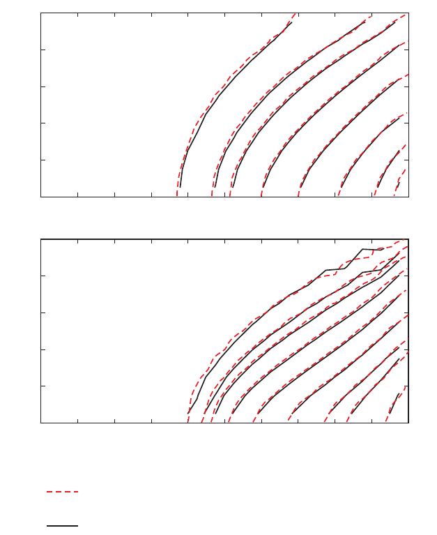
CHAPTER 7--Benchmark Problems 71
1%
0 0.2 0.4 0.6 0.8 1 1.2 1.4 1.6 1.8 2
Case 1:
molecular diffusion = 1.6295 m /d
(meters squared per day)
2
ELEVATION, IN METERS
1
0.8
0.6
0.4
0.2
0
Case 2:
molecular diffusion = 0.57024 m /d
(meters squared per day)
2
ELEVATION, IN METERS
1
0.8
0.6
0.4
0.2
0
X-DISTANCE, IN METERS
0 0.2 0.4 0.6 0.8 1 1.2 1.4 1.6 1.8 2
X-DISTANCE, IN METERS
5% 10%
25%
50%
75%
90%
95%
1%
25%
50%
75%
90%
95%
99%
5%
10%
EXPLANATION
SUTRA contours of relative concentration, in percent
(Segol, 1993)
SEAWAT contours of relative concentration, in percent
The Henry problem caused further confusion among the modeling community because some
researchers attempting to verify numerical codes calculated an erroneous value for molecular diffusion that
did not correlate with the original value used by Henry (Voss and Souza, 1987). For this reason, some
researchers consider there to be two cases of the Henry problem: one in which the value for molecular
diffusion (Dm) is 1.62925 m2/d and another with a value of 0.57024 m2/d.
The finite-difference model grid used to discretize the problem domain consists of 1 row with 21
columns and 10 layers. Each cell, with the exception of the cells in column 21, is 0.1 by 0.1 m in size. Cells
in column 21 are 0.01-m horizontal by 0.1-m vertical. The narrow column of cells in column 21 was used
to more precisely locate the seawater hydrostatic boundary at a distance of 2 m. The WEL package was used
to assign injection wells, with constant inflow rates of 0.5702 m3/d to each cell of column 1. Constant fresh-
water heads were assigned to the cells in column 21 using a head value of 1.0 m and a concentration of
35 kg/m3. The concentration for inflow from these constant head cells was specified at 35 kg/m3.
For both cases of the Henry problem, the implicit finite-difference solver (GCG) with the upstream-
weighting scheme was used to solve the transport equation. The initial timestep was specified as 0.001 day,
and a timestep multiplier of 1.9 was used to increase subsequent timesteps. For both cases, 23 timesteps were
required to run the 1-day simulation period. The comparison between SEAWAT results and results from
SUTRA (Segol, 1993) are shown for the Henry problem in figure 13. Contours of relative salinity concen-
tration are in good agreement for both cases.
Figure 13. Comparison between SEAWAT and SUTRA for the Henry problem.
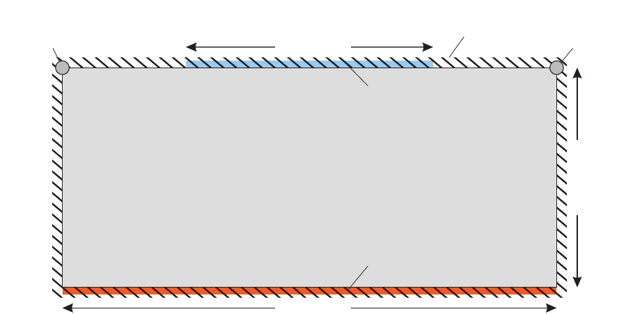
72 User’s Guide to SEAWAT: A Computer Program for Simulation of Three-Dimensional Variable-Density Ground-Water Flow
No-flow boundary
Constant-concentration
boundary
Cs= 285.7
Constant-concentration
boundary C= 0.0
Constant
pressure
boundary
P=0
Constant
pressure
boundary
P=0
150 METERS
300 METERS
600 METERS
porosity, = 0.10
salt concentration, = 285.7 kilograms per cubic meter
fluid density at = 1,200 kilograms per cubic meter
fluid density of freshwater, = 1,000 kilograms per cubic meter
equivalent freshwater hydaulic conductivity, = 0.411 meter per day
longitudinal and transverse dispersivity, = = 0.0 meter
molecular diffusion coefficient, = 0.308 square meter per day
θ
ρ
ρ
αα
C
C
K
D
s
ss
,
f
f
LT
m
Elder Problem
The Elder problem was originally designed for heat flow (Elder, 1967), but Voss and Souza (1987)
recast the problem as a variable-density ground-water problem in which fluid density is a function of salt
concentration. The Elder problem is commonly used to verify variable-density ground-water codes. The
geometry and boundary conditions for the problem are shown in figure 14. A constant-concentration bound-
ary is specified for a portion of the upper boundary. Molecular diffusion is the sole mechanism for hydro-
dynamic dispersion during the simulation, which runs for 20 years. Salt from the constant-concentration
boundary diffuses into the model domain and initiates complex vortices that redistribute the salt mass
throughout the model. A constant-concentration boundary with a value of zero is specified for the lowest
layer in the model. Two outlet cells with constant head values of zero are specified for the upper left and
right boundaries. These constant head cells allow salt to diffuse into the model by providing an outlet for
fluid and salt mass.
The finite-difference grid used with SEAWAT to simulate the revised Elder problem (fig. 15) is simi-
lar in resolution to the finite-element grid used by Voss and Souza (1987). The SEAWAT grid consists of
1 row with 44 columns and 27 layers. Each cell is 13.63-m horizontal by 6-m vertical. For layer 1, cells in
columns 1 to 11 and 34 to 44 are inactive. Cells in layer 1 from columns 12 to 33 are designated as constant
concentration with a value of 285.7 kg/m3. Using the equation of state in SEAWAT, this concentration value
corresponds to the appropriate fluid density of 1,200 kg/m3. In layer 2, constant heads are specified with a
value of 150.0 m for the first and last columns, which provide a fluid outlet. For layers 2 to 27, the first and
last columns are bounded by no-flow conditions. All of the cells in layer 27 also have a specified concen-
tration of 0.0 kg/m3, and there are no-flow conditions along the bottom face.
Initial concentrations within the model domain are set to zero, except for those in layer 1, which are
set to 285.7 kg/m3. Initial heads are set everywhere to zero. Hydraulic conductivity generally is uniform and
isotropic with a value of 0.411 m/d. For layers 1 and 27, however, the horizontal and vertical hydraulic
conductivities are set to 1 x 10⁻⁵ m/d to restrict flow within the top and bottom layers. The storage coefficient
is uniformly set to zero, and the porosity value is uniformly set to 0.1. A value of 0.308 m2/d is used as the
coefficient of molecular diffusion.
Figure 14. Boundary conditions and model parameters for the Elder problem.
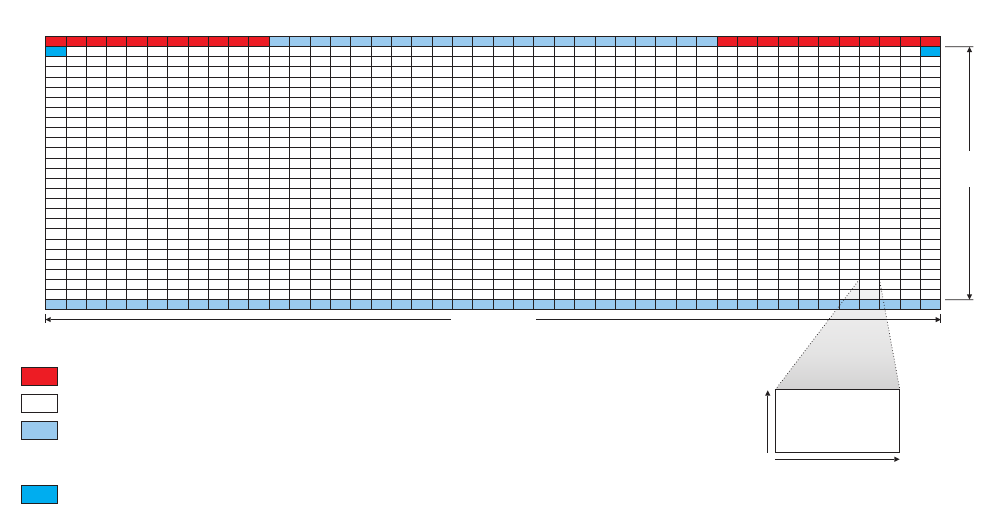
CHAPTER 7--Benchmark Problems 73
1
EXPLANATION
11 12 33 34 44
COLUMN
1
LAYER
27
INACTIVE
ACTIVE
CONSTANT CONCENTRATION Layer 1 has a concentration value
of 285.7 kilograms per cubic meter. Layer 27 has a concentration
value of 0.0 kilograms per cubic meter.
CONSTANT HEAD A value of 150 meters is specified for the
constant heads
–
–
600 meters
150
meters
∆x = 13.63 meters
∆z = 6 meters
The PCG solver was used with a head convergence criterion of 1 x 10⁻⁷ m and a flow convergence of
1 kg/d. For the transport equation, the GCG solver was used with a courant number of 0.1 to limit the size
of the timesteps. The average size of the timesteps was about 3 days, taking 2,321 timesteps to run the
20-year simulation. Relative salinity concentrations from SEAWAT are compared with results from SUTRA
(Voss and Souza, 1987) and the original documentation results from Elder (1967) for six different times
(fig. 16). Although some differences are evident, there appears to be a reasonably good match between the
patterns from SEAWAT and those of SUTRA (Voss and Souza, 1987) and Elder (1967).
HYDROCOIN Problem
The purpose of the Hydrologic Code Intercomparison (HYDROCOIN) project was to evaluate the
accuracy of selected ground-water modeling codes. One of the problems used for testing is the HYDRO-
COIN problem. The problem presented here is based on case 5 that was reevaluated with the MOCDENSE
code by Konikow and others (1997). The general geometry and boundary conditions for the HYDROCOIN
problem are shown in figure 17. A sloping pressure boundary is imposed across the top of the box that is
surrounded on the sides and bottom by no-flow conditions. Along the base of the middle part of the model,
a constant-concentration condition is applied to represent the top of a salt dome. As ground water flows
along the bottom boundary and over the salt dome, salt disperses into the system and collects in the lower
right corner of the model domain.
The finite-difference grid used by SEAWAT (and MOCDENSE) consists of 1 row with 45 columns
and 76 layers. Each cell is 20-m horizontal by 4-m vertical. The head values for the sloping constant-head
boundary vary linearly between 10.080 m at the center of the first column and 0.113 m at the center of the
last column (column 45). Fluid that enters the model domain from this upper boundary has a concentration
Figure 15. Finite-difference grid used to simulate the Elder problem.
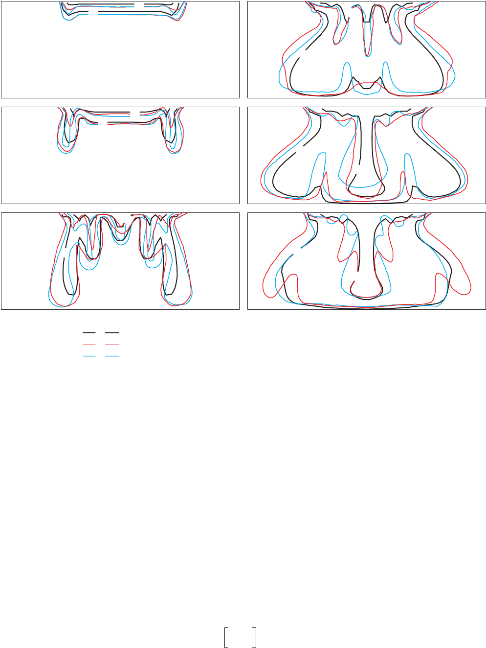
74 User’s Guide to SEAWAT: A Computer Program for Simulation of Three-Dimensional Variable-Density Ground-Water Flow
of zero and a fluid density of 1,000 kg/m3. The left and right boundaries are no flow. For the bottom layer,
cells in columns 1 to 15 and 31 to 45 are inactive. Between these inactive cells, a constant-concentration
boundary is specified with a concentration value of 280 kg/m3.
A uniform and isotropic value of 0.8476 m/d was assigned for equivalent freshwater hydraulic
conductivity in all layers, except for the bottom layer where the hydraulic conductivity was set at 8.475 x
10-4 m/d (three orders of magnitude lower than the rest of the model domain). This low value for hydraulic
conductivity in the bottom layer limits salt from entering the model domain through advection−an important
stipulation of the HYDROCOIN problem (Konikow and others, 1997). A value of 0.2 was uniformly
assigned for porosity; the values of longitudinal and transverse dispersivity were set at 20 and 2 m, respec-
tively; and molecular diffusion was set at zero.
For the HYDROCOIN problem, the standard version of MOCDENSE was modified to use a nonlin-
ear equation of state to relate fluid density to solute concentration (Konikow and others, 1997). The
SEAWAT code also was modified to use this slightly different equation of state. The equation of state used
by the modified SEAWAT and MOCDENSE programs is represented by the following equation:
(135)
1
ρ
---C
ρs
-----1C–
ρf
-------------
+=
SEAWAT line of relative salinity concentration, in percent
SUTRA line of relative salinity concentration, in percent (Voss and Souza, 1987)
Elder line of relative salinity concentration, in percent (Voss and Souza, 1987)
EXPLANATION
1 year 10 years
2 years 15 years
3 years 20 years
20
60
20
60
20
60
20
60
20
60
20
60
20
20
20
Figure 16. Comparison between SEAWAT, SUTRA, and Elder’s solution for the Elder problem over time.
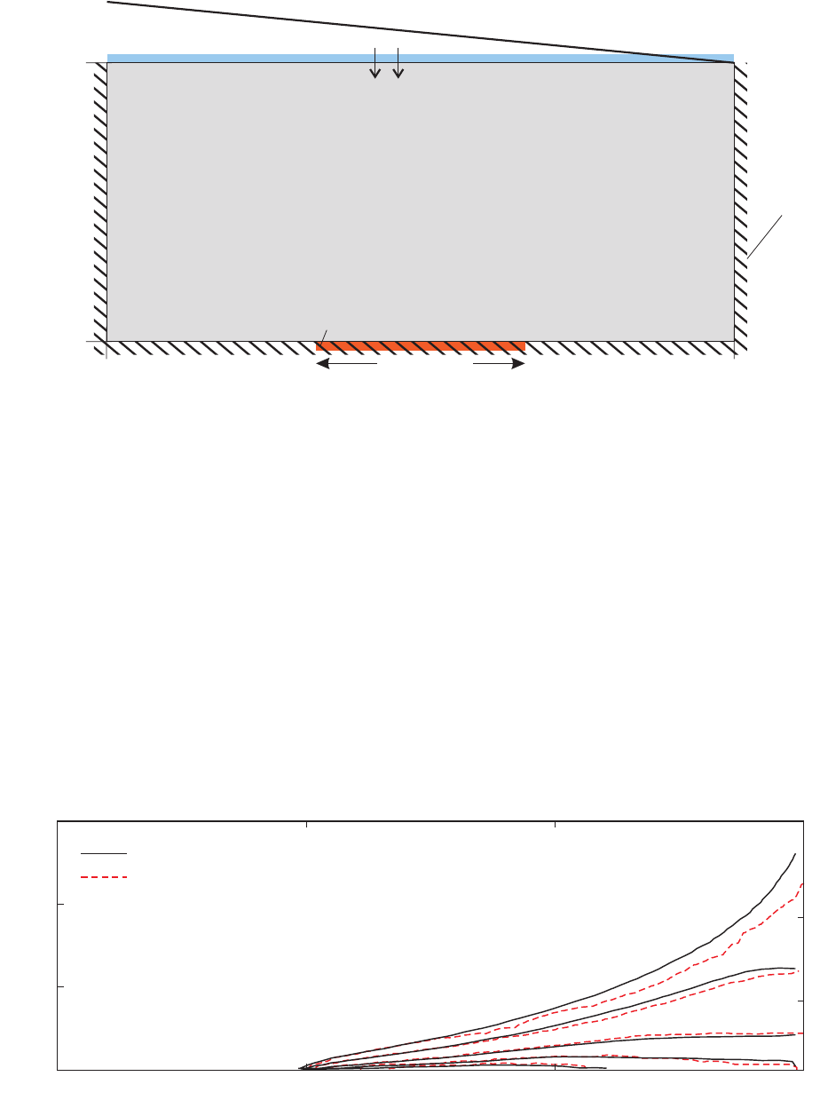
CHAPTER 7--Benchmark Problems 75
Sloping pressure boundary
DISTANCE, IN METERS
0
300
900
0
No-flow
boundary
Salt dome (C,
ss
ρ)
DEPTH, IN METERS
porosity, = 0.2
equivalent freshwater hydraulic conductivity, = 0.8476 meter per day
longitudinal dispersivity, = 20 meters
molecular diffusion coefficient, = 0 square meters per day
relative inflow concentration, = 0 kilograms per cubic meter
inflow
θ
α
K
D
C
f
L
m
f
transverse dispersivity, = 2 meters
fluid density, = 1,000 kilograms per cubic meter
salt dome relative concentration, = 1.0
fluid density at = 1,200 kilograms per cubic meter
α
ρ
ρ
T
f
ss
C
C
s
,
(C,
fρf)
300 METERS
where ρsis the density of the brine (1,200 kg/m3) at a relative salinity concentration of 1.0 (Konikow and
others, 1997). In the SEAWAT data sets, the salinity value for the salt dome is set at 280 kg/m3-
concentration that would result in a fluid density of 1,200 kg/m3with the equation of state normally used by
SEAWAT. Because equation 135 requires relative concentrations, the modified version of SEAWAT
converts the concentrations to relative concentrations before applying equation 135.
The comparison of simulated results between SEAWAT and MOCDENSE is shown in figure 18.
The relative salinity concentrations simulated by the two codes generally are consistent with one another;
however, there is a discrepancy toward the upper right part of the model domain. While SEAWAT tends to
produce slightly higher salinity concentrations in this region, the comparison between the two codes is
considered acceptable.
Figure 17. Boundary conditions and model parameters for the HYDROCOIN problem.
0
0
-100
-200
-300
ELEVATION, IN METERS
300 600 900
0.1
0.2
0.3
0.05
SEAWAT salinity contours, in relative concentration
MOCDENSE salinity contours, in relative concentration (Konikow and others, 1997)
X-DISTANCE, IN METERS
Figure 18. Comparison between SEAWAT and MOCDENSE for the HYDROCOIN problem.
76 User’s Guide to SEAWAT: A Computer Program for Simulation of Three-Dimensional Variable-Density Ground-Water Flow
REFERENCES CITED
Anderson, M.P., and Woessner, W.W., 1992, Applied groundwater modeling: Simulation of flow and
advective transport: San Diego, Calif., Academic Press, 381 p.
Baxter, G.P., and Wallace, C.C., 1916, Changes in volume upon solution in water of halogen salts of alkali
metals: IX, American Chemical Society Journal, no. 38, p. 70-104.
Bear, J. 1972, Dynamics of fluids in porous media: New York, Dover Publications, Inc., 764 p.
——— 1979, Hydraulics of groundwater: New York, McGraw-Hill Book Company, 569 p.
Chow, V.T., 1964, Handbook of Applied Hydrology: New York, McGraw-Hill Book Company.
Croucher, A.E., and O’Sullivan, M.J., 1995, The Henry problem for saltwater intrusion: Water Resources
Research, v. 31, no. 7, p. 1809-1814.
de Marsily, G., 1986, Quantitative hydrogeology: Groundwater hydrology for engineers: San Diego, Calif.,
Academic Press, 440 p.
Elder, J.W.,1967, Transient convection in a porous medium: Journal of Fluid Mechanics, v. 27, no. 3,
p. 609-623.
Evans, D.G. and Raffensperger, J.P., 1992, On the stream function for variable-density groundwater flow:
Water Resources Research, v. 28, no. 8, p. 2141-2145.
Freeze, R.A. and Cherry, J.A., 1979, Groundwater: Englewood Cliffs, N.J., Prentice-Hall, 604 p.
Ghyben, W.B., 1888, Nota in verband met de voorgenomen putboring nabij Amsterdam, Tijdschrift van Let
Koninklijk Inst. Van Ing.
Guo, Weixing, and Bennett, G.D., 1998, Simulation of saline/fresh water flows using MODFLOW, in
Poeter, E., and others, MODFLOW ‘98 Conference, Golden, Colorado, 1998, Proceedings: Golden,
Colorado, v. 1, p. 267-274.
Guo, Weixing, Langevin, C.D., and Bennett, G.D., 2001, Improvements to SEAWAT and application of the
variable-density modeling program in southern Florida, in Poeter, E., and others, MODFLOW 2001
and Other Modeling Odysseys Conference, Colorado School of Mines, Golden, Colorado, v. 2, p. 621-
627.
Henry, H.R., 1964, Effects of dispersion on salt encroachment in coastal aquifers: U.S. Geological Survey
Water-Supply Paper, 1613-C, p. C71-C84.
Herzberg, A. 1901, Die Wasserversorgung einiger nordseebader: J. Gasbeleucht. Wasserversorg., 44,
p. 815-819.
Hill, M., 1990, Preconditioned conjugate-gradient 2 (PCG2), a computer program for solving groundwater
equations: U.S. Geological Survey Water-Resources Investigations Report 90-4048, 43 p.
Hubbert, M.K., 1940, The theory of groundwater motion: Journal of Geology, v. 48, no. 8, p. 785-944.
Huyakorn, P.S., Anderson, P.F., Mercer, J.W., and White, Jr., H.O., 1987, Saltwater intrusion in aquifer:
Development and testing of a three-dimensional finite-element model: Water Resources Research,
v. 23, no. 2, p. 293-312.
Kipp, K.L., 1997, Guide to the revised heat and solute transport simulator: HST3D—Version 2:
U.S.Geological Survey Water-Resources Investigations Report 97-4157, 149 p.
References Cited 77
Konikow, L.F., Sanford, W.E. and Campbell, P.J., 1997, Constant-concentration boundary condition:
Lessons from the HYDROCOIN variable-density groundwater benchmark problem: Water Resources
Research, v. 33, no. 10, p. 2253-2261.
Langevin, C.D., 2001, Simulation of ground-water discharge to Biscayne Bay, southeastern Florida: U.S.
Geological Survey Water-Resources Investigations Report 00-4251, 127 p.
Langevin, C.D., and Guo, Weixing, 1999, Improvements to SEAWAT, a variable-density modeling code
[abs.], in EOS, Transactions, v. 80, no. 46., p. F-373.
Leake, S.A. and Prudic, D.E., 1988, Documentation of a computer program to simulate aquifer-system
compaction using the modular finite-difference ground-water flow model: U. S. Geological Survey
Open-File Report 88-482, 80 p.
Lee, C., and Cheng, R., 1974, On seawater encroachment in coastal aquifers: Water Resources Research,
v. 10, no. 5, p. 1039-1043.
McDonald, M.G., and Harbaugh, A.W., 1988, A modular three-dimensional finite-difference ground-water
flow model: U.S. Geological Survey Techniques of Water Resources Investigations, book 6, chapter
A1, 586 p.
McDonald, M.G., Harbaugh, A.W., Orr, B.R., and Ackerman, D.J., 1992, A method of converting no-flow
cells to variable-head cells for the U.S. Geological Survey modular finite-difference groundwater flow
model: U. S. Geological Survey Open-File Report 91-536, 99 p.
Pinder, G.F., and Cooper, H.H., 1970, A numerical technique for calculating the transient position of the
saltwater front: Water Resources Research, v. 6, no. 3, p. 875-882.
Sanford, W.E., and Konikow, L.F., 1985, A two-constituent solute-transport model for ground-water having
variable density. U.S. Geological Survey Water-Resources Investigations Report 85-4279, 88 p.
Segol, G., 1993, Classic groundwater simulations: Proving and improving numerical models: Englewood
Cliffs, N.J., PTR Prentice Hall, 531 p.
Swain, E.D., Howie, B.B., and Dixon, Joann, 1996, Description and field analysis of a coupled ground-
water/surface-water flow model (MODFLOW/BRANCH) with modifications for structures and
wetlands in southern Dade County, Florida: U.S. Geological Survey Water-Resources Investigations
Report 96-4118, 67 p.
Voss, C.I., 1984, A finite-element simulation model for saturated-unsaturated, fluid-density-dependent
ground-water flow with energy transport or chemically-reactive single-species solute transport: U.S.
Geological Survey Water-Resources Investigation Report 84-4369, 409 p.
Voss, C. I. and Souza, W. R, 1987, Variable density flow and solute transport simulation of regional aquifers
containing a narrow freshwater-saltwater transition zone: Water Resources Research, v. 23, no. 10,
p. 1851-1866.
Weiss, Emanual, 1982, A model for the simulation of flow of variable-density ground water in three
dimensions under steady-state conditions: U.S. Geological Survey Open-File Report 82-352, 59 p.
Zheng, C., and Bennett, G.D., 1995, Applied contaminant transport modeling, theory and practice:
Van Nostrand Reinhold, 440 p.
Zheng, C., and Wang, P.P., 1998, MT3DMS, A modular three-dimensional multispecies transport model for
simulation of advection, dispersion and chemical reactions of contaminants in groundwater systems:
Vicksburg, Miss., Waterways Experiment Station, U.S. Army Corps of Engineers.
