SHARC Manual
User Manual:
Open the PDF directly: View PDF ![]() .
.
Page Count: 159 [warning: Documents this large are best viewed by clicking the View PDF Link!]
- Title Page
- Contact
- Contents
- Introduction
- Installation
- Execution
- Input files
- Output files
- Interfaces
- Auxilliary Scripts
- Wigner Distribution Sampling: wigner.py
- Amber Trajectory Sampling: amber_to_initconds.py
- Sharc Trajectory Sampling: sharctraj_to_initconds.py
- Setup of Initial Calculations: setup_init.py
- Excitation Selection: excite.py
- Setup of Trajectories: setup_traj.py
- Laser field generation: laser.x
- Calculation of Absorption Spectra: spectrum.py
- File transfer: retrieve.sh
- Data Extractor: data_extractor.x
- Plotting the Extracted Data: make_gnuscript.py
- Ensemble Diagnostics Tool: diagnostics.py
- Calculation of Ensemble Populations: populations.py
- Calculation of Numbers of Hops: transition.py
- Fitting population data to kinetic models: make_fitscript.py
- Estimating Errors of Fits: bootstrap.py
- Obtaining Special Geometries: crossing.py
- Internal Coordinates Analysis: geo.py
- Essential Dynamics Analysis: trajana_essdyn.py
- Normal Mode Analysis: trajana_nma.py
- General Data Analysis: data_collector.py
- Optimizations: orca_External and setup_orca_opt.py
- Single Point Calculations: setup_single_point.py
- Format Data from QM.out Files: QMout_print.py
- Diagonalization Helper: diagonalizer.x
- Methodology
- Absorption Spectrum
- Active and inactive states
- Amdahl's Law
- Bootstrapping for Population Fits
- Damping
- Decoherence
- Essential Dynamics Analysis
- Excitation Selection
- Global fits and kinetic models
- Gradient transformation
- Internal coordinates definitions
- Kinetic energy adjustments
- Laser fields
- Laser interactions
- Normal Mode Analysis
- Optimization of Crossing Points
- Phase tracking
- Random initial velocities
- Representations
- Sampling from Wigner Distribution
- Scaling
- Seeding of the RNG
- Selection of gradients and nonadiabatic couplings
- State ordering
- Surface Hopping
- Velocity Verlet
- Wavefunction propagation
- Bibliography
- List of Tables
- List of Figures

SHARC2.0:
Surface Hopping Including
Arbitrary Couplings
Manual
Version 2.0
AG González
Institute of Theoretical Chemistry
University of Vienna, Austria
Vienna, May 23, 2018

Contents
1 Introduction 9
1.1 Capabilities .................................................... 11
1.1.1 New features in Sharc Version 2.0 .................................. 11
1.2 References .................................................... 12
1.3 Authors ...................................................... 13
1.4 Suggestions and Bug Reports .......................................... 13
1.5 Notation in this Manual ............................................. 13
2 Installation 14
2.1 How To Obtain ................................................. 14
2.2 Terms of Use ................................................... 14
2.3 Installation .................................................... 20
2.3.1 WFoverlap Program .......................................... 22
2.3.2 Libraries ................................................. 22
2.3.3 Test Suite ................................................ 22
2.3.4 Additional Programs .......................................... 23
2.3.5 Quantum Chemistry Programs .................................... 24
3 Execution 25
3.1 Running a single trajectory ........................................... 25
3.1.1 Input les ................................................ 25
3.1.2 Running the dynamics code ...................................... 26
3.1.3 Output les ............................................... 26
3.2 Typical workow for an ensemble of trajectories ............................... 26
3.2.1 Initial condition generation ...................................... 26
3.2.2 Running the dynamics simulations .................................. 28
3.2.3 Analysis of the dynamics results ................................... 28
3.3 Auxilliary Programs and Scripts ........................................ 29
3.3.1 Setup ................................................... 29
3.3.2 Analysis ................................................. 30
3.3.3 Interfaces ................................................ 30
3.3.4 Others .................................................. 31
4 Input files 32
4.1 Main input le .................................................. 32
4.1.1 General remarks ............................................ 32
4.1.2 Input keywords ............................................. 32
4.1.3 Detailed Description of the Keywords ................................ 36
4.1.4 Example ................................................. 40
4.2 Geometry le .................................................. 40
4.3 Velocity le ................................................... 41
4.4 Coecient le .................................................. 41
4.5 Laser le ..................................................... 41
4.6 Atom mask le .................................................. 42
5 Output files 43
5.1 Log le ...................................................... 43
5.2 Listing le .................................................... 43
5.3 Data le ..................................................... 44
5.3.1 Specication of the data le ...................................... 44
4
Sharc Manual Contents |Contents
5.4 XYZ le ...................................................... 45
6 Interfaces 46
6.1 Interface Specications ............................................. 46
6.1.1 QM.in Specication ........................................... 46
6.1.2 QM.out Specication .......................................... 47
6.1.3 Further Specications ......................................... 51
6.1.4 Save Directory Specication ...................................... 51
6.2 Overview over Interfaces ............................................ 52
6.2.1 Example Directory ........................................... 52
6.3 MOLPRO Interface ............................................... 53
6.3.1 Template le: MOLPRO.template .................................... 53
6.3.2 Resource le: MOLPRO.resources ................................... 54
6.3.3 Error checking ............................................. 54
6.3.4 Things to keep in mind ......................................... 55
6.3.5 Molpro input generator: molpro_input.py .............................. 55
6.4 MOLCAS Interface ............................................... 57
6.4.1 Template le: MOLCAS.template .................................... 57
6.4.2 Resource le: MOLCAS.resources ................................... 57
6.4.3 Template le generator: molcas_input.py .............................. 59
6.4.4 QM/MM key le: MOLCAS.qmmm.key .................................. 60
6.4.5 QM/MM connection table le: MOLCAS.qmmm.table ......................... 60
6.5 COLUMBUS Interface .............................................. 61
6.5.1 Template input ............................................. 61
6.5.2 Resource le: COLUMBUS.resources .................................. 62
6.5.3 Template setup ............................................. 63
6.6 Analytical PESs Interface ............................................ 63
6.6.1 Parametrization ............................................. 63
6.6.2 Template le: Analytical.template ................................. 64
6.7 ADF Interface .................................................. 66
6.7.1 Template le: ADF.template ...................................... 66
6.7.2 Resource le: ADF.resources ..................................... 66
6.7.3 QM/MM force eld le: ADF.qmmm.ff ................................. 69
6.7.4 QM/MM connection table le: ADF.qmmm.table ........................... 70
6.7.5 Input le generator: ADF_input.py .................................. 71
6.7.6 Frequencies converter: ADF_freq.py ................................. 72
6.8 RICC2 Interface ................................................. 72
6.8.1 Template le: RICC2.template .................................... 72
6.8.2 Resource le: RICC2.resources .................................... 73
6.9 LVC Interface .................................................. 75
6.9.1 Input les ................................................ 75
6.9.2 Preparing Template Files: wigner.py and QMout2LVC.py ...................... 76
6.10 Gaussian Interface ............................................... 77
6.10.1 Template le: GAUSSIAN.template .................................. 77
6.10.2 Resource le: GAUSSIAN.resources .................................. 77
6.11 The WFoverlap Program ............................................ 78
6.11.1 Installation ............................................... 80
6.11.2 Workow ................................................ 80
6.11.3 Calling the program .......................................... 81
6.11.4 Input data ................................................ 82
6.11.5 Output .................................................. 84
7 Auxilliary Scripts 86
7.1 Wigner Distribution Sampling: wigner.py .................................. 86
7.1.1 Usage .................................................. 86
7.1.2 Normal mode types ........................................... 87
7.1.3 Non-default masses ........................................... 87
5
Sharc Manual Contents |Contents
7.1.4 Sampling at nite temperatures .................................... 87
7.1.5 Output .................................................. 87
7.2 Amber Trajectory Sampling: amber_to_initconds.py ............................ 88
7.2.1 Usage .................................................. 88
7.2.2 Time Step ................................................ 88
7.2.3 Atom Types and Masses ........................................ 89
7.2.4 Output .................................................. 89
7.3 Sharc Trajectory Sampling: sharctraj_to_initconds.py ......................... 89
7.3.1 Usage .................................................. 89
7.3.2 Random Picking of Time Step ..................................... 89
7.3.3 Output .................................................. 90
7.4 Setup of Initial Calculations: setup_init.py ................................. 90
7.4.1 Usage .................................................. 90
7.4.2 Input ................................................... 90
7.4.3 Interface-specic input ......................................... 91
7.4.4 Input for Run Scripts .......................................... 95
7.4.5 Output .................................................. 96
7.5 Excitation Selection: excite.py ........................................ 97
7.5.1 Usage .................................................. 97
7.5.2 Input ................................................... 97
7.5.3 Matrix diagonalization ......................................... 98
7.5.4 Output .................................................. 99
7.5.5 Specication of the initconds.excited le format ......................... 99
7.6 Setup of Trajectories: setup_traj.py .....................................100
7.6.1 Input ...................................................100
7.6.2 Interface-specic input .........................................103
7.6.3 Output control .............................................103
7.6.4 Run script setup .............................................103
7.6.5 Output ..................................................103
7.7 Laser eld generation: laser.x ........................................104
7.7.1 Usage ..................................................104
7.7.2 Input ...................................................104
7.8 Calculation of Absorption Spectra: spectrum.py ...............................105
7.8.1 Input ...................................................105
7.8.2 Output ..................................................106
7.8.3 Error Analysis ..............................................106
7.9 File transfer: retrieve.sh ...........................................106
7.10 Data Extractor: data_extractor.x ......................................106
7.10.1 Usage ..................................................107
7.10.2 Output ..................................................107
7.11 Plotting the Extracted Data: make_gnuscript.py ...............................107
7.12 Ensemble Diagnostics Tool: diagnostics.py .................................109
7.12.1 Usage ..................................................109
7.12.2 Input ...................................................110
7.13 Calculation of Ensemble Populations: populations.py ...........................111
7.13.1 Usage ..................................................111
7.13.2 Output ..................................................113
7.14 Calculation of Numbers of Hops: transition.py ..............................113
7.14.1 Usage ..................................................113
7.15 Fitting population data to kinetic models: make_fitscript.py .......................114
7.15.1 Usage ..................................................114
7.15.2 Input ...................................................114
7.15.3 Output ..................................................115
7.16 Estimating Errors of Fits: bootstrap.py ....................................116
7.16.1 Usage ..................................................116
7.16.2 Input ...................................................116
7.16.3 Output ..................................................117
6
Sharc Manual Contents |Contents
7.17 Obtaining Special Geometries: crossing.py .................................117
7.17.1 Usage ..................................................117
7.17.2 Output ..................................................118
7.18 Internal Coordinates Analysis: geo.py .....................................118
7.18.1 Input ...................................................118
7.18.2 Options .................................................119
7.19 Essential Dynamics Analysis: trajana_essdyn.py ..............................119
7.19.1 Usage ..................................................120
7.19.2 Input ...................................................120
7.19.3 Output ..................................................120
7.20 Normal Mode Analysis: trajana_nma.py ...................................120
7.20.1 Usage ..................................................121
7.20.2 Input ...................................................121
7.20.3 Output ..................................................122
7.21 General Data Analysis: data_collector.py .................................122
7.21.1 Usage ..................................................122
7.21.2 Input ...................................................122
7.21.3 Output ..................................................125
7.22 Optimizations: orca_External and setup_orca_opt.py ...........................126
7.22.1 Usage ..................................................127
7.22.2 Input ...................................................127
7.22.3 Output ..................................................128
7.22.4 Description of orca_External .....................................128
7.23 Single Point Calculations: setup_single_point.py .............................129
7.23.1 Usage ..................................................129
7.23.2 Input ...................................................129
7.23.3 Output ..................................................129
7.24 Format Data from QM.out Files: QMout_print.py ...............................129
7.24.1 Usage ..................................................130
7.24.2 Output ..................................................130
7.25 Diagonalization Helper: diagonalizer.x ...................................130
8 Methodology 131
8.1 Absorption Spectrum ..............................................131
8.2 Active and inactive states ............................................131
8.3 Amdahl’s Law ..................................................132
8.4 Bootstrapping for Population Fits .......................................132
8.5 Damping .....................................................133
8.6 Decoherence ...................................................133
8.6.1 Energy-based decoherence .......................................133
8.6.2 Augmented FSSH decoherence ....................................133
8.7 Essential Dynamics Analysis ..........................................135
8.8 Excitation Selection ...............................................135
8.8.1 Excitation Selection with Diabatization ................................136
8.9 Global ts and kinetic models .........................................136
8.9.1 Reaction networks ...........................................136
8.9.2 Kinetic models .............................................136
8.9.3 Global t .................................................137
8.10 Gradient transformation ............................................138
8.10.1 Dipole moment derivatives ......................................138
8.11 Internal coordinates denitions ........................................138
8.12 Kinetic energy adjustments ...........................................139
8.12.1 Reection for frustrated hops .....................................140
8.13 Laser elds ....................................................140
8.13.1 Form of the laser eld .........................................140
8.13.2 Envelope functions ...........................................140
8.13.3 Field functions .............................................141
7
Sharc Manual Contents |Contents
8.13.4 Chirped pulses .............................................141
8.13.5 Quadratic chirp without Fourier transform ..............................142
8.14 Laser interactions ................................................142
8.14.1 Surface Hopping with laser elds ...................................142
8.15 Normal Mode Analysis .............................................142
8.16 Optimization of Crossing Points ........................................143
8.17 Phase tracking ..................................................143
8.17.1 Phase tracking of the transformation matrix .............................143
8.17.2 Tracking of the phase of the MCH wave functions .........................144
8.18 Random initial velocities ............................................145
8.19 Representations .................................................145
8.19.1 Current state in MCH representation .................................145
8.20 Sampling from Wigner Distribution ......................................146
8.20.1 Sampling at Non-zero Temperature ..................................146
8.21 Scaling ......................................................146
8.22 Seeding of the RNG ...............................................147
8.23 Selection of gradients and nonadiabatic couplings ..............................147
8.24 State ordering ..................................................147
8.25 Surface Hopping .................................................148
8.26 Velocity Verlet ..................................................148
8.27 Wavefunction propagation ...........................................149
8.27.1 Propagation using nonadiabatic couplings ..............................149
8.27.2 Propagation using overlap matrices ..................................150
Bibliography 150
List of Tables 157
List of Figures 158
8
1 Introduction
When a molecule is irradiated by light, a number of dynamical processes can take place, in which the molecule
redistributes the energy among dierent electronic and vibrational degrees of freedom. Kasha’s rule [
1
] states that
radiationless transfer from higher excited singlet states to the lowest-lying excited singlet state (
S1
) is faster than
uorescence (F). This radiationless transfer is called internal conversion (IC) and involves a changes between electronic
states of the same multiplicity. If a transition occurs between electronic states of dierent spin, the process is called
intersystem crossing (ISC). A typical ISC process is from a singlet to a triplet state, and once the lowest triplet is
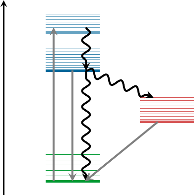
populated, phosphorescence (P) can take place. In gure 1.1, radiative (F and P) and radiationless (IC and ISC) processes
are summarized in a so-called Jabłonski diagram.
E
Singlet Triplet
S0
S1
S2
T1
hν
FIC
IC
ISC
P
Figure 1.1:
Jabłonski diagram showing the conceptual photophysical processes. Straight arrows show radiative pro-
cesses: absorption (
hν
), uorescence (F), and phosphorescence (P); wavy arrows show radiationless processes:
internal conversion (IC) and intersystem crossing (ISC).
The non-radiative IC and ISC processes are fundamental concepts which play a decisive role in photochemistry and
photobiology. IC processes are present in the excited-state dynamics of many organic and inorganic molecules, whose
applications range from solar energy conversion to drug therapy. Even many, very small molecules, for example
O2
and
O3
,
SO2
,
NO2
and other nitrous oxides, show ecient IC, which has important consequences in atmospheric chemistry
and the study of the environment and pollution. IC is also the rst step of the biological process of visual perception,
where the retinal moiety of rhodopsin absorbs a photon and non-radiatively performs a torsion around one of the
double bonds, changing the conformation of the protein and inducing a neural signal. Similarly, protection of the human
body from the inuence of UV light is achieved through very ecient IC in DNA, proteins and melanins. Ultrafast IC to
the electronic ground state allows quickly converting the excitation energy of the UV photons into nuclear kinetic
energy, which is spread harmlessly as heat to the environment.
ISC processes are completely forbidden in the frame of the non-relativistic Schrödinger equation, but they become
allowed when including spin-orbit couplings, a relativistic eect [
2
]. Spin-orbit coupling depends on the nuclear charge
and becomes stronger for heavy atoms, therefore it is typically known as a ”heavy atom” eect. However, it has been
recently recognized that even for molecules with only rst- and second-row atoms, ISC might be relevant and can
be competitive in time scales with IC. A small selection of the growing number of molecules where ecient ISC in a
sub-ps time scale has been predicted are
SO2
[
3
–
5
], benzene [
6
], aromatic nitrocompounds [
7
] or DNA nucleobases and
derivatives [8–12].
9
Sharc Manual 1 Introduction |1 Introduction
Theoretical simulations can greatly contribute to understand non-radiative processes by following the nuclear motion
on the excited-state potential energy surfaces (PES) in real time. These simulations are called excited-state dynamics
simulations. Since the Born-Oppenheimer approximation is not applicable for this kind of dynamics, nonadiabatic
eects need to be incorporated into the simulations.
The principal methodology to tackle excited-state dynamics simulations is to numerically integrate the time-dependent
Schrödinger equation, which is usually called full quantum dynamics simulations (QD). Given accurate PESs, QD is
able to match experimental accuracy. However, the need for the ”a priori” knowledge of the full multi-dimensional
PES renders this type of simulations quickly unfeasible for more than few degrees of freedom. Several alternative
methodologies are possible to alleviate this problem. One of the most popular ones is to use surface hopping nonadiabatic
dynamics.
Surface hopping was originally devised by Tully [
13
] and greatly improved later by the “fewest-switches criterion”[
14
]
and it has been reviewed extensively since then, see e.g. [
15
–
19
]. In surface hopping, the motion of the excited-state
wave packet is approximated by the motion of an ensemble of many independent, classical trajectories. Each trajectory
is at every instant of time tied to one particular PES, and the nuclear motion is integrated using the gradient of this PES.
However, nonadiabatic population transfer can lead to the switching of a trajectory from one PES to another PES. This
switching (also called “hopping”, which is the origin of the name “surface hopping”) is based on a stochastic algorithm,
taking into account the change of the electronic population from one time step to the next one.
The advantages of the surface hopping methodology and thus its popularity are well summarized in Ref. [15]:
•
The method is conceptually simple, since it is based on classical mechanics. The nuclear propagation is based
on Newton’s equations and can be performed in Cartesian coordinates, avoiding any problems with curved
coordinate systems as in QD.
•
For the propagation of the trajectories only local information of the PESs is needed. This avoids the calculation of
the full, multi-dimensional PES in advance, which is the main bottleneck of QD methods. In surface hopping
dynamics, all degrees of freedom can be included in the simulation. Additionally, all necessary quantities can be
calculated on-demand, usually called “on-the-y” in this context.
•The independent trajectories can be trivially parallelized.
The strongest of these points of course is the fact that all degrees of freedom can be included easily in the calculations,
allowing to describe large systems. One should note, however, that surface hopping methods in the standard formula-
tion [
13
,
14
]—due to the classical nature of the trajectories—do not allow to treat some purely quantum-mechanical
eects like tunneling, (tunneling for selected degrees of freedom is possible [
20
]). Additionally, quantum coherence
between the electronic states is usually described poorly, because of the independent-trajectory ansatz. This can be
treated with some ad-hoc corrections, e.g., in [21].
In the original surface hopping method, only nonadiabatic couplings are considered, only allowing for population
transfer between electronic states of the same multiplicity (IC). The Sharc methodology is a generalization of standard
surface hopping since it allows to include any type of coupling. Beyond nonadiabatic couplings (for IC), spin-orbit
couplings (for ISC) or interactions of dipole moments with electric elds (to explicitly describe laser-induced processes)
can be included. A number of methodologies for surface hopping including one or the other type of potential couplings
have been proposed in references [
22
–
28
], but Sharc can include all types of potential couplings on the same footing.
The Sharc methodology is an extension to standard surface hopping which allows to include these kinds of couplings.
The central idea of Sharc is to obtain a fully diagonal Hamiltonian, which is adiabatic with respect to all couplings.
The diagonal Hamiltonian is obtained by unitary transformation of the Hamiltonian including all couplings. Surface
hopping is conducted on the transformed electronic states. This has a number of advantages over the standard surface
hopping methodology, where no diagonalization is performed:
•
Potential couplings (like spin-orbit couplings and laser-dipole couplings) are usually delocalized. Surface hopping,
however, rests on the assumption that the couplings are localized and hence surface hops only occur in the small
region where the couplings are large. Within Sharc, by transforming away the potential couplings, additional
terms of nonadiabatic (kinetic) couplings arise, which are localized.
•
The potential couplings have an inuence on the gradients acting on the nuclei. To a good approximation, within
Sharc it is possible to include this inuence in the dynamics.
•
When including spin-orbit couplings for states of higher multiplicity, diagonalization solves the problem of
rotational invariance of the multiplet components (see [26]).
The Sharc suite of programs is an implementation of the Sharc method. Besides the core dynamics code, it comes
with a number of tools aiding in the setup, maintenance and analysis of the trajectories.
10

Sharc Manual 1 Introduction |1.1 Capabilities
1.1 Capabilities
The main features of the Sharc2.0 suite are:
•
Non-adiabatic dynamics based on the surface hopping methodology able to describe internal conversion and
intersystem crossing with any number of states (singlets, doublets, triplets, or higher multiplicities).
•Algorithms for stable wave function propagation in the presence of very small or very large couplings.
•
Inclusion of interactions with laser elds in the long-wavelength limit. The derivatives of the dipole moments
can be included in strong-eld applications.
•
Propagation using either nonadiabatic couplings vectors
hα|∂
∂R|βi
or wave function overlaps
hα(t0)|β(t)i
(via the
local diabatization procedure [21]).
•
Gradients including the eects of spin-orbit couplings (with the approximation that the diabatic spin-orbit
couplings are slowly varying).
•Flexible interface to quantum chemistry programs. Existing interfaces to:
–Molpro 2010 and 2012: SA-CASSCF
–Openmolcas 18.0: SA-CASSCF, SS-CASPT2, MS-CASPT2, SA-CASSCF+QM/MM
–Columbus 7: SA-CASSCF, SA-RASSCF, MR-CISD
–ADF 2017+: TD-DFT, TD-DFT+QM/MM
–Turbomole 7: ADC(2), CC2
–Gaussian 09 and 16: TD-DFT
–Interface for analytical potentials
–Interface for linear-vibronic coupling (LVC) models
•Energy-dierence-based partial coupling approximation to speed up calculations [29].
•Energy-based decoherence correction [21] or augmented-FSSH decoherence correction [30].
•Calculation of Dyson norms for single-photon ionization spectra (for most interfaces) [31].
•On-the-y wave function analysis with TheoDORE [32–34] (for some interfaces).
•Suite of auxiliary Python scripts for all steps of the setup procedure and for various analysis tasks.
•Comprehensive tutorial.
1.1.1 New features in Sharc Version 2.0
These features are new in Sharc Version 2.0 (2018):
•Dynamics program sharc.x:
–New methods: AFSSH for decoherence, GFSH for hopping probabilities, reection after frustrated hop.
–Atom masking for size-extensive decoherence and rescaling.
–Improved wave function and Umatrix phase tracking.
–Support for on-the-y computation of Dyson norms and TheoDORE descriptors.
–Option to gracefully stop trajectories after any time step.
•Fully integrated, ecient wave function overlap program wfoverlap.x
•Quantum chemistry interfaces:
–
Molpro: overhauled, uses
wfoverlap.x
, gives consistent phase between CASSCF and CI wave functions,
can do Dyson norms, parallelizes independent job parts.
–
Molcas: overhauled, can do (MS)-CASPT2 (only numerical gradients), QM/MM, Cholesky decomposition,
Dyson norms, parallelizes independent job parts, works with Openmolcas version 18.
–
Columbus: overhauled, uses
wfoverlap.x
, can use Dalton integrals, can use Molcas orbitals, can do
Dyson norms.
–Analytical: —
–
Turbomole: new interface, can do ADC(2) and CC2; has SOC (for ADC(2)), uses
wfoverlap.x
, works with
TheoDORE.
–
ADF: new interface, can do TD-DFT; has SOC, uses
wfoverlap.x
, Dyson norms, has QM/MM, works with
TheoDORE.
–Gaussian: new interface, can do TD-DFT; uses wfoverlap.x, has Dyson norms, works with TheoDORE.
11

Sharc Manual 1 Introduction |1.2 References
–LVC: new interface, can do (analytical) linear vibronic coupling models.
•Auxilliary scripts:
–wigner.py: elevated temperature sampling, LVC model setup.
–amber_to_initconds.py: new script, converts Amber trajectories to Sharc initial conditions.
–sharctraj_to_initconds.py: new script, converts Sharc trajectories to Sharc initial conditions.
–spectrum.py: log-normal convolution, density of state spectra.
–data_extractor.x: new quantities to extract.
–diagnostics.py: new script, checks all trajectories prior to analysis.
–populations.py: new analysis modes.
–transition.py: new script, computes total number of hops in ensemble.
–make_fitscript.py: new script, prepares kinetic model ts to obtain time constants from populations.
–bootstrap.py: new script, calculates error estimates for time constants.
–trajana_essdyn.py: new script, performs essential dynamics analysis.
–trajana_nma.py: new script, performs normal mode analysis.
–data_collector.py
: new script, performs generic data analysis (collecting, smoothing, convolution, inte-
gration).
–orca_External: new script, allows optimization with Orca and Sharc.
–Several input generation helpers.
•Reworked tutorial using Openmolcas (which is available at no cost).
1.2 References
The following references should be cited when using the Sharc suite:
•
[
35
] M. Richter, P. Marquetand, J. González-Vázquez, I. Sola, L. González: “SHARC: Ab Initio Molecular Dynamics
with Surface Hopping in the Adiabatic Representation Including Arbitrary Couplings”.J. Chem. Theory Comput.,
7, 1253–1258 (2011).
•
[
36
] S. Mai, P. Marquetand, L. González: “Nonadiabatic Dynamics: The SHARC Approach”.WIREs Comput. Mol.
Sci., DOI: 10.1002/wcms.1370 (2018).
•
[
37
] S. Mai, M. Richter, M. Heindl, M. F. S. J. Menger, A. J. Atkins, M. Ruckenbauer, F. Plasser, M. Oppel, P. Mar-
quetand, L. González: “SHARC2.0: Surface Hopping Including Arbitrary Couplings – Program Package for
Non-Adiabatic Dynamics”. sharc-md.org (2018).
Details can be found in the following references:
The theoretical background of Sharc is described in Refs. [35,36,38–42].
Applications of the Sharc code can be found in Refs. [4,9,11,43–69].
Other features implemented in the Sharc suite are described in the following references:
•Energy-based decoherence correction: [21].
•Augmented-FSSH decoherence correction: [30].
•Global ux SH: [70].
•Local diabatization and wave function overlap calculation: [71–73].
•Sampling of initial conditions from a quantum-mechanical harmonic Wigner distribution: [74–76].
•Excited state selection for initial condition generation: [77].
•Calculation of ring puckering parameters and their classication: [78,79].
•Normal mode analysis [80,81] and essential dynamics analysis: [81,82].
•Bootstrapping for error estimation: [83].
•Crossing point optimization: [84,85]
•Computation of ionization spectra: [31,86].
•Wave function comparison with overlaps: [87].
12
Sharc Manual 1 Introduction |1.3 Authors
The quantum chemistry programs to which interfaces with Sharc exist are described in the following sources:
•Molpro: [88,89],
•Molcas: [90–92],
•Columbus: [93–96],
•ADF: [97],
•Turbomole: [98],
•Gaussian: [99,100].
Others:
•TheoDORE: [32–34]
•WFoverlap: [73,87]
1.3 Authors
The current version of the Sharc suite has been programmed by Sebastian Mai, Martin Richter, Moritz Heindl,
Maximilian F. S. J. Menger, Andrew Atkins, Felix Plasser, and Philipp Marquetand of the AG González of the Institute
of Theoretical Chemistry of the University of Vienna with contributions from Jesús González-Vázquez, Matthias
Ruckenbauer, Markus Oppel, Patrick J. Zobel, and Leticia González.
1.4 Suggestions and Bug Reports
Bug reports and suggestions for possible features can be submitted to sharc@univie.ac.at.
1.5 Notation in this Manual
Names of programs
The Sharc suite consists of Fortran90 programs as well as Python and Shell scripts. The
executable Fortran90 programs are denoted by the extension
.x
, the Python scripts have the extension
.py
and the
Shell scripts .sh. Within this manual, all program names are given in bold monospaced font.
Shaded Sections Important sections are given in blue boxes like the following one:
Important sections are given in blue boxes like this one.
On the other hand, examples of input les and command lines are marked like this:
user@host>example example.dat
13

2 Installation
2.1 How To Obtain
Sharc can be obtained from the Sharc homepage www.sharc-md.org. In the Download section, register with your
e-mail adress and aliation. You will receive a download link to the stated e-mail adress. Clicking on the link in the
email will download the archive le containing the Sharc package. Note that the link is active only for 24 h and the
number of downloads is limited.
Note that you must accept the Terms of Use given in the following section in order to download Sharc.
2.2 Terms of Use
Sharc Program Suite
Copyright ©2018, University of Vienna
SHARC is free software: you can redistribute it and/or modify it under the terms of the GNU General Public License as
published by the Free Software Foundation, either version 3 of the License, or (at your option) any later version.
SHARC is distributed in the hope that it will be useful, but WITHOUT ANY WARRANTY; without even the implied
warranty of MERCHANTABILITY or FITNESS FOR A PARTICULAR PURPOSE. See the GNU General Public License
for more details.
A copy of the GNU General Public License is given below. It is also available at www.gnu.org/licenses/.
GNU General Public License
1. Preamble
The GNU General Public License is a free, copyleft license for software and other kinds of works.
The licenses for most software and other practical works are designed to take away your freedom to share and change
the works. By contrast, the GNU General Public License is intended to guarantee your freedom to share and change all
versions of a program–to make sure it remains free software for all its users. We, the Free Software Foundation, use the
GNU General Public License for most of our software; it applies also to any other work released this way by its authors.
You can apply it to your programs, too.
When we speak of free software, we are referring to freedom, not price. Our General Public Licenses are designed
to make sure that you have the freedom to distribute copies of free software (and charge for them if you wish), that
you receive source code or can get it if you want it, that you can change the software or use pieces of it in new free
programs, and that you know you can do these things.
To protect your rights, we need to prevent others from denying you these rights or asking you to surrender the rights.
Therefore, you have certain responsibilities if you distribute copies of the software, or if you modify it: responsibilities
to respect the freedom of others.
For example, if you distribute copies of such a program, whether gratis or for a fee, you must pass on to the recipients
the same freedoms that you received. You must make sure that they, too, receive or can get the source code. And you
must show them these terms so they know their rights.
Developers that use the GNU GPL protect your rights with two steps: (1) assert copyright on the software, and (2) oer
you this License giving you legal permission to copy, distribute and/or modify it.
For the developers’ and authors’ protection, the GPL clearly explains that there is no warranty for this free software.
For both users’ and authors’ sake, the GPL requires that modied versions be marked as changed, so that their problems
will not be attributed erroneously to authors of previous versions.
14

Sharc Manual 2 Installation |2.2 Terms of Use
Some devices are designed to deny users access to install or run modied versions of the software inside them, although
the manufacturer can do so. This is fundamentally incompatible with the aim of protecting users’ freedom to change
the software. The systematic pattern of such abuse occurs in the area of products for individuals to use, which is
precisely where it is most unacceptable. Therefore, we have designed this version of the GPL to prohibit the practice for
those products. If such problems arise substantially in other domains, we stand ready to extend this provision to those
domains in future versions of the GPL, as needed to protect the freedom of users.
Finally, every program is threatened constantly by software patents. States should not allow patents to restrict
development and use of software on general-purpose computers, but in those that do, we wish to avoid the special
danger that patents applied to a free program could make it eectively proprietary. To prevent this, the GPL assures
that patents cannot be used to render the program non-free.
The precise terms and conditions for copying, distribution and modication follow.
2. Terms and Conditions
0. Denitions.
“This License” refers to version 3 of the GNU General Public License.
“Copyright” also means copyright-like laws that apply to other kinds of works, such as semiconductor masks.
“The Program” refers to any copyrightable work licensed under this License. Each licensee is addressed as “you”.
“Licensees” and “recipients” may be individuals or organizations.
To “modify” a work means to copy from or adapt all or part of the work in a fashion requiring copyright permission,
other than the making of an exact copy. The resulting work is called a “modied version” of the earlier work or a
work “based on” the earlier work.
A “covered work” means either the unmodied Program or a work based on the Program.
To “propagate” a work means to do anything with it that, without permission, would make you directly or
secondarily liable for infringement under applicable copyright law, except executing it on a computer or modifying
a private copy. Propagation includes copying, distribution (with or without modication), making available to
the public, and in some countries other activities as well.
To “convey” a work means any kind of propagation that enables other parties to make or receive copies. Mere
interaction with a user through a computer network, with no transfer of a copy, is not conveying.
An interactive user interface displays “Appropriate Legal Notices” to the extent that it includes a convenient and
prominently visible feature that (1) displays an appropriate copyright notice, and (2) tells the user that there is no
warranty for the work (except to the extent that warranties are provided), that licensees may convey the work
under this License, and how to view a copy of this License. If the interface presents a list of user commands or
options, such as a menu, a prominent item in the list meets this criterion.
1. Source Code.
The “source code” for a work means the preferred form of the work for making modications to it. “Object code”
means any non-source form of a work.
A “Standard Interface” means an interface that either is an ocial standard dened by a recognized standards
body, or, in the case of interfaces specied for a particular programming language, one that is widely used among
developers working in that language.
The “System Libraries” of an executable work include anything, other than the work as a whole, that (a) is
included in the normal form of packaging a Major Component, but which is not part of that Major Component,
and (b) serves only to enable use of the work with that Major Component, or to implement a Standard Interface
for which an implementation is available to the public in source code form. A “Major Component”, in this context,
means a major essential component (kernel, window system, and so on) of the specic operating system (if any)
on which the executable work runs, or a compiler used to produce the work, or an object code interpreter used to
run it.
The “Corresponding Source” for a work in object code form means all the source code needed to generate,
install, and (for an executable work) run the object code and to modify the work, including scripts to control
those activities. However, it does not include the work’s System Libraries, or general-purpose tools or generally
available free programs which are used unmodied in performing those activities but which are not part of the
work. For example, Corresponding Source includes interface denition les associated with source les for the
work, and the source code for shared libraries and dynamically linked subprograms that the work is specically
designed to require, such as by intimate data communication or control ow between those subprograms and
other parts of the work.
15

Sharc Manual 2 Installation |2.2 Terms of Use
The Corresponding Source need not include anything that users can regenerate automatically from other parts of
the Corresponding Source.
The Corresponding Source for a work in source code form is that same work.
2. Basic Permissions.
All rights granted under this License are granted for the term of copyright on the Program, and are irrevocable
provided the stated conditions are met. This License explicitly arms your unlimited permission to run the
unmodied Program. The output from running a covered work is covered by this License only if the output, given
its content, constitutes a covered work. This License acknowledges your rights of fair use or other equivalent, as
provided by copyright law.
You may make, run and propagate covered works that you do not convey, without conditions so long as your
license otherwise remains in force. You may convey covered works to others for the sole purpose of having them
make modications exclusively for you, or provide you with facilities for running those works, provided that you
comply with the terms of this License in conveying all material for which you do not control copyright. Those
thus making or running the covered works for you must do so exclusively on your behalf, under your direction
and control, on terms that prohibit them from making any copies of your copyrighted material outside their
relationship with you.
Conveying under any other circumstances is permitted solely under the conditions stated below. Sublicensing is
not allowed; section 10 makes it unnecessary.
3. Protecting Users’ Legal Rights From Anti-Circumvention Law.
No covered work shall be deemed part of an eective technological measure under any applicable law fullling
obligations under article 11 of the WIPO copyright treaty adopted on 20 December 1996, or similar laws prohibiting
or restricting circumvention of such measures.
When you convey a covered work, you waive any legal power to forbid circumvention of technological measures
to the extent such circumvention is eected by exercising rights under this License with respect to the covered
work, and you disclaim any intention to limit operation or modication of the work as a means of enforcing,
against the work’s users, your or third parties’ legal rights to forbid circumvention of technological measures.
4. Conveying Verbatim Copies.
You may convey verbatim copies of the Program’s source code as you receive it, in any medium, provided that
you conspicuously and appropriately publish on each copy an appropriate copyright notice; keep intact all notices
stating that this License and any non-permissive terms added in accord with section 7 apply to the code; keep
intact all notices of the absence of any warranty; and give all recipients a copy of this License along with the
Program.
You may charge any price or no price for each copy that you convey, and you may oer support or warranty
protection for a fee.
5. Conveying Modied Source Versions.
You may convey a work based on the Program, or the modications to produce it from the Program, in the form
of source code under the terms of section 4, provided that you also meet all of these conditions:
a) The work must carry prominent notices stating that you modied it, and giving a relevant date.
b)
The work must carry prominent notices stating that it is released under this License and any conditions
added under section 7. This requirement modies the requirement in section 4 to “keep intact all notices”.
c)
You must license the entire work, as a whole, under this License to anyone who comes into possession of a
copy. This License will therefore apply, along with any applicable section 7 additional terms, to the whole of
the work, and all its parts, regardless of how they are packaged. This License gives no permission to license
the work in any other way, but it does not invalidate such permission if you have separately received it.
d)
If the work has interactive user interfaces, each must display Appropriate Legal Notices; however, if the
Program has interactive interfaces that do not display Appropriate Legal Notices, your work need not make
them do so.
A compilation of a covered work with other separate and independent works, which are not by their nature
extensions of the covered work, and which are not combined with it such as to form a larger program, in or
on a volume of a storage or distribution medium, is called an “aggregate” if the compilation and its resulting
copyright are not used to limit the access or legal rights of the compilation’s users beyond what the individual
works permit. Inclusion of a covered work in an aggregate does not cause this License to apply to the other parts
of the aggregate.
6. Conveying Non-Source Forms.
16

Sharc Manual 2 Installation |2.2 Terms of Use
You may convey a covered work in object code form under the terms of sections 4 and 5, provided that you also
convey the machine-readable Corresponding Source under the terms of this License, in one of these ways:
a)
Convey the object code in, or embodied in, a physical product (including a physical distribution medium),
accompanied by the Corresponding Source xed on a durable physical medium customarily used for software
interchange.
b)
Convey the object code in, or embodied in, a physical product (including a physical distribution medium),
accompanied by a written oer, valid for at least three years and valid for as long as you oer spare parts or
customer support for that product model, to give anyone who possesses the object code either (1) a copy of
the Corresponding Source for all the software in the product that is covered by this License, on a durable
physical medium customarily used for software interchange, for a price no more than your reasonable cost
of physically performing this conveying of source, or (2) access to copy the Corresponding Source from a
network server at no charge.
c)
Convey individual copies of the object code with a copy of the written oer to provide the Corresponding
Source. This alternative is allowed only occasionally and noncommercially, and only if you received the
object code with such an oer, in accord with subsection 6b.
d)
Convey the object code by oering access from a designated place (gratis or for a charge), and oer equivalent
access to the Corresponding Source in the same way through the same place at no further charge. You need
not require recipients to copy the Corresponding Source along with the object code. If the place to copy
the object code is a network server, the Corresponding Source may be on a dierent server (operated by
you or a third party) that supports equivalent copying facilities, provided you maintain clear directions
next to the object code saying where to nd the Corresponding Source. Regardless of what server hosts the
Corresponding Source, you remain obligated to ensure that it is available for as long as needed to satisfy
these requirements.
e)
Convey the object code using peer-to-peer transmission, provided you inform other peers where the object
code and Corresponding Source of the work are being oered to the general public at no charge under
subsection 6d.
A separable portion of the object code, whose source code is excluded from the Corresponding Source as a System
Library, need not be included in conveying the object code work.
A “User Product” is either (1) a “consumer product”, which means any tangible personal property which is
normally used for personal, family, or household purposes, or (2) anything designed or sold for incorporation into
a dwelling. In determining whether a product is a consumer product, doubtful cases shall be resolved in favor of
coverage. For a particular product received by a particular user, “normally used” refers to a typical or common
use of that class of product, regardless of the status of the particular user or of the way in which the particular
user actually uses, or expects or is expected to use, the product. A product is a consumer product regardless of
whether the product has substantial commercial, industrial or non-consumer uses, unless such uses represent the
only signicant mode of use of the product.
“Installation Information” for a User Product means any methods, procedures, authorization keys, or other
information required to install and execute modied versions of a covered work in that User Product from
a modied version of its Corresponding Source. The information must suce to ensure that the continued
functioning of the modied object code is in no case prevented or interfered with solely because modication has
been made.
If you convey an object code work under this section in, or with, or specically for use in, a User Product, and
the conveying occurs as part of a transaction in which the right of possession and use of the User Product is
transferred to the recipient in perpetuity or for a xed term (regardless of how the transaction is characterized),
the Corresponding Source conveyed under this section must be accompanied by the Installation Information. But
this requirement does not apply if neither you nor any third party retains the ability to install modied object
code on the User Product (for example, the work has been installed in ROM).
The requirement to provide Installation Information does not include a requirement to continue to provide
support service, warranty, or updates for a work that has been modied or installed by the recipient, or for
the User Product in which it has been modied or installed. Access to a network may be denied when the
modication itself materially and adversely aects the operation of the network or violates the rules and protocols
for communication across the network.
Corresponding Source conveyed, and Installation Information provided, in accord with this section must be in a
format that is publicly documented (and with an implementation available to the public in source code form), and
17

Sharc Manual 2 Installation |2.2 Terms of Use
must require no special password or key for unpacking, reading or copying.
7. Additional Terms.
“Additional permissions” are terms that supplement the terms of this License by making exceptions from one
or more of its conditions. Additional permissions that are applicable to the entire Program shall be treated as
though they were included in this License, to the extent that they are valid under applicable law. If additional
permissions apply only to part of the Program, that part may be used separately under those permissions, but the
entire Program remains governed by this License without regard to the additional permissions.
When you convey a copy of a covered work, you may at your option remove any additional permissions from
that copy, or from any part of it. (Additional permissions may be written to require their own removal in certain
cases when you modify the work.) You may place additional permissions on material, added by you to a covered
work, for which you have or can give appropriate copyright permission.
Notwithstanding any other provision of this License, for material you add to a covered work, you may (if
authorized by the copyright holders of that material) supplement the terms of this License with terms:
a)
Disclaiming warranty or limiting liability dierently from the terms of sections 15 and 16 of this License; or
b)
Requiring preservation of specied reasonable legal notices or author attributions in that material or in the
Appropriate Legal Notices displayed by works containing it; or
c)
Prohibiting misrepresentation of the origin of that material, or requiring that modied versions of such
material be marked in reasonable ways as dierent from the original version; or
d) Limiting the use for publicity purposes of names of licensors or authors of the material; or
e)
Declining to grant rights under trademark law for use of some trade names, trademarks, or service marks; or
f)
Requiring indemnication of licensors and authors of that material by anyone who conveys the material (or
modied versions of it) with contractual assumptions of liability to the recipient, for any liability that these
contractual assumptions directly impose on those licensors and authors.
All other non-permissive additional terms are considered “further restrictions” within the meaning of section 10.
If the Program as you received it, or any part of it, contains a notice stating that it is governed by this License
along with a term that is a further restriction, you may remove that term. If a license document contains a further
restriction but permits relicensing or conveying under this License, you may add to a covered work material
governed by the terms of that license document, provided that the further restriction does not survive such
relicensing or conveying.
If you add terms to a covered work in accord with this section, you must place, in the relevant source les, a
statement of the additional terms that apply to those les, or a notice indicating where to nd the applicable
terms.
Additional terms, permissive or non-permissive, may be stated in the form of a separately written license, or
stated as exceptions; the above requirements apply either way.
8. Termination.
You may not propagate or modify a covered work except as expressly provided under this License. Any attempt
otherwise to propagate or modify it is void, and will automatically terminate your rights under this License
(including any patent licenses granted under the third paragraph of section 11).
However, if you cease all violation of this License, then your license from a particular copyright holder is reinstated
(a) provisionally, unless and until the copyright holder explicitly and nally terminates your license, and (b)
permanently, if the copyright holder fails to notify you of the violation by some reasonable means prior to 60
days after the cessation.
Moreover, your license from a particular copyright holder is reinstated permanently if the copyright holder
noties you of the violation by some reasonable means, this is the rst time you have received notice of violation
of this License (for any work) from that copyright holder, and you cure the violation prior to 30 days after your
receipt of the notice.
Termination of your rights under this section does not terminate the licenses of parties who have received copies
or rights from you under this License. If your rights have been terminated and not permanently reinstated, you
do not qualify to receive new licenses for the same material under section 10.
9. Acceptance Not Required for Having Copies.
You are not required to accept this License in order to receive or run a copy of the Program. Ancillary propagation
of a covered work occurring solely as a consequence of using peer-to-peer transmission to receive a copy likewise
does not require acceptance. However, nothing other than this License grants you permission to propagate or
18

Sharc Manual 2 Installation |2.2 Terms of Use
modify any covered work. These actions infringe copyright if you do not accept this License. Therefore, by
modifying or propagating a covered work, you indicate your acceptance of this License to do so.
10. Automatic Licensing of Downstream Recipients.
Each time you convey a covered work, the recipient automatically receives a license from the original licensors,
to run, modify and propagate that work, subject to this License. You are not responsible for enforcing compliance
by third parties with this License.
An “entity transaction” is a transaction transferring control of an organization, or substantially all assets of one,
or subdividing an organization, or merging organizations. If propagation of a covered work results from an entity
transaction, each party to that transaction who receives a copy of the work also receives whatever licenses to
the work the party’s predecessor in interest had or could give under the previous paragraph, plus a right to
possession of the Corresponding Source of the work from the predecessor in interest, if the predecessor has it or
can get it with reasonable eorts.
You may not impose any further restrictions on the exercise of the rights granted or armed under this License.
For example, you may not impose a license fee, royalty, or other charge for exercise of rights granted under this
License, and you may not initiate litigation (including a cross-claim or counterclaim in a lawsuit) alleging that
any patent claim is infringed by making, using, selling, oering for sale, or importing the Program or any portion
of it.
11. Patents.
A “contributor” is a copyright holder who authorizes use under this License of the Program or a work on which
the Program is based. The work thus licensed is called the contributor’s “contributor version”.
A contributor’s “essential patent claims” are all patent claims owned or controlled by the contributor, whether
already acquired or hereafter acquired, that would be infringed by some manner, permitted by this License, of
making, using, or selling its contributor version, but do not include claims that would be infringed only as a
consequence of further modication of the contributor version. For purposes of this denition, “control” includes
the right to grant patent sublicenses in a manner consistent with the requirements of this License.
Each contributor grants you a non-exclusive, worldwide, royalty-free patent license under the contributor’s
essential patent claims, to make, use, sell, oer for sale, import and otherwise run, modify and propagate the
contents of its contributor version.
In the following three paragraphs, a “patent license” is any express agreement or commitment, however denomi-
nated, not to enforce a patent (such as an express permission to practice a patent or covenant not to sue for patent
infringement). To “grant” such a patent license to a party means to make such an agreement or commitment not
to enforce a patent against the party.
If you convey a covered work, knowingly relying on a patent license, and the Corresponding Source of the work
is not available for anyone to copy, free of charge and under the terms of this License, through a publicly available
network server or other readily accessible means, then you must either (1) cause the Corresponding Source to be
so available, or (2) arrange to deprive yourself of the benet of the patent license for this particular work, or (3)
arrange, in a manner consistent with the requirements of this License, to extend the patent license to downstream
recipients. “Knowingly relying” means you have actual knowledge that, but for the patent license, your conveying
the covered work in a country, or your recipient’s use of the covered work in a country, would infringe one or
more identiable patents in that country that you have reason to believe are valid.
If, pursuant to or in connection with a single transaction or arrangement, you convey, or propagate by procuring
conveyance of, a covered work, and grant a patent license to some of the parties receiving the covered work
authorizing them to use, propagate, modify or convey a specic copy of the covered work, then the patent license
you grant is automatically extended to all recipients of the covered work and works based on it.
A patent license is “discriminatory” if it does not include within the scope of its coverage, prohibits the exercise
of, or is conditioned on the non-exercise of one or more of the rights that are specically granted under this
License. You may not convey a covered work if you are a party to an arrangement with a third party that is in
the business of distributing software, under which you make payment to the third party based on the extent of
your activity of conveying the work, and under which the third party grants, to any of the parties who would
receive the covered work from you, a discriminatory patent license (a) in connection with copies of the covered
work conveyed by you (or copies made from those copies), or (b) primarily for and in connection with specic
products or compilations that contain the covered work, unless you entered into that arrangement, or that patent
license was granted, prior to 28 March 2007.
Nothing in this License shall be construed as excluding or limiting any implied license or other defenses to
infringement that may otherwise be available to you under applicable patent law.
19

Sharc Manual 2 Installation |2.3 Installation
12. No Surrender of Others’ Freedom.
If conditions are imposed on you (whether by court order, agreement or otherwise) that contradict the conditions
of this License, they do not excuse you from the conditions of this License. If you cannot convey a covered work
so as to satisfy simultaneously your obligations under this License and any other pertinent obligations, then as a
consequence you may not convey it at all. For example, if you agree to terms that obligate you to collect a royalty
for further conveying from those to whom you convey the Program, the only way you could satisfy both those
terms and this License would be to refrain entirely from conveying the Program.
13. Use with the GNU Aero General Public License.
Notwithstanding any other provision of this License, you have permission to link or combine any covered work
with a work licensed under version 3 of the GNU Aero General Public License into a single combined work, and
to convey the resulting work. The terms of this License will continue to apply to the part which is the covered
work, but the special requirements of the GNU Aero General Public License, section 13, concerning interaction
through a network will apply to the combination as such.
14. Revised Versions of this License.
The Free Software Foundation may publish revised and/or new versions of the GNU General Public License from
time to time. Such new versions will be similar in spirit to the present version, but may dier in detail to address
new problems or concerns.
Each version is given a distinguishing version number. If the Program species that a certain numbered version
of the GNU General Public License “or any later version” applies to it, you have the option of following the
terms and conditions either of that numbered version or of any later version published by the Free Software
Foundation. If the Program does not specify a version number of the GNU General Public License, you may
choose any version ever published by the Free Software Foundation.
If the Program species that a proxy can decide which future versions of the GNU General Public License can be
used, that proxy’s public statement of acceptance of a version permanently authorizes you to choose that version
for the Program.
Later license versions may give you additional or dierent permissions. However, no additional obligations are
imposed on any author or copyright holder as a result of your choosing to follow a later version.
15. Disclaimer of Warranty.
THERE IS NO WARRANTY FOR THE PROGRAM, TO THE EXTENT PERMITTED BY APPLICABLE LAW.
EXCEPT WHEN OTHERWISE STATED IN WRITING THE COPYRIGHT HOLDERS AND/OR OTHER PARTIES
PROVIDE THE PROGRAM “AS IS” WITHOUT WARRANTY OF ANY KIND, EITHER EXPRESSED OR IMPLIED,
INCLUDING, BUT NOT LIMITED TO, THE IMPLIED WARRANTIES OF MERCHANTABILITY AND FITNESS
FOR A PARTICULAR PURPOSE. THE ENTIRE RISK AS TO THE QUALITY AND PERFORMANCE OF THE
PROGRAM IS WITH YOU. SHOULD THE PROGRAM PROVE DEFECTIVE, YOU ASSUME THE COST OF ALL
NECESSARY SERVICING, REPAIR OR CORRECTION.
16. Limitation of Liability.
IN NO EVENT UNLESS REQUIRED BY APPLICABLE LAW OR AGREED TO IN WRITING WILL ANY COPYRIGHT
HOLDER, OR ANY OTHER PARTY WHO MODIFIES AND/OR CONVEYS THE PROGRAM AS PERMITTED
ABOVE, BE LIABLE TO YOU FOR DAMAGES, INCLUDING ANY GENERAL, SPECIAL, INCIDENTAL OR
CONSEQUENTIAL DAMAGES ARISING OUT OF THE USE OR INABILITY TO USE THE PROGRAM (INCLUDING
BUT NOT LIMITED TO LOSS OF DATA OR DATA BEING RENDERED INACCURATE OR LOSSES SUSTAINED BY
YOU OR THIRD PARTIES OR A FAILURE OF THE PROGRAM TO OPERATE WITH ANY OTHER PROGRAMS),
EVEN IF SUCH HOLDER OR OTHER PARTY HAS BEEN ADVISED OF THE POSSIBILITY OF SUCH DAMAGES.
17. Interpretation of Sections 15 and 16.
If the disclaimer of warranty and limitation of liability provided above cannot be given local legal eect according
to their terms, reviewing courts shall apply local law that most closely approximates an absolute waiver of all
civil liability in connection with the Program, unless a warranty or assumption of liability accompanies a copy of
the Program in return for a fee.
2.3 Installation
In order to install and run Sharc under Linux (Windows and OS X are currently not supported), you need the following:
•A Fortran90 compiler (This release is tested against GNU Fortran 4.4.7 and Intel Fortran 15.0).
•The BLAS,LAPACK and FFTW3 libraries.
20
Sharc Manual 2 Installation |2.3 Installation
•Python 2 (This release is tested against Python 2.6 and 2.7).
•make.
The source code of the Sharc suite is distributed as a tar archive le. In order to install it, rst extract the content of
the archive to a suitable directory:
tar -xzvf sharc.tgz
This should create a new directory called
sharc/
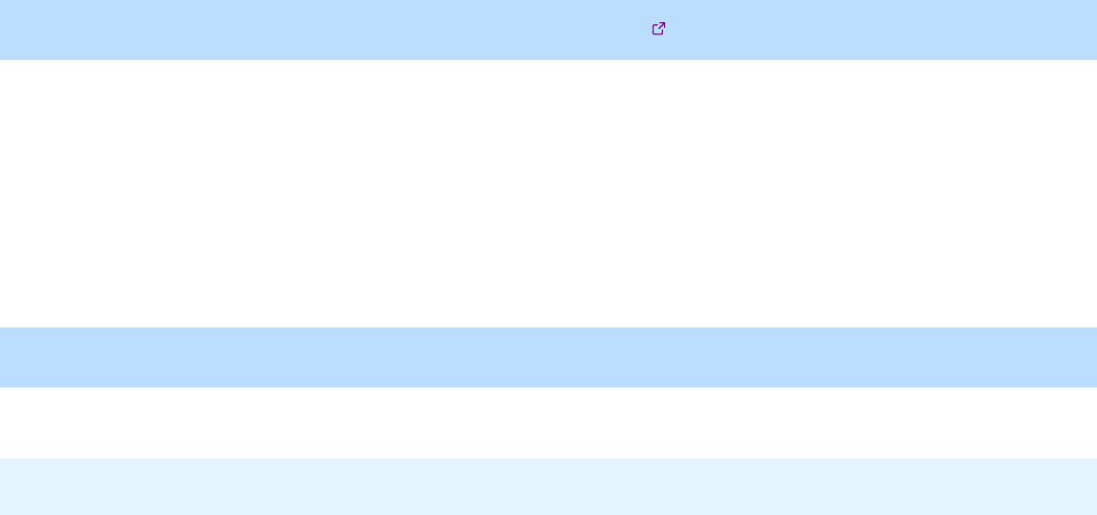
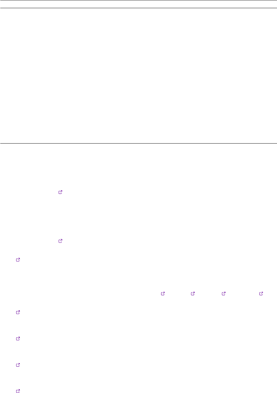
which contains all the necessary subdirectories and les. In gure 2.1
the directory structure of the complete Sharc directory is shown.
sharc/
bin/
sharc.x
data extractor.x
Interface code
Auxilliary scripts
doc/
manual.pdf
tutorial.pdf
examples/
lib/
source/
Makefile
Fortran code
tests/
INPUT/
Test Cases .../
RESULTS/
Test Cases .../
wfoverlap/
scripts/
source/
test jobs/
=$SHARC
Figure 2.1: Directory tree containing a complete Sharc installation.
To compile the Fortran90 programs of the Sharc suite, go to the source/ directory.
cd source/
and edit the
Makefile
by adjusting the
F90
variable to point to the Fortran compiler of your choice. Issuing the
command:
make
will compile the source and create all the binaries.
21
Sharc Manual 2 Installation |2.3 Installation
make install
will copy the binary les into the
sharc/bin/
directory of the Sharc distribution, which already contains all the python
scripts which come with Sharc.
In order to use the Sharc suite, set the environment variable
$SHARC
to the
bin/
directory of the Sharc installation.
This ensures that all programs of the Sharc suite nd the other executables and all calls are successful. For example, if
you have unpacked Sharc into your home directory, just set:
export SHARC=~/sharc/bin (for bourne shell users)
or
setenv SHARC $HOME/sharc/bin (for c-shell type users)
Note that it is advisable to put this line into your shell’s login scripts.
2.3.1 WFoverlap Program
The Sharc package contains as a submodule the program WFoverlap, which is necessary for many functionalities of
Sharc. In order to install and test this program, see section 6.11.
2.3.2 Libraries
Sharc requires the BLAS, LAPACK and FFTW3 libraries. During the installation, it might be necessary to alter the
LDFLAGS
string in the
Makefile
, depending on where the relevant libraries are located on your system. In this way, it is
for example possible to use vendor-provided libraries like the Intel MKL. For more details see the
INSTALL
le which
is included in the Sharc distribution.
2.3.3 Test Suite
After the installation, it is advisable to rst execute the test suite of Sharc, which will test the fundamental functionality
of SHARC. Change to an empty directory and execute
$SHARC/tests.py
The interactive script will rst verify the Python installation (no message will appear if the Python installation is ne).
Subsequently, the script prompts the user to enter which tests should be executed. The script will also ask for a number
of environment variables, which are listed in Table 2.1.
Their is at least one test for each of the auxiliary scripts and interfaces. Tests whose names start with
scripts_
test the
functionality of the auxiliary programs in the Sharc suite. Tests whose names start with
ADF_
,
Analytical_
,
COLUMBUS_
,
GAUSSIAN_
,
LVC_
,
MOLCAS_MOLPRO_
, or
TURBOMOLE_
run short trajectories, testing whether the main dynamics code, the
interfaces, the quantum chemistry programs, and auxiliary programs (TheoDORE,WFoverlap,Orca,Tinker) work
together correctly.
If the installation was successful and Python is installed correctly,
Analytical_overlap
,
LVC_overlap
, and most tests
named scripts_<NAME> should execute without error.
The test calculations involving the quantum chemistry programs can be used to check that Sharc can correctly call
these programs and that they are installed correctly.
If any of the tests show dierences between output and reference output, it is advisable to check the respective les (i.e.,
compare
$SHARC/../tests/RESULTS/<job>/
to
./RUNNING_TESTS/<job>/
). Note that small dierences (dierent sign
of values or small numerical deviations) in the output can already occur when using a dierent version of the quantum
chemistry programs, dierent compilers, dierent libraries, or dierent parallization schemes. It should be noted that
along trajectories, these small changes can add up to notably inuence the trajectories, but across the ensemble these
small changes will likely cancel out.
22
Sharc Manual 2 Installation |2.3 Installation
Table 2.1: Environment variables for Sharc test jobs. These variables need to be set before the test job execution.
Keyword Description
$ADF Points to the main directory of the ADF installation, which contains the le adfrc.sh.
$COLUMBUS Points to the directory containing the Columbus executables, e.g., runls.
$GAUSSIAN
Points to the main directory of the Gaussian installation, which contains the Gaussian
executables (e.g., g09/g16 or l9999.exe).
$MOLCAS
Points to the main directory of the Openmolcas installation, containing
molcas.rte
and
directories basis_library/ and bin/.
$MOLPRO
Points to the
bin/
directory of the Molpro installation, which contains the
molpro.exe
le.
$TURBOMOLE
Points to the main directory of the Turbomole installation, which contains subdirectories
like basen/,bin/, or scripts/.
$ORCA
Points to the directory containing the Orca executables, e.g.,
orca
,
orca_gtoint
, or
orca_scf.
$THEODORE
Points to the main directory of the TheoDORE installation.
$THEODORE/bin/
should contain
analyze_tden.py.
$TINKER
Points to the
bin/
directory of a Molcas-modied Tinker installation. It contains les like
tkr2qm_s.
$molcas
Should point to the same location as
$MOLCAS
, or another Molcas installation. Note that
$molcas
is only used by some Columbus test jobs. Also note that
$molcas
does not need to
point to the Molcas installation interfaced to Columbus.
2.3.4 Additional Programs
For full functionality of the Sharc suite, several additional programs are recommended (all of these programs are
currently freely available, except for Amber):
•The Python package NumPy.
Optimally, within your Python installation the NumPy package (which provides many numerical methods, e.g.,
matrix diagonalization) should be available. If NumPy is not available, the Sharc suite is still functional, and
the aected scripts will fall back to use a small Fortran code (front-end for LAPACK) within the Sharc package.
Since in the Python scripts no large-scale matrix calculations are carried out, there should be no signicant
performance loss if NumPy is not available.
•The Python package Matplotlib.
If the Matplotlib package, some auxiliary scripts can automatically generate certain plots.
•The Gnuplot plotting software.
Gnuplot is not strictly necessary, since all output les could be plotted using other plotting programs. However,
a number of scripts from the Sharc suite automatically generate Gnuplot scripts after data processing, allowing
to quickly plot the output les or carry out data ts.
•A molecular visualization software able to read xyz les (e.g. Molden,Gabedit,Molekel or VMD).
Molecular visualization software is needed in order to visualize molecular motion in the dynamics.
•The Maxima computer algebra system.
The computer algebra system Maxima is necessary for the use of
make_fitscript.py
, a program which allows
to perform global ts of chemical kinetics models to populations data.
•The TheoDORE wave function analysis suite.
The wave function analysis package TheoDORE allows to compute various descriptors of electronic wave
functions (supported by some interfaces), which is helpful to follow the state characters along trajectories.
•The Amber molecular dynamics package.
Amber can be used to prepare initial conditions based on ground state molecular dynamics simulations (instead
of using a Wigner distribution), which is especially useful for large systems.
•The Orca ab initio package.
Orca can be employed as external optimizer. In combination with the Sharc interfaces, it is possible to perform
optimizations of minima, conical intersections, and crossing points for any method interfaced to Sharc.
23

Sharc Manual 2 Installation |2.3 Installation
2.3.5 antum Chemistry Programs
Even though Sharc comes with two interfaces for analytical potentials (and hence can be used without any quantum
chemistry program), the main application of Sharc is certainly on-the-y ab initio dynamics. Hence, one of the
following interfaced quantum chemistry programs is necessary:
•Molpro (this release was checked against Molpro 2010 and 2012).
•Openmolcas (this release was checked against Openmolcas 18).
–Tinker,interfaced to Openmolcas 18, for QM/MM dynamics.
•Columbus 7
–Columbus-Molcas interface for spin-orbit couplings.
•Amsterdam Density Functional (ADF 2017 needed for overlaps, ADF 2018 for all QM/MM functionality)
•
Turbomole (this release was checked against Turbomole 6.6 and 7.0; version 7.1 is currently not supported).
–Orca (version 3 or 4) for spin-orbit couplings.
•Gaussian (this release was checked against Gaussian 09 and 16).
See the relevant sections in chapter 6for a description of the quantum chemical methods available with each of these
programs.
24
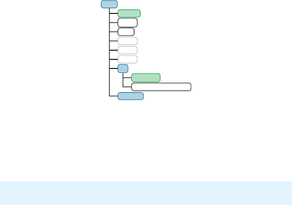
3 Execution
The Sharc suite consists of the main dynamics code
sharc.x
and a number of auxiliary programs, like setup scripts and
analysis tools. Additionally, the suite comes with interfaces to several quantum chemistry software: Molpro,Molcas,
Columbus,Turbomole,ADF, and Gaussian.
In the following, rst it is explained how to run a single trajectory by setting up all necessary input for the dynamics
code
sharc.x
manually. Afterwards, the usage of the auxiliary scripts is explained. Detailed infos on the Sharc input
les is given in chapter 4. Chapter 5documents the dierent output les Sharc produces. The interfaces are described
in chapter 6and the auxiliary scripts in chapter 7. All relevant theoretical background is given in chapter 8.
3.1 Running a single trajectory
3.1.1 Input files
Sharc requires a number of input les, which contain the settings for the dynamics simulation (
input
), the initial
geometry (
geom
), the initial velocity (
veloc
), the initial coecients (
coeff
) and the laser eld (
laser
). Only the rst
two (
input
,
geom
) are mandatory, the others are optional. The necessary les are shown in gure 3.1. The content of
the main input le is explained in detail in section 4.1, the geometry le is specied in section 4.2. The specications of
the velocity, coecient and laser les are given in sections 4.3,4.4 and 4.5, respectively.
TRAJ
run.sh
input
geom
veloc
coeff
laser
QM
runQM.sh
<Interface files>
restart
Figure 3.1:
Input les for a Sharc dynamics simulation. Directories are in blue, executable scripts in green, regular
les in white and optional les in grey.
Additionally, the directory
QM/
and the script
QM/runQM.sh
need to be present, since the on-the-y ab initio calculations
are implemented through these les. The script
QM/runQM.sh
is called each time Sharc performs an on-the-y calculation
of electronic properties (usually by a quantum chemistry program). In order to do so, Sharc rst writes the request
for the calculation to
QM/QM.in
, then calls
QM/runQM.sh
, waits for the script to nish and then reads the requested
quantities from
QM/QM.out
. The script
QM/runQM.sh
is fully responsible to generate the requested results from the
provided input. In virtually all cases, this task is handled by the Sharc-quantum chemistry interfaces (see chapter 6), so
that the script QM/runQM.sh has a particularly simple form:
cd QM/
$SHARC/<INTERFACE> QM.in
25

Sharc Manual 3 Execution |3.2 Typical workow for an ensemble of trajectories
with the corresponding interface name given. Note that the interfaces in all cases need additional input les, which
must be present in
QM/
. Those input les contain the specications for the quantum chemistry information, e.g., basis
set, active and reference space, memory settings, path to the quantum chemistry program, path to scratch directories;
or for
SHARC_Analytical.py
and
SHARC_LVC.py
the parameters for the analytical potentials. For each interface, the
input les are slightly dierent. See sections 6.3,6.4,6.5,6.6,6.8,6.7,6.9,or6.10 for the necessary information.
3.1.2 Running the dynamics code
Given the necessary input les, Sharc can be started by executing
user@host> $SHARC/sharc.x input
Note that besides the input le, at least the geometry le needs to be present (see chapter 4for details).
A running trajectory can be stopped after the current time step by creating an empty le STOP:
user@host> touch STOP
This is usually preferable to simply killing Sharc, because the current time step is properly nished and all les are
correctly written for analysis and restart.
3.1.3 Output files
Figure 3.2 shows the content of a trajectory directory after the execution of Sharc. There will be six new les. These
les are output.log,output.lis,output.dat and output.xyz, as well as restart.ctrl and restart.traj.
The le
output.log
contains mainly a listing of the chosen options and the resulting dynamics settings. At higher print
levels, the log le contains also information per time step (useful for debugging).
output.lis
contains a table with one
line per time step, giving active states, energies and expectation values.
output.dat
contains a list of all important
matrices and vectors at each time step. This information can be extracted with
data_extractor.x
to yield plottable
table les.
output.xyz
contains the geometries of all time steps (the comments to each geometry give the active state).
For details about the content of the output les, see chapter 5.
The restart les contain the full state of a trajectory and its control variables from the last successful time step. These
les are needed in order to restart a trajectory at this time step (either because the calculation failed, or in order to
extend the simulation time beyond the original maximum simulation time).
3.2 Typical workflow for an ensemble of trajectories
Usually, one is not interested in running only a single trajectory, since a single trajectory cannot reproduce the branching
of a wave packet into dierent reaction channels. In order to do so, within surface hopping an ensemble of independent
trajectories is employed.
When dealing with a (possibly large) ensemble of trajectories, setup and analysis need to be automatized. Hence, the
Sharc suite contains a number of scripts fullling dierent tasks in the usual workow of setting up ensembles of
trajectories. The typical workow is given schematically in gure 3.3.
3.2.1 Initial condition generation
In the typical workow, the user will rst create a set of suitable initial conditions. In the context of the Sharc package,
an initial condition is a set of an initial geometry, initial velocity, initial occupied state and initial wave function
coecients. Many such sets are needed in order to setup physically sound dynamics simulations.
Generation of initial geometries and velocities
Currently, within the Sharc suite, initial geometries and velocities
can be generated based on a quantum harmonic oscillator Wigner distribution. The theoretical background is given in
section 8.20. The calculation is performed by wigner.py, which is explained in section 7.1.
26
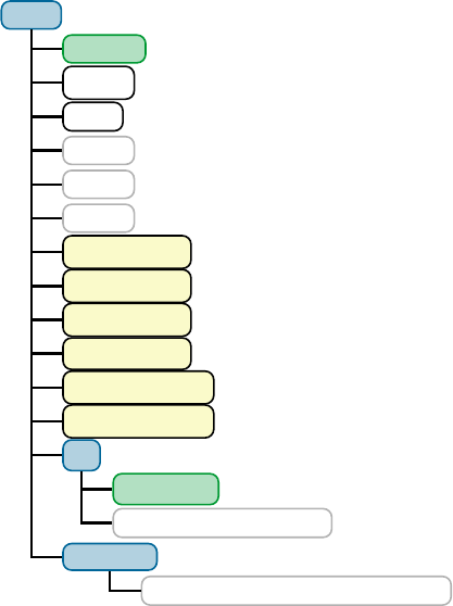
Sharc Manual 3 Execution |3.2 Typical workow for an ensemble of trajectories
TRAJ
run.sh
input
geom
veloc
coeff
laser
output.lis
output.log
output.dat
output.xyz
restart.ctrl
restart.traj
QM
runQM.sh
<Interface files>
restart
<Interface restart files>
Figure 3.2:
Files of a Sharc dynamics simulation after running. Directories are in blue, executable scripts in green,
regular les in white and optional les in grey. Output les are in yellow.
As given in gure 3.3,
wigner.py
needs as input the result of a frequency calculation in Molden format. The calculation
can be performed by any quantum chemistry program and any method the user sees t (there are some scripts which
can aid in the frequency calculation, see sections 6.3.5,6.4.3,6.7.6).
wigner.py
produces the le
initconds
, which
contains a list of initial conditions ready for further processing.
Alternatively, initial geometries and velocities can be extracted from molecular dynamics simulations in the ground
state. Currently, it is possible to either convert restart les Amber to an
initconds
le (using
amber_to_initconds.py
,
see section 7.2) or to randomly sample snapshots from Sharc trajectories (using
sharctraj_to_initconds.py
, see
section 7.3).
Generation of initial coeicients and states
In the second preparation step, for each of the sampled initial
geometries it has to be decided which excited state should be the initial one. In simple cases, the user may manually
choose the initial excited state using excite.py (optionally after diabatization; see 7.5). Alternatively, the selection of
initial states can be performed based on the excitation energies and oscillator strengths of the excited states at each
initial geometry (this approximately simulates a delta-pulse excitation).
The latter options (diabatization or energies/oscillator strengths) make it necessary to carry out vertical excitation
calculation before the selection of the initial states. The calculations can be set up with
setup_init.py
(see section 7.4).
This script prepares for each initial condition in the
initconds
le a directory with the necessary input to perform the
calculation. The user should then execute the run script (
run.sh
) in each of the directories (either manually or through
a batch queueing system).
After the vertical excitation calculations are completed, the vertical excitation energies and oscillator strengths of each
calculation are collected by
excite.py
(see 7.5). The same script then performs the selection of the initial electronic state
for each initial geometry. The results are written to a new le,
initconds.excited
. This le contains all information
needed to setup the ensemble.
Additionally,
spectrum.py
(7.8) can calculate absorption spectra based on the
initconds.excited
le. This may be
useful to verify that the level of theory chosen is appropriate (e.g., by comparing to an experimental spectrum), or to
choose a suitable excitation window for the determination of the initial state.
27
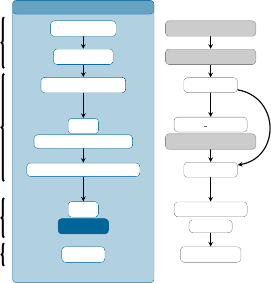
Sharc Manual 3 Execution |3.2 Typical workow for an ensemble of trajectories
Sharc Workflow
Optimization
Frequencies
Wigner Sampling
Setup
Excited-State Calcs.
Excited-State Selection
Setup
Dynamics
Analysis
Req
Req,{νi},{ni}
{(R,v)k}
{∆Ek,β},{Fosc
k,β}
{(R,v,α)k}
Quantum Chemistry
Quantum Chemistry
wigner.py
setup init.py
Quantum Chemistry
excite.py
setup traj.py
sharc.x
many tools...
freq.molden
initconds
QM.out
initconds.excited
output.dat, output.xyz
initconds
Preparation
Initial Conditions
Dynamics Simulations
Aftermath
Figure 3.3: Typical workow for conducting excited-state dynamics simulations with Sharc.
3.2.2 Running the dynamics simulations
Based on the initial conditions given in
initconds.excited
, the input for all trajectories in the ensemble can be setup
by
setup_traj.py
(see section 7.6). The script produces one directory for each trajectory, containing the input les for
Sharc and the selected interface.
In order to run a particular trajectory, the user should execute the run script (
run.sh
) in the directory of the trajectory.
Since those calculations can run between minutes and several weeks (depending on the level of theory used and the
number of time steps), it is advisable to submit the run scripts to a batch queueing system.
The progress of the simulations can be monitored most conveniently in the
output.lis
les. If the calculations are
running in some temporary directory, the output les can be copied to the local directory (where they were setup)
with the
scp
wrapper
retrieve.sh
(see 7.9). This allows to perform ensemble analysis while the trajectories are still
running.
If a trajectory fails, the temporary directory where the calculation is running is not deleted. The le
README
will be
created in the trajectory’s directory, giving the time of the failure and the location of the temporary data, so that the
case can be investigated.
In order to signal Sharc to terminate a trajectory after the current time step is completed, the user can create a (possibly
empty) le STOP in the working directory of the trajectory (the directory where sharc.x is running).
The status of the ensemble of trajectories can be checked with
diagnostics.py
(section 7.12). This script checks the
presence and integrity of all relevant les, the progress of all trajectories, and warns if trajectories behave unexpectedly
(non-conversion of total energy, intruder states, etc).
3.2.3 Analysis of the dynamics results
Each trajectory can be analyzed independently by inspecting the output les (see chapter 5). Most importantly, calling
data_extractor.x
(7.10) on the
output.dat
le of a trajectory creates a number of formatted les which can be plotted
with the help of
make_gnuscript.py
(7.11) and Gnuplot. The nuclear geometries in
output.xyz
le can be analyzed in
terms of internal coordinates (bond lengths, angles, ring conformations, etc.) using
geo.py
(7.18). The manual analysis
of all individual trajectories is usually a good idea to verify that the trajectories are correctly executing, and in order to
28
Sharc Manual 3 Execution |3.3 Auxilliary Programs and Scripts
nd general reaction pathways. The manual analysis often permits to formulate some hypotheses, which can then be
veried with the statistical analysis tools.
For the complete ensemble, the rst step should usually be to run
diagnostics.py
(section 7.12). This script will
determine how long the dierent trajectories are, and, more importantly, will check the trajectories for le integrity,
conservation of total energy, and continuity of potential/kinetic energy. Based on a set of customizable criteria, the
script determines for each trajectory a “maximum usable time”. The script then can mark all trajectories with maximum
usable time below a given threshold to be excluded from analysis (by creating a le
DONT_ANALYZE
in the trajectory’s
directory). The other analysis scripts will then ignore trajectories marked by
diagnostics.py
. Trajectories can also be
manually excluded from analysis, by creating a le called CRASHED,DEAD, or RUNNING in the respective directory.
After the trajectories were checked and unsuitable ones excluded, the statistical analysis scripts can be used. The script
populations.py
(section 7.13) can calculate average excited-state populations. The script
transition.py
(section 7.14)
can analyze the total number of hops between all pairs of states in an ensemble, allowing to identify relevant relaxation
routes in the dynamics. Using the script
make_fitscript.py
(7.15), it is possible to make elaborate global ts of
chemical kinetics models to the populations data, allowing to extract rate constants from the populations. With
bootstrap.py
(7.16) one can compute errors for these rate constants. The script
crossing.py
(7.17) can nd and
extract notable geometries, e.g., those geometries where a surface hop between two particular states occurred. Using
trajana_essdyn.py
(7.19) and
trajana_nma.py
(7.20) it is furthermore possible to perform essential dynamics analysis
and normal mode analysis. Finally,
data_collector.py
can merge arbitrary tabulated data from the trajectories and
perform various analysis procedures (compute mean/standard deviation, data convolution, summation, integration),
which can be used to compute, e.g., time-dependent distribution functions or time-dependent spectra.
3.3 Auxilliary Programs and Scripts
The following tables list the auxiliary programs in the Sharc suite. The rightmost column gives the section where the
program is documented.
3.3.1 Setup
wigner.py Creates initial conditions from Wigner distribution. 7.1
amber_to_initconds.py Creates initial conditions from Amber restart les. 7.2
sharctraj_to_initconds.py Creates initial conditions from Sharc trajectories. 7.3
setup_init.py Sets up initial vertical excitation calculations. 7.4
excite.py
Generates excited state lists for initial conditions and selects initial states.
7.5
setup_traj.py Sets up the dynamics simulations based on the initial conditions. 7.6
laser.x Prepares les containing laser elds. 7.7
molpro_input.py Prepares Molpro input les and template les for the Molpro interface. 6.3.5
molcas_input.py Prepares Molcas input les and template les for the Molcas interface. 6.4.3
ADF_input.py Prepares ADF input les. 6.7.5
ADF_freq.py Converts ADF output les of frequency calculations to Molden format. 6.7.6
QMout2LVC.py
Converts output from a single point calculation to template for the LVC
interface.
6.9.2
29
Sharc Manual 3 Execution |3.3 Auxilliary Programs and Scripts
3.3.2 Analysis
spectrum.py Generates absorption spectra from initial conditions les. 7.8
retrieve.sh scp wrapper to retrieve dynamics output during the simulation. 7.9
data_extractor.x Extracts plottable results from the Sharc output data le. 7.10
make_gnuscript.py Creates gnuplot scripts to plot trajectory data. 7.11
diagnostics.py Checks ensembles for integrity, progress, energy conservation. 7.12
populations.py Calculates ensemble populations. 7.13
transition.py Calculates total number of hops within an ensemble. 7.14
make_fitscript.py Creates gnuplot scripts to t kinetic models to population data. 7.15
bootstrap.py Computes errors for kinetic model ts. 7.16
crossing.py Extracts specic geometries from ensembles. 7.17
geo.py Calculates internal coordinates from xyz les. 7.18
trajana_essdyn.py Performs an essential dynamics analysis for an ensemble. 7.19
trajana_nma.py Performs a normal mode analysis for an ensemble. 7.20
data_collector.py Collects data from tabular les and performs various analyses 7.21
3.3.3 Interfaces
SHARC_MOLPRO.py
Calculates SOCs, gradients, nonadiabatic couplings, overlaps, dipole mo-
ments, and Dyson norms at the CASSCF level of theory (using Molpro).
Symmetry or RASSCF are not supported. Only segmented basis sets are
possible.
6.3
SHARC_MOLCAS.py
Calculates SOCs, gradients, overlaps, dipole moments, Dyson norms, dipole
moment derivatives, and spin-orbit coupling derivatives at the CASSCF and
(MS-)CASPT2 level of theory (using Molcas). Symmetry is not supported.
Numerical dierentiation is used for some tasks.
6.4
SHARC_COLUMBUS.py
Calculates SOCs, gradients, nonadiabatic couplings, overlaps, dipole mo-
ments, and Dyson norms at the CASSCF, RASSCF, and MRCISD levels of
theory (using Columbus). Symmetry is not supported. Works with the
either Dalton or Seward integrals (through the Columbus-Molcas in-
terface), but SOCs are only available with Seward integrals. Nonadiabatic
couplings are only available with Dalton integrals.
6.5
SHARC_Analytical.py
Calculates SOCs, gradients, overlaps, dipole moments, and dipole moment
derivatives based on analytical expressions of diabatic matrix elements
dened in Cartesian coordinates.
6.6
SHARC_ADF.py
Calculates SOCs, gradients, overlaps, dipole moments, and Dyson norms at
the TD-DFT level of theory with GGA and hybrid functionals (using ADF).
Symmetry is not supported.
6.7
SHARC_RICC2.py
Calculates SOCs, gradients, overlaps, and dipole moments at the ADC(2)
and CC2 levels of theory (using Turbomole). Symmetry is not supported.
For SOCs, only ADC(2) can be used and Orca has to be installed in addition
to Turbomole.
6.8
SHARC_LVC.py
Calculates SOCs, gradients, nonadiabatic couplings, overlaps, and dipole
moments based on linear-vibronic coupling models dened in mass-
weighted normal mode coordinates.
6.9
SHARC_GAUSSIAN.py
Calculates gradients, overlaps, dipole moments, and Dyson norms at the
TD-DFT level of theory (using Gaussian). Symmetry is not supported.
6.10
30
Sharc Manual 3 Execution |3.3 Auxilliary Programs and Scripts
3.3.4 Others
tests.py Script to automatically run the Sharc test suite. 2.3.3
wfoverlap.x Program to compute wave function overlaps, used by most interfaces. 6.11
Orca_External
Script to carry out optimizations with Orca as optimizer and Sharc as
gradient provider.
7.22
setup_orca_opt.py
Script to setup optimizations with Orca as optimizer and Sharc as gradient
provider.
7.22
setup_single_point.py Script to setup single point calculations with Sharc interfaces. 7.23
QMout_print.py
Script to convert a
QM.out
le to a table with energies and oscillator
strengths.
7.24
diagonalizer.x Helper program for excite.py. Only required if NumPy is not available. 7.25
31

4 Input files
In this chapter, the format of all Sharc input les are presented. Those are the main input le (here called
input
),
the geometry le, the velocity le, the coecients le, the laser le, and the atom mask le. Only the rst two are
mandatory, the others are optional input les. All input les are ASCII text les.
4.1 Main input file
This section presents the format and all input keywords for the main Sharc input. Note that when using
setup_traj.py
,
full knowledge of the Sharc input keywords is not required.
4.1.1 General remarks
The input le has a relatively exible structure. With very few exceptions, each single line is independent. An input
line starts with a keyword, followed optionally by a number of arguments to this keyword. Example:
stepsize 0.5
Here,
stepsize
is the keyword, referring to the size of the time steps for the nuclear motion in the dynamics.
0.5
gives
the size of this time step, in this example 0.5 fs.
A number of keywords have no arguments and act as simple switches (e.g.,
restart
,
gradcorrect
,
grad_select
,
nac_select
,
ionization
,
track_phase
,
dipole_gradient
). Those keywords can be prexed with
no
to explicitly
deactivate the option (e.g., norestart deactivates restarts).
In each line a trailing comment can be added in the input le, by using the special character
#
. Everything after
#
is
ignored by the input parser of Sharc. The input le also can contain arbitrary blank lines and lines containing only
comments. All input is case-insensitive.
The input le is read by Sharc by subsequently searching the le for all known keywords. Hence, unknown or
misspelled keywords are ignored. Also, the order of the keywords is completely arbitray. Note however, that if a
keyword is repeated in the input only the rst instance is used by the program.
4.1.2 Input keywords
In Table 4.1, all input keywords for the Sharc input le are listed.
32

Sharc Manual 4 Input les |4.1 Main input le
Table 4.1:
Input keywords for
sharc.x
. The rst column gives the name of the keyword, the second lists possible
arguments and the third line provides an explanation. Defaults are marked like
this
. $
n
denotes the
n
-th
argument to the keyword.
Keyword Arguments Explanation
— General control keywords —
printlevel integer Controls the verbosity of the log le.
$1=0 Log le is empty
$1=1 + List of internal steps
$1=2 + Input parsing information
$1=3 + Some information per time step
$1=4 + More information per time step
$1=5 + Much more information per time step
restart Dynamics is resumed from restart les.
norestart Dynamics is initialized from input les.
norestart takes precedence.
rngseed integer Seed for the random number generator.
10997279 Used for surface hopping and AFSSH decoherence.
— Input le keywords —
geomfile quoted string File name containing the initial geometry.
"geom"
velocfile quoted string File containing the initial velocities.
"veloc" Only read if veloc external.
coefffile quoted string File containing the initial wave function coecients.
"coe" Only read if coeff external.
laserfile quoted string File containing the laser eld.
"laser" Only read if laser external.
atommaskfile quoted string File containing the atom mask.
"atommask" Only read if atommask external.
— Trajectory initialization keywords —
veloc string Sets the initial velocities.
$1=zero Initial velocities are zero.
$1=random $2 oat Random initial velocities with $2 eV kinetic energy per atom.
$1=external Initial velocities are read from le.
nstates list of integers Number of states per multiplicity.
$1 (1)Number of singlet states
$2 (0)Number of doublet states
$3 (0)Number of triplet states
$...(0)Number of states of higher multiplicities
actstates list of integers Number of active states per multiplicity.
same as nstates By default, all states are active.
state integer,string Species the initial state.
(no default; Sharc exits if state is missing).
$1 Initial state.
$2=MCH Initial state and coecients are given in MCH representation.
$2=diag Initial state and coecients are given in diagonal representation.
coeff string Sets the wave function coecients.
$1=auto Initial coecient are determined automatically from initial state.
$1=external Initial coecients are read from le.
— Laser eld keywords —
laser string Sets the laser eld.
$1=none No laser eld is applied.
$1=internal Laser eld is calculated at each time step from internal function.
$1=external Laser eld for each time step is read during initialization.
laserwidth oat Laser bandwidth used to detect induced hops.
Continued on next page
33

Sharc Manual 4 Input les |4.1 Main input le
Table 4.1 – Continued from previous page
Keyword Arguments Explanation
1.0 eV
— Time step keywords —
stepsize oat Length of the nuclear dynamics time steps in fs.
0.5 fs
nsubsteps integer
Number of substeps for the integration of the electronic
equation of motion.
25
nsteps integer Number of simulation steps.
3
tmax oat Total length of the simulation in fs.
No eect if nsteps is present.
killafter oat Terminates the trajectory after $1 fs in the lowest state.
-1 If $1<0, trajectories are never killed.
— Surface hopping setting keywords —
surf string Potential energy surfaces used in surface hopping.
$1=diagonal,sharc Uses diagonal potentials.
$1=MCH Uses MCH potentials.
coupling string Quantities describing the nonadiabatic couplings.
$1=ddr,nacdr Uses vectorial nonadiabatic couplings hψα|∂/∂R|ψβi.
$1=ddt,nacdt Uses temporal nonadiabatic couplings hψα|∂/∂t|ψβi.
$1=overlap Uses the overlaps hψα(t0)|ψβ(t)i (local diabatization).
gradcorrect
Include
(Eα−Eβ)hψα|∂/∂R|ψβi
in gradient transformation.
nogradcorrect Transform only the gradient matrix.
ekincorrect string Adjustment of the kinetic energy after a surface hop.
$1=none Kinetic energy is not adjusted. Jumps are never frustrated.
$1=parallel_vel Velocity is rescaled to adjust kinetic energy.
$1=parallel_nac
Only the velocity component in the direction of
hψα|∂/∂R|ψβi
is rescaled.
reflect_frustrated string Reection of trajectory after frustrated hop.
$1=none No reection.
$1=parallel_vel Full velocity vector is reected.
$1=parallel_nac
Only the velocity component in the direction of
hψα|∂/∂R|ψβi
is reected.
decoherence_scheme string Method for decoherence correction.
$1=none No decoherence correction.
$1=edc Energy-dierence based correction.[101]
$1=afssh Augmented FSSH.[30]
decoherence_param oat Value αin EDC decoherence (in Hartree).
0.1 $1>0.0
decoherence Applies decoherence correction (EDC by default).
nodecoherence No decoherence correction.
nodecoherence takes precedence.
hopping_procedure string Method for hopping probabilities.
$1=o No hops (same as no_hops).
$1=sharc,standard Standard Sharc hopping probabilities.
$1=gfsh Global ux SH hopping probabilities.[70]
no_hops Disables surface hopping.
no_hops takes precedence.
atommask string Activates masking of atoms (for EDC, parallel_vel).
$1=none No atoms are masked.
$1=external Atom mask is read from external le.
— Energy control keywords —
ezero oat Energy shift for Hamiltonian diagonal elements (Hartree).
0.0 Is not determined automatically!
scaling oat Scaling factor for Hamiltonian matrix and gradients.
Continued on next page
34

Sharc Manual 4 Input les |4.1 Main input le
Table 4.1 – Continued from previous page
Keyword Arguments Explanation
1.0 0. <$1
dampeddyn oat Scaling factor for kinetic energy at each time step.
1.0 0.≤$1≤1.
— Gradient and NAC selection keywords —
grad_select Only some gradients are calculated at every time step.
grad_all
All gradients are calculated at every time step (Alias:
nograd_select).
grad_all takes precedence.
nac_select Only some hψα|∂/∂R|ψβiare calculated at every time step.
nac_all
All
hψα|∂/∂R|ψβi
are calculated at every time step (Alias:
nonac_select).
nac_all takes precedence.
eselect oat Parameter for selection of gradients and NACs (in eV).
0.5 eV
select_directly
Do not do a second QM calculation for gradients and NACs.
— Phase tracking keywords —
track_phase Track the phase of the transformation matrix U.
notrack_phase No phase tracking of U(only for debugging).
phases_from_interface Request phase information from interface.
nophases_from_interface Try to recover phase information from QM data.
phases_at_zero Request phase from interface at t=0.
— Property computation keywords —
spinorbit Include spin-orbit couplings into the Hamiltonian.
nospinorbit Neglect spin-orbit couplings.
dipole_gradient Include dipole moments derivatives in the gradients.
nodipole_gradient Neglect dipole moments derivatives.
ionization Calculate ionization probabilities on-the-y.
noionization No ionization probabilities.
ionization_step integer Calculate ionization probabilities every $1 time step.
1By default calculated every time step (if ionization).
theodore Calculate wavefunction descriptors on-the-y.
notheodore No wavefunction descriptors.
theodore_step integer Calculate wavefunction descriptors every $1 time step.
1By default calculated every time step (if theodore).
n_property1d integer Allocate for that many 1D properties.
1
n_property2d integer Allocate for that many 2D properties.
1
— Output control keywords —
write_grad Writes gradients to output.dat.
nowrite_grad
write_nacdr Writes NACs to output.dat.
nowrite_nacdr
write_overlap Writes overlaps to output.dat.
nowrite_overlap Not written if not requested.
write_property1d on if theodore Writes 1D properties to output.dat.
nowrite_property1d
write_property2d on if ionization Writes 2D properties to output.dat.
nowrite_property2d
35

Sharc Manual 4 Input les |4.1 Main input le
4.1.3 Detailed Description of the Keywords
Printlevel
The
printlevel
keyword controls the verbosity of the log le. The data output le (
output.dat
) and the
listing le (output.lis) are not aected by the print level. The print levels are described in section 5.1.
Restart
There are two keywords controlling trajectory restarting. The keyword
restart
enables restarting, while
norestart disables restart. If both keywords are present, norestart takes precedence. The default is no restart.
When restarting, all control variables are read from the restart le instead of the input le. The only exceptions are
nsteps
and
tmax
. In this way, a trajectory which ran for the full simulation time can easily be restarted to extend the
simulation time.
Note that none of the auxiliary scripts adds the
restart
keyword to the input le. The user has to manually add the
restart le to the input les of the relevant trajectories.
RNG Seed
The RNG seed is used to initialize the random number generator, which provides the random numbers
for the surface hopping procedure (and the AFSSH decoherence scheme). For details how the seed is used internally,
see section 8.22.
Note that in the case of a restart, the random number generator is seeded normally, and then the appropriate number of
random numbers is drawn so that the random number sequence is consistent.
Geometry Input
The initial geometry must be given in a second le in the input format also used by Columbus.
The default name for this le is
geom
. The geometry lename can be given in the input le with the
geomfile
keyword.
Note that the lename has to be enclosed in single or double quotes. See section 4.2 for more details.
Velocity Input
Using the
veloc
keyword, the initial velocities can be either set to zero, determined randomly or read
from a le. Random determination of the velocities is such that each atom has the same kinetic energy, which must be
specied after
veloc random
in units of eV. Determination of the random velocities is detailed in 8.18. Note that after
the initial velocities are generated, the RNG is reseeded (i.e., the sequence of random numbers in the surface hopping
procedure is independent of whether random initial velocities are used).
Alternatively, the initial velocities can be read from a le. The default velocity lename is
veloc
, but the lename can
be specied with the
velocfile
keyword. Note that the lename has to be enclosed in single or double quotes. The
le must contain the Cartesian components of the velocity for each atom on a new line, in the same order as in the
geomety le. The velocity is interpreted in terms of atomic units (bohr/atu). See section 4.3 for more details.
Number of States and Active States
The keyword
nstates
controls how many states are taken into account in the
dynamics. The keyword arguments specify the number of singlet, doublet, triplet, etc. states. There is no hard-coded
maximum multiplicity in the Sharc code, however, some interfaces may restrict the maximum multiplicity.
Using the
actstates
keyword, the dynamics can be restricted to some lowest states in each multiplicity. For each
multiplicity, the number of active states must not be larger than the number of states. All couplings between the active
states and the frozen states are deleted. These couplings include o-diagonal elements in the
HMCH
matrix, in the
overlap matrix, and in the matrix containing the nonadiabatic couplings. Freezing states can be useful if transient
absorption spectra are to be calculated without increasing computational cost due to the large number of states.
Note that the initial state must not be frozen.
Initial State
The initial state can be given either in MCH or diagonal representation. The keyword
state
is followed
by an integer specifying the initial state and either the string
mch
or
diag
. For the MCH representations, states are
enumerated according to the canonical state ordering, see 8.24. The diagonal states are ordered according to energy.
Note that the initial state must be active.
If the initial state is given in the MCH basis but the dynamics is carried out in the diagonal basis, determination of the
initial diagonal state is carried out after the initial QM calculation.
36
Sharc Manual 4 Input les |4.1 Main input le
Initial Coeicients
The initial coecients can be determined automatically from the initial state, using
coeff auto
in the input le. If the initial state is given in the diagonal representation as
i
, the initial coecients are
cdiag
j=δi j
. If
the initial state is, however, given in the MCH representation, then
cMCH
j=δi j
and the determination of
cdiag =U†cMCH
is carried out after the initial QM calculation. Currently, coeff auto is always used by the automatic setup scripts.
Besides automatic determination, the initial coecients can be read from a le. The default lename is
coeff
, but
the lename can be given with the keyword
coefffile
. Note that the lename has to be enclosed in single or double
quotes. The le must contain the real and imaginary part of the initial coecients, one line per state with no blank
lines inbetween. These coecients are interpreted to be in the same representation as the initial state, i.e. the
state
keyword inuences the initial coecients. For details on the le format, see section 4.4. Note that the setup scripts
currently cannot setup trajectories with coeff external, so this can be considered an expert option.
Laser Input
The keyword
laser
controls whether a laser eld is included in the dynamics (inuencing the coecient
propagation and the energies/gradients by means of the Stark eect).
The input of an external laser eld uses the le laser. This le is specied in 4.5.
In order to detect laser-induced hops, Sharc compares the instantaneous central laser energy with the energy gap
between the old and new states. If the dierence between the laser energy and the energy gap is smaller than the laser
bandwidth (given with the
laserwidth
keyword), the hop is classied as laser-induced. Those hops are never frustrated
and the kinetic energy is not scaled to preserve total energy (instead, the kinetic energy is preserved).
Simulation Timestep
The keyword
stepsize
controls the length of a time step (in fs) for the dynamics. The nuclear
motion is integrated using the Velocity-Verlet algorithm with this time step. Surface hopping is performed once per time
step and 1–3 quantum chemistry calculations are performed per time step (depending on the selection schedule). Each
time step is divided in
nsubsteps
substeps for the integration of the electronic equation-of-motion. Since integration
is performed in the MCH representation, the default of 25 substeps is usually sucient, even if very small potential
couplings are encountered. A larger number of substeps might be necessary if high-frequency laser elds are included
or if the energy shift (ezero) is not well-chosen.
Simulation Time
The keyword
nsteps
controls the total length of the simulation. The total simulation time is
nsteps
times
stepsize
.
nsteps
does not include the initial quantum chemistry calculation. Instead of the number of
steps, the total simulation time can be given directly (in fs) using the keyword
tmax
. In this case,
nsteps
is calculated
as
tmax
divided by
stepsize
. If both keywords (
nsteps
and
tmax
) are present,
nsteps
is used. All setup scripts will
generally use the tmax keyword.
Using the keyword
killafter
, the dynamics can be terminated before the full simulation time.
killafter
species
(in fs) the time the trajectory can move in the lowest-energy state before the simulation is terminated. By default,
simulations always run to the full simulation time and are not terminated prematurely.
Surface Treatment
The keyword
surf
controls whether the dynamics runs on diagonal potential energy surfaces
(which makes it a Sharc simulation) or on the MCH PESs (which corresponds to a spin-diabatic [
26
] or FISH [
25
]
simulation, or a regular surface hopping simulation). Internally, dynamics on the MCH potentials is conducted by
setting the Umatrix equal to the unity matrix at each time step.
Description of Non-adiabatic Coupling
The code allows propagating the electronic wave function using three
dierent quantities describing nonadiabatic eects, see 8.27. The keyword
coupling
controls which of these quantities is
requested from the QM interfaces and used in the propagation. The rst option is
nacdr
, which requires the nonadiabatic
coupling vectors
hψα|∂/∂R|ψβi
. For the wave function propagation, the scalar product of these vectors and the nuclear
velocity is calculated to obtain the matrix
hψα|∂/∂t|ψβi
. During the propagation, this matrix is interpolated linearly
within each classical time step. Currently, only few Sharc interfaces can provide these couplings.
Alternatively, one can directly request the matrix elements
hψα|∂/∂t|ψβi
, which can be used for the propagation. The
corresponding argument to
coupling
is
nacdt
. In this case, the matrix is taken as constant throughout each classical
time step. Currently, none of the interfaces in Sharc can deliver these couplings, because they are computed via
overlaps, and if overlaps are known it is preferable to use local diabatization.
The third possibility is the use of the overlap matrix, requested with
coupling overlaps
(this is the default). The
overlap matrix is used subsequently in the local diabatization algorithm for the wave function propagation. Currently,
all Sharc interfaces can provide these couplings.
37
Sharc Manual 4 Input les |4.1 Main input le
Correction to the Diagonal Gradients
As detailed in 8.10, the correct transformation of the gradients to the
diagonal representation includes contributions from the nonadiabatic coupling vectors. Using
gradcorrect
, these
contributions are included. In this case Sharc will request the calculation of the nonadiabatic coupling vectors, even
if they are not used in the wave function propagation. In order to explicitly turn o this gradient correction, use the
nogradcorrect keyword.
Frustrated Hops and Adjustment of the Kinetic Energy
The keyword
ekincorrect
controls how the kinetic
energy is adjusted after a surface hop to preserve total energy. ekincorrect none deactivates the adjustment, so that
the total energy is not preserved after a hop. Using this option, jumps can never be frustrated and are always performed
according to the hopping probabilities. Using
ekincorrect parallel_vel
, the kinetic energy is adjusted by simply
rescaling the nuclear velocities so that the new kinetic energy is
Etot −Epot
. Jumps are frustrated if the new potential
energy would exceed the total energy. Finally, using
ekincorrect parallel_nac
, the kinetic energy is adjusted by
rescaling the component of the nuclear velocities parallel to the nonadiabatic coupling vector between the old and new
state. The hop is frustrated if there is not enough kinetic energy in this direction to conserve total energy. Note that
ekincorrect parallel_nac
implies the calculation of the nonadiabatic coupling vector, even if they are not used for
the wave function propagation.
The keyword
reflect_frustrated
furthermore controls whether the velocities are inverted after a frustrated hop.
With
reflect_frustrated none
(the default), after a frustrated hop, the velocity vector is not modied. Using
reflect_frustrated parallel_vel
, the full velocity vector is inverted when a frustrated hop is encountered. With the
third option,
reflect_frustrated parallel_nac
, only the velocity component parallel to the nonadiabatic coupling
vector between the active and frustrated states is inverted. This implies the calculation of the nonadiabatic coupling
vector, even if they are not used for the wave function propagation.
Decoherence Correction Scheme
There are three options for the decoherence correction (see 8.6) in Sharc, which
can be selected with the decoherence_scheme keyword.
With the default
decoherence_scheme none
, no decoherence correction is applied. The energy-dierence based
decoherence (EDC) scheme of Granucci et al. [
101
] can be activated with
decoherence_scheme edc
. The keyword
decoherence_param
can be used to change the relevant parameter
α
(see 8.6). The default is 0.1 Hartree, which
is the value recommended by Granucci et al. [
101
]. Alternatively, the AFSSH (augmented fewest-switches surface
hopping) scheme of Jain et al. [
30
] can be employed. This scheme does not use any parameters, so the keyword
decoherence_param
will have no eect. Note that in any case, the decoherence correction is applied to the states in the
representation chosen with the surf keyword.
The keywords
decoherence
(activates EDC decoherence) and
nodecoherence
are present for backwards compatibility.
Surface Hopping Scheme
There are three options for the computation of the hopping probabilities (see 8.25) in
Sharc, which can be selected with the hopping_procedure keyword.
Using
hopping_procedure off
, surface hopping will be disabled, such that the active state (in the representation
chosen with the
surf
keyword) will never change. With the default,
hopping_procedure sharc
, the standard hopping
probability equation from Ref. [
41
] will be used. Alternatively, one can use the global ux surface hopping scheme [
70
],
which might be advantageous in super-exchange situations.
One can also turn o surface hopping with the no_hops keyword.
Atom Masking
Some of the above surface hopping settings might not be fully size consistent: (i) in
ekincorrect
parallel_vel
, all atoms are uniformly accelerated/slowed during velocity rescaling; (ii) in
reflect_frustrated
parallel_vel
, the velocities of all atoms are inverted; (iii) with
decoherence_scheme edc
, the kinetic energy of all
atoms determines the decoherence rate. In large systems (e.g., in solution), these eects might be unrealistic, because,
e.g., a surface hop in the chromophore should not uniformly slow down all water molecules.
The
atommask
keyword can then be used to exclude certain atoms from the three mentioned procedures. With
atommask
external
, the list of masked and active atoms is read from the le specied with the
atommaskfile
keyword (default
"atommask"
). The format of this le is described in section 4.6. With the other possible option,
atommask none
(the
default), all atoms are considered for these procedures.
Note that the
atommask
keyword has no eect on
ekincorrect parallel_nac
,
reflect_frustrated parallel_nac
,
and decoherence_scheme afssh, because these procedures are size consistent by themselves.
38
Sharc Manual 4 Input les |4.1 Main input le
Reference Energy
The keyword
ezero
gives the energy shift for the diagonal elements of the Hamiltonian. The shift
should be chosen so that the shifted diagonal elements are reasonably small (large diagonal elements in the Hamiltonian
lead to rapidly changing coecients, requiring extremely short subtime steps).
Note that the energy shift default is 0, i.e., Sharc does not choose an energy shift based on the energies at the rst time
step (this would lead to each trajectory having a dierent energy shift).
Scaling and Damping
The scaling factor for the energies and gradients must be positive (not zero), see section 8.21.
The damping factor must be in the interval
[
0
,
1
]
(rst, since the kinetic energy is always positive; second, because a
damping factor larger than 1 would lead to exponentially growing kinetic energy). Also see section 8.5.
Selection of Gradients and Non-Adiabatic Couplings
Sharc allows to selectively calculate only certain gradients
and nonadiabatic coupling vectors at each time step. Those gradients and nonadiabatic coupling vectors not selected are
not requested from the interfaces, thus decreasing the computational cost. The selection procedure is detailed in 8.23.
Selection of gradients is activated by
grad_select
, selection for nonadiabatic couplings by
nac_select
. Selection is
turned o by default.
The selection procedure picks only states which are closer in energy to the classically occupied state than a given
threshold. The threshold is 0.5 eV by default and can be adjusted using the eselect keyword.
By default, if Sharc performs such selection it will do two quantum chemistry calls per time step. In the rst call, all
quantities are requested except for the ones to be selected. The energies are used to determine which gradients and
NACs to calculate in a second quantum chemistry call. The keyword
select_directly
tells Sharc instead to use the
energies of the last time step, so that only one call per time step is necessary.
Phase Tracking
Phase tracking is an important ingredient in Sharc. It is necessary for two reasons: (i) the columns
of the transformation matrix
U
are determined only up to an arbitrary phase factor e
iϕ
(and additional mixing angles in
case of degeneracy), and (ii) the wave functions produced by any quantum chemistry code are determined only up to
an arbitrary sign. Both kind of phases need to be tracked in Sharc in order to obtain smoothly varying matrix elements
which can be properly integrated.
By default, Sharc automatically tracks the phases in the
U
matrix (explicit keyword:
track_phase
), because all required
information is always available. This phase tracking can be deactivated with the
notrack_phase
keyword, but this
option should only be used for debugging purposes.
The tracking of the wave function signs depends on the interfaces, because only they have access to the explicit form of
the wave functions. Sharc by default (explicit keyword:
phases_from_interface
) requests that the interface tracks
the signs and reports any sign changes to Sharc. Currently, all interfaces can provide this phase information, but all of
them need to perform overlap calculations to do so. The
nophases_from_interface
keyword can be used to deactivate
these requests.
In some situations, it might be necessary to have consistent wave function signs between dierent trajectories. In this
case, the
phases_at_zero
keyword can be used to compute sign information at
t=
0; this requires that the relevant
wave function data of the reference is already located in the
restart/
directory before the trajectory is started. Note
that phases_at_zero is therefore an expert option.
Spin-Orbit Couplings
Using the keyword
nospinorbit
the calculation of spin-orbit couplings is disabled. Sharc
will only request the diagonal elements of the Hamiltonian from the interfaces. If the interface returns a non-diagonal
Hamiltonian anyways, the o-diagonal elements are deleted.
The keyword spinorbit (which is the default) enables spin-orbit couplings.
Dipole Moment Gradients
The derivatives of the dipole moments can be included in the gradients. This can be
activated with the keyword
dipole_gradient
. Currently, only the analytical and Molcas interfaces can deliver these
quantities.
Ionization
The keyword
ionization
activates (
noionization
deactivates) the on-the-y calculation of ionization
transition properties. If the keyword is given, by default these properties are calculated every time step. The keyword
ionization_step
can be used to calculate these properties only every
n
-th time step. If the keyword is given, Sharc
will request the calculation of the ionization properties from the interface, which needs to be able to calculate them.
39

Sharc Manual 4 Input les |4.2 Geometry le
The ionization probabilities are treated as one 2D property matrix, hence n_property2d should be at least 1.
TheoDORE
The keyword
theodore
activates (
notheodore
deactivates) the on-the-y calculation of wave function
descriptors with the TheoDORE program. This can be very useful to track the wave function character of the states
on-the-y. The interface must be able to execute and TheoDORE and return its output to Sharc (currently, the
ADF, Gaussian, and Turbomole interfaces can do this). The keyword
theodore_step
can be used to calculate these
descriptors only every n-th time step.
The TheoDORE descriptors are treated as one 1D property vector for each descriptor, and
n_property1d
should be at
least as large as the number of descriptors computed by the interface.
Output control
There are a number of keywords which control what information is written to the
output.dat
le. These keywords are
write_grad
,
write_nacdr
,
write_overlap
,
write_property1d
, and
write_property2d
(and
the inverse of each one, e.g.,
nowrite_grad
). Only
write_overlap
is activated by default, because it does not enlarge
the data le by much, and contains important information which is read by
data_extractor.x
.
write_grad
and
write_nacdr
are turned o by default; they are primarily intended for users who want to keep all quantum chemical
data, e.g., for training in machine learning. The keywords
write_property1d
and
write_property2d
are automatically
activated if theodore or ionization (respectively) are activated.
4.1.4 Example
The following input sample shows a typical input for excited-state dynamics including IC within a singlet manifold plus
intersystem crossing to triplet states. It includes a large number of excited singlet states in order to calculate transient
absorption spectra. Only the lowest three singlet states actually participate in the dynamics.
nstates 8 0 3 # many singlet states for transient absorption
actstates 3 0 3 # only few states to reduce gradient costs
stepsize 0.5 # typical time step for a molecule containing H
tmax 1000.0 # one picosecond
surf diagonal
state 3 mch # start on the S2 singlet state
coeff auto # coefficient of S2 will be set to one
coupling overlap # \
decoherence_scheme edc # | typical settings
ekincorrect parallel_vel # |
gradcorrect # /
grad_select # \
nac_select # | improve performance
eselect 0.3 # /
veloc external # velocities come from file "veloc"
velocfile "veloc" #
RNGseed 65435
ezero -399.41494751 # ground state energy of molecule
4.2 Geometry file
The geometry le (default le name is
geom
) contains the initial coordinates of all atoms. This le must be present when
starting a new trajectory.
The format is based on the Columbus geometry le format (however, Sharc is more exible with the formatting
of the numbers). For each atom, the le contains one line, giving the chemical symbol (a string), the atomic number
40

Sharc Manual 4 Input les |4.3 Velocity le
(a real number), the
x
,
y
and
z
coordinates of the atom in Bohrs (three real numbers), and the relative atomic weight
of the atom (a real number). The six items must be separated by spaces. The real numbers are read in using Fortran
list-directed I/O, and hence are free format (can have any numbers of decimals, exponential notation, etc.). Element
symbols can have at most 2 characters.
The following is an example of a geom le for CH2:
C 6.0 0.0 0.0 0.0 12.000
H 1.0 1.7 0.0 -1.2 1.008
H 1.0 1.7 0.0 3.7 1.008
4.3 Velocity file
The velocity le (default
veloc
) contains the initial nuclear velocities (e.g., from a Wigner distribution sampling). This
le is optional (the velocities can be initialized with the veloc input keyword).
The le contains one line of input for each atom, where the order of atoms must be the same as in the
geom
le. Each
line consists of three items, separated by spaces, where the rst is the
x
component of the nuclear velocity, followed by
the yand zcomponents (three real numbers). The input is interpreted in atomic units (Bohr/atu).
The following is an example of a veloc le:
0.0001 0.0000 0.0002
0.0002 0.0000 0.0012
0.0003 0.0000 -0.0007
4.4 Coeicient file
The coecient le contains the initial wave function coecients. The le contains one line per state (total number of
states, i.e., multiplets count multiple times). Each line species the initial coecient of one state. If the initial state
is specied in the MCH representation (input keyword
state
), then the order of the initial coecients must be as
given by the canonical ordering (see section 8.24). If the initial state is given in diagonal representation, then the initial
coecients correspond to the states given in energetic ordering, starting with the lowest state. Each line contains two
real numbers, giving rst the real and then the imaginary part of the initial coecient of the respective state. Note that
after read-in, the coecient vector is normalized to one.
Example:
0.0 0.0
1.0 0.0
0.0 0.0
4.5 Laser file
The laser le contains a table with the amplitude of the laser eld
ϵ(t)
at each time step of the electronic propagation.
Given a laser eld of the general form:
ϵ(t)=©«
<(ϵx(t)) +i=(ϵx(t))
<(ϵy(t)) +i=(ϵy(t))
<(ϵz(t)) +i=(ϵz(t))ª®¬(4.1)
each line consists of 8 elements:
t
(in fs),
<(ϵx(t))
,
=(ϵx(t))
,
<(ϵy(t))
,
=(ϵy(t))
,
<(ϵz(t))
,
=(ϵz(t))
, (all in atomic units),
and nally the instantaneous central frequency (also atomic units).
The time step in the laser le must exactly match the time step used for the electronic propagation, which is the time
step used for the nuclear propagation (keyword
stepsize
) divided by the number of substeps (keyword
nsubsteps
).
The rst line of the laser le must correspond to t=0 fs.
41

Sharc Manual 4 Input les |4.6 Atom mask le
Example:
0.00E+00 -0.68E-03 0.00E+00 0.00E+00 0.00E+00 0.00E+00 0.00E+00 0.31E+00
0.10E-02 -0.77E-02 0.00E+00 0.00E+00 0.00E+00 0.00E+00 0.00E+00 0.33E+00
0.20E-02 -0.13E-01 0.00E+00 0.00E+00 0.00E+00 0.00E+00 0.00E+00 0.35E+00
... ... ... ... ... ... ... ...
4.6 Atom mask file
The atom mask le contains for each atom a line with a Boolean entry ("T" or "F"), which indicates whether the atom
should be considered in the relevant procedures. Specically, the atom masking settings aect the options
ekincorrect
parallel_vel
,
reflect_frustrated parallel_vel
, and
decoherence_scheme edc
. In all cases, "T" indicates that the
atom should be considered (as if
atommask
was not given), whereas "F" indicates that the atom should be ignored for
these procedures.
Example:
T
T
F
F
...
42
5 Output files
This chapter documents the content of the output les of Sharc. Those output les are
output.log
,
output.lis
,
output.dat and output.xyz.
5.1 Log file
The log le
output.log
contains general information about all steps of the Sharc simulation, e.g., about the parsing of
the input les, results of quantum chemistry calls, internal matrices and vectors, etc. The content of the log le can be
controlled with the keyword printlevel in the Sharc main input le.
In the following, all printlevels are explained.
Printlevel 0
At printlevel 0, only the execution infos (date, host and working directory at execution start) and build
infos (compiler, compile date, building host and working directory) are given.
Printlevel 1
At printlevel 1, also the content of the input le (cleaned of comments and blank lines) is echoed in the
log le. Also, the start of each time step is given.
Printlevel 2
At printlevel 2, the log le also contains information about the parsing of the input les (echoing all
enabled options, initial geometry, velocity and coecients, etc.) and about the initialization of the coecients after the
rst quantum chemistry calculation. This printlevel is recommended for production calculations, since it is the highest
printlevel where no output per time step is written to the log le.
Printlevel 3
This and higher printlevels add output per time step to the log le. At printlevel 3, the log le contains at
each time step the data from the velocity-Verlet algorithm (old and new acceleration, velocity and geometry), the old and
new coecients, the surface hopping probabilities and random number, the occupancies before and after decoherence
correction as well as the kinetic, potential and total energies.
Printlevel 4
At printlevel 4, additionally the log le contains information on the quantum chemistry calls (le names,
which quantities were read, gradient and nonadiabatic coupling vector selection) and the propagator matrix.
Printlevel 5
At printlevel 5, additionally the log le contains the results of each quantum chemistry calls (all matrices
and vectors), all matrices involved in the propagation as well as the matrices involved in the gradient transformation.
This is the highest printlevel currently implemented.
5.2 Listing file
The listing le
output.lis
is a tabular summary of the progress of the dynamics simulation. At the end of each time
step (including the initial time step), one line with 11 elements is printed. These are, from left to right:
1. current step (counting starts at zero for the initial step),
2. current simulation time (fs),
3. current state in the diagonal representation,
4. approximate corresponding MCH state (see subsection 8.19.1),
5. kinetic energy (eV),
6. potential energy (eV),
7. total energy (eV),
43
Sharc Manual 5 Output les |5.3 Data le
8. current gradient norm (in eV/Å),
9. current expectation values of the state dipole moment (Debye),
10. current expectation values of total spin,
11. wallclock time needed for the time step.
The listing le also contains one extra line for each surface hopping event. For accepted hops, the old and new states
(in diagonal representation) and the random number are given. Frustrated hops and resonant hops are also mentioned.
Note that the extra line for surface hopping occurs before the regular line for the time step.
The listing le can be plotted with standard tools like Gnuplot and can be read with data_collector.py.
Energies
The kinetic energy is calculated at the end of each time step (i.e., after surface hopping events and the
corresponding adjustments). The potential energy is the energy of the currently active diagonal state. The total energy
is the sum of those two.
Expectation values The gradient norms given in the listing le is calculated as follows:
дlist =v
u
u
t1
3Natom
Natom
Õ
aÕ
d=x,y,z
д2
ad (5.1)
which is then transformed to eV/Å.
The expectation values of the dipole moment for the active state βis calculated from:
µ=v
u
u
tÕ
p=x,y,z Õ
σÕ
τ<hU†
βσ µp
σ τ Uτ β i!2
(5.2)
The expectation value of the total spin of the active state βis calculated as follows:
S=Õ
α|Uα β |2Sα(5.3)
where Sαis the total spin of the MCH state with index α.
5.3 Data file
The data le
output.dat
contains all relevant data from the simulation for all time steps, in ASCII format. Accordingly,
this le can become quite large for long trajectories or if many states are included, but for most le systems it is easier
to deal with a single large le than with many small les.
Usually, after the simulation is nished the data le is processed by
data_extractor.x
to obtain a number of tabular
les which can be plotted or post-processed (e.g., with
data_collector.py
). For this, see sections 7.25 for the data
extractor, 7.11 for plotting, and 7.21 for post-processing.
5.3.1 Specification of the data file
The data le format was changed from the rst release version of Sharc. The new format uses a dierent header, which
is keyword-based (like the
input
le) and starts with
SHARC_version 2.0
. The general structure of the time step data
is the same as in the rst release version.
The data le contains a short header followed by the data per time step. All quantities are commented in the data le.
The header is keyword-based and contains at least the following entries:
1. number of states per multiplicity,
2. number of atoms,
3. number of 1D properties,
4. number of 2D properties,
5. time step,
44
Sharc Manual 5 Output les |5.4 XYZ le
6. write_overlap,
7. write_grad,
8. write_nacdr,
9. write_property1d,
10. write_property2d,
11. information whether a laser eld is included.
At the end of the header, the data le contains a header array section. Currently, this includes:
1. atomic numbers,
2. elements,
3. masses,
4. full laser eld for all substeps (only if ag is set).
The entry for each time step contains:
1. step index
2. Hamiltonian in MCH representation,
3. transformation matrix U,
4. MCH dipole moment matrices (x,y,z),
5. overlap matrix in MCH representation (only if ag is set),
6. coecients in the diagonal representation,
7. hopping probablities in the diagonal representation
8. kinetic energy,
9. currently active state in diagonal representation and approximate state in MCH representation,
10. random number for surface hopping,
11. wallclock time (in seconds)
12. geometry (Bohrs),
13. velocities (atomic units),
14. 2D property matrices (only if ag is set),
15. 1D property vectors (only if ag is set),
16. gradient vectors (only if ag is set),
17. nonadiabatic coupling vectors (only if ag is set).
5.4 XYZ file
The le
output.xyz
contains the geometries of all time steps in standard xyz le format. It can be used with visualization
programs like Molden,Gabedit or Molekel to create movies of the molecular motion, or with
geo.py
(see 7.18) to
calculate internal coordinates for each time step. Furthermore,
trajana_nma.py
(see 7.20) and
trajana_essdyn.py
(see 7.19) read this le.
The comments of the geometries (given in the second line of each geometry block) contain information about the
simulation time and the active state (rst in diagonal basis, then in MCH basis).
45
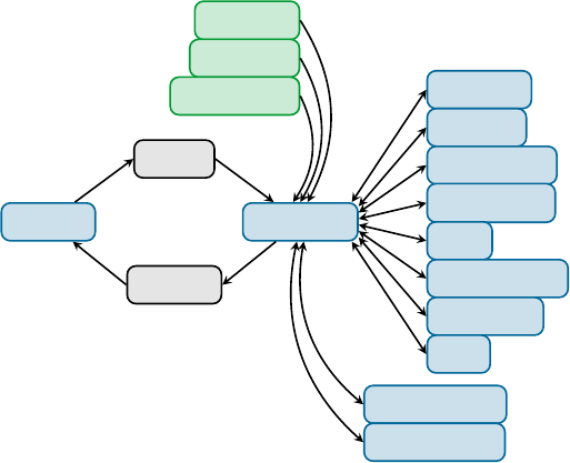
6 Interfaces
This chapter describes the interface between Sharc and quantum chemistry programs. In the rst section, the interface
is specied (e.g., for users who attempt to create their own interfaces). The description of the currently existing
interfaces takes the remainder of this chapter.
6.1 Interface Specifications
From the Sharc point of view, quantum chemical calculation proceeds as follows in the QM directory:
1. write a le called QM/QM.in
2. call a script called QM/runQM.sh
3. read the output from a le called QM/QM.out
For specications of the formats of these two les (
QM.in
and
QM.out
) see below. The executable script
QM/runQM.sh
must accomplish that all necessary quantum chemical output is available in QM/QM.out.
sharc.x Interface
Molpro
Molcas
Columbus
Analytical
ADF
Turbomole
Gaussian
LVC
Wfoverlap
TheoDORE
QM.in
QM.out
template
resources
initial MOs
Figure 6.1: Communication between sharc.x, the interfaces, and the quantum chemistry codes.
6.1.1 QM.in Specification
The
QM.in
le is written by Sharc every time a quantum chemistry calculation is necessary. It contains all information
available to Sharc. This information includes the current geometry (and velocity), the time step, the number of states,
the time step and the unit used to specify the atomic coordinates. The le also contains control keywords and request
keywords.
The le format is consistent with a standard xyz le. The rst line contains the number of atoms, the second line is a
comment. Sharc writes the trajectory ID (a hash of all Sharc input les) to this line. The following lines specify the
atom positions. As a fourth, fth and sixth column, these lines may contain the atomic velocities. All following lines
contain keywords, one per line and possibly with arguments. Comments can be inserted with ’#’, and empty lines are
permitted. Comments and empty lines are only permitted below the xyz le part. An examplary
QM.in
le is given in
the following:
46

Sharc Manual 6 Interfaces |6.1 Interface Specications
3
Jobname
S 0.0 0.0 0.0 0.000 -0.020 0.002
H 0.0 0.9 1.2 0.000 -0.030 0.000
H 0.0 -0.9 1.2 0.000 0.010 -0.000
# This is a comment
Init
States 3 0 2
Unit Angstrom
SOC
DM
GRAD 1 2
OVERLAP
NACDR select
1 2
end
There exist two types of keywords, control keywords and request keywords. Control keywords pass some information
to the interface. Request keywords tell the interface to provide a quantity in the
QM.out
le. Table 6.1 contains all
control keywords while table 6.2 lists all request keywords.
6.1.2 QM.out Specification
The
QM.out
le communicates back the results of the quantum chemistry calculation to the dynamics code. After Sharc
called QM/runQM.sh, it expects that the le QM/QM.out exists and contains the relevant data.
The following quantities are expected in the le (depending whether the corresponding keyword is in the
QM.in
le):
Hamiltonian matrix, dipole matrices, gradients, nonadiabatic couplings (either NACDR or NACDT), overlaps, wave
function phases, property matrices. The format of QM.out is described in the following.
Each quantity is given as a data block, which has a xed format. The order of the blocks is arbitrary, and between
blocks arbitrary lines can be written. However, within a block no extraneous lines are allowed. Each data block starts
with a exclamation mark !, followed by whitespace and an integer ag which species the type of data:
Table 6.1: Control keywords for Sharc interfaces. These keywords pass information from Sharc to the interface.
Keyword Description
init
Species that this is the rst calculation. The interface should create a save directory (if not
existing already) to save all information necessary for a restart.
samestep
Species that this is an additional calculation at the same geometry/time step. Implies that,
e.g., the converged orbitals from the savedir could be reused or that the wave function
calculations could be skipped.
restart
Species that this is a calculation after a restart of
sharc.x
, possibly after a crash. Implies
that in the savedir some les might be incomplete, the interface should therefore act as if a
new step is requested, except that the savedir les should be managed accordingly.
cleanup
Species that all output les of the interface (except
QM.out
) should be deleted (including
the save directory).
backup
Species that the content of the save directory should be stored in a persistent location (such
that it is not overwritten in the next time step).
unit
Species in which unit the atomic coordinates are to be interpreted. Possible arguments are
“angstrom” and “bohr”.
states Gives the number of excited states per multiplicity (singlets, doublet, triplets, ...).
dt Gives the time between the last calculation and the current calculation in atomic units.
savedir
Gives a path to the directory where the interface should save les needed for restart and
between time steps. If the interface-specic input les also have this keyword, Sharc assumes
that the path in QM.in takes precedence.
47

Sharc Manual 6 Interfaces |6.1 Interface Specications
Table 6.2: Request keywords for Sharc interfaces. See Table 6.3 for which interfaces can fulll these requests.
Keyword Description
H
Calculate the molecular Hamiltonian (diagonal matrix with the energies of the states of the
model space). This request is always available.
SOC
Calculate the molecular Hamiltonian including the SOCs (not diagonal anymore within the
model space).
DM Calculate the state dipole moments and transition dipole moments between all states.
GRAD
Calculate gradients for all states. If followed by a list of states, calculate only gradients for
the specied states.
NACDT
Calculate the time-derivatives
hΨ1|∂/∂t|Ψ2i
by nite dierences between the last time step
and the current time step. This request is currently not supported by any interface.
NACDR
Calculate nonadiabatic coupling vectors
hΨ1|∂/∂R|Ψ2i
between all pairs of states. If followed
by “select”, read the list of pairs on the following lines until “end” and calculate nonadiabatic
coupling vectors between the specied pairs of states.
OVERLAP
Calculate overlaps
hΨ1(t0)|Ψ2(t)i
between all pairs of states (between the last and current
time step). If followed by “select”, read the list of pairs on the following lines until “end” and
calculate overlaps between the specied pairs of states.
DMDR
Calculate the Cartesian gradients of the dipole moments and transition dipole moments of
all states.
ION Calculate transition properties between neutral and ionic wave functions.
THEODORE Run TheoDORE to compute electronic descriptors for all states.
MOLDEN Generate Molden les of the relevant orbitals and copy them to the savedir.
1 Hamiltonian matrix
2 Dipole matrices
3 Gradients
4 Non-adiabatic couplings (NACDT)
5 Non-adiabatic couplings (NACDR)
6 Overlap matrix
7 Wavefunction phases
8 Wallclock time for QM calculation
11 Property matrix (e.g., ionization probabilities) this ag is deprecated
12 Dipole moment gradients
20 Property matrices with number and labels (e.g., ionization probabilities)
21 Property vectors with number and labels (e.g., TheoDORE output)
On the next line, two integers are expected giving the dimensions of the following matrix. Note, that all these matrices
must be square matrices. On the following lines, the matrix or vector follows. Matrices are in general complex, and real
and imaginary part of each element is given as a pair of oating point numbers.
The following shows an example of a 4
×
4Hamiltonian matrix. Note that the imaginary parts directly follow the real
parts (in this example, the Hamiltonian is real).
! 1
4 4
-548.6488 0.0000 0.0000 0.0000 0.0003 0.0000 0.0003 0.0000
0.0000 0.0000 -548.6170 0.0000 0.0003 0.0000 0.0003 0.0000
0.0003 0.0000 0.0003 0.0000 -548.5986 0.0000 0.0000 0.0000
0.0003 0.0000 0.0003 0.0000 0.0000 0.0000 -548.5912 0.0000
The three dipole moment matrices (
x
,
y
and
z
polarization) must follow directly after each other, where the dimension
specier must be present for each matrix. The dipole matrices are also expected to be complex-valued.
! 2
2 2
48

Sharc Manual 6 Interfaces |6.1 Interface Specications
0.1320 0.0000 -0.0020 0.0000
-0.0020 0.0000 -1.1412 0.0000
2 2
0.0000 0.0000 0.0000 0.0000
0.0000 0.0000 0.0000 0.0000
2 2
2.1828 0.0000 0.0000 0.0000
0.0000 0.0000 0.6422 0.0000
Gradient and nonadiabatic couplings vectors are written as 3
×natom
matrices, with the
x
,
y
and
z
components of one
atom per line. These vectors are expected to be real valued. Each vector is preceeded by its dimensions.
6 3
0.0000 -6.5429 -8.1187
0.0000 5.8586 8.0160
0.0000 6.8428 1.0265
0.0000 6.5429 8.1187
0.0000 -5.8586 -8.0160
0.0000 -6.8428 -1.0265
If gradients are requested, Sharc expects every gradient to be present, even if only some gradients are requested. The
gradients are expected in the canonical ordering (see section 8.24), which implies that for higher multiplets the same
gradient has to be present several times. For example, with 3 singlets and 3 triplets, Sharc expects 12 gradients in the
QM.out le (each triplet has three components with Ms=-1, 0 or 1).
Similarly, for nonadiabatic coupling vectors, Sharc expects all pairs, even between states of dierent multiplicity. The
vectors are also in canonical ordering, where the inner loop goes over the ket states. For example, with 3 singlets and 3
triplets (12 states), Sharc expects 144 (122) nonadiabatic coupling vectors in the QM.out le.
! 5 Non-adiabatic couplings (ddr) (2x2x1x3, real)
13!m11s11ms10 m21s21ms20
0.0e+0 0.0e+0 0.0e+0
13!m11s11ms10 m21s22ms20
+2.0e+0 0.0e+0 0.0e+0
13!m11s12ms10 m21s21ms20
-2.0e+0 0.0e+0 0.0e+0
13!m11s12ms10 m21s22ms20
0.0e+0 0.0e+0 0.0e+0
The nonadiabatic coupling matrix (NACDT keyword), the overlap matrix and the property matrix are single
n×n
matrices (nis the total number of states), respectively, like the Hamiltonian.
The wave function phases are a vector of complex numbers.
The wallclock time is a single real number.
The dipole moment gradients are a list of 3
×natom
vectors, each specifying the gradient of one polarization of one
dipole moment matrix element. In the outmost loop, the bra index is counted, then the ket index, then the polarization.
Hence, the respective entry in QM.out would look like (for 2 states and 1 atom):
! 12 Dipole moment derivatives (2x2x3x1x3, real)
13!m11s11ms10 m21s21ms20 pol0
0.000000000000E+00 0.000000000000E+00 0.000000000000E+00
1 3 ! m1 1 s1 1 ms10 m2 1 s2 1 ms2 0 pol 1
0.000000000000E+00 0.000000000000E+00 0.000000000000E+00
1 3 ! m1 1 s1 1 ms10 m2 1 s2 1 ms2 0 pol 2
0.000000000000E+00 0.000000000000E+00 0.000000000000E+00
49

Sharc Manual 6 Interfaces |6.1 Interface Specications
1 3 ! m1 1 s1 1 ms10 m2 1 s2 2 ms2 0 pol 0
1.000000000000E+00 0.000000000000E+00 0.000000000000E+00
1 3 ! m1 1 s1 1 ms10 m2 1 s2 2 ms2 0 pol 1
0.000000000000E+00 0.000000000000E+00 0.000000000000E+00
1 3 ! m1 1 s1 1 ms10 m2 1 s2 2 ms2 0 pol 2
0.000000000000E+00 0.000000000000E+00 0.000000000000E+00
1 3 ! m1 1 s1 2 ms10 m2 1 s2 1 ms2 0 pol 0
1.000000000000E+00 0.000000000000E+00 0.000000000000E+00
1 3 ! m1 1 s1 2 ms10 m2 1 s2 1 ms2 0 pol 1
0.000000000000E+00 0.000000000000E+00 0.000000000000E+00
1 3 ! m1 1 s1 2 ms10 m2 1 s2 1 ms2 0 pol 2
0.000000000000E+00 0.000000000000E+00 0.000000000000E+00
1 3 ! m1 1 s1 2 ms10 m2 1 s2 2 ms2 0 pol 0
0.000000000000E+00 0.000000000000E+00 0.000000000000E+00
1 3 ! m1 1 s1 2 ms10 m2 1 s2 2 ms2 0 pol 1
0.000000000000E+00 0.000000000000E+00 0.000000000000E+00
1 3 ! m1 1 s1 2 ms10 m2 1 s2 2 ms2 0 pol 2
0.000000000000E+00 0.000000000000E+00 0.000000000000E+00
The section containing the 2D property matrices consists of three subsequent parts: (i) the number of property matrices
contained, (ii) a label for each property matrix (as the property matrices might contain arbitrary data, depending on the
interface and the requests), and (iii) the matrices (full, complex-valued matrices like above):
! 20 Property Matrices
2 ! number of property matrices
! Property Matrix Labels (1 strings)
Dyson norms
Example matrix
! Property Matrices (1x4x4, complex)
4 4 ! Dyson norms
0.000E+00 0.000E+00 0.000E+00 0.000E+00 9.663E-01 0.000E+00 9.663E-01 0.000E+00
0.000E+00 0.000E+00 0.000E+00 0.000E+00 4.822E-01 0.000E+00 4.822E-01 0.000E+00
9.663E-01 0.000E+00 4.822E-01 0.000E+00 0.000E+00 0.000E+00 0.000E+00 0.000E+00
9.663E-01 0.000E+00 4.822E-01 0.000E+00 0.000E+00 0.000E+00 0.000E+00 0.000E+00
4 4 ! Example matrix
1.000E+00 1.000E+00 0.000E+00 0.000E+00 0.000E+00 0.000E+00 0.000E+00 0.000E+00
0.000E+00 0.000E+00 2.000E+00 2.000E+00 0.000E+00 0.000E+00 0.000E+00 0.000E+00
0.000E+00 0.000E+00 0.000E+00 0.000E+00 3.000E+00 3.000E+00 0.000E+00 0.000E+00
0.000E+00 0.000E+00 0.000E+00 0.000E+00 0.000E+00 0.000E+00 4.000E+00 4.000E+00
The section containing the 1D property vectors also consists of three subsequent parts: (i) the number of property
vectors contained, (ii) a label for each property vector (as the property vectors might contain arbitrary data, depending
on the interface and the requests), and (iii) the vectors (real-valued):
! 21 Property Vectors
2 ! number of property vectors
! Property Vector Labels (2 strings)
Om
PRNTO
! Property Vectors (9x8, real)
! TheoDORE descriptor 1 (Om)
0.000000000000E+000
4.318700000000E-001
2.688600000000E-001
50

Sharc Manual 6 Interfaces |6.1 Interface Specications
2.590000000000E-002
! TheoDORE descriptor 2 (PRNTO)
0.000000000000E+000
2.318700000000E-001
1.688600000000E-001
1.590000000000E-002
6.1.3 Further Specifications
The interfaces may require additional input les beyond
QM.in
, which contain static information. This may include
paths to the quantum chemistry executable, paths to scratch directories, or input templates for the quantum chemistry
calculation (e.g. active space specications, basis sets, etc.). The dynamics code does not depend on these additional
les, but they should all be stored in the QM/ subdirectory.
The current conventions in the Sharc suite are that the quantum chemistry interfaces use two additional input les,
one specifying the level of theory (template le, e.g.,
MOLCAS.template
,
MOLPRO.template
, ...) and one specifying
the computational resources like paths, memory, number of CPU cores, initial orbital source (resource le, e.g.,
MOLCAS.resources
,
MOLPRO.resources
, ...). Furthermore, the current interfaces allow to read in initial orbitals (e.g.,
MOLCAS.*.RasOrb.init
,
mocoef.init
, ...). For interfaces with QM/MM capabilities, additional les could be used to
specify connection table, parameters, etc.
6.1.4 Save Directory Specification
The interfaces must be able to save all information necessary for restart to a given directory. The absolute path is
written to
QM.in
by Sharc. Hence, for the trajectories the path to the save directory is always a subdirectory of the
working directory of Sharc.
51

Sharc Manual 6 Interfaces |6.2 Overview over Interfaces
6.2 Overview over Interfaces
The Sharc suite comes with a number of interfaces to dierent quantum chemistry programs. Their capabilities and
usage are explained in the following sections. Table 6.3 gives an overview over the capabilities of the interfaces. Table 6.4
shows the le names for interface-related input les of the dierent interfaces.
Table 6.3:
Overview over capabilities of Sharc interfaces. For each method and program, the table shows which
multiplicities (S2), which quantities, and whether QM/MM are available.
Method Program S2SOC TDMaGrad. NACDR OVLbDMDR ION Theo.cQM/MM
SA-CASSCF Molpro any √ √ √ √ √ √
Molcas any √ √ √ √ √d√ √
Columbus any √e√ √ √e√ √
MR-CISD Columbus any √e√ √ √e√ √
MS-CASPT2 Molcas any √ √ √d√ √d√
TD-DFT ADF any √f√д√ √ √ √ √
Gaussian any √д√ √ √ √
ADC2 Turbomole S, T √f√ √ √ √
CC2 Turbomole S, T √д√ √ √
Analytical — any √ √ √ √ √
LVC — any √ √ √ √ √
aTDM: transition dipole moments; bOVL: wave function overlaps; cTheo.: TheoDORE;dnumerical gradients; e
either NAC or SOC, but not both at the same time;
f
SOCs only between singlets and triplets;
д
TDMs only between
S0
and excited singlets.
Table 6.4: Overview over les of Sharc interfaces.
Interface Template le Resource le Initial MOs QM/MM
Molpro MOLPRO.template MOLPRO.resources wf.init
wf.<job>.init
Molcas MOLCAS.template MOLCAS.resources MOLCAS.<mult>.RasOrb.init MOLCAS.qmmm.table
MOLCAS.<mult>.JobIph.init MOLCAS.qmmm.key
Columbus a directory COLUMBUS.resources mocoef_mc.init
mocoef_mc.init.<job>
molcas.RasOrb.init
molcas.RasOrb.init.<job>
ADF ADF.template ADF.resources ADF.t21.<job>.init ADF.qmmm.table
ADF.qmmm.ff
Gaussian GAUSSIAN.template GAUSSIAN.resources GAUSSIAN.chk.init
GAUSSIAN.chk.<job>.init
Turbomole RICC2.template RICC2.resources mos.init
Analytical Analytical.template N/A N/A
LVC LVC.template N/A N/A
6.2.1 Example Directory
The directory
$SHARC/../examples/
contains for all quantum chemistry interfaces comprehensively commented
examples of input les (template, resource les). These example les should be regarded as supplementary les to the
documentation of the interfaces. For the interfaces without the possibility for automated template generation (e.g.,
SHARC_RICC2.py), it is recommended that users copy the example template le and modify it to their needs.
However, note that it might not necessarily work to directly start the respective interface in the example directories. In
order to make the example calculations work, some paths or variables in the resource les need to be adjusted. If you
need automatically working test calculations for Sharc, consider using tests.py instead.
52
Sharc Manual 6 Interfaces |6.3 MOLPRO Interface
6.3 MOLPRO Interface
The Sharc-Molpro interface allows to run Sharc dynamics with Molpro’s CASSCF wave functions. RASSCF is
not supported, since on RASSCF level state-averaging over dierent multiplicities is not possible. The interface
uses Molpro’s CI program in order to calculate transition dipole moments and spin-orbit couplings. Gradients and
nonadiabatic coupling vectors are calculated using Molpro’s CADPACK code (hence no generally contracted basis sets
can be used). In the new version of the interface, overlaps are calculated using the WFoverlap code. Time-derivative
couplings (NACDT) are not supported anymore in the Sharc-Molpro interface. Wavefunction phases between the
CASSCF and MRCI wave functions are automatically adjusted. The interface can trivially parallelize the computation
of gradients and coupling vectors over several processors. Execution of parallel Molpro binaries is currently not
supported.
The Sharc-Molpro interface needs two additional input les, which should be present in
QM/
. Those input les are
MOLPRO.resources
, which contains, e.g., the paths to Molpro and the scratch directory, and
MOLPRO.template
, which
is a keyword-argument input le specifying the CASSCF level of theory. If
QM/wf.init
is present, it will be used as a
Molpro wave function le containing the initial MOs. For calculations with several “jobs” (see below), initial orbitals
can also given as QM/wf.<job>.init.
6.3.1 Template file: MOLPRO.template
During the rework of the Molpro interface, the template le structure was completely changed. In the new version, the
template le is a keyword-argument list le, similar to the template les of most other interfaces. A fully commented
template le with all possible options is located in $SHARC/../examples/SHARC_MOLPRO/.
For simple cases, an example for the template le looks like this:
basis def2-svp
dkho 2 # Douglas-Kroll second order
occ 14
closed 10
nelec 24
roots 4 0 3
rootpad 1 0 1
This species a SA(4S+3T)-CASSCF(4,4)/def2-SVP calculation for 24 electrons. Note the
rootpad
keyword, which adds
one singlet and one triplet with zero weight to the state-averaging (so technically this is a SA(5S+4T) calculation, but the
results are the same as SA(4S+3T)). These zero-weight states are sometimes useful to improve convergence of CASSCF.
The new interface can also be used to perform several independent CASSCF calculations for dierent multiplicities
(e.g., one CASSCF for the neutral states and another one for the ionic states). In this case, each independent CASSCF
calculation is called a “job”. In the template, most settings can be modied independently for each job. An example is
given here:
# In this way, users can employ custom basis sets
basis_external /path/to/basisset # no spaces in path allowed
dkho 2
# job 1 for singlet+triplet; job 2 for doublets
jobs 1 2 1
occ 14 13 # for job 1 and 2
closed 11 10 # for job 1 and 2
nelec 24 23 24 # for job 1
nelec 24 23 24 # for job 2
roots 4 0 3 # for job 1
53

Sharc Manual 6 Interfaces |6.3 MOLPRO Interface
roots 0 2 0 # for job 2
rootpad 1 0 1 # for job 1
rootpad 0 2 0 # for job 2
This template species two jobs, where job 1 should be used to compute singlet and triplet states, and job 2 used for
doublet states. Job 1 is a SA(4S+3T)-CASSCF(2,3) computation, with singlets and triplets each having 24 electrons. Job 2
is a SA(2D)-CASSCF(3,3) computation, with 23 electrons. Note how for dierent jobs it is possible to have dierent
active spaces and state-averaging schemes. However, keep in mind that all states of a given multiplicity are always
calculated in the same job (e.g., it is not possible to have one job for S0and another job for S1and S2).
It is also possible to do a mixed input, for example having two jobs, but only giving one number after
occ
or
closed
.
The interface provides comprehensive error messages during the template check.
Also note the
basis_external
keyword. It provides a le, whose content is used in the basis set denition (it is inserted
verbatim into
basis={...}
in the Molpro input). It is possible to use the generated input from the Basis Set Exchange
Library, but the basis={ and }need to be deleted from the le.
Remember that molpro_input.py cannot create multi-job templates or templates with the basis_external keyword.
6.3.2 Resource file: MOLPRO.resources
The interface requires some additional information beyond the content of
QM.in
. This information is given in the le
MOLPRO.resources
, which must reside in the directory where the interface is started. This le uses a simple “
keyword
argument
” syntax. Comments using # and blank lines are possible, the order of keywords is arbitrary. Lines with
unknown keywords are ignored, since the interface just searches the le for certain keywords.
Table 6.5 lists the existing keywords. A fully commented resource le for this interface with all possible options is
located in $SHARC/../examples/SHARC_MOLPRO/.
Mandatory keywords are the paths to Molpro, the scratch directory, and to the WFoverlap executable (the latter for
overlap, Dyson, or NACDR calculations).
Parallel execution of MOLPRO
In the new version of the Sharc-Molpro interface, calculations of multiple
independent active spaces (“jobs”), of several gradients, and of several nonadiabatic coupling vectors are automatically
parallelized over the given number of CPU cores.
Note that in the new version of the interface, Molpro calls itself cannot be run with multiple CPUs.
6.3.3 Error checking
The interface is written such that the output of Molpro is checked for commonly occuring errors, mostly bad
convergence in the MCSCF or CP-MCSCF parts. In these cases, the input is adjusted and Molpro restarted. This will
be done until all calculations are nished or an unrecoverable error is detected. The interface will try to solve the
following error messages:
EXCESSIVE GRADIENT IN CI
This error message can occur in the MCSCF part. The calculation is restarted with a
P-space threshold (see Molpro manual) of 1. If the error remains, the threshold is quadrupled until the calculation
converges or the threshold is above 100.
NO CONVERGENCE IN REFERENCE CI
The error occurs in the CI part. The calculation is restarted with a
P-space threshold (see Molpro manual) of 1. If the error remains, the threshold is quadrupled until the calculation
converges or the threshold is above 100.
NO CONVERGENCE OF CP-MCSCF
This error occurs when solving the linear equations needed for the calculation
of MCSCF gradients or nonadiabatic coupling vectors. In this case, the interface nds in the output the value of closest
convergence and restarts the calculation with the value found as the new convergence criterion. This ensures that the
CP-MCSCF calculation converges, albeit with lower accuracy for this gradient for this time step.
54

Sharc Manual 6 Interfaces |6.3 MOLPRO Interface
Table 6.5: Keywords for the MOLPRO.resources input le.
Keyword Description
molpro
Is followed by a string giving the path to the Molpro executable. Relative and absolute
paths, environment variables and ~can be used.
scratchdir
Is a path to the temporary directory. Relative and absolute paths, environment
variables and
~
can be used. If the directory does not exist, the interface will create it.
In any case, the interface will delete this directory after the calculation.
savedir
Is a path to another temporary directory. Relative and absolute paths, environment
variables and ~can be used. The interface will store les needed for restart there.
memory (int) Memory for Molpro and WFoverlap in MB.
ncpu (int) Number of CPU cores for parallel computation of gradients/NAC vectors.
delay
(oat) Time in seconds between starting parallel Molpro runs. Useful to lessen the
I/O burden when having many runs starting at the same time.
gradaccudefault (oat) Default accuracy for CP-MCSCF.
gradaccumax (oat) Worst acceptable accuracy for CP-MCSCF (see below).
always_orb_init
Do not use the orbital guesses from previous calculations/time steps, but always use
the provided initial orbitals.
always_guess Always use the orbital guess from Molpro’s guess module.
wfoverlap
Is the path to the WFoverlap executable. Relative and absolute paths, environment
variables and ~can be used.
numfrozcore Number of neglected core orbitals for overlap and Dyson calculations.
numocc Number of doubly occupied orbitals for Dyson calculations.
nooverlap Do not save determinant les for overlap computations.
debug Increases the verbosity of the interface.
no_print Reduces interface standard output.
This error check is controlled by two keywords in the
MOLPRO.resources
le. The interface rst tries to converge
the CP-MCSCF calculation to
gradaccudefault
. If this fails, it tries to converge to the best value possible within 900
iterations.
gradaccumax
denes the worst accuracy accepted by the interface. If a CP-MCSCF calculation cannot be
converged below gradaccumax then the interface exits with an error, leading to the abortion of the trajectory.
6.3.4 Things to keep in mind
Initial orbital guess
For CASSCF calculations it is always a good idea to start from converged MOs from a nearby
geometry. For the rst time step, if a le
QM/wf.init
is present, the Sharc-Molpro interface will take this le
for the starting orbitals. In case of multi-job calculations, separate initial orbitals can be provided with les called
QM/wf.<job>.init
, where
<job>
is an integer. In subsequent calculations, the MOs from the previous step will be used
(unless the always_orb_init keyword is used).
Basis sets
Note that the Molpro interface cannot calculation SA-CASSCF gradients for generally contracted basis
sets (like Dunning’s “cc” basis sets or Roos’ “ANO” basis sets). Only segmented basis sets are allowed, like the Pople
basis sets and the “def” family from Turbomole.
In order to employ user-dened basis sets, in the template the keyword
basis_external
, followed by a lename, can
be used. The interface will then take the content of this le and insert it as basis set denition in the Molpro input les
(i.e., it will add in the input basis={ <content of the file> }. Note that the lename must not contain spaces.
6.3.5 Molpro input generator: molpro_input.py
In order to quickly setup simple inputs for Molpro, the Sharc suite contains a small script called
molpro_input.py
.
It can be used to setup single point calculations, optimizations and frequency calculations on the HF, DFT, MP2 and
CASSCF level of theory. Of course, Molpro has far more capabilities, but these are not covered by
molpro_input.py
.
However,
molpro_input.py
can also prepare template les which are compatible with the Sharc-Molpro interface
(MOLPRO.template le).
55
Sharc Manual 6 Interfaces |6.3 MOLPRO Interface
The script interactively asks the user to specify the calculation and afterwards writes an input le and optionally a run
script.
Input
Type of calculation
Choose to either perform a single-point calculation or a minimum optimization (including
optionally frequency calculation), to generate a template le, or an optimization of a state crossing. For the template
generation, no geometry le is needed, but the script looks for a
MOLPRO.input
in the same directory and allows to
copy the settings.
For single-point calculations, optimizations and frequency calculations, les in Molden format called
geom.molden
,
opt.molden
or
freq.molden
, respectively, are created (containing the orbitals, optimization steps and normal modes,
respectively). The le freq.molden can be used to generate initial conditions with wigner.py.
Geometry
Specify the geometry le in xyz format. Number of atoms and total nuclear charge is detected automatically.
After the user inputs the total charge, the number of electrons is calculated automatically.
In the case of the generation of a template le, instead only the number of electrons is required.
Non-default atomic masses
If a frequency calculation is requested, the user may modify the mass of specic atoms
(e.g. to investigate isotopic eects). In the following menu, the user can add or remove atoms with their mass to a list
containing all atoms with non-default masses. Each atom is referred to by its number as in the geometry le. Using the
command show the user can display the list of atoms with non-default masses. Typing end conrms the list.
Note that when using the produced Molden le later with
wigner.py
, the user has to enter the same non-default
masses again, since the Molden le does not contain the masses and
wigner.py
has no way to retrieve these numbers.
Level of theory
Supported are Hartree-Fock (HF), density functional theory (DFT), Møller-Plesset perturbation theory
(MP2), equation-of-motion coupled-cluster with singles and doubles (EOM-CCSD) and CASSCF (either single-state or
state-averaged). All methods (except EOM-CCSD) are compatible with odd-electron wave functions (
molpro_input.py
will use the corresponding UHF, UMP2 and UKS keywords in the input le, if necessary).
For template generation, state-average CASSCF is automatically chosen. All methods (except EOM-CCSD) can be
combined with optimizations and frequency calculations, however, the frequency calculation is much more ecient
with HF or SS-CASSCF.
DFT functional
For DFT calculations, enter a functional and choose whether dispersion correction should be applied.
Note that the functional is just a string which is not checked by molpro_input.py.
Basis set The basis set is just a string which is not checked by molpro_input.py.
CASSCF seings For CASSCF calculations, enter the number of active electrons and orbitals.
For SS-CASSCF, only the multiplicity needs to be specied. For SA-CASSCF, specify the number of states per multiplicity
to be included. Note that Molpro allows to average over states with dierent numbers of electrons. This feature is not
supported in
molpro_input.py
. However, the user can generate a closely-matching input and simply add the missing
states to the CASSCF block manually.
For optimizations at SA-CASSCF level, the state to be optimized has to be given. For crossing point optimizations, two
states need to be entered. The script automatically detects whether a conical intersection or a crossing between states
of dierent multiplicity is requested and sets up the input accordingly.
EOM-CCSD seings
EOM-CCSD calculations allow to calculate relatively accurate excited-state energies and
oscillator strengths from a Hartree-Fock reference, but only for singlet excited states.
The user has to specify the number of states to be calculated. If only one state is requested, the script will setup a
regular ground state CCSD calculation, while for more than one states, an EOM-CCSD calculation is setup. Note that
the calculation of transition properties takes twice as long as the energy calculation itself.
56
Sharc Manual 6 Interfaces |6.4 MOLCAS Interface
Memory
Enter the amount of memory for Molpro. Note that values smaller than 50 MB are ignored, and 50 MB are
used in this case.
Run script
If requested, the script also generates a simple Bash script (
run_molpro.sh
) to directly execute Molpro.
The user has to enter the path to Molpro and the path to a suitable (fast) scratch directory.
Note that the scratch directory will be deleted after the calculation, only the wave function le
wf
will be copied back
to the main directory.
6.4 MOLCAS Interface
The Sharc-Molcas interface can be used to conduct excited-state dynamics based on Molcas’ CASSCF wave functions,
and with CASPT2 or MS-CASPT2 energies (and numerical gradients). RASSCF wave functions are not supported
currently. It is important to note that currently, Sharc was only tested to work with Openmolcas 18, which is freely
available. Some versions of Molcas 8 might also work, but no guarantee is given. Note that within this Manual, Molcas
and Openmolcas are used synonymously.
The interface uses the modules GATEWAY, SEWARD (integrals), RASSCF (wave function, energies), RASSI (transition
dipole moments, spin-orbit couplings, overlaps), MCLR, and ALASKA (gradients). For CASPT2 and MS-CASPT2,
numerical gradients can be calculated, where the interface itself controls the calculations at the displaced geometries.
The interface can also numerically dierentiate dipole moments and spin-orbit couplings. Since Molcas is not able to
calculate the full nonadiabatic coupling vectors, only wave function overlaps are currently implemented in the interface
(overlaps are calculated via RASSI). Using the WFoverlap code, it is possible to calculate Dyson norms between neutral
and ionic states. Note that (unlike Molpro)Molcas cannot average over states of dierent multiplicities; hence, the
multiplicities are always computed in separate jobs which all share the same CAS settings.
The Sharc-Molcas interface furthermore allows to perform QM/MM dynamics (CASSCF plus force elds), through the
Molcas-Tinker interface.
The interface needs two additional input les, a template le for the quantum chemistry (le name is
MOLCAS.template
)
and a resource le (
MOLCAS.resources
). If the interface nds les with the name
QM/MOLCAS.<i>.JobIph.init
or
QM/MOLCAS.<i>.RasOrb.init
, they are used as initial wave function les, where
<i>
is the multiplicity. In the case of
QM/MM calculations, two more input les are needed:
MOLCAS.qmmm.key
, which contains the path to the force eld
parameters and the partitioning into QM and MM regions, and
MOLCAS.qmmm.table
, which contains the connectivity
and force eld IDs per atom.
6.4.1 Template file: MOLCAS.template
This le contains the specications for the wave function. Note that this is not a valid Molcas input le. No sections
like
$GATEWAY
, etc., can be used. The le only contains a number of keywords, given in table 6.6. The actual input les
are automatically generated.
A fully commented template le with all possible options is located in $SHARC/../examples/SHARC_MOLCAS/.
The template le can be setup with the tool molcas_input.py.
6.4.2 Resource file: MOLCAS.resources
The le
MOLCAS.resources
contains mainly paths (to the Molcas executables, to the scratch directory, etc.). This le
must reside in the same directory where the interface is started. It uses a simple “
keyword argument
” syntax. Comments
using # and blank lines are possible, the order of keywords is arbitrary. Lines with unknown keywords are ignored,
since the interface just searches the le for certain keywords.
Table 6.7 lists the existing keywords. A fully commented resource le for this interface with all possible options is
located in $SHARC/../examples/SHARC_MOLCAS/.
Note that the interface sets all environment variables necessary to run Molcas (e.g.,
$MOLCAS
,
$MOLCASMEM
,
$WorkDir
,$Project) automatically, based on the input from MOLCAS.resources and QM.in.
Some explanations on parallelization: There are two parallel modes in which the interface can act. In the rst mode, the
wave function and expectation values are calculated serially rst, and then all analytical gradients are computed in
57

Sharc Manual 6 Interfaces |6.4 MOLCAS Interface
Table 6.6: Keywords for the MOLACS.template le.
Keyword Description
basis
The basis set used. Note that some basis sets (e.g., Pople basis sets) do not work, since
the spin-orbit integrals cannot be calculated.
baslib
Can be used to provide the path to a custom basis set library (analogous to the baslib
keyword in Molcas).
nactel Number of active electrons for CASSCF.
ras2 Number of active orbitals for CASSCF.
inactive Number of inactive orbitals.
roots
Followed by a list of integers, giving the number of states per multiplicity in the
state-averaging procedure.
rootpad
Followed by a list of integers, giving the number of extra, zero-weight states in the
state-averaging.
method
Followed by a string, which is either “CASSCF”, “CASPT2” or “MS-CASPT2” (case
insensitive), dening the level of theory. Default is “CASSCF”.
no-douglas-kroll
Deactivates the use of the scalar-relativistic DK Hamiltonian and uses a non-relativistic
Hamiltonian instead. Default is Douglas-Kroll-Hess 2nd order (In Molcas standard
parametrization).
ipea
Followed by a oat giving the IP-EA shift for CASPT2 (see Molcas manual for more
information). The default is 0.25, as in Molcas.
imaginary
Followed by a oat giving the imaginary level shift for CASPT2 (see Molcas manual
for more information). The default is 0.0, as in Molcas.
frozen
Number of frozen orbitals for CASPT2. Default is -1, which lets Molcas choose the
number of frozen orbitals.
cholesky
Activates Cholesky decomposition in Molcas. Recommended for large basis sets.
Will use numerical gradients even for CASSCF. Default is to use regular 4-electron
integrals.
cholesky_analytical
Activates analytical SA-CASSCF gradients with Cholesky decomposition. This is only
possible with Molcas 8.
gradaccudefault (oat) Default accuracy for CP-MCSCF.
gradaccumax (oat) Worst acceptable accuracy for CP-MCSCF.
displ Cartesian displacement (in Å) for numerical dierentiation (default 0.005 Å).
qmmm
Activates the QM/MM mode. In this case, two more input les need to be present (see
below).
58

Sharc Manual 6 Interfaces |6.4 MOLCAS Interface
Table 6.7: Keywords for the MOLCAS.resources le.
Keyword Description
molcas
Is the path to the Openmolcas installation. Relative and absolute paths, environment
variables and
~
can be used. The interface will set
$MOLCAS
to this path. If this keyword
is not present in
MOLCAS.resources
, the interface will use the environment variable
$MOLCAS, if it is set.
tinker The path to the Tinker installation, usable with Molcas.
wfoverlap
Is the path to the WFoverlap executable. Relative and absolute paths, environment
variables and ~can be used. Only needed for Dyson norm calculations.
scratchdir
Is a path to the temporary directory. Relative and absolute paths, environment
variables and
~
can be used. If it does not exist, the interface will create it. In any case,
the interface will delete this directory after the calculation.
savedir
Is a path to another temporary directory. Relative and absolute paths, environment
variables and ~can be used. The interface will store les needed for restart there.
memory
The memory usable by Molcas. The interface will set
$MOLCASMEM
to this value. The
default is 10 MB.
ncpu
The number of CPUs used by the interface. If zero or negative, one CPU will be used
and all subtasks (Hamiltonian, dipole moments, analytical gradients, overlaps) will
be done in one Molcas call. If positive, analytical gradients will be calculated by
separate calls to Molcas, parallelized over the given number of CPUs.
delay
Followed by a oat giving the delay in seconds between starting parallel jobs to avoid
excessive disk I/O.
always_orb_init
Do not use the orbital guesses from previous calculations/time steps, but always use
the provided initial orbitals.
always_guess Always use the orbital guess from Molcas’s guessorb module.
debug Increases the verbosity of the interface.
no_print Reduces interface standard output.
parallel, over the given number of CPUs. If the number of CPUs is one, then still the interface prepares independent
computations for each gradient, and runs those sequentially on one CPU. If the given number of CPUs is negative
or zero, then the gradients are not prepared as separate Molcas calculations, but together with the other quantities.
The latter variant has less overhead, but is only recommended if the user is sure that the gradient calculations (MCLR)
will converge in virtually all cases. If MCLR does not converge occasionally, it is advisable to use NCPU=1 instead of
NCPU≤0.
In the second parallelization mode, used for numerical gradients, the central point is calculated rst and then all
displacements are computed in parallel. This mode will be used for gradients on CASPT2, MS-CASPT2 and Cholesky-
CASSCF level as well as for spin-orbit/dipole moment derivatives on all levels. In this mode there is no distinction
between NCPU=1 and NCPU≤0.
6.4.3 Template file generator: molcas_input.py
This is a small interactive script to generate template les for the Sharc-Molcas interface. It simply queries the user
for some input parameters and then writes the le
MOLCAS.template
, which can be used to run Sharc simulations with
the Sharc-Molcas interface. The input generator can also be used to write proper Molcas input les for single-point
calculations and optimizations/frequency calculations on CASSCF and (MS-)CASPT2 level of theory.
Type of calculation
Choose to either perform a single-point calculation or a minimum optimization (including
optionally frequency calculation), or to generate a template le. For the template generation, no geometry le is needed,
but the script looks for a MOLCAS.input in the same directory and allows to copy the settings.
For single-point calculations, optimizations and frequency calculations, les in Molden format are created (containing
the orbitals, optimization steps and normal modes, respectively). The le
MOLCAS.freq.molden
can be used to generate
initial conditions with wigner.py.
Geometry file The geometry le is only used to calculate the nuclear charge.
59
Sharc Manual 6 Interfaces |6.4 MOLCAS Interface
Charge
This is the overall charge of the molecule. This number is used with the nuclear charge to calculate the
number of electrons.
Method Choose either CASSCF or CASPT2. Multi-state CASPT2 can be requested later.
Basis set This is simply a string, which is not checked by the script to be a valid basis set of the Molcas library.
Number of active electrons and orbitals
These settings are necessary for the denition of the CASSCF wave
function. The number of inactive orbitals is automatically calculated from the total number of electrons and the number
of active electrons.
States for state-averaging
For each multiplicity, the number of states for the state-averaging procedure must be
equal or larger than the number of states used in the dynamics.
Further seings
Depending on the run type and method, the script might ask further questions regarding the root
to optimize, CASPT2 settings (whether to do multi-state CASPT2, IPEA shift, imaginary level shift), or whether a
spin-orbit RASSI should be performed (for input le generation only).
6.4.4 QM/MM key file: MOLCAS.qmmm.key
This le denes some aspects of the QM/MM calculation. An example is given below:
parameters $MOLCAS/tinker/params/amber99sb.prm
QMMM 18
QM -1 15
MM -16 18
QMMM-ELECTROSTATICS ESPF
The rst line denes the force eld parameters, which are read from Tinker’s library here. Note that in the le path,
environment variables are expanded by the interface. The next three lines dene the QM and MM regions of the system,
where in this case atoms 1–15 are in the QM region and atoms 16–18 are in the MM region (note the minus signs
indicating the begin of an interval). The last line denes how to treat electrostatics in the calculation (currently, only
ESPF is implemented for Molcas, so this line has to be present as shown, or omitted).
6.4.5 QM/MM connection table file: MOLCAS.qmmm.table
This is the template to generate the Tinker xyz le, which besides the geometry contains the force eld atom type
number and the connectivity information. A sample looks like:
8
1 N*1.6 3.3 -2.0 1132 2
2 CK 0.3 3.1 -2.6 1136 1 3 4
3 H5 -0.4 2.9 -1.9 1145 2
4 NB 0.3 3.2 -3.9 1135 2 5
5 CB 1.6 3.5 -4.2 1134 4 6
6 CA 2.2 3.8 -5.4 1140 5 7
7 N2 1.6 3.8 -6.6 1142 6 8
8 H 2.1 3.9 -7.5 1143 7
The rst line contains the number of atoms. In each following line, the atom index, the atomic symbol (or name), the
coordinates of the atom, the force eld atom type number and the index of atoms bonded to the current atom. The
60

Sharc Manual 6 Interfaces |6.5 COLUMBUS Interface
coordinates in this le are not used and are replaced by the Sharc-Molcas interface by the actual coordinates of the
atoms. The atom type number can be looked up in the .prm les of the Tinker parameter directory.
6.5 COLUMBUS Interface
The Sharc-Columbus interface allows to run Sharc dynamics based on Columbus’ CASSCF, RASSCF and MRCI wave
functions. The interface is compatible to Columbus calculations utilizing the Columbus-Molcas interface (Seward
integrals and Alaska gradients), or using the Dalton integral code distributed with Columbus. Using Seward integrals,
spin-orbit couplings can be calculated, but no nonadiabatic couplings (only overlaps can thus be used). Using Dalton
integrals, spin-orbit couplings are not possible, but nonadiabatic couplings can be calculated. The CASSCF step can be
done with either Columbus’
mcscf
code (all features available) or with Molcas’
rasscf
code (faster, but no gradients
possible). The interface utilizes the WFoverlap program to calculate the overlap matrices. The interface can also
calculate Dyson norms between neutral and ionic wave functions using the WFoverlap code.
The interface needs as additional input the le
QM/COLUMBUS.resources
and a template directory containing all input
les needed for the Columbus calculations. Initial MOs can be given in the le
QM/mocoef_mc.init
. For multiple
jobs, initial MOs can be given as
QM/mocoef_mc.init.<job>
. For runs with
rasscf
, initial MOs have to be given as
molcas.RasOrb.init or molcas.RasOrb.init.<job>.
6.5.1 Template input
The interface does not generate the full Columbus input on-the-y. Instead, the interface uses an existing set of input
les and performs only necessary modications (e.g., the number of states). The set of input les must be provided by
the user. Please see the Columbus online documentation and, most importantly, the Columbus SOCI tutorial for a
documentation of the necessary input. The Sharc tutorial also has a section about generating the required Columbus
input le collection. An example template directory is located in $SHARC/../examples/SHARC_COLUMBUS/.
Generally, the input consists of a directory with one subdirectory with input for each multiplicity (singlets, doublets,
triplets, ...). However, even-electron wave functions of dierent multiplicities can be computed together in the same
job if spin-orbit couplings are desired. Independent multiple-DRT inputs (ISC keyword) are also acceptable. Note that
symmetry is not allowed when using the interface.
The path to the template directory must be given in COLUMBUS.resources, along with the other resources settings.
Integral input
The interface is able to use input for calculations using Seward or Dalton integrals. If you want
to calculate SOCs, you have to use Seward and have to include the AMFI keyword in the integral input. If you use
Dalton, SOCs are not available, but it is possible to compute nonadiabatic couplings.
It is important to make sure that
the order of atoms
in the template input les and in the Sharc input
is consistent
.
Furthermore, it is necessary to prepare all template subdirectories with the same integral code and the same AO basis
set.
MCSCF input
The MCSCF section can use any desired state-averaging scheme, since the number of states in MCSCF
is independent of the number of states in the MRCI module. However, frozen core orbitals in the MCSCF step are not
possible (since otherwise gradients cannot be computed). Prepare the MCSCF input for CI gradients. It is advisable to
use very tight MCSCF convergence criteria.
If gradients are not needed, you can also manually prepare a Molcas RASSCF input in
molcas.input
, in order to use
Molcas RASSCF instead of Columbus MCSCF (see molcas_rasscf keyword).
MRCI input
Either prepare a single-DRT input without SOCI (to cover a single multiplicity), a single-DRT input
with SOCI and a sucient maximum multiplicity for spin-orbit couplings or an independent multiple-DRT input (as,
e.g., for ISC optimizations). Make sure that all multiplicities are covered with all input directories.
In the MRCI input, make sure to use sequential ciudg. Also take care to setup gradient input on MRCI level.
61

Sharc Manual 6 Interfaces |6.5 COLUMBUS Interface
Job control Setup a single-point calculation with the following steps:
•SCF
•MCSCF
•MR-CISD (serial operation) or SO-CI coupled to non-rel CI (for SOCI DRT inputs)
•one-electron properties for all methods
•transition moments for MR-CISD
•nonadiabatic couplings (and/or gradients)
Request rst transition moments and interstate couplings (or alternatively full nonadiabatic couplings if Dalton integrals
are used) in the following dialogues. Analysis in internal coordinates and intersection slope analysis are not required.
6.5.2 Resource file: COLUMBUS.resources
Beyond the information from
QM.in
the interface needs additional input, which is read from the le
COLUMBUS.resources
.
Table 6.8 lists the keywords which can be given in the le. A fully commented resource le with all possible options is
located in $SHARC/../examples/SHARC_COLUMBUS/.
Table 6.8: Keywords for the COLUMBUS.resources le.
Keyword Description
columbus
Path to the Columbus main directory. Relative and absolute paths, environment
variables and ~can be used.
molcas
Path to the Molcas main directory. Relative and absolute paths, environment variables
and
~
can be used. This path is only used for overlap/Dyson calculations (since in this
case the interface calls Molcas explicitly). Otherwise Columbus will use the path to
Molcas specied during the installation of Columbus.
wfoverlap
Path to the wave function overlap and Dyson norm code. Relative and absolute paths,
environment variables and
~
can be used. Only necessary if overlaps or Dyson norms
are calculated. Needs a suitable code that computes overlaps of CI wave functions.
runc
Path to the
runc
script for Columbus execution. Default is
$COLUMBUS/runc
. This
keyword is intended for users who like to modify runc.
scratchdir
Path to the temporary directory, used to perform the Columbus calculations. Relative
and absolute paths, environment variables and
~
can be used. If it does not exist, the
interface will create it. The interface will delete this directory after the calculation.
savedir
Path to another directory. Relative and absolute paths, environment variables and
~
can be used. The interface will store les needed for restart in this directory. Default
is a subdirectory of the directory where the interface is executed.
memory
(integer, MB) Memory for Columbus. The maximum amount of memory used by the
wfoverlap code is also controlled with this keyword.
ncpu
(integer) Number of CPU cores to use for SMP-parallel execution of the wfoverlap
code. Parallel Columbus is currently not supported.
wfthres
(oat) Gives the amount of wave function norm which will be kept in the truncation
of the determinant les for Dyson and overlap calculations. Default is 0.97 (i.e., the
wave functions in the determinant les will have a norm of 0.97)
nooverlap
(no argument) Do not keep the les necessary to calculate wave function overlaps in
the next time step. If Dyson norms are requested, nooverlap is ignored.
always_orb_init
Use the initial MO guess (
mocoef_mc.init
) for all time steps, not only for the rst
step.
always_guess
In all time steps obtain the MO guess from an SCF calculation, instead of using the
MOs from the previous step.
integrals
Followed by a string which is either
seward
or
dalton
. Chooses the integral program
for Columbus. Note that with Dalton integrals SOC is not available. Default is
seward.
molcas_rasscf
Use Molcas’ RASSCF program instead of Columbus’ MCSCF program. Needs a
properly prepared Columbus input (
&RASSCF
section in
molcas.input
). Note that
gradients are not available in this mode.
Continued on next page
62
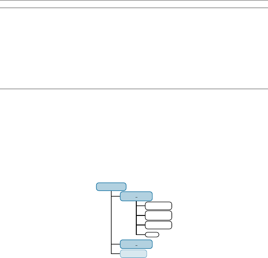
Sharc Manual 6 Interfaces |6.6 Analytical PESs Interface
Table 6.8 – Continued from previous page
Keyword Description
template
Is followed by the path to the directory containing the template subdirectories. Rela-
tive and absolute paths, environment variables and ~can be used. See also 6.5.3.
DIR See 6.5.3.
MOCOEF See 6.5.3.
numfrozcore
Can be used to override the number of frozen orbitals in Dyson calculations (Default
is the value from the cidrt input).
numocc
Can be used to declare orbitals above the frozen orbitals as doubly occupied in Dyson
calculations. No ionization from these orbitals is calculated, but otherwise they are
considered in the Dyson calculations. Default is zero.
debug Increases the verbosity of the interface.
no_print Reduces interface standard output.
6.5.3 Template setup
The template directory contains several subdirectories with input for dierent multiplicities. An example is given
in gure 6.2. In
COLUMBUS.resources
, the user has to associate each multiplicity to a subdirectory. The line “
DIR 1
Sing_Trip
” would make the interface use the input les from the subdirectory
Sing_Trip
when calculating singlet
states (the 1refers to singlet calculations). All calculations using a particular input subdirectory are called a job.
Additionally, the user must specify which job(s) provide the MO coecients (e.g., the calculation for doublet states
could be based on the same MOs as the singlet and triplet calculation). The line “
MOCOEF Doub_Quar Sing_Trip
” would
tell the interface to do a MCSCF calculation in the
Sing_Trip
job, and reuse the MOs when doing the
Doub_Quar
job
without reoptimizing the MOs.
TEMPLATE
Sing Trip
cidrtin
ciudgin
mcscfin
...
Doub Quar
Mult...
Figure 6.2: Example directory structure of the Columbus template directory
6.6 Analytical PESs Interface
The Sharc suite also contains an interface which allows to run dynamics simulations on PESs expressed with analytical
functions. In order to allow dynamics simulations in the same way as it is done on-the-y, the interface uses two kinds
of potential couplings:
•couplings that are pre-diagonalized in the interface (yielding the equivalent of the MCH basis),
•couplings given by the interface to Sharc as o-diagonal elements.
The interface needs one additional input le, called
Analytical.template
, which contains the denitions of all analytical
expressions.
6.6.1 Parametrization
The interface has to be provided with analytical expressions for all matrix elements of the following matrices in the
diabatic basis:
•Hamiltonian: H
63

Sharc Manual 6 Interfaces |6.6 Analytical PESs Interface
•Derivative of the Hamiltonian with respect to each atomic coordinate: Hxi
•(Transition) dipole matrices for each polarization direction: Mi
•Real and imaginary part of the SOC matrix: Σ
•(Optionally) the derivatives of the transition dipole matrices: Di,xj
The diabatic Hamiltonian is diagonalized:
Hd=W†HW (6.1)
Then the following calculations lead to the MCH matrices which are passed to Sharc:
HMCH =Hd+W†ΣW(6.2)
gMCH
αxi
=W†HxiWα α (6.3)
MMCH
i=W†MiW(6.4)
SMCH(t0,t)=W†(t0)W(t)(6.5)
DMCH
i,xj=W†Di,xjW(6.6)
The MCH Hamiltonian is the diagonalized diabatic Hamiltonian plus the SO matrix transformed into the MCH basis. The
gradients in the MCH basis are obtained by transforming the derivative matrices into the MCH basis. The dipole matrices
are also simply transformed into the MCH basis. The overlap matrix is the overlap of old and new transformation
matrix.
6.6.2 Template file: Analytical.template
The interface-specic input le is called
Analytical.template
. It contains the analytical expressions for all matrix
elements mentioned above. All analytical expressions in this le are evaluated considering the atomic coordinates read
from QM.in.
The le consists of a le header and the le body. The le body consists of variable denition blocks and matrix blocks.
A commented template le is located in $SHARC/../examples/SHARC_Analytical/.
Header The header looks similar to an xyz le:
2
2
IxI00
Br xBr 0 0
Here, the rst line gives the number of atoms and the second line the number of states.
On the remaining lines, each Cartesian component of the atomic coordinates is associated to a variable name, which can
be used in the analytical expressions. If a zero (
0
) is given instead of a variable name, then the corresponding Cartesian
coordinate is neglected. In the above example, the variable name
xI
is associated with the
x
coordinate of the rst atom
given in QM.in. The yand zcoordinates of the rst atom are neglected.
All variable names must be valid Python identiers and must not start with an underscore. Hence, all strings starting
with a letter, followed by an arbitrary number of letters, digits and underscores, are valid. It is not allowed to use a
variable name twice.
Note that the le header also contains the atom labels, which are just used for cross-checking against the atom labels in
QM.in.
The le header must not contain comments, neither at the end of a line nor separate lines. Also, blank lines are not
allowed in the header. After the last line of the header (where the variables for the
natom
-th atom are dened), blank
lines and comments can be used freely (except in matrix blocks).
Variable definition blocks
Variable denition blocks can be used to store additional numerical values (beyond the
atomic coordinates) in variables, which can then be used in the equations in the matrix blocks. The most obvious use
for this is of course to dene values which will appear several times in the equations.
A variable denition block looks like:
64

Sharc Manual 6 Interfaces |6.6 Analytical PESs Interface
Variables
A1 0.067
g1 0.996 # Trailing comment
# Blank line with comment only
R1 4.666
End
Each block starts with the keyword “Variables” and is terminated with “End”. Inbetween, on each line a variable name
and the corresponding numerical value (separated by blanks) can be given. Note that the naming conventions given
above also apply to variables dened in these blocks.
There can be any number of complete variable denitions blocks in the input le. All blocks are read rst, before any
matrix expressions are evaluated. Hence, the relative order of the variable blocks and the matrix blocks does not matter.
Also, note that variable names must not appear twice, so variables cannot be redened halfway through the le.
Matrix blocks
The most important information in the input le are of course contained in the expressions in the
matrix blocks. In general, a matrix block has the following format:
Matrix_Identifier
V11
V12, V22
V13, V23, V33
...
The rst line identies the type of matrix. Those are valid identiers:
Hamiltonian
Denes the Hamiltonian including the diabatic potential cou-
plings.
Derivatives
followed by a variable
name
Derivative of the Hamiltonian with respect to the given variable.
Dipole followed by 1, 2 or 3
(Transition) dipole moment matrix for Cartesian direction
x
,
y
or z, respectively.
Dipolederivatives
followed by 1,
2 or 3 followed by a variable name
Derivative of the respective dipole moment matrix.
SpinOrbit followed by Ror I
Real or Imaginary (respectively) part of the spin-orbit coupling
matrix Σ.
Since the interface searches the le for these identiers starting from the top until it is found, for each matrix only the
rst block takes eect. Note that the Hamiltonian and all relevant derivatives must be present. If dipole matrix, dipole
derivative matrix or SO matrix denitions are missing, they will be assumed zero.
In the lines after the identier, the expressions for each matrix element are given. Note the lower triangular format
(all matrices are assumed symmetric, except the imaginary part of the SO matrix, which is assumed antisymmetric).
Matrix elements must be separated by commas (so that whitespace can be used inside the expressions). There must be
at least as many lines as the number of states (additional lines are neglected). If any line or matrix element is missing,
the interface will abort.
An examplary block looks like:
Hamiltonian
A1*( (1.-math.exp(g1*(R1-xI+xBr)))**2-1.),
0.0006, 3e-5*(xI-xBr)**2
It is important to understand that the expressions are directly evaluated by the Python interpreter, hence all expressions
must be valid Python expressions which evaluate to numeric (integer or oat) values. Only the variables dened above
can be used.
65

Sharc Manual 6 Interfaces |6.7 ADF Interface
Note that exponentiation in Python is
**
. In order to provide most usual mathematical functions, the
math
module is
available. Among others, the math module provides the following functions:
•math.exp(x): Exponential function
•math.log(x): Natural logarithm
•math.pow(x,y):xy
•math.sqrt(x):√x
•math.cos(x),math.sin(x),math.tan(x)
•math.acos(x),math.asin(x),math.atan(x)
•math.atan2(y,x):tan−1y
x, as in many programming languages (takes care of phases)
•math.pi,math.e:πand Euler’s number
•math.cosh(x),math.sinh(x): Hyperbolic functions (also tanh, acosh, asinh, atanh are available)
6.7 ADF Interface
The Sharc-ADF interface allows to run Sharc simulations with ADF’s TD-DFT functionality. The interface is compatible
with restricted and unrestricted ground states, but not with symmetry. Spin-orbit couplings are obtained with the
perturbative ZORA formalism, and wave function overlaps from the WFoverlap code are available (but no nonadiabatic
couplings). Dyson norms can also be computed through the WFoverlap code. TheoDORE can be used to perform
automatic wave function analysis. QM/MM is possible through ADF’s internal implementation, but only mechanical
embedding is currently available in ADF.
The interface needs two additional input les, a template le for the quantum chemistry (le name is
ADF.template
)
and a resource le (
ADF.resources
). If les
QM/ADF.t21.<job>.init
are are present, they are used to provide an initial
orbital guess for the SCF calculation of the respective job.
Before running the ADF interface, it is necessary to source one of the
adfrc
les, so that Python can nd the
kf
module
of ADF.
Note that for full functionality of the interface, a very new ADF version is necessary. The computation of wave function
overlaps requires at least ADF2017 (Dyson norms work with older ADF). Using the
dvd_residu
or
qmmm_coupling
2
options (see below) requires at least ADF2017.207 or ADF2018. Using
rihartreefock
(see below) requires at least
ADF2016.
6.7.1 Template file: ADF.template
This le contains the specications for the quantum chemistry calculation. Note that this is not a valid ADF input
le. The le only contains a number of keywords, given in table 6.9. The actual input for ADF will be generated
automatically through the interface. In order to enable many functionalities of ADF and to allow ne-tuning of the
performance for large calculations, the template has a relatively large number of keywords.
A fully commented template le—with all possible options, a comprehensive descriptions, and some practical hints—is
located in
$SHARC/../examples/SHARC_ADF/ADF.template
. We recommend that users start from this template le and
modify it appropriately for their calculations.
6.7.2 Resource file: ADF.resources
The le
ADF.resources
contains mainly paths (to the ADF executables, to the scratch directory, etc.) and other resources,
plus settings for
wfoverlap.x
and TheoDORE. This le must reside in the same directory where the interface is started.
It uses a simple “
keyword argument
” syntax. Comments using # and blank lines are possible, the order of keywords is
arbitrary. Lines with unknown keywords are ignored, since the interface just searches the le for certain keywords.
Table 6.10 lists the existing keywords. A fully commented resource le with all possible options and comprehensive
descriptions is located in $SHARC/../examples/SHARC_ADF/.
Parallelization
ADF usually shows very good parallel scaling for most calculations. However, it is more ecient to
carry out multiple ADF calculations (dierent multiplicities, multiple gradients) in parallel, each one using a smaller
number of CPUs.
66

Sharc Manual 6 Interfaces |6.7 ADF Interface
Table 6.9: Keywords for the ADF.template le.
Keyword Description
relativistic
If not given, perform a nonrelativistic calculation. Otherwise, copy the line verbatim to the
ADF input.
basis Gives the basis set for all atoms (default SZ).
basis_path gives the path to the basis library of ADF (~ and $ can be used).
basis_per_element
Followed by an elemental symbol (e.g., "Fe", "H.1") and then by a path to the desired ADF basis
set le. Files with frozen core should not be used.
define_fragment
Followed by an elemental symbol (e.g., "Fe", "H.1") and then by a list of atom numbers which
should belong to this atom type.
functional
Followed by two strings. First argument gives the type of functional (LDA, GGA, hybrid),
second argument gives the functional (VWN, BP86, B3LYP, ...).
functional_xcfun Enables functional evaluation with the XCFun library within ADF.
dispersion If present, is written verbatim to ADF input with all arguments.
charge
Sets the total charge of the (QM) system. Can be either followed by a single integer (then
the interface will automatically assign the charges to the multiplicities) or by one charge per
multiplicity. Automatic assignment might not work correctly for QM/MM computations.
totalenergy
Activates the computation of total energies (by default, ADF computes binding energies). Does
not work for relativistic or QM/MM calculations.
cosmo Followed by a string giving a solvent. Activates COSMO (no gradients possible).
cosmo_neql
Activates non-equilibrium solvation, which is needed for vertical excitation calculations. Is
followed by a oat giving the square of the refractive index of the solvent.
grid
Followed by two strings (e.g.,
beckegrid normal
or
integration 4.0
) dening which integra-
tion grid and accuracy to use. For details, see the example template le.
grid_qpnear
Followed by a oat giving the maximum distance (in Bohr) an MM point charge can have from
a QM atom, such that integration grid points are generated around the MM charge.
grid_per_atom
Followed by a string (e.g.,
basic
,
normal
,
good
) and a list of the atoms which should have the
given integration accuracy. Can be used multiple times with dierent qualities.
fit
Followed by two strings (e.g.,
zlmfit normal
or
stofit
) dening which Coulomb integration
method and accuracy to use. For details, see the example template le.
fit_per_atom Works like grid_per_atom, but for the Coulomb method accuracy.
exactdensity Enables the exactdensity keyword in the ADF input.
rihartreefock
Followed by a quality keyword (e.g.,
basic
,
normal
,
good
). If not present, the old HF exchange
routines in ADF are used.
rihf_per_atom Works like grid_per_atom, but for the RI Hartree Fock method.
occupations If present, the foll line is copied verbatim to the ADF input.
scf_iterations Followed by the maximum number of SCF iterations (default: 100)
linearscaling
Followed by an integer (between 0 and 99), which controls whether certain terms are neglected
in ADF.
cpks_eps
Followed by a oat (default 0.0001) giving the convergence threshold in the CPKS equations
for excited-state gradients.
no_tda This keyword deactivates TDA, which the interface requests by default.
paddingstates
Followed by a list of integers, which give the number of extra states to compute by ADF, but
which are neglected in the output. Should not be changed between time steps, as this will break
ADF’s restart routines.
dvd_vectors Number of Davidson vectors. Default: min(40,nstates+40).
dvd_tolerance Energy convergence criterion for the excited states (in Hartree).
dvd_residu
Residual norm convergence criterion for the excited states. Only works for ADF version
≥2017.207 or ADF2018.
dvd_mblocksmall
Activates the
mblocksmall
keyword in the ADF input. This undocumented keyword changes
how the Davidson algorithm works. In reduces computation time, but might lead to incomplete
convergence in certain cases.
unrestricted_triplets
Requests that the triplets are calculated in a separate job from an unrestricted ground state.
Default is to compute triplets as linear response of the restricted singlet ground state.
modifyexcitations
Followed by an integer, indicating that excitation should only be possible from the rst
n
MOs.
Can be used to compute core-excitation states (for X-Ray spectra).
qmmm
Activates QM/MM. In this case, the interface will look for two additional input les (see below).
qmmm_coupling
Followed by an integer (1=mechanical embedding, 2=electrostatic embedding). Default is 1,
option 2 only works for ADF version ≥2017.207 or ADF2018.
67

Sharc Manual 6 Interfaces |6.7 ADF Interface
Table 6.10: Keywords for the ADF.resources le.
Keyword Description
adfhome
Is the path to the ADF installation. Relative and absolute paths, environment variables
and
~
can be used. The interface will set
$ADFHOME
to this path, and will set the
$ADFBIN.
scmlicense
Is the path to the ADF license le. Relative and absolute paths, environment variables
and ~can be used.
scm_tmpdir
Path to the ADF-internal scratch directory. Usually, this is set at installation, but can
be overridden here. Should not exist and must not be identical to scratchdir.
scratchdir
Is a path to the temporary directory. Relative and absolute paths, environment
variables and
~
can be used. If it does not exist, the interface will create it. In any case,
the interface will delete this directory after the calculation.
savedir
Is a path to another temporary directory. Relative and absolute paths, environment
variables and ~can be used. The interface will store les needed for restart there.
memory
The memory usable by WFoverlap. The default is 100 MB. The ADF memory usage
cannot be controlled.
ncpu
The number of CPUs used by the interface. Is overridden by environment variables
from queuing engines (e.g.,
$NSLOTS
or
$SLURM_NTASKS_PER_NODE
). Will either be
used to run ADF in parallel or to run several independent ADF runs at the same time.
schedule_scaling
Gives the expected parallelizable fraction of the ADF run time (Amdahl’s law). With a
value close to zero, the interface will try to run all jobs at the same time. With values
close to one, jobs will be run sequentially with the maximum number of cores.
delay
Followed by a oat giving the delay in seconds between starting parallel jobs to avoid
excessive disk I/O (usually not necessary).
qmmm_table Followed by the path to the connection table le, in ADF format.
qmmm_ff_file Followed by the path to the force eld le, in Amber95-like format for ADF.
wfoverlap Path to the WFoverlap code. Needed for overlap and Dyson norm calculations.
wfthres
(oat) Gives the amount of wave function norm which will be kept in the truncation
of the determinant les. Default is 0.99 (i.e., the wave functions in the determinant
les will have a norm of 0.99). Note that if hybrid functionals and no TDA are used,
the response vector can have a norm larger than one, and wfthres should be increased.
numfrozcore
Number of frozen core orbitals for overlap and Dyson norm calculations. A value of
-1 enables automatic frozen core.
numocc Number of ignored occupied orbitals in Dyson calculations.
nooverlap Do not save determinant les for overlap computations.
theodir
Path to the TheoDORE installation. Relative and absolute paths, environment vari-
ables and ~can be used. The interface will set $PYTHONPATH automatically.
theodore_prop
Followed by a list with the descriptors which TheoDORE should compute. Note that
descriptors will only be computed for restricted singlets (and triplets). Instead of a
simple list, a Python literal can also be used, as in the TheoDORE input les.
theodore_fragment
Followed by a list of atom numbers which should constitute a fragment in TheoDORE.
For multiple fragments, the keyword can be used multiple times. Instead, the keyword
can be followed by a Python literal, as in the TheoDORE input les.
always_orb_init
Do not use the orbital guesses from previous calculations/time steps, but always use
the provided initial orbitals.
always_guess Always use the orbital guess from ADF.
debug
Increases the verbosity of the interface (standard out). Does not clean up the scratch
directory. Copies all ADF outputs to the save directory.
no_print Reduces interface standard output.
68

Sharc Manual 6 Interfaces |6.7 ADF Interface
In the Sharc-ADF interface, parallelization is controlled by the keywords
ncpu
and
schedule_scaling
. The rst
keyword controls the maximum number of CPUs which the interface is allowed to use for all ADF runs simultaneously.
The second keyword is the parallel fraction from Amdahl’s Law, see Section 8.3. With a value close to zero, the interface
will try to run all jobs at the same time. With values close to one, jobs will be run sequentially with the maximum
number of cores. Typical values for
schedule_scaling
are 0.95 for GGA functionals, 0.75 for hybrid functionals, and
0.90 for hybrid functions in combination with the rihartreefock option.
Note that it is very advantageous to set
schedule_scaling
appropriately if the ADF installation is older than version
2017.207, because in this case all gradients need to be done in separate ADF runs, leading to a relatively large number
of ADF runs. If one uses ADF2018 (or ADF
≥
2017.207), then multiple gradients can be computed in one ADF run, so
that in many cases only one ADF run is carried out and schedule_scaling becomes irrelevant.
6.7.3 QM/MM force field file: ADF.qmmm.ff
The force eld le for ADF contains all force eld parameters for the MM part of the QM/MM calculation. The interface
uses this le without any modication, except that it will copy the le into the relevant scratch directory.
The force eld le needs to be in the format specied in the ADF manual, which is similar in format to an Amber
parameter le.
$SHARC/../examples/SHARC_ADF_qmmm/ADF.qmmm.ff
contains a functioning example of the le format.
Here, we only show briey the general format:
FORCE_FIELD_SETTINGS
=================================
ELSTAT_1-4_SCALE 0.8333
ELSTAT_NB_CUTOFF none
VDW_1-4_SCALE 0.5
VDW_DEFAULT_POTENTIAL 1 (1:6-12 2:exp-6 3:exp purely repulsive)
VDW_NB_CUTOFF none
DIELECTRIC_CONSTANT 1.000
=================================
MASSES & ATOM LABELS
--------------------------------
force_field atomic
atom_type symbol mass NOTES
================================
BR Br 79.9000 bromine
================================
BONDS Ebond = 0.5*K(r-ro)**2
--------------------------------
Atoms pot
i - j type K R NOTES
==============================
C CT 1 634.00 1.522 JCC,7,(1986),230; AA
==============================
BENDS Ebend = 0.5*k(a-ao)^2 (K in kcal/mol*rad^2)
--------------------------------
Atoms pot
i - j - k type K theta NOTES
===================================
H1 CT HC 1 70.00 109.50 M. Swart added
===================================
69

Sharc Manual 6 Interfaces |6.7 ADF Interface
TORSIONS Etors=K(1+cos(nt-to))
--------------------------------
Atoms pot per. shift
i - j - k - l type k n to NOTES
=================================================
*C CT *1 0.0000 2 0.0 JCC,7,(1986),230
=================================================
OUT-OF-PLANE Etors=K(1-cos(2t-to))
--------------------------------
Atoms pot
i - j - k - l type K to NOTES
=====================================
* * CC *1 1.00 180.0 HEME improper
=====================================
VAN DER WAALS
--------------------------------
atom(s) Emin Rmin gamma NOTES
====================================
H 0.0157 1.2000 12.00 Ferguson base pair geom.
====================================
CHARGES
--------------------------------
type charge(e) NOTES
=====================
OW -0.8340 Amber95 water charges (TIP3P had -0.82)
=====================
6.7.4 QM/MM connection table file: ADF.qmmm.table
The connection table le denes the topology of the QM/MM system, by dening which atoms belong to QM or MM,
and which atoms have MM bonds between them. The le can also be used to dene link atoms or to override the MM
charges of specic atoms.
In the ADF input le, the interface will automatically add the line
MM_CONNECTION_TABLE
(so this line should not be
present in
ADF.qmmm.table
), then copy the content of
ADF.qmmm.table
verbatim to the ADF input, and then add a line
END
. Hence,
ADF.qmmm.table
needs to follow the format required by ADF. See the ADF manual for details on this
input section.
An example of the le is given in
$SHARC/../examples/SHARC_ADF_qmmm/ADF.qmmm.table
. In the simplest form, the
content of the le could look like:
1 SO QM 2
2CQM134
3 H1 QM 2
4 H1 QM 2
5 OW MM 6 7
6 HW MM 5
7 HW MM 5
Here, the rst column is the atom index, the second is the MM atom type (as dened in the force eld le), the third
70

Sharc Manual 6 Interfaces |6.7 ADF Interface
column is the atom designation (either
QM
,
MM
, or
LI
for a link atom), and the remaining entries are the atom indices to
which the current atom is bonded in MM. Note that in the connection table, all MM atoms must come at the very end.
As the le content is copied verbatim, it is possible to add further sublocks to the QM/MM input section. This is
necessary if any of the atoms is designated as link atom (label
LI
). In this case, the
LINK_BONDS
section needs to be
added:
1 SO QM 2
2CQM134
3 HP QM 2
4 CT QM 2 5 6 7
5 H1 QM 4
6 H1 QM 4
7 CT LI 4 8 9 10
8 HC MM 7
9 HC MM 7
10 HC MM 7
subend
link_bonds
7 - 4 1.4 H.1 HC
Note how the
MM_CONNECTION_TABLE
block is terminated by
subend
and then the
LINK_BONDS
section starts; the
LINK_BONDS
section is not terminated by
subend
because the interface adds a
subend
after the le content. Within the
LINK_BONDS
section, each line has the following structure: (i) atom index of the
LI
atom; (ii) a
-
separated by spaces; (iii)
atom index of a
QM
atom bonded to the link atom; (iv) a oating point number giving the parameter
f
; (v) the atomic
fragment type of the atom which replaces the
LI
atom in the QM calculation; (vi) the MM atom type of the replacing
atom. Given these parameters, internally ADF will replace the
LI
atom by an atom of the specied atomic fragment
type, which will be placed on the QM–LI bond where the new bond length is the old bond length divided by f.
The le can also be used to override the MM charges for specic atoms:
1 SO QM 2
2CQM134
3 H1 QM 2
4 H1 QM 2
5 OW MM 6 7
6 HW MM 5
7 HW MM 5
subend
charges
5 -0.96
6 +0.48
7 +0.48
The same rules regarding the subend as above apply.
6.7.5 Input file generator: ADF_input.py
In order to quickly setup simple calculations using ADF, the Sharc suite contains a small script called
ADF_input.py
. It
can be used to setup single point calculations, optimizations, and frequency calculations on the DFT and TD-DFT level
of theory. Of course, ADF has far more capabilities, but these are not covered by
ADF_input.py
. For more complicated
inputs, users should manually adjust the generated input or employ adfinput.
The script interactively asks the user to specify the calculation and writes an input le and optionally a run script.
71

Sharc Manual 6 Interfaces |6.8 RICC2 Interface
Input
Type of calculation
Choose to either perform a single-point calculation or a minimum optimization (including
optionally frequency calculation).
The standard output or
TAPE21
les from a frequency calculation can be converted (see section 6.7.6) to a le in Molden
format, which can then be used to generate initial conditions with wigner.py.
Geometry, Charge, Multiplicity
Specify the geometry le in xyz format. Number of atoms and total nuclear charge
is detected automatically. After the user inputs the total charge, the number of electrons is calculated automatically.
The number of unpaired electrons can be specied to dene the multiplicity.
Basis set
With
ADF_input.py
it is only possible to enter a single basis set for all atoms. More complicated basis
setups can be achieved by manually adjusting the generated input le.
Level of theory
One can setup calculations with any ADF-supported functional, and for ground state or excited state.
The user is also queried whether relativistic eects need to be included, and for the most important accuracy settings.
6.7.6 Frequencies converter: ADF_freq.py
The small script
ADF_freq.py
can be used to convert the standard output or the
TAPE21
le created by an ADF frequency
calculation. The usage is very simple:
$SHARC/ADF_freq.py ADF.out
or:
$SHARC/ADF_freq.py TAPE21
The script detects automatically the le format. Note that in ADF, the infrared intensities are only accessible from the
standard output, so use this for IR spectrum generation. However, the data in
TAPE21
has a higher numeric precision, so
it is recommended to convert the
TAPE21
le if no intensities are needed. In any case, a le called
<filename>.molden
is written, containing the frequencies and normal modes. This le can then be used with wigner.py.
6.8 RICC2 Interface
The Sharc-Ricc2 interface can be used to conduct excited-state dynamics based on Turbomole’s CC2 and ADC(2)
methods, for singlet and triplet states. The interface uses the programs
define
,
dscf
and
ricc2
. For spin-orbit couplings,
Orca needs to be installed in addition to Turbomole. Only ADC(2) can be used to calculate spin-orbit couplings, but
not CC2 (hence, it is not recommended to perform CC2 calculations with both singlet and triplet states). Even with
ADC(2), only singlet-triplet SOCs are obtained, but no triplet-triplet SOCs;
S0
-triplet SOCs are also missing currently.
Wavefunction overlaps are calculated using the WFoverlap code of the González group.[73]
The interface needs two additional input les, a template le for the quantum chemistry (le name is
RICC2.template
)
and a general input le (
RICC2.resources
). If a le
QM/mos.init
is are present, it is used to provide an initial orbital
guess for the SCF calculation.
6.8.1 Template file: RICC2.template
This le contains the specications for the quantum chemistry calculation. Note that this is not a valid Turbomole
input le. The le only contains a number of keywords, given in table 6.11. The actual input for Turbomole will
be generated automatically through
define
. A fully commented template le with all possible options is located in
$SHARC/../examples/SHARC_RICC2/.
72

Sharc Manual 6 Interfaces |6.8 RICC2 Interface
Table 6.11: Keywords for the RICC2.template le.
Keyword Description
basis
The basis set used. The interface will convert this string to the correct case for
Turbomole.
auxbasis
The auxiliary basis set used in
ricc2
. If no auxbasis is given, the interface will let
define decide on a suitable auxbasis.
basislib Path to external basis set library. Can be used to employ custom basis sets.
charge
The total molecular charge. The interface will calculate the number of electrons
automatically during setup.
method
Followed by a string, which is either “CC2” or “ADC(2)” (case insensitive), dening
the level of theory. Default is “ADC(2)”.
douglas-kroll
Activates the use of the scalar-relativistic DK Hamiltonian of 2nd order. Default (if
no keyword is given) is to use the non-relativistic Hamiltonian.
spin-scaling
Followed by a string, which is either “none”, “scs” or “sos”. Using these options,
spin-component scaling can be activated. Under certain restrictions (no SOC, no
transition dipole moments, no SMP), “lt-sos” can be used to perform cheaper “sos”
calculations.
scf
Followed by a string which is either “dscf” or “ridft”. Using this option, the SCF
program can be chosen. Note that currently, there is no advantage of using “ridft”.
frozen
Followed by an integer giving the number of frozen core orbitals in the
ricc2
calcula-
tions. Default is to use frozen core orbitals and let
define
decide on the number. If
frozen core is not wanted, use frozen 0 in the template.
External basis set libary
If users want to employ their own basis sets, they can create a basis set library directory with the required les, and use
the
basislib
keyword to tell the interface to use this directory. The
basislib
keyword cannot be used together with
the auxbasis keyword.
The specied directory must contain
basen/
and
cbasen/
subdirectories. These must contain one le per element,
containing the desired basis set parameters. The les in
cbasen/
must auxiliary basis sets of the same name as the basis
sets in basen/. See the Turbomole directory structure to see how the directories and les need to be prepared.
6.8.2 Resource file: RICC2.resources
The le
RICC2.resources
contains mainly paths (to the Turbomole and Orca executables, to the scratch directory,
etc.). This le must reside in the same directory where the interface is started. It uses a simple “
keyword argument
”
syntax. Comments using # and blank lines are possible, the order of keywords is arbitrary. Lines with unknown
keywords are ignored, since the interface just searches the le for certain keywords.
Table 6.12 lists the existing keywords. A fully commented resource le with all possible options is located in
$SHARC/../examples/SHARC_RICC2/.
Note that the interface sets all environment variables necessary to run Turbomole (e.g.,
$PATH
) automatically, based on
the input from RICC2.resources and QM.in.
For parallel calculations, the interface will call the SMP executables of Turbomole and WFoverlap.
Note that the
dipolelevel
keyword can have signicant impact on the calculation time. Generally, in response methods
like CC2 and ADC(2), extra computational eort is required for the calculation of state and transition dipole moments
. However, dipole moments have only inuence in the dynamics simulations if a laser eld is present. Using the
dipolelevel
keyword, it is possible to deactivate dipole moment calculations if they are not required. There are three
dierent settings for dipolelevel:
•dipolelevel
=0: The interface will return only dipole moments which can be calculated at no cost (state dipole
moments of states where a gradient is calculated; excited-excited transition dipole moments if SOCs are calculated)
•dipolelevel
=1: In addition, the interface will calculate transition dipole moments between
S0
and excited singlet
states. Use at least this level for the initial condition setup (setup_init.py takes care of this).
•dipolelevel=2: The interface will calculate all state and transition dipole moments
73

Sharc Manual 6 Interfaces |6.8 RICC2 Interface
Table 6.12: Keywords for the RICC2.resources le.
Keyword Description
turbodir
Is the path to the Turbomole installation. Relative and absolute paths, environment
variables and
~
can be used. The interface will set
$TURBODIR
to this path, and will set
the
$PATH
correctly (using Turbomole’s
sysname
tool. If this keyword is not present
in
RICC2.resources
, the interface will use the environment variable
$TURBODIR
, if it
is set.
orcadir
Is the path to the Orca installation, which is necessary when spin-orbit couplings
are calculated. Relative and absolute paths, environment variables and
~
can be
used. If this keyword is not present in
RICC2.resources
, the interface will use the
environment variable $ORCADIR, if it is set.
scratchdir
Is a path to the temporary directory. Relative and absolute paths, environment
variables and
~
can be used. If it does not exist, the interface will create it. In any case,
the interface will delete this directory after the calculation.
savedir
Is a path to another temporary directory. Relative and absolute paths, environment
variables and ~can be used. The interface will store les needed for restart there.
memory The memory usable by Turbomole and WFoverlap. The default is 100 MB.
ncpu
The number of CPUs used by the interface. If larger than one, the interface will use
the SMP executables of Turbomole with the given number of CPUs.
always_orb_init
Do not use the orbital guesses from previous calculations/time steps, but always use
the provided initial orbitals.
always_guess Always use the orbital guess from the EHT calculation of define.
dipolelevel
Followed by an integer which is either 0, 1, or 2. Controls which dipole moment
calculations are skipped by the interface.
wfoverlap
Is the path to the WFoverlap executable. Relative and absolute paths, environment
variables and
~
can be used. This keyword is only necessary if overlaps need to be
calculated.
wfthres
Threshold for the truncation of the response vectors which are used in the overlap
calculations. A threshold of
x
implies that only the minimal number of determinants
needed to give a norm of 1−xare included.
numfrozcore
Overrides the number of frozen core orbitals for the overlap calculation. Default is to
use the frozen orbitals from the RICC2 steps.
nooverlap Do not save les necessary to do overlaps.
debug Increases the verbosity of the interface.
no_print Reduces interface standard output.
74

Sharc Manual 6 Interfaces |6.9 LVC Interface
If only energies and dipole moments are calculated,
dipolelevel
=1 is only slightly more expensive than
dipolelevel
=0,
while
dipolelevel
=2 increases computation time more strongly. However, the computation time also depends on
whether or not spin-orbit couplings and gradients are calculated.
6.9 LVC Interface
The purpose of the LVC interface is to allow performing computationally ecient dynamics using a linear vibronic
coupling (LVC) model [
102
]. In the vibronic coupling model the diabatic energy and coupling matrix
V
is constructed as
V=V01+W(6.7)
To construct these matrices, the Cartesian coordinate displacements
rα
are rst converted to dimensionless mass-
frequency scaled normal coordinates, which are given as
Qi=√ωiÕ
α
KαipMαrα(6.8)
where
ωi
is the frequency of normal mode
i
,
Mα
is an atomic mass, and
Kαi
denotes the conversion matrix between
mass-weighted Cartesian and normal coordinates. Using these coordinates, the harmonic ground state potential is
given as
V0=Õ
i
ωi
2Q2
i.(6.9)
In the case of the linear vibronic coupling model, one additionally considers the following state-specic terms that
constitute the Wmatrix.
Wnn =ϵn+Õ
i
κ(n)
iQi(6.10)
Wmn =ηmn +Õ
j
λ(m,n)
jQj(6.11)
Here the
ϵn
are the vertical excitation energies, the
ηmn
are the SOC constants, and the
κ(n)
i
and
λ(m,n)
j
are termed
intrastate and interstate vibronic coupling constant [102].
6.9.1 Input files
Two input les are needed:
V0.txt
Contains all information to describe
V0
: the equilibrium geometry, the frequencies
ωi
, and an orthogonal
matrix containing the normal coordinates Kαi.
Geometry
S 16. 0.00000000 0.00000000 -0.00039079 31.97207180
O 8. 0.00000000 -2.38362453 1.36159121 15.99491464
O 8. 0.00000000 2.38362453 1.36159120 15.99491464
Frequencies
0.0000 0.0000 0.0000 0.0000 0.0000 0.0000 0.00234 0.0053 0.0064
Mass-weighted normal modes
0.0000 1.0000 0.0000 0.0000 0.0000 0.0000 0.0000 0.0000 0.0000
0.6564 0.0000 0.0000 0.3108 0.0494 0.2004 0.0000 0.0000 -0.6557
...
V0.txt can be created from a Molden le using wigner.py.
75

Sharc Manual 6 Interfaces |6.9 LVC Interface
LVC.template
Contains the state-specic information:
ϵi
,
κ(n)
i
,
λ(m,n)
j
,
ηmn
, as well as (transition) dipole moments.
Here, for multiplets
ϵi
,
κ(n)
i
, and
λ(m,n)
j
are shared between the multiplet components, whereas in the SOC and dipole
moment matrices the multiplet components need to be considered explicitly.
V0.txt
403
epsilon
7
1 1 0.0000000000
1 2 0.1640045037
1 3 0.1781507393
1 4 0.2500917150
3 1 0.1341247878
3 2 0.1645714941
3 3 0.1700512159
kappa
12
1 2 7 1.19647e-03
1 2 8 1.21848e-02
...
lambda
3
1 1 4 9 -1.83185e-02
1 2 3 9 7.32022e-03
3 1 3 9 5.71746e-03
SOC R
0.000e+00 0.000e+00 0.000e+00 0.000e+00 0.000e+00 0.000e+00 ...
0.000e+00 0.000e+00 0.000e+00 0.000e+00 0.000e+00 -1.086e-04 ...
...
SOC I
0.000e+00 0.000e+00 0.000e+00 0.000e+00 0.000e+00 0.000e+00 ...
0.000e+00 0.000e+00 0.000e+00 1.000e+00 0.000e+00 1.000e-04 ...
...
DMX R
-7.400e-07 -1.639e-01 0.000e+00 3.000e-06 0.000e+00 0.000e+00 ...
-1.639e-01 3.930e-06 0.000e+00 2.400e-05 0.000e+00 0.000e+00 ...
...
DMX I
...
DMY R
...
DMY I
...
DMZ R
...
DMZ I
...
Only the two rst lines are mandatory, but then all states will have the same potentials (the ground state potential).
This le can be prepared with QMout2LVC.py.
6.9.2 Preparing Template Files: wigner.py and QMout2LVC.py
Both input les can be conveniently created using the Sharc tools.
V0.txt
is created using the
wigner.py
script, which
is also used for initial condition generation. Simply call, e.g.
76

Sharc Manual 6 Interfaces |6.10 Gaussian Interface
$SHARC/wigner.py -l <filename.molden>
Note that this only works if all 3
N
normal modes are present in the le (unfortunately, some programs omit translations
and rotations in the output).
To obtain the LVC parameters, it is rst necessary to perform a single-point computation at the ground state equilibrium
geometry. Using the
QM.in
le, you can specify, which types of properties to compute. For the full LVC model,
SOC
,
DM
,
Grad, and NACDR are needed, so use
3
S 0.00000000 0.00000000 -0.00039079
O 0.00000000 -2.38362453 1.36159121
O 0.00000000 2.38362453 1.36159120
Unit Bohr
States 4 0 3
INIT
SOC
DM
Grad
NACDR
Copy the V0.txt to the same directory containing the QM.out le of this computation and run
$SHARC/QMout2LVC.py
to create the le LVC.template. Note that currently, the script only works for singlets and triplets.
6.10 Gaussian Interface
The Sharc-Gaussian interface allows to run Sharc simulations with Gaussian’s TD-DFT functionality. The interface
is compatible with restricted and unrestricted ground states, but not with symmetry. Spin-orbit couplings cannot be
computed, but wave function overlaps from the WFoverlap code are available (no nonadiabatic couplings). Dyson
norms can also be computed through the WFoverlap code. TheoDORE can be used to perform automatic wave function
analysis.
The interface needs two additional input les, a template le for the quantum chemistry (le name is
GAUSSIAN.template
)
and a resource le (
GAUSSIAN.resources
). If les
QM/GAUSSIAN.chk.init
or
QM/GAUSSIAN.chk.<job>.init
are are
present, they are used to provide an initial orbital guess for the SCF calculation of the respective job.
6.10.1 Template file: GAUSSIAN.template
This le contains the specications for the quantum chemistry calculation. Note that this is not a valid Gaussian input
le. The le only contains a number of keywords, given in table 6.13. The actual input for Gaussian will be generated
automatically through the interface.
A fully commented template le—with all possible options, a comprehensive descriptions, and some practical hints—
is located in
$SHARC/../examples/SHARC_GAUSSIAN/GAUSSIAN.template
. We recommend that users start from this
template le and modify it appropriately for their calculations.
6.10.2 Resource file: GAUSSIAN.resources
The le
GAUSSIAN.resources
contains mainly paths (to the Gaussian executables, to the scratch directory, etc.) and
other resources, plus settings for
wfoverlap.x
and TheoDORE. This le must reside in the same directory where the
interface is started. It uses a simple “
keyword argument
” syntax. Comments using # and blank lines are possible, the
77

Sharc Manual 6 Interfaces |6.11 The WFoverlap Program
Table 6.13: Keywords for the GAUSSIAN.template le.
Keyword Description
basis Gives the basis set for all atoms (default 6-31G).
functional followed by one string giving the exchange-correlation functional. Default is PBEPBE.
dispersion
Activates dispersion correction. Arguments are written verbatim to Gaussian input (in
EmpiricalDispersion=()). Default is no dispersion. An example argument would be GD3.
charge
Sets the total charge of the system. Can be either followed by a single integer (then the interface
will automatically assign the charges to the multiplicities) or by one charge per multiplicity.
scrf
Activates solvation. All arguments (e.g.,
iefpcm solvent=water
) are copied to Gaussian input
(in scrf=()).
grid
Followed by a string (e.g.,
grid finegrid
) dening which integration grid and accuracy to use.
For details, see the example template le.
denfit Activates density tting, which might speed up the computation.
scf Arguments are written verbatim to Gaussian input (in scf=()).
no_tda This keyword deactivates TDA, which the interface requests by default.
paddingstates
Followed by a list of integers, which give the number of extra states to compute by Gaussian,
but which are neglected in the output. Should not be changed between time steps, as this will
break Gaussian’s restart routines.
unrestricted_triplets
Requests that the triplets are calculated in a separate job from an unrestricted ground state.
Default is to compute triplets as linear response of the restricted singlet ground state.
iop Arguments are written verbatim to Gaussian input (in iop=()). Expert option.
keys Arguments are written verbatim to Gaussian input as separate keywords. Expert option.
order of keywords is arbitrary. Lines with unknown keywords are ignored, since the interface just searches the le for
certain keywords.
Table 6.14 lists the existing keywords. A fully commented resource le with all possible options and comprehensive
descriptions is located in $SHARC/../examples/SHARC_GAUSSIAN/.
Parallelization
Gaussian usually shows very good parallel scaling for most TD-DFT calculations. However, it is
more ecient to carry out multiple Gaussian calculations (dierent multiplicities, multiple gradients) in parallel, each
one using a smaller number of CPUs.
In the Sharc-Gaussian interface, parallelization is controlled by the keywords
ncpu
and
schedule_scaling
. The
rst keyword controls the maximum number of CPUs which the interface is allowed to use for all Gaussian runs
simultaneously. The second keyword is the parallel fraction from Amdahl’s Law, see Section 8.3. With a value close to
zero, the interface will try to run all jobs at the same time. With values close to one, jobs will be run sequentially with
the maximum number of cores. Typical values for
schedule_scaling
are around 0.90 for both GGA functionals and
hybrid functionals, possibly less for very small computations.
6.11 The WFoverlap Program
This section does not describe an interface to Sharc, but rather the WFoverlap program. This program is part of
the Sharc distribution, but can also be obtained as a stand-alone package (including a more detailed manual and
a set of auxiliary scripts). It computes overlaps between many-electron wave functions expressed in terms of linear
combinations of Slater determinant, which are based on molecular orbitals (from an LCAO ansatz). It can also compute
Dyson orbitals and Dyson norms between wave functions diering by one
α
or one
β
electron. The program is based on
the ecient and general algorithm published in Ref. [
73
]. It is possible to vary the geometry, the basis set, the molecular
orbitals, and the wavefunction expansion between the calculations.
The resulting wave function overlaps or Dyson norms can be used for example for:
•Propagation in local diabatization, the main application inside Sharc,
•Computation of photoionization spectra [31,86],
•Comparison of wave functions at dierent levels of theory [87].
If you employ the wfoverlap.x code inside the Sharc suite for these purposes, please cite these references!
78

Sharc Manual 6 Interfaces |6.11 The WFoverlap Program
Table 6.14: Keywords for the GAUSSIAN.resources le.
Keyword Description
groot
Is the path to the Gaussian installation. Relative and absolute paths, environment
variables and ~can be used. The interface will set $GAUSS_EXEDIR to this path. Note
that this needs to be the path to the directory containing the Gaussian executables,
e.g., g09/g16,l9999.exe, etc.
scratchdir
Is a path to the temporary directory. Relative and absolute paths, environment
variables and
~
can be used. If it does not exist, the interface will create it. In any
case, the interface will delete this directory after the calculation. The interface will
set $GAUSS_SCRDIR to this path.
savedir
Is a path to another temporary directory. Relative and absolute paths, environment
variables and ~can be used. The interface will store les needed for restart there.
memory The memory usable by Gaussian and WFoverlap. The default is 100 MB.
ncpu
The number of CPUs used by the interface. Is overridden by environment variables
from queuing engines (e.g.,
$NSLOTS
or
$SLURM_NTASKS_PER_NODE
). Will either be
used to run Gaussian in parallel or to run several independent Gaussian runs at the
same time.
schedule_scaling
Gives the expected parallelizable fraction of the Gaussian run time (Amdahl’s law).
With a value close to zero, the interface will try to run all jobs at the same time. With
values close to one, jobs will be run sequentially with the maximum number of cores.
delay
Followed by a oat giving the delay in seconds between starting parallel jobs to avoid
excessive disk I/O (usually not necessary).
wfoverlap Path to the WFoverlap code. Needed for overlap and Dyson norm calculations.
wfthres
(oat) Gives the amount of wave function norm which will be kept in the truncation
of the determinant les. Default is 0.99 (i.e., the wave functions in the determinant
les will have a norm of 0.99). Note that if hybrid functionals and no TDA are used,
the response vector can have a norm larger than one, and wfthres should be increased.
numfrozcore
Number of frozen core orbitals for overlap and Dyson norm calculations. A value of
-1 enables automatic frozen core.
numocc Number of ignored occupied orbitals in Dyson calculations.
nooverlap Do not save determinant les for overlap computations.
theodir
Path to the TheoDORE installation. Relative and absolute paths, environment vari-
ables and ~can be used. The interface will set $PYTHONPATH automatically.
theodore_prop
Followed by a list with the descriptors which TheoDORE should compute. Note that
descriptors will only be computed for restricted singlets (and triplets). Instead of a
simple list, a Python literal can also be used, as in the TheoDORE input les.
theodore_fragment
Followed by a list of atom numbers which should constitute a fragment in TheoDORE.
For multiple fragments, the keyword can be used multiple times. Instead, the keyword
can be followed by a Python literal, as in the TheoDORE input les.
always_orb_init
Do not use the orbital guesses from previous calculations/time steps, but always use
the provided initial orbitals.
always_guess Always use the orbital guess from Gaussian.
debug
Increases the verbosity of the interface (standard out). Does not clean up the scratch
directory. Copies all Gaussian outputs to the save directory.
no_print Reduces interface standard output.
79
Sharc Manual 6 Interfaces |6.11 The WFoverlap Program
The documentation here only gives a brief overview over the input options of wfoverlap.x, because within the Sharc
suite the
wfoverlap.x
program is always called automatically by the interfaces. For the full manual (and for access to
the auxiliary scripts of wfoverlap.x), please download the separate WFoverlap package.
6.11.1 Installation
Using precompiled binaries
After unpacking, the directory
$SHARC
should contain a binary
wfoverlap_ascii.x
and a link called
wfoverlap.x
pointing to the binary. With this setup, most interfaces should work without problems.
Manual installation
The only exceptions are the following: Columbus (overlaps and Dyson norms) and Molcas
(only Dyson norms). These features are only available if
wfoverlap.x
is recompiled with proper support for these
programs. Alternatively, you may want to link
wfoverlap.x
against your favorite libraries. In these cases, a manual
installation is necessary.
For the manual installation you need a working Fortran90 compatible compiler (Intel’s ifort is recommended), some
reasonably fast BLAS/LAPACK libraries (Intel’s MKL is recommended, although atlas is also ne).
Optionally, with a working Columbus Installation you can install the Columbus bindings, which will allow direct
reading of SIFS integral les generated by Dalton. To use this option, it is necessary to use the
read_dalton.o
object le. Molcas/Seward integral les can be read by linking with the Columbus/Molcas interface. Link against
read_molcas.o for this purpose.
To compile the source code, switch to the
source
directory and edit the Makele to adjust it to your Fortran compiler
and BLAS/LAPACK installation. The location of your Columbus installation has to be set via the enviroment variable
$COLUMBUS.
Issuing the command:
cd $SHARC/../wfoverlap/source/
make
will compile the source and create the binaries.
If you are unable to link against Columbus and/or Molcas, simply call
make wfoverlap_ascii.x
to compile a minimal version of the CI Overlap program that only reads ASCII les. In this case, overlap and Dyson
calculations with SHARC_COLUMBUS.py and Dyson calculations with SHARC_MOLCAS.py will not be possible.
Testing The command
make test
will run a couple of tests to check if the program is working correctly (alternatively you can call
ovl_test.bash $OVDIR
,
but $OVDIR needs to be set before).
6.11.2 Workflow
The workow of the overlap program is shown in Figure 6.3. Four pieces of input, as shown on top, have to be given:
•Overlaps between the two sets of AOs used to construct the bra and ket wavefunctions,
•MO coecients of the bra and ket wavefunctions,
•information about the Slater determinants,
•the corresponding CI coecients.
Two main intermediates are computed, the MO overlaps and the unique factors
Skl ,¯
Skl
where the latter may require
signicant amounts of memory to be stored. The reuse of these intermediates is one of the main reasons for the decent
performance of the wfoverlap. program.
80
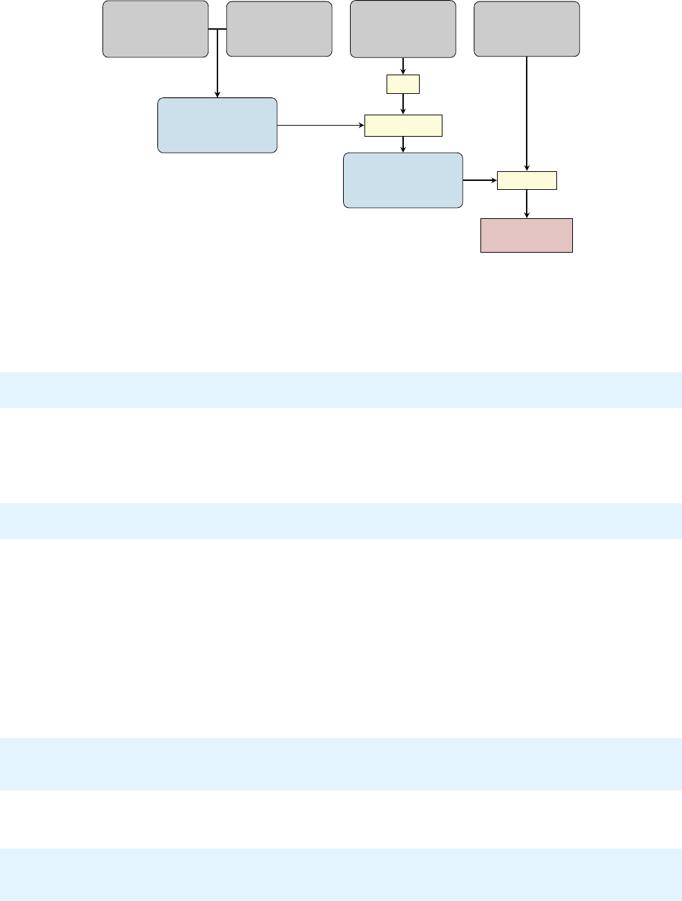
Sharc Manual 6 Interfaces |6.11 The WFoverlap Program
DΨI|Ψ0
JE
Contract
Unique factors
Skl,¯
Skl
Precompute
Sort
Slater
Determinants
|Φki,Φ0
lCI coeicients
dkI,d0
lJ
MO overlaps
Dφp|φ0
qE
MO coeicients
Cpµ,C0
qν
Double molecule
AO overlaps
χµ|χ0
ν
Figure 6.3: Workow of the wavefunction overlap program.
6.11.3 Calling the program
The main program is called in the following form
wfoverlap.x [-m <mem=1000>] [-f <input_file=cioverlap.input>]
with the command line options
•-m : amount of memory in MB
•-f : input le
Example:
wfoverlap.x -m 2000 -f wfov.in
Mode
The program automatically detects whether overlaps or Dyson orbitals should be calculated. If the number
of electrons in the bra and ket wavefunctions is the same, wavefunction overlaps are computed. If the number of
α
electrons or the number of
β
electrons dier by exactly 1, Dyson orbitals are computed. If the wave functions dier by
more than one electron, the program will stop with an error message.
Memory
The amount of
memory
given is a decisive factor for the performance of the code. Depending on the
amount of memory, one of three dierent modes is chosen:
(i) All Skl and ¯
Skl terms are kept in core (using arrays called P_ovland Q_ovl).
(ii) Only the Skl factors (P_ovl) are kept in core. This is indicated by
Allocation of Q block overlap matrix failed.
- Using on-the-fly algorithm for Q determinants.
This mode is generally as ecient as 1. but shows somewhat worse parallel scaling.
(iii) Not even all Skl factors can be stored
Only 437 out of 886 columns of the P_ovl matrix are stored in memory (3 MB)!
Increase the amount of memory to improve the efficiency.
This mode is signicantly slower than (i) and (ii) and should be avoided by increasing the amount of memory.
81
Sharc Manual 6 Interfaces |6.11 The WFoverlap Program
Table 6.15:
List of keywords given in the input le. The
a_mo, b_mo, a_det, b_det
keywords are mandatory, all
others are optional.
Keyword Default Description
a_mo — MO coecient le (bra)
b_mo — MO coecient le (ket)
a_mo_read 0 Format for the MO coecients (bra):
0: Columbus, 1: Molcas, 2: Turbomole
b_mo_read 0 Format for the MO coecients (ket)
a_det — Determinant le (bra)
b_det — Determinant le (ket)
ncore 0 Number of discarded core orbitals
ndocc 0
Number of doubly occupied orbitals that are not used for anni-
hilation in Dyson orbital calculations (only has eect if larger
than ncore)
ao_read 0 Format for overlap integrals:
0: ASCII, 1: Molcas, 2: Columbus/SIFS,
-1: Compute by inversion of MO coecient matrx
mix_aoovl S_mix/ONEINT/aoints AO overlap le
for ao_read=0/1/2
same_aos .false.
If both calculations were performed with the same set of AOs
(specify only for ao_read=1/2)
nao_aautomatic
Number of bra AOs for
ao_read=1/2
(specify only if dierent
from ket AOs)
nao_bautomatic Number of ket AOs (see above)
moprint 0 Print Dyson orbitals: 1: coecients to std. out,
2: as Jmol script
force_direct_dets .false.
Compute
Skl
terms directly (turn o "superblocks"). Recom-
mended if the number of CPU-cores is large (on the same order
as the number of "superblocks").
force_noprecalc .false. Do not precalculate the ¯
Skl factors.
mixing_angles .false. Compute mixing angles as a matrix logarithm.
Input file An example input le is shown below:
a_mo=mocoef_a
b_mo=mocoef_b
a_det=dets_a
b_det=dets_b
ao_read=2
same_aos
The full list of keywords is given in Table 6.15.
6.11.4 Input data
Typically, three types of input need to be provided: AO overlaps, MO coecients, and a combined le with determinant
information and CI coecients (cf. Figure 6.3). The le formats are explained here. Within Sharc, these les are
automatically extracted or converted by the interfaces, so the user does not need to create them.
AO overlaps
The mixed AO overlaps
χµ|χ0
ν
between the AOs used to expand the bra and ket wavefunctions are
required. They are in general created by a "double molecule" calculation, i.e. an AO integral calculation where every
atom is found twice in the input le.
The native format (
ao_read=0
) is a simple ASCII le containing the relevant o-diagonal block of the mixed AO overlap
matrix, e.g.
82

Sharc Manual 6 Interfaces |6.11 The WFoverlap Program
7 7
9.97108464676133E-001 2.36720699813181E-001 ...
2.36720699813181E-001 9.99919192433940E-001 ...
1.00147985713321E-002 6.52340422397770E-003 ...
...
In addition, Molcas (ao_read=1) and Columbus/SIFS (ao_read=2) les can be read in binary form.
If the same AOs are used for the bra and ket wavefunctions and the MO coecient matrix is square, it is possible to
reconstruct the overlaps by inversion of the MO coecient matrix (
ao_read=-1
). In this case it is not necessary to
supply a mix_aoovl le.
MO coeicients
MO coecients of the bra and ket wavefunctions can usually be read in directly in the form written
by the quantum chemistry program. The supported options for
a_mo_read
and
b_mo_read
are
0
for Columbus format,
1for Molcas lumorb format, and 2for Turbomole format.
Because the number of electrons strongly aects the run time of
wfoverlap.x
, it is generally benecial to apply a frozen
core approximation, even if the actual wave function calculation did not do so. Most interfaces which use
wfoverlap.x
have a keyword
numfrozcore
in the resource le, which only aects the number of frozen core orbitals for the overlap
calculation (If the interface support frozen core for the quantum chemistry itself, there will be a keyword in the template
le).
Slater determinants and CI coeicients
Slater determinants and CI coecients are currently supplied by an ASCII
le of the form
3 7 168
dddddee 0.979083342437 0.979083342437 -0.122637656388
ddddabe -0.094807515471 -0.094807515471 -0.663224542162
ddddbae 0.094807515471 0.094807515471 0.663224542162
...
The rst line species
•the number of states (columns in the le),
•the number of MOs (length of the determinant strings), and
•the number of determinants in the le (length of the le).
Every subsequent line gives the determinant string and the corresponding CI coecients for the dierent states. The
following symbols are used in the determinant string:
d - doubly occupied
a - singly occupied (α)
b - singly occupied (β)
e - empty
Most relevant for Sharc users, the
wfoverlap.x
program fully considers all determinants inside these les, without
applying any form of truncation. Hence, truncation of long wave functions is done during the creation of the determinant
les. Most interfaces which write these les have a keyword
wfthres
in their resource le. This threshold is a number
between 0.0 and 1.0, and is the minimum wave function norm to which the wave functions should be truncated. During
truncation, the interfaces generally retain the largest-amplitude CI coecients, and remove determinants with small
coecients, i.e., they nd the truncated expansion with the fewest determinants which has a norm above the
wfthres
.
Choosing this threshold properly can very strongly aect the computational time spent in the overlap calculation.
Generally, for CASSCF wave functions the threshold can be set to 1 (
SHARC_MOLPRO.py
and
SHARC_MOLCAS.py
always
use all determinants and do not have the
wfthres
option), for TDA-DFT/ADC(2) it should usually be above 0.99, for and
for MRCI wave functions it might be necessary to go as low as 0.95, depending on the accuracy and performance needed.
For TD-DFT calculations without the Tamm-Damco approximation, the response vectors are usually normalized to
|X|2− |Y|=
1, but only
X
is used in the overlap calculation; since the norm of
X
can thus exceed 1, the
wfthres
should
be increased above 1, too. As a rule of thumb, the threshold should always be chosen such that each state is represented
83

Sharc Manual 6 Interfaces |6.11 The WFoverlap Program
by at least a few 100 determinants in the le, in order to obtain smoothly varying overlaps. If unsure, the user should
perform a test calculation, varying the wfthres until a suitable one is found.
6.11.5 Output
Usually, the output of
wfoverlap.x
is automatically extracted by the interfaces, and reported in
QM.out
in the overlap
or 2D-property sections.
Wavefunction overlaps
The output rst lists some information about the wavefunction structure and about the
computational time taken for the individual steps (cf. Figure 6.3).
A typical result of a wavefunction overlap computation is shown here:
Overlap matrix <PsiA_i|PsiB_j>
|PsiB 1> |PsiB 2>
<PsiA 1| 0.5162656622 -0.2040109070
<PsiA 2| -0.2167057391 -0.5266552021
Renormalized overlap matrix <PsiA_i|PsiB_j>
|PsiB 1> |PsiB 2>
<PsiA 1| 0.5162656622 -0.2040109070
<PsiA 2| -0.2167057391 -0.5266552021
Performing Lowdin orthonormalization by SVD...
Orthonormalized overlap matrix <PsiA_i|PsiB_j>
|PsiB 1> |PsiB 2>
<PsiA 1| 0.9273847015 -0.3741090956
<PsiA 2| -0.3741090956 -0.9273847015
Overlap matrix gives the raw overlap values
hΨI|Ψ0
Ji(6.12)
of the wavefunctions supplied.
Renormalized overlap matrix gives the renormalized overlap values
hΨI|Ψ0
Ji
||ΨI||2||Ψ0
J||2(6.13)
relevant in the case of wavefunction truncation.
The Orthonormalized overlap matrix is constructed according to a procedure described in more detail in Ref. [73].
Dyson orbitals The matrix of Dyson norms is printed at the end of the le
ALPHA ionization
Dyson norm matrix |<PsiA_i|PsiB_j>|^2
|PsiB 1> |PsiB 2> |PsiB 3>
<PsiA 1| 0.8817323437 0.4716319904 0.0680618001
<PsiA 2| 0.0615587916 0.4657174978 0.8772909828
<PsiA 3| 0.0000000000 0.0363130811 0.0000000000
<PsiA 4| 0.9634885049 0.0000000000 0.0017379586
<PsiA 5| 0.0000000000 0.9261839484 0.0000000000
In the case of
moprint=1
the orbitals are printed, as well. The expansion is given with respect to the MOs of the neutral
system.
84

Sharc Manual 6 Interfaces |6.11 The WFoverlap Program
Dyson orbitals in reference |ket> MO basis:
<PsiA 1|
|PsiB 1> |PsiB 2> |PsiB 3>
MO 1 -1.24032037E-03 0.00000000E+00 9.98160731E-04
MO 2 -5.90277699E-02 0.00000000E+00 6.14517859E-02
MO 3 -1.23295110E-09 0.00000000E+00 3.08416849E-10
MO 4 0.00000000E+00 -6.86713110E-01 0.00000000E+00
MO 5 9.31351013E-01 0.00000000E+00 -2.49427166E-01
MO 6 -3.50106110E-02 0.00000000E+00 4.19935829E-02
MO 7 -1.83303166E-10 0.00000000E+00 -3.67409953E-12
MO 8 -1.91183349E-10 0.00000000E+00 9.40768334E-11
...
85

7 Auxilliary Scripts
In this chapter, all auxiliary scripts and programs are documented. Input generators (like
molpro_input.py
and
molcas_input.py) are documented in the relevant interface sections.
All auxiliary scripts are either interactive—prompting user input from stdin in order to setup a certain task—or non-
interactive, meaning they are controlled by command-line arguments and options, in the same way as many standard
command-line tools work.
All interactive scripts sequentially ask a number of questions to the user. In many cases, a default value is presented,
which is either preset or detected by the scripts based on the availability of certain les. Furthermore, the scripts feature
auto-completion of paths and lenames (use TAB), which is active only in questions where auto-completion is relevant.
For certain questions where lists of integers needs to be entered, ranges can be indicated with the tilde symbol (~), e.g.,
-8~-2
(note that no spaces are allowed between the tilde and the two numbers) to indicate the list
-8 -7 -6 -5 -4 -3
-2.
All interactive scripts write a le called
KEYSTROKES.<script_name>
which contains the user input from the last
completed session. These les can be piped to the interactive scripts to perform the same task again, for example:
user@host> cat KEYSTROKES.excite - | $SHARC/excite.py
Note the
-
, which tells
cat
to switch to stdin after the le ends, so that the user can proceed if the script asks for more
input than contained in the KEYSTROKES le.
All non-interactive scripts can be called with the
-h
option to obtain a short description, usage information and a list of
the command line options. Non-interactive scripts also write a
KEYSTROKES.<script_name>
le, which will contain the
last command entered to execute the script (including all options and arguments).
All scripts can be safely killed during a run by using
Ctrl-C
. In the case of interactive scripts, a
KEYSTROKES.tmp
le
remains, containing the user input made so far. Note that the
KEYSTROKES.tmp
le cannot be directly piped to the
scripts, because KEYSTROKES.tmp will be overwritten when the script starts.
7.1 Wigner Distribution Sampling: wigner.py
The rst step in preparing the dynamics calculation is to obtain a set of physically reasonable initial conditions. Each
initial condition is a set of initial atomic coordinates, initial atomic velocities and initial electronic state. The initial
geometry and velocities can be obtained in dierent ways. With Sharc, often sampling of a quantum-harmonic Wigner
distribution is performed.
The sampling is carried out with the non-interactive Python script
wigner.py
. The theoretical background is summarized
in section 8.20.
7.1.1 Usage
The general usage is
user@host> $SHARC/wigner.py [options] filename.molden
wigner.py
takes exactly one command-line argument (the input le with the frequencies and normal modes), plus
some options. Usually, the -n option is necessary, since the default is to only create 3 initial conditions.
The argument is the lename of the le containing the information about the vibrational frequencies and normal modes.
The le is by default assumed to be in the Molden format. For usage with
wigner.py
, only the following blocks have
to be present:
•[FREQ]
•[FR-COORD]
•[FR-NORM-COORD]
The script accepts a number of command-line options, specied in table 7.1.
86

Sharc Manual 7 Auxilliary Scripts |7.1 Wigner Distribution Sampling: wigner.py
Table 7.1: Command-line options for script wigner.py.
Option Description Default
-h Display help message and quit —
-n INTEGER Number of initial conditions to generate 3
-m Modify atom masses (starts interactive dialog) Most common isotopes
-s FLOAT Scaling factor for the frequencies 1.0
-t FLOAT
Use Boltzmann-weighted distribution at the given temperature
0.0 K
-T Discard very high vibrational states at high temperatures Don’t discard, but warn
-L FLOAT Discard frequencies below the given one (in cm−1) 10.0
-o FILENAME Output lename initconds
-x Creates an xyz le with the sampled geometries initconds.xyz
-l
Instead of generating
initconds
, create input for
SHARC_LVC.py Create initconds
-r INTEGER Seed for random number generator 16661
-f F
Type of normal modes read (0=detect automatically, 1–4=see
below)
0
--keep_trans_rot Do not remove translations and rotations from velocity vector
--use_eq_geom Sample only velocities, but keep equilibrium geometry Sample normally
--use_zero_veloc Sample only geometries, but set velocities to zero Sample normally
7.1.2 Normal mode types
The normal mode vectors contained in a Molden le can follow dierent conventions, e.g., unscaled Cartesian
displacements or dierent kinds of mass-weighted displacements. By default,
wigner.py
attempts to identify which
convention is followed by the le (by performing dierent renormalizations and checking if the so-obtained matrix is
orthogonal). In order to use this automatic detection, use
-f 0
, which is the default. Otherwise, there are four possible
options:
-f 1
to assume normal modes in the Gaussian convention (used by Gaussian,Turbomole,Q-Chem, ADF,
and Orca);
-f 2
to assume Cartesian normal modes (used by Molcas and Molpro);
-f 3
to assume the Columbus
convention; or -f 4 for mass-weighted, orthogonal normal modes.
7.1.3 Non-default masses
When the
-m
option is used, the script will ask the user to interactively modify the atom masses. For each atom (referred
to by the atom index as in the Molden le), a mass can be given (relative atomic weights). Note that the frequency
calculation which produces the Molden should be done with the same atomic masses.
7.1.4 Sampling at finite temperatures
When the
-t
option is used, the script assumes a nite, non-zero temperature. The sampling will then consist of
two steps, where rst randomly a vibrational state is picked from the Boltzmann distribution, and then the Wigner
distribution of that state is employed. For more details, see Section 8.20.
At high temperatures and for low-frequency modes it is possible that very large vibrational quantum numbers will be
selected. Because of the occurrence of factorials in the Laguerre polynomials in the excited Wigner distributions, this
leads to variable overow for
νvib >
150. Hence, the highest vibrational quantum number considered is 150, and higher
ones are set to 150. Since this can lead to an overrepresentation of
νvib =
150, with the
-T
option one can instead discard
all samplings where
νvib >
150. No matter whether
-T
is used or not, keep in mind that usually such high vibrational
states might invalidate the assumption of an harmonic oscillator, and other sampling methods (e.g., molecular dynamics)
should be considered.
7.1.5 Output
The script
wigner.py
generates a single output le, by default called
initconds
. All information about the initial
conditions is stored in this le. Later steps in the preparation of the initial conditions add information about the excited
states to this le. The le is formatted in a human-readable form.
The initconds le format is specied in section 7.5.5.
87

Sharc Manual 7 Auxilliary Scripts |7.2 Amber Trajectory Sampling: amber_to_initconds.py
When the
-x
option is given, additionally the script produces a le called
initconds.xyz
, which contains the sampled
geometries in standard xyz format. This can be useful to inspect the distribution of geometry parameters (e.g., bond
lengths) or to perform single point calculations at the sampled geometries.
When the
-l
option is given, the script only produces a le called
V0.txt
, which is a necessary input le for the LVC
interface (see section 6.9). If this option is activated, no initconds or initconds.xyz les are produced.
7.2 Amber Trajectory Sampling: amber_to_initconds.py
The rst step in preparing the dynamics calculation is to obtain a set of physically reasonable initial conditions. Each
initial condition is a set of initial atomic coordinates, initial atomic velocities and initial electronic state. The initial
geometry and velocities can be obtained in dierent ways. Besides sampling from a quantum mechanical Wigner
distribution (with
wigner.py
), it is a widespread approach to sample geometries and velocities from a ground state
molecular dynamics simulation.
Using amber_to_initconds.py, one can convert the results of an Amber simulation to a Sharc initconds le.
7.2.1 Usage
In order to use
amber_to_initconds.py
, it is necessary to rst carry out an Amber simulation. You need to add the
following options to the Amber MD input le: (i)
ntxo=1
to tell Amber to write ASCII restart les, (ii)
ntwr=-5000
to
create a restart le every 5000 steps (other values are possible, but use the minus to not overwrite the restart les). This
will create a set of Amber restart les called, e.g., md.rst_5000,md.rst_10000, ...
Note that it is also necessary to reimage the Amber restart les, because Sharc does not work with periodic boundary
conditions, but the Amber trajectories might use them. The reimaging can be performed with Amber’s tool
cpptraj
,
using the following input:
parm <filename>.prmtop
trajin <filename>.rst7
autoimage
trajout <filename2>.rst7
run
This command has to be repeated for each restart le which needs to be reimaged. Note that
amber_to_initconds.py
only works with the rst7 ASCII le format, not with the rst format (even if it is ASCII-formatted).
If you saved the restart les in Amber’s newer NetCDF format,
cpptraj
can also be used to convert them to ASCII
rst7
restart les. If you did not save restart les,
cpptraj
can even be used to generate restart les from the trajectory le
(.mdcrd and .mdvel), but for this way it is necessary to save the velocities (.mdvel le).
With the restart les prepared, call amber_to_initconds.py like this:
user@host> $SHARC/amber_to_initconds.py [options] md.prmtop md.rst_0 md.rst_5000 md.rst_10000 ...
The possible options are shown in Table 7.2.
7.2.2 Time Step
Note that the option
-t
(giving the time step used in Amber in femtoseconds) is mandatory; if not given, an error message
is produced. This is because Amber uses a Leapfrog algorithm and thus stores in the restart le
R(t)
and
v(t−∆t/
2
)
,
Table 7.2: Command-line options for script amber_to_initconds.py.
Option Description Default
-h Display help message and quit —
-t FLOAT Time step (in femtoseconds) used in the Amber simulation —
-o FILENAME Output lename initconds
-x Creates an xyz le with the sampled geometries initconds.xyz
-m Modify atom masses (starts interactive dialog) As in prmtop le
--keep_trans_rot Do not remove translations and rotations from velocity vector
--use_zero_veloc Sample only geometries, but set velocities to zero Sample normally
88
Sharc Manual 7 Auxilliary Scripts |7.3 Sharc Trajectory Sampling: sharctraj_to_initconds.py
whereas Sharc uses the velocity-Verlet algorithm and requires geometry and velocity at the same time, e.g.,
R(t−∆t/
2
)
and
v(t−∆t/
2
)
. To compensate this,
amber_to_initconds.py
computes
R(t−∆t/
2
)
from
R(t)−v(t−∆t/
2
)∆t/
2. Hence,
∆tof the Amber trajectory needs to be known.
7.2.3 Atom Types and Masses
By default, atom types and masses are read from the
prmtop
le (from ags
ATOMIC_NUMBER
and
MASS
). If the atomic
number is not sensible (e.g., -1 for a transition metal) then
amber_to_initconds.py
prompts the user to dene the
element. The masses in the
prmtop
le can be overridden if the
-m
option is given; then the user can adjust the mass of
each atom individually.
7.2.4 Output
amber_to_initconds.py
produces the same output as
wigner.py
(section 7.1). By default, a le called
initconds
is
generated for the converted initial conditions. It is important to note that the rst restart le given (the second command
line argument) is treated as the “equilibrium” geometry for the purpose of generating the
initconds
le. The second
given restart le is then converted to the initial condition with index 1, and so on. Note that it is possible to give the
same restart le multiple times as an argument (so that the same geometry can be used as “equilibrium” geometry and
as proper initial condition.
7.3 Sharc Trajectory Sampling: sharctraj_to_initconds.py
The rst step in preparing the dynamics calculation is to obtain a set of physically reasonable initial conditions. Each
initial condition is a set of initial atomic coordinates, initial atomic velocities and initial electronic state. The initial
geometry and velocities can be obtained in dierent ways. Besides sampling from a quantum mechanical Wigner
distribution, it is often appropriate to sample geometries and velocities from a ground state molecular dynamics
simulation.
Using
sharctraj_to_initconds.py
, one can convert the results of a Sharc simulation to a new Sharc
initconds
le.
7.3.1 Usage
In order to use
sharctraj_to_initconds.py
, it is necessary to rst run a number of Sharc trajectories (the initial
conditions for those need to be obtained with
wigner.py
or
amber_to_initconds.py
). The trajectories can be run with
any number of states and in any state, and with any desirable options; only geometries and velocities are converted to
the new initconds le.
With the trajectories prepared, call sharctraj_to_initconds.py like this:
user@host> $SHARC/sharctraj_to_initconds.py [options] Singlet_0 ...
Alternatively, with the --give_TRAJ_paths option, one can also do:
user@host> $SHARC/sharctraj_to_initconds.py --give_TRAJ_paths [options] TRAJ_00001 TRAJ_00002 ...
The possible options are shown in Table 7.3.
7.3.2 Random Picking of Time Step
For each directory specied as command line argument,
sharctraj_to_initconds.py
picks exactly one time step and
extracts geometries and velocities of that time step. Note that a directory can be given several times as argument, so
that multiple time steps can be selected.
The time steps are generally picked randomly (uniform probabilities) from an interval specied with the
-S
option. This
option takes two integers, e.g.,
-S 50 -50
, which can be positive or negative. The meaning of positive/negative/zero is
the same as in Python: positive numbers simply denote a time step (start counting with zero for the step zero of the
trajectory); for negative numbers, start counting at the end, i.e., -1 is the last time step of the trajectory. In this way, it is
possible to select the snapshot from the last nsteps of all trajectories, even if they have dierent length. The example
above,
-S 50 -50
, means picking a time step between the 50th and the 50th-last step. Note that if a trajectory is shorter
than 100 steps, in this example it is skipped because there are no steps between the 50th and the 50th-last step.
89

Sharc Manual 7 Auxilliary Scripts |7.4 Setup of Initial Calculations: setup_init.py
Table 7.3: Command-line options for script sharctraj_to_initconds.py.
Option Description Default
-h Display help message and quit —
-r INTEGER Seed for the random number generator 16661
-S INTEGER INTEGER Range of time steps from which a step is randomly chosen last step
-o FILENAME Output lename initconds
-x Creates an xyz le with the sampled geometries initconds.xyz
--keep_trans_rot Do not remove translations and rotations from velocity
--use_zero_veloc Sample only geometries, but set velocities to zero Sample normally
--debug Show timings
--give_TRAJ_paths Allows specifying individual trajectories Specify parent directories
7.3.3 Output
sharctraj_to_initconds.py
produces the same output as
wigner.py
(section 7.1). By default, a le called
initconds
is generated for the converted initial conditions. It is important to note that the rst directory given (the rst command
line argument) is treated as the “equilibrium” geometry for the purpose of generating the
initconds
le. The second
given directory is then converted to the initial condition with index 1, and so on. Note that it is possible to give the
same directory multiple times as an argument (so that the same geometry can be used as “equilibrium” geometry and as
proper initial condition.
7.4 Setup of Initial Calculations: setup_init.py
The interactive script
setup_init.py
creates input for single point calculations at the initial geometries given in an
initconds
le. These calculations might be necessary for some schemes to select the initial electronic state of the
trajectory, e.g., based on the excitation energies and oscillator strength of the transitions from ground state to the
excited state, or based on overlaps with a reference wave function.
There are other choices of the initial state possible, which do not require single point calculations at all initial geometries.
See the description of
excite.py
(section 7.5). In this case,
setup_init.py
can be used to set up only the calculation at
the equilibrium geometry (see below at “Range of Initial Conditions”).
7.4.1 Usage
The script is interactive, and can be started by simply typing
user@host> $SHARC/setup_init.py
Please be aware that the script will setup the calculations in the directory where it was started, so the user should
cd
to
the desired directory before executing the script.
Please note that the script does not expand ~or shell variables, except where noted otherwise.
7.4.2 Input
The script will prompt the user for the input. In the following, all input parameters are documented:
Initial Conditions File
Enter the lename of the initial conditions le, which was generated beforehand with
wigner.py
. If the script nds a le called
initconds
, the user is asked whether to use this le, otherwise the user has
to enter an appropriate lename. The script detects the number of initial conditions and number of atoms automatically
from the initial conditions le.
Range of Initial Conditions
The initial conditions in
initconds
are indexed, starting with the index 1. In order to
prepare ab initio calculations for a subset of all initial conditions, enter a range of indices, e.g.
a
and
b
. This will prepare
all initial conditions with indices in the interval
[a,b]
. In any case, the script will additionally prepare a calculation for
the equilibrium geometry (except if a nished calculation for the equilibrium geometry was found).
If the interval [0,0]is given, the script will only setup the calculation at the equilibrium geometry.
90
Sharc Manual 7 Auxilliary Scripts |7.4 Setup of Initial Calculations: setup_init.py
Number of states
Here the user can specify the number of excited states to be calculated. Note that the ground
state has to be counted as well, e.g., if 4 singlet states are specied, the calculation will involve the
S0
,
S1
,
S2
and
S3
.
Also states of higher multiplicity can be given, e.g. triplet or quintet states. For even-electron molecules, including
odd-electron states (e.g. doublets) is only useful if transition properties for ionization can be computed (e.g. Dyson
norms with some of the interfaces). These transition properties can be used to calculate ionization spectra or to obtain
initial conditions for dynamics after ionization.
Interface
In this point, choose any of the displayed interfaces to carry out the ab initio calculations. Enter the
corresponding number.
Spin-orbit calculation
Usually, it is sucient to calculate the spin-free excitation energies and oscillator strengths
in order to decide for the initial state. However, using this option, the eects of spin-orbit coupling on the excitation
energies and oscillator strengths can be included. Note that the script will never calculate spin-orbit couplings if
only singlet states are included in the calculation, or if the chosen interface does not support calculation of spin-orbit
couplings.
Reference overlaps
The calculations can be setup in such a way that the wave function overlaps between states at
the equilibrium geometry and the displaced geometries is computed. This allows correlating the states at the displaced
geometries with the reference states, such that one can know the state characters of all states without inspection. This
is useful for a crude “diabatization” of the states, e.g., if one wants to start all trajectories in the
nπ∗
state of the molecule
although this state can be S1,S2, or S3(use excite.py to setup initial conditions in such a way, see section 7.5).
When activating this option, keep in mind that the calculation in
ICOND_00000
must be successfully nished before any
of the other ICOND_XXXXX calculations can be started.
TheoDORE analysis
If the chosen interface supports wave function analysis with TheoDORE, then this option can
be activated here.
setup_init.py
will then include the relevant keywords in the computations, and the results of the
TheoDORE analysis will be written to the QM.out les.
The remaining settings for TheoDORE (fragment and descriptor input) will be asked later in setup_init.py.
7.4.3 Interface-specific input
The following input in
setup_init.py
depends on the chosen interface. However, some input is similar between several
interfaces and is discussed (out of input order) in section 7.4.3. Note that most of the questions asked in the input
dialogue have some counterpart in the resource le of the chosen interface, so you might nd additional information in
chapter 6.
Input which is similar between interfaces
Path to quantum chemistry programs and licenses
Here the user is prompted to provide the path to the relevant
executables or installation directories.
Note that the setup script will not expand the user (
~
) and shell variables (since the calculations might be running on a
dierent machine than the one used for setup, so the meaning of shell variables could be dierent).
~
and shell variables
will only be expanded by the interfaces during the actual calculation.
For some interfaces, also the path to a license le might need to be specied.
Scratch directory
The script takes the string without any checking. Each individual initial condition uses a subdi-
rectory of the given path, so that there are no clashes between the initial conditions.
~
and shell variables will only be
expanded by the interface during the actual calculation.
Note that you can use, e.g.,
./temp/
as scratch directory, which is a subdirectory of the working directory of the
interface. Using ./ as scratch directory is not recommended, since the interface will delete the scratch directory.
91
Sharc Manual 7 Auxilliary Scripts |7.4 Setup of Initial Calculations: setup_init.py
Template file
For almost all interfaces,
setup_init.py
will ask for a template le containing the quantum chemistry
specics of the calculations. The format of the template le depends on the interface; formats are described in the
interface chapter 6.
For most interfaces,
setup_init.py
will perform some basic checks, but ultimately the template le will be checked by
the interface once the calculation is submitted.
Initial orbital guess
For some interfaces,
setup_init.py
will ask for les containing initial orbital guesses. providing
initial is especially important for multi-reference calculations, because otherwise it is very likely that the calculations
converge to an undesirable active space.
Resource usage
For most interfaces,
setup_init.py
will ask for the amount of memory and the number of CPU
cores to use. For some interfaces, additionally a delay between the start of parallel calculation can be provided (this
might be helpful if many calculations starting at the same time is problematic for I/O). For the ADF and
Gaussian
interfaces, furthermore the schedule_scaling is queried for (see section 8.3 for details).
Wavefunction overlap program
The scripts asks for the path to the wavefunction overlap program. In a complete
Sharc installation, the overlap program should be located at
$/SHARC/wfoverlap.x
. Depending on the interface, the
script might also ask for the threshold to truncate the wave function les, or for the memory for
wfoverlap.x
(if the
memory of the quantum chemistry program cannot be set). For some interfaces, it is also possible to control the number
of frozen core orbitals for the overlap calculation (and the number of inactive orbitals for Dyson orbital calculations).
TheoDORE setup
If TheoDORE is enabled,
setup_init.py
will query for the path to the TheoDORE installation
directory. Furthermore, the user needs to enter a list of the descriptors to be calculated by TheoDORE, as well as the
atom indices for each fragment for the charge transfer number computation.
QM/MM setup
For some interfaces,
setup_init.py
will ask for QM/MM-related les if the template le species a
QM/MM calculation. Currently, the QM/MM setup consists simply of providing the relevant interface-specic les to
setup_init.py, which it simply copies accordingly.
Input for Molpro
Path to Molpro
Here the user is prompted to provide the path to the Molpro executable. For more details, see
section 7.4.3.
Scratch directory See section 7.4.3.
Template file
Enter the lename for the Molpro template input. This le should contain at least the basis set, active
orbitals and electrons, number of electrons and number of states for state-averaging. For details, see the section about
the Sharc-Molpro interface (6.3). The setup script will check whether the template le contains the necessary entries.
Initial wave function file
You can provide an initial wave function (with an appropriate MO guess) to Molpro.
This usually provides a drastic speedup for the CASSCF calculations and helps in ensuring that all calculations are
based on the same active space. In simple cases it might be acceptable to not provide an initial wave function.
Resource usage
The script asks for the memory and number of CPU cores to be used. Note that both settings apply
to Molpro and to
wfoverlap.x
, if the latter is required (but note that the two programs are never run simultaneously).
If more than one CPU core is used, the interface will parallelize dierent Molpro runs (but will not run Molpro in
parallel mode); wfoverlap.x will be run in SMP-parallel mode.
Wavefunction overlap program
See section 7.4.3. Note that for the Molpro interface, no truncation threshold can
be given, since wfoverlap.x is very ecient for CASSCF wavefunctions.
92
Sharc Manual 7 Auxilliary Scripts |7.4 Setup of Initial Calculations: setup_init.py
Input for Molcas
Path to Molcas
Here the user is prompted to provide the path to the Molcas directory. For more details, see
section 7.4.3.
Scratch directory See section 7.4.3.
Template file
Enter the lename for the Molcas template input. This le should contain at least the basis set, active
orbitals and electrons, number of inactive orbitals, and number of states for state-averaging. For details, see the section
about the Sharc-Molcas interface (6.4). The setup script will check whether the template le contains the necessary
entries.
QM/MM
If the keyword
qmmm
is contained in the template le, the user will be queried for the path to Tinker’s
bin/
directory. Note that only Tinker installations with the necessary modications for Molcas can be used.
The script will also ask for the key le (containing the path to the force eld le and the QM/MM partition) and the
connection table le. See section 6.4 for details.
Initial wave function file
You can provide initial MO coecients to Molcas. This usually provides a drastic speedup
for the CASSCF calculations and helps in ensuring that all calculations are based on the same active space. In simple
cases it might be acceptable to not provide an initial wave function. For Molcas, you have to specify one le for each
multiplicity (but you can use the same le as guess for several multiplicities). Initial orbital les can either be in
JobIph
or RasOrb format.
Resource usage
The script asks for the memory and number of CPU cores to be used. Note that both settings apply
to Molcas and to
wfoverlap.x
, if the latter is required (but note that the two programs are never run simultaneously).
If more than one CPU core is used, the interface will parallelize dierent Molcas runs (but will not run Molcas in
parallel mode); wfoverlap.x will be run in SMP-parallel mode.
Wavefunction overlap program
See section 7.4.3. The
wfoverlap.x
program is only required if Dyson norms
need to be calculated. Note that for the Molcas interface, no truncation threshold can be given, since
wfoverlap.x
is
very ecient for CASSCF wavefunctions.
Input for Columbus
Path to Columbus
Here the user is prompted to provide the path to the Columbus directory. For more details, see
section 7.4.3.
Scratch directory See section 7.4.3.
Template directory
Enter the path to a directory containing subdirectories with Columbus input les necessary for
the calculations. The setup script will expand ~and shell variables and will pass the absolute path to the calculations.
The script will auto-detect (based on the
cidrtin
les) which subdirectory contains the input for each multiplicity.
The user has to check in the following dialog whether the association of multiplicities with job directories is correct.
Additionally, the association of MO coecient les to the jobs has to be checked. See the section on the Sharc-Columbus
interface (6.5) for further details.
Note that the setup script does not check any content of the input les beyond the multiplicity. Note that
transmomin
and
control.run
do not need to be present (and that their content has no eect on the calculation), since these les are
written on-the-y by the interface.
The template directory can either be linked or copied to the initial condition calculations.
Initial orbital coeicient file
You can provide initial MO coecients for the Columbus calculation. This usually
provides a drastic speedup for the CASSCF calculations and helps to ensure that all calculations are based on the same
active space. In simple cases it might be acceptable to not provide an initial wave function.
93
Sharc Manual 7 Auxilliary Scripts |7.4 Setup of Initial Calculations: setup_init.py
Memory
For Columbus, the available memory must be given here. The Columbus interface does not allow for
parallelization currently.
Wavefunction overlap program
See section 7.4.3. For CASSCF calculations with Columbus, use a truncation
threshold of 1.0, for MRCIS/MRCISD calculations, 0.97-0.99 should provide sucient performance and accuracy.
Input for analytical potentials
Template file
Enter the lename for the template input specifying the analytical potentials. For details, see the
section about the Sharc-Analytical interface (6.6). The setup script will check whether the template le is valid.
Input for ADF
Path to ADF
Here the user is rst asked if setup should be made from an
adfrc.sh
le. If yes, only the path to this
le is needed.
Otherwise, the path to the ADF installation directory and the path to the license le need to be provided. For more
details, see section 7.4.3.
Scratch directory See section 7.4.3.
Template file
Enter the lename for the ADF template input. This le should contain at least the basis set, functional,
and charge keywords. For details, see the section about the Sharc-ADF interface (6.7). The setup script will check
whether the template le contains the necessary entries.
QM/MM
The script will ask for the two QM/MM-specic input les for the interface, which are called
ADF.qmmm.ff
and ADF.qmmm.table. See section 6.7 for details on these les.
Initial orbital coeicient file
You can provide initial MO coecients for the ADF calculation. This can provide a
small speedup for the calculations and helps to ensure that all calculations are based on the same orbitals. In many
cases, no initial orbitals are required.
Resource usage
For ADF, the amount of memory to be used cannot be controlled. However, the number of CPU
cores needs to be given. If more than one core is used, also the parallel scaling needs to be specied (see section 8.3).
Wavefunction overlap program
See section 7.4.3.
setup_init.py
will ask for the memory usage of
wfoverlap.x
.
The truncation threshold for TD-DFT can usually be chosen as 0.99–1.00 (depending on the system and functional, but
it is recommended that it is high enough that each state is described by around 100 determinants in the generated les).
See section 6.7 for details.
TheoDORE setup See section 7.4.3.
Input for Ricc2
Path to Turbomole
The path to the Turbomole installation directory needs to be provided. If spin-orbit couplings
are requested, also the path to the Orca installation directory is needed. For more details, see section 7.4.3.
Scratch directory See section 7.4.3.
Template file
Enter the lename for the Ricc2 template input. This le should contain at least the basis set and
charge keywords. For details, see the section about the Sharc-Ricc2 interface (6.8). The setup script will check whether
the template le contains the necessary entries.
94
Sharc Manual 7 Auxilliary Scripts |7.4 Setup of Initial Calculations: setup_init.py
Initial orbital coeicient file
You can provide initial MO coecients for the ADF calculation. This can provide a
small speedup for the calculations and helps to ensure that all calculations are based on the same orbitals. In many
cases, no initial orbitals are required.
Resource usage
The amount of memory and the number of CPU cores are required in this section. Note that the
Sharc-Ricc2 interface always runs only one Turbomole instance at the same time (if the number of CPU cores is
larger than one, it will use the SMP/OMP binaries of Turbomole).
Wavefunction overlap program
See section 7.4.3.
setup_init.py
will ask for the memory usage of
wfoverlap.x
.
The truncation threshold can usually be chosen as 0.99–1.00 (depending on the system, but it is recommended that it is
high enough that each state is described by around 100 determinants in the generated les). See section 6.8 for details.
TheoDORE setup See section 7.4.3.
Input for LVC interface
Template file Enter the lename for the template input specifying the LVC parameters. For details, see the section
about the Sharc-LVC interface (6.9). The setup script will not check whether the template le is valid.
Input for Gaussian interface
Path to Gaussian
The path to the Gaussian installation directory needs to be provided. Note that this needs to
be the path to the directory containing the Gaussian executables, e.g.,
g09
/
g16
,
l9999.exe
, etc. The interface will
automatically detect which Gaussian version is used. For more details, see section 7.4.3.
Scratch directory See section 7.4.3.
Template file
Enter the lename for the Gaussian template input. This le should contain at least the basis set,
functional, and charge keywords. For details, see the section about the Sharc-Gaussian interface (6.10). The setup
script will check whether the template le contains the necessary entries.
Initial orbital coeicient file
You can provide initial MO coecients for the Gaussian calculation. This can provide
a small speedup for the calculations and helps to ensure that all calculations are based on the same orbitals. In many
cases, no initial orbitals are required.
Resource usage
The amount of memory and the number of CPU cores are required in this section. If more than one
core is used, also the parallel scaling needs to be specied (see section 8.3).
Wavefunction overlap program
See section 7.4.3.
setup_init.py
will ask for the memory usage of
wfoverlap.x
.
The truncation threshold for TD-DFT can usually be chosen as 0.99–1.00 (depending on the system and functional, but
it is recommended that it is high enough that each state is described by around 100 determinants in the generated les).
See section 6.10 for details.
TheoDORE setup See section 7.4.3.
7.4.4 Input for Run Scripts
Run script mode
The script
setup_init.py
generates a run script (Bash) for each initial condition calculation. Due
to the large variety of cluster architectures, these run scripts might not work in every case. It is the user’s responsibility
to adapt the generated run scripts to his needs.
setup_init.py
can generate run scripts for two dierent schemes how to execute the calculations. With the rst
scheme, the ab initio calculations are performed in the directory where they were setup (subdirectories of the directory
95
Sharc Manual 7 Auxilliary Scripts |7.4 Setup of Initial Calculations: setup_init.py
where
setup_init.py
was started). Note that the interfaces will still use their scratch directories to perform the actual
quantum chemistry calculations. Currently, this is the default option.
With the second option, the run scripts will transfer the input les for each ab initio calculation to a temporary directory,
where the interface is started. After the interface nishes all calculations, the results les are transferred back to the
primary directory and the temporary directory is deleted. Note that
setup_init.py
in any case creates the directory
structure in the directory where it was started. The name of the temporary directory can contain shell variables, which
will be expanded when the script is running (on the compute host).
Submission script
The setup script can also create a Bash script for the submission of all ab initio calculations to
a queueing system. The user has to provide a submission command for that, including any options which might be
necessary. This submission script might not work with all queueing systems.
Project name
The user can enter a project name. This is used currently only for the job names of submitted jobs (
-N
option for queueing system).
7.4.5 Output
setup_init.py
will create for each initial condition in the given range a directory whose names follow the format
ICOND_%05i/
, where
%05i
is the index of the initial condition padded with zeroes to 5 digits. Additionally, the directory
ICOND_00000/ is created for the calculation of the excitation energies at the equilibrium geometry.
To each directory, the following les will be added:
•QM.in
: Main input le for the interface, contains the geometry and the control keywords (to specify which
quantities need to be calculated).
•run.sh
: Run script, which can be started interactively in order to perform the ab initio calculation in this directory.
Can also be adapted to a batch script for submission to a queue
•Interface-specic les: Usually a template le, a resource le, and an initial wave function.
The calculations in each directory can be simply executed by starting
run.sh
in each directory. In order to perform this
task consecutively on a single machine, the script
all_run.sh
can be executed. The le
DONE
contains the progress of
this calculation. Alternatively, each run script can be sent to a queueing system (you might need to adapt this script to
you cluster system). Note that if reference overlaps were requested, the calculation in
ICOND_00000/
must be nished
before starting any of the other calculations.
In gure 7.1, the directory tree structure setup by setup_init.py is given.
After all calculations are nished, excite.py can be used to collect the results.
$(pwd)
all qsub.sh
all run.sh
INIT 00000
QM.in
runQM.sh
<Interface files>
INIT 00001
INIT .....
Figure 7.1:
Directory structure created by
setup_init.py
. Directories are in blue, executable scripts in green and
regular les in black and white. Interface les usually include initial MO coecients, template les and
interface input les.
96
Sharc Manual 7 Auxilliary Scripts |7.5 Excitation Selection: excite.py
7.5 Excitation Selection: excite.py
excite.py
has two tasks: adding excited-state information to the
initconds
le, and deciding which excited state for
which initial condition is a valid initial state for the dynamics.
7.5.1 Usage
The script is interactive, and can be started by simply typing
user@host> $SHARC/excite.py
7.5.2 Input
Initial condition file
Enter the path to the initial conditions le, to which
excite.py
will add excited-state informa-
tion. This le can already contain excited-state information (in this case this information can be reused).
Generate excited state list There are three possibilities to add excited-state information to the initconds le:
1. generate a list of dummy excited states,
2.
read excited-state information from the output of the initial ab initio calculations (prepare the calculations with
setup_init.py),
3. keep the existing excited-state information in the initconds le.
The rst option is mainly used if no initial ab initio calculations need to be performed (e.g., the initial state is known).
In order to use the second option, one should rst setup initial excited-state calculations using
setup_init.py
(see 7.4)
and run the calculations.
excite.py
can then read the output of the initial calculations and calculate excitation energies
and oscillator strengths.
The third option can be used to reuse the information in the
initconds
le, e.g., to apply a dierent selection scheme
to the states or to just read the number of states.
Path to ab initio results
If
excite.py
will read the excited-state information from the ab initio calculation results,
here the user has to provide the path to the directory containing the ICOND_%05i subdirectories.
Number of states
If a dummy list of states will be generated, the user has to provide the number of states per
multiplicity. Note that a singlet ground state has to be counted as well, e.g. if 4 singlet states are specied, the calculation
will involve the
S0
,
S1
,
S2
and
S3
. Also states of higher multiplicity can be given, e.g. doublet or triplet states (e.g.,
221
for two singlets, two doublets and one triplet).
If the ab initio results are read the number of states will be automatically determined from the results.
Excited-state representation
When generating new lists of excited states (either dummy states or from ab initio
results), the user has to specify the representation of the excited states (either MCH or diagonal representation). The
MCH representation is spin-free, meaning that transition dipole moments are only allowed between states of the same
multiplicity. For molecules without heavy atoms, this option is sucient. For heavier atoms, the diagonal representation
can be used, which includes the eects of spin-orbit coupling on the excitation energies and oscillator strengths. Note,
however, that excited-state selection with delta pulse excitation (option 3 under “Initial state selection”) should be
carried out in the MCH representation if the ground state is not signicantly spin-orbit-mixed.
When reading ab initio results,
excite.py
will diagonalize the Hamiltonian and transform the transition dipole matrices
for each initial condition to obtain the diagonal representation.
When a dummy state list is generated, the representation will only be written to
initconds.excited
(but has no actual
numeric eect for
excite.py
). Note that the representation which is declared in the
initconds.excited
le inuences
how Sharc determines the initial coecients (see the paragraph on initial coecients in 4.1.3).
Note that the representation cannot be changed if existing excited-state information is kept.
Hint: If the
ICOND_%05i
directories need to be deleted (e.g., due to disk space restrictions), making one read-out with
excite.py
for each representation and saving the results to two dierent les will preserve most necessary information.
97
Sharc Manual 7 Auxilliary Scripts |7.5 Excitation Selection: excite.py
Ionization probabilities
If
excite.py
detects that the ab initio results contain ionization probabilities, then those
can be used instead of the transition dipole moments. Note that in this case the transition dipole moments are not
written to the initconds.excited le.
Reference energy excite.py
can read the reference energy (ground state equilibrium energy) directly from the
ab initio results. If the ab initio data is read anyways,
excite.py
already knows the relevant path. If a dummy list of
states is generated, the user can provide just the path to the
QM.out
le of the ab initio calculation for the equilibrium
geometry. Otherwise, excite.py will prompt the user to enter a reference energy manually (in hartree).
Initial state selection
Every excited state of each initial condition has a ag specifying it either as a valid initial
state or not. excite.py has four modes how to ag the excited states:
1. Unselect all excited states,
2. User provides a list of initial states,
3. States are selected stochastically based on excitation energies and oscillator strengths,
4. Keep all existing ags.
The rst option can be used if
excite.py
is only used to read the ab initio results for the generation of an absorption
spectrum (using spectrum.py).
The second option can be used to directly specify a list of initial states, if the initial state is known (e.g., starting in the
ground state and exciting with an explicit laser eld). In this case, the given states of all initial conditions are agged as
initial states. This option is also useful if reference overlaps were computed (see 7.4.
The third option is only available if excited-state information exists (i.e., if no dummy list is generated). For details on
the stochastic selection procedure, see section 8.8.
The fourth option can only be used if the existing state information is kept. In this case
excite.py
does nothing except
counting the number of agged initial states.
Excitation window
This option allows to exclude excited states from the selection procedure if they are outside a
given energy window. This option is only available if excited state information exists, but not if a dummy list of states
is generated (because the dummy states have no dened excitation energy).
For the stochastic selection procedure, states outside the excitation window do not count for the determination of
pmax
(see equation (8.37)). This allows to excite, e.g., to a dark nπ∗state despite the presence of a much brighter ππ∗state.
For the keep-ags option, this option can be used to count the number of excited states in the energy window.
Considered states
Here the user can specify the list of desired initial states. If reference overlaps are present in the
excitation calculations, then the user can choose to specify the initial state in terms of diabatized states (as dened by
the overlap with the reference, where the diabatized states are identical to the computed states). See section 8.8.1 for
how the diabatization is carried out.
For the stochastic selection procedure, the user can instead exclude certain states from the procedure. Excluded states
do not count for the determination of pmax (see equation (8.37)).
If the number of states per multiplicity is known,
excite.py
will print a table giving for each state index the multiplicity,
quantum number and Msvalue.
Random number generator seed
The random number generator in
excite.py
is used in the stochastic selection
procedure. Instead of typing an integer, typing “
!
” will initialize the RNG from the system time. Note that this will not
be reproducible, i.e. repeating the excite.py run with “!” as random seed will give a dierent selection in each run.
7.5.3 Matrix diagonalization
When using the diagonal representation,
excite.py
needs to diagonalize and multiply matrices. By default, the Python
package NumPy is used, if available. If the script does not nd a NumPy installation, it will use a small Fortran code
which comes with the Sharc suite. In order for this to work, you need to set the environment variable
$SHARC
to the
bin/ directory within your Sharc installation. See section 7.25 for more details.
98

Sharc Manual 7 Auxilliary Scripts |7.5 Excitation Selection: excite.py
7.5.4 Output
excite.py
writes all output to a le
<BASE>.excited
, where
<BASE>
is the name of the initial conditions le used as
input. The output le is also an initial conditions le, but contains additional information regarding the excited states,
the reference energy and the representation of the excited states. An initial conditions le with excited-state information
is needed for the nal preparatory step: setting up the dynamics with
setup_traj.py
. Additionally,
spectrum.py
can
calculate absorption spectra from excited-state initial condition les.
7.5.5 Specification of the initconds.excited file format
The initial conditions les
initconds
and
initconds.excited
contain lists of initial conditions, which are needed
for the setup of trajectories. An initial condition is a set of initial coordinates of all atoms and corresponding initial
velocities of each atom, and optionally a list of excited state informations. In the following, the format of this le is
specied.
The le contains of a header, followed by the body of the le containing a list of the initial conditions.
File header An examplary header looks like:
SHARC Initial conditions file, version 0.2 <Excited>
Ninit 100
Natom 2
Repr MCH
Eref -0.50
Eharm 0.04
States 2 0 1
Equilibrium
H 1.0 0.0 0.0 0.0 1.00782503 0.0 0.0 0.0
H 1.0 1.5 0.0 0.0 1.00782503 0.0 0.0 0.0
The rst line must read
SHARC Initial conditions file, version <VERSION>
, with the correct version string fol-
lowed. The string
Excited
is optional, and marks an initial conditions le as being an output le of
excite.py
(setup_traj.py will only accept les marked like this). The following lines contain:
1. the number of initial conditions,
2. the number of atoms,
3. the electronic state representation (a string which is None,MCH or diag),
4. the reference energy (hartree),
5. the harmonic energy (zero point energy in the harmonic approximation, hartree),
6. optionally the number of states per multiplicity.
After the header, rst the equilibrium geometry is expected. It is demarked with the keyword
Equilibrium
, followed
by
natom
lines, each specifying one atom. Unlike the actual initial conditions, the equilibrium geometry does not have a
list of excited states or dened energies.
File body
The le body contains a list of initial conditions. Each initial condition is specied by a block starting with
a line containing the string
Index
and the number of the initial condition. In the le, the initial conditions are expected
to appear in order.
A block specifying an initial condition looks like:
Index 1
Atoms
H 1.0 -0.02 0.0 0.0 1.00782503 -0.001 0.0 0.0
H 1.0 1.52 0.0 0.0 1.00782503 0.001 0.0 0.0
States
001 -0.49 -0.49 -0.16 0.0 -0.03 0.0 0.05 0.0 0.0 0.00 False
002 -0.25 -0.49 0.02 0.0 0.43 0.0 -1.77 0.0 6.5 0.53 True
003 -0.40 -0.49 0.00 0.0 0.00 0.0 0.00 0.0 2.5 0.00 False
004 -0.40 -0.49 0.00 0.0 0.00 0.0 0.00 0.0 2.5 0.00 False
99

Sharc Manual 7 Auxilliary Scripts |7.6 Setup of Trajectories: setup_traj.py
005 -0.40 -0.49 0.00 0.0 0.00 0.0 0.00 0.0 2.5 0.00 False
Ekin 0.004 a.u.
Epot_harm 0.026 a.u.
Epot 0.013 a.u.
Etot_harm 0.030 a.u.
Etot 0.018 a.u.
The formal structure of such a block is as follows. After the line containing the keyword
Index
and the index number,
the keyword Atoms indicates the start of the list of atoms. Each atom is specied on one line:
1. symbol,
2. nuclear charge,
3. x,y,zcoordinate in Bohrs,
4. atomic mass,
5. x,yand zcomponent of nuclear velocity in atomic units.
After the atom list, the keyword
States
indicates the list of electronic states. This list consists of one line per electronic
state, but can be empty, if no information of the electronic states is available. Each line consists of:
1. state number (starting with 1),
2. state energy in Hartree,
3. reference energy in Hartree (usually the energy of the lowest state),
4. six numbers dening the transition dipole moment to the reference state (usually the lowest state),
5. the excitation energy in eV,
6. the oscillator strength,
7.
a string which is either
True
or
False
, specifying whether the electronic state was selected by
excite.py
as
initial electronic state.
The transition dipole moments are specied by six oating point numbers, which are real part of the
x
component,
imaginary part of the
x
component, then the real and imaginary parts for the
y
and nally the
z
component (the
transition dipole moments can be complex in the diagonal representation).
The electronic state list is terminated with the keyword
Ekin
, which at the same time gives the kinetic energy of all
atoms. The remaining entries give the potential energy in the harmonic approximation and the actual potential energy,
as well as the total energy.
7.6 Setup of Trajectories: setup_traj.py
This interactive script prepares the input for the excited-state dynamics simulations with Sharc. It works similarly to
setup_init.py
, reading an initial conditions le, prompting the user for a number of input parameters, and nally
prepares one directory per trajectory. However, the
setup_traj.py
input section is noticeably longer, because most
options for the Sharc dynamics are covered.
7.6.1 Input
Initial conditions file
Please be aware that
setup_traj.py
needs an initial conditions le generated by
excite.py
(les generated by
wigner.py
,
amber_to_initconds.py
, or
sharctraj_to_initconds.py
are not allowed). The script
reads the number of initial states, the representation, and the reference energy automatically from the le.
Number of states
This is the total number of states per multiplicity included in the dynamics calculation. Aects
the keyword nstates in the Sharc input le.
Only advanced users should use here a dierent number of states than given to
setup_init.py
. In this case, the
excited-state information in the initial conditions le might be inconsistent. For example, if 10 singlets and 10 triplets
were included in the initial calculations, but only 5 singlets and 5 triplets in the dynamics, then the sixth entry in the
initial conditions le corresponds to S5, while setup_traj.py assumes the sixth entry to correspond to T1.
Active states
States can be frozen for the dynamics calculation here. See section 8.2 for a general description of state
freezing in Sharc. Only the highest states in each multiplicity can be frozen, it is not possible to, e.g., freeze the ground
state in simulations where ground state relaxation is negligible. Aects the keyword actstates.
100
Sharc Manual 7 Auxilliary Scripts |7.6 Setup of Trajectories: setup_traj.py
Contents of the initial conditions file
Optionally, a map of the contents of the initial conditions le can be
displayed during the execution of
setup_traj.py
, showing for each state which initial conditions were selected (and
which initial conditions do not have the necessary excited-state information). For each state, a table is given, where
each symbol represents one initial condition. A dot “
.
” represents an initial condition where information about the
current excited state is available, but which is not selected for dynamics. A hash mark “
#
” represents an initial condition
which is selected for dynamics. A question mark “
?
” represents initial conditions for which no information about the
excited state is available (e.g. if the initial excited-state calculation failed). The tutorial shows an example of this output.
The content of the initial conditions le is also summarized in a table giving the number of initial conditions selected
per state.
Initial states for dynamics setup
The user has to input all states from which trajectories should be launched. The
numbers must be entered according to the above table giving the number of selected initial conditions per state. It is
not allowed to specify inactive states as initial states. The script will give the number of trajectories which can be setup
with the specied set of states. If no trajectories can be setup, the user has to specify another set of initial states. The
initial state will be written to the Sharc input, specied in the same representation as given in the initial conditions le.
The initial coecients will be determined automatically by Sharc, according to the description in section 4.1.3.
Starting index for dynamics setup
Species the rst initial condition within the initial condition le to be included
in the setup. This is useful, for example, if the user might setup 50 trajectories starting with index 1.
setup_traj.py
reports afterwards the last initial condition to be used for setup, e.g. index 90. Later, the user can setup additional
trajectories, starting with index 91.
Random number generator seed
The random number generator in
setup_traj.py
is used to randomly generate
RNG seeds for the Sharc input. Instead of typing an integer, typing “
!
” will initialize the RNG from the system time.
Note that this will not be reproducible, i.e. repeating the
setup_traj.py
run (with the same input) with “
!
” as random
seed will give for the same trajectories dierent RNG seeds. Aects the keyword RNGseed.
Interface
In this point, choose any of the displayed interfaces to carry out the ab initio calculations. Enter the
corresponding number. The choice of the interface inuences some dynamics options which can be set in the next
section of the setup_traj.py input.
Simulation Time
This is the maximum time that Sharc will run the dynamics simulation. If trajectories need to be
run for longer time, it is recommended to rst let the simulation nish. Afterwards, increase the simulation time in
the corresponding Sharc input le (keyword
tmax
) and add the restart keyword (also make sure that the
norestart
keyword is not present). Then the simulation can be restarted by running again the
run.sh
script. Sets the keyword
tmax in the Sharc input les.
Simulation Timestep
This gives the time step for the dynamics. The on-the-y ab initio calculations are performed
with this time step, as is the propagation of the nuclear coordinates. A shorter time step gives more accurate results,
especially if light atoms (hydrogen) are subjected to high kinetic energies or steep gradients. Of course a shorter time
step is computationally more expensive. A good compromise in many situations is 0.5 fs. Sets the keyword
stepsize
in
the Sharc input les.
Number of substeps
This gives the number of substeps for the interpolation of the Hamiltonian for the propagation
of the electronic wave function. Usually, 25 substeps are sucient. In cases where the diagonal elements of the
Hamiltonian are very large (very large excitation energies or a badly chosen reference energy) more substeps are
necessary. Sets the keyword nsubsteps in the Sharc input les.
Prematurely terminate trajectories
Usually, trajectories which relaxed to the ground state do not recross to an
excited state, but vibrate indenitely in the ground state. If the user is not interested in these vibrations, such trajectories
can be terminated prematurely in order to save computational resources. A threshold of 10–20 fs is usually a good
choice to safely detect ground state relaxation. Sets the keyword killafter in the Sharc input les.
101
Sharc Manual 7 Auxilliary Scripts |7.6 Setup of Trajectories: setup_traj.py
Representation for the dynamics
Either the diagonal representation can be chosen (by typing “
yes
”) to perform
dynamics with the Sharc methodology, or the dynamics can be performed on the MCH states (spin-diabatic dynamics
[26], FISH [25]). Sets the keyword surf in the Sharc input les.
Spin-orbit couplings
If more than just singlet states are requested, the script asks whether spin-orbit couplings
should be computed. If the chosen interface cannot provide spin-orbit couplings, this question is automatically answered.
Non-adiabatic couplings
Electronic propagation can be performed with temporal derivatives, nonadiabatic coupling
vectors or overlap matrices (Local diabatization). Enter the corresponding number. Note that depending on the chosen
interface, some options might not be available, as displayed by
setup_traj.py
. Also note that currently, no interface
can provide temporal derivatives (because their computation involves calculating the overlap matrix and then local
diabatization can be done instead). Sets the keyword coupling in the Sharc input les.
If nonadiabatic coupling vectors are chosen, the user is asked whether overlap matrices should be computed anyways
to provide wave function phase information. As the overlap calculations are usually fast compared to other steps, this
is recommended.
Gradient transformation
The nonadiabatic coupling vectors can be used to correctly transform the gradients to
the diagonal representation. If nonadiabatic coupling vectors are used anyways, this option is strongly recommended,
since it gives more accurate gradients for no additional cost. Sets the keyword
gradcorrect
in the Sharc input les. If
the dynamics uses the MCH representation, this question is not asked.
Surface hop treatment
This option determines how the total energy is conserved after a surface hop and whether
frustrated hops lead to reection. Sets the keywords ekincorrect and reflect_frustrated in the Sharc input les.
Decoherence correction
For most applications, a decoherence correction should be enabled. This controls the
decoherence_scheme (and decoherence_param keywords in the Sharc input les.
Note that
setup_traj.py
does not allow to modify the
α
parameter for the energy-based decoherence (keyword
decoherence_param). In order to change decoherence_param, the user has to manually edit the Sharc input les.
Surface hopping scheme
Choose one of the available schemes to compute the hopping probabilities or turn o
hopping.
Scaling and Damping
These two prompts set the keywords
scaling
and
damping
in the Sharc input les. The
scaling parameter has to be positive, and the damping parameter has to be in the interval [0,1].
Atom masking
In some cases, the script will ask to specify the atoms to which decoherence/rescaling/reection
should be applied. See section 4for explanations (keyword atommask).
Gradient and nonadiabatic coupling selection
For dynamics in the MCH representation, selection of gradients
is used by default, and only one gradient (of the current state) is calculated. Selection of nonadiabatic couplings is only
relevant if they are used (for propagation, gradient correction or rescaling of the velocities after a surface hop). For the
selection threshold, usually 0.5 eV is sucient, except if spin-orbit coupling is very strong and hence the gradients mix
strongly. Sets the keywords grad_select and nac_select in the Sharc input les.
Laser file
The user can specify to use an external laser eld during the dynamics, and has to provide the path to
the laser le (see section 7.7 and 4.5).
setup_traj.py
will check whether the number of steps and the time steps are
compatible to the dynamics. If the interface can provide dipole moment gradients,
setup_traj.py
will also ask whether
dipole moment gradients should be included in the simulations.
Dyson norm calculation
If the interface is compatible, the user can request that Dyson norms are calculated on-the-
y. This option is only asked if Dyson norms can be computed (i.e., if states are present which dier by one electron,
e.g., singlets and doublets).
102
Sharc Manual 7 Auxilliary Scripts |7.6 Setup of Trajectories: setup_traj.py
TheoDORE calculations If the interface is compatible, the user can request that TheoDORE is run on-the-y.
7.6.2 Interface-specific input
This input section is basically the same as for
setup_init.py
(section 7.4.3 and following sections). Note that for the
dynamics simulations an initial wave function le is even more strongly recommended than for the initial excited-state
calculations.
7.6.3 Output control
setup_traj.py
will ask a number of questions regarding the content of the
output.dat
le, specically about writing
gradients, nonadiabatic coupling vectors, properties (1D and 2D), and overlap matrices to this le. Note that this is only
possible if these quantities are actually calculated; otherwise, sharc.x will ignore these requestes.
7.6.4 Run script setup
Also this input section is very similar to the one in setup_init.py (see section 7.4).
7.6.5 Output
setup_traj.py
will create for each initial state a directory where all trajectories starting in this state will be put. If the
initial conditions le specied that the initial conditions are in the MCH representation, then the initial states will be
assumed to be in the MCH representation as well. In this case, the directories will be named
Singlet_0
,
Singlet_1
, ...,
Doublet_0
,
Triplet_1
, ... If the initial states are in the diagonal representation, then the directories are simply called
X_1, ... since they do not have a denite spin.
In each directory, subdirectories called
TRAJ_%05i
are created, where
%05i
is the initial condition index, padded to 5
digits with zeroes. In each trajectory’s directory, an Sharc input le called
input
will be created, which contains all the
dynamics options chosen during the
setup_traj.py
run. Also, les
geom
and
veloc
will be created. For trajectories
setup with
setup_traj.py
, the determination of the initial wave function coecients is done by Sharc. Furthermore,
$(pwd)
all qsub.sh
Singlet 1
TRAJ 00001
input
geom
veloc
run.sh
QM
runQM.sh
<Interface files>
TRAJ 00002
TRAJ .....
Singlet 2
Singlet ...
Figure 7.2:
Directory structure created by
setup_traj.py
. Directories are in blue, executable scripts in green and
regular les in black and white. Interface les usually include initial MO coecients, template les and
interface input les.
103
Sharc Manual 7 Auxilliary Scripts |7.7 Laser eld generation: laser.x
in each trajectory directory a subdirectory
QM
is created, where the
runQM.sh
script containing the call to the interface
is put. In the directory QM also all interface-specic input les will be copied.
For each trajectory, a
run.sh
script will be created, which can be executed to run the dynamics simulation. You might
need to adapt the run script to your cluster setup.
setup_traj.py
also creates a script
all_run_traj.sh
, which can be used to execute all trajectories sequentially. Note
that this is intended for small test trajectories, and should not be used for expensive production trajectories. For the
latter,
setup_traj.py
can optionally create a script
all_qsub_traj.sh
, which can be executed to submit all trajectories
to a queueing system. You might need to adapt also this script to your cluster setup.
The full directory structure created by setup_traj.py is given in gure 7.2.
7.7 Laser field generation: laser.x
The Fortran code
laser.x
can generate les containing laser elds which can be used with Sharc. It is possible to
superimpose several lasers, use dierent polarizations and apply a number of chirp parameters.
7.7.1 Usage
The program is simply called by
user@host> $SHARC/laser.x
It will interactively ask for the laser parameters. After input is complete, it writes the laser eld to the le
laser
in the
format which Sharc expects (see 4.5).
Similar to the interactive Python scripts,
laser.x
will also write the user input to
KEYSTROKES.laser
. After modifying
this le, it can be used to directly execute laser.x without doing the interactive input again:
user@host> $SHARC/laser.x < KEYSTROKES.laser
7.7.2 Input
The rst four options are global and need to be entered only once, all remaining input options need to be given for
every laser pulse. For the denition of laser elds see section 8.13.
Number of lasers
Any number of lasers can be used. The output le will contain the sum of all laser pulses dened.
Real-valued field
If this is true, the output le will only contain the real parts of the laser eld, while the columns
dening the imaginary part of the eld will be zero. Note, however, that Sharc will anyways only use the real part of
the eld in the simulations.
Time interval and steps
The denitions of the starting time, end time and time step of the laser eld must exactly
match the simulation time and time substeps of the Sharc simulation. Note, that the laser eld must always start at
t
=0
fs to be used with Sharc. The end time for the laser eld must therefore coincide with the total simulation time given
in the Sharc input. The number of time steps for the laser eld is ttotal/∆tsub +1.
Files for debugging
This option is normally not needed, and can be set to False. If set to True, the chirped and
unchirped laser elds in both time and frequency domain will be written to les called DEBUG_....
Polarization vector The polarization vector p(will be normalized).
Type of envelope
There are two options possible for the envelope function
E(t)
, either a Gaussian envelope or a
sinusoidal one (see 8.13).
Field strength
There are two input lines for the eld strength
E0
, the rst dening the unit in which the eld strength
is dened, the second gives the corresponding number. Field strength can be read in in GV/m, TW/cm
−2
or atomic units.
104

Sharc Manual 7 Auxilliary Scripts |7.8 Calculation of Absorption Spectra: spectrum.py
FWHM and time intervals
This option depends on the type of envelope chosen. While in both cases all 5 numbers
need to be entered, for a Gaussian pulse only the rst and third number have an eect. For a sinusoidal pulse all but the
rst number has an eect.
For a Gaussian pulse, the rst argument corresponds to FWHM in equation
(8.63)
and the third argument to
tc
in
(8.62)
.
For a sinusoidal pulse, the second, third, fourth and fth argument correspond to
t0
,
tc
,
tc2
and
te
, respectively, in
equation (8.64).
Central frequency
There are two input lines for the central frequency
ω0
. The rst denes the unit (wavelength in
nm, energy in eV, or atomic units). The second line gives the value.
Phase The total phase ϕis given in multiples of π. For example, the input “1.5” gives a phase of 3π
2.
Chirp parameters
There are four lines giving the chirp parameters
b1
,
b2
,
b3
and
b4
. See equation
(8.66)
for the
meaning of these parameters.
7.8 Calculation of Absorption Spectra: spectrum.py
Aside from setting up trajectories, the
initconds.excited
les can also be used to generate absorption spectra based
on the excitation energies and oscillator strengths in the le. The script
spectrum.py
calculates Gaussian, Lorentzian,
or Log-normal convolutions of these data in order to obtain spectra. See section 8.1 for further details.
spectrum.py
evaluates the absorption spectrum on a grid for all states it nds in an initial conditions le. Using
command-line options, some initial conditions can be omitted in the convolution, see table 7.4.
7.8.1 Input
The script is executed with the initial conditions le as argument:
user@host> $SHARC/spectrum.py [OPTIONS] initconds.excited
The script accepts a number of command-line options, which are given in table 7.4.
Table 7.4: Command-line options for script spectrum.py.
Option Description Default
-h Display help message and quit. —
-o FILENAME Output lename for the spectrum spectrum.out
-n INTEGER Number of grid points 500
-e FLOAT FLOAT Energy range (eV) for the spectrum 1 to 10 eV
-i INTEGER INTEGER Index range for the initial conditions 1 to 1000
-f FLOAT FWHM (eV) for the spectrum 0.1 eV
-G Gaussian convolution Gaussian
-L Lorentzian convolution Gaussian
-N Log-normal convolution Gaussian
-s Use only selected initial conditions Use all
-l Make a line spectrum Convolution
-D Compute density of states (ignore fosc) Compute absorption
--gnuplot FILENAME Write a Gnuplot script No Gnuplot script
-B INTEGER Perform Bbootstrapping cycles (error estimation) 0
-b FILENAME Output lename for bootstrapping spectrum_bootstrap.out
-r INTEGER Seed for random number generator (for bootstrap) 16661
105
Sharc Manual 7 Auxilliary Scripts |7.9 File transfer: retrieve.sh
7.8.2 Output
The script writes the absorption spectrum to a le (by default
spectrum.out
). Using the
-o
option, the user can redirect
the output to a suitable le. The output is a table containing
n+
2columns, where
n
is the number of states found in
the initial conditions le. The rst column gives the energy in eV, within the given energy interval. In columns 2 to
n+
1the state-wise absorption spectra are given. The last column contains the total absorption spectrum, i.e., the sum
over all states. The table has
ngrid +
1rows. For line spectra the output format is exactly the same, however, the le
will contain one row for each excited state of each initial condition in the initial conditions le. If density of states is
computed, the script replaces the oscillator strength by a factor of 1 for all states.
Additionally, the script writes some information about the calculation to standard output, among these the maximum
of the spectrum, which can be used in order to normalize the spectrum. The reported maximum is simply the largest
value in the last column of the spectrum.
If requested, the script generates a Gnuplot script, which can be used to directly plot the spectrum.
7.8.3 Error Analysis
The shape of the spectrum is strongly inuenced by the number of initial conditions included and by the width of the
broadening function (FWHM). In principle, the FWHM of the broadening function should be as small as possible and
the number of initial conditions extremely large, in order to obtain a correctly sampled spectrum. In reality, if only few
initial conditions were considered, the FWHM should be chosen large enough to smooth out any artical structure of
the spectrum arising solely from the small sample size.
In order to estimate whether the number of initial conditions and the FWHM are well-chosen,
spectrum.py
can
compute error estimates for the total absorption spectrum. This estimate is computed by a bootstrapping procedure
(similar to the one used in
bootstrap.py
). In order to use it, use the
-B
option with a positive integer argument (the
default is zero, and hence no bootstrapping is performed). The procedure will generate a second output le, called
spectrum_bootstrap.out
by default. It contains in the rst column the energy in eV, in the second the geometric
average spectrum from all bootstrap cycles, in column 3 and 4 the positive and negative errors of the spectrum, and in
all further columns the individual spectra obtained in the bootstrap cycles. In
gnuplot
, in order to plot the average
spectrum and the upper and lower error bounds, plot u 1:2,u 1:($2+$3), and u 1:($2+$4).
A suitable procedure is to start with a rather small FWHM, compute the spectrum with errors, and if the errors are
unsatisfactorily large, increase stepwise the FWHM. Note that the bootstrapping estimate will give very small errors if
the FWHM is very large—even though the actual spectrum can look very dierent in this case.
7.9 File transfer: retrieve.sh
Usually, Sharc will run on some temporary directory, and not in the directory where the trajectories have been
submitted from. The shell script retrieve.sh is a simple scp wrapper, which can be executed (in a directory where a
trajectory has been sent from) in order to retrieve the output les of this trajectory. This might not work for every
cluster setup.
It relies on the presence of the le
host_infos
. All trajectories set up with
setup_traj.py
create this le after the
trajectory has been started with
run.sh
.
retrieve.sh
reads
host_infos
to determine the hostname and working
directory of the trajectory and then uses scp to retrieve the output and restart les.
The script can be called with the option “
-lis
” in order to only retrieve the
output.lis
le, but not the other output
les.
If the script is called with the option “
-res
” then also the restart les and the content of the
restart/
directory are
copied.
It is advisable to congure public-key authentication for the hosts running the trajectories, so that not for every
execution of retrieve.sh a password has to be entered.
7.10 Data Extractor: data_extractor.x
The output of Sharc is mainly written to
output.dat
. In order to obtain plottable les in tabular format, the Fortran
program data_extractor.x is used.
106

Sharc Manual 7 Auxilliary Scripts |7.11 Plotting the Extracted Data: make_gnuscript.py
Table 7.5: Command-line options for data_extractor.x.
Option Description Default
-h Display help message and quit. —
-e Write energy.out True
-d Write fosc.out True
-da Write fosc_act.out True
-sp Write spin.out True
-cd Write coeff_diag.out True
-cm Write coeff_MCH.out True
-cb Write coeff_diab.out True (if overlaps present)
-p Write prob.out True
-x Write expec.out True
-xm Write expec_MCH.out True
-id Write ion_diag.out False
-im Write ion_MCH.out False
-z -e,-cd,-cm,-p,-x —
-s All options except -id and -im —
-a All options —
7.10.1 Usage
The
data_extractor.x
is a command line tool, and is called with the
output.dat
le as an argument, and possibly
with some options.
user@host> $SHARC/data_extractor.x [options] output.dat
The program will create a directory
output_data/
in the current working directory (not necessarily in the directory
where
output.dat
resides). In this directory, several les are written, containing, e.g., the potential energies depending
on time, populations depending on time, etc. Which les are created can be controlled with the command line options,
which are summarized in Table 7.5. For most applications, using the
-z
or
-s
ags should be sucient. The default is
equivalent to -s.
The program will extract the complete output.dat le until it reaches the EOF.
The
data_extractor.x
program will automatically detect the format of the
output.dat
le (the rst Sharc release
had a dierent le format than the current Sharc release).
7.10.2 Output
After the program nishes, the directory
output_data/
contains a number of les. In each le, the number of columns
is dependent in the total number nof states i∈ {1...n}. The content of the les is listed in Table 7.6.
The le
expec.out
contains the information of
energy.out
,
spin.out
and
fosc.out
in one le. The content of
expec.out can be conveniently plotted by using make_gnuscript.py to generate a Gnuplot script.
7.11 Ploing the Extracted Data: make_gnuscript.py
The contents of the output les of
data_extractor.x
can be plotted with Gnuplot. In order to quickly generate an
appropriate Gnuplot script, make_gnuscript.py can be used. The usage is:
user@host> $SHARC/make_gnuscript.py <S> [<D> [<T> [<Q> ... ] ] ]
make_gnuscript.py
takes between 1 and 8 integers as command-line arguments, specifying the number of singlet,
doublet, triplet, etc. states. It writes an appropriate Gnuplot script to standard out, hence redirect the output to a le,
e.g.:
user@host> $SHARC/make_gnuscript.py 3 0 2 > gnuscript.gp
Then, Gnuplot can be run in the output_data directory of a trajectory:
user@host> gnuplot gnuscript.gp
107

Sharc Manual 7 Auxilliary Scripts |7.11 Plotting the Extracted Data: make_gnuscript.py
Table 7.6:
Content of the les written by
data_extractor.x
.
n
is the total number of states,
j
is a state index (
j∈ {
1
..n}
).
File # Columns Columns
energy.out 4+n1Time t(fs)
2Kinetic energy (eV)
3Potential energy (eV) of active state (diagonal)
4Total energy (eV)
4+jPotential energy (eV) of state j(diagonal)
fosc.out 2+n1Time t(fs)
2Oscillator strength from lowest to active state (diagonal)
2+jOscillator strength from lowest state to state j(diagonal)
fosc_act.out 1+2n1Time t(fs)
1+j Ej−Eactive (in eV, diagonal)
1+n+jOscillator strength from active state to state j(diagonal)
spin.out 2+n1Time t(fs)
2Total spin expectation value of active state
2+jTotal spin expectation value of state j
coeff_diag.out 2+2n1Time t(fs)
2Norm of wave function Íj|cdiag
j|2
1+2j<(cdiag
j)
2+2j=(cdiag
j)
coeff_MCH.out 2+2n1Time t(fs)
2Norm of wave function Íj|cMCH
j|2
1+2j<(cMCH
j)
2+2j=(cMCH
j)
coeff_diab.out 2+2n1Time t(fs)
2Norm of wave function Íj|cdiab
j|2
1+2j<(cdiab
j)
2+2j=(cdiab
j)
prob.out 2+n1Time t(fs)
2Random number from surface hopping
2+jCumulated hopping probability Íj
k=1Pk
expec.out 4+3n1Time t(fs)
2Kinetic energy (eV)
3Potential energy (eV) of active state (diagonal)
4Total energy (eV)
4+jPotential energy (eV) of state j(diagonal)
4+n+jTotal spin expectation value of state j(diagonal)
4+2n+jOscillator strength of state j(diagonal)
expec_MCH.out 4+3n1Time t(fs)
2Kinetic energy (eV)
3Potential energy (eV) of approximate active state (MCH)
4Total energy (eV)
4+jPotential energy (eV) of state j(MCH)
4+n+jTotal spin expectation value of state j(MCH)
4+2n+jOscillator strength of state j(MCH)
ion_diag.out 4+3n1Time t(fs)
1+j Ej−Eactive (in eV, diagonal)
1+n+jDyson norm from active state to state j(diagonal)
ion_MCH.out 4+3n1Time t(fs)
1+j Ej−Eapproximate active (in eV, mCH)
1+n+jDyson norm from approximate active state to state j(MCH)
108
Sharc Manual 7 Auxilliary Scripts |7.12 Ensemble Diagnostics Tool: diagnostics.py
This can also be accomplished in one step using a pipe, e.g.:
user@host> $SHARC/make_gnuscript.py 3 0 2 | gnuplot
The created plot script generates four dierent plots (press ENTER in the command-line where you started Gnuplot to
go to the next plot). The rst plot shows the potential energy of all states in the dynamics over time in the diagonal
representation. The currently occupied state is marked with black circles. A thin black line gives the total energy (sum
of the kinetic energy and the potential energy of the currently occupied state). Each state is colored, with one color as
contour and one color at the core of the line. The contour color represents the total spin expectation value of the state.
The core color represents the oscillator strength of the state with the lowest state. See gure 7.3 for the relevant color
code. Note that by denition the “oscillator strength” of the lowest state with itself is exactly zero, hence the lowest
state is also light grey. This dual coloring allows for a quick recognition of dierent types of states in the dynamics, e.g.
singlets vs. triplets or nπ∗vs. ππ ∗states.
The second plot shows the population
|cMCH
i|2
of the MCH electronic states over time. The line colors are auto-generated
in order to give a large spread of all colors over the excited states, but the colors might be sub-optimal, e.g. for printing.
In this cases, the user should manually adjust the colors in the generated script.
The third plot shows the population
|cdiag
i|2
of the diagonal electronic states over time. These are the populations which
are actually used for surface hopping. However, since these states are spin-mixed, it is usually dicult to interpret
these populations.
The fourth plot shows the surface hopping probabilities over time. The plot is setup in such a way that the visible area
corresponding to a certain state is proportional to the probability to hop into the state. Hence, if for a given time step
the random number (black circles) lies within a colored area, a surface hop to the corresponding state is performed.
7.12 Ensemble Diagnostics Tool: diagnostics.py
The purpose of this script is to automatize the critical step of checking the trajectories in an ensemble for sanity before
beginning the ensemble analysis.
The tool can check several dierent aspects of the trajectories. First, it checks whether all relevant output les of
the trajectories are present, and if they are complete and consistent (e.g., no missing lines due to network/le system
problems). Second, it checks simulation progress and status (e.g., whether the trajectory is running, crashed, nished, or
stopped). Third, it can check several energy-related requirements: total energy conservation, smoothness of kinetic and
potential energy, and hopping energy dierences. It also checks for conservation of total population, and for trajectories
using local diabatization also intruder states are checked.
Note that the diagnostics script can also be used to automatically run the data_extractor.x for all trajectories.
Also note that diagnostics.py will not work if the printlevel in the Sharc trajectories was lower than 2.
7.12.1 Usage
The script is interactive, simply start it with no command-line arguments or options:
user@host> $SHARC/diagnostics.py
Oscillator strength
0.0 10−510−410−310−210−11.0
Spin expectation value
S d T q Q 6 7 8
Figure 7.3: Color code for plots generated with the use of make_gnuscript.py.
109

Sharc Manual 7 Auxilliary Scripts |7.12 Ensemble Diagnostics Tool: diagnostics.py
7.12.2 Input
Paths to trajectories
First the script asks the user to specify all directories for whose content the analysis should be
performed. Enter one directory path at a time, and nish the directory input section by typing “
end
”. Please do not
specify each trajectory directory separately, but specify their parent directories, e.g. the directories
Singlet_1
and
Singlet_2.diagnostics.py will automatically include all trajectories contained in these directories.
Unlike the ensemble analysis scripts (these are
populations.py
,
transition.py
,
crossing.py
,
trajana_essdyn.py
,
trajana_nma.py
, and
data_collector.py
, see below),
diagnostics.py
ignores les which indicate the status of a
trajectory (
CRASHED
,
RUNNING
,
DONT_ANALYZE
) and carries out the diagnostics routines as long as it identies a directory
as a Sharc trajectory.
Seings
The settings for the diagnostics run can be modied with a simple menu, which can be navigated with the
commands
show
,
help
,
end
, and where the settings can be modied with
<key> <value>
(e.g.,
hop_energy 0.2
sets the
corresponding option to 0.2 eV). A list of the settings is given in Table 7.7.
Generally, the keywords
missing_output
,
missing_restart
, and
normal_termination
should always be left at
True
,
since checking them is cheap and the obtained information is important. Note that
data_extractor.x
is always run
for all trajectories, except if
output.dat
is older than the les in
output_data/
. During the check of each trajectory,
output.lis
,
output_data/energies.out
, and
output_data/coeff_diag.out
are furthermore checked for missing
time steps.
Trajectory Flagging diagnostics.py
determines for each trajectory a “maximum usable time” value (
Tmu
). This
value is either the total simulation time or the time when the rst violation (problems with time step consistency,
total energy conservation, potential/kinetic energy smoothness, hopping energy restriction, or intruder states) in the
trajectory appeared. The script prints the Tmu values for all trajectories at the end.
The user can then give a threshold for
Tmu
, so that
diagnostics.py
excludes all trajectories with values smaller than the
threshold from analysis (the script will create a le
DONT_ANALYZE
in the directory of each aected trajectory). In this
way it is possible to perform ensemble analysis for a given simulation length while ignoring problematic trajectories.
When choosing the threshold for
Tmu
, keep in mind that a compromise usually has to be made. A small value of the
threshold will mean that many trajectories are admitted for analysis (because problems occurring late do not matter),
Table 7.7: List of the settings for diagnostics.py.
Key Value Explanation
missing_output Boolean
Checks if "output.lis", "output.log", "output.xyz", "output.dat" are existing. Set-
ting to False only suppresses output, but les are always checked.
missing_restart Boolean
Checks if "restart.ctrl", "restart.traj", "restart/" are existing. Files are not checked
if set to False.
normal_termination Boolean Checks for status of trajectory:
RUNNING: no nish message in output.log, last step started recently.
STUCK: no nish message in output.log, last step started long ago.
CRASHED: error message in output.log.
FINISHED: nish message in output.log.
FINISHED (stopped by user): nished due to STOP le.
etot_window Float Maximum permissible drift (along full trajectory) in the total energy (in eV).
etot_step Float
Maximum permissible total energy dierence between two successive time
steps (in eV).
epot_step Float
Maximum permissible active state potential energy dierence between two
successive time steps (in eV). Not checked for time steps where a hop occurred.
ekin_step Float
Maximum permissible kinetic energy dierence between two successive time
steps (in eV).
pop_window Float Maximum permissible drift in total population.
hop_energy Float
Maximum permissible change in active state energy during a surface hop (in
eV).
intruders Boolean Checks if intruder state messages in "output.log" refer to active state.
110

Sharc Manual 7 Auxilliary Scripts |7.13 Calculation of Ensemble Populations: populations.py
giving good statistics, but that the analysis can only be carried out for the rst part of the simulation time. On the other
hand, choosing a large threshold allows analysis of a satisfactory simulation time, but only few trajectories will be
included in the analysis (only the ones where no problems occurred for many time steps).
It is advisable that the chosen threshold value is used as input for the ensemble analysis scripts which ask for a maximum
analysis time (populations.py,transition.py,crossing.py,trajana_essdyn.py,trajana_nma.py).
7.13 Calculation of Ensemble Populations: populations.py
For an ensemble of trajectories, usually one of the most relevant results are ensemble-averaged populations. The
interactive script populations.py collects these populations from a set of trajectories.
Dierent methods to obtain populations or quantities approximating populations can be collected, as described below.
7.13.1 Usage
The script is interactive, simply start it with no command-line arguments or options:
user@host> $SHARC/populations.py
Depending on the analysis mode (see below) it might be necessary to run
data_extractor.x
for each trajectory prior
to running populations.py (but populations.py can also call data_extractor.x for each subdirectory, if desired).
Paths to trajectories
First, the script asks the user to specify all directories for whose content the analysis should
be performed. Enter one directory path at a time, and nish the directory input section by typing “
end
”. Please do not
specify each trajectory directory separately, but specify their parent directories, e.g. the directories
Singlet_1
and
Singlet_2.populations.py will automatically include all trajectories contained in these directories.
If you want to exclude certain trajectories from the analysis, it is sucient to create an empty le called
CRASHED
or
RUNNING
in the corresponding trajectory directory.
populations.py
will ignore all directories containing one of these
les. The le name is case insensitive, i.e., also les like
crashed
or even
cRasHED
will lead to the trajectory being
ignored. Additionally, populations.py will ignore trajectories with a DONT_ANALYZE le from diagnostics.py.
Analysis mode
Using
populations.py
, there are two basic ways in obtaining the excited-state populations. The rst
way is to count the number of trajectories for which a certain condition holds. For example, the number of trajectories
in each classical state can be obtained in this way. However, it is also possible to count the number of trajectories for
which the total spin expectation value is within a certain interval. The second way to obtain populations is to obtain
the sum of the absolute squares of the quantum amplitudes over all trajectories. Table 7.8 contains a list of all possible
analysis modes.
Run data extractor
For analysis modes 6, 7, 8, 9 and 20 it is necessary to rst run the data extractor (see section 7.10).
This task can be accomplished by
populations.py
. However, for a large ensemble or for long trajectories this may take
some time. Hence, it is not necessary to perform this step each time populations.py is run.
populations.py
will detect whether the le
output.dat
or the content of
output_data/
is more recent. Only if
output.dat is newer the data_extractor.x will be run for this trajectory.
Note that mode 20 can only be used for trajectories using local diabatization propagation (keyword
coupling overlap
in Sharc input le) or .
Number of states
For analysis modes 1, 2, 3, 7, 8 and 9 it is necessary to specify the number of states in each
multiplicity. The number is auto-detected from the input le of one of the trajectories.
Intervals
For analysis modes 4, 5 and 6 the user must specify the intervals (i.e., the histogram bins) for the classication
of the trajectories. The user has to input a list of interval borders, e.g.:
Please enter the interval limits, all on one line.
Interval limits: 1e-3 0.01 0.1 1
111

Sharc Manual 7 Auxilliary Scripts |7.13 Calculation of Ensemble Populations: populations.py
Table 7.8:
Analysis modes for
populations.py
. The last column indicates whether
data_extractor.x
has to be run
prior to the ensemble analysis.
Mode Description From which le? Extract?
1
For each diagonal state count how many trajectories have
this state as active state.
output.lis No
2
For each MCH state count how many trajectories have this
state as approximate active state (see section 8.19.1).
output.lis No
3
For each MCH state count how many trajectories have this
state as approximate active state (see section 8.19.1). Multi-
plet components are summed up.
output.lis No
4
Generate a histogram with denable bins (variable width).
Bin the trajectories according to their total spin expectation
value (of the currently active diagonal state).
output.lis No
5
Generate a histogram with denable bins (variable width).
Bin the trajectories according to their state dipole moment
expectation value (of the currently active diagonal state).
output.lis No
6
Generate a histogram with denable bins (variable width).
Bin the trajectories according to the oscillator strength be-
tween lowest and currently active diagonal states.
output_data/fosc.out Yes
7
Calculate the sum of the absolute squares of the diagonal
coecients for each state.
output_data/coeff_diag.out Yes
8
Calculate the sum of the absolute squares of the MCH coe-
cients for each state.
output_data/coeff_MCH.out Yes
9
Calculate the sum of the absolute squares of the MCH coef-
cients for each state. Multiplet components are summed
up.
output_data/coeff_MCH.out Yes
10
Transform option 1 to MCH basis (trajectory-wise transfor-
mation with Umatrix).
output.dat No
11
Transform option 1 to MCH basis (trajectory-wise transfor-
mation with
U
matrix). Multiplet components are summed
up.
output.dat No
20
Calculate the sum of the absolute squares of the diabatic
coecients for each state (Only for trajectories with local
diabatization).
output_data/coeff_diab.out Yes
112
Sharc Manual 7 Auxilliary Scripts |7.14 Calculation of Numbers of Hops: transition.py
Note that scientic notation can be used. Based on this input, for each time step a histogram is created with the number
of trajectories in each interval. The histogram bins are:
1. x≤10−3
2. 10−3<x≤0.01
3. 0.01 <x≤0.1
4. 0.1<x≤1
5. 1<x
Note that there is always one more bin that interval borders entered.
Normalization
If desired,
populations.py
can normalize the populations by dividing the populations by the number
of trajectories.
Maximum simulation time
This gives the maximum simulation time until which the populations are analyzed.
For trajectories which are shorter than this value, the last population information is used to make the trajectory long
enough. Trajectories which are longer are not analyzed to the end.
populations.py
prints the length of the shortest
and longest trajectories after the analysis.
If
diagnostics.py
was executed previously, the user can enter here the threshold for the maximum usable time (see
section 7.12).
Setup for bootstrapping
The output le of
populations.py
is sucient to perform kinetic model ts with the script
make_fitscript.py
. However, if error estimates for the kinetic model are desired (using
bootstrap.py
), the output
le of
populations.py
is not enough. The user can tell
populations.py
to save additional data which is required by
bootstrap.py.
Gnuplot script populations.py
can generate an appropriate Gnuplot script for the performed population analysis.
7.13.2 Output
By default,
populations.py
writes the resulting populations to
pop.out
. If the le already exists, the user is ask whether
it shall be overwritten, or to provide an alternative lename. Note that the output le is checked only after the analysis
is completed, so the program might run for a considerable amount of time before asking for the output le.
7.14 Calculation of Numbers of Hops: transition.py
Another important information from the trajectory ensemble is the number of hopping events and the involved states,
for example to judge the relative importance of competing reaction pathways.
The interactive script
transition.py
calculates from an ensemble the number of hops between each pair of states
and presents the results as “transition matrices”. Currently, the script employs the MCH active state information from
output.lis
for this computations. Note that since the MCH active state is only an approximate quantity (since hops are
actually performed in the diagonal basis in Sharc), the results should be checked carefully. The script
transition.py
is still partly work-in-progress.
7.14.1 Usage
The script is interactive, simply start it with no command-line arguments or options:
user@host> $SHARC/transition.py
Paths to trajectories
First the script asks the user to specify all directories for whose content the analysis should be
performed. Enter one directory path at a time, and nish the directory input section by typing “
end
”. Please do not
specify each trajectory directory separately, but specify their parent directories, e.g. the directories
Singlet_1
and
Singlet_2.populations.py will automatically include all trajectories contained in these directories.
113

Sharc Manual 7 Auxilliary Scripts |7.15 Fitting population data to kinetic models: make_fitscript.py
If you want to exclude certain trajectories from the analysis, it is sucient to create an empty le called
CRASHED
or
RUNNING
in the corresponding trajectory directory.
populations.py
will ignore all directories containing one of these
les. The le name is case insensitive, i.e., also les like
crashed
or even
cRasHED
will lead to the trajectory being
ignored. Additionally, transition.py will ignore trajectories with a DONT_ANALYZE le from diagnostics.py.
Analysis mode The dierent analysis modes for transition.py are given in Table 7.9.
7.15 Fiing population data to kinetic models: make_fitscript.py
Often it is interesting to t some functions to the population data from a trajectory ensemble, in order to provide a
way to abstract the data and to obtain some kind of rate constants for population transfer, which allows to compare to
experimental works. In simple cases, it might be sucient to t basic mono- and biexponential functions to the data,
which provides the sought-after time constants. However, often a more meaningful approach is based on a chemical
kinetics model. Such a model is specied by a set of chemical species (e.g., electronic states, reactants, products, etc)
connected by elementary reactions with associated rate constants, which together form a reaction network graph. For
an explanation of those graphs, see section 8.9.
The script make_fitscript.py helps the user in implementing and executing such global ts to a kinetics model.
The script employs the open-source computer algebra system Maxima as back-end to solve the dierential equation
systems which describe the model kinetics. The script writes a Gnuplot script containing all commands necessary for
the global t. The tting itself is performed with Gnuplot.
7.15.1 Usage
The script is interactive, simply start it with no command-line arguments or options:
user@host> $SHARC/make_fitscript.py
Before you start the script, you need to prepare a le with the relevant populations data (usually, the output le of
populations.py
will suce). You also might want to run
transition.py
rst, which can help in developing a suitable
kinetic model.
7.15.2 Input
The interactive input for this script consists of specifying the reaction network graph, the initial conditions and the
data le. Additionally, the user has to specify which species should be tted to which data columns in the le.
Kinetic model species
As a rst step, the user has to specify the set of species in the model. Each species is fully
described by its label. A label must start with a letter and can be followed by letters, numbers and underscores (although
an underscore must not be directly followed by another underscore).
During input, the user can add one or several labels to the set of species, remove labels and display the current set of
dened labels. It is not possible to add a label twice. Once all labels are dened, the keyword
end
brings the user to the
next input section (hence, end is not a valid label).
Table 7.9:
Analysis modes for
transition.py
. The last column indicates whether
data_extractor.x
has to be run
prior to the ensemble analysis.
Mode Description From which Extract?
le?
1 Get transition matrix in MCH basis. output.lis No
2
Get transition matrix in MCH basis, ignoring hops within
multiplets.
output.lis No
3
Write a tabular le with the transition matrix in the MCH
basis for each time step.
output.lis No
4
Write a tabular le with the transition matrix in the MCH
basis for each time step, ignoring hops within multiplets.
output.lis No
114
Sharc Manual 7 Auxilliary Scripts |7.15 Fitting population data to kinetic models: make_fitscript.py
Kinetic model elementary reactions
Next, the reactions have to be dened. A reaction is specied by its initial
species, nal species, and reaction rate label. Reaction rate labels are under the same restrictions as species labels and
must not be already used as a species label. Furthermore, initial and nal species must be both dened previously and
they must be dierent. There can only be one reaction from any species to another species (If a second reaction is
dened, the rst reaction label is simply overwritten).
During input, the user can add and remove reactions and display the currently dened reactions (displayed as a matrix).
Unlike species labels, only one reaction can be added per line. Once all reactions are dened, the keyword
end
brings
the user to the next input section.
Kinetic model initial values
In order to specify the initial values for each species, the user simply has to dene
which species have non-zero initial population. These species will then be assigned an initial population constant (e.g.,
for species
A
the initial population constant would be
A__0
). These constants will show up in the Gnuplot script and
their value can edited there. It is also possible to t the initial populations to the data.
During input, the user can add and remove species from the set of species with non-zero initial population. Once all
reactions are dened, the keyword end brings the user to the next input section.
Populations data file
The user has to specify a path (autocomplete is enabled) to the le containing the population
data to which the model functions should be tted. The script reads the le and automatically detects the maximum
time and the number of data columns.
The le should be formatted as a table, with one time step per line (e.g., an output le of
populations.py
). On each
line, the rst number is interpreted as the time in femtoseconds and all consecutive numbers (separated by spaces)
as the populations at this time. Note that the rst entry must be at
t
=0 and all subsequent lines must be in strictly
increasing order. Time steps can be unevenly spaced if necessary.
Species–Data mapping
In the nal setup section, the user has to specify which functions should be tted to which
data column from the data le. In the simplest case, one species is tted to a single data column (e.g., the species
S0
is
tted to data column 2). However, it is also possible to t the sum of two species to a column (this can be useful, e.g., to
describe biexponential processes) and to t a species to the sum of several columns (e.g., one can t to the total triplet
population to obtain a total ISC rate constant). In general, it is also possible to t sums of species to sums of columns.
It is not allowed to use one species or one column in more than one mapping. However, it is possible to leave species or
data columns unused in the global t. While unused species still aect the outcome (through the reaction network
denitions), unused data columns are simply ignored in the t.
During input, the user can add one mapping per line as well as display the current mappings. If a typo is made, the user
can reset the mappings and repeat only the mapping input without the need to repeat the previous input. Once all
mappings are dened, the keyword end nishes the input section.
Running Maxima
Before the script attempts to call Maxima, it prints the command to be executed and asks the
user for permission to execute. If permission is denied, the user may enter another command to call maxima. After
permission is granted, the script calls Maxima and waits for up to 30 seconds before killing it (this is an error and the
script cannot proceed to generate the output les). If Maxima runs for long durations, often this is due to complicated
reaction networks which need additional assumptions (e.g., whether certain linear combinations of rate constants are
positive, negative or, zero). In this cases the script cannot automatically continue, but the user can use the
MAXIMA.input
and MAXIMA.output les to identify the problem.
7.15.3 Output
After successful execution of the script, two les are created,
model_fit.dat
and
model_fit.gp
. The former le
contains the populations data formatted appropriately for the global t. The latter le contains the Gnuplot script
which can be executed by
user@host> gnuplot model_fit.gp
to perform the global t. Please follow the instructions printed by
make_fitscript.py
at the end of the execution, in
particular by adjusting the starting guesses for the tting parameters (you have to open and edit
model_fit.gp
for
this). Please do not change the structure of model_fit.gp if you intend to use this le with bootstrap.py.
115
Sharc Manual 7 Auxilliary Scripts |7.16 Estimating Errors of Fits: bootstrap.py
7.16 Estimating Errors of Fits: bootstrap.py
As was described in section 7.15, the population data from
populations.py
can be tted to a kinetic model to obtain
interpretable rate constants. Often, one is also interested in obtaining an estimate of the error associated to these
rate constants, e.g., in order to decide whether enough trajectories were computed. A possible way to obtain such
error estimates is the statistical bootstrapping procedure. The idea of bootstrapping is to generate resamples of the
original ensemble; for an ensemble of
n
trajectories, one draws
n
random trajectories with replacement to obtain one
resample. The resample can then be tted like the original ensemble to obtain a second estimate of the rate constants.
By generating many resamples, one can thus obtain a “probability” distribution of the rate constants, from which a
statistical error measure can be calculated. For details on these statistical measures, see section 8.4.
The script
bootstrap.py
implements this resampling–tting–statistics procedure. It is dependent on the output of
populations.py and make_fitscript.py, and employs Gnuplot to perform the actual ts.
7.16.1 Usage
The script is interactive, simply start it with no command-line arguments or options:
user@host> $SHARC/bootstrap.py
Before you start the script, you need to run
populations.py
to generate the bootstrapping data (
populations.py
asks
the related question near the end of the input query).
Additionally, you need to use
make_fitscript.py
to generate a Gnuplot tting script. Please, do not modify the script
(beyond initial values for the tting constants), as
bootstrap.py
relies on the proper format of this le. It is advisable
to create the Gnuplot tting script from one of the les contained in the bootstrap data directory (because then the
simulation time is consistent between the tting script and the bootstrapping data).
7.16.2 Input
The interactive input consists in specifying the paths to the bootstrapping data directory (from
populations.py
), the
path to the tting script, the number of resamples, and some other minor options.
Path to the bootstrapping data directory
The user should enter here the path to the directory which was created
by
populations.py
and which contains the bootstrapping raw data (i.e., the populations for each individual trajectory
before summing up over the ensemble).
bootstrap.py
automatically detects the number of trajectories, time step,
number of steps, and number of data columns.
Note that
bootstrap.py
only considers les in this directory if their lename starts with
pop_
. Also note that
bootstrap.py creates a temporary subdirectory inside the bootstrapping data directory as scratch area.
Number of bootstrapping cycles
Here, the number of resamples to generate and t needs to be entered. The
default, 10 resamples, is very small and not sucient to achieve convergence in the errors for most applications. It is
advisable to employ several hundred or thousand resamples to achieve good statistical convergence.
Note that the script can be interrupted during the iterations (using
Ctrl-C
) and then skips to the nal analysis, so it is
no problem to enter a too large number of cycles.
Random number generator seed
The script employs random numbers to generate the random resamples. For
reproducible results, do not use the default option (!), but enter an integer.
Path to the fiing script
The user should enter the path to the appropriate Gnuplot tting script, generated with
make_fitscript.py
. It is strongly advisable to adjust the initial guesses for the tting parameters in the script in order
to ensure quick and stable convergence of the ts. Please, do not modify the generated Gnuplot script in any other
way, as this might break bootstrap.py.
Command to execute
Here, the user should enter the command to be used to call Gnuplot. In most cases, this will
simply be gnuplot, but the user might want to use another installation of Gnuplot for the tting.
116
Sharc Manual 7 Auxilliary Scripts |7.17 Obtaining Special Geometries: crossing.py
Number of CPUs bootstrap.py
can be run in parallel mode, where multiple Gnuplot processes are employed at
the same time. Currently, this parallelization is not very ecient due to process creation overheads, but for complicated
tting scripts (where each t takes relatively long), large data sets, or many resamples it can be useful.
Note that if more than one CPU is used, users should not prematurely terminate
bootstrap.py
with
Ctrl-C
, as some
of the subprocesses might get stuck and the script will not properly go to the nal analysis.
7.16.3 Output
During the resample iterations,
bootstrap.py
prints the current values and errors (geometric mean and geometric
standard deviation) of the tting parameters every few iterations. In this way, the user can monitor the convergence of
these values, to decide whether more iterations are required. Typically, the values and errors will vary strongly during
the rst iterations and stabilize later. The convergence rate is strongly dependent on the tting model and the data.
After all iterations are done (or the script is interrupted with
Ctrl-C
), the script will print a summary of the statistical
analysis. For each tting parameter (all time constants and all initial populations), the script will list the arithmetic
mean and standard deviation (absolute and relative), the geometric mean and standard deviation (separately for
+
and
−
,
absolute and relative), and the minimum and maximum values. The script will also print a histogram with the obtained
distribution for each parameter. For details on these statistical measures, see section 8.4.
bootstrap.py
also creates two output les. The rst le,
bootstrap_cycles.out
, is written on-the-y while the
resample iterations are running. It contains the same tabular output as is shown in standard output, and can be used to
visualize the convergence behavior of the parameters. For example, the rst parameter can be monitored using Gnuplot
with this command:
plot "bootstrap_cycles.out" using 1:6:8 w yerrorbars
. The scond le,
bootstrap.out
, is
written once the nal analysis is complete. It contains the summary of the statistical analysis with the computed
statistical measures and the histograms. Additionally, at the end this le contains a table with all obtained tting
parameters for resamples (e.g., for further statistical or correlation analysis).
7.17 Obtaining Special Geometries: crossing.py
In many cases, it is also important to obtain certain special geometries from the trajectories. The script
crossing.py
extracts geometries fullling special conditions from an ensemble of trajectories.
Currently,
crossing.py
nds geometries where the approximate MCH state (see section 8.19.1) of the last time step is
dierent from the MCH state of the current time step (i.e.
crossing.py
nds geometries where surface hops occured).
7.17.1 Usage
The script is interactive, simply start it with no command-line arguments or options:
user@host> $SHARC/crossing.py
The input to the script is very similar to the one of populations.py.
Paths to trajectories
First the script asks the user to specify all directories for whose content the analysis should be
performed. Enter one directory path at a time, and nish the directory input section by typing “
end
”. Please do not
specify each trajectory directory separately, but specify their parent directories, e.g. the directories
Singlet_1
and
Singlet_2.crossing.py will automatically include all trajectories contained in these directories.
If you want to exclude certain trajectories from the analysis, it is sucient to create an empty le called
CRASHED
or
RUNNING
in the corresponding trajectory directory.
crossing.py
will ignore all directories containing one of these les.
Additionally, crossing.py will ignore trajectories with a DONT_ANALYZE le from diagnostics.py.
Analysis mode
Currently,
crossing.py
only supports one analysis mode, where
crossing.py
is scanning for each
trajectory the le
output.lis
. If the occupied MCH state (column 4 in output le
output.lis
) changes from one
time step to the next, it is checked whether the old and new MCH states are the ones specied by the user. If this is
the case, the geometry corresponding to the new time step (
t
) is retrieved from
output.xyz
(lines
t(natom +
2
)+
1to
t(natom +2)+natom).
117
Sharc Manual 7 Auxilliary Scripts |7.18 Internal Coordinates Analysis: geo.py
States involved in surface hop
First, the user has to specify the permissible old MCH state. The state has to be
specied with two integers, the rst giving the multiplicity (
1
=singlet, ...), the second the state within the multiplicity (
1
1
=
S0
,
1 2
=
S1
, etc.). If a state of higher multiplicity is given,
crossing.py
will report all geometries where the old MCH
state is any of the multiplet components.
For the new MCH state, the same is valid.
Third, the direction of the surface hop has to be specied. Choosing “Backwards” has the same eect as exchanging the
old and new MCH states.
7.17.2 Output
All geometries are in the end written to an output le, by default
crossing.xyz
. The le is in standard xyz format. The
comment of each geometry gives the path to the trajectory where this geometry was extracted, the simulation time and
the diagonal and MCH states at this simulation time.
7.18 Internal Coordinates Analysis: geo.py
Sharc writes at every time step the molecular geometry to the le
output.xyz
. The non-interactive script
geo.py
can
be used in order to extract internal coordinates from xyz les. The usage is:
user@host> $SHARC/geo.py [options] < Geo.inp > Geo.out
By default, the coordinates are read from
output.xyz
, but this can be changed with the
-g
option (see table 7.11). Note
that the internal coordinate specications are read from standard input and the result table is written to standard out.
7.18.1 Input
The specications for the desired internal coordinates are read from standard input. It follows a simple syntax, where
each internal coordinate is specied by a single line of input. Each line starts with a one-letter key which species the
type of internal coordinate (e.g. bond length, angle, dihedral, ...). The key is followed by a list of integers, specifying
which atoms should be measured. As a simple example,
r12
species the bond length (
r
is the key for bond lengths)
between atoms 1 and 2. Note that the numbering of the atoms starts with 1. Each line of input is checked for consistency
(whether any atom index is larger than the number of atoms, repeated atom indices, misspelled keys, wrong number of
atom indices, ...), and erroneous lines are ignored (this is indicate by an error message).
Table 7.10 lists the available types of internal coordinates. The output is a table, where the rst column is the time
(Actually, the geometries are just enumerated starting with zero, and the number multiplied by the time step from the
-t
option). The successive columns in the output table list the results of the internal coordinates calculations. Each
request generates at least one column, see table 7.10.
Note that for most internal coordinates, the order of the atoms is crucial, since e.g.
a123 ,a213
. This also holds for the
Cremer-Pople parameter requests. For these input lines, the atoms should be listed in the order they appear in the ring
(clockwise or counter-clockwise).
As an advice, it is always a good idea to put the comment as the last request, if needed. Since the comment may contain
blanks, having the comment not as the very last column might make it impossible to plot the resulting table.
The Boeyens classication symbols which are output for 6-membered rings are reported in L
A
T
E
X math code. Note
that in the Boeyens classication scheme by denition a number of symbols are equivalent, and only one symbol is
reported. These are the equivalent symbols:
1C4=3C6=5C2
,
4C1=6C3=2C5
,
1T3=4T6
,
2T6=5T3
,
2T4=5T1
,
3T1=6T4
,
6T2=3T5and 4T2=1T5.
For 5-membered rings, the classication symbols are chosen similar to the Boeyens symbols. For the
aE
and
Ea
symbols,
atom
a
is puckered out of the plane and the four other atoms are coplanar, while for the
aHb
symbols the neighboring
atoms aand bare puckered out of the plane in opposite directions and only the three remaining atoms are coplanar.
It is also possible to measure angles between the average planes through two
n
-membered rings. Currently, this is only
possible if both rings have the same number of atoms (3, 4, 5, or 6).
118

Sharc Manual 7 Auxilliary Scripts |7.19 Essential Dynamics Analysis: trajana_essdyn.py
Table 7.10: Possible types of internal coordinates in geo.py.
Key Atom Description Output columns
Indices
xaxcoordinate of atom ax
yaycoordinate of atom ay
zazcoordinate of atom az
ra b Bond length between aand br
aabc Angle between a–band b–ca
dabcd Dihedral, i.e., angle between normal vectors of (a,b,c) and (b,c,d)d
(between -180◦and 180◦, same sign conventions as Molden)
pabcd Pyramidalization angle: 90◦minus angle between bond a–bp
and normal vector of (b,c,d)
qabcd Pyramidalization angle (alternative denition; angle between q
bond a–band average of bonds b–cand b–d
5abcde Cremer-Pople parameters for 5-membered rings [78] and q2,ϕ2, Boeyens
comformation classication.
6abcdef Cremer-Pople parameters for 6-membered rings [78] and Q,ϕ,θ, Boeyens
Boeyens classication [79].
ia-f Angle between average plane through 3-rings (a-c) and (d-f)i
ja-h Angle between average plane through 4-rings (a-d) and (e-f)j
ka-j Angle between average plane through 5-rings (a-e) and (f-j)k
la-l Angle between average plane through 6-rings (a-f) and (g-l)l
cWrites the comment (second line of the Comment
xyz format) to the table.
7.18.2 Options
geo.py
accepts a number of command-line options, see table 7.11. All options have sensible defaults. However, especially
if long comments should be written to the output le, it might be necessary to increase the eld width. Note that
the minimum column width is 20 so that the table header can be printed correctly. Also note that the column for the
comment is enlarged by 50 characters.
Table 7.11: Command-line options for geo.py.
Option Description Default
-h Display help message and quit. —
-b Report x,y,z,r,q2and Qin Bohrs Angstrom
-r Report a,d,p,q,ϕ2,ϕ,θ,i,j,k, and lin Radians Degrees
-g FILENAME Read coordinates from the specied le output.xyz
-t FLOAT Assumed time step between successive geometries (fs) 1.0 fs
-w INTEGER Width of each column (min=20) 20
-p INTEGER Precision (Number of decimals, min=width–3) 4
7.19 Essential Dynamics Analysis: trajana_essdyn.py
An essential dynamics analysis [
82
] is a procedure to nd the most active vibrational modes in an ensemble of trajectories.
It is based on the computation of the covariance matrix between all Cartesian (or mass-weighted Cartesian) coordinates
of all steps of all trajectories and a singular value decomposition of this covariance matrix. For details on the computation,
see section 8.7.
The interactive script trajana_essdyn.py can be used to perform such an analysis.
119
Sharc Manual 7 Auxilliary Scripts |7.20 Normal Mode Analysis: trajana_nma.py
7.19.1 Usage
trajana_essdyn.py is an interactive script, which is started with:
user@host> $SHARC/trajana_essdyn.py
Note that before executing the script you should prepare an XYZ geometry le with the reference geometry (e.g., the
ground state minimum or the average geometry from the trajectories).
7.19.2 Input
During interactive input, the script queries for the paths to the trajectories, the path to the reference structure, and a
few other settings.
Path to the trajectories
First the script asks the user to specify all directories for whose content the analysis should
be performed. Enter one directory path at a time, and nish the directory input section by typing “
end
”. Please do not
specify each trajectory directory separately, but specify their parent directories, e.g. the directories
Singlet_1
and
Singlet_2.trajana_essdyn.py will automatically include all trajectories contained in these directories.
If you want to exclude certain trajectories from the analysis, it is sucient to create an empty le called
CRASHED
or
RUNNING
in the corresponding trajectory directory.
trajana_essdyn.py
will ignore all directories containing one of
these les. Additionally, trajana_essdyn.py will ignore trajectories with a DONT_ANALYZE le from diagnostics.py.
Path to reference structure
For the essential dynamics analysis, a reference structure is required. This structure is
substracted from all geometries for the correlation analysis. The structure can be in any format understandable by
OpenBabel, but the type of format needs to be specied. In most cases, the reference structure will be either in XYZ or
Molden format.
Mass-weighted coordinates
If enabled, the correlation analysis will be carried out in mass-weighted Cartesian
coordinates. In the output le, the mass-weighting will be removed properly.
Number of steps and time step
These parameters are automatically detected and suggested as defaults. It is not
necessary to change them.
Time step intervals
By default,
trajana_essdyn.py
will analyze the full length of the simulations together. However,
it is also possible to compute the essential dynamics for dierent time intervals (e.g., if the molecular motion is dierent
in the beginning of the dynamics). Multiple, possibly overlapping, intervals can be entered; for each of the intervals,
one set of output les is produced.
Results directory
The path to the directory where the output les are stored. The path has to be entered as a relative
or absolute path. If it does not exist, trajana_essdyn.py will create it.
7.19.3 Output
Inside the results directory,
trajana_essdyn.py
will create two subdirectories,
total_cov/
and
cross_av/
. In the
directory
total_cov/
the results of the full covariance analysis are stored (i.e., essential modes found here have large
total activity, but the trajectories could behave very dierently). On the contrary,
cross_av/
will contain the results
of the analysis of the average trajectory (i.e., essential modes found here have strongly coherent activity, where all
trajectories behave similarly).
For each time step interval entered, one output le (e.g., 0-1000.molden) is created in each of the two subdirectories.
7.20 Normal Mode Analysis: trajana_nma.py
A normal mode analysis [
80
] is a procedure to nd the activity of given normal modes in an ensemble of trajectories
For details on the computation, see section 8.15.
The interactive script trajana_nma.py can be used to perform such an analysis.
120
Sharc Manual 7 Auxilliary Scripts |7.20 Normal Mode Analysis: trajana_nma.py
7.20.1 Usage
trajana_nma.py is an interactive script, which is started with:
user@host> $SHARC/trajana_nma.py
Note that before executing the script you should prepare a Molden le with the relevant normal modes.
7.20.2 Input
During interactive input, the script queries for the paths to the trajectories, the path to the normal mode le, and a few
other settings.
Path to the trajectories
First the script asks the user to specify all directories for whose content the analysis should
be performed. Enter one directory path at a time, and nish the directory input section by typing “
end
”. Please do not
specify each trajectory directory separately, but specify their parent directories, e.g. the directories
Singlet_1
and
Singlet_2.trajana_nma.py will automatically include all trajectories contained in these directories.
If you want to exclude certain trajectories from the analysis, it is sucient to create an empty le called
CRASHED
or
RUNNING
in the corresponding trajectory directory.
trajana_nma.py
will ignore all directories containing one of these
les. Additionally, trajana_nma.py will ignore trajectories with a DONT_ANALYZE le from diagnostics.py.
Path to normal mode file
The normal mode le (in Molden format) needs to contain the normal modes for which
the analysis should be carried out. The le needs to have the same atom ordering as the trajectories.
Mass-weighted coordinates
If enabled, the correlation analysis will be carried out in mass-weighted Cartesian
coordinates. In the output le, the mass-weighting will be removed properly.
Number of steps and time step
These parameters are automatically detected and suggested as defaults. It is not
necessary to change them.
Automatic plot creation
If available, the user can choose to automatically create total activity and temporal plots
of the normal mode analysis.
Non-totally symmetric modes
For symmetry reasons, the average value of a non-totally symmetric normal mode
will always be close to zero for a suciently large ensemble. In order to still obtain useful information for such modes,
the user can specify modes whose absolute value should be considered. Note that in the input it is possible to specify
ranges, e.g., 2~8 for all modes from 2 to 8.
Multiplication by -1
The user can choose to multiply certain normal modes by -1. This is only for convenience
when viewing the results. Note that in the input it is possible to specify ranges, e.g., 2~8 for all modes from 2 to 8.
Time step intervals
By default,
trajana_nma.py
will analyze the full length of the simulations together. However,
it is also possible to compute the essential dynamics for dierent time intervals (e.g., if the molecular motion is dierent
in the beginning of the dynamics). Multiple, possibly overlapping, intervals can be entered; for each of the intervals,
one set of output les is produced.
Results directory
The path to the directory where the output les are stored. The path has to be entered as a relative
or absolute path. If it does not exist, trajana_nma.py will create it.
121
Sharc Manual 7 Auxilliary Scripts |7.21 General Data Analysis: data_collector.py
7.20.3 Output
Inside the results directory,
trajana_nma.py
will create one subdirectory,
nma/
. By default, four output les are written
into this subdirectory. The le
total_std.txt
will contain the mode activity for each normal mode and for each
time interval; a large value indicates that across all time steps and trajectories there is a large variance in that normal
mode. Similarly, the le
cross_av_std.txt
will contain the mode activity for each normal mode and for each time
interval; this is computed from the average trajectory, therefore only showing coherent mode activity. The les
mean_against_time.txt
and
std_against_time.txt
contain for all normal modes and for all time steps the mean and
standard deviation, respectively.
Also by default, additionally, inside each of the trajectory directories,
trajana_nma.py
generates three output les. The
le
nma_nma.txt
is a table containing the normal mode coordinates of the trajectory for each time step; functionally, it
is very similar to the output of
geo.py
. The les
nma_nma_av.txt
and
nma_nma_std.txt
contain for each time interval
and each normal mode the mean and average for that trajectory.
Finally, if automatic plots were requested, the results subdirectory will contain two directories,
bar_graphs/
and
time_plots/
. The former contains plots of the data in
total_std.txt
and
cross_av_std.txt
, whereas the latter will
contain plots of mean_against_time.txt and std_against_time.txt.
7.21 General Data Analysis: data_collector.py
Whereas most of the other analysis scripts in the Sharc suite are intended for rather specic tasks,
data_collector.py
is aimed at providing a general analysis tool to carry out a large variety of tasks. The primary task of
data_collector.py
is to collect tabular data from les which are present in all trajectories, possibly perform some analysis procedures
(smoothing, averaging, convoluting, integrating, summing), and output the combined data as a single le. Possible
applications of this functionality are statistical analysis of internal coordinates (e.g., mean and variation in a bond length),
the creation of hair gures (e.g., a specic bond length plotted for all trajectories), data convolutions (e.g., distribution
of bond length over time, simulation of time- and energy-resolved spectra), or data integration (e.g., computation of
time-resolved intensities).
7.21.1 Usage
data_collector.py is an interactive script, which is started with:
user@host> $SHARC/data_collector.py
7.21.2 Input
In general, the rst step in
data_collector.py
is to collect tabular data les which exist in the directories of multiple
trajectories. For each trajectory, this le needs to have the same le name and the same tabular format; for example,
one could read for all trajectories the output.lis les.
Collecting
Hence, in the rst input section, the script asks the user to specify all directories for whose content the
analysis should be performed. Enter one directory path at a time, and nish the directory input section by typing
“
end
”. Please do not specify each trajectory directory separately, but specify their parent directories, e.g. the directories
Singlet_1
and
Singlet_2
.
data_collector.py
will automatically include all trajectories contained in these directories.
If you want to exclude certain trajectories from the analysis, it is sucient to create an empty le called
CRASHED
or
RUNNING
in the corresponding trajectory directory.
data_collector.py
will ignore all directories containing one of
these les. Additionally, data_collector.py will ignore trajectories with a DONT_ANALYZE le from diagnostics.py.
In the second step,
data_collector.py
displays all les which appear in multiple trajectories and which might be
suitable for analysis (the script ignores les which it knows to be not suitable, e.g.,
output.dat
,
output.xyz
, most les
in the
QM/
or
restart/
subdirectories, ...). All other les (e.g.,
output.lis
, les in
output_data/
, ...) will be displayed,
together with the number of appearances.
Once one of the les has been selected, one needs to assign the dierent data columns. (i) One column is designated the
time column T, which denes the sequentiality of the data: (ii) Multiple columns can then be designated as data columns,
called X columns in the following. (iii) The same number of columns is designated as weight columns, called Y columns
here (weights can be set equal to 1 by selecting column “0” in the relevant menu). For example, for a time-resolved
122
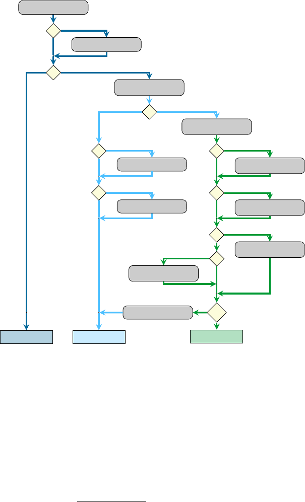
Sharc Manual 7 Auxilliary Scripts |7.21 General Data Analysis: data_collector.py
spectrum, the transition energies would be the X data, whereas the oscillator strengths would be the Y data (weights).
With these assignments, the full data set is dened:
•For each trajectory a
–For each time step t
∗For each X column ithere will be a value pair (xa
i(t),ya
i(t)) or (xa
i(t),1).
In the simplest case, there will be exactly one (
xa(t)
,1) pair for each trajectory and time, which is a two-dimensional
data set. Keep in mind that in general, each trajectory could have dierent time steps at this point. We refer to this kind
of data set (independent trajectories with possibly dierent time axes) as
Type1
data set. As will be described below, in
data_collector.py, during certain processing steps the format of the data set is changed, which will create Type2 or
Type3 data sets.
Once this data set is collected from the les (where too short or commented lines are ignored),
data_collector.py
allows for a number of subsequent processing steps, which are summarized in Figure 7.4.
Collecting
1
Smoothing
2
Synchronizing
3
4
Averaging
5
Statistics
Convoluting(X)
6
Summing(Y)
7
Integrating(X)
8
9
Convoluting(T)
Integrating(T)
10
Converting
Type1 Type2 Type3
Figure 7.4:
Possible workows in
data_collector.py
. Grey boxes denote the dierent computational actions, yellow
diamonds denote the dierent decisions which are queried in the input dialog, and the boxes at the denote
the three dierent data set types (dark blue=
Type1
, light blue=
Type2
, green=
Type3
). The dierent actions
and data set types are explained in the text.
Smoothing
In this step, each trajectory is individually smoothed, using one of several smoothing kernels (Gaussian,
Lorentzian, Log-normal, rectangular). Smoothing does not change the size or format of the data set, each value is simply
replaced by the corresponding smoothed value; hence, a new
Type1
data set is obtained. Smoothing is applied to each X
and each Y column independently, but always with the same kernel.
Xa
i(t):=Ít0Xa
i(t0)f(t,t0)
Ít0f(t,t0)and analogously for Ya
i(t). (7.1)
123
Sharc Manual 7 Auxilliary Scripts |7.21 General Data Analysis: data_collector.py
Here, f(t,t0)is the smoothing kernel.
Synchronizing
In this step, the
Type1
data set is reformatted, by merging all trajectories together. This step creates a
Type2
data set, which has a common T axis for all trajectories (simply the union of the T columns from all trajectories).
For each time step, all X and Y values of all trajectories are collected. If a trajectories does not have data at a particular
time step, NaNs will be inserted. In this way, a rectangular, two-dimensional data set is obtained, with as many rows as
time steps, and 2ntrajnXdata columns.
A simple application of Collecting+Synchronizing could be to generate a table with the bond length for all time steps
for all trajectories, in order to generate a “hair gure”. This task could in principle also be accomplished with Bash tools
like
awk
and
paste
, but this is troublesome if the trajectories are of dierent length, with dierent time steps, or if the
table les contain comments.
Averaging
The
Type2
data set from the Synchronizing step can contain a large number of data columns (2
ntrajnX
).
In order to reduce this amount of information, the Averaging step can be used to compute the mean and standard
deviation across all trajectories, separately for each time step. This will create a new
Type2
data set, which still has a
common time axis, but will only contain 4
nX+
1data columns; these are the mean and standard deviation of all X and
Y columns, plus one column giving the number of trajectories for each time step.
Currently, this step can be performed with either arithmetic mean/standard deviation or geometric mean/standard
deviation.
Statistics
Similar to the Averaging step, the Statistics step computes mean and standard deviations from a
Type2
data
set. The dierence is that during Statistics, these values are computed for all values from the rst to the current time
step. The data in the last time step thus gives the total statistics over all time steps and trajectories. The
Type2
data set
from the Statistics step contains the same number of data columns as the one from the Averaging step.
Currently, this step can be performed with either arithmetic mean/standard deviation or geometric mean/standard
deviation.
With the Averaging and Statistics steps, it is possible to compute the same data as with
trajana_nma.py
(if the
appropriate les are read), namely the total (Statistics) and coherent (Averaging+Statistics) activity of the normal modes.
Using data_collector.py, the same analysis can also be applied to internal coordinates computed with geo.py.
Convoluting(X)
In order to create a data set which has common T and X axes (a
Type3
data set), it is in general
necessary to perform some kind of data convolution involving the X column data. In order to do this,
data_collector.py
creates a grid along the X axis (
ngrid
points from the minimum value to the maximum value of all X data in the data set,
plus some padding).
Yi(t,X):=Õ
a
Ya
i(t)f(X,Xa
i(t)).(7.2)
The created Type3 data set has nXdata points for each time step and each X grid point.
Using energies as X columns and oscillator strengths/intensities as Y columns, in this way it is possible to compute
time-dependent spectra.
Summing(Y)
When
nX
is larger than one, the Summing step can be used to compute the sum over all data points for
each time step and each X grid point.
Y(t,X):=Õ
i
Yi(t,X).(7.3)
This creates a new Type3 data set, which will only contain one data point for each time step and each X grid point.
For example, for a transient spectrum involving multiple nal states (
nX>
1), after the Convoluting(X) step one obtains
one transient spectrum for each nal state. With the Summing(Y) step, one can then compute the total transient
absorption spectrum.
124

Sharc Manual 7 Auxilliary Scripts |7.21 General Data Analysis: data_collector.py
Integrating(X)
When computing transient spectra, one is often interested in integrating the spectrum within a
certain energy window. This can be done with the Integrating(X) step. After entering a lower and upper X limit, a
new
Type3
data set is created, with only three data points per time step. The rst data point contains the integral from
minus innity to the lower limit, the second data point the integral between lower and upper limit, and the third data
point the integral from the upper limit to innity. If Summing(Y) was not carried out, this integration is carried out
independently for each of the nXdata columns.
Convoluting(T)
The
Type3
data set can also be convoluted along the time axis (e.g., in order to apply an instrument
response function to a time-resolved spectrum). In order to do this, a uniform grid along the T axis is generated (with
nTgrid points from the minimum value to the maximum value of the previous T axis, plus some padding).
Yi(t0,X):=Õ
t
Yi(t,X)f(t,t0).(7.4)
The created
Type3
data set has as many data points for each X grid point as before, but the number of time steps is now
nTgrid
. Convoluting(T) can be applied also if Summing(Y) and/or Integrating(X) were used (in this case, the kernel is
applied to the summed up or integrated data).
Integrating(T) This step carries out a cumulative summation along the T axis.
Yi(t,X):=
t
Õ
t0=0
Yi(t0,X).(7.5)
In this way, the data in the last time step constitute the integral over all time steps. Since all the partial cumulative sums
are also computed, integrals within some bounds can simply be computed as dierences between partial cumulative
sums.
Converting
At the end of the workow, a
Type3
data set can be converted back into a
Type2
data set, which aects
how the output le is formatted. This is usually a good idea if the Integrating(X) step was performed, but might not be
a good idea otherwise. See below for how the dierent data set types are formatted on output.
7.21.3 Output
After the input dialog is nished,
data_collector.py
will start carrying out the requested analyses. For each of
the workow steps, one output le is written, so that all intermediate results can be used as well. Output les have
automatically generated lenames, which describe how the data was obtained. Filenames are always in the form
collected_data_<T>_<X>_<Y>_<steps>.<type>.txt
, where
<T>
is an integer giving the T column index,
<X>
and
<y>
are lists of integers of the X and Y column indices,
<steps>
is a string denoting which workow steps were carried out, and
<type>
denotes the data set type. For example, an output le could be named
collected_data_1_2_0_sy_cX.type3.txt
,
where column 1 was the T column, column 2 the X column, no Y column was used, Synchronizing and Convoluting(X)
were performed, resulting in a Type3 data set.
Format of Type1 data set output Type1
data sets are formatted such that each trajectory is given as a continuous
block, separated by an empty line. Within each block, each line contains the data of one time step, order increasingly.
Each line contains a trajectory index, the relative le path, the time, all X column data, and then all Y column data.
#1 234567
#Index Filename Time X Column 5 X Column 6 Y Column 0 Y Column 0
0 Singlet_1//TRAJ_00001/./Geo.out 0.00000000E+00 1.13340000E-01 7.99096900E+00 1.00000000E+00 1.00000000E+00
0 Singlet_1//TRAJ_00001/./Geo.out 5.00000000E-01 1.59173000E-01 7.94395200E+00 1.00000000E+00 1.00000000E+00
0 Singlet_1//TRAJ_00001/./Geo.out 1.00000000E+00 2.10868000E-01 7.89084000E+00 1.00000000E+00 1.00000000E+00
...
1 Singlet_1//TRAJ_00002/./Geo.out 0.00000000E+00 5.03990000E-02 7.99078100E+00 1.00000000E+00 1.00000000E+00
1 Singlet_1//TRAJ_00002/./Geo.out 1.00000000E+00 3.80370000E-02 8.00349700E+00 1.00000000E+00 1.00000000E+00
1 Singlet_1//TRAJ_00002/./Geo.out 2.00000000E+00 1.09515000E-01 7.93073500E+00 1.00000000E+00 1.00000000E+00
125

Sharc Manual 7 Auxilliary Scripts |7.22 Optimizations: orca_External and setup_orca_opt.py
...
2 Singlet_1//TRAJ_00004/./Geo.out 0.00000000E+00 2.10908000E-01 8.29417600E+00 1.00000000E+00 1.00000000E+00
2 Singlet_1//TRAJ_00004/./Geo.out 5.00000000E-01 1.49506000E-01 8.35651800E+00 1.00000000E+00 1.00000000E+00
2 Singlet_1//TRAJ_00004/./Geo.out 1.00000000E+00 1.05887000E-01 8.40056700E+00 1.00000000E+00 1.00000000E+00
...
Note here in the example that the second trajectory has a time step of 1.0 fs and thus no data at 0.5 fs.
Format of Type2 data set output Type2
data sets are formatted such that all trajectories share a common time axis,
hence for each time step there will be one line of data. Each line starts with the time, followed columns with the data for
the rst trajectory, followed by the data for the second trajectory, etc. Within each trajectory, rst all X columns, then
all Y columns are given. If a Y column contains only unit weights (using special le column “0”), then this Y column is
omitted from the Type2 formatted output.
#1234567...
# Time X Column 5 X Column 6 X Column 5 X Column 6 X Column 5 X Column 6 ...
0.00000000E+00 1.13340000E-01 7.99096900E+00 5.03990000E-02 7.99078100E+00 2.10908000E-01 8.29417600E+00 ...
5.00000000E-01 1.59173000E-01 7.94395200E+00 NaN NaN 1.49506000E-01 8.35651800E+00 ...
1.00000000E+00 2.10868000E-01 7.89084000E+00 3.80370000E-02 8.00349700E+00 1.05887000E-01 8.40056700E+00 ...
...
Note here in the example that the second trajectory does not have data at 0.5 fs.
Format of Typ3 data set output Type3 data sets are formatted such that all trajectories share common time and X
axes. The data is formatted block-wise, with the rst block corresponding to the rst time step and containing all points
on the X grid, followed by an empty line, followed by the second block, etc. Each block consists of
ngrid
lines, each
starting with the time and X value in the rst two columns and followed by nXcolumns with the convoluted data.
#1234
# Time X_axis Conv(5,0) Conv(6,0)
0.00000000E+00 -1.45534000E-01 2.38544715E-05 0.00000000E+00
0.00000000E+00 2.30671958E-01 1.51462322E+00 0.00000000E+00
0.00000000E+00 6.06877917E-01 1.07930050E-01 0.00000000E+00
...
5.00000000E-01 -1.45534000E-01 1.31312692E-04 0.00000000E+00
5.00000000E-01 2.30671958E-01 1.28614756E+00 0.00000000E+00
5.00000000E-01 6.06877917E-01 4.46251462E-10 0.00000000E+00
...
1.00000000E+00 -1.45534000E-01 8.75871124E-05 0.00000000E+00
1.00000000E+00 2.30671958E-01 2.42291042E+00 0.00000000E+00
1.00000000E+00 6.06877917E-01 1.60277894E-16 0.00000000E+00
...
7.22 Optimizations: orca_External and setup_orca_opt.py
All Sharc interfaces can deliver gradients for (multiple) ground and excited states in a uniform manner. This allows in
principle to perform optimizations of excited-state minima, conical intersections, or crossing points. In order to employ
a high-quality geometry optimizer for this task, the Sharc suite is interfaced to the external optimizer feature of Orca.
This is accomplished by providing the script
orca_External
, which is called by Orca, runs any of the Sharc interfaces,
constructs the appropriate gradient, and returns that to
Orca
. For the methodology used to construct the gradients, see
section 8.16.
In order to easily prepare the input les for such an optimization, the script
setup_orca_opt.py
can be used. It takes a
geometry le, interface input les, and the path to Orca, and creates a directory containing all relevant input les. In the
following,
setup_orca_opt.py
is described rst, because it is the script which the user directly employs. Afterwards,
orca_External is specied.
126
Sharc Manual 7 Auxilliary Scripts |7.22 Optimizations: orca_External and setup_orca_opt.py
7.22.1 Usage
setup_orca_opt.py is an interactive script, which is started with:
user@host> $SHARC/setup_orca_opt.py
Note that before executing the script you should prepare a template for the interface you want to use (as, e.g., in
setup_init.py or setup_traj.py).
7.22.2 Input
In the input section, the script asks for: (i) the path to Orca, (ii) the input geometries, (iii) the optimization settings, (iv)
the interface settings.
Path to Orca
Here the user is prompted to provide the path to the Orca directory. Note that the script will not
expand the user (
~
) and shell variables (since possibly the calculations are running on a dierent machine than the one
used for setup). ~and shell variables will only be expanded during the actual calculation.
Interface
In this point, choose any of the displayed interfaces to carry out the ab initio calculations. Enter the
corresponding number.
Input geometry
Here the user is prompted for a geometry le in XYZ format, containing one or more geometries
(with consistent number of atoms). For each geometry in this le, a directory with all input les is created, in order to
carry out multiple optimizations (e.g., with output from crossing.py).
Number of states
Here the user can specify the number of excited states to be calculated. Note that the ground state
has to be counted as well, e.g., if 4 singlet states are specied, the calculation will involve the
S0
,
S1
,
S2
and
S3
. Also
states of higher multiplicity can be given, e.g. triplet or quintet states.
States to optimize
Two dierent optimization tasks can be carried out: optimization of a minimum (ground or
excited state) or optimization of a crossing point (either a conical intersection between states of the same multiplicity
or a minimum-energy crossing points between states of dierent multiplicities; this is detected automatically).
For minima, the state to optimize needs to be specied. For crossing points, the two involved states need to be specied.
In all cases, the specied states need to be included in the number of states given before.
CI optimization parameters
If you are optimizing a conical intersection (states of same multiplicity) with an inter-
face which cannot provide nonadiabatic coupling vectors (e.g.,
SHARC_RICC2.py
,
SHARC_ADF.py
, or
SHARC_GAUSSIAN.py
),
then the optimization will employ the the penalty function method of Levine, Coe, and Martínez [
85
]. In this method, a
penalty function is optimized, which depends on the energies of the two states and on two parameters,
σ
and
α
(see
section 8.16 for their mathematical meaning).
Practically, the parameters aect how close the minimum of the penalty function is to the true minimum on the crossing
seam and how hard the optimization will be to converge. Generally, a large
σ
will allow going closer to the true conical
intersection, but will make the penalty function more sti (steeper harmonic) and thus harder to optimize. A small
α
will also allow going closer to the true conical intersection, but will make the penalty function less harmonic; at
α=
0,
the penalty function will have a cusp at the minimum, making it unoptimizable because the gradient never becomes
zero.
The default values, 3.5 and 0.02, are the ones suggested in [
85
]. They can be regarded as relatively soft, i.e., they enable
a very smooth convergence but might lead to unacceptably large energy gaps at convergence (i.e., the minimum of
the penalty function is too far from the true minimum of the crossing seam). In this case, it is advisable to restart the
optimization from the last point with increased
σ
(e.g., by a factor of 4), and simultaneously reducing the maximum
step (see next point). The αis best left at the suggested value of 0.02 to avoid the cusp problem.
127
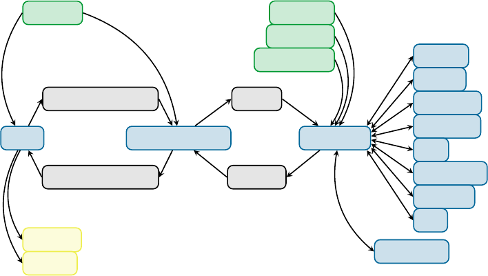
Sharc Manual 7 Auxilliary Scripts |7.22 Optimizations: orca_External and setup_orca_opt.py
Maximum allowed displacement
Within Orca, it is possible to restrict the maximum step (the trust radius) of the
optimizer. A larger maximum step might decrease the number of iterations necessary, but might also lead to instabilities
in the optimization (if the potential energy surface is very steep or anharmonic). Hence, it can be advisable to reduce
the maximum allowed step (from the default of 0.3 a.u.), especially if the starting geometry is already very good (e.g.,
after restart with increase of
σ
) or if the potential is known to be sti (strong bond, large
σ
, small
α
, ...). Note that the
maximum step can be restricted even the penalty function method is not used and σand αare not relevant.
Interface-specific input
This input section is basically the same as for
setup_init.py
(sections 7.4.3). Also for the
optimizations an initial wave function le should be provided, especially for the multi-reference methods.
Run script setup
Here the user needs to provide the path to the directory where the optimizations should be setup.
7.22.3 Output
Inside the specied directory,
setup_orca_opt.py
creates one subdirectory for each geometry in the input geometry le.
Each subdirectory is prepared with the corresponding initial geometry le (
geom.xyz
), the Orca input le (
orca.inp
),
the appropriate interface-specic les (template, resources, QM/MM), and a shell script for execution (
run_EXTORCA.sh
).
In order to run one of the optimizations, execute the shell script or send it to a batch queuing system. Note that
$SHARC needs to be added to the $PATH so that Orca can nd
orca_External
(this is automatically done inside
run_EXTORCA.sh).
When the shell script is started, Orca will write a couple of output les, where the two most relevant are
orca.trj
and
orca.log
. The former is an XYZ le with all geometries from the optimization steps. The latter (the Orca standard
output) contains all details of the optimization (convergence, step size, etc) as well as a summary of what
orca_External
did (after the line
EXTERNAL SHARC JOB
). This summary contains all relevant energies and shows how the gradient is
constructed. Note that in each iteration, a line starting with
»>
is written, which contains the energies of the optimized
state(s). This line can easily be extracted with grep to follow the optimization of a crossing point.
7.22.4 Description of orca_External
orca_External
provides a connection between the external optimizer of Orca and any of the Sharc interfaces. In
gure 7.5, the le communication between Orca,orca_External, and the interfaces is presented.
Orca orca_External Interface
Molpro
Molcas
Columbus
Analytical
ADF
Turbomole
Gaussian
LVC
Wfoverlap
orca.log
orca.trj
QM.in
QM.out
orca.extcomp.inp
orca.extcomp.out
template
resources
initial MOs
orca.inp
Figure 7.5: Communication between Orca,orca_External, the interfaces, and the quantum chemistry codes.
As can be seen,
orca_External
writes
QM.in
and
QM.out
les, in the same way that
sharc.x
is doing. All information
to write the
QM.in
le comes from the Orca communication le
orca.extcomp.inp
(geometry) and the Orca input
le (number of states, interface, states to optimize). To provide the latter information,
orca_External
reads specially
128
Sharc Manual 7 Auxilliary Scripts |7.23 Single Point Calculations: setup_single_point.py
marked comments from the Orca input le which are ignored by Orca. These comments start with
#SHARC:
, followed
by a keyword (states,interface,opt, or param) and the keyword arguments.
7.23 Single Point Calculations: setup_single_point.py
It is possible to run single point calculations through the Sharc interfaces. This is useful, e.g., to do a computation in
exactly the same way as during the dynamics simulations. Single point calculations using the interfaces can also be
easily automatized.
7.23.1 Usage
setup_single_point.py is an interactive script, which is started with:
user@host> $SHARC/setup_single_point.py
Note that before executing the script you should prepare a template for the interface you want to use (as, e.g., in
setup_init.py or setup_traj.py).
7.23.2 Input
In the input section, the script asks for: (i) the input geometries, (ii) the number of states, and (iii) the interface settings.
Interface
First, choose any of the displayed interfaces to carry out the ab initio calculations. Enter the corresponding
number.
Input geometry
Here the user is prompted for a geometry le in XYZ format, containing one or more geometries
(with consistent number of atoms). For each geometry in this le, a directory with all input les is created, in order to
carry out multiple optimizations (e.g., with output from crossing.py).
Number of states
Here the user can specify the number of excited states to be calculated. Note that the ground state
has to be counted as well, e.g., if 4 singlet states are specied, the calculation will involve the
S0
,
S1
,
S2
and
S3
. Also
states of higher multiplicity can be given, e.g. triplet or quintet states.
Interface-specific input
This input section is basically the same as for
setup_init.py
(sections 7.4.3). Also for the
optimizations an initial wave function le should be provided, especially for the multi-reference methods.
Run script setup
Here the user needs to provide the path to the directory where the optimizations should be setup.
7.23.3 Output
Inside the specied directory,
setup_single_point.py
creates one subdirectory for each geometry in the input geometry
le. Each subdirectory is prepared with the corresponding geometry le (
QM.in
), the appropriate interface-specic les
(template, resources, QM/MM), and a shell script for execution (run.sh).
In order to run one of the optimizations, execute the shell script or send it to a batch queuing system.
When the shell script is started, the chosen Sharc interface is executed. The interface writes a le called
QM.log
which
contains details of the computation and progress status. The nal results of the computation are written to
QM.out
,
which can be inspected manually. Alternatively, some basic data (excitation energies, oscillator strengths) can be
computed with QMout_print.py (section 7.24).
7.24 Format Data from QM.out Files: QMout_print.py
With the script
QMout_print.py
one can print a table with energies and oscillator strengths from a
QM.out
le, as it is
produced by the interfaces.
129
Sharc Manual 7 Auxilliary Scripts |7.25 Diagonalization Helper: diagonalizer.x
7.24.1 Usage
QMout_print.py is a command line tool, and is executed like this:
user@host> $SHARC/QMout_print.py [options] QM.out
The options are summarized in Table 7.12
Table 7.12: Command-line options for QMout_print.py.
Option Description Default
-h Display help message and quit. —
-i FILENAME Path to QM.in le (to read number of states) —
-s INTEGERS List of numbers of states per multiplicity 1
-e FLOAT Absolute energy shift in Hartree 0.0
-D Output diagonal states MCH states
7.24.2 Output
The script prints a table with state index, state label, energy, relative energy, oscillator strength, and spin expectation
value to standard output.
7.25 Diagonalization Helper: diagonalizer.x
The small program
diagonalizer.x
is used by the Python scripts to diagonalize matrices if the NumPy library is
not available. Currently, only
excite.py
and
SHARC_Analytical.py
need to diagonalize matrices. The program
diagonalizer.x is implemented as a simple front-end to the LAPACK libary.
The program reads from stdin. The rst line consists of the letter “r” or “c”, followed by two integers giving the matrix
dimensions. For “r”, the program assumes a real symmetric matrix, for “c” a Hermitian matrix. The matrix must be
square. The second line is a comment and is ignored. In the following lines, the matrix elements are given. On each
line one row of the matrix has to be written. If the matrix is complex, each line contains the double number of entries,
where real and imaginary part are always given subsequently. The following is an example input:
c22
comment
1.0 0.0 2.0 0.1
2.0 -0.1 6.0 0.0
for the matrix
A=1 2 +0.1i
2−0.1i6.(7.6)
The diagonal matrix and the matrix of eigenvectors is written to stdout.
130

8 Methodology
In this chapter dierent aspects of Sharc simulations are discussed in detail. The topics are ordered alphabetically.
8.1 Absorption Spectrum
Using
spectrum.py
, an absorption spectrum can be calculated as the sum over the absorption spectra of each individual
initial condition:
σ(E)=
ninit
Õ
i
σi(E),(8.1)
where iruns over the initial conditions.
The spectrum of a single initial condition is the convolution of its line spectrum, dened through a set of tuples
(Eα,fα
osc)
for each electronic state α, where Eαis the excitation energy and fα
osc)is the oscillator strength.
The convolution of the line spectrum can be performed with
spectrum.py
using either Gaussian or Lorentzian functions.
The contribution of a state αto the absorption spectrum σα(E)is given by:
σα
Gaussian(E)=(fosc)α
iec(E−Eα
i)2
,(8.2)
with c=−4 ln(2)
FWHM2,(8.3)
or
σα
Lorentzian(E)=(fosc)α
i
1
cE−Eα
i2+1,(8.4)
with c=1
4FWHM2,(8.5)
or
σα
Log-normal(E)=(fosc)α
i
Eα
i
Ee−c
4 ln(2)−ln(2)
c(ln(E)−ln(Eα
i))2
,(8.6)
with c=
ln ©«
FWHM +qFWHM2+4(Eα
i)2
2Eα
iª®®¬
2
,(8.7)
where FWHM is the full width at half maximum.
8.2 Active and inactive states
Sharc allows to “freeze” certain states, which then do not participate in the dynamics. Only energies and dipole
moments are calculated, but all couplings are disabled. In this way, these states are never visited (hence also no gradients
and nonadiabatic couplings are calculated, making the inclusion of these states cheap). Example:
nstates 2 0 2
actstates 2 0 1
In the example given, state T2is frozen. The corresponding Hamiltonian looks like:
131

Sharc Manual 8 Methodology |8.3 Amdahl’s Law
H=
©«
E(S0)a∗
01 a∗
02 b∗
01 b∗
02 a01 a02
E(S1)a∗
11 a∗
12 b∗
11 b∗
12 a11 a12
a01 a11 E(T1)p∗
12 −q∗
12
a02 a12 p12 E(T2)q∗
12
b01 b11 −q12 E(T1) −q∗
12
b02 b12 q12 E(T2)q∗
12
a∗
01 a∗
11 −q12 E(T1)p12
a∗
02 a∗
12 q12 p∗
12 E(T2)
ª®®®®®®®®®®®¬
(8.8)
where all matrix elements marked red are deleted, since T2is frozen.
The corresponding matrix elements are also deleted from the nonadiabatic coupling and overlap matrices. For propaga-
tion including laser elds, also the corresponding transition dipole moments are neglected, while the transition dipole
moments still show up in the output (in order to characterize the frozen states).
Active and frozen states are dened with the
states
and
actstates
keywords in the input le. Note that only the
highest states in each multiplicity can be frozen, i.e., it is not possible to freeze the
T1
while having
T2
active. However,
it is possible to freeze all states of a certain multiplicity.
8.3 Amdahl’s Law
Some of the interfaces (
SHARC_ADF.py
and
SHARC_GAUSSIAN.py
) use Amdahl’s law to predict the most ecient way to
run multiple calculations in parallel, where each calculation itself is parallelized. For example, in
SHARC_GAUSSIAN.py
it
might be necessary to compute the gradients of ve states, using four CPU cores. The most ecient way to run these
ve jobs depends on how well the Gaussian computation scales with the number of cores—for bad scaling, running
four jobs on one core each followed by the fth job might be best, whereas for good scaling, running each job on four
cores subsequently is better because no core is idle at any time. In order to automatically distribute the jobs eciently,
the interfaces use Amdahl’s law, which can be stated as:
T(ncore)=T(1)1−r+r
ncore .(8.9)
Here,
T(
1
)
is the run time of the job with one CPU core, and
r
is the fraction of
T(
1
)
which benets from parallelization.
The parameter
r
can be given to the interfaces; it is between 0 and 1, where 0 means that the calculation does not get
faster at all with multiple cores, whereas 1 means that the run time scales linearly with the number of cores.
8.4 Bootstrapping for Population Fits
Bootstrapping, in the context of population tting, is a statistical method to obtain the statistical distribution of the tted
parameters, which can be used to infer the error associated with the tted parameter. The general idea of bootstrapping
is to take the original sample (the set of trajectories in the ensemble), and generate new samples (resamples) by randomly
drawing trajectories “with replacement” from the original ensemble. These resamples will dier form the original
ensemble by containing some trajectories multiple times while other trajectories might be missing. For each of the
resamples, the tting parameter are obtained normally and saved for later analysis.
After many resamples, we obtain a list of many “alternative” parameters, which can be plotted in a histogram to see the
statistical distribution of the tting parameter. The number of resamples should generally be large (several hundred or
thousand resamples), although with
bootstrap.py
, one can inspect the convergence of the tting parameters/errors to
decide how many resamples are sucient.
From the computed list of parameters, error measures can be computed. Assume that
{xi}
is the set of tting parameters
obtained. bootstrap.py computes the arithmetic mean and standard deviation like this:
¯
xarith =1
N
N
Õ
i
xi,(8.10)
σarith(x)=v
u
t1
N−1
N
Õ
i(x−¯
x)2.(8.11)
132

Sharc Manual 8 Methodology |8.5 Damping
Because the distribution of
{xi}
might be skewed (e.g., contains some very large values but few very small ones), the
script also computes the geometric mean and standard deviation like this:
¯
xgeom =e1
NÍN
iln(xi),(8.12)
σgeom(x)=eq1
N−1ÍN
i(ln(x)−ln(¯
x))2(8.13)
Note that the geometric standard deviation is a dimensionless factor (unlike the arithmetic standard deviation, which
has the same dimension as the mean). Therefore, within
bootstrap.py
the geometric errors are always displayed with
separate upper and lower bounds as
¯
x+¯
x(σ(x)−1)
−¯
x(1/σ(x)−1)
. Note that
bootstrap.py
will always report one times the standard
deviation in the output. If larger condence intervals are desired, simply multiply the arithmetic error as usual. For the
geometric error, use for example ¯
x+¯
x(σ(x)2−1)
−¯
x(1/σ(x)2−1).
8.5 Damping
If damping is activated in Sharc (keyword
dampeddyn
), in each time step the following modication to the velocity
vector is made
v0=v·√C(8.14)
where Cis the damping factor given in the input. Hence, in each time step the kinetic energy is modied by
E0
kin =Ekin ·C(8.15)
The damping factor Cmust be between 0 and 1.
8.6 Decoherence
In surface hopping, without any corrections the coherence between the states is usually too large [
21
]. A trajectory
in state
β
, but where state
α
has a large coecient, will still travel according to the gradient of state
β
. However, the
gradients of state
α
are almost certainly dierent to the ones of state
β
. As a consequence, too much population of
state
α
is following the gradient of state
β
. Decoherence corrections damp in dierent ways the population of all states
α,β, so that only population of βfollows the gradient of state β.
Currently, in Sharc there are two decoherence corrections implemented, “energy-based decoherence”, or EDC, as given
in [101] and “augmented fewest-switches surface hopping”, or AFSSH, as described in [30].
8.6.1 Energy-based decoherence
In this scheme, after the surface hopping procedure, when the system is in state
β
, the coecients are updated by the
following relation
c0
α=cα·exp "−∆t|Eα−Eβ|
~1+C
Ekin −1#,α,β,(8.16)
c0
β=
cβ
|cβ|·1−Õ
α,β|c0
α|2
1
2
(8.17)
where
C
is the decoherence parameter. The decoherence correction can be activated with the keyword
decoherence
in
the input le. The decoherence parameter
C
can be set with the keyword
decoherence_param
(the default is 0.1 hartree,
as suggested in [101]).
8.6.2 Augmented FSSH decoherence
Augmented FSSH by Subotnik and coworkers is described in [
30
]. For Sharc, the augmented FSSH algorithm was
adjusted to the case of the diagonal representation.
133

Sharc Manual 8 Methodology |8.6 Decoherence
The basic idea is that besides the actual trajectory, the program maintains an auxiliary trajectory for each state. The
auxiliary trajectories are propagated using the gradients of the associated (not active) state, and because the gradients
are dierent, the auxiliary trajectories eventually diverge from each other and from the main trajectory. From this
diverging, one can compute decoherence rates which can be used to stochastically set the electronic coecients of the
diverging state to zero.
First, we compute two matrices:
Sdiag(t,t+∆t)=U†(t)S(t,t+∆t)U(t+∆t),(8.18)
Holddiag(t+∆t)=U†(t)S(t,t+∆t)HMCH(t+∆t)S†(t,t+∆t)U(t),(8.19)
where
S
is the overlap matrix, as used in 8.27. Hence,
Sdiag(t,t+∆t)
is the overlap matrix in the diagonal basis and
Holddiag(t+∆t)is the Hamiltonian at time t+∆texpressed in the diagonal basis of time step t.
We then propagate the auxiliary trajectories for each state
j
, considering that the active state is
α
. For this, we need the
gradient matrix Gdiag from section 8.10. We dene:
σj=|cj(t)|2,(8.20)
(8.21)
We do the Xstep of the velocity-Verlet algorithm:
aj
A(t)=−((Gdiag)j j − (Gdiag)α α )A
MA
,(8.22)
Rj(t+∆t)=Rj(t)+vj(t)∆t+1
2aj(t)∆t2σj,(8.23)
where Agoes over the atoms. Then, we compute the new gradient:
gj(t+∆t)=−(Gdiag)α α +Õ
i(Sdiag(t,t+∆t))ji (Gdiag)ii .(8.24)
We then carry out the vstep:
aj
A(t+∆t)=1
2aj
A(t) − (gj(t+∆t))A
MA
,(8.25)
vj(t+∆t)=vj(t)+aj
A(t+∆t)∆tσj.(8.26)
We then perform a diabatization of the auxiliary trajectories (e.g., for a trivially avoided crossing, the moments between
the crossing states are interchanged):
Rj=Õ
i(Sdiag(t,t+∆t))i j Ri,(8.27)
vj=Õ
i(Sdiag(t,t+∆t))i j vi,(8.28)
(8.29)
to transform the data back into the adiabatic basis at time t+∆t.
Finally, we carry out the decoherence correction procedure for each auxiliary trajectory. We compute the displacement
from the auxiliary trajectory of the active state:
D=Rj−Rα(8.30)
We compute two rate constants:
rj
1=−1
2gj(t+∆t) · D,(8.31)
rj
2=2|(Gdiag)αj·D|,(8.32)
134

Sharc Manual 8 Methodology |8.7 Essential Dynamics Analysis
or if no nonadiabatic coupling vectors are available:
rj
2=2|Holddiag
αj|
∆t
D·v
v·v.(8.33)
We draw a random number (identical for all states)
r
between 0 and 1. If
r<∆t(rj
1−rj
2)
, then we collapse state
j
, by
setting its coecient to zero and enlarging the coecient of the active state such that the total norm is conserved; we
also set the moments Rjand vjto zero. If no collapse occurred, if r<−∆tr j
1, we set the moments Rjand vjto zero.
After a surface hop occurred, we reset all auxiliary trajectories.
8.7 Essential Dynamics Analysis
As an alternative to normal mode analysis (see section 8.15), essential dynamics analysis can be used to identify important
modes in the dynamics. This procedure is a principal component analysis of the geometric displacements.[
81
,
82
]
Unlike normal mode analysis, it does not depend on the availability of the normal mode vectors.
The covariance matrix is computed from the following equation (
µ
and
ν
are indices over the 3
Natom
degrees of freedom):
¯
Rµ=1
Ntraj(kend −kstart)
Ntraj
Õ
i=1
kend
Õ
k=kstart
Ri
µ(k∆t)(8.34)
and
Aµν =1
Ntraj(kend −kstart)
Ntraj
Õ
i=1
kend
Õ
k=kstart
Ri
µ(k∆t)Ri
ν(k∆t)(8.35)
as a matrix Cwith elements:
Cµν =Aµν −RµRν.(8.36)
Diagonalization of the symmetric matrix
C
gives a set of eigenvalues and eigenvectors. The eigenvectors represent
the essential dynamics modes, and the corresponding eigenvalues are the variances of the modes. Modes with large
variances show strong motion in the dynamics, whereas small variances are found for modes which show weak motion.
Because the modes are uncorrelated, the few modes with the largest variance describe most of the molecular motion,
which shows that essential dynamics analysis can be used to for data reduction.
8.8 Excitation Selection
excite.py
can select initial active states for the dynamics based on the excitation energies
Ek,α
and the oscillator
strengths fosc
k,αfor each initial condition kand excited state α.
First, for all excited states of all initial conditions, the maximum value pmax of
pk,α=
fosc
k,α
E2
k,α
(8.37)
is found. Then for each excited state, a random number rk,αis picked from [0,1]. If
rk,α<pk,α
pmax
(8.38)
then the excited state is selected as a valid initial condition. This excited-state selection scheme is taken from [103].
Within
excite.py
it is possible to restrict the selection to a subset of all excited states (only certain adiabatic states/within
a given energy range). In this case, also pmax is only determined based on this subset of excited states.
135

Sharc Manual 8 Methodology |8.9 Global ts and kinetic models
8.8.1 Excitation Selection with Diabatization
The active states can be selected based on a diabatization. This necessitates the wave function overlaps between a
reference geometry (ICOND_00000/) and the current initial condition k.
The overlap matrix with elements
S0k
i j =Ψi(R0)|Ψj(Rk)(8.39)
can be computed with
wfoverlap.x
(calculations can be setup with
setup_init.py
). This overlap matrix is rescaled
during the excitation selection procedure such
S0k
11
is equal to one (by dividing all elements by
|S0k
11 |2
). Then, assume
we want to start all trajectories in the state which corresponds to state
x
at the reference geometry. The excitation
selection will select a state yas initial state if S0k
xy>0.5.
8.9 Global fits and kinetic models
In this section, we specify the basic assumptions of the chemical kinetic models used with the script
make_fitscript.py
and the globals ts of these models to data.
8.9.1 Reaction networks
The kinetic models used by
make_fitscript.py
is based on a chemical reaction network, where chemical species react
via unimolecular reactions.
The reaction networks allowed in the script are a simple directed graphs, where the species are the vertices and the
reactions are the directed edges. Each reaction is characterized by an associated rate constant and connects exactly one
reactant species to exactly one product species.
In order to obtain rate laws which can analytically be integrated easily, there are a number of restrictions imposed on
the network graphs. Some restrictions and possible features of the graphs are depicted exemplarily in Figure 8.1. First,
each species and each reaction rate needs to have a unique label. There cannot be two species with the same label and
there cannot be two reactions with the same reaction rate constant. Second, the graph must be a simple directed graph,
hence there cannot be any (self-) loops or more than one reaction with the same initial and the same nal species. All
restrictions marked as “Not allowed” in the Figure are enforced in the input dialogue of
make_fitscript.py
However,
back reactions are allowed (as a back reaction has a dierent initial and a dierent nal species as the corresponding
reaction). Except from these restrictions, the graph may contain combinations of sequential and parallel reactions. The
graph may also be disjoint, i.e., it can be the union of several independent sub-networks.
There are two kinds of cycles possible, called here parallel pathways and closed walks. Parallel pathways are independent
sequences of reactions with the same initial and nal species (e.g.,
A→C
and
A→B→C
). A closed walk is a sequence
of reactions where the initial species is equal to the nal species. These cycles can sometimes lead to problems, either
in solving the system of dierential equations of the rate laws (for some networks containing cycles, the integrated rate
equations cannot be stated in closed form and hence cannot be used with Gnuplot) or in the tting procedure (rate
constants in parallel pathways can be strongly correlated and cause large errors and bad convergence in tting).
An example reaction network graph is shown in Figure 8.2. In this graph, there are 5 species (
S2
,
S1
,
S0
,
T2
, and
T1
) and
6 reactions, each with a rate constant (
kS
,
kRlx
,
k22
,
k11
,
k21
,
k12
). This graph shows some features which are allowed in
the reaction networks for
make_fitscript.py
: sequential reactions, parallel reactions, back reactions, and converging
reaction pathways. Note that this reaction network is likely to cause problems in the integrating or tting steps.
8.9.2 Kinetic models
Based on the reaction network graph, a system of dierential equations describing the rate laws of all species can be
setup. The system of equations (equivalently, the matrix dierential equation) can be written as:
∂
∂ts(t)=A·s(t),(8.40)
where
s
is the vector of the time-dependent populations of each species and
A
is the matrix containing the rate constants.
In order to construct
A
, start with
A=
0and, for each reaction from species
i
to species
j
with rate
k
, substract
k
from
Aii and add kto Aji .
136
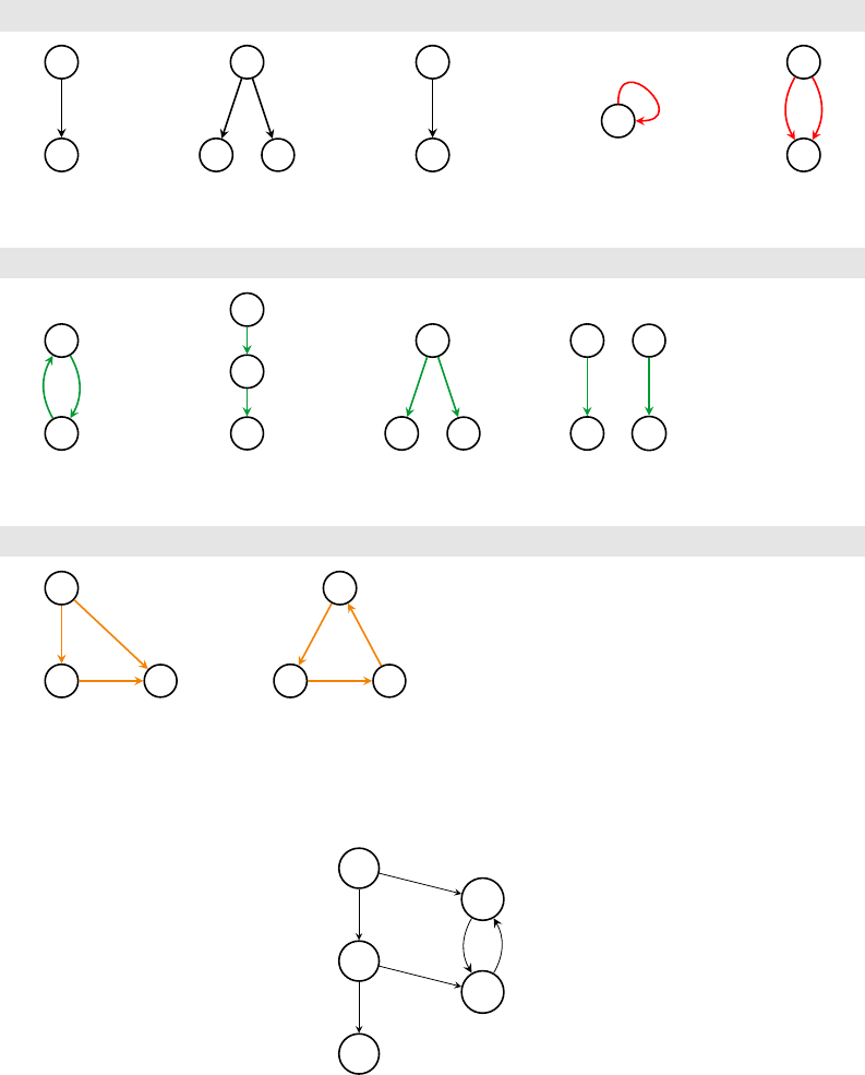
Sharc Manual 8 Methodology |8.9 Global ts and kinetic models
Not allowed
A
A
a
Repeated
species label
A
B C
aa
Repeated
rate label
A
B
A
Repeated
label
A
a
Loop
A
B
a
b
Repeated
reaction
Allowed
A
B
a
b
Back
reaction
A
B
C
a
b
Sequential
reactions
A
B C
bc
Parallel
reactions
A C
B D
ac
Disjoint
network
Problematic
A
B C
ab ac
bc
Parallel
pathways
A
B C
ab ca
bc
Closed
walks
Figure 8.1: Forbidden and allowed features of the reaction network graphs.
S2
S1
S0
T2
T1
kS
kRlx
k22
k11
k21 k12
Figure 8.2: Example reaction network graph. For explanation see text.
In order to integrate this system of equations, in practice one also needs to dene initial conditions. In the present
context, the initial conditions are fully specied by
s(t=
0
)=s0
, where
s0
are constant expressions dened by the user.
Solving
(8.40)
yields (in not too complicated cases) the closed-form expressions for the functions
s(t)
, which contain as
parameters all rate constants kand all initial values s0.
8.9.3 Global fit
Suppose there is a data set
p(t)=(p1(t),p2(t), . . . )
of time-dependent populations of several states
k=
1
,
2
, . . .
and
which is given at several points of time
{ti
: 0
<ti<tmax}
. We can t to one data set
pk(t)
a function
sl(t)
from
s(t)
by
optimizing the parameters (mainly the rate constants) such that Íi|pk(ti) −sl(ti)|2becomes minimal.
137

Sharc Manual 8 Methodology |8.10 Gradient transformation
In order to perform global t including several species
l
and several states
k
, we construct piecewise global functions
from p(t)and s(t)and then optimize the parameters accordingly.
8.10 Gradient transformation
Since the actual dynamics is performed on the PESs of the diagonal states, also the gradients have to be transformed to
the diagonal representation. To this end, rst a generalized gradient matrix
GMCH
is constructed from the gradients
gMCH
α=−∇RHMCH
α α and the nonadiabatic coupling vectors KMCH
βα :
GMCH =©«
g1−(H11 −H22)K12 −(H11 −H33)K13 ···
−(H22 −H11)K21 g2−(H22 −H33)K23 ···
−(H33 −H11)K31 −(H33 −H22)K32 g3
.
.
..
.
....ª®®®®¬
(8.41)
Note that all quantities in the matrix are in the MCH representation, the superscripts were omitted for brevity.
The matrix GMCH is subsequently transformed into the diagonal representation, using the transformation matrix U:
Gdiag =U†GMCHU.(8.42)
The diagonal elements of
Gdiag
now contain the gradients of the diagonal states, while the o-diagonal elements contain
the scaled nonadiabatic couplings
−(Hdiag
β β −Hdiag
α α )Kdiag
βα
. The gradients are needed in the Velocity Verlet algorithm in
order to propagate the nuclear coordinates. The nonadiabatic couplings are necessary if the velocity vector is to be
rescaled along the nonadiabatic coupling vector.
Since the matrix
GMCH
contains elements which are itself vectors with 3
N
components, the transformation is done
component-wise (e.g. rst a matrix
Gx,atom1
is constructed from the
x
components of all gradients (and nonadiabatic
couplings) for atom 1, this matrix is transformed and written to the
x
, atom 1component of
Gdiag
, then this is repeated
for all components).
Since the calculation of the nonadiabatic couplings
KMCH
βα
might add considerable computational cost, there is the input
keyword nogradcorrect which tells Sharc to neglect the KMCH
βα in the gradient transformation.
8.10.1 Dipole moment derivatives
For strong laser elds, the derivative of the dipole moments might be a non-negligible contribution to the gradients. In
this case, they should be included in the gradient transformation step:
Gdiag =U†GMCH −ϵ(t) · ∂
∂RµU.(8.43)
This can be activated with the keyword dipole_grad in the Sharc input le.
8.11 Internal coordinates definitions
In this section, the internal coordinates available in geo.py are dened.
Bond length The bond length between two atoms aand bis:
rab =p(xa−xb)2+(ya−yb)2+(za−zb)2(8.44)
Bond angle The bond angle for atoms a,band cis dened as the angle
θ=cos−1vba ·vbc
|vba |·|vbc |(8.45)
where vba is the vector from atom bto atom a.
138

Sharc Manual 8 Methodology |8.12 Kinetic energy adjustments
Dihedral The dihedral angle is dened via the vectors w1and w2:
w1=vab ×vbc and w2=vbc ×vcd .(8.46)
The dihedral is given as the angle between
w1
and
w2
according to equation
(8.45)
. In order to distinguish left- and
right-handed rotation, also the vector
Q=w1×w2
is computed, and if the angle between
Q
and
vbc
is larger than 90
◦
then the value of the dihedral is multiplied by -1.
Pyramidalization angle The pyramidalization angle is dened via the vectors vba and
w1=vbc ×vbd .(8.47)
The pyramidalization angle is then given as 90
◦−θ(vba ,w1)
. This denition of the pyramidalization angle works best
for nearly planar arrangements, like in amino groups.
An alternative denition of the pyramidalization angle works better for strongly pyramidalized situations (e.g., fac-
arranged atoms in a octahedral metal complex). This pyramidalization angle is dened as 180
◦
minus the angle between
vab and the average of vbc and vbd .
Cremer-Pople parameters
The denitions of the Cremer-Pople parameters for 5- and 6-membered rings is described
in [78].
Boeyens classification For 6-membered rings, the Boeyens classication scheme is described in [79].
Angle between two rings
In order to compute angles between the mean planes of two rings, we compute the
normal vector of the two rings as in [78]. We then compute the angle between the two normal vectors.
8.12 Kinetic energy adjustments
There are several options how to adjust the kinetic energy after a surface hop occurred. The simplest option is to not
adjust the kinetic energy at all (input:
ekincorrect none
), but this obviously leads to violation of the conservation of
total energy.
Alternatively, the velocities of all atoms can be rescaled so that the new kinetic energy and the potential energy of the
new state βagain sum up to the total energy.
f=sEtotal −Eβ
Ekin
(8.48)
v0=fv(8.49)
E0
kin =f2Ekin (8.50)
Within this methodology, when the energy of the old state
α
was lower than the energy of the new state
β
the kinetic
energy is lowered. Since the kinetic energy must be positive, this implies that there might be states which cannot be
reached (their potential energy is above the total energy). A hop to such a state is called “frustrated hop” and will be
rejected by Sharc. Rescaling parallel to the nuclear velocity vector is requested with ekincorrect parallel_vel.
Alternatively, according to Tully’s original formulation of the surface hopping method [
14
], after a hop from
α
to
β
only
the component of the velocity along the direction of the nonadiabatic coupling vector Kβ α should be rescaled. With
a=
Natom
Õ
i
Kβα,i·Kβα,i
2Mi
(8.51)
b=
Natom
Õ
i
vi·Kβα,i(8.52)
the available energy can be calculated:
∆=4aEα−Eβ+b2.(8.53)
139

Sharc Manual 8 Methodology |8.13 Laser elds
If ∆<0, the hop is frustrated and will be rejected. Otherwise, the scaled velocities v0can be calculated as
v0
i=vi−fKβα,i
Mi
(8.54)
with f=(b+√∆
2a,b<0,
b−√∆
2a,b≥0.(8.55)
This procedure can be requested with
ekincorrect parallel_nac
. Note that in this case Sharc will request the
nonadiabatic coupling vectors, even if they are not used for the wave function propagation.
8.12.1 Reflection for frustrated hops
As suggested by Tully [
14
], during a frustrated hop one might want to reect the trajectory (i.e., invert some component of
the velocity vector). In Sharc, there are three possible options to this, the rst being no reection (
reflect_frustrated
none). Alternatively, one can invert the total velocity vector v:=−v(reflect_frustrated parallel_vel).
As this leads to a nearly complete time reversal and might be inappropriate, as a third option one can choose to only
reect the velocity component parallel to the nonadiabatic coupling vector between the active state and the state to
which the frustrated hop was attempted. The condition for reection in this case is based on three scalar products:
k1=gα·tαf,(8.56)
k2=gf·tαf,(8.57)
k3=Õ
A
MAvA(tαf)A,(8.58)
Reection is only carried out if k1k2<0and k2k3<0. In order to reect, we compute:
vA:=vA−2vA·tA
tA·tA
tA.(8.59)
where tAis the component of tαfcorresponding to atom A.
8.13 Laser fields
The program
laser.x
can calculate laser elds as superpositions of several analytical, possibly chirped, laser pulses. In
the following, the laser parametrization is given (see [104] for further details).
8.13.1 Form of the laser field
In general, the laser eld ϵ(t)is a linear superposition of a number of laser pulses li(t):
ϵ(t)=Õ
i
pili(t),(8.60)
where piis the normalized polarization vector of pulse i.
A pulse l(t)is formed as the product of an envelope function and a eld function.
l(t)=E(t)f(t)(8.61)
8.13.2 Envelope functions
There are two types of envelope function dened in laser.x, which are Gaussian and sinusoidal.
The Gaussian envelope is dened as:
E(t)=E0e−β(t−tc)2(8.62)
β=4 ln 2
FWHM2(8.63)
140

Sharc Manual 8 Methodology |8.13 Laser elds
where
E0
is the peak eld strength, FWHM is the full width at half maximum and
tc
is the temporal center of the pulse.
The sinusoidal envelope is dened as:
E(t)=E0
0if t<t0,
sin2π(t−t0)
2(tc−t0)if t0<t<tc,
1if tc<t<tc2,
cos2π(t−tc2)
2(te−tc2)if tc2<t<te,
0if te<t,
(8.64)
where again
E0
is the peak eld strength,
t0
and
tc
dene the interval where the eld strength increases, and
tc2
and
te
dene the interval where the eld strength decreases. Figure 8.3 shows the general form of the envelope functions and
the meaning of the temporal parameters t0,tc,t2cand te.
tc
a) Gaussian
Envelope E(t)
t0tctc2te
b) Sinusoidal
Time t
Envelope E(t)
Figure 8.3: Types of laser envelopes implemented in laser.x.
8.13.3 Field functions
The eld function f(t)is dened as:
f(t)=ei(ω0(t−tc)+ϕ),(8.65)
where
ω0
is the central frequency and
ϕ
is the phase of the pulse. Even though the laser eld is complex in this
expression, in the propagation of the electronic wave function in Sharc only the real part is used.
8.13.4 Chirped pulses
In order to apply a chirp to the laser pulse
l(t)
, it is rst Fourier transformed to the frequency domain, giving the
function ˜
l(ω). The chirp is applied by calculating:
˜
l0(ω)=˜
l(ω)e−ihb1|ω−ω0|+b2
2(ω−ω0)2+b3
6(ω−ω0)3+b4
24 (ω−ω0)4i(8.66)
The chirped laser in the time domain l0(t)is then obtained by Fourier transform of the chirped pulse ˜
l0(ω).
141

Sharc Manual 8 Methodology |8.14 Laser interactions
8.13.5 adratic chirp without Fourier transform
If
laser.x
was compiled without the FFTW package, the only accessible chirps are quadratic chirps for Gaussian pulses:
l(t)=E0
0e−β0(t−tc)2e−i(ω0(t−tc)+a2(t−tc)2+ϕ)(8.67)
β=4 ln 2
FWHM2(8.68)
β0=1
1
β+4βb2
2
(8.69)
a2=b2
1
4β2+b2
2
(8.70)
E0
0=E0s1
2ib2β+1(8.71)
Other chirps are only possible with the Fourier transformation.
8.14 Laser interactions
The laser eld
ϵ
is included in the propagation of the electronic wave function. In each substep of the propagation, the
interaction of the laser eld with the dipole moments is included in the Hamiltonian. The contribution
Vi
is in each
time step added to the Hamiltonian in equations (8.126) or (8.131), respectively:
Vi=− < µi·ϵi,(8.72)
µi=µMCH(t)+i
nµMCH(t+∆t) − µMCH(t),(8.73)
ϵi=ϵt+i
n∆t(8.74)
where i,n t and ∆tare dened as in section 8.27.
8.14.1 Surface Hopping with laser fields
If laser elds are present, there can be two fundamentally dierent types of hops: laser-induced hops and nonadiabatic
hops. The latter ones are the same hops as in the laser-free simulations, and demand that the total energy is conserved.
The laser-induced hops on the other hand demand that the momentum (kinetic energy) is conserved. Hence, Sharc
needs to decide for every hop whether it is laser-induced or not.
Consider a previous state
α
and a new state
β
. Currently, the hop is classied based on the energy gap
∆E=|Ediag
β−Ediag
α|
and the instantaneous central energy of the laser pulse ω. The hop is assumed to be laser-induced if
|∆E−ω|<W,(8.75)
where Wis a xed parameter. Wcan be set using the input keyword laserwidth.
If a hop has been classied as laser-free, the momentum is adjusted according to the equations given in section 8.12.
8.15 Normal Mode Analysis
The normal mode analysis can be used to nd important vibrational modes in the excited-state dynamics.[80,81]
Given a matrix Qcontaining the normal mode vectors and a reference geometry Rref, calculate for each trajectory
Ri(t)=Q−1(Ri(t) − Rref)(8.76)
to obtain the displacements in normal mode coordinates. Averaging over the displacements gives the average trajectory:
¯
R(t)=1
Ntraj
Ntraj
Õ
i=1
Ri(t)(8.77)
142

Sharc Manual 8 Methodology |8.16 Optimization of Crossing Points
which should contain only coherent motion, since random motion cancels out in an ensemble.
A measure for the coherent activity in a mode is the standard deviation (over time) of the average trajectory:
R2
coh =1
kend −kstart
kend
Õ
k=kstart
¯
R(k∆t)2− 1
kend −kstart
kend
Õ
k=kstart
¯
R(k∆t)!2
,(8.78)
where
kstart
and
kend
are the start and end time steps for the analysis.
Rcoh
a vector with one number per normal mode,
where larger number mean that there is more coherent activity in this mode.
A measure for the total motion in a mode is the total standard deviation:
R2
total =1
Ntraj(kend −kstart)
Ntraj
Õ
i=1
kend
Õ
k=kstart
Ri(k∆t)2−©«
1
Ntraj(kend −kstart)
Ntraj
Õ
i=1
kend
Õ
k=kstart
Ri(k∆t)ª®¬
2
.(8.79)
8.16 Optimization of Crossing Points
With
orca_External
it is possible to optimize dierent kinds of crossing points. In all cases, these optimizations involve
the energies of the lower state
El
and upper state
Eu
, the energy dierence
∆E=Eu−El
, the gradients of the lower
state gland upper state gu, the gradient dierence vector d, and/or the nonadiabatic coupling vector t.
The simplest case is the optimization of minimum-energy crossing points between states of dierent multiplicity,
because in this case the nonadiabatic coupling vector is zero and the branching space is one-dimensional. In this case
[
84
], the energy to optimize is
Eu
inside the intersection space, and
∆E
inside the branching space. The corresponding
gradient to follow Fcan be written as:
F=gu−gu·d
d·dd+2(Eu−El)d
|d|.(8.80)
More complicated is the optimization of a conical intersection, between states of the same multiplicity, because the
branching space is two-dimensional. The corresponding gradient to follow Fis:
F=gu−gu·d
d·dd−gu·t
t·tt+2(Eu−El)d
|d|,(8.81)
where dand tneed to be orthogonalized.
If no nonadiabatic coupling vector is available because the interface cannot deliver them, conical intersections are
optimized with the penalty function method of Levine et al. [85]. The eective energy to optimize is dened as:
Ee =El+Eu
2+σ(Eu−El)2
Eu−El+α.(8.82)
This equation is a combination of the two main targets of the optimization, the average energy and the energy gap. The
parameter
σ
allows prioritizing either of the two, with a larger
σ
leading to smaller energy gaps. The parameter
α
is
there to avoid the discontinuity at Eu=El. The corresponding gradient to follow Fis:
F=gl+gu
2+2σ"Eu−El
Eu−El+α−1
2Eu−El
Eu−El+α2#d.(8.83)
Note that
σ
and
α
might strongly inuence the quality (i.e., with the penalty function method the optimization will not
converge to the true minimum energy conical intersection point) of the result and the convergence behavior. A large
σ
and a small αwill improve the quality of the result, but make the optimization harder to converge.
8.17 Phase tracking
8.17.1 Phase tracking of the transformation matrix
A Hermitian matrix
HMCH
can always be diagonalized. Its eigenvectors form the rows of a unitary matrix
U
, which can
be used to transform between the original basis and the basis of the eigenfunctions of H.
Hdiag =U†HMCHU.(8.84)
143
Sharc Manual 8 Methodology |8.17 Phase tracking
However, the condition that
U
diagonalizes
HMCH
is not sucient to dene
U
uniquely. Each normalized eigenvector
u
can be multiplied by a complex number on the unit circle and still remains a normalized eigenvector:
Hu =huand u†u=1(8.85)
⇒
Heiϕu=eiϕ(Hu)=eiϕhu=heiϕu(8.86)
and
eiϕu†eiϕu=u†e−iϕeiϕu=u†u=1(8.87)
Thus, for all diagonal matrices
Φ
with elements
δβα
e
iϕβ
, also the matrix
U0=UΦ
diagonalizes
HMCH
(if
U
diagonalizes
it).
The propagation of the coecients in the diagonal basis is written as (see section 8.27):
cdiag(t+∆t)=U†(t+∆t)RMCH(t+∆t,t)U(t)
| {z }
Rdiag(t+∆t,t)
cdiag(t)(8.88)
where
U(t)
and
U(t+∆t)
are determined independently from diagonalizing the matrices
HMCH(t)
and
HMCH(t+∆t)
,
respectively. However, depending on the implementation of the diagonalization,
U(t)
and
U(t+∆t)
may carry unrelated,
random phases. Even if HMCH(t)and HMCH(t+∆t)were identical, U(t)and U(t+∆t)might still dier, e.g.:
U(t)=1 0
0 1and U(t+∆t)=i 0
0−i(8.89)
The result is that the coecients
c
pick up random phases during the propagation, leading to random changes in the
direction of population transfer, invalidating the whole propagation.
In order to make the phases of
U(t)
and
U(t+∆t)
as similar as possible, Sharc employs a projection technique. First,
we dene the overlap matrix Vbetween U(t)and U(t+∆t):
V=U†(t+∆t)U(t)(8.90)
For ∆t=0, clearly
U(t+∆t)V=U(t)(8.91)
and Vcan be identied with the phase matrix Φ.
For ∆t,0, we must now nd a matrix Pso that
U(t+∆t)P=U0(t+∆t)(8.92)
still diagonalizes
HMCH(t+∆t)
, but which minimizes the phase change with regard to
U(t)
. The matrix
P
has elements
Pβα =Vβ α δEβ−Eα.(8.93)
where Eβis the β-th eigenvalue of HMCH(t+∆t).
Within the Sharc algorithm, the phase of
U(t+∆t)
is adjusted to be most similar to
U(t)
by calculating rst
V
, generating
Pfrom Vand the eigenvalues of HMCH(t+∆t)and calculating the phase-corrected matrix U0(t+∆t)as U(t+∆t)P.
8.17.2 Tracking of the phase of the MCH wave functions
Additionally, within the quantum chemistry programs, the phases of the electronic wave functions may change from
one time step to the next one. This will result in changes of the phase of all o-diagonal matrix elements (spin-orbit
couplings, transition dipole moments, nonadiabatic couplings). Sharc has several possibilities to correct for that:
•The interface can provide wave function phases through QM.out.
•If the overlap matrix is available, its diagonal contains the necessary phase information.
•
Otherwise the scalar products of old and new nonadiabatic couplings and the relative phase of SOC matrix
elements can be used to construct phase information.
144

Sharc Manual 8 Methodology |8.18 Random initial velocities
8.18 Random initial velocities
Random initial velocities are calculated with a given amount of kinetic energy
E
per atom
a
. For each atom, the velocity
is calculated as follows, with two uniform random numbers θand ϕ, from the interval [0,1[:
v=p2E/ma©«
cosθsin ϕ
sinθsin ϕ
cos ϕª®¬(8.94)
This procedure gives a uniform probability distribution on a sphere with radius p2E/ma.
Note that the translational and rotational components of random initial velocities are not projected out in the current
implementation.
Random initial velocities can be requested in the input with
veloc random E
, where
E
is a oat dening the kinetic
energy per atom (in eV).
8.19 Representations
Within Sharc, two dierent representations for the electronic states are used. The rst is the so-called MCH basis,
which is the basis of the eigenfunctions of the molecular Coulomb Hamiltonian. The molecular Coulomb Hamiltonian
is the standard electronic Hamiltonian employed by the majority of quantum chemistry programs. It contains only the
kinetic energy of the electrons and the potential energy arising from the Coulomb interaction between the electrons
and nuclei. ˆ
HMCH
el =ˆ
Ke+ˆ
Vee +ˆ
Vne +ˆ
Vnn.(8.95)
With this hamiltonian, states of the same multiplicity couple via the nonadiabatic couplings, while states of dierent
multiplicity do not interact at all.
The second representation used in Sharc is the so-called diagonal representation. It is the basis of the eigenfunctions
of the total Hamiltonian. ˆ
Htotal
el =ˆ
HMCH
el +ˆ
Hcoup
el .(8.96)
The term
ˆ
Hcoup
el
contains additional couplings not contained in the molecular Coulomb Hamiltonian. The most common
couplings are spin-orbit couplings and interactions with an external electric eld.
ˆ
Hcoup
el =ˆ
HSOC
el −µϵ ext (8.97)
Both of these couplings introduce o-diagonal elements in the total Hamiltonian. Thus, the eigenfunctions of the
molecular Coulomb Hamiltonian are not the eigenfunctions of the total Hamiltonian.
Within Sharc, usually quantum chemistry information is read in the MCH representation, while the surface hopping is
performed in the diagonal one.
8.19.1 Current state in MCH representation
Oftentimes, it is very useful to know to which MCH state the currently active diagonal state corresponds. If
ˆ
Hcoup
el
is
small or the state separation is large, then each diagonal state approximately corresponds to one MCH state. Only in
the case of large couplings and/or near-degenerate states are the MCH states strongly mixed in the diagonal states.
In order to obtain for a given time step from the currently active diagonal state
β
the corresponding MCH state
α
, a
vector cdiag with cdiag
i=δiβis generated. The vector is transformed into the MCH representation
cMCH =Ucdiag.(8.98)
The corresponding MCH state αis the index of the (absolute) largest element of vector cMCH.
145

Sharc Manual 8 Methodology |8.20 Sampling from Wigner Distribution
8.20 Sampling from Wigner Distribution
The sampling is based on references [74,75].
Besides the equilibrium geometry
Req
, the optimization plus frequency calculation provides a set of vibrational frequen-
cies {νi}and the corresponding normal mode vectors {ni}, where iruns from 1 to N=3natom.
The normal mode vectors need to be provided in terms of mass-weighted Cartesian normal modes, in units of
[l[a.u.] ·
pm[a.u.]]
. Most quantum chemistry programs follow dierent conventions when writing Molden les. Molpro and
Molcas write these les with unweighted Cartesian normal modes, with units of
[l[a.u.]]
.Gaussian,Turbomole,
Q-Chem,ADF, and Orca employ what could be called the "Gaussian convention", which are normalized Cartesian
normal modes. Columbus uses yet another convention in the output of their
suscal.x
module. The script
wigner.py
automatically transforms these dierent conventions; it does so by applying all possible transformations to the input
data until it nds one transformation which produces an orthonormal normal mode matrix. The latter one is then used
for the Wigner sampling.
In order to create an initial condition
(R,v)
, the following procedure is applied. Initially,
R0=Req
and
v0=
0. Then, for
each normal mode
i
, two random numbers
Pi
and
Qi
are chosen uniformly from the interval
[−
3
,
3
]
. The value of a
ground state quantum Wigner distribution for these values is calculated:
Wi=e−(P2
i+Q2
i).(8.99)
Wi
is compared to a uniform random
ri
number from
[
0
,
1
]
. If
Wi>ri
, then
Pi
and
Qi
are accepted and the coordinates
and velocities are updated:
Ri=Ri−1+Q
√2νi
ni(8.100)
vi=vi−1+
P√νi
√2ni(8.101)
The random number procedure and updates are repeated for all normal modes, until
(RN,v)N
is obtained, which
constitutes one initial condition. Finally, the center of mass is restored and translational and rotational components are
projected out of v. The harmonic potential energy is given by:
Epot =1
2Õ
i
νiQ2
i(8.102)
8.20.1 Sampling at Non-zero Temperature
In the case of a non-zero temperature, the molecule might not be in the vibrational ground state of the harmonic
oscillator, but rather in an excited vibrational state. For a given mode
i
, the probability to be in any given vibrational
state j(j=0is the ground state) is:
wi j =e−yj+1
2 e−y
2
1−e−y!−1
,(8.103)
where yis νidivided by kBT. In order to nd the vibrational state for mode i, a random number is drawn (from [0,1])
and used as in equation (8.109).
The displacements and velocity contributions for mode
i
in state
j
are then obtained as in equations
(8.100)
and
(8.101)
,
except that the Wigner distribution for state jis calculated as:
Wi j =(−1)je−(P2
i+Q2
i)
j
Õ
m(−1)mj!
(j−m)!(m!)22P2
i+2Q2
im.(8.104)
8.21 Scaling
The scaling factor (keyword
scaling
) applies to all energies and derivatives of energies. Hence, the full Hamiltonian is
scaled, and the gradients are scaled. Nothing else is scaled (no dipole moments, nonadiabatic couplings, overlaps, etc).
146

Sharc Manual 8 Methodology |8.22 Seeding of the RNG
8.22 Seeding of the RNG
The standard Fortran 90 random number generator (used for sharc.x, but not for the auxiliary scripts) is seeded by a
sequence of integers of length
n
, where
n
depends on the computer architecture. The input of Sharc, however, takes
only a single RNG seed, which must reproducibly produce the same sequence of random numbers for the same input.
In order to generate the seed sequence from the single input x, the following procedure is applied:
•Query for the number n,
•Generate a rst seed sequence swith si=x+37i+17i2,
•Seed with the sequence s,
•Obtain a sequence rof nrandom numbers on the interval [0,1[,
•Generate a second seed sequence s0with s0
i=int 65536(ri−1
2),
•Reseed with the sequence s0.
The fth step will generate a sequence of nearly uncorrelated numbers, distributed uniformly over the full range of
possible integer values.
8.23 Selection of gradients and nonadiabatic couplings
In order to increase performance, it is possible to omit the calculation of certain gradients and nonadiabatic couplings.
An energy-gap-based algorithm selects at each time step a subset of all possible gradients and nonadiabatic couplings
to be calculated. Given the diagonal energy
Ediag
ξ
of the current active state
ξ
, the gradient
gMCH
α
of MCH state
α
is
calculated if: Ediag
ξ−EMCH
α<εgrad (8.105)
where εgrad is the selection threshold.
Similarly, a nonadiabatic coupling vector KMCH
βα is calculated if:
Ediag
ξ−EMCH
α<εnac and Ediag
ξ−EMCH
β<εnac (8.106)
with selection threshold εnac.
Neither gMCH
αnor KMCH
βα are ever calculated if αor βare frozen states.
There is only one keyword (eselect) to set the selection threshold, so εgrad and εnac are the same in most cases.
8.24 State ordering
The canonical ordering of MCH states of dierent
S
and
MS
in Sharc is as follows. In the innermost loop, the quantum
number is increased; then MSand nally S. Example:
nstates 3 0 3
In this example, the order of states is given as:
Number Label S MSn
1S00 0 1
2S10 0 2
3S20 0 3
4T−
12 -1 1
5T−
22 -1 2
6T−
32 -1 3
7T0
12 0 1
8T0
22 0 2
9T0
32 0 3
10 T+
12 +1 1
11 T+
22 +1 2
12 T+
32 +1 3
147

Sharc Manual 8 Methodology |8.25 Surface Hopping
The canonical ordering of states is for example important in order to specify the initial state in the MCH basis (using
the state keyword in the input le).
Note that the diagonal states do not follow the same prescription. Since the diagonal states are in general not
eigenfunctions of the total spin operator, they do not have a well-dened multiplicity. Hence, the diagonal states are
simply ordered by increasing energy.
8.25 Surface Hopping
Given two coecient vectors
cdiag(t)
and
cdiag(t+∆t)
and the corresponding propagator matrix
Rdiag(t+∆t,t)
, the
surface hopping probabilities are given by
Pβ→α=©«
1−cdiag
β(t+∆t)2
cdiag
β(t)2ª®®¬×<hcdiag
α(t+∆t)R∗
α β cdiag
β(t)∗i
cdiag
β(t)2− < hcdiag
β(t+∆t)R∗
β β cdiag
β(t)∗i.(8.107)
where, however,
Pβ→β=
0and all negative
Pβ→α
are set to zero. This equation is the default in Sharc, and can be used
with hopping_procedure sharc.
Alternatively, the hopping probabilities can be obtained with the “global ux surface hopping” method by Prezhdo and
coworkers [70]. The equation is:
Pβ→α=©«
1−cdiag
β(t+∆t)2
cdiag
β(t)2ª®®¬×|cdiag
α(t+∆t)|2− |cdiag
α(t)|2
Íimax h0,−(|cdiag
i(t+∆t)|2− |cdiag
i(t)|2)i.(8.108)
As above,
Pβ→β=
0and all negative
Pβ→α
are set to zero. This equation and can be used with
hopping_procedure
gfsh.
In any case, the hopping procedure itself obtains a uniform random number
r
from the interval
[
0
,
1
]
. A hop to state
α
is performed, if
α−1
Õ
i=1
Pβ→i<r≤Pβ→α+
α−1
Õ
i=1
Pβ→i(8.109)
See section 8.12.1 for further details on how frustrated hops (hops according to the hopping probabilities, but where not
enough energy is available to execute the hop) are handled.
8.26 Velocity Verlet
The nuclear coordinates of atom
A
are updated according to the Velocity Verlet algorithm [
105
], based on the gradient
of state βat R(t)and R(t+∆t):
aA(t)=−1
mA∇RAEβ(R(t)) (8.110)
aA(t+∆t)=−1
mA∇RAEβ(R(t+∆t)) (8.111)
RA(t+∆t)=RA(t)+vA(t)∆t+1
2aA(t)∆t2(8.112)
vA(t+∆t)=vA(t)+1
2[aA(t)+aA(t+∆t)]∆t(8.113)
Currently, there are no other integrators for the nuclear motion implemented in Sharc.
148

Sharc Manual 8 Methodology |8.27 Wavefunction propagation
8.27 Wavefunction propagation
The electronic wave function is needed in order to carry out surface hopping. The electronic wave function is expanded
in the basis of the so-called model space
S
, which includes the few lowest states
|ψMCH
αi
of the multiplicities under
consideration (e.g. the 3 lowest singlet and 2 lowest triplet states).
Ψel(t)=Õ
α∈S
cMCH
αψMCH
α(8.114)
All multiplet components are included explicitly, i.e., the inclusion of an MCH triplet state adds three explicit states to
the model space (the three components of the triplet).
Within Sharc, the wave function is represented just by the vector
cMCH
. The Hamiltonian
HMCH
is represented in
matrix form with elements:
HMCH
βα =DψMCH
βˆ
Htotal
el ψMCH
αE(8.115)
From the MCH representation, the diagonal representation can be obtained by unitary transformation within the model
space S(U†HMCHU=Hdiag and U†cMCH =cdiag):
Ψel(t)=Õ
α∈S
cdiag
αψdiag
αE(8.116)
and
Hdiag
βα =Dψdiag
βˆ
Htotal
el ψdiag
αE(8.117)
The propagation of the electronic wave function from time
t
to
t+∆t
can then be written as the product of a propagation
matrix with the coecients at time t:
cdiag(t+∆t)=Rdiag(t+∆t,t)cdiag(t)(8.118)
or
cdiag(t+∆t)=U†(t+∆t)RMCH(t+∆t,t)U(t)
| {z }
Rdiag(t+∆t,t)
cdiag(t)(8.119)
In order to calculate RMCH(t+∆t,t),Sharc uses (unitary) operator exponentials.
8.27.1 Propagation using nonadiabatic couplings
Here we assume that in the dynamics the interaction between the electronic states is described by a matrix of nonadiabatic
couplings KMCH(t), such that KMCH(t)βα
=ψβ(t)∂
∂tψα(t)(8.120)
or KMCH(t)βα
=
∂R
∂t·ψβ(t)∂
∂Rψα(t).(8.121)
In equation
(8.120)
, the time-derivative couplings are directly calculated by the quantum chemistry program (use
coupling ddt
in the Sharc input), while in
(8.121)
the matrix
KMCH(t)
is obtained from the scalar product of the
nuclear velocity and the nonadiabatic coupling vectors (use coupling ddr in the input).
The propagation matrix can then be written as
RMCH(t+∆t,t)=ˆ
Texp −
t+∆t
∫ti
~HMCH(τ)+KMCH(τ)dτ(8.122)
with the time-ordering operator ˆ
T. For small time steps ∆t,HMCH(τ)and KMCH(τ)can be interpolated linearly
RMCH(t+∆t,t)=exp −1
2i
~HMCH(t)+i
~HMCH(t+∆t)+KMCH(t)+KMCH(t+∆t)∆t(8.123)
149

Sharc Manual 8 Methodology |8.27 Wavefunction propagation
And in order to have a suciently small time step for this to work, the interval (t,t+∆t)is further split into subtime
steps ∆τ=∆t
n.
RMCH(t+∆t,t)=
n
Ö
i=1
Ri(8.124)
Ri=exp −i
~Hi+Ki∆τ(8.125)
Hi=HMCH(t)+i
nHMCH(t+∆t) − HMCH(t)(8.126)
Ki=KMCH(t)+i
nKMCH(t+∆t) − KMCH(t)(8.127)
8.27.2 Propagation using overlap matrices
In many situations, the nonadiabatic couplings in
KMCH
are very localized on the potential hypersurfaces. If this is the
case, in the dynamics very short time steps are necessary to properly sample the nonadiabatic couplings. If too large
time steps are used, part of the coupling may be missed, leading to wrong population transfer. The local diabatization
algorithm gives more numerical stability in these situations. It can be requested with the line
coupling overlap
in the
input le.
Within this algorithm, the change of the electronic states between time steps is described by the overlap matrix
SMCH(t,t+∆t)SMCH(t,t+∆t)β α
=ψβ(t)ψα(t+∆t)(8.128)
With this, the propagator matrix can be written as
RMCH(t+∆t,t)=SMCH(t,t+∆t)†
n
Ö
i=1
Ri(8.129)
Ri=exp −i
~Hi∆τ(8.130)
Hi=HMCH(t)+i
nHMCH
tra −HMCH(t)(8.131)
HMCH
tra =SMCH(t,t+∆t)HMCH(t+∆t)SMCH(t,t+∆t)†(8.132)
150

Bibliography
[1]
M. Kasha: “Characterization of electronic transitions in complex molecules”.Discuss. Faraday Soc.,
9
, 14 (1950).
[2]
C. M. Marian: “Spin-orbit coupling and intersystem crossing in molecules”.WIREs Comput. Mol. Sci.,
2
, 187–203
(2012).
[3]
I. Wilkinson, A. E. Boguslavskiy, J. Mikosch, D. M. Villeneuve, H.-J. Wörner, M. Spanner, S. Patchkovskii, A. Stolow:
“Non-adiabatic and intersystem crossing dynamics in SO
2
I: Bound State Relaxation Studied By Time-Resolved
Photoelectron Photoion Coincidence Spectroscopy”.J. Chem. Phys.,140, 204 301 (2014).
[4]
S. Mai, P. Marquetand, L. González: “Non-Adiabatic Dynamics in SO
2
: II. The Role of Triplet States Studied by
Surface-Hopping Simulations”.J. Chem. Phys.,140, 204 302 (2014).
[5]
C. Lévêque, R. Taïeb, H. Köppel: “Communication: Theoretical prediction of the importance of the
3B2
state in
the dynamics of sulfur dioxide”.J. Chem. Phys.,140, 091101 (2014).
[6]
T. J. Penfold, R. Spesyvtsev, O. M. Kirkby, R. S. Minns, D. S. N. Parker, H. H. Fielding, G. A. Worth: “Quantum
dynamics study of the competing ultrafast intersystem crossing and internal conversion in the ”channel 3” region
of benzene”.J. Chem. Phys.,137, 204310 (2012).
[7]
R. A. Vogt, C. Reichardt, C. E. Crespo-Hernández: “Excited-State Dynamics in Nitro-Naphthalene Derivatives:
Intersystem Crossing to the Triplet Manifold in Hundreds of Femtoseconds”.J. Phys. Chem.,
117
, 6580–6588
(2013).
[8]
C. E. Crespo-Hernández, B. Cohen, P. M. Hare, B. Kohler: “Ultrafast Excited-State Dynamics in Nucleic Acids”.
Chem. Rev.,104, 1977–2020 (2004).
[9]
M. Richter, P. Marquetand, J. González-Vázquez, I. Sola, L. González: “Femtosecond Intersystem Crossing in the
DNA Nucleobase Cytosine”.J. Phys. Chem. Lett.,3, 3090–3095 (2012).
[10]
L. Martínez-Fernández, L. González, I. Corral: “An Ab Initio Mechanism for Ecient Population of Triplet
States in Cytotoxic Sulfur Substituted DNA Bases: The Case of 6-Thioguanine”.Chem. Commun.,
48
, 2134–2136
(2012).
[11]
S. Mai, P. Marquetand, M. Richter, J. González-Vázquez, L. González: “Singlet and Triplet Excited-State Dynamics
Study of the Keto and Enol Tautomers of Cytosine”.ChemPhysChem,14, 2920–2931 (2013).
[12]
C. Reichardt, C. E. Crespo-Hernández: “Ultrafast Spin Crossover in 4-Thiothymidine in an Ionic Liquid”.Chem.
Commun.,46, 5963–5965 (2010).
[13]
J. C. Tully, R. K. Preston: “Trajectory Surface Hopping Approach to Nonadiabatic Molecular Collisions: The
Reaction of H+with D2”.J. Chem. Phys.,55, 562–572 (1971).
[14] J. C. Tully: “Molecular dynamics with electronic transitions”.J. Chem. Phys.,93, 1061–1071 (1990).
[15]
M. Barbatti: “Nonadiabatic dynamics with trajectory surface hopping method”.WIREs Comput. Mol. Sci.,
1
,
620–633 (2011).
[16]
J. E. Subotnik, A. Jain, B. Landry, A. Petit, W. Ouyang, N. Bellonzi: “Understanding the Surface Hopping View
of Electronic Transitions and Decoherence”.Annu. Rev. Phys. Chem.,67, 387–417 (2016).
[17]
L. Wang, A. Akimov, O. V. Prezhdo: “Recent Progress in Surface Hopping: 2011–2015”.J. Phys. Chem. Lett.,
7
,
2100–2112 (2016).
[18]
N. L. Doltsinis: “Molecular Dynamics Beyond the Born-Oppenheimer Approximation: Mixed Quantum-Classical
Approaches”. In J. Grotendorst, S. Blügel, D. Marx (editors), Computational Nanoscience: Do It Yourself!, volume 31
of NIC Series, 389–409, John von Neuman Institut for Computing, Jülich (2006).
151
Sharc Manual Bibliography |Bibliography
[19]
N. L. Doltsinis, D. Marx: “First Principles Molecular Dynamics Involving Excited States And Nonadiabatic
Transitions”.J. Theor. Comput. Chem.,1, 319–349 (2002).
[20]
S. Hammes-Schier, J. C. Tully: “Proton transfer in solution: Molecular dynamics with quantum transitions”.J.
Chem. Phys.,101, 4657–4667 (1994).
[21]
G. Granucci, M. Persico: “Critical appraisal of the fewest switches algorithm for surface hopping”.J. Chem.
Phys.,126, 134 114 (2007).
[22]
M. Thachuk, M. Y. Ivanov, D. M. Wardlaw: “A semiclassical approach to intense-eld above-threshold dissocia-
tion in the long wavelength limit”.J. Chem. Phys.,105, 4094–4104 (1996).
[23]
B. Maiti, G. C. Schatz, G. Lendvay: “Importance of Intersystem Crossing in the S(3P, 1D) + H2
→
SH + H
Reaction”.J. Phys. Chem. A,108, 8772–8781 (2004).
[24]
G. A. Jones, A. Acocella, F. Zerbetto: “On-the-Fly, Electric-Field-Driven, Coupled Electron–Nuclear Dynamics”.
J. Phys. Chem. A,112, 9650–9656 (2008).
[25]
R. Mitrić, J. Petersen, V. Bonačıć-Koutecký: “Laser-eld-induced surface-hopping method for the simulation
and control of ultrafast photodynamics”.Phys. Rev. A,79, 053 416 (2009).
[26]
G. Granucci, M. Persico, G. Spighi: “Surface hopping trajectory simulations with spin-orbit and dynamical
couplings”.J. Chem. Phys.,137, 22A501 (2012).
[27]
B. F. E. Curchod, T. J. Penfold, U. Rothlisberger, I. Tavernelli: “Local Control Theory using Trajectory Surface
Hopping and Linear-Response Time-Dependent Density Functional Theory”.Chimia,67, 218–221 (2013).
[28]
G. Cui, W. Thiel: “Generalized trajectory surface-hopping method for internal conversion and intersystem
crossing”.J. Chem. Phys.,141, 124 101 (2014).
[29]
J. Pittner, H. Lischka, M. Barbatti: “Optimization of mixed quantum-classical dynamics: Time-derivative
coupling terms and selected couplings”.Chem. Phys.,356, 147 – 152 (2009).
[30]
A. Jain, E. Alguire, J. E. Subotnik: “An Ecient, Augmented Surface Hopping Algorithm That Includes
Decoherence for Use in Large-Scale Simulations”.J. Chem. Theory Comput.,12, 5256–5268 (2016).
[31]
M. Ruckenbauer, S. Mai, P. Marquetand, L. González: “Revealing Deactivation Pathways Hidden in Time-
Resolved Photoelectron Spectra”.Sci. Rep.,6, 35 522 (2016).
[32]
F. Plasser, M. Wormit, A. Dreuw: “New tools for the systematic analysis and visualization of electronic
excitations. I. Formalism”.J. Chem. Phys.,141, 024 106 (2014).
[33]
F. Plasser, S. A. Bäppler, M. Wormit, A. Dreuw: “New tools for the systematic analysis and visualization of
electronic excitations. II. Applications”.J. Chem. Phys.,141, 024 107 (2014).
[34]
F. Plasser: “TheoDORE: A package for theoretical density, orbital relaxation, and exciton analysis”. http://theodore-
qc.sourceforge.net (2017).
[35] M. Richter, P. Marquetand, J. González-Vázquez, I. Sola, L. González: “SHARC: Ab Initio Molecular Dynamics
with Surface Hopping in the Adiabatic Representation Including Arbitrary Couplings”.J. Chem. Theory Comput.,
7, 1253–1258 (2011).
[36]
S. Mai, P. Marquetand, L. González: “Nonadiabatic Dynamics: The SHARC Approach”.WIREs Comput. Mol. Sci.,
DOI: 10.1002/wcms.1370 (2018).
[37]
S. Mai, M. Richter, M. Heindl, M. F. S. J. Menger, A. J. Atkins, M. Ruckenbauer, F. Plasser, M. Oppel, P. Marquetand,
L. González: “SHARC2.0: Surface Hopping Including Arbitrary Couplings – Program Package for Non-Adiabatic
Dynamics”. sharc-md.org (2018).
[38]
M. Richter, P. Marquetand, J. González-Vázquez, I. Sola, L. González: “Correction to SHARC: Ab Initio Molecular
Dynamics with Surface Hopping in the Adiabatic Representation Including Arbitrary Couplings”.J. Chem. Theory
Comput.,8, 374–374 (2012).
152

Sharc Manual Bibliography |Bibliography
[39]
J. J. Bajo, J. González-Vázquez, I. Sola, J. Santamaria, M. Richter, P. Marquetand, L. González: “Mixed Quantum-
Classical Dynamics in the Adiabatic Representation to Simulate Molecules Driven by Strong Laser Pulses”.J.
Phys. Chem. A,116, 2800–2807 (2012).
[40]
P. Marquetand, M. Richter, J. González-Vázquez, I. Sola, L. González: “Nonadiabatic ab initio molecular dynamics
including spin-orbit coupling and laser elds”.Faraday Discuss.,153, 261–273 (2011).
[41]
S. Mai, P. Marquetand, L. González: “A General Method to Describe Intersystem Crossing Dynamics in Trajectory
Surface Hopping”.Int. J. Quantum Chem.,115, 1215–1231 (2015).
[42]
S. Mai, F. Plasser, P. Marquetand, L. González: “General trajectory surface hopping method for ultrafast nonadia-
batic dynamics”. In M. Vrakking, F. Lepine (editors), Chemistry and Molecular Physics on the Attosecond Timescale.
Theoretical Approaches (2018).
[43]
S. Mai, M. Richter, P. Marquetand, L. González: “Excitation of Nucleobases from a Computational Perspective
II: Dynamics”. In M. Barbatti, A. C. Borin, S. Ullrich (editors), Photoinduced Phenomena in Nucleic Acids I, volume
355 of Topics in Current Chemistry, 99–153, Springer Berlin Heidelberg (2015).
[44]
L. González, P. Marquetand, M. Richter, J. González-Vázquez, I. Sola: “Ultrafast laser-induced processes described
by ab initio molecular dynamics”. In R. de Nalda, L. Bañares (editors), Ultrafast Phenomena in Molecular Sciences,
volume 107 of Springer Series in Chemical Physics, 145–170, Springer (2014).
[45]
M. Richter, S. Mai, P. Marquetand, L. González: “Ultrafast Intersystem Crossing Dynamics in Uracil Unravelled
by Ab Initio Molecular Dynamics”.Phys. Chem. Chem. Phys.,16, 24 423–24 436 (2014).
[46]
L. Martínez-Fernández, J. González-Vázquez, L. González, I. Corral: “Time-resolved insight into the photosensi-
tized generation of singlet oxygen in endoperoxides”.J. Chem. Theory Comput., accepted (2014).
[47]
M. E. Corrales, V. Loriot, G. Balerdi, J. González-Vázquez, R. de Nalda, L. Bañares, A. H. Zewail: “Structural
dynamics eects on the ultrafast chemical bond cleavage of a photodissociation reaction”.Phys. Chem. Chem.
Phys.,16, 8812–8818 (2014).
[48]
C. E. Crespo-Hernández, L. Martínez-Fernández, C. Rauer, C. Reichardt, S. Mai, M. Pollum, P. Marquetand,
L. González, I. Corral: “Electronic and Structural Elements That Regulate the Excited-State Dynamics in Purine
Nucleobase Derivatives”.J. Am. Chem. Soc.,137, 4368–4381 (2015).
[49]
M. Marazzi, S. Mai, D. Roca-Sanjuán, M. G. Delcey, R. Lindh, L. González, A. Monari: “Benzophenone Ultrafast
Triplet Population: Revisiting the Kinetic Model by Surface-Hopping Dynamics”.J. Phys. Chem. Lett.,
7
, 622–626
(2016).
[50]
M. Richter, B. P. Fingerhut: “Simulation of Multi-Dimensional Signals in the Optical Domain: Quantum-Classical
Feedback in Nonlinear Exciton Propagation”.J. Chem. Theory Comput.,12, 3284–3294 (2016).
[51]
J. Cao, Z.-Z. Xie, X. Yu: “Excited-state dynamics of oxazole: A combined electronic structure calculations and
dynamic simulations study”.Chem. Phys.,474, 25 – 35 (2016).
[52]
A. Banerjee, D. Halder, G. Ganguly, A. Paul: “Deciphering the cryptic role of a catalytic electron in a photo-
chemical bond dissociation using excited state aromaticity markers”.Phys. Chem. Chem. Phys.,
18
, 25 308–25 314
(2016).
[53]
S. Mai, P. Marquetand, L. González: “Intersystem Crossing Pathways in the Noncanonical Nucleobase 2-
Thiouracil: A Time-Dependent Picture”.J. Phys. Chem. Lett.,7, 1978–1983 (2016).
[54]
S. Mai, M. Pollum, L. Martínez-Fernández, N. Dunn, P. Marquetand, I. Corral, C. E. Crespo-Hernández, L. González:
“The Origin of Ecient Triplet State Population in Sulfur-Substituted Nucleobases”.Nat. Commun.,
7
, 13 077
(2016).
[55]
F. Peccati, S. Mai, L. González: “Insights into the Deactivation of 5-Bromouracil after UV Excitation”.Phil. Trans.
R. Soc. A,375, 20160 202 (2017).
[56]
M. Murillo-Sánchez, S. M. Poullain, J. González-Vázquez, M. Corrales, G. Balerdi, L. Bañares: “Femtosecond
photodissociation dynamics of chloroiodomethane in the rst absorption band”.Chem. Phys. Lett.,
683
, 22 – 28
(2017), ahmed Zewail (1946-2016) Commemoration Issue of Chemical Physics Letters.
153
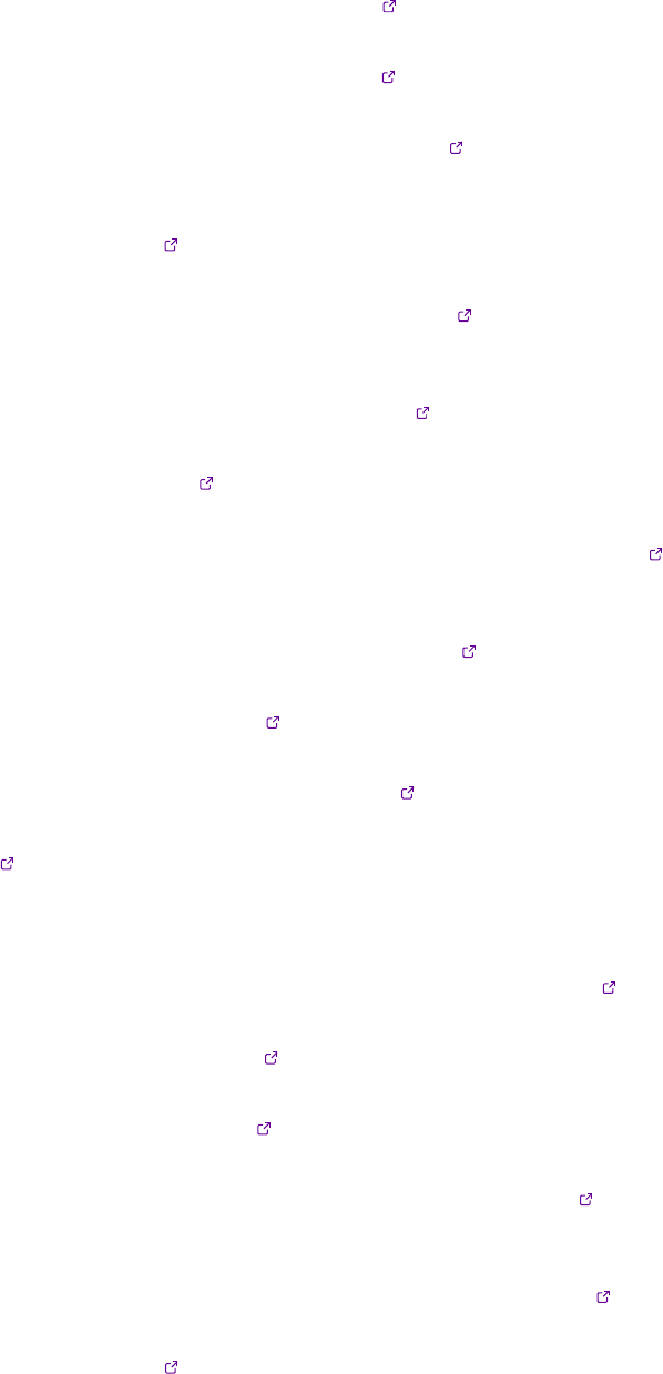
Sharc Manual Bibliography |Bibliography
[57]
A. C. Borin, S. Mai, P. Marquetand, L. González: “Ab initio molecular dynamics relaxation and intersystem
crossing mechanisms of 5-azacytosine”.Phys. Chem. Chem. Phys.,19, 5888–5894 (2017).
[58]
S. Mai, M. Richter, P. Marquetand, L. González: “The DNA Nucleobase Thymine in Motion – Intersystem
Crossing Simulated with Surface Hopping”.Chem. Phys.,482, 9–15 (2017).
[59]
F. M. Siouri, S. Boldissar, J. A. Berenbeim, M. S. de Vries: “Excited State Dynamics of 6-Thioguanine”.J. Phys.
Chem. A,121, 5257–5266 (2017).
[60]
D. Bellshaw, D. A. Horke, A. D. Smith, H. M. Watts, E. Jager, E. Springate, O. Alexander, C. Cacho, R. T. Chapman,
A. Kirrander, R. S. Minns: “Ab-initio surface hopping and multiphoton ionisation study of the photodissociation
dynamics of CS2”.Chem. Phys. Lett.,683, 383–388 (2017).
[61]
S. Sun, B. Mignolet, L. Fan, W. Li, R. D. Levine, F. Remacle: “Nuclear Motion Driven Ultrafast Photodissociative
Charge Transfer of the PENNA Cation: An Experimental and Computational Study”.J. Phys. Chem. A,
121
,
1442–1447 (2017).
[62]
C. Rauer, J. J. Nogueira, P. Marquetand, L. González: “Cyclobutane Thymine Photodimerization Mechanism
Revealed by Nonadiabatic Molecular Dynamics”.J. Am. Chem. Soc.,138, 15 911–15 916 (2016).
[63]
A. J. Atkins, L. González: “Trajectory Surface-Hopping Dynamics Including Intersystem Crossing in
[Ru(bpy)3]2+”.J. Phys. Chem. Lett.,8, 3840–3845 (2017).
[64]
T. Schnappinger, P. Kolle, M. Marazzi, A. Monari, L. González, R. de Vivie-Riedle: “Ab initio molecular dynamics
of thiophene: the interplay of internal conversion and intersystem crossing”.Phys. Chem. Chem. Phys.,
19
,
25 662–25 670 (2017).
[65]
S. Mai, F. Plasser, M. Pabst, F. Neese, A. Köhn, L. González: “Surface Hopping Dynamics Including Intersystem
Crossing using the Algebraic Diagrammatic Construction Method”.J. Chem. Phys.,147, 184 109 (2017).
[66]
J. P. Zobel, J. J. Nogueira, L. González: “The Mechanism of Ultrafast Intersystem Crossing in 2-Nitronaphthalene”.
Chem. Eur. J., DOI:10.1002/chem.201705854 (2018).
[67]
C. Rauer, J. J. Nogueira, P. Marquetand, L. González: “Stepwise photosensitized thymine dimerization mediated
by an exciton intermediate”.Monatsh. Chem.,149, 1–9 (2018).
[68]
J. Cao: “The position of the N atom in the pentacyclic ring of heterocyclic molecules aects the excited-state
decay: A case study of isothiazole and thiazole”.J. Mol. Struct., DOI:10.1016/j.molstruc.2017.11.008 (2018).
[69]
R. J. Squibb, M. Sapunar, A. Ponzi, R. Richter, A. Kivimäki, O. Plekan, P. Finetti, N. Sisourat, V. Zhaunerchyk,
T. Marchenko, L. Journel, R. Guillemin, R. Cucini, M. Coreno, C. Grazioli, M. Di Fraia, C. Callegari, K. C. Prince,
P. Decleva, M. Simon, J. H. D. Eland, N. Došlić, R. Feifel, M. N. Piancastelli: “Acetylacetone photodynamics at a
seeded free-electron laser”.Nat. Commun.,9, 63 (2018).
[70]
L. Wang, D. Trivedi, O. V. Prezhdo: “Global Flux Surface Hopping Approach for Mixed Quantum-Classical
Dynamics”.J. Chem. Theory Comput.,10, 3598–3605 (2014).
[71]
G. Granucci, M. Persico, A. Toniolo: “Direct Semiclassical Simulation of Photochemical Processes with Semiem-
pirical Wave Functions”.J. Chem. Phys.,114, 10 608–10 615 (2001).
[72]
F. Plasser, G. Granucci, J. Pittner, M. Barbatti, M. Persico, H. Lischka: “Surface Hopping Dynamics using a
Locally Diabatic Formalism: Charge Transfer in The Ethylene Dimer Cation and Excited State Dynamics in the
2-Pyridone Dimer”.J. Chem. Phys.,137, 22A514 (2012).
[73]
F. Plasser, M. Ruckenbauer, S. Mai, M. Oppel, P. Marquetand, L. González: “Ecient and Flexible Computation
of Many-Electron Wave Function Overlaps”.J. Chem. Theory Comput.,12, 1207 (2016).
[74]
J. P. Dahl, M. Springborg: “The Morse oscillator in position space, momentum space, and phase space”.J. Chem.
Phys.,88, 4535–4547 (1988).
[75]
R. Schinke: Photodissociation Dynamics: Spectroscopy and Fragmentation of Small Polyatomic Molecules. Cambridge
University Press (1995).
154
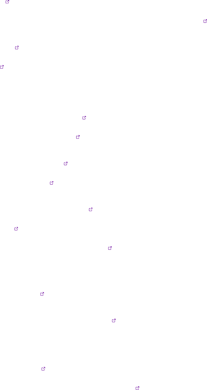
Sharc Manual Bibliography |Bibliography
[76]
M. Barbatti, K. Sen: “Eects of dierent initial condition samplings on photodynamics and spectrum of pyrrole”.
Int. J. Quantum Chem.,116, 762–771 (2016).
[77]
M. Barbatti, G. Granucci, M. Persico, M. Ruckenbauer, M. Vazdar, M. Eckert-Maksić, H. Lischka: “The on-
the-y surface-hopping program system Newton-X: Application to ab initio simulation of the nonadiabatic
photodynamics of benchmark systems”.J. Photochem. Photobiol. A,190, 228–240 (2007).
[78]
D. Cremer, J. A. Pople: “General denition of ring puckering coordinates”.J. Am. Chem. Soc.,
97
, 1354–1358
(1975).
[79] J. C. A. Boeyens: “The conformation of six-membered rings”.J. Cryst. Mol. Struct.,8, 317 (1978).
[80]
L. Kurtz, A. Hofmann, R. de Vivie-Riedle: “Ground state normal mode analysis: Linking excited state dynamics
and experimental observables”. J. Chem. Phys.,114, 6151–6159 (2001).
[81]
F. Plasser: Dynamics Simulation of Excited State Intramolecular Proton Transfer. Master’s thesis, University of
Vienna (2009).
[82]
A. Amadei, A. B. M. Linssen, H. J. C. Berendsen: “Essential dynamics of proteins”.Proteins: Struct., Funct.,
Bioinf.,17, 412–425 (1993).
[83]
S. Nangia, A. W. Jasper, T. F. Miller, D. G. Truhlar: “Army Ants Algorithm for Rare Event Sampling of Delocalized
Nonadiabatic Transitions by Trajectory Surface Hopping and the Estimation of Sampling Errors by the Bootstrap
Method”.J. Chem. Phys.,120, 3586–3597 (2004).
[84]
M. J. Bearpark, M. A. Robb, H. B. Schlegel: “A direct method for the location of the lowest energy point on a
potential surface crossing”.Chem. Phys. Lett.,223, 269 (1994).
[85]
B. G. Levine, J. D. Coe, T. J. Martínez: “Optimizing Conical Intersections without Derivative Coupling Vectors:
Application to Multistate Multireference Second-Order Perturbation Theory (MS-CASPT2)”.J. Phys. Chem. B,
112, 405–413 (2008).
[86]
M. Ruckenbauer, S. Mai, P. Marquetand, L. González: “Photoelectron spectra of 2-thiouracil, 4-thiouracil, and
2,4-dithiouracil”.J. Chem. Phys.,144, 074 303 (2016).
[87]
F. Plasser, L. González: “Communication: Unambiguous comparison of many-electron wavefunctions through
their overlaps”.J. Chem. Phys.,145, 021 103 (2016).
[88]
H.-J. Werner, P. J. Knowles, G. Knizia, F. R. Manby, M. Schütz: “Molpro: A general-purpose quantum chemistry
program package”.WIREs Comput. Mol. Sci.,2, 242–253 (2012).
[89]
H.-J. Werner, P. J. Knowles, G. Knizia, F. R. Manby, et al.: “MOLPRO, version 2012.1, a package of ab initio
programs”. www.molpro.net (2012).
[90]
G. Karlström, R. Lindh, P.-Å. Malmqvist, B. O. Roos, U. Ryde, V. Veryazov, P.-O. Widmark, M. Cossi, B. Schim-
melpfennig, P. Neogrady, L. Seijo: “MOLCAS: a program package for computational chemistry”.Comput. Mater.
Sci.,28, 222 – 239 (2003).
[91]
F. Aquilante, L. De Vico, N. Ferré, G. Ghigo, P.-Å. Malmqvist, P. Neogrády, T. B. Pedersen, M. Pitoňák, M. Reiher,
B. O. Roos, L. Serrano-Andrés, M. Urban, V. Veryazov, R. Lindh: “MOLCAS 7: The Next Generation”.J. Comput.
Chem.,31, 224–247 (2010).
[92]
F. Aquilante, J. Autschbach, R. K. Carlson, L. F. Chibotaru, M. G. Delcey, L. De Vico, I. Fdez. Galván, N. Ferré,
L. M. Frutos, L. Gagliardi, M. Garavelli, A. Giussani, C. E. Hoyer, G. Li Manni, H. Lischka, D. Ma, P.-Å. Malmqvist,
T. Müller, A. Nenov, M. Olivucci, T. B. Pedersen, D. Peng, F. Plasser, B. Pritchard, M. Reiher, I. Rivalta, I. Schapiro,
J. Segarra-Martí, M. Stenrup, D. G. Truhlar, L. Ungur, A. Valentini, S. Vancoillie, V. Veryazov, V. P. Vysotskiy,
O. Weingart, F. Zapata, R. Lindh: “Molcas 8: New Capabilities for Multicongurational Quantum Chemical
Calculations Across the Periodic Table”.J. Comput. Chem.,37, 506–541 (2015).
[93]
H. Lischka, T. Müller, P. G. Szalay, I. Shavitt, R. M. Pitzer, R. Shepard: “Columbus – a program system for
advanced multireference theory calculations.” WIREs Comput. Mol. Sci.,1, 191–199 (2011).
155

Sharc Manual Bibliography |Bibliography
[94]
H. Lischka, R. Shepard, I. Shavitt, R. M. Pitzer, M. Dallos, T. Müller, P. G. Szalay, F. B. Brown, R. Ahlrichs, H. J.
Böhm, A. Chang, D. C. Comeau, R. Gdanitz, H. Dachsel, C. Ehrhardt, M. Ernzerhof, P. Höchtl, S. Irle, G. Kedziora,
T. Kovar, V. Parasuk, M. J. M. Pepper, P. Scharf, H. Schier, M. Schindler, M. Schüler, M. Seth, E. A. Stahlberg,
J.-G. Zhao, S. Yabushita, Z. Zhang, M. Barbatti, S. Matsika, M. Schuurmann, D. R. Yarkony, S. R. Brozell, E. V.
Beck, , J.-P. Blaudeau, M. Ruckenbauer, B. Sellner, F. Plasser, J. J. Szymczak: “COLUMBUS, an ab initio electronic
structure program, release 7.0” (2012).
[95]
S. Yabushita, Z. Zhang, R. M. Pitzer: “Spin-Orbit Conguration Interaction Using the Graphical Unitary Group
Approach and Relativistic Core Potential and Spin-Orbit Operators”.J. Phys. Chem. A,103, 5791–5800 (1999).
[96]
S. Mai, T. Müller, P. Marquetand, F. Plasser, H. Lischka, L. González: “Perturbational Treatment of Spin-Orbit
Coupling for Generally Applicable High-Level Multi-Reference Methods”.J. Chem. Phys.,141, 074 105 (2014).
[97]
E. J. Baerends, T. Ziegler, A. J. Atkins, J. Autschbach, D. Bashford, O. Baseggio, A. Bérces, F. M. Bickelhaupt, C. Bo,
P. M. Boerritger, L. Cavallo, C. Daul, D. P. Chong, D. V. Chulhai, L. Deng, R. M. Dickson, J. M. Dieterich, D. E.
Ellis, M. van Faassen, A. Ghysels, A. Giammona, S. J. A. van Gisbergen, A. Goez, A. W. Götz, S. Gusarov, F. E.
Harris, P. van den Hoek, Z. Hu, C. R. Jacob, H. Jacobsen, L. Jensen, L. Joubert, J. W. Kaminski, G. van Kessel,
C. König, F. Kootstra, A. Kovalenko, M. Krykunov, E. van Lenthe, D. A. McCormack, A. Michalak, M. Mitoraj,
S. M. Morton, J. Neugebauer, V. P. Nicu, L. Noodleman, V. P. Osinga, S. Patchkovskii, M. Pavanello, C. A. Peeples,
P. H. T. Philipsen, D. Post, C. C. Pye, H. Ramanantoanina, P. Ramos, W. Ravenek, J. I. Rodríguez, P. Ros, R. Rüger,
P. R. T. Schipper, D. Schlüns, H. van Schoot, G. Schreckenbach, J. S. Seldenthuis, M. Seth, J. G. Snijders, M. Solà,
S. M., M. Swart, D. Swerhone, G. te Velde, V. Tognetti, P. Vernooijs, L. Versluis, L. Visscher, O. Visser, F. Wang, T. A.
Wesolowski, E. M. van Wezenbeek, G. Wiesenekker, S. K. Wol, T. K. Woo, A. L. Yakovlev: “Amsterdam density
functional modeling suite 2017”. SCM, Theoretical Chemistry, Vrije Universiteit, Amsterdam, The Netherlands,
https://www.scm.com (2017).
[98]
“TURBOMOLE V7.0, A development of University of Karlsruhe and Forschungszentrum Karlsruhe GmbH” (2015).
[99]
M. J. Frisch, G. W. Trucks, H. B. Schlegel, G. E. Scuseria, M. A. Robb, J. R. Cheeseman, G. Scalmani, V. Barone,
B. Mennucci, G. A. Petersson, H. Nakatsuji, M. Caricato, X. Li, H. P. Hratchian, A. F. Izmaylov, J. Bloino, G. Zheng,
J. L. Sonnenberg, M. Hada, M. Ehara, K. Toyota, R. Fukuda, J. Hasegawa, M. Ishida, T. Nakajima, Y. Honda, O. Kitao,
H. Nakai, T. Vreven, J. A. Montgomery, Jr., J. E. Peralta, F. Ogliaro, M. Bearpark, J. J. Heyd, E. Brothers, K. N. Kudin,
V. N. Staroverov, R. Kobayashi, J. Normand, K. Raghavachari, A. Rendell, J. C. Burant, S. S. Iyengar, J. Tomasi,
M. Cossi, N. Rega, J. M. Millam, M. Klene, J. E. Knox, J. B. Cross, V. Bakken, C. Adamo, J. Jaramillo, R. Gomperts,
R. E. Stratmann, O. Yazyev, A. J. Austin, R. Cammi, C. Pomelli, J. W. Ochterski, R. L. Martin, K. Morokuma, V. G.
Zakrzewski, G. A. Voth, P. Salvador, J. J. Dannenberg, S. Dapprich, A. D. Daniels, Ö. Farkas, J. B. Foresman, J. V.
Ortiz, J. Cioslowski, , D. J. Fox: “Gaussian 09, Revision A.1”. Gaussian, Inc.: Wallingford CT, 2009.
[100]
M. J. Frisch, G. W. Trucks, H. B. Schlegel, G. E. Scuseria, M. A. Robb, J. R. Cheeseman, G. Scalmani, V. Barone, G. A.
Petersson, H. Nakatsuji, X. Li, M. Caricato, A. V. Marenich, J. Bloino, B. G. Janesko, R. Gomperts, B. Mennucci,
H. P. Hratchian, J. V. Ortiz, A. F. Izmaylov, J. L. Sonnenberg, D. Williams-Young, F. Ding, F. Lipparini, F. Egidi,
J. Goings, B. Peng, A. Petrone, T. Henderson, D. Ranasinghe, V. G. Zakrzewski, J. Gao, N. Rega, G. Zheng, W. Liang,
M. Hada, M. Ehara, K. Toyota, R. Fukuda, J. Hasegawa, M. Ishida, T. Nakajima, Y. Honda, O. Kitao, H. Nakai,
T. Vreven, K. Throssell, J. A. Montgomery, Jr., J. E. Peralta, F. Ogliaro, M. J. Bearpark, J. J. Heyd, E. N. Brothers,
K. N. Kudin, V. N. Staroverov, T. A. Keith, R. Kobayashi, J. Normand, K. Raghavachari, A. P. Rendell, J. C. Burant,
S. S. Iyengar, J. Tomasi, M. Cossi, J. M. Millam, M. Klene, C. Adamo, R. Cammi, J. W. Ochterski, R. L. Martin,
K. Morokuma, O. Farkas, J. B. Foresman, D. J. Fox: “Gaussian16 Revision A.03” (2016), gaussian Inc. Wallingford
CT.
[101]
G. Granucci, M. Persico, A. Zoccante: “Including quantum decoherence in surface hopping”.J. Chem. Phys.,
133, 134 111 (2010).
[102]
H. Köppel, W. Domcke, L. S. Cederbaum: “Multimode molecular dynamics beyond the Born-Oppenheimer
approximation”. Adv. Chem. Phys.,57, 59–246 (1984).
[103]
M. Barbatti, G. Granucci, M. Ruckenbauer, F. Plasser, J. Pittner, M. Persico, H. Lischka: “NEWTON-X: a package
for Newtonian dynamics close to the crossing seam, version 1.2”. www.newtonx.org (2011).
[104]
P. Marquetand: Vectorial properties and laser control of molecular dynamics. Ph.D. thesis, University of Würzburg
(2007), http://opus.bibliothek.uni-wuerzburg.de/volltexte/2007/2469/.
156

List of Tables
2.1 Environment variables for Sharc test jobs. .................................. 23
4.1 Input keywords for sharc.x........................................... 33
6.1 Control keywords for Sharc interfaces. .................................... 47
6.2 Request keywords for Sharc interfaces. .................................... 48
6.3 Overview over capabilities of Sharc interfaces. ............................... 52
6.4 Overview over les of Sharc interfaces. ................................... 52
6.5 Keywords for the MOLPRO.resources input le. ................................ 55
6.6 Keywords for the MOLACS.template le. .................................... 58
6.7 Keywords for the MOLCAS.resources le. ................................... 59
6.8 Keywords for the COLUMBUS.resources le. .................................. 62
6.9 Keywords for the ADF.template le. ...................................... 67
6.10 Keywords for the ADF.resources le. ..................................... 68
6.11 Keywords for the RICC2.template le. .................................... 73
6.12 Keywords for the RICC2.resources le. .................................... 74
6.13 Keywords for the GAUSSIAN.template le. .................................. 78
6.14 Keywords for the GAUSSIAN.resources le. .................................. 79
6.15 List of keywords given in the input le. .................................... 82
7.1 Command-line options for script wigner.py.................................. 87
7.2 Command-line options for script amber_to_initconds.py.......................... 88
7.3 Command-line options for script sharctraj_to_initconds.py....................... 90
7.4 Command-line options for script spectrum.py.................................105
7.5 Command-line options for data_extractor.x.................................107
7.6 Content of the les written by data_extractor.x...............................108
7.7 List of the settings for diagnostics.py.....................................110
7.8 Analysis modes for populations.py......................................112
7.9 Analysis modes for transition.py.......................................114
7.10 Possible types of internal coordinates in geo.py...............................119
7.11 Command-line options for geo.py.......................................119
7.12 Command-line options for QMout_print.py..................................130
158
List of Figures
1.1 Jabłonski diagram showing the conceptual photophysical processes. .................... 9
2.1 Directory tree containing a complete Sharc installation. .......................... 21
3.1 Input les for a Sharc dynamics simulation. ................................. 25
3.2 Files of a Sharc dynamics simulation after running. ............................. 27
3.3 Typical workow for conducting excited-state dynamics simulations with Sharc............. 28
6.1 Communication between sharc.x, the interfaces, and the quantum chemistry codes. .......... 46
6.2 Example directory structure of the Columbus template directory ..................... 63
6.3 Workow of the wavefunction overlap program. ............................... 81
7.1 Directory structure created by setup_init.py................................. 96
7.2 Directory structure created by setup_traj.py.................................103
7.3 Color code for plots generated with the use of make_gnuscript.py.....................109
7.4 Possible workows in data_collector.py..................................123
7.5 Communication between Orca,orca_External, the interfaces, and the quantum chemistry codes. . . . 128
8.1 Forbidden and allowed features of the reaction network graphs. ......................137
8.2 Example reaction network graph. For explanation see text. .........................137
8.3 Types of laser envelopes implemented in laser.x...............................141
159
