SLi M Manual
User Manual:
Open the PDF directly: View PDF ![]() .
.
Page Count: 517 [warning: Documents this large are best viewed by clicking the View PDF Link!]
SLiM: An Evolutionary Simulation Framework
Benjamin C. Haller and Philipp W. Messer
Dept. of Biological Statistics and Computational Biology
Cornell University, Ithaca, NY 14853
Correspondence: bhaller@benhaller.com
Last revised 29 January 2019, for SLiM version 3.2.1.

Author Contributions:
SLiM 2 and later were conceived and designed by BCH and PWM, based upon the previous design of SLiM
by PWM. BCH designed and implemented the Eidos scripting language, wrote almost all of the code for
SLiM 2 and later (but see the acknowledgements below), and wrote this manual. PWM provided feedback
and edited this manual.
Acknowledgements:
The authors want to thank Andrew Sackman, Aaron Sams, Nathan Oakes, Madeline Kwicklis, Jamal
Elkhader, and all members of the Messer lab for helpful feedback and bug reports. Thanks to Kevin Thornton
and Ryan Hernandez for many discussions and for their general help in promoting forward population
genetic simulations. Thanks to Jared Galloway, Jerome Kelleher, and Peter Ralph for their considerable work
in implementing tree-sequence recording in SLiM 3. Thanks to Simon Aeschbacher, Jorge Amaya, Bill Amos,
Chenling Antelope, Jaime Ashander, Hannes Becher, Emma Berdan, Jeremy Berg, Tom Booker, Gideon
Bradburd, Yoann Buoro, Deborah Charlesworth, Jeremy Van Cleve, Jean Cury, Michael DeGiorgio, A.P. Jason
de Koning, Emily Dennis, Jordan Rohmeyer Dherby, Jared Galloway, Jesse Garcia, Kimberley Gilbert,
Alexandre Harris, Kelley Harris, Rebecca Harris, Matthew Hartfield, Ding He, Kathryn Hodgins, Christian
Huber, Melissa Jane Hubisz, Emilia Huerta-Sanchez, Jacob Malte Jensen, Peter Keightley, Jerome Kelleher,
Andy Kern, Bhavin Khatri, Bernard Kim, Athanasios Kousathanas, Chris Kyriazis, Benjamin Laenen, Áki
Láruson, Stefan Laurent, Eugenio Lopez, Kathleen Lotterhos, Andrew Marderstein, Sebastian Matuszewski,
Mikhail Matz, Rupert Mazzucco, Maéva Mollion, !Miguel Navascués, Dominic Nelson, Bruno Nevado,
Etsuko Nonaka, Greg Owens, Harvinder Pawar, Martin Petr, Denis Pierron, Fernando Racimo, Peter Ralph,
David Rinker, Murillo Fernando Rodrigues, Andrew Sackman, Kieran Samuk, Derek Setter, Onuralp
Söylemez, Stefan Strütt, Rob Unckless, Christos Vlachos, Silu Wang, Aaron Wolf, Yan Wong, and Justin Yeh
for comments and feedback that has led to improvements in SLiM. Thanks also to everyone on
stackoverflow, an invaluable resource and a great community. Finally, we want to thank Dmitri Petrov,
whose support was instrumental in the initial conception of SLiM.
Citation:
To cite SLiM 3 in a publication, please cite:
Haller, B.C., and Messer, P.W. (2017). SLiM 2: Flexible, interactive forward genetic simulations.
Molecular Biology and Evolution (early access). DOI: https://doi.org/10.1093/molbev/msy228
Papers using tree-sequence recording should perhaps also cite that paper:
Haller, B.C., Galloway, J., Kelleher, J., Messer, P.W., & Ralph, P.L. (2018). Tree-sequence recording in
SLiM opens new horizons for forward-time simulation of whole genomes.!Molecular Ecology
Resources (early access). DOI: https://doi.org/10.1111/1755-0998.12968
Papers which only use SLiM 2 can still cite that paper:
Haller, B.C., and Messer, P.W. (2017). SLiM 2: Flexible, interactive forward genetic simulations.
Molecular Biology and Evolution 34(1), 230–240. DOI: http://dx.doi.org/10.1093/molbev/msw211
Papers which wish to cite this manual (perhaps because they make reference to a recipe) should cite:
Haller, B.C., and Messer, P.W. (2016). SLiM: An Evolutionary Simulation Framework.!
URL: http://benhaller.com/slim/SLiM_Manual.pdf
And if you wish to cite a publication about Eidos, please cite the Eidos manual:
Haller, B.C. (2016). Eidos: A Simple Scripting Language.!
URL: http://benhaller.com/slim/Eidos_Manual.pdf
2

URL:
http://messerlab.org/slim
License:
Copyright © 2016–2019 Philipp Messer. All rights reserved.
SLiM is a free software: you can redistribute it and/or modify it under the terms of the GNU General Public
License as published by the Free Software Foundation, either version 3 of the License, or (at your option) any
later version.
Disclaimer:
The program is distributed in the hope that it will be useful, but WITHOUT ANY WARRANTY; without even
the implied warranty of MERCHANTABILITY or FITNESS FOR A PARTICULAR PURPOSE. See the GNU
General Public License (http://www.gnu.org/licenses/) for more details.
3

Contents
PART I: THE SLIM COOKBOOK
1. SLiM overview 12 .................................................................................................................................
1.1 Introduction 12 ..........................................................................................................................
1.2 Why SLiM? 13 ............................................................................................................................
1.3 A quick summary of SLiM 14 .....................................................................................................
1.4 The typical SLiM usage pattern 17 ..............................................................................................
1.5 Conceptual overview 18 ............................................................................................................
1.5.1 Individuals and genomes 18!...........................................................................................
1.5.2 Mutations and substitutions 20!.......................................................................................
1.5.3 Mutation stacking 22!......................................................................................................
1.5.4 Genomic elements, genomic element types, mutation types, and the chromosome 26!........
1.5.5 Subpopulations and migration 27!...................................................................................
1.5.6 Other concepts 28 ..........................................................................................................
1.6 Wright-Fisher (WF) versus non-Wright-Fisher (nonWF) models 29 ...................................................
1.7 Tree-sequence recording 31 .......................................................................................................
1.8 Online resources for SLiM users 34 .................................................................................................
2. Installation 36 .......................................................................................................................................
2.1 Installation on Mac OS X 36 .......................................................................................................
2.1.1 Installing the prebuilt SLiM package on Mac OS X 36!..........................................................
2.1.2 Building SLiM from sources on Mac OS X 36 .................................................................
2.2 Installation on Linux and other Un*x platforms 40 .....................................................................
2.3 Installation on non-Un*x platforms 42 ........................................................................................
2.4 Testing the SLiM installation 42 ..................................................................................................
3. Running simulations in SLiMgui 43 ......................................................................................................
3.1 The SLiMgui simulation window 43 ...........................................................................................
3.2 The script help window 44 .........................................................................................................
3.3 The Eidos console 45 .................................................................................................................
3.4 The Eidos variable browser 46 ....................................................................................................
3.5 Automatic code completion and command syntax lookup 46 ....................................................
3.6 Automated script generation 48 ..................................................................................................
3.7 Script prettyprinting 51 ...............................................................................................................
3.8 Further SLiMgui features 52 ........................................................................................................
4. Getting started: Neutral evolution in a panmictic population 53 ...........................................................
4.1 A basic neutral simulation 53 .....................................................................................................
4.1.1 initialize() callbacks 54!...................................................................................................
4.1.2 Mutation rate 55!.............................................................................................................
4.1.3 Mutation types 55!...........................................................................................................
4.1.4 Genomic element types 57!.............................................................................................
4.1.5 Genomic elements 58!....................................................................................................
4.1.6 Recombination rate 59!...................................................................................................
4.1.7 Eidos events 60!...............................................................................................................
4.1.8 Subpopulations 60!..........................................................................................................
4.1.9 Executing the simulation 61 ............................................................................................
4

4.2 Basic output 62 ..........................................................................................................................
4.2.1 Entire population 62!.......................................................................................................
4.2.2 Random population sample 64!.......................................................................................
4.2.3 Sampling individuals rather than genomes 66!.................................................................
4.2.4 Substitutions 67!..............................................................................................................
4.2.5 Custom output with Eidos 68!..........................................................................................
4.2.6 The simulation endpoint 70 ............................................................................................
5. Demography and population structure 72 .............................................................................................
5.1 Subpopulation size 72 ................................................................................................................
5.1.1 Instantaneous changes 72!....................................................................................................
5.1.2 Exponential growth 72!....................................................................................................
5.1.3 The population visualization graph 76!............................................................................
5.1.4 Cyclical changes 77!........................................................................................................
5.1.5 Context-dependent changes: Muller’s Ratchet 77 ............................................................
5.2 Population structure 78 ..............................................................................................................
5.2.1 Adding subpopulations 78!..............................................................................................
5.2.2 Removing subpopulations 80!..........................................................................................
5.2.3 Splitting subpopulations 81 ............................................................................................
5.3 Migration and admixture 81 .......................................................................................................
5.3.1 A linear island model 81!................................................................................................
5.3.2 A non-spatial metapopulation 83!....................................................................................
5.3.3 A two-dimensional subpopulation matrix 84!..................................................................
5.3.4 A random, sparse spatial metapopulation 85!..................................................................
5.3.5 Reading a migration matrix from a file 88 .......................................................................
5.4 The Gravel et al. (2011) model of human evolution 90 ...............................................................
5.5 Rescaling population sizes to improve simulation performance 92 ..................................................
6. Sexual reproduction 96 ........................................................................................................................
6.1 Recombination 96 ......................................................................................................................
6.1.1 Crossing over: Making a random recombination map 96!.....................................................
6.1.2 Crossing over: Reading a recombination map from a file 97!................................................
6.1.3 Gene conversion 99 .......................................................................................................
6.2 Separate sexes 99 .......................................................................................................................
6.2.1 Enabling separate sexes 99!.............................................................................................
6.2.2 Sex ratios 100!...................................................................................................................
6.2.3 Modeling sex-chromosome evolution 101 ........................................................................
6.3 Selfing and cloning 103 ................................................................................................................
6.3.1 Selfing in hermaphroditic populations 103!.......................................................................
6.3.2 Cloning 103 .....................................................................................................................
7. Mutation types, genomic elements, and chromosome structure 105 .......................................................
7.1 Mutation types and fitness effects 105 ..........................................................................................
7.2 Genomic element types 107 .........................................................................................................
7.3 Chromosome organization 108 ....................................................................................................
7.4 Custom display colors in SLiMgui 110 ..........................................................................................
8. SLiMgui visualizations for polymorphism patterns 114 ...........................................................................
8.1 Mutation frequency spectra 114 ...................................................................................................
8.2 Mutation frequency trajectories 115 .............................................................................................
8.3 Times to fixation and loss 116 ...................................................................................................... ...
5

8.4 Population fitness over time 117 ...................................................................................................
9. Context-dependent selection using fitness() callbacks 118 ......................................................................
9.1 Temporally varying selection 118 .................................................................................................
9.2 Spatially varying selection 119 .....................................................................................................
9.3 Fitness as a function of genomic background 121 ........................................................................
9.3.1 Epistasis 121!.....................................................................................................................
9.3.2 Polygenic selection 123 ....................................................................................................
9.4 Fitness as a function of population composition 125 ....................................................................
9.4.1 Frequency-dependent selection 125!.................................................................................
9.4.2 Kin selection and inclusive fitness 127!..............................................................................
9.4.3 Cultural effects on fitness 128!...........................................................................................
9.4.4 The green-beard effect 130 ...............................................................................................
9.5 Changing selection coefficients with setSelectionCoeff() 134 ...........................................................
10. Selective sweeps 136 ..............................................................................................................................
10.1 Introducing adaptive mutations 136 .............................................................................................
10.2 Making sweeps conditional on fixation 138 .................................................................................
10.3 Making sweeps conditional on establishment 140 ........................................................................
10.4 Partial sweeps 142 ........................................................................................................................
10.5 Soft sweeps from de novo mutations 143 .....................................................................................
10.5.1 A soft sweep from recurrent de novo mutations in a large population 143!...........................
10.5.2 A soft sweep with a fixed mutation schedule 145!................................................................
10.5.3 A soft sweep with a random mutation schedule 147 .........................................................
10.6 Sweeps from standing genetic variation 149 .................................................................................
10.6.1 A sweep from standing variation at a random locus 149!......................................................
10.6.2 A sweep from standing variation at a predetermined locus 150 ...........................................
10.7 Adaptive introgression 152 ...........................................................................................................
10.8 Fixation probabilities under Hill-Robertson interference 153 ........................................................
11. Complex mating schemes using mateChoice() callbacks 156 ..................................................................
11.1 Assortative mating 156 .................................................................................................................
11.2 Sequential mate search 162 ..........................................................................................................
11.3 Gametophytic self-incompatibility 165 .........................................................................................
12. Direct child modifications using modifyChild() callbacks 170 .................................................................
12.1 Social learning of cultural traits 170 .............................................................................................
12.2 Lethal epistasis 172 ......................................................................................................................
12.3 Simulating gene drive 173 ............................................................................................................
12.4 Suppressing hermaphroditic selfing 178 .......................................................................................
13. Advanced models 180 ............................................................................................................................
13.1 Quantitative genetics and phenotypically-based fitness 180 ............................................................
13.2 Relatedness, inbreeding, and heterozygosity 186 .........................................................................
13.3 Mortality-based fitness 188 ..............................................................................................................
13.4 Reading initial simulation state from an MS output file 192 .............................................................
13.5 Modeling chromosomal inversions with a recombination() callback 195 .........................................
13.6 Modeling both X and Y Chromosomes with a Pseudo-Autosomal Region (PAR) 200 .....................
13.7 Forcing a specific pedigree through arranged matings 204 ...........................................................
6

13.8 Estimating model parameters with ABC 207 .................................................................................
13.9 Tracking true local ancestry along the chromosome 210 ..............................................................
13.10 A quantitative genetics model with heritability 214 ......................................................................
13.11 Live plotting with R using system() 219 .........................................................................................
13.12 Modeling nucleotides at a locus 222 ............................................................................................
13.13 Modeling haploid organisms 227 .................................................................................................
13.14 Using mutation rate variation to model varying functional density 228 ............................................
13.15 Modeling microsatellites 230 .......................................................................................................
13.16 Modeling transposable elements 235 ...........................................................................................
13.17 A QTL-based model with two quantitative phenotypic traits and pleiotropy 241 .............................
13.18 Modeling opposite ends of a chromosome 248 ............................................................................
13.19 Biased gene conversion 251 .........................................................................................................
14. Continuous-space models and interactions 258 ......................................................................................
14.1 A simple 2D continuous-space model 258 ...................................................................................
14.2 Spatial competition 260 ...............................................................................................................
14.3 Boundaries and boundary conditions 262 ....................................................................................
14.4 Mate choice with a spatial kernel 264 ..........................................................................................
14.5 Mate choice with a nearest-neighbor search 266 ..........................................................................
14.6 Divergence due to phenotypic competition with an interaction() callback 267 ................................
14.7 Modeling phenotype as a spatial dimension 272 ..........................................................................
14.8 Sympatric speciation facilitated by assortative mating 275 ...............................................................
14.9 Speciation due to spatial variation in selection 278 ......................................................................
14.10 A simple biogeographic landscape model 282 .............................................................................
14.11 Local adaptation on a heterogeneous landscape map 288 ............................................................
14.12 Periodic spatial boundaries 293 ...................................................................................................
15. Going beyond Wright-Fisher models: nonWF model recipes 298 ..............................................................
15.1 A minimal nonWF model 298 ......................................................................................................
15.2 Age structure (a life table model) 301 ...........................................................................................
15.3 Monogamous mating and variation in litter size 303 ....................................................................
15.4 Beneficial mutations and absolute fitness 306 ..............................................................................
15.5 A metapopulation extinction-colonization model 308 ..................................................................
15.6 Habitat choice 312 .......................................................................................................................
15.7 Evolutionary rescue after environmental change 315 ....................................................................
15.8 Pollen flow 320 ............................................................................................................................
15.9 Litter size and parental investment 322 ........................................................................................
15.10 Spatial competition and spatial mate choice in a nonWF model 325 ...............................................
15.11 A spatial model with carrying-capacity density 330 ......................................................................
15.12 Forcing a specific pedigree in a nonWF model 333 ......................................................................
15.13 Modeling clonal haploids in a nonWF model with addRecombinant() 338 ......................................
15.14 Modeling clonal haploid bacteria with horizontal gene transfer 340 ...............................................
15.15 Implementing a Wright–Fisher model with a nonWF model 343 .....................................................
15.16 Alternation of generations 345 .....................................................................................................
7

16. Tree-sequence recording: tracking population history and true local ancestry 349 .................................. ...
16.1 A minimal tree-seq model 349 .....................................................................................................
16.2 Overlaying neutral mutations 350 ................................................................................................
16.3 Simulation conditional upon fixation of a sweep, preserving ancestry 351 ......................................
16.4 Detecting the “dip in diversity”: analyzing tree heights in Python 353 .............................................
16.5 Mapping admixture: analyzing ancestry in Python 356 ................................................................
16.6 Measuring the coalescence time of a model 359 ..........................................................................
16.7 Analyzing selection coefficients in Python with pyslim 361 .............................................................
16.8 Starting a hermaphroditic WF model with a coalescent history 362 .................................................
16.9 Starting a sexual nonWF model with a coalescent history 364 .........................................................
16.10 Adding a neutral burn-in after simulation with recapitation 366 ......................................................
17. Runtime control 371 ...............................................................................................................................
17.1 The random number generator 371 ..............................................................................................
17.2 Defining constants on the command line 372 ..............................................................................
17.3 Other command-line options 374 ................................................................................................
17.4 File input and output 376 .............................................................................................................
17.5 Lambda execution 377 .................................................................................................................
17.6 Debugging 379 ............................................................................................................................
18. Implementation and performance 380 ....................................................................................................
18.1 Writing fast SLiM simulations 380 ................................................................................................
18.2 Performance evaluation 382 .........................................................................................................
18.3 Memory usage considerations 384 ...............................................................................................
18.4 Mutation runs and runtime optimization 385 ...............................................................................
18.5 Profiling simulations in SLiMgui 388 ............................................................................................
18.6 Profiling memory usage in SLiMgui, or with outputUsage() 394 .......................................................
PART II: THE SLIM REFERENCE
19. SLiM architecture (WF models) 399 ........................................................................................................
19.1 Step 1: Execution of early() Eidos events 399 ................................................................................
19.2 Step 2: Generation of offspring 399 ..............................................................................................
19.2.1 The order of offspring generation 399!...............................................................................
19.2.2 Mate choice 400!..............................................................................................................
19.2.3 Mutation and recombination 401!.....................................................................................
19.2.4 Child modification 401!....................................................................................................
19.2.5 Child generation 402 ........................................................................................................
19.3 Step 3: Removal of fixed mutations 402 .......................................................................................
19.4 Step 4: Offspring become parents 403 ..........................................................................................
19.5 Step 5: Execution of late() Eidos events 403 ..................................................................................
19.6 Step 6: Fitness value recalculation 403 .........................................................................................
19.7 Step 7: Generation count increment 404 ......................................................................................
20. SLiM architecture (nonWF models) 405 ..................................................................................................
20.1 Step 1: Generation of offspring 405 ..............................................................................................
20.1.1 The order of offspring generation 405!...............................................................................
20.1.2 Individual-based reproduction with reproduction() callbacks 406!.......................................
8

20.1.3 Mutation and recombination 406!.....................................................................................
20.1.4 Child modification 406!....................................................................................................
20.1.5 Child generation 406 ........................................................................................................
20.2 Step 2: Execution of early() Eidos events 407 ................................................................................
20.3 Step 3: Fitness value recalculation 407 .........................................................................................
20.4 Step 4: Viability/survival selection 408 ..........................................................................................
20.5 Step 5: Removal of fixed mutations 408 .......................................................................................
20.6 Step 6: Execution of late() Eidos events 409 ..................................................................................
20.7 Step 7: Generation count increment 409 ......................................................................................
21. SLiM classes 410 ....................................................................................................................................
21.1 Simulation initialization: initialize() callbacks 410 ........................................................................
21.2 Class Chromosome 417 ................................................................................................................
21.2.1 Chromosome properties 417!............................................................................................
21.2.2 Chromosome methods 419 ..............................................................................................
21.3 Class Genome 420 .......................................................................................................................
21.3.1 Genome properties 420!....................................................................................................
21.3.2 Genome methods 421 ......................................................................................................
21.4 Class GenomicElement 425 ..........................................................................................................
21.4.1 GenomicElement properties 425!......................................................................................
21.4.2 GenomicElement methods 426 ........................................................................................
21.5 Class GenomicElementType 426 ..................................................................................................
21.5.1 GenomicElementType properties 426!...............................................................................
21.5.2 GenomicElementType methods 426 .................................................................................
21.6 Class Individual 427 .....................................................................................................................
21.6.1 Individual properties 427!.................................................................................................
21.6.2 Individual methods 430 ....................................................................................................
21.7 Class InteractionType 432 ............................................................................................................
21.7.1 InteractionType properties 434!.........................................................................................
21.7.2 InteractionType methods 435 ...........................................................................................
21.8 Class Mutation 439 ......................................................................................................................
21.8.1 Mutation properties 439!...................................................................................................
21.8.2 Mutation methods 440 .....................................................................................................
21.9 Class MutationType 441 ...............................................................................................................
21.9.1 MutationType properties 442!............................................................................................
21.9.2 MutationType methods 444 ..............................................................................................
21.10 Class SLiMEidosBlock 444 ............................................................................................................
21.10.1 SLiMEidosBlock properties 444!......................................................................................
21.10.2 SLiMEidosBlock methods 445 ........................................................................................
21.11 Class SLiMgui 445 ........................................................................................................................
21.11.1 SLiMgui properties 445!..................................................................................................
21.11.2 SLiMgui methods 445 .....................................................................................................
21.12 Class SLiMSim 446 .......................................................................................................................
21.12.1 SLiMSim properties 446!.................................................................................................
21.12.2 SLiMSim methods 447 ....................................................................................................
9

21.13 Class Subpopulation 455 ..............................................................................................................
21.13.1 Subpopulation properties 456!........................................................................................
21.13.2 Subpopulation methods 457 ...........................................................................................
21.14 Class Substitution 467 ..................................................................................................................
21.14.1 Substitution properties 467!.............................................................................................
21.14.2 Substitution methods 468 ...............................................................................................
22. Writing Eidos events and callbacks 469 ..................................................................................................
22.1 Defining Eidos events 469 ...............................................................................................................
22.2 Defining mutation fitness with a fitness() callback 470 .................................................................
22.3 Defining mate choice with a mateChoice() callback 473 ..............................................................
22.4 Defining child generation with a modifyChild() callback 475 .......................................................
22.5 Defining recombination behavior with a recombination() callback 477 ...........................................
22.6 Defining interaction behavior with a interaction() callback 478 .......................................................
22.7 Defining reproduction behavior with a reproduction() callback 480 ................................................
22.8 Further details on Eidos events and callbacks 481 ........................................................................
23. SLiM output formats 483 ........................................................................................................................
23.1 SLiMSim output methods 483 .......................................................................................................
23.1.1 outputFull() 484!................................................................................................................
23.1.2 outputFixedMutations() 486!..............................................................................................
23.1.3 outputMutations() 486 ......................................................................................................
23.2 Subpopulation output methods 487 ..............................................................................................
23.2.1 outputSample() 487!..........................................................................................................
23.2.2 outputMSSample() 488!.....................................................................................................
23.2.3 outputVCFSample() 488 ...................................................................................................
23.3 Genome output methods 490 .......................................................................................................
23.3.1 output() 491!.....................................................................................................................
23.3.2 outputMS() 491!................................................................................................................
23.3.3 outputVCF() 491 ...............................................................................................................
23.4 SLiM additions to the .trees file format 492 ...................................................................................
24. SLiM extensions to the Eidos language 498 .............................................................................................
24.1 Extensions to the Eidos grammar 498 ...........................................................................................
24.2 SLiM scoping rules 499 ................................................................................................................
25. SLiM reference sheet 501 .......................................................................................................................
26. Revision history 506 ...............................................................................................................................
27. Credits and licenses for incorporated software 513 .................................................................................
28. References 516".......................................................................................................................................
10

!
!
!
!
!
!
!
!
PART I: THE SLIM COOKBOOK"

1. SLiM overview
1.1 Introduction
SLiM is an evolutionary simulation package that provides facilities for very easily and quickly
constructing genetically explicit individual-based evolutionary models. By default, SLiM is based
upon a Wright-Fisher or “WF” model of evolution; in particular, (1)!generations are non-
overlapping and discrete, (2)!the probability of an individual being chosen as a parent for a child
in the next generation is proportional to the individual’s fitness, (3)!individuals are diploid, and
(4)!offspring are generated by recombination of parental chromosomes with the addition of new
mutations. Some of these assumptions can be relaxed in WF models using techniques described in
this manual, and an alternative non-Wright-Fisher or “nonWF” type of model can even be used
instead; nevertheless, the default WF model is the conceptual foundation of SLiM, and it should be
understood thoroughly before venturing into more advanced models.
The original version of SLiM (through version 1.8; Messer 2013) was written by Philipp Messer,
now of Cornell University; its name stands for Selection on Linked Mutations. SLiM 2 and later –
the subject of this manual, hereafter simply referred to as SLiM – is a ground-up redesign of SLiM
(by Benjamin C. Haller, now of the Messer Lab at Cornell) that provides much greater power,
flexibility, and speed on top of the same foundational architecture as the original.
SLiM is based upon two main components: a simple scripting language called Eidos that was
invented for use with SLiM, and a set of Eidos classes that implement entities such as
subpopulations, mutations, and chromosomes. A minimal SLiM simulation, such as you will see in
section 4.1, comprises just a few lines of Eidos code; virtually all of the simulation details are
handled by SLiM, so the Eidos script needs only to set up basic parameters such as the population
size and mutation rate. Because of the extensibility provided by Eidos, however, it is
straightforward to extend such a simulation to model almost any scenario.
Regardless of the specific problem studied, evolutionary simulations will often entail common
design elements: multiple subpopulations connected by migration, for example, or selective
sweeps, or spatial and temporal variation in selection. Such design elements will come up over
and over for users of SLiM, and it might not be obvious – particularly to biologists with little
programming experience – how to model them using the toolbox provided by Eidos and SLiM.
The first part of this manual has thus been structured as a “cookbook”, an assemblage of recipes
showing how to build different sorts of models in SLiM. The design of each recipe will be
explained, so that users of SLiM feel comfortable modifying the recipes to build their own models.
Under the hood, SLiM is a complex piece of software, with dozens of source files devoted to
implementing both the Eidos language and the Eidos classes provided by SLiM. However, users of
SLiM should not need to confront that complexity; SLiM users should literally never need to delve
into the C++ and Objective-C code that drives SLiM. All that you need to understand, as an end
user, is the Eidos scripting interface that SLiM presents for your use. Understanding the Eidos
language itself is an important part of using SLiM effectively; this manual will briefly introduce
Eidos concepts as they arise, but for a more thorough and complete introduction to Eidos it is
recommended that you refer to its separate manual (Haller 2016). Eidos is similar to the popular R
language (R Core Team 2015); if you have used R, Eidos should feel natural. (The Eidos manual
discusses why we invented a new language for SLiM, rather than using an existing language.)
This manual does not need to be read from cover to cover; each recipe is designed to stand
alone, so if you are interested in a specific problem – how to model epistasis in SLiM, say – it may
be possible to turn directly to that recipe. However, concepts do build on each other, and a
familiarity with Eidos also builds through the course of this manual. We recommend that all SLiM
users read at least this introductory chapter, which lays out the conceptual foundations of SLiM.
TOC I TOC II WF nonWF initialize() Genome Individual Mutation SLiMSim Subpopulation!
Eidos events fitness() mateChoice() modifyChild() recombination() interaction() reproduction() 12

1.2 Why SLiM?
Many evolutionary simulation packages already exist, from custom-built one-off models that
address only a single problem, to simulation toolkits designed to fit a wide variety of tasks. It
would be reasonable to ask why we have made yet another toolkit, and what sets SLiM apart. This
section will explain what SLiM is designed to do and why it adds something important and unique
to existing modeling tools. Note that here we are discussing SLiM 2 and later, which is quite
different in its design philosophy and approach than earlier versions of SLiM.
The primary reason for SLiM is flexibility. Most evolutionary modeling toolkits, including SLiM
1.8, are quite limited in their abilities. They are not easily extensible or modifiable; typically, if
you wish to make such a toolkit do something new, you need to modify the actual source code
(often C or C++) in which the toolkit is written – a non-trivial task. Some toolkits embrace this
shortcoming as a feature, and are thus designed as a set of C++ templates or other reusable
objects; but again, although this approach is flexible, a great deal of programming experience is
needed. Because existing toolkits are so difficult to modify and extend, it is often simpler for
researchers to write their own purpose-built model from scratch; however, this also entails
substantial drawbacks. First, it involves reinventing the wheel over and over. Second, it limits the
level of complexity attainable, since each research project begins again more or less from scratch.
Third, it is a very bug-prone approach, since the code underlying such simulations is often
complex, and all of the debugging and testing that went into previous models is lost with each
new model. SLiM is designed to radically simplify the process of making an evolutionary model,
because of the way that the inner mechanisms of the SLiM simulation are exposed in the Eidos
scripting language. Modifying a simulation to add a new and complex behavior such as epistasis
or sequential mate choice can often be expressed in just a couple of lines of simple Eidos code – a
much simpler proposition than trying to do the same thing in the underlying C++ in which the
toolkit is written. The underlying SLiM engine is quite complex – it contains a full interpreter for
the Eidos language – but it can be treated as a black box, and never needs to be modified or
understood by the end user at all. The script that drives a particular simulation, on the other hand,
can usually be trivially short, easily understood, and quickly modified. The end result is immense
power and flexibility coupled with immense simplicity and reusability.
A second reason for SLiM’s existence is performance. When writing a one-off model, it is often
prohibitive – in terms of both time and effort – to optimize the model for fast execution, and once
code is optimized it becomes much harder to maintain and modify, hindering reusability. Because
SLiM will be used for many different models, however, we deemed it worthwhile to spend the
effort on optimization. Months of hard work have gone into making SLiM run fast, including a
number of complex and non-obvious algorithmic optimizations. By using SLiM, you get all of the
speed benefits of those optimizations for free. Individual-based simulations are often speed-
limited; one is often forced to explore only a limited range of parameter space, or use smaller
population sizes than desired, or make other such compromises because of limited computing
resources. SLiM helps to lift that constraint.
A third reason for SLiM’s existence is to provide interactive execution and graphical debugging.
With SLiMgui on OS X, you can visualize your simulation as it runs, with graphical depictions of
mutations, genomic elements, subpopulations, migration patterns, and simulation metrics. You
can single-step through your simulations, examine the values of all of the underlying objects, and
even execute arbitrary Eidos code to modify your simulation as it runs. This allows much more
rapid and bug-free simulation development. We highly recommend that you use SLiMgui on OS X
for development even if your production runs will be on Linux or elsewhere; the value of graphical
model development and debugging is immense (Grimm 2002).
We believe that flexibility, performance, and graphical interactivity make SLiM a worthy
addition to the ecosystem of evolutionary modeling toolkits. We hope that you will agree.
TOC I TOC II WF nonWF initialize() Genome Individual Mutation SLiMSim Subpopulation!
Eidos events fitness() mateChoice() modifyChild() recombination() interaction() reproduction() 13

1.3 A quick summary of SLiM
This section is a quick summary of SLiM’s design, as a brief introduction to provide context for
the recipes in this cookbook. See part II of this manual, the SLiM Reference, for further details.
Glossary. We begin with a glossary of terms that have a special meaning in SLiM:
simulation: The simulation in SLiM is the top-level Eidos object, of class SLiMSim,
corresponding to the running simulation model. All other objects defined by SLiM
are contained within the simulation object.
population: The population in SLiM comprises all of the individuals being simulated by SLiM.
There is no Eidos object corresponding to the population; the simulation object
handles everything related to the population.
subpopulation: The population is divided into subpopulations, discrete groups of individuals
which may or may not be connected to each other by migration. The Eidos class
Subpopulation is used to represent the subpopulations in a simulation.
individual: An individual, in SLiM, is a diploid organism composed of two haploid genomes
(see below). Individuals are represented by the Eidos class Individual. The
individual is the conceptual level at which fitness is computed, mate choice is
conducted, and so forth.
genome: A genome is the haploid set of all mutations occurring in the genetic material
represented by the genome object. Each individual contains two genomes,
representing the two homologous chromosomes of the individual. The Eidos class
Genome is used to represent genomes.
mutation: A mutation is a change in the genetic information of an individual, represented by
the Eidos class Mutation. Mutations have a defined position in the genome, a
selection coefficient, and information about when and where they arose. Each
mutation references a mutation type (see below) that governs some additional
properties of the mutation, such as its dominance coefficient.
mutation type: Mutations are drawn from a particular mutation type, representing
simulation-dependent categories of mutations (neutral, beneficial, lethal,
synonymous, etc.). In general, the mutation type determines the distribution of
fitness effects (DFE) from which mutations of that mutation type are drawn. The
mutation type also determines the dominance coefficient of all mutations of that
type. The Eidos class MutationType is used to represent mutation types in SLiM.
chromosome: In SLiM’s terminology, the chromosome is the positional map of regions, such
as genes, being modeled by SLiM; the term does not refer to a single chromosome
carried by a particular individual (the term genome is used for that purpose). The
chromosome, represented by the Eidos class Chromosome, defines regions according
to both their recombination rate and their mutational profile.
genomic element: The chromosome is spanned by non-overlapping genomic elements, of
Eidos class GenomicElement, each referencing a genomic element type (see below).
genomic element type: A genomic element type defines the particular mutation types that
can occur in genomic elements of the given type. It is represented by Eidos class
GenomicElementType. Biological examples of genomic element types could be
introns, exons, or non-coding regions. All of the genomic elements referencing a
type use that type’s mutational profile.
substitution: When mutations reach fixation in the entire population, they are generally
replaced by substitution objects, of Eidos class Substitution, for efficiency reasons.
The substitution provides a permanent record of the fixed mutation’s characteristics.
TOC I TOC II WF nonWF initialize() Genome Individual Mutation SLiMSim Subpopulation!
Eidos events fitness() mateChoice() modifyChild() recombination() interaction() reproduction() 14
Population structure. SLiM allows arbitrary population structure; any number of
subpopulations may exist, connected by any pattern of migration, and subpopulations may come
into existence, change size, and be removed at any time. Mate choice occurs within
subpopulations; adult organisms do not migrate or mate between subpopulations. Migration
occurs at the juvenile stage. Individuals in SLiM are always diploid, and gametes are always
haploid; at present, SLIM does not support other ploidy levels (but haploids can be modeled with
scripting; see the recipe in section 13.13). These topics are discussed further in chapter 5.
Sexual reproduction. SLiM can model either hermaphroditic individuals (no distinction
between sexes) or sexual individuals (distinct males and females). In either case, individuals
normally undergo biparental mating to produce offspring
through sexual recombination (including both crossing over
and, optionally, gene conversion). Clonal reproduction is
also supported instead of or in addition to biparental mating,
and in the hermaphroditic case, SLiM also supports self-
fertilization. When modeling sexual individuals, the sex ratio
is controllable, and sex chromosomes may be modeled.
These topics are discussed further in chapter 6.
!!!!Genetics. SLiM is genetically explicit in the sense that it
models mutations at specific base positions in genomes with
an explicit chromosome structure; SLiM does not, however,
model nucleotide sequences (but see section 13.12). The
chromosome modeled by SLiM is composed of genomic
elements (e.g., sections of a gene), each of a particular
genomic element type (e.g., intron versus exon). The
genomic element type defines the mutational profile of
elements of that type, using a set of mutation types and
associated probabilities. These topics are discussed further in
chapter 7.
!!!!Fitness. By default, SLiM calculates fitness multiplicatively,
based upon all of the mutations possessed by each individual.
The selection coefficient s of a given mutation defines the
mutation’s fitness effect when homozygous (1+s); when
heterozygous, the fitness effect is modified by a dominance
coefficient h (1+hs). The fitness effects of mutations may be
altered by fitness() callbacks that provide full control over
how the fitness of an individual is calculated given the
particular set of mutations present in its genome, and possibly
other properties of the population. These topics are discussed
further in chapter 9.
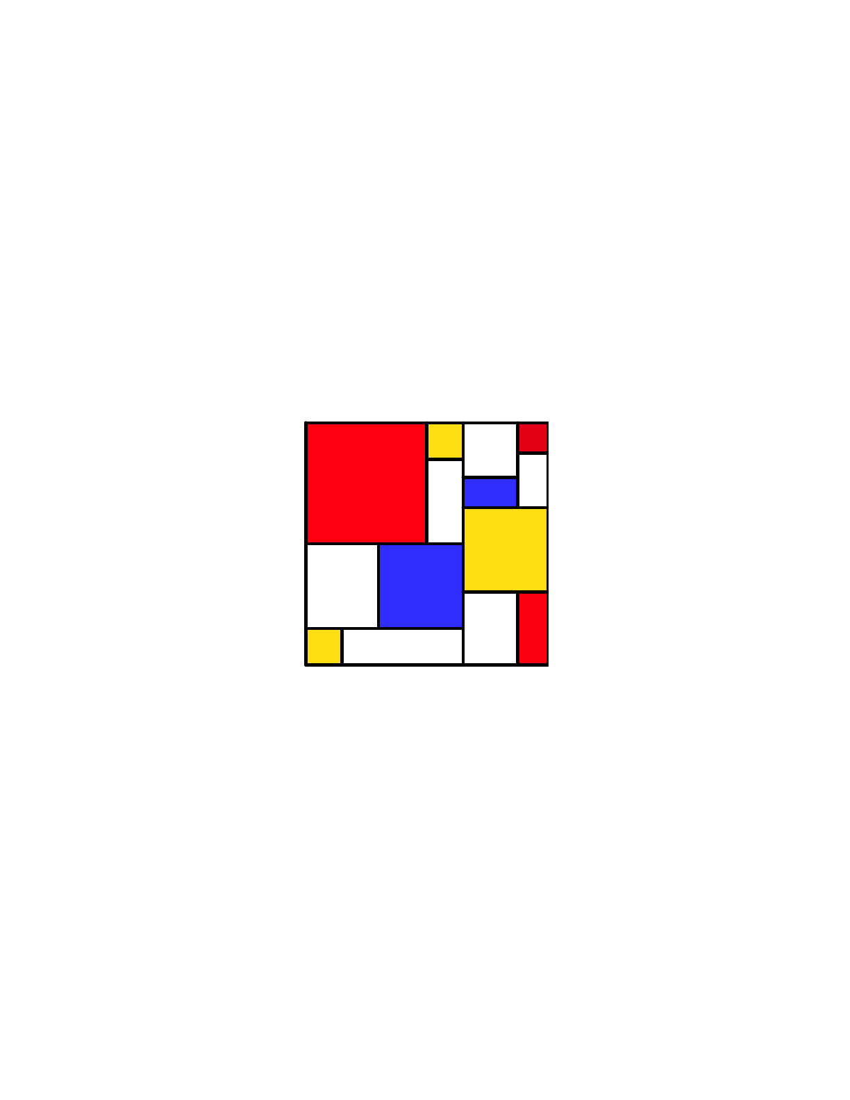
!!!!Life cycle. SLiM is based, by default, on an extended
Wright-Fisher or “WF” model with non-overlapping, discrete
generations (a non-Wright-Fisher or “nonWF” model can also
be used, as discussed in section 1.6 and chapters 15 and 20,
but that is an advanced topic that we will pass over here).
Within each generation, events occur in a fixed order (see
left). Each generation begins with the execution of user-
defined Eidos scripts called early() events. Examples of
early() events might be demographic events, such as
changes in population size, population splits, changes in
TOC I TOC II WF nonWF initialize() Genome Individual Mutation SLiMSim Subpopulation!
Eidos events fitness() mateChoice() modifyChild() recombination() interaction() reproduction() 15
1. Execution of early() events
2. Generation of offspring;
for each offspring generated:
3. Removal of fixed mutations
unless convertToSubstitution==F
4. Offspring become parents
6. Fitness value recalculation
using fitness() callbacks
7. Generation count increment
2.1. Choose source subpop
for parental individuals,
based on migration rates
2.2. Choose parent 1, based
on cached fitness values
2.3. Choose parent 2, based
on fitness and any defined
mateChoice() callbacks
2.4. Generate the candidate
offspring, with mutation
and recombination (incl.
recombination() callbacks)
2.5. Suppress/modify the
candidate, using defined
modifyChild() callbacks
5. Execution of late() events
The sequence of events within one
generation in WF models.

migration rates, etc. Offspring are then generated by drawing gametes from the parent population
according to fitness; this default mating scheme may be modified to implement non-standard
mating scenarios via user-defined mateChoice() callbacks (see chapter 11). Gametes are
generated from the genomes of the candidate parents, modified by mutation and recombination;
the standard user-defined recombination map can be modified arbitrarily for each gamete
generated using a recombination() callback (see sections 13.5 and 21.5). After offspring have
been created, their genomes can be modified according to user-defined rules using modifyChild()
callbacks (see chapter 12). After (optional) removal of fixed mutations from the model, the
offspring become the parents. Next is another opportunity for Eidos events – in this case, late()
events – to run. This is where output events, such as drawing a random sample of individuals from
the populations, would typically be specified. Fitness values are then calculated, modified by
fitness() callbacks (see chapter 9). Finally, the simulation advances to the next generation.
Tags. User-defined “tag” values can be attached to almost all of the objects defined by SLiM in
order to associate your own information with SLiM’s objects, whether short-term flags or long-term
state. Tags are used in the recipes in sections 9.4.3, 9.4.4, 10.5.2, 12.1, 13.1, and 13.3, which
provide a variety of examples of their utility. In SLiM 2.2, a dictionary-like getValue() /
setValue() mechanism was added to the Individual, SLiMSim, and Subpopulation classes (and in
SLiM 2.4, now MutationType, GenomicElementType and InteractionType too; and in SLiM 2.5,
Mutation also; and in SLiM 3.0, Substitution also). This facility provides an even broader and
more flexible way to attach model state to those objects; see the class references in chapter 21 for
details on these functions, and see the recipe in section 11.1 for an example of their use.
Continuous space. Beginning in SLiM 2.3, SLiM adds support for continuous space. If this
optional feature is enabled, individuals in SLiM maintain a spatial position – either (x), (x,!y), or
(x,!y,!z) – within their subpopulation. These spatial positions can be changed at any time
(simulating phenomena such as foraging and migration, for example), and are used to create a
spatial visualization of the subpopulation in SLiMgui. Positions can used in script in any way,
allowing models to incorporate a concept of continuous space in any way desired. In particular,
spatial positions may be used as the basis for spatial interactions between individuals (see below),
and may be used in conjunction with spatial maps that define variation in environmental variables
across continuous space. This advanced feature is first introduced in recipes in chapter 14.
Interactions. Beginning in SLiM 2.3, SLiM adds a new class, InteractionType, which can
govern interactions between individuals. Interactions can still be handled with pure Eidos code,
but the use of InteractionType automates and accelerates many common tasks, such as finding
the total interaction strength felt by an individual (as a result of competition, for example).
InteractionType can also manage spatial interactions, providing features such as interaction
strengths that vary according to distance, and handling spatial queries such as nearest-neighbor
searches. This advanced feature is first introduced in recipes in chapter 14.
Section 1.4 sketches out some practical details of how SLiM is typically used. Section 1.5
provides a more detailed overview of some of the concepts above. Section 1.6 then introduces
non-Wright-Fisher or “nonWF” models, and section 1.7 introduces tree-sequence recording; these
are both advanced topics, but it is good to be aware of the existence of these features and the
reasons why you might wish to use them. Chapter 2 provides instructions on building and
installing SLiM on various platforms. Chapter 3 gives an introduction to SLiMgui, the graphical
modeling environment provided for use on Mac OS X. The remainder of Part I of this manual, the
SLiM Cookbook, then provides “recipes” demonstrating the core concepts of SLiM. Part II of this
manual, the SLiM Reference, provides technical reference documentation for SLiM, including such
aspects as the generation cycle, the Eidos classes provided by SLiM, the various types of events and
callbacks, and the output formats supported by SLiM, beginning in chapter 19.
TOC I TOC II WF nonWF initialize() Genome Individual Mutation SLiMSim Subpopulation!
Eidos events fitness() mateChoice() modifyChild() recombination() interaction() reproduction() 16

1.4 The typical SLiM usage pattern
Before delving more deeply into the concepts introduced in the previous section, it might be
helpful to clarify how a typical user would use SLiM, in practical terms.
First of all, many or most users will use the SLiMgui modeling environment on Mac OS X for
their model development and testing, and perhaps for exploratory, non-production runs as well.
SLiMgui provides many tools for model development, such as code completion, syntax coloring,
online documentation, interactive model execution, and graphical debugging. It also makes
model development logistically simpler; there is no need to write a dispatch script, no need to
execute Unix commands in a terminal, etc. When learning how to use SLiM, it is therefore
strongly recommended that you find a Mac and use SLiMgui. Note that all of the recipes in this
manual are directly accessible in SLiMgui through the Open Recipe submenu of the File menu.
Second, many or most SLiM users will do their “production” model runs on a computing
cluster. One reason is that individual-based models often take a long time to execute; SLiM is
highly optimized, but simulating the genomic details of a large number of individuals over many
generations is inevitably slow. Another reason is that many replicate runs are typically needed;
one run of an individual-based model provides just one data point, one solitary example of what
could happen, so one usually needs to perform many runs and then use statistical methods to draw
inferences (just as one often would in field-based or lab-based research). Finally, most studies
involving individual-based modeling explore a “parameter space”, examining how the model’s
outcome depends upon the parameters of the model; each set of parameter values explored
implies another full set of replicated runs. Together, these facts mean that a single study using
SLiM might entail many years of processor time; a computing cluster is thus often needed.
For this reason, SLiM is designed to fully utilize a single processor; it is not designed to take
advantage of multiple processors using multithreading or MPI. A single run of the slim command
runs a given model a single time; to conduct the many runs that are typically needed, slim will be
run many times. This single-threaded design makes it straightforward for the user to run a separate
instance of a model on each processor on a multicore machine or a computing cluster. This can
be done manually in some cases, but is more typically done using a batch-queueing system such
as Open Grid Scheduler. Either way, some sort of a dispatch script is generally needed to schedule
each of the individual runs of slim. Because there are so many different possible ways that the
user might want to run SLiM, and so many different computing environments in which it might be
run, such a dispatch script is not provided as a part of the SLiM package; you will need to write
your own. However, this is usually extremely straightforward. It can usually be done in whatever
scripting language you prefer, from R or Python to a Bash shell script, and often just consists of a
loop over all of the parameter values and replicates desired, with a call to launch or schedule a run
of slim inside that loop. In Python, sublaunching a Unix process can be done with the
subprocess package; in R, with system() or system2(); in a Bash shell script, by just invoking
slim directly. If you are working on an institutional computing cluster, the cluster administrator
may be able to provide you with examples of dispatch scripts appropriate for that environment.
Finally, SLiM users will typically want to collect results from model runs and perform statistics
and other analyses on them. This can sometimes be done directly in the dispatch script; that script
might collect the model output and tabulate simple results as runs complete. In other cases, each
invocation of slim will be set up to produce its own output files, and then a separate analysis script
– typically written in a language like R or Python that has support for statistics and plotting – will
read in those output files, parse the relevant information out of them, and conduct the desired
analyses. In this undertaking, you are on your own. However, it is worth noting that SLiM can
generate output in some standard file formats, such as VCF and MS, and that many tools already
exist to read in and analyze such standard-format files, so in some cases you might be able to use
pre-existing software for at least some of your analysis. If your model uses tree-sequence recording
TOC I TOC II WF nonWF initialize() Genome Individual Mutation SLiMSim Subpopulation!
Eidos events fitness() mateChoice() modifyChild() recombination() interaction() reproduction() 17

(see section 1.7), you can also output a .trees file that can be read and processed in Python using
the msprime package, making many types of post-run analysis much easier (see examples in
chapter 16); indeed, this could in itself be a compelling reason to use tree-sequence recording,
since parsing output files is otherwise such an annoyance. Finally, in some cases you might want
to do some of the needed analysis inside the SLiM model, in Eidos code, to simplify the post-
processing needed. For example, if your analysis needs the number of mutations fixed at the end
of each model run, it might be simpler to count the fixed mutations inside the SLiM model, and
just output that count, than to parsing full genomic output files from each model run just to extract
the count of fixed mutations. It will be beneficial to think, up front, about how to design your
model and your analysis code so that they communicate as cleanly and simply as possible.
1.5 Conceptual overview
This section will delve into further detail on some of the concepts set out in section 1.3 (which
should be read before this section), to present a more complete picture of how SLiM works at a
conceptual level. We will not show any Eidos code here; that will be left for the recipes in the
“cookbook” that begins in chapter 4. We will, however, make reference to the Eidos classes used
by SLiM to represent various concepts, and to some of the properties and methods of those classes.
We will gloss over some minor details here in order to present the big picture as clearly as
possible; for more comprehensive information, see the SLiM Reference that begins in chapter 19.
1.5.1 Individuals and genomes
SLiM is a framework for running individual-based models; this means that every individual
organism in the model is simulated explicitly. Each individual is represented in SLiM as an
instance of the Individual class in the Eidos scripting language (see section 21.6). At the most
minimal level individuals are born and die, and in between they find mates and produce offspring
(or they reproduce by selfing or cloning); these actions are built into SLiM. If optional extensions
to SLiM are enabled (using the initializeSLiMOptions() function; see section 21.1), SLiM can
also keep some pedigree information regarding individuals (up to the grandparental level), and can
keep track of the spatial positions of individuals on a landscape. In more complex models
individuals may also do things like gather resources, learn things, interact with other individuals,
be subject to events that alter their state, and exhibit behavior; these actions are not built into
SLiM, but may easily be implemented in Eidos script.
Perhaps most importantly, since SLiM models genetically explicit simulations, individuals
contain genetic information. Individuals in SLiM are diploid; each individual thus possesses two
homologous chromosomes (or one X and one Y chromosome, if sex chromosomes are being
simulated), referred to as the genomes of that individual. (It is possible to model more than one
chromosome in SLiM, conceptually, but this is done by using a recombination map that specifies
free recombination at particular positions, effectively subdividing the chromosome into unlinked
sub-chromosomes; see, e.g., section 13.1.) Each of the two genomes of an individual is
represented using an instance of the Genome class in Eidos (see section 21.3).
A genome is essentially a container that holds a set of mutations. If both of an individual’s
genomes contain exactly the same mutation (a surprisingly subtle concept, which will be defined
rigorously in the next subsection), the individual is homozygous for that mutation; if a given
mutation is contained in only one of the two genomes, the individual is heterozygous for that
mutation. Note that SLiM does not model nucleotides explicitly (although it is possible to layer a
concept of nucleotides on top of SLiM, in script; see section 13.12), but it does model explicit,
discrete base positions along the genome.
TOC I TOC II WF nonWF initialize() Genome Individual Mutation SLiMSim Subpopulation!
Eidos events fitness() mateChoice() modifyChild() recombination() interaction() reproduction() 18
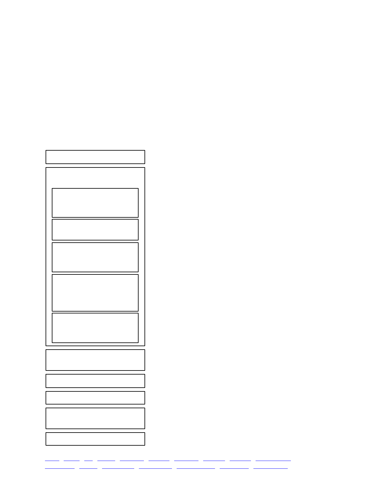
The overall picture, then, looks like this:
Each yellow square represents one individual. Each individual contains two genomes; and each
genome contains the state of all of the base positions along the chromosome, from beginning
(position 0) to end (position L−1, so that the chromosome is of length L). Each base position is
represented here as an empty box, and all of the boxes from 0 to L−1 together represent a genome.
A key concept in SLiM is that genomes begin, by default, as empty: they contain no mutations
and no genetic information. This can be thought of as the “wild type”, in a sense, and we will
refer it to in that way sometimes in what follows, but it does not have to represent the wild-type
state of the organism you are modeling. Instead, it simply represents the base, un-mutated state of
individuals, whatever you want to consider that to be. All mutations in SLiM can be thought of as
modifications that are layered on top of this empty base state. The base state can also be thought
of as “neutral”, in terms of fitness, but it does not have to actually be neutral (i.e., 1.0) in absolute
fitness. Instead, the base state can have any absolute fitness value you like – but in general that is
unimportant, since SLiM’s core engine is only concerned with relative fitness (in WF models, the
default mode of operation, which we will limit ourselves to in this discussion). When the
simulation begins, and all genomes are empty, it does not matter to SLiM what the absolute fitness
of those empty genomes is; since they all have the same absolute fitness, they all have a relative
fitness of 1.0, and that is what matters to SLiM. The fitness effects of mutations then modify those
relative fitnesses, multiplicatively.
You can, of course, set up your simulation to begin with whatever mutational state you want;
even more commonly, a simulation will begin with a “burn-in” period that establishes an
equilibrium level of genetic diversity through mutation–selection–migration balance before the
more interesting part of the simulation begins. It is important to understand that such genetic
diversity is always built on top of empty chromosomes in SLiM, however. In general, if two
mutations are segregating at a given base position, there are effectively three alleles in the
population at that base position: the first mutation, the second mutation, and what you could think
of as the “wild-type allele” represented by the absence of either of those mutations. In script, you
could force a mutation to exist at every base position in every genome, so that there are no empty
positions in any of the genomes in your simulation; if you do so, however, you will find that your
simulation then runs quite slowly, since SLiM is having to track and manage all of those mutations,
so such a strategy is usually undesirable.
Learning to let go of the idea of chromosomes filled with genetic information at every position
(as would be the case in a nucleotide-based model) and think instead in terms of mutations layered
on top of the empty “wild-type” state is an essential conceptual leap to make in using SLiM. To
move from one conceptual model to the other, imagine the “wild-type” nucleotide sequence for
your study organism: some specified sequence of A, T, G, and C. Whatever that sequence might
be, it is represented in SLiM by the absence of any genetic information at all: empty chromosomes.
SLiM tracks only mutations on top of that sequence: SNPs, in the nucleotide-based paradigm. But
any individual that does not possess a SNP at a given location instead possesses the “wild-type”
nucleotide, conceptually – represented in SLiM by an empty base position.
TOC I TOC II WF nonWF initialize() Genome Individual Mutation SLiMSim Subpopulation!
Eidos events fitness() mateChoice() modifyChild() recombination() interaction() reproduction() 19
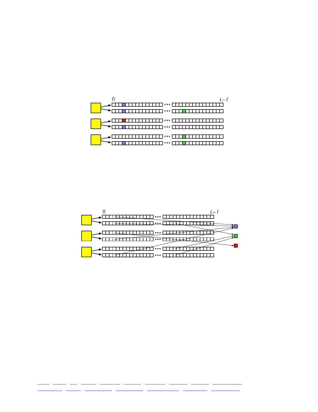
1.5.2 Mutations and substitutions
With the foundation of individuals and genomes laid by the previous section, let’s now explore
the idea of mutations in SLiM in more detail. In SLiM, a mutation is an instance of class Mutation
in Eidos (see section 21.8). A mutation has various properties – its base position and its selection
coefficient, most importantly. In SLiM, the multiplicative fitness effect of a mutation with selection
coefficient s is 1+s for a homozygote; in a heterozygote it is 1+hs, where h is the dominance
coefficient (kept by the mutation type; see section 1.5.4). Let’s update our conceptual schematic to
include some mutations:
This simulation has three mutations, represented here with blue, red, and green. At position 3,
the first individual is homozygous for the blue mutation, the second individual is heterozygous for
red and heterozygous for blue, and the third individual is heterozygous for blue (the other allele in
that individual being the empty “wild-type allele” as discussed above).
An important concept to absorb is that the genomes that contain the blue mutation do not just
contain their own particular copies of blue-mutation-type information; they actually contain
references to the very same shared blue-mutation object. A more accurate conceptual diagram
might therefore look like this:
Since that is quite difficult to interpret visually, we will stick with showing mutations as residing
inside genomes; but you should always keep in mind that mutations are really shared objects. A
new mutation object is created either (1) when a random mutation event occurs in SLiM (as
governed by the overall mutation rate set for the simulation), or (2) when requested by the
simulation script with the addNewMutation() or addNewDrawnMutation() methods of Genome (see
section 21.3.2). In both cases, these events always create a new mutation object, even if a
mutation with exactly the same properties – position, selection coefficient, etc. – already exists in
SLiM. In our conceptual diagram above, the blue and red mutations might be identical in every
detail; they are nevertheless considered to be different mutations by SLiM, and will be tracked
separately and never merged into a single identity. You can think of this as representing a
mutational lineage, a sort of identity by descent; the red and blue mutations might represent the
very same SNP, but they arose due to separate mutational events, and thus they seeded separate
mutational lineages.
This distinction becomes particularly important when you ask whether two genomes contain
“the same mutation” – if you ask, for example, whether a given individual is heterozygous or
homozygous for a given mutation. The second individual in the diagram is heterozygous for blue
TOC I TOC II WF nonWF initialize() Genome Individual Mutation SLiMSim Subpopulation!
Eidos events fitness() mateChoice() modifyChild() recombination() interaction() reproduction() 20
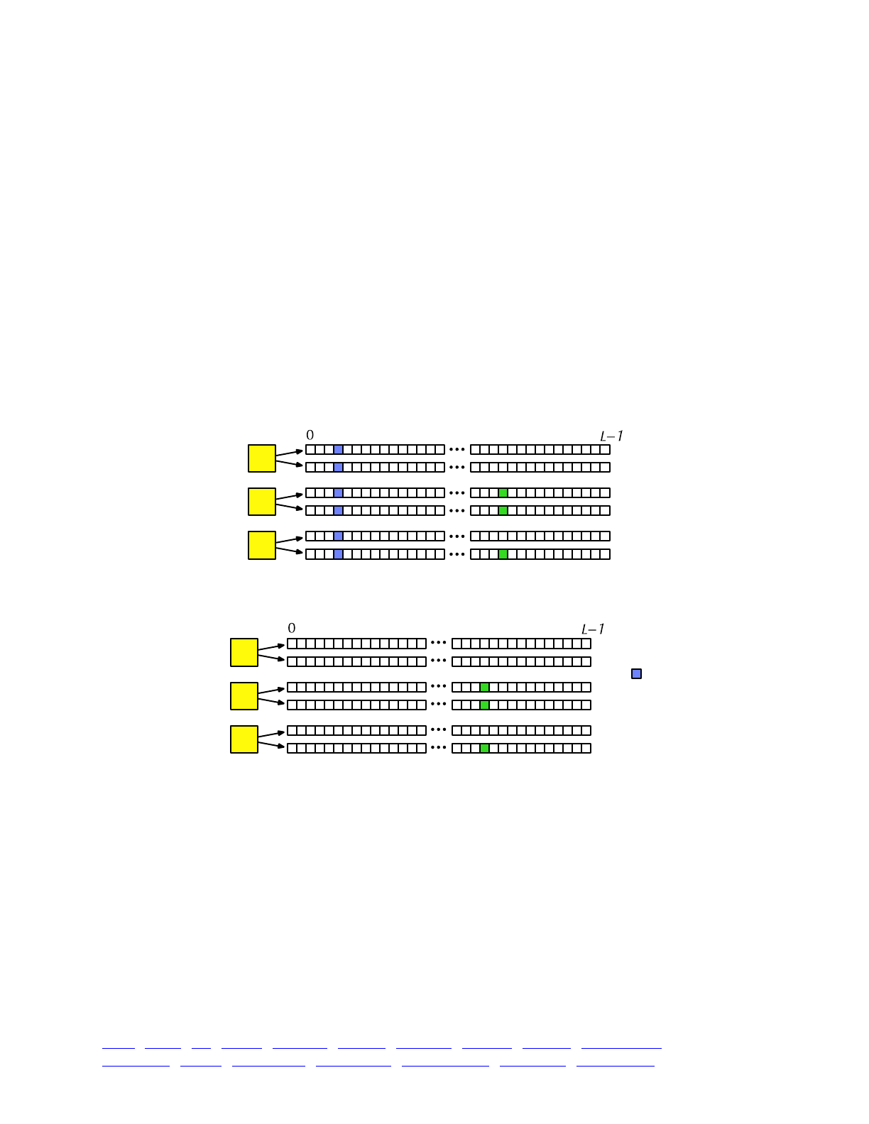
and heterozygous for red; even if the blue and red mutations are identical, the individual is not
considered by SLiM to be homozygous. If the fitness effects of these mutations entail a dominance
effect, this could be important – the fitness effect of being red/blue would then be different from
the fitness effect of being red/red or blue/blue. Often this can be ignored; if mutations are neutral
then dominance doesn’t matter, and if mutational effects are drawn from a distribution of fitness
effects then in general no two new mutations will be the same anyway. However, if some
mutations in a simulation use a fixed, non-neutral fitness effect with dominance then this might
become important; this could be important in some soft-sweep models, for example. In such
cases, you may wish to ensure that all references to identical mutations are transmuted into
references to the same object, maintaining a single mutation for all lineages (see, e.g., section
13.12). When new mutations are being introduced in script, rather than by SLiM, you can ensure
that an existing mutation object is used by using the addMutations() method of Genome (see
section 21.3.2), which adds already existing mutations to a genome instead of creating new
mutation objects (and thereby new mutational lineages).
Another key concept involving mutations is that by default, mutations are removed from the
simulation when they become fixed. Suppose that, after mate choice and biparental mating, the
next generation of our conceptual diagram looked like this:
This state will never be visible to the simulation script, because at the end of offspring
generation it will be replaced by this state instead:
The fixed mutation has been removed from the simulation and stored as a “substitution” object
(represented here by the blue square to the right). This substitution object will be kept by SLiM
forever, to remember the fixed mutation, and this substitution object is available to the script; but
the mutation is no longer contained by the genomes of each individual, and it no longer influences
SLiM’s fitness computations. This is usually a good idea, because it allows SLiM to run much faster
than it otherwise would; without removal of fixed mutations, simulations would slowly bog down
under the weight of more and more accumulated fixed mutations. It is also usually safe, since a
mutation that is possessed by every individual will usually have an effect on absolute fitness but
not on relative fitness – since its multiplicative fitness effect is the same in every individual, it can
be neglected. However, simulations that involve epistasis, or that otherwise depend upon
mutations in ways that go beyond their direct effect on relative fitness, may wish to disable this
automatic conversion for the mutations involved in such effects; this can be done easily in SLiM
using the convertToSubstitution property (see section 21.9.1).
TOC I TOC II WF nonWF initialize() Genome Individual Mutation SLiMSim Subpopulation!
Eidos events fitness() mateChoice() modifyChild() recombination() interaction() reproduction() 21
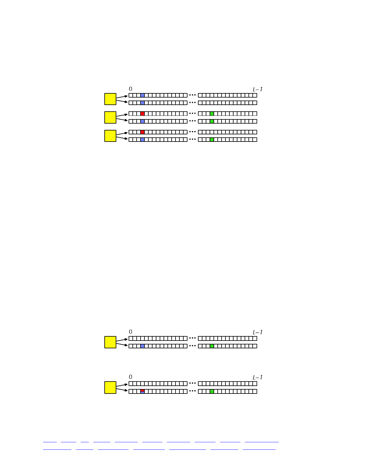
The above ideas, about the distinct identity of each mutational lineage and the way that fixation
is defined in SLiM, combine in a way that is worth mentioning since it might be unexpected.
Suppose that there are two mutations, blue and red, segregating at base position 3, as above, and
suppose further that these mutations are identical in every detail but arose separately, as described
above. Finally, suppose that the population reaches this state:
It might be natural to suppose that the mutations at position 3 would be considered to have
fixed, and would be removed, as above, given that they are all identical and merely represent
independent mutational lineages of what you might think to be the same mutation. As above,
however, this is not how SLiM thinks! Since the blue and red mutations are different mutation
objects, neither is considered to have reached fixation; fixation in SLiM occurs when a specific
mutation reaches a frequency of 1.0, without any consideration for other identical mutations
segregating in the population. In a scenario like this, such as a soft-sweep model, if you want
fixation of independent mutational lineages to be detected you will need to either merge the
independent lineages yourself in script, as described above, or simply detect fixation yourself
directly. You could detect fixation by checking that every genome in the model contains an
appropriate mutation (either red or blue, in this case), or by summing the counts of all of the
appropriate mutations in the population to confirm that the total count is equal to 2N (where N is
the population size and the constant factor of 2 accounts for diploidy). (You might be inclined to
sum the mutation frequencies instead and compare to 1.0, but this strategy is vulnerable to
floating-point roundoff error, so it is not advisable.) This is all simpler than it sounds; the soft-
sweep recipes in sections 10.5 provide some examples of this.
1.5.3 Mutation stacking
There is one more key concept about mutations in SLiM to consider, and it is this: by default, a
given base position in a given genome may actually contain more than one mutation – indeed, it
may contain an arbitrarily large number of mutations. This is referred to as “mutation stacking”;
the multiple mutations at a single base position in a given genome are referred to as being
“stacked”. For example, imagine that this individual exists in a SLiM simulation:
And then imagine that a new mutation, which we will show as red, occurs at the same position,
in the same genome, where the blue mutation already exists. By default, here is what will happen:
The red mutation has stacked on top of the blue mutation; both mutations now exist at that
position in that genome. This does not fit terribly well into the concept of “genotype” – SLiM does
not really think in terms of genotypes. You could perhaps say that the genotype of this individual is
something like “wild/red-blue”, if you wished, where “red-blue” is the allele created by the
TOC I TOC II WF nonWF initialize() Genome Individual Mutation SLiMSim Subpopulation!
Eidos events fitness() mateChoice() modifyChild() recombination() interaction() reproduction() 22
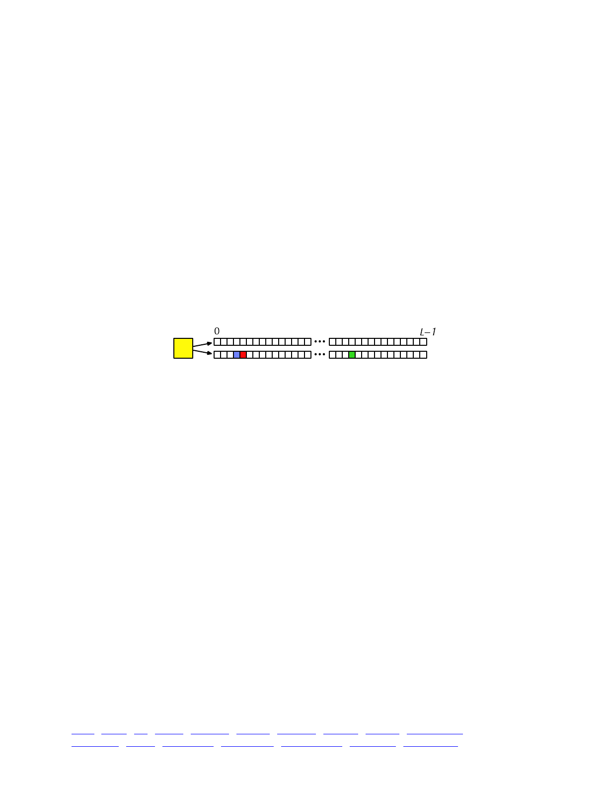
stacking of a red and a blue mutation together at the same locus. SLiM, however, just thinks in
terms of the mutations actually possessed by each genome, so in SLiM’s terms, rather than talking
about genotype, we would simply say that the individual is wild-type (i.e., empty) at the given
position in one genome and has a red mutation and a blue mutation at that position in the other
genome. We could also say that the individual is heterozygous for red and heterozygous for blue;
that is true, but is a bit ambiguous since the same would be said of a red/blue heterozygote that
had a red allele in one genome and a blue allele in the other; unless the red and blue mutations
are epistatic, however, that distinction is probably unimportant. Note that further mutations at the
same position could occur as well, and would stack on top of those already present, making all
this even more complex. Probably the simplest thing is to learn to think in the same terms in
which SLiM thinks: which mutations are present in which genomes.
This behavior of SLiM is perhaps quirky, but usually harmless. It is not common for mutations
to end up stacked in practice, since normal mutation–selection balance in finite populations
usually clears out genetic diversity quickly enough that it is unusual for a new mutation to occur
right on top of another mutation that is still segregating in the population. Furthermore, when
mutations do occasionally stack, it is usually not important to the dynamics of the model; in most
cases the resulting behavior is identical, for practical purposes, to if the new mutation had
occurred at an immediately adjacent base position instead, which would result in the two
mutations being extremely tightly physically linked rather than actually being stacked:
In principle these mutations could be separated by recombination, whereas the stacked
mutations cannot be, but in practice that is unlikely enough that it will probably not make a
difference to the model’s dynamics. It is therefore important to understand that SLiM works in this
way, but in most cases models do not need to concern themselves with stacking.
However, there are cases where it does present problems. If you want to simulate actual
nucleotides (see section 13.12), for example, then each base position must be unambiguously
either A, T, G, or C; it makes no biological sense for an A and a G to be “stacked” at a single
position. Similarly, if you want to make a quantitative-genetics model with particular discrete
quantitative effects for the alleles at each QTL (see section 13.1), such as a −1/0/+1 allelic system,
you would not want mutation stacking to occur since stacking of more than one mutation at a
given QTL would violate your design. The default mutation stacking behavior may therefore be
modified, and indeed, the two example recipes cited above do so.
The stacking behavior of mutations is governed by their mutation type, a concept we haven’t yet
discussed. All mutations in SLiM belong to a mutation type, represented by the Eidos class
MutationType (section 21.9). Mutation types are important primarily because they dictate the
distribution of fitness effects from which mutations are drawn; all of the mutations of a given
mutation type might be neutral, for example, or they might be deleterious and drawn from a
gamma distribution, for example. When a new mutation is generated by SLiM, the selection
coefficient for the mutation is drawn from the distribution specified by the relevant mutation type,
as will be discussed in detail in section 1.5.4. Simulations may define as many mutation types as
desired, but most simulations contain just one or a few mutation types.
Besides defining the distribution of fitness effects from which mutations are drawn, mutation
types define a few other behaviors for mutations too. For example, the convertToSubstitution
property mentioned in section 1.5.2, which determines whether a mutation will be removed when
it fixes, is actually a property of MutationType, not of each individual mutation, since it makes
TOC I TOC II WF nonWF initialize() Genome Individual Mutation SLiMSim Subpopulation!
Eidos events fitness() mateChoice() modifyChild() recombination() interaction() reproduction() 23
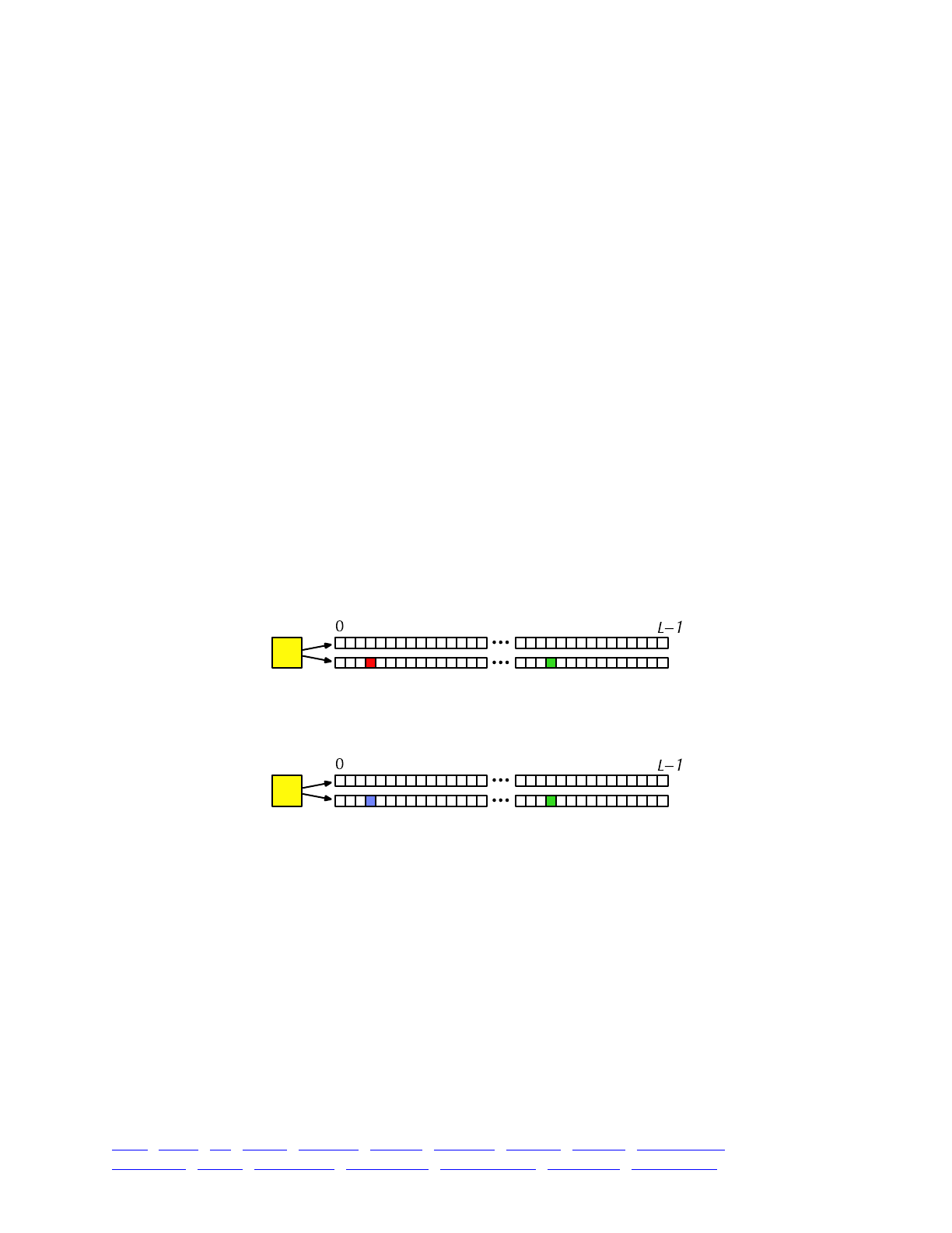
sense for this behavior to be uniform across each class of mutations. The dominance coefficient of
mutations is also a property of the mutation type, not individual mutations, for the same reason.
For our discussion of mutation stacking here, however, mutation types are important because
stacking behavior is controlled by the mutationStackGroup and mutationStackPolicy properties of
MutationType (see section 21.9.1); all of the mutations of a given mutation type follow the same
stacking policy. In fact, more than one mutation type can be joined together into a single
“mutation stacking group” using mutationStackGroup, and then all of the mutations in that
stacking group follow the same policy. This is a power-user feature that we will mostly gloss over
for the rest of the discussion here, however; we will just assume that each mutation type
constitutes a separate stacking group (which is the default behavior).
Given this, in the example above the red mutation needs to be of the same mutation type (or in
the same stacking group) as the blue mutation before stacking can be prevented. If they are not of
the same mutation type (or more precisely, not in the same stacking group), then they will stack,
regardless of what stacking policy has been set for each mutation type. The idea is that you
generally don’t want different kinds of mutations to interfere with each other in a model. If a QTL
mutation exists at a given position, for example, then you might want a new QTL mutation at the
same locus to replace the old one, rather than stacking – but if a neutral mutation occurred at the
same locus, you would certainly not want that neutral mutation to replace the existing QTL
mutation! Whatever you might think of that argument, you can always modify it by placing all of
your mutation types into a single stacking group.
So let’s now assume that the red and blue mutations are in the same stacking group – of the
same mutation type, most trivially. Now the stacking policy can be modified. The default policy is
referred to as type "s" (for “stack”), and yields the stacked result we saw above. Instead, you can
set the policy to type "l" (for “last”), which produces this result after the red mutation occurs:
The red mutation has replaced the mutation in this genome, because this stacking policy
dictates that the last mutation at a given position should be kept. This is the common alternative to
the "s" policy, but you can also set a policy of "f" (for “first”) which produces this result:
Here the red mutation has simply been thrown away, because the blue mutation was there first.
The post-mutation state is therefore identical to the pre-mutation state (note that this means the
effective mutation rate will be lower than the requested mutation rate, since some mutations will
be suppressed). In general, this policy retains the first mutation at a given position in a given
genome; new mutations are only allowed in if the position is presently empty. This is less
commonly used, since its biological motivation is unclear, but it is provided as an option in SLiM
just in case it is called for in some unusual situation.
Note that all three stacking policies – "s", "l", and "f" – depend only upon the existing
mutation(s) at the specific base position in the specific genome where a new mutation is occurring.
The state at other positions, or in other genomes, is completely irrelevant. Changing the mutation
stacking policy is not a way to prevent more than one allele from existing in a population at a
given locus; it is only a way to prevent more than one mutation from existing in one genome at a
given locus. Suppose, in our ongoing example, that the new red mutation had occurred in the
other genome of the individual instead; regardless of the stacking policy, the result would then be:
TOC I TOC II WF nonWF initialize() Genome Individual Mutation SLiMSim Subpopulation!
Eidos events fitness() mateChoice() modifyChild() recombination() interaction() reproduction() 24
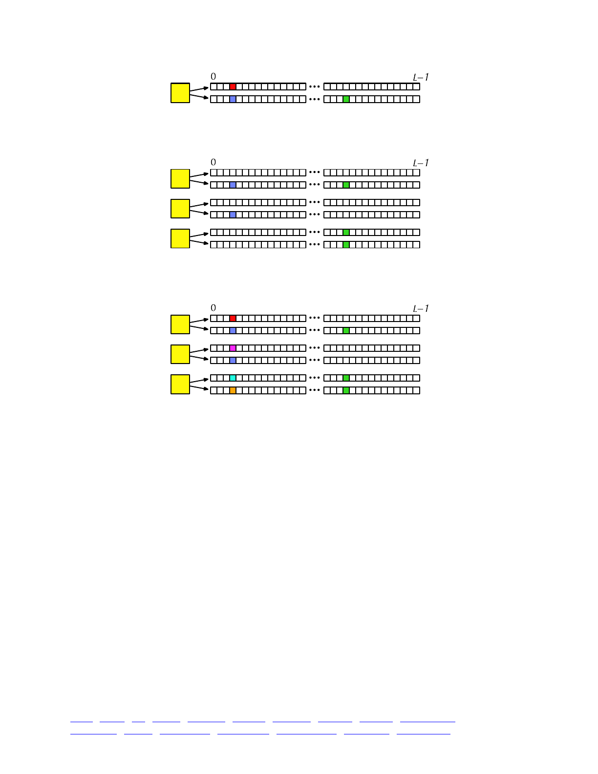
That base position in that genome was empty; the stacking policy is therefore irrelevant, since
there is no pre-existing mutation to stack on top of, so the red mutation is always added. More
generally, suppose we have a population of three individuals, with a few mutations:
Different new mutations could occur at each of the empty sites at base position 3, regardless of
the stacking policy. So whether the stacking policy is "s", "l", or "f", new mutations could easily
lead to this state:
If the stacking policy were "f", further new mutations at position 3 beyond this could not be
introduced; now that every genome has a mutation at position 3, those pre-existing mutations
would prevent the new mutations from being added. Under stacking policy "l", new mutations
would still be possible at position 3 even in this state; the new mutations would just replace the
old mutations. Under policy "s", the new mutations would stack, the default behavior.
Sometimes it is desirable to allow for the possibility of back-mutation in a model. This can be
accomplished in several ways in SLiM. One way is to use a mutational distribution of fitness
effects that provides only a limited set of possible values (perhaps four values, to represent the four
possible nucleotide at a base position), and use type "l" stacking so that new mutations replace
existing mutations; new mutations are then automatically sometimes back-mutations. See section
13.12 for an example of this sort of strategy. Another possibility, if you only need back-mutation to
the “wild type” empty-genome state, is to remove existing mutations yourself, in script; if done
with the appropriate probability, this could simulate back-mutation to the wild type.
Finally, note that the stacking policy is applied to new mutations introduced in script, as well as
to new mutations added by SLiM as a result of the overall mutation rate. New mutations that you
add will be allowed to stack unless you change the stacking policy; and conversely, if you change
the stacking policy then new mutations that you add might result in the removal of pre-existing
mutations, or might not be added at all, in accordance with the policy you have chosen. However,
when the stacking policy is changed in mid-run it is not retroactively enforced upon existing
mutations, and when a saved population is loaded the current stacking policy is not enforced upon
the individuals loaded.
The issue of mutation stacking is a bit complicated and confusing; if the discussion above has
left you with more questions than answers, rest assured that this is an advanced topic that generally
TOC I TOC II WF nonWF initialize() Genome Individual Mutation SLiMSim Subpopulation!
Eidos events fitness() mateChoice() modifyChild() recombination() interaction() reproduction() 25
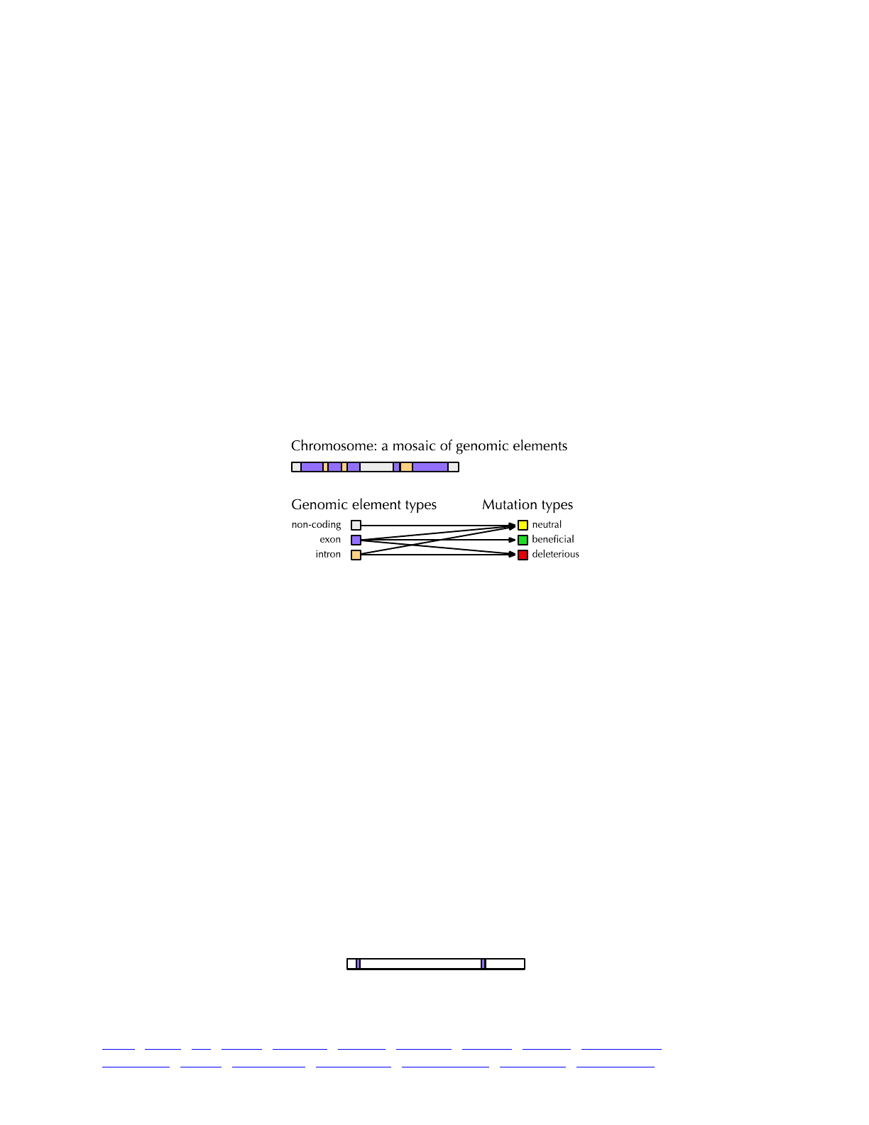
does not impact simple models at all. Play around with SLiM for a while, and then when you
revisit this section it will probably make much more sense.
1.5.4 Genomic elements, genomic element types, mutation types, and the chromosome
SLiM allows you to model complex chromosomes with genomic regions that have different
mutational effects. For example, exons would be expected to sustain beneficial, deleterious, and
neutral mutations, whereas introns might sustain only deleterious and neutral mutations, and non-
coding regions might only allow neutral mutations. You set up this structure in SLiM using a
hierarchical configuration: the chromosome (class Chromosome, section 21.2) contains genomic
elements (class GenomicElement, section 21.4), which are each of a given genomic element type
(class GenomicElementType, section 21.5), and each genomic element type draws new mutations
from a weighted set of mutation types (class MutationType, section 21.9), each of which specifies a
distribution of fitness effects for that type of mutation. In an exon/intron/non-coding model, for
example, each type of genomic region – “exon”, “intron”, and “non-coding” – would be a
genomic element type, and the chromosome would be a mosaic of genomic elements using these
three genomic element types. Each of these genomic element types would draw its mutations from
a different set of mutation types – perhaps “beneficial”, “deleterious”, and “neutral”, in this case.
In practice, that might look something like this:
Here the chromosome contains two genes, each of which is composed of an alternation of
exons and introns, and non-coding regions are interspersed around the genes. Those regions along
the chromosome are defined by genomic elements, which reference the three genomic element
types defined here (non-coding, exon, and intron). Those three genomic element types each
utilize some subset of the mutation types that have been defined here (neutral, beneficial, and
deleterious). Although this diagram simply shows arrows from genomic element types to mutation
types, there are in fact weights associated with the mutation types of a given genomic element
type; in this case, you might specify that 90% of mutations within introns are neutral and 10% are
deleterious, by giving those weights to SLiM when the intron genomic element type is configured.
In this way, new mutations that are automatically generated by SLiM will have appropriate fitness
effects depending upon the genomic region in which they occur.
Note that this example is entirely arbitrary; you can define whatever mutation types, genomic
element types, and genomic elements you wish. You could make your chromosome entirely
neutral, or you could model the specific mutational effects of each region in an empirical genome
map, right down to the full level of detail known for your study organism. There is no practical
limit to the number of mutation types and genomic element types you may define. In the opposite
direction, you can also make a much simpler model than the one above. Not all of the
chromosome needs to be assigned to a genomic element; much of the chromosome can simply be
empty. For example, you could make a model of epistatic interactions between two loci with a
chromosome like this:
Here most of the chromosome is empty, containing no genomic elements. No mutations will
be generated in these regions, since mutation generation in SLiM is governed by genomic
TOC I TOC II WF nonWF initialize() Genome Individual Mutation SLiMSim Subpopulation!
Eidos events fitness() mateChoice() modifyChild() recombination() interaction() reproduction() 26
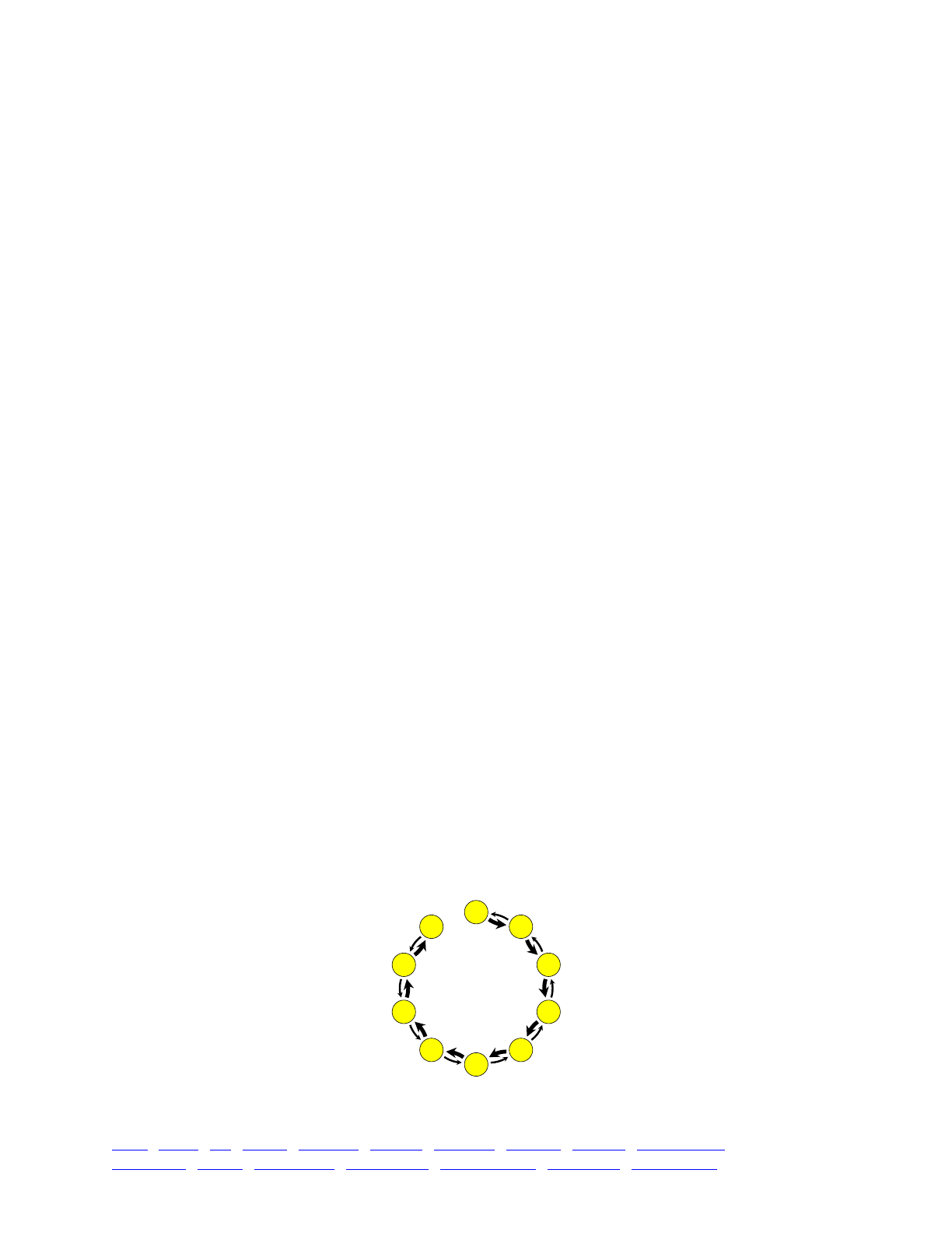
elements. Only the purple loci will be active; we have one genomic element type and one
mutation type in this model, and quite possibly only two mutations (one at each locus). A simple
genetic structure like this will often run much faster in SLiM than simulating a whole chromosome;
if you are not interested in what is going on in some regions of the chromosome, just don’t
simulate it. The only limitation in setting up your chromosome structure in SLiM is that genomic
elements must be non-overlapping.
Note also that in general, this chromosomal structure only influences the way that SLiM
generates new mutations. When offspring are generated, the overall mutation rate is used to draw
the number of mutations that have occurred in a given gamete. The position of each mutation is
then drawn, and SLiM determines which genomic element the mutation falls within. Given that,
SLiM can find the genomic element type, and it then chooses a mutation type from the weighted
set of mutation types used by that genomic element type. Finally, knowing the mutation type for
the mutation, it draws a selection coefficient from the distribution of fitness effects for that
mutation type. That yields a new mutation object, which is placed in the gamete. That is the only
time that SLiM uses the genomic elements and genomic element types you have defined; none of
the other machinery inside SLiM’s core cares about those constructs at all. You may consult the
chromosomal structure in your script and use it in whatever way you wish, but doing so would be
quite unusual. By and large, the behavior of SLiM simulations depends upon the mutations
contained by the genomes of individuals, without reference to the chromosomal structure after the
point when new mutations are created.
Mutation types, however, do continue to be used, in a minimal fashion, as we saw in section
1.5.3; each mutation knows its mutation type, and some properties of mutations, such as their
dominance coefficient, their stacking behavior, and their fixation behavior, are specified by their
mutation type.
1.5.5 Subpopulations and migration
The previous section discussed hierarchy levels from the individual to the genome to the
mutation, and the dependence of mutations upon mutation types, genomic element types,
genomic elements, and ultimately the chromosome itself. However, there are also higher
hierarchy levels: individuals live within subpopulations, and all of the subpopulations together
exist within the whole modeled population.
Subpopulations are represented by the class Subpopulation in Eidos. A subpopulation is a set
of individuals, and is characterized primarily by the fact that random mating occurs (weighted by
individual fitness) within each subpopulation. In other words, subpopulations primarily influence
reproductive isolation; each subpopulation is internally panmictic (again, weighted by individual
fitness), but externally isolated. Migration rates can be configured between subpopulations in
order to allow gene flow, but by default the migration rate among subpopulations is zero.
For example, one might have a population structure like this:
p1
p2
p3
p4
p5
p6
p7
p8
p9
p10
TOC I TOC II WF nonWF initialize() Genome Individual Mutation SLiMSim Subpopulation!
Eidos events fitness() mateChoice() modifyChild() recombination() interaction() reproduction() 27

Here we have ten subpopulations linked into a “stepping-stone” model that might represent a
river system; subpopulation p1 is upstream, and relatively high levels of migration produce gene
flow in the downstream direction, while much lower levels of migration exist in the upstream
direction (as shown by the relative widths of the arrows). This is just an example; you can have as
many subpopulations as you wish, linked by any pattern of migration. The effect of the population
structure on SLiM will manifest in the pattern of reproductive isolation among individuals.
The details of this conceptual model can be important. Offspring are always generated by
parents within a single subpopulation; parentals do not migrate between subpopulations for the
purposes of mating (in WF models, to which we are still limiting this discussion; see section 1.6).
Instead, migration occurs at the juvenile stage in SLiM; generated offspring are placed into
particular subpopulations in accordance with the specified migration rates. SLiM allows you to
define spatial simulations involving one-, two-, or three-dimensional landscapes for each
subpopulation; again, even in such spatial models, panmixis (weighted by individual fitness) is the
default, although effects like spatial competition and spatial mate choice preference may be added
in script. The subpopulation is the fundamental unit of reproductive isolation in SLiM.
An important conceptual point is that when setting the size of a subpopulation in SLiM, this
should be thought of as a request for a future change, not as a present-time change. If a
subpopulation contains 800 individuals and the script requests that it be 900 or 700 instead, that
change does not happen immediately (which individuals would be removed? how exactly would
the new individuals be created – with what genetic state?); instead, the subpopulation size change
is a request that will take effect in the next generation. That is, when offspring are generated, 900
or 700 offspring will be generated from the current subpopulation of 800, and the requested
subpopulation size will thus take effect in the child generation. This is always the case in SLiM;
there is actually no straightforward way to create new individuals or kill existing individuals within
a single generation (although the fitness of an individual can be set to zero, which has much the
same effect as killing it, all else being equal).
Another key concept is that zero-size subpopulations do not exist in SLiM. If a subpopulation is
set to size zero, it will (in the child generation) cease to exist entirely. For this reason, a new
subpopulation cannot be created with a size of zero, since that has no meaning in SLiM. Instead,
you should create the new subpopulation with a non-zero size at the moment that its size grows
above zero. This can be inconvenient in metapopulation models that involve dynamic local
extinction and re-colonization; such models are better written as nonWF models, which follow
very different rules (see section 1.6, and section 15.5 for an example of a nonWF extinction/
recolonization model).
1.5.6 Other concepts
That completes our overview of the foundational concepts underlying SLiM. There is a lot more
to SLiM that will be covered in the following chapters, but if you understand these fundamental
ideas the rest should be fairly straightforward.
Other sections of this manual also provide important conceptual information. Section 1.3
contains a brief introduction to some other key SLiM concepts that did not merit an in-depth
discussion here, such as fitness, the life cycle, continuous space, interactions, and tags; it would be
good to read now, if you haven’t already. Part II of this manual, the SLiM Reference, also has some
conceptual sections; chapter 19 contains detailed information on the stages of the generational life
cycle in SLiM for WF models (and chapter 20, for nonWF models), including details on how mate
choice, migration, offspring generation, fitness calculation, and other stages are implemented, and
chapter 22 describes how to modify those default life cycle stages through the use of several
different types of scripted callbacks, which provides much of the power and flexibility of SLiM.
Reading those chapters might be deferred until you have become more familiar with SLiM,
TOC I TOC II WF nonWF initialize() Genome Individual Mutation SLiMSim Subpopulation!
Eidos events fitness() mateChoice() modifyChild() recombination() interaction() reproduction() 28

however, as they are more technical; if you are a beginning SLiM user, it is recommended that you
finish reading this chapter and then proceed with installing SLiM and begin experimenting with the
recipes presented in the chapters that follow.
1.6 Wright-Fisher (WF) versus non-Wright-Fisher (nonWF) models
SLiM 1.x and 2.x supported only one type of model, Wright-Fisher models (henceforth referred
to as WF models). In SLiM 3.0, support has been added for a second type of model, non-Wright-
Fisher models (henceforth, nonWF models). The choice between these types of models is made
with an optional initialization call, initializeSLiMModelType(); if no call to that function is made,
the WF model type is used by default, providing complete backward compatibility with SLiM 2.x.
Use of the nonWF model type is an advanced topic, recommended only for users experienced
with SLiM. Most of this manual will be about the default WF model type. Only three areas of this
manual will discuss nonWF models: section 1.6 (e.g., this section, which summarizes the
differences between WF and nonWF models), chapter 15 (which introduces nonWF models in
more detail, and then presents nonWF model recipes), and the SLiM Reference (Part II of this
manual).
The differences between WF and nonWF models are pervasive, but may be regarded as falling
into a few major categories:
• Age structure. In WF models, generations are discrete and non-overlapping. Each “tick”
of SLiM’s generation counter is associated with the creation of a new offspring generation
and the demise of the previous parental generation. There is thus no concept of the age of
an individual, since all individuals live for a single “tick”. In nonWF models, generations
may instead be overlapping. Each “tick” of SLiM’s generation counter is associated with
the opportunity for creation of new offspring and the opportunity for mortality among
existing individuals. SLiM keeps track of the age of individuals, which may live for many
“ticks”. This makes it simple to construct models of overlapping generations with any type
of age structure and any age-related behaviors desired.
• Offspring generation. In WF models, offspring are generated automatically by SLiM each
generation. This process may be modified by various callbacks, but the process itself –
how many offspring to generate, from which parental individuals, into which
subpopulations – is managed by SLiM in such a way as to “fill out” each subpopulation
with a fresh batch of offspring while satisfying the constraints imposed by parameters such
as subpopulation size, sex ratio, cloning rate, and selfing rate. In nonWF models,
offspring are instead generated in response to a request from the model script, made in a
reproduction() callback, and the script itself is in charge of managing the process. In
nonWF models, SLiM no longer attempts to enforce any particular subpopulation size, sex
ratio, cloning rate, or selfing rate; typically, these are instead emergent properties of the
individual-based dynamics of the model. This approach is somewhat more complex, but
allows the genetics and state of each individual to influence the way that individual
reproduces – its expected litter size, its reproductive behavior (cloning, selfing, biparental
mating), the sex of its offspring, and so forth.
• Population regulation. In WF models, population regulation (keeping population size
within bounds) is managed automatically by SLiM, which keeps each subpopulation at the
initial size it is given, or at whatever new size is set by a setSubpopulationSize() call.
Subpopulation size is therefore a parameter of the model, in effect. In nonWF models,
TOC I TOC II WF nonWF initialize() Genome Individual Mutation SLiMSim Subpopulation!
Eidos events fitness() mateChoice() modifyChild() recombination() interaction() reproduction() 29

population regulation is instead an emergent property, a side effect of how many offspring
are created versus how many individuals die due to selection in each generation. This
makes it much more natural to construct models with realistic population dynamics such
as density-dependence, fitness-dependence, resource limitation (i.e., carrying capacity),
and so forth. In a nonWF model, the parameters of the model that result in population
regulation would more likely be things like carrying capacity, the strength of density-
dependent selection, or the size of a limited resource pool.
• Fitness. In WF models, all offspring survive to maturity, and fitness specifies the
probability that an individual will be chosen as a parent in the next generation. Higher-
fitness individuals thus have a larger expected litter size, but fitness in WF models is
relative fitness because the population size is held to whatever size is set by the model as
described above. In nonWF models, fitness influences survival instead (mating success
and fecundity can be modified also, but in script, not through SLiM’s automatic fitness
evaluation mechanism). Fitness differences are thus expressed through the likelihood that
a given individual will survive to maturity. This allows a more realistic modeling of the
variance in reproductive output, as well as simplifying model dynamics that are
influenced by the survival of individuals, such as competition. In nonWF models, fitness
is absolute fitness, which is more realistic but can be more challenging to model since it
forces you to think explicitly about population regulation in concrete, individual-based,
mechanistic terms.
• Migration. In WF models, migration is governed by model parameters set on each
subpopulation, specifying what rate of migration SLiM should enforce with each other
subpopulation. Migration is simulated in these models as the movement of an offspring
individual, immediately after it is generated in the parental subpopulation; thus, only
juvenile migration can be modeled. In nonWF models, migration is instead implemented
in script, by explicitly moving individuals from subpopulation to subpopulation. This can
be done at any time; migration of adults as well as juveniles can be modeled, or multiple
migrations over the course of an individual’s life. This design also makes it much simpler
to implement migration that depends upon the circumstances of each individual: habitat
choice, condition-dependent migration, genetic variation in dispersal, sex differences in
migration behavior, and so forth.
• Subpopulation splits. In WF models, the splitting of a subpopulation is modeled as a new
subpopulation being founded by a wave of such migrant offspring. In nonWF models,
subpopulation splits are modeled as the migration of a set of individuals (of any age) to
form a new subpopulation. Particularly in models with small population sizes, this can
produce more realistic splits, particularly when migration of parental individuals, rather
than juveniles, is desired to found new populations.
The general trend across all of the above points is that nonWF models are more individual-
based, more script-controlled, and potentially more biologically realistic – but also more complex
in some respects, because the SLiM core is managing fewer details of the model’s dynamics
automatically. In particular, all nonWF models must implement at least one reproduction()
callback in order to generate new offspring. Each type of model has its appropriate uses; nonWF
models are not “better”, although they are more flexible in some respects. WF models may be
simpler to design, and may run considerably faster; and of course staying within the WF
TOC I TOC II WF nonWF initialize() Genome Individual Mutation SLiMSim Subpopulation!
Eidos events fitness() mateChoice() modifyChild() recombination() interaction() reproduction() 30

conceptual framework may make it easier to compare simulation results with theoretical
expectations from analytical models that are based in the Wright-Fisher paradigm.
As mentioned above, most of the remainder of this manual will discuss WF models, since they
are SLiM’s original mode of operation and remain the default model type. Whenever a given
section does not explicitly state otherwise, it should be assumed that the focus in on WF models.
All of the recipes in Part I of the manual are WF recipes up until chapter 15, which specifically
presents nonWF models.
The reference section of this manual, Part II, will provide reference information covering both
WF and nonWF models. A color-coding convention will thus be used in Part II: items which apply
only to WF models will be highlighted in green, and items which apply only to nonWF models (or
primarily so) will be highlighted in blue. For example:
–!(void)a_WF_only_method(...)
and:
–!(void)a_nonWF_only_method(...)
Again: nonWF models are an advanced topic. As a beginning SLiM user, it’s good to know that
nonWF models exist, but don’t worry if all of the above information is not clear. You can forget
about nonWF models for now, and focus on familiarizing yourself with the default, WF models.
1.7 Tree-sequence recording
SLiM 3 introduces a major feature called tree-sequence recording. This is essentially a method
of tracking the true local ancestry of every chromosome position in every individual as a SLiM
model runs. Such ancestry information can be saved out to files called .trees files, and can be
loaded in to SLiM from .trees files as long as they are in the correct SLiM-compliant format.
These .trees files can also be loaded into Python, where their ancestry information can be
browsed, analyzed, and even modified using the msprime coalescent simulation package. When
moving data between SLiM and msprime, the pyslim Python package is also essential, since it
knows how to translate some types of SLiM-specific information in .trees files from SLiM into a
form that msprime can work with, and vice versa. Models that use tree-sequence recording will
sometimes be referred to as tree-seq models for brevity.
Use of tree-sequence recording is an advanced topic, recommended only for users experienced
with SLiM. Most of this manual will be about models that do not use tree-sequence recording.
Only three areas of this manual will discuss tree-seq models: section 1.7 (e.g., this section, which
summarizes the concept of tree-sequence recording), chapter 16 (which presents tree-seq model
recipes), and the SLiM Reference (Part II of this manual).
Tree-sequence recording does not record the full pedigree of a model. Instead, it records only
the specific ancestral information needed to reconstruct the mutational and recombinational
history of each extant individual’s genomes. Over time, some information that originally needed to
be recorded in the tree sequence may become unnecessary to keep; perhaps a whole branch of
the evolutionary tree went extinct and so the information recorded about it is no longer relevant,
for example. Through the process of simplification, which is performed periodically upon the
recorded tree sequence, all information that is not relevant to any extant genomes gets pruned
away, which keeps the memory requirements of tree-sequence recording manageable.
This recorded information is referred to as a “tree sequence” because it is literally a sequence of
trees. Conceptually, each position along the chromosome has its own ancestry tree, which is the
result of recombination at that position; as one walks along the chromosome, one encounters a
sequence of such ancestry trees, from which the pattern of inheritance can be traced from every
TOC I TOC II WF nonWF initialize() Genome Individual Mutation SLiMSim Subpopulation!
Eidos events fitness() mateChoice() modifyChild() recombination() interaction() reproduction() 31
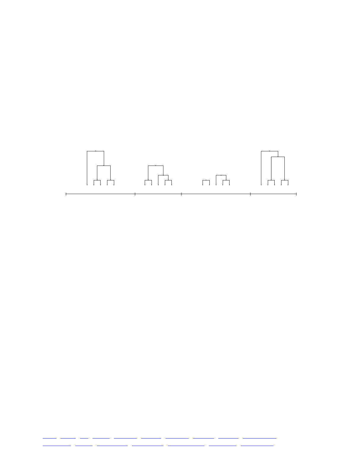
extant genome back to the most recent common ancestor for the population at that chromosome
position. The ancestry tree at a given position may have multiple roots, if there is no common
ancestor for all of the individuals in the population at that position; forward simulations begin with
every individual unrelated to every other, and common ancestry is only built over time through the
process of coalescence. The ancestry trees at adjacent chromosome positions are generally highly
correlated, and indeed are often identical (since those adjacent positions may never have been
split by recombination, or traces of such recombination might not have survived in any living
individual). Tree-sequence recording accounts for this correlation, tracking each distinct ancestry
tree along successive chromosome intervals rather than at every position. This is one reason why
the tree sequence is sometimes called a succinct tree sequence; it is much more compact than the
full set of trees for every position, because it omits the redundant information shared between
positions with identical ancestry. This multiplicity of trees is not easy to depict, but here is a sketch
of the concept:
The intervals between the ticks on the x axis are intervals on the chromosome that have distinct
ancestry trees (this example chromosome is only ten base positions long, and has four intervals
with distinct trees). Each interval’s ancestry tree reflects its particular pattern of inheritance along
the chromosome; however, the trees at adjacent sites tend to be highly correlated, with redundant
information that is represented concisely by the tree sequence data structure. Within each tree, the
leaf nodes at the bottom (labeled 0 through 4) might be extant genomes with no descendants,
whereas the internal nodes might be ancestral genomes that are no longer extant; however, with
overlapping generations things might be less clear-cut, since ancestors might still be extant. As
mentioned above, the tree for a given interval might have multiple roots, if coalescence is not yet
complete; that situation is found in the ancestry tree for the third chromosome interval pictured
above.
This is just a brief summary of tree-sequence recording, and may or may not be
comprehensible; for a full overview of tree-sequence recording, including details of how
simplification works, please refer to the definitive paper on the topic, Kelleher et al. (2018).
Tree-sequence recording enables some very powerful techniques, such as:
• Overlaying neutral mutations. You can run a model without any neutral mutations (which
is generally much faster), and then overlay neutral mutations afterwards. This gains
tremendous efficiency from the fact that neutral mutations only need to be overlaid on
branches of the ancestry tree that lead to extant individuals; neutral mutations on all
branches that went extinct before the end of the simulation do not need to be considered
at all. For models that contain many neutral mutations, this can result in a speedup of an
order of magnitude or more.
• Analyzing ancestry directly. You can sometimes avoid simulating neutral mutations
altogether, when it is actually the pattern of ancestry you are interested in. Often the
9
75
12
10423
8
75
9
04123
75
0 4
8
123
10
56
11
31402
10530
Genome coordinates
8
TOC I TOC II WF nonWF initialize() Genome Individual Mutation SLiMSim Subpopulation!
Eidos events fitness() mateChoice() modifyChild() recombination() interaction() reproduction() 32

pattern of neutral mutations from a forward simulation is used to infer things about a
population’s history – selection, bottlenecks, immigration, and so forth. Using neutral
mutations for this purpose is a blunt instrument, however, since they are sparse and occur
stochastically; inference from them is difficult, time-consuming, and inexact. Instead, it is
often possible to draw such inferences from the recorded tree sequence itself, which in a
sense embodies every possible mutational history that the population could have had
given its actual history of inheritance and recombination. The inferential power can
therefore be much higher. This means that inferences from the tree sequence can often be
exact, and can also often be computed much more quickly and easily than from neutral
mutations.
• Detecting coalescence during forward simulation. Often you want to “burn in” a model
until it has reached an equilibrium state, which can often be defined as occurring when
full coalescence across the whole chromosome has occurred. The time at which this
happens, however, is often hard to know. A heuristic of “10N” (running for a number of
generations equal to ten times the population size) is often used, but even for simple
models it can be an underestimate. For models with a variable population size, multiple
subpopulations, or non-neutral dynamics of any kind, the proper burn-in duration is often
just a guess, and it is often necessary to make a large overestimation “just to be safe”.
With tree-sequence recording enabled, SLiM can tell you whether your model has
coalesced fully or not; it has all the information needed. You can then use that
information to decide when to end the burn-in period of the model.
• Moving between coalescent and forward simulation methods. Tree-sequence recording
and the .trees file format build a sort of bridge between coalescent and forward
simulation methods, allowing both methods to be used in a single simulation. For
example, a neutral “burn-in” period for a model could be simulated using the coalescent,
and the results saved to a .trees file in the proper SLiM-compatible format using pyslim.
That .trees file could then be loaded into SLiM as the starting state for forward
simulation; perhaps the neutral mutations from the coalescent become non-neutral at that
point in time, for example, due to a change in the environment, and so now one wishes to
simulate the resulting non-neutral dynamics. Since the coalescent is so fast, this can result
in much quicker burn-in compared to simulating the burn-in with SLiM. Overlaying
neutral mutations after a run, mentioned above, is another strategy that moves between
coalescent and forward simulation methods. Moving between methods in this manner
allows the strengths of each method to be leveraged, while avoiding their weaknesses. As
mentioned above, the pyslim package is essential to this sort of interoperability, as we will
see in chapter 16. The pyslim package is not yet able to annotate mutations that were
overlaid with msprime in a way that renders them SLiM-compatible, unfortunately; this
planned feature is still being implemented. Several other ways of moving .trees data
between SLiM and msprime using pyslim have been implemented, and will be shown in
chapter 16.
• “Recapitating” to construct the ancestral history of a simulation. With this technique,
you could run a model forward with no neutral burn-in period at all, from a set of empty
genomes, and then reconstruct the ancestry of the initial genomes using the coalescent
after the forward simulation has completed. This technique, called recapitation, is much
more efficient even than generating a burned-in state using the coalescent directly,
TOC I TOC II WF nonWF initialize() Genome Individual Mutation SLiMSim Subpopulation!
Eidos events fitness() mateChoice() modifyChild() recombination() interaction() reproduction() 33

because only the ancestry trees present at the end of forward simulation need to be
coalesced back; any part of any genome that was present in the initial state of the model
but was later lost does not need to be coalesced, so most of the work of burn-in can be
avoided. As before, neutral mutations can be overlaid at the end of the model run, after
recapitation has constructed the ancestral history, rather than having to be simulated. This
technique can allow very large models to be simulated relatively efficiently, since most of
the work of burn-in can be eliminated. Support for this technique is presently being
added to the msprime Python package; this feature will be rolled out in a later release of
SLiM.
Tree-sequence recording has a large impact on the performance of models, in terms of both
runtime and memory usage. It is therefore disabled by default, and needs to be enabled with a
call to an initialization function, initializeTreeSeq(). When it is enabled, you can control the
frequency of simplification (more frequent simplification means a lower memory footprint but a
longer runtime), and you can turn on checking for coalescence if your model needs to know when
full coalescence has been attained (for a small additional performance penalty on top of each
simplification).
Again, tree-seq models are an advanced topic; it is good to know that tree-sequence recording
is an option, but beginning SLiM users should postpone trying to use it until they have become
fairly familiar with the basics of SLiM. However, if you’re finding that performance is an issue, and
you’re bogged down simulating huge numbers of neutral mutations or running endless burn-in
periods, tree-sequence recording may be able to help. Similarly, if you want to detect
coalescence, or obtain a record of the ancestry at every chromosome position, tree-sequence
recording can provide a solution. Tree-sequence recording also provides an output format for
saving simulation state that can be much more compact than either VCF or SLiM’s native output
file format (even though it includes information about ancestry that those file formats do not), and
that can be analyzed and manipulated in Python with pyslim; these advantages can also be a
reason to use tree-sequence recording.
1.8 Online resources for SLiM users
Users of SLiM should be aware of various online resources that are available to support their
work. This section summarizes them and provides links.
• First of all, there is the SLiM home page at the Messer lab website. This is the primary
place from which to download SLiM, and provides a history of SLiM releases as well as a
list of publications that have used SLiM. https://messerlab.org/slim/
• The slim-announce mailing list is only for announcements from our group, such as new
versions of SLiM, new SLiM publications related to SLiM, and plans for conferences where
you could connect with us. https://groups.google.com/forum/#!forum/slim-announce
• The slim-discuss mailing list is for questions from SLiM users that might be of general
interest. Please feel free to post your own questions – and even to answer other people’s
questions, if you can. https://groups.google.com/forum/#!forum/slim-discuss
• The SLiM-Extras GitHub repository is a place for the SLiM community to share useful
resources related to SLiM. This could include reuseable Eidos functions (see, e.g., section
TOC I TOC II WF nonWF initialize() Genome Individual Mutation SLiMSim Subpopulation!
Eidos events fitness() mateChoice() modifyChild() recombination() interaction() reproduction() 34

11.1), full SLiM models that might be of general interest, code for reading or analyzing
SLiM output in languages like R or Python, code for sublaunching multiple SLiM runs on
computing clusters (see section 1.4), and so forth. Please feel free to email us your own
submissions for additions to SLiM-Extras. https://github.com/MesserLab/SLiM-Extras
• The SLiM GitHub repository is where SLiM’s source code lives. SLiM is open-source, but
unless you have some specific reason to want to access the source, you probably don’t
need to. As described in chapter 2, users on Mac OS X can install SLiM with the double-
click installer we provide, and users on Linux will usually want to build from the official
release source archive provided on the SLiM home page. The GitHub repository, then, is
mostly useful for people who want to be on the cutting edge, running the latest version of
SLiM before it has been publicly released. Be aware doing this will mean you are more
exposed to bugs, and that sometimes the sources on GitHub may not even build (although
we try to avoid that). https://github.com/MesserLab/SLiM
That’s what we’ve got for now. As always, please contact us if you have suggestions for
additions that would be useful, or reports of problems with any of the above.
TOC I TOC II WF nonWF initialize() Genome Individual Mutation SLiMSim Subpopulation!
Eidos events fitness() mateChoice() modifyChild() recombination() interaction() reproduction() 35
2. Installation
The command-line tool for SLiM is designed to be portable; it is written in pure C++, with no
external dependencies. Code from various third-party libraries such the GNU Scientific Library
(Galassi et al. 2009), Boost (Boost 2015), and msprime (Kelleher et al. 2016) is used in SLiM (see
chapter 27), but that code has been integrated directly into SLiM, so those libraries are not
required to build or run SLiM. SLiM should be buildable on Mac OS X, Linux, other Un*x
platforms, and – possibly with minor modifications – on other platforms as well. The SLiMgui
application, on the other hand, is written for Mac OS X only, in Objective-C++ using Apple’s
Cocoa library, and is available only on that platform. The steps to install SLiM depend upon the
platform you are on; please refer to the appropriate subsection below.
2.1 Installation on Mac OS X
On Mac OS X you have a choice between (1) installing a prebuilt package containing the slim
command-line tool and the SLiMgui application (as well as EidosScribe, the eidos command-line
tool, and manual PDFs), or (2) cloning the SLiM GitHub repository and building the projects
yourself using Apple’s Xcode development environment. Unless you are an experienced
developer, the first option is recommended. Building SLiM on OS X at the command line is not
recommended, although it is possible; use of the Xcode project will provide the proper compiler
settings, etc., for a standard OS X build.
2.1.1 Installing the prebuilt SLiM package on Mac OS X
This is quite straightforward. First, download the installer package from SLiM’s home page at
http://messerlab.org/slim/:
If multiple versions are available, be sure to download the appropriate version for your system.
Once it is downloaded, double-click the package in the Finder to run the installer. Click through
all steps in the installer, and SLiM will now be installed on your system. The applications (SLiMgui
and EidosScribe) will be installed in your /Applications folder; the command-line tools (slim and
eidos) will be installed in /usr/local/bin/. Pre-existing Terminal windows may not find slim and
eidos; open a new Terminal window to get the updated paths.
2.1.2 Building SLiM from sources on Mac OS X
This option is relatively complex. If you are not an experienced developer it is recommended
that you install SLiM using the prebuilt package instead (see the previous section). There is no
advantage to building SLiM from sources unless you wish to run it under the debugger, modify its
code, or other similarly advanced tasks, or wish to run the current development version of SLiM.
First of all, you need to have Xcode and Apple’s other developer tools installed on your
machine. SLiM’s project is generally kept synchronized with the current version of Xcode; older
versions of Xcode may be unable to open the SLiM project. To run the current version of Xcode,
you generally need to be on the current version of OS X as well, so you may need to upgrade your
OS X installation before installing Xcode. Once you have done that, you will need to obtain and
install Xcode itself. This will probably involve registering as a developer with Apple (which is free,
for the basic level) at their developer website, developer.apple.com, and then downloading and
TOC I TOC II WF nonWF initialize() Genome Individual Mutation SLiMSim Subpopulation!
Eidos events fitness() mateChoice() modifyChild() recombination() interaction() reproduction() 36

installing the developer tools package including the latest version of Xcode (which may be possible
through the App Store, otherwise through the developer website’s Member Center). It is quite a
large download, so do it through a fast connection. Once you have completed this step, you
should see Xcode.app in your /Applications folder, and you should be able to launch it by
double-clicking it.
Second, you need to obtain the SLiM source code. If you are following these instructions, you
probably want to obtain the current development version of SLiM from its GitHub repository at
https://github.com/MesserLab/SLiM. Go to that URL, click the big green “Clone or download”
button, and then click “Download ZIP”:
Locate the downloaded file and double-click it to decompress the zip file if that has not already
been done for you automatically by your browser. This distribution will include the sources to
allow you build both the slim command-line tool and the SLiMgui interactive graphical modeling
environment. Be aware that the current development version on GitHub may not be thoroughly
tested – indeed, it may not even compile.
Third, open the SLiM project in Xcode. To do so, locate the Xcode project file within the
archive you have just downloaded; it is at the root level, with the name SLiM.xcodeproj. Double-
click it to open the project in Xcode. You should see a big project window.
Fourth, choose a build target. A target is basically a product that an Xcode project knows how
to build. The SLiM project has four targets that may be selected: SLiM (the slim command-line
tool), SLiMgui, EidosScribe (an interactive Eidos script development environment), and eidos (the
Eidos interpreter command-line tool, eidos). For now, select SLiMgui. You do this in the pop-up
near the upper left of the project window:
Fifth, build and run the selected target by pressing command-R (which is the Run command in
the Product menu). It should build fairly cleanly (perhaps apart from some nib warnings that are
difficult to eliminate). Once it finishes building (which may take several minutes, depending on
your machine), SLiMgui should launch automatically. Assuming that worked, quit SLiMgui for
now, as we are not quite done setting things up in Xcode.
TOC I TOC II WF nonWF initialize() Genome Individual Mutation SLiMSim Subpopulation!
Eidos events fitness() mateChoice() modifyChild() recombination() interaction() reproduction() 37
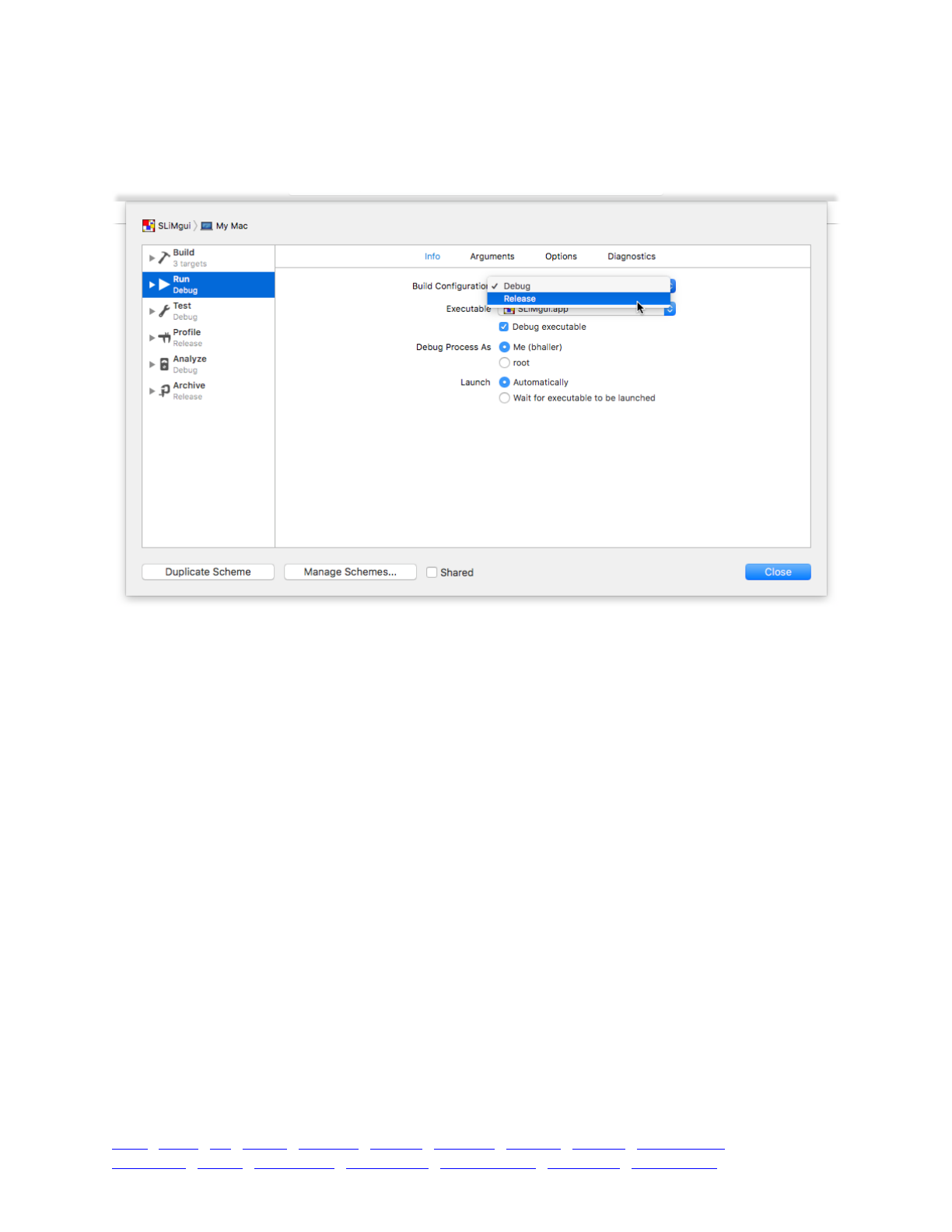
Sixth, there is an additional twist: the build configuration and other build scheme options.
These options are accessed by choosing the “Edit Scheme...” menu item that can be seen in the
pop-up menu in the above screenshot. Choose this, and you will see a sheet:
In this screenshot, the “Run” action has been selected on the left, so we are configuring what
Running this target (the SLiMgui target) will do. At the top, the Info tab is selected, which provides
the most basic configuration options. Finally, the pop-up menu next to the label “Build
Configuration” has been clicked in order to choose the Release build configuration. In general,
you will want to build and run SLiM and SLiMgui using the Release build configuration unless you
have a specific reason to wish to do otherwise; Release builds are much faster than Debug builds,
partly because of optimization, and partly because additional runtime checks are turned on in
SLiM’s code when building in the Debug configuration. After choosing Release, you can click the
Close button, and command-R (run) will now build and run a Release build of SLiMgui.
If your goal is to run SLiMgui, you can simply run it from within Xcode; there is no particular
disadvantage to doing so. If your goal is to run the slim command-line tool, doing so from within
Xcode is a little bit inconvenient (since it is a little bit complicated to supply command-line
arguments to it, for example), so the simplest course is to build slim in Xcode and put the built
executable wherever you want it to be so that you can run it in Terminal as usual.
To do this, first select the SLiM target from the target pop-up in the project window, as described
above (since the SLiMgui target is presently selected, if you have been following along). Second,
choose Edit Scheme... again and make sure that the SLiM target is using the Release build
configuration for its Run action, as described above (since we set that for the SLiMgui target above,
not for the SLiM target – each target has its own settings), and close the Edit Scheme... sheet.
Third, press command-B to build the target (this is the Build command in the Product menu).
TOC I TOC II WF nonWF initialize() Genome Individual Mutation SLiMSim Subpopulation!
Eidos events fitness() mateChoice() modifyChild() recombination() interaction() reproduction() 38

Once the build completes, you will want to locate the built product in the Finder. To do this,
first select the Project Navigator in the project window by clicking the folder icon at the left edge
of the strip of icons at the top left of the project window:
Then click disclosure triangles to open the SLiM top-level item and the Products subfolder in the
outline view shown there:
The slim product may be shown in red even if it has been successfully built; this appears to be
a bug in Xcode. Right-click (i.e., click with the right-hand mouse button) or control-click (i.e.,
hold down the control key and click) on the slim product, and choose “Show in Finder” from the
context menu displayed, as shown in the screenshot above. Your computer should switch to the
Finder and open a new window in the Finder, showing the contents of a folder that is probably
named “Release” (because the Release build configuration has been chosen). A file named slim
should be selected in this window. This is the built executable for the slim command-line tool.
(There are other, more standard ways to get to this point, but they are a bit more complicated.) You
should copy this file to whatever location you wish, and then run slim using that copy. The
standard install location for slim is at /usr/local/bin/, but since this is a custom build it might be
wise not to put it at that location to avoid confusion. Instead, a location like ~/bin/ inside your
home directory might be appropriate (you might need to create this folder first, in the Finder). In
any case, once you have installed slim at the desired location, you can open a Terminal window
and cd to that location (your Terminal shell prompts may look different from mine, of course):
darwin:~ bhaller $ cd ~/bin!
darwin:~/bin bhaller $
TOC I TOC II WF nonWF initialize() Genome Individual Mutation SLiMSim Subpopulation!
Eidos events fitness() mateChoice() modifyChild() recombination() interaction() reproduction() 39

Then you can run the local copy of slim that is at that location:
./slim <rest of command line>
The syntax ./slim tells Terminal to run the copy of SLiM in the current directory, rather than
running the standard version that might be installed at /usr/local/bin/ on your machine. You
can verify that the correct version of SLiM is being run using the -v (version) option:
darwin:~/bin bhaller $ ./slim -v!
SLiM version 2.3, built Apr 18 2017 17:20:34
The build date and time should correspond with the build you just did in Xcode; if not, you
have done something wrong and should re-check the steps above.
You can in fact follow the same steps to locate the built SLiMgui application in the Finder and
install it somewhere on your machine for later use; the ~/Applications/ folder might be a good
choice of location. However, it is probably simpler to run it from within Xcode.
Obviously Xcode is a very complicated application, and we can’t possibly provide a thorough
introduction to using it, but the steps above should allow you to build and run both slim and
SLiMgui using the current development head sources from GitHub. If you run into any problems
with these instructions, please let us know.
2.2 Installation on Linux and other Un*x platforms
Details of building SLiM may vary depending on the platform, but the basic gist should be the
same. First, you need to obtain the SLiM source code. It is recommended that you obtain the
code for the latest supported release, from SLiM’s home page at http://messerlab.org/slim/:
However, you may also obtain the current development version from SLiM’s GitHub repository
at https://github.com/MesserLab/SLiM. Be aware that the version on GitHub may not be
thoroughly tested – indeed, it may not even compile.
The following steps have changed considerably with the release of SLiM 3, since we have
switched from using the make build tool to using a tool called cmake that is considerably more
modern (but also a bit more complicated to use). The cmake tool is often preinstalled on Linux
systems, but if it is not installed on your machine, you will need to install it before proceeding.
You can tell whether cmake is installed on your system by executing this in a terminal window:
which cmake
If a path is printed in response, cmake is installed; if not, it needs to be installed. On Mac OS X,
cmake can be installed using MacPorts (https://www.macports.org) or Homebrew (https://brew.sh);
which installation system you use seems to be largely a matter of taste, although you can read
strong opinions in both directions online. On Linux and other Un*x systems, the cmake home page
at https://cmake.org/download/ provides downloadable source packages with installation
instructions. Apologies for this additional complication; with the integration of more third-party
code into SLiM, using make directly just became too unwieldy. The cmake tool builds a makefile for
us, which can then be used to build with make, as we will see next.
TOC I TOC II WF nonWF initialize() Genome Individual Mutation SLiMSim Subpopulation!
Eidos events fitness() mateChoice() modifyChild() recombination() interaction() reproduction() 40

With cmake installed, go to a new Un*x shell window and type:
cd SLiM!
cd ..!
mkdir build!
cd build!
cmake ../SLiM!
make slim
The first cd command changes the current directory to your SLiM source directory (you will
need to supply the appropriate path there instead of just SLiM), and the next cd command changes
to the enclosing directory (of course you can just cd there directly). We then use mkdir to create a
build directory adjacent to the SLiM source directory in the filesystem; this keeps all of the cruft
associated with the build process separate from SLiM’s sources. We cd into that build directory,
and then tell cmake to update its information regarding SLiM. The last command actually builds
the slim command-line tool. Note that SLiM uses C++11 extensions; the g++ compiler installed
on your machine must be recent enough to support C++11 or your build will fail. The slim tool
will appear as an executable file in the build directory once the build is finished (not, as in SLiM
2.x, in a bin directory inside the source directory). You can copy the built executable to a different
location, such as /usr/bin/, if you wish; the standard location for user-built executables depends
upon your Un*x flavor, so consult your documentation if you wish to install it in a standard
location.
The eidos command-line tool can also be built on Un*x platforms following the same
procedure, with the final command make!eidos; a simple make command will build both. The
SLiMgui and EidosScribe targets are buildable only on Mac OS X using Xcode (see section 2.1.2).
Once cmake’s information has been set up, rebuilding after minor source changes can generally
be done just by re-executing the make!slim command in the build directory. If you make major
changes to the SLiM sources – and in particular, if you add or remove source files, or do a
git!pull of new changes from GitHub – you might need to tell cmake to update its information
before you run make to rebuild the project. This is necessary because SLiM’s CMakeLists.txt
configuration file uses a cmake feature called GLOB to collect a list of source files to be used for
building, and that means that cmake cannot automatically re-update in all cases. If you make such
changes to the sources, you should do the following:
cd SLiM!
touch ./CMakeLists.txt
Then cd to the build directory and execute make slim to rebuild; cmake’s cached information
will be rebuilt, since the configuration file was touched, so you do not need to re-run cmake.
The build instructions above use a build directory named build, and use a default “build type”
with cmake (a Release build), and this will suffice for almost all SLiM users; you need not read
further unless you really want to complicate your life. In fact, however, you can name your build
directory whatever you wish, and you can have more than one build directory if you wish; and you
can specify a build type of either Release or Debug with cmake. For example, you could do
something like this to make a build directory named Release, using the Release build type:
cd SLiM!
cd ..!
mkdir Release!
cd Release!
cmake -D CMAKE_BUILD_TYPE=Release ../SLiM!
make slim
TOC I TOC II WF nonWF initialize() Genome Individual Mutation SLiMSim Subpopulation!
Eidos events fitness() mateChoice() modifyChild() recombination() interaction() reproduction() 41

A Release build has optimization turned on and debugging symbols turned off, giving you a
lean, fast executable suitable for most purposes. This is cmake’s default when building SLiM; the
original build instructions above produced a Release build since no build type was specified.
Similarly, you could make a Debug build in a directory named Debug:
cd SLiM!
cd ..!
mkdir Debug!
cd Debug!
cmake -D CMAKE_BUILD_TYPE=Debug ../SLiM!
make slim
A Debug build has optimization turned off and debugging symbols turned on, giving a large
symbolicated build suitable for runtime debugging. Debug builds also have some additional
runtime error checking turned on in SLiM, designed to catch a variety of internal error states that
might cause a Release build to crash or produce incorrect output. Most users, however, will be
fine with just the standard build directory named build and the default cmake build type.
2.3 Installation on non-Un*x platforms
Building and installing SLiM on non-Un*x platforms should be reasonably straightforward since
the code is standard C and C++. However, there may be minor differences that lead to compile
and/or link problems, particularly on non-POSIX-compliant operating systems such as Windows.
We will probably not be able to give you any useful help in solving these problems; we know
nothing about programming on Windows, for example. If you work through such problems and
have useful patches for us to allow the project to build on a new platform (using #ifdef or similar
for conditional compilation), feel free to send us a pull request on GitHub.
Overall, the build steps should be similar to the sections above: you will download the sources
or clone the GitHub repository (see above), and then you will execute compile commands with (1)
a flag indicating the C++11 standard, which is required for SLiM, (2) a nice high optimization level
such as -O3, (3) all of the source files necessary, and (4) the appropriate header search paths. You
can look at the project’s CMakeLists.txt file for further guidance.
2.4 Testing the SLiM installation
Regardless of your platform or method of installation, it is a good idea to run some self-tests
after installing SLiM. In your Terminal window, Un*x shell window, or platform equivalent, run the
following two commands (while in the build directory where the slim executable resides):
./slim -testEidos!
./slim -testSLiM
Each command should print a result line beginning with SUCCESS and then a count of successful
self-tests. If any other lines print, indicating failure of a test, you should probably contact us to ask
how to proceed.
TOC I TOC II WF nonWF initialize() Genome Individual Mutation SLiMSim Subpopulation!
Eidos events fitness() mateChoice() modifyChild() recombination() interaction() reproduction() 42
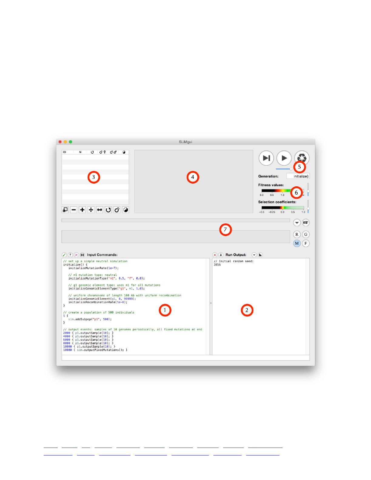
3 Running simulations in SLiMgui
This chapter introduces the SLiMgui graphical development environment for SLiM. This app is
available only on Mac OS X; on other platforms you will need to run SLiM directly from the
command line, in which case you can skip ahead to chapter 4.
On OS X, SLiMgui is typically located in /Applications/ if you installed from the prebuilt
package; if you built SLiM from sources, you may run SLiMgui directly from Xcode.
3.1 The SLiMgui simulation window
When you first launch SLiMgui, you should see a window similar to this:
The main sections of the window are indicated with red numbered circles; they are:
1. The scripting pane. This is where input commands for SLiM – in the form of an Eidos script –
are entered. A simple script is given by SLiMgui by default, as a starting point. At the top of this
pane you can see the pane’s title, “Input Commands”, and to the left of that title are buttons for
four commands: Check Script, Script Help, Show Eidos Console, and Show Eidos Variable Browser
TOC I TOC II WF nonWF initialize() Genome Individual Mutation SLiMSim Subpopulation!
Eidos events fitness() mateChoice() modifyChild() recombination() interaction() reproduction() 43

(all of the buttons in the window have tooltips, so you can just hover the mouse over them to be
reminded of what they do). The use of these buttons will become clear in later sections.
2. The output pane. This is where run output from SLiM – diagnostic output as well as output
explicitly generated by your simulation script – is shown. At the top of this pane you can see the
pane’s title, “Run Output”, surrounded by buttons for four commands: Clear Output, Dump
Population State, Add Output Command (a pop-up menu button), and Show Graph (also a pop-up
menu button). Again, these buttons will be covered in later sections.
3. The population view. This is a table view that displays all of the subpopulations in the current
simulation population. Since the simulation has not yet been started, there are presently no
subpopulations, and thus the table is empty. This will be covered in more detail once we have a
running simulation. Directly below the table view are eight buttons: Change Subpopulation Size,
Remove Subpopulation, Add Subpopulation, Split Subpopulation, Change Migration Rates,
Change Selfing Rate, Change Cloning Rate, and Change Sex Ratio. Again, these buttons will be
covered in later sections.
4. The individual view. This is where individual “organisms” in the simulation are displayed
from the subpopulation(s) selected in the population view. At present this is empty since there are
no individuals to display.
5. The generation controls. The three large buttons are, from left to right, for the commands
Step (to run forward one generation), Play (to run forward continuously), and Recycle (to reset back
to the initialization stage of the simulation). The slider below the Play button controls the speed at
which the simulation runs; usually you will want this to be the maximum speed, but occasionally
it is useful to slow the simulation down to better see what is happening on short timescales.
Finally, the Generation textfield shows the generation that is about to execute; if you press the Step
button, the generation shown will execute. At present the simulation is paused prior to the
execution of initialize() callbacks, a special initialization state that happens first before the
simulation begins to run.
6. The color controls. The two color stripes show the colors that will be used by SLiMgui to
indicate different fitness values (for individuals) and different selection coefficients (for mutations).
In both cases, yellow is always neutral, but the scale of the color ramps around yellow can be
adjusted using the vertical sliders to the right, in order to make the color scale better reveal fine or
coarse differences in fitness and selection coefficients in your simulation.
7. The chromosome views. The two wide stripes show views onto the simulated chromosome
(empty at present since the simulation has not yet started); these will be discussed later. To the
right of those views are buttons for six commands. In the top row are buttons for Add Genetic
Command (a pop-up menu button) and Show Details (a toggle button that shows and hides a
drawer). Below those is a cluster of four buttons labeled R, G, M, and F; these toggle visibility on
and off in the chromosome views of, respectively, rate maps (for recombination and mutation),
genomic elements, mutations, and fixed mutations (i.e., substitutions). By default only mutations
are shown.
This is a lot of information, and to avoid drowning you in details we will not cover all these
elements in detail now; you will see them again later as they come up in context.
3.2 The script help window
Before moving on to writing your first Eidos script for SLiM, there are a few other components of
SLiMgui that it might be useful to briefly mention. One such is the script help window. If you
click the Script Help button , the script help window will open:
?
TOC I TOC II WF nonWF initialize() Genome Individual Mutation SLiMSim Subpopulation!
Eidos events fitness() mateChoice() modifyChild() recombination() interaction() reproduction() 44
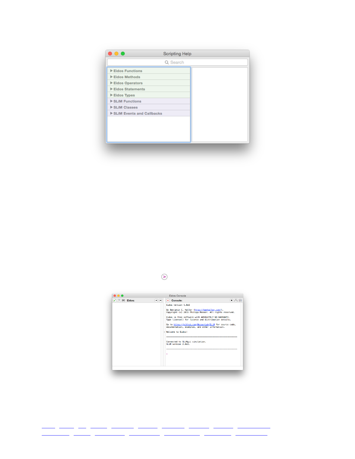
This window can be used to browse information about both Eidos and SLiM. A list of top-level
topic headings appears on the left; you can click on these headings to expand them to show the
sub-headings they contain, which may in turn be expanded to show sub-sub-headings and so
forth. When you click on a “leaf” – an actual topic – the information about that topic will be
shown in the pane on the right. You can also use the search field at the top of the window to
search for information about a given topic; note that there is a pop-up menu under the magnifying
glass that allows you to choose whether the search is done on topic titles only (for fewer and
probably more relevant results), or is done on the full help text of each topic (for more results).
A useful shortcut: option-click on anything in the Eidos script of the simulation window’s input
area to pop up the script help window with search results for the item you option-clicked. This is
very useful for quickly looking up functions, language keywords, and other such topics.
3.3 The Eidos console
Clicking the Show Eidos Console button will show the console (or hide it, if already open):
We won’t go into detail about this now, since you are not yet familiar with Eidos at all, but in
essence, this console is a window where you can execute arbitrary Eidos commands at any point
in your simulation. Commands are entered, and their output is shown, in the console pane on the
right-hand side of the window. The left-hand side is a scratch area where you can work on longer
TOC I TOC II WF nonWF initialize() Genome Individual Mutation SLiMSim Subpopulation!
Eidos events fitness() mateChoice() modifyChild() recombination() interaction() reproduction() 45
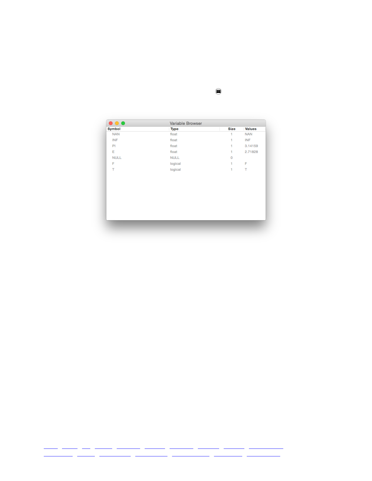
blocks of script. If you want to experiment with Eidos and try out ideas interactively, this is the
place to do it; so as new Eidos concepts are introduced in this manual, you may wish to return to
the Eidos console to play around with them.
3.4 The Eidos variable browser
Finally, clicking the Show Eidos Variable Browser button will show (or hide, as appropriate) a
variable browser that looks like this:
Only a few variables are presently defined; these are all constants – unmodifiable values
defined for your use by Eidos (or by SLiM, but the constants shown are all Eidos constants). These
constants include the values T and F representing true and false, the values PI and E representing
those mathematical constants (3.1415... and 2.7182...), and some others; these will be
discussed as they come up.
Constants are shown in gray in the variable browser since they are unmodifiable. The variable
browser will also show variables that you define yourself (in black rather than gray). For example,
you might try now entering x=10 at the console prompt in the Eidos console window. After you
press return to execute that command, you will see the variable x appear in the variable browser,
defined with a type of integer, a size of 1 (because 10 is a single value, as opposed to a vector of
values), and a value of 10.
We will return to the variable browser in later sections to examine some of the objects defined
by SLiM. In general, however, just be aware that the variable browser exists, and that you can use
it to examine all of the Eidos variables that you will be working with in later sections.
3.5 Automatic code completion and command syntax lookup
In the next chapter, we will start exploring a simple neutral model in SLiM. As you start writing
scripts like that, you will sometimes find it difficult to remember the name of something you need
to use in your script – a function, a property, or a method. We are getting a bit ahead of ourselves,
but there is a final feature of SLiMgui to discuss here. Suppose you were writing a script, but you
couldn’t remember the name of the initializeGeneConversion() function. You could look it up
in the documentation, but there is an easier way. First click in your script at the appropriate spot
inside an initialize() callback, and then start typing with init since you know you’re looking
TOC I TOC II WF nonWF initialize() Genome Individual Mutation SLiMSim Subpopulation!
Eidos events fitness() mateChoice() modifyChild() recombination() interaction() reproduction() 46
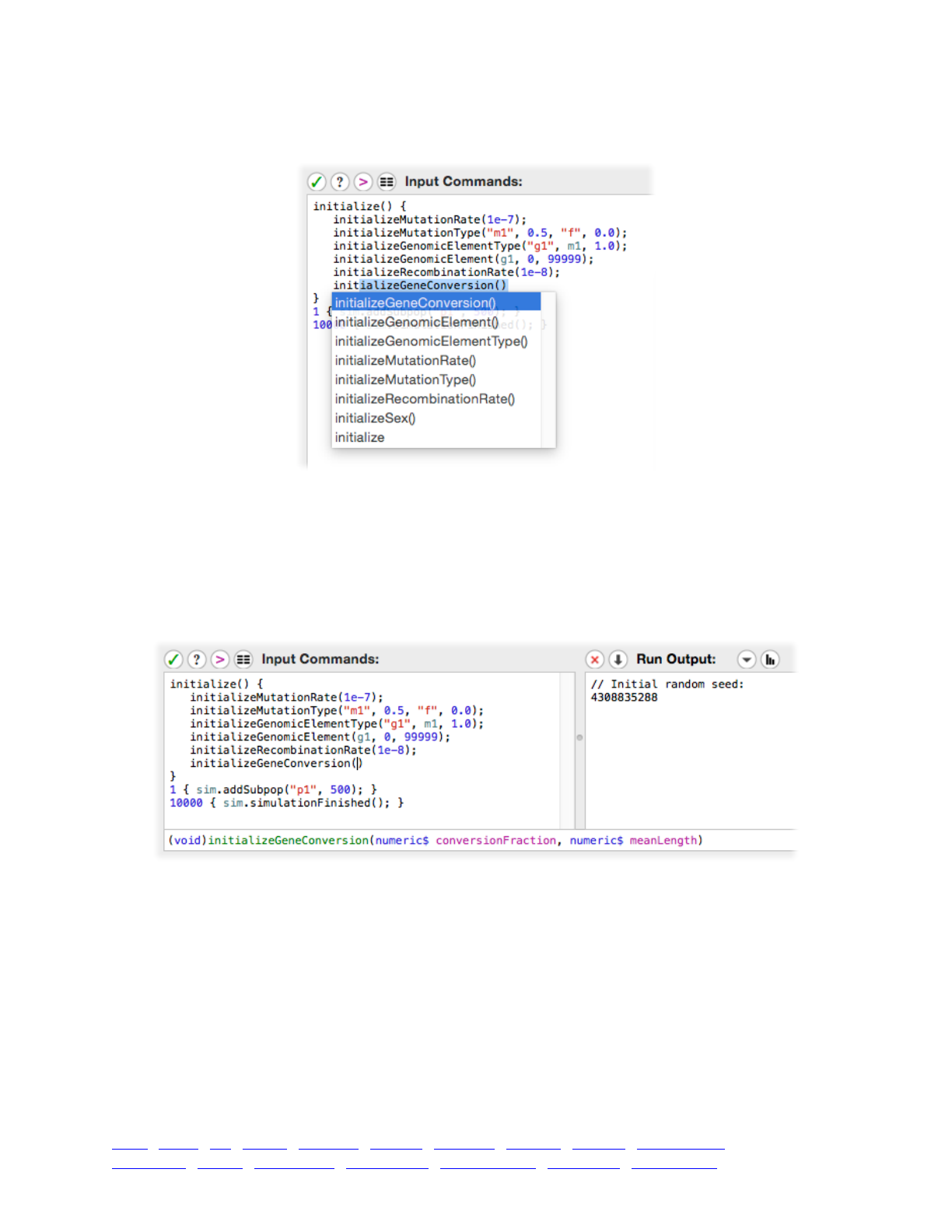
for an initialize...() function. Now press the <esc> key. This requests code completion from
SLiMgui. In response, you should see something like this:
This is a pop-up list of all of the things Eidos knows about that start with init. Conveniently,
initializeGeneConversion() is even selected for you, since it happens to be alphabetically first in
the list. You can simply press return or click outside the box to accept the default choice; you
could also double-click a different choice, or use the arrow keys to move to a different choice.
Having accepted initializeGeneConversion() as your choice, you might now also be unable
to remember what its parameters are. Simply click between the parentheses of the function call,
and then look at the status bar at the bottom of the window:
The function signature shown there reminds you of the parameters needed, including their types
and their names. Section 4.1.3 has further discussion about this feature, getting into details of the
structure and symbolism of the function signature, which would have little meaning before we
have started scripting.
As described in section 3.2, there is a script help facility provided in SLiMgui, which can be
called up with an option-click on any part of your script. If the function signature shown above is
not sufficient to jog your memory, and you want to see the full documentation for the
initializeGeneConversion() function, just option-click on the function name,
initializeGeneConversion, and the script help window will come up showing the results of a
search on that term:
TOC I TOC II WF nonWF initialize() Genome Individual Mutation SLiMSim Subpopulation!
Eidos events fitness() mateChoice() modifyChild() recombination() interaction() reproduction() 47
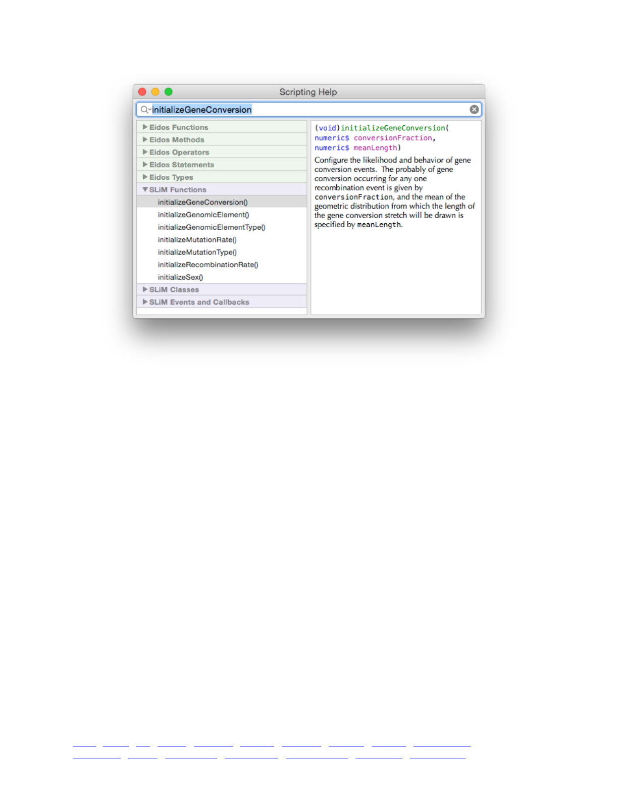
The full documentation for initializeGeneConversion() is shown, which should clarify any
outstanding questions.
The code completion (with <esc>) and context help (with option-click) features work for
properties and methods as well. This may not mean much to you yet, since functions, properties,
and methods have not yet been formally introduced, but keep all this in the back of your mind as
you start exploring scripting in chapter 4.
3.6 Automated script generation
In section 3.1, a few controls were skimmed over with a promise that they would be covered in
later sections. Here we will cover some of those controls: various buttons and pop-up menus that
add automatically generated script blocks to the simulation.
SLiMgui provides quite a few different facilities for automated script generation. Through the
buttons under the subpopulation table, you can change the size of a subpopulation, remove or add
subpopulations, split subpopulations, change migration rates, change selfing and cloning rates, or
change a subpopulation’s sex ratio. Through the pop-up menu to the right of the chromosome
view, you can define a new mutation type or genomic element type, add a genomic element or a
recombination interval to the chromosome, or make your simulation sexual rather than
hermaphroditic (and even simulate a sex chromosome rather than an autosome). Finally, through
the pop-up menu at the top of the Run Output area, you can add output of the full population
state, output of a sample from a subpopulation, or output of a list of fixed mutations. You can see
these three access points for automated script generation in the screenshot below:
TOC I TOC II WF nonWF initialize() Genome Individual Mutation SLiMSim Subpopulation!
Eidos events fitness() mateChoice() modifyChild() recombination() interaction() reproduction() 48

All of these automated script generation commands will not be covered individually here, as
that would be too repetitive and tedious. The buttons have tooltips (visible if you hover the cursor
over them), and the menu items are named in a way that indicates their function, so you can easily
find the command you need. All of these commands work in essentially the same way, so we will
take just one of them as a representative example. The leftmost button under the subpopulation
table is the Change Subpopulation Size button. If you recycle and click it, you will likely see
something like this:
This illustrates the first point about SLiMgui’s automated script generation: it depends upon the
current state of the simulation. Immediately after doing a Recycle, no subpopulations have been
defined in the current simulation, and so SLiMgui has no information about which subpopulations
exist (and thus might be resized). The first step in using these facilities is therefore to get yourself
into a state in which SLiMgui has enough information to make modifications to the objects you are
interested in. In this example (using SLiMgui’s default model), stepping forward twice (once to
execute the initialize() callback, and another to execute the generation 1 event that defines
subpopulation p1) provides that information. Now if you click the Change Subpopulation Size
button, you should see a more useful panel:
TOC I TOC II WF nonWF initialize() Genome Individual Mutation SLiMSim Subpopulation!
Eidos events fitness() mateChoice() modifyChild() recombination() interaction() reproduction() 49

Other automated-script-generation panels will differ in their specifics, but the idea is always the
same: you supply the information needed for the script generation, and then you either do an
Insert Only operation (generating the script block but leaving the current state of the simulation
unchanged) or you do an Insert & Execute operation (generating the script block and putting it into
effect in the current simulation). In this case, suppose we enter a value of 5 for “Generation for
resize”, and then click “Insert & Execute”. The first thing you will note is that a new script block
has been inserted into your script by SLiMgui:
5 {!
p1.setSubpopulationSize(1000);!
}
This simply implements the requested change using an Eidos event. The other thing you will
notice is that this event is active in the current simulation, with no need to recycle. If you step
forward through generation 5, subpopulation p1 will resize to 1000 individuals as requested (see
section 5.1.1 for a proper introduction to the setSubpopulationSize() method). This allows you
to develop the dynamics of a simulation as you go, adding events one by one without needing to
recycle and step forward to see the effects of each event added.
If you choose a generation for the event that is prior to the next generation to be executed,
SLiMgui will display a warning that the event cannot be executed in the current simulation
(because its target generation has already come and gone, and it is not possible to modify the past
simulation state retroactively). In this case, the Insert & Execute button will change to Insert &
Recycle, so that you easily restart the simulation with the new event in effect.
Finally, it is worth noting that the automated script generation always provides you with a new
event or callback, even if the command could be merged into an existing event or callback. For
example, if we use the Add Mutation Type command to make a new m2 mutation type (see section
4.1.3), we will get a new initialize() callback like this:
initialize() {!
initializeMutationType(2, 0.5, "f", 0.5);!
}
Almost certainly, you will want to copy the call to initializeMutationType() into your main
initialize() callback and delete the extra callback provided by SLiMgui; it is quite unusual to
actually want to have more than one initialize() callback in a script, although it is legal.
SLiMgui can’t guess exactly where the call ought to be inserted, however, so it leaves that to you.
TOC I TOC II WF nonWF initialize() Genome Individual Mutation SLiMSim Subpopulation!
Eidos events fitness() mateChoice() modifyChild() recombination() interaction() reproduction() 50

3.7 Script prettyprinting
As you start writing your own scripts in SLiMgui, you may find that they look a bit raggedy
because their line indentation doesn’t follow standard coding conventions, like this:
initialize() {!
initializeMutationRate(1e-7);!
initializeMutationType("m1", 0.5, "f", 0.0);!
initializeGenomicElementType("g1", m1, 1.0);!
initializeGenomicElement(g1, 0, 99999);!
initializeRecombinationRate(1e-8);!
}!
1 {!
subpopCount = 5;!
!
for (i in 1:subpopCount)!
sim.addSubpop(i, 500);!
for (i in 1:subpopCount)!
for (j in 1:subpopCount)!
if (i != j)!
sim.subpopulations[i-1].setMigrationRates(j, 0.05);!
}!
10000 late() {!
sim.outputFull();!
}
This is a contrived example (based on the recipe in section 5.3.2), but you really will find that
your script indentation starts to suffer as you change the structure of your code, moving code from
block to block, wrapping some code in loops and unwrapping other code, and so forth.
Indentation issues can make your code hard to read and maintain, but manually fixing the
indentation of each line is a hassle. Instead, you can just use SLiMgui’s automatic script
prettyprinting facility. Select “Prettyprint Script” from the Script menu, or click the button just
above the scripting pane, and your code will be reformatted:
initialize() {!
initializeMutationRate(1e-7);!
initializeMutationType("m1", 0.5, "f", 0.0);!
initializeGenomicElementType("g1", m1, 1.0);!
initializeGenomicElement(g1, 0, 99999);!
initializeRecombinationRate(1e-8);!
}!
1 {!
subpopCount = 5;!
!
for (i in 1:subpopCount)!
sim.addSubpop(i, 500);!
for (i in 1:subpopCount)!
for (j in 1:subpopCount)!
if (i != j)!
sim.subpopulations[i-1].setMigrationRates(j, 0.05);!
}!
10000 late() {!
sim.outputFull();!
}
Only the line indentation is changed; all other aspects of your coding style are preserved,
including blank lines, brace style, spacing around operators, and so forth.
TOC I TOC II WF nonWF initialize() Genome Individual Mutation SLiMSim Subpopulation!
Eidos events fitness() mateChoice() modifyChild() recombination() interaction() reproduction() 51

3.8 Further SLiMgui features
SLiMgui has many more features, but they won’t make much sense until we have gotten into
writing scripts. For future reference, here is a cross-reference to some sections that present more
features of SLiMgui:
Running a simulation: section 4.1.9.
Viewing script block registration/deregistration: section 5.1.2.
Executing a simulation up to a specified generation: section 5.1.2.
Visualizing population structure and migration: sections 5.1.3 and 5.3.3.
Using the Play speed slider: section 5.2.2.
Viewing recombination regions: section 6.1.1.
Viewing the sex ratio, cloning rate, and selfing rate: sections 6.2.2, 6.3.1, and 6.3.2.
Viewing the registered mutation types and their distributions of fitness effects: section 7.1.
Viewing the registered genomic element types: section 7.2.
Viewing genomic elements and selecting a subrange of the chromosome: section 7.3.
Customizing display colors for mutations, genomic elements, and individuals: section 7.4.
Graphing of mutation and population dynamics in SLiMgui: chapter 8.
Alternative population display modes: section 12.3.
Haplotype display in the chromosome view, and haplotype plots: section 13.5.
Finally, note that SLiMgui knows the recipes presented in this cookbook, and can open them for
you directly. Just choose the recipe you want from the “Open Recipe” menu under SLiMgui’s File
menu, and the recipe will open in a new SLiMgui window.
TOC I TOC II WF nonWF initialize() Genome Individual Mutation SLiMSim Subpopulation!
Eidos events fitness() mateChoice() modifyChild() recombination() interaction() reproduction() 52

4. Getting started: Neutral evolution in a panmictic population
This chapter will introduce the basic concepts involved in making, configuring, running, and
obtaining output from a simple neutral simulation.
4.1 A basic neutral simulation
There is a tradition in computer programming of introducing a new language by writing a
“hello, world” program. In Eidos, this minimal “hello, world” program is quite simple:
print("hello, world");
This single-line program calls a built-in function named print(), which prints whatever you tell it
to. Here, print is called with a single argument, the string "hello, world", enclosed in quotes
that indicate it is a string. The semicolon at the end indicates to Eidos that the statement – the line
of code – ends at that point. If you are using SLiMgui on OS X, you can open the Eidos console
window now and enter this command at the prompt; after you press return, "hello, world" will
be shown as output. In SLiM, we use Eidos as a tool for building and controlling SLiM simulations;
for a complete introduction to Eidos, see the manual Eidos: A Simple Scripting Language.
That was a minimal Eidos program; now let’s look at a minimal SLiM simulation script, which is
a bit more involved. We’ll start with a basic neutral simulation that models a genomic region of
length 100 kb in a population of 500 diploid individuals, evolving over 10000 generations.
Neutral mutations occur uniformly in this region at a rate of 10-7 per bp per generation.
Recombination also occurs uniformly at a rate of 10-8 per bp per generation (corresponding to 1
cM/Mbp). The Eidos commands for specifying this simulation are as follows:
// set up a simple neutral simulation!
initialize()!
{!
// set the overall mutation rate!
initializeMutationRate(1e-7);!
!
// m1 mutation type: neutral!
initializeMutationType("m1", 0.5, "f", 0.0);!
!
// g1 genomic element type: uses m1 for all mutations!
initializeGenomicElementType("g1", m1, 1.0);!
!
// uniform chromosome of length 100 kb!
initializeGenomicElement(g1, 0, 99999);!
!
// uniform recombination along the chromosome!
initializeRecombinationRate(1e-8);!
}!
!
// create a population of 500 individuals!
1!
{!
sim.addSubpop("p1", 500);!
}!
!
// run to generation 10000!
10000!
{!
sim.simulationFinished();!
}
TOC I TOC II WF nonWF initialize() Genome Individual Mutation SLiMSim Subpopulation!
Eidos events fitness() mateChoice() modifyChild() recombination() interaction() reproduction() 53

Running this script at the command line on a Un*x system (including Mac OS X) is very simple.
If it is saved in the current directory as a file named test.txt, and if the slim command-line tool is
in the shell’s executable path, then the command:
slim test.txt
should suffice to run it. Otherwise, paths will be needed, which depend upon where the slim
command-line tool and the test.txt file are located. On OS X, the SLiM installer will install slim
in /usr/local/bin; if test.txt is in your home directory, then the command would be:
/usr/local/bin/slim ~/test.txt
Running this script in the SLiMgui application on OS X is also straightforward. Just launch
SLiMgui (installed in /Applications by the SLiM installer), copy/paste the script into the script area
of SLiMgui’s window (or, even easier: select the section 4.1 recipe from the Open Recipe submenu
of SLiMgui’s File menu), press the big Recycle button at the upper right of the window to reset the
simulation with the new script, and then press the Play button just to the left of the Recycle button.
Chapter 3 provided a brief introduction to SLiMgui and the parts of its window, and the sections
below will walk through running this particular simulation in SLiMgui in more detail.
There are a couple of general things to say first about the whole script. First of all, comments in
Eidos begin with two slashes, //, and continue to the end of their line; the script above has a
comment for most of the lines of executable code.
Second, this code snippet utilizes syntax coloring to make the meaning of the script clearer, just
as shown in SLiM’s input area. Numeric constants are shown in blue, string constants in red, SLiM
object constants such as m1, g1, and sim in sage, and comments in green. Syntax coloring will
generally be used in this manual for Eidos scripts.
Third, braces {} are used in Eidos to enclose whole blocks of code. The code above has three
such blocks: an initialize() callback that sets up the simulation, an Eidos event that is set to
execute in generation 1 – the beginning of simulation execution – to add a subpopulation, and an
Eidos event that runs in generation 10000 and stops the simulation.
Fourth, whitespace such as spaces, tabs, and newlines is not generally significant in Eidos;
comments, also, are considered whitespace and do not matter to the execution of your code. The
above script could thus be written more compactly as:
initialize() {!
initializeMutationRate(1e-7);!
initializeMutationType("m1", 0.5, "f", 0.0);!
initializeGenomicElementType("g1", m1, 1.0);!
initializeGenomicElement(g1, 0, 99999);!
initializeRecombinationRate(1e-8);!
}!
1 { sim.addSubpop("p1", 500); }!
10000 { sim.simulationFinished(); }
With that prelude, the following subsections will explore each of the commands in this script in
detail. If you wish to following along in SLiMgui, you should copy the example script out of this
document and paste it into your SLiMgui simulation window, then press the Recycle button (which
abandons the previous simulation run, based on the old script, and begins a new simulation based
on the new script you have just pasted in).
4.1.1 initialize() callbacks
Before a simulation can really begin running, some initialization tasks need to be done. SLiM
needs to know basic simulation parameters like the mutation rate, the length of the chromosome,
TOC I TOC II WF nonWF initialize() Genome Individual Mutation SLiMSim Subpopulation!
Eidos events fitness() mateChoice() modifyChild() recombination() interaction() reproduction() 54

and so forth. Setting up this foundational state is done before the execution of the first generation,
at what is called “initialization time”. At initialization time, SLiM calls any blocks in your script
that are designated as initialize() callbacks (simply by having initialize() before their starting
brace). Our sample script defines one initialize() callback; you are allowed to have more than
one, in which case they are called sequentially in the order in which they are defined in the script.
This would be useful mostly for conceptual division of your code into discrete sections.
An initialize() callback may contain arbitrary Eidos code; you can define variables, execute
loops, and call functions (all topics we will explore in future sections). However, the simulation is
not yet set up, so you do not have access to SLiM’s sim constant, and this cuts you off from most of
SLiM’s functionality. Mostly what you will do in your initialize() callbacks, in practice, is call
initialization functions that are built into SLiM to help set up your simulation. These functions
have names that begin with the word initialize; the initialize() callback here calls five such
functions, discussed in the following sections. (A full reference of all of the initialize...()
functions provided by SLiM is given in Part II of this manual, the reference section; in general all of
the topics discussed in Part I are summarized in a more reference-oriented format there).
4.1.2 Mutation rate
The first line of our initialize() callback is:
initializeMutationRate(1e-7);
This calls the SLiM function initializeMutationRate(), passing a single parameter, the
numeric constant 1e-7. This is written in a sort of scientific notation commonly used in
programming; 1e-7 means 1.0×10⁻⁷, and could also be written in Eidos as 0.0000001. Numeric
values in Eidos may be of type integer, like 6 or -17, or of type float, like 1e-7 or 0.0000001.
The effect of this statement is to tell SLiM that the simulation will use a uniform mutation rate of
1e-7 (per base position per generation) across the whole chromosome. SLiM uses this rate to
determine how many mutations arise in each offspring that it generates in each generation in the
genomic elements being simulated (see section 21.1 for a more precise definition of the mutation
rate in SLiM). It is also possible to set a mutation rate map that varies the mutation rate along the
chromosome, but we will defer that until later. Precisely what mutations can arise in a given
element is governed by other aspects of the simulation configuration, discussed next.
4.1.3 Mutation types
The next line in the initialize() callback is:
initializeMutationType("m1", 0.5, "f", 0.0);
This calls the SLiM function initializeMutationType() to set up a new mutation type. You
may define as many mutation types in SLiM as you wish. Each is given a unique symbolic name;
the mutation type defined here is given the name m1, as requested by the first parameter to the
function call. A mutation type encapsulates a few key pieces of information about a particular
type of mutations: the dominance coefficient for mutations of this type (0.5 here), the distribution
of fitness effects (DFE) to be used (a fixed fitness effect here, as represented by "f"), and any
parameters that configure the distribution of fitness effects (0.0 here, giving the fixed selection
coefficient that will be used by all mutations of this type). This call creates a new Eidos variable
named m1, and so henceforth we can use the symbol m1 to refer to this mutation type.
This mutation type, m1, thus represents neutral mutations – always with a selection coefficient of
0.0. Mutation types might represent things like neutral mutations, beneficial mutations,
deleterious mutations, nearly neutral mutations, etc., with different distributions of fitness effects.
Each time that a mutation is created, its selection coefficient is drawn from the distribution of
TOC I TOC II WF nonWF initialize() Genome Individual Mutation SLiMSim Subpopulation!
Eidos events fitness() mateChoice() modifyChild() recombination() interaction() reproduction() 55

fitness effects specified by the mutation type to which the new mutation belongs. It can be useful
to use different mutation types to represent mutations that are conceptually different in your
simulation even if they share the same DFE. For example, you might use mutation type to
represent neutral mutations created by SLiM randomly as a result of normal mutational processes,
and a different mutation type with exactly the same DFE to represent a particular neutral mutation
that you deliberately create in your script and want to track separately during the simulation.
You might notice that it seems hard to remember what all four parameters are and which order
they are supposed to go in. If you are using SLiMgui, a helpful feature is provided to address this
problem (introduced in section 3.5, with a screenshot). If you click anywhere inside the
parentheses of the initializeMutationType() call, a summary of the syntax of the call is shown in
the status bar at the bottom of the window:
(object<MutationType>$)initializeMutationType(is$!id,!
numeric$!dominanceCoeff, string$!distributionType, ...)
The Eidos manual has a complete description of meaning of these summaries, called function
signatures. Briefly, this function signature first gives the type of value returned by the function –
here, an object value of class MutationType, representing the new mutation type created by the
function call. This returned value is a singleton, meaning that there will be only a single value
present, rather than a vector containing multiple values; this singleton property is represented by
the trailing $. You could therefore assign the result of initializeMutationType() into a variable:
x = initializeMutationType("m1", 0.5, "f", 0.0);
This would define x to refer to the new mutation type. Since the variable m1 is defined
automatically with the same value, this is usually not necessary; you would use m1 to refer to the
new mutation type. In some cases, however, it can be useful, particularly if you are defining more
than one mutation type using a loop.
Now we get to the parameters listed in the function signature. The first parameter may be either
an integer or a string (thus the designation is, from the leading character of each permitted type
name). This parameter should be a singleton, and is named id; it gives the identifier to be used for
the new mutation type, either as an integer like 1 or as a string like "m1" (both of which would lead
to a variable named m1 being defined). The second parameter must be numeric (meaning either an
integer or a float), is a singleton, and is named dominanceCoeff; this is self-explanatory. The
third parameter must be a singleton string, and is named distributionType. Then there is ..., a
signifier that zero or more additional parameters might be supplied of unspecified type and name.
In the case of initializeMutationType(), these additional parameters configure the distribution of
fitness effects (DFE), and their number and type depend upon the distribution specified by
distributionType. Exponential, gamma, and normal DFEs are also supported by SLiM, for
example, and require different parameters for their specification; consult the reference manual for
details about all of the DFE types currently supported in SLiM.
For now, the overall point is that the function signature is always available in the status bar
whenever you click inside a function, and can be used as a quick reference to remind you of the
meaning and type of each parameter. Remember that in SLiMgui you can also option-click in
Eidos code to bring up the script help window showing a search on the clicked term (see section
3.5); an option-click on initializeMutationType would bring up not only the function signature
for the function, but the full text from the reference section regarding the function. You might try
this now, as an experiment.
TOC I TOC II WF nonWF initialize() Genome Individual Mutation SLiMSim Subpopulation!
Eidos events fitness() mateChoice() modifyChild() recombination() interaction() reproduction() 56

4.1.4 Genomic element types
Let’s now turn to the third line of the initialize() callback:
initializeGenomicElementType("g1", m1, 1.0);
This creates a new genomic element type named g1. A genomic element type represents a
particular type of chromosomal region – introns, exons, UTRs, etc. As with mutation types, you
might wish to use a special genomic element type for a particular chromosomal region that you
want to track separately in your simulation, even if it has the same characteristics as other similar
regions – an exon of particular interest, for example.
Each genomic element type has a particular mutational profile. Mutations occur in all genomic
elements at the same uniform rate, as set by the overall mutation rate; but the types of mutations
that can occur in a particular genomic element type are determined by the mutational profile of
that genomic element type. Here, genomic element type g1 is defined as using mutation type m1
for all of its mutations (as specified by the proportion 1.0 supplied as the third parameter).
Suppose we wanted to define g1 as using a mix of three mutation types, m1, m2, and m3? Let’s
look at the function signature for initializeGenomicElementType() to see how we might do this:
(object<GenomicElementType>$)initializeGenomicElementType(is$!id,!
io<MutationType>!mutationTypes, numeric!proportions)
In some ways this is quite similar to the function signature for initializeMutationType() that
we examined above; it returns an object (this time of class GenomicElementType), and it takes an
integer or string named id to specify the identifier for the new object. The second parameter is
named mutationTypes, and can be either of type integer or object (with class MutationType); so
we could specify the mutation type for the genomic element type either using an object like m1, as
we did in the example script, or using an integer like 1 (identifying mutation type m1), which might
be more convenient. The third parameter is of type numeric (integer or float, remember) and
specifies the proportion of all mutations that will be drawn from the given mutation type.
The second and third parameters are not designated as singletons (they do not have a $ in their
type specifier). This means that they can be vectors of values, which allows us to specify multiple
mutation types for a genomic element type:
initializeGenomicElementType("g1", c(m1,m2,m3), c(1,2,10));
The c() built-in function returns all of its parameters pasted together into a single vector; we use
it here to make a vector containing the three mutation types, and another vector containing
proportions. Notice the proportions don’t have to sum to 1; they are just relative proportions.
In Eidos, all values are in fact vectors; singletons are just vectors containing exactly one value.
Even when you write a numeric constant like 10, that is actually an Eidos vector that happens to be
a singleton. Many Eidos operators and functions are built to work with whole vectors; this
simplifies your code by removing the need for many of the loops that would be necessary in other
languages in order to loop over the elements in an array. It also makes Eidos much faster, since a
whole vector can be processed in a single statement. For example, take this Eidos statement:
sum(1:10);
This adds the numbers from 1 to 10 using the built-in sum() function. A vector containing the
numbers from 1 to 10 is generated using the sequence operator of Eidos, :, which counts upwards
(or downward) from its first operand to its second operand. Once you get used to the way vectors
work in Eidos, you will find that they often make complicated tasks very easy.
TOC I TOC II WF nonWF initialize() Genome Individual Mutation SLiMSim Subpopulation!
Eidos events fitness() mateChoice() modifyChild() recombination() interaction() reproduction() 57

4.1.5 Genomic elements
Having set up genomic element type g1 in the third line, the fourth line of the initialize()
callback now uses g1 to set up a genomic element:
initializeGenomicElement(g1, 0, 99999);
A genomic element is simply a region of the chromosome that uses a particular genomic
element type. For example, you might have one genomic element type that represents introns, and
you might then have dozens (or thousands) of genomic elements in your chromosome that use that
genomic element type to represent a specific intron at a particular position. The call here sets up a
single genomic element that stretches from base position 0 to base position 99999, and is thus
100000 bases long, using genomic element type g1.
A chromosome can consist of many genomic elements, but two genomic elements cannot
overlap. Genomic elements also do not have to cover the entire chromosome. For example, you
can run a simulation with only two genomic elements of length 1 kb each, separated by 50 kb of
“empty space”. Mutations are only simulated in those regions of the chromosome where a
genomic element has been specified. Recombination events, however, are still simulated across
the whole chromosome. The end position of the last genomic element determines the length of the
chromosome being simulated. You can see the genomic elements you have defined by turning on
the display of genomic elements in SLiMgui’s chromosome view (see section 3.1).
The following example shows how we can set up a chromosome consisting of ten genomic
elements of type g1, with gaps between them at regular intervals:
for (index in 1:10)!
initializeGenomicElement(g1, index*1000, index*1000 + 499);
This introduces a few new Eidos concepts. First of all, 1:10 makes a vector containing the
sequence from 1 to 10, as we saw above; it is equivalent to c(1,2,3,4,5,6,7,8,9,10).
Second, the for...in construct loops over that vector; for every value in 1:10, the value will be
assigned to the variable index and then the body of the loop – the statement on the next line – will
be executed. In this way, initializeGenomicElement() will be called ten times, first with index
equal to 1, then with index equal to 2, and on up to index equal to 10.
Third, you can see that Eidos, like most programming languages, allows you to write
mathematical expressions that are evaluated when the script executes. The * operator indicates
multiplication and the + operator indicates addition, so the expressions here calculate start and
end positions based upon the current value of index. All in all, this for loop is essentially
equivalent to:
initializeGenomicElement(g1, 1000, 1499);!
initializeGenomicElement(g1, 2000, 2499);!
...!
initializeGenomicElement(g1, 10000, 10499);
It should now be fairly obvious how one might extend the for loop above to create a much
more complex chromosome involving multiple genes, each with UTRs and introns and exons,
interspersed with non-coding regions, and so forth. You would likely want to use additional
features of Eidos that are described in the Eidos language manual, such as nested for loops and the
modulo operator %. You could also potentially read in a chromosome map from a file on disk,
parse that map in whatever format it is written in, and execute the corresponding commands to
build the map in Eidos; Eidos has all of the tools you would need to do this, including file input/
output and string processing.
TOC I TOC II WF nonWF initialize() Genome Individual Mutation SLiMSim Subpopulation!
Eidos events fitness() mateChoice() modifyChild() recombination() interaction() reproduction() 58

4.1.6 Recombination rate
The final line of the initialize() callback in our script is:
initializeRecombinationRate(1e-8);
This specifies the recombination rate for the whole chromosome to be 1e-8, which means that a
crossing-over event will occur between any two adjacent bases with a probability of 1e-8 per
genome per generation (see section 21.1 for a more precise definition of the recombination rate in
SLiM). In this case, a single recombination rate is used along the whole chromosome. The
function signature for initializeRecombinationRate(), however, is:
(void)initializeRecombinationRate(numeric!rates, [Ni!ends!=!NULL],!
[string$!sex!=!"*"])
Parameters named ends and sex are listed; however, they are in brackets []. This indicates that
these parameters are optional and may be omitted (in which case they are assigned the default
values shown in the signature; see the Eidos manual for further discussion of optional arguments).
That is what we did in the example script, so ends was assigned its default value of NULL (and sex
was assigned its default value of "*", which we won’t discuss here). If we included ends, which
must be either NULL or an integer value according to its Ni type-specifier in the signature, then it
should be the last base position of the chromosome, like this:
initializeRecombinationRate(1e-8, 99999);
Notice that the rates and ends parameters are not singletons (no $). In fact, we may supply a
vector of end positions and a matching vector of rates, defining a series of recombination regions,
each starting at the base position after the previous range ends (or at the beginning of the
chromosome, for the first range). For a simple example, we could make the first half of the
chromosome experience a much higher recombination rate than the second half:
initializeRecombinationRate(c(1e-7,1e-8), c(49999,99999));
You may supply as many recombination regions as you wish, specifying recombination
hotspots, etc. These recombination regions are not related to genomic elements; the boundaries of
recombination regions and genomic elements do not need to match up at all. You can see the
recombination regions you have defined by turning on the display of recombination regions in
SLiMgui’s chromosome view (see section 3.1). Note also that recombination can be tailored on an
individual-level basis using a recombination() callback to model things such as chromosomal
inversions; see sections 13.5 and 21.5.
As mentioned in section 4.1.2, it is also possible to define a mutation rate map that varies the
mutation rate along the chromosome. In fact, that is done with exactly the same syntax that we
have just seen here to configure a recombination rate map; a vector of rates and end positions is
supplied to initializeMutationRate() instead a singleton rate.
With this, we’re done discussing the initialize() callback section of the script. After the
initialize() callback finishes, the generation counter will be set to 1 and the first generation will
be ready to execute, as discussed next. If you’re following along in SLiMgui (which you can do by
pressing the Step button in the simulation window once), the generation counter will change from
initialize() to 1, indicating that the initialization phase is done and generation 1 is next up to be
executed (but has not executed yet). If you have the variables browser open (you can open it now
if you wish), you will see that the variables m1 and g1, defined by the initialize() callback, are
now listed, along with another variable named sim that will be discussed below.
TOC I TOC II WF nonWF initialize() Genome Individual Mutation SLiMSim Subpopulation!
Eidos events fitness() mateChoice() modifyChild() recombination() interaction() reproduction() 59

4.1.7 Eidos events
The next section of our script is:
1!
{!
sim.addSubpop("p1", 500);!
}
This defines an Eidos event that is scheduled to run in generation 1 – at the very beginning of
the simulation, but after the initialize() callbacks have completed. This is the usual time at
which new subpopulations are constructed, and that is what this event does, as will be discussed
in the next section. For now, however, we’re interested in this idea of defining Eidos events.
Eidos events are run at the beginning of each generation, by default, as shown in the generation
schedule in section 1.3. Each event is scheduled to run in a specific generation or range of
generations. A single generation is specified with a single number, as here. A range of generations
is specified with the Eidos sequence operator; we could make an event run in generations 10
through 19, for example, by writing:
10:19 { ... }
The ... here is the script for the event, of course; it can be whatever Eidos code you wish. We
will see a great many Eidos events in later examples.
4.1.8 Subpopulations
The Eidos event scheduled to run in generation 1 has a single line in its body:
sim.addSubpop("p1", 500);
This looks a bit like a function named sim.addSubpop() is being called – and that is almost
right, but not quite. After initialize() callbacks complete, SLiM defines a new Eidos constant
named sim that represents the simulation itself. The sim object is used to access all sorts of
simulation properties, as we will see later. It is also a sort of gateway for a specialized sort of
function calls referred to as methods. A method is a call that can be made to a particular object,
to request that that object perform some operation. All values of type object in Eidos support a
handful of basic methods (as you can read about in the Eidos manual), and the object classes
defined by SLiM often support several more specialized methods as well.
So here we call the addSubpop() method of the sim object. This adds a new subpopulation to
the simulation; it will be represented by the new variable p1, as specified by the first parameter,
and it will have an initial size of 500 diploid individuals (the second parameter). The individuals in
the new subpopulation are blank slates; they contain no mutations as of yet. The method call is
done using the member operator of Eidos, a period (“.”); this operator selects one member, such as
a method, from an object. Apart from this syntactic difference, methods are in many ways quite
similar to functions, but they encapsulate an “object-oriented” perspective; instead of a globally
defined function performing an operation, a specific object is asked to perform the operation.
Subpopulations “belong” to the simulation, and therefore the simulation – the sim object – is asked
to add new subpopulations.
If you have been following in SLiMgui, you can now press Step again, and you will see that a
new variable named p1 appears in the variable browser to represent the new subpopulation. You
might now open the Eidos console and enter sim.methodSignature(). This is a method that
returns the signatures for all of the methods supported by an object. Among other methods in this
list (all documented in the reference section of this manual), you will see the signature for
addSubpop():
TOC I TOC II WF nonWF initialize() Genome Individual Mutation SLiMSim Subpopulation!
Eidos events fitness() mateChoice() modifyChild() recombination() interaction() reproduction() 60
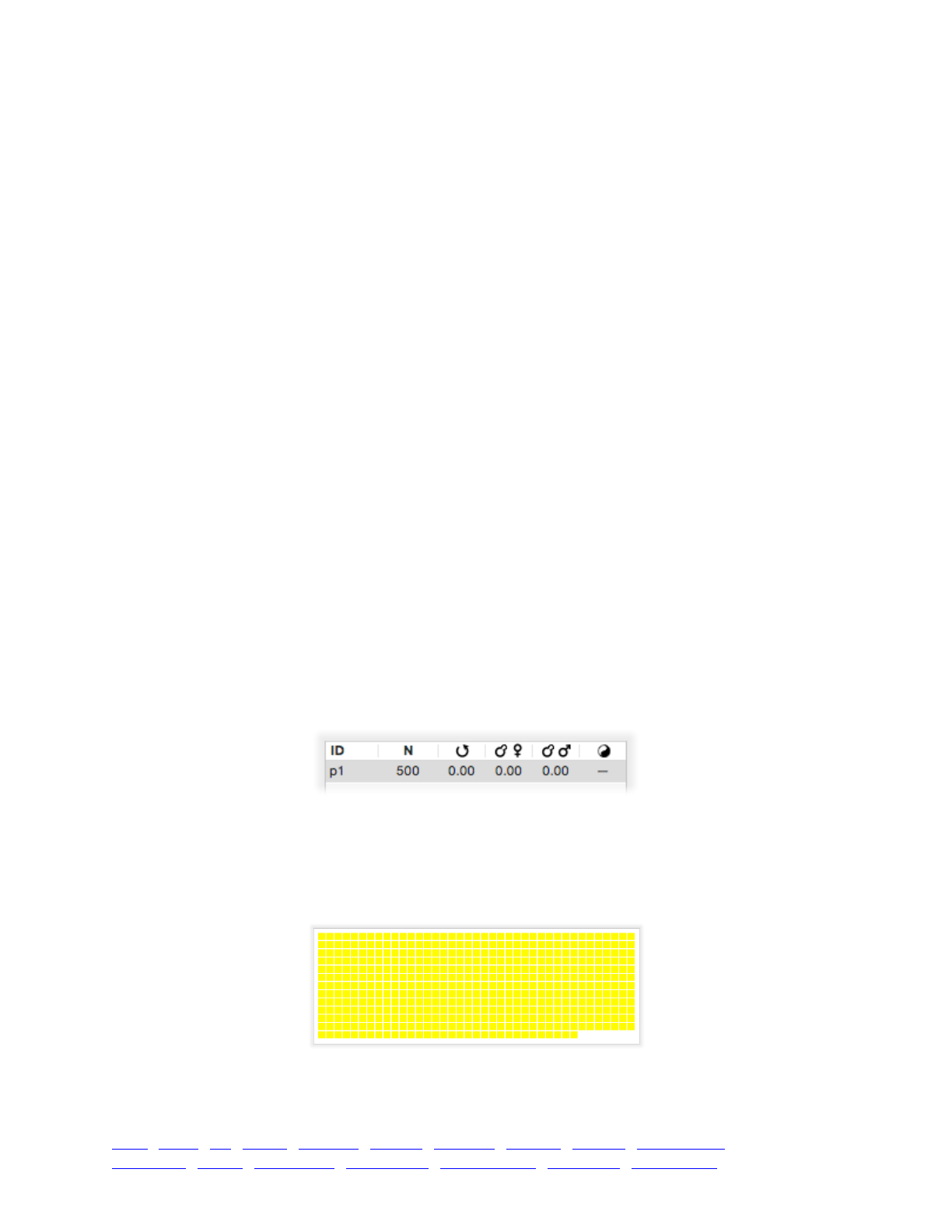
–!(object<Subpopulation>$)addSubpop(is$!subpopID, integer$!size,!
[float$!sexRatio!=!0.5])
Notice there is a third parameter, which is optional, named sexRatio. This will be discussed
when sexual simulations are covered in chapter 6. The dash at the very beginning indicates that
the signature is for a method, as opposed to a function signature, which has no leading dash.
Methods are sometimes referred to by name with this leading dash; the addSubpop() method is
thus sometimes called -addSubpop(). The meanings are identical.
4.1.9 Executing the simulation
We have already executed the initialization phase and the first generation of the simulation (if
you are following along in SLiMgui). Now try pressing the Play button. The simulation will
suddenly run at full speed, which is probably pretty fast in this case. You will see mutations flicker
in and out of existence, and rise and fall in frequency, along the length of the chromosome, as
displayed in the chromosome views. If you let the simulation run, it will go until it reaches
generation 10000, at which point it will stop because of the final snippet of code in our example
script:
10000!
{!
sim.simulationFinished();!
}
This defines an Eidos event that executes in generation 10000. The event calls a method named
simulationFinished() on the sim object, and that method declares that the simulation is finished
(although it continues to execute until the end of the current generation). This is actually not the
typical way that a simulation ends, as we will see in the next section; but it will serve for now.
When the simulation stops, the generation counter will read 10001 because generation 10000
finished executing and the next generation to execute (were the simulation not finished) would be
10001.
Having reached the end of the simulation, let’s look at a few parts of the simulation window.
The population table view now looks something like this:
This shows the subpopulation that the generation 1 Eidos event created, named p1 as sown in
the ID column, along with its size (500) and its selfing and cloning rates (all 0.00). The last column
shows the sex ratio (M:M+F); simulations in SLiM are hermaphroditic by default, so the sex ratio is
undefined.
The individual view now looks something like this:
Each yellow square represents one individual; there are 500 squares since the subpopulation
size is 500. Each individual is colored according to the calculated fitness of that individual;
TOC I TOC II WF nonWF initialize() Genome Individual Mutation SLiMSim Subpopulation!
Eidos events fitness() mateChoice() modifyChild() recombination() interaction() reproduction() 61
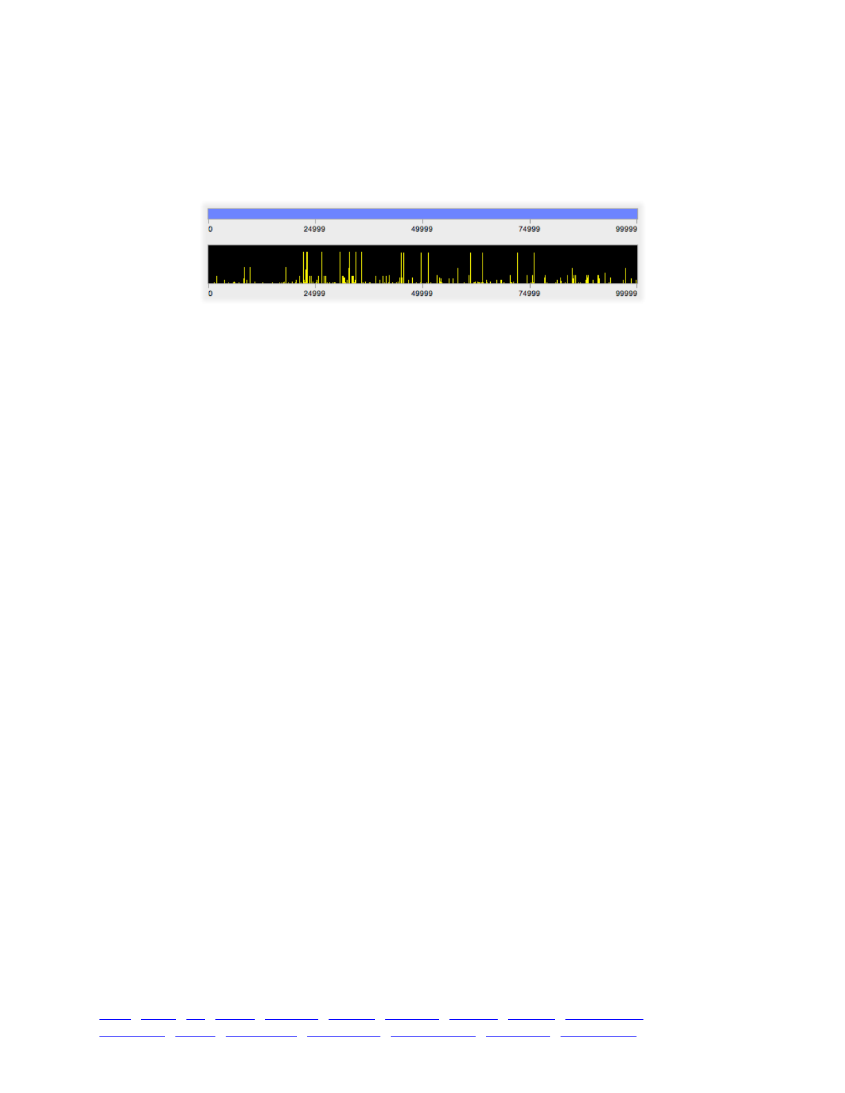
however, in this simulation all mutations are neutral, so all individuals have the same relative
fitness, 1.0, and so they are all yellow (as expressed by the color stripe for fitness values, discussed
in section 3.1). In a simulation with beneficial and deleterious mutations you would see a range of
colors, giving you an immediate visual sense of the fitness distribution across the subpopulation.
Finally, the chromosome view area looks something like this:
The top band shows the whole chromosome; the numbers and ticks below indicate base
positions. You can click and drag here to select a subrange of the chromosome for display in the
bottom view; a simple click in the top band will return you to viewing the full chromosome. The
bottom band displays the selected range of the chromosome (here, the full range). Each yellow bar
is a mutation that exists at that position in the chromosome. The height of the bar indicates the
frequency of the mutation; if the bar reaches the full height of the band, it has reached fixation and
is removed from the display (but you can turn on display of fixed mutations with the F button, in
which case they will display as full-height blue bars, by default). Here, all the bars are yellow
because all the mutations in this simulation are neutral, and neutral mutations are colored yellow
as shown by the color stripe at upper right (see section 3.1).
You might have noticed that whole sets of yellow bars tend to rise and fall in synchrony. These
are haplotypes that have become associated with each other through genetic drift. The dynamics
of mutations, haplotypes, and genetic drift is immediately visually apparent here, underlining the
value of having an interactive graphical interface in which you can develop, debug, test, and
experiment with your simulations. This visual, interactive workflow also makes SLiMgui a
potentially valuable tool for classroom instruction in population genetics and evolutionary biology.
4.2 Basic output
So far, our basic neutral simulation simply stops in generation 10000. Typically, it is desirable
for a simulation to produce some output. We will look at a few output options in this section.
4.2.1 Entire population
One option is to output the full state of the population (i.e., all individuals in all
subpopulations). To do this, we might change our script just a bit:
initialize() {!
initializeMutationRate(1e-7);!
initializeMutationType("m1", 0.5, "f", 0.0);!
initializeGenomicElementType("g1", m1, 1.0);!
initializeGenomicElement(g1, 0, 99999);!
initializeRecombinationRate(1e-8);!
}!
1 { sim.addSubpop("p1", 500); }!
10000 late() { sim.outputFull(); }
The only change here is that the final event, including the sim.simulationFinished() call, has
been replaced by a different event to generate output using the sim.outputFull() method:
10000 late() { sim.outputFull(); }
TOC I TOC II WF nonWF initialize() Genome Individual Mutation SLiMSim Subpopulation!
Eidos events fitness() mateChoice() modifyChild() recombination() interaction() reproduction() 62

Note the keyword late() here. SLiM can run user-defined Eidos events at two different points
in the generational life cycle, as shown in section 1.3. These two points are referred to as early()
and late() events. Events are early() by default, so the original line:
10000 { sim.simulationFinished(); }
defined an early() event, and could just as well have been written as:
10000 early() { sim.simulationFinished(); }
Most of the time, running events early in the generation, prior to the generation of offspring, is
desirable (which is why that is the default). In some cases, however, it is better for an event to run
toward the end of the generation, after the generation of offspring – and events that produce output
are usually such a case. If the late() specifier were omitted, the output would be generated at the
beginning of generation 10000, instead of at the end, and would thus reflect the results of running
the model for only 9999 generations. After the output was generated, the model would then run
for the final generation, with no effect on the model’s output.
That would be quite a subtle bug, and easy to miss. In fact, generating output at the beginning
of a generation, in an early() event, is so likely to be a bug that SLiM will output a warning if you
try to do it using one of SLiM’s standard output generation methods. For example, if we delete the
late() designation on the output event above, SLiM will generate a warning when the model
executes:
#WARNING (SLiMSim::ExecuteInstanceMethod): outputFull() should probably
not be called from an early() event; the output will reflect state at the
beginning of the generation, not the end.
There are a few other common situations in which you want to use a late() event instead of
the default early() events, most notably when you introduce new mutations into the simulation in
script; these situations will be discussed as they arise.
Once you have copied and pasted this new script into your simulation window, press Recycle
and then Play, and let the simulation run to the end. Notice that the full state of the population has
been printed, as requested in an output section that looks something like this (with large chunks of
output skipped over with ellipses):
#OUT: 10000 A!
Populations:!
p1 500 H!
Mutations:!
29 68306 m1 34640 0 0.5 p1 6848 450!
2 68503 m1 7251 0 0.5 p1 6867 561!
...!
Individuals:!
p1:i0 H p1:0 p1:1!
p1:i1 H p1:2 p1:3!
...!
Genomes:!
p1:0 A 0 1 2 3 4 5 6 7 8 9 10 11 12 13 14 15!
p1:1 A 16 17 18 7 8 19 9 20 21 22 23 24 25 26 27 28!
...
The format here is fairly simple and easily parsable by something like an R script; it can also be
read by SLiM in order to read in a population from a saved state, as we will see later. It begins
with an output prefix, #OUT:, followed by the generation (10000) and the type of output (A for all).
TOC I TOC II WF nonWF initialize() Genome Individual Mutation SLiMSim Subpopulation!
Eidos events fitness() mateChoice() modifyChild() recombination() interaction() reproduction() 63

The next section describes the subpopulations; p1 is of size 500 and is hermaphroditic (H).
Next comes a list of all mutations present; each line shows one mutation, including (1) a
temporary unique identifier used only in this output section, (2) a permanent unique identifier kept
by SLiM throughout a run, (3) the mutation type, (4) the base position, (5) the selection coefficient
(here always 0 since this is a neutral model), (6) the dominance coefficient (here always 0.5), (7)
the identifier of the subpopulation in which the mutation first arose, (8) the generation in which it
arose, and (9) the prevalence of the mutation (the number of genomes that contain the mutation,
where – in the way that SLiM uses the term “genome” – there are two genomes per individual).
Next comes a list of individuals. The first line of this section as shown above, for example,
shows that individual 0 in subpopulation 1 (p1:i0) is a hermaphrodite (H) and is comprised of two
genomes, p1:0 and p1:1, that will be listed in the following section. This section makes it easier to
figure out which genomes correspond to which individuals, but is largely redundant.
The final section lists all of the genomes in the simulation. The first line in this section as shown
above, for example, shows that genome p1:0 (which the Individuals section told us belonged to
individual p1:i0) is an autosome (A) and contains the mutations with the identifiers 0, 1, 2, ... 19.
From all of this information, the complete state of the population can be reconstructed – every
individual, and every mutation contained by every individual – thus the method name
outputFull().
4.2.2 Random population sample
Often the outputFull() method is overkill; you might just want a sample of genomes that is
randomly drawn from a particular subpopulation. For example, to output a 10-genome sample at
the halfway point of the simulation, here is a modified script:
initialize() {!
initializeMutationRate(1e-7);!
initializeMutationType("m1", 0.5, "f", 0.0);!
initializeGenomicElementType("g1", m1, 1.0);!
initializeGenomicElement(g1, 0, 99999);!
initializeRecombinationRate(1e-8);!
}!
1 { sim.addSubpop("p1", 500); }!
5000 late() { p1.outputSample(10); }!
10000 late() { sim.outputFull(); }
The only change relative to the previous script is the added line:
5000 late() { p1.outputSample(10); }
This calls the method outputSample() on the subpopulation from which the sample should be
taken, p1, with a requested sample size of 10 genomes (not 10 individuals, note; outputSample()
outputs randomly selected haploid genomes). If you copy and paste this script into SLiMgui,
Recycle and Play, you will see that at generation 5000 some output appears:
#OUT: 5000 SS p1 10!
Mutations:!
21 203188 m1 92838 0 0.5 p1 4489 4!
4 203247 m1 73991 0 0.5 p1 4495 6!
...!
Genomes:!
p1:0 A 0 1 2 3 4 5 6!
p1:1 A 0 7 1 3 4 5 8 6 9!
...
TOC I TOC II WF nonWF initialize() Genome Individual Mutation SLiMSim Subpopulation!
Eidos events fitness() mateChoice() modifyChild() recombination() interaction() reproduction() 64

The format here is very similar to that of outputFull(), but the header #OUT: 5000 SS p1 10
indicates that in generation 5000 a sample (S) was taken from p1 of size 10 genomes and was
output in SLiM (S) format. The list of mutations and genomes is identical in format to
outputFull(), except that only those mutations are shown that are actually present in the sample,
and that prevalence now refers to the sample rather than the entire population. The list of
populations and the list of individuals are also omitted in this output style.
SLiM also supports output of samples in MS format. The previous recipe can be modified to use
the outputMSSample() method instead of the outputSample() method; running the recipe in
SLiMgui would then produce MS-style output at generation 5000:
segsites: 73!
positions: 0.0262003 0.0351204 0.0445104 0.0597206 0.0647306 0.0702307
0.0871209 0.1039710 0.1046410 0.1162212 0.1222912 0.1407114 0.1608916
0.1728717 0.1775018 0.2036920 0.2366524 0.2462625 0.2468625 0.2475225
0.2531725 0.2858329 0.2880929 0.2913729 0.2998330 0.3045530 0.3048630
0.3132831 0.3279533 0.3400434 0.3484835 0.3544035 0.3547335 0.3586336
0.3594236 0.3765438 0.3845438 0.4385444 0.4441644 0.4460845 0.4483745
0.4692747 0.4801248 0.5282953 0.5387154 0.5493255 0.5563656 0.5660457
0.5810758 0.5871859 0.5880459 0.6183762 0.6271763 0.6368964 0.6389064
0.6678067 0.6880269 0.6961170 0.6961970 0.7082871 0.7340373 0.7362074
0.8214782 0.8450485 0.8694387 0.8696087 0.9022290 0.9114191 0.9187892
0.9264793 0.9364694 0.9835098 0.9969800!
1011010000000100001100110001001010100010000010010000000011001011001010001!
0011010000010100001111110101001001100000000010010000000000101011011000011!
0001010000000100000000001000010000000101100101100100111000010000000001000!
1011010000100100001100110001001010100010000010010000000011001111001010101!
1011010000000100001100110011001010101010000010010000000011001011001010001!
0011010000010100001110110101001001100000000010010000000000101011011000011!
0000101111001011111100010001101100110000011000011011000100001010101100000!
0101010000000100000000001000010000000101100101100100111000010000000001000!
1011010000000100001100110011001010101010000010010000000011001011001010001!
1011010000100100001100110001001010100010000010010000000011001011001010001
Finally, SLiM supports output of samples in VCF format. If the outputVCFSample() method is
used instead of outputSample() in the above recipe, VCF-style output would be produced:
##fileformat=VCFv4.2!
##fileDate=20160609!
##source=SLiM!
##INFO=<ID=S,Number=1,Type=Float,Description="Selection Coefficient">!
##INFO=<ID=DOM,Number=1,Type=Float,Description="Dominance">!
##INFO=<ID=PO,Number=1,Type=Integer,Description="Population of Origin">!
##INFO=<ID=GO,Number=1,Type=Integer,Description="Generation of Origin">!
##INFO=<ID=MT,Number=1,Type=Integer,Description="Mutation Type">!
##INFO=<ID=AC,Number=1,Type=Integer,Description="Allele Count">!
##INFO=<ID=DP,Number=1,Type=Integer,Description="Total Depth">!
##INFO=<ID=MULTIALLELIC,Number=0,Type=Flag,Description="Multiallelic">!
##FORMAT=<ID=GT,Number=1,Type=String,Description="Genotype">!
#CHROM POS ID REF ALT QUAL FILTER INFO FORMAT p1:i166 p1:i100!
p1:i462 p1:i8 p1:i0 p1:i314 p1:i318 p1:i488 p1:i81 p1:i287!
1 547 . A T 1000 PASS S=0;DOM=0.5;PO=1;GO=4822;MT=1;AC=4;DP=1000!
GT 1|0 0|1 1|0 0|0 0|0 0|0 0|0 0|0 0|0 0|1!
1 826 . A T 1000 PASS S=0;DOM=0.5;PO=1;GO=4342;MT=1;AC=5;DP=1000!
GT 0|0 0|0 0|0 1|1 0|1 0|0 1|0 0|0 0|0 1|0!
...
See sections 20.12.2 and 22.2 for details on these different output methods.
TOC I TOC II WF nonWF initialize() Genome Individual Mutation SLiMSim Subpopulation!
Eidos events fitness() mateChoice() modifyChild() recombination() interaction() reproduction() 65

4.2.3 Sampling individuals rather than genomes
The previous section showed how to use methods of the Subpopulation class to output a
sample of genomes from a subpopulation, in either SLiM’s own format, or in MS or VCF format.
However, in many situations you want to output information about a sample of individuals, rather
than a sample of genomes – you want to ensure that pairs of genomes, each belonging to an
individual, are the level of granularity at which the sampling for output occurs. Also, the
Subpopulation output methods only support sampling from a single subpopulation at a time, but
sometimes you want to output a sample drawn from multiple subpopulations, or from the full
population. Finally, sometimes you want to output a custom sample that your script chooses itself,
rather than a random, equally-weighted sample of the sort that the Subpopulation methods allow.
These tasks are all quite straightforward using lower-level methods of the Genome class. As an
illustration of this approach, we will look at a recipe that outputs the genomes of a weighted
sample of individuals drawn from the whole population:
initialize() {!
initializeMutationRate(1e-7);!
initializeMutationType("m1", 0.5, "f", 0.0);!
initializeMutationType("m2", 0.5, "f", 0.01);!
initializeGenomicElementType("g1", c(m1,m2), c(1.0,0.01));!
initializeGenomicElement(g1, 0, 99999);!
initializeRecombinationRate(1e-8);!
}!
1 {!
sim.addSubpop("p1", 500);!
sim.addSubpop("p2", 500);!
p1.setMigrationRates(p2, 0.01);!
p2.setMigrationRates(p1, 0.01);!
}!
10000 late() {!
allIndividuals = sim.subpopulations.individuals;!
w = asFloat(allIndividuals.countOfMutationsOfType(m2) + 1);!
sampledIndividuals = sample(allIndividuals, 10, weights=w);!
sampledIndividuals.genomes.output();!
}
This model involves a few things that we haven’t looked at yet, such as multiple subpopulations
connected by migration (see section 5.2.1) and multiple mutation types (see section 7.1).
However, those details are not our focus here. For our current purposes, it suffices to recognize
that there are two subpopulations, p1 and p2, connected by migration, and there are two mutation
types, m1 and m2, with m1 representing common neutral mutations and m2 representing less
common beneficial mutations. Our focus is on the late() event in generation 10000, which
produces the output for the model. We will follow through its logic one line at a time.
The first line defines the set of individuals from which our sample will be drawn, here called
allIndividuals. The sim.subpopulations property gives us a vector of all of the subpopulations
in the model (i.e., p1 and p2). The individuals property of that vector is then all of the individuals
(that is, objects of class Individual; see section 21.6) gathered from across those subpopulations.
The second line determines the weights that we will use for sampling, here called w. Note that
the use of weights here is optional; if you want an unweighted sample, you can skip this line and
omit the weights vector in the call to sample() below. In this recipe, however, we want the
likelihood that an individual is chosen for sampling to be related to the number of m2 mutations the
individual possesses, so we use countOfMutationsOfType(m2). We add 1 to that count, so that
individuals with no m2 mutations have a weight of 1, individuals with one m2 mutation have a
weight of 2, and so forth. This is somewhat arbitrary, but it does have the nice property that we are
TOC I TOC II WF nonWF initialize() Genome Individual Mutation SLiMSim Subpopulation!
Eidos events fitness() mateChoice() modifyChild() recombination() interaction() reproduction() 66

guaranteed that the weights vector is not all zero (which would cause a runtime error, since it
would not be possible to draw a sample). If you draw your own samples, you probably want to
ensure that the sample can always be drawn, to avoid runtime errors.
The third line draws a sample of 10 individuals from allIndividuals, using the sample()
function and passing it the weights vector w (using the named arguments syntax of Eidos, for
readability). The sample is put into the temporary variable sampledIndividuals.
Finally, the fourth line outputs the genomes of the sampled individuals using the output()
method of Genome. This outputs the sample in SLiM’s own format, similarly to what we saw in the
previous sections; there are also outputMS() and outputVCF() methods on Genome that can be used
similarly to produce MS and VCF output. Since there are two genomes per individual, twenty
genomes will be output. Each pair of genomes in the output will come from one sampled
individual; in the SLiM and MS output formats this is not explicit, but in the VCF format, since it is
a diploid format (as used by SLiM), this pairing into individuals is explicit in the output. See
section 21.3.2 for more information on these output methods, and section 23.3 for details on the
format of output they generate.
While this recipe implemented one particular sampling scheme, the Genome methods used here
can be used to output any vector of genomes, whether a random sample or a specifically selected
set. The higher-level output methods of SLiMSim and Subpopulation are a little easier to use, but
these low-level methods provide greater power and generality.
4.2.4 Substitutions
The outputFull() method of SLiMSim does output the full state of the population, but there is
some historical state that it does not output. Most notably, it does not output substitutions –
mutations which have been fixed and have thus been removed from the population by SLiM for
efficiency. If fixed mutations are of interest, SLiM does keep a record of them and can output that
record on request. For example, we could output substitutions, in addition to other state, with this
script:
initialize() {!
initializeMutationRate(1e-7);!
initializeMutationType("m1", 0.5, "f", 0.0);!
initializeGenomicElementType("g1", m1, 1.0);!
initializeGenomicElement(g1, 0, 99999);!
initializeRecombinationRate(1e-8);!
}!
1 { sim.addSubpop("p1", 500); }!
5000 late() { p1.outputSample(10); }!
10000 late() { sim.outputFull(); }!
10000 late() { sim.outputFixedMutations(); }
The only change relative to the previous script is the added line:
10000 late() { sim.outputFixedMutations(); }
If you copy and paste this script into SLiMgui, Recycle and Play, you will see that at simulation
end some additional output appears:
#OUT: 10000 F !
Mutations:!
0 220169 m1 98564 0 0.5 p1 107 1053!
1 221802 m1 1217 0 0.5 p1 268 1152!
...
TOC I TOC II WF nonWF initialize() Genome Individual Mutation SLiMSim Subpopulation!
Eidos events fitness() mateChoice() modifyChild() recombination() interaction() reproduction() 67

The header #OUT: 10000 F indicates simply that in generation 10000 fixed mutations (F) were
output. The rest is a list of mutations in almost the same format as before. However, the final
number in each line is no longer a prevalence; since the mutation fixed, we know that it was
present in every genome in the simulation. Instead, the final number shows the generation
number in which the mutation reached fixation. Note that the default behavior of SLiM – that
substitutions are removed from all individual genomes – can be deactivated if necessary (see
section 21.9.1).
Display of fixed mutations in SLiMgui can also be enabled by clicking the F button to the right
of the chromosome view; when this display is enabled, fixed mutations will be displayed as full-
height bars (blue, by default) in the chromosome view.
4.2.5 Custom output with Eidos
The outputFull(), outputSample(), outputMSSample(), outputVCFSample(), and
outputFixedMutations() methods described in the preceding sections generate output in very
fixed formats that may or may not be useful to you. There is one more built-in output method that
is described in the reference section – outputMutations() – but it, too, may not be what you
need. What to do?
This is an area where the power of Eidos really shines, since you can write whatever Eidos script
you like to generate whatever kind of output you want. Some of the more advanced recipes in this
cookbook will generate custom output of interesting kinds; section 11.1’s recipe will include code
to calculate and print the FST between two subpopulations to assess their genetic divergence, for
example, and section 13.2’s recipe calculates and prints the nucleotide heterozygosity, π, of a
population to assess the effects of inbreeding. In this section, we will look at a much simpler
example, as an introduction to the topic of custom output using Eidos.
Suppose you are interested only in the base positions of all of the mutations in the population;
you can achieve this with the following output event:
100 late() { cat(paste(sim.mutations.position, "\n")); }
With our basic neutral simulation script, this generates output like:
31113!
57761!
...
This is precisely what we want. How does it work? Let’s dissect it, step by step, since it is more
complex than the Eidos code we’ve seen so far.
First of all, we have seen the sim object before, representing the simulation. This object, which
is an Eidos object of class SLiMSim, has a property named mutations that yields a vector containing
all of the mutations in the simulation (a vector of type object and class Mutation, to be precise).
This is the first use we have seen of a property; a property is somewhat like a method, in that it is a
member of an object, but whereas a method performs an operation (perhaps involving a lot of
computation, and perhaps altering the state of the simulation), a property simply corresponds to a
value that exists inside the object. The sim object knows all of the mutations it contains; it doesn’t
have to calculate them or create them, it just has to return the value it already has. It is therefore a
property – the mutations property. The member operator is used to access properties, just as it is
used to access methods, so the value of sim.mutations is the vector of mutations contained by the
simulation.
That value is itself an object. As mentioned before, all values in Eidos are actually vectors; the
vector of mutations might contain many elements (each of which is called an object-element), but
it is nevertheless a single Eidos object. The Mutation class in SLiM defines a property, position,
TOC I TOC II WF nonWF initialize() Genome Individual Mutation SLiMSim Subpopulation!
Eidos events fitness() mateChoice() modifyChild() recombination() interaction() reproduction() 68

that is the base position of the mutation; we can access this property on our vector of mutations to
get a vector of positions. This involves a certain amount of work behind the scenes; each mutation
has its own position, and Eidos must loop over all of the mutations in the vector of mutations,
getting the position of each one and pasting all the positions together to make a new vector. Eidos
does this for you, though, since Eidos is a vector-based language; so sim.mutations.position is all
the Eidos code that is needed to get a vector of the positions of all mutations in the simulation.
Peeling the onion back a layer, this expression is contained in a function call:
paste(sim.mutations.position, "\n")
This function takes a vector argument (sim.mutations.position) and pastes all of the elements
together to form a single value of type string. We haven’t really talked about string yet; a string
is simply a sequence of characters, like "hello, world". Eidos can paste strings together, split
them apart, and print them out; it can also convert most other types into string for the purpose of
output. The paste() function always produces a string as its result; it converts the elements of the
vector it is given into string elements in order to do so. The second parameter of paste(), "\n",
is a string containing a single character, the newline character, represented with the escape
sequence \n (you can read more about strings and escape sequences in the Eidos manual; it is not
worth getting into here). The final result is that each of the integer positions in
sim.mutations.position is converted to a string representation and then pasted together with the
others, with newlines in between, to produce the desired output as seen above.
Note that this output event is designated as a late() event, for the reasons outlined in section
4.2.1; in this case, we wish to see the positions of mutations at the end of generation 100, not the
beginning. With custom output code of this sort, SLiM is not able to infer that it is likely to be an
error if it runs in an early() event instead, however; so if the late() designation is removed here,
SLiM will not produce a warning. When writing custom output script events, you need to think
carefully about whether they should be early() or late() events (but a late() event is usually
what you want).
The simplicity of this example – just a single line of Eidos code! – should make it clear that
generating output in whatever format you desire is likely to be straightforward once you get the
hang of how Eidos works.
Since the power of this may not be entirely apparent yet, let’s consider a problem that might
arise in using SLiM. You might wish to produce MS-style output for a sample of genomes spanning
the whole population, but the built-in outputMSSample() method of Subpopulation (sections 4.2.2,
20.12.2, and 22.2.3) only supports generation of MS-style output from a sample of a single
subpopulation. As of SLiM 2.1, you can solve this problem with the outputMS() method of Genome
(sections 20.3.2 and 22.3.2), but let’s pretend that method doesn’t exist; the same general problem
will arise whenever you want to output data in a format that SLiM does not, in fact, intrinsically
support. Generating MS-style output using Eidos is trivial:
initialize() {!
initializeMutationRate(1e-7);!
initializeMutationType("m1", 0.5, "f", 0.0);!
initializeGenomicElementType("g1", m1, 1.0);!
initializeGenomicElement(g1, 0, 99999);!
initializeRecombinationRate(1e-8);!
}!
1 {!
sim.addSubpop("p1", 500);!
sim.addSubpop("p2", 500);!
}!
TOC I TOC II WF nonWF initialize() Genome Individual Mutation SLiMSim Subpopulation!
Eidos events fitness() mateChoice() modifyChild() recombination() interaction() reproduction() 69

// custom MS-style output from a multi-subpop sample!
2000 late() {!
// obtain a random sample of genomes from the whole population!
g = sample(sim.subpopulations.genomes, 10, T);!
!
// get the unique mutations in the sample, sorted by position!
m = sortBy(unique(g.mutations), "position");!
!
// print the number of segregating sites!
cat("\n\nsegsites: " + size(m) + "\n");!
!
// print the positions!
positions = format("%.6f", m.position / sim.chromosome.lastPosition);!
cat("positions: " + paste(positions, " ") + "\n");!
!
// print the sampled genomes!
for (genome in g)!
{!
hasMuts = (match(m, genome.mutations) >= 0);!
cat(paste(asInteger(hasMuts), "") + "\n");!
}!
}
This model is quite straightforward; the only complication is that there are two subpopulations,
and we wish to produce MS-style output for a sample across both of them. The generation 2000
event does precisely that. First it obtains the genomes upon which the output will be based; here
this is done using sample() on the vector of all genomes in the simulation, but any other sampling
scheme could be used instead. To sample specifically from subpopulations p1 and p2, for
example, without sampling from any other subpopulations that might exist, you could do:
g = sample(c(p1.genomes, p2.genomes), 10, T);
The sample size is 10, and sampling is done with replacement (the T parameter to sample()),
but that can obviously be customized. Next unique() and sortBy() are used to get a vector of the
mutations present in the sample, sorted by position. The size() of that vector is the number of
segregating sites, so that is trivial to output. Printing the positions is also simple; format() is used
to guarantee that every position is formatted with six digits to the right of the decimal, in decimal
rather than scientific notation even for very small values. Finally, the sampled genomes are printed
in MS format, using asInteger() to convert logical values from match() into 0s and 1s.
4.2.6 The simulation endpoint
The astute reader will have noticed that in the previous sections we not only added output
events, we also removed one line from the original script:
10000 { sim.simulationFinished(); }
We can do this because SLiM will generally stop after the last generation in which an event is
scheduled. In our basic neutral simulation, however, we had no output commands; if we had
omitted the line above with the simulationFinished() call the simulation would have ended at
the end of generation 1. Alternatively, we could have just written:
10000 { }
This “empty event” would have caused SLiM to run out to the end of generation 10000, because
there was still a future event scheduled. At the end of generation 10000 SLiM would then stop,
since there was no future event after generation 10000 scheduled. In fact, simulationFinished()
TOC I TOC II WF nonWF initialize() Genome Individual Mutation SLiMSim Subpopulation!
Eidos events fitness() mateChoice() modifyChild() recombination() interaction() reproduction() 70

is really useful only when you wish to end a simulation before it would naturally end on its own.
You might check for an equilibrium condition, for example, and end the simulation if it has been at
equilibrium for the past 1000 generations, even though it would otherwise have run further.
There is one further caveat to mention regarding how simulations end. It is possible to define
an Eidos event that runs in every generation. For example, we could write the following script:
initialize() {!
initializeMutationRate(1e-7);!
initializeMutationType("m1", 0.5, "f", 0.0);!
initializeGenomicElementType("g1", m1, 1.0);!
initializeGenomicElement(g1, 0, 99999);!
initializeRecombinationRate(1e-8);!
}!
1 { sim.addSubpop("p1", 500); }!
late() { p1.outputSample(10); }
Notice that there is no generation number before the Eidos event defined in the last line; this
indicates that the event should be run in every generation, from here to eternity. If you copy and
paste this into SLiMgui and Recycle and Play, it will stop at the end of generation 1, however; there
is always a scheduled future event (the output event), but SLiM does not use it in determining
when the simulation should end, precisely because it has no expiration date. SLiM assumes that it
is not your wish to run a simulation that runs forever – commonly known as an “infinite loop” in
programming – so the simulation end is determined without reference to that event.
To define a final generation for the simulation in this situation, you would use precisely the trick
described above: just add an “empty event”, like:
100 { }
The simulation will now run to the end of generation 100. Note that there is no need to
designate the event as a late() event; SLiM always runs the last generation to completion, even if
simulationFinished() is called. The only way to halt a simulation immediately, within a
generation, is to call the Eidos error function stop().
TOC I TOC II WF nonWF initialize() Genome Individual Mutation SLiMSim Subpopulation!
Eidos events fitness() mateChoice() modifyChild() recombination() interaction() reproduction() 71

5. Demography and population structure
The previous chapter discussed in detail the structure of a basic neutral simulation in SLiM,
including initialize() callbacks, Eidos events, the SLiMSim class, and many of the conceptual
underpinnings of SLiM such as mutation types, genomic element types, and chromosome
organization. It also covered some basic features of the Eidos language, such as vectors and vector
operations, function calls, objects, and method calls. From here, we assume a working knowledge
of these topics; you can consult the Eidos manual regarding features of the Eidos language, and the
reference section of this manual for details regarding SLiM.
In this chapter, we will focus on building on this foundation to make some simple “recipes” for
simulations that do interesting things with demography and population structure.
5.1 Subpopulation size
5.1.1 Instantaneous changes
As we saw in section 4.1.8, we can create a new subpopulation with sim.addSubpop(), a
method call which takes the initial size of the subpopulation as a parameter. What if we want the
population size to change later? This is very straightforward; for example, here is a simple script
that models a population that goes through a bottleneck:
initialize() {!
initializeMutationRate(1e-7);!
initializeMutationType("m1", 0.5, "f", 0.0);!
initializeGenomicElementType("g1", m1, 1.0);!
initializeGenomicElement(g1, 0, 99999);!
initializeRecombinationRate(1e-8);!
}!
1 { sim.addSubpop("p1", 1000); }!
1000 { p1.setSubpopulationSize(100); }!
2000 { p1.setSubpopulationSize(1000); }!
10000 late() { sim.outputFull(); }
The initialize() callback is unchanged from previous models. In generation 1 a
subpopulation named p1 is set up with an initial size of 1000. In generation 1000, a method named
setSubpopulationSize() is called on p1 to change its size to 100, the beginning of the bottleneck.
In generation 2000 the size is set back to 1000, ending the bottleneck. The simulation then
executes until it ends in generation 10000 with full output.
If you run this in SLiMgui (don’t forget to Recycle), the population size changes as expected.
5.1.2 Exponential growth
Sometimes you may want the size of a subpopulation to vary in a continuous fashion, rather
than experiencing discrete changes as in the previous recipe. This is straightforward in SLiM
because of the power of Eidos to express mathematical relationships. We will look at several
different versions of this recipe in order to explore different aspects of the problem.
As a first example, to make a population experience a period of exponential growth:
initialize() {!
initializeMutationRate(1e-7);!
initializeMutationType("m1", 0.5, "f", 0.0);!
initializeGenomicElementType("g1", m1, 1.0);!
initializeGenomicElement(g1, 0, 99999);!
initializeRecombinationRate(1e-8);!
}!
TOC I TOC II WF nonWF initialize() Genome Individual Mutation SLiMSim Subpopulation!
Eidos events fitness() mateChoice() modifyChild() recombination() interaction() reproduction() 72

1 { sim.addSubpop("p1", 100); }!
1000:1099 {!
newSize = asInteger(p1.individualCount * 1.03);!
p1.setSubpopulationSize(newSize);!
}!
10000 late() { sim.outputFull(); }
Most of the script is unchanged; the work is done in the second Eidos event, which is scheduled
to run from generation 1000 to 1099, producing exponential growth for 100 generations. This event
calculates a new size, assigning it into newSize, and then sets the subpopulation size using that
variable. The use of the variable is for readability; it would be essentially equivalent to write:
p1.setSubpopulationSize(asInteger(p1.individualCount * 1.03));
Let’s look more closely at that statement. First, the current size of the subpopulation is accessed
through the individualCount property of p1. That size is then multiplied by 1.03 to produce a
new size based on an exponential growth rate of 1.03. Finally, the size is converted to an integer
by the asInteger() function (since setSubpopulationSize() does not allow you to set a non-
integer size), and the integer size is passed to setSubpopulationSize(). There is a suite of as...
() functions in Eidos that allow you to convert values to various new types, but converting float
values to integer with asInteger() is probably the most common conversion.
An important point here is that the setSubpopulationSize() call does not change the current
size of the subpopulation; after all, what would the genetics of the new individuals be? Instead, it
sets a new target size that will be used the next time that an offspring generation is created; a few
additional offspring will be made to reach the new target size. If you access the individualCount
property immediately after calling setSubpopulationSize(), you therefore observe that the
individual count has not changed. This is the reason why setSubpopulationSize() is not called
setIndividualCount(); the difference in name is intended to emphasize how SLiM works.
Since the population size gets rounded down to an integer in each generation, this code does
not actually achieve the precise exponential growth rate of 1.03 that we wanted. Let’s fix that:
initialize() {!
initializeMutationRate(1e-7);!
initializeMutationType("m1", 0.5, "f", 0.0);!
initializeGenomicElementType("g1", m1, 1.0);!
initializeGenomicElement(g1, 0, 99999);!
initializeRecombinationRate(1e-8);!
}!
1 { sim.addSubpop("p1", 100); }!
1000:1099 {!
newSize = asInteger(round(1.03^(sim.generation - 999) * 100));!
p1.setSubpopulationSize(newSize);!
}!
10000 late() { sim.outputFull(); }
Running this in SLiMgui shows that the population reaches a size of 1922, whereas the previous
version reached a size of 1630 – a significant difference! Beware accumulated roundoff error.
How does the new version work? The expression sim.generation-999 computes the number of
generations of exponential growth that have occurred; in generation 1000 this is 1, in generation
1099 it is 100. Next, 1.03^(sim.generation-999) raises 1.03 to that power; ^ is the exponentiation
operator in Eidos, as in many programming languages. That calculates the result of the exponential
growth over the requisite number of generations. Finally, that result is rounded to the nearest
whole number by round(), which produces a float result, and then that whole number is
converted to an integer by asInteger().
TOC I TOC II WF nonWF initialize() Genome Individual Mutation SLiMSim Subpopulation!
Eidos events fitness() mateChoice() modifyChild() recombination() interaction() reproduction() 73

Sometimes we may want the population size to increase exponentially until a specific target
size is reached, without knowing how many generations that might take. This is a bit trickier. One
possible implementation does this by brute force (leaving out the initialize() code):
1 { sim.addSubpop("p1", 100); }!
1000:2000 {!
if (p1.individualCount < 2000)!
{!
newSize = asInteger(round(1.03^(sim.generation - 999) * 100));!
p1.setSubpopulationSize(newSize);!
}!
}!
10000 late() { sim.outputFull(); }
This uses an if statement to increase the size of the subpopulation only if it is still less than
2000 (this is the first time we’ve seen the if statement in Eidos, but it should be pretty obvious what
it does here; see the Eidos manual for clarification). The generation range for the event has been
expanded to 1000:2000, because we don’t know what generation the target size will be reached in;
it will be well before generation 2000, so this is good enough, but is a bit sloppy. Alternatively, we
could calculate the exact generation in which the target size is reached (1101, as it happens), and
use that instead of 2000; if we did that, we wouldn’t even need the if statement, since the
exponential growth would reach its target in the event’s last invocation.
To ensure that the last generation of growth produces exactly 2000 individuals, we can use the
following solution:
initialize() {!
initializeMutationRate(1e-7);!
initializeMutationType("m1", 0.5, "f", 0.0);!
initializeGenomicElementType("g1", m1, 1.0);!
initializeGenomicElement(g1, 0, 99999);!
initializeRecombinationRate(1e-8);!
}!
1 { sim.addSubpop("p1", 100); }!
1000: {!
newSize = round(1.03^(sim.generation - 999) * 100);!
if (newSize > 2000)!
newSize = 2000;!
p1.setSubpopulationSize(asInteger(newSize));!
}!
10000 late() { sim.outputFull(); }
First of all, notice that the generation range for the exponential growth event is now written as
1000:, omitting the end generation. Just as supplying no generation range at all for an event means
“run in every generation”, omitting the end generation means “run in every generation after the
specified start generation”. One may similarly omit the start generation with the syntax :end,
meaning “run in every generation from the beginning until the specified end generation”.
The logic inside the event has also changed. Now the code always calculates a new size. If
that size is greater than 2000 it gets clamped to 2000, which enforces the maximum population size
we wanted. The clamped size is then set on the subpopulation.
The drawback to this solution is that the event runs in every generation from 1000 onward,
calling setSubpopulationSize() to set the size to 2000 over and over in generations after the target
size has been reached. That is inefficient; more importantly, it might interfere with other changes
we might want to make to the population size later in the simulation. We’d really like our event to
run for exactly the needed duration to reach the target size, and then not run in subsequent
TOC I TOC II WF nonWF initialize() Genome Individual Mutation SLiMSim Subpopulation!
Eidos events fitness() mateChoice() modifyChild() recombination() interaction() reproduction() 74

generations, without having to hard-code a final generation for it. There is a simple solution to this
problem – and this, you will be relieved to read, is the final, polished version of our exponential
growth recipe (so the initialize() callback is provided to make the recipe complete):
initialize() {!
initializeMutationRate(1e-7);!
initializeMutationType("m1", 0.5, "f", 0.0);!
initializeGenomicElementType("g1", m1, 1.0);!
initializeGenomicElement(g1, 0, 99999);!
initializeRecombinationRate(1e-8);!
}!
1 { sim.addSubpop("p1", 100); }!
1000: {!
newSize = asInteger(round(1.03^(sim.generation - 999) * 100));!
if (newSize >= 2000)!
{!
newSize = 2000;!
sim.deregisterScriptBlock(self);!
}!
p1.setSubpopulationSize(newSize);!
}!
10000 late() { sim.outputFull(); }
Braces have been added around the if statement’s consequent to make a group of statements;
all of the statements in the group will be executed if the condition of the if statement is true. This
use of braces makes what is called a compound statement; compound statements are legal
anywhere in Eidos that a single statement is legal.
The interesting change here, though, is the addition of the line:
sim.deregisterScriptBlock(self);
This line prevents the event from continuing to run after the target size has been reached. It is a
common pattern in SLiM scripting, so it is worth a bit of discussion. SLiM keeps track of script
blocks that are registered for execution in the simulation. All of the events and callbacks that you
write in your input script are automatically registered; it is also possible to construct and register
new script blocks dynamically, as we will see in a later chapter. Script blocks that are registered
can be deregistered, using the deregisterScriptBlock() method of SLiMSim, as we are doing
here. Once a block is deregistered, SLiM forgets about it and no longer executes it.
The other thing to be explained here is self. This is a variable that is defined whenever SLiM is
executing an event or callback; it refers to the currently executing script block. We use it here so
that our exponential growth event can deregister itself. Once deregistered, the event is no longer
executed, and will remain deregistered until the Recycle button is pressed.
You can see the dynamics of script registration and deregistration graphically in SLiMgui, by the
way. Start by pressing Recycle, with the recipe above already pasted into the window. Now if you
open the drawer for the simulation window by pressing the drawer button to the right of the
chromosome view area, you will see a list of registered scripts:
TOC I TOC II WF nonWF initialize() Genome Individual Mutation SLiMSim Subpopulation!
Eidos events fitness() mateChoice() modifyChild() recombination() interaction() reproduction() 75
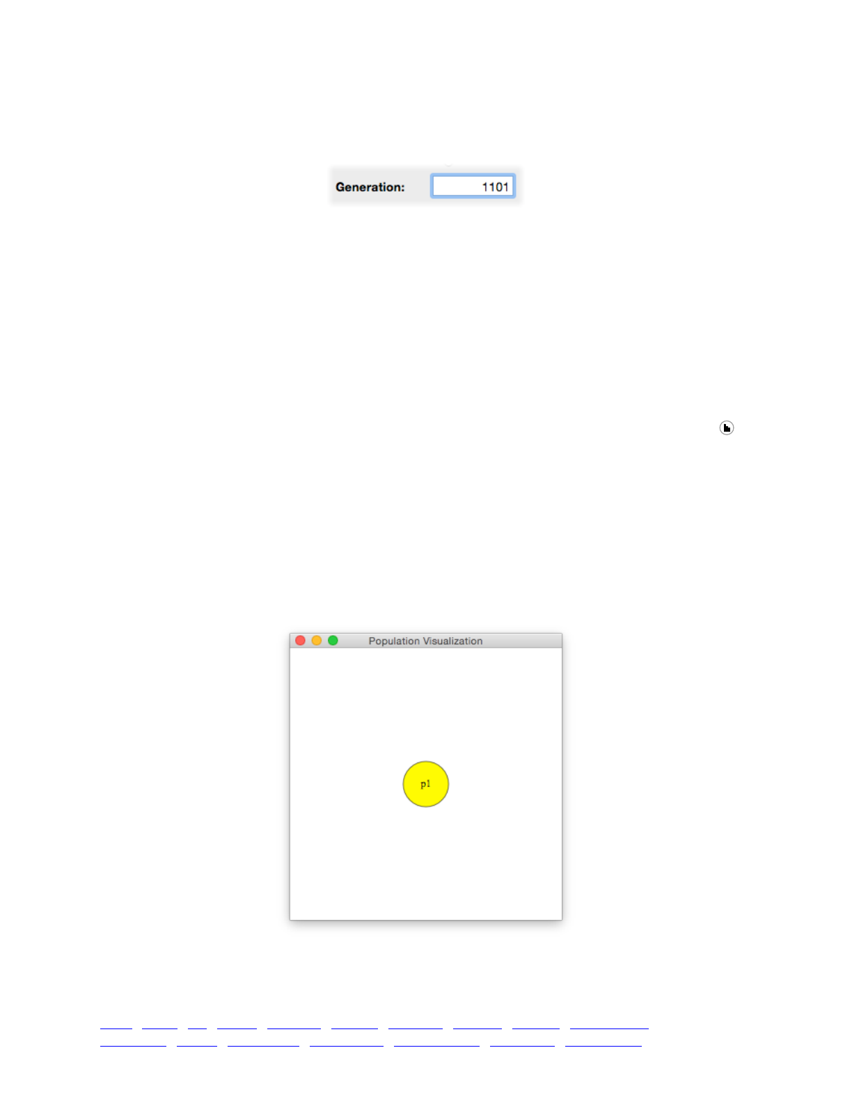
The exponential growth event is listed as the third entry there; if you hover the mouse over its
entry for a second or two, you will even see the code for it, shown in a tooltip. Now click in the
generation field, enter 1101, and press return:
This causes SLiMgui to execute the simulation up to the beginning of the requested generation,
which is just before the target population size is attained. If you now click Step, you will see the
exponential growth event disappear from the list of registered events.
If your scripting gets complicated, with script blocks registering and deregistering frequently,
this facility for viewing all of the registered script blocks can prove quite useful.
5.1.3 The population visualization graph
In the previous section, we saw several different ways to make a subpopulation grow
exponentially for a period of time. In this section, we show how to visualize the dynamics of
demography and population structure graphically in SLiMgui on Mac OS X.
Start by copying and pasting the last recipe into a new SLiMgui simulation window, and then
Recycle to parse the script and get ready to execute it. Now click on the Show Graph button, ,
and from its pop-up menu select “Graph Population Visualization”. This will bring up a small
window, presently empty.
If you click Step twice, in order to execute the initialization phase and then generation 1, you
should see a small yellow circle labeled “p1” appear. This circle represents subpopulation p1; in
particular, its radius represents the size of the subpopulation, and its color represents the mean
fitness value of the subpopulation.
Now press Play, and keep your eyes on the subpopulation circle. When the simulation reaches
generation 1000 the circle for p1 will begin to grow, and it will continue growing until the
subpopulation size reaches its target, 2000:
In this instance the visualization is fairly trivial; still, it is useful for verifying that the population
expansion happens in the way that it was planned. In future sections we will see that the
TOC I TOC II WF nonWF initialize() Genome Individual Mutation SLiMSim Subpopulation!
Eidos events fitness() mateChoice() modifyChild() recombination() interaction() reproduction() 76

population visualization graph can also help us to visualize migration dynamics, fitness dynamics,
and other such things, making it a very useful tool for simulation debugging.
5.1.4 Cyclical changes
Another common demographic dynamic is a cyclically varying subpopulation size, perhaps
representing seasonality, or a decadal oscillation in resource availability. Implementing this in
SLiM is quite trivial; for example:
initialize() {!
initializeMutationRate(1e-7);!
initializeMutationType("m1", 0.5, "f", 0.0);!
initializeGenomicElementType("g1", m1, 1.0);!
initializeGenomicElement(g1, 0, 99999);!
initializeRecombinationRate(1e-8);!
}!
1 { sim.addSubpop("p1", 1500); }!
{!
newSize = cos((sim.generation - 1) / 100) * 500 + 1000;!
p1.setSubpopulationSize(asInteger(newSize));!
}!
10000 late() { sim.outputFull(); }
The initialize() callback is unchanged. The interesting work is done by the second event –
the one with no generation specifier, which you might recall means that it will be executed in
every generation. This event first calculates a new size, and then sets the new size in the
subpopulation (converting to integer as usual). The new size is calculated based upon the current
generation, sim.generation, passed through the cos() function, which calculates a cosine. The
generation is scaled and translated in order to arrange that the first offspring generation has a size
of 1500, matching the size of the parental generation set up by addSubpop(). Of course that is not
required; this particular arrangement is just for demonstration purposes.
The cos() function calculates a cosine based on a given angle in radians, as is standard. The
periodicity of the cycling is therefore based upon the fact that there are 2π radians in a circle;
given the scaling factor of 100, the population will complete a full cycle in 100*2π generations,
which is about 628. To make a subpopulation cycle with whatever periodicity you wish, just adjust
the scaling factor accordingly. Similarly, since cosine varies between -1 and 1, the scaling factor
of 500 on that, plus the translation of 1000, means that the population size cycles between 500 and
1500. You might wish to view these dynamics in SLiMgui’s population visualization graph, as
described in the previous section.
This recipe uses cos() to generate cyclical dynamics, but you can plug in whatever formula you
wish. The population size does not have to depend only upon the generation, either; the flexibility
of Eidos allows you to implement whatever demographic model you wish, including demography
that depends upon the model dynamics themselves, as we will see in the next section.
5.1.5 Context-dependent changes: Muller’s Ratchet
Sometimes you might want subpopulation size to depend upon something other than time. An
example would be a situation in which population size depends upon mean fitness (e.g., a model
of so-called “hard” selection); if the mean fitness is low then the subpopulation size would be
small (perhaps because the subpopulation is getting outcompeted by individuals of some other
species, or perhaps because the subpopulation is just so unfit that individuals are having trouble
surviving and feeding themselves even without competition). Here we will examine such
dynamics in a model of Muller’s Ratchet:
TOC I TOC II WF nonWF initialize() Genome Individual Mutation SLiMSim Subpopulation!
Eidos events fitness() mateChoice() modifyChild() recombination() interaction() reproduction() 77

initialize() {!
initializeMutationRate(1e-7);!
initializeMutationType("m1", 0.5, "f", 0.0);!
initializeMutationType("m2", 0.5, "e", -0.01);!
m2.convertToSubstitution = F;!
initializeGenomicElementType("g1", c(m1,m2), c(1,1));!
initializeGenomicElement(g1, 0, 99999);!
initializeRecombinationRate(1e-8);!
}!
1 { sim.addSubpop("p1", 100); }!
{!
meanFitness = mean(p1.cachedFitness(NULL));!
newSize = asInteger(100 * meanFitness);!
p1.setSubpopulationSize(newSize);!
}!
10000 late() { sim.outputFull(); }
The initialize() callback here has been modified so that there are two mutation types, m1 and
m2, produced with equal probability in genomic element type g1. The m1 type represents neutral
mutations as usual (a fixed DFE with selection coefficient 0.0); the m2 type represents deleterious
mutations (an exponential DFE with mean selection coefficient -0.1). In our model we want
deleterious mutations to continue to affect fitness even after fixation, progressively reducing the
population size. For this reason, the convertToSubstitution property of m2 is set to F to prevent
fixed mutations of that type from being replaced by Substitution objects (see sections 18.3 and
20.9.1 for further information on this property).
The cachedFitness() method of class Subpopulation, called on p1, provides a vector of the
fitness values of all individuals in the subpopulation (a vector of indices could be passed, to
request fitness values only for specified individuals; the NULL value passed simply requests fitness
values for all individuals). The mean() function calculated the arithmetic mean of the vector it is
passed, resulting in the mean subpopulation fitness. A new size for the subpopulation is then
calculated using a base size of 100, representing the size if the population were of mean fitness
1.0. In our scenario, the base size is simply multiplied by the mean fitness, but one can of course
use any other function for this.
This recipe is a very primitive toy model of fitness-based population dynamics; nevertheless, it is
interesting to look at it in the population visualization graph, where the population size changes
visibly and is clearly correlated with mean fitness, shown as the color of the subpopulation. As
deleterious mutations accumulate in the subpopulation, its circle both reddens and shrinks,
showing visually that demography is being driven by mean fitness. When the subpopulation
reaches extinction due to the accumulation of deleterious mutations by Muller’s Ratchet, this
model terminates with an error (“undefined identifier p1”), because after subpopulation p1 is set to
a size of 0 the symbol p1 ceases to exist; setting a size of 0 tells SLiM to remove the subpopulation
entirely. One could end the simulation more gracefully by testing for (newSize == 0) and calling
sim.simulationTerminated(), perhaps after producing some sort of output regarding the
generation and the number of deleterious mutations fixed.
5.2 Population structure
5.2.1 Adding subpopulations
We have already seen in previous recipes how to add a single subpopulation by calling the
addSubpop() method of sim (which is of class SLiMSim). Creating population structure by adding
multiple subpopulations – of different sizes, linked by migration – is a very simple extension of
that:
TOC I TOC II WF nonWF initialize() Genome Individual Mutation SLiMSim Subpopulation!
Eidos events fitness() mateChoice() modifyChild() recombination() interaction() reproduction() 78
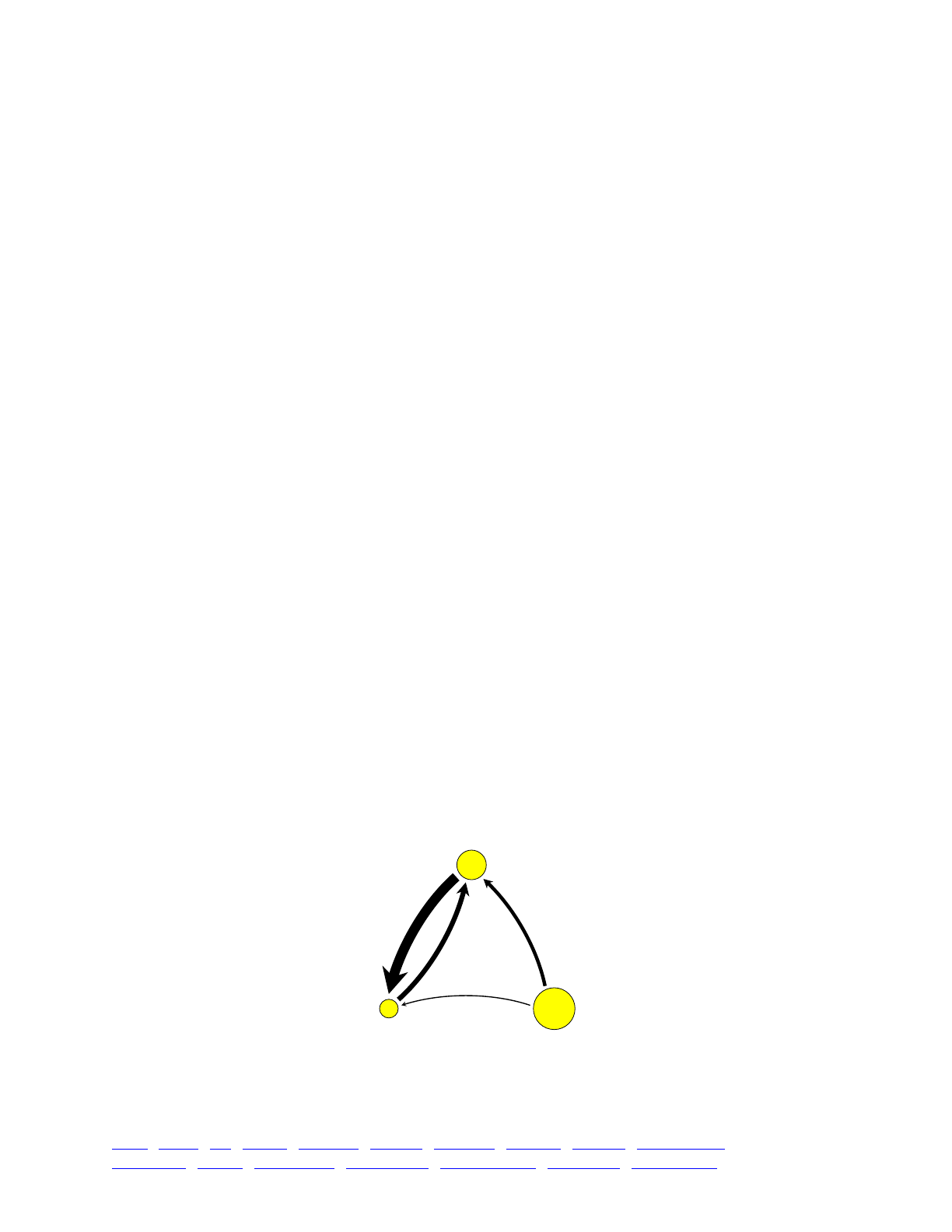
initialize() {!
initializeMutationRate(1e-7);!
initializeMutationType("m1", 0.5, "f", 0.0);!
initializeGenomicElementType("g1", m1, 1.0);!
initializeGenomicElement(g1, 0, 99999);!
initializeRecombinationRate(1e-8);!
}!
1 {!
sim.addSubpop("p1", 500);!
sim.addSubpop("p2", 100);!
sim.addSubpop("p3", 1000);!
p1.setMigrationRates(c(p2,p3), c(0.2,0.1));!
p2.setMigrationRates(c(p1,p3), c(0.8,0.01));!
}!
10000 late() { sim.outputFull(); }
For this recipe we have returned to the simple initialize() callback we started with, with only
one mutation type. The new action happens in the generation 1 event, where we now add three
subpopulations of different sizes. Those populations are then connected by migration using calls
to the setMigrationRates() method of Subpopulation. Let’s examine the first such call:
p1.setMigrationRates(c(p2,p3), c(0.2,0.1));
Since this method call is made on p1, it is setting the immigration into p1. Both p2 and p3 are
given as sources of immigration, with rates of 0.2 and 0.1 respectively. In SLiM’s design, this does
not mean that individuals from p2 and p3 will move from those populations into p1. Rather, it
means that when p1 generates an offspring generation, and parents are chosen for a new offspring
individual, a proportion of 0.2 of those parents will be chosen from p2, a proportion of 0.1 from
p3, and the remaining proportion of 0.7 will be chosen from p1 itself, since the default behavior is
that parents are chosen from the subpopulation into which the new offspring will be placed. The
next line sets up migration into p2, in the same way. Since migration into p3 is not configured, p3
acts as a source only. Note that, as discussed further in section 19.2.1, migration rates specify the
probability that any given offspring individual will come from a particular source subpopulation;
the actual number of migrants in a given generation is thus stochastic, not deterministic.
It can be hard to visualize complex population structure just from code like this; happily,
SLiMgui’s population visualization graph provides a nice way to see what’s going on. If you copy
and paste the above recipe into a simulation window, Recycle, press Step twice so that generation
1 has been executed, and then open the population visualization graph, you will see a nice
graphical representation of the population structure:
As before, the size of the circle for a subpopulation represents the subpopulation’s size, and the
color of the circle indicates the mean fitness of that subpopulation. The arrows show migration
links, with the thicknesses of the arrows indicating the strength of each link. Here it is immediately
p1
p2 p3
TOC I TOC II WF nonWF initialize() Genome Individual Mutation SLiMSim Subpopulation!
Eidos events fitness() mateChoice() modifyChild() recombination() interaction() reproduction() 79

obvious that p3 is a source, and that p2 is somewhat close to being a sink but does contribute some
immigrants to p1.
Of course there is no need for the population structure to all be set up in generation 1; you can
add subpopulations, remove subpopulations, and change migration rates in each generation if you
wish, as we will explore in the next section. The population visualization graph will update to
show the current population structure as your simulation runs.
5.2.2 Removing subpopulations
The population structure set up in the previous recipe was quite static, established in generation
1 and unchanging subsequently. Let’s explore more dynamic population structure by both adding
and removing subpopulations over time and dynamically changing migration. The recipe here is
longer because it does more things, but it is only a small extension of previous concepts:
initialize() {!
initializeMutationRate(1e-7);!
initializeMutationType("m1", 0.5, "f", 0.0);!
initializeGenomicElementType("g1", m1, 1.0);!
initializeGenomicElement(g1, 0, 99999);!
initializeRecombinationRate(1e-8);!
}!
1 { sim.addSubpop("p1", 500); }!
100 { sim.addSubpop("p2", 100); }!
100:150 {!
migrationProgress = (sim.generation - 100) / 50;!
p1.setMigrationRates(p2, 0.2 * migrationProgress);!
p2.setMigrationRates(p1, 0.8 * migrationProgress);!
}!
1000 { sim.addSubpop("p3", 10); }!
1000:1100 {!
p3Progress = (sim.generation - 1000) / 100;!
p3.setSubpopulationSize(asInteger(990 * p3Progress + 10));!
p1.setMigrationRates(p3, 0.1 * p3Progress);!
p2.setMigrationRates(p3, 0.01 * p3Progress);!
}!
2000 { p2.setSubpopulationSize(0); }!
10000 late() { sim.outputFull(); }
The initialize() callback is as before. Subpopulations p1, p2, and p3 are now set up in
generations 1, 100, and 1000 respectively. Subpopulation p2 is removed in generation 2000 by
setting its size to 0; that is all that is needed to remove a subpopulation.
The rest of the code – the 100:150 event and the 1000:1100 event – introduces some continuous
change into the population structure. In the 100:150 event the migration rates between p1 and the
newly established p2 grow over time until they reach a target rate. In the 1000:1100 event the new
subpopulation p3 grows in size over time, from a very small founder population, and its
migrational contribution to p1 and p2 grows over time as p3 grows in size.
Watching these dynamics in SLiMgui’s population visualization graph is useful for confirming
that they are functioning correctly. However, the simulation may go too fast for the dynamics to be
seen clearly. You can use the speed slider, directly below the Play button, to slow it down:
TOC I TOC II WF nonWF initialize() Genome Individual Mutation SLiMSim Subpopulation!
Eidos events fitness() mateChoice() modifyChild() recombination() interaction() reproduction() 80

If you set a slower speed, as above, and then Recycle and Play, it should be easier to follow the
action.
5.2.3 Splitting subpopulations
By default, when new subpopulations are added in SLiM they are composed of “brand-new”
individuals with no mutations. To produce more realistic dynamics, we might like the new
subpopulations to be split off from an existing subpopulation. Modifying the recipe above, this is
quite a simple change:
initialize() {!
initializeMutationRate(1e-7);!
initializeMutationType("m1", 0.5, "f", 0.0);!
initializeGenomicElementType("g1", m1, 1.0);!
initializeGenomicElement(g1, 0, 99999);!
initializeRecombinationRate(1e-8);!
}!
1 { sim.addSubpop("p1", 500); }!
100 { sim.addSubpopSplit("p2", 100, p1); }!
100:150 {!
migrationProgress = (sim.generation - 100) / 50;!
p1.setMigrationRates(p2, 0.2 * migrationProgress);!
p2.setMigrationRates(p1, 0.8 * migrationProgress);!
}!
1000 { sim.addSubpopSplit("p3", 10, p2); }!
1000:1100 {!
p3Progress = (sim.generation - 1000) / 100;!
p3.setSubpopulationSize(asInteger(990 * p3Progress + 10));!
p1.setMigrationRates(p3, 0.1 * p3Progress);!
p2.setMigrationRates(p3, 0.01 * p3Progress);!
}!
2000 { p2.setSubpopulationSize(0); }!
10000 late() { sim.outputFull(); }
The only change is that the addSubpop() calls that established p2 and p3 have been changed to
addSubpopSplit(). This call is very similar to addSubpop(), but takes an extra parameter: the
existing subpopulation from which the new subpopulation should be split. The split is
accomplished by copying the individuals for the new subpopulation from the source
subpopulation. In other words, each new individual is an exact genetic clone of an existing
individual in the source population, mimicking a founding event in which a subset of the
individuals in the source subpopulation find themselves split off into founders of a new
subpopulation. (From this perspective it is a bit odd that the founders also remain in the source
subpopulation, admittedly, but this is unlikely to be important to simulation dynamics in realistic
scenarios since source subpopulations are typically large and founding subpopulations are
typically small.)
5.3 Migration and admixture
The previous subsections already showed how to set up patterns of migration among multiple
subpopulations. Here, we will focus on recipes for a few standard types of population structure to
show how the flexibility of Eidos makes setting up complex population structure easy.
5.3.1 A linear island model
This model describes a linear chain of subpopulations, each of which is connected by migration
only to its nearest neighbors. This is quite easy to set up:
TOC I TOC II WF nonWF initialize() Genome Individual Mutation SLiMSim Subpopulation!
Eidos events fitness() mateChoice() modifyChild() recombination() interaction() reproduction() 81
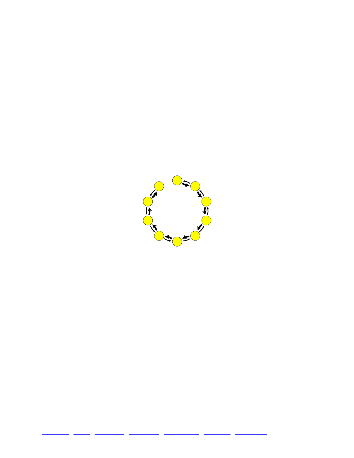
initialize() {!
initializeMutationRate(1e-7);!
initializeMutationType("m1", 0.5, "f", 0.0);!
initializeGenomicElementType("g1", m1, 1.0);!
initializeGenomicElement(g1, 0, 99999);!
initializeRecombinationRate(1e-8);!
}!
1 {!
subpopCount = 10;!
for (i in 1:subpopCount)!
sim.addSubpop(i, 500);!
for (i in 2:subpopCount)!
sim.subpopulations[i-1].setMigrationRates(i-1, 0.2);!
for (i in 1:(subpopCount-1))!
sim.subpopulations[i-1].setMigrationRates(i+1, 0.05);!
}!
10000 late() { sim.outputFull(); }
If you copy and paste this into SLiMgui, Recycle, do Step twice to step through generation 1,
and open the population visualization graph, you will see the resulting structure:
As you can see, migration is stronger in one direction than in the other; this might represent
gene flow in a river system, for example, where gene flow is more likely to go downstream than
upstream. Indeed, it would be trivial to interrupt the upstream gene flow completely in certain
spots to represent the effect of waterfalls that prevent upstream migration. Using the techniques
shown in previous sections, it would also be trivial to make the migration pattern change over
time; a major flooding event in one generation could allow gene flow to pass upstream past a
small waterfall, for example.
This population structure is achieved using three for loops. We saw for loops briefly in section
4.1.5; let’s revisit the concept now. The first loop in this recipe is:
for (i in 1:subpopCount)!
sim.addSubpop(i, 500);
This causes the statement sim.addSubpop(i, 500); to be executed repeatedly as the loop index
variable i varies from 1 up to subpopCount, following the sequence defined by 1:subpopCount.
The result is that new subpopulations are created in order: p1, p2, p3, and on up to subpopCount.
The second loop is almost as straightforward:
for (i in 2:subpopCount)!
sim.subpopulations[i-1].setMigrationRates(i-1, 0.2);
This sets up migration into each subpopulation from the previous subpopulation: into p2 from
p1, into p3 from p2, and so forth. Since p1 receives no such migration (there being no p0
p1
p2
p3
p4
p5
p6
p7
p8
p9
p10
TOC I TOC II WF nonWF initialize() Genome Individual Mutation SLiMSim Subpopulation!
Eidos events fitness() mateChoice() modifyChild() recombination() interaction() reproduction() 82
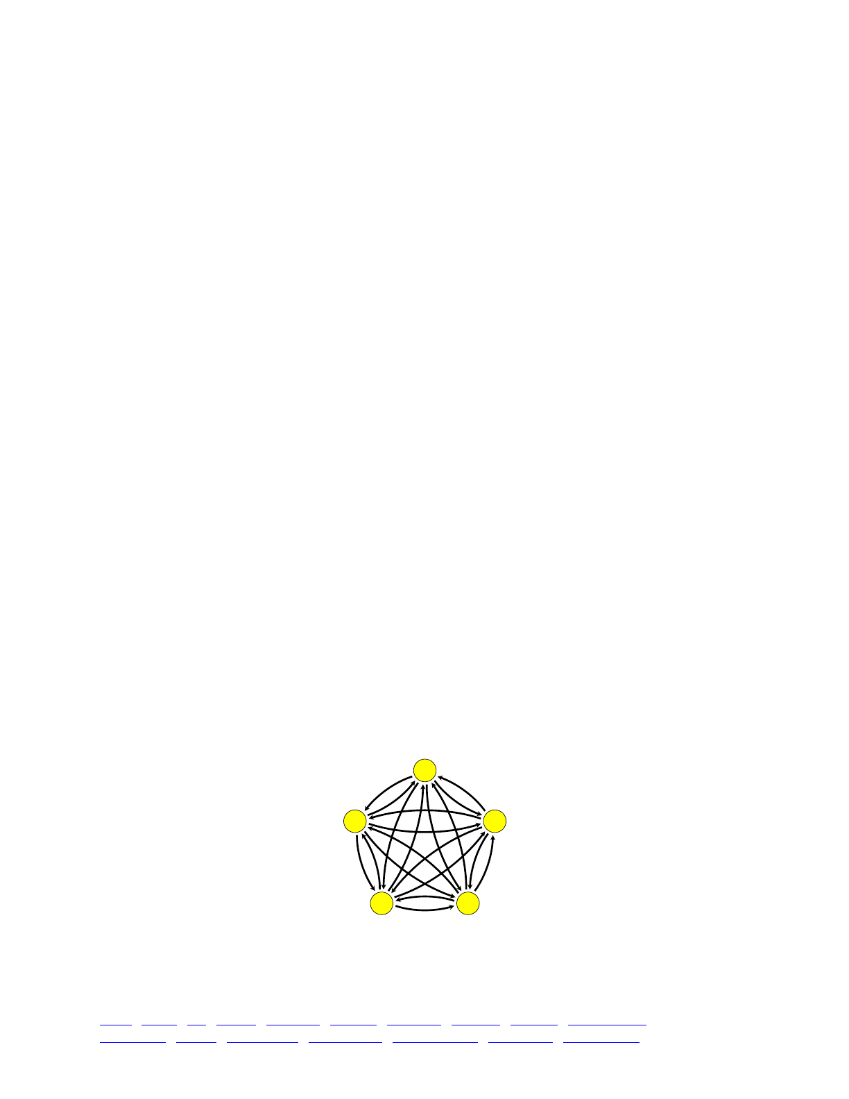
subpopulation), the loop starts at 2, not 1. For each value of i, the corresponding subpopulation is
looked up in the simulations subpopulation array, which is a property of SLiMSim, using
sim.subpopulations[i-1]; the use of i-1 here instead of i is because p1 will be at index 0 in the
subpopulation array (since vectors in Eidos are numbered starting at 0, not 1). Given the proper
subpopulation, the setMigrationRates() call then sets up migration from the previous
subpopulation (which is the purpose of i-1 in that call).
Given that explanation, the operation of the third loop should be fairly obvious. The power of
this algorithmic approach to setting up population structure should be clear; if we want 1000
subpopulations arranged in this manner, all we have to do is change subpopCount = 10; to
subpopCount = 1000;. The population visualization graph in SLiMgui will find this a bit
challenging to display, but it should be possible to test and debug such a model with just 10
subpopulations, and then scale up to 1000 subpopulations for your production runs.
5.3.2 A non-spatial metapopulation
Another possible scenario is a non-spatial metapopulation in which migration between each
pair of subpopulations occurs at some constant rate. This can be set up as follows:
initialize() {!
initializeMutationRate(1e-7);!
initializeMutationType("m1", 0.5, "f", 0.0);!
initializeGenomicElementType("g1", m1, 1.0);!
initializeGenomicElement(g1, 0, 99999);!
initializeRecombinationRate(1e-8);!
}!
1 {!
subpopCount = 5;!
for (i in 1:subpopCount)!
sim.addSubpop(i, 500);!
for (i in 1:subpopCount)!
for (j in 1:subpopCount)!
if (i != j)!
sim.subpopulations[i-1].setMigrationRates(j, 0.05);!
}!
10000 late() { sim.outputFull(); }
Here a nested pair of for loops using index variables i and j sets up the migration from j into i
for each pair of subpopulations. The test if (i!=j) prevents the code from attempting to set the
migration rate from a subpopulation into itself, which is illegal.
SLiMgui’s visualization of this population structure looks like what we wanted:
This recipe uses only five subpopulations (subpopCount = 5), but again the code is general and
may be scaled up to however many subpopulations you want in your metapopulation (although
SLiMgui may not be very good at visualizing these scenarios once they become too complex).
p1
p2
p3p4
p5
TOC I TOC II WF nonWF initialize() Genome Individual Mutation SLiMSim Subpopulation!
Eidos events fitness() mateChoice() modifyChild() recombination() interaction() reproduction() 83

5.3.3 A two-dimensional subpopulation matrix
A third common population structure is a two-dimensional grid or matrix of subpopulations,
representing a spatial metapopulation in which each subpopulation exchanges migrants only with
its direct neighbors. SLiM has no intrinsic concept of geographic space in its simulations, but with
a population structure like this a pseudo-geographic regime can be imposed upon a SLiM
simulation such that new beneficial mutations, for example, will spread from subpopulation to
subpopulation in a similar manner to how they might spread across a real landscape.
initialize() {!
initializeMutationRate(1e-7);!
initializeMutationType("m1", 0.5, "f", 0.0);!
initializeGenomicElementType("g1", m1, 1.0);!
initializeGenomicElement(g1, 0, 99999);!
initializeRecombinationRate(1e-8);!
}!
1 {!
metapopSide = 3; // number of subpops along one side of the grid!
metapopSize = metapopSide * metapopSide;!
for (i in 1:metapopSize)!
sim.addSubpop(i, 500);!
!
subpops = sim.subpopulations;!
for (x in 1:metapopSide)!
for (y in 1:metapopSide)!
{!
destID = (x - 1) + (y - 1) * metapopSide + 1;!
destSubpop = subpops[destID - 1];!
if (x > 1) // left to right!
destSubpop.setMigrationRates(destID - 1, 0.05);!
if (x < metapopSide) // right to left!
destSubpop.setMigrationRates(destID + 1, 0.05);!
if (y > 1) // top to bottom!
destSubpop.setMigrationRates(destID - metapopSide, 0.05);!
if (y < metapopSide) // bottom to top!
destSubpop.setMigrationRates(destID + metapopSide, 0.05);!
}!
}!
10000 late() { sim.outputFull(); }
This code is a bit more complex than previous recipes. In the generation 1 event, we first
decide how large of a metapopulation we want; metapopSide=3 means that we will make a 3x3
metapopulation (trivially small, but easier to check for correctness). This can be scaled up
arbitrarily; it works well in SLiMgui for values as large as a 1000x1000 metapopulation with 10
individuals per subpopulation. We calculate the number of subpopulations we will need, and
make them all with the first for loop.
Then comes the trickier part. We loop over the grid of subpopulations using x and y, which
each range from 1 to metapopSide. For each subpopulation in the grid, as determined by x and y,
we calculate the ID of the subpopulation in destID, and then fetch the subpopulation itself into
destSubpop, getting it from the simulation’s subpopulation array as before. We then set the
migration into destSubpop from each of its four sides; if it is at the edge of the matrix, it receives no
migrants from that side (although it would be trivial to modify this code to make a wrap-around
pattern of migration simulating a toroidal world). Simple arithmetic is used to determine the
identifier of neighboring subpopulations based upon destID.
TOC I TOC II WF nonWF initialize() Genome Individual Mutation SLiMSim Subpopulation!
Eidos events fitness() mateChoice() modifyChild() recombination() interaction() reproduction() 84
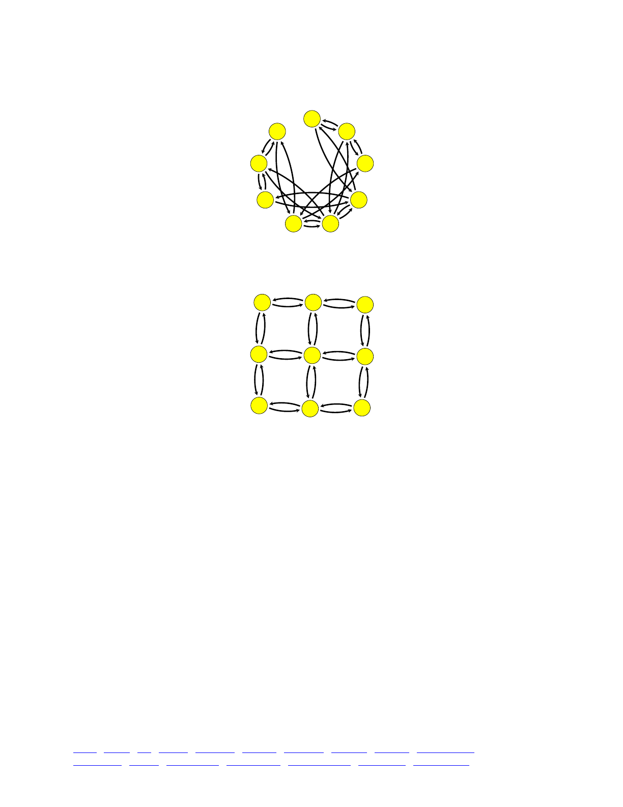
SLiMgui’s visualization of this setup is complicated; it is not immediately obvious that it
represents a two-dimensional metapopulation, but it does:
However, SLiMgui has an alternate method of display for these population visualizations. If you
control-click or right-click on the graph, you will get a pop-up menu. Select “Optimized
Positions” from that menu, and you should see something more like this:
Here it is much more obvious that the migration pattern is as desired. This positioning
optimization algorithm is based on a concept called force-directed layout. It is a somewhat
experimental feature in SLiMgui, and may not always give layouts that look good; it is also quite
slow for layouts involving more than a dozen or so subpopulations. However, it is worth a try if
you want to get a publication-worthy picture of your population structure.
Speaking of “publication-worthy”, note that when you control-click or right-click on the
visualization graph, the pop-up menu also has an item entitled “Copy Graph”. That copies the
graph to the clipboard as a PDF – very handy for pasting into documents or slides.
5.3.4 A random, sparse spatial metapopulation
The recipe in section 5.3.3 showed how to make a small spatial metapopulation in which
subpopulations are arranged spatially in a grid that is connected by orthogonal migration. Here
we will extend that recipe to a larger size and a more random metapopulation configuration, and
we’ll look at a very simple sweep of a beneficial mutation across the metapopulation.
The initialize() callback for this model is largely unchanged from section 5.3.3:
initialize() {!
initializeMutationRate(1e-7);!
initializeMutationType("m1", 0.5, "f", 0.0);!
initializeMutationType("m2", 0.5, "f", 0.3);!
initializeGenomicElementType("g1", m1, 1.0);!
initializeGenomicElement(g1, 0, 99999);!
initializeRecombinationRate(1e-8);!
}
p1
p2
p3
p4
p5p6
p7
p8
p9
p1 p2 p3
p4 p5 p6
p7 p8 p9
TOC I TOC II WF nonWF initialize() Genome Individual Mutation SLiMSim Subpopulation!
Eidos events fitness() mateChoice() modifyChild() recombination() interaction() reproduction() 85

The only modification here is the addition of a new mutation type, m2, which has been defined
to represent beneficial mutations (with a selection coefficient of 0.3). New mutations are still
always neutral (mutation type m1); we will introduce the sweep mutation ourselves in script.
The final output event is also unchanged:
10000 late() { sim.outputFull(); }
The interesting changes are to the 1 late() event that configures the initial state of the
metapopulation:
1 late() {!
mSide = 10; // number of subpops along one side of the grid!
for (i in 1:(mSide * mSide))!
sim.addSubpop(i, 500);!
!
subpops = sim.subpopulations;!
for (x in 1:mSide)!
for (y in 1:mSide)!
{!
destID = (x - 1) + (y - 1) * mSide + 1;!
ds = subpops[destID - 1];!
if (x > 1) // left to right!
ds.setMigrationRates(destID - 1, runif(1, 0.0, 0.05));!
if (x < mSide) // right to left!
ds.setMigrationRates(destID + 1, runif(1, 0.0, 0.05));!
if (y > 1) // top to bottom!
ds.setMigrationRates(destID - mSide, runif(1, 0.0, 0.05));!
if (y < mSide) // bottom to top!
ds.setMigrationRates(destID + mSide, runif(1, 0.0, 0.05));!
!
// set up SLiMgui's population visualization nicely!
xd = ((x - 1) / (mSide - 1)) * 0.9 + 0.05;!
yd = ((y - 1) / (mSide - 1)) * 0.9 + 0.05;!
ds.configureDisplay(c(xd, yd), 0.4);!
}!
!
// remove 25% of the subpopulations!
subpops[sample(0:99, 25)].setSubpopulationSize(0);!
!
// introduce a beneficial mutation!
target_subpop = sample(sim.subpopulations, 1);!
sample(target_subpop.genomes, 10).addNewDrawnMutation(m2, 20000);!
}
This creates a 10×10 spatial metapopulation in much the same way as section 5.3.3 created a
3×3 metapopulation: first by creating the subpopulations themselves in a simple loop, and then
setting up the migration among them with a pair of nested loops over x and y (see section 5.3.3 for
further comments on that basic design).
For each subpopulation, however, it also does something new, under the // set up SLiMgui
comment: it calculates a visual position for the subpopulation, as xd and yd, and then calls
configureDisplay() on the subpopulation to tell SLiMgui to use that position in its display. The
coordinate system used by SLiMgui for subpopulation display spans [0,1] in x and y, so the xd and
yd values calculated here are within that range. We pass a value of 0.4 for the second parameter
to configureDisplay(); this is a scaling factor for the circle used to represent the subpopulation,
so here we are telling SLiMgui to use unusually small circles (so that all 100 subpopulations fit into
the display without overlapping).
TOC I TOC II WF nonWF initialize() Genome Individual Mutation SLiMSim Subpopulation!
Eidos events fitness() mateChoice() modifyChild() recombination() interaction() reproduction() 86
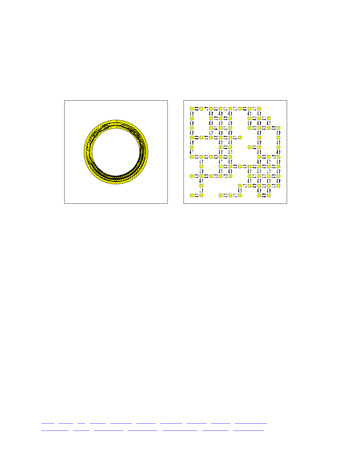
If we ran the model without this display configuration (just comment out the call to
configureDisplay(), we would get the left-hand plot; the subpopulations are all overlapping and
nothing can be discerned at all. (The “Optimized Positions” technique shown in section 5.3.3 is
not up to the task either; optimizing such a large network is a difficult problem. Perhaps that
experimental feature will eventually be improved to the point that it produces acceptable results
for this model, but at present it does not.) If we run it with the display configuration, we get the
right-hand plot, which is obviously much better:
Looking at the right-hand visualization, it is now immediately apparent that this is not a
complete metapopulation, but rather a sparse metapopulation in which some subpopulations are
missing. That brings us to the next lines in the event:
// remove 25% of the subpopulations!
subpops[sample(0:99, 25)].setSubpopulationSize(0);
This takes a sample, of size 25, from the sequence 0:99, selects those subpopulations (using the
subset operator on subpops), and sets their size to zero. As we saw in section 5.2.2, this removes
those subpopulations from the simulation; any connections they have to other subpopulations by
migration are broken. That one line, then, very easily produces a random sparse metapopulation.
The only caveat is that, depending upon which subpopulations get removed, the remaining
metapopulation might not be connected; there might be two or more isolated networks with no
connection between them via migration at all. If that is undesirable, further steps would have to
be taken to avoid the possibility.
You might also notice that the arrows in the population visualization now vary in their
thickness; this is because we now draw random migration rates using runif(), rather than using a
fixed migration rate as we did in section 5.3.3. This code draws migration rates from a uniform
distribution, and makes no attempt to ensure that migration rates between a given pair of
subpopulations are symmetric; since this is just scripting, one could implement any pattern of
random migration one wished.
That brings us to the final lines of the event:
// introduce a beneficial mutation!
target_subpop = sample(sim.subpopulations, 1);!
sample(target_subpop.genomes, 10).addNewDrawnMutation(m2, 20000);
p1
p2
p3
p6
p8
p9
p11
p12
p13
p15
p16
p17
p18
p19
p22
p23
p24
p25
p27
p28
p29
p30
p31
p32
p33
p34
p35
p36
p37
p38
p39
p40
p41
p42
p43
p44
p45
p46p47
p48
p49
p51
p52
p53
p54
p55
p56
p57
p58
p59
p60
p61
p63
p64
p65
p68
p69
p72
p77
p78
p79
p81
p83
p84
p87
p88
p89
p90
p91
p94
p96
p97
p98
p99
p100
p1 p2 p4 p5 p6 p8 p9
p12 p16 p17 p18 p19 p20
p21 p22 p23 p24 p25 p27 p28 p29 p30
p32 p34 p35 p36 p37 p38 p39 p40
p41 p42 p43 p44 p45 p48 p49 p50
p51 p54 p55 p57 p58 p60
p61 p62 p63 p64 p65 p66 p68 p70
p71 p73 p74 p75 p77 p78 p79 p80
p81 p83 p84 p85 p87 p88 p89
p91 p92 p93 p94 p95 p96 p97 p98
TOC I TOC II WF nonWF initialize() Genome Individual Mutation SLiMSim Subpopulation!
Eidos events fitness() mateChoice() modifyChild() recombination() interaction() reproduction() 87
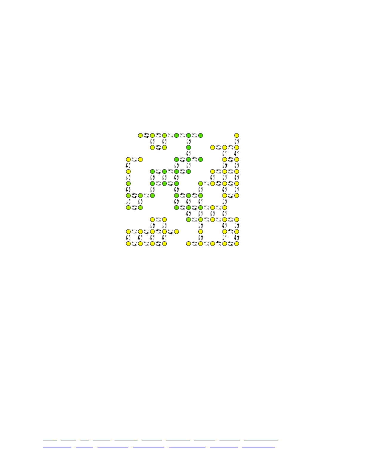
This manual will cover introduced mutations and selective sweeps in great detail in chapter 10,
so this is just a tiny bit of foreshadowing of that complex topic. The idea here is simple: we choose
one subpopulation from the subpopulations that remain in the model using sample(), and then we
choose ten genomes at random from the chosen subpopulation again using sample() (starting with
ten rather than just one to make it more likely that the mutation will not be lost due to drift early
on, for pedagogical purposes), and finally we call addNewDrawnMutation() to add a new m2
mutation to those ten genomes at position 20000. This code, then, introduces a beneficial mutation
that will, we hope, sweep through our sparse metapopulation.
And if it doesn’t get lost, and if the metapopulation is connected, sweep it does. Here is a
screenshot from midway through the sweep:
As per the default behavior in SLiM, subpopulations are colored according to their mean fitness;
populations where the sweep mutation is approaching fixation are thus a dark green, while
populations that are still neutral are still yellow. Note that the configureDisplay() method has a
third (optional) argument that would allow us to customize the color of each subpopulation as
well, coloring them according to whatever model variable we wish; we have not used that here,
since the default fitness-based coloring is in fact exactly what we want.
5.3.5 Reading a migration matrix from a file
Sometimes, when modeling an empirical population, migration rates are specified in a file, and
you would like to read that file in and create a corresponding SLiM model. This is very easy to
accomplish using Eidos in SLiM. Let’s start by looking at a very simple migration matrix file:
// For the recipe of section 5.3.4.!
// Format: <src>, <dest>, <rate>.!
1,1,0.78!
1,2,0.10!
1,3,0.12!
2,1,0.01!
2,2,0.96!
2,3,0.03!
3,1,0.33!
3,2,0.17!
3,3,0.50
p1 p2 p3 p4 p6 p7 p8 p9 p10
p11 p12 p13 p14 p15 p17 p19 p20
p23 p24 p26 p27 p28 p29 p30
p31 p32 p35 p36 p37 p38 p39
p41 p42 p43 p45 p46 p47 p49 p50
p51 p53 p54 p55 p57 p58 p59 p60
p61 p63 p64 p65 p66 p68 p69 p70
p71 p72 p75 p76 p77 p79 p80
p83 p84 p86 p88 p89 p90
p92 p93 p94 p95 p96 p97 p100
TOC I TOC II WF nonWF initialize() Genome Individual Mutation SLiMSim Subpopulation!
Eidos events fitness() mateChoice() modifyChild() recombination() interaction() reproduction() 88

This file expresses the model’s migration rates as a series of lines, each of which is a series of
comma-separated values; this format is often called a CSV file. Let us suppose that it exists on disk
at the path ~/Desktop/migration.csv. The first two lines are comments, describing the file. The
rest of the lines each have three values: the identifier of the source subpopulation, the identifier of
the destination subpopulation, and the migration rate (sometimes the destination is listed before
the source in these sorts of files, so be careful). Note that there are lines expressing the fraction of
each subpopulation that does not migrate – the remainder after all migrants have left. This is not
optimal for SLiM’s purposes, but we want to work with the file as it is.
We can read this file in and create a model based on it with a simple script:
initialize() {!
initializeMutationRate(1e-7);!
initializeMutationType("m1", 0.5, "f", 0.0);!
initializeGenomicElementType("g1", m1, 1.0);!
initializeGenomicElement(g1, 0, 99999);!
initializeRecombinationRate(1e-8);!
}!
1 {!
for (i in 1:3)!
sim.addSubpop(i, 1000);!
subpops = sim.subpopulations;!
!
lines = readFile("~/Desktop/migration.csv");!
lines = lines[substr(lines, 0, 1) != "//"];!
!
for (line in lines)!
{!
fields = strsplit(line, ",");!
i = asInteger(fields[0]);!
j = asInteger(fields[1]);!
m = asFloat(fields[2]);!
!
if (i != j)!
{!
p_i = subpops[subpops.id == i];!
p_j = subpops[subpops.id == j];!
p_j.setMigrationRates(p_i, m);!
}!
}!
}!
10000 late() { sim.outputFull(); }
The generation 1 event is where the action is. It first creates the three subpopulations of the
model with a simple for loop. It would be simple to extend this model to determine the number
of subpopulations from the contents of the migration.csv file, and to read subpopulation sizes in
from that file, and so forth. Here, however, we hard-code those values for simplicity. Once the
subpopulations have been created, we cache the vector of subpopulations in subpops for brevity in
the script that follows.
Next, the script reads in the contents of the migration.csv file using readFile(). This creates a
string vector, with each line of the file being a separate element in the vector. The following line
uses the substr() function to find lines that begin with "//", and removes those lines by
subsetting the lines vector, stripping out the comment lines from the file.
Now we can loop through the lines with a for loop and handle each line in turn. The
strsplit() function is used to split line into its components, separated by commas; this is often a
TOC I TOC II WF nonWF initialize() Genome Individual Mutation SLiMSim Subpopulation!
Eidos events fitness() mateChoice() modifyChild() recombination() interaction() reproduction() 89
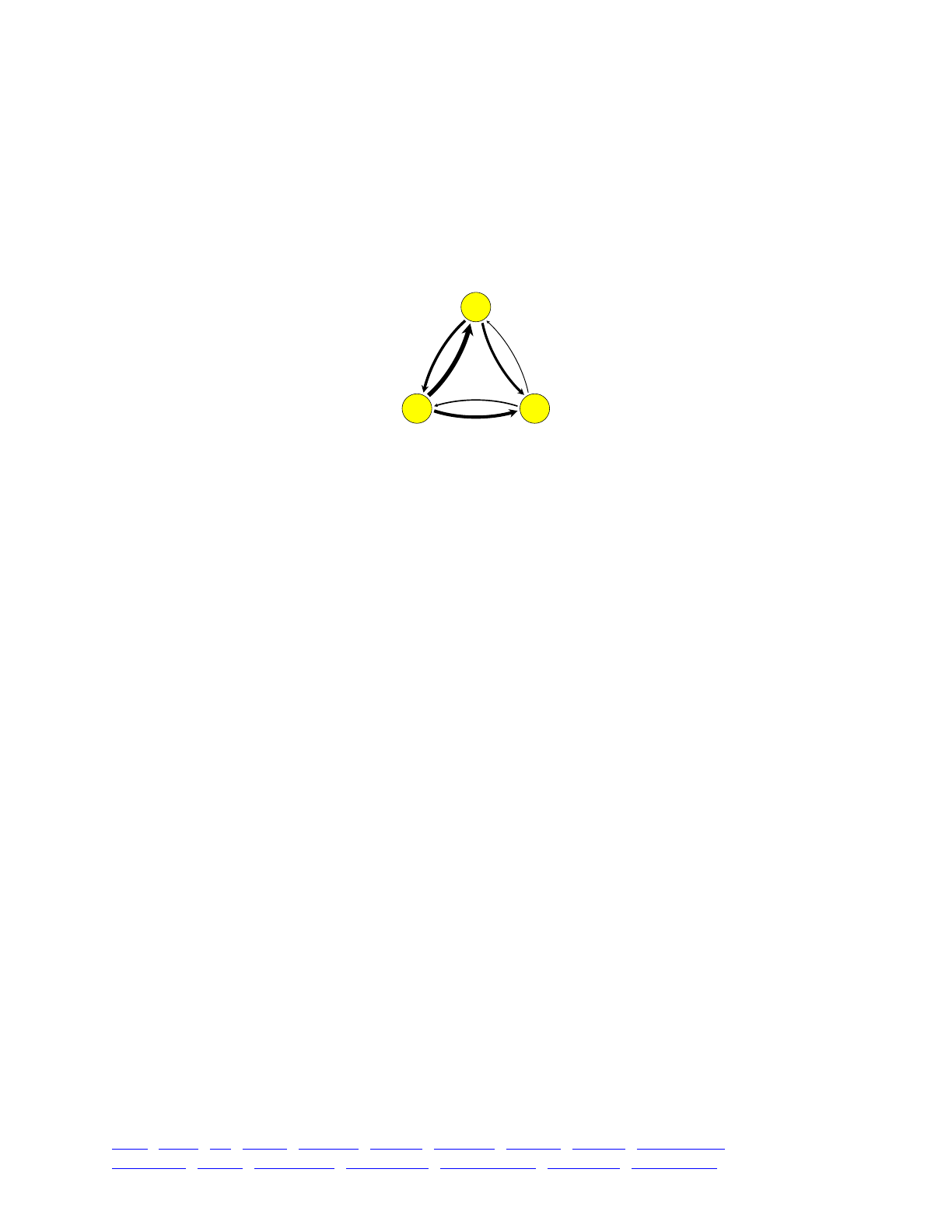
very convenient way to parse CSV files. The three values of the line are then extracted from the
fields vector, which is of type string, and are converted to their appropriate types.
The last block actually sets the migration rate. First it checks that i and j are not the same; this
filters away the lines that express the non-migrating fractions, which SLiM does not need to know
about. Then it looks up the subpopulations referenced by i and j, using the id property, which
corresponds to the numeric part of the subpopulation’s symbol (i.e., subpopulation p3 has an id of
3). Finally, it sets the migration rate from p_j to p_i to be the rate m that was read from the file.
When executed, SLiMgui’s visualization of this population structure looks like this:
That looks like what we would expect from looking at the file; p2 is a sink, p3 is a source, and
p1 is close to balanced. This is a very simple population model, but this script could just as easily
read in a migration matrix file for hundreds or even thousands of subpopulations; its code is in
quite general. As mentioned above, it could easily be extended to read subpopulation sizes from
the CSV file as well; indeed, other subpopulation properties, such as selfing rates and sex ratios,
could also easily be added to the file format and set up by this script, and the script could easily be
adapted to work with whatever empirical data files already exist.
5.4 The Gravel et al. (2011) model of human evolution
In this section we will look at a recipe that brings together all of the elements of demography
and population structure that have been discussed in this chapter. This is a SLiM implementation
of a model of human evolution presented by Gravel et al. (2011); in particular, we here model the
“Low-coverage + exons” model described in their Table 2. The recipe:
initialize() {!
initializeMutationRate(2.36e-8);!
initializeMutationType("m1", 0.5, "f", 0.0);!
initializeGenomicElementType("g1", m1, 1.0);!
initializeGenomicElement(g1, 0, 10000);!
initializeRecombinationRate(1e-8);!
}!
!
// Create the ancestral African population!
1 { sim.addSubpop("p1", 7310); }!
!
// Expand the African population to 14474!
// This occurs 148000 years (5920) generations ago!
52080 { p1.setSubpopulationSize(14474); }!
!
// Split non-Africans from Africans and set up migration between them!
// This occurs 51000 years (2040 generations) ago!
55960 {!
sim.addSubpopSplit("p2", 1861, p1);!
p1.setMigrationRates(c(p2), c(15e-5));!
p2.setMigrationRates(c(p1), c(15e-5));!
}!
p1
p2p3
TOC I TOC II WF nonWF initialize() Genome Individual Mutation SLiMSim Subpopulation!
Eidos events fitness() mateChoice() modifyChild() recombination() interaction() reproduction() 90
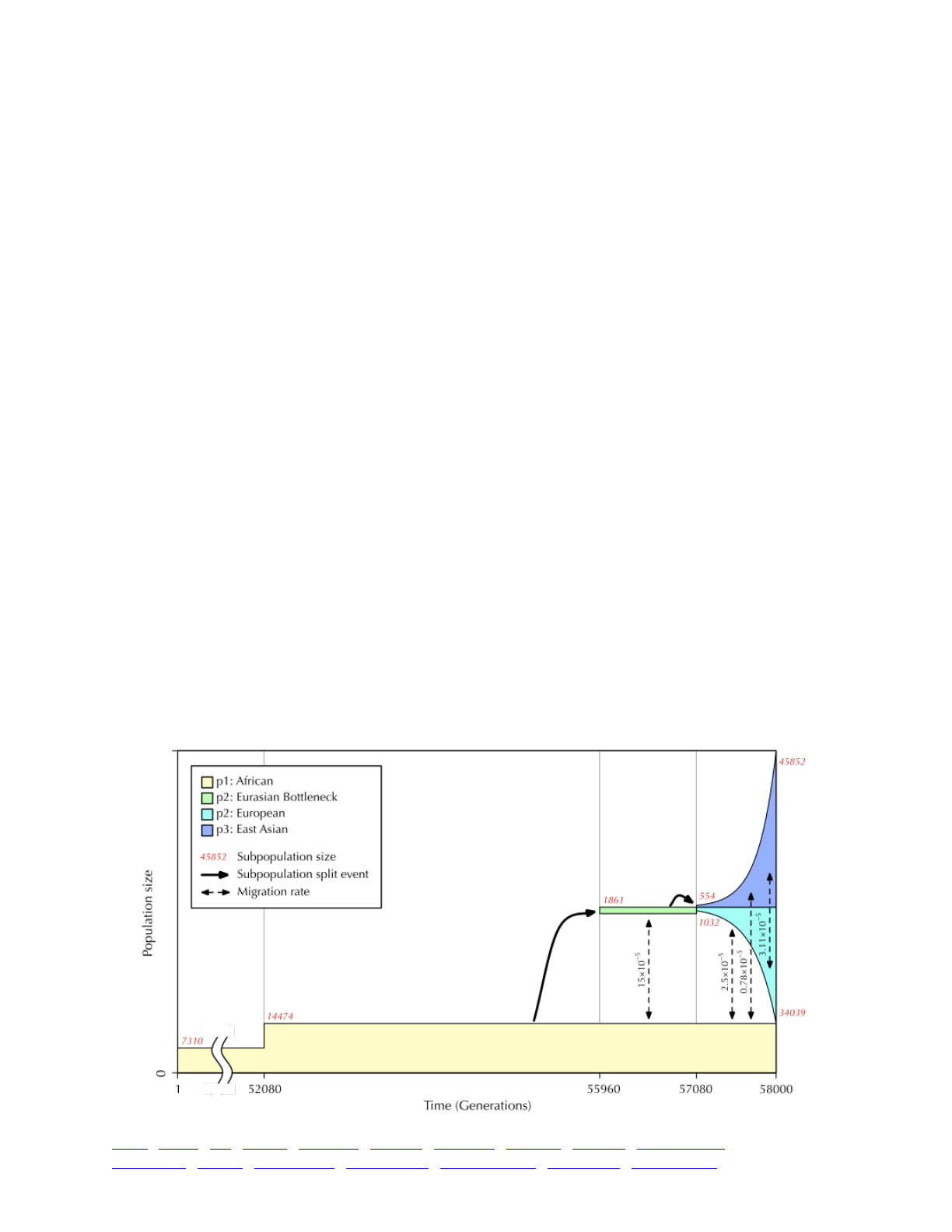
!
// Split p2 into European and East Asian subpopulations!
// This occurs 23000 years (920 generations) ago!
57080 {!
sim.addSubpopSplit("p3", 554, p2);!
p2.setSubpopulationSize(1032); // reduce European size!
!
// Set migration rates for the rest of the simulation!
p1.setMigrationRates(c(p2, p3), c(2.5e-5, 0.78e-5));!
p2.setMigrationRates(c(p1, p3), c(2.5e-5, 3.11e-5));!
p3.setMigrationRates(c(p1, p2), c(0.78e-5, 3.11e-5));!
}!
!
// Set up exponential growth in Europe and East Asia!
// Where N(0) is the base subpopulation size and t = gen - 57080:!
// N(Europe) should be int(round(N(0) * e^(0.0038*t)))!
// N(East Asia) should be int(round(N(0) * e^(0.0048*t)))!
57080:58000 {!
t = sim.generation - 57080;!
p2_size = round(1032 * exp(0.0038 * t));!
p3_size = round(554 * exp(0.0048 * t));!
!
p2.setSubpopulationSize(asInteger(p2_size));!
p3.setSubpopulationSize(asInteger(p3_size));!
}!
!
// Generation 58000 is the present. Output and terminate.!
58000 late() {!
p1.outputSample(216); // YRI phase 3 sample of size 108!
p2.outputSample(198); // CEU phase 3 sample of size 99!
p3.outputSample(206); // CHB phase 3 sample of size 103!
}
Three subpopulations are modeled in this recipe, as shown in the diagram below (solid arrows
showing subpopulation splitting events, dotted arrows showing migration rates between
subpopulations, and red italic numbers showing subpopulation effective sizes).
TOC I TOC II WF nonWF initialize() Genome Individual Mutation SLiMSim Subpopulation!
Eidos events fitness() mateChoice() modifyChild() recombination() interaction() reproduction() 91

The first subpopulation, present from the beginning of the simulation, is p1; it represents
Africans (YRI). The second, p2, initially represents the Ancestral Eurasian Bottleneck, and then
becomes the Europeans (CEU). The third, p3, represents East Asians (CHB). As you can see in the
diagram and in the recipe above, p2 splits from p1 at generation 55960, and then p3 splits off from
p2 at generation 57080. Beginning with the split of p3 from p2, both p2 and p3 undergo
exponential growth until the end of the model.
The model begins 58000 generations ago (1.45 million years if we assume 25 years per
generation). It spends quite a long time doing neutral burn-in before the action really starts in
generation 52080 with the expansion of the African subpopulation. Running the full model only
takes a couple of minutes, but if you’re impatient, you can decrease the generation ranges for all
events by 52000, providing an 80-generation burn-in that should suffice for illustrative purposes
(but will not produce the correct pattern of neutral diversity at the end of the run).
This model is a neutral model; the only mutation type modeled is m1, which represents neutral
mutations. At the end of the model, random samples are output from each of the three
subpopulations to provide a view on the neutral diversity present in each subpopulation. The
empirical samples that this output is intended to match were taken from (diploid) humans; the
outputSample() method of Subpopulation, on the other hand, takes as its argument the number of
(haploid) genomes to sample and output. The sample sizes in SLiM are therefore double the
number of humans sampled empirically.
It is worth noting that the population sizes used in this model are effective population sizes.
The actual population sizes in human history were likely much larger, but geography and other
factors greatly reduced the effective population size. This is also the reason that the sizes of p2 and
p3 post-split are not modeled as adding up to the same size as the pre-split p2 subpopulation.
The model for this recipe was written by Aaron Sams of the Messer Lab at Cornell.
5.5 Rescaling population sizes to improve simulation performance
The limiting factor in most forward population genetic simulations tends to be the actual
number of individuals simulated. In SLiM, every individual in the population is modeled
explicitly. Thus, in larger populations more time is consumed per generation creating the children
that make up the population, and more memory is needed for storing their genetic information.
Perhaps we can approximate the evolution of a large population using simulation of a smaller
population? In some ways, we can: analytical theory predicts that under certain assumptions
many important population genetic parameters, such as the expected levels of diversity,
polymorphism frequency spectra, levels of linkage disequilibrium, etc., should primarily depend
on products of the form Nµ, Nr, and Ns, where N is the effective population size, µ is the mutation
rate, r the recombination rate, and s the selection coefficient of a given mutation.
Thus, for many analyses we do not have to simulate a population of the true size, but can
obtain similar results by simulating a much smaller population while rescaling µ, r, and s such that
the products Nµ, Nr, and Ns remain the same. Importantly, when rescaling population sizes, time
has to be rescaled as well, because drift will be faster in a smaller population. The amount of drift
in a Wright-Fisher population of 1000 individuals, observed over 100 generations, will be similar
to that in a population of 100 individuals observed over just 10 generations. In this way, rescaling
a simulation to a smaller population size not only helps us by having to model fewer individuals
per generation, but also by reducing the number of generations we need to simulate.
This rescaling “trick” can be tremendously helpful in practice, allowing the simulation of
scenarios featuring large populations that would not be feasible to simulate when using their actual
population sizes. However, there are clear limitations to rescaling as well. Most obviously, there
will be limits to how far downscaling of population sizes can be pushed in the light of an
TOC I TOC II WF nonWF initialize() Genome Individual Mutation SLiMSim Subpopulation!
Eidos events fitness() mateChoice() modifyChild() recombination() interaction() reproduction() 92

increasing impact of discretization effects: as simulated population sizes become smaller, there
will be fewer possible population frequencies at which mutations can segregate, with the lowest
possible frequency being 1/(2N). Thus, the rescaling approach will break down if the goal is to
study the characteristics of very low-frequency polymorphisms.
The discreteness of generations can increasingly become a problem as time is rescaled
downwards. For example, if a selective sweep that takes 100 generations in a population of 10000
individuals takes the same amount of “time” in a downscaled population of 500 individuals, it
would complete in only 5 generations (assuming selection coefficients were rescaled upwards
accordingly). In that case, the frequency changes of the selected allele will no longer be small
over the timescale of a single generation, violating a key assumption in many analytical models.
Furthermore, since the time for a beneficial allele to sweep scales with log(N), we actually expect
the sweep in the smaller population to complete even faster than we would expect after
accounting for rescaling.
This discretization can also have unexpected and undesirable side effects on processes such as
adaptation. Rescaling by a factor Q preserves the influx of mutations per generation (since N
µ!=!(N / Q) µ Q). One rescaled generation is Q original generations, so this implies a lower influx
of mutations per unit of time, but since mean TMRCA scales with N, genetic diversity at neutral
sites is preserved. Since the probability of fixation of a beneficial mutation scales with s, the influx
of successfully established beneficial mutations per unit time is preserved (since N µ s dt!=!(N / Q) µ
Q s Q (dt / Q)), implying a smaller number of fixed selected mutations since the mean TMRCA in
the population. Since rescaled values of s are larger, this has the net effect of substituting many
mutations of small effect with a single one of large effect (with Q!=!100, replacing 100 mutations
with s!=!0.001 by a single one of s!=!0.1), a very different model of adaptation.
While it may be tempting to always rescale any given scenario to a very small population size,
then, one must be careful that finite-size effects do not distort results too much. It is therefore
generally advisable to test any rescaled scenario at larger and smaller sizes in order to make sure
that the results are consistent. When tree-sequence recording can be used to speed up a
simulation, by allowing simulation of neutral mutations to be deferred (see section16.2), or even
by allowing the coalescent to be used for neutral burn-in with recapitation (see section 16.10), that
will usually be strongly preferable, since tree-sequence recording does not introduce such artifacts.
Nevertheless, since tree-sequence recording may not be applicable to a given model, or may
provide insufficient performance enhancement, rescaling is still sometimes needed. Rescaling may
be used in conjunction with tree-sequence recording, with the appropriate adjustment of
parameters such as µ and r for mutation overlay and recapitation.
As an example of the use of rescaling, consider the following recipe, in which we model neutral
and deleterious mutations occurring over a 10 kb locus in a population of initial size 5000. In
generation 50000, the population experiences a bottleneck that lasts for 5000 generations. A
random population sample is then taken in generation 60000:
initialize() {!
initializeMutationRate(1e-8);!
initializeMutationType("m1", 0.5, "f", 0.0);!
initializeMutationType("m2", 0.5, "f", -0.01);!
initializeGenomicElementType("g1", c(m1,m2), c(0.8,0.2));!
initializeGenomicElement(g1, 0, 9999);!
initializeRecombinationRate(1e-8);!
}!
1 { sim.addSubpop("p1", 5000); }!
50000 { p1.setSubpopulationSize(1000); }!
55000 { p1.setSubpopulationSize(5000); }!
60000 late() { p1.outputSample(10); }
TOC I TOC II WF nonWF initialize() Genome Individual Mutation SLiMSim Subpopulation!
Eidos events fitness() mateChoice() modifyChild() recombination() interaction() reproduction() 93

The patterns of diversity observed in the population sample retrieved at the end of the
simulation should be very similar to those obtained from the following recipe, in which we
downscaled the population size by a factor of ten:
initialize() {!
initializeMutationRate(1e-7);!
initializeMutationType("m1", 0.5, "f", 0.0);!
initializeMutationType("m2", 0.5, "f", -0.1);!
initializeGenomicElementType("g1", c(m1,m2), c(0.8,0.2));!
initializeGenomicElement(g1, 0, 9999);!
initializeRecombinationRate(1e-7);!
}!
1 { sim.addSubpop("p1", 500); }!
5000 { p1.setSubpopulationSize(100); }!
5500 { p1.setSubpopulationSize(500); }!
6000 late() { p1.outputSample(10); }
Note how the population sizes, times, mutation rates, recombination rates, and selection
coefficients were all rescaled in this scenario. On a 2.26 GHz Intel Xeon Mac Pro running the
models in SLiMgui, the first recipe runs in 218 seconds, whereas the second runs in 12 seconds –
quite a significant difference.
One caveat is that if the original model uses very high recombination rates, those rates should
not be scaled in the simple multiplicative fashion described above. In particular, consider that a
recombination rate of 0.5 represents completely independent assortment from one base to the
next, due to a probability of crossover between bases of 0.5 (see section 21.1’s documentation of
initializeRecombinationRate()). If a model uses a rate of 0.5 between sites, a rescaled version
of that model would still use a rate of 0.5 between those sites, because completely independent
assortment can’t get more independent; indeed, if the rescaling factor were, e.g., 10, then
multiplying the original recombination rate by the rescaling factor would result in a nonsensical
scaled rate of 5.0 that would not even be interpretable as a probability. In point of fact, the simple
multiplication of rates when rescaling a model is always just an approximation, but for rates less
than 0.001 and rescaling factors of 10.0 or less it will be such a close approximation that the
difference shouldn’t matter. The correct formula for rescaling of recombination rates in SLiM, that
gives the rescaled, per-locus recombination rate rscaled corresponding to an original per-locus
recombination rate of r with a rescaling factor of n, is (thanks to Peter Ralph):
For small values of r this produces an essentially linear scaling by n, but as r approaches 0.5 the
scaling saturates in the desired manner. For an original rate of 0.001 and a rescaling factor n of 10,
this suggests a rescaled recombination rate of 0.00991, which is only very slightly lower than the
rate of 0.01 produced by naive multiplication. If the original rate were 0.01, however, the rescaled
rate would be 0.0915, almost 10% off from the rate of 0.1 provided by naive multiplication.
This formula is based upon the probability that a binomial draw will be odd; as a region of
length n squeezes down to a single site, the important question for rescaling the recombination
rate is the probability that the original region of length n would have an even number of
recombination events (cancelling out to produce no effect, once rescaled) or an odd number of
recombination events (producing the same effect as a single crossover, once rescaled). In practice,
however, if you are rescaling a model in a parameter regime where the effects of this formula
matter to your results (besides the fact that a rate of 0.5 should stay 0.5 to produce independence),
you may be pushing the limits of safe rescaling, and should proceed with extreme caution. See
rscaled =1
2(1 −(1 −2r)n)
TOC I TOC II WF nonWF initialize() Genome Individual Mutation SLiMSim Subpopulation!
Eidos events fitness() mateChoice() modifyChild() recombination() interaction() reproduction() 94

section 13.18 for a somewhat unusual application of this formula to scaling one particular region
of the chromosome in a model.
TOC I TOC II WF nonWF initialize() Genome Individual Mutation SLiMSim Subpopulation!
Eidos events fitness() mateChoice() modifyChild() recombination() interaction() reproduction() 95

6. Sexual reproduction
The standard model of reproduction in SLiM assumes (1) hermaphroditic diploid individuals, (2)
reproduction by biparental sexual mating, (3) a uniform rate of crossing over without gene
conversion during recombination, and (4) modeling of an autosome rather than a sex
chromosome. In this chapter, we will explore how each of these assumptions can be modified to
study various other scenarios of reproduction. The only limitations are that SLiM remains restricted
to diploid organisms (but haploids can be simulated with some creative scripting; see the recipe in
section 13.13), hermaphroditism or two-sex systems, and X–Y sex chromosome systems.
6.1 Recombination
6.1.1 Crossing over: Making a random recombination map
Section 4.1.6 introduced the initializeRecombinationRate() method in our basic neutral
simulation. That section also discussed the possibility of supplying different recombination rates
for different stretches of the chromosome, since initializeRecombinationRate() takes a vector of
rates and a vector of end positions.
Here, then, let’s examine a recipe for setting up random variation in the recombination rate
along a chromosome, to simulate the presence of “hot spots” and “cold spots”:
initialize() {!
initializeMutationRate(1e-7);!
initializeMutationType("m1", 0.5, "f", 0.0);!
initializeGenomicElementType("g1", m1, 1.0);!
initializeGenomicElement(g1, 0, 99999);!
!
// 1000 random recombination regions!
ends = c(sort(sample(0:99998, 999)), 99999);!
rates = runif(1000, 1e-9, 1e-7);!
initializeRecombinationRate(rates, ends);!
}!
1 { sim.addSubpop("p1", 500); }!
10000 { sim.simulationFinished(); }
First of all, please note that this recipe is not empirically based; the choice of 1000
recombination regions, and the choice of uniform distribution from which the recombination rates
are drawn, are both arbitrary. However, it would be straightforward to tailor this recipe to match
whatever empirical information about recombination rates and regions one might have.
Let’s look at how this code works. Everything new is in the initialize() callback, under the
comment “// 1000 random recombination regions”. The initializeRecombinationRates() call
sets all of the rates in one fell swoop, using a vector named rates that contains the recombination
rates (in recombination events per base pair per generation), and a vector named ends that
contains the ends of the recombination regions (in base pairs along the chromosome). Each of
these vectors has 1000 elements.
The previous script line creates the rates vector by calling the runif() function of Eidos. This
function generates random draws from a specified uniform distribution. The first parameter
requests 1000 samples; the next two parameters give the minimum and maximum values for the
uniform distribution to be used. Note that Eidos has several other functions for drawing from other
distributions, such as rnorm() for a normal distribution, rpois() for a Poisson distribution,
rbinom() for a binomial distribution, and rexp() for an exponential distribution. Using these
facilities, it is quite easy to make simulations based upon some sort of random configuration or
behavior, as in this recipe.
TOC I TOC II WF nonWF initialize() Genome Individual Mutation SLiMSim Subpopulation!
Eidos events fitness() mateChoice() modifyChild() recombination() interaction() reproduction() 96
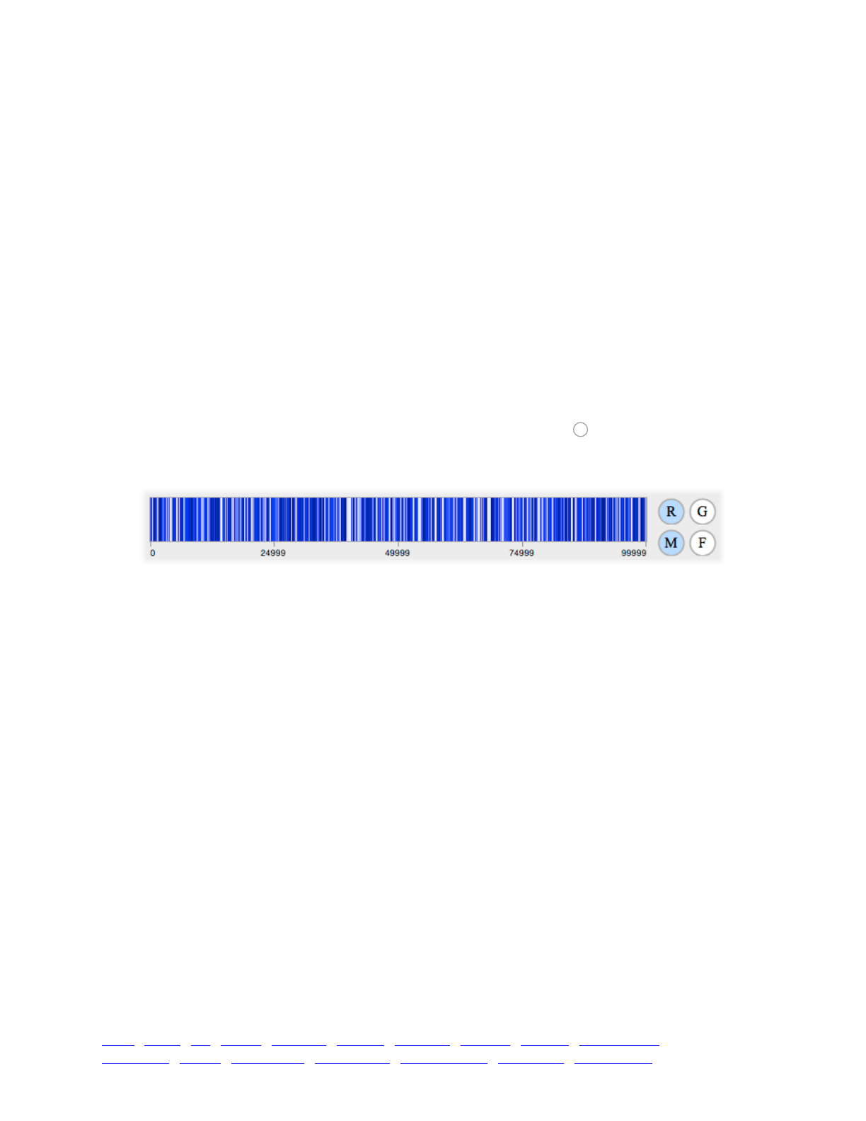
Continuing to work backwards, the preceding script line sets up the vector of recombination
region endpoints:
ends = c(sort(sample(0:99998, 999)), 99999);
Let’s analyze this from the inside out. The innermost call is sample(0:99998, 999). The Eidos
function sample() returns a random sample from a given vector. The given vector here is the
sequence 0:99998, containing every base pair position along the chromosome except for the very
last position (for reasons we will see momentarily). The second parameter requests 999 samples.
The sample() function draws its samples without replacement by default, which is what we want;
each recombination region should end at a different base pair. Next, the result from sample() is
passed to the sort() function, which sorts the vector (because initializeRecombinationRates()
requires the vector of end positions to be in sorted order). Finally, the c() function is used to
concatenate the value 99999 onto the end of the vector, providing the final entry for the vector; this
is the reason that only 999 samples were drawn, from positions up to only 99998. The last end
position is required by initializeRecombinationRates() to be the last position in the
chromosome.
If we paste this recipe into SLiMgui and do a Recycle and a Step, the random recombination
map is loaded into the simulation. To see that it has worked, click the button to turn on display
of rate maps (for recombination and mutation – in this case, just recombination, since that is the
rate map that has been set). The chromosome view should then show you something like this:
The regions shown in the darkest blues are cold spots, with low rates closer to 10−9, whereas
the regions shown in shades close to white are hot spots, with high rates closer to 10−7.
Remember that you can drag out a display range in the upper chromosome view, which changes
what you see in the lower chromosome view – including the recombination map.
Note that SLiM also allows the recombination map to be tailored at an individual level using a
recombination() callback; see sections 13.5 and 21.5. Also, note that a mutation rate map may
be configured in exactly the same way as this recipe’s recombination rate map, using
initializeMutationRate().
6.1.2 Crossing over: Reading a recombination map from a file
Rather than generating a random recombination map, you might want to read in and use an
empirically determined recombination map such as the map from Drosophila melanogaster
presented by Comeron et al. (2012) (dataset available in Fiston-Lavier & Petrov 2013). Let’s work
with chromosome arm 2L, which looks like this:
1 0!
100001 0!
200001 0!
300001 0.234550139!
400001 0.234550139!
500001 1.993676178!
...!
22800001 0.234550139!
22900001 0!
23000001 0
R
TOC I TOC II WF nonWF initialize() Genome Individual Mutation SLiMSim Subpopulation!
Eidos events fitness() mateChoice() modifyChild() recombination() interaction() reproduction() 97

The length of the 2L arm is given as 23011544 bases; positions in SLiM will thus range from 0 to
23011543 (always beware of off-by-one errors!). The file gives start positions in bases, beginning
with 1, with rates in the second column in cM/Mbp (centimorgans per megabasepair). We have a
little format conversion to do, but reading this file in and using it in SLiM is quite straightforward:
initialize() {!
initializeMutationRate(1e-7);!
initializeMutationType("m1", 0.5, "f", 0.0);!
initializeGenomicElementType("g1", m1, 1.0);!
initializeGenomicElement(g1, 0, 23011543);!
!
// read Drosophila 2L map from Comeron et al. 2012!
lines = readFile("/Users/bhaller/Desktop/Comeron_100kb_chr2L.txt");!
rates = NULL;!
ends = NULL;!
!
for (line in lines)!
{!
components = strsplit(line, "\t");!
ends = c(ends, asInteger(components[0]));!
rates = c(rates, asFloat(components[1]));!
}!
!
ends = c(ends[1:(size(ends)-1)] - 2, 23011543);!
rates = rates * 1e-8;!
initializeRecombinationRate(rates, ends);!
}!
1 { sim.addSubpop("p1", 500); }!
10000 { sim.simulationFinished(); }
The action is in the initialize() callback after the comment, as before. The first line calls the
readFile() function of Eidos to read in a text file at the given filesystem path; you will need to
change this path to the correct path to the file on your computer. The result of readFile() is a
string vector of lines; each line in the input file becomes a separate string-element.
Next, we set rates and ends both to NULL. These will be the rates and endpoints vectors that we
will give to SLiM; we will add entries to them one at a time as we process each line in the input
file. NULL is a special type indicating “no value”; it often provides a good initial state.
Now comes a loop over the lines read from the file; each line is placed into the loop index
variable line, and that line is then processed by the loop body. The strsplit() call splits the line
into substrings separated by tab ("\t") characters; since each line has two values separated by a
tab, components end up as a string vector of length 2. The next two lines handle those two
components by converting them to the correct type and then concatenating them on to the tail of
ends and rates using the c() function. This method of building a vector by successive
concatenation is a common quick-and-dirty approach, although it is not terribly fast. When the
loop finishes, we have rates and positions as specified by the input file.
Finally, we need to convert that data into the format expected by SLiM. The input file specifies
start positions, but we want end positions. The expression ends[1:(size(ends)-1)] thus strips off
the first value, the start position 1, which is not needed. The -2 correction accomplishes two
things: (1) it shifts from starts to ends (each region ends at the base position one less than the base
position at which the next region starts), accounting for -1, and (2) it shifts from the 1-based system
of the input file, in which the first base is at position 1, to the 0-based system of SLiM, in which the
first base is at position 0, accounting for another -1. Finally, the c() call adds the last base
position, 23011543, to the tail of the vector.
TOC I TOC II WF nonWF initialize() Genome Individual Mutation SLiMSim Subpopulation!
Eidos events fitness() mateChoice() modifyChild() recombination() interaction() reproduction() 98
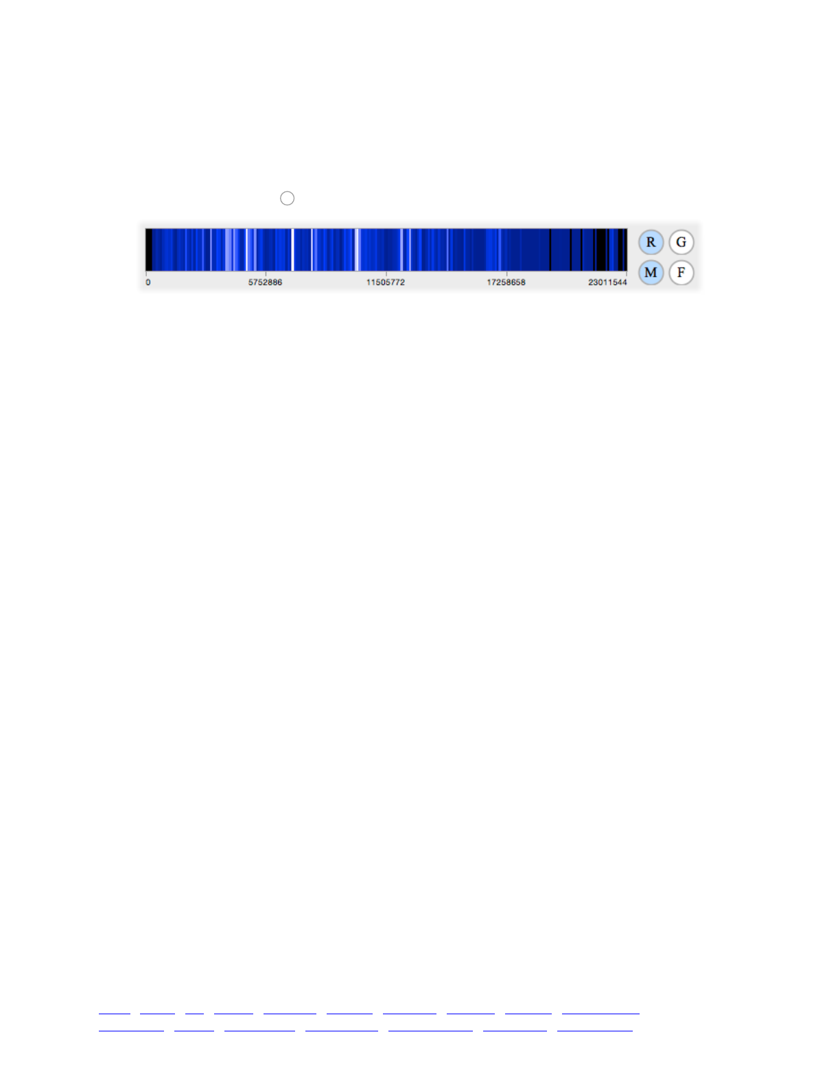
The second conversion line just converts the recombination rates from cM/Mbp to a rate per
base pair per generation, as used by SLiM, by multiplying by 10−8, a conversion ratio that comes
from the units involved. 1 cM means that there is a probability of 0.01 of crossover during
meiosis. Therefore, 1 cM/Mbp = 10−6 cM/bp = 10−8 probability of crossover per base pair.
If you paste this recipe into SLiMgui, Recycle, Step, and turn on display of rate maps in the
chromosome view with the button, you should see something like this:
This is the Drosophila 2L recombination map according to Comeron et al. (2012). Note that a
mutation rate map could be read in and set up in SLiM in much the same manner.
6.1.3 Gene conversion
In addition to crossing over, recombination can also lead to gene conversion, the copying of a
stretch of the genetic sequence from one chromosome to its homologous chromosome (Chen at al.
2007). By default gene conversion is not enabled in SLiM, but it can be turned on easily:
initialize() {!
initializeMutationRate(1e-7);!
initializeMutationType("m1", 0.5, "f", 0.0);!
initializeGenomicElementType("g1", m1, 1.0);!
initializeGenomicElement(g1, 0, 99999);!
initializeRecombinationRate(1e-8);!
initializeGeneConversion(0.2, 25);!
}!
1 { sim.addSubpop("p1", 500); }!
10000 { sim.simulationFinished(); }
The initializeGeneConversion() call takes two parameters. The first is the fraction of
recombination events that will result in gene conversion; here we decide that 0.2 or 20% will.
The second is the mean length of the gene conversion tract, in base pairs; here we specify 25.
When a gene conversion event occurs, the length of the converted tract is drawn by SLiM from a
geometric distribution with the specified mean. Note that SLiM does not presently support
variation in the gene conversion rate along the chromosome; however, gene conversion can be
tailored on a per-individual basis using a recombination() callback, which would allow much the
same thing (see sections 13.5 and 21.5).
6.2 Separate sexes
6.2.1 Enabling separate sexes
Simulations in SLiM involve hermaphroditic individuals by default. If you wish to simulate
separate sexes, however, doing so is essentially just the flip of a switch:
initialize() {!
initializeMutationRate(1e-7);!
initializeMutationType("m1", 0.5, "f", 0.0);!
initializeGenomicElementType("g1", m1, 1.0);!
initializeGenomicElement(g1, 0, 99999);!
initializeRecombinationRate(1e-8);!
initializeSex("A");!
}!
R
TOC I TOC II WF nonWF initialize() Genome Individual Mutation SLiMSim Subpopulation!
Eidos events fitness() mateChoice() modifyChild() recombination() interaction() reproduction() 99

1 { sim.addSubpop("p1", 500); }!
10000 { sim.simulationFinished(); }
This recipe is identical to the basic neutral recipe from section 4.1, apart from the addition of a
call to the function initializeSex():
initializeSex("A");
The parameter here specifies the type of chromosome that is to be modeled; "A" specifies
modeling of an autosome, but it is also possible to model the X or Y chromosome in SLiM (see
section 6.2.3).
Once sex is turned on in a simulation, there is no way to turn it off; it is not possible to make a
SLiM simulation in which individuals switch between being sexual and being hermaphroditic. A
similar effect could probably be produced by modifying the mate choice algorithm, however (see
chapter 11).
Having turned sex on, all subpopulations will keep track of male and female individuals
separately, and biparental matings will always involve a male parent and a female parent. A few
things work a bit differently when sex is enabled; each subpopulation has a sex ratio that can be
specified and modified (see section 6.2.2), for example, and selfing (see section 6.3.1) is not
allowed when sex is enabled. Usually you will know whether your code is running with sex
enabled or disabled, but if you wish to write general-purpose code that works in either
environment, the sexEnabled property of SLiMSim will tell you whether sex is presently enabled.
Section 4.2 discussed output of basic simulation state using the outputFull() and
outputSample() methods of SLiMSim. When sex is enabled, the output generated by these
methods changes slightly. In particular, the H symbol that was used to designate individuals as
hermaphrodites will change to indicate the sex of each individual with M or F. In addition, if sex
chromosomes are modeled (see section 6.2.3), the A that designated genomes in the output as
autosomes will change to an X or Y as appropriate.
6.2.2 Sex ratios
When individuals are one of two sexes, rather than being hermaphroditic, the question of the
sex ratio immediately arises. A sex ratio of 0.5 is maintained by default in SLiM; if that is what you
want, no further action is required. To set a sex ratio (i.e., male fraction; see below) of 0.6, on the
other hand, you simply supply an extra parameter to addSubpop() (or to addSubpopSplit(), which
works in the same way):
initialize() {!
initializeMutationRate(1e-7);!
initializeMutationType("m1", 0.5, "f", 0.0);!
initializeGenomicElementType("g1", m1, 1.0);!
initializeGenomicElement(g1, 0, 99999);!
initializeRecombinationRate(1e-8);!
initializeSex("A");!
}!
1 { sim.addSubpop("p1", 500, 0.6); }!
10000 { sim.simulationFinished(); }
If you paste this recipe into SLiMgui, Recycle, and Step twice to get through generation 1, you
can see in the population table view that this sex ratio has been used by SLiM:
TOC I TOC II WF nonWF initialize() Genome Individual Mutation SLiMSim Subpopulation!
Eidos events fitness() mateChoice() modifyChild() recombination() interaction() reproduction() 100

The column labeled shows the current sex ratio of each subpopulation; the subpopulations
in the simulation do not all need to have the same sex ratio. The sex ratio of a subpopulation can
be accessed in script through the sexRatio property of Subpopulation; in the recipe above, for
example, p1.sexRatio would be equal to 0.6.
The “sex ratio” in SLiM refers to the male fraction, the fraction of the total subpopulation that is
male. Symbolically, it is therefore M/(M+F), where M and F are the number of males and females
respectively. A sex ratio of 0 would imply all females; a sex ratio of 1 would imply all males; the
default sex ratio of 0.5 is half males and half females.
You are free to set almost any sex ratio you wish; SLiM will raise an error, however, if the
simulation is forced into a situation in which a subpopulation would become unisexual (whether
due to the sex ratio, cloning rate, or other factors). All subpopulations must be viable, which
means that at least one parent of each sex must be available to produce offspring.
It is possible for the sex ratio of a subpopulation to change over time. For example, here is a
recipe for a simulation in which the sex ratio fluctuates randomly around 0.5:
initialize() {!
initializeMutationRate(1e-7);!
initializeMutationType("m1", 0.5, "f", 0.0);!
initializeGenomicElementType("g1", m1, 1.0);!
initializeGenomicElement(g1, 0, 99999);!
initializeRecombinationRate(1e-8);!
initializeSex("A");!
}!
1 { sim.addSubpop("p1", 500); }!
1: { p1.setSexRatio(runif(1, 0.3, 0.7)); }!
10000 { sim.simulationFinished(); }
The setSexRatio() method of Subpopulation simply takes a float representing the new sex
ratio. As with setSubpopulationSize(), the change is not effected immediately; instead, the call
sets the target sex ratio that will be used when offspring are generated. The recipe above draws a
new random sex ratio between 0.3 and 0.7 in each generation using runif().
6.2.3 Modeling sex-chromosome evolution
So far we have always seen simulations of autosomal evolution, but SLiM also supports
simulation of sex chromosome evolution. The choice of chromosome type is made in the
initializeSex() call, so to simulate X chromosome evolution one would simply do:
initialize() {!
initializeMutationRate(1e-7);!
initializeMutationType("m1", 0.5, "f", 0.0);!
initializeGenomicElementType("g1", m1, 1.0);!
initializeGenomicElement(g1, 0, 99999);!
initializeRecombinationRate(1e-8);!
initializeSex("X");!
}!
1 { sim.addSubpop("p1", 500); }!
10000 { sim.simulationFinished(); }
The "X" passed to initializeSex() sets SLiM to model the X chromosome. SLiM will handle
all of the necessary details; females in the simulation will be XX, whereas males will be XY. Since
the Y chromosome is not being modeled in this scenario, it will be a “null chromosome”, a
placeholder kept by SLiM simply to make the diploid bookkeeping balance. Null chromosomes
have no structure, receive no mutations, and raise an error if you attempt to do much of anything
with them. It is also possible to supply "Y" to initializeSex(), to model the Y chromosome; in
TOC I TOC II WF nonWF initialize() Genome Individual Mutation SLiMSim Subpopulation!
Eidos events fitness() mateChoice() modifyChild() recombination() interaction() reproduction() 101

this case it is the X chromosome that will be a “null chromosome”. If you need to work directly
with Genome objects in your script (we will see some examples of this later), you can find out
whether a given genome is null or not with the isNullGenome property of Genome.
When modeling sex chromosomes, recombination works as you would expect it to. To be
specific, if you are modeling the X chromosome, recombination will occur between the two X
chromosomes of female parents when generating their gametes, whereas no recombination will
occur between the X and Y chromosomes of a male. If you are modeling the Y chromosome,
recombination does not occur, since the X chromosome in this case is a null chromosome, and
individuals never possess two Y chromosomes.
When modeling the X chromosome, there are two different ways in which an individual can be
heterozygous for a given mutation: the individual might be XX (i.e., female) and possess the
mutation on just one X chromosome, or the individual might be XY (i.e., male) and possess the
mutation on the one X chromosome present. These cases are handled differently by SLiM when it
calculates the fitness effect of a mutation. The first case is handled in the same way as when
modeling an autosome: the dominance coefficient for the mutation type of the mutation, as
supplied to initializeMutationType(), specifies a multiplicative modifier for the selection
coefficient of the mutation (see section 4.1.3). The second case is unique to the case of modeling
the X chromosome, and is handled using a special X-dominance coefficient. This coefficient is 1.0
by default, meaning that an XY individual possessing an X-linked mutation will experience the
same fitness effect from that mutation as an XX individual that is homozygous for that mutation (a
reasonable assumption because of X inactivation). The X-dominance coefficient may be changed
by supplying an optional second parameter to the initializeSex() function:
initializeSex("X", 0.8);
The dominanceCoeffX property of SLiMSim can also be used to get and set the X-dominance
coefficient; for example, one could vary its value over time. However, this mechanism is presently
much less flexible than the standard dominance coefficient, since a single X-dominance coefficient
value is used for all mutations in all subpopulations at present. Of course it would be possible to
introduce a more complex fitness calculation scheme using a fitness() callback, as discussed in
chapter 9.
When modeling the Y chromosome, individuals can only possess zero or one copy of a given
mutation, since males possess one Y and females possess none. For this reason, SLiM does not use
a dominance coefficient at all in this case. The selection coefficient of the mutation determines its
fitness effect, and the dominance coefficient supplied in the mutation type is simply ignored.
It is worth noting that the way in which the Y chromosome is modeled in SLiM is in some ways
similar to how one might model mitochondrial genomes. If SLiM is used in this way, the XY
“males” are really the females, with a single genome possessed by all of the mitochondria in a
given female. The XX “females” are really the males; they possess mitochondria too, of course, but
they do not pass them down to their offspring, so their mitochondria are an evolutionary dead end
that does not need to be modeled. This equivalence should work unless you need to model the
fitness effects of mitochondrial mutations in males; that would probably also be possible in SLiM,
using an autosomal model with a modifyChild() callback, but it is beyond the scope of this
manual.
TOC I TOC II WF nonWF initialize() Genome Individual Mutation SLiMSim Subpopulation!
Eidos events fitness() mateChoice() modifyChild() recombination() interaction() reproduction() 102

6.3 Selfing and cloning
6.3.1 Selfing in hermaphroditic populations
Selfing, or self-fertilization, is the mating of an individual with itself: male and female gametes
from one individual combine to form a zygote. Selfing is different from cloning in that gametes are
produced and fertilize, so offspring are not clones of their parent; notably, recombination occurs in
selfing. It is an essentially hermaphroditic phenomenon, since hermaphroditic individuals can
produce both eggs and sperm, can produce both X and Y gametes, and are fertile. There are
probably counterexamples somewhere in biology, where it sometimes seems that anything that is
possible exists; but in SLiM, at least, selfing is limited to the hermaphroditic case.
Returning to a hermaphroditic model, then, selfing can be turned on with a single call:
initialize() {!
initializeMutationRate(1e-7);!
initializeMutationType("m1", 0.5, "f", 0.0);!
initializeGenomicElementType("g1", m1, 1.0);!
initializeGenomicElement(g1, 0, 99999);!
initializeRecombinationRate(1e-8);!
}!
1 {!
sim.addSubpop("p1", 500);!
p1.setSelfingRate(0.8);!
}!
10000 { sim.simulationFinished(); }
The setSelfingRate() method call here on p1 tells SLiM that selfing should be used to generate
80% of the offspring in subpopulation p1. The selfing rate may be anything from 0.0 (the default)
to 1.0. The setSelfingRate() method may be called at any time, so the selfing rate can be varied
over time or in response to other simulation conditions. The current selfing rate for a
subpopulation is shown in the population table view under the column.
Usually it is not important, but it should be noted that in non-sexual simulations SLiM does not
prevent a parent from being chosen twice, as both parents in a biparental mating event. Even
when the selfing rate is set to 0, therefore, a low background rate of selfing may occur. This can
easily be prevented if necessary; see the recipe in section 12.4.
6.3.2 Cloning
SLiM also supports clonal reproduction, in which offspring are an exact genetic copy of a single
parent (except for new mutations introduced during the copying of the DNA). Indeed,
hermaphroditic simulations may have a combination of biparental mating, self-fertilization, and
cloning. In a hermaphroditic model, setting up clonal reproduction is a single call:
initialize() {!
initializeMutationRate(1e-7);!
initializeMutationType("m1", 0.5, "f", 0.0);!
initializeGenomicElementType("g1", m1, 1.0);!
initializeGenomicElement(g1, 0, 99999);!
initializeRecombinationRate(1e-8);!
}!
1 {!
sim.addSubpop("p1", 500);!
p1.setCloningRate(0.1);!
}!
10000 { sim.simulationFinished(); }
TOC I TOC II WF nonWF initialize() Genome Individual Mutation SLiMSim Subpopulation!
Eidos events fitness() mateChoice() modifyChild() recombination() interaction() reproduction() 103

The setCloningRate() call here tells SLiM to generate 10% of the offspring in p1 clonally (the
remaining 90% will be generated biparentally as usual). The cloning rate may be anything from
0.0 (the default) to 1.0. The setCloningRate() method may be called at any time, so the cloning
rate can be varied over time or in response to other simulation conditions. The current cloning
rate for each subpopulation is shown in the population table view under the and
columns; in the hermaphroditic case the same number will be shown in both columns (the icon
depicts a little Athena budding parthenogenically from the head of Zeus, if that is not immediately
obvious).
Clonal reproduction is also supported in the case of separate sexes. It works in essentially the
same way:
initialize() {!
initializeMutationRate(1e-7);!
initializeMutationType("m1", 0.5, "f", 0.0);!
initializeGenomicElementType("g1", m1, 1.0);!
initializeGenomicElement(g1, 0, 99999);!
initializeRecombinationRate(1e-8);!
initializeSex("A");!
}!
1 {!
sim.addSubpop("p1", 500);!
p1.setCloningRate(c(0.5,0.0));!
}!
10000 { sim.simulationFinished(); }
The only difference is that when separate sexes are enabled by initializeSex(), the
setCloningRate() method can take a vector of two rates, as above. Here the cloning rate is set to
0.5 for females, but 0.0 for males, reflecting a somewhat common situation in some taxa, in which
females can reproduce parthenogenically but males can reproduce only sexually. You may still
pass a singleton value to setCloningRate(); when separate sexes are enabled, that value is then
taken as the cloning rate for both males and females. The current cloning rates for the females and
males in each subpopulation is shown in the population table view under the and
columns.
TOC I TOC II WF nonWF initialize() Genome Individual Mutation SLiMSim Subpopulation!
Eidos events fitness() mateChoice() modifyChild() recombination() interaction() reproduction() 104

7. Mutation types, genomic elements, and chromosome structure
A number of concepts such as mutation types, genomic element types, genomic elements, and
chromosome structure were already introduced in chapter 4 in our basic neutral simulation. Here
we return to those foundational concepts and explore them in more detail, showing how
simulations might use multiple mutation types, multiple genomic element types, and many
genomic elements to simulate more realistic chromosome structures with mutations of varying
selective effects.
The structure of this chapter will be a bit different from that of previous chapters. In this chapter
each subsection will build upon the recipe introduced by the previous subsection, working
towards making a relatively large final recipe for a full-chromosome simulation.
7.1 Mutation types and fitness effects
In section 4.1.3 the concept of a mutation type was introduced: a category of mutations that
represents some particular subset of the mutations in a simulation. Examples might include
“neutral mutations”, “beneficial mutations introduced by the simulation script in generation 10”,
or “mutations that will be forced to sweep to fixation”. Mutation types are represented in SLiM
with the MutationType class, and each defined mutation type has a unique symbolic identifier of
the form mX, like m1 or m27. Whenever you want to be able to generate or refer to a particular type
of mutations separately from other types, you will want to define a new mutation type.
Section 4.1.3 also introduced the function used to create new mutation types at initialization
time, initializeMutationType(). This function can only be called inside an initialize()
callback; in fact, it is not even defined at other times. Mutation types can therefore be set up only
at initialization time; you must set up all of the types that your simulation will need for the entire
run. After initialization, mutation types are typically static entities; however, there is a method,
setDistribution(), that may be used to change a mutation type’s distribution of fitness effects,
affecting new mutations generated from that point onward.
A mutation type is basically defined by two things: its dominance coefficient, and its
distribution of fitness effects (DFE). Both of these properties are important only because they affect
new mutations that are generated from a given mutation type: (1) each mutation of a given
mutation type receives a selection coefficient drawn from the mutation type’s DFE, and (2)
individuals that are heterozygous for a mutation will use the dominance coefficient, obtained from
the mutation type of the mutation, to modify the selection coefficient of the mutation.
For the purposes of this recipe, let’s define four mutation types: two for neutral mutations (non-
coding and synonymous), one for mildly deleterious mutations, and one for strongly beneficial
mutations:
initialize() {!
initializeMutationRate(1e-7);!
initializeMutationType("m1", 0.5, "f", 0.0); // non-coding!
initializeMutationType("m2", 0.5, "f", 0.0); // synonymous!
initializeMutationType("m3", 0.1, "g", -0.03, 0.2); // deleterious!
initializeMutationType("m4", 0.8, "e", 0.1); // beneficial!
initializeGenomicElementType("g1", m1, 1.0);!
initializeGenomicElement(g1, 0, 99999);!
initializeRecombinationRate(1e-8);!
}!
1 { sim.addSubpop("p1", 5000); }!
10000 { sim.simulationFinished(); }
TOC I TOC II WF nonWF initialize() Genome Individual Mutation SLiMSim Subpopulation!
Eidos events fitness() mateChoice() modifyChild() recombination() interaction() reproduction() 105
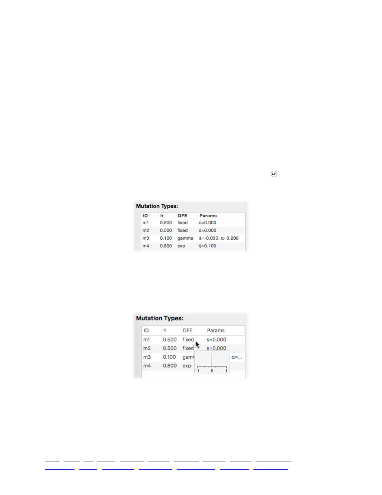
The neutral mutation types, m1 and m2, are defined with a dominance coefficient of 0.5 (which
does not matter for neutral mutations), and mutations drawn from them receive a fixed selection
coefficient (DFE type "f") of 0.0 as specified by the DFE parameter. Note that they are exactly
identical in their parameters; however, they will be used to represent different conceptual types of
neutral mutations, with m1 representing neutral mutations in non-coding regions and m2
representing synonymous mutations in coding regions. Drawing this distinction will allow us to
distinguish these two classes of mutations later on, when we are observing the simulation running.
The deleterious mutation type, m3, has a dominance coefficient of only 0.1, meaning that
heterozygous individuals feel very little effect from these mutations; they are almost recessive.
These mutations are drawn from a gamma distribution (see section 21.9) with a mean of −0.03,
with a shape parameter (alpha) of 0.2.
Finally, the beneficial mutation type, m4, has a dominance coefficient of 0.8, representing
incomplete dominance. Mutations of this type are drawn from an exponential DFE with a mean of
0.1.
All defined mutation types can be viewed in the drawer on the simulation window. If you paste
in the recipe so far, Recycle, and Step, then open the drawer by pressing the button, you can
see the mutation types listed, which can be quite useful if mutation types are manufactured en
masse with a for loop or similar automated construction method:
We are not using the new mutation types yet, just defining them; we’ll make more progress with
this recipe in the next section. Before we move on to that, however, there is one hidden feature
worth mentioning. The mutation type table that is depicted in the screenshot above has a nice
hidden addition: tooltips that show the mutation type’s DFE graphically. If you place the mouse
cursor over the m1 line without moving it for a second or a bit more (often called a “hover” of the
cursor), a “tooltip” – a little informational tab – will appear:
(Ignore the somewhat different appearance of the two screenshots above; they were taken on
different versions of OS X, and Apple changed the standard system font and other aspects of table
appearance from one OS X release to the next.) The tooltip shown above contains a plot of the
mutation type’s distribution of fitness effects; the x-axis is the selection coefficient, and the y-axis is
the distribution’s relative density. In this case, since the mutation type has a fixed selection
coefficient of 0.0, the distribution consists of a single peak at 0.0. Hover over m3, and a more
interesting tooltip appears:
TOC I TOC II WF nonWF initialize() Genome Individual Mutation SLiMSim Subpopulation!
Eidos events fitness() mateChoice() modifyChild() recombination() interaction() reproduction() 106
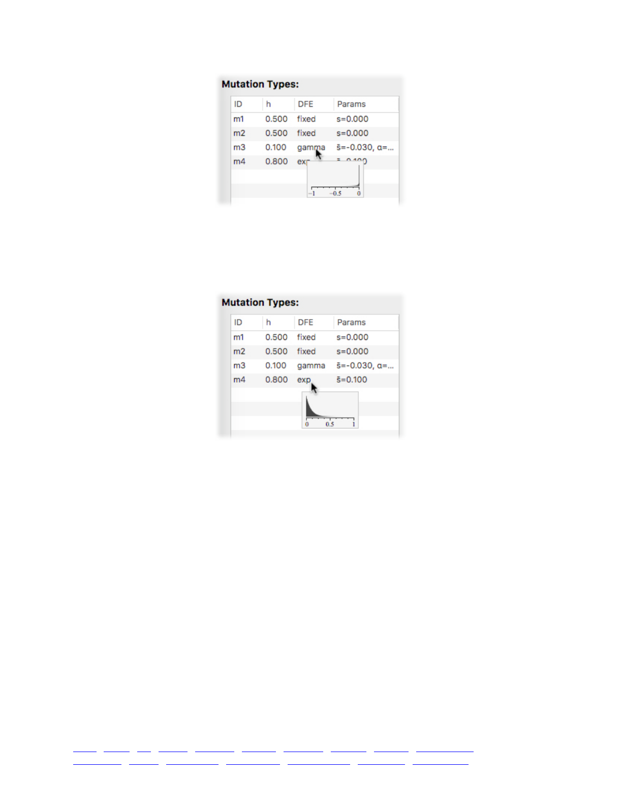
This plot shows the specific gamma distribution specified by the parameters for m3; note that the
x-axis now spans the range −1 to 0 only, since this DFE does not include any positive selection
coefficients. The distribution shown has most of its density very close to zero, but a tail is visible
extending downward perhaps as far as −0.25.
Hovering over m4 shows its DFE:
This is a non-negative DFE, so the x-axis spans 0 to 1, and this distribution is much broader.
This sort of visualization can prove quite helpful in configuring and debugging DFEs.
7.2 Genomic element types
Now that we have a couple of mutation types defined, we can make some genomic element
types that use these mutation types. Genomic element types were introduced in section 4.1.4;
they represent a type of region in the genome with a particular mutational profile. For this simple
toy model, let’s focus on exons, introns, and non-coding regions:
initialize() {!
initializeMutationRate(1e-7);!
initializeMutationType("m1", 0.5, "f", 0.0); // non-coding!
initializeMutationType("m2", 0.5, "f", 0.0); // synonymous!
initializeMutationType("m3", 0.1, "g", -0.03, 0.2); // deleterious!
initializeMutationType("m4", 0.8, "e", 0.1); // beneficial!
initializeGenomicElementType("g1", c(m2,m3,m4), c(2,8,0.1)); // exon!
initializeGenomicElementType("g2", c(m1,m3), c(9,1)); // intron!
initializeGenomicElementType("g3", c(m1), 1); // non-coding!
initializeGenomicElement(g1, 0, 99999);!
initializeRecombinationRate(1e-8);!
}!
1 { sim.addSubpop("p1", 5000); }!
10000 { sim.simulationFinished(); }
TOC I TOC II WF nonWF initialize() Genome Individual Mutation SLiMSim Subpopulation!
Eidos events fitness() mateChoice() modifyChild() recombination() interaction() reproduction() 107
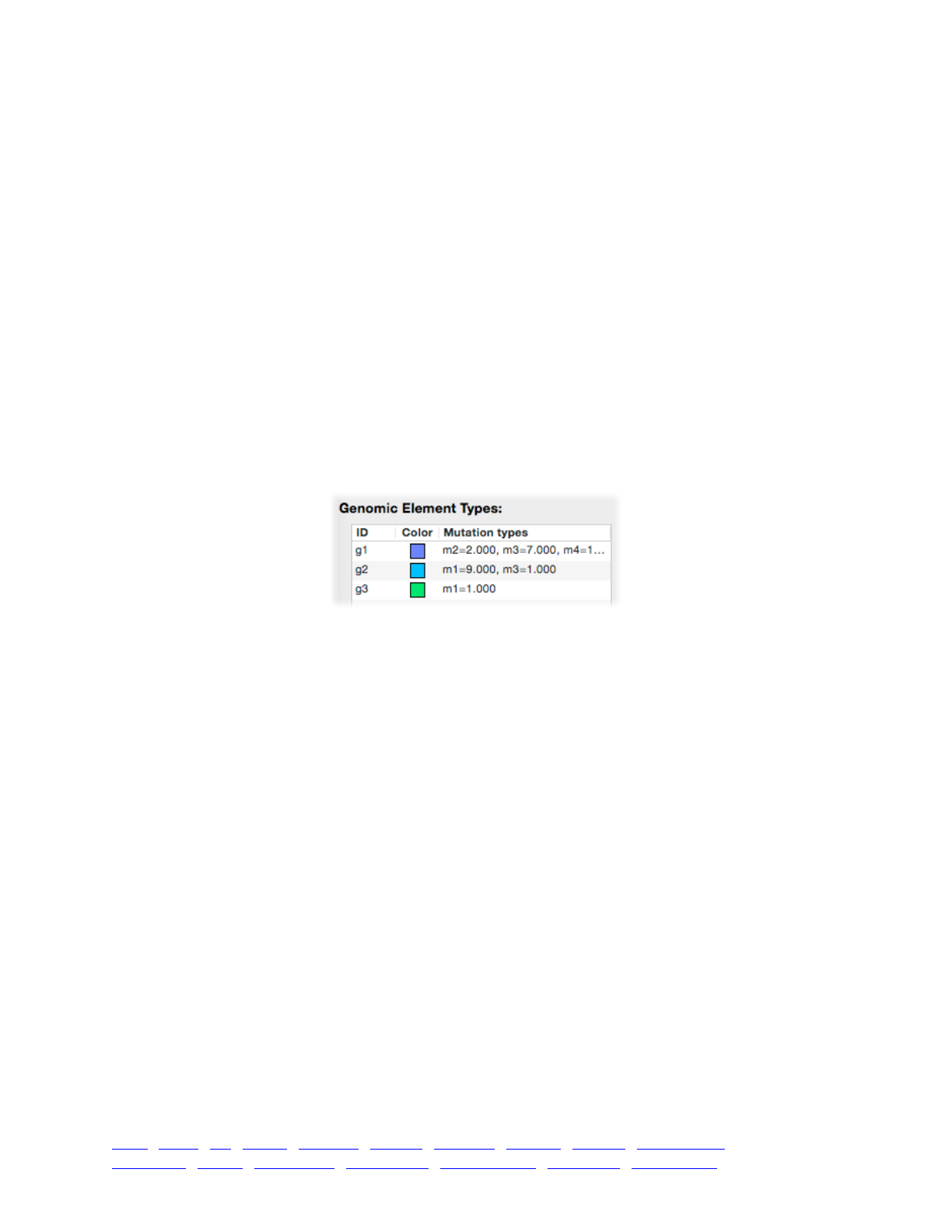
Genomic element type g1 defines exons, which often suffer deleterious mutations, sometimes
get neutral (synonymous) mutations, and very rarely get beneficial mutations. Type g2 defines
introns, which often get neutral (non-coding) mutations, and occasionally get deleterious
mutations. Type g3 defines non-coding regions, which get neutral (non-coding) mutations only.
Each genomic element type is defined with a call to initializeGenomicElementType(), as
previously discussed in section 4.1.5; its parameters supply the identifier for the new type, a vector
of mutation types, and a vector of relative proportions for those mutation types among the new
mutations that occur in the genomic elements of this type.
Notice that there is not a one-to-one correspondence between mutation types and genomic
element types; this is typical, since the two classes represent quite different objects. A genomic
element often draws from a variety of different mutation types, with various probabilities. If this
model were expanded to be more biologically realistic, it might have quite a few more genomic
element types (3′ and 5′ UTRs, promoters and enhancers and silencers, various different types of
non-coding regions...) but might have only a couple more mutation types (a strongly deleterious
mutation type, to represent things like premature stop codons and broken promoters, for example).
Again, this recipe is not yet complete; now that we have defined genomic element types we
need to make genomic elements that use those types. However, at this point we can Recycle,
Step, and observe the defined genomic element types in the simulation window’s drawer:
Note that each genomic element type is automatically assigned a color by SLiMgui. We will
soon see how these colors are used.
7.3 Chromosome organization
As previously discussed in section 4.1.5, genomic elements are regions of a chromosome that
use a particular genomic element type. The genomic element types define what possibilities exist
in the chromosome; the genomic elements determine what actually does exist. Having defined
genomic element types for exons, introns, and non-coding regions, we now need to create
genomic elements to express how the genomic element types are distributed in the chromosome.
As has been the case all along with this recipe, the goal here is not biological realism;
nevertheless, it is interesting to try to come up with a recipe that broadly approximates the
structure of a real chromosome, just to show how the problem might be approached. In this
recipe, then, the formulas used for the lengths of exons and introns are very loosely based on
empirical length distributions.
This is by far the longest recipe we’ve seen so far, so a bit of preamble to prepare the way for it
is helpful. We have previously used for loops to iterate over a specified vector. This example uses
two new looping constructs, a do loop and a do–while loop. These both iterate as long as a given
condition remains true; when the conditions tests false, the loop terminates. The only difference
between them is that do–while tests its condition at the end of the loop body, and thus the loop
body always executes at least once. The other new thing in this recipe is use of the rlnorm()
function, which draws samples from a lognormal distribution. In addition to the number of
samples to draw, it takes the mean and standard deviation of the distribution as parameters, on the
log scale. With that preface, here is the recipe:
TOC I TOC II WF nonWF initialize() Genome Individual Mutation SLiMSim Subpopulation!
Eidos events fitness() mateChoice() modifyChild() recombination() interaction() reproduction() 108

initialize() {!
initializeMutationRate(1e-7);!
!
initializeMutationType("m1", 0.5, "f", 0.0); // non-coding!
initializeMutationType("m2", 0.5, "f", 0.0); // synonymous!
initializeMutationType("m3", 0.1, "g", -0.03, 0.2); // deleterious!
initializeMutationType("m4", 0.8, "e", 0.1); // beneficial!
!
initializeGenomicElementType("g1", c(m2,m3,m4), c(2,8,0.1)); // exon!
initializeGenomicElementType("g2", c(m1,m3), c(9,1)); // intron!
initializeGenomicElementType("g3", c(m1), 1); // non-coding!
!
// Generate random genes along an approximately 100000-base chromosome!
base = 0;!
!
while (base < 100000) {!
// make a non-coding region!
nc_length = asInteger(runif(1, 100, 5000));!
initializeGenomicElement(g3, base, base + nc_length - 1);!
base = base + nc_length;!
!
// make first exon!
ex_length = asInteger(rlnorm(1, log(50), log(2))) + 1;!
initializeGenomicElement(g1, base, base + ex_length - 1);!
base = base + ex_length;!
!
// make additional intron-exon pairs!
do!
{!
in_length = asInteger(rlnorm(1, log(100), log(1.5))) + 10;!
initializeGenomicElement(g2, base, base + in_length - 1);!
base = base + in_length;!
!
ex_length = asInteger(rlnorm(1, log(50), log(2))) + 1;!
initializeGenomicElement(g1, base, base + ex_length - 1);!
base = base + ex_length;!
}!
while (runif(1) < 0.8); // 20% probability of stopping!
}!
!
// final non-coding region!
nc_length = asInteger(runif(1, 100, 5000));!
initializeGenomicElement(g3, base, base + nc_length - 1);!
!
// single recombination rate!
initializeRecombinationRate(1e-8);!
}!
1 { sim.addSubpop("p1", 5000); }!
10000 { sim.simulationFinished(); }
This is too much code to parse through line by line, but it should be fairly clear what is going
on. The outer loop adds one non-coding region and then one gene each time that it iterates; the
inner loop adds one intron-exon pair with each iteration. The overall algorithm is not targeted to
end at a fixed chromosome length (doing that without biasing the metrics of the final gene
generated would be a bit tricky); instead, genes are added until the chromosome length exceeds
100000 and then the process is ended with a final non-coding region. Eidos does not have any
built-in facility for graphing, so you can’t directly see the distributions used to generate the lengths
TOC I TOC II WF nonWF initialize() Genome Individual Mutation SLiMSim Subpopulation!
Eidos events fitness() mateChoice() modifyChild() recombination() interaction() reproduction() 109
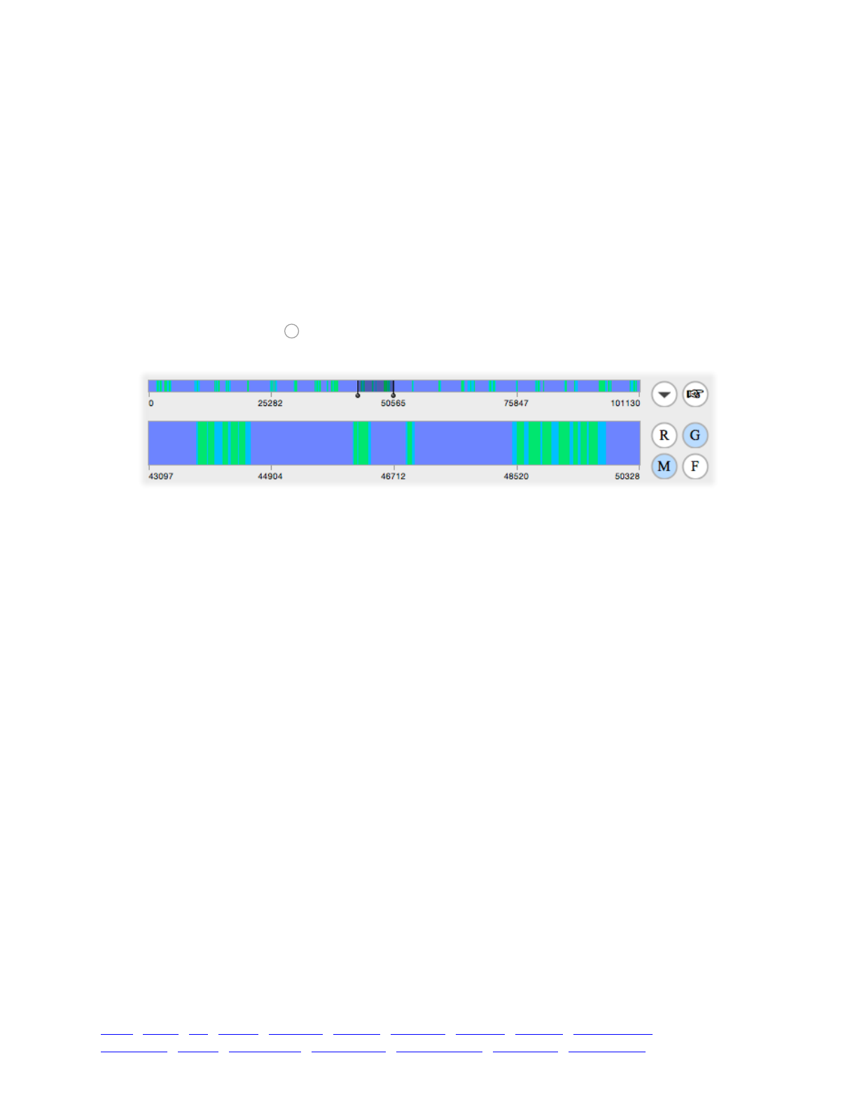
of the exons and introns; however, since the syntax of Eidos is so similar to that of R, it is quite
easy to use R to plot these distributions. The only hitch is that conversion to integer is asInteger()
in Eidos but as.integer() in R, so that has to be tweaked. If you are so inclined, try running this
code in R:
x = as.integer(rlnorm(100000, log(50), log(2))) + 1!
hist(x[x < 250], breaks=100)
That will produce a plot of the distribution of exon lengths, which may be compared to the
distribution shown in Deutsch & Long (1999), which was loosely used as a reference for this
model. The distribution of intron lengths may be compared similarly.
If you paste in the recipe above, Recycle, and Step, you will see the random chromosome
structure that it generated, which might look something like this (after turning on display of
genomic elements with the button, and selecting a subrange in the upper chromosome view to
show some detail):
The structure of non-coding regions (purple) interspersed with genes made up on exons (blue)
alternating with introns (green) appears to be as intended. It should now be clear, of course, how
SLiMgui uses the colors that it assigns to genomic element types, as seen in the previous section.
Rather than generating a random chromosome organization, you might wish to read in an
actual chromosome map and generate genomic regions based upon that information, to simulate
the evolution of a particular organism. That is left as an exercise for the reader, but with the recipe
in section 6.1.2 as guidance it should not be too difficult.
7.4 Custom display colors in SLiMgui
The model that we built in the previous three sections uses various default colors schemes
supplied by SLiMgui: mutations are colored according to their selection coefficients, genomic
element types are automatically assigned colors from a standard palette, and individuals are
colored according to their fitness. For simple models these default colors generally suffice, but
when constructing complex models it may be helpful to customize the color scheme used in
SLiMgui to improve the clarity of the models’ visual representation. In this section we will briefly
explore SLiM’s facilities for doing so.
First of all, the colors used for genomic regions, as shown in the figure above in section 7.3, is
perhaps less than ideal. It would be nice if non-coding regions were shown in a distinctive color
suggestive of the unimportance of those regions to the organism, such as black. Similarly, perhaps
exons could be in the brightest color, connoting their importance, whereas introns could be shown
in a more muted fashion. This can be accomplished by simply adding these lines after the calls to
initializeGenomicElementType() have set up the genomic element types:
g1.color = "cornflowerblue";!
g2.color = "#00009F";!
g3.color = "black";
G
TOC I TOC II WF nonWF initialize() Genome Individual Mutation SLiMSim Subpopulation!
Eidos events fitness() mateChoice() modifyChild() recombination() interaction() reproduction() 110
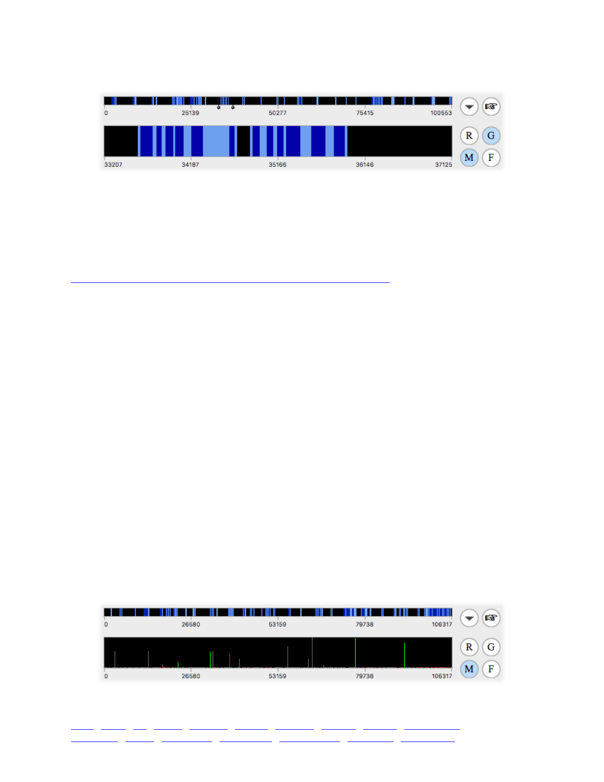
This produces a chromosome view like this:
It works by setting values on the color property of the genomic element types. By default, these
color properties are the empty string, "", which tells SLiM to use a color from its default color
palette. Here we have instead told SLiM to use a light blue named "cornflowerblue" for the
exons represented by g1, and "black" for non-coding regions represented by g3. These names are
two of the 657 named colors supported by SLiM. The complete list of named colors is identical to
the named color list provided by the R language, for simplicity, and so there are various web
resources available that show all of the names and their corresponding colors (one such resource:
http://research.stowers-institute.org/efg/R/Color/Chart/ColorChart.pdf). You can browse such a list,
and then simply use the name for the color you want in SLiM.
The color used for g2 is not a named color, however; instead, it is the rather cryptic string value
"#00009F". This specifies the color in hexadecimal, or base 16, as two-digit values for the red,
green, and blue components of the color. With values of zero for red and green, and a value of 9F
for blue, this string represents a dark blue that works well for introns here.
The Eidos manual has further discussion of how colors are specified in SLiM (this is actually part
of the Eidos language). Note that setting colors on SLiM objects in this way only has an effect in
SLiMgui, but it is entirely legal when running SLiM models at the command line; the properties
still exist, but are unused by SLiM outside of SLiMgui.
Now that the genomic elements are colored nicely, let’s set up new colors for the mutations. By
default, SLiMgui displays neutral mutations in yellow, beneficial mutations in shades of green and
blue, and deleterious mutations in shades of orange and red. Let’s suppose we want to de-
emphasize neutral mutations in this model; we want them to display, but in a less visible color
than the default bright yellow color. We also want all beneficial mutations to be a single shade of
green (the blue doesn’t show up well against the blues we’ve chosen for our genomic elements),
and we want all deleterious mutations to be bright red so we can see them very clearly. This can
be achieved with a few lines placed after the mutation types have been defined:
m1.color = "gray40";!
m2.color = "gray40";!
m3.color = "red";!
m4.color = "green";
That produces a display like this (with display of the genomic elements turned off now, for
greater clarity):
TOC I TOC II WF nonWF initialize() Genome Individual Mutation SLiMSim Subpopulation!
Eidos events fitness() mateChoice() modifyChild() recombination() interaction() reproduction() 111
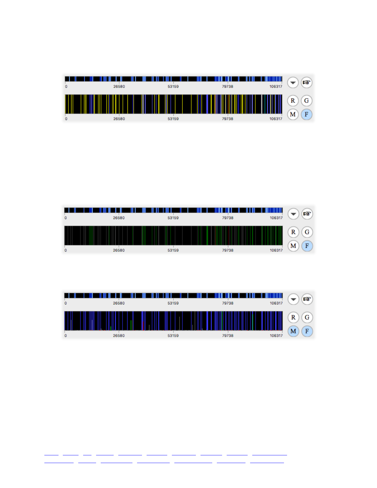
That looks like what we had in mind. If we turn on display of fixed mutations instead of
segregating mutations, however, we see that those are still being displayed in SLiM’s default color
scheme:
This is obviously not what we want. Instead, let’s use darker shades of the same colors used for
the mutations when they are still segregating. This can be done by setting the colorSubstitution
property of the mutation types:
m1.colorSubstitution = "gray20";!
m2.colorSubstitution = "gray20";!
m3.colorSubstitution = "#550000";!
m4.colorSubstitution = "#005500";
That produces the desired result:
There’s one thing left for us to tweak. If we turn on display of both segregating and fixed
mutations, SLiMgui displays the fixed mutations using a shade of blue, rather than the colors we
just set up above:
This is deliberate, to prevent too much clutter and chaos in the chromosome view. However,
we deliberately chose dark colors above for our fixed mutations with the intention of having them
coexist aesthetically, so we’d like to tell SLiMgui to use our color scheme in all cases. The default
dark blue color SLiMgui uses for fixed mutations when both are being displayed is a property on
the Chromosome object named colorSubstitution. By default, it is set to "#3333FF", the dark blue
color being used. We can set it to the empty string, "", instead; this eliminates the use of this
default color. Since the Chromosome object is not available until the simulation has been fully
initialized, we can do this at the beginning of generation 1, by adding a line to the generation 1
event:
sim.chromosome.colorSubstitution = "";
TOC I TOC II WF nonWF initialize() Genome Individual Mutation SLiMSim Subpopulation!
Eidos events fitness() mateChoice() modifyChild() recombination() interaction() reproduction() 112
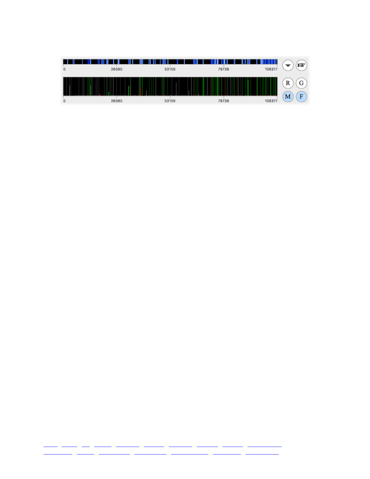
Now our model displays as intended:
The fixed mutations are now in dark, dimmed colors, whereas the currently segregating
mutations are in bright, clear colors that are easily visible against that background.
We won’t give an example of it here, but the Individual class in SLiM also has a color
property that can be set to override the default fitness-based color scheme for display of
individuals. Setting this property should be done in a late() event, since SLiMgui updates its
display at the very beginning of each generation; early() events are executed after SLiMgui has
already displayed, and so setting display colors for individuals at that time will have no visible
effect. Generally SLiMgui’s fitness-based coloring works well, but in some special cases it might
be useful to give a specific color to individuals that possess some particular property – especially
in models in with the tag values of individuals are being used to keep track of extra state
information.
TOC I TOC II WF nonWF initialize() Genome Individual Mutation SLiMSim Subpopulation!
Eidos events fitness() mateChoice() modifyChild() recombination() interaction() reproduction() 113
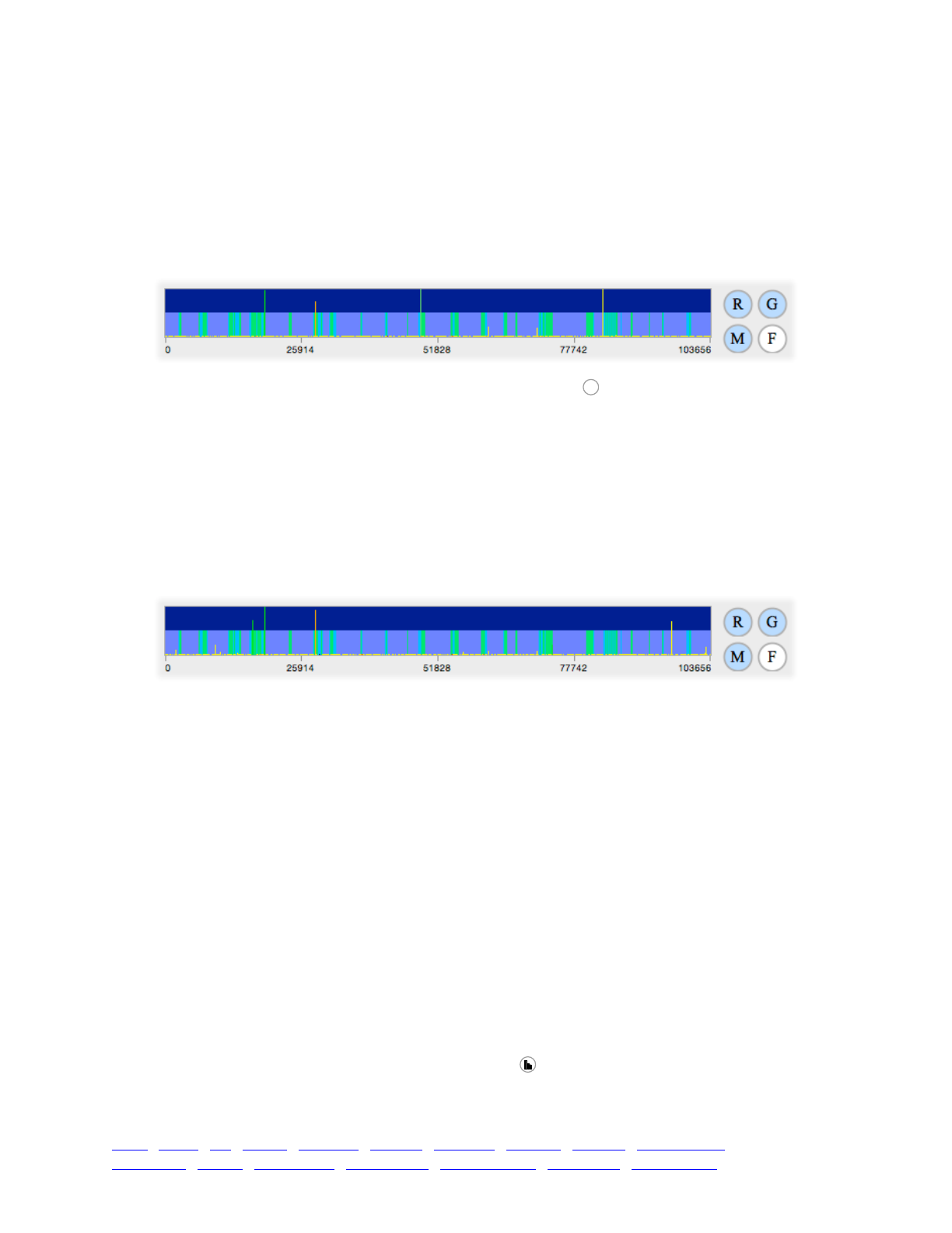
8. SLiMgui visualizations for polymorphism patterns
The previous chapter developed a model of evolutionary dynamics in a scenario involving
neutral, deleterious, and beneficial mutations. Given the full recipe from section 7.3 (not 7.4) of
the previous chapter, we will look briefly in this chapter at the interplay of selection, drift, and
hitchhiking when it executes, since it’s the most complex model we’ve made thus far.
First of all, if you Recycle and Play, you should see a fairly complicated dance of mutations,
some fixing quickly, others struggling, but most flickering in and out of existence quickly:
Notice that display of rate maps has been turned on with the button; otherwise, the genomic
elements display spans the full view height and makes it hard to see mutations that are at high
frequency. Notice also that the mutation lines are distinct colors; neutral mutations are yellow,
beneficial are green, and deleterious are orange or sometimes even red. You might need to play
with the selection coefficients color scale slider (see section 3.1) to optimize these colors.
A cloud of neutral and deleterious mutations occupies the bottom row of pixels; most mutations
in the model are neutral or deleterious. A few beneficial mutations are visible in green, near 19000
and 48000. A neutral mutation near 83000 and a deleterious mutation near 29000 have been
dragged up to high frequency by the two beneficial mutations they are linked to, both of which are
about to fix. A few dozen generations later, this is the situation:
The beneficial mutation near 48000 has fixed, and is thus no longer displayed. The one near
19000 has not yet fixed, but a new beneficial mutation has arisen near 17000 on top of both the
beneficial mutation near 48000 and the deleterious mutation near 29000. With that added selective
pressure, the deleterious mutation has risen near fixation. After another couple of dozen
generations, however, recombination produced a new variant containing the beneficial mutation
without the deleterious mutation. That variant rose very quickly, fixing the beneficial mutation
while leaving the deleterious mutation at a frequency of only ~0.5. It then dropped and was lost
fairly quickly, no longer having the benefit of its linked companions. In this model it is fairly rare
for a deleterious mutation to make it all the way to fixation, although it does occasionally happen.
As the simulation is running, you can watch the colors of the individuals, shown in the top
center view, to see the mix of different fitnesses present. As a beneficial mutation sweeps, more
and more individuals will turn green (if the fitness color scale slider is set appropriately); once the
mutation fixes, they will suddenly revert toward yellow, since the fitness benefit of that mutation is
no longer part of SLiM’s fitness calculations.
8.1 Mutation frequency spectra
SLiMgui has a number of graphs it can display to help analyze and understand the simulation.
While running this recipe, for example, if you click the button and select “Graph Mutation
Frequency Spectrum” you should see something like this:
R
TOC I TOC II WF nonWF initialize() Genome Individual Mutation SLiMSim Subpopulation!
Eidos events fitness() mateChoice() modifyChild() recombination() interaction() reproduction() 114
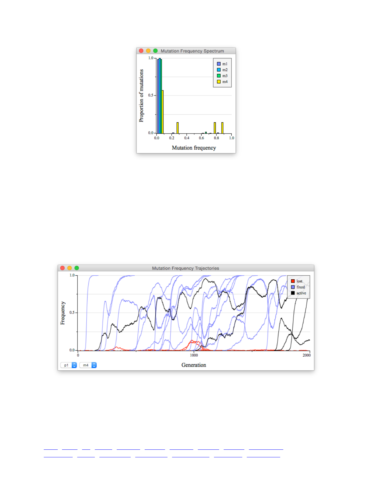
Remember that m1 and m2 are neutral, m3 is deleterious, and m4 is beneficial. What this plot tells
us is that out of all mutations that are of type m1, for example, the vast majority are at very low
frequency; the same is true of m2 and m3. Out of all mutations that are of type m4, however – the
beneficial mutations – a fairly large proportion are at middle or high frequency, because they are
on their way to fixation.
8.2 Mutation frequency trajectories
The next graph in SLiMgui’s graph menu is “Graph Mutation Frequency Trajectories”. Whereas
the previous graph showed us only an analysis of the frequencies of different mutation types at the
present moment in time (try opening it while the simulation is actually playing), this graph shows
us similar information across the whole run of the model so far:
Using the popups at the lower left of the window, you can select a particular subpopulation and
mutation type. The data collected for this graph can be quite large, and quite slow to collect. For
this reason, the data are not normally collected when you run a model; doing so would slow SLiM
down too much. Instead, the data are collected only when the graph window is open, and only
for the subpopulation and mutation type chosen. If you want a plot for an entire simulation run, as
shown above, you should therefore (1) Recycle, (2) Step once to advance to generation 1, (3) open
TOC I TOC II WF nonWF initialize() Genome Individual Mutation SLiMSim Subpopulation!
Eidos events fitness() mateChoice() modifyChild() recombination() interaction() reproduction() 115
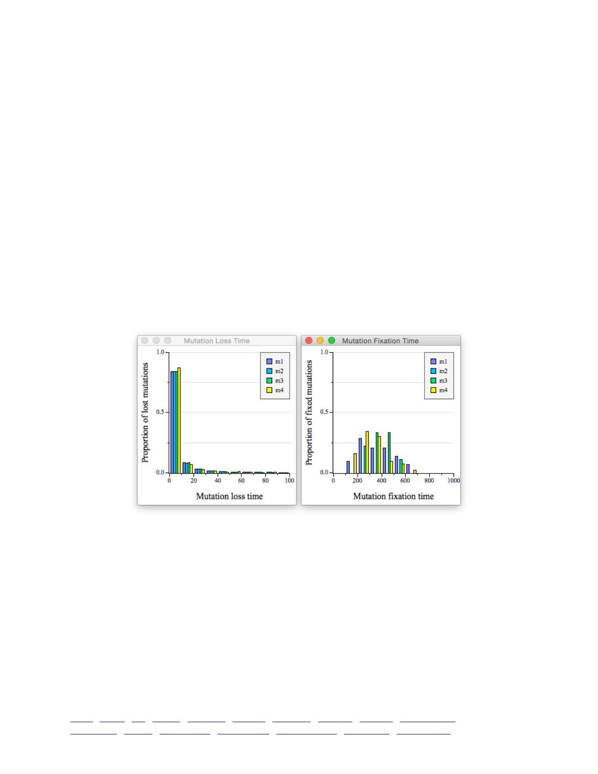
the graph window, (4) select the mutation type you want from the popup, and (5) press Play to run
your simulation with data collection.
The result at the end of a simulation run might look something like the graph shown above. The
complete trajectory of every mutation of the selected mutation type in the selected subpopulation
is shown with an individual curve in this plot; here we’re looking at beneficial mutations (type m4),
and there is only one subpopulation. The color of each curve indicates whether the mutation was
lost (red), fixed (blue), or is still segregating (black).
SLiMgui provides various options to configure the visual appearance of plots. If you control-
click or right-click on the graph window here, for example, you will get a context menu with
menu items that allow you to show/hide grid lines, show/hide the legend, and so forth. If you’re
following along in SLiMgui, try experimenting with these options; you can’t do any harm. SLiMgui
graph windows also make their data available to you, if you want to regenerate them or perform
further analysis; from the context menu, just select “Copy Data” to copy the underlying data for the
plot to the clipboard, or “Export Data...” to export the data to a text file readable by other programs
such as R. The format of the data should be pretty self-explanatory.
8.3 Times to fixation and loss
Next let’s look at the plots for “Graph Mutation Loss Time Histogram” and “Graph Mutation
Fixation Time Histogram”, side by side:
These plots show an analysis of metrics gathered over the course of the entire run. The loss time
plot, on the left, shows the distribution of loss times, in generations, for each of the four mutation
types. The loss profile for all four types is quite similar. Remember that this is not saying that
beneficial mutations are just as likely to be lost as deleterious mutations, but only that when a
beneficial mutation is lost, the amount of time it takes to be lost is similar to the amount of time it
takes a deleterious mutation to be lost. In other words, this plot is conditional upon mutations
being lost; it implies nothing about the likelihood of loss.
The fixation time plot, on the right, similarly shows the distribution of fixation times, in
generations, for each of the four mutation types (conditional, similarly, upon the mutations having
fixed).
TOC I TOC II WF nonWF initialize() Genome Individual Mutation SLiMSim Subpopulation!
Eidos events fitness() mateChoice() modifyChild() recombination() interaction() reproduction() 116
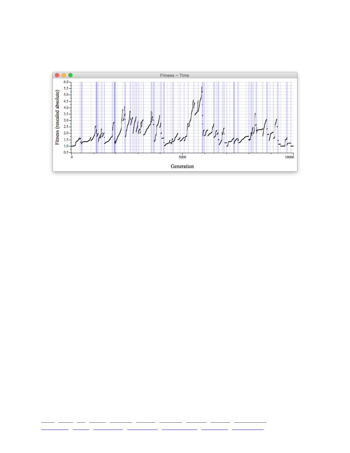
8.4 Population fitness over time
The next graph we will examine is “Graph Fitness ~ Time”. At the end of a run of this recipe, it
might look something like this:
This plot shows the fitness of the population over time. More specifically it shows mean
absolute fitness, and (following the SLiM engine) it rescales whenever a mutation fixes, dropping
the fixed mutation from the calculation. Without that rescaling, the plot would be nearly a
monotonically rising curve; with the rescaling, a drop in the curve occurs each time that a
beneficial mutation fixes (shown in blue). In fact neutral and deleterious mutations that fix are also
shown with a blue line in this plot, but since, in this model, they almost always fix at the same
time as a beneficial mutation, there are only a few fixation events in the plot that do not
correspond to a drop in mean fitness due to a rescaling.
A few things can be observed in this plot. First of all, a bunch of mutations fixed over 10000
generations; the probability of beneficial mutations is probably much higher than the typical
empirical rate. For the same reason, the strong-selection-weak-mutation assumption emphatically
does not hold here; beneficial mutations are stacking up and competing with each other, as can be
seen from both the complex wiggling of the curve in between fixation events, and from the fact
that fixation events usually do not drop the mean fitness back down to 1.0 (indicating that at least
one other beneficial mutation exists at intermediate frequency in the population at the same time).
We have seen the “Graph Population Visualization” plot before, and since there is no
population structure in this recipe it is not interesting here; so this concludes our tour of SLiMgui’s
graphing facilities. If you want to graph other things, you can of course generate an output file
with the data you need, read the data into R, and generate your plots there. Also, don’t forget that
you can copy SLiMgui’s graphs to the clipboard, or save them out as PDF files, using the “Copy
Graph” and “Export Graph...” context menu commands.
TOC I TOC II WF nonWF initialize() Genome Individual Mutation SLiMSim Subpopulation!
Eidos events fitness() mateChoice() modifyChild() recombination() interaction() reproduction() 117

9. Context-dependent selection using fitness() callbacks
In this and following chapters, we will show how Eidos callbacks can be used to modify SLiM’s
standard behavior. You have seen one Eidos callback already, initialize() callbacks that are
called by SLiM at initialization time to modify the default initialization behavior (which sets up
only the SLiMSim object). At least one initialize() callback in required, since SLiM’s default
initialization is insufficient to produce a working simulation. Other Eidos callbacks are optional,
because SLiM’s default behavior is sufficient. In this chapter we will look at one particular Eidos
callback, the fitness() callback, used to modify how SLiM calculates the fitness of an individual
as a function of the mutations present in this individual and potentially other simulation state.
There are just a few conceptual points to discuss before the first recipe. First of all, fitness()
callbacks return a relative fitness value for a focal mutation in a focal individual. Neutrality is
indicated by a relative fitness of 1.0; fitness uses a different scale than selection coefficients, for
which 0.0 indicates neutrality. A fitness() callback is called once for each mutation possessed
by each individual; the callback can therefore assign a different fitness value to the same mutation
depending upon the focal individual possessing the mutation. If a given individual is homozygous
for a mutation, the fitness() callback is still called only once; a flag provided to the callback
indicates whether the focal mutation is homozygous or heterozygous in the focal individual. This
is because fitness() callbacks return a relative fitness rather than a selection coefficient: they take
all of the information regarding the focal mutation in the focal individual – selection coefficient,
dominance coefficient, homozygosity versus heterozygosity, genetic background, subpopulation,
sex, etc. – and condense all of it into a determination of the fitness effect of the focal mutation.
Each mutation in the focal individual is evaluated separately – by one or more fitness() callbacks
if any apply, otherwise by SLiM’s standard fitness equation – to produce a set of relative fitness
values, one for each mutation. SLiM then multiplies these relative fitness values to determine the
fitness of the individual. This process is repeated for each individual in the simulation. This is just
a quick summary; see sections 19.6, 20.3, and 22.2 for a fuller explanation.
9.1 Temporally varying selection
One way to model temporally varying selection in SLiM is to use the setSelectionCoeff()
method of Mutation; you can find the mutation(s) whose selection coefficient you want to change,
and then use that method to make the change at a specific point in time. However, there are
several disadvantages to this approach in general. First of all, the change is permanent; it would be
difficult to later restore the original selection coefficient (if the modified selection regime ends, for
example). Second, each mutation that you wish to modify must be changed individually. (To be
fair, there are also advantages to this method; the change is done once and then is finished with,
and subsequently you pay no speed penalty whatsoever for the change.)
Here we will examine another possible solution to this problem, using a fitness() callback:
initialize() {!
initializeMutationRate(1e-7);!
initializeMutationType("m1", 0.5, "f", 0.0); // neutral!
initializeMutationType("m2", 0.5, "f", 0.1); // beneficial!
initializeGenomicElementType("g1", c(m1,m2), c(0.995,0.005));!
initializeGenomicElement(g1, 0, 99999);!
initializeRecombinationRate(1e-8);!
}!
1 { sim.addSubpop("p1", 500); }!
2000:3999 fitness(m2) { return 1.0; }!
10000 { sim.simulationFinished(); }
TOC I TOC II WF nonWF initialize() Genome Individual Mutation SLiMSim Subpopulation!
Eidos events fitness() mateChoice() modifyChild() recombination() interaction() reproduction() 118

The initialize() callback sets up two mutation types: a very common neutral mutation type
(m1), and an uncommon beneficial mutation type (m2). This produces distinctive simulation
dynamics in which occasional beneficial mutations arise and sweep quickly.
However, from generation 2000 to 3999, the simulation switches to pure neutral dynamics,
because mutation type m2 reverts to neutrality for that period of time due to the fitness() callback
that is defined. This change in dynamics can be seen quite clearly in SLiMgui if you Recycle and
then Play. Let’s look at the callback in more detail:
2000:3999 fitness(m2) { return 1.0; }
The generation range used, 2000:3999, is expressed in the usual syntax. Following that comes
the declaration that this block is a fitness() callback, rather than an ordinary Eidos event:
fitness(m2). A fitness() callback must be declared as applying to one specific mutation type –
in this case, m2; the callback modifies the fitness effect only of mutations belonging to that
mutation type. (This is both for conceptual clarity and for efficiency.) The rest of the callback
definition is a compound statement that returns a float value, used by SLiM as the fitness effect of
the mutation. Here the value 1.0 is returned, which represents neutrality. (Remember that a
neutral mutation has a selection coefficient of 0.0 but a multiplicative fitness effect of 1.0). This is
the first time we have seen the Eidos keyword return; it simply causes the executing script block
to return immediately, passing its (optional) value out to the caller of the block, which in this case
is the SLiM engine itself. It can be used in Eidos events too, although any value returned will not
be used for anything.
This recipe is trivially simple, but of course the code in a fitness() callback can do anything,
so the potential power of this mechanism should be apparent. In the context of temporally varying
selection, you could make the fitness effect vary sinusoidally through time using an expression
based on sin(sim.generation), or make it be random in each generation with rnorm(), or any
other effect you wish.
9.2 Spatially varying selection
The previous example showed a simple recipe implementing temporally varying selection. In
this section we will see how to make selection vary spatially between subpopulations. More
specifically, we will examine a model in which mutations have beneficial effects in one
subpopulation, but deleterious effects in another subpopulation. Whether such mutations fix or
not depends on the strength of the fitness effects, the migration rates between the subpopulations,
and various other factors. The recipe:
initialize() {!
initializeMutationRate(1e-7);!
initializeMutationType("m1", 0.5, "f", 0.0); // neutral!
initializeMutationType("m2", 0.5, "e", 0.1); // deleterious in p2!
initializeGenomicElementType("g1", c(m1,m2), c(0.99,0.01));!
initializeGenomicElement(g1, 0, 99999);!
initializeRecombinationRate(1e-8);!
}!
1 {!
sim.addSubpop("p1", 500);!
sim.addSubpop("p2", 500);!
p1.setMigrationRates(p2, 0.1); // weak migration p2 -> p1!
p2.setMigrationRates(p1, 0.5); // strong migration p1 -> p2!
}!
fitness(m2, p2) { return 1/relFitness; }!
10000 { sim.simulationFinished(); }
TOC I TOC II WF nonWF initialize() Genome Individual Mutation SLiMSim Subpopulation!
Eidos events fitness() mateChoice() modifyChild() recombination() interaction() reproduction() 119

Here we set up two subpopulations of equal size, with weak migration from p2 to p1, but with
strong migration from p1 to p2 (remember that you can use the population visualization graph in
SLiMgui to see a graphical depiction of the population structure, after you Recycle and then Step
through the setup). Mutations are mostly neutral, but occasionally beneficial mutations are drawn
from an exponential distribution with mean 0.1. This is all review; the interesting part is the
fitness() callback:
fitness(m2, p2) { return 1/relFitness; }
Here no generation range is specified; this fitness() callback is therefore active in every
generation. Subpopulation p2 is given as a parameter to the callback definition; this restricts the
operation of the callback to only the specified subpopulation, producing spatial variation in
selection. The body of the callback returns 1/relFitness as the modified fitness effect of each m2
mutation.
We haven’t seen relFitness before; it is a variable defined by SLiM when a fitness() callback
is called, and it contains the fitness value that SLiM would normally use for the mutation. By
returning 1/relFitness, we are telling SLiM to invert the normal fitness effect of all m2 mutations
in p2; if they are of high fitness in p1 (2.0, say) they become low fitness in p2 (1/2.0 == 0.5), and
vice versa.
There is a point worth clarifying here. Mutation type m2 draws selection coefficients from an
exponential DFE; each mutation of type m2 is thus unique. Because of this, the fitness() callback
here is not called just once per generation, to calculate a modified fitness effect for all mutations of
type m2; it is called once per individual per m2 mutation, and it calculates a modified fitness effect
for that mutation in that individual. These calculations can therefore depend upon both the
specific mutation and the specific individual. In addition to the relFitness variable that contains
the default relative fitness effect for the mutation, SLiM also defines mut, the mutation being
assessed; subpop, the subpopulation containing the individual possessing the mutation;
homozygous, a flag which is true if the individual is homozygous for the mutation, false otherwise;
and a few others as well that we will see in the next sections. The code in a fitness() callback
can use all of these variables to calculate its modified fitness effect.
Because fitness() callbacks might be called thousands or even millions of times every
generation, SLiM and Eidos are highly optimized to make those calls as fast as possible. You
should do your part by making your Eidos code as tight as possible; writing an inefficient
fitness() callback is an excellent way to make your simulation slow to a crawl. See section 18.1
for some tips on how to write fast Eidos code.
If you paste this recipe into SLiMgui, Recycle, and Play, you will see the spatial dynamics very
clearly; mutations will spread that are beneficial in p1, turning that subpopulation’s individuals
green, but deleterious in p2, turning that subpopulation’s individuals red. With the recipe as
written, these mutations will often fix; the strong migration from p1 versus the weak migration from
p2 gives p1 an advantage, allowing it to force p2 to fix mutations that are deleterious in that
context. If you reverse the migration bias, that will no longer happen; instead p2 will be able to
force p1 to lose mutations that are beneficial in that context. One could easily use this model to
explore this scenario in detail, with questions such as the effect of subpopulation size, migration
rate, selection strength, and so forth. Since neutral mutations are also in the model, one could also
ask questions about how these sorts of dynamics affect neutral diversity and divergence. Not bad
for sixteen lines of code!
TOC I TOC II WF nonWF initialize() Genome Individual Mutation SLiMSim Subpopulation!
Eidos events fitness() mateChoice() modifyChild() recombination() interaction() reproduction() 120

9.3 Fitness as a function of genomic background
9.3.1 Epistasis
The fitness() callback mechanism can also make the fitness effect of a mutation depend upon
the genetic background of the individual that possesses the mutation. One example of this is
epistasis, in which two loci interact to produce a non-additive fitness effect (Philipps 2008). The
recipe here is a bit contrived – a more realistic model would probably use introduced epistatic
mutations rather than random mutations – but it serves to illustrate the concept:
initialize() {!
initializeMutationRate(1e-8);!
initializeMutationType("m1", 0.5, "f", 0.0); // neutral!
initializeMutationType("m2", 0.5, "f", 0.1); // epistatic mut 1!
initializeMutationType("m3", 0.5, "f", 0.1); // epistatic mut 2!
initializeGenomicElementType("g1", m1, 1);!
initializeGenomicElementType("g2", m2, 1); // epistatic locus 1!
initializeGenomicElementType("g3", m3, 1); // epistatic locus 2!
initializeGenomicElement(g1, 0, 10000);!
initializeGenomicElement(g2, 10001, 13000);!
initializeGenomicElement(g1, 13001, 70000);!
initializeGenomicElement(g3, 70001, 73000);!
initializeGenomicElement(g1, 73001, 99999);!
initializeRecombinationRate(1e-8);!
}!
1 { sim.addSubpop("p1", 500); }!
10000 { sim.simulationFinished(); }!
fitness(m3) {!
if (genome1.countOfMutationsOfType(m2))!
return 0.5;!
else if (genome2.countOfMutationsOfType(m2))!
return 0.5;!
else!
return relFitness;!
}
The initialize() callback sets the stage by making three mutation types, three genomic
element types, and five genomic elements. Over the majority of the chromosome, genomic
element type g1 is used; it generates only neutral mutations. In a locus spanning 10001:13000,
genomic element type g2 is used, which generates mutations of type m2, which are beneficial with
a selection coefficient of 0.1. In a second locus spanning 70001:73000, genomic element type g3
is used, which generates mutations of type m3, which are also beneficial. If you turn on display of
genomic elements in SLiMgui, the resulting setup looks like this:
The twist, however, comes in the fitness() callback, which makes mutations of types m2 and
m3 interact epistatically. Any mutation of type m3 has a fitness effect of 0.5 – strongly deleterious –
if it is found in the same genome as any mutation of type m2. This is achieved in several steps.
First of all, genome1 and genome2 are defined by SLiM for fitness() callbacks; they are the two
TOC I TOC II WF nonWF initialize() Genome Individual Mutation SLiMSim Subpopulation!
Eidos events fitness() mateChoice() modifyChild() recombination() interaction() reproduction() 121
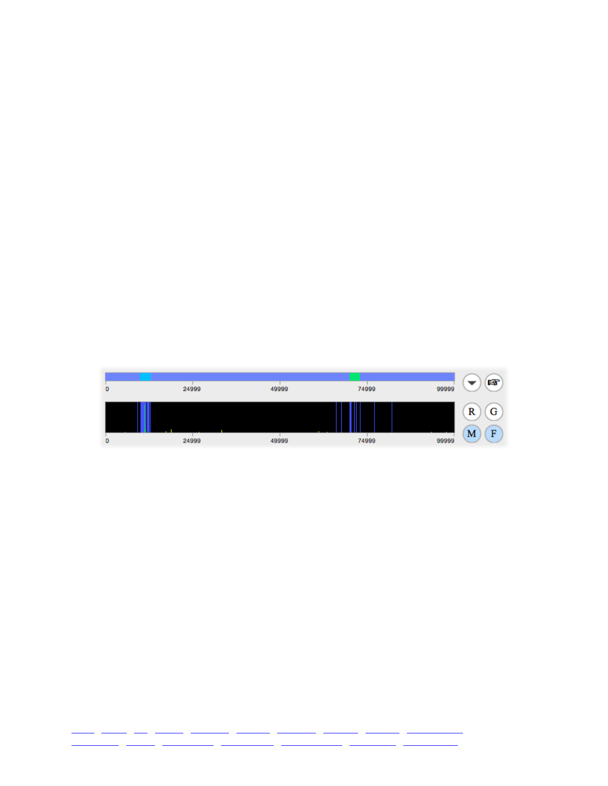
genomes (the two homologous chromosomes) of the individual carrying the mutation that is being
evaluated. The call genome1.countOfMutationsOfType() method counts the mutations of type m2
in the first genome; if that count is non-zero, the if statement evaluates it as true (T), and 0.5 is
returned, making the focal mutation deleterious. The next two lines perform the same check for
genome2 (these two if conditions could be combined into a single test using the “logical or”
operator, |, but the line of code would then be too long to fit without wrapping here). If neither
Genome object contains a mutation of type m2, the final else clause will execute and relFitness
will be returned, keeping the normal fitness effect of the focal mutation without modification.
There are some new concepts here, and this manual is not going to explain them all in detail; for
full discussions of the logical type, the behavior of true and false values in Eidos, and so forth,
please refer to the Eidos manual, which explains these ideas thoroughly.
Note that mutations of type m2 suffer no fitness penalty from sharing an individual with an m3
mutation; the fitness() callback affects only m3 mutations. Since the fitness of the carrying
individual will be severely compromised, however, the net effect is that m2 and m3 mutations are
rarely found together; collocation effectively harms m2 mutations just as much as m3 mutations.
This produces some interesting dynamics. Type m2 and m3 mutations arise fairly often, and
quickly sweep to fixation; however, they never sweep together, so if a mutation at one of the two
epistatic loci is sweeping, the other locus will have no active mutations. The two loci thus “take
turns” sweeping new mutations to fixation. Since new beneficial loci sweep so often, neutral loci
generally fix only if they are linked to a beneficial mutation. Because of recombination, that is
most likely to happen close to one of the two epistatic loci, so if we run the full simulation and
then turn on display of fixed mutations, we see a pattern of clustering near the epistatic loci:
All of the fixed mutations within the loci are beneficial epistatic mutations, since the two loci
generate only those mutation types. All of the bands for fixed mutations outside of those loci,
however, are for neutral mutations that hitchhiked.
The astute reader will have noticed a problem with all this. Biologically, this dynamic of
“taking turns” sweeping at one or the other locus makes no sense. If a mutation of type m2 sweeps
to fixation at the g2 locus, that mutation still exists in the genome, and the epistatic interaction
between m2 and m3 mutations should prevent an m3 mutation from sweeping, forever after. That
objection is correct, and points out a very important issue.
The reason that this recipe behaves in this manner has to do with the way that SLiM handles
fixed mutations (see section 19.3). When a mutation fixes, SLiM normally removes it from the
simulation, replacing it with a Substitution object that provides a permanent record of the fixed
mutation. The assumption is that since every individual possesses the fixed mutation, it has the
same fitness effect in every individual, and therefore can be ignored. However, epistasis violates
that assumption, since the fixed mutation causes a differential fitness effect among individuals
based upon the genetic background in which it is found. SLiM’s replacement of fixed m2 and m3
mutations in this model thus produces incorrect behavior that does not accurately model epistasis.
What to do? Happily, SLiM provides a way to handle this situation. The MutationType class has
a logical property named convertToSubstitution; by default it is T, indicating to SLiM that fixed
mutations of that type should be replaced by Substitution objects. We can set it to F instead,
TOC I TOC II WF nonWF initialize() Genome Individual Mutation SLiMSim Subpopulation!
Eidos events fitness() mateChoice() modifyChild() recombination() interaction() reproduction() 122

telling SLiM to keep all mutations of that type active in the simulation even once fixed. (See
sections 18.3 and 20.9.1 for further discussion of this property). The new recipe:
initialize() {!
initializeMutationRate(1e-8);!
initializeMutationType("m1", 0.5, "f", 0.0); // neutral!
initializeMutationType("m2", 0.5, "f", 0.1); // epistatic mut 1!
m2.convertToSubstitution = F;!
initializeMutationType("m3", 0.5, "f", 0.1); // epistatic mut 2!
m3.convertToSubstitution = F;!
initializeGenomicElementType("g1", m1, 1);!
initializeGenomicElementType("g2", m2, 1); // epistatic locus 1!
initializeGenomicElementType("g3", m3, 1); // epistatic locus 2!
initializeGenomicElement(g1, 0, 10000);!
initializeGenomicElement(g2, 10001, 13000);!
initializeGenomicElement(g1, 13001, 70000);!
initializeGenomicElement(g3, 70001, 73000);!
initializeGenomicElement(g1, 73001, 99999);!
initializeRecombinationRate(1e-8);!
}!
1 { sim.addSubpop("p1", 500); }!
10000 { sim.simulationFinished(); }!
fitness(m3) {!
if (genome1.countOfMutationsOfType(m2))!
return 0.5;!
else if (genome2.countOfMutationsOfType(m2))!
return 0.5;!
else!
return relFitness;!
}
This will now produce the correct epistatic dynamics. If you run this model in SLiMgui, you
will see that one or the other epistatic locus wins an initial contest by fixing a mutation. Once that
happens, the other locus will never manage to establish.
The convertToSubstitution property should be used to prevent fixed mutation substitution
whenever the assumption of equal effects in all individuals would be violated, whether by a
fitness() callback introducing a mechanism like epistasis, or by differential effects of the
mutation type on mate choice or other dynamics. SLiM is not able to guess when substitution
should be turned off, so you must keep this caveat in mind. However, also keep in mind that
turning off substitution will make your models run much more slowly.
9.3.2 Polygenic selection
Another way in which the fitness effect of one mutation can depend upon the genetic
background is polygenic selection. As in epistasis, multiple mutations collocated in a single
individual produce a non-additive effect; but whereas epistasis produces an effect on mutations at
locus A based upon the simple presence or absence of mutations at locus B, polygenic selection
produces an overall fitness effect that depends upon how many mutations of a given type exist.
That description contrasts the concept of polygenic selection with epistasis, but technically, it
really is a type of epistasis; the genetic background against which a given mutation is found
influences the fitness effect of that mutation. Given this, we will need to use the
convertToSubstitution property of MutationType to suppress the substitution of the epistatic
mutations, as in the previous example, so that even after they fix they continue to be taken into
account by the fitness calculations of the model.
Here is a recipe for a simple polygenic selection scenario:
TOC I TOC II WF nonWF initialize() Genome Individual Mutation SLiMSim Subpopulation!
Eidos events fitness() mateChoice() modifyChild() recombination() interaction() reproduction() 123
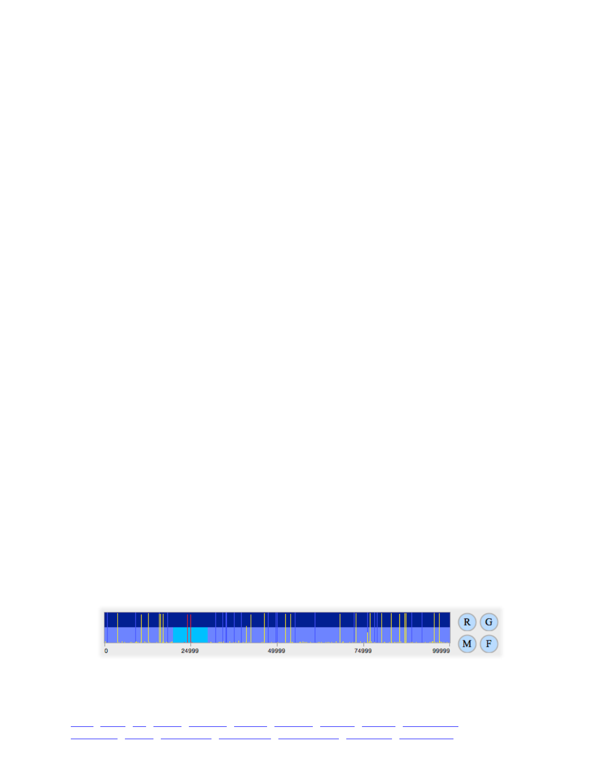
initialize() {!
initializeMutationRate(1e-7);!
initializeMutationType("m1", 0.5, "f", 0.0); // neutral!
initializeMutationType("m2", 0.5, "f", -0.04); // polygenic!
m2.convertToSubstitution = F;!
initializeGenomicElementType("g1", m1, 1);!
initializeGenomicElementType("g2", m2, 1);!
initializeGenomicElement(g1, 0, 20000);!
initializeGenomicElement(g2, 20001, 30000);!
initializeGenomicElement(g1, 30001, 99999);!
initializeRecombinationRate(1e-8);!
}!
1 { sim.addSubpop("p1", 500); }!
1:10000 {!
if (sim.mutationsOfType(m2).size() > 100)!
sim.simulationFinished();!
}!
fitness(m2) {!
count = sum(c(genome1,genome2).countOfMutationsOfType(m2));!
if ((count > 2) & homozygous)!
return 1.0 + count * 0.1;!
else!
return relFitness;!
}
The initialize() callback here sets up a chromosome with a genomic element of type g2 in a
central locus, generating mutations of mutation type m2 that are under polygenic selection; the rest
of the chromosome uses g1 and m1, generating neutral mutations.
The fitness() callback, defined on mutation type m2, sets up the conditions for polygenic
selection. First it counts the total number of mutations of type m2 on both chromosomes of the
focal individual, using the countOfMutationsOfType() method we saw in the previous section, and
assigns that value to count. It does it in a slightly odd way; it first creates an object vector
containing both genomes, with c(genome1,genome2), then calls countOfMutationsOfType() on that
vector to produce a result vector containing two integer values (the counts for genome1 and
genome2, respectively), and then uses sum() to add the two values together to get an overall count.
(You can read more about the mechanics of how this works in the Eidos manual, as usual.) Then, if
count is greater than 2 and the focal mutation is homozygous in the focal individual (using the flag
homozygous that is set by SLiM for fitness() callbacks), a beneficial fitness effect is returned by
1.0 + count * 0.1 (where the 1.0 provides a baseline of neutrality). Otherwise, relFitness is
returned so that the normal (deleterious) fitness effect of the mutation is unchanged.
Running this recipe in SLiMgui shows the expected dynamics: within the locus where polygenic
selection is active, pairs (or more) of mutations drive to fixation simultaneously, because single
mutations on their own are deleterious. Many deleterious mutations flicker in and out of existence
in that locus; when, by chance, one manages to become both homozygous and collocated with
another mutation within the locus, the combination is favorable and they fix together:
Once one pair of these mutations has fixed, all individuals possess a homozygous mutation
(two, in fact) in their genetic background, and so the requirements for further mutations to be
beneficial are greatly relaxed. Individual mutations are then immediately beneficial, through their
TOC I TOC II WF nonWF initialize() Genome Individual Mutation SLiMSim Subpopulation!
Eidos events fitness() mateChoice() modifyChild() recombination() interaction() reproduction() 124
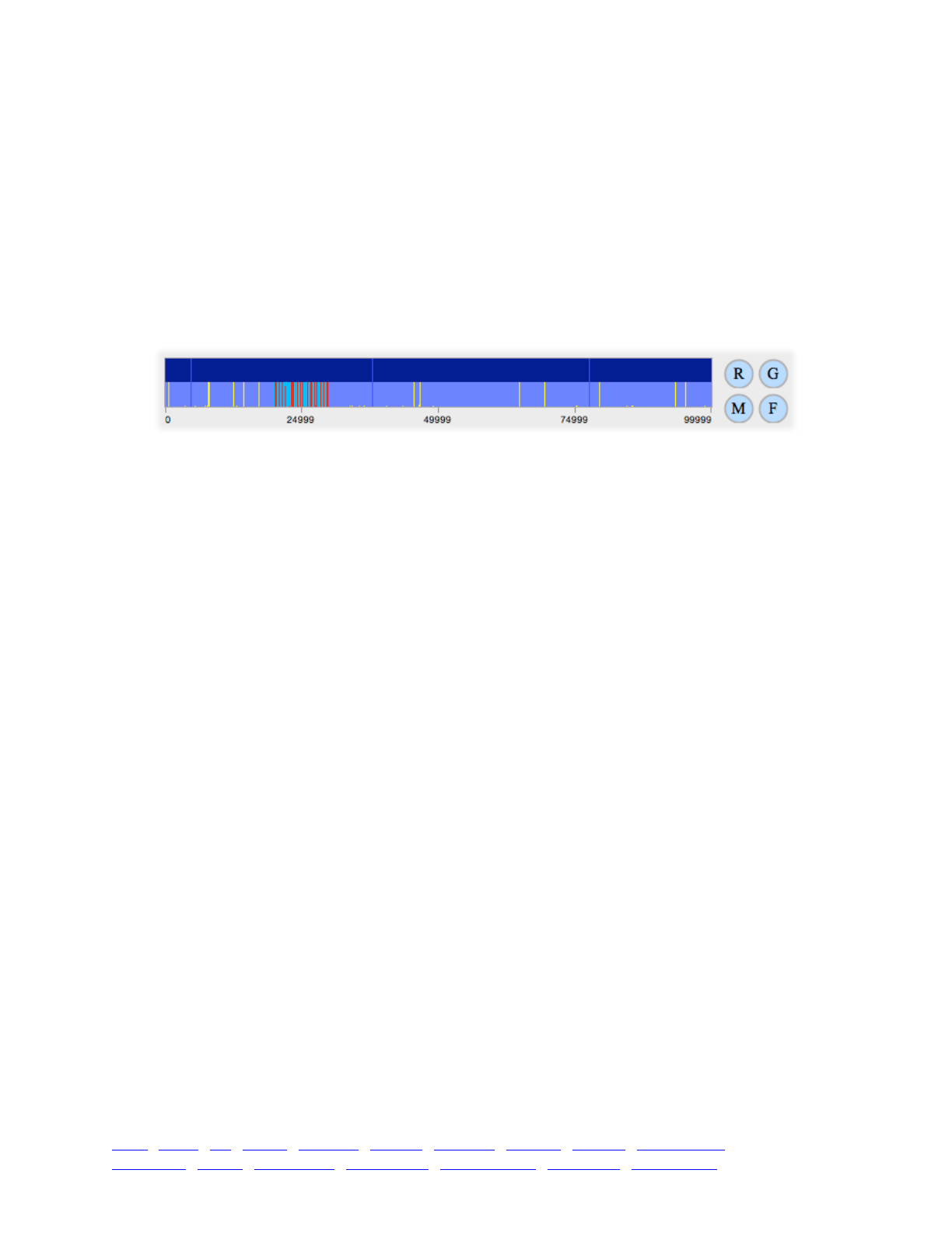
epistatic effect on the fixed mutations, even though their own fitness effect will remain deleterious
until they become homozygous.
Incidentally, the use of homozygous in the fitness() callback here may seem strange; a
mutation only gets the polygenic selection bump-up if it is homozygous in the focal individual.
This is a quick hack to prevent a particular type of dynamics from taking over, in which mutations
of type m2 are prevented from going to fixation because recombination is suppressed.
Recombination gets suppressed because it would break apart linked collections of mutations that
are presently benefiting from the polygenic selection. Without the homozygous requirement, the
highest possible fitness for an individual comes from having completely different sets of mutations
in its two genomes; fixation is therefore blocked. If you delete the “& homozygous” check from the
recipe, you can see the effect of this in SLiMgui:
As in the previous section, models involving polygenic selection in SLiM are likely to involve
introduced mutations, and might thus avoid this issue.
See sections 13.1 and 13.10 for more sophisticated recipes that construct a quantitative trait
based upon the additive effects of multiple loci.
9.4 Fitness as a function of population composition
9.4.1 Frequency-dependent selection
In previous sections we have seen how we can use a fitness() callback to modify the fitness
effects of mutations in order to model scenarios such as epistasis, polygenic selection, and
spatiotemporal variation in selection. Now we will shift to making the fitness of mutations be a
function of population composition. First we’ll look at frequency-dependent selection, in which
the fitness effect of a mutation depends upon the frequency of the mutation in the population
(Ayala & Campbell 1974). Let’s start with a simple recipe for negative frequency-dependence:
initialize() {!
initializeMutationRate(1e-7);!
initializeMutationType("m1", 0.5, "f", 0.0); // neutral!
initializeMutationType("m2", 0.5, "f", 0.1); // balanced!
initializeGenomicElementType("g1", c(m1,m2), c(999,1));!
initializeGenomicElement(g1, 0, 99999);!
initializeRecombinationRate(1e-8);!
}!
1 { sim.addSubpop("p1", 500); }!
10000 { sim.simulationFinished(); }!
fitness(m2) {!
return 1.5 - sim.mutationFrequencies(p1, mut);!
}
The idea here should be pretty clear; if the mutationFrequencies() method tells us that mut is
rare in p1, then the mutation will be highly beneficial, but if it tells us that mut is common, the
mutation will be deleterious. These dynamics prevent the mutation from either fixing or being lost;
instead we have what is called “balancing selection”, in which selection favors keeping mutations
of that type at an intermediate frequency. (See section 9.5 for an adaptation of this recipe using
setSelectionCoeff() instead; and see section 11.3 for a very different model of balancing
TOC I TOC II WF nonWF initialize() Genome Individual Mutation SLiMSim Subpopulation!
Eidos events fitness() mateChoice() modifyChild() recombination() interaction() reproduction() 125

selection, using a modifyChild() callback instead of a fitness() callback.) Running this for a
while in SLiMgui gives us a picture something like this (where the yellow lines are neutral
mutations and the green lines are the mutations under balancing selection):
There are five m2 mutations under balancing selection, all at frequency ~0.5 since that is the
point at which the fitness effect changes from beneficial to deleterious according to the callback.
Next let’s look at a model of positive frequency-dependence:
initialize() {!
initializeMutationRate(1e-7);!
initializeMutationType("m1", 0.5, "f", 0.0); // neutral!
initializeMutationType("m2", 0.5, "f", 0.1); // positive freq. dep.!
initializeGenomicElementType("g1", c(m1,m2), c(999,1));!
initializeGenomicElement(g1, 0, 99999);!
initializeRecombinationRate(1e-8);!
}!
1 { sim.addSubpop("p1", 500); }!
10000 { sim.simulationFinished(); }!
fitness(m2) {!
return 1.0 + sim.mutationFrequencies(p1, mut);!
}
The way this works is probably pretty obvious at this point; at low frequencies (as calculated by
mutationFrequencies()) mutations of type m2 are close to neutral, but at higher frequencies they
become strongly beneficial. Note that these mutations still do not sweep to fixation as quickly as
one might expect. This is because fitness() callbacks get called only once per mutation per
individual. If an individual carries one copy of a mutation (i.e., is a heterozygote), the fitness()
callback is called once. If an individual carries two copies (i.e., is a homozygote), the fitness()
callback is still called only once. Thus, if a fitness() callback does not explicitly consult the
homozygous flag, as described in sections 9.3.2 and 21.2, it will produce an effect of complete
dominance, regardless of the original dominance coefficient set in the mutation type, thereby
hindering fixation. If you wish to model codominance in the above scenario, just include the
homozygous flag in your calculations. In this case, we could alter our recipe in the following way:
initialize() {!
initializeMutationRate(1e-7);!
initializeMutationType("m1", 0.5, "f", 0.0); // neutral!
initializeMutationType("m2", 0.5, "f", 0.1); // positive freq. dep.!
initializeGenomicElementType("g1", c(m1,m2), c(999,1));!
initializeGenomicElement(g1, 0, 99999);!
initializeRecombinationRate(1e-8);!
}!
1 { sim.addSubpop("p1", 500); }!
10000 { sim.simulationFinished(); }!
fitness(m2) {!
dominance = asInteger(homozygous) * 0.5 + 0.5;!
return 1.0 + sim.mutationFrequencies(p1, mut) * dominance;!
}
TOC I TOC II WF nonWF initialize() Genome Individual Mutation SLiMSim Subpopulation!
Eidos events fitness() mateChoice() modifyChild() recombination() interaction() reproduction() 126

9.4.2 Kin selection and inclusive fitness
According to the theory of kin selection and inclusive fitness (Hamilton 1964ab; Dawkins
1976), a mutation that promotes altruism towards kin can spread even if its direct fitness effect on
individuals is negative (because they are devoting energy to behaving altruistically towards related
individuals), if the mutation has indirect benefits (in the form of related individuals behaving
altruistically towards carriers of the mutation). In other words, one cannot look at things solely
from the perspective of the individual; one must look from the perspective of the gene, and see
whether the indirect benefits that accrue to carriers of that gene outweigh the direct costs of
possessing the gene.
This is a little tricky to model directly in SLiM, since all fitness calculations are done from the
perspective of the individual, and since there is no phase of the life cycle in which individuals
interact socially to affect survival probabilities, etc. This kin selection model will therefore look a
bit tautological, because the fitness calculation for an individual just tots up to a net benefit: the
indirect benefit outweighs the direct cost. (But see section 9.4.4 for a much more satisfying
approach.) Nevertheless, we can cook up a recipe that shows the concept by using mutations at
two different loci to serve as the two halves of the inclusive fitness equation:
initialize() {!
initializeMutationRate(1e-7);!
initializeMutationType("m1", 0.5, "f", 0.0); // neutral!
initializeMutationType("m2", 0.5, "f", 0.1); // kin recognition!
m2.convertToSubstitution = F;!
initializeMutationType("m3", 0.5, "f", 0.1); // kin benefit!
m3.convertToSubstitution = F;!
initializeGenomicElementType("g1", m1, 1);!
initializeGenomicElementType("g2", m2, 1);!
initializeGenomicElementType("g3", m3, 1);!
initializeGenomicElement(g1, 0, 10000);!
initializeGenomicElement(g2, 10001, 13000);!
initializeGenomicElement(g1, 13001, 70000);!
initializeGenomicElement(g3, 70001, 73000);!
initializeGenomicElement(g1, 73001, 99999);!
initializeRecombinationRate(1e-8);!
}!
1 { sim.addSubpop("p1", 500); }!
3000 { sim.simulationFinished(); }!
fitness(m2) {!
// count our kin and suffer a fitness cost for altruism!
dominance = asInteger(homozygous) * 0.5 + 0.5;!
return 1.0 - sim.mutationFrequencies(p1, mut) * dominance * 0.1;!
}!
fitness(m3) {!
// count our kin and gain a fitness benefit from them!
m2Muts = individual.uniqueMutationsOfType(m2);!
kinCount = sum(sim.mutationFrequencies(p1, m2Muts));!
return 1.0 + sim.mutationFrequencies(p1, mut) * kinCount;!
}
Here we have a locus spanning 10001:13000 that contains mutations governing kin recognition
(using mutation type m2 in genomic element type g2), and a locus spanning 70001:73000 with
mutations which reap a benefit from having kin (using mutation type m3 in genomic element type
g3). Mutations at the m2 locus are always deleterious; their fitness effect decreases from 1.0,
growing smaller as they become more common (negative frequency-dependence, but without a
TOC I TOC II WF nonWF initialize() Genome Individual Mutation SLiMSim Subpopulation!
Eidos events fitness() mateChoice() modifyChild() recombination() interaction() reproduction() 127

positive fitness effect even at low frequency). This locus represents a facility for kin recognition
and costly altruistic behavior towards kin. By itself, m2 mutations would almost invariably die out.
However, mutations at the m3 locus represent the target of altruism from kin. The fitness()
callback here computes a metric based upon how many other individuals share the focal
individual’s mutations at the kin-recognition locus. Carriers of mutations at the m3 locus (a locus
that attracts altruistic behavior from kin) benefit from these interactions based upon the magnitude
of shared kinship.
If you run this model in SLiMgui, you can see that mutations at the m2 locus sometimes fix,
despite the fact that the direct fitness benefit of those mutations is negative. This does not happen
in isolation; instead, a mutation at the kin recognition locus will rise to fixation at the same time
that an mutation at the benefit locus rises, and the mutation at the benefit locus needs to initiate
the process. Together, however, the mutations at the two loci can rise to fixation.
This model is somewhat unsatisfying from an individual-based perspective – one would like to
see individual interactions in which the altruistic individual suffers without benefit, while the kin
individual gains without cost (see section 9.4.4 for such a recipe) – but the fitness() callback
equations in this recipe essentially encapsulate such interactions on an aggregated level. If you
consider the effects of kin recognition and altruism to be composed of many small acts that can be
averaged over the lifetime of an individual – as is likely to be the case in most empirical systems
involving kin selection – then this approach is actually quite reasonable.
9.4.3 Cultural effects on fitness
Sometimes fitness might be influenced by environmental factors as well as genetic factors. In
some cases, these environmental factors would be associated with the subpopulation in which an
individual resides; in that case, they can be modeled as spatial variation in selection (see section
9.2). In other cases, however, the environmental factors might be a matter of individual variation
that is not correlated with the subpopulation; that possibility is what we will explore in this recipe.
In particular, we will make a simple model of cultural differences between individuals. Each
individual will be assigned to one of two cultural groups at birth. If an individual belongs to one
cultural group, a particular type of mutation will be beneficial; if the individual belongs to the
other cultural group, those mutations will be neutral. An analogue to this in human history, which
we will loosely follow here, would be the allele conferring the ability to digest lactose as an adult;
if an individual belongs to a cultural group that drinks milk in adulthood, mutations promoting the
retention of the lactase enzyme into adulthood are beneficial, whereas if the individual belongs to
a cultural group that does not drink milk in adulthood, such mutations are nearly neutral (or
perhaps slightly deleterious, due to the energetic investment of producing an unneeded enzyme).
For the initial version of this model, the cultural group into which an individual is assigned will
be entirely random. The cultural group of an individual will be tracked using the tag property of
Individual, an integer property that is not used at all by SLiM, and is thus free for you to use as
you wish. We will use a tag value of 1 to indicate a milk-drinker, and a value of 0 to indicate a
non-milk-drinker. The tag value will be set up in a late() event that runs after offspring are
generated but before fitness values are calculated. The recipe:
initialize() {!
initializeMutationRate(1e-7);!
initializeMutationType("m1", 0.5, "f", 0.0); // neutral!
initializeMutationType("m2", 0.5, "f", 0.1); // lactase-promoting!
m2.convertToSubstitution = F;!
initializeGenomicElementType("g1", c(m1,m2), c(0.99,0.01));!
initializeGenomicElement(g1, 0, 99999);!
initializeRecombinationRate(1e-8);!
}!
TOC I TOC II WF nonWF initialize() Genome Individual Mutation SLiMSim Subpopulation!
Eidos events fitness() mateChoice() modifyChild() recombination() interaction() reproduction() 128
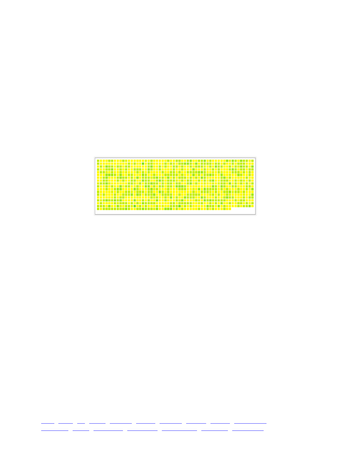
1 { sim.addSubpop("p1", 1000); }!
10000 { sim.simulationFinished(); }!
late() {!
// Assign a cultural group: milk-drinker == 1, non-milk-drinker == 0!
p1.individuals.tag = rbinom(1000, 1, 0.5);!
}!
fitness(m2) {!
if (individual.tag == 0)!
return 1.0; // neutral for non-milk-drinkers!
else!
return relFitness; // beneficial for milk-drinkers!
}
When run, the occasional mutations of type m2 sweep to fixation, as you might expect, but even
when they are close to fixation only about half of the population – the milk-drinkers – are
experiencing a fitness benefit from the mutation. This can be seen easily in the pattern of
individual fitness values displayed in SLiMgui when an m2 mutation was at a frequency of 0.95:
The m2 mutations are prevented from being removed at fixation, by setting the
convertToSubstitution property of m2 to F. As the model runs, m2 mutations accumulate, and the
fitness benefits of being a milk-drinker become larger and larger. Since that status is assigned
randomly, however, this does not affect the frequency of milk-drinking; a randomly chosen half of
the population is less likely to pass on its genes to the next generation, but milk-drinking remains a
random choice.
The late() event assigns cultural tag values to all of the individuals in the new offspring
generation. We first generate 1000 random values, either 0 or 1, using rbinom() to draw from a
simple binomial distribution. The resulting vector is assigned directly into p1.individuals.tag
using the multiplexed assignment semantics of Eidos to put each value in the vector into the tag
property of the corresponding individual in subpopulation p1 (see the Eidos manual for further
discussion of multiplexed assignment).
Given those tag values, the fitness() callback is then trivial: for the lactase-promoting
mutations of type m2, the fitness is neutral if the tag value of a given individual carrying the
mutation is 0, indicating a non-milk-drinker, whereas for milk-drinkers, with a tag value of 1,
relFitness is returned to accept SLiM’s default calculated fitness for the mutation (which uses
both the selection coefficient of 0.1 and the dominance coefficient of 0.5 defined for m2). This
could be modified to make the mutations slightly deleterious in non-milk-drinkers, if one wished,
of course.
In this model, the cultural group of an individual is assigned randomly. In many cases one
would wish this trait to have some degree of heritability, even though it is not genetically based; in
humans and some other species, individuals inherit their culture from their parents through social
learning. To implement that, a modifyChild() callback is needed; we will therefore take this
model up again in section 12.1.
TOC I TOC II WF nonWF initialize() Genome Individual Mutation SLiMSim Subpopulation!
Eidos events fitness() mateChoice() modifyChild() recombination() interaction() reproduction() 129

9.4.4 The green-beard effect
The recipe in section 9.4.2 modeled kin-selection effects by averaging the beneficial and
deleterious effects of altruistic acts across the whole population. That was unsatisfying, because it
looked somewhat tautological; each individual received an average benefit from the existence of
kin in the population (directing altruistic acts toward the individual), and each individual received
an average harm from the existence of kin (by committing costly altruistic acts), and if the average
benefit outweighed the average harm, kin-directed altruism spread because the net effect on every
individual was beneficial. In a large population, with many small altruistic acts occurring between
all kin, that model is actually quite reasonable; but it leaves open the question of whether inclusive
fitness theory is really correct that kin-directed altruism can evolve even when the individuals
committing the altruistic acts (at a cost to themselves) do not necessarily receive a benefit from
altruistic acts by others. In a more individual-oriented model that doesn’t average the benefits and
costs across the whole population, does kin-directed altruism still evolve? Using the tag property
of the Individual class, as shown in the previous section, we can develop a model to answer that
question.
Here we will explore this question in a closely related evolutionary problem, the modeling of
green-beard alleles (Hamilton 1964ab; Dawkins 1976). A green-beard allele causes three
pleiotropic effects: (1) a phenotypic trait of some kind (the “green beard”), (2) the ability to
recognize other individuals possessing this phenotypic trait, and (3) a tendency to direct altruistic
acts toward other individuals possessing this phenotypic trait (at some cost to the altruistic
individual, and some benefit to the receiving individual).
The idea for this recipe is to, in effect, add a new stage to the generation life cycle. In this new
life cycle stage, a finite number of one-on-one interactions between randomly chosen individuals
in the population are modeled. If the individuals both have the green-beard allele, an altruistic act
occurs and one receives a benefit and the other receives a cost; if either individual does not have
the green-beard allele, no altruistic act occurs and the interaction is neutral. The benefits and costs
incurred by each individual are tallied up separately, and are taken into account in a fitness()
callback that models the fitness effect of the green-beard allele for each individual based upon its
particular interaction tally. Some individuals with the green-beard allele will, by chance, incur
nothing but costs from their interactions, harming themselves to the point where they are unlikely
to reproduce. Other individuals with the green-beard allele will, by chance, incur a mixture of
costs and benefits, or if they’re lucky, nothing but benefits; their outcome will thus be neutral or
positive.
Let’s get to the recipe. We’ll build it one step at a time; the first step is just to set up a single
subpopulation with two mutation types:
initialize() {!
initializeMutationRate(1e-7);!
initializeMutationType("m1", 0.5, "f", 0.0); // neutral!
initializeMutationType("m2", 0.5, "f", -0.01); // green-beard!
m2.convertToSubstitution = F;!
initializeGenomicElementType("g1", m1, 1);!
initializeGenomicElement(g1, 0, 99999);!
initializeRecombinationRate(1e-8);!
}!
1 { sim.addSubpop("p1", 500); }!
fitness(m2) { return 1.0; } // neutral!
10000 { sim.simulationFinished(); }
Mutation type m2 will be used for green-beard alleles, but is not used yet. It is set to not convert
into a Substitution object upon fixation, using the convertToSubstitution property of
TOC I TOC II WF nonWF initialize() Genome Individual Mutation SLiMSim Subpopulation!
Eidos events fitness() mateChoice() modifyChild() recombination() interaction() reproduction() 130

MutationType, so that we can easily see whether or not it has fixed at the end of a model run. Its
selection coefficient of -0.01 is just to give it a distinctive color in SLiMgui; the green-beard allele
is neutral here, because the fitness() callback gives a relative fitness of 1.0 for the allele,
overriding selection coefficient of the mutation type. And in any case m2 is not used yet; as it
stands, then, this is just a model of neutral drift using only m1.
Now let’s add a system for tagging individuals with costs and benefits, replacing the fitness()
callback in the code above:
1: late() {!
p1.individuals.tag = 0;!
}!
fitness(m2) { return 1.0 + individual.tag / 10; }
Every individual in SLiM has a tag property that can be set to any value. As explained in the
previous section, the tag field is not used by SLiM; it’s just scratch space for models to use as they
please. In this recipe, we use it to hold the cost/benefit tallies for individuals. The fitness()
callback then adds the tag value for the individual it is evaluating to a neutral relative fitness of
1.0. The tag value is an integer, so we divide it by 10 in the callback; each increment or
decrement of an individual’s tag will represent a change to its relative fitness of 0.1 or -0.1.
Let’s introduce a green-beard allele into the population. It won’t be very interesting if it just gets
lost due to drift in the first generation or two, at green-beard alleles at low frequency generally drift
freely since interactions between the rare green-beards are unlikely – so we’ll introduce several
copies of it to give it an initial boost. The concept of introducing a mutation is covered in depth in
section 10.1, but it should be pretty clear what’s going on here:
1 late() {!
target = sample(p1.genomes, 100);!
target.addNewDrawnMutation(m2, 10000);!
}
This code draws 100 target genomes from the population using the sample() function (which
samples without replacement, by default). It then adds a new mutation of type m2 to those target
genomes with a single call to addNewDrawnMutation(). This call adds the same new mutation to all
of the target genomes, rather than a different new mutation to each genome, because the
addNewDrawnMutation() method is a class method of Genome, not an instance method, and it is
therefore called just once, rather than being multicast out to each instance. This is conceptually
similar to writing a static member function in C++ (which is like a class method in Eidos) to
perform an operation across a vector of objects. That static member function would take a vector
of objects as one of its parameters; in Eidos, you instead call the class method on the target vector,
as seen here, just like calling an instance method. If this is not clear, don’t worry; it is not an
essential point, since the syntax for calling class methods and instance methods is identical in
Eidos. You can consult the Eidos manual for more details on class versus instance methods.
Some individuals might receive two copies of the green-beard mutation (one in each of their
genomes), and end up being homozygous, but there is no harm in that, and most of the individuals
targeted by this code will end up heterozygous for the new green-beard allele. (You could
guarantee heterozygosity by sampling individuals instead of genomes, and then getting just one
genome from each sampled individual; conversely, you could guarantee homozygosity by
sampling individuals and then adding to both of the genomes of each sampled individual.) Again,
it should be emphasized that adding 100 copies is in no way “cheating”; this is just a model of
whether a green-beard allele can rise from low frequency to fixation, rather than a model of
TOC I TOC II WF nonWF initialize() Genome Individual Mutation SLiMSim Subpopulation!
Eidos events fitness() mateChoice() modifyChild() recombination() interaction() reproduction() 131

whether a single copy of a green-beard allele can rise all the way to fixation. It would be easy to
construct the latter model in SLiM using the tools introduced in section 10.2.
Now we need to make our green-beards interact! We’ll do this with an extension to our
previous 1: event:
1: late() {!
p1.individuals.tag = 0;!
!
for (rep in 1:50) {!
individuals = sample(p1.individuals, 2);!
i0 = individuals[0];!
i1 = individuals[1];!
i0greenbeards = i0.countOfMutationsOfType(m2);!
i1greenbeards = i1.countOfMutationsOfType(m2);!
!
if (i0greenbeards & i1greenbeards) {!
alleleSum = i0greenbeards + i1greenbeards;!
i0.tag = i0.tag - alleleSum; // cost to i0!
i1.tag = i1.tag + alleleSum * 2; // benefit to i1!
}!
}!
}
This bears some explaining. First, we zero out all of the individual tag values, as before. Then
we run a loop 50 times, to produce 50 interactions between pairs of individuals (which might or
might not possess green beards). Each time through the loop, we draw two individuals from the
population using sample(), giving us a vector individuals containing two objects of class
Individual which we extract into i0 and i1.
The next two lines count the number of m2 mutations contained in the two genomes belonging
to each individual. The value of i0greenbeards and i1greenbeards, then, is 0 if the corresponding
individual does not have the green-beard mutation at all, 1 if it is heterozygous, or 2 if it is
homozygous. This is equivalent to, but more concise than, writing:
i0greenbeards = i0.genomes[0].countOfMutationsOfType(m2)!
+ i0.genomes[1].countOfMutationsOfType(m2);
(and the same for i1greenbeards).
Next comes an if statement that will execute if both i0greenbeards and i1greenbeards are
non-zero (since in Eidos, as in many languages, 0 is considered false and any non-0 value is
considered true). So this executes if and only if both of the interacting individuals are at least
heterozygous for the green-beard allele. In that case, alleleSum is computed as the total number
of green-beard alleles between the two individuals; this makes the green-beard effect stronger
when homozygotes are involved, weaker when heterozygotes are involved. Finally, the tag values
of the two interacting individuals are modified to reflect the interaction; individual i0 acts
altruistically and incurs a cost, whereas individual i1 receives the altruistic act and gets a benefit.
The costs and benefits are added to the tag value of each individual. Note that the benefit is larger
than the cost; this makes the average fitness effect of the green-beard allele positive, and thus
means that the green-beard allele is selected for, on average, in each generation. But as promised,
the benefit and the cost are incurred by different individuals in this model. Indeed, the altruistic
individual feels a nearly lethal fitness effect, if both interacting individuals are homozygous. From
the perspective of the individual, it is a truly selfless altruistic sacrifice. From the perspective of the
green-beard allele, it is an entirely selfish act, however – which is why the “selfish gene”
perspective has so much explanatory power.
TOC I TOC II WF nonWF initialize() Genome Individual Mutation SLiMSim Subpopulation!
Eidos events fitness() mateChoice() modifyChild() recombination() interaction() reproduction() 132
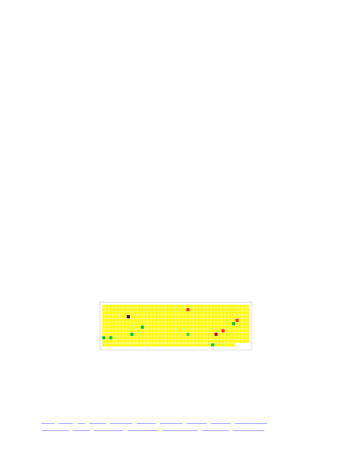
For the record, here is the full recipe for our green-beard model:
initialize() {!
initializeMutationRate(1e-7);!
initializeMutationType("m1", 0.5, "f", 0.0); // neutral!
initializeMutationType("m2", 0.5, "f", -0.01); // green-beard!
m2.convertToSubstitution = F;!
initializeGenomicElementType("g1", m1, 1);!
initializeGenomicElement(g1, 0, 99999);!
initializeRecombinationRate(1e-8);!
}!
1 { sim.addSubpop("p1", 500); }!
1 late() {!
target = sample(p1.genomes, 100);!
target.addNewDrawnMutation(m2, 10000);!
}!
1: late() {!
p1.individuals.tag = 0;!
!
for (rep in 1:50) {!
individuals = sample(p1.individuals, 2);!
i0 = individuals[0];!
i1 = individuals[1];!
i0greenbeards = i0.countOfMutationsOfType(m2);!
i1greenbeards = i1.countOfMutationsOfType(m2);!
!
if (i0greenbeards & i1greenbeards) {!
alleleSum = i0greenbeards + i1greenbeards;!
i0.tag = i0.tag - alleleSum; // cost to i0!
i1.tag = i1.tag + alleleSum * 2; // benefit to i1!
}!
}!
}!
fitness(m2) { return 1.0 + individual.tag / 10; }!
10000 { sim.simulationFinished(); }
If you Recycle and run this recipe in SLiMgui, it may take several tries before the green-beard
mutation “catches” and rises to fixation. Again, this is because its fitness effect is close to neutral
when it is at low frequency; early on, it is quite liable to be lost simply due to drift. Once the
mutation “catches”, though, the population view will show something like this:
This display, of the model when the green-beard allele is at a frequency of around 0.3, shows
the result of the individual interactions between green-beards. Some benefit from those
interactions, and are colored in a shade of green or blue (depending on the magnitude of the
benefit); some are harmed, and are colored in a shade of orange or red, shading down to black
(depending on the magnitude of the harm).
Even once the green-beard mutation has fixed, the majority of individuals will be yellow
(indicating neutrality – a relative fitness of exactly 1.0), because only 50 pairs of individuals are
TOC I TOC II WF nonWF initialize() Genome Individual Mutation SLiMSim Subpopulation!
Eidos events fitness() mateChoice() modifyChild() recombination() interaction() reproduction() 133

chosen to interact in each generation. The larger the number of interactions, relative to the
population size, the stronger the selection will be in favor of the green-beard allele. If you
increase the number of interactions from 50 to 5000, for example, there will be so many
interactions relative to the population size that the green-beard allele will rise to fixation almost
deterministically. In this case, this recipe has approached almost to the realm of the section 9.4.2’s
recipe, where computing averaged effects across the whole population was used to model the
behavior of the system. With only 50 interactions, however, the model is quite stochastic in its
behavior, and the green-beard allele will sometimes be lost even when it has risen as high as a
frequency of 0.5.
This recipe is, from a rather sidelong angle, basically a model of a selective sweep, and as such,
it showed how to introduce a new mutation into a population and watch it sweep to fixation. In
the next chapter, that subject will be treated comprehensively.
9.5 Changing selection coefficients with setSelectionCoeff()
The preceding recipes have demonstrated the use of fitness() callbacks to implement a wide
variety of different types of selection in SLiM. It is worth noting, however, that it is also possible to
simply change the selection coefficient of a mutation using the setSelectionCoeff() method of
Mutation (see section 21.8.2). Indeed, this can have large performance advantages, since
executing Eidos callbacks is relatively slow. However, this strategy can only be applied in very
limited cases.
First of all, if you want the fitness effect of a mutation to vary from individual to individual –
whether because of the genetic background of the individual, or the subpopulation the individual
is in, or any other individual-specific model state – then a fitness() callback is necessary. This is
because changing the selection coefficient of a mutation using setSelectionCoeff() changes that
mutation’s selection coefficient for all individuals, in all subpopulations. The recipes in sections
9.2 (spatially varying selection) and 9.3 (genomic background effects) could therefore not be
implemented using setSelectionCoeff(), nor could those of sections 9.4.3 (cultural effects on
fitness) or 9.4.4 (green-beard alleles).
Second, if you want a fitness effect to be temporary then it is often best to use a fitness()
callback, because when the callback is no longer active mutations will automatically revert to their
original effect. To take the recipe in section 9.1 (temporally varying selection) as an example,
when the callback expires the m2 mutations revert back to their original selection coefficient of 0.1
without needing to be re-set to 0.1; indeed, their selection coefficients are 0.1 the entire time, the
fitness() callback just overrides that with its own effect. If this recipe used setSelectionCoeff()
instead, the original selection coefficients would need to be restored when the altered fitness
regime expired. In this case that would be straightforward – just set them all to 0.1 with another
call to setSelectionCoeff() – but if the m2 mutations were drawn from a distribution of fitness
effects, and thus all had different selection coefficients, this would be more complicated.
The recipes in section 9.4.1, on the other hand, can in fact be improved by rewriting them to
use setSelectionCoeff(). Here is a modified version of the first recipe from that section, which
used a fitness() callback to model a dominant frequency-dependent mutation type:
initialize() {!
initializeMutationRate(1e-7);!
initializeMutationType("m1", 0.5, "f", 0.0); // neutral!
initializeMutationType("m2", 1.0, "f", 0.1); // balanced!
initializeGenomicElementType("g1", c(m1,m2), c(999,1));!
initializeGenomicElement(g1, 0, 99999);!
initializeRecombinationRate(1e-8);!
}!
TOC I TOC II WF nonWF initialize() Genome Individual Mutation SLiMSim Subpopulation!
Eidos events fitness() mateChoice() modifyChild() recombination() interaction() reproduction() 134

1 { sim.addSubpop("p1", 500); }!
late() {!
m2muts = sim.mutationsOfType(m2);!
freqs = sim.mutationFrequencies(NULL, m2muts);!
for (index in seqAlong(m2muts))!
m2muts[index].setSelectionCoeff(0.5 - freqs[index]);!
}!
10000 { sim.simulationFinished(); }
Note that this recipe uses a dominance coefficient of 1.0, to match the behavior caused by the
fitness() callback in the section 9.4.1’s first recipe; any dominance coefficient could be used
here, however. The late() event here calculates the frequency of each m2 mutation, and then uses
a loop to set the selection coefficient of each mutation accordingly. The recipe in section 9.4.1
used a fitness formula of 1.5-frequency in its callback, but here we use 0.5-frequency; this is
because fitness() callbacks return relative fitness values, where 1.0 is neutral, whereas with
selection coefficients – the currency in which the present recipe trades – 0.0 is neutral instead. As
always, this distinction should be treated with care since it is a common cause of errors.
This recipe runs about two orders of magnitude faster than the original recipe – not a small
difference. It might not produce exactly identical results, because of the aggregated effects of tiny
differences in floating-point roundoff error due to the different way in which fitness values are
juggled in the two models, but it is effectively identical for all practical purposes.
However, this recipe’s strategy using setSelectionCoeff() only works because this is a single-
subpopulation model; with multiple subpopulations, one would presumably want the frequency-
dependent effect to be different in each subpopulation, and to depend upon the frequency within
that subpopulation. Such a model could no longer be achieved using setSelectionCoeff().
Section 9.4.1 thus presented a more generally applicable recipe, albeit a slower one.
TOC I TOC II WF nonWF initialize() Genome Individual Mutation SLiMSim Subpopulation!
Eidos events fitness() mateChoice() modifyChild() recombination() interaction() reproduction() 135

10. Selective sweeps
This chapter shows how SLiM can be used to model selective sweeps and various associated
phenomena such as hitchhiking, background selection, and genetic draft. SLiM’s ability to
accurately model such scenarios is the origin of its name, Selection on Linked Mutations. This
chapter will use very simple one-population models; of course these recipes can be combined
with the recipes of previous chapters to model sweeps with complex demography and population
structure, complex genetic architecture, spatiotemporal variation in selection, and so forth.
10.1 Introducing adaptive mutations
The simplest selective sweep scenario is of an explicitly introduced adaptive mutation sweeping
against a background of neutral mutations. We can simulate such a sweep in just a few lines:
initialize() {!
initializeMutationRate(1e-7);!
initializeMutationType("m1", 0.5, "f", 0.0);!
initializeMutationType("m2", 1.0, "f", 0.5); // introduced mutation!
initializeGenomicElementType("g1", m1, 1.0);!
initializeGenomicElement(g1, 0, 99999);!
initializeRecombinationRate(1e-8);!
}!
1 { sim.addSubpop("p1", 500); }!
1000 late() {!
target = sample(p1.genomes, 1);!
target.addNewDrawnMutation(m2, 10000);!
}!
10000 { sim.simulationFinished(); }
The call to initializeMutationType() sets up m2, a new mutation type used to represent the
introduced beneficial mutation. Note that a dominance coefficient of 1.0 (fully dominant) is used
with a selection coefficient of 0.5; these values provide strong selection for the introduced
mutation, making it less likely to be lost due to genetic drift while still at low frequency. This is
useful for illustrative purposes here, but of course in real simulations less favorable values would
likely be needed, making it more probable that the mutation would be lost rather than sweeping.
There are two ways to handle this. One is to simply accept that some runs of the simulation will
fail to sweep – do many runs of the model, and collect statistics only across those runs where the
sweep succeeds. The second way to handle the problem is to write additional Eidos code to make
the simulation run conditional on fixation (see the next section).
The other interesting code here is the Eidos event at generation 1000. The first line of this event
selects a target genome into which the added mutation will be placed. It does this using the
sample() function, by drawing a single sample from subpopulation p1’s vector of genomes. This is
important, because SLiM does not – for reasons of speed – guarantee a random order to the
individuals in a subpopulation. In this simple model all individuals are produced identically, so
this is not an issue, but if features of SLiM are used such as migration, separate sexes, selfing,
cloning, or mateChoice()/modifyChild()/recombination() callbacks, the individuals in the
subpopulation will be produced in a specific and non-random order, and thus whenever a random
individual is desired sample() must be used (rather than just using the genome at index 0 in the
subpopulation, for example).
The second line then adds a new mutation to the target genome, drawn from mutation type m2;
the remaining parameter specifies the position of the mutation in the chromosome as 10000 (this
could be drawn randomly using sample() as well, if desired).
TOC I TOC II WF nonWF initialize() Genome Individual Mutation SLiMSim Subpopulation!
Eidos events fitness() mateChoice() modifyChild() recombination() interaction() reproduction() 136
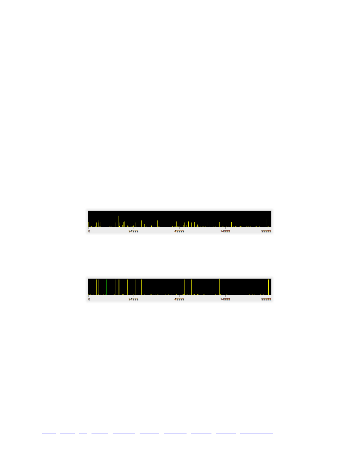
Note that this event is a late() event, specified in its declaration. These were introduced back
in section 4.2.1 as a way to make scripted events happen late in the generation, after offspring
generation has occurred (see the generation life cycle overview in section 1.3). It is important that
introducing new mutations occurs in a late() event, because it makes script-introduced mutations
act in exactly the same way as mutations added by SLiM due to the normal process of mutation
during offspring generation. If this event were an early() event instead (as is the default if no
explicit designation is given), the mutation would be introduced immediately before offspring
generation, and it would have no effect on fitness values since fitnesses would have been
calculated before it was added (at the end of the preceding generation). The mutation would
therefore be subject to one generation of drift before its correct fitness effect would be accounted
for. This would likely not be the desired behavior, so SLiM will issue a warning if you add a
mutation during an early() event – you can delete the late() designation here to see that.
The introduced mutation in this model typically sweeps quite quickly (or is lost almost
immediately due to drift), so perhaps the simplest way to see what is going on in SLiMgui is to
recycle and then enter 1000 in the generation textfield and press return (as illustrated in section
5.1.2). The simulation will advance to the beginning of generation 1000, and you can then press
Step to single-step forward and watch the progress of the introduced mutation. Alternatively, you
could slow down the simulation speed using the speed slider (as illustrated in section 5.2.2) to see
the simulation play more slowly. In either case, you should observe that at generation 1000, just
before the beneficial mutation is introduced, there is lots of neutral diversity across the
chromosome:
But just before the mutation finishes sweeping (assuming it is not lost – you may need to recycle
and repeat this procedure several times to get a run in which the sweep establishes), most of that
diversity has been lost, and just a few neutral sites have hitchhiked along with the introduced
mutation, producing the characteristic signature of a selective sweep (Smith & Haigh 1974):
Note the green line at position 10000, representing the beneficial mutation itself.
We can automatically halt the model immediately after the introduced mutation has fixed (or
has been lost). This requires just a simple modification of the final line of the model, with the call
to simulationFinished():
1000:10000 late() {!
if (sim.countOfMutationsOfType(m2) == 0)!
sim.simulationFinished();!
}
Now simulationFinished() is called immediately when the number of mutations of mutation
type m2 falls to zero, which happens either when the introduced mutation fixes (because SLiM then
converts the mutation into a substitution object), or when it is lost. Note the generation range of
1000:10000 on this event; this means that this termination condition will be checked each
generation from 1000 (when the introduced mutation originates) until 10000 (when the model ends,
TOC I TOC II WF nonWF initialize() Genome Individual Mutation SLiMSim Subpopulation!
Eidos events fitness() mateChoice() modifyChild() recombination() interaction() reproduction() 137

regardless). Also note that a late() designation has been added, so that the simulation ends in the
same generation that the m2 mutation is lost or fixed.
It might be nice to have some indication, in the output stream of the simulation, as to whether
the introduced mutation fixed or was lost. One simple way to do this is to check for a
Substitution object of the right mutation type, in a small extension to the event above:
1000:100000 late() {!
if (sim.countOfMutationsOfType(m2) == 0)!
{!
fixed = (sum(sim.substitutions.mutationType == m2) == 1);!
cat(ifelse(fixed, "FIXED\n", "LOST\n"));!
sim.simulationFinished();!
}!
}
The variable fixed is assigned a logical value that comes from checking the list of substitutions
for elements with mutation type m2. Each match will produce a value of T in the logical vector
that results from the == operator; and since T is equal to 1 in Eidos, whereas F is equal to 0, the
sum() function then adds up the total number of matches. If the sum is 1, the mutation fixed;
otherwise (when it is 0) the mutation was lost.
The next line calls cat() to concatenate a string to the output stream. The string comes from
the ifelse() function, which looks at the logical value of its first parameter (fixed) and returns its
second parameter ("FIXED\n") if that value is T; otherwise, it returns its third parameter ("LOST\n").
This function is based on the ifelse() function of R; it is similar to the “trinary conditional”
operator, ?:, of C and other languages, but ifelse() is a vectorized function and can thus perform
this operation across whole vectors at once – a useful tool. Even when using it with singletons, as
here, it is a compact way to express things that would otherwise require an if–else construct and
other complications, as in the alternative way of coding this output directive:
if (fixed)!
cat("FIXED\n");!
else!
cat("LOST\n");
10.2 Making sweeps conditional on fixation
The recipe in the previous section did not guarantee that the introduced mutation would sweep
to fixation. That is not necessarily a flaw; sometimes one is interested in the outcome of a model
both when a sweep completes and when it does not. Sometimes, however, one wishes to make a
model that guarantees that a sweep completes:
initialize() {!
initializeMutationRate(1e-7);!
initializeMutationType("m1", 0.5, "f", 0.0);!
initializeMutationType("m2", 1.0, "f", 0.5); // introduced mutation!
initializeGenomicElementType("g1", m1, 1.0);!
initializeGenomicElement(g1, 0, 99999);!
initializeRecombinationRate(1e-8);!
}!
1 {!
// save this run's identifier, used to save and restore!
defineConstant("simID", getSeed());!
!
sim.addSubpop("p1", 500);!
}!
TOC I TOC II WF nonWF initialize() Genome Individual Mutation SLiMSim Subpopulation!
Eidos events fitness() mateChoice() modifyChild() recombination() interaction() reproduction() 138

1000 late() {!
// save the state of the simulation!
sim.outputFull("/tmp/slim_" + simID + ".txt");!
!
// introduce the sweep mutation!
target = sample(p1.genomes, 1);!
target.addNewDrawnMutation(m2, 10000);!
}!
1000:100000 late() {!
if (sim.countOfMutationsOfType(m2) == 0)!
{!
fixed = (sum(sim.substitutions.mutationType == m2) == 1);!
!
if (fixed)!
{!
cat(simID + ": FIXED\n");!
sim.simulationFinished();!
}!
else!
{!
cat(simID + ": LOST – RESTARTING\n");!
!
// go back to generation 1000!
sim.readFromPopulationFile("/tmp/slim_" + simID + ".txt");!
!
// start a newly seeded run!
setSeed(rdunif(1, 0, asInteger(2^32) - 1));!
!
// re-introduce the sweep mutation!
target = sample(p1.genomes, 1);!
target.addNewDrawnMutation(m2, 10000);!
}!
}!
}
To make a model that is conditional on fixation, there are some simple “solutions” that don’t
work. You can’t force the introduced mutation to increase in frequency each generation; that
would produce abnormal evolutionary trajectories that would distort the model dynamics.
Similarly, you can’t just reintroduce a new mutation if the previous one is lost; in the process of
getting lost, the previous mutation may have affected the genetic background. What you really
want is that if the introduced mutation has been lost, the simulation gets reset to precisely the
same state as it was in prior to the previous introduction, but with a different random number seed
to ensure that events take a different course. If you do this repeatedly until the mutation fixes, you
have a proper simulation of a selective sweep conditional upon fixation. SLiM provides a
convenient solution for this by allowing the user to save the relevant state of a simulation to disk.
Doing this is actually pretty simple; there are just a few key steps that need to be taken to save the
state and then restore it when we want to try a different trajectory.
First of all, the generation 1 event now stores the initial random number seed, obtained from
getSeed(), as a constant named simID, using the Eidos function defineConstant(). Such
constants persist until the simulation terminates or is recycled; unlike variables, defined constants
do not disappear at the end of the currently executing event in SLiM, but instead go into the global
scope. This value is thus a unique identifier for the model run; if many model runs were being
done, each would presumably have a different seed, and thus the initial seed identifies the run.
The event in generation 1000 saves the current population state to a file in the /tmp directory, a
standard place used in all Un*x systems (including Mac OS X) to store temporary files. The
TOC I TOC II WF nonWF initialize() Genome Individual Mutation SLiMSim Subpopulation!
Eidos events fitness() mateChoice() modifyChild() recombination() interaction() reproduction() 139

filename used inside the /tmp directory is generated using string concatenation with the + operator
(described in detail in the Eidos manual), based on the value stored earlier in simID; the temporary
file therefore gets named according to the initial random number seed of the run, with a name like
"slim_92631.txt". This event also adds the new mutation that we want to sweep. Note that this
event is designated as a late() event; this is logical, both because it produces output (by saving
the simulation state to disk), and because it adds a mutation to the simulation.
The generation 1000:100000 event checks, each generation, whether the introduced mutation is
still present. If it has fixed, it prints a message and terminates the simulation. If it has been lost, it
prints a message and reads the saved population state back in (which sets the generation counter
back to 1000). It then changes the random number seed, to start a new evolutionary trajectory
(reproducible by starting again at the new seed – see section 17.1 for discussion), and then re-
introduces the sweep mutation as before. This event is also a late() event; this way if the
simulation has to be restored to the saved state, it picks up exactly where it was saved out (it
should also be a late() event because it adds a new mutation). Finally, note that when we set the
generation back to 1000, the generation 1000 event that did our initial setup does not execute
again; the events that will run for a given generation are determined at the beginning of that
generation and do not change even if sim.generation is changed. If we set sim.generation to 999
instead, then the generation 1000 event would execute again, in the next generation.
If you recycle and run this model, sometimes the introduced mutation will fix on the first
attempt, but sometimes it will take repeated attempts and you will see output like this:
1452090492983: LOST – RESTARTING!
1452090492983: LOST – RESTARTING!
1452090492983: LOST – RESTARTING!
1452090492983: FIXED
This demonstrates that the model is working as intended; three introduced mutations were lost
before the fourth attempt resulted in fixation. You could change the dominance coefficient and
selection coefficient of m2 to be less favorable, which would result in more restarts but should work
fine. You could even make m2 neutral or deleterious, while still making runs conditional on
fixation; we’ll see an example of that in section 10.6.2. Since the probability of a new neutral
mutation drifting to fixation is small, many restarts will be needed, but no harm is done by that.
One caveat is that outputFull() writes out only a specific set of information: the
subpopulations that exist, the individuals they contain, and the mutations contained by the
genomes of those individuals. When readFromPopulationFile() is called, any other state
associated with the subpopulation, individuals, genomes, and mutations is wiped away. If the
model had set up other properties – setting a cloning rate on a subpopulation, say, or setting up
values with tag or setValue() – that state will be lost, and will need to be set up again.
Given the relative complexity of this recipe, most of the other selective sweep recipes in this
chapter will assume that conditionality on fixation is not desired, so that their different topics are
not obscured by the conditionality machinery. However, the key elements of this recipe can be
combined with any selective sweep strategy – or indeed, can be used to make a simulation that is
conditional upon any outcome you wish. In the next section, we will see how to make a
simulation conditional upon establishment of a mutation, rather than upon fixation.
10.3 Making sweeps conditional on establishment
In the previous section, we saw how to make a model conditional on fixation of the introduced
mutation. Sometimes one may want to relax this condition and require only that the mutation
reaches a certain threshold frequency at which selection outweighs drift, rendering subsequent loss
TOC I TOC II WF nonWF initialize() Genome Individual Mutation SLiMSim Subpopulation!
Eidos events fitness() mateChoice() modifyChild() recombination() interaction() reproduction() 140

unlikely. This threshold frequency is commonly referred to as the establishment frequency, and is a
function of the selection coefficient of the mutation. Making our model conditional on
establishment, rather than fixation, requires just a simple modification to the previous recipe:
initialize() {!
initializeMutationRate(1e-7);!
initializeMutationType("m1", 0.5, "f", 0.0);!
initializeMutationType("m2", 1.0, "f", 0.5); // introduced mutation!
initializeGenomicElementType("g1", m1, 1.0);!
initializeGenomicElement(g1, 0, 99999);!
initializeRecombinationRate(1e-8);!
}!
1 {!
// save this run's identifier, used to save and restore!
defineConstant("simID", getSeed());!
!
sim.addSubpop("p1", 500);!
}!
1000 late() {!
// save the state of the simulation!
sim.outputFull("/tmp/slim_" + simID + ".txt");!
!
// introduce the sweep mutation!
target = sample(p1.genomes, 1);!
target.addNewDrawnMutation(m2, 10000);!
}!
1000: late() {!
mut = sim.mutationsOfType(m2);!
!
if (size(mut) == 1)!
{!
if (sim.mutationFrequencies(NULL, mut) > 0.1)!
{!
cat(simID + ": ESTABLISHED\n");!
sim.deregisterScriptBlock(self);!
}!
}!
else!
{!
cat(simID + ": LOST – RESTARTING\n");!
!
// go back to generation 1000!
sim.readFromPopulationFile("/tmp/slim_" + simID + ".txt");!
!
// start a newly seeded run!
setSeed(rdunif(1, 0, asInteger(2^32) - 1));!
!
// re-introduce the sweep mutation!
target = sample(p1.genomes, 1);!
target.addNewDrawnMutation(m2, 10000);!
}!
}!
10000 {!
sim.simulationFinished();!
}
Much of the machinery here is carried over from the previous recipe; see section 10.2 for
discussion of the way the simulation state is saved and restored. Here, however, the 1000: event
TOC I TOC II WF nonWF initialize() Genome Individual Mutation SLiMSim Subpopulation!
Eidos events fitness() mateChoice() modifyChild() recombination() interaction() reproduction() 141

checks for the existence of the introduced mutation, using size(). If it exists, its frequency is
checked against the threshold frequency 0.1 (an arbitrary choice that can be adjusted to whatever
threshold frequency you wish). If the mutation’s frequency is above that threshold, a message is
printed and the script block deregisters itself so that further checks are not done – once the
mutation has established, the simulation runs freely to its end, whether the mutation is
subsequently fixed or lost. (See section 5.1.2 for discussion of deregisterScriptBlock(), as well
as sections 10.5.3 and 20.11.2). On the other hand, if the introduced mutation no longer exists,
the simulation is reset back to the point of introduction, just as in section 10.2.
When this model is run, you will typically see output like:
1459603349880: LOST – RESTARTING!
1459603349880: LOST – RESTARTING!
1459603349880: LOST – RESTARTING!
1459603349880: ESTABLISHED
10.4 Partial sweeps
Sometimes it is desirable to make a selective sweep stop or change when the sweep mutation
reaches a specific frequency. This recipe will initiate a selective sweep with a beneficial mutation,
which will convert into a neutral mutation when it reaches a frequency of 0.5.
initialize() {!
initializeMutationRate(1e-7);!
initializeMutationType("m1", 0.5, "f", 0.0);!
initializeMutationType("m2", 1.0, "f", 0.5); // introduced mutation!
initializeGenomicElementType("g1", m1, 1.0);!
initializeGenomicElement(g1, 0, 99999);!
initializeRecombinationRate(1e-8);!
}!
1 { sim.addSubpop("p1", 500); }!
1000 late() {!
target = sample(p1.genomes, 1);!
target.addNewDrawnMutation(m2, 10000);!
}!
1000:10000 late() {!
mut = sim.mutationsOfType(m2);!
if (size(mut) == 0)!
sim.simulationFinished();!
else if (mut.selectionCoeff != 0.0)!
if (sim.mutationFrequencies(NULL, mut) >= 0.5)!
mut.setSelectionCoeff(0.0);!
}
Most of this is similar to previous recipes in this chapter; the difference lies in the 1000:10000
event. This event now uses mutationsOfType() to recover the introduced mutation object (which,
as usual, can’t be stored anywhere persistent). If the mutation is no longer present – if size(mut) is
zero – the simulation terminates; this is equivalent to the countOfMutationsOfType(m2) check
done in previous recipes. Otherwise, it uses mutationFrequences() to check the frequency of the
introduced mutation; if it has cleared the 0.5 threshold, it is converted to neutral with
setSelectionCoeff(). That last bit of code is protected by a test that the selection coefficient has
not already been changed; that check is purely for speed, as mutationFrequencies() can be slow.
This recipe could incorporate parts of the previous recipes, in order to determine whether the
introduced mutation was lost or had fixed, or in order to make the simulation conditional on the
mutation reaching the threshold frequency; the basic idea is easily adapted.
TOC I TOC II WF nonWF initialize() Genome Individual Mutation SLiMSim Subpopulation!
Eidos events fitness() mateChoice() modifyChild() recombination() interaction() reproduction() 142

10.5 Soft sweeps from de novo mutations
In the previous recipes in this chapter, we’ve seen “hard” selective sweeps originating from a
single new mutation. If, on the other hand, a sweep proceeds from multiple copies of the same
mutation, present in different individuals, it is termed a “soft” sweep, because it preserves a more
diverse genetic background (Messer & Petrov 2013). Soft sweeps can arise from standing genetic
variation (seen in section 10.6), or can occur when multiple copies of the same de novo mutation
arise during a sweep. This section will model the latter scenario, in three different ways.
10.5.1 A soft sweep from recurrent de novo mutations in a large population
In this recipe, we will model a soft sweep by de novo mutations generated by SLiM. In order to
get a soft sweep to occur from recurrent de novo mutations at the same locus, the population
needs to be very large or the mutation rate needs to be very high, so that new copies of the
mutation tend to arise before the previous copy has fixed. In this recipe, unlike most recipes in
this book, we will not model a background of neutral mutations; instead, this is a model of
competing beneficial mutations at a single site. We are, in effect, modeling the sweep of multiple,
separate instances of a particular single-nucleotide change, such as the transition of a particular
nucleotide from G to A (conceptually – SLiM does not model actual nucleotides). The model
terminates when the sweep completes: when every individual genome possesses an instance of the
mutation, regardless of where and when this instance arose. With no further ado, the recipe:
initialize() {!
initializeMutationRate(1e-5);!
initializeMutationType("m1", 0.45, "f", 0.5); // sweep mutation!
m1.convertToSubstitution = F;!
m1.mutationStackPolicy = "f";!
initializeGenomicElementType("g1", m1, 1.0);!
initializeGenomicElement(g1, 0, 0);!
initializeRecombinationRate(0);!
}!
1 {!
sim.addSubpop("p1", 100000);!
}!
1:10000 {!
counts = p1.genomes.countOfMutationsOfType(m1);!
freq = mean(asInteger(counts > 0));!
!
if (freq == 1.0)!
{!
cat("\nTotal mutations: " + size(sim.mutations) + "\n\n");!
!
for (mut in sortBy(sim.mutations, "originGeneration"))!
{!
mutFreq = mean(asInteger(p1.genomes.containsMutations(mut)));!
cat("Origin " + mut.originGeneration+ ": " + mutFreq + "\n");!
}!
!
sim.simulationFinished();!
}!
}
The chromosome is defined as having a single genomic element that spans from position 0 to
position 0: a single base position. This recipe uses a relatively high mutation rate (1e-5) with a
large population size (100000) so that multiple mutations arise at that single site before the sweep
TOC I TOC II WF nonWF initialize() Genome Individual Mutation SLiMSim Subpopulation!
Eidos events fitness() mateChoice() modifyChild() recombination() interaction() reproduction() 143

completes. An even larger population size could be used with a lower mutation rate (N=1e6 and
u=1e-6, say, or even N=1e7 and u=1e-7), but the model would take somewhat longer to complete.
There is one unusual complication in this model: SLiM, by default, allows multiple mutations of
a given mutation type to occur at the same site in the same individual (“stacked” mutations, as we
will call them). In other words, an individual that has already undergone the G-to-A transition
might nevertheless be given another mutation at the same site, representing the same G-to-A
transition. While this behavior is desirable in many instances, it is inconvenient in this particular
model, and so this recipe tells SLiM to use a different behavior: “stacked” mutations will not be
allowed, and new mutations that collide with an existing mutation at the same site will be
suppressed. This is achieved by setting the mutationStackPolicy property of m1 to "f", which tells
SLiM to prevent stacking by keeping only the first (thus "f") mutation of type m1 at a given site (see
section 21.9.1 for details). This simplifies the model’s code considerably; without this change in
policy, the model would have to carefully take account of the possibility of stacking and
compensate for it. Note that if this model contained other mutation types as well, those would still
be allowed to coexist, both with each other and with an m1 mutation at the same site; only stacking
of m1 mutations with other m1 mutations is prevented (by default; see section 21.9.1).
Second, the dominance coefficient of 0.45 for m1 is actually a special and important value.
SLiM tracks each independent origin of the sweep mutation as a separate Mutation object; those
mutations are all of type m1, but they are distinct mutations as far as SLiM is concerned. If an
individual has different versions of the sweep mutation in its two genomes, SLiM will evaluate the
fitness of that individual according to the fact that it contains two different mutations, each of
which is heterozygous, and each of which therefore uses the mutation type’s dominance
coefficient. The value 0.45 makes this work out, because the relative fitness for one heterozygous
mutation is 1.0+0.45*0.5, which is 1.225, and then when the relative fitness values for the two
mutations are multiplied together, 1.225*1.225=1.5 (almost exactly), and 1.5 is the relative fitness
of the sweep mutation when homozygous. In other words, h=(sqrt(1+s)−1)/s, and therefore
(1+hs)2=1+s. This model could be written to use a dominance coefficient that did not satisfy this
relationship, but a fitness() callback would then be needed to produce the desired fitness values.
The 1:10000 event tallies up the overall frequency of the sweep mutation, regardless of which
particular Mutation objects are possessed by each individual. To do this, it first uses the
countOfMutationsOfType() method to produce a vector of the number of mutations in each
genome in the population. Then it tests counts > 0, producing a logical vector that is T if a
genome contains at least one mutation, F otherwise. The asInteger() function converts that
vector to integer (where T is 1 and F is 0, as defined by Eidos), and mean() then computes the
frequency of the sweep as the average of those values. If the frequency is equal to 1.0, the sweep
has completed and the simulation is stopped.
This model executes and stops, but it is hard to tell what’s going on; there is only a single base
position on the chromosome, so all of the mutations are displayed in a single column in SLiMgui’s
chromosome view. We can sort of see the sweep progressing, but we can’t tell how many
mutations are involved, or what the distribution of their frequencies might be. The model therefore
has some custom output code that processes the final state of the simulation and prints a summary.
Because stacking is prevented by mutationStackPolicy, as described above, this output code is
quite simple; it just loops through all of the mutations in the simulation (sorted by origin
generation, using sortBy()), and calculates the frequency of each mutation as the average of the
values returned by p1.genomes.containsMutations() for that mutation – a very similar strategy to
the calculation of the overall frequency of the sweep, as described above. Typical output might
indicate that 25 mutations existed in the population at the end of the run (and thus participated in
the soft sweep), and would then list the final frequencies of those mutations, sorted in ascending
order by origin generation:
TOC I TOC II WF nonWF initialize() Genome Individual Mutation SLiMSim Subpopulation!
Eidos events fitness() mateChoice() modifyChild() recombination() interaction() reproduction() 144

Total mutations: 25!
!
Origin 4: 0.22628!
Origin 6: 0.04301!
Origin 7: 0.18139!
Origin 7: 0.215995!
Origin 10: 0.10995!
Origin 12: 0.0709!
...
10.5.2 A soft sweep with a fixed mutation schedule
The previous recipe relied upon SLiM’s standard mutation-generation machinery to generate
new instances of a mutation that executed a soft sweep. Sometimes one might wish to have more
control over the process than that; our next recipe therefore adds the multiple copies of the sweep
mutation at predetermined times during the run, according to a scripted schedule:
initialize() {!
initializeMutationRate(1e-7);!
initializeMutationType("m1", 0.5, "f", 0.0);!
initializeMutationType("m2", 1.0, "f", 0.5); // sweep mutation!
initializeGenomicElementType("g1", m1, 1.0);!
initializeGenomicElement(g1, 0, 99999);!
initializeRecombinationRate(1e-8);!
}!
1 {!
sim.addSubpop("p1", 500);!
p1.tag = 0; // indicate that a mutation has not yet been seen!
}!
1000:1100 late() {!
if (sim.generation % 10 == 0) {!
target = sample(p1.genomes, 1);!
if (target.countOfMutationsOfType(m2) == 0)!
target.addNewDrawnMutation(m2, 10000);!
}!
}!
1:10000 late() {!
if (p1.tag != sim.countOfMutationsOfType(m2)) {!
if (any(sim.substitutions.mutationType == m2)) {!
cat("Hard sweep ended in generation " + sim.generation + "\n");!
sim.simulationFinished();!
} else {!
p1.tag = sim.countOfMutationsOfType(m2);!
cat("Gen. " + sim.generation + ": " + p1.tag + " lineage(s)\n");!
!
if ((p1.tag == 0) & (sim.generation > 1100)) {!
cat("Sweep failed to establish.\n");!
sim.simulationFinished();!
}!
}!
}!
if (all(p1.genomes.countOfMutationsOfType(m2) > 0)) {!
cat("Soft sweep ended in generation " + sim.generation + "\n");!
cat("Frequencies:\n");!
print(sim.mutationFrequencies(p1, sim.mutationsOfType(m2)));!
sim.simulationFinished();!
}!
}
TOC I TOC II WF nonWF initialize() Genome Individual Mutation SLiMSim Subpopulation!
Eidos events fitness() mateChoice() modifyChild() recombination() interaction() reproduction() 145

There’s a lot going on here; let’s unpack it. First of all, there are a bunch of cat() calls to print
out diagnostic information about the sweep. A run of this model might produce output like:
Gen. 1000: 1 lineage(s)!
Gen. 1010: 2 lineage(s)!
Gen. 1020: 3 lineage(s)!
Gen. 1030: 4 lineage(s)!
Gen. 1032: 3 lineage(s)!
Gen. 1040: 4 lineage(s)!
Gen. 1041: 3 lineage(s)!
Sweep ended in generation 1043!
Frequencies:!
0.55 0.006 0.444
Each time a new copy of the sweep mutation is introduced, it produces a new lineage that is
conceptually distinct from other lineages containing the same mutation; although each copy of the
mutation is identical (same position, same selection coefficient, etc.), SLiM tracks each introduced
copy separately, since each is generated with a separate call to addNewDrawnMutation(). (If you
wanted SLiM to simulate just a single mutation object, without tracking lineages in this way, you
could look up the existing mutation object and add it to new individuals with the addMutation()
method instead.) As the output shows, the number of lineages increases as new copies get added
during the soft sweep; sometimes the lineage count goes down, though, as particular lineages go
extinct due to genetic drift. The model uses a value stored in p1.tag to track the number of
lineages; each time that the current lineage count differs from that tag value, a new output line is
generated. That’s the function of the first half of the 1:10000 event: to track the number of lineages,
produce output when it changes, and halt the simulation if a hard sweep completes from a single
introduced mutation (indicated by the existence of a substitution of type m2) or if the sweep fails to
establish (indicated by a lack of active sweep mutations, if we’re past the end of the mutation
introduction period).
The second half of the 1:10000 event detects when the soft sweep has completed, and prints a
message giving the generation at which it completed, along with the frequencies of each of the
mutational lineages that ended up being part of the completed sweep. These frequencies sum to 1,
indicating that every individual in the population possesses mutations from one or another of those
lineages; given that all of the mutational lineages are genetically identical, this means that the
mutation has really fixed, even though it is divided into distinct lineages by the design of the
simulation. The way this event detects completion might need a bit of explanation. First,
p1.genomes gives a vector containing the genomes for all individuals in the subpopulation. The
method countOfMutationsOfType(m2) performs a count on each genome in that vector, and
returns a new vector containing the corresponding counts. The > 0 test then generates a logical
vector containing T for each genome that had a copy of the sweep mutation; if any genome is still
missing the sweep mutation, this vector will have an F in that position. Finally, all() returns T if
all of the elements of that logical vector are T; if any genome failed the test, all() returns F. You
can compare this to the strategy for detecting soft sweep fixation used in the previous section,
which actually computes the frequency of the sweep.
The 1000:1100 event is the engine that generates the new mutational lineages of the soft sweep.
For simplicity, it starts a new lineage every 10 generations, using the modulo operator, %, to test for
generations which are evenly divisible by 10; it would of course be trivial to modify this to
generate the new lineages at whatever fixed generations you wished, or to generate a new lineage
randomly with a given probability. In any case, when it is decided that a new lineage should be
created this event adds a new mutation, identical to the previous mutations, to a randomly chosen
genome, much as we have seen before.
TOC I TOC II WF nonWF initialize() Genome Individual Mutation SLiMSim Subpopulation!
Eidos events fitness() mateChoice() modifyChild() recombination() interaction() reproduction() 146

The only tricky bit here is that we want to prevent more than one sweep mutation from existing
in the same individual, so before we add the new mutation, we check whether one is already
there. Normally SLiM allows two mutations to occupy exactly the same position in the
chromosome; the check here avoids that possibility, so as to guarantee that the final lineage
frequencies will sum to exactly 1. In the previous section, we used the mutationStackPolicy
property of MutationType to prevent such “stacked” mutations; that solution would work equally
well here, since the mutation type’s stacking policy applies to introduced mutations as well as to
mutations generated by SLiM. A different strategy is employed here simply to show a different
approach to the same issue.
10.5.3 A soft sweep with a random mutation schedule
As mentioned above, the previous recipe could be modified to follow a random schedule quite
easily; for example, the (sim.generation % 10 == 0) test could be changed to (runif(1) < 0.1)
to provide a new mutational lineage at random times averaging every ten generations. But perhaps
your model would like to know the mutation schedule ahead of time, for some reason; you would
like to have, at the outset, a list of the generations in which a new lineage will be created. This
would allow you to prune out schedules that didn’t satisfy some criterion, or run statistics on the
schedule in advance, or other such tasks. Here is an alternative recipe, then, that generates a
schedule ahead of time and then uses it to generate lineages:
initialize() {!
initializeMutationRate(1e-7);!
initializeMutationType("m1", 0.5, "f", 0.0);!
initializeMutationType("m2", 1.0, "f", 0.5); // sweep mutation!
m2.mutationStackPolicy = "f";!
initializeGenomicElementType("g1", m1, 1.0);!
initializeGenomicElement(g1, 0, 99999);!
initializeRecombinationRate(1e-8);!
}!
1 {!
sim.addSubpop("p1", 500);!
!
gens = cumSum(rpois(10, 10)); // make a vector of start gens!
gens = gens + (1000 - min(gens)); // align to start at 1000!
!
for (gen in gens)!
sim.registerLateEvent(NULL, s1.source, gen, gen);!
!
sim.deregisterScriptBlock(s1);!
}!
s1 1000 late() {!
sample(p1.genomes, 1).addNewDrawnMutation(m2, 10000);!
}!
1:10000 late() {!
if (all(p1.genomes.countOfMutationsOfType(m2) > 0))!
{!
cat("Frequencies at completion:\n");!
print(sim.mutationFrequencies(p1, sim.mutationsOfType(m2)));!
sim.simulationFinished();!
}!
if ((sim.countOfMutationsOfType(m2) == 0) & (sim.generation > 1100))!
{!
cat("Soft sweep failed to establish.\n");!
sim.simulationFinished();!
}!
}
TOC I TOC II WF nonWF initialize() Genome Individual Mutation SLiMSim Subpopulation!
Eidos events fitness() mateChoice() modifyChild() recombination() interaction() reproduction() 147

The 1:10000 event checks for loss or completion of the sweep and reacts accordingly, much as
we have seen previously. This recipe has been simplified somewhat from the previous one, for
brevity, however; some of the output has been removed, the lineage-counting mechanism using
p1.tag has been removed, and if the final result is a hard sweep this recipe considers it as a
“failure to establish”, unlike the previous recipe – after all, the goal is to produce a soft sweep. Of
course those pieces could be added back in to this recipe if desired. “Stacked” mutations are
prevented here using mutationStackPolicy, as in section 10.5.1 but unlike section 10.5.2, to show
the alternative approach in a model using introduced mutations (see those sections for further
discussion of the issue of stacked mutations).
More interesting is how the lineage addition works now. There is an event declared using a
syntax that has not been seen up until now:
s1 1000 late() {
This event is named; an Eidos constant, s1, will be defined as referring to the script block for the
event. To some extent this is just a shorthand for convenience; all defined script blocks in a
simulation are available through sim.scriptBlocks, as objects of type SLiMEidosBlock, and this
block could be looked up from that vector using the properties of that class (by looking for a block
running only in generation 1000, for example). Being able to just use the name s1 is obviously
more convenient, and mirrors the syntax of being able to refer to a subpopulation as p1, a genomic
element type as g1, or a mutation type as m1.
Putting that aside, this event schedules the addition of a new lineage in much the same way as
in the previous recipe. Notably, however, the generation 1000 event now schedules a new lineage
just once. The trick behind this recipe is that this block gets re-scheduled by the model to run in
an assortment of other generations. The code to do this is in the generation 1 event. First, a vector
of all the generations in which the event will run is constructed by drawing from a Poisson
distribution to get waiting times, using rpois(), and then calculating cumulative sums from that
vector of waiting times, using cumSum(); the Eidos documentation gives details on these functions,
of course. This vector is then realigned so that its smallest element is equal to 1000, giving us the
final schedule of lineage additions that will be followed. The event then loops through that vector,
and for each generation in it, it calls sim.registerLateEvent() to schedule a lineage addition in
that generation. It does this by scheduling the source code from the s1 event over again, obtained
simply with s1.source. Finally, the s1 event itself is deregistered; the loop has already scheduled a
lineage addition in generation 1000, so s1 is not needed. In this way, s1 itself never runs at all, but
its source code is used as a template for ten other events that do run.
The fact that Eidos is an interpreted language gives you the freedom to play all sorts of games
like this with the code of your simulation, even as it runs; you can register new events and
callbacks, deregister existing ones, and even generate code on the fly and then execute it with the
executeLambda() command. These sorts of techniques should be used in moderation, as they can
make the code of a model difficult to understand and maintain; but in some situations, as here,
they can prove exceedingly useful for implementing highly dynamic model behavior.
Incidentally, SLiMgui provides graphical tools for inspecting the event list, which can be useful
for understanding the behavior of models like this. This feature was previously described in
section 5.1.2, in a very different context; you might try opening the window drawer as described in
that section, and then recycling this model and stepping through generation 1. You will see that
initially, the event list contains s1; after generation 1 has executed, s1 has disappeared from the
list, because it has been deregistered, and ten new events have been added programmatically.
TOC I TOC II WF nonWF initialize() Genome Individual Mutation SLiMSim Subpopulation!
Eidos events fitness() mateChoice() modifyChild() recombination() interaction() reproduction() 148

10.6 Sweeps from standing genetic variation
The previous section showed recipes for simulating soft selective sweeps with de novo
mutations – either introduced explicitly, or resulting from the normal mutational processes of SLiM.
Soft sweeps can also originate from standing genetic variation, however. In this case, a mutation
that was previously neutral becomes beneficial (presumably due to a change in the environment),
suddenly exposing the mutation to selection. Because the mutation was initially neutral, it will
generally occur in the population against a variety of genetic backgrounds; a soft selective sweep
will therefore generally occur, although a hard sweep is possible if just one of the mutation-
containing lineages happens to eliminate all of the others.
There are several ways that a sweep from standing genetic variation might be modeled. We will
examine two recipes in this section: a sweep from standing variation at a randomly chosen locus,
and a sweep from standing variation at a predetermined locus that is triggered when a mutation at
that locus reaches a threshold frequency.
10.6.1 A sweep from standing variation at a random locus
In this first recipe, a randomly chosen mutation will be picked out of the standing neutral
genetic diversity that has accumulated in the model; the only criterion for the selection of the
mutation will be that it must be above a threshold frequency. The chosen mutation will be
changed to be beneficial (reflecting an environmental change), and the model will terminate when
the mutation has either been lost or has completed a sweep:
initialize() {!
initializeMutationRate(1e-7);!
initializeMutationType("m1", 1.0, "f", 0.0);!
initializeGenomicElementType("g1", m1, 1.0);!
initializeGenomicElement(g1, 0, 99999);!
initializeRecombinationRate(1e-8);!
}!
1 {!
sim.addSubpop("p1", 500);!
}!
1000 late() {!
muts = sim.mutations;!
muts = muts[sim.mutationFrequencies(p1, muts) > 0.1];!
!
if (size(muts))!
{!
mut = sample(muts, 1);!
mut.setSelectionCoeff(0.5);!
}!
else!
{!
cat("No contender of sufficient frequency found.\n");!
}!
}!
1000:10000 late() {!
if (sum(sim.mutations.selectionCoeff) == 0.0)!
{!
if (sum(sim.substitutions.selectionCoeff) == 0.0)!
cat("Sweep mutation lost in gen. " + sim.generation + "\n");!
else!
cat("Sweep mutation reached fixation.\n");!
sim.simulationFinished();!
}!
}
TOC I TOC II WF nonWF initialize() Genome Individual Mutation SLiMSim Subpopulation!
Eidos events fitness() mateChoice() modifyChild() recombination() interaction() reproduction() 149

The generation 1000 event chooses the target mutation and transmogrifies it. The muts variable
is set up initially as the full set of mutations in the simulation, and is then whittled down to only
those mutations above a minimum threshold frequency of 0.1. Note that it would be
straightforward to modify this further and also require that the mutation is below a given maximum
threshold frequency; in that case, we would be studying a scenario of a selective sweep from a
standing genetic variant with starting frequency within the interval (min, max). The sample()
function is then used to choose one mutation from that set, at random, and the chosen mutation
has its selection coefficient altered to be beneficial. Note that this event is a late() event; this is
for essentially the same reasons as explicated in section 4.2.1. We are changing the selection
coefficient of an existing mutation; for the fitness effect of that change to be realized immediately,
it must happen in a late() event so that the change occurs after offspring generation but before
fitness recalculation.
The 1000:10000 event just checks for termination conditions: either the chosen mutation has
been lost, or it has fixed. Since a separate mutation type is not used for the sweep mutation in this
model, unlike the other sweep models we have seen, these termination conditions are detected
using the property that the chosen mutation has a non-zero selection coefficient.
This could be tailored in all sorts of ways; for example, the transition from neutral to beneficial
could be made gradual, or the new selection coefficient could be drawn from a distribution rather
than being a fixed value.
10.6.2 A sweep from standing variation at a predetermined locus
In this recipe we want to model a soft sweep from standing genetic variation. Specifically, we
want to assume that a previously neutral mutation suddenly becomes beneficial as a consequence
of an environmental change, and then subsequently sweeps in the population. In this scenario, we
can choose the “starting frequency” of the mutation at the time the environment changes. Our
recipe for this scenario is based on the conditional-on-establishment machinery of section 10.3,
which restarts the simulation if the mutation is lost prior to reaching the chosen starting frequency
(here defined as a frequency of 0.1). If the mutation does manage to drift to this frequency, it is
then converted to be beneficial. After that point, the model runs without conditionality, and
detects whether the mutation fixes or is lost prior to generation 10000.
initialize() {!
initializeMutationRate(1e-7);!
initializeMutationType("m1", 0.5, "f", 0.0);!
initializeMutationType("m2", 1.0, "f", 0.0); // introduced mutation!
initializeGenomicElementType("g1", m1, 1.0);!
initializeGenomicElement(g1, 0, 99999);!
initializeRecombinationRate(1e-8);!
}!
1 {!
// save this run's identifier, used to save and restore!
defineConstant("simID", getSeed());!
!
sim.addSubpop("p1", 500);!
}!
1000 late() {!
// save the state of the simulation!
sim.outputFull("/tmp/slim_" + simID + ".txt");!
!
// introduce the sweep mutation!
target = sample(p1.genomes, 1);!
target.addNewDrawnMutation(m2, 10000);!
}!
TOC I TOC II WF nonWF initialize() Genome Individual Mutation SLiMSim Subpopulation!
Eidos events fitness() mateChoice() modifyChild() recombination() interaction() reproduction() 150

1000: late() {!
mut = sim.mutationsOfType(m2);!
!
if (size(mut) == 1)!
{!
if (sim.mutationFrequencies(NULL, mut) > 0.1)!
{!
cat(simID + ": ESTABLISHED – CONVERTING TO BENEFICIAL\n");!
mut.setSelectionCoeff(0.5);!
sim.deregisterScriptBlock(self);!
}!
}!
else!
{!
cat(simID + ": LOST BEFORE ESTABLISHMENT – RESTARTING\n");!
!
// go back to generation 1000!
sim.readFromPopulationFile("/tmp/slim_" + simID + ".txt");!
!
// start a newly seeded run!
setSeed(rdunif(1, 0, asInteger(2^32) - 1));!
!
// re-introduce the sweep mutation!
target = sample(p1.genomes, 1);!
target.addNewDrawnMutation(m2, 10000);!
}!
}!
1000:10000 late() {!
if (sim.countOfMutationsOfType(m2) == 0)!
{!
fixed = (sum(sim.substitutions.mutationType == m2) == 1);!
cat(simID + ifelse(fixed, ": FIXED\n", ": LOST\n"));!
sim.simulationFinished();!
}!
}
Most of the code here is identical to the recipe in section 10.3, so please refer to that section for
further discussion. Compared to that recipe, mutation type m2 now has an initial selection
coefficient of 0.0, making it neutral. If the mutation reaches the threshold frequency of 0.1, an
extra line of code calls setSelectionCoeff() to convert the mutation to beneficial. Finally, a
1000:10000 event has been added that checks for fixation or loss. Note that this event runs after
the 1000: event, because it is declared later in the source code; the 1000: event catches cases of
loss prior to establishment and restarts the model before the 1000:10000 event notices the loss.
If you run this model, it will probably emit a long string of restart messages before it fixes, due
to loss of the introduced mutation while it is still neutral. Once it reaches the threshold frequency
and is converted to beneficial, it will usually fix. Typical output is therefore something like:
1460585630465: LOST BEFORE ESTABLISHMENT – RESTARTING!
1460585630465: LOST BEFORE ESTABLISHMENT – RESTARTING!
...!
1460585630465: LOST BEFORE ESTABLISHMENT – RESTARTING!
1460585630465: LOST BEFORE ESTABLISHMENT – RESTARTING!
1460585630465: ESTABLISHED – CONVERTING TO BENEFICIAL!
1460585630465: FIXED
It would be simple to convert the introduced mutation to be initially deleterious; the model
would still work. In that case, however, it would usually take a very long time to complete a run,
TOC I TOC II WF nonWF initialize() Genome Individual Mutation SLiMSim Subpopulation!
Eidos events fitness() mateChoice() modifyChild() recombination() interaction() reproduction() 151
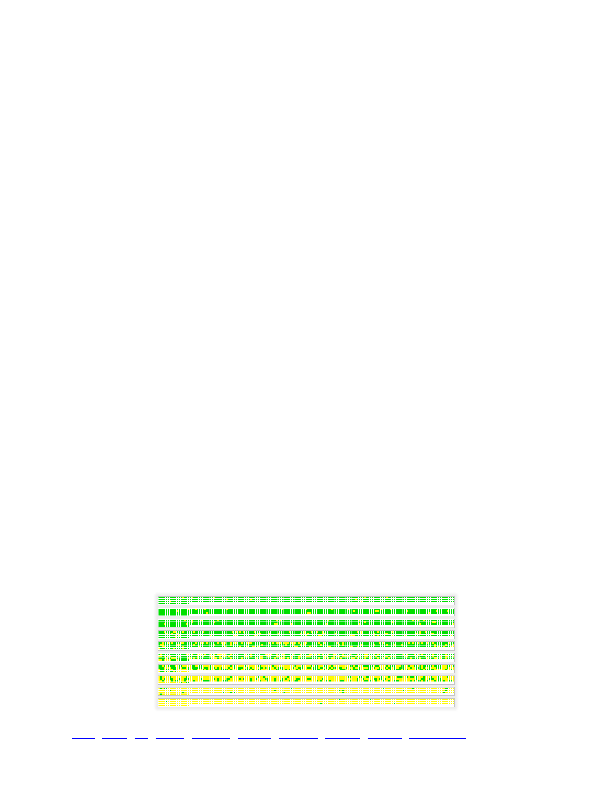
because the introduced mutation would frequently be lost unless we chose a very low threshold
frequency.
10.7 Adaptive introgression
All of the selective sweep recipes thus far have involved just a single subpopulation. Here we
want to extend this to model adaptive introgression, the progress of an adaptive allele from its
subpopulation of origin into another subpopulation via migration and gene flow. Section 5.3
introduced techniques for setting up structured populations with migration; all we need to do is
add a selective sweep to such a model. Here’s a simple model combining the population structure
of section 5.3.1’s recipe with the hard sweep dynamics of section 10.1 (both slightly modified):
initialize() {!
initializeMutationRate(1e-7);!
initializeMutationType("m1", 0.5, "f", 0.0);!
initializeMutationType("m2", 1.0, "f", 0.5); // introduced mutation!
initializeGenomicElementType("g1", m1, 1.0);!
initializeGenomicElement(g1, 0, 99999);!
initializeRecombinationRate(1e-8);!
}!
1 {!
subpopCount = 10;!
for (i in 1:subpopCount)!
sim.addSubpop(i, 500);!
for (i in 2:subpopCount)!
sim.subpopulations[i-1].setMigrationRates(i-1, 0.01);!
for (i in 1:(subpopCount-1))!
sim.subpopulations[i-1].setMigrationRates(i+1, 0.2);!
}!
100 late() {!
target = sample(p1.genomes, 1);!
target.addNewDrawnMutation(m2, 10000);!
}!
100:100000 late() {!
if (sim.countOfMutationsOfType(m2) == 0)!
{!
fixed = (sum(sim.substitutions.mutationType == m2) == 1);!
cat(ifelse(fixed, "FIXED\n", "LOST\n"));!
sim.simulationFinished();!
}!
}
If you run this model and stop the run in the middle, while the adaptive introgression is in
progress (assuming it is not lost by chance early on – you may have to recycle and restart several
times before it catches), the population shown in SLiMgui may look something like this:
TOC I TOC II WF nonWF initialize() Genome Individual Mutation SLiMSim Subpopulation!
Eidos events fitness() mateChoice() modifyChild() recombination() interaction() reproduction() 152
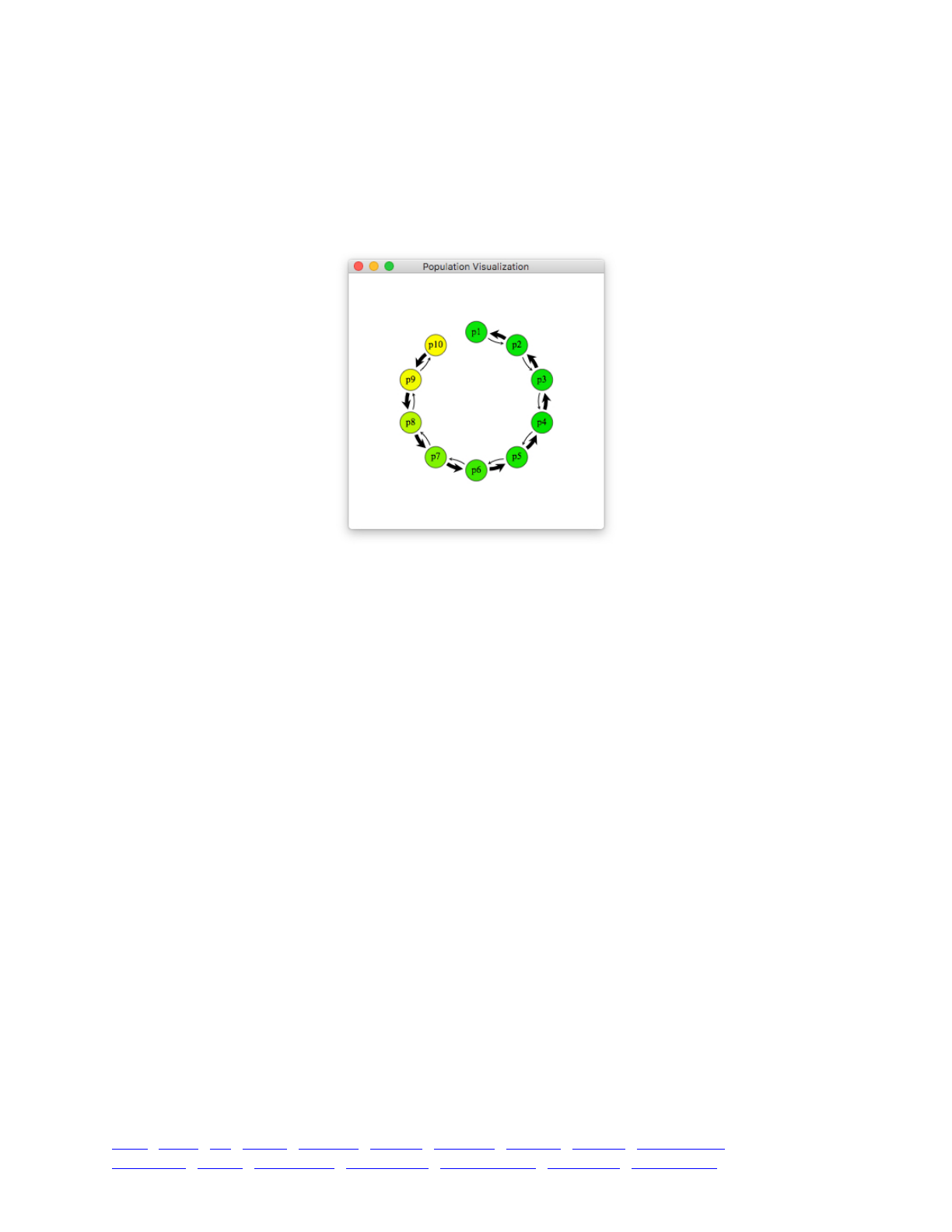
Individuals possessing the introgressing allele are colored green; note that there are no
intermediate-colored individuals because m2 is fully dominant. The mutation was introduced into
subpopulation p1, and so it is closest to fixation there, whereas it has only just begun to sweep in
p10. Of course it is not possible to see the connectivity between the subpopulations, and the
migration rates between them, in this view. As described in section 5.1.3, you can open the
population visualization window to see what the population structure looks like:
Here we see that we have a stepping-stone model, with gene flow mostly from p10 toward p1,
opposing the spread of the introduced mutation. Nevertheless, the mutation introgresses quite
rapidly given the parameters for this model; you could play with migration rates, selection
coefficients, etc. to test how they affect the time until completion of the sweep. It would be easy
to introduce spatial variation in selection into this model, too, using the techniques of section 9.2,
in order to allow the introgression to proceed only so far along the chain of subpopulations before
further introgression is blocked by local selection against it (see section 12.3).
10.8 Fixation probabilities under Hill-Robertson interference
In this final section, we’ll see how a simple sweep model can test the predictions of population
genetic theory. The recipe here will model Hill-Robertson interference, the interference of
beneficial mutations that have arisen in different lineages and thus compete against each other
(Hill & Robertson 1966). The recipe’s code then compares the predicted mean fixation time for a
beneficial allele without such interference to the actual mean fixation time observed by the
simulation.
The design of this recipe is that the first 5000 generations of the run are a burn-in period during
which a dynamic equilibrium is reached, and then the final 1000 generations are measured. The
formulas for the probability of fixation of a beneficial mutation without interference and the
expected number of fixed mutations are calculated according to standard population genetic
theory (Kimura 1962). The actual number of fixed mutations is obtained from the information
stored in SLiM’s substitution objects, which record the generation of fixation of all mutations; the
number of fixed mutations with a generation of fixation after the end of the burn-in can then be
counted. As we shall see below, the actual count is much lower than the expected count; fixation
is being highly suppressed in this model compared to the expectations without Hill-Robertson
interference.
Without further ado, the recipe:
TOC I TOC II WF nonWF initialize() Genome Individual Mutation SLiMSim Subpopulation!
Eidos events fitness() mateChoice() modifyChild() recombination() interaction() reproduction() 153

initialize() {!
initializeMutationRate(1e-6);!
initializeMutationType("m1", 0.5, "f", 0.05);!
initializeGenomicElementType("g1", m1, 1.0);!
initializeGenomicElement(g1, 0, 99999);!
initializeRecombinationRate(1e-8);!
}!
1 {!
sim.addSubpop("p1", 1000);!
}!
6000 late() {!
// Calculate the fixation probability for a beneficial mutation!
s = 0.05;!
N = 1000;!
p_fix = (1 - exp(-2 * s)) / (1 - exp(-4 * N * s));!
!
// Calculate the expected number of fixed mutations!
n_gens = 1000; // first 5000 generations were burn-in!
mu = 1e-6;!
locus_size = 100000;!
expected = mu * locus_size * n_gens * 2 * N * p_fix;!
!
// Figure out the actual number of fixations after burn-in!
subs = sim.substitutions;!
actual = sum(subs.fixationGeneration >= 5000);!
!
// Print a summary of our findings!
cat("P(fix) = " + p_fix + "\n");!
cat("Expected fixations: " + expected + "\n");!
cat("Actual fixations: " + actual + "\n");!
cat("Ratio, actual/expected: " + (actual/expected) + "\n");!
}
Running this produces output like this (a typical result):
P(fix) = 0.0951626!
Expected fixations: 19032.5!
Actual fixations: 302!
Ratio, actual/expected: 0.0158676
This is obviously a very simple model; the point is just to demonstrate that it is straightforward
to make models that test theoretical predictions like this – and that Hill-Robertson interference can
make a large difference to dynamics! If you run the model in SLiMgui, the way that the
competition of different lineages slows progress towards fixation is quite apparent. Of course if the
mutational input is constant, and the time to fixation increases, that has to mean (assuming
equilibrium) that fewer mutations are fixing. That can also be observed with this model in
SLiMgui; you can see many substantial bars, representing beneficial mutations at reasonably high
frequencies, getting pushed down to zero by the rise of a competing haplotype. Far fewer
beneficial mutations would be lost if they were not competing with each other. Recombination
occasionally resolves these conflicts by bringing competing mutations together onto the same
chromosome.
A very simple way to check this model is to decrease the mutation rate. The lower the mutation
rate, the less competition there should be between different mutations existing simultaneously in
the population (to the limiting case of a single extant mutation at any given time, which would
experience no Hill-Robertson interference at all). This is very easy to test; just change the mutation
rate to 1e-7, both where it is set with initializeMutationRate() and where it is assigned to the
TOC I TOC II WF nonWF initialize() Genome Individual Mutation SLiMSim Subpopulation!
Eidos events fitness() mateChoice() modifyChild() recombination() interaction() reproduction() 154

variable mu for the calculations at the end. With both of those set to 1e-7, typical output is
something like:
P(fix) = 0.0951626!
Expected fixations: 1903.25!
Actual fixations: 88!
Ratio, actual/expected: 0.0462367
And if we change the rate to 1e-8, again in both places, we get:
P(fix) = 0.0951626!
Expected fixations: 190.325!
Actual fixations: 16!
Ratio, actual/expected: 0.0840667
With 1e-9, we get something like this (with a lot of stochasticity in the result, at this point –
1000 generations post-burn-in is not nearly long enough to get an accurate estimate of the model’s
behavior when the mutation rate is so low):
P(fix) = 0.0951626!
Expected fixations: 19.0325!
Actual fixations: 6!
Ratio, actual/expected: 0.31525
So as predicted, the lower the mutation rate, the less Hill-Robertson interference influences the
dynamics, and the more closely the model approximates the theoretical ideal of independent
mutations without interference. And indeed, if you run the model with the mutation rate of 1e-9 in
SLiMgui, you will see that sometimes multiple mutations still interfere, but fairly often, too, single
mutations arise and fix individually. Of course a rigorous analysis would want to use a longer
burn-in, a longer post-burn-in runtime, multiple runs averaged together for each mutation rate,
calculation of a standard error of the mean across each set of multiple runs, statistical tests for
significance of differences, and so forth; but even this very simple analysis is sufficient to make the
trend quite clear.
TOC I TOC II WF nonWF initialize() Genome Individual Mutation SLiMSim Subpopulation!
Eidos events fitness() mateChoice() modifyChild() recombination() interaction() reproduction() 155

11. Complex mating schemes
Since SLiM is based on the Wright-Fisher model, biparental mating in SLiM is normally random;
for each offspring individual to be generated in a subpopulation, two parents are chosen at random
from the appropriate subpopulation (which may not be the same subpopulation as the offspring’s
subpopulation, if migration is involved). It is possible to modify this default behavior, however, by
writing a special type of Eidos script block called a mateChoice() callback. These callbacks are
documented comprehensively in the SLiM reference, in section 22.3. Here we will explore
recipes that illustrate the use of mateChoice() callbacks to implement two different types of non-
random mating: assortative mating, and sequential mate search.
Some mating schemes are actually better modeled using a different type of callback, a
modifyChild() callback. Mostly, modifyChild() callbacks are used for purposes other than mating
schemes; recipes using them are mostly in chapter 12 (and they are documented in the SLiM
reference in section 22.4). However, the last recipe in this chapter will implement an interesting
type of non-random mating, gametophytic self-incompatibility based on an S-locus, using a
modifyChild() callback. See section 13.7 for another type of non-random mating, forcing SLiM to
execute a specified pedigree, also done with a modifyChild() callback.
11.1 Assortative mating
Assortative mating is the preference of an individual for mates that resemble the individual itself
in some way. A species could exhibit assortative mating by size, for example, which would mean
that smaller individuals tend to prefer other smaller individuals as mates, whereas larger
individuals tend to prefer other larger individuals. Assortative mating is an important topic in
evolutionary biology because it is thought to be important to the process of speciation: a
population can diverge into genetically distinct lineages if assortative mating becomes strong
enough to reproductively isolate phenotypically distinct subsets of the population from each other.
Indeed, this mechanism can be so effective that if a single gene provides both adaptive phenotypic
divergence and assortative mating based upon the diverging trait, the trait governed by the gene is
called a “magic trait” because of its power to facilitate speciation (Servedio et al. 2011).
In this section we’ll look at a simple magic-trait model in SLiM (see sections 13.1 and 14.8 for
further investigations of this topic). Since this is a relatively complex model, let’s put it together
one piece at a time. The first piece is to set up the genetic and population structure:
initialize() {!
initializeMutationRate(1e-7);!
initializeMutationType("m1", 0.5, "f", 0.0);!
initializeMutationType("m2", 1.0, "f", 0.5); // introduced mutation!
initializeGenomicElementType("g1", m1, 1.0);!
initializeGenomicElement(g1, 0, 99999);!
initializeRecombinationRate(1e-8);!
}!
1 {!
sim.addSubpop("p1", 500);!
sim.addSubpop("p2", 500);!
p1.setMigrationRates(p2, 0.1);!
p2.setMigrationRates(p1, 0.1);!
}!
1000 late() {!
target = sample(p1.genomes, 1);!
target.addNewDrawnMutation(m2, 10000);!
}!
3499 { sim.simulationFinished(); }
TOC I TOC II WF nonWF initialize() Genome Individual Mutation SLiMSim Subpopulation!
Eidos events fitness() mateChoice() modifyChild() recombination() interaction() reproduction() 156
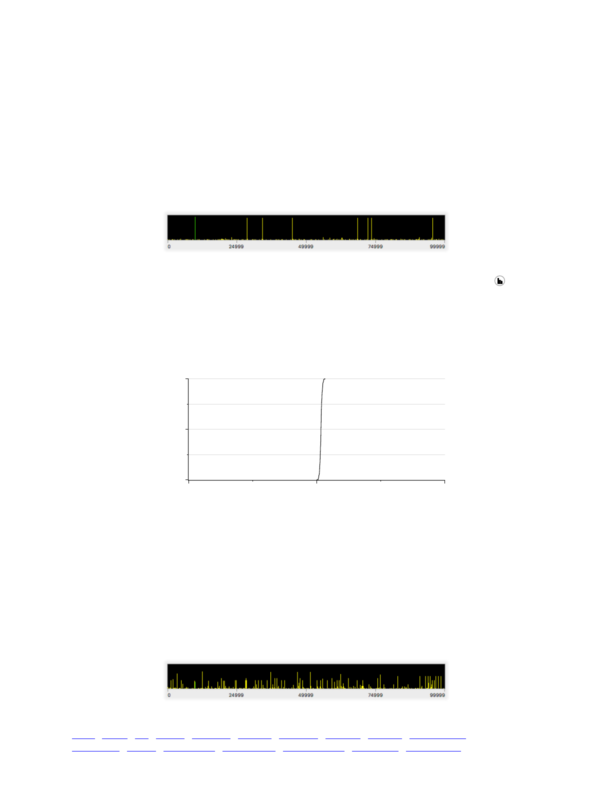
This is very similar to the “introduced adaptive mutation” recipe of section 10.1: we have two
mutation types, one neutral (m1) and the other adaptive (m2), and after running a burn-in period of
1000 generations using only type m1, we introduce a single mutation of type m2 into a randomly
chosen genome. The main difference between section 10.1’s recipe and this model is that here we
have two subpopulations connected by migration; the gene flow introduced by the migration rate
of 0.1 in both directions between the subpopulations is substantial.
When run, this model provides sweep dynamics similar to those seen in some recipes in the
previous chapter. In the snapshot below, most of the neutral diversity has been swept away by the
beneficial mutation introduced at position 10000, which is about to fix and is carrying a few
neutral mutations along with it:
We can also examine the behavior of this model in SLiMgui using the Mutation Frequency
Trajectories graph. First recycle the simulation, then click the Show Graph popup button and
open the Mutation Frequency Trajectories graph window from that menu. At this point, the
simulation is not yet initialized, and so the graph is empty. Step forward one generation, over the
initialize() callback; now the mutation types have been defined, and so you can choose
mutation type m2 from the popup in the graph window. Play the simulation forward, and you
should end up with a plot something like this, if the introduced mutation is not lost (if it is lost, you
can just recycle and try again):
This plot illustrates that from the point at which the mutation was introduced, in generation
1000, it swept very rapidly to fixation.
For our magic-trait model we need divergent ecological selection between the subpopulations,
which we introduce by adding a fitness() callback that flips the fitness effect of the introduced
mutation in subpopulation p2:
fitness(m2, p2) { return -0.2; }
That’s all it takes. For simplicity, we are modeling a dominant mutation here, but we could
easily use a scheme such as that in section 9.4.1 if the mutation were not dominant.
A little while after the introduced mutation arose, this looks like:
0 1000 2000
0.0
0.5
1.0
Generation
Frequency
TOC I TOC II WF nonWF initialize() Genome Individual Mutation SLiMSim Subpopulation!
Eidos events fitness() mateChoice() modifyChild() recombination() interaction() reproduction() 157
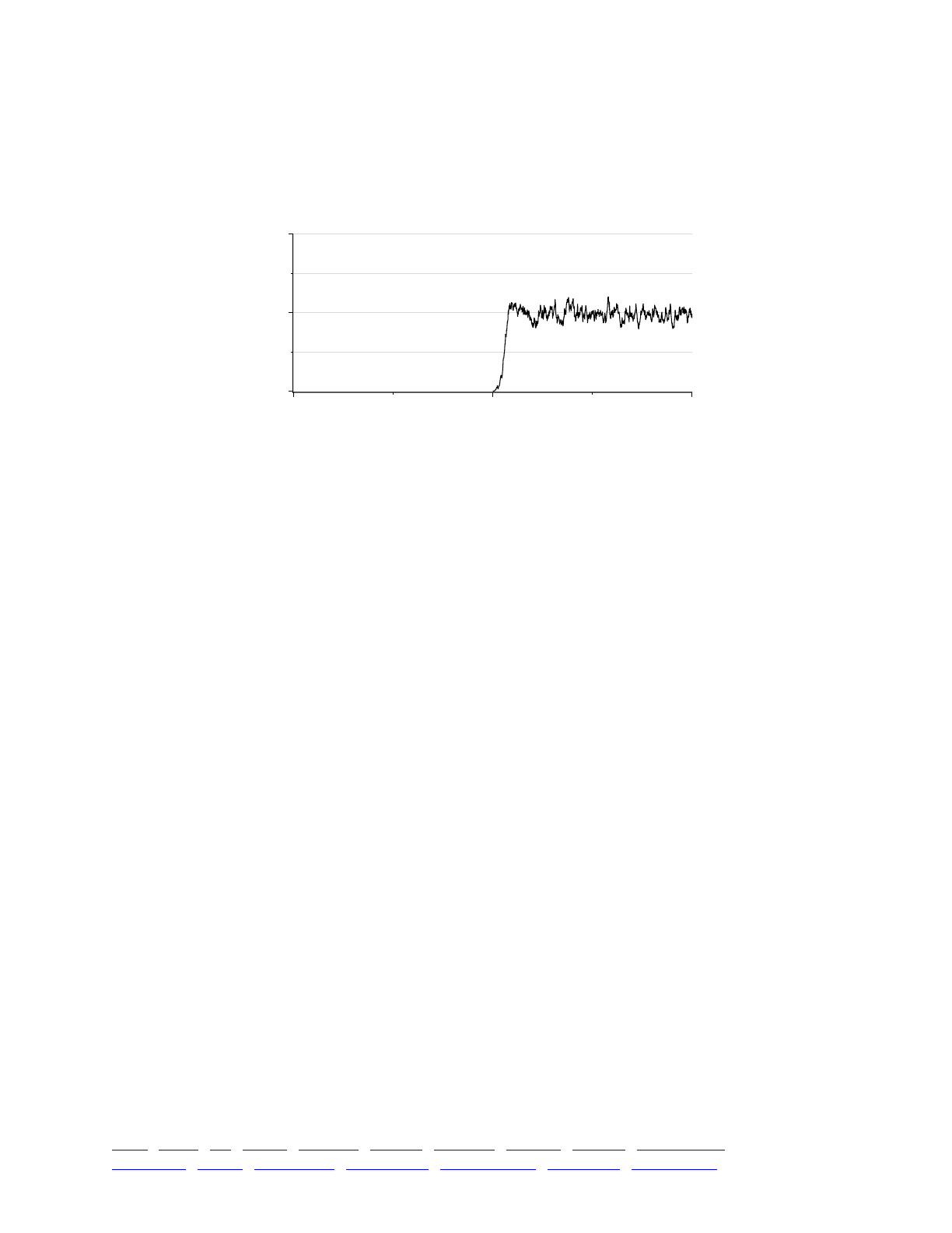
The introduced mutation is not fixing in this version of the model; indeed, it is stuck fluctuating
around a frequency of 0.5, unable to increase further because it is deleterious in p2. Note that
there is lots of neutral variation in this run, in contrast to the previous version of the model.
If we look at the Mutation Frequency Trajectories graph now, we see a very different pattern,
illustrating how the spatial variation in selection is preventing the introduced mutation from fixing:
Finally, for a magic-trait model we need assortative mating based upon the same locus that is
under divergent selection. In this model, that assortative mating will be provided by a
mateChoice() callback, which we can add now:
2000: mateChoice() {!
parent1HasMut = (individual.countOfMutationsOfType(m2) > 0);!
parent2HasMut = (sourceSubpop.individuals.countOfMutationsOfType(m2)!
> 0);!
if (parent1HasMut)!
return weights * ifelse(parent2HasMut, 2.0, 1.0);!
else!
return weights * ifelse(parent2HasMut, 0.5, 1.0);!
}
This callback is a bit complicated, so let’s walk through it. The first line determines whether the
parent that is choosing a mate possesses the magic-trait mutation. The choosing parent is provided
to the callback as an object named individual, of class Individual; this class is essentially a bag
containing the two Genome objects belonging to the individual. The countOfMutationsOfType()
method of Individual counts all occurrences of mutations of the given type in both of the
individual’s genomes; in other words, if the individual is homozygous for a given m2 mutation, that
mutation is represented twice in the count. Comparing the total count to 0 yields a single logical
truth value indicating whether any mutation of that type is present in the individual. Note that the
use of > 0 means that we are ignoring dominance; for purposes of mate choice, we are treating the
mutation as dominant. If we wanted heterozygotes to prefer heterozygotes and homozygotes
prefer homozygotes, or some such mating scheme, we could use the actual count instead; with a
little change to the following logic that would work fine too.
Similarly, we can assess whether the other individuals in the subpopulation – the potential
mates – possess the mutation using countOfMutationsOfType(m2) for all the individuals in the
subpopulation. As previously, we use a > 0 comparison to get a vector of logical values,
parent2HasMut, indicating whether each individual in the subpopulation possess the magic-trait
mutation in either of its genomes.
Finally, we have a little logic at the end to determine the mating preferences we want to return.
The standard fitness-based mating weights are supplied to the mateChoice() callback in the
weights variable, and we don’t want to ignore that; if we didn’t use that vector at all, we would be
0 1000 2000
0.0
0.5
1.0
Generation
Frequency
TOC I TOC II WF nonWF initialize() Genome Individual Mutation SLiMSim Subpopulation!
Eidos events fitness() mateChoice() modifyChild() recombination() interaction() reproduction() 158
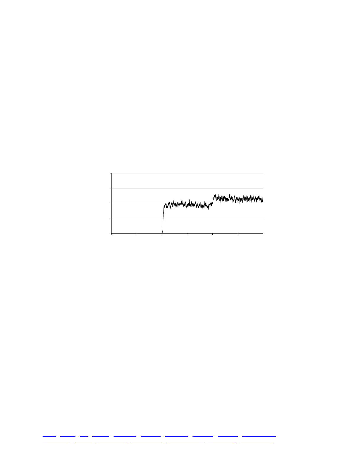
overriding SLiM’s built-in fitness calculations, based on the selection coefficients of mutations,
entirely (which you may do if you wish, but which is usually not what is wanted). Here, we start
with weights, and combine it multiplicatively with an assortative-mating term computed with
ifelse(). The ifelse() function produces a result by looking at each element of its first
parameter (here, parent2HasMut) and choosing a corresponding element for the result; if the
element from the first parameter is T, an element from the second parameter is chosen, whereas if
the element from the first parameter is F, an element from the third parameter is chosen. The
second and third parameters may be non-singleton vectors, too; ifelse() is a very powerful
vectorized comparison function, which you can read more about in the Eidos documentation.
Here, its use is really quite simple. If the parent choosing a mate possesses the magic-trait
mutation, then candidate mates that also possess it get a multiplier of 2.0, expressing the
preference of carriers for other carriers. If the parent choosing a mate does not possess the magic-
trait mutation, then candidate mates that possess it get a multiplier of 0.5, expressing the dislike of
non-carriers for carriers.
If we recycle and run, and then look at the Mutation Frequency Trajectories graph, we can see
the effects of this callback kick in at generation 2000, when the callback becomes active:
At generation 2000, when the mateChoice() callback becomes active, the frequency of the
magic-trait allele jumps upward. If the two subpopulations were able to reach complete
reproductive isolation through this mechanism, we would expect the frequency plotted here to
equilibrate at 1.0 (because this graph shows the frequencies in subpopulation p1 only). In
practice, full divergence is not possible, because SLiM is a model of juvenile dispersal, and fitness
acts during mating (as opposed to causing mortality earlier in the generation life cycle). Given the
migration rates declared in the model, approximately 10% of the individuals in each
subpopulation will come from matings in the other population, every generation. Those migrants
are also mating assortatively – they might be maladapted in their new home, but they will
nevertheless preferentially mate with each other to produce offspring that are also maladapted.
Given the very high migration rate, adaptive divergence is helped only a little by the addition of
assortative mating (but see below).
The rest of the chromosome, outside the magic-trait locus, is subject only to neutral mutations
in this simple model. These neutral mutations can provide a means of monitoring the degree of
divergence between the subpopulations in the model; if the subpopulations become fully
reproductively isolated from each other, divergence at neutral sites should be observed, whereas
without reproductive isolation divergence at neutral sites should be small or absent. This is often
measured with a metric called FST: higher FST indicates greater genetic divergence among
subpopulations. We can add code to start calculating the mean FST between p1 and p2 at
generation 3000:
0 1000 2000 3000
0.0
0.5
1.0
Generation
Frequency
TOC I TOC II WF nonWF initialize() Genome Individual Mutation SLiMSim Subpopulation!
Eidos events fitness() mateChoice() modifyChild() recombination() interaction() reproduction() 159

// Calculate the FST between two subpopulations!
function (f$)calcFST(o<Subpopulation>$ subpop1, o<Subpopulation>$ subpop2)!
{!
p1_p = sim.mutationFrequencies(subpop1);!
p2_p = sim.mutationFrequencies(subpop2);!
mean_p = (p1_p + p2_p) / 2.0;!
H_t = 2.0 * mean_p * (1.0 - mean_p);!
H_s = p1_p * (1.0 - p1_p) + p2_p * (1.0 - p2_p);!
fst = 1.0 - H_s/H_t;!
fst = fst[!isNAN(fst)]; // exclude muts where mean_p is 0.0 or 1.0!
return mean(fst);!
}!
!
3000: late() {!
sim.setValue("FST", sim.getValue("FST") + calcFST(p1, p2));!
}!
3499 late() {!
cat("Mean FST at equilibrium: " + (sim.getValue("FST") / 500));!
sim.simulationFinished();!
}
This recipe introduces a new feature in Eidos that was introduced in SLiM 2.5: user-defined
functions (see the Eidos manual for details on the syntax, etc.). Most of the code above defines a
new function, named calcFST(), that calculates the FST between two subpopulations. The rest of
the code just calls that function, records the results, and prints out a summary at the end of the run
(discussed below). Writing a new function like this is a good way to encapsulate general-purpose
code that could be reused in other models. In fact, user-defined functions like this have so much
potential to be useful that we have started a Github repository just for sharing them with other
users of SLiM: https://github.com/MesserLab/SLiM-Extras. Some of the functions shared there have
been written by us; we’re hoping that SLiM users will contribute more. You can send us a
contribution via a git pull request, or you can just email us your code and we’ll put it into the
repository for you if you prefer. If you’re a regular user of SLiM, it might be a good idea for you to
check that repository from time to time, to see what new goodies might have been added!
Besides the quirk of the user-defined function, this code is just an Eidos implementation of
Wright’s definition of FST:
where is the average heterozygosity in the two subpopulations, and is the total
heterozygosity when both subpopulations are combined. Note that all of the calculations here are
vectorized; the FST for each mutation in the simulation is calculated simultaneously in the code
above, leveraging the vectorized syntax of Eidos, and only at the end (with mean(F_ST)) are those
values combined into a mean FST value across the chromosome.
The mean FST for the generation is added to a value kept by the simulation using its dictionary-
like getValue() / setValue() mechanism (see section 21.12.2), to keep a running total; that total is
then used in generation 3499 to calculate the average FST over the generations 3000:3499. The
getValue() / setValue() facility simply provides a way to attach named state to the simulation; it
is similar to the tag property we have used in various other recipes, but is more flexible (allowing
us to keep track of state of type float here, for example, whereas tag is limited to integer values).
We also need to add a line to the generation 1 event, to zero out the running FST total:
sim.setValue("FST", 0.0);
FST = 1 −HS
HT
HS
HT
TOC I TOC II WF nonWF initialize() Genome Individual Mutation SLiMSim Subpopulation!
Eidos events fitness() mateChoice() modifyChild() recombination() interaction() reproduction() 160

If we run the model with the mateChoice() callback commented out, we get this output at the
end of the run (for a run in which the focal mutation is not lost):
Mean FST at equilibrium: 0.0208799
Running it with the mateChoice() callback active, on the other hand, produces this output at
the end of the run:
Mean FST at equilibrium: 0.0322724
The magic trait therefore appears to have increased the level of divergence between the
subpopulations at neutral loci, relative to the divergence for the same trait under natural selection
but without the “magic” effect on mate choice, due to a decrease in gene flow. Single runs are of
course not sufficient to show this convincingly; in practice, you would want to do many
replications of both models, and do some statistics to show that the difference between the
outcomes of the two models is significant. You might also wish to run for more than 1000
generations before starting to gather the FST statistics, to assure that equilibrium had been reached.
You might also wish to verify that the magic trait was not lost from the simulation; that happens
occasionally, which of course defeats the purpose of the model. Finally, you might look separately
at the FST at different positions along the chromosome, since it might be much higher near the
magic trait locus than at more distant locations, due to linkage.
For the record, the complete model with all of the above components is:
// Calculate the FST between two subpopulations!
function (f$)calcFST(o<Subpopulation>$ subpop1, o<Subpopulation>$ subpop2)!
{!
p1_p = sim.mutationFrequencies(subpop1);!
p2_p = sim.mutationFrequencies(subpop2);!
mean_p = (p1_p + p2_p) / 2.0;!
H_t = 2.0 * mean_p * (1.0 - mean_p);!
H_s = p1_p * (1.0 - p1_p) + p2_p * (1.0 - p2_p);!
fst = 1.0 - H_s/H_t;!
fst = fst[!isNAN(fst)]; // exclude muts where mean_p is 0.0 or 1.0!
return mean(fst);!
}!
!
initialize() {!
initializeMutationRate(1e-7);!
initializeMutationType("m1", 0.5, "f", 0.0);!
initializeMutationType("m2", 1.0, "f", 0.5); // introduced mutation!
initializeGenomicElementType("g1", m1, 1.0);!
initializeGenomicElement(g1, 0, 99999);!
initializeRecombinationRate(1e-8);!
}!
1 {!
sim.setValue("FST", 0.0);!
sim.addSubpop("p1", 500);!
sim.addSubpop("p2", 500);!
p1.setMigrationRates(p2, 0.1);!
p2.setMigrationRates(p1, 0.1);!
}!
1000 late() {!
target = sample(p1.genomes, 1);!
target.addNewDrawnMutation(m2, 10000);!
}!
fitness(m2, p2) { return -0.2; }!
TOC I TOC II WF nonWF initialize() Genome Individual Mutation SLiMSim Subpopulation!
Eidos events fitness() mateChoice() modifyChild() recombination() interaction() reproduction() 161

2000: mateChoice() {!
parent1HasMut = (individual.countOfMutationsOfType(m2) > 0);!
parent2HasMut = (sourceSubpop.individuals.countOfMutationsOfType(m2)!
> 0);!
if (parent1HasMut)!
return weights * ifelse(parent2HasMut, 2.0, 1.0);!
else!
return weights * ifelse(parent2HasMut, 0.5, 1.0);!
}!
3000: late() {!
sim.setValue("FST", sim.getValue("FST") + calcFST(p1, p2));!
}!
3499 late() {!
cat("Mean FST at equilibrium: " + (sim.getValue("FST") / 500));!
sim.simulationFinished();!
}
This model runs very slowly after generation 2000. The mateChoice() callback computes the
same values over and over; using the Eidos functions defineConstant() and rm() to cache those
values yields about a 10× speedup. This is left as an advanced exercise for the reader.
11.2 Sequential mate search
In the previous section we saw how to use a mateChoice() callback to implement assortative
mating with a mateChoice() that modified the standard mating weights vector, weights, by
multiplying it with an additional term derived from the genetic match between the focal individual
and the other individuals in the subpopulation. In other words, the ultimate choice of mate was
left to SLiM’s machinery; the mateChoice() callback just modified the mating weights.
In this section we will explore a completely different kind of mateChoice() callback, one which
makes the mate choice determination itself and tells SLiM’s machinery which mate was chosen (if
any). The standard weights vector will be used internally, within the mateChoice() callback; but
the callback will return a weights vector with 1 for the chosen mate and 0 for all other candidates.
In certain circumstances, it will instead return a zero-length vector as a signal to SLiM that no
suitable mate could be found, initiating a new mate search with a new choosing parent.
The biological scenario here has to do with sequential mate search, the search by the choosy
parent for a suitable mate by examining candidates sequentially until a suitable candidate is found
or the breeding season runs out. Conceptually, we will model a species like peacocks, in which
the choosy parent is looking for a mate with a large ornament that is costly in fitness but that
makes the mate attractive; however, to keep the model relatively simple we will do a
hermaphroditic model in which all individuals can play both the chooser and the chosen.
Let’s build the model one step at a time, first constructing the genetic and population structure:
initialize() {!
initializeMutationRate(1e-7);!
initializeMutationType("m1", 0.5, "f", 0.0); // neutral!
initializeMutationType("m2", 0.5, "f", -0.01); // ornamental!
initializeGenomicElementType("g1", c(m1, m2), c(1.0, 0.01));!
initializeGenomicElement(g1, 0, 99999);!
initializeRecombinationRate(1e-8);!
}!
1 { sim.addSubpop("p1", 500); }!
2001 early() {!
sim.simulationFinished();!
}
TOC I TOC II WF nonWF initialize() Genome Individual Mutation SLiMSim Subpopulation!
Eidos events fitness() mateChoice() modifyChild() recombination() interaction() reproduction() 162

This is straightforward: one population of 500 individuals, and a genetic structure that allows
both neutral mutations (m1) and mutations that influence the ornament size of the individuals (m2).
The ornamental mutations occur only about 1% as often as the neutral mutations, but may occur
anywhere in the genome; this could be thought of as a “many genes of small effect”, quantitative-
genetics sort of scenario. These ornamental mutations are all slightly deleterious, as genes that
increase the size of a peacock’s tail presumably would be (apart from their positive effect on
mating). If run, this model behaves as you might expect: neutral mutations accumulate, but no
ornamental mutations fix, or even reach appreciable frequency, because of their deleterious effect.
Now we want to introduce the effect of the ornamental mutations on mating; to do so, we add a
mateChoice() callback. This callback should implement sequential choosy mate choice by
searching for a mate, preferring potential mates with more ornamental mutations:
mateChoice() {!
fixedMuts = sum(sim.substitutions.mutationType == m2);!
for (attempt in 1:5)!
{!
mate = sample(0:499, 1, T, weights);!
osize = 1.0 + (fixedMuts * 0.01) - p1.cachedFitness(mate);!
!
if (runif(1) < osize * 10 + 0.1)!
return p1.individuals[mate];!
}!
return float(0);!
}
The first line of this callback just totals up the number of ornamental mutations that have fixed.
Once a mutation fixes, SLiM removes it from the active simulation, and from fitness calculations;
since all individuals possess the fixed mutation, it has no differential effect on fitness or dynamics,
in general. In this model, however, we want such fixed mutations to continue to influence mate
choice, as described below. This could also be done (perhaps better) by setting the
convertToSubstitution property of m2 to F, as we have seen in some previous recipes; we’re using
a different strategy here just to show a different angle on this common issue.
Next, the callback uses a for loop to make up to five attempts at finding a mate. Each attempt
is a little less picky than the previous attempt, reflecting declining standards as breeding season
proceeds. If all five attempts fail, float(0) is returned to indicate that the individual failed to find
a mate. Within each attempt, a candidate mate is chosen using the sample() function, with the
standard fitness-based weights vector as the weights for sampling; the deleterious effect of the
ornamental mutations is thus still taken into account, reducing the likelihood that highly
ornamented individuals will be chosen as mates for survival- or growth-based reasons. The
ornament size of the candidate mate is calculated, using both fixed and unfixed ornamental
mutations. Finally, runif() generates a random uniform draw (between 0 and 1, by default), and
that drawn value is compared to a threshold value determined by the candidate mate’s ornament
size; if the candidate gets sufficiently lucky, it ends up as the chosen mate. (The addition of 0.1
here ensures that the mate choice algorithm is guaranteed to terminate eventually; without it, a
hang would be possible if no individual can ever find a suitable mate because no individuals with
any ornamental mutations exist.) When a mate is chosen, it is simply returned; it just needs to be
looked up from p1.individuals since mate is just the index of the chosen mate. It would be
possible instead to construct a new weights vector, with 1 for the chosen mate and 0 for all other
entries, and return that to force SLiM to choose that individual; simply returning the individual is a
shorthand that can be handled by SLiM far more efficiently than can a returned weights vector.
TOC I TOC II WF nonWF initialize() Genome Individual Mutation SLiMSim Subpopulation!
Eidos events fitness() mateChoice() modifyChild() recombination() interaction() reproduction() 163

If you run this model, you can now see the ornamental mutations increasing in frequency and
fixing despite their deleterious fitness effect, because they are favored by sexual selection.
We might be interested in the final ornament size attained, so we can flesh out the final event:
2001 early() {!
fixedMuts = sum(sim.substitutions.mutationType == m2);!
osize = 1.0 + (fixedMuts * 0.01) - mean(p1.cachedFitness(NULL));!
cat("Mean ornament size: " + osize);!
sim.simulationFinished();!
}
By writing this as a 2001 early() event, we are effectively running at the very end of generation
2000, after fitness values have been evaluated (see the generation cycle diagram in section 1.3, or
the more in-depth discussion in chapter 19). This distinction is important, since this event calls
cachedFitness() to get the fitness values of individuals; in a late() event those values would not
yet be calculated, and in fact calling cachedFitness() at that time would result in an error.
If you run this model until completion, you will likely see an output line like:
Mean ornament size: 0.0905
Individuals have evolved to possess, on average, about nine ornamental mutations. If you
modify the model to run until generation 10001, the final state is not much different:
Mean ornament size: 0.09
The fact that the mate choice algorithm takes fixed mutations into account, comparing the true
ornament sizes of candidate mates, means that having an ornament above a certain threshold size
provides no marginal benefit; indeed, because of the deleterious fitness effect of the ornamental
mutations, additional ornamental mutations above that threshold are selected against. The model
therefore reaches an equilibrium ornament size, just as happens in reality with ornamented species
subject to both natural selection against the ornament and sexual selection for the ornament, such
as peacocks. In this toy model, the equilibrium value is easily predicted from the structure of the
model itself (the key predictor is the mathematics of the runif() comparison in the callback).
For the record, here is the full model with all of the above components:
initialize() {!
initializeMutationRate(1e-7);!
initializeMutationType("m1", 0.5, "f", 0.0); // neutral!
initializeMutationType("m2", 0.5, "f", -0.01); // ornamental!
initializeGenomicElementType("g1", c(m1, m2), c(1.0, 0.01));!
initializeGenomicElement(g1, 0, 99999);!
initializeRecombinationRate(1e-8);!
}!
1 { sim.addSubpop("p1", 500); }!
mateChoice() {!
fixedMuts = sum(sim.substitutions.mutationType == m2);!
for (attempt in 1:5)!
{!
mate = sample(0:499, 1, T, weights);!
osize = 1.0 + (fixedMuts * 0.01) - p1.cachedFitness(mate);!
!
if (runif(1) < osize * 10 + 0.1)!
return p1.individuals[mate];!
}!
return float(0);!
}!
TOC I TOC II WF nonWF initialize() Genome Individual Mutation SLiMSim Subpopulation!
Eidos events fitness() mateChoice() modifyChild() recombination() interaction() reproduction() 164

2001 early() {!
fixedMuts = sum(sim.substitutions.mutationType == m2);!
osize = 1.0 + (fixedMuts * 0.01) - mean(p1.cachedFitness(NULL));!
cat("Mean ornament size: " + osize);!
sim.simulationFinished();!
}
Any kind of preference, bias, search, benefit, or cost influencing mate choice or mating
eligibility can be modeled with mateChoice() callbacks; this recipe only scratches the surface.
11.3 Gametophytic self-incompatibility
In the previous sections we have seen the use of mateChoice() callbacks to implement
assortative mating and sequential mate choice, two types of non-random mating. In this section,
we will see the use of a different type of callback, a modifyChild() callback, to model an
interesting type of non-random mating, gametophytic self-incompatibility based on S-locus alleles.
Gametophytic self-incompatibility is quite a common mating scheme in plants. In a nutshell,
the pollen grain (the male gamete, which is haploid) expresses the particular allele that it possesses
at a special locus called the S-locus. When a pollen grain lands on the stigma of a female flower
and begins to grow a pollen tube down the style towards the ovaries of the flower, the pollen tube
expresses the S-locus allele of the pollen grain as it grows. Female flowers, in their styles, do some
sort of check of the S-locus allele being expressed by the pollen tube, and if it exactly matches an
S-locus allele possessed by the female plant (on either of its two copies of that locus, since the
female flower is part of a diploid plant), it halts the growth of the pollen tube, preventing
fertilization. The reasons why this mechanism might be beneficial are thought to be related to
promotion of outcrossing and prevention of selfing.
Why use a modifyChild() callback instead of a mateChoice() callback to model a mate choice
scheme such as gametophytic self-incompatibility? There are several considerations.
Conceptually, a mateChoice() callback allows control over how likely every possible mating pair
in a population is to form, whereas a modifyChild() callback is about controlling the outcome of a
specific mating – governing whether that mating is fertile and what the genetic outcome of the
mating is. Gametophytic self-incompatibility is not really about the choice of mates across the
population (pollen lands indiscriminately on all female flowers, at least without complications
such as heterostyly or enantiostyly); instead, it is about whether the combination of a specific
pollen grain and a specific flower is fertile or infertile, making modifyChild() a natural choice.
Another consideration is that mateChoice() callbacks are about pre-mating reproductive
isolation, whereas modifyChild() callbacks are about post-mating reproductive isolation (among
other uses). Gametophytic self-incompatibility depends upon the S-locus allele expressed by the
haploid pollen grain; that information is simply not available in a mateChoice() callback, since
gametes have not yet been produced at that stage. From this perspective, then, modifyChild() is
actually a forced choice for this recipe.
A third consideration is that if a mateChoice() callback rejects a first parent completely, SLiM’s
mating algorithm goes back to try a different first parent within the same source subpopulation,
whereas if a modifyChild() callback suppresses a child completely, SLiM’s mating algorithm re-
chooses the source subpopulation as well, based upon the migration rates set for the target
subpopulation (see section 19.2). This difference reflects the pre-mating versus post-mating
semantics of the two callbacks, and makes good sense here; if a particular source subpopulation’s
pollen grains have a high probability of being incompatible with the female flowers of the target
subpopulation, that source subpopulation should be underrepresented in gene flow into the target
subpopulation, compared to the expected gene flow based upon pollen flow alone.
TOC I TOC II WF nonWF initialize() Genome Individual Mutation SLiMSim Subpopulation!
Eidos events fitness() mateChoice() modifyChild() recombination() interaction() reproduction() 165

A final consideration, if none of the previous issues decides the question, might be speed.
Unfortunately, mateChoice() callbacks tend to be quite slow. In computer science parlance, they
are generally O(N), meaning that the computation time taken by a mateChoice() callback is
proportional to the number of individuals in the subpopulation; this is because each individual
must be evaluated to produce a mating weight. On the other hand, modifyChild() callbacks are
generally O(1), meaning they take a constant amount of time regardless of population size; this is
because only the product of one mating event is considered by the callback. In practice, this
algorithmic speed difference can result in a very large difference to the running speed of a model.
Usually, however, the previous considerations will dictate the choice of implementation.
Let’s build the model in two steps, beginning without the modifyChild() callback:
initialize() {!
initializeMutationRate(1e-7);!
initializeMutationType("m1", 0.5, "f", 0.0);!
initializeMutationType("m2", 0.5, "f", 0.0); // S-locus mutations!
initializeGenomicElementType("g1", m1, 1.0);!
initializeGenomicElementType("g2", m2, 1.0);!
initializeGenomicElement(g1, 0, 20000);!
initializeGenomicElement(g2, 20001, 21000);!
initializeGenomicElement(g1, 21001, 99999);!
initializeRecombinationRate(1e-8);!
}!
1 { sim.addSubpop("p1", 500); }!
10000 late() {!
cat("m1 mutation count: " + sim.countOfMutationsOfType(m1) + "\n");!
cat("m2 mutation count: " + sim.countOfMutationsOfType(m2) + "\n");!
}
We have two mutation types, both neutral, and a chromosome that uses mutation type m1 over
most of its length (with g1) but mutation type m2 within a small (1000-bp) locus (with g2). That
small locus is of course the S-locus, but without the mateChoice() callback it acts identically to the
rest of the chromosome. Since there is not yet any code to enforce a difference between the S-
locus and the rest of the chromosome, this recipe is, at this point, simply a model of neutral drift.
In the generation 10000 event, it outputs two metrics prior to termination: the number of
mutations of type m1 and of type m2. These serve as a quick-and-dirty measure of genetic diversity,
both across the bulk of the chromosome (the m1 count) and within the S-locus (the m2 count). A
typical test run of this recipe produces something like:
m1 mutation count: 124!
m2 mutation count: 1
You can run the model a bunch of times and confirm that there is not a whole lot of variation
around these numbers; the m1 count is typically 100–200, the m2 count typically 0–5.
It is also interesting to look at the graphical representation of the chromosome in SLiMgui.
Selecting a subrange of the chromosome, so as to zoom in on just one section, a typical run of the
recipe so far looks like:
TOC I TOC II WF nonWF initialize() Genome Individual Mutation SLiMSim Subpopulation!
Eidos events fitness() mateChoice() modifyChild() recombination() interaction() reproduction() 166

This view has display of genomic elements turned on, with the button, so that the location of
the S-locus is clear. The two things to note here are that the distribution of neutral mutations is
fairly sparse, and that the distribution of neutral mutations inside versus outside the S-locus is
comparable.
Now let’s add in the modifyChild() callback that implements the gametophytic self-
incompatibility system:
modifyChild(p1) {!
pollenSMuts = childGenome2.mutationsOfType(m2);!
styleSMuts1 = parent1Genome1.mutationsOfType(m2);!
styleSMuts2 = parent1Genome2.mutationsOfType(m2);!
if (identical(pollenSMuts, styleSMuts1))!
if (runif(1) < 0.99)!
return F;!
if (identical(pollenSMuts, styleSMuts2))!
if (runif(1) < 0.99)!
return F;!
return T;!
}
First, the callback gets a vector of all of the S-locus mutations present in the pollen grain. The
childGenome2 variable is defined by SLiM within modifyChild() callbacks, and represents the
gamete produced by the second parent in the mating; see section 22.4 for details. The result,
pollenSMuts, represents the S-locus allele expressed by the pollen grain. All mutations at the S-
locus are considered, in this model, to change the expressed S-allele; it would be trivial to add in
the possibility of neutral mutations at the S-locus as well, by adding in a probability of type m1
mutations in genomic element type g2.
Next, the callback gets the two S-locus alleles of the female flower by fetching the vector of
mutations of type m2 from parent1Genome1 and parent1Genome2, the two homologous genomes of
the first parent (again, defined by SLiM in these callbacks, and documented in section 22.4).
Next comes the crucial step at which the growth of the pollen tube is stopped if there is an
incompatibility between the S-allele of the pollen and either of the S-alleles of the female flower.
This is checked using the Eidos function identical(), which checks whether its two arguments are
exactly identical. We don’t need to worry about non-identicality due to mutations being listed in a
different order in the vectors, because Genome keeps its list of mutations in sorted order, and
mutationsOfType() returns a sorted subset of that list.
If the pollen S-allele is identical to either of the female flower’s S-alleles, there is a 99%
probability (in this model) of the pollen tube being blocked, as implemented by the test
(runif(1)!<!0.99). Returning F in these cases tells SLiM to suppress generation of the proposed
child altogether; this is, conceptually, the stoppage of the pollen tube. It is important to guarantee
that a modifyChild() callback will never suppress 100% of all proposed children, for any state that
your model might reach; if that ever happens, SLiM will hang, stuck in an infinite loop generating
an infinite succession of proposed children that all get suppressed. In this case, the model would
not quite hang without the runif() test, since eventually SLiM would manage to generate pollen
grains that all happened to have a mutation within the S-locus that made them compatible with the
available female flowers; but it would take an awfully long time. Indeed, even at 99% the first
generation can take quite a while to finish, and many of the individuals in the second generation
will have an S-locus mutation because of the effective imposition of gametophytic self-
incompatibility in a single generation. A more realistic model might perhaps “phase in” the
gametophytic self-incompatibility slowly over some thousands of generations, reflecting the
gradual evolution of an increasingly strong mechanism, by making the threshold against which
G
TOC I TOC II WF nonWF initialize() Genome Individual Mutation SLiMSim Subpopulation!
Eidos events fitness() mateChoice() modifyChild() recombination() interaction() reproduction() 167

runif() is compared depend upon sim.generation. This is left as an exercise for the reader; it
should not change the final state of the model at equilibrium (although equilibrium might take a
lot more than the 10000 generations we use here).
The final line simply returns T, indicating that since the pollen grain was compatible with the
female flower, the proposed child can be generated.
The full recipe, for the record:
initialize() {!
initializeMutationRate(1e-7);!
initializeMutationType("m1", 0.5, "f", 0.0);!
initializeMutationType("m2", 0.5, "f", 0.0); // S-locus mutations!
initializeGenomicElementType("g1", m1, 1.0);!
initializeGenomicElementType("g2", m2, 1.0);!
initializeGenomicElement(g1, 0, 20000);!
initializeGenomicElement(g2, 20001, 21000);!
initializeGenomicElement(g1, 21001, 99999);!
initializeRecombinationRate(1e-8);!
}!
1 { sim.addSubpop("p1", 500); }!
10000 late() {!
cat("m1 mutation count: " + sim.countOfMutationsOfType(m1) + "\n");!
cat("m2 mutation count: " + sim.countOfMutationsOfType(m2) + "\n");!
}!
modifyChild(p1) {!
pollenSMuts = childGenome2.mutationsOfType(m2);!
styleSMuts1 = parent1Genome1.mutationsOfType(m2);!
styleSMuts2 = parent1Genome2.mutationsOfType(m2);!
if (identical(pollenSMuts, styleSMuts1))!
if (runif(1) < 0.99)!
return F;!
if (identical(pollenSMuts, styleSMuts2))!
if (runif(1) < 0.99)!
return F;!
return T;!
}
If you run the full recipe, you should get output something like:
m1 mutation count: 582!
m2 mutation count: 55
There is vastly more genetic diversity now, both within the S-locus (mutation type m2) and across
the whole chromosome (type m1). Gametophytic self-incompatibility basically imposes a regime of
balancing selection (i.e., negative frequency-dependent selection) at the S-locus, and that regime
tends to preserve allelic diversity at the locus (see section 9.4.1 for a different model of negative
frequency-dependent selection). It also increases the outcrossing rate in the population,
particularly when there are relatively few S-alleles (when there are many S-alleles, it would mostly
tend to diminish selfing, since most non-selfing mating pairs would possess different S-alleles
anyway; it would be trivial, of course, to add selfing to this model to experiment with that
additional nuance, as seen in section 6.3.1).
Examining the same subsection of the chromosome as before, in SLiMgui, it now looks like this:
TOC I TOC II WF nonWF initialize() Genome Individual Mutation SLiMSim Subpopulation!
Eidos events fitness() mateChoice() modifyChild() recombination() interaction() reproduction() 168

Compare this to the previous snapshot, and the increase in genetic diversity across the
chromosome is immediately apparent. It is also striking how much more diversity is contained
within the S-locus itself (due to the balancing selection there) compared to the rest of the
chromosome. Note that in the implementation of this model, the number of S-alleles is not just
the number of different mutations within the S-locus that are circulating in the population.
Instead, every unique haplotype within the S-locus as a whole represents a different S-allele, and
new S-alleles can be generated in this model by recombination as well as by mutation. Other
schemes for evaluating what an S-allele “really” is, based upon the mutations present at the S-
locus, could of course be implemented using a different test than identical() in the
modifyChild() callback.
TOC I TOC II WF nonWF initialize() Genome Individual Mutation SLiMSim Subpopulation!
Eidos events fitness() mateChoice() modifyChild() recombination() interaction() reproduction() 169

12. Direct child modifications
Thus far we have seen two ways of modifying SLiM’s basic Wright-Fisher model: fitness()
callbacks that modify the default fitness of mutations (chapter 9), and mateChoice() callbacks that
alter the default behavior of random mating (chapter 11). In this chapter we will look at a third
type of modification, modifyChild() callbacks. These allow you to modify children generated by
SLiM (by adding or removing mutations, for example), or to suppress particular children entirely
(see section 1.5 for a full technical discussion). Here, we will look at how to use a modifyChild()
callback to solve three specific problems: social learning of cultural traits that modify fitness, lethal
epistasis, and simulating a “gene drive” based upon CRISPR/Cas9. Note that section 11.3 also
used a modifyChild() callback, to implement a gametophytic self-incompatibility system.
12.1 Social learning of cultural traits
In section 9.4.3 we explored a simple model of a cultural trait; the tag value of Individual was
used to track whether each individual was a milk-drinker or not, and a fitness() callback was
used to make mutations promoting the production of lactase into adulthood beneficial for milk-
drinkers but neutral for non-milk-drinkers. In that model, whether a given individual was a milk-
drinker or not was determined at random, in a late() callback that tagged all offspring with their
assigned cultural group. We will now take up that model again and extend it to be a model of
social learning: individuals will tend to inherit milk-drinking from their parents, although a
substantial random factor in the cultural assignment will be retained. To achieve this, instead of
assigning the cultural group in a late() event, we will do it in a modifyChild() callback, so that
we have the information we need regarding the culture of the parents. The recipe:
initialize() {!
initializeMutationRate(1e-7);!
initializeMutationType("m1", 0.5, "f", 0.0); // neutral!
initializeMutationType("m2", 0.5, "f", 0.1); // lactase-promoting!
m2.convertToSubstitution = F;!
initializeGenomicElementType("g1", c(m1,m2), c(0.99,0.01));!
initializeGenomicElement(g1, 0, 99999);!
initializeRecombinationRate(1e-8);!
}!
1 {!
sim.addSubpop("p1", 1000);!
p1.individuals.tag = rbinom(1000, 1, 0.5);!
}!
modifyChild() {!
parentCulture = (parent1.tag + parent2.tag) / 2;!
childCulture = rbinom(1, 1, 0.1 + 0.8 * parentCulture);!
child.tag = childCulture;!
return T;!
}!
fitness(m2) {!
if (individual.tag == 0)!
return 1.0; // neutral for non-milk-drinkers!
else!
return relFitness; // beneficial for milk-drinkers!
}!
10000 { sim.simulationFinished(); }
The setup of the model is similar to its predecessor in section 9.4.3: mutation type m2 is used to
represent alleles that promote retention of lactase production (and removal of fixed m2 mutations is
prevented with convertToSubstitution), tag values of 1 are used to indicate milk-drinkers, and
TOC I TOC II WF nonWF initialize() Genome Individual Mutation SLiMSim Subpopulation!
Eidos events fitness() mateChoice() modifyChild() recombination() interaction() reproduction() 170

the same fitness() callback as in section 9.4.3 produces a differential fitness effect of m2
mutations depending upon the culture of the individual. What has changed is the way that the tag
values are maintained. The late() event has been removed. We now assign initial tag values in
generation 1, immediately after creating subpopulation p1. Thenceforth, the tag values of new
individuals are assigned in the modifyChild() callback:
modifyChild() {!
parentCulture = (parent1.tag + parent2.tag) / 2;!
childCulture = rbinom(1, 1, 0.1 + 0.8 * parentCulture);!
child.tag = childCulture;!
return T;!
}
This callback is called once for every new offspring individual created, throughout the run of
the model. Its first line gets the tag values of the two parents (using parent1 and parent2 variables
that are set up for all modifyChild() callbacks; see section 22.4 for a complete list of these
variables), and averages them to get a parentCulture value that will be 0, 0.5, or 1. The next line
determines what the child’s culture will be (0 or 1) using rbinom() to draw from a binomial
distribution; the trial success probability used for the draw depends on parentCulture in such a
way as to make children tend to follow the culture of their parents, but with a 10% chance of
deviating even if the parents share the same culture. To make this cultural determination take
effect, childCulture is assigned into the tag property of the child (using the child variable defined
for the callback by SLiM). Finally, a value of T is returned to indicate that the child should be
generated; it is possible for a modifyChild() callback to suppress the generation of some children
by returning F.
In the original model of section 9.4.3, the fraction of milk-drinkers remained about 0.5,
because assignment into a cultural group was random. In this model, in contrast, the fraction of
milk-drinkers can increase over time as individuals learn milk-drinking from their parents; the
fitness benefit of milk-drinking increases as more m2 mutations sweep. It is easy to observe this in
SLiMgui by adding a custom output event:
{!
if (sim.generation % 100 == 0)!
cat(sim.generation + ": " + mean(p1.individuals.tag) + "\n");!
}
This prints the fraction of milk-drinkers in the population, every 100 generations. Running this
model produces output that shows the progressive increase in milk-drinking:
100: 0.465!
200: 0.567!
300: 0.552!
400: 0.681!
500: 0.735!
...
However, there will always be a minimum of about 10% non-milk-drinkers in the population,
because of the element of chance provided by the binomial draw in the modifyChild() callback.
It would be possible to modify that to allow a specific culture to fix in the population. On the
other hand, one could also model the fact that milk-drinkers who do not retain lactase production
into adulthood will typically suffer from symptoms of lactose intolerance, making milk-drinking
disadvantageous in some circumstances. One could also model a slight deleterious effect of
lactase retention genes among non-milk-drinkers, since they are devoting energy to producing an
enzyme that they do not use. There is always more complexity to be added; but as it stands, this
TOC I TOC II WF nonWF initialize() Genome Individual Mutation SLiMSim Subpopulation!
Eidos events fitness() mateChoice() modifyChild() recombination() interaction() reproduction() 171

model shows the coevolution of both genetic and cultural factors related to milk-drinking, using
tag values in combination with a modifyChild() callback to model social learning in SLiM.
12.2 Lethal epistasis
In section 9.3.1 we saw a model of epistasis that influenced the fitness of the epistatic alleles
using a fitness() callback. Sometimes the situation is simpler than the scenario presented in that
model: sometimes the fitness of individuals carrying both epistatic alleles is zero, making the
epistatic interaction lethal. In this case, a modifyChild() callback is well-suited to the task, since
it can suppress the generation of particular offspring depending upon their genetics (or other
factors). In this case, we will model two introduced mutations, A and B, which are normally
beneficial, but are lethal when they occur in the same offspring:
initialize() {!
initializeMutationRate(1e-7);!
initializeMutationType("m1", 0.5, "f", 0.0);!
initializeMutationType("m2", 0.5, "f", 0.5); // mutation A!
m2.convertToSubstitution = F;!
initializeMutationType("m3", 0.5, "f", 0.5); // mutation B!
m3.convertToSubstitution = F;!
initializeGenomicElementType("g1", m1, 1.0);!
initializeGenomicElement(g1, 0, 99999);!
initializeRecombinationRate(1e-8);!
}!
1 {!
sim.addSubpop("p1", 500);!
}!
1 late() {!
sample(p1.genomes, 20).addNewDrawnMutation(m2, 10000); // add A!
sample(p1.genomes, 20).addNewDrawnMutation(m3, 20000); // add B!
}!
modifyChild() {!
childGenomes = c(childGenome1, childGenome2);!
hasMutA = any(childGenomes.countOfMutationsOfType(m2) > 0);!
hasMutB = any(childGenomes.countOfMutationsOfType(m3) > 0);!
if (hasMutA & hasMutB)!
return F;!
return T;!
}!
10000 { sim.simulationFinished(); }
The mechanics here for the introduction of mutations A and B follow the pattern we have seen
in other recipes: a target vector of genomes is chosen with sample(), and then a mutation is added
to the target genomes with addNewDrawnMutation(). Unlike most previous recipes, however, here
we sample 20 genomes, not just one, in order to add the new mutation to multiple individuals.
Because addNewDrawnMutation() is a class method of Genome, not an instance method, a single
new mutation is added to all of the target genomes, rather than a different new mutation being
added to each target genome as a result of multicasting; see section 9.4.4 for discussion of the
mechanics of this. No effort is made here to avoid adding A and B to the same individuals, but that
would be trivial to add by refining the choice of targets for B. The mutation types for A and B, m2
and m3, are set not to convert fixed mutations to substitutions, so that their epistatic interaction
persists even after fixation; see section 9.3.1 for extensive discussion of this.
The new and interesting behavior is in the modifyChild() callback. First it determines whether
the proposed child possesses mutation A and mutation B, setting up logical flags hasMutA and
TOC I TOC II WF nonWF initialize() Genome Individual Mutation SLiMSim Subpopulation!
Eidos events fitness() mateChoice() modifyChild() recombination() interaction() reproduction() 172

hasMutB by checking whether the count of mutations of the relevant type is greater than zero in
either of the child’s genomes. Then, if the child has both A and B, it returns F, indicating that this
child should be suppressed. New parents will be chosen and a new child will be generated
instead (also subject to the approval of the modifyChild() callback). Otherwise it returns T,
indicating the generation of the child should proceed.
When this model is run, either A or B quickly “wins”, fixing while its epistatic competitor is lost.
If the modifyChild() callback is removed, on the other hand, both A and B will typically fix. We
can try an interesting variant by making the epistatic interaction lethal only if A and B are both
homozygous, by replacing the previous modifyChild() callback with a new version:
modifyChild() {!
childGenomes = c(childGenome1, childGenome2);!
mutACount = sum(childGenomes.countOfMutationsOfType(m2));!
mutBCount = sum(childGenomes.countOfMutationsOfType(m3));!
if ((mutACount == 2) & (mutBCount == 2))!
return F;!
return T;!
}
This results in a form of balancing selection between A and B, since now homozygosity is
disadvantageous but heterozygosity is advantageous. Both will tend to fluctuate around a
frequency of 0.5, although one may stochastically manage to fix eventually (in which case the
other will immediately be lost).
This type of model could also be used to represent an epistatic interaction during development
that is lethal in some fraction of cases, but is otherwise harmless – either the epistatic interaction
causes a lethal anomaly during development, or it doesn’t, in which case the offspring is normal.
This could be modeled simply by adding a random factor to the if statement in the modifyChild()
callback.
12.3 Simulating gene drive
There has recently been a lot of buzz about a new genetic-engineering technology called
CRISPER/Cas9 that allows genetic modifications to be performed much more quickly and easily
than previous methods (Doudna & Charpentier 2014). One potential application of the CRISPER/
Cas9 machinery is to use it for the construction of a so-called gene drive, which can quickly drive
genetically modified alleles to high frequency in a population even if they carry a fitness cost. We
will here refer to a CRISPR/Cas9-based gene drive with the term mutagenic chain reaction, or
MCR.
The basic idea of MCR is that the CRISPR/Cas9 machinery embedded into the organism’s
genome could cause the machinery itself to be spliced into any homologous chromosome that
does not already contain it. If a fertilized egg ends up with one copy of the MCR machinery,
inherited from one parent, the machinery could then splice itself into the homologous
chromosome in the egg, changing the egg from being heterozygous to homozygous for the MCR
locus. This is in some ways similar to the idea of meiotic drive and related concepts in
evolutionary biology, and it clearly underlines the fundamental truth of the “selfish gene”
perspective: an MCR gene of this type could, as we shall see, spread to fixation in a population
even if it has a deleterious fitness effect at the level of the individual organism.
Just for fun, we’re going to make this model relatively complex in terms of population structure,
and we’re going to introduce spatial variation in selection using a fitness() callback as well.
We’ll build this model one step at a time, starting with the demographic structure:
TOC I TOC II WF nonWF initialize() Genome Individual Mutation SLiMSim Subpopulation!
Eidos events fitness() mateChoice() modifyChild() recombination() interaction() reproduction() 173
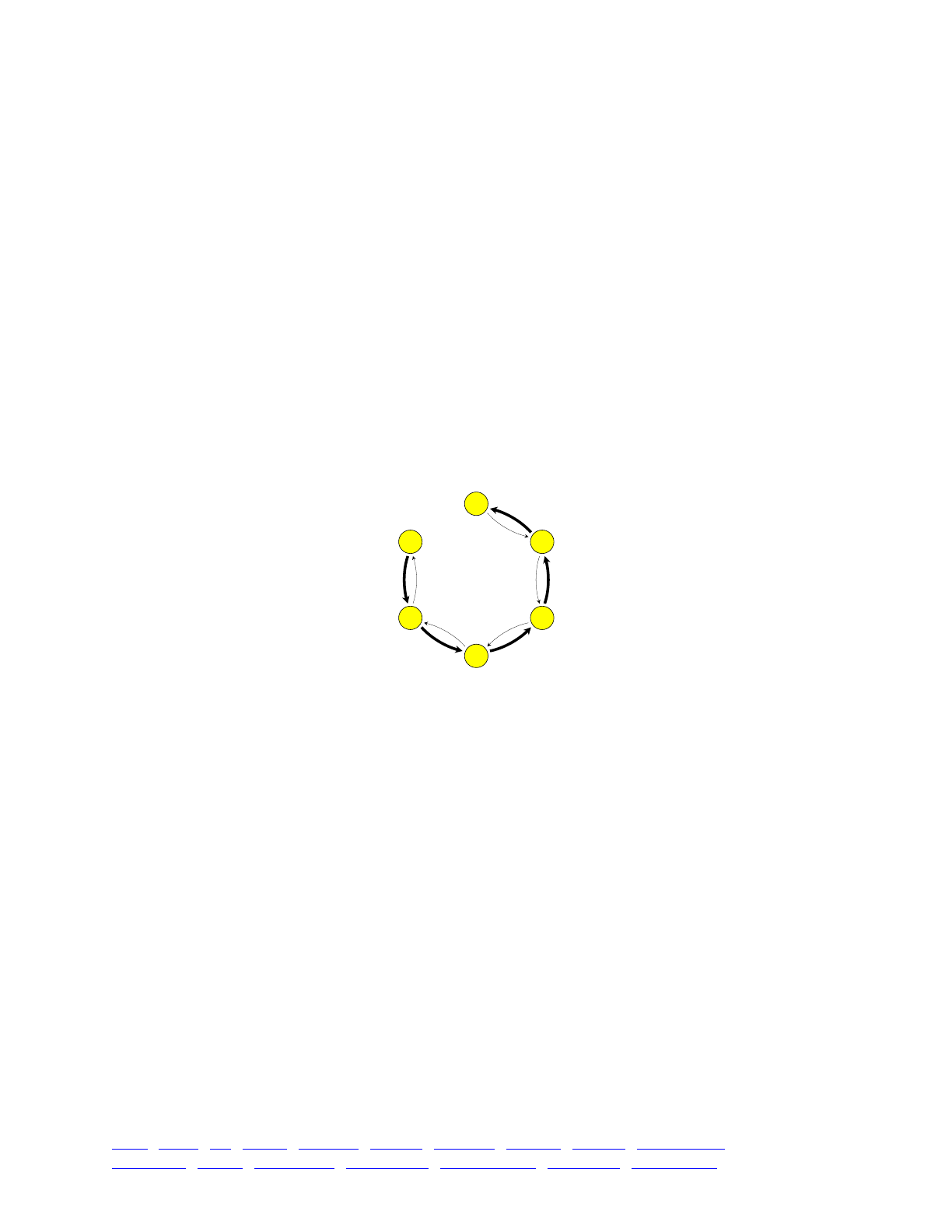
initialize() {!
initializeMutationRate(1e-7);!
initializeMutationType("m1", 0.5, "f", 0.0); // neutral!
initializeMutationType("m2", 0.5, "f", -0.1); // MCR complex!
initializeGenomicElementType("g1", m1, 1.0);!
initializeGenomicElement(g1, 0, 99999);!
initializeRecombinationRate(1e-8);!
}!
1 {!
for (i in 0:5)!
sim.addSubpop(i, 500);!
for (i in 1:5)!
sim.subpopulations[i].setMigrationRates(i-1, 0.001);!
for (i in 0:4)!
sim.subpopulations[i].setMigrationRates(i+1, 0.1);!
}!
10000 { sim.simulationFinished(); }
This sets up a six-subpopulation stepping-stone model, similar to that previously discussed in
section 5.3.1. Note that migration in this model is primarily from p5 down to p0; the migration
rate in that direction is a hundred times higher than in the direction from p0 up to p5:
The code above sets up a mutation type m2 for the MCR complex, but doesn’t use it, so at
present this is just a simulation of neutral drift in a stepping-stone model. Let’s start using mutation
type m2, although not yet with its planned MCR capabilities, by adding a little code to introduce an
m2 mutation and track its fate (the tracking block can replace the final script block in the previous
model):
100 late() {!
p0.genomes[0:49].addNewDrawnMutation(m2, 10000);!
}!
100:10000 late() {!
if (sim.countOfMutationsOfType(m2) == 0)!
{!
fixed = any(sim.substitutions.mutationType == m2);!
cat(ifelse(fixed, "FIXED\n", "LOST\n"));!
sim.simulationFinished();!
}!
}
The introduction code here simply introduces the mutation into the first 50 genomes of
subpopulation p0, without bothering to randomly select target individuals using sample().
Introducing the mutation into many genomes at once is a quick-and-dirty trick to help an
introduced mutation avoid being lost due to genetic drift at the earliest stages of establishment,
without putting in the machinery to make the simulation truly conditional on establishment as we
p0
p1
p2
p3
p4
p5
TOC I TOC II WF nonWF initialize() Genome Individual Mutation SLiMSim Subpopulation!
Eidos events fitness() mateChoice() modifyChild() recombination() interaction() reproduction() 174
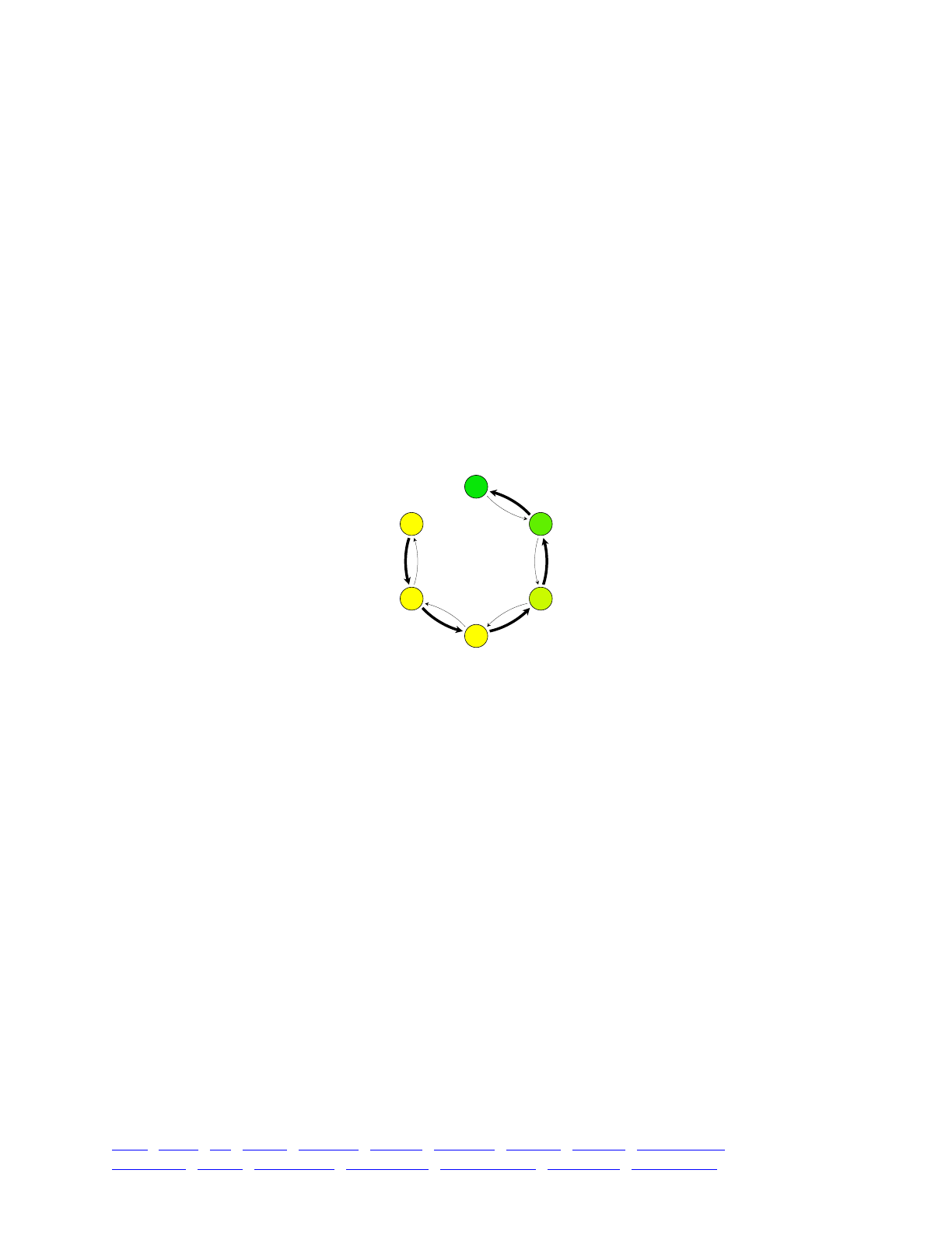
did in section 10.3. Biologically, it could be viewed as a large-scale immigration event, or as a
planned introduction of mutant individuals orchestrated by humans. See section 9.4.4 for
discussion of the Eidos mechanics underlying this mutation introduction code.
This model will generally terminate, perhaps around generation 140, with the message "LOST".
This is because mutation type m2 is strongly deleterious, as presently defined, and so gets
eliminated by selection fairly quickly even though it is initially introduced in fifty copies. Since
this is not very interesting, let’s move on to the next step: making mutation type m2 strongly
beneficial in subpopulation p0 and strongly deleterious in subpopulation p5, with gradations in
between, using a fitness() callback:
fitness(m2) {!
return 1.5 - subpop.id * 0.15;!
}
This fitness() callback uses subpop.id, the identifier of the subpopulation in which the
mutation is presently being evaluated, to generate a fitness of 1.5 for p0, but a fitness of 0.75 for
p5. If we run the model now, we see that it soon reaches an equilibrium state of migration-
selection balance:
It is at high frequency in p0 – nearly fixed, but prevented from fixing completely by gene flow
from p1. It is essentially absent from p5, on the other hand, since it is weeded out by selection,
and since gene flow in the p0 to p5 direction is so weak. The model will tend to maintain this
dynamic equilibrium.
Let’s add the modifyChild() callback that implements the MCR behavior of m2:
100:10000 modifyChild() {!
mut = sim.mutationsOfType(m2);!
if (size(mut) == 1)!
{!
hasMutOnChromosome1 = childGenome1.containsMutations(mut);!
hasMutOnChromosome2 = childGenome2.containsMutations(mut);!
if (hasMutOnChromosome1 & !hasMutOnChromosome2)!
childGenome2.addMutations(mut);!
else if (hasMutOnChromosome2 & !hasMutOnChromosome1)!
childGenome1.addMutations(mut);!
}!
return T;!
}
The first line just finds the introduced mutation by searching for it in the list of mutations kept by
the simulation; this is necessary because SLiM and Eidos don’t allow you to keep permanent
references to objects. The if statement tests whether we found the MCR mutation; in the final
generation of the simulation, when the mutation has either fixed or been lost, we won’t find it.
p0
p1
p2
p3
p4
p5
TOC I TOC II WF nonWF initialize() Genome Individual Mutation SLiMSim Subpopulation!
Eidos events fitness() mateChoice() modifyChild() recombination() interaction() reproduction() 175
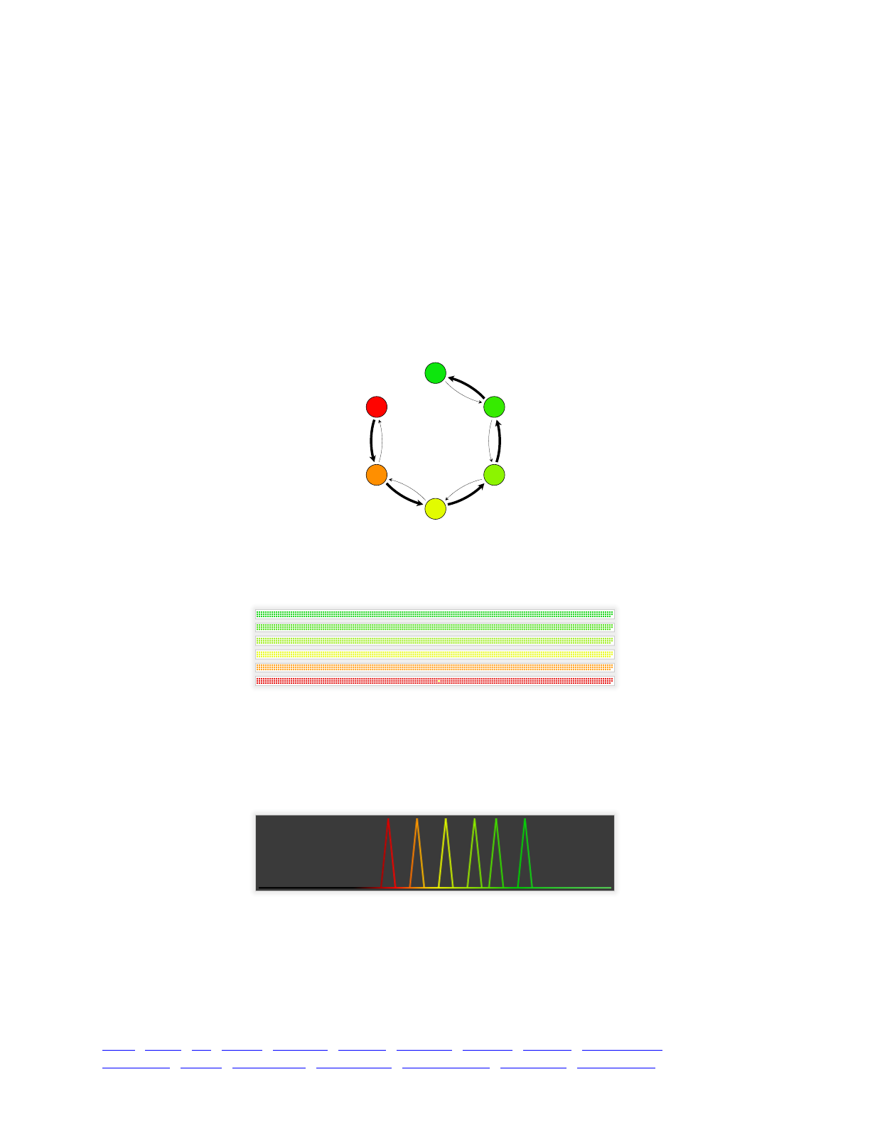
Assuming we do find the MCR mutation, we then check whether the particular child that we are
working with – the target of this modifyChild() operation – has the MCR mutation in either of its
genomes, using the containsMutations() method of Genome. With that information, the rest is
simple: if it is in one genome but not the other, we add the MCR mutation to the genome that
doesn’t already contain it, just as the CRISPR/Cas9 gene drive machinery for MCR would do in an
actual organism. If neither genome of the target contains the MCR gene, or if both genomes do,
we leave the child as it is. Finally, we return T, indicating that the child in question should in fact
be generated (a return of F would suppress generation; we saw an example of this in section 12.2).
If we recycle and run this model, it shows a consistent behavior of rapid fixation, even in the
subpopulations where it is deleterious, and even despite having to “swim upstream” against the
predominant direction of gene flow. At the moment just prior to complete fixation, the model
looks something like this (note that once the mutation actually fixes, it is removed from the
simulation and replaced by a substitution object, so the populations revert to yellow):
Incidentally, in snapshots like the one above, we’ve been using the Population Visualization
graph to see the state of the model, because it is a bit more informative than the default population
view, which doesn’t show population connectivity:
This display shows every individual in the model, colored according to its fitness. There are two
other display modes for the population view that can be useful, both of which summarize that
fitness distribution by binning the individual fitness values. These alternative display modes can be
selected with a right-click or control-click on the population view.
One alternative is to see line plots of binned fitness for each subpopulation, superimposed:
The x-axis represents fitness (from 0.0 to 2.0 in this case, but this is configurable in the options
panel that appears when this display mode is chosen). Fitness values are tallied into 50 bins (also
configurable), and the y-axis represents the frequency within each bin, from 0.0 to 1.0 within each
subpopulation. For this model, the resulting plot looks a bit like modern art, but the six peaks
correspond to the six subpopulations; the different fitness effects in the different subpopulations is
clearly visible, as is the fact that the mutation is about to fix.
p0
p1
p2
p3
p4
p5
TOC I TOC II WF nonWF initialize() Genome Individual Mutation SLiMSim Subpopulation!
Eidos events fitness() mateChoice() modifyChild() recombination() interaction() reproduction() 176

Another possibility is to see a histogram of binned fitness values across all of the
subpopulations. This is similar to the line plot of fitness frequencies above, except that all of the
subpopulations are tallied together, not individually:
Again the x-axis represents fitness and the y-axis represents frequency within a bin (now from
0.0 to 1.0 population-wide). The six subpopulations can again be seen here.
These alternative population visualizations can be a useful tool in understanding model
dynamics, especially for models with many subpopulations and/or many individuals.
For reference, here is the full gene drive model with all of the components introduced above:
initialize() {!
initializeMutationRate(1e-7);!
initializeMutationType("m1", 0.5, "f", 0.0); // neutral!
initializeMutationType("m2", 0.5, "f", -0.1); // MCR complex!
initializeGenomicElementType("g1", m1, 1.0);!
initializeGenomicElement(g1, 0, 99999);!
initializeRecombinationRate(1e-8);!
}!
1 {!
for (i in 0:5)!
sim.addSubpop(i, 500);!
for (i in 1:5)!
sim.subpopulations[i].setMigrationRates(i-1, 0.001);!
for (i in 0:4)!
sim.subpopulations[i].setMigrationRates(i+1, 0.1);!
}!
100 late() {!
p0.genomes[0:49].addNewDrawnMutation(m2, 10000);!
}!
100:10000 late() {!
if (sim.countOfMutationsOfType(m2) == 0) {!
fixed = any(sim.substitutions.mutationType == m2);!
cat(ifelse(fixed, "FIXED\n", "LOST\n"));!
sim.simulationFinished();!
}!
}!
fitness(m2) {!
return 1.5 - subpop.id * 0.15;!
}!
100:10000 modifyChild() {!
mut = sim.mutationsOfType(m2);!
if (size(mut) == 1) {!
hasMutOnChromosome1 = childGenome1.containsMutations(mut);!
hasMutOnChromosome2 = childGenome2.containsMutations(mut);!
if (hasMutOnChromosome1 & !hasMutOnChromosome2)!
childGenome2.addMutations(mut);!
else if (hasMutOnChromosome2 & !hasMutOnChromosome1)!
childGenome1.addMutations(mut);!
}!
return T;!
}
TOC I TOC II WF nonWF initialize() Genome Individual Mutation SLiMSim Subpopulation!
Eidos events fitness() mateChoice() modifyChild() recombination() interaction() reproduction() 177

It has been proposed that MCR could have many compelling applications, such as driving
particular mosquito species – those that carry important human diseases such as malaria – toward
extinction, or at least driving a potentially deleterious gene for resistance to diseases like malaria
toward fixation in those mosquito species. To know whether such proposals are realistic, however,
we need to model them. In this section we developed a simple toy model of MCR; a model useful
for real-world prediction would need many additional ramifications, of course, but this is a starting
point for further exploration.
12.4 Suppressing hermaphroditic selfing
In section 6.3.1, it was noted that a low rate of selfing will normally be observed in SLiM in
hermaphroditic models, even when the selfing rate is explicitly set to zero. This occurs because
SLiM chooses each of the parents in a biparental mating randomly (weighted according to fitness),
and does not explicitly prevent the same individual from being chosen as both parents. Normally
this does not present a problem; it is typically a very small effect, and indeed it is sometimes
desirable since the model will then better match the predictions from some simple analytical
models. Sometimes, however, this selfing does prove to be an issue (particularly with small
effective population sizes or high variance in fitness). In such cases, it can be prevented with a
call at the beginning of the initialize() callback of your script:
initializeSLiMOptions(preventIncidentalSelfing=T);
Before this option was added to SLiM, preventing incidental selfing required a simple
modifyChild() callback, illustrated by this section’s recipe. This recipe is now obsolete, since it
has been superseded by the configuration flag shown above; but it has been retained in the
cookbook as an illustration of how modifyChild() callbacks can be used to perform simple
changes to mating behavior of this sort. The original, now-obsolete recipe used this callback:
modifyChild()!
{!
// prevent hermaphroditic selfing!
if (parent1 == parent2)!
return F;!
return T;!
}
This can simply be dropped in to more or less any hermaphroditic model, such as this:
initialize() {!
initializeMutationRate(1e-7);!
initializeMutationType("m1", 0.5, "f", 0.0);!
initializeGenomicElementType("g1", m1, 1.0);!
initializeGenomicElement(g1, 0, 99999);!
initializeRecombinationRate(1e-8);!
}!
1 { sim.addSubpop("p1", 500); }!
2000 late() { sim.outputFixedMutations(); }
It will then suppress the selfing events, by returning F (and thus suppressing the proposed child)
whenever the two parents of the proposed child are the same. This could be implemented as a
mateChoice() callback instead, by changing the weight for the already-chosen first parent to 0, but
that would be much slower since a modified mating-weights vector would have to be built for
each mating event. Often, as here, suppressing specific mating combinations is most easily and
efficiently done with a modifyChild() callback instead.
TOC I TOC II WF nonWF initialize() Genome Individual Mutation SLiMSim Subpopulation!
Eidos events fitness() mateChoice() modifyChild() recombination() interaction() reproduction() 178

There are two caveats. The first is that if you turn selfing on in your model this modifyChild()
callback will then cause your model to hang, because SLiM will keep trying to satisfy your
requested selfing rate, whereas the callback will keep preventing it from doing so. If you need to
attain exactly the requested selfing rate, however, while suppressing the background selfing events
generated randomly by SLiM, you can just add a check of the isSelfing flag provided to the
modifyChild() callback (see section 22.4). For selfing events that are intended by SLiM to satisfy
the requested selfing rate, this flag will be T; for any additional background selfing events caused
by random mate choice, this flag will be F. Suppressing only the selfing events in which
isSelfing is F ought to produce the desired effect. (You could also do a bit of math and set an
adjusted selfing rate that accounts for the background selfing rate, but that is perhaps more error-
prone.)
The other caveat is that if you define other modifyChild() callbacks as well, you might want to
think about how the multiple callbacks will stack together. Typically you would want this selfing-
suppression callback to occur first in the chain, and thus you would want to define it earliest in
your script. See section 22.8 for discussion of this issue.
TOC I TOC II WF nonWF initialize() Genome Individual Mutation SLiMSim Subpopulation!
Eidos events fitness() mateChoice() modifyChild() recombination() interaction() reproduction() 179

13. Advanced models
This chapter will present some advanced models that draw upon many of the concepts covered
in previous chapters, while also using relatively advanced features of Eidos and SLiM that may not
have been covered in previous recipes. A knowledge of the topics covered in previous chapters
will be assumed, and simple details will not be explained in depth, to keep things short.
13.1 Quantitative genetics and phenotypically-based fitness
In this recipe we will explore a quantitative genetics model in which a phenotypic trait is based
upon multiple loci with additive effects. In some respects this is similar to the model of polygenic
selection developed in section 9.3.2; however, this model goes much further, explicitly modeling
the phenotypic effect of the quantitative trait and producing a fitness effect based upon that
phenotype. This recipe will model a trait based on 10 quantitative trait loci (QTLs), each of which
can have a value of either −1 or +1; this is a common design for models of quantitative traits, but
the model does not strongly depend upon this choice. (For a quantitative genetics model that uses
QTLs with continuous effects and incorporates heritability, see section 13.10.)
This model also incorporates two-subpopulation structure, with limited gene flow between the
subpopulations. The two subpopulations experience different environments that are selecting for
different optima; unlike the model in section 9.2, however, the two environments are selecting for
different phenotypes, as determined by all of the loci underlying the trait, rather than just exerting
differential selection on each individual locus.
This model also includes assortative mating. Unlike the model of section 11.1, where mating
was assortative based upon possession of a single introduced mutation, here mating is assortative
based upon the phenotype produced by all the underlying loci. This means that mating can
actually be disassortative at the genetic level, because individuals with the same phenotype might
achieve that phenotype through entirely different QTLs alleles.
The genetic structure used here simulates ten separate chromosomes, with one QTL on each
chromosome. SLiM simulates only one Chromosome object, but since the recombination map can
be specified arbitrarily, a recombination rate of 0.5 between specific pairs of bases can be used to
effectively subdivide that Chromosome object into separate chromosomes that have no linkage
between them. This model places each QTL at the center of its chromosome, with 1000 bases on
each side experiencing neutral mutations, but those choices are easily changed.
Finally, relatively complex custom output code in this model assesses and prints information
about the genetic structure and fitness of each subpopulation at the beginning and end of the
simulation, illustrating how SLiM’s output can be customized.
We will start with the initialization portion of this model’s script:
initialize() {!
initializeMutationRate(1e-5);!
!
// neutral mutations in non-coding regions!
initializeMutationType("m1", 0.5, "f", 0.0);!
initializeGenomicElementType("g1", m1, 1.0);!
!
// mutations representing alleles in QTLs!
scriptForQTLs = "if (runif(1) < 0.5) -1; else 1;";!
initializeMutationType("m2", 0.5, "s", scriptForQTLs);!
initializeGenomicElementType("g2", m2, 1.0);!
m2.convertToSubstitution = F;!
m2.mutationStackPolicy = "l";!
!
TOC I TOC II WF nonWF initialize() Genome Individual Mutation SLiMSim Subpopulation!
Eidos events fitness() mateChoice() modifyChild() recombination() interaction() reproduction() 180

// set up our chromosome: 10 QTLs, surrounded by neutral regions!
defineConstant("C", 10); // number of QTLs!
defineConstant("W", 1000); // size of neutral buffer on each side!
pos = 0;!
q = NULL;!
!
for (i in 1:C)!
{!
initializeGenomicElement(g1, pos, pos + W-1);!
pos = pos + W;!
!
initializeGenomicElement(g2, pos, pos);!
q = c(q, pos);!
pos = pos + 1;!
!
initializeGenomicElement(g1, pos, pos + W-1);!
pos = pos + W;!
}!
!
defineConstant("Q", q); // remember our QTL positions!
!
// we want the QTLs to be unlinked; build a recombination map for that!
rates = c(rep(c(1e-8, 0.5), C-1), 1e-8);!
ends = (repEach(Q + W, 2) + rep(c(0,1), C))[0:(C*2 - 2)];!
initializeRecombinationRate(rates, ends);!
}
This sets up two mutation types: m1, representing neutral mutations, and m2, representing
mutations at QTLs. The m2 mutation type draws its mutational effects from a user-specified
distribution, rather than from one of SLiM’s built-in mutational distributions. It does this by
specifying the mutation type as "s", for “script”, and then supplying a short Eidos snippet as a
string. That snippet is run as a lambda (see section 17.5) by SLiM whenever it needs to draw a
new selection coefficient. The m2 mutation type is also set not to be removed when it fixes
(because QTLs will continue to influence phenotype, and thus relative fitness, even after fixation);
and it is set to use a “last mutation” stacking policy, so that when a new mutation occurs at a given
QTL it replaces the allele that was previously at that site, rather than “stacking” with it as is SLiM’s
default behavior.
Two genomic element types are also set up by this code: g1, representing neutral buffer zones
around the QTLs, and g2, representing QTLs themselves. The rest of this initialize() callback
sets up the chromosome by tiling these genomic element types, and setting up a recombination
map that effectively places each QTL on an independent chromosome as explained above.
This model makes somewhat liberal use of the defineConstant() call of Eidos to set up
constants related to the genomic structure of the simulation. Defined constants are much like
variables, except that they cannot be redefined (except by removing them with rm() first), and they
persist for the lifetime of the simulation rather than disappearing at the end of the callback in
which they are defined. They are thus very useful for symbolically representing model parameters;
this model also defines a constant Q to remember the positions of all of the QTLs being simulated.
After this initialization() callback has run, the genetic structure of the simulation looks like
this in SLiMgui (with display of genomic elements and recombination rates enabled):
TOC I TOC II WF nonWF initialize() Genome Individual Mutation SLiMSim Subpopulation!
Eidos events fitness() mateChoice() modifyChild() recombination() interaction() reproduction() 181

This shows the pattern of non-coding regions and QTLs (below), and the recombination
breakpoints that define the breaks between effective chromosomes in the model (above).
Next we will set up (most of) the initial population state of the simulation:
1 early() {!
sim.addSubpop("p1", 500);!
sim.addSubpop("p2", 500);!
!
// set up migration; comment these out for zero gene flow!
p1.setMigrationRates(p2, 0.01);!
p2.setMigrationRates(p1, 0.01);!
!
sim.registerEarlyEvent("s2", s1.source, 2, 2);!
}!
1 late() {!
// optional: give m2 mutations to everyone, as standing variation!
// if this is commented out, QTLs effectively start as 0!
g = sim.subpopulations.genomes;!
n = size(g);!
!
for (q in Q)!
{!
isPlus = asLogical(rbinom(n, 1, 0.5));!
g[isPlus].addNewMutation(m2, 1.0, q);!
g[!isPlus].addNewMutation(m2, -1.0, q);!
}!
}
The early() callback sets up two subpopulations with migration between them. It also
contains a call to registerEarlyEvent() that will not run right now; if you want to run the model
at this stage you will need to comment that out. It will be explained below.
The late() callback is optional, and sets up the initial state of the QTLs in the model by placing
initial mutations in them. It does this by looping over all of the QTLs, and for each QTL, deciding
whether each genome in the simulation will start with a + or a − allele by drawing from a binomial
distribution. It then distributes the + and − alleles to all of the genomes by calling
addNewMutation() to add the chosen allele to each genome, in a twist on the pattern seen
previously in section 9.4.4 and elsewhere. This code results in just two mutation objects being
created to represent the + and − alleles of each QTL, rather than a different mutation object being
created for each genome, for reasons explained in detail in section 9.4.4; here this is a non-
essential detail, but it improves the efficiency of the model since fewer mutation objects need to be
tracked. This whole callback can be removed, in which case the model starts with no QTL
mutations, producing an effective value of zero for each QTL until new mutations arise. That
would be a model of emerging genetic diversity from a clonal population, then, rather than this
model of selection beginning with a high degree of random standing genetic variation.
Next comes a bunch of callbacks that implement the quantitative trait machinery:
1: late() {!
// construct phenotypes for the additive effects of QTLs!
inds = sim.subpopulations.individuals;!
inds.tag = asInteger(inds.sumOfMutationsOfType(m2));!
}!
fitness(m2) {!
// the QTLs themselves are neutral; their effect is handled below!
return 1.0;!
}!
TOC I TOC II WF nonWF initialize() Genome Individual Mutation SLiMSim Subpopulation!
Eidos events fitness() mateChoice() modifyChild() recombination() interaction() reproduction() 182

fitness(NULL, p1) {!
// optimum of +10!
return 1.0 + dnorm(10.0 - individual.tag, 0.0, 5.0);!
}!
fitness(NULL, p2) {!
// optimum of -10!
return 1.0 + dnorm(-10.0 - individual.tag, 0.0, 5.0);!
}
The late() callback is called in every generation to calculate the phenotypes of individuals by
summing up the additive effects of all QTLs possessed by each individual. We get a vector
containing all individuals in the model, and for each individual we sum up the selection
coefficients of all of the m2 mutations possessed by that individual using sumOfMutationsOfType()
method, and place the sums into the individuals’ tag properties with a vectorized assignment.
Note that this code would work with QTLs of any effect size, not just the +/− scheme used here,
except that the individual’s tag property is of type integer, which would lead to roundoff
problems with QTLs of fractional value. That could be avoided by using the tagF property, which
stores float values instead of integer values. Once that change was made, across the whole
recipe, the phenotype values would then be saved and retrieved as type float, so the distribution
of fitness effects could then be changed to any DFE desired (see section 13.10). This recipe uses a
+/− DFE and integer phenotypes, partly because that is common in theoretical multilocus models,
and partly for historical reasons. One could also use the getValue() and setValue() methods of
Individual to keep the phenotype state, rather than using tag or tagF (see section 21.6.2). In
other words, where this recipe saves away the calculated phenotypic value of an individual with
individual.tag = ..., one would use individual.setValue("phenotype", ...) instead, and
everywhere that this recipe gets a saved phenotypic value using individual.tag, one would use
individual.getValue("phenotype") instead. (The string identifier "phenotype" is not special; it
could just as well be "foo".) This would, however, be substantially slower than using tagF.
The first fitness() callback simply makes all m2 mutations neutral, regardless of their stated
selection coefficient. This is because we are using the selection coefficients of m2 mutations here
to represent their phenotypic effect size, in the sense of additive quantitative genetics, rather than
their actual selection coefficients; we therefore wish to disable their direct effect on fitness.
Finally, we have a pair of fitness() callbacks declared with a mutation type identifier of NULL:
one for subpopulation p1, one for p2. We haven’t seen this use of fitness() callbacks before; the
NULL identifier indicates that the callback is not intended to modify the fitness effects of mutations
of a particular mutation type, but rather, provides a fitness effect for the individual as a whole. For
this reason, fitness(NULL) callbacks are referred to as global fitness callbacks (see section 22.2).
They are called once for each individual in the specified subpopulation, and the fitness effect they
return is multiplied into all of the other fitness effects for the individual. The fitness effect of a
global fitness() callback might depend upon any state of the individual; here it depends on the
phenotype of the individual compared to the phenotypic optimum. Since m1 and m2 mutations are
all neutral in this model, these fitness(NULL) callbacks are the sole determinants of individual
fitness in this model. They implement fitness based on a Gaussian fitness function, as is typical in
models of this sort, with fitness being highest at some phenotypic optimum, and falling away for
phenotypic values both lower and higher than that optimum. The phenotypic values of individuals
are fetched out of their tag properties, which were set up by the late() event that ran previously.
Note that a baseline of 1.0 is added to the Gaussian value since 1.0 indicates neutrality on the
relative fitness scale; see section 13.10 for further discussion of this choice.
This implements the bulk of the model. We will now add assortative mate choice based on
phenotype, which is very simple since the underlying machinery has already been constructed:
TOC I TOC II WF nonWF initialize() Genome Individual Mutation SLiMSim Subpopulation!
Eidos events fitness() mateChoice() modifyChild() recombination() interaction() reproduction() 183

mateChoice() {!
phenotype = asFloat(individual.tag);!
others = asFloat(sourceSubpop.individuals.tag);!
return weights * dnorm(others, phenotype, 5.0);!
}
This multiplicatively combines the existing fitness-based weights for all potential mates with
mating weights based on a Gaussian function that rewards phenotypic similarity.
Incidentally, it might be of interest to note that now the quantitative trait is something
resembling a magic trait, since it is under divergent ecological selection and influences mate
choice. However, it is not in fact a magic trait, since it is based upon multiple loci. The individual
QTLs might be considered “magic genes” since they perhaps satisfy the criteria of the formal
definition (Servedio et al. 2011), but since there is epistasis between them (because of the way they
combine additively to determine the quantitative phenotype that is actually under selection), it is
not entirely clear how they relate to the usual intuitive meaning of “magic trait”.
Finally, we will add some custom output by tallying up fitnesses, phenotypes, and frequencies:
s1 2001 early() {!
cat("-------------------------------\n");!
cat("Output for end of generation " + (sim.generation - 1) + ":\n\n");!
!
// Output population fitness values!
cat("p1 mean fitness = " + mean(p1.cachedFitness(NULL)) + "\n");!
cat("p2 mean fitness = " + mean(p2.cachedFitness(NULL)) + "\n");!
!
// Output population additive QTL-based phenotypes!
cat("p1 mean phenotype = " + mean(p1.individuals.tag) + "\n");!
cat("p2 mean phenotype = " + mean(p2.individuals.tag) + "\n");!
!
// Output frequencies of +1/-1 alleles at the QTLs!
muts = sim.mutationsOfType(m2);!
plus = muts[muts.selectionCoeff == 1.0];!
minus = muts[muts.selectionCoeff == -1.0];!
!
cat("\nOverall frequencies:\n\n");!
for (q in Q)!
{!
qPlus = plus[plus.position == q];!
qMinus = minus[minus.position == q];!
pf = sum(sim.mutationFrequencies(NULL, qPlus));!
mf = sum(sim.mutationFrequencies(NULL, qMinus));!
pf1 = sum(sim.mutationFrequencies(p1, qPlus));!
mf1 = sum(sim.mutationFrequencies(p1, qMinus));!
pf2 = sum(sim.mutationFrequencies(p2, qPlus));!
mf2 = sum(sim.mutationFrequencies(p2, qMinus));!
!
cat(" QTL " + q + ": f(+) == " + pf + ", f(-) == " + mf + "\n");!
cat(" in p1: f(+) == " + pf1 + ", f(-) == " + mf1 + "\n");!
cat(" in p2: f(+) == " + pf2 + ", f(-) == " + mf2 + "\n\n");!
}!
}
This runs at the beginning of generation 2001, so as to produce output regarding the very end of
generation 2000, after fitness values have been calculated; calling cachedFitness() in a late()
event in generation 2000 would raise an error, since fitness values are not yet available at that point
in the generation cycle. Note that the purpose is now clear of the line we saw before:
TOC I TOC II WF nonWF initialize() Genome Individual Mutation SLiMSim Subpopulation!
Eidos events fitness() mateChoice() modifyChild() recombination() interaction() reproduction() 184

sim.registerEarlyEvent("s2", s1.source, 2, 2);
This output callback is script block s1, which that line of code replicates as an early() event in
generation 2, so that it produces output at both the beginning and the end of the model run. If
SLiM’s syntax for specifying the generations in which a callback runs were more general, this trick
would not be needed; but there is no way to say “run this callback only in generations 2 and
2001”, at present, so this is a simple way to achieve that.
Running this model produces output something like this:
Output for generation 1:!
!
p1 mean fitness = 1.02108!
p2 mean fitness = 1.0219!
p1 mean phenotype (optimum +10) = 0.176!
p2 mean phenotype (optimum -10) = -0.34!
!
Overall frequencies:!
!
QTL at 1000: f(+) == 0.5125, f(-) == 0.4875!
in p1: f(+) == 0.527, f(-) == 0.473!
in p2: f(+) == 0.498, f(-) == 0.502!
...!
-------------------------------!
Output for generation 2000:!
!
p1 mean fitness = 1.06406!
p2 mean fitness = 1.06221!
p1 mean phenotype (optimum +10) = 8.296!
p2 mean phenotype (optimum -10) = -8.14!
!
Overall frequencies:!
!
QTL at 1000: f(+) == 0.504, f(-) == 0.496!
in p1: f(+) == 0.848, f(-) == 0.152!
in p2: f(+) == 0.16, f(-) == 0.84!
...
It can be seen that in the initial state of the model both subpopulations have phenotypes near
0.0, fitnesses of essentially 1.0, and a random distribution of + and − QTL alleles. In the final
state, on the other hand, phenotypes have diverged most of the way to their local environmental
optima of +10 and −10, mean relative fitness is up to about 1.06 in both subpopulations as a result,
and substantial divergence at the level of individual QTL alleles can be observed. This divergence
appears to be substantially due to the assortative mating in the model, since a sample run with the
mateChoice() callback commented out results in considerably less divergence:
p1 mean fitness = 1.04107!
p2 mean fitness = 1.04752!
p1 mean phenotype (optimum +10) = 3.876!
p2 mean phenotype (optimum -10) = -5.584
Of course lots of replicate runs with different parameter values, etc., would be needed to
substantiate this; but it seems to agree with other models of assortative mating and divergence.
This model includes neutral diversity at loci surrounding each QTL; no attempt has been made
to analyze that here, but presumably there might be interesting patterns related to patterns of gene
flow, hitchhiking, and so forth. Increasing the length of the neutral buffers around the QTL
TOC I TOC II WF nonWF initialize() Genome Individual Mutation SLiMSim Subpopulation!
Eidos events fitness() mateChoice() modifyChild() recombination() interaction() reproduction() 185

(defined constant W), and/or increasing the recombination rate, would probably be helpful for
making these patterns more clear.
Section 13.10 presents a fairly different quantitative genetics model, using QTLs with effect
sizes drawn from a continuous distribution, and incorporating heritability, but with only a single
subpopulation, with no predetermined genetic structure, and without assortative mating.
13.2 Relatedness, inbreeding, and heterozygosity
Inbreeding is an important concept in evolutionary biology, but it is not very precisely defined.
It can result from a variety of processes, from small population size to assortative mating, and it
can manifest in a variety of genetic patterns, such as decreased heterozygosity, loss of genetic
diversity, and a decreased time to the most recent common ancestor of pairs of individuals. The
particular effects of inbreeding observed in a system may depend on the process generating the
inbreeding. So before embarking on a study of inbreeding, one should define one’s terms clearly.
Here, we will construct a model of inbreeding that results from a tendency of individuals to
mate with their close kin, as defined by their pedigree-based relatedness. SLiM (beginning in
version 2.1) has a built-in facility for tracking this type of relatedness, which can be turned on with
the call initializeSLiMOptions(keepPedigrees=T) in the initialize() callback of a script (see
section 21.1). When this call is made, individuals in a simulation will keep track of the identities
of their parents and grandparents, and the relatedness between individuals can then be assessed
using the relatedness() method of Individual (see section 21.6.2). The pedigree information is
also available through properties on the Individual class (section 21.6.1), for purposes such as
locating “trios” (two parents and an offspring that they generated) for analysis.
It should be emphasized that the relatedness metric available through this mechanism is purely
pedigree-based. This can be quite different from genetic relatedness, which depends not only on
pedigree but also on factors such as assortment and recombination (see section 13.9). The
inbreeding generated by this model will be based upon this relatedness metric.
With that as preamble, here is the first stage of the model:
initialize() {!
initializeSLiMOptions(keepPedigrees = T);!
initializeMutationRate(1e-5);!
initializeMutationType("m1", 0.5, "f", 0.0);!
initializeGenomicElementType("g1", m1, 1.0);!
initializeGenomicElement(g1, 0, 99999);!
initializeRecombinationRate(1e-7);!
}!
1 {!
sim.addSubpop("p1", 100);!
}!
1000 late() {!
// Calculate mean nucleotide heterozygosity across the population!
total = 0.0;!
!
for (ind in p1.individuals)!
{!
// Calculate the nucleotide heterozygosity of this individual!
muts0 = ind.genomes[0].mutations;!
muts1 = ind.genomes[1].mutations;!
!
// Count the shared mutations!
shared_count = sum(match(muts0, muts1) >= 0);!
!
TOC I TOC II WF nonWF initialize() Genome Individual Mutation SLiMSim Subpopulation!
Eidos events fitness() mateChoice() modifyChild() recombination() interaction() reproduction() 186

// All remaining mutations are unshared (i.e. heterozygous)!
unshared_count = muts0.size() + muts1.size() - 2 * shared_count;!
!
// pi is the mean heterozygosity across the chromosome!
pi_ind = unshared_count / (sim.chromosome.lastPosition + 1);!
total = total + pi_ind;!
}!
!
pi = total / p1.individuals.size();!
!
cat("Mean nucleotide heterozygosity = " + pi + "\n");!
}
This is a simple neutral model, similar to those we have seen before. It turns on pedigree
tracking in its initialize() callback, and then runs for 1000 generations. At the end of the run, a
late() callback computes the mean nucleotide heterozygosity (π) across the population. For one
individual, the nucleotide heterozygosity is the fraction of base positions that are heterozygous.
This is calculated by getting the mutations from the two genomes of the individual and finding the
number of mutations that are shared between them (adding the number of matches from match()
with sum()). The two genomes must together contain 2 * shared_count of these shared mutations;
all the remaining mutations in the genomes are unshared, and thus heterozygous. Dividing the
number of unshared mutations by the length of the chromosome (+1 because lastPosition is a
zero-based value) yields the individual’s nucleotide heterozygosity. (Note that reuseable functions
to calculate heterozygosity are now in the SLiM-Extras repository online, too, with a different
implementation using setSymmetricDifference(); for now, this recipe doesn't use that code.)
So now we have a baseline model that has only whatever inbreeding results from its small
population size of 100 individuals. Now let’s add a mateChoice() callback that uses the pedigree
tracking information to create a mating preference for kin:
mateChoice() {!
// Prefer relatives as mates!
return weights * (individual.relatedness(sourceSubpop.individuals) +!
0.01);!
}
This uses the relatedness() method of Individual to calculate the relatedness between the
focal individual that is choosing a mate (individual) and all of its potential mates
(sourceSubpop.individuals). A constant of 0.01 is added to those values to guard against the
possibility that all of the values would be exactly zero; that would result in a weights vector of all
zeros being returned to SLiM, which is illegal (see the discussion in section 22.3). In fact, this
particular model is safe from that problem, because the relatedness of an individual to itself is 1.0,
and so individuals will always be able to mate with themselves; but the safeguard is shown here to
raise awareness of the issue, since in many other types of models this issue will need to be
considered – sexual models, models with multiple subpopulations and migration, etc. Finally, the
relatedness values are multiplied by weights, the vector of default mating weights supplied to the
callback by SLiM. Again, this is not important for this model (as a neutral, non-sexual model,
weights will be a vector of all 1), but it is important for models more generally, so that the fitness-
based mating weights are taken into account even when a mateChoice() callback is implemented.
Without this, the fitness-based mating weights computed by SLiM would be completely replaced
by the mateChoice() callback, making all selection coefficients and fitness() callbacks irrelevant
– rarely what is wanted.
This particular callback makes the mating weights be (almost) proportional to relatedness.
Individuals that share no grandparents will have a mating weight of only 0.01, whereas full siblings
TOC I TOC II WF nonWF initialize() Genome Individual Mutation SLiMSim Subpopulation!
Eidos events fitness() mateChoice() modifyChild() recombination() interaction() reproduction() 187

will have a weight of 0.51 and an individual will have a weight of 1.01 for hermaphroditic selfing.
This should generate fairly strong inbreeding. Of course a mateChoice() callback could rescale or
otherwise modify these values to produce whatever mating preferences are desired.
That’s all of the code needed for the model; the bulk of the code is actually the heterozygosity
calculation, and the relatedness-based mating preference requires just a one-line mateChoice()
callback. If we run this model five times with the mateChoice() callback, the average of the
reported heterozygosity values across those runs is 0.00163, whereas the average across five runs
without the mate choice callback is 0.00426. Clearly the mateChoice() callback is having a
pronounced effect on the nucleotide heterozygosity observed in the model, as intended (with a
two-sample independent t-test p-value of 0.0011, if you’re skeptical).
Incidentally, it would also be possible to implement the tendency towards mating with kin using
a modifyChild() callback instead. That callback would evaluate the relatedness of the two parents
of the proposed child, and would tell SLiM to short-circuit generation of the child, with some
probability, if the relatedness of the parents was not sufficiently high. If only a weak inbreeding
effect is desired, this might be much faster than the mateChoice() scheme shown above, since for
the generation of a typical child only one or a few relatedness values would need to be calculated,
and the relatively large overhead of running the mateChoice() callback would be avoided. This
should be very simple, so it is left as an exercise for the reader.
13.3 Mortality-based fitness
Normally, SLiM uses fitness values as mating weights: high-fitness individuals are more likely to
be chosen as mates than low-fitness individuals (see section 19.2.2). By default, SLiM does not
model mortality; there is no concept of individuals dying before reaching reproductive age (except
for the suppression of child generation with a modifyChild() callback, which can be viewed as a
type of mortality-based fitness; see chapter 12). However, it is straightforward to add mortality to a
model: if model mechanics dictate that an individual dies, then it can be given a fitness of zero,
which means that it cannot possibly be chosen as a mate; effectively, it has been removed from the
population (although it will remain as an individual in the population until the next generation
starts; there is no way to actually remove dead individuals from the population).
(Note that this section is aimed primarily towards WF models; in nonWF models, as discussed
in section 1.6, fitness translates into mortality anyway, rather than influencing mating, so every
nonWF model is a model of mortality-based fitness. However, in nonWF models it can still be
useful to explicitly kill off a specific individual by making its fitness zero; see, for example, the
recipe in section 15.5.)
Here we will look at three different models of how mortality might be implemented. One
model converts the fitness effects of mutations directly into mortality using a fitness() callback.
This might be a good way to model death due to deleterious genetic factors. The second model is
a tag-based model (see section 1.3 and sections cited therein); if individuals die, their tag value is
set to zero, and then a special fitness() callback is used to reduce the fitness of tagged
individuals to zero. This might be a good way to model death due to non-genetic factors, such as
predation. The third model uses the fitnessScaling property of Individual, a new feature
introduced in SLiM 3.0.
One question regarding mortality-based fitness might be: what difference does this make? Why
would one wish to model mortality-based fitness rather than (or in addition to) mating-based
fitness? The answer is that the two types of fitness have different effects on the distribution of the
number of offspring generated by individuals. With mating-based fitness, all individuals of a given
low fitness value are equal in the offspring-production game; the expected number of offspring is
the same for all, and is lower than the expected number of offspring for a high-fitness individual.
TOC I TOC II WF nonWF initialize() Genome Individual Mutation SLiMSim Subpopulation!
Eidos events fitness() mateChoice() modifyChild() recombination() interaction() reproduction() 188

With mortality-based fitness, however, all individuals of a given low fitness value are not equal, by
the time mating season arrives: some are alive, and some are dead. Those that are alive have an
expected number of offspring that is just as high as a high-fitness individual; they survived to
mating season, and now the playing field is even. Those that are dead, on the other hand, have an
expected number of offspring of zero. What the evolutionary consequences of this difference
might be is not the focus here; but there clearly is a difference, and so we want to be able to
model mortality-based fitness.
So, with no further ado, let’s look at our first model:
initialize() {!
initializeMutationRate(1e-7);!
!
initializeMutationType("m1", 0.5, "f", 0.0);!
initializeMutationType("m2", 0.5, "f", -0.005); // deleterious!
m2.convertToSubstitution = F;!
!
initializeGenomicElementType("g1", c(m1,m2), c(1.0,0.1));!
initializeGenomicElement(g1, 0, 99999);!
initializeRecombinationRate(1e-8);!
}!
1 {!
sim.addSubpop("p1", 500);!
}!
fitness(m2)!
{!
// convert fecundity-based selection to survival-based selection!
if (runif(1) < relFitness)!
return 1.0;!
else!
return 0.0;!
}!
10000 late() {!
sim.outputMutations(sim.mutationsOfType(m2));!
}
Mutations are mostly neutral (m1) but occasionally slightly deleterious (m2), and the deleterious
mutations are not converted to substitutions when they fix (using m2.convertToSubstitution = F),
since they should continue to cause mortality. At the end of a run, the model uses
outputMutations() to print information about all of the m2 mutations existing in the population
(include those that have fixed, since they do not get substituted).
The interesting part of the model is the fitness() callback. It converts a fitness effect for an m2
mutation (which will be 0.995 if homozygous and 0.9975 if heterozygous, given the dominance
coefficient of 0.5 used for m2) into either 0 or 1, with the probability of a fitness of 1 being equal to
the fitness effect of the focal mutation in the individual. If the new fitness value is 0, the focal m2
mutation has resulted in mortality; the individual will not mate, and is effectively dead. If the new
fitness is 1, on the other hand, the individual has survived the deleterious effects of the focal m2
mutation, and that mutation will have no further deleterious effect; it will not influence the
individual’s expected number of offspring, since its fitness effect has been converted to 1.
There are a couple of things to note here. First of all, the mortality effects of multiple m2
mutations in a single individual will combine multiplicatively, just as their non-mortality-based
fitness effects would combine multiplicatively in SLiM without the fitness() callback. This is
because the fitness() callback will be called for each m2 mutation, and the probabilities of
TOC I TOC II WF nonWF initialize() Genome Individual Mutation SLiMSim Subpopulation!
Eidos events fitness() mateChoice() modifyChild() recombination() interaction() reproduction() 189

mortality that these callbacks cause will combine multiplicatively (as independent probabilities
generally do).
Second, the way that this fitness() callback works depends on the m2 mutations being
deleterious, not beneficial. This is because for a beneficial mutation, relFitness would be greater
than 1, and so the comparison with runif(1) would always be T. On a more conceptual level,
you can’t be more likely to survive than a survival probability of 1. If you wish to model beneficial
mutations with a mortality-based effect, you would need to provide some baseline probability of
mortality in the model, such that an individual with no mutations would still have, say, a
probability of 0.5 of dying before reaching reproductive age. The presence of beneficial mutations
could then reduce this probability of dying, down to the limit of a probability of 0.0.
Third, there is no obstacle to combining this sort of mortality-based fitness effect with the usual
mating-based fitness effects of SLiM, using other mutation types. There is nothing magical about
this model; the fitness() callback here is just another fitness() callback, albeit one that
(somewhat unusually) models a stochastic fitness effect that varies from individual to individual.
Now let’s look at the second recipe for mortality-based fitness, this one driven by tags:
initialize() {!
initializeMutationRate(1e-7);!
initializeMutationType("m1", 0.5, "f", 0.0);!
initializeGenomicElementType("g1", m1, 1.0);!
initializeGenomicElement(g1, 0, 99999);!
initializeRecombinationRate(1e-8);!
}!
1 {!
sim.addSubpop("p1", 500);!
}!
late() {!
// initially, everybody lives!
sim.subpopulations.individuals.tag = 1;!
!
// here be dragons!
sample(sim.subpopulations.individuals, 100).tag = 0;!
}!
fitness(NULL) {!
// individuals tagged for death die here!
if (individual.tag == 1)!
return 1.0;!
else!
return 0.0;!
}!
10000 late() { sim.outputFull(); }
This model involves only neutral mutations of type m1. It has a fitness() callback that
evaluates phenotypic fitness (in this case, mortality). Because the mutation type identifier for the
fitness() callback is NULL, this is a global fitness() callback (see section 22.2) that is called
once per individual per generation, without reference to any focal mutation, allowing a fitness
effect to be generated that depends upon the overall state of each individual. This technique was
previously used in section 13.1, where it was used to define the fitness effect of individual
phenotypes determined by additive QTLs.
In this case, the “overall state” that the fitness(NULL) callback models is mortality due to
having previously been tagged as dead. The fitness(NULL) callback simply returns 1.0 (lived) for
individuals with a tag of 1, and 0.0 (dead) for all others. The tag values are assigned in a late()
event that runs near the end of every generation. In this model, 100 individuals out of the 500 in
TOC I TOC II WF nonWF initialize() Genome Individual Mutation SLiMSim Subpopulation!
Eidos events fitness() mateChoice() modifyChild() recombination() interaction() reproduction() 190

the population are chosen for death at random using the sample() function, but that is just an
arbitrary placeholder for whatever sort of mortality-generating logic you might wish to implement
in your model – predation, social interactions, developmental disorders, or anything else. Indeed,
the logic could depend on the genetics of individuals in some way, combining the approach of this
recipe with that of the previous recipe.
One note here is that the tagging logic occurs in a late() event. That is because tag values for
newly generated offspring need to be assigned before fitness values for the new offspring
generation are calculated, and a late() event is the right time to do that (see the generation cycle
diagram in chapter 19). This has the side effect that mortality does not occur in the first generation
at all; tag values have not been assigned, and so the whole set of machinery that generates
mortality is not yet active. This might sound unfortunate, but in fact it is the way the previous
recipe worked as well, and indeed it is the way that models in SLiM generally work: since the first
parental generation starts out with empty chromosomes, and since new mutations are added to
genomes during offspring generation, the first generation generally is not subject to any selection
unless a model explicitly adds mutations to the first generation and then forces a re-evaluation of
the fitness of that generation using SLiMSim’s recalculateFitness() method. That would be an
option here as well, if deemed necessary; code could be added to set up tag values in an early()
event in generation 1, and then a call to recalculateFitness() in an early() event in generation
1 could cause the tag values to produce mortality in the parentals. However, having a first
generation of neutral dynamics is usually not a problem, since models usually want to start from a
neutral equilibrium state anyway; in practice, a model would usually run neutrally for many
generations as “burn-in”, and then some mortality-generating mechanism of interest would “kick
in”. In that sort of scenario, this issue of whether or not mortality occurs in the first parental
generation is irrelevant. Alternatively, another type of model would start off immediately with the
mortality effect being active, but would run until equilibrium was reached; in that case, again,
whether mortality occurs in the first parental generation is unlikely to be important, since the final
equilibrium state will usually not depend upon that detail. Nevertheless, it can be forced to occur,
as described above, if deemed necessary.
OK, with that discussion out of the way it is time for the third and final recipe for mortality-
based fitness:
initialize() {!
initializeMutationRate(1e-7);!
initializeMutationType("m1", 0.5, "f", 0.0);!
initializeGenomicElementType("g1", m1, 1.0);!
initializeGenomicElement(g1, 0, 99999);!
initializeRecombinationRate(1e-8);!
}!
1 {!
sim.addSubpop("p1", 500);!
}!
late() {!
// here be dragons!
sample(sim.subpopulations.individuals, 100).fitnessScaling = 0;!
}!
10000 late() { sim.outputFull(); }
This is equivalent to the second recipe, but is much simpler and runs much faster. In this
recipe, we use the fitnessScaling property of Individual, which was added in SLiM 3.0, to
directly kill off individuals in the late() event, rather than using tag values and a fitness(NULL)
callback that translates those tag values into fitness effects. The fitnessScaling values get
multiplied into each individual’s calculated fitness value, just as the value returned by the
TOC I TOC II WF nonWF initialize() Genome Individual Mutation SLiMSim Subpopulation!
Eidos events fitness() mateChoice() modifyChild() recombination() interaction() reproduction() 191

fitness(NULL) callback did in the second recipe. Note that it is not necessary to initialize the
fitnessScaling values to 1.0 in each new generation; SLiM does that automatically.
The second recipe, then, is generally inferior, but is included for a couple of reasons. One is
simply the historical reason that, prior to SLiM 3.0, it was the right way to implement mortality-
based fitness, and might still be of interest for that reason alone. It also illustrates the use of tag
values in a very simple model, which is perhaps useful. Finally, since it is strictly equivalent to the
third recipe, it might expose the underlying logic of the third recipe more clearly; using the
fitnessScaling property is a bit “magical”, with a lot of what is happening hidden behind the
scenes, whereas the second recipe shows the mechanism more explicitly.
Note that something along the lines of the first recipe could also be implemented using
fitnessScaling, in fact, with a little bit of scripting. To achieve this, you would first make the
selection coefficient of the m2 mutations be 0.0, rather than -0.005, so that they are neutral as far
as SLiM’s fitness-calculation machinery is concerned. Then, you would loop through the
individuals in a late() event, and for each individual you would count the number of m2
mutations, determine the survival probability based upon that count (0.995^(count/2), perhaps),
draw a random number to determine survival, and set fitnessScaling to 0 for the individuals that
did not survive. This would not be quite the same as the first recipe, though, since it would not
account for homozygosity versus heterozygosity (i.e., dominance effects) in the same way. Which
strategy is preferable would depend upon the biology you were trying to model.
13.4 Reading initial simulation state from an MS file
At the beginning of execution of a SLiM model, the genomes of all individuals are empty; they
contain no mutations. Mutations can be introduced explicitly in script (see section 10.1), or the
saved state of a SLiM simulation can be read in to provide a non-empty initial state (see section
21.12.2, and section 10.2 for an example). Sometimes, however, information about the desired
initial state of the model will be in a file that is in a non-SLiM format, and you will want to read
that file in and create that initial state in the model. In this section, we will examine a recipe for
reading in a file that is in the popular “MS” format. This can be useful, since MS uses a very fast
coalescent method to generate genetic diversity in a neutral model; it can be used to generate an
initial “burn-in” state that a SLiM model can then use as a starting state simulations.
As a first step, we need a file in MS format to read in. We could use MS to generate that, of
course, but instead, for illustration purposes here, we will use a simple neutral SLiM model:
initialize() {!
initializeMutationRate(1e-7);!
initializeMutationType("m1", 0.5, "f", 0.0);!
initializeGenomicElementType("g1", m1, 1.0);!
initializeGenomicElement(g1, 0, 99999);!
initializeRecombinationRate(1e-8);!
}!
1 {!
sim.addSubpop("p1", 1000);!
}!
20000 late() {!
p1.outputMSSample(2000, replace=F, filePath="~/Desktop/ms.txt");!
}
Notice that the outputMSSample() call samples without replacement, using replace=F, and it
requests 2000 samples – twice the size of the population, because there are two genomes per
diploid individual. This means that the call will output not just a sample, but the full state of the
entire population. The result of this model is a standard MS-format file, saved out to ms.txt:
TOC I TOC II WF nonWF initialize() Genome Individual Mutation SLiMSim Subpopulation!
Eidos events fitness() mateChoice() modifyChild() recombination() interaction() reproduction() 192

//!
segsites: 345!
positions: 0.0047300 0.0048000 0.0053201 0.0063001 0.0068701 0.0072201
0.0078301 0.0098501 0.0140401 0.0144601 0.0162002 0.0196102 0.0236902...!
00100000000010000000000000001000100100101100000000100001010000000000000000
00000000000000000001000000010011000100000000111000100000000000000000001100
10000001111000100000000000000001001000001001000000101100100000001000010001
00100000000000000000000000001000000000010000000000000000000000010000000000
0000000000000000100000000000000000000000000000100!
01100000000000000000000000000000100001000001100001000010101000001000000010
00000000000010000000000000000000000000001010000000000000100010000000000001
00000100000000000000000000000000000010000000010000000100100000000000010000
00000000001100000000000000001000000000010000000000000000001000010000000000
0000000000000000100000000000000000000000000000000!
...
Ellipses have been used here to abbreviate the lengthy content of the file. It begins with a //
line that marks the beginning of a sample block. A segsites: line then gives the number of
segregating sites per sample, and a positions: line gives the positions, in the interval [0,1], of
each segregating site. The remainder is a series of samples, one per line, with 1 and 0 values
indicating whether each corresponding mutation is (1) or is not (0) present in that genomes.
Now let’s look at a recipe for reading this file back in and instantiating it into neutral mutations.
Here we use the same chromosome length, population size, and other parameters, so that the
loaded state corresponds to the model’s defined dynamics. This is not required, but be careful that
what you are doing makes sense. Here is the recipe:
initialize() {!
initializeMutationRate(1e-7);!
initializeMutationType("m1", 0.5, "f", 0.0);!
initializeGenomicElementType("g1", m1, 1.0);!
initializeGenomicElement(g1, 0, 99999);!
initializeRecombinationRate(1e-8);!
}!
1 late() {!
sim.addSubpop("p1", 1000);!
!
// READ MS FORMAT INITIAL STATE!
lines = readFile("~/Desktop/ms.txt");!
index = 0;!
!
// skip lines until reaching the // line, then skip that line!
while (lines[index] != "//")!
index = index + 1;!
index = index + 1;!
!
if (index + 2 + p1.individualCount * 2 > size(lines))!
stop("File is too short; terminating.");!
!
// next line should be segsites:!
segsitesLine = lines[index];!
index = index + 1;!
parts = strsplit(segsitesLine);!
if (size(parts) != 2) stop("Malformed segsites.");!
if (parts[0] != "segsites:") stop("Missing segsites.");!
segsites = asInteger(parts[1]);!
TOC I TOC II WF nonWF initialize() Genome Individual Mutation SLiMSim Subpopulation!
Eidos events fitness() mateChoice() modifyChild() recombination() interaction() reproduction() 193

// and next is positions:!
positionsLine = lines[index];!
index = index + 1;!
parts = strsplit(positionsLine);!
if (size(parts) != segsites + 1) stop("Malformed positions.");!
if (parts[0] != "positions:") stop("Missing positions.");!
positions = asFloat(parts[1:(size(parts)-1)]);!
!
// create all mutations in a genome in a dummy subpopulation!
sim.addSubpop("p2", 1);!
g = p2.genomes[0];!
L = sim.chromosome.lastPosition;!
intPositions = asInteger(round(positions * L));!
muts = g.addNewMutation(m1, 0.0, intPositions);!
!
// add the appropriate mutations to each genome!
for (g in p1.genomes)!
{!
f = asLogical(asInteger(strsplit(lines[index], "")));!
index = index + 1;!
g.addMutations(muts[f]);!
}!
!
// remove the dummy subpopulation!
p2.setSubpopulationSize(0);!
!
// (optional) set the generation to match the save point!
sim.generation = 20000;!
}!
30000 late() { sim.outputFull(); }
The action is in the generation 1 late() event, which first creates the p1 subpopulation and then
reads in the MS file and adds mutations to the individuals in p1 as needed. It would be too tedious
to explain this code line by line, so we will focus on just a few salient points.
First of all, the readFile() function is used to read in the MS data. This function returns a
string vector, with one string element per line in the file. The rest of the code then processes
these lines. First, a scan through the lines is conducted to find the // line that indicates the start of
the actual sample data; MS files can have various information above that point that this code does
not attempt to parse. Below that line should be a segsites: line and then a positions: line, as
shown in the snippet above; the code scans for those lines and does some minimal error-checking.
Next, the recipe creates all of the mutations referenced by the MS data. This recipe assumes
that these mutations are all neutral, since that is how MS would typically be used as input to a
SLiM script. One twist here is that mutations cannot be created in isolation; according to SLiM’s
design, mutations must always reside in a Genome object. This recipe therefore creates a dummy
subpopulation with a single individual, and throws all of the MS mutations into the first genome of
that individual. This design may seem a bit odd, but it is harmless (nevertheless, it could be
avoided if necessary, by adding the mutations in p1 instead and then removing unreferenced
mutations rather than adding referenced mutations).
Having created all of the mutations, the recipe then returns to processing input lines, which
now are each a representation of one genome, as explained above. The strsplit() function is
used to separate the 0 and 1 values into separate string elements, which are then converted to
integer and then to logical. This results in a logical vector that indicates whether each
corresponding mutation is or is not referenced by the focal genome. A call to addMutations()
adds the selected mutations to the focal genome, and then the code moves to the next input line.
TOC I TOC II WF nonWF initialize() Genome Individual Mutation SLiMSim Subpopulation!
Eidos events fitness() mateChoice() modifyChild() recombination() interaction() reproduction() 194

At the end, the dummy p2 subpopulation is removed. Finally, the generation is set to 20000, to
dovetail with the fact that the simulation that generated the MS data ended at generation 20000.
This is optional, but can be helpful for keeping track of a multi-stage simulation of this sort.
This recipe is tailored to a somewhat specific situation – a neutral MS simulation to conduct a
burn-in – but it should be adaptable to a wide variety of other situations. Indeed, a strategy very
much like this could be used to read in empirical data regarding the genotypes of individuals in a
natural population at various ecologically-relevant SNPs.
13.5 Modeling chromosomal inversions with a recombination() callback
In previous chapters we have seen four types of callbacks: initialize(), fitness(),
mateChoice(), and modifyChild(). There is actually a fifth type of callback that is less commonly
used: the recombination() callback (see section 22.5). This type of callback allows the script to
modify the recombination breakpoints used by SLiM when generating a gamete to produce a new
offspring individual. In most models, the standard user-defined recombination map set by
initializeRecombinationRate() and perhaps setRecombinationRate() suffices, since usually all
individuals in a simulation use the same recombination map (or perhaps different maps for males
and females, which is supported by those calls as well). In some cases, however, recombination
behavior needs to vary at the individual level. That would be true in a model of the evolution of
recombination itself, for example; one would want individual-level variation in recombination
behavior, presumably controlled by the genetics of individuals, to evolve in response to natural
selection. It is also true in the model we will explore here: a model of the evolutionary effects of
chromosomal inversions. We’ll build this model step by step. Here’s our starting point:
initialize() {!
initializeMutationRate(1e-7);!
initializeMutationType("m1", 0.5, "f", 0.0);!
initializeMutationType("m2", 0.5, "f", -0.05); // inversion marker!
initializeGenomicElementType("g1", m1, 1.0);!
initializeGenomicElement(g1, 0, 99999);!
initializeRecombinationRate(1e-6);!
}!
1 {!
sim.addSubpop("p1", 500);!
}!
1 late() {!
// give half the population the inversion!
inverted = sample(p1.individuals, integerDiv(p1.individualCount, 2));!
inverted.genomes.addNewDrawnMutation(m2, 25000);!
}!
1:9999 late() {!
// assess the prevalence of the inversion!
pScr = "sum(applyValue.genomes.containsMarkerMutation(m2, 25000));";!
p = sapply(p1.individuals, pScr);!
p__ = sum(p == 0);!
pI_ = sum(p == 1);!
pII = sum(p == 2);!
cat("Generation " + format("%4d", sim.generation) + ": ");!
cat(format("%3d", p__) + " -- ");!
cat(format("%3d", pI_) + " I- ");!
cat(format("%3d", pII) + " II\n");!
!
if (p__ == 0) stop("Inversion fixed!");!
if (pII == 0) stop("Inversion lost!");!
}
TOC I TOC II WF nonWF initialize() Genome Individual Mutation SLiMSim Subpopulation!
Eidos events fitness() mateChoice() modifyChild() recombination() interaction() reproduction() 195

This initial model is just a model of neutral drift with an introduced deleterious mutation. The
generation 1 late() event makes half of the population homozygous for a “marker mutation”, of
type m2, that indicates the presence of an inversion; however, the machinery to implement the
inversion behavior is not yet present. Indeed, in this version of the model the marker mutation is
typically rapidly lost, since it is deleterious with a selection coefficient of -0.05; this selection
coefficient makes the marker mutation easy to see in SLiMgui, because it gets colored red. Below,
we will fix the marker mutation to not be deleterious while retaining this helpful coloration in
SLiMgui.
The other late() event in the above model produces output. Every generation, it prints a
summary of how many individuals do not have the inversion, how many are heterozygous for it,
and how many are homozygous for it (assessed using the very useful sapply() function with a
script, pScr, that checks for the marker mutation using the fast special-purpose Genome method
containsMarkerMutation()). It also checks for the inversion having been fixed or lost, and prints a
message and stops if either of those outcomes has occurred. If we run the model as it now stands,
we will get output something like this:
Generation 1: 250 -- 0 I- 250 II!
Generation 2: 134 -- 256 I- 110 II!
Generation 3: 142 -- 223 I- 135 II!
...!
Generation 82: 467 -- 32 I- 1 II!
Inversion lost!
Producing this output in every generation makes for a whole lot of output, and it slows down
the simulation, too. Let’s add a couple of lines to the top of the late() event to make it run only
every 50th generation instead:
if (sim.generation % 50 != 0)!
return;
As explained above, we don’t want the marker mutation to actually be deleterious; the purpose
of that selection coefficient is just so that SLiMgui colors the marker mutations red. Instead, in this
model we want the inversion marker to be subject to balancing selection strong enough to keep it
near intermediate frequency. This is a proxy for the inversion itself (or more realistically, an
unmodeled mutation within the inversion) having some sort of phenotypic effect that is under
balancing selection in the environment. So now let’s add a fitness() callback to create that
balancing selection (see section 9.4.1 for more discussion of modeling frequency-dependent
selection):
fitness(m2) {!
// fitness of the inversion is frequency-dependent!
f = sim.mutationFrequencies(NULL, mut);!
return 1.0 - (f - 0.5) * 0.2;!
}
Notice that now, since the fitness() callback redefines the fitness effect of the marker
mutations in all cases, the default fitness value of -0.05 is no longer actually used by SLiM – but
SLiMgui still uses that value to color the mutations red in its chromosome view. This is a nice trick
for giving special mutation types, such as marker mutations, particular colors in SLiMgui.
Running the model now produces output that indicates that the marker mutation is indeed
under balancing selection and is not lost:
TOC I TOC II WF nonWF initialize() Genome Individual Mutation SLiMSim Subpopulation!
Eidos events fitness() mateChoice() modifyChild() recombination() interaction() reproduction() 196

Generation 50: 140 -- 266 I- 94 II!
Generation 100: 123 -- 255 I- 122 II!
Generation 150: 90 -- 235 I- 175 II!
Generation 200: 176 -- 237 I- 87 II!
Generation 250: 148 -- 250 I- 102 II!
Generation 300: 205 -- 229 I- 66 II!
...
So far so good, but our marker mutation is still just an ordinary mutation under balancing
selection; we still have no machinery to make it model a chromosomal inversion in particular.
Now we add the core of this recipe – a recombination() callback that prevents recombination
within the inversion between homologous chromosomes that are heterozygous for the inversion:
recombination() {!
if (genome1.containsMarkerMutation(m2, 25000) ==!
genome2.containsMarkerMutation(m2, 25000))!
return F;!
!
inInv = (breakpoints > 25000) & (breakpoints < 75000);!
if (sum(inInv) == 0)!
return F;!
!
breakpoints = breakpoints[!inInv];!
return T;!
}
Let’s walk through this in some detail. First, the callback determines whether the parent
individual that is generating the focal gamete is heterozygous for the inversion. The inversion only
affects recombination if the parent is heterozygous, so in other cases the callback returns F
immediately, a flag value indicating that no change to the proposed breakpoints is needed.
Next, a logical vector, inInv, is constructed that has T for proposed breakpoints that are within
the inversion region, F otherwise. The positions of proposed breakpoints are supplied to the
callback by SLiM in the breakpoints variable; that variable can also be set by the callback to
change the proposed breakpoints as we will see momentarily. The inversion region is defined by
the code here to stretch from base position 25000 to 74999 inclusive. Recombination positions fall
immediately to the left of the given base position; in other words, crossover occurs between the
specified base and the preceding base. For this reason, the logic here considers a breakpoint
exactly at position 25000 to be outside the inversion. If there are no proposed breakpoints inside
the inversion region, the callback returns F immediately. Note that our marker mutations were
created originally, with the addNewDrawnMutation() call, at position 25000, the first position within
the inversion region that we have just defined. Any position within the inversion region would
work equally well, but positions outside of the inversion region would not work, since
recombination could then separate the marker mutation from the contents of the inversion.
Finally, the callback removes all proposed breakpoints inside the inversion by subsetting
breakpoints with the negation of inInv, and then it returns T to indicate that the proposed
breakpoints were changed. This achieves the desired goal of suppressing all recombination within
the inversion region for gametes generated by heterozygote parents.
Note this callback is written to be very efficient, since it is called for every gamete produced by
every individual in every generation. Whenever possible, it returns F to indicate that no change to
the proposed breakpoints is needed; this allows SLiM to skip a bunch of extra work. It could be
made even faster by caching each individual’s inversion count in the individual’s tag value in an
early() event. We will not explore that here, but it is worth keeping in mind that pre-cacheing
the results of static computations outside of frequently-called callbacks can improve performance.
TOC I TOC II WF nonWF initialize() Genome Individual Mutation SLiMSim Subpopulation!
Eidos events fitness() mateChoice() modifyChild() recombination() interaction() reproduction() 197
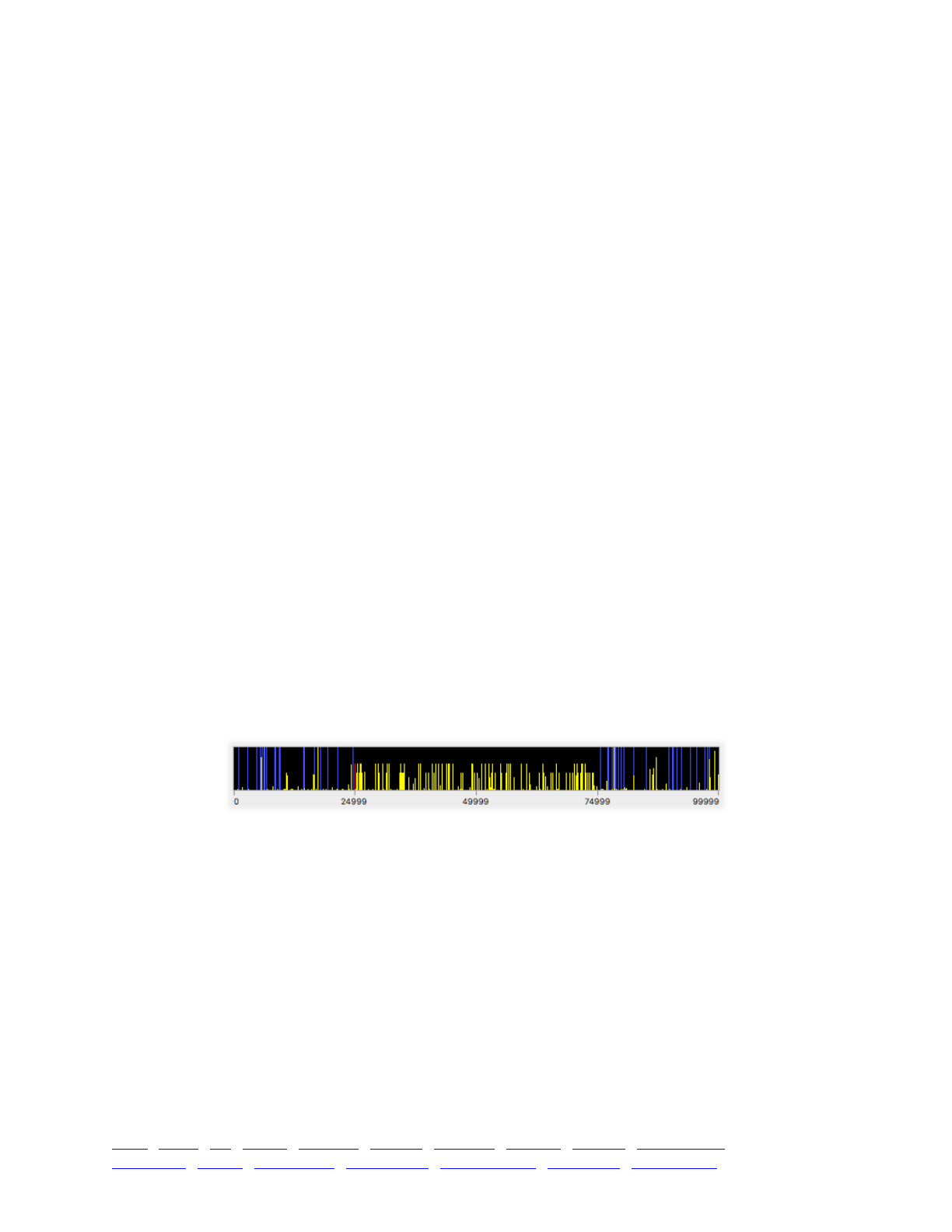
Note also that this callback handles only suppression of ordinary recombination breakpoints. If
you enabled gene conversion in your model (see section 6.1.3), you may also wish to make
inversions modify how gene conversion occurs. That is easy to do, but is not shown in this recipe;
see section 22.5 for further information.
So now we have a working model of chromosomal inversions, but it would be nice to have
some quantitative evidence that it is working properly. For that, let’s add a final output event:
9999 late() {!
sim.outputFixedMutations();!
!
// Assess fixation inside vs. outside the inversion!
pos = sim.substitutions.position;!
cat(sum((pos >= 25000) & (pos < 75000)) + " inside inversion.\n");!
cat(sum((pos < 25000) | (pos >= 75000)) + " outside inversion.\n");!
}
This event prints a list of the fixed mutations using outputFixedMutations(), as we’ve seen in
other recipes. Then it looks at all of the mutations that have fixed during the simulation (kept by
the sim object in its substitutions property), and extracts their positions. Finally, it tallies and
prints the number of fixed mutations that occurred within the inversion region, versus the number
that occurred outside. Without the inversion, these numbers would be expected to the roughly
equal, since there are 50000 bases inside the inversion and 50000 outside, and indeed, if you
comment out the recombination() callback and run the model, you will see something like this:
37 inside inversion.!
40 outside inversion.
But with the recombination callback active, the results are very different:
0 inside inversion.!
43 outside inversion.
This can be seen graphically in SLiMgui. If display of fixed mutations is turned on with the F
button to the right of the chromosome view, this is what things look like at the end of the run:
Many mutations outside the inversion have drifted to fixation. (To facilitate that happening
quickly, this model uses a recombination rate of 1e-6, so that linkage disequilibrium with the
inversion gets broken down quickly, but that is not an essential component of the model, just a
way to get it to show interesting results more quickly.) Inside the inversion, however, there are two
major haplotypes, and mutations within the inversion can’t fix because they can’t cross from one
haplotype to the other. This is the result of suppression of recombination within the inversion;
chromosomes containing the inversion accumulate one set of fixed mutations through drift, while
chromosomes not containing the inversion accumulate a different set of fixed mutations.
While we’re on the subject of haplotypes, this model is a particularly good testbed for looking
at some advanced features of SLiMgui that facilitate the examination of haplotypes and linkage
disequilibrium in SLIM. Let’s run the model out to the end again, to reach a similar state to that
shown above, and then control-click on the chromosome view to get a context menu that allows
us to configure its display:
TOC I TOC II WF nonWF initialize() Genome Individual Mutation SLiMSim Subpopulation!
Eidos events fitness() mateChoice() modifyChild() recombination() interaction() reproduction() 198
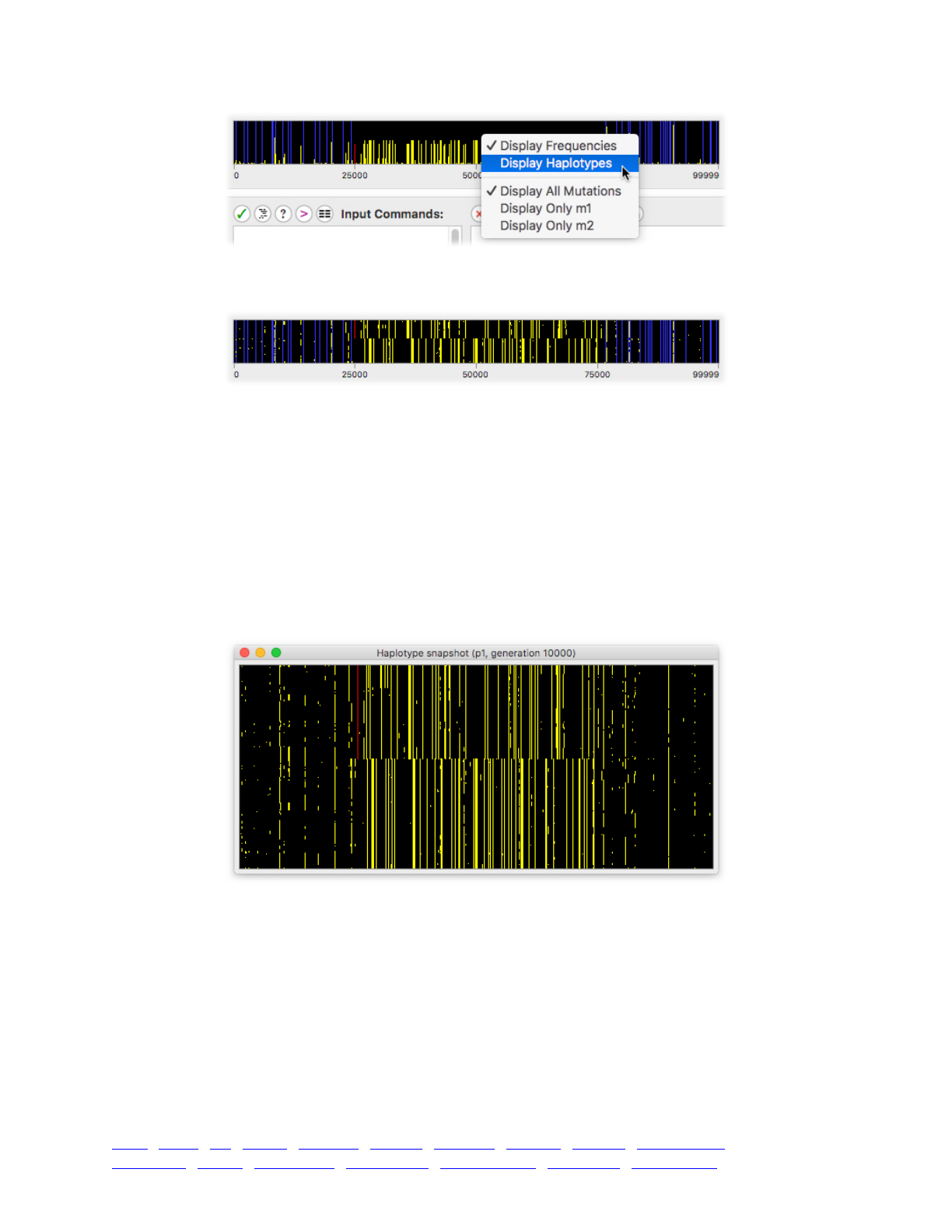
Select “Display Haplotypes” from the context menu, and the chromosome view changes to
show the haplotypes that are in the population, clustered according to their genetic similarity:
Here the effect of the inversion is even clearer; outside of the inversion there are few mutations
at high frequency and no apparent population structure, but inside the inversion the population
has clearly differentiated into two completely different haplotypes with no admixture. The marker
mutation indicating the inversion can be seen, associated with one of the two haplotypes.
This alternate display mode for the chromosome view is based upon just a small sample of the
genomes from the selected subpopulation(s), allowing genetic clustering and display to be done in
real time. It can also be useful to get a more comprehensive haplotype plot, based upon a larger
sample or upon the entire population. To obtain that, choose Create Haplotype Plot from the
Show Graph button’s pop-up menu (or from the Simulation menu). This shows a panel that allows
us to choose plot options; we can use the default options here, so click OK. After a progress panel
(since the analysis can be quite lengthy with a large sample), a new plot window opens:
This shows essentially the same information as the chromosome view did above, but it is based
upon all 1000 genomes in the population, and thus provides some additional detail. A context
menu on the plot window, obtained with control-click or right-click, allows the appearance of the
plot to be adjusted, and also allows the plot’s image to be copied or saved as a file.
That completes this model of chromosomal inversions using a recombination() callback, but as
usual there is much more that could be done. Rather than using balancing selection, for example,
spatially varying selection among subpopulations could allow adaptive ecological divergence
between subpopulations to arise as a result of the protection from recombination afforded by the
inversion. It would also be interesting to model the rise of an inversion to high local frequency, in
a model like that, to explore how inversions can facilitate divergence and speciation.
TOC I TOC II WF nonWF initialize() Genome Individual Mutation SLiMSim Subpopulation!
Eidos events fitness() mateChoice() modifyChild() recombination() interaction() reproduction() 199

13.6 Modeling both X and Y Chromosomes with a Pseudo-Autosomal Region (PAR)
SLiM has built-in support for modeling either the X or Y chromosome when sex is enabled (see
section 6.2.3). However, some models need to go beyond this built-in support. You might wish to
model both the X and Y chromosomes, and you might even wish to model a pseudo-autosomal
region (PAR) – a region in which recombination between the X and Y occurs freely, giving the
region evolutionary dynamics similar to those of an autosome. Both males and females are diploid
for genes in the PAR; females have two copies of the PAR on their two X chromosomes, whereas
males have the same PAR on their X, and a homologous PAR on their Y. Because crossing over
occurs freely between the X and Y within the PAR, genes in the PAR exhibit an autosomal pattern
of inheritance rather than sex-linked inheritance.
Modeling this in SLiM is possible by implementing your own sex-chromosome mechanics,
which is fairly straightforward. In this section we’ll explore a simple model of neutral X and Y
chromosome evolution with a single PAR connecting them. This model was provided by Melissa
Jane Hubisz, and has been adapted for publication as a recipe here.
The basic model is quite simple:
initialize()!
{!
initializeMutationRate(1.5e-8);!
initializeMutationType("m1", 0.5, "f", 0.0); // PAR!
initializeMutationType("m2", 0.5, "f", 0.0); // non-PAR!
initializeMutationType("m3", 1.0, "f", 0.0); // Y marker!
!
// 6 Mb chromosome; the PAR is 2.7 Mb at the start!
initializeGenomicElementType("g1", m1, 1.0); // PAR: m1 only!
initializeGenomicElementType("g2", m2, 1.0); // non-PAR: m2 only!
initializeGenomicElement(g1, 0, 2699999); // PAR!
initializeGenomicElement(g2, 2700000, 5999999); // non-PAR!
!
// turn on sex and model as an autosome!
initializeSex("A");!
!
// no recombination in males outside PAR!
initializeRecombinationRate(c(1e-8, 0), c(2699999, 5999999), sex="M");!
initializeRecombinationRate(1e-8, sex="F");!
}!
!
// initialize the pop, with a Y marker for each male!
1 late() {!
sim.addSubpop("p1", 1000);!
i = p1.individuals;!
males = (i.sex == "M");!
maleGenomes = i[males].genomes;!
yChromosomes = maleGenomes[rep(c(F,T), sum(males))];!
yChromosomes.addNewMutation(m3, 0.0, 5999999);!
}!
!
modifyChild() {!
numY = sum(child.genomes.containsMarkerMutation(m3, 5999999));!
!
// no individual should have more than one Y!
if (numY > 1)!
stop("### ERROR: got too many Ys");!
TOC I TOC II WF nonWF initialize() Genome Individual Mutation SLiMSim Subpopulation!
Eidos events fitness() mateChoice() modifyChild() recombination() interaction() reproduction() 200

// females should have 0 Y's!
if (child.sex == "F" & numY > 0)!
return F;!
!
// males should have 1 Y!
if (child.sex == "M" & numY == 0)!
return F;!
!
return T;!
}!
!
10000 late() {!
p1.outputMSSample(10, replace=F, requestedSex="F");!
}
The initialize() callback sets up the genetic structure. This model turns on sex, because we
want SLiM to track males and females for us, but it requests modeling of an autosome with
initializeSex("A"); we will handle the tracking of the X versus Y chromosomes ourselves. To do
that, we set up a special “marker” mutation type, m3, that will be used to tag Y chromosomes, as
we will see shortly. We set up a 6 Mb chromosome with a 2.7 Mb PAR at the beginning; the PAR
uses mutation type m1 (through genomic element type g1), while the rest of the chromosome uses
mutation type m2 (through genomic element type g2), so that we can easily tell sex-linked
mutations from pseudo-autosomal mutations later on. The only wrinkle during initialization is that
we set up a recombination map in males that prevents recombination outside the PAR; females,
which have two X chromosomes, are allowed to recombine freely.
Next we have a generation 1 late() event that sets up the initial population. After making a
new subpopulation in the usual way with addSubpop(), it gets the male individuals, selects only
their second Genome objects, and adds an m3 mutation to them to mark them as Y chromosomes.
These marker mutations will be handled in the usual way by SLiM, so they will be inherited and
will continue to mark Y chromosomes in future generations. Because recombination is prevented
in males outside the PAR, they will stay associated with the non-PAR Y chromosome genetic
information.
There is one problem with this scheme, however. When SLiM generates offspring, it has its own
ideas about whether a given child ought to be male or female. We need to follow SLiM’s guidance
on this, otherwise our model will end up with individuals that SLiM considers female but that
possess a Y chromosome, and individuals SLiM thinks are male but that have no Y. This is the
purpose of the modifyChild() callback. It simply compares what SLiM expects for the sex of the
child (child.sex) with the genetics that SLiM is proposing that the child will inherit
(child.genomes). If they don’t match, then it returns F to indicate that SLiM needs to choose new
parents and try again. Note the containsMarkerMutation() method; this just checks for a
mutation of a given type at a given position, which can be done quite quickly by SLiM. It is thus
optimal when the position of a mutation (if it exists) is already known, as it is here.
Because modifyChild() callbacks get called quite frequently (once for each new offspring
generated by SLiM, or even more in this case since the callback rejects some proposed children),
the speed of callback code is essential. The callback above has very clear logic, but it is slow in
several ways. It does a safety check that is never, in fact, hit (since the model works properly); it
assigns a value into a variable, numY, which is relatively slow because it requires Eidos to set up a
symbol table entry; it performs some unnecessary logical operations and tests (if child.sex is not
"F" then it must be "M", for example), and worst of all, it always calls containsMarkerMutation()
for both child genomes even though in many cases the answer returned by one genome will
TOC I TOC II WF nonWF initialize() Genome Individual Mutation SLiMSim Subpopulation!
Eidos events fitness() mateChoice() modifyChild() recombination() interaction() reproduction() 201

already allow the callback to choose its action. With an optimized version of the callback, the
model runs about 25% faster, a not-insignificant difference. The optimized callback:
modifyChild() {!
// females should not have a Y, males should have a Y!
if (child.sex == "F")!
{!
if (childGenome1.containsMarkerMutation(m3, 5999999))!
return F;!
if (childGenome2.containsMarkerMutation(m3, 5999999))!
return F;!
return T;!
}!
else!
{!
if (childGenome1.containsMarkerMutation(m3, 5999999))!
return T;!
if (childGenome2.containsMarkerMutation(m3, 5999999))!
return T;!
return F;!
}!
}
If you examine this carefully, you should find that it will produce the same result in all cases
(unless the model has already broken, such as by an individual having two Y chromosomes).
Finally, we have a late() event that outputs an MS-format sample from the females in the
population; among other things, this establishes the end of the model as generation 10000.
There is one remaining issue. Addressing it is optional, in a sense, but if we don’t address it the
model will run slower and slower until it grinds nearly to a halt. The problem is that while PAR
mutations will fix and be converted into Substitution objects automatically by SLiM as usual,
non-PAR mutations will not. This is because their threshold for fixation is lower than SLiM
realizes; only a quarter of Genome objects are Y chromosomes, and only three-quarters are X
chromosomes, so sex-linked mutations need to fix when they reach those frequencies, not a
frequency of 1.0 as SLiM expects. Fixing this is not difficult, but it does require a bit of code:
1:10000 late() {!
// periodically remove m2 (non-PAR) mutations that are fixed in X or Y!
// m1 (PAR) mutations will be automatically removed when fixed!
if (sim.generation % 1000 == 0) {!
numY = sum(p1.individuals.sex == "M");!
numX = 2 * size(p1.individuals) - numY;!
!
// look at the mutations in a single Y chromosome!
// to find mutations that are fixed in all Y's!
firstMale = p1.individuals[p1.individuals.sex == "M"][0];!
fMG = firstMale.genomes;!
!
if (fMG[0].containsMarkerMutation(m3, 5999999)) {!
firstY = fMG[0];!
firstX = fMG[1];!
} else if (fMG[1].containsMarkerMutation(m3, 5999999)) {!
firstY = fMG[1];!
firstX = fMG[0];!
} else!
stop("### ERROR: no Ys in first male");!
!
TOC I TOC II WF nonWF initialize() Genome Individual Mutation SLiMSim Subpopulation!
Eidos events fitness() mateChoice() modifyChild() recombination() interaction() reproduction() 202
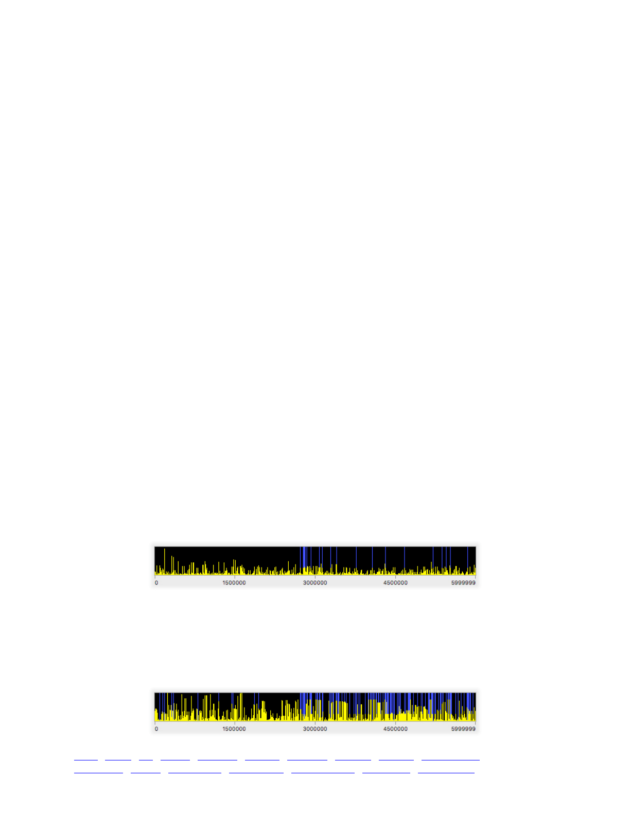
ymuts = firstY.mutationsOfType(m2);!
ycounts = sim.mutationCounts(NULL, ymuts);!
removeY = ymuts[ycounts == numY];!
!
// now do the same for the X!
xmuts = firstX.mutationsOfType(m2);!
xcounts = sim.mutationCounts(NULL, xmuts);!
removeX = xmuts[xcounts == numX];!
!
cat("Gen. " + sim.generation + ": Removing ");!
cat(removeX.size() + "/" + removeY.size() + " on X/Y\n");!
!
removes = c(removeY, removeX);!
sim.subpopulations.genomes.removeMutations(removes, T);!
}!
}
This event should ideally be inserted before the generation 10000 late() event that produces
final output. It runs every 1000 generations, since the operation it performs is somewhat time-
consuming; doing it every generation would be wasteful. It finds a male individual, and uses that
individual as a template for finding and removing fixed sex-linked mutations. Any mutation that
has fixed must be possessed by the template male (by the definition of “fixation”), so the code just
gets all the mutations of type m2 (non-PAR mutations) from the male’s X and Y and checks them all
for fixation. The fixation check itself is done using mutationCounts(), which returns the number of
occurrences of the mutations – population-wide, in this case, because of the NULL passed for the
first parameter. The event prints the number of X-linked and Y-linked mutations that it intends to
remove, and then it removes them with removeMutations(). The optional T value passed for the
second argument to removeMutations() (which is named substitute) indicates that SLiM should
create Substitution objects for the removed mutations; we are notifying SLiM that those
mutations are in fact fixed, even though SLiM doesn’t realize it. If you don’t care about that
record-keeping, you can omit that optional T value, and the mutations will simply be removed.
And that’s it. We’ve implemented tracking of Y chromosomes with marker mutations, we’ve
guaranteed that those markers stay correctly synchronized with offspring sex, and we’ve added
machinery to detect fixed sex-linked mutations and turn them into Substitutions just as SLiM does
for autosomal mutations. If we run this model in SLiMgui with display of fixed mutations turned
on (the F button to the right of the chromosome view), the behavior of the PAR versus the non-PAR
regions is easy to see as soon as the first pass of the fixation check has run in generation 1000:
The PAR, on the left, behaves as an autosome, so it takes a while for mutations to fix; one is
close to fixation, but none has made it there yet. The non-PAR region, on the right, behaves as
separate sex chromosomes that cannot recombine, and each sex chromosome is present in fewer
copies than the PAR; mutations in that region thus have a smaller effective population size, and fix
more rapidly. The Y, present in only a quarter as many copies as the PAR, fixes particularly quickly;
all 20 of the fixations here are in fact on the Y. After generation 3000, the situation is similar:
TOC I TOC II WF nonWF initialize() Genome Individual Mutation SLiMSim Subpopulation!
Eidos events fitness() mateChoice() modifyChild() recombination() interaction() reproduction() 203

There have now been 19 fixations on the X, 120 on the Y, and only 11 in the PAR. The trend is
clear, and it appears that our model of a pseudo-autosomal region is functioning as expected.
13.7 Forcing a specific pedigree through arranged matings
As we’ve seen in previous recipes, SLiM allows mating probabilities to be adjusted with
mateChoice() callbacks, and sometimes modifyChild() callbacks can also be useful for
implementing specific mating patterns since they can reject proposed offspring on the basis of
information about the parents (as in, for example, the gametophytic self-incompatibility system
implemented in section 11.3). Sometimes, however, it is desirable to go a step further, and simply
dictate exactly what matings will occur in a given generation, in order to obtain a specific pedigree
structure. This can also be implemented in SLiM, through a combination of tagging individuals
and using a mateChoice() callback to allow only matings between individuals with specific tag
values. In this section, we will look at a recipe that implements a very simple example of this: a
founding event that begins with two mating events, involving disjoint sets of parents, to produce a
founding population of two offspring (one from each mating). Note that this recipe is quite clunky
and scales poorly, because the WF modeling framework is ill-suited to this task; see section 15.12
for a much more graceful and scaleable nonWF recipe for forcing a specific pedigree.
To begin with, here’s a model that does what we want except for the forced pedigree:
initialize() {!
initializeMutationRate(1e-7);!
initializeMutationType("m1", 0.5, "f", 0.0);!
initializeGenomicElementType("g1", m1, 1.0);!
initializeGenomicElement(g1, 0, 99999);!
initializeRecombinationRate(1e-8);!
}!
1 { sim.addSubpop("p1", 500); }!
1000 late() { p1.setSubpopulationSize(2); }!
1002: early()!
{!
newSize = (sim.generation - 1001) * 10;!
p1.setSubpopulationSize(newSize);!
}!
!
1010 late() { p1.outputSample(10); }
This sets up an initial population of size 500, lets it evolve to generation 1000, and then triggers
a bottleneck down to a population size of 2 (set in a late() event in generation 1000, but actually
taking effect for the offspring generation that is generated in 1001). In effect, then, the original
subpopulation is discarded, and we model the new founder subpopulation thereafter; modeling
both could be done by adding the founder population as a new subpopulation, of course (see
section 5.2.1). In generation 1002 and onward, the population grows linearly (for exponential
growth, see section 5.1.2). The model terminates at the end of generation 1010 with the output of
a subsample of the population. So far, so good; we’ve seen this sort of model many times.
The problem here is that with a severe bottleneck such as this, two undesirable things could
happen. One, the same parent(s) could be chosen for both of the two founding offspring
individuals, making the bottleneck more severe than we want. And two, because this is a
hermaphroditic model (in which SLiM allows selfing by chance, if the same parent happens to be
chosen twice), one or both of the founding offspring could be generated through selfing rather than
biparental mating, again making the bottleneck more severe than intended. There are various ways
to handle these issues (selfing in hermaphroditic models can be blocked with a simple
mateChoice() callback, for example; see section 12.4).
TOC I TOC II WF nonWF initialize() Genome Individual Mutation SLiMSim Subpopulation!
Eidos events fitness() mateChoice() modifyChild() recombination() interaction() reproduction() 204

For our purposes here, however, let’s handle them by forcing SLiM to follow a specific pedigree
for the founding event. We will choose four parents, A, B, C, and D, from the population, and we
will force SLiM to mate A with B and C with D, each mating producing exactly one offspring.
We’ll do that by first modifying the 1000 late() event that triggers the bottleneck:
1000 late() {!
p1.setSubpopulationSize(2);!
p1.individuals.tag = 0;!
parents = sample(p1.individuals, 4);!
parents[0].tag = 1;!
parents[1].tag = 2;!
parents[2].tag = 3;!
parents[3].tag = 4;!
}
This event now not only triggers the founding bottleneck, but also chooses four parents from the
original subpopulation using sample() – which by defaults samples without replacement, as
desired – and marking them with unique tag values. The tag values of all other individuals are set
to 0. We can now identify A, B, C, and D using the tag values 1:4. Next we need to force matings
only between A and B, and C and D. We’ll do that with a modifyChild() callback:
1001 modifyChild()!
{!
t1 = parent1.tag;!
t2 = parent2.tag;!
!
if (((t1 == 1) & (t2 == 2)) | ((t1 == 2) & (t2 == 1)) |!
((t1 == 3) & (t2 == 4)) | ((t1 == 4) & (t2 == 3)))!
{!
cat("Accepting tags " + t1 + " & " + t2 + "\n");!
parent1.tag = 0;!
parent2.tag = 0;!
return T;!
}!
!
cat("Rejecting tags " + t1 + " & " + t2 + "\n");!
return F;!
}
This callback gets the tag values of the two parents of each proposed child. If the parents are A
and B (which could be tags 1 and 2, or tags 2 and 1), the child is accepted; similarly if the parents
are C and D. In that case, the tag values of the parents are set to 0 to ensure that those parents will
not be allowed to mate a second time. If the parents don’t pass the test, the callback simply rejects
the proposed child by returning F, causing SLiM to try a new pair of parents.
This works well, except that there will be a noticeable pause at generation 1001. Looking at the
diagnostic output produced by the model shows why; there are a great many lines stating
“Rejecting tags 0 & 0”, quite a few lines stating things like “Rejecting tags 2 & 0”, and
exactly two lines stating something like “Accepting tags 4 & 3” and “Accepting tags 1 & 3”. In
other words, the model is having to reject a very large number of proposed children in order to
achieve the desired pedigree. If the initial subpopulation were, say, 50000 individuals instead of
500, this small problem would become a huge problem, as the model ground to a halt for perhaps
days or weeks searching for acceptable mating pairs. Happily, there is a way to optimize the
model to eliminate the problem, by adding a fitness() callback:
TOC I TOC II WF nonWF initialize() Genome Individual Mutation SLiMSim Subpopulation!
Eidos events fitness() mateChoice() modifyChild() recombination() interaction() reproduction() 205

1000 fitness(m1)!
{!
if (individual.tag == 0)!
return 0.0;!
else!
return relFitness;!
}
This callback simply removes all individuals with a tag value of 0 from the mating pool, by
declaring their fitness to be 0.0. Although it removes all unchosen parents from the mating pool, it
does not suffice in itself; without the modifyChild() callback as well, this fitness() callback
would still allow A to mate with C, D to self, etc. But in conjunction with the modifyChild()
callback, it reduces the mating pool to just the focal individuals we want, and thus greatly speeds
up the process of filling the desired pedigree.
Note that this callback is defined for generation 1000; we want to manipulate the fitness values
of the individuals that will be parents in generation 1001 (the founding event generation), and
those individuals are the offspring generated in generation 1000, and thus have their fitness values
calculated at the end of generation 1000. When you’re juggling individuals with different callbacks
like this, you need to consult the generation life cycle (see chapter 19) very carefully!
With this callback in place, it takes only a few tries to get the matings we want, as for example:
Rejecting tags 2 & 4!
Rejecting tags 1 & 1!
Accepting tags 1 & 2!
Rejecting tags 0 & 4!
Rejecting tags 0 & 3!
Accepting tags 4 & 3
The appearance of tag value 0 here is because parents 1 and 2 were accepted and produced an
offspring, and thus their tag values were set to 0. This did not remove them from SLiM’s mating
pool, since their fitness values were not recalculated; it merely marks them so that the
modifyChild() callback can avoid using them again. Of course these diagnostic messages are just
for illustration purposes anyway, and would be removed from a production model.
Note that the scheme here using sample() chooses parents for the founding population with
equal weights. This is a neutral model, so that is fine, but even in a non-neutral model this might
be desirable, depending upon the nature of the founding event; a storm that blows a handful of
birds off-course to an isolated island, for example, might select the founding individuals
completely at random, without regard for the fitness they would have had in their original habitat,
and so the simple call to sample() shown here would be appropriate. But of course any other
method of choosing the founders may be used. To sample parents weighted by their fitness values,
as SLiM normally does when choosing parents, one could just obtain the fitness values for all
parents, with a call to cachedFitness(NULL) on the parental subpopulation, and pass that vector
directly to sample() as the weights to be used in sampling.
This is almost the simplest possible pedigree we could force, but the recipe can be generalized
easily. For example, we could force more than one offspring to be generated by a given pair of
parents if we wished, either by using more tag values to represent different states (when A and B
are about to generate their first child, change their tag values to 5 and 6, and allow parental pair
5/6 to also generate an offspring, for example), or by adding a counter to the parental individuals
using the setValue() / getValue() facility of the Individual class (see section 21.6.2) to track how
many children they have generated already; their tag values would not be reset to 0, removing
them from the parent pool, until that counter reached the desired value.
TOC I TOC II WF nonWF initialize() Genome Individual Mutation SLiMSim Subpopulation!
Eidos events fitness() mateChoice() modifyChild() recombination() interaction() reproduction() 206

Similarly, this recipe could be extended to a larger pedigree, involving more parents and more
offspring, simply by using more tag values. However, if you wanted to implement a large,
complex pedigree involving many matings the implementation might get rather lengthy and
cumbersome, with manual setting and checking of a large number of different tag values.
This recipe could also be extended to work over multiple generations, just by doing the same
thing over again: tag the chosen parents, reject offspring that aren’t from parents with the desired
tag values. It would be straightforward, if admittedly a bit clunky, to reproduce an entire
multigenerational pedigree of, say, a given royal family with a high rate of inbreeding and a
deleterious trait such as hemophilia. To do this, first assign a unique number to each individual on
the pedigree chart you want to model; then use those numbers as the tag values for the individuals
in the model. If C is the child of A and B, the modifyChild() call back would, when deciding to
allow A and B to mate to produce C, also set the tag value for the proposed offspring to mark that
individual as C. Implemented across the board, this would allow the identity of every specific
individual throughout the multigenerational pedigree to be tracked with precision.
As mentioned above, section 15.12 has a much more scalable recipe for forcing a specified
pedigree using a nonWF model; that recipe is recommended for most users over this recipe.
13.8 Estimating model parameters with ABC
One major use of simulation models is to try to better understand an empirical system by
comparing simulated results with empirical data. For example, one might have an observation
from an empirical system, and have a guess as to a model that approximates that empirical system
well; one might then want to know the value of a particular parameter of that model that produces
the best possible fit of the model to the data. In this recipe we’ll explore doing this using a
technique called Approximate Bayesian Computation (ABC). This is quite a complex topic, and we
will not attempt to provide a thorough introduction to it here; please use the internet to inform
yourself further regarding the assumptions, limitations, and caveats involved in this method, as
well as about the underlying theoretical framework upon which it rests.
In this recipe we’re going to branch out a bit and present R code as well as Eidos code. The R
code will run the ABC process, while the Eidos code will run the SLiM simulation that provides the
ABC process with the information it needs. Let’s start with the Eidos code:
initialize() {!
initializeMutationRate(1e-7);!
initializeMutationType("m1", 0.5, "f", 0.0);!
initializeGenomicElementType("g1", m1, 1.0);!
initializeGenomicElement(g1, 0, 999999);!
initializeRecombinationRate(1e-8);!
}!
1 { sim.addSubpop("p1", 100); }!
1000 late() { cat(sim.mutations.size() + "\n"); }
This is a trivial model, obviously. We start with a population of size 100, and model neutral
mutations in that population. The model is allowed to equilibrate until generation 1000, at which
point the number of segregating mutations detected in the population is printed. Simple and fast,
which is important since ABC is going to run it a whole bunch of times.
To tie this back to an empirical question, this model would be a reasonable starting place if you
said: “I have a population of size 100 that I have sampled comprehensively, and the analysis I’ve
done tells me there are 262 segregating mutations in the population. I think the population has
been about size 100 for a long time, so it’s at equilibrium (to the extent that a small population
evolving under drift is ever at equilibrium). I know the recombination rate and the chromosome
TOC I TOC II WF nonWF initialize() Genome Individual Mutation SLiMSim Subpopulation!
Eidos events fitness() mateChoice() modifyChild() recombination() interaction() reproduction() 207

length, but not the mutation rate. What’s my best guess, and what’s the posterior distribution
around that guess?” So now we’ve got a SLiM model of that scenario, with a guess of 1e-7 hard-
coded into it. Let’s tweak the model by replacing the mutation rate with a symbolic constant:
initializeMutationRate(mu);
We could define the constant mu at initialization time with a call to the Eidos function
defineConstant(), like:
defineConstant("mu", 1e-7);
But let’s not do that; instead, we will pass a value for it in to the simulation on the command
line. To do this, let’s first save the model to a file called “abc.slim” in our home directory (we will
assume that the file is then at the path ~/abc.slim, as it is on most Unix systems including Mac
OS!X). If we run this model at the command line, we get an error about the undefined constant:
darwin:~ bhaller $ slim ~/abc.slim!
...!
ERROR (EidosSymbolTable::_GetValue): undefined identifier mu.!
!
Error on script line 2, character 24:!
!
initializeMutationRate(mu);!
^^
But we can pass a value for the constant in, using the -d (-define) command-line option (see
section 17.2):
darwin:~ bhaller $ slim -d mu=1e-7 ~/abc.slim!
...!
262
This defines mu to be 1e-7 at the very beginning of the model, before the first initialize()
callback is called. This run of SLiM is actually where the value of 262 came from, above; it’s the
value from our “empirical system” (i.e., this first run of our model), for which we’re going to try to
recover an estimate of mu using ABC. In practice, such observed values would probably come
from actual empirical data.
So now we have a working model at ~/abc.slim that expects a value for a constant mu to be
supplied to it on the command line, and the last line of the output it generates is the outcome of
the model – the number of segregating mutations observed in the population at equilibrium. The
next step is to write some R code to run our model, given a random number seed and mu:
runSLiM <- function(x)!
{!
seed <- x[1]!
mu <- x[2]!
#cat("Running SLiM with seed ", seed, ", mu = ", mu, "\n");!
output <- system2("/usr/local/bin/slim", c("-d", paste0("mu=", mu),!
"-s", seed, " ~/abc.slim"), stdout=T)!
as.numeric(output[length(output)])!
}
The system2() function of R is used to run SLiM with the desired command-line arguments, and
the output is collected as a character vector of output lines. Note that this function takes the seed
and mu values as a single vector, x; this is because of the design of the R package we will use to run
the ABC in a moment. First, let’s test this function:
TOC I TOC II WF nonWF initialize() Genome Individual Mutation SLiMSim Subpopulation!
Eidos events fitness() mateChoice() modifyChild() recombination() interaction() reproduction() 208

> runSLiM(c(100030, 1e-7))!
[1] 281
We get a different result than before, since a different random number seed was used, but it
seems to work fine. So now we have R running our SLiM model for us; the next step is to actually
run an ABC analysis. For this, we will use the package EasyABC, available through CRAN:
library(EasyABC)!
!
# Set up and run our ABC!
prior <- list(c("unif", 1e-9, 1e-6))!
observed <- 262!
!
ABC_SLiM <- ABC_sequential(method="Lenormand", use_seed=TRUE,!
model=runSLiM, prior=prior, summary_stat_target=observed,!
nb_simul=1000)
The EasyABC package has many different options for running ABC analyses, including several
“sequential” ABC methods that try to arrive at an answer more quickly through successive rounds
of ABC, and several ways of running the ABC inside an MCMC (Markov Chain Monte Carlo)
process, a particularly powerful way of converging rapidly on the posterior distribution of the ABC.
We have chosen the “Lenormand” method, since it is simple to set up, is happy to run with only
one unknown parameter (which some of the other methods don’t seem to be), and converges fairly
quickly. Since ABC is a Bayesian method, we also need a prior for mu; we have chosen a uniform
prior from 1e-9 to 1e-6, since that encompasses the range of mutation rates we think would be
likely in our empirical system, and since we have no information about which values within this
range are more or less likely. We also need to tell EasyABC how many runs we want to perform;
the nb_simul parameter does that (sort of – see the documentation), and the value of 1000 here
should give us quite a good posterior distribution at the expense of longer runtime (a value of 100
actually works pretty well already).
The final line, which actually runs the ABC analysis, will probably take several minutes,
depending upon the speed of your machine. When it finishes, ABC_SLiM contains information
about the ABC run. Details about that information can be found in EasyABC’s documentation; we
will not explain it here, but we will use it to extract the results we want. First of all, to get the best
fit estimate from a one-parameter ABC like this, one typically wants the sum of the weighted
average of the values chosen by the ABC:
> sum(ABC_SLiM$param * ABC_SLiM$weights)!
[1] 0.0000001134854
The ABC did quite a good job of recovering the actual value of mu, 1e-7, that was used to
generate the target value of 262. We can also plot the posterior distribution for mu that was arrived
at by the ABC analysis, using this R code:
log_param <- log(ABC_SLiM$param, 10)!
breaks <- seq(from=min(log_param), to=max(log_param), length.out=8)!
!
quartz(width=4, height=4)!
hist(log_param, xlim=c(-9, -6), breaks=breaks, col="gray",!
main="Posterior distribution of mu", xlab="Estimate of mu", xaxt="n")!
axis(side=1, at=-6:-9, labels=c("1e-6", "1e-7", "1e-8", "1e-9"))
This code converts the posterior distribution data to a log scale manually and plots it on that
scale, for clarity; there are probably better ways to do that. The quartz() call just opens a graphics
TOC I TOC II WF nonWF initialize() Genome Individual Mutation SLiMSim Subpopulation!
Eidos events fitness() mateChoice() modifyChild() recombination() interaction() reproduction() 209
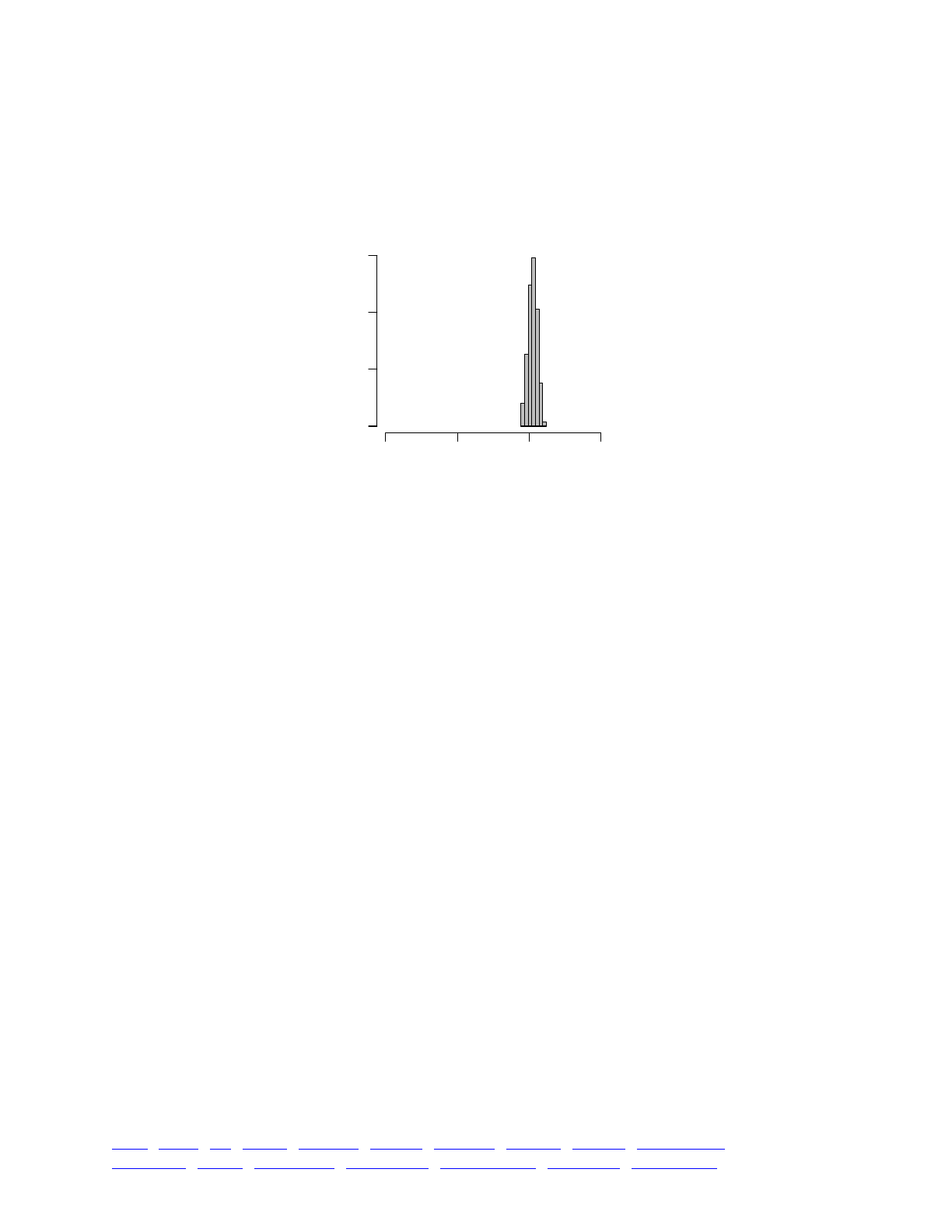
device on Mac OS X; if you’re on a different platform you will probably have to change that to
your platform-specific graphics device call. Apart from those details, the code is pretty standard.
The resulting plot looks like this:
We started with a uniform prior from 1e-9 through to 1e-6, providing the ABC analysis with no
information as to which values within that range were more likely. By doing quite a few runs of
SLiM (12500, as it happens), the ABC narrowed that range down considerably, effectively ruling
out a large part of it completely, and it gave us a posterior distribution showing which values of mu
would be most likely to produce the observed number of segregating mutations, 262, that was
observed empirically. All in just a few lines of Eidos and a few lines of R; not bad!
This completes our foray into Approximate Bayesian Computation in SLiM and R. This topic can
be pursued much further: estimation of the joint distribution of multiple parameters, usage of a
Markov Chain Monte Carlo (MCMC) method for running the ABC (which is also supported by the
EasyABC package), delving into the often difficult problem of priors, and so forth. But this recipe
should provide a starting point for such explorations.
13.9 Tracking true local ancestry along the chromosome
Ancestry, relatedness, pedigree, and similar concepts are often important in forward genetic
simulations such as those run by SLiM. Depending upon exactly what you need, there are several
different approaches to these sorts of questions in SLiM:
•The subpopID property of mutations (section 21.8.1) keeps track of the subpopulation in
which a given mutation originated. In an admixture model in which you want to
determine whether a given mutation originally arose in one subpopulation or another,
this is often all you need. Note also that if you are adding mutations yourself using
addNewMutation() or addNewDrawnMutation(), you can set the subpopID in those calls to
whatever value you wish. The subpopID property is writeable, so you can also change it
later to any integer value (including some type of ancestry information).
•Mutation types can also be useful for tracking ancestry information. If different mutation
types are used for mutations with different origins in your model, they can then be used
to determine the origin of each mutation later, and SLiM’s methods for retrieving and
counting the mutations of a given mutation type can be used to separate out mutations
of different origins. This approach will work even in non-admixture models in which all
Posterior distribution of mu
Estimate of mu
Frequency
0 50 100 150
1e-9 1e-8 1e-7 1e-6
TOC I TOC II WF nonWF initialize() Genome Individual Mutation SLiMSim Subpopulation!
Eidos events fitness() mateChoice() modifyChild() recombination() interaction() reproduction() 210

mutations originate in a single subpopulation, as long as you can classify mutations
according to their ancestry at the point when they originate (in a modifyChild()
callback that looks at the parents to determine an ancestry group, for example). The
mutation type of mutations can be changed with the setMutationType() method.
•By enabling an optional feature, SLiM can do pedigree-based tracking of the ancestry of
individuals for the purposes of calculating relatedness, finding “trios” of parents and an
associated offspring, and so forth (see section 13.2). This provides information about
relatedness and ancestry at the level of individuals, rather than the level of mutations.
Pedigree-based arranged matings can also be implemented (see section 13.7).
•If tree-sequence recording is turned on (see section 1.7 and chapter 16), it provides a
type of true local ancestry tracking for every position along the chromosome. This is
similar in some ways to this recipe, but much more efficient, and was added in SLiM 3.
Sometimes it is desirable to track relatedness not at the individual level with a pedigree, or at a
mutational level with subpopID or mutation types, but instead at the level of chromosomal regions
– perhaps down to the ancestry of each individual base position along the chromosome. In this
way, the ways that assortment, recombination, selection, and drift determine the ancestry at each
position can be analyzed. This type of relatedness tracking is also possible in SLiM, even when not
using tree-sequence recording; we will explore an example in this section.
Models can implement “true local ancestry” tracking themselves using marker mutations –
mutations which have no selective effect, and are not meant to represent actual mutational
changes to genomes, but instead simply mark particular positions on particular genomes for future
reference. The recipe in section 13.5 used a marker mutation to track individuals possessing a
chromosomal inversion, for example, and in 13.6 a marker mutation was used to mark Y
chromosomes in a model of a pseudo-autosomal region shared between sex chromosomes. Here
marker mutations will be used at every position, to indicate ancestry. At the end, the model will
assess the average ancestry, across the subpopulation, at every chromosome position.
Here is the complete recipe:
initialize() {!
defineConstant("L", 1e4); // chromosome length!
!
initializeMutationRate(0);!
initializeMutationType("m1", 0.5, "f", 0.1); // beneficial!
initializeMutationType("m2", 0.5, "f", 0.0); // p1 marker!
m2.convertToSubstitution = F;!
initializeGenomicElementType("g1", m1, 1.0);!
initializeGenomicElement(g1, 0, L-1);!
initializeRecombinationRate(1e-7);!
}!
!
1 {!
sim.addSubpop("p1", 500);!
sim.addSubpop("p2", 500);!
}!
!
1 late() {!
// p1 and p2 are each fixed for one beneficial mutation!
p1.genomes.addNewDrawnMutation(m1, asInteger(L * 0.2));!
p2.genomes.addNewDrawnMutation(m1, asInteger(L * 0.8));!
!
// p1 has marker mutations at every position, to track ancestry!
p1.genomes.addNewMutation(m2, 0.0, 0:(L-1));!
!
TOC I TOC II WF nonWF initialize() Genome Individual Mutation SLiMSim Subpopulation!
Eidos events fitness() mateChoice() modifyChild() recombination() interaction() reproduction() 211

// make p3 be an admixture of p1 and p2 in the next generation!
sim.addSubpop("p3", 1000);!
p3.setMigrationRates(c(p1, p2), c(0.5, 0.5));!
}!
!
2 late() {!
// get rid of p1 and p2!
p3.setMigrationRates(c(p1, p2), c(0.0, 0.0));!
p1.setSubpopulationSize(0);!
p2.setSubpopulationSize(0);!
}!
!
2: late() {!
if (sim.mutationsOfType(m1).size() == 0)!
{!
p3g = p3.genomes;!
!
p1Total = sum(p3g.countOfMutationsOfType(m2));!
maxTotal = p3g.size() * (L-1);!
p1TotalFraction = p1Total / maxTotal;!
catn("Fraction with p1 ancestry: " + p1TotalFraction);!
!
p1Counts = integer(L);!
for (g in p3g)!
p1Counts = p1Counts +!
integer(L, 0, 1, g.positionsOfMutationsOfType(m2));!
maxCount = p3g.size();!
p1Fractions = p1Counts / maxCount;!
catn("Fraction with p1 ancestry, by position:");!
catn(format("%.3f", p1Fractions));!
!
sim.simulationFinished();!
}!
}!
!
100000 late() {!
stop("Did not reach fixation of beneficial alleles.");!
}
The broad outline here is straightforward. We model two subpopulations, p1 and p2, which are
created in the generation 1 event and configured in the generation 1 late() event. That late()
event also sets up a new subpopulation, p3, that will be produced by admixing migrants from p1
and p2 in generation 2. At the end of generation 2, p1 and p2 are removed, and p3 is allowed to
evolve thenceforth until the termination of the model. This model is therefore a very simple model
of the admixture of two subpopulations; more complex population dynamics could easily be used
with the same ancestry-tracking mechanism shown here.
When p1 and p2 were configured, they were each set up to contain a beneficial mutation of
type m1, fixed within the respective subpopulation. The new p3 subpopulation therefore contains
some genomes that originated in p1 and contain that subpopulation’s beneficial mutation (located
at L * 0.2 on the chromosome), and some genomes that originated in p2 and contain that
subpopulation’s beneficial mutation (located at L * 0.8 on the chromosome). The expectation is
that recombination between those points will eventually produce at least one new genome that
contains both beneficial mutations, and that subsequently both beneficial mutations will sweep to
fixation in p3. The question we wish to investigate is the precise pattern of true local ancestry
along the chromosome at the point when fixation of both beneficial mutations has just occurred.
TOC I TOC II WF nonWF initialize() Genome Individual Mutation SLiMSim Subpopulation!
Eidos events fitness() mateChoice() modifyChild() recombination() interaction() reproduction() 212

To do this, the model adds a marker mutation of type m2 at every position along every genome
in p1, in the 1 late() event. This is done using a single vectorized call to addNewMutation(), for
greater efficiency; adding the mutations one by one would take a very long time, especially with a
longer chromosome. These added markers indicate that a given chromosome position traces its
ancestry to p1. In models with more complex demography involving more than two “parental”
subpopulations, additional mutation types could be employed to indicate derivation from each of
the possible ancestral subpopulations. An important point to understand is that because mutations
in SLiM “stack” by default, these marker mutations have no effect whatsoever on the other
mutations that might occur during a simulation; they are simply carried along, almost as if they
were epigenetic marks of some sort on the genomes being simulated. For simplicity, this model
does not include neutral mutations along the chromosome, and indeed it uses a mutation rate of 0;
but the ancestry-tracking mechanism shown here is compatible with any other model dynamics.
Thus configured, the model runs until both beneficial mutations either fix or are lost. This
termination condition is checked in the 2: late() event. When there are no longer any circulating
m1 mutations, the model outputs some final analysis and terminates. The final analysis here is in
two parts. The first part simply calculates the fraction of all chromosome positions in all genomes
that derives from p1. In one run of this model, the output happens to be:
Fraction with p1 ancestry: 0.398137
The second part calculates the fraction of all genomes derived from p1 at each individual
position along the chromosome, and outputs those fractions as a big vector:
Fraction with p1 ancestry at each chromosome position:!
0.946 0.946 0.946 0.946 0.946 0.946 0.946 0.946 0.946 0.946 0.946 0.946...
It does that by looping through the genomes of p3, and for each genome getting the positions at
which m2 mutations exist using positionsOfMutationsOfType(). Those vectors of positions can be
converted into integer vectors that have a 1 at the positions where m2 mutations occurred (and a 0
everywhere else), using the integer() function of Eidos. Summing those vectors across all of the
p3 genomes gives a count of the number of m2 mutations at each position; dividing that by the
maximum possible count gives a frequency, which indicates the pattern of ancestry.
This pattern can also be seen in SLiMgui, with the neutral marker mutations shown in yellow:
This indicates that the left-hand half of the chromosome mostly derives from p1 – albeit with
some variation due to multiple recombination events that created some haplotype variation –
whereas the right-hand half of the chromosome derives from p2 in all individuals.
The recipe here tracks true local ancestry down to the level of individual base positions. This
does involve some overhead, in terms of both memory usage and processor power, so if this level
of granularity is not needed, it would be much more efficient to place marker mutations every 10,
100, or even 1000 positions along the chromosome. This could be done with a few trivial
modifications to the recipe presented here. However, this recipe can be scaled up to L!=!1 Mbp
and still run in only a couple of minutes, so the overhead is really not too bad. For even larger
models, however, both the runtime and the memory usage of this recipe can become prohibitive;
at L!=!108, the memory usage of this recipe is estimated to be over 8 TB (that is not a typo). Tree-
sequence recording, added in SLiM 3, can provide a far more efficient alternative (see section 1.7
and chapter 16).
TOC I TOC II WF nonWF initialize() Genome Individual Mutation SLiMSim Subpopulation!
Eidos events fitness() mateChoice() modifyChild() recombination() interaction() reproduction() 213
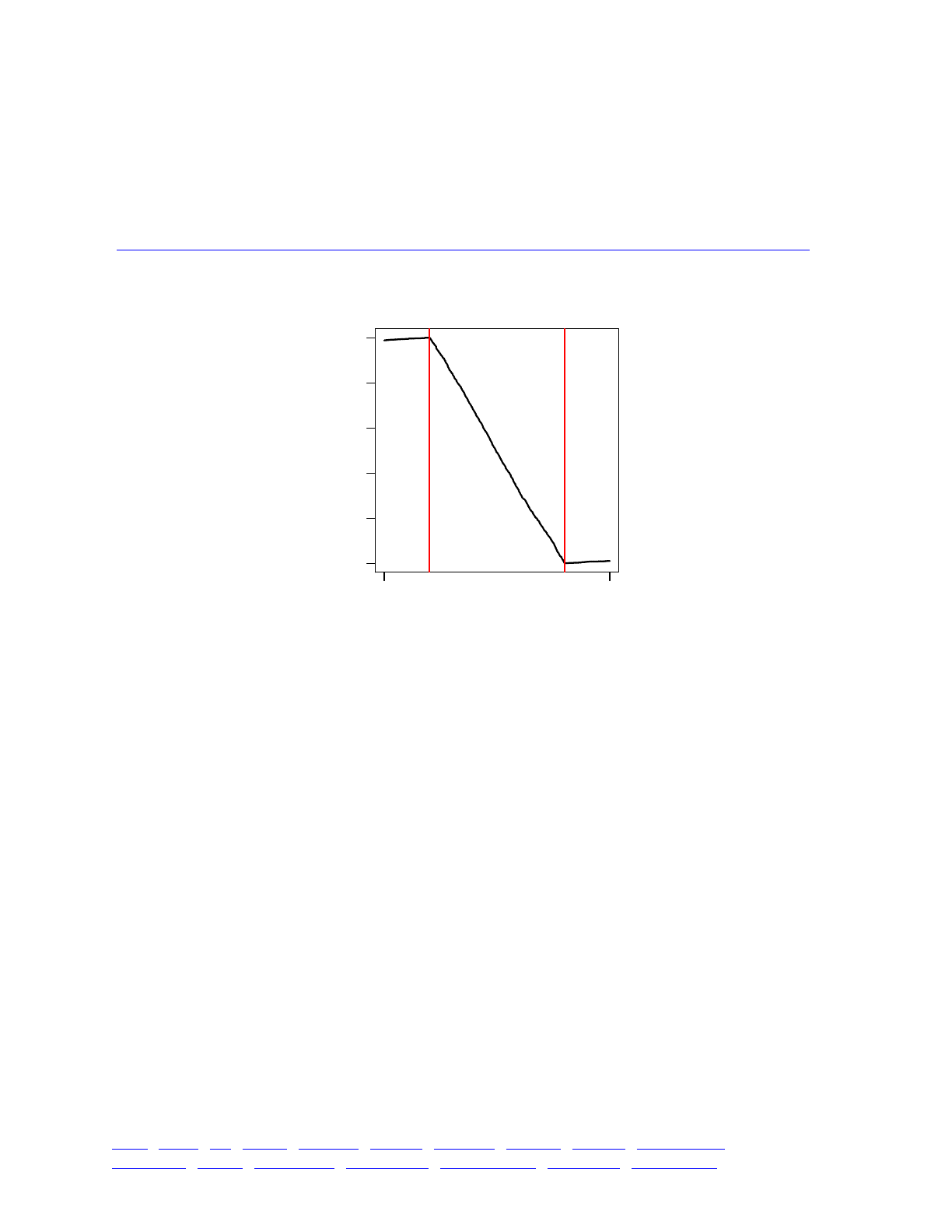
A final note: having done one run of the recipe and seen the pattern of ancestry in SLiMgui, it
would be natural to wonder what the average pattern of ancestry would be across many runs. That
is straightforward to do, by simply running the model many times, collecting the data from each
run, and averaging the ancestry pattern across the runs. A simple R script to do this is provided in
the online SLiM-Extras repository, in the “sublaunching” folder since it illustrates how to sublaunch
runs of SLiM from a script (in this case, an R script). The script is named aggregateLocalAncestry.R
(https://github.com/MesserLab/SLiM-Extras/blob/master/sublaunching/aggregateLocalAncestry.R). If
you have R installed you should be able to run it easily, after modifying the file paths in the script
to point to your installed slim and your copy of this recipe. If you do that, you will get a plot:
The locations where the beneficial mutations were placed in p1 and p2 are shown with red
lines. The mean true local ancestry (the fraction of the genomes in p3 that derive from p1 at a
given chromosome position) is exactly 1.0 at the first beneficial mutation’s location, and exactly
0.0 at the second’s; this makes sense, since the model did not terminate until both beneficial
mutations had fixed, which would imply pure p1 or p2 ancestry at those positions. In between, the
local ancestry changes linearly from p1 to p2; it might seem plausible that the pattern would be
sigmoid instead, but apparently it is not. Toward the ends of the chromosomes, outside the
beneficial mutations, the ancestry falls toward 0.5; it’s hard to see here, but that fall-off is not
linear, in fact. This pattern presumably recapitulates known results from population genetics, but a
modified version of this model could explore much more complex scenarios.
13.10 A quantitative genetics model with heritability
Section 13.1 presented a recipe for a quantitative genetics model in which phenotype was
calculated as the additive effect of a set of QTLs, and fitness was determined by individual
phenotype compared to a phenotypic optimum. In this section we will extend this type of
quantitative genetics model to incorporate heritability, generated by adding random deviations
(representing environmental variance) to the additive genetic variation of the QTLs. Rather than
extending the model of section 13.1 directly, however, we will develop a somewhat different
model here. This recipe utilizes QTLs with effect sizes drawn from a continuous Gaussian
distribution, rather than the −1/+1 effect size distribution of section 13.1. The genetic structure
here, unlike the earlier recipe, is not predetermined; new QTLs can arise spontaneously at any
location. This recipe has only a single subpopulation, and does not contain assortative mating.
09999
0.0 0.2 0.4 0.6 0.8 1.0
chromosome position
fractional ancestry
TOC I TOC II WF nonWF initialize() Genome Individual Mutation SLiMSim Subpopulation!
Eidos events fitness() mateChoice() modifyChild() recombination() interaction() reproduction() 214

The mechanics of this model are quite simple. Here is the entire model except the final output
event and the implementation of heritability:
initialize() {!
initializeMutationRate(1e-6);!
!
initializeMutationType("m1", 0.5, "f", 0.0); // neutral!
initializeMutationType("m2", 0.5, "n", 0.0, 1.0); // QTL!
m2.convertToSubstitution = F;!
!
initializeGenomicElementType("g1", c(m1, m2), c(1, 0.01));!
initializeGenomicElement(g1, 0, 1e5 - 1);!
initializeRecombinationRate(1e-8);!
}!
1 late() {!
sim.addSubpop("p1", 1000);!
}!
1: late() {!
// construct phenotypes from the additive effects of QTLs!
inds = sim.subpopulations.individuals;!
inds.tagF = inds.sumOfMutationsOfType(m2);!
}!
fitness(m2) {!
return 1.0; // QTLs are neutral; fitness effects are handled below!
}!
fitness(NULL) {!
return 1.0 + dnorm(10.0 - individual.tagF, 0.0, 5.0); // optimum +10!
}
Section 13.1 explained the mode of operation of this type of model in some detail. In brief,
QTLs are here represented by mutation type m2, and the selection coefficient of m2 mutations is
used as the additive genetic value of the QTL. A fitness(m2) callback makes all m2 mutations be
neutral regardless of these selection coefficients. A fitness(NULL) callback (a so-called “global
fitness() callback” because it evaluates overall individual fitness, rather than the fitness of a focal
mutation) returns a fitness value that depends upon the phenotype as compared to a phenotypic
optimum of 10.0, using a Gaussian function as in many such models.
Note that, as in section 13.1, a baseline value of 1.0 is added to the Gaussian function value
returned by dnorm(). Section 13.1 didn’t really discuss that choice in any detail, however; let’s
embark on that digression now. Fundamentally, the problem is that of trying to choose a function
that provides a reasonable phenotype-to-fitness map. There is not a lot of empirical data to guide
this choice in most systems, so it is a difficult and somewhat arbitrary decision. In a hard selection
model, where low mean population fitness results in a decrease in population size, an appropriate
fitness function might have a minimum value of zero, allowing the modeling of phenomena such
as lethal mutations and population extinction. In such a model, if most individuals have a fitness
of 0.001 and one has a fitness of 0.1 (having just received a beneficial mutation, for example),
most of the individuals will produce no offspring at all, while the individual with fitness of 0.1
might produce just one or two, leading to a very small population in the next generation. This
seems quite reasonable. The same situation in a soft selection model, where population size does
not depend upon mean population fitness, makes considerably less sense, however. In this
scenario, the child generation must be filled with the requisite number of individuals, so the
individual with fitness 0.1 will end up generating most of the offspring – perhaps hundreds or even
thousands of offspring – while all the rest of the individuals survive but generate few or no
offspring. For some organisms this might be realistic, but for many it would be nonsensical – no
matter how much more fit one elephant is than all of the other elephants in Africa, it is not going
TOC I TOC II WF nonWF initialize() Genome Individual Mutation SLiMSim Subpopulation!
Eidos events fitness() mateChoice() modifyChild() recombination() interaction() reproduction() 215

to generate thousands of offspring all across Africa all by itself! In short, fitness in soft selection
models works differently than in hard selection models, and is often modeled more appropriately
with a fitness function that does not allow such large differences in relative fitness to exist, so that
one individual does not completely dominate the reproductive output of the population. Adding a
constant value to a Gaussian function is a simple way to achieve this; the larger the constant
added, the more the relative fitness values in the population are effectively homogenized. Using a
constant of 1.0 makes some superficial sense, since 1.0 represents neutrality and the Gaussian
function can then be thought of as being some marginal increase in fitness beyond neutrality.
However, this constant is actually arbitrary; after the rescaling that is implicit in the concept of
relative fitness, 1.0 will not be neutral anyway. The constant added should probably therefore be
considered to be a free parameter of the model, if a fitness function of this form is used.
To continue this digression a bit longer, it is also worth noting that if large differences in relative
fitness are allowed in a model, as with the situation above where most individuals have fitness
0.001 and one has fitness 0.1, this can lead to undesirable mate-choice dynamics, too. By default,
SLiM models are hermaphroditic, and while they employ biparental mating by default, they do not
prevent the same parent from being chosen as both parents in a biparental mating event, resulting
in hermaphroditic selfing. Normally this is not a problem, since for typical population sizes it is
unlikely to occur often enough to make a significant difference to the model’s results. In some
sense it is even desirable, since this behavior means that SLiM’s default configuration mirrors
simple analytical population genetics models more closely; this is the reason why SLiM does not
prevent it by default. However, when there is large variance in fitness or when the effective
population size is very small, the chance of hermaphroditic selfing can become quite high; the
fitness 0.1 individual may be quite likely to be chosen as both parents of a given offspring, and it
may therefore generate most of its offspring through selfing. In that case it may be desirable to
suppress it. See section 12.4 for further discussion of this issue and how to deal with it in SLiM.
Returning from that digression: In this model, phenotypes are calculated as the sum of the
effects of all of the QTLs possessed by each individual, and are stored in the tagF property of
individuals for use within the global fitness() callback. The core calculation is done here by the
sumOfMutationsOfType() method, which loops over all of the mutations in each individual and
sums up the selection coefficients of all of the mutations of type m2, which represent the QTLs
possessed by the individual. The sum of the selection coefficients of those mutations represents the
total of the additive effects of the QTLs. These result values – calculated phenotypes – are assigned
into the tagF property of the individuals. Note that this implementation produces a codominant
model; each QTL allele possessed has the same additive effect. It would be possible to implement
a dominant QTL model; it would require replacing the sumOfMutationsOfType() call with method
calls to get the mutations possessed by each individual with mutationsOfType(), unique them with
unique(), get their selection coefficients, and total them up with sum(). This can be done in one
line for the whole vector of individuals, using sapply(), but is not shown here.
QTLs are about 1% of all new mutations, and thus new QTLs arise spontaneously throughout
the run. If they tend to improve the phenotypes of individuals in the population, then they tend to
be retained; if not, they tend to be lost. The population as a whole begins with a mean phenotype
of 0.0, since no QTLs exist. Over the model run, the population will execute an adaptive walk
towards the fitness peak at +10.0. The only other component we need for the base model is an
event that checks for the termination condition (arrival at the fitness peak) and prints output:
TOC I TOC II WF nonWF initialize() Genome Individual Mutation SLiMSim Subpopulation!
Eidos events fitness() mateChoice() modifyChild() recombination() interaction() reproduction() 216

1:100000 late() {!
if (sim.generation == 1)!
cat("Mean phenotype:\n");!
!
meanPhenotype = mean(p1.individuals.tagF);!
cat(format("%.2f", meanPhenotype));!
!
// Run until we reach the fitness peak!
if (abs(meanPhenotype - 10.0) > 0.1)!
{!
cat(", ");!
return;!
}!
!
cat("\n\n-------------------------------\n");!
cat("QTLs at generation " + sim.generation + ":\n\n");!
!
qtls = sim.mutationsOfType(m2);!
f = sim.mutationFrequencies(NULL, qtls);!
s = qtls.selectionCoeff;!
p = qtls.position;!
o = qtls.originGeneration;!
indices = order(f, F);!
!
for (i in indices)!
cat(" " + p[i] + ": s = " + s[i] + ", f == " + f[i] +!
", o == " + o[i] + "\n");!
!
sim.simulationFinished();!
}
This event runs in every generation. It prints the mean phenotype in each generation, forming a
comma-separated list that can be easily copied into an environment such as R for plotting. When
the fitness peak is reached, within a small tolerance, it prints a list of all of the QTLs in the
population and terminates. The QTL list contains the position, effect size, frequency, and origin
generation of each QTL, and is sorted by frequency using the order() function.
A run of the model produces output like this:
Mean phenotype:!
0.00, -0.00, -0.00, -0.01, -0.00, -0.00, -0.01, -0.01, -0.01, -0.01, ...,
9.77, 9.77, 9.82, 9.81, 9.83, 9.83, 9.84, 9.85, 9.85, 9.82, 9.89, 9.91!
!
-------------------------------!
QTLs at generation 1793:!
!
45907: s = 1.28919, f == 1, o == 489!
98721: s = 2.78947, f == 1, o == 257!
53961: s = 1.59969, f == 0.592, o == 1274!
21414: s = -1.09245, f == 0.0515, o == 1639!
93840: s = -0.338536, f == 0.0345, o == 1657!
74095: s = 1.35625, f == 0.026, o == 1762!
...
Plotting the mean phenotype time series in R produces a visualization of the adaptive walk:
TOC I TOC II WF nonWF initialize() Genome Individual Mutation SLiMSim Subpopulation!
Eidos events fitness() mateChoice() modifyChild() recombination() interaction() reproduction() 217
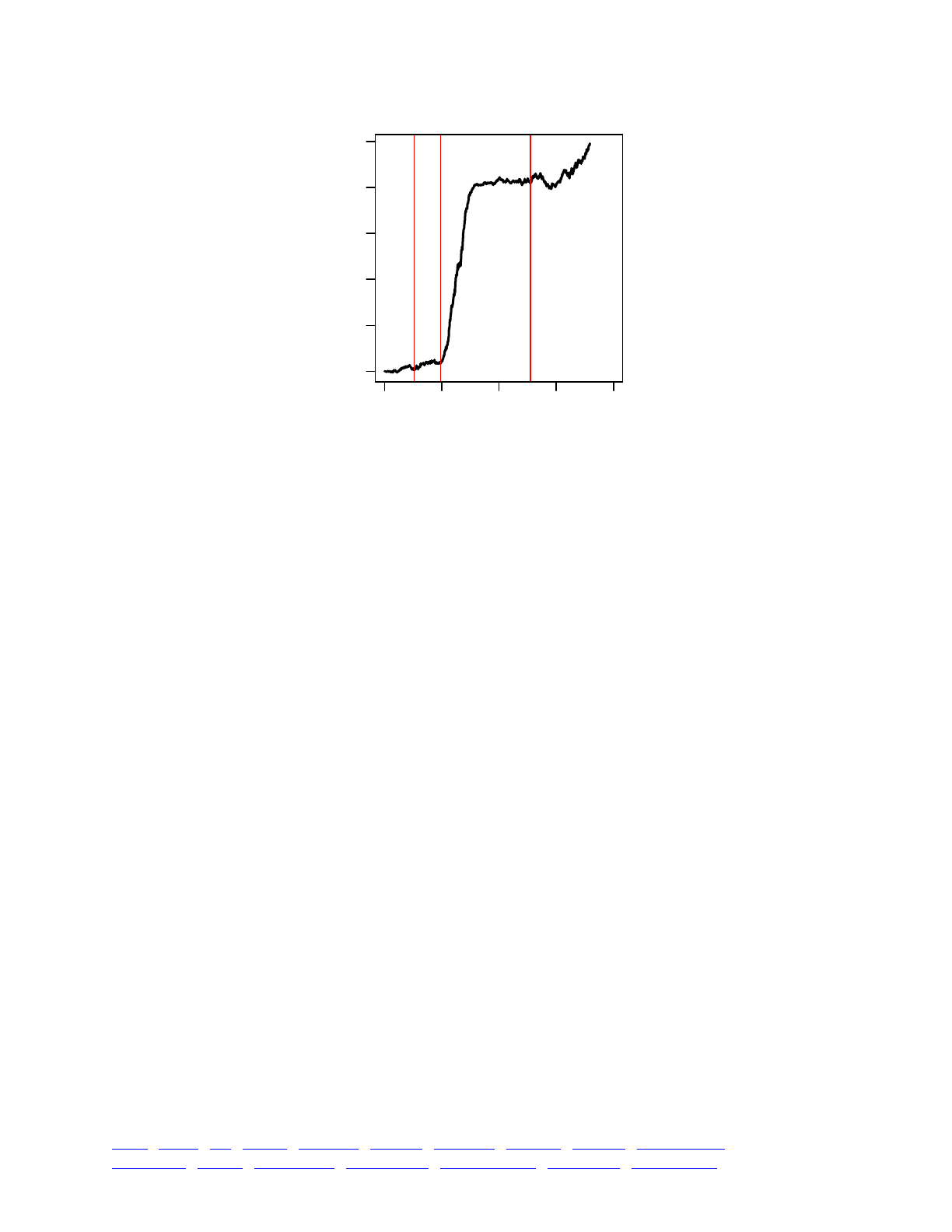
The black curve shows the mean phenotype over time; the three red lines show the generations
of origin of the three high-frequency QTLs listed in the output above. This visualization shows that
the adaptive walk involved a joint sweep by the first two QTLs, followed by a second sweep by the
third QTL, which arose later. At the end of the run, the population has reached the adaptive peak
only on average, since the third QTL is present at a frequency of only 0.592. Individuals that do
not possess this QTL at all have a phenotype of ~8.16; those with only one copy have a phenotype
of ~9.76; and those with two copies have a phenotype of ~11.36. In the final state of the model,
heterozygote advantage thus produces balancing selection upon the third QTL.
So far so good; but earlier it was promised that this model would incorporate heritability as
well. Let’s add that now, beginning with the addition of a line at the top of the initialize()
callback that sets up a constant representing the desired heritability, h2:
defineConstant("h2", 0.1);
And then, here is a complete replacement for the 1: late() event that calculates phenotypes:
1: late() {!
// construct phenotypes from the additive effects of QTLs!
inds = sim.subpopulations.individuals;!
tags = inds.sumOfMutationsOfType(m2);!
!
// add in environmental variance, according to the target heritability!
V_A = sd(tags)^2;!
V_E = (V_A - h2 * V_A) / h2; // from h2 == V_A / (V_A + V_E)!
env = rnorm(size(inds), 0.0, sqrt(V_E));!
!
// set phenotypes!
inds.tagF = tags + env;!
}
This replacement event calculates phenotypes in much the same way as the original, but with
the addition of random noise representing environmental variance. The desired environmental
variance is calculated based upon the additive genetic variance and the heritability, following
standard quantitative genetics, and rnorm() is used to generate random values with
(approximately) the desired variance.
0 500 1000 1500 2000
0 2 4 6 8 10
Generation
Mean phenotype
TOC I TOC II WF nonWF initialize() Genome Individual Mutation SLiMSim Subpopulation!
Eidos events fitness() mateChoice() modifyChild() recombination() interaction() reproduction() 218

The model above produces somewhat different results than the original model without
heritability. The most obvious difference is that the plot of mean phenotype over time is noisier,
because the mean phenotype itself is noisier. Other effects of the heritability on the evolutionary
trajectory are more difficult to see in a single run; statistical analysis of a large number of runs
would be needed to draw firm conclusions.
We have often used the term “phenotype” here, rather than just referring to, e.g., the breeding
value of the quantitative trait. This is deliberate, because this model really is a model of selection
on the organism phenotype. Here the phenotype is determined by just a single quantitative trait,
but it would be quite simple to extend the model to encompass multiple traits that all influenced
the organism’s phenotype in different ways. The 1: late() event here encapsulates the genotype-
to-phenotype map, and can be broadened to any such map desired, for any number of traits. In
this model, the global fitness() callback defines the phenotype-to-fitness map according to the
Gaussian fitness function used there. In a model in which phenotype encompassed multiple traits,
the definition of the phenotype-to-fitness map would probably move to the 1: late() event as
well, and the final fitness effect of the whole phenotype would be stored in tagF; the global
fitness() function would then simply return the individual.tagF fitness value previously stored.
It should be noted that this model demonstrates just one possible way of adding environmental
variance to influence heritability. The method used here does not change the magnitude of the
additive genetic variance, and so the overall phenotypic variance will be larger with lower
heritability. Alternatively, one could scale the additive genetic variance down so that the
phenotypic variance remains constant regardless of the heritability value chosen. Both methods
would achieve the same target heritability value, but with different overall phenotypic variance.
In fact, trying to attain a target heritability value, as done here, is rather artificial to begin with; it
is common in analytical quantitative genetics models, but from an individual-based perspective
such as that of SLiM, the heritability is properly regarded as an emergent property of the model,
not a value the model should impose. From that perspective, the better approach would be to
simply add in environmental variation of a particular magnitude (determined from empirical data,
perhaps). The magnitude of the environmental variance, rather than the heritability, would be the
model parameter, and the heritability would be a consequence of the model’s dynamics. The code
above can of course be easily modified to implement such a scheme instead.
It should also be noted that in this model the heritability being modeled is both the narrow-
sense heritability h2 and the broad-sense heritability H2; they are the same here, because VA is
equal to VG, which is true because the only source of genetic variance is the additive effects of the
QTLs. If that were no longer the case (due to epistasis, maternal effects, dominance, etc.), then the
model might need to be modified to correctly implement the particular type of heritability desired;
that gets into quantitative genetics theory that we will not explore further here.
The heritability algorithm used here is adapted from code kindly provided by Mikhail Matz.
13.11 Live plotting with R using system()
The previous section presented a final analysis of the results from its recipe using a plot
generated in R after the model had finished. SLiMgui provides some built-in plots, as we saw in
chapter 8, but it would be awfully nice to be able to make custom plots through R’s extensive
plotting facilities within a running SLiM model – and even better, to have those plots update live as
the model runs in SLiMgui. That is the goal of this section’s recipe.
To achieve this goal, we will use several tools we haven’t encountered before now. Most
important is the Eidos system() function, which allows any Un*x command to be executed; we
will use it to sublaunch R processes that will generate plots for us. We will also use the Eidos
writeTempFile() function, which facilitates the generation of temporary files with unique, non-
TOC I TOC II WF nonWF initialize() Genome Individual Mutation SLiMSim Subpopulation!
Eidos events fitness() mateChoice() modifyChild() recombination() interaction() reproduction() 219

colliding filenames; we will use it to create both the R script we will execute and the PDF plot file
we will display. Let’s launch into it:
initialize() {!
initializeMutationRate(1e-7);!
initializeMutationType("m1", 0.5, "f", 0.0);!
initializeGenomicElementType("g1", m1, 1.0);!
initializeGenomicElement(g1, 0, 99999);!
initializeRecombinationRate(1e-8);!
}
Just a vanilla neutral model setup, nothing surprising. Next is the generation 1 setup:
1 {!
sim.addSubpop("p1", 5000);!
sim.setValue("fixed", NULL);!
!
defineConstant("pdfPath", writeTempFile("plot_", ".pdf", ""));!
!
// If we're running in SLiMgui, open a plot window!
if (exists("slimgui"))!
slimgui.openDocument(pdfPath);!
}!
50000 late() { sim.outputFixedMutations(); }
In generation 1, we create a new subpopulation as usual. We also start a new value kept by the
simulation, named fixed; this will keep a record of the number of fixed mutations over time as the
simulation runs, and that is what we will plot.
Next we call writeTempFile() to make a temporary file with a filename that begins with
"plot_" and ends with ".pdf"; several characters in between will be randomly generated by
writeTempFile() to create a unique filename that is not presently used in the /tmp/ directory
where the file will be placed. This call returns the filesystem path to the file it creates, and we
define that as a constant named pdfPath for future use.
The last couple of lines execute only if the model is running in SLiMgui; when running at the
command line, the slimgui object does not exist. When running in SLiMgui, on the other hand,
slimgui is a global singleton object (of Eidos class SLiMgui) that represents the SLiMgui application
itself, and can be used to control SLiMgui from a model’s script (see section 21.11). If the slimgui
object exists, as tested by the Eidos function exists(), then we are indeed running in SLiMgui, in
which case we call the openDocument() method of slimgui with the path to the PDF file we have
just created. A new window should open in SLiMgui as a result; initially it will be blank since the
PDF file is empty, but it will update automatically whenever the PDF file changes.
Since we are running in SLiMgui, we can rely upon it for the automatically updating PDF
display facility used here. Note that users running SLiM at the command line in Linux could
presumably do something very similar to open the plot file in the PDF preview app of their choice,
and get live plotting even without running SLiMgui. This could probably be done, for example,
with a call to the Eidos function system() to request the operating system to open the PDF file in
the user’s preferred application; on macOS a command named open exists to perform such tasks,
so presumably something similar exists on Linux. (If a Linux user reads this and figures out how to
do this in a general way, please let us know and we’ll document it here). Note, however, that
many PDF display programs do not notice when the file changes, and will not automatically
redisplay it.
Finally, we have a generation 50000 event that ends the simulation. All we need in addition to
that code is an event to tabulate results and generate plots:
TOC I TOC II WF nonWF initialize() Genome Individual Mutation SLiMSim Subpopulation!
Eidos events fitness() mateChoice() modifyChild() recombination() interaction() reproduction() 220

1: {!
if (sim.generation % 10 == 0)!
{!
count = sim.substitutions.size();!
sim.setValue("fixed", c(sim.getValue("fixed"), count));!
}!
!
if (sim.generation % 1000 != 0)!
return;!
!
y = sim.getValue("fixed");!
!
rstr = paste(c('{',!
'x <- (1:' + size(y) + ') * 10',!
'y <- c(' + paste(y, sep=", ") + ')',!
'quartz(width=4, height=4, type="pdf", file="' + pdfPath + '")',!
'par(mar=c(4.0, 4.0, 1.5, 1.5))',!
'plot(x=x, y=y, xlim=c(0, 50000), ylim=c(0, 500), type="l",',!
'xlab="Generation", ylab="Fixed mutations", cex.axis=0.95,',!
'cex.lab=1.2, mgp=c(2.5, 0.7, 0), col="red", lwd=2,',!
'xaxp=c(0, 50000, 2))',!
'box()',!
'dev.off()',!
'}'), sep="\n");!
!
scriptPath = writeTempFile("plot_", ".R", rstr);!
system("/usr/local/bin/Rscript", args=scriptPath);!
}
First of all, every tenth generation we add the current count of fixed mutations to the value
we’re using to tabulate those results, using getValue() and setValue() to update the saved value.
Second, every 1000th generation we generate a new plot. First, we get the current tabulation of
counts using getValue(). Then we assemble an R script into rstr using a rather complicated
command that spans twelve lines. A call to c() is used to piece together a vector of script lines,
some of which are simple strings, others of which are themselves assembled using the + operator to
concatenate strings and so forth. The vector of script lines is then pasted together using a newline
character as the separator, to make a more or less readable R script (you could add a print() call to
see the final result if you wish). We write that script to a temporary file using writeTempFile(), and
then we call system() to request that Rscript should run our script. (Rscript is a command-line
utility for running R scripts, typically installed as part of a standard R installation; see the R
documentation for more information on it.)
That is all that is needed. SLiMgui will automatically notice that the PDF file has been
overwritten with new data, and will redisplay it more or less continuously (there is a short lag
because of delays involved in filesystem notifications and other factors, but typically less than a
second). At the end of a typical run, the plot window in SLiMgui shows something like this:
TOC I TOC II WF nonWF initialize() Genome Individual Mutation SLiMSim Subpopulation!
Eidos events fitness() mateChoice() modifyChild() recombination() interaction() reproduction() 221
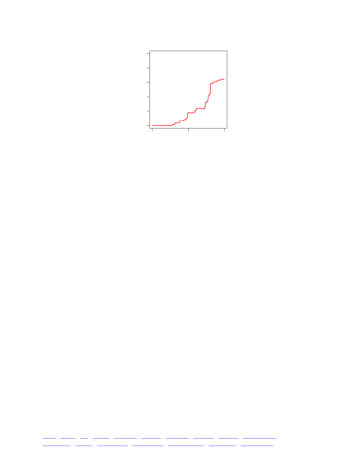
The plotting code that we sent to R included niceties like axis labels, font sizes, and line colors,
so the final plot is reasonably nice-looking. Beyond aesthetics, we can see a few interesting things
in this plot. First of all, there is a long delay – perhaps 15000 generations – before any mutations
fix at all. This is because the chromosome starts empty, in this model, and it takes some time to
accumulate neutral diversity and have it drift to fixation. This is why it is usually important to run
models for a burn-in period before collecting data, of course; the early state of a model is usually
far from equilibrium. Second, even after mutations start to fix the line is quite jagged; there are
long periods without any fixation, and then sudden jumps when many mutations fix
simultaneously. This is because whole haplotypes representing many individual mutations often fix
as a single unit, followed by periods in which competing haplotypes are drifting up and down in
frequency without fixation; these dynamics are also very visible in SLiMgui’s chromosome view.
Apart from a little bit of hassle involved in assembling an R script as an Eidos string, this recipe
is quite short and simple considering that it is continuously writing new script files and then
sublaunching R processes to generate PDF plots! This example is quite simple, but there is no limit
to the complexity possible here; arbitrary plots could be made, multiple plots could be generated
simultaneously, and other processing, such as statistical analysis, could be done in R.
13.12 Modeling nucleotides at a locus
SLiM provides no intrinsic support for explicitly modeling the nucleotide sequence along the
chromosome. In general, such models are conceptually quite different from SLiM; they tend to be
concerned with the probability that each ATGC base will mutate into each other type of base, and
use Markov models and similar constructs to model changes to the nucleotide sequence as
realistically as possible, for the purpose of, for example, accurately calculating divergence time
using molecular data, or calculating a maximum likelihood phylogeny given sequence data. They
also often concern themselves with things like codons and amino acids, codon degeneracy,
synonymous and nonsynonymous mutations, stop codons, nonsense mutations, and so forth, for
example to model the evolution of protein sequences. None of those concepts is really within
SLiM’s domain, and although in principle they could all be modeled in script, at some point the
question arises as to whether, for driving in a screw, a better tool than a hammer might exist.
Nevertheless, in some cases it is desirable to model in SLiM the possibility that a given base
position can take on exactly one of four distinct values, representing nucleotides, while ignoring
the aforementioned issues involved in more realistic modeling of nucleotide sequences. This
could be useful if, for example, it is important that a given base position can possess only four
possible discrete fitness effects – that there be just four distinct alleles at that location. It could also
0 25000 50000
0 100 200 300 400 500
Generation
Fixed mutations
TOC I TOC II WF nonWF initialize() Genome Individual Mutation SLiMSim Subpopulation!
Eidos events fitness() mateChoice() modifyChild() recombination() interaction() reproduction() 222

be important for models in which back-mutation is important, such that a new mutation that arises
at a given location leads to the previous allelic state with a one-in-three chance.
This is possible to model in SLiM, using a little bit of scripting to modify SLiM’s default behavior.
Here we will look at one strategy for doing so.
To begin with, here is the initialize() callback we will use to set up the simulation:
initialize() {!
defineConstant("C", 10); // number of loci!
!
// Create our loci!
for (locus in 0:(C-1))!
{!
// Effects for the nucleotides ATGC are drawn from a normal DFE!
effects = rnorm(4, mean=0, sd=0.05);!
!
// Each locus is set up with its own mutType and geType!
mtA = initializeMutationType(locus*4 + 0, 0.5, "f", effects[0]);!
mtT = initializeMutationType(locus*4 + 1, 0.5, "f", effects[1]);!
mtG = initializeMutationType(locus*4 + 2, 0.5, "f", effects[2]);!
mtC = initializeMutationType(locus*4 + 3, 0.5, "f", effects[3]);!
mt = c(mtA, mtT, mtG, mtC);!
geType = initializeGenomicElementType(locus, mt, c(1,1,1,1));!
initializeGenomicElement(geType, locus, locus);!
!
// We do not want mutations to stack or fix!
mt.mutationStackPolicy = "l";!
mt.mutationStackGroup = -1;!
mt.convertToSubstitution = F;!
!
// Each mutation type knows the nucleotide it represents!
mtA.setValue("nucleotide", "A");!
mtT.setValue("nucleotide", "T");!
mtG.setValue("nucleotide", "G");!
mtC.setValue("nucleotide", "C");!
}!
!
initializeMutationRate(1e-6); // includes 25% identity mutations!
initializeRecombinationRate(1e-8);!
}
First of all, note that the length of the chromosome is a defined constant, C, but here we will
work with just 10 bases just to keep the output simple. This recipe will work for longer
chromosomes too, although there is a price paid in speed and memory usage.
The initialization code loops over the loci, from 0 to C-1, and sets up each locus with its own
mutation types, genomic element type, and genomic element. Each locus will have four
nucleotides, ATGC, each of which has a random fitness effect; those effects are drawn from a
normal distribution using rnorm(). The code creates a mutation type for each nucleotide type,
each using one of the fixed selection coefficients drawn. In other words, each nucleotide type gets
its own mutation type at each locus; since this recipe contains 10 loci, there will be 40 mutation
types in all. A genomic element type is created using those four mutation types in equal
proportions (different proportions could be used if mutational bias is desired), and a genomic
element at the locus in question is created using that genomic element type.
We want new mutations to replace the old mutation at a locus, since that is how nucleotides
work (a base position is never two nucleotides at the same time), so we set mutationStackPolicy
TOC I TOC II WF nonWF initialize() Genome Individual Mutation SLiMSim Subpopulation!
Eidos events fitness() mateChoice() modifyChild() recombination() interaction() reproduction() 223

and mutationStackGroup accordingly. By setting all of the mutation types to the same
mutationStackGroup, nucleotides will all replace each other; there will be no mutation stacking in
this model. We never want these mutation types to fix – this model will never allow a locus to be
empty (as normally occurs in SLiM), since a base position is always either A,T, G, or C – so we set
convertToSubstitution to F. Finally, we use setValue() to save each mutation type’s nucleotide
under the name "nucleotide" for later reference; this is only for purposes of output (note that it
would be more memory-efficient to use integer values of the tag property of the mutation types to
represent the nucleotides instead, but would be less clear for presentation here).
Next, the initialize() callback sets the mutation rate. Note that in this model a nucleotide
can mutate into itself; an A can mutate to become an A, a T to become a T, etc. This is not
prohibited because the mutation-generation machinery in SLiM generates new mutations without
reference to what mutation might already exist at that locus. The mutation rate specified for this
model is therefore higher than the “real” mutation rate will be; approximately 25% of mutations
will be no-ops that do not change the existing nucleotide.
Finally, the recombination rate is set. This recipe models a linked string of ten nucleotides; to
model ten unlinked loci instead, a recombination rate of 0.5 could be used.
Next, we need to create an initial population:
1 late() {!
sim.addSubpop("p1", 2000);!
!
// The initial population is fixed for a single wild-type!
// nucleotide fixed at each locus in the chromosome!
geTypes = sim.chromosome.genomicElements.genomicElementType;!
mutTypes = sapply(geTypes, "sample(applyValue.mutationTypes, 1,!
weights=applyValue.mutationFractions);");!
p1.genomes.addNewDrawnMutation(mutTypes, 0:(C-1));!
!
cat("Initial nucleotide sequence:");!
cat(" " + paste(mutTypes.getValue("nucleotide")) + "\n\n");!
}
The first step is, as usual, a call to addSubpop(). Then we need to set up each locus with an
initial nucleotide. To do that, we first get a vector of the genomic element types for each genomic
element (and thus for each base position, since we have one genomic element per base position).
These genomic element types determine the candidate mutation types for each position, so we can
use sapply() to draw one of the mutation types from each genomic element type, according to the
probabilities specified by the genomic element type; this gives us a vector of mutation types to use
for each base position. Finally, we add all of the new mutations with a single vectorized call to
addNewDrawnMutation(). This design is far faster than adding the new mutations one by one in a
loop. In short, this code chooses a random nucleotide sequence; it then prints out the chosen
sequence using cat(). For example, this code might output:
Initial nucleotide sequence: C G T T A A G G A G
Next, we need to deal with a small issue in our scheme. Because a mutation to the same
nucleotide at the same position can happen multiple times independently, even within one
generation, multiple mutations representing the same nucleotide can be circulating in the
population; a locus might be fixed for G, for example, but that might be represented in SLiM by
82% of genomes having one G mutation, 17% having another, and 1% having a third G mutation,
all with the same selection coefficient and mutation type. This gives SLiM itself no difficulties, but
depending upon the assumptions made in the rest of the model’s script, it could be undesirable, at
TOC I TOC II WF nonWF initialize() Genome Individual Mutation SLiMSim Subpopulation!
Eidos events fitness() mateChoice() modifyChild() recombination() interaction() reproduction() 224

least for purposes of output. This next chunk of code is optional, but many models will want to
include it for this reasons. It looks for such duplicates and fixes them, in each generation:
2: late() {!
// optionally, we can unique new mutations onto existing mutations!
// this runs only in 2: - it is assumed the gen. 1 setup is uniqued!
allMuts = sim.mutations;!
newMuts = allMuts[allMuts.originGeneration == sim.generation];!
!
if (size(newMuts))!
{!
genomes = sim.subpopulations.genomes;!
oldMuts = allMuts[allMuts.originGeneration != sim.generation];!
oldMutsPositions = oldMuts.position;!
newMutsPositions = newMuts.position;!
uniquePositions = unique(newMutsPositions, preserveOrder=F);!
overlappingMuts = (size(newMutsPositions) != size(uniquePositions));!
!
for (newMut in newMuts)!
{!
newMutLocus = newMut.position;!
newMutType = newMut.mutationType;!
oldLocus = oldMuts[oldMutsPositions == newMutLocus];!
oldMatched = oldLocus[oldLocus.mutationType == newMutType];!
!
if (size(oldMatched) == 1)!
{!
// We found a match; this nucleotide already exists, substitute!
containing = genomes[genomes.containsMutations(newMut)];!
containing.removeMutations(newMut);!
containing.addMutations(oldMatched);!
}!
else if (overlappingMuts)!
{!
// First instance; it is now the standard reference mutation!
oldMuts = c(oldMuts, newMut);!
oldMutsPositions = c(oldMutsPositions, newMutLocus);!
}!
}!
}!
}
This gets all of the new mutations in the simulation, using originGeneration. It then gathers
information about the pre-existing mutations, the new mutations, and their positions. Then, for
each new mutation, it determines whether there is a pre-existing mutation with the same position
and type; if so, it substitutes the pre-existing mutation for the new mutation in every genome.
The only twist is that when there is no pre-existing mutation, the new mutation needs to
become the new “canonical” mutation for its position and type, and so it needs to be added to the
vector of pre-existing mutations. This only really needs to be done if more than one new mutation
exists at the same position, however, as it will only matter if a second new mutation comes along,
in the same generation, that matches the first; in that case, the first needs to be used as the pre-
existing mutation to replace the second. Detecting the necessity of this case is the purpose of the
overlappingMuts flag; it allows us to skip updating the list of pre-existing mutations in most cases.
(If the length of the chromosome, C, is increased to a large number like 10000 or more, this
optimization actually makes a substantial difference to the runtime of the recipe.)
TOC I TOC II WF nonWF initialize() Genome Individual Mutation SLiMSim Subpopulation!
Eidos events fitness() mateChoice() modifyChild() recombination() interaction() reproduction() 225

There is only one more step, which is to output something about the final state of the model:
10000 late() {!
muts = p1.genomes.mutations; // all mutations, no uniquing!
!
for (locus in 0:(C-1))!
{!
locusMuts = muts[muts.position == locus];!
totalMuts = size(locusMuts);!
uniqueMuts = unique(locusMuts);!
!
catn("Base position " + locus + ":");!
!
for (mut in uniqueMuts)!
{!
// figure out which nucleotide mut represents!
mutType = mut.mutationType;!
nucleotide = mutType.getValue("nucleotide");!
cat(" " + nucleotide + ": ");!
!
nucCount = sum(locusMuts == mut);!
nucPercent = format("%0.1f%%", (nucCount / totalMuts) * 100);!
!
cat(nucCount + " / " + totalMuts + " (" + nucPercent + ")");!
cat(", s == " + mut.selectionCoeff + "\n");!
}!
}!
}
This code loops through the loci and prints out the fraction (if any) of each nucleotide at that
locus. For example, it might print:
Base position 0:!
C: 4000 / 4000 (100.0%), s == -0.0918891!
Base position 1:!
T: 4000 / 4000 (100.0%), s == 0.0157156!
Base position 2:!
T: 4000 / 4000 (100.0%), s == 0.0301955!
Base position 3:!
T: 4000 / 4000 (100.0%), s == 0.0325203!
Base position 4:!
C: 4000 / 4000 (100.0%), s == -0.0183944!
Base position 5:!
A: 4000 / 4000 (100.0%), s == 0.0376738!
Base position 6:!
G: 4000 / 4000 (100.0%), s == -0.0226032!
Base position 7:!
G: 3103 / 4000 (77.6%), s == 0.0413104!
C: 897 / 4000 (22.4%), s == 0.0477822!
Base position 8:!
A: 4000 / 4000 (100.0%), s == -0.0814816!
Base position 9:!
C: 4000 / 4000 (100.0%), s == 0.0666566
This shows us that position 7 appears to be caught in mid-sweep, with a superior C nucleotide
replacing the existing G nucleotide. All of the other loci are fixed for one nucleotide. We can
compare this output to the initial output:
TOC I TOC II WF nonWF initialize() Genome Individual Mutation SLiMSim Subpopulation!
Eidos events fitness() mateChoice() modifyChild() recombination() interaction() reproduction() 226

Initial nucleotide sequence: C G T T A A G G A G
The comparison indicates that the model has undergone complete substitution at positions 1, 4,
and 9, in addition to the ongoing sweep at position 7 which may or may not complete.
This design allows each nucleotide to have its own dominance coefficient, providing for a fair
amount of flexibility in the evaluation of fitness effects. If more complex dominance interactions
are needed, in which each possible pair of homologous nucleotides could have a different
arbitrary fitness value, that could be implemented by first making the mutation types intrinsically
neutral, and then writing a global fitness(NULL) callback that examines the nucleotides at the
locus in question and returns the overall fitness effect.
On the flip side, a purely neutral model of nucleotide evolution would not need separate
mutation types for each locus at all; just four mutation types, representing A, T, G, and C, could be
used for the whole model. This is a very easy modification of the recipe, and should be
considerably more memory-efficient. A hybrid model in which neutral nucleotides are represented
by four standard ATGC mutation types, while non-neutral nucleotides get their own mutation
types, should also be possible; or setSelectionCoefficient() could probably be used.
As mentioned above, modeling explicit nucleotides could probably be done in a variety of
ways. This recipe should be fairly efficient, provides quite a bit of flexibility in fitness assessment,
and makes no assumptions regarding the fitness effects of nucleotides; it works just as well
modeling neutral drift of nucleotides, in fact. In models of explicit nucleotides such as this,
fundamentally there has to be some way of telling what nucleotide a given mutation represents.
This recipe uses the mutation type to make that distinction, which is ultimately why there are four
mutation types per locus. It is tempting to try to differentiate nucleotides using the tag property of
mutations instead, setting the initial tag value of new mutations in a late() callback similar to the
2: callback shown here. However, the present recipe should be suitable for most purposes.
13.13 Modeling haploid organisms
SLiM models diploid individuals that contain two haploid genomes; this is, at present, a design
constraint in SLiM that cannot be modified. However, it is still possible to model haploids in SLiM
quite easily with scripting, by effectively suppressing one of the two haploid genomes of each
diploid individual. Section 13.6’s recipe, which shows how to model X and Y chromosomes with
a pseudo-autosomal region, shares some aspects of its design with the recipe shown here, but
modeling haploids is actually much simpler. Similar techniques could be used to model
mitochondrial DNA; to model systems such as haplodiploidy; and to model “alternation of
generations”, in which alternate generations in the model are diploid sporophytes and haploid
gametophytes (although in many cases that might be more easily modeled using a modifyChild()
callback to simulate selection during the haploid life stage). Here, however, we will stick with a
simple model of haploids that reproduce clonally. This model is simple enough that we will just
present it in its entirety, rather than building it incrementally:
initialize() {!
initializeMutationRate(1e-7);!
initializeMutationType("m1", 1.0, "f", 0.0);!
initializeGenomicElementType("g1", m1, 1.0);!
initializeGenomicElement(g1, 0, 99999);!
initializeRecombinationRate(0);!
}!
1 {!
sim.addSubpop("p1", 500);!
p1.setCloningRate(1.0);!
}!
TOC I TOC II WF nonWF initialize() Genome Individual Mutation SLiMSim Subpopulation!
Eidos events fitness() mateChoice() modifyChild() recombination() interaction() reproduction() 227

late() {!
// remove any new mutations added to the disabled diploid genomes!
sim.subpopulations.individuals.genome2.removeMutations();!
!
// remove mutations in the haploid genomes that have fixed!
muts = sim.mutationsOfType(m1);!
freqs = sim.mutationFrequencies(NULL, muts);!
sim.subpopulations.genomes.removeMutations(muts[freqs == 0.5], T);!
}!
200000 late() {!
sim.outputFixedMutations();!
}
We begin with a typical initialize() callback, except that the recombination rate is set to
zero since there is no recombination in this clonal model. Note also that although this is a neutral
model for simplicity, the dominance coefficient is set to 1.0 on mutation type m1 as a reminder;
since mutations will never be homozygous in this model, dominance coefficients should always be
1.0 for conceptual clarity. Next we add a new subpopulation in generation 1 as usual; but in
addition, we set the subpopulation to reproduce clonally, as befits haploids (but see section 15.14).
At the end of the model we output fixed mutations, as a placeholder for whatever output would be
desired. The interesting model mechanics occur in between, with the late() callback.
The first part of the late() callback removes mutations in the second haploid genome of each
new child generated. SLiM doesn’t know that we’re modeling haploids, and thus not using the
second genomes, so it adds new mutations to them as usual during offspring generation. This call
removes them again in order to keep all of the second genomes of individuals empty.
The second part of the late() callback solves another problem: removing fixed mutations.
SLiM automatically converts fixed mutations into Substitution objects and removes them from
the simulation; however, it defines fixation as occurring when the frequency of a mutation reaches
1.0. In this haploid model, mutations fix when they reach a frequency of 0.5, because of the
empty second genomes. We therefore need to remove mutations manually, rather than relying on
SLiM’s built-in machinery. This callback achieves that, passing T for the substitute parameter of
removeMutations() so that Substitution objects are created for the fixed mutations as usual.
Those are the only overrides needed in script to produce a model of haploids. The mechanisms
used here to enforce haploidy, such as removal of mutations on the unused chromosome and
substitution of fixed mutations at a frequency of 0.5, could also be used to make just one segment
of the simulated chromosome haploid. This would allow mitochondrial DNA and autosomal DNA
to be jointly simulated in SLiM, for example. Some modifications to the recipe above would be
needed to achieve this; you would probably want to use a sexual autosomal model with biparental
mating, add code to the modifyChild() callback to enforce maternal inheritance of the
mitochondrial DNA (i.e., to block any proposed child that received its mitochondrial DNA from
the father, or both parents, or neither), and use a recombination map to prevent recombination in
the mitochondrial portion of the genome, for example. Section 13.6 provides an example of a
scenario that is in many ways parallel to that. Other ploidy schemes, such as haplodiploidy and
alternation of generations, should also be implementable with modifications of these basic ideas.
For an alternative model of haploid organisms that is more compatible with tree-sequence
recording (chapter 16), but which requires the nonWF model type, see sections 15.13 and 15.14.
13.14 Using mutation rate variation to model varying functional density
Beginning with SLiM 2.5, it is possible to set up a mutation-rate map that varies the mutation
rate along the length of the chromosome, similarly to setting up a recombination-rate map as
TOC I TOC II WF nonWF initialize() Genome Individual Mutation SLiMSim Subpopulation!
Eidos events fitness() mateChoice() modifyChild() recombination() interaction() reproduction() 228

already supported by SLiM; see sections 6.1.1 and 6.1.2, for example. This feature can, of course,
be used for the obvious purpose of configuring mutational “hot” and “cold” spots along the
chromosome, and the code for doing so would look much like the code for those recipes. Here,
we will instead explore a less obvious use: modeling positional variation in functional density.
We know that different regions of chromosomes often have higher or lower functional density,
as a consequence of variation in the density of genes and the importance of those genes.
Regardless of the literal appropriateness of the term “junk DNA”, it is clear that large chromosomal
regions exist that are non-coding, and mutations in these regions generally appear to have
relatively little effect on fitness compared to mutations in coding regions. This is quite orthogonal
to mutational “hot” and “cold” spots; the variation we are concerned with here is not in the
mutation rate per se, but in the rate at which mutations actually influence fitness.
Prior to SLiM 2.5, modeling this would have required that one define a complex map of
genomic elements along the chromosome, all experiencing the same mutation rate (since that
could not be varied), but using a different fraction of neutral mutations to deleterious mutations
(and/or beneficial mutations, but for simplicity we will here focus on deleterious mutations). This
design would have been necessary in order to achieve the desired variation in the rate of
deleterious mutations, even if one was not actually interested in the neutral mutations at all. Such
a model would run much more slowly than necessary because of the neutral mutation overhead.
By defining a mutation-rate map, however, it is now straightforward to build a model in which
functional density varies along the chromosome, without having to model the neutral mutations. A
proof-of-concept model for this is so simple as to be trivial:
initialize() {!
initializeMutationType("m1", 0.5, "f", -0.01); // deleterious!
initializeGenomicElementType("g1", m1, 1.0);!
initializeGenomicElement(g1, 0, 99999);!
initializeRecombinationRate(1e-8);!
!
// Use the mutation rate map to vary functional density!
ends = c(20000, 30000, 70000, 90000, 99999);!
densities = c(1e-9, 2e-8, 1e-9, 5e-8, 1e-9);!
initializeMutationRate(densities, ends);!
}!
1 {!
sim.addSubpop("p1", 500);!
}!
200000 late() { sim.outputFixedMutations(); }
The variables ends and densities are set up to encode the desired mutation-rate map, with the
end position for each chromosomal range and the effective functional density – the rate of
mutations having a deleterious effect, in this model – of that chromosomal range. As the recipes of
sections 6.1.1 and 6.1.2 illustrate, such maps can easily be generated randomly based upon
empirical metrics, or can even be read in from a file with empirical map data; in this model, to
keep things simple, we instead just specify a very simple map with five regions of different
functional density. After the model has been initialized, clicking the button in SLiMgui will
show the mutation-rate map (we have seen that button show the recombination-rate map before; it
shows whichever map has been defined, or both if both have been defined):
R
TOC I TOC II WF nonWF initialize() Genome Individual Mutation SLiMSim Subpopulation!
Eidos events fitness() mateChoice() modifyChild() recombination() interaction() reproduction() 229

The highest rate is in the region from base position 70000 to 89999, and indeed quite a few
deleterious mutations can be seen in that region (but none at very high frequency; the parameters
used in this model mean that the deleterious mutations are eliminated fairly efficiently). There is a
somewhat less active region from 20000 to 30000, with a handful of mutations; the rest of the
chromosome has a lower functional density, and receives deleterious mutations relatively rarely.
In this recipe we work with only one mutation type, modeling deleterious mutations. It would
be possible to extend it to include several types of functional mutations, each with a different rate
of occurrence along the chromosome. In that case, the mutation-rate map would be set to encode
the sum of the rates for each of the mutation types in each chromosomal region, and genomic
elements would be used to partition mutations in each region into the correct fraction for each of
the functional mutation types. This would be somewhat more complex than this recipe, but
manageably so; and it would again be much more efficient than using a constant mutation rate
along the chromosome together with a varying fraction of neutral mutations, since modeling all of
the neutral mutations could again be avoided.
13.15 Modeling microsatellites
A microsatellite (also known as a short tandem repeat or simple sequence repeat) is a
chromosomal region in which a specific nucleotide sequence repeats, often many times.
Microsatellites are important in many areas of applied genetics, from kinship analysis to forensics,
and are also often used to assess the similarity among individuals or subpopulations in ecology
and evolutionary biology. It is thus useful to be able to include them in evolutionary models.
Since SLiM does not model actual nucleotides, explicitly modeling the repeated nucleotide
sequence of a microsatellite doesn’t fit well into its conceptual model; explicitly modeling
mutations that change the number of repeats in a microsatellite would also change the length of
the chromosome, which is not allowed in SLiM. Nevertheless, it is possible to model microsats
more abstractly in SLiM, using mutations that conceptually represent a microsat with a particular
number of repeats at a given locus. This recipe will illustrate one simple approach to this.
We will build this model step by step. First, the model initialization:
initialize() {!
defineConstant("L", 1e6); // chromosome length!
defineConstant("msatCount", 10); // number of microsats!
defineConstant("msatMu", 0.0001); // mutation rate per microsat!
defineConstant("msatUnique", F); // T = unique msats, F = lineages!
!
initializeMutationRate(1e-7);!
initializeMutationType("m1", 0.5, "f", 0.0); // neutral!
initializeGenomicElementType("g1", m1, 1.0);!
initializeGenomicElement(g1, 0, L-1);!
initializeRecombinationRate(1e-8);!
!
// microsatellite mutation type; also neutral, but magenta!
initializeMutationType("m2", 0.5, "f", 0.0);!
m2.convertToSubstitution = F;!
m2.color = "#900090";!
}
We define the length of the chromosome (L), and several constants related to our microsats: the
number of microsats we will model, the mutation rate per microsat (per genome per generation),
and a flag that indicates whether to unique the microsats as the model runs (more on this below).
The rest sets up a simple neutral model structure, plus a mutation type, m2, that will represent our
microsatellites. We prevent microsatellites from fixing, with convertToSubstitution, since they
TOC I TOC II WF nonWF initialize() Genome Individual Mutation SLiMSim Subpopulation!
Eidos events fitness() mateChoice() modifyChild() recombination() interaction() reproduction() 230

are a permanent feature of the chromosomal structure. We also set them to display in SLiMgui
using a shade of magenta, to set them apart from the other neutral mutations in the model.
Next we create a subpopulation with microsatellites:
1 late() {!
sim.addSubpop("p1", 500);!
!
// create some microsatellites at random positions!
genomes = sim.subpopulations.genomes;!
positions = rdunif(msatCount, 0, L-1);!
repeats = rpois(msatCount, 20) + 5;!
!
for (msatIndex in 0:(msatCount-1))!
{!
pos = positions[msatIndex];!
mut = genomes.addNewDrawnMutation(m2, pos);!
mut.tag = repeats[msatIndex];!
}!
!
// remember the microsat positions for later!
defineConstant("msatPositions", positions);!
}
We call addSubpop() to create the subpopulation, and then we create our microsatellites. Each
microsat is simply an m2 mutation at a given position; the number of repeats in a given microsat is
represented using the tag property of the mutation. This code draws the positions and repeats for
all of the microsats first, and then loops to create each microsat using that information. Finally, we
remember the positions of the microsats in a defined constant for later use.
This code makes the initial population homogenous: the number of repeats of a given microsat
is the same across all genomes. It would of course be possible to start with a non-homogenous
state instead. To avoid creating a new Mutation for every microsat in every genome, however, it
would be best to determine all of the genomes containing a given repeat count at a given position,
and then call addNewDrawnMutation() just once on that entire genome vector so as to create a
single Mutation object that is shared among all of those genomes. Alternatively, a uniquing
strategy could be employed, similar to what we will see below, such that the first microsatellite
created at a given position with a given number of repeats is instantiated with a new Mutation, and
then all subsequent microsats with the same number of repeats at the same position look up and
use that existing Mutation object. Such extensions are left as an exercise for the reader.
With the initial subpopulation state set up, let’s define an endpoint for the model:
10000 late() {!
// print frequency information for each microsatellite site!
all_msats = sim.mutationsOfType(m2);!
!
for (pos in sort(msatPositions))!
{!
catn("Microsatellite at " + pos + ":");!
!
msatsAtPos = all_msats[all_msats.position == pos];!
!
for (msat in sortBy(msatsAtPos, "tag"))!
catn(" variant with " + msat.tag + " repeats: " +!
sim.mutationFrequencies(NULL, msat));!
}!
}
TOC I TOC II WF nonWF initialize() Genome Individual Mutation SLiMSim Subpopulation!
Eidos events fitness() mateChoice() modifyChild() recombination() interaction() reproduction() 231

This output callback loops over the (sorted) positions of the microsats. For each microsat
position, it looks up all of the microsats that exist at that position, and outputs frequency counts for
each variant (sorted by repeat count).
We’ll see some example output below, but the model isn’t finished yet; let’s finish it first. The
remaining piece in the puzzle is for our microsatellites to mutate. Microsats mutate in an
interesting way: they add or remove repeats. Furthermore, the probability of this happening is
much higher than the usual mutation rate in most organisms – often as high as one in ten
thousand. We model all this with a special modifyChild() callback:
modifyChild() {!
// mutate microsatellites with rate msatMu!
for (genome in child.genomes)!
{!
mutCount = rpois(1, msatMu * msatCount);!
!
if (mutCount)!
{!
mutSites = sample(msatPositions, mutCount);!
msats = genome.mutationsOfType(m2);!
!
for (mutSite in mutSites)!
{!
msat = msats[msats.position == mutSite];!
repeats = msat.tag;!
!
// modify the number of repeats by adding -1 or +1!
repeats = repeats + (rdunif(1, 0, 1) * 2 - 1);!
!
if (repeats < 5)!
next;!
!
// if we're uniquing microsats, do so now!
if (msatUnique)!
{!
all_msats = sim.mutationsOfType(m2);!
msatsAtSite = all_msats[all_msats.position == mutSite];!
matchingMut = msatsAtSite[msatsAtSite.tag == repeats];!
!
if (matchingMut.size() == 1)!
{!
genome.removeMutations(msat);!
genome.addMutations(matchingMut);!
next;!
}!
}!
!
// make a new mutation with the new repeat count!
genome.removeMutations(msat);!
msat = genome.addNewDrawnMutation(m2, mutSite);!
msat.tag = repeats;!
}!
}!
}!
!
return T;!
}
TOC I TOC II WF nonWF initialize() Genome Individual Mutation SLiMSim Subpopulation!
Eidos events fitness() mateChoice() modifyChild() recombination() interaction() reproduction() 232

There’s a lot to parse there; let’s take it step by step. First of all, the microsats in each genome in
the proposed child mutate independently, so we loop over them and mutate them separately. For
each genome, we draw the number of mutations that occur from a Poisson distribution; this is
faster than doing a separate random draw to determine the fate of each individual microsat, but is
otherwise equivalent. If the number of microsat mutations is zero, we’re done; we loop back to
handle the other genome, and then we’re done and return T. When the number of microsat
mutations is greater than zero, though, we have work to do.
In that case, the next thing we do is to draw the positions of the microsats that mutated, using
sample() to draw from the vector of positions we defined when we set up the simulation. Each
microsat thus has an equal probability of mutating (see below for discussion of this). We loop over
those positions and mutate each chosen microsat in turn. To mutate a microsat, we first look up
the existing mutation by position and find out how many repeats it has. We then decide what the
new, mutated repeat count will be; here we just add or subtract 1, and limit the repeat count to a
minimum of 5, but more sophisticated and realistic dynamics could be introduced. Finally,
ignoring the “if (msatUnique)” section for a moment (since msatUnique is presently defined as F
anyway), we effect the mutation event by removing the old microsat mutation from the genome
and adding a newly created microsat mutation at the same position, with the new repeat count for
its tag. (We can’t simply set the tag of the existing microsat mutation, because it is potentially
shared among many genomes; changing its tag would change the repeat count in all of those
genomes!)
Running this model produces output like:
Microsatellite at 60933:!
variant with 21 repeats: 0.001!
variant with 21 repeats: 0.026!
variant with 21 repeats: 0.001!
variant with 22 repeats: 0.741!
variant with 23 repeats: 0.105!
variant with 23 repeats: 0.126!
Microsatellite at 98509:!
variant with 34 repeats: 1!
Microsatellite at 123123:!
variant with 20 repeats: 0.964!
variant with 21 repeats: 0.001!
variant with 21 repeats: 0.035!
Microsatellite at 142781:!
variant with 23 repeats: 0.795!
variant with 24 repeats: 0.205!
...
This looks reasonable, except that more than one variant with the same repeat count sometimes
exists for a given microsatellite. Each such variant represents an independent mutational lineage;
each time a microsat mutation occurs, it is represented by a new Mutation object that SLiM tracks
forevermore. In some cases, keeping track of each mutational lineage may be desirable; it could
provide a sort of ancestry tracking, for example, that goes beyond what the repeat counts alone
would provide. Often, however, one would like such replicate mutational lineages to be merged,
such that just a single microsat mutation exists to represent a microsat with a given number of
repeats at a given position. This is what that “if (msatUnique)” code, which we skipped over
above, is for: it “uniques” the microsatellite lineages. To see the effect of this, let’s change that flag
by modifying its definition in the initialize() callback:
defineConstant("msatUnique", T); // T = unique msats, F = lineages
TOC I TOC II WF nonWF initialize() Genome Individual Mutation SLiMSim Subpopulation!
Eidos events fitness() mateChoice() modifyChild() recombination() interaction() reproduction() 233

If we run the model again (using the same random number seed, so as to reproduce the same
evolutionary dynamics), the output now looks like this:
Microsatellite at 60933:!
variant with 21 repeats: 0.028!
variant with 22 repeats: 0.741!
variant with 23 repeats: 0.231!
Microsatellite at 98509:!
variant with 34 repeats: 1!
Microsatellite at 123123:!
variant with 20 repeats: 0.964!
variant with 21 repeats: 0.036!
Microsatellite at 142781:!
variant with 23 repeats: 0.795!
variant with 24 repeats: 0.205!
...
The microsats have been uniqued, as desired. The “if (msatUnique)” code in the callback,
which implements this feature, is actually quite straightforward. It gets a vector of all existing
microsat mutations from the simulation, and then narrows that down to those at the desired
position, and then finally down to those with the desired number of repeats. If it found an exact
match, then it removes the existing microsat mutation and adds the match; the next statement then
loops forward to the next mutation site, if any. If it did not find a match, the code drops through to
add a newly created mutation instead; that is the case we saw before.
That’s all that’s needed: a little initialization code, a little output code, and a modifyChild()
callback to handle mutating the microsats. Although that modifyChild() callback is not
particularly short, conceptually it is really quite simple: decide on how many microsat mutation
events there will be in each genome and where they will be, and then change the mutations in the
genome to reflect those mutation events with new (or uniqued) mutations that have the appropriate
repeat count in their tag values.
There are a few ways in which greater realism could be added to this model. We already
discussed, above, the possibility of starting with a heterogenous subpopulation state; any initial
state could be set up, although care should be taken to unique the microsat mutations, both to
keep memory usage down and to provide a single mutational lineage for each unique
microsatellite state.
Another way in which this model oversimplifies the biology is in its mutational model. In
reality, microsats can sometimes mutate by adding or subtracting more than a single repeat, and
their probability of mutating at all can depend upon the number of repeats present, as well as
upon things like the sex of the parent. The mutation rate for microsats can even depend upon the
similarity or dissimilarity in repeat counts between the two copies of the microsat in the parent that
generated the gamete, due to effects during meiosis. All of these effects could be modeled with
extensions to the modifyChild() callback presented here. To implement this, it would probably be
necessary (or at least simpler) to get rid of the rpois() call that draws the number of microsat
mutations for each genome, and instead simply loop over all of the existing microsat positions and
determine whether a mutation occurred at each position with a runif() draw that is compared to
the calculated probability of mutation for that microsat in that genome.
A third oversimplification is that this recipe does not explicitly track variation in microsats due
to point mutations rather than repeat-count mutations. Perhaps a good approach for this would
involve modeling repeat-count changes just as in this model, while adding in similar code that
would model nucleotide changes as well (using an appropriate mutation probability based on the
length of the microsat). If such a model was run without uniquing, each mutational lineage would
TOC I TOC II WF nonWF initialize() Genome Individual Mutation SLiMSim Subpopulation!
Eidos events fitness() mateChoice() modifyChild() recombination() interaction() reproduction() 234

then be tracked separately, and so point mutations would create new mutational lineages that
would be considered distinct from other mutation lineages with the same repeat count. However,
this design would overcount the number of genetically distinct lineages, since repeat-count
mutations as well as point mutations would generate distinct mutational lineages. To account for
things better would require additional state information to be attached to each Mutation object,
using the setValue()/getValue() mechanism; in this way, two mutational lineages with the same
repeat count and no nucleotide differences could be merged together by the uniquing code, while
two mutational lineages with the same repeat count but with nucleotide differences could be kept
separate. In the extreme of maximal realism, one could actually store generated string
representations of nucleotide sequences inside the Mutation objects, but that would be overkill for
most purposes. Usually, a single token attached to each mutation, such as a random number
generated with runif(), could probably provide sufficient realism. Whenever a point mutation
occurred, a new mutation object would be created (with no uniquing necessary) and would be
given a new random token representing its unique new nucleotide sequence. Whenever a repeat-
count mutation occurred, on the other hand, the token value would be inherited from the old
microsat mutation at that position, indicating that the nucleotide difference, whatever it might be,
was (assumed to be) preserved across the repeat count change. If the uniquing code then re-used
an existing mutation only when the token values of the desired mutation and the existing mutation
were the same, a closer approximation of the correct pattern of microsatellite diversity might
emerge. Implementing this goes beyond the scope of this recipe, and so is left as an exercise for
the reader, but in essence it is actually quite simple; the design simply adds another piece of state,
tracked with setValue()/getValue(), that is handled very similarly to the tag value in the existing
recipe. That token value is inherited (just as tag is), changes its value upon mutation (just like tag,
but for point mutation events instead of repeat-count mutation events), and must be equal in order
for uniquing to find a match (just as tag is used by the existing uniquing code). Token values
would be set up when the subpopulation is initialized, just as tag values are, either with zero
values (representing a homogenous initial state) or with some sort of population structure indicated
by different random token values on different genomes to represent standing variation in
microsatellite diversity.
Depending upon the level of realism desired, therefore, this recipe might provide a complete
solution, or it might merely point the way. In either case, the basic strategy outlined here of using
tag values to indicate repeat counts on mutations that represent a microsatellite at a given locus is
the recommended approach in SLiM. In general, using mutations to represent some conceptual
difference between genomes, rather than necessarily representing a literal nucleotide difference,
can be a useful strategy for advanced models in SLiM.
13.16 Modeling transposable elements
A transposable element, or transposon, is a chromosomal region which is capable of replication
or positional change within the genome, either on its own or with the assistance of an enzyme
such as reverse transcriptase or transposase. Transposons constitute a substantial fraction of the
genome of many species, and can have evolutionary effects through side effects such as disabling
genes into which they “jump”, altering the regulation of nearby genes, and copying genetic
material within the genome. Given their evolutionary importance, incorporating transposons into
evolutionary models may be useful; in this recipe we will therefore explore a simple model of
transposons in SLiM.
There are various subtypes and classifications of transposons; here we will explore autonomous
Class I transposons, which “copy and paste” themselves to new locations in the genome under
their own power. Given the diversity of evolutionary effects transposons can have, and the
TOC I TOC II WF nonWF initialize() Genome Individual Mutation SLiMSim Subpopulation!
Eidos events fitness() mateChoice() modifyChild() recombination() interaction() reproduction() 235

diversity of ways in which they can function, this recipe cannot provide a general formula for
modeling transposons and all of their effects; all this recipe will do is point the way. At the end of
this section, we will discuss ways in which this recipe could be extended to model further aspects
of the behavior of transposons.
Since SLiM does not model nucleotides explicitly, we will not model the actual nucleotide
sequence of transposons here. Furthermore, since copying a transposon to a new location changes
the length of the chromosome (which is not possible in SLiM), we will model transposons
conceptually rather than literally, as loci in the genome that are capable of copying themselves.
This approach is similar to the approach taken in section 13.15 for modeling microsatellites.
We will also model the vulnerability of transposons to mutations that disable them by
deactivating their ability to jump; we will track disabled transposons, and assess the fraction of
each transposon that has been disabled. This is important, since even disabled transposons may
have evolutionary effects such as changes in gene regulation, and since most of the transposons in
typical organisms appear to be disabled.
We will start with the model’s initialization:
initialize() {!
defineConstant("L", 1e6); // chromosome length!
defineConstant("teInitialCount", 100); // initial number of TEs!
defineConstant("teJumpP", 0.0001); // TE jump probability!
defineConstant("teDisableP", 0.00005); // disabling mut probability!
!
initializeMutationRate(1e-7);!
initializeMutationType("m1", 0.5, "f", 0.0); // neutral!
initializeGenomicElementType("g1", m1, 1.0);!
initializeGenomicElement(g1, 0, L-1);!
initializeRecombinationRate(1e-8);!
!
// transposon mutation type; also neutral, but red!
initializeMutationType("m2", 0.5, "f", 0.0);!
m2.convertToSubstitution = F;!
m2.color = "#FF0000";!
!
// disabled transposon mutation type; dark red!
initializeMutationType("m3", 0.5, "f", 0.0);!
m3.convertToSubstitution = F;!
m3.color = "#700000";!
}
This defines the chromosome length and a few constants governing the behavior of TEs in the
model. It then sets up a simple neutral simulation, and defines two additional mutation types: one
for active TEs, m2, which displays as red in SLiMgui, and one for TEs that have been disabled by
mutation, m3, which display as a darker red.
Next we set up the initial state of our subpopulation. In this recipe, the tag values on the m2
and m3 mutations are used as identifiers; each TE gets its own unique tag value, which is used for
both its active (m2) and disabled (m3) forms, allowing the mutations representing the two forms to
be matched up. The tag value on the simulation itself, sim.tag, is used to keep track of the next
unused tag value; it starts at 0 and counts up. The setup thus looks like this:
1 late() {!
sim.addSubpop("p1", 500);!
!
sim.tag = 0; // the next unique tag value to use for TEs!
!
TOC I TOC II WF nonWF initialize() Genome Individual Mutation SLiMSim Subpopulation!
Eidos events fitness() mateChoice() modifyChild() recombination() interaction() reproduction() 236

// create some transposons at random positions!
genomes = sim.subpopulations.genomes;!
positions = rdunif(teInitialCount, 0, L-1);!
!
for (teIndex in 0:(teInitialCount-1))!
{!
pos = positions[teIndex];!
mut = genomes.addNewDrawnMutation(m2, pos);!
mut.tag = sim.tag;!
sim.tag = sim.tag + 1;!
}!
}
We make a new subpop, start sim.tag at 0, and then create new TEs that are fixed across the
whole population. (As in the recipe of section 13.15, creating an initial state that involves
heterogeneity in the TEs possessed by individuals would also be possible but is more complex; see
that recipe for discussion.) The positions for the TEs are drawn randomly across the chromosome,
and each TE is tagged with a sequential value from sim.tag.
Before implementing any more of the TE dynamics, let’s implement the final output event:
5000 late() {!
// print information on each TE, including the fraction of it disabled!
all_tes = sortBy(sim.mutationsOfType(m2), "position");!
all_disabledTEs = sortBy(sim.mutationsOfType(m3), "position");!
genomeCount = size(sim.subpopulations.genomes);!
!
catn("Active TEs:");!
for (te in all_tes)!
{!
cat(" TE at " + te.position + ": ");!
!
active = sim.mutationCounts(NULL, te);!
disabledTE = all_disabledTEs[all_disabledTEs.tag == te.tag];!
!
if (size(disabledTE) == 0)!
{!
disabled = 0;!
}!
else!
{!
disabled = sim.mutationCounts(NULL, disabledTE);!
all_disabledTEs = all_disabledTEs[all_disabledTEs != disabledTE];!
}!
!
total = active + disabled;!
!
cat("frequency " + format("%0.3f", total / genomeCount) + ", ");!
catn(round(active / total * 100) + "% active");!
}!
!
catn("\nCompletely disabled TEs: ");!
for (te in all_disabledTEs)!
{!
freq = sim.mutationFrequencies(NULL, te);!
cat(" TE at " + te.position + ": ");!
catn("frequency " + format("%0.3f", freq));!
}!
}
TOC I TOC II WF nonWF initialize() Genome Individual Mutation SLiMSim Subpopulation!
Eidos events fitness() mateChoice() modifyChild() recombination() interaction() reproduction() 237

This prints all of the active TEs in the model (sorted by position), with information on their
overall frequency in the population and on the fraction of their occurrences that have been
disabled by mutations. After that, it prints a list of the completely disabled TEs (sorted as well);
frequencies are also given for those, since TEs could conceivably be disabled before fixing. The
logic of this code is quite straightforward, so there is no need to belabor it here.
We want our TEs to copy themselves; this occurs during the life of the organism, not during
meiosis, so we model it with a late() event:
late() {!
// make active transposons copy themselves with rate teJumpP!
for (individual in sim.subpopulations.individuals)!
{!
for (genome in individual.genomes)!
{!
tes = genome.mutationsOfType(m2);!
teCount = tes.size();!
jumpCount = teCount ? rpois(1, teCount * teJumpP) else 0;!
!
if (jumpCount)!
{!
jumpTEs = sample(tes, jumpCount);!
!
for (te in jumpTEs)!
{!
// make a new TE mutation!
pos = rdunif(1, 0, L-1);!
jumpTE = genome.addNewDrawnMutation(m2, pos);!
jumpTE.tag = sim.tag;!
sim.tag = sim.tag + 1;!
}!
}!
}!
}!
}
This loops through the genomes of all individuals in the simulation. For each genome, it gets all
of the TEs present, and decides how many (if any) will “jump” according to the probability teJumpP
for each TE, using a draw from a Poisson distribution. (This is faster than doing a separate random
draw for each TE, but is otherwise equivalent.) If any TEs did jump, the ones that jumped are
selected at random. Each jump is simulated by creating a new TE at a new, randomly chosen
location. The new TEs get new tag values assigned sequentially from sim.tag, so that their
corresponding disabled versions can be looked up. And that is it for jumping; its logic is fairly
straightforward since disabled TEs are not involved at all.
Finally, we need to implement the disabling of TEs by random point mutations. Since TEs are
simulated here as point mutations themselves, we need to simulate this disabling process
ourselves; SLiM’s automatic mutation generation will never modify our TEs for us. We model
disabling mutations in a modifyChild() callback. Its logic is similar to that of the jumping code
above, except that when a TE is disabled, a mutation of type m3 needs to be substituted in place of
the existing m2 mutation that represents the TE. The m3 mutation corresponding to any given m2 TE
is created just once, and then the same m3 mutation is looked up and reused every time that same
m2 TE is disabled in another genome. This “uniquing” of the m3 mutations makes the model much
more memory-efficient, and makes the output code much simpler. The main purpose of the tag
values we have been managing is, in fact, to facilitate this uniquing process. The disabling
callback looks like this:
TOC I TOC II WF nonWF initialize() Genome Individual Mutation SLiMSim Subpopulation!
Eidos events fitness() mateChoice() modifyChild() recombination() interaction() reproduction() 238

modifyChild() {!
// disable transposons with rate teDisableP!
for (genome in child.genomes)!
{!
tes = genome.mutationsOfType(m2);!
teCount = tes.size();!
mutatedCount = teCount ? rpois(1, teCount * teDisableP) else 0;!
!
if (mutatedCount)!
{!
mutatedTEs = sample(tes, mutatedCount);!
!
for (te in mutatedTEs)!
{!
all_disabledTEs = sim.mutationsOfType(m3);!
disabledTE = all_disabledTEs[all_disabledTEs.tag == te.tag];!
!
if (size(disabledTE))!
{!
// use the existing disabled TE mutation!
genome.removeMutations(te);!
genome.addMutations(disabledTE);!
next;!
}!
!
// make a new disabled TE mutation with the right tag!
genome.removeMutations(te);!
disabledTE = genome.addNewDrawnMutation(m3, te.position);!
disabledTE.tag = te.tag;!
}!
}!
}!
!
return T;!
}
For each genome in the proposed child, we get the TEs contained, and calculate the number
that will be disabled using a Poisson draw as before. We select the TEs that actually mutated, and
for each, attempt to look up a corresponding m3 mutation using the tag value of the m2 mutation. If
we find one, we substitute that. If not, we create a new m3 mutation to represent the disabled
state, marking it with the TE’s tag value so we can look it up next time. That’s it for the TE
disabling code; a bit lengthy, but the logic is simple.
If this model is run, typical output might look like this:
Active TEs:!
TE at 1793: frequency 0.011, 100% active!
TE at 2435: frequency 0.208, 100% active!
TE at 3629: frequency 0.002, 100% active!
TE at 6339: frequency 0.208, 94% active!
TE at 7081: frequency 0.020, 100% active!
TE at 7728: frequency 1.000, 79% active!
...!
Completely disabled TEs: !
TE at 24821: frequency 1.000!
TE at 83627: frequency 1.000!
TE at 98286: frequency 1.000!
...
TOC I TOC II WF nonWF initialize() Genome Individual Mutation SLiMSim Subpopulation!
Eidos events fitness() mateChoice() modifyChild() recombination() interaction() reproduction() 239

That output shows a mix of TEs at high frequency (perhaps present already in the initial
population setup, since not that many generations have elapsed) and TEs at low frequency (which
must be copies due to jumping). Some TEs are completely active, whereas others have been
partially or fully disabled by mutations. (Once even a single copy of a TE is disabled by mutation,
that copy might drift to fixation; the fact that TEs have been completely disabled does not mean
that TE-disabling mutations are particularly common.)
Note that this model is never at equilibrium; the number of TEs is likely to grow without bound,
since the probability of jumping is greater than the probability of TEs being disabled by mutations.
That means that the model runs ever more slowly, since the TE mutations are not allowed to fix. If
a model didn’t care about disabled TEs at all, it would be much simpler and faster to simply delete
TEs from a genome when they are disabled.
Note also that the probabilities of jumping and of being disabled in this recipe are arbitrary and
have almost no empirical basis; they just worked well for testing the code. Please do not use these
values in any production code of your own.
With that, we have wrapped up this recipe, but obviously there are a great many aspects of the
biology of transposons that we haven’t covered here:
• Effects of transposons on fitness could be modeled through fitness() callbacks, either
modifying the fitness effects of other mutations due to the proximity of transposons, or
modeling a direct fitness effect for the transposons themselves in their own fitness()
callback. Alternatively, at the moment of a transposon’s jump a genetic effect could be
modeled by examining and altering other mutations in the vicinity of the jump
destination, to simulate up/down-regulation of those mutations (taking care to make a
private copy of any modified mutations first, so that other genomes sharing the same
mutations do not receive the same modifications as an unintended side effect).
• Transposons that relocate themselves, rather than copying themselves, could be
implemented by adding a call to genome.removeMutations(te) in the jump code.
• Attempts by the organism to suppress TEs en masse, for example through epigenetic
controls such as methylation, could be simulated by converting TEs in a given individual
into a suppressed version (perhaps using a new mutation type to represent suppression);
such suppression could be temporary, since one could write code to convert suppressed
TEs back into active TEs again, too.
• Non-autonomous TEs that can jump only in the presence of a separate enabling gene
could easily be modeled simply by checking for the presence of the enabling gene in an
individual prior to allowing any TEs in that individual to jump.
• It is not clear exactly what, if anything, restricts the proliferation of TEs in real organisms,
but one could certainly model some sort of balancing factor that would limit the
proliferation of TEs in this model. The probability of jumping could decrease as the
number of active TEs increases (for some unclear reason), or the fitness of organisms could
start to decrease sharply as their TE load increases above some bound (with perhaps a bit
more biological justification), or whatever other mechanism one wished.
• One of the most interesting aspects of transposons is that they sometimes jump more
frequently when an individual is subject to environmental stress; that could be modeled
by calculating a jump probability for the TEs in an individual that depends upon that
individual’s fitness, or upon the mismatch between its phenotype and its environment in
some specific trait, if desired.
The point is that although this recipe is fairly rudimentary, many aspects of the evolutionary
dynamics of transposons could be easily modeled in SLiM by implementing whatever extensions to
this recipe are desired, as outlined above.
TOC I TOC II WF nonWF initialize() Genome Individual Mutation SLiMSim Subpopulation!
Eidos events fitness() mateChoice() modifyChild() recombination() interaction() reproduction() 240

13.17 A QTL-based model with two quantitative phenotypic traits and pleiotropy
Sections 13.1 and 13.10 introduced some strategies for modeling quantitative traits in SLiM,
where a phenotypic trait’s quantitative value is based upon the additive effects of multiple QTLs
(quantitative trait loci). Chapter 14 will show more QTL-based models that incorporate continuous
space and spatial interactions. All of these quantitative-trait models share the same basic
approach: QTL mutations are intrinsically neutral (enforced with a fitness() callback), but have
an additive effect upon a phenotypic trait value possessed by each individual. Individual fitness is
then modeled using some form of fitness function (often Gaussian), based upon the deviation of
the individual’s phenotype from the optimum phenotype in its environment (determined by a
fitness(NULL) callback that evaluates each individual). All of these recipes model a single
phenotypic trait, however, with the QTL mutations influencing only that one trait. In this section
we will look at an extension of the same basic approach, modeling two phenotypic traits. QTL
mutations in this model will influence both phenotypic traits, pleiotropically, with effect sizes
drawn from a multivariate normal distribution (thus allowing the effects on the phenotypic traits to
be either independent or correlated). This recipe can be trivially extended to encompass any
number of QTL-based phenotypic traits, with any type of pleiotropy. Finally, at the end, we will
add in live R-based plotting, as introduced in section 13.11, to plot the adaptive trajectory of the
population. You may wish to review sections 13.1, 13.10, and 13.11 before proceeding.
Let’s begin with the initialize() callback as usual:
initialize() {!
initializeMutationRate(1e-7);!
!
initializeMutationType("m1", 0.5, "f", 0.0); // neutral!
initializeMutationType("m2", 0.5, "f", 0.0); // QTLs!
m2.convertToSubstitution = F;!
m2.color = "red";!
!
// g1 is a neutral region, g2 is a QTL!
initializeGenomicElementType("g1", m1, 1.0);!
initializeGenomicElementType("g2", c(m1,m2), c(1.0, 0.1));!
!
// chromosome of length 100 kb with two QTL regions!
initializeGenomicElement(g1, 0, 39999);!
initializeGenomicElement(g2, 40000, 49999);!
initializeGenomicElement(g1, 50000, 79999);!
initializeGenomicElement(g2, 80000, 89999);!
initializeGenomicElement(g1, 90000, 99999);!
initializeRecombinationRate(1e-8);!
!
// QTL-related constants used below!
defineConstant("QTL_mu", c(0, 0));!
defineConstant("QTL_cov", 0.25);!
defineConstant("QTL_sigma", matrix(c(1,QTL_cov,QTL_cov,1), nrow=2));!
defineConstant("QTL_optima", c(20, -20));!
!
catn("\nQTL DFE means: ");!
print(QTL_mu);!
catn("\nQTL DFE variance-covariance matrix: ");!
print(QTL_sigma);!
}
QTLs will be represented by m2; it is declared to be neutral here, so a fitness(m2) callback
making it neutral will not be needed. In other QTL recipes the selection coefficient of the
TOC I TOC II WF nonWF initialize() Genome Individual Mutation SLiMSim Subpopulation!
Eidos events fitness() mateChoice() modifyChild() recombination() interaction() reproduction() 241

mutations was used to store the additive effect of each QTL mutation, but we will take a different
approach here. The m2 mutations are colored red in SLiMgui, and are not converted to
substitutions when they fix, since their phenotypic effect will continue to be important. The
chromosome is a mixture of g1 neutral regions and g2 regions that can contain QTL mutations.
Finally, we define some QTL-related constants: QTL_mu gives the mean effect of new QTL
mutations on the two phenotypes, QTL_cov gives the covariance between the two effects, and
QTL_sigma is a variance-covariance matrix derived from QTL_cov that will govern new mutational
effects (this matrix is sometimes called an M-matrix). QTL_optima gives the optimal phenotypic
values for the two quantitative traits; note that the optima have different signs, but the M-matrix
encodes a positive mutational correlation, so adaptation in this model will be contrary to the
pleiotropically preferred direction of evolution. Finally, the means and M-matrix are printed; the
M-matrix looks like this:
QTL DFE variance-covariance matrix: !
[,0] [,1]!
[0,] 1 0.25!
[1,] 0.25 1
Support for matrices was added to Eidos in SLiM 2.6, so the matrix() function and other
aspects of working with matrices in Eidos may be new; see the Eidos language manual.
Next we start a new subpopulation:
1 late() {!
sim.addSubpop("p1", 500);!
}
Then we need to draw the effects of new mutations in each generation, which is a bit complex
since SLiM doesn’t do it for us in this recipe the way it usually does:
late() {!
// add effect sizes into new mutation objects!
all_m2 = sim.mutationsOfType(m2);!
new_m2 = all_m2[all_m2.originGeneration == sim.generation];!
!
if (size(new_m2))!
{!
// draw mutational effects for all new mutations at once!
effects = rmvnorm(size(new_m2), QTL_mu, QTL_sigma);!
!
// remember all drawn effects, for our final output!
old_effects = sim.getValue("all_effects");!
sim.setValue("all_effects", rbind(old_effects, effects));!
!
for (i in seqAlong(new_m2))!
{!
e = effects[i,]; // each draw is one row in effects!
mut = new_m2[i];!
mut.setValue("e0", e[0]);!
mut.setValue("e1", e[1]);!
}!
}!
}
This late() event runs in every generation. It finds new m2 mutations just introduced by SLiM
during offspring generation, and patches in QTL effects sizes for them. First, new_m2 is set to the
mutations whose originGeneration property is the current generation; these are are new
TOC I TOC II WF nonWF initialize() Genome Individual Mutation SLiMSim Subpopulation!
Eidos events fitness() mateChoice() modifyChild() recombination() interaction() reproduction() 242

mutations. If there are any, it calls rmvnorm() to draw their effect sizes. This function draws from
the multivariate normal distribution defined by QTL_mu and QTL_sigma; we ask it to draw a pair of
effects for each new mutation, and it returns a matrix with one row for each mutation and two
columns, one for each effect size. We keep a record of all drawn effect sizes in the "all_effects"
key of the simulation object, for purposes of output. After that, all that remains is to loop through
the new mutations and put their drawn effect sizes into their "e0" and "e1" keys.
Now that mutations have effect sizes assigned to them, we can add code to calculate the
phenotypes of individuals as the sum of those additive effects:
late() {!
// construct phenotypes from additive effects of QTL mutations!
inds = sim.subpopulations.individuals;!
!
for (ind in inds)!
{!
muts = ind.genomes.mutationsOfType(m2);!
!
// we have to special-case when muts is empty!
if (size(muts)) {!
ind.setValue("phenotype0", sum(muts.getValue("e0")));!
ind.setValue("phenotype1", sum(muts.getValue("e1")));!
} else {!
ind.setValue("phenotype0", 0.0);!
ind.setValue("phenotype1", 0.0);!
}!
}!
}
This event must be after the previous late() event in the script, so that it runs after mutation
effects have been assigned. It loops through the individuals in the subpopulation, and for each
individual it gets all of the m2 mutations possessed in both genomes, adds up their effects, and
stores the result as a phenotype. There are only two important differences between this and
previous QTL recipes. First, it gets the effects from the "e0" and "e1" keys of the mutations, rather
than from tag or tagF properties; and second, it stores the phenotypes in "phenotype0" and
"phenotype1" keys on the individuals, rather than in tag or tag properties. Using tags works well
when you have only a single value to store; they are simple to use, and are fast to get and set.
Using key-value pairs as in this recipe is a bit more complex, and a bit slower, but more general
and extensible; any number of keys can be defined on an object, and so this recipe can be easily
extended to any number of phenotypic traits, each influenced by separate mutational effects.
Next, we need those phenotypes to influence the fitness of individuals:
fitness(NULL) {!
// phenotype 0 fitness effect, with optimum of QTL_optima[0]!
phenotype = individual.getValue("phenotype0");!
return 1.0 + dnorm(QTL_optima[0] - phenotype, 0.0, 20.0) * 10.0;!
}!
fitness(NULL) {!
// phenotype 1 fitness effect, with optimum of QTL_optima[1]!
phenotype = individual.getValue("phenotype1");!
return 1.0 + dnorm(QTL_optima[1] - phenotype, 0.0, 20.0) * 10.0;!
}
This should be familiar from previous QTL recipes; fitness is drawn from a Gaussian function
based on the difference between the individual’s phenotype and the optimum. Here we have two
separate callbacks, one for each phenotype, for conceptual clarify; these could be combined into a
TOC I TOC II WF nonWF initialize() Genome Individual Mutation SLiMSim Subpopulation!
Eidos events fitness() mateChoice() modifyChild() recombination() interaction() reproduction() 243

single fitness(NULL) callback, of course, combining the fitness effects of the two traits
multiplicatively. Furthermore, if one wished the two traits to be subject to a single multivariate
Gaussian fitness function, instead of having independent effects on fitness, a dmvnorm() function is
available in Eidos to facilitate such scenarios, but we shall not do so here. A width of 20.0 is hard-
coded here for the fitness functions, but the optima are taken from the constant we defined earlier,
and the individual phenotypic values are fetched by key. The 10.0 multiplier makes it so an
individual precisely at the phenotypic optimum has a fitness of 10.0 relative to an individual with
a phenotype infinitely far from the optimum; strong selection, but not unrealistically so.
All that remains is output and a termination condition. For this model, this is quite complex
since we want to look at a bunch of things:
1:1000000 late() {!
// output, run every 1000 generations!
if (sim.generation % 1000 != 0)!
return;!
!
// print final phenotypes versus their optima!
inds = sim.subpopulations.individuals;!
p0_mean = mean(inds.getValue("phenotype0"));!
p1_mean = mean(inds.getValue("phenotype1"));!
!
catn();!
catn("Generation: " + sim.generation);!
catn("Mean phenotype 0: " + p0_mean + " (" + QTL_optima[0] + ")");!
catn("Mean phenotype 1: " + p1_mean + " (" + QTL_optima[1] + ")");!
!
// keep running until we get within 10% of both optima!
if ((abs(p0_mean - QTL_optima[0]) > abs(0.1 * QTL_optima[0])) |!
(abs(p1_mean - QTL_optima[1]) > abs(0.1 * QTL_optima[1])))!
return;!
!
// we are done with the main adaptive walk; print final output!
!
// get the QTL mutations and their frequencies!
m2muts = sim.mutationsOfType(m2);!
m2freqs = sim.mutationFrequencies(NULL, m2muts);!
!
// sort those vectors by frequency!
o = order(m2freqs, ascending=F);!
m2muts = m2muts[o];!
m2freqs = m2freqs[o];!
!
// get the effect sizes!
m2e0 = m2muts.getValue("e0");!
m2e1 = m2muts.getValue("e1");!
!
// now output a list of the QTL mutations and their effect sizes!
catn("\nQTL mutations (f: e0, e1):");!
for (i in seqAlong(m2muts))!
{!
mut = m2muts[i];!
f = m2freqs[i];!
e0 = m2e0[i];!
e1 = m2e1[i];!
catn(f + ": " + e0 + ", " + e1);!
}!
!
TOC I TOC II WF nonWF initialize() Genome Individual Mutation SLiMSim Subpopulation!
Eidos events fitness() mateChoice() modifyChild() recombination() interaction() reproduction() 244

// output the covariance between e0 and e1 among the QTLs that fixed!
fixed_m2 = m2muts[m2freqs == 1.0];!
e0 = fixed_m2.getValue("e0");!
e1 = fixed_m2.getValue("e1");!
e0_mean = mean(e0);!
e1_mean = mean(e1);!
cov_e0e1 = sum((e0 - e0_mean) * (e1 - e1_mean)) / (size(e0) - 1);!
!
catn("\nCovariance of effects among fixed QTLs: " + cov_e0e1);!
catn("\nCovariance of effects specified by the QTL DFE: " + QTL_cov);!
!
// output the covariance between e0 and e1 across all draws!
effects = sim.getValue("all_effects");!
e0 = effects[,0];!
e1 = effects[,1];!
e0_mean = mean(e0);!
e1_mean = mean(e1);!
cov_e0e1 = sum((e0 - e0_mean) * (e1 - e1_mean)) / (size(e0) - 1);!
!
catn("\nCovariance of effects across all QTL draws: " + cov_e0e1);!
!
sim.simulationFinished();!
}
This should be fairly self-explanatory, so we won’t go through it in any great detail. Every
thousand generations it prints a summary of the adaptation so far, like this:
Generation: 1000!
Mean phenotype 0: 0 (20)!
Mean phenotype 1: 0 (-20)!
!
Generation: 2000!
Mean phenotype 0: 2.89204 (20)!
Mean phenotype 1: -3.42491 (-20)!
!
Generation: 3000!
Mean phenotype 0: 2.95127 (20)!
Mean phenotype 1: -5.91266 (-20)!
!
...
The mean trait value is printed for each phenotypic trait, with the optimum in parentheses; the
population didn’t manage to adapt at all by generation 1000 (no QTL mutations had arisen without
being lost), but by generation 3000 things are moving along better, especially for the second trait.
The model continues running until both phenotypic means get within 10% of their optima. That
can take a while, since evolution has to run counter to the M-matrix, and since selection gets
weaker as the optima are approached. When it gets there, the model produces some final output:
...!
!
Generation: 31000!
Mean phenotype 0: 21.2388 (20)!
Mean phenotype 1: -17.9747 (-20)!
!
Generation: 32000!
Mean phenotype 0: 20.7437 (20)!
Mean phenotype 1: -18.6298 (-20)!
!
TOC I TOC II WF nonWF initialize() Genome Individual Mutation SLiMSim Subpopulation!
Eidos events fitness() mateChoice() modifyChild() recombination() interaction() reproduction() 245

QTL mutations (f: e0, e1):!
1: 2.70148, -0.0621418!
1: -0.291556, -1.16253!
1: 0.923384, -1.24329!
1: -0.431645, 0.170891!
1: 1.82426, 0.911538!
1: 0.0652766, -1.76526!
1: 0.444558, -1.22771!
1: 1.62655, -1.33047!
1: 1.47864, -0.957393!
1: 1.44353, -1.7145!
1: 0.496692, -0.441125!
1: 1.25745, 1.08043!
1: -0.707134, -1.06546!
0.801: -0.566786, -0.611955!
0.017: -0.308758, -1.02767!
0.001: -0.408555, -0.222152!
!
Covariance of effects among fixed QTLs: 0.26061!
!
Covariance of effects specified by the QTL DFE: 0.25!
!
Covariance of effects across all QTL draws: 0.236848
After the output of the mean phenotypes, we get a dump of all of the segregating QTL mutations
in the population, sorted by frequency. Most of the QTLs have fixed, one is approaching fixation,
and two are at very low frequency. Their effect sizes on the two phenotypic traits are shown in the
next two columns. Finally, we get a summary of the observed covariance in effects among the
QTL mutations that fixed, the requested covariance, and the observed covariance across all effects
drawn during the run (including many QTL mutations that were lost). You might expect that the
covariance among the fixed QTLs would have to be negative, in order for adaptation to reach the
two optima with different signs, but that is not the case; often it is true, but sometimes, as in this
run, the optima can be reached even with a positive covariance among the mutational effects.
So we have a two-trait QTL-based adaptive walk model with pleiotropy and correlated
mutational effects! As an aside, for advanced users planning to implement QTL models of their
own: it is not, in fact, necessary to prevent the QTL mutations from fixing by setting
convertToSubstitution=F. Instead, you can allow them to fix, and then add in the effects of the
Substitution objects on the calculated phenotypes. This will be faster, if implemented carefully
(tip: add newly fixed substitutions to an accumulator total), since the SLiM core won’t get bogged
down managing the bookkeeping on an ever-growing set of QTL mutations.
Now let’s add a little extra code to plot the trajectory of the adaptive walk in SLiMgui, using the
live R plotting technique of section 13.11. First let’s open a PDF-based plot window in SLiMgui:
1 late() {!
sim.setValue("history", matrix(c(0.0, 0.0), nrow=1));!
defineConstant("pdfPath", writeTempFile("plot_", ".pdf", ""));!
!
// If we're running in SLiMgui, open a plot window!
if (exists("slimgui"))!
slimgui.openDocument(pdfPath);!
}
This starts a history of the population’s adaptive walk in a new key named "history" on the
simulation object. It also makes a temporary PDF file with writeTempFile(), and tells SLiMgui to
open that file; see section 13.11 for details.
TOC I TOC II WF nonWF initialize() Genome Individual Mutation SLiMSim Subpopulation!
Eidos events fitness() mateChoice() modifyChild() recombination() interaction() reproduction() 246
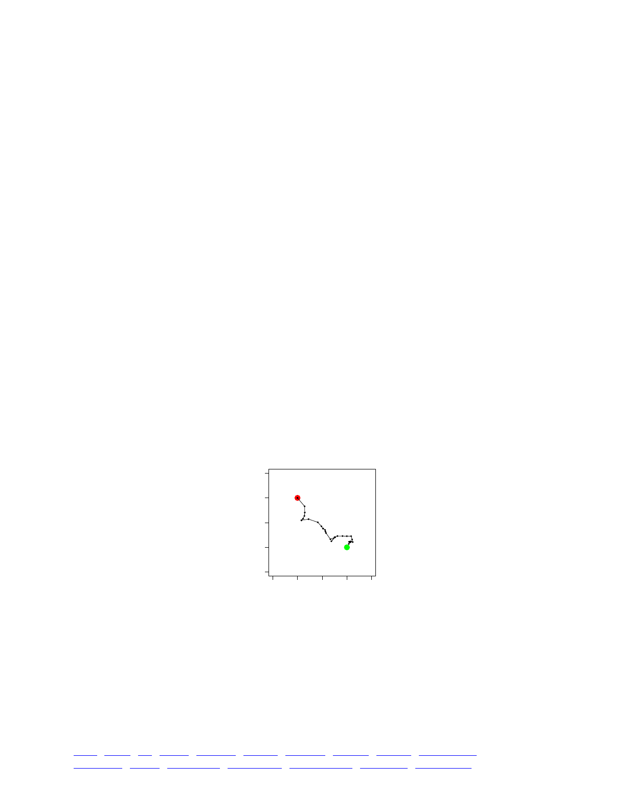
Now we just need to update that plot with periodic callouts to R. To do so, insert the following
code inside the 1:1000000 final output event, immediately above the comment “keep running until
we get within 10% of both optima”:
// update our plot!
history = sim.getValue("history");!
history = rbind(history, c(p0_mean, p1_mean));!
sim.setValue("history", history);!
!
rstr = paste(c('{',!
'x <- c(' + paste(history[,0], sep=", ") + ')',!
'y <- c(' + paste(history[,1], sep=", ") + ')',!
'quartz(width=4, height=4, type="pdf", file="' + pdfPath + '")',!
'par(mar=c(4.0, 4.0, 1.5, 1.5))',!
'plot(x=c(-10,30), y=c(-30,10), type="n", xlab="x", ylab="y")',!
'points(x=0,y=0,col="red", pch=19, cex=2)',!
'points(x=20,y=-20,col="green", pch=19, cex=2)',!
'points(x=x, y=y, col="black", pch=19, cex=0.5)',!
'lines(x=x, y=y)',!
'dev.off()',!
'}'), sep="\n");!
!
scriptPath = writeTempFile("plot_", ".R", rstr);!
system("/usr/local/bin/Rscript", args=scriptPath);
This updates the "history" key with the latest data, and then generates a string contain R
plotting code and sends that code to R to run. The R code is based on Mac OS X, using the
quartz() function of R to open a new plotting device. Again, see section 13.11 for details on this
technique).
When run in SLiMgui, a plot window will open and update every 1000 generations to show the
adaptive trajectory thus far. For the same run of the model as shown in the output above, the
resulting plot looks like this (the walk begins at the red disc, and the green disc is the optimum):
This sort of live visualization of model dynamics can be extremely help for both model design
and graphical debugging, and is quite simple to set up, as we have seen here.
In closing, it is perhaps emphasizing once more that although this recipe models two
phenotypic traits, it is designed to be extensible. It uses key-value pairs set on the mutations and
individuals to track the QTL mutational effects and phenotypic trait values; any number of such
key-value pairs can be maintained. The rmvnorm() function can also draw from a multivariate
normal distribution of any dimensionality, with any (positive-definite) M-matrix. This design is thus
quite open-ended.
-10 010 20 30
-30 -20 -10 010
x
y
TOC I TOC II WF nonWF initialize() Genome Individual Mutation SLiMSim Subpopulation!
Eidos events fitness() mateChoice() modifyChild() recombination() interaction() reproduction() 247

13.18 Modeling opposite ends of a chromosome
This recipe is not about how to model something complicated; instead, it is intended to
illuminate something conceptual about using SLiM in certain situations.
Consider the following recipe:
initialize() {!
initializeMutationRate(1e-7);!
initializeMutationType("m1", 0.5, "f", 0.0);!
initializeGenomicElementType("g1", m1, 1.0);!
initializeGenomicElement(g1, 0, 99999);!
initializeGenomicElement(g1, 9900000, 9999999);!
initializeRecombinationRate(1.5e-7);!
}!
1 { sim.addSubpop("p1", 500); }!
200000 late() { sim.outputFixedMutations(); }
This is a simple neutral model of a chromosome of length L==1e7 bases. The only unusual thing
about it is that we are actually only modeling the two ends of the chromosome; we have defined a
genomic element spanning the first 1e5 bases, and another spanning the last 1e5 bases, and the
intervening region, which is 98% of the length of the chromosome, is not modeled. In SLiMgui,
the model looks like this after a little while:
This is perfectly fine; all that it means is that SLiM will not automatically generate mutations
within the region that is not covered by any genomic element, and so that central region remains
empty. The region does not have to remain empty; it would be legal to call addNewMutation() to
create a new mutation within that region, and SLiM would then track that added mutation
normally. The only effect that genomic elements have, in SLiM, is in causing the automatic
generation of new mutations by the SLiM core. But let’s keep the model as it is, and ask: what is
the behavior of the two end regions, with respect to recombination between them? Do they assort
independently, as if they were separate chromosomes, since they are separated by a rather long
stretch of chromosome? Or if not, then what is the effective recombination rate between them?
First of all, let’s make sure we understand exactly what “recombination rate” really means in
SLiM. As section 21.1 states, the recombination rate is the probability that a crossover will occur
between two adjacent bases. This is binomial; conceptually, a coin is flipped, and the coin lands
“heads” (crossover) with probability p, and “tails” (no crossover) with probability 1-p, and that is
done at every position between adjacent bases along the whole chromosome. There are L-1
positions between bases in a chromosome of length L. In this model, 2e5-2 of them occur
between the bases spanned by the two genomic elements, and the remainder, 9800002, occur
between those two regions. Those are the positions we’re interested in, and at each position a
crossover occurs with probability r=1.5e-7.
To get the probability that the two genomic elements will assort apart, rather than together, we
cannot simply multiply the number of positions (9800002) by the probability per position (1.5e-7),
of course; that would give us 1.47, a nonsensical result that isn’t even a valid probability. Instead,
we need to observe that the key question is actually whether the number of crossovers that occur
between the two regions is even or odd. An even number of crossovers will cancel out; we will
cross over and then cross back, perhaps repeatedly, with no net effect. The two genomic elements
TOC I TOC II WF nonWF initialize() Genome Individual Mutation SLiMSim Subpopulation!
Eidos events fitness() mateChoice() modifyChild() recombination() interaction() reproduction() 248

will then assort together. An odd number of crossovers, on the other hand, will result in all but
one crossover canceling out, and one crossover will remain; the two genomic elements will then
assort apart.
So the question then becomes: for a binomial draw with 9800002 trials and a probability per
trial of 1.5e-7, what is the probability that the result of the draw will be odd? There is, of course,
established mathematical theory on this point, but let’s answer the question through simulation. In
an Eidos console, such as the one we can open inside SLiMgui, we can do a large number of
draws from that binomial distribution:
> draws = rbinom(1e8, 9800002, 1.5e-7)
That will take a moment, and then we have 1e8 draws from the requisite binomial distribution.
Next let’s ask what fraction of them is odd:
> sum(draws % 2 == 1) / 1e8!
!
0.473642
So, the two genomic elements will assort apart about 47.4% of the time, and the remaining time
will assort together.
So now suppose we want to construct a SLiM model that just elides that central region (since
we weren’t using it anyway) and places the two chromosome ends immediately next to each other.
There is no particular obstacle to doing this, except that we need to know what recombination rate
to use for the join point between the two halves – which we have just figured out. So we could
now rewrite our model as:
initialize() {!
initializeMutationRate(1e-7);!
initializeMutationType("m1", 0.5, "f", 0.0);!
initializeGenomicElementType("g1", m1, 1.0);!
initializeGenomicElement(g1, 0, 99999);!
initializeGenomicElement(g1, 100000, 199999);!
!
rates = c(1.5e-7, 0.473642, 1.5e-7);!
ends = c(99999, 100000, 199999);!
initializeRecombinationRate(rates, ends);!
}!
1 { sim.addSubpop("p1", 500); }!
200000 late() { sim.outputFixedMutations(); }
This model ought to behave identically to the previous model, and ought to be somewhat more
efficient, too (although the difference may not be large enough to be noticeable). This is because
when running the first model SLiM would potentially be generating two or more breakpoints
between the two ends, and then resolving whether there were an even or odd number as it ran,
whereas when running the second model SLiM either generates zero breakpoints or one
breakpoint, with the correct calculated probability.
As turns out, we could get the same probability by using the rate-rescaling formula of section
5.5, since what we are effectively doing is rescaling a region of length 9800002 down to a length of
1 (length in terms of potential recombination positions, that is). That formula, executed in the
Eidos console, gives us:
> 0.5*(1-(1-2*1.5e-7)^9800002)!
!
0.473567
TOC I TOC II WF nonWF initialize() Genome Individual Mutation SLiMSim Subpopulation!
Eidos events fitness() mateChoice() modifyChild() recombination() interaction() reproduction() 249

Which is very close to the number we got before (which, remember, was inexact since it came
from simulation). So that’s pleasing.
The point of this recipe, then, is twofold. One point is to provide another angle of view on the
rate-rescaling formula of section 5.5, to illustrate that it applies in situations other than the
rescaling of an entire model. The second, more important, point is to illustrate once again that the
recombination rate as specified by SLiM is the probability of a crossover occurring between two
adjacent bases, and the consequences that that has for reasoning about how recombination works
on larger scales.
This is as good a place as any for a digression that I think this manual ought to contain
somewhere: how SLiM actually generates recombination breakpoint positions under the hood.
This is worth demystifying because for models that use very high recombination rates the subtleties
of this process can be important. Mostly, though, this digression is just for those who are curious,
and beginning users of SLiM should feel free to skip it.
Overall, SLiM does this in several steps: (1) it decides upon the number of breakpoints it will
generate, (2) it chooses the location for each breakpoint based upon a weighted uniform draw
along the chromosome (where the weights are equal to the recombination rates for each individual
base, as defined by the recombination map), and then (3) it sorts and uniques the list of
breakpoints to provide a final list. The uniquing of the list means that there is, at most, one
crossover (i.e., breakpoint) between any two base positions; this is biologically realistic, and also
computationally simpler.
So the big question is: how to decide upon the number of breakpoints to generate? One way
would be to start from the fact that between each pair of bases the question is one of a binomial
draw, with a single trial of probability equal to the recombination rate (by SLiM’s definition). One
could do one such draw per pair of bases, add up the results, and that’s the number of crossovers
that occurred. The immediate problem with that approach is simply that it is immensely
computationally expensive, and if the user has supplied a complex recombination map with
different rates at every position it can’t be reduced to a single binomial draw with a larger number
of trials.
So perhaps we might wish to model recombination as a Poisson process instead, leveraging the
fact that Poisson draws can be added together: Poisson(λ1) + Poisson(λ2) = Poisson(λ1 + λ2). If two
adjacent base positions have a probability of a crossover between them of λ, then the mean of the
binomial draw can be used as the mean of a Poisson draw instead (the Poisson distribution being
well-known as a viable approximation for the binomial distribution with small λ and largish n).
Then we can add up the λ values across the chromosome and get the number of recombination
events with a single Poisson draw that uses that total λ value. And indeed, this is precisely what
SLiM 2.x and earlier did.
Unfortunately, as SLiM users started moving towards new areas of modeling in SLiM such as
multiple chromosomes, it became clear that there was a problem with this approach. When
modeling multiple chromosomes, you want, intuitively, to connect them together in SLiM with a
recombination rate of 0.5 to represent perfect independence of assortment. Unfortunately, this
value is large enough that the Poisson approximation of the binomial distribution breaks down.
The Poisson draw can not only be 0 or 1 (as with the binomial), but also larger values, and with a
rate of 0.5 this happens often enough to matter. In SLiM’s case, if the Poisson draw indicated that
(for example) two crossovers occurred, their positions would be sorted and uniqued (to prevent
multiple crossovers at the same exact location, as described above), resulting in just one crossover
where the Poisson draw had specified two. The net effect of this would be that the probability of a
crossover at the given location would be somewhat lower than desired – about 0.39, in fact, rather
TOC I TOC II WF nonWF initialize() Genome Individual Mutation SLiMSim Subpopulation!
Eidos events fitness() mateChoice() modifyChild() recombination() interaction() reproduction() 250

than 0.5. (It is lower than 0.5 because more than half of the Poisson draws for λ=0.5 will be zero,
compensating for the fact that some of the draws are greater than one and making the mean of the
Poisson distribution come out to 0.5).
So at first blush it looks like we can’t use a binomial draw (too complicated in the case of
complex recombination maps) and we can’t use a Poisson draw (inaccurate with large
recombination rates such as 0.5). What to do?
The solution we arrived at, thanks to Peter Ralph, is to reparameterize the Poisson draws that
we’re doing. If the user has requested a recombination rate of p (probability of crossover between
two adjacent bases), but we want to use a Poisson draw and have it generate a crossover, after
sorting and uniquing, with probability p, then we can transform the requested p into a
reparameterized value λ such that Prob[(Poisson(λ) > 0) = p]. The formula for this
reparameterization is:
With this reparameterization, we end up with the correct probability of crossover after using a
Poisson(λ) draw, accounting for SLiM’s sorting and uniquing of the breakpoint vector. This means
that we can add up the λ values for each region along a whole chromosome, even with a complex
recombination map, and draw a preliminary number of crossovers from a Poisson distribution with
the total λ, and then after we select locations with the usual weighted uniform draws, and sort and
unique them, the probability of crossover at every specific site will be as the user requested. It will
work even when some positions have a rate of 0.5; and even though the Poisson distribution is
only an approximate estimation for the binomial distribution, this solution is in fact exact, since it
is based upon the probability that the Poisson draw for a specific position is greater than zero, not
upon the mean of the Poisson distribution.
If that was all gibberish, never mind. The point is that, as of SLiM 3, recombination rates should
be accurate (within numerical precision limits) even for large recombination rates like 0.5, with no
sacrifice in speed.
13.19 Biased gene conversion
SLiM intrinsically supports gene conversion (see section 6.1.3), but it does not intrinsically
support biased gene conversion. This is unsurprising, since SLiM has no intrinsic support for
modeling nucleotides – biased gene conversion has to do with a bias in the gene conversion
process based upon the specific nucleotides in or near the gene conversion tract (Galtier et al.
2001; Ratnakumar et al. 2010). Nevertheless, it is possible to wedge a concept of biased gene
conversion into SLiM, and in this section we will do so in two very different recipes. The first
recipe will be a nucleotide-based model, using the techniques introduced in section 13.12 to
model nucleotides in SLiM. The second recipe will not be nucleotide-based, even those biased
gene conversion is a nucleotide-based phenomenon; it will model it as a more abstract process.
Which approach is better will depend upon your purposes. Indeed, we do not necessarily
recommend either approach; a different software package that is more specifically designed to
model nucleotide evolution might be more appropriate for this task. But for those who wish to do
it in SLiM, we will look at how it might be done.
Our first model, then, is nucleotide-based. See section 13.12 for an introduction to how
nucleotide-based models can be simulated in SLiM; we will follow a somewhat different approach
here but the underlying idea is the same. We will discuss the model in parts, but will not build it
step by step. We will begin with the initialize() callback:
λ=−log(1 −p)
TOC I TOC II WF nonWF initialize() Genome Individual Mutation SLiMSim Subpopulation!
Eidos events fitness() mateChoice() modifyChild() recombination() interaction() reproduction() 251

initialize() {!
defineConstant("L", 1e4); // number of loci!
!
// mutation type for each nucleotide, all neutral!
mtA = initializeMutationType(0, 0.5, "f", 0.0);!
mtT = initializeMutationType(1, 0.5, "f", 0.0);!
mtG = initializeMutationType(2, 0.5, "f", 0.0);!
mtC = initializeMutationType(3, 0.5, "f", 0.0);!
mt = c(mtA, mtT, mtG, mtC);!
!
mtA.setValue("nucleotide", "A");!
mtT.setValue("nucleotide", "T");!
mtG.setValue("nucleotide", "G");!
mtC.setValue("nucleotide", "C");!
c(mtA,mtT).color = "blue";!
c(mtG,mtC).color = "red";!
!
// We do not want mutations to stack or fix!
mt.mutationStackPolicy = "l";!
mt.mutationStackGroup = -1;!
mt.convertToSubstitution = F;!
!
// chromosome of nucleotides, with gene conversion!
initializeGenomicElementType("g1", mt, c(1,1,1,1));!
initializeGenomicElement(g1, 0, L-1);!
initializeMutationRate(1e-6); // includes 25% identity mutations!
initializeRecombinationRate(1e-6);!
initializeGeneConversion(0.5, 100);!
}
This is a simpler setup than in section 13.12; we have one mutation type for each nucleotide
type, rather than one mutation type per nucleotide type per base position. This simplicity is
possible here because this will be a pure neutral model; the different mutation types were used in
section 13.12 to allow each nucleotide at each position to have an independent fitness effect, but
since this model will be neutral that complexity is not necessary. It ought to be possible to
generalize this recipe to the non-neutral model of section 13.12, but we will not explore that here.
As in section 13.12, we use stacking policy to prevent mutations from stacking or fixing. We
model a chromosome 1e4 bases long, and we turn on gene conversion for 50% of all
recombination events, with a mean conversion tract length of 100.
Next we define a utility function:
function (f)gcContent(void)!
{!
nucs = sim.mutations.mutationType.getValue("nucleotide");!
counts = sim.mutationCounts(NULL);!
totalA = sum(counts[nucs == "A"]);!
totalT = sum(counts[nucs == "T"]);!
totalG = sum(counts[nucs == "G"]);!
totalC = sum(counts[nucs == "C"]);!
total = totalA + totalT + totalG + totalC;!
return (totalC + totalG)*100/total;!
}
This gets the nucleotides used by all mutations, and count information for all mutations, and
uses that information to calculate the percent GC content across the genome. We will use this
later to print status updates as the model runs.
TOC I TOC II WF nonWF initialize() Genome Individual Mutation SLiMSim Subpopulation!
Eidos events fitness() mateChoice() modifyChild() recombination() interaction() reproduction() 252

Next we set up the initial population:
1 late() {!
sim.addSubpop("p1", 1000);!
!
// The initial population is fixed for a random wild-type!
// nucleotide at each locus in the chromosome!
mutTypes = sample(g1.mutationTypes, L, replace=T);!
p1.genomes.addNewDrawnMutation(mutTypes, 0:(L-1));!
!
catn("Initial GC content: " + gcContent());!
}
We make 1000 individuals, set up random wild-type nucleotides in their genomes (the same
nucleotide sequence in every genome, initially), and call our gcContent() utility function to print
the initial GC content.
Next comes the heart of the model, a recombination() callback that implements biased gene
conversion based upon the nucleotide sequence:
recombination() {!
if (size(gcStarts) != 1)!
return F; // no change unless a gene conversion!
if (size(breakpoints) > 0)!
return F; // no change if any recombination!
!
// We have a gene conversion event; we will accept it if it!
// increases the GC content of the tract in question!
gcMuts1 = genome1.mutations;!
gcMuts1 = gcMuts1[gcMuts1.position >= gcStarts];!
gcMuts1 = gcMuts1[gcMuts1.position < gcEnds];!
gcNucs1 = gcMuts1.mutationType.getValue("nucleotide");!
gcGC1 = sum((gcNucs1 == "G") | (gcNucs1 == "C")) / size(gcNucs1);!
!
gcMuts2 = genome2.mutations;!
gcMuts2 = gcMuts2[gcMuts2.position >= gcStarts];!
gcMuts2 = gcMuts2[gcMuts2.position < gcEnds];!
gcNucs2 = gcMuts2.mutationType.getValue("nucleotide");!
gcGC2 = sum((gcNucs2 == "G") | (gcNucs2 == "C")) / size(gcNucs2);!
!
if (gcGC2 > gcGC1)!
return F; // no change if we like the new tract!
!
// reject the new tract!
gcStarts = integer(0);!
gcEnds = integer(0);!
return T;!
}
First we check that we have been called with recombination breakpoints representing a single
gene conversion event with no other recombination; the code could be made more general, but
we will leave that as an exercise for the reader. Given that situation, we get the nucleotides
present in the proposed gene conversion tract, from both genomes, and evaluate their GC content.
If the GC content of the tract that would be copied by gene conversion is greater than the GC
content of the tract that would be overwritten, we allow the proposed gene conversion event to
proceed, by returning F to SLiM. Otherwise, we reject the proposed tract, causing that gene
conversion event not to occur. (See section 22.5 for background on how recombination()
TOC I TOC II WF nonWF initialize() Genome Individual Mutation SLiMSim Subpopulation!
Eidos events fitness() mateChoice() modifyChild() recombination() interaction() reproduction() 253

callbacks work and what their return values mean.) Note that this is probably a ridiculously
simplified model of how gene conversion actually works; it doesn’t even have any sort of
probabilistic component, but rather always accepts conversions that will increase GC content and
always rejects others. Again, a more sophisticated model is left as an exercise for the reader; but
the code here should illustrate the skeleton of how such a sophisticated model would be
approached.
Finally, we output the GC content of the population every thousand generations as the model
runs:
1:1000000 late() {!
if (sim.generation % 1000 == 0)!
catn(sim.generation + " GC content: " + gcContent());!
}
This model gives us output like this:
Initial GC content: 48.8!
1000 GC content: 48.8026!
2000 GC content: 48.8009!
3000 GC content: 48.803!
...
The accumulation of increased GC content in this model is a slow affair, but if we run to
generation 1000000 and plot the result, we can see that progress is steady:
Of course the rate will depend upon the mutation rate, gene conversion rate, tract length, and
other variables; the slow pace here is not inherent to the model, just a consequence of the chosen
parameters.
That recipe simulated actual nucleotide sequences, with mutations explicitly changing the
sequence in a given genome; at the end of a model run we could print out the nucleotide
sequences of all individuals, in FASTA format, perhaps. The next recipe is very different; we will
not model nucleotides at all. Instead, we will model a chromosome that is assumed to be an even
mix of AT and GC initially (50% GC content, in other words), but we won’t try to keep track of
which initial locations are AT and which are GC; we have no sequence information at all. We
then model two types of mutations on that background: GC to AT, and AT to GC. By counting
these mutations, we can know whether a given tract is GC-rich or GC-poor, and we can assess the
overall GC content of a genome. Avoiding explicit modeling of nucleotides will make this recipe
much simpler and faster than the previous recipe. Again, let’s look at this model one block at a
time, starting with initialize():
0.48 0.50 0.52
Generation
GC fraction
0
TOC I TOC II WF nonWF initialize() Genome Individual Mutation SLiMSim Subpopulation!
Eidos events fitness() mateChoice() modifyChild() recombination() interaction() reproduction() 254

initialize() {!
defineConstant("L", 1e5); // number of loci!
!
mtAT = initializeMutationType(0, 0.5, "f", 0.0);!
mtAT.color = "blue";!
mtAT.tag = -1;!
!
mtGC = initializeMutationType(1, 0.5, "f", 0.0);!
mtGC.color = "red";!
mtGC.tag = 1;!
!
// chromosome of length L, with gene conversion!
initializeGenomicElementType("g1", c(mtAT, mtGC), c(1,1));!
initializeGenomicElement(g1, 0, L-1);!
initializeMutationRate(1e-6);!
initializeRecombinationRate(1e-6);!
initializeGeneConversion(0.5, 100);!
}
We’ll model a chromosome of length 1e5 this time, since this model is faster. We set up the
GC-to-AT and AT-to-GC mutation types, give them different colors in SLiMgui, and give them tag
values of -1 and +1 respectively; we will use those tag values to easily total up the effect of a
vector of mutations on GC content. We use the same mutation rate, recombination rate, and gene
conversion properties as in the previous model. Then we set up an initial subpopulation:
1 late() {!
sim.addSubpop("p1", 1000);!
}
And then we introduce a recombination() callback that implements the biased gene
conversion:
recombination() {!
if (size(gcStarts) != 1)!
return F; // no change unless a gene conversion!
if (size(breakpoints) > 0)!
return F; // no change if any recombination!
!
// We have a single gene conversion event!
gcMuts = genome2.mutations;!
gcMuts = gcMuts[gcMuts.position >= gcStarts];!
gcMuts = gcMuts[gcMuts.position < gcEnds];!
gcGC = sum(gcMuts.mutationType.tag);!
take = (gcGC > 0);!
!
if (take)!
return F; // no change if we like the new tract!
!
// reject!
gcStarts = integer(0);!
gcEnds = integer(0);!
return T;!
}
As in the first recipe, this callback runs only is a single gene conversion event with no
recombination is being proposed, for simplicity. In that case, we total up the GC-influencing
mutations in the proposed gene conversion tract, and if their net effect is to increase GC content
TOC I TOC II WF nonWF initialize() Genome Individual Mutation SLiMSim Subpopulation!
Eidos events fitness() mateChoice() modifyChild() recombination() interaction() reproduction() 255
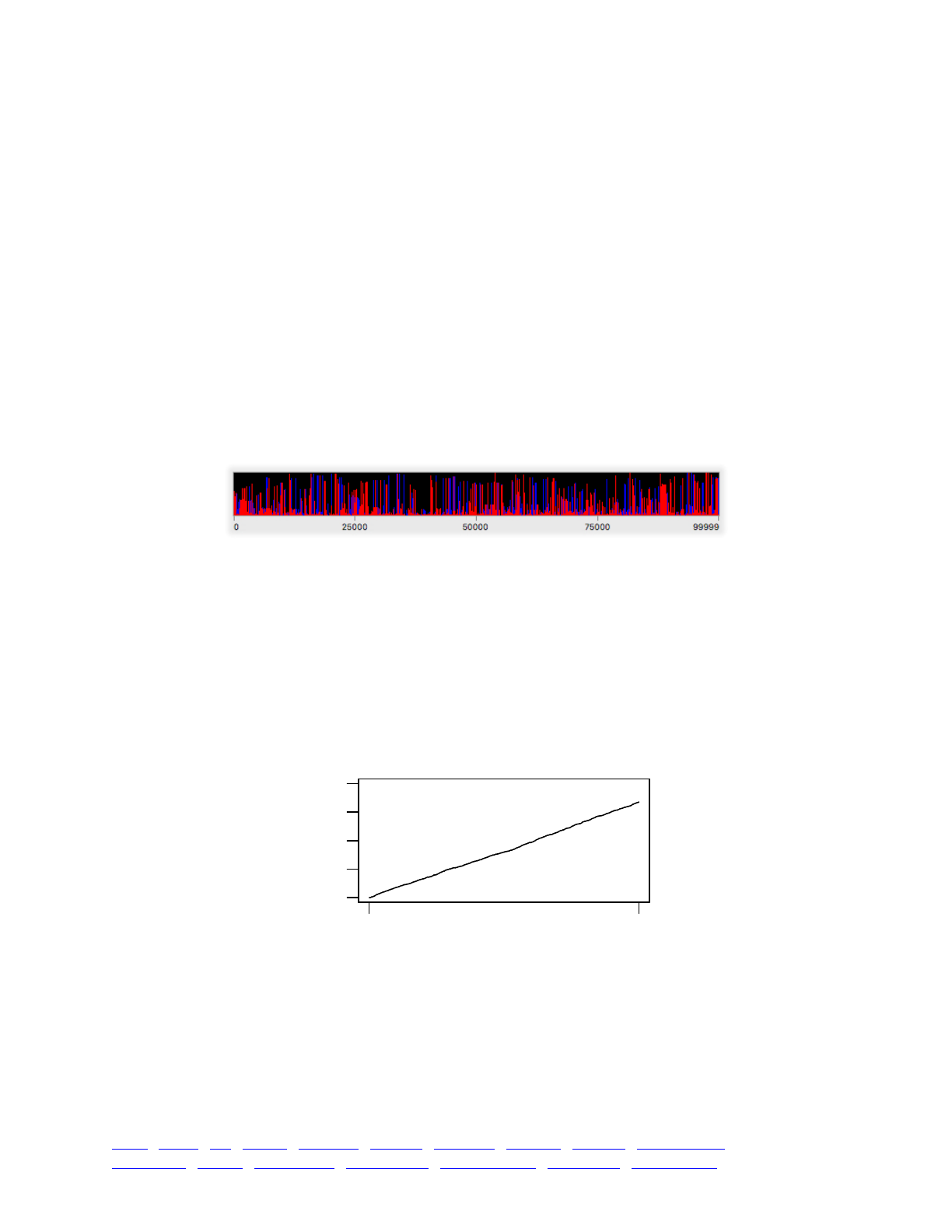
we accept the proposed gene conversion event, otherwise we reject it. (Note that this code does
not compare the tracts from the two genomes, so its criterion is a bit different from that of the first
recipe, but it would be easy to make it match; we’re just exploring possibilities here.)
Finally, we have a periodic output event:
1:10000000 late() {!
if (sim.generation % 1000 == 0)!
catn(sim.generation + " GC sum: " +!
sum(sim.substitutions.mutationType.tag));!
}
Since we can tot up the effect of all mutations on GC content very easily, we don’t use a utility
function here. Note that this code just totals up the substitutions; we don’t bother assessing the
mean GC content across all genomes. The first recipe didn’t use substitutions, since nucleotide-
based models generally don’t convert fixed mutations to substitutions (because a new mutation
that introduces a different nucleotide could always occur).
When running in SLiMgui, we can see all of the AT-to-GC (red) and GC-to-AT (blue) mutations
circulating in the population:
Since this model, like the previous recipe, is neutral, we can have large numbers of these
mutations segregating in the population without it getting too slow. As it runs, this model will
produce output like:
1000 GC sum: 0!
2000 GC sum: -1!
3000 GC sum: 0!
4000 GC sum: 8!
...
If plotted, this shows an even steadier increase:
The smoother trajectory here, compared to the previous recipe, may in part be a result of the
larger population size. This plot also spans a generation range ten times that of the previous
recipe, which smooths the plot out. Finally, there may be some way in which the details of the
model, particularly the different criterion used in the recombination() callback, produces a
smoother increase.
0.00 0.02 0.04
Generation
GC bias
01e7
TOC I TOC II WF nonWF initialize() Genome Individual Mutation SLiMSim Subpopulation!
Eidos events fitness() mateChoice() modifyChild() recombination() interaction() reproduction() 256

Again, which of these models is best will depend upon the application, and it may be that
neither model is particularly ideal, since SLiM is not really designed to simulate nucleotides.
However, the output from both models shows clear evidence of biased gene conversion; if a
simple model of that process is all that it needed, to simulate its effects upon some other
evolutionary process, this level of sophistication may suffice. The second model, in particular,
provides relatively low overhead in a SLiM model of biased gene conversion by “thinking outside
the box” and modeling the effects of the process – the tendency to accept some gene conversion
events and reject others, based upon the mutations present in the gene conversion tract – without
explicitly modeling the nucleotides involved. If it is the effects of the process that are important,
rather than the specific nucleotide sequences generated, that level of realism may suffice, with
considerable savings in computation time.
TOC I TOC II WF nonWF initialize() Genome Individual Mutation SLiMSim Subpopulation!
Eidos events fitness() mateChoice() modifyChild() recombination() interaction() reproduction() 257

14. Continuous-space models and interactions
This chapter introduces two new features added in SLiM 2.3: continuous space, and the
InteractionType class. These two features will be treated together in this chapter, since many of
the uses of InteractionType involve modeling spatial interactions, but in fact each feature may be
used independently of the other. Note that these are advanced, optional features.
Continuous-space support in SLiM is enabled by supplying a dimensionality parameter to the
initializeSLiMOptions() call during model initialization. This parameter may be "x", "xy", or
"xyz"; these set up SLiM to support 1D, 2D, or 3D continuous space, respectively, within each
subpopulation using the coordinate axes specified. (Setting up spaces using different coordinate
axes than these, such as 2D space using y and z, is not presently supported.) The corresponding x,
y, and z properties of Individual will then be interpreted by SLiM as spatial coordinates, rather
than simply as type float tag values. Model code can then set the positions of individuals as
desired; this is typically done in a modifyChild() callback, so that the positions of new offspring
are immediately set, but it can also be done at any other point in the generation cycle. Individual
positions can also be used by model code in any way desired; for example, spatially continuous
variation in selection could be implemented in a fitness() callback by computing an
environmental value at the spatial location of the focal individual, and then comparing the
individual’s phenotype to that environmental value (see section 14.9). When continuous space is
enabled, SLiMgui will display subpopulations graphically using the spatial positions of individuals.
Interactions between individuals can be implemented in pure Eidos, as seen previously in the
frequency-dependent model of section 9.4.1 and the green-beard model of section 9.4.4. This can
be cumbersome, however, since all of the interaction mechanics must be written by the user in
Eidos, which – as an interpreted language – is not nearly as fast as the C++ in which the SLiM
engine is written. The InteractionType class provides a solution to this problem, by providing
built-in support for fast interaction evaluation while still allowing scripted customization of the
interactions through a new type of callback, the interaction() callback. InteractionType can be
used to model non-spatial interactions, as we will see in section 14.6; but it is particularly well-
suited to modeling interactions in continuous space, since it is able to translate distances into
interaction strengths automatically using any of several different “spatial kernels” (Gaussian,
negative exponential, etc.). In addition, InteractionType is optimized for spatial searches (such as
nearest-neighbor searches) through the use of a data structure called a “k-d tree”. Together, these
features allow complex spatial interactions to be implemented in just a few lines of Eidos code,
with performance that can be orders of magnitude better than would otherwise be possible.
When continuous space is enabled in a model, the Subpopulation class now contains several
features to support that functionality. First, Subpopulation is now aware of its spatial boundaries
(the spatial coordinates of the edges of the subpopulation). Second, it can help to enforce those
boundaries through various boundary conditions. Third, it now supports “landscape maps”, grid-
based maps that define the values of particular environmental variables across the spatial extent of
the subpopulation. Landscape maps allow simulations to incorporate spatial variation in
properties such as elevation or temperature – any variable relevant to the model’s dynamics.
With that introduction, let’s delve into some recipes that exemplify these new features.
14.1 A simple 2D continuous-space model
In this recipe we will explore a very simple model utilizing continuous space. In this model,
individuals will live on a two-dimensional landscape. Individuals will not interact spatially in this
model; that will be introduced in section 14.2. The model:
TOC I TOC II WF nonWF initialize() Genome Individual Mutation SLiMSim Subpopulation!
Eidos events fitness() mateChoice() modifyChild() recombination() interaction() reproduction() 258
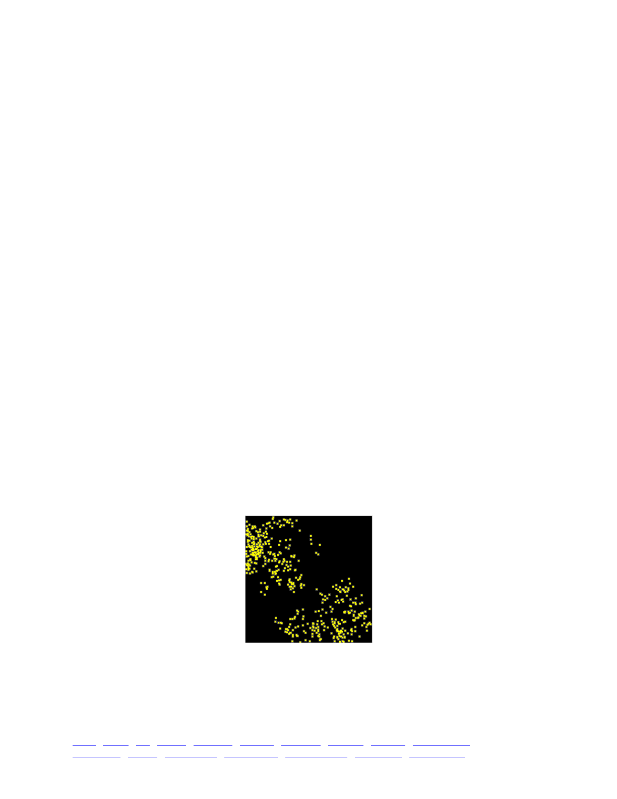
initialize() {!
initializeSLiMOptions(dimensionality="xy");!
initializeMutationRate(1e-7);!
initializeMutationType("m1", 0.5, "f", 0.0);!
initializeGenomicElementType("g1", m1, 1.0);!
initializeGenomicElement(g1, 0, 99999);!
initializeRecombinationRate(1e-8);!
}!
1 late() {!
sim.addSubpop("p1", 500);!
!
// initial positions are random in ([0,1], [0,1])!
p1.individuals.x = runif(p1.individualCount);!
p1.individuals.y = runif(p1.individualCount);!
}!
modifyChild() {!
// draw a child position near the first parent, within bounds!
do child.x = parent1.x + rnorm(1, 0, 0.02);!
while ((child.x < 0.0) | (child.x > 1.0));!
!
do child.y = parent1.y + rnorm(1, 0, 0.02);!
while ((child.y < 0.0) | (child.y > 1.0));!
!
return T;!
}!
2000 late() { sim.outputFixedMutations(); }
There are only a few new things about this model. First of all, continuous 2-D space is enabled
in the model with the call to initializeSLiMOptions(). Second, when the subpopulation is
created in the 1 late() event initial positions for all individuals are generated using runif().
Note that by default the spatial extent of the subpopulation spans the interval [0,1] in x and y, so
the default min and max values for runif() suffice. Third, a modifyChild() callback generates a
spatial position for the offspring individual. In this recipe, the offspring position is based upon the
position of the first (i.e. maternal) parent, as given by parent1.x and parent1.y, with random
deviations drawn from a normal distribution using rnorm(). The new positions could fall outside
of the subpopulation’s boundaries, so they are redrawn until they fall inside using while loops.
When run in SLiMgui, a typical snapshot of this model looks like this:
Here, SLiMgui is displaying each individual at its corresponding spatial position, as a small
square (colored according to fitness, as usual). Notably, spatial structure has emerged already in
this simple model, because of the way that child positions are based upon maternal positions; this
tends to encourage spatial clustering. Since spatial position is of no consequence in the model,
however, this makes no difference to the evolutionary dynamics observed.
TOC I TOC II WF nonWF initialize() Genome Individual Mutation SLiMSim Subpopulation!
Eidos events fitness() mateChoice() modifyChild() recombination() interaction() reproduction() 259

14.2 Spatial competition
The recipe in the previous section set up spatiality but did not use it. In this section we will
extend that recipe to include spatial competition between individuals. The strength of competition
between two individuals will depend upon the spatial distance between them, falling off with
increasing distance according to a Gaussian kernel with a characteristic width. This could
represent, for example, competitive interference due to overlap in foraging areas. The recipe:
initialize() {!
initializeSLiMOptions(dimensionality="xy");!
initializeMutationRate(1e-7);!
initializeMutationType("m1", 0.5, "f", 0.0);!
initializeGenomicElementType("g1", m1, 1.0);!
initializeGenomicElement(g1, 0, 99999);!
initializeRecombinationRate(1e-8);!
!
// Set up an interaction for spatial competition!
initializeInteractionType(1, "xy", reciprocal=T, maxDistance=0.3);!
i1.setInteractionFunction("n", 3.0, 0.1);!
}!
1 late() {!
sim.addSubpop("p1", 500);!
!
// initial positions are random in ([0,1], [0,1])!
p1.individuals.x = runif(p1.individualCount);!
p1.individuals.y = runif(p1.individualCount);!
}!
1: late() {!
// evaluate interactions before fitness calculations!
i1.evaluate();!
}!
fitness(NULL) {!
// spatial competition!
totalStrength = i1.totalOfNeighborStrengths(individual);!
return 1.1 - totalStrength / p1.individualCount;!
}!
modifyChild() {!
// draw a child position near the first parent, within bounds!
do child.x = parent1.x + rnorm(1, 0, 0.02);!
while ((child.x < 0.0) | (child.x > 1.0));!
!
do child.y = parent1.y + rnorm(1, 0, 0.02);!
while ((child.y < 0.0) | (child.y > 1.0));!
!
return T;!
}!
2000 late() { sim.outputFixedMutations(); }
Here we have added a few new elements. First of all, a call to initializeInteractionType()
creates a new interaction type with identifier 1, which is therefore referred to as i1, in much the
same way that mutation types, genomic element types, and subpopulations are numbered and
named in SLiM. This call also defines the interaction type as using both the x and y coordinates of
the model, and sets the maximum range for the interaction as 0.3; beyond that limit interaction
strengths are always assumed to be zero, allowing better performance. The interaction is also
configured with reciprocal=T; this guarantees that the interaction strength exerted upon A by B is
equal to the interaction strength exerted upon B by A, allowing computational optimizations.
Interactions are non-reciprocal by default, so that bugs are not inadvertently introduced by an
TOC I TOC II WF nonWF initialize() Genome Individual Mutation SLiMSim Subpopulation!
Eidos events fitness() mateChoice() modifyChild() recombination() interaction() reproduction() 260
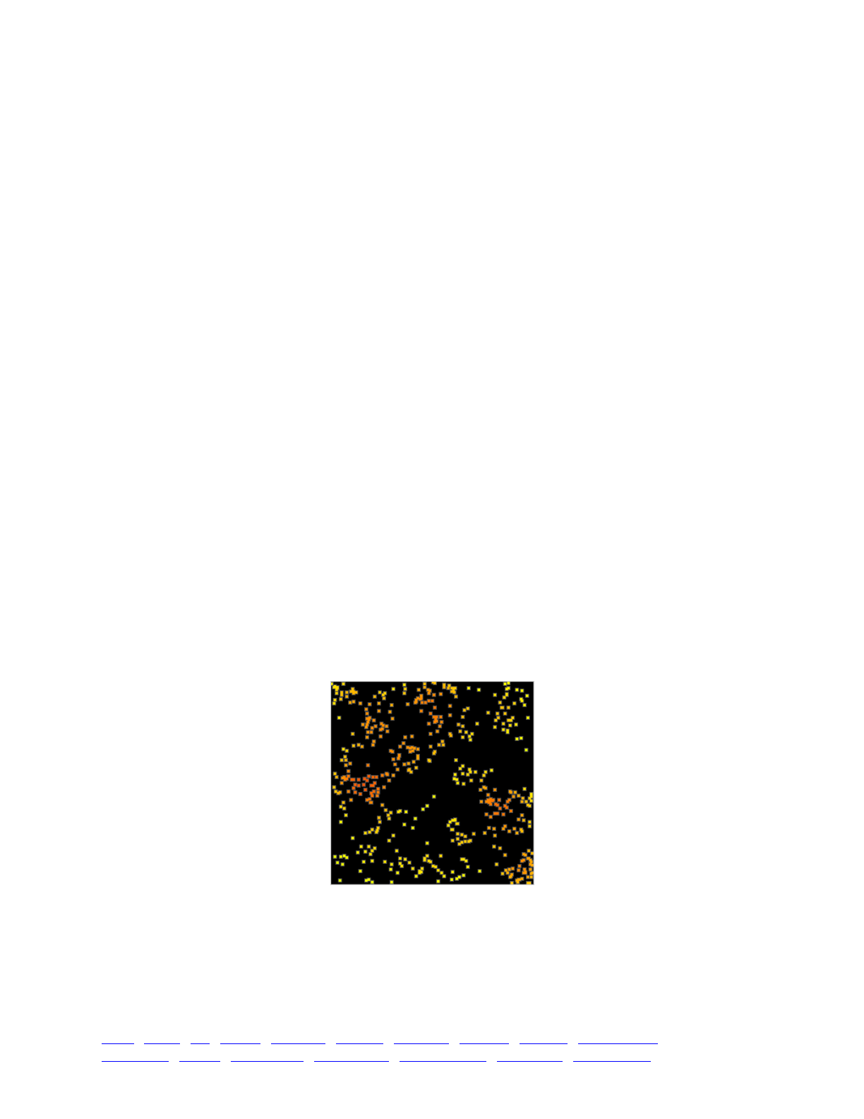
implicit assumption of reciprocality; but in practice most interactions are reciprocal and should be
specified as such for maximal performance.
Second, a call to setInteractionFunction() tells i1 that it should convert spatial distances into
interaction strengths using a Gaussian function (represented by "n" for “normal”, to avoid
confusion with the "g" for “gamma” used elsewhere in SLiM). This Gaussian function is scaled to
have a maximum value of 3.0 and a standard deviation of 0.1, representing fairly local
interactions. It can now be seen how the maximum distance set for i1 was chosen; it is three
times the standard deviation of the interaction kernel. Interaction strengths beyond that distance
would be extremely small anyway, and are thus neglected by this model for efficiency.
Next, interaction type i1 needs to actually be used. A precondition for this is that i1 be
“evaluated” in each generation. This is done in the 1: late() event, with a call to its evaluate()
method. This takes a snapshot of the model’s spatial state at that moment in time, and i1 will then
calculate all interactions based upon that snapshot. This is necessary because under the hood,
InteractionType performs a lot of time-consuming analysis to set up spatial data structures
representing the state of the model, allowing it to respond quickly to spatial queries. It does that
analysis just once, at the point of evaluation, and the results are cached and used for all queries
until the interaction is evaluated again. (In fact, this is not quite accurate; interaction() callbacks
may be called in a deferred fashion, as discussed when we introduce interaction() callbacks.)
Having evaluated i1 in the late() event, just before fitness calculation in the generation cycle,
the model then uses i1 in a global fitness() callback to calculate fitness values that represent the
effects of spatial competition. The call to totalOfNeighborStrengths() totals up the interaction
strengths between individual (the focal individual) and all other interacting individuals in its
subpopulation. These interaction strengths, as we saw above, were configured to be calculated
using a particular Gaussian kernel, and a maximum distance of 0.3 was chosen. Those settings are
now used to find the interaction strength between individual and every other individual, and the
sum of those strengths is returned. The fitness() callback divides that total by the number of
individuals in the subpopulation to get a mean interaction strength, and subtracts that mean value
from 1.1 to get a fitness value. Those details are fairly arbitrary; the overall intent, however, is that
the stronger the competition felt by an individual, the lower the individual’s fitness.
If we run this model in SLiMgui, it looks markedly different from the previous model:
Perhaps the most obvious difference is that individuals are no longer all yellow (which indicated
neutrality). Now, individuals in relatively tight spatial clusters are orange or even red, indicating
they have fitness values below 1.0 due to the effects of competition. Those individuals will be less
likely to reproduce, whereas the individuals enjoying a lack of competition in isolated areas will
be more likely to reproduce. That leads to the other obvious difference: the space is more
completely and uniformly occupied. This model uses the same offspring positioning algorithm as
TOC I TOC II WF nonWF initialize() Genome Individual Mutation SLiMSim Subpopulation!
Eidos events fitness() mateChoice() modifyChild() recombination() interaction() reproduction() 261

the previous recipe, which promotes spatial clustering; however, excessive clustering is now
opposed by the effects of competition, producing that more uniform distribution.
14.3 Boundaries and boundary conditions
Here we will pause to examine the question of boundaries and boundary conditions in spatial
models. When a new offspring individual is given a position that is based upon the parental
position(s) plus some random deviation, as is commonly done, the question arises of how to
constrain those new positions; we have already confronted that question, in fact, in the
modifyChild() callbacks we have used to set offspring positions.
One option is simply to impose no constraint; space is then considered to be infinite in extent
in all directions. This is the default in SLiM, simply because SLiM imposes no default constraint;
however, it is rarely desirable in individual-based models since a finite population on an infinite
landscape has zero density – rarely an interesting or biologically relevant case. Instead, models
generally use one of several standard boundary conditions. In this section we will break from our
usual conventions and will simply assume all of the code from the previous recipe (section 14.2);
here we will present only replacement modifyChild() callbacks to implement each of four
standard boundary conditions. The literature contains a good deal of discussion of these different
boundary conditions and the effects they may have on evolutionary dynamics; we will not review
that literature here. We will focus on implementation.
First of all, with “stopping” boundaries, new positions are simply clamped to the spatial
boundary; points outside the boundary are forced to the nearest point inside bounds. In SLiM, this
can be implemented as:
modifyChild() {!
// Stopping boundary conditions!
pos = parent1.spatialPosition + rnorm(2, 0, 0.02);!
child.setSpatialPosition(p1.pointStopped(pos));!
!
return T;!
}
This introduces several new concepts. The spatialPosition property of Individual provides a
float vector of the spatial coordinates of the individual; since this model has "xy" dimensionality,
this vector has two elements, with the same values as the x and y properties that we have been
using. The setSpatialPosition() is just the reciprocal of this, taking a float vector of
coordinates and setting them into the x and y properties of the Individual in one operation, as a
convenient shorthand. Finally, the pointStopped() method of Subpopulation implements the
spatial boundary condition by clamping the coordinates in the float vector it is passed to the
boundaries of the subpopulation and returning the clamped vector. So all in all, this callback gets
the coordinates of the parent, adds a normal draw to each (thus deviating the offspring’s x and y
coordinates from those of the parent), asks the subpopulation to clamp the new position into
bounds, and sets the final position into the child. All of this is just convenient shorthand; it could
easily be implemented by using the x and y properties of the Individual directly, as well as the
spatial boundaries of the Subpopulation (available through its spatialBounds property) – it would
just be longer, less readable, and more error-prone.
Second, with “reflecting” boundaries, new positions outside the spatial boundary are reflected
to fall inside it; the extent to which a point lies outside an edge is translated into the extent to
which the point lies inside that edge instead. This requires just a trivial modification of the
previous recipe, substituting the pointReflected() method in place of pointStopped():
TOC I TOC II WF nonWF initialize() Genome Individual Mutation SLiMSim Subpopulation!
Eidos events fitness() mateChoice() modifyChild() recombination() interaction() reproduction() 262

modifyChild() {!
// Reflecting boundary conditions!
pos = parent1.spatialPosition + rnorm(2, 0, 0.02);!
child.setSpatialPosition(p1.pointReflected(pos));!
!
return T;!
}
Third, with “absorbing” boundaries, new offspring whose proposed positions lie outside bounds
are absorbed – their generation is terminated. This is accomplished in SLiM by returning F from
the modifyChild() callback, which tells SLiM to start over from scratch by choosing new parents
and generating a completely new offspring:
modifyChild() {!
// Absorbing boundary conditions!
pos = parent1.spatialPosition + rnorm(2, 0, 0.02);!
if (!p1.pointInBounds(pos))!
return F;!
!
child.setSpatialPosition(pos);!
return T;!
}
This uses the pointInBounds() method of Subpopulation to test whether the new position lies
inside the spatial boundaries. If not, F is returned, terminating generation of the proposed child.
Fourth, with “reprising” boundaries, if a proposed position falls outside bounds a new position
is generated until a position within bounds is obtained. This is the boundary condition we
implemented the hard way in the previous recipes, but it can be done a little more easily (and
more generally, since the spatial boundaries are now not hard-coded):
modifyChild() {!
// Reprising boundary conditions!
do pos = parent1.spatialPosition + rnorm(2, 0, 0.02);!
while (!p1.pointInBounds(pos));!
child.setSpatialPosition(pos);!
!
return T;!
}
This again uses pointInBounds(), but this time if the point is not inside bounds the code loops
back to generate a new point, until a point within bounds is obtained.
Finally, with “periodic” boundaries space is constructed in such a manner that boundaries do
not exist but the spatial extent is nevertheless finite; the spatial topology is instead cylindrical or
toroidal, wrapping around at some or all edges. This boundary condition is a more complex topic
than the other boundary conditions, since it actually changes the way in which distances are
calculated; we will therefore defer a presentation of it until section 14.12. It’s an important topic,
though, since periodic boundaries can avoid problematic “edge effects” as discussed there.
We have been using Subpopulation methods to check/enforce the boundary conditions for us.
Subpopulation is the class responsible for landscape-level properties such as the coordinates of the
spatial boundaries, as well as other state we will see later. By default the spatial boundaries used
by Subpopulation span the interval [0,1] in each dimension, and we have allowed that default to
stand in the models shown here. This can be changed, using the setSpatialBounds() method of
Subpopulation, but we will not pursue that here (see section 14.7 for an example). In any case,
the Subpopulation methods we have seen will check and enforce whatever boundaries are set.
TOC I TOC II WF nonWF initialize() Genome Individual Mutation SLiMSim Subpopulation!
Eidos events fitness() mateChoice() modifyChild() recombination() interaction() reproduction() 263

One final point worth mentioning is that Subpopulation provides a more general way to set up
initial random positions. These recipes will use this code to do so:
1 late() {!
sim.addSubpop("p1", 500);!
!
// Initial positions are random within spatialBounds!
for (ind in p1.individuals)!
ind.setSpatialPosition(p1.pointUniform());!
}
The pointUniform() method generates a point drawn at random from within the spatial bounds
of the subpopulation (drawing each coordinate from a uniform distribution spanning the range
within bounds). This is equivalent to the code presented in earlier recipes, but it will also work
properly if the spatial bounds of the subpopulation have been changed from the default, whereas
the earlier code would not (since the [0,1] interval is hard-coded there).
14.4 Mate choice with a spatial kernel
Now we will work with the “reprising” boundary condition model of section 14.3, and we will
add the element of spatial mate choice. The likelihood that one individual will choose another
individual as a mate will depend upon the spatial distance between them, falling off with
increasing distance according to a Gaussian kernel (but a different one from the competition
kernel). This could represent, for example, mate-finding based upon auditory cues such as
birdsong which become progressively less perceptible as distance increases.
Doing this is remarkably easy. We just need to add a second interaction type, and utilize it in a
mateChoice() callback:
initialize() {!
initializeSLiMOptions(dimensionality="xy");!
initializeMutationRate(1e-7);!
initializeMutationType("m1", 0.5, "f", 0.0);!
initializeGenomicElementType("g1", m1, 1.0);!
initializeGenomicElement(g1, 0, 99999);!
initializeRecombinationRate(1e-8);!
!
// spatial competition!
initializeInteractionType(1, "xy", reciprocal=T, maxDistance=0.3);!
i1.setInteractionFunction("n", 3.0, 0.1);!
!
// spatial mate choice!
initializeInteractionType(2, "xy", reciprocal=T, maxDistance=0.1);!
i2.setInteractionFunction("n", 1.0, 0.02);!
}!
1 late() {!
sim.addSubpop("p1", 500);!
!
for (ind in p1.individuals)!
ind.setSpatialPosition(p1.pointUniform());!
}!
1: late() {!
i1.evaluate();!
i2.evaluate();!
}
TOC I TOC II WF nonWF initialize() Genome Individual Mutation SLiMSim Subpopulation!
Eidos events fitness() mateChoice() modifyChild() recombination() interaction() reproduction() 264

fitness(NULL) {!
totalStrength = i1.totalOfNeighborStrengths(individual);!
return 1.1 - totalStrength / p1.individualCount;!
}!
1: mateChoice() {!
// spatial mate choice!
return i2.strength(individual);!
}!
modifyChild() {!
do pos = parent1.spatialPosition + rnorm(2, 0, 0.02);!
while (!p1.pointInBounds(pos));!
child.setSpatialPosition(pos);!
!
return T;!
}!
2000 late() { sim.outputFixedMutations(); }
Interaction type i1 is used for competitive interactions, as before. We now declare i2 as well,
which we will use for mate choice. It also uses a Gaussian kernel, this time with a maximum
value of 1.0, a standard deviation of 0.02, and a maximum distance of 0.1. This is quite a narrow,
short-range mate-choice function that will promote local mating quite strongly.
Having declared i2, we then need to evaluate it in the 1: late() event, just as we did with i1.
We are then prepared to use it in the 1: mateChoice() callback, which simply returns the result of
the call i2.strength(individual). This call asks i2 to evaluate the strength of interaction
between the first parent (individual) and all other individuals in its subpopulation. The result is
returned as a vector. Happily, that is precisely what mateChoice() callbacks are expected to return
– a vector of mating weights between the first parent and all other individuals. The result can
therefore simply be passed on to SLiM without further processing.
That is all that is needed; we now have a model that includes both spatial competition and
spatial mate choice, using different kernels. If we run this model in SLiMgui, it looks essentially
identical to the model of sections 14.2, but the evolutionary dynamics under the hood are quite
different. We can explore that with a quick modification of these recipes, by dropping in the
heterozygosity calculator used in section 13.2. The code from the final output event of that recipe
can be used without modification. In a quick experiment, we can do 25 runs of the models, run to
generation 10000 to allow equilibration, and output the mean nuclear heterozygosity at the end of
each run. Let’s also do runs of the equivalent non-spatial model (constructed by simply removing
all of the interaction code, the fitness() callback, the mateChoice() callback, and all references
to spatial positions). Simple summary statistics across the mean nuclear heterozygosity values
obtained from the 25 runs of each of the three models look like this:
The first thing to note is that the outcomes of the non-spatial and competition-only models are
quite similar. Indeed, even with 25 samples each, a t-test finds that they do not differ significantly
(p!=!0.3651). Apparently local offspring generation and spatial competition do not suffice to drive
much, if any, genetic divergence among spatial clusters. This is not too surprising, since with non-
spatial mating in each generation the gene flow blending clusters together is very high.
Model
Mean
Std. Deviation
Non-spatial
0.0002148
0.000092
Competition only (14.2)
0.0001934
0.000071
Competition and mate choice (14.4)
0.0001005
0.000067
TOC I TOC II WF nonWF initialize() Genome Individual Mutation SLiMSim Subpopulation!
Eidos events fitness() mateChoice() modifyChild() recombination() interaction() reproduction() 265

The second thing to note, however, is that the model with spatial mate choice – this section’s
recipe – is quite different from the other two. This is confirmed by t-test; it is highly significantly
different from both the non-spatial model (p!=!0.0000104) and the competition-only model
(p!=!0.0000204). The addition of spatial mate choice (especially with a narrow kernel) has driven
substantial genetic divergence among spatial clusters. We have ourselves a real spatial model.
14.5 Mate choice with a nearest-neighbor search
In this section we will modify the previous recipe to implement spatial mate choice using a
nearest-neighbor search instead of a spatial kernel. Each individual choosing a mate will make a
choice from among its three nearest neighbors, without further consideration of distance. In this
recipe the selection will be random, but it would be simple to make the mate choice depend upon
some genetic or non-genetic trait of the prospective mates, reflecting choosy mate selection from
within a small pool of nearby candidates.
We will begin with the recipe of section 14.4. To modify it for the present recipe, we need only
to replace the mateChoice() callback with the following:
1: mateChoice() {!
// nearest-neighbor mate choice!
neighbors = i2.nearestNeighbors(individual, 3);!
mates = rep(0.0, p1.individualCount);!
mates[neighbors.index] = 1.0;!
!
return mates;!
}
The nearestNeighbors() method returns the three (3) nearest neighbors of the first parent
(individual). In SLiM, a “neighbor” is an individual within the maximum interaction distance of
the focal individual (other than the focal individual itself); individuals beyond that maximum
cannot be “neighbors”, even if they are the nearest individual to the focal individual. It is therefore
possible for this method to return fewer than three individuals; indeed, if individual is spatially
isolated this method might return an empty vector. The rest of the callback is written with that
possibility in mind, however. First, a mating vector is constructed with 0 for all potential mates.
Then the values for the neighbors found (if any) are changed to 1, using the subpopulation indices
of the neighbors. Finally, that modified vector is returned. If individual had no neighbors, no
indices will be changed, and the returned vector will contain nothing but zeros; this will cause
SLiM to draw a new first parent, just as a return value of float(0) would.
Note that the nearestNeighbors() call is purely a spatial query; it does not involve the
calculation of interaction strengths at all. In this recipe, the parameters that configure i2 – the
Gaussian function’s maximum value and standard deviation, and indeed the fact that a Gaussian
function is to be used at all – are therefore irrelevant and can be removed. The complete recipe:
initialize() {!
initializeSLiMOptions(dimensionality="xy");!
initializeMutationRate(1e-7);!
initializeMutationType("m1", 0.5, "f", 0.0);!
initializeGenomicElementType("g1", m1, 1.0);!
initializeGenomicElement(g1, 0, 99999);!
initializeRecombinationRate(1e-8);!
!
// spatial competition!
initializeInteractionType(1, "xy", reciprocal=T, maxDistance=0.3);!
i1.setInteractionFunction("n", 3.0, 0.1);!
TOC I TOC II WF nonWF initialize() Genome Individual Mutation SLiMSim Subpopulation!
Eidos events fitness() mateChoice() modifyChild() recombination() interaction() reproduction() 266

// spatial mate choice!
initializeInteractionType(2, "xy", reciprocal=T, maxDistance=0.1);!
}!
1 late() {!
sim.addSubpop("p1", 500);!
!
for (ind in p1.individuals)!
ind.setSpatialPosition(p1.pointUniform());!
}!
1: late() {!
i1.evaluate();!
i2.evaluate();!
}!
fitness(NULL) {!
totalStrength = i1.totalOfNeighborStrengths(individual);!
return 1.1 - totalStrength / p1.individualCount;!
}!
1: mateChoice() {!
// nearest-neighbor mate choice!
neighbors = i2.nearestNeighbors(individual, 3);!
mates = rep(0.0, p1.individualCount);!
mates[neighbors.index] = 1.0;!
!
return mates;!
}!
modifyChild() {!
do pos = parent1.spatialPosition + rnorm(2, 0, 0.02);!
while (!p1.pointInBounds(pos));!
child.setSpatialPosition(pos);!
!
return T;!
}!
2000 late() { sim.outputFixedMutations(); }
We have now seen three different types of spatial query using InteractionType. The first is the
use of totalOfNeighborStrengths() to add up all of the interactions felt by a focal individual from
every other interacting individual; we used this to build spatial competition. The second is
strength(), which we used to obtain a vector of interaction strengths between the focal individual
and all other individuals (it can also calculate the interaction strengths with specific other
individuals). And the third is the nearestNeighbors() method used here, which returns a vector
with (up to) a specified number of the nearest neighbors of a focal individual. IndividualType
supports several other queries, such as distance() to get distances between the focal individual
and others, distanceToPoint() and nearestNeighborsOfPoint() to do those queries using an
arbitrary spatial point rather than a focal individual, and drawByStrength() to draw neighbors of a
focal individual weighted by interaction strength (a fast combination of nearestNeighbors(),
strength(), and sample(), conceptually). Instead of providing examples of the use of all these
methods – which are all documented in section 21.7.2 – we will now change direction to start
building – gradually – towards models of landscape heterogeneity using landscape maps.
14.6 Divergence due to phenotypic competition with an interaction() callback
Here we will depart from the previous recipes, which have all used neutral spatial models, to
explore a different topic: a non-neutral, non-spatial model. This recipe will involve a quantitative
trait, using a strategy similar to that in the recipe of section 13.10. It will use an InteractionType
to model competition among individuals based upon their phenotype: individuals with a more
TOC I TOC II WF nonWF initialize() Genome Individual Mutation SLiMSim Subpopulation!
Eidos events fitness() mateChoice() modifyChild() recombination() interaction() reproduction() 267

similar phenotype will compete more strongly (since they utilize similar resources). The goal here
is to demonstrate the use of an interaction() callback to influence the interaction strengths
calculated by SLiM. It is most straightforward to introduce this first in a non-spatial model; in a
later section we will see the use of an interaction() callback in a spatial model.
This recipe is a first step toward something like the model of Dieckmann & Doebeli (1999): a
model demonstrating that phenotypic competition and assortative mating can produce speciation
in a non-spatial (i.e. sympatric) model. More specifically, we will be working toward the sexual,
“ecological trait” model described in that paper, although our model will be different in many
ways – it will be a generational model rather than a continuous-time model, and we will not
include the “mating trait” used in that paper, for example. We will continue the development of
this model in the next several sections. Here’s how we start:
initialize() {!
defineConstant("optimum", 5.0);!
defineConstant("sigma_C", 0.4);!
defineConstant("sigma_K", 1.0);!
!
initializeMutationRate(1e-6);!
initializeMutationType("m1", 0.5, "f", 0.0); // neutral!
initializeMutationType("m2", 0.5, "n", 0.0, 1.0); // QTL!
m2.convertToSubstitution = F;!
!
initializeGenomicElementType("g1", c(m1, m2), c(1, 0.01));!
initializeGenomicElement(g1, 0, 1e5 - 1);!
initializeRecombinationRate(1e-8);!
}!
1 late() {!
sim.addSubpop("p1", 500);!
}!
1: late() {!
// construct phenotypes from the additive effects of QTLs!
inds = sim.subpopulations.individuals;!
inds.tagF = inds.sumOfMutationsOfType(m2);!
}!
fitness(m2) { // make QTLs intrinsically neutral!
return 1.0;!
}!
fitness(NULL) { // reward proximity to the optimum!
return 1.0 + dnorm(optimum - individual.tagF, mean=0.0, sd=sigma_K);!
}!
1:2001 late() {!
if (sim.generation == 1)!
cat(" gen mean sd\n");!
!
if (sim.generation % 100 == 1)!
{!
tags = p1.individuals.tagF;!
cat(format("%5d ", sim.generation));!
cat(format("%6.2f ", mean(tags)));!
cat(format("%6.2f\n", sd(tags)));!
}!
}
This is a simple model of randomly arising QTLs with additive effects that produce a phenotype;
we have seen this sort of model before in sections 13.1 and 13.10 (see those recipes for further
discussion). A phenotypic optimum is defined at 5.0, and a global fitness() callback produces
TOC I TOC II WF nonWF initialize() Genome Individual Mutation SLiMSim Subpopulation!
Eidos events fitness() mateChoice() modifyChild() recombination() interaction() reproduction() 268

stabilizing selection around that optimum by calculating a relative fitness based on divergence
from the optimum, using a Gaussian function with a width governed by the defined constant
sigma_K. The individual QTLs are made effectively neutral with the fitness(m2) callback, so that
fitness is determined only by the overall phenotype they produce additively. That phenotype is
calculated in the 1: late() event and assigned into the tagF properties of the individuals.
Now let’s add something new: an interaction to govern phenotypic competition. First, we
create the InteractionType by adding these lines to the end of the initialize() callback:
initializeInteractionType(1, "", reciprocal=T); // competition!
i1.setInteractionFunction("f", 1.0);
Now i1 will evaluate our phenotypic competition interaction, which is a reciprocal interaction
as in previous recipes. It has a spatiality of "" because this is a non-spatial model. This means that
it has no concept of distance, so the only interaction formula we are allowed to use is a fixed
value, type "f". So in its present form this interaction is not terribly useful; every individual
interacts with every other individual with a strength of 1.0. We will fix that momentarily. First,
however, let’s add code to evaluate the interaction, at the end of the 1: late() event:
// evaluate interactions!
i1.evaluate();
At this point, let’s pause for a moment. We have stabilizing selection toward an optimum at
5.0, and we start with a mean phenotype of 0.0 since the model starts with no QTLs. At the end
of every tenth generation, the output event prints out the generation with the mean and standard
deviation of the population’s phenotypic values. A typical run looks something like this:
gen mean sd!
1 0.00 0.00!
101 -0.00 0.36!
201 0.00 0.12!
301 0.02 0.26!
401 -0.06 0.38!
501 -0.21 1.16!
601 -0.27 0.91!
701 0.12 0.46!
801 0.21 0.38!
901 0.17 0.30!
1001 1.26 1.40!
1101 4.52 0.46!
1201 4.86 0.50!
1301 4.87 0.43!
1401 4.93 0.48!
1501 5.12 0.39!
1601 4.96 0.41!
1701 4.97 0.39!
1801 5.01 0.35!
1901 4.84 0.30!
2001 4.92 0.27
It took a little while for the population to develop enough useful variance to be able to reach
the fitness peak, but it got there in the end. The population often contains an appreciable amount
of variance in the middle of the evolutionary trajectory, but as it settles onto the optimum the
variance decreases and tends toward zero, since any deviation from the phenotypic optimum is
punished by the global fitness function. In practice, as seen above, the standard deviation
fluctuates around 0.3 or 0.4 for quite a while after the population reaches the optimum.
TOC I TOC II WF nonWF initialize() Genome Individual Mutation SLiMSim Subpopulation!
Eidos events fitness() mateChoice() modifyChild() recombination() interaction() reproduction() 269

Now let’s finish the model by implementing phenotypic competition. First of all, we will make
the interaction i1 more useful by adding an interaction() callback:
interaction(i1) {!
return dnorm(exerter.tagF, mean=receiver.tagF, sd=sigma_C) /!
dnorm(0.0, mean=0, sd=sigma_C);!
}
Since this is the first time we’ve seen one of these, let’s examine it closely. It defines the
interaction strength of interaction type i1. It uses two variables, exerter and receiver, that are
defined by SLiM; they are pseudo-parameters of the interaction() callback, similar to those we
have seen with other types of callbacks. The exerter is the individual exerting the interaction, and
the receiver is the individual receiving the interaction; since this interaction is reciprocal, the
distinction between the two is arbitrary. The callback looks up the phenotypic values of the two
individuals (from their tagF fields) and uses dnorm() to calculate the degree of competition
between the two, based upon a Gaussian kernel with width sigma_C. Finally, the interaction
strength is normalized to have a maximum value of 1.0 here by dividing by dnorm(0.0, mean=0,
sd=sigma_C), so that the maximum strength of competition is independent of the width of the
competition kernel.
SLiM will now use this interaction() callback to determine the strength of i1 between every
pair of individuals. Note that this callback calculates the strength from scratch; it is also possible
for an interaction() callback to modify the default strength calculated by the interaction
function, which is supplied to the callback in the pseudo-parameter strength (see section 22.6 on
other pseudo-parameters available to interaction() callbacks).
Now, finally, we need to actually use i1 to influence the fitnesses of individuals. We will do
that in a global fitness() callback:
fitness(NULL) { // phenotypic competition!
totalStrength = sum(i1.strength(individual));!
return 1.0 - totalStrength / p1.individualCount;!
}
For each individual, this callback adds up the interaction strengths it feels from every other
individual (with sum()), divides by p1.individualCount to get the mean interaction strength, and
subtracts that from 1.0 to get a relative fitness value, which is returned. In short, the more
competition an individual feels from other individuals of similar phenotype, the lower the
individual’s fitness will be. If we run this full model now, we see something like:
gen mean sd!
1 0.00 0.00!
101 1.62 2.71!
201 4.57 1.38!
301 4.76 1.41!
401 4.87 1.22!
501 4.75 1.44!
... ... ...!
1301 4.98 1.38!
1401 5.04 1.60!
1501 5.43 1.61!
1601 5.01 1.32!
1701 5.20 1.30!
1801 5.50 1.78!
1901 5.22 1.39!
2001 5.54 1.75
TOC I TOC II WF nonWF initialize() Genome Individual Mutation SLiMSim Subpopulation!
Eidos events fitness() mateChoice() modifyChild() recombination() interaction() reproduction() 270

Note that the phenotypic variance rises to higher levels now, and stays high for the remainder of
the run. The theoretical expectation is that the variance will remain high indefinitely because the
presence of phenotypic competition rewards divergence from the mean phenotype.
A key point to understand regarding this model is that the interaction() callbacks will be
called while fitness values are being calculated, as a side effect of the i1.strength() call in the
global fitness() callback. When evaluate() is called on an InteractionType, the positions of all
individuals are saved in a snapshot, and distances and interaction strengths are calculated based
upon that snapshot. When interaction() callbacks are involved, however, they are called in a
deferred fashion because they are slow; calling them may not be necessary at all, if particular
interaction strengths are never queried, so deferring the calls can provide a very large performance
gain. It is admittedly strange, however, that interaction() callbacks are called at a later time than
the “official” evaluation of the interaction; indeed, they can be called up until mating begins in the
following generation, depending upon when the model queries the interaction. If this fact proves
difficult to manage in a model, it is possible to supply an immediate=T option to evaluate() that
forces all interactions to be fully and synchronously evaluated at that point, including callouts to
all interaction() callbacks. This is not necessary in this model, since having interaction()
callbacks get called during fitness evaluation poses no logistical difficulties; but this is a point
worth keeping in mind when developing your own interaction() callbacks.
The full model looks like this:
initialize() {!
defineConstant("optimum", 5.0);!
defineConstant("sigma_C", 0.4);!
defineConstant("sigma_K", 1.0);!
!
initializeMutationRate(1e-6);!
initializeMutationType("m1", 0.5, "f", 0.0); // neutral!
initializeMutationType("m2", 0.5, "n", 0.0, 1.0); // QTL!
m2.convertToSubstitution = F;!
!
initializeGenomicElementType("g1", c(m1, m2), c(1, 0.01));!
initializeGenomicElement(g1, 0, 1e5 - 1);!
initializeRecombinationRate(1e-8);!
!
initializeInteractionType(1, "", reciprocal=T); // competition!
i1.setInteractionFunction("f", 1.0);!
}!
1 late() {!
sim.addSubpop("p1", 500);!
}!
1: late() {!
// construct phenotypes from the additive effects of QTLs!
inds = sim.subpopulations.individuals;!
inds.tagF = inds.sumOfMutationsOfType(m2);!
!
// evaluate interactions!
i1.evaluate();!
}!
fitness(m2) { // make QTLs intrinsically neutral!
return 1.0;!
}!
fitness(NULL) { // reward proximity to the optimum!
return 1.0 + dnorm(optimum - individual.tagF, mean=0.0, sd=sigma_K);!
}
TOC I TOC II WF nonWF initialize() Genome Individual Mutation SLiMSim Subpopulation!
Eidos events fitness() mateChoice() modifyChild() recombination() interaction() reproduction() 271

interaction(i1) {!
return dnorm(exerter.tagF, mean=receiver.tagF, sd=sigma_C) /!
dnorm(0.0, mean=0, sd=sigma_C);!
}!
fitness(NULL) { // phenotypic competition!
totalStrength = sum(i1.strength(individual));!
return 1.0 - totalStrength / p1.individualCount;!
}!
1:2001 late() {!
if (sim.generation == 1)!
cat(" gen mean sd\n");!
!
if (sim.generation % 100 == 1)!
{!
tags = p1.individuals.tagF;!
cat(format("%5d ", sim.generation));!
cat(format("%6.2f ", mean(tags)));!
cat(format("%6.2f\n", sd(tags)));!
}!
}
Since this model does not include assortative mating, it is not expected to produce speciation
(and we will see in the next section that it does not). At present, it is merely a model of what
Haller & Hendry (2013) called “squashed stabilizing selection”: selection based upon a fitness
function that is stabilizing around an optimum, but has been squashed downward at its center due
to negative frequency-dependent selection, producing disruptive selection that nevertheless keeps
the population in the vicinity of the fitness peak. We will add assortative mating to this model in
the recipe of section 14.8, but first, let’s examine a way to improve upon the model as it now
stands.
14.7 Modeling phenotype as a spatial dimension
In the previous section, we built a model of a quantitative trait constructed from randomly
arising QTLs that combined additively to determine the phenotype. We then built an interaction to
model competition based upon similarity in phenotype. In this section we will modify that recipe
slightly, to better utilize the power of InteractionType. Although this model will remain a non-
spatial model for the time being, we will now model the phenotype in SLiM as if it were a spatial
dimension. This will bring us two benefits: speed, and additional visualization power.
This change is quite straightforward. Beginning with the model of section 14.6, we first need to
enable spatiality at the beginning of the initialize() callback:
initializeSLiMOptions(dimensionality="x");
We will use the x property of individuals to store their phenotypes now, instead of tagF:
inds.x = inds.sumOfMutationsOfType(m2);
The fitness() callback that enforces the phenotypic optimum should change to use x:
fitness(NULL) { // reward proximity to the optimum!
return 1.0 + dnorm(optimum - individual.x, mean=0.0, sd=sigma_K);!
}
The interaction() callback also needs the same change:
TOC I TOC II WF nonWF initialize() Genome Individual Mutation SLiMSim Subpopulation!
Eidos events fitness() mateChoice() modifyChild() recombination() interaction() reproduction() 272
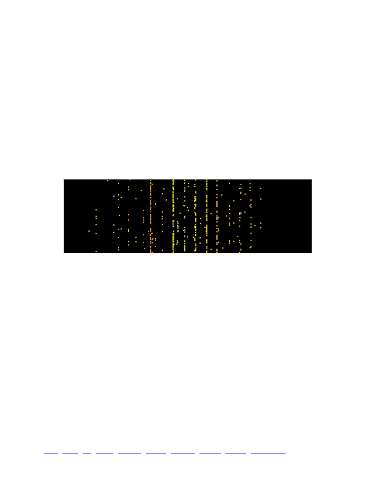
interaction(i1) {!
return dnorm(exerter.x, mean=receiver.x, sd=sigma_C) /!
dnorm(0.0, mean=0, sd=sigma_C);!
}
Finally, the output code should also use x instead of tagF (see the full model below).
Let’s make one other change. Previously, we’ve seen two-dimensional spatial models that used
the default boundaries of [0, 1] in x and y. In section 14.3 we mentioned that this default could be
changed; let’s change it now, because in this model phenotypic values often go outside that range.
We can add a line immediately after p1 is defined, telling p1 its spatial boundaries:
p1.setSpatialBounds(c(0.0, 10.0));
That’s it; we now have a model in which phenotype is considered to be a pseudo-spatial
dimension. Why is this model better? The first reason is that it provides us with better
visualization capabilities in SLiMgui. If we run the model now, we get a display that shows
individuals in a one-dimensional phenotypic space (with random y coordinates chosen by SLiM to
spread the individuals out for greater visibility):
Since we told p1 that its spatial boundaries were [0.0, 10.0], that is the spatial extent displayed
by SLiMgui here, so the phenotypic optimum is at the horizontal center of the display here. This
snapshot, taken at about generation 300, shows that the population has already reached the
optimum; the mean phenotype here is 4.91, in fact, with a standard deviation of 1.40 – typical of
the model’s equilibrium state. Colors correspond to fitness as usual; the band of individuals on the
left is particularly low-fitness because it is far off of the optimum, and yet is also quite crowded –
there are a lot of individuals with that phenotype at this instant in time. All of the discrete banding
here is the result of variation in QTLs of relatively large effect. Note that individuals quite far off
the fitness peak can still be fairly high-fitness, as long as their phenotype is rare.
So this is one benefit of treating phenotype as a spatial dimension: the dynamic evolution of the
phenotypic distribution can be watched in real time, color-coded by fitness as the fitness function
resulting from the squashed stabilizing selection fluctuates from generation to generation.
The other benefit is that the model is much faster, because InteractionType’s optimizations for
spatial interactions are brought to bear. First, if we realize that the Gaussian phenotypic
competition function we’re presently simulating with an interaction() callback is equivalent to
one of SLiM’s built-in interaction functions, then we can completely remove the interaction()
callback. We then need to change the definition of the i1 interaction like so:
initializeInteractionType(1, "x", reciprocal=T, maxDistance=sigma_C * 3);!
i1.setInteractionFunction("n", 1.0, sigma_C);
This defines i1 as a spatial interaction using x, which is our phenotypic “dimension”. It then
tells i1 to use a Gaussian function with a maximum value of 1.0 and a width of sigma_C –
TOC I TOC II WF nonWF initialize() Genome Individual Mutation SLiMSim Subpopulation!
Eidos events fitness() mateChoice() modifyChild() recombination() interaction() reproduction() 273

precisely what the interaction() callback used to do. Indeed, this model is exactly equivalent;
running it with the same random number seed produces the same result as shown in the snapshot
above. The difference is that it runs much faster – it completes about 4750 generations in 30
seconds (on my machine), whereas the version using an interaction() callback completes about
420 generations in 30 seconds. Not a bad speed improvement! The key is that we have avoided
having to make a call to an Eidos interaction() callback for every interaction, which is slow.
Indeed, even a little more speed can be squeezed out, at the price of accuracy. If a maximum
distance of 0.8 is set for i1, and totalOfNeighborStrengths() is used instead of strength() in the
global fitness() callback that calculates phenotypic competition, about 5030 generations can be
completed in 30 seconds. Since a maximum distance of 0.8 is two standard deviations of the
competition kernel, the effects of this change should be relatively small in terms of the overall
behavior of the model, but it is nevertheless a sacrifice in accuracy, and the performance gain in
this case is not large, so we will not consider this change to be a part of the official recipe for this
section. In other cases, however, the performance gain can be very large; a maximum distance
should always be considered for spatial interactions, particularly if it can safely be set to a short
enough distance to exclude most other individuals from interacting with the focal individual at all.
The full recipe for this section, for posterity, is:
initialize() {!
defineConstant("optimum", 5.0);!
defineConstant("sigma_C", 0.4);!
defineConstant("sigma_K", 1.0);!
!
initializeSLiMOptions(dimensionality="x");!
initializeMutationRate(1e-6);!
initializeMutationType("m1", 0.5, "f", 0.0); // neutral!
initializeMutationType("m2", 0.5, "n", 0.0, 1.0); // QTL!
m2.convertToSubstitution = F;!
!
initializeGenomicElementType("g1", c(m1, m2), c(1, 0.01));!
initializeGenomicElement(g1, 0, 1e5 - 1);!
initializeRecombinationRate(1e-8);!
!
initializeInteractionType(1, "x", reciprocal=T,!
maxDistance=sigma_C * 3); // competition!
i1.setInteractionFunction("n", 1.0, sigma_C);!
}!
1 late() {!
sim.addSubpop("p1", 500);!
p1.setSpatialBounds(c(0.0, 10.0));!
}!
1: late() {!
// construct phenotypes from the additive effects of QTLs!
inds = sim.subpopulations.individuals;!
inds.x = inds.sumOfMutationsOfType(m2);!
!
// evaluate interactions!
i1.evaluate();!
}!
fitness(m2) { // make QTLs intrinsically neutral!
return 1.0;!
}!
fitness(NULL) { // reward proximity to the optimum!
return 1.0 + dnorm(optimum - individual.x, mean=0.0, sd=sigma_K);!
}!
TOC I TOC II WF nonWF initialize() Genome Individual Mutation SLiMSim Subpopulation!
Eidos events fitness() mateChoice() modifyChild() recombination() interaction() reproduction() 274

fitness(NULL) { // phenotypic competition!
totalStrength = sum(i1.strength(individual));!
return 1.0 - totalStrength / p1.individualCount;!
}!
1:2001 late() {!
if (sim.generation == 1)!
cat(" gen mean sd\n");!
!
if (sim.generation % 100 == 1)!
{!
tags = p1.individuals.x;!
cat(format("%5d ", sim.generation));!
cat(format("%6.2f ", mean(tags)));!
cat(format("%6.2f\n", sd(tags)));!
}!
}
14.8 Sympatric speciation facilitated by assortative mating
In the previous section we refined our non-spatial model of phenotypic competition, by treating
phenotype as though it were a spatial dimension so that SLiM could run the model more quickly
and with better visualization. It is now time to take another step toward the model of Dieckmann
& Doebeli (1999) by changing mating in the model to be assortative by phenotype. This will in
some ways be similar to what we did in section 14.4; but there mating was spatially assortative,
whereas here mating will be phenotypically assortative.
Beginning with the model of section 14.7, the changes needed are quite small. First, we need
to add code in our initialize() callback to define a new interaction type, i2, that we will use to
evaluate mates:
initializeInteractionType(2, "x", reciprocal=T, maxDistance=sigma_M * 3);!
i2.setInteractionFunction("n", 1.0, sigma_M);
We have to add a definition of the sigma_M kernel width as well, at the beginning of the
initialize() callback:
defineConstant("sigma_M", 0.5);
Since this interaction is based on "x", which is our pseudo-spatial phenotype dimension, it
represents phenotypic proximity just as i1, our phenotypic competition interaction, does. Indeed,
the only reason not to use i1 to govern mate choice as well is that we want to be able to make it
use a different interaction function than competition, so that we can play with the width of the
mate-choice kernel independently of the width of the competition kernel.
Next, we need to evaluate that interaction in our 1: late() event every generation:
i2.evaluate();
And finally, we need a mate choice callback that uses that interaction:
mateChoice() {!
// spatial mate choice!
return i2.strength(individual);!
}
And that’s it. We now have a model in which phenotype, as determined by randomly arising
additive QTLs, is something like a “magic trait” (Servedio et al. 2011) – a trait that simultaneously
determines both fitness (because of the phenotypic optimum) and assortative mating (because of
TOC I TOC II WF nonWF initialize() Genome Individual Mutation SLiMSim Subpopulation!
Eidos events fitness() mateChoice() modifyChild() recombination() interaction() reproduction() 275
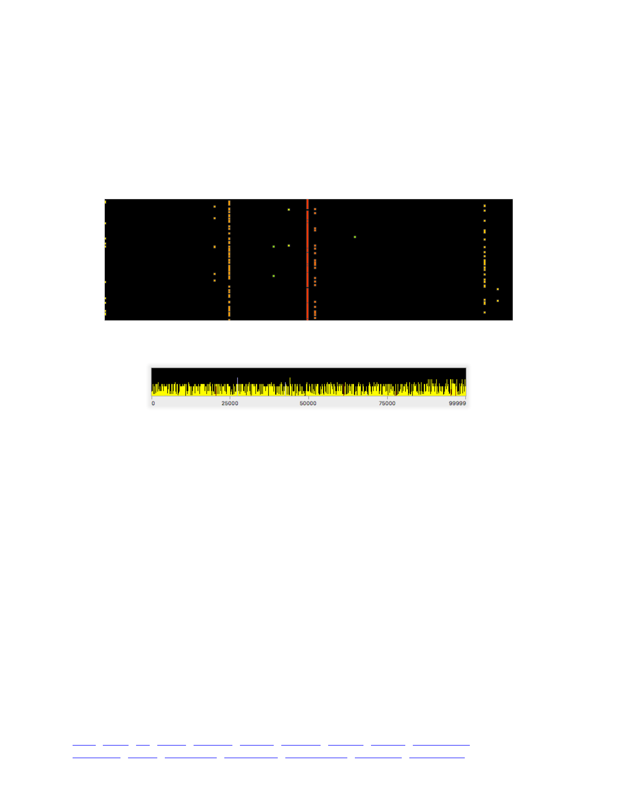
the mateChoice() callback) (although it is perhaps not strictly a magic trait since it is governed by
underlying QTLs; see sections 11.1 and 13.1 for more discussion of this topic). When exposed to
the disruptive selection caused by phenotypic competition in the model, the magic-ish trait here
readily produces speciation. (Note that this is true speciation, not evolutionary branching, because
this is a sexual model in the sense that matters – biparental mating with assortment and
recombination of gametes – even though it models hermaphrodites, not separate sexes).
We can see evidence for speciation in two different ways in SLiMgui. First of all, instead of the
cloud of different phenotypes around the optimum that the previous model generated, we now see
a set of discrete phenotypic clusters:
Second, we now see strong genetic separation between these clusters in the pattern of neutral
variation exhibited by the population:
Note that there are no neutral mutations at high frequency at all; instead, there is a large
amount of neutral diversity that is pinned at a couple of intermediate frequencies. These are blocs
of neutral mutations that have fixed within one of the species in the model, but are unable to
spread more widely because of the reproductive isolation between the species. Hybridization is
not impossible; it does occur occasionally, as can be seen in the snapshot above. But it is rare
enough that gene flow between the species is insufficient to allow that neutral diversity to spread.
It would be fair to argue that although this is a model of speciation given a pre-existing magic
trait, it is not a model of the emergence of the magic trait itself, because it lacks the “mating trait”
of the Dieckmann & Doebeli (1999) model. Adding in such a trait would be a simple extension of
the present model, and would presumably support the result found by Dieckmann & Doebeli
(1999) – that in an ecological scenario such as this, assortative mating will readily emerge,
transforming an ordinary trait into a magic trait that then facilitates speciation. We will leave that
extension of the model as an exercise for the reader, since pursuing it would not serve the aims of
this chapter. Instead, in the next section we will turn back toward spatial models, while
incorporating what we have done here with QTLs and phenotype-based competition and mating.
Here’s the full model, for the record:
initialize() {!
defineConstant("optimum", 5.0);!
defineConstant("sigma_C", 0.4);!
defineConstant("sigma_K", 1.0);!
defineConstant("sigma_M", 0.5);!
!
initializeSLiMOptions(dimensionality="x");!
TOC I TOC II WF nonWF initialize() Genome Individual Mutation SLiMSim Subpopulation!
Eidos events fitness() mateChoice() modifyChild() recombination() interaction() reproduction() 276

initializeMutationRate(1e-6);!
initializeMutationType("m1", 0.5, "f", 0.0); // neutral!
initializeMutationType("m2", 0.5, "n", 0.0, 1.0); // QTL!
m2.convertToSubstitution = F;!
!
initializeGenomicElementType("g1", c(m1, m2), c(1, 0.01));!
initializeGenomicElement(g1, 0, 1e5 - 1);!
initializeRecombinationRate(1e-8);!
!
initializeInteractionType(1, "x", reciprocal=T,!
maxDistance=sigma_C * 3); // competition!
i1.setInteractionFunction("n", 1.0, sigma_C);!
!
initializeInteractionType(2, "x", reciprocal=T,!
maxDistance=sigma_M * 3); // mate choice!
i2.setInteractionFunction("n", 1.0, sigma_M);!
}!
1 late() {!
sim.addSubpop("p1", 500);!
p1.setSpatialBounds(c(0.0, 10.0));!
}!
1: late() {!
// construct phenotypes from the additive effects of QTLs!
inds = sim.subpopulations.individuals;!
inds.x = inds.sumOfMutationsOfType(m2);!
!
// evaluate interactions!
i1.evaluate();!
i2.evaluate();!
}!
fitness(m2) { // make QTLs intrinsically neutral!
return 1.0;!
}!
fitness(NULL) { // reward proximity to the optimum!
return 1.0 + dnorm(optimum - individual.x, mean=0.0, sd=sigma_K);!
}!
fitness(NULL) { // phenotypic competition!
totalStrength = sum(i1.strength(individual));!
return 1.0 - totalStrength / p1.individualCount;!
}!
mateChoice() {!
// spatial mate choice!
return i2.strength(individual);!
}!
1:5001 late() {!
if (sim.generation == 1)!
cat(" gen mean sd\n");!
!
if (sim.generation % 100 == 1)!
{!
tags = p1.individuals.x;!
cat(format("%5d ", sim.generation));!
cat(format("%6.2f ", mean(tags)));!
cat(format("%6.2f\n", sd(tags)));!
}!
}
TOC I TOC II WF nonWF initialize() Genome Individual Mutation SLiMSim Subpopulation!
Eidos events fitness() mateChoice() modifyChild() recombination() interaction() reproduction() 277

14.9 Speciation due to spatial variation in selection
In the previous section, we observed that speciation can occur as a result of phenotypic
competition and assortative mate choice in a non-spatial model. In this section we will return to
spatial modeling, while preserving many aspects of the previous recipe. We will now introduce
spatial variation in selection, and will observe adaptive speciation among spatial groups as a result
of local selection pressures in combination with phenotypic competition. The optimum trait value
for the quantitative trait – the phenotypic optimum, in other words – will vary according to the x
position in space, producing a linear environmental gradient. This model is broadly inspired by
the model of Doebeli & Dieckmann (2003), although again there are many differences.
This recipe has enough differences from the previous recipe that we will build it here from
scratch, rather than just giving changes relative to the previous recipe. Let’s start with the setup:
initialize() {!
defineConstant("sigma_C", 0.1);!
defineConstant("sigma_K", 0.5);!
defineConstant("sigma_M", 0.1);!
defineConstant("slope", 1.0);!
defineConstant("N", 500);!
!
initializeSLiMOptions(dimensionality="xyz");!
initializeMutationRate(1e-6);!
initializeMutationType("m1", 0.5, "f", 0.0); // neutral!
initializeMutationType("m2", 0.5, "n", 0.0, 1.0); // QTL!
m2.convertToSubstitution = F;!
!
initializeGenomicElementType("g1", c(m1, m2), c(1, 0.1));!
initializeGenomicElement(g1, 0, 1e5 - 1);!
initializeRecombinationRate(1e-8);!
!
initializeInteractionType(1, "xyz", reciprocal=T,!
maxDistance=sigma_C * 3); // competition!
i1.setInteractionFunction("n", 1.0, sigma_C);!
!
initializeInteractionType(2, "xyz", reciprocal=T,!
maxDistance=sigma_M * 3); // mate choice!
i2.setInteractionFunction("n", 1.0, sigma_M);!
}!
1 late() {!
sim.addSubpop("p1", N);!
p1.setSpatialBounds(c(0.0, 0.0, -slope, 1.0, 1.0, slope));!
!
for (ind in p1.individuals)!
ind.setSpatialPosition(p1.pointUniform());!
p1.individuals.z = 0.0;!
}
This model is our first to use dimensionality "xyz". The x and y dimensions are true spatial
dimensions; this is a 2-D model. The z dimension will be used here for phenotype, just as we used
x as a pseudo-spatial phenotypic dimension in previous recipes. We set up QTL machinery for the
phenotype much as we did before; the fraction of mutations that are QTLs is higher in this model
just so that we don’t have to wait as long to get interesting behavior. We create two interaction
types, i1 for competition and i2 for mating, as before. Note that both of these interaction types
have spatiality "xyz"; i1 therefore encompasses both spatial and phenotypic competition in a
single interaction, and i2 encompasses both spatially and phenotypically assortative mate choice.
For our purposes here this is sufficient, but more interaction types could be defined as desired.
TOC I TOC II WF nonWF initialize() Genome Individual Mutation SLiMSim Subpopulation!
Eidos events fitness() mateChoice() modifyChild() recombination() interaction() reproduction() 278

Then we set up the population, in the 1 late() event. We set spatial boundaries of [0.0, 1.0]
for x and y, and of [-slope, slope] for z. The optimum phenotype will actually vary from
−slope/2 to slope/2, from the left edge to the right edge of the environment; the wider interval
here is used just to allow for some phenotypic variation beyond that interval. (In fact, the spatial
boundary for z is not used in this model, nor by SLiMgui, so it is irrelevant anyway). Finally, we set
random spatial positions for all of the initial individuals, and zero out their phenotypes.
Next, let’s implement the machinery to manage spatial positions and phenotypes:
modifyChild() {!
// set offspring position based on parental position!
do!
pos = c(parent1.spatialPosition[0:1] + rnorm(2, 0, 0.005), 0.0);!
while (!p1.pointInBounds(pos));!
child.setSpatialPosition(pos);!
!
return T;!
}!
1: late() {!
// construct phenotypes from the additive effects of QTLs!
inds = sim.subpopulations.individuals;!
phenotype = inds.sumOfMutationsOfType(m2);!
inds.z = phenotype;!
!
// color individuals according to phenotype!
for (ind in inds)!
{!
hue = ((ind.z + slope) / (slope * 2)) * 0.66;!
ind.color = rgb2color(hsv2rgb(c(hue, 1.0, 1.0)));!
}!
!
// evaluate interactions!
i1.evaluate();!
i2.evaluate();!
}
As in previous recipes, we use a modifyChild() callback to place offspring near their first
parent, with a small random deviation. We ensure that the offspring phenotype is 0.0 here, so that
it doesn’t cause the pointInBounds() call to return F; we don’t want SLiM to bounds-check
offspring phenotypes for us. The phenotype of 0.0 set here is overwritten a moment later, in the
1:!late() event above, when phenotypes are calculated for all individuals and placed into their z
coordinate. A bit of extra code here calculates color values for individuals; in this model
individuals are colored according to their phenotype, rather than their fitness, so that spatial
adaptive divergence is directly visible in SLiMgui, as we’ll see below. The code here calculates a
hue in the HSV (hue/saturation/value) color system, then converts that to the RGB (red/green/blue)
color system and then to a hexadecimal color string which it sets as the color of the individual (see
the Eidos manual for details on these functions). Finally, the two interaction types are evaluated.
Next, let’s add all of our fitness callbacks and other interaction-related machinery:
fitness(m2) { // make QTLs intrinsically neutral!
return 1.0;!
}!
fitness(NULL) { // reward proximity to the optimum!
optimum = (individual.x - 0.5) * slope;!
return 1.0 + dnorm(optimum - individual.z, mean=0.0, sd=sigma_K);!
}!
TOC I TOC II WF nonWF initialize() Genome Individual Mutation SLiMSim Subpopulation!
Eidos events fitness() mateChoice() modifyChild() recombination() interaction() reproduction() 279
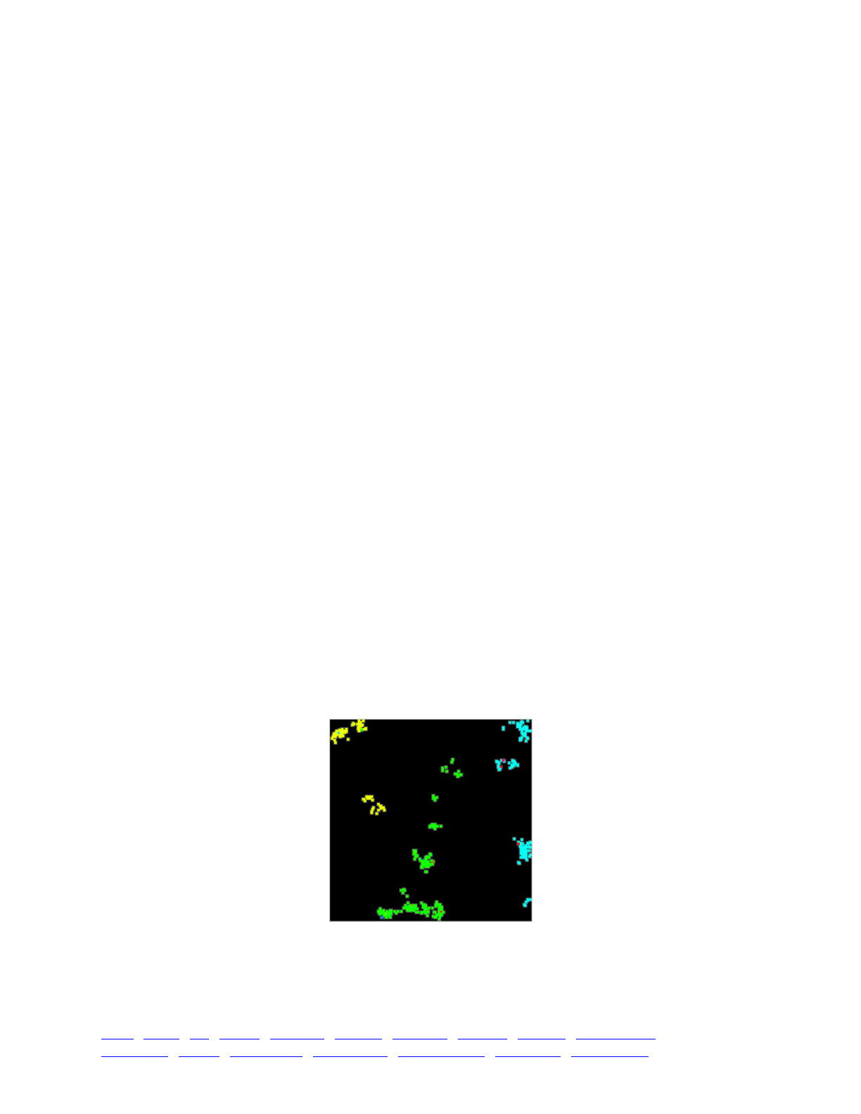
fitness(NULL) { // phenotypic competition!
totalStrength = sum(i1.strength(individual));!
return 1.0 - totalStrength / p1.individualCount;!
}!
mateChoice() {!
// spatial mate choice!
return i2.strength(individual);!
}
The m2 fitness() callback zeroes out the individual fitness effects of our QTLs, as usual. The
first global fitness() callback rewards individuals for proximity to the fitness optimum; in
previous recipes the optimum was a constant value, but now the optimum depends upon the
individual’s position in space, since we are now modeling a linear spatial environmental gradient.
Apart from the fact that the optimum now depends upon individual.x and slope, this is much the
same as before. The second global fitness() callback implements competition, both spatial and
phenotypic; it is actually unchanged from the previous recipe. Similarly, the mateChoice()
callback is unchanged, although it now scores mates based upon both spatial and phenotypic
similarity.
Finally, let’s use the same output event that we used before:
1:5001 late() {!
if (sim.generation == 1)!
cat(" gen mean sd\n");!
!
if (sim.generation % 100 == 1)!
{!
tags = p1.individuals.z;!
cat(format("%5d ", sim.generation));!
cat(format("%6.2f ", mean(tags)));!
cat(format("%6.2f\n", sd(tags)));!
}!
}
This prints out a history of the phenotypic mean and standard deviation every 100 generations.
Running this model does indeed produce speciation. One sign of that is that we can see
discrete clusters of individuals of different colors, representing the fact that they have adapted to
different parts of the environmental gradient:
There are three species present here, colored yellow, green, and cyan, adapted to the conditions
at the left, center, and right of the environmental gradient, respectively. (There are also a few
mutants of other colors sprinkled in.)
TOC I TOC II WF nonWF initialize() Genome Individual Mutation SLiMSim Subpopulation!
Eidos events fitness() mateChoice() modifyChild() recombination() interaction() reproduction() 280

Another piece of evidence for speciation is the presence of large amounts of neutral diversity
that is not mixing between the different phenotypic clusters, as we saw before in section 14.8:
Many mutations are at a frequency of approximately 2/3 because they are shared between two
species; the yellow species split from the green species only about 1000 generations before these
snapshots were taken, and so the two species share a great deal of their genetic background.
Many other mutations are at a frequency of approximately 1/3 because they are shared only within
the cyan species, which split from the green species more than 8000 generations earlier.
Remarkably, not a single mutation has fixed across the whole population after 9000 generations of
runtime; the onset of speciation is quite early (in this run of the model, at least), and the
reproductive barrier is quite strong with the parameter values used here.
One could bring in other machinery to further assess the extent of adaptive divergence and
reproductive isolation, such as the FST calculation code we’ve used in a couple of recipes before.
Indeed, one could dump out the neutral diversity to a file and run a STRUCTURE analysis on it to
see whether the groups that appear to be species fall out as genetic clusters naturally. We won’t
pursue that here since the divergence is so readily apparent.
The full model, for reference:
initialize() {!
defineConstant("sigma_C", 0.1);!
defineConstant("sigma_K", 0.5);!
defineConstant("sigma_M", 0.1);!
defineConstant("slope", 1.0);!
defineConstant("N", 500);!
!
initializeSLiMOptions(dimensionality="xyz");!
initializeMutationRate(1e-6);!
initializeMutationType("m1", 0.5, "f", 0.0); // neutral!
initializeMutationType("m2", 0.5, "n", 0.0, 1.0); // QTL!
m2.convertToSubstitution = F;!
!
initializeGenomicElementType("g1", c(m1, m2), c(1, 0.1));!
initializeGenomicElement(g1, 0, 1e5 - 1);!
initializeRecombinationRate(1e-8);!
!
initializeInteractionType(1, "xyz", reciprocal=T,!
maxDistance=sigma_C * 3); // competition!
i1.setInteractionFunction("n", 1.0, sigma_C);!
!
initializeInteractionType(2, "xyz", reciprocal=T,!
maxDistance=sigma_M * 3); // mate choice!
i2.setInteractionFunction("n", 1.0, sigma_M);!
}!
1 late() {!
sim.addSubpop("p1", N);!
p1.setSpatialBounds(c(0.0, 0.0, -slope, 1.0, 1.0, slope));!
!
for (ind in p1.individuals)!
ind.setSpatialPosition(p1.pointUniform());!
p1.individuals.z = 0.0;!
}
TOC I TOC II WF nonWF initialize() Genome Individual Mutation SLiMSim Subpopulation!
Eidos events fitness() mateChoice() modifyChild() recombination() interaction() reproduction() 281

modifyChild() {!
// set offspring position based on parental position!
do!
pos = c(parent1.spatialPosition[0:1] + rnorm(2, 0, 0.005), 0.0);!
while (!p1.pointInBounds(pos));!
child.setSpatialPosition(pos);!
!
return T;!
}!
1: late() {!
// construct phenotypes from the additive effects of QTLs!
inds = sim.subpopulations.individuals;!
phenotype = inds.sumOfMutationsOfType(m2);!
inds.z = phenotype;!
!
// color individuals according to phenotype!
for (ind in inds)!
{!
hue = ((ind.z + slope) / (slope * 2)) * 0.66;!
ind.color = rgb2color(hsv2rgb(c(hue, 1.0, 1.0)));!
}!
!
// evaluate interactions!
i1.evaluate();!
i2.evaluate();!
}!
fitness(m2) { // make QTLs intrinsically neutral!
return 1.0;!
}!
fitness(NULL) { // reward proximity to the optimum!
optimum = (individual.x - 0.5) * slope;!
return 1.0 + dnorm(optimum - individual.z, mean=0.0, sd=sigma_K);!
}!
fitness(NULL) { // phenotypic competition!
totalStrength = sum(i1.strength(individual));!
return 1.0 - totalStrength / p1.individualCount;!
}!
mateChoice() {!
// spatial mate choice!
return i2.strength(individual);!
}!
1:5001 late() {!
if (sim.generation == 1)!
cat(" gen mean sd\n");!
!
if (sim.generation % 100 == 1)!
{!
tags = p1.individuals.z;!
cat(format("%5d ", sim.generation));!
cat(format("%6.2f ", mean(tags)));!
cat(format("%6.2f\n", sd(tags)));!
}!
}
14.10 A simple biogeographic landscape model
The time has come to introduce a new topic: landscape maps. For this, we will temporarily
abandon the spatial quantitative-trait local adaptation model we have been building, and switch to
TOC I TOC II WF nonWF initialize() Genome Individual Mutation SLiMSim Subpopulation!
Eidos events fitness() mateChoice() modifyChild() recombination() interaction() reproduction() 282

a much simpler model. Our goal in this section is to build a simple biogeographic model that uses
a landscape map. Just for fun, the map we will use is a map of the world. There are no end of
issues with this – the map projection distorts the geography, Russia and Alaska are not connected
across the Bering Strait because the spatial boundary intervenes, and so forth. But as a simple toy
model to illustrate the concept and the potential of landscape maps, it should serve our purposes.
Let’s start with the model, and then delve into the concepts:
initialize() {!
initializeSLiMOptions(dimensionality="xy");!
initializeMutationRate(1e-7);!
initializeMutationType("m1", 0.5, "f", 0.0);!
initializeGenomicElementType("g1", m1, 1.0);!
initializeGenomicElement(g1, 0, 99999);!
initializeRecombinationRate(1e-8);!
!
// spatial competition!
initializeInteractionType(1, "xy", reciprocal=T, maxDistance=30.0);!
i1.setInteractionFunction("n", 5.0, 10.0);!
!
// spatial mate choice!
initializeInteractionType(2, "xy", reciprocal=T, maxDistance=30.0);!
i2.setInteractionFunction("n", 1.0, 10.0);!
}!
1 late() {!
sim.addSubpop("p1", 1000);!
!
p1.setSpatialBounds(c(0.0, 0.0, 540.0, 217.0));!
!
mapLines = rev(readFile("~/Desktop/world_map_540x217.txt"));!
mapLines = sapply(mapLines, "strsplit(applyValue, '') == '#';");!
mapValues = asFloat(mapLines);!
!
p1.defineSpatialMap("world", "xy", c(540, 217), mapValues,!
valueRange=c(0.0, 1.0), colors=c("#0000CC", "#55FF22"));!
!
// start near a specific map location!
for (ind in p1.individuals) {!
ind.x = rnorm(1, 300.0, 1.0);!
ind.y = rnorm(1, 100.0, 1.0);!
}!
}!
1: late() {!
i1.evaluate();!
i2.evaluate();!
}!
fitness(NULL) {!
comp = i1.totalOfNeighborStrengths(individual) / p1.individualCount;!
comp = min(c(comp, 0.99));!
return 1.0 - comp;!
}!
1: mateChoice() {!
return i2.strength(individual);!
}
TOC I TOC II WF nonWF initialize() Genome Individual Mutation SLiMSim Subpopulation!
Eidos events fitness() mateChoice() modifyChild() recombination() interaction() reproduction() 283
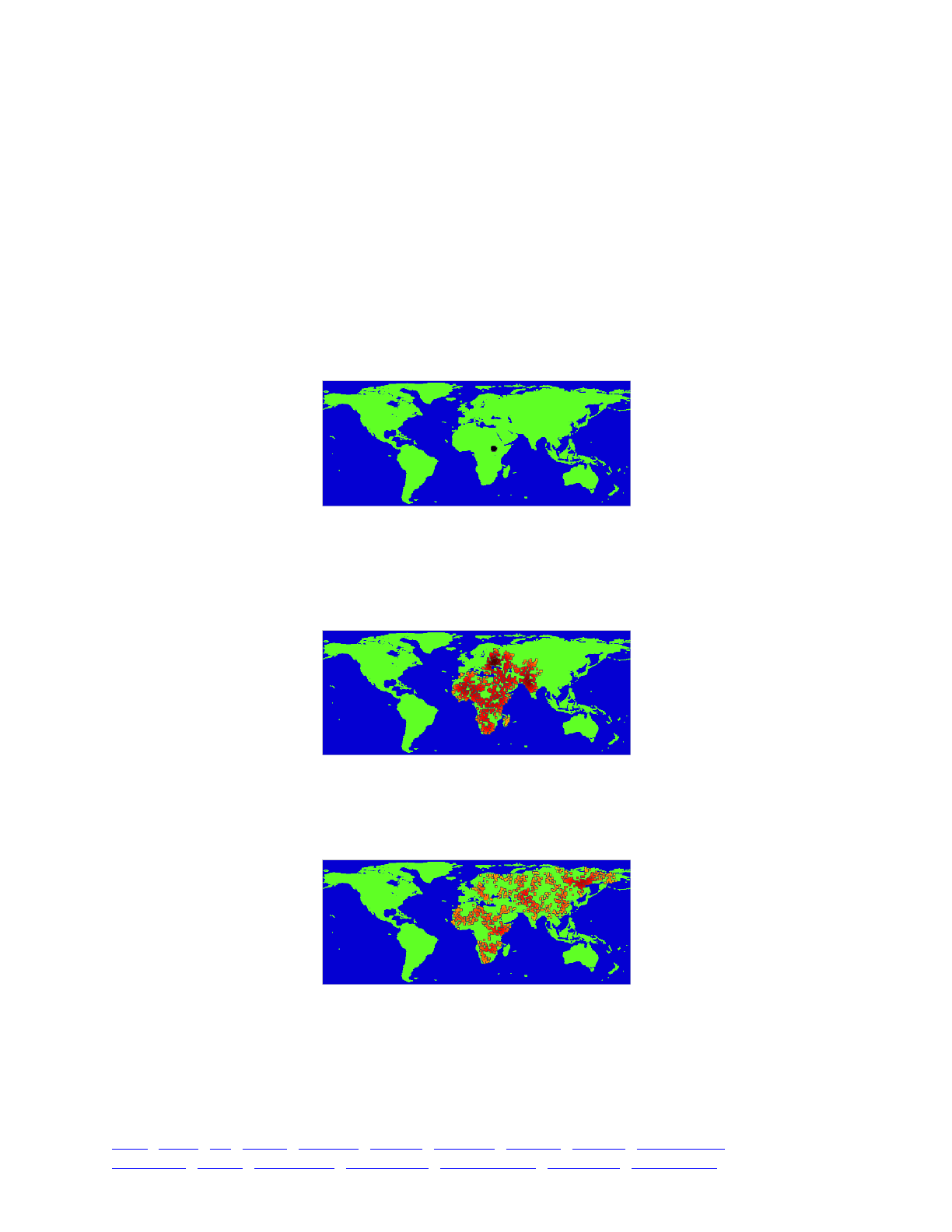
modifyChild() {!
do pos = parent1.spatialPosition + rnorm(2, 0, 2.0);!
while (!p1.pointInBounds(pos));!
!
// prevent dispersal into water!
if (p1.spatialMapValue("world", pos) == 0.0)!
return F;!
!
child.setSpatialPosition(pos);!
return T;!
}!
20000 late() { sim.outputFixedMutations(); }
Here’s what the model looks like in SLiMgui at the end of generation 1, right after the
population has been set up:
The black dot in eastern Africa is the initial population; this model seeds the population at a
specific location, perhaps simulating – not realistically, obviously! – the origin of Homo sapiens in
Africa. This model has spatial competition and spatial mate choice, as we have seen in previous
recipes, so the population rapidly spreads to occupy new territory in order to escape the local
competition from other individuals. Here is the population at the end of generation 63:
Notice that the individuals are constrained to occupy only land locations. It is also interesting
that they have managed to reach Madagascar; the dispersal kernel used can jump small distances,
so the population can sometimes bridge the Mozambique Channel. Some water gaps are too large
to bridge, however. Here is the population at the end of generation 1000:
The population has spread across all of mainland Asia, but has not been able to enter Indonesia,
and has thus not reached Australia; the land area provided by the Indonesian islands is probably
too small to support a subpopulation (and similarly, the subpopulation that colonized Madagascar
has died out). Reaching the New World would be even more difficult, given the fact that the
Bering Strait is unavailable (a periodic boundary condition in the x direction would be needed to
TOC I TOC II WF nonWF initialize() Genome Individual Mutation SLiMSim Subpopulation!
Eidos events fitness() mateChoice() modifyChild() recombination() interaction() reproduction() 284

make that work); individuals would have to make like the Vikings and jump from mainland Europe
to Iceland, Greenland, and thence to North America.
The fact that this particular biogeographic pattern is observed is not necessarily a problem, of
course; a great many organisms are unable to disperse from Eurasia to Australia or the Americas.
But it is a consequence of the details of this model – the particular dispersal kernel chosen, the
particular way in which dispersal is constrained to land, the details of the map used (the fact that it
does not include elevation, rivers, etc.), the way in which competition and mating are
implemented, and so forth. There is no obstacle to changing these details to match the biological
details of a particular species, to produce a more empirically based biogeographic model.
So, how was this recipe constructed? Let’s now delve into a few of the details. Most of the
model is familiar boilerplate: the setup in initialize(), the 1: late() event that evaluates the
spatial interactions, and the fitness() and mateChoice() callbacks, for example. Let’s start, then,
by looking at the 1 late() event that initializes the population:
1 late() {!
sim.addSubpop("p1", 1000);!
!
p1.setSpatialBounds(c(0.0, 0.0, 540.0, 217.0));!
!
mapLines = rev(readFile("~/Desktop/world_map_540x217.txt"));!
mapLines = sapply(mapLines, "strsplit(applyValue, '') == '#';");!
mapValues = asFloat(mapLines);!
!
p1.defineSpatialMap("world", "xy", c(540, 217), mapValues,!
valueRange=c(0.0, 1.0), colors=c("#0000CC", "#55FF22"));!
!
// start near a specific map location!
for (ind in p1.individuals) {!
ind.x = rnorm(1, 300.0, 1.0);!
ind.y = rnorm(1, 100.0, 1.0);!
}!
}
It begins by creating a subpopulation, p1, as usual. It then sets up spatial boundaries for p1,
from (0, 0) to (540, 217); this is dictated by the size of the map that we are about to load, which is
540x217 pixels in size. The spatial bounds do not need to match that, but it is usually desirable for
them to at least match the aspect ratio of the map, so that the map is not stretched.
The map is then read in from a file; note that the path to this file will probably be different on
your system (it can be found inside the Recipes folder that can be downloaded from SLiM’s home
page). This is just a simple text file; each line is comprised of a series of spaces and hash marks
(“#”), where the hash marks indicate land. If you open this file in a text editor and view it in a
monospace font at a very small point size (like 3 pt), you will see the world map. It is read with
readFile(), which returns a vector of string objects representing the lines of the file.
SLiM uses Cartesian coordinates for spatial models, which means that x increases to the right
and y increases to the top. Our world map, on the other hand, is rendered from top to bottom, as
is common for pixel-based image formats. We use the rev() function to reverse the order of the
lines in the map so that it matches SLiM’s coordinate system. We then use sapply() and
strsplit() to split each line into individual characters, and then convert those into logical values
– T for land, F for water. Finally, these logical values are converted to float, according to the
Eidos rule that T is 1 and F is 0. The map, now in mapValues, is now ready for use.
Now we call the defineSpatialMap() method of Subpopulation to give the map to SLiM. The
first parameter, "world", is a name for the map; you can define as many spatial maps as you wish,
TOC I TOC II WF nonWF initialize() Genome Individual Mutation SLiMSim Subpopulation!
Eidos events fitness() mateChoice() modifyChild() recombination() interaction() reproduction() 285

and you refer to them by name. The "xy" parameter indicates the spatiality of the map, which
must be a subset of the dimensionality of the model as a whole; here our map covers dimensions x
and y. Next we give the dimensions of the map, in pixels; it is 540x217, because those are the
dimensions of the data we read from the file. Next we provide the raw pixel data of the map as a
single vector of float values, scanning the map horizontally from left to right and vertically from
bottom to top (Cartesian coordinates); this is the mapValues variable that we prepared above.
The last two parameters here are optional, and are for SLiMgui’s benefit. The first parameter,
valueRange, gives the permissible range of values for the map data; this need not match the actual
range of the data. The purpose of this is to tell SLiMgui what value range should be displayed
using distinct colors; values outside this range will be clamped to be within the range for display.
The second parameter, colors, gives a vector of color strings that specify how particular values
should be displayed (see the Eidos manual for details on color strings). The lowest value in
valueRange will be displayed using the first color in colors; the highest value in valueRange will
be displayed using the last color in colors. Color values in between will be evenly distributed
across valueRange, and intermediate values – those not corresponding exactly to a given color –
will be displayed using an interpolation between the two nearest color values. Here, the values
supplied for these parameters indicate that a value of 0.0 should be displayed with the color
"#0000CC" (a dark blue), whereas a value of 1.0 should use color "#55FF22" (a medium green).
Values between 0.0 and 1.0 would use an interpolation between those shades, but in fact our map
data is binary, so that does not arise.
With that, we have defined a spatial map and told SLiMgui how to display it. We now just need
to use it to govern the model dynamics. At the end of the 1 late() event the positions of all
individuals are initialized to be near a particular spot in East Africa, using rnorm() to draw the
coordinates instead of using the pointUniform() method we have used in previous recipes. Then
in our modifyChild() callback we enforce that individuals can only disperse to land:
modifyChild() {!
do pos = parent1.spatialPosition + rnorm(2, 0, 2.0);!
while (!p1.pointInBounds(pos));!
!
// prevent dispersal into water!
if (p1.spatialMapValue("world", pos) == 0.0)!
return F;!
!
child.setSpatialPosition(pos);!
return T;!
}
The first couple of lines generate a random offspring position based upon the position of the first
parent, as we have seen in previous recipes. That code loops until a point inside the spatial
bounds of the subpopulation in generated. Next, the callback consults the spatial map to find out
the value at the candidate point using the spatialMapValue() method, giving it the name of the
map and the candidate point. This method simply looks up the value nearest to the given point in
the map data. If it is 0.0 – the value we used for water – then the callback returns F, rejecting the
proposed child. Otherwise, the location is on land, so it is set as the new child’s position and T is
returned to accept the proposed child.
Notice, then, that a reprising boundary condition is used for the edges of the map, but an
absorbing boundary condition is used for the coastlines. This means that individuals close to a
coastline suffer a fitness penalty; their children are relatively likely to land in water, and when they
do, they don’t get another chance to generate a different child location. This is part of the reason
that colonizing areas like Indonesia is difficult in this model (that fact that locations in places like
TOC I TOC II WF nonWF initialize() Genome Individual Mutation SLiMSim Subpopulation!
Eidos events fitness() mateChoice() modifyChild() recombination() interaction() reproduction() 286

Indonesia are relatively unlikely to be chosen as child locations in the first place is also important).
We can change the modifyChild() callback’s code a bit to change that:
modifyChild() {!
do {!
do pos = parent1.spatialPosition + rnorm(2, 0, 2.0);!
while (!p1.pointInBounds(pos));!
} while (p1.spatialMapValue("world", pos) == 0.0);!
!
child.setSpatialPosition(pos);!
return T;!
}
Now the boundary condition on coastlines is reprising also, and a quick run of the model
shows that that allows much more dispersal into small land areas:
Indonesia and Australia are soon reached, and the UK and Madagascar often also support
populations. Reaching North America is still quite difficult, however.
This is obviously just a fun toy model, but it would be easy to extend. A map using more
values, to indicate things like mountain ranges, could be used, and the map could be much higher
resolution (SLiM places no limit on the size of spatial maps, as long as your computer has enough
memory). Dispersal on a high-resolution map could be much more short-range, making it so that
even small barriers like rivers would present obstacles to dispersal. A much larger population size
would probably be appropriate, for most organisms. Moreover, instead of using a constant
population size as this model does, which is clearly unrealistic, the population size could be
related to fitness in such a way that when the population discovers a new area and expands into it,
thereby increasing in fitness since the effects of competition are diminished, the population size
would increase to reflect the new higher carrying capacity; this might fall out naturally in a nonWF
model (see section 15.10), but would have to be implemented in a WF model such as the one
shown here. Mate choice could be based not only on spatial distance, but also upon, for example,
the map value at a point intermediate between the two proposed parents, so that a mountain range
would produce vicariance between even closely adjacent subpopulations. All of these sorts of
features could be added with just a few more lines of code. Note also that although this model
reads its spatial map in from a text file, it is also straightforward to construct a map
programmatically, at runtime; see twoHabitatMap.txt in the online SLiM-Extras repository.
One particularly interesting feature for a biogeographic model like this would be to include
spatial heterogeneity that affects the selection on individuals, such that there is selection pressure
towards local adaptation. For instance, with this world map the more polar regions might exert
selection toward more cold-adapted phenotypes whereas the more tropical regions might select for
more warm-adapted phenotypes. In section 14.9 we saw a very primitive stab at this sort of
model, with the introduction of a simple linear environmental gradient. Real landscapes are more
complicated than that, though – mountaintops are similar to polar environments, whereas
coastlines tend to have more moderate climates, for example. In the next section, we’ll look at a
model of adaptation to spatial heterogeneity that goes beyond a simple linear environmental
gradient by using a spatial map.
TOC I TOC II WF nonWF initialize() Genome Individual Mutation SLiMSim Subpopulation!
Eidos events fitness() mateChoice() modifyChild() recombination() interaction() reproduction() 287

14.11 Local adaptation on a heterogeneous landscape map
The previous section introduced the ability to define an arbitrary landscape map, whereas in
section 14.9 we explored a model of adaptation to a linear environmental gradient. Let’s try
combining those two approaches, to see how complex environmental heterogeneity influences
evolutionary outcomes like divergence and speciation. This recipe will demonstrate such an
approach, inspired by the model of Haller, Mazzucco & Dieckmann (2013), although the
landscapes generated here will be fairly different from those used in that paper. This recipe will
generate a random “landscape map” representing the local phenotypic optimum across the
landscape, and will then simulate the local adaptation of spatial groups to the conditions of that
landscape. Here the landscape is generated algorithmically, but it would be trivial to instead read
a landscape map from a file as was done in the previous recipe.
The model of section 14.9 provides us with a quantitative trait based upon underlying randomly
arising QTLs, with phenotypic competition and assortative mating based upon that quantitative
trait. Let’s assume that machinery for now (the full recipe will be presented at the end), and look at
the parts that are new. Most importantly, we have gotten rid of the slope constant of section 14.9,
and instead here generate a heterogeneous landscape:
1 late() {!
sim.addSubpop("p1", N);!
!
p1.setSpatialBounds(c(0.0, 0.0, 0.0, 1.0, 1.0, 1.0));!
!
defineConstant("mapValues", runif(25, 0, 1));!
p1.defineSpatialMap("map1", "xy", c(5, 5), mapValues, interpolate=T,!
valueRange=c(0.0, 1.0), colors=c("red", "yellow"));!
!
for (ind in p1.individuals)!
ind.setSpatialPosition(p1.pointUniform());!
p1.individuals.z = 0.0;!
}
We define spatial bounds of [0, 1] for each dimension, including the z dimension that is used
for phenotype. A map is then generated simply as a set of 25 draws from a uniform distribution
between 0 and 1. This map, saved off in the defined constant mapValues (we will use it later), is
set as a spatial map on subpopulation p1 with a call to defineSpatialMap(). We specify that it
corresponds to dimensions "xy", that it is based on a 5x5 pixel grid (thus the 25 values), that values
are expected to range between 0.0 and 1.0, and that colors for that range should range from red to
yellow.
We’ll look at what this ends up looking like in a moment, but first let’s finish building the
model. In the 1: late() event, we will replace the code from section 14.9 that colors individuals
according to phenotype with new code that uses the same color scheme as the landscape
coloring:
// color individuals according to phenotype!
inds.color = p1.spatialMapColor("map1", phenotype);
This uses the spatialMapColor() method of Subpopulation, which translates a value into a
color using the mapping established by a particular spatial map. In this way, the colors of
individuals adapted to a given phenotypic optimum will exactly match the colors of map areas
where that phenotypic optimum exists. Individuals that are perfectly adapted to their environment
will therefore be displayed in SLiMgui in a color that matches their environment, whereas a
mismatch in color between an individual and its environment will indicate maladaptation.
TOC I TOC II WF nonWF initialize() Genome Individual Mutation SLiMSim Subpopulation!
Eidos events fitness() mateChoice() modifyChild() recombination() interaction() reproduction() 288
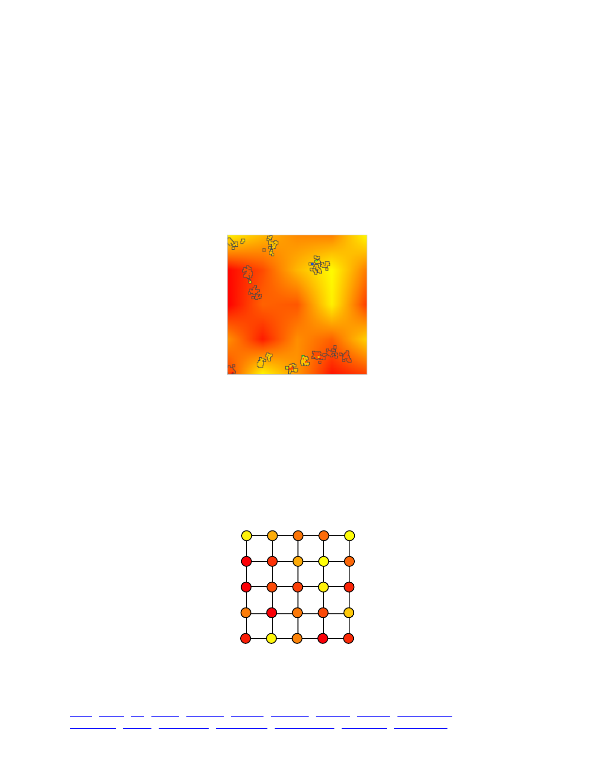
Finally, the global fitness() callback needs to change to use spatialMapValue() to find the
phenotypic optimum for the point in space occupied by the focal individual. The map is looked
up by name, as we saw in the previous section, and the location of the focal individual is obtained
using its spatialPosition() method. We select just the x and y coordinates of the location, since
those are the dimensions used by the spatial map. The final callback looks like this:
fitness(NULL) { // reward proximity to the optimum!
location = individual.spatialPosition[0:1];!
optimum = subpop.spatialMapValue("map1", location);!
return 1.0 + dnorm(optimum - individual.z, mean=0.0, sd=sigma_K);!
}
The rest of the recipe is as it was before. When we run the model, here’s an example of what
we see:
We have a nice randomly heterogeneous landscape, and the population has clearly adapted to
it; we have reddish individuals in two of the more reddish areas, and orange individuals in three
more orange areas. As before, the structure of neutral diversity visible in the chromosome view
provides clear evidence of reproductive isolation and speciation.
There is one thing that may be surprising, however. We supplied a 5x5 map to
defineSpatialMap(), but the snapshot above shows what appears to be a continuous landscape.
This is a result of the interpolation=T parameter we supplied to defineSpatialMap(), which
instructed it to use interpolation (bilinear interpolation, in this case, to be precise) to make the
landscape continuous. To understand better how that works, let’s look in a little more detail at
how SLiM builds landscape maps. First of all, here is the 5x5 grid of values that we supplied to
defineSpatialMap(), colored according to the given color map:
Given this particular pixel grid, if we were to supply interpolate=F to defineSpatialMap()
instead, the landscape displayed by SLiMgui would look like this:
TOC I TOC II WF nonWF initialize() Genome Individual Mutation SLiMSim Subpopulation!
Eidos events fitness() mateChoice() modifyChild() recombination() interaction() reproduction() 289
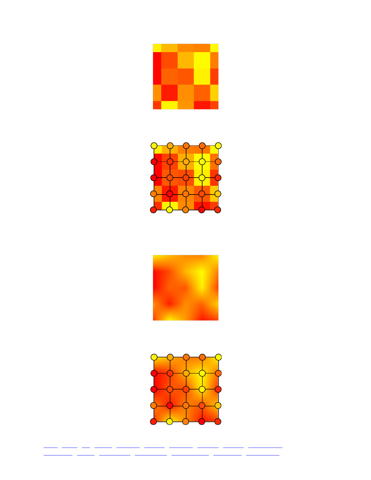
Note that because the pixel grid is aligned with the corners of the spatial bounds of the
subpopulation, only ½ or ¼ of the area of the outer pixels is contained within bounds. The reason
for this is clear if we look at the pixel grid superimposed on that landscape:
This is by design; it is the most natural way to handle such spatial maps when interpolation is
involved (try thinking through the alternative to see why), and for consistency it is also how SLiM
handles spatial maps when interpolation is not used.
So now when interpolation is turned on, the landscape looks like this:
This is the result of bilinear interpolation, which shades continuously between the defined
points to produce a continuous map. The values defined by the pixel grid remain fixed, however.
To illustrate that, here is the pixel grid superimposed on the interpolated landscape:
TOC I TOC II WF nonWF initialize() Genome Individual Mutation SLiMSim Subpopulation!
Eidos events fitness() mateChoice() modifyChild() recombination() interaction() reproduction() 290
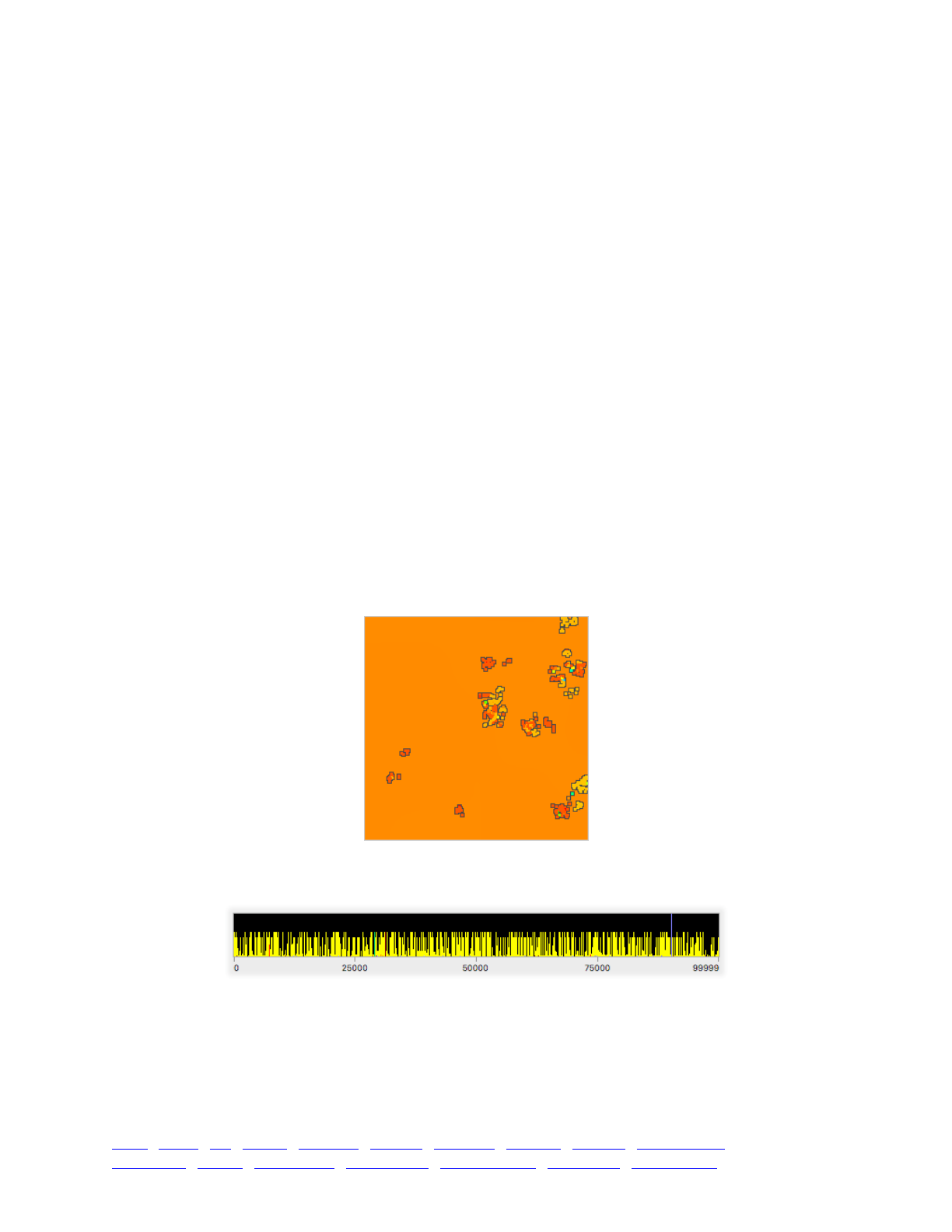
SLiM does not interpolate statically; it does not generate and store an interpolated map of some
large but fixed size. Instead, when interpolation is enabled for a given spatial map, it calculates
the exact interpolated value for a given point upon request. Interpolated maps are therefore
completely continuous and effectively infinite-resolution (within the precision limits of floating-
point numbers). With only 25 defined values, we therefore have an infinitely detailed landscape.
In the previous recipe, using the world map, we did not enable interpolation, because we actually
wanted the pixel grid; we wanted a world of binary pixels, either land or water, without allowing
any shading between the two.
A logical step following the work of Haller, Mazzucco & Dieckmann (2013) would be to
introduce temporal change in the landscape as well. We will not delve into that idea in any detail;
but it is worth noting that that, too, is quite easy in SLiM. This is not part of the official recipe for
this section – but try adding this code:
1: late()!
{!
weight = (cos((sim.generation - 1) / 1000.0) + 1.0) / 2.0;!
newMap = weight * mapValues + (1 - weight) * 0.5;!
p1.defineSpatialMap("map1", "xy", c(5, 5), newMap, interpolate=T,!
valueRange=c(0.0, 1.0), colors=c("red", "yellow"));!
}
This will cause the landscape to slowly cycle between heterogeneity and homogeneity. During
the heterogeneous phases, speciation generally occurs as seen above. As the landscape fades into
homogeneity, these species can persist, preserved by assortative mating and by the negative
frequency-dependence of the competition function, such that speciation continues even when the
landscape heterogeneity is completely gone:
Although the two species appear to have become sympatric in some areas, considerable
reproductive isolation remains:
And when the heterogeneity returns to the landscape, the species can find their way back to
areas where they are well-adapted – albeit with some evidence of genetic intermingling with the
other species, such as some partially introgressed haplotypes. There is probably a lot of interesting
work to be done on these sorts of temporal dynamics.
In any case, here is the full model (without the temporal-change code discussed just above), for
posterity:
TOC I TOC II WF nonWF initialize() Genome Individual Mutation SLiMSim Subpopulation!
Eidos events fitness() mateChoice() modifyChild() recombination() interaction() reproduction() 291

initialize() {!
defineConstant("sigma_C", 0.1);!
defineConstant("sigma_K", 0.5);!
defineConstant("sigma_M", 0.1);!
defineConstant("N", 500);!
!
initializeSLiMOptions(dimensionality="xyz");!
initializeMutationRate(1e-6);!
initializeMutationType("m1", 0.5, "f", 0.0); // neutral!
initializeMutationType("m2", 0.5, "n", 0.0, 1.0); // QTL!
m2.convertToSubstitution = F;!
!
initializeGenomicElementType("g1", c(m1, m2), c(1, 0.1));!
initializeGenomicElement(g1, 0, 1e5 - 1);!
initializeRecombinationRate(1e-8);!
!
initializeInteractionType(1, "xyz", reciprocal=T,!
maxDistance=sigma_C * 3); // competition!
i1.setInteractionFunction("n", 1.0, sigma_C);!
initializeInteractionType(2, "xyz", reciprocal=T,!
maxDistance=sigma_M * 3); // mate choice!
i2.setInteractionFunction("n", 1.0, sigma_M);!
}!
1 late() {!
sim.addSubpop("p1", N);!
p1.setSpatialBounds(c(0.0, 0.0, 0.0, 1.0, 1.0, 1.0));!
!
defineConstant("mapValues", runif(25, 0, 1));!
p1.defineSpatialMap("map1", "xy", c(5, 5), mapValues, interpolate=T,!
valueRange=c(0.0, 1.0), colors=c("red", "yellow"));!
!
for (ind in p1.individuals)!
ind.setSpatialPosition(p1.pointUniform());!
p1.individuals.z = 0.0;!
}!
modifyChild() {!
// set offspring position based on parental position!
do!
pos = c(parent1.spatialPosition[0:1] + rnorm(2, 0, 0.005), 0.0);!
while (!p1.pointInBounds(pos));!
child.setSpatialPosition(pos);!
!
return T;!
}!
1: late() {!
// construct phenotypes from the additive effects of QTLs!
inds = sim.subpopulations.individuals;!
phenotype = inds.sumOfMutationsOfType(m2);!
inds.z = phenotype;!
!
// color individuals according to phenotype!
inds.color = p1.spatialMapColor("map1", phenotype);!
!
// evaluate interactions!
i1.evaluate();!
i2.evaluate();!
}
TOC I TOC II WF nonWF initialize() Genome Individual Mutation SLiMSim Subpopulation!
Eidos events fitness() mateChoice() modifyChild() recombination() interaction() reproduction() 292

fitness(m2) { // make QTLs intrinsically neutral!
return 1.0;!
}!
fitness(NULL) { // reward proximity to the optimum!
location = individual.spatialPosition[0:1];!
optimum = subpop.spatialMapValue("map1", location);!
return 1.0 + dnorm(optimum - individual.z, mean=0.0, sd=sigma_K);!
}!
fitness(NULL) { // phenotypic competition!
totalStrength = sum(i1.strength(individual));!
return 1.0 - totalStrength / p1.individualCount;!
}!
mateChoice() {!
// spatial mate choice!
return i2.strength(individual);!
}!
10000 late() {!
sim.simulationFinished();!
}
This is the most complex recipe we will build involving spatiality, interactions, and landscape
maps, but there is so much more that could be done. Interactions could be based upon genetics in
ways beyond the QTL-based models we have explored; a spatial green-beard model would be
interesting, for example. SLiM allows multiple landscape maps to be defined; it would be
interesting to bring in empirical data on elevation, rainfall, mean temperature, and a host of other
variables, and allow a population to evolve in a complex, multidimensional landscape to see
whether realistic patterns of spatial biodiversity might be realized. One could even create a model
in which the behavior of the organisms on the landscape modify the landscape itself – a model of
desertification driven by overgrazing, for example.
Before we wrap up our discussion of spatial models, however, there is one remaining topic that
we deferred.
14.12 Periodic spatial boundaries
In section 14.3, various options for spatial boundary conditions were introduced: stopping,
absorbing, reflecting, and reprising boundaries. The possibility of periodic spatial boundaries was
also mentioned, but was deferred as an advanced topic. The time has come to explore this
concept.
A periodic spatial boundary is one which wraps around: one edge of a spatial dimension is
connected seamlessly to the opposite edge. A non-periodic one-dimensional bounded space is a
line segment: points in this space may fall anywhere between x0 and x1. An individual might travel
from x0 to x1, at which point the end of the line segment is reached and motion must stop or
reverse. The periodic version of this is a circle: x0 and x1 have been joined together to form a
closed curve:
Here, an individual might travel from x0 to x1 and continue onwards; at the moment it reaches
x1 it has also, simultaneously, returned to x0, and may continue towards x1 again (and again, and
x0x1
x0
x1
TOC I TOC II WF nonWF initialize() Genome Individual Mutation SLiMSim Subpopulation!
Eidos events fitness() mateChoice() modifyChild() recombination() interaction() reproduction() 293
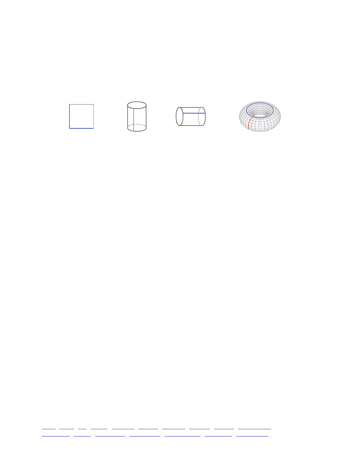
again). Note that there is no “seam” and no “privileged point” in this space; the spatial topology at
every point is identical.
A non-periodic two-dimensional bounded space is a rectangle with extents [x0, x1] and [y0, y1].
There are three periodic versions of this: x0 and x1 may be joined, y0 and y1 may be joined, or both
pairs may be joined. The first two options produce a topology like the surface of a cylinder
without end caps; the third option produces not a sphere (as one might guess), but a torus, like the
surface of a doughnut:
Again, movement along the periodic dimension(s) may continue indefinitely, wrapping around
at the boundary; and again, there is no “seam” or “privileged point” in these spaces (along the
periodic axis or axes).
Finally, a non-periodic three-dimensional bounded space is a cube; it may be made periodic in
x, y, z, x and y, x and z, y and z, or x and y and z, yielding seven different periodic versions of
three-dimensional space. The topology of these is harder to visualize, but the principle is the
same: movement along the periodic axis or axes may continue indefinitely because it wraps
around, and along the periodic axis or axes there is no “seam”.
This is all rather abstract, but periodic boundary conditions are very useful in modeling,
especially when doing theoretical work rather than trying to simulate a real landscape. The reason
is simple: periodic spatial boundaries eliminate edge effects, which are otherwise a source of bias
in spatial models. In effect, periodic boundaries allow you to model an infinite space with no
edges at all. Of course the space is not really infinite, but instead repeats periodically; but if the
spatial scale of important interactions and dynamics in the model is small compared to the size of
the periodic space, this is often an acceptable approximation.
Setting up periodic spatial boundaries in SLiM is a little bit more complex than implementing
other boundary conditions. The reason is that periodic spatial boundaries fundamentally change
many aspects of SLiM’s spatial engine; enforcing the boundary condition is no longer just a
question of modifying generated offspring positions in a particular way (although that is one part of
it). For instance, consider two individuals that occupy positions (0.0, 0.1) and (0.0, 0.9) in a two-
dimensional space with extent [0.0, 1.0] in both x and y. With any other boundary condition, the
distance between these two individuals is 0.8 (0.9 − 0.1). With periodic boundaries, however, the
distance between them is 0.2, because a line of length 0.2 may be drawn between them that wraps
around the boundary in the y dimension. By definition, the distance between two points in a
periodic space is always the shortest distance possible out of the infinitely many different distances
that could be calculated. This means that distances, interaction strengths, and indeed all of the
underlying mechanics of InteractionType’s spatial queries must take the periodicity of the space
into account.
For this reason, periodic spatial boundaries must be declared up front, and cannot be changed
subsequently. This declaration is done with a parameter to initializeSLiMOptions() named
periodicity, which specifies the periodic spatial dimensions as a string. In this recipe, we will
work with a two-dimensional model that is periodic in both dimensions – a toroidal model, as
pictured above. This can be set up as follows:
x0
x1
y0
y1
x0
x1
y0y1
x0x1
y0y1
y0
y1
x0x1
TOC I TOC II WF nonWF initialize() Genome Individual Mutation SLiMSim Subpopulation!
Eidos events fitness() mateChoice() modifyChild() recombination() interaction() reproduction() 294

initialize() {!
initializeSLiMOptions(dimensionality="xy", periodicity="xy");!
initializeMutationRate(1e-7);!
initializeMutationType("m1", 0.5, "f", 0.0);!
initializeGenomicElementType("g1", m1, 1.0);!
initializeGenomicElement(g1, 0, 99999);!
initializeRecombinationRate(1e-8);!
initializeInteractionType("i1", "xy", reciprocal=T, maxDistance=0.2);!
i1.setInteractionFunction("n", 1.0, 0.1);!
}
The initializeSLiMOptions() call establishes a 2-D space (with dimensionality="xy") and
then declares both of those dimensions to be periodic (with periodicity="xy"). We also set up a
spatial interaction here, involving both spatial dimensions; it uses a Gaussian interaction function
with a standard deviation of 0.1, so it falls off at well under the spatial scale of the model as a
whole. We declare it to have a maximum distance of 0.2, for efficiency; the interaction strength
will be very low further than two standard deviations out anyway.
Next, let’s set up a subpopulation with random initial positions:
1 late() {!
sim.addSubpop("p1", 2000);!
p1.individuals.x = runif(p1.individualCount);!
p1.individuals.y = runif(p1.individualCount);!
}
Nothing surprising here. Let’s implement a modifyChild() callback to set up offspring
positions, very much as we did in the recipes in section 14.3:
modifyChild() {!
pos = parent1.spatialPosition + rnorm(2, 0, 0.02);!
child.setSpatialPosition(p1.pointPeriodic(pos));!
return T;!
}
This uses a function named pointPeriodic() that is similar to the pointStopped() and
pointReflected() functions we saw before; it translates the point it is passed so that it falls within
the spatial boundaries, while implementing the periodic boundary conditions requested. In this
case, pointPeriodic() wraps a point that lies beyond the periodic spatial boundaries, just as if the
offspring had walked off of one edge of the space and re-appeared at the opposite edge.
We need an event to define the end of the simulation, as usual:
1000 late() { sim.outputFixedMutations(); }
And now let’s do something a bit more interesting: let’s use the interaction type that we defined
above to show, visually in SLiMgui, how interactions work in periodic space:
late()!
{!
i1.evaluate();!
focus = sample(p1.individuals, 1);!
s = i1.strength(focus);!
inds = p1.individuals;!
for (i in seqAlong(s))!
inds[i].color = rgb2color(c(1.0 - s[i], 1.0 - s[i], s[i]));!
focus.color = "red";!
}
TOC I TOC II WF nonWF initialize() Genome Individual Mutation SLiMSim Subpopulation!
Eidos events fitness() mateChoice() modifyChild() recombination() interaction() reproduction() 295
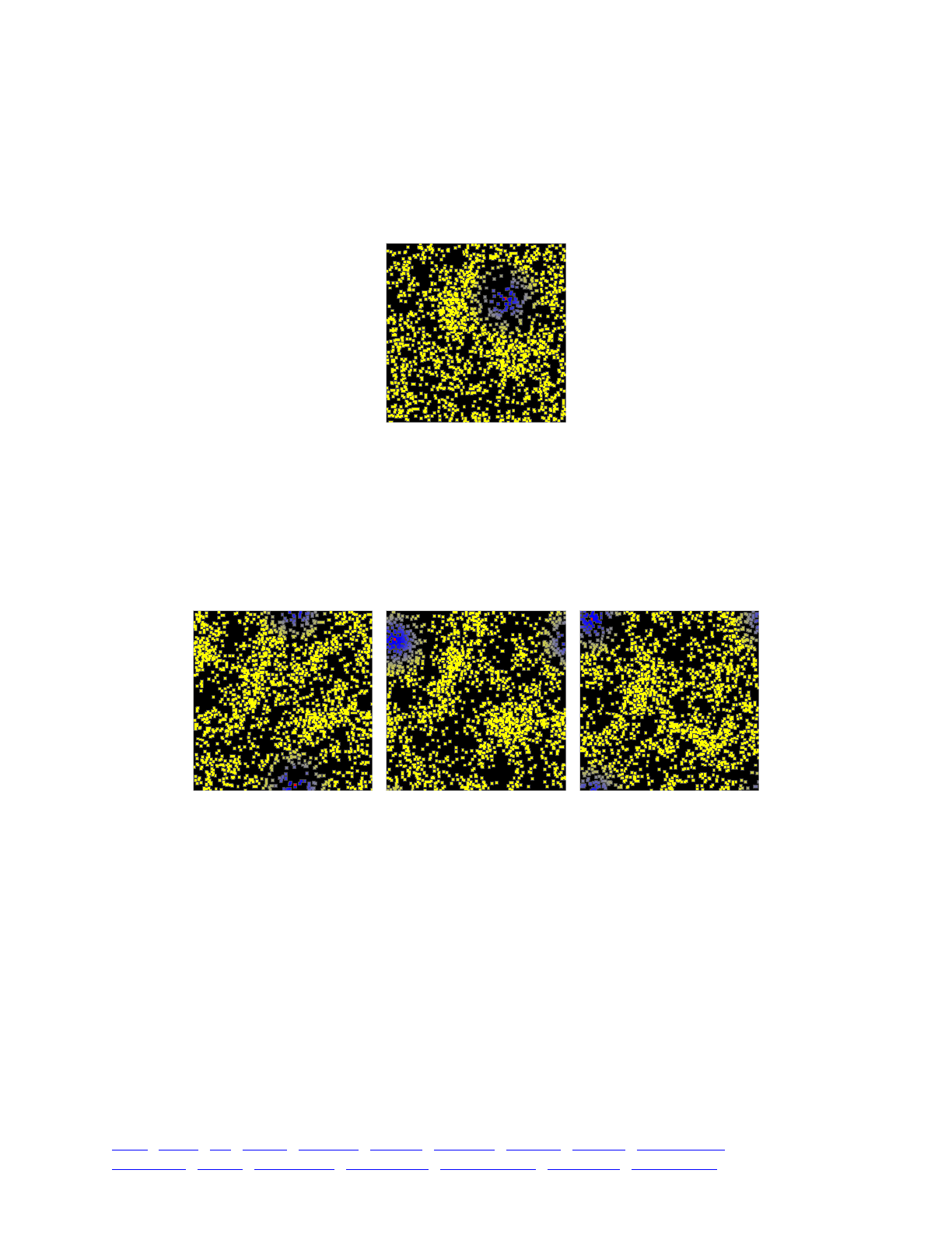
This late() event runs in every generation. It evaluates the interaction, then chooses a focal
individual randomly from the population. It asks the interaction type to calculate the interaction
strength between the focal individual and all other individuals; then it loops over the individuals
(by index) and sets each one’s color in SLiMgui using a particular formula (see the Eidos manual
for discussion of the rgb2color() function). Finally, it sets the color of the focal individual itself to
red. When this model is run, a typical generation looks like this:
The focal individual can be seen in red. The individuals closest to it are blue, while those
farthest away are yellow. Because of the particular RGB (red, green, blue) color values passed to
rgb2color(), the color of individuals at intermediate distances fades smoothly from blue to yellow.
This is a nice illustration of the shape of the interaction kernel, and in fact this sort of coloration
strategy can be quite useful in testing and visualizing spatial models.
The snapshot above, however, involved a focal individual that was far from any of the spatial
boundaries. When a different focal individual is chosen, we can see that the spatial interaction
wraps around the edges of the periodic space:
The third snapshot illustrates that wrapping occurs in both spatial dimensions, not just one at a
time. Due to the toroidal geometry of the space, the four corners of the space as displayed in
SLiMgui are actually all the same point! In the diagram above of the toroidal geometry of this
space, the four corners as displayed in SLiMgui correspond to the intersection of the blue and red
lines drawn on the torus. Note that topologically, there is nothing special about the blue and red
lines in particular; every point on the torus lies at the intersection between a curve that circles
around the major circumference of the torus (like the blue line) and a curve that circles around the
minor circumference of the torus (like the red line). An individual living in this space cannot tell
whether it is at the periodic boundary or not; as was emphasized earlier, there is no seam.
If you wish, you can play with this model by making only the x dimension periodic, or only the
y dimension, to see how that affects the spatial interaction and what the resulting cylindrical
topology feels like in practice. If you do so, note that pointPeriodic() will enforce only the
periodic boundary condition; it will leave coordinates that are not periodic unmodified. To keep
the modeled individuals inside bounds, some boundary condition – whether stopping, reflecting,
absorbing, or reprising – must be enforced for the non-periodic coordinates. This can be done just
TOC I TOC II WF nonWF initialize() Genome Individual Mutation SLiMSim Subpopulation!
Eidos events fitness() mateChoice() modifyChild() recombination() interaction() reproduction() 296

as it was in section 14.3; in particular, it is useful to note that a call to pointPeriodic() can be
wrapped inside a call to pointStopped() or pointReflected() to achieve the desired effect. This
works because pointPeriodic() has already brought the periodic coordinates into bounds, so they
will not be modified by pointStopped() or pointReflected(). So a model that used periodic
boundaries for only one of the two axes, and that enforced reflecting boundaries on the non-
periodic axis, could use a modifyChild() callback like this:
modifyChild() {!
pos = parent1.spatialPosition + rnorm(2, 0, 0.02);!
child.setSpatialPosition(p1.pointReflected(p1.pointPeriodic(pos)));!
return T;!
}
All of the other elements of spatial modeling that were introduced in earlier recipes in this
chapter – spatial competition, spatial mate choice, landscape maps – will work with periodic
spatial boundaries. You can still model phenotype as a spatial dimension, too, as in section 14.7
for example; you will just (probably) not want that dimension to be periodic, since phenotypic
traits are usually linear – being very short is not the same thing as being very tall!
The concept of periodic space can take some getting used to; cylindrical or toroidal space may
seem rather artificial at first. But in fact, because of the absence of edge effects, periodic space is
actually less artificial than other arbitrarily-chosen boundary conditions, in many ways; it will not
exhibit biases in the spatial density of individuals in one part of the space versus another,
individuals everywhere will feel the same average interaction strength if they are randomly
distributed, and motion in particular directions from particular locations will not be artificially
impeded.
Because of the greater underlying complexity, models using periodic space will be a little
slower in SLiM than non-periodic models, but unless population size is large the difference in
performance should be slight. Unless you actually want a particular edge effect in your model,
perhaps reflecting some real-world landscape’s dynamics, periodic boundaries may be the best
option.
TOC I TOC II WF nonWF initialize() Genome Individual Mutation SLiMSim Subpopulation!
Eidos events fitness() mateChoice() modifyChild() recombination() interaction() reproduction() 297

15. Going beyond Wright-Fisher models: nonWF model recipes
Beginning with SLiM 3.0, two fairly different types of models are supported in SLiM: Wright-
Fisher or WF models, and non-Wright-Fisher or nonWF models. See section 1.6 for a discussion of
the differences between these two types of models. All of the recipes presented so far have been
WF models, since that is the default model type in SLiM. In this chapter, we will go beyond the
assumptions and constraints of Wright-Fisher models, and will examine recipes for a variety of
nonWF models.
A great deal of the overall design of SLiM is shared between WF and nonWF models. All of the
Eidos classes that embody SLiM are the same (SLiMSim, Subpopulation, Individual, etc.), and the
way that SLiM models the chromosome, genomes, mutations, and so forth is unchanged. Since
that foundation is all shared, a good understanding of the concepts in the preceding chapters will
be assumed. Many of the techniques presented in the preceding recipes will also work in nonWF
models. We will not re-cast all of those techniques in a nonWF context, since that would mostly
just be repetitive and uninteresting; instead, we will focus on the important ways in which nonWF
models are different from WF models.
As discussed in more detail in section 1.6, the main differences between WF and nonWF
models fall into a few major categories. First of all, in nonWF models generations may be
overlapping and individuals can live for more than one generation; for this reason, in nonWF
models the model’s script is responsible for creating new offspring as needed, rather than that
happening automatically every generation as in WF models. Second, for the same reason, in
nonWF models the parental generation does not die off automatically after offspring are generated;
instead, fitness governs mortality (rather than governing mating success as in WF models). Third –
as a consequence of the previous two differences, really – in nonWF models population regulation
is a consequence of the balance between individual reproduction and individual mortality, just as
it is in natural populations, rather than being enforced through a set population size as in WF
models. Fourth, migration in nonWF models is similarly managed on an individual basis in the
model’s script, rather than being done automatically by the SLiM engine based upon set migration
rates.
All of this points to two basic observations. One observation is that the generation cycle is
quite different between WF and nonWF models. Chapter 19 discusses the generation cycle for WF
models, whereas chapter 20 discusses the generation cycle for nonWF models and the important
conceptual ways in which it differs from the WF generation cycle. An understanding of those
differences, such as the way in which the semantics of early() and late() events have changed
and the way that the meaning of fitness has shifted, will be important to understand the recipes
that follow, so chapter 20 should be consulted for further information as needed. The other
observation is that nonWF models are generally more individual-based and more complex than
WF models, because more responsibilities like offspring generation and migration have been
pushed from SLiM onto the model’s script. With this additional complexity comes considerable
additional power and flexibility, however, as we will see.
15.1 A minimal nonWF model
Let’s begin with a minimal nonWF model, similar to the minimal WF model presented in
section 4.1. This will illustrate several of the fundamentals of nonWF models: how to switch SLiM
into nonWF “mode”, how to implement individual-based reproduction and density-dependent
population regulation, and how to work with non-overlapping generations.
With no further ado, here is the recipe:
TOC I TOC II WF nonWF initialize() Genome Individual Mutation SLiMSim Subpopulation!
Eidos events fitness() mateChoice() modifyChild() recombination() interaction() reproduction() 298

initialize() {!
initializeSLiMModelType("nonWF");!
defineConstant("K", 500);!
!
initializeMutationType("m1", 0.5, "f", 0.0);!
m1.convertToSubstitution = T;!
!
initializeGenomicElementType("g1", m1, 1.0);!
initializeGenomicElement(g1, 0, 99999);!
initializeMutationRate(1e-7);!
initializeRecombinationRate(1e-8);!
}!
reproduction() {!
subpop.addCrossed(individual, subpop.sampleIndividuals(1));!
}!
1 early() {!
sim.addSubpop("p1", 10);!
}!
early() {!
p1.fitnessScaling = K / p1.individualCount;!
}!
late() {!
inds = p1.individuals;!
catn(sim.generation + ": " + size(inds) + " (" + max(inds.age) + ")");!
}!
2000 late() {!
sim.outputFull(ages=T);!
}
The first line of the initialize() callback is a call to initializeSLiMModelType("nonWF"); this
tells SLiM that we are building a nonWF model. That has various consequences; it activates the
nonWF generation cycle shown in chapter 20, for example, and it enables some properties and
methods on SLiM’s objects while disabling others. It is possible, when writing a WF model, to
include a call to initializeSLiMModelType("WF"), but unnecessary, since that is the default.
The next line sets up a defined constant, K. This will be the carrying capacity for the model’s
population regulation; we’ll cover that below.
The rest of the initialize() callback is much as we have seen before, but you might notice
one surprising thing: we set the convertToSubstitution property of mutation type m1 to T. In WF
models, mutations convert to substitutions automatically; the default value of that property is T, so
it would be redundant to set it to T again. In nonWF models, however, mutations do not convert
to substitutions automatically; the convertToSubstitution property is F by default and must be set
to T when desired. The reason is that in nonWF models fitness is absolute, not relative, and so
only completely neutral mutations with no side effects are safe to convert to Substitution objects
(see section 20.4 for further discussion). Since m1 mutations are completely neutral in this model,
we tell SLiM to allow them to fix; this will make the model run much faster.
The next script block is a new type of callback, a reproduction() callback, that may be used
only in nonWF models. Such reproduction() callbacks are called once per individual, at the
beginning of each generation; this provides an opportunity for that focal individual to generate
offspring (which it might or might not do); see section 20.1 for further discussion. This callback
calls p1.sampleIndividuals(1) to draw one random individual from p1 as a mate, and then calls
subpop.addCrossed() to add a new offspring individual that is the result of crossing – biparental
sexual reproduction – between the focal individual for the callback (individual) and the chosen
mate. The new individual is created, and is in fact returned to the caller, but is not actually added
to the subpopulation until offspring generation is finished. Note that although each individual will
TOC I TOC II WF nonWF initialize() Genome Individual Mutation SLiMSim Subpopulation!
Eidos events fitness() mateChoice() modifyChild() recombination() interaction() reproduction() 299

generate exactly one offspring of its own here, as the focal individual or “first parent”, it might also
be chosen as a mate by another individual (perhaps more than once, or perhaps not at all).
The next script block returns us to more familiar territory, since it simply calls addSubpop() to
create subpopulation p1 with ten initial individuals. The only point to be made here is that while
in a WF model this would set the subpopulation’s size forever (until setSubpopulationSize() was
called, at least), in a nonWF model this only sets the initial subpopulation size; the size of the
subpopulation will henceforth be governed by birth and death events, not by the initial size set for
it.
Speaking of death, the next early() event governs that. It calculates an absolute fitness value,
K!/!p1.individualCount, and sets that into the fitnessScaling property of p1. We haven’t seen
this property before; in effect, it scales the absolute fitness of the subpopulation, because the
calculated fitness for every individual in p1 is multiplied by this value. It is essentially the same as
writing a global fitness(NULL) callback that returns the same constant value for every individual,
but it is much faster than that model design would be, since the fitness(NULL) callback would
have to actually be called for every individual in every generation.
This fitnessScaling property may be used in WF models too, in fact, but is not generally useful
in that context; since WF models use relative fitness, scaling the fitness of all individuals by the
same constant has no effect. In nonWF models, however, it has a very important effect! This
fitnessScaling factor is what regulates the population size in the model; if this line were
commented out, the population would grow exponentially forever (until SLiM crashed, or got so
slow as to be effectively halted). Instead, when the subpopulation size is less than K,
fitnessScaling will be greater than 1.0 (and so no mortality will occur and the subpopulation
size will grow); but if it is larger than K, fitnessScaling will be less than 1.0 and mortality will
bring it back toward K. Since new individuals get generated at the beginning of each generation by
our reproduction() callback, once the model reaches equilibrium the population size will double
during offspring generation to around 1000, then a fitnessScaling value of approximately 0.5 will
be set, and then approximately half of the individuals will die during the survival life cycle stage,
bringing the population size down to approximately 500 (i.e., K).
Note that there is nothing magical about this particular formula; any formula or model design
that influences individual fitness in such a manner as to regulate the population size will work.
This particular formula produces logistic growth until K is reached, and then stochastic population
size fluctuation around K thenceforth. The population size will be stochastic around K because in
nonWF models fitness is the probability of death, but of course sometimes more individuals will
die than expected, sometimes less; the fate of each individual is in the hands of SLiM’s random
number generator.
Next we have a late() event that outputs two pieces of information in each generation: the
population size, and the age of the oldest individual. Here’s the initial output from one run:
1: 10 (0)!
2: 20 (1)!
3: 40 (2)!
4: 80 (3)!
5: 160 (4)!
6: 320 (5)!
7: 496 (6)!
8: 485 (7)!
9: 500 (6)!
10: 522 (7)!
...
TOC I TOC II WF nonWF initialize() Genome Individual Mutation SLiMSim Subpopulation!
Eidos events fitness() mateChoice() modifyChild() recombination() interaction() reproduction() 300

You can see the exponential growth at the start settling in around 500 once the model reaches
carrying capacity. You can also see that we already have overlapping generations in this model;
the individuals at the end of generation 1 are of age 0 (newly generated juveniles), and that initial
cohort ages without mortality during exponential growth (since we have not implemented a
maximum age or any sort of age-dependent reduction in fitness). By generation 7, though, the
carrying capacity has filled up and individuals start to die. Since every individual in this model
has the same fitness, mortality is purely random, and sometimes you will get a Methuselah that
lives to be 20 or even older; but most individuals will die through sheer bad luck before then, and
the maximum age in this model will tend to fluctuate around 10 or 15. Later recipes will explore
how to control the population age in biologically realistic ways, but for now let’s just bask in the
glory of the fact that we have already modeled something that can’t be modeled in WF SLiM:
overlapping generations.
The final event produces output from the model with outputFull(), as we have seen many
times before. The only new element is the ages=T parameter, which requests that age information
be added to the output (the details of the output format are given in section 23.1.1).
That’s it; that completes our first nonWF recipe! In subsequent sections we will explore the
greater power the nonWF paradigm affords us, because we can now control the mating, fecundity,
migration, fitness, and survival of each individual.
15.2 Age structure (a life table model)
In the previous recipe, the probability of survival was the same regardless of age, and that
produced a particular emergent age structure in the population. In most biological systems,
however, the probability of survival is age-dependent. Commonly, this is modeled with a life table
that gives the probability that an individual of a given age will die within the next time period (the
next year, often).
To model non-overlapping generations in a nonWF model (as is always the case in WF models),
one might use a life table that gives a probability of survival of 0.0 for all individuals of age 1 or
older (newly generated juveniles having an age of 0); with such a life table, offspring would be
generated and then the parental individuals (all having an age of 1) would all immediately die. In
this model we will implement a slightly more complex life table, for an imaginary species that has
high juvenile mortality, low adult mortality, and a maximum age of seven generations. We will
also implement age-dependent fertility and density-dependent population regulation.
Let’s look at this model one piece at a time, beginning with initialization:
initialize() {!
initializeSLiMModelType("nonWF");!
defineConstant("K", 30);!
defineConstant("L", c(0.7, 0.0, 0.0, 0.0, 0.25, 0.5, 0.75, 1.0));!
!
initializeMutationType("m1", 0.5, "f", 0.0);!
m1.convertToSubstitution = T;!
!
initializeGenomicElementType("g1", m1, 1.0);!
initializeGenomicElement(g1, 0, 99999);!
initializeMutationRate(1e-7);!
initializeRecombinationRate(1e-8);!
}
This is identical to the previous recipe except for the addition of the defined constant L, which
is our life table. It gives the probability of mortality for each age; newly generated juveniles have a
mortality of 0.7 (i.e., 70%), then the mortality drops to zero for several years, and then it ramps
TOC I TOC II WF nonWF initialize() Genome Individual Mutation SLiMSim Subpopulation!
Eidos events fitness() mateChoice() modifyChild() recombination() interaction() reproduction() 301

gradually upward with increasing age until it reaches 1.0 for age 7; all individuals of age 7 will die.
Note that this is only the age-related mortality; density-dependence will also cause mortality, as we
will see below, but that will be additional to this age-related mortality, which would occur even in
a population that was not limited by its density.
Next, let’s implement reproduction:
reproduction() {!
if (individual.age > 2)!
subpop.addCrossed(individual, subpop.sampleIndividuals(1));!
}
This is the same as the reproduction() callback in the previous recipe, except that here we
have prevented reproduction by individuals of age 2 or below. One could similarly limit or
prevent reproduction in a nonWF model based upon genetics, individual state, resource
acquisition, mate compatibility, or any other factor.
Population initialization looks like this:
1 early() {!
sim.addSubpop("p1", 10);!
p1.individuals.age = rdunif(10, min=0, max=7);!
}
We again start at a population size of 10 and allow the population to grow upward to the
carrying capacity (only 30 in this model, to make reading the output of the model easier). Since
addSubpop() sets the age of all new individuals to 0, that would provide our model with a bit of an
artificial start, and it might also present difficulties since juvenile mortality in this model is so high
– sometimes the population might go extinct before it reaches reproductive age. We therefore
draw random ages from a discrete uniform distribution from 0 to 7. If one had empirical data
about the age distribution in one’s system, that might of course be an even better starting point.
And here we manage both age-related and density-dependent mortality:
early() {!
// life table based individual mortality!
inds = p1.individuals;!
ages = inds.age;!
mortality = L[ages];!
survival = 1 - mortality;!
inds.fitnessScaling = survival;!
!
// density-dependence, factoring in individual mortality!
p1.fitnessScaling = K / (p1.individualCount * mean(survival));!
}
We calculate the age-related mortality by getting all of the individuals in p1, getting their ages,
and then looking up those ages in L to get a vector of the mortality rates for the individuals.
Survival rates are the opposite of mortality rates, so we subtract from 1; if an individual has a
mortality rate of 1 it has a survival rate of 0, and vice versa. Finally, we set those survival rates into
the fitnessScaling properties of the individuals. We saw the fitnessScaling property of
Subpopulation in the previous recipe, where it scaled the fitness of all individuals in the
subpopulation by the same constant factor. The fitnessScaling property of Individual has much
the same effect, but on an individual basis; each individual can have a different fitnessScaling
value, which is multiplied into that individual’s calculated fitness. This is equivalent to
implementing a fitness(NULL) callback that returns a survival-based fitness effect for the focal
TOC I TOC II WF nonWF initialize() Genome Individual Mutation SLiMSim Subpopulation!
Eidos events fitness() mateChoice() modifyChild() recombination() interaction() reproduction() 302

individual based upon that individual’s age; but this way is much faster since it is done in a
vectorized fashion without fitness() callbacks.
Next, the callback above calculates density-dependent mortality based upon K and the current
population size, as before, but also factors in the mean survival rate in the population due to age-
related mortality. Without that correction, the population would equilibrate around a lower size
than K, because age-related mortality would occur in addition to the density-dependent mortality
necessary to bring the population down to K. With the correction, the population size should
fluctuate stochastically around K, as desired. One could of course get fancier, and come up with
equations that made the probability of density-dependent mortality depend upon age (or any other
individual state) in some manner; perhaps older individuals would be weaker and more vulnerable
to diseases and parasites that are common when population density is high, for example.
late() {!
// print our age distribution after mortality!
catn(sim.generation + ": " + paste(sort(p1.individuals.age)));!
}!
2000 late() { sim.outputFixedMutations(); }
These are the last components of our model: output and termination. The late() output event
prints the population’s age distribution in each generation; this is post-mortality, since late()
events run after the survivial/viability generation cycle stage in nonWF models. A typical run:
1: 0 0 1 1 3 3 3 6 6 6!
2: 0 0 0 0 0 0 1 1 2 2 4 4 4!
3: 0 0 0 0 0 1 1 1 1 1 1 2 2 3 3 5 5 5!
4: 0 0 0 0 1 1 1 1 1 2 2 2 2 2 2 3 3 4 4 6 6 6!
5: 0 0 0 0 1 1 1 1 2 2 2 2 2 3 3 3 3 3 3 4 4 5!
...!
1996: 0 0 0 0 0 0 1 1 1 1 1 1 1 1 2 2 2 2 3 3 3 4 4 4 4 4 5 6!
1997: 0 0 0 0 0 0 0 1 1 1 1 1 1 2 2 2 2 2 2 2 2 3 3 3 3 4 4 4 5 5 5!
1998: 0 0 0 0 1 1 1 1 1 1 2 2 2 2 2 3 3 3 3 3 3 3 3 4 4 4 4 5 5 6 6!
1999: 0 0 0 0 1 1 1 1 2 2 2 2 2 2 3 3 3 3 3 4 4 4 4 5 5 5 5!
2000: 0 0 0 0 0 0 0 1 1 1 1 2 2 2 2 3 3 3 3 3 3 4 4 5 6
The beginning of the output shows growth toward the carrying capacity; even before the
carrying capacity is reached some age-related mortality occurs. The end of the output shows the
(somewhat stochastic) equilibrium population size and age structure. With this life table, the
population is dominated by middle-aged individuals; most juveniles die, and few individuals make
it to age 7 since the mortality rate ramps upward beginning at age 4. Note that no individuals of
age 7 are visible here because this output is post-mortality; no individual of age 7 should ever exist
at this point in the generation cycle. If this output event were an early() event instead, however,
we would expect to see the occasional age 7 individual.
This model uses a life table, but the larger point is that nonWF models allow one to model any
individual-based mortality effects, whether due to genetics (which would typically occur through
SLiM’s built-in fitness calculations), age (as with a life table or similar scheme), density (as also
modeled here), individual state, environmental effects, or anything else. Fitness effects influencing
survival can be expressed through fitness() callbacks, or using the fitnessScaling properties of
Subpopulation and Individual that we used here.
15.3 Monogamous mating and variation in litter size
In the previous recipe we explored how to manipulate individual fitness values in order to
implement age-dependent mortality using a life table. In this recipe we will look at the other end
TOC I TOC II WF nonWF initialize() Genome Individual Mutation SLiMSim Subpopulation!
Eidos events fitness() mateChoice() modifyChild() recombination() interaction() reproduction() 303

of the circle of life: mate choice and fertility. The previous nonWF models we have built have used
an extremely simplistic model of reproduction in which each individual of reproductive age
produces exactly one offspring per generation itself with a randomly selected mate (and may be
chosen as a mate by another individual, too). Here we will implement a very different model of
reproduction: monogamy (within a single breeding season), and generation of a litter of offspring
of non-deterministic size.
This model will look very similar to section 15.1’s recipe, so let’s just see the whole model all at
once:
initialize() {!
initializeSLiMModelType("nonWF");!
defineConstant("K", 500);!
!
initializeMutationType("m1", 0.5, "f", 0.0);!
m1.convertToSubstitution = T;!
!
initializeGenomicElementType("g1", m1, 1.0);!
initializeGenomicElement(g1, 0, 99999);!
initializeMutationRate(1e-7);!
initializeRecombinationRate(1e-8);!
}!
reproduction() {!
// randomize the order of p1.individuals!
parents = sample(p1.individuals, p1.individualCount);!
!
// draw monogamous pairs and generate litters!
for (i in seq(0, p1.individualCount - 2, by=2))!
{!
parent1 = parents[i];!
parent2 = parents[i + 1];!
litterSize = rpois(1, 2.3);!
!
for (j in seqLen(litterSize))!
p1.addCrossed(parent1, parent2);!
}!
!
// disable this callback for this generation!
self.active = 0;!
}!
1 early() {!
sim.addSubpop("p1", 10);!
}!
early() {!
p1.fitnessScaling = K / p1.individualCount;!
}!
late() {!
inds = p1.individuals;!
catn(sim.generation + ": " + size(inds) + " (" + max(inds.age) + ")");!
}!
2000 late() {!
sim.outputFull(ages=T);!
}
TOC I TOC II WF nonWF initialize() Genome Individual Mutation SLiMSim Subpopulation!
Eidos events fitness() mateChoice() modifyChild() recombination() interaction() reproduction() 304

This is, in fact, identical to section 15.1 except for the reproduction() callback, so let’s look at
that in detail:
reproduction() {!
// randomize the order of p1.individuals!
parents = sample(p1.individuals, p1.individualCount);!
!
// draw monogamous pairs and generate litters!
for (i in seq(0, p1.individualCount - 2, by=2))!
{!
parent1 = parents[i];!
parent2 = parents[i + 1];!
litterSize = rpois(1, 2.7);!
!
for (j in 1:litterSize)!
p1.addCrossed(parent1, parent2);!
}!
!
// disable this callback for this generation!
self.active = 0;!
}
We do something quite different here: this reproduction() callback runs only once per
generation, not once per individual! It disables itself at the end of its own execution by setting its
active flag to 0 (see section 22.8 for discussion of this feature, which we haven’t seen much before
now). The reproduction() callback is called by SLiM for some particular focal individual, but it
ignores that individual and instead generates offspring for all of the individuals in the whole
population all at once. This is perfectly fine, and can be a useful strategy when the reproduction
behavior of individuals is non-independent; with monogamy, for example, once two individuals
have formed a mating pair those individuals are not available to be chosen as mates by any other
individuals, so mating behavior in this model is non-independent.
The first thing we want to do is choose all of the monogamous mating pairs. The order of
individuals in SLiM is not guaranteed to be random in SLiM, so it would be unwise to simply pair
individuals 0 and 1, 2 and 3, etc.; that could lead to biases in mate choice that could manifest in
strangely skewed genetics over time. Instead, we use the sample() function to draw a complete
sample from the population, without replacement, effectively randomizing its order. Then we pair
individuals 0 and 1, 2 and 3, etc., from that, which is safe. We do that pairing with a for loop over
the even values up to p1.individualCount - 2 (guaranteeing that a pair of individuals remains the
last time through the loop, not just an odd one out at the end). Individuals i and i+1 are then
taken to be a monogamous mating pair. Of course one could implement any mating scheme at
all; females could choose males assortatively, or based upon their physical condition, or in any
other manner, and monogamy does not need to be enforced (as we saw in the previous two
recipes).
Next, we want to generate a litter for that mating pair. We draw the size of the litter from a
Poisson distribution with a mean of 2.7, arbitrarily. At the risk of sounding like a broken record, of
course litter size could depend upon anything at all – the genetics of the two parents, their genetic
compatibility, their respective conditions, their ages, their fecundity the previous year, their
phenotypic match with their environment, etc. Here, we happen to use a Poisson distribution with
a mean of 2.7. That gives us a litter size; we then generate the litter by calling addCrossed() that
many times with the same parents.
TOC I TOC II WF nonWF initialize() Genome Individual Mutation SLiMSim Subpopulation!
Eidos events fitness() mateChoice() modifyChild() recombination() interaction() reproduction() 305

The only thing left is for the reproduction() callback to deactivate itself, as explained above.
This model has the same output code as section 15.1’s recipe; a typical run produces:
...!
1995: 497 (6)!
1996: 531 (7)!
1997: 524 (6)!
1998: 497 (7)!
1999: 529 (8)!
2000: 511 (6)
Note that the equilibrium age here is around 6 to 7, where in section 15.1 it was more around
10 to 15. That is because section 15.1’s recipe produced one offspring per individual per
generation (not counting being chosen as a mate by another reproducing individual), whereas this
recipes produces about 1.35 (half of 2.7). That floods this model with young individuals, relative
to the earlier model. Density-dependent mortality and carrying capacity remain the same,
however, so skewing the age distribution towards juveniles in that manner inevitably means fewer
old individuals and a shorter expected lifespan. That happens because with more offspring
generated, the pre-mortality population size is larger, and so (given that the carrying capacity is the
same) density-dependent selection is stronger, individual fitness is lower, and the probability of
mortality per individual is higher, reducing the expected lifespan.
15.4 Beneficial mutations and absolute fitness
Thus far, we have only looked at neutral nonWF models. Fitness in nonWF models is absolute
and affects survival, where in WF models it is relative and affects mating success; this makes fitness
dynamics a bit different between nonWF and WF models. In particular, since one cannot survive
with more than a 100% probability, fitness values above 1.0 in nonWF models do not benefit the
individual at all; fitness values above 1.0 are interpreted as being 1.0. However, fitness is also
multiplicative (in both nonWF and WF models), and the important thing is the final fitness value
for an individual. The way this works out in practice can be a bit counterintuitive, so in this
section we will explore a simple model of an introduced beneficial mutation that sweeps to
fixation in a population, and we will look at the population dynamics as it does so.
The recipe is again based on that of section 15.1:
initialize() {!
initializeSLiMModelType("nonWF");!
defineConstant("K", 500);!
!
initializeMutationType("m1", 0.5, "f", 0.0);!
m1.convertToSubstitution = T;!
initializeMutationType("m2", 1.0, "f", 0.5); // dominant beneficial!
!
initializeGenomicElementType("g1", m1, 1.0);!
initializeGenomicElement(g1, 0, 99999);!
initializeMutationRate(1e-7);!
initializeRecombinationRate(1e-8);!
}!
reproduction() {!
for (i in 1:5)!
subpop.addCrossed(individual, subpop.sampleIndividuals(1));!
}!
1 early() {!
sim.addSubpop("p1", 10);!
}!
TOC I TOC II WF nonWF initialize() Genome Individual Mutation SLiMSim Subpopulation!
Eidos events fitness() mateChoice() modifyChild() recombination() interaction() reproduction() 306

100 early() {!
mutant = sample(p1.individuals.genomes, 10);!
mutant.addNewDrawnMutation(m2, 10000);!
}!
early() {!
p1.fitnessScaling = K / p1.individualCount;!
}!
late() {!
inds = p1.individuals;!
catn(sim.generation + ": " + size(inds) + " (" + max(inds.age) + ")");!
}!
2000 late() {!
sim.outputFull(ages=T);!
}
The changes from section 15.1 are minor. In the initialize() callback we create a mutation
type m2, for beneficial mutations; this has quite a strong selection coefficient and is dominant, to
make it less likely to be lost to drift at the very beginning, but that is unimportant to the point of
this recipe; we just don’t want to have to get into making the recipe conditional on fixation since
that is an extra complication (see section 10.2). In the reproduction() callback each individual
now reproduces five times per generation, creating very strong density-dependent selection; this is
a highly fecund species. That is not essential to the point of this recipe, but it will make the effect
more obvious. In a new 100 early() event we now select one genome from the population at
random, and add an m2 mutation to it. The rest of the model is the same. The m2 mutation will
(usually) sweep to fixation, and we will look at the resulting population size and age structure.
At the beginning, the model rapidly grows to the carrying capacity and stays there (each output
line, remember is a generation followed by the population size and the age of the oldest
individual, post-mortality):
1: 10 (0)!
2: 60 (1)!
3: 360 (2)!
4: 513 (3)!
5: 473 (4)!
6: 460 (4)!
7: 480 (3)!
8: 504 (3)!
9: 505 (4)
The population size is around 500, the oldest individual usually 3 or 4. So far so good. Now
let’s look at the output at the end of the run, in a run in which the beneficial mutation fixes:
1996: 768 (4)!
1997: 771 (3)!
1998: 781 (4)!
1999: 763 (3)!
2000: 802 (4)
The population size is now fluctuating around 760 to 800, although the typical age of the oldest
individual is still 3 to 4. What happened to our carrying capacity of 500?
The answer lies in the fitness values calculated by SLiM. Two things affect fitness in this model.
One is density-dependent mortality, as embodied in the fitnessScaling value set by the early()
callback. When the population is above carrying capacity (as it is in every generation from 4
onwards, in this model, due to the many juveniles), this scaling value will be less than 1.0; given
how many juveniles this model makes, it is probably usually 0.2 or lower, in fact. The other thing
TOC I TOC II WF nonWF initialize() Genome Individual Mutation SLiMSim Subpopulation!
Eidos events fitness() mateChoice() modifyChild() recombination() interaction() reproduction() 307

affecting fitness is the beneficial mutation; since it is dominant, it gives any individual possessing it
a fitness effect of 1.5 since its selection coefficient is 0.5. These fitness effects are multiplicative,
so once the beneficial mutation has fixed, every individual will have a fitness value of
approximately 0.2 * 1.5, or 0.3. This means, in effect, that fewer individuals will die, and the
carrying capacity will increase. Which is precisely what we see.
This may be unexpected for those who are used to the world of Wright-Fisher models, but it
makes good biological sense. If every individual possesses a mutation that makes them more fit –
more likely to survive – then the population size ought to increase. If there is some reason why
that shouldn’t happen, such as a hard limit on the amount of available food, then you ought to add
that biological detail to your model explicitly. This sort of thing is precisely why the individual-
based nature of nonWF models, with emergent dynamics for things like population size and age
structure, has the potential to be more biologically realistic.
This point becomes even more pointed if you write a model in which new beneficial mutations
can arise spontaneously. In such a nonWF model, absolute fitness would increase a little bit more
with every new beneficial mutation, and the population would evolve toward a “Darwinian
demon” with infinite absolute fitness and infinite population size. Fundamentally, that is just a
more extreme case of the same situation as in this recipe: if your model tells SLiM that absolute
fitness has increased, population size will increase concomitantly. If you want some mechanism to
hold that tendency in check, you need to add that mechanism to your model yourself.
In this recipe, for example, it would certainly be possible to force the model to maintain the
same carrying capacity throughout, but trying to do so might just expose how biologically
unrealistic that constraint really is. If the carrying capacity is the same before and after the
beneficial mutation fixes, that means that the survival probability is the same (assuming we don’t
alter reproductive output). So once the beneficial mutation has fixed, it apparently no longer
confers any benefit to the carrier – even though it did confer a benefit (relative to the non-carrier
individuals) earlier on, before the beneficial mutation had fixed. What has changed? Nothing
about the environment, and the population size has not changed (since we are making the carrying
capacity fixed) – and yet somehow, almost magically, the fitness benefit that used to exist has
evaporated. The only thing that has changed, in fact, is that now other individuals also possess the
mutation, whereas early on in the sweep few or none did. And that suggests one way that we
could make the carrying capacity fixed in this model: add in negative frequency-dependent
selection (see section 9.4.1). Maybe there’s a good biological reason for that: limited resources, for
example, such that a mutation that makes an individual better at obtaining those resources confers
less and less benefit as the mutation gets more and more common. If that’s the biology, then great,
model that. But if one is tempted to hold the population size fixed simply because one is used to
Wright-Fisher models that hold the population size fixed – not for any biological reason – then it
would probably be best to think twice. The lesson of this recipe, in other words, might be: Model
the biology, not your own modeling assumptions. Let emergent dynamics emerge.
Or if you really want to stay in the world of Wright-Fisher assumptions, then write a WF model;
there’s nothing wrong with that, as long as you understand the assumptions you’re making.
15.5 A metapopulation extinction-colonization model
Our models so far have been of a single subpopulation, but nonWF models have many
advantages for modeling migration that we will explore in this recipe and the next. Here, we will
model a metapopulation undergoing local extinctions and then re-colonizations from other
subpopulations. This would be difficult to implement in a WF model, because population size is
not allowed to go to zero (that signifies removal of the subpopulation from the model), and
because re-colonization by migrants does not happen naturally (it would have to be done as re-
TOC I TOC II WF nonWF initialize() Genome Individual Mutation SLiMSim Subpopulation!
Eidos events fitness() mateChoice() modifyChild() recombination() interaction() reproduction() 308

creation of the extinct subpopulation using addSubpopSplit(), and the founders could come only
from a single source subpopulation). In a nonWF model, however, this is quite straightforward.
For simplicity, we will model a non-spatial metapopulation in which every subpopulation is
connected to every other by migration of equal strength:
initialize() {!
initializeSLiMModelType("nonWF");!
defineConstant("K", 50); // carrying capacity per subpop!
defineConstant("N", 10); // number of subpopulations!
defineConstant("m", 0.01); // migration rate!
defineConstant("e", 0.1); // subpopulation extinction rate!
!
initializeMutationType("m1", 0.5, "f", 0.0);!
m1.convertToSubstitution = T;!
!
initializeGenomicElementType("g1", m1, 1.0);!
initializeGenomicElement(g1, 0, 99999);!
initializeMutationRate(1e-7);!
initializeRecombinationRate(1e-8);!
}!
reproduction() {!
subpop.addCrossed(individual, subpop.sampleIndividuals(1));!
}!
1 early() {!
for (i in 1:N)!
sim.addSubpop(i, (i == 1) ? 10 else 0);!
}!
early() {!
// random migration!
nIndividuals = sum(sim.subpopulations.individualCount);!
nMigrants = rpois(1, nIndividuals * m);!
migrants = sample(sim.subpopulations.individuals, nMigrants);!
!
for (migrant in migrants)!
{!
do dest = sample(sim.subpopulations, 1);!
while (dest == migrant.subpopulation);!
!
dest.takeMigrants(migrant);!
}!
!
// density-dependence and random extinctions!
for (subpop in sim.subpopulations)!
{!
if (runif(1) < e)!
subpop.fitnessScaling = 0.0;!
else!
subpop.fitnessScaling = K / subpop.individualCount;!
}!
}!
late() {!
if (sum(sim.subpopulations.individualCount) == 0)!
stop("Global extinction in generation " + sim.generation + ".");!
}!
2000 late() {!
sim.outputFixedMutations();!
}
TOC I TOC II WF nonWF initialize() Genome Individual Mutation SLiMSim Subpopulation!
Eidos events fitness() mateChoice() modifyChild() recombination() interaction() reproduction() 309

We start off by defining constants for the carrying capacity K, the subpopulation count N, the
per-individual migration rate m, and the per-generation probability e of a local extinction event in a
given subpopulation, such as might occur due to a forest fire or flood. We then set up a neutral
nonWF model with simple offspring generation (one offspring per individual per generation), and
create N subpopulations. The first subpopulation begins with 10 individuals; the rest begin empty,
awaiting migrants (which is legal in nonWF models; subpopulations can be empty). At the end of
the model, we have a late() event that halts the model with a message if all subpopulations have
gone extinct; if we make it to generation 2000 we output fixed mutations and stop.
The interesting code is in the middle, in the large early() event. This first implements random
migration by drawing the number of migrants from a Poisson distribution and then sampling
migrants at random from the full population; this gives each individual the same probability m of
migrating, and is more efficient than doing a random draw for each individual. It then loops
through the chosen migrants, finds their destination subpopulation (ensuring that it is not the
subpopulation the migrant already occupies), and finally calls takeMigrants() to move the
individual to its new home. The takeMigrants() call removes the individual from its old
subpopulation and adds it immediately to the target subpopulation; it is the way that migration is
implemented in nonWF models. Note that the design of this code avoids choosing and moving a
migrant, and then accidentally choosing that same individual as a migrant again and moving it
again; all migrants are selected, and then all migrants are moved. This design is generally a good
idea, to avoid accidentally skewing the migration rates for subpopulations away from their
intended rates. The migrant property of Individual could also be used to prevent this, together
with the ability of sampleIndividuals() to select individuals that have not already migrated.
The second half of the early() event implements both density-dependence and random local
extinction events. It draws from a random uniform distribution, and if the draw is less than the
probability of local extinction e, it sets the subpopulation’s fitnessScaling property to zero,
effectively reducing the fitness of all individuals in the subpopulation to zero and thus killing them
all. The rest of the time, fitnessScaling is set based on subpopulation density as usual, producing
growth up to the carrying capacity K for each subpopulation.
When run, this model produces fairly realistic extinction-colonization dynamics; after a
subpopulation is hit by an extinction event, it will eventually be recolonized and then undergo
rapid growth until reaching carrying capacity again. Here’s a snapshot from SLiMgui mid-run:
Three subpopulations are presently empty, two have just been recolonized by a single migrant,
two others are at intermediate stages of growth, and three are roughly at carrying capacity (which
is, as usual in nonWF models, not a hard limit). Note that all individuals are displayed here in
yellow, because SLiMgui normalizes away subpopulation-level fitnessScaling constants in order
to display individual fitness prior to density-dependent scaling, since that is generally what one is
interested in seeing; it does the same thing, in a sense, in WF models too. In fact, though, the
populations below carrying capacity have a fitness greater than 1.0 that is driving their growth,
TOC I TOC II WF nonWF initialize() Genome Individual Mutation SLiMSim Subpopulation!
Eidos events fitness() mateChoice() modifyChild() recombination() interaction() reproduction() 310
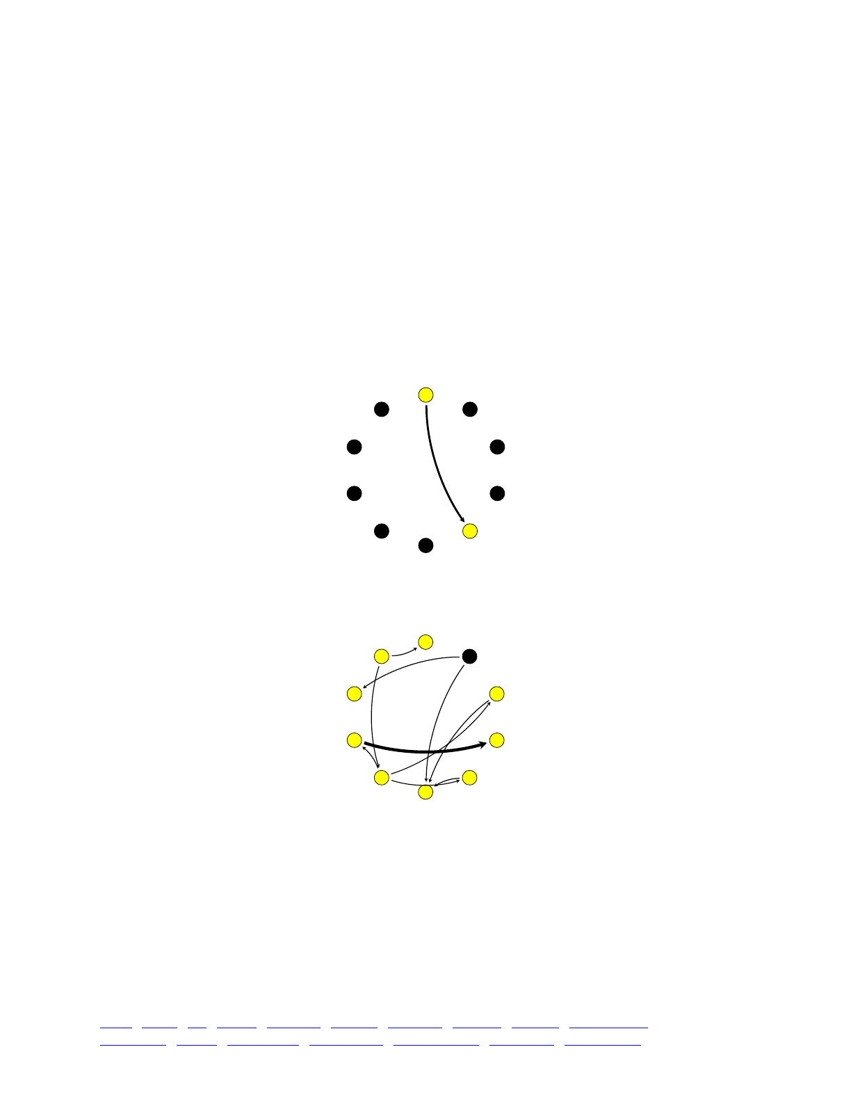
and the populations at carrying capacity have a fitness less than 1.0 that compensates for their
births to keep them at equilibrium.
If the migration rate is too low, or the extinction rate is too high, the whole population will often
go extinct; but with less apocalyptic parameter values recolonization will keep up with extinction
and the population will persist (for a while, anyway; the design of the extinction events in this
model means that sudden global extinction of all subpopulations will happen with probability e^N,
so eventually the model will always go extinct as long as e > 0).
A nice feature in SLiMgui that is worth pointing out is that it keeps metrics regarding the
behavior of your model, and can display those metrics for you. You might recall the Population
Visualization graph that SLiMgui can display to show population sizes, fitnesses, and migration
patterns (see, e.g., sections 5.1.3 and 5.2.1). In nonWF models the migration rates between
subpopulations are not set ahead of time, but are instead an emergent property of the model, as
we have seen in this recipe. SLiMgui will monitor the actual migration generated in the running
nonWF model and display it in the Population Visualization graph. For example, here’s the pattern
of migration in generation 3 of a run of this recipe:
This shows that p5 has just received a migrant from p1; this is the initial colonization of p5, in
fact. The other subpopulations are black because they are empty at this point. Later in the run, it
might look like this instead:
Lots is going on here; p8 sent a relatively large proportion of its population to p4, by chance
(thus the thicker arrow) – maybe two or three or four migrants. Migrants were sent from p2 to both
p6 and p9, and then, immediately after, p2 got hit by an extinction event. And so forth. This
facility can be quite useful for debugging migration code, or for seeing how the pattern of
migration changes over time when it depends upon other model state (as in the next recipe).
In fact, SLiMgui monitors and displays other emergent metrics in nonWF models, too. In the
subpopulation table, for example, where things like the cloning rate, selfing rate, and sex ratio are
displayed for WF models, the actual, observed metrics for those properties will be displayed by
SLiMgui for nonWF models. This particular recipe is not a good showcase for that feature,
however, since it is an asexual model involving only biparental mating.
p1
p2
p3
p4
p5
p6
p7
p8
p9
p10
p1
p2
p3
p4
p5
p6
p7
p8
p9
p10
TOC I TOC II WF nonWF initialize() Genome Individual Mutation SLiMSim Subpopulation!
Eidos events fitness() mateChoice() modifyChild() recombination() interaction() reproduction() 311

15.6 Habitat choice
In the previous section migration in nonWF models using the takeMigrants() method was
introduced. Here we will further explore migration in nonWF models. In WF models, as you may
recall, migration occurs during offspring generation: parents from one subpopulation mate, but
their offspring gets added to a different subpopulation if it migrates. This type of juvenile migration
is the only possibility in WF models; but nonWF models are not restricted in that way, and here we
will construct a nonWF model of migration that can occur at any age. Each generation,
individuals will choose which environment they will live in, a phenomenon commonly called
“habitat choice”. All else equal, they will prefer the environment they are already in; but if the
other environment is better for them, then with a non-zero probability they will decide to move.
This model will also include variation in the individual propensity to migrate, and emergent
variation in the total number of migrants in each generation – both difficult to capture in WF
models.
The basic design of this model is patterned after recipe in section 9.2: we have two
subpopulations, p1 and p2, and a mutation type, m2, that represents relatively rare mutations that
are beneficial in p1 but deleterious in p2. For balance, let’s also have a mutation type m3 for
mutations that are deleterious in p1 but beneficial in p2. Finally, let’s throw a spanner into the
works by making offspring initially go to a random subpopulation, not always to the subpopulation
of their parents (perhaps representing some sort of shared spawning environment from which
juveniles initially disperse randomly).
Here is the model except for the habitat choice code:
initialize() {!
initializeSLiMModelType("nonWF");!
defineConstant("K", 500);!
!
initializeMutationType("m1", 0.5, "f", 0.0);!
m1.convertToSubstitution = T;!
initializeMutationType("m2", 0.5, "e", 0.1); // deleterious in p2!
m2.color = "red";!
initializeMutationType("m3", 0.5, "e", 0.1); // deleterious in p1!
m3.color = "green";!
!
initializeGenomicElementType("g1", c(m1,m2,m3), c(0.98,0.01,0.01));!
initializeGenomicElement(g1, 0, 99999);!
initializeMutationRate(1e-7);!
initializeRecombinationRate(1e-8);!
}!
reproduction() {!
dest = sample(sim.subpopulations, 1);!
dest.addCrossed(individual, subpop.sampleIndividuals(1));!
}!
1 early() {!
sim.addSubpop("p1", 10);!
sim.addSubpop("p2", 10);!
}!
early() {!
p1.fitnessScaling = K / p1.individualCount;!
p2.fitnessScaling = K / p2.individualCount;!
}!
fitness(m2, p2) { return 1/relFitness; }!
fitness(m3, p1) { return 1/relFitness; }!
!
!
TOC I TOC II WF nonWF initialize() Genome Individual Mutation SLiMSim Subpopulation!
Eidos events fitness() mateChoice() modifyChild() recombination() interaction() reproduction() 312

1000 late() {!
for (id in 1:2)!
{!
subpop = sim.subpopulations[sim.subpopulations.id == id];!
s = subpop.individualCount;!
inds = subpop.individuals;!
c2 = sum(inds.countOfMutationsOfType(m2));!
c3 = sum(inds.countOfMutationsOfType(m3));!
catn("subpop " + id + " (" + s + "): " + c2 + " m2, " + c3 + " m3");!
}!
}
The structure of this model is quite predictable. The initialize() callback sets up the local-
adaptation m2 and m3 mutation types, and the two fitness() callbacks render mutations of those
types deleterious in one or the other subpopulation. The reproduction() callback generates each
new offspring in a randomly chosen subpopulation, representing random juvenile dispersal from a
spawning environment as mentioned above. We also have the usual nonWF density-dependent
fitness scaling, and we have an output event that prints information about the two subpopulations
(as we will discuss below).
The interesting part, then, is the large early() event for habitat choice, which should be
inserted just above the density-dependence early() event (so that density-dependence is based
upon post-migration subpopulation sizes, not the pre-migration sizes):
early() {!
// habitat choice!
inds = sim.subpopulations.individuals;!
inds_m2 = inds.countOfMutationsOfType(m2);!
inds_m3 = inds.countOfMutationsOfType(m3);!
pref_p1 = 0.5 + (inds_m2 - inds_m3) * 0.1;!
pref_p1 = pmax(pmin(pref_p1, 1.0), 0.0);!
inertia = ifelse(inds.subpopulation.id == 1, 1.0, 0.0);!
pref_p1 = pref_p1 * 0.75 + inertia * 0.25;!
choice = ifelse(runif(inds.size()) < pref_p1, 1, 2);!
moving = inds[choice != inds.subpopulation.id];!
from_p1 = moving[moving.subpopulation == p1];!
from_p2 = moving[moving.subpopulation == p2];!
p2.takeMigrants(from_p1);!
p1.takeMigrants(from_p2);!
}
The logic of this event goes through several steps, but is not complicated. First it gets a vector of
all individuals, and derives vectors of the number of m2 and m3 mutations possessed by each
individual; each of these is a vector of counts corresponding to the original vector of individuals.
It then computes a vector of habitat preferences for each individual: starting from a neutral
preference of 0.5, the more m2 mutations an individual has, and the fewer m3 mutations it has, the
more that individual prefers p1 over p2. Each m2 or m3 mutation shifts its preference by only 10%,
however, so these preferences are not initially very strong; and this preference is clamped to the
range [0.0, 1.0] so that even once many m2 and m3 mutations exist this preference is still
bounded. Next the script computes an “inertial” habitat preference for p1 over p2, expressing a
simple desire not to move; for individuals presently in p1 this is 1.0, whereas for those in p2 it is
0.0. The final habitat preference is computed as a weighted average of these two considerations;
in this recipe the genetically-based preference is given a weight of 0.75 and the inertial preference
is given a weight of 0.25, making individuals fairly strongly inclined to move, but this balance is a
free parameter in the model. Next, we actually decide which subpopulation each individual
TOC I TOC II WF nonWF initialize() Genome Individual Mutation SLiMSim Subpopulation!
Eidos events fitness() mateChoice() modifyChild() recombination() interaction() reproduction() 313

chooses, by comparing a random uniform draw to the individual’s weighted preference. (Note that
these calculations continue to be vectorized; this event handles all migration with a single
sequence of calculations.) The moving vector is the subset of individuals that chose a different
subpopulation than they currently occupy; these individuals will migrate, while the rest stay put.
The script then finds which migrants are currently in p1 (moving to p2) and which are in p2
(moving to p1), and then, finally, it makes takeMigrants() calls that actually move those
individuals. This method simply removes the given individuals from their current subpopulation
and inserts them into the target subpopulation. One could implement habitat choice in many
different ways, embodying different decision-making processes for the individuals involved,
different degrees of knowledge about the available habitat options, different approaches to the
stochasticity of the choice, and so forth; this is just one simple algorithm for demonstration
purposes.
Without any migration (if the habitat-choice early() event is commented out, in other words),
this model will “flip” to favor one subpopulation based upon the m2 and m3 mutations that happen
to do well early on; the successful subpopulation will grow very large (as its carrying capacity
increases, because so many individuals carry mutations that are beneficial in that environment; see
section 15.4), whereas the unsuccessful subpopulation will shrink toward zero (swamped by vast
numbers of offspring from the other subpopulation that are massively maladapted and immediately
die). Output from that version of the model typically looks like this:
subpop 1 (191): 0 m2, 1180 m3!
subpop 2 (1314): 0 m2, 8072 m3
The model has “flipped” toward subpop p2, which is now 1314 individuals to p1’s 191
individuals. There are quite a large number of copies of m3-type alleles in play, whereas there are
no m2-type alleles. Subpop p1 will never be able to dig itself out of this hole, since it gets
swamped with new offspring from p2 every generation that carry m3 alleles and not m2 alleles, and
any m2 alleles it manages to scrape together get diluted into p2 and selected out. If the model runs
longer, p1 will effectively go extinct except for whatever cohort of confused migrants arrives to
repopulate it in each generation.
But with the early() event that implements habitat choice, the story is very different. Now, if
the probability of correct habitat choice is sufficiently high, the subpopulations can diverge; even
though they still sabotage each other with maladapted offspring, those offspring tend to migrate
over to the subpopulation where they are more fit. One subpop often grows significantly larger
than the other, but the model no longer “flips”; the smaller subpop is much more able to persist.
Output from the model with habitat choice:
subpop 1 (620): 2838 m2, 173 m3!
subpop 2 (1065): 149 m2, 7177 m3
The subpopulations are now much closer in size, and show clear divergence in their m2 and m3
profiles. In SLiMgui the different haplotypes of the two subpopulations are immediately visible,
since the m2 and m3 mutations have been given different colors. Subpopulation p2 is larger here,
since there are more m3 alleles segregating, but it is no longer swamping p1 or diluting away the m2
alleles to such an extent that p1 can’t also thrive, and if new m2 mutations arise they will often be
able to establish themselves in p1 so the current imbalance may not even persist. Divergence here
is much more successful, and in fact it is effective enough that neutral sites will diverge as well,
indicating that this mechanism is sufficient to generate substantial reproductive isolation. The
degree of isolation will depend upon parameters such as the strength of habitat choice versus the
“inertial” preference for the current habitat, and the strength of the divergent selection on the m2
and m3 alleles, of course.
TOC I TOC II WF nonWF initialize() Genome Individual Mutation SLiMSim Subpopulation!
Eidos events fitness() mateChoice() modifyChild() recombination() interaction() reproduction() 314

This recipe goes beyond the capabilities of WF models in several important ways. One way is
that individuals of all ages migrate in this model, not just newly created juveniles as in WF models.
Indeed, in this model the same individual may just back and forth between p1 and p2 several
times, if it has no strong preference. A second way is that the migratory behavior here is based
upon individual genetic state. This is possible to implement in WF models, using a modifyChild()
callback that accepts or rejects proposed migrant offspring based upon their genetics, but in
practice it would be difficult and problematic. A third way is that the amount of migration in this
model is itself condition-dependent; if there are many maladapted individuals, there will be many
migrants, if fewer, fewer migrants. This would be difficult to do in a WF model since SLiM then
fulfills a pre-set migration rate; that pre-set rate would have to be carefully predicted and altered in
every generation in order to try to foretell the desired result from offspring generation, which
would be very clumsy if it worked at all. Migration is an individual choice, so it is much simpler
and more natural to model it as such, as nonWF models do.
Many interesting extensions to this model could be made. For example, one could impose a
fitness cost upon migration, and then allow the propensity for migration to itself evolve by making
the weighting between habitat choice and “inertia” depend upon a quantitative trait. Individuals
that chose to migrate too often would suffer a high cost, but those that did not migrate at all, even
when strongly maladapted, would also be penalized, and so some intermediate, optimal migration
tendency would perhaps tend to evolve. Such a model would rely heavily upon the advantages of
the individual-based migration of nonWF models; it would be very difficult to fit it into the WF
paradigm.
15.7 Evolutionary rescue after environmental change
The evolutionary response of a population to environmental change, and the probability of
extinction if that response is insufficient, is the subject of an important class of models called
“evolutionary rescue” models – particularly relevant in this era of anthropogenic climate change.
Evolutionary rescue can be based upon standing genetic variation, new mutations that provide
new adaptive potential, or genetic variation brought in by migrants. Here we will look at a QTL-
based model of evolutionary rescue that may (or may not) occur as a result of both standing
genetic variation and new mutations. This model is based heavily upon other QTL models in this
manual (see sections 13.1, 13.10, and 13.17), adapted here to illustrate that QTL-based
approaches are entirely compatible with nonWF models.
Let’s look at this model piece by piece, beginning with initialize():
initialize() {!
initializeSLiMModelType("nonWF");!
defineConstant("K", 500);!
defineConstant("opt1", 0.0);!
defineConstant("opt2", 10.0);!
defineConstant("Tdelta", 10000);!
!
initializeMutationType("m1", 0.5, "n", 0.0, 1.0); // QTL!
initializeGenomicElementType("g1", m1, 1.0);!
initializeGenomicElement(g1, 0, 99999);!
initializeMutationRate(1e-7);!
initializeRecombinationRate(1e-8);!
}
For simplicity and speed, we define only a QTL mutation type, m1; this model has no neutral
mutations in it (but of course they would be trivial to add). Each QTL is drawn from a normal
distribution centered on 0.0 with a standard deviation of 1.0 (which are important parameters for
TOC I TOC II WF nonWF initialize() Genome Individual Mutation SLiMSim Subpopulation!
Eidos events fitness() mateChoice() modifyChild() recombination() interaction() reproduction() 315

this model, since the exact nature of the standing genetic variation and mutational variance will be
important). Besides this, the initialization is quite standard. We set up defined constants for the
carrying capacity (K), for the phenotypic optimum before and after environmental change (opt1
and opt2), and for the time when the environmental change will occur (Tdelta).
Next we set up our reproduction and our initial population:
reproduction() {!
subpop.addCrossed(individual, subpop.sampleIndividuals(1));!
}!
1 early() {!
sim.addSubpop("p1", 500);!
}
This is boilerplate, except that here we start at the carrying capacity so that if we configure the
environmental change to occur immediately at the beginning of the model (as we will try below),
the population is not at a disadvantage due to not yet having grown to capacity.
We need our QTL machinery, which is quite simple in this model:
early() {!
// QTL-based fitness!
inds = sim.subpopulations.individuals;!
phenotypes = inds.sumOfMutationsOfType(m1);!
optimum = (sim.generation < Tdelta) ? opt1 else opt2;!
deviations = optimum - phenotypes;!
fitnessFunctionMax = dnorm(0.0, 0.0, 5.0);!
adaptation = dnorm(deviations, 0.0, 5.0) / fitnessFunctionMax;!
inds.fitnessScaling = 0.1 + adaptation * 0.9;!
inds.tagF = phenotypes; // just for output below!
!
// density-dependence with a maximum benefit at low density!
p1.fitnessScaling = min(K / p1.individualCount, 1.5);!
}!
fitness(m1) { return 1.0; }
The fitness(m1) callback makes the direct fitness effect of m1 mutations neutral, as usual in
such QTL models; the only effect of QTL mutations on fitness is indirect, through their effect on
individual phenotypic values.
The early() event calculates individual phenotypes as the sum of the effects of all QTLs
possessed by the individual. It then decides which phenotypic optimum is in effect, calculates the
deviation of each individual from that optimum, and calculates the degree of adaptation of each
individual from that using dnorm() (normalizing the adaptation values to the range (0,1] with
fitnessFunctionMax). Finally, fitnessScaling values for individuals are set based upon their
adaptation; a perfectly adapted individual will have an adaptation value of 1.0 and thus a
fitnessScaling value of 1.0, whereas an infinitely maladapted individual will have an adaptation
value of 0.0 and thus a fitnessScaling value of 0.1, the “floor” in this model (a crucial parameter
that will influence the probability of evolutionary rescue).
The early() event also, at the end, implements density-dependent population regulation. This
is done in the usual way, except that a maximum of 1.5 is imposed with min(). In principle, this
sort of correction ought to have been imposed on all our other nonWF models, but in models that
do not include deleterious mutations, and which are not expected to spend time at low density, it
is unimportant. The rationale for the correction is that being at low population density does
convey some benefit (assuming the absence of Allee effects, as we have been doing), allowing
individuals to survive and reproduce at their full capacity even when they carry some minor
TOC I TOC II WF nonWF initialize() Genome Individual Mutation SLiMSim Subpopulation!
Eidos events fitness() mateChoice() modifyChild() recombination() interaction() reproduction() 316

deleterious mutations that would negatively impact them if they were in a population at full
carrying capacity – but this benefit is surely limited! Typically, a population will not thrive if it
carries many large-effect deleterious mutations, even if it is released from all density-dependent
pressures. The maximum of 1.5 here embodies that intuitive fact, by stating that the fitness benefit
of low density can never be more than a multiplicative fitness effect of 1.5. (This is another
important model parameter, of course.)
Finally, we have our output and termination events:
late() {!
if (p1.individualCount == 0)!
{!
// stop at extinction!
catn("Extinction in generation " + sim.generation + ".");!
sim.simulationFinished();!
}!
else!
{!
// output the phenotypic mean and pop size!
phenotypes = p1.individuals.tagF;!
!
cat(sim.generation + ": " + p1.individualCount + " individuals");!
cat(", phenotype mean " + mean(phenotypes));!
if (size(phenotypes) > 1)!
cat(" (sd " + sd(phenotypes) + ")");!
catn();!
}!
}!
20000 late() { sim.simulationFinished(); }
The simulation checks for extinction in every generation, and stops with a termination message.
Otherwise, it prints a summary with the current population size, and the mean and standard
deviation of the distribution of phenotypes. If extinction is avoided, the model stops after
generation 20000.
Running this recipe as configured, we begin with no genetic diversity at all:
1: 500 individuals, phenotype mean 0 (sd 0)!
2: 529 individuals, phenotype mean 0.000628046 (sd 0.107673)!
3: 499 individuals, phenotype mean -0.00650893 (sd 0.152125)!
4: 470 individuals, phenotype mean -0.00802766 (sd 0.188649)!
5: 497 individuals, phenotype mean 0.00997383 (sd 0.225336)!
...
By generation 10000, when the environment changes, we have built up some standing genetic
variation – although really not much more than we had just a few generations in:
...!
9995: 493 individuals, phenotype mean -0.101779 (sd 0.616717)!
9996: 498 individuals, phenotype mean -0.139806 (sd 0.592579)!
9997: 518 individuals, phenotype mean -0.146021 (sd 0.55228)!
9998: 493 individuals, phenotype mean -0.127487 (sd 0.537018)!
9999: 500 individuals, phenotype mean -0.139612 (sd 0.531529)
Then we hit generation 10000, the optimum suddenly changes to 10.0, and things get very ugly
very fast:
TOC I TOC II WF nonWF initialize() Genome Individual Mutation SLiMSim Subpopulation!
Eidos events fitness() mateChoice() modifyChild() recombination() interaction() reproduction() 317

10000: 123 individuals, phenotype mean -0.095242 (sd 0.560048)!
10001: 77 individuals, phenotype mean 0.0100077 (sd 0.628869)!
10002: 54 individuals, phenotype mean -0.191957 (sd 0.624277)!
10003: 35 individuals, phenotype mean -0.0215701 (sd 0.55838)!
10004: 18 individuals, phenotype mean 0.211882 (sd 0.862124)!
10005: 7 individuals, phenotype mean 0.196655 (sd 1.07714)!
10006: 5 individuals, phenotype mean 0.200521 (sd 0.144637)!
10007: 3 individuals, phenotype mean 0.123028 (sd 0.0531924)!
10008: 2 individuals, phenotype mean 0.153739 (sd 0)!
10009: 1 individuals, phenotype mean 0.153739!
Extinction in generation 10010.
The population evolved toward the new optimum, but not quickly enough to overcome its crash
in population size, and it went extinct in only eleven generations. However, this is actually not the
typical outcome for the model. Here’s another run just before the environmental change:
...!
9995: 494 individuals, phenotype mean 0.152236 (sd 0.576086)!
9996: 511 individuals, phenotype mean 0.144287 (sd 0.590623)!
9997: 503 individuals, phenotype mean 0.151616 (sd 0.616162)!
9998: 489 individuals, phenotype mean 0.115655 (sd 0.617752)!
9999: 508 individuals, phenotype mean 0.11127 (sd 0.611983)
And here’s what happened after:
10000: 112 individuals, phenotype mean 0.373886 (sd 0.714775)!
10001: 84 individuals, phenotype mean 0.394201 (sd 0.768464)!
10002: 58 individuals, phenotype mean 0.447692 (sd 0.855927)!
10003: 48 individuals, phenotype mean 0.689259 (sd 0.925998)!
10004: 31 individuals, phenotype mean 0.877411 (sd 1.12496)!
10005: 29 individuals, phenotype mean 1.12907 (sd 1.10892)!
10006: 25 individuals, phenotype mean 1.50111 (sd 1.29306)!
10007: 20 individuals, phenotype mean 1.45553 (sd 1.30944)!
10008: 17 individuals, phenotype mean 1.88997 (sd 1.42636)!
10009: 15 individuals, phenotype mean 2.67739 (sd 1.60781)!
10010: 16 individuals, phenotype mean 2.92828 (sd 1.58097)!
10011: 26 individuals, phenotype mean 3.32725 (sd 1.53169)!
10012: 35 individuals, phenotype mean 3.87526 (sd 1.24333)!
10013: 56 individuals, phenotype mean 4.13832 (sd 1.10771)!
10014: 98 individuals, phenotype mean 4.27727 (sd 1.12148)!
10015: 158 individuals, phenotype mean 4.54129 (sd 0.940975)!
10016: 285 individuals, phenotype mean 4.66029 (sd 0.881386)!
10017: 321 individuals, phenotype mean 4.84315 (sd 0.807692)!
10018: 314 individuals, phenotype mean 4.98733 (sd 0.726859)!
10019: 355 individuals, phenotype mean 5.08917 (sd 0.712417)!
10020: 337 individuals, phenotype mean 5.18797 (sd 0.735515)!
10021: 328 individuals, phenotype mean 5.28416 (sd 0.70728)!
...
The population size dips down as low as 15 individuals, and the phenotypic optimum still
seems quite distant, but it manages to stage a full recovery; it’s back up to carrying capacity within
about a hundred generations.
In twenty runs of the model, extinction occurred nine times and evolutionary rescue occurred
eleven times. We can test the importance of standing genetic variation for rescue by simply setting
Tdelta to 0, making the optimum be 10.0 from the start of the model with no chance for standing
genetic variation to build up; in this variant of the model, extinction occurred sixteen out of twenty
times, rescue only four times. So: probably important. Which might seem a bit surprising, since
TOC I TOC II WF nonWF initialize() Genome Individual Mutation SLiMSim Subpopulation!
Eidos events fitness() mateChoice() modifyChild() recombination() interaction() reproduction() 318

the variance in phenotype is really not large in generation 9999; but there are, nevertheless, a lot of
useful QTLs that can be brought together by recombination and applied to the problem of rapid
evolution.
We can also test the importance of new mutations to evolutionary rescue, by setting the
mutation rate to 0.0 when the environment changes; the population will then have nothing but
standing variation at its disposal. A proper test of this would require many runs of the model, but I
can state that evolutionary rescue does sometimes occur from the standing variation alone. Here’s
the population just before the change, in one run of that variant of the model:
...!
9995: 462 individuals, phenotype mean -0.020969 (sd 0.842111)!
9996: 489 individuals, phenotype mean -0.0413428 (sd 0.843401)!
9997: 488 individuals, phenotype mean 0.0205512 (sd 0.805816)!
9998: 496 individuals, phenotype mean -0.0103366 (sd 0.744229)!
9999: 488 individuals, phenotype mean -0.0287371 (sd 0.829185)
And here’s the recovery, in all its glory:
10000: 110 individuals, phenotype mean 0.0798129 (sd 0.941083)!
10001: 86 individuals, phenotype mean 0.199899 (sd 0.936995)!
10002: 70 individuals, phenotype mean 0.369471 (sd 0.986702)!
10003: 52 individuals, phenotype mean 0.643418 (sd 1.1836)!
10004: 46 individuals, phenotype mean 0.780035 (sd 1.25709)!
10005: 42 individuals, phenotype mean 1.23978 (sd 1.55453)!
10006: 43 individuals, phenotype mean 1.86605 (sd 1.7264)!
10007: 39 individuals, phenotype mean 2.62644 (sd 1.805)!
10008: 48 individuals, phenotype mean 3.24882 (sd 1.82018)!
10009: 67 individuals, phenotype mean 3.83253 (sd 1.69954)!
10010: 101 individuals, phenotype mean 4.43066 (sd 1.53875)!
10011: 165 individuals, phenotype mean 4.76209 (sd 1.42616)!
10012: 289 individuals, phenotype mean 5.14574 (sd 1.27371)!
10013: 325 individuals, phenotype mean 5.48173 (sd 1.19875)!
10014: 360 individuals, phenotype mean 5.79835 (sd 1.02552)!
10015: 369 individuals, phenotype mean 5.93227 (sd 0.973104)!
10016: 386 individuals, phenotype mean 5.96707 (sd 0.959739)!
10017: 372 individuals, phenotype mean 6.00515 (sd 0.953603)!
10018: 371 individuals, phenotype mean 6.2132 (sd 0.813674)!
10019: 364 individuals, phenotype mean 6.31304 (sd 0.698918)!
10020: 380 individuals, phenotype mean 6.37598 (sd 0.604686)!
10021: 427 individuals, phenotype mean 6.45539 (sd 0.471641)!
10022: 370 individuals, phenotype mean 6.51224 (sd 0.363968)!
10023: 412 individuals, phenotype mean 6.53184 (sd 0.305041)!
10024: 415 individuals, phenotype mean 6.54332 (sd 0.277311)!
10025: 404 individuals, phenotype mean 6.53433 (sd 0.299239)!
10026: 380 individuals, phenotype mean 6.55845 (sd 0.234658)!
10027: 386 individuals, phenotype mean 6.55116 (sd 0.256157)!
10028: 421 individuals, phenotype mean 6.53684 (sd 0.293376)!
10029: 390 individuals, phenotype mean 6.53791 (sd 0.29318)!
10030: 401 individuals, phenotype mean 6.53193 (sd 0.307162)!
10031: 403 individuals, phenotype mean 6.55492 (sd 0.248401)!
10032: 418 individuals, phenotype mean 6.57826 (sd 0.165723)!
10033: 428 individuals, phenotype mean 6.57869 (sd 0.163795)!
10034: 399 individuals, phenotype mean 6.58121 (sd 0.151873)!
10035: 420 individuals, phenotype mean 6.5856 (sd 0.128374)!
10036: 402 individuals, phenotype mean 6.58132 (sd 0.15131)!
10037: 422 individuals, phenotype mean 6.58565 (sd 0.128071)!
10038: 419 individuals, phenotype mean 6.59647 (sd 0)
TOC I TOC II WF nonWF initialize() Genome Individual Mutation SLiMSim Subpopulation!
Eidos events fitness() mateChoice() modifyChild() recombination() interaction() reproduction() 319

This is somewhat remarkable, since the new optimum is more than twelve standard deviations
away from the population’s phenotypic mean at the moment of the environmental change. The
population fixes for a single QTL haplotype by the end (thus, a standard deviation of 0), and that
haplotype provides a phenotype of 6.59647, which is almost exactly eight standard deviations
away from where it started – quite impressive. So rescue appears to be possible from standing
variation alone (sometimes), and from new mutations alone (sometimes), and most often from both
together (but still, only sometimes).
These outcomes will depend – perhaps quite sensitively – on the various parameters of the
model, such as the carrying capacity, the distance from the old optimum to the new one, the
mutational distribution and rate, the “floor” of the fitness function, and the maximum fitness
benefit from low population density. There are other implicit parameters here too, such as the
level of individual fecundity and the variance in that fecundity (here, zero). This is also a
hermaphroditic model, and hermaphroditic selfing is not prevented; switching to a sexual model
would make evolutionary rescue that much more difficult, since a non-zero number of both males
and females would need to be present in every generation. In short, gaining a proper
understanding of the dynamics of even this rather simple model would require some real work.
Nevertheless, the population dynamics of the model seem fairly realistic, and adding in even
more realism – sex, Allee effects, gradual environmental change instead of a sudden shift, etc. –
would not be difficult. Simulating this in a WF model would be more difficult to do with this level
of realism, since the population size would have to be set explicitly in every generation (rather
than being emergent from the birth/death dynamics), and would be fulfilled deterministically by
SLiM rather than exhibiting the natural stochastic variation around the carrying capacity that this
nonWF model exhibits.
Another interesting direction to take this model would be to use it to investigate the advantages
of sexual versus clonal reproduction. It has long been theorized that one of the disadvantages of
clonal reproduction is the difficulty of responding to environmental changes without the ability to
recombine parental genomes to bring adaptive alleles together onto the same chromosome. One
could experiment, in this model, with the effect of sexual versus clonal reproduction on
evolutionary rescue – and even the evolution of the reproductive mode in response to
environmental change. One could add a second QTL-based trait (see section 13.17) that governed
the probability that an individual would clone or reproduce sexually, and see whether
environmental change – perhaps cyclical or unpredictable – would provide enough of an
advantage to sexual reproduction to prevent clonal reproduction from taking over the population.
This would be straightforward to simulate in a nonWF model, since each individual generates its
own offspring and can choose its own reproductive mode, based upon genetics or anything else. It
would be considerably harder to implement in a WF model since the reproductive mode is
controlled only by the subpopulation-wide cloning rate and cannot easily be influenced by
individual genetics or other state.
15.8 Pollen flow
Plants reproduce sexually when a pollen grain from a flower reaches another (or perhaps the
same) flower and fertilizes an ovule. The pollen might be transmitted by a pollinator, or by wind or
water or other vectors. An important aspect of plant reproductive biology, then, is that pollen from
a flower in one subpopulation might end up fertilizing a flower in a different subpopulation. In
animals, gene flow between subpopulations generally results from the migration of individuals,
such as we modeled in sections 15.5 and 15.6 (and in many WF recipes as well). In plants, in
contrast, gene flow between subpopulations usually results from the migration of gametes (or, in
some species, gametophytes).
TOC I TOC II WF nonWF initialize() Genome Individual Mutation SLiMSim Subpopulation!
Eidos events fitness() mateChoice() modifyChild() recombination() interaction() reproduction() 320

Pollen flow between subpopulations is a very important aspect of plant reproduction, then, but
it is quite difficult to model with a WF model in SLiM since offspring in WF models always come
from the mating of two individuals in the same subpopulation. Another advantage of nonWF
models, then, is that they can easily simulate pollen flow, because sexual reproduction can involve
any two individuals in the model.
This will be a very quick model since the concept is very simple and we have no complicated
analysis to do with the results:
initialize() {!
initializeSLiMModelType("nonWF");!
defineConstant("K", 200);!
!
initializeMutationType("m1", 0.5, "f", 0.0);!
m1.convertToSubstitution = T;!
!
initializeGenomicElementType("g1", m1, 1.0);!
initializeGenomicElement(g1, 0, 99999);!
initializeMutationRate(1e-7);!
initializeRecombinationRate(1e-8);!
}!
reproduction() {!
// determine how many ovules were fertilized, out of the total!
fertilizedOvules = rbinom(1, 30, 0.5);!
!
// determine the pollen source for each fertilized ovule!
other = (subpop == p1) ? p2 else p1;!
pollenSources = ifelse(runif(fertilizedOvules) < 0.99, subpop, other);!
!
// generate seeds from each fertilized ovule!
// the ovule belongs to individual, the pollen comes from source!
for (source in pollenSources)!
subpop.addCrossed(individual, source.sampleIndividuals(1));!
}!
1 early() {!
sim.addSubpop("p1", 10);!
sim.addSubpop("p2", 10);!
}!
early() {!
for (subpop in sim.subpopulations)!
subpop.fitnessScaling = K / subpop.individualCount;!
}!
10000 late() {!
sim.outputFixedMutations();!
}
Most of this model is boilerplate that should be familiar by now. The interesting part is the
reproduction() callback. Here we model hermaphroditic (or perhaps monoecious) flowering
plants, so we do not model separate sexes, but we assume that selfing is no more common than
would be expected by chance (when an individual happens to choose itself as a pollen source in
this reproduction() code, which we do not prevent here). Each flower has 30 ovules, each with a
probability of 0.5 of being fertilized, so the total number of fertilized ovules is drawn from a
binomial distribution. We then determine the subpopulation that supplied the pollen for each of
those ovules (assuming independence), with a 99% chance that the pollen came from the local
subpopulation and a 1% chance that it was carried from the other subpopulation. Finally, we loop
to generate seeds for the fertilized ovules, using the proper pollen sources.
TOC I TOC II WF nonWF initialize() Genome Individual Mutation SLiMSim Subpopulation!
Eidos events fitness() mateChoice() modifyChild() recombination() interaction() reproduction() 321

This model doesn’t show any particularly exciting behavior; it’s just a two-subpopulation neutral
model with a little gene flow. But it models pollen flow correctly, and thus provides a good
foundation for building a more complex model of plant evolution.
Those interesting in modeling plants might also wish to look at the recipe in section 11.3, which
shows how to model gametophytic self-incompatibility. That recipe enforces self-incompatibility
with a modifyChild() callback, which ought to be compatible with this nonWF model. Note,
however, that in nonWF models suppression of a proposed child by a modifyChild() callback is
the end of that proposed child; in WF models, SLiM loops until the set subpopulation size is filled,
but in nonWF models SLiM simply attempts to generate each requested offspring, and those that
are rejected by a modifyChild() callback are abandoned. That behavior might be realistic and
desirable (if pollen limitation is severe, or if stigmas are getting clogged by a large amount of
incompatible pollen that prevents fertilization); if not, if is easy enough to make the
reproduction() callback loop until offspring generation succeeds. (The addCrossed() method will
return NULL if the requested offspring is not generated.) Alternatively, one could implement the
self-incompatibility system directly in the reproduction() callback, rather than in a modifyChild()
callback, ensuring that the flower chosen as a pollen source for each fertilized ovule is compatible.
The latter approach is perhaps simpler, and should be faster.
15.9 Litter size and parental investment
Litter size (clutch size, brood size) is often involved in evolutionary trade-offs. All else being
equal, a larger litter is obviously better; the more offspring, the higher the fraction of one’s own
genes will be in the next generation. But all else is never equal, because each offspring requires
an investment of some sort – at least the energy required to make the egg and sperm, and often
quite a bit more beyond that. Offspring that receive insufficient parental investment will suffer
lower fitness, and at some point the disadvantages of that, in higher offspring mortality and/or
lower offspring mating success, will outweigh the advantages of having the extra offspring. In
some species, particularly those in harsh and extreme environments, scraping together enough
resources to produce even a single offspring is difficult, and the optimum may lie around one
offspring per breeding season or even less; other species pursue a strategy of extremely low
parental investment and produce as many offspring as they can. These different life history
strategies can sometimes be simplified (or oversimplified) into “K strategists” and “r strategists”;
more broadly, life-history tradeoffs are clearly of central importance in evolutionary biology.
In this recipe we will simulate a species with a quantitative trait that governs its litter size.
Section 15.3’s recipe included litter size variation, but here it will be governed by genetics, not just
chance. We will also account for parental investment and the resulting impact of larger litter size
on offspring fitness due to limited parental resources. The initialize() callback:
initialize() {!
initializeSLiMModelType("nonWF");!
initializeSex("A");!
defineConstant("K", 500);!
!
initializeMutationType("m1", 0.5, "f", 0.0);!
m1.convertToSubstitution = T;!
initializeMutationType("m2", 0.5, "n", 0.0, 0.3); // QTL!
!
initializeGenomicElementType("g1", c(m1,m2), c(1.0,0.1));!
initializeGenomicElement(g1, 0, 99999);!
initializeMutationRate(1e-7);!
initializeRecombinationRate(1e-8);!
}
TOC I TOC II WF nonWF initialize() Genome Individual Mutation SLiMSim Subpopulation!
Eidos events fitness() mateChoice() modifyChild() recombination() interaction() reproduction() 322

This is a sexual nonWF model, with both neutral mutations (m1) and QTL mutations (m2). This
initialization is probably rote by now.
Moving on to the reproduction() callback:
reproduction(NULL, "F") {!
mate = subpop.sampleIndividuals(1, sex="M");!
!
if (mate.size())!
{!
qtlValue = individual.tagF;!
expectedLitterSize = max(0.0, qtlValue + 3);!
litterSize = rpois(1, expectedLitterSize);!
penalty = 3.0 / litterSize;!
!
for (i in seqLen(litterSize))!
{!
offspring = subpop.addCrossed(individual, mate);!
offspring.setValue("penalty", rgamma(1, penalty, 20));!
}!
}!
}
This callback applies only to females (the "F" in its declaration). The focal female chooses a
male mate using sampleIndividuals(), and assuming that succeeds (i.e., there is at least one male
in the population), the female will generate a litter with that mate. The script gets the female’s
litter-size phenotype from the tagF property where it will be stored (as we will see below) and
derives an expected litter size from its value such that the new individuals at the beginning of the
simulation, with no QTL mutations, have an expected litter size of 3. We then calculate the actual
litter size by doing a Poisson draw with the expectation as mean, and calculate a fitness penalty for
the offspring based upon the litter size they come from. The initial litter size of 3 entails no fitness
penalty, but larger litter sizes will have correspondingly larger penalties because of the decreased
amount of parental investment per offspring.
Having determined the litter size and the fitness penalty, we then make the litter’s offspring in a
loop. (Note the use of seqLen(litterSize), which will produce the correct number of loops even
if the litter size is zero; using the sequence operator with 1:litterSize would be incorrect, since a
litter size of 0 would generate the sequence 1 0 and the loop would then run twice instead of zero
times. Be careful using the sequence operator in such cases!) Each offspring is generated with a
call to addCrossed(), and then the fitness penalty due to parental underinvestment is set into a key
named "penalty" on the offspring for later use. Note that the actual penalty for each individual is
drawn from a gamma distribution with a mean of the expected penalty; this is a bit gratuitous,
probably, but makes the actual penalty somewhat non-deterministic.
Next we create our initial population:
1 early() {!
sim.addSubpop("p1", 500);!
p1.individuals.setValue("penalty", 1.0);!
}
We set the initial fitness penalty on the new subpopulation’s individuals to 1.0 (i.e., no penalty,
since this is a multiplicative fitness effect).
Now comes an early() event that, together with the reproduction() callback, really does the
bulk of the work in this model:
TOC I TOC II WF nonWF initialize() Genome Individual Mutation SLiMSim Subpopulation!
Eidos events fitness() mateChoice() modifyChild() recombination() interaction() reproduction() 323

early() {!
// QTL calculations!
inds = sim.subpopulations.individuals;!
inds.tagF = inds.sumOfMutationsOfType(m2);!
!
// parental investment fitness penalties!
inds.fitnessScaling = inds.getValue("penalty");!
!
// non-overlapping generations!
inds[inds.age >= 1].fitnessScaling = 0.0;!
!
// density-dependence, assuming 50% die of old age!
p1.fitnessScaling = K / (p1.individualCount / 2);!
}
This callback has four parts, as commented. The first part totals the effects of all QTL (m2)
mutations for all individuals and puts those totals into the tagF property of the individuals; the
reproduction() callback expects to find the total there, as we already saw, and the output code
below uses it as well. The second part fetches individual fitness penalty values using the
"penalty" key and sets them into the fitnessScaling property of the individuals to create the
desired fitness effect. The third part makes generations non-overlapping in this model, by setting
the fitness of all individuals to 0.0 unless they are new juveniles; of course the same life-history
tradeoffs apply with overlapping generations too, but having discrete generations makes the
model’s operation easier to observe. Finally, the fourth part implements density-dependence with
the usual use of the fitnessScaling property of the subpopulation; here, however, we account for
the fact that we have already effectively killed half of the population from old age, to make the
final population size be closer to the desired carrying capacity.
OK, since this is a QTL model we need to zero out the fitness effect of the QTL mutations as
usual, so that their only fitness effects are indirect:
fitness(m2) { return 1.0; }
Then we do a little output in each generation, and provide a termination event:
late() {!
// output the phenotypic mean and pop size!
qtlValues = p1.individuals.tagF;!
expectedSizes = pmax(0.0, qtlValues + 3);!
!
cat(sim.generation + ": " + p1.individualCount + " individuals");!
cat(", mean litter size " + mean(expectedSizes));!
catn();!
}!
20000 late() { sim.simulationFinished(); }
The model starts off like this:
1: 500 individuals, mean litter size 3!
2: 492 individuals, mean litter size 2.99977!
3: 485 individuals, mean litter size 2.99929!
...
The mean litter sizes printed in the output are calculated in the same way as in the
reproduction() callback. The model starts with the default litter size of 3, and then QTLs start to
arise that modify that value. By the end of the model, we’re in a fairly different place:
TOC I TOC II WF nonWF initialize() Genome Individual Mutation SLiMSim Subpopulation!
Eidos events fitness() mateChoice() modifyChild() recombination() interaction() reproduction() 324

19998: 335 individuals, mean litter size 6.95885!
19999: 326 individuals, mean litter size 6.95713!
20000: 336 individuals, mean litter size 6.95985
With these parameter values and configuration, the model tends to equilibrate at a litter size
around 6.5 to 7.5, but the range of outcomes is fairly broad and values as high as 9 or 10 are often
seen; apparently the selection on litter size imposed by this model is not terribly strong, so the
fitness peak is pretty broad. In any case, somewhere in this vicinity there seems to be a crossover
point where the benefit of more offspring is counterbalanced by the decrease in parental
investment. In this simple model, that result could probably be calculated analytically, but of
course that would be impossible in a more complex model involving other biological realism as
well.
One interesting thing to note about the output above is that the population size at the end is
much smaller than it was at the beginning. This is because every individual at the end is suffering
from a lack of parental investment, and that depresses the population size below the carrying
capacity. We don’t even need to think about that; it just happens automatically, as an emergent
property of the model.
In this recipe, the penalty for each offspring depends upon the size of the litter to which the
offspring belonged. This makes sense when parental investment is, in fact, per offspring, such as
feeding newly hatched juveniles in a nest. In other cases, investment might depend upon the
expected litter size, not the actual litter size; if a bird adds body fat before the breeding season and
uses that energy to generate a predetermined number of eggs, but only a subset of those eggs
hatch, the investment is per egg, not per hatched chick. We can modify the recipe for that case by
changing the penalty calculation to be:
penalty = 3.0 / expectedLitterSize;
Interestingly, even though litterSize is drawn from a distribution with a mean of
expectedLitterSize, this produces fairly different outcomes. The equilibrium litter size reached is
now typically around 3.5 to 4.0 – much smaller.
This model has a lesson that goes far beyond litter size and parental investment: nonWF models
can include genetic variation, and evolution, of traits that it is difficult or impossible to model in
such a way in WF models. One could easily write a nonWF model of the evolution of the sex
ratio, or of the selfing or cloning rate, or of migration or dispersal behavior, or of – as here – litter
size or parental investment. WF models can include all of those phenomena, but since they are
handled by SLiM’s core engine in WF models, it is quite difficult to include individual, genetically-
based variation in them.
15.10 Spatial competition and spatial mate choice in a nonWF model
In chapter 14 a variety of spatial models were explored, all of which were WF models. Those
spatial modeling techniques work just as well in nonWF models – indeed, better in some ways, as
we will see. The model here is derived from the recipe of section 14.5, and includes both spatial
competition and spatial mate choice.
Let’s begin with the initialize() callback as usual:
initialize() {!
initializeSLiMModelType("nonWF");!
initializeSLiMOptions(dimensionality="xy", periodicity="xy");!
defineConstant("K", 300); // carrying capacity!
defineConstant("S", 0.1); // spatial competition distance!
!
TOC I TOC II WF nonWF initialize() Genome Individual Mutation SLiMSim Subpopulation!
Eidos events fitness() mateChoice() modifyChild() recombination() interaction() reproduction() 325

initializeMutationType("m1", 0.5, "f", 0.0);!
m1.convertToSubstitution = T;!
!
initializeGenomicElementType("g1", m1, 1.0);!
initializeGenomicElement(g1, 0, 99999);!
initializeMutationRate(1e-7);!
initializeRecombinationRate(1e-8);!
!
// spatial competition!
initializeInteractionType(1, "xy", reciprocal=T, maxDistance=S);!
!
// spatial mate choice!
initializeInteractionType(2, "xy", reciprocal=T, maxDistance=0.1);!
}
We set up "xy" dimensionality with periodic boundary conditions for both dimensions, in order
to get a toroidal space (see section 14.12). We will still need density-dependent population
regulation of some kind, but since this is a continuous-space model our concept of density ought
to depend upon local density, not overall population size; K is the carrying capacity that we will
aim for by calibrating our local density function. We also define the maximum spatial competition
distance with the symbol S. We set up a neutral model with the usual boilerplate code, and
initialize spatial interactions for competition and mate choice.
Next let’s look at reproduction:
reproduction() {!
// choose our nearest neighbor as a mate, within the max distance!
mate = i2.nearestNeighbors(individual, 1);!
!
for (i in seqLen(rpois(1, 0.1)))!
{!
if (mate.size())!
offspring = subpop.addCrossed(individual, mate);!
else!
offspring = subpop.addSelfed(individual);!
!
// set offspring position!
pos = individual.spatialPosition + rnorm(2, 0, 0.02);!
offspring.setSpatialPosition(p1.pointPeriodic(pos));!
}!
}
We use interaction i2 to find a mate within the maximum mating distance. If one is found,
addCrossed() is used for biparental mating, otherwise addSelfed() is used for selfing (note this
variation in individual mating behavior based on spatial dynamics, which would be quite difficult
to achieve in a WF model). In either case, we draw a litter size using rpois() with an expected
mean size of 0.1, so individuals will reproduce relatively infrequently and generations will be
highly overlapping; if we’re at equilibrium and a new individual is born from a given parent 10%
of the time, then individuals ought to have an average lifespan of 10 generations. We loop over
our litter size (note the use of seqLen(), so that if the litter size is zero we get the correct behavior;
using 1:rpois() instead would yield the sequence 1 0 when the litter size is zero, erroneously
producing two offspring). Each offspring is positioned a small distance from the first parent, with
accounting for the periodic boundaries.
TOC I TOC II WF nonWF initialize() Genome Individual Mutation SLiMSim Subpopulation!
Eidos events fitness() mateChoice() modifyChild() recombination() interaction() reproduction() 326

Population initialization is very similar to the WF model:
1 early() {!
sim.addSubpop("p1", 1);!
!
// random initial positions!
for (ind in p1.individuals)!
ind.setSpatialPosition(p1.pointUniform());!
}
Note that because individuals that can’t find mates self, we can start the model with just a single
individual and let it grow to capacity. Next we have spatial competition:
early() {!
i1.evaluate();!
!
// spatial competition provides density-dependent selection!
inds = p1.individuals;!
competition = i1.totalOfNeighborStrengths(inds);!
competition = (competition + 1) / (PI * S^2);!
inds.fitnessScaling = K / competition;!
}
We evaluate i1, and then we evaluate the effect of competition for all individuals in a
vectorized fashion. The call to totalOfNeighborStrengths() returns a vector of the interaction
strength felt by each individual, and we rescale these values to normalize them (discussed below).
The fitness effect on each individual is then calculated as the carrying capacity K divided by the
rescaled strength of competition felt by the individual. If that strength is equal to K, we are at
equilibrium; the individual will feel no fitness effect, positive or negative, from spatial competition.
If the local population density around the individual is higher than that equilibrium density, its
fitness will be lower, and vice versa; local density is what is actually enforced by this formula, not
total population size. If the population happens to be uniformly distributed in space, then its
equilibrium size will be equal to K; but if there are areas of space that are uninhabitable, or if
individuals tend to cluster for whatever reason, then the equilibrium population size may be
different from K.
To understand how the rescaling works, it is useful to imagine that the maximum competition
distance, S, is set such that the circle covered by the interaction radius around a focal individual
has an area of exactly 1.0. The term (PI * S^2) is the area of this interaction circle, so in this case
it would be 1.0. The focal individual’s interaction circle would then include every individual in
the model (since the area of the space defined by p1 is also 1.0, since we didn’t change its
dimensions from a unit square; if we had, this formula would need to be tweaked accordingly).
The value of competition will thus be the population size, minus one because the focal individual
is not itself included in the total interaction strength; we compensate by using (competition + 1).
For our hypothetical situation in which the interaction circle has area 1.0, it can thus be seen that
the fitness scaling value for every individual will be exactly 1.0 when the population is at carrying
capacity. The same logic applies for other values of S – except for the caveat above that a non-
uniform spatial distribution might lead to a different equilibrium population size.
Finally, note that periodic boundary conditions are important when modeling competition in
this sort of way, because they provide a uniform strength of competition across space, without
edge effects. With any non-periodic boundary condition, the strength of spatial competition felt by
individuals at the edge of the space will be lower, and that will encourage the population density
to be higher at the edges than in the center (because, in effect, the local population density being
regulated by the competition function includes the empty areas beyond the edges of the space).
TOC I TOC II WF nonWF initialize() Genome Individual Mutation SLiMSim Subpopulation!
Eidos events fitness() mateChoice() modifyChild() recombination() interaction() reproduction() 327
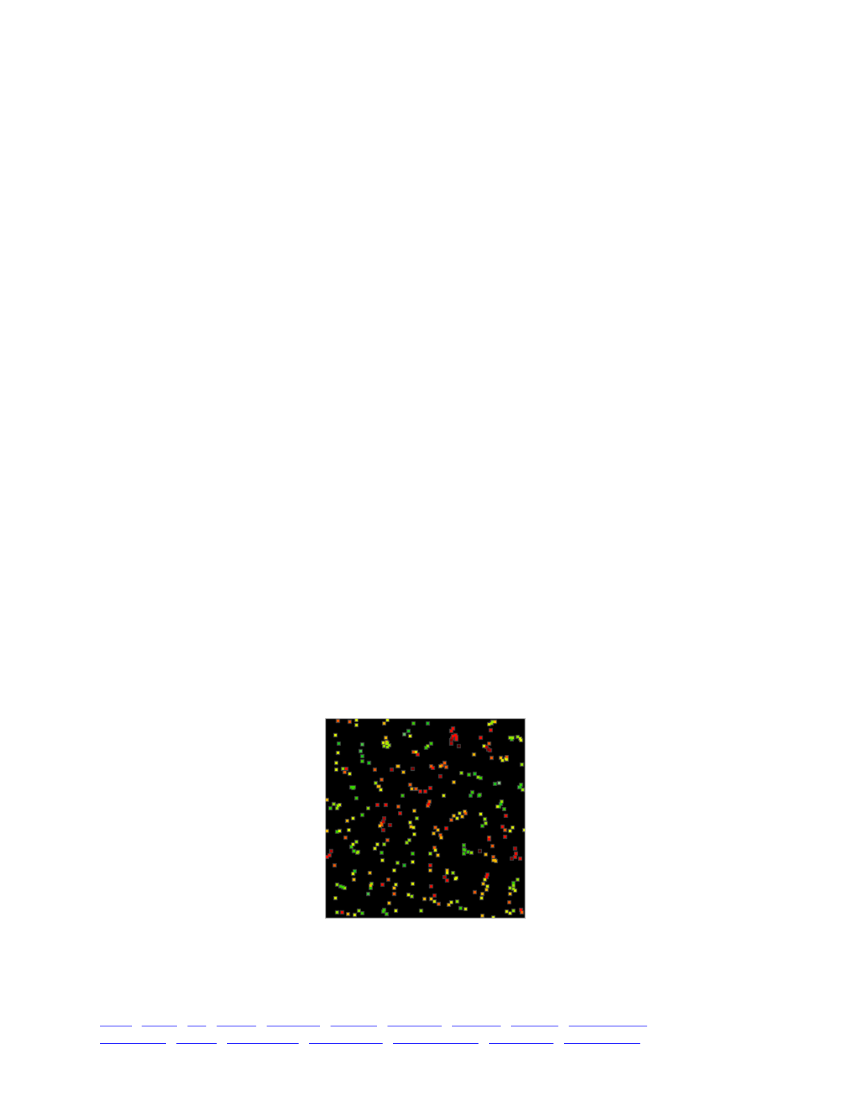
So far so good. Since we have overlapping generations, it would be nice to model some
movement by the individuals in the model, rather than just representing them as motionless points.
To do that, we have a late() event that moves everybody around:
late()!
{!
// move around a bit!
for (ind in p1.individuals)!
{!
newPos = ind.spatialPosition + runif(2, -0.01, 0.01);!
ind.setSpatialPosition(p1.pointPeriodic(newPos));!
}!
!
// then look for mates!
i2.evaluate();!
}
This just deviates individual positions by a small random factor, with accounting for periodic
boundaries. After doing that, it evaluates i2 in preparation for the mate-searching that will occur
in reproduction() callbacks at the start of the next generation; this just happens to be a
convenient moment for that evaluation, right after final positions for the generation have been
established.
Finally, we have a termination event:
10000 late() {!
sim.outputFixedMutations();!
}
Something worth noting about this model is that it contains no modifyChild() callback.
Because nonWF models create their own offspring, we can fix the spatial positions of offspring
directly in the reproduction() callback. It would also work to do it in a separate modifyChild()
callback, as in section 14.5, but that would be a bit more complex and a bit slower. Similarly,
notice that this model contains no fitness(NULL) callback, even though spatial competition
modifies individual fitness values in the model, because we can use the fitnessScaling property
of the individuals to implement the fitness effect. Often, nonWF models can get away with fewer
callbacks, or even no callbacks except initialize() and reproduction(), as shown here.
When this recipe is run, it looks a lot like the recipe from section 14.5:
There are differences from section 14.5’s recipe, though: individuals are moving around in
space during their lifetimes, and generations are clearly overlapping; there is much more
continuity from generation to generation. The population size is no longer fixed at K, either; it
TOC I TOC II WF nonWF initialize() Genome Individual Mutation SLiMSim Subpopulation!
Eidos events fitness() mateChoice() modifyChild() recombination() interaction() reproduction() 328
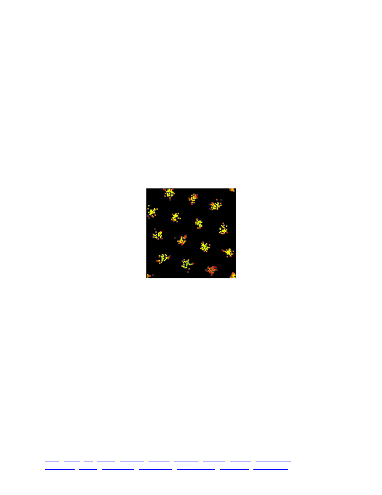
starts at 1 and grows organically, with a natural pattern of population growth that spreads across
space. Even once it reaches carrying capacity it is not fixed at exactly K, as the WF model was, but
fluctuates around the carrying capacity stochastically, depending in part upon how non-uniform
the spatial clustering at any given moment happens to be. This added realism could be very
important in some models. For example, if something were to suddenly perturb the population – if
a disease outbreak in one corner of the space suddenly killed off all the individuals within a small
radius, say – the WF model would nevertheless force the total population size to be K in every
generation, and so the population density would increase in all the other areas of the space, which
clearly makes no sense. This model’s more robust implementation of population regulation based
upon local population density prevents that aberration; the population size would initially be
depressed by the perturbation, and the hole created by the disease outbreak would fill back in
from its edges naturally, over time.
It has been mentioned several times now that spatial clustering might cause this model to reach
an equilibrium population size different from K. In the snapshot above, it is not immediately
obvious that this is happening, but in fact it is, and the population size of this recipe fluctuates
around roughly 310, slightly above the intended carrying capacity of 300. This can be made much
more obvious by increasing S to 0.2; the model at equilibrium then looks like this:
Rather remarkably, the population has naturally clustered itself into fifteen clumps, equidistantly
arranged across the periodic space in a hexagonal pattern; this seems to be the optimal
arrangement for this value of S, and the model finds it fairly quickly every time it is run. The
equilibrium population size is now about 500 individuals. In the next section, we will discuss this
phenomenon further, and look at a way of preventing it if it is undesirable.
For now, let’s just note that this is not a bug; this is the emergent behavior of the model, and it is
not necessarily unbiological. For one thing, some species are territorial, and what this model is
doing could be seen as a sort of territoriality; if the carrying capacity were adjusted appropriately,
each cluster could contain the appropriate number of individuals for family groups of the modeled
species. For another, complex spatial clustering has been observed in various natural systems;
Vincenot et al. (2016) provide an overview of some examples in plants, for instance, and discuss
the modeling of such clustering. Of course these clusters might not behave precisely as one might
wish; they are probably almost completely genetically isolated from each other, for one thing, so
one might wish to model dispersal that would provide gene flow (such as the way that young male
lions leave their natal pride and head out to form their own pride, if they can).
There is one more interesting aside to be explored here. We can modify this recipe a bit more,
by removing the periodic boundaries and instead implemented reprising boundaries following the
appropriate recipe from section 14.3. With S still set to 0.2, if we run this modified model we will
see a fairly different pattern of spatial clustering:
TOC I TOC II WF nonWF initialize() Genome Individual Mutation SLiMSim Subpopulation!
Eidos events fitness() mateChoice() modifyChild() recombination() interaction() reproduction() 329
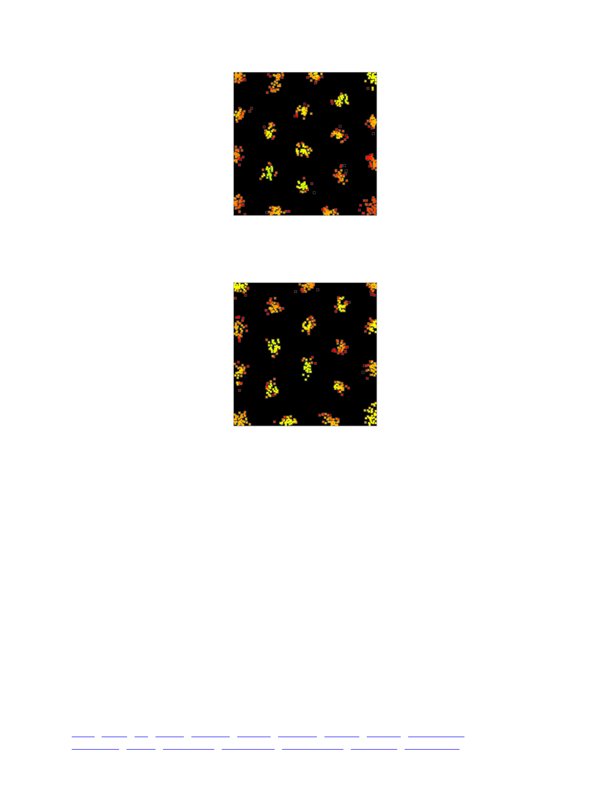
Twelve clusters are now arranged around the edges, and another eight clusters are packed into
the interior in an asymmetrical pattern. This is one way that the model can satisfy the constraints it
has been given, but it is not entirely stable, and there are several other configurations with either
nineteen or twenty clusters that are commonly observed. Here is another, with nineteen:
The equilibrium population size here is about 680 in the top configuration, and about 660 in the
bottom configuration. This is higher than it was with periodic boundaries, and of course the
nineteen or twenty clusters observed now is more than the fifteen observed with periodic
boundaries too. This difference is because reprising boundaries provide the model with more
elbow room; the clusters can now take advantage of the fact that they feel no competition from the
empty space beyond the edges, whereas periodic boundaries did not afford this luxury.
The overall point, then, is that spatial models are considerably more subtle than one might
initially appreciate, and that choices such as boundary conditions can have large consequences for
dynamics that might not be immediately obvious. In the next section we shall explore this further.
15.11 A spatial model with carrying-capacity density
The previous section provided a recipe for a nonWF model with both spatial competition and
spatial mate choice. Spatial competition provided population regulation, since more individuals
would produce more competition, reducing absolute fitness. However, as we saw at the end of
the section, that model tends to produce spatial clustering that might be undesirable. This occurs
because of the shape of the competition function. The competitive interaction strength felt
between two individuals in that recipe was constant out to the maximum interaction distance, and
then fell off abruptly to zero. This produces an incentive for clustering, for two reasons: (1) being
tightly clustered implies no more fitness penalty than being loosely clustered, since the interaction
strength is constant, and (2) clustering allows the empty spaces between clusters to be shared; if
the clusters arrange themselves into a regularly spaced configuration, they can efficiently share the
TOC I TOC II WF nonWF initialize() Genome Individual Mutation SLiMSim Subpopulation!
Eidos events fitness() mateChoice() modifyChild() recombination() interaction() reproduction() 330

empty spaces between them. That effect allows the mean interaction strength felt by individuals to
decrease, in turn allowing the model to somewhat exceed its carrying capacity.
For this reason (and others), a Gaussian competition kernel is often preferred in this sort of
spatial model; it seems to produce fewer artifacts of this type. In chapter 14 we constructed a
series of models inspired by classic papers such as Dieckmann & Doebeli (1999) and Doebeli &
Dieckmann (2003), and here we return to that thread. Doebeli & Dieckmann (2003) introduced a
concept that they called “carrying-capacity density”, based upon a Gaussian competition kernel;
with the proper scaling, as set out in their paper, the population will equilibrate at the intended
carrying capacity if the environment is homogeneous, just as it did in the previous recipe, but
clustering artifacts driven by the shape of the competition kernel will be minimized. Here, we will
adjust the model of section 15.10 to implement this concept of carrying-capacity density, which
requires only a few minor modifications. Since the modifications are small, we will here review
only the sections of the model that are changed (as usual, the full recipe is available in SLiMgui
and online).
One part that requires changes is the initialize() callback:
initialize() {!
initializeSLiMModelType("nonWF");!
initializeSLiMOptions(dimensionality="xy", periodicity="xy");!
defineConstant("K", 300); // carrying-capacity density!
defineConstant("S", 0.1); // sigma_S, the spatial competition width!
!
initializeMutationType("m1", 0.5, "f", 0.0);!
m1.convertToSubstitution = T;!
!
initializeGenomicElementType("g1", m1, 1.0);!
initializeGenomicElement(g1, 0, 99999);!
initializeMutationRate(1e-7);!
initializeRecombinationRate(1e-8);!
!
// spatial competition!
initializeInteractionType(1, "xy", reciprocal=T, maxDistance=S * 3);!
i1.setInteractionFunction("n", 1.0, S);!
!
// spatial mate choice!
initializeInteractionType(2, "xy", reciprocal=T, maxDistance=0.1);!
}
We now call K the carrying-capacity density, and S the spatial competition width, which is
referred to with the symbol σs in Doebeli & Dieckmann (2003). The spatial competition function
now uses a Gaussian kernel (type "n"), with a maximum distance of three standard deviations (so
by the time it cuts off it should be very close to zero anyway). Otherwise this initialize() callback is
the same as in section 15.10.
The other element that changes is the population regulation event:
early() {!
i1.evaluate();!
!
// spatial competition provides density-dependent selection!
inds = p1.individuals;!
competition = i1.totalOfNeighborStrengths(inds);!
competition = competition / (2 * PI * S^2);!
inds.fitnessScaling = K / competition;!
}
TOC I TOC II WF nonWF initialize() Genome Individual Mutation SLiMSim Subpopulation!
Eidos events fitness() mateChoice() modifyChild() recombination() interaction() reproduction() 331
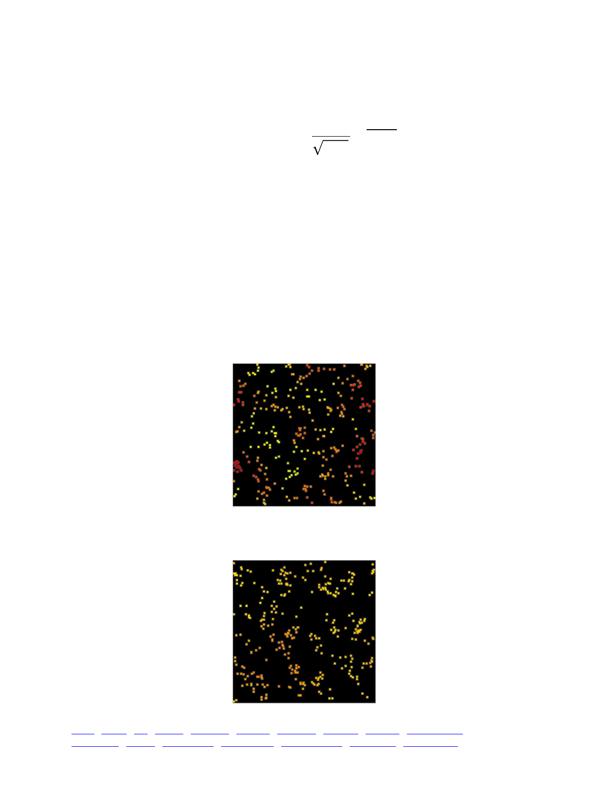
This is quite similar to section 15.10’s code, but the rescaling of the competition strength has
changed in accord with the new Gaussian competition kernel shape. The new rescaling is parallel
to the rescaling that is applied in the standard formula for the normal distribution:
Without the rescaling constant, that formula would produce a maximum value of 1.0; rescaled,
it produces a lower maximum density, such that the total probability density – the integral under
the curve – is exactly 1.0 (as required by the definition of a probability density function). Now,
note that the Gaussian interaction function we’re using here utilizes the same formula, but without
that rescaling factor; we just want to introduce that rescaling factor to normalize the Gaussian
interaction function. This is parallel to the reasoning followed in section 15.10 that led us to
rescale using the formula for the area of a circle of radius S. The rescaling factor is squared in this
recipe (no square root) because we have two spatial dimensions; the spatial competition function
is really the product of two Gaussian functions, one for x and one for y. See Doebeli &
Dieckmann (2003) and related papers, from which this mathematical framework is derived, for
further discussion, since a full derivation is beyond the scope of this manual. Note that, in terms of
implementation, we could just rescale the maximum strength for i1 instead, supplying the same
rescaling constant directly to setInteractionFunction(), and that would run faster, too; the
design shown here is more explicit for pedagogical purposes.
When this recipe is run, it looks a lot like the recipe from section 14.10:
Close examination, however, shows that this spatial distribution is less regularly clustered than
that previous recipe’s distribution. Changing S to 0.2 shows that the clustering previously
observed at that interaction scale is all but gone too:
f(x|μ,σ2) = 1
2πσ2
e
−(x−μ)2
2σ2
TOC I TOC II WF nonWF initialize() Genome Individual Mutation SLiMSim Subpopulation!
Eidos events fitness() mateChoice() modifyChild() recombination() interaction() reproduction() 332

A little bit of clustering still occurs, partly because offspring land near their first parent, and
partly just as a result of stochasticity (one would not expect a stochastic process to produce a
perfectly uniform spatial distribution, after all). But the competition function is no longer
contributing heavily to that clustering as it was before; indeed, it may be working to smooth it
away by favoring new offspring that land in relatively unoccupied areas.
Incidentally, these effects of interaction kernel shape have been explored in various papers; see
Payne et al. (2011) for a model of this based upon the same Dieckmann and Doebeli models that
we have been exploring, although that paper concerns itself more with clustering in phenotypic
space than in the regular spatial dimensions (as we saw in chapter 14, phenotype can in some
ways be treated similarly to a spatial dimension). Payne et al. (2011) found that a box-shaped (i.e.,
platykurtic) kernel encouraged clustering, just as did the cut-off kernel we used in section 15.10,
which was of course also platykurtic. Leimar et al. (2008) explored competition kernel shape in
more detail, and found that a characteristic of the Fourier transform of the competition kernel was
predictive of its effects upon clustering. A Gaussian competition kernel does not promote
clustering, according to their findings, and this is one reason why this kernel shape is popular
(although mathematical convenience also plays a role, as they explain).
15.12 Forcing a specific pedigree in a nonWF model
In section 13.7, we saw a recipe for forcing a SLiM model to follow a specific pedigree through
arranged matings between individuals. That recipe worked within the WF model framework,
which made its task rather difficult, since matings in WF models are arranged by SLiM’s core
engine. To make it work, that recipe had to reject undesired proposed children with a
modifyChild() callback, a solution that is slow and scales poorly to larger pedigrees. It was, in
short, an exercise in trying to pound a square peg into a round hole.
With a nonWF model we can do much better, since in nonWF models matings are arranged by
the model’s script, not by SLiM’s core engine; in a nonWF model we can simply request the
matings we want to get. That is what we will do in this section’s recipe. In other respects the
approach here is similar to that of section 13.7’s recipe; we use the tag values of individuals to
identify each individual, with a unique value for every individual in the entire pedigree.
This section actually has two recipes in it. The first recipe is for a nonWF model that allows
random matings with overlapping generations; it tracks each individual’s ancestry and outputs two
files that record the population’s history. The first output file records the generation in which each
individual died (since we are modelling overlapping generations), and the second records every
mating event and the identities of the individuals involved.
The second recipe reads those files back in, and reproduces the exact pedigree and population
history that occurred during the run of the first recipe. It reproduces death events by setting a
fitness of zero for individuals slated to die in a given generation, and it reproduces mating events
by calling addCrossed() for each pair of individuals slated to mate in a given generation, in the
model’s reproduction() callback.
If you want to reproduce the pedigree followed in a “baseline” model run, these two recipes
should allow you to do exactly that, with little modification. If, on the other hand, you have
pedigree information from source other source (such as empirical data from a real population), you
can use the second recipe to force SLiM to follow that pedigree; you would just need to either
encode your pedigree in the file format expected by the recipe, or modify the recipe to read in
whatever file format you already have.
So, let’s begin with the first recipe, which tracks and outputs the pedigree realized by a model
run:
TOC I TOC II WF nonWF initialize() Genome Individual Mutation SLiMSim Subpopulation!
Eidos events fitness() mateChoice() modifyChild() recombination() interaction() reproduction() 333

initialize() {!
initializeSLiMModelType("nonWF");!
defineConstant("K", 10);!
!
initializeMutationType("m1", 0.5, "f", 0.0);!
m1.convertToSubstitution = T;!
initializeGenomicElementType("g1", m1, 1.0);!
initializeGenomicElement(g1, 0, 99999);!
initializeMutationRate(1e-7);!
initializeRecombinationRate(1e-8);!
!
// delete any existing pedigree log files!
deleteFile("~/Desktop/mating.txt");!
deleteFile("~/Desktop/death.txt");!
}!
reproduction() {!
// choose a mate and generate an offspring!
mate = subpop.sampleIndividuals(1);!
child = subpop.addCrossed(individual, mate);!
child.tag = sim.tag;!
sim.tag = sim.tag + 1;!
!
// log the mating!
line = paste(c(sim.generation, individual.tag, mate.tag, child.tag));!
writeFile("~/Desktop/mating.txt", line, append=T);!
}!
1 early() {!
sim.addSubpop("p1", 10);!
!
// provide initial tags and remember the next tag value!
p1.individuals.tag = 1:10;!
sim.tag = 11;!
}!
early() {!
// density-dependence!
p1.fitnessScaling = K / p1.individualCount;!
!
// remember the extant individual tags!
sim.setValue("extant", sim.subpopulations.individuals.tag);!
}!
late() {!
// log out the individuals that died!
oldExtant = sim.getValue("extant");!
newExtant = sim.subpopulations.individuals.tag;!
survived = (match(oldExtant, newExtant) >= 0);!
died = oldExtant[!survived];!
!
for (indTag in died)!
{!
line = sim.generation + " " + indTag;!
writeFile("~/Desktop/death.txt", line, append=T);!
}!
}!
100 late() {!
sim.simulationFinished();!
}
TOC I TOC II WF nonWF initialize() Genome Individual Mutation SLiMSim Subpopulation!
Eidos events fitness() mateChoice() modifyChild() recombination() interaction() reproduction() 334

This recipe is quite straightforward; in most respects it follows the typical skeleton of a nonWF
model, but with some logging code added in. In the initialize() callback we delete any pre-
existing log files; the paths for the log files are of course something you are likely to want to
customize. The reproduction() callback chooses a random mate and calls addCrossed() to
generate a child, as usual; but it also sets that child up with a unique identifying tag value, and
appends a line summarizing the mating event to the mating.txt log file. The 1 early() event sets
the subpopulation up as usual, and also sets up initial tag values for the new individuals; the value
of sim.tag is used to track the next unused tag value in the run. The early() event provides
density-dependent population regulation, as we have seen in previous nonWF models; it also
remembers the tag values of all of the extant individuals prior to the survival generation cycle
stage, storing that list away in the simulation object using setValue(). Finally, the late() event
compares the post-mortality list of individuals to the pre-mortality list, determines which
individuals died, and appends lines representing those deaths to the death.txt log file. (This
recipe uses match(), but one of the Eidos set-theoretic methods like setDifference() could
probably be used just as easily.) The model ends at the end of generation 100.
A run of this model produces death.txt and mating.txt files on the user’s desktop (on Mac
OS!X, at least; the output paths in the recipe may need to be modified on other platforms). The
death.txt file is simply a series of lines, each of which has a generation and then the tag value of
an individual that died in that generation, like this:
2 2!
2 4!
2 6!
...!
3 7!
3 19!
...!
4 20!
4 21!
...
This file records that in generation 2 the individuals with tag values 2, 4, 6, etc., died; in
generation 3, individuals with tag values 7, 19, etc.; in generation 4, individuals with tag values
20, 21, etc.; and so forth, through to the end of the run.
The mating.txt file is almost as simple; here, each line records a generation, the tag values of
the first and second parent, and then the tag value of the generated offspring:
2 1 3 11!
2 2 10 12!
2 3 2 13!
...!
3 1 13 21!
3 3 20 22!
...!
4 1 13 30!
4 3 22 31!
...
The first line in this example, for example, specifies that in generation 2 the individuals with tag
values 1 and 3 mated to produce an offspring individual with tag value 11.
These files, then provide all the information we need to reproduce the full pedigree and
population history of the model run. So much for the first recipe; now let’s move on to the second
recipe and see how it uses these files to force a replication of the logged pedigree:
TOC I TOC II WF nonWF initialize() Genome Individual Mutation SLiMSim Subpopulation!
Eidos events fitness() mateChoice() modifyChild() recombination() interaction() reproduction() 335

function (i)readIntTable(s$ path)!
{!
l = readFile(path);!
t(sapply(l, "asInteger(strsplit(applyValue));", simplify="matrix"));!
}!
!
initialize() {!
initializeSLiMModelType("nonWF");!
defineConstant("K", 10);!
!
initializeMutationType("m1", 0.5, "f", 0.0);!
m1.convertToSubstitution = T;!
initializeGenomicElementType("g1", m1, 1.0);!
initializeGenomicElement(g1, 0, 99999);!
initializeMutationRate(1e-7);!
initializeRecombinationRate(1e-8);!
!
// read in the pedigree log files!
defineConstant("M", readIntTable("~/Desktop/mating.txt"));!
defineConstant("D", readIntTable("~/Desktop/death.txt"));!
!
// extract the generations for quick lookup!
defineConstant("Mg", drop(M[,0]));!
defineConstant("Dg", drop(D[,0]));!
}!
reproduction() {!
// generate all offspring for the generation!
m = M[Mg == sim.generation,];!
!
for (index in seqLen(nrow(m))) {!
row = m[index,];!
ind = subpop.subsetIndividuals(tag=row[,1]);!
mate = subpop.subsetIndividuals(tag=row[,2]);!
child = subpop.addCrossed(ind, mate);!
child.tag = row[,3];!
}!
!
self.active = 0;!
}!
1 early() {!
sim.addSubpop("p1", 10);!
!
// provide initial tags matching the original model!
p1.individuals.tag = 1:10;!
}!
early() {!
// execute the predetermined mortality!
inds = p1.individuals;!
inds.fitnessScaling = 1.0;!
!
d = drop(D[Dg == sim.generation, 1]);!
indices = match(d, inds.tag);!
inds[indices].fitnessScaling = 0.0;!
}!
100 late() {!
sim.simulationFinished();!
}
TOC I TOC II WF nonWF initialize() Genome Individual Mutation SLiMSim Subpopulation!
Eidos events fitness() mateChoice() modifyChild() recombination() interaction() reproduction() 336

Let’s walk through how it works. First of all, we define a new function named readIntTable()
that reads in a text file from a given filesystem path, assumed to be composed of lines of integer
values, and returns a matrix representing the contents of the file. (Note that this function is
supplied separately in the online SLiM-Extras repository, too.) We haven’t used matrices much in
previous recipes; they are a relatively new feature of Eidos, and work in much the same way as
matrices in R do (see the Eidos manual for further discussion). Indeed, we haven’t seen many
examples of user-defined functions either (again, see the Eidos manual). Without worrying too
much about such details, however, if we treat this function as a black box and call it with the path
of our death.txt file, we get this matrix:
[,0] [,1]!
[0,] 2 2!
[1,] 2 4!
[2,] 2 6!
...
And for our mating.txt file we get this:
[,0] [,1] [,2] [,3]!
[0,] 2 1 3 11!
[1,] 2 2 10 12!
[2,] 2 3 2 13!
...
The initialize() callback of this recipe sets up the model in the usual way (mirroring the
setup of the first recipe, which is what one would probably want in most cases). It then calls
readIntTable() to read in the log files, and retains the resulting matrices as defined constants, M
and D. Finally, it extracts the first column from M and D (which contains the generations for each
logged event) and retains those as constants Mg and Dg, for simplicity and speed later. So far so
good; this is the information the recipe will use to reproduce the logged pedigree.
Next, the reproduction() callback executes the pedigree’s mating events. It does this by
fetching the rows of M that refer to the current generation, and looping through those rows to
generate each mating event (again, you may wish to refer to the Eidos manual for information on
the syntax involved in working with matrices). The tag value of the offspring is set according to
the logged pedigree as well, so that the new individual will match up with the tag values used in
the log files. The callback triggers all of the mating events for the generation in a single call, rather
than working with the individual supplied to the reproduction() callback, so it then disables itself,
by setting self.active to 0, ensuring that it is not called again in the current generation (as we
saw before in section 15.3).
The 1 early() event creates the initial subpopulation, as in the first recipe, and sets the tag
values of individuals in the same way so that both models get the same setup.
Finally, we have the early() event. This does not cause density-dependent population
regulation in the usual way of nonWF models; instead, it uses the fitnessScaling property values
of individuals to weed out specifically the individuals that died in each generation in the original
model run. It begins by setting fitnessScaling to 1.0 on all individuals. Then it looks up the
mortality events for the current generation, similarly to how the reproduction() callback looked
up mating events. It then uses match() to find the indices of the individuals in question, and sets
fitnessScaling to 0.0 for those individuals. Those individuals will be killed by SLiM during the
survival generation cycle stage that follows the early() event. The model terminates at the end of
generation 100, matching the behavior of the original model.
In this way, this recipe reproduces the saved pedigree, even when a different random number
seed is used. If you run the second recipe repeatedly, you will therefore get replicates of the saved
TOC I TOC II WF nonWF initialize() Genome Individual Mutation SLiMSim Subpopulation!
Eidos events fitness() mateChoice() modifyChild() recombination() interaction() reproduction() 337

pedigree, but with different mutational and recombinational histories and thus different segregating
mutations at the end of the runs. Of course you may not wish to take on faith that the pedigree is
replicated exactly, so if you wish you can add calls to catn() in the appropriate spots to log out
each mating and mortality event, to confirm that they follow the pedigree as intended.
This basic scheme could be extended in various ways, as needed. For example, the log files
presently support only biparental matings; if you wanted to force a pedigree that involved cloning
in some cases, you could extend the mating.txt file format to have an extra column with a value
indicating whether the offspring was generated by cloning or not, or you could add a third log file,
named something like cloning.txt, to record those events; either strategy would work. You could
also log out, and then reproduce, other model events if you wished, such as migration events;
since you are in complete control of such events in nonWF models, doing this would be quite a
straightforward extension of these recipes. You could probably even record, and then reproduce,
the recombination breakpoints used in the generation of each offspring individual, using a
recombination() callback, so as to make the replicate run duplicate exactly the same pattern of
local ancestry along the chromosome as the original model run, if you wanted to. This strategy, of
driving model dynamics from file-based data, is quite general and can be applied to many tasks. It
is much cleaner to implement with nonWF models, however, since nonWF models are so much
more strongly script-driven than WF models; it would presumably be possible to make section
13.7’s recipe file-driven in this manner, but it would scale very poorly to large pedigrees.
15.13 Modeling clonal haploids in a nonWF model with addRecombinant()
In section 13.13 we saw a recipe for modeling clonal haploids in SLiM by keeping the second
genome of each individual empty. New mutations arising in those second genomes were removed
in each generation, and a recombination rate of zero was used to prevent any recombination with
those empty genomes. That recipe is general and flexible; as noted there, similar strategies could
be employed to model haploid mitochondrial DNA alongside diploid autosomal chromosomes, or
to model haplodiploidy and other such systems.
However, that strategy does have some drawbacks, particularly when tree-sequence recording is
being used (discussed in detail in chapter 16, but see section 1.7 for a quick introduction). With
tree-sequence recording, the recipe of section 13.13 records rather odd dynamics, with mutations
appearing and then disappearing in each generation, and the empty second genomes of
individuals inheriting from each other. These bizarre inheritance records are probably harmless,
but may complicate post-simulation analysis, and in any case constitute something of an offense
against clean design. Even more problematic for section 13.13’s strategy, when doing tree-
sequence recording, is the question of how to model horizontal gene transfer, as we will discuss in
section 15.14.
Here, then, we will look at an alternative strategy for modeling clonal haploids. This strategy
can be employed only in nonWF models, but integrates much more smoothly with tree-sequence
recording and is conceptually more straightforward as well.
The recipe, in full:
initialize() {!
initializeSLiMModelType("nonWF");!
defineConstant("K", 500); // carrying capacity!
initializeMutationType("m1", 0.5, "f", 0.0);!
initializeGenomicElementType("g1", m1, 1.0);!
initializeGenomicElement(g1, 0, 99999);!
initializeMutationRate(1e-7);!
initializeRecombinationRate(1e-8);!
}!
TOC I TOC II WF nonWF initialize() Genome Individual Mutation SLiMSim Subpopulation!
Eidos events fitness() mateChoice() modifyChild() recombination() interaction() reproduction() 338

reproduction() {!
subpop.addRecombinant(genome1, NULL, NULL, NULL, NULL, NULL);!
}!
1 early() {!
sim.addSubpop("p1", 500);!
}!
early() {!
p1.fitnessScaling = K / p1.individualCount;!
}!
late() {!
// remove neutral mutations in the haploid genomes that have fixed!
muts = sim.mutationsOfType(m1);!
freqs = sim.mutationFrequencies(NULL, muts);!
!
if (sum(freqs == 0.5))!
sim.subpopulations.genomes.removeMutations(muts[freqs == 0.5], T);!
}!
50000 late() { sim.outputFixedMutations(); }
This has the typical nonWF setup and population regulation, as we have seen before. The
late() event removes neutral mutations (type m1) when they reach fixation at a frequency of 0.5,
since SLiM doesn’t know enough to do so, following a similar strategy to section 13.13; see that
section for discussion.
The interesting and new part of this model is the reproduction() callback, which uses a
method we have not seen before, addRecombinant(). Like addCrossed(), addCloned(),
addSelfed(), and addEmpty(), this adds a new offspring individual to the target subpopulation, but
it provides greater control over precisely how that new individual is generated. Section 21.13.2
provides full documentation on this complex method, but in short, it allows you to supply two
parent genomes for each genome in the new offspring, with a list of recombination breakpoints to
be used in stitching together those parent genomes through crossover. The first three parameters to
its call here specify that genome1 from the focal parent should be used to generate the offspring’s
first genome, with no second recombinant strand (NULL), and no recombination breakpoints (NULL);
this provides clonal reproduction of the first genome. New mutations will be added by SLiM as
usual. The second group of three parameters to addRecombinant() are all NULL here; that specifies
that the second genome of the offspring should be generated with no parent genomes at all,
leaving it empty, just as addEmpty() would have done. In this case, addRecombinant() does not
add new mutations to the genome, since conceptually there is no parental genome to mutate.
This approach, using addRecombinant(), allows the model to tell SLiM precisely how to
generate offspring. This has several benefits. One is that, unlike the recipe of section 13.13, we
don’t have to go back and remove mutations added by SLiM to the second genomes of individuals;
SLiM knows not to add mutations to those genomes in the first place. Another is that tree-
sequence recording, if enabled, is able to better understand and record what is going on; it does
not record the addition and removal of spurious mutations, and all of the second genomes of
individuals in this model will be recorded as having no parents and no descendants, producing a
cleaner recorded tree sequence that better reflects the fact that those second genomes do not
actually exist at all, conceptually. The third benefit of using addRecombinant() is that is allows
more complex modes of offspring generation to be expressed as well; as an example, in the next
section we will see how to model horizontal gene transfer in bacteria using addRecombinant() to
express the horizontal gene transfer to SLiM.
TOC I TOC II WF nonWF initialize() Genome Individual Mutation SLiMSim Subpopulation!
Eidos events fitness() mateChoice() modifyChild() recombination() interaction() reproduction() 339

15.14 Modeling clonal haploid bacteria with horizontal gene transfer
In section 15.13 we looked at a model of clonal haploids using addRecombinant(), as an
alternative to the original haploid clonal model presented in section 13.13. The use of
addRecombinant() allowed the details of child generation to be expressed precisely to SLiM,
facilitating a simpler model design and more accurate recording of ancestry in the tree sequence (if
tree-sequence recording were enabled; see section 1.7). In this section we’ll explore those
benefits in more detail in a model of horizontal gene transfer in bacteria.
This is a more complex model than that of section 15.13, so let’s take things in two steps. First,
here is all of the code except the reproduction() callback:
initialize() {!
initializeSLiMModelType("nonWF");!
defineConstant("K", 1e5); // carrying capacity!
defineConstant("L", 1e5); // chromosome length!
defineConstant("H", 0.001); // HGT probability!
initializeMutationType("m1", 1.0, "f", 0.0); // neutral (unused)!
initializeMutationType("m2", 1.0, "f", 0.1); // beneficial!
initializeGenomicElementType("g1", m1, 1.0);!
initializeGenomicElement(g1, 0, L-1);!
initializeMutationRate(0); // no mutations!
initializeRecombinationRate(0); // no recombination!
}!
1 early() {!
// start from two bacteria with different beneficial mutations!
sim.addSubpop("p1", 2);!
!
// add beneficial mutations to each bacterium, but at different loci!
g = p1.individuals.genome1;!
g[0].addNewDrawnMutation(m2, asInteger(L * 0.25));!
g[1].addNewDrawnMutation(m2, asInteger(L * 0.75));!
}!
early() {!
// density-dependent population regulation!
p1.fitnessScaling = K / p1.individualCount;!
}!
late() {!
// detect fixation/loss of the beneficial mutations!
muts = sim.mutations;!
freqs = sim.mutationFrequencies(NULL, muts);!
!
if (all(freqs == 0.5))!
{!
catn(sim.generation + ": " + sum(freqs == 0.5) + " fixed.");!
sim.simulationFinished();!
}!
}!
1e6 late() { catn(sim.generation + ": no result."); }
The initialize() code defines a few constants: the carrying capacity, the chromosome length,
and the probability that horizontal gene transfer will occur during a given mitosis event. Note that
we will model horizontal gene transfer as occurring during reproduction, rather than as a discrete
event occurring later in a bacterium’s lifetime. This design is much simpler, particularly if tree-
sequence recording is enabled; horizontal gene transfer changes the genealogical relationships
among individuals, and tree-sequence recording is not designed to accommodate such changes in
the middle of an individual’s lifespan. The approximation seems unlikely to matter.
TOC I TOC II WF nonWF initialize() Genome Individual Mutation SLiMSim Subpopulation!
Eidos events fitness() mateChoice() modifyChild() recombination() interaction() reproduction() 340

Note also that although we define a neutral mutation type here, m1, we do not model neutral
mutations, and indeed, we use a mutation rate of 0.0. This is because a model of this sort is likely
to use tree-sequence recording to overlay neutral mutations after the fact for much greater speed;
since we haven’t gotten into tree-sequence recording yet, however, we will defer that topic until
sections 16.1 and 16.2. For now, it suffices to say that we do not model neutral mutations here.
The initial population here consists of just two bacteria, which are set up to carry different
beneficial mutations at different locations in the genome. The population will expand
exponentially until reaching the carrying capacity of 1e5. We have used a fairly large population
size since we are modeling bacteria, but a carrying capacity of 1e6 or even higher might be
desirable for some purposes. Apart from taking more time and memory, this model should scale
up without difficulties; the fact that neutral mutations are not included makes it scale much better.
In the late() event we detect the fixation or loss of the beneficial mutations; if both mutations
have fixed or been lost, the model prints a message indicating how many mutations fixed, and
then stops. If the model runs for 1e6 generations without fixation or loss, it stops with a diagnostic
message.
All of that is fairly routine. Now here’s the reproduction() callback, where the interesting
action happens:
reproduction() {!
if (runif(1) < H)!
{!
// horizontal gene transfer from a randomly chosen individual!
HGTsource = p1.sampleIndividuals(1, exclude=individual).genome1;!
!
// draw two distinct locations; redraw if we get a duplicate!
do breaks = rdunif(2, max=L-1);!
while (breaks[0] == breaks[1]);!
!
// HGT from breaks[0] forward to breaks[1] on a circular chromosome!
if (breaks[0] > breaks[1])!
breaks = c(0, breaks[1], breaks[0]);!
!
subpop.addRecombinant(genome1, HGTsource, breaks, NULL, NULL, NULL);!
}!
else!
{!
// no horizontal gene transfer; clonal replication!
subpop.addRecombinant(genome1, NULL, NULL, NULL, NULL, NULL);!
}!
}
Each bacterium reproduces exactly once each generation, producing two bacteria from one,
which makes sense from the perspective of reproduction by mitosis. This reproduction can happen
in two different ways, depending upon a random draw from runif(). If the draw is greater than or
equal to H, reproduction is purely clonal as in the model of section 15.13; that is the else clause
here. If the draw is less than H, horizontal gene transfer occurs, which needs some explanation.
In that case, we first draw a random individual (other than the focal individual) to act as the
source for the transfer, and get its first genome. Next we use a do–while loop to draw two distinct
locations along the genome; these will be the endpoints of the transfer. Specifically, the transfer
will start at breaks[0] and go forward to breaks[1]. For a bit of extra biological realism, we will
model a circular chromosome here, so if breaks[0] is greater than breaks[1] the transfer will wrap
around from the end of the genome to the start, as modelled in SLiM; we check for that case and
patch up the breaks vector to reflect what we want to happen in that situation. Finally, we call
TOC I TOC II WF nonWF initialize() Genome Individual Mutation SLiMSim Subpopulation!
Eidos events fitness() mateChoice() modifyChild() recombination() interaction() reproduction() 341

addRecombinant() to generate the offspring bacterium including the horizontal gene transfer. We
pass it to the parent genomes – that of the reproducing bacterium, and that of the horizontal gene
transfer source – with the breakpoint vector that describes when SLiM should switch between
those strands as it produces the offspring genome by recombination. As before, we pass NULL for
the next three parameters to indicate that the second offspring genome should be empty. (A
diploid model that wanted to generate its own recombination breakpoints might use those
parameters, for example.)
Without horizontal gene transfer, this would be a model of clonal competition: one lineage
would end up “winning” and the other would go extinct, although it might take a long time for
that outcome to be reached since it would depend on drift. This behavior can be seen by setting
the defined constant H to 0.0. With horizontal gene transfer, however, the bacteria will often
stumble upon a lineage (or perhaps more than one lineage) that combines both mutations in the
same genome, providing them with an advantage similar to that provided by recombination in
sexual reproduction. Once such a lineage arises it will almost always win, and we will get output
like this from the model:
197: 2 fixed.
Both beneficial mutations fixed in generation 197, thanks to horizontal gene transfer.
The details of the breakpoint generation here might need to be modified in a more realistic
model. Here we draw the start and end positions of the transfer region independently, but perhaps
it would be better to draw the start location randomly and then draw a transfer length from a
geometric distribution or some other distribution. This would constrain the horizontal gene
transfer to generally be a small minority of the genome, as is typical in the transfer of a plasmid or
a transposon. The location and length of the transfer could also be constrained by some sort of
genetic structure to explicitly model the transfer of a plasmid that spans a given range of the
genome, of course. The reproduction() callback could also base the choice of whether or not
horizontal gene transfer occurs upon the contents of the two genomes in question, not just upon a
random probability; one could model a selfish gene in the transfer donor that makes horizontal
gene transfer more likely to occur, for example. Since all of the logic governing the horizontal
gene transfer is in the model’s script, it can include whatever biological realism is of interest.
Note that prior to the addition of addRecombinant() in SLiM, it would have been possible to
model horizontal gene transfer by actually getting all of the mutations from the transfer region out
of the source’s genome, and then adding them into the target’s genome with addMutations()
(removing any existing mutations from the target region first). This would work fine except that it
obscures what is actually going on in terms of genealogy and inheritance. If tree-sequence
recording were used with such a model, the transferred region would not be recorded as
originating in the source genome; instead, the mutations would just magically appear in the target
genome, with no genealogical relationship between source and target recorded in the tree
sequence. The method presented here, using addRecombinant(), is therefore preferable. (If one
needed to model even more complex patterns of inheritance – offspring genomes that consist of a
mosaic of genetic material from more than two parental genomes, for example – using the
addMutations() technique might still be necessary, however, since addRecombinant() is designed
to record at most two parental genomes for each offspring genome. Tree-sequence recording
would not work well in such a model, however.)
To make a relatively realistic models of bacterial evolution with SLiM, this sort of realistic
inheritance and horizontal gene transfer is one important ingredient. The other important
ingredient is the ability to make models with a sufficiently large population size, which is made
possible by the enormous performance benefits provided by tree-sequence recording as we will
see in chapter 16.
TOC I TOC II WF nonWF initialize() Genome Individual Mutation SLiMSim Subpopulation!
Eidos events fitness() mateChoice() modifyChild() recombination() interaction() reproduction() 342

15.15 Implementing a Wright–Fisher model with a nonWF model
In this chapter, we have focused on the aspects of nonWF models that go beyond the Wright–
Fisher model, such as overlapping generations, age structure, and individual-level control over
events such as reproduction and migration. Sometimes, however, it can be useful to implement a
Wright–Fisher model as a nonWF model in SLiM – or at least some aspects of a Wright–Fisher
model. You might want to have discrete, non-overlapping generations, for example; or you might
want panmictic offspring generation as in the Wright–Fisher model, with each offspring being
generated from an independent, randomly drawn pair of parents. Implementing such a model
using the nonWF model type might still be desirable, because you might also want some non-
Wright–Fisher dynamics in your model that would be difficult to implement in a WF model in
SLiM, or you might want to take advantage of certain features of SLiM that are only available in
nonWF models (such as the addRecombinant() method used in the previous two sections). In this
section, then, we will build a nonWF model that incorporates most aspects of the Wright–Fisher
model.
The recipe here is quite simple, so we will look at it in full:
initialize() {!
initializeSLiMModelType("nonWF");!
initializeMutationType("m1", 0.5, "f", 0.0);!
m1.convertToSubstitution = T;!
initializeGenomicElementType("g1", m1, 1.0);!
initializeGenomicElement(g1, 0, 99999);!
initializeMutationRate(1e-7);!
initializeRecombinationRate(1e-8);!
}!
reproduction() {!
K = sim.getValue("K");!
for (i in seqLen(K))!
{!
firstParent = p1.sampleIndividuals(1);!
secondParent = p1.sampleIndividuals(1);!
p1.addCrossed(firstParent, secondParent);!
}!
self.active = 0;!
}!
1 early() {!
sim.setValue("K", 500);!
sim.addSubpop("p1", sim.getValue("K"));!
}!
early()!
{!
inds = sim.subpopulations.individuals;!
inds[inds.age > 0].fitnessScaling = 0.0;!
}!
10000 late() { sim.outputFixedMutations(); }
In the initialize() callback, we set up this simple nonWF model with neutral mutations and a
uniform chromosome as usual. Note that we do not set up a constant K for the population carrying
capacity there; instead, in the 1 early() event, we set K up as a value kept by the simulation using
setValue(), making it easier to vary K over time (although we don’t do so in this simple recipe).
The p1 subpopulation begins with a size equal to the value of K just defined.
The reproduction() callback implements a Wright–Fisher style of reproduction. It gets the
current subpopulation size using getValue(), and then generates that many offspring into p1 with
randomly drawn parents for each offspring. It then deactivates itself by setting self.active to 0, to
TOC I TOC II WF nonWF initialize() Genome Individual Mutation SLiMSim Subpopulation!
Eidos events fitness() mateChoice() modifyChild() recombination() interaction() reproduction() 343

prevent SLiM from calling it again, since it has reproduced the entire subpopulation; we first saw
this strategy in section 15.3. Note that this code does not prevent firstParent and secondParent
from being the same individual, so a certain amount of “incidental selfing” will occur (as is typical
in the Wright–Fisher model); it would be easy to fix that with this revised line:
secondParent = p1.sampleIndividuals(1, exclude=firstParent);
This draws the second parent from p1 while explicitly excluding firstParent as a choice; the
sampleIndividuals() method has many useful options of this sort. Changing this model to be
sexual instead of hermaphroditic would also be easy, since sampleIndividuals() can similarly be
told to draw only females (for the first parent) or only males (for the second). One could also
easily implement Wright–Fisher style migration between subpopulations by generating some
fraction m of the new offspring in p1 from parents drawn from a different subpopulation instead.
The early() event implements non-overlapping generations by simply killing off all non-
juvenile individuals, by setting their fitnessScaling to 0.0. This is, in effect, an extremely simple
version of the sort of life table we saw in section 15.2. Note that unlike most nonWF models, this
model has no other population regulation; the usual density-dependence code is absent. Since the
reproduction() callback always generates exactly K offspring, and all non-juveniles are killed off
each generation, the size of the population is deterministic and does not require further regulation.
This model remains non-Wright–Fisher in one key way: fitness is still expressed through pre-
mating mortality, not through an individual’s probability of mating. This has two important
consequences. First of all, if the model were changed to be non-neutral – with deleterious
mutations, in particular – then the population size would be K after offspring generation, but would
drop below K during the viability/survival generation cycle stage due to fitness-based mortality.
The model would thus be a “hard selection” model, not a “soft selection” model as is typical for
Wright–Fisher models. Second, the distribution of fecundity among individuals here is different
from that of a Wright–Fisher model; in this model, as in most nonWF models, either an individual
survives (in which case it has the same expected fecundity as any other surviving individual) or it
dies (in which case it has an expected fecundity of zero, being dead). In the Wright–Fisher model,
on the other hand, fitness modifies the probability that an individual will be chosen as a mate, and
so the distribution of fecundity is continuous rather than bimodal. The fact that fitness influences
mortality in nonWF models is an assumption built into SLiM’s core code, and would not be easy to
change in script; one would have to do a complete end-run around SLiM’s built-in fitness
calculations. If this difference from the Wright–Fisher model presents a problem, the WF model
type probably ought to be used. In many cases, however, the difference may be unimportant.
The other big differences, of course, are that the script for this model is much more complex
than the script for the equivalent WF model, and it runs several times slower – about 4×, in an
informal test. The speed penalty for switching to a nonWF model is large here because all this
model really does is reproduce, and the reproduction for the nonWF model is handled in script
rather than in SLiM’s core as it is for the WF model. The penalty associated with switching to
nonWF is therefore maximized here; if the model had other things to do besides reproduce, the
penalty would be smaller. For example, if the chromosome length in this model were 107 instead
of 105, SLiM would spend much more time handling the genetics of the model – doing mutation
and recombination, as well as checking for fixation or loss of mutations – and in that case, this
recipe would take only 1.35× as long as the equivalent WF model. With a chromosome length of
108, the slowdown is only a factor of 1.07×. This underlines that when making the choice
between a WF and a nonWF model, that choice should almost always be made based upon which
model type is a better fit for the scenario being simulated, rather than upon performance. If a
model is big and complex enough that its runtime is problematic – i.e., is measured in hours to
days – the overhead due to choosing the nonWF model type will probably be small.
TOC I TOC II WF nonWF initialize() Genome Individual Mutation SLiMSim Subpopulation!
Eidos events fitness() mateChoice() modifyChild() recombination() interaction() reproduction() 344

15.16 Alternation of generations
SLiM is generally a framework for modeling diploid organisms, but with some creative scripting
that assumption can be modified. We have seen some recipes for modeling haploids, as in
sections 13.13, 15.13, and 15.14. In nonWF models a similar strategy can be used to fully model
the phenomenon of alternation of generations, the way that diploid and haploid life cycle stages
generally alternate in organisms that are often thought of simply as “diploids”. Many sexual
animals, for example, have a multicellular diploid phase that produces a unicellular haploid phase
– sperm and eggs – that then fuse, in fertilization, to produce the next diploid generation. In plants
this situation is generally even more pronounced, often with a multicellular haploid phase, the
gametophyte, that can be free-living and large – often larger and more obvious than the diploid
sporophyte, which is often reduced. For many organisms, then, it may be important to model both
the haploid and diploid phases explicitly; mutations may be expressed differently between them,
selection may act differently upon them, they may migrate or disperse differently, and so forth.
SLiM does not have intrinsic support for modeling this alternation of generations, but it is
straightforward to implement in script in a nonWF model, as we will see in this section.
This model will be somewhat complicated, so let’s start with the setup:
initialize()!
{!
defineConstant("K", 500); // carrying capacity (diploid)!
defineConstant("MU", 1e-7); // mutation rate!
defineConstant("R", 1e-7); // recombination rate!
defineConstant("L1", 1e5-1); // chromosome end (length - 1)!
!
initializeSLiMModelType("nonWF");!
initializeSex("A");!
initializeMutationRate(MU);!
initializeMutationType("m1", 0.5, "f", 0.0);!
m1.convertToSubstitution = T;!
initializeGenomicElementType("g1", m1, 1.0);!
initializeGenomicElement(g1, 0, L1);!
initializeRecombinationRate(R);!
}!
1 early()!
{!
sim.addSubpop("p1", K);!
sim.addSubpop("p2", 0);!
}
We use defined constants for several of the model parameters in this recipe. The recipe here
involves only neutral mutations, but extending it to other types of mutations should present no
difficulties.
This is a sexual model, so we set up separate sexes with initializeSex(). We are not
modeling sex chromosomes, but we will track the sex of individuals in both the diploid and
haploid phase; sperm will be considered “male”, and eggs “female”, in this model.
A key point in the design of this model is that although we are modeling only a single
subpopulation, we use two subpopulations in the model, p1 and p2. The first, p1, is used to hold
diploids; the second, p2, is used to hold the haploid sperm and eggs. This separation is not strictly
necessary, but it makes the design of the model simpler, because this way we can define a
reproduction() callback for p1 that reproduces the diploids (producing sperm and eggs), and a
separate reproduction() callback for p2 that reproduces the haploids (producing fertilized eggs
that develop into diploids). For other processing of the individuals in the model, such as
fitness() callbacks, this partitioning will also prove useful, as we will see below.
TOC I TOC II WF nonWF initialize() Genome Individual Mutation SLiMSim Subpopulation!
Eidos events fitness() mateChoice() modifyChild() recombination() interaction() reproduction() 345

The next step is to define the reproduction() callbacks. Let’s start with the one for p1:
reproduction(p1)!
{!
g_1 = genome1;!
g_2 = genome2;!
!
for (meiosisCount in 1:5)!
{!
if (individual.sex == "M")!
{!
breaks = sim.chromosome.drawBreakpoints(individual);!
s_1 = p2.addRecombinant(g_1, g_2, breaks, NULL, NULL, NULL, "M");!
s_2 = p2.addRecombinant(g_2, g_1, breaks, NULL, NULL, NULL, "M");!
!
breaks = sim.chromosome.drawBreakpoints(individual);!
s_3 = p2.addRecombinant(g_1, g_2, breaks, NULL, NULL, NULL, "M");!
s_4 = p2.addRecombinant(g_2, g_1, breaks, NULL, NULL, NULL, "M");!
}!
else if (individual.sex == "F")!
{!
breaks = sim.chromosome.drawBreakpoints(individual);!
if (runif(1) <= 0.5)!
e = p2.addRecombinant(g_1, g_2, breaks, NULL, NULL, NULL, "F");!
else!
e = p2.addRecombinant(g_2, g_1, breaks, NULL, NULL, NULL, "F");!
}!
}!
}
The definitions of g_1 and g_2 at the beginning are just shorthand, to keep the lines later in the
callback from being so long that they wrap when shown here. As usual in nonWF models, this
callback is called by SLiM once per individual in p1, giving the individual an opportunity to
reproduce – in this model, an opportunity to produce gametes. The top-level loop causes the focal
diploid individual to undergo meiosis exactly five times; this is an oversimplification, obviously,
but there is no need, in most models, to generate millions of sperm. Within the loop, male
individuals undergo meiosis by producing four sperm, whereas females produce just a single egg
(plus three “polar bodies” that are discarded by meiosis in most sexual species, due to anisogamy;
the polar bodies are not modeled here).
Gametes are produced by the addRecombinant() method, adding the resulting haploid
individuals to p2. The calls to addRecombinant() here pass NULL for the genomes and breakpoints
that generate the second genome of the offspring; this results in an empty second genome in the
offspring, as is typical when modeling haploids in SLiM. The genomes used to generate the first
genome of the offspring can be supplied as either (g_1, g_2) or (g_2, g_1); the first of the two
genomes supplied is the copy strand at the beginning of recombination. Since the sperm
generated use all of the genetic material from meiosis, both of those options are used (twice,
because of the homologous chromosomes involved in meiosis); since egg generation produces
only a single gamete, the choice of initial copy strand is randomized with a call to runif().
Particularly for the sperm, since we want to generate the gametes in a realistic fashion following
the rules of meiosis, we generate the recombination breakpoints ourselves and use them to
generate complementary gametes. To generate breakpoints in the standard SLiM fashion, we call
the drawBreakpoints() method of Chromosome; by default this produces a set of breakpoints
identical to what SLiM would generate for its own internal use in reproduction. The number of
TOC I TOC II WF nonWF initialize() Genome Individual Mutation SLiMSim Subpopulation!
Eidos events fitness() mateChoice() modifyChild() recombination() interaction() reproduction() 346

recombination breakpoints generated is chosen by drawBreakpoints(), by default, using the
overall recombination rate defined by the model.
Now let’s look at the reproduction() callback for p2, which contains haploid gametes:
reproduction(p2, "F")!
{!
mate = p2.sampleIndividuals(1, sex="M", tag=0);!
mate.tag = 1;!
!
child = p1.addRecombinant(individual.genome1, NULL, NULL,!
mate.genome1, NULL, NULL);!
}
This callback is defined only for females – i.e., eggs. Each eggs gets to “reproduce” – be
fertilized – to produce a new diploid organism in p1. In this model a random sperm is chosen to
fertilize each egg, but one could easily implement phenomena such as sperm competition here to
make the choice non-random. We mark sperm that have been used to fertilize an egg with a tag
value of 1, so that they will not be used again; when we draw a random sperm, we specify in the
call to sampleIndividuals() that the sperm chosen must have a tag value of 0, indicating that it
has not already been used. Once the fertilizing sperm has been selected, it is tagged with a value
of 1, and the diploid zygote is generated with a call to addRecombinant(). The call to
addRecombinant() here supplies only a single genome for each of the offspring genomes, with
NULL for the breakpoint vectors; this makes the offspring’s genomes a clonal copy of the
corresponding genomes from the gametes. Normally, new mutations would be generated and
added by SLiM during this clonal replication; we will fix that momentarily.
These callbacks implement the generation of gametes and then the fusion of gametes to
produce diploid zygotes; but there is a little bit of additional machinery needed, which we
implement in an early() callback that cleans up after reproduction and sets up for the next
reproduction event:
early()!
{!
if (sim.generation % 2 == 0)!
{!
p1.fitnessScaling = 0.0;!
p2.individuals.tag = 0;!
sim.chromosome.setMutationRate(0.0);!
}!
else!
{!
p2.fitnessScaling = 0.0;!
p1.fitnessScaling = K / p1.individualCount;!
sim.chromosome.setMutationRate(MU);!
}!
}
In even-numbered generations the top half of this event will execute; in odd-numbered
generations the bottom half will execute. In an even-numbered generation, at the point that early()
events are called, p1 will have just generated gametes. This recipe assumes non-overlapping
generations, so here we kill off the diploids by setting their fitnessScaling to 0.0; p1 will be
emptied out completely. Next, we set the tag values of all of the gametes in p2 to 0; this marks all
of the sperm as unused, in preparation for the way the reproduction(p2) callback uses the tag
field. Finally, we set the mutation rate to 0.0; we do not want new mutations to be generated by
SLiM during fertilization, so we need to disable mutation temporarily.
TOC I TOC II WF nonWF initialize() Genome Individual Mutation SLiMSim Subpopulation!
Eidos events fitness() mateChoice() modifyChild() recombination() interaction() reproduction() 347

In odd-numbered generations, gametes have just undergone fertilization, filling p1 up with new
diploid offspring. We therefore kill off the haploid gametes by setting their fitnessScaling to 0.0;
p2 will be emptied out completely. Since each egg produces a zygote, we will have way too many
diploids; we will be far above carrying capacity. The next line thus implements density-dependent
selection on p1, as usual in nonWF models; note that no such density-dependence was imposed
upon the gametes in this model. Finally, we set the mutation rate back up to the defined constant
MU, since we want new mutations to arise during gamete production.
With this design, the population will flip back and forth between p1 and p2 and it flips between
diploidy and haploidy, and the mutation rate will flip on and off as well. It would be
straightforward to implement overlapping generations of diploids in this model; one could even
delve into more esoteric ideas such as sperm storage. Fitness effects could differ in the haploid
and diploid phases easily, by implementing fitness() callbacks that apply only to p1 or p2 as
needed.
All that is left to finish off the model is a termination event, which here is trivial:
1000 late()!
{!
sim.simulationFinished();!
}
This approach to modeling the alternation of generations may be overkill in many practical
situations. This model runs much more slowly than the equivalent model of only the diploid
phase; for one thing, it is generating a population of gametes that is more than ten times larger
than the population of diploids, every generation. Other strategies for modeling life cycle
complexity may be usable instead; section 15.8, for example, presents a model of pollen flow
between subpopulations of plants, which is simple to model without getting down to the details of
modeling individual pollen grains and the sperm cells they produce as separate entities.
Additional biological realism should generally be incorporated into a model only when there is
reason to believe that it matters – that it would affect the results of the model. In some cases,
however – such as when one wishes to have selection operate in the haploid phase – the
additional biological realism of modeling alternation of generations may be useful.
Even more esoterically, one could use the same basic concepts to develop models of mating
systems such as haplodiploidy; all that is really needed is to set up rules of reproduction that move
the genomes around from individual to individual in the correct way using addRecombinant(),
which is designed to be as flexible as possible in order to accommodate these sorts of purposes.
Partitioning the population according to genetics – here, diploids versus haploids – is a trick that
would probably also be useful in a model of haplodiploidy or other mating systems; indeed, such
artificial partitioning can be very useful in other contexts too, such as storing non-reproducing
juveniles separately from reproductive adults.
TOC I TOC II WF nonWF initialize() Genome Individual Mutation SLiMSim Subpopulation!
Eidos events fitness() mateChoice() modifyChild() recombination() interaction() reproduction() 348

16. Tree-sequence recording: tracking population history and true local ancestry
This manual has already discussed a variety of ways of tracking ancestry in SLiM models, such
as pedigree recording (section 13.2; see also section 15.12 for a related model) and using
mutations to mark the population of origin of chromosome positions (section 13.9). In this chapter
we will look at a very powerful way of tracking ancestry called tree-sequence recording. Tree-
sequence recording is a new feature added in SLiM!3, and is introduced in some detail in section
1.7; you should read that section now if you haven’t already. This is an advanced feature, and so
this chapter will assume a familiarity with general SLiM and Eidos topics and techniques.
The use of tree-sequence recording leans heavily upon Python, where the tree sequence saved
in a .trees file can be read, analyzed, and modified. To run most of the recipes in this chapter,
you will need to have Python installed (Python 3.4.8 was used to construct and test these recipes).
Some familiarity with Python will come in useful, but the Python scripts here will not be extensive.
You will also need to have two Python packages installed: msprime and pyslim. The recipes in this
chapter are based upon a minimum version of SLiM 3.1, msprime 0.6.1, and pyslim 0.1.
The msprime package is used to analyze tree sequences, overlay mutations onto a tree
sequence, and perform coalescent simulations, among other tasks. The msprime project lives at
https://github.com/tskit-dev/msprime, and installation instructions and documentation are there.
The pyslim package essentially provides a bridge between SLiM and msprime; it should be used
to load SLiM .trees files into Python, to parse the SLiM-specific annotations in such files, to add
such annotations to an existing tree sequence, and to write out SLiM-compliant .trees files. The
pyslim project lives at https://github.com/tskit-dev/pyslim, and again, installation instructions and a
link to its documentation are provided there.
In general, tree-sequence recording is compatible with all other SLiM features. It can be used
with both WF and nonWF models, with all types of callbacks, with any population structure, and
so forth. In this chapter we will not attempt to show a tree-seq version of every recipe we’ve
already seen; instead we will focus upon the usage of the tree-sequence recording feature itself, to
show what it is capable of and how it should be used. The early recipes will use pyslim only
incidentally, to load .trees for use with msprime; later recipes will use pyslim more extensively.
16.1 A minimal tree-seq model
To begin, we will look at a minimal tree-sequence recording model based upon a simple
neutral model. This recipe enables tree-seq recording and then runs much as usual:
initialize() {!
initializeTreeSeq();!
initializeMutationRate(0);!
initializeMutationType("m1", 0.5, "f", 0.0);!
initializeGenomicElementType("g1", m1, 1.0);!
initializeGenomicElement(g1, 0, 1e8-1);!
initializeRecombinationRate(1e-8);!
}!
1 {!
sim.addSubpop("p1", 500);!
}!
5000 late() {!
sim.treeSeqOutput("./recipe_16.1.trees");!
}
There are three notable differences here from the vanilla neutral model we have seen before.
First, we now call initializeTreeSeq() to turn tree-seq recording on. This is all that is needed;
TOC I TOC II WF nonWF initialize() Genome Individual Mutation SLiMSim Subpopulation!
Eidos events fitness() mateChoice() modifyChild() recombination() interaction() reproduction() 349

SLiM will now record all tree-sequence information throughout the run, and will automatically
conduct simplification periodically using the default simplification interval (which can be
customized with the simplificationRatio parameter to initializeTreeSeq(); see section 21.1).
Second, we now set the mutation rate to zero, because we don’t want to model neutral
mutations. Typically, when using tree-seq recording, neutral mutations are overlaid onto the
ancestry tree after forward simulation has completed; we will show that technique in the next
subsection, so in anticipation of that we have turned off neutral mutations here. Note that it is not
necessary to turn off neutral mutations; there is no problem with including them in a tree-seq
model, apart from the additional performance penalty of simulating them. It is just usually not
desirable, because avoiding the overhead of simulating neutral mutations is one of the primary
motivations for using tree-seq recording in the first place. Also, note that if the model had a mix of
neutral and non-neutral mutations we would probably want to remove only the neutral mutations
from the model, with a concomitant adjustment to the mutation rate; we will see an example of
this in 16.3. (We would not want to remove the non-neutral mutations, since they affect the
model’s dynamics and thus cannot be overlaid after simulation.)
Third, we call treeSeqOutput() to write out a .trees file containing the full tree sequence that
was recorded. This file is in a binary format defined by the msprime package (see section 23.4 for
some details). However, it can be loaded back into SLiM with readFromPopulationFile(), just
like a regular SLiM output file, and it can also be read in Python using msprime; we will see
examples of both techniques in later recipes.
That’s all there is to it; we will use the .trees file generated here in the next recipe, but for now
we’re done. It's worth noting, though, that an informal test of this model indicates that it runs in
about 5 seconds, whereas the same model with tree-sequence recording turned off and a mutation
rate of 1e-7 took 294 seconds to run. This performance improvement is not atypical; this is one
major reason why tree-sequence recording is useful.
16.2 Overlaying neutral mutations
This recipe is actually a Python recipe, not a SLiM recipe. It depends upon having run the
previous recipe, in section 16.1, to generate a .trees file representing the execution of a simple
neutral model. Since mutation was turned off in that model, the .trees file contains no mutations;
but it contains all of the ancestry information needed to overlay them. That is trivial in Python:
import msprime, pyslim!
!
ts = pyslim.load("./recipe_16.1.trees").simplify()!
mutated = msprime.mutate(ts, rate=1e-7, random_seed=1, keep=True)!
mutated.dump("./recipe_16.1_overlaid.trees")
First we import the msprime and pyslim packages (which need to be installed, as discussed at
the beginning of the chapter). Then we load the saved .trees file into a tree sequence object with
pyslim.load(); this method, rather than msprime.load(), should generally be used to load
SLiM .trees files since it knows how to handle SLiM metadata and SLiM provenance information.
We then call simplify() to simplify the loaded tree sequence. SLiM 3.1 produces .trees files
that contain the first ancestral individuals in each new subpopulation created by addSubpop();
these individuals are useful for various purposes, such as recapitation (see section 16.10) and
tracing ancestry, so they are provided by SLiM for convenience. However, they are not marked as
“remembered”, so they disappear when the tree sequence is simplified; this makes it easy to get rid
of them when they are not wanted. Here we do not need them (although they would do no harm),
so we simplify them away to demonstrate this typical usage pattern. Note that this means that
TOC I TOC II WF nonWF initialize() Genome Individual Mutation SLiMSim Subpopulation!
Eidos events fitness() mateChoice() modifyChild() recombination() interaction() reproduction() 350

mutations will be overlaid only back to the point of coalescence; if we want fixed mutations
overlaid past coalescence back to the start of forward simulation, we should not simplify().
Next, we overlay mutations with msprime.mutate() to generate a new tree sequence (with a
given mutation rate and random number generator seed), and finally we write the mutated tree
sequence out to a new .trees file. The keep=True parameter to msprime.mutate() indicates that
any existing mutations should be kept, not overwritten; in this example there are no mutations
already present in the tree, but if there were, we would typically want to keep them.
This script runs in about 0.2 seconds. Why is it so much faster than modeling the neutral
mutations in SLiM? The key is that when mutations are overlaid after the forward simulation has
completed, they only need to be generated along those branches of the ancestry tree that led to
extant individuals at the end of the run. All of the branches of the evolutionary tree that went
extinct – the vast majority of branches, in most models – need not have mutations overlaid.
The new .trees file written out at the end could be read by a different Python script to perform
further analysis or modification, again using msprime and pyslim. We could also, instead, simply
work with the new tree sequence object in further analysis code in this script; or we could write
out the mutation information to a different file format, such as MS format, if the ancestry
information encapsulated by the .trees file is no longer needed.
It should also be possible to read a .trees file with overlaid mutations back into SLiM with the
readFromPopulationFile() method, to use its state as the starting point for further forward
simulation. However, to do that the mutation information provided by msprime would need to be
annotated with additional data required by SLiM about the overlaid mutations, such as their
selection coefficients and mutation types. Furthermore, mutation positions would have to be
rounded, or somehow guaranteed to be integers already, since SLiM expects integer mutation
positions. We will add a recipe showing these techniques when it becomes possible.
16.3 Simulation conditional upon fixation of a sweep, preserving ancestry
In the recipe of section 16.1 we saw a tree-seq model for a trivial neutral model, but this
method is not limited to neutral models. Here we will look at a model involving both neutral and
deleterious mutations, into which a beneficial mutation is introduced. We want the beneficial
mutation to sweep, and we want this model to run conditional upon a successful sweep. This will
be quite similar to the recipe of section 10.2, then; however, here we have a background of
deleterious as well as neutral mutations. When we convert the model to use tree-sequence
recording, we will remove the neutral mutations from the model (since they can be overlaid later,
as in section 16.2). The ancestry information for all of the individuals in the model will be
preserved, even though the model will restart itself repeatedly until fixation is achieved.
First, here is the model without tree-sequence recording:
initialize() {!
initializeMutationRate(1e-7);!
initializeMutationType("m1", 0.5, "f", 0.0);!
initializeMutationType("m2", 0.5, "g", -0.01, 1.0); // deleterious!
initializeMutationType("m3", 1.0, "f", 0.05); // introduced!
initializeGenomicElementType("g1", c(m1, m2), c(0.9, 0.1));!
initializeGenomicElement(g1, 0, 99999);!
initializeRecombinationRate(1e-8);!
}!
1 {!
defineConstant("simID", getSeed());!
sim.addSubpop("p1", 500);!
}!
TOC I TOC II WF nonWF initialize() Genome Individual Mutation SLiMSim Subpopulation!
Eidos events fitness() mateChoice() modifyChild() recombination() interaction() reproduction() 351

1000 late() {!
target = sample(p1.genomes, 1);!
target.addNewDrawnMutation(m3, 10000);!
sim.outputFull("/tmp/slim_" + simID + ".txt");!
}!
1000:100000 late() {!
if (sim.countOfMutationsOfType(m3) == 0) {!
if (sum(sim.substitutions.mutationType == m3) == 1) {!
cat(simID + ": FIXED\n");!
sim.simulationFinished();!
} else {!
cat(simID + ": LOST - RESTARTING\n");!
!
sim.readFromPopulationFile("/tmp/slim_" + simID + ".txt");!
setSeed(rdunif(1, 0, asInteger(2^32) - 1));!
}!
}!
}
Since this is very similar to the recipe of section 10.2, we won’t discuss it here; see that section
for discussion. Here, our goal is to convert it into a tree-seq model:
initialize() {!
initializeTreeSeq();!
initializeMutationRate(1e-8);!
initializeMutationType("m2", 0.5, "g", -0.01, 1.0); // deleterious!
initializeMutationType("m3", 1.0, "f", 0.05); // introduced!
initializeGenomicElementType("g1", m2, 1.0);!
initializeGenomicElement(g1, 0, 99999);!
initializeRecombinationRate(1e-8);!
}!
1 {!
defineConstant("simID", getSeed());!
sim.addSubpop("p1", 500);!
}!
1000 late() {!
target = sample(p1.genomes, 1);!
target.addNewDrawnMutation(m3, 10000);!
sim.treeSeqOutput("/tmp/slim_" + simID + ".trees");!
}!
1000:100000 late() {!
if (sim.countOfMutationsOfType(m3) == 0) {!
if (sum(sim.substitutions.mutationType == m3) == 1) {!
cat(simID + ": FIXED\n");!
sim.treeSeqOutput("slim_" + simID + "_FIXED.trees");!
sim.simulationFinished();!
} else {!
cat(simID + ": LOST - RESTARTING\n");!
!
sim.readFromPopulationFile("/tmp/slim_" + simID + ".trees");!
setSeed(rdunif(1, 0, asInteger(2^32) - 1));!
}!
}!
}
We have added a call to initializeTreeSeq(), and changed the file save and load code to use
a .trees file instead of a standard SLiM text output file. We also removed the neutral mutations
from the model; note that this required changing the mutation rate. Since 90% of the mutations in
TOC I TOC II WF nonWF initialize() Genome Individual Mutation SLiMSim Subpopulation!
Eidos events fitness() mateChoice() modifyChild() recombination() interaction() reproduction() 352

the original model were neutral, the new model has a mutation rate one-tenth as high, so that the
rate of deleterious mutations remains unchanged. In this simple model, with only one genomic
element type, the adjustment to the mutation rate is very straightforward; in a model with a more
complex genetic architecture in which the fraction of mutations that are neutral varies from region
to region along the chromosome, the necessary adjustment to the mutation rate after removal of
neutral mutations might require switching to a mutation-rate map, rather than using a single fixed
mutation rate. A mutation-rate map may be supplied to initializeMutationRate(), rather than a
single fixed rate; see section 21.1.
Otherwise, the model is unchanged. This model will run in much the same manner as the first
version, restarting itself whenever the m3 mutation is lost until it achieves fixation. The deleterious
mutations present when the beneficial mutation is introduced will be saved to the .trees file and
restored each time the model restarts.
When this model achieves fixation, it writes out the final state of the model to a new .trees file
(not in the /tmp directory, this time). This file can be loaded into Python with pyslim, as in the
recipe of section 16.2, to overlay neutral mutations, or to perform any other analysis desired. Note
that since this model contains non-neutral mutations as well as neutral mutations, the mutation
rate used in neutral mutation overlay would not be the original rate of 1e-7, but instead the rate
specifically of neutral mutations along the chromosome, and that with a complex genetic
architecture this might necessitate the specification of a mutation-rate map rather than the use of a
single fixed rate, similarly to the issue with the mutation rate in SLiM discussed above.
16.4 Detecting the “dip in diversity”: analyzing tree heights in Python
It has been mentioned several times that one can perform “other analysis” in Python using the
information saved in a .trees file. In this recipe and the next, we will look at two examples.
Because .trees files contain information about the true local ancestry of every location along the
genome of every extant individual, including the times when recombination and mutation events
occurred in the past, there are many interesting analyses that can be conducted.
The recipe in this section will model “background selection”, which is the effect of selection
against deleterious mutations upon nearby neutral sites. Background selection is, in a sense,
similar to “genetic hitchhiking”, which is the effect of selection for beneficial mutations upon
nearby neutral sites. Although they are different, both of these types of so-called “linked selection”
have been found to reduce genetic diversity in non-coding regions near genes; because mutations
within genes often have functional effects (whether positive or negative), they often exert linked
selection upon nearby neutral regions that reduces diversity. The reduction in diversity falls off as
distance to the nearest gene increases, producing a characteristic “dip in diversity” near genes
(Charlesworth et al. 1993; Hudson 1994; Sattath et al. 2011; Elyashiv et al. 2016).
The SLiM model for this is complicated only because, for higher statistical power, we want to
model many genes interspersed with many non-coding regions, so that a single run of the model
generates enough data for us to see the effect we’re interested in:
initialize() {!
defineConstant("N", 10000); // pop size!
defineConstant("L", 1e8); // total chromosome length!
defineConstant("L0", 200e3); // between genes!
defineConstant("L1", 1e3); // gene length!
initializeTreeSeq();!
initializeMutationRate(1e-7);!
initializeRecombinationRate(1e-8, L-1);!
initializeMutationType("m2", 0.5, "g", -(5/N), 1.0);!
initializeGenomicElementType("g2", m2, 1.0);!
TOC I TOC II WF nonWF initialize() Genome Individual Mutation SLiMSim Subpopulation!
Eidos events fitness() mateChoice() modifyChild() recombination() interaction() reproduction() 353

!
for (start in seq(from=L0, to=L-(L0+L1), by=(L0+L1)))!
initializeGenomicElement(g2, start, (start+L1)-1);!
}!
1 {!
sim.addSubpop("p1", N);!
sim.rescheduleScriptBlock(s1, 10*N, 10*N);!
}!
s1 10 late() {!
sim.treeSeqOutput("./recipe_16.4.trees");!
}
The chromosome is defined as a set of genes of length L1, separated by non-coding regions of
length L0. The model doesn’t define the non-coding regions with genomic elements; we don’t
want mutations to occur in the non-coding regions, since we will not need any neutral mutations
to conduct our analysis (and even if we did, it would be better to overlay them afterwards in
Python). A subpopulation of size N is defined, and then the final output event is rescheduled to
generation 10N (a rough guess at a coalescence time for the model; the results will not be terribly
sensitive to the accuracy of this guess since diversity near the genes will be suppressed
continuously throughout the run of the model).
To run this model and then conduct the analysis, we can run the following Python script
(assuming that we’re in the directory containing the SLiM model file):
import subprocess, msprime, pyslim!
import matplotlib.pyplot as plt!
import numpy as np!
!
# Run the SLiM model and load the resulting .trees!
subprocess.check_output(["slim", "-m", "-s", "0", "./recipe_16.4.slim"])!
ts = pyslim.load("./recipe_16.4.trees").simplify()!
!
# Measure the tree height at each base position!
height_for_pos = np.zeros(int(ts.sequence_length))!
for tree in ts.trees():!
mean_height = np.mean([tree.time(root) for root in tree.roots])!
left, right = map(int, tree.interval)!
height_for_pos[left: right] = mean_height!
!
# Convert heights along chromosome into heights at distances from gene!
height_for_pos = height_for_pos - np.min(height_for_pos)!
L, L0, L1 = int(1e8), int(200e3), int(1e3)!
gene_starts = np.arange(L0, L - (L0 + L1) + 1, L0 + L1)!
gene_ends = gene_starts + L1 - 1!
max_d = L0 // 4!
height_for_left = np.zeros(max_d)!
height_for_right = np.zeros(max_d)!
for d in range(max_d):!
height_for_left[d] = np.mean(height_for_pos[gene_starts - d - 1])!
height_for_right[d] = np.mean(height_for_pos[gene_ends + d + 1])!
height_for_distance = np.hstack([height_for_left[::-1], height_for_right])!
distances = np.hstack([np.arange(-max_d, 0), np.arange(1, max_d + 1)])!
!
# Make a simple plot!
plt.plot(distances, height_for_distance)!
plt.show()
TOC I TOC II WF nonWF initialize() Genome Individual Mutation SLiMSim Subpopulation!
Eidos events fitness() mateChoice() modifyChild() recombination() interaction() reproduction() 354
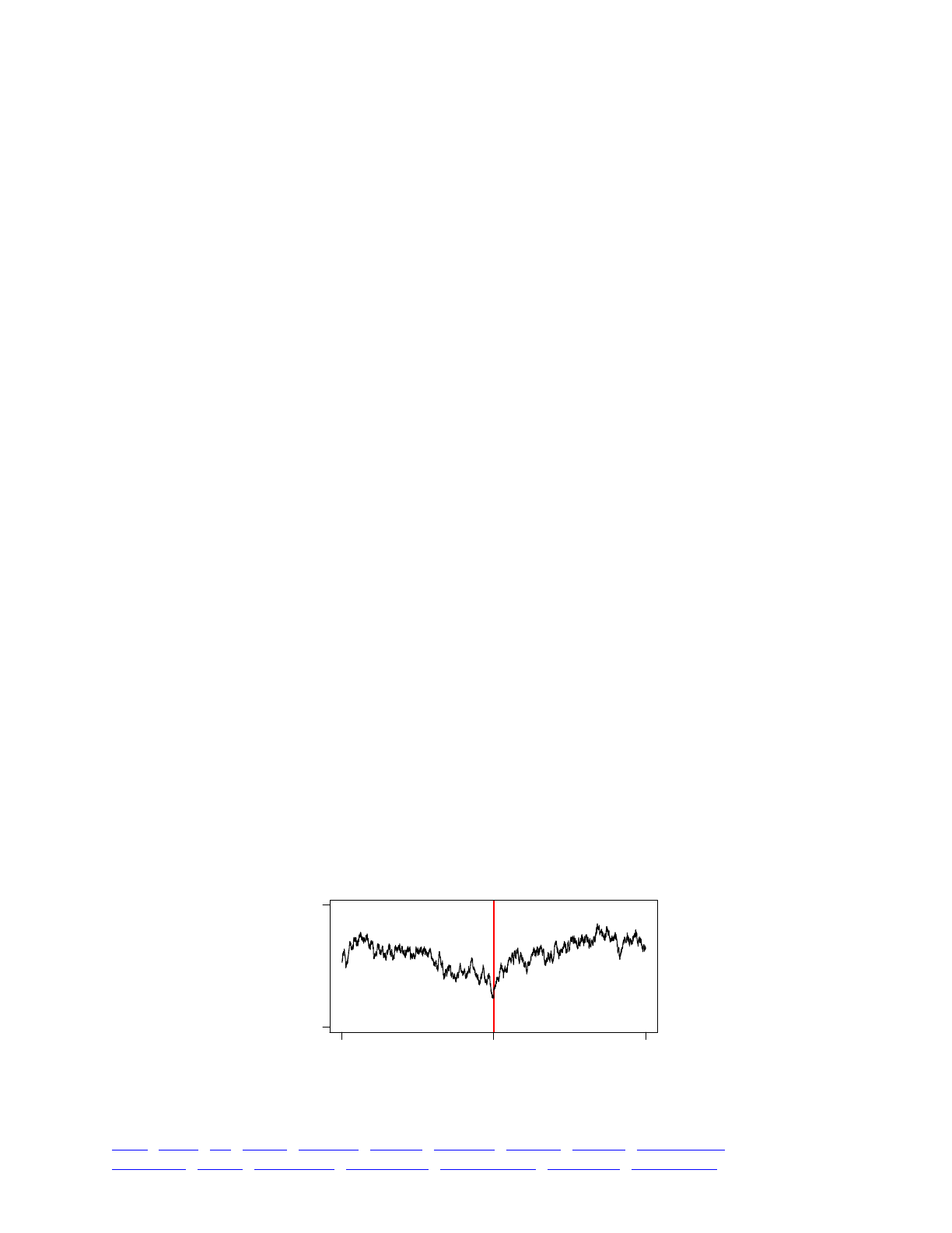
After importing packages, we run the SLiM model with subprocess.check_output(), which
generates the recipe_16.4.trees file. We read that file in using pyslim.load() and gather tree
heights, which are a proxy for diversity, from it; but let’s examine that process step by step.
First of all, pyslim.load() reads in the .trees file as tree sequence, which is a collection of
ancestry trees (section 1.7 introduces these concepts, but we will quickly review them here). The
tree sequence thinks of the genome as being divided into successive intervals, each of which has a
particular pattern of ancestry. Because the ancestry at adjacent positions along the genome tends
to be highly correlated, this representation makes the tree sequence very compact and efficient.
When we loop over the trees in ts.trees, we are actually looping over these chromosome
intervals, getting the ancestry tree for each successive interval.
Second, the ancestry tree for a given interval is not quite a tree in the usual sense, because it
can have multiple roots. This is because a given position will not necessarily share a common
ancestor, in forward simulation; at the beginning of simulation every individual is an island unto
itself, with no known relationship to any other individual, and ancestral relationships will be
constructed by coalescence as the model runs forward. The tree for a given interval, in a
simulation of N individuals, might therefore have anywhere from one root (if coalescence has
produced a single common ancestor for the whole population) to N roots (if no coalescence has
occurred yet). When we loop over roots in tree.roots, we are looping over common ancestors
shared by subsets of the extant population.
The code gathers tree heights across all roots for the current interval, using tree.time(root),
and uses np.mean() to get the mean height. This is our metric of diversity for the interval. Since an
interval can span more than one base position, we replicate that mean height across the tree’s
interval in height_for_pos, which we want to have a height value for each base position.
Note that in this recipe the simplify() of the loaded tree sequence is essential (whereas in
section 16.2 it was not); without it, every tree would have a root in the first generation, in one or
another original ancestor, and all the tree heights would be the same. The simplify() strips away
the original ancestors, giving us trees with roots representing the most recent common ancestors
for each tree.
With that done, we now need to convert that vector of tree heights along the chromosome into
heights at a given distance from the nearest gene. This involves a sort of descrambling of the data
based upon the genetic structure of the model, which (as described above) interleaved non-coding
regions of length L0 with genes of length L1. The details of this descrambling aren’t worth getting
into in detail; this is just data analysis, and is fairly routine Python code with no dependency upon
msprime or SLiM. The end result of this analysis is a vector named height_for_distance that has
mean heights for the corresponding distances in the vector distances. This is what we wanted, so
we can plot it (this plot is prettified using R code not shown here, but the Python plot looks
essentially the same):
-50000 050000
25000 35000
distance from gene
mean tree height (generations)
TOC I TOC II WF nonWF initialize() Genome Individual Mutation SLiMSim Subpopulation!
Eidos events fitness() mateChoice() modifyChild() recombination() interaction() reproduction() 355

This plot is noisy; that could presumably be smoothed out with more genes on a longer
chromosome, a larger population size, and averaging across multiple runs of the model.
Nevertheless, the “dip in diversity” is very clear: the mean tree height drops to a clear minimum
value precisely at zero on the plot.
Note that this analysis is not based upon the patterns of neutral mutation diversity around the
simulated genes. Instead, the pattern of inheritance itself – the mean time to the most recent
common ancestor at each base position – is used to generate the plot. This is far more powerful
than using the pattern of neutral mutation diversity, because neutral mutations are sparse and
stochastic. You certainly could overlay neutral mutations onto the tree sequence, as we did in
section 16.2, and then feed that into the analysis methods used by empirical studies (and perhaps
that would be a useful thing to do, to test the power or accuracy of those empirical methods). But
the analysis here is, in a sense, the average across many such analyses – across an infinite number
of such mutation overlays, in fact – and so it is far more powerful.
This recipe shows an analysis using just one metric provided by msprime, the height of a given
root using tree.time(root). The ancestry information provided by the tree sequence could be
mined in countless other ways. In the next recipe, we will look at another example of post-
simulation analysis using msprime.
16.5 Mapping admixture: analyzing ancestry in Python
It is often useful to be able to trace the true local ancestry at each location along the
chromosome. In section 13.9, a recipe was presented that provided this ability by introducing a
marker mutation at every base position along the chromosome in all of the individuals of one
subpopulation, while leaving the other subpopulation unmarked. After admixture of the two
subpopulations, the ancestry of each individual at each position could be determined by the
presence or absence of the marker mutation. That method works, but it comes at a cost of
considerable overhead in both runtime and memory usage. A chromosome of length 1e6 is close
to the practical limit for that recipe; a chromosome of length 1e8 is estimated by extrapolation to
take 7.2 days to run and – even worse – to require 8.1 TB of memory. Since the tree sequence is a
sparse data structure that records information about the ancestry at each chromosome position in a
highly compact form, one might suppose that it could provide information about true local
ancestry more efficiently, and indeed it can.
In this section we will look at a recipe very similar to that of section 13.9; refer back to that
section for further discussion of the design and motivation of that model. Here we will not use
marker mutations; instead we will use tree-sequence recording:
initialize() {!
defineConstant("L", 1e8);!
initializeTreeSeq();!
initializeMutationRate(0);!
initializeMutationType("m1", 0.5, "f", 0.1);!
initializeGenomicElementType("g1", m1, 1.0);!
initializeGenomicElement(g1, 0, L-1);!
initializeRecombinationRate(1e-8);!
}!
1 late() {!
sim.addSubpop("p1", 500);!
sim.addSubpop("p2", 500);!
sim.treeSeqRememberIndividuals(sim.subpopulations.individuals);!
!
p1.genomes.addNewDrawnMutation(m1, asInteger(L * 0.2));!
p2.genomes.addNewDrawnMutation(m1, asInteger(L * 0.8));!
TOC I TOC II WF nonWF initialize() Genome Individual Mutation SLiMSim Subpopulation!
Eidos events fitness() mateChoice() modifyChild() recombination() interaction() reproduction() 356

!
sim.addSubpop("p3", 1000);!
p3.setMigrationRates(c(p1, p2), c(0.5, 0.5));!
}!
2 late() {!
p3.setMigrationRates(c(p1, p2), c(0.0, 0.0));!
p1.setSubpopulationSize(0);!
p2.setSubpopulationSize(0);!
}!
2: late() {!
if (sim.mutationsOfType(m1).size() == 0)!
{!
sim.treeSeqOutput("./recipe_16.5.trees");!
sim.simulationFinished();!
}!
}!
10000 late() {!
stop("Did not reach fixation of beneficial alleles.");!
}
Only two mutations ever exist in this model: the beneficial mutations introduced at 0.2L in p1
and at 0.8L in p2. After admixture to form p3, when both mutations have fixed, a .trees file is
written out and the simulation ends. The .trees file will then be read and analyzed in Python, as
we will see below.
The only twist here is the call to sim.treeSeqRememberIndividuals(). Our goal is to trace the
ancestry at each position in each individual to either p1 or p2. In point of fact, in SLiM 3.1 and
later this call is not strictly necessary, because the original ancestors of each subpopulation created
by addSubpop() are kept by SLiM automatically. If we did not simplify() after loading the tree
sequence with pyslim, those ancestors would be available for us to trace ancestry back to,
allowing us to determine whether a particular genomic region originated in p1 or p2. We have
shown the call here, however, for a couple of reasons: (1) it makes the way this recipe works more
explicit and less magic, (2) you may wish to remember other individuals in a simulation to trace
ancestry back to them, so showing the treeSeqRememberIndividuals() call here makes it clear
how to do that, and (3) by explicitly remembering the ancestors we can simplify() on load,
which may be desirable – we may want to have a simplified tree sequence for other purposes.
The run of the SLiM model, along with post-run analysis and plotting, is all done in a single
Python script, as before:
import subprocess, msprime, pyslim!
import matplotlib.pyplot as plt!
import numpy as np!
!
# Run the SLiM model and load the resulting .trees file!
subprocess.check_output(["slim", "-m", "-s", "0", "./recipe_16.5.slim"])!
ts = pyslim.load("./recipe_16.5.trees").simplify()!
!
# Load the .trees file and assess true local ancestry!
breaks = np.zeros(ts.num_trees + 1)!
ancestry = np.zeros(ts.num_trees + 1)!
for tree in ts.trees(sample_counts=True):!
subpop_sum, subpop_weights = 0, 0!
for root in tree.roots:!
leaves_count = tree.num_samples(root) - 1 // the root is a sample!
subpop_sum += tree.population(root) * leaves_count!
subpop_weights += leaves_count!
TOC I TOC II WF nonWF initialize() Genome Individual Mutation SLiMSim Subpopulation!
Eidos events fitness() mateChoice() modifyChild() recombination() interaction() reproduction() 357
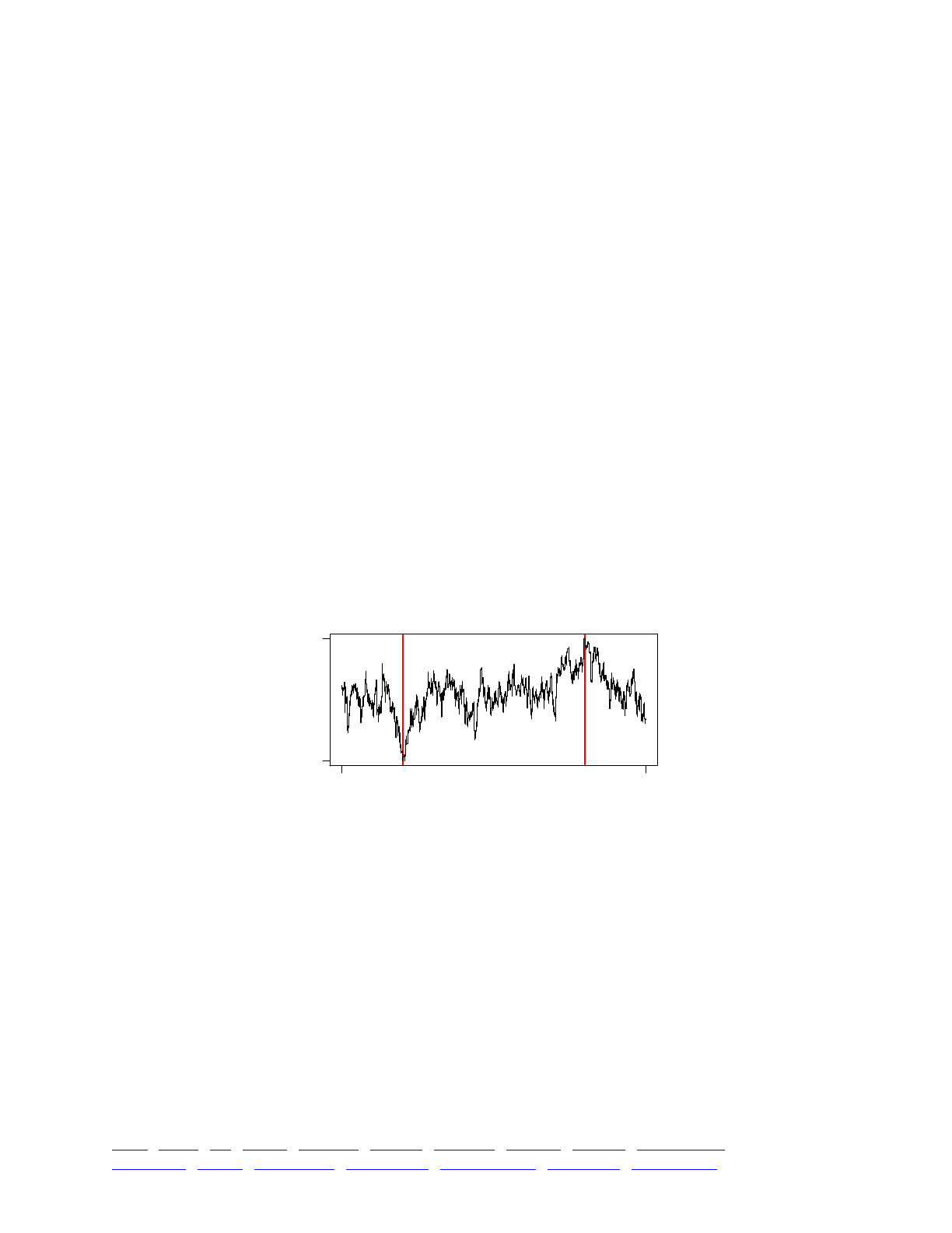
breaks[tree.index] = tree.interval[0]!
ancestry[tree.index] = subpop_sum / subpop_weights!
breaks[-1] = ts.sequence_length!
ancestry[-1] = ancestry[-2]!
!
# Make a simple plot!
plt.plot(breaks, ancestry)!
plt.show()
After imports, the SLiM model (named recipe_16.5.slim) is run with subprocess, and
the .trees file saved by the model is then read in using pyslim.load() as usual, with a
simplify() call since we have explicitly remembered the ancestors we are interested in (see
discussion above). We then loop over the trees in the tree sequence, and over the roots for each
tree (see section 16.4 for discussion of these concepts). For each root, we want to assess ancestry
as tracing back to either p1 or p2; this can be done simply by calling tree.population(root),
since every node in the tree sequence is marked with its subpopulation of origin. We average the
ancestry of all roots for an interval to get the mean ancestry, but this is a weighted average; each
root is weighted according to the number of descendants it has, effectively computing the average
ancestry across all extant individuals, rather than across roots. The start position on the
chromosome is recorded in parallel with these calculated mean ancestry values, and a terminating
entry in both vectors brings us to the end of the chromosome.
That’s it for the analysis; this model is much simpler structurally than the previous recipe. All
that is left is to plot the data. The values in starts and ends are used as the endpoints of line
segments, interleaved with zip(); the mean ancestries in subpops are duplicated to match. (For
those not familiar with Python, these lines may seem a bit magical, sorry.) The final plot (produced
by an R script for polish, rather than by the Python code here) looks like:
This is much the same as what the recipe of section 13.9 provided. Since the two beneficial
mutations both fixed, the ancestry of the final population is pure, p1 or p2, at the points where they
were introduced. The ancestry then shades continuously (but stochastically) between those two
points due to recombination (see section 13.9 for further discussion). The SLiM model here took
only 0.415 seconds to run, however – somewhat of an improvement over 7.2 days. The post-run
analysis took about 62 seconds; looping over all of the roots of all of the trees in the tree sequence
is not entirely trivial, but is still far simpler than simulating 1e8 marker mutations in SLiM.
This recipe will generalize easily to any number of ancestral subpopulations, as long as the
original founders of each subpopulation are remembered with treeSeqRememberIndividuals() so
that ancestry can be traced back to them (of course taking the mean of the subpopulations of the
tree roots wouldn’t be the right analysis then). Since every node knows the subpopulation to
which it belonged, the ancestral history at each position can be assessed by walking up the
ancestry chain from the extant nodes to the roots, as long as one ensures that the appropriate
ancestors are remembered forever; one might remember every individual that migrates to a new
0e+00 1e+08
chromosome position
ancestry proportion
p1 p2
TOC I TOC II WF nonWF initialize() Genome Individual Mutation SLiMSim Subpopulation!
Eidos events fitness() mateChoice() modifyChild() recombination() interaction() reproduction() 358

subpopulation, for example, using the migrant property of Individual, so that the migratory
history through the ancestry tree can be traced. All of this goes far beyond what would be
reasonable to implement with marker mutations using the methods of section 13.9.
16.6 Measuring the coalescence time of a model
A common problem in forward simulation is deciding how to conduct model burn-in. A burn-
in period is a period of simulation executed in order to arrive at an appropriate starting state for the
model one wishes to execute; often this starting state is for a neutral model at equilibrium, but not
necessarily so. But how long should the burn-in period be, to provide such an equilibrium state?
Running until coalescence ensures that no genetic diversity in the population could date back to
the start of the simulation, so all polymorphic loci derive from after the start of the simulation.
However, to attain equilibrium takes longer: in a truly neutral population of constant size, a total of
two or three times the time required to reach coalescence should suffice. But that just kicks the
can down the road; how long does it take to achieve coalescence? A heuristic of 10N is often
used: run for ten times the population size (N), in generations. But this heuristic is less than
satisfactory; the model may not have coalesced even at 10N generations, or it may have coalesced
long before (meaning wasted simulation time). And with any additional complexity, such as
multiple subpopulations connected by migration, the 10N rule is potentially even more
problematic. What to do?
Tree-sequence recording provides a very easy solution, because the ancestry information that it
records is well-suited to determining whether the model has achieved coalescence. The only
complication is that coalescence can only be evaluated immediately after simplification has been
performed; the coalescence test requires that the tree sequence be in a simplified state. SLiM
largely hides this detail from the user; you can query the coalescence state at any time, but the
answer you get will actually be the coalescence state at the time that the last simplification was
performed, not the state at the present time. Sometimes, then, one will want to exert some control
over the simplification process, so that one knows at what granularity coalescence is actually
being assessed, as described below.
Here is a recipe demonstrating the coalescence-detection technique:
initialize() {!
initializeTreeSeq(checkCoalescence=T);!
initializeMutationRate(0);!
initializeMutationType("m1", 0.5, "f", 0.0);!
initializeGenomicElementType("g1", m1, 1.0);!
initializeGenomicElement(g1, 0, 1e8-1);!
initializeRecombinationRate(1e-8);!
}!
1 {!
sim.addSubpop("p1", 500);!
}!
1: late() {!
if (sim.treeSeqCoalesced())!
{!
catn(sim.generation + ": COALESCED");!
sim.simulationFinished();!
}!
}!
100000 late() {!
catn("NO COALESCENCE BY GENERATION 100000");!
}
TOC I TOC II WF nonWF initialize() Genome Individual Mutation SLiMSim Subpopulation!
Eidos events fitness() mateChoice() modifyChild() recombination() interaction() reproduction() 359

This model turns on coalescence checking with checkCoalescence=T (see section 21.1;
coalescence checking needs to be turned on explicitly because there is a small performance
penalty associated with it). Then, every generation, we check for coalescence with
sim.treeSeqCoalesced(). As mentioned above, this only tells us whether coalescence was
observed at the last simplification; when auto-simplification finds that coalescence has occurred,
treeSeqCoalesced() will then return T when it is next called. Usually it is not necessary to detect
coalescence in the very generation in which it occurs; it is typically enough to simply know that it
has occurred at some recent time, as this model does.
When this model is run, typical output looks like this:
9984: COALESCED
Coalescence was probably achieved some time before generation 9984; 9984 is just the
generation in which auto-simplification noticed that coalescence. Note that this is higher than the
10N value of 5000 (and auto-simplification occurs every couple of hundred generations in this
model); so at generation 5000 the model would not yet have coalesced. The time to coalescence is
variable, depending as it does upon stochastic events, but repeated runs of this model will show
that in fact it typically coalesces around 10000 generations, or approximately 20N.
To control the granularity of coalescence checking more precisely, one may turn off auto-
simplification by passing simplificationRatio=INF to initializeTreeSeq(), and then call
treeSeqSimplify() to simplify on demand, after which treeSeqCoalesced() will return an up-to-
date assessment. Simplifying every generation is very slow, however, so simplifying and checking
at a regular interval, such as every hundredth generation, is generally preferable.
Note that certain actions in script, such as adding a new subpopulation, can break the
coalescence of a model; all of the individuals in the population no longer share a common
ancestor, even though they previously did. The value returned by treeSeqCoalesced() will not
immediately reflect this; instead, as usual, that value will reflect the coalescence state after the last
simplification that was performed. If this poses a problem, one can always explicitly simplify
immediately after such model events, forcing the coalescence state to be re-checked.
Coalescence checking will work in all types of models (with the above caveats about timing and
granularity), regardless of selection, population structure, etc. However, coalescence is only a
useful indicator of the timescale needed for equilibration in fairly simple neutral models. If model
dynamics during burn-in change over time, or are substantially non-neutral, coalescence may be a
poor indicator of equilibration; indeed, such models may not even have an equilibrium state.
What constitutes a proper burn-in for such models is a difficult question.
It is worth noting that the point of coalescence, in a forward simulation, is not itself an unbiased
or equilibrium state. In particular, as a forward simulation runs the mean tree height will grow
over time until coalescence is reached, at which point it will drop suddenly (because a more
recent common ancestor has just emerged); then it will rise steadily again until the next
coalescence, at which point it will again drop, and so forth. A plot of mean tree height over time
therefore exhibits a “saw-tooth” pattern, and the moment of any given coalescence event is the
bottom point of one saw-tooth – a special point in time, not a typical or average one. It is
therefore advisable to continue neutral burn-in well beyond the point of coalescence; this is why,
at the beginning of this subsection, we recommended running for two or three times the time
required to reach coalescence. For an even better solution to this problem of neutral burn-in, see
the “recapitation” technique described in section 16.10.
TOC I TOC II WF nonWF initialize() Genome Individual Mutation SLiMSim Subpopulation!
Eidos events fitness() mateChoice() modifyChild() recombination() interaction() reproduction() 360

16.7 Analyzing selection coefficients in Python with pyslim
So far we have used the pyslim package only minimally, to load in .trees files generated by
SLiM. The next several recipes will delve into its capabilities more. In this section, we will see
how to use pyslim to obtain SLiM-specific information about a simulation from the metadata
stored in the .trees file generated by SLiM.
Let’s begin with a simple SLiM model of beneficial and neutral mutations on a uniform
chromosome:
initialize() {!
initializeTreeSeq();!
initializeMutationRate(1e-10);!
initializeMutationType("m1", 0.5, "g", 0.1, 0.1);!
initializeMutationType("m2", 0.5, "g", -0.1, 0.1);!
initializeGenomicElementType("g1", c(m1, m2), c(1.0, 1.0));!
initializeGenomicElement(g1, 0, 1e8-1);!
initializeRecombinationRate(1e-8);!
}!
1 {!
sim.addSubpop("p1", 500);!
}!
20000 late() { sim.treeSeqOutput("./recipe_16.7.trees"); }
Beneficial mutations are drawn from a gamma DFE with a mean of 0.1, deleterious mutations
from a gamma DFE with a mean of -0.1. After the model has run for a while, the expectation
would be that the mutations generated as the model runs would indeed have those means, but that
the mutations fixed would be biased towards the higher end of the distribution for both mutation
types. This would be simple enough to evaluate in Eidos at the end of the model run, but let’s do it
in Python instead, using pyslim, as a proof on concept. Here is a Python script that assumes that a
.trees file has been saved to the path used by the model above (we’ve shown already how to run
a SLiM model from inside Python using subprocess.check_output(), so there’s no need to keep
reiterating that point):
import msprime, pyslim!
!
ts = pyslim.load("recipe_16.7.trees").simplify()!
!
coeffs = []!
for mut in ts.mutations():!
md = pyslim.decode_mutation(mut.metadata)!
sel = [x.selection_coeff for x in md]!
if any([s != 0 for s in sel]):!
coeffs += sel!
!
b = [x for x in coeffs if x > 0]!
d = [x for x in coeffs if x < 0]!
!
print("Beneficial: " + str(len(b)) + ", mean " + str(sum(b) / len(b)))!
print("Deleterious: " + str(len(d)) + ", mean " + str(sum(d) / len(d)))
We start by loading the .trees file with pyslim.load() as usual. We then loop through all of
the mutations in the tree sequence, provided by ts.mutations(). We are interested in the
selection coefficients of the mutations, which are not part of the base information provided by
the .trees format; instead, they are stored in SLiM-specific metadata attached to each mutation.
To access them, then, we ask pyslim to decode the metadata for us, from the binary format it is in,
and return it to us, using the pyslim.decode_mutation() method. We can then fetch selection
TOC I TOC II WF nonWF initialize() Genome Individual Mutation SLiMSim Subpopulation!
Eidos events fitness() mateChoice() modifyChild() recombination() interaction() reproduction() 361

coefficients (more on this in a moment) and append them to the coeffs list. Once we have that
list, it is a trivial matter to select the beneficial and deleterious mutations from it and print a
summary of each. A test run produces this output:
Beneficial: 3580, mean 1.0382685732466397!
Deleterious: 103, mean -0.04902286211917154
A great many more beneficial mutations than deleterious mutations are present, even though
they arise at equal rates in the SLiM model, which is unsurprising. Furthermore, the mean of the
mutations present is considerably biased relative to the mean of the DFEs for these mutation types
(which were 0.1 and -0.1).
There are a few points to note here, regarding the way in which the selection coefficients are
gathered. First of all, the tree sequence retains fixed mutations, unlike SLiM. As the SLiM model
ran, mutations that fixed were converted to substitutions as usual in SLiM; but in the tree-sequence
no such conversion occurs. The list of mutations provided by the tree sequence therefore includes
both fixed and segregating mutations; no distinction is made.
Second, note that the return value from pyslim.decode_mutation() is a list, not a single object.
We end up looping through the elements in this list and getting a selection coefficient from each
element. The reason for this has to do with mutation stacking in SLiM (see section 1.5.3 for a
review of this concept). A “mutation”, as far as the tree sequence is concerned, is a unique
mutational state at a given position, which encompasses all of the mutations that have stacked at
that position. When we call pyslim.decode_mutation(), it helpfully deconstructs this stacked
state into the component mutations within it. If a particular mutation occurs in more than one
configuration in the tree sequence – by itself at a position and also stacked with another mutation
at that position, in different genomes, say – we will actually encounter that mutation more than
once during this process, and we will therefore overcount it. Since stacking will be extremely
uncommon in this model, we don’t worry about it much; it will not skew our results noticeably. If
we wanted to be more rigorous, however, we could use the mutation IDs from SLiM (also available
through pyslim) to construct a uniqued list of mutations, with each mutation counted only once
even if it is stacked with other mutations in various ways, and could then do the rest of the analysis
using that uniqued list. Since that is just elementary Python wrangling, we will not go into that
level of detail here.
16.8 Starting a hermaphroditic WF model with a coalescent history
In section 16.6, we saw how to assess whether a model has coalesced or not using
treeSeqCoalesced(), allowing us to run a model for an appropriate burn-in period rather than
relying upon the (problematic) 10N heuristic. If the burn-in period for a model is neutral and can
be run with msprime’s coalescent simulation, we can avoid running our burn-in with forward
simulation at all. Instead, we can run the burn-in period using the coalescent, save the result as
a .trees file (annotated with pyslim as needed), and load the result into SLiM where we continue
the simulation from the endpoint of the coalescent. This may sound complicated, but in fact it is
remarkably simple.
However, note that starting a simulation with the coalescent in this way is often not the best
technique. In many cases, the “recapitation” technique presented in section 16.10 is superior, for
reasons that will be explained there. This recipe is for primarily for illustration.
We begin with a Python script:
import msprime, pyslim!
!
ts = msprime.simulate(sample_size=10000, Ne=5000, length=1e8,!
TOC I TOC II WF nonWF initialize() Genome Individual Mutation SLiMSim Subpopulation!
Eidos events fitness() mateChoice() modifyChild() recombination() interaction() reproduction() 362

mutation_rate=0.0, recombination_rate=1e-8)!
slim_ts = pyslim.annotate_defaults(ts, model_type="WF", slim_generation=1)!
slim_ts.dump("recipe_16.8.trees")
The msprime.simulate() method is used to run a coalescent simulation with n=2Ne=10000 (n
being a haploid sample size, Ne being in terms of diploids), a chromosome of length 1e8, and a
recombination rate of 1e-8. A mutation rate of 0.0 is used, since we only want the coalescent
history, not mutations within it (those can be overlaid later if needed). This returns a tree sequence
object, but it is in msprime’s format; it does not have any of the metadata annotations expected by
SLiM. The next step is to use pyslim.annotate_defaults() to add those annotations. We tell it to
annotate the data for a WF SLiM model, and to align the times in the tree sequence so that the
current generation has index 1; when we load the model into SLiM, it will start at generation 1
even though there are many generations of history stretching back in time. After annotating,
the .trees file is saved.
Now we can run a SLiM model that loads it and continues the run with some non-neutral
dynamics:
initialize() {!
initializeTreeSeq();!
initializeMutationRate(0);!
initializeMutationType("m1", 0.5, "f", 0.0);!
initializeMutationType("m2", 0.5, "f", 0.1);!
initializeGenomicElementType("g1", m2, 1.0);!
initializeGenomicElement(g1, 0, 1e8-1);!
initializeRecombinationRate(1e-8);!
}!
1 late() {!
sim.readFromPopulationFile("recipe_16.8.trees");!
target = sample(sim.subpopulations.genomes, 1);!
target.addNewDrawnMutation(m2, 10000);!
}!
1: {!
if (sim.mutationsOfType(m2).size() == 0) {!
print(sim.substitutions.size() ? "FIXED" else "LOST");!
sim.treeSeqOutput("recipe_16.8_II.trees");!
sim.simulationFinished();!
}!
}!
2000 { sim.simulationFinished(); }
At the end of this model (note that an initial seed of 2178208680098 produces fixation in SLiM
3.1), a new .trees file is saved out. This contains the full ancestry information for the simulation –
not just for the period simulated in SLiM, but also for the coalescent. Just to verify here that the
full history is present, let’s check the final tree sequence:
import msprime, pyslim!
!
ts = pyslim.load("recipe_16.8_II.trees").simplify()!
!
for tree in ts.trees():!
for root in tree.roots:!
print(tree.time(root))
This just prints the heights of the trees in the final tree sequence; in a test run, it prints a wide
range of values, ranging from less than 10,000 to more than 60,000. The simulation is fully
coalesced (that could be confirmed by checking that the number of roots per tree is always exactly
TOC I TOC II WF nonWF initialize() Genome Individual Mutation SLiMSim Subpopulation!
Eidos events fitness() mateChoice() modifyChild() recombination() interaction() reproduction() 363

1), but it reached coalescence at different times at different positions along the chromosome, so the
tree heights are not all identical. However, all of the heights are considerably larger than the 324
generations that the SLiM model ran for; the rest is the height of the coalescent history, which has
indeed been preserved. We could now overlay neutral mutations upon the final .trees file as we
did in section 16.2, or perform ancestry analyses with it such as those we did in section 16.4 and
16.5, or whatever else we might wish to do.
16.9 Starting a sexual nonWF model with a coalescent history
In the previous recipe, we saw how to run an msprime coalescent simulation as a burn-in period
and save it as a SLiM-compliant .trees file which could then be used to run non-neutral dynamics
on top of the coalescent burn-in history. The scenario presented there was very simple, however: a
hermaphroditic WF model. What if we want to use msprime to construct a coalescent burn-in for a
model complex model? We will need to annotate the tree sequence appropriately for the type of
model that we intend to load it into in SLiM. Here we will see how to do this for a sexual nonWF
model. As mentioned in the previous recipe, however, starting a simulation with the coalescent is
often not the best technique; the “recapitation” technique presented in section 16.10 is usually
preferable, for reasons discussed there. This recipe is offered for illustration of the relevant
techniques.
To get SLiM to accept the .trees file from the burn-in as legitimate input for a sexual nonWF
model, we will need to assign sexes to each individual. We will assign ages too; if we didn’t do
so, all of the individuals would be given a default age of 0, but here we would like the initial
population to have some age structure. Finally, we will tell pyslim to mark the tree sequence as
being from a nonWF simulation, so that it matches SLiM’s expectations.
The Python script for this recipe is a bit longer, naturally, since the annotation adds a bit of
complication:
import msprime, pyslim, random!
!
ts = msprime.simulate(sample_size=10000, Ne=5000, length=1e8,!
mutation_rate=0.0, recombination_rate=1e-8)!
!
tables = ts.dump_tables()!
pyslim.annotate_defaults_tables(tables, model_type="nonWF",!
slim_generation=1)!
individual_metadata = list(pyslim.extract_individual_metadata(tables))!
for j in range(len(individual_metadata)):!
individual_metadata[j].sex = random.choice(!
[pyslim.INDIVIDUAL_TYPE_FEMALE, pyslim.INDIVIDUAL_TYPE_MALE])!
individual_metadata[j].age = random.choice([0, 1, 2, 3, 4])!
!
pyslim.annotate_individual_metadata(tables, individual_metadata)!
slim_ts = pyslim.load_tables(tables)!
slim_ts.dump("recipe_16.9.trees")
As in section 16.8, we start by running a coalescent simulation with msprime, generating a tree
sequence. We want to modify the individual metadata here, so at this point we need to switch to
msprime’s table representation with ts.dump_tables(), which unpacks the tree sequence into
modifiable tables (tree sequences are immutable, for efficiency reasons, so modifications must be
made to tables). We can then perform the default nonWF annotation on those tables using
pyslim.annotate_defaults_tables(); this is parallel to our use of pyslim.annotate_defaults()
in section 16.8. We then extract a list of individual metadata records from the tables, and loop
through it setting random sexes and ages. (The age structure used here is just a placeholder for a
TOC I TOC II WF nonWF initialize() Genome Individual Mutation SLiMSim Subpopulation!
Eidos events fitness() mateChoice() modifyChild() recombination() interaction() reproduction() 364

more realistic distribution, of course.) Once the metadata records have been modified, they get
loaded back into the tables, and then the tables get used to create a new SLiM-annotated tree
sequence. Finally, the tree sequence gets written out to a .trees file. This is the typical workflow
when modifying metadata: convert to tables, fetch the metadata from the tables, modify it, load it
back into the tables, and finally recreate a tree sequence from the modified tables. This is
necessary because the tree sequence is an immutable object, not designed to allow modification
of this sort.
Having produced a .trees file from the script above, we can load it into a matching SLiM
model and run, as we did before. For clarity, we’ll leave every else the same about this model, so
that the essential differences can be seen more easily:
initialize() {!
initializeSLiMModelType("nonWF");!
initializeTreeSeq();!
initializeSex("A");!
initializeMutationRate(0);!
initializeMutationType("m1", 0.5, "f", 0.0);!
initializeMutationType("m2", 0.5, "f", 0.1);!
m2.convertToSubstitution=T;!
initializeGenomicElementType("g1", m2, 1.0);!
initializeGenomicElement(g1, 0, 1e8-1);!
initializeRecombinationRate(1e-8);!
}!
reproduction(NULL, "F") {!
subpop.addCrossed(individual, subpop.sampleIndividuals(1, sex="M"));!
}!
1 early() {!
sim.readFromPopulationFile("recipe_16.9.trees");!
target = sample(sim.subpopulations.genomes, 1);!
target.addNewDrawnMutation(m2, 10000);!
}!
early() {!
p0.fitnessScaling = 5000 / p0.individualCount;!
}!
1: late() {!
if (sim.mutationsOfType(m2).size() == 0) {!
print(sim.substitutions.size() ? "FIXED" else "LOST");!
sim.treeSeqOutput("recipe_16.9_II.trees");!
sim.simulationFinished();!
}!
}!
2000 { sim.simulationFinished(); }
Since this is a nonWF model, we have added a minimal reproduction() callback and an
early() event that provides population regulation through density-dependence, as well as a call to
initializeSLiMModelType() (see chapter 15 for discussion). Since it is a sexual model, we also
added a call to initializeSex(). We want the model to terminate upon fixation or loss, as before,
but in nonWF models mutations are not converted to substitutions automatically, so we add
m2.convertToSubstitution=T to ensure that; of course we could just adapt the termination code to
check the frequency of the introduced mutation instead. The rest of the model is unchanged, apart
from filenames.
Note that the subpopulation loaded in from the .trees file is p0, not p1; msprime starts counting
subpopulation IDs from zero. It is conventional in SLiM, in general, to number subpopulations
TOC I TOC II WF nonWF initialize() Genome Individual Mutation SLiMSim Subpopulation!
Eidos events fitness() mateChoice() modifyChild() recombination() interaction() reproduction() 365

from p1, but of course it doesn’t really matter; it would be possible to reassign the subpopulation
index before writing out the .trees file, but we do not do so here.
The only important caveat here is that the coalescent was not run with separate sexes, nor with
overlapping generations, so it does not precisely reflect the dynamics involved in the non-neutral
portion of the simulation. The coalescent is an approximation anyway; in fact, this would have
been a concern in the previous recipe too, if exact Wright-Fisher dynamics were needed. Whether
these sorts of deviations from exact SLiM dynamics are a concern or not will depend upon the
nature of the analysis to be conducted downstream. If it is an issue, a further burn-in period could
be run in SLiM with the correct dynamics, prior to introducing the sweep mutation; that burn-in
would perhaps not need to be very long to wipe away any important traces of the incorrect burn-in
dynamics (but it would be a good idea to confirm that with appropriate tests, of course). If
absolutely exact dynamics are needed then the burn-in will have to be simulated in SLiM; that can
still be done with tree-sequence recording with neutral mutations turned off, though, as in section
16.1, so it will still be much faster than a regular SLiM burn-in would have been.
When this model is run (an initial seed of 1661016094949 produces fixation in SLiM 3.1), we
see the sweep occur and then a new .trees file is written out. We could conduct the same post-
run analysis as before, printing out tree heights to verify that this burn-in procedure worked, but to
avoid repetitiveness we will just end here. It is worth noting, in closing, that pyslim allows all sorts
of annotation; it would be possible, with a similar strategy, to mark genomes as being X or Y
chromosomes and then load them into a sex-chromosome simulation in SLiM, or to set the spatial
positions of individuals before loading them into a spatial SLiM model, or whatever is needed. Of
course, getting coalescent simulation results for such complex scenarios, even without any
selected loci, may be a challenge.
16.10 Adding a neutral burn-in after simulation with recapitation
Very often, in forward genetic simulation, a “burn-in” period of neutral dynamics is desirable to
allow the model to reach an equilibrium state of mutation–drift balance before non-neutral
dynamics begin. Without a burn-in period, the pattern of neutral mutations observed at the end of
the simulation may depend as much upon the initial state of the model as on the model’s
dynamics, which can make it difficult to interpret results. The modeling of this burn-in period is a
persistent problem, however, because it is generally so time-consuming. An often-quoted rule of
thumb is that the burn-in period should run for 10N generations – ten times the initial population
size. For a model with 100,000 individuals, then, a million generations of burn-in is recommend,
which – with such a large population size – will take an exceedingly long time. Worse, the 10N
rule is often an underestimate of the time needed to equilibrate, particularly when simulating a
very long chromosome; and there is no number of generations at which coalescence is guaranteed.
To cope with this issue, a wide variety of techniques are attempted. One might try to rescale
the model during the burn-in period (see section 5.5), although this can introduce significant
artifacts; or one might initialize the model with the output from a coalescent simulation (see
sections 16.8 and 16.9); or one might run the burn-in period without neutral mutations, using tree-
sequence recording to preserve the ancestry information that will allow them to be overlaid late
(see sections 16.1 and 16.2). With SLiM 3.1, there is an option that is often better than any of
these, which we will examine in this section: recapitation.
Recapitation is the addition of a neutral coalescent history to a simulation after the fact. The
non-neutral portion of the simulation is run first, in SLiM, with tree-sequence recording enabled so
that the genealogical history of all extant individuals is preserved. The result is saved to a .trees
file, as in previous recipes. That .trees file is then loaded in Python, and msprime and pyslim are
TOC I TOC II WF nonWF initialize() Genome Individual Mutation SLiMSim Subpopulation!
Eidos events fitness() mateChoice() modifyChild() recombination() interaction() reproduction() 366

used to construct a coalescent history stretching back in time from the original ancestors of the
simulation.
Enough discussion; let’s see it in action. We will begin with a SLiM model of non-neutral
dynamics, specifically a selective sweep:
initialize() {!
initializeTreeSeq(simplificationRatio=INF);!
initializeMutationRate(0);!
initializeMutationType("m2", 0.5, "f", 1.0);!
m2.convertToSubstitution = F;!
initializeGenomicElementType("g1", m2, 1);!
initializeGenomicElement(g1, 0, 1e6 - 1);!
initializeRecombinationRate(3e-10);!
}!
1 late() {!
sim.addSubpop("p1", 1e5);!
}!
100 late() {!
sample(p1.genomes, 1).addNewDrawnMutation(m2, 5e5);!
}!
100:10000 late() {!
mut = sim.mutationsOfType(m2);!
if (mut.size() != 1)!
stop(sim.generation + ": LOST");!
else if (sum(sim.mutationFrequencies(NULL, mut)) == 1.0)!
{!
sim.treeSeqOutput("recipe_16.10_decap.trees");!
sim.simulationFinished();!
}!
}
This is a pretty typical tree-sequence-based model, with a mutation rate of zero. It involves a
fairly large population size (1e5), and a reasonably long chromosome (1e6), so running the neutral
burn-in for this model in SLiM would take quite a long time. Incidentally, the size of this
simulation also means that simplification can take quite a long time, and so as well as recapitating,
we have also chosen to speed up the simulation by setting the simplificationRatio parameter of
initializeTreeSeq() to INF. We have not discussed the simplificationRatio option much
before: in general, it controls how often simplification occurs, and a value specifically of INF tells
SLiM not to simplify the tree sequence at all until a .trees file is generated (see section 21.1).
Although this speeds up the model’s execution considerably, it can greatly increase memory usage,
so it should be done with care; it is easy to overflow the memory available to the process. As this
particular example has a short runtime, we’re probably safe to trade off memory to achieve
maximum simulation speed, but for longer-running simulations you will probably want to tune the
simplification interval as appropriate before recapitating.
This model involves a selective sweep, introduced in generation 100. We do not attempt to run
this simulation conditional on fixation (see chapter 10); for simplicity, we just detect fixation or
loss in the 100:10000 late() event. On fixation, the model dumps a .trees file and stops.
So now, if we run the model until we get a run in which the sweep mutation fixes, we have a
file named recipe_16.10_decap.trees that contains the genealogical history of that run. Now we
run a Python script that performs the recapitation:
import msprime, pyslim!
import numpy as np!
import matplotlib.pyplot as plt!
TOC I TOC II WF nonWF initialize() Genome Individual Mutation SLiMSim Subpopulation!
Eidos events fitness() mateChoice() modifyChild() recombination() interaction() reproduction() 367

!
# Load the .trees file!
ts = pyslim.load("recipe_16.10_decap.trees") # no simplify!!
!
# Calculate tree heights, giving uncoalesced sites the maximum time!
def tree_heights(ts):!
heights = np.zeros(ts.num_trees + 1)!
for tree in ts.trees():!
if tree.num_roots > 1: # not fully coalesced!
heights[tree.index] = ts.slim_generation!
else:!
children = tree.children(tree.root)!
real_root = tree.root if len(children) > 1 else children[0]!
heights[tree.index] = tree.time(real_root)!
heights[-1] = heights[-2] # repeat the last entry for plotting!
return heights!
!
# Plot tree heights before recapitation!
breakpoints = list(ts.breakpoints())!
heights = tree_heights(ts)!
plt.step(breakpoints, heights, where='post')!
plt.show()!
!
# Recapitate!!
recap = ts.recapitate(recombination_rate=3e-10, Ne=1e5, random_seed=1)!
recap.dump("recipe_16.10_recap.trees")!
!
# Plot the tree heights after recapitation!
breakpoints = list(recap.breakpoints())!
heights = tree_heights(recap)!
plt.step(breakpoints, heights, where='post')!
plt.show()
The first step is to load the .trees file. Note that we specifically do not call simplify() here,
because we need the first generation individuals to recapitate from; this is, in fact, precisely why
SLiM 3.1 preserves those individuals for us.
Then we define a function that calculates tree heights along the chromosome. This is similar to
what we did in section 16.4, but here we have to be a bit smarter because of those original
ancestors preserved in the tree sequence. Every tree will have a root in one of those original
ancestors, but we are interested in whether the tree has coalesced below that original ancestor
(and if so, at what height), or if the tree still has multiple roots, indicating that it has not yet
coalesced.
We use that function to plot tree heights along the chromosome before recapitation. Then we
recapitate, which is very easy – just a single method call on our tree sequence, returning a new
tree sequence that has had a coalescent history traced backward from its original ancestors. The
recapitation process just needs to know the recombination rate to use, and the population size (Ne)
to use for the coalescent. Finally, we plot again, after recapitation, to see what it has done. A
combined plot of these results, made in R, looks like this:
TOC I TOC II WF nonWF initialize() Genome Individual Mutation SLiMSim Subpopulation!
Eidos events fitness() mateChoice() modifyChild() recombination() interaction() reproduction() 368
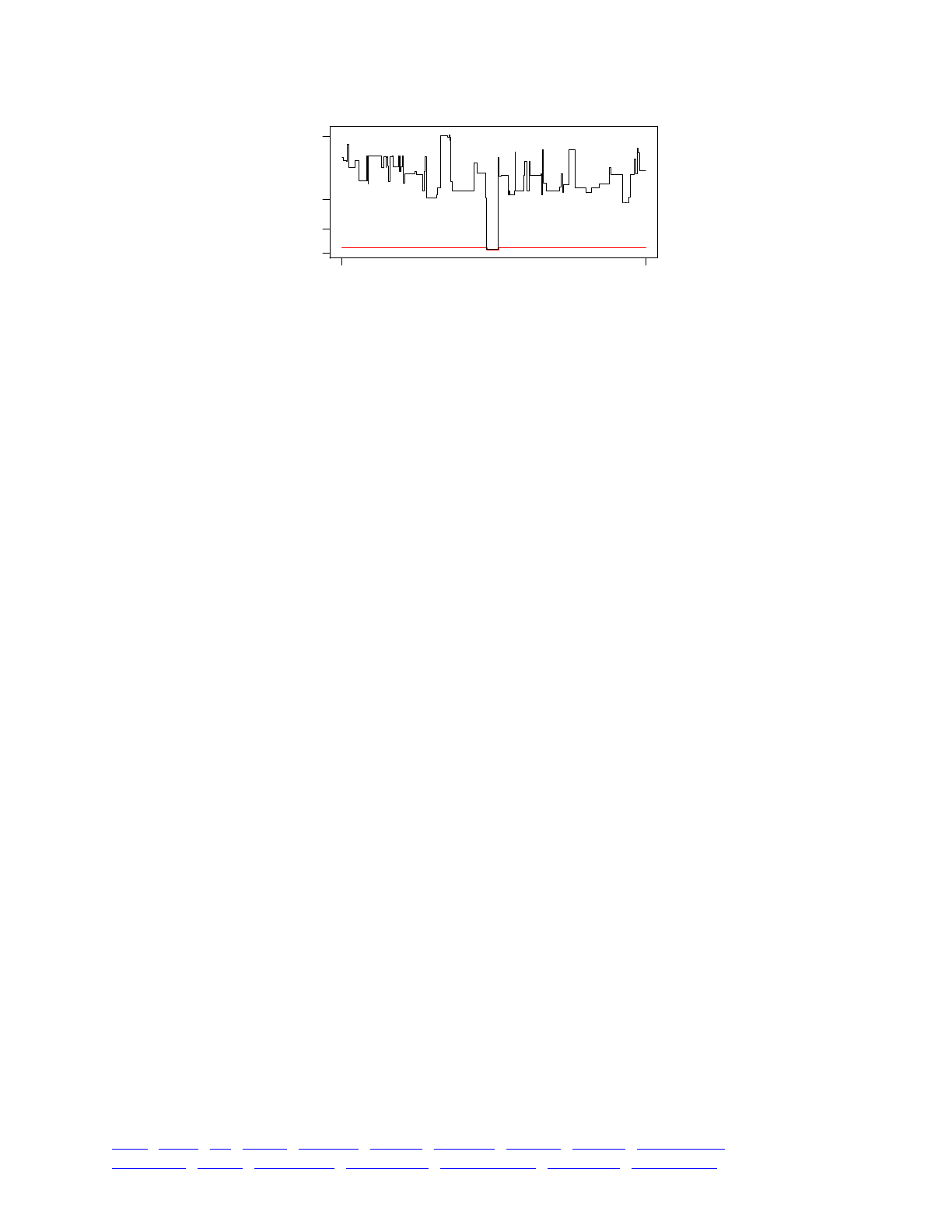
Note that the y-axis is rescaled according to the cube root of the number of generations, to
bring out detail at both the low and high ends of the scale. The red line here shows the tree
heights along the chromosome prior to recapitation. The area surrounding the sweep has
coalesced at the generation in which the sweep mutation was introduced, due to strong
hitchhiking in the vicinity of the mutation. The area further out has not coalesced, and therefore
has a tree height that dates back to the beginning of forward simulation, 100 generations before
the sweep began. The black line shows tree heights after recapitation; here the uncoalesced
regions farther from the sweep have been coalesced backward in time as far as a million
generations (reflecting the fact that we would have needed to run the burn-in in SLiM for at least a
million generations to have any likelihood of coalescence). Regions closer to the sweep tend to
coalesce more recently, reflecting the effect of the sweep on the diversity present at different
regions along the chromosome at the end of simulation.
In short, we can see that recapitation has provided us with a full neutral burn-in history for the
simulation, after the fact. Notably, this is very fast; this example run executed in 0.41 seconds. If
we wanted neutral mutations overlaid over the whole population history, including the recapitated
burn-in, that would also be extremely fast; using the technique shown in section 16.2, that
operation would take another 0.58 seconds. These times can be compared to an estimate,
obtained by extrapolation, of how long the burn-in would take in SLiM: more than 114 hours.
Recapitation, then, is optimal for computing burn-in for several reasons. One reason is that it is
extremely fast, as we have seen; the only branches that need to be coalesced are those leading to
the final individuals present at the end of forward simulation, which is generally a small minority
of the branches that were present at the beginning of forward simulation. Recapitation is therefore
much, much faster than simulating the burn-in period in SLiM, and should even be faster than
constructing an initial population state with the coalescent; it is based upon the coalescent, but
needs to do much less work since far fewer branches typically need to be coalesced. Then too,
recapitation is very convenient, since it can be done after forward simulation, even as an
afterthought on existing model output. In this way, it allows a focus on the non-neutral dynamics
of interest, with burn-in handled later. It also allows one to ignore the question of how long to run
burn-in for – the whole “10N” question – since recapitation will coalesce back in time as far as
necessary to achieve full coalescence.
Of course, recapitation can only be used in scenarios where a neutral coalescent process is
appropriate for burn-in. In some cases the burn-in period needs to itself be non-neutral; in this
case using tree-sequence recording to run without neutral mutations may be the best one can do
(see sections 16.1 and 16.2). But for many models, recapitation will enable modeling at a larger
scale than previously possible, by greatly reducing the overhead of the burn-in period.
One point was glossed over in the discussion above: why was the sweep mutation introduced in
generation 100, and not, say, in generation 2 immediately after the simulation has started? The
easy answer is: to make the plot look nice. In the mean tree height plot above, there is a nice stair-
0e+00 1e+06
chromosome position
mean tree height (generations)
11e4 1e5 1e6
TOC I TOC II WF nonWF initialize() Genome Individual Mutation SLiMSim Subpopulation!
Eidos events fitness() mateChoice() modifyChild() recombination() interaction() reproduction() 369

step in the red line (showing mean tree height prior to recapitation), and that bump is there
because of the delay between starting forward simulation and introducing the sweep mutation.
But there is a deeper benefit as well: running a little bit of forward simulation after recapitation can
smooth out differences introduced by the coalescent burn-in. The standard Kingman coalescent,
as simulated here via the recapitate() command, produces evolutionary dynamics that are
extremely similar to a neutral forward Wright–Fisher simulation such as the model shown above;
but the two are not, in fact, exactly identical, and small differences introduced by the use of the
coalescent could conceivably produce detectable bias in simulation results if non-neutral
dynamics commenced immediately after the end of the coalescent. Doing a little extra neutral
burn-in after the recapitated period shuffles things around so that any such bias is minimized.
Indeed, this technique can sometimes be used even to approximate a non-neutral burn-in
period using the coalescent; one can forward-simulate the non-neutral burn-in dynamics in SLiM
for some relatively short period of time (like 100 or 1000 generations), and then add a coalescent
history to that using recapitation as a sort of convenient approximation to the truth. This is
obviously not ideal; but if forward-simulating the full non-neutral burn-in period would take a
prohibitively long time, it may be the only option available, and it may, for some models, prove to
produce acceptable results. Of course any approximation like this should be carefully tested to
ensure that any bias or artifacts introduced by it are within acceptable bounds.
TOC I TOC II WF nonWF initialize() Genome Individual Mutation SLiMSim Subpopulation!
Eidos events fitness() mateChoice() modifyChild() recombination() interaction() reproduction() 370

17. Runtime control
In this chapter we’ll look at topics related to what might be called “runtime control”:
manipulating the random number generator, saving simulation snapshots and data to files,
executing “lambdas” as a way of making code dynamic and/or reusable, and debugging your
models in SLiMgui. We will no longer be looking at complete recipes for models as we did in the
previous chapters; instead, we will use shorter snippets of code to briefly explore a few topics
likely to come up when you are developing models of your own.
17.1 The random number generator
We have encountered the (pseudo-)random number generator in various recipes, but it is worth
focusing our attention on it briefly since random numbers are generally quite important for SLiM
simulations.
SLiM and Eidos use a random number generator that is part of the GNU Scientific Library (GSL).
More specifically, at present the GSL’s taus2 random number generator is used. It is possible to
change this by modifying Eidos’s internal code, but it is not recommended since Eidos and SLiM
rely heavily on various properties of this generator, such as the number of random bits it outputs
per draw, and the independence of the bits within each draw. It is a good generator with a long
period, and should be suitable for most purposes. Starting in SLiM 3.0, a 64-bit Mersenne Twister
generator is also used, for purposes where 64-bit random numbers are needed (since the taus2
generator is only a 32-bit generator, but is significantly faster than the Mersenne Twister generator);
the seeds of the two generators are synchronized, and the fact that there are two independent
generators used under the hood should be essentially invisible to users of SLiM and Eidos; it can,
for practical purposes, be considered a single generator.
The random number generator is seeded at the very beginning of each simulation run (each
press of the Recycle button, in SLiMgui) using a combination of the current Un*x process ID and
the clock time. This is not a particularly robust way to seed the generator; if you are doing
production runs of a model, you will generally want to ensure that each run uses a different seed
value. Perhaps the simplest way to ensure this is to pass a seed value to SLiM on the command
line via the -seed or -s option; for example:
slim -seed 12345 ./script.txt
If you write a Un*x script (or an R script, or whatever) to launch all of your SLiM model runs,
that script can use this command-line option to set up each model run with a distinct seed value.
Within the code for a model, it is also possible to manipulate the random number generator’s
seed value; the recipe in section 10.2 did this in order to re-run the model from the same starting
point with different seeds, for example. The getSeed() function returns the last seed value set, and
the setSeed() function sets a new seed value. Note that calling setSeed(getSeed()) generally
changes the state of the random number generator; the seed returned by getSeed() is the last seed
value set to initiate a random sequence, but since random numbers may have been generated
since that seed was set, the seed does not necessarily reflect the current state of the generator.
The recipe of section 10.2, and some other recipes in the cookbook, change the random
number seed with a particular formula:
setSeed(rdunif(1, 0, asInteger(2^32) - 1));
This is a useful way to change to a new seed (allowing the subsequent run to be reproduced
directly by starting at the saved simulation point with the same new seed value) while still
preserving a dependency upon the original seed value. These recipes used to do
TOC I TOC II WF nonWF initialize() Genome Individual Mutation SLiMSim Subpopulation!
Eidos events fitness() mateChoice() modifyChild() recombination() interaction() reproduction() 371

setSeed(getSeed() + 1)) instead, but that could be problematic if a set of replicate runs are done
using sequential initial seed values; the replicate run starting with seed 1 will graduate to
successive seeds of 2, 3, etc., and will thus end up using exactly the same pseudorandom
sequence as the replicate runs that started with (or graduated to) those higher seed values. Since
the identical pseudorandom sequences would be used in conjunction with a different simulation
state, it might not end up mattering; but there is no point in taking the risk of accidental correlation
between runs, so it is best to follow this new strategy, which should avoid this issue. (Thanks to
Matthew Hartfield for pointing this out.) The rdunif() call generates a seed within the unsigned
32-bit range of the taus2 generator; values outside this range would still work (they are taken
modulo 232 anyway), but this range makes the intent of the code clear.
When running a SLiM model, the seed value set when the simulation is initialized is
automatically printed to the output. For example, you might see:
// Initial random seed:!
1455193095666
If a particular model run catches your interest and you wish to reproduce it, you can copy that
initial seed value and add a statement to the beginning of your model’s initialize() callback
like:
setSeed(1455193095666);
If you recycle the model after adding such a line, you will see a different initial seed value
printed; but after you step over the initialize() phase, you should see the model repeat its
previous sequence, because the different initial seed value was replaced by the setSeed() call.
17.2 Defining constants on the command-line
It is common to want to run a model many times, perhaps varying some of the basic parameters
that define the model, or perhaps just varying the random number seed in a predictable way in
order to produce independent replicates of the simulation. To make this simpler, SLiM provides a
command-line option, -define (or just -d) that allows you to specify definitions for Eidos constants
that your script can then use. For example, consider this simple script:
initialize() {!
setSeed(seed);!
initializeMutationRate(mu);!
initializeMutationType("m1", 0.5, "f", 0.0);!
initializeGenomicElementType("g1", m1, 1.0);!
initializeGenomicElement(g1, 0, 99999);!
initializeRecombinationRate(r);!
}!
1 {!
sim.addSubpop("p1", N);!
}!
2000 late() { sim.outputFixedMutations(); }
This is just a simple neutral drift model, as we have used for the basis of many recipes in this
cookbook. However, it references four undefined variables: the random number seed seed, the
mutation rate mu, the recombination rate r, and the population size N. Run “as is”, the script
would therefore fail with an “undefined identifier” error.
But when invoking this model at the command line, these values can be defined as Eidos
constants using the -d command-line option. Assuming that slim and the script test_defines.txt
are at findable paths, this would be an example invocation of the model:
TOC I TOC II WF nonWF initialize() Genome Individual Mutation SLiMSim Subpopulation!
Eidos events fitness() mateChoice() modifyChild() recombination() interaction() reproduction() 372

slim -d seed=7 -d mu=1e-7 -d r=1e-8 -d N=500 test_defines.txt
The values would then be defined and available to the script. (Note that setting the random
number seed at the command line can also be achieved with the -seed command-line option; see
section 17.1). With this mechanism, it is easy to set up a script that runs a large number of slim
jobs on a computing cluster, for example, to produce replicated runs across a whole parameter
space. A call to cat() at the beginning of your script could output the values for all of the
constants defined externally, so that the output from each run of SLiM is marked with the
parameter values that generated it.
Incidentally, one might wish to write the above model such that the final generation depends
upon the defined value of N; it is common, for example, to run a neutral burn-in period for 10N
generations (although this practice is not without problems). It would be nice to be able to write:
10*N late() { sim.outputFixedMutations(); }
Unfortunately, this does not work; the generation range for script blocks must use simple
integer constants. (This is difficult to fix because “constants” like N are not, in fact, necessarily
constant – they can be removed with rm() and redefined – and because the values of constants
may not be known at the time the script is parsed, such as when they are defined with
defineConstant().) Instead, the standard “trick” is to define the script block with a symbol, like
this:
s1 2000 late() { sim.outputFixedMutations(); }
The symbol s1 now refers to this script block. Then the script block can easily be rescheduled
to the desired generation (or generation range) using the rescheduleScriptBlock() method, as in
this rewritten generation 1 early() event:
1 {!
sim.addSubpop("p1", N);!
sim.rescheduleScriptBlock(s1, start=10*N, end=10*N);!
}
The s1 event will now run in generation 10*N as desired. Note that the generation declared for
s1 – 2000, here – is no longer important, since s1 will be rescheduled anyway. The only caveat is
that the declared generation should be after the generation in which the rescheduling occurs, to
ensure that s1 does not get executed before the rescheduling takes place. See section 22.1 for
further discussion on the declaration of event script blocks.
One might wish to supply constants definitions in this manner when running at the command
line, but have the model still run properly under SLiMgui, with default values for constants, rather
than producing an “undefined identifier” error. Here is a version of the initialize() callback for
the above model that achieves this:
initialize() {!
if (exists("slimgui"))!
{!
defineConstant("seed", 1);!
defineConstant("mu", 1e-7);!
defineConstant("r", 1e-8);!
defineConstant("N", 1000);!
}!
!
setSeed(seed);!
initializeMutationRate(mu);!
TOC I TOC II WF nonWF initialize() Genome Individual Mutation SLiMSim Subpopulation!
Eidos events fitness() mateChoice() modifyChild() recombination() interaction() reproduction() 373

initializeMutationType("m1", 0.5, "f", 0.0);!
initializeGenomicElementType("g1", m1, 1.0);!
initializeGenomicElement(g1, 0, 99999);!
initializeRecombinationRate(r);!
}
The slimgui object, which provides an Eidos interface to SLiMgui (see section 21.11), is defined
only when running under SLiMgui, so the constants will be defined only in that case.
One could similarly use exists() to test for the existence of each constant, and define their
values only if they are undefined; this would allow the model to run at the command line with no
-d definitions supplied, using default values, but would allow those default values to be overridden
with a -d command-line flag when desired. For example, this defines seed only if it has not
already been supplied:
if (!exists("seed"))!
defineConstant("seed", 1);
Defined constants can be of type logical, integer, float, or string; defining string constants
probably requires playing quoting games with your Un*x shell, such as:
slim -d "foo='bar'" test.txt
The fact that Eidos strings such as 'bar' can be enclosed in either single or double quotes
comes in useful here. If the -l[ong] command-line option is supplied (turning on more verbose
output from SLiM), the argument for each -d[efine] command-line option will be printed as it
was received by SLiM after processing by the shell, making it somewhat simpler to diagnose
quoting issues.
In fact, the values for defined constants can be any Eidos expression, and can even reference
previously defined constants. For example, one may accomplish scaling of model parameters by
the population size with an invocation such as:
slim -d N=1000 -d THETA=5 -d "mu=THETA/(4*N)" model.txt
Here the mutation rate mu is calculated from the population size N and the scaled model
parameter THETA. Note that with such expressions, as with string literals, quoting is probably
necessary to avoid issues with your Un*x command shell, as shown above. Expressions of any
kind are allowed, including calls to Eidos functions, and the result of the expression need not be a
singleton. The random number generator will be initialized (with the supplied -seed value, if any;
see section 17.1) before the command-line definition expressions are evaluated, so functions that
rely upon random numbers will use values based upon the model’s initial seed.
It is a good idea to use unique names for defined constants that do not collide with any symbols
defined by Eidos or SLiM. Some such names will be flagged as errors; others, such as collisions
with the names of pseudo-parameters that SLiM provides to callbacks, may just cause confusion.
You might wish to employ a naming convention for your constants to avoid all possibility of
collisions, such as using names that begin with d_.
See section 13.8 for an example of using this feature with ABC-MCMC parameter estimation.
17.3 Other command-line options
Previous sections have touched upon a few of the command-line options for SLiM. In
particular, section 17.1 showed how to pass a seed for the random number generator using the -s
or -seed option, and section 17.2 showed how to define Eidos constants on the command line
TOC I TOC II WF nonWF initialize() Genome Individual Mutation SLiMSim Subpopulation!
Eidos events fitness() mateChoice() modifyChild() recombination() interaction() reproduction() 374

with the -d or -define option. There are a few other commend-line options supported by SLiM,
which we will briefly summarize here.
First of all, there are options that are not related to running simulations. The -v or -version
option prints out the version number of the slim executable you are using:
$ slim -v!
SLiM version 3.2, built Nov 6 2018 09:41:03
The -u or -usage option causes SLiM to print out a summary of how it can be invoked on the
command line (i.e., more or less the same information we’re summarizing here), in case you forget
an option and want a quick reminder.
The -testEidos or -te option makes SLiM run a self-test of the Eidos language interpreter.
Similarly, the -testSLiM or -ts option runs a self-test of the SLiM core. Typically you would use
these after building SLiM to verify that the built executable is functioning properly (see section
2.4):
$ slim -te!
SUCCESS count: 5439!
$ slim -ts!
SUCCESS count: 68424
The success counts are not important, and will depend upon the version of SLiM being run; the
important thing is that no failed tests are reported.
Then there are command-line options that influence a simulation run in some way. Setting the
random number seed with the -s / -seed option, and defining Eidos constants at the command
line with the -d / -define option, have already been discussed; several other options also exist.
The -l or -long option enables “long” output, which provides additional information about the
run. At the moment this is primarily useful for getting information about mutation run usage (see
section 18.4); other long output may be added in future.
The -t or -time option enables output of the total runtime of the simulation (see section 18.2).
When this option is enabled, a final line will be printed showing the CPU usage of the process (in
seconds), like:
// ********** CPU time used: 0.11412
The -m or -mem option similarly enables output about the memory usage of the simulation (see
section 18.3). When this option is enabled, final lines will be printed showing the initial and peak
memory usage of the simulation (in bytes, K, and MB), like:
// ********** Initial memory usage: 1069056 bytes (1044K, 1.01953MB)!
// ********** Peak memory usage: 4325376 bytes (4224K, 4.125MB)
The -M or -Memhist option provides more extensive output regarding the memory usage of the
process as it runs, in the form of a final dump of usage statistics encapsulated within R code that
can be copied and pasted into an R interpreter to produce a plot of memory usage over time (see
section 18.3). This is not likely to be useful to end users; it is mostly a tool for debugging SLiM
itself.
The -x option disables some of SLiM’s runtime checks for consistency and safety. It is not
recommended for general use, since it may mean that error conditions are not caught and
reported. However, it may occasionally be useful if one of SLiM’s runtime checks is actually faulty
and needs to be disabled (see section 18.3).
TOC I TOC II WF nonWF initialize() Genome Individual Mutation SLiMSim Subpopulation!
Eidos events fitness() mateChoice() modifyChild() recombination() interaction() reproduction() 375

When running a simulation, the path to the SLiM script file is typically supplied at the end of
the command line. After SLiM 3.2, this may be omitted if a script file is instead piped in to SLiM’s
standard input (“stdin”, in Un*x parlance). In other words, this invocation of SLiM:
$ slim ~/Desktop/foo.slim
may instead be written as:
$ cat ~/Desktop/foo.slim | slim
This allows the input script to be assembled dynamically (in Python, say) and passed to SLiM via
stdin, without having to create a temporary script file on disk to pass to SLiM.
17.4 File input and output
Output generated by a simulation with print(), cat(), and similar output functions goes into
SLiM’s output stream, which (assuming you are running at the command line) can be redirected to
a file to save the results of the model run. Often, however, you will want a model to explicitly
write output to a file. Eidos provides a few simple functions for file input and output, as well as
operators and functions for string manipulation, and SLiM adds to those capabilities with some
model-specific output functions. It should be possible for you to use these facilities to achieve
whatever sort of customized output you wish; it is trivial, for example, to output information about
the current state of a model as a comma-separated value (CSV) file that can be read by R and other
such software in order to perform further analysis.
The simplest way to output simulation state to a file is to use the SLiMSim method outputFull(),
such as by calling:
sim.outputFull("~/model_output.txt");
This produces a population dump in a standard format that is compatible with the SLiMSim
method readFromPopulationFile(); these two methods can thus be used to save and restore the
population state at any point in time, as discussed further in section 10.2.
But suppose this standard output format is not suitable; instead, you want to save a CSV file
with a list of all of the mutations currently active in the simulation, listing their positions and
selection coefficients. A recipe to achieve that might look like:
lines = NULL;!
for (mut in sim.mutations)!
{!
mutLine = paste(c(mut.position, ", ", mut.selectionCoeff, "\n"), "");!
lines = c(lines, mutLine);!
}!
file = paste(lines, "");!
file = "position, selcoeff\n" + file;!
if (!writeFile("~/out.txt", file))!
stop("Error writing file.");
This recipe assembles a vector of output lines, naturally called lines, starting with NULL and
adding new lines with c(lines, mutLine). A for loop is used to loop over all the mutations in the
simulation, and for each mutation an output line is assembled using paste(). Each line ends with
a newline pasted on to the end with "\n".
After the for loop, the next line uses paste() to join all of the lines produced by the loop into a
single string, and the following line prepends a header line with column names for the output. At
this point, file contains the string to be written to a file in the filesystem. Writing it out is
TOC I TOC II WF nonWF initialize() Genome Individual Mutation SLiMSim Subpopulation!
Eidos events fitness() mateChoice() modifyChild() recombination() interaction() reproduction() 376

achieved simply by calling writeFile(), passing the filesystem path for the first parameter and the
string to write as the second. The writeFile() function returns a logical value: T if the file was
written successfully, or F if a filesystem error occurred. It is a good idea to check the return value,
as shown here, so that you are aware if your model’s output is not working as expected.
The recipe above will work fine, but the use of the for loop is quite inefficient and is not true
Eidos style; Eidos is a vectorized language, and it is generally better to use vectorized solutions
when possible. Similarly, assembling a long vector with a series of c() calls to add one element at
a time is highly inefficient in Eidos, requiring memory allocation and bulk copying of data with
each successive addition. A better recipe to achieve the same result, then, would be:
lines = sapply(sim.mutations, "paste(c(applyValue.position, ', ',!
applyValue.selectionCoeff, '\\n'), '');");!
file = paste(lines, "");!
file = "position, selcoeff\n" + file;!
if (!writeFile("~/out.txt", file))!
stop("Error writing file.");
The first statement (wrapped onto two lines in the code shown above, but entered as a single
line of code without the newline in the middle of the string literal) uses the sapply() function to
assemble a vector containing string output lines for each mutation in the simulation.
Conceptually, this is similar to the for loop across sim.mutations in the previous example, with
applyValue as the index variable for the loop, and executing the Eidos code within sapply()’s
second parameter as the for loop’s body. However, sapply() also collects the result of each
iteration of the loop and assembles all of those results in a single vector, here assigned into the
variable lines; it thus does the work that lines = NULL and c(lines, mutLine) did above, but
much more efficiently. The sapply() function is immensely useful for bulk processing of data, and
should become a part of every Eidos programmer’s toolbox; it is documented in detail in the Eidos
manual.
Note that because we want the code executed by sapply() to paste a newline at the end of
each line using the escape sequence \n, we have to escape the backslash; \\n in the original code
becomes \n in the string literal representing the code run by sapply(), which becomes a newline
in the string literal passed to paste(). Similarly, the double-quoted parameters to paste() in the
first version of the recipe are now single-quoted, allowing the quotes to nest without escaping
issues. Confusing, yes; section 17.5 below will show a different approach that may be clearer and
easier.
17.5 Lambda execution
A few recipes have touched on the ability of Eidos to execute code that was dynamically
assembled as a string. For example, section 10.5.3 added new script blocks to the running
simulation to schedule future mutation events, and section 17.4 passed a string representing an
executable code block to the sapply() function. Such dynamic execution of code is a relatively
advanced technique, but can be very powerful.
The first step in this technique is simply to assemble a string containing the Eidos code you wish
to execute. This is generally done with the + operator, which performs string concatenation when
given at least one string operand, and the paste() function, which pastes together a vector of
strings joined by a fixed separator string. Sometimes, as in section 17.4, the string can even just be
a literal; this technique does not necessarily involve dynamically generated code. Usually the
main difficulties in this step involve correct escaping of special characters, and the related issue of
quoting and nested quotes. The fact that Eidos allows strings to be quoted with either single or
double quotes can be helpful; see, for example, the way that section 17.4 avoids having to escape
TOC I TOC II WF nonWF initialize() Genome Individual Mutation SLiMSim Subpopulation!
Eidos events fitness() mateChoice() modifyChild() recombination() interaction() reproduction() 377

quote characters by using single quotes inside the double-quoted code string. Another useful
technique for handling quoting and escaping difficulties is the so-called “here document” style of
string literal in Eidos (a terrible term, which I did not invent), documented in the Eidos manual. For
example, section 17.4 used a small snippet of code:
lines = sapply(sim.mutations, "paste(c(applyValue.position, ', ',!
applyValue.selectionCoeff, '\\n'), '');");
This could be rewritten with the “here document” style as:
lines = sapply(sim.mutations, <<---!
paste(c(applyValue.position, ", ", applyValue.selectionCoeff, "\n"), "");!
>>---);
Note that double quotes can now be used without any escaping issues, and that the newline
escape sequence desired in the string literal can be given directly as \n, without the necessity of
quoting it as \\n to prevent an actual newline character from being inserted in the string. It is
worth getting used to the “here document” string literal style; it will simplify your life
tremendously if you work with Eidos code as string literals.
In any case, once the code string in this example is assembled, it is passed to sapply(), and
sapply() treats it as Eidos code – the string gets tokenized, parsed, and interpreted just as the
literal code in your model’s script is tokenized, parsed, and interpreted. The sapply() function is
one of several functions in Eidos that executes a string as code in this manner; another is the
executeLambda() function, which simply executes the string it is passed as code. This can be
used, to some extent, in a similar way to how functions are used in many other programming
languages, but with a more dynamic twist. For example, suppose we wanted to write code that
performed an operation on pairs of operands – but we don’t know what operation we want to
perform ahead of time. It might be addition, subtraction, multiplication, division, or
exponentiation; all we have is a string indicating the desired operation. Without
executeLambda(), we would have to write:
[... code that sets up operand1, operand2, and operator somehow ...]!
!
if (operator == "+")!
result = operand1 + operand2;!
else if (operator == "-")!
result = operand1 - operand2;!
else if (operator == "*")!
result = operand1 * operand2;!
else if (operator == "/")!
result = operand1 / operand2;!
else if (operator == "^")!
result = operand1 ^ operand2;
With executeLambda(), this becomes trivial:
[... code that sets up operand1, operand2, and operator somehow ...]!
!
result = executeLambda(paste(c("operand1", operator, "operand2;")));
This is a rather contrived example, admittedly, but such situations do arise from time to time; it
is worth being aware of this facility.
SLiM leverages this facility in Eidos to allow you to add new script blocks to a simulation
dynamically, with code that can be assembled dynamically as a string and passed in to the SLiM
engine. Both Eidos events and callbacks can be added, using the SLiMSim methods
TOC I TOC II WF nonWF initialize() Genome Individual Mutation SLiMSim Subpopulation!
Eidos events fitness() mateChoice() modifyChild() recombination() interaction() reproduction() 378

registerEarlyEvent(), registerLateEvent(), registerFitnessCallback(),
registerMateChoiceCallback(), registerModifyChildCallback(), and
registerRecombinationCallback().
17.6 Debugging
One of the weaker points of the Eidos language at present is its facilities for debugging. There is
no runtime debugger for Eidos, no ability to pause executing code at an arbitrary point in order to
examine variables, no breakpoints or watchpoints. However, Eidos does nevertheless have some
facilities for debugging that you should be aware of.
The first is simply the ability to print to the output console at any point in your code. If you are
wondering whether a calculation you have written produces the correct value, simply add a call to
print() or cat() to see the value in the output. This is primitive, admittedly, but still powerful,
and in fact is often quicker and simpler to produce an answer than a debugger would be.
The variable browser, opened with the Show Eidos Variable Browser button in SLiMgui’s
main window, is a useful debugging facility. This is described in section 3.4, and is quite useful
since it can browse into SLiM’s state as well as your own variables. Unfortunately it can only show
you the state of things in between generations; there is no way to pause while inside the execution
of a fitness() callback, say, and browse the variables at that moment in time. Nevertheless, it is a
powerful tool.
The console window, opened with the Show Eidos Console button in SLiMgui’s main
window, provides a third debugging facility. This is described in section 3.3. In the console
window, you can work with Eidos interactively, defining your own variables and executing your
own code. All of SLiM’s top-level variables are available to you in the console, so you can test out
code that manipulates genomes and mutations and so forth. If you set up some dummy variables
with the same names that SLiM uses in callbacks (such as mut, homozygous, relFitness, etc., for a
fitness() callback), you can test out your callback code interactively in the console. It’s not quite
the same as working in a debugger, but it’s not bad. Note that all of the variables you define in the
console are visible in the variable browser, too. You can even use the console window to change
the state of the running SLiM simulation; code executed in the console is executed in the same
Eidos context as the simulation to which the console is attached.
Often the help documentation, available through the Script Help button , is an overlooked
tool for debugging. If your code isn’t doing what you think it should do, often the best approach is
to examine your underlying assumptions: is your mental model correct regarding all of the objects,
methods, properties, functions, etc., used by your code? There is a reason why RTFM is often the
first debugging advice given by experienced programmers. The help window is documented
further in section 3.2.
A key step in debugging is often to find a reproducible case. A bug that crops up rarely and
unpredictably can be terribly hard to track down; a bug that you can make happen over and over,
while examining it from different angles, is usually much more tractable. In SLiM, since so much
of what happens is usually guided by the random number generator, using setSeed() to make a
simulation follow the same path in each run is often an important step in debugging. See section
17.1 for more information on working with the random number generator.
Debugging is never easy; it is detective work, often reminiscent of the thought process
advocated by Sherlock Holmes: eliminate hypotheses one by one until only one possibility
remains, and that must be the answer. Good luck!
?
TOC I TOC II WF nonWF initialize() Genome Individual Mutation SLiMSim Subpopulation!
Eidos events fitness() mateChoice() modifyChild() recombination() interaction() reproduction() 379

18. Implementation and performance
Following the lead of the previous chapter, this chapter will also present shorter snippets of
Eidos code, rather than complete models, to illustrate selected topics in model development. In
this chapter, we will focus on topics related to technical considerations in model implementation
and performance: speed, memory usage, and evaluation of performance.
18.1 Writing fast SLiM simulations
Evolutionary simulations are often limited not by ideas (there are always lots of interesting
questions to explore), and not by the difficulty of writing the models to test those ideas (especially
when using tools such as SLiM and Eidos that facilitate that process), but rather by time and
processing power. Individual-based modeling is computationally intensive, and since it is
generally not practical to spend years of computer time on a single problem, it often becomes
necessary to limit the scope of one’s investigation. Naturally this is undesirable, and so squeezing
every last bit of speed out of one’s simulation is beneficial; it may allow you to ask a broader
question, or explore a larger parameter space, or use a larger population size.
When using a high-level modeling framework like SLiM, the most important thing in gaining
high performance is to understand the design of the framework; often there are different ways to
solve the same problem that provide vastly different performance. For example, SLiM allows you
to define a fitness() callback with an optional subpopulation constraint. Without using that
optional constraint, you might write:
fitness(m2) {!
if (subpop == p2)!
return 0.5;!
else!
return relFitness;!
}
Using the optional constraint feature, you would instead write:
fitness(m2, p2) {!
return 0.5;!
}
These are identical in their behavior, but the second version will perform orders of magnitude
(literally) better than the first version. There are a bunch of reasons for this. The first version
requires that the fitness() callback be called for every mutation in every subpopulation, rather
than just for the mutations in subpopulation p2, and the setup and teardown costs for running a
callback are non-trivial, so that in itself has a large impact. Looking up the values of variables such
as relFitness and subpop is also time-consuming. Doing the (subpop == p2) test in interpreted
Eidos code is vastly slower than doing the same test internally in SLiM, since SLiM’s core code is
compiled and optimized C++. Even beyond all of those considerations, however, there is also the
fact that the second callback above is specifically optimized by SLiM: a callback that does nothing
except return a constant value gets short-circuited by SLiM’s internal machinery completely. In
that case, there is no setup and teardown for an Eidos interpreter to run the callback, because there
is no interpreted execution of the callback’s code at all; SLiM is smart enough to know to simply
use the value 0.5 for the relative fitness in the cases where that callback would execute. The same
optimization cannot be done for the first version.
To some extent, these sorts of implementation details of the SLiM engine are private and should
not be relied upon; they might change from version to version of SLiM. But an overall take-home
TOC I TOC II WF nonWF initialize() Genome Individual Mutation SLiMSim Subpopulation!
Eidos events fitness() mateChoice() modifyChild() recombination() interaction() reproduction() 380

point is clear: whenever possible, write as little Eidos code as possible, and let the internals of
SLiM and Eidos do as much work for you as possible.
There are lots of other examples of this principle. For example, you should use the vectorized
facilities of Eidos whenever possible. To add a bunch of numbers, use one call to sum(), not a for
loop performing sequential addition with the + operator. Similarly, to perform some repetitive
operation on every element of a vector, consider using sapply() instead of a for loop. If the
repetitive operation involves a conditional – if you’re considering writing a for loop with an if
statement inside it – consider using ifelse() instead (or at least, again, using sapply()). In
general, it is safe to say that whenever you start writing a for loop in Eidos you should stop and
ask yourself, “Can this be vectorized instead?”
Another example is the problem of looking up mutations of a given type in SLiM. Often you
want to get a list of all mutations in the simulation that are of type m2 (for example). To do this, the
natural Eidos idiom, as in R, would be to subset with a logical vector, like:
muts = sim.mutations[sim.mutations.mutationType == m2];
To execute this statement for a simulation with N active mutations, Eidos must (1) fetch the
mutations property from sim, assembling a vector of size N, (2) fetch the mutationType property of
that vector, constructing a new vector with size N, (3) do an == comparison with m2, constructing a
logical vector of size N, (4) fetch the mutations property from sim a second time, again
assembling a vector of size N, and (6) do a size-N subset operation with the [] operator, using the
two vectors constructed in the previous steps, to produce the final result. This is a huge amount of
work, often to construct a result vector that might have just one element in it (since often the
mutation type of interest involves a single introduced mutation). Precisely because this is such a
common task, SLiM provides a shortcut:
muts = sim.mutationsOfType(m2);
Conceptually, this does the same thing as the previous version, but it does it in C++, inside
SLiM’s internal code, and that allows it to be orders of magnitude faster. When SLiM offers you
facilities like this, use them! On SLiMSim, another such method is countOfMutationsOfType(),
which is even faster than taking the size() of the result of mutationsOfType() if you just need to
know how many there are without getting the objects themselves. Similar methods exist on some
other SLiM classes, such as Genome.
Eidos itself also has quite a few such time-saving functions, from standard fare like min() and
max() to more esoteric functions like cumProduct(), unique(), and sapply(). Indeed, most of the
functions defined by Eidos are technically unnecessary; the tasks they perform could be written in
pure Eidos code without the use of any functions. Eidos nevertheless provides you with a large
library of predefined functions, for convenience, clarity, reuse, and speed; learn and use this
toolkit. If you find yourself writing out some operation in lengthy and inefficient Eidos code, it
might be time to take a step back and ask whether some or all of that operation could be recast in
terms of built-in Eidos functions. Some Eidos functions, such as which() and sapply(), take some
effort to learn to use effectively, but the payoff is large.
Another performance consideration is that defining and looking up variables in Eidos code is
relatively slow. This is not an issue most of the time, but in code that gets executed a lot (a
fitness() callback on a common mutation type, for example) it can make a large difference.
Using variables to represent temporary, intermediate computations can make code much easier to
understand, but unfortunately it can also run much more slowly. For example, consider this code
to compute the Euclidean distance between two points, (x1,y1) and (x2,y2), and execute some
code only if that distance is less than a constant threshold distance:
TOC I TOC II WF nonWF initialize() Genome Individual Mutation SLiMSim Subpopulation!
Eidos events fitness() mateChoice() modifyChild() recombination() interaction() reproduction() 381

dx = x1 - x2;!
dx_sq = dx * dx;!
dy = y1 - y2;!
dy_sq = dy * dy;!
dist = sqrt(dx_sq + dy_sq);!
if (dist < 4.0)!
...
Don’t do that unless you don’t care at all how slowly it runs (which often is true – optimize only
when you need to optimize). Instead, if you care about speed, do this:
if (sqrt((x1 - x2)^2 + (y1 - y2)^2) < 4.0)!
...
Sometimes, of course, defining a temporary variable can improve performance, if the temporary
value is used more than once. If the value of that Euclidean distance computation will be used
more than once, then by all means assign it into a variable; looking up variable values may be
slow, but it’s not nearly as slow as performing a complex, multistep calculation. But at least avoid
defining the temporary variables dx, dx_sq, dy, and dy_sq if those values are used only once.
Of course it also pays to actually think about the necessity of the calculations you’re
performing. In the above example, there is actually no point to calculating the square root;
instead, you can just compare the square of the distance to the square of the threshold:
if ((x1 - x2)^2 + (y1 - y2)^2 < 16.0)!
...
Learning to see such opportunities for optimization is largely a matter of patiently and
methodically examining each line of your code to think about how steps might be folded together
or eliminated entirely. A few hours of such effort might save you weeks or months of runtime.
These tips provide some general approaches and rules of thumb for improving simulation
performance. The following sections will discuss more concrete tools that can be brought to bear.
18.2 Performance evaluation
Sometimes you want to know exactly how long a piece of code or a whole simulation takes to
run; this can be useful when trying to optimize the performance of a model, for example, for
comparing alternative formulations of the model quantitatively. SLiM and Eidos provide several
tools for this purpose. See section 18.5, on profiling simulations in SLiMgui, for another extremely
useful tool for performance evaluation.
First of all, to measure the total execution time of an entire simulation run on the command
line, you can pass the command-line option -time or -t to SLiM and it will print a total time
measurement to the output at the end of the run. The same facility is not presently offered in
SLiMgui, since production runs are generally done at the command line, and the time taken in
SLiM may not accurately reflect the time that will be taken in a command-line run, given the
overhead of user-interface updating. When using the -time option, keep in mind that a given
model may exhibit a wide variance in execution time depending upon the random number
sequence used by a run; comparing runs using a fixed random number seed is therefore wise. See
section 17.1 for details on using -seed or setSeed() to set up a reproducible model run.
If you want to measure the performance of Eidos code or even a whole SLiM model, the
clock() function can also be a good way to go. This function returns the amount of CPU time
used by the running process; the difference between the result of clock() at one point versus
TOC I TOC II WF nonWF initialize() Genome Individual Mutation SLiMSim Subpopulation!
Eidos events fitness() mateChoice() modifyChild() recombination() interaction() reproduction() 382

another point is thus the amount of CPU time that was used between the two points. Measuring a
single chunk of code is therefore trivial:
start = clock();!
for (i in 1:100000)!
q = i;!
cat("Elapsed: " + (clock() - start));
Measuring the performance of code that spans multiple code blocks (such as the full execution
time of a SLiM model) is just a little more complicated, because the start variable would not be
persistent for long enough. Using the defineConstant() function of Eidos to store the start time
fixes that problem. So in the initialize() callback of your model, you could put this:
defineConstant("start", clock());
And then in a late() event in the final generation, you could write:
cat("Elapsed: " + (clock() - start));
The elapsed time printed is in seconds, but not of user (i.e. wall-clock) time; rather, it is in CPU
time (the amount of time your computer’s processor actually dedicated to running the model,
which might be much less than the wall-clock time, particularly if your computer is busy doing
other things as well).
For measuring the performance of just a small block of code, the executeLambda() function has
a timing option that can also be useful. Just pass T as the second, optional parameter to
executeLambda() and it will print a time measurement for the lambda. For example, suppose we
wanted to measure the time it takes to execute this code:
mean(runif(10000000) * 10);
We could simply execute it inside an executeLambda() call, like so:
executeLambda("mean(runif(10000000) * 10);", T);
On my machine, this produces this output:
// ********** executeLambda() elapsed time: 1.07904!
5.00037
The return value of the call is 5.00037, and running the lambda took 1.07904 seconds.
Supposing that to be unacceptable, we could try a simple optimization, changing the range of the
runif() call, which draws random deviates from a uniform distribution, rather than reshaping the
drawn values with multiplication afterwards. Since we’re drawing ten million values, it is
reasonable to wonder whether this might make a difference, so let’s try it:
executeLambda("mean(runif(10000000, 0, 10));", T);
This produces this output:
// ********** executeLambda() elapsed time: 0.644127!
4.99945
So incorporating the scaling into the runif() call sped up the code by about a third; not bad.
The final result in the two cases is different, of course, because the random number generator is
not in the same state; you could use setSeed() to do tests with identical random number
sequences if you wished, but it should be irrelevant in this case.
TOC I TOC II WF nonWF initialize() Genome Individual Mutation SLiMSim Subpopulation!
Eidos events fitness() mateChoice() modifyChild() recombination() interaction() reproduction() 383

Section 17.5 has further advice about how to use the executeLambda() function, including a
discussion of the “here document” string literal style, which makes it much less painful to convert
Eidos code into the form of a string literal that can be passed to executeLambda().
Section 18.5 provides an overview of profiling simulations in SLiMgui, which – for users on
Mac OS X – provides a particularly useful way of evaluating simulation performance.
18.3 Memory usage considerations
Sometimes memory usage is a major concern when running individual-based simulations.
SLiM has been engineered to keep its memory usage relatively low, but simulations involving large
population sizes and large numbers of mutations can burn through megabytes and even gigabytes
of memory. Reducing memory usage can be difficult, unless you are willing to change the
parameters of your simulation, but it is at least possible to assess SLiM’s memory usage.
Several tools are provided to assess SLiM’s total memory usage, including SLiM’s code,
operating system overhead, and so forth. The first tool is the -mem or -m command-line option,
which causes SLiM to keep track of the high-water mark of its memory usage and print out that
high-water mark when the model finishes. The second tool is the -Memhist or -M command-line
option, which causes SLiM to track and print the memory usage of the simulation over time, rather
than just the high-water mark. A third tool is the Eidos function usage(), which returns the current
or peak memory usage of the running process, in megabytes (MB).
To get more detail about SLiM’s internal memory usage, the outputUsage() method of SLiMSim
can be called at any time to get a breakdown of the current memory usage by the simulation (see
section 21.12.2), and in SLiMgui the same information is available in profile reports (see section
18.6). These facilities do not assess SLiM’s total memory usage; instead, they provide a detailed
picture of the memory that SLiM itself allocates and has direct control over. For large simulations
this should be the large majority of total memory usage, however, so this should not prove limiting
in practice. These features are covered in more detail in section 18.6.
It is usually the case that the large majority of the memory used by SLiM is for the references
kept by Genome objects to the Mutation objects that the genomes contain (by MutationRun objects,
internally, beginning in SLiM 2.4, but those objects are not visible to the user of SLiM; see section
18.4). Genomes refer to mutations using 32-bit indexes (4 bytes), for memory efficiency (pointers,
by comparison, are typically 64-bits, or 8 bytes, on modern systems). A single genome containing
1000 mutations thus takes about 4K of memory, a diploid individual with that mutational density
would take ~8K, and a population of 1000 such individuals would take ~8MB (although if shared
haplotypes were common that overhead might be reduced by MutationRun’s ability to share
mutation references between genomes). It is easy to see that with very large population sizes or
very large numbers of active mutations the memory overhead becomes quite large (particularly if
genetic diversity is high so that haplotype sharing is minimal). This overhead is more or less
unavoidable, since a genome simply must keep a list of the mutations it contains; there would be
possible ways to compress the memory footprint of that list, but such schemes would inevitably
make SLiM much slower. If your simulation is taking too much memory, you typically really have
only a few options: (1) make your population size and/or chromosome size smaller, (2) change
your model to have a lower mean number of active mutations per genome (modeling fewer
background neutral mutations, for example – or none at all, as tree-sequence recording can allow;
see section 1.7), (3) change your model to have more haplotype sharing (with a lower
recombination rate, for example), or (4) buy more memory.
Note that, interestingly, it is the references to the mutations that burn the memory, in most
typical simulations, not the Mutation objects themselves. This is because in a typical simulation
one mutation is often contained by a large number of individual genomes. A single Mutation
TOC I TOC II WF nonWF initialize() Genome Individual Mutation SLiMSim Subpopulation!
Eidos events fitness() mateChoice() modifyChild() recombination() interaction() reproduction() 384

object presently takes up 80 bytes on OS X (implementation details like this are of course subject
to change). If a single reference to that Mutation object takes 4 bytes, as we saw above, then once
20 genomes contain that mutation, the memory footprint of the references is already as large as the
footprint of the Mutation object itself. A mutation near fixation in a population of only 1000
diploid individuals would use the same 80 bytes for the Mutation object, but 4*1000*2 = 8K bytes
for the references to the object (again, potentially reduced by haplotype sharing through
MutationRun). That footprint is so large that all other memory usage is typically irrelevant.
Beginning in SLiM 2.1, runtime checks of SLiM’s memory usage are performed periodically, if
and only if SLiM is running under a process memory limit (as indicated by the results of the Un*x
function getrlimit()). Such memory limits are often enforced for jobs running on computing
clusters, and exceeding the limits causes immediate termination of the process by the operating
system. To make such memory overflow terminations easier to debug, SLiM will print a diagnostic
message if its memory usage approaches within 10 MB of the limit, stating what SLiM was doing
when the overflow occurred; if the operating system kills the process soon after that point, this
diagnostic message may prove useful for determining the problem. This runtime checking should
not add significant performance overhead to SLiM, but it can be disabled with the -x command-
line flag if so desired. Note that some systems will report that there is no memory limit, even when
a limit is actually in force, so this feature may or may not work on a given system.
18.4 Mutation runs and runtime optimization
Beginning in SLiM version 2.4, a change was made to SLiM’s core engine. With this change,
each genome in the simulation can be broken into multiple “mutation runs”, each of which
contains the mutations that occur within a given subsection of the genome. A simulation might
use four mutation runs per genome, for example, in which case every genome is divided into four
roughly equal-sized chunks – the mutation runs – that are stored separately. This is an internal
implementation detail that is not visible to SLiM models in Eidos, and normally it is of no concern.
However, in some circumstances an awareness of the existence of mutation runs can allow a
model to be optimized to run faster than it otherwise would.
The purpose of mutation runs is to allow some operations performed by SLiM to be performed
faster than they otherwise could be. For example, suppose a gamete needs to be produced by
recombination of the two parental genomes, and a single recombination breakpoint has been
drawn. Without mutation runs, generating the gamete would require copying all of the mutation
pointers from the first parental genome up to the breakpoint, and then copying all of the mutation
pointers from the second parental genome from the breakpoint onward; if a typical genome
contains 1000 mutations, generating a gamete will require copying 1000 pointers. Now suppose
the genomes are divided into 10 mutation runs each. The breakpoint occurs inside one of those 10
runs, and mutation pointers will need to be copied from the parental mutation runs for those; that
will be about 100 pointer copies. But for the other nine runs – this is the crucial bit – only the
pointer to the mutation run itself needs to be copied to the gamete, because the gamete can share
the mutation runs with other genomes. That makes 109 pointer copies total – a big improvement
on 1000. Similar gains can be realized in other parts of the SLiM core engine as well. Using
mutation runs adds in some bookkeeping overhead, but it usually at least breaks even in terms of
performance, and often it results in a substantial speedup. It also improves memory usage, since
long runs of pointers to mutation objects can be shared among many genomes.
The tricky question is: how many mutation runs should be used? If too few are used, then most
of the benefits evaporate. If too many are used, SLiM spends most of its time just handling the
bookkeeping involved; if every genome contains 1000 mutation runs, there are now 1000 times
more objects involved in the simulation than there were, with immense performance implications.
TOC I TOC II WF nonWF initialize() Genome Individual Mutation SLiMSim Subpopulation!
Eidos events fitness() mateChoice() modifyChild() recombination() interaction() reproduction() 385

Choosing the right number of mutation runs to use can thus be very important; the performance of
the simulation can change dramatically depending upon this value. Unfortunately, there is no
general way to make this choice; factors such as the chromosome length, mutation rate, and
population size are important, but so are things like population dynamics, the type of selection
being experienced, and the effects of custom Eidos events and callbacks in the SLiM script.
In order to manage this problem, SLiM 2.4 and later actually conducts little experiments
continuously: it times every generation, while occasionally varying the number of mutation runs
being used. As it collects datasets, it compares those datasets against each other (using t-tests, in
fact!) to determine how many mutation runs is optimal. These experiments take very little time,
and run continuously in the background. This means that the end user of SLiM usually doesn’t
have to think about all of this; the optimal number of mutation runs is used most of the time, and
simulations run a little bit (or a lot) faster with no effort on the part of the user. It also means that if
simulation dynamics change partway through – perhaps a neutral burn-in ends and a regime of
strong selection begins – SLiM will notice the changed dynamics and automatically adjust the
number of mutation runs to be optimal in each part of the simulation.
So far, so good. However, all of these experiments do have a small effect on performance. This
can be particularly true for models for which the optimal number of mutation runs is not clear or
changes frequently, as well as models with a very short generation time. Sometimes, telling SLiM
to use a fixed number of mutation runs can be beneficial – but you need to know how many.
As an example, let’s look at a very simple neutral model:
initialize() {!
initializeMutationRate(1e-5);!
initializeMutationType("m1", 0.5, "f", 0.0);!
initializeGenomicElementType("g1", m1, 1.0);!
initializeGenomicElement(g1, 0, 1e5-1);!
initializeRecombinationRate(1e-5);!
}!
1 { sim.addSubpop("p1", 500); }!
10000 late() { sim.outputFixedMutations(); }
In SLiM 2.3, this model takes approximately 205 seconds to run (on my machine). In SLiM 2.4,
if a single mutation run is used, this model runs in approximately 77 seconds, thanks to other
performance optimizations added to version 2.4. If 32 mutations are used in SLiM 2.4, on the
other hand, it runs in approximately 24 seconds – more than three times faster! As it happens, 32
is the optimum for this model, for most of its runtime (a small number of runs is better early on,
when neutral diversity is still building). Actually, the optimum might be different in a different
hardware/software environment (things like how much processor cache memory is available can
be very important), so to be precise, 32 is the optimum on my machine at the present moment.
Running the model in SLiM 2.4 with no mutation run count specified, and therefore allowing
SLiM to perform its “experiments” continuously in the background, results in a runtime of 30
seconds, with 78.5% of the generations in the simulation using 32 mutation runs (in one trial run;
this will vary from run to run, even with the same random number seed, since it depends upon
timing information). SLiM therefore does a reasonably good job of finding the optimum, but
telling it explicitly to use 32 mutation runs rather than conducting experiments results in even
better performance – about a 20% speedup.
So in practice, how could we arrive at this result? The first step is to run the model at the
command line with a few extra command-line options:
$ ./slim -m -t -l -s 0 ~/neutral.slim
TOC I TOC II WF nonWF initialize() Genome Individual Mutation SLiMSim Subpopulation!
Eidos events fitness() mateChoice() modifyChild() recombination() interaction() reproduction() 386

This command runs, at the $ prompt in my Un*x terminal, the slim executable in the current
directory (.), executing the model named neutral.slim in my home directory (~). The “-s 0”
option tells SLiM to use a random number seed of 0 (see section 17.1); I chose this so that all of my
test runs use exactly the same modeled sequence of events, which you may or may not want to do
as well. The “-m” flag turns on memory monitoring (see section 18.3), and the “-t” flag turns on
timing of the overall runtime (see section 18.2); that is how I collected the timing information
given above. Finally, the “-l” flag (short for “-long”, which may be used instead) tells SLiM to
output long (i.e., verbose) output. Exactly what gets added to verbose output is version-specific (so
try not to make assumptions about it, and probably don’t use it in your production model runs),
but one of the things added is information about the mutation run experiments conducted by
SLiM. When the model finishes executing, among the verbose output is a snippet like this:
// Mutation run modal count: 32 (78.5% of generations)!
//!
// It might (or might not) speed up your model to add a call to:!
//!
// initializeSLiMOptions(mutationRuns=32);!
//!
// to your initialize() callback. The optimal value will change!
// if your model changes. See the SLiM manual for more details.
This tells us what we want to know: 32 is the optimal mutation run count for this model. Again,
that is on this hardware in the present software environment; if you plan to do your production
runs on a computing cluster, for example, you should ascertain the optimal mutation run count on
the cluster – ideally when it is busy running other tasks on its other cores – since the optimum
there may be different than on your local machine. (Note that similar, and even more detailed,
information on mutation run usage can be obtained in SLiMgui using its profiling feature; see
section 18.5. However, this might or might not indicate the optimum number of mutation runs for
command-line runs, since the runtime environment for SLiM is somewhat different when it is
running inside SLiMgui. The above method using the -l command-line flag is therefore
recommended.)
Knowing that 32 is the optimal mutation run count, we can now modify our model as the
output above suggests by adding an initializeSLiMOptions() configuration call at the beginning
of the initialize() callback that tells SLiM how many mutation runs to use (see section 21.1):
initializeSLiMOptions(mutationRuns=32);
This will yield the desired 20% speedup, because SLiM will no longer conduct mutation run
experiments, and will instead simply use 32 mutation runs throughout the model’s execution.
Note that in some cases this could actually make a model perform worse! Earlier, for example,
we mentioned the possibility of a model involving a neutral burn-in period followed by a period of
strong selection. The optimal number of mutation runs might be very different in those two phases
of the model – 64 in the first half and 1 in the second half, say – but if SLiM is conducting its own
mutation run experiments, it should be able to adjust to that fact. If you specify a fixed number of
runs, however, then either the first half or the second half of the model might perform quite poorly.
It is not possible to change the number of mutation runs dynamically in Eidos, at present, so in
such cases the best option is to allow SLiM to run its experiments and do its runtime optimization.
Such cases can be detected simply by looking at the total runtime of the model with and without a
specified number of mutation runs; if specifying the number of runs makes the model run more
slowly, then you probably shouldn’t do it.
In summary, the ability to specify the mutation run count is an advanced feature, the correct use
of which requires some experimentation and careful timing using the appropriate hardware and
TOC I TOC II WF nonWF initialize() Genome Individual Mutation SLiMSim Subpopulation!
Eidos events fitness() mateChoice() modifyChild() recombination() interaction() reproduction() 387

software. If done properly, however, it can produce performance gains of as much as 20%, or
probably even more for some models. For very large models with long runtimes, it is therefore an
important tool.
18.5 Profiling simulations in SLiMgui
The previous sections have provided some pointers and tips regarding measuring and
optimizing the memory usage and performance of a SLiM model. For users on Mac OS X, SLiMgui
provides a particularly useful performance tool, called profiling, beginning in SLiM version 2.4.
For the purposes of this section, we will reuse the recipe from section 12.4, which shows how
to use a modifyChild() callback to disable incidental selfing in hermaphroditic models (defined as
occurring when the same individual happens to be chosen for both the first and second parent in a
biparental mating event). Note that this recipe has been deprecated, since there is now a
configuration flag for SLiM that disables incidental selfing more easily and efficiently (see section
12.4). Nevertheless, this recipe still works, and is a good one for our purposes here:
initialize() {!
initializeMutationRate(1e-7);!
initializeMutationType("m1", 0.5, "f", 0.0);!
initializeGenomicElementType("g1", m1, 1.0);!
initializeGenomicElement(g1, 0, 99999);!
initializeRecombinationRate(1e-8);!
}!
1 { sim.addSubpop("p1", 500); }!
modifyChild()!
{!
// prevent hermaphroditic selfing!
if (parent1 == parent2)!
return F;!
return T;!
}!
10000 late() { sim.outputFixedMutations(); }
This is a very simple neutral simulation; the only twist is the modifyChild() callback that checks
whether the two parents of the focal offspring are the same, and if so, rejects the offspring by
returning F. The recipe has been changed here to run for 10000 generations, to provide more
accurate measurements that are more focused on the steady state of the model rather than its
initialization.
To profile this model in SLiMgui, simply click the profiling button that is overlaid with the play
button in the SLiMgui main window:
This will play the simulation forward from the current generation, just as the Play button would;
the only difference is that SLiMgui will tabulate performance information about the simulation
while it is running. You can start profiling at any point in a simulation run; for example, you can
play up to the generation in which a critical section of your model begins, and then profile from
there onward. Similarly, you can stop profiling at any time by clicking the profiling button again;
you do not need to wait for the model run to complete. When the current profiling operation
TOC I TOC II WF nonWF initialize() Genome Individual Mutation SLiMSim Subpopulation!
Eidos events fitness() mateChoice() modifyChild() recombination() interaction() reproduction() 388
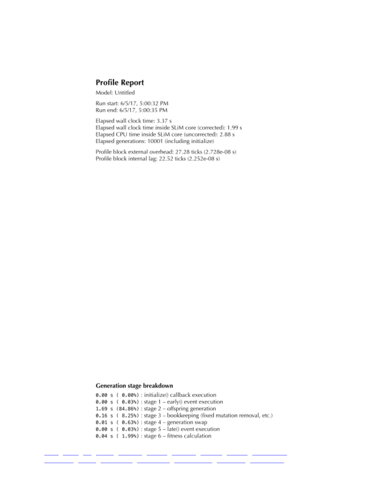
completes, a new window opens that shows a profile report. This report contains several sections;
we will discuss them one by one.
The first section is the report header:
The header contains general information: the title of the model, when the profiling run began
and ended, and some overall timing and memory usage information. (i) The first “wall clock time”
listed is the actual time spent running the model in SLiMgui; in this case, 3.37 seconds. (ii) The
second wall clock time is time spent inside SLiM’s core code; this excludes time spent in SLiMgui,
doing things like updating the user interface. It is also stated to be “corrected”; what this means is
that an attempt has been made to subtract out time spent inside the profiling code itself, reading
the system clock and tabulating profiling results. This number is thus SLiMgui’s best guess as to
how long the model would take if it were run at the command line with the slim command
instead. Since this is the runtime that is generally of interest, it is used as a baseline in the profile
report; later in the report, when timing percentages are reported, they are always percentages out
of this correct wall clock time. (iii) Third comes the elapsed CPU time inside the SLiM core; CPU
time is time spent keeping the processor of the computer busy. This time can be quite different
from the other times reported, as it is here. On the one hand, it excludes time spent in SLiMgui, so
it is generally lower than the total elapsed wall clock time. On the other hand, it is uncorrected –
it does not exclude time spent inside the profiling code itself – so it is typically longer than the
corrected wall clock time. And then, too, CPU time is often different from wall clock times
anyway, particularly if your machine is busy with other tasks that are also occupying the processor.
(Incidentally, to obtain optimal profiling results it is a good idea to quit all other applications and
run the profile when your machine is otherwise completely idle.) (iv) Next is shown the number of
generations over which the profile ran, including the initialization phase of the model. (v) Finally,
two lines profile information about the measured overhead and lag of the profiling code; these
numbers are used to produce the corrected wall clock time, and are not generally of interest to end
users of SLiMgui. (Note that in SLiM 3.2 another two lines were added at the end, providing
information about SLiM’s overall memory usage; these will be discussed in the next section.)
The next section is the “Generation stage breakdown”:
TOC I TOC II WF nonWF initialize() Genome Individual Mutation SLiMSim Subpopulation!
Eidos events fitness() mateChoice() modifyChild() recombination() interaction() reproduction() 389
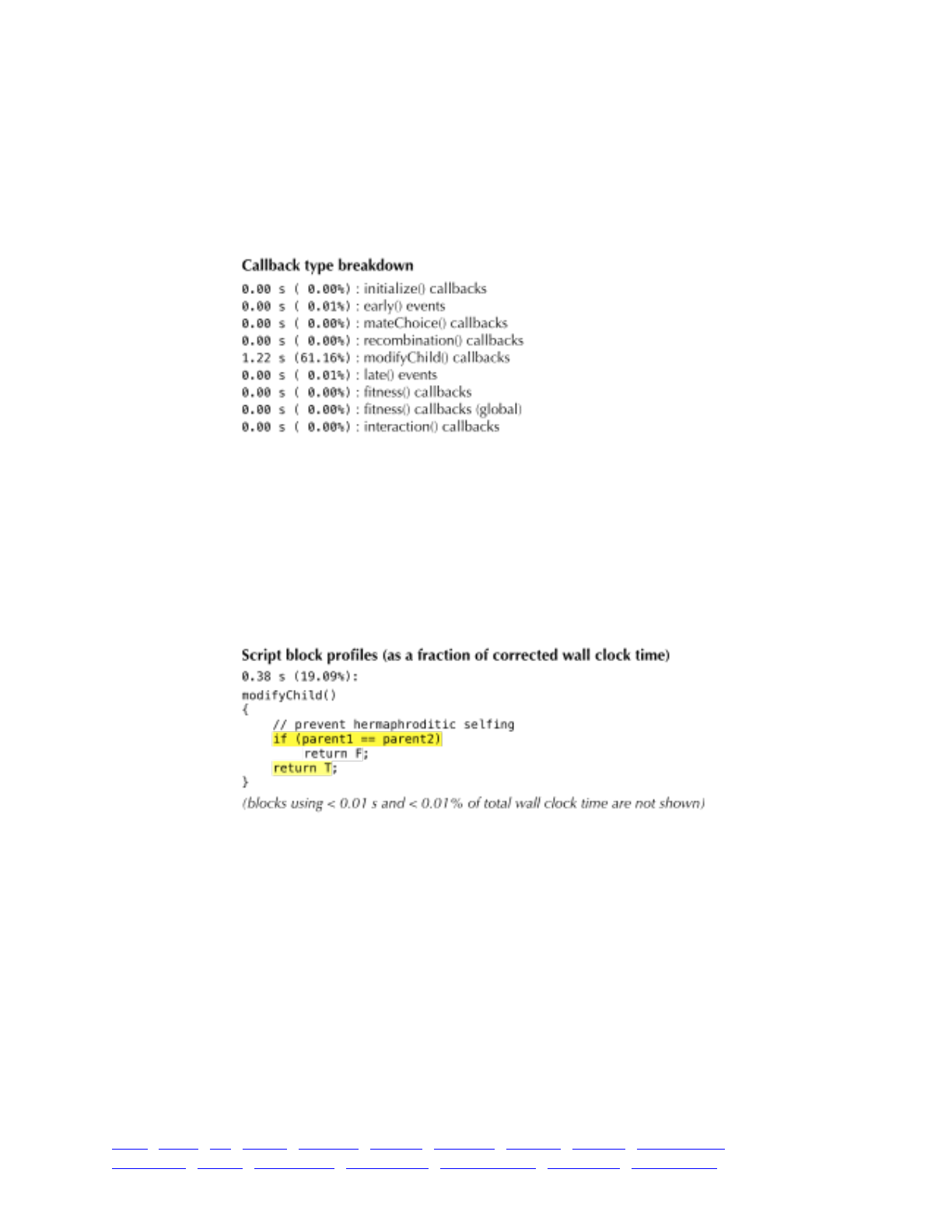
This is a tabulation of where SLiM is spending its time, broken down according to generation
stage. The fact that 84.86% of SLiM’s time is being spent in offspring generation is a red flag; that
generation stage does often take quite a bit of time, but not typically this much. So this is
something to note – depending upon the model it is not necessarily an indication of a problem,
but it is certainly an indication of where you ought to focus your optimization efforts.
Next is the “Callback type breakdown” section:
This section shows a tabulation of where SLiM is spending its time, broken down according to
callback types. This does not add up to 100% because SLiM is spending almost 40% of its time
outside of callbacks, in the SLiM core engine. But it is spending 61.16% of its time inside
modifyChild() callbacks – again, an indication of where to focus optimization efforts. You might
also wonder why 61.16% is different from 84.86%. This is because the additional time, above
61.16%, is being spent by SLiM in offspring generation, but not inside modifyChild() callbacks.
This time would be spent doing mutation generation and recombination, for example.
The next section is titled “Script block profiles (as a fraction of corrected wall clock time)”:
This shows the model’s code, with color highlighting indicating where time is being spent.
Colors range from white (essentially no time spent here) through yellow and up to orange and
finally red (most of the simulation’s time spent here). This section colors the code according to the
time spent as a fraction of the total corrected wall clock time. We can see that the modifyChild()
callback is taking 19.09% of SLiM’s time, and two parts of it are responsible: the test for the two
parents being identical, and the returning of T to indicate that the child should be generated. The
callback does occasionally return F, but that is so rare that that line is more or less white. Again
you might wonder: why is 19.09% different from 61.16%? The reason is that 19.09% is spent
specifically on interpreting the lines of code inside the callback – inside the Eidos interpreter –
whereas 61.16% is spent overall on calling the callback. Calling out to callbacks involves a
certain amount of overhead in SLiM; the Eidos interpreter environment for the callback must be set
up, variable values for it must be initialized, and so forth. The difference between 19.09% and
61.16% reflects all of this overhead. The overhead is very high in this case because the callback is
TOC I TOC II WF nonWF initialize() Genome Individual Mutation SLiMSim Subpopulation!
Eidos events fitness() mateChoice() modifyChild() recombination() interaction() reproduction() 390
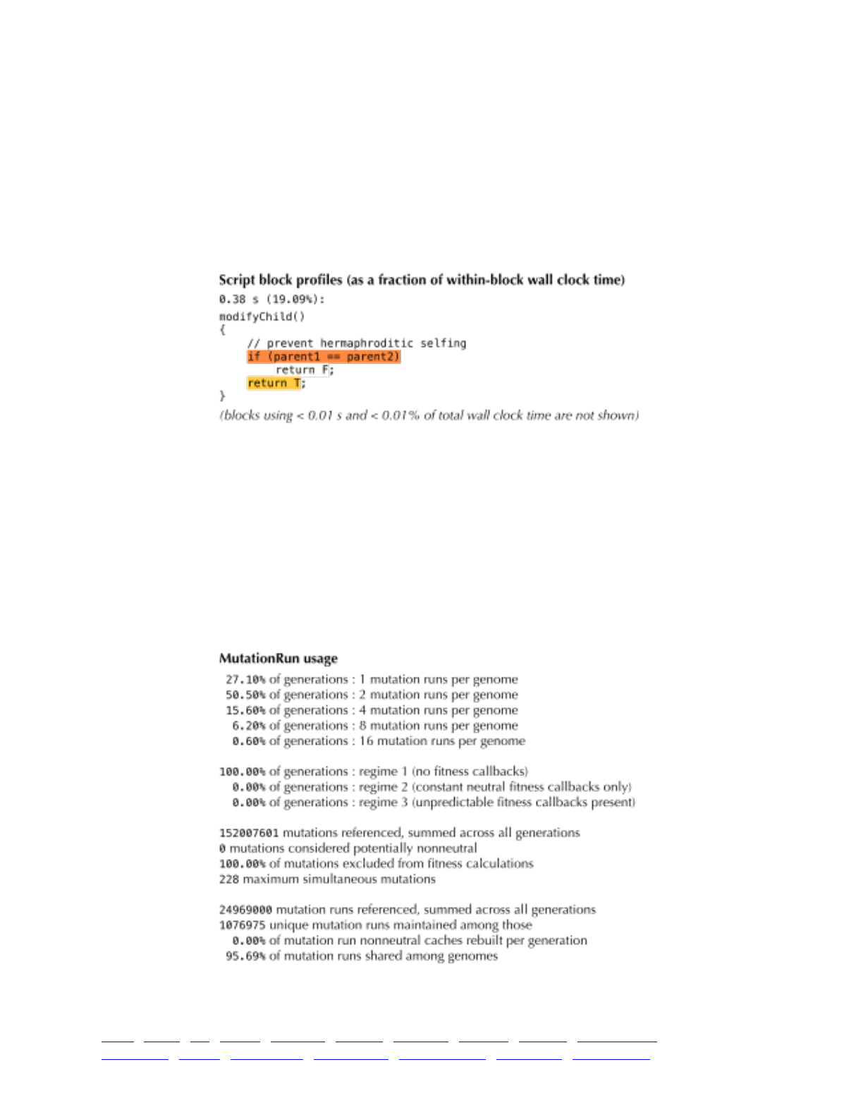
so simple; the more complex a callback’s code is, the less this constant overhead will matter. But
in this case, the profile report is telling us that it is not so much the callback’s code that is hurting
us – it is the fact that we have a callback at all.
Note, by the way, that only the modifyChild() script block is shown here. As the italic
comment at the bottom of the section notes, only script blocks that take more than a certain
amount of time are shown, since script blocks that take a tiny fraction of the total time are
generally not of interest from an optimization perspective.
Following that section is “Script block profiles (as a fraction of within-block wall clock time)”:
This section shows a similar view of the model’s code, but here the colors are scaled to the time
spent within each block. Even a block that takes up almost none of the total time, therefore, will
show “hotspots” that may be close to red. Here the two hotspot lines we noticed before are
colored orange, but the first line is a darker shade, closer to red, indicating that it takes more time
than the second line. This can also be seen in the shades of yellow used in the previous section of
the report, but it is much more subtle; the point of this section, with colors according to within-
block time, is precisely this, to increase the visibility of the hotspot lines. However, this section is
usually of less interest than the previous section, since the proportion of the total corrected wall
clock time is what ultimately matters.
Finally, the last section is “MutationRun usage”:
TOC I TOC II WF nonWF initialize() Genome Individual Mutation SLiMSim Subpopulation!
Eidos events fitness() mateChoice() modifyChild() recombination() interaction() reproduction() 391
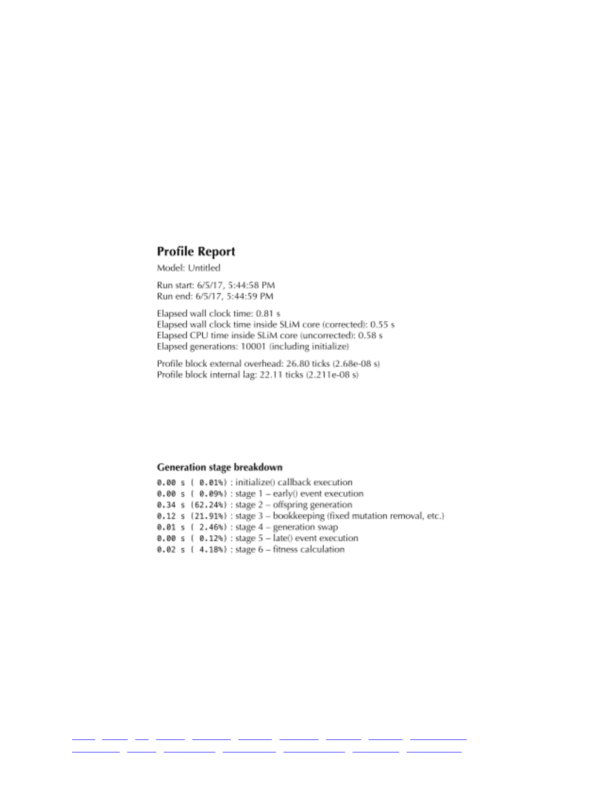
This section contains fairly technical information about some of SLiM’s internal bookkeeping
mechanisms, such as mutation runs and their caching of fitness-related information. Section 18.4
of this manual describes the basic idea behind mutation runs, and so may shed some light on the
meaning of this section. Mostly, however, it is intended for internal use by the developers of SLiM
(the royal we, in other words). If you send us a profile report from your simulation, this section
will help us diagnose the situation. We will not discuss this section further here.
Overall, this report focuses our attention very clearly on the source of the performance problem
with this model: the modifyChild() callback. Happily, as section 12.4 discusses, we can eliminate
that callback now with a call to initializeSLiMOptions(preventIncidentalSelfing=T), which
sets a configuration option that causes SLiM to block incidental selfing internally instead. If we
add that call to the model, remove the modifyChild() callback, and profile the model again, the
header of the report now looks like this:
The total runtime is much shorter now – 0.55 seconds of corrected wall clock time inside the
SLiM core, instead of 1.99 seconds! If we look at the generation stage breakdown, it now shows a
healthier mix of time spent in various generation stages; the runtime is no longer being completely
dominated by one stage:
Offspring generation is now 62.24% instead of 84.86%, so SLiM is busy doing other things too;
and even more encouraging, the total time spent in offspring generation is now 0.34 seconds
instead of 1.69 seconds, so we have shaved off quite a bit of the actual time spent.
The callback type breakdown shows that we are now spending a negligible amount of time in
callbacks:
TOC I TOC II WF nonWF initialize() Genome Individual Mutation SLiMSim Subpopulation!
Eidos events fitness() mateChoice() modifyChild() recombination() interaction() reproduction() 392
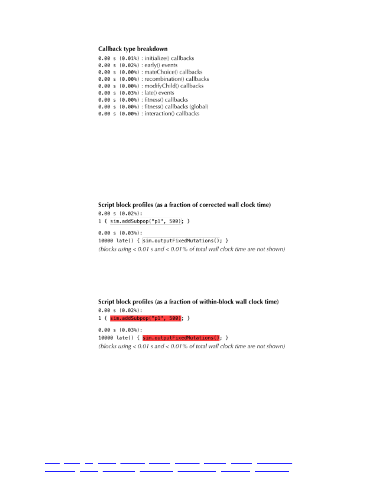
None is over 0.03% of the total time, so they are all basically irrelevant. What this says is that
SLiM is no longer spending a significant amount of time inside the model’s Eidos callbacks;
virtually all of the time is being spent inside the SLiM core. If you still wanted to make this model
faster, you would therefore have to decrease SLiM’s core workload, by doing things like reducing
the population size, reducing the recombination rate or mutation rate, etc. If such revisions to the
model are not possible, then the model might be running about as fast as it possibly can (assuming
there are no design flaws in the model causing it to waste time).
The first script block profile section confirms this; there are no hotspots in the code at all:
Two script blocks are now shown that weren’t shown before, since they are now over the
threshold to be listed; but they take 0.03% or less of the total time.
The second script block profile section shows some red hotspots:
Remember, however, that in this section the coloring indicates the time spent as a fraction of the
within-block time. These lines might be taking 100% of the within-block time; indeed, they could
hardly fail to do so, since each block is only one line long! But the fact remains that their fraction
of the total runtime is inconsequential, so they should be ignored.
Particularly perspicacious readers may have noticed that if the original model took 1.99
seconds, 61.16% of which was dealing with modifyChild() callbacks, one might expect the
modified model to take 0.77 seconds, but in fact it took only 0.58 seconds, so we got an even
larger speedup than expected. Why is this? The main reason is probably that when callbacks are
present, SLiM is often forced to take a slower code path, which adds runtime even beyond the
overhead of handling the callbacks themselves. When modifyChild() callbacks are in force, for
TOC I TOC II WF nonWF initialize() Genome Individual Mutation SLiMSim Subpopulation!
Eidos events fitness() mateChoice() modifyChild() recombination() interaction() reproduction() 393

example, SLiM has to generate children in a random order, to eliminate possible order-dependency
bugs that could otherwise crop up. When no such callbacks are active, SLiM can generate
offspring in a fixed order – females before males, migrants before residents, etc. – which is
substantially faster since it doesn’t require randomization.
All of this might prompt the question: “OK, I’ve got all this profile information, so what?” Well,
in some cases it might allow you to see a way to modify your model to avoid the hotspot in
question; if your profile showed that you were spending an inordinate amount of time doing
addition in a for loop, for example, you might question why you are doing so much addition, and
whether you could use sum() instead – or whether perhaps you don’t need to do all that addition
at all. Eidos also provides quite a few functions that can perform various tasks very quickly; using
functions like unique(), setSymmetricDifference(), which(), and so forth can lead to much faster
code than attempting to code such logic in Eidos by hand.
In other cases, it will allow you to start a conversation with us about the performance problem
you’re seeing; if you say “I’ve got this model and it’s spending 80% of its time inside the
mateChoice() callback running the second for loop, what can I do about that?” that’s a much
better starting point than “My model is slow, help”. If you are having to perform a multistep
algorithm in Eidos for a task that is common, we might be able to add a new utility method to
SLiM to perform this task for you with a single call. This can often result in a big speedup for the
code in question, and it benefits all of SLiM’s users for such utility methods to exist. The
sumOfMutationsOfType() method, for example, was added in response to a performance-related
question from a SLiM user, and is now available to speed up a wide variety of QTL-based models
that need to calculate the additive effects of all mutations of a given type.
18.6 Profiling memory usage in SLiMgui, or with outputUsage()
The previous section introduced SLiMgui’s profiling feature, with an extended example showing
how it can be useful for improving the runtime of a simulation. Beginning in SLiM 3.2, the
profiling feature has been extended to include information about memory usage as well; we will
discuss that extension in this section. Note that sections 18.3 and 18.4 cover some important
ideas about SLiM’s memory usage; you may wish to read those sections first.
First of all, when running SLiM 3.2 or later the header section of a profile report will be a bit
longer due to a subsection added at the end. For a somewhat large spatial simulation with tree-
sequence recording enabled, the report might show something like this:
These lines report statistics about SLiM’s overall memory usage. The first line gives the average
usage, across a samples taken once per generation during the profiling period. The second line
gives the sampled usage in the final generation profiled. Note that these memory usage samples
are always taken at the end of each generation; if memory usage spikes within a generation but
decreases again before the generation’s end that will not be reflected in any of the profiling
statistics discussed in this section (but would be captured by the overall usage statistics discussed
in section 18.3). Also, importantly, these samples – which provide all of the information to be
discussed in this section – reflect only memory allocated and directly controlled by SLiM.
Memory can be used by other factors too: SLiM’s own executable code takes up memory, the
operating system has memory overhead of various types, the C++ standard library makes
allocations that SLiM has no way to measure, etc. However, in large simulations where memory
TOC I TOC II WF nonWF initialize() Genome Individual Mutation SLiMSim Subpopulation!
Eidos events fitness() mateChoice() modifyChild() recombination() interaction() reproduction() 394
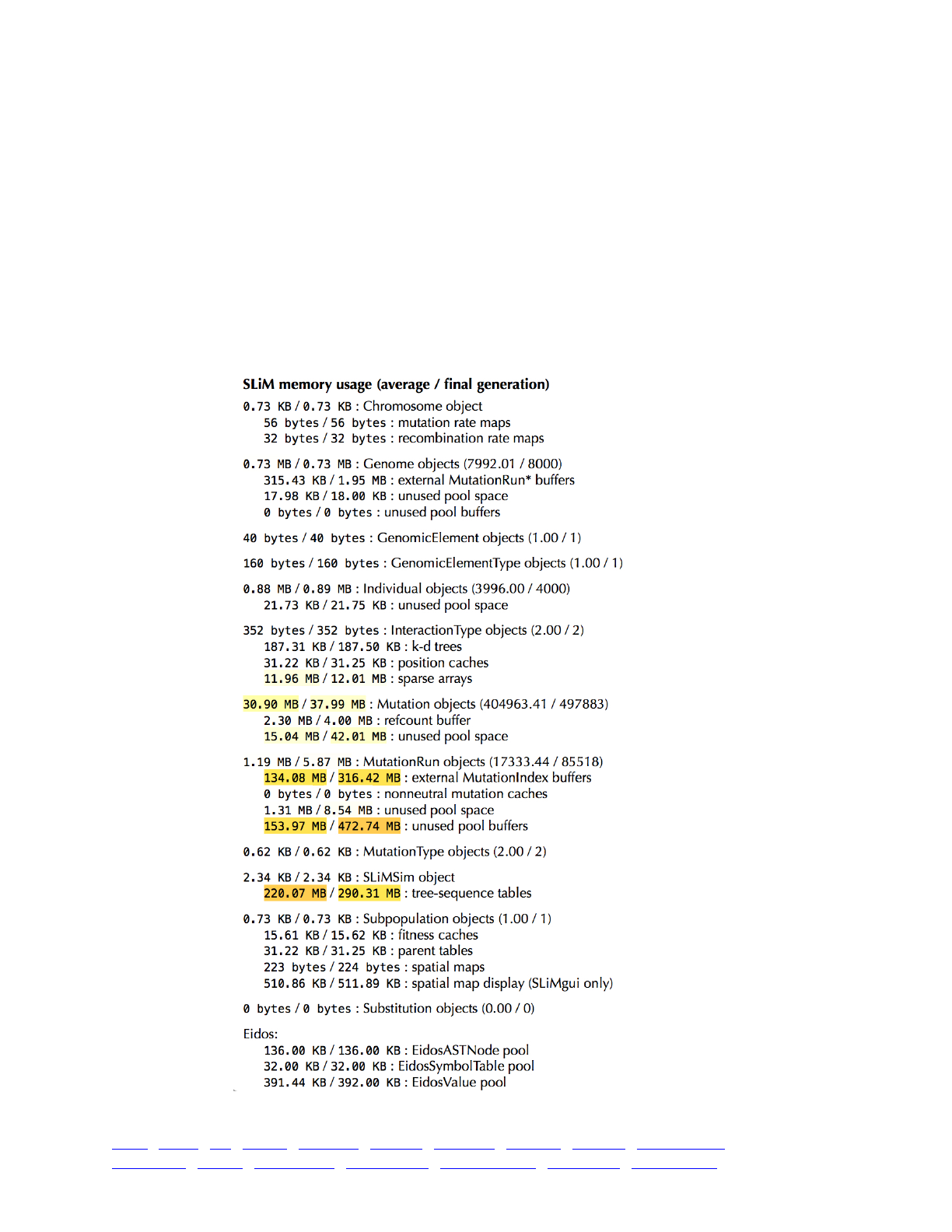
usage is a concern, the memory allocated and directly controlled by SLiM is typically the large
majority of the total memory usage, so this caveat should not prove limiting in practice.
So here we discover that in an average generation SLiM was using 0.56 GB of memory, but that
at the end of the simulation the usage was 1.17 GB in the final generation. That suggests that the
memory usage was increasing over the course of the simulation, which is typical since genetic
diversity often builds up over time. Since the peak memory usage is typically the main concern,
the final generation’s statistics may usually be of the most interest. One might also wish to profile
only the last 100 generations of a model, for example, in order to get averaged statistics that are
not biased downward by the low memory usage toward the beginning of a run.
So far, so good; but these are only summary statistics. How does the memory usage by SLiM
break down? What is all that memory actually being used for? A new section at the end of the
profile report gives much more information:
TOC I TOC II WF nonWF initialize() Genome Individual Mutation SLiMSim Subpopulation!
Eidos events fitness() mateChoice() modifyChild() recombination() interaction() reproduction() 395

Each line in this section gives average and final-generation usage statistics, separated by a slash,
as suggested by the header. Usage is in bytes, KB, MB, GB, or potentially TB; since the units are
mixed they must be noted carefully when comparing numbers. To make it easier to pick out the
areas of highest impact, the usage statistics are color-coded in a similar way to the coloring of
timing statistics earlier in the profile report; white is the lowest proportional usage (inconsequential
in the big picture), and then shades of yellow, orange, and finally red reflect increasing proportions
of total memory usage.
The report is broken down by the object responsible for the usage, sorted alphabetically;
Chromosome comes first, Substitution last, with a small section on memory usage by Eidos at the
end. The first line of each of these subsections gives the memory usage for the objects themselves;
for the Chromosome section it gives the memory used by the one Chromosome object present in the
simulation, for example. Subsequent lines give additional memory usage, by those objects, for
particular purposes. For Chromosome, for example, the memory used by mutation rate maps and
recombination rate maps is listed. This memory is not part of the Chromosome object itself; it is
allocated by the Chromosome object. Each line thus stands on its own; the usage reported by lines
under a given object type is not included in the first line. In other words, the hierarchy here is a
conceptual hierarchy, not a breakdown of totals into sub-totals and sub-sub-totals. For most object
types the number of objects allocated is also reported in parentheses; for example, there were
404963.41 mutation objects allocated in an average generation, and 497883 allocated in the final
generation.
This breakdown shows that the majority of memory is taken up by MutationIndex buffers
allocated by MutationRun; some are being used by currently allocated MutationRun objects, while
others are attached to currently unused MutationRun objects in a pool of reusable mutation runs
kept by SLiM for speed. These MutationIndex buffers are the way that SLiM keeps track of which
mutations are present in each genome; they are like pointers to Mutation objects, but more
compact since they are 32-bit indexes instead of 64-bit pointers. The Mutation objects themselves
take up far less space, and are colored just a light yellow here; this is unsurprising and typical, for
reasons discussed further in section 18.3.
Quite a substantial amount of memory is also taken up by the tree-sequence recording tables
kept by SLiM, since tree-sequence recording is enabled in this model (see section 1.7). Tree-
sequence recording can take up quite a bit of memory, but that memory usage can often be
controlled (at the price of longer runtimes) by controlling the frequency of simplification of the
tree-sequence tables; see the simplificationRatio parameter to initializeTreeSeq() in section
21.1). The model profiled here includes neutral mutations even though tree-sequence recording is
enabled, which is usually not desirable or necessary, so it is paying a hefty price in memory usage
(for illustration purposes).
Finally, a faint yellow tinge tells us that the sparse arrays kept by InteractionType are taking up
a small but noticeable amount of memory. These keep track of the distances and interaction
strengths between individuals; their size will scale with the number of individuals in a model, but
will also be strongly affected by the maximum distance set for the spatial interactions in the model.
The model profiled here uses very short maximum interaction distances, simulating a large
landscape with very local interaction dynamics, which means that these data structures are quite
small. In spatial models with broader spatial interaction kernels, these sparse arrays can take up
much more space; indeed, in the worst case they can scale with the square of the number of
individuals, and can account for the large majority of SLiM’s memory usage. Keeping maximum
interaction distances as small as possible is extremely important for SLiM’s memory usage, and for
its runtime too.
These memory usage statistics can, in some cases, provide a clear picture of how SLiM’s
memory usage could be reduced. This report, for example, could serve as a reminder that we
TOC I TOC II WF nonWF initialize() Genome Individual Mutation SLiMSim Subpopulation!
Eidos events fitness() mateChoice() modifyChild() recombination() interaction() reproduction() 396

probably want to turn off neutral mutations in the model, since tree-sequence recording would
allow us to overlay them after simulation has completed (see section 16.2). If most of the memory
usage of a simulation is in the MutationIndex buffers kept by MutationRun, that would similarly
suggest that the simulation might benefit from the use of tree-sequence-recording. When that is
not possible – when the mutations being simulated are non-neutral, for example – it may be
necessary to reduce the scale of the model, in terms of population size, chromosome length,
mutation rate, recombination rate, etc. Sections 5.5 and 18.3 have some further discussion of this.
TOC I TOC II WF nonWF initialize() Genome Individual Mutation SLiMSim Subpopulation!
Eidos events fitness() mateChoice() modifyChild() recombination() interaction() reproduction() 397

!
!
!
!
!
!
!
!
PART II: THE SLIM REFERENCE"
19. SLiM architecture (WF models)
By default, SLiM uses a Wright-Fisher-type model of evolution,
known in SLiM as a WF model (see section 1.6). This chapter
will discuss the details of the generation cycle in WF models;
chapter 20 provides the same type of discussion for nonWF
models, a more advanced type of SLiM model.
Section 1.3 presented a summary of the life cycle followed by
SLiM within each generation in WF models. The figure shown in
that section is reproduced at right. In this chapter, we will
examine each of these life cycle stages in more detail, in order to
provide a more complete specification of the internal mechanics
of SLiM.
19.1 Step 1: Execution of early() Eidos events
The very first thing that happens in each generation is that the
active property of all script blocks is reset to -1 at the beginning
of the generation, activating all script blocks for the remainder of
the generation unless they are explicitly deactivated again. This
is followed by the execution of early() Eidos events defined by
the user, if any. Details on how to specify an Eidos event are
given in section 22.1, with some further details in section 22.8
regarding their scheduling and the active property.
The salient point here is primarily that these events occur first
in each generation, prior to the generation of offspring. If you
wish to execute an Eidos event after offspring generation has
completed, you should use a late() event; see section 19.5.
Since the details of this step depend entirely on the script you
write, there is little more to say about this step.
19.2 Step 2: Generation of offspring
This is the most complex step in SLiM’s architecture, and it is
broken down into five sub-steps that are executed for each
offspring generated, as shown in the figure at right. Processes
involved in the generation of offspring include migration, mate
choice, mutation, recombination, and the actual production of
offspring individuals.
19.2.1 The order of offspring generation
For each offspring generated, there are generally several decisions to be made: (1) is the
offspring local, or if not, from which other subpopulation are its parents drawn, (2) is it male or
female (in sexual simulations), and (3) is it produced by cloning, selfing, or biparental mating? In
SLiM, the sex ratio specified for a subpopulation is deterministic; SLiM will produce that exact sex
ratio in each generation (so as to avoid the possibility of extinction due to the chance production
of a single-sex child generation). The other decisions are made stochastically; migration rates,
selfing rates, and cloning rates are all probabilities, not deterministic ratios, and you can think of
SLiM as rolling the dice to make these decisions for each offspring individual. This means that the
sex ratio of a subpopulation does not fluctuate over time, but the fraction of offspring that are
migrants, or clones, or selfed, will vary stochastically around the specified rates.
TOC I TOC II WF nonWF initialize() Genome Individual Mutation SLiMSim Subpopulation!
Eidos events fitness() mateChoice() modifyChild() recombination() interaction() reproduction() 399
1. Execution of early() events
2. Generation of offspring;
for each offspring generated:
3. Removal of fixed mutations
unless convertToSubstitution==F
4. Offspring become parents
6. Fitness value recalculation
using fitness() callbacks
7. Generation count increment
2.1. Choose source subpop
for parental individuals,
based on migration rates
2.2. Choose parent 1, based
on cached fitness values
2.3. Choose parent 2, based
on fitness and any defined
mateChoice() callbacks
2.4. Generate the candidate
offspring, with mutation
and recombination (incl.
recombination() callbacks)
2.5. Suppress/modify the
candidate, using defined
modifyChild() callbacks
5. Execution of late() events
The sequence of events within one
generation in WF models.

The order in which offspring are generated, with respect to these decisions, depends upon the
details of your simulation. In the base case, SLiM produces offspring in deterministic tranches; for
example, migrants before locals, and within that, males before females, and within that, cloned
before selfed before biparental. The specifics of this ordering are not guaranteed; the main point is
that you should not rely on the order of offspring being random. In particular, you should
randomly select genomes when doing things like inserting new mutations, to overcome the
possibility of order-dependency and bias (as shown in the recipe in section 10.1). If mateChoice(),
modifyChild(), or recombination() callbacks are defined, SLiM switches its behavior to generate
offspring in a randomized order, rather than in these deterministic tranches. This presents mating
and offspring decisions to those callbacks in a random order, so that bias is not inadvertently
introduced by callbacks.
SLiM is fundamentally a model of juvenile migration, not migration at the adult stage. This has
several consequences for these decisions that are made for each offspring. First of all, if the
offspring is a migrant produced biparentally, it should be noted that both parents will be drawn
from the same source subpopulation; matings between parents in different subpopulations never
occur in SLiM, since adults do not migrate. Second, it should be noted that the parental source
subpopulation is “in charge” of most of the decisions made regarding the offspring, since the
offspring is produced within that source subpopulation by the mating of parentals in that
subpopulation. In particular, the source subpopulation determines the cloning rate and selfing
rate, as well as the mateChoice(), modifyChild(), and recombination() callbacks used. The only
exception is sex ratio; the sex ratio of the destination subpopulation governs the ratio of males to
females produced in that subpopulation, regardless of the sex ratios specified by the various source
subpopulations contributing migrants.
19.2.2 Mate choice
Once the decisions outlined in the previous section have been made for a given offspring
(parental subpopulation, sex, clonal/selfed/biparental), the next step in offspring generation is
choosing the parent(s) for the offspring. The precise way in which this is done depends upon the
type of offspring being produced:
(1) If the offspring is to be clonal, a single parent is drawn randomly, according to probabilities
proportional to fitness, from the source subpopulation. Any mateChoice() callbacks defined are
not called; there is presently no way to influence the choice of clonal parents except by modifying
fitness values with a fitness() callback. Offspring generation proceeds along a different path in
this case, introducing mutations as usual (see below) but without recombination.
(2) If the offspring is to be selfed, a single parent is drawn according to fitness, as with cloning.
That parent is then considered to be a forced choice for the second parent; mateChoice() callbacks
are not used. Offspring generation proceeds thereafter as with biparental mating.
(3) If the offspring is to be the result of biparental mating, a first parent is drawn according to
fitness; in sexual simulations the first parent will always be female, since SLiM models female
choice. If no mateChoice() callbacks are defined, a second parent is then drawn according to
fitness – in sexual simulations, always a male. If mateChoice() callbacks are defined, on the other
hand, those callbacks will be called to determine mating weights for all eligible parents given the
chosen first parent, as detailed in section 22.3 and 17.6, and a second parent will then be drawn
according to those mating weights. If the mateChoice() callbacks completely reject the first
parent, offspring generation will go back to almost the beginning of the process, but the source
subpopulation will remain unchanged, as will the sex of the offspring to be produced (but the
cloned/selfed/biparental decision, and the choice of the first parent, will be made over from
scratch).
TOC I TOC II WF nonWF initialize() Genome Individual Mutation SLiMSim Subpopulation!
Eidos events fitness() mateChoice() modifyChild() recombination() interaction() reproduction() 400

19.2.3 Mutation and recombination
Once a parent or parents have been successfully selected, as detailed in the previous
subsection, a candidate offspring is generated from the chosen parent(s). As the first step in this
process, the mutations to be introduced into each of the two offspring genomes are generated. The
number of mutations is determined by the current mutation rate, using a draw from the appropriate
Poisson distribution. The particular mutations are then generated one by one, each with a position
drawn at random from within all of the defined genomic elements in the chromosome. Given that
position, the identity of the genomic element and thus the controlling genomic element type is
determined. Using the list of mutation types and associated probabilities for the genomic element
type, a particular mutation type is chosen probabilistically. Finally, a selection coefficient is drawn
from the chosen mutation type (see section 21.8), and a new Mutation object is constructed with
the selection coefficient. In this manner, all of the new mutations to be introduced into each of the
two offspring genomes are generated.
If the offspring is to be produced clonally, what follows is then relatively simple: conceptually,
the parental genomes are replicated exactly in the offspring, and then the mutations are interleaved
into the offspring genomes at their particular positions.
If the offspring is to be produced by selfing or biparentally (which are identical at this stage of
the process), recombination is also involved, making the process somewhat more complex. The
first offspring genome is produced via recombination between the two genomes of the first parent,
and the second offspring genome is produced via recombination between the two genomes of the
second parent (mimicking the process of meiosis to produce haploid gametes that merge to form a
fertilized egg). For each offspring genome, the number of recombination breakpoints is drawn
from a Poisson distribution based upon the overall recombination rate (computed internally by
SLiM). The position of each breakpoint is then drawn, based upon the recombination ranges and
rates set on the chromosome. If a non-zero probability of gene conversion is set, and a random
draw indicates that gene conversion actually occurs for a given breakpoint, an additional
breakpoint (above and beyond the drawn number of breakpoints) will be added following the
converted breakpoint, with a positional offset drawn from a geometric distribution satisfying the
requested average gene conversion length. Note that occasionally this additional breakpoint will
fall after another drawn breakpoint position; this will result in a gene conversion stretch that is
shorter than the drawn gene conversion length, since the first breakpoint position will end gene
conversion. If recombination() callbacks are defined, they are called at this point to allow them
to modify the crossover points and the gene conversion stand and end points. Finally, given the
two genomes from the parent, the list of recombination breakpoints, and the set of mutations to be
introduced, SLiM then weaves together the final genome of the offspring, alternating between the
two parental genomes as dictated by the recombination breakpoints, and introducing mutations at
the chosen positions.
By default, SLiM allows multiple mutations to exist at the same site in a single individual –
“stacked” mutations, as we call them. This behavior is often desirable, but sometimes it is useful to
prevent stacked mutations of a given mutation type. The stacking policy of a given mutation type
can be changed using MutationType’s mutationStackPolicy and mutationStackGroup properties,
as documented in section 21.9.1.
19.2.4 Child modification
Once the two genomes of the candidate offspring have been generated, as described in the
previous section, child modification by modifyChild() callbacks (described in sections 21.4 and
21.8) occurs, if any callbacks are active. These callbacks are called regardless of whether the
offspring was the product of cloning, selfing, or biparental mating; all types of children may be
modified.
TOC I TOC II WF nonWF initialize() Genome Individual Mutation SLiMSim Subpopulation!
Eidos events fitness() mateChoice() modifyChild() recombination() interaction() reproduction() 401

These callbacks may modify the candidate offspring in any way desired. For our purposes here,
the only question arises with the possibility that a modifyChild() callback will suppress the
candidate offspring altogether, rather than just modifying it. This can be thought of as representing
juvenile mortality, if you wish; it could also represent postmating reproductive isolation, such as
infertility or developmental inviability. In some cases, suppression of a candidate offspring can
also be thought of as representing a type of mate choice.
When a candidate offspring is suppressed, generation of the offspring goes back almost to the
beginning of the process, as with rejection of the first parent by a mateChoice() callback. In fact,
in this case the process goes back even further; a new source subpopulation for the offspring is
chosen, in addition to re-making the cloned/selfed/biparental decision and re-choosing the
parents. The only aspect of the offspring generation that is not re-decided in this case is the sex of
the planned offspring individual; that remains fixed since the sex ratio is deterministic, not
stochastic. Note that this means that if a modifyChild() callback suppresses a candidate offspring,
the next time it is called the new candidate will be the same sex as the previously suppressed
candidate. Because of this, it is not possible for a modifyChild() callback to influence the sex
ratio of a subpopulation; attempting to do so will produce an infinite loop.
19.2.5 Child generation
Once a candidate offspring has been generated and modified, and was not suppressed by a
modifyChild() callback, it is added to the target subpopulation. Note that the newly added child
will not be visible as a member of the subpopulation until the point in the lifecycle when the child
generation becomes the parental generation (see section 19.4). This prevents order-dependencies
in which the first children generated might otherwise influence the remainder of the child
generation process.
19.3 Step 3: Removal of fixed mutations
After all offspring have been generated for all subpopulations, SLiM performs bookkeeping
regarding the mutations in the simulation. In particular, it scans through every genome in every
individual in every subpopulation, and tallies up how many times each of the mutations in the
simulation is actually present in the child generation.
The results from this scan are used to clean house. If a mutation is no longer referenced by any
genome in the simulation, that mutation has been lost (whether due to selection or drift), and SLiM
forgets about it. If, on the other hand, a mutation is now contained by every genome in the
simulation, that mutation has fixed. In this case, SLiM normally creates a new Substitution
object as a placeholder, to record the details of the fixed mutation, and then removes the mutation
from the simulation. This is essentially an optimization for efficiency; if fixed mutations were not
removed, a long-running simulation would accumulate ever more mutations needing to be
tracked. In general the substitution is harmless; a fixed mutation cannot generally decrease in
frequency, and generally no longer influences fitness (since it is possessed by all individuals, and
thus has an identical effect on the fitness of all individuals).
However, there are specific circumstances in which the removal of fixed mutations is not
desirable. In particular, if the fixed mutation would continue exerting a varying effect on fitness
among individuals (because of epistasis, for example), the substitution of the mutation would result
in incorrect fitness values. Also, if the script for a simulation intends to remove the mutation from
some genomes later in the simulation run (perhaps simulating a back-mutation) then it would be
desirable to prevent the substitution of the mutation. To accommodate these possibilities, the
convertToSubstitution property of a mutation type can be set to F to suppress substitution of
mutations of that type; see section 21.9.1.
TOC I TOC II WF nonWF initialize() Genome Individual Mutation SLiMSim Subpopulation!
Eidos events fitness() mateChoice() modifyChild() recombination() interaction() reproduction() 402

19.4 Step 4: Offspring become parents
As mentioned in section 19.2.5, newly generated offspring are kept by SLiM as members of a
child generation that is not visible to the model mechanics (or to your Eidos scripts), to avoid
order-dependencies and other confusion. After fixed mutations have been removed, as described
in the previous section, the child generation becomes the new parental generation, and the old
parental generation is discarded.
19.5 Step 5: Execution of late() Eidos events
After the child generation is promoted to the parental generation, the next step is to execute
late() Eidos events defined by the user, if any. Details on how to specify an Eidos event are given
in section 22.1, with some further details in section 22.8 regarding their scheduling and the active
property. Eidos late() events are most often used when output is being generated (since you
typically want to output the state of the simulation at the end of a generation, not at the
beginning), and when adding or removing mutations (since you want those changes to be reflected
in the fitness values calculated for individuals, prior to the next offspring generation step).
Changing of selection or dominance coefficients should also typically be done in a late() event,
for the same reason. See sections 4.2.1, 10.1, and 10.6.1 for discussion and examples.
19.6 Step 6: Fitness value recalculation
After the child generation is promoted to the parental generation, the next step is to compute
fitness values for the new adult individuals, including the effects of any fitness() callbacks.
Fitness values computed at the end of one generation are actually used during mating in the
following generation; this is something to keep in mind if you are designing fitness() callbacks
that you want to be active only across a specific generation range. The reason SLiM does this has
to do mostly with running in SLiMgui; it is desirable that SLiMgui should show newly-calculated
fitness values for the new parental generation when single-stepping through generations. If fitness
values were not calculated until the beginning of the next generation, they would not yet be
available for display.
If fitness() callbacks are not active for a given subpopulation, calculating the fitness of an
individual is relatively straightforward. SLiM uses a model of multiplicative fitness between sites.
An initial relative fitness w of 1.0 is assumed for the individual (unless fitnessScaling values have
been set; in fact, the initial fitness w is the product of the individual’s fitnessScaling property and
its subpopulation’s fitnessScaling property, but these properties are 1.0 by default). Then, each
mutation possessed by the individual is evaluated as to whether it is present in just one of the
individual’s genomes (i.e. is heterozygous) or is present in both genomes (i.e. is homozygous). If a
mutation is homozygous, the individual’s relative fitness is updated as:
w = w * (1.0 + selectionCoefficient),
whereas if the mutation is heterozygous, the relative fitness is updated as:
w = w * (1.0 + dominanceCoeff * selectionCoeff).
where the dominance coefficient of the mutation is defined by the mutation’s mutation type, in the
default case of simulating autosomes. For simulations of the X chromosome, the mutation type’s
dominance coefficient is used for heterozygous XX females, whereas XY males that are
“heterozygous” because they possess the mutation on their lone X chromosome use a global
dominance coefficient (see initializeSex(), section 21.1, and the dominanceCoeffX property of
SLiMSim, section 21.12.1). Simulations of the Y chromosome do not use a dominance coefficient
TOC I TOC II WF nonWF initialize() Genome Individual Mutation SLiMSim Subpopulation!
Eidos events fitness() mateChoice() modifyChild() recombination() interaction() reproduction() 403

at all; the first of the two formulas above is used. If the new relative fitness is zero or less, the
mutation just evaluated was lethal, and so the final relative fitness of the individual is 0.0.
Otherwise, SLiM proceeds with evaluating the next mutation, until all mutations have been
evaluated to produce a final relative fitness value.
If fitness() callbacks are defined (as described in section 22.2), this procedure is modified
slightly. In this case, the multiplicative effect on relative fitness that would be produced by a given
mutation is calculated, exactly as above, but instead of simply multiplying w by that fitness effect,
SLiM calls out to fitness() callbacks to allow them to modify the relative fitness value. After
callbacks, w is multiplied by the final fitness effect for the mutation. The fitness() callback
calculates the relative fitness of the mutation in the individual, whether the mutation is
heterozygous or homozygous; if you wish the calculated fitness value to be different in those two
cases, then the fitness() callback needs to explicitly take the heterozygosity of the mutation into
account (which is part of the information provided to the callback by SLiM, so doing so is not
difficult; see section 22.2).
In SLiM version 2.3 and later, it is possible to define global fitness() callbacks, which are
applied exactly once to every individual without reference to a focal mutation or a particular
mutation type (see section 22.2). The fitness values returned by global fitness() callbacks are
multiplied in to the fitness value previously computed for the individual, as:
w = w * relativeFitness.
The fitness effects of global fitness() callbacks thus combine multiplicatively with all of the
fitness effects of mutations, and multiple global fitness() callbacks may be defined. Unlike other
types of callbacks, the order in which global fitness() callbacks are called is formally undefined,
both relative to other global fitness() callbacks and relative to ordinary (i.e., non-global)
fitness() callbacks. Also note that global fitness callbacks might not be called at all for a given
individual if that individual’s fitness has already been determined, by previous callbacks or fitness
effects, to be equal to zero. Models should therefore be extremely cautious in making any
assumptions whatsoever regarding the timing or order in which global fitness() callbacks will be
executed, or whether they will be executed at all; global fitness() callbacks that have external
side effects, such as changing the active property of script blocks or defining Eidos constants, are
not recommended.
In SLiM 3.0 and later, the fitnessScaling property may be set on the subpopulation or the
individual (or both) to multiplicatively influence individual fitness values, as mentioned above.
This is often a more efficient and simpler alternative to defining a global fitness() callback.
One caveat is that fitness calculations are done sequentially for all of the individuals in each
subpopulation, rather than being done in a random order. This means that fitness() callbacks
should be written in such a way as to make each fitness computation independent of all others,
and independent of the order in which they are done. A fitness() callback that produces a
different result the first time it is run in a generation compared to subsequent times, for example,
would introduce bias and order-dependency into a model, particularly since the order of genomes
in each subpopulation is not necessarily random (see section 19.2.1).
19.7 Step 7: Generation count increment
The final step in each generation is that the generation count is incremented. SLiM then checks
whether the simulation is over; if there are no events or callbacks scheduled to execute in the new
generation or any subsequent generation (not counting events and callbacks with no specified end
generation), the simulation is deemed to be over, and execution halts.
TOC I TOC II WF nonWF initialize() Genome Individual Mutation SLiMSim Subpopulation!
Eidos events fitness() mateChoice() modifyChild() recombination() interaction() reproduction() 404
20. SLiM architecture (nonWF models)
By default, SLiM uses a Wright-Fisher-type model of evolution,
known in SLiM as a WF model – but an alternative non-Wright-
Fisher, or nonWF, model type may be chosen instead (see section
1.6 and chapter 15). This chapter will discuss the details of the
generation cycle in such models. Chapter 19 provides such
discussion for WF models; to avoid a lot of duplicated verbiage,
this chapter will assume familiarity with the WF generation cycle
as described in chapter 19, and will make reference to that
chapter rather than spelling out every detail a second time.
The figure shown at right is a summary of the life cycle
followed by SLiM within each generation in nonWF models. In
this chapter, we will examine each of these life cycle stages in
more detail, in order to provide a more complete specification of
the internal mechanics of SLiM.
20.1 Step 1: Generation of offspring
In nonWF models, the first thing to happen each generation is
the generation of new offspring. (OK – technically, as in WF
models, this is preceded by resetting the active properties of all
script blocks; see section 19.1). This is the most complex step in
SLiM’s architecture, and in nonWF models it is broken down into
four sub-steps that are executed for each offspring generated, as
shown at right. Processes involved in the generation of offspring
include mate choice, mutation, recombination, and the actual
production of offspring individuals. (In WF models, migration is
also effected during offspring generation, but this is not the case
in nonWF models.)
20.1.1 The order of offspring generation
For each offspring generated, there are generally several
decisions to be made: (1) what are its parents, (2) is it male or
female (in sexual simulations), and (3) is it produced by cloning,
selfing, or biparental mating? In WF models, these decisions are
made by SLiM’s core engine, as described in section 19.2.1,
based upon parameters such as the sex ratio, cloning rate, and
selfing rate, as well as upon individual fitness values and the
results from mateChoice() callbacks. In nonWF models, in
contrast, all of these decisions are made by the model’s script: reproduction() callbacks are called
once for each individual in the model, to request that each individual generates its own offspring
to be added to the population.
The order in which individuals are asked to generate their offspring is always random in nonWF
models, across the entire population, to try to prevent order-dependencies from biasing offspring
generation. In addition to this, however, it is important to design your reproduction() callbacks to
be independent; in general, the reproductive behavior of each individual should probably be
independent of the reproductive behavior of every other individual, so whether A is asked to
reproduce before B, or B before A, does not bias the outcome of the model. There are certainly
cases where you might violate this principle; in a model of monogamous mating, for example, the
TOC I TOC II WF nonWF initialize() Genome Individual Mutation SLiMSim Subpopulation!
Eidos events fitness() mateChoice() modifyChild() recombination() interaction() reproduction() 405
2. Execution of early() events
1. Generation of offspring;
for each extant individual:
5. Removal of fixed mutations
unless convertToSubstitution==F
4. Viability/survival selection,
based on fitness values and
(optionally) carrying capacity
3. Fitness value recalculation
using fitness() callbacks
7. Generation count increment,
individual age increments
1.1. Call reproduction()
callbacks defined for each
reproducing individual
1.2. The callback(s) make
Subpopulation calls
requesting new offspring
1.3. Generate the candidate
offspring, with mutation
and recombination (incl.
recombination() callbacks)
1.4. Suppress/modify the
candidate, using defined
modifyChild() callbacks
6. Execution of late() events
The sequence of events within one
generation in nonWF models.

first female asked to reproduce might be able to claim her choice of males, whereas the last female
asked to reproduce might have little or no choice since most males would already be claimed.
Sometimes such asymmetries are acceptable or even desirable; sometimes, however, they would
constitute a bug. So the message of this subsection is primarily: think carefully about the order of
offspring generation, and about the independence of each reproductive event (or the lack thereof),
and make sure your models does what you really want it to.
20.1.2 Individual-based reproduction with reproduction() callbacks
As mentioned above, reproduction() callbacks are called for each individual in the model.
The task of each callback is to generate the offspring from one focal individual. In sexual models,
perhaps females would generate offspring and males would not (or perhaps the opposite, if males
are the choosy sex in the biological system being modeled). In monogamous-mating models, a
single mate might be chosen and then a litter of offspring generated through crosses with that
mate; in a non-monogamous model each offspring generated might be with a different mate.
Some offspring might be generated via cloning or selfing, rather than biparental mating. The sex of
offspring in sexual models might be equally likely to be male or female, or there might be some
sex-ratio bias. Most importantly, in nonWF models all of these decisions can depend upon the
genetics and other state of each individual, rather than being dictated by overall parameters as in
WF models.
Regardless of how a given model makes these decisions, it always expresses them to SLiM in
one way: by making method calls on Subpopulation objects, requesting the addition of new
offspring. There are four methods that can be called: addCrossed() to add an offspring resulting
from a biparental cross, addSelfed() to add an offspring resulting from selfing (i.e., sexual self-
fertilization in a hermaphroditic individual), addCloned() to add an offspring resulting from clonal
reproduction, or addEmpty() to an offspring with no parents and no empty genomes (presumably
to be filled in some special way by script, subsequently). Each such method call made sets off the
chain of events described in the following subsections: mutation and recombination, child
modification, and child generation.
20.1.3 Mutation and recombination
Mutation and recombination occur in nonWF models exactly as they do in WF models; see
section 19.2.3 for details.
20.1.4 Child modification
Child modification, via modifyChild() callbacks, occurs in nonWF models largely as it does in
WF models; see section 19.2.4 for details. The important difference is that whereas WF models
have a target subpopulation size to reach, and thus must keep generating offspring until that target
is reached, the same is not true of nonWF models. In nonWF models, therefore, if a
modifyChild() callback returns F to indicate that a given offspring should not be generated (due to
postmating reproductive isolation or genetic incompatibility, for example), that is the end of it.
That offspring will simply not be generated; there will be one fewer offspring individual, in the
end, than there would have been if the modifyChild() callback had returned T. In this case, the
Subpopulation method call that initiated offspring generation, such addCrossed(), will return NULL
to its caller. This is generally desirable; see section 22.7 for further discussion of how this behavior
interacts with reproduction() callbacks.
20.1.5 Child generation
Once a candidate offspring has been generated and modified, and was not suppressed by a
modifyChild() callback, it is queued for addition to the target subpopulation. Note that the newly
added child will not be visible as a member of the subpopulation until the end of offspring
TOC I TOC II WF nonWF initialize() Genome Individual Mutation SLiMSim Subpopulation!
Eidos events fitness() mateChoice() modifyChild() recombination() interaction() reproduction() 406

generation. This prevents newly generated offspring from being chosen as mates, or otherwise
influencing the remainder of the child generation process.
20.2 Step 2: Execution of early() Eidos events
Offspring is followed by the execution of early() Eidos events defined by the user, if any. The
mechanics of this are the same as in WF models, but the semantics of early() versus late()
events are actually reversed in nonWF models, in some ways.
In WF models, early() events occur just before offspring generation and late() events happen
just after; in nonWF models this positioning is reversed, because offspring generation has been
moved earlier in the generation cycle. Similarly, in WF models late() events are usually the best
place to add new mutations, because the next stage is fitness evaluation, which immediately
incorporates the fitness effects of the new mutations; but in nonWF models early() events are
usually the best place to add new mutations, for the same reason.
In WF models, late() events are generally the best place to put output events so that they
reflect the final state at the end of a generation; in nonWF models, however, output can make
sense in either an early() or a late() event, depending upon whether you want to see the state of
the population before or after viability selection. However, reading in a previously written output
file, or otherwise setting up new population state, is generally best done in an early() event in
nonWF models so that fitness values are recalculated immediately after the change (just as with
adding new mutations). So if you call outputFull() with the intention of reading the output back
in with readFromPopulationFile() later, you will probably want to do the output in an early()
event so that you can, correspondingly, do the read in an early() event as well without skipping
or doubling any generation cycle stages.
For those who are curious: the reason for this reordering of the generation cycle in nonWF
models is the addition of the viability/survival generation cycle stage, which does not exist in WF
models. It is desirable to have an opportunity for scripted events between offspring generation and
selection, and then between selection and the next offspring generation stage. It is also desirable
for selection to happen after offspring generation in the cycle, so that the population state at the
end of each generation (as displayed in SLiMgui, for example) is after selection has occurred.
These constraints, taken together, dictate the order of the generation cycle in nonWF models.
20.3 Step 3: Fitness value recalculation
After the execution of early() events, the next stage in nonWF models is to compute fitness
values for all individuals, including the effects of any fitness() callbacks. The mechanics of this
are exactly the same in nonWF models as in WF models; see the extensive discussion in section
19.6.
However, because of the reordering of the generation cycle, the semantics of fitness evaluation
in nonWF models are a bit different. In WF models, as section 19.6 explains, the fitness values
calculated in generation T are actually used, to influence mating, in generation T+1. In nonWF
models, however, fitness values calculated in generation T are then used immediately, in
generation T, to influence survival (see the next subsection). This oddity of WF models is therefore
not present in nonWF models, making them a bit conceptually simpler.
The actual meaning of individual fitness values is also different between WF and nonWF
models; see the next section for discussion.
TOC I TOC II WF nonWF initialize() Genome Individual Mutation SLiMSim Subpopulation!
Eidos events fitness() mateChoice() modifyChild() recombination() interaction() reproduction() 407

20.4 Step 4: Viability/survival selection
After fitness values have been recalculated for all individuals, viability selection then occurs
immediately. In WF models, viability selection does not exist (or you could consider new offspring
to have a survival rate of 100%, and the parental generation to have a survival rate of 0%, if you
like). In nonWF models, in contrast, viability selection is the primary way in which differential
fitness is expressed; individual fitness values influence survival, not mating success.
Viability selection in nonWF models is mechanistically simple. For a given individual, a fitness
of 0.0 or less results in certain death; that individual is immediately removed from its
subpopulation. A fitness of 1.0 or greater results in certain survival; that individual remains in its
subpopulation, and will live into the next generation cycle. A fitness greater than 0.0 and less than
1.0 is interpreted as a survival probability; SLiM will do a random draw to determine whether the
individual survives or not.
This change in the way individual fitness is used has large consequences. First of all, it means
that in nonWF models fitness is absolute fitness, whereas in WF models fitness is relative fitness.
Second, it means that in nonWF models selection is generally hard selection, reducing the size of
the population proportionate to mean population fitness, whereas in WF models it is generally soft
selection, changing the relative success of particular genes but not changing the size of the
population. Third, it means that in nonWF models the population is not automatically regulated –
both extinction and unbounded exponential growth are very real possibilities – whereas in WF
models SLiM automatically regulates the population size. These three observations are all really
different ways of looking at the same basic fact.
Because of this shift, nonWF models need to treat individual fitness differently than WF models.
For one thing, there is generally a need to introduce some sort of density-dependent fitness, in a
global fitness() callback, that prevents exponential growth by decreasing individual fitness as the
population size gets larger. Second, there may be a need to rethink how beneficial mutations
work, since increasing the fitness of an individual above 1.0 has no effect in nonWF models (since
guaranteed survival is as good as it gets); it may be desirable to have a baseline fitness, for
individuals possessing empty genomes, of less than 1.0 so that beneficial mutations can increase
the probability of survival above that baseline. This would also be achieved with a global
fitness() callback (perhaps in conjunction with density-dependence). All of this is entirely up to
the model’s script.
Finally, it is worth noting that it is certainly to have genetics and other individual state influence
mating success and/or fecundity in nonWF models, as in WF models. In nonWF models that is
done by influencing the dynamics in the offspring generation stage in script, however; it is not an
automatic consequence of the fitness values calculated by SLiM.
20.5 Step 5: Removal of fixed mutations
After viability selection, SLiM tallies mutation frequencies and removes fixed and lost
mutations. The mechanics of this are essentially the same as in WF models; see section 19.3.
However, there is one important difference here between WF and nonWF models. In WF
models, fixed mutations can generally be removed because they no longer influence evolutionary
dynamics, as a consequence of fitness values being relative fitness. If every individual in the
population is fixed for a given mutation, then that mutation has no effect on relative fitness,
regardless of what its selection coefficient might be; the only exceptions are cases where the fitness
effect of the mutation varies from individual to individual, such as when epistatic interactions with
other segregating mutations are present. In WF models, the convertToSubstitution property of
mutation types therefore defaults to T, allowing SLiM to remove fixed mutations by default; when
TOC I TOC II WF nonWF initialize() Genome Individual Mutation SLiMSim Subpopulation!
Eidos events fitness() mateChoice() modifyChild() recombination() interaction() reproduction() 408

that is not desirable, models need to set convertToSubstitution to F to prevent that automatic
removal.
In nonWF models, in contrast, the convertToSubstitution property defaults to F, because in
general it is not safe for SLiM to remove fixed mutations; models need to set it to T to allow
automatic removal. Generally, in nonWF models automatic removal of fixed mutations only
makes sense if several conditions are met: (1)!the mutation is neutral, (2)!the mutation has no direct
non-neutral effects due to any fitness() callback, and (3)!the mutation has no indirect non-
neutral effects on the model through epistasis, mate choice, fecundity, or any other such influences
on the model. If these conditions are met – as is commonly the case for simple neutral
background mutations – it is very important to set convertToSubstitution to T; the effect on
SLiM’s performance can be very large!
20.6 Step 6: Execution of late() Eidos events
Once fixed mutations have been removed, the next step is to execute any defined and active
late() events. This works identically to WF models (see section 19.5). The only important
difference is the way in which the semantics and common uses of early() and late() events differ
between WF and nonWF models, as discussed in section 20.2.
20.7 Step 7: Generation count increment
As in WF models, the last stage of the generation cycle is the incrementing of the generation
count and the check for the simulation being finished (see section 19.7). In nonWF models, the
age of all surviving individuals is also incremented by one during this stage.
TOC I TOC II WF nonWF initialize() Genome Individual Mutation SLiMSim Subpopulation!
Eidos events fitness() mateChoice() modifyChild() recombination() interaction() reproduction() 409

21. SLiM classes
This chapter presents reference documentation for all of the Eidos classes built into SLiM. It
assumes an understanding of the syntax of type-specifiers and method signatures, including the use
of optional arguments and default values. It also assumes an understanding of how classes are
used in Eidos, including how properties are accessed and how methods are called. Part I of this
manual attempts to introduce those topics to some degree, but see the Eidos manual for more
extensive discussion and documentation of these fundamental language features.
A caveat to keep in mind throughout this section is that SLiM 2 and later (unlike SLiM 1.8 and
earlier) generally uses zero-based values; a chromosome might start at index 0 and go to index
99999, for example. Eidos and SLiMgui present this zero-based worldview as well.
21.1 Simulation initialization: initialize() callbacks
Before a SLiM simulation can be run, the various classes underlying the simulation need to be
set up with an initial configuration. In SLiM 1.8 and earlier, this was done by means of # directives
in the simulation’s input file. In SLiM 2 and later, simulation parameters are instead configured
using Eidos.
Configuration in Eidos is done in initialize() callbacks that run prior to the beginning of
simulation execution. Eidos callbacks are discussed more broadly in chapter 22, but for our
present purposes, the idea is very simple. In your input file, you can simply write something like
this:
initialize() { ... }
The initialize() specifies that the script block is to be executed as an initialize() callback
before the simulation starts. The script between the braces {} would set up various aspects of the
simulation by calling initialization functions. These are SLiM functions that may be called only in
an initialize() callback, and their names begin with initialize to mark them clearly as such.
You may also use other Eidos functionality, of course; for example, you might automate generating
a large number of subpopulations with complex migration patterns by using a for loop.
One thing worth mentioning is that in the context of an initialize() callback, the sim global
for the simulation itself is not defined. This is because the state of the simulation is not yet
constructed fully, and accessing partially constructed state would not be safe.
Without further ado, then, here are the initialization functions provided by SLiM:
(void)initializeGeneConversion(numeric$!conversionFraction, numeric$!meanLength)
Configure the likelihood and behavior of gene conversion events. The probability of gene conversion
occurring for any one recombination event is given by conversionFraction, and the mean of the
geometric distribution from which the length of the gene conversion stretch will be drawn is specified
by meanLength (specified in base positions). Note that chromosome positions with a recombination
rate of exactly 0.5 will not be candidates for gene conversion, as it is assumed that they represent
junction points between discrete chromosomes.
(void)initializeGenomicElement(io<GenomicElementType>$!genomicElementType,
integer$!start, integer$!end)
Add a genomic element to the chromosome at initialization time. The start and end parameters give
the first and last base positions to be spanned by the new genomic element. The new element based
upon the genomic element type identified by genomicElementType, which can be either an
integer, representing the ID of the desired element type, or an object of type
GenomicElementType, specified directly.
TOC I TOC II WF nonWF initialize() Genome Individual Mutation SLiMSim Subpopulation!
Eidos events fitness() mateChoice() modifyChild() recombination() interaction() reproduction() 410

(object<GenomicElementType>$)initializeGenomicElementType(is$!id,
io<MutationType>!mutationTypes, numeric!proportions)
Add a genomic element type at initialization time. The id must not already be used for any genomic
element type in the simulation. The mutationTypes vector identifies the mutation types used by the
genomic element, and the proportions vector should be of equal length, specifying the relative
proportion of mutations that will be draw from the corresponding mutation type (proportions do not
need to add up to one; they are interpreted relatively). The id parameter may be either an integer
giving the ID of the new genomic element type, or a string giving the name of the new genomic
element type (such as "g5" to specify an ID of 5). The mutationTypes parameter may be either an
integer vector representing the IDs of the desired mutation types, or an object vector of
MutationType elements specified directly. The global symbol for the new genomic element type is
immediately available; the return value also provides the new object.
(object<InteractionType>$)initializeInteractionType(is$!id, string$!spatiality,
[logical$!reciprocal!=!F], [numeric$!maxDistance!=!INF],
[string$!sexSegregation!=!"**"])
Add an interaction type at initialization time. The id must not already be used for any interaction type
in the simulation. The id parameter may be either an integer giving the ID of the new interaction
type, or a string giving the name of the new interaction type (such as "i5" to specify an ID of 5).
The spatiality may be "", for non-spatial interactions (i.e., interactions that do not depend upon
the distance between individuals); "x", "y", or "z" for one-dimensional interactions; "xy", "xz", or
"yz" for two-dimensional interactions; or "xyz" for three-dimensional interactions. The dimensions
referenced by spatiality must have been previously defined as spatial dimensions with
initializeSLiMOptions(); if the simulation has dimensionality "xy", for example, then
interactions in the simulation may have spatiality "", "x", "y", or "xy", but may not reference spatial
dimension z and thus may not have spatiality "xz", "yz", or "xyz". If no spatial dimensions have
been configured, only non-spatial interactions may be defined.
The reciprocal flag may be T, in which case the interaction is guaranteed by the user to be
reciprocal: whatever the interaction strength is for individual B upon individual A, it will be equal (in
magnitude and sign) for A upon B. This allows the InteractionType to reduce the amount of
computation necessary by up to a factor of two. If reciprocal is F, the interaction is not guaranteed
to be reciprocal and each interaction will be computed independently. The built-in interaction
formulas are all reciprocal, but if you implement an interaction() callback (see section 22.6), you
must consider whether the callback you have implemented preserves reciprocality or not. For this
reason, the default is reciprocal=F, so that bugs are not inadvertently introduced by an invalid
assumption of reciprocality. See below for a note regarding reciprocality in sexual simulations when
using the sexSegregation flag.
Note that even if an interaction is reciprocal, it may occasionally be slightly faster for reciprocal to
be set to F. This is most likely when the amount of computation per interaction is very small
(particularly if no interaction() callbacks are involved), and when it is unlikely that the reciprocal
of a queried interaction will also be queried. Even in such cases, however, the slowdown for
reciprocal=T should be fairly small. In most usage cases, setting reciprocal to T (when the
interaction is in fact reciprocal) will result in at least equal performance, if not better; with a very slow
interaction() callback, the performance can be as much as double, making it generally worthwhile
to use reciprocal=T when possible. However, for maximal performance one might wish to time and
compare runs with reciprocality enabled and disabled (using the same random number seed).
The maxDistance parameter supplies the maximum distance over which interactions of this type will
be evaluated; at greater distances, the interaction strength is considered to be zero (for efficiency). The
default value of maxDistance, INF (positive infinity), indicates that there is no maximum interaction
distance; note that this can make some interaction queries much less efficient, and is therefore not
recommended. In SLiM 3.1 and later, a warning will be issued if a spatial interaction type is defined
with no maximum distance to encourage a maximum distance to be defined.
TOC I TOC II WF nonWF initialize() Genome Individual Mutation SLiMSim Subpopulation!
Eidos events fitness() mateChoice() modifyChild() recombination() interaction() reproduction() 411

The sexSegregation parameter governs the applicability of the interaction to each sex, in sexual
simulations. It does not affect distance calculations in any way; it only modifies the way in which
interaction strengths are calculated. The default, "**", implies that the interaction is felt by both sexes
(the first character of the string value) and is exerted by both sexes (the second character of the
string value). Either or both characters may be M or F instead; for example, "MM" would indicate a
male-male interaction, such as male-male competition, whereas "FM" would indicate an interaction
influencing only females that is influenced only by males, such as male mating displays that influence
female attraction. This parameter may be set only to "**" unless sex has been enabled with
initializeSex(). Note that a value of sexSegregation other than "**" may imply some degree of
non-reciprocality, but it is not necessary to specify reciprocal to be F for this reason; SLiM will take
the sex-segregation of the interaction into account for you. The value of reciprocal may therefore be
interpreted as meaning: in those cases, if any, in which A interacts with B and B interacts with A, is the
interaction strength guaranteed to be the same in both directions?
By default, the interaction strength is 1.0 for all interactions within maxDistance. Often it is
desirable to change the interaction function using setInteractionFunction(); modifying
interaction strengths can also be achieved with interaction() callbacks if necessary (see section
22.6). In any case, interactions beyond maxDistance always have a strength of 0.0, and the
interaction strength of an individual with itself is always 0.0, regardless of the interaction function or
callbacks.
The global symbol for the new interaction type is immediately available; the return value also provides
the new object.
(void)initializeMutationRate(numeric!rates, [Ni!ends!=!NULL], [string$!sex!=!"*"])
Set the mutation rate per base position per generation along the chromosome. To be precise, this
mutation rate is the expected mean number of mutations that will occur per base position per
generation (per new offspring genome being generated); note that this is different from how the
recombination rate is defined (see initializeRecombinationRate()). The number of mutations
that actually occurs at a given base position when generating an offspring genome is, in effect, drawn
from a Poisson distribution with that expected mean (but under the hood SLiM uses a mathematically
equivalent but much more efficient strategy). It is possible for this Poisson draw to indicate that two or
more new mutations have arisen at the same base position, particularly when the mutation rate is very
high; in this case, the new mutations will be added to the site one at a time, and as always the
mutation stacking policy (see section 1.5.3) will be followed.
There are two ways to call this function. If the optional ends parameter is NULL (the default), then
rates must be a singleton value that specifies a single mutation rate to be used along the entire
chromosome. If, on the other hand, ends is supplied, then rates and ends must be the same length,
and the values in ends must be specified in ascending order. In that case, rates and ends taken
together specify the mutation rates to be used along successive contiguous stretches of the
chromosome, from beginning to end; the last position specified in ends should extend to the end of
the chromosome (i.e. at least to the end of the last genomic element, if not further).
For example, if the following call is made:
initializeMutationRate(c(1e-7, 2.5e-8), c(5000, 9999));
then the result is that the mutation rate for bases 0...5000 (inclusive) will be 1e-7, and the rate for
bases 5001...9999 (inclusive) will be 2.5e-8.
Note that mutations are generated by SLiM only within genomic elements, regardless of the mutation
rate map. In effect, the mutation rate map given is intersected with the coverage area of the genomic
elements defined; areas outside of any genomic element are given a mutation rate of zero. There is no
harm in supplying a mutation rate map that specifies rates for areas outside of the genomic elements
defined; that rate information is simply not used. The overallMutationRate family of properties on
Chromosome provide the overall mutation rate after genomic element coverage has been taken into
account, so it will reflect the rate at which new mutations will actually be generated in the simulation
as configured.
TOC I TOC II WF nonWF initialize() Genome Individual Mutation SLiMSim Subpopulation!
Eidos events fitness() mateChoice() modifyChild() recombination() interaction() reproduction() 412

If the optional sex parameter is "*" (the default), then the supplied mutation rate map will be used for
both sexes (which is the only option for hermaphroditic simulations). In sexual simulations sex may
be "M" or "F" instead, in which case the supplied mutation rate map is used only for that sex (i.e.,
when generating a gamete from a parent of that sex). In this case, two calls must be made to
initializeMutationRate(), one for each sex, even if a rate of zero is desired for the other sex; no
default mutation rate map is supplied.
(object<MutationType>$)initializeMutationType(is$!id, numeric$!dominanceCoeff,
string$!distributionType, ...)
Add a mutation type at initialization time. The id must not already be used for any mutation type in
the simulation. The id parameter may be either an integer giving the ID of the new mutation type,
or a string giving the name of the new mutation type (such as "m5" to specify an ID of 5). The
dominanceCoeff parameter supplies the dominance coefficient for the mutation type; 0.0 produces
no dominance, 1.0 complete dominance, and values greater than 1.0, overdominance. The
distributionType may be "f", in which case the ellipsis ... should supply a numeric$ fixed
selection coefficient; "e", in which case the ellipsis should supply a numeric$ mean selection
coefficient for an exponential distribution; "g", in which case the ellipsis should supply a numeric$
mean selection coefficient and a numeric$ alpha shape parameter for a gamma distribution; "n", in
which case the ellipsis should supply a numeric$ mean selection coefficient and a numeric$ sigma
(standard deviation) parameter for a normal distribution; "w", in which case the ellipsis should supply
a numeric$ λ scale parameter and a numeric$ k shape parameter for a Weibull distribution; or "s",
in which case the ellipsis should supply a string$ Eidos script parameter. See section 21.9 for
discussion of the various DFEs and their uses. The global symbol for the new mutation type is
immediately available; the return value also provides the new object.
Note that by default in WF models, all mutations of a given mutation type will be converted into
Substitution objects when they reach fixation, for efficiency reasons. If you need to disable this
conversion, to keep mutations of a given type active in the simulation even after they have fixed, you
can do so by setting the convertToSubstitution property of MutationType to T.
In contrast, by default in nonWF models mutations will not be converted into Substitution objects
when they reach fixation; convertToSubstitution is F by default in nonWF models. To enable
conversion in nonWF models for neutral mutation types with no indirect fitness effects, you should
therefore set convertToSubstitution to T.
See sections 18.3, 19.5, and 20.9.1 for further discussion regarding the convertToSubstitution
property.
(void)initializeRecombinationRate(numeric!rates, [Ni!ends!=!NULL],
[string$!sex!=!"*"])
Set the recombination rate per base position per generation along the chromosome. To be precise,
this recombination rate is the probability that a breakpoint will occur between one base and the next
base; note that this is different from how the mutation rate is defined (see
initializeMutationRate()). All rates must be in the interval [0.0, 0.5]. A rate of 0.5 implies
complete independence between the adjacent bases, which might be used to implement independent
assortment of loci located on different chromosomes (see the example below). Whether a breakpoint
occurs between two bases is then, in effect, determined by a binomial draw with a single trial and the
given rate as probability (but under the hood SLiM uses a mathematically equivalent but much more
efficient strategy). Unlike the mutational process in SLiM, then, which can generate more than one
mutation at a given site (in one generation/genome), the recombinational process in SLiM will never
generate more then one crossover between one base and the next (in one generation/genome), and a
supplied rate of 0.5 will therefore result in an actual probability of 0.5 for a crossover at the relevant
position. (Note that this was not true in SLiM 2.x and earlier, however; their implementation of
recombination resulted in a crossover probability of about 39.3% for a rate of 0.5, due to the use of
an inaccurate approximation method. Recombination rates lower than about 0.01 would have been
essentially exact, since the approximation error became large only as the rate approached 0.5.)
TOC I TOC II WF nonWF initialize() Genome Individual Mutation SLiMSim Subpopulation!
Eidos events fitness() mateChoice() modifyChild() recombination() interaction() reproduction() 413

There are two ways to call this function. If the optional ends parameter is NULL (the default), then
rates must be a singleton value that specifies a single recombination rate to be used along the entire
chromosome. If, on the other hand, ends is supplied, then rates and ends must be the same length,
and the values in ends must be specified in ascending order. In that case, rates and ends taken
together specify the recombination rates to be used along successive contiguous stretches of the
chromosome, from beginning to end; the last position specified in ends should extend to the end of
the chromosome (i.e. at least to the end of the last genomic element, if not further). Note that a
recombination rate of 1 centimorgan/Mbp corresponds to a recombination rate of 1e-8 in the units
used by SLiM.
For example, if the following call is made:
initializeRecombinationRate(c(0, 0.5, 0), c(5000, 5001, 9999));
then the result is that the recombination rates between bases 0!/!1, 1!/!2, ..., 4999!/!5000 will be 0, the
rate between bases 5000!/!5001 will be 0.5, and the rate between bases 5001!/!5002 onward (up to
9998!/!9999) will again be 0. Setting the recombination rate between one specific pair of bases to 0.5
forces recombination to occur with a probability of 0.5 between those bases, which effectively breaks
the simulated locus into separate chromosomes at that point; this example effectively has one
simulated chromosome from base position 0 to 5000, and another from 5001 to 9999.
If the optional sex parameter is "*" (the default), then the supplied recombination rate map will be
used for both sexes (which is the only option for hermaphroditic simulations). In sexual simulations
sex may be "M" or "F" instead, in which case the supplied recombination map is used only for that
sex. In this case, two calls must be made to initializeRecombinationRate(), one for each sex,
even if a rate of zero is desired for the other sex; no default recombination map is supplied.
(void)initializeSex(string$!chromosomeType, [numeric$!xDominanceCoeff!=!1])
Enable and configure sex in the simulation. The argument chromosomeType gives the type of
chromosome to be simulated; this should be "A", "X", or "Y". If the chromosomeType is "X", the
optional xDominanceCoeff parameter can supply the dominance coefficient used when a mutation is
present in an XY male, and is thus “heterozygous” (but in a different sense than the heterozygosity of
an XX female with one copy of the mutation). Calling this function has the side effect of enabling sex
in the simulation; individuals will be male and female (rather than hermaphroditic) regardless of the
chromosomeType chosen for simulation. There is no way to disable sex once it has been enabled; if
you don’t want to have sex, don’t call this function.
(void)initializeSLiMModelType(string$!modelType)
Configure the type of SLiM model used for the simulation. At present, one of two model types may be
selected. If modelType is "WF", SLiM will use a Wright-Fisher (WF) model; this is the model type that
has always been supported by SLiM, and is the model type used if initializeSLiMModelType() is
not called. If modelType is "nonWF", SLiM will use a non-Wright-Fisher (nonWF) model instead; this
is a new model type supported by SLiM 3.0 and above (see section 1.6).
If initializeSLiMModelType() is called at all then it must be called before any other initialization
function, so that SLiM knows from the outset which features are enabled and which are not.
(void)initializeSLiMOptions([logical$!keepPedigrees!=!F],
[string$!dimensionality!=!""], [string$!periodicity!=!""],
[integer$!mutationRuns!=!0], [logical$!preventIncidentalSelfing!=!F])
Configure options for the simulation. If initializeSLiMOptions() is called at all then it must be
called before any other initialization function (except initializeSLiMModelType()), so that SLiM
knows from the outset which optional features are enabled and which are not.
If keepPedigrees is T, SLiM will keep pedigree information for every individual in the simulation,
tracking the identity of its parents and grandparents. This allows individuals to assess their degree of
pedigree-based relatedness to other individuals (see Individual’s relatedness() method, section
21.6.2), as well as allowing a model to find “trios” (two parents and an offspring they generated) using
the pedigree properties of Individual (section 21.6.1). As a side effect of keepPedigrees being T,
TOC I TOC II WF nonWF initialize() Genome Individual Mutation SLiMSim Subpopulation!
Eidos events fitness() mateChoice() modifyChild() recombination() interaction() reproduction() 414

the pedigreeID, pedigreeParentIDs, and pedigreeGrandparentIDs properties of Individual
will have defined values (see section 21.6.1), as will the genomePedigreeID property of Genome (see
section 21.3.1). Note that pedigree-based relatedness doesn’t necessarily correspond to genetic
relatedness, due to effects such as assortment and recombination. For an overview of other ways of
tracking genetic ancestry, including true local ancestry at each position on the chromosome, see
section 13.9.
If dimensionality is not "", SLiM will enable its optional “continuous space” facility. Three values
for dimensionality are presently supported: "x", "xy", and "xyz", specifying that continuous space
should be enabled for one, two, or three dimensions, respectively, using (x), (x, y), and (x, y, z)
coordinates respectively. This has a number of side effects. First of all, it means that the specified
properties of Individual (x, y, and/or z) will be interpreted by SLiM as spatial positions; in particular,
SLiMgui will use those properties to display subpopulations spatially. Second, it allows spatial
interactions to be defined, evaluated, and queried using initializeInteractionType() and
interaction() callbacks. And third, it enables the use of any other properties and methods related
to continuous space, such as setting the spatial boundaries of subpopulations, which would otherwise
raise an error.
If periodicity is not "", SLiM will designate the specified spatial dimensions as being periodic –
wrapping around at the edges of the spatial boundaries of that dimension. This option may only be
used if the dimensionality parameter to initializeSLiMOptions() has been used to enable
spatiality in the model, and only spatial dimensions that were specified in the dimensionality of the
model may be declared to be periodic (but if desired, it is permissible to make just a subset of those
dimensions periodic; it is not an all-or-none proposition). For example, if the specified dimensionality
is "xy", the model’s periodicity may be "x", "y", or "xy" (or "", the default, to specify that there are
no periodic dimensions). A one-dimensional periodic model would model a space like the perimeter
of a circle. A two-dimensional model periodic in one of those dimensions would model a space like a
cylinder without its end caps; if periodic in both dimensions, the modeled space is a torus. The
shapes of three-dimensional periodic models are harder to visualize, but are essentially higher-
dimensional analogues of these concepts. Periodic boundary conditions are commonly used to model
spatial scenarios without “edge effects”, since there are no edges in the periodic spatial dimensions.
The pointPeriodic() method of Subpopulation is typically used in conjunction with this option,
to actually implement the periodic boundary condition for the specified dimensions.
If mutationRuns is not 0, SLiM will use the value given as the number of mutation runs inside Genome
objects; if it is 0 (the default), SLiM will calculate a number of mutation runs that it estimates will work
well. Internally, SLiM divides genomes into a sequence of consecutive mutation runs, allowing more
efficient internal computations. The optimal mutation run length is short enough that each mutation
run is relatively unlikely to be modified by mutation/recombination events when inherited, but long
enough that each mutation run is likely to contain a relatively large number of mutations; these
priorities are in tension, so an intermediate balance between them is generally desirable. The optimal
number of mutation runs will depend upon the machine and even the compiler used to build SLiM, so
SLiM’s default value may not be optimal; for maximal performance it can thus be beneficial to
experiment with different values and find the optimal value for the simulation – a process which SLiM
can assist with (see section 18.4). Specifying the number of mutation runs is an advanced technique,
but in certain cases it can improve performance significantly.
If preventIncidentalSelfing is T, incidental selfing in hermaphroditic models will be prevented by
SLiM. By default (i.e., if preventIncidentalSelfing is F), SLiM chooses the first and second
parents in a biparental mating event independently. It is therefore possible for the same individual to
be chosen as both the first and second parent, resulting in selfing events even when the selfing rate is
zero. In many models this is unimportant, since it happens fairly infrequently and does not have large
consequences. This behavior is SLiM’s default because it is the simplest option, and produces results
that most closely align with simple analytical population genetics models. However, in some models
this selfing can be undesirable and problematic. In particular, models that involve very high variance
in fitness or very small effective population sizes may see elevated rates of selfing that substantially
influence model results. If preventIncidentalSelfing is set to T, all such incidental selfing will be
TOC I TOC II WF nonWF initialize() Genome Individual Mutation SLiMSim Subpopulation!
Eidos events fitness() mateChoice() modifyChild() recombination() interaction() reproduction() 415

prevented (by choosing a new second parent if the first parent was chosen again). Non-incidental
selfing, as requested by the selfing rate, will still be permitted. Note that if incidental selfing is
prevented, SLiM will hang if it is unable to find a different second parent; there must always be at least
two individuals in the population with non-zero fitness, and mateChoice() and modifyChild()
callbacks must not absolutely prevent those two individuals from producing viable offspring.
Enforcement of the prohibition on incidental selfing will occur after mateChoice() callbacks have
been called (and thus the default mating weights provided to mateChoice() callbacks will not
exclude the first parent!), but will occur before modifyChild() callbacks are called (so those
callbacks may assume that the first and second parents are distinct).
This function will likely be extended with further options in the future, added on to the end of the
argument list. Using named arguments with this call is recommended for readability. Note that
turning on optional features may increase the runtime and memory footprint of SLiM.
(void)initializeTreeSeq([logical$!recordMutations!=!T],
[float$!simplificationRatio!=!10], [logical$!checkCoalescence!=!F],
[logical$!runCrosschecks!=!F])
Configure options for tree sequence recording. Calling this function turns on tree sequence recording,
as a side effect, for later reconstruction of the simulation’s evolutionary dynamics; if you do not want
tree sequence recording to be enabled, do not call this function.
The recordMutations flag controls whether information about individual mutations is recorded or
not. Such recording takes time and memory, and so can be turned off if only the tree sequence itself is
needed, but it is turned on by default since mutation recording is generally useful.
The simplificationRatio parameter controls how often automatic simplification of the recorded
tree sequence occurs. This is a speed–memory tradeoff: more frequent simplification (lower
simplificationRatio) means the stored tree sequences will use less memory, but at a cost of
somewhat longer run times. Conversely, a larger simplificationRatio means that SLiM will wait
longer between simplifications. SLiM will try to find an optimal generation interval for simplification
such that the ratio of the memory used by the tree sequence tables, (before:after) simplification, is
close to the requested ratio. The default of 10 thus requests that SLiM try to find a generation interval
such that the maximum size of the stored tree sequences is ten times the size after simplification. INF
may be supplied as a special value indicating that automatic simplification should never occur; 0 may
be supplied to indicate that automatic simplification should be performed at the end of every
generation.
The checkCoalescence parameter controls whether a check for full coalescence is conducted after
each simplification. If a model will call treeSeqCoalesced() to check for coalescence during its
execution, checkCoalescence should be set to T. Since the coalescence checks entail a performance
penalty, the default of F is preferable otherwise. See the documentation for treeSeqCoalesced() for
further discussion.
The runCrosschecks parameter controls whether cross-checks between SLiM’s internal data
structures and the tree-sequence recording data structures will be conducted. These two sets of data
structures record much the same thing (mutations in genomes), but using completely different
representations, so such cross-checks can be useful to confirm that the two data structures do indeed
represent the same conceptual state. This slows down the model considerably, however, and would
normally be turned on only for debugging purposes, so it is turned off by default.
Once all initialize() callbacks have executed, in the order in which they are specified in the
SLiM input file, the simulation will begin. The generation number at which it starts is determined
by the Eidos events you have defined (see section 22.1); the first generation in which an Eidos
event is scheduled to execute is the generation at which the simulation starts. Similarly, the
simulation will terminate after the last generation for which a script block (either an event or a
callback) is registered to execute, unless the stop() function is called to end the simulation earlier.
TOC I TOC II WF nonWF initialize() Genome Individual Mutation SLiMSim Subpopulation!
Eidos events fitness() mateChoice() modifyChild() recombination() interaction() reproduction() 416

21.2 Class Chromosome
This class represents the layout and properties of the chromosome being simulated. The
chromosome currently being simulated is available through the sim.chromosome global. Section
1.5.4 presents an overview of the conceptual role of this class.
21.2.1 Chromosome properties
colorSubstitution <–> (string$)
The color used to display substitutions in SLiMgui when both mutations and substitutions are being
displayed in the chromosome view. Outside of SLiMgui, this property still exists, but is not used by
SLiM. Colors may be specified by name, or with hexadecimal RGB values of the form "#RRGGBB" (see
the Eidos manual). If colorSubstitution is the empty string, "", SLiMgui will defer to the color
scheme of each MutationType, just as it does when only substitutions are being displayed. The
default, "3333FF", causes all substitutions to be shown as dark blue when displayed in conjunction
with mutations, to prevent the view from becoming too noisy. Note that when substitutions are
displayed without mutations also being displayed, this value is ignored by SLiMgui and the
substitutions use the color scheme of each MutationType.
geneConversionFraction <–> (float$)
The fraction of crossover events that result in gene conversion; see SLiM’s manual for details.
geneConversionMeanLength <–> (float$)
The mean length of a gene conversion event (in base positions).
genomicElements => (object<GenomicElement>)
All of the GenomicElement objects that comprise the chromosome.
lastPosition => (integer$)
The last valid position in the chromosome; its length, essentially.
mutationEndPositions => (integer)
The end positions for mutation rate regions along the chromosome. Each mutation rate region is
assumed to start at the position following the end of the previous mutation rate region; in other words,
the regions are assumed to be contiguous. When using sex-specific mutation rate maps, this property
will unavailable; see mutationEndPositionsF and mutationEndPositionsM.
mutationEndPositionsF => (integer)
The end positions for mutation rate regions for females, when using sex-specific mutation rate maps;
unavailable otherwise. See mutationEndPositions for further explanation.
mutationEndPositionsM => (integer)
The end positions for mutation rate regions for males, when using sex-specific mutation rate maps;
unavailable otherwise. See mutationEndPositions for further explanation.
mutationRates => (float)
The mutation rate for each of the mutation rate regions specified by mutationEndPositions. When
using sex-specific mutation rate maps, this property will be unavailable; see mutationRatesF and
mutationRatesM.
mutationRatesF => (float)
The mutation rate for each of the mutation rate regions specified by mutationEndPositionsF, when
using sex-specific mutation rate maps; unavailable otherwise.
TOC I TOC II WF nonWF initialize() Genome Individual Mutation SLiMSim Subpopulation!
Eidos events fitness() mateChoice() modifyChild() recombination() interaction() reproduction() 417

mutationRatesM => (float)
The mutation rate for each of the mutation rate regions specified by mutationEndPositionsM, when
using sex-specific mutation rate maps; unavailable otherwise.
overallMutationRate => (float$)
The overall mutation rate across the whole chromosome determining the overall number of mutation
events that will occur anywhere in the chromosome, as calculated from the individual mutation
ranges and rates as well as the coverage of the chromosome by genomic elements (since mutations are
only generated within genomic elements, regardless of the mutation rate map). When using sex-
specific mutation rate maps, this property will unavailable; see overallMutationRateF and
overallMutationRateM.
overallMutationRateF => (float$)
The overall mutation rate for females, when using sex-specific mutation rate maps; unavailable
otherwise. See overallMutationRate for further explanation.
overallMutationRateM => (float$)
The overall mutation rate for males, when using sex-specific mutation rate maps; unavailable
otherwise. See overallMutationRate for further explanation.
overallRecombinationRate => (float$)
The overall recombination rate across the whole chromosome determining the overall number of
recombination events that will occur anywhere in the chromosome, as calculated from the individual
recombination ranges and rates. When using sex-specific recombination maps, this property will
unavailable; see overallRecombinationRateF and overallRecombinationRateM.
overallRecombinationRateF => (float$)
The overall recombination rate for females, when using sex-specific recombination maps; unavailable
otherwise. See overallRecombinationRate for further explanation.
overallRecombinationRateM => (float$)
The overall recombination rate for males, when using sex-specific recombination maps; unavailable
otherwise. See overallRecombinationRate for further explanation.
recombinationEndPositions => (integer)
The end positions for recombination regions along the chromosome. Each recombination region is
assumed to start at the position following the end of the previous recombination region; in other
words, the regions are assumed to be contiguous. When using sex-specific recombination maps, this
property will unavailable; see recombinationEndPositionsF and recombinationEndPositionsM.
recombinationEndPositionsF => (integer)
The end positions for recombination regions for females, when using sex-specific recombination
maps; unavailable otherwise. See recombinationEndPositions for further explanation.
recombinationEndPositionsM => (integer)
The end positions for recombination regions for males, when using sex-specific recombination maps;
unavailable otherwise. See recombinationEndPositions for further explanation.
recombinationRates => (float)
The recombination rate for each of the recombination regions specified by
recombinationEndPositions. When using sex-specific recombination maps, this property will
unavailable; see recombinationRatesF and recombinationRatesM.
TOC I TOC II WF nonWF initialize() Genome Individual Mutation SLiMSim Subpopulation!
Eidos events fitness() mateChoice() modifyChild() recombination() interaction() reproduction() 418

recombinationRatesF => (float)
The recombination rate for each of the recombination regions specified by
recombinationEndPositionsF, when using sex-specific recombination maps; unavailable
otherwise.
recombinationRatesM => (float)
The recombination rate for each of the recombination regions specified by
recombinationEndPositionsM, when using sex-specific recombination maps; unavailable
otherwise.
tag <–> (integer$)
A user-defined integer value. The value of tag is initially undefined (i.e., has an effectively random
value that could be different every time you run your model); if you wish it to have a defined value,
you must arrange that yourself by explicitly setting its value prior to using it elsewhere in your code.
The value of tag is not used by SLiM; it is free for you to use.
21.2.2 Chromosome methods
–!(integer)drawBreakpoints([No<Individual>$!parent!=!NULL], [Ni$!n!=!NULL])
Draw recombination breakpoints, using the chromosome’s recombination rate map, the current gene
conversion parameters, and (in some cases – see below) any active and applicable recombination()
callbacks. The number of breakpoints to generate, n, may be supplied; if it is NULL (the default), the
number of breakpoints will be drawn based upon the overall recombination rate and the chromosome
length (following the standard procedure in SLiM). Note that if gene conversion is enabled, the
number of breakpoints generated may not be equal to the number requested, because any given
breakpoint might become a gene conversion event, which entails an additional breakpoint (to
terminate the gene conversion tract).
It is generally recommended that the parent individual be supplied to this method, but parent is NULL
by default. The individual supplied in parent is used for two purposes. First, in sexual models that
define separate recombination rate maps for males versus females, the sex of parent will be used to
determine which map is used; in this case, a non-NULL value must be supplied for parent, since the
choice of recombination rate map must be determined. Second, in models that define
recombination() callbacks, parent is used to determine the various pseudo-parameters that are
passed to recombination() callbacks (individual, genome1, genome2, subpop), and the
subpopulation to which parent belongs is used to select which recombination() callbacks are
applicable; given the necessity of this information, recombination() callbacks will not be called as a
side effect of this method if parent is NULL. Apart from these two uses, parent is not used, and the
caller does not guarantee that the generated breakpoints will actually be used to recombine the
genomes of parent in particular.
–!(void)setMutationRate(numeric!rates, [Ni!ends!=!NULL], [string$!sex!=!"*"])
Set the mutation rate per base position per generation along the chromosome. There are two ways to
call this method. If the optional ends parameter is NULL (the default), then rates must be a singleton
value that specifies a single mutation rate to be used along the entire chromosome. If, on the other
hand, ends is supplied, then rates and ends must be the same length, and the values in ends must
be specified in ascending order. In that case, rates and ends taken together specify the mutation
rates to be used along successive contiguous stretches of the chromosome, from beginning to end; the
last position specified in ends should extend to the end of the chromosome (as previously determined,
during simulation initialization). See the initializeMutationRate() function for further discussion
of precisely how these rates and positions are interpreted.
If the optional sex parameter is "*" (the default), then the supplied mutation rate map will be used for
both sexes (which is the only option for hermaphroditic simulations). In sexual simulations sex may
be "M" or "F" instead, in which case the supplied mutation rate map is used only for that sex. Note
that whether sex-specific mutation rate maps will be used is set by the way that the simulation is
TOC I TOC II WF nonWF initialize() Genome Individual Mutation SLiMSim Subpopulation!
Eidos events fitness() mateChoice() modifyChild() recombination() interaction() reproduction() 419

initially configured with initializeMutationRate(), and cannot be changed with this method; so if
the simulation was set up to use sex-specific mutation rate maps then sex must be "M" or "F" here,
whereas if it was set up not to, then sex must be "*" or unsupplied here. If a simulation needs sex-
specific mutation rate maps only some of the time, the male and female maps can simply be set to be
identical the rest of the time.
The mutation rate intervals are normally a constant in simulations, so be sure you know what you are
doing.
–!(void)setRecombinationRate(numeric!rates, [Ni!ends!=!NULL], [string$!sex!=!"*"])
Set the recombination rate per base position per generation along the chromosome. All rates must be
in the interval [0.0, 0.5]. There are two ways to call this method. If the optional ends parameter is
NULL (the default), then rates must be a singleton value that specifies a single recombination rate to
be used along the entire chromosome. If, on the other hand, ends is supplied, then rates and ends
must be the same length, and the values in ends must be specified in ascending order. In that case,
rates and ends taken together specify the recombination rates to be used along successive
contiguous stretches of the chromosome, from beginning to end; the last position specified in ends
should extend to the end of the chromosome (as previously determined, during simulation
initialization). See the initializeRecombinationRate() function for further discussion of precisely
how these rates and positions are interpreted.
If the optional sex parameter is "*" (the default), then the supplied recombination rate map will be
used for both sexes (which is the only option for hermaphroditic simulations). In sexual simulations
sex may be "M" or "F" instead, in which case the supplied recombination map is used only for that
sex. Note that whether sex-specific recombination maps will be used is set by the way that the
simulation is initially configured with initializeRecombinationRate(), and cannot be changed
with this method; so if the simulation was set up to use sex-specific recombination maps then sex
must be "M" or "F" here, whereas if it was set up not to, then sex must be "*" or unsupplied here. If
a simulation needs sex-specific recombination maps only some of the time, the male and female maps
can simply be set to be identical the rest of the time.
The recombination intervals are normally a constant in simulations, so be sure you know what you are
doing.
21.3 Class Genome
This class represents one full genome of an individual (one of the two genomes contained by a
diploid individual, that is, in the way that SLiM uses the term), composed of the mutations carried
by that individual. Section 1.5.1 presents an overview of the conceptual role of this class.
21.3.1 Genome properties
genomePedigreeID => (integer$)
If pedigree tracking is turned on with initializeSLiMOptions(keepPedigrees=T),
genomePedigreeID is a unique non-negative identifier for each genome in a simulation, never re-
used throughout the duration of the simulation run. Furthermore, the genomePedigreeID of a given
genome will be equal to either (2*pedigreeID) or (2*pedigreeID + 1) of the individual that the
genome belongs to (the former for the first genome of the individual, the latter for the second genome
of the individual); this invariant relationship is guaranteed. If pedigree tracking is not on, the value of
genomePedigreeID will be a singleton -1.
genomeType => (string$)
The type of chromosome represented by this genome; one of "A", "X", or "Y".
isNullGenome => (logical$)
T if the genome is a “null” genome, F if it is an ordinary genome object. When a sex chromosome (X
or Y) is simulated, the other sex chromosome also exists in the simulation, but it is a “null” genome
TOC I TOC II WF nonWF initialize() Genome Individual Mutation SLiMSim Subpopulation!
Eidos events fitness() mateChoice() modifyChild() recombination() interaction() reproduction() 420

that does not carry any mutations. Instead, it is a placeholder, present to allow SLiM’s code to operate
in much the same way as it does when an autosome is simulated. Null genomes should not be
accessed or manipulated.
mutations => (object<Mutation>)
All of the Mutation objects present in this genome.
tag <–> (integer$)
A user-defined integer value. The value of tag is initially undefined (i.e., has an effectively random
value that could be different every time you run your model); if you wish it to have a defined value,
you must arrange that yourself by explicitly setting its value prior to using it elsewhere in your code.
The value of tag is not used by SLiM; it is free for you to use.
Note that the Genome objects used by SLiM are new with every generation, so the tag value of each
new offspring generated in each generation will be initially undefined. If you set a tag value for an
offspring genome inside a modifyChild() callback, that tag value will be preserved as the offspring
individual becomes a parent (across the generation boundary, in other words). If you take advantage
of this, however, you should be careful to set up initial values for the tag values of all offspring,
otherwise undefined initial values might happen to match the values that you are trying to use to tag
particular individuals. A rule of thumb in programming: undefined values should always be assumed
to take on the most inconvenient value possible.
21.3.2 Genome methods
+!(void)addMutations(object<Mutation>!mutations)
Add the existing mutations in mutations to the genome, if they are not already present (if they are
already present, they will be ignored), and if the addition is not prevented by the mutation stacking
policy (see the mutationStackPolicy property of MutationType, section 21.9.1).
Calling this will normally affect the fitness values calculated at the end of the current generation; if
you want current fitness values to be affected, you can call SLiMSim’s method
recalculateFitness() – but see the documentation of that method for caveats.
+!(object<Mutation>)addNewDrawnMutation(io<MutationType>!mutationType,
integer!position, [Ni!originGeneration!=!NULL],
[Nio<Subpopulation>!originSubpop!=!NULL])
Add new mutations to the target genome(s) with the specified mutationType (specified by the
MutationType object or by integer identifier), position, originGeneration (which may
be NULL, the default, to specify the current generation), and originSubpop (specified by the
Subpopulation object or by integer identifier, or by NULL, the default, to specify the
subpopulation to which the first target genome belongs). If originSubpop is supplied as an
integer, it is intentionally not checked for validity; you may use arbitrary values of
originSubpop to “tag” the mutations that you create (see section 21.8.1). The selection
coefficients of the mutations are drawn from their mutation types; addNewMutation() may be
used instead if you wish to specify selection coefficients.
Beginning in SLiM 2.5 this method is vectorized, so all of these parameters may be singletons
(in which case that single value is used for all mutations created by the call) or non-singleton
vectors (in which case one element is used for each corresponding mutation created). Non-
singleton parameters must match in length, since their elements need to be matched up one-
to-one.
The new mutations created by this method are returned, even if their actual addition is
prevented by the mutation stacking policy (see the mutationStackPolicy property of
MutationType, section 21.9.1). However, the order of the mutations in the returned vector is
not guaranteed to be the same as the order in which the values are specified in parameter
vectors, unless the position parameter is specified in ascending order. In other words, pre-
sorting the parameters to this method into ascending order by position, using order() and
TOC I TOC II WF nonWF initialize() Genome Individual Mutation SLiMSim Subpopulation!
Eidos events fitness() mateChoice() modifyChild() recombination() interaction() reproduction() 421

subsetting, will guarantee that the order of the returned vector of mutations corresponds to the
order of elements in the parameters to this method; otherwise, no such guarantee exists.
Beginning in SLiM 2.1, this is a class method, not an instance method. This means that it does
not get multiplexed out to all of the elements of the receiver (which would add a different
new mutation to each element); instead, it is performed as a single operation, adding the
same new mutation objects to all of the elements of the receiver. Before SLiM 2.1, to add the
same mutations to multiple genomes, it was necessary to call addNewDrawnMutation() on
one of the genomes, and then add the returned Mutation object to all of the other genomes
using addMutations(). That is not necessary in SLiM 2.1 and later, because of this change
(although doing it the old way does no harm and produces identical behavior). Pre-2.1 code
that actually relied upon the old multiplexing behavior will no longer work correctly (but this
is expected to be an extremely rare pattern of usage).
Calling this will normally affect the fitness values calculated at the end of the current
generation (but not sooner); if you want current fitness values to be affected, you can call
SLiMSim’s method recalculateFitness() – but see the documentation of that method for
caveats.
+!(object<Mutation>)addNewMutation(io<MutationType>!mutationType,
numeric!selectionCoeff, integer!position, [Ni!originGeneration!=!NULL],
[Nio<Subpopulation>!originSubpop!=!NULL])
Add new mutations to the target genome(s) with the specified mutationType (specified by the
MutationType object or by integer identifier), selectionCoeff, position,
originGeneration (which may be NULL, the default, to specify the current generation), and
originSubpop (specified by the Subpopulation object or by integer identifier, or by NULL,
the default, to specify the subpopulation to which the first target genome belongs). If
originSubpop is supplied as an integer, it is intentionally not checked for validity; you may
use arbitrary values of originSubpop to “tag” the mutations that you create (see section
21.8.1). The addNewDrawnMutation() method may be used instead if you wish selection
coefficients to be drawn from the mutation types of the mutations.
The new mutations created by this method are returned, even if their actual addition is
prevented by the mutation stacking policy (see the mutationStackPolicy property of
MutationType, section 21.9.1). However, the order of the mutations in the returned vector is
not guaranteed to be the same as the order in which the values are specified in parameter
vectors, unless the position parameter is specified in ascending order. In other words, pre-
sorting the parameters to this method into ascending order by position, using order() and
subsetting, will guarantee that the order of the returned vector of mutations corresponds to the
order of elements in the parameters to this method; otherwise, no such guarantee exists.
Beginning in SLiM 2.1, this is a class method, not an instance method. This means that it does
not get multiplexed out to all of the elements of the receiver (which would add a different
new mutation to each element); instead, it is performed as a single operation, adding the
same new mutation object to all of the elements of the receiver. Before SLiM 2.1, to add the
same mutation to multiple genomes, it was necessary to call addNewMutation() on one of
the genomes, and then add the returned Mutation object to all of the other genomes using
addMutations(). That is not necessary in SLiM 2.1 and later, because of this change
(although doing it the old way does no harm and produces identical behavior). Pre-2.1 code
that actually relied upon the old multiplexing behavior will no longer work correctly (but this
is expected to be an extremely rare pattern of usage).
Calling this will normally affect the fitness values calculated at the end of the current
generation (but not sooner); if you want current fitness values to be affected, you can call
SLiMSim’s method recalculateFitness() – but see the documentation of that method for
caveats.
TOC I TOC II WF nonWF initialize() Genome Individual Mutation SLiMSim Subpopulation!
Eidos events fitness() mateChoice() modifyChild() recombination() interaction() reproduction() 422

–!(Nlo<Mutation>$)containsMarkerMutation(io<MutationType>$!mutType,
integer$!position, [logical$!returnMutation!=!F])
Returns T if the genome contains a mutation of type mutType at position, F otherwise (if
returnMutation has its default value of F; see below). This method is, as its name suggests, intended
for checking for “marker mutations”: mutations of a special mutation type that are not literally
mutations in the usual sense, but instead are added in to particular genomes to mark them as
possessing some property. Marker mutations are not typically added by SLiM’s mutation-generating
machinery; instead they are added explicitly with addNewMutation() or addNewDrawnMutation() at
a known, constant position in the genome. This method provides a check for whether a marker
mutation of a given type exists in a particular genome; because the position to check is known in
advance, that check can be done much faster than the equivalent check with containsMutations()
or countOfMutationsOfType(), using a binary search of the genome. See section 13.5 for one
example of a model that uses marker mutations – in that case, to mark chromosomes that possess an
inversion.
If returnMutation is T (an option added in SLiM 3), this method returns the actual mutation found,
rather than just T or F. More specifically, the first mutation found of mutType at position will be
returned; if more than one such mutation exists in the target genome, which one is returned is not
defined. If returnMutation is T and no mutation of mutType is found at position, NULL will be
returned.
–!(logical)containsMutations(object<Mutation>!mutations)
Returns a logical vector indicating whether each of the mutations in mutations is present in the
genome; each element in the returned vector indicates whether the corresponding mutation is present
(T) or absent (F). This method is provided for speed; it is much faster than the corresponding Eidos
code.
–!(integer$)countOfMutationsOfType(io<MutationType>$!mutType)
Returns the number of mutations that are of the type specified by mutType, out of all of the mutations
in the genome. If you need a vector of the matching Mutation objects, rather than just a count, use -
mutationsOfType(). This method is provided for speed; it is much faster than the corresponding
Eidos code.
– (object<Mutation>)mutationsOfType(io<MutationType>$!mutType)
Returns an object vector of all the mutations that are of the type specified by mutType, out of all of
the mutations in the genome. If you just need a count of the matching Mutation objects, rather than
a vector of the matches, use -countOfMutationsOfType(); if you need just the positions of matching
Mutation objects, use -positionsOfMutationsOfType(); and if you are aiming for a sum of the
selection coefficients of matching Mutation objects, use -sumOfMutationsOfType(). This method is
provided for speed; it is much faster than the corresponding Eidos code.
+!(void)output([Ns$!filePath!=!NULL], [logical$!append!=!F])
Output the target genomes in SLiM’s native format (see section 23.3.1 for output format details). This
low-level output method may be used to output any sample of Genome objects (the Eidos function
sample() may be useful for constructing custom samples, as may the SLiM class Individual). For
output of a sample from a single Subpopulation, the outputSample() of Subpopulation may be
more straightforward to use. If the optional parameter filePath is NULL (the default), output is
directed to SLiM’s standard output. Otherwise, the output is sent to the file specified by filePath,
overwriting that file if append if F, or appending to the end of it if append is T.
See outputMS() and outputVCF() for other output formats. Output is generally done in a late()
event, so that the output reflects the state of the simulation at the end of a generation.
TOC I TOC II WF nonWF initialize() Genome Individual Mutation SLiMSim Subpopulation!
Eidos events fitness() mateChoice() modifyChild() recombination() interaction() reproduction() 423

+!(void)outputMS([Ns$!filePath!=!NULL], [logical$!append!=!F],
[logical$!filterMonomorphic!=!F])
Output the target genomes in MS format (see section 23.3.2 for output format details). This low-level
output method may be used to output any sample of Genome objects (the Eidos function sample()
may be useful for constructing custom samples, as may the SLiM class Individual). For output of a
sample from a single Subpopulation, the outputMSSample() of Subpopulation may be more
straightforward to use. If the optional parameter filePath is NULL (the default), output is directed to
SLiM’s standard output. Otherwise, the output is sent to the file specified by filePath, overwriting
that file if append if F, or appending to the end of it if append is T. Positions in the output will span
the interval [0,1].
If filterMonomorphic is F (the default), all mutations that are present in the sample will be included
in the output. This means that some mutations may be included that are actually monomorphic within
the sample (i.e., that exist in every sampled genome, and are thus apparently fixed). These may be
filtered out with filterMonomorphic = T if desired; note that this option means that some mutations
that do exist in the sampled genomes might not be included in the output, simply because they exist
in every sampled genome.
See output() and outputVCF() for other output formats. Output is generally done in a late()
event, so that the output reflects the state of the simulation at the end of a generation.
+!(void)outputVCF([Ns$!filePath!=!NULL], [logical$!outputMultiallelics!=!T],
[logical$!append!=!F])
Output the target genomes in VCF format (see section 23.3.3 for output format details). The target
genomes are treated as pairs comprising individuals for purposes of structuring the VCF output, so an
even number of genomes is required. This low-level output method may be used to output any
sample of Genome objects (the Eidos function sample() may be useful for constructing custom
samples, as may the SLiM class Individual). For output of a sample from a single Subpopulation,
the outputVCFSample() of Subpopulation may be more straightforward to use. If the optional
parameter filePath is NULL (the default), output is directed to SLiM’s standard output. Otherwise,
the output is sent to the file specified by filePath, overwriting that file if append if F, or appending to
the end of it if append is T.
In SLiM, it is often possible for a single individual to have multiple mutations at a given base position.
Because the VCF format is an explicit-nucleotide format, this property of SLiM does not fit well into
VCF. Since there are only four possible nucleotides at a given base position in VCF, at most one
“reference” state and three “alternate” states could be represented at that base position. SLiM, on the
other hand, can represent any number of alternative possibilities at a given base; in general, if N
different mutations are segregating at a given position, there are 2N different allelic states at that
position in SLiM. For this reason, SLiM does not attempt to represent multiple mutations at a single
site as being alternative alleles in a single output line, as is typical in VCF format. Instead, SLiM
produces a separate line of VCF output for each segregating mutation at a given position. SLiM always
declares base positions as having a “reference base” of A (representing the state in individuals that do
not carry a given mutation) and an “alternate base” of T (representing the state in individuals that do
carry the given mutation). Multiallelic positions will thus produce VCF output showing multiple A-to-T
changes at the same position, possessed by different but possibly overlapping sets of individuals.
Many programs that process VCF output may not behave correctly with this style of output. SLiM
therefore provides a choice, using the outputMultiallelics flag; if that flag is T (the default), SLiM
will produce multiple lines of output for multiallelic base positions, but will mark those lines with a
MULTIALLELIC flag in the INFO field of the VCF output so that those lines can be filtered or processed
in a special manner. If outputMultiallelics is F, on the other hand, SLiM will completely suppress
output of all mutations at multiallelic sites – often the simplest option, if doing so does not lead to bias
in the subsequent analysis. This flag has no effect upon the output of sites with only a single mutation
present. Assessment of whether a site is multiallelic is done only within the sample; segregating
mutations that are not part of the sample are ignored.
TOC I TOC II WF nonWF initialize() Genome Individual Mutation SLiMSim Subpopulation!
Eidos events fitness() mateChoice() modifyChild() recombination() interaction() reproduction() 424

See outputMS() and output() for other output formats. Output is generally done in a late() event,
so that the output reflects the state of the simulation at the end of a generation.
–!(integer)positionsOfMutationsOfType(io<MutationType>$!mutType)
Returns the positions of mutations that are of the type specified by mutType, out of all of the mutations
in the genome. If you need a vector of the matching Mutation objects, rather than just positions, use
-mutationsOfType(). This method is provided for speed; it is much faster than the corresponding
Eidos code.
+!(void)removeMutations([No<Mutation>!mutations!=!NULL], [logical$!substitute!=!F])
Remove the mutations in mutations from the target genome(s), if they are present (if they are not
present, they will be ignored). If NULL is passed for mutations (which is the default), then all
mutations will be removed from the target genomes; in this case, substitute must be F (a specific
vector of mutations to be substituted is required). Note that the Mutation objects removed remain
valid, and will still be in the simulation’s mutation registry (i.e. will be returned by SLiMSim’s
mutations property), until the next generation.
Changing this will normally affect the fitness values calculated at the end of the current generation; if
you want current fitness values to be affected, you can call SLiMSim’s method
recalculateFitness() – but see the documentation of that method for caveats.
The optional parameter substitute was added in SLiM 2.2, with a default of F for backward
compatibility. If substitute is T, Substitution objects will be created for all of the removed
mutations so that they are recorded in the simulation as having fixed, just as if they had reached
fixation and been removed by SLiM’s own internal machinery. This will occur regardless of whether
the mutations have in fact fixed, regardless of the convertToSubstitution property of the relevant
mutation types, and regardless of whether all copies of the mutations have even been removed from
the simulation (making it possible to create Substitution objects for mutations that are still
segregating). It is up to the caller to perform whatever checks are necessary to preserve the integrity of
the simulation’s records. Typically substitute will only be set to T in the context of calls like
sim.subpopulations.genomes.removeMutations(muts, T), such that the substituted mutations
are guaranteed to be entirely removed from circulation. As mentioned above, substitute may not
be T if mutations is NULL.
–!(float$)sumOfMutationsOfType(io<MutationType>$!mutType)
Returns the sum of the selection coefficients of all mutations that are of the type specified by mutType,
out of all of the mutations in the genome. This is often useful in models that use a particular mutation
type to represent QTLs with additive effects; in that context, sumOfMutationsOfType() will provide
the sum of the additive effects of the QTLs for the given mutation type. This method is provided for
speed; it is much faster than the corresponding Eidos code. Note that this method also exists on
Individual, for cases in which the sum across both genomes of an individual is desired.
21.4 Class GenomicElement
This class represents a genomic element of a particular genomic element type, with a start and
end; the chromosome is composed of a series of such genomic elements. Section 1.5.4 presents
an overview of the conceptual role of this class.
21.4.1 GenomicElement properties
endPosition => (integer$)
The last position in the chromosome contained by this genomic element.
genomicElementType => (object<GenomicElementType>$)
The GenomicElementType object that defines the behavior of this genomic element.
TOC I TOC II WF nonWF initialize() Genome Individual Mutation SLiMSim Subpopulation!
Eidos events fitness() mateChoice() modifyChild() recombination() interaction() reproduction() 425

startPosition => (integer$)
The first position in the chromosome contained by this genomic element.
tag <–> (integer$)
A user-defined integer value. The value of tag is initially undefined (i.e., has an effectively random
value that could be different every time you run your model); if you wish it to have a defined value,
you must arrange that yourself by explicitly setting its value prior to using it elsewhere in your code.
The value of tag is not used by SLiM; it is free for you to use.
21.4.2 GenomicElement methods
–!(void)setGenomicElementType(io<GenomicElementType>$!genomicElementType)
Set the genomic element type used for a genomic element (see sections 1.3 and 4.1.5). The
genomicElementType parameter should supply the new genomic element type for the element, either
as a GenomicElementType object or as an integer identifier. The genomic element type for a
genomic element is normally a constant in simulations, so be sure you know what you are doing.
21.5 Class GenomicElementType
This class represents a type of genomic element, with particular mutation types. The genomic
element types currently defined in the simulation are defined as global constants with the same
names used in the SLiM input file – g1, g2, and so forth. Section 1.5.4 presents an overview of the
conceptual role of this class.
21.5.1 GenomicElementType properties
color <–> (string$)
The color used to display genomic elements of this type in SLiMgui. Outside of SLiMgui, this property
still exists, but is not used by SLiM. Colors may be specified by name, or with hexadecimal RGB
values of the form "#RRGGBB" (see the Eidos manual). If color is the empty string, "", SLiMgui’s
default color scheme is used; this is the default for new GenomicElementType objects.
id => (integer$)
The identifier for this genomic element type; for genomic element type g3, for example, this is 3.
mutationFractions => (float)
For each MutationType represented in this genomic element type, this property has the
corresponding fraction of all mutations that will be drawn from that MutationType.
mutationTypes => (object<MutationType>)
The MutationType instances used by this genomic element type.
tag <–> (integer$)
A user-defined integer value. The value of tag is initially undefined (i.e., has an effectively random
value that could be different every time you run your model); if you wish it to have a defined value,
you must arrange that yourself by explicitly setting its value prior to using it elsewhere in your code.
The value of tag is not used by SLiM; it is free for you to use. See also the getValue() and
setValue() methods, for another way of attaching state to genomic element types.
21.5.2 GenomicElementType methods
–!(+)getValue(string$!key)
Returns the value previously set for the dictionary entry identifier key using setValue(), or NULL if
no value has been set. This dictionary-style functionality is actually provided by the superclass of
GenomicElementType, SLiMEidosDictionary, although that fact is not presently visible in Eidos
since superclasses are not introspectable.
TOC I TOC II WF nonWF initialize() Genome Individual Mutation SLiMSim Subpopulation!
Eidos events fitness() mateChoice() modifyChild() recombination() interaction() reproduction() 426

–!(void)setMutationFractions(io<MutationType>!mutationTypes, numeric!proportions)
Set the mutation type fractions contributing to a genomic element type. The mutationTypes vector
should supply the mutation types used by the genomic element (either as MutationType objects or as
integer identifiers), and the proportions vector should be of equal length, specifying the relative
proportion of mutations that will be draw from each corresponding type (see sections 1.3 and 4.1.3).
This is normally a constant in simulations, so be sure you know what you are doing.
–!(void)setValue(string$!key, +!value)
Sets a value for the dictionary entry identifier key. The value, which may be of any type other than
object, can be fetched later using getValue(). This dictionary-style functionality is actually
provided by the superclass of GenomicElementType, SLiMEidosDictionary, although that fact is
not presently visible in Eidos since superclasses are not introspectable.
21.6 Class Individual
This class represents a single simulated individual. Individuals in SLiM are diploid, and thus
contain two Genome objects. Most functionality in SLiM is contained in the Genome class; the
Individual class is mostly a convenient way to treat the pairs of genomes associated with an
individual as a single object, and to associate a tag value with individuals. Section 1.5.1 presents
an overview of the conceptual role of this class.
21.6.1 Individual properties
age <–> (integer$)
The age of the individual, measured in generation “ticks”. A newly generated offspring individual will
have an age of 0 in the same generation in which is was created. The age of every individual is
incremented by one at the same point that the generation counter is incremented. The age of
individuals may be changed; usually this only makes sense when setting up the initial state of a model,
however.
color <–> (string$)
The color used to display the individual in SLiMgui. Outside of SLiMgui, this property still exists, but
is not used by SLiM. Colors may be specified by name, or with hexadecimal RGB values of the form
"#RRGGBB" (see the Eidos manual). If color is the empty string, "", SLiMgui’s default (fitness-based)
color scheme is used; this is the default for new Individual objects.
fitnessScaling <–> (float$)
A float scaling factor applied to the individual’s fitness (i.e., the fitness value computed for the
individual will be multiplied by this value). This provides a simple, fast way to modify the fitness of an
individual; conceptually it is similar to returning a fitness effect for the individual from a
fitness(NULL) callback, but without the complexity and performance overhead of implementing
such a callback. To scale the fitness of all individuals in a subpopulation by the same factor, see the
fitnessScaling property of Subpopulation.
The value of fitnessScaling is reset to 1.0 every generation, so that any scaling factor set lasts for
only a single generation. This reset occurs immediately after fitness values are calculated, in both WF
and nonWF models.
genomes => (object<Genome>)
The pair of Genome objects associated with this individual. If only one of the two genomes is desired,
the genome1 or genome2 property may be used.
genome1 => (object<Genome>$)
The first Genome object associated with this individual. This property is particularly useful when you
want the first genome from each of a vector of individuals, as often arises in haploid models.
TOC I TOC II WF nonWF initialize() Genome Individual Mutation SLiMSim Subpopulation!
Eidos events fitness() mateChoice() modifyChild() recombination() interaction() reproduction() 427

genome2 => (object<Genome>$)
The second Genome object associated with this individual. This property is particularly useful when
you want the second genome from each of a vector of individuals, as often arises in haploid models.
index => (integer$)
The index of the individual in the individuals vector of its Subpopulation.
migrant => (logical$)
Set to T if the individual migrated during the current generation, F otherwise.
In WF models, this flag is set at the point when a new child is generated if it is a migrant (i.e., if its
source subpopulation is not the same as its subpopulation), and remains valid, with the same value,
for the rest of the individual’s lifetime.
In nonWF models, this flag is F for all new individuals, is set to F in all individuals at the end of the
reproduction generation cycle stage, and is set to T on all individuals moved to a new subpopulation
by takeMigrants(); the T value set by takeMigrants() will remain until it is reset at the end of the
next reproduction generation cycle stage.
pedigreeID => (integer$)
If pedigree tracking is turned on with initializeSLiMOptions(keepPedigrees=T), pedigreeID is
a unique non-negative identifier for each individual in a simulation, never re-used throughout the
duration of the simulation run. If pedigree tracking is not on, the value of pedigreeID will be a
singleton -1.
pedigreeParentIDs => (integer)
If pedigree tracking is turned on with initializeSLiMOptions(keepPedigrees=T),
pedigreeParentIDs contains the values of pedigreeID that were possessed by the parents of an
individual; it is thus a vector of two values. If pedigree tracking is not on, pedigreeParentIDs will
contain two -1 values. Parental values may also be -1 if insufficient generations have elapsed for that
information to be available (because the simulation just started, or because a subpopulation is new).
pedigreeGrandparentIDs => (integer)
If pedigree tracking is turned on with initializeSLiMOptions(keepPedigrees=T),
pedigreeGrandparentIDs contains the values of pedigreeID that were possessed by the
grandparents of an individual; it is thus a vector of four values. If pedigree tracking is not on,
pedigreeGrandparentIDs will contain four -1 values. Grandparental values may also be -1 if
insufficient generations have elapsed for that information to be available (because the simulation just
started, or because a subpopulation is new).
sex => (string$)
The sex of the individual. This will be "H" if sex is not enabled in the simulation (i.e., for
hermaphrodites), otherwise "F" or "M" as appropriate.
spatialPosition => (float)
The spatial position of the individual. The length of the spatialPosition property (the number of
coordinates in the spatial position of an individual) depends upon the spatial dimensionality declared
with initializeSLiMOptions(). If the spatial dimensionality is zero (as it is by default), it is an
error to access this property. The elements of this property are identical to the values of the x, y, and z
properties (if those properties are encompassed by the spatial dimensionality of the simulation). In
other words, if the declared dimensionality is "xy", the individual.spatialPosition property is
equivalent to c(individual.x,!individual.y); individual.z is not used since it is not
encompassed by the simulation’s dimensionality. This property cannot be set, but the
setSpatialPosition() method may be used to achieve the same thing.
TOC I TOC II WF nonWF initialize() Genome Individual Mutation SLiMSim Subpopulation!
Eidos events fitness() mateChoice() modifyChild() recombination() interaction() reproduction() 428

subpopulation => (object<Subpopulation>$)
The Subpopulation object to which the individual belongs.
tag <–> (integer$)
A user-defined integer value (as opposed to tagF, which is of type float). The value of tag is
initially undefined (i.e., has an effectively random value that could be different every time you run
your model); if you wish it to have a defined value, you must arrange that yourself by explicitly setting
its value prior to using it elsewhere in your code. The value of tag is not used by SLiM; it is free for
you to use. See also the getValue() and setValue() methods, for another way of attaching state to
individuals.
Note that the Individual objects used by SLiM are (conceptually) new with every generation, so the
tag value of each new offspring generated in each generation will be initially undefined. If you set a
tag value for an offspring individual inside a modifyChild() callback, that tag value will be
preserved as the offspring individual becomes a parent (across the generation boundary, in other
words). If you take advantage of this, however, you should be careful to set up initial values for the tag
values of all offspring, otherwise undefined initial values might happen to match the values that you
are trying to use to tag particular individuals. A rule of thumb in programming: undefined values
should always be assumed to take on the most inconvenient value possible.
tagF <–> (float$)
A user-defined float value (as opposed to tag, which is of type integer). The value of tagF is
initially undefined (i.e., has an effectively random value that could be different every time you run
your model); if you wish it to have a defined value, you must arrange that yourself by explicitly setting
its value prior to using it elsewhere in your code. The value of tagF is not used by SLiM; it is free for
you to use. See also the getValue() and setValue() methods, for another way of attaching state to
individuals.
Note that at present, although many classes in SLiM have an integer-type tag property, only
Individual has a float-type tagF property, because attaching model state to individuals seems to
be particularly common and useful. If a tagF property would be helpful on another class, it would be
easy to add.
See the description of the tag property above for additional comments.
uniqueMutations => (object<Mutation>)
All of the Mutation objects present in this individual. Mutations present in both genomes will occur
only once in this property, and the mutations will be given in sorted order by position, so this
property is similar to sortBy(unique(individual.genomes.mutations), "position"). It is not
identical to that call, only because if multiple mutations exist at the exact same position, they may be
sorted differently by this method than they would be by sortBy(). This method is provided primarily
for speed; it executes much faster than the Eidos equivalent above. Indeed, it is faster than just
individual.genomes.mutations, and gives uniquing and sorting on top of that, so it is
advantageous unless duplicate entries for homozygous mutations are actually needed.
x <–> (float$)
A user-defined float value. The value of x is initially undefined (i.e., has an effectively random value
that could be different every time you run your model); if you wish it to have a defined value, you
must arrange that yourself by explicitly setting its value prior to using it elsewhere in your code,
typically in a modifyChild() callback. The value of x is not used by SLiM unless the optional
“continuous space” facility is enabled with the dimensionality parameter to
initializeSLiMOptions(), in which case x will be understood to represent the x coordinate of the
individual in space. If continuous space is not enabled, you may use x as an additional tag value of
type float.
TOC I TOC II WF nonWF initialize() Genome Individual Mutation SLiMSim Subpopulation!
Eidos events fitness() mateChoice() modifyChild() recombination() interaction() reproduction() 429

y <–> (float$)
A user-defined float value. The value of y is initially undefined (i.e., has an effectively random value
that could be different every time you run your model); if you wish it to have a defined value, you
must arrange that yourself by explicitly setting its value prior to using it elsewhere in your code,
typically in a modifyChild() callback. The value of y is not used by SLiM unless the optional
“continuous space” facility is enabled with the dimensionality parameter to
initializeSLiMOptions(), in which case y will be understood to represent the y coordinate of the
individual in space (if the dimensionality is "xy" or "xyz"). If continuous space is not enabled, or the
dimensionality is not "xy" or "xyz", you may use y as an additional tag value of type float.
z <–> (float$)
A user-defined float value. The value of z is initially undefined (i.e., has an effectively random value
that could be different every time you run your model); if you wish it to have a defined value, you
must arrange that yourself by explicitly setting its value prior to using it elsewhere in your code,
typically in a modifyChild() callback. The value of z is not used by SLiM unless the optional
“continuous space” facility is enabled with the dimensionality parameter to
initializeSLiMOptions(), in which case z will be understood to represent the z coordinate of the
individual in space (if the dimensionality is "xyz"). If continuous space is not enabled, or the
dimensionality is not "xyz", you may use z as an additional tag value of type float.
21.6.2 Individual methods
–!(logical)containsMutations(object<Mutation>!mutations)
Returns a logical vector indicating whether each of the mutations in mutations is present in the
individual (in either of its genomes); each element in the returned vector indicates whether the
corresponding mutation is present (T) or absent (F). This method is provided for speed; it is much
faster than the corresponding Eidos code.
–!(integer$)countOfMutationsOfType(io<MutationType>$!mutType)
Returns the number of mutations that are of the type specified by mutType, out of all of the mutations
in the individual (in both of its genomes; a mutation that is present in both genomes counts twice). If
you need a vector of the matching Mutation objects, rather than just a count, you should probably
use uniqueMutationsOfType(). This method is provided for speed; it is much faster than the
corresponding Eidos code.
–!(+)getValue(string$!key)
Returns the value previously set for the dictionary entry identifier key using setValue(), or NULL if
no value has been set. This dictionary-style functionality is actually provided by the superclass of
Individual, SLiMEidosDictionary, although that fact is not presently visible in Eidos since
superclasses are not introspectable.
–!(float)relatedness(object<Individual>!individuals)
Returns a vector containing the degrees of relatedness between the receiver and each of the
individuals in individuals. The relatedness between A and B is always 1.0 if A and B are actually
the same individual; this facility works even if SLiM’s optional pedigree tracking is turned off (in which
case all other relatedness values will be 0.0). Otherwise, if pedigree tracking is turned on with
initializeSLiMOptions(keepPedigrees=T), this method will use the pedigree information
described in section 21.6.1 to construct a relatedness estimate. More specifically, if information about
the grandparental generation is available, then each grandparent shared by A and B contributes 0.125
towards the total relatedness, for a maximum value of 0.5 with four shared grandparents. If
grandparental information in unavailable, then if parental information is available it is used, with each
parent shared by A and B contributing 0.25, again for a maximum of 0.5. If even parental
information is unavailable, then the relatedness is assumed to be 0.0. Again, however, if A and B are
the same individual, the relatedness will be 1.0 in all cases.
TOC I TOC II WF nonWF initialize() Genome Individual Mutation SLiMSim Subpopulation!
Eidos events fitness() mateChoice() modifyChild() recombination() interaction() reproduction() 430

Note that this relatedness is simply pedigree-based relatedness. This does not necessarily correspond
to genetic relatedness, because of the effects of factors like assortment and recombination.
+!(void)setSpatialPosition(float!position)
Sets the spatial position of the individual (as accessed through the spatialPosition property). The
length of position (the number of coordinates in the spatial position of an individual) depends upon
the spatial dimensionality declared with initializeSLiMOptions(). If the spatial dimensionality is
zero (as it is by default), it is an error to call this method. The elements of position are set into the
values of the x, y, and z properties (if those properties are encompassed by the spatial dimensionality
of the simulation). In other words, if the declared dimensionality is "xy", calling
individual.setSpatialPosition(c(1.0, 0.5)) property is equivalent to individual.x!=!1.0;
individual.y!=!0.5; individual.z is not set (even if a third value is supplied in position) since
it is not encompassed by the simulation’s dimensionality in this example.
Note that this is an Eidos class method, somewhat unusually, which allows it to work in a special way
when called on a vector of individuals. When the target vector of individuals is non-singleton, this
method can do one of two things. If position contains just a single point (i.e., is equal in length to
the spatial dimensionality of the model), the spatial position of all of the target individuals will be set
to the given point. Alternatively, if position contains one point per target individual (i.e., is equal in
length to the number of individuals multiplied by the spatial dimensionality of the model), the spatial
position of each target individual will be set to the corresponding point from position (where the
point data is concatenated, not interleaved, just as it would be returned by accessing the
spatialPosition property on the vector of target individuals). Calling this method with a position
vector of any other length is an error.
–!(void)setValue(string$!key, +!value)
Sets a value for the dictionary entry identifier key. The value, which may be of any type other than
object, can be fetched later using getValue(). This dictionary-style functionality is actually
provided by the superclass of Individual, SLiMEidosDictionary, although that fact is not presently
visible in Eidos since superclasses are not introspectable.
–!(float$)sumOfMutationsOfType(io<MutationType>$!mutType)
Returns the sum of the selection coefficients of all mutations that are of the type specified by mutType,
out of all of the mutations in the genomes of the individual. This is often useful in models that use a
particular mutation type to represent QTLs with additive effects; in that context,
sumOfMutationsOfType() will provide the sum of the additive effects of the QTLs for the given
mutation type. This method is provided for speed; it is much faster than the corresponding Eidos code.
Note that this method also exists on Genome, for cases in which the sum for just one genome is
desired.
–!(object<Mutation>)uniqueMutationsOfType(io<MutationType>$!mutType)
Returns an object vector of all the mutations that are of the type specified by mutType, out of all of
the mutations in the individual. Mutations present in both genomes will occur only once in the result
of this method, and the mutations will be given in sorted order by position, so this method is similar
to sortBy(unique(individual.genomes.mutationsOfType(mutType)), "position"). It is not
identical to that call, only because if multiple mutations exist at the exact same position, they may be
sorted differently by this method than they would be by sortBy(). If you just need a count of the
matching Mutation objects, rather than a vector of the matches, use -countOfMutationsOfType().
This method is provided for speed; it is much faster than the corresponding Eidos code. Indeed, it is
faster than just individual.genomes.mutationsOfType(mutType), and gives uniquing and sorting
on top of that, so it is advantageous unless duplicate entries for homozygous mutations are actually
needed.
TOC I TOC II WF nonWF initialize() Genome Individual Mutation SLiMSim Subpopulation!
Eidos events fitness() mateChoice() modifyChild() recombination() interaction() reproduction() 431

21.7 Class InteractionType
This class represents a type of interaction between individuals. This is an advanced feature, the
use of which is optional. Once an interaction type is set up with initializeInteractionType()
(see section 21.1), it can be evaluated and then queried to give information such as the nearest
interacting neighbor of an individual, or the total strength of interactions felt by an individual,
relatively efficiently. Interactions are often spatial, depending upon the spatial dimensionality
established with initializeSLiMOptions() (section 21.1), but do not need to be spatial. Spatial
interactions can have – and almost always should have – a maximum distance, which allows them
to be evaluated more efficiently (since all interactions beyond the maximum distance can be
assumed to have a strength of zero).
Note that if there are N individuals in a given subpopulation, each of which interacts with M
other individuals, then InteractionType’s internal data structures will occupy an amount of memory
roughly proportional to N×M, for each evaluated subpopulation. Depending upon the queries
executed, interactions may also take computational time proportional to N×M, or even
proportional to N2, in each evaluated subpopulation. Modeling interactions with large population
sizes can therefore be expensive, although InteractionType goes to considerable lengths to
minimize the overhead.
The first step in InteractionType’s evaluation of an interaction is to determine the distance from
the individual receiving the interaction to the individual exerting the interaction. This is computed
as the Euclidean distance between the spatial positions of the individuals, based upon the
spatiality of the interaction (i.e., the spatial dimensions used by the interaction, which may be less
than the dimensionality of the simulation as a whole). Second, this distance is compared to the
maximum distance for the interaction type; if it is beyond that limit, the interaction strength is
always zero (and it is also always zero for the interaction of an individual with itself). Third (when
the distance is less than the maximum), the distance is converted into an interaction strength by an
interaction function (IF), which is a characteristic of the InteractionType. Finally, this interaction
strength may be modified by the interaction() callbacks currently active in the simulation, if any
(see section 22.6).
InteractionType is actually a wrapper for three different spatial query engines that share some
of their data but work very differently. The first engine is a brute-force engine that simply
computes distances and interaction strengths in response to queries. This engine is usually used in
response to queries for simple information, such as the distance(), distanceToPoint(), and
strength() methods.
The second engine is based upon a data structure called a “k-d tree” that is designed to
optimize searches for spatially proximate points. This engine is usually used in response to queries
involving “neighbors”, such as nearestNeighbors() and nearestNeighborsOfPoint(). In SLiM,
the term “neighbor” means an individual that is within the maximum interaction distance of a
focal individual or point (excluding the focal individual itself); the neighbors of the focal individual
or point are therefore those that fall within the fixed radius defined by the maximum interaction
distance. Calls with “neighbor” in their name explicitly use the k-d tree engine, and may therefore
be called only for spatial interactions; in non-spatial interactions there is no concept of a
“neighbor”. In terms of computational complexity, finding the nearest neighbor of a given
individual using the brute-force engine is an O(N) computation, whereas with the k-d tree engine it
is typically an O(log N) computation – a very important difference, especially for large N. In
general, to get the best performance from a spatial model, you should (1) set a maximum distance
for the model interactions that is as small as possible without introducing unwanted artifacts, and
(2) use neighbor-based calls to make minimal queries when possible – if all you really care about
is the distance to the nearest neighbor, use nearestNeighbors() to find the neighbor and then call
TOC I TOC II WF nonWF initialize() Genome Individual Mutation SLiMSim Subpopulation!
Eidos events fitness() mateChoice() modifyChild() recombination() interaction() reproduction() 432

distance() to get the distance to that neighbor, rather than getting the distances to all individuals
with distance() and then using min() to select the smallest, for example.
The third engine, introduced in SLiM 3.1, is based upon a data structure called a “sparse array”
that is designed to track sparse non-zero values within a dataset that contains mostly zeros. It
applies to spatial interactions because most pairs of interactions probably interact with a strength
of zero (because typically N!>>!M, because few individuals fall within the maximum interaction
radius from a given individual). The sparse array is used to cache all calculated distance/strength
pairs for interactions within a given subpopulation. It is built using the k-d tree to find the
interacting neighbors of each individual, and once built it can respond extremely quickly to
queries from methods such as totalOfNeighborStrengths(); the interacting neighbors of a given
individual are already known, allowing response in O(M) time. The sparse array is built on
demand, when queries that would benefit from it are made. For it to be effective, it is particularly
important that a maximum interaction distance be used that is as small as possible, so beginning
with SLiM 3.1 a warning is issued when no maximum distance is defined for spatial interactions.
There are currently four options for interaction functions (IFs) in SLiM, represented by single-
character codes:
"f" – a fixed interaction strength. This IF type has a single parameter, the interaction strength to
be used for all interactions of this type. By default, interaction types use a type "f" IF with a value
of 1.0, so interactions are binary: on within the maximum distance, off outside.
"l" – a linear interaction strength. This IF type has a single parameter, the maximum interaction
strength to be used at distance 0.0. The interaction strength falls off linearly, reaching exactly zero
at the maximum distance. In other words, for distance d, maximum interaction distance dmax, and
maximum interaction strength fmax, the formula for this IF is f(d) = fmax(1 − d / dmax).
"e" – A negative exponential interaction strength. This IF type is specified by two parameters, a
maximum interaction strength and a shape parameter. The interaction strength falls off non-
linearly from the maximum, and cuts off discontinuously at the maximum distance; typically a
maximum distance is chosen such that the interaction strength at that distance is very small
anyway. The IF for this type is f(d) = fmaxexp(−λd), where λ is the specified shape parameter. Note
that this parameterization is not the same as for the Eidos function rexp().
"n" – A normal interaction strength (i.e., Gaussian, but "g" is avoided to prevent confusion with
the gamma-function option provided for, e.g., MutationType). The interaction strength falls off
non-linearly from the maximum, and cuts off discontinuously at the maximum distance; typically a
maximum distance is chosen such that the interaction strength at that distance is very small
anyway. This IF type is specified by two parameters, a maximum interaction strength and a
standard deviation. The Gaussian IF for this type is f(d) = fmaxexp(−d2/2σ2), where σ is the standard
deviation parameter. Note that this parameterization is not the same as for the Eidos function
rnorm(). A Gaussian function is often used to model spatial interactions, but is relatively
computation-intensive.
"c" – A Cauchy-distributed interaction strength. The interaction strength falls off non-linearly
from the maximum, and cuts off discontinuously at the maximum distance; typically a maximum
distance is chosen such that the interaction strength at that distance is very small anyway. This IF
type is specified by two parameters, a maximum interaction strength and a scale parameter. The IF
for this type is f(d) = fmax/(1+(d/λ)2), where λ is the scale parameter. Note that this parameterization
is not the same as for the Eidos function rcauchy(). A Cauchy distribution can be used to model
interactions with relatively fat tails.
An InteractionType may be allocated using the initializeInteractionType() function (see
section 21.1). It must then be evaluated, with the evaluate() method, for any given
subpopulation before it will respond to queries regarding that subpopulation. This causes the
TOC I TOC II WF nonWF initialize() Genome Individual Mutation SLiMSim Subpopulation!
Eidos events fitness() mateChoice() modifyChild() recombination() interaction() reproduction() 433

positions of all individuals to be cached, thus defining a snapshot in time that the InteractionType
will then use to respond to queries (necessary since the positions of individuals may change at any
time). This evaluated state will last until the current parental generation expires, at the end of the
next offspring-generation phase. Before the InteractionType may be used with the new parental
generation (the offspring of the old parental generation), the interaction must be evaluated again.
InteractionType will automatically account for any periodic spatial boundaries established
with the periodicity parameter of initializeSLiMOptions(); interactions will wrap around the
periodic boundaries without any additional configuration of the interaction. Interactions involving
periodic spatial boundaries entail some additional overhead in both memory usage and processor
time; in particular, setting up the k-d tree after the interaction is evaluated may take many times
longer than in the non-periodic case. Once the k-d tree has been set up, however, responses to
spatial queries involving it should then be nearly as fast as in the non-periodic case. Spatial
queries that do not involve the k-d tree will generally be marginally slower than in the non-
periodic case, but the difference should not be large.
21.7.1 InteractionType properties
id => (integer$)
The identifier for this interaction type; for interaction type i3, for example, this is 3.
maxDistance <–> (float$)
The maximum distance over which this interaction will be evaluated. For inter-individual distances
greater than maxDistance, the interaction strength will be zero.
reciprocal => (logical$)
The reciprocality of the interaction, as specified in initializeInteractionType(). This will be T
for reciprocal interactions (those for which the interaction strength of B upon A is equal to the
interaction strength of A upon B), and F otherwise.
sexSegregation => (string$)
The sex-segregation of the interaction, as specified in initializeInteractionType(). For non-
sexual simulations, this will be "**". For sexual simulations, this string value indicates the sex of
individuals feeling the interaction, and the sex of individuals exerting the interaction; see
initializeInteractionType() for details.
spatiality => (string$)
The spatial dimensions used by the interaction, as specified in initializeInteractionType(). This
will be "" (the empty string) for non-spatial interactions, or "x", "y", "z", "xy", "xz", "yz", or
"xyz", for interactions using those spatial dimensions respectively. The specified dimensions are used
to calculate the distances between individuals for this interaction. The value of this property is always
the same as the value given to initializeInteractionType().
tag <–> (integer$)
A user-defined integer value. The value of tag is initially undefined (i.e., has an effectively random
value that could be different every time you run your model); if you wish it to have a defined value,
you must arrange that yourself by explicitly setting its value prior to using it elsewhere in your code.
The value of tag is not used by SLiM; it is free for you to use. See also the getValue() and
setValue() methods, for another way of attaching state to interaction types.
TOC I TOC II WF nonWF initialize() Genome Individual Mutation SLiMSim Subpopulation!
Eidos events fitness() mateChoice() modifyChild() recombination() interaction() reproduction() 434

21.7.2 InteractionType methods
–!(float)distance(object<Individual>!individuals1,
[No<Individual>!individuals2!=!NULL])
Returns a vector containing distances between individuals in individuals1 and individuals2. At
least one of individuals1 or individuals2 must be singleton, so that the distances evaluated are
either from one individual to many, or from many to one (which are equivalent, in fact); evaluating
distances for many to many individuals cannot be done in a single call. (There is one exception: if
both individuals1 and individuals2 are zero-length or NULL, a zero-length float vector will be
returned.) If individuals2 is NULL (the default), then individuals1 must be singleton, and a vector
of the distances from that individual to all individuals in its subpopulation (including itself) is returned;
this case may be handled differently internally, for greater speed, so supplying NULL is preferable to
supplying the vector of all individuals in the subpopulation explicitly even though that should produce
identical results. If the InteractionType is non-spatial, this method may not be called.
Importantly, distances are calculated according to the spatiality of the InteractionType (as declared
in initializeInteractionType()), not the dimensionality of the model as a whole (as declared in
initializeSLiMOptions()). The distances returned are therefore the distances that would be used
to calculate interaction strengths. However, distance() will return finite distances for all pairs of
individuals, even if the individuals are non-interacting; the distance() between an individual and
itself will thus be 0. See interactionDistance() for an alternative distance definition.
–!(float)distanceToPoint(object<Individual>!individuals1, float!point)
Returns a vector containing distances between individuals in individuals1 and the point given by
the spatial coordinates in point. The point vector is interpreted as providing coordinates precisely as
specified by the spatiality of the interaction type; if the interaction type’s spatiality is "xz", for
example, then point[0] is assumed to be an x value, and point[1] is assumed to be a z value. Be
careful; this means that in general it is not safe to pass an individual’s spatialPosition property for
point, for example (although it is safe if the spatiality of the interaction matches the dimensionality of
the simulation). A coordinate for a periodic spatial dimension must be within the spatial bounds for
that dimension, since coordinates outside of periodic bounds are meaningless (pointPeriodic()
may be used to ensure this); coordinates for non-periodic spatial dimensions are not restricted.
Importantly, distances are calculated according to the spatiality of the InteractionType (as declared
in initializeInteractionType()) not the dimensionality of the model as a whole (as declared in
initializeSLiMOptions()). The distances are therefore interaction distances: the distances that are
used to calculate interaction strengths. If the InteractionType is non-spatial, this method may not
be called. The vector point must be exactly as long as the spatiality of the InteractionType.
–!(object<Individual>)drawByStrength(object<Individual>$!individual,
[integer$!count!=!1])
Returns up to count individuals drawn from the subpopulation of individual. The probability of
drawing particular individuals is proportional to the strength of interaction they exert upon
individual. This method may be used with either spatial or non-spatial interactions, but will be
more efficient with spatial interactions that set a short maximum interaction distance. Draws are done
with replacement, so the same individual may be drawn more than once; sometimes using unique()
on the result of this call is therefore desirable. If more than one draw will be needed, it is much more
efficient to use a single call to drawByStrength(), rather than drawing individuals one at a time.
Note that if no individuals exert a non-zero interaction upon individual, the vector returned will be
zero-length; it is important to consider this possibility.
If the needed interaction strengths have already been calculated, those cached values are simply used.
Otherwise, calling this method triggers evaluation of the needed interactions, including calls to any
applicable interaction() callbacks.
TOC I TOC II WF nonWF initialize() Genome Individual Mutation SLiMSim Subpopulation!
Eidos events fitness() mateChoice() modifyChild() recombination() interaction() reproduction() 435

–!(void)evaluate([No<Subpopulation>!subpops!=!NULL], [logical$!immediate!=!F])
Triggers evaluation of the interaction for the subpopulations specified by subpops (or for all
subpopulations, if subpops is NULL). By default, the effects of this may be limited, however, since the
underlying implementation may choose to postpone some computations lazily. At a minimum, is it
guaranteed that this method will discard all previously cached data for the subpopulation(s), and will
cache the current positions of all individuals (so that individuals may then move without disturbing the
state of the interaction at the moment of evaluation). Notably, interaction() callbacks may not be
called in response to this method; instead, their evaluation may be deferred until required to satisfy
queries (at which point the generation counter may have advanced by one, so be careful with the
generation ranges used in defining such callbacks).
If T is passed for immediate, the interaction will immediately and synchronously evaluate all
interactions between all individuals in the subpopulation(s), calling any applicable interaction()
callbacks as necessary. However, depending upon what queries are later executed, this may represent
considerable wasted computation, since it is an O(N2) operation. Immediate evaluation usually
generates only a slight performance improvement even if the interactions between all pairs of
individuals are eventually accessed; the main reason to choose immediate evaluation, then, is that
deferred calculation of interactions would lead to incorrect results due to changes in model state.
You must explicitly call evaluate() at an appropriate time in the life cycle before the interaction is
used, but after any relevant changes have been made to the population. SLiM will invalidate any
existing interactions after any portion of the generation cycle in which new individuals have been
born or existing individuals have died. In a WF model, these events occur just before late() events
execute (see the WF generation cycle diagram in chapter 19), so late() events are often the
appropriate place to put evaluate() calls, but early() events can work too if the interaction is not
needed until that point in the generation cycle anyway. In nonWF models, on the other hand, new
offspring are produced just before early() events and then individuals die just before late() events
(see the nonWF generation cycle diagram in chapter 20), so interactions will be invalidated twice
during each generation cycle. This means that in a nonWF model, an interaction that influences
reproduction should usually be evaluated in a late() event, while an interaction that influences
fitness or mortality should usually be evaluated in an early() event (and an interaction that affects
both may need to be evaluated at both times).
If an interaction is never evaluated for a given subpopulation, it is guaranteed that there will be
essentially no memory or computational overhead associated with the interaction for that
subpopulation. Furthermore, attempting to query an interaction for an individual in a subpopulation
that has not been evaluated is guaranteed to raise an error.
–!(+)getValue(string$!key)
Returns the value previously set for the dictionary entry identifier key using setValue(), or NULL if
no value has been set. This dictionary-style functionality is actually provided by the superclass of
InteractionType, SLiMEidosDictionary, although that fact is not presently visible in Eidos since
superclasses are not introspectable.
–!(integer)interactingNeighborCount(object<Individual>!individuals)
Returns the number of interacting individuals for each individual in individuals, within the
maximum interaction distance according to the distance metric of the InteractionType. More
specifically, this method counts the number of individuals which can exert an interaction upon each
focal individual; it does not count individuals which only feel an interaction from a focal individual.
This method is similar to nearestInteractingNeighbors() (when passed a large count so as to
guarantee that all interacting individuals are returned), but this method returns only a count of the
interacting individuals, not a vector containing the individuals. This method may also be called in a
vectorized fashion, with a non-singleton vector of individuals, unlike
nearestInteractingNeighbors().
TOC I TOC II WF nonWF initialize() Genome Individual Mutation SLiMSim Subpopulation!
Eidos events fitness() mateChoice() modifyChild() recombination() interaction() reproduction() 436

Note that this method uses interaction eligibility as a criterion; it will not count neighbors that cannot
exert an interaction upon a focal individual (due to sex-segregation, e.g.). (It also does not count a
focal individual as a neighbor of itself.)
–!(float)interactionDistance(object<Individual>$!receiver,
[No<Individual>!exerters!=!NULL])
Returns a vector containing interaction-dependent distances between receiver and individuals in
exerters that exert an interaction strength upon receiver. If exerters is NULL (the default), then a
vector of the interaction-dependent distances from receiver to all individuals in its subpopulation
(including receiver itself) is returned; this case may be handled much more efficiently than if a
vector of all individuals in the subpopulation is explicitly provided. If the InteractionType is non-
spatial, this method may not be called.
Importantly, distances are calculated according to the spatiality of the InteractionType (as declared
in initializeInteractionType()), not the dimensionality of the model as a whole (as declared in
initializeSLiMOptions()). The distances returned are therefore the distances that would be used
to calculate interaction strengths. In addition, interactionDistance() will return INF as the
distance between receiver and any individual which does not exert an interaction upon receiver;
the interactionDistance() between an individual and itself will thus be INF, and likewise for pairs
excluded from interacting by the sex segregation or max distance of the interaction type. See
distance() for an alternative distance definition.
–!(object<Individual>)nearestInteractingNeighbors(object<Individual>$!individual,
[integer$!count!=!1])
Returns up to count interacting individuals that are spatially closest to individual, according to the
distance metric of the InteractionType. More specifically, this method returns only individuals
which can exert an interaction upon the focal individual; it does not include individuals that only feel
an interaction from the focal individual. To obtain all of the interacting individuals within the
maximum interaction distance of individual, simply pass a value for count that is greater than or
equal to the size of individual’s subpopulation. Note that if fewer than count interacting
individuals are within the maximum interaction distance, the vector returned may be shorter than
count, or even zero-length; it is important to check for this possibility even when requesting a single
neighbor. If only the number of interacting individuals is needed, use
interactingNeighborCount() instead.
Note that this method uses interaction eligibility as a criterion; it will not return neighbors that cannot
exert an interaction upon the focal individual (due to sex-segregation, e.g.). (It will also never return
the focal individual as a neighbor of itself.) To find all neighbors of the focal individual, whether they
can interact with it or not, use nearestNeighbors().
–!(object<Individual>)nearestNeighbors(object<Individual>$!individual,
[integer$!count!=!1])
Returns up to count individuals that are spatially closest to individual, according to the distance
metric of the InteractionType. To obtain all of the individuals within the maximum interaction
distance of individual, simply pass a value for count that is greater than or equal to the size of
individual’s subpopulation. Note that if fewer than count individuals are within the maximum
interaction distance, the vector returned may be shorter than count, or even zero-length; it is
important to check for this possibility even when requesting a single neighbor.
Note that this method does not use interaction eligibility as a criterion; it will return neighbors that
could not interact with the focal individual due to sex-segregation. (It will never return the focal
individual as a neighbor of itself, however.) To find only neighbors that are eligible to exert an
interaction upon the focal individual, use nearestInteractingNeighbors().
TOC I TOC II WF nonWF initialize() Genome Individual Mutation SLiMSim Subpopulation!
Eidos events fitness() mateChoice() modifyChild() recombination() interaction() reproduction() 437

–!(object<Individual>)nearestNeighborsOfPoint(object<Subpopulation>$!subpop,
float!point, [integer$!count!=!1])
Returns up to count individuals in subpop that are spatially closest to point, according to the
distance metric of the InteractionType. To obtain all of the individuals within the maximum
interaction distance of point, simply pass a value for count that is greater than or equal to the size of
subpop. Note that if fewer than count individuals are within the maximum interaction distance, the
vector returned may be shorter than count, or even zero-length; it is important to check for this
possibility even when requesting a single neighbor.
–!(void)setInteractionFunction(string$!functionType, ...)
Set the function used to translate spatial distances into interaction strengths for an interaction type.
The functionType may be "f", in which case the ellipsis ... should supply a numeric$ fixed
interaction strength; "l", in which case the ellipsis should supply a numeric$ maximum strength for a
linear function; "e", in which case the ellipsis should supply a numeric$ maximum strength and a
numeric$ lambda (shape) parameter for a negative exponential function; "n", in which case the
ellipsis should supply a numeric$ maximum strength and a numeric$ sigma (standard deviation)
parameter for a Gaussian function; or "c", in which case the ellipsis should supply a numeric$
maximum strength and a numeric$ scale parameter for a Cauchy distribution function. See section
21.7 above for discussions of these interaction functions. Non-spatial interactions must use function
type "f", since no distance values are available in that case.
The interaction function for an interaction type is normally a constant in simulations; in any case, it
cannot be changed when an interaction has already been evaluated for a given generation of
individuals.
–!(void)setValue(string$!key, +!value)
Sets a value for the dictionary entry identifier key. The value, which may be of any type other than
object, can be fetched later using getValue(). This dictionary-style functionality is actually
provided by the superclass of InteractionType, SLiMEidosDictionary, although that fact is not
presently visible in Eidos since superclasses are not introspectable.
–!(float)strength(object<Individual>$!receiver, [No<Individual>!exerters!=!NULL])
Returns a vector containing the interaction strengths exerted upon receiver by the individuals in
exerters. If exerters is NULL (the default), then a vector of the interaction strengths exerted by all
individuals in the subpopulation of receiver (including receiver itself) is returned; this case may be
handled much more efficiently than if a vector of all individuals in the subpopulation is explicitly
provided.
If the strengths of interactions exerted by a single individual upon multiple individuals is needed
instead (the inverse of what this method provides), multiple calls to this method will be necessary, one
per pairwise interaction queried; the interaction engine is not optimized for the inverse case, and so it
will likely be quite slow to compute. If the interaction is reciprocal and sex-symmetric, the opposite
query should provide identical results in a single efficient call (because then the interactions exerted
are equal to the interactions received); otherwise, the best approach might be to define a second
interaction type representing the inverse interaction that you wish to be able to query efficiently.
If the needed interaction strengths have already been calculated, those cached values are simply
returned. Otherwise, calling this method triggers evaluation of the needed interactions, including
calls to any applicable interaction() callbacks.
–!(float)totalOfNeighborStrengths(object<Individual>!individuals)
Returns a vector of the total interaction strength felt by each individual in individuals, which does
not need to be a singleton; indeed, it can be a vector of all of the individuals in a given subpopulation.
However, all of the individuals in individuals must be in the same subpopulation.
For one individual, this is essentially the same as calling nearestNeighbors() with a large count so
as to obtain the complete vector of all neighbors, calling strength() for each of those interactions to
TOC I TOC II WF nonWF initialize() Genome Individual Mutation SLiMSim Subpopulation!
Eidos events fitness() mateChoice() modifyChild() recombination() interaction() reproduction() 438

get each interaction strength, and adding those interaction strengths together with sum(). This method
is much faster than that implementation, however, since all of that work is done as a single operation.
Also, totalOfNeighborStrengths() can total up interactions for more than one focal individual in
a single call.
Similarly, for one individual this is essentially the same as calling strength() to get the interaction
strengths between the focal individual and all other individuals, and then calling sum(). Again, this
method should be much faster, since this algorithm looks only at neighbors, whereas calling
strength() directly assesses interaction strengths with all other individuals. This will make a
particularly large difference when the subpopulation size is large and the maximum distance of the
InteractionType is small.
If the needed interaction strengths have already been calculated, those cached values are simply used.
Otherwise, calling this method triggers evaluation of the needed interactions, including calls to any
applicable interaction() callbacks.
–!(void)unevaluate(void)
Discards all evaluation of this interaction, for all subpopulations. The state of the InteractionType
is reset to a state prior to evaluation. This can be useful if the model state has changed in such a way
that the evaluation already conducted is no longer valid. For example, if the maximum distance or the
interaction function of the InteractionType need to be changed with immediate effect, or if the data
used by an interaction() callback has changed in such a way that previously calculated interaction
strengths are no longer correct, unevaluate() allows the interaction to begin again from scratch.
Note that all interactions are automatically reset to an unevaluated state at the moment when the new
offspring generation becomes the parental generation (at step 4 in the generation cycle; see section
19.4). Most simulations therefore never have any reason to call unevaluate().
21.8 Class Mutation
This class represents a single point mutation. Mutations can be shared by the genomes of many
individuals; if they reach fixation, they are converted to Substitution objects.
Although Mutation has a tag property, like most SLiM classes, the subpopID can also store
custom values if you don’t need to track the origin subpopulation of mutations (see below).
Section 1.5.2 presents an overview of the conceptual role of this class.
21.8.1 Mutation properties
id => (integer$)
The identifier for this mutation. Each mutation created during a run receives an immutable identifier
that will be unique across the duration of the run. These identifiers are not re-used during a run,
except that if a population file is loaded from disk, the loaded mutations will receive their original
identifier values as saved in the population file.
mutationType => (object<MutationType>$)
The MutationType from which this mutation was drawn.
originGeneration => (integer$)
The generation in which this mutation arose.
position => (integer$)
The position in the chromosome of this mutation.
TOC I TOC II WF nonWF initialize() Genome Individual Mutation SLiMSim Subpopulation!
Eidos events fitness() mateChoice() modifyChild() recombination() interaction() reproduction() 439

selectionCoeff => (float$)
The selection coefficient of the mutation, drawn from the distribution of fitness effects of its
MutationType. If a mutation has a selectionCoeff of s, the multiplicative fitness effect of the
mutation in a homozygote is 1+s; in a heterozygote it is 1+hs, where h is the dominance coefficient
kept by the mutation type (see section 21.9.1).
Note that this property has a quirk: it is stored internally in SLiM using a single-precision float, not the
double-precision float type normally used by Eidos. This means that if you set a mutation mut’s
selection coefficient to some number x, mut.selectionCoeff==x may be F due to floating-point
rounding error. Comparisons of floating-point numbers for exact equality is often a bad idea, but this
is one case where it may fail unexpectedly. Instead, it is recommended to use the id or tag properties
to identify particular mutations.
subpopID <–> (integer$)
The identifier of the subpopulation in which this mutation arose. This property can be used to track
the ancestry of mutations through their subpopulation of origin. For an overview of other ways of
tracking genetic ancestry, including true local ancestry at each position on the chromosome, see
section 13.9.
If you don’t care which subpopulation a mutation originated in, the subpopID may be used as an
arbitrary integer “tag” value for any purpose you wish; SLiM does not do anything with the value of
subpopID except propagate it to Substitution objects and report it in output. (It must still be >= 0,
however, since SLiM object identifiers are limited to nonnegative integers).
tag <–> (integer$)
A user-defined integer value. The value of tag is initially undefined (i.e., has an effectively random
value that could be different every time you run your model); if you wish it to have a defined value,
you must arrange that yourself by explicitly setting its value prior to using it elsewhere in your code.
The value of tag is not used by SLiM; it is free for you to use.
21.8.2 Mutation methods
–!(+)getValue(string$!key)
Returns the value previously set for the dictionary entry identifier key using setValue(), or NULL if
no value has been set. This dictionary-style functionality is actually provided by the superclass of
Mutation, SLiMEidosDictionary, although that fact is not presently visible in Eidos since
superclasses are not introspectable.
–!(void)setMutationType(io<MutationType>$!mutType)
Set the mutation type of the mutation to mutType (which may be specified as either an integer
identifier or a MutationType object). This implicitly changes the dominance coefficient of the
mutation to that of the new mutation type, since the dominance coefficient is a property of the
mutation type. On the other hand, the selection coefficient of the mutation is not changed, since it is
a property of the mutation object itself; it can be changed explicitly using the setSelectionCoeff()
method if so desired.
The mutation type of a mutation is normally a constant in simulations, so be sure you know what you
are doing. Changing this will normally affect the fitness values calculated at the end of the current
generation; if you want current fitness values to be affected, you can call SLiMSim’s method
recalculateFitness() – but see the documentation of that method for caveats.
–!(void)setSelectionCoeff(float$!selectionCoeff)
Set the selection coefficient of the mutation to selectionCoeff. The selection coefficient will be
changed for all individuals that possess the mutation, since they all share a single Mutation object
(note that the dominance coefficient will remain unchanged, as it is determined by the mutation type).
This is normally a constant in simulations, so be sure you know what you are doing; often setting up a
fitness() callback (see section 22.2) is preferable, in order to modify the selection coefficient in a
TOC I TOC II WF nonWF initialize() Genome Individual Mutation SLiMSim Subpopulation!
Eidos events fitness() mateChoice() modifyChild() recombination() interaction() reproduction() 440

more limited and controlled fashion (see section 9.5 for further discussion of this point). Changing
this will normally affect the fitness values calculated at the end of the current generation; if you want
current fitness values to be affected, you can call SLiMSim’s method recalculateFitness() – but
see the documentation of that method for caveats.
–!(void)setValue(string$!key, +!value)
Sets a value for the dictionary entry identifier key. The value, which may be of any type other than
object, can be fetched later using getValue(). This dictionary-style functionality is actually
provided by the superclass of Mutation, SLiMEidosDictionary, although that fact is not presently
visible in Eidos since superclasses are not introspectable.
21.9 Class MutationType
This class represents a type of mutation with a particular distribution of fitness effects, such as
neutral mutations or weakly beneficial mutations. Sections 1.5.3 and 1.5.4 present an overview of
the conceptual role of this class. The mutation types currently defined in the simulation are
defined as global constants with the same names used in the SLiM input file – m1, m2, and so forth.
There are currently six options for the distribution of fitness effects in SLiM, represented by
single-character codes:
"f" – A fixed fitness effect. This DFE type has a single parameter, the selection coefficient s to
be used by all mutations of the mutation type.
"g" – A gamma-distributed fitness effect. This DFE type is specified by two parameters, a shape
parameter and a mean value. The gamma distribution from which mutations are drawn is given by
the probability density function P(s | α,β) = [Γ(α)βα]−1sα−1exp(−s/β), where α is the shape parameter,
and the specified mean for the distribution is equal to αβ. Note that this parameterization is the
same as for the Eidos function rgamma(). A gamma distribution is often used to model deleterious
mutations at functional sites.
"e" – An exponentially-distributed fitness effect. This DFE type is specified by a single
parameter, the mean of the distribution. The exponential distribution from which mutations are
drawn is given by the probability density function P(s | β) = β−1exp(−s/β), where β is the specified
mean for the distribution. This parameterization is the same as for the Eidos function rexp(). An
exponential distribution is often used to model beneficial mutations.
"n" – A normally-distributed fitness effect. This DFE type is specified by two parameters, a
mean and a standard deviation. The normal distribution from which mutations are drawn is given
by the probability density function P(s | µ,σ) = (2πσ2)−1/2exp(−(s−µ)2/2σ2), where µ is the mean and σ
is the standard deviation. This parameterization is the same as for the Eidos function rnorm(). A
normal distribution is often used to model mutations that can be either beneficial or deleterious,
since both tails of the distribution are unbounded.
"w" – A Weibull-distributed fitness effect. This DFE type is specified by a scale parameter and a
shape parameter. The Weibull distribution from which mutations are drawn is given by the
probability density function P(s | λ,k) = (k/λk)sk−1exp(−(s/λ)k), where λ is the scale parameter and k is
the shape parameter. This parameterization is the same as for the Eidos function rweibull(). A
Weibull distribution is often used to model mutations following extreme-value theory.
"s" – A script-based fitness effect. This DFE type is specified by a script parameter of type
string, specifying an Eidos script to be executed to produce each new selection coefficient. For
example, the script "return rbinom(1);" could be used to generate selection coefficients drawn
from a binomial distribution, using the Eidos function rbinom(), even though that mutational
distribution is not supported by SLiM directly. The script must return a singleton float or integer.
TOC I TOC II WF nonWF initialize() Genome Individual Mutation SLiMSim Subpopulation!
Eidos events fitness() mateChoice() modifyChild() recombination() interaction() reproduction() 441

Note that these distributions can in principle produce selection coefficients smaller than -1.0.
In that case, the mutations will be evaluated as “lethal” by SLiM, and the relative fitness of the
individual will be set to 0.0.
21.9.1 MutationType properties
color <–> (string$)
The color used to display mutations of this type in SLiMgui. Outside of SLiMgui, this property still
exists, but is not used by SLiM. Colors may be specified by name, or with hexadecimal RGB values of
the form "#RRGGBB" (see the Eidos manual). If color is the empty string, "", SLiMgui’s default
(selection-coefficient–based) color scheme is used; this is the default for new MutationType objects.
colorSubstitution <–> (string$)
The color used to display substitutions of this type in SLiMgui (see the discussion for the
colorSubstitution property of the Chromosome class for details). Outside of SLiMgui, this property
still exists, but is not used by SLiM. Colors may be specified by name, or with hexadecimal RGB
values of the form "#RRGGBB" (see the Eidos manual). If colorSubstitution is the empty string, "",
SLiMgui’s default (selection-coefficient–based) color scheme is used; this is the default for new
MutationType objects.
convertToSubstitution <–> (logical$)
This property governs whether mutations of this mutation type will be converted to Substitution
objects when they reach fixation.
In WF models this property is T by default, since conversion to Substitution objects provides large
speed benefits; it should be set to F only if necessary, and only on the mutation types for which it is
necessary. This might be needed, for example, if you are using a fitness() callback to implement an
epistatic relationship between mutations; a mutation epistatically influencing the fitness of other
mutations through a fitness() callback would need to continue having that influence even after
reaching fixation, but if the simulation were to replace the fixed mutation with a Substitution
object the mutation would no longer be considered in fitness calculations (unless the callback
explicitly consulted the list of Substitution objects kept by the simulation). Other script-defined
behaviors in fitness(), interaction(), mateChoice(), modifyChild(), and recombination()
callbacks might also necessitate the disabling of substitution for a given mutation type; this is an
important consideration to keep in mind. See section 19.3 for further discussion of
convertToSubstitution in WF models.
In contrast, for nonWF models this property is F by default, because even mutations with no epistatis
or other indirect fitness effects will continue to influence the survival probabilities of individuals. For
nonWF models, only neutral mutation types with no epistasis or other side effects can safely be
converted to substitutions upon fixation. When such a pure-neutral mutation type is defined in a
nonWF model, this property should be set to T to tell SLiM that substitution is allowed; this may have
very large positive effects on performance, so it is important to remember when modeling background
neutral mutations. See section 20.5 for further discussion of convertToSubstitution in nonWF
models.
SLiM consults this flag at the end of each generation when deciding whether to substitute each fixed
mutation. If this flag is T, all eligible fixed mutations will be converted at the end of the current
generation, even if they were previously left unconverted because of the previous value of the flag.
Setting this flag to F will prevent future substitutions, but will not cause any existing Substitution
objects to be converted back into Mutation objects.
distributionParams => (float)
The parameters that configure the chosen distribution of fitness effects. This will be of type string for
DFE type "s", and type float for all other DFE types.
TOC I TOC II WF nonWF initialize() Genome Individual Mutation SLiMSim Subpopulation!
Eidos events fitness() mateChoice() modifyChild() recombination() interaction() reproduction() 442

distributionType => (string$)
The type of distribution of fitness effects; one of "f", "g", "e", "n", "w", or "s" (see section 21.9,
above).
dominanceCoeff <–> (float$)
The dominance coefficient used for mutations of this type when heterozygous. Changing this will
normally affect the fitness values calculated at the end of the current generation; if you want current
fitness values to be affected, you can call SLiMSim’s method recalculateFitness() – but see the
documentation of that method for caveats.
Note that the dominance coefficient is not bounded. A dominance coefficient greater than 1.0 may
be used to achieve an overdominance effect. By making the selection coefficient very small and the
dominance coefficient very large, an overdominance scenario in which both homozygotes have the
same fitness may be approximated, to a nearly arbitrary degree of precision.
Note that this property has a quirk: it is stored internally in SLiM using a single-precision float, not the
double-precision float type normally used by Eidos. This means that if you set a mutation type
muttype’s dominance coefficient to some number x, muttype.dominanceCoeff==x may be F due to
floating-point rounding error. Comparisons of floating-point numbers for exact equality is often a bad
idea, but this is one case where it may fail unexpectedly. Instead, it is recommended to use the id or
tag properties to identify particular mutation types.
id => (integer$)
The identifier for this mutation type; for mutation type m3, for example, this is 3.
mutationStackGroup <–> (integer$)
The group into which this mutation type belongs for purposes of mutation stacking policy. This is
equal to the mutation type’s id by default. See mutationStackPolicy, below, for discussion.
mutationStackPolicy <–> (string$)
This property and the mutationStackGroup property together govern whether mutations of this
mutation type’s stacking group can “stack” – can occupy the same position in a single individual. A
set of mutation types with the same value for mutationStackGroup is called a “stacking group”, and
all mutation types in a given stacking group must have the same mutationStackPolicy value, which
defines the stacking behavior of all mutations of the mutation types in the stacking group. In other
words, one stacking group might allow its mutations to stack, while another stacking group might not,
but the policy within each stacking group must be unambiguous.
This property is "s" by default, indicating that mutations in this stacking group should be allowed to
stack without restriction. If the policy is set to "f", the first mutation of stacking group at a given site
is retained; further mutations of this stacking group at the same site are discarded with no effect. This
can be useful for modeling one-way changes to single nucleotides, for example; once a T changes to
an A, further changes of the A to an A are not changes at all. If the policy is set to "l", the last
mutation of this stacking group at a given site is retained; earlier mutation of this stacking group at the
same site are discarded. This can be useful for modeling an “infinite-alleles” scenario in which every
new mutation at a site generates a completely new allele, rather than retaining the previous mutations
at the site.
The mutation stacking policy applies only within the given mutation type’s stacking group; mutations
of different stacking groups are always allowed to stack in SLiM. The policy applies to all mutations
added to the model after the policy is set, whether those mutations are introduced by calls such as
addMutation(), addNewMutation(), or addNewDrawnMutation(), or are added by SLiM’s own
mutation-generation machinery. However, no attempt is made to enforce the policy for mutations
already existing at the time the policy is set; typically, therefore, the policy is set in an initialize()
callback so that it applies throughout the simulation. The policy is also not enforced upon the
mutations loaded from a file with readFromPopulationFile(); such mutations were governed by
whatever stacking policy was in effect when the population file was generated.
TOC I TOC II WF nonWF initialize() Genome Individual Mutation SLiMSim Subpopulation!
Eidos events fitness() mateChoice() modifyChild() recombination() interaction() reproduction() 443

tag <–> (integer$)
A user-defined integer value. The value of tag is initially undefined (i.e., has an effectively random
value that could be different every time you run your model); if you wish it to have a defined value,
you must arrange that yourself by explicitly setting its value prior to using it elsewhere in your code.
The value of tag is not used by SLiM; it is free for you to use. See also the getValue() and
setValue() methods, for another way of attaching state to mutation types.
21.9.2 MutationType methods
–!(+)getValue(string$!key)
Returns the value previously set for the dictionary entry identifier key using setValue(), or NULL if
no value has been set. This dictionary-style functionality is actually provided by the superclass of
MutationType, SLiMEidosDictionary, although that fact is not presently visible in Eidos since
superclasses are not introspectable.
–!(void)setDistribution(string$!distributionType, ...)
Set the distribution of fitness effects for a mutation type. The distributionType may be "f", in
which case the ellipsis ... should supply a numeric$ fixed selection coefficient; "e", in which case
the ellipsis should supply a numeric$ mean selection coefficient for the exponential distribution; "g",
in which case the ellipsis should supply a numeric$ mean selection coefficient and a numeric$ alpha
shape parameter for a gamma distribution; "n", in which case the ellipsis should supply a numeric$
mean selection coefficient and a numeric$ sigma (standard deviation) parameter for a normal
distribution; "w", in which case the ellipsis should supply a numeric$ λ scale parameter and a
numeric$ k shape parameter for a Weibull distribution; or "s", in which case the ellipsis should
supply a string$ Eidos script parameter. See section 21.9 above for discussions of these distributions
and their uses. The DFE for a mutation type is normally a constant in simulations, so be sure you
know what you are doing.
–!(void)setValue(string$!key, +!value)
Sets a value for the dictionary entry identifier key. The value, which may be of any type other than
object, can be fetched later using getValue(). This dictionary-style functionality is actually
provided by the superclass of MutationType, SLiMEidosDictionary, although that fact is not
presently visible in Eidos since superclasses are not introspectable.
21.10 Class SLiMEidosBlock
This class represents a block of Eidos code registered in a SLiM simulation. All Eidos events and
Eidos callbacks defined in the SLiM input file of the current simulation are instantiated as
SLiMEidosBlock objects and are available through the read-only scriptBlocks property of
SLiMSim; see section 21.12.1. In addition, new script blocks can be created programmatically and
registered with the simulation, and registered script blocks can be deregistered; see the
‑register...() and ‑deregisterScriptBlock() methods of SLiMSim in section 21.12.2. The
currently executing script block is available through the self global; see section 22.8.
21.10.1 SLiMEidosBlock properties
active <–> (integer$)
If this evaluates to logical F (i.e., is equal to 0), the script block is inactive and will not be called.
The value of active for all registered script blocks is reset to -1 at the beginning of each generation,
prior to script events being called, thus activating all blocks. Any integer value other than -1 may be
used instead of -1 to represent that a block is active; for example, active may be used as a counter to
make a block execute a fixed number of times in each generation. This value is not cached by SLiM; if
it is changed, the new value takes effect immediately. For example, a callback might be activated and
inactivated repeatedly during a single generation.
TOC I TOC II WF nonWF initialize() Genome Individual Mutation SLiMSim Subpopulation!
Eidos events fitness() mateChoice() modifyChild() recombination() interaction() reproduction() 444

end => (integer$)
The last generation in which the script block is active.
id => (integer$)
The identifier for this script block; for script s3, for example, this is 3. A script block for which no id
was given will have an id of -1.
source => (string$)
The source code string of the script block.
start => (integer$)
The first generation in which the script block is active.
tag <–> (integer$)
A user-defined integer value. The value of tag is initially undefined (i.e., has an effectively random
value that could be different every time you run your model); if you wish it to have a defined value,
you must arrange that yourself by explicitly setting its value prior to using it elsewhere in your code.
The value of tag is not used by SLiM; it is free for you to use.
type => (string$)
The type of the script block; this will be "early" or "late" for the two types of Eidos events, or
"initialize", "fitness", "mateChoice", "modifyChild", or "recombination" for the
respective types of Eidos callbacks (see section 21.1 and chapter 22).
21.10.2 SLiMEidosBlock methods
SLiMEidosBlock provides no methods to modify a script block. You may, however, reschedule a
block to run in a different set of generations using the rescheduleScriptBlock() method of
SLiMSim, or register a new script block using the source and type of an existing block using the
register...() methods of SLiMSim (see section 21.12.2).
21.11 Class SLiMgui
This class represents the SLiMgui application. When running under SLiMgui, a global object
singleton constant of class SLiMgui will be defined, named slimgui. This object can be used to
query and control the SLiMgui application. When running at the command line, the slimgui
object will not exist; to determine whether the simulation is running under SLiMgui, one may
therefore test exists("slimgui"). If a model needs to run both at the command line and under
SLiMgui, all uses of the slimgui object should be protected by if (exists("slimgui")) to avoid
errors.
21.11.1 SLiMgui properties
pid => (integer$)
The Un*x process identifier (commonly called the “pid”) of the running SLiMgui application. This can
be useful for scripts that wish to use system calls to influence the SLiMgui application.
21.11.2 SLiMgui methods
–!(void)openDocument(string$!filePath)
Open the document at filePath in SLiMgui, if possible. Supported document types include SLiM
model files (typically with a .slim path extension), text files (typically with a .txt path extension,
and opened as untitled model files), and PDF files (typically with a .pdf path extension). This can be
particularly useful for opening PDF documents created by the simulation itself, often by sublaunching
a plotting process in R or another environment; see section 13.11 for an example.
TOC I TOC II WF nonWF initialize() Genome Individual Mutation SLiMSim Subpopulation!
Eidos events fitness() mateChoice() modifyChild() recombination() interaction() reproduction() 445

–!(void)pauseExecution(string$!filePath)
Pauses a model that is playing in SLiMgui. This is essentially equivalent to clicking the “Play” button
to stop the execution of the model. Execution can be resumed by the user, by clicking the “Play”
button again; unlike calling stop() or simulationFinished(), the simulation is not terminated.
This method can be useful for debugging or exploratory purposes, to pause the model at a point of
interest. Execution is paused at the end of the currently executing generation, not mid-generation.
If the model is being profiled, or is executing forward to a generation number entered in the
generation field, pauseExecution() will do nothing; by design, pauseExecution() only pauses
execution when SLiMgui is doing a simple “Play” of the model.
21.12 Class SLiMSim
This class represents a SLiM simulation. The current SLiMSim instance is defined as a global
constant named sim.
21.12.1 SLiMSim properties
chromosome => (object<Chromosome>$)
The Chromosome object used by the simulation.
chromosomeType => (string$)
The type of chromosome being simulated; this will be one of "A", "X", or "Y".
dimensionality => (string$)
The spatial dimensionality of the simulation, as specified in initializeSLiMOptions(). This will be
"" (the empty string) for non-spatial simulations (the default), or "x", "xy", or "xyz", for simulations
using those spatial dimensions respectively.
dominanceCoeffX <–> (float$)
The dominance coefficient value used to modify the selection coefficients of mutations present on the
single X chromosome of an XY male (see the SLiM documentation for details). Used only when
simulating an X chromosome; setting a value for this property in other circumstances is an error.
Changing this will normally affect the fitness values calculated at the end of the current generation; if
you want current fitness values to be affected, you can call SLiMSim’s method
recalculateFitness() – but see the documentation of that method for caveats.
generation <–> (integer$)
The current generation number.
genomicElementTypes => (object<GenomicElementType>)
The GenomicElementType objects being used in the simulation.
inSLiMgui => (logical$)
This property has been deprecated, and may be removed in a future release of SLiM. In SLiM 3.2.1
and later, use exists("slimgui") instead.
If T, the simulation is presently running inside SLiMgui; if F, it is running at the command line. In
general simulations should not care where they are running, but in special circumstances such as
opening plot windows it may be necessary to know the runtime environment.
interactionTypes => (object<InteractionType>)
The InteractionType objects being used in the simulation.
TOC I TOC II WF nonWF initialize() Genome Individual Mutation SLiMSim Subpopulation!
Eidos events fitness() mateChoice() modifyChild() recombination() interaction() reproduction() 446

modelType => (string$)
The type of model being simulated, as specified in initializeSLiMModelType(). This will be "WF"
for WF models (Wright-Fisher models, the default), or "nonWF" for nonWF models (non-Wright-Fisher
models; see section 1.6 for discussion).
mutationTypes => (object<MutationType>)
The MutationType objects being used in the simulation.
mutations => (object<Mutation>)
The Mutation objects that are currently active in the simulation.
periodicity => (string$)
The spatial periodicity of the simulation, as specified in initializeSLiMOptions(). This will be
"" (the empty string) for non-spatial simulations and simulations with no periodic spatial dimensions
(the default). Otherwise, it will be a string representing the subset of spatial dimensions that have
been declared to be periodic, as specified to initializeSLiMOptions().
scriptBlocks => (object<SLiMEidosBlock>)
All registered SLiMEidosBlock objects in the simulation.
sexEnabled => (logical$)
If T, sex is enabled in the simulation; if F, individuals are hermaphroditic.
subpopulations => (object<Subpopulation>)
The Subpopulation instances currently defined in the simulation.
substitutions => (object<Substitution>)
A vector of Substitution objects, representing all mutations that have been fixed.
tag <–> (integer$)
A user-defined integer value. The value of tag is initially undefined (i.e., has an effectively random
value that could be different every time you run your model); if you wish it to have a defined value,
you must arrange that yourself by explicitly setting its value prior to using it elsewhere in your code.
The value of tag is not used by SLiM; it is free for you to use. See also the getValue() and
setValue() methods, for another way of attaching state to the simulation.
21.12.2 SLiMSim methods
–!(object<Subpopulation>$)addSubpop(is$!subpopID, integer$!size,
[float$!sexRatio!=!0.5])
Add a new subpopulation with id subpopID and size individuals. The subpopID parameter may be
either an integer giving the ID of the new subpopulation, or a string giving the name of the new
subpopulation (such as "p5" to specify an ID of 5). Only if sex is enabled in the simulation, the initial
sex ratio may optionally be specified as sexRatio (as the male fraction, M:M+F); if it is not specified,
a default of 0.5 is used. The new subpopulation will be defined as a global variable immediately by
this method (see section 21.13), and will also be returned by this method. Subpopulations added by
this method will initially consist of individuals with empty genomes. In order to model subpopulations
that split from an already existing subpopulation, use addSubpopSplit().
–!(object<Subpopulation>$)addSubpopSplit(is$!subpopID, integer$!size,
io<Subpopulation>$!sourceSubpop, [float$!sexRatio!=!0.5])
Split off a new subpopulation with id subpopID and size individuals derived from subpopulation
sourceSubpop. The subpopID parameter may be either an integer giving the ID of the new
subpopulation, or a string giving the name of the new subpopulation (such as "p5" to specify an ID
of 5). The sourceSubpop parameter may specify the source subpopulation either as a
Subpopulation object or by integer identifier. Only if sex is enabled in the simulation, the initial
TOC I TOC II WF nonWF initialize() Genome Individual Mutation SLiMSim Subpopulation!
Eidos events fitness() mateChoice() modifyChild() recombination() interaction() reproduction() 447

sex ratio may optionally be specified as sexRatio (as the male fraction, M:M+F); if it is not specified,
a default of 0.5 is used. The new subpopulation will be defined as a global variable immediately by
this method (see section 21.13), and will also be returned by this method.
Subpopulations added by this method will consist of individuals that are clonal copies of individuals
from the source subpopulation, randomly chosen with probabilities proportional to fitness. The fitness
of all of these initial individuals is considered to be 1.0, to avoid a doubled round of selection in the
initial generation, given that fitness values were already used to choose the individuals to clone. Once
this initial set of individuals has mated to produce offspring, the model is effectively of parental
individuals in the source subpopulation mating randomly according to fitness, as usual in SLiM, with
juveniles migrating to the newly added subpopulation. Effectively, then, then new subpopulation is
created empty, and is filled by migrating juveniles from the source subpopulation, in accordance with
SLiM’s usual model of juvenile migration.
–!(integer$)countOfMutationsOfType(io<MutationType>$!mutType)
Returns the number of mutations that are of the type specified by mutType, out of all of the mutations
that are currently active in the simulation. If you need a vector of the matching Mutation objects,
rather than just a count, use -mutationsOfType(). This method is often used to determine whether
an introduced mutation is still active (as opposed to being either lost or fixed). This method is
provided for speed; it is much faster than the corresponding Eidos code.
–!(void)deregisterScriptBlock(io<SLiMEidosBlock>!scriptBlocks)
All SLiMEidosBlock objects specified by scriptBlocks (either with SLiMEidosBlock objects or
with integer identifiers) will be scheduled for deregistration. The deregistered blocks remain valid,
and may even still be executed in the current stage of the current generation (see section 22.8); the
blocks are not actually deregistered and deallocated until sometime after the currently executing script
block has completed. To immediately prevent a script block from executing, even when it is
scheduled to execute in the current stage of the current generation, use the active property of the
script block (see sections 20.10.1 and 21.8).
–!(+)getValue(string$!key)
Returns the value previously set for the dictionary entry identifier key using setValue(), or NULL if
no value has been set. This dictionary-style functionality is actually provided by the superclass of
SLiMSim, SLiMEidosDictionary, although that fact is not presently visible in Eidos since
superclasses are not introspectable.
–!(integer)mutationCounts(No<Subpopulation>!subpops,
[No<Mutation>!mutations!=!NULL])
Return an integer vector with the frequency counts of all of the Mutation objects passed in
mutations, within the Subpopulation objects in subpops. The subpops argument is required, but
you may pass NULL to get population-wide frequency counts. If the optional mutations argument is
NULL (the default), frequency counts will be returned for all of the active Mutation objects in the
simulation – the same Mutation objects, and in the same order, as would be returned by the
mutations property of sim, in other words.
See the -mutationFrequencies() method to obtain float frequencies instead of integer counts.
–!(float)mutationFrequencies(No<Subpopulation>!subpops,
[No<Mutation>!mutations!=!NULL])
Return a float vector with the frequencies of all of the Mutation objects passed in mutations,
within the Subpopulation objects in subpops. The subpops argument is required, but you may pass
NULL to get population-wide frequencies. If the optional mutations argument is NULL (the default),
frequencies will be returned for all of the active Mutation objects in the simulation – the same
Mutation objects, and in the same order, as would be returned by the mutations property of sim, in
other words.
See the -mutationCounts() method to obtain integer counts instead of float frequencies.
TOC I TOC II WF nonWF initialize() Genome Individual Mutation SLiMSim Subpopulation!
Eidos events fitness() mateChoice() modifyChild() recombination() interaction() reproduction() 448

–!(object<Mutation>)mutationsOfType(io<MutationType>$!mutType)
Returns an object vector of all the mutations that are of the type specified by mutType, out of all of
the mutations that are currently active in the simulation. If you just need a count of the matching
Mutation objects, rather than a vector of the matches, use -countOfMutationsOfType(). This
method is often used to look up an introduced mutation at a later point in the simulation, since there
is no way to keep persistent references to objects in SLiM. This method is provided for speed; it is
much faster than the corresponding Eidos code.
–!(void)outputFixedMutations([Ns$!filePath!=!NULL], [logical$!append!=!F])
Output all fixed mutations – all Substitution objects, in other words (see section 4.2.4) – in a SLiM
native format (see section 23.1.2 for output format details). If the optional parameter filePath is
NULL (the default), output will be sent to Eidos’s output stream (see section 4.2.1). Otherwise, output
will be sent to the filesystem path specified by filePath, overwriting that file if append if F, or
appending to the end of it if append is T. Mutations which have fixed but have not been turned into
Substitution objects – typically because convertToSubstitution has been set to F for their
mutation type (see section 21.9.1) – are not output; they are still considered to be segregating
mutations by SLiM.
Output is generally done in a late() event, so that the output reflects the state of the simulation at
the end of a generation.
–!(void)outputFull([Ns$!filePath!=!NULL], [logical$!binary!=!F],
[logical$!append!=!F], [logical$!spatialPositions!=!T], [logical$!ages!=!T])
Output the state of the entire population (see section 23.1.1 for output format details). If the optional
parameter filePath is NULL (the default), output will be sent to Eidos’s output stream (see section
4.2.1). Otherwise, output will be sent to the filesystem path specified by filePath, overwriting that
file if append if F, or appending to the end of it if append is T. When writing to a file, a logical flag,
binary, may be supplied as well. If binary is T, the population state will be written as a binary file
instead of a text file (binary data cannot be written to the standard output stream). The binary file is
usually smaller, and in any case will be read much faster than the corresponding text file would be
read. Binary files are not guaranteed to be portable between platforms; in other words, a binary file
written on one machine may not be readable on a different machine (but in practice it usually will be,
unless the platforms being used are fairly unusual). If binary is F (the default), a text file will be
written.
Beginning with SLiM 2.3, the spatialPositions parameter may be used to control the output of the
spatial positions of individuals in simulations for which continuous space has been enabled using the
dimensionality option of initializeSLiMOptions(). If spatialPositions is F, the output will
not contain spatial positions, and will be identical to the output generated by SLiM 2.1 and later. If
spatialPositions is T, spatial position information will be output if it is available (see section
23.1.1 for format details). If the simulation does not have continuous space enabled, the
spatialPositions parameter will be ignored. Positional information may be output for all output
destinations – the Eidos output stream, a text file, or a binary file.
Beginning with SLiM 3.0, the ages parameter may be used to control the output of the ages of
individuals in nonWF simulations. If ages is F, the output will not contain ages, preserving backward
compatibility with the output format of SLiM 2.1 and later. If ages is T, ages will be output for nonWF
models (see section 23.1.1 for format details). In WF simulations, the ages parameter will be ignored.
Output is generally done in a late() event, so that the output reflects the state of the simulation at
the end of a generation.
–!(void)outputMutations(object<Mutation>!mutations, [Ns$!filePath!=!NULL],
[logical$!append!=!F])
Output all of the given mutations (see section 23.1.3 for output format details). This can be used to
output all mutations of a given mutation type, for example. If the optional parameter filePath is
NULL (the default), output will be sent to Eidos’s output stream (see section 4.2.1). Otherwise, output
TOC I TOC II WF nonWF initialize() Genome Individual Mutation SLiMSim Subpopulation!
Eidos events fitness() mateChoice() modifyChild() recombination() interaction() reproduction() 449

will be sent to the filesystem path specified by filePath, overwriting that file if append if F, or
appending to the end of it if append is T.
Output is generally done in a late() event, so that the output reflects the state of the simulation at
the end of a generation.
–!(void)outputUsage(void)
Output the current memory usage of the simulation to Eidos’s output stream. The specifics of what is
printed, and in what format, should not be relied upon as they may change from version to version of
SLiM. This method is primarily useful for understanding where the memory usage of a simulation
predominantly resides, for debugging or optimization. Note that it does not capture all memory usage
by the process; rather, it summarizes the memory usage by SLiM and Eidos in directly allocated
objects and buffers. To get the total memory usage of the running process (either current or peak), use
the Eidos function usage().
–!(integer$)readFromPopulationFile(string$!filePath)
Read from a population initialization file, whether in text or binary format as previously specified to
outputFull(), and return the generation counter value represented by the file’s contents (i.e., the
generation at which the file was generated). Although this is most commonly used to set up initial
populations (often in an Eidos event set to run in generation 1, immediately after simulation
initialization), it may be called in any Eidos event; the current state of all populations will be wiped
and replaced by the state in the file at filePath. All Eidos variables that are of type object and have
element type Subpopulation, Genome, Mutation, Individual, or Substitution will be removed
as a side effect of this method, since all such variables would refer to objects that no longer exist in
the SLiM simulation; if you want to preserve any of that state, you should output it or save it to a file
prior to this call. New symbols will be defined to refer to the new Subpopulation objects loaded
from the file.
If the file being read was written by a version of SLiM prior to 2.3, then for backward compatibility
fitness values will be calculated immediately for any new subpopulations created by this call, which
will trigger the calling of any activated and applicable fitness() callbacks. When reading files
written by SLiM 2.3 or later, fitness values are not calculated as a side effect of this call (because the
simulation will often need to evaluate interactions or modify other state prior to doing so).
In SLiM 2.3 and later when using the WF model, calling readFromPopulationFile() from any
context other than a late() event causes a warning; calling from a late() event is almost always
correct in WF models, so that fitness values can be automatically recalculated by SLiM at the usual
time in the generation cycle without the need to force their recalculation (see chapter 19, and
comments on recalculateFitness() below).
In SLiM 3.0 when using the nonWF model, calling readFromPopulationFile() from any context
other than an early() event causes a warning; calling from an early() event is almost always
correct in nonWF models, so that fitness values can be automatically recalculated by SLiM at the
usual time in the generation cycle without the need to force their recalculation (see chapter 20, and
comments on recalculateFitness() below).
As of SLiM 2.1, this method changes the generation counter to the generation read from the file. If
you do not want the generation counter to be changed, you can change it back after reading, by
setting sim.generation to whatever value you wish. Note that restoring a saved past state and
running forward again will not yield the same simulation results, because the random number
generator’s state will not be the same; to ensure reproducibility from a given time point, setSeed()
can be used to establish a new seed value. Any changes made to the simulation’s structure (mutation
types, genomic element types, etc.) will not be wiped and re-established by
readFromPopulationFile(); this method loads only the population’s state, not the simulation
configuration, so care should be taken to ensure that the simulation structure meshes coherently with
the loaded data. Indeed, state such as the selfing and cloning rates of subpopulations, values set into
tag properties, and values set onto objects with setValue() will also be lost, since it is not saved out
by outputFull(). Only information saved by outputFull() will be restored; all other state associated
TOC I TOC II WF nonWF initialize() Genome Individual Mutation SLiMSim Subpopulation!
Eidos events fitness() mateChoice() modifyChild() recombination() interaction() reproduction() 450

with the simulation’s subpopulations, individuals, genomes, mutations, and substitutions will be lost,
and should be re-established by the model if it is still needed.
As of SLiM 2.3, this method will read and restore the spatial positions of individuals if that information
is present in the output file and the simulation has enabled continuous space (see outputFull() for
details). If spatial positions are present in the output file but the simulation has not enabled
continuous space (or the number of spatial dimensions does not match), an error will result. If the
simulation has enabled continuous space but spatial positions are not present in the output file, the
spatial positions of the individuals read will be undefined, but an error is not raised.
As of SLiM 3.0, this method will read and restore the ages of individuals if that information is present
in the output file and the simulation is based upon the nonWF model. If ages are present but the
simulation uses a WF model, an error will result; the WF model does not use age information. If ages
are not present but the simulation uses a nonWF model, an error will also result; the nonWF model
requires age information.
–!(void)recalculateFitness([Ni$!generation!=!NULL])
Force an immediate recalculation of fitness values for all individuals in all subpopulations. Normally
fitness values are calculated at a fixed point in each generation, and those values are cached and used
throughout the following generation. If simulation parameters are changed in script in a way that
affects fitness calculations, and if you wish those changes to take effect immediately rather than taking
effect at the end of the current generation, you may call recalculateFitness() to force an
immediate recalculation and recache.
The optional parameter generation provides the generation for which fitness() callbacks should
be selected; if it is NULL (the default), the simulation’s current generation value, sim.generation, is
used. If you call recalculateFitness() in an early() event in a WF model, you may wish this to
be sim.generation - 1 in order to utilize the fitness() callbacks for the previous generation, as if
the changes that you have made to fitness-influencing parameters were already in effect at the end of
the previous generation when the new generation was first created and evaluated (usually it is simpler
to just make such changes in a late() event instead, however, in which case calling
recalculateFitness() is probably not necessary at all since fitness values will be recalculated
immediately afterwards). Regardless of the value supplied for generation here, sim.generation
inside fitness() callbacks will report the true generation number, so if your callbacks consult that
parameter in order to create generation-specific fitness effects you will need to handle the discrepancy
somehow. (Similar considerations apply for nonWF models that call recalculateFitness() in a
late() event, which is also not advisable in general.)
After this call, the fitness values used for all purposes in SLiM will be the newly calculated values.
Calling this method will trigger the calling of any enabled and applicable fitness() callbacks, so
this is quite a heavyweight operation; you should think carefully about what side effects might result
(which is why fitness recalculation does not just occur automatically after changes that might affect
fitness values).
–!(object<SLiMEidosBlock>$)registerEarlyEvent(Nis$!id, string$!source,
[Ni$!start!=!NULL], [Ni$!end!=!NULL])
Register a block of Eidos source code, represented as the string singleton source, as an Eidos
early() event in the current simulation, with optional start and end generations limiting its
applicability. The script block will be given identifier id (specified as an integer, or as a string
symbolic name such as "s5"); this may be NULL if there is no need to be able to refer to the block
later. The registered event is added to the end of the list of registered SLiMEidosBlock objects, and is
active immediately; it may be eligible to execute in the current generation (see section 22.8 for
details). The new SLiMEidosBlock will be defined as a global variable immediately by this method
(see section 21.10), and will also be returned by this method.
TOC I TOC II WF nonWF initialize() Genome Individual Mutation SLiMSim Subpopulation!
Eidos events fitness() mateChoice() modifyChild() recombination() interaction() reproduction() 451

–!(object<SLiMEidosBlock>$)registerFitnessCallback(Nis$!id, string$!source,
Nio<MutationType>$!mutType, [Nio<Subpopulation>$!subpop!=!NULL],
[Ni$!start!=!NULL], [Ni$!end!=!NULL])
Register a block of Eidos source code, represented as the string singleton source, as an Eidos
fitness() callback in the current simulation, with a required mutation type mutType (which may be
an integer mutation type identifier, or NULL to indicate a global fitness() callback – see section
22.2), optional subpopulation subpop (which may also be an integer identifier, or NULL, the default,
to indicate all subpopulations), and optional start and end generations all limiting its applicability.
The script block will be given identifier id (specified as an integer, or as a string symbolic name
such as "s5"); this may be NULL if there is no need to be able to refer to the block later. The registered
callback is added to the end of the list of registered SLiMEidosBlock objects, and is active
immediately; it may be eligible to execute in the current generation (see section 22.8 for details). The
new SLiMEidosBlock will be defined as a global variable immediately by this method (see section
21.10), and will also be returned by this method.
–!(object<SLiMEidosBlock>$)registerInteractionCallback(Nis$!id, string$!source,
io<InteractionType>$!intType, [Nio<Subpopulation>$!subpop!=!NULL],
[Ni$!start!=!NULL], [Ni$!end!=!NULL])
Register a block of Eidos source code, represented as the string singleton source, as an Eidos
interaction() callback in the current simulation, with a required interaction type intType (which
may be an integer identifier), optional subpopulation subpop (which may also be an integer
identifier, or NULL, the default, to indicate all subpopulations), and optional start and end
generations all limiting its applicability. The script block will be given identifier id (specified as an
integer, or as a string symbolic name such as "s5"); this may be NULL if there is no need to be
able to refer to the block later. The registered callback is added to the end of the list of registered
SLiMEidosBlock objects, and is active immediately; it will be eligible to execute the next time an
InteractionType is evaluated. The new SLiMEidosBlock will be defined as a global variable
immediately by this method (see section 21.10), and will also be returned by this method.
–!(object<SLiMEidosBlock>$)registerLateEvent(Nis$!id, string$!source,
[Ni$!start!=!NULL], [Ni$!end!=!NULL])
Register a block of Eidos source code, represented as the string singleton source, as an Eidos
late() event in the current simulation, with optional start and end generations limiting its
applicability. The script block will be given identifier id (specified as an integer, or as a string
symbolic name such as "s5"); this may be NULL if there is no need to be able to refer to the block
later. The registered event is added to the end of the list of registered SLiMEidosBlock objects, and is
active immediately; it may be eligible to execute in the current generation (see section 22.8 for
details). The new SLiMEidosBlock will be defined as a global variable immediately by this method
(see section 21.10), and will also be returned by this method.
–!(object<SLiMEidosBlock>$)registerMateChoiceCallback(Nis$!id, string$!source,
[Nio<Subpopulation>$!subpop!=!NULL], [Ni$!start!=!NULL], [Ni$!end!=!NULL])
Register a block of Eidos source code, represented as the string singleton source, as an Eidos
mateChoice() callback in the current simulation, with optional subpopulation subpop (which may
be an integer identifier, or NULL, the default, to indicate all subpopulations) and optional start and
end generations all limiting its applicability. The script block will be given identifier id (specified as
an integer, or as a string symbolic name such as "s5"); this may be NULL if there is no need to be
able to refer to the block later. The registered callback is added to the end of the list of registered
SLiMEidosBlock objects, and is active immediately; it may be eligible to execute in the current
generation (see section 22.8 for details). The new SLiMEidosBlock will be defined as a global
variable immediately by this method (see section 21.10), and will also be returned by this method.
TOC I TOC II WF nonWF initialize() Genome Individual Mutation SLiMSim Subpopulation!
Eidos events fitness() mateChoice() modifyChild() recombination() interaction() reproduction() 452

–!(object<SLiMEidosBlock>$)registerModifyChildCallback(Nis$!id, string$!source,
[Nio<Subpopulation>$!subpop!=!NULL], [Ni$!start!=!NULL], [Ni$!end!=!NULL])
Register a block of Eidos source code, represented as the string singleton source, as an Eidos
modifyChild() callback in the current simulation, with optional subpopulation subpop (which may
be an integer identifier, or NULL, the default, to indicate all subpopulations) and optional start and
end generations all limiting its applicability. The script block will be given identifier id (specified as
an integer, or as a string symbolic name such as "s5"); this may be NULL if there is no need to be
able to refer to the block later. The registered callback is added to the end of the list of registered
SLiMEidosBlock objects, and is active immediately; it may be eligible to execute in the current
generation (see section 22.8 for details). The new SLiMEidosBlock will be defined as a global
variable immediately by this method (see section 21.10), and will also be returned by this method.
–!(object<SLiMEidosBlock>$)registerRecombinationCallback(Nis$!id, string$!source,
[Nio<Subpopulation>$!subpop!=!NULL], [Ni$!start!=!NULL], [Ni$!end!=!NULL])
Register a block of Eidos source code, represented as the string singleton source, as an Eidos
recombination() callback in the current simulation, with optional subpopulation subpop (which
may be an integer identifier, or NULL, the default, to indicate all subpopulations) and optional start
and end generations all limiting its applicability. The script block will be given identifier id (specified
as an integer, or as a string symbolic name such as "s5"); this may be NULL if there is no need to
be able to refer to the block later. The registered callback is added to the end of the list of registered
SLiMEidosBlock objects, and is active immediately; it may be eligible to execute in the current
generation (see section 22.8 for details). The new SLiMEidosBlock will be defined as a global
variable immediately by this method (see section 21.10), and will also be returned by this method.
–!(object<SLiMEidosBlock>$)registerReproductionCallback(Nis$!id, string$!source,
[Nio<Subpopulation>$!subpop!=!NULL], [Ns$!sex!=!NULL], [Ni$!start!=!NULL],
[Ni$!end!=!NULL])
Register a block of Eidos source code, represented as the string singleton source, as an Eidos
reproduction() callback in the current simulation, with optional subpopulation subpop (which may
be an integer identifier, or NULL, the default, to indicate all subpopulations), optional sex-specificity
sex (which may be "M" or "F" in sexual simulations to make the callback specific to males or females
respectively, or NULL for no sex-specificity), and optional start and end generations all limiting its
applicability. The script block will be given identifier id (specified as an integer, or as a string
symbolic name such as "s5"); this may be NULL if there is no need to be able to refer to the block
later. The registered callback is added to the end of the list of registered SLiMEidosBlock objects,
and is active immediately; it may be eligible to execute in the current generation (see section 22.8 for
details). The new SLiMEidosBlock will be defined as a global variable immediately by this method
(see section 21.10), and will also be returned by this method.
–!(object<SLiMEidosBlock>)rescheduleScriptBlock(object<SLiMEidosBlock>$!block,
integer$!start, [Ni$!end!=!NULL], [Ni!generations!=!NULL])
Reschedule the target script block given by block to execute in a specified set of generations.
The first way to specify the generation set is with start and end parameter values; block will then
execute from start to end, inclusive. In this case, block is returned.
The second way to specify the generation set is using the generations parameter; this is more
flexible but more complicated. Since script blocks execute across a contiguous span of generations
defined by their start and end properties, this may result in the duplication of block; one script
block will be used for each contiguous span of generations in generations. The block object itself
will be rescheduled to cover the first such span, whereas duplicates of block will be created to cover
subsequent contiguous spans. A vector containing all of the script blocks scheduled by this method,
including block, will be returned; this vector is guaranteed to be sorted by the (ascending) scheduled
execution order of the blocks. Any duplicates of block created will be given values for the active,
source, tag, and type properties equal to the current values for block, but will be given an id of -1
since script block identifiers must be unique; if it is necessary to find the duplicated blocks again later,
TOC I TOC II WF nonWF initialize() Genome Individual Mutation SLiMSim Subpopulation!
Eidos events fitness() mateChoice() modifyChild() recombination() interaction() reproduction() 453

their tag property should be used. The vector supplied for generations does not need to be in
sorted order, but it must not contain any duplicates.
Because this method can create a large number of duplicate script blocks, it can sometimes be better
to handle script block scheduling in other ways. If an early() event needs to execute every tenth
generation over the whole duration of a long model run, for example, it would not be advisable to use
a call like sim.rescheduleScriptBlock(s1, generations=seq(10, 100000, 10)) for that
purpose, since that would result in thousands of duplicate script blocks. Instead, it would be
preferable to add a test such as if (sim.generation % 10 != 0) return; at the beginning of the
event. It is legal to reschedule a script block while the block is executing; a call like
sim.rescheduleScriptBlock(self, sim.generation + 10, sim.generation + 10); made
inside a given block would therefore also cause the block to execute every tenth generation, although
this sort of self-rescheduling code is probably harder to read, maintain, and debug.
Whichever way of specifying the generation set is used, the discussion in section 22.8 applies: block
may continue to be executed during the current life cycle stage even after it has been rescheduled,
unless it is made inactive using its active property, and similarly, the block may not execute during
the current life cycle stage if it was not already scheduled to do so. Rescheduling script blocks during
the generation and life cycle stage in which they are executing, or in which they are intended to
execute, should be avoided.
Note that new script blocks can also be created and scheduled using the register...() methods of
SLiMSim; by using the same source as a template script block, the template can be duplicated and
scheduled for different generations. In fact, rescheduleScriptBlock() does essentially that
internally.
–!(void)setValue(string$!key, +!value)
Sets a value for the dictionary entry identifier key. The value, which may be of any type other than
object, can be fetched later using getValue(). This dictionary-style functionality is actually
provided by the superclass of SLiMSim, SLiMEidosDictionary, although that fact is not presently
visible in Eidos since superclasses are not introspectable.
–!(void)simulationFinished(void)
Declare the current simulation finished. Normally SLiM ends a simulation when, at the end of a
generation, there are no script events or callbacks registered for any future generation (excluding
scripts with no declared end generation). If you wish to end a simulation before this condition is met,
a call to simulationFinished() will cause the current simulation to end at the end of the current
generation. For example, a simulation might self-terminate if a test for a dynamic equilibrium
condition is satisfied. Note that the current generation will finish executing; if you want the
simulation to stop immediately, you can use the Eidos method stop(), which raises an error
condition.
–!(logical$)treeSeqCoalesced(void)
Returns the coalescence state for the recorded tree sequence at the last simplification. The returned
value is a logical singleton flag, T to indicate that full coalescence was observed at the last tree-
sequence simplification (meaning that there is a single ancestral individual that roots all ancestry trees
at all sites along the chromosome – although not necessarily the same ancestor at all sites), or F if full
coalescence was not observed. For simple models, reaching coalescence may indicate that the model
has reached an equilibrium state, but this may not be true in models that modify the dynamics of the
model during execution by changing migration rates, introducing new mutations programmatically,
dictating non-random mating, etc., so be careful not to attach more meaning to coalescence than it is
due; some models may require burn-in beyond coalescence to reach equilibrium, or may not have an
equilibrium state at all. Also note that some actions by a model, such as adding a new subpopulation,
may cause the coalescence state to revert from T back to F (at the next simplification), so a return
value of T may not necessarily mean that the model is coalesced at the present moment – only that it
was coalesced at the last simplification.
TOC I TOC II WF nonWF initialize() Genome Individual Mutation SLiMSim Subpopulation!
Eidos events fitness() mateChoice() modifyChild() recombination() interaction() reproduction() 454

This method may only be called if tree sequence recording has been turned on with
initializeTreeSeq(); in addition, checkCoalescence=T must have been supplied to
initializeTreeSeq(), so that the necessary work is done during each tree-sequence simplification.
Since this method does not perform coalescence checking itself, but instead simply returns the
coalescence state observed at the last simplification, it may be desirable to call treeSeqSimplify()
immediately before treeSeqCoalesced() to obtain up-to-date information. However, the speed
penalty of doing this in every generation would be large, and most models do not need this level of
precision; usually it is sufficient to know that the model has coalesced, without knowing whether that
happened in the current generation or in a recent preceding generation.
–!(void)treeSeqOutput(string$!path, [logical$!simplify!=!T])
Outputs the current tree sequence recording tables to the path specified by path. This method may
only be called if tree sequence recording has been turned on with initializeTreeSeq(). If
simplify is T (the default), simplification will be done immediately prior to output; this is almost
always desirable, unless a model wishes to avoid simplification entirely. A binary tree sequence file
will be written to the specified path; a filename extension of .trees is suggested for this type of file.
–!(void)treeSeqRememberIndividuals(object<Individual>!individuals)
Permanently adds the individuals specified by individuals to the sample retained across tree
sequence table simplification. This method may only be called if tree sequence recording has been
turned on with initializeTreeSeq(). All currently living individuals are always retained across
simplification; this method does not need to be called, and indeed should not be called, for that
purpose. Instead, treeSeqRememberIndividuals() is for permanently adding particular individuals
to the retained sample. Typically this would be used, for example, to retain particular individuals that
you wanted to be able to trace ancestry back to in later analysis. However, this is not the typical
usage pattern for tree sequence recording; most models will not need to call this method.
The metadata (age, location, etc) that are stored in the resulting tree sequence are those values present
at either (a) the final generation, if the individual is alive at the end of the simulation, or (b) the last
time that the individual was remembered, if not. Calling treeSeqRememberIndividuals() on an
individual that is already remembered will cause the archived information about the remembered
individual to be updated to reflect the individual’s current state. A case where this is particularly
important is for the spatial location of individuals in continuous-space models. SLiM automatically
remembers the individuals that comprise the first generation of any new subpopulation created with
addSubpop(), for easy recapitation and other analysis (see section 16.10). However, since these first-
generation individuals are remembered at the moment they are created, their spatial locations have
not yet been set up, and will contain garbage – and those garbage values will be archived in their
remembered state. If you need correct spatial locations of first-generation individuals for your post-
simulation analysis, you should call treeSeqRememberIndividuals() explicitly on the first
generation, after setting spatial locations, to update the archived information with the correct spatial
positions.
–!(void)treeSeqSimplify(void)
Triggers an immediate simplification of the tree sequence recording tables. This method may only be
called if tree sequence recording has been turned on with initializeTreeSeq(). A call to this
method will free up memory being used by entries that are no longer in the ancestral path of any
individual within the current sample (currently living individuals, in other words, plus those explicitly
added to the sample with treeSeqRememberIndividuals()), but it can also take a significant
amount of time. Typically calling this method is not necessary; the automatic simplification performed
occasionally by SLiM should be sufficient for most models.
21.13 Class Subpopulation
This class represents one subpopulation in the simulated population. Section 1.5.5 presents an
overview of the conceptual role of this class. The subpopulations currently defined in the
TOC I TOC II WF nonWF initialize() Genome Individual Mutation SLiMSim Subpopulation!
Eidos events fitness() mateChoice() modifyChild() recombination() interaction() reproduction() 455

simulation are defined as global constants with the same names used in the SLiM input file – p1,
p2, and so forth.
21.13.1 Subpopulation properties
cloningRate => (float)
The fraction of children in the next generation that will be produced by cloning (as opposed to
biparental mating). In non-sexual (i.e. hermaphroditic) simulations, this property is a singleton float
representing the overall subpopulation cloning rate. In sexual simulations, this property is a float
vector with two values: the cloning rate for females (at index 0) and for males (at index 1).
firstMaleIndex => (integer$)
The index of the first male individual in the subpopulation. The genomes vector is sorted into females
first and males second; firstMaleIndex gives the position of the boundary between those sections.
Note, however, that there are two genomes per diploid individual, and the firstMaleIndex is not
premultiplied by 2; you must multiply it by 2 before using it to decide whether a given index into
genomes is a genome for a male or a female. The firstMaleIndex property is also the number of
females in the subpopulation, given this design. For non-sexual (i.e. hermaphroditic) simulations, this
property has an undefined value and should not be used.
fitnessScaling <–> (float$)
A float scaling factor applied to the fitness of all individuals in this subpopulation (i.e., the fitness
value computed for each individual will be multiplied by this value). This is primarily of use in
nonWF models, where fitness is absolute, rather than in WF models, where fitness is relative (and thus
a constant factor multiplied into the fitness of every individual will make no difference); however, it
may be used in either type of model. This provides a simple, fast way to modify the fitness of all
individuals in a subpopulation; conceptually it is similar to returning the same fitness effect for all
individuals in the subpopulation from a fitness(NULL) callback, but without the complexity and
performance overhead of implementing such a callback. To scale the fitness of individuals by different
(individual-specific) factors, see the fitnessScaling property of Individual.
The value of fitnessScaling is reset to 1.0 every generation, so that any scaling factor set lasts for
only a single generation. This reset occurs immediately after fitness values are calculated, in both WF
and nonWF models.
genomes => (object<Genome>)
All of the genomes contained by the subpopulation; there are two genomes per diploid individual.
id => (integer$)
The identifier for this subpopulation; for subpopulation p3, for example, this is 3.
immigrantSubpopFractions => (float)
The expected value of the fraction of children in the next generation that are immigrants arriving from
particular subpopulations.
immigrantSubpopIDs => (integer)
The identifiers of the particular subpopulations from which immigrants will arrive in the next
generation.
individualCount => (integer$)
The number of individuals in the subpopulation; one-half of the number of genomes.
individuals => (object<Individual>)
All of the individuals contained by the subpopulation. Each individual is diploid and thus contains
two Genome objects. See the sampleIndividuals() and subsetIndividuals() for fast ways to get
a subset of the individuals in a subpopulation.
TOC I TOC II WF nonWF initialize() Genome Individual Mutation SLiMSim Subpopulation!
Eidos events fitness() mateChoice() modifyChild() recombination() interaction() reproduction() 456

selfingRate => (float$)
The expected value of the fraction of children in the next generation that will be produced by selfing
(as opposed to biparental mating). Selfing is only possible in non-sexual (i.e. hermaphroditic)
simulations; for sexual simulations this property always has a value of 0.0.
sexRatio => (float$)
For sexual simulations, the sex ratio for the subpopulation. This is defined, in SLiM, as the fraction of
the subpopulation that is male; in other words, it is actually the M:(M+F) ratio. For non-sexual (i.e.
hermaphroditic) simulations, this property has an undefined value and should not be used.
spatialBounds => (float)
The spatial boundaries of the subpopulation. The length of the spatialBounds property depends
upon the spatial dimensionality declared with initializeSLiMOptions(). If the spatial
dimensionality is zero (as it is by default), the value of this property is float(0) (a zero-length float
vector). Otherwise, minimums are supplied for each coordinate used by the dimensionality of the
simulation, followed by maximums for each. In other words, if the declared dimensionality is "xy",
the spatialBounds property will contain values (x0,!y0,!x1,!y1); bounds for the z coordinate
will not be included in that case, since that coordinate is not used in the simulation’s dimensionality.
This property cannot be set, but the setSpatialBounds() method may be used to achieve the same
thing.
tag <–> (integer$)
A user-defined integer value. The value of tag is initially undefined (i.e., has an effectively random
value that could be different every time you run your model); if you wish it to have a defined value,
you must arrange that yourself by explicitly setting its value prior to using it elsewhere in your code.
The value of tag is not used by SLiM; it is free for you to use. See also the getValue() and
setValue() methods, for another way of attaching state to subpopulations.
21.13.2 Subpopulation methods
–!(No<Individual>$)addCloned(object<Individual>$!parent)
Generates a new offspring individual from the given parent by clonal reproduction, queues it for
addition to the target subpopulation, and returns it. The new offspring will not be visible as a member
of the target subpopulation until the end of the offspring generation life cycle stage. The
subpopulation of parent will be used to locate applicable modifyChild() callbacks governing the
generation of the offspring individual.
Note that this method is only for use in nonWF models. See addCrossed() for further general notes
on the addition of new offspring individuals.
–!(No<Individual>$)addCrossed(object<Individual>$!parent1,
object<Individual>$!parent2, [Nfs$!sex!=!NULL])
Generates a new offspring individual from the given parents by biparental sexual reproduction, queues
it for addition to the target subpopulation, and returns it. The new offspring will not be visible as a
member of the target subpopulation until the end of the offspring generation life cycle stage.
Attempting to use a newly generated offspring individual as a mate, or to reference it as a member of
the target subpopulation in any other way, will result in an error. In most models the returned
individual is not used, but it is provided for maximal generality and flexibility.
The new offspring individual is generated from parent1 and parent2 by crossing them. In sexual
models parent1 must be female and parent2 must be male; in hermaphroditic models, parent1 and
parent2 are unrestricted. If parent1 and parent2 are the same individual in a hermaphroditic
model, that parent self-fertilizes, or “selfs”, to generate the offspring sexually (note this is not the same
as clonal reproduction). Such selfing is considered “incidental” by addCrossed(), however; if the
preventIncidentalSelfing flag of initializeSLiMOptions() is T, supplying the same individual
TOC I TOC II WF nonWF initialize() Genome Individual Mutation SLiMSim Subpopulation!
Eidos events fitness() mateChoice() modifyChild() recombination() interaction() reproduction() 457

for parent1 and parent2 is an error (you must check for and prevent incidental selfing if you set that
flag in a nonWF model). If non-incidental selfing is desired, addSelfed() should be used instead.
The sex parameter specifies the sex of the offspring. A value of NULL means “make the default
choice”; in non-sexual models it is the only legal value for sex, and does nothing, whereas in sexual
models it causes male or female to be chosen with equal probability. A value of "M" or "F" for sex
specifies that the offspring should be male or female, respectively. Finally, a float value from 0.0 to
1.0 for sex provides the probability that the offspring will be male; a value of 0.0 will produce a
female, a value of 1.0 will produce a male, and for intermediate values SLiM will draw the sex of the
offspring randomly according to the specified probability. Unless you wish the bias the sex ratio of
offspring, the default value of NULL should generally be used.
Note that any defined, active, and applicable recombination() and modifyChild() callbacks will
be called as a side effect of calling this method, before this method even returns. For
recombination() callbacks, the subpopulation of the parent that is generating a given gamete is
used; for modifyChild() callbacks the situation is more complex. In most biparental mating events,
parent1 and parent2 will belong to the same subpopulation, and modifyChild() callbacks for that
subpopulation will be used, just as in WF models. In certain models (such as models of pollen flow
and broadcast spawning), however, biparental mating may occur between parents that are not from
the same subpopulation; that is legal in nonWF models, and in that case, modifyChild() callbacks
for the subpopulation of parent1 are used (since that is the maternal parent).
If the modifyChild() callback process results in rejection of the proposed child (see section 22.4), a
new offspring individual will not be generated, and this method will return NULL. To force the
generation of an offspring individual from a given pair of parents, you could loop until addCrossed()
succeeds, but note that if your modifyChild() callback rejects all proposed children from those
particular parents, your model will then hang, so care must be taken with this approach. Usually,
nonWF models do not force generation of offspring in this manner; rejection of a proposed offspring
by a modifyChild() callback typically represents a phenomenon such as post-mating reproductive
isolation or lethal genetic incompatibilities that would reduce the expected litter size, so the default
behavior is typically desirable.
Note that this method is only for use in nonWF models, in which offspring generation is managed
manually by the model script; in such models, addCrossed() must be called only from
reproduction() callbacks, and may not be called at any other time. In WF models, offspring
generation is managed automatically by the SLiM core.
–!(No<Individual>$)addEmpty([Nfs$!sex!=!NULL])
Generates a new offspring individual with empty genomes (i.e., containing no mutations), queues it
for addition to the target subpopulation, and returns it. The new offspring will not be visible as a
member of the target subpopulation until the end of the offspring generation life cycle stage. No
recombination() callbacks will be called. The target subpopulation will be used to locate
applicable modifyChild() callbacks governing the generation of the offspring individual (unlike the
other addX() methods, because there is no parental individual to reference). The offspring is
considered to have no parents for the purposes of pedigree tracking. The sex parameter is treated as
in addCrossed().
Note that this method is only for use in nonWF models. See addCrossed() for further general notes
on the addition of new offspring individuals.
–!(No<Individual>$)addRecombinant(No<Genome>$!strand1, No<Genome>$!strand2,
Ni!breaks1, No<Genome>$!strand3, No<Genome>$!strand4, Ni!breaks2,
[Nfs$!sex!=!NULL])
Generates a new offspring individual from the given parental genomes with the specified
recombination breakpoints, queues it for addition to the target subpopulation, and returns it. The new
offspring will not be visible as a member of the target subpopulation until the end of the offspring
generation life cycle stage. The target subpopulation will be used to locate applicable
modifyChild() callbacks governing the generation of the offspring individual (unlike the other
TOC I TOC II WF nonWF initialize() Genome Individual Mutation SLiMSim Subpopulation!
Eidos events fitness() mateChoice() modifyChild() recombination() interaction() reproduction() 458

addX() methods, because there is no parental individual to reference); recombination() callbacks
will not be called by this method. This method is an advanced feature; most models will use
addCrossed(), addSelfed(), or addCloned() instead.
This method supports several possible configurations for strand1, strand2, and breaks1 (and the
same applies for strand3, strand4, and breaks2). If strand1 and strand2 are both NULL, the
corresponding genome in the generated offspring will be empty, as from addEmpty(), with no
parental genomes and no added mutations; in this case, breaks1 must be NULL or zero-length. If
strand1 is non-NULL but strand2 is NULL, the corresponding genome in the generated offspring will
be a clonal copy of strand1 with mutations added, as from addCloned(); in this case, breaks1 must
similarly be NULL or zero-length. If strand1 and strand2 are both non-NULL, the corresponding
genome in the generated offspring will result from recombination between strand1 and strand2
with mutations added, as from addCrossed(), with strand1 being the initial copy strand; copying
will switch between strands at each breakpoint in breaks1, which must be non-NULL but need not be
sorted or uniqued (SLiM will sort and unique the supplied breakpoints internally). (It is not currently
legal for strand1 to be NULL and strand2 non-NULL; that variant may be assigned some meaning in
future.) Again, this discussion applies equally to strand3, strand4, and breaks2, mutatis mutandis.
Note that when new mutations are generated by addRecombinant(), their subpopID property will be
the id of the offspring’s subpopulation, since the parental subpopulation is ambiguous in the general
case; this behavior differs from the other add...() methods.
The sex parameter is interpreted exactly as in addCrossed(); see that method for discussion. If the
offspring sex is specified in any way (i.e., if sex is non-NULL), the strands provided must be compatible
with the sex chosen. If the offspring sex is not specified (i.e., if sex is NULL), the sex will be inferred
from the strands provided where possible (when modeling an X or Y chromosome), or will be chosen
randomly otherwise (when modeling autosomes); it will not be inferred from the sex of the individuals
possessing the parental strands, even when the reproductive mode is essentially clonal from a single
parent, since such inference would be ambiguous in the general case. Similarly, the offspring is
considered to have no parents for the purposes of pedigree tracking, since there may be more than
two “parents” in the general case. When modeling the X or Y, strand1 and strand2 must be X
genomes (or NULL), and strand3 and strand4 must both be X genomes or both be Y genomes (or
NULL).
These semantics allow several uses for addRecombinant(). When all strands are non-NULL, it is
similar to addCrossed() except that the recombination breakpoints are specified explicitly, allowing
very precise offspring generation without having to override SLiM’s breakpoint generation with a
recombination() callback. When only strand1 and strand3 are supplied, it is very similar to
addCloned(), creating a clonal offspring, except that the two parental genomes need not belong to
the same individual (whatever that might mean biologically). Supplying only strand1 is useful for
modeling clonally reproducing haploids; the second genome of every offspring will be kept empty and
will not receive new mutations. For a model of clonally reproducing haploids that undergo horizontal
gene transfer (HGT), supplying only strand1 and strand2 will allow HGT from strand2 to replace
segments of an otherwise clonal copy of strand1, while the second genome of the generated
offspring will again be kept empty; this could be useful for modeling bacterial conjugation, for
example. Other variations are also possible.
Note that this method is only for use in nonWF models. See addCrossed() for further general notes
on the addition of new offspring individuals.
–!(No<Individual>$)addSelfed(object<Individual>$!parent)
Generates a new offspring individual from the given parent by selfing, queues it for addition to the
target subpopulation, and returns it. The new offspring will not be visible as a member of the target
subpopulation until the end of the offspring generation life cycle stage. The subpopulation of parent
will be used to locate applicable recombination() and modifyChild() callbacks governing the
generation of the offspring individual.
TOC I TOC II WF nonWF initialize() Genome Individual Mutation SLiMSim Subpopulation!
Eidos events fitness() mateChoice() modifyChild() recombination() interaction() reproduction() 459

Since selfing requires that parent act as a source of both a male and a female gamete, this method
may be called only in hermaphroditic models; calling it in sexual models will result in an error. This
method represents a non-incidental selfing event, so the preventIncidentalSelfing flag of
initializeSLiMOptions() has no effect on this method (in contrast to the behavior of
addCrossed(), where selfing is assumed to be incidental).
Note that this method is only for use in nonWF models. See addCrossed() for further general notes
on the addition of new offspring individuals.
–!(float)cachedFitness(Ni!indices)
The fitness values calculated for the individuals at the indices given are returned. If NULL is passed,
fitness values for all individuals in the subpopulation are returned. The fitness values returned are
cached values; fitness() callbacks are therefore not called as a side effect of this method. It is
always an error to call cachedFitness() from inside a fitness() callback, since fitness values are
in the middle of being set up. In WF models, it is also an error to call cachedFitness() from a
late() event, because fitness values for the new offspring generation have not yet been calculated
and are undefined. In nonWF models, the population may be a mixture of new and old individuals,
so instead, NAN will be returned as the fitness of any new individuals whose fitness has not yet been
calculated. When new subpopulations are first created with addSubpop() or addSubpopSplit(),
the fitness of all of the newly created individuals is considered to be 1.0 until fitness values are
recalculated.
–!(void)configureDisplay([Nf!center!=!NULL], [Nf$!scale!=!NULL],
[Ns$!color!=!NULL])
This method customizes the display of the subpopulation in SLiMgui’s Population Visualization graph.
When this method is called by a model running outside SLiMgui, it will do nothing except type-
checking and bounds-checking its arguments. When called by a model running in SLiMgui, the
position, size, and color of the subpopulation’s displayed circle can be controlled as specified below.
The center parameter sets the coordinates of the center of the subpopulation’s displayed circle; it
must be a float vector of length two, such that center[0] provides the x-coordinate and center[1]
provides the y-coordinate. The square central area of the Population Visualization occupies scaled
coordinates in [0,1] for both x and y, so the values in center must be within those bounds. If a value
of NULL is provided, SLiMgui’s default center will be used (which currently arranges subpopulations in
a circle).
The scale parameter sets a scaling factor to be applied to the radius of the subpopulation’s displayed
circle. The default radius used by SLiMgui is a function of the subpopulation’s number of individuals;
this default radius is then multiplied by scale. If a value of NULL is provided, the default radius will
be used; this is equivalent to supplying a scale of 1.0. Typically the same scale value should be
used by all subpopulations, to scale all of their circles up or down uniformly, but that is not required.
The color parameter sets the color to be used for the displayed subpopulation’s circle. Colors may be
specified by name, or with hexadecimal RGB values of the form "#RRGGBB" (see the Eidos manual). If
color is NULL or the empty string, "", SLiMgui’s default (fitness-based) color will be used.
–!(void)defineSpatialMap(string$!name, string$!spatiality, Ni!gridSize,
float!values, [logical$!interpolate!=!F], [Nf!valueRange!=!NULL],
[Ns!colors!=!NULL])
Defines a spatial map for the subpopulation. The map will henceforth be identified by name. The map
uses the spatial dimensions referenced by spatiality, which must be a subset of the dimensions defined
for the simulation in initializeSLiMOptions(). Spatiality "x" is permitted for dimensionality "x";
spatiality "x", "y", or "xy" for dimensionality "xy"; and spatiality "x", "y", "z", "xy", "yz", "xz",
or "xyz" for dimensionality "xyz". The spatial map is defined by a grid of values of a size specified
by gridSize, which must have one value per spatial dimension (or gridSize may be NULL; see
below); for a spatiality of "xz", for example, gridSize must be of length 2, specifying the size of the
values grid in the x and z dimensions. The parameter values then gives the values of the grid; it must
TOC I TOC II WF nonWF initialize() Genome Individual Mutation SLiMSim Subpopulation!
Eidos events fitness() mateChoice() modifyChild() recombination() interaction() reproduction() 460

be of length equal to the product of the gridSize elements, and specifies values varying first (i.e.,
fastest) in the x dimension, then in y, then in z.
Beginning in SLiM 2.6, the values parameter may be a matrix/array with the number of dimensions
appropriate for the declared spatiality of the map; for example, a map with spatiality "xy" would
require a (two-dimensional) matrix, whereas a map with spatiality of "xyz" would require a three-
dimensional array. (See the Eidos manual for discussion of matrices and arrays.) If a matrix/array
argument is supplied for values, gridSize must either be NULL, or (for backward compatibility) may
match the dimensions of values as they would be given by dim(values). The data in values is
interpreted just as is described above for the vector case: varying first in x, then in y, then in z.
BEWARE: since the values in Eidos matrices and arrays are stored in column-first order (following the
convention established by R), this means that for a map with spatiality "xy" each column of the
values matrix will provide map data as x varies and y remains constant. This will be confusing if you
think of matrix columns as being “x” and matrix rows as being “y”, so try not to think that way; the
opposite is true. This behavior is actually simple, self-consistent, and backward-compatible; if you
before created a spatial map with a vector values before and a gridSize of c(x, y) specifying the
dimensions of that vector, you can now supply matrix(values, nrow=x) for values to get exactly
the same spatial map, and you can still supply the same value of c(x, y) for gridSize if you wish
(or you may supply NULL). If, however, you are looking at a matrix as printed in the Eidos console,
and want that matrix to be used as a spatial map in SLiM in the same orientation, you should use the
transpose of the matrix, as supplied by the t() function. Actually, since matrices are printed in the
console with each successive row having a larger index, whereas in Cartesian (x, y) coordinates y-
values increase as you go upward, you may also wish to reverse the order of rows in your matrix prior
to transposing (or the order of columns after transposing), with an expression such as
t(map[(nrow(map)-1):0,]), in order to make the spatial map display in SLiMgui as you expect
(since SLiMgui displays everything in Cartesian coordinates). Apologies if this is confusing; it would
be nice if matrix notation, programming languages, and Descartes all agreed on such things, but they
do not, so be very careful that your spatial maps are oriented as you wish them to be!
Moving on to the other parameters of defineSpatialMap(): if interpolate is F, values across the
spatial map are not interpolated; the value at a given point is equal to the nearest value defined by the
grid of values specified. If interpolate is T, values across the spatial map will be interpolated (using
linear, bilinear, or trilinear interpolation as appropriate) to produce spatially continuous variation in
values. In either case, the corners of the value grid are exactly aligned with the corners of the spatial
boundaries of the subpopulation as specified by setSpatialBoundary(), and the value grid is then
stretched across the spatial extent of the subpopulation in such a manner as to produce equal spacing
between the values along each dimension. The setting of interpolation only affects how values
between these grid points are calculated: by nearest-neighbor, or by linear interpolation. Interpolation
of spatial maps with periodic boundaries is not handled specially; to ensure that the edges of a
periodic spatial map join smoothly, simply ensure that the grid values at the edges of the map are
identical, since they will be coincident after periodic wrapping.
The valueRange and colors parameters travel together; either both are unspecified, or both are
specified. They control how map values will be transformed into colors, by SLiMgui and by the
spatialMapColor() method. The valueRange parameter establishes the color-mapped range of
spatial map values, as a vector of length two specifying a minimum and maximum; this does not need
to match the actual range of values in the map. The colors parameter then establishes the
corresponding colors for values within the interval defined by valueRange: values less than or equal
to valueRange[0] will map to colors[0], values greater than or equal to valueRange[1] will map
to the last colors value, and intermediate values will shade continuously through the specified vector
of colors, with interpolation between adjacent colors to produce a continuous spectrum. This is much
simpler than it sounds in this description; see the recipes in chapter 14 for an illustration of its use.
Note that at present, SLiMgui will only display spatial maps of spatiality "x", "y", or "xy"; the color-
mapping parameters will simply be ignored by SLiMgui for other spatiality values (even if the spatiality
is a superset of these values; SLiMgui will not attempt to display an "xyz" spatial map, for example,
TOC I TOC II WF nonWF initialize() Genome Individual Mutation SLiMSim Subpopulation!
Eidos events fitness() mateChoice() modifyChild() recombination() interaction() reproduction() 461

since it has no way to choose which 2D slice through the xyz space it ought to display). The
spatialMapColor() method will return translated color strings for any spatial map, however, even if
SLiMgui is unable to display the spatial map. If there are multiple spatial maps with color-mapping
parameters defined, SLiMgui will choose just one for display; it will prefer an "xy" map if one is
available, but beyond that heuristic its choice will be arbitrary.
–!(+)getValue(string$!key)
Returns the value previously set for the dictionary entry identifier key using setValue(), or NULL if
no value has been set. This dictionary-style functionality is actually provided by the superclass of
Subpopulation, SLiMEidosDictionary, although that fact is not presently visible in Eidos since
superclasses are not introspectable.
–!(void)outputMSSample(integer$!sampleSize, [logical$!replace!=!T],
[string$!requestedSex!=!"*"], [Ns$!filePath!=!NULL], [logical$!append!=!F],
[logical$!filterMonomorphic!=!F])
Output a random sample from the subpopulation in MS format (see section 23.2.2 for output format
details). Positions in the output will span the interval [0,1]. A sample of genomes (not entire
individuals, note) of size sampleSize from the subpopulation will be output. The sample may be
done either with or without replacement, as specified by replace; the default is to sample with
replacement. A particular sex of individuals may be requested for the sample, for simulations in
which sex is enabled, by passing "M" or "F" for requestedSex; passing "*", the default, indicates
that genomes from individuals should be selected randomly, without respect to sex. If the sampling
options provided by this method are not adequate, see the outputMS() method of Genome for a more
flexible low-level option.
If the optional parameter filePath is NULL (the default), output will be sent to Eidos’s output stream
(see section 4.2.1). Otherwise, output will be sent to the filesystem path specified by filePath,
overwriting that file if append if F, or appending to the end of it if append is T.
If filterMonomorphic is F (the default), all mutations that are present in the sample will be included
in the output. This means that some mutations may be included that are actually monomorphic within
the sample (i.e., that exist in every sampled genome, and are thus apparently fixed). These may be
filtered out with filterMonomorphic = T if desired; note that this option means that some mutations
that do exist in the sampled genomes might not be included in the output, simply because they exist
in every sampled genome.
See outputSample() and outputVCFSample() for other output formats. Output is generally done in
a late() event, so that the output reflects the state of the simulation at the end of a generation.
–!(void)outputSample(integer$!sampleSize, [logical$!replace!=!T],
[string$!requestedSex!=!"*"], [Ns$!filePath!=!NULL], [logical$!append!=!F])
Output a random sample from the subpopulation in SLiM’s native format (see section 23.2.1 for output
format details). A sample of genomes (not entire individuals, note) of size sampleSize from the
subpopulation will be output. The sample may be done either with or without replacement, as
specified by replace; the default is to sample with replacement. A particular sex of individuals may
be requested for the sample, for simulations in which sex is enabled, by passing "M" or "F" for
requestedSex; passing "*", the default, indicates that genomes from individuals should be selected
randomly, without respect to sex. If the sampling options provided by this method are not adequate,
see the output() method of Genome for a more flexible low-level option.
If the optional parameter filePath is NULL (the default), output will be sent to Eidos’s output stream
(see section 4.2.1). Otherwise, output will be sent to the filesystem path specified by filePath,
overwriting that file if append if F, or appending to the end of it if append is T.
See outputMSSample() and outputVCFSample() for other output formats. Output is generally done
in a late() event, so that the output reflects the state of the simulation at the end of a generation.
TOC I TOC II WF nonWF initialize() Genome Individual Mutation SLiMSim Subpopulation!
Eidos events fitness() mateChoice() modifyChild() recombination() interaction() reproduction() 462

–!(void)outputVCFSample(integer$!sampleSize, [logical$!replace!=!T],
[string$!requestedSex!=!"*"], [logical$!outputMultiallelics!=!T],
[Ns$!filePath!=!NULL], [logical$!append!=!F])
Output a random sample from the subpopulation in VCF format (see section 23.2.3 for output format
details). A sample of individuals (not genomes, note – unlike the outputSample() and
outputMSSample() methods) of size sampleSize from the subpopulation will be output. The sample
may be done either with or without replacement, as specified by replace; the default is to sample
with replacement. A particular sex of individuals may be requested for the sample, for simulations in
which sex is enabled, by passing "M" or "F" for requestedSex; passing "*", the default, indicates
that genomes from individuals should be selected randomly, without respect to sex. If the sampling
options provided by this method are not adequate, see the outputVCF() method of Genome for a
more flexible low-level option.
In SLiM, it is often possible for a single individual to have multiple mutations at a given base position.
Because the VCF format is an explicit-nucleotide format, this property of SLiM does not fit well into
VCF. Since there are only four possible nucleotides at a given base position in VCF, at most one
“reference” state and three “alternate” states could be represented at that base position. SLiM, on the
other hand, can represent any number of alternative possibilities at a given base; in general, if N
different mutations are segregating at a given position, there are 2N different allelic states at that
position in SLiM. For this reason, SLiM does not attempt to represent multiple mutations at a single
site as being alternative alleles in a single output line, as is typical in VCF format. Instead, SLiM
produces a separate line of VCF output for each segregating mutation at a given position. SLiM always
declares base positions as having a “reference base” of A (representing the state in individuals that do
not carry a given mutation) and an “alternate base” of T (representing the state in individuals that do
carry the given mutation). Multiallelic positions will thus produce VCF output showing multiple A-to-T
changes at the same position, possessed by different but possibly overlapping sets of individuals.
Many programs that process VCF output may not behave correctly with this style of output. SLiM
therefore provides a choice, using the outputMultiallelics flag; if that flag is T (the default), SLiM
will produce multiple lines of output for multiallelic base positions, but will mark those lines with a
MULTIALLELIC flag in the INFO field of the VCF output so that those lines can be filtered or processed
in a special manner. If outputMultiallelics is F, on the other hand, SLiM will completely suppress
output of all mutations at multiallelic sites – often the simplest option, if doing so does not lead to bias
in the subsequent analysis. This flag has no effect upon the output of sites with only a single mutation
present. Assessment of whether a site is multiallelic is done only within the sample; segregating
mutations that are not part of the sample are ignored.
If the optional parameter filePath is NULL (the default), output will be sent to Eidos’s output stream
(see section 4.2.1). Otherwise, output will be sent to the filesystem path specified by filePath,
overwriting that file if append if F, or appending to the end of it if append is T.
See outputMSSample() and outputSample() for other output formats. Output is generally done in a
late() event, so that the output reflects the state of the simulation at the end of a generation.
–!(logical)pointInBounds(float!point)
Returns T if point is inside the spatial boundaries of the subpopulation, F otherwise. For example, for
a simulation with "xy" dimensionality, if point contains exactly two values constituting an (x,y) point,
the result will be T if and only if ((point[0]>=x0) & (point[0]<=x1) & (point[1]>=y0) &
(point[1]<=y1)) given spatial bounds (x0, y0, x1, y1). This method is useful for implementing
absorbing or reprising boundary conditions. This may only be called in simulations for which
continuous space has been enabled with initializeSLiMOptions().
The length of point must be an exact multiple of the dimensionality of the simulation; in other words,
point may contain values comprising more than one point. In this case, a logical vector will be
returned in which each element is T if the corresponding point in point is inside the spatial
boundaries of the subpopulation, F otherwise.
TOC I TOC II WF nonWF initialize() Genome Individual Mutation SLiMSim Subpopulation!
Eidos events fitness() mateChoice() modifyChild() recombination() interaction() reproduction() 463

–!(float)pointPeriodic(float!point)
Returns a revised version of point that has been brought inside the periodic spatial boundaries of the
subpopulation (as specified by the periodicity parameter of initializeSLiMOptions()) by
wrapping around periodic spatial boundaries. In brief, if a coordinate of point lies beyond a periodic
spatial boundary, that coordinate is wrapped around the boundary, so that it lies inside the spatial
extent by the same magnitude that it previously lay outside, but on the opposite side of the space; in
effect, the two edges of the periodic spatial boundary are seamlessly joined. This is done iteratively
until all coordinates lie inside the subpopulation’s periodic boundaries. Note that non-periodic spatial
boundaries are not enforced by this method; they should be enforced using pointReflected(),
pointStopped(), or some other means of enforcing boundary constraints (which can be used after
pointPeriodic() to bring the remaining coordinates into bounds; coordinates already brought into
bounds by pointPeriodic() will be unaffected by those calls). This method is useful for
implementing periodic boundary conditions. This may only be called in simulations for which
continuous space and at least one periodic spatial dimension have been enabled with
initializeSLiMOptions().
The length of point must be an exact multiple of the dimensionality of the simulation; in other words,
point may contain values comprising more than one point. In this case, each point will be processed
as described above and a new vector containing all of the processed points will be returned.
–!(float)pointReflected(float!point)
Returns a revised version of point that has been brought inside the spatial boundaries of the
subpopulation by reflection. In brief, if a coordinate of point lies beyond a spatial boundary, that
coordinate is reflected across the boundary, so that it lies inside the boundary by the same magnitude
that it previously lay outside the boundary. This is done iteratively until all coordinates lie inside the
subpopulation’s boundaries. This method is useful for implementing reflecting boundary conditions.
This may only be called in simulations for which continuous space has been enabled with
initializeSLiMOptions().
The length of point must be an exact multiple of the dimensionality of the simulation; in other words,
point may contain values comprising more than one point. In this case, each point will be processed
as described above and a new vector containing all of the processed points will be returned.
–!(float)pointStopped(float!point)
Returns a revised version of point that has been brought inside the spatial boundaries of the
subpopulation by clamping. In brief, if a coordinate of point lies beyond a spatial boundary, that
coordinate is set to exactly the position of the boundary, so that it lies on the edge of the spatial
boundary. This method is useful for implementing stopping boundary conditions. This may only be
called in simulations for which continuous space has been enabled with initializeSLiMOptions().
The length of point must be an exact multiple of the dimensionality of the simulation; in other words,
point may contain values comprising more than one point. In this case, each point will be processed
as described above and a new vector containing all of the processed points will be returned.
–!(float)pointUniform([integer$!n!=!1])
Returns a new point (or points, for n > 1) generated from uniform draws for each coordinate, within
the spatial boundaries of the subpopulation. The returned vector will contain n points, each
comprised of a number of coordinates equal to the dimensionality of the simulation, so it will be of
total length n*dimensionality. This may only be called in simulations for which continuous space has
been enabled with initializeSLiMOptions().
–!(void)removeSubpopulation(void)
Removes this subpopulation from the model. The subpopulation is immediately removed from the list
of active subpopulations, and the symbol representing the subpopulation is undefined. The
subpopulation object itself remains unchanged until children are next generated (at which point it is
deallocated), but it is no longer part of the simulation and should not be used.
TOC I TOC II WF nonWF initialize() Genome Individual Mutation SLiMSim Subpopulation!
Eidos events fitness() mateChoice() modifyChild() recombination() interaction() reproduction() 464

Note that this method is only for use in nonWF models, in which there is a distinction between a
subpopulation being empty and a subpopulation being removed from the simulation; an empty
subpopulation may be re-colonized by migrants, whereas as a removed subpopulation no longer
exists at all. WF models do not make this distinction; when a subpopulation is empty it is
automatically removed. WF models should therefore call setSubpopulationSize(0) instead of this
method; setSubpopulationSize() is the standard way for WF models to change the subpopulation
size, including to a size of 0.
–!(object<Individual>)sampleIndividuals(integer$!size, [logical$!replace!=!F],
[No<Individual>$!exclude!=!NULL], [Ns$!sex!=!NULL],[Ni$!tag!=!NULL],
[Ni$!minAge!=!NULL], [Ni$!maxAge!=!NULL], [Nl$!migrant!=!NULL])
Returns a vector of individuals, of size less than or equal to parameter size, sampled from the
individuals in the target subpopulation. Sampling is done without replacement if replace is F (the
default), or with replacement if replace is T. The remaining parameters specify constraints upon the
pool of individuals that will be considered candidates for the sampling. Parameter exclude, if non-
NULL, may specify a specific individual that should not be considered a candidate (typically the focal
individual in some operation). Parameter sex, if non-NULL, may specify a sex ("M" or "F") for the
individuals to be drawn, in sexual models. Parameter tag, if non-NULL, may specify a tag value for the
individuals to be drawn; only individuals whose tag property matches this value will be candidates.
Parameters minAge and maxAge, if non-NULL, may specify a minimum or maximum age for the
individuals to be drawn, in nonWF models. Parameter migrant, if non-NULL, may specify a required
value for the migrant property of the individuals to be drawn (so T will require that individuals be
migrants, F will require that they not be). If the candidate pool is smaller than the requested sample
size, all eligible candidates will be returned (in randomized order); the result will be a zero-length
vector if no eligible candidates exist (unlike sample()).
This method is similar to getting the individuals property of the subpopulation, using operator [] to
select only individuals with the desired properties, and then using sample() to sample from that
candidate pool. However, besides being much simpler than the equivalent Eidos code, it is also much
faster, and it does not fail if less than the full sample size is available. See subsetIndividuals() for
a similar method that returns a full subset, rather than a sample.
–!(void)setCloningRate(numeric!rate)
Set the cloning rate of this subpopulation. The rate is changed to rate, which should be between 0.0
and 1.0, inclusive. Clonal reproduction can be enabled in both non-sexual (i.e. hermaphroditic) and
sexual simulations. In non-sexual simulations, rate must be a singleton value representing the overall
clonal reproduction rate for the subpopulation. In sexual simulations, rate may be either a singleton
(specifying the clonal reproduction rate for both sexes) or a vector containing two numeric values (the
female and male cloning rates specified separately, at indices 0 and 1 respectively). During mating
and offspring generation, the probability that any given offspring individual will be generated by
cloning – by asexual reproduction without gametes or meiosis – will be equal to the cloning rate (for
its sex, in sexual simulations) set in the parental (not the offspring!) subpopulation.
–!(void)setMigrationRates(io<Subpopulation>!sourceSubpops, numeric!rates)
Set the migration rates to this subpopulation from the subpopulations in sourceSubpops to the
corresponding rates specified in rates; in other words, rates gives the expected fractions of the
children in this subpopulation that will subsequently be generated from parents in the subpopulations
sourceSubpops (see section 19.2.1). This method will only set the migration fractions from the
subpopulations given; migration rates from other subpopulations will be left unchanged (explicitly set
a zero rate to turn off migration from a given subpopulation). The type of sourceSubpops may be
either integer, specifying subpopulations by identifier, or object, specifying subpopulations directly.
–!(void)setSelfingRate(numeric$!rate)
Set the selfing rate of this subpopulation. The rate is changed to rate, which should be between 0.0
and 1.0, inclusive. Selfing can only be enabled in non-sexual (i.e. hermaphroditic) simulations.
TOC I TOC II WF nonWF initialize() Genome Individual Mutation SLiMSim Subpopulation!
Eidos events fitness() mateChoice() modifyChild() recombination() interaction() reproduction() 465

During mating and offspring generation, the probability that any given offspring individual will be
generated by selfing – by self-fertilization via gametes produced by meiosis by a single parent – will be
equal to the selfing rate set in the parental (not the offspring!) subpopulation.
–!(void)setSexRatio(float$!sexRatio)
Set the sex ratio of this subpopulation to sexRatio. As defined in SLiM, this is actually the fraction of
the subpopulation that is male; in other words, the M:(M+F) ratio. This will take effect when children
are next generated; it does not change the current subpopulation state. Unlike the selfing rate, the
cloning rate, and migration rates, the sex ratio is deterministic: SLiM will generate offspring that
exactly satisfy the requested sex ratio (within integer roundoff limits). See section 19.2.1 for further
details.
–!(void)setSpatialBounds(float!bounds)
Set the spatial boundaries of the subpopulation to bounds. This method may be called only for
simulations in which continuous space has been enabled with initializeSLiMOptions(). The
length of bounds must be double the spatial dimensionality, so that it supplies both minimum and
maximum values for each coordinate. More specifically, for a dimensionality of "x", bounds should
supply (x0,!x1) values; for dimensionality "xy" it should supply (x0,!y0,!x1,!y1) values; and for
dimensionality "xyz" it should supply (x0,!y0,!z0,!x1,!y1,!z1) (in that order). These
boundaries will be used by SLiMgui to calibrate the display of the subpopulation, and will be used by
methods such as pointInBounds(), pointReflected(), pointStopped(), and pointUniform().
The default spatial boundaries for all subpopulations span the interval [0,1] in each dimension.
Spatial dimensions that are periodic (as established with the periodicity parameter to
initializeSLiMOptions()) must have a minimum coordinate value of 0.0 (a restriction that allows
the handling of periodicity to be somewhat more efficient). The current spatial bounds for the
subpopulation may be obtained through the spatialBounds property.
–!(void)setSubpopulationSize(integer$!size)
Set the size of this subpopulation to size individuals. This will take effect when children are next
generated; it does not change the current subpopulation state. Setting a subpopulation to a size of 0
does have some immediate effects that serve to disconnect it from the simulation: the subpopulation is
removed from the list of active subpopulations, the subpopulation is removed as a source of migration
for all other subpopulations, and the symbol representing the subpopulation is undefined. In this
case, the subpopulation itself remains unchanged until children are next generated (at which point it is
deallocated), but it is no longer part of the simulation and should not be used.
–!(void)setValue(string$!key, +!value)
Sets a value for the dictionary entry identifier key. The value, which may be of any type other than
object, can be fetched later using getValue(). This dictionary-style functionality is actually
provided by the superclass of Subpopulation, SLiMEidosDictionary, although that fact is not
presently visible in Eidos since superclasses are not introspectable.
–!(string)spatialMapColor(string$!name, float!value)
Looks up the spatial map indicated by name, and uses its color-translation machinery (as defined by
the valueRange and colors parameters to defineSpatialMap()) to translate each element of value
into a corresponding color string. If the spatial map does not have color-translation capabilities, an
error will result. See the documentation for defineSpatialMap() for information regarding the
details of color translation. See the Eidos manual for further information on color strings.
–!(float$)spatialMapValue(string$!name, float!point)
Looks up the spatial map indicated by name, and uses its mapping machinery (as defined by the
gridSize, values, and interpolate parameters to defineSpatialMap()) to translate the
coordinates of point into a corresponding map value. The length of point must be equal to the
spatiality of the spatial map; in other words, for a spatial map with spatiality "xz", point must be of
length 2, specifying the x and z coordinates of the point to be evaluated. Interpolation will
TOC I TOC II WF nonWF initialize() Genome Individual Mutation SLiMSim Subpopulation!
Eidos events fitness() mateChoice() modifyChild() recombination() interaction() reproduction() 466

automatically be used if it was enabled for the spatial map. Point coordinates are clamped into the
range defined by the spatial boundaries, even if the spatial boundaries are periodic; use
pointPeriodic() to wrap the point coordinates first if desired. See the documentation for
defineSpatialMap() for information regarding the details of value mapping.
–!(object<Individual>)subsetIndividuals([No<Individual>$!exclude!=!NULL],
[Ns$!sex!=!NULL],[Ni$!tag!=!NULL], [Ni$!minAge!=!NULL], [Ni$!maxAge!=!NULL],
[Nl$!migrant!=!NULL])
Returns a vector of individuals subset from the individuals in the target subpopulation. The parameters
specify constraints upon the subset of individuals that will be returned. Parameter exclude, if non-
NULL, may specify a specific individual that should not be included (typically the focal individual in
some operation). Parameter sex, if non-NULL, may specify a sex ("M" or "F") for the individuals to be
returned, in sexual models. Parameter tag, if non-NULL, may specify a tag value for the individuals to
be returned; only individuals whose tag property matches this value will be returned. Parameters
minAge and maxAge, if non-NULL, may specify a minimum or maximum age for the individuals to be
returned, in nonWF models. Parameter migrant, if non-NULL, may specify a required value for the
migrant property of the individuals to be returned (so T will require that individuals be migrants, F
will require that they not be).
This method is shorthand for getting the individuals property of the subpopulation, and then using
operator [] to select only individuals with the desired properties; besides being much simpler than the
equivalent Eidos code, it is also much faster. See sampleIndividuals() for a similar method that
returns a sample taken from a chosen subset of individuals.
–!(void)takeMigrants(object<Individual>!migrants)
Immediately moves the individuals in migrants to the target subpopulation (removing them from
their previous subpopulation). Individuals in migrants that are already in the target subpopulation
are unaffected. Note that the indices and order of individuals and genomes in both the target and
source subpopulations will change unpredictably as a side effect of this method.
Note that this method is only for use in nonWF models, in which migration is managed manually by
the model script. In WF models, migration is managed automatically by the SLiM core based upon
the migration rates set for each subpopulation with setMigrationRates().
21.14 Class Substitution
This class represents a mutation that has been fixed; Mutation objects are converted to
Substitution objects upon fixation. Its properties are thus very similar to those of Mutation.
Section 1.5.2 presents an overview of the conceptual role of this class.
Although Substitution has a tag property, like most SLiM classes, an associated value for
Substitution objects may also be kept in the subpopID property (see section 21.8).
21.14.1 Substitution properties
id => (integer$)
The identifier for this mutation. Each mutation created during a run receives an immutable identifier
that will be unique across the duration of the run, and that identifier is carried over to the
Substitution object when the mutation fixes.
fixationGeneration => (integer$)
The generation in which this mutation fixed.
mutationType => (object<MutationType>$)
The MutationType from which this mutation was drawn.
TOC I TOC II WF nonWF initialize() Genome Individual Mutation SLiMSim Subpopulation!
Eidos events fitness() mateChoice() modifyChild() recombination() interaction() reproduction() 467

originGeneration => (integer$)
The generation in which this mutation arose.
position => (integer$)
The position in the chromosome of this mutation.
selectionCoeff => (float$)
The selection coefficient of the mutation, drawn from the distribution of fitness effects of its
MutationType.
subpopID <–> (integer$)
The identifier of the subpopulation in which this mutation arose. This value is carried over from the
Mutation object directly; if a “tag” value was used in the Mutation object (see section 21.8.1), that
value will carry over to the corresponding Substitution object. The subpopID in Substitution is
a read-write property to allow it to be used as a “tag” in the same way, if the origin subpopulation
identifier is not needed.
tag <–> (integer$)
A user-defined integer value. The value of tag is carried over automatically from the original
Mutation object. Apart from that, the value of tag is not used by SLiM; it is free for you to use.
21.14.2 Substitution methods
Since Substitution objects represent fixation events that occurred in the past, they are
relatively immutable. However, since it may be useful to attach (possibly dynamic) state to
substitutions, their tag and subpopID properties are mutable, and they also provide the same
getValue() / setValue() functionality as Mutation. Values set on a Mutation object will carry
over to the corresponding Substitution object automatically upon fixation.
–!(+)getValue(string$!key)
Returns the value previously set for the dictionary entry identifier key using setValue(), or NULL if
no value has been set. This dictionary-style functionality is actually provided by the superclass of
Substitution, SLiMEidosDictionary, although that fact is not presently visible in Eidos since
superclasses are not introspectable.
–!(void)setValue(string$!key, +!value)
Sets a value for the dictionary entry identifier key. The value, which may be of any type other than
object, can be fetched later using getValue(). This dictionary-style functionality is actually
provided by the superclass of Substitution, SLiMEidosDictionary, although that fact is not
presently visible in Eidos since superclasses are not introspectable.
TOC I TOC II WF nonWF initialize() Genome Individual Mutation SLiMSim Subpopulation!
Eidos events fitness() mateChoice() modifyChild() recombination() interaction() reproduction() 468

22. Writing Eidos events and callbacks
In the preceding recipes, we have seen many examples of Eidos events and callbacks, but we
have not systematically described their syntax and semantics. Eidos events and callbacks are
typically used in SLiM simulations by defining them in the SLiM input file; they can also be
registered with the simulation dynamically at runtime (see sections 10.5.3 and 16.4, for example).
There are two main ways to use Eidos in the input file. One way is by defining an Eidos event, a
block of Eidos code that is executed during each generation. The other way is by defining an Eidos
callback, a block of code that is called by SLiM in specific circumstances to extend the
functionality of SLiM in particular areas. One type of Eidos callback, the initialize() callback,
was described in section 21.1. The sections below will detail the remaining possibilities.
22.1 Defining Eidos events
An Eidos event is a block of Eidos code that is executed every generation, within a generation
range, to perform a desired task. The syntax of an Eidos event declaration looks like one of these:
[id] [gen1 [: gen2]] { ... }!
[id] [gen1 [: gen2]] early() { ... }!
[id] [gen1 [: gen2]] late() { ... }
The first two declarations are exactly equivalent, and declare an early() event that executes at
the beginning of the generation cycle; the early() designation is therefore optional. The third
declaration declares a late() event that executes near the end of the generation cycle (see chapter
19 for a discussion of the stages of the generation cycle and the differences between these two
types of events).
The id is an optional identifier like s1 (or more generally, sX, where X is an integer greater than
or equal to 0) that defines an identifier that can be used to refer to the script block. In most
situations it can be omitted, in which case the id is implicitly defined as -1, a placeholder value
that essentially represents the lack of an identifier value. Supplying an id is only useful if you wish
to manipulate your script blocks programmatically (see section 22.8).
Then comes a generation or a range of generations, and then a block of Eidos code enclosed in
braces to form a compound statement. A trivial example might look like this:
1000:5000 {!
p1.size = 1000 * sin(sim.generation / 100.0);!
}
This would set the size of subpopulation p1 to the result of an expression based on the sin()
function, resulting in a fluctuating subpopulation size. This idea is further developed in the recipe
in section 5.1.4; here, the point is that the Eidos code in the braces {} is executed near the end of
every generation in the specified range of generations. In this case, the generation range is 1000 to
5000, and so the Eidos event will be executed 4001 times. A range of generations can be given, as
in the example above, or a single generation can be given with a single integer:
100 late() {!
print("Finished generation 100!");!
}
In fact, you can omit specifying a generation altogether, in which case the Eidos event runs
every generation. However, since it takes a little time to set up the Eidos interpreter and interpret a
script, it is advisable to use the narrowest range of generations possible.
TOC I TOC II WF nonWF initialize() Genome Individual Mutation SLiMSim Subpopulation!
Eidos events fitness() mateChoice() modifyChild() recombination() interaction() reproduction() 469

The generations specified for a Eidos event block can be any positive integer. All scripts that
apply to a given time point will be run in the order in which they are given; scripts specified higher
in the input file will run before those specified lower. Sometimes it is desirable to have a script
block execute in a generation which is not fixed, but instead depends upon some parameter,
defined constant, or calculation; this may be achieved by rescheduling the script block with the
SLiMSim method rescheduleScriptBlock() (see section 17.2 for an example).
When Eidos events are executed, several global variables are defined by SLiM for use by the
Eidos code. These have been mentioned in previous sections, but here is a summary:
sim A SLiMSim object representing the current SLiM simulation
g1, ... GenomicElementType objects representing the genomic element types defined
i1, ... InteractionType objects representing the interaction types defined
m1, ... MutationType objects representing the mutation types defined
p1, ... Subpopulation objects representing the subpopulations that exist
s1, ... SLiMEidosBlock objects representing the named events and callbacks defined
self A SLiMEidosBlock object representing the script block currently executing
Note that the sim global is not available in initialize() callbacks, since the simulation has not
yet been initialized (see section 21.1). Similarly, the globals for subpopulations, mutation types,
and genomic element types are only available after the point at which those objects have been
defined by an initialize() callback.
22.2 Defining mutation fitness with a fitness() callback
An Eidos callback is a block of Eidos code that is called by SLiM in specific circumstances, to
allow the customization of particular actions taken by SLiM in running a simulation. Five types of
callbacks are presently supported (in addition to the initialize() callbacks described in section
21.1): fitness() callbacks, discussed here, and mateChoice(), modifyChild(), recombination(),
and interaction() callbacks, discussed in the following sections.
A fitness() callback is called by SLiM when it is determining the fitness effect of a mutation
carried by an individual. Normally, the fitness effect of a mutation is determined by the selection
coefficient of the mutation and the dominance coefficient of the mutation (the latter used only if
the individual is heterozygous for the mutation). More specifically, the standard calculation for the
fitness effect of a mutation takes one of two forms. If the individual is homozygous, then
w = w * (1.0 + selectionCoefficient),
where w is the relative fitness of the individual carrying the mutation. This equation is also used if
the chromosome being simulated has no homologue – when the Y sex chromosome is being
simulated. If the individual is heterozygous, then the dominance coefficient enters the picture as
w = w * (1.0 + dominanceCoeff * selectionCoeff).
For simulations of autosomes, the dominance coefficient is defined by the mutation type; for
simulations of X sex chromosomes, the mutation type’s dominance coefficient is used for XX
females that are heterozygous, whereas XY males that are “heterozygous” for the mutation because
they possess only one X chromosome use a global dominance coefficient (see initializeSex(),
section 21.1, and the dominanceCoeffX property of SLiMSim, section 21.12.1).
That is the standard behavior of SLiM, reviewed here to provide a conceptual baseline.
Supplying a fitness() callback allows you to substitute any calculation you wish for the relative
fitness effect of a mutation; the new relative fitness effect computation becomes
TOC I TOC II WF nonWF initialize() Genome Individual Mutation SLiMSim Subpopulation!
Eidos events fitness() mateChoice() modifyChild() recombination() interaction() reproduction() 470

w = w * fitness()
where fitness() is the value returned by your callback. This value is a relative fitness value, so
1.0 is neutral, unlike the selection coefficient scale, where 0.0 is neutral; be careful with this
distinction! Like Eidos events, fitness() callbacks are defined as script blocks in the input file,
but they use a variation of the syntax for defining a Eidos event:
[id] [gen1 [: gen2]] fitness(<mut-type-id> [, <subpop-id>]) { ... }
For example, if the callback were defined as:
1000:2000 fitness(m2, p3) { 1.0; }
then a relative fitness of 1.0 (i.e. neutral) would be used for all mutations of mutation type m2 in
subpopulation p3 from generation 1000 to generation 2000. The very same mutations, if also
present in individuals in other subpopulations, would preserve their normal selection coefficient
and dominance coefficient in those other subpopulations; this callback would therefore establish
spatial heterogeneity in selection, in which mutation type m2 was neutral in subpopulation p3 but
under selection in other subpopulations, for the range of generations given (see the recipe in
section 9.2 for a fuller explication of this idea).
In addition to the SLiM globals listed in section 22.1, a fitness() callback is supplied with
some additional information passed through global variables:
mut A Mutation object, the mutation whose relative fitness is being evaluated
homozygous A value of T (the mutation is homozygous), F (heterozygous), or NULL (it is!
paired with a null chromosome, which can occur with sex chromosomes)
relFitness The default relative fitness value calculated by SLiM
individual The individual carrying this mutation (an object of class Individual)
genome1 One genome of the individual carrying this mutation
genome2 The other genome of that individual
subpop The subpopulation in which that individual lives
These globals may be used in the fitness() callback to compute a fitness value. To implement
the standard fitness functions used by SLiM for an autosomal simulation, for example, you could
do something like this:
fitness(m1) {!
if (homozygous)!
return 1.0 + mut.selectionCoeff;!
else!
return 1.0 + mut.mutationType.dominanceCoeff * mut.selectionCoeff;!
}
As mentioned above, a relative fitness of 1.0 is neutral (whereas a selection coefficient of 0.0 is
neutral); the 1.0 + in these calculations converts between the selection coefficient scale and the
relative fitness scale, and is therefore essential. However, the relFitness global variable
mentioned above would already contain this value, precomputed by SLiM, so you could simply
return relFitness to get that behavior when you want it:
fitness(m1) {!
if (<conditions>)!
<custom fitness calculations...>;!
else!
TOC I TOC II WF nonWF initialize() Genome Individual Mutation SLiMSim Subpopulation!
Eidos events fitness() mateChoice() modifyChild() recombination() interaction() reproduction() 471

return relFitness;!
}
This would return a modified fitness value in certain conditions, but would return the standard
fitness value otherwise.
More than one fitness() callback may be defined to operate in the same generation. As with
Eidos events, multiple callbacks will be called in the order in which they were defined in the input
file. Furthermore, each callback will be given the relFitness value returned by the previous
callback – so the value of relFitness is not necessarily the default value, in fact, but is the result
of all previous fitness() callbacks for that individual in that generation. In this way, the effects of
multiple callbacks can “stack”.
In SLiM version 2.3 and later, it is possible to define global fitness() callbacks, which are
applied exactly once to every individual (within a given subpopulation, if the fitness() callback
is declared to be limited to one subpopulation, as usual). Global fitness() callbacks do not
reference a particular mutation type, and are not called in reference to any specific mutation in the
individual; instead, they provide an opportunity for the model script to define fitness effects that
are independent of specific mutations (although their fitness effects may still depend upon some
aggregate genetic state). For example, they are useful for defining the fitness effect of an
individual’s overall phenotype (perhaps determined by multiple loci, and perhaps by
developmental noise, phenotypic plasticity, etc.), or for defining the fitness effects of behavioral
interactions between individuals such as competition or altruism. A global fitness() callback is
defined by giving NULL as the mutation type identifier in the callback’s declaration. These callbacks
will generally be called once per individual in each generation, in an order that is formally
undefined, as described in detail in section 19.6. When a global fitness() callback is running,
the mut and homozygous variables are defined to be NULL (since there is no focal mutation), and
relFitness is defined to be 1.0. The fitness effect for the callback is simply returned as a singleton
float value, as usual. Examples of global fitness() callbacks can be found in the recipes of
sections 13.1, 13.3, 13.10, 14.2, 14.4, and 14.5 (and perhaps others).
Beginning in SLiM 3.0, it is also possible to set the fitnessScaling property on a subpopulation
to scale the fitness values of every individual in the subpopulation by the same constant amount,
or to set the fitnessScaling property on an individual to scale the fitness value of that specific
individual. These scaling factors are multiplied together with all other fitness effects for an
individual to produce the individual’s final fitness value. The fitnessScaling properties of
Subpopulation and Individual can often provide similar functionality to fitness(NULL) callbacks
with greater efficiency and simplicity. They are reset to 1.0 in every generation, immediately after
fitness values are calculated, so they only need to be set when a value other than 1.0 is desired.
One caveat to be aware of is that fitness() callbacks are called at the end of each generation,
just before the next generation begins. If you have a fitness() callback defined for generation 10,
for example, it will actually be called at the very end of generation 10, after child generation has
finished, after the new children have been promoted to be the next parental generation, and after
late() events have been executed. The fitness values calculated will thus be used during
generation 11; the fitness values used in generation 10 were calculated at the end of generation 9.
(This is primarily so that SLiMgui, which refreshes its display in between generations, has
computed fitness values at hand that it can use to display the new parental individuals in the
proper colors.)
Many other possibilities can be implemented with a fitness() callback. For example, one
could implement epistatic interactions by checking the genomes provided to see whether they
contain the other mutations involved in the epistasis (section 9.3.1); one could implement negative
frequency-dependent selection (balancing selection) by checking the frequency of the mutation in
TOC I TOC II WF nonWF initialize() Genome Individual Mutation SLiMSim Subpopulation!
Eidos events fitness() mateChoice() modifyChild() recombination() interaction() reproduction() 472

the subpopulation (section 9.4.1); one could implement a polygenic fitness calculation by
counting how many mutations of a given mutation type were present in the genome of the
individual (section 9.3.2); or one could implement spatial variation in the fitness of heterozygotes
by varying the dominance coefficient depending upon the subpopulation (similar to section 9.2).
The fitness() callback mechanism is thus extremely powerful and flexible. However, since
fitness() callbacks involve Eidos code being executed for the evaluation of fitness of every
mutation of every individual (within the generation range, mutation type, and subpopulation
specified), they can slow down a simulation considerably, so use them as sparingly as possible.
22.3 Defining mate choice with a mateChoice() callback
Normally, a SLiM simulation defines mate choice according to fitness; individuals of higher
fitness are more likely to be chosen as mates. However, one might wish to simulate more complex
mate-choice dynamics such as assortative or disassortative mating, mate search algorithms, and so
forth. Such dynamics can be handled in SLiM with the mateChoice() callback mechanism.
A mateChoice() callback is established in the input file with a syntax very similar to that of
fitness() callbacks (section 22.2):
[id] [gen1 [: gen2]] mateChoice([<subpop-id>]) { ... }
The only difference between the two is that the mateChoice() callback does not allow you to
specify a mutation type to which the callback applies, since that makes no sense.
Note that if a subpopulation is given to which the mateChoice() callback is to apply, the
callback is used for all matings that will generate a child in the stated subpopulation (as opposed to
all matings of parents in the stated subpopulation); this distinction is important when migration
causes children in one subpopulation to be generated by matings of parents in a different
subpopulation.
When a mateChoice() callback is defined, the first parent in a mating is still chosen
proportionally according to fitness (if you wish to influence that choice, you can use a fitness()
callback; see section 22.2). In a sexual (rather than hermaphroditic) simulation, this will be the
female parent; SLiM does not currently support males as the choosy sex. The second parent – the
male parent, in a sexual simulation – will then be chosen based upon the results of the
mateChoice() callback.
More specifically, the callback must return a vector of weights, one for each individual in the
subpopulation; SLiM will then choose a parent with probability proportional to weight. The
mateChoice() callback could therefore modify or replace the standard fitness-based weights
depending upon some other criterion such as assortativeness. A singleton vector of type
Individual may be returned instead of a weights vector to indicate that that specific individual has
been chosen as the mate (beginning in SLiM 2.3); this could also be achieved by returned a vector
of weights in which the chosen mate has a non-zero weight and all other weights are zero, but
returning the chosen individual instead is much more efficient. A zero-length return vector – as
generated by float(0), for example – indicates that a suitable mate was not found; in that event, a
new first parent will be drawn from the subpopulation. Finally, if the callback returns NULL, that
signifies that SLiM should use the standard fitness-based weights to choose a mate; the
mateChoice() callback did not wish to alter the standard behavior for the current mating (this is
equivalent to returning the unmodified vector of weights, but returning NULL is much faster since it
allows SLiM to drop into an optimized case). Apart from the special cases described above – a
singleton Individual, float(0), and NULL – the returned vector of weights must contain the same
number of values as the size of the subpopulation, and all weights must be non-negative. Note
TOC I TOC II WF nonWF initialize() Genome Individual Mutation SLiMSim Subpopulation!
Eidos events fitness() mateChoice() modifyChild() recombination() interaction() reproduction() 473

that the vector of weights is not required to sum to 1, however; SLiM will convert relative weights
on any scale to probabilities for you.
If the sum of the returned weights vector is zero, SLiM treats it as meaning the same thing as a
return of float(0) – a suitable mate could not be found, and a new first parent will thus be drawn.
(This is a change in policy beginning in SLiM 2.3; prior to that, returning a vector of sum zero was
considered a runtime error.) There is a subtle difference in semantics between this and a return of
float(0): returning float(0) immediately short-circuits mate choice for the current first parent,
whereas returning a vector of zeros allows further applicable mateChoice() callbacks to be called,
one of which might “rescue” the first parent by returning a non-zero weights vector or an
individual. In most models this distinction is irrelevant, since chaining mateChoice() callbacks is
uncommon (see section 22.8). When the choice is otherwise unimportant, returning float(0) will
be handled more quickly by SLiM; but if a model is constructing a vector of weights anyway,
checking for sum(...)!==!0 in order to return float(0) if the weights all happen to be zero is
complicated and slow – which is why this policy was changed.
In addition to the SLiM globals listed in section 22.1, a mateChoice() callback is supplied with
some additional information passed through global variables:
individual The parent already chosen (the female, in sexual simulations)
genome1 One genome of the parent already chosen
genome2 The other genome of the parent already chosen
subpop The subpopulation into which the offspring will be placed
sourceSubpop The subpopulation from which the parents are being chosen
weights The standard fitness-based weights for all individuals
If sex is enabled, the mateChoice() callback must ensure that the appropriate weights are zero
and nonzero to guarantee that all eligible mates are male (since the first parent chosen is always
female, as explained above). In other words, weights for females must be 0. The weights vector
given to the callback is guaranteed to satisfy this constraint. If sex is not enabled – in a
hermaphroditic simulation, in other words – this constraint does not apply.
For example, a simple mateChoice() callback might look like this:
1000:2000 mateChoice(p2) {!
return weights ^ 2;!
}
This defines a mateChoice() callback for generations 1000 to 2000 for subpopulation p2. The
callback simply transforms the standard fitness-based probabilities by squaring them. Code like
this could represent a situation in which fitness and mate choice proceed normally in one
subpopulation (p1, here, presumably), but are altered by the effects of a social dominance
hierarchy or male-male competition in another subpopulation (p2, here), such that the highest-
fitness individuals tend to be chosen as mates more often than their (perhaps survival-based) fitness
values would otherwise suggest. Note that by basing the returned weights on the weights vector
supplied by SLiM, the requirement that females be given weights of 0 is finessed; in other
situations, care would need to be taken to ensure that.
More than one mateChoice() callback may be defined to operate in the same generation. As
with Eidos events, multiple callbacks will be called in the order in which they were defined.
Furthermore, each callback will be given the weights vector returned by the previous callback – so
the value of weights is not necessarily the default fitness-based weights, in fact, but is the result of
all previous weights() callbacks for the current mate-choice event. In this way, the effects of
multiple callbacks can “stack”. If any mateChoice() callback returns float(0), however –
TOC I TOC II WF nonWF initialize() Genome Individual Mutation SLiMSim Subpopulation!
Eidos events fitness() mateChoice() modifyChild() recombination() interaction() reproduction() 474

indicating that no eligible mates exist, as described above – then the remainder of the callback
chain will be short-circuited and a new first parent will immediately be chosen.
Note that matings in SLiM do not proceed in random order. Offspring are generated for each
subpopulation in turn, and within each subpopulation the order of offspring generation is also
non-random with respect to both the source subpopulation and the sex of the offspring. It is
important, therefore, that mateChoice() callbacks are not in any way biased by the offspring
generation order; they should not treat matings early in the process any differently than matings
late in the process. Any failure to guarantee such invariance could lead to large biases in the
simulation outcome. In particular, it is usually dangerous to activate or deactivate mateChoice()
callbacks while offspring generation is in progress.
A wide variety of mate choice algorithms can easily be implemented with mateChoice()
callbacks. For example, mating could be assortative, based upon some type of genetic similarity
(section 11.1), or a sequential mate search could be conducted with some probability of failing to
find a mate at all if the female is too choosy (section 11.2).
22.4 Defining child generation with a modifyChild() callback
Normally, a SLiM simulation defines child generation with its rules regarding selfing versus
crossing, recombination, mutation, and so forth. However, one might wish to modify these rules
in particular circumstances – by preventing particular children from being generated, by modifying
the generated children in particular ways, or by generating children oneself. All of these dynamics
can be handled in SLiM with the modifyChild() callback mechanism.
A modifyChild() callback is established in the input file with a syntax very similar to that of
other callbacks:
[id] [gen1 [: gen2]] modifyChild([<subpop-id>]) { ... }
The modifyChild() callback may optionally be restricted to the children generated to occupy a
specified subpopulation.
When a modifyChild() callback is called, a parent or parents have already been chosen, and a
candidate child has already been generated. The genomes of the parent or parents are provided to
the callback, as is the genome of the generated child. The callback may accept the generated
child, modify it, substitute completely different genomic information for it, or reject it (causing a
new parent or parents to be selected and a new child to be generated, which will again be passed
to the callback).
In addition to the SLiM globals listed in section 22.1, a modifyChild() callback is supplied with
additional information passed through global variables:
child The generated child (an object of class Individual)
childGenome1 One genome of the generated child
childGenome2 The other genome of the generated child
childIsFemale T if the child will be female, F if male (defined only if sex is enabled)
parent1 The first parent (an object of class Individual)
parent1Genome1 One genome of the first parent
parent1Genome2 The other genome of the first parent
isCloning T if the child is the result of cloning
isSelfing T if the child is the result of selfing (but see note below)
parent2 The second parent (an object of class Individual)
parent2Genome1 One genome of the second parent
parent2Genome2 The other genome of the second parent
TOC I TOC II WF nonWF initialize() Genome Individual Mutation SLiMSim Subpopulation!
Eidos events fitness() mateChoice() modifyChild() recombination() interaction() reproduction() 475

subpop The subpopulation in which the child will live
sourceSubpop The subpopulation of the parents (==subpop if not a migration mating)
These globals may be used in the modifyChild() callback to decide upon a course of action.
The childGenome1 and childGenome2 variables may be modified by the callback; whatever
mutations they contain on exit will be used for the new child. Alternatively, they may be left
unmodified (to accept the generated child as is). These variables may be thought of as the two
gametes that will fuse to produce the fertilized egg that results in a new offspring; childGenome1 is
the gamete contributed by the first parent (the female, if sex is turned on), and childGenome2 is the
gamete contributed by the second parent (the male, if sex is turned on).
Importantly, a logical singleton return value is required from modifyChild() callbacks.
Normally this should be T, indicating that generation of the child may proceed (with whatever
modifications might have been made to the child’s genomes). A return value of F indicates that
generation of this child should not continue; this will cause new parent(s) to be drawn, a new child
to be generated, and a new call to the modifyChild() callback. A modifyChild() callback that
always returns F can cause SLiM to hang, so be careful that it is guaranteed that your callback has
a nonzero probability of returning T for every state your simulation can reach.
Note that isSelfing is T only when a mating was explicitly set up to be a selfing event by SLiM;
an individual may also mate with itself by chance (by drawing itself as a mate) even when SLiM
did not explicitly set up a selfing event, which one might term de facto selfing. If you need to
know whether a mating event was a de facto selfing event, you can compare the parents; self-
fertilization will always entail parent1==parent2, even when isSelfing is F. See the recipe in
section 12.4 for an example of how to use this to suppress de facto selfing. Since selfing is
enabled only in non-sexual simulations, isSelfing will always be F in sexual simulations (and de
facto selfing is also impossible in sexual simulations).
Note that matings in SLiM do not proceed in random order. Offspring are generated for each
subpopulation in turn, and within each subpopulation the order of offspring generation is also
non-random with respect to the source subpopulation, the sex of the offspring, and the
reproductive mode (selfing, cloning, or autogamy). It is important, therefore, that modifyChild()
callbacks are not in any way biased by the offspring generation order; they should not treat
offspring generated early in the process any differently than offspring generated late in the process.
Similar to mateChoice() callbacks, any failure to guarantee such invariance could lead to large
biases in the simulation outcome. In particular, it is usually dangerous to activate or deactivate
modifyChild() callbacks while offspring generation is in progress. When SLiM sees that
mateChoice() or modifyChild() callbacks are defined, it randomizes the order of child generation
within each subpopulation, so this issue is mitigated somewhat. However, offspring are still
generated for each subpopulation in turn. Furthermore, in generations without active callbacks
offspring generation order will not be randomized (making the order of parents nonrandom in the
next generation), with possible side effects. In short, order-dependency issues are still possible and
must be handled very carefully.
As with the other callback types, multiple modifyChild() callbacks may be registered and
active. In this case, all registered and active callbacks will be called for each child generated, in
the order that the callbacks were registered. If a modifyChild() callback returns F, however,
indicating that the child should be generated, the remaining callbacks in the chain will not be
called.
There are many different ways in which a modifyChild() callback could be used in a
simulation; see the recipes in chapter 12 for illustrations of the power of this technique.
TOC I TOC II WF nonWF initialize() Genome Individual Mutation SLiMSim Subpopulation!
Eidos events fitness() mateChoice() modifyChild() recombination() interaction() reproduction() 476

22.5 Defining recombination behavior with a recombination() callback
Typically, a simulation sets up a recombination map at the beginning of the run with
initializeRecombinationRate(), and that map is used for the duration of the run. Less
commonly, the recombination map is changed dynamically from generation to generation, with
Chromosome’s method setRecombinationRate(); but still, a single recombination map applies for
all individuals in a given generation. However, in unusual circumstances a simulation may need
to modify the way that recombination works on an individual basis; for this, the recombination()
callback mechanism is provided. This can be useful for models involving chromosomal inversions
that prevent recombination within a region for some individuals (see section 13.5), for example, or
for models of the evolution of recombination.
A recombination() callback is defined with a syntax much like that of other callbacks:
[id] [gen1 [: gen2]] recombination([<subpop-id>]) { ... }
The recombination() callback will be called during the generation of every gamete during the
generation(s) in which it is active. It may optionally be restricted to apply only to gametes
generated by parents in a specified subpopulation, using the <subpop-id> specifier.
When a recombination() callback is called, a parent has already been chosen to generate a
gamete, and candidate recombination breakpoints for use in recombining the parental genomes
have been drawn. The genomes of the focal parent are provided to the callback, as is the focal
parent itself (as an Individual object) and the subpopulation in which it resides. Furthermore, the
proposed breakpoints are provided to the callback, divided into three categories: ordinary
recombination breakpoints, and start/end positions for gene conversion events (if gene conversion
is enabled). The callback may modify these variables in order to change the breakpoints used, in
which case it must return T to indicate that changes were made, or it may leave the proposed
breakpoints unmodified, in which case it must return F. (The behavior of SLiM is undefined if the
callback returns the wrong logical value.)
In addition to the SLiM globals listed in section 22.1, then, a recombination() callback is
supplied with additional information passed through global variables:
individual The focal parent that is generating a gamete
genome1 One genome of the focal parent; this is the initial copy strand
genome2 The other genome of the focal parent
subpop The subpopulation to which the focal parent belongs
breakpoints An integer vector of ordinary recombination breakpoints
gcStarts An integer vector of the start positions of gene conversion spans
gcEnds An integer vector of the end positions of gene conversion spans
These globals may be used in the recombination() callback to determine the final
recombination breakpoints used by SLiM. The positions in gcStarts and gcEnds constitute
matched pairs (a corresponding end for each start), so the lengths of those two vectors are
guaranteed to be equal. If values are set into breakpoints, gcStarts, and/or gcEnds, the new
values must be of type integer, and gcStarts and gcEnds must be set to vectors of the same length
(again, constituting matched pairs). If any of breakpoints, gcStarts, or gcEnds are modified by
the callback, T should be returned, otherwise F should be returned (this is a speed optimization, so
that SLiM does not have to spend time checking for changes when no changes have been made).
The positions specified in breakpoints, gcStarts, and gcEnds mean that a crossover will occur
immediately before the specified base position (between the preceding base and the specified
base, in other words). The genome specified by genome1 will be used as the initial copy strand
when SLiM executes the recombination; this cannot presently be changed by the callback.
TOC I TOC II WF nonWF initialize() Genome Individual Mutation SLiMSim Subpopulation!
Eidos events fitness() mateChoice() modifyChild() recombination() interaction() reproduction() 477

In this design, the recombination callback does not specify a custom recombination map
(although that is a possible extension to this design that could be implemented if it would be
useful). Instead, the callback can add or remove breakpoints at specific locations. To implement a
chromosomal inversion, as is done in the recipe in section 13.5, for example, if the parent is
heterozygous for the inversion mutation then crossovers within the inversion region are removed
by the callback. As another example, to implement a model of the evolution of the overall
recombination rate, a model could (1) set the global recombination rate to the highest rate
attainable in the simulation, (2) for each individual, within the recombination() callback,
calculate the fraction of that maximum rate that the focal individual would experience based upon
its genetics, and (3) probabilistically remove proposed crossover points based upon random
uniform draws compared to that threshold fraction, thus achieving the individual effective
recombination rate desired. Other similar treatments could actually vary the effective
recombination map, not just the overall rate, by removing proposed crossovers with probabilities
that depend upon their position, allowing for the evolution of localized recombination hot-spots
and cold-spots. Crossovers and gene conversion events may also be added, not just removed, by
recombination() callbacks.
Note that the positions in breakpoints, gcStarts, and gcEnds are not, in the general case,
guaranteed to be sorted or uniqued; in other words, positions may appear out of order, and the
same position may appear more than once. After all recombination() callbacks have completed,
the positions from breakpoints, gcStarts, and gcEnds will be merged together into a single vector,
sorted, uniqued, and used as the crossover points in generating the prospective gamete genome.
The essential point here is that if the same position occurs more than once, across breakpoints,
gcStarts, and gcEnds, the multiple occurrences of the position do not cancel; SLiM does not cross
over and then “cross back over” given a pair of identical positions. Instead, the multiple
occurrences of the position will simply be uniqued down to a single occurrence.
As with the other callback types, multiple recombination() callbacks may be registered and
active. In this case, all registered and active callbacks will be called for each gamete generated, in
the order that the callbacks were registered.
22.6 Defining interaction behavior with an interaction() callback
The InteractionType class (section 21.7) provides various built-in interaction functions that
translate from distances to interaction strengths. However, it may sometimes be useful to define a
custom function for that purpose; for that reason, SLiM allows interaction() callbacks to be
defined that modify the standard interaction strength calculated by InteractionType. In particular,
this mechanism allows the strength of interactions to depend upon not only the distance between
individuals, but also the genetics and other state of the individuals, the spatial position of the
individuals, and other environmental variables.
An interaction() callback is called by SLiM when it is determining the strength of the
interaction between one individual (the receiver of the interaction) and another individual (the
exerter of the interaction). This may occur when the evaluate() method of InteractionType is
called, if immediate evaluation is requested (see section 21.7.2); or it may occur at some point
after evaluation of the InteractionType, when the interaction strength is needed, if immediate
evaluation was not requested. This means that interaction() callbacks() may be called at a
variety of points in the generation cycle, unlike the other callback types in SLiM, which are each
called at a specific point. If you write an interaction() callback, you need to take this into
account; assuming that the generation cycle is at a particular stage, or even that the generation
count is the same as it was when evaluate() was called, may be dangerous.
TOC I TOC II WF nonWF initialize() Genome Individual Mutation SLiMSim Subpopulation!
Eidos events fitness() mateChoice() modifyChild() recombination() interaction() reproduction() 478

When an interaction strength is needed, the first thing SLiM does is calculate the default
interaction strength using the interaction function that has been defined for the InteractionType
(see section 21.7). If the receiver is the same as the exerter, the interaction strength is always zero;
and in spatial simulations if the distance between the receiver and the exerter is greater than the
maximum distance set for the InteractionType, the interaction strength is also always zero. In these
cases, interaction() callbacks will not be called, and there is no way to redefine these interaction
strengths.
Otherwise, SLiM will then call interaction() callbacks that apply to the interaction type and
subpopulation for the interaction being evaluated. An interaction() callback is defined with a
variation of the syntax used for other callbacks:
[id] [gen1 [: gen2]] interaction(<int-type-id> [, <subpop-id>]) { ... }
For example, if the callback were defined as:
1000:2000 interaction(i2, p3) { 1.0; }
then an interaction strength of 1.0 would be used for all interactions of interaction type i2 in
subpopulation p3 from generation 1000 to generation 2000.
In addition to the SLiM globals listed in section 22.1, an interaction() callback is supplied
with some additional information passed through global variables:
distance The distance from receiver to exerter, in spatial simulations; NAN otherwise
strength The default interaction strength calculated by the interaction function
receiver The individual receiving the interaction (an object of class Individual)
exerter The individual exerting the interaction (an object of class Individual)
subpop The subpopulation in which the receiver and exerter live
These globals may be used in the interaction() callback to compute an interaction strength.
To simply use the default interaction strength that SLiM would use if a callback had not been
defined for interaction type i1, for example, you could do this:
interaction(i1) {!
return strength;!
}
Usually an interaction() callback will modify that default strength based upon factors such as
the genetics of the receiver and/or the exerter, the spatial positions of the two individuals, or some
other simulation state. Any finite float value greater than or equal to 0.0 may be returned. The
value returned will be cached by SLiM; if the interaction strength between the same two
individuals is needed again later, the interaction() callback will not be called again (something
to keep in mind if the interaction strength includes a stochastic component).
More than one interaction() callback may be defined to operate in the same generation. As
with other callbacks, multiple callbacks will be called in the order in which they were defined in
the input file. Furthermore, each callback will be given the strength value returned by the
previous callback – so the value of strength is not necessarily the default value, in fact, but is the
result of all previous interaction() callbacks for the interaction in question. In this way, the
effects of multiple callbacks can “stack”.
The interaction() callback mechanism is extremely powerful and flexible, allowing any sort of
user-defined interactions whatsoever to be queried dynamically using the methods of
InteractionType. However, in the general case a simulation may call for the evaluation of the
interaction strength between each individual and every other individual, making the computation
TOC I TOC II WF nonWF initialize() Genome Individual Mutation SLiMSim Subpopulation!
Eidos events fitness() mateChoice() modifyChild() recombination() interaction() reproduction() 479

of the full interaction network an O(N2) problem. Since interaction() callbacks may be called
for each of those N2 interaction evaluations, they can slow down a simulation considerably, so it is
recommended that they be used sparingly. This is the reason that the various interaction functions
of InteractionType were provided; when an interaction does not depend upon individual state,
the intention is to avoid the necessity of an interaction() callback altogether. Furthermore,
constraining the number of cases in which interaction strengths need to be calculated – using a
short maximum interaction distance, querying the nearest neighbors of the focal individual rather
than querying all possible interactions with that individual, and specifying the reciprocality and
sex segregation of the InteractionType, for example – may greatly decrease the computational
overhead of interaction evaluation.
22.7 Defining reproduction behavior with a reproduction() callback
In WF models (the default model type in SLiM), the SLiM core manages the reproduction of
individuals in each generation. In nonWF models, however, reproduction is managed by the
model script, in reproduction() callbacks. These callbacks may only be defined in nonWF
models.
A reproduction() callback is defined with a syntax much like that of other callbacks:
[id] [gen1 [: gen2]] reproduction([<subpop-id> [, <sex>]]) { ... }
The reproduction() callback will be called once for each individual during the generation(s) in
which it is active. It may optionally be restricted to apply only to individuals in a specified
subpopulation, using the <subpop-id> specifier; this may be a subpopulation specifier such as p1,
or NULL indicating no restriction. It may also optionally be restricted to apply only to individuals of
a specified sex (in sexual models), using the <sex> specifier; this may be "M" or "F", or NULL
indicating no restriction.
When a reproduction() callback is called, the expectation is that the callback will trigger the
reproduction of a focal individual by making method calls to add new offspring individuals.
Typically the offspring added are the offspring of the focal individual, and typically they are added
to the subpopulation to which the focal individual belongs, but neither of these is required; a
reproduction() callback may add offspring generated by any parent(s), to any subpopulation. The
focal individual is provided to the callback (as an Individual object), as are its genomes and the
subpopulation in which it resides.
In addition to the SLiM globals listed in section 22.1, then, a reproduction() callback is
supplied with additional information passed through global variables:
individual The focal individual that is expected to reproduce
genome1 One genome of the focal individual
genome2 The other genome of the focal individual
subpop The subpopulation to which the focal individual belongs
At present, the return value from reproduction() callbacks is not used, and must be void (i.e., a
value may not be returned). It is possible that other return values will be defined in future.
It is possible, of course, to do actions unrelated to reproduction inside reproduction()
callbacks, but it is not recommended. The late() event phase of the previous generation provides
an opportunity for actions immediately before reproduction, and the early() event phase of the
current generation provides an opportunity for actions immediately after reproduction, so only
actions that are intertwined with reproduction itself should occur in reproduction() callbacks.
Besides providing conceptual clarity, following this design principle will also decrease the
TOC I TOC II WF nonWF initialize() Genome Individual Mutation SLiMSim Subpopulation!
Eidos events fitness() mateChoice() modifyChild() recombination() interaction() reproduction() 480

probability of bugs, since actions that are unrelated to reproduction should not influence or be
influenced by the dynamics of reproduction.
As with the other callback types, multiple reproduction() callbacks may be registered and
active. In this case, all registered and active callbacks will be called for each individual, in the
order that the callbacks were registered.
22.8 Further details on Eidos events and callbacks
Section 22.1 described Eidos events, and sections 22.2 – 22.6 described several different Eidos
callbacks that can be defined to modify the standard behavior of SLiM. This section describes a
few additional details that apply to events and callbacks. These details were mentioned previously,
but were not detailed, in the interests of simplicity; they are of interest mainly to the most
advanced users of SLiM.
Every Eidos block – an event or a callback – is defined in SLiM using a class called
SLiMEidosBlock. All of the registered instances of this class – all of the Eidos blocks scheduled to
run in the simulation – are available through the scriptBlocks property of SLiMSim (section
21.12.2). New script blocks may be added programmatically (rather than in the SLiM input file)
using SLiMSim’s ‑register...() methods; those methods take a string parameter, which is
interpreted as Eidos code. Existing script blocks may be deregistered, which removes them from
the current simulation permanently, using the ‑deregisterScriptBlock() method of SLiMSim. In
this way, the script blocks defined in the SLiM input file are only the beginning; by adding and
removing script blocks dynamically, SLiM simulations can modify their own code as they run.
Obviously this feature would, if used indiscriminately, result in incomprehensible and
unmaintainable code; but in some circumstances, it can be extremely useful and powerful.
Generally, code that manipulates SLiMEidosBlock objects finds the operand blocks using the id
property of SLiMEidosBlock. Alternatively, a script block that references itself (to deregister itself,
for example, or to set its own active property) can use a global constant called self that is defined
whenever an Eidos block is executing. The self constant refers to the executing SLiMEidosBlock
object. It may be passed to ‑deregisterScriptBlock() in order to deregister the current block;
this is safe to do, as the executing block will not actually be deregistered until it has finished
executing. It may also be used to change the properties of the currently executing script block.
In particular, SLiMEidosBlock defines an integer property, active. The active property is
normally -1; this means that script blocks are normally active. If set to 0, the script block will be
inactive for the remainder of the current generation; it will not be called or used in any way
(except that if it is currently executing when active is set to 0, that execution will complete). At
the beginning of each generation, prior to the execution of any script blocks, the active flag of all
registered script blocks will be set back to -1, activating them all again; if you want a script block
to be inactive permanently, you must deregister it rather than just marking it as inactive. Values
other than -1 may be used for active; any value other than 0 indicates that the block is active
(because active is evaluated as a logical value; only 0 is F). This facility is provided to allow
script blocks to run a limited number of times in each generation; the block can check whether
active is -1 (indicating that it is being called for the first time in a generation), and can set active
to a counter value. In each call to the script block, the script can decrement the active counter by
1; when it reaches 0, the block will not be called again in that generation. The active property
could even be used to implement a more complex state machine.
The precise way in which SLiM handles the scheduling of SLiMEidosBlock objects may be
important for some scripts. Because new script blocks can be added dynamically with
‑register...(), and existing blocks can be removed with ‑deregisterScriptBlock(), the right
way to schedule block is not entirely clear. If SLiM is partway through generating children, and
TOC I TOC II WF nonWF initialize() Genome Individual Mutation SLiMSim Subpopulation!
Eidos events fitness() mateChoice() modifyChild() recombination() interaction() reproduction() 481

then a new modifyChild() callback is added, for example, should that callback be used for the
remaining children generated in the current generation? What if an existing modifyChild()
callback is removed, partway through the process of child generation – should that callback stop
being used immediately? For consistency, SLiM’s answer to both of these questions is “no”; a
consistent set of scripts are used across each stage of each generation. However, if a
modifyChild() callback is added before generating children begins, then that callback is used in
the same generation. In essence, the rule is this: whenever SLiM starts on a new stage of the
generational life cycle that involves calling a particular kind of Eidos block, SLiM gathers up a list
of all of the currently defined script blocks applicable to that stage, and it uses that list throughout
the duration of that stage, regardless of what changes are made to the registered script blocks
during the stage. The state of the active property of each script block is checked immediately
before each time that the script block is called, however; the active property is specifically
intended to change the active status of a script block within a single generation.
TOC I TOC II WF nonWF initialize() Genome Individual Mutation SLiMSim Subpopulation!
Eidos events fitness() mateChoice() modifyChild() recombination() interaction() reproduction() 482

23. SLiM output formats
In addition to allowing custom output in any format whatsoever, produced with Eidos code,
SLiM also has numerous ways to produce output in fixed formats using built-in methods:
– Methods on SLiMSim (section 21.12.2): outputFull(), outputFixedMutations(), and
outputMutations().
– Methods on Subpopulation (section 21.13.2): outputSample(), outputMSSample(), and
outputVCFSample().
– Methods on Genome (section 21.3.2): output(), outputMS(), and outputVCF().
The documentation cited for these classes above summarizes the method calls themselves, but
does not document the precise format they produce; that will be covered in this chapter.
Note that these methods, and the format of the output produced by SLiM, changed in various
ways in SLiM version 2.1. This documentation will discuss only the format of output from SLiM
2.1 and later, for simplicity.
As will be shown below, all of these output methods can generate a header line beginning with
the tag #OUT: followed by (1) the generation in which the output was generated, (2) a one- or two-
letter output type code, (3) additional values depending upon the output type, and (4) if output was
directed to a file, the filename to which output was directed (except in the case of the SLiMSim
method outputMutations()). The output code in the header line may be used to detect which type
of output follows, which is useful for automated parsing of simulation output files. The codes are
as follows:
SLiMSim methods:
outputFull() A
outputFixedMutations() F
outputMutations() T
Subpopulation methods:
outputSample() SS
outputMSSample() SM
outputVCFSample() SV
Genome methods:
output() GS
outputMS() GM
outputVCF() GV
All of these methods support output to either the SLiM output stream or to a designated file.
When output is sent to a file, all of these methods support either overwriting an existing file at the
specified path, or appending to any existing file.
These output methods are some of the more complex methods in SLiM, often with many
optional arguments that are typically specified by name. See the Eidos manual for discussion of
how to use optional arguments and named arguments, how to interpret complex type-specifiers
and method signatures, and so forth; that information is not repeated here.
23.1 SLiMSim output methods
The output methods of SLiMSim produce output regarding state that spans the whole population,
rather than just a single subpopulation or a selected set of genomes.
TOC I TOC II WF nonWF initialize() Genome Individual Mutation SLiMSim Subpopulation!
Eidos events fitness() mateChoice() modifyChild() recombination() interaction() reproduction() 483

23.1.1 outputFull()
The outputFull() method outputs complete information on all subpopulations, individuals,
and genomes, including all currently segregating mutations (but not including mutations that have
fixed and been converted into Substitution objects). Sample output for outputFull(),
abbreviated with ellipses:
#OUT: 10000 A!
Version: 3!
Populations:!
p1 50 H!
p2 50 H!
...!
Mutations:!
10 387752 m1 1308 0 0.5 p2 9404 130!
47 387966 m1 5994 0 0.5 p1 9415 130!
...!
Individuals:!
p1:i0 H p1:0 p1:1!
p1:i1 H p1:2 p1:3!
...!
Genomes:!
p1:0 A 0 1 2 3 4 5 6 7 8 9 10 11 12 13 14 15 16 17 18 19...!
p1:1 A 68 69 70 71 72 73 74 75 76 77 78 79 80 81 82 83 84...!
...
The header line begins with #OUT: and then gives the generation in which the output was
produced, followed by an A (for “all”). If the output is sent to a file with outputFull()’s filePath
option, this is followed by the full path of the file to which the output was saved; for example:
#OUT: 10000 A /Users/bhaller/Desktop/full.txt
Beginning in SLiM 2.3, the header line followed by a single line that indicates the version of the
outputFull() file format. SLiM 2.3’s format is indicated by a version number of 3 (for internal
reasons); if the version line is missing, it may be inferred that the file format is pre-2.3. The reason
for this addition is that it allows SLiM (and other software) to more accurately read in output files
generated by different versions of SLiM, since the version number indicates what the reader
software can expect to find in the file. A version of 4 is used by SLiM 3.0 and later to indicate that
age values are included in the Individuals section; see below.
After this comes the Populations section, which lists all currently existing subpopulations. First
is given the subpopulation’s identifier, such as p1. Next is listed its current size, in individuals (not
genomes). Finally, an H indicates that the population is composed of hermaphroditic individuals; if
sex has been enabled with initializeSex(), this will instead be an S followed by the current sex
ratio of the subpopulation (i.e., S 0.5).
Next is the Mutations section, which lists all of the currently segregating mutations in the
population. Each mutation is listed on a separate line. The first field is a within-file numeric
identifier for the mutation, beginning at 0 and counting up (although mutations are not listed in
sorted order according to this value); see below for a note on why this field exists. Second is the
mutation’s id property (see section 21.8.1), a within-run unique identifier for mutations that does
not change over time, and can thus be used to match up information on the same mutation within
multiple output dumps made at different times. Third is the identifier of the mutation’s mutation
type, such as m1. Fourth is the position of the mutation on the chromosome, as a zero-based base
position. Fifth is the selection coefficient of the mutation, and sixth is its dominance coefficient
(the latter being a property of the mutation type, in fact). Seventh is the identifier for the
TOC I TOC II WF nonWF initialize() Genome Individual Mutation SLiMSim Subpopulation!
Eidos events fitness() mateChoice() modifyChild() recombination() interaction() reproduction() 484

subpopulation in which the mutation originated, and eighth is the generation in which it
originated. Finally, the ninth field gives the mutation’s prevalence: an integer count of the number
of times that it occurs in any genome in the population.
Following this section is the Individuals section. This describes each individual in each
subpopulation and specifies which genomes belong to it. The first field is an identifier for the
individual, such as p1:i0 (which indicates the 0th individual in p1). Next is the sex of the
individual: H for a hermaphrodite, or if sex has been enabled, M for a male or F for a female.
Following that come two genome specifiers, of the form p1:0 (indicating the 0th genome in p1).
Beginning in SLiM 2.3, the genome specifiers may be followed by spatial positioning
information for each individual. This will be the case if continuous space has been enabled with
the dimensionality parameter to initializeSLiMOptions() and the spatialPositions parameter
to outputFull() is T (which is the default). If both of those preconditions are satisfied, then the
properties of Individual that represent spatial positions (x, y, and/or z) will be output as floating-
point values. Only properties that are included in the dimensionality of the simulation will be
output. For example, if the simulation has been configured to have dimensionality "xy" with
initializeSLiMOptions(), then the Individuals section might look like this:
Individuals:!
p1:i0 H p1:0 p1:1 0.397687 0.522408!
p1:i1 H p1:2 p1:3 0.066159 0.74749!
...
The first floating-point value on each line is the value of x for that individual; the second is the
value of y. The value of the z property is not output because the z-coordinate is not included in
the dimensionality of the simulation. If spatialPositions=F were specified in the call to
outputFull(), this positional information would not be output and the file format would be
identical to that produced by version 2.1 (apart from the addition of the Version line in SLiM 2.3,
described above).
Beginning in SLiM 3.0, the genome specifiers may be followed by the age of each individual.
This will be the case if the simulation is using the nonWF model type (which is not the default) and
the ages parameter to outputFull() is T (which is the default). If both of those preconditions are
satisfied, then the age property of each individual will be output as an integer at the end of each
line in the Individuals section, following the genome specifiers and (if present) the optional spatial
positioning information controlled by spatialPositions. If age information is not output, the
output format is just as it was before SLiM 3.0, for backward compatibility. Note that if age
information is included in the output, the version number specified in the Version line will be 4; if
not, the version will remain 3 (as it was before SLiM 3.0).
Last comes the Genomes section, which specifies all of the mutations carried by each genome
in the population. The first field is a genome specifier, such as p1:0, as described above. Second
is the type of genome: an A for an autosome, or an X or Y for those types if modeling of sex
chromosomes has been enabled. This is followed by a list of within-file mutation identifiers, as
given in the Mutations section described above, that identify all the mutations carried on the
genome. Alternatively, if the genome is a “null genome” that is not allowed to carry any mutations
in SLiM (such as a Y chromosome if SLiM is modeling the X), the tag <null> will appear instead of
any mutation identifiers.
The reader might wonder why the within-file index for mutations (the first field in each
mutation’s output line) even exists. Couldn’t the mutation’s id (the second field) be used for that
purpose, since it also uniquely identifies mutations? The answer is: yes, in principle it could. In
practice, however, id values for mutations are often very large numbers – six, seven, or even more
digits long. Because the bulk of a SLiM output file consists of the sequences of mutation identifiers
TOC I TOC II WF nonWF initialize() Genome Individual Mutation SLiMSim Subpopulation!
Eidos events fitness() mateChoice() modifyChild() recombination() interaction() reproduction() 485

listed in the Genome section, using small zero-based numbers for these identifiers actually makes
SLiM’s output files markedly smaller than they would be if mutation id values were used instead.
Keeping output files small is an end in itself, since disk space is limited, but also has the benefit of
making file writes and reads faster.
On the topic of file size and read/write speed, note that the outputFull() method also provides
the option of writing out a binary file. The format of that file is not documented, and is subject to
change at any time (although we will try to preserve backward compatibility when possible).
Binary files can be smaller, and their read and write times are much faster.
Note that the output from outputFull() is the only output format that SLiM can read as well as
write. This is done with the readFromPopulationFile() method of SLiMSim (see section 21.12.2).
23.1.2 outputFixedMutations()
The outputFixedMutations() method outputs information on all mutations that have fixed and
been turned into Substitution objects. It therefore complements the information produced by
outputFull(). Sample output for outputFixedMutations(), abbreviated with ellipses:
#OUT: 10000 F!
Mutations:!
0 390 m1 701 0 0.5 p2 20 650!
1 1114 m1 957 0 0.5 p1 55 650!
...
The header line has the standard SLiM output tag #OUT: followed by the generation and then an
F (for “fixed”). If the output is sent to a file with outputFixedMutations()’s filePath option, this is
followed by the full path of the file to which the output was saved.
Following this is one section of output, Mutations. This lists every mutation that has fixed and
been turned into a Substitution object. The first eight fields used are identical to those used in the
Mutations section of outputFull() as described above: (1) a within-file identifier counting upward
from 0, (2) the mutation’s id property that uniquely identifies in within a run, (3) the identifier for
the mutation type, (4) the position on the chromosome, (5) the selection coefficient, (6) the
dominance coefficient, (7) the originating subpopulation, and (8) the origination generation. The
last field is different, however; instead of being a prevalence (which would be useless since these
mutations are, by definition, fixed), this field indicates the generation in which the mutation was
converted to a Substitution object (which is the same as the generation in which it fixed, unless
you are dynamically changing the convertToSubstitution flag).
23.1.3 outputMutations()
The outputMutations() method is intended to be used to output information about particular
mutations of interest that are being “tracked” – mutations of a particular mutation type, for
example, or perhaps a specific introduced mutation. Sample output for outputMutations():
#OUT: 10000 T p1 388376 m1 673 0 0.5 p2 9434 43!
#OUT: 10000 T p2 388376 m1 673 0 0.5 p2 9434 27
These two lines of output are the result of an outputMutations() call requesting output for just
a single mutation. The first line gives information about the prevalence of the mutation in
subpopulation p1, whereas the second line gives the same for p2. If you requested output for more
than one mutations, you get a line for each mutation requested:
#OUT: 10000 T p1 388376 m1 673 0 0.5 p2 9434 43!
#OUT: 10000 T p1 388788 m1 9394 0 0.5 p2 9455 57!
#OUT: 10000 T p1 390206 m1 6232 0 0.5 p2 9523 57!
...!
TOC I TOC II WF nonWF initialize() Genome Individual Mutation SLiMSim Subpopulation!
Eidos events fitness() mateChoice() modifyChild() recombination() interaction() reproduction() 486

#OUT: 10000 T p2 388376 m1 673 0 0.5 p2 9434 27!
#OUT: 10000 T p2 388788 m1 9394 0 0.5 p2 9455 73!
#OUT: 10000 T p2 390206 m1 6232 0 0.5 p2 9523 73!
...
Note that the output is sorted by subpopulation, not by mutation, so the lines for a particular
mutation do not necessarily end up adjacent. If a mutation is not present in a given subpopulation
at all, no output line is produced for that mutation in that subpopulation.
The format of each output line follows a similar pattern to other output methods. First comes
the #OUT: tag, followed by the generation and then a T (for “tracked”, for historical reasons). Next
comes the subpopulation identifier, such as p1, for which the line is being produced. The
remaining fields are the same mutation information as produced by outputFull(): (1) the
mutation’s id property, (2) the identifier of its mutation type, (3) its position, (4) its selection
coefficient, (5) its dominance coefficient, (6) origin subpopulation identifier, (7) origin generation,
and (8) prevalence. Note that even if outputMutations()’s filePath parameter is used to send the
output to a file, the filename is not added at the end of the header line as it is with SLiM’s other
output commands, to keep the output from this command concise (since it really consists of
nothing but header lines).
23.2 Subpopulation output methods
The output methods of Subpopulation produce output about the mutations carried by a
sampled subset of the Subpopulation. Three different formats of output are presently available:
SLiM’s native format, MS, and VCF.
23.2.1 outputSample()
The outputSample() method takes a random sample of genomes from the subpopulation as
requested (with options regarding sample size, replacement, and sex) and outputs information on
them in SLiM’s native format. If the sampling options provided by outputSample() are
insufficiently flexible, the output() method of Genome is a more general-purpose method (see
section 23.3.1). Sample output for outputSample(), abbreviated with ellipses:
#OUT: 10000 SS p1 10!
Mutations:!
65 587710 m1 1308 0 0.5 p2 9404 5!
101 587924 m1 5994 0 0.5 p1 9415 5!
...!
Genomes:!
p1:0 A 0 1 2 3 4 5 6 7 8 9 10 11 12 13 14 15 16 17 18 19 20 21 22 23...!
p1:1 A 0 1 2 3 4 5 6 8 9 10 49 50 11 12 13 14 15 16 17 18 51 19 22 23...!
...
The header line starts with the usual tag, #OUT:, followed by the generation and then SS
(representing “sample, SLiM format”). It then gives the identifier for the subpopulation sampled,
such as p1, and finally the size of the sample (in genomes, not individuals). If the output is sent to
a file with outputSample()’s filePath option, this is followed by the full path of the file to which
the output was saved.
This is followed by a Mutations section and then a Genomes section. The formats of these is
identical to the same sections in the output of outputFull(), described in section 23.1.1, except
that the prevalence values given for mutations are their prevalence within the sample of genomes,
not in the population as a whole. Note that the Individuals section provided by outputFull() is
also not present in the output from outputSample(), because the sample is of genomes, not
complete individuals.
TOC I TOC II WF nonWF initialize() Genome Individual Mutation SLiMSim Subpopulation!
Eidos events fitness() mateChoice() modifyChild() recombination() interaction() reproduction() 487

23.2.2 outputMSSample()
The outputMSSample() method takes a random sample of genomes from the subpopulation as
requested (with options regarding sample size, replacement, and sex) and outputs information on
them in MS format. If the sampling options provided by outputMSSample() are insufficiently
flexible, the outputMS() method of Genome is a more general-purpose method (see section 23.3.2).
Sample output for outputMSSample(), abbreviated with ellipses:
#OUT: 10000 SM p1 10!
//!
segsites: 179!
positions: 0.1308131 0.4991499 0.5994599 0.6999700 0.9599960...!
00101001000001101011111000000011111000100100111100001000011000100000...!
00101001000001101011111000000011111000100100111100001000011000100000...!
...
The first line is a header in the same format as for outputSample(), as described in the previous
section. The output type code here, SM, represents “sample, MS format”. The outputMSSample()
method allows output to be sent to a file, with the optional filePath argument. In this case, the
#OUT: header line is not emitted, since it would not be conformant with the MS data format
specification.
This is followed by an empty comment line //, and then a line stating the total number of
segregating sites output. Note that, as with all other output methods in SLiM, these sites are
segregating in the population, but every genome in the sample may be identical at a given site.
Next comes a line giving the position on the chromosome of each of the segregating sites.
These positions have been converted by SLiM from base positions to floating-point positions in the
interval [0,1] as expected for the MS format. Note that SLiM allows multiple mutations at exactly
the same position, so even without roundoff (which may also be an issue for very long
chromosomes), two positions in this list may be specified with exactly the same number.
Finally, the output has one line for each genome in the sample. Each line is a simple sequences
of 0’s and 1’s, indicating whether the genome in question possesses (1) or does not possess (0) the
mutation at the corresponding position in the list of positions.
23.2.3 outputVCFSample()
The outputVCFSample() method takes a random sample of individuals (not genomes!) from the
subpopulation as requested (with options regarding sample size, replacement, and sex) and
outputs information on them. If the sampling options provided by outputVCFSample() are
insufficiently flexible, the outputVCF() method of Genome is a more general-purpose method (see
section 23.3.3). Sample output for outputVCFSample(), abbreviated with ellipses:
#OUT: 10000 SV p1 10!
##fileformat=VCFv4.2!
##fileDate=20160613!
##source=SLiM!
##INFO=<ID=MID,Number=1,Type=Integer,Description="Mutation ID in SLiM">!
##INFO=<ID=S,Number=1,Type=Float,Description="Selection Coefficient">!
##INFO=<ID=DOM,Number=1,Type=Float,Description="Dominance">!
##INFO=<ID=PO,Number=1,Type=Integer,Description="Population of Origin">!
##INFO=<ID=GO,Number=1,Type=Integer,Description="Generation of Origin">!
##INFO=<ID=MT,Number=1,Type=Integer,Description="Mutation Type">!
##INFO=<ID=AC,Number=1,Type=Integer,Description="Allele Count">!
##INFO=<ID=DP,Number=1,Type=Integer,Description="Total Depth">!
##INFO=<ID=MULTIALLELIC,Number=0,Type=Flag,Description="Multiallelic">!
##FORMAT=<ID=GT,Number=1,Type=String,Description="Genotype">!
TOC I TOC II WF nonWF initialize() Genome Individual Mutation SLiMSim Subpopulation!
Eidos events fitness() mateChoice() modifyChild() recombination() interaction() reproduction() 488

#CHROM POS ID REF ALT QUAL FILTER INFO FORMAT i0 i1 i2 i3 i4 i5...!
1 1309 . A T 1000 PASS
MID=987550;S=0;DOM=0.5;PO=2;GO=9404;MT=1;AC=11;DP=1000 GT 0|1 0|0 0|1...!
1 5995 . A T 1000 PASS
MID=987764;S=0;DOM=0.5;PO=1;GO=9415;MT=1;AC=11;DP=1000 GT 0|1 0|0 0|1...!
...
The first line is a header, similar to that produced by outputSample() and outputMSSample().
The output code SV here represents “sample, VCF format”. The outputVCFSample() method allows
output to be sent to a file, with the optional filePath argument. In this case, the #OUT: header line
is not emitted, since it would not be conformant with the VCF data format specification.
Following that is the VCF header, which provides various information about the information in
the file; the VCF format is quite complex so we will not attempt to document it in detail here.
Note that the INFO fields provided by SLiM include fields for a lot of SLiM-specific information that
is not part of the VCF standard itself: the mutation’s id property, selection and dominance
coefficients, subpopulation of origin and generation of origin, and mutation type (the numeric part
of a mutation type identifier like m1). These will have no meaning to most VCF tools, but may be
useful for filtering or other analysis. The VCF header also describes two standard INFO tags: AC and
DP. AC gives the “allele count”, the number of occurrences of the given mutation within the
sample. DP gives the “total depth”, a property of empirical genomic samples that is meaningless
for SLiM output; it is supplied, and is always equal to 1000, in SLiM output to facilitate processing
with VCF tools that expect this tag to be present. The last INFO tag described in the header is
MULTIALLELIC; it is discussed below.
Following the VCF header are lines describing each mutation. Because of word-wrapping and
line-breaking issues, these lines look a little funny here, but this is actually a single line, with fields
separated by tab characters:
1 1309 . A T 1000 PASS
MID=987550;S=0;DOM=0.5;PO=2;GO=9404;MT=1;AC=11;DP=1000 GT 0|1 0|0 0|1...
These fields correspond to the column headings given in the last line of the VCF header:
#CHROM POS ID REF ALT QUAL FILTER INFO FORMAT i0 i1 i2 i3 i4 i5...
The first field is the chromosome identifier; SLiM always emits 1 for this. Next is the position of
the mutation; note that VCF uses 1-based positions, so this is the position used internally by SLiM
plus 1. The next five fields have VCF-oriented meanings that are unimportant for SLiM; they will
always be . A T 1000 PASS. The next field is very long, and consists of a series of INFO tags
separated by semicolons; the meaning of those fields is as specified by the ##INFO lines in the VCF
header. Next comes a GT tag indicating the start of genotype data, and finally a sequence of “calls”
of the format 0|0, 0|1, 1|0, or 1|1, indicating whether a given individual in the sample possessed
(1) or did not possess (0) the mutation in each of its two genomes. This data has essentially the
same meaning as MS-format data, but in a notation that groups the 0’s and 1’s into homologous
chromosomes in diploid individuals.
There are several things to note about this. First of all, calls are normally diploid (0|0, 1|0, etc.),
but if SLiM is modeling sex chromosomes, calls may be haploid instead (just a 0 or a 1). For
example, if you are modeling the X chromosome, males will be emitted as haploid while females
will be emitted as diploid. There is no way to represent a 0-ploid individual in VCF format, so if
you are modeling the Y chromosome you may not include females in your sample; there would be
no genetic information to emit for them.
Second, it is important to emphasize that VCF output, unlike all other output from SLiM, is
based on individuals, not on genomes. The subpopulation sample taken by outputVCFSample() is
TOC I TOC II WF nonWF initialize() Genome Individual Mutation SLiMSim Subpopulation!
Eidos events fitness() mateChoice() modifyChild() recombination() interaction() reproduction() 489

a sample of individuals, not genomes, and thus a sample of size 10 will include twice as many
genomes as a sample of size 10 would include for outputMSSample() or outputSample().
Third, you might have noticed one incongruous INFO field in the VCF header above, called
MULTIALLELIC. This is used by SLiM to designate mutations that occur at chromosome positions
that have other segregating mutations also at the same position; such mutations will be tagged
MULTIALLELIC in their INFO field information. In essence, the problem is this. SLiM is, in a sense,
an infinite-alleles-per-site model. Any number of mutations can occur at the same position, all
having different selection and dominance coefficients, etc., and these mutations can even co-occur
within a single genome. VCF format, on the other hand, is more tightly tied to the biological
reality of genetic information, that a given position has only four possible bases (A, T, G, C)
ignoring epigenetic information like methylation. There is no very graceful way to wedge SLiM’s
perspective into VCF format, so we simply emit each mutation as its own VCF line. However,
many VCF analysis tools may choke on this, or produce incorrect results, because VCF files
normally contain only a single line per base position. In order to help alleviate this issue, SLiM
tags all lines that possess this problem with the MULTIALLELIC tag. You can use this tag to filter out
those sites – either to treat them specially, or to simply exclude them from your analysis. If you
want to exclude them completely, you can also request that with a flag value passed to
outputVCFSample(), in which case all lines that would have been tagged MULTIALLELIC will be
suppressed.
Finally, note that SLiM designates all mutations as being a change from an A to a T. Since SLiM
has no concept of nucleotide sequence, this is simply an arbitrary choice. If you wished to
construct a FASTA file for the ancestral sequence, for example, it would simply be the length of the
chromosome, filled with A’s.
23.3 Genome output methods
The output methods of Genome produce output about the specific vector of Genome objects for
which the method is called. Whereas the sampling output methods of Subpopulation limit you to
a sample drawn from a single subpopulation, and provide only a few options regarding how that
sample is conducted, with the Genome output methods you can construct your own vector of
genomes in whatever way you wish, and produce standardized output from that sample. The
sample() function of Eidos may prove useful for this, providing options such as weighted sampling
that Subpopulation’s methods don’t support. The Individual class of SLiM may also be useful; you
can get a vector of individuals from the subpopulations you are interested in, use sample() to get a
sample of individuals from that vector, get the genomes from those individuals using the genomes
property of Individual, and then produce output from the resulting vector of genomes using these
methods.
Incidentally, you might wonder why these Genome output methods behave differently from
most Eidos methods – they do not multicast out to all of the objects in the target vector, producing
a separate output block for each, but instead produce a single output block for the whole target
vector. This is because these methods are designated as class methods, which do not multicast.
This is parallel to defining a static member function in a class in C++, taking a parameter that is a
std::vector containing elements of that same class; that would be the natural way to represent
this concept in C++, whereas in Eidos such methods are class methods that are called on the target
vector but do not multicast. If this is gibberish to you, you can ignore it; the upshot is that it just
works.
TOC I TOC II WF nonWF initialize() Genome Individual Mutation SLiMSim Subpopulation!
Eidos events fitness() mateChoice() modifyChild() recombination() interaction() reproduction() 490

23.3.1 output()
The output() method is parallel to the outputSample() method of Subpopulation (see section
23.2.1), but allows output based upon any vector of genomes. Sample output for output(),
abbreviated with ellipses:
#OUT: 10000 GS 10!
Mutations:!
9 187870 m1 1308 0 0.5 p2 9404 12!
47 188084 m1 5994 0 0.5 p1 9415 12!
...!
Genomes:!
p*:0 A 0 1 2 3 4 5 6 7 8 9 10 11 12 13 14 15 16 17 18 19 20 21 22 23...!
p*:1 A 0 1 2 3 4 5 6 68 7 8 9 69 10 12 13 14 15 16 17 18 19 20 21 22...!
...
This is almost identical to the output from outputSample(), so see section 23.2.1 for further
discussion. The main differences are in the header line. The output type here is GS (for “genomes,
SLiM format”), and no subpopulation identifier is given since the genome vector being output may
originate from more than one subpopulation. If the output is sent to a file with output()’s
filePath option, the last field of the header provides the full path of the file to which the output
was saved.
The other difference is in the genome identifiers in the Genomes section. Here, since the
subpopulation of origin of the genomes is not known to output() – since it was just handed a
vector of genomes that could have come from anywhere – the genome identifiers are of the form
p*:0, p*:1, etc., with the * symbolizing an unknown source subpopulation. This syntax is
intended to parallel the syntax used by SLiM’s other output functions, to make it easier to share
parsing code.
23.3.2 outputMS()
The outputMS() method is parallel to the outputMSSample() method of Subpopulation (see
section 23.2.2), but allows output based upon any vector of genomes. Sample output for
outputMS(), abbreviated with ellipses:
#OUT: 10000 GM 10!
//!
segsites: 165!
positions: 0.1308131 0.4991499 0.5994599 0.6999700 0.9599960...!
11010110111110010100000111111100000111011011000011110111100111000010...!
11010110111110010100000111111100000111011011000011110111100111000010...
This is almost identical to the output from outputMSSample(), so see section 23.2.2 for further
discussion. The differences are in the header line; output type GM is used here (representing
“genomes, MS format”), and no subpopulation identifier is given since the genome vector being
output may originate from more than one subpopulation.
The outputMS() method allows output to be sent to a file, with the optional filePath argument.
In this case, the #OUT: header line is not emitted, since it would not be conformant with the MS
data format specification.
23.3.3 outputVCF()
The outputVCF() method is parallel to the outputVCFSample() method of Subpopulation (see
section 23.2.3), but allows output based upon any vector of genomes. Sample output for
outputVCF(), abbreviated with ellipses:
TOC I TOC II WF nonWF initialize() Genome Individual Mutation SLiMSim Subpopulation!
Eidos events fitness() mateChoice() modifyChild() recombination() interaction() reproduction() 491

#OUT: 10000 GV 20!
##fileformat=VCFv4.2!
##fileDate=20160613!
##source=SLiM!
##INFO=<ID=MID,Number=1,Type=Integer,Description="Mutation ID in SLiM">!
##INFO=<ID=S,Number=1,Type=Float,Description="Selection Coefficient">!
##INFO=<ID=DOM,Number=1,Type=Float,Description="Dominance">!
##INFO=<ID=PO,Number=1,Type=Integer,Description="Population of Origin">!
##INFO=<ID=GO,Number=1,Type=Integer,Description="Generation of Origin">!
##INFO=<ID=MT,Number=1,Type=Integer,Description="Mutation Type">!
##INFO=<ID=AC,Number=1,Type=Integer,Description="Allele Count">!
##INFO=<ID=DP,Number=1,Type=Integer,Description="Total Depth">!
##INFO=<ID=MULTIALLELIC,Number=0,Type=Flag,Description="Multiallelic">!
##FORMAT=<ID=GT,Number=1,Type=String,Description="Genotype">!
#CHROM POS ID REF ALT QUAL FILTER INFO FORMAT i0 i1 i2 i3 i4 i5...!
1 1309 . A T 1000 PASS
MID=987550;S=0;DOM=0.5;PO=2;GO=9404;MT=1;AC=11;DP=1000 GT 0|1 0|0 0|1...!
1 5995 . A T 1000 PASS
MID=987764;S=0;DOM=0.5;PO=1;GO=9415;MT=1;AC=11;DP=1000 GT 0|1 0|0 0|1...!
...
This is almost identical to the output from outputVCFSample(), so see section 23.2.3 for further
discussion. The differences are in the header line; type GV is used here (representing “genomes,
VCF format”), and no subpopulation identifier is given since the genome vector being output may
originate from more than one subpopulation. Also note that the sample size here is reported in
genomes (i.e., 20) whereas with outputVCFSample() it is reported in individuals (i.e., 10). This is
because this method operates on a vector of genomes, and thus that is the natural unit for the
sample size. Nevertheless, since VCF output naturally groups genomes into diploid individuals,
the target genome vector must have an even number of elements, and each pair of elements will
be assumed to represent one individual.
The outputVCF() method allows output to be sent to a file, with the optional filePath
argument. In this case, the #OUT: header line is not emitted, since it would not be conformant with
the VCF data format specification.
23.4 SLiM additions to the .trees file format
The .trees files produced by the treeSeqOutput() method (section 21.12.2) are in a complex
binary format, defined at the top level by the kastore library and at the next level by msprime; it is
not documented here. Reading or writing compliant .trees files is a topic well beyond the scope
of this manual. However, if the pyslim.load() method is used to load a .trees file into Python,
the entities defined by the file, such as nodes, edges, and mutations, can then be accessed through
the pyslim and msprime APIs in Python. Those entities often have a column for metadata, and this
is where SLiM attaches its additional state information. The contents of those metadata fields is
documented here. Directly using or generating this metadata information in Python is, again,
beyond the scope of this manual, but the information provided here at least documents what you
would need to know in order to do so. The pyslim package provides the more usual route to
accessing this metadata information, and should suffice for the needs of almost all users.
This metadata is generally in a binary format. The descriptions below will give the number of
bytes for each field, their C / C++ type, and a brief description.
TOC I TOC II WF nonWF initialize() Genome Individual Mutation SLiMSim Subpopulation!
Eidos events fitness() mateChoice() modifyChild() recombination() interaction() reproduction() 492

23.4.1 Metadata for mutations
The derived state field for each mutation entry is actually a comma-separated list of mutation
IDs, in ASCII, representing all of the stacked mutations present at the position in question after the
addition (or removal) of a mutation; this is rather different from the way the derived state field is
used in most .trees files.
Each mutation entry’s metadata will then consist of a series of 16 byte metadata records,
corresponding to the mutation IDs listed for the derived state:
4 bytes (int32_t): the id of the mutation type the mutation belongs to (i.e., 5 for m5)
4 bytes (float): the selection coefficient of the mutation
4 bytes (int32_t): the id of the subpopulation in which the mutation arose (i.e., 3 for p3)
4 bytes (int32_t): the simulation generation in which the mutation arose
Note that the same mutation ID may be described by multiple mutation entries, if differences in
stacking or other factors lead to it being recorded multiple times. Furthermore, the metadata for
these multiple descriptions may not match, since it is recorded at the time the mutation is added,
and metadata such as the selection coefficient of a mutation can change as a mutation runs.
When reading, SLiM will use the metadata associated with the last recorded version of each
mutation.
23.4.2 Metadata for nodes
Each node will have 10 bytes of metadata attached:
8 bytes (int64_t): the SLiM genome ID for this node, as from genomePedigreeID
1 byte (uint8_t): true (1) if this node represents a null genome, as from isNullGenome
1 byte (uint8_t): the type of the genome (0 for autosome, 1 for X, 2 for Y)
23.4.3 Metadata for individuals
Each individual will have 24 bytes of metadata attached:
8 bytes (int64_t): the SLiM pedigree ID for this individual, as from pedigreeID
4 bytes (int32_t): the age of this individual, as from age
4 bytes (int32_t): the subpopulation the individual belongs to (i.e., 3 for p3)
4 bytes (int32_t): the sex of the individual (0 for female, 1 for male, -1 for hermaphrodite)
4 bytes (uint32_t): flags; see below.
At present, only the low-order bit of the flags metadata, 0x01, is used; if set, it indicates that this
individual migrated between subpopulations during the current generation (following the migrant
property of Individual described in section 21.6.1). Other flag bits are reserved and should be set
to 0 until such time as they are defined.
The individual table also has a flags field, outside of the metadata record, and SLiM uses some
bits in that field; that will be explained below since it is not part of the metadata record itself.
TOC I TOC II WF nonWF initialize() Genome Individual Mutation SLiMSim Subpopulation!
Eidos events fitness() mateChoice() modifyChild() recombination() interaction() reproduction() 493

23.4.4 Metadata for populations
Each population will have 88 bytes of metadata attached at a minimum, followed by a variable
number of 12-byte sections. The initial 88-byte section is structured as:
4 bytes (int32_t): the ID of this subpopulation, as from id
8 bytes (double): the selfing fraction (WF) or unused (nonWF)
8 bytes (double): the cloning fraction for females or hermaphrodites (WF) or unused (nonWF)
8 bytes (double): the cloning fraction for males or hermaphrodites (WF) or unused (nonWF)
8 bytes (double): the sex ratio as M:M+F (WF) or unused (nonWF)
8 bytes (double): spatial bounds x0 value, unused in non-spatial models
8 bytes (double): spatial bounds x1 value, unused in non-spatial models
8 bytes (double): spatial bounds y0 value, unused in non-spatial models
8 bytes (double): spatial bounds y1 value, unused in non-spatial models
8 bytes (double): spatial bounds z0 value, unused in non-spatial models
8 bytes (double): spatial bounds z1 value, unused in non-spatial models
4 bytes (int32_t): the number of migration records, as from immigrantSubpopFractions
The value of the last field above dictates the number of 12-byte metadata sections that follow,
each of this format:
4 bytes (int32_t): the ID of the source subpopulation (i.e., 3 for p3)
8 bytes (double): the migration rate from the source subpopulation
23.4.5 The SLiM provenance table entry format
The provenance table is designed to hold an entry for each software program that has been
involved in the creation of the file, providing a sort of “chain of custody” for the data in the file.
For a .trees file to be openable in SLiM, there must be a provenance entry that indicates that the
file was created by SLiM; it does not need to be the last entry, but the assumption is that any later
entries represent software that understands how to preserve SLiM metadata conformance as
described above. As long as the expected SLiM metadata format described above is strictly
followed, the SLiM provenance may be spoofed to make a file openable in SLiM, too; this is what
the pyslim package does, after attaching SLiM metadata. A SLiM provenance entry is an ASCII
string, with no terminating NULL (the end of the string is dictated by the length of the entry itself, as
tracked by kastore). A typical provenance table entry from SLiM 3.0 (file_version of "0.1") looks
like:
{"program":"SLiM", "version":"3.0", "file_version":"0.1",!
"model_type":"WF", "generation":1000, "remembered_node_count":0}
In SLiM 3.1 this has been extended to include more information (file_version of "0.2"). The
new provenance table entry format provides a superset of the information in file_version "0.1"
format, but some keys were renamed or moved within the JSON hierarchy. Nevertheless,
backward compatibility should be possible if handled carefully. The new format looks like this:
TOC I TOC II WF nonWF initialize() Genome Individual Mutation SLiMSim Subpopulation!
Eidos events fitness() mateChoice() modifyChild() recombination() interaction() reproduction() 494

{!
"environment": {!
"os": {!
"machine": "x86_64",!
"node": "anonymized.uoregon.edu",!
"release": "17.6.0",!
"system": "Darwin",!
"version": "Darwin Kernel Version 17.6.0: Tue May 8!
15:22:16 PDT 2018; root:xnu-4570.61.1~1/RELEASE_X86_64"!
}!
},!
"metadata": {!
"individuals": {!
"flags": {!
"16": {!
"description": "the individual was alive at the time the!
file was written",!
"name": "SLIM_TSK_INDIVIDUAL_ALIVE"!
},!
"17": {!
"description": "the individual was requested by the user!
to be remembered",!
"name": "SLIM_TSK_INDIVIDUAL_REMEMBERED"!
},!
"18": {!
"description": "the individual was in the first generation!
of a new population",!
"name": "SLIM_TSK_INDIVIDUAL_FIRST_GEN"!
}!
}!
}!
},!
"parameters": {!
"command": ["/usr/local/bin/slim", "-seed", "1", "~/test.slim"],!
"model": "initialize() {\n\tinitializeTreeSeq();
\n\tinitializeMutationRate(1e-7);\n\tinitializeMutationType(\"m1\", 0.5,
\"f\", 0.0);\n\tinitializeGenomicElementType(\"g1\", m1, 1.0);
\n\tinitializeGenomicElement(g1, 0, 99999);
\n\tinitializeRecombinationRate(1e-8);\n}\n1 {\n\tsim.addSubpop(\"p1\",
500);\n}\n2000 late() { sim.treeSeqOutput(\"~/Desktop/junk.trees\"); }\n",!
"model_type": "WF",!
"seed": 1!
},!
"schema_version": "1.0.0",!
"slim": {!
"file_version": "0.2",!
"generation": 2000,!
},!
"software": {!
"name": "SLiM",!
"version": "3.1"!
}!
}
These provenance strings are a JSON strings (https://www.json.org). For SLiM 3.0, the keys must
be provided in exactly the order given in the file_version "0.1" example above, including the
exact positions of spaces and punctuation. For SLiM 3.1 and later, any JSON-compliant string
supplying the expected keys will work, as a proper JSON reader has been incorporated into SLiM.
TOC I TOC II WF nonWF initialize() Genome Individual Mutation SLiMSim Subpopulation!
Eidos events fitness() mateChoice() modifyChild() recombination() interaction() reproduction() 495

The top-level keys have the following meanings:
environment: This has information about the environment in which the simulation was
executed. Right now it has an os key under it, with machine, node, release,
system, and version keys under that, providing information vended by the POSIX
function uname(). These keys are for diagnostic purposes, and are not particularly
standardized, and should not be relied upon by reading software.
metadata: This has information about the metadata annotations used in the file. Right now it
describes only the three bits that are used by SLiM in the flags column of the
individuals table (not the flags field inside the metadata record for each individual).
Further entries may be added describing all the metadata documented above.
parameters: This provides information that would be necessary to recreate the model run.
The command key provides the command-line parameters (beginning with slim itself)
that were used to run the model; for models run in SLiMgui this will be an empty
array. The model key provides the script that was run by SLiM to generate the saved
file; this is archived in the .trees file for easier identification and reproducibility of
runs. Note that other files that may be sourced or read by the script are not
archived; for full reproducibility it would be necessary to archive such auxiliary files
alongside the .trees file. The script is a JSON-quoted string, so it should be un-
JSON-quoted to reproduce the original script. The file_version key gives the
version of the SLiM annotations in the file (provenance and metadata); at present
only "0.1" and "0.2" are supported. The metadata format is the same for "0.1"
and "0.2"; only the provenance format changed, as described here. The
model_type key should be either "WF" or "nonWF", depending upon the type of
model that generated the file. This has some implications for the other metadata; in
particular, some of the population metadata is required for WF models but unused
in nonWF models, and individual ages in WF model data are expected to be -1.
Finally, the seed key provides the original random number generator seed. If a seed
is supplied at the command line with the -s option, that will be given here.
Otherwise, the seed will be a randomly generated seed provided by SLiM. Note
that this is only the original seed; if the seed is set in script using setSeed(), that
will not be reflected here (but might be reflected in the script supplied by the model
key).
schema_version: The version of the JSON schema used. The schema for provenance entries
is documented at https://msprime.readthedocs.io/en/stable/provenance.html. Note
that the schema is fairly minimal; most of the information emitted by SLiM is not
described by it.
slim: This provides SLiM-specific information needed to correctly read .trees files into
SLiM. The file_version key describes the overall version of the SLiM-specific
information in the file, such as metadata and the provenance entry information
itself, as outlined above. The generation key provides the generation at which the
file was written, so that that generation can be restored when the file is read. The
remembered_node_count key, which exists in file_version "0.1" files but not
file_version "0.2" and later, specifies how many rows at the top of the nodes
table are “remembered” by the user with the treeSeqRememberIndividuals()
method; in file_version "0.2" and later, remembered individuals and genomes
are controlled by the flags set on the rows of the individual table.
TOC I TOC II WF nonWF initialize() Genome Individual Mutation SLiMSim Subpopulation!
Eidos events fitness() mateChoice() modifyChild() recombination() interaction() reproduction() 496

software: This provides information about the software program that produced this
provenance entry. The name key gives the name of the software, and the version
key gives the version number of the software. Note that in file_version "0.1"
these were top-level keys instead, and the name key was called program, as
illustrated by the file_version "0.1" example earlier.
With file_version 0.2, the hope is that this existing provenance information will now be fairly
stable, although further fields may be added.
TOC I TOC II WF nonWF initialize() Genome Individual Mutation SLiMSim Subpopulation!
Eidos events fitness() mateChoice() modifyChild() recombination() interaction() reproduction() 497
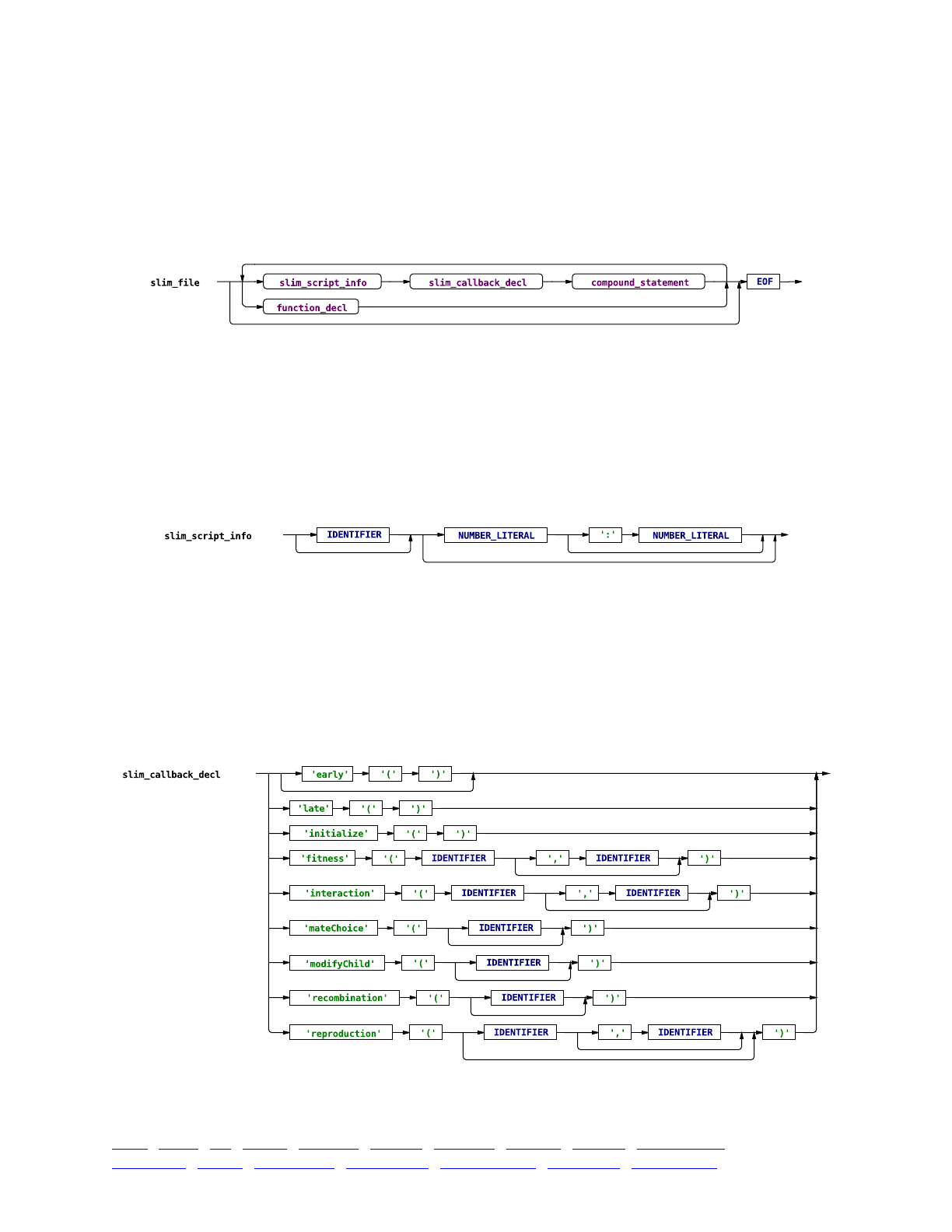
24. SLiM extensions to the Eidos language
24.1 Extensions to the Eidos grammar
The Eidos language itself is defined by the grammar given in the Eidos manual. However, SLiM
defines the grammar of a SLiM input file, which defines a small extension to the Eidos language –
in particular, by using a different start rule than Eidos’s interpreter normally uses:
This start rule defines a SLiM input file as a series of zero or more SLiM Eidos blocks, each of
which is a compound statement preceded by an informational section and a callback declaration.
Definitions of user-defined Eidos functions may also be sprinkled in among those blocks. Note
that ordinary Eidos statements are not allowed at the top level of the SLiM input file; they must be
within the body of a SLiM Eidos block or a user-defined function. The SLiM input file therefore
structures Eidos statements into encapsulated blocks.
In the definition of a SLiM Eidos block, the informational section is optional, since each of its
components is optional; it looks like this:
The informational section begins with an optional identifier that can be used to later identify the
script block programmatically. If supplied, it should be an identifier like "s1", or more generally,
"sX" where X is an integer greater than or equal to 0. The rest of the informational section
comprises an optional generation or range of generations in which the script block will be used by
SLiM. The generation numbers are defined syntactically by the grammar as numeric literals, but
semantically, there are further restrictions (see section 22.1).
The callback declaration section is also an addition by SLiM to the base Eidos grammar. It is
also optional, since it can be empty:
TOC I TOC II WF nonWF initialize() Genome Individual Mutation SLiMSim Subpopulation!
Eidos events fitness() mateChoice() modifyChild() recombination() interaction() reproduction() 498

This rule defines a SLiM script block as being one of the supported types of Eidos event or Eidos
callback (early(), late(), initialize(), fitness(), interaction(), mateChoice(),
modifyChild(), recombination(), or reproduction()). If no type specifier is provided, the script
block is an early() event by default. The identifier tokens in this rule specify restrictions on the
circumstances in which the callback will be used by SLiM. See chapter 22 for further details.
In all other respects the grammar of Eidos is unmodified in SLiM.
24.2 SLiM scoping rules
Eidos is largely a scopeless language; variables do not exist until they are defined, and once
defined they continue to exist forever, unless/until they are subsequently undefined. The only
exception to this, in Eidos, is that user-defined functions run within their own private scope. (See
the Eidos manual for further discussion of scope in Eidos.)
SLiM, however, imposes some scoping rules upon the Eidos language. This occurs almost as a
side effect of the way SLiM uses Eidos, albeit an intentional side effect. In particular, every call to
a SLiM event or callback is run within a new Eidos interpreter, created solely for the purpose of
running that particular invocation of that particular event or callback. These Eidos interpreters are
torn down and thrown away as soon as the callout ends. Because of this, variables defined inside
an event or callback have a scope that is limited to that callout; they will cease to exist as soon as
the callout finishes.
This is actually desirable, in general, because it prevents the global namespace from becoming
cluttered up with all of the local, temporary variables defined by particular events and callbacks. It
also provides a clean way for SLiM to, in effect, pass values in to callbacks, as described in chapter
22. It mimics the scoping of languages like C and C++, albeit only at the level of whole functions/
methods; even in SLiM there is no such thing as “block scope”. In fact, this scoping behavior is
identical to the way that user-defined functions in Eidos have their own private scope, and SLiM
events and callbacks can actually be thought of as a special kind of user-defined function that is
called automatically by SLiM, with a non-standard syntax for their declaration.
This design is not without drawbacks, however. The most obvious drawback is that in SLiM
there isn’t really such a thing as a global scope; there is only the local scope defined within events
and callbacks. Only the special variables defined by SLiM, such as sim, possess the privileged
status of being available everywhere (because SLiM sets them up before every callout).
SLiM provides some facilities to get around this problem. One such facility is the presence of
tag properties on many of SLiM’s classes, which can hold singleton integer values persistently
(and the tagF property on some SLiM classes can hold singleton float values, as well). Another is
the setValue()/getValue() facility provided by many of SLiM’s classes, which allows persistent
storage of arbitrarily named values that do not have to be singletons; this is much more flexible
and open-ended than the tag facility, but is also not as fast or as easy to use.
The other way to keep a value persistently is to define it as a constant rather than a variable,
using the Eidos function defineConstant(). In SLiM, the constants table is shared by all Eidos
interpreters, and therefore constants defined in one event or callback are available in all
subsequently executed code; SLiM’s scoping rules do not apply to defined constants. For values
that are in fact constant, this is straightforward and useful; SLiM models will often use
defineConstant() to define constants related to population sizes, locus lengths, etc., in the
initialize() callback of the model, and will then use those defined constants everywhere.
Because even constants can be undefined with the rm() function, however, it is even possible to
use this method to place non-constant values into the global namespace; when the value needs to
change, simply remove the previous constant definition with rm() (with the optional parameter
removeConstants=T); and then add a new constant definition with defineConstant(). This feels
TOC I TOC II WF nonWF initialize() Genome Individual Mutation SLiMSim Subpopulation!
Eidos events fitness() mateChoice() modifyChild() recombination() interaction() reproduction() 499

like a hack, since it violates the intended semantics of defineConstant(), but it is perfectly legal,
and in some cases is a good solution to the global scope problem.
One thing that it is impossible to do in SLiM is to persistently keep values of object type.
Values of object type cannot be placed into tag properties; they cannot be set as named values
with setValue(); and they cannot be defined as constants with defineConstant(). The only
object values that are persistent, in SLiM, are those set up by SLiM itself, such as sim. This is
deliberate and necessary, because otherwise stale references to objects that no longer exist in the
SLiM simulation could persist in variables. Since no persistent reference to an object can be
created, stale references can never exist in a SLiM model, which greatly simplifies object lifetime
management and error-checking issues. SLiM objects are only disposed of in between calls out to
Eidos, at points in time when no Eidos reference to them can possibly exist because of the design
of SLiM’s scoping and persistence rules. See section 2.8.2 of the Eidos manual for further
discussion."
TOC I TOC II WF nonWF initialize() Genome Individual Mutation SLiMSim Subpopulation!
Eidos events fitness() mateChoice() modifyChild() recombination() interaction() reproduction() 500

25. SLiM reference sheet
This reference sheet may be downloaded as a separate PDF from http://messerlab.org/slim/.
Defining Eidos functions, events, and callbacks in a SLiM script:
(ret-type)functionName(params) { ... } user-defined function
[<id>] initialize() { ... } initialize() callback
[<id>] [gen1 [: gen2]] [early()] { ... } early() Eidos event
[<id>] [gen1 [: gen2]] late() { ... } late() Eidos event
[<id>] [gen1 [: gen2]] fitness(<mutTypeId> [, <subpopId>]) { ... } fitness() callback
[<id>] [gen1 [: gen2]] interaction(<intTypeId> [, <subpopId>]) { ... } interaction() callback
[<id>] [gen1 [: gen2]] mateChoice([<subpopId>]) { ... } (WF) mateChoice() callback
[<id>] [gen1 [: gen2]] modifyChild([<subpopId>]) { ... } modifyChild() callback
[<id>] [gen1 [: gen2]] recombination([<subpopId>]) { ... } recombination() callback
[<id>] [gen1 [: gen2]] reproduction([<subpopId> [, <sex>]]) ... (nonWF) reproduction() callback
Invoking SLiM at the command line:
slim -version | -usage | -testEidos | -testSLiM |
[-seed <seed>] [-time] [-mem] [-Memhist] [-long] [-x] [-define <def>] <script file>
fitness():
mut (o<Mutation>$)
homozygous (l$)
relFitness (f$)
individual (o<Ind>$)
genome1 (o<Genome>$)
genome2 (o<Genome>$)
subpop (o<Subpop>$)
recombination():
individual (o<Ind>$)
genome1 (o<Genome>$)
genome2 (o<Genome>$)
subpop (o<Subpop>$)
breakpoints (i)
gcStarts (i)
gcEnds (i)
mateChoice(): (WF)
individual (o<Ind>$)
genome1 (o<Genome>$)
genome2 (o<Genome>$)
subpop (o<Subpop>$)
sourceSubpop (o<Subpop>$)
weights (f)
SLiM globals:
sim (o<SLiMSim>$)
g1, ... (o<GEType>$)
i1, ... (o<IntType>$)
m1, ... (o<MutType>$)
p1, ... (o<Subpop>$)
s1, ... (o<SEBlock>$)
self (o<SEBlock>$)
modifyChild():
child (o<Ind>$)
childGenome1 (o<Genome>$)
childGenome2 (o<Genome>$)
childIsFemale (l$)
parent1 (o<Ind>$)
parent1Genome1 (o<Genome>$)
parent1Genome2 (o<Genome>$)
isCloning (l$)
isSelfing (l$)
parent2 (o<Ind>$)
parent2Genome1 (o<Genome>$)
parent2Genome2 (o<Genome>$)
subpop (o<Subpop>$)
sourceSubpop (o<Subpop>$)
interaction():
distance (f$)
strength (f$)
exerter (o<Ind>$)
receiver (o<Ind>$)
subpop (o<Subpop>$)
Types: N:NULL, l:logical, i:integer, f:float, n:numeric, s:string, o<X>:object of class X
reproduction(): (nonWF)
individual (o<Ind>$)
genome1 (o<Genome>$)
genome2 (o<Genome>$)
subpop (o<Subpop>$)
1. Execution of early() events
2. Generation of offspring:
3. Removal of fixed mutations
4. Offspring become parents
6. Fitness value recalculation
using fitness() callbacks
7. Generation count increment
2.1. Choose source subpop
2.2. Choose parent 1
2.3. Choose parent 2
(mateChoice() callbacks)
2.4. Generate the offspring
(recombination() callbacks)
2.5. Suppress/modify child
(modifyChild() callbacks)
5. Execution of late() events
The sequence of events within one
generation in WF models.
2. Execution of early() events
1. Generation of offspring:
5. Removal of fixed mutations
4. Viability/survival selection
3. Fitness value recalculation
using fitness() callbacks
7. Generation count increment,
individual age increments
1.1. Call reproduction()
callbacks for individuals
1.2. The callback(s) make
calls requesting offspring
1.3. Generate the offspring
(recombination() callbacks)
1.4. Suppress/modify child
(modifyChild() callbacks)
6. Execution of late() events
The sequence of events within one
generation in nonWF models.
SLiMgui quick help:
opt-click on keyword
Code completion:
escape (␛) or
cmd-period (⌘.)
501

SLiMSim:
chromosome => (o<Chromosome>$)
chromosomeType => (s$)
dimensionality => (s$)
dominanceCoeffX <–> (f$)
generation <–> (i$)
genomicElementTypes => (o<GEType>)
inSLiMgui => (l$)!(deprecated in SLiM 3.2.1)
interactionTypes => (o<IntType>)
modelType => (s$)
mutationTypes => (o<MutType>)
mutations => (o<Mut>)
periodicity => (string$)
scriptBlocks => (o<SEBlock>)
sexEnabled => (l$)
subpopulations => (o<Subpop>)
substitutions => (o<Substitution>)
tag <–> (i$)
–!(o<Subpop>$)addSubpop(is$ subpopID, i$ size, [f$ sexRatio])
–!(o<Subpop>$)addSubpopSplit(is$ subpopID, i$ size, io<Subpop>$ sourceSubpop,
[f$!sexRatio])!(WF)
–!(i$)countOfMutationsOfType(io<MutType>$ mutType)
–!(void)deregisterScriptBlock(io<SEBlock> scriptBlocks)
–!(+)getValue(s$ key)
–!(i)mutationCounts(No<Subpop> subpops, [No<Mut> mutations])
–!(f)mutationFrequencies(No<Subpop> subpops, [No<Mut> mutations])
–!(o<Mut>)mutationsOfType(io<MutType>$ mutType)
–!(void)outputFixedMutations([Ns$ filePath], [l$ append])
–!(void)outputFull([Ns$ filePath], [l$ binary], [l$ append], [l$ spatialPositions], [l$ ages])
–!(void)outputMutations(o<Mut> mutations, [Ns$ filePath], [l$ append])
–!(void)outputUsage(void)
–!(i$)readFromPopulationFile(s$ filePath)
–!(void)recalculateFitness([Ni$ generation])
–!(o<SEBlock>$)register[Early/Late]Event(Nis$ id, s$ source, [Ni$ start], [Ni$ end])
–!(o<SEBlock>$)registerFitnessCallback(Nis$ id, s$ source, Nio<MutType>$ mutType,
[Nio<Subpop>$ subpop], [Ni$ start], [Ni$ end])
–!(o<SEBlock>$)registerInteractionCallback(Nis$ id, s$ source, io<IntType>$ intType,
[Nio<Subpop>$ subpop], [Ni$ start], [Ni$ end])
–!(o<SEBlock>$)register[MateChoice (WF)/ModifyChild/Recombination]Callback(Nis$ id, s$ source,
[Nio<Subpop>$ subpop], [Ni$ start], [Ni$ end])
–!(o<SEBlock>$)registerReproductionCallback(Nis$ id, s$ source, [Nio<Subpop>$ subpop],
[Ns$ sex], [Ni$ start], [Ni$ end])!(nonWF)
–!(o<SEBlock>$)rescheduleScriptBlock(o<SEBlock>$ block, [Ni$ start], [Ni$ end],
[Ni generations])
–!(void)setValue(s$ key, + value)
–!(void)simulationFinished(void)
–!(l$)treeSeqCoalesced(void)
–!(void)treeSeqOutput(s$ path, [l$ simplify])
–!(void)treeSeqRememberIndividuals(o<Ind> individuals)
–!(void)treeSeqSimplify(void)
Initialization functions (callable only from initialize() callbacks):
(void)initializeGeneConversion(n$ conversionFraction, n$ meanLength)
(void)initializeGenomicElement(io<GEType>$ genomicElementType, i$ start, i$ end)
(o<GEType>$)initializeGenomicElementType(is$ id, io<MutType> mutationTypes, n proportions)
(o<IntType>$)initializeInteractionType(is$ id, s$ spatiality, [l$ reciprocal],
[n$ maxDistance], [s$ sexSegregation])
(void)initializeMutationRate(n rates, [Ni ends], [s$ sex])
(o<MutType>$)initializeMutationType(is$ id, n$ dominanceCoeff, s$ distributionType, ...)
(void)initializeRecombinationRate(n rates, [Ni ends], [s$ sex])
(void)initializeSex(s$ chromosomeType, [n$ xDominanceCoeff])
(void)initializeSLiMModelType(s$ modelType)
(void)initializeSLiMOptions([l$ keepPedigrees], [s$ dimensionality], [s$ periodicity],
[i$ mutationRuns], [l$ preventIncidentalSelfing])
(void)initializeTreeSeq([l$ recordMutations], [f$ simplificationRatio],
[l$ checkCoalescence], [l$ runCrosschecks])
502

Subpopulation (Subpop):
cloningRate => (f) (WF)
firstMaleIndex => (i$)
fitnessScaling <–> (f$)
genomes => (o<Genome>)
id => (i$)
immigrantSubpopFractions => (f) (WF)
immigrantSubpopIDs => (i) (WF)
individualCount => (i$)
individuals => (o<Ind>)
selfingRate => (f$) (WF)
sexRatio => (f$) (WF)
spatialBounds => (f)
tag <–> (i$)
–!(No<Ind>$)addCloned(o<Ind>$ parent) (nonWF)
–!(No<Ind>$)addCrossed(o<Ind>$ parent1, o<Ind>$ parent2, [Nfs$ sex]) (nonWF)
–!(No<Ind>$)addEmpty([Nfs$ sex]) (nonWF)
–!(No<Ind>$)addRecombinant(No<Genome>$ strand1, No<Genome>$ strand2, Ni breaks1,
No<Genome>$ strand3, No<Genome>$ strand4, Ni breaks2, [Nfs$ sex]) (nonWF)
–!(No<Ind>$)addSelfed(o<Ind>$ parent) (nonWF)
–!(f)cachedFitness(Ni indices)
–!(void)configureDisplay([Nf center], [Nf$ scale], [Ns$ color])
–!(void)defineSpatialMap(s$ name, s$ spatiality, Ni gridSize, f values, [l$ interpolate],
[Nf valueRange], [Ns colors])
–!(+)getValue(s$ key)
–!(void)outputMSSample(i$ sampleSize, [l$ replace], [s$ requestedSex],
[Ns$ filePath], [l$ append], [l$ filterMonomorphic])
–!(void)outputSample(i$ sampleSize, [l$ replace], [s$ requestedSex],
[Ns$ filePath], [l$ append])
–!(void)outputVCFSample(i$ sampleSize, [l$ replace], [s$ requestedSex],
[l$ outputMultiallelics], [Ns$ filePath], [l$ append])
–!(l)pointInBounds(f point)
–!(f)point[Periodic|Reflected|Stopped](f point)
–!(f)pointUniform([i$ n])
–!(void)removeSubpopulation(void) (nonWF)
–!(void)sampleIndividuals(i$ size, [l$ replace], [No<Ind>$ exclude], [Ns$ sex], [Ni$ tag],
[Ni$ minAge], [Ni$ maxAge], [Nl$ migrant])
–!(void)setCloningRate(n rate) (WF)
–!(void)setMigrationRates(io<Subpop> sourceSubpops, n rates) (WF)
–!(void)setSelfingRate(n$ rate) (WF)
–!(void)setSexRatio(f$ sexRatio) (WF)
–!(void)setSpatialBounds(f bounds)
–!(void)setSubpopulationSize(i$ size) (WF)
–!(void)setValue(s$ key, + value)
–!(s)spatialMapColor(s$ name, f value)
–!(f$)spatialMapValue(s$ name, f point)
–!(void)subsetIndividuals([No<Ind>$ exclude], [Ns$ sex], [Ni$ tag], [Ni$ minAge],
[Ni$ maxAge], [Nl$ migrant])
–!(void)takeMigrants(o<Ind> migrants) (nonWF)
Chromosome:
colorSubstitution <–> (s$)
geneConversionFraction <–> (f$)
geneConversionMeanLength <–> (f$)
genomicElements => (o<GElement>)
lastPosition => (i$)
mutationEndPositions[F|M] => (i)
mutationRates[F|M] => (f)
overallMutationRate[F|M] => (f$)
overallRecombinationRate[F|M] => (f$)
recombinationEndPositions[F|M] => (i)
recombinationRates[F|M] => (f)
tag <–> (i$)
–!(integer)drawBreakpoints([No<Ind>$ parent], [Ni$ n])
–!(void)setMutationRate(n rates, [Ni ends], [s$ sex])
–!(void)setRecombinationRate(n rates, [Ni ends], [s$ sex])
503

Mutation (Mut):
id => (i$)
mutationType => (o<MutType>$)
originGeneration => (i$)
position => (i$)
selectionCoeff => (f$)
subpopID <–> (i$)
tag <–> (i$)
–!(+)getValue(s$ key)
- (void)setMutationType(io<MutType>$!mutType)
–!(void)setSelectionCoeff(f$ selectionCoeff)
–!(void)setValue(s$ key, + value)
Genome:
genomePedigreeID => (i$)
genomeType => (s$)
isNullGenome => (l$)
mutations => (o<Mut>)
tag <–> (i$)
+!(void)addMutations(o<Mut> mutations)
+!(o<Mut>)addNewDrawnMutation(io<MutType> mutationType, i position, [Ni originGeneration],
[Nio<Subpop> originSubpop])
+!(o<Mut>)addNewMutation(io<MutType> mutationType, n selectionCoeff, i position,
[Ni originGeneration], [Nio<Subpop> originSubpop])
–!(l$)containsMarkerMutation(io<MutType>$ mutType, i$ position, [l$!returnMutation])
–!(l)containsMutations(o<Mut> mutations)
–!(i$)countOfMutationsOfType(io<MutType>$ mutType)
–!(o<Mut>)mutationsOfType(io<MutType>$ mutType)
+!(void)output([Ns$ filePath], [l$ append])
+!(void)outputMS([Ns$ filePath], [l$ append], [l$ filterMonomorphic])
+!(void)outputVCF([Ns$ filePath], [l$ outputMultiallelics], [l$ append])
–!(i)positionsOfMutationsOfType(io<MutType>$ mutType)
+!(void)removeMutations([No<Mut> mutations], [l$ substitute])
–!(f$)sumOfMutationsOfType(io<MutType>$ mutType)
Substitution:
id => (i$)
fixationTime => (i$)
mutationType => (o<MutType>$)
originGeneration => (i$)
position => (i$)
selectionCoeff => (f$)
subpopID <–> (i$)
tag <–> (i$)
–!(+)getValue(s$ key)
–!(void)setValue(s$ key, + value)
Individual (Ind):
age <–> (i$) (nonWF)
color <–> (s$)
fitnessScaling <–> (f$)
genomes => (o<Genome>)
genome1 => (o<Genome>$)
genome2 => (o<Genome>$)
index => (i$)
migrant => (l$)
pedigreeID => (i$)
pedigreeParentIDs => (i)
pedigreeGrandparentIDs => (i)
sex => (s$)
spatialPosition => (f)
subpopulation => (o<Subpop>$)
tag <–> (i$)
tagF <–> (f$)
uniqueMutations => (o<Mut>)
x <–> (f$)
y <–> (f$)
z <–> (f$)
–!(l)containsMutations(o<Mut> mutations)
–!(i$)countOfMutationsOfType(io<MutType>$ mutType)
–!(+)getValue(s$ key)
–!(f)relatedness(o<Ind> individuals)
+!(void)setSpatialPosition(f position)
–!(void)setValue(s$ key, + value)
–!(f$)sumOfMutationsOfType(io<MutType>$ mutType)
–!(o<Mut>)uniqueMutationsOfType(io<MutType>$ mutType)
504

MutationType (MutType):
color <–> (s$)
colorSubstitution <–> (s$)
convertToSubstitution <–> (l$)
distributionParams => (f)
distributionType => (s$)
dominanceCoeff <–> (f$)
id => (i$)
mutationStackGroup <–> (i$)
mutationStackPolicy <–> (s$)
tag <–> (i$)
–!(+)getValue(s$ key)
–!(void)setDistribution(s$ distType, ...)
–!(void)setValue(s$ key, + value)
GenomicElementType (GEType):
color <–> (s$)
id => (i$)
mutationFractions => (f)
mutationTypes => (o<MutType>)
tag <–> (i$)
–!(+)getValue(s$ key)
–!(void)setMutationFractions(io<MutType> mutationTypes, n proportions)
–!(void)setValue(s$ key, + value)
GenomicElement (GElement):
endPosition => (i$)
genomicElementType => (o<GEType>$)
startPosition => (i$)
tag <–> (i$)
–!(void)setGenomicElementType(io<GEType>$ genomicElementType)
SLiMEidosBlock (SEBlock):
active <–> (i$)
end => (i$)
id => (i$)
source => (s$)
start => (i$)
tag <–> (i$)
type => (s$)
InteractionType (IntType):
id => (i$)
maxDistance <–> (f$)
reciprocal => (l$)
sexSegregation => (s$)
spatiality => (s$)
tag <–> (i$)
–!(f)distance(o<Ind> individuals1, [No<Ind> individuals2])
–!(f)distanceToPoint(o<Ind> individuals1, f point)
–!(o<Ind>)drawByStrength(o<Ind>$ individual, [i$ count])
–!(void)evaluate([No<Subpop> subpops], [l$ immediate])
–!(+)getValue(s$ key)
–!(i)interactingNeighborCount(o<Ind>!individuals)
–!(f)interactionDistance(o<Ind> individuals1, [No<Ind> individuals2])
–!(o<Ind>)nearestInteractingNeighbors(o<Ind>$ individual, [i$ count])
–!(o<Ind>)nearestNeighbors(o<Ind>$ individual, [i$ count])
–!(o<Ind>)nearestNeighborsOfPoint(o<Subpop>$ subpop, f point, [i$ count])
–!(void)setInteractionFunction(s$ functionType, ...)
–!(void)setValue(s$ key, + value)
–!(f)strength(o<Ind>$ receiver, [No<Ind> exerters])
–!(f)totalOfNeighborStrengths(o<Ind> individuals)
–!(void)unevaluate(void)
Fitness effects of mutations:
no mutation present 1
heterozygote 1 + h*s
homozygote 1 + s
s = mut.selectionCoeff
h = mutType.dominanceCoeff
SLiMgui: (in SLiMgui only)
pid => (i$)
–!(void)openDocument(s$ filePath)
–!(void)pauseExecution(void)
505

26. Revision history
This is a history of the revisions of SLiM since version 2.0. It focuses on new features, not bug
fixes (which rapidly become ancient history), and it does not contain every detail. The VERSIONS
file in the SLiM source code provides more detail, including changes that might not be user-visible
at all. Beyond that, the commit history in GitHub is of course the definitive history of the project.
For those wanting a quick overview of SLiM’s history, however, this is a good place to start.
Version 3.2.1
Feature: drawBreakpoints() method on Chromosome to draw breakpoints using SLiM’s logic
Feature: rbeta() function in Eidos for draws from a beta distribution
Feature: pnorm() function in Eidos for the CDF of the normal distribution
Feature: new SLiMgui class, with an instance named slimgui, available only under SLiMgui
Feature: SLiMgui.openDocument() method to open a file in SLiMgui from script
Feature: SLiMgui.pauseExecution() method to pause a running SLiMgui simulation from script
Feature: SLiMgui.pid property to get the process ID of SLiMgui from script
Feature: Subpopulation.configureDisplay() method to customize SLiMgui display of subpops
Tweak: revised recipes 13.11 and 13.17 to use the new SLiMgui class
Tweak: slim (the command-line tool) can now read its script from stdin (i.e., from a pipe)
Tweak: new recipe 15.15 (Implementing a Wright–Fisher model with a nonWF model)
Tweak: new recipe 15.16 (Alternation of generations)
Tweak: added support for make install with cmake, thanks to Peter Ralph
Tweak: added support for link-time optimization (LTO), thanks to Kevin Thornton
Tweak: improved the reseeding procedure in recipes 10.2, 10.3, 10.6.2, and 16.3
Tweak: SLiMgui should now run on macOS 10.10 and later (formerly 10.11 and later)
Policy change: inSLiMgui property of SLiMSim deprecated; use exists("slimgui")
Bug fix: setValue() did not copy the value, allowing corruption of the set value in rare cases
Bug fix: calling deregisterScriptBlock() more than once on the same block did bad things
Bug fix: the pedigreeGrandparentIDs property returned incorrect values
Bug fix: loading a .trees file with a mismatched chromosome length now gives an error
Bug fix: SLiMgui crash when displaying a large number of genomic element types
Bug fix: code completion bug when completing off a base of return/else/do/in
Bug fix: fixed poor error-reporting for malformed command-line definitions
Bug fix: fixed a raise that would crash SLiMgui, triggered by an illegal numeric constant in script
Version 3.2
Feature: keyword-based “Find Recipe…” panel in SLiMgui to make recipe lookup easier
Feature: code completion in SLiMgui is now much smarter (iTR -> initializeTreeSeq(), e.g.)
Feature: memory usage summary in SLiMgui’s profile, also from new outputUsage() method
Feature: usage() function in Eidos to get the current / peak total memory usage
Feature: addRecombinant() method for nonWF for horizontal gene transfer, haploid models, etc.
Feature: rgeom() function in Eidos for draws from a geometric distribution
Feature: button in SLiMgui’s output area to view/change the current working directory
Feature: outputMS() and outputMSSample() can now filter out in-sample-monomorphic sites
Feature: new color-palette functions heatColors(), rainbow(), terrainColors(), cmColors()
506

Tweak: new recipe 15.13, modeling clonal haploids in nonWF models with addRecombinant()
Tweak: new recipe 15.14, modeling clonal haploid bacteria with horizontal gene transfer
Tweak: vectorized the Eidos color-manipulation functions, using matrix arguments/returns
Tweak: add a [print=T] flag to version() so switching on version can avoid unwanted output
Tweak: vectorized the exists() function so a vector of symbols can be checked in one call
Tweak: some minor optimization work, especially on property / method dispatch in Eidos
Policy change: asString(NULL) now returns "NULL" for easier output generation
Policy change: string concatenation with + now adds "NULL" for NULL, for easier output
Policy change: scheduling an event/callback into the past now produces an error
Bug fix: fixed a major performance issue for large nonWF models with a lot of genetic diversity
Bug fix: recipe 11.1 issue with the calcFST() function returning NAN in some marginal cases
Bug fix: code completion in SLiMgui after return, in, else, and do now works correctly
Bug fix: many Eidos functions are now more robust to being passed NAN (e.g., rpois() hang)
Bug fix: corrupted spatial location data for some individuals in .trees files
Bug fix: minor issue with SLiMgui’s population visualization graph’s migration rate arrows
Bug fix: symbol table bug that would bite models defining a very large number of symbols
Bug fix: crash in addEmpty() that nobody noticed because nobody uses it
Bug fix: incorrect modifyChild() source subpop when using addCloned()/Crossed()/Selfed()
Bug fix: incorrect isCloning/isSelfing in modifyChild() when using addCloned()/addSelfed()
Bug fix: incorrect parent2 values in modifyChild() in clonal models (shouldn’t be used anyway)
Version 3.1
Feature: greatly increased the performance of spatial interactions with large population size
Feature: added interactionDistance() method to get interaction-conditional distances
Feature: added nearestInteractingNeighbors() to get interaction-conditional neighbors
Feature: added interactingNeighborCount() to count interaction-conditional neighbors
Feature: rememberIndividuals() now actually remembers individuals (as well as genomes)
Feature: added automatic remembering of the initial generation, for easier recapitation
Feature: dmvnorm() added to Eidos to get probability densities from a multivariate normal dist.
Tweak: extended the .trees provenance format for better reproducibility / self-documentation
Tweak: new recipe 13.19, biased gene conversion (two recipes actually)
Tweak: improved recipe 13.4 (reading MS format files), with big performance benefits for it
Tweak: updated all chapter 16 recipes (tree-sequence recording) to reflect changes
Policy change: strength() now requires a singleton first argument, receiver
Policy change: .trees files now have their time rebased to msprime-style times on save
Policy change: initializeInteractionType() now warns if no maximum distance is given
Bug fix: memory leak with cycling/varying subpopulation size (genome recycling bug)
Bug fix: nodes in .trees files occasionally being marked as null genomes incorrectly
Bug fix: incorrect fitness in WF models using only fitnessScaling to modify fitness
Version 3.0
Feature: non-Wright-Fisher (nonWF) models, chosen with initializeSLiMModelType()
Feature: nonWF additions (age, addX() methods, takeMigrants(), removeSubpopulation())
Feature: nonWF additions (reproduction() callbacks, registerReproductionCallback())
507

Feature: new sampleIndividuals() and subsetIndividuals() methods on Subpopulation
Feature: new fitnessScaling property on Subpopulation and Individual to alter fitness
Feature: tree-sequence recording, enabled with initializeTreeSeq()
Feature: tree-sequence recording additions (treeSeqX() methods)
Feature: new seqLen() function in Eidos to generate a zero-based sequence of a given length
Feature: new getwd() / setwd() functions in Eidos to get and change the working directory
Feature: new var() / cov() / cor() stats functions in Eidos for variance / covariance / correlation
Feature: new rcauchy() function for Cauchy distribution (also new interaction function, “c”)
Feature: new genome1 and genome2 properties on Individual for easier haploid models etc.
Feature: new migrant property on Individual, usable in both WF and nonWF models
Feature: display interaction types in SLiMgui’s drawer, with hover preview for the function
Feature: improved subpopulation display options in SLiMgui, including spatial map choice
Feature: increase maximum chromosome length from 1e9 to 1e15
Feature: code completion in SLiMgui can now supply argument names when in a call
Feature: added getValue() / setValue() functionality to Substitution
Feature: optimization work across SLiM and Eidos
Tweak: new recipes for nonWF (chapter 15) and tree-sequence recording (chapter 16)
Tweak: new recipe 13.3 III (mortality-based fitness using fitnessScaling)
Tweak: new recipe 13.18 (modeling opposite ends of a chromosome)
Tweak: recipe fixes to conform with changes (13.1, 13.2, 13.9, 13.13, 11.2)
Tweak: mean() now works with a logical vector argument
Tweak: vectorize point-processing methods (pointX(), setSpatialPosition())
Tweak: add removeMutations(NULL) option to quickly remove all mutations from a Genome
Tweak: add [returnMutation!=!F] argument to containsMarkerMutation() to get the mutation
Tweak: new suppressWarnings() function in Eidos to… suppress warnings
Policy change: return values are no longer implied by the value of the last statement
Policy change: void is now a true value type in Eidos, not a synonym for NULL
Policy change: property/method accesses on zero-length vectors now raise if ambiguous in type
Policy change: cachedFitness() may no longer be called from a late() event in WF models
Policy change: the default working directory when running in SLiMgui is now ~/Desktop
Bug fix: incorrect strengths from InteractionType with periodic boundaries
Bug fix: gene conversion rate of exactly 1.0 would be treated as 0.0
Bug fix: crash when setSubpopulationSize(0) was called twice on the same subpop
Bug fix: crash with the “fitness over time” graph in SLiMgui with an invalid simulation
Bug fix: rare crash on quit in SLiMgui
Bug fix: crash due to stack overflow with large population size and callbacks
Bug fix: display glitch in SLiMgui on Retina displays
Bug fix: fix incorrect actual recombination rate for specified rate of 0.5, impose <= 0.5 limit
Bug fix: rdunif() can now generate draws over the full 64-bit range, not limited to 32-bit
Bug fix: crash in SLiMgui displaying haplotypes in a model with null genomes (X/Y models)
Bug fix: dropped model output from just before a simulation terminates due to an error
Version 2.6
Feature: Eidos now supports matrices (2-D) and arrays (n-D), with new related functions
508

Feature: haplotype plots and haplotype-based chromosome view display mode
Feature: periodic spatial boundary conditions now supported, including in InteractionType
Feature: visualize MutationType DFEs in the info drawer in SLiMgui (hover the mouse to see)
Feature: new rdunif() Eidos function for draws from discrete uniform distributions
Feature: new rmvnorm() Eidos function for draws from multivariate normal distributions
Feature: optimizations of the Eidos core may lead to ~20% speedup for Eidos-intensive models
Tweak: the apply() function is now renamed sapply(), following R
Tweak: increased display flexibility of individual mutation types in the chromosome view
Tweak: the number of bins in the frequency spectrum plot in SLiMgui can now be changed
Tweak: improved display of mutation/recombination maps in SLiMgui, with a broader range
Tweak: addNew[Drawn]Mutation() are now vectorized for speed when adding many mutations
Tweak: new positionsOfMutationsOfType() method on Genome for speed of some models
Tweak: extended the integer() function of Eidos to be able to create two-valued filled vectors
Tweak: defineSpatialMap() now accepts a matrix/array of values (backward compatible)
Tweak: sapply() (which was apply()) has a new simplify parameter to get a matrix/array result
Tweak: extended recipe 13.5 to show off the new haplotype display options, check it out
Tweak: revised recipe 13.9 (tracking true local ancestry) for much greater speed
Tweak: recipe 13.12 (modeling nucleotides) is now much faster, with optimizations in SLiM
Tweak: added recipes 13.15 (modeling microsatellites) and 13.16 (modeling transposons)
Tweak: added recipe 13.17: multiple QTL-based quantitative phenotypic traits with pleiotropy
Tweak: added recipe 14.12 to demonstrate periodic boundary conditions in spatial models
Tweak: revised recipes to use sapply() instead of apply(), other minor recipe tweaks
Policy change: assignment into a subset of a property is no longer legal in Eidos (you don’t care)
Policy change: version() now returns a numeric version number, for runtime version checking
Policy change: Chromosome properties that are undefined now raise when accessed
Policy change: addNew[Drawn]Mutation() returns requested mutations whether added or not
Policy change: periodicity inserted in initializeSLiMOptions(); use named arguments there!
Bug fix: possible incorrect mutation freqs/counts after addMutations() / removeMutations()
Bug fix: fixed a long-standing display bug in SLiMgui with added/removed mutations
Bug fix: very minor bug fixes in doCall(), SLiMgui, etc.; very unlikely impact on model results
Version 2.5
Feature: add support for user-defined Eidos functions in SLiM – make your own functions
Feature: support for variable mutation rate along the chromosome (i.e., “hot” and “cold” spots)
Feature: display of the mutation-rate map in SLiMgui with the R button
Feature: Mutation now supports the getValue()/setValue() mechanism
Feature: SLiMgui can do script prettyprinting, for nice code formatting
Feature: new ternary conditional operator, ?else, added to Eidos, like ?: in C/C++
Feature: support for block-style /* */ comments added to Eidos, as in C/C++
Feature: added a function source() to read in and execute Eidos code from a given file
Feature: the SLiM and Eidos documentation now has hyperlinks in its table of contents
Major bug fix: new mutations were not added correctly in clonal reproduction, in 2.4–2.4.2
Tweak: improved pmax(), pmin(), max(), min(), range(), seq(), any(), all(), unique()
Tweak: added a sumExact() function to Eidos for exact summation of floating-point numbers
509

Tweak: fixed a bug in recipe 11.1’s FST calculation code, and split it into a standalone function
Tweak: added recipe 13.13, illustrating how to make a simple haploid clonal model in SLiM
Tweak: added recipe 13.14, modeling variation in functional density along the chromosome
Policy change: removed the mutationRate property of Chromosome in favor of new API
Policy change: function(), method(), property() renamed to functionSignature(), etc.
Policy change: argument function for doCall() renamed to functionName
Bug fix: improved numerical accuracy for complex recombination maps
Bug fix: incorrect results from InteractionType if individuals had an identical coordinate value
Version 2.4.2
Major bug fix: fix non-unique mutation id bug (incorrect output from many/most models)
Version 2.4.1
Bug fix: fix stale subpop pointer bug (possible crash or incorrect data in multi-subpop sims)
Version 2.4
Feature: extensive internal optimizations for better performance of many models
Feature: model runtime profiling added in SLiMgui for performance evaluation
Feature: sumOfMutationsOfType() method added for fast QTL effect addition
Feature: preventIncidentalSelfing option added to initializeSLiMOptions()
Feature: optionally configure the mutation run count in initializeSLiMOptions()
Feature: system() function to call out to Unix to run commands
Feature: added PDF viewing to SLiMgui for R plotting integration (see recipe 13.11)
Feature: chromosome view display customization via right-click in SLiMgui
Feature: population view display customization via right-click in SLiMgui
Feature: writeTempFile() function for creating randomly named temporary files
Feature: new catn() and paste0() functions for simpler output generation
Feature: MutationType, GenomicElementType, InteractionType now support get/setValue()
Feature: add mutationStackGroup property to MutationType and improve stacking options
Major bug fix: significant bug in the Eidos function setDifference() (no impact if not using it)
Tweak: added top/bottom splitview in SLiMgui to allow greater display flexibility
Tweak: the play speed slider in SLiMgui now shows the chosen play speed in a tooltip
Tweak: added font size preference in SLiMgui for presentations, etc.
Tweak: new inSLiMgui property on SLiMSim to tell whether the model is running in SLiMgui
Tweak: rescheduleScriptBlock() method added on SLiMSim for easier block rescheduling
Tweak: ttest() function added for performing t-tests in Eidos
Tweak: added -l (-long) command-line option for more verbose output
Policy change: scripted (type “s”) DFEs in MutationType now have access to SLiM constants
Bug fix: for loops on seqAlong() vectors with a zero-length parameter were incorrect
Version 2.3
Feature: continuous space (1D, 2D, or 3D) and spatial positions for Individual (x, y, and z)
Feature: landscape maps that can define environmental values across space
Feature: interactions (both non-spatial and spatial), including interaction() callbacks
Feature: “global” fitness() callbacks that are called once for every individual
Tweak: outputFull() and readFromPopulationFile() now save/restore spatial positions
510

Tweak: mateChoice() callbacks can now return a vector of all zero to reject the first parent
Tweak: mateChoice() callbacks can now return a singleton Individual as the chosen parent
Tweak: added several color-conversion functions to Eidos (RGB to/from HSV, etc.)
Policy change: readFromPopulationFile() no longer recalculates fitness values
Policy change: readFromPopulationFile() now warns if called outside a late() event
Version 2.2.1
Feature: SLiMgui is now a proper document-based app using the .slim file extension
Feature: tagF property on Individual for storage of float custom state
Feature: order() function that provides sorting indices, like the R order() function
Feature: custom coloring of individuals, etc., in SLiMgui using new color properties
Tweak: SLiMgui’s recycle button now highlights green when the script has been changed
Tweak: arbitrary Eidos expressions are now legal in command-line constant definitions
Policy change: multiple calls to initializeRecombinationRate() is now explicitly illegal
Version 2.2
Feature: recombination() callbacks allow scripted alteration of recombination breakpoints
Feature: containsMarkerMutation() method allows fast checking for “marker” mutations
Feature: clock() function gives the CPU usage of the process, for measuring performance
Feature: setValue() / getValue() methods provide several classes with dictionary-like values
Feature: command-line constant definition using a -define or -d flag passed to slim
Tweak: “tips & tricks” panel for SLiMgui that introduces some obscure features of the app
Version 2.1.1
Feature: mutationCounts() method provides raw mutation reference counts
Version 2.1
Feature: Individual class added to represent individuals, with many associated changes
Feature: optional pedigree-based relatedness tracking for individuals
Feature: overhaul of SLiM output methods to provide file-based output and appending
Feature: new Genome output methods allow output of custom samples
Feature: VCF format output added to the existing SLiM and MS formats
Feature: Mutation now has a unique identifier usable for tracking mutations through time
Feature: Mutation and Substitution now have a tag property like many other SLiM classes
Feature: DFE type "s" now allows scripted DFEs for MutationType
Feature: sex-specific recombination rates and/or recombination maps
Feature: default arguments and named arguments supported for Eidos functions and methods
Feature: deleteFile() and createDirectory() functions added to Eidos
Feature: set operation functions (union, intersection, etc.) added to Eidos
Tweak: size() method added to the Eidos object base class
Tweak: recipes now openable directly from the Recipes submenu in SLiMgui
Policy change: output of mutations now includes a mutation identifier field (format change)
Policy change: readFromPopulationFile() now sets the generation as a side effect
Policy change: class methods in Eidos now provide non-multicasted method invocation
Policy change: addNewMutation() and addNewDrawnMutation() changed to class methods
511

Version 2.0.4
Minor bug fixes.
Version 2.0.3
Minor bug fixes.
Version 2.0.2
Feature: binary format for outputFull(), for smaller files and much faster save/load
Feature: setMutationType() added to allow mutations to be assigned to a different type
Feature: beep() function allows audible output from scripts
Tweak: readFromPopulationFile() can now read the new binary file format
Version 2.0.1
Feature: format() function added to Eidos for customized formatting of output
Version 2.0
This was the original version of SLiM 2, which was an almost complete rewrite of SLiM and
introduced such major features as Eidos and SLiMgui. The full list of changes is far too extensive to
detail here. Before SLiM 2 came SLiM 1, which was documented in Messer (2013).
512

27. Credits and licenses for incorporated software
SLiM incorporates code from various other software frameworks and packages. This section
provides credit and license information for the software thus incorporated, as well as for SLiM
itself.
27.1 SLiM
SLiM is free software: you can redistribute it and/or modify it under the terms of the GNU
General Public License as published by the Free Software Foundation, either version 3 of the
License, or (at your option) any later version.
SLiM is distributed in the hope that it will be useful, but WITHOUT ANY WARRANTY; without
even the implied warranty of MERCHANTABILITY or FITNESS FOR A PARTICULAR PURPOSE. See
the GNU General Public License for more details.
You should have received a copy of the GNU General Public License along with SLiM. If not,
see http://www.gnu.org/licenses/.
27.2 GNU Scientific Library (GSL)
SLiM contains a modified distribution of the GNU Scientific Library (GSL), which is also
licensed under the GNU General Public License under the same terms stated above. Thanks to the
authors of the GSL for their very useful software, which can be found in full form at!
http://www.gnu.org/software/gsl/.
27.3 kastore / msprime
SLiM contains code from the msprime and kastore software packages (enabling the tree-
sequence recording feature of SLiM 3, and the ability to save and load .trees files). Thanks to the
msprime and kastore developers for this code, and to Peter Ralph and Jared Galloway for
contributing code to SLiM to integrate it with these software packages. The msprime package is
licensed under the GPL, and is available at https://github.com/tskit-dev/msprime. The kastore
package is MIT licensed and available at https://github.com/tskit-dev/.
27.4 Boost
SLiM contains modified code from Boost (for a smart pointer implementation), which is licensed
under the Boost Software License version 1.0 (http://www.boost.org/LICENSE_1_0.txt). The Boost
Software License is compatible with the GPL, allowing its use here. Thanks to all of the authors of
Boost for their very useful software, which can be downloaded in its full form from their website at
http://www.boost.org/users/download/#live. Thanks especially to Peter Dimov, who appears to be
the author of the class in question.
27.5 MT19937-64
SLiM contains a 64-bit Mersenne Twister implementation (a random number generator) by
Takuji Nishimura and Makoto Matsumoto; thanks to them for this code, which was obtained from
http://www.math.sci.hiroshima-u.ac.jp/~m-mat/MT/VERSIONS/C-LANG/mt19937-64.c. Following
the terms of their license, the following text is provided from them:
Copyright (C) 2004, Makoto Matsumoto and Takuji Nishimura,
All rights reserved.
513

Redistribution and use in source and binary forms, with or without
modification, are permitted provided that the following conditions are
met:
1. Redistributions of source code must retain the above copyright notice,
this list of conditions and the following disclaimer.
2. Redistributions in binary form must reproduce the above copyright
notice, this list of conditions and the following disclaimer in the
documentation and/or other materials provided with the distribution.
3. The names of its contributors may not be used to endorse or promote
products derived from this software without specific prior written
permission.
THIS SOFTWARE IS PROVIDED BY THE COPYRIGHT HOLDERS AND CONTRIBUTORS "AS
IS" AND ANY EXPRESS OR IMPLIED WARRANTIES, INCLUDING, BUT NOT LIMITED TO,
THE IMPLIED WARRANTIES OF MERCHANTABILITY AND FITNESS FOR A PARTICULAR
PURPOSE ARE DISCLAIMED. IN NO EVENT SHALL THE COPYRIGHT OWNER OR
CONTRIBUTORS BE LIABLE FOR ANY DIRECT, INDIRECT, INCIDENTAL, SPECIAL,
EXEMPLARY, OR CONSEQUENTIAL DAMAGES (INCLUDING, BUT NOT LIMITED TO,
PROCUREMENT OF SUBSTITUTE GOODS OR SERVICES; LOSS OF USE, DATA, OR
PROFITS; OR BUSINESS INTERRUPTION) HOWEVER CAUSED AND ON ANY THEORY OF
LIABILITY, WHETHER IN CONTRACT, STRICT LIABILITY, OR TORT (INCLUDING
NEGLIGENCE OR OTHERWISE) ARISING IN ANY WAY OUT OF THE USE OF THIS
SOFTWARE, EVEN IF ADVISED OF THE POSSIBILITY OF SUCH DAMAGE.
27.6 WiggleTools
SLiM contains code from WiggleTools to perform t-tests. WiggleTools is licensed under the
Apache 2.0 license (http://www.apache.org/licenses/LICENSE-2.0), which is compatible with the
GPL, allowing its use here. Thanks to EMBL-European Bioinformatics Institute for making this code
available.
27.7 ObjectPool
SLiM contains a modified version of a C++ object pool class published by Paulo Zemek at
http://www.codeproject.com/Articles/746630/O-Object-Pool-in-Cplusplus. His code is under the
Code Project Open License (CPOL), available at http://www.codeproject.com/info/cpol10.aspx.
The CPOL is not compatible with the GPL. Paulo Zemek has explicitly granted permission for his
code to be used in Eidos and SLiM, and thus placed under the GPL as an alternative license. An
email granting this permission has been archived and can be provided upon request. This code is
therefore now under the same GPL license as the rest of SLiM and Eidos, as stated above.
27.8 Exact summation
SLiM contains modified (translated to C from Python) code to compute the exact summation
(within available precision limits) of a vector of floating-point numbers. This code is adapted from
Python’s fsum() function, as implemented in the file mathmodule.c in the math_fsum() C function,
from Python version 3.6.2, downloaded from https://www.python.org/getit/source/. The authors of
that code appear to be Raymond Hettinger and Mark Dickinson; thanks to them. The PSF open-
source license for Python 3.6.2, which the PSF states is GSL-compatible, may be found on their
website at https://docs.python.org/3.6/license.html.
514

27.9 JSON for Modern C++
SLiM contains code from the JSON for Modern C++ project (https://github.com/nlohmann/json).
Diffs from a pull request (https://github.com/nlohmann/json/pull/212) from Henry Schreiner (i.e.,
not the pull request’s diffs, but his diffs in the discussion) have been applied to allow the class to
compile under GCC 4.8.x; otherwise the code is unmodified. Thanks to Niels Lohmann, Henry
Schreiner, and other contributors for this very useful library. This code is under the MIT license,
and is governed by the following notice:
The class is licensed under the MIT License:
Copyright © 2013-2018 Niels Lohmann
Permission is hereby granted, free of charge, to any person obtaining a
copy of this software and associated documentation files (the “Software”),
to deal in the Software without restriction, including without limitation
the rights to use, copy, modify, merge, publish, distribute, sublicense,
and/or sell copies of the Software, and to permit persons to whom the
Software is furnished to do so, subject to the following conditions:
The above copyright notice and this permission notice shall be included in
all copies or substantial portions of the Software.
THE SOFTWARE IS PROVIDED “AS IS”, WITHOUT WARRANTY OF ANY KIND, EXPRESS OR
IMPLIED, INCLUDING BUT NOT LIMITED TO THE WARRANTIES OF MERCHANTABILITY,
FITNESS FOR A PARTICULAR PURPOSE AND NONINFRINGEMENT. IN NO EVENT SHALL
THE AUTHORS OR COPYRIGHT HOLDERS BE LIABLE FOR ANY CLAIM, DAMAGES OR OTHER
LIABILITY, WHETHER IN AN ACTION OF CONTRACT, TORT OR OTHERWISE, ARISING
FROM, OUT OF OR IN CONNECTION WITH THE SOFTWARE OR THE USE OR OTHER
DEALINGS IN THE SOFTWARE.
The class contains the UTF-8 Decoder from Bjoern Hoehrmann which is
licensed under the MIT License (see above). Copyright © 2008-2009 Björn
Hoehrmann bjoern@hoehrmann.de
The class contains a slightly modified version of the Grisu2 algorithm
from Florian Loitsch which is licensed under the MIT License (see above).
Copyright © 2009 Florian Loitsch
27.10 Other contributions
Smaller snippets of code have been gleaned from the web, particularly from stackoverflow.
Credit is given in the SLiM source code where this has occurred, and in all cases the code is
licensed under terms compatible with the GSL (as far as we, who are not lawyers, can tell). Thanks
to everyone whose code has found its way into SLiM.
515

28. References
Ayala, F.J., and Campbell, C. (1974). Frequency-dependent selection. Annual Review of Ecology,
Evolution, and Systematics 5, 115–138.
Boost. (2015). Boost C++ Libraries [version 1.59.0]. URL: http://www.boost.org
Charlesworth, B., Morgan, M.T., and Charlesworth, D. (1993). The effect of deleterious mutations on
neutral molecular variation. Genetics 134(4), 1289–1303.
Chen, J.-M., Cooper, D.N., Chuzhanova, N., Férec, C., and Patrinos, G.P. (2007). Gene conversion:
Mechanisms, evolution and human disease. Nature Reviews Genetics 8(10), 762–775.
Comeron, J.M., Ratnappan, R., and Bailin, S. (2012). The many landscapes of recombination in
Drosophila melanogaster. PLoS Genetics 8(10), e1002905.
Dawkins, R. (1976). The Selfish Gene. Oxford University Press.
Deutsch, M., and Long, M. (1999). Intron–exon structures of eukaryotic model organisms. Nucleic
Acids Research 27(15), 3219–3228.
Dieckmann, U., and Doebeli, M. (1999). On the origin of species by sympatric speciation. Nature
400(6742), 354–357.
Doebeli, M., and Dieckmann, U. (2003). Speciation along environmental gradients. Nature 421(6920),
259–264.
Doudna, J.A., and Charpentier, E. (2014). The new frontier of genome engineering with CRISPR- Cas9.
Science 346(6213), 1258096-1–1258096-9.
Elyashiv, E., Sattath, S., Hu, T. T., Strutsovsky, A., McVicker, G., Andolfatto, P., Coop, G. & Sella, G.
(2016). A genomic map of the effects of linked selection in Drosophila. PLoS Genetics 12(8),
e1006130.
Fiston-Lavier, A.S., and Petrov, D.A. (2013). Drosophila melanogaster recombination rate calculator.
URL: http://petrov.stanford.edu/cgi-bin/recombination-rates_updateR5.pl.!
Drosophila chromosome map URL: http://petrov.stanford.edu/RRC_scripts/RRCv2.3.tar.gz
Galassi, M., Davies, J., Theiler, J., Gough, B., Jungman, G., Alken, P., Booth, M., and Rossi, F. (2009).
GNU Scientific Library Reference Manual [3rd Ed.]. ISBN 0954612078.
Galtier, N., Piganeau, G., Mouchiroud, D., and Duret, L. (2001). GC-content evolution in mammalian
genomes: The biased gene conversion hypothesis. Genetics 159(2), 907–911.
Gravel, S., Henn, B.M., Gutenkunst, R.N., Indap, A.R., Marth, G.T., Clark, A.G., Yu, F., Gibbs, R.A.,
Bustamante, C.D., Altshuler, D.L., and Durbin, R.M. (2011). Demographic history and rare
allele sharing among human populations. PNAS 108(29), 11983–11988.
Grimm, V. (2002.) Visual debugging: A way of analyzing, understanding and communicating bottom-up
simulation models in ecology. Natural Resource Modeling 15(1): 23–38.
Haller, B.C. (2016). Eidos: A Simple Scripting Language. URL: http://messerlab.org/slim/
Haller, B.C., and Hendry, A.P. (2013). Solving the paradox of stasis: Squashed stabilizing selection and
the limits of detection. Evolution 68(2), 483–500.
Haller, B.C., Mazzucco, R., and Dieckmann, U. (2013). Evolutionary branching in complex landscapes.
American Naturalist 182(4), E127–E141.
Hamilton, W.D. (1964a). The genetical evolution of social behaviour I. Journal of Theoretical Biology
7(1), 1–16.
Hamilton, W.D. (1964b). The genetical evolution of social behaviour II. Journal of Theoretical Biology
7(1), 17–52.
516

Hill, W. G., and Robertson, A. (1966). The effect of linkage on limits to artificial selection. Genetical
Research 8(3), 269–294.
Hudson, R.R. (1994). How can the low levels of DNA sequence variation in regions of the Drosophila
genome with low recombination rates be explained? PNAS 91(15), 6815–6818.
Kelleher, J., Etheridge, A.M., and McVean, G. (2016). Efficient coalescent simulation and genealogical
analysis for large sample sizes. PLoS Computational Biology 12(5): e1004842.
Kelleher, J., Thornton, K.R., Ashander, J., and Ralph, P.L. (2018). Efficient pedigree recording for fast
population genetics simulation. bioRxiv 248500. DOI: https://doi.org/10.1101/248500
Kimura, M. (1962). On the probability of fixation of mutant genes in a population. Genetics 47(6), 713–
719.
Leimar, O., Doebeli, M., and Dieckmann, U. (2008). Evolution of phenotypic clusters through
competition and local adaptation along an environmental gradient. Evolution 62(4), 807–822.
Messer, P.W. (2013). SLiM: Simulating evolution with selection and linkage. Genetics 194(4), 1037–
1039.
Messer, P.W., and Petrov, D.A. (2013). Population genomics of rapid adaptation by soft selective
sweeps. Trends In Ecology & Evolution 28(1), 659–669.
Newbigin, E., Anderson, M.A., and Clarke, A.E. (1993). Gametophytic self-incompatibility systems. The
Plant Cell 5(10), 1315–1324.
Payne, J.L., Mazzucco, R., and Dieckmann, U. (2011). The evolution of conditional dispersal and
reproductive isolation along environmental gradients. Journal of Theoretical Biology 273(1),
147–155.
Philipps, P.C. (2008). Epistasis – the essential role of gene interactions in the structure and evolution of
genetic systems. Nature Reviews Genetics 9(11), 855–867.
R Core Team. (2015). R: A language and environment for statistical computing. R Foundation for
Statistical Computing, Vienna, Austria. URL: https://www.R-project.org/
Ratnakumar, A., Mousset, S., Glémin, S., Berglund, J., Galtier, N., Duret, L., and Webster, M.T. (2010).
Detecting positive selection within genomes: The problem of biased gene conversion.
Philosophical Transactions of the Royal Society B 365(1552), 2571–2580.
Sattath, S., Elyashiv, E., Kolodny, O., Rinott, Y., and Sella, G. (2011). Pervasive adaptive protein
evolution apparent in diversity patterns around amino acid substitutions in Drosophila
simulans. PLoS Genetics 7(2), e1001302.
Servedio, M.R., Van Doorn, G.S., Kopp, M., Frame, A.M., and Nosil, P. (2011). Magic traits in
speciation: ‘Magic’ but not rare?. Trends in Ecology & Evolution 26(8), 389–397.
Smith, J.M., and Haigh, J. (1974). The hitch-hiking effect of a favorable gene. Genetical Research 23(1),
23–25.
Vincenot, C.E., Carteni, F., Mazzoleni, S., Rietkerk, M., and Giannino, F. (2016). Spatial Self-
Organization of Vegetation Subject to Climatic Stress—Insights from a System Dynamics—
Individual-Based Hybrid Model. Frontiers in Plant Science 7, 636.
517
