SS3.30.12 User Manual
User Manual:
Open the PDF directly: View PDF ![]() .
.
Page Count: 230 [warning: Documents this large are best viewed by clicking the View PDF Link!]
- Introduction
- New Features Available in Version 3.30
- File Organization
- Starting SS
- Converting Files from 3.24
- Starter File
- Forecast File
- Data File
- Overview of Data File
- Units of Measure
- Time Units
- Model Dimensions
- Fleet Definitions
- Optional Bycatch Fleets
- Catch
- Indices
- Discard
- Mean Body Weight or Length
- Population Length Bins
- Dirichlet Parameter Number and Effective Sample Sizes
- Length Composition Data
- Age Composition Option
- Conditional Age-at-Length
- Mean Length or Body Weight-at-Age
- Environmental Data
- Generalized Size Composition Data
- Tag-Recapture Data
- Stock Composition Data
- Selectivity Empirical Data
- Excluding Data
- Data Super Periods
- Control File
- Overview of Control File
- Parameter Line Elements
- Terminology
- Beginning of Control File Inputs:
- Biology
- Spawner-Recruitment
- Fishing Mortality Method
- Catchability
- Selectivity and Discard
- Tag Recapture Parameters
- Variance Adjustment Factors
- Lambdas (Emphasis Factors)
- Controls for Variance of Derived Quantities
- Using Time-Varying Parameters
- Parameter Priors
- Optional Inputs
- Likelihood components
- Running SS
- Output Files
- Using R To View Model Output (r4ss)
- Special Set-ups
- Change Log
- Appendix A: Recruitment Variability and Bias Correction
- Appendix B: Data Weighting
- Appendix C: Forecast Module
- Appendix D: Code Examples
- Appendix E: In Process and Wish List Items for Future Versions
- Appendix F: Example Model Files
Stock Synthesis
User Manual
Version 3.30.12
July 13, 2018
Richard D. Methot
Chantel Wetzel
Ian Taylor
NOAA Fisheries
Seattle, WA USA
Contents
1 Introduction 1
2 New Features Available in Version 3.30 1
2.1 SS v.3.24 Issues Detected . . . . . . . . . . . . . . . . . . . . . . . . . . . . 5
3 File Organization 6
3.1 InputFiles.................................... 6
3.2 OutputFiles................................... 6
3.3 AuxiliaryFiles.................................. 7
4 Starting SS 9
5 Converting Files from 3.24 10
6 Starter File 11
6.1 Jitter....................................... 19
7 Forecast File 19
7.1 Benchmark Calculations . . . . . . . . . . . . . . . . . . . . . . . . . . . . 26
7.2 Forecast Recruitment Adjustment . . . . . . . . . . . . . . . . . . . . . . . 28
8 Data File 29
8.1 OverviewofDataFile ............................. 29
8.2 UnitsofMeasure ................................ 30
8.3 TimeUnits ................................... 30
8.3.1 Seasons ................................. 31
8.3.2 Subseasons and Timing of events in SS v.3.30 . . . . . . . . . . . . 31
8.4 ModelDimensions................................ 32
8.5 FleetDefinitions ................................ 33
8.6 Optional Bycatch Fleets . . . . . . . . . . . . . . . . . . . . . . . . . . . . 36
8.7 Catch....................................... 37
8.7.1 Bycatch ................................. 38
8.8 Indices...................................... 39
8.9 Discard...................................... 42
8.10 Mean Body Weight or Length . . . . . . . . . . . . . . . . . . . . . . . . . 44
8.11 PopulationLengthBins............................. 46
8.12 Dirichlet Parameter Number and Effective Sample Sizes . . . . . . . . . . . 49
8.13 Length Composition Data . . . . . . . . . . . . . . . . . . . . . . . . . . . 49
8.14 Age Composition Option . . . . . . . . . . . . . . . . . . . . . . . . . . . . 51
8.14.1 Age Composition Bins . . . . . . . . . . . . . . . . . . . . . . . . . 51
8.14.2 AgeingError .............................. 52
8.15 Conditional Age-at-Length . . . . . . . . . . . . . . . . . . . . . . . . . . . 54
i

8.16 Mean Length or Body Weight-at-Age . . . . . . . . . . . . . . . . . . . . . 55
8.17 EnvironmentalData .............................. 56
8.18 Generalized Size Composition Data . . . . . . . . . . . . . . . . . . . . . . 57
8.19 Tag-RecaptureData .............................. 58
8.20 Stock Composition Data . . . . . . . . . . . . . . . . . . . . . . . . . . . . 60
8.21 Selectivity Empirical Data . . . . . . . . . . . . . . . . . . . . . . . . . . . 61
8.22 ExcludingData ................................. 61
8.23 DataSuperPeriods............................... 61
9 Control File 63
9.1 Overview of Control File . . . . . . . . . . . . . . . . . . . . . . . . . . . . 63
9.2 Parameter Line Elements . . . . . . . . . . . . . . . . . . . . . . . . . . . . 65
9.3 Terminology................................... 67
9.4 Beginning of Control File Inputs: . . . . . . . . . . . . . . . . . . . . . . . 67
9.4.1 Recruitment Timing and Distribution . . . . . . . . . . . . . . . . . 69
9.4.2 Movement................................ 72
9.4.3 Blocks .................................. 73
9.4.4 Time-varying Parameter Controls . . . . . . . . . . . . . . . . . . . 75
9.5 Biology...................................... 75
9.5.1 NaturalMortality............................ 75
9.5.2 Growth ................................. 77
9.5.3 Maturity-Fecundity . . . . . . . . . . . . . . . . . . . . . . . . . . . 79
9.5.4 Hermaphroditism............................ 79
9.5.5 Parameter offset method . . . . . . . . . . . . . . . . . . . . . . . . 80
9.5.6 CatchMultiplier ............................ 80
9.5.7 Ageing Error Parameters . . . . . . . . . . . . . . . . . . . . . . . . 81
9.5.8 Sexratio................................. 81
9.5.9 Read Biology Parameters . . . . . . . . . . . . . . . . . . . . . . . 82
9.5.10 Time-Varying Biology Parameters . . . . . . . . . . . . . . . . . . . 86
9.5.11 Seasonal Biology Parameters . . . . . . . . . . . . . . . . . . . . . . 87
9.6 Spawner-Recruitment.............................. 88
9.6.1 Spawner-Recruitment Function . . . . . . . . . . . . . . . . . . . . 94
9.6.2 RecruitmentEras............................ 98
9.6.3 Recruitment Likelihood with Bias Adjustment . . . . . . . . . . . . 98
9.6.4 Recruitment Autocorrelation . . . . . . . . . . . . . . . . . . . . . . 100
9.6.5 RecruitmentCycle ........................... 100
9.6.6 Initial Age Composition . . . . . . . . . . . . . . . . . . . . . . . . 101
9.7 Fishing Mortality Method . . . . . . . . . . . . . . . . . . . . . . . . . . . 101
9.7.1 Initial Fishing Mortality . . . . . . . . . . . . . . . . . . . . . . . . 102
9.8 Catchability ................................... 103
9.9 Selectivity and Discard . . . . . . . . . . . . . . . . . . . . . . . . . . . . . 105
9.9.1 Reading the Selectivity and Retention Parameters . . . . . . . . . . 106
9.9.2 Selectivity Patterns . . . . . . . . . . . . . . . . . . . . . . . . . . . 107
ii

9.9.3 Selectivity Pattern Details . . . . . . . . . . . . . . . . . . . . . . . 109
9.9.4 Retention ................................ 121
9.9.5 DiscardMortality............................ 122
9.9.6 MaleSelectivity............................. 123
9.9.7 Dirichlet Multinomial Error for Data Weighting . . . . . . . . . . . 124
9.9.8 Time-varying Options . . . . . . . . . . . . . . . . . . . . . . . . . 125
9.9.9 Two-Dimensional Auto-Regressive Selectivity . . . . . . . . . . . . . 125
9.10 Tag Recapture Parameters . . . . . . . . . . . . . . . . . . . . . . . . . . . 128
9.11 Variance Adjustment Factors . . . . . . . . . . . . . . . . . . . . . . . . . . 129
9.12 Lambdas (Emphasis Factors) . . . . . . . . . . . . . . . . . . . . . . . . . . 130
9.13 Controls for Variance of Derived Quantities . . . . . . . . . . . . . . . . . . 132
9.14 Using Time-Varying Parameters . . . . . . . . . . . . . . . . . . . . . . . . 133
9.15 ParameterPriors ................................ 137
10 Optional Inputs 140
10.1 Empirical Weight-at-Age (wtatage.ss) . . . . . . . . . . . . . . . . . . . . . 140
10.2 runnumbers.ss.................................. 142
10.3 profilevalues.ss.................................. 142
11 Likelihood components 142
12 Running SS 143
12.1 Command Line Interface . . . . . . . . . . . . . . . . . . . . . . . . . . . . 143
12.1.1 Example of DOS batch input file . . . . . . . . . . . . . . . . . . . 144
12.1.2 SimpleBatch .............................. 145
12.1.3 Complicated Batch . . . . . . . . . . . . . . . . . . . . . . . . . . . 145
12.1.4 Batch Using PROFILEVALUES.SS . . . . . . . . . . . . . . . . . . 146
12.1.5 Re-StartingaRun ........................... 146
12.2 DebuggingTips ................................. 147
12.3 KeyboardTips ................................. 148
12.4 RunningMCMC................................. 148
13 Output Files 149
13.1 Standard ADMB output files . . . . . . . . . . . . . . . . . . . . . . . . . . 149
13.2 SSSummary................................... 150
13.3 SIStable..................................... 150
13.4 DerivedQuantities ............................... 150
13.4.1 Virgin Spawning Biomass (B0) vs Unfished Spawning Biomass . . . 150
13.4.2 Metric for Fishing Mortality . . . . . . . . . . . . . . . . . . . . . . 151
13.4.3 EquilibriumSPR ............................ 151
13.4.4 Fstd................................... 152
13.4.5 F-at-Age................................. 153
13.4.6 MSY and other Benchmark Items . . . . . . . . . . . . . . . . . . . 153
iii
13.5 Brief cumulative output . . . . . . . . . . . . . . . . . . . . . . . . . . . . 154
13.6 Output for Rebuilder Package . . . . . . . . . . . . . . . . . . . . . . . . . 154
13.7 BootstrapDataFiles .............................. 157
13.8 Forecast and Reference Points . . . . . . . . . . . . . . . . . . . . . . . . . 157
13.9 Main Output File, report.sso . . . . . . . . . . . . . . . . . . . . . . . . . . 162
14 Using R To View Model Output (r4ss) 168
15 Special Set-ups 174
15.1 Continuous seasonal recruitment . . . . . . . . . . . . . . . . . . . . . . . . 174
16 Change Log 175
17 Appendix A: Recruitment Variability and Bias
Correction 175
17.1 Issues with Including Environmental Effects . . . . . . . . . . . . . . . . . 181
17.2 Initial Age Composition . . . . . . . . . . . . . . . . . . . . . . . . . . . . 182
18 Appendix B: Data Weighting 183
18.1 Applyingthemethods ............................. 183
18.1.1 McAllister-Ianelli . . . . . . . . . . . . . . . . . . . . . . . . . . . . 183
18.1.2 Francis.................................. 185
18.1.3 Dirichlet-Multinomial . . . . . . . . . . . . . . . . . . . . . . . . . . 187
19 Appendix C: Forecast Module 190
19.1 Introduction................................... 190
19.2 Multiple Pass Forecast . . . . . . . . . . . . . . . . . . . . . . . . . . . . . 191
19.3 Example Effects on Correlations . . . . . . . . . . . . . . . . . . . . . . . . 193
19.4 FutureWork................................... 194
20 Appendix D: Code Examples 195
20.1 Ageing Error Estimation . . . . . . . . . . . . . . . . . . . . . . . . . . . . 195
20.2 Survival Based SRR Code . . . . . . . . . . . . . . . . . . . . . . . . . . . 195
20.3 Random Walk Selectivity: Pattern 17 . . . . . . . . . . . . . . . . . . . . . 197
20.4 Cubic Spline Selectivity . . . . . . . . . . . . . . . . . . . . . . . . . . . . . 199
21 Appendix E: In Process and Wish List Items for Future Versions 200
22 Appendix F: Example Model Files 201
22.1 starter.ss..................................... 201
22.2 forecast.ss .................................... 201
22.3 data.ss...................................... 203
22.4 control.ss..................................... 220

1 Introduction
This manual provides a guide for using the stock assessment program, Stock Synthesis
(SS). The guide contains a description of the input and output files and usage
instructions. A technical description of the model itself is in Methot and Wetzel (2013).
SS is programmed using Auto Differentiation Model Builder (ADMB; Fournier 2001.
ADMB is now available at admb-project.org). SS currently is compiled using ADMB
version 11.using various compilers to provide Windows, MacOS and Linux executables.
The model and a graphical user interface are available from the NOAA VLAB at
https://vlab.ncep.noaa.gov/group/stock-synthesis/home. The VLAB site also provides a
user forum for posting Q&A and for accessing various additional materials. An output
processor package, r4ss, in R is available for download from CRAN or GitHub. Additional
information about the package can be located at github.com/r4ss/r4ss.
Additional guidance for new users is available from the NOAA VLAB at
https://vlab.ncep.noaa.gov/group/stock-synthesis/document-library. The "Begin Here
- Introduction to Stock Synthesis" folder located in the Document Library contains
step-by-step guidance for running Stock Synthesis.
2 New Features Available in Version 3.30
Stock Synthesis version v.3.30 was designed specifically to provided more precise temporal
control of growth, expected values for data, and for recruitment. In additional, a large
number of new features that make substantial changes to the input formats have been
introduced. Two executables of SS are provided. One, ss_trans.exe, will read SS v.3.24
input files and produce SS v.3.30 formatted versions of those input files. Nearly every
feature in v.3.24 can be converted by this program. The other executable, ss.exe, will then
be your primary new assessment tool. Additional information on each new feature available
by clicking on the item.
Category Item Description
General Generic Fleets Fleet specification section of data file is much changed
and now includes fleet type, so fishery fleets, bycatch
fleets, surveys, and someday predators are specified in
any order
List-oriented
inputs
Rather than specify the number of items to be read, now
SS can figure it out on its own with lists terminated by
-9999 in first field of the read vector
1

Category Item Description
Internal
sub-seasons
SS v3.24 inherently has 2 subseasons each season
(begin and middle) at which the age-length-key (ALK)
is calculated; now user specifies an even number of
sub-seasons to use (2 to many)
Observation
Timing
Timing of observations now is input as year, month
where month is real; e.g. April 15 is 4.5; age-length-key
(ALK) used for each observation is calculated to the
nearest sub-season. Old "survey_timing" replaced by
the month specific inputs. Season is calculated at
runtime from the input month and the input season
durations.
Speed Smarter at when to re-calculate the age-length-key
(ALK); trims tails of size-at-age so calculations avoid
many inconsequential cells of the age-length matrix.
ALK tail compression is specified in the starter file.
Converter Special version of SS, ss_trans.exe, will read files in 3.24
format and write *.ss_new files in 3.30 format. This is
the advised method for converting previous version files,
but always do a side-by-side comparison.
Empirical
Weight-at-Age
Implementing empirical weight-at-age is now specified
separately in the control file rather than under the
maturity options.
Prior Type Change in the prior numbering for parameters. Now, 0
indicates no prior, and 6 indicates a normal distribution
prior.
Fishery
and Catch
Catch multiplier Each fishing fleet’s catch can now have a "q" that is a
parameter in the MGparm section.
Catch input Catch input now as list: yr, seas, fleet, amount, se.
Observations Fishery composition observations can be related to
season long catch-at-age, or to a month-specific timing.
2

Category Item Description
Retention Option for dome-shaped retention function and for
age-based retention.
Selectivity Scaling Options A new non-parametric selectivity types that are scaled
by the raw values at particular ages, rather than the
max age.
Survey Special Survey
Types
Special selectivity options (type 30 or >) are no longer
specified within the control file. Specifying the use of
one of these selectivity types is now done within the
data file by selecting the survey "units".
Link functions Q_power is now one of several, and growing, set of link
functions.
Catchability
setup
reorganization
Major reorganization of catchability (Q) setup,
including the link specification.
Q as a parameter Each survey now must have a Q parameter and its value
still can float (as old option 5).
Recruitment Shepherd SRR A 3-parameter Shepherd stock-recruitment curve is now
an option.
Recruitment
timing
Replace "birthseason" with "settlement event" that has
explicit timing offset from spawning. Month of spawning
and each settlement event must be specified and need
not be at beginning of a season.
Benchmark Global MSY Global MSY based on knife edge age selection; also do
calculation with single age selection. The global MSY
value will automatically be included in the report file.
Mean
recruitment
distribution
In multi-area model, can now specify range of years
to use for the average recruitment distribution for
forecasting. This feature is not yet implemented.
Forecast Process error Propagate random walk in MGparms, catchability, and
selectivity into forecast. Specifying the end year for
process error in the forecast period will implement this
option. This option has only been partial implemented
at this junction and will be completed in later versions.
3

Category Item Description
Biology Parameter order MGparms now have maturity, fecundity, sex ratio, and
weight-length by growth pattern.
Sex ratio Change sex ratio at birth from a constant to a
morph-specific MG parameter. This feature was not
correctly implemented in versions of 3.30 earlier than
3.30.12.
Statistical Input variance
adjuster
Added variance adjustment factor for generalized size
comp.
Deviation
vectors
Variance of deviation vectors is now specified with
2 parameters for standard error and auto-correlation
(rho), so can be estimated.
Dirichlet
multinomial
Dirichlet multinomial now a fleet-specific option; takes
one parameter per fleet.
Parameters Parameter order The prior standard deviation column for all parameter
lines has been moved before the prior type column.
This modification improves formatting output between
integer and decimal inputs.
Density
dependence
Beginning of year summary biomass and the recruitment
deviation parameters are mapped to the "environmental"
matrix so that parameters can be density-dependent.
Re-order Pay attention to the new order of the time-varying
adjustments to parameters (block/trend, then
environmental, then deviations).
Time-varying
parameters
Long parameter lines for spawner-recruit relationship
(SRR), catchability (Q), and tag parameters and
complete re-vamp of the way that time-varying
parameters are implemented for SRR and Q. Now shares
same internal code as mortality-growth and selectivity
parameters for time-varying capabilities.
4

Category Item Description
Software
version
control
Version
numbering
The implementation of as new version control has
changed how executable versions will be specified.
The executable releases are now named SS3.3x.xx.xx
representing, in order; major features, minor features,
and code fixes.
2.1 SS v.3.24 Issues Detected
The process of updating and adding new features within SS v.3.30 expose several issues with
the previous version that have been corrected:
1. Recruitment timing in multi-season models: When spawning occurred in a late season
one year and recruits occurred at beginning of a season the next year, the recruits were
starting at age-0, which was illogical. SS v.3.30 corrects this so that recruits are age-0
only if recruiting at or between the time of spawning and the end of the year, and
recruits after January 1st start at age-0. A manual option allows users to attempt to
replicate the SS v.3.24 protocol.
2. Lorenzen Mand time-varying growth interaction: There needs to be a revision to SS
v.3.30 so that growth can be updated each season prior to calculating Lorenzen M.
3. Length at maximum age: SS v.3.24 intended to decay this length over-time at M+F
decreased the abundance of fish implicitly older than the maximum age (agemax).
However, this decay was only implemented in years for which time-varying growth was
updated. This will go on the the SS v.3.30 future features wishlist.
4. SS v.3.24 had a lower bound of 1 when adjusting annual sample size (Nsamp) downward
for composition data (length and age). The variance adjustment factors in the specified
in the control file are multiplied across all annual sample size values for each data source
(fleet and composition type). The issue with the lower bound of 1 resulted in sample
size adjustment not being constant across small and large sample size years, possibly
resulting in smaller samples have higher impact than may be desired. SS v3.30 has
reduced this lower bound to a value of 0.001 but has retained user control over this
value within the data file ("minsamplesize" column in the Composition Data Structure
matrix at the top of the length and age data sections) to allow comparison with older
model versions.
5
3 File Organization
3.1 Input Files
1. starter.ss: required file containing filenames of the data file and the control file plus
other run controls (required).
2. datafile: file containing model dimensions and the data (required)
3. control file: file containing set-up for the parameters (required)
4. forecast.ss: file containing specifications for reference points and forecasts (required)
5. ss.par: previously created parameter file that can be read to overwrite the initial
parameter values in the control file (optional)
6. wtatage.ss: file containing empirical input of body weight by fleet and population and
empirical fecundity-at-age (optional)
7. runnumber.ss: file containing a single number used as runnumber in output to CumReport.sso
and in the processing of profilevalues.ss (optional)
8. profilevalues.ss: file contain special conditions for batch file processing (optional)
3.2 Output Files
1. data.ss_new: contains a user-specified number of datafiles, generated through a parametric
bootstrap procedure, and written sequentially to this file
2. control.ss_new: updated version of the control file with final parameter values replacing
the Init parameter values.
3. starter.ss_new: new version of the starter file with annotations
4. Forecast.ss_new: new version of the forecast file with annotations.
5. warning.sso: this file contains a list of warnings generated during program execution.
6. echoinput.sso: this file is produced while reading the input files and includes an
annotated echo of the input. The sole purpose of this output file is debugging input
errors.
6
7. Report.sso: this file is the primary report file.
8. ss_summary.sso: output file that contains all the likelihood components, parameters,
derived quantities, total biomass, summary biomass, and catch. This file offers an
abridged version of the report file that is useful for quick model evaluation. This file
is only available in version 3.30.08.03 and greater.
9. CompReport.sso: observed and expected composition data in a list-based format
10. Forecast-report.sso: output of management quantities and for forecasts
11. CumReport.sso: this file contains a brief version of the run output, output is appended
to current content of file so results of several runs can be collected together. This is
useful when a batch of runs is being processed.
12. Covar.sso: this file replaces the standard ADMB ss.cor with an output of the parameter
and derived quantity correlations in database format
13. ss.par: this file contains all estimated and fixed parameters from the model run.
14. ss.std, ss.rep, ss.cor etc. standard ADMB output files
15. checkup.sso: contains details of selectivity parameters and resulting vectors. This is
written during the first call of the objective function.
16. Gradient.dat: new for SS3.30, this file shows parameter gradients at the end of the
run.
17. rebuild.dat: output formatted for direct input to Andre Punt’s rebuilding analysis
package. Cumulative output is output to REBUILD.SS (useful when doing MCMC or
profiles).
18. SIS_table.sso: output formatted for reading into the NMFS Species Information System.
19. Parmtrace.sso: parameter values at each iteration.
20. posteriors.sso, derived_posteriors.sso, posterior_vectors.sso: files associated with MCMC.
3.3 Auxiliary Files
These files are additional files (e.g. excel files) which allow for exploration or understanding
of specific parameterization which can assist in selecting appropriate starting values. These
files are available for download from the VLAB website.
7
1. SS3-OUTPUT.xls: Excel file with macros to read report.sso and display results.
2. Selex24_dbl_normal.xls:
(a) This excel file is used to show the shape of a double normal selectivity (option
number 20 for age-based and 24 for length-based selectivity) given user-selected
parameter values.
(b) Instructions are noted in the XLS file but, to summarize
i. Users should only change entries in a yellow box.
ii. Parameter values are changed manually or using sliders, depending on the
value of cell I5.
(c) It is recommend that users select plausible starting values for double-normal
selectivity options, especially when estimating all 6 parameters
(d) Please note that the XLS does NOT show the impact of setting parameters 5 or
6 to ”-999”. In SS v3.30, this allows the the value of selectivity at the initial and
final age or length to be determined by the shape of the double-normal arising
from parameters 1-4, rather than forcing the selectivity at the intial and final age
or length to be estimated separately using the value of parameters 5 and 6.
3. Selex17_age_randwalk.xls:
(a) This excel file is used to show the shape of age-based selectivity arising from
option 17 given user-selected parameter values
(b) Users should only change entries in the yellow box.
(c) The red box is the maximum cumulative value, which is subtracted from all
cumulative values. This is then exponentiated to yield the estimated selectivity
curve. Positive values yield increasing selectivity and negative values yield decreasing
selectivity.
4. Prior_Tester.xls:
(a) The ’compare’ tab of this spreadsheet shows how the various options for defining
parameter priors work
5. SS_330_Control_Setup.xls:
(a) Shows how to setup an example control file for SS
8
6. SS_330_Data_Input.xls:
(a) Shows how to setup an example data input for SS
7. SS_330_Starter&Forecast.xls:
(a) Shows how to setup an example data input for SS
8. Growth_Comparison.xls:
(a) Excel file to test parameterization between the growth curve options within SS.
(b) Instructions are noted in the XLS file but, to summarize
i. Users should only change entries in a yellow box.
ii. Entries in a red box are used internally, and can be compared with other
parameterizations, but should not be changed.
(c) The SS-VB is identical to the standard VB, but uses a parameterization where
length is estimated at pre-defined ages, rather than A=0 and A=Inf. The Schnute-
Richards is identical to the Richards-Maunder, but similarly uses the parameterization
with length at pre-defined ages. The Richards coefficient controls curvature, and
if the curvature coefficient = 1, it reverts to the standard VB curve.
9. Movement.xls:
(a) Excel file to explore SS movement parameterization
4 Starting SS
SS is typically run through the command line interface although it can also be called from
another program such as R or the SS-GUI or a script file (such as a DOS batch file). SS
is compiled for Windows, Mac, and Linux operating systems. The memory requirements
depend on the complexity of the model you run, but in general, SS will run much slower on
computers with inadequate memory. See the section 12 for additional notes on methods of
running SS.
Communication with the program is through text files. When the program first starts, it
reads the file starter.ss, which typically must be located in the same directory from which
SS is being run. The file starter.ss contains required input information plus references to
other required input files, as described in section 3. The names of the control and data
9
files must match the names specified in the starter.ss file. File names, including starter.ss,
are case-sensitive on Linux and Mac systems but not on Windows. The echoinput.sso file
outputs how the executable read each input file and can be used for troubleshooting when
trying to get a model setup correctly. Output from SS is as text files containing specific
keywords. Output processing programs, such as the SS GUI, Excel, or R can search for
these keywords and parse the specific information located below that keyword in the text
file.
5 Converting Files from 3.24
Converting files from v.3.24 to v.3.30 can be easily performed by using the program sstrans.exe.
The following file structure and steps are recommended for converting model files:
•Create "transition" folder. Place four model files from version 3.24 within the transition
folder along with the SS transition executable ("ss_trans.exe"). One tip is to use the
control.ss_new from the 3.24 estimated model rather than the control.ss file which
will set all parameter values at the previous estimated MLE parameters. Run the
transition executable with phase = 0 within the starter file, with the read par file
turned off (option 0).
•Create "converted" folder. Place the ss_new (data.ss_new, control.ss_new, starter.ss_new,
forecast.ss_new)files created by the transition executable contained within the "transition"
folder into this new folder. Rename the ss_new files to the appropriate suffixes and
change the names in the starter.ss file accordingly.
•Review the control file to determine that all model functions converted correctly. The
structural changes and assumptions for a couple of the advanced model features are
too complicated to convert automatically. See below for some known features that may
not convert.
•Change the max phase to a value greater than the last phase in which the a parameter
is set to estimated within the control file. Run the new 3.30 executable (ss.exe) within
the "converted" folder using the renamed ss_new files created from the transition
executable.
•Compare likelihood and model estimates between the 3.24 and 3.30 model versions.
There are some options that have been substantially changed in version 3.30 which impedes
the automatic converting of 3.24 model files. Known examples of 3.24 options that cannot
be converted, but for which better alternatives are available in 3.30 are:
10
•The use of Q deviations,
•Complex birth seasons,
•Environmental effects on spawner-recruitment parameters,
•Setup of time-varying quantities for models that used the no-longer-available (e.g
logistic bound constraint).
6 Starter File
SS begins by reading the file starter.ss. Its format and content is as follows. Note that the
term COND in the Typical Value column means that the existence of input shown there is
conditional on a value specified earlier in the file. Omit or comment out these entries if the
appropriate condition has not been selected.
11

STARTER.SS
Typical
Value
Options Description
#C
this is
a starter
comment
Must begin with #C then rest of the
line is free form
All lines in this file beginning with #C will be retained and written
to the top of several output files
data_file.dat File name of the data file
control_file.ctl File name of the control file
0 Initial Parameter Values: Don’t use this if there have been any changes to the control file that
would alter the number or order of parameters stored in the ss.par file.
Values in ss.par can be edited, carefully. Do not run sstrans.exe from
a ss.par from SS v.3.24.
0 = use values in control file;
1 = use ss.par after reading setup in the
control file
1 Run display detail: With option 2, the display shows value of each -logL component for
each iteration and it displays where crash penalties are created
0 = none other than ADMB outputs;
1 = one brief line of display for each
iteration;
2 = fuller display per iteration
1 Detailed age-structure report Detailed age-structured report in Report.sso
0 = minimal (no Report file);
1 = include all output;
2 = brief output
0 Check-up This output is largely unformatted and undocumented and is mostly
used by the developer.
0 = omit
1 = write detailed intermediate
calculations to echoinput.sso during
first call
12

Typical
Value
Options Description
0 Parameter Trace This controls the output to parmtrace.sso. The contents of this output
can be used to determine which values are changing when a model
approaches a crash condition. It also can be used to investigate
patterns of parameter changes as model convergence slowly moves
along a ridge.
0 = omit
1 = write good iteration and active
parameters
2 = write good iterations and all
parameters
3 = write every iteration and all
parameters
4 = write every iteration and active
parameters
1 Cumulative Report Controls reporting to the file Cumreport.sso. This cumulative report is
most useful when accumulating summary information from likelihood
profiles or when simply accumulating a record of all model runs within
the current subdirectory
0 = omit
1 = brief
2 = full
1 Full Priors Turning on this option causes all prior values to be calculated.
With this option off, the total log likelihood, which includes the log
likelihood for priors, would change between model phases as more
parameters became active.
0 = only calculate priors for active
parameters
1 = calculate priors for all parameters
that have a defined prior
1 Soft Bounds This option creates a weak symmetric beta penalty for the selectivity
parameters. This becomes important when estimating selectivity
functions in which the values of some parameters cause other
parameters to have negligible gradients, or when bounds have been
set too widely such that a parameter drifts into a region in which it
has negligible gradient. The soft bound creates a weak penalty to
move parameters away from the bounds.
0 = omit
1 = use
13

Typical
Value
Options Description
1 Data File Output All output files are sequentially output to data.ss_new and will need
to be parsed by the user into separate data files. The output of the
input data file makes no changes, so retains the order of the original
file. Output files 2-N contain only observations that have not been
excluded through use of the negative year denotation, and the order
of these output observations is as processed by the model. The N obs
values are adjusted accordingly. At this time, the tag recapture data
is not output to DATA.SS_new.
0 = none
1 = output an annotated replicate of
the input data file
2 = add a second data file containing
the model’s expected values with no
added error
3+ = add N-2 parametric bootstrap
data files
8 Turn off estimation The 0 option is useful for (1) quickly reading in a messy set of input
files and producing the annotated control.ss_new and data.ss_new
files, or (2) examining model output based solely on input parameter
values. Similarly, the value option allows examination of model output
after completing a specified phase. Also see usage note for restarting
from a specified phase.
-1 = exit after reading input files
0 = exit after one call to the calculation
routines and production of sso and
ss_new files
<positive value> = exit after
completing this phase
10 MCMC burn interval Need to document this and set good default
2 MCMC thin interval Need to document this and set good default
0.0 Jitter The jitter function has been revised with v3.30. Starting values are
now jittered based on a normal distribution based on the pr(PMIN) =
0.1% and the pr(PMAX) = 99.9%, click here for more information
A positive value here will add a small
random jitter to the initial parameter
values. When using the jitter option,
care should be given when defining
PMIN and PMAX values and particularly
-999 or 999 should not be used to define
bounds.
14

Typical
Value
Options Description
-1 SD Report Start
-1 = begin annual SD report in start
year
<year> = begin SD report this year
-1 SD Report End
-1 = end annual SD report in end year
-2 = end annual SD report in last
forecast year
<value> = end SD report in this year
2 Extra SD Report Years In a long time series application, the model variance calculations will
be smaller and faster if not all years are included in the SD reporting.
For example, the annual SD reporting could start in 1960 and the
extra option could select reporting in each decade before then.
0 = none
<value> = number of years to read
COND: If Extra SD report years > 0
1940 1950 Vector of years for additional SD reporting
0.0001 Final convergence This is a reasonable default value for the change in log likelihood
denoting convergence. For applications with much data and thus a
large total log likelihood value, a larger convergence criterion may
still provide acceptable convergence
0 Retrospective year Adjusts the model end year and disregards data after this year. May
not handle time varying parameters completely.
0 = none
-x = retrospective year relative to end
year
0 Summary biomass min age Minimum integer age for inclusion in the summary biomass used for
reporting and for calculation of total exploitation rate
15

Typical
Value
Options Description
1 Depletion basis Selects the basis for the denominator when calculating degree of
depletion in SSB. The calculated values are reported to the SD report.
0 = skip
1 = X*SB0
2 = X*SBMSY
3 = X*SBstyr
4 = X*SBendyr
0.40 Fraction (X) for depletion denominator So would calculate the ratio of SSBy/(0.40*SSB0)
1 SPR report basis SPR is the equilibrium SSB per recruit that would result from the
current year’s pattern and intensity of F’s. The SPR approach to
measuring fishing intensity was implemented because the concept of a
single annual F does not exist in SS. The quantities identified by 1, 2,
and 3 here are all calculated in the benchmarks section. Then the one
specified here is used as the selected denominator in a ratio with the
annual value of (1 – SPR). This ratio (and its variance) is reported
to the SD report output for the years selected above in the SD report
year selection.
0 = skip
1 = use 1-SPRtarget
2 = use 1-SPR at MSY
3 = use 1-SPR at Btarget
4 = no denominator, so report actual
1-SPR values
16

Typical
Value
Options Description
4 F std report value In addition to SPR, an additional proxy for annual F can be specified
here. As with SPR, the selected quantity will be calculated annually
and in the benchmarks section. The ratio of the annual value to the
selected (see F report basis below) benchmark value is reported to
the SD report vector. Options 1 and 2 use total catch for the year
and summary abundance at the beginning of the year, so combines
seasons and areas. But if most catch occurs in one area and there
is little movement between areas, this ratio is not informative about
the F in the area where the catch is occurring. Option 3 is a simple
sum of the full F’s by fleet, so may provide non-intuitive results when
there are multi areas or seasons or when the selectivities by fleet do
not have good overlap in age. Option 4 is a real annual F calculated
as a numbers weighted F for a specified range of ages (read below).
The F is calculated as Z-M where Z and M are each calculated an
ln(Nt+1/Nt) with and without F active, respectively. The numbers
are summed over all biology morphs and all areas for the beginning of
the year, so subsumes any seasonal pattern.
0 = skip
1 = exploitation rate in biomass
2 = exploitation rate in numbers
3 = sum(full F’s by fleet)
4 = population F for range of ages
5 = unweighted average F for range of
ages
COND: If F std reporting > 4 Specify range of ages. Upper age must be less than max age because
of incomplete handling of the accumulator age for this calculation.
13 17 Age range if F std reporting = 4
1 F report basis Selects the denominator to use when reporting the F std report values.
Note that order of these options differs from the biomass report basis
options.
0 = not relative, report raw values
1 = use F std value corresponding to
SPRtarget
2 = use F std value corresponding to
FMSY
3 = use F std value corresponding to
FBtarget
17

Typical
Value
Options Description
0.01 MCMC output detail Specify format of MCMC output. This input requires the specification
of two items; the output detail and a bump value to be added to the
ln(R0) in the first call to MCMC. A bias adjustment of 1.0 is applied
to recruitment deviations in the MCMC phase, which could result
in reduced recruitment estimates relative to the MLE when a lower
bias adjustment value is applied. A small value, called the "bump",
is added to the ln(R0) for the first call to MCMC in order to prevent
the stock from hitting the lower bounds when switching from MLE to
MCMC. If you wanted to select the default output option and apply
a bump value of 0.01 this is specified by 0.01 where the integer value
represents the output detail and the decimal is the bump value.
0 = default
1 = output likelihood components and
associated lambda values
2 = expanded output
3 = make output subdirectory for each
MCMC vector.
0 Age-length-key (ALK) tolerance level,
0 >= values required
Value of 0 will not apply any compression. Values > 0 (e.g. 0.0001)
will apply compression to the ALK which will increase the speed of
calculations. The size of this value will impact the run time of your
model, but one should be careful to ensure that the value used does not
appreciably impact the estimated quantities relative to no compression
of the ALK. The suggested value if applied is 0.0001.
3.30 3.30: Indicates that the control and
data files are currently in SS v3.30
format.
The transition executable for SS v3.30 will create converted files in the
new format from previous versions (must be 3.24) when 999 is given.
All ss_new files are in the 3.30 format, so starter.ss_new has 3.30 on
the last line. Some Mgparms are in new sequence, so 3.30 cannot read
a ss.par file produced by version 3.24 and earlier, so please ensure that
read par file option at the top of the starter file is set to 0. Please
see Converting Files from 3.24 section for additional information on
model features that may impede file conversion.
999: Indicates that the control and
data file are in a previous SS 3.24
version. The sstrans.exe executable
should be used which will convert
the files to the new format in the
control.ss_new and data.ss_new files.
End of Starter File
18
6.1 Jitter
The jitter function has been updated with v.3.30. The following steps are now performed to
determine the jittered starting parameter values:
1. A normal distribution is calculated such that the pr(PMIN) = 0.01% and the pr(PMAX)
= 99.9%.
2. A jitter shift value, termed "K", is calculated from the distribution based on the
pr(PCURRENT).
3. A random value is drawn, "J", from the range of K-jitter to K+jitter with the constraint
that it cannot be <0.1% or >99.9% of the distribution.
4. Jis a new cumulative normal probability value.
5. Calculate a new parameter value, PJITTERED, such that pr(PJITTERED) = J.
7 Forecast File
The specification of options for forecasts is contained in the mandatory input file named
forecast.ss. For additional detail on the forecast file see Appendix B.
19

FORECAST.SS
Typical Value Options Description
1 Benchmarks/Reference Points SS checks for consistency of the Forecast specification and
the benchmark specification. It will turn benchmarks on if
necessary and report a warning. Please click here for more
information
0 = omit
1 = calculate FSPR, FBtarget, and FMSY
2 = calculate FSPR, FBtarget, FMSY, F0.10
1 MSY Method Specifies basis for FMSY.
1 = FSPR as proxy
2 = calculate FMSY
3 = FBtarget as proxy or F0.10
4 = Fend year as proxy
0.45 SPRtarget SS searches for F multiplier that will produce this level of
spawning biomass per recruit (reproductive output) relative
to unfished value.
0.40 Relative Biomass Target SS searches for F multiplier that will produce this level of
spawning biomass relative to unfished value. This is not
“per recruit” and takes into account the spawner-recruitment
relationship.
0 0 0 0 0 0 0 0 0 0 Benchmark Years Requires 10 values, (1,2) beginning and ending years
for biology (growth, natmort, maturity, fecundity), (3,4)
selectivity, (5,6) relative Fs, (7,8) movement and recruitment
distribution; (9,10) SRparms for averaging years in calculating
benchmark quantities
-999: start year
>0: absolute year
<= 0: year relative to end year
1 Benchmark Relative F Basis Does not affect year range for selectivity and biology.
1 = use year range
2 = set range for relF same as forecast
below
20

Typical Value Options Description
2 Forecast This input is required but is ignored if benchmarks are turned
off. If FMSY is selected, it uses whatever proxy, e.g. FSPR or
FBTGT is selected in the benchmark section.
0 = none (no forecast years)
1 = use FSPR
2 = use FMSY
3 = use FBtarget or F0.10
4 = set to average F scalar for the
forecast relative F years below
5 = input annual F scalar
10 N forecast years (must be >= 1) At least one forecast year now required which differs from
version 3.24 that allowed zero forecast years.
1 F scalar Only used if Forecast option = 5 (input annual F scalar).
0 0 0 0 0 0 Forecast Years Requires 6 values: beginning and ending years for selectivity,
relative Fs, and recruitment distribution that will be used to
create averages to use in forecasts. In future, hope to allow
random effects to propagate into forecast.
NOTE: Relative F for bycatch only fleets is scaled just like
other fleets. More options for this in future.
>0 = absolute year
<= 0 = year relative to end year
0 Forecast Selectivity Option Determines the selectivity used in the forecast years.
0 = forecast selectivity is mean from
year range
1 = forecast selectivity from annual
time-varying parameters
21

Typical Value Options Description
1 Control Rule
1 = catch as function of SSB, buffer on
F
2 = F as function of SSB, buffer on F
3 = catch as function of SSB, buffer on
catch
4 = F is a function of SSB, buffer on
catch
0.40 Control Rule Upper Limit Biomass level (as a fraction of SSB0) above which F is constant
at control rule Ftarget.
0.10 Control Rule Lower Limit Biomass level (as a fraction of SSB0) below which F is set to
0.
0.75 Control Rule Buffer Control rule Ftarget as a fraction of selected FMSY proxy. Note,
if using Pope’s F, then this value will be applied to the catch
rather than the F. Model’s that use either continuous F or
the hybrid F will apply this value directly to the F. Future
versions will allow a user to specify whether the adjustment
should be applied to either the catch or F independent of the
fishing mortality method selected.
3 Number of forecast loops (1,2,3) SS sequentially goes through the forecast up to three times.
Maximum number of forecast loops: 1=OFL only, 2=ABC
control rule, 3=set catches equal to control rule or input catch
and redo forecast implementation error.
3 First forecast loop with stochastic
recruitment
If this is set to 1 or 2, then OFL and ABC will be as if there
was perfect knowledge about recruitment deviations in the
future. For additional information on forecast loops, click
here for more information
22

Typical Value Options Description
0 Forecast recruitment Option 0, ignore input and do forecast recruitment as before
SS v.3.30.10, if 1, then use next value as a multiplier
applied after env/block/regime is applied, if 2, then use
value as multiplier times adjusted virgin recruitment (after
time-varying adjustments to R0), and if 3, then use value as
the number of years from end of main recruitment deviations
to average (mean is the recruitments, not the deviations).
Click here for more information
0 = spawner recruit curve
1 = value*(spawner recruit curve)
2 = value*(virgin recruitment)
3 = recent mean from year range above
1 Scaler or N years recent main
recruitments to average
This input depends upon option selected directly above. If
option 1 or 2 selected this value should be a scalar value to
be applied to recruitment. If option 3 is selected above this
should be input as the number of years to average recruitment.
0 Forecast loop control #5 Reserved for future model features.
2015 First year for caps and allocations Should be after years with fixed inputs.
0 Implementation Error The standard deviation of the log of the ratio between the
realized catch and the target catch in the forecast. (set value
>0.0 to cause implementation error devs to be an estimated
parameter that will add variance to forecast).
0 Rebuilder Creates a rebuild.dat file to be used for West Coast groundfish
rebuilder program.
0 = omit West Coast rebuilder output
1 = do West Coast rebuilder output
2004 Rebuilder catch (Year Declared)
>0 = year first catch should be set to
zero
-1 = set to 1999
23

Typical Value Options Description
2004 Rebuilder start year (Year Initial)
>0 = year for current age structure
-1 = set to end year +1
1 Fleet Relative F
1 = use first-last allocation year
2 = read season(row) x fleet (column)
set below
2 Basis for maximum forecast catch
2 = total catch biomass
3 = retained catch biomass
5 = total catch numbers
6 = retained total numbers
COND 2: Conditional input for fleet relative F
0.1 0.8 0.1 Fleet allocation by relative F fraction The fraction of the forecast F value. For a multiple area
model user must define a fraction for each fleet and each
area. The total fractions must sum to one over all fleets and
areas. Starting in version 3.3 this now also includes surveys
which are treated similar to fleets.
Ex: # Fleet 1 Fleet 2 Survey X (rows are seasons)
1 50 Maximum total catch by fleet Enter fleet number and its max. Last line of the entry must
have fleet number = -9999.
-9999 -1
-9999 -1 Maximum total catch by area Enter area number and its max. Last line of the entry must
have area number = -9999.
-1 = no maximum
1 1 Fleet assignment to allocation group Enter list of fleet number and its allocation group number if
it is in a group. Last line of the entry must have fleet number
= -9999.
-9999 -1
COND: if N allocation groups is >0
24

Typical Value Options Description
2002 1 Allocation to each group for each year
of the forecast
Enter a year and the allocation fraction to each group for
that year. SS will fill those values to the end of the forecast,
then read another year from this list. Terminate with -9999
in year field. Annual values are rescaled to sum to 1.0.
-9999 1
-1 Basis for forecast catch
-1 = Read basis with each observation,
allows for a mixture of dead, retained,
or F basis by different fleets for the
fixed catches below.
2 = Dead catch
3 = Retained catch
99 = Input harvest rate (F)
COND: == -1 Forecasted catches - enter one line per number of fixed forecast year catch
2012 1 1 1200 2 Year & Season & Fleet & Catch or F value & Basis
2013 1 1 1400 3 Year & Season & Fleet & Catch or F value & Basis
-9999 1 1 0000 2 Indicates end of inputted catches to read
COND: > 0 Forecasted catches - enter one line per number of fixed forecast year catch
2012 1 1 1200 Year & Season & Fleet & Catch or F value
2013 1 1 1200 Year & Season & Fleet & Catch or F value
-9999 1 1 0000 Indicates end of inputted catches to read
999 End of Input
End of Forecast File
25
7.1 Benchmark Calculations
This feature of SS is designed to calculate an equilibrium fishing rate intended to serve as
a proxy for the fishing rate that would provide maximum sustainable yield (MSY). Then in
the forecast module these fishing rates can be used in the projections.
Four reference points can be calculated by SS:
•FMSY: Search for the F that produces maximum equilibrium (e.g. dead catch), or set
FMSY equal to one of the other three options
•FSPR: Search for the F that produces spawning biomass per recruit this is a specific
fraction, termed SPRtarget, of spawning biomass per recruit under unfished conditions.
Note that this is in relative terms so it does not take into account the spawner-recruit
relationship.
•FBtarget: Search for the F that produces an absolute spawning biomass that is a specified
fraction, termed relative biomass target, of the unfished spawning biomass. Note that
this is in absolute terms so takes into account the spawner-recruit relationship.
•F0.10: Search for the F that produces a slope in yield per recruit, dY/dF, that is 10%
of the slope at the origin. Note that this option is mutually exclusive with FBtarget.
Only one will be calculated and the one that is calculated can serve as the proxy for
FMSY and forecasting.
Estimation: Each of the potential reference points is calculated by searching across a
range of F multiplier levels, calculating equilibrium biomass and catch at that F, using
Newton-Raphson method to calculate a better F multiplier value, and iterating a fixed
number of times to achieve convergence on the desired level.
Calculations: The calculation of equilibrium biomass and catch uses the same code that is
used to calculate the virgin conditions and the initial equilibrium conditions. This equilibrium
calculation code takes into account all morph, timing, biology, selectivity, and movement
conditions as they apply while doing the time series calculations. You can verify this by
running SS to calculate FMSY then hardwire initial F to equal this value, use the F_method
approach 2 so each annual F is equal to FMSY and then set forecast F to be the same FMSY.
Then run SS without estimation and no recruitment deviations. You should see that the
population has an initial equilibrium abundance equal to BMSY and stays at this level during
the time series and forecast.
Catch Units: For each fleet, SS always calculates catch in terms of biomass (mt) and
numbers (1000s) for encountered (selected) catch, dead catch, and retained catch. These
three categories differ only when some fleets have discarding or are designated as a bycatch
26
fleet. SS uses total dead catch biomass as the quantity that is principally reported and
the quantity that is optimized when searching for FMSY. The quantity “dead catch” may
occasionally be referred to as “yield”.
Biomass Units: The principle measure of fish abundance, for the purpose of reference
point calculation, is female reproductive output. This is referred to as SSB (spawning
stock biomass) and sometimes just “B” because the typical user settings have one unit
of reproductive output (fecundity) per kg of mature female biomass. So when the output
label says BMSY, this is actually the female reproductive output at the proxy for FMSY.
Fleet Allocation: An important concept for the reference point calculation is the allocation
of fishing rate among fleets. Internally, this is Bmark_relF(f, s) and it is the fraction
of the F multiplier assigned to each fleet, fand season, s. The value, F_multiplier *
Bmark_relF(f, s), is the F level for a particular fleet in a particular season and for the
age that has a selectivity of 1.0. Other ages will have different F values according to their
selectivity.
•The Bmark_relF values can be calculated by SS from a range of years specified in the
input for Benchmark Years or it can be set to be the same as the Forecast_RelF, which
in turn can be based on a range of years or can be input as a set of fixed values.
•Note that for Bycatch Fleets, the F’s calculated by application of Bmark_relF for a
bycatch fleet can be overridden by a F value calculated from a range of years or a fixed
F value that is input by the user. If such an override is selected for a bycatch fleet,
that F value is not adjusted by changes to the F multiplier. This allows the user to
treat a bycatch fleet as a constant background F while the optimal F for other fleets
is sought. Also for bycatch fleets, there is user control for whether or not the dead
catch from the bycatch fleet is included in the total dead catch that is optimized when
searching for FMSY.
Virgin vs. Unfished: The concept of unfished spawning biomass, SSB_unf, is important
to the reference points calculations. Unfished spawning biomass can be potentially different
than virgin spawning biomass, SSB_virgin.
•Virgin spawning biomass is calculated from the parameter values associated with
the start year of the model configuration and it serves as the basis from which the
population model starts and the basis for calculation of stock depletion.
•Unfished spawning biomass can be calculated for any year or range of years, so can
change over time as R0, steepness, or biological parameters change.
•In the reference points calculation, the Benchmark Years input specifies the range of
time over which various quantities are averaged to calculate the reference points. For
27
biology, selectivity, F’s, and movement the values being averaged are the year-specific
derived quantities. But for the SRparms (R0 and steepness), the parameter values
themselves are averaged over time.
•During the time series or forecast, the current year’s unfished spawning output (SSB_unf)
is used as the basis for the spawner-recruitment curve against which deviations from
the spawner-recruitment curve are applied. So if R0 is made time-varying, then the
spawner-recruit curve itself is changed. However, if the regime shift parameter is
time-varying, then this is an offset from the spawner-recruitment curve and not a
change in the curve itself. So changes in R0 will change year-specific reference points
and change the expected value for annual recruitments, but changes in regime shift
parameter only change the expected value for annual recruitments.
•In reporting the time series of depletion level, the denominator can be based on virgin
spawning output (SSB_virgin) or BMSY. Note that BMSY is based on unfished spawning
output (SSB_unf) for the specified range of Benchmark years, not on SSB_virgin.
7.2 Forecast Recruitment Adjustment
Recruitment during the forecast years sometimes needs to be set at a level other than that
determined by the spawner-recruitment curve. One way to do this is by an environmental or
block effect on the regime shift parameter. A more straightforward approach is now provided
by the special forecast recruitment feature described here. There are 4 options provided for
this feature. These are:
•0 = Do nothing. This is the default and will invoke no special treatment for the forecast
recruitments.
•1 = Multiplier on spawner-recruitment: The expected recruitment from the SRR is
multiplied by this factor.
–This is a multiplier, so null effect comes from a value of 1.0;
–The order of operations is to apply the SRR, then the regime effect, then this
special forecast effect, then bias adjustment, then the deviations;
–In the spawner recruit output of the report.sso there are 4 recruitment values
stored.
•2 = Multiplier on virgin recruitment: The virgin recruitment is multiplied by this
factor.
28
–This is a multiplier, so null effect comes from a value of 1.0;
–The order of operations is to apply any environmental or block effects to R0, then
apply the special forecast effect, then bias adjustment, then the deviations;
–Note that environmental or block effects on R0 are rare and are different than
environment or block effects on the regime parameter.
•3 = Mean recent recruitment: calculate the mean recruitment and use it.
–Note that bias adjustment is not applied to this mean because the values going
into the mean have already been bias adjusted.
This feature affects the expected recruitment in all years after the last year of the main
recruitment deviations. This means that if the last year of main recruitment deviations
is before end year, then the last few recruitments, termed “late”, are also affected by this
forecast option. For example, option 3 would allow you to set the last 2 years of the time
series and all forecast years to have recruitment equal to the mean recruitment for the last
10 years of the main recruitment era.
8 Data File
8.1 Overview of Data File
1. Dimensions (years, ages, N fleets, N surveys, etc.)
2. Fleet and survey names, timing, etc.
3. Catch amount (biomass or numbers)
4. Discard
5. Mean body weight or mean body length
6. Length composition set-up
7. Length composition
8. Age composition set-up
9. Age imprecision definitions
29
10. Age composition
11. Mean length-at-age or mean bodyweight-at-age
12. Generalized size composition (e.g. weight frequency)
13. Tag-recapture
14. Stock composition (e.g. morphs ID’ed by otolith microchemistry)
15. Environmental data
16. Selectivity observations (new placeholder, not yet implemented)
8.2 Units of Measure
The normal units of measure are as follows:
•Catch biomass – metric tons
•Body weight – kilograms
•Body length – usually in centimeters. Weight at length parameters must correspond
to the units of body length and body weight.
•Survey abundance – any units if catchability (Q) is freely scaled; metric tons or
thousands of fish if Q has a quantitative interpretation
•Output biomass – metric tons
•Numbers – thousands of fish, because catch is in metric tons and body weight is in
kilograms
•Spawning biomass – metric tons of mature females if eggs/kg = 1 for all weights;
otherwise has units that are based on the user-specified fecundity
8.3 Time Units
•Spawning is restricted to happening once per year at a specified date (in real months).
•Recruitment happens at specified recruitment events that occur at user-specified dates
(in real months).
30
•There can be 1 to many recruitment events; each producing a platoon as a portion of
the total recruitment.
•A settlement platoon enters the model at age 0 if settlement is between the time of
spawning and the end of the year; it enters at age 1 if settlement is after the first of
the year; these ages at settlement can be overridden in the settlement setup
•All fish advance to the next older integer age on January 1, no matter when they were
born during the year. Consult with your ageing lab to assure consistent interpretation.
•Time-varying parameters are allowed to change annually, not seasonally.
•Rates like growth and mortality are per year.
8.3.1 Seasons
•Seasons are the time step during which constant rates apply
•Catch and discard amounts are per season and F is calculated per season
•The year can have just 1 annual season, or be subdivided into seasons of unequal
length.
•Season duration is input in real months and is converted into fractions of an annum.
Annual rate values are multiplied by the per annum season duration.
•If the sum of the input season durations is not close to 12.0, then the input durations
is divided by 12. This allows for a special situation in which the year could be only
0.25 in duration (e.g. seasons as years) so that spawning and time-varying parameters
can occur more frequently.
8.3.2 Subseasons and Timing of events in SS v.3.30
SS v.3.24 and all earlier versions effectively had two subseasons per season because the
age-length-key (ALK) for each observation used the mid-season mean length-at-age and
spawning occurred at the beginning of a specified season. Subseasons in SS v.3.30 provide
more precision in the timing of events.
•Even number (min = 2) of subseasons per season (regardless of season duration):
–2 subseasons will mimic SS v.3.24
31
–Specifying more sub seasons will give finer temporal resolution, but will slow the
model down, the effect of which is mitigated by only calculating growth as needed.
•Survey timing is now cruise-specific and specified in units of months (e.g. April 15 =
4.5).
–sstrans.exe will convert year, season in 3.24 format to year, real month in 3.30
format.
•Survey integer season and spawn integer season assigned at runtime based on real
month and season duration(s).
•The closest subseason is calculated for each observation.
•Growth and the age-length-key (ALK) is only calculated at beginning and mid-season
or when there is an observation in that subseason.
•Fishery body weight uses mid-subseason growth.
•Survey body weight and size composition is calculated using the nearest subseason.
•Reproductive output now has specified spawn timing (in months fraction) and interpolates
growth to that timing.
•Survey numbers calculated at cruise survey timing using e−z.
•Continuous Z for entire season. Same as applied in version 3.24.
8.4 Model Dimensions
32

Typical Value Description
#V3.30.XX.XX Model version number. This is written by SS in the new files and
a good idea to keep updated in the input files.
#C data using new
survey
Data file comment. Must start with #C to be retained then written
to top of various output files. These comments can occur anywhere
in the data file, but must have #C in columns 1-2.
1971 Start year
2001 End year
1 Number of seasons per year
12 Vector with N months in each season. These do not need to be
integers. Note: If the sum of this vector is close to 12.0, then it
is rescaled to sum to 1.0 so that season duration is a fraction of a
year. But if the sum is not close to 12.0, then the entered values are
simply divided by 12. So with one season per year and 3 months
per season, the calculated season duration will be 0.25, which allows
a quarterly model to be run as if quarters are years. All rates in
SS are calculated by season (growth, mortality, etc.) using annual
rates * season duration.
2The number of subseasons. Entry must be even and the minimum
value is 2. This is for the purpose of finer temporal granularity in
calculating growth and the associated age-length key.
1.5
Spawning month; spawning biomass is calculated at this time
of year (1.5 means January 15) and used as basis for the total
recruitment of all settlement events resulting from this spawning.
2 Number of sexes (1/2)
20 Number of ages. The value here will be the plus-group age. SS
starts at age 0.
1 Number of areas
2 Total number of fishing and survey fleets (which now can be in any
order).
8.5 Fleet Definitions
The catch data input has been modified to improve the user flexibility to add/subtract fishing
and survey fleets to a model set-up. The fleet setup input is transposed so each fleet is now
a row. Previous versions (3.24 and earlier) required that fishing fleets be listed first followed
by survey only fleets. In version 3.30 all fleets now have the same status within the model
33

structure and each has a specified fleet type (except for models that use tag recapture data,
this will be corrected in future versions). Available types are: catch fleet, bycatch only, or
survey.
Inputs that define the fishing and survey fleets:
2 #Number of fleets which includes survey in any order
#Fleet
Type
Timing Area Catch
Units
Catch
Mult.
Fleet Name
1 -1 1 1 0 FISHERY1
3 1 1 2 0 SURVEY1
Fleet Type
•1 = fleet with input catches
•2 = bycatch fleet (all catch discarded)
•3 = survey: assumes no catch removals even if associated catches are specified
below. If you would like to remove survey catch set fleet type to option = 1 with
specific month timing for removals (defined below in Timing)
•4 = ignored (not yet implemented)
Timing
Timing for data observations has been revised in v3.30.
•fishery = -1 treat as catch occurred over the whole season or a user can override
this assumption by using the code 10XX (e.g 1007 would indicate that catch was
removed mid-year in July). Fishery fleets can either have a -1 which means
that CPUE and composition observations default to using the total seasonal
catch-at-age and midseason length-at-age, or they can have a timing value of
1 (actually any positive value) in which case the expected value for CPUE and
composition observations will be sampled at the time indicated by the month value
associated with the observation. If the -1 code is entered here, then individual
observations (e.g., compositional data) can override the midseason default by
entering the month as 1000+month. For example, 1004.5 would be entered for a
mid-April observation.
•survey = 1 The fleet timing here for surveys is not used and only the month
value with the observation is relevant (e.g., month specification in the indices of
abundance or the month for composition data).
34

Time steps in SSv3.30 can have finer granularity compared to previous versions
where season can be broken into subseason and the age-length key (ALK) can be
calculated multiple times over the course of a year:
ALK ALK* ALK* ALK ALK* ALK
Subseason
1
Subseason
2
Subseason
3
Subseason
4
Subseason
5
Subseason
6
•Continuous Z for entire season;
•Even number (min = 2) of subseasons per season (regardless of season duration);
•Fishery bodywt uses mid subseason ALK;
•SpawnBio has specified spawn_timing (in months.fraction); uses closest ALK to
that timing;
•Survey timing is now observation-specific and specified in units of months.fraction
(Apr 15 = 4.5);
•Survey season and spawn season assigned at runtime based on month and on
season duration(s);
•Survey body weight and length composition uses closest ALK to survey timing;
•ALK* only re-calculated when there is a survey that subseason;
•Survey numbers calculated at survey timing using e-Z
Area
An integer value indicating the area in which a fleet operates.
Catch Units
Ignored for survey fleets, their units are read later
•1 = biomass (in metric tons)
•2 = numbers (thousands of fish)
See Units of Measure for more information.
Catch Multiplier
Invokes use of a catch multiplier, which is then entered as a parameter in the MG
parameter section. The estimated value or fixed value of the catch multiplier is
multiplied by the estimated catch before being compared to the observed catch.
35

•0 = No catch multiplier used.
•1 = Apply a catch multiplier which is defined as an estimable parameter in the
control file after the cohort growth deviation in the biology parameter section.
The model’s estimated retained catch will be multiplied by this factor before
being compared to the observed retained catch.
8.6 Optional Bycatch Fleets
The option to include bycatch fleets was introduced in Stock Synthesis version 3.30.10. This
is an optional input and if no bycatch is to be included in the catches this section can be
ignored.
If a fleet above was set as a bycatch fleet (fleet type = 2), the following line is required:
Optional inputs that define bycatch fleet:
#Fleet
Index
Include in
MSY
Fmult F or First
Year
F or Last
Year
Not used
1 1 1 1982 2010 999
Fleet Index
•Fleet to include bycatch catch for. The fleet type above in the fleet definition
should be fleet type =2. If there are multiple bycatch fleets, then a line for each
fleet is required in the bycatch section.
Include in MSY
•1 = deadfish in MSY, ABC, and other benchmark and forecast output
•2 = omit from MSY and ABC (but still include the mortality)
Fmult
•1 = F multiplier scales with other fleets
•2 = Bycatch F constant at input value
•3 = Bycatch F from range of years
F First Year
36
•F or first year of range
Last Year
•Last year of range
Not Used
•This column is not yet used and is reserved for future features.
8.7 Catch
After reading the fleet-specific indicators, a list of catch values by fleet and season are read
in by the model. The format for the catches is year, season that the catch will be attributed
to, fleet, a catch value, and a year specific catch standard error. Only positive catches need
to be entered, so there is no need for records for the survey fleets. To include an equilibrium
catch value the year should be noted as -999 and this is now season specific . There is no
longer a need to specify the number of records to be read; instead the list is terminated by
entering a record with the value of -9999 in the year field. The updated list based approach
extends throughout the data file (e.g. catch, length- and age-composition data), the control
file (e.g. lambdas), and the forecast file (e.g. total catch by fleet, total catch by area,
allocation groups, forecasted catch).
In addition, it is possible to collapse the number of seasons. So if a season value is greater
than the N seasons for a particular model, that catch is added to the catch for N seasons.
This is generally to collapse a seasonal model into an annual model. In a seasonal model,
use of season=0 will cause SS to distribute the input value of catch equally among the N
seasons. SS assumes that catch occurs continuously over seasons and hence is not specified
as month in the catch data section. However, all other data types will need to be specified
by month.
The new format for version 3.30 for a 2 season model with 2 fisheries looks like the table
below. The example is sorted by fleet, but the sort order does not matter. In data.ss_new,
the sort order is fleet, year, season.
37

#Catches by year, season for every fleet:
# Year Season Fleet Catch Catch SE
-999 1 1 56 0.05
-999 2 1 62 0.05
1975 1 1 876 0.05
1975 2 1 343 0.05
... ... ... ... ...
-999 1 2 55 0.05
-999 2 2 22 0.05
1975 1 2 555 0.05
1975 2 2 873 0.05
... ... ... ... ...
-9999 0 0 0 0
•Catch can be in terms of biomass or numbers for each fleet.
•Catch is retained catch. If there is discard also, then it is handled in the discard section
below. This is the recommended setup which results in a model estimated retention
curve based upon the discard data (specifically discard composition data). However,
there may be instances where the data do not support estimation of retention curves.
In these instances catches can be specified as all dead (retained + discard estimates).
•If there is reason to believe that the retained catch values underestimate the true catch,
then it is possible in the retention parameter set up to create the ability for the model
to estimate the degree of unrecorded catch. However, this is better handled with the
new catch multiplier option.
8.7.1 Bycatch
Bycatch fleets have an F so impose mortality and catch fish. All this catch is discarded.
There must be a value entered for retained catch so that SS knows to calculate an F for
that season, but this catch amount is ignored in the log likelihood. The amount of discarded
catch can be entered as a discard observation(s). Bycatch fleets have selectivity, which must
be specified or estimated if observations of the size or age composition of the discards is
entered.
•Because there is no retained catch amount to match, the F for bycatch only fleets must
be by th continuous F method (F_method = 2).
•MSY and yield per recruit are calculated in terms of dead catch, and they currently
include catch from bycatch fleets. So the search for Fmsy scales the bycatch F along
38

with the F for the fleets that retain catch. A future version of SS3.30 will implement
more controls for how bycatch fleets are handled in MSY and in forecast calculations.
8.8 Indices
Indices are data that are compared to aggregate quantities in the model. Typically the index
is a measure of fish abundance, but this data section also allows for the index to be related
to a fishing fleet’s F, or to another quantity estimated by the model. The first section of
the Indices setup contains the fleet ID, Units, and error distribution for each fleet that has
index data.
#CPUE and Suvey Abundance Observations:
#Fleet/Survey Units #Error
Distribution SD_Report
1 1 0 0
2 1 0 0
... ... ... ...
Units
•0 = numbers
•1 = biomass
•2 = F
–Note the “F” option can only be used for a fishing fleet and not for a survey,
even if the survey selectivity is mirrored to a fishing fleet. The values of
these effort data are interpreted as proportional to the level of the fishery F
values. No adjustment is made for differentiating between continuous F values
versus exploitation rate values coming from Pope’s approximation. A normal
error structure is recommended so that the input effort data are compared
directly to the model’s calculated F, rather than to loge(F). The resultant
proportionality constant has units of 1/Q. The options for units are:
•>=30 special survey types. These options bypass the calculation of survey selectivity
so no selectivity parameters should be entered and especially not estimated. The
expected values for these types are:
–30 = spawning biomass (e.g. for an egg and larvae survey)
39

–31 = exp(recruitment deviation), useful for environmental index affecting
recruitment
–32 = spawning biomass * exp(recruitment deviation), for a pre-recruit survey
occurring before density-dependence
–33 = recruitment, age-0 recruits
–34 = depletion (spawning biomass/virgin spawning biomass). Special survey
option 34 automatically adjusts phases of parameters. There are options for
additional control over this in the control file Q setup section under the link
information column where:
∗0 = add 1 to phases of all parameters; only R0 active in new phase 1;
mimics the default option of previous model versions
∗1 = only R0 active in phase 1; then finish with no other parameters
becoming active; useful for data-limited draws of other fixed parameters.
Essentially, this option allows SS to mimic DB-SRA.
∗2 = no phase adjustments, can be used when profiling on fixed R0
–35 = survey of a deviation vector (e(survey(y)) = f(parm_dev(k, y))), can
be used for an environmental time-series with soft linkage to the index. The
selected deviation vector is specified in Q section of the control file. The index
of the dev vector to which the index is related is specified in the 2nd column
of the Q setup table (see Catchability).
Error Distribution
•-1 = normal error
•0 = lognormal error
•>0 = Student’s t-distribution in log space with degrees of freedom equal to
this value. For DF>30, results will be nearly identical to that for lognormal
distribution. A DF value of about 4 gives a fat-tail to the distribution (see Chen
(2003)). The se values entered in the data file must be the standard error in loge
space.
Abundance indices typically have a lognormal error structure with units of standard
error of loge(index). If the variance of the observations is available only as a CV, then
the value of se can be approximated as q(loge(1 + (CV )2)) where CV is the standard
error of the observation divided by the mean value of the observation.
40

For the normal error structure, the entered values for se are interpreted directly as a
se in arithmetic space and not as a CV. Thus switching from a lognormal to a normal
error structure forces the user to provide different values for the se input in the data
file.
If the data exist as a set of normalized Z-scores, you can either: assert a lognormal
error structure after entering the data as exp(Z-score) because it will be logged by
SS. Preferably, the Z-scores would be entered directly and the normal error structure
would be used.
Enable SD_Report
Indices with SD_Report enabled will have the expected values for their historical values
appear in the ss.std and ss.cor files. The default value is for this option is 0.
•0 = SD_Report not enabled for this index
•1 = SD_Report enabled for this index
Data Format
#Year Month Fleet/Survey Observation SE
1991 7 3 80000 0.056
1995 7.2 3 65000 0.056
... ... ... ... ...
2000 7.1 3 42000 0.056
-9999 1 1 1 1
•For fishing fleets, catch-per-unit-effor (CPUE) is defined in terms of retained catch
(biomass or numbers).
•For fishery independent surveys, retention/discard is not defined so CPUE is
implicitly in terms of total CPUE.
•If a survey has its selectivity mirrored to that of a fishery, only the selectivity is
mirrored so the expected CPUE for this mirrored survey does not use the retention
curve (if any) for the fishing fleet.
•If the fishery or survey has time-varying selectivity, then this changing selectivity
will be taken into account when calculating expected values for the CPUE or
survey index.
•Year values that are before start year or after end year are excluded from model,
41

so the easiest way to include provisional data in a data file is to put a negative
sign on its year value.
•Duplicate survey observations are not allowed.
•Observations can be entered in any order, except if the super-year feature is used.
•Observations that are to be included in the model but not included in the negative
log likelihood need to have a negative sign on their fleet ID. Previously the code
for not using observations was to enter the observation itself as a negative value.
However, that old approach prevented use of a Z-score environmental index as a
“survey”. This approach is best for single or select years from an index rather
than an approach to remove a whole index. Removing a whole index from the
model should be done through the use of lambdas at the bottom of the control
file which will eliminate the index from model fitting.
•Super-periods are turned on and then turned back off again by putting a negative
sign on the season. Previously, super-periods were started and stopped by entering
-9999 and the -9998 in the SE field. See the “Data Super-Period” section of this
manual for more information.
•RESEARCH NOTE: If the statistical analysis used to create the CPUE index of
a fishery has been conducted in such a way that its inherent size/age selectivity
differs from the size/age selectivity estimated from the fishery’s size and age
composition, then you may want to enter the CPUE as if it was a separate survey
and with a selectivity that differs from the fishery’s estimated selectivity. The need
for this split arises because the fishery size and age composition should be derived
through a catch-weighted approach (to appropriately represent the removals by
the fishery) and the CPUE should be derived through an area-weighted approach
to better serve as a survey of stock abundance.
8.9 Discard
If discard is not a feature of the model specification, then just a single input is needed:
#Input Description
0 #Number of fleets with discard observations
If discard is being used, the input syntax is:
42

#Input Description
1 #Number of fleets with discard observations
#Fleet Units Error Distribution
1 2 -1
#Year Month Fleet Observation Standard Error
1980 7 1 0.05 0.25
1991 7 1 0.10 0.25
-9999 1 1 0 0
Discard Units
•1 = values are amount of discard in either biomass or numbers according to the
selection made for retained catch
•2 = values are fraction (in biomass or numbers) of total catch discarded; bio/num
selection matches that of retained catch
•3 = values are in numbers (thousands) of fish discarded, even if retained catch
has units of biomass
Discard Error Distribution
The four options for discard error are:
•>0 = degrees of freedom for Student’s t-distribution used to scale mean body
weight deviations. Value of error in data file in interpreted as CV of the observation.
•0 = normal distribution, value of error in data file is interpreted as CV of the
observation
•-1 = normal distribution, value of error in data file is interpreted as standard error
of the observation
•-2 = lognormal distribution, value of error in data file is interpreted as standard
error of the observation in log space
•-3 = truncate normal distribution (new with 3.30, needs further testing), value
of error in data file is interpreted as standard error of the observation. This is a
good option for low observed discard rates.
Discard notes
•Since discard refers to catch, its time units are in seasons, not months.
•Year values that are before start year or after end year are excluded from model,
43
so the easiest way to include provisional data in a data file is to put a negative
sign on its year value.
•Negative value for fleet causes it to be included in the calculation of expected
values, but excluded from the log likelihood.
•Zero (0.0) is a legitimate discard observation, unless lognormal error structure is
used.
•Duplicate discard observations are not allowed.
•Observations can be entered in any order, except if the super-period feature is
used.
•Note that in the control file you will enter information for retention such that
1-retention is the amount discarded. All discard is assumed dead, unless you
enter information for discard mortality. Retention and discard mortality can be
either size-based of (new with 3.30) age-based.
Cautionary Note
The use of CV as the measure of variance can cause a small discard value to appear to
be overly precise, even with the minimum standard error of the discard observation set
to 0.001. In the control file, there is an option to add an extra amount of variance. This
amount is added to the standard error, not to the CV, to help correct this problem of
underestimated variance.
8.10 Mean Body Weight or Length
This is the overall mean body weight or length across all selected sizes and ages. This may
be useful in situations where individual fish are not measured but mean weight is obtained
by counting the number of fish in a specified sample, e.g. a 25 kg basket. Observations can
be in terms of mean length by setting switching the partition code to a negative value (e.g.
-0, -1, -2) rather than 0, 1, and 2 typically used with the mean body weight approach.
44

#Mean Body Weight Data Section
1 Use mean body size data (0/1)
30 #Degrees of freedom for Student’s t-distribution used to evaluate mean
body weight deviation. This is not a conditional input, must be here
even if there are no mean body weight observations.
#Year Month Fleet Partition Type Observation Standard
Error
1990 7 1 0 1 4.0 0.95
1990 7 1 0 1 1.0 0.95
-9999 0 0 0 0 0 0
Partition
Mean weight data and composition data require specification of what group the sample
originated from (e.g. discard, retained, discard + retained).
•0 = whole catch in units of weight (discard + retained)
•1 = discarded catch in units of weight
•2 = retained catch in units of weight
•-0 = whole catch in units of length (discard + retained)
•-1 = discarded catch in units of length
•-2 = retained catch in units of length
Type
Specify the type of data:
•1 = mean length
•2 = mean body weight
Observation - Units
Units must correspond to the units of body weight, normally in kilograms, (or mean
length in cm). The expected value of mean body weight (or mean length) is calculated
in a way that incorporates effect of selectivity and retention.
Error
Error is entered as the CV of the observed mean body weight (or mean length)
45

8.11 Population Length Bins
The first part of the length composition section sets up the bin structure for the population.
These bins define the granularity of the age-length key and the coarseness of the length
selectivity. Fine bins create smoother distributions, but a larger and slower running model.
First read a single value to select one of three population length bin methods, then any
conditional input for options 2 and 3:
1 use data bins to be read later. No additional input here
2 generate from bin width min max, read next:
2 Bin width
10 Lower size of first bin
82 Lower size of largest bin
The number of bins is then calculated from: (max Lread - min Lread)/(bin width) + 1
3 Read 1 value for number of bins, and then read vector of bin boundaries
25 Number of population length bins to be read
26 28 30 ... Vector containing lower edge of each
population size bin
Notes:
•For option 2, bin width should be a factor of min size and max size. For options 2
and 3, the population length bins must not be wider than the length data bins, but
the boundaries of the bins do not have to align. The transition matrix between
population and data length bins is output to echoinput.sso.
•The mean size at settlement (virtual recruitment age) is set equal to the min size
of the first population length bin.
•When using more, finer population length bins, SS will create smoother length
selectivity curves and smoother length distributions in the age-length key, but run
slower (more calculations to do).
•The mean weight-at-length, maturity-at-length and size-selectivity are based on
the mid-length of the population bins. So these quantities will be rougher approximations
if broad bins are defined.
•Provide a wide enough range of population size bins so that the mean body
weight-at-age will be calculated correctly for the youngest and oldest fish. If the
growth curve extends beyond the largest size bin, then these fish will be assigned
a length equal to the mid-bin size for the purpose of calculating their body weight.
•While exploring the performance of models with finer bin structure, a potentially
46

pathological situation has been identified. When the bin structure is coarse (note
that some applications have used 10 cm bin widths for the largest fish), it is
possible for a selectivity slope parameter or a retention parameter to become so
steep that all of the action occurs within the range of a single size bin. In this
case, the model will see zero gradient of the log likelihood with respect to that
parameter and convergence will be hampered.
•ALK Tolerance: A value read near the end of the starter.ss file defines the degree of
tail compression used for age-length key. If this is set to 0.0, then no compression
is used and all cells of the age-length key are processed , even though they
may contain trivial (e.g. 1 e-13) fraction of the fish at a given age. With tail
compression of, say 0.0001, SS will at the beginning of each phase calculate the
min and max length bin to process for each age of each morphs ALK and compress
accordingly. Depending on how many extra bins are outside this range, you may
see speed increases near 10-20%. Large values of ALK tolerance, say 0.1, will
create a sharp end to each distribution and likely will impede convergence. Try
out ALK tolerance.
Length Composition Data Structure
Enter a code to indicate whether or not length composition data will be used.
1 Use length composition data (0/1)
If the value 0 is entered, then skip all length related inputs below and skip to the age
data setup section. Otherwise continue:
Specify bin compression and error structure for length composition data for each fleet:
#Min Tail
Compression
Constant
added to
proportions
Combine
males &
females
Compress
Bins Comp
Error
Dist.
Dirichlet
Parameter
Select
Min
Sample
Size
0 0.0001 0 0 0 0 1
0 0.0001 0 0 0 0 1
Minimum Tail Compression
Compress tails of composition until observed proportion is greater than this value;
negative value causes no compression; Advise using no compression if data are very
sparse, and especially if the set-up is using agecomp within length bins because of the
sparseness of these data.
Added Constant
Constant added to observed and expected proportions at length and age to make
47
logL calculations more robust. Tail compression occurs before adding this constant.
Proportions are renormalized to sum to 1.0 after constant is added.
Combine Males & Females
Combine males into females at or below this bin number. This is useful if the sex
determination of very small fish is doubtful so allows the small fish to be treated as
combined sex. If CombM+F>0, then add males into females for bins 1 thru this
number, zero out the males, set male data to start at the first bin above this bin. Note
that CombM+F is entered as a bin index, not as the size associated with that bin.
Comparable option is available for age composition data.
Compress Bins
This options allows for the compression of length or age bins beyond a specific length
or age by each data source. As an example, a value of 5 in the compress bins column
would condense the final five length bins for the specified data source.
Composition Error Distribution
•0 = Multinomial Error
•1 = Dirichlet Multinomial Error
–The Dirichlet Multinomial Error distribution requires the addition of a parameter
lines for the natural log of the effective sample size multiplier (θ) at the end
of the selectivity parameter section in the control file. Click here to see the
parameter setup in the control file.
–The Parameter Select option needs be used to specified which data sources
should be weighted together or separate.
Parameter Select
•0 = Default
•1-N = Only used for the Dirichlet option. Set to a sequence of numbers from 1
to N where N is the total number of combinations of fleet and age/length. That
is, if you have 3 fleets with length data, but only 2 also have age data, you would
have values 1 to 3 in the length comp setup and 4 to 5 in the age comp setup.
You can also have a data weight that is shared across fleets by repeating values
in Parameter Select.
Minimum Sample Size
The minimum value (floor) for all sample sizes. This value must be at least 0.001.
Conditional age-at-length data may have observations with sample sizes less than 1.
48

Stock Synthesis 3.24 has an implicit minimum sample size value of 1.
8.12 Dirichlet Parameter Number and Effective Sample Sizes
If the Dirichlet multinomial error distribution is selected, indicate here which of a list of
Dirichlet multinomial parameters will be used for this fleet. So each fleet could use a unique
Dirichlet multinomial parameter, or all could share the same, or any combination of unique
and shared. The requested number of Dirichlet multinomial parameters will be read from
the control file. Please note that age-compositions Dirichlet multinomial parameters are
continued after length-compositions, so a model with one fleet and both data types would
presumably require two new Dirichlet multinomial parameters.
The Dirichlet estimates the effective sample size as Neff =1
1+θ+Nθ
1+θwhere θis the estimated
parameter and Nis the input sample size. Stock Synthesis estimates the log of the Dirichlet
multinomial parameter such that ˆ
θfishery =e−0.6072 = 0.54 where assuming N= 100 for the
fishery would result in an effective sample size equal to 35.7.
This formula for effective sample size implies that, as the Stock Synthesis parameter log_Theta
goes to large values (i.e., 20), then Neff will converge to the input sample size (Ninput). In
this case, small changes in the value of the log_Theta parameter has no action, and the
derivative of the negative log-likelihood is zero with respect to the parameter, which means
the Hessian will be singular and cannot be inverted. To avoid this non-invertible Hessian
when the log_Theta parameter becomes large, turn it off while fixing it at the high value. In
summary, we recommend setting the upper bound for the Dirichlet multinomial parameter
log_Theta to a high value (i.e., 20-25), and then if any fleet has an estimate of log_Theta
>15 then turn that Dirichlet multinomial parameter off while starting it at the estimated
high value. This is equivalent to turning off down-weighting of fleets where evidence suggests
that Neff =Ninput.
For additional information about the Dirichlet multinomial please see Thorson et al. 2017.
Model-based estimates of effective sample size in stock assessment models using the Dirichlet-multinomial
distribution. Fisheries Research, 192: 84-93.
8.13 Length Composition Data
49

30 #Number of length bins for data
26 28 30 ... 88 90 #Vector of length bins associated with the length data
Example of a single length composition observation:
#Year Month Fleet Sex Partition Nsamp data vector
1986 1 1 3 0 20 <female then male data>
... ... ... ... ... ... ...
-9999 0 0 0 0 0 0
Sex
If model has only one sex defined in the set-up, all observations must have sex set equal
to 0 or 1. In a 2 sex model, the data vector always has female data followed by male
data, even if only one of the two sexes has data that will be used.
•Sex = 0 means combined male and female (must already be combined and information
placed in the female portion of the data vector) (male entries must exist for correct
data reading, then will be ignored).
•Sex = 1 means female only (male entries must exist for correct data reading, then
will be ignored).
•Sex = 2 means male only (female entries must exist and will be ignored after
being read).
•Sex = 3 means data from both sexes will be used and they are scaled so that they
together sum to 1.0; i.e. sex ratio is preserved.
Partition
Partition indicates samples from either discards,retained, or combined.
•0 = combined
•1 = discard
•2 = retained
Excluding Data
•If the value of year is negative, then that observation is not transferred into the
working array. This feature is the easiest way to include observations in a data
file but not to use them in a particular model scenario.
•If the value of fleet is negative, then the observation is processed and its expected
value and log likelihood is calculated, but this log likelihood is not included in
50

the total log likelihood. This feature allows the user to see the fit to a provisional
observation without having that observation affect the model.
Note:
•Version 3.30 no longer requires that the number of length composition data lines
be specified. Entering -9999 at the end of the data matrix will indicate to the
model the end of length composition lines to be read.
•Each observation can be stored as one row for ease of data management in a
spreadsheet and for sorting of the observations. However, the 6 header values,
the female vector and the male vector could each be on a separate line because
ADMB reads values consecutively from the input file and will move to the next
line as necessary to read additional values.
•The composition observations can be in any order and replicate observations are
allowed (unlike survey and discard data). However, if the super-period approach
is used, then each super-periods’ observations must be contiguous in the data file.
8.14 Age Composition Option
The age composition section begins by reading the number of age bins. If the value 0 is
entered for the number of age bins, then SS skips reading the bin structure and all reading
of other age composition data inputs.
17 #Number of age’ bins; can be equal to 0 if age data not used; do
not include a vector of agebins if Nage’ bins is set equal to 0.
8.14.1 Age Composition Bins
If a positive number of age bins is read, then SS reads the bin definition next.
1 2 3 ... 20 25 # Vector of ages
The bins are in terms of observed age (here age’) and entered as the lower edge of each bin.
Each ageing imprecision definition is used to create a matrix that translates true age structure
into age’ structure.
The first and last age’ bins work as accumulators. So in the example any age 0 fish that are
caught would be assigned to the age’=1 bin.
51

8.14.2 Ageing Error
Here, the capability to create a distribution of age’ (e.g. age with possible bias and imprecision)
from true age is created. One or many age error definitions can be created. For each, there
is input of a vector of mean age’ and stddev of age’. For one definition, the input vectors can
be replaced by vectors created from estimable parameters. In the future, capability to read
a full age’ – age matrix could be created. The dimension of the ageing error matrix requires
the column length match the population maximum age specified at the top of the data
file. However, the maximum age for binning of age data may be lower that the population
maximum age.
2 # Number of ageing error matrices to generate
#Age-0 Age-1 Age-2 ... Max Age
-1 -1 -1 ... -1 #Mean Age
0.001 0.001 0.001 ... 0.001 #SD
0.5 1.5 2.3 ... Max Age + 0.5 #Mean Age
0.5 0.65 0.67 ... 4.3 #SD Age
The above table shows the values for the first 3 ages for each of two age transition definitions:
the first defines a matrix with no bias and negligible imprecision and the second shows a
small negative bias beginning at age 2.
Note:
•In principle, one could have year or laboratory specific matrices.
•For each matrix, enter a vector with mean age’ for each true age; if there is no
ageing bias, then set age’ equal to true age + 0.5. Alternatively, -1 value for mean
age’ means to set it equal to true age plus 0.5. The addition of +0.5 is needed so
that fish will get assigned to the intended interger age’.
•The length of the input vector is Nage+1, with the first entry being for age 0
fish and the last for fish of age Nage. The following line is a a vector with the
standard deviation (stddev) of age’ for each true age.
•SS is able to create one ageing error matrix from parameters, rather than from an
input vector. The range of conditions in which this new feature will perform well
has not been evaluated, so it should be considered as a preliminary implementation
and subject to modification.
–To invoke this option, for the selected ageing error vector, set the stddev of
ageing error to a negative value for age 0. This will cause creation of an ageing
52

error matrix from parameters and any age or size-at-age data that specify use
of this age error pattern will use this matrix. Then in the control file, add
7 parameters below the cohort growth dev parameter. These parameters are
described in the control file section of this manual.
Specify bin compression and error structure for age composition data for each fleet:
#Min Tail
Compression
Constant
added to
proportions
Combine
males &
females
Compress
Bins
Error
Dist.
Dirichlet
Parameter
Number
Minimum
Sample
Size
0 0.0001 1 0 0 0 1
0 0.0001 1 0 0 0 1
0 0.0001 1 0 0 0 1
Specify method by which length bin range for age obs will be interpreted:
1 Bin method for age data
1 = value refers to population bin index
2 = value refers to data bin index
3 = value is actual length (which must correspond to population length bin
boundary)
An example age composition observation:
#Year Month Fleet Sex Partition Age
Err
Lbin
lo
Lbin
hi
Nsamp Data
Vector
1987 1 1 3 0 2 -1 -1 79 <enter
data
values>
-9999 0 0 0 0 0 0 0 0 0
Note:
•Syntax for Sex, Partition, and data vector are same as for length.
•Ageerr identifies which ageing error matrix to use to generate expected value for
this observation.
•The data vector has female values then male values, just as for the length composition
data.
•As with the length comp data, a negative value for year causes the observation
to not be read into the working matrix, a negative value for fleet causes the
53
observation to be included in expected values calculation, but not in contribution
to total logL, a negative value for month causes start-stop of super-period.
•Lbin lo, and Lbin hi are the range of length bins that this age composition
observation refers to. Normally these are entered with a value of -1 and -1 to
select the full size range. Whether these are entered as population bin number,
length data bin number, or actual length is controlled by the value of the length
bin range method above.
–Entering value of 0 or -1 for Lbin lo converts Lbin lo to 1;
–Entering value of 0 or -1 for Lbin hi converts Lbin hi to Maxbin;
–It is strongly advised to use the “-1” codes to select the full size range. If you
use explicit values, then the model could unintentionally exclude information
from some size range if the population bin structure is changed.
–In reporting to the comp_report.sso, the reported Lbin_lo and Lbin_hi
values are always converted to actual length.
8.15 Conditional Age-at-Length
Use of conditional age’-at-length will greatly increase the total number of age’ composition
observations and associated model run time, but it is a superior approach for several reasons.
First, it avoids double use of fish for both age’ and size information because the age’
information is considered conditional on the length information. Second, it contains more
detailed information about the relationship between size and age so provides stronger ability
to estimate growth parameters, especially the variance of size-at-age. Lastly, where age
data are collected in a length-stratified program, the conditional age’-at-length approach
can directly match the protocols of the sampling program.
In a two sex model, it is best to enter these conditional age’-at-length data as single sex
observations (sex =1 for females and = 2 for males), rather than as joint sex observations
(sex = 3). Inputting joint sex observations comes with a more rigid assumption about sex
ratios within each length bin. Using separate vectors with sex = 1 and 2 allows 100% of
the expected comp to be fit to 100% observations within each sex, whereas with sex=3, you
would have a bad fit if the sex ratio were out of balance with the model expectation, even if
the observed proportion at age within each sex exactly matched the model expectation for
that age. Additionally, inputting the conditional age-at-length data as single sex observations
isolates the age composition data from any sex selectivity as well.
When Lbin_lo and Lbin_hi are used to select a subset of the total size range, the expected
54

value for these age’ data is calculated within that specified size range, so is age’ conditional
on length.
8.16 Mean Length or Body Weight-at-Age
SS also accepts input of mean length-at-age’ or mean bodywt-at-age’. This is done in terms
of age’, not true age, to take into account the effects of ageing imprecision on expected mean
size-at-age’. If the value of “AgeErr” is positive, then the observation is interpreted as mean
length-at-age’. If the value of “AgeErr” is negative, then the observation is interpreted as
mean bodywt-at-age’ and the abs(AgeErr) is used as AgeErr.
1 #Use mean size-at-age obsevation (0 = none, 1 = read data matrix)
An example observation:
#Yr Month Fleet Sex Part AgeErr Ignore Data Vector
(Female - Male)
Sample Size
(Female - Male)
1989 7 1 3 0 1 999 <Mean Size
values>
<Sample Sizes>
...
-9999 7 1 3 0 1 999
Note:
•Negatively valued mean size entries with be ignored in fitting.
•Nfish value of 0 will cause mean size value to be ignored in fitting.
•Negative value for year causes observation to not be included in the working
matrix.
•Each sexes’ data vector and N fish vector has length equal to the number of age’
bins.
•The "Ignore" column is not used but still needs to have default values in that
column.
•Where age data are being entered as conditional age’-at-length and growth parameters
are being estimated, it may be useful to include a mean length-at-age vector with
nil emphasis to provide another view on the model’s estimates.
•An experiment that may be of interest might be to take the body weight-at-age
data an enter it to SS as empirical body wt-at-true age in the wtatage.ss file,
and to contrast results to entering the same body weight-at-age data here and
55

to attempt to estimate growth parameters, potentially time-varying, that match
these body weight data.
8.17 Environmental Data
SS accepts input of time series of environmental data. Parameters can be made to be
time-varying by making them a function of one of these environmental time series.
# Parameter values can be a function of an environmental data series:
1 #Number of environmental variables
COND > 0 Example of 2 environmental observations:
#Year Variable Value
1990 1 0.10
1991 1 0.15
-9999 0 0
Note:
•Any years for which environmental data are not read are assigned a value of 0.0.
•It is permissible to include a year that is one year before the start year in order to
assign environmental conditions for the initial equilibrium year. But this works
only for recruitment parameters, not biology or selectivity parameters.
•Environmental data can be read for up to 100 years after the end year of the
model. Then, if the recruitment-environment link has been activated, the future
recruitments will be influenced by any future environmental data. This could be
used to create a future “regime shift” by setting historical values of the relevant
environmental variable equal to zero and future values equal to 1, in which case the
magnitude of the regime shift would be dictated by the value of the environmental
linkage parameter. Note that only future recruitment and growth can be modified
by the environmental inputs; there are no options to allow environmentally-linked
selectivity in the forecast years.
•Note that some model derived quantities like summary biomass and recruitment
deviation are assigned to some negative valued environmental variables. This is a
stepping stone towards creating ability for parameters to be density-dependent.
56

8.18 Generalized Size Composition Data
A flexible feature with SS is a generalized approach to size composition information. It was
designed initially to provide a means to include weight frequency data, but was implemented
to provide a generalized capability. The user can define as many size frequency methods as
necessary.
•Each method has a specified number of bins.
•Each method has "units" so the frequencies can be in units of biomass or numbers.
•Each method has “scale” so the bins can be in terms of weight or length (including
ability to convert bin definitions in pounds or inches to kg or cm).
•The composition data is input as females then males, just like all other composition
data in SS. So, in a two-sex model, the new composition data can be combined sex,
single sex, or both sex.
•If a retention function has been defined, then the new composition data can be from
the combined discard + retained, discard only or retained only.
Example entry:
0 #N of size frequency methods
COND > 0
25 15 #Nbins per method
2 3 #Units per each method (1 = biomass, 2 = numbers)
3 3 #Scale per each method (1 = kg, 2 = lbs, 3 = cm, 4 = inches)
1e-9 1e-9 #Min compression to add to each observation (entry for each method)
2 2 #N observations per weight frequency method
Then enter the lower edge of the bins for each method. The two row vectors shown
below contain the bin definitions for methods 1 and 2 respectively:
-26 28 30 32 34 36 38 40 42 ... 60 62 64 68 72 76 80 90
-26 28 30 32 34 36 38 40 42 44 46 48 50 52 54
Note:
•There is no tail compression for generalized size frequency data.
•Super-period capability is enabled in same way as for length and age composition
data.
•There are two options for treating fish that in population size bins that are smaller
57

than the smallest size frequency bin.
–Option 1: By default, these fish are excluded (unlike length composition data
where the small fish are automatically accumulated up into the first bin.
–Option 2: If the first size bin is given a negative value, then: accumulation is
turned on and the negative of the entered value is used as the lower edge of
the first size bin;
•By choosing units=2 and scale=3, the size comp method can be nearly identical
to the length comp method if the bins are set identically;
•Bin boundaries can be real numbers so obviously do not have to align with
population length bin boundaries, SS interpolates as necessary;
•Size bins cannot be defined to be narrower than the population binwidth; an
untrapped error will occur;
•Because the transition matrix can depend upon weight-at-length, it is calculated
internally for each sex and for each season because weight-at-length can differ
between sexes and can vary seasonally.
An example observation is below. Note that its format is identical to the length composition
data, including sex and partition options, except for the addition of the first column to
indicate the size frequency method.
#Method Year Month Fleet Sex Part Sample
Size
<composition females then
males>
1 1975 1 1 3 0 43 <data>
1 1977 1 1 3 0 43 <data>
1 1979 1 1 3 0 43 <data>
1 1980 1 1 3 0 43 <data>
8.19 Tag-Recapture Data
An ability to analyze tag-recapture data is available with SS. Each released tag group is
characterized by an area, time, sex and age at release. Each recapture event is characterized
by a time and fleet. Because SS fleet’s each operate in only one area, it is not necessary
to record the area of recapture. Inside the model, the tagged cohort is apportioned across
all growth patterns in that area at that time (with options to apportion to only one sex
or to both). The tag cohort x growth pattern then behaves according to the movement
58

and mortality of that growth pattern. The number of tagged fish is modeled as a negligible
fraction of the total population. This means that a tagging event does not move fish from an
untagged group to a tagged group. Instead it acts as if the tags are seeded into the population
with no impact at all on the total population abundance or mortality. The choice to require
assignment of a predominant age at release for each tag group is a pragmatic coding and
model efficiency choice. By assigning a tag group to a single age, rather than distributing
it across all possible ages according to the size composition of the release group, it can be
tracked as a single diagonal cohort through the age x time matrix with minimal overhead
to the rest of the model. Tags are considered to be released at the beginning of a season
(period) and recaptures follow the timing of the fleet that made the recapture.
Example set-up for tagging data:
1 #Do tags - if this value is 0, then omit all entries below
COND = 1 All subsequent tag-recapture entries must be omitted if "Do Tags" = 0
3 #Number of tag groups
12 #Number of recapture events
2 #Mixing latency period: N periods to delay before comparing
observed to expected recoveries (0 = release period)
10 #Max periods (months) to track recoveries, after which tags enter
accumulator
#Release Data
#TG Area Year Month <tfill> Sex Age N Release
1 1 1980 1 999 0 24 2000
2 1 1995 1 999 1 24 1000
3 1 1985 1 999 2 24 10
#Recapture Data
#TG Year Month Fleet Number
1 1982 1 1 7
1 1982 1 2 5
1 1985 1 2 0
2 1997 1 1 6
2 1997 2 1 4
3 1986 1 1 7
3 1986 2 1 5
Note:
•The release data must be enter in TG order.
•<tfill> values are place holders and are replaced by program generated values for
model time.
59

•Analysis of the tag-recapture data has one -logL component for the distribution
of recaptures across areas and another -logL component for the decay of tag
recaptures from a group over time, hence informative about mortality. More on
this in the control file.
8.20 Stock Composition Data
It is sometimes possible to observe the fraction of a sample that is composed of fish from
different stocks. These data could come from genetics, otolith microchemistry, tags or other
means. The growth pattern feature in SS allows definition of cohorts of fish that have different
biological characteristics and which are independently tracked as they move among areas.
SS now incorporates the capability to calculate the expected proportion of a sample of fish
that come from different growth patterns. In the inaugural application of this feature, there
was a 3 area model with one stock spawning and recruiting in area 1, the other stock in area
3, then seasonally the stocks would move into area 2 where stock composition observations
were collected, then they moved back to their natal area later in the year.
Stock composition data can be entered in SS as follows:
1 #Do morphcomp (if zero, then do not enter any further input below)
COND = 1
3 #Number of observations
2 #Number of stocks
0.0001 #Minimum Compression
#Year Month Fleet Part Nsamp Data Vector
1980 1 1 0 36 0.4 0.6 ...
1981 1 1 0 40 0.44 0.62 ...
1982 1 1 0 50 0.49 0.50 ...
Note:
•The N stocks entered with these data must match the N growth patterns in the
control file.
•The expected value is combined across sexes.
•The “partition” flag is included here in the data, but cannot be used because
the expected value is calculated before the catch is partitioned into discard and
retained components.
•Note that there is a specific value of mincomp to add to all values of observed
and expected.
60

8.21 Selectivity Empirical Data
It is sometimes possible to conduct field experiments or other studies to provide direct
information about the selectivity of a particular length or age relative to the length or
age that has peak selectivity, or to have a prior for selectivity that is more easily stated
than a prior on a highly transformed selectivity parameter. This section provides a way to
input data that would be compared to the specified derived value for selectivity. This is a
placeholder at this time and will be fully implemented soon.
Selectivity data can be entered in SS as follows:
0 #Do data read for selectivity (if zero, then do not enter any further input below)
#Year Month Fleet Age/Size Bin# _datum datum_se
End of Data File
999 #End of data file marker
8.22 Excluding Data
Data that are before the model start year or greater than the retrospective year are not
moved into the internal working arrays at all. So if you have any alternative observations
that are used in some model runs and not in others, you can simply give them a negative year
value rather than having to comment them out. The first output to data.ss_new has the
unaltered and complete input data. Subsequent reports to data.ss_new produce expected
values or bootstraps only for the data that are being used.
Data that are to be included in the calculations of expected values, but excluded from the
calculation of negative log likelihood, are flagged by use of a negative value for fleet ID.
8.23 Data Super Periods
The “Super-Period” capability allows the user to introduce data that represent a blend across
a set of time steps and to cause the model to create an expected value for this observation
that uses the same set of time steps. The option is available for all types of data and a
similar syntax is used. Super-periods are started with a negative value for month, and then
stopped with a negative value for month, placeholder observations within the super-period
are designated with a negative fleet field. The standard error (se) or Nsamp field is now used
for weighting of the expected values. An error message is generated if the super-period does
61

not contain exactly one observation with a positive fleet field.
All super-period observations must be contiguous in the data file. All but one of the
observations in the sequence will have a negative value for fleet ID so the data associated
with these dummy observations will be ignored. The observed values must be combined
outside of the model and then inserted into the data file for the one observation with a
positive fleet ID. An expected value for the observation will be computed for each selected
time period within in the super-period. The expected values are weighted according to the
values entered in the se (or Nsamp) field for all observations expect the single observation
holding the combined data. The expected value for that year gets a relative weight of 1.0.
So in the example below, the relative weights are: 1982, 1.0 (fixed); 1983, 0.85; 1985, 0.4;
1986, 0.4. These weights are summed and rescaled to sum to 1.0, and are output in the
echoinput.sso file.
Not all time steps within the extent of a super-period need be included. For example, in a 3
season model a super-period could be set up to combine information from season 2 across 3
years, e.g. skip over the season 1 and season 2 for the purposes of calculating the expected
value for the super-period. The key is to create a dummy observation (negative fleet value)
for all time steps, except 1, that will be included in the super-period and to include one real
observation (positive fleet value; which contains the real combined data from all the specified
time steps).
Example:
#Year Month Fleet Obs SE Comment
1982 -2 3 34.2 0.3 Start super-period. This observation has positive
fleet value, so is expected to contain combined data
from all identified periods of the super-period. The
se entered here is use as the se of the combined
observation. The expected value for the survey in
1982 will have a relative weight of 1.0 (default) in
calculating the combined expected value.
1983 2 -3 55 0.3 In super-period; entered obs is ignored. The
expected value for the survey in 1983 will have
a relative weight equal to the value in the se field
(0.85) in calculating the combined expected value.
1985 2 -3 88 0.40 Note that 1984 is not included in the supe-rperiod.
Relative weight for 1985 is 0.4
1986 -2 -3 88 0.40 End super-period
A time step that is within the time extent of the super-period can still have its own separate
observation. In the above example, the survey observation in 1984 could be entered as a
separate observation, but it must not be entered inside of the contiguous block of super-period
62
observations. For composition data (which allow for replicate observations), a particular
time steps’ observations could be entered as a member of a super-period and as a separate
observation.
The super-period concept can also be used to combine seasons within a year with multiple
seasons. This usage could be preferred if fish are growing rapidly within the year so their
effective age selectivity is changing within year as they grow; fish are growing within the
year so fishery data collected year round have a broader size-at-age modes than a mid-year
model approximation can produce; and it could be useful in situations with very high fishing
mortality.
9 Control File
9.1 Overview of Control File
These listed model features are denoted in the control file in the following order:
1. Number of growth patterns and platoons
2. Design matrix for assignment of recruitment to area/settle_event/growth pattern
3. Design matrix for movement between areas
4. Definition of time blocks that can be used for time-varying parameters
5. Controls far all time-varying parameters
6. Specification for growth and fecundity
7. Natural mortality and growth parameters for each sex x growth pattern
8. Maturity, fecundity and weight-length for each sex
9. Recruitment distribution parameters for each area, settle_event, growth pattern
10. Cohort growth deviation
11. Movement between areas
12. Catch Multiplier
63
13. Fraction female
14. Setup for any MG parameters are time-varying
15. Seasonal effects on biology parameters
16. Spawner-recruitment parameters
17. Setup for any SR parameters are time-varying
18. Recruitment deviations
19. F ballpark value in specified year
20. Method for calculating fishing mortality (F)
21. Initial equilibrium F for each fleet
22. Catchability (Q) setup for each fleet and survey
23. Catchability parameters
24. Setup for any Q parameters are time-varying
25. Length selectivity, retention, discard mortality setup for each fleet and survey
26. Age selectivity setup for each fleet and survey
27. Parameters for length selectivity, retention, discard mortality for each fleet and survey
28. Parameters for age selectivity, retention, discard mortality for each fleet and survey
29. Setup for any selectivity parameters are time-varying
30. Tag-recapture parameters
31. Variance adjustments
32. Lambdas for likelihood components
64
The order in which they appear in the control file has grown over time rather opportunistically,
so it may not appear particularly logical at this time, especially various aspects of recruitment
distribution and growth. When the same information is entered via the GUI, it is organized
more logically and then written in this form to the text control file.
9.2 Parameter Line Elements
The primary role of the SS control file is to define the parameters to be used by the model.
The general syntax of the 14 elements of a long parameter line is described here. The
first seven elements of a parameter line are used for time-varying parameters that cannot
themselves be time-varying and will be referred to as a short parameter line. Three types of
time-varying properties can be applied to a base parameter: blocks or trend, environmental
linkage, and random deviation. Each parameter line contains:
65

Column Element Description
1 LO Minimum value for the parameter
2 HI Maximum value for the parameter
3 INIT Initial value for the parameter. If the ss.par file is read,
it overwrites these INIT values.
4 PRIOR Expected value for the parameter. This value is ignored
if the prior type is 0 (no prior) or 1 (symmetric beta).
5 PRIOR STDEV Standard deviation for the prior, used to calculate
likelihood of the current parameter value. This value
is ignored if prior type is 0.
6 PRIOR TYPE 0 = none, 1 = symmetric beta, 2 = full beta,
3 = lognormal without bias adjustment (P rlike =
0.5((log(Pval)−P r)/P rsd)2), 4 = lognormal with bias
adjustment (P rlike = 0.5((log(Pval)−P r + 0.5∗
P r2
sd)/P rsd)2), 5 = gamma, 6 = normal
7 PHASE Phase in which parameter begins to be estimated. A
negative value causes the parameter to retain its INIT
value (or value read from the PAR file).
Note that relative to SS v.3.24, the order of Prior stdev and Prior type have been
switched and the prior type options have been renumbered.
Short parameter lines have only the above 7 elements. The full parameter line
syntax for the mortality-growth, spawn-recruitment, selectivity, and Q sections provides
additional controls to give the parameter time-varying properties. These are listed briefly
below and described in more detail in the section time varying parameter options found
in the Time-Varying Parameters section.
8 Env Var & Link Create a linkage to an input environmental time-series
9 Dev Link Invokes use of the deviation vector in the linkage
function
10 Dev min yr Beginning year for the deviation vector
11 Dev max yr Ending year for the deviation vector
12 Dev Phase Phase for estimation for elements in the deviation vector
13 Block Specify time block or trend to be applied
14 Block Fxn Function form for the block offset
66

9.3 Terminology
Where the term “COND” appears in the value column of this documentation (it does not
actually appear in the control file), it indicates that the following section is omitted except
under certain conditions, or that the factors included in the following section depend upon
certain conditions. In most cases, the description in the Definition column is the same as
the label output to the control.ss_new file.
9.4 Beginning of Control File Inputs:
Typical Value Description and Options
#C comment Comments beginning with #C at the top of the file will be retained
and included in output
0 0 = do not read the wtatage.ss file
1 = read the wtatage.ss file, also read and use the growth
parameters
2 = Future option to read the wtatage.ss file, then omit reading
and using growth parameters and all length-based data
NOTE: With version 3.04, SS added the capability to read
empirical body weight at age for the population and each fleet,
in lieu of generating these weights internally from the growth
parameters, weight-at-length, and size-selectivity. The values are
read from a separate file named, wtatage.ss. This file is only
required to exist if this option is selected. See the section on
weight-at-age for additional information on file formatting for
empirical weight-at-age.
67

Typical Value Description and Options
2 N growth patterns (GP)
These are collections of fish with unique biological characteristics
(growth, M, wt-len, reproduction.) The GP x sex x
settlement_events constitute unique morphs that are tracked in
SS. They are assigned these characteristics at birth and retain
them throughout their lifetime. At recruitment, morph members
are distributed across areas (if any) and they retain their biological
characteristics even if they move to another area in which a different
cohort with different biological characteristics might predominate.
For example, one could assign a fast-growing morph to recruit
predominately in a southern areas and a slow-gorwing morph to
a northern area. The natural mortality and growth parameters are
specified for each growth pattern in the MG parameters section in
the order of females growth pattern 1 to growth pattern N followed
by males growth pattern 1 to growth pattern N.
3 Number of platoons within a morph.
This allows exploration of size-dependent survivorship. A value of
1 will not create additional platoons. Odd-numbered values of 3 -
5 will break the overall morph into that number of platoons. More
platoons slows model execution, so values above 5 not advised. The
fraction of each morph assigned to each platoon is custom-input or
designated to be a normal approximation. When multiple platoons
are designated, an additional input is the ratio of between platoon
to within platoon variability in size-at-age. This is used to partition
the total growth variability. For the platoons, their size-at-age
is calculated as a factor (determined from the between-within
variability calculation) times the size-at-age of the central morph
which is determined from the growth parameters for that growth
pattern x sex.
COND > 1 Following 2 lines are conditional on N platoons > 1
0.7 Platoon between/within stdev ratio. Ratio of the amount of
variability in length-at-age between platoons to within platoons.
0.2 0.6 0.2 Distribution among platoons. Enter custom vector or enter -1
to first value of vector to get a normal approximation: (0.15,
0.70, 0.15) for 3 platoons, (0.031, 0.237, 0.464, 0.237, 0.031) for
5 platoons.
68

9.4.1 Recruitment Timing and Distribution
In older versions of SS one value of spawning biomass was calculated annually at the
beginning of one specified spawning season and this spawning biomass produces one annual
total recruitment value and this annual recruitment was distributed among seasons, areas,
and growth types according to other model parameters.
In SS v.3.30, more control of the seasonal timing is provided and there now is an explicit
time delta between spawning and recruitment. Spawning still occurs just once per year, but
its timing can be at any specified time, not just the beginning of a season. Recruitment
of the progeny from an annual spawning enter the population in one or more settlement
events.
Example set-up where there are multiple settlement events:
3 Number of recruitment settlement events
0 Unused option
Growth
Pattern
Month Area Age (for each
settlement
assignment)
1 11.0 1 0
1 12.0 1 0
1 1.0 1 1
Recruitment timing and settlement
•Recruitment happens in specified settlement events (growth_pattern, Month,
Area);
•Number of unique settlement timings calculated at runtime;
•Now there is explicit elapsed time between spawning and recruitment;
•Growth and natural mortality of the platoon begins at time of settlement, which
is its real age 0.0 for growth; but pre-settlement fish exist from the beginning of
the season of settlement, so can be caught if selected;
•Age at recruitment now user-controlled (should be 0 if in year of spawning)
•All fish become integer age 1 (for age determination) on their first January 1st;
•Recruitment can occur >12 months after spawning
69

The distribution of recruitment among these settlement events is controlled by recruitment
apportionment parameters. There must be a parameter line for each GP, then for each area,
then for each settlement. All of these are required, but only those GP x area x settlements
designated to receive recruits in the recruitment design matrix will have the parameter used in
the recruitment distribution calculation. For the recruitment apportionment, the parameter
values are the ln(apportionment weight). The sum of all apportionment weights is calculated
for each pattern x area x settlements that have been designated to receive recruits in the
recruitment design matrix. Then the apportionment weights are scaled to sum to 1.0 so
that the total recruitment from the spawning event is distributed among the cells designated
to receive recruitment. These distribution parameters can be time-varying, so the fraction
of the recruits that occur in a particular GP, area, or settlement can change from year to
year.
Recruitment distribution parameters
•SS processes the parameter values according to the following equation:
apportionmenti=epi
PN
j=1 epi(1)
•Set the value for one of these parameters to 0.0 and not estimate it so that other
parameters will be estimated relative to its fixed value.
•Give the estimated parameters a min-max of something like -5 and 5, so they
have a good range relative to the base parameter.
•In order to get a different distribution of recruitments in different years, you will
need to make at least one of the recruitment distribution parameters time-varying.
•In a seasonal model, all cohorts graduate to the age of 1 when they first reach
January 1, even if the seasonal structure of the model has them being born in
the late fall. In general, this means that SS operates under the assumption that
all age data have been adjusted so that fish are age 0 at the time of spawning
and all fish graduate to the next age on Jan 1. This can be problematic if the
ageing structures deposit a ring at another time of year. Consequently, you may
need to add or subtract a year to some of your age data to make it conform to
the SS structure, or you may need to define the SS calendar year to start at the
beginning of the season at which ring deposition occurs. Talk with your ageing
lab about their criteria for seasonal ring deposition!
•Seasonal recruitment is coded to work smoothly with growth. If the recruitment
occurring in each season is assigned the same growth pattern, then each seasonal
cohort’s growth trajectory is simply shifted along the age/time axis. At the end of
the year, the early born cohorts will be larger, but all are growing with the same
70

growth parameters so all will converge in size as they approach their common
Lmax.
•At the time of settlement, fish are assigned a size equal to the lower edge of the
first population size bin and they grow linearly until they reach the age A1. SS
generates a warning if the first population length bin is greater than 10 cm as
this seems an unreasonably large value for a larval fish. A1 is in terms of real age
elapsed since birth. All fish advance to the next integer age on Jan 1, regardless
of birth season. For example, consider a 2 season model with some recruitment
in each season and with each season’s recruits coming from the same GP. At the
end of the first year, the early born fish will be larger but both of the seasonal
cohorts will advance to an integer age of 1 on Jan 1 of the next year. The full
growth curve is still calculated below A1, but the size-at-age used by SS is the
linear replacement. Because the linear growth trajectory can never go negative,
there is no need for the additive constant to the standard deviation (necessary for
the growth model used in SS2 V1.x), but the option to add a constant has been
retained in the model.
Typical Value Description
1 Recruitment distribution method.
This section controls which combinations of GP x area x settlement
will get a portion of the total recruitment coming from each
spawning.
Options: 1 = use the 3.24 or earlier setup, 2 = main effects for GP,
settle timing, and area, 3 = each settle entity.
1 Spawner-Recruitment: 1 = global, 2 = by area (by area is not
yet implemented; there is a conceptual challenge to doing the
equilibrium calculation when there is fishing)
1 Number of recruitment settlement assignments. Must be at least
1 even if only 1 settlement and 1 area because the timing of that
settlement must be specified.
0 Year x Area x Settlement Event Interaction Requested (only for
recruitment distribution method = 1)
1 5.5 1 0 Recruitment assignment to GP, month, area, and age (for each
settlement event). Here settlement is set to mid-May (month 5.5)
NOTE: Normally the calendar age at settlement is 0 if settlement
happens between the time of spawning and the end of that year,
and at age 1 if settlement is in the year after spawning. In 3.24,
settlement always happened at age 0 even if in following year. That
is illogical, but this age option allows replication of 3.24 for testing
purposes.
71

9.4.2 Movement
Here we define movement among the areas. This is a box transfer with no explicit adjacency
of areas, so fish can move from any area to any other area in each time step. Future Need:
augment the capability further to allow sex-specific movement, and also to allow some sort
of mirroring so that sexes and growth patterns can share the same movement parameters if
desired.
Typical Value Description
4 Enter Number of movement definitions, COND: only if areas > 1
1.0 First age that moves. This value is a real number, not an integer,
to allow for an in-year start to movement in a multi-season model.
It is the real age at the beginning of a season, even though
movement does not occur until the end of the season. For
example, in a setup with two 6-month seasons: a value of 0.5 will
cause the age 0 fish to not move when they complete their first 6
month season of life, and then to move at the end of their second
season because they start movement capability when they reach
the age of 0.5 years (6 months).
1112410 The four requested movement definitions appear here. Each
definition specifies: season, morph, source area, destination age1,
age2. The rate of movement will be controlled by the movement
parameters later. Here the age1 and age2 controls specify the
range over which the movement parameters are interpolated with
movement costant below age1 and above age2.
1121410
1212410
1221410
Two parameters will be entered later for each growth pattern, area pair and season.
•movement is constant at P1 below the specified minage for movement change, constant
at P2 above maxage for movement change, and linearly interpolated for intermediate
ages;
•For each source area the implicit movement parameter value is 0.0, but this default
value is replaced if the stay movement is selected to have an explicit pair of parameter
(e.g. specify movement rate for area 1 to area 1).
•the parameter is exponentiated so that a movement parameter value of 0 becomes 1.0;
•for each source area, all movement rates are then summed and divided by this sum so
72

that 100% of the fish are accounted for in the movement calculations;
ratei=epi
PN
j=1 epi(2)
•at least one movement parameter must be fixed so that all other movement parameters
are estimated relative to it. This is achieved naturally by not specifying the stay rate
parameter so it has a fixed value of 0.0;
•the resultant movement rates are multiplied by season duration in a seasonal model;
9.4.3 Blocks
Typical Value Description and Options
3Number of block patterns. These patterns can be referred to in the
parameter sections to create a separate parameter value for each
block.
COND: Following inputs are omitted if N Block patterns equals 0
3 2 1 Blocks per pattern
1975 1985
1986 1990
1995 2001
Beginning and ending years for blocks in design 1; years not
assigned to a block period retain the baseline value for a
parameter that uses this pattern.
1987 1990
1995 2001
Beginning and ending years for blocks in design 2.
1999 2002 Beginning and ending years for blocks in design 3.
When using time blocks, it is important to consider which parameters will affect which years
of the time series. There are three main situations:
1. Offset approach: One or more time blocks are created and cover all or a subset of the
years. Each block gets a parameter that is used as an offset from the base parameter.
In this situation you typically will allow SS to estimate the base parameter and each
of the offset parameters. In years not covered by blocks, the base parameter alone is
used. However, if blocks cover all the years, then the value of the block parameter is
completely correlated with the mean of the block offsets, so model convergence and
variance estimation could be affected. The recommended approach when using offsets
73
is to not have all the years be covered by blocks when doing offsets, or to fix the base
parameter value at a reasonable level when doing offsets for all years.
2. Replacement approach-Option A: Here time blocks are created which cover a subset
of the years. The base parameter is used in the non-block years and the value of that
base parameter is replaced by the block parameter in each respective block. In this
situation, you typically allow SS to estimate the base parameter and each of the block
parameters.
3. Replacement-Option B: Here replacement time blocks are created for all the years.
In this case the base parameter is simply a placeholder that is always replaced by a
block parameter. In this situation, do not allow SS to estimate the base parameter and
only estimate the corresponding block replacement parameters, otherwise, the search
algorithm will be attempting to estimate parameters that do not contribute to the
log-likelihood, so model convergence and variance estimation could be effected. Note
however, that the minimum and maximum for the base parameter are used as checks
on the minimum and maximum of the blocks.
Regardless of the block set-up approach, special consideration should be given regarding
which parameter values are should be applied during forecast years. The model will default
to use all base parameter values during the forecast period. However, there are controls in
the forecast file which allow the user to specify specific parameter years to be applied during
the forecast period for selectivity, relative F, and recruitment.
74

9.4.4 Time-varying Parameter Controls
In SS v.3.30, several changes are introduced to the implementation of time-varying parameters.
•Time-varying parameters for biology, spawner-recruitment, catchability, and selectivity
are implemented using the same approach and share code.
•The block feature that allowed input of one block parameter line and replication of that
line by SS as often as needed has been replaced. Now there is a complete time-varying
parameter auto-generation capability.
•The logistic bound constraint is no longer implemented due to the challenges it created
to interpreting parameter values. Instead, the auto-generate feature now creates bounds
on time-varying parameters for blocks such that the combination of a bounded value of
the time-varying parameter and the base parameter will not violate the base parameter
bounds.
•For more information on the implementation of time-varying parameters, see the Using
Time-varying Parameters section
Typical Value Description and Options
1env/block/dev adjust method for all time-vary parameters
(1=warning relative to base parameter bounds; 3=no bound check).
Note: logistic bound check form previous SS versions (e.g., 3.24) is
no longer an option.
0 0 0 0 0 Five values control auto-generation for: 1-biology, 2-spawnrecr,
3-catchability, 4-tag (future), 5-selectivity.
The accepted values are:
0 to auto-generate all time-varying parameters;
1 to read each time-varying parameter line;
2 to read each line and auto-generation if read value for parameter
min = -12345
9.5 Biology
9.5.1 Natural Mortality
Natural mortality (M) has some options that are referenced to integer age, and some to real
age since settlement. So, if M varies by age, M will change by season and cohorts born early
in the year will have different M than late born cohorts.
75

Lorenzen natural mortality is based on the concept that natural mortality varies over the
life cycle of a fish, which is driven by physiological and ecological processes. So, natural
mortality is scaled by the length of the fish.
Typical Value Description and Options
1 Natural Mortality Options:
0 = A single parameter
1 = N breakpoints
2 = Lorenzen
3 = Read age specific M and do not do seasonal interpolation
4 = Read age specific and do seasonal interpolation, if appropriate
COND = 0 No additional natural mortality controls
COND = 1
4Number of breakpoints. Then read a vector of ages for these
breakpoints. Later, per sex x GP, read N parameters for the
natural mortality at each breakpoint.
2.0 4.5 9.0
15.0
Vector of age breakpoints
COND = 2
4Reference age for Lorenzen Natural Mortality: read one additional
integer value that is the reference age. Later read one parameter
for each sex x GP that will be the M at the reference age. Other
ages will have an M scaled to its body size-at-age. However, if
platoons are used, all will have the same M as their growth
pattern. Lorenzen M calculation will be updated if the starting
year growth parameters are active, but if growth parameters vary
during the time-series, the M is not further updated. So be careful
in using Lorenzen when there is time-varying growth.
COND = 3 or 4 Do not read any natural mortality parameters. With option 2,
these M values are held fixed for the integer age (no seasonality or
birth season considerations). With option 4, there is seasonal
interpolation based on real age, just as in options 1 and 2.
0.20 0.25 ...
0.20 0.23 ...
Age-specific M values: row 1 is female GP1, row 2 is female 2
GP2, row 3 is male GP1, etc.
76
9.5.2 Growth
Timing - When fish recruit at the real age of 0.0 at settlement, they have body size equal
to the lower edge of the first population size bin. The fish then grow linearly until they
reach a real age equal to the input value “growth_age_for_L1” and have a size equal
to the parameter value for L1. As they age further, they grow according the selected
growth equation. The growth curve is calibrated to go through the size L2 when they
reach the age “Growth_age_for_L2”.
Linf - If “Growth_age_for_L2” is set equal to 999, then the size L2 is used as Linf. If
MGparm_def option = 1 (direct estimate, not offsets), then setting a male growth
or natural mortality parameter value to 0.0 and not estimating it will cause SS to
use the corresponding female parameter value for the males. This check is done on a
parameter, by parameter basis and is probably most useful for setting male L1 equal
to female L1, then letting males and females have separate K and Linf parameters.
Schnute growth function - The Schnute implementation of a 3-parameter growth function
is invoked by entering 2 in the grow type field. Then a fourth parameter is read after
reading the von Bertalanffy K parameter. When this fourth parameter has a value of
1.0, it is equivalent to the standard von Bertalanffy growth curve. When this function
was first introduced in SS, it required that A0 be set to 0.0.
Mean size-at-maxage - The mean size of fish in the max age age bin depends upon how
close the growth curve is to Linf by the time it reaches max age AND the mortality
rate of fish after they reach max age. SS provides an option for the mortality rate to
use in this calculation during the initial equilibrium year. This must be specified by
the user and should be reasonably close to M plus initial F. In SS v.3.30, this uses the
von Bertalanffy growth out to 3*nages and decays the numbers at age by exp(-value
set here). For subsequent years of the time series, SS should update the size-at-maxage
according to the weighted average mean size of fish already at max age and the size of
fish just graduating into max age. Unfortunately, this updating is only happening in
years with time-varying growth. Hope to fix that in the future.
Age-specific K - This option creates age-specific K multipliers for each age of a user-specified
age range, with independent multiplicative factors for each age in the range and for
each growth pattern / sex. The null value is 1.0 and each age’s K is set to the
next earlier age’s K times the value of the current aged’s multiplier. Each of these
multipliers is entered as a full parameter line, so inherits all time-varying capabilities
of full parameters. The lower end of this age range cannot extend younger than the
specified age for which the first growth parameter applies. This is a beta model
feature, so examine output closely to assure you are getting the size-at-age pattern
you expect. Beware of using this option in a model with seasons within year because
the K deviations are indexed solely by integer age according to birth year. There is
77

no offset for birth season timing effects, nor is there any seasonal interpolation of the
age-varying K.
Typical Value Description
1 Growth Model:
1 = von Bertalanffy (2 parameters)
2 = Schnute’s generalized growth curve (aka Richards curve) with
3 parameters. Third parameter has null value of 1.0.
3 = von Bertalanffy with age-specific kmultipliers for specified
range of ages
4 = age specific K. Set base kas kfor age = nages and working
backwards and the age-specific k=kfor the next older age *
multiplier.
5 = age specific k. Set base kas kfor nages and work backwards
and the age-specific k= base k* multiplier.
1.66 Growth Amin (A1): Reference age for first size-at-age parameter
(click here for more information)
25 Growth Amax (A2): Reference age for second size-at-age parameter
(999 to use as L infinity).
0.20 Exponential decay for growth above maximum age (fixed at 0.20
in 3.24; should approximate initial Z). Setting value to -999 will
replicate the simpler calculation done in SS v.3.24.
0 Placeholder for future growth feature.
COND >= 3 Growth option age-specific k
2 Number of (k) multipliers to read
5 Minimum age for age-specific k
7 Maximum age for age-specific k
0 Standard deviation added to length-at-age: Enter 0.10 to mimic
SS2 V1.xx. Recommend using a value of 0.0. (click here for more
information)
1 CV Pattern
0: CV=f(LAA), so the 2 parameters are in terms of CV of the
distribution of length-at-age and the interpolation between these 2
parameters is a function of mean length-at-age.
1: CV=f(A), so interpolation is a function of age.
2: SD=f(LAA), so parameters define the standard deviations of
length-at-age and interpolation is a function of mean length-at-age.
3: SD=f(A)
78

4: Lognormal distribution of size-at-age. Input parameters will
specify the standard deviation of loge size at age. E.g. entered
values will typically be between 0.05 and 0.15. A bias adjustment
is applied so the lognormal distribution of size-at-age will have the
same mean size as when a normal distribution is used.
9.5.3 Maturity-Fecundity
Typical Value Description
2 Maturity Option:
1 = length logistic,
2 = age logistic,
3 = read age-maturity for each female GP
4 = read an empirical age-maturity vector for all ages
NOTE: need to read 2 parameters even if option 3 or 4 is selected
COND = 3 or 4 Maturity Option
0 0.05 0.10
...
Vector of age-specific maturity or fecundity. One row of length
Nages + 1 for each female GP
1 First Mature Age: Overridden if maturity option is 3 or 4 or if
empirical wtatage.ss is used, but still must exist here. Otherwise,
all ages below the first mature age will have maturity set to zero.
1 Fecundity Option (irrelevant if maturity option is 4 or wtatage.ss
is used):
1 = to interpret the 2 egg parameters as linear eggs/kg on body
weight (current SS default), so fecundity = wt∗(a+b∗wt), so value
of a=1, b=0 causes eggs to be equivalent to spawning biomass.
2 = to set fecundity= a∗Lb
3 = to set fecundity= a∗Wb, so values of a=1, b=1 causes fecundity
to be equiv to spawning biomass
4 = fecundity = a+b∗L
5 = Eggs = a+b∗wt
9.5.4 Hermaphroditism
Typical Value Description
0 Hermaphroditism Option:
0 = not used,
1 = invoke female to male age-specific function,
79

-1 = invoke male to female age-specific function
NOTE: this creates the annual, age-specific fraction that change
sex, it is not the fraction that is each sex.
COND = 1 Read 2 lines below if hermaphroditism. is selected; also read 3
parameters after reading the male weight-length parameter
-1 Hermaphroditism Season:
-1 to do transition at the end of each season (after mortality and
before movement)
<positive integer> to select just one season
1 Include males in spawning biomass
0 = no males in spawning biomass
1 = simple addition of males to females
xx = more options to come later
9.5.5 Parameter offset method
Typical Value Description
2 Parameter Offset Method
1 = direct assignment
2 = for each GP x sex, parameter defines offset from sex 1, offsets
are in exponential terms, so for example: Mold male =Mold female ∗
exp(Mold male).
3 = for each GP x sex, parameter defines offset from GP 1
sex 1. For females, given that “natM option” is breakpoint and
there are two breakpoints, parameter defines offset from early age
(e.g., Mold female =Myoung female ∗exp(Mold female). For males, given
that “natM option” is breakpoint and there are two breakpoints,
parameter is defined as offset from females AND from early age
(e.g., Mold male =Myoung female ∗exp(Myoung male)∗exp(Mold male))
9.5.6 Catch Multiplier
These parameter lines are only included in the control file if the catch multiplier field in the
data file is set to 1 for a fleet:
Cadj =Cexp ∗cmult (3)
80
where Cexp is the expected catch from the fishing mortality and cmult is the catch multiplier.
It has year-specific, not season-specific, time-varying capabilities. In the catch likelihood
calculation, expected catch is multiplied by the catch multiplier by year and fishery to get
Cadj before being compared to the observed retained catch, so Cadj value of 1.1 means that
the observed catch is 10% greater than modeled catch.
9.5.7 Ageing Error Parameters
These parameters are only included in the control file if one of the ageing error definitions
in the data file has requested this feature (by putting a negative value for the ageing error
of the age zero fish of one ageing error definition). As of version 3.30.12, these parameters
now have time-varying capability. Seven additional full parameter lines are required. The
parameter lines specify:
•age at which the estimated pattern begins (just linear below this age). This is “start
age”
•bias at start age (as additive offset from unbiased age’)
•bias at maxage (as additive offset from unbiased age’)
•power function coefficient for interpolating between those 2 values (value of 0.0 produces
linear interpolation in the bias)
•standard deviation at age
•standard deviation at max age
•power function coefficient for interpolating between those 2 values
Code for implementing vectors of mean age’ and standard deviation of age’ within SS can
be located in Appendix C. Click here for more information.
9.5.8 Sex ratio
The last line in the mortality-growth parameter section allows the user to fix or estimate
the sex ratio between female and male fish. The parameter is specified in the fraction of
female fish. The default option is a sex ratio of 0.50 with this parameter not being estimated.
Estimation of the sex ratio is a new feature within SS and should be done with care with
the user checking that the answer is reflective of the data.
81

As of v.3.30.12, this parameter now has time-varying capability similar to other parameters
in the mortality-growth section.
9.5.9 Read Biology Parameters
Next, SS reads the MG parameters in generally the following order (may vary based on
selected options):
Parameter Description
Females Female natural mortality and growth parameters in the
following order by GP
natM Natural mortality for female GP1, where the number
of natural mortality parameters depends on the option
selected.
Lmin Length at Amin (units in cm) for female, GP1
Lmax Length at Amax (units in cm) for female, GP1
VBK Von Bertanlaffy growth coefficient (units are per year)
for females, GP1
COND if growth type =2
Richards
Coefficient
Only include this parameter if Richards growth function
is used. If included, a parameter value of 1.0 will have
a null effect and produce a growth curve identical to
Bertalanffy.
COND if growth type >=3 Age-Specific k
kdeviations for first age in range
kdeviations for next age in range
...
kdeviations for last age in range
CV young Variability for size at age <= AFIX (units are fraction)
for females, GP1. Note that CV cannot vary over
time, so do not set up env-link or a deviation vector.
Also, units are either as CV or as standard deviation,
depending on assigned value of CV pattern.
CV old Variability for size at age >= AFIX (units are fraction)
for females, GP1. For intermediate ages, do a linear
interpolation of CV on means size-at-age. Note that the
units for CV will depend on the CV pattern and the
value of MGparm as offset. The CV value cannot vary
over time.
82

Parameter Description
WtLen scale Coefficient to convert length in cm to weight in kg for
females
WtLen exp Exponent in to convert length to weight for females
Mat-50 Maturity logistic inflection (in cm or years). Where
female maturity-at-length (or age) is a logistic function:
Ml= 1/(1 + exp(α∗(la−β))) where αis the slope, la
is the size-at-age, and βis the inflection of the maturity
curve.
Mat-slope Logistic slope (must have negative value)
Eggs-alpha Two fecundity parameters; usage depends on the
selected fecundity option. Must be included here eve
if vector is read in the control section above.
Eggs-beta
COND: GP > 1 Repeat female parameters in the above order for GP2
Males Male natural mortality and growth parameters in the
following order by GP
natM Natural mortality for male GP1, where the number of
natural mortality parameters depends on the option
selected.
Lmin Length at Amin (units in cm) for male, GP1
Lmax Length at Amax (units in cm) for male, GP1
VBK Von Bertanlaffy growth coefficient (units are per year)
for males, GP1
COND if growth type =2
Richards
Coefficient
Only include this parameter if Richards growth function
is used. If included, a parameter value of 1.0 will have
a null effect and produce a growth curve identical to
Bertalanffy.
COND if growth type =3 Age-Specific K
K deviations for first age in range
K deviations for next age in range
...
K deviations for last age in range
CV young Variability for size at age <= AFIX (units are fraction)
for males, GP1. Note that CV cannot vary over time,
so do not set up env-link or a dev vector. Also, units
are either as CV or as standard deviation, depending on
assigned value of CV pattern.
83

Parameter Description
CV old Variability for size at age >= AFIX (units are fraction)
for males, GP1. For intermediate ages, do a linear
interpolation of CV on means size-at-age. Note that
the units for CV will depend on the CV pattern and the
value of MGparm as offset.
COND: GP > 1 Repeat male parameters in the above order for GP2
WtLen scale Coefficient to convert length in cm to weight in kg for
males
WtLen exp Exponent in to convert length to weight for males
COND: GP > 1 Repeat male parameters in the above order for GP2
COND: Hermaphrodism 3 parameters define a normal distribution for the
transition rate of females to males (or vice versa)
Inflect Age Hermaphrodite inflection age
StDev Hermaphrodite standard deviation (in age)
Asmp Rate Hermaphrodite asymptotic rate
Recr Dist GP Recruitment apportionment by GP, if multiple GP,
multiple entries required
Recr Dist Area Recruitment apportionment by area, if multiple areas,
multiple entries required
Recr Dist Seas Recruitment apportionment by season, if multiple
seasons, multiple entries required
COND: If recruitment distribution interaction = 1 (on)
N patterns x
N areas x N
seasons
Note that the order of recruitment distribution
parameters has areas then seasons for main effect, and
seasons then areas for interactions.
Cohort growth deviation Set equal to 1.0 and do not estimate; it is deviations
from this base that matter.
2 x N selected movement pairs Movement parameters
COND: The following lines are only required when the associated
features are turned on
Ageing Error Turned on in the data file
Catch
Multiplier
For each fleet selected for this option in the data file
Fraction female Fraction female by GP, if multiple GP, multiple entries
required
Example format for MG parameter section with 2 sexes, 2 areas. Parameters marked with
84

COND are conditional on selecting that feature:
Prior <other Block
LO HI INIT Value entries>Fxn Parameter Label
0 0.50 0.15 0.1 ... 0 #NatM_p_1_Fem_GP_1
0 45 21 36 ... 0 #L_at_Amin_Fem_GP_1
40 90 70 70 ... 0 #L_at_Amax_Fem_GP_1
0 0.25 0.15 0.10 ... 0 #VonBert_K_Fem_GP_1
0.10 0.25 0.15 0.20 ... 0 #CV_young_Fem_GP_1
0.10 0.25 0.15 0.20 ... 0 #CV_old_Fem_GP_1
-3 3 2e-6 0 ... 0 #Wtlen_1_Fem
-3 4 3 3 ... 0 #Wtlen_2_Fem
50 60 55 55 ... 0 #Mat50%_Fem
-3 3 -0.2 -0.2 ... 0 #Mat_slope_Fem
-5 5 0 0 ... 0 #Eggs/kg_inter_Fem
-50 5 0 0 ... 0 #Eggs/kg_slope_wt_Fem
0 0.50 0.15 0.1 ... 0 #NatM_p_1_Mal_GP_1
0 45 21 36 ... 0 #L_at_Amin_Mal_GP_1
40 90 70 70 ... 0 #L_at_Amax_Mal_GP_1
0 0.25 0.15 0.10 ... 0 #VonBert_K_Mal_GP_1
0.10 0.25 0.15 0.20 ... 0 #CV_young_Mal_GP_1
0.10 0.25 0.15 0.20 ... 0 #CV_old_Mal_GP_1
-3 3 2e-6 0 ... 0 #Wtlen_1_Mal
-3 4 3 3 ... 0 #Wtlen_2_Mal
0 0 0 0 ... 0 #RecrDist_GP_1
0 0 0 0 ... 0 #RecrDist_Area_1
0 0 0 0 ... 0 #RecrDist_Area_2
0 0 0 0 ... 0 #RecrDist_Settlement_1
0.2 5 1 1 ... 0 #CohortGrowDev
-5 5 -4 1 ... 0 #Move_A_seas1_GP1_from_1to2 (CND)
-5 5 -4 1 ... 0 #Move_B_seas1_GP1_from_1to2 (CND)
-99 99 1 0 ... 0 #AgeKeyParm1 (COND)
-99 99 0.288 0 ... 0 #AgeKeyParms 2 to 5 (COND)
-99 99 0.715 0 ... 0 #AgeKeyParm6 (COND)
0.2 3.0 1.0 0 ... 0 #Catch_mult_fleet1 (COND)
0.001 0.999 0.5 0.5 ... 0 #FracFemale_GP_1
85
9.5.10 Time-Varying Biology Parameters
Any of the parameters defined above can be made time-varying through linkage to an
environmental data series, through time blocks or trend, or by setting up annual deviations.
The options for making biology, spawner-recruitment, catchability and selectivity parameters
change over time is detailed in the section labeled Time-Varying Parameters. After reading
the biology parameters above, which will include possible instructions to create environmental
link, blocks, or deviation vectors, then read the following section. Note that all inputs
in this section are conditional (COND) on entries in the biology parameter section. So
if no biology parameters invoke any time-varying properties, this section is left blank (or
completely commented out with #).
When time-varying growth is used, there are some additional considerations to be aware
of:
•Growth deviations propagate into the forecast. The user can select which growth
parameters get used during the forecast by setting the end year of the last block. If the
last block ends in the model’s end year, then the growth parameters in effect during
the forecast will revert to the “no-block” baseline level. By setting the end year of the
last block to end year (endyr) + 1, the model will continue the last block’s growth
parameter levels throughout the forecast.
•The equilibrium benchmark quantities (MSY, F40%, etc.) previously used end year
(endyr) body size-at-age, which is a disequilibrium vector. There is a capability to
specify a range of years over which to average the size-at-age used in the benchmark
calculations.
•An addition issue occurred in versions prior to 3.20. Its description is retained here,
but it was resolved with the growth code modification for version 3.20.
–Issue for versions prior to 3.20: When the growth reference ages have A1>0 and
A2<999, the effect of time-varying K has a non-intuitive aspect. This occurs
because the virtual size at age 0.0 and the actual Linf are calculated annually
from the current L1, L2 and K parameters. Because these calculated quantities
are outside the age range A1, A2, a reduction in K will cause an increase in the
calculated size-at-age 0.0 that year. So there is a ripple effect as the block’s growth
parameters affect the young cohorts in existence at the time of the change. The
workaround for this is to set A1=0 and A2=999. However, this may create another
incompatibility because the size-at-age 0.0 cannot be allowed to be negative and
should not be allowed to be less than the size of the first population length bin.
Therefore, previous use of A1=2 might have implied a virtual size at age 0.0 that
was negative (which is ok), but setting A1=0 does not allow the size at age=A1
to be negative.
86

Time-varying parameter specification:
Prior Prior Prior
LO HI INIT Value SD Type Phase Parameter Label
COND: Only if MG parameters are time-varying
-99 99 1 0 0.01 0 -1 #Wtlen_1_Fem_ENV_add
-99 99 1 0 0.01 0 -1 #Wtlen_2_Fem_ENV_add
9.5.11 Seasonal Biology Parameters
Seasonal effects are available for weight-length parameters and for the growth K. Seasonality
is not needed for the maturity and fecundity parameters because spawning is only defined
to occur in one season. Seasonal L1 may be implemented at a later date. The seasonal
parameter values adjust the base parameter value for that season.
P0=P∗exp(seas_value)(4)
Control file continued:
Value Description
#Seasonality for selected biology parameters (not a conditional input)
0 0 0 0 0 0 0 0 0 0 Read 10 integers to specify which biology parameters have
seasonality: fem-wtlen1, fem-wtlen2, mat1, mat2, fec1, fec2,
male-wtlen1, male-wtlen2, L1, K. Reading a positive value
selects that factor for seasonality
COND: If any factors have seasonality, then read N seasons
parameters that define the seasonal offsets from the base
parameter value.
<short parameter
line(s)>
Read N seasons short parameter lines for each factor selected
for seasonality. The parameter values define an exponential
offset from the base parameter value.
87

9.6 Spawner-Recruitment
The spawner-recruitment section starts by specification of the functional relationship that
will be used.
Value Label Description
3 Spawner- The options are:
Recruitment 1: null
Relationship 2: Ricker (2 parameters: log(R0) and steepness)
3: standard Beverton-Holt (2 parameters: log(R0) and
steepness)
4: ignore steepness and no bias adjustment. Use this in
conjunction with very low emphasis on recruitment deviations
to get CAGEAN-like unconstrained recruitment estimates. (2
parameters, but only uses the first one.)
5: Hockey stick (3 parameters: log(R0), steepness, and Rmin)
for ln(R0), fraction of virgin SSB at which inflection occurs,
and the R level at SSB=0.0. Click here for more information.
6: Beverton-Holt with flat-top beyond Bzero (2 parameters:
log(R0) and steepness)
7: Survivorship function (3 parameters: log(R0), zfrac, and
β). Suitable for sharks and low fecundity stocks to assure
recruits are <= population production. Click here for more
information
8: Shepherd (3 parameters: log(R0), steepness, and shape
parameter, c). Click here for more information.
9(beta): Shepherd re-parameterization (3 parameters:
log(R0), steepness, and shape parameter, c). Click here for
more information.
10(beta): Ricker re-parameterization (3 parameters: log(R0),
steepness, and Ricker power, γ). This SRR is was added to
version 3.30.11 and is in beta mode. Click here for more
information.
1 Equilibrium
recruitment
Use steepness in initial equilibrium recruitment calculation
0 = none
1 = use steepness
0 future feature Reserved for the future option to make realized sigmaR a
function of the stock-recruitment curve.
88

The number of parameters needed by each relationship is stored internally. In SS v.3.24
and before, only a short parameter line was used for the spawner-recruitment section. SS
v3.30 now requires long parameter lines in the spawner-recruitment section because it now
uses the same time-varying parameter approach as the biology and selectivity parameters.
This generic time-varying approach replaces the SR envlink concept in SS v.3.24. Also the
R1 offset was effectively a block to implement a regime shift for the initial equilibrium year.
Now in 3.30, the R1 offset parameter is replaced by a parameter termed "regime shift".
The SR regime parameter is intended to have a base value of 0.0 and not be estimated.
Similar to the cohort-growth deviation, it serves simply as a base for adding time-varying
adjustments. This regime shift parameter can have blocks, environmental links or random
deviations.
If the R0 or steepness parameters are time-varying, then SS will use the current year’s
parameters to calculate recruits as a function of the spawning biomass. If the SR regime
parameter is time-varying, then SS applies this offset after calculating recruits as function
of spawning biomass. The expected deviations can no longer be linked to "env": instead the
environmental effect will be on the "regime".
Read the required number of long parameter set-up lines (e.g. LO, HI, INIT, PRIOR,
PRIOR TYPE, SD, PHASE, ..., and BLOCK TYPE). These parameters are:
Value Label Description
8.5 log(R0) Log of virgin recruitment level
0.60 Steepness Steepness of S-R, bound by 0.2 and 1.0 for the Beverton-Holt
COND: If SRR = 5, 7, or 8
3rd Parameter Optional depending on which SRR function is used
0.60 sigma-R Standard deviation of log recruitment. This parameter
has two related roles. It penalizes deviations from the
spawner-recruitment curve, and it defines the offset between
the arithmetic mean spawner-recruitment curve (as calculated
from log(R0) and steepness) and the expected geometric mean
(which is the basis from which the deviations are calculated.
Thus the value of sigmaR must be selected to approximate
the true average recruitment deviation.
89

0 Regime
Parameter
This replaces the R1 offset parameter. It can have a block
for the initial equilibrium year, so can fully replicate the
functionality of the previous R1 offset approach. The SR
regime parameter is intended to have a base value of 0.0
and not be estimated. Similar to cohort-growth deviation, it
serves simply as a based for adding time-varying adjustments.
This concept is similar to the old environment effect on
deviates feature in v.3.24 and earlier.
0 Autocorrelation Autocorrelation in recruitment
Example set-up of the spawner-recruitment section:
LO HI INIT PRIOR <other
entries>
Block
Fxn
Parameter Label
3 31 8.81 10.3 ... 0 #SR_LN(R0)
0.2 1 0.61 0.70 ... 0 #SR_BH_steep
0 2 0.60 0.80 ... 0 #SR_sigmaR
-5 5 0 0 ... 0 #SR_regime
-99 99 0 0 ... 0 #SR_autocorr
•The R0, steepness, and regime shift parameters can be time-varying by blocks, trends,
environmental linkages, or random deviation. However, not all of these options make
sense for all parameters. Before discussing these, another important change must be
noted.
•The sigmaR and autocorrelation parameters can not be time-varying.
•In SS v.3.24, the R0 and steepness parameter was used for both the virgin calculation
and for the MSY (benchmark) calculations. In SS v.3.30, these usages are more
explicitly defined. The value of R0 and steepness in the initial year is used for virgin
and for calculation the denominator in depletion estimates. The average value of R0
and steepness in the range of years specified as the benchmark years 9 and 10 (see
forecast.ss) is used for MSY type calculations. So, for example, a long-term climate
effect could cause R0 to change over time and BMSY could now be calculated for some
future range of years.
•Since R0 can be time-varying, what is regime shift for? Regime shift is for multi-year
90

or environmentally driven deviations from R0 without changing R0 itself. Then the
recruitment deviations are annual deviations from the current regime. And these
recruitment deviations can have autocorrelation.
–WARNING! Use these options judiciously because the same algebraic effect on the
calculated recruitment can be achieved by different combinations of these options.
•Preliminary recommendation: Use block, trend or environmental effects on R0 only for
very long-term and highly persistent effects; use time-vary effects on regime shift for
transitory, but multi-year deviations from R0.
•The time-vary parameter lines are short lines because they themselves cannot be
time-varying.
•The order of time-vary parameters are; R0, steepness, then regime shift. The number
of time-varying parameters from each of these can range from zero to many.
•Note that setting a block for just the initial equilibrium year is equivalent to R1_offset.
If R1 offset is being used in 3.24, then sstrans.exe will automatically add a new block
for the initial equilibrium year so that you can easily re-implement a R1 offset effect.
Control file continued:
Value & Label Description
Then read additional spawner-recruitment conditions:
1 Do Recruitment
Deviations
This selects the way in which recruitment deviations are
coded:
0: none (so all recruitments come from S-R curve)
1: deviation vector (previously the only option). Here the
deviations are encoded as a deviation vector, so ADMB
enforces a sum-to-zero constraint.
2: simple deviations. Here the deviations do not have an
explicit constraint to sum to zero, although they still should
end up having close to a zero sum. The difference in model
performance between options (1) and (2) has not been fully
explored to date.
1971 Main
recruitment
deviations begin
year
If begin year is less than the model start year, then the early
deviations are used to modify the initial age composition.
However, if set to be more than Nages before start year, it
is changed to equal Nages before start year.
1999 Main
recruitment
deviations end
year
If recruitment deviations end year is later than retro year, it
is reset to equal retro year.
91

Value & Label Description
3 Main
recruitment
deviations phase
1 Advanced 0: Use default values for advanced options
Options 1: Read values for the 11 advanced options
COND = 1 Beginning of advanced options
1950 Early Recruitment Deviation Start Year:
0: skip (default)
+year: absolute year (must be less than begin year of main
recruitment deviations)
-integer: set relative to main recruitment deviations start year
NOTE: because this is a deviation vector, it should be long
enough so that recruitment deviations for individual years are
not unduly constrained.
6 Early Recruitment Deviation Phase:
Users may want to set to a late phase if there is not much
early data; Default: -4
0 Forecast Recruitment Phase:
Forecast recruitment deviations always begin in the first year
after the end of the main recruitment deviations. Recruitment
in the forecast period is deterministic derived from the
specified stock-recruitment relationship. Setting their phase
to 0 causes their phase to be set to max lambda phase +1
(so that they become active after rest of parameters have
converged.). However, it is possible here to set an earlier phase
for their estimation, or to set a negative phase to keep the
forecast recruitment deviations at a constant level. Default:
0
1 Forecast Recruitment Deviations Lambda:
This lambda is for the log-likelihood of the forecast
recruitment deviations that occur before endyr + 1. Use a
larger value here if solitary, noisy data at end of time series
cause unruly recruitment deviation estimation. Default: 1.0
1956 Last Year With No Bias Adjustment
1970 First Year With Full Bias Adjustment
2001 Last Year With Full Bias Adjustment
2002 First Recent Year With No Bias Adjustment
92

Value & Label Description
These four entries control how the bias adjustment is
phased in and then phased back out when the model is
searching for the maximum log-likelihood. Bias adjustment
is automatically turned off when in MCMC mode. For
intervening years between the first and second years in this
list, the amount of bias adjustment that will be applied is
linearly phased in. The first year with full bias adjustment
should be a few years into the data-rich period so that SS
will apply the full bias-correction only to those recruitment
deviations that have enough data to inform the model about
the full range of recruitment variability. Defaults for the four
year values: Start year – 1000, Start year – Nages, Main
recruitment deviation final year, End year +1. Click here
for more information..
0.85 Max Bias Adjustment:
Value for the maximum bias adjustment during the MLE
mode. A value of -1 will set the bias adjustment to 1.0 for
all years with estimated recruitment deviations. Likewise, all
estimated recruitment deviations, even those within a ramped
era, switch to maxbias=1.0 during MCMC.
0 Period For Recruitment Cycles:
Use this when SS is configured to model seasons as years
and there is a need to impose a periodicity to the expected
recruitment level. If value is >0, then read that number of
full parameter lines below define the recruitment cycle
-5 Minimum Recruitment Deviation: Min value for recruitment
deviation. Default: -5
5 Maximum Recruitment Deviation: Max value for recruitment
deviation. Default: 5
2 Number of Explicit Recruitment Deviations to Read:
0: Do not read any recruitment deviations; Integer: read this
number of recruitment deviations; Default: 0
END OF ADVANCED OPTIONS
COND = Enter N full parameter lines below if N recruitment cycles is > 0
<parameter
line>
Full parameter line for each of the N periods of recruitment
cycle
COND = If N explicit recruitment deviations is > 0, then enter N lines below
1977 3.0 Enter Year and Deviation
93

Value & Label Description
1984 3.0 Two example recruitment deviations being read. NOTE:
SS will rescale the entire vector of recrdevs after reading
these deviations, so by reading two positive values, all other
recrdevs will be scaled to a small negative value to achieve a
sum to zero condition before starting model estimation
9.6.1 Spawner-Recruitment Function
The number of age-0 fish is related to spawning biomass according to a stock-recruitment
relationship. SS has the option of the Beverton-Holt, Ricker, Hockey-Stick, and a survival-based
stock recruitment relationship.
Beverton-Holt
The Beverton-Holt Stock Recruitment curve is calculated as:
Ry=4hR0SBy
SB0(1 −h) + SBy(5h−1)e−0.5byσ2
R+˜
Ry˜
Ry∼N(0; σ2
R)(5)
where R0is the unfished equilibrium recruitment, SB0is the unfished equilibrium
spawning biomass (corresponding to R0), SByis the spawning biomass at the start
of the spawning season during year y, h is the steepness parameter, by is the bias
adjustment fraction applied during year y, is the standard deviation among recruitment
deviations in log space, and is the lognormal recruitment deviation for year y. The
bias-adjustment factor (Methot and Taylor 2011) ensures unbiased estimation of mean
recruitment even during data-poor eras in which the maximum likelihood estimate of
the is near 0.0.
Ricker
The Ricker Stock Recruitment curve is calculated as:
Ry=R0SBy
SB0
eh(1−SBy/SB0)e−0.5byσ2
R+˜
Ry˜
Ry∼N(0; σ2
R)(6)
Hockey-Stick
The hockey-stick recruitment curve is calculated as:
Ry=RminR0+SBy
hSB0
(R0−Rmin(join) + R0(1 −join)(7)
94

where Rmin is the minimum recruitment level predicted at a spawning size of zero and
is set by the user in the control file, his defined as the fraction of SB0below which
recruitment declines linearly, and join is defined as:
join ="1 + e1000∗(SB0−hSB0)
SB0#−1
(8)
Survivorship
The survivorship stock recruitment relationship based on Taylor et al. 2013 is a
stock-recruitment model that enables explicit modeling of survival between embryos
and age 0 recruits, and allows the description of a wide rage of pre-recruit survival
curves based. The model is especially useful for low fecundity species that produce
relatively few offspring per litter and exhibit a more direct connection between spawning
output and recruitment than species generating millions of eggs.
Survival-based recruitment is constrained so that the recruitment rate cannot exceed
fecundity. The relationship between survival and spawning output is based on parameters
which are on a log scale. These are:
z0=−log(S0)(9)
which is the negative of the log of the equilibrium survival S0, and can be thought of
as a pre-recruit instantaneous mortality rate at equilibrium, and
zmin =−log(Smax) = z0(1 −zfrac)(10)
which is the negative of the log of the maximum pre-recruit survival rate (Smax, the
limit as spawning output approaches 0), and is parameterized as a function of zfrac
(which represents the reduction in mortality as a fraction of z0) so the expression is
well defined over the parameter range 0<zfrac<1.
Recruitment at age 0 for each year in the time series is calculated as:
Ry=SBye−z0+(z0−zmin)1−(SBy/SB0)βe˜
Ry˜
Ry∼N(0; σ2
R)(11)
where SByis the spawning output in year y, βis a parameter controlling the shape
of density-dependent relationship between relative spawning depletion SBy/SB0and
pre-recruit survival (with limit β< 1), ˜
Ryis the recruitment in year y, and σRis the
standard deviation of recruitment in log space.
95

As implemented in Stock Synthesis, the parameters needed to apply the stock-recruitment
relationship based on the pre-recruit survival are log(R0), zfrac, and β. The value of
log(R0) defines the equilibrium quantities of SB0,S0, and z0for a given set of biological
inputs (either estimated of fixed), regardless of the values of zfrac and β.
The interpretation of the quantity z0=−log(S0)as pre-recruit instantaneous mortality
rate at unfished equilibrium is imperfect because the recruitment in a given year is
calculated as a product of the survival fraction Syand the spawning output SByfor
that same time period so that there is not a 1-year lag between quantification of eggs
or pups and recruitment at age 0, which is when recruits are calculated within Stock
Synthesis. However, if age 0 or some set of youngest ages is not selected by any fishery
of survey, then density dependent survival may be assumed to occur anywhere before
the first appearance of any cohort in the data or model expectations. In such cases,
the upper limit on survival up to age ais given by Smaxe−aM .
Nevertheless, interpreting z0as an instantaneous mortality helps with the understanding
of zfrac. This parameter controls the magnitude of the density-dependent increase in
survival associated with a reduction in spawning output. It represents the fraction by
which this mortality-like rate is reduced as spawning output is reduced from SB0to 0.
This is approximately equal to the increase in survival as a fraction of the maximum
possible increase in survival. That is:
zfrac =log(Smax)−log(S0)
−log(S0)≈Smax −S0
1−S0
(12)
For example, if S0= 0.4,zfrac = 0.8, then the resulting fraction increase in survival is
(Smax −S0)/(1 −S0)=0.72.
The parameter βcontrols the point where survival changes fastest as a function of
spawning depletion. A value of β= 1 corresponds to a linear change in log survival and
an approximately linear relationship between survival and spawning depletion. Values
of β<1 have survival increasing fastest at low spawning output (concave decreasing
survival) whereas β>1 has the increase in survival occurring fastest closer to the
unfished equilibrium (convex decreasing survival).
The steepness (h) of the spawner-recruit curve (defined as recruitment relative to R0 at
a spawning depletion level of 0.2) based on pre-recruit survival can be derived from the
parameters discussed above according to the relationship and associated inequality:
h= 0.2ez0zfrac(1−0.2β)<0.2ez0=1
5S0
=SB0
5R0
(13)
96

Unlike the Beverton-Holt stock-recruitment relationship, recruitment can increase above
R0for stocks that are below SB0and thus the steepness is not fundamentally constrained
below 1. However, in many cases, steepness will be limited well below 1 by the
inequality above, which implies an inverse relationship between the maximum steepness
and equilibrium survival. Specifically, the inequality above bounds steepness below 1
for all cases where S0>0.2, which are those with the lowest fecundity, an intuitively
reasonable result. For example, with S0=0.4, the steepness is limited below 0.5,
regardless of the choice of zfrac or β. This natural limit on steepness may be one
of the most valuable aspects of this stock-recruitment relationship.
Code for the survival based recruitment can be found in Appendix C. Click here for
more information.
Shepherd
The Shepherd stock recruit curve is calculated as:
Ry= SBy
SB0!5hadj R0(1 −0.2c)
(1 −5hadj 0.2c) + (5hadj −1)(SBy
SB0)ce−0.5byσ2
R+˜
Ry˜
Ry∼N(0; σ2
R)(14)
where c is the shape parameter for the stock recruitment curve, and hadj is the
transformed steepness parameter defined as:
hadj = 0.2 + h−0.2
0.8! 1
5∗0.2c−0.2!(15)
Shepherd re-parameterization
The Shepherd stock recruit curve re-parameterized version (More details can be found
in Punt and Cope. in press. Extending integrated stock assessment models to use
non-depensatory three parameter stock-recruitment relationships. Fisheries Research)
Ry=R0SBy
SB0 5h(1 −0.2c)
1−5h0.2c+ (5h−1)(SBy/SB0)c!(16)
where cis the shape parameter for the stock recruitment curve.
Ricker re-parameterization
The Ricker stock recruit curve re-parameterized version (More details can be found
in Punt and Cope. in press. Extending integrated stock assessment models to use
non-depensatory three parameter stock-recruitment relationships. Fisheries Research)
Ry=R0∗(1 −temp)∗eln(5h)(1−SBy/SB0)γ/0.8γ(17)
where γis the Ricker shape parameter and temp is defined as:
temp =
1−SBy/SB0if 1−SBy/SB0>0
0.001 if 1−SBy/SB0≤0(18)
97
where temp stabilizes recruitment at R0if SBy> SB0.
9.6.2 Recruitment Eras
Conceptually, SS treats the early, data-poor period, the main data-rich period, and the
recent/forecast time period as three eras along a continuum. The user has control of the break
year between eras. Each era has its own vector. The early era is defined as a vector (prior to
V3.10 this was a deviation vector) so it can have zeros during the earliest years not informed
by data and then a few years with non-zero values without imposing a zero-centering on this
collection of deviations. The main era can be a vector of simple deviations, or a deviation
vector but it is normally implemented as a deviation vector so that the spawner-recruitment
function is its central tendency. The last era does not force a zero-centered deviation vector
so it can have zeros during the actual forecast and non-zero values in last few years of the
time series. The early and last eras are optional, but their use can help prevent SS from
balancing a preponderance of negative deviations in early years against a preponderance of
positive deviations in later years. When the 3 eras are used, it would be typically to turn on
the main era during an early model phase, turn on the early era during a later phase, then
have the last era turn on in the final phase.
9.6.3 Recruitment Likelihood with Bias Adjustment
For each year in the total recruitment deviation time series (early, mid, late/forecast) the
contribution of that year to the log-likelihood is equal to: dev2/(2.0∗sigmaR2) + offset ∗
log(sigmaR); where offset is the recruitment bias adjustment between the arithmetic and
geometric mean of expected recruitment for that year. With this approach, years with a zero
or small offset value do not contribute to the second component. SigmaR may be estimable
when there is good data to establish the time series of recruitment deviations, but see recent
work (Thorson et al) on use of a superior approach.
The recruitment bias adjustment implemented in SS is based upon the work documented in
Methot and Taylor (2011) and following the work of Maunder and Deriso (2003). The concept
is based upon the following logic. SigmaR represents the true variability of recruitment
in the population. It provides the constraining penalty for the estimates of recruitment
deviations and it is not affected by data. Where data that are informative about recruitment
deviations are available, the total variability in recruitment, sigmaR, is partitioned into a
signal (the variability among the recruitment estimates) and the residual, the variance of
each recruitment estimate (see eq. below). Where there are no data, no signal can be
estimated and the individual recruitment deviations collapse towards 0.0 and the variance of
each recruitment deviation approaches sigmaR. Conversely, where there highly informative
data about the recruitment deviations, then the variability among the estimated recruitment
98
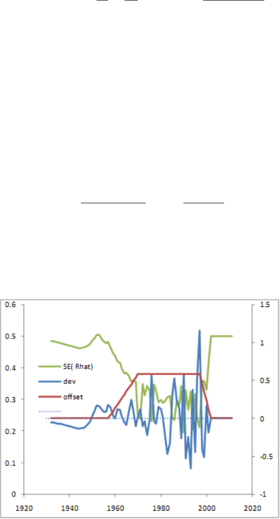
deviations will approach sigmaR and the variance of each recruitment deviation will approach
zero. Perfect data will estimate the recruitment time series signal perfectly. Of course, we
never have perfect data so we should always expect the estimated signal (variability among
the recruitment deviations) to be less than the true population recruitment variability.
SE(ˆry)2+SD(ˆr)2=
1
σ2
d
+1
σ2
R!−1/2
2
+
σ2
R
(σ2
R+σ2
d)1/2
2
=σ2
R(19)
The correct offset (bias adjustment) to apply to the expected value for recruitment is based
on the concept that a time series of estimated recruitments should be mean unbiased, not
median unbiased, because the biomass of a stock depends upon the cumulative number of
recruits, which is dominated by the large recruitments. The degree of offset depends upon
the degree of recruitment signal that can be estimated. Where no recruitment signal can
be estimated, the median recruitment is the same as the mean recruitment, so no offset is
applied. Where lognormal recruitment signal can be estimated, the mean recruitment will
be greater than the median recruitment. The value
by=
ESD(ˆry)2
σ2
R
= 1 −SE(ˆry)2
σ2
R
(20)
of the offset then depends upon the partitioning of sigmaR into between and within recruitment
variability. The most appropriate degree of bias adjustment can be approximated from the
relationship among sigmaR, recruitment variability (the signal), and recruitment residual
error.
99
Because the quantity and quality of data varies during a time series, SS allows the user to
control the rate at which the offset is ramped in during the early, data-poor years, and then
ramped back to zero for the forecast years. On output to report.sso, SS calculates the mean
bias adjustment during the early and main eras and compares it to the RMSE of estimated
recruitment deviations. A warning is generated if the RMSE is small and the bias adjustment
is larger than 2.0 times the ratio of rmse2to sigmaR2.
In MCMC mode, the model still draws recruitment deviations from the lognormal distribution,
so the full offset is used such that the expected mean recruitment from this lognormal
distribution will stay equal to the mean from the spawner-recruitment curve. When SS
reaches the MCMC and MCEVAL phases, all bias adjustment values are set to 1.0 for all
active recruitment deviations because the model is now re-sampling from the full lognormal
distribution of each recruitment.
9.6.4 Recruitment Autocorrelation
The autocorrelation parameter is implemented. It is not performance tested and it has no
effect on the calculation of the offsets described in the section above.
9.6.5 Recruitment Cycle
When SS is configured such that seasons are modeled as years, the concept of season within
year disappears. However, there may be reason to still want to model a repeating pattern
in expected recruitment to track an actual seasonal cycle in recruitment. If the recruitment
cycle factor is set to a positive integer, this value is interpreted as the number of time units
in the cycle and this number of full parameter lines will be read. The cyclic effect is modeled
as an exp(p) factor times R0, so a parameter value of 0.0 has nil effect. In order to maintain
the same number of total recruits over the duration of the cycle, a penalty is introduced so
that the cumulative effect of the cycle produces the same number of recruits as Ncycles *
R0. Because the cyclic factor operates as an exponential, this penalty is different than a
penalty that would cause the sum of the cyclic factors to be 0.0. This is done by adding a
penalty to the parameter likelihood, where:
X=X(ep)
Y=Ncycle
P enalty = 100000 ∗(X−Y)2
(21)
100

9.6.6 Initial Age Composition
A non-equilibrium initial age composition is achieved by setting the first year of the recruitment
deviations before the model start year. These pre-start year recruitment deviations will be
applied to the initial equilibrium age composition to adjust this composition before starting
the time series. The model first applies the initial F level to an equilibrium age composition
to get a preliminary N-at-age vector and the catch that comes from applying the F’s to that
vector, then it applies the recruitment deviations for the specified number of younger ages
in this vector. If the number of estimated ages in the initial age composition is less than
Nages, then the older ages will retain their equilibrium levels. Because the older ages in the
initial age composition will have progressively less information from which to estimate their
true deviation, the start of the bias adjustment should be set accordingly.
9.7 Fishing Mortality Method
There are three methods available for calculation of fishing mortality. These are: Pope’s
approximation, continuous F with each F as a model parameter, and a hybrid method
that does a Pope’s approximation to provide initial values for iterative adjustment of the
continuous F values to closely approximate the observed catch. With the hybrid method, the
final values are in terms of continuous F, but do not need to be specified as full parameters.
In a 2 fishery, low F case, the hybrid method is just as fast as the Pope approx. and produces
identical result. When F is very high, the problem becomes quite stiff for Pope’s and the
hybrid method so convergence may slow. It may be better to use F option 2 (continuous
F as full parameters) in these high F cases. F as parameter is also preferred for situations
where catch is known imprecisely and you are willing to accept a solution in which the final
F values do not reproduce the input catch levels exactly. For the F as parameter approach,
there is an option to do early phases using hybrid, then switch to F as parameter in later
phases and transfer the hybrid F values to the parameter initial values.
Option 1 (Pope’s approx) still exists, but it is recommended to switch to option 3.
Control file continued:
Value Description
0.2 F ballpark
This value is compared to the sum of the F’s for the specified
year. The sum is over all seasons and areas. The lambda for
the comparison goes down by a factor of 10 each phase and goes
to 0.0 in the final phase.
-1990 F ballpark year
Negative value disable F ballpark
3 F Method
101

Value Description
1 = Pope’s
2 = Continuous F as a parameter
3 = Hybrid F (recommended)
2.9 Maximum F
This maximum is applied within each season and area. A value
of 0.9 is recommended for F method 1, and a value of about 4
is recommended for F method 2 and 3.
COND: Depending on the F method
COND = 1: No additional input for Pope’s approximation
COND = 2: Continuous F
0.10 1 1 Inital F value, Phase, N F detail setup lines to read. Starting
value for each F. Initializing value for each F parameter.
For phases prior to the phase of the F value becoming active,
SS will use the hybrid option and the F values so calculated
become the starting values for the F parameters when this phase
is reached.
If F method = 2 and N for F detail is > 0
1 1980 1 0.20 0.05 4 fleet, year, season, F, SE, phase - these values override the catch
se values in the data file and the overall starting F value and
phase read just above.
COND = 3: Hybrid F
4 Number of tuning iterations in hybrid method. A value of 2 or
3 is sufficient with a single fleet and low Fs. A value of 5 or so
may be needed to match the catch near exactly when there are
many fleets and high F.
9.7.1 Initial Fishing Mortality
Read a short parameter setup line for each fishery. The parameters are the fishing mortalities
for the initial equilibrium. Do not try to estimate parameters for fisheries with zero initial
equilibrium catch. If there is catch, then give a starting value greater than zero and it
generally is best to estimate the parameter in phase 1.
In SS3.30, the initial equilibrium year has explicit seasons, so the needed initial F values will
also be by season. Initial F values are only needed for fleet/seasons that have catch. So if
no fleet/season combo has catch, then no parameters are needed.
102
It is possible to use the initial F method to achieve an estimate of the initial equilibrium Z
in cases where the initial equilibrium catch is unknown. To do this:
•Include a positive value for the initial equilibrium catch;
•Set the lambda for the logL for initial equilibrium catch to a nil value (hence causing
SS to ignore the lack of fit to the input catch level;
•Allow the initial F parameter to be estimated. It will be influenced by the early age
and size comps which should have some information about the early levels of Z.
9.8 Catchability
Catchability is the scaling factor that relates a model quantity to the expected value for
some type of data (index). Typically this is used to converted selected numbers or biomass
for a fleet into the expected value for a survey or CPUE by that fleet. In SS, the concept has
been extended so that, for example, a time series of an environmental factor could be treated
as a survey of the time series of deviations for some parameter. This flexibility means that
a family of link functions beyond simple proportionality is needed.
For each fishery and survey with an index, enter a row with the entries as described below:
1. Fleet Number
2. Link type or index of dev vector: An assumed functional form between Q, the expected
value, and the survey observation.
(a) 1 = simple Q, proportional assumption about Q: y=q∗x.
(b) 2 = mirror simple Q, 1 mirrored parameter.
(c) 3 = Q with power, 2 parameters establish a parameter for non-linearity in survey-abundance
linkage. Assumes proportional with offset and power function: y=qxcwhere
q=exp(lnQbase)) thus the cis not related to expected biomass but vulnerable
biomass to Q. Therefore, c < 0 leads to hyper-stability and c > 0leads to
hyper-depletion.
(d) If the parameter is for an index of a dev vector (index units = 35), use this column
to enter the index of the dev vector to which the index is related
3. Extra input for link (i.e. mirror fleet)
(a) >0 = mirror the Q from another (lower numbered survey designated by abs(value))
103

4. Do extra SD
(a) 0 = skip (typical)
(b) 1 = estimate a parameter that will contain an additive constant to be added to
the input standard deviation of the survey variability. This extra SD approach
accomplishes the same thing in principle as the older code, but may not give
exactly the same answer as the older code. The newer code for extra SD estimation
is recommended.
5. Bias adjustment
(a) 0 = no bias adjustment applied
(b) 1 = apply bias adjustment
6. Q float
(a) 0 = no float (parameter is estimated)
(b) 1 = float (analytical solution is used, but parameter line still required)
So for a setup with a single survey, the Q setup matrix could be:
#Fleet
Num.
Link Type Link Info Extra SD Bias
Adjust
Float Label
3 1 0 1 1 0 #Survey
-9999 0 0 0 0 0 #End Read
A long parameter line is expected for each link parameter (i.e. Q) and for the
extra SD parameter.
#LO HI INIT PRIOR PR SD PR
TYPE
PHASE ENV (Cont. below)
-2 2 -0.12 0 0 0 9 0
0 0.5 0.05 0.05 0 0 9 0
Cont: USE
DEV
DEV
MINY
DEV
MAXY
DEV
PH
BLOCK BLOCK
FXN
LABEL
1 1982 2015 -5 0 0 #Survey1 LnQ base
0 0 0 0 0 0 #Survey1 extra sd
Then because the Q base parameter specifies that it is time-varying by the annual dev
104

method, short parameter lines to specify the specifications of the dev vector come after all
the base Q parameters.
#LO HI INIT PRIOR PR
SD
PRIOR
TYPE
PHASE LABEL
0.001 2 0.079 0.079 0.5 4 -5 #LnQ base Survey dev se
-0.99 0.99 0.00 0.00 0.5 4 -6 #LnQ base Survey dev
autocorrelated
NOTE: In 3.24 it was common to use the deviation approach and this deviation approach in
SS v.3.24 was implemented as if it was survey specific blocks. In some cases, only one year’s
deviation was made active in order to implement, in effect, a block for Q. sstrans.exe cannot
convert this, but an analogous approach is available in SS3.30 because true blocks can now
be used, as well as env links and annual deviations. Also note that deviations in 3.24 were
survey specific (so no parameter for years with no survey). But in SS3.30, deviations are
always year-specific, so you might have a deviation created for a year with no survey.
9.9 Selectivity and Discard
For each fleet and survey, read a definition line for size selectivity and retention. The four
values read from each line are:
Pattern
Valid length selectivity pattern code.
Discard
(0/1/2/3/4 or -index) If value is 1, then program will read 4 retention parameters
after reading the specified number of selectivity parameters and all discarded fish are
assumed dead. If the value is 2, then the program will read 4 retention parameters and
4 discard mortality parameters. If the value is 3, then no additional parameters are
read and all fish are assumed discarded and dead. If the value is 4, then the program
will read 7 retention parameters (for dome-shaped retention) and 4 discard mortality
parameters. If the value is a negative number, then it will mirror the retention and
discard mortality pattern of the lower numbered fleet.
Male
(0/1/2/3/4) If value is 1, then program will read 4 additional parameters to define
the male selectivity relative to the female selectivity. Anytime the male selectivity
is caused to be greater than 1.0; the entire male/female matrix of selectivity values
is scaled by the max so that the realized max is 1.0. Hopefully this does not cause
105

gradient problems. If the value is 2, then the main selectivity parameters define male
selectivity and female selectivity is estimated as an offset from male selectivity. This
alternative is preferable if female selectivity is less than male selectivity. The option 3 is
only available if the selectivity pattern is 1, 20, or 24 and it causes the male selectivity
parameters to be offset from the female parameters, rather than the male selectivity
being an offset from the female selectivity.
Special
(0/value). This value is used in different ways depending on the context. If the
selectivity type is to mirror another selectivity type, then put the index of that source
fleet or survey here. It must refer to a lower numbered fleet/survey. If the selectivity
type is 6 (linear segment), then put the number of segments here. If the selectivity
type is 7, then put a 1 here to keep selectivity constant above the mean average size
for old fish of morph 1.
For each fleet and survey, read a definition line for age selectivity. The 4 values to be read
are the same as for the size-selectivity. However, the retention value must be set to 0.
#Example Setup for Size Selectivity Types
#Pattern Discard Male Special Label
1 2 0 0 #Fishery1
1 0 0 0 #Survey1
0 0 0 0 #Survey2
#Age Selectivity Types
#Pattern Discard Male Special Label
11 0 0 0 #Fishery1
11 0 0 0 #Survey1
11 0 0 0 #Survey2
9.9.1 Reading the Selectivity and Retention Parameters
Read the required number of parameter setup lines as specified by the definition lines above.
The complete order of the parameter setup lines is:
1. Size selectivity for fishery 1
2. Retention for fishery 1 (if discard specified)
3. Discard Mortality for fishery 1 (if discard specified)
106

4. Male offsets for size selectivity for fishery 1 (if offsets used)
5. <repeat for additional fleets and surveys>
6. Age selectivity for fishery 1
7. Male offsets for age selectivity for fishery 1 (if offsets used)
8. <repeat for additional fleets and surveys>.
The list of parameters to be read from the above setup would be:
#LO HI INIT PRIOR PR SD ... BLOCK
FXN
LABEL
19 80 53.5 50 0.5 ... 0 #SizeSel p1 fishery 1
0.01 60 18.9 15 0.5 ... 0 #SizeSel p2 fishery 1
20 70 38.6 40 0.5 ... 0 #Retain p1 fishery 1
0.1 10 6.5 1 0.5 ... 0 #Retain p2 fishery 1
0.001 1 0.98 1 0.5 ... 0 #Retain p3 fishery 1
-10 10 1 0 0.5 ... 0 #Retain p4 fishery 1
0.1 1 0.6 0.6 0.5 ... 0 #DiscMort p1 fishery 1
-2 2 0 0 0.5 ... 0 #DiscMort p2 fishery 1
20 70 40 40 0.5 ... 0 #DiscMort p3 fishery 1
0.1 10 1 1 0.5 ... 0 #DiscMort p4 fishery 1
19 80 53.5 50 0.5 ... 0 #SizeSel p1 survey 1
0.01 60 18.9 15 0.5 ... 0 #SizeSel p2 survey 1
0 40 0 5 0.5 ... 0 #AgeSel p1 fishery 1
0 40 40 5 0.5 ... 0 #AgeSel p2 fishery 1
0 40 0 5 0.5 ... 0 #AgeSel p1 survey 1
0 40 40 5 0.5 ... 0 #AgeSel p2 survey 1
0 40 0 5 0.5 ... 0 #AgeSel p1 survey 2
0 40 0 5 0.5 ... 0 #AgeSel p2 survey 2
9.9.2 Selectivity Patterns
The currently defined selectivity patterns, and corresponding required number of parameters,
are:
107

Pattern N Parameters Description
SIZE BASED SELECTIVITY
Pattern N Parameters Description
0 0 Selectivity equals 1.0 for all sizes
1 2 Logistic
2 8 Discontinued: Double logistic with defined peak (uses
IF joiners). Use pattern #8 instead.
3 6 Discontinued
4 0 Discontinued: Set size selectivity equal to female
fecundity. Use pattern #30 instead.
5 2 Mirror another selectivity. The two parameters select
bin range.
6 2 + special value Non-parametric
7 8 Discontinued: Double logistic with defined peak, uses
smooth joiners; special = 1 causes constant selectivity
above Linf for morph 1. Use pattern #8.
8 8 Double logistic, with defined peak, uses smooth joiners;
special=1 causes constant selectivity above Linf for
morph 1.
9 6 Simple double logistic with no defined peak.
15 0 Mirror another selectivity (same as for age selectivity).
22 4 Double normal; similar to CASAL.
23 6 Same as the double normal pattern #24 except the final
selectivity is now directly interpreted as the terminal
selectivity value.
24 6 Double normal with defined initial and final selectivity
level – Recommended option. Test using SELEX-24.xls.
25 3 Exponential-logistic
27 3 + 2*N nodes Cubic spline
42 5 + 2*N nodes Selectivity pattern 27 with user-defined scaling
43 4 + special value Selectivity pattern 6 with user-defined scaling
AGE BASED SELECTIVITY
Pattern N Parameters Description
108

Pattern N Parameters Description
10 0 Age selectivity = 1.0 for all ages beginning at age 1. If
it is desired that age-0 fish be selected, then use pattern
#11 and set minimum age to 0.0.
11 2 Pick min-max age
12 2 Logistic
13 8 Double logistic, IF joiners. Use discouraged. Use
pattern #18 instead.
14 nages + 1 Each age, value at age is 1
1+exp(−x)
15 0 Mirror another selectivity
16 2 Coleraine single Gaussian
17 nages + 1 Each age as random walk from previous age. For all
ages in the population beginning with Amin = 1 for the
fishery and 2 for the survey, there is a corresponding set
of selectivity parameters for each fleet, pa.
18 8 Double logistic, with defined peak, uses smooth joiners.
19 6 Simple double logistic with no defined peak.
20 6 Double normal with defined initial and final level.
Recommended option. Test using SELEX-24.xls.
26 3 Exponential logistic
27 3 + 2*N nodes Cubic Spline
41 2 + nages + 1 Selectivity pattern 17 with user-defined scaling
42 5 + 2*N nodes Selectivity pattern 27 with user-defined scaling
44 4 + nages Similar to age selectivity pattern 17 but with separate
parameters for males and with revised controls
45 4 + nages Similar to age selectivity pattern 14 but with separate
parameters for males and with revised controls
Special Selectivity Options
Special selectivity options (type 30 in size based selectivity) are no longer specified
within the control file. Specifying the use of one of these selectivity types is now done
within the data file by selecting the survey "units" (see the section on Index units).
9.9.3 Selectivity Pattern Details
Pattern #1 (size) and #12 (age) - Simple Logistic
Within SS logistic selectivity for the primary sex (if selectivity varies by sex) is formulated
109

as:
Sl=1.0
1 + exp(−ln(19)(Ll−p1)/p2) (22)
where Llis the length bin. If age based selectivity is selected then the length bin is
replaced by the age vector. If sex specific selectivity is specified the non-primary sex
the p1 and p2 parameters are estimated as offsets. Note that with a large p2 parameter,
selectivity may not reach 1.0 at the largest size bin. The parameters are:
•p1 - size/age at inflection
•p2 - width for 95% selection; a negative width causes a descending curve.
Pattern #5 (size) - Mirror Selectivity
Two parameters select the min and max bin number (not min max size) of the source
pattern. If first parameter has value <=0, then interpreted as a value of 1 (e.g. first
bin). If second parameter has value <=0, then interpreted as nlength (e.g. last bin).
The source pattern must have a lower type number
Pattern #6 (size) - Non-parametric Selectivity
Non-parametric size selectivity uses a set of linear segments. The first waypoint is at
Length = p1 and the last waypoint is at Length = p2. The total number of waypoints is
specified by the value of the Special factor in the selectivity set-up, so the N intervals
is one less than the number of waypoints. Intermediate waypoints are located at
equidistant intervals between p1 and p2. Parameters 3 to N are the selectivity values
at the waypoints, entered as logistic, e.g. 1/(1 + exp(−x)). Ramps from –10 to p3 if
L<p1. Constant at pN if L>p2. Note that prior to version 3.03 the waypoints were
specified in terms of bin number, rather than length.
Pattern #8 (size) and #18 (age) - Double Logistic
•p1 – PEAK: size (age) for peak. Should be an integer and should be at bin
boundary and not estimated. But options 7 and 18 may allow estimation.
•p2 – INIT: selectivity at lengthbin=1 (minL) or age=0.
•p3 – INIT: selectivity at lengthbin=1 (minL) or age=0. A logit transform (1/(1 +
exp(−x)) is used so that the transformed value will be between 0 and 1. So a p1
value of –1.1 will be transformed to 0.25 and used to set the selectivity equal to
0.5 at a size (age) equal to 0.25 of the way between minL and PEAK.
•p4 – SLOPE1: log(slope) of left side (ascending) selectivity.
•p5 – FINAL: logit transform for selectivity at maxL (or maxage).
•p6 – INFL2: logit transform for size(age) at right side selectivity equal to half
110

way between PEAK+PEAKWIDTH and maxL (or max age).
•p7 – SLOPE2: log(slope) of right side (descending) selectivity
•p8 – PEAKWIDTH: in width of flattop.
Pattern #14 (age) - Revise Age
Age-selectivity pattern #14 to allow selectivity-at-age to be the same as selectivity at
the next younger age. When using this option, the range on each parameter should be
approximately -5 to 9 to prevent the parameters from drifting into extreme values with
nil gradient. SS calculates the age-based selectivity as where a= 1 to a=Amax + 1:
temp = 9 −max(p(a))
Sa=1
1 + exp(−(p(a+ 1) + temp))
(23)
Pattern #17 (age) - Random Walk
This selectivity pattern provides for a random walk in ln(selectivity). For each age
a≥Amin, where Amin is the minimum age for which selectivity is allowed to be non-zero,
there is a selectivity parameter, pa, controlling the changein selectivity from age a−1
to age a.
The selectivity at age ais computed as
Sa= exp(S0
a−S0
max),(24)
where
S0
a=
a
X
i=Amin
pi(25)
and
S0
max =max{S0
a}.(26)
Selectivity is fixed at Sa= 0 for a<Amin.
This formulation has the properties that the maximum selectivity equals 1, positive
values of paare associated with increasing selectivity between ages a−1and a, and
negative values are associated with decreasing selectivity between those ages and pa= 0
gives constant selectivity.
The condition that maximum selectivity equals 1 results in one fewer degree of freedom
than the number of estimated pa. Therefore, at least one parameter should be fixed at
an arbitrary value, typically pAmin = 0.
In typical usage:
111
•First parameter (for age 0) could have a value of -1000 so that the age 0 fish would
get a selectivity of 0.0;
•Second parameter (for age 1) could have a value of 0.0 and not be estimated, so
age 1 is the reference age against which subsequent changes occur;
•Next parameters get estimated values. To assure that selectivity increases for the
younger ages, the parameter min for these parameters could be set to 0.0 or a
slightly negative value.
•If dome-shaped selectivity is expected, then the parameters for older ages could
have a range with the max set to 0.0 so they cannot increase further.
•To keep selectivity at a particular age the same as selectivity at the next younger
age, set its parameter value to 0.0 and not estimated. This allows for all older
ages to have the same selectivity.
•To keep a constant rate of change in selectivity across a range of ages, use the
-999 flag to keep the same rate of change in ln(selectivity) as for the previous age.
•Code for implementing random walk selectivity within SS can be found in Appendix
C. Click here for more information.
Pattern #9 (size) and #19 (age) - Simple Double Logistic with no defined peak
•p1 - INFL1: ascending inflection size (in cm)
•p2 – SLOPE1: ascending slope
•p3 – INFL2: descending inflection size (in cm)
•p4 – SLOPE2: descending slope
•p5 – first BIN: bin number for the first bin with non-zero selectivity (must be an
integer bin number, not a size)
•p6 – offset: enter 0 if P3 is independent of P1; enter 1 if P3 is an offset from P1
Pattern #22 (size) - Double Normal with Plateau
•p1 – PEAK1: beginning size for the plateau (in cm)
•p2 – PEAK2: ending size for the plateau. Calculated as a fraction of the distance
between PEAK1 and 99% of the lower edge of the last size bin in the model.
112
Transformed as (1/(1+exp(-p2)). So a value of 0 results in PEAK2 being halfway
between PEAK1 and 99% of the last bin
•p3 – upslope: ln(variance) on ascending side
•p4 – downslope: ln(variance) on descending side
Pattern#23 (size) and #24 (size) - Double Normal Selectivity
•p1 – PEAK: beginning size for the plateau (in cm)
•p2 – TOP: width of plateau, as logistic between PEAK and MAXLEN
•p3 – ASC-WIDTH: parameter value is ln(width)
•p4 – DESC-WIDTH: parameter value is ln(width)
•p5 – INIT: selectivity at first bin, as logistic between 0 and 1.
•p6 – FINAL: selectivity at last bin, as logistic between 0 and 1. (for pattern #24)
or
•p6 – FINAL: selectivity at last bin, as absolute value, so can be >1.0. (for
pattern #23). Warning: Do not allow this value to go above 1.0 if the F_method
uses Pope’s approximation. OK to go above 1.0 when F is in exponential form.
When this parameter is above 1.0, the overall selectivity pattern will have an
intermediate plateau at 1.0 (according to peak and top), then will ascend further
to the final value.
Notes for Double Normal Selectivity:
•See spreadsheet SELEX-24.xls for parameterization example.
•For the initial selectivity parameter (#5)
–-999 or –1000: ignore the initial selectivity algorithm and simply decay the
small fish selectivity according to P3,
–< -1000: ignore the initial selectivity algorithm as above and then set selectivity
equal to 1.0e-06 for size bins 1 through bin = -1001 –value. So a value of –1003
would set selectivity to a nil level for bins 1 through 2 and begin using the
modeled selectivity in bin 3.
•For the final selectivity parameter (#6)
113
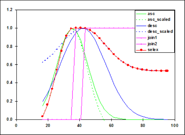
–-999 or –1000: ignore the final selectivity algorithm and simply decay the
large fish selectivity according to parameter #4,
–<-1000: set selectivity constant for bins greater than bin number = -1000 –
value.
Selectivity pattern #24, double normal, showing sub-functions and steep logistic joiners:
Pattern #15 (age) - Mirror
No parameters. Whole age range is mirrored from a user-specified fleet.
Pattern #16 - Gaussian (similar to Coleraine)
•p1 – age below which selectivity declines
•p2 – scaling factor for decline
Pattern #9 (size) and #19 (age) - Simple Double Logistic
•p1 – ascending inflection age/size
•p2 – ascending slope
•p3 – descending inflection age/size
•p4 – descending slope
•p5 – age or size at first selection; this is a specification parameter, so must not be
114
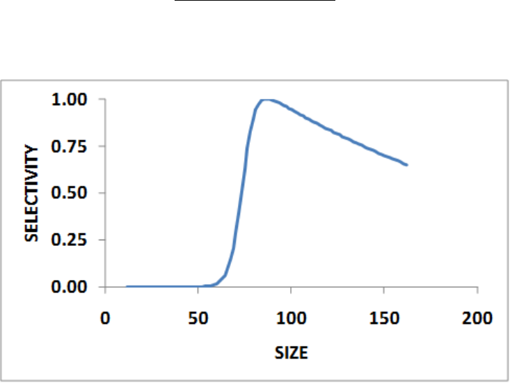
estimated. Enter integer that is age for pattern 19 and is bin number for pattern
9
•p6 – (0/1) where a value of 0 causes the descending inflection to be a standalone
parameter, and a value of 1 causes the descending inflection to be interpreted as
an offset from the ascending inflection. This is a specification parameter, so must
not be estimated.
A value of 1.0e-6 is added to the selectivity for all ages, even those below the minage.
Pattern #25 (size) and #26 (age) - Exponential logistic
•p1 – ascending rate, min: 0.02, max: 1.0, reasonable start value: 0.1
•p2 – peak, as fraction of way between min size and max size. Parameter min
value: 0.01; max: 0.99; reasonable start value: 0.5
•p2 – minsize + p2*(maxsize-minsize)
•p3 – descending rate, min: 0.001, max: 0.5, reasonable start value: 0.01. A value
of 0.001 provides a nearly asymptotic curve. Values above 0.2 provide strongly
dome-shaped function in which the p3 and p1 parameters interact strongly.
ep3∗p1(p20−size)
1−p3(1 −ep1(p20−size))(27)
Example: Exponential logistic selectivity with p1 = 0.30, p2 = 0.50, and p3 = 0.02:
115
Pattern #27 (size and age)- Cubic Spline
This selectivity pattern uses the ADMB implementation of the cubic spline function.
This function requires input of the number of nodes, the positions of those nodes, the
parameter values at those nodes, and the slope of the function at the first and last
node. In SS, the number of nodes is specified in the “special” column of the selectivity
set-up. The pattern number 27 is used to invoke cubic spline for size selectivity and
for age selectivity; the input syntax is identical.
For a 3 node setup, the SS input parameters would be:
•p1 – code for initial set-up (0, 1 or 2) as explained below
•p2 – gradient at the first node (should be a small positive value)
•p3 – gradient at the last node (should be zero or a small negative value)
•p4-p6 – the nodes in units of cm; must be in rank order and inside of the range
of the population length bins. These must be held constant (not estimated, e.g.
negative phase value) during a model run.
•p7-p9 – the values at the nodes. Units are ln(selectivity).
Notes:
•There must be at least 3 nodes.
•One of these selectivity parameter values should be held constant so others are
estimated relative to it.
•Selectivity is forced to be constant for sizes greater than the size at the last node
•The overall selectivity curve is scaled to have a peak equal to 1.0.
•Terminal nodes cannot be at the min or max population length bins.
Code for implementing cubic spline selectivity within SS can be found in Appendix C.
Click here for more information.
The figure below compares a 3 node and a 6 node cubic spline with a 2 parameter
logistic function. In fitting these functions, the 2 cubic spline approaches fit slightly
better than the logistic, presumably because the data were slightly indicative of a small
dome in selectivity.
116
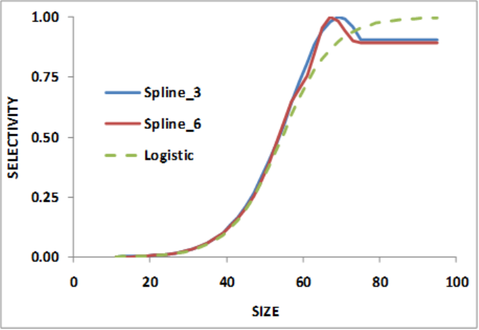
Auto-Generation of Cubic Spline Control File Set-Up:
A New SS feature pioneered with the cubic spline function is a capability to produce
more specific parameter labels and to auto-generate selectivity parameter setup. The
auto-generation feature is controlled by the first selectivity parameter value for each
fleet that is specified to use the cubic spline. There are 3 possible values for this setup
parameter:
•0: no auto-generation, process parameter setup as read.
•1: auto-generate the node locations based on the specified number of nodes and
on the cumulative size distribution of the data for this fleet/survey.
•2: auto-generate the nodes and also the min, max, prior, init, and phase for each
parameter.
With either the auto-generate option #1 or #2, it still is necessary to include in the
parameter file placeholder rows of values so that the init_matrix command can input
the current number of values because all selectivity parameter lines are read as a single
matrix dimensioned as N parameters x 14 columns. The read values of min, max, init,
prior, prior type, prior stddev, and phase will be overwritten.
Cumulative size and age distribution is calculated for each fleet, summing across all
samples and both sexes. These distributions are output in echoinput.sso and in a new
OVERALL_COMPS section of report.sso.
When the nodes are auto-generated, the first node is placed at the size corresponding to
117

the 2.5% percentile of the cumulative size distribution, the last is placed at the 97.5%
percentile of the size distribution, and the remainder are placed at equally spaced
percentiles along the cumulative size distribution. These calculated node values are
output into control.ss_new. So, the user could extract these nodes from control.ss_new,
edit them to desired values, then, insert them into the input control file. Remember
to turn off auto-generation in the revised control file.
When the complete auto-generation is selected, the control.ss_new would look like the
table below:
#LO HI INIT PR PR_SD ... BLOCK
FXN
#Label
0 2 2.0 0 0 ... 0 #SizeSpline Code
-0.001 1 0.13 0 0.1 ... 0 #SizeSpline GradLo
-1 0.001 -0.03 0 0.1 ... 0 #SizeSpline GradHi
11 95 38 0 0 ... 0 #SizeSpline Knot1
11 95 59 0 0 ... 0 #SizeSpline Knot2
11 95 74 0 0 ... 0 #SizeSpline Knot3
-9 7 -3 0 0.1 ... 0 #SizeSpline Value1
-9 7 -1 0 0.1 ... 0 #SizeSpline Value2
-9 7 -0.78 0 0.1 ... 0 #SizeSpline Value3
Pattern #41 (age) - Random Walk with User-Defined Scaling
Selectivity pattern 17 with two additional parameters. The two additional parameters
are the bin numbers to define the range of bins for scaling. All of the selectivity values
will be scaled (divided) by the mean value over this range. The low and high bin
numbers are defined before the other selectivity parameters.
#LO HI INIT PR PR_SD ... BLOCK
FXN
#Label
0 20 10 0 0.5 ... 0 #AgeSel_ScaleAgeLo
0 20 20 0 0.5 ... 0 #AgeSel_ScaleAgeHi
Pattern #42 (size and age) - Cubic Spline with User-Defined Scaling
Selectivity pattern 27 with two additional parameters. The two additional parameters
are the bin numbers to define the range of bins for scaling. All of the selectivity values
will be scaled (divided) by the mean value over this range. The low and high bin
118

numbers are defined before the other selectivity parameters.
#LO HI INIT PR PR_SD ... BLOCK
FXN
Label
0 20 10 0 0.5 ... 0 #AgeSpline_ScaleAgeLo
0 20 20 0 0.5 ... 0 #AgeSpline_ScaleAgeHi
Pattern #43 (size) - Non-parametric with User-Defined Scaling
Selectivity pattern 6 with two additional parameters. The two additional parameters
are the bin numbers to define the range of bins for scaling. All of the selectivity values
will be scaled (divided) by the mean value over this range. The low and high bin
numbers are defined before the other selectivity parameters.
#LO HI INIT PR PR_SD ... BLOCK
FXN
#Label
1 80 50 0 0.5 ... 0 #SizeSel_ScaleBinLo
1 80 70 0 0.5 ... 0 #SizeSel_ScaleBinHi
Pattern #44 (age)
Similar to pattern #17 but with separate parameters for males and females. This
selectivity pattern provides for a random walk in ln(selectivity). In typical usage:
•p1 - First parameter (for age 0) could have a value of -1000 so that the age 0 fish
would get a selectivity of 0.0.
•p2 - The first age for which mean selectivity = 1.
•p3 - The last age for which mean selectivity = 1.
•p4 - Male mean selectivity relative to the female selectivity mean entered as
ln(ratio) for the male relative female selectivity.
•p5-pn- Additional parameter lines for the log of the selectivity change between
ages corresponding to the user specified number of changes in the "special" column
for the selectivity specification for each sex with females entered first then males.
•-999 input indicates to the model to keep the change unchanged from the previous
age (keeps same rate of change).
119

•-1000 input indicates used only for male selectivity indicates to the model to set
the change in male selectivity equal to the female change in selectivity.
An example specification and setup for this selectivity option where selectivity is
dome-shaped, peaking at age 2 with female and male selectivity are equal with 4
change points per sex:
#Pattern Discard Male Special
44 0 0 4
#LO HI INIT PR PR_SD ... BLOCK
FXN
#Label
0 20 0 0 0.5 ... 0 #first selex age
0 20 2 2 0.5 ... 0 #first age peak selex (mean)
0 20 2 2 0.5 ... 0 #last age peak selex (mean)
-1 2 -0.001 -0.001 0.5 ... 0 #male ln(ratio)
-10 10 3.01 3.01 0.5 ... 0 #female ln(selex) change 1
-10 10 1.56 1.56 0.5 ... 0 #female ln(selex) change 2
-10 10 -0.15 -0.15 0.5 ... 0 #female ln(selex) change 3
-10 10 -0.15 -0.15 0.5 ... 0 #female ln(selex) change 4
-1000 10 -1000 -0.9 0.5 ... 0 #male ln(selex) change 1
-1000 10 -1000 -0.9 0.5 ... 0 #male ln(selex) change 2
-1000 10 -1000 -0.9 0.5 ... 0 #male ln(selex) change 3
-1000 10 -1000 -0.9 0.5 ... 0 #male ln(selex) change 4
Pattern #45 (age) - Revise Age
Similar to pattern #14 but with separate parameters for males and females. Age-selectivity
pattern #45 to allow selectivity-at-age to be the same as selectivity at the next younger
age.
•p1 - is the first age with non-zero selectivity.
•p2 - The first age in mean for peak selectivity
•p3 - The last age in mean for peak selectivity
•p4 - The male mean selectivity relative to the female mean, entered as ln(ratio)
120

for the male relative female selectivity
•-999 input indicates to the model to keep the change unchanged from the previous
age (keeps same rate of change).
•-1000 input indicates used only for male selectivity indicates to the model to set
the change in male selectivity equal to the female change in selectivity.
An example specification and setup for this selectivity option where selectivity is
asymptotic, with female and male selectivity are equal with 4 change points per sex:
#Pattern Discard Male Special
45 0 0 3
#LO HI INIT PR PR_SD ... BLOCK
FXN
#Label
0 20 2 0 0.5 ... 0 #first selex age
0 20 5 2 0.5 ... 0 #first age peak selex (mean)
0 20 5 2 0.5 ... 0 #last age peak selex (mean)
-1 2 -0.001 -0.001 0.5 ... 0 #male ln(ratio)
-10 10 -8.1 -8.1 0.5 ... 0 #female ln(selex) change 1
-10 10 -4.1 -4.1 0.5 ... 0 #female ln(selex) change 2
-10 10 -1.8 -1.8 0.5 ... 0 #female ln(selex) change 3
-1000 10 -1000 -0.9 0.5 ... 0 #male ln(selex) change 1
-1000 10 -1000 -0.9 0.5 ... 0 #male ln(selex) change 2
-1000 10 -1000 -0.9 0.5 ... 0 #male ln(selex) change 3
9.9.4 Retention
Retention is defined as a logistic function of size. It does not apply to surveys. Four
parameters (for asymptotic retention) or seven parameters (for dome-shaped retention) are
used:
•p1 – ascending inflection
•p2 – ascending slope
121

•p3 – maximum retention (often a time-varying quantity to match the observed amount
of discard)
•p4 – male offset to ascending inflection (arithmetic, not multiplicative)
•p5 – descending inflection
•p6 – descending slope
•p7 – male offset to descending inflection (arithmetic, not multiplicative)
Retention = P3
1 + e−(L−(P1+P4∗male))
P2!∗ 1−1
1 + e−(L−(P5+P7∗male))
P6!(28)
9.9.5 Discard Mortality
Discard mortality is defined as a logistic function of size such that mortality declines from
1.0 to an asymptotic level as fish get larger. It does not apply to surveys and it does not
affect the calculation of expected values for discard data. It is applied so that the total
mortality rate is:
deadfish = selex * (retain + (1.0-retain)*discmort)
If discmort is 1.0, all selected fish are dead; if discmort is 0.0, only the retained fish are
dead.
Four parameters are used:
•p1 – descending inflection
•p2 – descending slope
•p3 – maximum discard mortality
•p4 – male offset to descending inflection (arithmetic, not multiplicative)
Discard mortality is calculated as:
Mortality = 1−1−P3
1 + e−(L−(P1+P4∗male))
P2!(29)
122
9.9.6 Male Selectivity
There are two approaches to specifying sex specific selectivity. One approach allows male
selectivity to be specified as a fraction of female selectivity (or vice versa). This first approach
can be used for any selectivity pattern. The other option allows for separate selectivity
parameters for each sex plus an additional parameter to define the scaling of one sex’s peak
selectivity relative to the other sex’s peak. This second approach has only been implemented
for a few selectivity patterns.
Approach #1:
If the “domale” flag is set to 1, then the selectivity parameters define female selectivity and
the offset defined below sets male selectivity relative to female selectivity. The two sexes
switch roles if the “domale” flag is set to 2. Generally it is best to select the option so that
the dependent sex has lower selectivity, thus obviating the need to rescale for selectivities
that are greater than 1.0. Sex specific selectivity is done the same way for all size and age
selectivity options.
•P1 – size (age) at which a dogleg occurs (set to an integer at a bin boundary and do
not estimate)
•P2 – log(relative selectivity) at minL or age=0. Typically this will be set to a value
of 0.0 (for no offset) and not estimated. It would be a rare circumstance in which the
youngest/smallest fish had sex-specific selectivity.
•P3 – log(relative selectivity) at the dogleg
•P4 – log(relative selectivity) at maxL or max age.
For intermediate ages, the log values are linearly interpolated on size (age).
If selectivity for the dependent sex is greater than the selectivity for the first sex (which
always peaks at 1.0), then the male-female selectivity matrix is rescaled to have a maximum
of 1.0.
Approach #2:
A new sex selectivity option (3 or 4) has been implemented for size selectivity patterns 1
(logistic) and 23 and 24 (double normal) or age selectivity pattern 20 (double normal age).
Rather than calculate male selectivity as an offset from female selectivity, here the male
selectivity is calculated by making the male parameters an offset from the female parameters
(option 3), or females are offset from males with option 4. The description below applies to
option 3. If the size selectivity pattern is 1 (logistic), then read 3 parameters:
•male parameter 1 is added to the first selectivity parameter (inflection)
123

•male parameter 2 is added to the second selectivity parameter (width of curve)
•male parameter 3 is the asymptotic selectivity
If the size selectivity pattern is 20, 23 or 24 (double normal), then:
•male parameter 1 is added to the first selectivity parameter (peak)
•male parameter 2 is added to the third selectivity parameter (width of ascending side);
then exp(this sum) per previous transform
•male parameter 3 is added to the fourth selectivity parameter (width of descending
side); then exp(sum) per previous transform
•male parameter 4 is added to the sixth selectivity parameter (selectivity at final size
bin); then 1/(1+exp(-sum)) per previous transform
•male parameter 5 is the apical selectivity for males
Note that the male selectivity offsets currently cannot be time-varying (need to check on this).
Because they are offsets from female selectivity, they inherit the time-varying characteristics
of the female selectivity.
9.9.7 Dirichlet Multinomial Error for Data Weighting
If the Dirichlet multinomial error distribution was selected in the data file for either length
or age data weighting an additional parameter line is required immediately following the
selectivity parameter block.
#LO HI INIT PRIOR PR SD ... BLOCK
FXN
LABEL
The list of parameters to be read from the above setup would be:
#LO HI INIT PRIOR PR SD ... BLOCK
FXN
LABEL
1 25 1 1 10 ... 0 #ln(EffN mult) Age or
Length 1 Dirichlet
1 25 1 1 10 ... 0 #ln(EffN mult) Age or
Length 2 Dirichlet
124

9.9.8 Time-varying Options
The time-varying options for selectivity parameters are identical to the time-varying options
for biology parameters. These options are described below in the Using Time-Varying
Parameter Options section. After reading the selectivity parameters, which will include
possible instructions to create environmental link, blocks, or deviation vectors, then read
the following section. Note that all inputs in this section are conditional (COND) on entries
in the selectivity parameter section. So if no selectivity parameters invoke any time-varying
properties, this section is left blank (or completely commented out with #).
Example short parameter lines for selectivity time-varying parameters:
#LO HI INIT PRIORPR_SD PRIOR
TYPE
PHASE #Label
0.01 2.0 0.58 0.58 0.5 4 -5 #AgeSel_P4_Fishery_dev_se
1 80 70 70 0.5 4 -5 #AgeSel_P4_Fishery_dev_autocorr
9.9.9 Two-Dimensional Auto-Regressive Selectivity
A new experimental feature added within SS v. 3.30.03.02. Earlier versions do not have this
feature and hence this input is not expected. This features allows for auto-correlation by
age and/or time. The age based random walk selectivity, pattern 17, should be selected to
implement the semiparametric auto-regressive selectivity.
Value Label Description
1 Two-dimensional auto-regressive selectivity 0 = not used
1 = use
COND = 1 Read the following long parameter lines:
Sigma Use Len(1)/ Before After
#Fleet Ymin Ymax Amin Amax Amax Rho Age(2) Phase Range Range
1 1979 2015 2 10 1 1 2 5 1980 2007
Continued:
PRIOR PRIOR
#LO HI INIT PRIOR SD TYPE PHASE LABEL
0 4 1 1 0.1 6 -4 #Sigma selex
-1 1 0 0 0.1 6 -4 #Rho year
125

-1 1 0 0 0.1 6 -4 #Rho age
#Terminator line of 11 in length indicates the end of parameter input lines
-9999 1 1 1 1 1 1 1 1 1 1
Parameter Definitions:
•Fleet: Fleet number to which semi-parametric deviations should be added
•Ymin: First year with deviations
•Ymax: Last year with deviations
•Amin: First integer age (or population length bin index) with deviations
•Amax: Last integer age (or population length bin index) with deviations
•Sigma Amax: Not currently implemented. It is recommended to set the Sigma Amax
equal to the Amin value. In future, Sigma Amax will be set to last age (or population
length bin index) for which a separate sigma should be read
•Use Rho: Use autocorrelation parameters
•Len(1)/Age(2): 1 or 2 to specify whether the deviations should be applied to length-
or age-based selectivity
•Phase: Phase to begin estimation of the deviation parameters
•Before Range: How should selectivity be modeled in the years prior to Ymin? Available
options are (0) apply no deviations, (1) use deviations from the first year with deviations
(Ymin), and (3) use average across all years with deviations (Ymin to Ymax)
•After Range: Similar to Before Range but defines how selectivity should be modeled
after Ymax
How is the two-dimensional autoregressive selectivity parameterized in SS?
When the two-dimensional autoregressive selectivity feature in turned on for a fleet,
the selectivity of which is calculated as a product of the assumed selectivity pattern
and a non-parametric deviation term away from this assumed pattern:
ˆ
Sa,t =Saexpa,t (30)
where Sais specified in the corresponding age/length selectivity types section and
it can be either parametric (recommended) or non-parametric (including any of the
126

existing selectivity options in Stock Synthesis); a,t is simulated as a two-dimensional
first-order autoregressive (2D AR1) process:
vec()∼MV N (0, σ2
sRtotal)(31)
where is the two-dimensional deviation matrix and σ2
sRtotal is the covariance matrix
for the 2D AR1 process. More specifically, σ2
squantifies the variance in selectivity
deviations and Rtotal is equal to the knonecker product (⊗) of the two correlation
matrices for the among-age and among-year AR1 processes:
Rtotal =R⊗˜
R(32)
Ra,˜a=ρ|a−˜a|
a(33)
˜
Rt,˜
t=ρ|t−˜
t|
t(34)
where ρaand ρtare the among-age year AR1 coefficients, respectively. When both of
them are zero, Rand ˜
Rare two identity matrices and their Kronecker product, Rtotal,
is also an identity matrix. In this case selectivity deviations are essentially identical
and mutually independent:
a,t ∼N(0, σ2
s)(35)
How should the two-dimensional autoregressive selectivity feature be used in SS?
First, fix the two AR1 coefficients (ρaand ρt) at 0 and tune σsiteratively to match
the relationship:
σ2
s=SD()2+1
(amax −amin + 1)(tmax −tmin + 1)
amax
X
a=amin
tmax
X
t=tmin
SE(a,t)2(36)
The minimal and maximal ages/lengths and years for the 2D AR1 process can be freely
specified by users in the control file. However, we recommend specifying the minimal
and maximal ages and years to cover the relatively "data-rich" age/length and year
ranges only. Particularly we introduce:
b= 1 −
1
(amax−amin +1)(tmax−tmin+1) Pamax
a=amin Ptmax
t=tmin SE(a,t)2
σ2
s
(37)
as a measure of how rich the composition data is regarding estimating selectivity
deviations. We also recommend using the Dirichlet-Multinomial method to "weight"
the corresponding composition data while σsis interactively tuned in this step.
Second, fix σsat the value iteratively tuned in the previous step and estimate a,t. Plot
both Pearson residuals and a,t out on the age-year surface to check their 2D dimensions.
127

If their distributions seems to be not random but rather be autocorrelated (deviation
estimates have the same sign several ages and/or years in a row), users should consider
estimating and then including the autocorrelations in a,t.
Third, extract the estimated selectivity deviation samples from the previous step for
estimating ρaand ρtexternally by fitting the samples to a stand-alone model written
in Template-Model Builder (TMB). In this model, both ρaand ρtare bounded between
0 and 1 via applying a logic transformation. If at least one of the two AR1 coefficients
are notably different from 0, Stock Synthesis should be run one more time by fixing
the two AR1 coefficients at their values externally estimated from deviation samples.
The Pearson residuals and a,t from this run are expected to distribute more randomly
as the autocorrelations in selectivity deviations can be at least partially included in
the 2D AR1 process.
9.10 Tag Recapture Parameters
Specify if tagging data are being used:
Value Label Description
1 Tagging Data Present 0 = no read
1 = read following lines
COND = 1 Read the following long parameter lines:
PRIOR PRIOR
#LO HI INIT PRIOR SD TYPE PHASE ... LABEL
-10 10 9 9 0.001 4 -4 0 #TG loss init 1
-10 10 9 9 0.001 4 -4 0 #TG loss init 2
-10 10 9 9 0.001 4 -4 0 #TG loss init 3
-10 10 9 9 0.001 4 -4 0 #TG loss chronic1
-10 10 9 9 0.001 4 -4 0 #TG loss chronic2
-10 10 9 9 0.001 4 -4 0 #TG loss chronic3
1 10 2 2 0.001 4 -4 0 #TG loss overdisperion1
1 10 2 2 0.001 4 -4 0 #TG loss overdisperion2
1 10 2 2 0.001 4 -4 0 #TG loss overdisperion3
-10 10 9 9 0.001 4 -4 0 #TG report fleet1
-10 10 9 9 0.001 4 -4 0 #TG report fleet2
-4 0 0 0 0.001 2 -4 0 #TG report decay1
-4 0 0 0 0.001 2 -4 0 #TG report decay2
128

The tagging reporting rate parameter is transformed within SS during estimation to maintain
a positive value and is reported according to the transformation:
Tagging Reporting Rate =einput parameter
1 + einput parameter (38)
9.11 Variance Adjustment Factors
When doing iterative reweighting of the input variance factors, it is convenient to do this in
the control file, rather than the data file. This section creates that capability.
Variance Adjustment Factors
-9999 1 0 No variance adjustment factors applied
If variance adjustment factors are to be applied:
Factor Fleet Value Description
1 2 0.5 # Survey CV for survey/fleet 2
4 1 0.25 # Length data for fleet 1
4 2 0.75 # Length data for fleet 2
-9999 0 0
Additive Survey CV - Factor 1
The survey input variance (labeled survey CV) is actually the standard deviation of the
ln(survey). The variance adjustment is added directly to this standard deviation. Set
to 0.0 for no effect. Negative values are OK, but will crash if adjusted value becomes
negative.
Additive Discard - Factor 2
The input variance is the CV of the observation. Because this will cause observations
of near zero discard to appear overly precise, the variance adjustment is added to the
discard standard deviation, not to the CV. Set to 0.0 for no effect.
Additive Mean Body Weight - Factor 3
The input variance is in terms of the CV of the observation. Because such data
are typically not very noisy, the variance adjustment is added to the CV and then
multiplied by the observation to get the adjusted standard deviation of the observation.
129

Multiplicative Length Composition - Factor 4
The input variance is in terms of an effective sample size. The variance adjustment is
multiplied times this sample size. Set variance adjustment to 1.0 for no effect.
Multiplicative Age Composition - Factor 5
Age composition is treated the same way as length composition.
Multiplicative Size-at-Age - Factor 6
Size-at-age input variance is the sample size for the N observations at each age. The
variance adjustment is multiplied by these N values. Set to 1.0 for no effect.
Multiplicative Generalized Size Composition - Factor 7
Generalized size composition input variance is the sample size for each observation.
The variance adjustment for each fleet is multiplied by these sample sizes. Set to 1.0
for no effect.
Usage Notes
•The report.sso output file contains information useful for determining if an adjustment
of these input values is warranted to better match the scale of the average residual
to the input variance scale.
•Because the actual input variance factors are modified, it is these modified variance
factors that are used when creating parametric bootstrap data files. So, the
control files used to analyze bootstrap generated data files should have the variance
adjustment factors reset to null levels.
9.12 Lambdas (Emphasis Factors)
These values are multiplied by the corresponding likelihood component to calculate the
overall negative log likelihood to be minimized.
Value Description
4 Max lambda phase: read this number of lambda values for each element below.
The last lambda value is used for all higher numbered phases.
1 sd offset; value=0 causes log(like) to omit the +log(s) term; value=1 causes
log(like) to include the log(s) term for CPUE, discard, growth CV, mean body
weight, recruitment deviations. If you are estimating any variance parameters,
sd offset must be set to 1.
Usage Note:
130

If the CV for size-at-age is being estimated and the model contains mean size-at-age
data, then the flag for inclusion of the +log(stddev) term in the likelihood must be
included. Otherwise, the model will always get a better fit to the mean size-at-age
data by increasing the parameter for CV of size-at-age.
The reading of the lambda values has been substantially altered with SS v3. Instead of
reading a matrix containing all the needed lambda values, SS now just reads those elements
that will be given a value other than 1.0. After reading the datafile, SS sets lambda equal to
0.0 if there are no data for a particular fleet/data type, and a value of 1.0 if data exist. So
beware if your data files had data but you had set the lambda to 0.0 in a previous version
of SS. First read an integer for the number of changes.
#Then read that number of lines containing the change information:
#Component Fleet/Survey Phase Lambda SizeFreq Method
1 2 2 1.5 1
4 2 2 10 1
4 2 3 0.2 1
-9999 1 1 1 1
The codes for component are:
1 survey 10 recruitment deviations
2 discard 11 parameter priors
3 mean weight 12 parameter deviations
4 length 13 crash penalty
5 age 14 morph composition
6 size frequency 15 tag composition
7 size-at-age 16 tag negative binomial
8 catch 17 F ballpark
9 initial equilibrium catch 18 regime shift
131

9.13 Controls for Variance of Derived Quantities
Additional standard deviation reported may be selected.
1 0 = no additional std dev reporting, 1 = read values
COND > 0 If the above value is "0", then do not include any more entries.
If the above value is "1", then read the 4 following lines:
Selex
Type
Len/Age
/Both
Year Nselex
Bins
Growth
Pattern
N
growth
ages
NatAge
Area
NatAge
year
N
Natage
1 1 -1 5 1 5 1 -1 5
#Vector with selex std bin picks (-1 in first bin to self-generate).
5 15 25 35 43
#Vector with growth std bin picks (-1 in first bin to self-generate).
1 2 14 26 40
#Vector with NatAge std bin picks (-1 in first bin to self-generate).
1 2 14 26 40
#End of the control file input
999
Where:
•Selex fleet: is the index of the fleet to be output. A value of zero causes there to be
no selectivity variance output;
•Len/Age/Both: enter "1" to select length selectivity, "2" to select age selectivity, or "3"
for both.
•Year: enter a value for the selected year, or enter -1 to get the selectivity in the end
year
•N Selex bins: enter the number of bins for which selectivity will be output. This
number controls the number of items to be read below, even if the Selex fleet is set to
zero. In other words, the read occurs even if the effect of the read is disabled.
•Growth pattern: growth pattern is the number of the growth pattern to be output.
Enter "0" to get no variance output for size-at-age. Note that in a multiple season
model, SS will output the size-at-age for the last birth season that gets any recruits
132
within the year. Also, if growth parameters are not estimated, then standard deviation
output of mean size-at-age is disabled.
•N growth bins: Number of ages for which size-at-age variance is requested. This
number controls the number of items to be read below, even if the growth pattern
selection is set to zero. In other words, the read occurs even if the effect of the read is
disabled.
•Area for Natage: specifies the area for which output of numbers at age is requested. A
value of 0 disables this output. A value of -1 requests that numbers-at-age be summed
across all areas. In all cases, numbers-at-age is summed across all growth patterns and
platoons and output for each sex.
•NatAge Year: specifies the year for which numbers-at-age are output. A value of -1
requests output for year equal to endyear+1, hence the year that starts the forecast
period.
•N Natage bins: as with the N growth bins.
9.14 Using Time-Varying Parameters
The approach to allowing parameters to have time-varying values has been completely
overhauled in the transition from SS v.3.24 to SS v.3.30. Fortunately, the sstrans.exe will
do the conversion for you, but you should review the new control file closely before simply
running with it, especially for time-varying catchability parameters.
Motivation: In SS v.3.24, the group of biology parameters (termed MGparm) and the
selectivity parameters used the same long parameter line approach, but it was implemented
with entirely different code, and hence was inefficient. The spawner-recruitment parameters
used short parameter lines and a different approach for linkage to an environmental variable
and the R1 offset provided a limited type of block. The catchability parameters also used
short parameter lines and had its own approach to doing environmental linkage and random
deviations, but not blocks. Then finally, the tagging parameters had long parameter lines,
but there was no code to interpret any time-varying info in those lines. The situation was
begging for a more modular approach.
New Code Flow: In SS v.3.30, mortality-growth, selectivity, stock recruitment relationship,
catchability, and tag base parameters all will use long parameter lines and will invoke blocks,
trends, environmental linkages, and random deviations using identical syntax. As SS v.3.30
executes the SS_readcontrol code, it calls a function in SS_global called “create_timevary”
whenever a base parameter has any one of the 4 types of time-varying options. In fact,
block/trend, env and devs all can be applied to the same base parameter. Only blocks and
133

trends are mutually exclusive. “Create_timevary” creates all needed information to describe
and index a list of time varying parameter specifications. Then as SS gets into iterative
parameter updating it starts by calling a function in SS_timevaryparm that processes
each time-varying parameter specification (each of which can contain any combination of
block/trend, env and dev specs) and creates a time-series of the parameter value that are
used as SS subsequently loops through the years.
New Parameter Order: The order of parameters has changed and the re-ordering is
handled by the sstrans.exe. Previously, for each of mortality-growth and selectivity parameters
all environmental link parameters were listed first, then block/trend parameters and then
deviation parameters. In SS v.3.30, these parameters are re-organized such that all parameters
that affect a base parameter are clustered together with block/trend first, then environmental,
then deviation. So, if mortality-growth (MG) base parameters 3 and 7 had time varying
changes, the order would look like:
MG base parameter 3 Block parameter 3-1
Block parameter 3-2
Environmental link parameter 3-1
Deviation se parameter 3
Deviation rho parameter 3
MG base parameter 7 Block parameter 7-1
Deviation se parameter 7
Deviation rho parameter 7
Link Functions: The functional form by which a time-varying parameter, Q, changes a base
parameter, P, is a link function: P0
y=f(P, Q). Typically, this is additive or multiplicative
function, but the parameter mirroring feature is essentially a link that takes no parameter.
Another type of link in SS is between a model state variable, such as available biomass,
and the expected value for a survey. Typically, this is a simple proportional link taking
one parameter, q, but the q power feature is essentially a 2 parameter link function. So, a
parameter link function can change q over time, and a survey link function then uses the
annual value of q to link the annual value of a state variable to the expected value for a
survey. In SS v.3.24, various usages of positive and negative codes and other conventions
were used to invoke additive vs multiplication links and other options. But as 3.30 builds
capability to allow an environment index to be a “survey” of a parameter deviation, we need
a larger family of link functions such as logistic and even dome-shaped.
The table below shows the link specifications in SS v.3.24 and the corresponding link
specification in SS v.3.30. Take special note of the environmental linkage specification
where two bits of information are coded into one number. The new specification has the
134

environmental link function denoted by the first of three numbers with the environmental
index to use specified by two additional numbers. (e.g. environmental link specification of
204 is parsed by SS to use link type 2 using environmental variable 4).
The new available options for time-varying parameters in SS v3.30 are described below (the
options available in v.3.24 are provided for comparison):
•Environmental Link and Variance - Element 8 in parameter setup
–Parsing: Link = value / 100; Env_var = value - Link*100
–Link = 1: Exponential environmental link (P0=P∗eL1∗env)
–Link = 2: Linear environmental link (P0=P+L1∗env)
–Link = 3: Reserved for density dependence
–Link = 4: Logistic MGparm environmental link (P0=P∗2
1+e−L1∗(env−L2) )
•Deviation Link - Element 9 in parameter setup
–1 = multiplicative
–2 = additive
–Random walk options are now implemented by using rho in the objective function
•Deviation Minimum Year - Element 10 in parameter setup
–Year for deviations to start for parameter
•Deviation Maximum Year - Element 11 in parameter setup
–Year for deviations to end for parameter
•Deviation Phase - Element 12 in parameter setup
–integer, this available element in the long parameter line is now a deviation vector
specific phase control
•Blocks - Element 13 in parameter setup. Currently, there are four options for applying
blocks:
–>0: block index for parameter
–-1: trend with final as offset from base parameter and offset values is in log space,
135

also inflection year is in log space and the offset from log(0.5). No additional
parameter lines are required. Three parameters will be estimated; end trend
parameter value logistic offset, inflection year logistic offset, and slope.
–-2: trend with final as standalone value. No additional parameter lines are
required. Three parameters will be estimated; end trend parameter value, inflection
year, and slope.
–-3 end value is a fraction of base parameter maximum - minimum; inflection year
is fraction of end year - start year. No additional parameter lines are required.
Three parameters will be estimated; end trend parameter value as a fraction,
inflection year as a fraction, and slope.
•Block Functional Form: Element 14 in parameter setup
–0: multiplicative
–1: additive
–2: replace
–3: random walk across blocks
–4: mean reverting random walk
Blocks:Additional information regarding the options for applying blocks (element 13):
•-1: Trend with final as offset
–Logistic approach to trend as offset from base parameter
–Transform the base parameter
temp =−0.5∗log
MGparm1(j, 2) −MGparm1(j, 1) + 0.0000002
MGparm(j)−MGparm1(j, 1) + 0.0000001 −1
(39)
–Add the offset. Note, that offset values in in the transform space.
temp+ = MGparm(k+ 1) (40)
–Back transform
temp1 = MGparm1(j, 1) + MGparm1(j, 2) −MGparm1(j, 1)
1 + e−2∗temp (41)
136

9.15 Parameter Priors
Priors on parameters fulfill two roles in SS. First, for parameters provided with an informative
prior, SS is receiving additional information about the true value of the parameter. This
information works with the information in the data through the overall log-likelihood function
to arrive at the final parameter estimate. Second, diffuse priors provide only weak information
about the value of a prior and serve to manage model performance during execution. For
example, some selectivity parameters may become unimportant depending upon the values
of other parameters of that selectivity function. In the double normal selectivity function,
the parameters controlling the width of the peak and the slope of the descending side become
redundant if the parameter controlling the final selectivity moves to a value indicating
asymptotic selectivity. The width and slope parameters would no longer have any effect
on the log-likelihood, so they would have no gradient in the log-likelihood and would drift
aimlessly. A diffuse prior would then steer them towards a central value and avoid them
crashing into the bounds. Another benefit of diffuse priors is the control of parameters that
are given unnaturally wide bounds. When a parameter is given too broad of a bound, then
early in a model run it could drift into this tail and potentially get into a situation where
the gradient with respect that parameter approaches zero even though it is not at its global
best value. Here the diffuse prior helps move the parameter back towards the middle of its
range where it presumably will be more influential and estimable. The options for parameter
priors are:
•0 = No prior applied.
•1 = Symmetric bet prior is scaled between parameter bounds, imposing a larger penalty
near the bounds. Prior standard deviation of 0.05 is very diffuse and a value of 5.0
provides a smooth U-shaped prior.
µ=−P_SD ∗(log((P max +P min)∗0.5−P min)−P_SD ∗(log(0.5)) (42)
Prior Likelihood =−(µ+ (P_SD ∗(log(P val −P min +P const)))+
(P_SD ∗(log(1 −((P val −P min −P const)
(P max −P min)))))) (43)
137
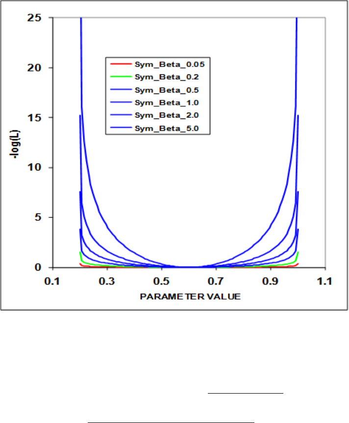
Prior distributions for the symmetric beta distribution.
•2 = Beta prior. The definition of µis consistent with CASAL’s formulation with the
Bprior and Aprior corresponding to the m and n parameter.
µ=P rior −P min
P max −P min
τ=(P rior −P min)(P max −P rior)
P_SD2−1.0
Bprior =τ∗µ;Aprior =τ(1.0−µ)
(44)
Prior Likelihood = (1.0−Bprior)∗log(P const +P val −P min)+
(1.0−Aprior)∗log(P const +P max −P val)−
(1.0−Bprior)∗log(P const +P rior −P min)−
(1.0−Aprior)∗log(P const +P max −P rior)
(45)
138
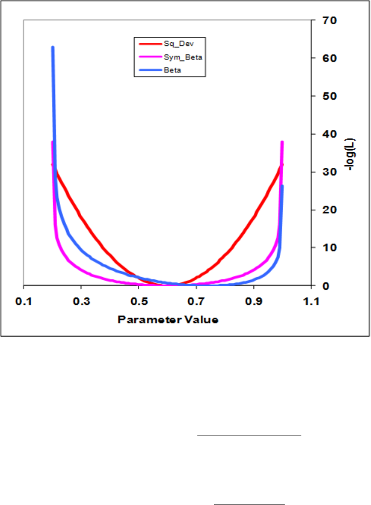
Comparison of the symmetric beta and the beta prior functions
•3 = Lognormal prior. Note that lower bound on the parameter must be >0.0. The
prior value is input into the parameter line in log space while the initial parameter
value is defined in normal space (e.g. INIT = 0.20, PRIOR = -1.609438).
Prior Likelihood = 0.50 ∗(log(P val)−P rior)
P r_SD 2
(46)
•6 = Normal prior. Note that this function is independent of the parameter.
Prior Likelihood = 0.50 ∗(P val −P rior
P rior_SD )2(47)
•Pval is the value of the parameter for which a prior is being calculated, Pmin and
Pmax are the bounds on the parameter, Prior is the value of the parameter prior, or
the first of the 2 factors controlling the calculation of the prior, Pr_SD is the value of
the prior’s standard deviation, or the second of the 2 factors controlling the calculation
of the prior, Pconst is a small constant (0.0001), and Prior_Like is the calculated value
of the prior’s contribution to the log likelihood.
139

10 Optional Inputs
10.1 Empirical Weight-at-Age (wtatage.ss)
SS has the capability to read empirical body weight at age for the population and each fleet,
in lieu of generating these weights internally from the growth parameters, weight-at-length,
and size-selectivity. Selection of this option is done by setting an explicit switch near the
top of the control file. The values are read from a separate file named, wtatage.ss. This file
is only required to exist if this option is selected.
The first value read is a single integer for the maxage used in reading this file.So if maxage
is 40, there will be 41 columns of wt-at-age entries to read, with the first column being for
age 0.
If N ages in this table is greater than maxage in the model, the extra wt-at-age values are
ignored.
If N ages in this table is less than maxage in the model, the wt-at-age for N ages in the file
is filled in for all unread ages out to maxage.
The format of this input file is:
#Year Season Gender GP Birth Season Fleet Age-0 Age-1 ...
1971 1 1 1 1 -2 0 0 0.1003
1971 1 1 1 1 -1 0.0169 0.0864 0.2495
1971 1 1 1 1 0 ... ... ...
1971 1 1 1 1 1 ... ... ...
1971 1 1 1 1 2 ... ... ...
-9999 1 1 1 1 0 ... ... ...
where:
•Fleet = -2 is age-specific fecundity*maturity, so time-varying fecundity is possible to
implement.
•Fleet = -1 is population wt-at-age at middle of the season.
•Fleet = 0 is population wt-at-age at the beginning of the season.
•There must be an entry for fecundity*maturity, population wt-at-age at the middle of
the season, population wt-at-age at the beginning of the season, and wt-at-age for each
fleet (even if these vectors are identical in some cases)
•Fleets that do not use biomass do not need to have wt-at-age assigned.
140
•GP and birthseas probably will never be used, but are included for completeness.
•A negative value for year will fill the table from that year through the ending year of
the forecast, overwriting anything that has already been read for those years.
•Judicious use of negative years in the right order will allow user to enter blocks without
having to enter a row of info for each year
•There is no internal error checking to verify that weight-at-age has been read for every
fleet and every year.
•In the future, there could be an option to use another value of the control file switch
to turn off all aspects of growth parameters and size selectivity.
•The values entered for endyr+1 will be used for the benchmark calculations and for
the forecast; this aspect needs a bit more checking.
Caveats:
•SS will still calculate growth curves from the input parameters and can still
calculate size-selectivity and can still examine size composition data.
•However, there is no calculation of wt-at-age from the growth input, so no way
to compare the input wt-at-age from the wt-at-age derived from the growth
parameters.
•If wt-at-age is read and size-selectivity is used, a warning is generated.
•If wt-at-age is read and discard/retention is invoked, then a BEWARE warning
is generated because of untested consequences for the body wt of discarded fish.
•Warning: age 0 fish seem to need to have weight=0 for spawning biomass calculation
(code -2).
Testing:
•A model was setup with age-maturity (option 2) and only age selectivity.
•The output calculation of wt-at-age and fecundity-at-age was taken from report.sso
and put into wtatage.ss (as shown above).
•Re-running SS with this input wt-at-age (Maturity_Option 5) produced identical
results to the run that had generated the weight-at-age from the growth parameters.
141
10.2 runnumbers.ss
This file contains a single integer value. It is read when the program starts, incremented
by 1, used when processing the profile value inputs (see below), used as an identifier in the
batch output, then saved with the incremented value. Note that this incrementation may
not occur if a run crashes.
10.3 profilevalues.ss
This file contains information for changing the value of selected parameters for each run in a
batch. In the ctl file, each parameter that will be subject to modification by profilevalues.ss
is designated by setting its phase to -9999 .
The first value in profilevalues.ss is the number of parameters to be batched. This value
MUST match the number of parameters with phase set equal to -9999 in the ctl file. The
program performs no checks for this equality. If the value is zero in the first field, then
nothing else will be read. Otherwise, the model will read runnumber * Nparameters values
and use the last Nparameters of these to replace the initial values of parameters designated
with phase = –9999 in the ctl file.
Usage Note: If one of the batch runs crashes before saving the updated value of runnumber.ss,
then the processing of the profilevalue.ss will not proceed as expected. Check the output
carefully until a more robust procedure is developed. Usage Note: This options was created
before use of R became widespread. You probably can create a more flexible approach using
R today.
11 Likelihood components
The objective function Lis the weighted sum of the individual components indexed by kind
of data i, and fishery/survey fas appropriate:
L=
I
X
i=1
Af
X
f=1
ωi,f Li,f +ωRLR+X
θ
ωθLθ+X
P
ωPLP(48)
where Lis the total objective function, iis the index of the objective function component,
Li,f is the objective function for data kind ifor the fishery/survey f, and ωi,f is a weighting
factor for each objective function component.
142

The components of the objective function based on the model set-up and data are:
Index Source Kind Error structure
ifishery/survey fCPUE or Abundance index user choice
ifishery fDiscard biomass user choice
ifishery/survey fMean body weight normal
ifishery/survey fLength composition multinomial or log-gamma
ifishery/survey fAge composition multinomial or log-gamma
ifishery/survey fMean size-at-age normal
ifishery/survey fTag-recapture 1 multinomial
ifishery/survey fTag-recapture 2 negative binomial
ifishery fInitial equilibrium catch normal
RRecruitment deviations lognormal
PRandom parameter devs normal
θParameter priors user choice
FBF ballpark penalty
CPCrash penalty
Full description of likelihood distributions by source will be added in the future.
12 Running SS
12.1 Command Line Interface
The name of the SS executable files often contains the phrase “safe” or “opt” (for optimized).
The safe version includes checking for out of bounds values and should always be used
whenever there is a change to the data file. The optimized version runs slightly faster but
can result in data not being included in the model as intended if the safe version hasn’t been
run first. A file named “ss.exe” is typically the safe version unless the result of renaming by
the user. In some situations, users may wish to rename the file they are using to ss.exe, but
the longer file name can be used.
On Mac and Linux computers, the executable does not include an extension (like .exe on
Windows). Running the executable on from the DOS command line in Windows simply
require typing the executable name (without the .exe extension):
> ss
143
On Mac and Linux computers, the executable name must be preceded by a period and slash
(unless it’s location has been added to the user’s PATH):
> ./ss
Additional ADMB commands can follow the executable name, such as “ –nohess” to avoid
calculating the Hessian matrix. To see a full list of options, add “ -?” after the executable
name (with a space in between).
On all operating systems, a copy of the SS executable can either be located in the same
directory as the model input files or in a central location and referenced either by adding
it to the PATH or by a script files. Further discussion on script files for Windows is below.
Editing the PATH is not covered here.
12.1.1 Example of DOS batch input file
One file management approach is to put ss.exe in its own folder (example: C:\SS_model)
and to put your input files in separate folder (example: C:\My Documents \SS_runs). Then
a DOS batch file in the SS_runs folder can be run at the command line to start ss.exe. All
output will appear in SS_runs folder.
A DOS batch file (e.g. SS.bat) might contain some explicit ADMB commands, some implicit
commands, and some DOS commands:
c:\SS_model\ss.exe -cbs 5000000000 -gbs 50000000000 \%1 \%2 \%3 \%4
del ss.r0*
del ss.p0*
del ss.b0*
In this batch file, the –cbs and –gbs arguments allocate a large amount of memory for SS
to use (you may need to edit these for your computer and SS configuration), and the %1,
%2 etc. allows passing of command line arguments such as –nox or –nohess. You add more
items to the list of % arguments as needed.
An easy way to start a command line in your current directory (SS_runs) is to create a
shortcut to the DOS command line prompt. The shortcut’s target would be:
> %SystemRoot%\system32\cmd.exe
And it would start in:
> %CURRDIR%
144
12.1.2 Simple Batch
This first example relies upon having a set of prototype files that can be renamed to starter.ss
and then used to direct the running of SS. The example also copies one of the output files to
save it from being overwritten. This sequence is repeated 3 times here and can be repeated
an unlimited number of times. The batch file can have any name with the .bat extension,
and there is no particular limit to the DOS commands invoked. Note that brief output from
each run will be appended to cumreport.sso (see below).
del ss.cor
del ss.std
copy starter.r01 starter.ss
c:\admodel\ss\ss.exe -sdonly
copy ss.std ss-std01.txt
copy starter.r01 starter.ss
c:\admodel\ss\ss.exe -sdonly
copy ss.std ss-std02.txt
12.1.3 Complicated Batch
This second example processes 25 dat files from a different directory, each time using the
same ctl and nam file. The loop index is used in the file names, and the output is searched
for particular keywords to accumulate a few key results into the file SUMMARY.TXT.
Comparable batch processing can be accomplished by using R or other script processing
programs.
del summary.txt
del ss-report.txt
copy /Y runnumber.zero runnumber.ss
FOR /L \%\%i IN (1,1,25) DO (
copy /Y ..\MakeData\A1-D1-%%i.dat Asel.dat
del ss.std
del ss.cor
del ss.par
c:\admodel\ss\ss.exe
copy /Y ss.par A1-D1-A1-%%i.par
copy /Y ss.std A1-D1-A1-%%i.std
find "Number" A1-D1-A1-%%i.par >> Summary.txt
find "hessian" ss.cor >> Summary.txt)
145
12.1.4 Batch Using PROFILEVALUES.SS
This example will run a profile on natural mortality and spawner-recruitment steepness, of
course. Edit the control file so that the natural mortality parameter and steepness parameter
lines have the phase set to –9999. Edit STARTER.SS to refer to this control file and the
appropriate data file.
Create a PROFILEVALUES.SS file
2 # number of parameters using profile feature
0.16 # value for first selected parameter when runnumber equals 1
0.35 # value for second selected parameter when runnumber equals 1
0.16 # value for first selected parameter when runnumber equals 2
0.40 # value for second selected parameter when runnumber equals 2
0.18 # value for first selected parameter when runnumber equals 3
0.40 # value for second selected parameter when runnumber equals 3
etc.; make it as long as you like.
Create a batch file that looks something like this. Or make it more complicated as in the
example above.
del cumreport.sso
copy /Y runnumber.zero runnumber.ss % so you will start with runnumber=0
C:\SS330\ss.exe
C:\SS330\ss.exe
C:\SS330\ss.exe
Repeat as many times as you have set up conditions in the PROFILEVALUES.SS file. The
summary results will all be collected in the cumreport.sso file. Each step of the profile
will have an unique Runnumber and its output will include the values of the natmort and
steepness parameters for that run.
12.1.5 Re-Starting a Run
SS model runs can be restarted from a previously estimated set of parameter values. In the
starter.ss file, enter a value of 1 on the first numeric input line. This will cause SS to read
the file ss.par and use these parameter values in place of the initial values in the control
file. This option only works if the number of parameters to be estimated in the new run is
the same as the number of parameters in the previous run because only actively estimated
parameters are saved to the file ss.par. The file ss.par can be edited with a text editor, so
values can be changed and rows can be added or deleted. However, if the resulting number of
146
elements does not match the setup in the control file, then unpredictable results will occur.
Because ss.par is a text file, the values stored in it will not give exactly the same initial
results as the run just completed. To achieve greater numerical accuracy, SS can also restart
from ss.bar which is the binary version of ss.par. In order to do this, the user must make
the change described above to the starter.ss file and must also enter –binp ss.bar as one of
the command line options.
12.2 Debugging Tips
When SS input files are causing the program to crash or fail to produce sensible results,
there are a few steps that can be taken to diagnose the problem. Before trying the steps
below, examine the ECHOINPUT.SSO file. It is highly annotated, so you should be able to
see if SS is interpreting your input files as you intended.
1. Set the turn_off_phase switch to 0 in the STARTER.SS file. This will cause the mode
to not attempt to adjust any parameters and simply converges a dummy parameter.
It will still produce a REPORT.SSO file, which can be examined to see what has been
calculated from the initial parameter values.
2. Turn the verbosity level to 2 in the STARTER.SS file. This will cause the program
to display the value of each likelihood component to the screen on each iteration. So
it the program is creating an illegal computation (e.g. divide by zero), it may show
you which likelihood component contains the problematic calculation. If the program
is producing a REPORT.SSO file, you may then see which observation is causing the
illegal calculation.
3. Run the program with the command ss »SSpipe.txt. This will cause all screen display
to go to the specified text file (note, delete this file before running because it will be
appended to). Examination of this file will show detailed statements produced during
the reading and preprocessing of input files.
4. CHECKUP.SSO: This file can be written during the first iteration of the program.
It contains details of selectivity and other calculations as an aid to debugging model
problems.
5. If SS fails to achieve a proper Hessian it exits without writing the detailed outputs in
the FINAL_SECTION. If this happens, you can do a run with the –nohess option so
you can view the report.sso to attempt to diagnose the problem.
147
12.3 Keyboard Tips
Typing “N” during a run will cause ADMB to immediately advance to the next phase of
estimation.
Typing “Q” during a run will cause ADMB to immediately go to the final phase. This
bypasses estimation of the Hessian and will produce all of the SS outputs, which are coded
in the FINAL_SECTION.
12.4 Running MCMC
Run SS v3.30
•This gives MPD estimates, report file, Hessian matrix and the .cor file
•(Recommended) Look for parameters stuck on bounds which will degrade efficiency of
MCMC implementation
•(Recommended) Look for very high correlations that may degrade the efficiency of
MCMC implementation
Run SS v3.30 with arguments -mcmc xxxx -mcsave yyyy
•Where: xxxx is the number of iterations for the chain, and yyyy is the thinning interval
(1000 is a good place to start)
•MCMC chain starts at the MPD values
•(Recommended) Remove existing .psv files in run directory to generate a new chain.
•(Recommended) Set DOS run detail switch in starter file to 0; reporting to screen will
dramatically slow MCMC progress
•(Optional) Add -nohess to use the existing Hessian file without re-estimating
•(Optional) To start the MCMC chain from specific values change the par file; run the
model with estimation, adjust the par file to the values that the chain should start
from, change within the starter file for the model to begin from the par file, and call
the MCMC function using ss –mcmc xxxx – mcsave yyyy -nohess –noest.
•(Optional) Add -noest -nohess and modify starter file so that run will now start from
the converged (or modified) parameter estimates in "ss.par"
148
Run SS v3.30 with argument -mceval
•This generates the posterior output files.
•(Optional) Modify starter file entries to add a burn-in and thinning interval above and
beyond the ADMB thinning interval applied at run time.
•(Recommended) MCMC always begins with the MPD values and so a burn-in >0
should always be used.
•This step can be repeated for alternate forecast options (e.g. catch levels) without
repeating step 2.
(Optional) Run SS v3.30 with arguments -mcr -mcmc xxxx -mcsave yyyy ...
•This restarts and extends an uninterrupted chain previously completed (note that any
intermediate runs without the -mcr command in the same directory will break this
option).
NOTES:
When SS switches to MCMC or MCEVAL mode, it sets all the bias adjustment factors to
1.0 for any years with recruitment deviations defined. SS does not create a report file after
completing MCMC because it would show values based on the last MCMC step.
13 Output Files
13.1 Standard ADMB output files
Standard ADMB files are created by SS. These are:
SS.PAR – This file has the final parameter values. They are listed in the order they are
declared in SS. This file can be read back into SS to restart a run with these values (see
running SS).
SS.STD – This file has the parameter values and their estimated standard deviation for those
parameters that were active during the model run. It also contains the derived quantities
declared as sdreport variables. All of this information is also report in the covar.sso. Also,
the parameter section of report.sso lists all the parameters with their SS generated names,
denotes which were active in the reported run, displays the parameter standard deviations,
then displays the derived quantities with their standard deviations.
149
SS.REP – This report file is created between phases so, unlike report.sso, will be created
even if the Hessian fails. It does not contain as much output as shown in report.sso.
SS.COR – This is the standard ADMB report for parameter and sdreport correlations.
It is in matrix form and challenging to interpret. This same information is reported in
covar.sso.
13.2 SS Summary
The ss_summary.sso file (available for versions 3.30.08.03 and later) is designed to put key
model outputs all in one concise place. It is organized as a list. At the top of the file are some
descriptors, followed by the likelihoods for each component, then the parameters and their
standard errors, then the derived quantities and their standard errors. The total biomass,
summary biomass, and catch were added to the quantities reported in this file in version
3.30.11 and later. This output was created to make it easy to compare the results between
different versions of the executable, however, this file could be useful for numerous other
uses.
13.3 SIS table
The SIS_table.sso file contains model output formatted for reading into the NMFS Species
Information System (SIS). This file includes an assessment summary for categories of information
(abundance, recruitment, spawners, catch estimates) that are input into the SIS database.
A time-series of estimated quantities which aggregates estimates across multiple areas and
seasons are provided to summarize model results. Access to the SIS database is granted to
all NOAA employees and can be accessed as: https://www.st.nmfs.noaa.gov/sis/.
13.4 Derived Quantities
Before listing the derived quantities reported to the sdreport, there are a couple of topics
that deserve further explanation.
13.4.1 Virgin Spawning Biomass (B0) vs Unfished Spawning Biomass
Unfished is the condition for which reference points (benchmark) are calculated. Virgin
Spawning Biomass (B0) is the initial condition on which the start of the time-series depends.
150
If biology or SR parameters are time-varying, then the benchmark year input in the forecast
file tells SS which years to average in order to calculate "unfished". In this case, virgin
recruitment and/or the virgin spawning biomass will differ from their unfished counterparts.
Virgin recruitment and spawning biomass are reported in the mgmt_quant portion of the
sd_report and are now labeled as "unfished" for clarity. Note that if ln(R0) is time-varying,
then this will cause unfished to differ from virgin. However, if regime shift parameter is
time-varying, then unfished will remain the same as virgin because the regime shift is treated
as a temporary offset from virgin. Virgin spawning biomass is denoted as SPB_virgin and
spawning biomass unfished is denoted as SPB_unf in the report file.
Virgin Spawning Biomass (B0) is used in four ways within SS:
1. Anchor for the spawner-recruitment relationship as virgin spawning biomass.
2. Basis for the initial equilibrium abundance.
3. Basis against which annual depletion is calculated.
4. Benchmark calculations.
However, if there is time-varying biology, then the 4th usage can have a different B0 calculation
compared to the other usages.
13.4.2 Metric for Fishing Mortality
A generic single metric of annual fishing mortality is difficult to define in a generalized
model that admits multiple areas, multiple biological cohorts, dome-shaped selectivity in
size and age for each of many fleets. Several separate indices are provided and others could
be calculated by a user from the detailed information in report.sso.
13.4.3 Equilibrium SPR
This index focuses on the effect of fishing on the spawning potential of the stock. It is
calculated as the ratio of the equilibrium reproductive output per recruit that would occur
with the current year’s F intensities and biology, to the equilibrium reproductive output per
recruit that would occur with the current year’s biology and no fishing. Thus it internalizes
all seasonality, movement, weird selectivity patterns, and other factors. Because this index
moves in the opposite direction than F intensity itself, it is usually reported as 1-SPR. A
benefit of this index is that it is a direct measure of common proxies used for FMSY, such
as F40%. A shortcoming of this index is that it does not directly demonstrate the fraction
of the stock that is caught each year. The SPR value is also calculated in the benchmarks
151
(see below). The derived quantities report shows an annual SPR statistic. The options, as
specified in the starter.ss file, are:
•0 = skip
•1 = (1-SPR)/(1-SPRTGT)
•2 = (1-SPR)/(1-SPRMSY)
•3 = (1-SPR)/(1-SPRBtarget)
•4 = raw SPR
13.4.4 F std
This index provides a direct measure of fishing mortality. The options are:
•0 = skip
•1 = exploitation(Bio)
•2 = exploitation(Num)
•3 = sum(Frates)
The exploitation rates are calculated as the ratio of the total annual catch (in either biomass
or numbers as specified) to the summary biomass or summary numbers on Jan 1. The sum
of the F rates is simply the sum of all the apical Fs. This makes sense if the F method is in
terms of instantaneous F (not Pope’s approximation) and if there are not fleets with widely
different size/age at peak selectivity, and if there is no seasonality, and especially if there is
only one area. In the derived quantities, there is an annual statistic that is the ratio of the
can be annual F_std value to the corresponding benchmark statistic. The available options
for the denominator are:
•0 = raw
•1 = F/FSPR
•2 = F/FMSY
•3 = F/FBtarget
152

13.4.5 F-at-Age
Because the annual F is so difficult to interpret as a sum of individual F components, an
indirect calculation of F-at-age is reported at the end of the report.sso file. This section of
the report calculates Z-at-age simply as ln(Na+1,t+1/Na,t). This is done on an annual basis
and summed over all areas. It is done once using the fishing intensities as estimated (to
get Z), and once with the F intensities set to 0.0 to get M-at-age. This latter sequence also
provides a measure of dynamic Bzero. The user can then subtract the table of M-at-age/year
from the table of Z-at-age/year to get a table of F-at-age/year. From this apical F, average
F over a range of ages, or other user-desired statistics could be calculated. Further work
within SS with this table of values is anticipated.
13.4.6 MSY and other Benchmark Items
The following quantities are included in the sdreport vector mgmt_quantities, so obtain
estimates of variance. Some additional quantities can be found in the benchmarks section of
the forecast_report.sso.
Benchmark Item Description
SSB_Unfished Unfished reproductive potential (SSB is commonly female
mature spawning biomass)
TotBio_Unfished Total age 0+ biomass on Jan 1
SmryBio_Unfished Biomass for ages at or above the summary age on Jan 1
Recr_Unfished Unfished recruitment
SSB_Btgt SSB at user specified SSB target
SPR_Btgt Spawner potential ratio (SPR) at F intensity that produces
user specified SSB target
Fstd_Btgt F statistic at F intensity that produces user specified SSB
target
TotYield_Btgt Total yield at F intensity that produces user specified SSB
target
SSB_SPRtgt SSB at user specified SPR target (but taking into account the
spawner-recruitment relationship)
Fstd_SPRtgt F intensity that produces user specified SPR target
TotYield_SPRtgt Total yield at F intensity that produces user specified SPR
target
SSB_MSY SSB at F intensity that is associated with MSY; this F
intensity may be directly calculated to produce MSY, or can
be mapped to F_SPR or F_Btgt
153

Benchmark Item Description
SPR_MSY Spawner potential ratio (SPR) at F intensity associated with
MSY
Fstd_MSY F statistic at F intensity associated with MSY
TotYield_MSY Total yield (biomass) at MSY
RetYield_MSY Retained yield (biomass) at MSY
13.5 Brief cumulative output
Cum_Report.sso: contains a brief version of the run output, which is appended to current
content of file so results of several runs can be collected together. This is especially useful
when a batch of runs is being processed. Unless this file is deleted, it will contain a cumulative
record of all runs done in that subdirectory. The first column contains the run number.
13.6 Output for Rebuilder Package
Output filename is REBUILD.DAT
#Title # various run summary outputs
SS#_default_rebuild.dat
# Number of sexes
2
# Age range to consider (minimum age; maximum age)
0 40
# Number of fleets
3
# First year of projection (Yinit)
2002
# First Year of rebuilding period (Ydecl)
1999
# Number of simulations
1000
# Maximum number of years
500
# Conduct proejctions with multiple starting values (0 = No, 1 = Yes)
0
154
# Number of parameter vectors
1000
# Is the maximum age a plus-group (1 = Yes; 2 = No)
1
#Generate future recruitments using historical recruitments (1) historical recruits/spawner
(2) or a stock-recruitment (3)
3
# Constant fishing mortality (1) or constant Catch (2) projections
1
# Fishing mortality based on SPR (1) or actual rate (2)
1v # Pre-specify the year of recovery (or -1) to ignore
-1
# Fecundity-at-age
# 0 1 2 3 4 5 6 7 8 9 10 <deleted values>
0 0.000450117 0.00436298 0.0271371 <deleted values>
# Age specific selectivity and weight adjusted for discard and discard mortality
#wt and selex for gender, fleet: 1 1
0.146708 0.320119 0.555587 0.830467 <deleted values>
0.0122887 0.0351722 0.0838682 0.165479 <deleted values>
#wt and selex for gender ,fleet: 2 1
0.150944 0.33768 0.588317 0.874376 <deleted values>
0.0127241 0.0380999 0.0922667 <deleted values>
# M and current age-structure in year Yinit: 2002
# gender = 1
0.1 0.1 0.1 0.1 0.1 <deleted values>
1425.96 797.624 1234.77 428.207 <deleted values>
# gender = 2
0.1 0.1 0.1 0.1 0.1 <deleted values>
1425.96 797.531 1233.66 <deleted values>
# Age-structure at Ydeclare= 1999
598.671 652.739 2925.76 2227.69 <deleted values>
598.671 652.666 2923.27 2221.05 <deleted values>
# Year for Tmin Age-structure (set to Ydecl by SS) 1999
1999
# recruitment and biomass
# Number of historical assessment years
33
# Historical data
# year recruitment spawner in B0 in R project in R/S project
1970 1971 1972 1973 1974 1975 1976 <deleted values> 2001 2002
#years (with first value representing R0)
8853.43 8658.22 8651.96 8645.41 8638.43 8630.75 <deleted values> 1594.53 2075.34 #recruits;
155
first value is R0 (virgin)
63679.5 63679.5 63679.3 63678.3 63673.9 63661.6 <deleted values> 8614.18 7313.2 #spbio;
first value is S0 (virgin)
1 0 0 0 0 0 0 0 0 0 0 0 0 0 0 0 0 0 0 0 0 0 0 <deleted values> 0 0 # in Bzero
0 1 1 1 1 1 1 <deleted values> 1 1 0 0 0 # in R project
0 1 1 1 1 1 1 <deleted values> 1 1 0 0 0 # in R/S project
# Number of years with pre-specified catches
0
# catches for years with pre-specified catches go next
# Number of future recruitments to override
3
# Process for overriding (-1 for average otherwise index in data list)
2000 1 2000
2001 1 2001
2002 1 2002
# Which probability to product detailed results for (1=0.5; 2=0.6; etc.)
3
# Steepness sigma-R Auto-correlation
0.610789 0.6 0
# Target SPR rate (FMSY Proxy); manually change to SPR_MSY if not using SPR_target
0.5
# Target SPR information: Use (1=Yes) and power
0 20
# Discount rate (for cumulative catch)
0.1
# Truncate the series when 0.4B0 is reached (1=Yes)
0
# Set F to FMSY once 0.4B0 is reached (1=Yes)
0
# Maximum possible F for projection (-1 to set to FMSY)
-1
# Defintion of recovery (1=now only; 2=now or before)
2
# Projection type
4
# Definition of the 40-10 rule
10 40
# Produce the risk-reward plots (1=Yes)
0
# Calculate coefficients of variation (1=Yes)
0
# Number of replicates to use
156
10
# Random number seed
-99004
# File with multiple parameter vectors
rebuild.SS0
# User-specific projection (1=Yes); Output replaced (1->9)
0 5
# Catches and Fs (Year; 1/2/3 (F or C or SPR); value); Final row is -1v 2002 1 1
-1 -1 -1
# Split of Fs
2002 1
-1 1 1 1
# Yrs to define TTARGET for projection type 4 (aka 5 pre-specified inputs)
2011 2012 2013 2014 2015 2016 2017 2018
# Time varying weight-at-age (1=Yes;0=No)
0
# File with time series of weight-at-age data
none
# Use bisection (0) or linear interpolation (1)
1
# Target Depletion
0.4
# CV of implementation error
0
13.7 Bootstrap Data Files
Data.ss_new: contains a user-specified number of data files, generated through a parametric
bootstrap procedure, and written sequentially to this file. These can be parsed into individual
data files and re-run with the model. The first output provides the unaltered input data
file (with annotations added). The second provides the expected values for only the data
elements used in the model run. The third and subsequent outputs provide parametric
bootstraps around the expected values.
13.8 Forecast and Reference Points
FORECAST-REPORT.sso: This file contains output of fishery reference points and forecasts.
It is designed to meet the needs of the Pacific Fishery Management Council’s Groundfish
157
Fishery Management Plan, but it should be quite feasible to develop other regionally specific
variants of this output.
The vector of forecast recruitment deviations is estimated during an additional model estimation
phase. This vector includes any years after the end of the recrdev time series and before or
at the end year. When this vector starts before the ending year of the time series, then the
estimates of these recruitments will be influenced by the data in these final years. This is
problematic, because the original reason for not estimating these recruitments at the end of
the time series was the poor signal/noise ratio in the available data. It is not that these data
are worse than data from earlier in the time series, but the low amount of data accumulated
for each cohort allows an individual datum to dominate the model’s fit. Thus, an additional
control is provided so that forecast recruitment deviations during these years can receive an
extra weighting in order to counter-balance the influence of noisy data at the end of the time
series.
An additional control is provided for the fraction of the log-bias adjustment to apply to
the forecast recruitments. Recall that R is the expected mean level of recruitment for a
particular year as specified by the spawner-recruitment curve and R’ is the geometric mean
recruitment level calculated by discounting R with the log-bias correction factor e-0.5sˆ
2.
Thus a lognormal distribution of recruitment deviations centered on R’ will produce a mean
level of recruitment equal to R. During the modeled time series, the virgin recruitment level
and any recruitments prior to the first year of recruitment deviations are set at the level of
R, and the lognormal recruitment deviations are centered on the R’ level. For the forecast
recruitments, the fraction control can be set to 1.0 so that 100% of the log-bias correction
is applied and the forecast recruitment deviations will be based on the R’ level. This is
certainly the configuration to use when the model is in MCMC mode. Setting the fraction
to 0.0 during maximum likelihood forecasts would center the recruitment deviations, which
all have a value of 0.0 in ML mode, on R. Thus would provide a mean forecast that would
be more comparable to the mean of the ensemble of forecasts produced in MCMC mode.
Further work on this topic is underway.
Note:
•Cohorts continue growing according to their specific growth parameters in the forecast
period rather than staying static at the endyr values.
•Environmental data entered for future years can be used to adjust expected recruitment
levels. However, environmental data will not affect growth or selectivity parameters in
the forecast.
The top of this file shows the search for FSPR and the search for FMSY so the user can verify
convergence. Note: if the STD file shows aberrant results, such as all the standard deviations
being the same value for all recruitments, then check the FMSY search for convergence.
158
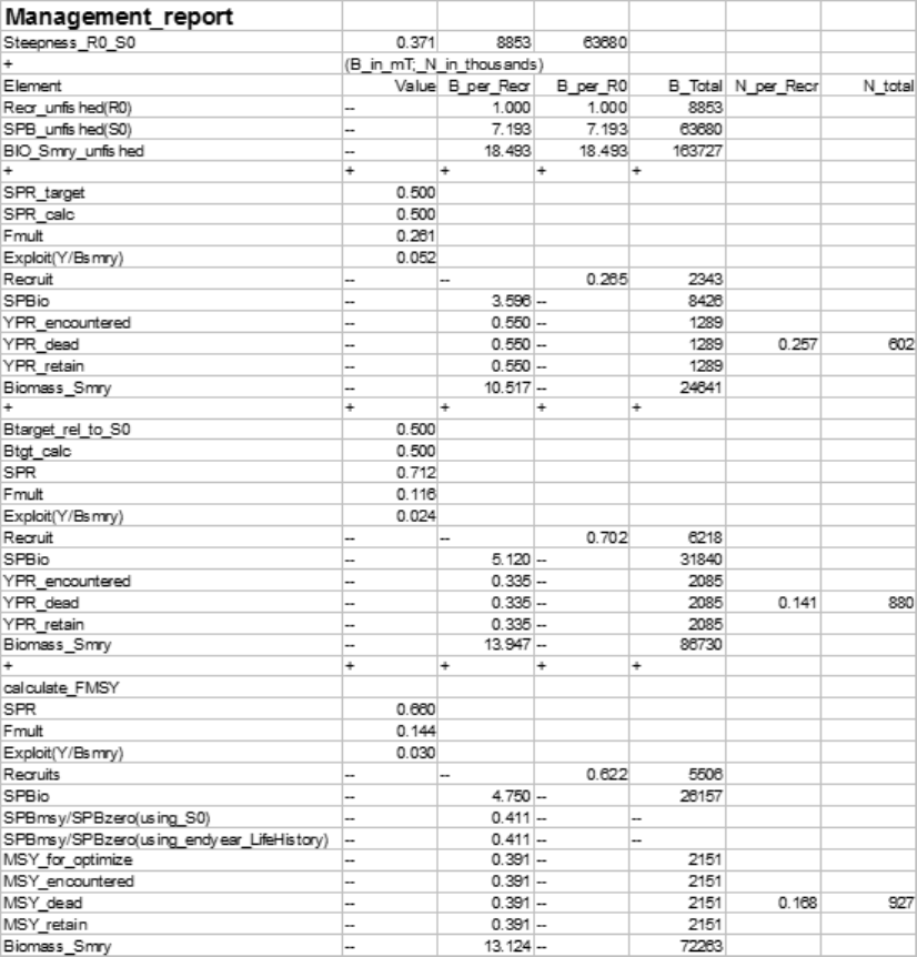
The FMSY can be calculated, or set equal to one of the other F reference points per the
selection made in STARTER.SS.
The reference point output is shown int he table below:
159
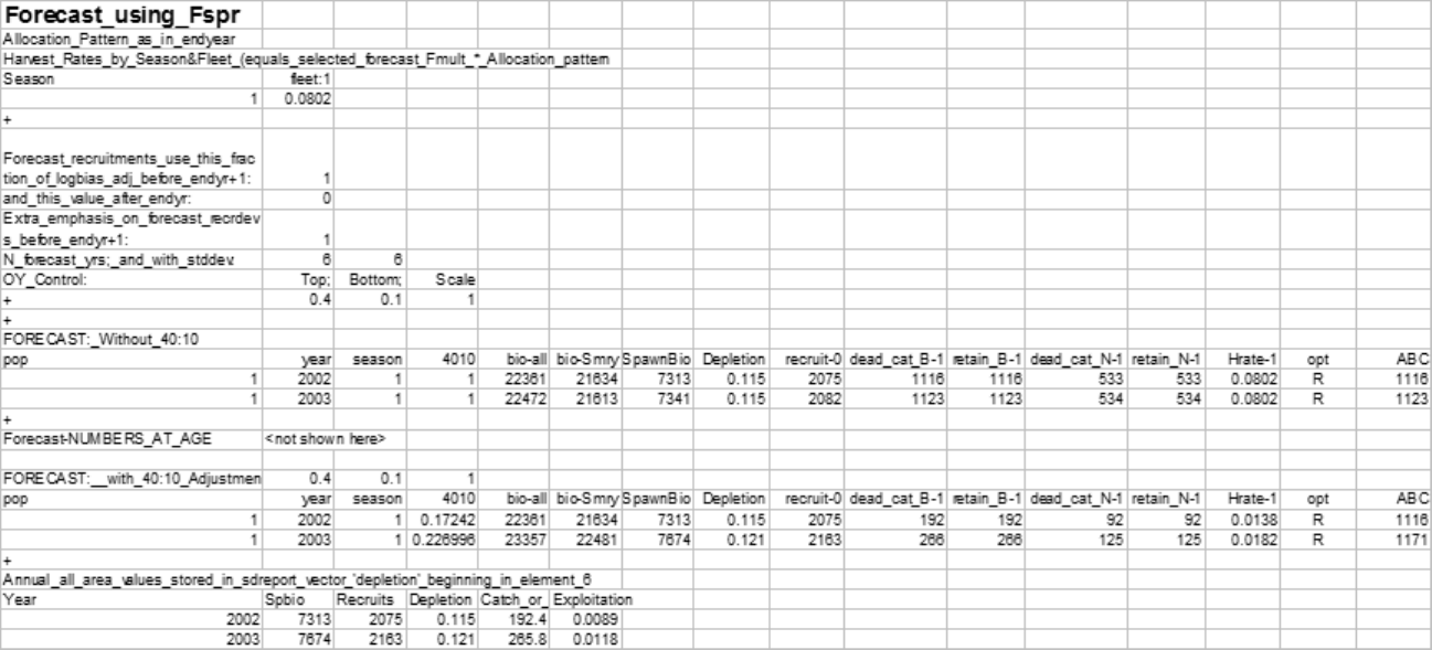
The forecast is done once using the Target SPR and once using the adjustments specified in the 40:10 section of forecast.ss
input. Each section contains a time series of seasonal biomass and catch, followed by a time series of population
numbers-at-age for each platoon.
160
where:
•40:10 is the magnitude of the adjustment of harvest multiplier to implement the OY
policy
•bio-all is the biomass of all ages
•bio-smry is the biomass for ages at or above the summary age
•Spawnbio - is the female spawning output
•Depletion is the spawnbio divided by the unfished spawnbio
•Recruit-0 is the recruitment of age-o fish in this year
•Dead_cat_B-1 is the total dead (retained plus dead discard) catch in MT for fleet 1
•Retain_B-1 is fleet 1’s retained catch in MT
•Equivalent catch in numbers is then reported.
•Hrate-1 is the harvest rate, as adjusted by the 40:10 policy. The units will depend on
the F method selected (Pope’s method giving mid-year harvest rate or the continuous
F.
•Opt=C means that the rate was calculated from an input catch level (and crashed
means that this caused an excessive harvest rate.
•Opt=R means that the catch was calculated from the target harvest rate.
•ABC is equal to the Total-Catch when the 40:10 option is not used (upper portion of
table). When the 40:10 is on (lower table), the ABC is the catch level corresponding
to no 40:10 adjustment after accounting for catch in previous year’s from the 40:10.
The time series output described above is detailed by season, area, platoon and fishery. It is
usually more convenient to have annual values summed across areas, platoons and fisheries.
This is done for the 40:10 output and a subset of these values are replicated in the depletion
vector in the sd_report so that variance estimates can be obtained. The elements of the
depletion vector in the sd_report are:
•depletion level in end year
•depletion level in end year+1
•MSY (if calculated, else spbio in endyr-1)
161
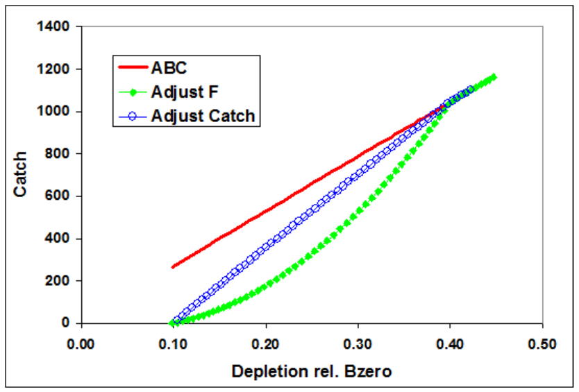
•BMSY (if calculated, else spbio in endyr)
•SPRMSY (if calculated, else spbio in endyr+1) then the time series of:
–Spawning biomass
–Recruitment
–Depletion level
–Total catch (if forecast calculated catch from rates) or sum of fishery-specific
harvest rates (if forecast is based on fixed input catch level in this year)
–Total exploitation rate (total dead catch divided by the summary biomass at the
beginning of the year).
Two examples of harvest forecast adjustment: one adjusts catch and the other adjusts F.
13.9 Main Output File, report.sso
This is the primary output file. Its major sections are listed below.
The sections of the output file are:
162
•SS version number with date compiled. Time and date of model run. This info appears
at the top of all output files.
•Comments
–Input file lines starting with #C are echoed here
•Keywords
–List of keywords used in searching for output sections.
•Fleet Names
–List of fishing fleet and survey names assigned in the data file
•Likelihood
–Final values of the negative log(likelihood) are presented.
•Input Variance Adjustments
–The matrix of input variance adjustments is output here because these values
affect the logL calculations
•Parameters
–The parameters are listed here. For the estimated parameters, the display shows:
Num (count of parameters), Label (as internally generated by SS), Value, Active_Cnt,
Phase, Min, Max, Init, Prior, Prior_type, Prior_SD, Prior_Like, Parm_StD
(standard deviation of parameter as calculated from inverse Hessian), Status (e.g.
near bound), Pr_atMin (value of prior penalty if parameter was near bound),
and Pr_atMin. The Active_Cnt entry is a count of the parameters in the same
order they appear in the ss.cor file.
•Derived Quantities
–This section starts by showing the options selected from the starter.ss and forecast.ss
input files:
∗SPR ratio basis
∗F report basis
∗B ratio denominator
Then the time series of output, with standard deviation of estimates, are produced with
163
internally generated labels. Note that these time series extend through the forecast era.
The order of the output is: spawning biomass, recruitment, SPRratio, Fratio, Bratio,
management quantities, forecast catch (as a target level), forecast catch as a limit level
(OFL), Selex_std, Grow_std, NatAge_std. For the three “ratio” quantities, there is an
additional column of output showing a Z-score calculation of the probability that the ratio
differs from 1.0. The “management quantities” section is designed to meet the terms of
reference for west coast groundfish assessments; other formats could be made available upon
request. The std quantities at the end are set up according to specifications at the end of
the control input file. In some cases, a user may specify that no derived quantity output
of a certain type be produced. In those cases, SS substitutes a repeat output of the virgin
spawning biomass so that vectors of null length are not created.
ADMB NOTE: while vectors of null length are very useful for controlling optional model
inputs, they cannot be used with current version of ADMB for sdreport quantities.
•MGparm by year after adjustments
–This block shows the time series of Mgparms by year after adjustment by environmental
links, blocks and deviations.
•SELparm (size) by year after adjustments
–This block shows the size selectivity parameters, after adjustment, for each year
in which a change occurs.
•SELparm (age) by year after adjustments
–This block shows the age selectivity parameters, after adjustment, for each year
in which a change occurs.
•Recruitment Distribution
–This block shows the distribution of recruitment across growth patterns, genders,
birthseasons, and areas in the endyr of the model.
•Platoon Indexing
–This block shows the internal index values for various quantities. It can be a
useful reference for complex model setups. The vocabulary is: Bio_Pattern refers
to a collection of cohorts with the same defined growth and natural mortality
parameters; sex is the next main index. If recruitment occurs in multiple seasons,
then Birthseas is the index for that factor. The index labeled “Platoon” is used as
a continuous index across all the other factor-specific indices. If sub-platoons are
used, they are nested within the Bio_Pattern x Sex x Birthseas platoon. However,
164
some of the output tables use the column label “platoon” as a continuous index
across platoons and sub-platoons. Note that there is no index here for area.
Each of the cohorts is distributed across areas and they retain their biological
characteristics as they move among areas.
•Size Freq Translation
–If the generalize size frequency approach is used, this block shows the translation
probabilities between population length bins and the units of the defined size
frequency method. If the method uses body weight as the accumulator, then
output is in corresponding units.
•Movement
–This block shows movement rate between areas in a multi-area model.
•Exploitation
–This block shows the time series of the selected F_std unit and the F multiplier
for each fleet in terms of harvest rate (if Pope’s approximation is used) or fully
selected F.
•Index 2
–This section reports the observed and expected values for each index. All are
reported in one list with index number included as a selection field. At the bottom
of this section, the root mean squared error of the fit to each index is compared
to the mean input error level to assist the user in gaging the goodness-of-fit and
potentially adjusting the input level of imprecision.
•Index 3
–This section shows the parameter number assigned to each parameter used in this
section.
•Discard
–This is the list of observed and expected values for the amount (or fraction)
discard.
•Mean Body Wt
–This is the list of observed and expected values for the mean body weight.
•Fit Len Comps
165
–This is the list of the goodness of fit to the length compositions. The input and
output levels of effective sample size are shown as a guide to adjusting the input
levels to better match the model’s ability to replicate these observations.
•Fit Age Comps
–This has the same format as the length composition section.
•Fit Size Comps
–This has the same format as the length composition section and is used for the
generalized size composition summary.
•Len Selex
–Here is the length selectivity and other length specific quantities for each fishery
and survey.
•Age Selex
–Here is reported the time series of age selectivity and other age-related quantities
for each fishery and survey. Some are directly computed in terms of age, and others
are derived from the combination of a length-based factor and the distribution of
size-at-age.
•Environmental Data
–The input values of environmental data are echoed here. In the future, the
summary biomass in the previous year will be mirrored into environmental column
–2 and that the age zero recruitment deviation into environmental column –1.
Once so mirrored, they may enable density-dependent effects on model parameters.
•Numbers at Age
–The output (in thousands of fish) is shown for each cohort tracked in the model.
•Numbers at Length
–The output is shown for each cohort tracked in the model.
•Catch at Age
–The output is shown for each fleet. It is not necessary to show by area because
each fleet operates in only one area.
166
•Biology
–The first biology section shows the length-specific quantities in the ending year of
the time series only. The derived quantity spawn is the product of female body
weight, maturity and fecundity per weight. The second section shows natural
mortality.
•Growth Parameters
–This section shows the growth parameters, and associated derived quantities, for
each year in which a change is estimated.
•Biology at Age
–This section shows derived size-at-age and other quantities. It is the basis for the
Bio report page of the Excel output processor.
•Mean Body Wt (begin)
–This section reports the time series of mean body weight for each platoon. Values
shown are for the beginning of each season of each year.
•Mean Size Timeseries
–This section shows the time series of mean length-at-age for each platoon. At the
bottom is the average mean size as the weighted average across all platoons for
each gender.
•Age Length Key
–This is reported for the midpoint of each season in the ending year.
•Age Age Key
–This is the calculated distribution of observed ages for each true age for each of
the defined ageing keys.
•Selectivity Database
–This section contains the selectivities organized as a database, rather than as a
set of vectors.
•Spawning Biomass Report 2, etc.
–The section shows annual total spawning biomass, then numbers-at-age at the
167
beginning of each year for each Bio_Pattern and Sex as summed over sub-platoons
and areas. Then Z-at-age is reported simply as ln(Nt+1,a+1Nt,a). Then the
Report_1 section loops back through the time series with all F values set to
zero so that a dynamic Bzero, N-at-age, and M-at-age can be reported. The
difference between Report_1 and Report_2 can be used to create an aggregate
F-at-age.
•Composition Database
–This section is reported to a separate file, compreport.sso, and contains the length
composition, age composition, and mean size-at-age observed and expected values.
It is arranged in a database format, rather than an array of vectors. Software to
filter the output allows display of subsets of the database.
14 Using R To View Model Output (r4ss)
A collection of functions developed as a package, r4ss, for the statistical software R has
been created to explore SS model output. The functions include tools for summarizing and
plotting results, manipulating files, visualizing model parameterizations, and various other
tasks. Currently, information on the code, including installation instructions, can be found
at https://github.com/r4ss/r4ss. The software package is under constant development to
maintain compatibility with new versions of SS and to improve functionality.
Two of the most commonly used functions for model diagnostics are SS_output and SS_plots.
After running a model using SS, the report can be read into R by the SS_output function
which stores quantities in a list with named objects. This list can then be passed to the
SS_plots function which creates a series of over 100 plots that are useful to visualize output
such as model fit to the data and time series of quantities of interest.
The latest r4ss version on CRAN can be installed using a command like:
> install.packages("r4ss")
However, more frequent enhancements and bug fixes are posted to the GitHub project. The
latest version of r4ss can be installed directly from GitHub at any time via the devtools
package in R with the following commands:
> install.packages("devtools")
> devtools::install_github("r4ss/r4ss")
Note: devtools will give this message: "WARNING: Rtools is required to build R packages,
but is not currently installed." However, Rtools is NOT required for installing r4ss via
168
devtools, so ignore this warning.
Once you have installed the r4ss package, it can be loaded in the regular manner:
> library(r4ss)
The results from a model run can be read in and plots created using the following commands:
> setwd("C:\directory where model was run")
> base.model = SS_output(getwd())
> SS_plots(base.model)
169
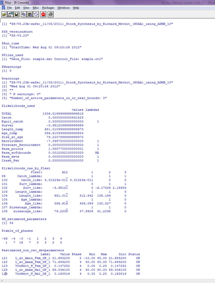
Example of the data displayed used by the SS_output function:
170
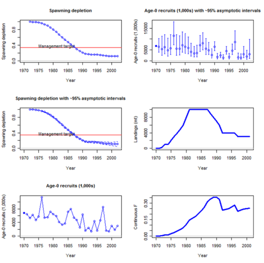
Example of the plots created using the SS_plots function:
171

The functions included in r4ss ranging from general use to functions developed for specific
model applications:
Core Functions
SS_output A function to create a list object for the output from Stock
Synthesis
SS_plots Plot many quantities related to output from Stock
Synthesis
Plot functions called by SS_plots
SSplotBiology Plot biology related quantities from Stock Synthesis model
output, including mean weight, maturity, fecundity, and
spawning output.
SSplotCatch Plot catch related quantities
SSplotCohorts Plot cumulative catch by cohort
SSplotComps Plot composition data and fits
SSplotData Timeline of presence/absence data by type, year, and fleet
SSplotDiscard Plot fit to discard fraction
SSplotIndices Plot indices of abundance and associated quantities
SSplotMnwt Plot mean weight data and fits
SSplotMovementMap Show movement rates on a map
SSplotMovementRates Show movement rates on a map
SSplotNumbers Plot numbers-at-age related data and fits
SSplotRecdevs Plot recruitment deviations
SSplotRecdist Plot of recruitment distribution among areas and seasons
SSplotSelex Plot selectivity
SSplotSexRatio Plot sex ratios
SSplotSummaryF Plot time series summary of F (or harvest rate)
SSplotSpawnrecruit Plot spawner-recruit curve
SSplotSPR Plot SPR quantities
SSplotTags Plot tagging data and fits
SSplotTimeseries Plot time series data
SSplotYield Plot yield and surplus production
SS_html Create HTML files to view figures in browser
SS_fitbiasramp Estimate bias adjustment for recruitment deviates
Model Comparisons and other diagnostics
SSplotPars Plot distributions of priors, posteriors, and estimates
SSplotProfile Plot likelihood profile results
172

PinerPlot Plot fleet-specific contributions to likelihood profile
SSplotRetroRecruits Make retrospective pattern of recruitment estimates (a.k.a.
squid plot) as seen in Pacific hake assessments
Functions related to MCMC diagnostics
mcmc_nuisance Summarize nuisance MCMC output
mcmc_out Summarize, analyze, and plot key MCMC output
SSgetMCMC Read MCMC output
SSplotMCMC_ExtraSelex Plot uncertainty around chosen selectivity ogive from
MCMC
Interactive tools for exploring functional forms
movepars Explore movement parameterization
selfit A function to visualize parameterization of double normal
and double logistic selectivity in SS
selfit_spline Visualize parameterization of cubic spline selectivity in SS
sel_line A function for drawing selectivity curves
File manipulation for inputs
SS_readdat Read data file
SS_readforecast Read forecast file
SS_readstarter Read starter file
SS_writedat Write data file
SS_writeforecast Write forecast file
SS_writestarter Write starter file
SS_makedatlist Make a list for SS data
SS_parlines Get parameter lines from SS control file
SS_changepars Change parameters in the control file
SSmakeMmatrix Create inputs for entering a matrix of natural mortality by
age and year
SS_profile Run a likelihood profile in SS (incomplete)
NegLogInt_Fn Calculated variances of time-varying parameters using SS
implementation of the Laplace Approximation
File manipulations for outputs
SS_recdevs Insert a vector of recruitment deviations into the control
file
SS_splitdat Split apart bootstrap data to make input file
173

Minor plotting functions
bubble3 Create a bubble plot
make_multifig Create multi-figure plots
Make_multifig_sexratio Create multi-figure plots of sex ratios
plotCI Plot points with confidence intervals
rich_colors_short Make a vector of colors
stackpoly Plot stacked polygons
mountains Make shaded polygons with a mountain-like appearance
Really specialized functions
DoProjectPlots Make plots from Rebuilder program
IOTCmove Make a map of movement for a 5-area Indian Ocean model
SSFishGraph A function for converting SS output to the format used by
FishGraph
TSCplot Create a plot for the TSC report
15 Special Set-ups
15.1 Continuous seasonal recruitment
It is awkward in SS to set up a seasonal model such that recruitment can occur with similar
and independent probability in any season of any year. Consequently, some users have
attempted to setup SS so that each quarter appears as a year. They have set up all the data
and parameters to treat quarters as if they were years (i.e. each still has a duration of 1.0
time step). This can work, but requires that all rate parameters be re-scaled to be correct
for the quarters being treated as years.
Another option is available. If there is one season per year and the season duration is set to 3
(rather than the normal 12), then the season duration is calculated to be 3/12 or 0.25. This
means that the rate parameters can stay in their normal per year scaling and this shorter
season duration makes the necessary adjustments internally. Some other adjustments to
make when doing quarters as years include:
•re-index all "year seas" inputs to be in terms of quarter-year because all are now season
1; increase endyr value in sync with this
174
•increase max age because age is now in quarters
•in the age error definitions, increase the number of entries in accord with new max age
•in the age error definitions, recode so that each quarter-age gets assigned to the correct
agebin; This is because the age data are still in terms of agebins; i.e. the first 4 entries
for quarter-ages 1 through 4 will all be assigned to agebin 1.5; the next four to agebin
2.5; you cannot accomplish the same result by editing the age bin values because the
stddev of ageing error is in terms of agebin
•in the control file, multiple the natM age breakpoints and growth AFIX values by
1/seasdur
•decrease the R0 parameter starting value because it is now the average number of
recruitments per qtryear
•edit the rec_dev start and endyrs to be in terms of qtryear
•edit any age selectivity parameters that refer to age to now refer to qtrage
•if there needs to be some degree of seasonality to recruitment or some parameter, then
you could create a cyclic pattern in the environmental input and make recruitment or
some other parameter a function of this cyclic pattern
A good test showing comparability of the 3 approaches to setting up a quarterly model
should be done.
16 Change Log
This section has been removed from the user manual. Information on changes to SS is
now recorded in the spreadsheet database, SS_Changes.xlsx. Fields include date, version
number, category (e.g. growth, selectivity), type (e.g. new, clarify, fix). Occasional model
tips will be added with the type=”Tip”.
17 Appendix A: Recruitment Variability and Bias
Correction
Recruitments in SS are defined as lognormal deviates around a log-bias adjusted spawner-
recruitment curve. The magnitude of the log-bias adjustment is calculated from the level of
175
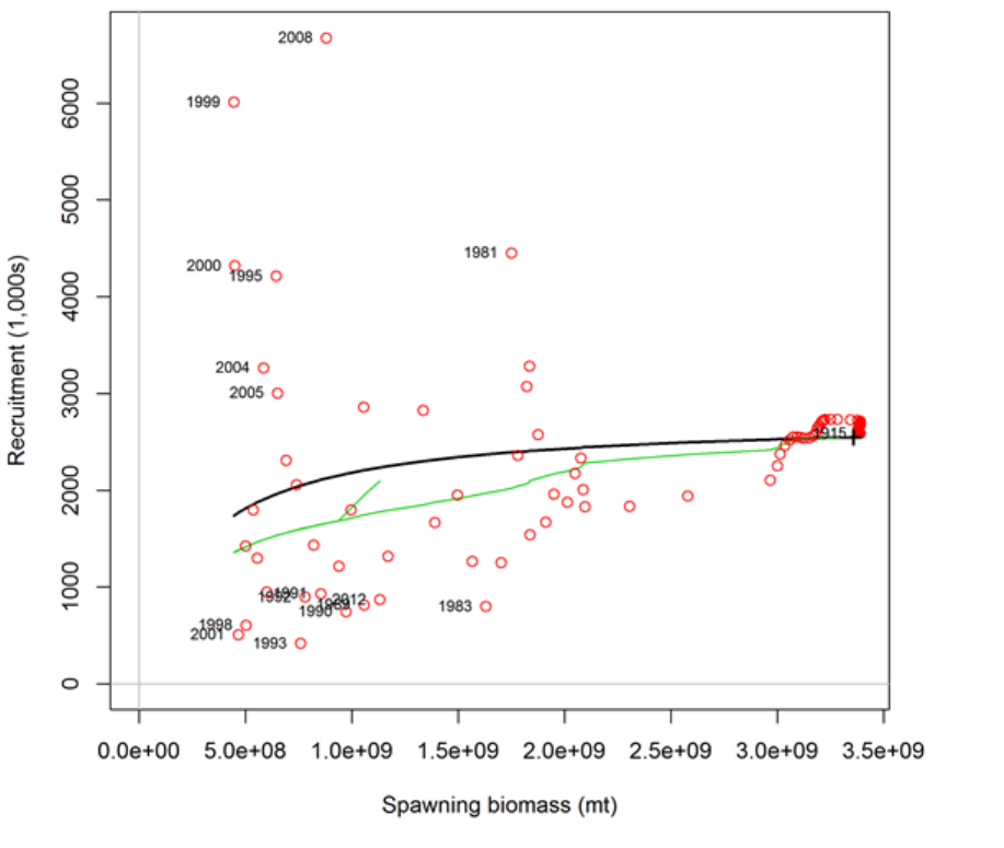
σR, which is the standard deviation of the recruitment deviations (in log-space). There are 5
segments of the time series in which to consider the effect of the log-bias adjustment: virgin;
initial equilibrium; early data-poor period; data-rich period; very-recent/forecast. The choice
of break points between these segments need not correspond directly with the settings for
the bias adjustment, although some alignment might be desired. Methot and Taylor (2011)
provide more detailed discussion of the bias adjustment than what is provided below but do
not address the separation of time periods into separate segments. The approach is illustrated
with figures associated with a recent assessment for darkblotched rockfish (Gertseva and
Thorson, 2013).
Figure A.1. Spawner-recruitment relationship for darkblotched rockfish (Gertseva and Thorson,
2013). Red points represent estimated recruitments, the solid black line is the stock-recruit
relationship and the green line represents the adjustment to this relationship after adjustment
to account for the lognormal distribution associated with each year. The “+” symbol labeled
1915 near the right side represents both the virgin and initial equilibrium of the model. The
numerous red points close to the initial conditions correspond to the early years of the model
176
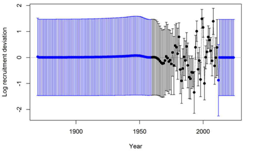
with low harvest rates.
Figure A.2. Timeseries of log recruitment deviations for darkblotched rockfish with 95%
uncertainty intervals. The start year of the model is 1915, but recruitment deviations
are estimates starting in 1870. The 45 deviation estimates for 1870–1914 inform the age
structure used in the start year. The black color for the years 1960–2011 indicates the “main”
recruitment deviation vector, while the blue color for the years 1870–1959 and 2012–2024
indicates the “early” and “late/forecast” recruitment deviation vectors, respectively.
Virgin
The R0 level of recruitment is a parameter of the spawner-recruitment curve. This
recruitment and the corresponding spawning biomass, S0, are expected to represent
the long-term arithmetic mean.
Initial Equilibrium
The level of recruitment is typically maintained at the R0 level even though the initial
equilibrium catch will reduce the spawning biomass below the virgin level. If steepness
is moderately low or the initial F is high, then the lack of response in recruitment
level may appear paradoxical. The logic is that building in the spawner-recruitment
response to initial F would significantly complicate the calculations and would imply
that the initial equilibrium catch level had been going on for multiple generations. If
the lack of response is considered to be problematic in a particular application, then
start the model at an earlier year and with a lower initial equilibrium catch so that the
dynamics of the spawner-recruitment response get captured in the early period, rather
than getting lost in the initial equilibrium.
177
Early data-poor period
This is the early part of the time series where the only data typically are landed catch.
There are no data to inform the model about the specific year-to-year fluctuations in
recruitment, although the ending years of this period will begin to be influenced by
the data. The “early time period” is not a formal concept. It is up to the user to
decide whether to start estimating recruitment deviations beginning with the first year
of the model, or to delay such estimation until the data become more informative.
Modeling recruitment deviations in this period may lead to a more realistic portrayal
of the uncertainty in depletion, but can also lead to spurious patterns in estimated
recruitments that may be driven by the fit to index data or other sources that would
not be expected to have accurate information on recruitment.
•Option A: Do not estimate recruitment deviations during this early period. During
years prior to the first year of recruitment deviations, the model will set the
recruitment equal to the level of the spawner-recruitment curve. Thus, it is a
mean-based level of recruitment. Because these annual parameters are fixed to
the level of the spawner-recruitment curve, they have no additional uncertainty
and make no contribution to the variance of the model. This approach may
produce relatively large, or small, magnitude deviations at the very beginning
of the subsequent period, as the model “catches up” to any slight signal that
could not be captured through estimated deviations in the early data-poor period.
There may be some effect on the estimate of R0 as a result of lack of model
flexibility in balancing early period removals with signal in the early portion of
the data-rich period.
•Option B: Estimate recruitment deviations for all the early years. Each of these
recruitment deviations is now a dev parameter so will have a variance that contributes
to the total model variance. The estimated standard deviation of each of these
dev parameters should be similar to σRbecause σRis the only constraint on these
parameters (however, the last few in the sequence will begin to feel the effect of
the data so may have lower standard deviations).
Data-rich period
Here the data inform the model on the year-to-year level of recruitment. These
fluctuations in recruitment are assumed to have a lognormal distribution around the
log-bias adjusted spawner-recruitment curve. The level of σRinput to the model should
match this level of fluctuation to a reasonable degree. Because the recruitments are
lognormal, they produce a mean biomass level that is comparable to the virgin biomass
and thus the depletion level can be calculated without bias. However, if the early
period has recruitment deviations estimated by MPD, then the depletion levels during
the early part of the data-rich period may have some lingering effect of negative bias
during the early time period. The level of σRshould be at least as large as the level
of variability in these estimated recruitments. If too high a level of σRis used, then a
178
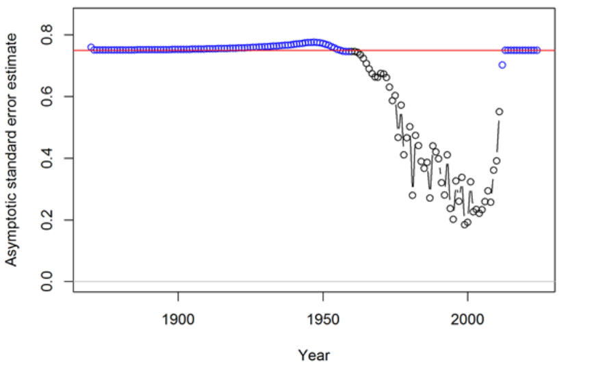
bias can occur in the estimate of spawner-recruitment steepness, which determines the
trend in recruitment. This occurs when the early recruitments are taken directly from
the spawner-recruitment curve, so are mean unbiased, then the later recruitments are
estimated as deviations from the log-bias adjusted curve. If σRis too large, then the
bias-adjustment is too large, and the model may compensate by increasing steepness
to keep the mean level of recent recruitments at the correct level.
Recent Years/Forecast
Here the situation is very similar to the early time period in that there are no data
to inform the model about the year-to-year pattern in recruitment fluctuations so all
devs will be pulled to a zero level in the MPD. The structure of SS creates no sharp
dividing line between the estimation period and the forecast period. In many cases one
or more recruitments at the end of the time series will lack appreciable signal in the
data and should therefore be treated as forecast recruit deviations. To the degree that
some variability is observed in these recruitments, partial or full bias correction may
be desirable for these devs separate from the purely forecast devs, there is therefore
an additional control for the level of bias correction applied to forecast deviations
occurring prior to endyear+1.
Figure A.3. Timeseries of standard error estimates for the log recruitment deviations for
darkblotched rockfish with 95% uncertainty intervals. As in Figure A.2, the black color
indicates the main recruitment period. This period with lower standard error is associated
with higher variability among deviations (Figure A.2). The red line at 0.75 indicates the σR
179
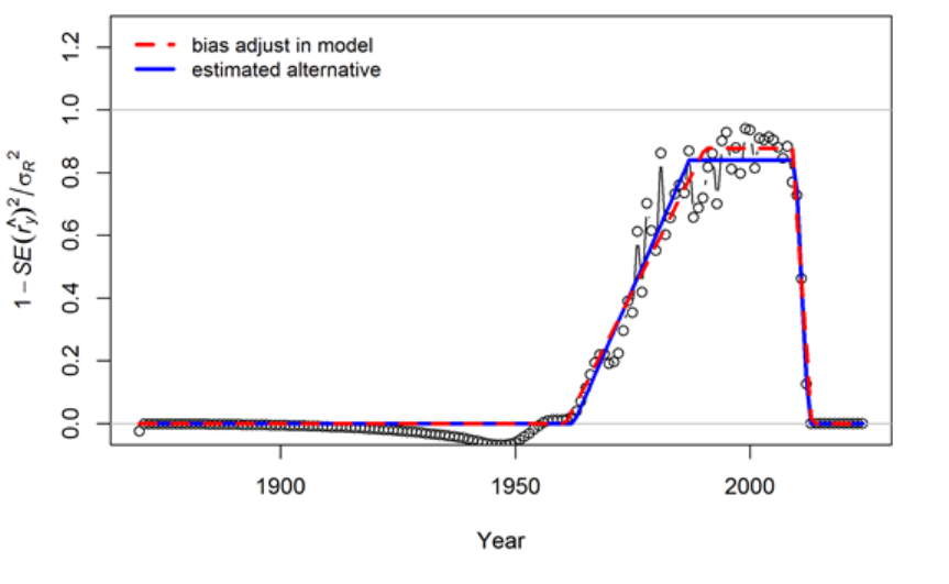
value in this model.
Figure A.4. Transformation of the standard error estimates (shown in Figure A.3) for
darkblotched rockfish following the approach suggested by Methot and Taylor (2011). These
values were used to set the 5 values controlling the degree of bias adjustment (as a fraction
of σR/2) to account for differences in the mean and median of the lognormal distribution
from which the recruitment deviations are drawn. The red line indicates a bias adjustment
of 0 up to the 1960.75, ramping up to a maximum adjustment level of 0.877 for the period
1990.4–2008.98,and reducing back to 0 starting in 2013.08. Note that these values controlling
the bias adjustment need not be integer year values. Also the break points in the bias
adjustment function need not match the break points between early, main, and late/forecast
recruitment deviation vectors (indicated by blue and black colors in Figures A.2 and A.3).
The blue line indicates a functional form that minimizes the sum of squared differences
between the bias adjustment function and the transformed standard error values. The subtle
differences between red and blue lines are unlikely to have any appreciable effect on the model
results.
180
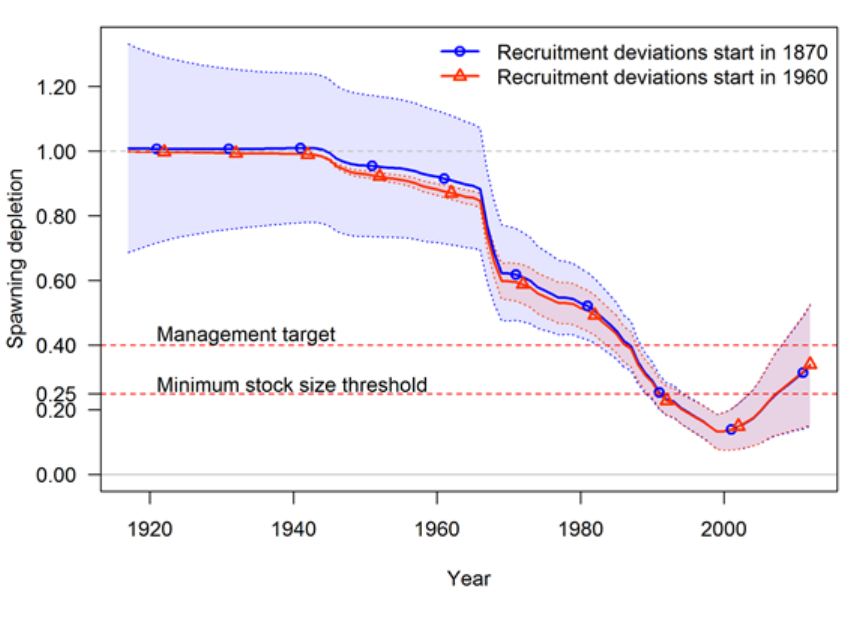
Figure A.5. Comparison of timeseries of spawning depletion for darkblotched rockfish models
with early recruitment deviations (starting in 1870) and without early deviations (only main
recruitment deviations starting in 1960). The point estimates are similar, but the 95%
uncertainty intervals are substantially different. With no recruitment deviations for the
early period, the estimates of spawning depletion in the early years are very precise and
uncertainty increases as the stock moves into the data rich period. In contrast, the addition
of the early recruitment deviations results in a large uncertainty in spawning depletion for
the early years and an increase in precision as the stock moves into the data rich period.
In this application, the uncertainty associated with the recent years is independent of the
assumptions about early recruitments.
17.1 Issues with Including Environmental Effects
The expected level of recruitment is a function of spawning biomass, an environmental time
series, and a log-bias adjustment.
E(Recruitment) = f(SpBio)∗exp(β∗envdata)∗exp(−0.5∗σ2
R)(49)
σRis the variability of the deviations, so it is in addition to the variance “created” by the
environmental effect. So, as more of the total recruitment variability is explained by the
181
environmental effect, the residual σRshould be decreased. The model does not do this
automatically.
The environmental effect is inherently lognormal. So when an environmental effect is included
in the model, the arithmetic mean recruitment level will be increased above the level predicted
by f(SpBio) alone. The consequences of this have not yet been thoroughly investigated, but
there probably should be another bias correction based on the variability of the environmental
data as scaled by the estimated linkage parameter, β. It is also problematic that the
environmental effect time series used as input is assumed to be measured without error.
The preferred approach to including environmental effects on recruitment is not to use the
environmental effect in the direct calculation of the expected level of recruitment. Instead,
the environmental data would be used as if it was a survey observation of the recruitment
deviation. This approach is similar to using the environmental index as if it was a survey
of age 0 recruitment abundance because by focusing on the fit to the deviations it removes
the effect of SpBio on recruitment. In this alternative, the σRwould not be changed by
the environmental data; instead the environmental data would be used to explain some of
the total variability represented by σR. This approach may also allow greater uncertainty in
forecasts, as the variability in projected recruitments would reflect both the uncertainty in
the environmental observations themselves and the model fit to these observations.
17.2 Initial Age Composition
If the first year with recruitment deviations is set less than the start year of the model, then
these early deviations will modify the initial age composition. The amount of information
on historical recruitment variability certainly will degrade as the model attempts to estimate
deviations for older age groups in the initial equilibrium. So the degree of bias correction
is reduced linearly in proportion to age so that the correction disappears when maximum
age is reached. The initial age composition approach normally produces a result that is
indistinguishable from a configuration that starts earlier in the time series and estimates a
longer time series of recruitments. However, because the initial equilibrium is calculated from
a recruitment level unaffected by spawner-recruitment steepness and initial age composition
adjustments are applied after the initial equilibrium is calculated, it is possible that the initial
age composition approach will produce a slightly different result than if the time series was
started earlier and the deviations were being applied to the recruitment levels predicted from
the spawner-recruitment curve.
182
18 Appendix B: Data Weighting
In 2015 there was a CAPAM workshop dedicated to data-weighting. Description of the
workshop can be found at http://www.capamresearch.org/data-weighting/workshop.
The presentations from the workshop are available through that website
and many of them were included in a special issue of Fisheries Research a
https://www.sciencedirect.com/journal/fisheries-research/vol/192.
Currently, there are three main methods for weighting length and data applied for U.S. West
Coast assessments using Stock Synthesis.
1. McAllister - Ianelli: Effective sample size is calculated from fit of observed to
expected length or age compositions. Tuning algorithm is intended to make the
arithmetic mean of the input sample size equal to the harmonic mean of the effective
sample size. Reference: McAllister, M.K. and J.N. Ianelli 1997. Bayesian stock
assessment using catch-age data and the sampling - importance resampling algorithm.
Can. J. Fish. Aquat. Sci, 1997, 54(2): 284-300.
2. Francis: Based on variability in the observed mean length or age by year, where the
sample sizes are adjusted such that the fit of the expected mean length or age should fit
within the uncertainty intervals at a rate which is consistent with variability expected
based on the adjusted sample sizes (Method "TA1.8"). Reference: Francis, R.I.C.C.
(2011). Data weighting in statistical fisheries stock assessment models. Can. J. Fish.
Aquat. Sci. 68: 1124-1138.
3. Dirichlet-Multinomial: A new likelihood (as opposed to the standard multinomial)
which includes an estimable parameter (theta) which scales the input sample size.
In this case, the term “Effective sample size” has a different interpretation than in
the McAllister-Ianelli approach. References: Thorson, J.T., Johnson, K.F., Methot,
R.D. and Taylor, I.G. 2017. Model-based estimates of effective sample size in stock
assessment models using the Dirichlet-multinomial distribution. Fish. Res. 192: 84-93.
Thorson, J.T. 2018. Perspective: Let’s simplify stock assessment by replacing tuning
algorithms with statistics. Fish. Res.
18.1 Applying the methods
18.1.1 McAllister-Ianelli
The “Length_Comp_Fit_Summary” and “Age_Comp_Fit_Summary” sections in the Report
file include information on the harmonic mean of the effective sample size and arithmetic
mean of the input sample size used in this tuning method. In the r4ss package, these
183
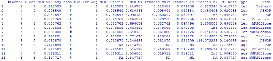
tables are returned by the SS_output function as $Length_comp_Eff_N_tuning_check
and $Age_comp_Eff_N_tuning_check.
A convenient way to process these values into the format required by the control file is to
use the function:
SS_tune_comps(replist, option = "MI")
where the input “replist” is the object created by SS_output. This function will return a
table and also write a matching file called “suggested_tuning.ss” to the directory where the
model was run.
For models using SS version 3.30, the table created by SS_tune_comps can be pasted into
the bottom of the control file in the section labeled “Input variance adjustments”, followed
by the terminator line which indicates the end of the section. Here’s an example of the first
few rows of the table followed by the terminator line (not added by the function):
Also see the help page for the r4ss function SS_varadjust which can be used to automatically
write a new control file if you want to streamline the process of applying multiple iterations
of this tuning method.
If the tuning has been implemented, the green lines in the figure below would intersect at
a point which is on the black 1-to-1 diagonal line in this figure created by the r4ss function
SS_plots.
184
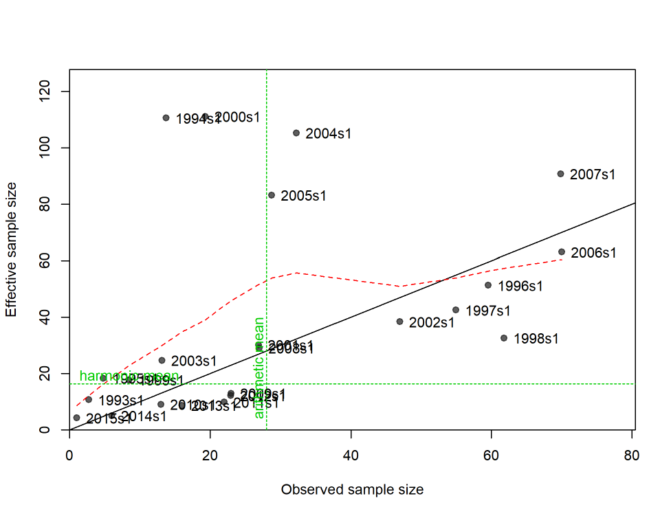
Figure B.1.N vs. EffN comparison, Length composition data as plotted by r4ss.
There are a couple of challenges posed by the McAllister-Ianelli data-weighting approach:
1. Subjective choice of how many iterations to take to achieve adequate convergence.
Often just one iteration is applied.
2. Takes time to implement so tuning is rarely repeated during retrospective or sensitivity
analyses.
18.1.2 Francis
Implementation: recommended adjustments are calculated by the r4ss functions SSMethod.TA1.8
and SSMethod.Cond.TA1.8. These functions are rarely used alone but are called by the
SS_plots function when making plots like the one below. For SS 3.30 models, the simplest
185
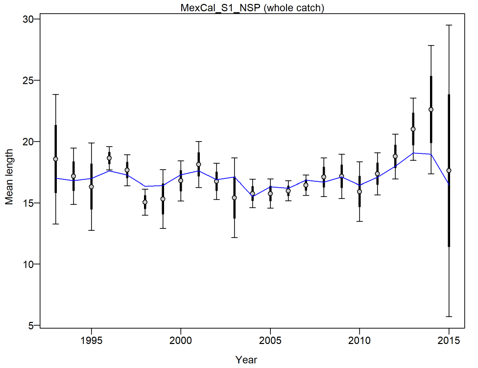
way to get the adjustments in the format required by the control file is to use the SS_tune_comps
function (described above under the McAllister-Ianelli method), but with a different option
specified:
SS_tune_comps(replist, option = "Francis")
The figure below shows the estimated 95% intervals around the observed mean length by
year based on the input sample size (thick lines) and the increase in that uncertainty which
would occur if the sample sizes were adjusted according to the proposed multiplier.
Figure B.2.Mean length for Fleet1 with 95% confidence intervals based on current samples
sizes. Francis data weighting method TA1.8: thinner intervals (with capped ends) show
result of further adjusting sample sizes based on suggested multiplier (with 95% interval) for
len data from Fleet1: 0.2739 (0.1661-0.6305)
186
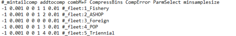
There are a several of challenges posed by the Francis data-weighting approach:
1. Subjective choice of how many iterations to take to achieve adequate convergence.
Often just one iteration is applied.
2. Takes time to implement so tuning is rarely repeated during retrospective or sensitivity
analyses.
3. Recommended adjustment can be sensitive to outliers (remove a few years of anomalous
composition data can lead to large change in recommended adjustment).
18.1.3 Dirichlet-Multinomial
Change the choice of likelihood and set parameter choices in the data file:
•In the specification of the length and/or age data, change "CompError" column in age
and length comp specifications from 0 to 1 and "ParmSelect" from 0 to a sequence
of numbers from 1 to N where N is the total number of combinations of fleet and
age/length.
•Resulting input should look similar to:
•The ParmSelect column can also have repeated values so that multiple fleets share the
same log(theta) parameter.
•If you have both length and age data, the ParmSelect should have separate numbers
for each, e.g. 1 and 2 for the length comps and 3 and 4 for the age comps for the same
two fleets.
Add parameter lines to the control file:
•Add as many parameter lines as the maximum numbers in the ParmSelect column.
The new parameter lines go after the main selectivity parameters but before any
time-varying selectivity parameters
•Jim Thorson initially recommended bounds of -5 to 20, with a starting value of 0 (which
corresponds to a weight of about 50% of the input sample size). However, parameter
estimates above 5 are associated with 99-100% weight with little information in the
187
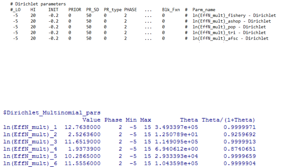
likelihood about the parameter value. Therefore, an upper bound of 5 may help identify
cases that otherwise would have convergence issues.
•Example parameter lines are below:
•Reset any existing variance adjustments factors that might have been used for the
McAllister-Ianelli or Francis tuning methods. In 3.24 this means setting the values
to 1, in SS version 3.30, you can simply delete or comment-out the rows with the
adjustments.
The SS_output function in r4ss returns table like the following:
The ratio shown in the final column is the estimated multiplier which can be compared to
the sample size adjustment estimated in the other tuning methods above (the New_Var_adj
column in the table produced by the SS_tune_comps function in r4ss).
If the reported θ/(1 + θ)ratio is close to 1.0, that indicates that the model is trying to tune
the sample size as high as possible. In this case, the ln(θ)parameters should be fixed at a
high value, like the upper bound of 20, which will result in 100% weight being applied to the
input sample sizes. An alternative would be to manually change the input sample sizes to a
higher value so that the estimated weighting will be less than 100
There is also information about this result produced in the plots created by the SS_plots
function:
188
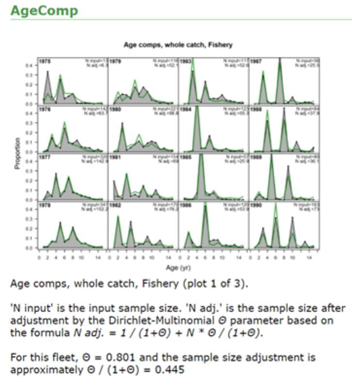
There are a several of challenges posed by the Dirichlet-Multinomial data-weighting approach:
1. Not yet widely used so little guidance is available.
2. Does not allow weights above 100% (by design) so it is not yet clear how best to deal
with the situation when the estimated weight is close to 100%.
3. Parameterization has potential to cause convergence issues or inefficient MCMC sampling
when weights are close to 100% (Jim Thorson has proposed a prior distribution that
may help with this, but has not yet been tested).
189
19 Appendix C: Forecast Module
19.1 Introduction
Version 3.20 of Stock Synthesis (SS) introduced substantial upgrades to the benchmark and
forecast module. The general intent was to make the forecast outputs more consistent with
the requirement to set catch limits that have a known probability of exceeding the overfishing
limit. In addition, this upgrade addressed several inadequacies with the previous module,
including:
•The average selectivity and relative F was the same for the benchmark and the forecast
calculations;
•The biology-at-age in endyr+1 was used as the biology for the benchmark, but biology–at-age
propagated forward in the forecast if there was time-varying growth;
•The forecast module had a kluge approach to calculation of OFL conditioned on
previously catching ABC;
•The forecast module implementation of catch caps was incomplete and applied some
caps on a seasonally, rather than the more logical annual basis;
•The Fmult scalar for fishing intensity presented a confusing concept for many users;
•No provision for specification of catch allocation among fleets;
•The forecast allowed for a blend of fixed input catches and catches calculated from
target F; this is not optimal for calculation of the variance of F conditioned on a catch
policy that sets ACLs.
The V3.20 module addressed these issues by:
•Providing for unique specification of a range of years from which to calculate average
selectivity for benchmark, average selectivity for forecast, relative F for benchmark,
and relative F for forecast;
•Create a new specification for the range of years over which to average size-at-age and
fecundity-at-age for the benchmark calculation. In a setup with time-varying growth,
it may make sense to do this over the entire range of years in the time series. Note that
some additional quantities still use their endyr values, notably the migration rates and
the allocation of recruitments among areas. This will be addressed shortly;
•Create a multiple pass approach that rectifies the OFL calculation;
190
•Improve the specification of catch caps and implement specification of catch allocations
so that there can be an annual cap for each fleet, an annual cap for each area, and an
annual allocation among groups of fleets (e.g. all recreational fleets vs. all commercial
fleets);
•Introduce capability to have implementation error in the forecast catch (single value
applied to all fleets in all seasons of the year).
19.2 Multiple Pass Forecast
The most complicated aspect of the changes is with regard to the multiple pass aspect of the
forecast. This multiple pass approach is needed to calculate both OFL and ABC in a single
model run. More importantly, the multiple passes are needed in order to mimic the actual
sequence of assessment-management action – catch over a multi-year period. The first pass
calculates OFL based on catching OFL each year, so presents the absolute maximum upper
limit to catches. The second pass forecasts a catch based on a harvest policy, then applies
catch caps and allocations, then updates the F’s to match these catches. In the third pass,
stochastic recruitment and catch implementation error are implemented and SS calculates
the F that would be needed in order to catch the adjusted catch amount previously calculated
in the second pass. With this approach, SS is able to produce improved estimates of the
probability that F would exceed the overfishing F. In effect it is the complement of the P*
approach. Rather than the P* approach that calculates the stream of annual catches that
would have an annual probability of F>Flimit, SS calculates the expected time series of P*
that would result from a specified harvest policy implemented as a buffer between Ftarget
and Flimit.
The sequence of multiple forecast passes is as follows:
1. Pass 1 (a.k.a. Fcast_Loop1)
(a) Loop Years
i. SubLoop (a.k.a. ABC_Loop) = 1
A. R=f(SSB) with no deviations
B. F=Flimit
C. Fixed input catch amounts ignored
D. No catch adjustments (caps and allocations)
E. No implementation error
191
F. Result: OFL conditioned on catching OFL each year
2. Pass 2
(a) Loop Years
i. SubLoop = 1
A. R=f(SSB) with no deviations
B. F=Flimit
C. Fixed input catch amounts ignored
D. No catch adjustments (caps and allocations)
E. No implementation error
F. Result: OFL conditioned on catching ABC previous year. Stored in
std_vector.
ii. SubLoop = 2
A. R=f(SSB) with no deviations
B. F=Ftarget to get catc for each fleet in each season
C. Fixed input catch amounts replace catch from step 2
D. Catch adjustments (caps and allocations) applied on annual basis (after
looping through seasons and and areas within this year). These adjustments
utilize the logistic joiner approach common in SS so the overall results
remain completely differentiable.
E. No implementation error
F. Result: ABC as adjusted for caps and allocations
iii. SubLoop = 3
A. R=f(SSB) with no deviations
B. Catches from Pass 2 multiplied by the random term for implementation
error
C. F=adjusted to match the catch*error while taking into account the random
192

recruitments. This is most easily visualized in a MCMC context where the
recruitment deviation and the implementation error deviations take on
non-zero values in each instance. In MLE, because the forecast recruitments
and implementation error are estimated parameters with variance, their
variance still propagates to the derived quantities in the forecast.
D. Result: Values for F, SSB, Recruitment, Catch are stored in std-vectors
•In addition, the ratios F/Flimit and SSB/SSBlimit or SSB/SSBtarget
are also stored in std_vectors.
•Estimated variance in these ratios allows calculation of annual probability
that F>Flimit or B<Blimit. This is essentially the realized P* conditioned
on the specified harvest policy.
19.3 Example Effects on Correlations
An example that illustrates the above process was conducted. The situation was a low
M, late-maturing species, so changes are not dramatic. The example conducted a 10 year
forecast and examined correlations with derived quantities in the last year of the forecast.
This was done once with the full set of 3 passes as described above, and again with only 2
passes and stochastic recruitment occurring in pass 2, rather than 3. This alternative setup
is more similar to forecasts done using previous model versions.
2 Forecast Passes with F from 2 Forecast Passes with catch from
ABC and random recruitment target F and equilibrium recruitment
Factor X Factor Y Corr Factor X Factor Y Corr
A1 F 2011 RecrDev 2002 -0.126 A2 F 2011 RecrDev
2002
0.090
B1 F 2011 Recr 2002 0.312 B2 F 2011 Recr 2002 0.518
C1 ForeCatch
2011
RecrDev 2002 0.000 C2 ForeCatch
2011
RecrDev
2002
0.129
D1 ForeCatch
2011
Recr 2002 0.455 D2 Forecatch 2011 Recr 2002 0.555
Correlation A2 shows a small positive correlation between the recruitment deviation in 2002
and the F in 2011. This is probably due to the fact that a positive deviation in recruitment in
2002 will reduce the chances that the biomass in 2011 will be below the inflection point in the
control rule. This occurs because in calculating catch from F, the model effectively “knows”
193
the future recruitments. I predict that this B1 correlation would be near zero if there was no
inflection in the control rule. Correlation A1 shows this turning into a negative correlation.
This is because the future catches are first calculated from equilibrium recruitment, then
when random recruitments are implemented, a positive recruitment deviation will cause a
negative deviation in the F needed to catch that now “fixed” amount of future catch.
Correlations B1 and B2 are in terms of absolute recruitment, not recruitment deviation.
Now overall model conditions that cause a higher absolute recruitment level will also result
in a higher forecast level. No surprise there, and the correlation is stronger when variance is
based on catch is calculated from F (B2).
Correlation C2 shows a positive correlation between recruitment deviation in 2002 and
forecast catch in 2011. However, correlation C1 is 0.0 because the forecast catch in 2011 is set
based on equilibrium recruitment and is not influenced by the recruitment deviations.
19.4 Future Work
•More testing with high M, rapid turnover conditions
•Testing without inflection in control rule
•Consider separating implementation error into a pass #4 so results will more clearly
show effect of assessment uncertainty separate from implementation uncertainty
•Consider adding a random “assessment” error which essentially is a random variable
that scales population abundance before passing into the forecast stage. Complication
is figuring out how to link it to the correlated error in the benchmark quantities
•Because all of these calculations occur only in the sdphase or the mceval phase, it
would be feasible for mceval calls to add an additional pass that is implemented many
times and in which random forecast recruitment draws are made.
•Factors like selectivity and fleet relative F levels are calculated as an average of these
values during the time series. This is internally consistent if these factors do not vary
during the time series (although clearly this is a stiff model that will underestimate
process variance). However, if these factors do vary over time, then the average used
for the forecast will under-represent the variance. A better approach would be to set up
the parameters of selectivity as a random process that extends throughout the forecast
period, and to update estimated selectivity in each year of the forecast based upon the
random realization of these parameters.
194
20 Appendix D: Code Examples
20.1 Ageing Error Estimation
/* SS_Label_FUNCTION 45 get_age_age */
FUNCTION void get_age_age(const int Keynum, const int AgeKey_StartAge, const int AgeKey_Linear1, const int AgeKey_Linear2)
{
// FUTURE: calculate adjustment to oldest age based on continued ageing of old fish
age_age(Keynum).initialize();
dvariable age;
dvar_vector age_err_parm(1,7);
dvariable temp;
if(Keynum==Use_AgeKeyZero)
{
// SS_Label_45.1 set age_err_parm to mgp_adj, so can be time-varying according to MGparm options
for (a=1;a<=7;a++)
{age_err_parm(a)=mgp_adj(AgeKeyParm-1+a);}
age_err(Use_AgeKeyZero,1)(0,AgeKey_StartAge)=r_ages(0,AgeKey_StartAge)+0.5;
age_err(Use_AgeKeyZero,2)(0,AgeKey_StartAge)=age_err_parm(5)*(r_ages(0,AgeKey_StartAge)+0.5)/
(age_err_parm(1)+0.5);
// SS_Label_45.3 calc ageing bias
if(AgeKey_Linear1==0)
{
age_err(Use_AgeKeyZero,1)(AgeKey_StartAge,nages)=0.5 + r_ages(AgeKey_StartAge,nages) +
age_err_parm(2)+(age_err_parm(3)-age_err_parm(2))*(1.0-mfexp(-age_err_parm(4)*
(r_ages(AgeKey_StartAge,nages)-age_err_parm(1)))) / (1.0-mfexp(-age_err_parm(4)*
(r_ages(nages)-age_err_parm(1))));
}
else
{
age_err(Use_AgeKeyZero,1)(AgeKey_StartAge,nages)=0.5 + r_ages(AgeKey_StartAge,nages) +
age_err_parm(2)+(age_err_parm(3)-age_err_parm(2))*
(r_ages(AgeKey_StartAge,nages)-age_err_parm(1))/(r_ages(nages)-age_err_parm(1));
}
// SS_Label_45.4 calc ageing variance
if(AgeKey_Linear2==0)
{
age_err(Use_AgeKeyZero,2)(AgeKey_StartAge,nages)=age_err_parm(5)+(age_err_parm(6)-age_err_parm(5))*
(1.0-mfexp(-age_err_parm(7)*(r_ages(AgeKey_StartAge,nages)-age_err_parm(1)))) /
(1.0-mfexp(-age_err_parm(7)*(r_ages(nages)-age_err_parm(1))));
}
else
{
age_err(Use_AgeKeyZero,2)(AgeKey_StartAge,nages)=age_err_parm(5)+(age_err_parm(6)-age_err_parm(5))*
(r_ages(AgeKey_StartAge,nages)-age_err_parm(1))/(r_ages(nages)-age_err_parm(1));
}
}
20.2 Survival Based SRR Code
Code for the survival based recruitment is shown below:
// SS_Label_43.3.7 survival based
case 7: // survival based, so constrained such that recruits cannot exceed fecundity
{
195
SRZ_0=log(1.0/(SSB_virgin_adj/Recr_virgin_adj));
SRZ_max=SRZ_0+SR_parm_work(2)*(0.0-SRZ_0);
SRZ_surv=mfexp((1.-pow((SSB_curr_adj/SSB_virgin_adj),SR_parm_work(3)) )*(SRZ_max-SRZ_0)+SRZ_0); // survival
NewRecruits=SSB_curr_adj*SRZ_surv;
exp_rec(y,1)=NewRecruits; // expected arithmetic mean recruitment
// SS_Label_43.3.7.1 Do variation in recruitment by adjusting survival
if(recdev_cycle>0)
{
gg=y - (styr+(int((y-styr)/recdev_cycle))*recdev_cycle)+1;
SRZ_surv*=mfexp(recdev_cycle_parm(gg));
}
exp_rec(y,2)=SSB_curr_adj*SRZ_surv;
SRZ_surv*=mfexp(-biasadj(y)*half_sigmaRsq); // bias adjustment
exp_rec(y,3)=SSB_curr_adj*SRZ_surv;
if(y <=recdev_end)
{
if(recdev_doit(y)>0) SRZ_surv*=mfexp(recdev(y)); // recruitment deviation
}
else if(Do_Forecast>0)
{
SRZ_surv *= mfexp(Fcast_recruitments(y));
}
join=1./(1.+mfexp(100*(SRZ_surv-1.)));
SRZ_surv=SRZ_surv*join + (1.-join)*1.0;
NewRecruits=SSB_curr_adj*SRZ_surv;
exp_rec(y,4) = NewRecruits;
break;
}
196
20.3 Random Walk Selectivity: Pattern 17
Code for selectivity pattern 17, random walk shown below:
// SS_Label_Info_22.7.17 #age selectivity: each age has parameter as random walk
// #41 each age has parameter as random walk scaled by average of values at low age through high age
// transformation as selex=exp(parm); some special codes */
case 41:
scaling_offset = 2;
case 17: //
{
lastsel=0.0; // value is the change in log(selex); this is the reference value for age 0
tempvec_a=-999.;
tempvec_a(0)=0.0; // so do not try to estimate the first value
int lastage;
if(seltype(f,4)==0)
{lastage=nages;}
else
{lastage=abs(seltype(f,4));}
for (a=1;a<=lastage;a++)
{
// with use of -999, lastsel stays constant until changed, so could create a linear change in ln(selex)
// use of (a+1) is because the first element, sp(1), is for age zero
if(sp(a+1+scaling_offset)>-999.) {lastsel=sp(a+1+scaling_offset);}
tempvec_a(a)=tempvec_a(a-1)+lastsel; // cumulative log(selex)
}
if (scaling_offset == 0)
{
temp=max(tempvec_a); // find max so at least one age will have selex=1.
}
else
{
int low_bin = int(value(sp(1)));
int high_bin = int(value(sp(2)));
if (low_bin < 0)
{
low_bin = 0;
N_warn++; warning<<" selex pattern 41; value for low bin is less than 0, so set to 0 "<<endl;
}
if (high_bin > nages)
{
high_bin = nages;
N_warn++; warning<<" selex pattern 41; value for high bin is greater than "<<nages<<", so set to "<<nages<<" "<<endl;
}
if (high_bin < low_bin) high_bin = low_bin;
if (low_bin > high_bin) low_bin = high_bin;
sp(1) = low_bin;
sp(2) = high_bin;
temp=mean(tempvec_a(low_bin,high_bin));
}
sel_a(y,fs,1)=mfexp(tempvec_a-temp);
a=0;
while(sp(a+1+scaling_offset)==-1000) // reset range of young ages to selex=0.0
{
sel_a(y,fs,1,a)=0.0;
a++;
}
scaling_offset = 0; // reset scaling offset
if(lastage<nages)
{
for (a=lastage+1;a<=nages;a++)
197
{
if(seltype(f,4)>0)
{sel_a(y,fs,1,a)=sel_a(y,fs,1,a-1);}
else
{sel_a(y,fs,1,a)=0.0;}
}
}
break;
}
198
20.4 Cubic Spline Selectivity
Code for cubic spline selectivity, option 42, shown below:
// SS_Label_Info_22.7.27 #age selectivity: cubic spline
// #42 cubic spline scaled by average of values at low age through high age
case 42:
scaling_offset = 2;
case 27:
{
k=seltype(f,4); // n points to include in cubic spline
for (i=1;i<=k;i++)
{
splineX(i)=value(sp(i+3+scaling_offset)); // "value" required to avoid error, but values should be always fixed anyway
splineY(i)=sp(i+3+k+scaling_offset);
}
z=nages;
while(r_ages(z)>splineX(k)) {z--;}
j2=z+1; // first age beyond last node
vcubic_spline_function splinefn=vcubic_spline_function(splineX(1,k),splineY(1,k),sp(2+scaling_offset),sp(3+scaling_offset));
tempvec_a= splinefn(r_ages); // interpolate selectivity at each age
if (scaling_offset == 0)
{
temp=max(tempvec_a(0,j2));
}
else
{
int low_bin = int(value(sp(1)));
int high_bin = int(value(sp(2)));
if (low_bin < 0)
{
low_bin = 0;
N_warn++; warning<<" selex pattern 42; value for low bin is less than 0, so set to 0 "<<endl;
}
if (high_bin > nages)
{
high_bin = nages;
N_warn++; warning<<" selex pattern 42; value for high bin is greater than "<<nages<<", so set to "<<nages<<" "<<endl;
}
if (high_bin < low_bin) high_bin = low_bin;
if (low_bin > high_bin) low_bin = high_bin;
sp(1) = low_bin;
sp(2) = high_bin;
temp=mean(tempvec_a(low_bin,high_bin));
scaling_offset = 0; // reset scaling offset
}
tempvec_a-=temp; // rescale to get max of 0.0
tempvec_a(j2+1,nages) = tempvec_a(j2); // set constant above last node
sel_a(y,fs,1)=mfexp(tempvec_a);
break;
}
199

21 Appendix E: In Process and Wish List Items for
Future Versions
Category Item Description
In process Environmental survey
of a deviation vector
Environmental survey data can be related to f(a deviation vector), but needs
more Q_link functions.
Retrospective Make blocks work when doing retrospective analyses.
Wishlist Tag-recapture major revamp
Area specific spawner-recruitment
Add automatic set-up for size selectivity option 6 and age selectivity option
17 given the data (comparable to the current capacity for cubic spline
selectivity).
More error checking on read of empirical weight-at-age and composition data.
New version of age-specific K needed because current version is inefficient.
Mean size in plus group uses a fixed erosion factor of 0.2; should be context
specific.
Consider Tim Miller’s state space model approach.
Add other options to CV growth patter for log(SD).
Add measure of auto-correlation in composition and in survey residuals.
Add SD report for survey expected values.
Add calculation of Francis composition weighting method.
Year-specific MSY.
200
22 Appendix F: Example Model Files
22.1 starter.ss
#V3.30.10.00-safe;_2018_01_09;_Stock_Synthesis_by_Richard_Methot_(NOAA)_using_ADMB_11.6
#_user_support_available_at:NMFS.Stock.Synthesis@noaa.gov
#_user_info_available_at:https://vlab.ncep.noaa.gov/group/stock-synthesis
#C starter comment here
simple.dat
simple.ctl
0 # 0=use init values in control file; 1=use ss.par
1 # run display detail (0,1,2)
1 # detailed age-structured reports in REPORT.SSO (0=low,1=high,2=low for data-limited)
0 # write detailed checkup.sso file (0,1)
4 # write parm values to ParmTrace.sso (0=no,1=good,active; 2=good,all; 3=every_iter,all_parms; 4=every,active)
1 # write to cumreport.sso (0=no,1=like×eries; 2=add survey fits)
1 # Include prior_like for non-estimated parameters (0,1)
1 # Use Soft Boundaries to aid convergence (0,1) (recommended)
3 # Number of datafiles to produce: 1st is input, 2nd is estimates, 3rd and higher are bootstrap
10 # Turn off estimation for parameters entering after this phase
0 # MCeval burn interval
1 # MCeval thin interval
0 # jitter initial parm value by this fraction
1969 # min yr for sdreport outputs (-1 for styr)
2011 # max yr for sdreport outputs (-1 for endyr; -2 for endyr+Nforecastyrs
0 # N individual STD years
#vector of year values
0.0001 # final convergence criteria (e.g. 1.0e-04)
0 # retrospective year relative to end year (e.g. -4)
1 # min age for calc of summary biomass
1 # Depletion basis: denom is: 0=skip; 1=rel X*B0; 2=rel X*Bmsy; 3=rel X*B_styr
0.4 # Fraction (X) for Depletion denominator (e.g. 0.4)
1 # SPR_report_basis: 0=skip; 1=(1-SPR)/(1-SPR_tgt); 2=(1-SPR)/(1-SPR_MSY); 3=(1-SPR)/(1-SPR_Btarget); 4=rawSPR
4 # F_report_units: 0=skip; 1=exploitation(Bio); 2=exploitation(Num); 3=sum(Frates); 4=true F for range of ages
20 23 #_min and max age over which average F will be calculated
1 # F_report_basis: 0=raw_F_report; 1=F/Fspr; 2=F/Fmsy ; 3=F/Fbtgt
0 # MCMC output detail (0=default; 1=obj func components; 2=expanded; 3=make output subdir for each MCMC vector)
0 # ALK tolerance (example 0.0001)
3.30 # check value for end of file and for version control
22.2 forecast.ss
#V3.30.10.00-safe;_2018_01_09;_Stock_Synthesis_by_Richard_Methot_(NOAA)_using_ADMB_11.6
201
#C generic forecast file
# for all year entries except rebuilder; enter either: actual year, -999 for styr, 0 for endyr, neg number for rel. endyr
1 # Benchmarks: 0=skip; 1=calc F_spr,F_btgt,F_msy; 2=calc F_spr,F0.1,F_msy
2 # MSY: 1= set to F(SPR); 2=calc F(MSY); 3=set to F(Btgt) or F0.1; 4=set to F(endyr)
0.4 # SPR target (e.g. 0.40)
0.342 # Biomass target (e.g. 0.40)
#_Bmark_years: beg_bio, end_bio, beg_selex, end_selex, beg_relF, end_relF, beg_recr_dist, end_recr_dist, beg_SRparm, end_SRparm (enter actual year, or values of 0 or -integer to be rel. endyr)
2001 2001 2001 2001 2001 2001 1971 2001 1971 2001
1 #Bmark_relF_Basis: 1 = use year range; 2 = set relF same as forecast below
#
1 # Forecast: 0=none; 1=F(SPR); 2=F(MSY) 3=F(Btgt) or F0.1; 4=Ave F (uses first-last relF yrs); 5=input annual F scalar
10 # N forecast years
0.2 # F scalar (only used for Do_Forecast==5)
#_Fcast_years: beg_selex, end_selex, beg_relF, end_relF, beg_recruits, end_recruits (enter actual year, or values of 0 or -integer to be rel. endyr)
0 0 -10 0 -999 0
0 # Forecast selectivity (0=fcast selex is mean from year range; 1=fcast selectivity from annual time-vary parms)
1 # Control rule method (1=catch=f(SSB) west coast; 2=F=f(SSB) )
0.4 # Control rule Biomass level for constant F (as frac of Bzero, e.g. 0.40); (Must be > the no F level below)
0.1 # Control rule Biomass level for no F (as frac of Bzero, e.g. 0.10)
0.75 # Control rule target as fraction of Flimit (e.g. 0.75)
3 #_N forecast loops (1=OFL only; 2=ABC; 3=get F from forecast ABC catch with allocations applied)
3 #_First forecast loop with stochastic recruitment
0 #_Forecast recruitment: 0= spawn_recr; 1=value*spawn_recr_fxn; 2=value*VirginRecr; 3=recent mean)
1 # value is ignored
0 #_Forecast loop control #5 (reserved for future bells&whistles)
2010 #FirstYear for caps and allocations (should be after years with fixed inputs)
0 # stddev of log(realized catch/target catch) in forecast (set value>0.0 to cause active impl_error)
0 # Do West Coast gfish rebuilder output (0/1)
1999 # Rebuilder: first year catch could have been set to zero (Ydecl)(-1 to set to 1999)
2002 # Rebuilder: year for current age structure (Yinit) (-1 to set to endyear+1)
1 # fleet relative F: 1=use first-last alloc year; 2=read seas, fleet, alloc list below
# Note that fleet allocation is used directly as average F if Do_Forecast=4
2 # basis for fcast catch tuning and for fcast catch caps and allocation (2=deadbio; 3=retainbio; 5=deadnum; 6=retainnum)
# Conditional input if relative F choice = 2
# enter list of: season, fleet, relF; if used, terminate with season=-9999
# 1 1 1
# enter list of: fleet number, max annual catch for fleets with a max; terminate with fleet=-9999
-9999 -1
# enter list of area ID and max annual catch; terminate with area=-9999
-9999 -1
# enter list of fleet number and allocation group assignment, if any; terminate with fleet=-9999
-9999 -1
#_if N allocation groups >0, list year, allocation fraction for each group
# list sequentially because read values fill to end of N forecast
# terminate with -9999 in year field
# no allocation groups
2 # basis for input Fcast catch: -1=read basis with each obs; 2=dead catch; 3=retained catch; 99=input Hrate(F)
#enter list of Fcast catches; terminate with line having year=-9999
#_Yr Seas Fleet Catch(or_F)
202
-9999 1 1 0
#
999 # verify end of input
22.3 data.ss
#V3.30.10.00-safe;_2018_01_09;_Stock_Synthesis_by_Richard_Methot_(NOAA)_using_ADMB_11.6
#_user_support_available_at:NMFS.Stock.Synthesis@noaa.gov
#_user_info_available_at:https://vlab.ncep.noaa.gov/group/stock-synthesis
#_Start_time: Fri Feb 2 10:54:21 2018
#_Number_of_datafiles: 3
#C data file for simple example
#_observed data:
#V3.30.10.00-safe;_2018_01_09;_Stock_Synthesis_by_Richard_Methot_(NOAA)_using_ADMB_11.6
1971 #_StartYr
2001 #_EndYr
1 #_Nseas
12 #_months/season
2 #_Nsubseasons (even number, minimum is 2)
1 #_spawn_month
2 #_Ngenders
40 #_Nages=accumulator age
1 #_Nareas
3 #_Nfleets (including surveys)
#_fleet_type: 1=catch fleet; 2=bycatch only fleet; 3=survey; 4=ignore
#_survey_timing: -1=for use of catch-at-age to override the month value associated with a datum
#_fleet_area: area the fleet/survey operates in
#_units of catch: 1=bio; 2=num (ignored for surveys; their units read later)
#_catch_mult: 0=no; 1=yes
#_rows are fleets
#_fleet_type timing area units need_catch_mult fleetname
1 0.5 1 1 0 FISHERY1 # 1
3 0.5 1 2 0 SURVEY1 # 2
3 0.5 1 2 0 SURVEY2 # 3
#Bycatch_fleet_input_goes_next
#a: fleet index
#b: 1=include dead bycatch in total dead catch for F0.1 and MSY optimizations and forecast ABC; 2=omit from total catch for these purposes (but still include the mortality)
#c: 1=Fmult scales with other fleets; 2=bycatch F constant at input value; 3=bycatch F from range of years
#d: F or first year of range
#e: last year of range
#f: not used
#abcdef
#_Catch data: yr, seas, fleet, catch, catch_se
#_catch_se: standard error of log(catch)
#_NOTE: catch data is ignored for survey fleets
-999 1 1 0 0.01
203
1971 1 1 0 0.01
1972 1 1 200 0.01
1973 1 1 1000 0.01
1974 1 1 1000 0.01
1975 1 1 2000 0.01
1976 1 1 3000 0.01
1977 1 1 4000 0.01
1978 1 1 5000 0.01
1979 1 1 6000 0.01
1980 1 1 8000 0.01
1981 1 1 10000 0.01
1982 1 1 10000 0.01
1983 1 1 10000 0.01
1984 1 1 10000 0.01
1985 1 1 10000 0.01
1986 1 1 10000 0.01
1987 1 1 10000 0.01
1988 1 1 9000 0.01
1989 1 1 8000 0.01
1990 1 1 7000 0.01
1991 1 1 6000 0.01
1992 1 1 4000 0.01
1993 1 1 4000 0.01
1994 1 1 4000 0.01
1995 1 1 4000 0.01
1996 1 1 4000 0.01
1997 1 1 3000 0.01
1998 1 1 3000 0.01
1999 1 1 3000 0.01
2000 1 1 3000 0.01
2001 1 1 3000 0.01
-9999 0 0 0 0
#
#_CPUE_and_surveyabundance_observations
#_Units: 0=numbers; 1=biomass; 2=F; >=30 for special types
#_Errtype: -1=normal; 0=lognormal; >0=T
#_SD_Report: 0=no sdreport; 1=enable sdreport
#_Fleet Units Errtype SD_Report
1 1 0 0 # FISHERY1
2 1 0 0 # SURVEY1
3 0 0 0 # SURVEY2
#_yr month fleet obs stderr
1977 7 2 339689 0.3 #_ SURVEY1
1980 7 2 193353 0.3 #_ SURVEY1
1983 7 2 151984 0.3 #_ SURVEY1
1986 7 2 55221.8 0.3 #_ SURVEY1
1989 7 2 59232.3 0.3 #_ SURVEY1
1992 7 2 31137.5 0.3 #_ SURVEY1
1995 7 2 35845.4 0.3 #_ SURVEY1
204
1998 7 2 27492.6 0.3 #_ SURVEY1
2001 7 2 37338.3 0.3 #_ SURVEY1
1990 7 3 5.19333 0.7 #_ SURVEY2
1991 7 3 1.1784 0.7 #_ SURVEY2
1992 7 3 5.94383 0.7 #_ SURVEY2
1993 7 3 0.770106 0.7 #_ SURVEY2
1994 7 3 16.318 0.7 #_ SURVEY2
1995 7 3 1.36339 0.7 #_ SURVEY2
1996 7 3 4.76482 0.7 #_ SURVEY2
1997 7 3 51.0707 0.7 #_ SURVEY2
1998 7 3 1.36095 0.7 #_ SURVEY2
1999 7 3 0.862531 0.7 #_ SURVEY2
2000 7 3 5.97125 0.7 #_ SURVEY2
2001 7 3 1.69379 0.7 #_ SURVEY2
-9999 1 1 1 1 # terminator for survey observations
#
0 #_N_fleets_with_discard
#_discard_units (1=same_as_catchunits(bio/num); 2=fraction; 3=numbers)
#_discard_errtype: >0 for DF of T-dist(read CV below); 0 for normal with CV; -1 for normal with se; -2 for lognormal; -3 for trunc normal with CV
# note, only have units and errtype for fleets with discard
#_Fleet units errtype
# -9999 0 0 0.0 0.0 # terminator for discard data
#
0 #_use meanbodysize_data (0/1)
#_COND_0 #_DF_for_meanbodysize_T-distribution_like
# note: use positive partition value for mean body wt, negative partition for mean body length
#_yr month fleet part obs stderr
# -9999 0 0 0 0 0 # terminator for mean body size data
#
# set up population length bin structure (note - irrelevant if not using size data and using empirical wtatage
2 # length bin method: 1=use databins; 2=generate from binwidth,min,max below; 3=read vector
2 # binwidth for population size comp
10 # minimum size in the population (lower edge of first bin and size at age 0.00)
94 # maximum size in the population (lower edge of last bin)
1 # use length composition data (0/1)
#_mintailcomp: upper and lower distribution for females and males separately are accumulated until exceeding this level.
#_addtocomp: after accumulation of tails; this value added to all bins
#_males and females treated as combined gender below this bin number
#_compressbins: accumulate upper tail by this number of bins; acts simultaneous with mintailcomp; set=0 for no forced accumulation
#_Comp_Error: 0=multinomial, 1=dirichlet
#_Comp_Error2: parm number for dirichlet
#_minsamplesize: minimum sample size; set to 1 to match 3.24, minimum value is 0.001
#_mintailcomp addtocomp combM+F CompressBins CompError ParmSelect minsamplesize
0 1e-07 0 0 0 0 0.001 #_fleet:1_FISHERY1
0 1e-07 0 0 0 0 0.001 #_fleet:2_SURVEY1
0 1e-07 0 0 0 0 0.001 #_fleet:3_SURVEY2
# sex codes: 0=combined; 1=use female only; 2=use male only; 3=use both as joint sexxlength distribution
# partition codes: (0=combined; 1=discard; 2=retained
25 #_N_LengthBins; then enter lower edge of each length bin
205
26 28 30 32 34 36 38 40 42 44 46 48 50 52 54 56 58 60 62 64 68 72 76 80 90
#_yr month fleet sex part Nsamp datavector(female-male)
197171301250000000004112415623118450000000000101303424591783800
19727130125000000000301211627410104530000000001324131447381141000
1973713012500000000000073456310126109000000000000030130726785530
1974713012500000000022011145388104700000000012040015664615115030
19757130125000000021211302562359101000000000000422123514513116400
1976713012500000002102203233371814422000000010000012466571264300
19777130125000000010202240267511785400000021301332014537795300
19787130125000000511101318446598365000000002112112241411396400
19797130125000000000035215055274755000000000221327244581086410
198071301250000000400102432323161112420000000001411235263110114200
198171301250000001000312245273139840000000211122331612175106700
1982713012500000000521323825446101100000000001030215618551052500
19837130125000000000071154226281386000000000004103304954786600
198471301250000001004303125247119680000000003311333224481145200
198571301250000000011225033511489324000000001012038343841374100
19867130125000310120420042835115661000000022012134234655646500
19877130125000011111021642763511954000000000210524344424765200
1988713012500000201421122174569921000000021131363304535998000
19897130125000001021332144342395112000000003621304332577933400
1990713012500000002222222944668441000000011223828663234651200
19917130125000000030335543301610440000000111134653566664733000
19927130125000022011133276442563600000000005313535834631341000
199371301250000001222224510573212760000000000311326484642431100
19947130125000000000414344946785320000000002021144105863561300
199571301250001001111225841155487000000001001133126344831243000
199671301250001021024332366334116600000000012033105467451034100
19977130125000200220031646294591200000000031053241164166564000
199871301250000312222313620745123120000004110220114625461374100
19997130125000010113012283473565700000000073423252113515742000
200071301250000010012431644334511000000000244336341835141115500
20017130125000021011027694256476400000000201023253833521063000
19777230125000030022312505653384100000000006332252338116583200
19807230125000011132213612513383341000001123444441115351475200
19837230125000023352452325565331800000002212242623524416100000
1986723012500002114623111555337732000001213215025673523744000
1989723012500000583351241224323320000002235258873243631800000
1992723012500000566532566551313400000000024365366254313123000
1995723012500002004755562565603410000000230121534953342543000
19987230125000311234646531211152200000001054237214453231862000
2001723012500000235759295441122800000000214656434451321320000
-99990000000000000000000000000000000000000000000000000000000
#
17 #_N_age_bins
1 2 3 4 5 6 7 8 9 10 11 12 13 14 15 20 25
2 #_N_ageerror_definitions
0.5 1.5 2.5 3.5 4.5 5.5 6.5 7.5 8.5 9.5 10.5 11.5 12.5 13.5 14.5 15.5 16.5 17.5 18.5 19.5 20.5 21.5 22.5 23.5 24.5 25.5 26.5 27.5 28.5 29.5 30.5 31.5 32.5 33.5 34.5 35.5 36.5 37.5 38.5 39.5 40.5
0.001 0.001 0.001 0.001 0.001 0.001 0.001 0.001 0.001 0.001 0.001 0.001 0.001 0.001 0.001 0.001 0.001 0.001 0.001 0.001 0.001 0.001 0.001 0.001 0.001 0.001 0.001 0.001 0.001 0.001 0.001 0.001 0.001 0.001 0.001 0.001 0.001 0.001 0.001 0.001 0.001
206
0.5 1.5 2.5 3.5 4.5 5.5 6.5 7.5 8.5 9.5 10.5 11.5 12.5 13.5 14.5 15.5 16.5 17.5 18.5 19.5 20.5 21.5 22.5 23.5 24.5 25.5 26.5 27.5 28.5 29.5 30.5 31.5 32.5 33.5 34.5 35.5 36.5 37.5 38.5 39.5 40.5
0.5 0.65 0.67 0.7 0.73 0.76 0.8 0.84 0.88 0.92 0.97 1.03 1.09 1.16 1.23 1.32 1.41 1.51 1.62 1.75 1.89 2.05 2.23 2.45 2.71 3 3 3 3 3 3 3 3 3 3 3 3 3 3 3 3
#_mintailcomp: upper and lower distribution for females and males separately are accumulated until exceeding this level.
#_addtocomp: after accumulation of tails; this value added to all bins
#_males and females treated as combined gender below this bin number
#_compressbins: accumulate upper tail by this number of bins; acts simultaneous with mintailcomp; set=0 for no forced accumulation
#_Comp_Error: 0=multinomial, 1=dirichlet
#_Comp_Error2: parm number for dirichlet
#_minsamplesize: minimum sample size; set to 1 to match 3.24, minimum value is 0.001
#_mintailcomp addtocomp combM+F CompressBins CompError ParmSelect minsamplesize
0 1e-07 1 0 0 0 0.001 #_fleet:1_FISHERY1
0 1e-07 1 0 0 0 0.001 #_fleet:2_SURVEY1
0 1e-07 1 0 0 0 0.001 #_fleet:3_SURVEY2
1 #_Lbin_method_for_Age_Data: 1=poplenbins; 2=datalenbins; 3=lengths
# sex codes: 0=combined; 1=use female only; 2=use male only; 3=use both as joint sexxlength distribution
# partition codes: (0=combined; 1=discard; 2=retained
#_yr month fleet sex part ageerr Lbin_lo Lbin_hi Nsamp datavector(female-male)
1971713021-17500003114210122132300421121221212658
1972713021-1752111031225312298300123130513021232
1973713021-1750010112331152274300041351231320536
1974713021-1750020142224111266600412212001211657
1975713021-175001231112122231034000010123210000936
1976713021-17500102221312311713000074321244008100
1977713021-1750000710024223172300214233422201834
1978713021-1750032110202431094600225102324204433
1979713021-1752015212333221037000201023251312691
1980713021-17501020112232110780000321112242221138
1981713021-1750403722221122144600322113220122533
1982713021-1750211332112210263900003501411121890
1983713021-1750006122211450062700313510113033534
1984713021-1750003403631402072300315423512120125
1985713021-1750005124502432334500012324202311722
1986713021-1750221374322222042200004441234001570
1987713021-1750313123423322132000715142432310214
1988713021-1751050233343310335001332214321240530
1989713021-1750311437151141017000534115315210220
1990713021-1750073730130111134001084332451510120
1991713021-1750041742321011333003425441330420410
1992713021-17500745104303102021100513833120130110
1993713021-1750074375721010400000334370042111500
1994713021-1750036444945100000300090722340320000
1995713021-1753120852625021400000025323561011311
1996713021-1750011543723233151002505412342301200
1997713021-1750535024345113220000031655234123000
1998713021-1755314123432020150000464272116300210
1999713021-1752233633383330110001333540424010100
2000713021-17502194422431010500008113122112102300
2001713021-1750116811052220340000534633143112300
1977723021-17521210433211011470022710101241227100
207
1980723021-1753346520230322221402353121121110314
1983723021-1753432300700311056002241234320112712
1986723021-1753025355313211130200236613311112230
1989723021-1757373210321211500004861235112040000
1992723021-17525340505200010300045510862120010100
1995723021-17505232354211200300023511265121200200
1998723021-1759443111133121700006535133232010000
2001723021-175404115342200000200024711520222000100
-9999 000000000000000000000000000000000000000000
#
1 #_Use_MeanSize-at-Age_obs (0/1)
# sex codes: 0=combined; 1=use female only; 2=use male only; 3=use both as joint sexxlength distribution
# partition codes: (0=combined; 1=discard; 2=retained
# ageerr codes: positive means mean length-at-age; negative means mean bodywt_at_age
#_yr month fleet sex part ageerr ignore datavector(female-male)
# samplesize(female-male)
1971 7 1 3 0 1 2 29.8931 40.6872 44.7411 50.027 52.5794 56.1489 57.1033 61.1728 61.7417 63.368 64.4088 65.6889 67.616 68.5972 69.9177 71.0443 72.3609 32.8188 39.5964 43.988 50.1693 53.1729 54.9822 55.3463 60.3509 60.7439 62.3432 64.3224 65.1032 64.1965 66.7452 67.5154 70.8749 71.2768 20 20 20 20 20 20 20 20 20 20 20 20 20 20 20 20 20 20 20 20 20 20 20 20 20 20 20 20 20 20 20 20 20 20
1995 7 1 3 0 1 2 32.8974 38.2709 43.8878 49.2745 53.5343 55.1978 57.4389 62.0368 62.1445 62.9579 65.0857 65.6433 66.082 65.6117 67.0784 69.3493 72.2966 32.6552 40.5546 44.6292 50.4063 52.0796 56.1529 56.9004 60.218 61.5894 63.6613 64.0222 63.4926 65.8115 69.5357 68.2448 66.881 71.5122 20 20 20 20 20 20 20 20 20 20 20 20 20 20 20 20 20 20 20 20 20 20 20 20 20 20 20 20 20 20 20 20 20 20
1971 7 2 3 0 1 2 34.1574 38.8017 43.122 47.2042 49.0502 51.6446 56.3201 56.3038 60.5509 60.2537 59.8042 62.9309 66.842 67.8089 71.1612 70.7693 74.5593 35.3811 40.7375 44.5192 47.6261 52.5298 53.5552 54.9851 58.9231 58.9932 61.8625 64.0366 62.7507 63.9754 64.5102 66.9779 67.7361 69.1298 20 20 20 20 20 20 20 20 20 20 20 20 20 20 20 20 20 20 20 20 20 20 20 20 20 20 20 20 20 20 20 20 20 20
1995 7 2 3 0 1 2 34.6022 38.3176 42.9052 48.2752 50.6189 53.476 56.7806 59.4127 60.5964 60.5537 65.3608 64.7263 67.4315 67.1405 68.9908 71.9886 74.1594 35.169 40.2404 43.8878 47.3519 49.9906 52.2207 54.9035 58.6058 60.0957 62.4046 62.2298 62.1437 66.2116 65.7657 69.9544 70.6518 71.4371 20 20 20 20 20 20 20 20 20 20 20 20 20 20 20 20 20 20 20 20 20 20 20 20 20 20 20 20 20 20 20 20 20 20
-9999 00000000000000000000000000000000000000000000000000000000000000000000000000
#
0 #_N_environ_variables
#Yr Variable Value
#
0 # N sizefreq methods to read
#
0 # do tags (0/1)
#
0 # morphcomp data(0/1)
# Nobs, Nmorphs, mincomp
# yr, seas, type, partition, Nsamp, datavector_by_Nmorphs
#
0 # Do dataread for selectivity priors(0/1)
# Yr, Seas, Fleet, Age/Size, Bin, selex_prior, prior_sd
# feature not yet implemented
#
999
#_expected values with no error added
#V3.30.10.00-safe;_2018_01_09;_Stock_Synthesis_by_Richard_Methot_(NOAA)_using_ADMB_11.6
1971 #_StartYr
2001 #_EndYr
1 #_Nseas
12 #_months/season
2 #_Nsubseasons (even number, minimum is 2)
1 #_spawn_month
2 #_Ngenders
40 #_Nages=accumulator age
208
1 #_Nareas
3 #_Nfleets (including surveys)
#_fleet_type: 1=catch fleet; 2=bycatch only fleet; 3=survey; 4=ignore
#_survey_timing: -1=for use of catch-at-age to override the month value associated with a datum
#_fleet_area: area the fleet/survey operates in
#_units of catch: 1=bio; 2=num (ignored for surveys; their units read later)
#_catch_mult: 0=no; 1=yes
#_rows are fleets
#_fleet_type timing area units need_catch_mult fleetname
1 0.5 1 1 0 FISHERY1 # 1
3 0.5 1 2 0 SURVEY1 # 2
3 0.5 1 2 0 SURVEY2 # 3
#Bycatch_fleet_input_goes_next
#a: fleet index
#b: 1=include dead bycatch in total dead catch for F0.1 and MSY optimizations and forecast ABC; 2=omit from total catch for these purposes (but still include the mortality)
#c: 1=Fmult scales with other fleets; 2=bycatch F constant at input value; 3=bycatch F from range of years
#d: F or first year of range
#e: last year of range
#f: not used
#abcdef
#_catch:_columns_are_year,season,fleet,catch,catch_se
#_Catch data: yr, seas, fleet, catch, catch_se
-999 1 1 0 0.01
1971 1 1 0 0.01
1972 1 1 200 0.01
1973 1 1 1000 0.01
1974 1 1 1000 0.01
1975 1 1 2000 0.01
1976 1 1 3000 0.01
1977 1 1 4000 0.01
1978 1 1 5000 0.01
1979 1 1 6000 0.01
1980 1 1 8000 0.01
1981 1 1 10000 0.01
1982 1 1 10000 0.01
1983 1 1 10000 0.01
1984 1 1 10000 0.01
1985 1 1 10000 0.01
1986 1 1 10000 0.01
1987 1 1 10000 0.01
1988 1 1 9000 0.01
1989 1 1 8000 0.01
1990 1 1 7000 0.01
1991 1 1 6000 0.01
1992 1 1 4000 0.01
1993 1 1 4000 0.01
1994 1 1 4000 0.01
1995 1 1 4000 0.01
1996 1 1 4000 0.01
209
1997 1 1 3000 0.01
1998 1 1 3000 0.01
1999 1 1 3000 0.01
2000 1 1 3000 0.01
2001 1 1 3000 0.01
-9999 0 0 0 0
#
#
#_CPUE_and_surveyabundance_observations
#_Units: 0=numbers; 1=biomass; 2=F; >=30 for special types
#_Errtype: -1=normal; 0=lognormal; >0=T
#_SD_Report: 0=no sdreport; 1=enable sdreport
#_Fleet Units Errtype SD_Report
1 1 0 0 # FISHERY1
2 1 0 0 # SURVEY1
3 0 0 0 # SURVEY2
#_year month index obs err
1977 7 2 185035 0.3 #_orig_obs: 339689 SURVEY1
1980 7 2 162288 0.3 #_orig_obs: 193353 SURVEY1
1983 7 2 124799 0.3 #_orig_obs: 151984 SURVEY1
1986 7 2 86178.3 0.3 #_orig_obs: 55221.8 SURVEY1
1989 7 2 58379.5 0.3 #_orig_obs: 59232.3 SURVEY1
1992 7 2 45851.3 0.3 #_orig_obs: 31137.5 SURVEY1
1995 7 2 38866.3 0.3 #_orig_obs: 35845.4 SURVEY1
1998 7 2 33173.2 0.3 #_orig_obs: 27492.6 SURVEY1
2001 7 2 33563.3 0.3 #_orig_obs: 37338.3 SURVEY1
1990 7 3 7.9626 0.7 #_orig_obs: 5.19333 SURVEY2
1991 7 3 2.07335 0.7 #_orig_obs: 1.1784 SURVEY2
1992 7 3 2.97781 0.7 #_orig_obs: 5.94383 SURVEY2
1993 7 3 1.6979 0.7 #_orig_obs: 0.770106 SURVEY2
1994 7 3 5.55711 0.7 #_orig_obs: 16.318 SURVEY2
1995 7 3 2.07302 0.7 #_orig_obs: 1.36339 SURVEY2
1996 7 3 5.81354 0.7 #_orig_obs: 4.76482 SURVEY2
1997 7 3 10.7034 0.7 #_orig_obs: 51.0707 SURVEY2
1998 7 3 1.98023 0.7 #_orig_obs: 1.36095 SURVEY2
1999 7 3 1.71246 0.7 #_orig_obs: 0.862531 SURVEY2
2000 7 3 3.80169 0.7 #_orig_obs: 5.97125 SURVEY2
2001 7 3 2.3342 0.7 #_orig_obs: 1.69379 SURVEY2
-9999 1 1 1 1 # terminator for survey observations
#
0 #_N_fleets_with_discard
#_discard_units (1=same_as_catchunits(bio/num); 2=fraction; 3=numbers)
#_discard_errtype: >0 for DF of T-dist(read CV below); 0 for normal with CV; -1 for normal with se; -2 for lognormal; -3 for trunc normal with CV
# note, only have units and errtype for fleets with discard
#_Fleet units errtype
# -9999 0 0 0.0 0.0 # terminator for discard data
#
0 #_use meanbodysize_data (0/1)
#_COND_0 #_DF_for_meanbodysize_T-distribution_like
210
# note: use positive partition value for mean body wt, negative partition for mean body length
#_yr month fleet part obs stderr
# -9999 0 0 0 0 0 # terminator for mean body size data
#
# set up population length bin structure (note - irrelevant if not using size data and using empirical wtatage
2 # length bin method: 1=use databins; 2=generate from binwidth,min,max below; 3=read vector
2 # binwidth for population size comp
10 # minimum size in the population (lower edge of first bin and size at age 0.00)
94 # maximum size in the population (lower edge of last bin)
1 # use length composition data (0/1)
#_mintailcomp: upper and lower distribution for females and males separately are accumulated until exceeding this level.
#_addtocomp: after accumulation of tails; this value added to all bins
#_males and females treated as combined gender below this bin number
#_compressbins: accumulate upper tail by this number of bins; acts simultaneous with mintailcomp; set=0 for no forced accumulation
#_Comp_Error: 0=multinomial, 1=dirichlet
#_Comp_Error2: parm number for dirichlet
#_minsamplesize: minimum sample size; set to 1 to match 3.24, minimum value is 0.001
#_mintailcomp addtocomp combM+F CompressBins CompError ParmSelect minsamplesize
0 1e-07 0 0 0 0 0.001 #_fleet:1_FISHERY1
0 1e-07 0 0 0 0 0.001 #_fleet:2_SURVEY1
0 1e-07 0 0 0 0 0.001 #_fleet:3_SURVEY2
# sex codes: 0=combined; 1=use female only; 2=use male only; 3=use both as joint sexxlength distribution
# partition codes: (0=combined; 1=discard; 2=retained
25 #_N_LengthBins
26 28 30 32 34 36 38 40 42 44 46 48 50 52 54 56 58 60 62 64 68 72 76 80 90
#_yr month fleet sex part Nsamp datavector(female-male)
1971 7 1 3 0 125 0 0 0 0 0 0 0 0 0 3.34814 1.15397 1.48309 1.87166 2.31601 2.80561 3.32197 3.83722 4.31242 4.69843 9.9337 9.25965 7.05824 7.32944 0 0 0 0 0 0 0 0 0 0 2.43891 0.896971 1.1836 1.54052 1.97211 2.4785 3.0501 3.66233 4.27121 4.81209 5.2061 10.6473 9.13652 6.13614 4.83803 0 0
1972 7 1 3 0 125 0 0 0 0 0 0 0 0 0 3.30584 1.15533 1.48473 1.8736 2.31826 2.80815 3.32479 3.84026 4.31564 4.70176 9.94029 9.26543 7.06248 4.28859 3.04513 0 0 0 0 0 0 0 0 0 2.39332 0.89806 1.18498 1.54221 1.97415 2.48089 3.05284 3.6654 4.27458 4.81569 5.20981 10.6545 9.14238 6.13996 4.84096 0 0
1973 7 1 3 0 125 0 0 0 0 0 0 0 0 0 0 0 0 7.76387 2.32478 2.81491 3.33151 3.84669 4.32157 4.70703 9.94858 9.27077 7.06544 7.33584 0 0 0 0 0 0 0 0 0 0 0 0 0 5.94964 1.98029 2.4877 3.06 3.67263 4.28161 4.82226 5.21575 10.664 9.14859 6.14334 3.16205 1.6811 0
1974 7 1 3 0 125 0 0 0 0 0 0 0 0 0 3.10018 1.15174 1.49144 1.88767 2.33691 2.8291 3.3464 3.86141 4.33553 4.71984 9.96983 9.28568 7.07455 7.34341 0 0 0 0 0 0 0 0 0 1.56019 0.63785 0.875966 1.1772 1.54635 1.98709 2.49957 3.07464 3.68841 4.29747 4.83751 5.22987 10.6875 9.16472 6.15255 3.16628 1.68314 0
1975 7 1 3 0 125 0 0 0 0 0 0 0 1.56742 0.610316 0.825134 1.10897 1.46133 1.875 2.33992 2.84306 3.36642 3.88371 4.35769 4.74048 10.0041 9.30955 7.08899 7.35528 0 0 0 0 0 0 0 0 0 0 0 2.98359 1.13045 1.5099 1.96849 2.49864 3.08688 3.70844 4.3209 4.86137 5.25239 10.7251 9.1903 6.16702 4.85918 0 0
1976 7 1 3 0 125 0 0 0 0 0 0 0 1.69087 0.601649 0.813398 1.08189 1.41842 1.82867 2.30516 2.82748 3.36837 3.89651 4.37436 4.75612 10.0241 9.31455 7.08609 4.29781 3.04883 0 0 0 0 0 0 0 1.23532 0.430718 0.601139 0.822434 1.10705 1.46947 1.92064 2.45902 3.06574 3.70627 4.33162 4.87758 5.26853 10.7473 9.19845 6.16769 4.85674 0 0
1977 7 1 3 0 125 0 0 0 0 0 0 0 1.98149 0.585955 0.787468 1.05544 1.39145 1.79511 2.26387 2.78647 3.33816 3.88186 4.37236 4.76002 10.0278 9.3026 7.06711 4.28241 3.03574 0 0 0 0 0 0 1.18691 0.351071 0.445308 0.590067 0.796228 1.07723 1.4398 1.8868 2.4183 3.02381 3.67314 4.31323 4.87242 5.27053 10.751 9.19064 6.15559 4.8426 0 0
1978 7 1 3 0 125 0 0 0 0 0 0 1.67363 0.625767 0.724506 0.860404 1.07132 1.37077 1.75642 2.21746 2.73584 3.28603 3.83293 4.33074 4.72602 9.96921 9.24076 7.009 4.24187 3.00385 0 0 0 0 0 0 0 0 2.27401 0.75635 0.89549 1.11074 1.42695 1.84878 2.36932 2.97023 3.61827 4.26111 4.82684 5.23241 10.688 9.13376 6.11042 4.80083 0 0
1979 7 1 3 0 125 0 0 0 0 0 0 0 0 0 0 5.53701 1.54817 1.835 2.21776 2.68938 3.21688 3.75454 4.24989 4.64631 9.81826 9.10294 6.89572 4.16726 2.94685 0 0 0 0 0 0 0 0 0 3.01978 1.15802 1.39298 1.64248 1.96044 2.38884 2.93 3.54731 4.17731 4.73946 5.14631 10.5293 9.0026 6.01792 3.08592 1.63533 0
1980 7 1 3 0 125 0 0 0 0 0 0 0 2.10473 0.838413 1.15359 1.50311 1.84208 2.15266 2.46113 2.81291 3.23115 3.69577 4.15204 4.5311 9.57695 8.88052 6.72058 4.05536 2.86261 0 0 0 0 0 0 0 0 0 2.89064 1.15143 1.52823 1.91438 2.2853 2.66025 3.08399 3.58115 4.12457 4.63826 5.02393 10.2784 8.79077 5.87315 4.60079 0 0
1981 7 1 3 0 125 0 0 0 0 0 0 1.6538 0.615708 0.814006 1.09088 1.45902 1.89383 2.34301 2.75687 3.12002 3.45553 3.79324 4.13243 4.43102 9.27274 8.56856 6.47471 6.64806 0 0 0 0 0 0 0 1.15675 0.463222 0.617275 0.818947 1.09767 1.47509 1.93732 2.43842 2.92808 3.38287 3.81302 4.23331 4.62454 4.92281 9.96849 8.4953 5.66948 4.43394 0 0
1982 7 1 3 0 125 0 0 0 0 0 0 0 0 3.25409 1.16001 1.48825 1.89301 2.36413 2.85971 3.32102 3.70688 4.01237 4.25318 4.43342 9.02176 8.20934 12.498 0 0 0 0 0 0 0 0 0 0 2.30815 0.904803 1.17896 1.52285 1.95032 2.45742 3.01037 3.55292 4.0349 4.43155 4.73277 4.91753 9.7124 8.15757 5.42165 4.23065 0 0
1983 7 1 3 0 125 0 0 0 0 0 0 0 0 0 0 6.08421 2.00466 2.45079 2.93052 3.41006 3.84025 4.17781 4.40274 4.51499 8.91198 7.88161 5.86043 5.96657 0 0 0 0 0 0 0 0 0 0 0 4.42928 1.64033 2.07202 2.55996 3.09322 3.64048 4.1503 4.56742 4.84967 4.97074 9.57436 7.84775 5.15994 4.00791 0 0
1984 7 1 3 0 125 0 0 0 0 0 0 1.4006 0.672662 0.949526 1.29195 1.69257 2.13665 2.6074 3.08567 3.54737 3.96176 4.29326 4.50999 4.59325 8.88769 7.62634 5.55881 5.59803 0 0 0 0 0 0 0 0 0 2.00382 0.938454 1.29339 1.71746 2.19748 2.71662 3.25514 3.7865 4.27422 4.67234 4.93288 5.01728 9.49893 7.5952 4.90974 3.77705 0 0
1985 7 1 3 0 125 0 0 0 0 0 0 0 0 3.00292 1.22483 1.67116 2.18163 2.72072 3.24881 3.72936 4.13261 4.43432 4.61407 4.65663 8.86849 7.41585 5.28036 3.08758 2.13519 0 0 0 0 0 0 0 0 2.08878 0.849989 1.21497 1.67913 2.22378 2.81413 3.4083 3.96427 4.44315 4.8081 5.02329 5.05777 9.42796 7.37378 4.67544 3.54262 0 0
1986 7 1 3 0 125 0 0 0 1.04524 0.338462 0.374853 0.45157 0.592879 0.811061 1.12772 1.55757 2.09054 2.68904 3.29466 3.84323 4.28252 4.58126 4.72686 4.71821 8.82608 7.19806 5.0043 4.83351 0 0 0 0 0 0 0 1.75517 0.45517 0.591322 0.807103 1.12389 1.56235 2.11959 2.76217 3.43147 4.05729 4.57546 4.93887 5.11802 5.09732 9.33833 7.14143 4.43857 3.29884 0 0
1987 7 1 3 0 125 0 0 0 0 1.73527 0.637043 0.753544 0.87393 1.00849 1.21104 1.53204 1.98589 2.55145 3.17506 3.77823 4.27928 4.61784 4.7668 4.7284 8.69845 6.91024 4.68513 4.40013 0 0 0 0 0 0 0 0 0 4.0085 1.04804 1.24892 1.56757 2.03135 2.6258 3.29923 3.96953 4.54389 4.94478 5.12635 5.07578 9.15663 6.84008 4.16123 3.02407 0 0
1988 7 1 3 0 125 0 0 0 0 0 2.47684 1.06644 1.32582 1.5464 1.74113 1.94601 2.20918 2.57545 3.04939 3.57731 4.06837 4.43224 4.60887 4.57968 8.35213 6.48518 4.28426 3.89865 0 0 0 0 0 0 0 2.38741 1.05897 1.34675 1.60015 1.82181 2.04731 2.32562 2.70614 3.20415 3.77276 4.31572 4.72715 4.92804 4.88432 8.74114 6.40076 6.50845 0 0 0
1989 7 1 3 0 125 0 0 0 0 0 2.17903 1.06477 1.47913 1.93178 2.3598 2.70534 2.95215 3.14212 3.34191 3.59197 3.8764 4.12956 4.27198 4.24867 7.73692 5.92407 3.82426 3.36562 0 0 0 0 0 0 0 0 3.1228 1.4549 1.93436 2.40714 2.80981 3.11199 3.3437 3.57168 3.84373 4.14909 4.41918 4.56356 4.51437 8.05497 5.8253 3.40042 2.34754 0 0
1990 7 1 3 0 125 0 0 0 0 0 0 0 4.39296 1.88743 2.4911 3.10798 3.62645 3.96201 4.10583 4.12011 4.08631 4.0479 3.99144 3.87086 6.95294 5.26655 3.34192 2.8483 0 0 0 0 0 0 0 1.98931 0.919147 1.33824 1.86327 2.48558 3.1448 3.73013 4.1425 4.35412 4.41435 4.40172 4.36236 4.28412 4.1189 7.22229 5.16043 2.96875 1.99991 0 0
1991 7 1 3 0 125 0 0 0 0 0 0 0 4.09296 1.64299 2.29507 3.03157 3.76509 4.37775 4.75688 4.85257 4.7066 4.41883 4.08131 3.73599 6.36937 4.67843 5.34272 0 0 0 0 0 0 0 1.57251 0.593367 0.757213 1.09034 1.60054 2.26364 3.02957 3.81101 4.48825 4.9417 5.10659 5.00768 4.73428 4.37673 3.98083 6.62084 4.57618 4.30059 0 0 0
1992 7 1 3 0 125 0 0 0 0 1.14817 0.714632 0.985086 1.23854 1.53592 1.99136 2.65426 3.45904 4.26297 4.90477 5.25657 5.26781 4.98156 4.5057 3.95521 6.2929 4.33271 4.74929 0 0 0 0 0 0 0 0 0 0 3.99585 1.56349 2.00186 2.65192 3.47212 4.32171 5.02694 5.44403 5.50747 5.2482 4.76673 4.17729 6.52145 4.23454 3.8299 0 0 0
1993 7 1 3 0 125 0 0 0 0 0 0 2.04406 1.13504 1.62108 2.12832 2.65352 3.25053 3.94618 4.66017 5.2264 5.49062 5.39221 4.97951 4.36912 6.70701 4.30723 4.41978 0 0 0 0 0 0 0 0 0 0 3.03125 1.59563 2.14632 2.71432 3.33539 4.04254 4.77541 5.37553 5.67713 5.6019 5.18653 4.54485 6.8763 4.19419 2.19774 1.37418 0 0
211
1994 7 1 3 0 125 0 0 0 0 0 0 0 0 0 5.89568 2.54279 3.27569 3.96913 4.59323 5.11492 5.4558 5.5195 5.26134 4.72559 7.29227 4.50824 2.45522 1.81618 0 0 0 0 0 0 0 0 0 2.70496 1.22716 1.80442 2.53058 3.32009 4.08106 4.7581 5.30752 5.65531 5.71096 5.42979 4.85414 7.37608 4.35271 2.16859 1.293 0 0
1995 7 1 3 0 125 0 0 0 0.961078 0.389094 0.406131 0.49252 0.694918 1.02484 1.49848 2.13254 2.9096 3.7518 4.53684 5.15066 5.52286 5.61943 5.42856 4.96962 7.84754 9.16501 0 0 0 0 0 0 0 0 1.33251 0.422612 0.492032 0.678865 1.00156 1.47487 2.11687 2.91726 3.80581 4.65641 5.33423 5.74328 5.83645 5.60586 5.084 7.86174 4.63441 3.49972 0 0 0
1996 7 1 3 0 125 0 0 0 1.04596 0.427028 0.62106 0.806664 0.949113 1.09574 1.35729 1.81475 2.47428 3.28097 4.13316 4.89479 5.43082 5.65278 5.54037 5.13151 8.24457 5.17611 4.45139 0 0 0 0 0 0 0 0 0 2.83787 0.984372 1.14101 1.38891 1.83091 2.49407 3.32847 4.22708 5.04277 5.62313 5.86006 5.72165 5.24965 8.23062 4.90294 2.34016 1.26797 0 0
1997 7 1 3 0 125 0 0 0 2.03415 0.511234 0.582804 0.756954 1.04813 1.38788 1.70904 2.01607 2.39164 2.92223 3.60821 4.34449 4.97249 5.34895 5.39415 5.1078 8.39217 9.95858 0 0 0 0 0 0 0 0 0 3.12949 0.744185 1.02847 1.39057 1.75462 2.10238 2.49917 3.03669 3.73442 4.4959 5.15162 5.53831 5.561 5.21689 8.35954 5.06466 3.70511 0 0 0
1998 7 1 3 0 125 0 0 0 0 3.02856 1.0242 1.10074 1.24198 1.45902 1.78319 2.19937 2.63924 3.06239 3.49381 3.96613 4.44458 4.82046 4.9725 4.83339 8.20873 5.42056 2.86441 1.80793 0 0 0 0 0 0 2.9636 1.07213 1.14496 1.28632 1.50089 1.81874 2.24684 2.72886 3.20817 3.68538 4.18228 4.6657 5.02779 5.14252 4.93944 8.16368 5.0899 2.46695 1.29465 0 0
1999 7 1 3 0 125 0 0 0 0 1.72612 1.29625 1.76775 2.07943 2.23115 2.3464 2.53382 2.82342 3.18493 3.56005 3.89911 4.17946 4.38159 4.46089 4.35973 7.5943 5.19991 4.59897 0 0 0 0 0 0 0 0 0 4.57648 2.15669 2.3674 2.49776 2.6776 2.96275 3.33678 3.74416 4.12333 4.42953 4.62563 4.66204 4.48681 7.56893 4.87277 3.68807 0 0 0
2000 7 1 3 0 125 0 0 0 0 0 1.79151 1.1645 1.88241 2.6607 3.29 3.64346 3.76672 3.80757 3.87654 3.98777 4.09501 4.14508 4.09994 3.93398 6.83379 9.16204 0 0 0 0 0 0 0 0 0 1.68287 1.07457 1.78751 2.61863 3.35623 3.82835 4.02801 4.08981 4.15054 4.25273 4.35623 4.395 4.31457 4.08243 6.85492 4.48806 2.2765 1.22207 0 0
2001 7 1 3 0 125 0 0 0 0 1.25614 0.444031 0.652456 1.0826 1.78799 2.73227 3.73653 4.53623 4.94475 4.97007 4.76953 4.50621 4.25343 4.00181 3.71259 6.28507 4.38296 4.12477 0 0 0 0 0 0 0 0 1.67609 0.624044 1.01745 1.69079 2.63393 3.69795 4.61856 5.16606 5.2923 5.12801 4.84807 4.55038 4.23881 3.8756 6.3447 4.1299 3.28794 0 0 0
1977 7 2 3 0 125 0 0 0 0 2.0441 1.40472 1.7148 1.96091 2.14696 2.31272 2.47604 2.63516 2.79381 2.95915 3.13169 3.30296 3.45834 3.57953 3.64503 7.14723 6.2374 9.20265 0 0 0 0 0 0 0 0 0 5.23899 1.97425 2.16203 2.33845 2.52717 2.72673 2.93651 3.16101 3.39844 3.6344 3.84264 3.98893 4.03596 7.66495 6.16419 3.9879 3.06424 0 0
1980 7 2 3 0 125 0 0 0 0 1.63467 1.36466 1.9349 2.46741 2.89668 3.19466 3.32507 3.2895 3.15911 3.03342 2.98101 3.01463 3.10466 3.20519 3.27173 6.43629 5.61465 4.10455 2.42964 1.6933 0 0 0 0 0 1.60989 1.35451 1.89855 2.4191 2.85694 3.18868 3.38062 3.41862 3.35376 3.27884 3.26829 3.34118 3.46487 3.58053 3.62759 6.90976 5.55957 3.58782 2.74513 0 0
1983 7 2 3 0 125 0 0 0 0 1.48096 1.53513 2.28053 2.83829 3.15536 3.31546 3.38779 3.41598 3.43201 3.44664 3.44844 3.41893 3.34897 3.24317 3.11089 5.7173 4.7554 6.80872 0 0 0 0 0 0 0 1.41799 1.48406 2.22345 2.80566 3.15648 3.35125 3.46254 3.53077 3.58489 3.638 3.68145 3.69496 3.66129 3.57239 3.4249 6.14378 10.0262 0 0 0 0
1986 7 2 3 0 125 0 0 0 0 2.44255 1.61281 2.00577 2.35511 2.66266 2.96752 3.27399 3.5473 3.74978 3.85858 3.8701 3.79661 3.6569 3.46724 3.23721 5.64057 4.32564 2.90446 2.7376 0 0 0 0 0 1.25091 1.20453 1.65837 2.02176 2.34893 2.64966 2.95743 3.28402 3.5966 3.85176 4.0188 4.08566 4.05631 3.94235 3.75417 3.49732 5.96919 4.2927 4.44715 0 0 0
1989 7 2 3 0 125 0 0 0 0 0 5.07382 3.78492 4.70213 5.07531 4.96947 4.55082 4.00885 3.50648 3.13222 2.89467 2.7502 2.63798 2.50773 2.33284 3.95796 2.84961 3.30236 0 0 0 0 0 0 1.03471 1.39403 2.46395 3.67087 4.62511 5.08207 5.06915 4.72656 4.22589 3.73143 3.34756 3.09755 2.94367 2.82299 2.6789 2.47874 9.56949 0 0 0 0 0
1992 7 2 3 0 125 0 0 0 0 0 4.51119 3.50728 3.94361 4.04173 4.20028 4.47207 4.7047 4.76493 4.60438 4.24291 3.74336 3.18735 2.64917 2.1752 3.22675 4.27431 0 0 0 0 0 0 0 0 0 4.26267 3.48252 4.01084 4.11428 4.22244 4.46812 4.72249 4.83058 4.71907 4.39422 3.91366 3.35794 2.80265 2.29733 3.3446 2.04106 1.76633 0 0 0
1995 7 2 3 0 125 0 0 0 0 2.48215 1.57748 1.97494 2.49204 3.03733 3.55975 4.04668 4.45705 4.72304 4.79672 4.68234 4.42011 4.04943 3.59476 3.07815 4.53333 2.63449 2.23882 0 0 0 0 0 0 0 2.50918 1.6415 1.97298 2.43447 2.96834 3.50366 4.01695 4.46879 4.79103 4.92313 4.84921 4.59652 4.20582 3.71217 3.149 4.54232 2.51675 1.81957 0 0 0
1998 7 2 3 0 125 0 0 0 2.57479 2.69615 3.50824 3.89239 3.92768 3.81327 3.73563 3.68043 3.56526 3.3997 3.25752 3.17954 3.13688 3.06329 2.90374 2.64008 4.17992 2.59515 2.14045 0 0 0 0 0 0 0 5.28151 3.67241 4.04877 4.06789 3.9227 3.8101 3.75986 3.68633 3.56154 3.43614 3.35282 3.29294 3.19504 3.00303 2.698 4.15791 2.43734 1.72558 0 0 0
2001 7 2 3 0 125 0 0 0 0 0 3.44211 2.26956 3.3678 4.59686 5.63053 6.15076 6.02792 5.39989 4.55839 3.76126 3.12852 2.65888 2.29879 1.99481 3.14773 3.92195 0 0 0 0 0 0 0 0 1.94163 1.4934 2.17073 3.16514 4.34695 5.42789 6.08727 6.13733 5.64156 4.85392 4.04396 3.36586 2.84451 2.43493 2.0824 3.17847 3.42833 0 0 0 0
-99990000000000000000000000000000000000000000000000000000000
#
17 #_N_age_bins
1 2 3 4 5 6 7 8 9 10 11 12 13 14 15 20 25
2 #_N_ageerror_definitions
0.5 1.5 2.5 3.5 4.5 5.5 6.5 7.5 8.5 9.5 10.5 11.5 12.5 13.5 14.5 15.5 16.5 17.5 18.5 19.5 20.5 21.5 22.5 23.5 24.5 25.5 26.5 27.5 28.5 29.5 30.5 31.5 32.5 33.5 34.5 35.5 36.5 37.5 38.5 39.5 40.5
0.001 0.001 0.001 0.001 0.001 0.001 0.001 0.001 0.001 0.001 0.001 0.001 0.001 0.001 0.001 0.001 0.001 0.001 0.001 0.001 0.001 0.001 0.001 0.001 0.001 0.001 0.001 0.001 0.001 0.001 0.001 0.001 0.001 0.001 0.001 0.001 0.001 0.001 0.001 0.001 0.001
0.5 1.5 2.5 3.5 4.5 5.5 6.5 7.5 8.5 9.5 10.5 11.5 12.5 13.5 14.5 15.5 16.5 17.5 18.5 19.5 20.5 21.5 22.5 23.5 24.5 25.5 26.5 27.5 28.5 29.5 30.5 31.5 32.5 33.5 34.5 35.5 36.5 37.5 38.5 39.5 40.5
0.5 0.65 0.67 0.7 0.73 0.76 0.8 0.84 0.88 0.92 0.97 1.03 1.09 1.16 1.23 1.32 1.41 1.51 1.62 1.75 1.89 2.05 2.23 2.45 2.71 3 3 3 3 3 3 3 3 3 3 3 3 3 3 3 3
#_mintailcomp: upper and lower distribution for females and males separately are accumulated until exceeding this level.
#_addtocomp: after accumulation of tails; this value added to all bins
#_males and females treated as combined gender below this bin number
#_compressbins: accumulate upper tail by this number of bins; acts simultaneous with mintailcomp; set=0 for no forced accumulation
#_Comp_Error: 0=multinomial, 1=dirichlet
#_Comp_Error2: parm number for dirichlet
#_minsamplesize: minimum sample size; set to 1 to match 3.24, minimum value is 0.001
#_mintailcomp addtocomp combM+F CompressBins CompError ParmSelect minsamplesize
0 1e-07 1 0 0 0 0.001 #_fleet:1_FISHERY1
0 1e-07 1 0 0 0 0.001 #_fleet:2_SURVEY1
0 1e-07 1 0 0 0 0.001 #_fleet:3_SURVEY2
1 #_Lbin_method_for_Age_Data: 1=poplenbins; 2=datalenbins; 3=lengths
# sex codes: 0=combined; 1=use female only; 2=use male only; 3=use both as joint sexxlength distribution
# partition codes: (0=combined; 1=discard; 2=retained
#_yr month fleet sex part ageerr Lbin_lo Lbin_hi Nsamp datavector(female-male)
1971 7 1 3 0 2 1 -1 75 0 0 0 0 5.35843 1.94253 2.08004 2.12736 2.10638 2.02926 1.9194 1.79896 1.67404 1.54816 6.02373 3.61648 5.84912 0 0 1.58776 1.40238 1.75166 1.97907 2.09454 2.12335 2.08885 2.00299 1.88818 1.76539 1.63985 1.5145 5.87928 3.52222 5.6861
1972 7 1 3 0 2 1 -1 75 0.795707 0.553478 0.929128 1.33609 1.69628 1.94449 2.08195 2.12915 2.10803 2.03076 1.92074 1.80017 1.67513 1.54914 6.02735 3.61855 5.85237 0 0 1.58696 1.40406 1.75358 1.98105 2.09646 2.12515 2.0905 2.00449 1.88953 1.7666 1.64094 1.51549 5.88294 3.52433 5.68942
1973 7 1 3 0 2 1 -1 75 0 0 2.2116 1.34153 1.70253 1.95043 2.08714 2.13345 2.11147 2.03344 1.92282 1.80178 1.67638 1.55011 6.02989 3.61942 5.85318 0 0 0 2.97363 1.7599 1.98699 2.10162 2.12944 2.09397 2.00726 1.89172 1.76834 1.64234 1.51661 5.8862 3.5257 5.69113
1974 7 1 3 0 2 1 -1 75 0 0 2.11019 1.34178 1.7148 1.9632 2.09862 2.14318 2.11945 2.03984 1.92791 1.80584 1.67964 1.55276 6.03764 3.62277 5.85742 0 0 1.47936 1.4095 1.77233 1.99976 2.11299 2.13907 2.1019 2.01368 1.89691 1.77256 1.64579 1.51947 5.89503 3.52982 5.69679
1975 7 1 3 0 2 1 -1 75 0 0 2.02583 1.29155 1.71719 1.98234 2.11725 2.1591 2.13252 2.0503 1.93619 1.81241 1.68489 1.55699 6.04989 3.62796 5.86392 0 0 0 0 4.53713 2.01885 2.13145 2.15478 2.11485 2.02414 1.9053 1.77933 1.65131 1.52401 5.90887 3.5362 5.70546
1976 7 1 3 0 2 1 -1 75 0 0 2.21108 1.20612 1.65157 1.98516 2.13969 2.17889 2.14744 2.06087 1.94328 1.81691 1.6875 1.55827 6.04721 3.62248 5.85171 0 0 0 0 4.36188 2.02064 2.15348 2.1742 2.12956 2.03474 1.91264 1.78425 1.65447 1.5259 5.9094 9.23063 0
1977 7 1 3 0 2 1 -1 75 0 0 0 0 5.25183 1.90846 2.14136 2.20214 2.16649 2.07345 1.95062 1.82037 1.68822 1.55712 6.03064 3.60648 5.8207 0 0 1.42577 1.27892 1.60897 1.94074 2.15391 2.1968 2.14824 2.04728 1.92028 1.78829 1.65597 1.52565 5.89762 3.52063 5.67305
1978 7 1 3 0 2 1 -1 75 0 0 2.765 1.17991 1.5686 1.81277 2.05133 2.19339 2.18086 2.08308 1.95331 1.8179 1.68225 1.54892 5.98095 3.56788 5.751 0 0 1.86173 1.23781 1.6185 1.84347 2.0616 2.18688 2.16201 2.05679 1.92332 1.78659 1.65105 1.5187 5.85469 3.48709 5.61261
212
1979 7 1 3 0 2 1 -1 75 0.908257 0.732806 1.37032 1.43928 1.53175 1.80957 1.95332 2.09031 2.15586 2.08242 1.94868 1.80696 1.66695 1.53103 5.88653 9.12915 0 0 0 2.25121 1.5156 1.58031 1.83886 1.96279 2.0826 2.13627 2.05592 1.91909 1.77657 1.63708 1.50241 5.76914 3.42502 5.50394
1980 7 1 3 0 2 1 -1 75 0 1.61676 1.23679 2.02299 1.92391 1.79026 1.93565 1.99222 2.0447 2.04179 1.93282 1.78834 1.64294 1.50363 5.74535 8.8506 0 0 0 0 4.08221 1.99144 1.81944 1.94334 1.9843 2.02511 2.01541 1.90381 1.75915 1.61479 1.47709 5.63964 3.33247 5.34307
1981 7 1 3 0 2 1 -1 75 0 1.78475 1.05936 1.80412 2.61666 2.29988 1.943 1.96155 1.94639 1.92558 1.87688 1.75658 1.60994 1.46648 5.55322 3.25952 5.21193 0 0 1.8746 1.88349 2.69669 2.342 1.95081 1.95212 1.92722 1.90043 1.84916 1.72908 1.58405 1.44266 5.46272 3.20588 5.12328
1982 7 1 3 0 2 1 -1 75 0 1.81054 1.24262 1.6111 2.31959 3.0094 2.52465 1.99406 1.90241 1.82712 1.75896 1.68836 1.5655 1.423 5.3261 3.09426 4.92326 0 0 0 0 6.2186 3.05011 2.53646 1.98425 1.88235 1.80295 1.73333 1.663 1.54204 1.40204 5.25221 7.91174 0
1983 7 1 3 0 2 1 -1 75 0 0 0 4.92087 2.13505 2.66731 3.17673 2.59009 1.95391 1.77266 1.66328 1.57448 1.49104 1.37166 5.08561 2.9158 4.61012 0 0 2.27222 1.97671 2.19499 2.69372 3.17831 2.57645 1.93272 1.74827 1.63896 1.55153 1.47008 1.35336 5.02761 2.88778 4.56869
1984 7 1 3 0 2 1 -1 75 0 0 0 4.90433 2.49274 2.51636 2.82998 3.15121 2.52332 1.83994 1.60336 1.48256 1.38477 1.29552 4.83436 2.72994 4.28156 0 0 2.15621 2.15517 2.56185 2.54535 2.82408 3.12421 2.49353 1.81375 1.57941 1.46124 1.36638 1.27994 4.79141 2.71431 4.26323
1985 7 1 3 0 2 1 -1 75 0 0 0 4.8915 2.70801 2.91581 2.71922 2.8256 2.97718 2.34887 1.67732 1.42007 1.29537 1.1957 4.54784 2.53598 3.93641 0 0 0 4.01847 2.77636 2.94641 2.71523 2.79623 2.93495 2.31265 1.65138 1.39964 1.27889 1.18277 4.51938 2.53231 3.94045
1986 7 1 3 0 2 1 -1 75 0 2.4258 1.06945 1.80133 2.65304 3.14247 3.11228 2.7443 2.67809 2.68028 2.10105 1.49008 1.22905 1.10542 4.20147 2.32758 3.56513 0 0 0 0 6.45935 3.16783 3.10327 2.71519 2.6368 2.63504 2.0663 1.46801 1.21393 1.09467 4.18702 5.92578 0
1987 7 1 3 0 2 1 -1 75 0 3.43121 1.30377 1.64253 2.34107 3.03681 3.29908 3.06986 2.59654 2.3996 2.29818 1.80436 1.28006 1.03075 3.78768 5.23761 0 0 0 2.65186 1.71068 2.38934 3.05347 3.282 3.03249 2.55466 2.35757 2.25905 1.77652 1.26422 1.02182 3.78645 2.10854 3.19223
1988 7 1 3 0 2 1 -1 75 2.22044 1.67316 2.20793 2.06151 2.1412 2.6263 3.09343 3.14888 2.79418 2.28202 2.02203 1.87345 1.47273 1.04776 3.32321 4.49088 0 0 1.79682 2.35148 2.15651 2.18716 2.63508 3.06973 3.10413 2.74483 2.23984 1.98733 1.84524 1.4544 1.03895 3.33231 4.57709 0
1989 7 1 3 0 2 1 -1 75 0 3.50542 2.96223 3.37401 2.72236 2.38659 2.6021 2.84669 2.75683 2.35158 1.87594 1.61315 1.44996 1.14239 2.93934 3.71232 0 0 0 4.895 3.52817 2.79251 2.3963 2.57716 2.80003 2.70338 2.30472 1.84165 1.58911 1.43328 1.13318 2.95353 3.81107 0
1990 7 1 3 0 2 1 -1 75 0 0 6.01594 4.25252 4.26614 3.05059 2.35091 2.33648 2.41087 2.23796 1.85646 1.46341 1.22895 1.07577 2.69653 2.97293 0 0 1.48717 2.92904 4.42487 4.36881 3.0723 2.32914 2.29414 2.35964 2.19006 1.81993 1.43978 1.21513 1.06845 2.7122 3.07386 0
1991 7 1 3 0 2 1 -1 75 0 0 5.49326 3.87979 5.14446 4.63047 3.05353 2.14359 1.97476 1.93663 1.74408 1.42601 1.11538 0.916779 2.49994 2.36724 0 0 1.24159 2.45681 4.02428 5.24249 4.65324 3.03009 2.10423 1.92947 1.89192 1.7073 1.40081 1.10116 0.910568 2.51638 2.46373 0
1992 7 1 3 0 2 1 -1 75 0 0 4.98534 3.20138 4.61525 5.40504 4.53089 2.84257 1.87087 1.61823 1.52818 1.35255 1.09592 0.853092 2.3324 0.818778 1.11626 0 0 3.61164 3.32124 4.69449 5.41165 4.4874 2.79116 1.82579 1.57733 1.49262 1.32577 1.07923 0.845094 2.34666 2.02317 0
1993 7 1 3 0 2 1 -1 75 0 0 4.59845 2.78357 3.80734 4.86652 5.22348 4.17673 2.54588 1.60063 1.3196 1.21459 1.06112 4.75829 0 0 0 0 0 3.74952 2.9016 3.87535 4.86934 5.16156 4.09521 2.48289 1.55701 1.2854 1.18737 1.04208 0.844815 3.99166 0 0
1994 7 1 3 0 2 1 -1 75 0 0 3.86802 3.36864 3.48569 4.0618 4.75692 4.7854 3.69901 2.2112 1.34757 1.07146 0.963143 0.832101 2.20375 0.669769 0.793073 0 0 0 6.24891 3.5685 4.06755 4.69997 4.6857 3.6035 2.14823 1.3094 1.04467 5.50603 0 0 0 0
1995 7 1 3 0 2 1 -1 75 1.67878 0.75097 1.30344 2.52186 4.13693 3.91958 4.04003 4.42554 4.23777 3.18446 1.8883 1.13363 0.871994 4.27314 0 0 0 0 0 0 4.79846 4.2284 3.94602 3.99604 4.33467 4.12628 3.09165 1.8319 1.10221 0.852069 0.752419 2.16992 0.675134 0.728414
1996 7 1 3 0 2 1 -1 75 0 0 4.52033 1.89583 3.07003 4.47156 4.03 3.79493 3.93045 3.60551 2.6585 1.58396 0.943903 0.702695 2.09572 1.22865 0 0 1.29502 1.42735 1.97239 3.12137 4.48944 4.00255 3.72214 3.82985 3.50135 2.57858 1.53749 0.919621 0.688902 3.38188 0 0
1997 7 1 3 0 2 1 -1 75 0 4.38331 2.07909 1.99907 2.33057 3.26667 4.3321 3.79694 3.35711 3.30635 2.93716 2.15052 1.29434 0.768088 3.1056 0 0 0 0 0 5.63026 2.37884 3.26973 4.29168 3.73447 3.27561 3.21344 2.85029 2.08701 1.25837 3.90337 0 0 0
1998 7 1 3 0 2 1 -1 75 3.87916 1.72279 2.04903 2.91731 2.51123 2.47973 3.13601 3.8696 3.34012 2.81875 2.66932 2.32399 1.69431 1.0325 2.98234 0 0 0 0 4.02341 3.05125 2.58088 2.49048 3.10248 3.79941 3.2649 2.74295 2.59255 2.25669 1.64676 1.00605 1.92446 1.09152 0
1999 7 1 3 0 2 1 -1 75 2.48817 2.72909 2.9563 2.83206 3.43092 2.71678 2.36485 2.76277 3.21911 2.74605 2.24345 2.06077 1.76392 1.28442 3.02286 0 0 0 2.93749 3.15626 2.95518 3.5163 2.74478 2.34578 2.71138 3.14378 2.67549 2.18177 2.00344 1.71615 1.25161 3.03907 0 0
2000 7 1 3 0 2 1 -1 75 0 3.22365 4.33057 4.21197 3.36249 3.47941 2.62525 2.09167 2.28238 2.52437 2.1484 1.72542 1.53869 1.29772 3.16886 0 0 0 0 6.5466 4.42566 3.44791 3.50353 2.61518 2.05701 2.22922 2.45904 2.09123 1.67962 1.49917 1.26624 3.16872 0 0
2001 7 1 3 0 2 1 -1 75 0 2.38814 2.71103 5.7528 5.15529 3.56656 3.23803 2.3685 1.77842 1.82494 1.93187 1.65256 1.31657 1.14095 3.28171 0 0 0 0 3.7471 6.00213 5.31227 3.59882 3.21679 2.33528 1.7396 1.77853 1.88112 1.60986 1.28435 1.11506 3.27174 0 0
1977 7 2 3 0 2 1 -1 75 3.24228 1.8733 2.27587 2.56585 2.48241 2.41674 2.32132 2.12807 1.92246 1.72835 1.55236 1.39933 1.264 1.14234 4.27212 6.41306 0 0 1.99619 2.33891 2.58973 2.48857 2.41648 2.31975 2.12686 1.92205 1.72872 1.55334 1.40072 1.26562 1.14407 4.28036 6.42879 0
1980 7 2 3 0 2 1 -1 75 2.59348 1.96897 3.15167 4.08931 3.09903 2.18911 1.9788 1.81393 1.70426 1.60254 1.45068 1.29676 1.16023 1.04036 3.83836 2.20207 3.47541 0 2.08325 3.2221 4.1198 3.1047 2.18528 1.97374 1.81012 1.70234 1.60251 1.45233 1.29969 1.16401 1.04463 3.86006 2.21753 3.50295
1983 7 2 3 0 2 1 -1 75 2.42912 2.43525 3.52387 3.67488 3.11797 2.99719 3.10825 2.31823 1.5789 1.33016 1.19103 1.088 1.00412 0.90575 3.24346 4.60723 0 0 2.56667 3.6087 3.69883 3.11163 2.97971 3.08816 2.30496 1.57313 1.32873 1.1928 1.09244 1.01055 0.913422 3.28485 1.83378 2.85822
1986 7 2 3 0 2 1 -1 75 3.82413 2.15877 2.70555 3.29115 3.72473 3.60891 3.07345 2.40323 2.11963 2.00496 1.51721 1.03492 0.825918 0.726875 2.66793 1.43376 2.15924 0 0 5.06345 3.29933 3.70204 3.57438 3.04086 2.37991 2.10467 1.99628 1.51504 1.03811 0.832512 0.735678 2.72361 3.71376 0
1989 7 2 3 0 2 1 -1 75 4.07818 4.10452 6.19585 5.52908 3.39519 2.23352 2.01207 1.96476 1.76115 1.41734 1.07782 0.890167 0.780278 3.91551 0 0 0 0 4.31016 6.32505 5.55001 3.37123 2.20259 1.9807 1.93641 1.74044 1.40599 1.07473 0.89326 4.85398 0 0 0 0
1992 7 2 3 0 2 1 -1 75 3.65422 3.89317 4.05137 4.69301 5.20119 5.00778 3.6873 2.06819 1.21549 0.969712 0.873742 0.749373 0.59246 0.451552 2.13994 0 0 0 4.12476 4.16045 4.68947 5.14332 4.92428 3.61664 2.02734 1.1941 0.957196 0.867228 0.748114 0.595233 0.457003 2.24639 0 0
1995 7 2 3 0 2 1 -1 75 0 5.8697 2.96959 3.96372 5.28192 4.20195 3.52575 3.44573 3.0616 2.1897 1.24439 0.714116 0.52963 0.454938 1.98912 0 0 0 2.17603 3.03227 3.96461 5.23791 4.15016 3.46733 3.38251 3.00423 2.15024 1.2248 0.706656 0.528061 0.456873 2.07646 0 0
1998 7 2 3 0 2 1 -1 75 8.52241 4.44497 4.15715 4.54022 3.10089 2.26106 2.3673 2.64921 2.14571 1.67935 1.51559 1.28095 0.914811 2.04397 0 0 0 0 4.76022 4.2718 4.55423 3.08608 2.23338 2.33148 2.60713 2.1123 1.65513 1.4961 1.26688 3.00169 0 0 0 0
2001 7 2 3 0 2 1 -1 75 2.95482 1.91293 4.65293 8.4292 6.39117 3.3858 2.51127 1.66752 1.11572 1.05885 1.07659 0.897032 0.694079 0.58832 1.63368 0 0 0 2.01759 4.70452 8.43215 6.3611 3.34957 2.4753 1.64253 1.09978 1.04588 1.06563 0.889927 0.690928 0.587606 1.66755 0 0
-9999 000000000000000000000000000000000000000000
#
1 #_Use_MeanSize-at-Age_obs (0/1)
# sex codes: 0=combined; 1=use female only; 2=use male only; 3=use both as joint sexxlength distribution
# partition codes: (0=combined; 1=discard; 2=retained
# ageerr codes: positive means mean length-at-age; negative means mean bodywt_at_age
#_yr month fleet sex part ageerr ignore datavector(female-male)
# samplesize(female-male)
1971 7 1 3 0 1 2 31.4528 39.4399 44.5453 48.7796 52.2939 55.2412 57.7416 59.8818 61.7242 63.3154 64.692 65.8838 66.9158 67.8093 69.6533 71.6518 73.0013 31.8953 40.019 45.1253 49.2868 52.6886 55.5009 57.8521 59.8337 61.5124 62.9384 64.1514 65.184 66.063 66.8113 68.3029 69.8373 70.7638
20 20 20 20 20 20 20 20 20 20 20 20 20 20 20 20 20 20 20 20 20 20 20 20 20 20 20 20 20 20 20 20 20 20
1995 7 1 3 0 1 2 32.4644 39.4399 44.5453 48.7796 52.2939 55.2412 57.7416 59.8818 61.7242 63.3154 64.692 65.8838 66.9158 67.8093 69.5291 71.6122 72.9698 32.9214 40.019 45.1253 49.2868 52.6886 55.5009 57.8521 59.8337 61.5124 62.9384 64.1514 65.184 66.063 66.8113 68.2111 69.8107 70.7458
20 20 20 20 20 20 20 20 20 20 20 20 20 20 20 20 20 20 20 20 20 20 20 20 20 20 20 20 20 20 20 20 20 20
1971 7 2 3 0 1 2 34.4005 39.3378 43.2293 46.9111 50.3042 53.3329 55.9881 58.2964 60.2957 62.0243 63.5177 64.8072 65.9205 66.8816 68.8439 70.9782 72.4046 34.7723 39.7586 43.7062 47.3832 50.7015 53.6057 56.1066 58.2444 60.0656 61.6148 62.9316 64.0504 65.0008 65.808 67.4026 69.0506 70.0375
20 20 20 20 20 20 20 20 20 20 20 20 20 20 20 20 20 20 20 20 20 20 20 20 20 20 20 20 20 20 20 20 20 20
1995 7 2 3 0 1 2 34.6678 39.3378 43.2293 46.9111 50.3042 53.3329 55.9881 58.2964 60.2957 62.0243 63.5177 64.8072 65.9205 66.8816 68.7102 70.9362 72.3713 35.0356 39.7586 43.7062 47.3832 50.7015 53.6057 56.1066 58.2444 60.0656 61.6148 62.9316 64.0504 65.0008 65.808 67.3033 69.0222 70.0183
20 20 20 20 20 20 20 20 20 20 20 20 20 20 20 20 20 20 20 20 20 20 20 20 20 20 20 20 20 20 20 20 20 20
-9999 0000000000000000000000000000000000000000
213
0000000000000000000000000000000000
#
0 #_N_environ_variables
#Yr Variable Value
#
0 # N sizefreq methods to read
#
0 # do tags (0/1)
#
0 # morphcomp data(0/1)
# Nobs, Nmorphs, mincomp
# yr, seas, type, partition, Nsamp, datavector_by_Nmorphs
#
0 # Do dataread for selectivity priors(0/1)
# Yr, Seas, Fleet, Age/Size, Bin, selex_prior, prior_sd
# feature not yet implemented
#
999
#_bootstrap file: 1
#V3.30.10.00-safe;_2018_01_09;_Stock_Synthesis_by_Richard_Methot_(NOAA)_using_ADMB_11.6
1971 #_StartYr
2001 #_EndYr
1 #_Nseas
12 #_months/season
2 #_Nsubseasons (even number, minimum is 2)
1 #_spawn_month
2 #_Ngenders
40 #_Nages=accumulator age
1 #_Nareas
3 #_Nfleets (including surveys)
#_fleet_type: 1=catch fleet; 2=bycatch only fleet; 3=survey; 4=ignore
#_survey_timing: -1=for use of catch-at-age to override the month value associated with a datum
#_fleet_area: area the fleet/survey operates in
#_units of catch: 1=bio; 2=num (ignored for surveys; their units read later)
#_catch_mult: 0=no; 1=yes
#_rows are fleets
#_fleet_type timing area units need_catch_mult fleetname
1 0.5 1 1 0 FISHERY1 # 1
3 0.5 1 2 0 SURVEY1 # 2
3 0.5 1 2 0 SURVEY2 # 3
#Bycatch_fleet_input_goes_next
#a: fleet index
#b: 1=include dead bycatch in total dead catch for F0.1 and MSY optimizations and forecast ABC; 2=omit from total catch for these purposes (but still include the mortality)
#c: 1=Fmult scales with other fleets; 2=bycatch F constant at input value; 3=bycatch F from range of years
#d: F or first year of range
#e: last year of range
#f: not used
#abcdef
214
#_catch_biomass(mtons):_columns_are_fisheries,year,season
#_catch:_columns_are_year,season,fleet,catch,catch_se
#_Catch data: yr, seas, fleet, catch, catch_se
-999 1 1 0 0.01
1971 1 1 0 0.01
1972 1 1 202.538 0.01
1973 1 1 986.866 0.01
1974 1 1 1002.43 0.01
1975 1 1 2018.8 0.01
1976 1 1 3065.7 0.01
1977 1 1 4001.68 0.01
1978 1 1 5009.88 0.01
1979 1 1 6009.19 0.01
1980 1 1 8114.01 0.01
1981 1 1 9933.76 0.01
1982 1 1 9966.44 0.01
1983 1 1 10047.9 0.01
1984 1 1 10060.2 0.01
1985 1 1 9845.76 0.01
1986 1 1 9870.06 0.01
1987 1 1 9877.96 0.01
1988 1 1 8992.91 0.01
1989 1 1 7803.49 0.01
1990 1 1 6993.29 0.01
1991 1 1 6021.81 0.01
1992 1 1 3999.49 0.01
1993 1 1 3988.58 0.01
1994 1 1 3987.35 0.01
1995 1 1 3989.31 0.01
1996 1 1 4005.95 0.01
1997 1 1 2957.3 0.01
1998 1 1 3005.3 0.01
1999 1 1 3023.5 0.01
2000 1 1 2976.62 0.01
2001 1 1 3057.63 0.01
-9999 0 0 0 0
#
#_CPUE_and_surveyabundance_observations
#_Units: 0=numbers; 1=biomass; 2=F; >=30 for special types
#_Errtype: -1=normal; 0=lognormal; >0=T
#_SD_Report: 0=no sdreport; 1=enable sdreport
#_Fleet Units Errtype SD_Report
1 1 0 0 # FISHERY1
2 1 0 0 # SURVEY1
3 0 0 0 # SURVEY2
#_year month index obs err
1977 7 2 206844 0.3 #_orig_obs: 339689 SURVEY1
1980 7 2 155990 0.3 #_orig_obs: 193353 SURVEY1
1983 7 2 79533.6 0.3 #_orig_obs: 151984 SURVEY1
215
1986 7 2 105534 0.3 #_orig_obs: 55221.8 SURVEY1
1989 7 2 66258.4 0.3 #_orig_obs: 59232.3 SURVEY1
1992 7 2 38114.7 0.3 #_orig_obs: 31137.5 SURVEY1
1995 7 2 52082.6 0.3 #_orig_obs: 35845.4 SURVEY1
1998 7 2 58874.6 0.3 #_orig_obs: 27492.6 SURVEY1
2001 7 2 36889.2 0.3 #_orig_obs: 37338.3 SURVEY1
1990 7 3 7.07716 0.7 #_orig_obs: 5.19333 SURVEY2
1991 7 3 1.5901 0.7 #_orig_obs: 1.1784 SURVEY2
1992 7 3 0.759259 0.7 #_orig_obs: 5.94383 SURVEY2
1993 7 3 1.76131 0.7 #_orig_obs: 0.770106 SURVEY2
1994 7 3 6.10527 0.7 #_orig_obs: 16.318 SURVEY2
1995 7 3 0.93583 0.7 #_orig_obs: 1.36339 SURVEY2
1996 7 3 11.0008 0.7 #_orig_obs: 4.76482 SURVEY2
1997 7 3 12.8587 0.7 #_orig_obs: 51.0707 SURVEY2
1998 7 3 0.965074 0.7 #_orig_obs: 1.36095 SURVEY2
1999 7 3 3.70735 0.7 #_orig_obs: 0.862531 SURVEY2
2000 7 3 0.704704 0.7 #_orig_obs: 5.97125 SURVEY2
2001 7 3 2.22424 0.7 #_orig_obs: 1.69379 SURVEY2
-9999 1 1 1 1 # terminator for survey observations
#
0 #_N_fleets_with_discard
#_discard_units (1=same_as_catchunits(bio/num); 2=fraction; 3=numbers)
#_discard_errtype: >0 for DF of T-dist(read CV below); 0 for normal with CV; -1 for normal with se; -2 for lognormal; -3 for trunc normal with CV
# note, only have units and errtype for fleets with discard
#_Fleet units errtype
# -9999 0 0 0.0 0.0 # terminator for discard data
#
0 #_use meanbodysize_data (0/1)
#_COND_0 #_DF_for_meanbodysize_T-distribution_like
# note: use positive partition value for mean body wt, negative partition for mean body length
#_yr month fleet part obs stderr
# -9999 0 0 0 0 0 # terminator for mean body size data
#
# set up population length bin structure (note - irrelevant if not using size data and using empirical wtatage
2 # length bin method: 1=use databins; 2=generate from binwidth,min,max below; 3=read vector
2 # binwidth for population size comp
10 # minimum size in the population (lower edge of first bin and size at age 0.00)
94 # maximum size in the population (lower edge of last bin)
1 # use length composition data (0/1)
#_mintailcomp: upper and lower distribution for females and males separately are accumulated until exceeding this level.
#_addtocomp: after accumulation of tails; this value added to all bins
#_males and females treated as combined sex below this bin number
#_compressbins: accumulate upper tail by this number of bins; acts simultaneous with mintailcomp; set=0 for no forced accumulation
#_Comp_Error: 0=multinomial, 1=dirichlet
#_Comp_Error2: parm number for dirichlet
#_minsamplesize: minimum sample size; set to 1 to match 3.24, minimum value is 0.001
#_mintailcomp addtocomp combM+F CompressBins CompError ParmSelect minsamplesize
0 1e-07 0 0 0 0 0.001 #_fleet:1_FISHERY1
0 1e-07 0 0 0 0 0.001 #_fleet:2_SURVEY1
216
0 1e-07 0 0 0 0 0.001 #_fleet:3_SURVEY2
25 #_N_LengthBins
26 28 30 32 34 36 38 40 42 44 46 48 50 52 54 56 58 60 62 64 68 72 76 80 90
# sex codes: 0=combined; 1=use female only; 2=use male only; 3=use both as joint sexxlength distribution
# partition codes: (0=combined; 1=discard; 2=retained
#_yr month fleet sex part Nsamp datavector(female-male)
19717130125 00000000062201422461289900000000002004122364211125400
19727130125 000000000411232124611910200000000003102423343214139400
19737130125 00000000000074206231271010000000000000061327484797220
19747130125 00000000060323215455191120000000002210202624537107310
19757130125 000000001011304626109149600000000000301130435112811100
19767130125 0000000211012652375612111500000000011020129637783500
19777130125 0000000010311421355841151000000211111103618481097600
19787130125 0000001103202314556768310000000020002010546514146800
19797130125 0000000000432202444913743000000000021131655241089520
19807130125 000000032334131224393692000000000402013253978128100
19817130125 0000002013112224165131261200000000020000503014210116800
19827130125 0000000031121345536881200000000003013212363641373600
19837130125 0000000000511352264109790000000000041325326449104400
19847130125 000000111201323335101112420000000002022003437461376200
19857130125 0000000011131135287109524000000003004453213241087600
19867130125 0001000011114343236159103000000010010211243845955700
19877130125 000000310011338652614833000000000710130348252685300
19887130125 000001111022311366681159000000010151114443775644000
19897130125 00000430124246334532663000000004044182235462954100
19907130125 00000006055223414627657000000010135442417564652000
19917130125 0000000432424661014110020000000411212422565626548000
19927130125 00001102342026335269660000000000506226757432942000
19937130125 00000022102473755447350000000000221743635346755100
19947130125 00000000054812663219534000000000223433814777447000
19957130125 0002000001233243113898000000001101214444644161076000
19967130125 000201121133554712373520000000003100135264884634000
19977130125 000102320234302695271300000000020311115874369640000
19987130125 000021103304546555892210000001001102165745103913000
19997130125 000020353444053438210520000000007415421235253545000
20007130125 00000212035726636218600000000010128476432173744100
20017130125 00001011241449644158540000000021121448532445843000
19777230125 000011232352213134567150000000004133324464522843100
19807230125 000012134022324731210684200000101412333155145691300
19837230125 000012483242432331464100000000313535266224323270000
19867230125 000050112117245723110543000000204213183515616544000
19897230125 0000064563321312100554000000143934311113532205500000
19927230125 00000246432856056224200000000076323994434242002000
19957230125 00002003051447595435340000000411632525624613343000
19987230125 00016644421535442204500000000337277145131340660000
20017230125 00000332247361446226900000000003263559625311550000
-99990000000000000000000000000000000000000000000000000000000
#
17 #_N_age_bins
217
1 2 3 4 5 6 7 8 9 10 11 12 13 14 15 20 25
2 #_N_ageerror_definitions
0.5 1.5 2.5 3.5 4.5 5.5 6.5 7.5 8.5 9.5 10.5 11.5 12.5 13.5 14.5 15.5 16.5 17.5 18.5 19.5 20.5 21.5 22.5 23.5 24.5 25.5 26.5 27.5 28.5 29.5 30.5 31.5 32.5 33.5 34.5 35.5 36.5 37.5 38.5 39.5 40.5
0.001 0.001 0.001 0.001 0.001 0.001 0.001 0.001 0.001 0.001 0.001 0.001 0.001 0.001 0.001 0.001 0.001 0.001 0.001 0.001 0.001 0.001 0.001 0.001 0.001 0.001 0.001 0.001 0.001 0.001 0.001 0.001 0.001 0.001 0.001 0.001 0.001 0.001 0.001 0.001 0.001
0.5 1.5 2.5 3.5 4.5 5.5 6.5 7.5 8.5 9.5 10.5 11.5 12.5 13.5 14.5 15.5 16.5 17.5 18.5 19.5 20.5 21.5 22.5 23.5 24.5 25.5 26.5 27.5 28.5 29.5 30.5 31.5 32.5 33.5 34.5 35.5 36.5 37.5 38.5 39.5 40.5
0.5 0.65 0.67 0.7 0.73 0.76 0.8 0.84 0.88 0.92 0.97 1.03 1.09 1.16 1.23 1.32 1.41 1.51 1.62 1.75 1.89 2.05 2.23 2.45 2.71 3 3 3 3 3 3 3 3 3 3 3 3 3 3 3 3
#_mintailcomp: upper and lower distribution for females and males separately are accumulated until exceeding this level.
#_addtocomp: after accumulation of tails; this value added to all bins
#_males and females treated as combined sex below this bin number
#_compressbins: accumulate upper tail by this number of bins; acts simultaneous with mintailcomp; set=0 for no forced accumulation
#_Comp_Error: 0=multinomial, 1=dirichlet
#_Comp_Error2: parm number for dirichlet
#_minsamplesize: minimum sample size; set to 1 to match 3.24, minimum value is 0.001
#_mintailcomp addtocomp combM+F CompressBins CompError ParmSelect minsamplesize
0 1e-07 1 0 0 0 0.001 #_fleet:1_FISHERY1
0 1e-07 1 0 0 0 0.001 #_fleet:2_SURVEY1
0 1e-07 1 0 0 0 0.001 #_fleet:3_SURVEY2
1 #_Lbin_method_for_Age_Data: 1=poplenbins; 2=datalenbins; 3=lengths
# sex codes: 0=combined; 1=use female only; 2=use male only; 3=use both as joint sexxlength distribution
# partition codes: (0=combined; 1=discard; 2=retained
#_yr month fleet sex part ageerr Lbin_lo Lbin_hi Nsamp datavector(female-male)
1971 71 3021-175 0000921111200234800222421133111639
1972 71 3021-175 10103223211110611000322231134110458
1973 71 3021-175 00210313310221103700045131224003533
1974 71 3021-175 0011061143111334400025222211010869
1975 71 3021-175 00221131322421724000041101131009611
1976 71 3021-175 00402014303412122500005240515010270
1977 71 3021-175 0000513543311121600112315450220454
1978 71 3021-175 0002213104210178500403350401241344
1979 71 3021-175 3002021462131468000412011600331523
1980 71 3021-175 0315121140133067000054132111221554
1981 71 3021-175 0210240531110152700232130402113657
1982 71 3021-175 0301232032303185200002343322211950
1983 71 3021-175 0003124211110066800001432510314339
1984 71 3021-175 0005252201131253600007350132142414
1985 71 3021-175 0004505040210451300024320884021304
1986 71 3021-175 0304011734203162300006044351102360
1987 71 3021-175 0300233440234155000235362123110313
1988 71 3021-175 2520321132221156000206133413102290
1989 71 3021-175 0423231341532121000571233321011720
1990 71 3021-175 0062714221210224001143421354213320
1991 71 3021-175 0042463312000442002178552310110220
1992 71 3021-175 00344537131000220003381234110200210
1993 71 3021-175 00443641220021400000627362011120200
1994 71 3021-175 00207233402110110000714748430100000
1995 71 3021-175 2211331781411200000044526841100300
1996 71 3021-175 0022435355232133000003233580200600
1997 71 3021-175 0600234762430020000041464414215000
1998 71 3021-175 4036122382440070000421051442121110
218
1999 71 3021-175 3142235525142240003332014112240400
2000 71 3021-175 0364552335113120000622421242212100
2001 71 3021-175 0206763103221210000274532314301400
1977 72 3021-175 6122421020121228000326512232111640
1980 72 3021-175 2304323111100372401240611421210535
1983 72 3021-175 6501311215200143002364452111100541
1986 72 3021-175 4115511127002163100544730510010130
1989 72 3021-175 5235410321110600008865101212250000
1992 72 3021-175 2537482300110000001587434211010200
1995 72 3021-175 0467223452001110001738624121110000
1998 72 3021-175 13522323455110200005332231410120000
2001 72 3021-175 105511425012101100036117201020120100
-9999 000000000000000000000000000000000000000000
#
1 #_Use_MeanSize-at-Age_obs (0/1)
# sex codes: 0=combined; 1=use female only; 2=use male only; 3=use both as joint sexxlength distribution
# partition codes: (0=combined; 1=discard; 2=retained
# ageerr codes: positive means mean length-at-age; negative means mean bodywt_at_age
#_yr month fleet sex part ageerr ignore datavector(female-male)
# samplesize(female-male)
1971 7 1 3 0 1 2 31.4162 38.6229 43.6231 48.0368 51.0399 54.4278 58.476 56.9059 63.0114 65.1603 63.9478 65.0109 66.4932 67.1987 69.9286 68.6615 71.6184 32.1109 39.5534 44.3028 50.4847 51.9323 54.4694 56.2276 60.83 60.4257 64.2749 63.3618 64.6688 66.3104 67.5702 67.9094 68.6782 70.722
20 20 20 20 20 20 20 20 20 20 20 20 20 20 20 20 20 20 20 20 20 20 20 20 20 20 20 20 20 20 20 20 20 20
1995 7 1 3 0 1 2 32.0027 38.7135 44.5384 49.3326 51.0093 55.1973 57.6228 59.3377 60.3642 62.1497 66.4974 62.3795 67.867 66.0373 69.7154 69.3185 72.2666 32.7867 41.3142 43.3295 48.046 50.7067 56.4385 57.7696 62.1555 62.3235 62.8589 62.6859 66.7405 66.9157 65.5271 68.9712 69.9304 66.7984
20 20 20 20 20 20 20 20 20 20 20 20 20 20 20 20 20 20 20 20 20 20 20 20 20 20 20 20 20 20 20 20 20 20
1971 7 2 3 0 1 2 33.3397 39.5351 43.8641 47.2807 51.3397 53.109 56.8232 60.592 58.6174 63.1289 62.9685 66.7526 66.6988 66.7211 69.473 70.579 72.5308 34.1885 40.2613 43.2173 49.2213 51.8578 52.4676 56.0092 60.0047 61.6688 61.8141 64.1234 63.6133 65.1565 67.0794 65.309 67.5909 69.4096
20 20 20 20 20 20 20 20 20 20 20 20 20 20 20 20 20 20 20 20 20 20 20 20 20 20 20 20 20 20 20 20 20 20
1995 7 2 3 0 1 2 34.3832 38.5101 43.913 46.921 49.815 53.992 57.6028 61.0538 59.5837 62.3403 63.837 66.6111 66.8381 68.6201 69.7881 71.8883 74.1751 34.7775 39.3016 43.5807 47.3892 52.9023 56.0222 56.1842 57.0555 61.8584 60.2383 62.0913 65.1373 63.0871 64.3621 67.1485 69.945 73.3388
20 20 20 20 20 20 20 20 20 20 20 20 20 20 20 20 20 20 20 20 20 20 20 20 20 20 20 20 20 20 20 20 20 20
-9999 0000000000000000000000000000000000000000
0000000000000000000000000000000000
#
0 #_N_environ_variables
#Yr Variable Value
#
0 # N sizefreq methods to read
#
0 # do tags (0/1)
#
0 # morphcomp data(0/1)
# Nobs, Nmorphs, mincomp
# yr, seas, type, partition, Nsamp, datavector_by_Nmorphs
#
0 # Do dataread for selectivity priors(0/1)
# Yr, Seas, Fleet, Age/Size, Bin, selex_prior, prior_sd
# feature not yet implemented
#
999
219
22.4 control.ss
#V3.30.10.00-safe;_2018_01_09;_Stock_Synthesis_by_Richard_Methot_(NOAA)_using_ADMB_11.6
#C growth parameters are estimated
#C spawner-recruitment bias adjustment Not tuned For optimality
#_data_and_control_files: simple.dat // simple.ctl
#V3.30.10.00-safe;_2018_01_09;_Stock_Synthesis_by_Richard_Methot_(NOAA)_using_ADMB_11.6
#_user_support_available_at:NMFS.Stock.Synthesis@noaa.gov
#_user_info_available_at:https://vlab.ncep.noaa.gov/group/stock-synthesis
0 # 0 means do not read wtatage.ss; 1 means read and use wtatage.ss and also read and use growth parameters
1 #_N_Growth_Patterns
1 #_N_platoons_Within_GrowthPattern
#_Cond 1 #_Morph_between/within_stdev_ratio (no read if N_morphs=1)
#_Cond 1 #vector_Morphdist_(-1_in_first_val_gives_normal_approx)
#
2 # recr_dist_method for parameters: 2=main effects for GP, Area, Settle timing; 3=each Settle entity
1 # not yet implemented; Future usage: Spawner-Recruitment: 1=global; 2=by area
1 # number of recruitment settlement assignments
0 # unused option
#GPattern month area age (for each settlement assignment)
1 1 1 0
#
#_Cond 0 # N_movement_definitions goes here if Nareas > 1
#_Cond 1.0 # first age that moves (real age at begin of season, not integer) also cond on do_migration>0
#_Cond 1 1 1 2 4 10 # example move definition for seas=1, morph=1, source=1 dest=2, age1=4, age2=10
#
1 #_Nblock_Patterns
1 #_blocks_per_pattern
# begin and end years of blocks
1970 1970
#
# controls for all timevary parameters
1 #_env/block/dev_adjust_method for all time-vary parms (1=warn relative to base parm bounds; 3=no bound check)
# autogen
0 0 0 0 0 # autogen: 1st element for biology, 2nd for SR, 3rd for Q, 4th reserved, 5th for selex
# where: 0 = autogen all time-varying parms; 1 = read each time-varying parm line; 2 = read then autogen if parm min==-12345
#
#
# setup for M, growth, maturity, fecundity, recruitment distibution, movement
#
0 #_natM_type:_0=1Parm; 1=N_breakpoints;_2=Lorenzen;_3=agespecific;_4=agespec_withseasinterpolate
#_no additional input for selected M option; read 1P per morph
1 # GrowthModel: 1=vonBert with L1&L2; 2=Richards with L1&L2; 3=age_specific_K; 4=not implemented
0 #_Age(post-settlement)_for_L1;linear growth below this
25 #_Growth_Age_for_L2 (999 to use as Linf)
-999 #_exponential decay for growth above maxage (fixed at 0.2 in 3.24; value should approx initial Z; -999 replicates 3.24)
0 #_placeholder for future growth feature
0 #_SD_add_to_LAA (set to 0.1 for SS2 V1.x compatibility)
220
0 #_CV_Growth_Pattern: 0 CV=f(LAA); 1 CV=F(A); 2 SD=F(LAA); 3 SD=F(A); 4 logSD=F(A)
1 #_maturity_option: 1=length logistic; 2=age logistic; 3=read age-maturity matrix by growth_pattern; 4=read age-fecundity; 5=disabled; 6=read length-maturity
1 #_First_Mature_Age
1 #_fecundity option:(1)eggs=Wt*(a+b*Wt);(2)eggs=a*L^b;(3)eggs=a*Wt^b; (4)eggs=a+b*L; (5)eggs=a+b*W
0 #_hermaphroditism option: 0=none; 1=female-to-male age-specific fxn; -1=male-to-female age-specific fxn
1 #_parameter_offset_approach (1=none, 2= M, G, CV_G as offset from female-GP1, 3=like SS2 V1.x)
#
#_growth_parms
#_ LO HI INIT PRIOR PR_SD PR_type PHASE env_var&link dev_link dev_minyr dev_maxyr dev_PH Block Block_Fxn
0.05 0.15 0.1 0.1 0.8 0 -3 0 0 0 0 0 0 0 # NatM_p_1_Fem_GP_1
-10 45 21.6552 36 10 6 2 0 0 0 0 0 0 0 # L_at_Amin_Fem_GP_1
40 90 71.6492 70 10 6 4 0 0 0 0 0 0 0 # L_at_Amax_Fem_GP_1
0.05 0.25 0.147282 0.15 0.8 6 4 0 0 0 0 0 0 0 # VonBert_K_Fem_GP_1
0.05 0.25 0.1 0.1 0.8 0 -3 0 0 0 0 0 0 0 # CV_young_Fem_GP_1
0.05 0.25 0.1 0.1 0.8 0 -3 0 0 0 0 0 0 0 # CV_old_Fem_GP_1
-3 3 2.44e-06 2.44e-06 0.8 0 -3 0 0 0 0 0 0 0 # Wtlen_1_Fem_GP_1
-3 4 3.34694 3.34694 0.8 0 -3 0 0 0 0 0 0 0 # Wtlen_2_Fem_GP_1
50 60 55 55 0.8 0 -3 0 0 0 0 0 0 0 # Mat50%_Fem_GP_1
-3 3 -0.25 -0.25 0.8 0 -3 0 0 0 0 0 0 0 # Mat_slope_Fem_GP_1
-3 3 1 1 0.8 0 -3 0 0 0 0 0 0 0 # Eggs/kg_inter_Fem_GP_1
-3 3 0 0 0.8 0 -3 0 0 0 0 0 0 0 # Eggs/kg_slope_wt_Fem_GP_1
0.05 0.15 0.1 0.1 0.8 0 -3 0 0 0 0 0 0 0 # NatM_p_1_Mal_GP_1
1 45 0 36 10 0 -3 0 0 0 0 0 0 0 # L_at_Amin_Mal_GP_1
40 90 69.5361 70 10 6 4 0 0 0 0 0 0 0 # L_at_Amax_Mal_GP_1
0.05 0.25 0.163516 0.15 0.8 6 4 0 0 0 0 0 0 0 # VonBert_K_Mal_GP_1
0.05 0.25 0.1 0.1 0.8 0 -3 0 0 0 0 0 0 0 # CV_young_Mal_GP_1
0.05 0.25 0.1 0.1 0.8 0 -3 0 0 0 0 0 0 0 # CV_old_Mal_GP_1
-3 3 2.44e-06 2.44e-06 0.8 0 -3 0 0 0 0 0 0 0 # Wtlen_1_Mal_GP_1
-3 4 3.34694 3.34694 0.8 0 -3 0 0 0 0 0 0 0 # Wtlen_2_Mal_GP_1
0 0 0 0 0 0 -4 0 0 0 0 0 0 0 # RecrDist_GP_1
0 0 0 0 0 0 -4 0 0 0 0 0 0 0 # RecrDist_Area_1
0 0 0 0 0 0 -4 0 0 0 0 0 0 0 # RecrDist_month_1
1 1 1 1 1 0 -1 0 0 0 0 0 0 0 # CohortGrowDev
1e-06 0.999999 0.5 0.5 0.5 0 -99 0 0 0 0 0 0 0 # FracFemale_GP_1
#
#_no timevary MG parameters
#
#_seasonal_effects_on_biology_parms
0 0 0 0 0 0 0 0 0 0 #_femwtlen1,femwtlen2,mat1,mat2,fec1,fec2,Malewtlen1,malewtlen2,L1,K
#_ LO HI INIT PRIOR PR_SD PR_type PHASE
#_Cond -2 2 0 0 -1 99 -2 #_placeholder when no seasonal MG parameters
#
#_Spawner-Recruitment
3 #_SR_function: 2=Ricker; 3=std_B-H; 4=SCAA; 5=Hockey; 6=B-H_flattop; 7=survival_3Parm; 8=Shepard_3Parm
0 # 0/1 to use steepness in initial equ recruitment calculation
0 # future feature: 0/1 to make realized sigmaR a function of SR curvature
#_ LO HI INIT PRIOR PR_SD PR_type PHASE env-var use_dev dev_mnyr dev_mxyr dev_PH Block Blk_Fxn # parm_name
3 31 8.81544 10.3 10 0 1 0 0 0 0 0 0 0 # SR_LN(R0)
0.2 1 0.613717 0.7 0.05 1 4 0 0 0 0 0 0 0 # SR_BH_steep
221
0 2 0.6 0.8 0.8 0 -4 0 0 0 0 0 0 0 # SR_sigmaR
-5 5 0 0 1 0 -4 0 0 0 0 0 0 0 # SR_regime
0 0 0 0 0 0 -99 0 0 0 0 0 0 0 # SR_autocorr
1 #do_recdev: 0=none; 1=devvector; 2=simple deviations
1971 # first year of main recr_devs; early devs can preceed this era
2001 # last year of main recr_devs; forecast devs start in following year
2 #_recdev phase
1 # (0/1) to read 13 advanced options
0 #_recdev_early_start (0=none; neg value makes relative to recdev_start)
-4 #_recdev_early_phase
0 #_forecast_recruitment phase (incl. late recr) (0 value resets to maxphase+1)
1 #_lambda for Fcast_recr_like occurring before endyr+1
1900 #_last_early_yr_nobias_adj_in_MPD
1900 #_first_yr_fullbias_adj_in_MPD
2001 #_last_yr_fullbias_adj_in_MPD
2002 #_first_recent_yr_nobias_adj_in_MPD
1 #_max_bias_adj_in_MPD (-1 to override ramp and set biasadj=1.0 for all estimated recdevs)
0 #_period of cycles in recruitment (N parms read below)
-5 #min rec_dev
5 #max rec_dev
0 #_read_recdevs
#_end of advanced SR options
#
#_placeholder for full parameter lines for recruitment cycles
# read specified recr devs
#_Yr Input_value
#
# all recruitment deviations
# 1971R 1972R 1973R 1974R 1975R 1976R 1977R 1978R 1979R 1980R 1981R 1982R 1983R 1984R 1985R 1986R 1987R 1988R 1989R 1990R 1991R 1992R 1993R 1994R 1995R 1996R 1997R 1998R 1999R 2000R 2001R 2002F 2003F 2004F 2005F 2006F 2007F 2008F 2009F 2010F 2011F
# 0.127812 -0.0629072 0.0999946 -0.173914 0.0306907 0.714754 -0.0229372 0.00347081 0.260891 0.173281 0.0891999 -0.227374 -0.440643 -0.312905 0.391936 0.551136 0.218287 0.15476 -0.384699 0.596713 -0.68218 -0.273103 -0.829262 0.365425 -0.604348 0.455566 1.11144 -0.545922 -0.65609 0.172111 -0.301188 0 0 0 0 0 0 0 0 0 0
# implementation error by year in forecast: 0 0 0 0 0 0 0 0 0 0
#
#Fishing Mortality info
0.3 # F ballpark
-2001 # F ballpark year (neg value to disable)
3 # F_Method: 1=Pope; 2=instan. F; 3=hybrid (hybrid is recommended)
2.9 # max F or harvest rate, depends on F_Method
# no additional F input needed for Fmethod 1
# if Fmethod=2; read overall start F value; overall phase; N detailed inputs to read
# if Fmethod=3; read N iterations for tuning for Fmethod 3
4 # N iterations for tuning F in hybrid method (recommend 3 to 7)
#
#_initial_F_parms; count = 0
#_ LO HI INIT PRIOR PR_SD PR_type PHASE
#2011 2022
# F rates by fleet
# Yr: 1971 1972 1973 1974 1975 1976 1977 1978 1979 1980 1981 1982 1983 1984 1985 1986 1987 1988 1989 1990 1991 1992 1993 1994 1995 1996 1997 1998 1999 2000 2001 2002 2003 2004 2005 2006 2007 2008 2009 2010 2011
#seas: 11111111111111111111111111111111111111111
# FISHERY1 0 0.00211063 0.010608 0.0107027 0.0217039 0.0333291 0.0459439 0.0599346 0.0757011 0.107712 0.146835 0.162479 0.180802 0.202809 0.230256 0.26605 0.314454 0.337993 0.354248 0.355798 0.338692 0.23792 0.242784 0.250578 0.263425 0.283222 0.227015 0.238035 0.247381 0.252164 0.252998 0.0130853 0.0280047 0.0380878 0.0447957 0.0493817 0.0527536 0.0555053 0.0579621 0.0602612 0.0624351
222
#
#_Q_setup for fleets with cpue or survey data
#_1: link type: (1=simple q, 1 parm; 2=mirror simple q, 1 mirrored parm; 3=q and power, 2 parm)
#_2: extra input for link, i.e. mirror fleet
#_3: 0/1 to select extra sd parameter
#_4: 0/1 for biasadj or not
#_5: 0/1 to float
#_ fleet link link_info extra_se biasadj float # fleetname
2 1 0 1 0 0 # SURVEY1
3 1 0 0 0 0 # SURVEY2
-9999 0 0 0 0 0
#
#_Q_parms(if_any);Qunits_are_ln(q)
#_ LO HI INIT PRIOR PR_SD PR_type PHASE env-var use_dev dev_mnyr dev_mxyr dev_PH Block Blk_Fxn # parm_name
-7 5 0.515263 0 1 0 1 0 0 0 0 0 0 0 # LnQ_base_SURVEY1(2)
0 0.5 0 0.05 1 0 -4 0 0 0 0 0 0 0 # Q_extraSD_SURVEY1(2)
-7 5 -6.62828 0 1 0 1 0 0 0 0 0 0 0 # LnQ_base_SURVEY2(3)
#_no timevary Q parameters
#
#_size_selex_patterns
#Pattern:_0; parm=0; selex=1.0 for all sizes
#Pattern:_1; parm=2; logistic; with 95% width specification
#Pattern:_5; parm=2; mirror another size selex; PARMS pick the min-max bin to mirror
#Pattern:_15; parm=0; mirror another age or length selex
#Pattern:_6; parm=2+special; non-parm len selex
#Pattern:_43; parm=2+special+2; like 6, with 2 additional param for scaling (average over bin range)
#Pattern:_8; parm=8; New doublelogistic with smooth transitions and constant above Linf option
#Pattern:_9; parm=6; simple 4-parm double logistic with starting length; parm 5 is first length; parm 6=1 does desc as offset
#Pattern:_21; parm=2+special; non-parm len selex, read as pairs of size, then selex
#Pattern:_22; parm=4; double_normal as in CASAL
#Pattern:_23; parm=6; double_normal where final value is directly equal to sp(6) so can be >1.0
#Pattern:_24; parm=6; double_normal with sel(minL) and sel(maxL), using joiners
#Pattern:_25; parm=3; exponential-logistic in size
#Pattern:_27; parm=3+special; cubic spline
#Pattern:_42; parm=2+special+3; // like 27, with 2 additional param for scaling (average over bin range)
#_discard_options:_0=none;_1=define_retention;_2=retention&mortality;_3=all_discarded_dead;_4=define_dome-shaped_retention
#_Pattern Discard Male Special
1 0 0 0 # 1 FISHERY1
1 0 0 0 # 2 SURVEY1
0 0 0 0 # 3 SURVEY2
#
#_age_selex_types
#Pattern:_0; parm=0; selex=1.0 for ages 0 to maxage
#Pattern:_10; parm=0; selex=1.0 for ages 1 to maxage
#Pattern:_11; parm=2; selex=1.0 for specified min-max age
#Pattern:_12; parm=2; age logistic
#Pattern:_13; parm=8; age double logistic
#Pattern:_14; parm=nages+1; age empirical
#Pattern:_15; parm=0; mirror another age or length selex
223
#Pattern:_16; parm=2; Coleraine - Gaussian
#Pattern:_17; parm=nages+1; empirical as random walk N parameters to read can be overridden by setting special to non-zero
#Pattern:_41; parm=2+nages+1; // like 17, with 2 additional param for scaling (average over bin range)
#Pattern:_18; parm=8; double logistic - smooth transition
#Pattern:_19; parm=6; simple 4-parm double logistic with starting age
#Pattern:_20; parm=6; double_normal,using joiners
#Pattern:_26; parm=3; exponential-logistic in age
#Pattern:_27; parm=3+special; cubic spline in age
#Pattern:_42; parm=2+nages+1; // cubic spline; with 2 additional param for scaling (average over bin range)
#_Pattern Discard Male Special
11 0 0 0 # 1 FISHERY1
11 0 0 0 # 2 SURVEY1
11 0 0 0 # 3 SURVEY2
#
#_ LO HI INIT PRIOR PR_SD PR_type PHASE env-var use_dev dev_mnyr dev_mxyr dev_PH Block Blk_Fxn # parm_name
19 80 53.6526 50 0.01 1 2 0 0 0 0 0 0 0 # SizeSel_P1_FISHERY1(1)
0.01 60 18.9204 15 0.01 1 3 0 0 0 0 0 0 0 # SizeSel_P2_FISHERY1(1)
19 70 36.6499 30 0.01 1 2 0 0 0 0 0 0 0 # SizeSel_P1_SURVEY1(2)
0.01 60 6.58921 10 0.01 1 3 0 0 0 0 0 0 0 # SizeSel_P2_SURVEY1(2)
0 40 0 5 99 0 -1 0 0 0 0 0 0 0 # AgeSel_P1_FISHERY1(1)
0 40 40 6 99 0 -1 0 0 0 0 0 0 0 # AgeSel_P2_FISHERY1(1)
0 40 0 5 99 0 -1 0 0 0 0 0 0 0 # AgeSel_P1_SURVEY1(2)
0 40 40 6 99 0 -1 0 0 0 0 0 0 0 # AgeSel_P2_SURVEY1(2)
0 40 0 5 99 0 -1 0 0 0 0 0 0 0 # AgeSel_P1_SURVEY2(3)
0 40 0 6 99 0 -1 0 0 0 0 0 0 0 # AgeSel_P2_SURVEY2(3)
#_no timevary selex parameters
#
0 # use 2D_AR1 selectivity(0/1): experimental feature
#_no 2D_AR1 selex offset used
#
# Tag loss and Tag reporting parameters go next
0 # TG_custom: 0=no read; 1=read if tags exist
#_Cond -6 6 1 1 2 0.01 -4 0 0 0 0 0 0 0 #_placeholder if no parameters
#
# no timevary parameters
#
#
# Input variance adjustments factors:
#_1=add_to_survey_CV
#_2=add_to_discard_stddev
#_3=add_to_bodywt_CV
#_4=mult_by_lencomp_N
#_5=mult_by_agecomp_N
#_6=mult_by_size-at-age_N
#_7=mult_by_generalized_sizecomp
#_Factor Fleet Value
-9999 1 0 # terminator
#
4 #_maxlambdaphase
224
1 #_sd_offset; must be 1 if any growthCV, sigmaR, or survey extraSD is an estimated parameter
# read 3 changes to default Lambdas (default value is 1.0)
# Like_comp codes: 1=surv; 2=disc; 3=mnwt; 4=length; 5=age; 6=SizeFreq; 7=sizeage; 8=catch; 9=init_equ_catch;
# 10=recrdev; 11=parm_prior; 12=parm_dev; 13=CrashPen; 14=Morphcomp; 15=Tag-comp; 16=Tag-negbin; 17=F_ballpark
#like_comp fleet phase value sizefreq_method
12211
42211
42311
-9999 1 1 1 1 # terminator
#
# lambdas (for info only; columns are phases)
# 0 0 0 0 #_CPUE/survey:_1
# 1 1 1 1 #_CPUE/survey:_2
# 1 1 1 1 #_CPUE/survey:_3
# 1 1 1 1 #_lencomp:_1
# 1 1 1 1 #_lencomp:_2
# 0 0 0 0 #_lencomp:_3
# 1 1 1 1 #_agecomp:_1
# 1 1 1 1 #_agecomp:_2
# 0 0 0 0 #_agecomp:_3
# 1 1 1 1 #_size-age:_1
# 1 1 1 1 #_size-age:_2
# 0 0 0 0 #_size-age:_3
# 1 1 1 1 #_init_equ_catch
# 1 1 1 1 #_recruitments
# 1 1 1 1 #_parameter-priors
# 1 1 1 1 #_parameter-dev-vectors
# 1 1 1 1 #_crashPenLambda
# 0 0 0 0 # F_ballpark_lambda
1 # (0/1) read specs for more stddev reporting
1 1 -1 5 1 5 1 -1 5 # selex type, len/age, year, N selex bins, Growth pattern, N growth ages, NatAge_area(-1 for all), NatAge_yr, N Natages
5 15 25 35 43 # vector with selex std bin picks (-1 in first bin to self-generate)
1 2 14 26 40 # vector with growth std bin picks (-1 in first bin to self-generate)
1 2 14 26 40 # vector with NatAge std bin picks (-1 in first bin to self-generate)
999
225
