SSI Profiler V3 Inertial Manual 32737
User Manual:
Open the PDF directly: View PDF ![]() .
.
Page Count: 101 [warning: Documents this large are best viewed by clicking the View PDF Link!]

8
Hardware Design & Fabrication
1845 Industrial Drive
Auburn, CA 95603
Tel: (530) 885-1482
Fax: (530) 885-0593
Email: info@smoothroad.com
Sales & Administration
P.O. Box 790
Larkspur, CA 94977
Tel: (415) 383-0570
Fax: (415) 358-4340
Email: info@smoothroad.com
Electronics & Software
307 Plymate Lane
Manhattan, Kansas 66502
Tel: (785) 539-6305
Fax: (415) 358-4340
Email: info@smoothroad.com
www.smoothroad.com
Profiler V3 Operation Manual
CS-9100/9300/9400
Version 3.2.7.37.
Surface Systems and
Instruments, Inc.

Table of Contents
SECTION A – DATA COLLECTION ..................................................................................................................................................................... 1
SAFETY .......................................................................................................................................................................................................... 1
STORAGE ....................................................................................................................................................................................................... 1
TRUCK MOUNTED INERTIAL PROFILERS ............................................................................................................................. 1
LIGHTWEIGHT INERTIAL PROFILERS ................................................................................................................................... 1
SYSTEM SETUP .............................................................................................................................................................................................. 1
RUN AS ADMINISTRATOR ................................................................................................................................................ 1
DMI ASSEMBLY ............................................................................................................................................................ 4
MAIN ELECTRONICS HOUSING ......................................................................................................................................... 5
CS9300 BUMPER MOUNT ............................................................................................................................................. 5
CS9300 HITCH RECEIVER MOUNT ................................................................................................................................... 5
FRONT MOUNT HARDWARE ............................................................................................................................................ 5
CONNECTING HARDWARE ............................................................................................................................................... 7
DISCONNECTING HARDWARE ........................................................................................................................................... 7
GPS SETUP .................................................................................................................................................................. 7
9350 Survey System ............................................................................................................................................. 7
Novatel GPS Setup ............................................................................................................................................... 8
CS9300 Bumper Mount GPS Setup ...................................................................................................................... 8
Trimble 5kHz GPS ................................................................................................................................................. 8
ARM ADJUSTMENT AND LASER PLACEMENT ....................................................................................................................... 9
DISTANCE CALIBRATION ................................................................................................................................................ 10
DISTANCE CALIBRATION WITH THE ELECTRIC EYE ............................................................................................................... 10
ACCELEROMETER CALIBRATION ...................................................................................................................................... 11
INCLINOMETER CALIBRATION (IF EQUIPPED) ..................................................................................................................... 14
CALIBRATION SUMMARY ............................................................................................................................................... 17
SYSTEM SETTINGS ........................................................................................................................................................................................17
Laser Type .......................................................................................................................................................... 17
COLLECTION SETTINGS TAB ........................................................................................................................................... 18
CAMERA SETTINGS ...................................................................................................................................................... 20
HOW TO BEGIN USING THE CAMERA ............................................................................................................................... 20
SYSTEM VERIFICATION ..................................................................................................................................................................................22
Laser Height Verification ................................................................................................................................... 22
Bounce Test ........................................................................................................................................................ 24
Inclinometer Verification ................................................................................................................................... 27
COLLECT .......................................................................................................................................................................................................26
COLLECTION INFORMATION ........................................................................................................................................... 27
COLLECTING DATA ....................................................................................................................................................... 27
Starting a Collection: Run Up ............................................................................................................................ 28
Starting a Collection: Back up ........................................................................................................................... 29
Starting a Collection Using the Electric Eye ...................................................................................................... 30
ENDING COLLECTIONS .................................................................................................................................................. 31
By Electric Eye .................................................................................................................................................... 31
Through the Stop Icon ....................................................................................................................................... 31
Speed Drop Out and Backing Up – “Save” ........................................................................................................ 31
ABORTING COLLECTION ................................................................................................................................................ 31
STOPPING A COLLECTION..............................................................................................................................................................................31
SAVING THE COLLECTION .............................................................................................................................................. 31
CHANGING UNITS OF PLOT ............................................................................................................................................ 32
POST-COLLECTION ANALYSIS .........................................................................................................................................................................32
1.0- FILE TAB .................................................................................................................................................................................................32
1.1. - NEW ................................................................................................................................................................ 32
1.2. – OPEN ............................................................................................................................................................... 32
1.3. - OPEN RECENT .................................................................................................................................................. 313
Clear Recent .................................................................................................................................................................... 32
1.4. – SAVE ................................................................................................................................................................ 33
1.5. - SAVE AS ............................................................................................................................................................ 33
1.6. - EXPORT ............................................................................................................................................................. 33
1.6.1. Export Location ........................................................................................................................................ 34
1.6.2. – Exporting to ERD Format ...................................................................................................................... 34
Station Extraction ........................................................................................................................................................... 35
Filter Settings—High & low pass length ......................................................................................................................... 35
1.6.3. – Exporting to PPF Format ...................................................................................................................... 36
1.6.4. – Exporting to PRO Format ...................................................................................................................... 40
1.6.5. – Exporting to Survey Format.................................................................................................................. 41
1.6.6. – Exporting to Excel Format .................................................................................................................... 42
EXPORT TO TEMPLATE .................................................................................................................................................. 42
1.6.7. – Exporting to Google Earth .................................................................................................................... 43
1.6.8. – Exporting to GPX Format ...................................................................................................................... 43
1.6.9 – Exporting to Sidewalk Format ............................................................................................................... 44
1.6.10 – Exporting to Localized Roughness ....................................................................................................... 44
1.6.11 – ProFAA ................................................................................................................................................. 46
1.6.12. – RMS Export ......................................................................................................................................... 46
1.6.13. – GIS Export ........................................................................................................................................... 46
1.6.14. – Exporting Raw Data ........................................................................................................................... 46
1.7. – Exiting Program ....................................................................................................................................... 47
1.8. – Shortcut Bar ............................................................................................................................................. 48
2.0. - EDIT .....................................................................................................................................................................................................48
2.1 – EDIT DATA ......................................................................................................................................................... 48
EDIT SEGMENTS .......................................................................................................................................................... 49
Edit Events .......................................................................................................................................................... 51
Crop Data ........................................................................................................................................................... 52
2.2.1. - Job Information ..................................................................................................................................... 52
Paving ................................................................................................................................................................ 53
Additional .......................................................................................................................................................... 53
2.2.2. - Report Memo......................................................................................................................................... 53
2.2.3. - User Defined .......................................................................................................................................... 54
2.2. - SETTINGS .......................................................................................................................................................... 54
2.2.1. – General Settings ................................................................................................................................... 54
Default File Type ................................................................................................................................................ 56
Default File Location .......................................................................................................................................... 56
Default File Name .............................................................................................................................................. 56
Creating a New Template .................................................................................................................................. 56
User Defined Parameter .................................................................................................................................... 56
Changing the Template Name ........................................................................................................................... 56
Adding Parameters to the Template ................................................................................................................. 56
On Startup .......................................................................................................................................................... 56
Data Collection Hardware ................................................................................................................................. 56
Report Generation ............................................................................................................................................. 57
2.2.2. – ANALYSIS PARAMETERS (RIDE VALUES) .............................................................................................................. 58
English Units ...................................................................................................................................................... 56
Metric Units ....................................................................................................................................................... 56
Metric Centimeters Unit .................................................................................................................................... 56
Metric Milimeters Units..................................................................................................................................... 56
CA Bridge ........................................................................................................................................................... 56
CA Bridge Metric ................................................................................................................................................ 56
Segment Length ................................................................................................................................................. 56
Merge Last Segment if Less Than ...................................................................................................................... 60
Creating a New Template .................................................................................................................................. 60
Exclude Paused Sections .................................................................................................................................... 60
Include Paused Sections .................................................................................................................................... 60
Paused Sections Only ......................................................................................................................................... 60
IRI ....................................................................................................................................................................... 62
PRI ...................................................................................................................................................................... 62
PRI Parameters .................................................................................................................................................. 62
Scallop Definition ............................................................................................................................................... 62
Blanking Band .................................................................................................................................................... 61
Minimum Scallop Width .................................................................................................................................... 61
Scallop Resolution ............................................................................................................................................. 61
HRI ...................................................................................................................................................................... 62
RN ....................................................................................................................................................................... 62
RMS Roughness ................................................................................................................................................. 62
2.2.3. – ANALYSIS PARAMETERS: FILTERS ....................................................................................................................... 63
Section 1 - IRI/HRI Filter----Same for IRI, HRI, RN ............................................................................................. 63
Section 2 - PRI Filter ........................................................................................................................................... 63
2.2.4. –LOCALIZED ROUGHNESS .................................................................................................................................... 64
Section 1 - Defect Detection .............................................................................................................................. 65
Section 2 - Bump Parameters ............................................................................................................................ 66
Section 4 - Localized Roughness Report Options .............................................................................................. 66
Section 5 - Defect Data Type ............................................................................................................................. 67
Relative Height ............................................................................................................................................................... 67
Texas-1001-S Method ..................................................................................................................................................... 67
IRI .................................................................................................................................................................................... 67
Section 6 – Advanced ......................................................................................................................................... 68
Section 7 – Correction Type ...................................................................................Error! Bookmark not defined.
2.2.5. - REPORT OPTIONS ............................................................................................................................................ 70
Multiple Track Reporting ................................................................................................................................... 70
Segment Reporting ............................................................................................................................................ 71
Trace Settings .................................................................................................................................................... 71
Note Reporting .................................................................................................................................................. 71
Summary Report ................................................................................................................................................ 72
2.2.6. – GPS OPTIONS .................................................................................................... ERROR! BOOKMARK NOT DEFINED.
GPS Lock-On to Run ...............................................................................................Error! Bookmark not defined.
Report GPS Notes in Trace .....................................................................................Error! Bookmark not defined.
Interpolate Lock-On ...............................................................................................Error! Bookmark not defined.
3. 0 – VIEW ...................................................................................................................................................................................................70
3.1. - REPORT ............................................................................................................................................................ 75
3.2 – COLLECT ............................................................................................................................................................ 77
3.3. – TRACE .............................................................................................................................................................. 77
Refresh ............................................................................................................................................................................ 77
Plot Options Settings ......................................................................................................................................... 78
Rendering Mode ................................................................................................................................................ 80
GPS Lock-On ....................................................................................................................................................... 80
Highlight IRI Thresholds .................................................................................................................................... 80
Localized Roughness in Trace View ................................................................................................................... 80
Display Localized Roughness ............................................................................................................................. 80
Use Localized Roughness Settings in Trace View (Recommended) .................................................................. 81
4.0 ADVANCED TOOLS ..................................................................................................................................................................................85
4.1 – IMAGES WINDOW ............................................................................................................................................... 84
4.2 – TRANSVERSE PROFILE ........................................................................................................................................... 85
4.3 – GRIND SECTIONS ................................................................................................................................................. 85
4.4 – PROFILE DESIGN .................................................................................................................................................. 86
5.0. – NAVIGATION (MAP VIEWS) ..................................................................................................................................................................86
5.1. – MICROSOFT MAPPOINT (PRE VERSION 3.2) .............................................................. ERROR! BOOKMARK NOT DEFINED.
5.2 – GOOGLE MAPS ................................................................................................................................................... 90
6.0 – ABOUT .................................................................................................................................................................................................92
MANUAL ................................................................................................................................................................... 92
CHECK FOR UPDATES .................................................................................................................................................... 92
SEND FEEDBACK .......................................................................................................................................................... 92
7.0 RECOMMENDED TOOLS ..........................................................................................................................................................................94
TROUBLESHOOTING AND SUPPORT ..............................................................................................................................................................90

Table of Figures
FIGURE 1: COMPATIBILITY WINDOW FOR RUNNING PROFILER SOFTWARE AS AN ADMINISTRATOR ........................................................ 1
FIGURE 2: SEARCHING FOR V3 PROGRAM FILE .......................................................................................................................... 5
FIGURE 3: SELECTING ‘PROPERTIES’ FROM DROP DOWN MENU .................................................................................................... 2
FIGURE 4: CHECK ‘RUN AS ADMINISTRATOR’ IN THE SHORT CUT TAB ............................................................................................ 3
FIGURE 5: CLICK ‘OK’ AND ‘CONTINUE’ TO CONFIRM AND RUN PROFILER AS ADMINISTRATOR ........................................................... 3
FIGURE 6: WINDOW FOR DISACTIVATING NOTIFICATION OF CHANGES TO COMPUTER ........................................................................ 4
FIGURE 7: THE DMI POLE AND RECEIVER................................................................................................................................. 5
FIGURE 8: THE DMI WHEEL ATTACHED TO AN 8-LUG VEHICLE WITH A 4-LUG EXTENDER CONFIGURATION. ............................................ 5
FIGURE 9: THE HITCH RECEIVER MOUNT WITH LOCK BRACKETS. .................................................................................................... 6
FIGURE 10: THE LED POWER INDICATOR ................................................................................................................................. 7
FIGURE 11: THE VERTICAL DOVETAIL AND LASER PLATE ASSEMBLY ................................................................................................. 9
FIGURE 12: THE OPTIONS FOR THE DISTANCE CALIBRATION ........................................................................................................ 10
FIGURE 13: THE CALIBRATION MENU ................................................................................................................................... 10
FIGURE 14: THE FIRST STEP TOWARDS A DISTANCE CALIBRATION ................................................................................................. 11
FIGURE 15: TO END THE CALIBRATION, ALIGN THE LASERS (OR OTHER FIXED POINT) ON THE END LINE ................................................ 11
FIGURE 16: THE FIRST STEP OF THE ACCELEROMETER COLLECTION .............................................................................................. 12
FIGURE 17: THE UPRIGHT ACCELEROMETER POSITION .............................................................................................................. 13
FIGURE 18: THE ACCELEROMETER UPSIDE DOWN .................................................................................................................... 13
FIGURE 19: THE ACCELEROMETER ON ITS SIDE ........................................................................................................................ 14
FIGURE 20: WINDOW TO ENTER INCLINOMETER ANGLE ........................................................................................................... 15
FIGURE 21: THE INCLINOMETER MUST BE LEVEL BEFORE STARTING THE CALIBRATION ...................................................................... 15
FIGURE 22: THE INCLINOMETER ON THE FLAT PLATE FOR A REAR-MOUNT. .................................................................................... 15
FIGURE 23: THE INCLINOMETER ON THE ANGLED PLATE FOR A REAR-MOUNTED SYSTEM .................................................................. 16
FIGURE 24: A THREE LASER SYSTEM WITH A LEVEL STRAIGHTEDGE FOR INCLINOMETER .................................................................... 16
FIGURE 25: THE CALIBRATION SUMMARY .............................................................................................................................. 17
FIGURE 26: THE LASER TYPE WINDOW FOR A SURVEY 3-LASER SYSTEM ....................................................................................... 18
FIGURE 27: THE HSP DOT LASER SYSTEM LASER OPTIONS WINDOW ............................................................................................ 18
FIGURE 28: GPS SETTINGS ................................................................................................................................................. 19
FIGURE 29: CAMERA SETTINGS ........................................................................................................................................... 20
FIGURE 30: ADVANCED SETTINGS FOR THE CHAMELEON CAMERA .............................................................................................. 21
FIGURE 31: CAMERA PREVIEW WINDOW IN COLLECT SCREEN ................................................................................................... 21
FIGURE 32: SYSTEM VERIFICATION MENU ............................................................................................................................. 22
FIGURE 33: THE INITIAL STEP FOR A HEIGHT VERIFICATION IS TO PLACE A BASE PLATE UNDER THE LASER BEING TESTED. .......................... 22
FIGURE 34: TO CONTINUE WITH THE HEIGHT VERIFICATION, SELECT THAT THERE ARE MORE BLOCKS BY SELECTING “YES”. ...................... 22
FIGURE 35: SAVING PREFERENCES AFTER A HEIGHT VERIFICATION .............................................................................................. 22
FIGURE 36: THE BLOCK ORIENTATION FOR THE HEIGHT VERIFICATION TEST ................................................................................. 23
FIGURE 37: THE STATIC TEST OF THE BOUNCE TEST. DO NOT TOUCH OR MOVE THE VEHICLE DURING THIS PORTION OF THE TEST. ............. 24
FIGURE 38: THE STATIC TEST BEING PERFORMED ..................................................................................................................... 25
FIGURE 39: WHEN THE DYNAMIC TEST COUNTDOWN. .............................................................................................................. 25
FIGURE 40: THE DYNAMIC TEST IS PERFORMED BY BOUNCING THE VEHICLE VERTICALLY, NOT HORIZONTALLY ........................................ 25
FIGURE 41: THE DYNAMIC TEST RESULTS .............................................................................................................................. 26
FIGURE 42: THE MAIN COLLECTION WINDOW. ........................................................................................................................ 26
FIGURE 43: THE SYSTEM DIAGNOSTICS ................................................................................................................................. 27
FIGURE 44: THE COLLECTION INFORMATION WINDOW ............................................................................................................. 27
FIGURE 45: THE COLLECTION SCREEN AFTER “BEGIN” WAS SELECTED .......................................................................................... 28
FIGURE 46: THE ELECTRIC EYE (EE) IS ARMED TO START THE COLLECTION .................................................................................... 30
FIGURE 47: THE PROCEDURE TO CHANGE UNITS OF THE DATA PLOT IS SHOWN ............................................................................... 32
FIGURE 48: OPENING A DATA FILE IN THE PROFILER V3 PROGRAM. ............................................................................................. 31
FIGURE 49: THE OPEN RECENT FEATURE ............................................................................................................................... 32
FIGURE 50: THE CLEAR RECENT FEATURE ............................................................................................................................... 32
FIGURE 51: SAVING A FILE THROUGH SAVE AS IN RSD FORMAT. ................................................................................................ 33
FIGURE 52: THE EXPORT WINDOW FOR EXPORTING THE DATA INTO EXCEL FORMAT. ....................................................................... 33
FIGURE 53: SELECTING A LOCATION TO SAVE THE EXPORTED FILE. ............................................................................................... 34
FIGURE 54: THE EXPORT FORMAT AND FOLDER LOCATION SELECTION .......................................................................................... 34
FIGURE 55: THE EXPORT TYPE DROP DOWN MENU .................................................................................................................. 34
FIGURE 56: THE ERD FORMAT EXPORT WINDOW WITH MATCH TRACKS SELECTED. ......................................................................... 35
FIGURE 57: THE ERD EXPORT WINDOW SETTINGS .................................................................................................................. 36
FIGURE 58: THE PPF EXPORT WINDOW ................................................................................................................................ 37
FIGURE 59: THE OPTIONAL SETTINGS WHEN EXPORTING IN PPF FORMAT. .................................................................................... 38
FIGURE 60: THE EXPORT WINDOW WHEN PRO FORMAT IS SELECTED. ......................................................................................... 39
FIGURE 61: THE DETAILS TAB CONTAINS INFORMATION ABOUT THE PROJECT. ................................................................................ 41
FIGURE 62: THE WINDOW FOR EXPORTING IN SURVEY FORMAT.................................................................................................. 41
FIGURE 63: THE ADVANCED OPTIONS OF THE SURVEY FORMAT ................................................................................................. 42
FIGURE 64: EXPORTING THE DATA INTO MICROSOFT EXCEL FORMAT ........................................................................................... 42
FIGURE 65: THE TYPES OF EXCEL FORMATS ARE LISTED IN THE DROP DOWN MENU. ........................................................................ 42
FIGURE 66: GOOGLE EARTH EXPORT SETTING AND ON A LAPTOP ............................................................................................... 43
FIGURE 67: GOOGLE EARTH VIEW ON LAPTOP ....................................................................................................................... 43
FIGURE 68: THE EXPORT WINDOW WHEN THE GPX FORMAT IS SELECTED. .................................................................................... 43
FIGURE 69: THE SIDEWALK EXPORT WINDOW. ...................................................................................................................... 44
FIGURE 70: THE LOCALIZED ROUGHNESS EXPORT OPTIONS WINDOW. ........................................................................................ 44
FIGURE 71: THE CUSTOMIZE WINDOW ................................................................................................................................. 45
FIGURE 72: PROFAA MATCHING ......................................................................................................................................... 46
FIGURE 73: RMS EXPORT SETTINGS .................................................................................................................................... 46
FIGURE 74: GIS EXPORT SETTINGS ...................................................................................................................................... 46
FIGURE 75: EXPORTING RAW DATA SETTINGS ........................................................................................................................ 46
FIGURE 76: EXITING THE PROGRAM- SAVING ......................................................................................................................... 47
FIGURE 77: THE SHORTCUT BAR WITH ALL OF THE FREQUENTLY USED WINDOWS ........................................................................... 48
FIGURE 78: THE EDIT RUN OPTIONS .................................................................................................................................... 48
FIGURE 79: ADDING OR REMOVING PAUSES FROM THE COLLECTION ............................................................................................ 50
FIGURE 80: EDIT EVENTS TAB ............................................................................................................................................. 52
FIGURE 81: THE CROP DATA TOOL ....................................................................................................................................... 52
FIGURE 82: THE PROJECT PARAMETERS WINDOW .................................................................................................................. 52
FIGURE 83: THE REPORT MEMO WINDOW ............................................................................................................................ 53
FIGURE 84: THE USER DEFINED SECTION ............................................................................................................................... 54
FIGURE 85: THE GENERAL SETTINGS WINDOW SHOWING THE CONFIGURATION PARAMETERS .......................................................... 54
FIGURE 86: THE CUSTOM FILE NAMING CONVENTION WINDOW ................................................................................................. 55
FIGURE 87: THE IRI ANALYSIS PARAMETERS WINDOW ............................................................................................................. 62
FIGURE 88: THE ANALYSIS TYPE DROP DOWN MENU DISPLAYING ALL OF THE RIDE VALUES OPTIONS .................................................. 62
FIGURE 89: AN EXAMPLE OF THE BLANKING BAND IN THE TRACE REPORT. .................................................................................... 61
FIGURE 90: THE HRI ANALYSIS WINDOW WITH THE AVAILABLE FILTER SETTINGS. ........................................................................... 62
FIGURE 91: THE RN ANALYSIS WINDOW WITH THE FILTER OPTIONS SHOWN.................................................................................. 62
FIGURE 92: THE FILTERS WITHIN THE IRI ANALYSIS PARAMETER WINDOW ..................................................................................... 63
FIGURE 93: THE FILTERS FOR THE PRI ANALYSIS PARAMETER ...................................................................................................... 64
FIGURE 94: THE LOCALIZED ROUGHNESS WINDOW WITH THE DEFECT SETTINGS. ........................................................................... 65
FIGURE 95: WHEN ONLY BUMPS ARE SELECTED FROM THE DROP DOWN MENU, THE DIP PARAMETERS BECOME UNAVAILABLE. ................ 65
FIGURE 96: WHEN ONLY DIPS ARE BEING TESTED FOR, THE BUMP PARAMETERS BECOME UNAVAILABLE. ............................................. 66
FIGURE 97: THE LOCALIZED ROUGHNESS SETTINGS FOR DISPLAYING DEFECTS ................................................................................ 66
FIGURE 98: THE TYPES OF TESTING AVAILABLE TO FIND THE DEFECTS IN THE DATA. .......................................................................... 67
FIGURE 99: MERGE DEFECTS .............................................................................................................................................. 68
FIGURE 100: THE REPORT OPTIONS WINDOW. ....................................................................................................................... 69
FIGURE 101: THE TRACK AND RUN SELECTION WINDOW ......................................................................................................... 70
FIGURE 102: THE REPORT CONTENT WINDOW ...................................................................................................................... 71
@@
FIGURE 102: THE GPS OPTIONS TAB ........................................................................................ ERROR! BOOKMARK NOT DEFINED.
FIGURE 103: THE SUMMARY HEADER OF A SINGLE TRACE REPORT. ............................................................................................. 75
FIGURE 104: ENABLE AND DISABLE REPORTS WINDOW ............................................................... ERROR! BOOKMARK NOT DEFINED.
FIGURE 105: THE TOOL BAR FOR THE REPORT WINDOW ............................................................... ERROR! BOOKMARK NOT DEFINED.
FIGURE 106: PRINTING OPTIONS WINDOW ........................................................................................................................... 75
FIGURE 107: THE DROP DOWN MENU FOR THE REPORT OPTIONS ............................................................................................... 76
FIGURE 109: THE BUILT IN ZOOM RATIOS................................................................................... ERROR! BOOKMARK NOT DEFINED.
FIGURE 110: THE SEGMENT OR DEFECT NAVIGATOR................................................................................................................. 76
FIGURE 111: GO TO LOCATION FEATURE ................................................................................... ERROR! BOOKMARK NOT DEFINED.
FIGURE 112: AN EXAMPLE OF THE PROFILE TRACE ................................................................................................................... 77
FIGURE 113: RECOMMENDED PLOT OPTIONS WINDOW ........................................................................................................... 77
FIGURE 114: THE DUAL PLOT OF THE CONTINUOUS IRI AND MEDIAN PROFILE TRACE .................................................................... 78
FIGURE 115: THE CONTINUOUS IRI TRACE WITH THE LOCALIZED ROUGHNESS DIAMONDS SHOWN .................................................... 80
FIGURE 116: DYNAMIC TAGGING FEATURE ............................................................................................................................ 81
FIGURE 117: STATIC TAGGING FEATURE ................................................................................................................................ 82
FIGURE 118: GRINDING NAVIGATION WITH GREEN CURRENT LOCATION DISPLAYED ........................................................................ 82
FIGURE 119: THE PRINT WINDOW THAT APPEARS AFTER THE PRINT ICON IS SELECTED .................................................................... 82
FIGURE 120: THE TOOL BAR FOR THE TRACE WINDOW ............................................................................................................. 82
FIGURE 123: WINDOWS EXPLORER TO SAVE A PICTURE OF THE GRAPH. ....................................................................................... 82
FIGURE 124: THE AVAILABLE PICTURE FORMATS TO SAVE THE TRACE GRAPH IN .............................................................................. 83
FIGURE 125: THE IMAGES WINDOW UNDER ADVANCED TOOLS ................................................................................................ 84
FIGURE 126: THE CONTINUOUS TRACE REPORT WITH IMAGES. ................................................................................................. 85
FIGURE 127: SAVING AN IMAGE BY LEFT CLICKING ...................................................................... ERROR! BOOKMARK NOT DEFINED.
FIGURE 128: MAIN MAP POINT WINDOW ................................................................................ ERROR! BOOKMARK NOT DEFINED.
FIGURE 129: MAPPOINT NAVIGATION ..................................................................................... ERROR! BOOKMARK NOT DEFINED.
FIGURE 130: A BUMP IS SELECTED IN MAPPING ..................................................................................................................... 90
FIGURE 131: INITIAL GOOGLE MAPS SCREEN ......................................................................................................................... 90
FIGURE 132: GOOGLE MAPS SHOWING THE LOCALIZED ROUGHNESS .......................................................................................... 91
FIGURE 133: THE ABOUT WINDOW ..................................................................................................................................... 92
1
Section A – Data Collection
SSI Inertial Profiling Systems
Safety
Turn on headlights when profiling to alert other drivers and co-workers of your presence.
Road profilers are precision instruments, handle with care. Improper maintenance and use will
reduce system life and collection accuracy.
Storage
Truck Mounted Inertial Profilers
When the inertial profiler is not in use remove the lasers and store them in a dry, shock protected
place. This will protect the glass sensor windows that are commonly damaged by rocks. Remove
the DMI (Distance Measurement Interface) when the IP will not be used for long periods of time
or during long distance traveling.
Lightweight Inertial Profilers
Place the lightweight profiler on stands with the wheels elevated off the ground. This will ensure
that the wheels remain true and round. Remove the lasers and protect them in a shock proof case
when not in use. When parking the lightweight in a trailer or truck bed, focus on the DMI and the
front of the cart so they are not damaged.
System Setup
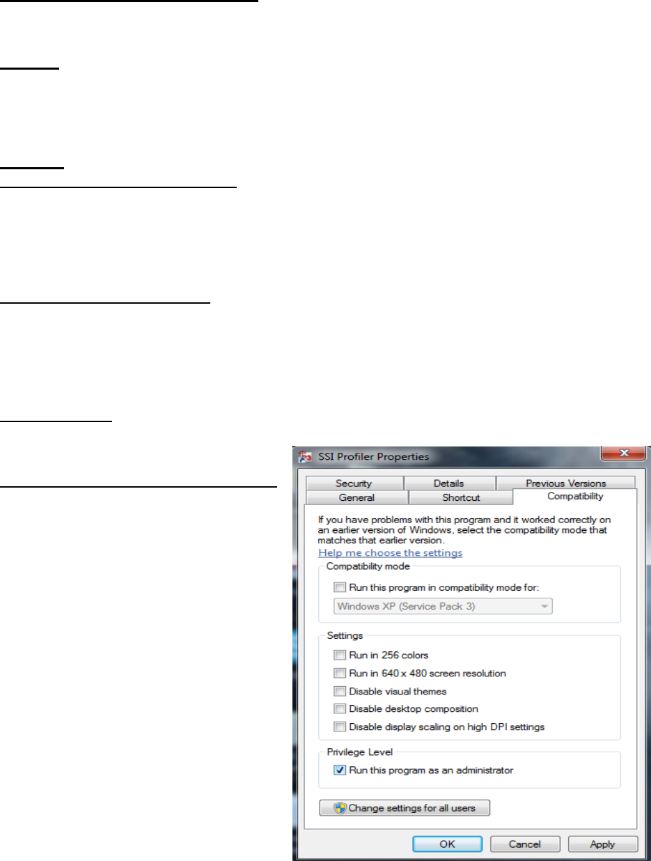
Run as Administrator (Windows 7)
Front arm laser models with ethernet
connection require Profiler to be run as
Administrator. Go to the Desktop, right
click on the SSI Profiler icon and select the
“Compatibility” tab. At the bottom of the
window under “Privilege Level”, select the
check box for “Run this program as an
administrator.”
Figure 1: Compatibility window for
running Profiler software as an
administrator in Windows 7.
2
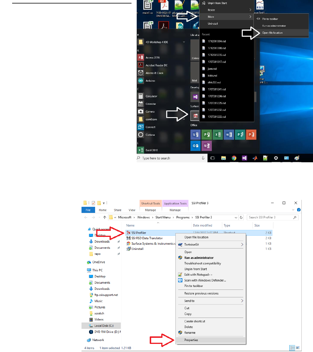
Run as Administrator (Windows 10)
Front arm laser models with ethernet
connection require Profiler to be run as
Administrator.
Right click on the Profiler V3 icon ‘P3’, go to
More>Open File Location.
Right click on SSI
Profiler shortcut, go to
properties
Figure 2: Searching for Profiler
V3 program file.
Figure 3: Selecting ‘Properties’
from drop down menu.
3
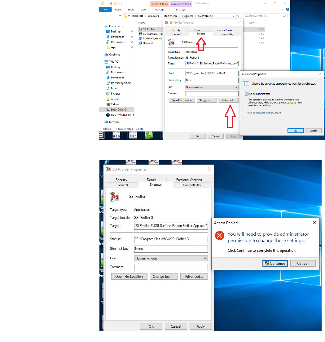
In Shortcut tab go to
Advanced... Check ‘Run as
Administrator’ and then ‘ok’.
Click ‘Continue’, in Access
Denied window for Profiler to
run as Administrator every
time opened.
Figure 4: Check ‘Run as
Administrator’ in the Short Cut tab.
Figure 5: Click ‘OK’ and
‘Continue’ to confirm and run
Profiler as Administrator.
4
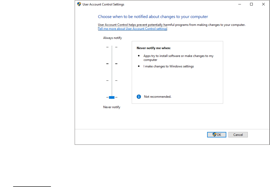
After setting Profiler
V3 to run as
Administrator, a
popup with appear
every time you open
the program. To get
rid of the popup
search "user account
control" and set to
"never notify" (this is
Optional)
Note: The settings.xml file goes in C:\Users\SSI PROFILER\AppData\Roaming\SSI\SSI.Surface.Roads.UDP.LaserRec
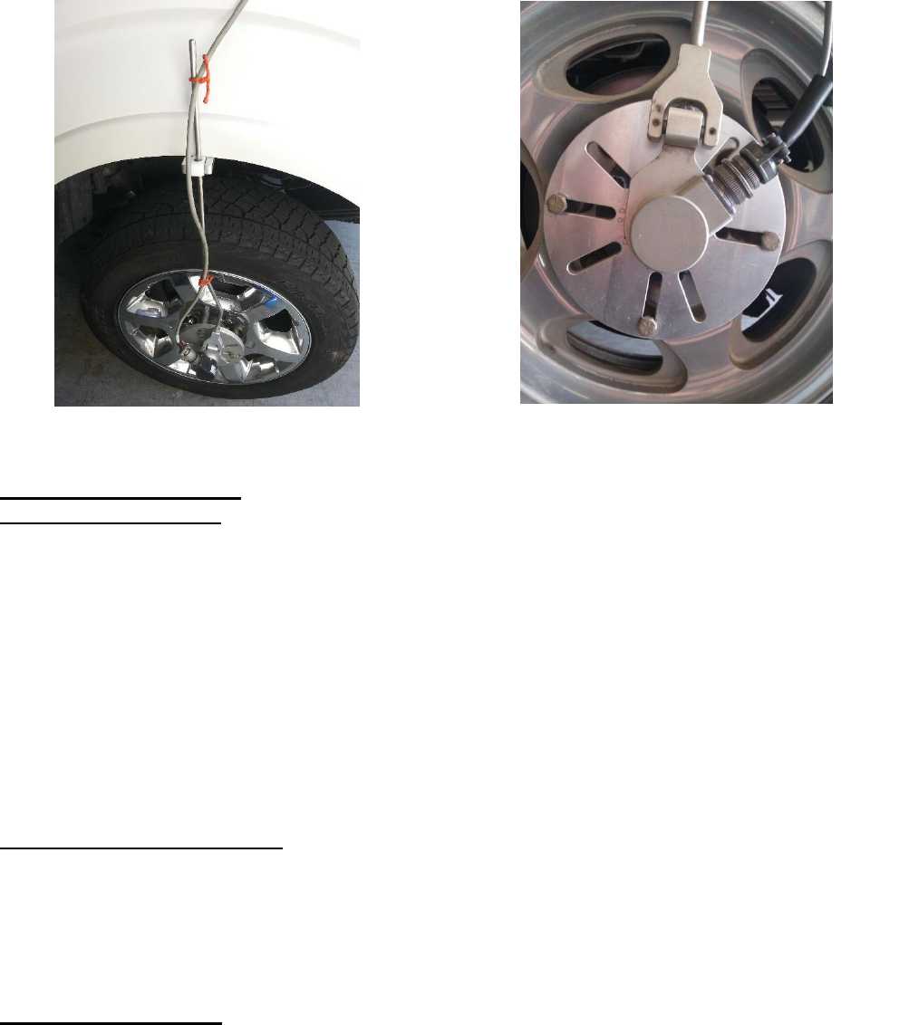
DMI Assembly
The installation of the DMI encoder assembly to the vehicle rim is the initial step of distance
calibrations. If the vehicle is a Polaris 570 the DMI may be embedded and does not require
assembly. Install the supplied collets onto the lug nuts of the vehicle. The collet assembly includes
the collet, the housing and a machined bolt with both male and female ends. Space the collets
depending on the number of lug nuts. For a six-lug wheel, use three collets in an approximately
equilateral triangle formation. For an eight-lug wheel, use a square collet formation. There are
machined numbers on the internal ring of the DMI disk to determine to correct placement and
number of collets. The design of the DMI forces the collets to center themselves if the collets are
in the correct position. If the DMI is installed off-center, the vertical movement of the position
pole will be large. The wire harness for the encoder can be tied to the vertical position pole to avoid
damage from tangling with the vehicle. Keep slack in the wire at the top of the pole using gear ties
or zip ties so there will be no tension on the wire. To install the position pole correctly, insert the
pole into the delrin guide attached to the vehicle body before attaching the DMI disk to the lug
extenders.
Figure 6: Window for
disactivating notification of
changes to computer.
5
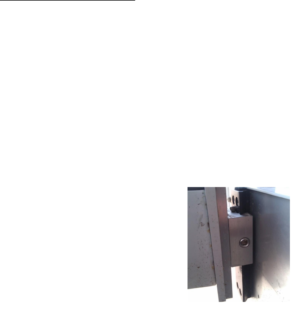
Main Electronics Housing
CS9300 Bumper Mount
The main housing for the 9300 systems is mounted to the hitch receiver. The 9300 hitch receiver
is bolted to the back plate of the housing. The height of the profiling system can be adjusted through
the machined slots on the hitch receiver. The laser heights can be changed by adjusting the
dovetails mounted on the laser plates by loosening the ½ inch set screw with a ¼ inch allen wrench.
The receiver hitch bolt is used to secure the system to the vehicle along with the supplied receiver
tube brackets. The thicker end of each bracket is bolted against the white receiver tube. Always
use both brackets and the receiver bolt to mount the profiling system. If the brackets are mounted
backwards, the face of the brackets will not be parallel to the walls of the vehicle’s hitch receiver.
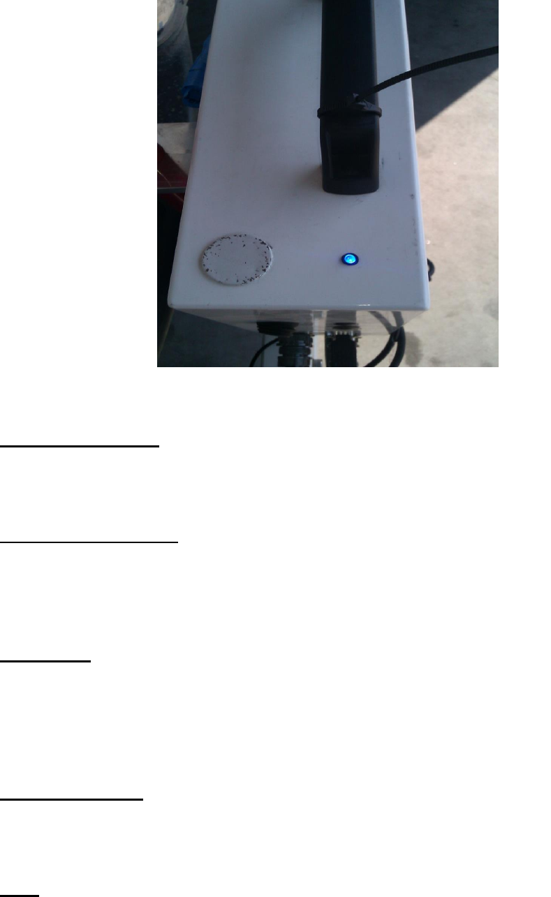
Power to the main housing is supplied by the seven pin connection through the trailer wiring. To
determine if power is reaching the profiling system, check the LED at the top of the housing. The
LED will illuminate when power is being supplied.
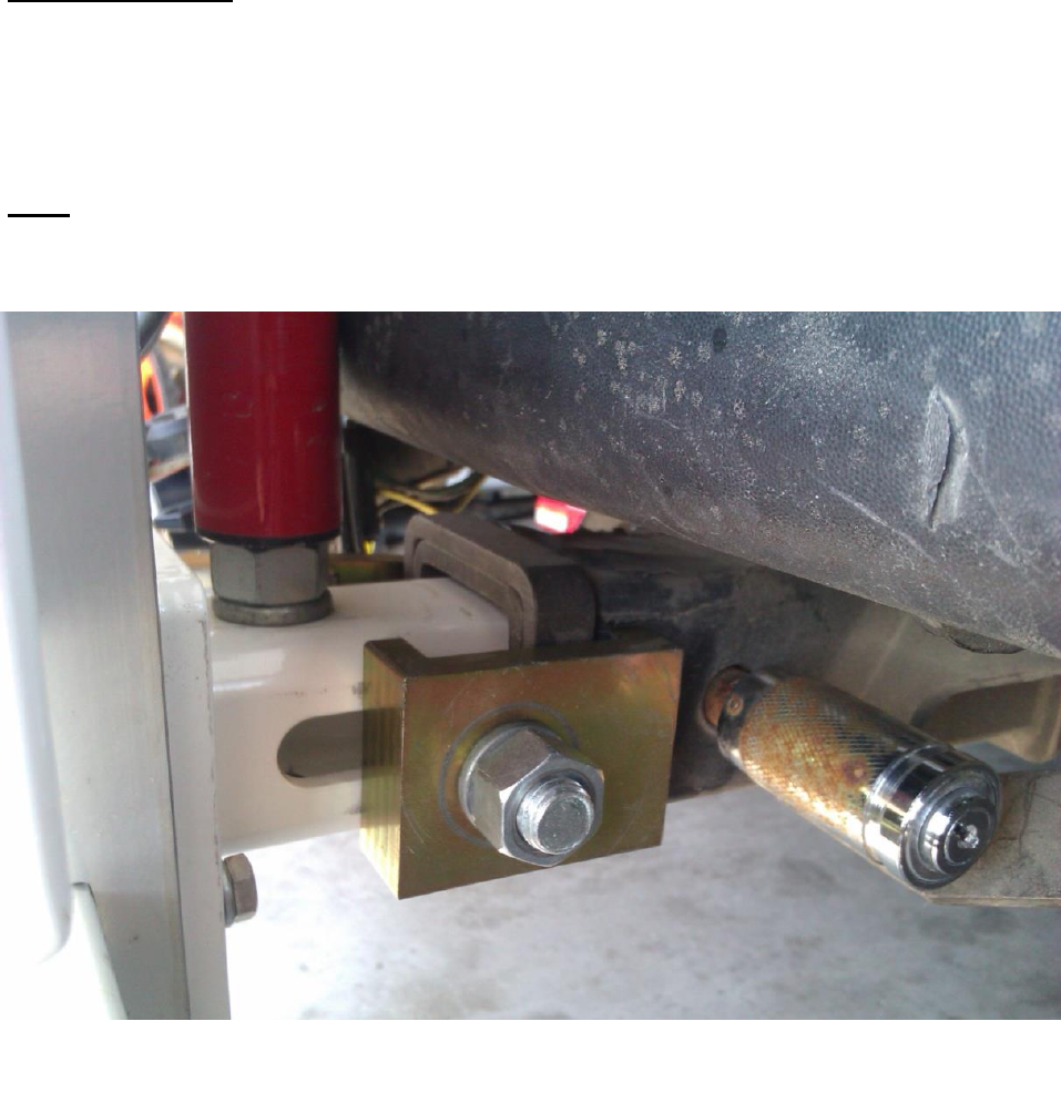
CS9300 Hitch Receiver Mount
The hitch receiver tube is connected to the vehicle using the hardware supplied with the system.
There will be four 5/16”-24 bolts supplied with the system that mount the receiver tube to the
aluminum back plate. The supplied bolts and bracket for the hitch receiver are oriented so that the
thicker end of the brackets are in contact with the profiler’s male end of the receiver tube. This
assembly can be seen in Figure .
Front Mount Hardware
When the system is mounted to the front of the vehicle by the tow-hook mounting tubes, there are
six bolts supporting the system; four 5/16”-24 bolts (1/2” wrench) and 2 U-bolts at the ends (9/16”
wrench). The U-bolts are paired with the plastic sleeves. Make sure that the system is as level as
possible when attaching the U-bolt supports.
Figure 7: The DMI pole and receiver
Figure 8: The DMI wheel attached to an 8-lug
vehicle with a 4-lug extender configuration.
6
CS9100 Mid Mount
The main electronics housing is mounted under the back seat for the CS9100 mid-mount profiling
systems. The laser heights can be changed by adjusting the dovetails mounted on the laser plates
by loosening the ½ inch set screw with a ¼ inch allen wrench. Power to the housing is supplied by
a 12V DC cigarette lighter plug. When power is reaching the housing the blue LED will be
illuminated.
Note: Connect the Amphenol harnesses to the housing without torsion being applied to the wire.
Turning the entire harness instead of the threaded connector will break off the soldered wires
within the harness.
Figure 9: The hitch receiver mount with lock brackets.
7
Connecting Hardware
During assembly, connect the serial cable coming out if the pelican case or the white housing (6
pin amphenol) to the computer’s DB-9 serial port. Once the program is opened and Collect is
selected the software will search for hardware.
Disconnecting Hardware
If the hardware, lasers, GPS, and DMI do not need to be used while the system is connected
through the serial port then the operator may use the Hardware Disconnect button at the bottom
right of the collection screen. To reconnect the hardware again, select Collect and the software will
search for hardware.
GPS Setup
Models with high resolution GPS for survey and cross slope applications may have additional
steps to set up GPS. For all internal GPS receivers built into the SSI electronics the operator will
use the USB cable to send commands. Otherwise, the commands will be sent through a serial or
USB cable directly connected to the GPS receiver. If the receiver is powered on and connected
with no signal, the SSI Profiler program wil display “No GPS Signal.”
9350 Survey System
The survey consists of three key components: base station receiver with tripod, pole with receiver
and the rover or embedded GPS board. The base station is the main transmission point. It receives
static GPS points for corrected GPS. The position of the profiling system is referenced off of the
base station to determine the corrected GPS coordinates.
Note: The base station in not needed for profile smoothness data. It is used only to receive
corrected GPS for survey data.
Figure 10: The LED power indicator

8
The GPS pole is secured by threading the pole to the bracket mounted to the backside of the white
housing. The cable from the antenna receiver is connected to the rover or SSI electronics box. If
no GPS signal is found, make sure the baud rate for the GPS receiver is matching the SSI
electronics at a rate of 9600, 38400 or 115200. This can be changed in the GPS manufacturer
software. For more assistance contact SSI Support.
Novatel GPS Setup
The Novatel GPS receivers used on the CS7900 and most high and mid-resolution GPS options
have multiple platforms for programming. Contact SSI if you are unsure which system you have
and the electronic limitations. Novatel systems can be mounted as stand-alone receivers, embedded
inside the SSI electronics or mounted in a self-contained Pelican case as in the CS7900. If the
receiver is embedded within the SSI electronics housing do not attempt to open the electronics or
program the board. Contact SSI for a technician assist. All external receivers (Flex2, Flex6 and
Span-CPT) can be programmed through a USB or direct cable.
Inertial Systems With Novatel External GPS Receiver
These systems run at 10Hz with a GPGGA string through the serial port on the outside of the White
SSI housing. If needed to reprogram the receiver enter the following commands in Putty or Novatel
Connect. You should see an “OK” after each command is entered.
1) unlogall
2) com com1 38400 n 8 1 n off on
3) log com1 gpgga ontime 0.1
4) saveconfig
Note: Newer systems with the latest firmware have a baudrate of 9600. Note the baud rate in which
you connected to the receiver and use the same number.
CS9300 Bumper Mount GPS Setup
Measurements must be taken to set up the GPS in order to accurately pinpoint the defects detected
by the inertial system. For this process a tape measure is required. There is only a need to re-
measure when the system changes dimensions or changing the vehicle host. A new dimension is
mainly from a change in the length of the arms from disassembling the system for storage. The
measurements are from the left laser (track 1) to the center laser (track 3), from the track 1 laser to
the track 2 laser, and the elevation measurement. The elevation measurement is the distance from
the bottom of the center laser (track 3) to the top of the GPS pole. The top of the GPS pole does
not include the antenna and is only to the end of the cylindrical pole.
The “GPS Distance Forward” is the distance from the center laser to the GPS antenna going from
back to front of the vehicle for rear mounted systems (it is a positive value when the GPS antenna
is closer to the front of the vehicle than the laser). For front mounted systems, this measurement is
from front to back of the vehicle (it is a positive value when the GPS antenna is closer to the
vehicle’s body than the laser).
Trimble 5kHz GPS
The Trimble GPS system is fully integrated to the profiler system. The coordinates will be found
when the collection program is initiated as long as the GPS antenna is not obstructed. The GPS
9
coordinates will be shown in the Main Collection Window beneath the status bar. Details about the
GPS system and the coordinates of the system can be viewed by selecting the GPS Details icon.
The electronics is searching for GPS signal when the GPS status bar displays, “No GPS Signal.”
Arm Adjustment and Laser Placement
The arms or dovetails of the profiling system can be used to move the lasers over the tracks that
need to be profiled. To adjust the arm length on the CS9300 and CS9350, all three brackets must
be loosened, a total of four bolts. If the profiling system has three lasers, the center laser is mounted
in front of the center 2 bolts. To adjust the arms, the center laser must be removed so that the two
bolts at the center of the system can be accessed. The laser heights (vertical distance to the ground)
can be adjusted through the receiver tube plate or the dovetails mounted to the laser plates. The
dovetails are secured by tightening the 1/2“set-screw which acts on nylon bushings to compress
the dovetail pair together.
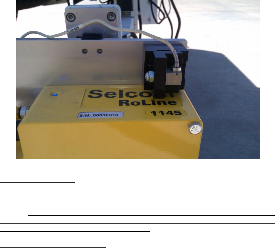
High standoff spot lasers (Selcom SLS5000 325/400) have a recommended height of 15 inches
above the ground. The range is plus or minus four inches of the recommended height (±4 inches).
The Selcom RoLine 1145, LMI Gocator 2342, and the Selcom low standoff (Selcom SLS5000
200/300) lasers have a recommended height of 11 inches above the ground. This is the reason the
RoLine three laser systems use a low standoff spot laser in the center track (Track 3). The minimum
height above the ground is 200mm or 7.8 inches. The height range is between 7.8 and 15 inches.
Gocator 2375 high standoff infrared lasers should be mounted 26 to 78 inches above the ground.
Be aware of the minimum laser range when performing the height verification. Always place
the lasers at the correct height. Be aware of your systems laser type if you fail the height
verification. The operator can view the laser type when System Settings is selected.
Even if the laser configuration is set to auto detect, review the
laser type under system settings to confirm its accuracy. The
laser type can be reviewed under the Collect Window, after
selecting the System Settings icon.
To adjust the height of the lasers, loosen the set screw in the center
of the female dovetail with a ¼ inch allen wrench. The set screw
does not need to be completely removed. When tightening the set
screw, do not over-tighten. The nylon bushing can be damaged
when excessive force is used. Tighten the set screw so that the
laser plate cannot slide vertically when pulled.
For the CS9100 Mid-mount systems the operator must slide the
horizontal dovetail outside the truck body to install the vertical
dovetail and laser plate assembly. The horizontal and vertical
dovetails of the mid mount assembly can be adjusted by loosening
the set screw with a ¼ inch allen wrench. Set the laser height and
spacing with this method. Only tighten the set screw so that the
dovetails cannot move when firmly pushed.
Figure 11: The vertical dovetail and laser
plate assembly
10
Calibration
Distance Calibration
A precise distance calibration is crucial to collecting accurate
surface profiles. The distance calibration is traditionally performed
on a tenth of a mile track (528 feet or 160 meters). The key
component of the distance calibration is the DMI assembly and
encoder. Prior to calibrating, measure a tenth of a mile track over
an ideally straight, flat and clean area. Open the distance calibration
within Profiler V3 and line the lasers on the starting line of the
calibration track. Follow the calibration instructions to complete the
distance calibration.
It may be necessary to perform multiple distance calibrations within
a day of profiling. As temperature changes the air pressure within
the tire also changes, modifying the wheel circumference.
Whenever this happens, the collected data will become further and
further from the actual distance depending on the temperature
gradient and the distance traveled. If the distance seems to be
deviating from the actual stationing, take the time to recalibrate.
Always calibrate on a straight 0.1 mile section of pavement at the
speed you will be collecting.
Distance Calibration with the Electric Eye
If an encoder distance calibration is selected, a traditional
distance calibration, not an electric eye calibration, will be
performed.
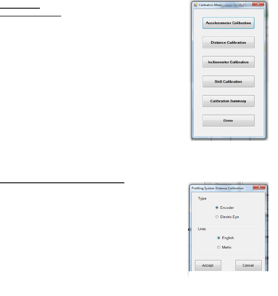
Distance calibrations can be completed quickly and efficiently by
using the electric eye (EE) to mark the beginning and end of the
calibration length. This feature requires two points with DOT-C2
compatible reflective tape in range of the electric eye sensors.
These two points should be at least 528 feet apart, or another
distance given by the resident engineer. It is important that the two
reflective tape stations are at accurate positions for the calibration
track.
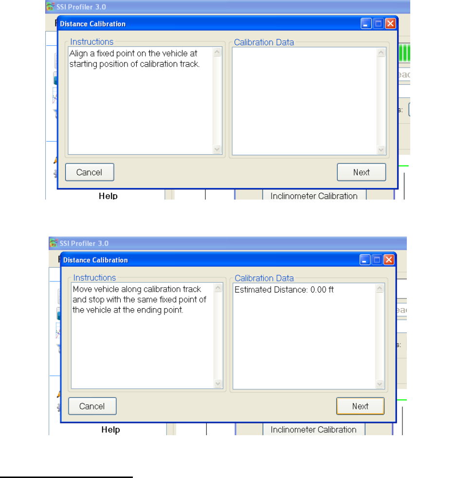
To begin the calibration, follow the message prompts in the
instruction window. Select “Next” and drive past the start position
electric eye to begin the calibration. After the EE begins the
calibration, an estimated distance will be shown (do not be alarmed
if the distance is way off from the actual distance). Near the final reflective tape location, arm the
EE by selecting “Next” again. The calibration will finish when the EE is triggered. The user will
then be prompted to enter the actual distance traveled.
Averaging the counts with previous calibration is a way to reduce error. The average of two
correctly calibrated runs will be more accurate than a single calibration run. Even so, this feature
is not required since one accurate calibration will work for the distance calibration. When the
information is entered the distance calibration may be started. Select accept to end the distance
calibration.
Figure 13: The options for the
distance calibration
Figure 12: The Calibration
Menu
11
Accelerometer Calibration
The accelerometers are an important component of the inertial profiling system. They are used to
determine the vehicle chassis’ vertical motion. The vehicle’s vertical motion is then subtracted
from the laser readings to determine the profile of the surface (integrating this data with the
distance encoder readings). It is important that the accelerometers are calibrated properly and their
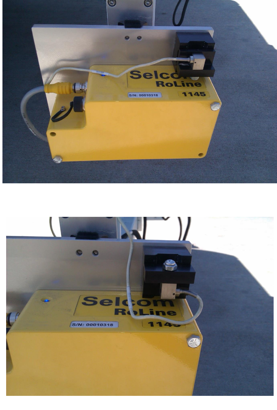
position on the profiler is constant and correct. The accelerometers should always be in the upright
position except during calibration (Accelerometer is upright when the arrow etched in the
accelerometer on the opposite side of the wire is point up). If the accelerometer is oriented in any
other way the data will be incorrect. Be aware of any vibration in the laser or accelerometer
hardware. Vibration will cause anomalies in the data.
Figure 14: The first step towards a distance calibration
Figure 15: To end the calibration, align the lasers (or other fixed point) on the end line
12
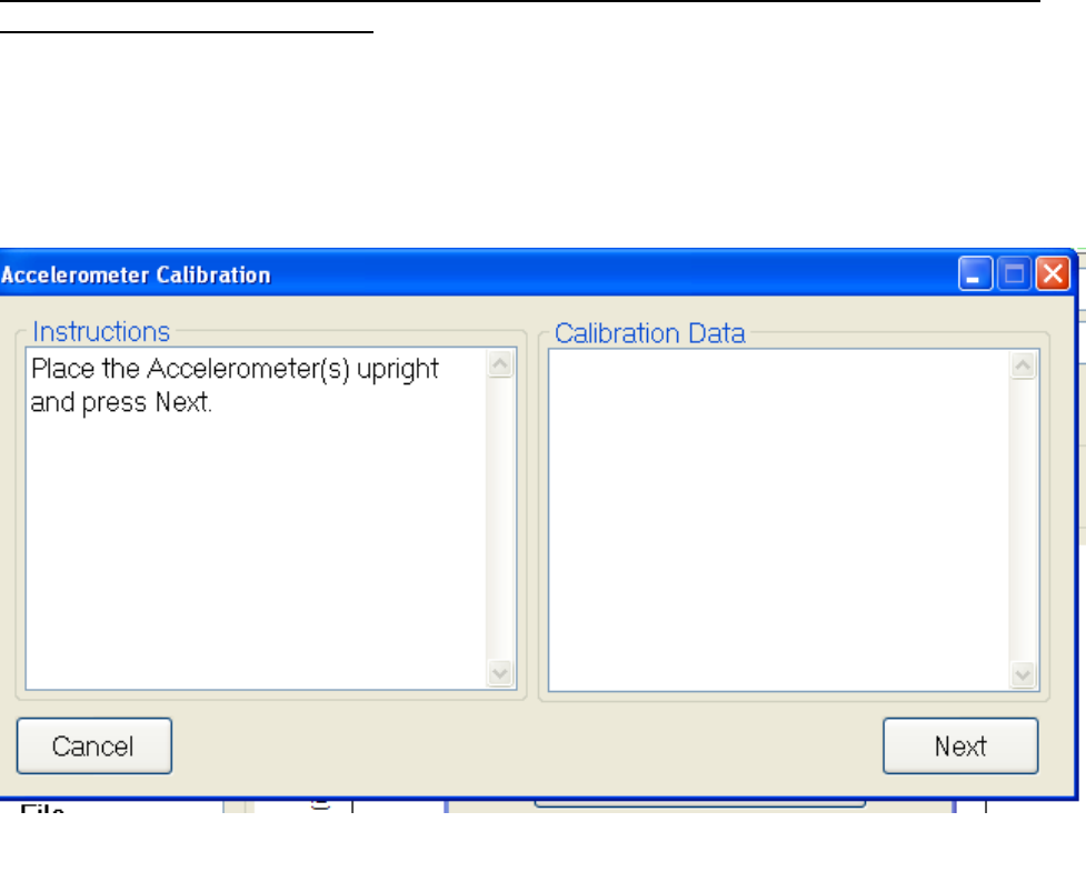
Note: Both accelerometers are calibrated at the same time. Make sure the vehicle is off (no
vibration) and on a level surface. To calibrate the accelerometers start with both in the upright
position (they should already be in this position). Follow the instructions on the computer screen
to complete the calibration. The accelerometers will be rotated from upright, to upside down, to
on their side and finally returning upright again to complete the calibration.
When placing the accelerometer on its side during calibration, the wire may face either up or
down.
Calibrate all of the accelerometers at the same time. The calibration is to begin with the
accelerometers in the upright position. This is the normal functioning position, the position the
accelerometers should be in during collections.
Figure 16: The first step of the accelerometer collection
13
Figure 18: The accelerometer upside down
Figure 17: The upright accelerometer position
14
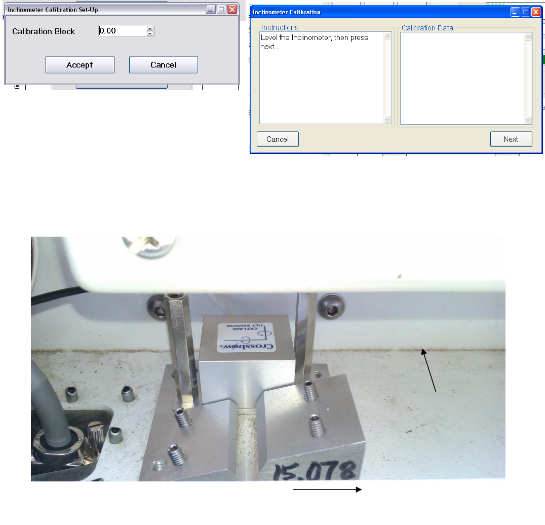
Inclinometer Calibration (If Equipped)
The inclinometer is used to calculate the cross slope of the profiled surfaces. All of the survey
systems are equipped with some type of incline measurement device. The inclinometer is located
under the grey electronics box inside the white housing or is embedded within the electronics
housing. For the inclinometer mounted under the white housing, the lead wire of the
inclinometer is always pointed in the direction of forward travel for the vehicle. The high side
of the angled block always faces the passenger side.
Dual Axis Inclinometer Calibration
The initial step is to level the white housing when it is mounted on the front or back of the truck
(or level the entire truck if the inclinometer is mounted to the truck body like on the mid-mount
system). For survey systems, set the straight-edge below each of the lasers and use the bolts to
level the bar. Set the inclinometer on the flat block while the entire system is level. When
prompted, enter the step block’s unique angle. Follow the on screen instructions and move the
inclinometer to the angled block (having the wire face the same direction of forward travel). Then
remove the inclinometer and replace on the flat plate when prompted. Never move the vehicle
while calibrating the inclinometer. Once the inclinometer is calibrated correctly, secure the
inclinometer to the flat plate with the thumb screws.
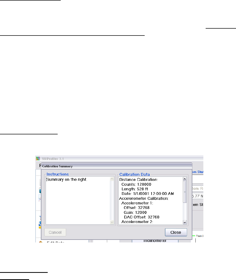
The entire system must be level during an inclinometer calibration. For bumper-mount systems
the white housing must be level. If the inclinometer is mounted to the truck chassis, the entire truck
must be level. For three laser systems the level straightedge is required. This level straight-edge
is used to notify the system what the lasers see as a level surface. This information can be used
with the inclinometer information to calculate the differences on slope for the profile data. The
level straightedge is not needed for the dual or single laser systems.
Figure 19: The accelerometer on its side
15
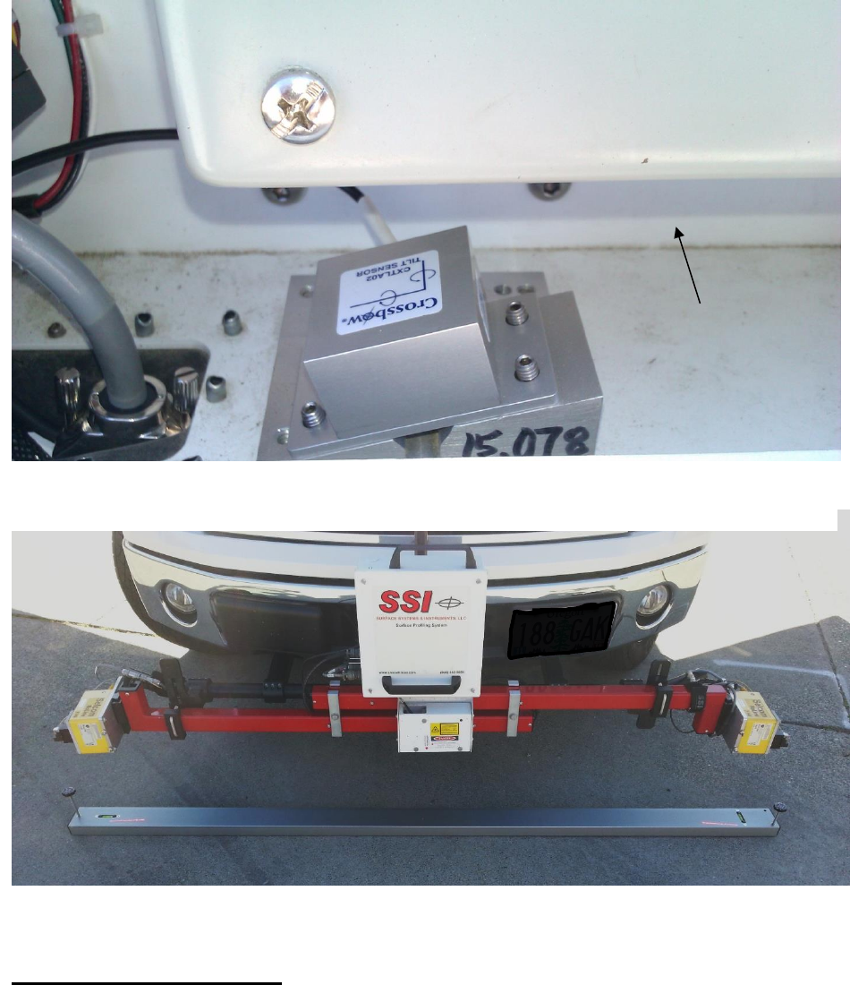
At all times the high side of the angled calibration plate faces the passenger side and the wire
of the inclinometer faces the direction of forward travel of the vehicle.
The housing and the surface the lasers act on must be level. Use the straight edge with the bubble
levels and bolts to level the surface the lasers act on.
Figure 21: The inclinometer must be level before
starting the calibration
Figure 22: The inclinometer on the flat
plate for a rear-mount.
Passenger Side
High side of angled plate faces towards passenger side for rear
bumper mount systems
Figure 20: Window to Enter Inclinometer Angle
Traffic
Direction
16
IMU Cross-Slope Calibration
The embedded IMU sensors are the high-resolution solution to measure cross-slope. All of the
IMU sensors are controlled by the SSI UDP collector; a variant of the SSI Profiler program.
When calibrating the IMU the first step is to align it with the satellites so the UDP collector
displays, “Solution Good” with a low standard deviation. Once aligned the IMU must be leveled.
This can be adjusted by getting close to zero on the UDP collector roll value and turning the tires
of the vehicle. Once the IMU’s roll value is rapidly changing between negative and positive,
place and level a bar under all lasers. This is the level reference for the system. At this point you
may run through the SSI calibration program under the calibration menu.
Figure 23: The inclinometer on the angled plate for a rear-mounted system
Figure 24: A three laser system with a level straightedge for inclinometer
Traffic
Direction
17
Transverse Calibration
The transverse calibration sets the Gocator 2375 transverse lasers at the correct offsets to
measure a level line. This calibration is required only when the supporting hardware is
changed or adjusted. This calibration shall be completed on a flat, level floor or long, flat and
level straightedge. The laser beam can be found by using an infrared card indicator. Do not look
into the laser emitter at any time when the system is on. Level the truck and IMU (if
applicable). The calibration will first level all of the lasers through the calibration menu. Follow
the prompts on the screen and verify that the post-calibration graph is acceptable within
tolerance.
A secondary calibration within the Gocator browser window may need to be completed if the
lasers are moved or the frame and mounting position is adjusted laterally. The lateral calibration
starts at an arbitrary number like 7000 for the X-axis value of the Gocator measurement output.
From the browser window, the two adjacent lasers are turned on and an object is placed between
the laser within the overlapping beams. The laser reading are fixed for the left laser, but the right
value is adjusted until the objects coordinates match between the two lasers. Save all changes
within the browser window. The Gocator IP address will be specific to the laser position and will
be with your profiler documents.
Calibration Summary
The current calibrations for the inclinometer, accelerometers, and distance encoder can be viewed
be selecting the Calibration Summary icon under the Calibration Menu.
System Settings
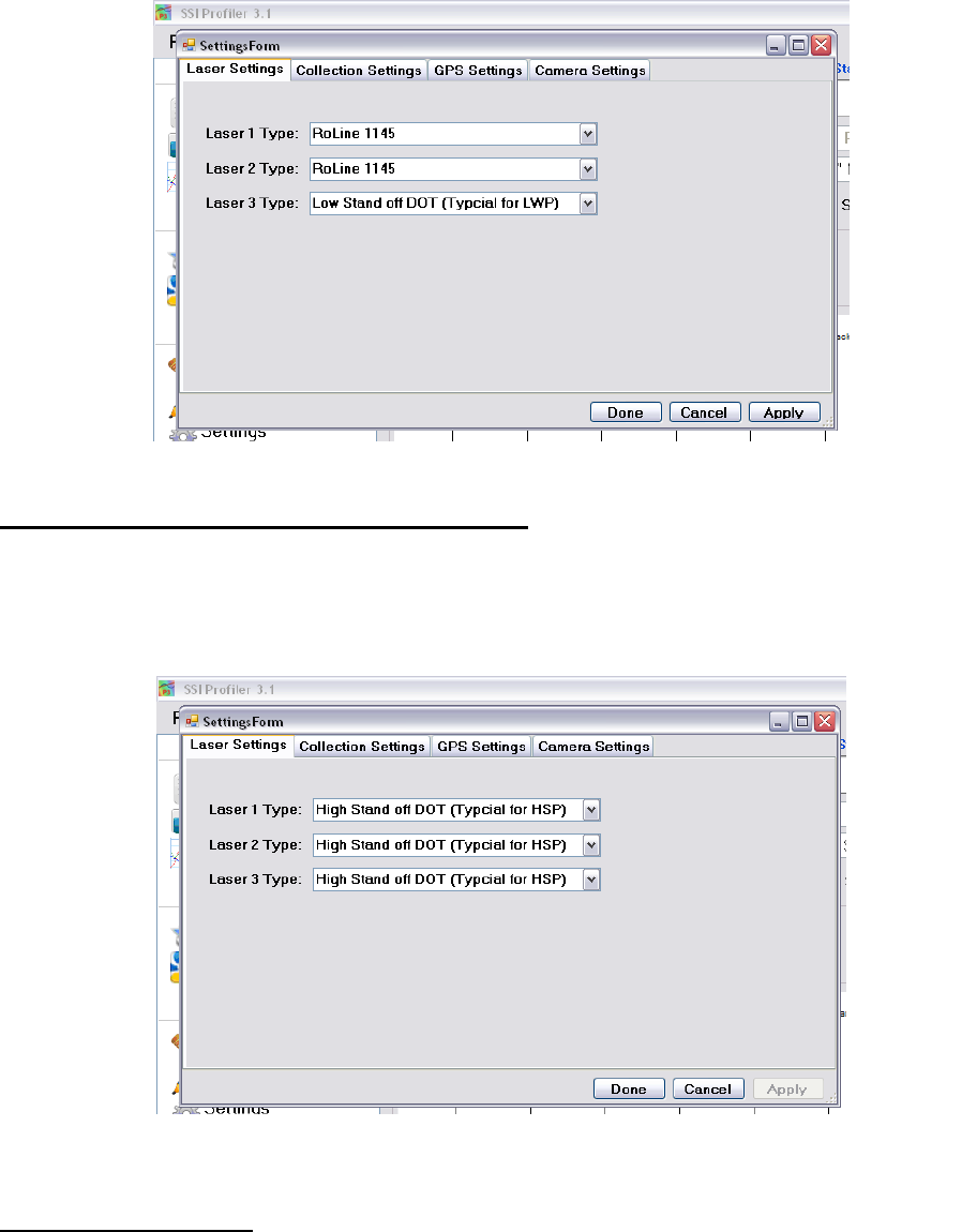
Laser Type
The laser type must be chosen within the System Settings. The choices are: Gocator/RoLine 1145,
High Standoff Sport Lasers (Selcom SLS5000 325/400) and Low Standoff Lasers (Selcom
SLS5000 200/300). If the system in your possession is a RoLine/Gocator three laser system, the
center laser is a Low Standoff Spot Laser. If the laser type is saved incorrectly, the laser height
verification will be inaccurate. If the laser height verification ever fails, review the laser type.
Figure 25: The Calibration Summary
18
It is very important that the laser type is correct. Incorrect laser settings will cause inaccurate
profiles and surveys. The inclinometer calibration will receive an error when the lasers are
incorrectly set. The error will state that the laser heights differ more than 1.5 inches. Completing
a height verification also determines the problem, which is resolved by changing the laser type to
match the actual lasers.
Collection Settings Tab
Simulated Travel is for troubleshooting and bounce tests. Simulated travel sends the system
through a simulated profile collection without moving. Laser data is still collected, but real
distance is not recorded. The sampling interval is the distance between measurements of the
simulated travel option.
Figure 26: The laser type window for a Survey 3-Laser system
Figure 27: The HSP dot laser system laser options window
19
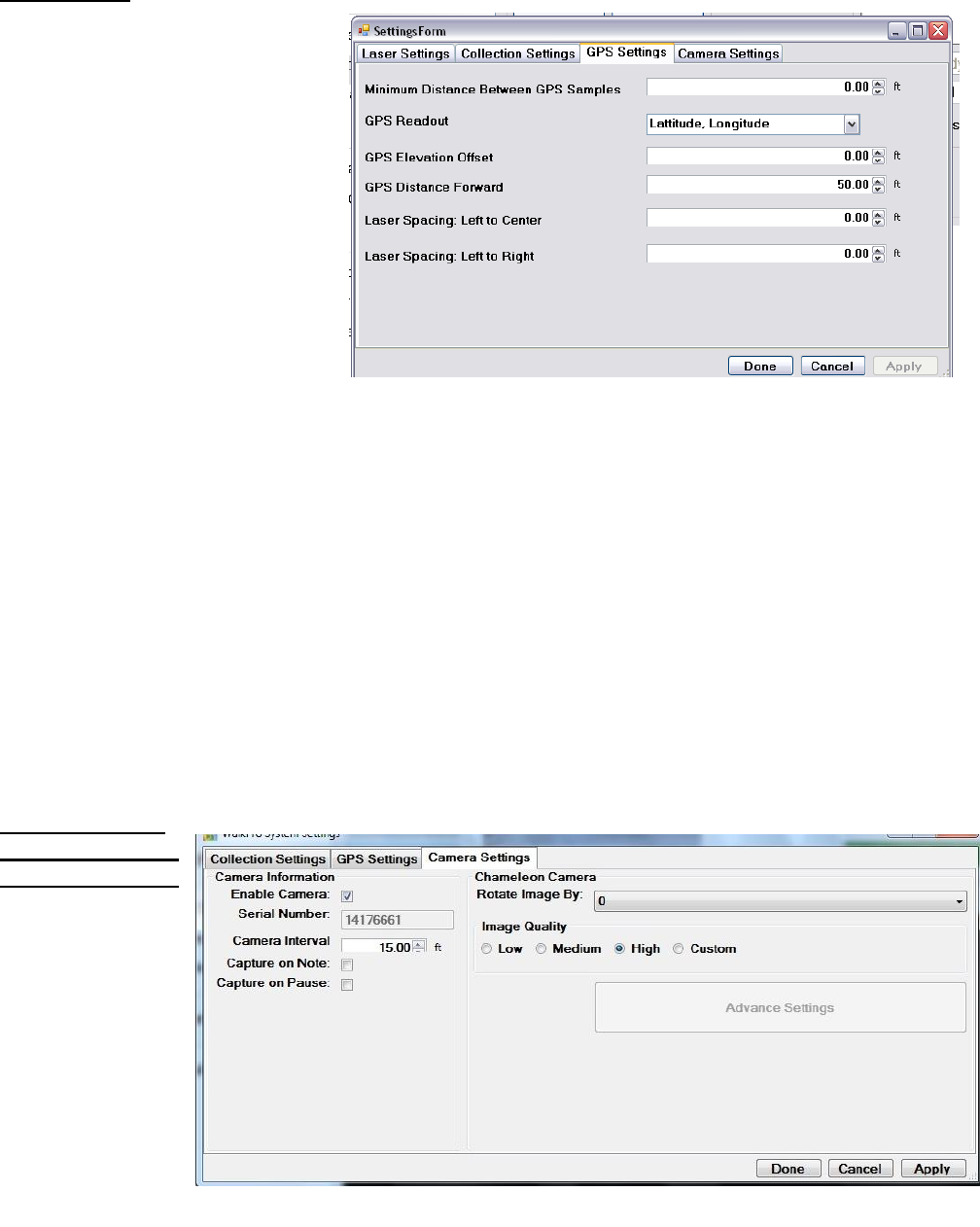
GPS Settings
The distance adjustments to make
more accurate GPS data is found
under this tab. Measurements must
be taken to set up the GPS to
accurately pinpoint the defects that
the system detects. For this process
a tape measure is needed. There is
only a need to do this measurement
when the system changes
dimensions. A new dimension is
mainly from a change in the length
of the arms from disassembling the
system for storage. The
measurements are from the left
laser (track 1) to the center laser,
from the center of the track 1 laser
to the center of the track 2 laser and the elevation measurement. The elevation measurement is the
distance from the bottom of the center laser (track 3) box to GPS antenna.
The “GPS Distance Forward” is the distance measurement from the middle laser to the GPS
antenna going from back to front of the vehicle for rear mounted systems (it is a positive value
when the GPS antenna is closer to the bumper of the vehicle than the laser). For front mounted
systems, this measurement is from front to back of the vehicle (it is a positive value when the GPS
antenna is closer to the vehicle’s body than the laser).
The distance between GPS sample should be left to the default value to collect the most accurate
data. The default value in Profiler V3 is zero feet or meters. The GPS readout changes the GPS
string in the collect window, not the GPS string within the reports.
Camera Settings
How to Begin
Using the Camera
Install the
Flycap2Viewer
driver located on
the disk supplied
by SSI (or already
installed on the
computer). The
correct driver
depends on if the
computer is 32 or
64 bit. To check
this, open the start
menu and right click
Figure 28: GPS Settings
Figure 29: Camera Settings
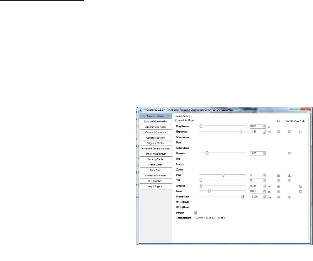
20
on My Computer (or My PC) and choose ‘Properties’. On this window find the System Type and
view if the system is 32 or 64 bit. If the computer is 32-bit, install the x86 flycap2viewer. If the
system is 64-bit, install the x64 flycap2viewer. Once the driver is installed, plug in the Chameleon
Camera to the computer’s USB port. The computer will sound two pings and install the driver
software for the camera. Once finished, a notification window will appear at the bottom right of
the screen saying the Chameleon camera is connected. Now the camera can be enabled in the
Profiler V3 program.
Enabling Camera Settings
Once the profiling system is connected and the Collect tab is open, the operator can enable the
camera. At this time make sure the flycap2viewer driver is installed and the camera is connected.
Open the collect window and once the hardware is found, select System Settings. Under the system
settings window, select the Camera Settings tab. To enable the camera feature select the check box
under the Camera Settings Tab. The camera interval is the distance traveled between each picture.
This can be set to any interval however, the more pictures taken results in more data saved to the
file and more time that post-processing will take. If the camera is not mounted upright, enter the
correct rotation angle in degrees, selecting one of the four options. The camera is focused on the
physical lens. Enter the serial number of the camera which is on the sticker on the back panel of
the camera. Once apply is selected the camera will be found in under one minute for the first use.
Once the settings are saved, the serial number will fade out, as seen below.
If the camera image preview is not in color:
Under Collect Window > System Settings >
Advanced Camera Settings > Standard
Video Mode, select the button for the
resolution and pixel type to be Y8 and 1280
x 960. The frame rate should be at 15 Hz.
This will make the camera take color
pictures (as seen in the preview window
also). Also make sure that the pixel type is
Raw 8 and the mode is ‘0’ under the custom
video modes tab.
The image preview should appear in the
Collect window in color and at the correct
orientation. If not, change the settings to the
appropriate orientation or open the
Advanced Settings.
To reduce the size of the image, change the
resolution of the camera to 640x480. This will decrease the processing time and RSD file size.
Under Custom Video Modes the operator can adjust the resolution and see the estimate of the file
size.
Figure 30: Advanced Settings for the Chameleon Camera
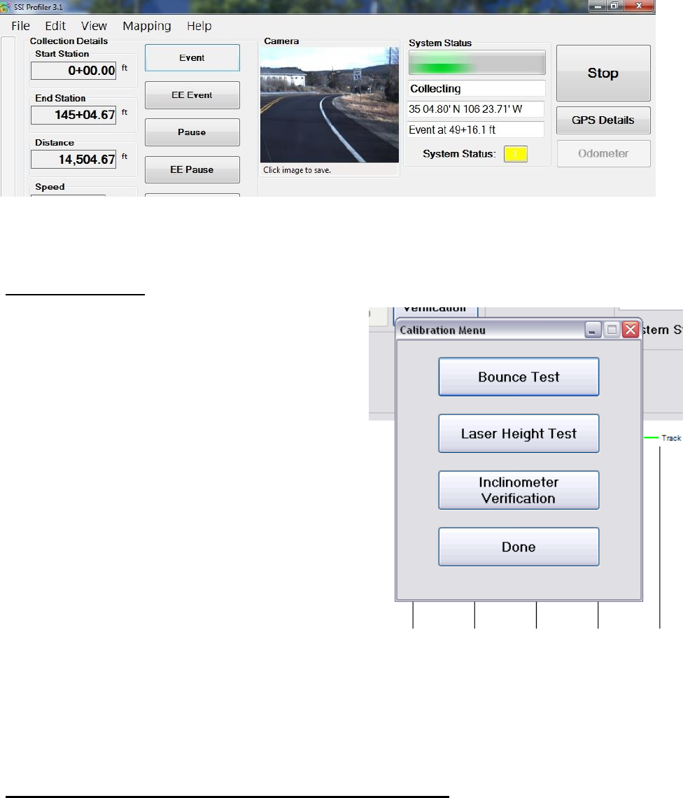
21
System Verification
The system verifications of the Profiler program are
the bounce test and the height verification. The
bounce test checks the validity of the accelerometer
calibration and the correct laser type. Depending on
the values of the static and dynamic bounce tests, the
health of the system can be determined. The height
verification is used to diagnose potential problems
with the lasers and the cables. The verification will
show if the lasers are connected incorrectly, or if the
heights the lasers are set to outside of the
recommended range. Another potential problem is
the settings have the wrong laser type saved for the
current system (e.g. Spot lasers saved instead of line
lasers on a line laser system). The line lasers (Selcom
1145, Gocator 2342) should be 12 inches above the
ground surface and their laser difference for the
height verification should be less than one
hundredths (0.01) of an inch. The dot lasers (Selcom
SLS5000 325/400) should be 15 inches above the
ground surface and have a measurement error of less
than one hundredths (0.01) of an inch.
If the laser type is saved incorrectly, the laser height verification will be inaccurate. If the laser
height verification ever fails, review the laser type.
Note: These procedures are not calibrations, only verifications
Figure 32: System Verification Menu
Figure 31: Camera Preview window in Collect Screen
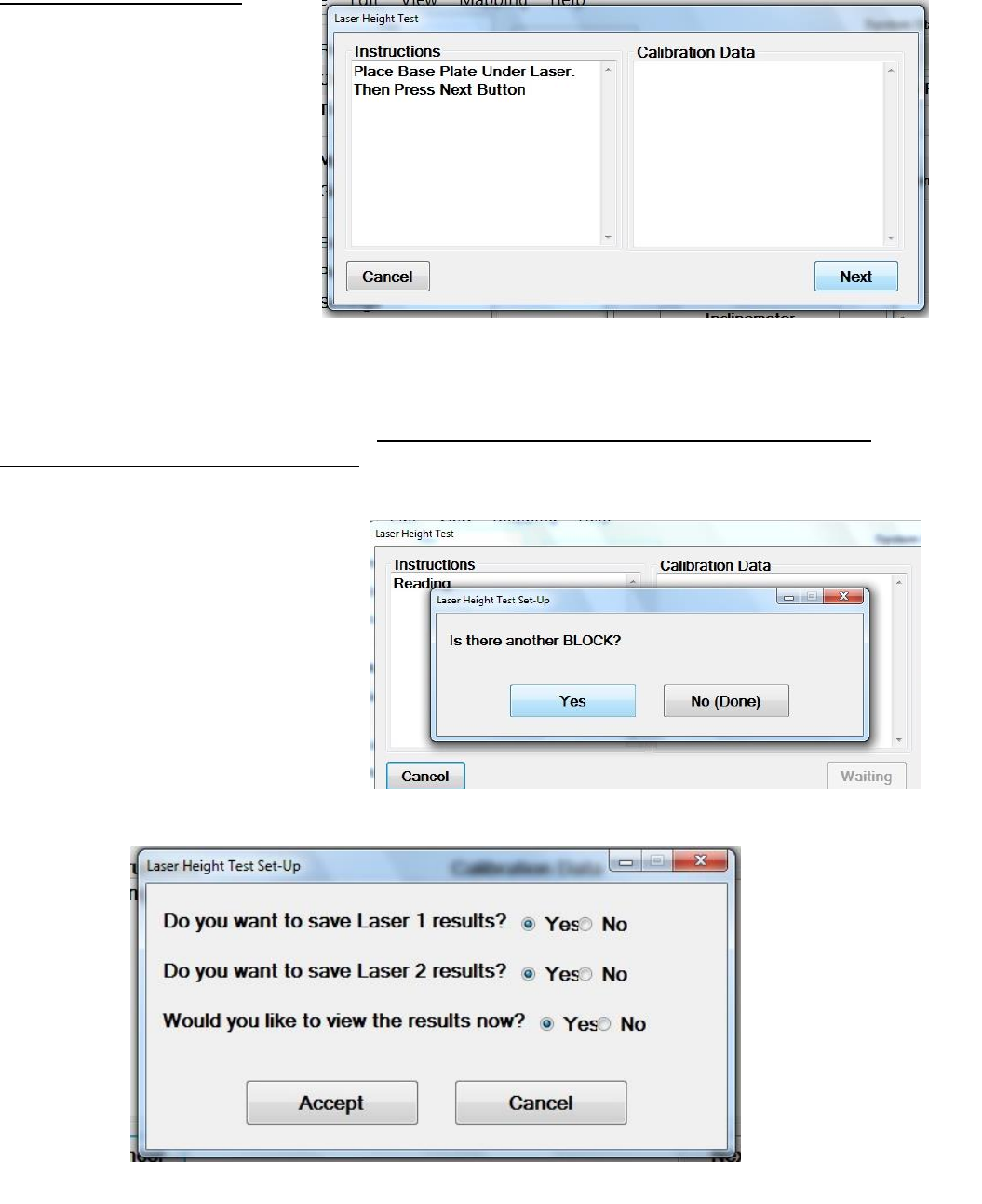
22
Laser Height Verification
The height verification assures the
operator that all of the lasers are
working properly. The height
verification is deemed a success
when each individual laser
deviates less than a hundredth
(0.01) of an inch. The height
verification will also determine if
the laser types are correct. The
laser types can be viewed under
System Settings.
The first step of a height
verification is to choose the
location on the computer to save
the height verification text file. Once chosen the program will ask the operator to place the base
plate on the ground below the laser beam. Check that the base plate does not wobble and there is
not a glare on the measurement blocks. Once base plate is firmly on the ground, select next and
start placing blocks according to the verification procedure.
Once all of the blocks have been placed
by following the procedure, select “No
(Done)” to set the saving preferences in
the next window. By shifting the bubble
to “No” or “Yes”, choose the laser
reading to save in the text file and if the
user would like to view the report
instantaneously.
Figure 33: The initial step for a height verification is to place a base
plate under the laser being tested.
Figure 34: To continue with the height verification, select that there are
more blocks by selecting “Yes”.
Figure 35: Saving Preferences after a Height Verification
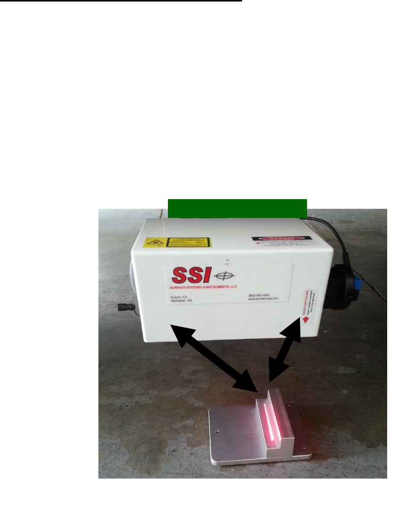
23
After the laser verification the user will have the choice to save Laser 1, Laser 2, Laser 3 readings
and to view the results instantaneously. Only choose the laser the height verification was performed
under. If the results are viewed instantaneously a text file will appear showing all of the laser
readings. The calculated height of the blocks will be displayed at the far right of the text file. These
values must be within a hundredth on an inch (0.01”) according to AASHTO r57.
Bundling Multiple Height Verification Reports
If the operator is running two successive laser verifications they will have the option to add the
results of the last verification to the current verification report. In this way there will be two or
three verification results in the text file. If bundled reports are not desired then select ‘No’ on this
option. The Profiler V3 program will ask the operator to choose to bundle the height verification
at the beginning of the second verification procedure. Select ´yes´ to bundle the files and ´no´ to
keep the next verification as an individual file. This option will appear after the
When performing the height verification make sure the receiving sensor has an unrestricted view
of the calibration block, as shown in the figure below. The high side of the calibration block should
be outside the body of the laser, not below the middle of the laser (see image below).
Emitter
Receiving
Sensor
Figure 36: The Block Orientation for the Height Verification Test
Correct Orientation
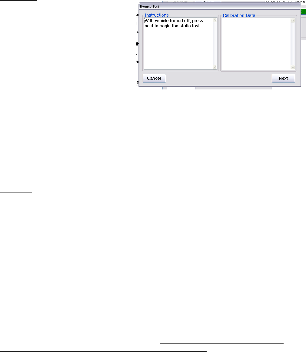
24
Bounce Test
The bounce test is a diagnostic procedure
used to determine if the system’s
accelerometers and height sensors are
working in unison and calibrated correctly.
The bounce test is not a calibration procedure
and its results are not used to reset or adjust
the profiling system. After the bounce test
has finished, three data segments will be
saved within a data file; two static and one
dynamic bounce test. The results of the
bounce test consist of an IRI value and
detailed profile for each of the three tests. The
IRI value is displayed at the end of the test,
and the detailed trace can be viewed like any other data file in Profiler V3. A successful bounce
test results in a completely flat profile trace and low IRI values. Industry standards and
requirements vary as to whether a bounce test is required, and as to the results required from the
test. For SSI’s inertial profiling systems, static bounce test IRI values below 5 in/mi (78.9 mm/km)
and dynamic results below 15 in/mi (236.7 mm/km) are within manufacturer’s specifications for
a properly functioning systems. Some agencies follow AASHTO R057, which specifies a static
bounce test IRI under 3 in/mile (47.35 mm/km) and a dynamic bounce test IRI under 8 in/mile
(126.26 mm/km). The bounce test procedure is sensitive and must be properly performed for
successful results.
Procedure
Once a bounce test is initiated, the program will ask to name and save the file before the test begins.
The static, dynamic, and again static data will be included in this file as Run 1, Run 2, and Run 3
respectively.
Verify before starting test that:
1) Only perform bounce test on a level surface, after accelerometers have been calibrated.
2) Vehicle’s engine is off.
3) Front tires are straight and in-line; Parking brake is off; No wheel chocks or other braces
are to be used
4) A smooth, non-metallic surface is beneath the lasers (at the appropriate standoff)
5) The operator should introduce 1 inch (25.4 mm) of vertical travel at the laser modules
With the vehicle turned off, begin the static test. Do not touch the vehicle at this time. For the
dynamic test, introduce one inch of vertical travel into the vehicle’s suspension at a frequency
between 1.25 Hz (which is a bounce every 0.8 seconds) to 2.5 Hz (which is a bounce every 0.4
seconds). Do not dramatically impact, or shock, the vehicle suspension when jumping on the
profiling vehicle. Use only fluid movement. Only introduce vertical motion into the vehicle
suspension during the dynamic portion bounce test. No lateral or side-to-side vehicle motion
should be introduced. Make sure the wheels are in a straight line. Allow the vehicle to sit
motionless for the final static test.
Figure 37: The static test of the bounce test. Do not touch
or move the vehicle during this portion of the test.
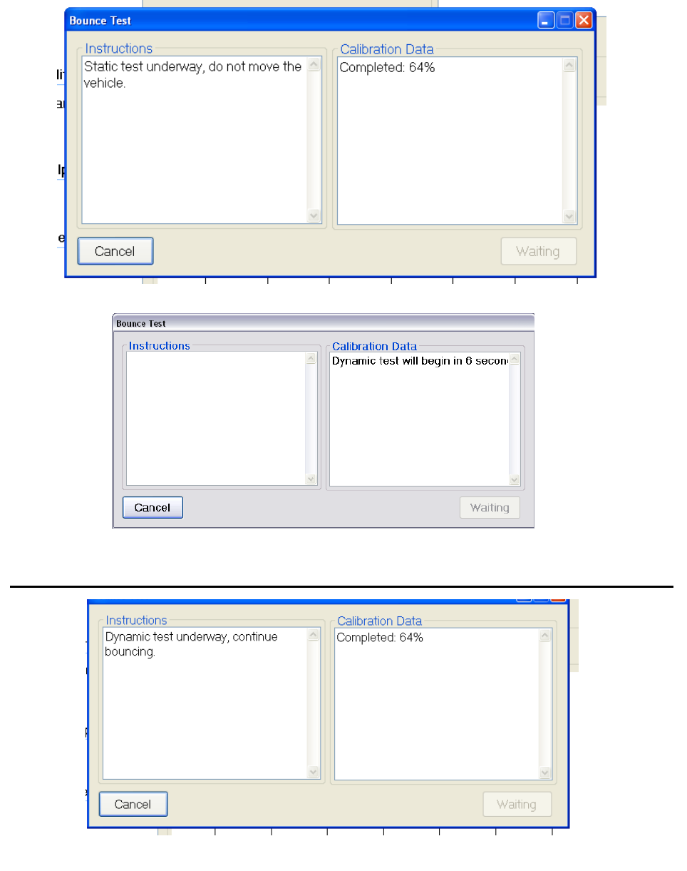
25
Figure 38: The static test being performed
Figure 39: When the dynamic test countdown.
Figure 40: The dynamic test is performed by bouncing the vehicle vertically, not horizontally
Note: The dynamic test will begin 10 seconds from the time next is selected after the static test.
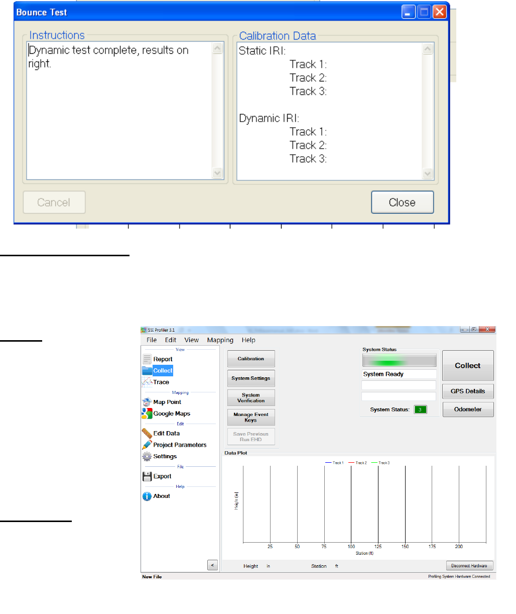
26
Inclinometer Verification
The inclinometer outputs can be verified by using the mounting block and a procedure similar to
the inclinometer calibration. Enter the block angle when prompted by the program. The block
angle is supplied with the system and can be found on the label attached to the grey box cover
within the white housing.
Collect
The optimal speed of
collection is 20+ miles per
hour. The accelerometers
are most accurate within
the range of 20 to 55 miles
per hour for high speed
profilers and trailers.
Height data cannot be
collected if the vehicle is
traveling slower than 5
miles per hour.
System Status
The systems status icon
(the colored box with a
number inside) is used as a
diagnostics tool for
Profiler V3 collection
systems. This window detects
connection problems with the
housing and electronics. SSI support staff may ask the diagnostic string (health string) while
troubleshooting. The type of lasers connected should be shown correct automatically based on
the type of system connected.
Figure 42: The main collection window.
Figure 41: The Dynamic Test Results
0.2 in/mi
0.2 in/mi
0.2 in/mi
7.5 in/mi
7.2 in/mi
7.4 in/mi
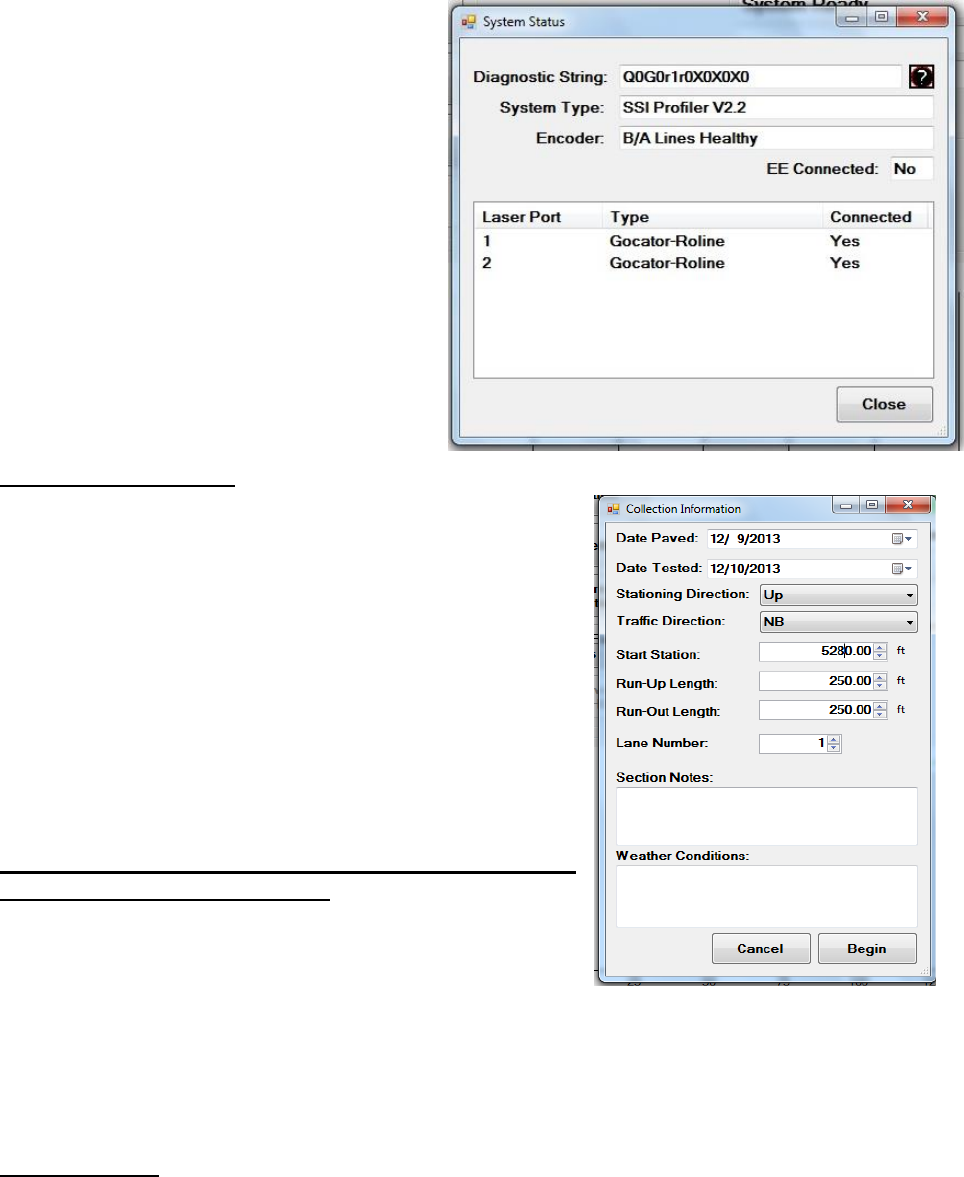
27
Select the diagnostic information button at
the top right of the window to better
understand the purpose and meaning of the
health string.
Collection Information
The Collection Information window appears when the
collect icon is selected. The most important information in
this window is the start station, the direction, lane number
and the run up lengths. Stationing, direction and run up/out
lengths can be changed later through Edit Run. When
"Begin" is selected, collection will initiate. Be in position to
start collection when “Begin” is selected. The “Direction” is
the direction of travel of the profiler (up station or down
station). It is important that the direction is correct. The
stationing can be changed at a later date if the direction of
travel was incorrectly entered. To change the stationing or
direction open the Edit Run feature.
When this window is open, the profiling vehicle should be
at the location to start collecting. As soon as the operator
selects begin, the collection will be ready to start. If the
vehicle is not in position to profile, the self-start collection
feature will start the collection at the wrong point. If the
collection will be started by using Starting Forward or
through the electric eye, “Begin” can be selected a reasonable
distance before the actual start of the collection is to take
place.
Collecting Data
The optimal speed of collection is 20+ miles per hour. The accelerometers are most accurate
within the range of 20 to 55 miles per hour for the high speed profilers and trailers. Height data is
not collected if the vehicle is traveling slower than 5 miles per hour.
Figure 43: The System Diagnostics
Figure 44: The Collection
Information window
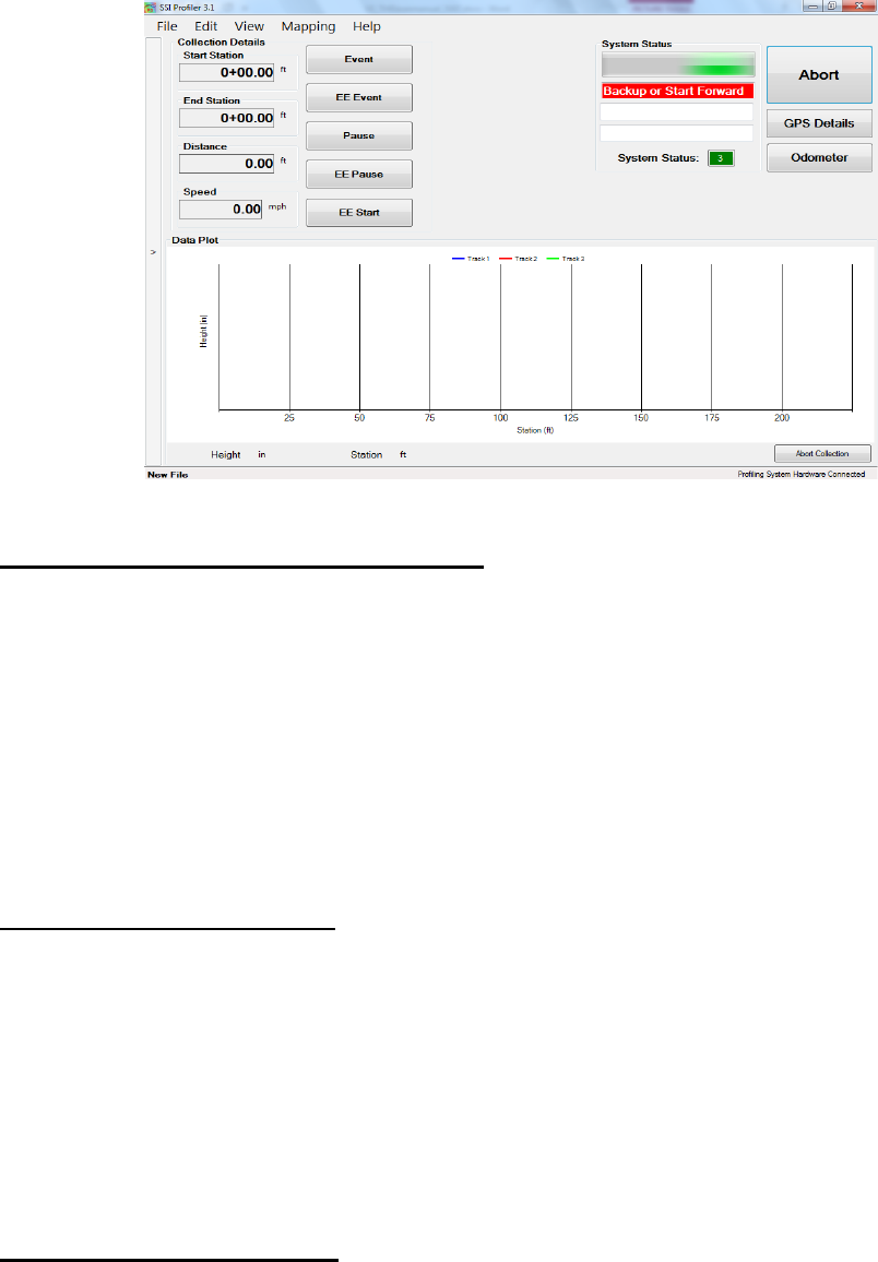
28
The Three Ways to Start a Collection
The operator can travel forward or backward once a collection is started. If the operator accelerates
forward the Run-up procedure will be used with or without an electric eye. If the operator moves
in reverse, the back-up collection procedure will be used. Both of these procedures can use the
electric eye to end the collection. The benefit of using Run-up is that traffic will not be stalled
while the operator begins a collection. The forward motion Run-up option can be started on a
shoulder or at a large distance from start point (a large run up distance).
If the operator uses the back-up option, the vehicle must begin over the starting point and then
move in reverse. Back up until the program instructs the operator to accelerate. The collection will
begin when the initial point is crossed.
Starting a Collection: Run Up
After “Begin” is selected from the collection information window the vehicle may move forward.
Once the vehicle is moving forward over 5 miles per hour and the run up distance is completed,
the collection can be started through an electric eye, selecting the start icon, or selecting a
programmed hot key. The collection can be ended by selecting the stop icon or using the electric
eye. The stop icon will replace the start icon once the collection has been initiated.
The electric eye is used by arming the eye after “Begin” is selected. Once the electric eye triggers
the start of the collection, a new icon appears giving the operator the option to end the collection
by using the electric eye. These buttons are labeled “Start EE” and “Stop EE”.
Starting a Collection: Back up
After selecting “Begin” from the collection information window and the operator has the beams
of the lasers over the starting point, the vehicle can be moved in reverse. The status bar will display
“Back up or start forward” in a red fill, then “Backing up” as soon as the vehicle starts backward
motion. The reverse distance will be measured by the profiling system. After 25 feet, the status bar
will display “Accelerate”. The operator should accelerate forward along the same path to reach a
Figure 45: The collection screen after “Begin” was selected
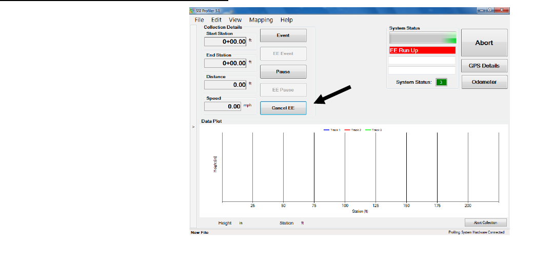
29
speed over 5 miles per hour. When the minimum speed and the run up length has been achieved,
the status bar will display “Self Start” and the collection will begin when the odometer reaches
zero.
Note: The path traveled in reverse should be the same path the vehicle makes when moving
forward. If the paths are different, the collection’s starting point will differ from the initial point
the lasers were aligned to.
The collection can be ended by selecting the stop icon within the main window as the vehicle is
moving. The collection can also be stopped by using an electric eye. To use the electric eye, select
“Arm EE Stop” and the Profiler program will wait for the EE to be triggered before ending the
collection. To trigger the EE properly and consistently, use the recommended DOT-C2 reflective
tape and mount it near the path of the vehicle in clear view of the EE sensor. It is recommended to
place the reflective tape within 10 feet of the electric eye and at the correct elevation of the sensor’s
beam.
Starting a Collection Using the Electric Eye
The electric eye can be used to start
and/or end a collection or end the
Run-up and Bach-up collections.
The recommended reflective tape to
use with the EE supplied by S.S.I. is
the DOT-C2 grade tape. Contact SSI
for supply information. The electric
eye tape can be mounted on a cone or
a stationing marker, as long as it is in
reach of the EE sensor which has an
optimal range of six feet. Sick EE’s
can sense the reflective tape 18 feet
away. The closer the reflective tape
is to the EE sensor, the more
consistent the starting and ending of
collections will be. If the reflective
tape is too far from the EE, the
sensor may not activate.
Most profiling systems have each side equipped with an electric eye. On the white housing there
is a two-way switch with a label of left and right. The left side is the driver’s side electric eye. To
determine if an electric eye is on, look for the amber light on the top side of the electric eye near
the outgoing cable. The diagnostic will also inform the user that the electric eye is attached. The
diagnostic will not inform the user which side the vehicle the electric eye is powered on.
Use DOT-C2 grade reflective tape for the electric eye collections. The reflective tape can be
mounted on a stationing marker or on a cone for repetitive use. Sick EE’s can sense the tape 18
feet away. Other brand EE’s should be placed 6 feet away to function.
Figure 46: The Electric Eye (EE) is armed to start the collection

30
Ending Collections
By Electric Eye
To end a collection using the electric eye, arm the electric eye after the collection has been
started by selecting the Arm EE Stop icon on the screen or through a hot key. When the
electric eye sensor detects a reflective surface, the collection will be ended and run out will
be collected
Through the Stop Icon
The collection can be ended by the operator selecting the Stop and Save icon with a left
click of the mouse. This option is not as precise as using an electric eye or backing up to
end the collection, but it is more efficient when collection multiple runs of data with a loose
tolerance and is sometimes necessary when collecting without traffic control.
Speed Drop Out and Backing Up – “Save”
When a speed drop out occurs (when the vehicle is moving less than 5 miles per hour) the
operator has the option to back up and save the data. This option of ending a collection is
an accurate alternative of completing a collection. The operator can just back up to the
desired ending location. All of the surface data that was collected when moving forward is
omitted while moving backward over the same surface. This creates profiles of the same
length which are convenient when comparing the profiles to a reference file.
Aborting Collection
The collection can be aborted at any time before the file is saved. The abort icon is displayed at
the bottom right of the Collect window. When a collection is not in progress the abort collection
icon is the disconnect hardware icon.
Stopping a Collection
A collection can be ended using the electric eye, selecting Stop Collection, or stopping the
vehicle and backing up to the end point, then hitting Save. If accurate end points are needed in
a lane closure, it is recommended to use the electric eye or stop and back up option. If operating
in traffic at highway speeds where stopping is not an option, use the electric eye end collection,
select the stop collection icon on the screen, or select a user programmed hot key. When using the
stop collection icon the distance collected may be off of your desired stop station. Post analysis
can fix this through the Edit Data feature and crop data tool or the GPS tagging tool located in the
Trace window.
Saving the Collection
When a run is finished Profiler V3 will open a window automatically asking the operator to save
the file. The three options are to Save as New File, Save File, and Do Not Save File. If the file
will be saved, windows explorer will open and the operator will be allowed to save the file to any
folder location on the computer or external device. If the operator selects do not save, the collected
data is still in the program until a new file is opened or the program is closed. If there is any
unsaved data when the program is closed, Profiler V3 will ask the operator to save their changes.
It is always possible to save the data by selecting File>Save or selecting Ctrl+S on the keyboard.
To always save a run in a separate file choose Save as New. This is recommended for multiple
runs and simple post-processing.
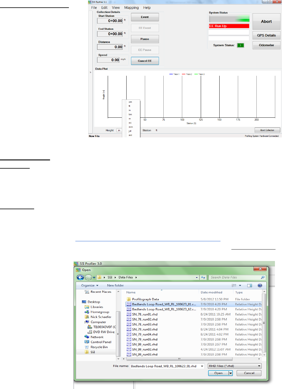
31
Changing Units of Plot
To change the units, click on
the current units and select
from the menu.
Post-Collection
Analysis
1.0- File Tab
1.1. - New
Selecting New creates a new project file to be saved on the operator’s computer or external device.
The file will open automatically and the bottom left corner of the program will display “New File.”
If data has been collected with this file, the name will be displayed with as asterisk as “New File*.”
1.2. – Open
Opens a project file previously saved on the operating computer or connected external device.
Profiler V3 creates RSD type files. The RHD file type from the previous version of Profiler can
also be opened Profiler V3. If your file is in another format, use the appropriate translators found
on the support website (http://www.smoothroad.com/support/download.asp) or contact S.S.I.
Customer Support. The only two file formats used in the Profiler V3 program are RHD and RSD.
Profiler V3 only collects data in the RSD format.
Figure 47: The procedure
to change units of the
data plot is shown
Figure 48: Opening a
data file in the Profiler
V3 program.
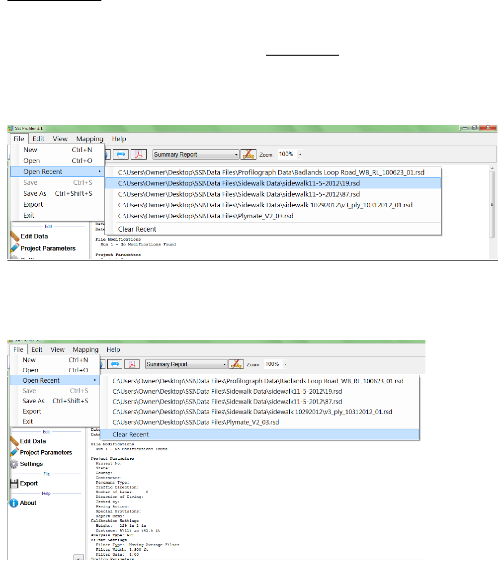
32
1.3. - Open Recent
Opens recently viewed or created project files. Files will only be available if they are saved on the
operating computer or connected external device. The Open Recent feature is a shortcut to find
current profiling data. It is also possible to use the File>Open tool to open saved data. The only
two file formats used in the Profiler V3 program are RHD and RSD. Files can only be saved in
RSD.
The default file to be searched for in Window’s Explorer can be changed under General Settings
and the “Default File Type.”
Clear Recent
Clear Recent deletes the history of previously viewed RHD and RSD files. Once the history is
cleared it cannot be reversed. The operator must navigate to File>Open to view saved files.
Figure 49: The Open Recent feature
Figure 50: The clear recent feature
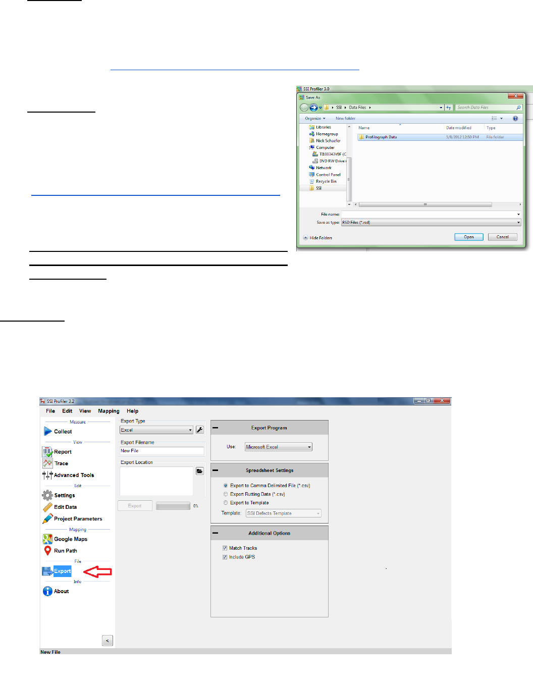
33
1.4. – Save
Save allows the operator to save the current file in RSD format on the operating computer or
connected external device. If ‘Save’ is selected while an unsaved file is open, the operator
will be prompted to choose a file name and folder destination to save the current file. The
file will be saved in SSI´s patented RSD format. If another format is required, visit the SSI
support website (http://www.smoothroad.com/support/download.asp) to download the latest
translators or contact SSI Customer Support.
1.5. - Save As
When Save As is selected, the operator will be
prompted to choose a file name and folder destination.
The file will be saved in SSI´s patented RSD format.
If another format is required, visit the SSI support
website
(http://www.smoothroad.com/support/download.asp)
to download the latest translators or contact SSI
Customer Support.
Note: Save and Save As are only available after data
has been collected or if changes are made to
preexisting file.
1.6. - Export
Exporting allows the operator to create files in ERD, PPF, PRO, Survey, GPS Matching, GIS,
Localized Roughness, RMS, GPX, ProFAA, and Excel formats. The settings for each export
feature are described below. For each of the exporting formats, a folder destination is required.
The Export feature can be found in the shortcut bar on the left hand side of the Profiler V3 window
and in File>Export.
Figure 51: Saving a file through Save As in RSD
format.
Figure 52: The export window for exporting the data into Excel format.
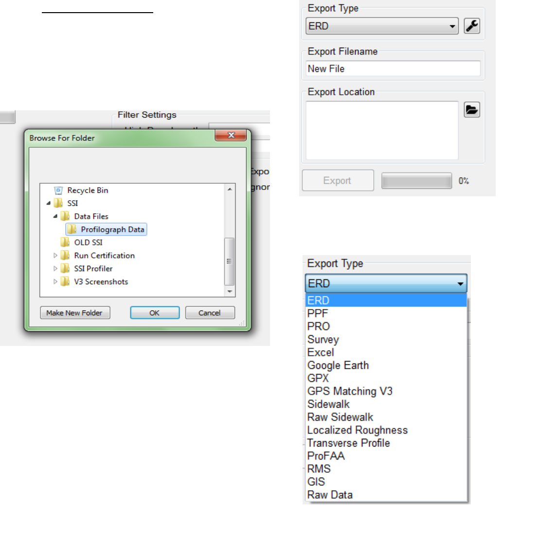
34
1.6.1. Export Location
To choose the folder destination, select ‘Browse’ and
navigate through Windows Explorer to the desired
folder. Once the folder destination is reached and
selected, left click on ‘OK’ at the bottom of the
window to save the folder location.
Figure 53: Selecting a location to save the exported file.
Figure 54: The export format and folder location selection
Figure 55: The export type drop down menu
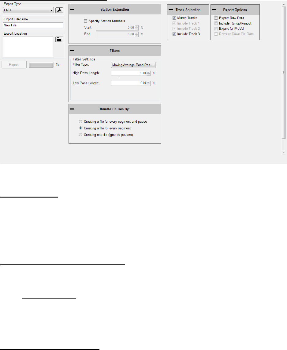
35
1.6.2. – Exporting to ERD Format
Station Extraction
The operator has the option to export only certain sections of the profile data, based on the
stationing set within the Profiler V3 software. To use this feature, select the check box near
“Specify Station Numbers.” When the box is selected, the operator will be able to adjust the
stationing numbers. The ‘Start’ stationing is the initial stationing where the exported file will begin,
while the ‘End’ stationing is the point where the exported file will finish. These values can be
adjusted by typing values into the box or by using the arrow keys to the right of the box.
Filter Settings—High & low pass length
The exported data file can have additional filters applied while being processed into the chosen
format. To not filter the data, leave the filter lengths at the default value of 0.00 feet.
Available Filters:
Moving Average High Pass Filter
Moving Average Band Pass Filter
Butterworth High Pass Filter
Butterworth Band Pass Filter
Include Run Up – Run Up Data
Some High-Speed Profiling data files have Run Up and/or Run out data associated with them,
depending on the practice used to collect the data. If this data exists, it will be included in the
exported file if this box is selected. Run Up and Run out is used to allow the electronics to settle
on the accurate profile.
Figure 56: The ERD format export window with ‘Match Tracks’ and ‘Include Laser 3’ selected.
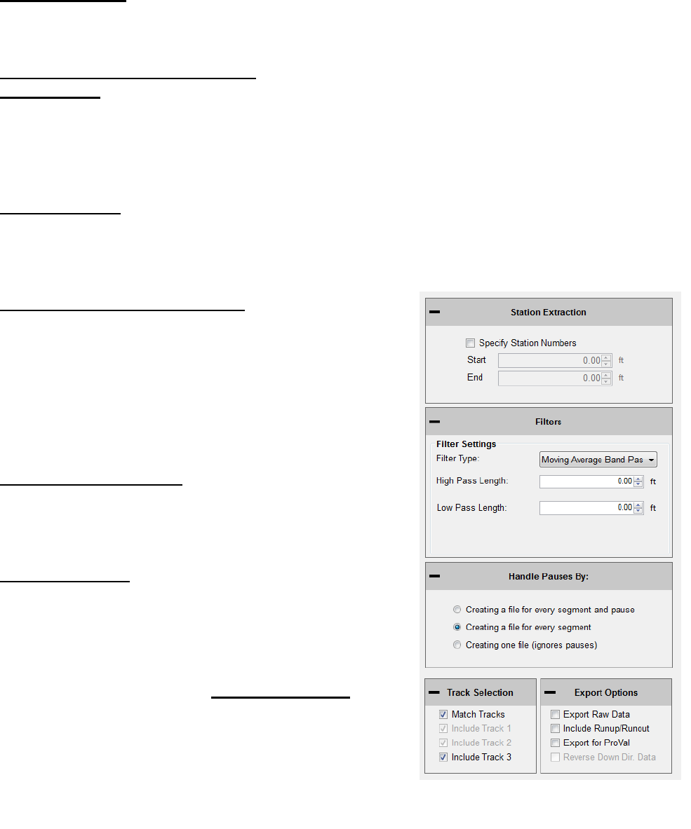
36
Run Up data exists in HSP data files if the operator selected a Run Up and/or Run out distance in
the initial stages of setting up a collection. In the HSP collection software, the Run Up and Run
out settings are found on the last window before performing a collection.
Export Raw Data
Selecting the Export Raw Data check box assures the operator that only unfiltered data collected
from the profile will be exported into the chosen file.
Match Tracks and Choosing Tracks
Match Tracks
Selecting ‘Match Tracks’ exports all of the tracks associated with the lane file. For the three laser
systems, this includes Track 1, 2 and the center trace (Track 3). For Profilograph files, the tracks
are matched based on the settings entered prior to profiling. The label of the track number and
stationing cannot be changed after collection.
Choosing Tracks
The exported tracks are checked under “Track Selection.” If Match Tracks is selected the user
cannot deselect track 1 or 2.
Creating One File (Ignore Pauses)
Pauses are useful when an obstruction comes into the
profiling path or when a section of pavement is not to be
profiled. When Pause is activated, the stationing remains
constant and under the same file. Pauses can either be
omitted or included in reports and exported files of the
Profiler V3 software. To omit pauses from the exported file,
select the check box, “Ignore Pauses.”
Include Run Up/ Run out
When this option is selected, the Run Up and Run out data
collected during the collection will be included in the export
data.
Export for ProVal
When the user exports an ERD file for use in ProVal, it adds
a negative sign in front of all stationing. This is done because
ProVal does not use stationing, it only uses forward distance.
If you collect data down station, you must check the Export
for ProVal box to keep accurate stationing through the
collection. Always choose “Export for ProVal” when
creating files to import into ProVal.
Figure 57: The ERD export window settings
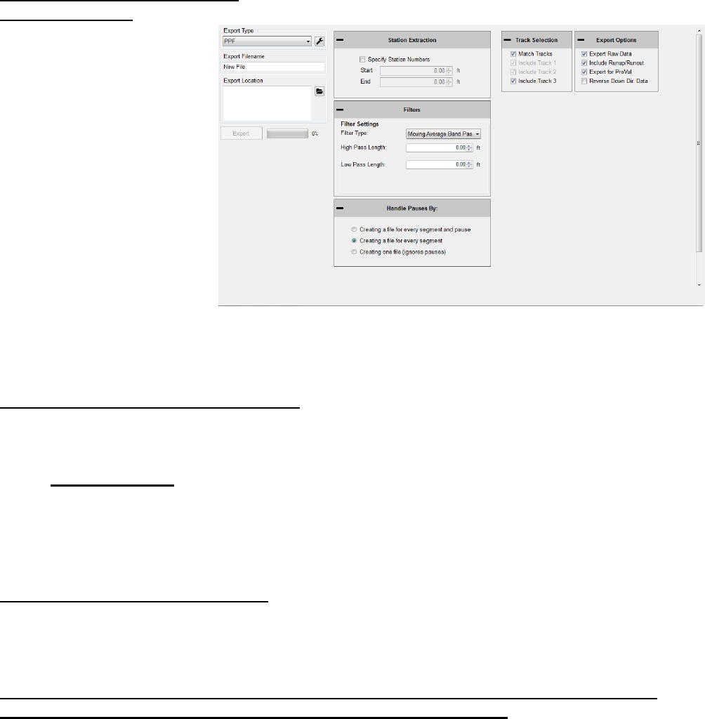
37
1.6.3. – Exporting to PPF Format
Station Extraction
The operator has the option to
export only certain sections of
the data, based on the
stationing set within the
profiling data. To use this
feature, select the check box
near “Specify Station
Numbers.” When the box is
selected, the operator will be
able to adjust the stationing
numbers. The ‘Start’ stationing
is the initial stationing where
the exported file will begin,
while the ‘End’ stationing is
the point where the exported
file will finish. The start and
end stationing can be
adjusted by typing values into the box or by using the arrow keys to the right of the box.
Filter Settings—High & Low Pass Length
The exported data file can have an additional filter applied while being processed into the chosen
format. To not filter the data, leave the filter lengths at the default value of 0.00 feet.
Available Filters:
Moving Average High Pass Filter
Moving Average Band Pass Filter
Butterworth High Pass Filter
Butterworth Band Pass Filter
Include Run Up and/or Run out Data
Some High-Speed Profiling data files have Run Up and/or Run out data associated with them,
depending on the practice used to collect the data. If this data exists in the data file, it will be
included in the exported file if this box is selected.
Run Up data only exists in HSP (High Speed Profiler) data files if the operator selected a Run
Up and/or Run out distance in the initial stages of setting up a collection. In the HSP collection
software, the Run Up and Run out settings are found on the last window before performing a
collection.
Figure 58: The PPF export window
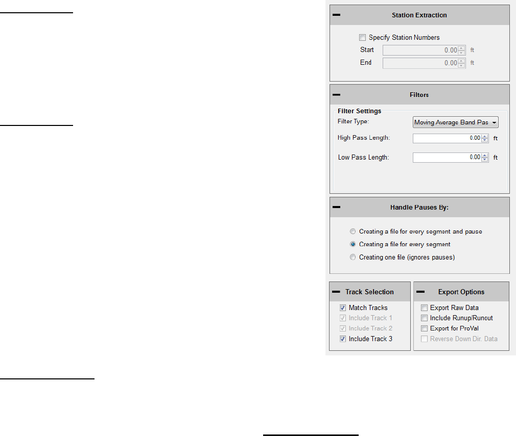
38
Match Tracks
Selecting ‘Match Tracks’ exports all of the tracks associated with
the lane file. For the three laser systems, this includes Track 1, 2
and the center trace (track 3). For the Profilograph files, the tracks
are matched based on settings entered prior to profiling. The
stationing and number label assigned to the track are settings that
cannot be changed after collection.
Ignore Pauses
Pauses are used when an obstruction comes into the profiling
path or when a section of pavement is not to be included in the
calculation of ride values and localized roughness. While Pause
is activated, the program will continue to collect stationing data,
but will not collect height data. Pauses can either be omitted or
included in reports and exported files. To omit pauses from the
exported file, select the check box, “Ignore Pauses.”
For importing into ProVal, the best method is to include pauses.
The pauses of the rsd file will turn into a leave-out section within
ProVal. If pauses are not included during export, it will result in
two PPF files for the same track. There will be one more PPF file
than the number of pauses.
Export for ProVal
When the user exports an ERD file for use in ProVal, it adds a negative sign in front of all
stationing. This is done because ProVal does not use stationing, it only uses forward distance. If
you collect data down station, you must check the Export for ProVal box to keep accurate
stationing through the collection. Always choose “Export for ProVal” when importing into
ProVal.
Figure 59: The optional settings when exporting in PPF format.
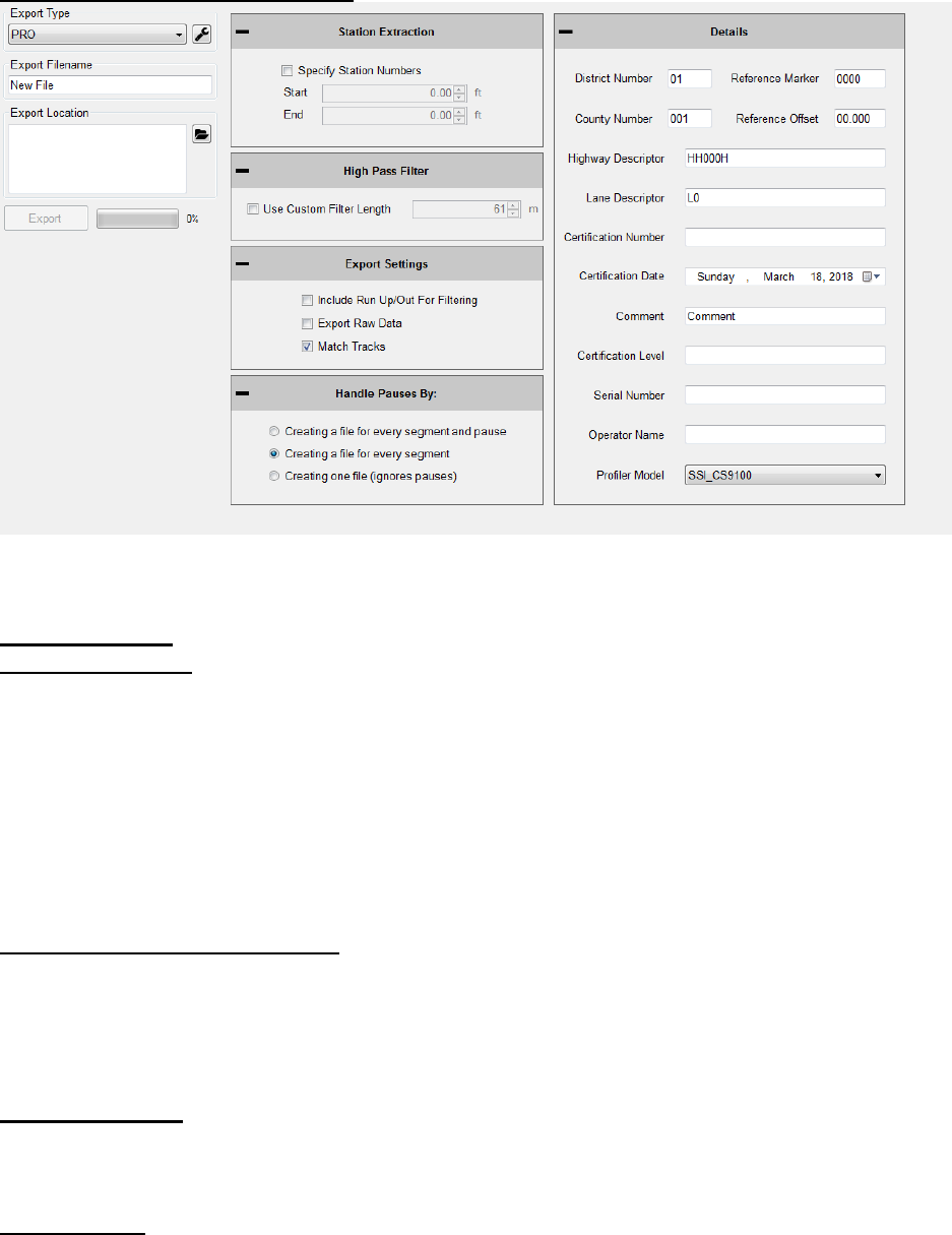
39
1.6.4. – Exporting to PRO Format
General Settings
Station Extraction
The operator has the option to export only certain sections of the data, based on the stationing set
within the profiling file. To use this feature, select the check box near “Specify Station Numbers.”
When the box is selected, the operator will be able to adjust the stationing numbers. The ‘Start’
stationing is the initial stationing where the exported file will begin, while the ‘End’ stationing is
the point where the exported file will finish. These values can be adjusted by typing values into
the box or by using the arrow keys to the right of the box.
Filter Settings-High Pass Length
The High pass filter length can be changed when exporting files to PRO format. A High Pass Filter
removes all of the data trends below the filter length. The default length of the High Pass Filter is
200 feet. In order to export the data without filtering, the ‘Export Raw Data’ check box must be
selected. See ‘Export Raw Data’ below.
Export Raw Data
Selecting the Export Raw Data check box assures the operator that only unfiltered data collected
from the profile will be exported into the chosen file.
Match Tracks
Selecting ‘Match Tracks’ exports all of the tracks associated with the lane file. For the three laser
systems, this includes Track 1, 2 and the center trace (Track 3). For the Profilograph files, the
Figure 60: The export window when PRO format is selected.
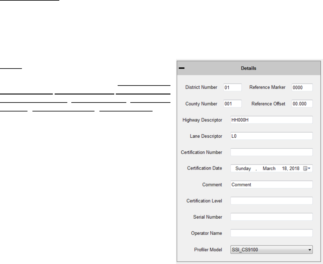
40
tracks are matched based on settings entered prior to profiling. The label of the track cannot be
changed after collection.
Handle Pauses By:
The paused sections within the collected data can be exported in two ways. Separate files can be
created for each segment or the profile data can be exported with the paused sections included in
one file. The difference in these two options is that creating separate files for each segment exports
multiple files into the folder location, while the “Using pause events” option exports one file
including all of the data. If the pauses were used to omit data because of pavement anomalies, use
the option of ignoring the pauses.
Details
The details section of PRO exporting is the job specific
information saved with the file, such as District Number,
County Number, Reference Marker, Reference Offset,
Highway Descriptor, Lane Descriptor, Certification
Number, Certification Date, and Comments. This
information is then saved with the PRO file to be
displayed when the file is opened or printed using another
program.
Figure 61: The Details tab contains
information about the project.
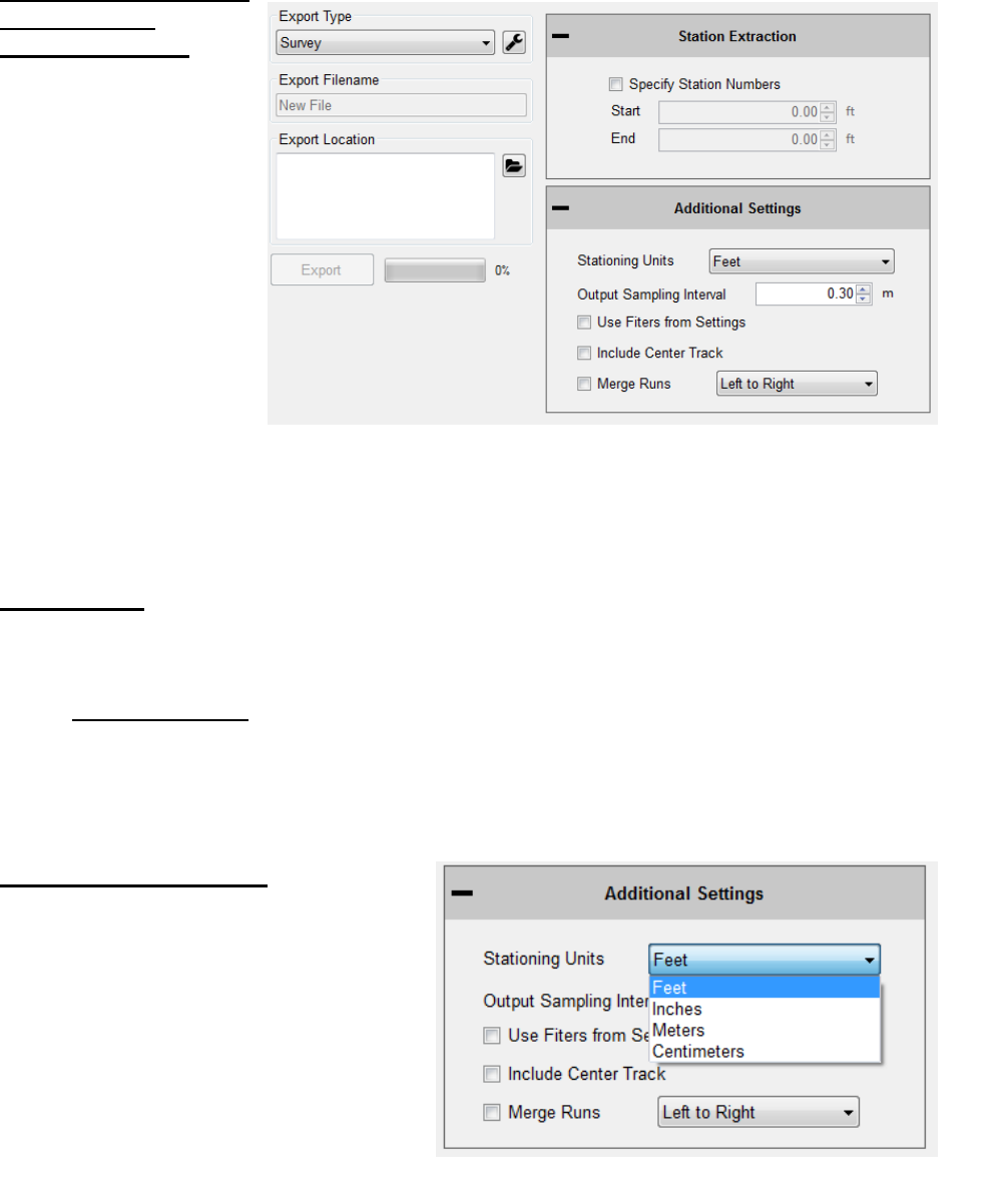
41
1.6.5. – Exporting to
Survey Format
Station Extraction
The operator has the
option to export only
certain sections of the
trace, based on the
stationing set within the
profiling data. To use this
feature, select the check
box near “Specify Station
Numbers.” When the box
is selected, the operator
will be able to adjust the
stationing numbers. The
‘Start’ stationing is the
initial stationing where
the exported file will begin, while
the ‘End’ stationing is the point
where the exported file will finish. These values can be adjusted by typing values into the box or
by using the arrow keys to the right of the box.
Filter Settings
High and Low Pass filters are optional when exporting to survey format. The exported data file
can have an additional filter applied while being processed into the chosen format. To not filter
the data, leave the filter lengths at the default value of 0.00 feet.
Available Filters:
Moving Average High Pass Filter
Moving Average Band Pass Filter
Butterworth High Pass Filter
Butterworth Band Pass Filter
Output Sampling Interval
The sampling interval is the distance
between readings of the SSI survey system.
The default length of this interval is 1 foot.
This feature allows other intervals to be
implemented, depending on the accuracy
specifications required in the surveying
program.
The raw GPS will be exported in a separate
text file in a NMEA (GPGGA) GPS string
format.To match tracks 1 and 2 within the
same file select the match tracks option.
Figure 63: Stationing units dropdown menu and options.
Figure 62: The window for exporting in Survey format
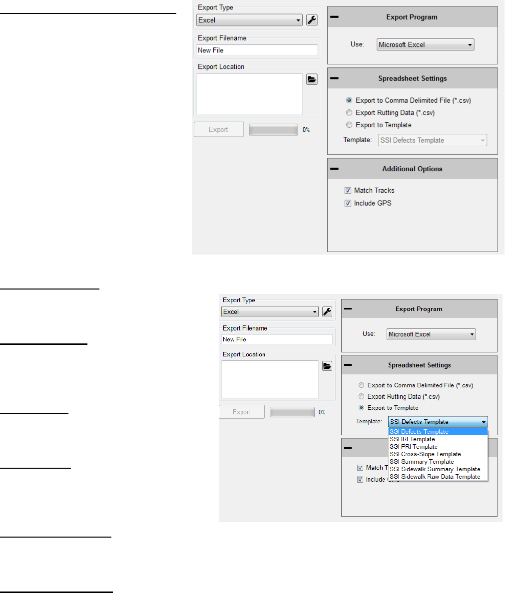
42
1.6.6. – Exporting to Excel Format
Exporting the profile data to excel
gives the operator versatility and
efficiency when an adjustable
numerical printout is needed.
Export to Template
To choose a SSI Excel Template, select
“Export to Template.”
Defects Template
The Defects Template shows the locations
and heights of the defects and information
about the file in spreadsheet form.
IRI Template
The IRI Template shows IRI statistics along
with the defect locations and heights.
PRI Template
The PRI Template lists the PRI for each
track along with the bump heights, locations
and settings.
Cross-Slope Template
The Cross-Slope template shows
the calculated cross-slope for systems with inclinometers or IMUs.
Summary Unmatched
The Summary Template shows a version of the summary report the calculated PRI for each track
along with the bump heights, locations and settings in spreadsheet form.
Note: Sidewalk templates are reserved for Sidewalk Profiler. For more info visit www.smoothroad.com
Figure 64: Exporting the data
into Microsoft Excel format.
Figure 65: The types of excel formats are listed in the drop down menu.
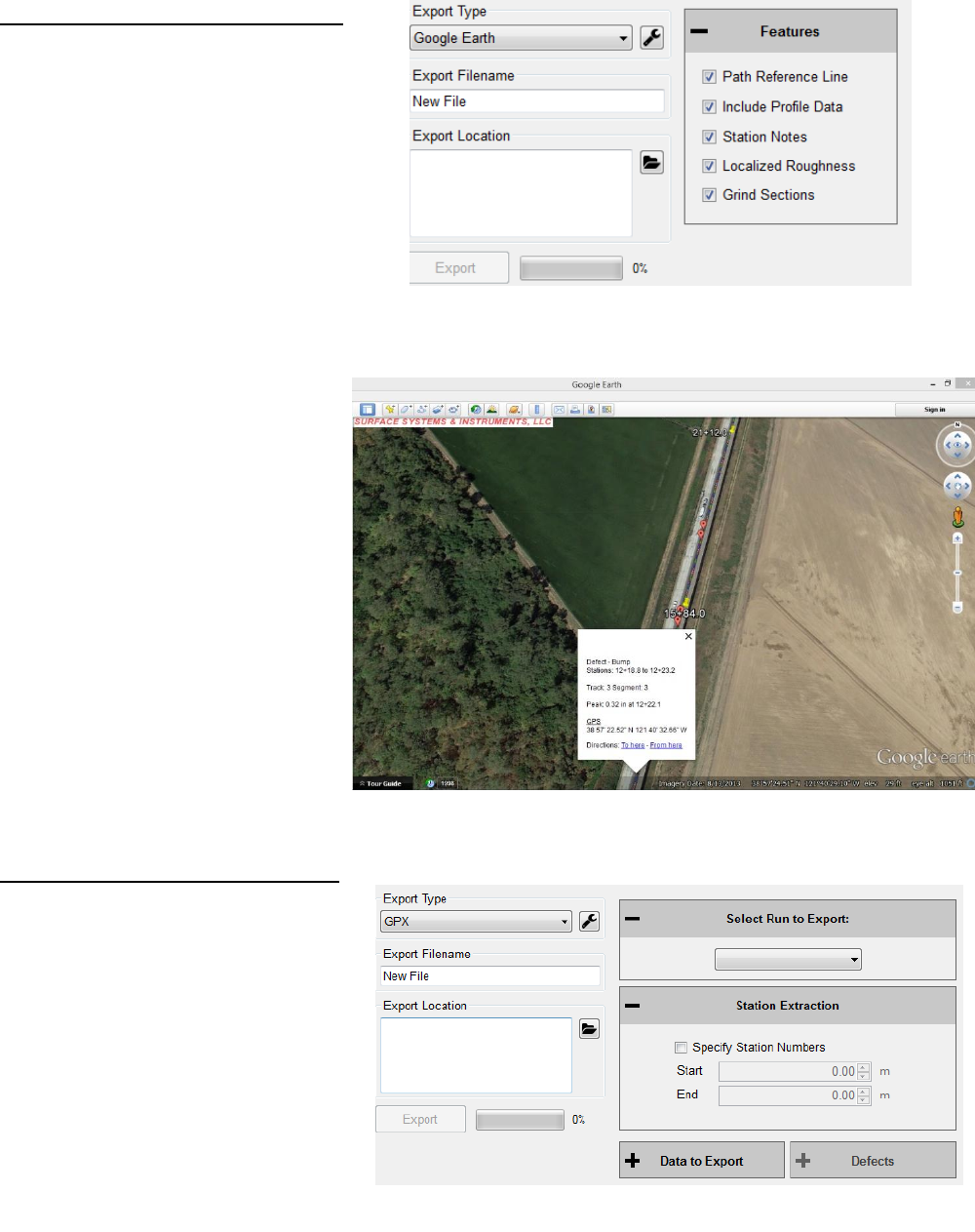
43
1.6.7. – Exporting to Google Earth
The export to Google Earth feature allows
operators with Google Earth installed on
their computers to view the test data in the
real environment. The view of the Google
Earth feature shows the project area with
the traces superimposed onto the window.
The user may view the traces and project
from any view or angle. For this feature to
be used, the operating computer must
have Google Earth installed.
The user may then use Google Earth
to view the profile trace in their
computer, tablet or smart phone as
long as the device has Google Earth
installed. The .kmz file can be
emailed to the device or sent via
Bluetooth if your Toughbook is
equipped.
Figure 67: Google Earth view on laptop.
1.6.8. – Exporting to GPX Format
The GPS coordinates can be exported
into a format for submittals. The GPS
coordinates of the defect can be
viewed through the defect start station,
defect end station or the defect peak
station. Specific runs can be chosen to
retrieve the GPS coordinates by
adjusting the drop-down menu under
the title, “Select Run to Export.”
Under the title "Data to Export" there
are multiple check boxes. In order to
export the defect’s GPS coordinates,
the "All Raw GPS Locations" check
box must be unchecked. Once the "All Raw GPS Locations" box is deselected, the options to
export the defect stationing GPS coordinates become available.
Figure 68: The export window when the GPX format is selected.
Figure 66: Google Earth export settings.
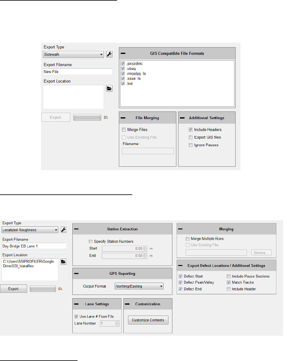
44
1.6.9 – Exporting to Sidewalk Format
This option is only to be used with files collected with the SSI Sidewalk Profiler (CS-8850). The
sidewalk format has all of the information of the collection exported into GIS compatible file types.
These files types and the corresponding information (See Glossary for explanation) within them
are: ngd, pxyzd, pxyzdg and pxyzdinc, rmpslp, rmpslpg, rmpslpg_ls, ubag.
1.6.10 – Exporting to Localized Roughness
The localized roughness export feature allows the user to create an excel spreadsheet of the
localized roughness, or defects, for the collected data.
Specify Station Numbers
If the user desires to only export a section of the collection, select this check box and enter the start
and end stationing of the soon to be exported section. If the specify station numbers is not selected,
the entire collection will be exported.
Figure 69: The Sidewalk Export Window options.
Figure 70: The Localized Roughness export options window.

45
GPS Reporting
To choose the type of GPS format used in the export, select Northing/Easting, Decimal Degrees,
or NMEA Format from the drop down list.
Lane Settings
The user may change the lane number that is currently in the collection file by selecting this check
box and entering the correct lane number. To change the lane number, deselect the check box and
change the lane number in the input location.
Customization
The user may add, move and remove
columns from the Excel spreadsheet
format. To do this, open the “Customize
Contents” window and use the arrow
keys. Move up and move down to change
the order of the included columns. The
columns types are at the top of the
“Columns in File” side the left-most
columns in the exported Excel file.
Merging
The ´Merge Multiple Runs´ check box
allows the user to include multiple
collection runs in the spreadsheet. Runs
that are saved in a separate file can be
opened and exported alongside the
current file by selecting “Use Existing File”
and browsing to enter the location of the file.
Export Defect Locations
Use the check boxes to select whether the program will export the start, peak and end of the defect
in the spreadsheet.
The user will have the option to match tracks 1 and 2, include the paused sections, and include the
header information. When paused sections are included the defects within the paused sections will
be listed.
Figure 71: The Customize Window
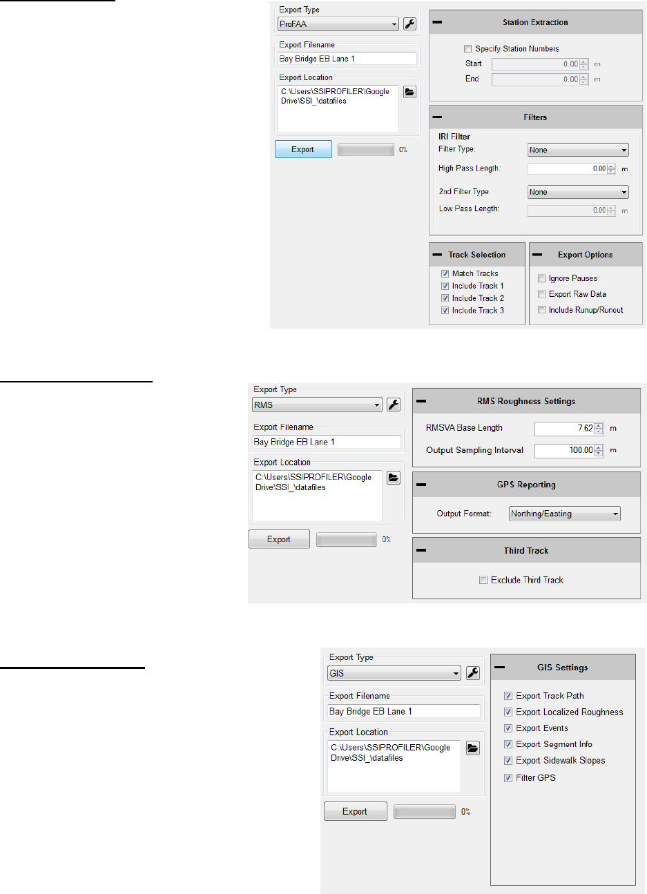
46
1.6.11 – ProFAA
ProFAA is the format used for the
Federal Aviation Administration
(FAA) profiling program. This is the
program that uses the Boeing Bump
test method.
The user can enable high and low pass
filters, change the start and end
stationing, including the pauses and
exclude specific tracks from the
exported data.
Exporting raw data will force the data
through a linear regression filter and
have the data begin and end at zero
elevation. The Run Up and Run out
data can be included by selecting the
check box.
1.6.12. – RMS Export
The RMS export is a normalization
of the profile data. RMS removes
the influences of long wavelengths
and grades while focusing on the
amplitudes of the wavelengths in
the profile. The RMS output does
not show the frequency of these
amplitudes in the profile, only that
they exist.
Set the RMS base length for
continuous RMS and the
sampling/segment interval.
1.6.13. – GIS Export
The GIS export will create shape files for the
segments, localized roughness, events, and
track path for the profile. These files will be
organized into their own folder entitled GIS
Files under the destination folder.
Figure 72: ProFAA Matching
Figure 73: RMS export settings
Figure 74: GIS export settings
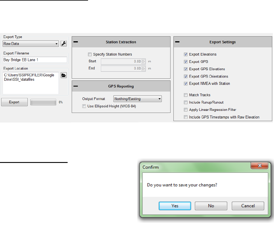
47
1.6.14. – Exporting Raw Data
The user can export raw elevation data, GPS data and GPS height data. The settings can be changed
to export certain GPS string formats. It is recommended to use the Linear Regression Removal
Filter to set the raw elevations along the null line. Otherwise there can be drift in the trace and give
inaccurate elevation data.
1.7. – Exiting Program
To exit the Profiler V3 program, save current
project and click the red “X” at the top right
corner or navigate to the File tab and select Exit.
If the current project is not saved when the
program is terminated, Profiler V3 will ask if
the operator would like to save the current
project. To save and exit the program, select
“Yes.” If you do not wish to exit to program,
select cancel and the program will remain open.
Figure 76: Exiting the program- Saving
Figure 75: Exporting Raw Data Settings.
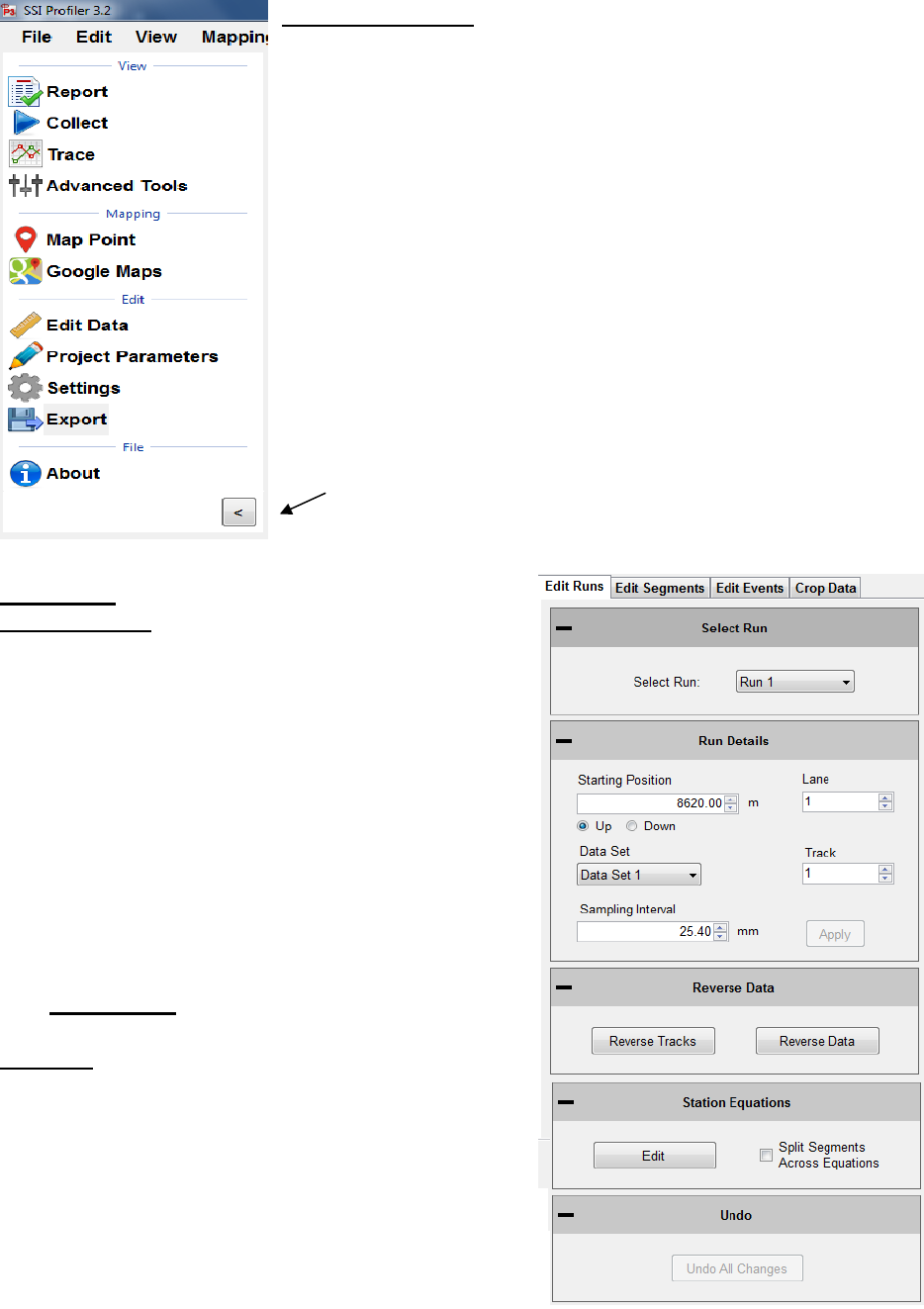
48
1.8. – Shortcut Bar
The Shortcut Bar is located at the left side of the main window. The
shortcut bar is used to navigate around the profiler program without
using the menu bar.
The shortcut bar can be hidden by selecting the arrow at the bottom
of the window. The direction that the arrow is pointing is the
direction that the shortcut bar will move. It will either become
hidden or reappear.
2.0. - Edit
2.1 – Edit Data
Note: Any edit to the data will be described in the
report header under File Modifications.
The edit data feature allows the user to adjust the
starting station, insert pauses, or add events. All of this
can be done in post processing, after a collection has
been completed. To edit the collection:
1) Open the tab that has the information that needs
adjustment. (Edit, Runs, Segments, Events)
2) Select the run that needs to be adjusted from the
drop-down menu.
3) Change the parameter of starting position, run
direction, and Run Up or Run out data.
4) Select apply.
Edit Run
Under Edit Runs the user can adjust the starting
position and change the Run Up or Run out lengths. If
the data was collected in the wrong station direction,
this can also be reversed by changing the bullet
selection to “Up” or “Down.”
Figure 77: The
shortcut bar with all
of the frequently
used windows
Hide the shortcut
bar by selecting
the Hide Icon
Figure 78: The Edit Run Options
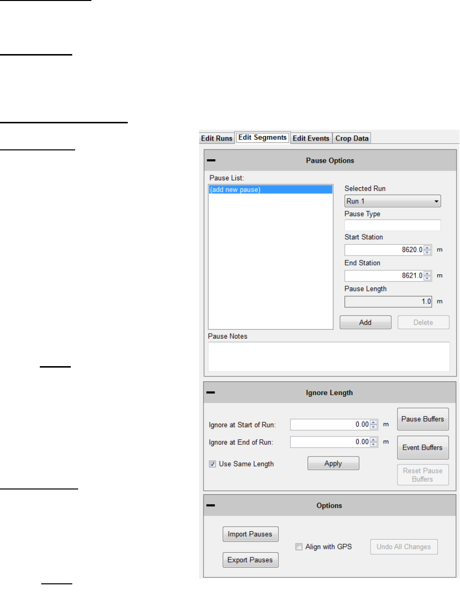
49
Sampling Interval
The sampling interval is the distance between readings of the electronics of the profiling system
(DMI, lasers, etc.). This is usually set to 1 inch.
Edit Segments
The Edit Segment feature allows the user to add pauses to the collection or to ignore a certain
distance of collected data at the beginning or end of the run. The data will not be included in
calculation of the PRI.
Adding & Editing Pauses
To add a pause
1.New Pause will be added above the
highlighted blue bar “(add new pause).”
2.Select the run number to add the pause
to from the drop down menu.
3.Select the pause type (Exclusion,
Bridge, Intersection)
4.Enter the start station for the pause
5.Enter the end station for the pause (The
pause length will be updated
automatically)
6.Select Add. The pause stations will
appear in the Pause List.
7. The user will now be able to add Pause
Notes.
a.Select Apply to save the pause note.
Note: A pause will not be added unless
the Start Station is different than the
End Station.
The pause can be edited at any time.
Any pause or edit made after collection
will be displayed in the report header
under file modifications.
To Edit a pause
1.Select the paused section to be edited
in the Paused list. It is selected when the
blue bar is highlighting the pause title
(Ex. “Run 1 - 0+00.0 to 0+010.0”)
2. Change the stationing.
3. Select Save to set the changes.
4.Select Apply for the changes to take
effect
Figure 79: Adding or removing pauses from the collection

50
Note: The run(s) that the pause is applied to cannot be changed through Edit Run. Please create
a new Pause to change the pauses of a run. See directions above to create a pause.
If the pause is going to be deleted, select the Delete icon to remove it from the list.
Pause Definition
When the collection system is paused, height data is omitted but the distance is still collected.
When the paused sections are excluded, the height values are not used in the calculation of
localized roughness or ride values.
Pause Notes
To explain the reason for the pause or the location, enter the information in the pause notes. This
information will appear in the track notes of the trace reports.
Pause List
The Pause List shows all of the paused sections of the selected runs. The runs are selected from
the drop down menu of “Add Pause to Run.”
Start Station
The Start Station in the stationing where the pause is to begin.
End Station
The End Station is the stationing where the pause will stop, and collection will resume.
Save Pause Icon
When the operator selects a created pause in the Pause List by left clicking on it and highlighting
it blue, the two options of Save and Delete appear in the middle of the window. To save the selected
pause in the Pause List, left click Save.
Ignore Length at Start/End
This feature ignores a distance at the start and end of a collection by adding a pause at these
locations. If the “Use Same Length” box is not selected, the ignored distance at start and end will
be the same.
Pause Buffers
The Pause Buffer icon opens a new window to add length around pauses in the Pause List. Choose
the Pause in the Pause Buffer window and add the buffer length. Select OK when finished.
Event Buffers
The Event Buffer icon opens a new window to add length around events around events in the
Events Tab. Choose the event in the Event Buffer window and add the buffer length. Select OK
when finished.
Use Same Length
When the Use Same Length check box is selected, the runs will be trimmed to the same length.
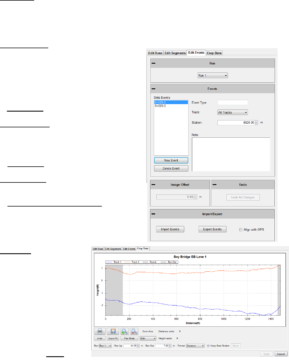
51
Edit Events
Edit Events allows the user to input events that were not added during collection, or to delete saved
events. The events can have information associated with them that is inputted into the text box.
The types of events for walking profilers (Sidewalk) are Height and Width obstruction. High speed
and Profilograph systems should use the “Default” Event Type.
To add an Event
1. Select the run to add the event to
2. Select New Event
3. Change the Stationing to the correct point
location
4. Adjust the Event type to explain the event
5. Under notes, add information about the event.
(Start Structure, manhole, drainage, etc.)
7. Select Apply
Editing an Event
1) Select the event in the Data Events list to
highlight it blue.
2) While highlighted, the event stationing, type or
notes can be changed
3) Select Apply
Deleting Events
1) Select the event in the Data Events list
2) Select Delete to remove the event.
3) Select Apply to save the changes
Crop Data
The Crop Data tool allows the
user to trim the collections
before analysis and reporting.
If any changes are made to the
file, the information that was
changed will be described in
the report header under File
Modifications.
To crop the collection, change
the distances for the run up
and/or run out distances. When
the lengths are at the desired
distances, select Apply.
Figure 80: Edit Events Tab
Figure 81: The Crop Data Tool
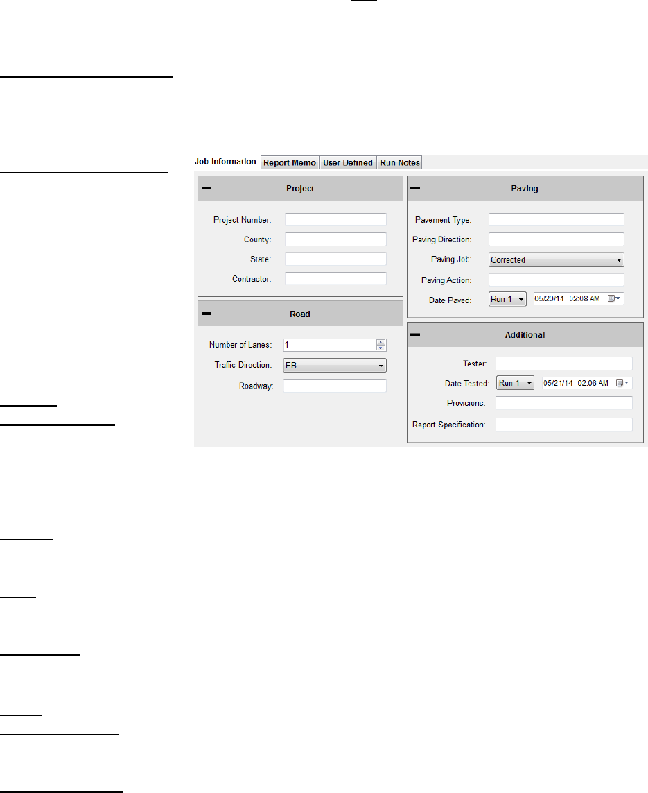
52
To reset the run up and run out to the original lengths select the rest icon next to run out. This icon
will become available once a change has been made and Apply has been selected.
It is recommended to use the dropdown menu and choose the “Station” option instead of the
distance option for cropping data.
2.2 - Project Parameters
The Project Parameters section is the location where the job information is inputted. This
information appears on the header of the reports and the exported excel templates. Before leaving
the Project Parameters window, always select ‘Apply’ if changes were made.
2.2.1. - Job Information
The job specific criteria
listed below are
descriptive information
about the project. Review
the contract to enter the
required information into
the sections listed below.
These sections can be
edited at any time within
Profiler V3.
Project
Project Number
The Project Number is
unique to each project. This is to be
determined by the State, Federal DOT or by
the contractor. This information will be listed in the project contract.
County
This location is reserved to list the county where the profiling is taking place.
State
The state in which the profiling is taking place and the job is located.
Contractor
This section is for the name of the paving company or for the company operating the profiler.
Road
Traffic Direction
The traffic direction of the lane to be profiled.
Number of Lanes
The number of lanes of the project. This section can be changed by inputting values directly or by
using the arrow keys. Traditionally, the number of lanes is the number of lanes travelling in the
same direction for main line freeways. Use a classification system that can be understood during
post-collection analysis.
Figure 82: The Project Parameters window
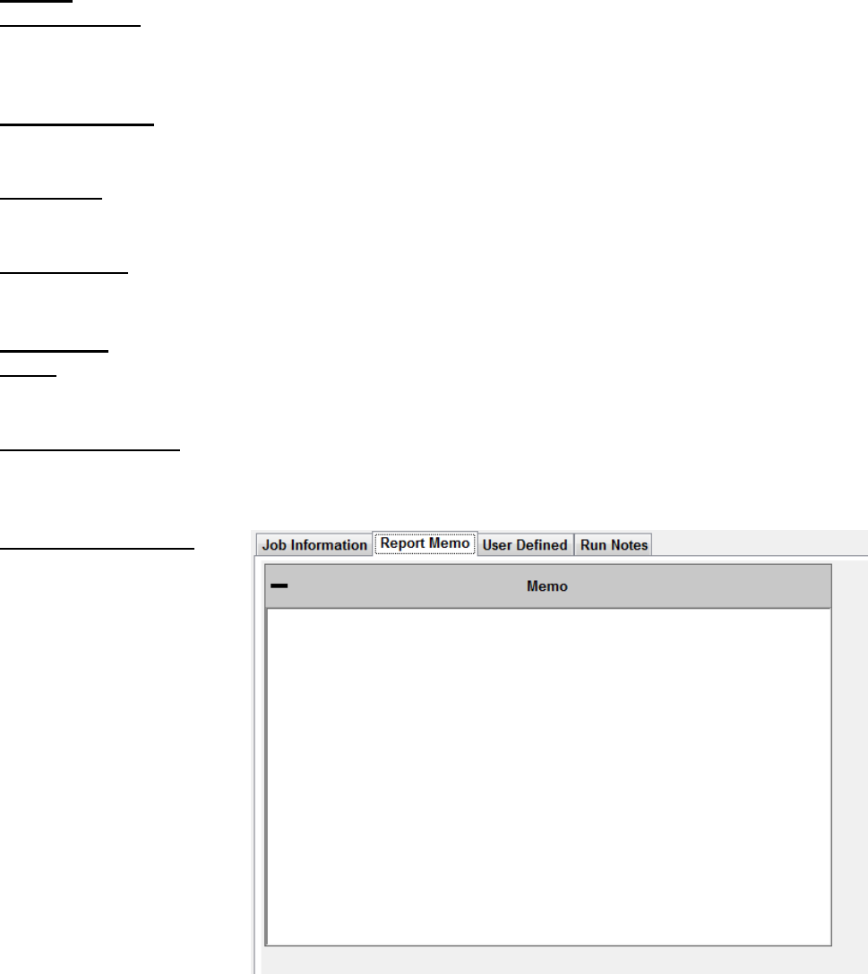
53
Paving
Pavement Type
Input the type of pavement here. Enter pavement types such as Cold–in–Place Asphalt, HMA,
JPCP, CRCP, Open Grade etc.
Paving Direction
Enter the direction of the paver when placing the pavement.
Paving Job
Specify the type of paving job, either corrected or original.
Paving Action
Under paving action list any further information about the paving process.
Additional
Tester
The individual operating the profiling equipment over the pavement surface.
Provisions/Weather
The weather at the time of profiling the pavement. Such as: Cold, Hot, Overcast, Morning,
Afternoon, Evening, etc.
2.2.2. - Report Memo
Report Memo is a section
available for inputting large
amounts of text to be saved
along with the data file.
Anything from reminders
to stationing can be
inputted into the Report
Memo and not influence
the data.
Figure 83: The Report
Memo window
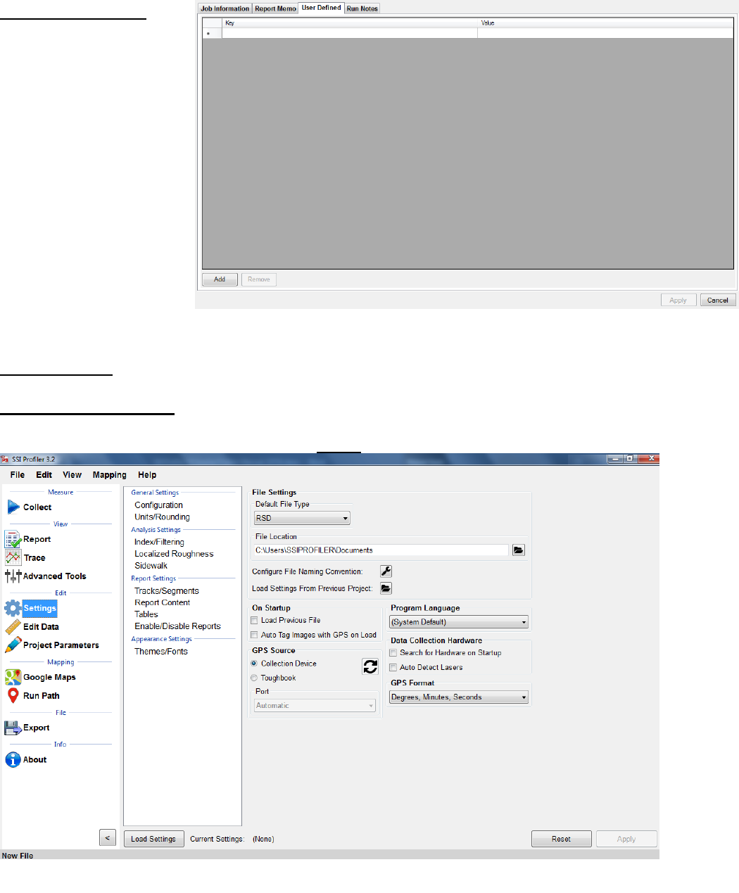
54
2.2.3. - User Defined
Additional parameters can
be stored in the data file as
desired by the operator.
Consult the contract for
any additional user defined
parameters that may be
required for the profile data
files.
Add new parameters by
selecting ‘Add’ at the
bottom of the window. The
parameters are entered by
double-left clicking on the
‘Key’ column and typing in
the required information.
2.2. - Settings
User defined parameters can be used in conjunction with the Default File Naming tool.
2.2.1. – General Settings
The default file preferences and settings for report generation can be changed under the “Settings”.
Whenever a change is made, always select the Apply icon in the lower right corner.
Figure 84: The User Defined section
Figure 85: The General Settings window showing the Configuration parameters.
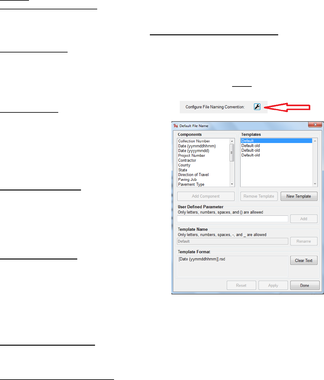
55
Section 1
Default File Type (RSD, RHD)
The drop-down menu can be used to select the type of file opened in Profiler V3. Both RHD and
RSD files can be imported into the program at any time. The default file type is the file format that
will be used automatically when files are opened. Profiler V3 only saves in the RSD format.
Default File Location
The default file location is the folder on the computer or external device that Profiler will search
for the default file type. This folder can be changed through the Browse icon. If a location is used
to open a file, the program will use this location to open files for future attempts. This feature saves
time opening files since the program opens directly to the file location. Select Apply after a folder
is chosen.
Default File Name
The file name can be chosen to have a name based on
parameters of the program or by using a pre-loaded
template. The parameters can be chosen from the list of
(multiple can be chosen): Contractor, Country, Tester,
etc. When a template is selected there will be a preview
at the bottom of the window. Select OK and Apply to set
this configuration as the default file name.
Creating a New Template
Create a New Template by selecting the “New
Template” icon on the right side of the window. Select
the template’s name to rename it and append parameters
to it. The template will be used as long as it is selected
when OK is selected at the bottom right corner when
exiting the Default File Name tool.
User Defined Parameter
To create parameters that are specific to the job, type a
new parameter name into the User Defined Parameter
text box and select “Add User Defined Parameter.” The
bracketed variable will appear in the filename preview.
To add information to the user defined parameter, open
Project Parameters and the User Defined Tab. The name
of the parameter will be under the Key column. Under the Value column, enter the information
that is needed in the filename.
Changing the Template Name
The template’s name can be changed by changing the characters under Template Name. Once a
change is made, the Rename icon will be available. Select OK or Apply to save the changes.
Adding Parameters to the Template
When adding parameters to the template they will only be added to the right end of the template,
as seen in the naming preview. Select Apply after changes are made to the template.
Figure 86: The custom file naming convention window

56
On Startup
Load Previous File on Startup
If this box is selected in figure 85, the file that was open when profiler closed last will be reopened
when the program is started. A report of this file will be generated when the program is opened.
Load Previous File’s Settings
The user may choose a previous file to save time if entering the same analysis parameters or project
parameters under “Settings.” To load a previous file’s setting’s, choose the file under General
Settings or start a new file and choose one of the three options.
Use Last File’s Parameters
This option will use the last file’s settings under the localized roughness and project parameters.
Choose from a Previous File (Browse)
When this option is chosen a window explorer window will appear and the user may select a file
that is saved on the computer to import the saved file’s parameters under analysis and project
parameters.
Set File Parameters after Collection
By choosing this option the user will not import a previously collected file but will instead
manually set the parameters after the collection has finished.
Automatically Refresh Reports
The reports will automatically refresh when the operator navigates to the report window from
another tab. When the user makes a change of report type within the report window, the refresh
button will have to be selected manually.
Data Collection Hardware
Search for Hardware on Startup
If this option is selected in figure 85, the program will search for hardware, and if available, will
connect to it upon opening the program.
Disconnect Hardware When Changing Tabs
If this feature is checked the program will disconnect from the hardware when the operator leaves
the collect tab.
Auto Detect Lasers
This feature will use the health string to determine the type of laser that is connected to the system.
This is not an end-all solution. Please check the laser type in the System Settings under the
collection window prior to any data collection or perform a height verification.

57
Report Generation
Generate Reports in Color
If the reports are generated in color, the defect types will be more visible. On the trace reports dips
will appear be highlighted blue and bumps will be highlighted red.
Include the Footer
If the footer is included, the file name and the page number will be printed at the bottom of each
page for the report. Select the check box to apply this feature.
Do not include the footer while printing with a Printrex 422.
Enable Animations
When enable animations is selected, the windows within Profiler V3 will slide across the screen
whenever the operator moves from one section to another (Reports to Collect). This feature does
not affect the functionality of the program, but adds an aesthetic behavior when changing windows.
Resize for Printrex
Check this box if printing with a Printrex 422 and uncheck include the footer. This option allows
the operator to correctly scale the trace for use with a sliding scale if necessary.
Report Scale
Depending on the specification and system type, the operator may choose between a 1”:25’ or a
1”:15’ scale. The bridge profilograph is usually a 1”:15’ scale while the California profilograph
and all road profiling is 1”:25’ scale.
Formatting
Font Settings
The report font can be changed by selecting the Font Settings icon under formatting. This allows
the user to make the size of the font smaller or larger. The image scaling allows the user to print
off less pages by increasing the scaling factor. The window that appears can also change the font
to a strike-through or an underline.
Image Scaling
The default for the image scaling is 100%. When image scaling is set to a percentage greater than
100%, it acts the same way as the zoom function. The size of the traces within the reports will
increase.
Profiler Software Update
Profiler V3 will check the internet connection by attempting to connect to the website listed under
this location. If the internet connection is found, the updates will be available for download from
the SSI server.

58
2.2.2. – Analysis Parameters (Ride Values)
Changing the units alters the specifications for defects and the ride numbers.
Section 1 – Units
Profiling Units
English
Selecting English units sets the segment length to 528 feet. English units use inches for the
height of the defects, counts for roughness settings, and feet for scallop width and filter
lengths. After every change of units, select apply in the lower right corner to save.
Metric Meters
Selecting Metric Meters units, the blanking band, scallop height and scallop resolution are
all in centimeters. The rest of the measurements for scallop width and filter lengths are in
meters. The Metric Meters and Metric Centimeters settings have the same units of
centimeters for height, and meters for length for all sections of defects and roughness. After
every adjustment of units, select apply in the lower right corner to save changes.
Metric Centimeters
Selecting Metric Centimeters units, the blanking band, scallop height and scallop resolution
are all in centimeters. The rest of the measurements for scallop width and filter lengths are
in meters. The Metric Meters and Metric Centimeters settings have the same units of
centimeters for height, and meters for length, for all sections of defects and roughness.
After every adjustment of units, select apply in the lower right corner to save changes.
Metric Millimeters
Selecting Metric Millimeters units, the blanking band, scallop height and scallop resolution
are all in millimeters. The rest of the measurements for scallop width and filter lengths are
in meters. After every adjustment of units, select apply in the lower right corner to save
changes.
CA Bridge
The CA Bridge setting is based off the California Bridge Profilograph specification, which
is twelve feet long instead of the California Profilograph's 25 foot length. The CA Bridge
setting is in English units and has a segment length of 100 feet. After every adjustment of
units, select apply in the lower right corner to save changes.
CA Bridge Metric
This setting is used for simulating the Bridge Profilograph's 12 foot frame. The Bridge
Metric setting is the metric version of the CA Bridge Profilograph. Its segment length is
90 meters and the defects and counts for roughness are in millimeters and meters. After
every adjustment of units, select apply in the lower right corner to save changes.
Segment Length
Segment length is the interval of profiling that is used to calculate ride values. Traditionally
the distance used for segment length is one-tenth of a mile, or 528 feet (160 meters).

59
This section is adjusted by using the arrow keys or double-left clicking in the box to type
the segment length.
Merge Last Segment if Less Than
If the last segment is shorter than the segment length, it can be merged into the segment
before it. This will prevent large ride values from short distances. Only use if your
specification does not require a specific segment length for pay incentives. The last
segment length will be changed if this feature is used.
Exclude Paused Sections
When Exclude Pause Sections is selected, the paused sections created during collection or
through the Segment Adjustment window will not be included in the report or the
calculation of the ride values.
Include Paused Sections
When Include Paused Sections is selected, the paused sections are included with the actual
collection when calculating the ride values. The report will show the paused sections in the
segment summary and the trace view.
Paused Sections Only
When ´Include Paused Sections Only´ is selected from the drop-down menu, only the
paused sections created during collection or through the Segment Adjustment Window will
be displayed in reports and used to calculate ride values and counts for roughness.
Section 3 - Analysis Type
IRI
The International Roughness Index is a universal ride index for concrete and asphalt roads around
the world. The profile is analyzed using a quarter-car simulation that is weighted towards the
frequencies of body and vehicle bounce; the most uncomfortable riding conditions.
To calculate IRI in Profiler V3, select IRI from the drop down menu, then adjust the filter settings
if necessary according to the contract specifications. View the report under the Report Tab to
observe IRI.
𝑰𝑹𝑰 = 𝑺𝒕𝒂𝒏𝒅𝒂𝒓𝒊𝒛𝒆𝒅 𝑽𝒆𝒉𝒊𝒄𝒍𝒆′𝒔 𝑨𝒄𝒄𝒖𝒎𝒖𝒍𝒂𝒕𝒆𝒅 𝑺𝒖𝒔𝒑𝒆𝒏𝒔𝒊𝒐𝒏 𝑴𝒐𝒕𝒊𝒐𝒏
𝑫𝒊𝒔𝒕𝒂𝒏𝒄𝒆 𝑻𝒓𝒂𝒗𝒆𝒍𝒆𝒅
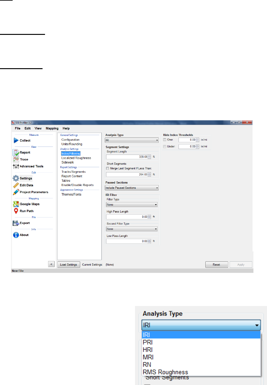
60
PRI
The Profile Ride Index is a simple calculation to classify the smoothness of a road profile against
other roads. The formula for this calculation is:
English Units:
𝟓𝟐𝟖𝟎 𝒇𝒕 × (𝑻𝒐𝒕𝒂𝒍 𝑹𝒐𝒖𝒈𝒉𝒏𝒆𝒔𝒔 𝒊𝒏 𝒊𝒏𝒄𝒉𝒆𝒔 𝒊𝒏 𝑺𝒆𝒈𝒎𝒆𝒏𝒕)(𝑺𝒆𝒈𝒎𝒆𝒏𝒕 𝑳𝒆𝒏𝒈𝒕𝒉 [𝒇𝒕])
⁄
Metric Units:
𝟏𝟎𝟎𝟎 𝒎 × (𝑻𝒐𝒕𝒂𝒍 𝑹𝒐𝒖𝒈𝒉𝒏𝒆𝒔𝒔 𝒊𝒏 𝒎, 𝒄𝒎,𝒐𝒓 𝒎𝒎 𝒊𝒏 𝒔𝒆𝒈𝒎𝒆𝒏𝒕) (𝑺𝒆𝒈𝒎𝒆𝒏𝒕 𝑳𝒆𝒏𝒈𝒕𝒉 [𝒎])
⁄
To calculate the PRI in Profiler V3, select PRI from the Analysis Type drop down menu. Once the
settings are correct, select Apply and then view a report to observe the PRI ride values.
Figure 87: The IRI Analysis Parameters window
Figure 88: The Analysis type drop
down menu displaying all of the Ride
Values options
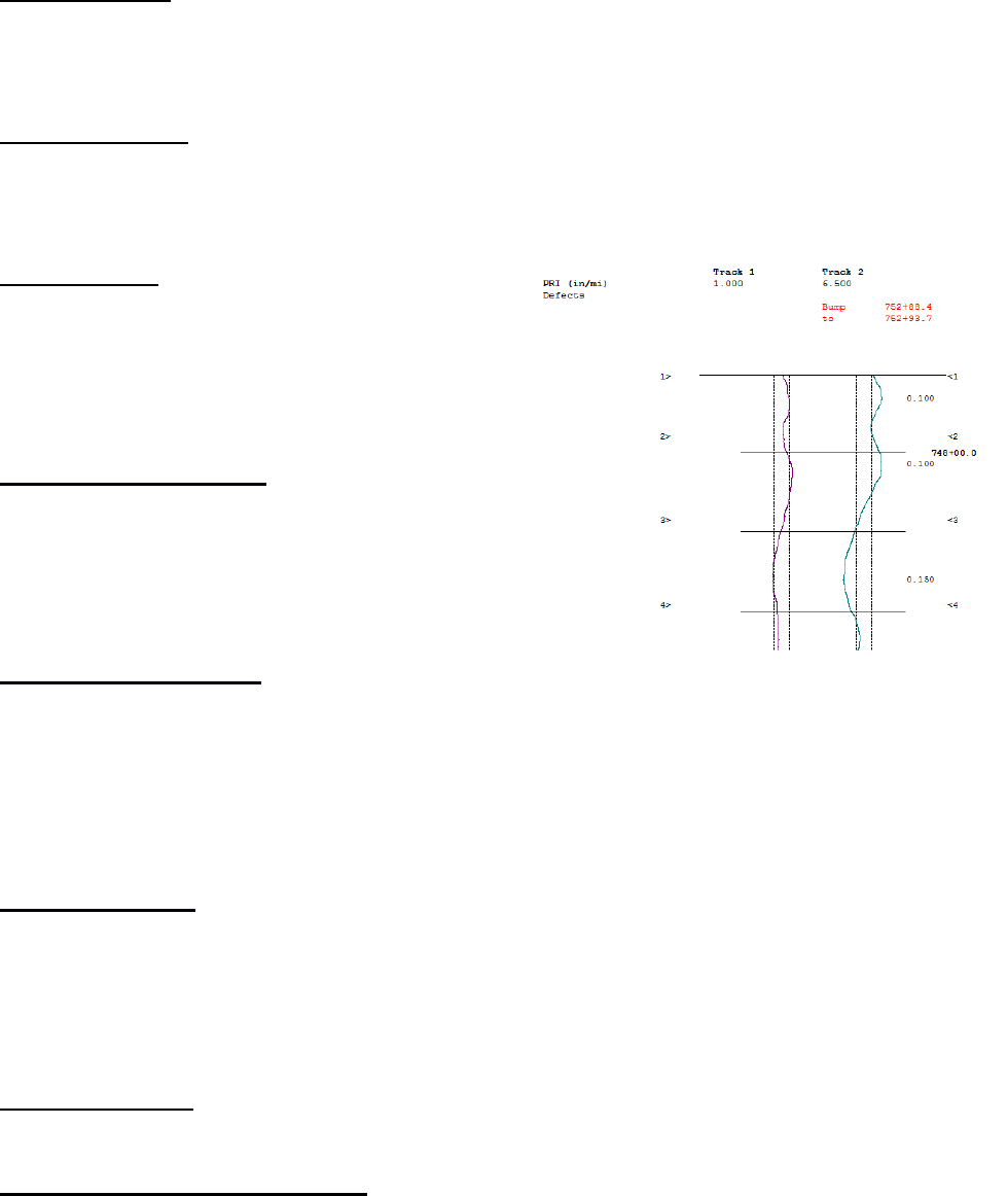
61
PRI Parameters
Note that the PRI Parameters are only for the calculation of the Profile Ride Index (PRI). Blanking
Band, and Scallops have no connection to the manner in which defects are found. For defect
settings, see Localized Roughness.
Scallop Definition
Scallops are the deviations of the profile trace from the blanking band. If the trace exceeds the
defect height but the minimum width of the scallop is not reached, the deviation is not included as
a defect. Although defects are not included in Ride Values, if the deviation still exceeds the defect
height parameter, it adds to counts for roughness.
Blanking Band
The blanking band is a null area that classifies the
height of all sections of the trace within its borders
as zero. Therefore, a trace that remains within the
borders of the blanking band would have zero
counts for roughness and a PRI of zero.
Minimum Scallop Height
The minimum scallop height is the minimum
deviation height from the blanking band or null line.
Frequently, the value for minimum scallop height is
0.035 or 0.9mm, which is the default value for the
Profiler V3 program.
Minimum Scallop Width
The minimum scallop width is traditionally 2 feet (0.61
meters). Review the Department of Transportation
smoothness specification that pertains to the project. The minimum scallop distance is the
minimum longitudinal length (the direction of traffic) that is used to find the deviations of the
profile off of the null line or blanking band. The setting of 2 feet or 0.61 meters is the default
setting for Profiler V3.
Scallop Resolution
The scallop resolution is the accuracy of the height measurement. Current equipment is accurate
to 0.01 inches, the default value for Profiler V3 software. A resolution of one-hundredth of an inch
means that the scallop heights will always be rounded to the hundredth decimal. Consult the recent
smoothness specification released by the overseeing agency to confirm the scallop resolution
value.
Reset File Settings
Selecting this icon brings all values in Settings to their default program values.
Minimum Scallop Height Inclusive
When this box is selected, the minimum scallop height will be included as a scallop. Meaning, if
the minimum scallop height is 0.035, 0.035 will be the minimum instead of 0.0351.
Figure 89: An example of the
blanking band in the trace report.
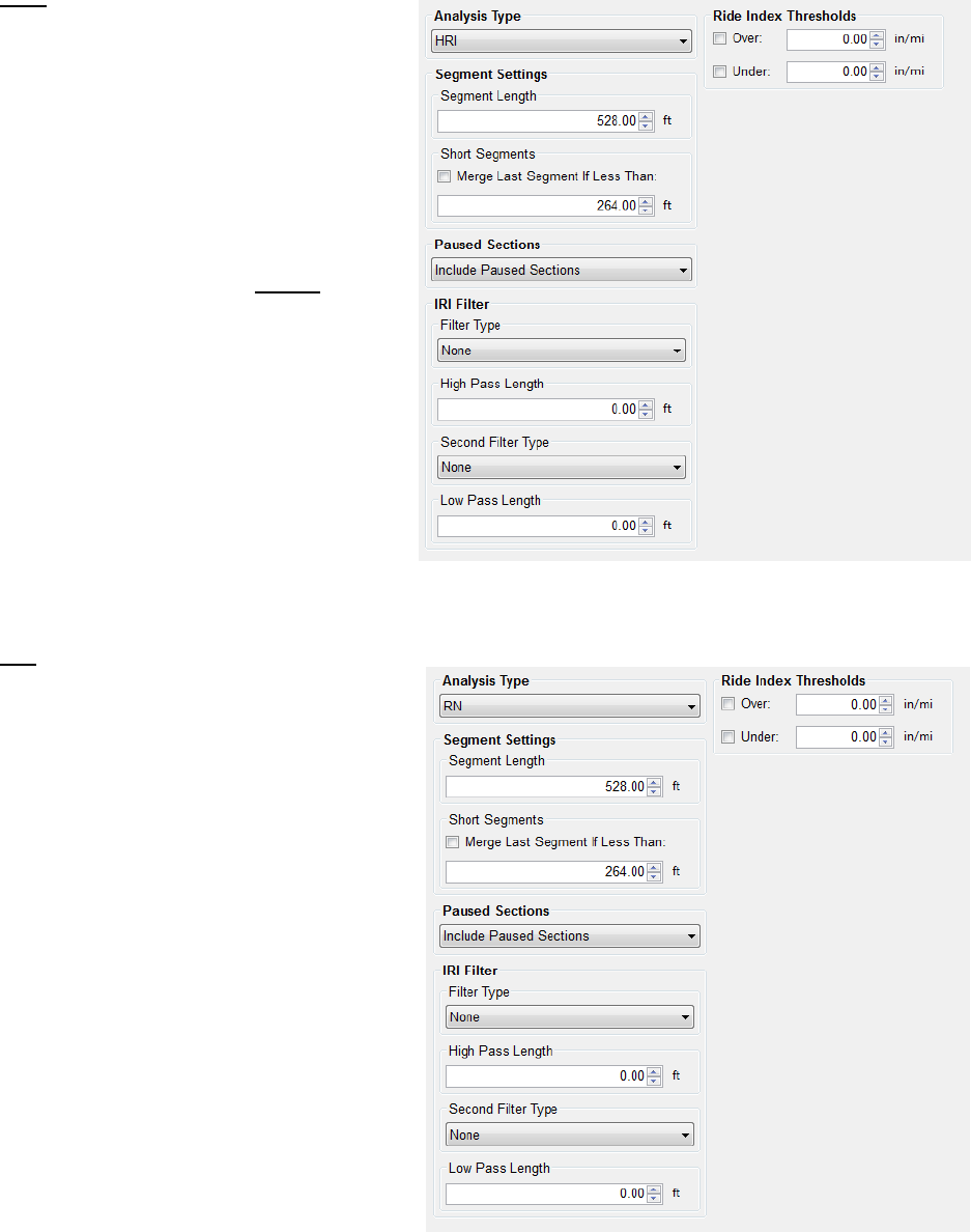
62
HRI
The Half Car Ride Index (HRI) is found
by applying IRI to an average of two
profiles. HRI uses a half car simulation,
unlike IRI which uses a quarter car
simulation. To calculate the HRI in
Profiler V3, select HRI from the
Analysis Type drop down menu and
verify the settings of filter length based
on the project specifications. Once the
filters are correct, select Apply to save
the settings. To view the calculated HRI,
view one of the reports under
View>Report.
RN
The Ride Number (RN) can be calculated
in Profiler V3 by selecting RN from the
Analysis Type drop down menu and
verifying the settings of filter length
based on the project specifications. Once
the filters are correct, select Apply to
save the settings. To view the calculated
RN values, view one of the reports under
View>Report.
Figure 90: The HRI analysis window
with the available filter settings.
Figure 91: The RN analysis
window with the filter options
shown.
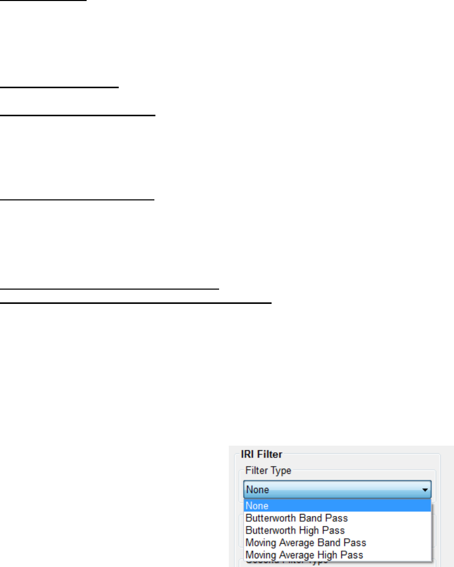
63
RMS Roughness
The RMS roughness is a ride value method calculated by profile height over a base length of 25
feet. This is how RMS roughness gets inches as it´s units. The RMS Roughness report gives a
depiction of the amplitude and wavelength but does not necessarily give the frequency that this
amplitude and wavelength occurs. The output is similar to a PSD plot.
Ride Index Thresholds
Highlight Index Values Above
The operator may choose the threshold in which to highlight a certain interval of ride index values
above a number. The highlight color is red and can be seen in the summary table of the reports.
Only the segment ride values are highlighted, not the total ride values. This is convenient for
comparing segment ride indexes to determine where grinding should be done.
Highlight Index Values Below
The operator may choose the threshold to highlight a certain interval of ride index values below a
chosen number. The highlight color will be green and it is seen in the summary table of the reports.
Only the segment ride values are highlighted, not the total ride values. This is convenient for
comparing segment ride indexes to determine where grinding should be done.
2.2.3. – Analysis Parameters: Filters
Section 1 - IRI/HRI Filter----Same for IRI, HRI, RN
High Pass Filter – The High Pass Filter will remove any trend in the data that is less than the
chosen length. The length can be selected by typing the value in the box or by using the arrows to
adjust the input.
Low Pass Filter – The Low Pass Filter will remove any trend in the data greater than the chosen
length. The length can be selected by typing the value in the box or by using the arrows to adjust
the input.
Figure 92: The filters within the
IRI analysis parameter window
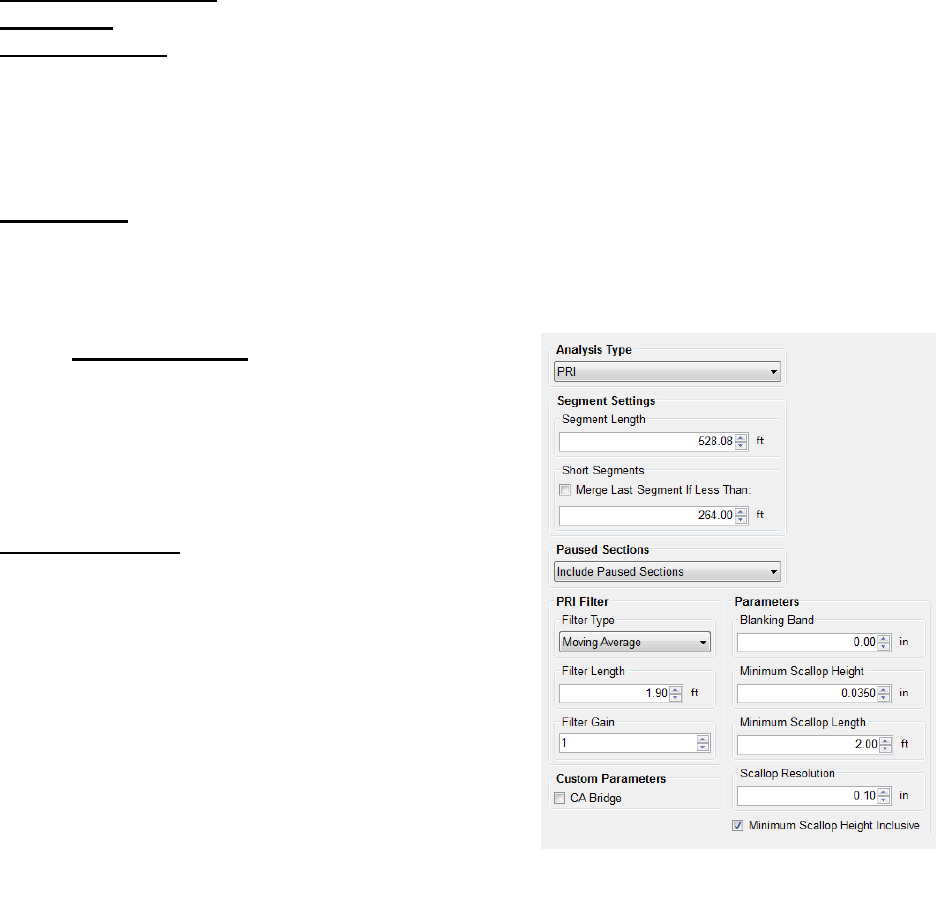
64
Section 2 - PRI Filter
Filter Type
Moving Average
A length of 2.0 feet can be chosen for the Moving Average Filter, depending on the contract
specification. The use of the moving average filter was initially used by the Kansas Department of
Transportation (see Report No. K-TRAN: KSU-9302 “An Automated System for Determination
of Pavement Profile Index and Location of Bumps for Grinding from the Profilograph Traces.)
Butterworth
The third order Butterworth filter has a default length of 2.0 feet. The Butterworth filter is not
required for updated profiling specifications. The Butterworth filter was used for the original
automated Profilograph systems.
Available Filters:
Moving Average High Pass Filter
Moving Average Band Pass Filter
Butterworth High Pass Filter
Butterworth Band Pass Filter
Filter Gain—1.00
The filter gain is only used for necessary adjustments
while comparing different profiling systems. The filter
gain does not need to be used in normal profiling
environments. When comparing high speed profiling
systems to other Profilograph systems, the filter gain
may be used to change the output of the data files. A
filter gain setting of 1.00 does not affect the collected
data. For typical profiling, use the default setting of 1.
Figure 93: The filters for the PRI analysis
parameter
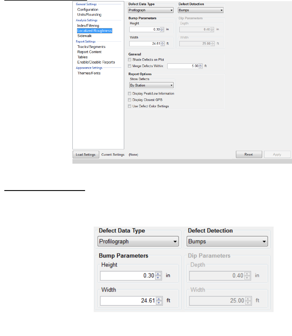
65
2.2.4. –Localized Roughness
Localized roughness
refers to the bumps and
dips that occur over a
determined distance.
Section 1 - Defect Detection
The operator may choose the mode of defect detection in Profiler V3. The options to choose from
are Bumps, Dips, Both, and None. To select the type, use the drop down menu labeled Defect
Detection. No filters are associated with localized roughness. “Both” is selected by default.
If only one defect type is
chosen, be sure to change the
correct settings. Do not change
the dip parameters instead of
the bump parameters by
mistake. The report section of
Profiler V3 can be used to
review the settings and traces
of the collection.
Figure 94: The
Localized Roughness
window with the defect
settings.
Figure 95: When only bumps are selected from the drop
down menu, the dip parameters become unavailable.
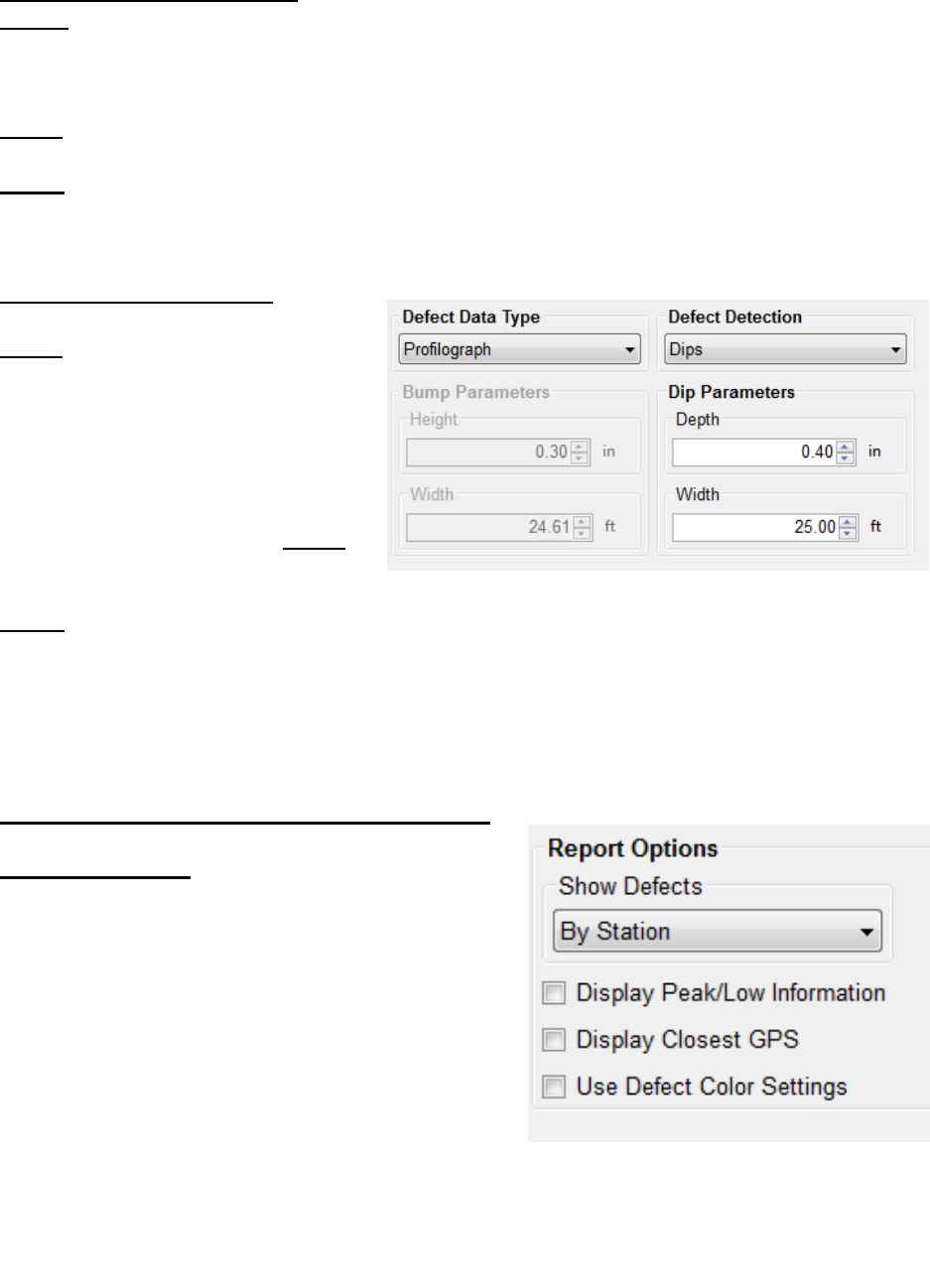
66
Section 2 - Bump Parameters
Height
Bump height is the maximum distance that a profile may deviate within the width of the bump.
The width of the bump is the length of a Profilograph, or 25 feet (7.62 meters). A typical value for
bump height is 0.3 inches. When the settings are changed for the bump parameters, always select
Apply to save changes.
Width
The width of a bump is based on the length of a Profilograph; 25 feet or 7.62 meters. This is the
default value for the Profiler software.
Section 3 - Dip Parameters
Depth
The depth of a dip is the maximum
distance a profile trace may deviate
within the width of the dip (25 ft or
7.62 m). The default value for dip
height is 0.4 inches or 10.2 millimeters.
When the settings are changed for the
dip parameters, always select Apply to
save changes.
Width
The width of a dip is based on the
length of a Profilograph; 25 feet or 7.62
meters. This is the default value for the
Profiler V3 software.
Section 4 - Localized Roughness Report Options
Display Defects By:
The operator has the option to display defects by the
station number or by the track in the report. To modify
this setting, choose the desired display setting then
select apply to save the changes. When displaying the
defects by track, the defects are split up into their
respective tracks. When the defects are organized by
stationing they are listed in the same classification.
Figure 96: When only dips are being tested for, the
bump parameters become unavailable.
Figure 97: The localized
roughness settings for
displaying defects
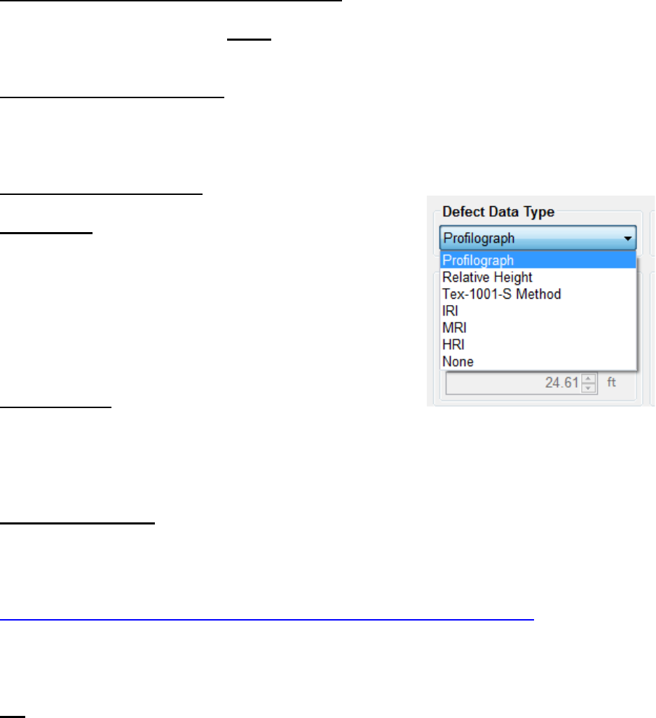
67
Display Maximum Peak/Low Values for Defects
Selecting this check box shows the peak values for the defects when viewing the summary report.
When altering the settings, select Apply to save the changes.
Identify GPS Closest to Defects
To show the closest GPS reading to each defect, select this check box. When viewing the summary,
the GPS coordinates will be in the table with Defect Type, Track, Segment, and Stationing of the
defect.
Section 5 - Defect Data Type
Profilograph
The Profilograph defect data type is the most common method
used to find defects. The settings are the same as described
above in Analysis Parameters, defect detection, bump
parameters and dip parameters.
Relative Height
Relative Height defect data type finds the defects of the profiled surface through the local
differences in the trace. The settings required to be inputted within the Localized Roughness tab
of the Settings Window are the bump and/or dip parameters.
Texas-1001-S Method
The Texas 1001-S Method is used mainly by the Texas DOT for profiling with inertial profilers.
The procedures and information for this test method can be found on the Texas DOT website; a
direct link is below.
ftp://ftp.dot.state.tx.us/pub/txdot-info/cst/TMS/1000-S_series/pdfs/spe1001.pdf
The Texas-1001-S method detects localized roughness (defects) of the profiled surface by applying
the base length and the threshold values saved in the Settings Window.
IRI
When IRI Defect Data type is selected, the IRI calculation will be used to find the road’s defects
(localized roughness) of the profiled surface. If this setting is selected the IRI ride value will not
be shown in the summary. To list the IRI ride values on the reports, select the analysis type to be
IRI in the Analysis Parameters tab. The ride interval is set (usually to 25 feet, in English units) and
is used as a sliding guide across the profile. When the summation of the profile’s IRI exceeds the
threshold, the entire continuous length which exceeds the threshold will be an area of localized
roughness.
Figure 98: The types of testing available
to find the defects in the data.
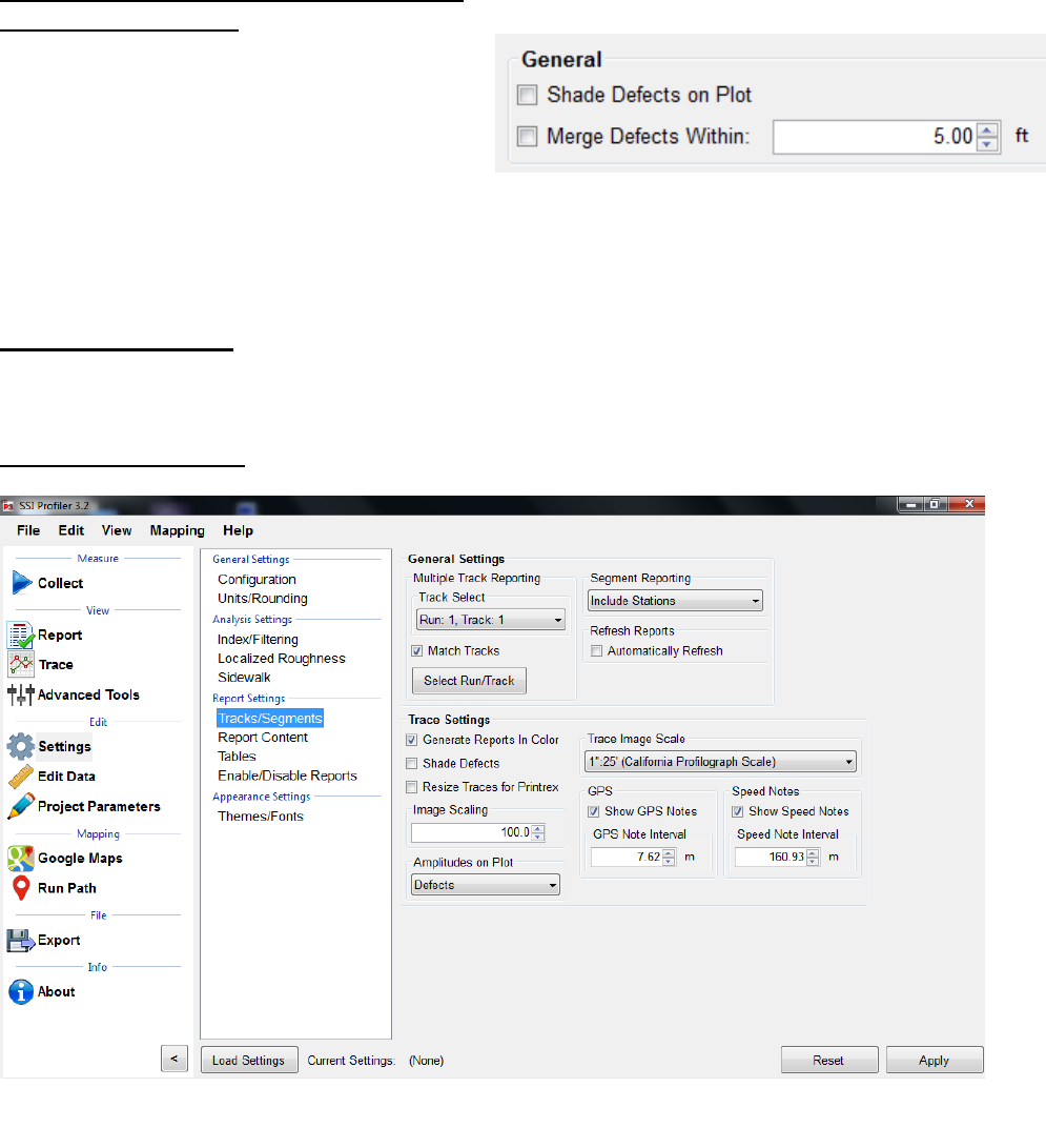
68
Section 6 –General in Localized Roughness
Merge Defects within:
The operator is able to merge multiple defects
into one defect to eliminate high frequency
grinding patterns. The action of merging
defects does not affect the ride values or the
defect heights. Merging adjusts the start and
end stationing of two defects into one length.
The default value of the merge defects tool is 5
feet. To use this feature, select the check box
next to “Merge Defects Within.”
Shade Defects on Plot
The operator may use this feature to help identify defects.
2.2.5. - Report Settings
Figure 100: The report options window.
Figure 99: Merge Defects
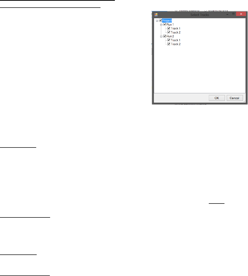
69
Track/Segments General Settings
Multiple Track Reporting Track Select
Track Select is the tool that is used to select the track which
will to be shown in the reports. From the drop-down menu,
select a single track based on the label of [Run: Number,
Track: Number].
When Match Tracks is not selected, the reports will only
show one trace. The selected run in the drop-down menu will
be the only run shown in the Reports of Single Trace,
Continuous Trace, and All Traces.
To plot multiple or all tracks that are saved within the file,
select Match Tracks. See below for information on Match
Tracks. When Match Tracks is selected, the run shown on the
collapsed Track Select drop down menu will be on the left
side of the trace in the report. The figure above will have Run
1, Track 1 on the left side trace report.
To report specific runs and tracks, select the “Select Runs”
icon under Multiple Track Reporting. Here the user can select
certain tracks or runs that will be included in the reports, localized roughness and ride value
calculations.
Match Tracks
When the Match Tracks check box is selected, all of the tracks associated with the file will be
displayed in the reports of Single Trace, Continuous Trace, and All Traces.
With Profilograph profiles for the Profilograph, there are only two-wheel paths, while with some
High-Speed Profiling Systems there have three traces. When dealing with multiple traces, the
Track Select can change the order in which the tracks are displayed in the reports. The track that
is selected in the drop-down menu within “Track Select” will be the trace that is on the left side of
the report of the single trace, continuous trace and all traces plots.
In order to save changes made to the Multiple Trace Reporting Section, always select Apply.
Segment Reporting
The operator can choose to Include Stations and Segments Only. To include station and segment
numbers in the continuous trace report select “Include Stations.” To only display the segment
numbers select, “Segments Only.”
Trace Settings
This section relates to the amplitudes of the collected data relative to the trace.
Amplitudes on Plot
The operator has the option of showing the amplitudes for either the scallops or the defects on the
plot. When comparing the reports to the SSI spreadsheet defects templates, the operators should
choose to show only the defect heights. Scallops are the deviations of the trace outside of the
centerline or blanking band. The defect heights will also be shown when scallops are selected,
however there will be more labels on the deviations. Therefore, it is acceptable to leave the
amplitudes on scallops.
Figure 101: The Track and Run
Selection Window
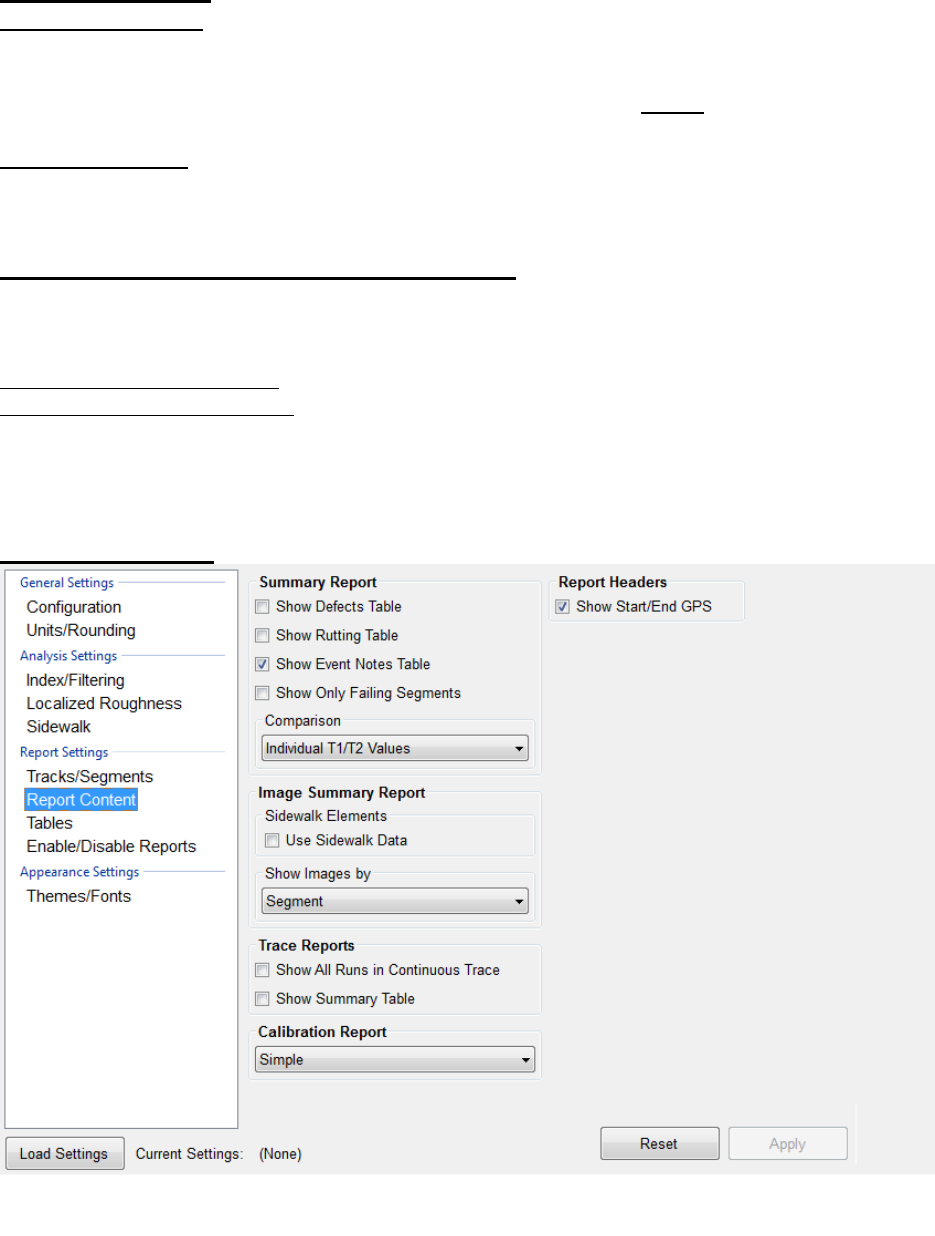
70
Note Reporting
Report Speed Notes
To have the speed notes included in the printed report, the check box to the left of “Report Speed
Notes” should be selected. To change the interval which the notes are reported, select the
“Customize Reporting Intervals” icon. If changes are made, select Apply.
Report GPS Notes
To have the GPS notes included in the report, select this box. If this box is not selected, the GPS
notes will not be shown at the bottom of the report.
Customize Reporting Intervals (GPS/Speed Notes)
The reporting intervals are the distances traveled while collecting data to between a GPS and or
the Speed note on the report. A new note will be shown each time the distance of the interval is
traveled. The types of intervals that can be adjusted are:
GPS Note Reporting Interval
Speed Note Reporting Interval
In the case that the report becomes cluttered with the report notes, the operator may increase the
reporting intervals to simplify the printout.
Report Content
Figure 102: The Report Content window
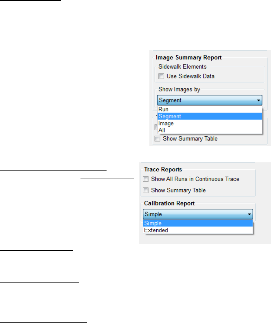
71
Summary Report
The operator can decide the data to report in the summary report. These include: The Defects Table,
the Rutting Table, the Events Note Table or to Show Only Failing Segments. The data can be
compared by individual Track 1 and Track 2 values or using the average of these.
The Report Headers option lets the operator choose the Show Start/End GPS coordinates for the
run.
Image Summary Report
This section of the Report Content Tab allows for the
operator to chose how to show the images collected
(applicable to systems with a camera). The images
can be shown by Run, Segment, Image or All.
For Sidewalk Profilers, the operator should select
the checkbox above the drop-down menu.
Trace and Calibration Reports
The operator can choose to Show All Runs in
Continuous Trace. When this box is selected,
all runs within the file will be displayed within
the continuous trace. The organization of the
runs and tracks is always the same when this
option is selected. If Run 1 will come first, then
Run 2. Track 1 will always be the left-most trace
on the report.
Show Summary in Table
When this box is selected, the summary header will
be included in the All Traces report.
Simple Calibration Report
The simple report contains information about the software version and the calibration summary.
The included calibrations are the accelerometer calibration constants, distance calibration counts,
and inclinometer calibration settings.
Extended Calibration Report
The extended report has the calibration and the verification data from the last verification
procedures. The verifications for the inclinometer, height sensor, and the bounce test are all
included along with the calibrations for the accelerometer, inclinometer, and distance encoder.
Figure 103: The Image Summary Report
options under Report Content.
Figure 104: The Trace and Calibration
Report options.
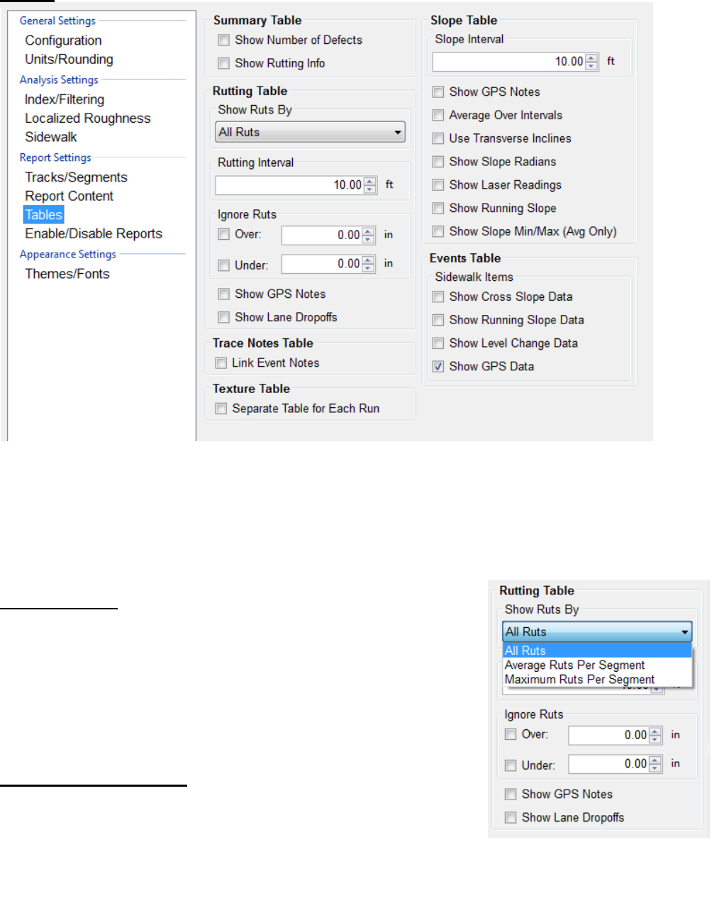
72
Tables
The table options under report setting lets the operator chose what tables to include in the report.
The Summary, Trace Notes and Events Table are used thought SSI’s Profiling systems. The
Summary Table section includes the ‘Show number of Defects’ and the ‘show Rutting Info’
checkboxes. Show GPS Data is selected by default in the Events Table.
Rutting Table
For systems with 3 or more lasers, the operator has the option to
change the rut reporting per segment to Report All Ruts, Report
Average Rut or Report Maximum Rut per segment. When All Ruts is
selected it’s possible to report more than one rut. While average or
maximum rut reporting is selected, the program will only report one
rut value per segment. The segment length is set below in the interval
of reporting.
Rut Interval of Reporting
The interval of reporting is set to quantify the segment length for the
calculation of maximum and average rut. The interval of reporting has
no effect on reporting every rut.
The operator may also choose to Ignore Ruts over or under any
specific value and include GPS Notes and Lane Dropoffs.
Figure 105: The Table options under Report Settings.
Figure 106: The Rutting Table options
under Report Settings.
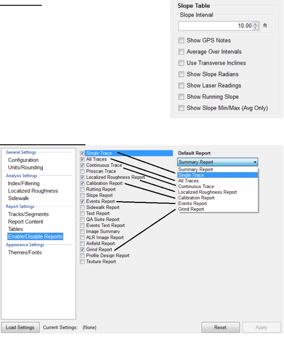
73
Slope Table
For systems with an inclinometer or an IMU (Inertial
Measuring Unit), The Slope Table lets the operator
configure the information reported. First chose the
interval by typing in or using the up/down arrows and
then select the units. 10.00 feet is the default interval.
Enable/Disable Reports
This feature allows the user to select the type of reports that appear in the drop-down menu. To
have a report not be displayed in the drop-down menu, deselect the check box. These reports will
be reflected in the dropdown menu to the right and also in the Reports Section of Profiler V3. See
figures 108 and 109.
Figure 107: The Slope Table options
under Report Settings.
Figure 108: The Enable/Disable Reports options under Report Settings.
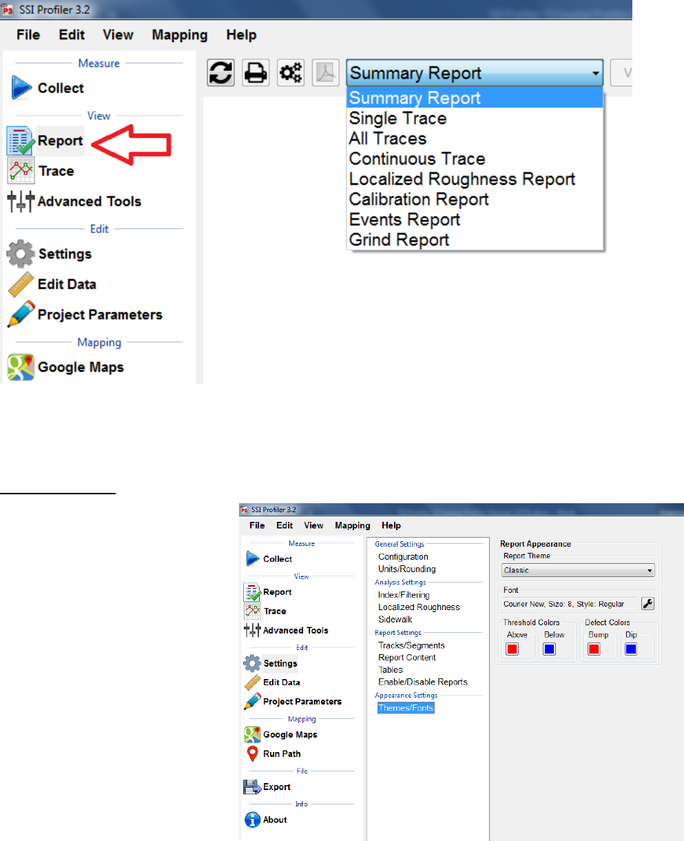
74
Themes/Fonts
Profiler V3 lets the operator
choose between two different
Reports Themes: Classic (default)
and Light. The Font can also be
changed along with the Threshold
Colors and the Defect Colors.
Figure 109: The Enable/Disable Reports selection reflected in the main Report tab of Profiler V3.
Figure 110: Themes and Fonts
option under Appearance settings.
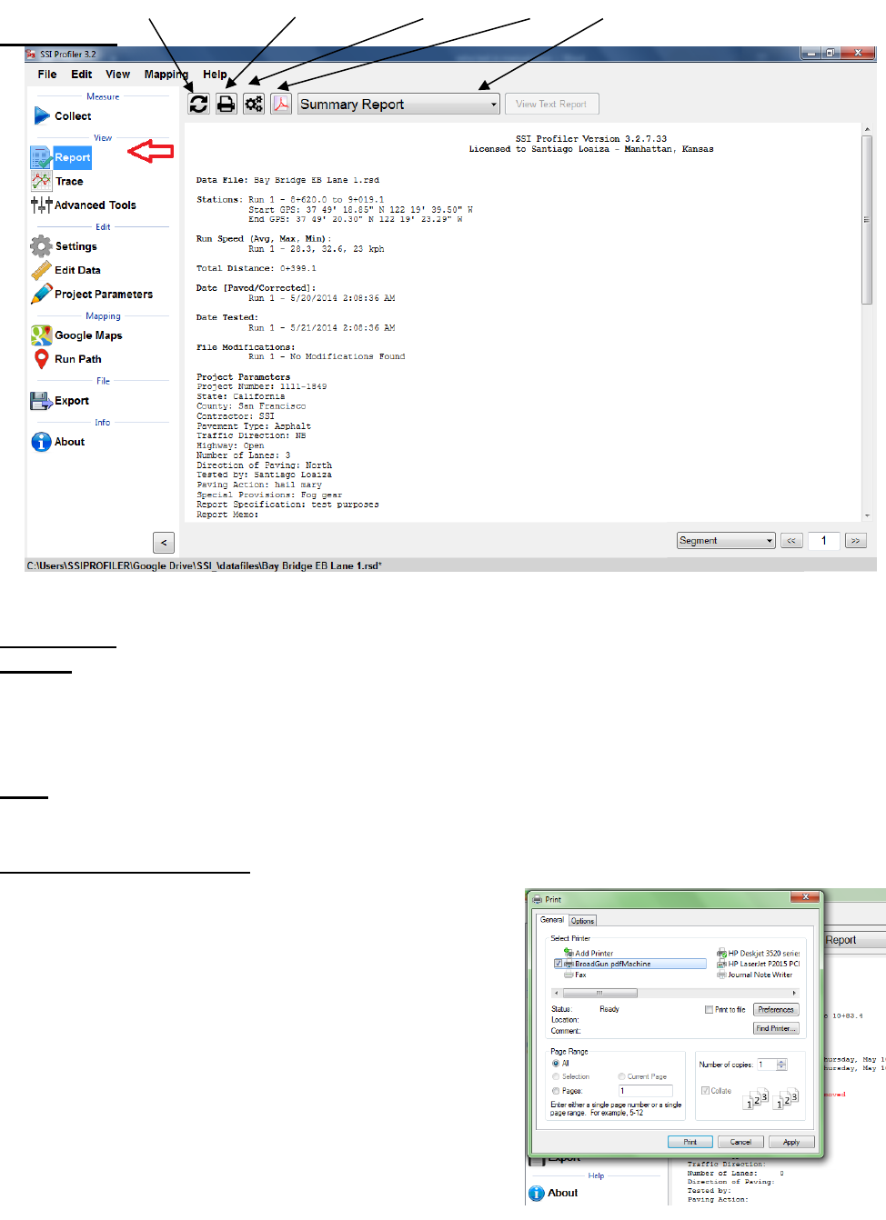
75
3. 0 – View
3.1. - Report
Refresh
It is required to refresh the Report window whenever a change is made to the Project Parameters,
Settings, or Report Options. The refresh icon is located at the top left of the Report window. Select
the refresh button and verify that the information is accurate before printing.
Print
Always confirm the correct report is being printed by selecting the refresh icon.
A Connected Local Printer
To print a report, select the print icon in the Report window
or select CTRL+P on the keyboard. The print window will
appear. Within the window, select the printer to be used and
verify that the printer settings are correct. When ‘Print’ is
selected, the document will be sent to the printer.
If more printing options are needed, select the
‘Preferences’ icon. This icon will open a window that is
printer specific that contains information about the
orientation, paper size, and image quality.
Figure 112: Printing Options Window
Refresh Icon Print Icons Page Setup PDF Drop Down Report Menu
Figure 111: The summary header of a single trace report.
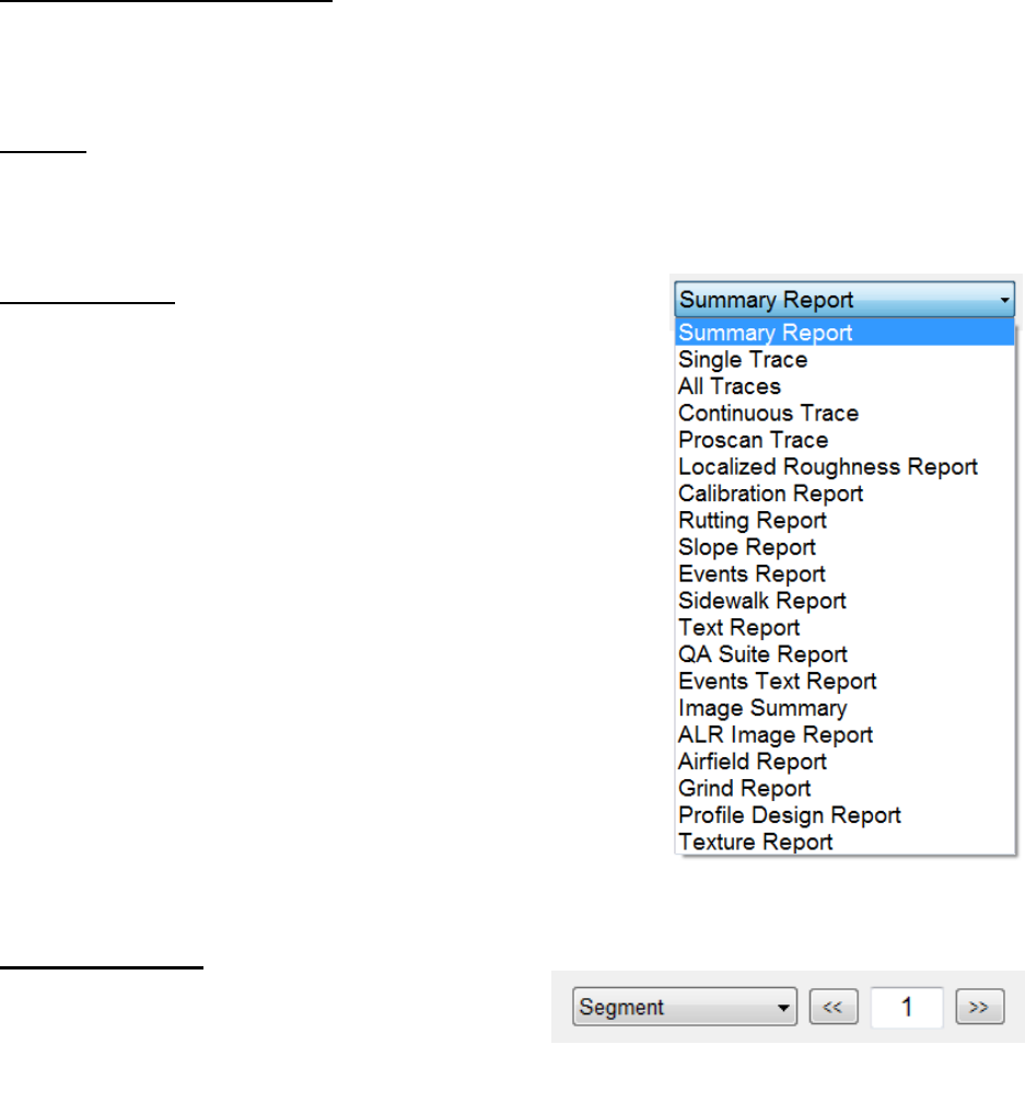
76
Printrex 422 Thermal Printer
Confirm under the settings for the Printrex 422 that the paper size is 4 inches wide on a 150-foot
roll. This setting can be chosen under Preferences>Advanced Settings. It is recommended to use
Contiguous as the end of page control.
To PDF
The Adobe Symbol between the Printer symbol and the report type will print the report to PDF
format if the Broadgun PDF printer is installed. Contact SSI support is Broadgun is not installed
or you are having issues with your PDF printer.
Report Options
The Report Options available in Profiler V3 are Summary
Report, Single Trace, All Traces, Continuous Trace, Proscan
Trace, Localized Roughness Report, Calibration Report,
Rutting Report, Slope Report, Events Report, Sidewalk
Report, Text Report, QA Suite Report, Events Text Report,
Image Summary, ALR Image Report, Airfield Report, Grind
Report, Profile Design Report, Texture Report.
Unless directed by the overseeing agency, the frequently used
reports are Summary Report, Single Trace, Continuous Trace
and Calibration Report. These reports are commonly used due
to the information provided within them. All of these reports
have the locations of defects and the information entered in
Project Parameters and Localized Roughness.
View by Segments
By selecting Segments (the default setting) the
operator may navigate through the segments of the
file by typing in the segment number and selecting
‘Enter’, or by using the arrow keys to the right of
the box.
If the operator is not in Single Trace while using this feature, the program will adapt and open
Single Trace when the Report window generates.
Figure 113: The drop-down menu for the report
options
Figure 114: The segment or defect navigator
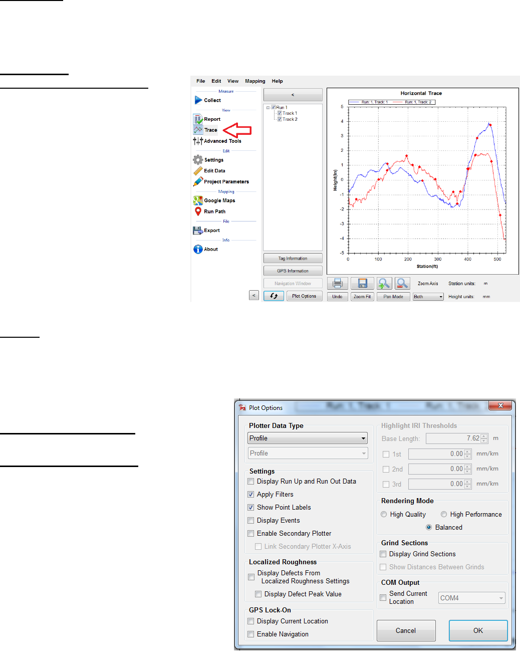
77
3.2 – Collect
To collect data the operator should select the Collect Icon when the hardware is attached. Once the
hardware is found, the data collection may begin. See the Collection section of this manual for
procedures to perform prior and during a collection.
3.3. – Trace
Choosing Tracks for Plotting
To choose tracks for plotting in the
trace window, select the check box
next to the desired tracks. Once all of
the necessary tracks are checked,
select the refresh icon to view the
tracks within the plot.
Whenever a change is made by
deselecting a track or checking a new
track, select the refresh icon to have it
appear in the trace. If the refresh icon
is not selected, the trace will not
update and the changes will not be
shown. Review the legend to verify
that all of the selected tracks are
shown in the plot.
Refresh
It is required to refresh the Trace window whenever a change is made to the track selections. The
refresh icon is located at the bottom left of the Trace window. Select the refresh button and verify
that the trace is accurate before a print is made.
Plot Options Icon
Profile/Continuous IRI
The drop-down menu allows the user to select
options of Profile and Continuous IRI, MRI or
HRI, Median Profile, Segmented Bar IRI and
Birds Eye View. It is recommended to use the
median profile option when reviewing the
collected relative elevation profile. The
operator may view two graphs simultaneously
by selecting the secondary plotter option.
When Continuous IRI is selected, the operator
may not choose the option to include Run Up
and Run out data.
Figure 115: An example of the profile trace
Figure 116: Recommended Plot Options window
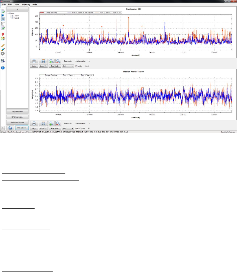
78
Plot Options Settings
Display Run in/ Run out Data
Many High Speed Profiler data files have Run in and/or Run out data associated with them. To
include this data in the trace, select the check box next to “Display Run Up and Run out Data.”
Apply filters
To apply the filters select the check box “Apply Filters.”
Show Point Labels
Showing point labels allows the user to move the cursor over the profile to find the stationing and
height at a certain point of the plot. When the cursor stays over a point for one second, a dialogue
box appears that gives information on station number and height at the cursors current position.
The units of the stationing and height are the same as the units of the axes.
Rendering Mode
Under the Rendering Mode section the operator can choose the type of rendering to increase the
speed or increase the quality when refreshing the graph. When using the high quality rendering,
the time it takes to refresh will be longer, however the resolution of the trace will be optimum.
Figure 117: The dual plot of the Continuous IRI and Median Profile Trace
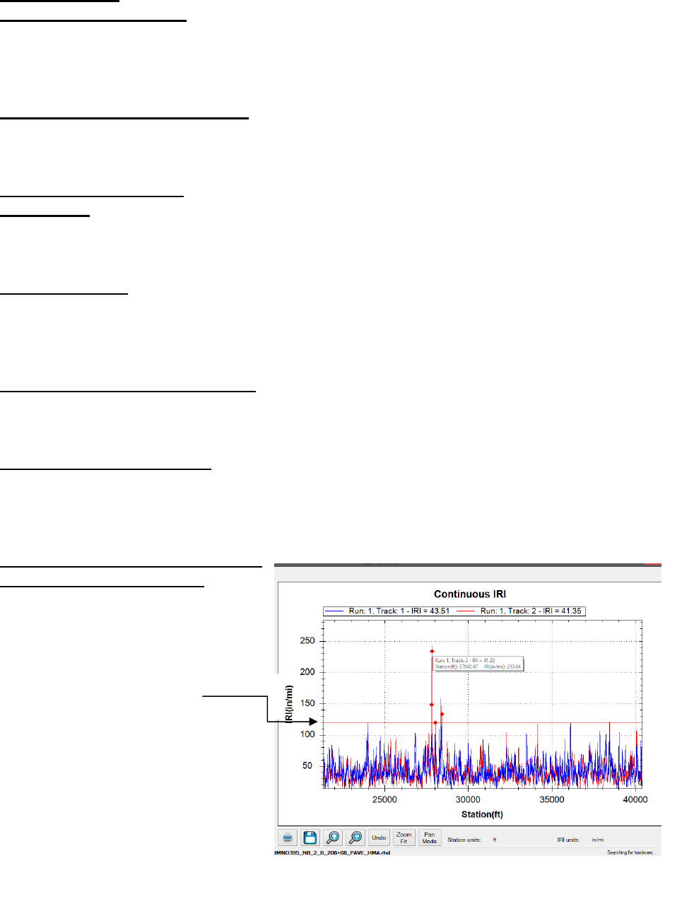
79
GPS Lock-On
Display Current Location
This feature will display a vertical line at the vehicle’s current GPS location. This vertical line will
move through the trace as the vehicle moves, allowing the user to locate the points of localized
roughness.
Center Trace on Current Location
Then this box is checked, the trace will pan with the motion of the vehicle so that the current
location is always in the center of the window. This option is required for any navigation feature.
Highlight IRI Thresholds
Base Length
The base length is the length of the California Profilograph or 25 feet. It will be the basis of the
IRI localized roughness calculations.
1st, 2nd, 3rd [in/mi]
Three separate thresholds can be set to depict which plots exceed the thresholds on the graph.
These thresholds will be plotted as a horizontal line across the trace graph at the IRI values of the
threshold in inches per mile.
Localized Roughness in Trace View
Be aware that when using the localized roughness the defects can appear below the threshold line.
This is because the localized roughness is based off of a 25 foot length and not the entire profile.
Display Localized Roughness
When this box is selected the trace view will have the localized roughness location marked with a
diamond. If the user places the cursor over the red diamond, the information about the localized
roughness will be displayed.
Use Localized Roughness Settings in
Trace View (Recommended)
By selecting this box the IRI Localized
Roughness threshold established under
the Settings and Localized Roughness
Tab will be used to find and display the
localized roughness in
Trace View. If the other
thresholds are used, the
number of defects displayed in the
trace may be different than the number
in the report. This selection displays
the same localized roughness as in the
report.
Figure 118: The Continuous IRI trace with the localized
roughness diamonds shown
Threshold
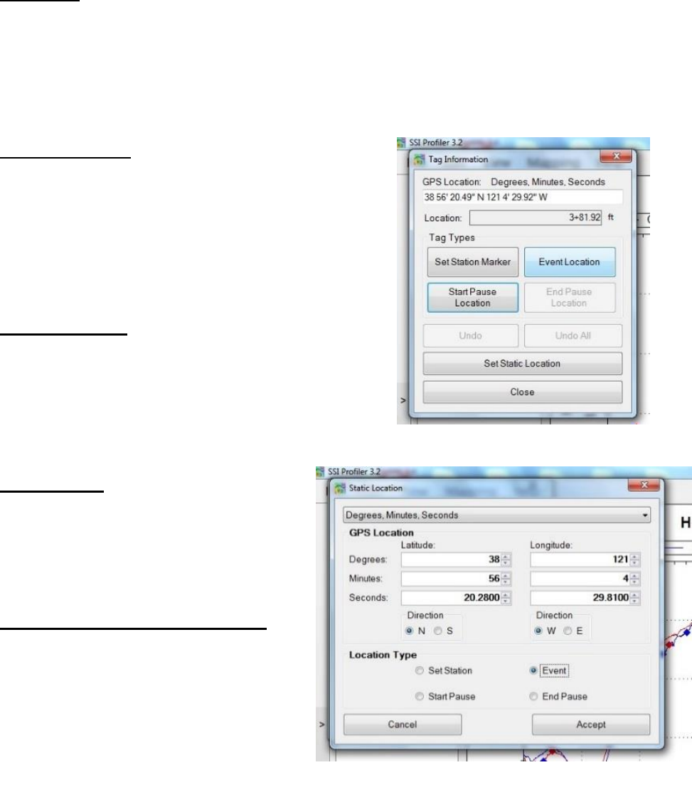
80
Navigation
Trace View has a navigation feature as long as the GPS is connected. See Section 4.3. – Trace
Navigation
In order to use the Navigation feature in Trace View the GPS must be connected and you must
select the “Display Current Location” check box under GPS Lock-On in the Plot Options
Window.
GPS Tagging Tool
Based on the GPS coordinates from the collection, the
program can add events and pauses to the collection
information. There are two ways of adding the events
and pauses; dynamic and static tagging. The tagging tool
is included in a deluxe Profiler license. Tagging
tolerances are dependent on the accuracy of the GPS
system used.
Dynamic Tagging
Dynamic tagging involves being physically at the
location of the start or end of the pause or the event. The
GPS string will be visible in the tagging window with the
option of also having your current location displayed on
the trace. Choose the type of location from the options
and move to the next area.
Static Tagging
The static tagging feature allows the operator
to enter a GPS location from a remote
location, like your office. As long as the
location’s GPS coordinates are known, a
pause or event can be created.
Grinding Simulation and Navigation
SSI has developed a feature to assist
contractors in the removal of IRI Areas of
Localized Roughness (ALR). The Grinding
Simulation is included in a deluxe license of
Profiler. Navigation tolerances are
dependent on the accuracy of the GPS
system used to collect and layout
roughness.
After collecting the data ALR can be determined from the amount of suspension movement over
certain locations. These areas can be determined in SSI Profiler’s Localized Roughness section.
However, grinding the ALR does not have the best result in removing roughness. This is because
ALR can now include dips and bumps. Grinding dips takes a special procedure.
Figure 119: Dynamic Tagging Feature
Figure 120: Static Tagging Feature
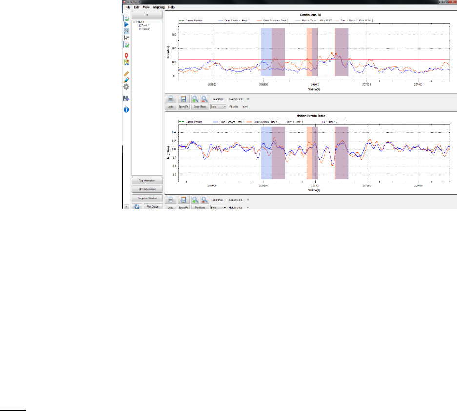
81
The FHWA program
ProVal
(roadprofile.com) has a
tool to simulate the best
grinding strategy for
grinding. Input the
correct settings for the
IRI tolerances in
ProVal’s SAM analysis
and choose AutoGrind,
then Grind. This will
give you locations along
to profile to grind.
Unfortunately, ProVal
does not accept GPS
coordinates so the table
can be copied (right
click in the grind table)
and pasted into a notepad file and saved for the lane and wheel path. This notepad file can be
imported into the SSI Profiler program within the Advanced Tools>Grind Sections>Manage Grind
Info. Confirm that the track is correct before applying these locations.
The locations for track 1 and 2 will appear in the trace window with paired GPS coordinates. You
can use the green line to display current location and visually track your position until you get to
the beginning and end of a grind, in order to layout the location on the pavement.
Under the navigation window icon in trace view you may choose to auto-center the current location
and choose the Simple Grinds option. The simple grinds window displays the location of the grinds
relative to the current position through numbers and colors.
Print
To print the trace, select the Print Icon in the window or select CTRL+P on the keyboard. The
print window will appear at this time. Within the window, select the printer to be used and verify
that the printer settings are correct. When ‘Print’ is selected, the document will be sent to the
printer.
Figure 121: Grinding Navigation with green current location displayed
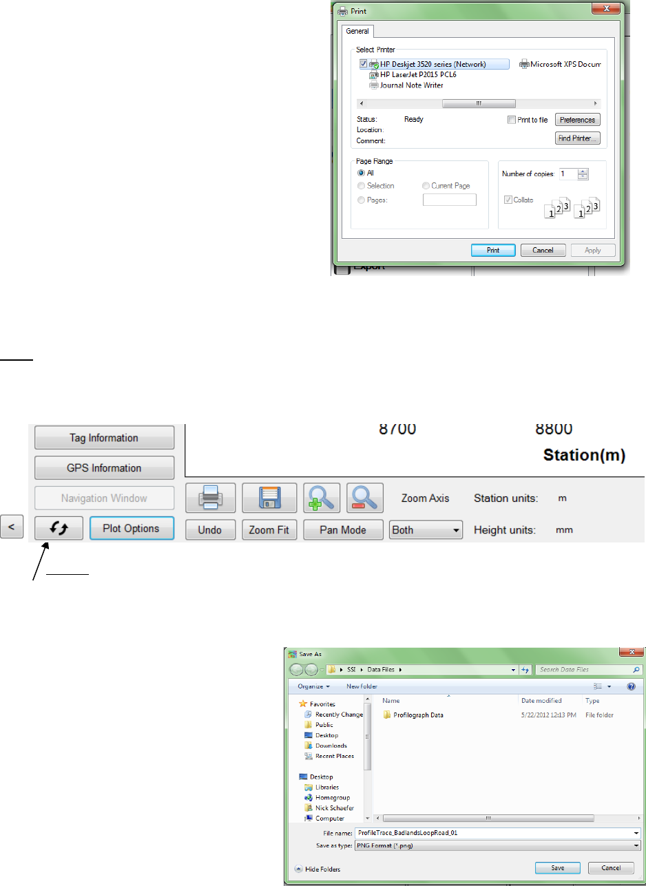
82
If more printing options are needed, select the
‘Preferences’ icon. This icon will open a
window that is printer specific containing
information about the orientation, paper size,
and image quality.
Save
When the Save icon is selected, the user is able to save the trace as an image in png, gif, jpeg, tiff,
and bmp format. The image can be saved on the operating computer or on a connected external
device.
Figure 122: The Print window that
appears after the print icon is selected
Figure 123: The tool bar for the trace window
Figure 124: Windows explorer
to save a picture of the graph.
Refresh
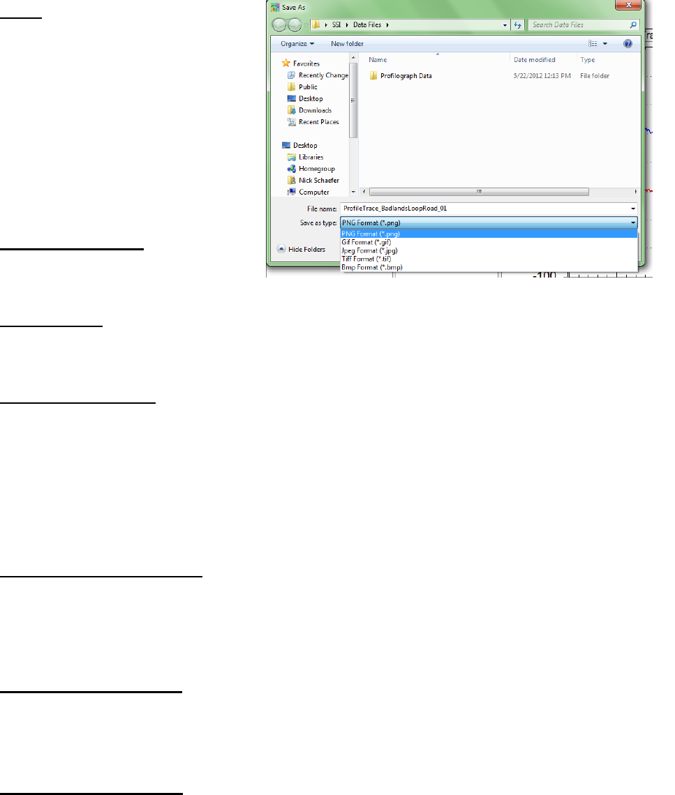
83
Zoom
To zoom in the trace window, verify
that the Pan/Zoom Mode icon
displays ‘Pan Mode.’ To zoom in on
the plot, left click and hold while
dragging the cursor over the area to be
blown up. While dragging the cursor,
a dotted box will appear. This dotted
box contains the area of the plot that
will be blown up, by being fit to the
size of the plot window.
Zoom Previous Icon
When Zoom Previous is selected, the
last ‘zoom in’ action is undone.
Zoom Fit Icon
To return to the original aspect ratio, also known as the home view, select Zoom Fit.
Pan/Zoom Mode Icon
The Pan/Zoom Mode icon has two functions. When Pan Mode is displayed, the cursor may be
used to zoom in on the plot. To zoom in on the plot, hold down the left mouse button and move
the cursor over the plot area to be blown up. The dashed box contains the area that will be enlarged.
When Zoom Mode is displayed, the operator may use the cursor to pan across the plot area. The
pan mode allows the user to navigate through the plot area without changing the aspect ratio, or
zooming out.
Units for Height and Station
The units for height (y-axis) and stationing (x-axis) can be changed by left clicking upon the
current units and selecting the necessary units from the dialogue box that appears. The units
available are mils, inches, feet, yard, miles, millimeters, centimeters, meters, and kilometers. The
units scale the plot area.
GPS Editing and Tagging
The operator can use the GPS signal to edit the start and stop locations of the collections and add
events to the collection.
4.0 Advanced Tools
The Advanced Tools window contains options for images, transverse profile viewer, grind
sections and profile design. These options will only be available if the user license permits this
additional analysis. Contact SSI for a license upgrade.
Figure 125: The available picture formats to save the trace graph.
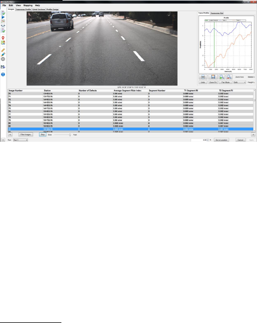
84
4.1 – Images Window
Within the images window the user can perform multiple filtering options to show only certain
characteristics of the collection. The data can be filtered by station, defects or ride value. The
software automatically enters the minimum and maximum values for each of these three fields.
The units of these parameters can be changed by selecting the current units to enable to drop
down menu to choose new units. After the operator has changed the parameters according to the
range desired, select “Filter”. The images will reorganize and the new images will not be
reverted until the parameters are changed to the original setting (“Reset”).
The information in the table below the image will be populated as long as the location is not in
the run up distance and there is sufficient data. If the system was not a full lane width 5-laser
system the rutting depths will read ‘N/A’.
The arrow keys on your computer’s keyboard can be used to advance the images. There will be a
lag using the computer’s keyboard until the images are populated from the files. After the images
are loaded the operator will be able to constantly hold the up/down arrow keys to view a slide
show of the collection.
The GPS string of the Images Window is based off of the nearest GPS coordinate and should not
be used as a reference station.
Images in the Report
The images captured during data collection can be viewed alongside the trace within the any of
the three trace reports. The user can view the images with the trace in the Single Trace, All
Traces, and Continuous Trace reports. If the user hovers the cursor over the camera icon the
image will appear.
Figure 126: The Images Window under Advanced Tools
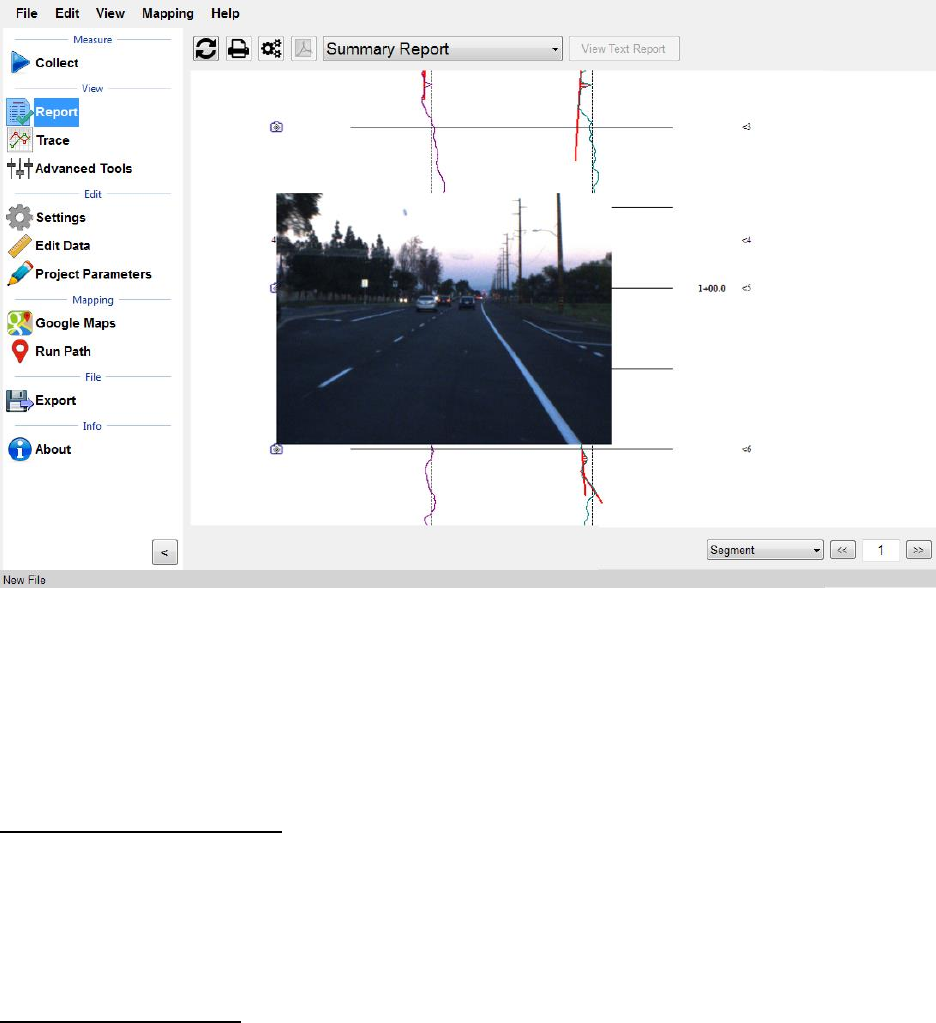
85
The user can right click on the image in the image window or on the trace to save it to the
computer or other external device. As long as the user left-clicks above the image, windows
explorer will open to choose where to save the image file. The following formats are available:
BMP, JPEG, GIF, PNG, TIF. Right click to save image.
4.2 – Transverse Profile
Under Advanced Tools>Transverse Profile there will be a table of transverse collections and
graph space for plotting the transverse profile. Only data collected within the current RSD file
will be displayed. Transverse profiles can be selected with the mouse through the table or
through the left/right arrows. Additional edits can be made to cutoff the edges of the profiles or
filter them for station, intensity, or rut depth.
4.3 – Grind Sections
Corrective grinding locations can be imported from a grinding plan into SSI Profiler through a
text or CSV file through the grind sections tab of the Advanced Tools under “Manage Grind
Info….” Grinds should be imported using wheel path (track 1 and track 2) or full lane width
grind plans. After the grinds have been imported, the user can merge grinds within a certain
length or combine all grinds transversely across the lane (merge tracks 1 and 2). The grind
locations can be edited or deleted within the manage grind info icon.
Figure 127: The Continuous Trace Report with Images.
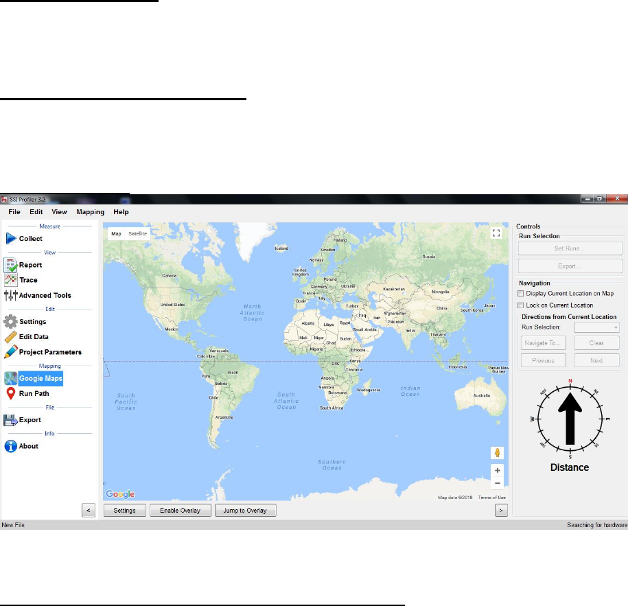
86
4.4 – Profile Design
SSI has developed a modeling process using inertial profiler data. The models can be used on
control systems for milling machines, pavers, and diamond grinders. For the settings and
parameters to input please contact SSI.
5.0. – Navigation (Map Views)
The Profiler V3 program has three methods of location navigation. Map Point, Google Earth or
Trace View can be used to travel to the point of localized roughness, Segments, Events, or a GPS
coordinate. For this reason, all three navigation options require a GPS device to function.
5.1 – Google Maps
*An internet connection is required for use of Google Maps
Google Maps can be used to show the location of the run path, segments, and localized roughness.
Google Maps can also be used within Profiler V3 to navigate to defects, the start of the run or the
end of the run.
To view the location of the collection without any collection information displayed:
1) To begin, select the Google Maps icon in the shortcut bar.
2) The world view will be the initial view in the window.
3) The right side of the window has the controls section. Choose the run number of
the collection to be viewed in the map.
4) Select Jump to Overlay or “Navigate To…” and select an event.
To view the Run Path, Segments, and Localized Roughness:
Figure 128: The Google Maps start window.
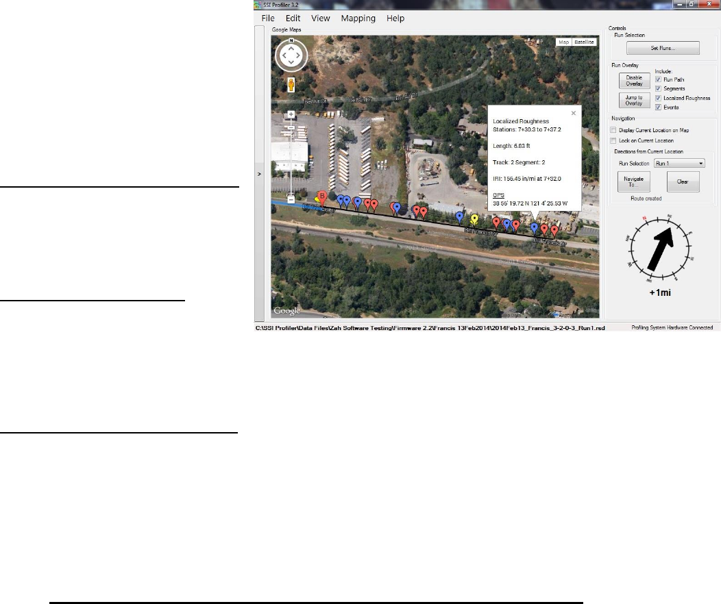
87
1) Select their corresponding check boxes of the parameters. If one parameter is not
desired, do not select its check box
2) Select the “Enable Overlay” icon.
3) Select Jump to Run
4) If the push-pin is selected, the statistics and information for that location will be
displayed.
For Localized Roughness: Red Pin is Track 1, Blue Pin is Track 2, and the Green Pin is Track 3.
To deselect a track to not show it on the map, select the “Set Runs” icon and uncheck the box next
to the unwanted track.
Once the run is displayed in Google
Maps, use the scrolling and cursor to
navigate through the run. The run
path, segments and localized
roughness are shown if their
respective box is selected. These
features can be shown if the box is
checked reading, “Disable Overlay.”
Display Current Location on Map
If this check box is selected, the
current location of the profiler is
marked by a large green arrow in the
map window.
Lock on Current Location
If the check box for “Lock on
Current Location” is selected, the
location of the profiling system will
remain in the center of the map
window.
Directions from Current Location
The V3 program will navigate to the start or end of the run and any defects found during collection.
Select the destination from the drop-down menu and select the calculate icon. The route will appear
as a black line from your current location to the “B” landmark.
To navigate to an event, pause, segment, or defect, select the correct run number and hen
the “Navigate To” icon. If GPS is connected the program will ask the user where to be
navigated to. Once the location is selected Profiler will direct the device to the location.
Note: GPS must be connected to use the Google Maps and Map Point features.
Figure 129: Google Maps showing the localized roughness
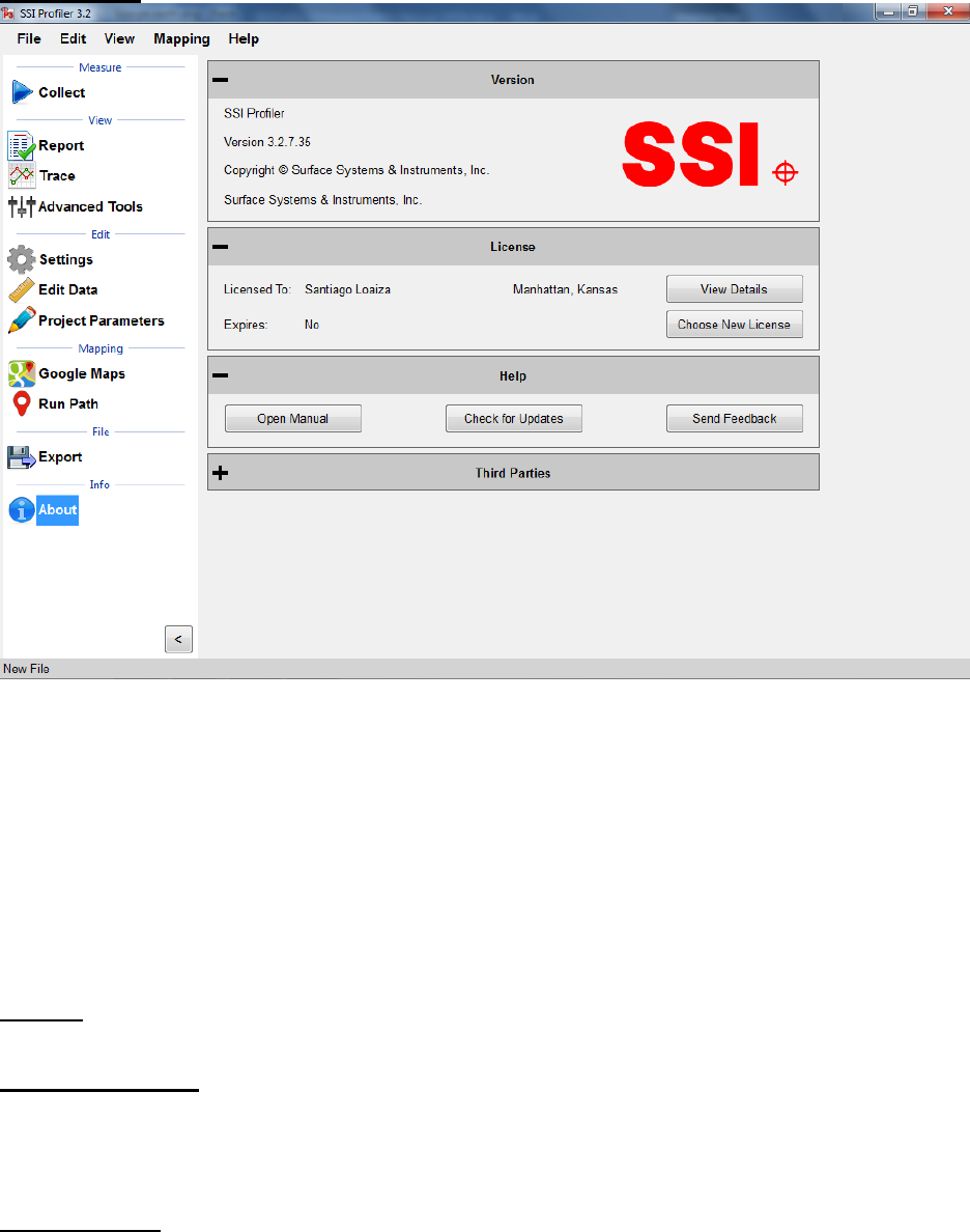
88
6.0 – About
The About section has information concerning Profiler V3 software and its licenses. The software
version, copyright and license can all be found in the ‘About’ window. Additionally, third party
software licenses are listed in the About window.
The About window is where the user can view the terms and features enabled with their license.
Select View details to see the applicable collection devices and software features that are enabled.
The update icon allows the user to update to the latest version of software.
Manual
The manual can be found under the Help Tab or on the About Section window.
Check for Updates
The operator can manually check for updates through Help>Check For Updates. By default, the
program will check for updates every time it is opened. To not check for updates at each opening,
deselect the check box in this window.
Send Feedback
If SSI should be informed of issues or advancements of the software, please send us feedback so
we can improve our services.
Figure 130: The About Window

89
Third Party Components
The Third Party Components of Profiler V3 are:
ZedGraph Copyright © 2004 John Champion under the LGPL 2.1 license.
Modified source code is available for download at:
http://www.smoothroad.com/support/download.asp.
SharpSSH Copyright © 2006 Tamir Gal
Mentalis.org Crypto Library Copyright © 2002-2007. The Mentalis.org Team
Full copies of all third party licenses can be found in the Licenses folder located inside the Profiler
V3 installation directory.
7.0 Recommended Tools
7.1 – Create a personal default file name convention for you project
Under General Settings the operator may select “Configure File Naming” to create a new file
name convention for FHWA and State DOT submissions.
7.2 – Load analysis parameters and settings from previous projects
When a previous file has the correct project information and settings saved within it, the operator
may load the previous file’s settings into the current file. By selecting “Load” under General
Settings the user may select the previous RSD file and load its settings into the current project.
7.3 – Set a default file location
The user may select a default folder to save all files and reports under General Settings. It is
recommended paste the folder destination into the address input.
7.4 – Use the extended calibration report to print PDFs
The extended calibration report option is located under Settings>Report Options. The extended
calibration report adds the bounce and laser height verifications to the calibration report.
7.5 – Use dual plotter in trace view
Under trace view the plotters can be viewed to see the elevation and the IRI roughness. This is
useful when determining if an area of roughness is caused by a bump or a dip in the profile trace.
It is highly recommended to use this feature for correction operations. The trace view can be
chosen under Trace>Plot Options and Enable Secondary Plotter. It is also recommended to link
the secondary plotter X-axis.
7.6 – Use GPS navigation within trace view
During correction operations it is important to be accurate. The SSI Profiler system allows for
the user to navigate along the collection path using GPS. Depending on your GPS system you
may have to connect to hardware and have your antenna attached. The GPS accuracy can be
found listed on your profiling documents or by calling your SSI representative. The GPS
navigation can be enabled under Trace>Plot Options>GPS Lock-On options. The check boxes
should be enabled for Display Current Location and Enable Navigation.

90
7.7 – Use hot keys during collection
During collection the operator can assign a command to any keyboard key except for the space
bar and the enter key. The keys can start or end a collection, arm and electric eye or create an
event for various types of scenarios such as pavement distresses or debris.
7.8 – Import grind locations into Profiler for use in trace view navigation
Once grind locations are created the grinding plan can be imported into Profiler through the
Advanced Tools>Grind Sections tab. The locations can be added through the Manage Grind Info
Icon. Once the locations are added, they will appear within the trace view to be used with the
GPS navigation. Under Trace View>Navigation>Simple Grinds the window can display the
distance to the grind locations per wheel path.
7.9 – Use Google Maps to crop and edit data based on stationing and pin information
Google Maps can be used to compare multiple runs to each other and determine the stations to
crop an RSD file back. The operator may use landmarks, a collection event or a previous
collection to adjust a starting location.
Troubleshooting and Support
When Contacting SSI Technical Support
If possible, have the profiler system type, profiler software version, operating system, computer
model number, and company of ownership ready. If an internet connection is available, SSI staff
may request your data files for comparison and troubleshooting.
Attaining Profiler Software and Replacement Parts
For technical support with the High Speed Profiler (HSP) software contact SSI to obtain a User ID
and Password to download the most recent updates from the www.smoothroad.com website.
Software issues should also be reported to SSI by email at support@smoothroad.com, with a copy
of any data files to be reviewed by SSI technical support staff. SSI support staff can also be
contacted by telephone at (530) 885-1482 (Auburn, CA); or (785) 539-6305 (Manhattan, KS).
Parts can be ordered online from SSI at http://www.smoothroad.com. For support issues involving
the profiler hardware (DMI, Pelican cases, hardware, cables, etc.), contact the SSI office in
Auburn, California at (530) 885-1482 or by email at support@smoothroad.com.
Panasonic Toughbook Computer
For technical support for Panasonic Toughbook computers, contact Panasonic Technical Support
at 1-800-Laptop5 (800- 527-8675) or go to the Panasonic support website at:
http://www.panasonic.com/business/toughbook/support.asp.
Paper Supplies or Printer Servicing.
For printer paper supplies or printer servicing, contact SSI at support@smoothroad.com or (530)
885-1482.
Is your Software Up to Date?

91
Contact SSI to upgrade your software if your problems reoccur after support assistance.
Do Not Attempt To Repair Electronic Components
All of the electronics within the SSI Profiler systems are built custom for Surface Systems and
Instruments. Do not attempt to fix issues without contacting SSI.
Is your Power LED Illuminated?
No power to the system would cause the hardware to disconnect from the software.
Hardware Not Found
Check the cables of your system for any wire breaks. If the Amphenol connections are twisted, it
can break the soldered wires. If problem persists, contact SSI Support Staff.
Example Diagnostics
By selecting the button on the upper right of the Collect screen with a single digit number on it.
The single digit number will be the same as the number of lasers on your system. The button is
colored green for systems without an issue, yellow for systems with a device disconnected and red
for connectivity issues.
SSI Profiler 2.1: Q0g0r0r0x0x0x0
‘0’ means that the device is connected.
Q is the encoder symbol
g is Trimble GPS
r is for a Roline laser. The order is Track 1 laser, Track 2 laser, Track 3 laser (if
equipped).
x is an open port
Topcon V2.1: Q0G0r1r0d0P0P0x0
‘0’ means that device is connected
G is Topcon GPS
‘r1r0’ means that the electric eye is disconnected.
d is the symbol for a dot laser
P0P0 is the symbol for connected inclinometer (only for 3 laser survey systems).
Failed Height Verification
1) Check block Orientation. Do not block receiving laser sensor.
2) Check Laser Type in System Settings
3) Check the integrity of the cables and pins. Make sure the pins are not bent inside the
connectors and that the cables are not damaged.
4) Check the height of the lasers from the measurement surface. For Roline and low stand-
off spot lasers the minimum height is 200 mm (7.8 inches). For high stand-off spot lasers
the minimum height is 12.8 inches (325mm).
5) Is there a glare on the verification blocks?
Failing Accelerometer Calibration
Main Cause: Not rotating both accelerometers at the same time or a connection issue.
Are you:

92
Rotating both accelerometers during calibration?
Matching the white lines on the accelerometer and cable disconnects?
Check the condition of the small pins within the disconnect cable and the
secureness of the serial connections to the grey box.
Lasers Not Firing
Main Cause: None/ not sufficient power reaching the lasers
▪ Is the blue light flashing on the Roline laser
▪ Is the blue LED on the white housing emitting light?
▪ Are the red lights on the grey box serial ports emitting solid red light?
▪ Check the condition of the pins in the cables.
▪ Is the vehicle off or running?
▪ Does the same problem happen with the engine running?
Failed Bounce Test
When were the accelerometers calibrated?
Are the front wheels straight?
Is the vehicle moving forward and backward while bouncing?
This causes the lasers to read additional height differences, adding to the ride
value.
Is the bouncing only vertical? (No transverse rocking)
Is the laser type correct under System Settings?
What are the shift calibration values?
If none of these work, try the Simulated Travel option under the ‘Advanced’ tab of the
Collection Parameters window. Follow AASHTO R57 to complete the bounce test.
Distance Not Correct
When was the last calibration performed?
Was the actual distance traveled during calibration entered correctly?
Is the DMI damaged or loose?
Is the DMI Amphenol cable attached correctly?
How long is your calibration track?
Is there a large temperature gradient?
Is the calibration track a straight line?
High IRI/Ride Value
Are the lasers firing and streaming?
What does the diagnostic string look like?
Are the lasers or accelerometers loose and/or vibrating?
When were the last accelerometer calibration and height verifications performed?
Is the laser type correct in the System Settings? (Check with a laser verification)
Electric Eye Events/Pause/Start/Stop Collection Did Not Work
Is the correct EE turned on?
There will be an amber or green light on the back of the EE. Flip the switch on
the white housing if it is not on.
Is DOT-C2 reflective tape being used?

93
Is the angle of the reflector matching with the EE orientation?
GPS Navigation Timed Out (Map Point, Google Maps, Trace View)
1) Check if the system lost GPS signal (Open the Collect window then GPS Options to
check the satellite reception).
2) Disconnect hardware and reconnect hardware.
3) Check that all cables are securely connected.
4) Check power source for consistency.
5) If using a Topcon system, review the MC-R3 rover settings for accurateness.
The Camera is not taking color pictures
1) Choose another pre-formatted option (Low, Medium and High Resolution).
Advanced User Options (Custom Resolution)
1) The camera settings can be found under the Collect window in System Settings.
2) Go to the Camera Settings tab
3) Open Advanced Camera Settings
4) Review Custom Video Mode to affirm that Raw 8 is the pixel type.
5) Select Standard Video Mode
6) Select the button for resolution and pixel type to be Y8 (Raw 8) and 1280x960.
a. Once this change is made the preview will also be in color
