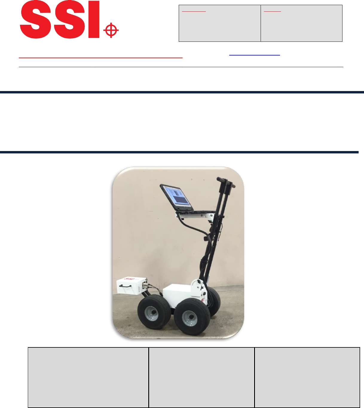
SSI Profiler V3 Walk Pro Manual 32713
User Manual:
Open the PDF directly: View PDF ![]() .
.
Page Count: 104 [warning: Documents this large are best viewed by clicking the View PDF Link!]
SURFACE SYSTEMS & INSTRUMENTS, INC.
Custom Test Equipment • Mobile Technology Solutions • Inertial Profilers • ADA Compliance • FF/FL Testing
California
1845 Industrial Drive
Auburn, California 95603
Telephone: (530) 885-1482
Facsimile: (530) 885-0593
Kansas
307 Plymate Lane
Manhattan, Kansas 66502
Telephone: (785) 539-6305
Facsimile: (415) 358-4340
Hardware Design & Fabrication
1845 Industrial Drive
Auburn, CA 95603
Tel: (530) 885-1482
Fax: (530) 885-0593
Email: info@smoothroad.com
Sales & Administration
P.O. Box 790
Larkspur, CA 94977
Tel: (415) 383-0570
Fax: (415) 358-4340
Email: info@smoothroad.com
Electronics & Software
307 Plymate Lane
Manhattan, Kansas 66502
Tel: (785) 539-6305
Fax: (785) 539-6210
Email: info@smoothroad.com
Profiler V3 Operation Manual
CS-8800
Version 3.2.7.10.
smoothroad.com
Table of Contents
SAFETY .................................................................................................................................................................... 1
AVOID EXCESSIVE SPEED ................................................................................................................................................... 1
CHARGE BATTERIES .......................................................................................................................................................... 1
SET UP ................................................................................................................................................................... 11
BRAKE ......................................................................................................................................................................... 11
COMPUTER................................................................................................................................................................... 11
CHARGING THE BATTERY ................................................................................................................................................. 22
CABLES ........................................................................................................................................................................ 22
LIGHTS......................................................................................................................................................................... 22
RUN AS ADMINISTRATOR ................................................................................................................................................... 2
TEXTURE TABLE SETTINGS (SYSTEMS WITH A LASER)................................................................................................................ 5
UPD SETTINGS (SYSTEMS WITH A LASER).............................................................................................................................. 6
COLLECT ................................................................................................................................................................ 88
OPENING PROFILER SOFTWARE ........................................................................................................................................ 88
HARDWARE DETECTED AND DISCOVERED ........................................................................................................................... 88
SYSTEM SETTINGS .......................................................................................................................................................... 88
Inclinometer Sensitivity ........................................................................................................................................ 88
Front Arm Setting (If Applicable) ............................................................................................................................ 9
GPS Settings ......................................................................................................................................................... 99
UDP Settings .................................................................................................................................................... 1110
UDP Advanced Settings ........................................................................................................................................ 10
Texture Settings .................................................................................................................................................... 11
CAMERA .................................................................................................................................................................... 11
HOW TO BEGIN USING THE CAMERA ............................................................................................................................. 1111
CALIBRATION ............................................................................................................................................................ 1212
DISTANCE CALIBRATION............................................................................................................................................... 2212
HEIGHT CALIBRATION ..................................................................................................................................................... 14
PROFILE SLOPE CALIBRATION (CLOSED LOOP CALIBRATION) - OPTIONAL .......................................................... 1919
GPS REPORTING NOTES ............................................................................................................................................. 2222
COLLECTING DATA .............................................................................................................................................. 2323
CLOSED LOOP COLLECTIONS ........................................................................................................................................ 2428
SLOPE COMPENSATION ............................................................................................................................................... 2828
ADD NOTE ............................................................................................................................................................... 2929
PAUSES .................................................................................................................................................................... 2929
SAVING THE NEW COLLECTION ..................................................................................................................................... 3030
TEXTURE MEASUREMENT ............................................................................................................................................ 3131
TRANSVERSE PROFILE COLLECTION ................................................................................................................... 3232
VIEWING TRANSVERSE PROFILES ....................................................................................................................................... 37
REPORTING AND EXPORTING ............................................................................................................................ 3737
1.0- FILE TAB ...................................................................................................................................................... 3737
1.1. - NEW .............................................................................................................................................................. 3737
1.2. – OPEN ............................................................................................................................................................. 3737
1.3. - OPEN RECENT .................................................................................................................................................. 3838
1.4. – SAVE .............................................................................................................................................................. 3939
1.5. - SAVE AS .......................................................................................................................................................... 3939
1.6. - EXPORT ........................................................................................................................................................... 4040
1.6.1. Export Location ...................................................................................................................................... 4040
1.6.2. – Exporting to ERD Format ..................................................................................................................... 4141
1.6.3. – Exporting to PPF Format ..................................................................................................................... 4444
1.6.4. – Exporting to PRO Format..................................................................................................................... 4646
1.6.5. – Exporting to Survey Format ..................................................................................................................... 47
1.6.6. – Exporting to Excel Format ................................................................................................................... 4849
EXPORT TO TEMPLATE................................................................................................................................................. 4949
1.6.7. – Exporting to Google Earth ................................................................................................................... 5050
1.6.8. – Exporting GPX...................................................................................................................................... 5050
1.6.9 – Exporting to Sidewalk Format .............................................................................................................. 5151
1.6.10 – Exporting to Localized Roughness ...................................................................................................... 5252
1.6.11 – Exporting to ProFAA ............................................................................................................................... 54
1.7. – Exiting Program ...................................................................................................................................... 5454
1.8. – Shortcut Bar ........................................................................................................................................... 5454
2.0. - EDIT .......................................................................................................................................................... 5555
2.1 – EDIT DATA ....................................................................................................................................................... 5555
Edit Segments................................................................................................................................................... 5656
Edit Events ........................................................................................................................................................ 5757
Crop Data ......................................................................................................................................................... 5858
2.2 - PROJECT PARAMETERS ........................................................................................................................................ 6060
2.2.1. - Job Information .................................................................................................................................... 6060
Paving .............................................................................................................................................................. 6060
Additional ......................................................................................................................................................... 6161
2.2.2. - Report Memo ....................................................................................................................................... 6161
2.2.3. - User Defined ........................................................................................................................................ 6161
2.2. - SETTINGS ........................................................................................................................................................ 6262
2.2.1. – General Settings .................................................................................................................................. 6262
On Startup ........................................................................................................................................................ 6464
Data Collection Hardware ................................................................................................................................ 6565
Report Generation ........................................................................................................................................... 6565
Formatting ........................................................................................................................................................... 65
2.2.2. – ANALYSIS PARAMETERS (RIDE VALUES) ............................................................................................................. 6666
Units ..................................................................................................................................................................... 66
Segment Length ................................................................................................................................................... 66
Merge Last Segment if Less Than ......................................................................................................................... 66
Paused Section Drop Down Menu ........................................................................................................................ 67
Analysis Type ........................................................................................................................................................ 67
IRI ......................................................................................................................................................................... 67
PRI .................................................................................................................................................................... 6767
PRI Parameters ..................................................................................................................................................... 68
Scallop Definition ............................................................................................................................................. 6868
Blanking Band .................................................................................................................................................. 6969
Minimum Scallop Width ................................................................................................................................... 6969
Scallop Resolution ............................................................................................................................................ 6969
HRI .................................................................................................................................................................... 6969
RN .................................................................................................................................................................... 7070
RMS Roughness ................................................................................................................................................ 7171
2.2.3. – ANALYSIS PARAMETERS: FILTERS ....................................................................................................................... 7171
Section 1 - IRI/HRI Filter----Same for IRI,HRI, RN .............................................................................................. 7171
Section 2 - PRI Filter ......................................................................................................................................... 7171
2.2.4. –LOCALIZED ROUGHNESS .................................................................................................................................. 7272
Section 1 - Defect Detection ............................................................................................................................. 7373
Section 2 - Bump Parameters ........................................................................................................................... 7373
Section 3 - Dip Parameters ................................................................................................................................... 73
Section 4 - Localized Roughness ....................................................................................................................... 7474
Section 5 - Defect Data Type ............................................................................................................................ 7474
Section 6 – Advanced ....................................................................................................................................... 7575
Section 7 – Correction Type .............................................................................................................................. 7575
2.2.5. - REPORT OPTIONS ........................................................................................................................................... 7575
Ride Index Thresholds ...................................................................................................................................... 7576
Trace Amplitudes ................................................................................................................................................. 76
Note Reporting ..................................................................................................................................................... 76
Segment Reporting .............................................................................................................................................. 77
2.2.6. – GPS OPTIONS .............................................................................................................................................. 7878
REPORT GPS NOTES IN TRACE ..................................................................................................................................... 7878
INTERPOLATE LOCK-ON ............................................................................................................................................... 7878
SIDEWALK OPTIONS ................................................................................................................................................... 7878
3. 0 – VIEW ........................................................................................................................................................ 8080
3.1. - REPORT ........................................................................................................................................................... 8080
3.2 – COLLECT .......................................................................................................................................................... 8383
3.3. – TRACE ............................................................................................................................................................ 8383
Plot Options Settings ................................................................................................................................................. 8686
GPS Lock-On ................................................................................................................................................................... 86
Print ............................................................................................................................................................................... 89
Save ............................................................................................................................................................................... 90
4.0. – MAPPING ................................................................................................................................................. 9191
4.1 – GOOGLE MAPS ................................................................................................................................................. 9393
5.0 – ABOUT ...................................................................................................................................................... 9595
PROFILER V3 LICENSE INFORMATION ............................................................................................................................. 9595
MANUAL.................................................................................................................................................................. 9595
CHECK FOR UPDATES .................................................................................................................................................. 9696
SEND FEEDBACK ........................................................................................................................................................ 9696
TROUBLESHOOTING .......................................................................................................................................... 9797

Table of Figures
FIGURE 1: THE CONFIGURATION FOR CHARGING THE WALKING PROFILER........................................................................................ 22
FIGURE 2: COMPATIBILITY WINDOW FOR RUNNING PROFILER SOFTWARE AS AN ADMINISTRATOR
………………………………………………………28
FIGURE 3: SEARCHING FOR V3 PROGRAM FILE ............................................................................................................................ 3
FIGURE 4: SELECTING ‘PROPERTIES’ FROM DROP DOWN MENU ...................................................................................................... 3
FIGURE 5: CHECK ‘RUN AS ADMINISTRATOR’ IN THE SHORT CUT TAB .............................................................................................. 4
FIGURE 6: CLICK ‘OK’ AND ‘CONTINUE’ TO CONFIRM AND RUN PROFILER AS ADMINISTRATOR ............................................................. 4
FIGURE 7: WINDOW FOR DISACTIVATING NOTIFICATION OF CHANGES TO COMPUTER .......................................................................... 5
FIGURE 8: GENERAL SETTINGS WINDOW ................................................................................................................................... 5
FIGURE 9: ‘TEXTURE TABLE’ SELECTED AND ‘SEPARATE TABLE FOR EACH RUN’ BOX CHECKED .............................................................. 6
FIGURE 10: UDP SETTINGS .................................................................................................................................................... 6
FIGURE 11: IP SETTINGS FOR OPERATOR TOUGHBOOK COMPUTER. ................................................................................................ 7
FIGURE 12: TEXTURE SETTING WINDOW FOR SYSTEMS WITH DOT LASERS. ....................................................................................... 7
FIGURE 13: MAIN PROFILER SOFTWARE COLLECTION WINDOW FOR THE WALKPRO........................................................................ 8 9
FIGURE 14: COLLECTION SETTINGS TAB................................................................................................................................ 9 11
FIGURE 15: THE GPS SETTINGS .......................................................................................................................................... 912
FIGURE 16: UDP SETTINGS WINDOW ................................................................................................................................ 1019
FIGURE 17: UDP ADVANCED SETTINGS WINDOW ................................................................................................................. 1022
FIGURE 18: TEXTURE SETTINGS WINDOW ........................................................................................................................... 1122
FIGURE 19: CAMERA SETTINGS WINDOW ............................................................................................................................ 1122
FIGURE 20: THE CALIBRATION MENU APPEARS AFTER THE “CALIBRATE” ICON IS SELECTED. ........................................................... 1222
FIGURE 21: THE INITIAL WINDOW OF THE DISTANCE CALIBRATION ............................................................................................ 1322
FIGURE 22: FOLLOW THE INSTRUCTIONS AND PUSH THE DEVICE. .............................................................................................. 2213
FIGURE 23: CALIBRATION WINDOW WITH FRONT ARM AT THE END OF THE TRACK. ....................................................................... 2213
FIGURE 24: WINDOW FOR ENTERING LENGTH OF CALIBRATION TRACK....................................................................................... 2214
FIGURE 25: FINAL DISTANCE CALIBRATION WINDOW. ............................................................................................................. 2214
FIGURE 26: FIRST HEIGHT CALIBRATION WINDOW. ................................................................................................................ 2215
FIGURE 27: TO BEGIN THE HEIGHT CALIBRATION, THE SURFACE MUST BE LEVEL. .......................................................................... 2215
FIGURE 28: MAKE SURE THE WHEEL’S AXELS ALIGN WITH THE MARKINGS ON THE FLOOR .............................................................. 2216
FIGURE 29: THE SOFTWARE WILL BRIEFLY FLASH THE “LEVELING” WINDOW ............................................................................... 2216
FIGURE 30: WALKING PROFILER MUST BE TURNED AROUND 180 DEGREES. ............................................................................... 2217
FIGURE 31: WALKPRO DEVICE ROTATED 180 DEGREESS ......................................................................................................... 1722
FIGURE 32: WINDOW INSTRUCTING TO TURN THE DEVICES AROUND SO THAT IT’S IN THE ORIGINAL POSITION ................................... 1822
FIGURE 33: THE SYSTEM TURNED BACK TO IT’S ORIGINAL POSITION .......................................................................................... 1822
FIGURE 34: AFTER A SUCCESSFUL CALIBRATION, THE SETTINGS WILL BE SAVED ................................................................................ 19
FIGURE 35: 1ST WINDOW OF THE PROFILE SLOPE CALIBRATION ................................................................................................ 1923
FIGURE 36: 2ND WINDOW OF THE PROFILE SLOPE CALIBRATION ............................................................................................... 2023
FIGURE 37:PROFILE SLOPE CALIBRATION WIDOW AFTER DEVICE HAS BEEN PUSHED FOR 25 FT ALONG A STRAIGHT CALIBRATION PATH .... 2024
FIGURE 38: WINDOW INDICATING OPERATOR TO COME BACK OVER THE SAME CALIBRATION LINE STARTING WITH THE LASER ................ 2025
FIGURE 39: WINDOW STARTING THE SECOND HALF OF THE CLOSED LOOP CALIBRATION................................................................. 2125
FIGURE 40: WINDOW AT THE END OF THE SECOND HALF OF THE CLOSED LOOP CALIBRATION ROUTINE ............................................. 2126
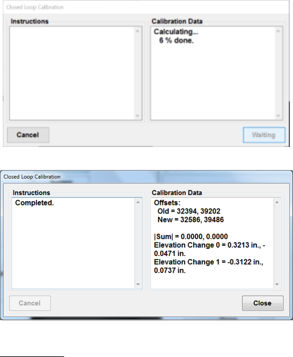
FIGURE 41: CALIBRATION WINDOW CALCULATING RESULTS ..................................................................................................... 2227
FIGURE 42: LAST CLOSE LOOP CALIBRATION WINDOW INDICATION A COMPLETED ROUTINE. ........................................................... 2722
FIGURE 43: THE MAIN COLLECTION WINDOW FOR THE WALKING PROFILER ................................................................................. 2723
FIGURE 44: FIRST WINDOW AFTER PRESSING THE “COLLECT” BUTTON ...................................................................................... 2823
FIGURE 45: COLLECTION PROCEDURE FOR A CLOSED LOOP COLLECTION ..................................................................................... 2924
FIGURE 46: STARTING COLLECTION .................................................................................................................................... 3025
FIGURE 47: THE COLLECTION WINDOW ............................................................................................................................... 3025
FIGURE 48: WINDOW AT THE END OF THE FIRST PART OF THE CLOSED LOOP. . ............................................................................. 3126
FIGURE 49: BEGIN SECOND LOOP ...................................................................................................................................... 2638
FIGURE 50: ONCE THE SECOND RUN IS STARTED THE OPTION TO STOP COLLECTING APPEARS .......................................................... 2738
FIGURE 51: END OF SECOND LOOP FOR CLOSED LOOP COLLECTION ......................................................................................... 2739
FIGURE 52: SECOND LOOP LENGTH FOR CLOSED LOOP IS INVALID ............................................................................................ 2839
FIGURE 53: PROMPT TO USE SLOPE COMPENSATION ON AN OPEN LOOP COLLECTION ................................................................. 2940
FIGURE 54: SAVING OPTIONS AFTER A COLLECTION ............................................................................................................... 3040
FIGURE 55: WINDOWS EXPLORER TO SAVE THE COLLECTION ................................................................................................... 3040
FIGURE 56: THE DIAGNOSTICS WINDOW IS SHOWN ABOVE WITH ALL OF THE COMPONENTS GREEN AND OPERATIONAL ........................ 3141
FIGURE 57: TEXTURE SETTING TAB UNDER SYSTEM SETTING .................................................................................................... 4132
FIGURE 58: FIRST COLLECTION WINDOW AFTER PRESSING COLLECT. ......................................................................................... 4332
FIGURE 59: VERIFICATION WINDOW FOR COLLECTING TRANSVERSE PROFILES .............................................................................. 3344
FIGURE 60: FIRST COLLECTION WINDOW FOR TRANSVERSE PROFILER ....................................................................................... 4533
FIGURE 61: WINDOW INDICATING OPERATOR TO IMPUT START STATION AND TRAVEL DIRECTION. ................................................... 4633
FIGURE 62: FIRST COLLECTION WINDOW AFTER PRESSING COLLECT .......................................................................................... 4734
FIGURE 63: COLLECTION WINDOW WHILE PROFILING ............................................................................................................ 4734
FIGURE 64: WINDOW ASKING FOR ANOTHER TRANSVERSE PROFILE. ......................................................................................... 4835
FIGURE 65: SAVE RUN WINDOW . ...................................................................................................................................... 4935
FIGURE 66: WINDOW AFTER SELECTING “YES” TO FIGURE 54 FOR COLLECTING ANOTHER PROFILE ................................................. 5036
FIGURE 67: COLLECTING ANOTHER TRANSVERSE PROFILE . ...................................................................................................... 5136
FIGURE 68: TRANSVERSE PROFILE VIEWING . ........................................................................................................................ 5237
FIGURE 69 : OPENING A DATA FILE IN THE PROFILER V3 PROGRAM. .............................................................................................. 38
FIGURE 70: THE OPEN RECENT FEATURE ................................................................................................................................. 38
FIGURE 71: THE CLEAR RECENT FEATURE ................................................................................................................................. 39
FIGURE 72: SAVING A FILE THROUGH SAVE AS IN RSD FORMAT. .................................................................................................. 39
FIGURE 73: THE EXPORT WINDOW FOR EXPORTING THE DATA INTO EXCEL FORMAT. ......................................................................... 40
FIGURE 74: SELECTING A LOCATION TO SAVE THE EXPORTED FILE. ................................................................................................. 40
FIGURE 75: THE EXPORT TYPE DROP DOWN MENU .................................................................................................................... 40
FIGURE 76: THE EXPORT FOLDER LOCATION SELECTION .............................................................................................................. 41
FIGURE 77: THE ERD FORMAT EXPORT WINDOW WITH MATCH TRACKS SELECTED. ........................................................................... 41
FIGURE 78: THE ERD EXPORT WINDOW SETTINGS .................................................................................................................... 43
FIGURE 79: THE PPF EXPORT WINDOW .................................................................................................................................. 44
FIGURE 80: THE OPTIONAL SETTINGS WHEN EXPORTING IN PPF FORMAT. ...................................................................................... 45
FIGURE 81: THE EXPORT WINDOW WHEN PRO FORMAT IS SELECTED. ........................................................................................... 46
FIGURE 82: THE DETAILS TAB CONTAINS INFORMATION ABOUT THE PROJECT................................................................................... 47
FIGURE 83: THE WINDOW FOR EXPORTING IN SURVEY FORMAT ................................................................................................... 47
FIGURE 84: THE ADVANCED OPTIONS OF THE SURVEY FORMAT ................................................................................................... 48
FIGURE 85: EXPORTING THE DATA INTO MICROSOFT EXCEL FORMAT ............................................................................................. 49
FIGURE 86: THE TYPES OF EXCEL FORMATS ARE LISTED IN THE DROP DOWN MENU. .......................................................................... 49
FIGURE 87: GOOGLE EARTH ................................................................................................................................................. 50
FIGURE 88: THE EXPORT WINDOW WHEN THE GPX FORMAT IS SELECTED. ..................................................................................... 51
FIGURE 89: THE SIDEWALK EXPORT WINDOW. ........................................................................................................................ 52
FIGURE 90: THE CUSTOMIZE WINDOW .................................................................................................................................. 53
FIGURE 91: THE LOCALIZED ROUGHNESS EXPORT TEMPLATE ...................................................................................................... 53
FIGURE 92: PROFAA MATCHING........................................................................................................................................... 54
FIGURE 93: EXITING THE PROGRAM- SAVING ........................................................................................................................... 54
FIGURE 94: THE SHORTCUT BAR WITH ALL OF THE FREQUENTLY USED WINDOWS ............................................................................. 55
FIGURE 95: THE EDIT RUN OPTIONS ...................................................................................................................................... 55
FIGURE 96: ADDING OR REMOVING PAUSES FROM THE COLLECTION.............................................................................................. 56
FIGURE 97: EDIT EVENTS TAB ............................................................................................................................................... 58
FIGURE 98: THE CROP DATA TOOL ........................................................................................................................................ 59
FIGURE 99: THE PROJECT PARAMETERS WINDOW ..................................................................................................................... 59
FIGURE 100: THE REPORT MEMO WINDOW ............................................................................................................................ 61
FIGURE 101: THE USER DEFINED SECTION .............................................................................................................................. 62
FIGURE 102: THE GENERAL SETTINGS WINDOW ....................................................................................................................... 62
FIGURE 103: THE CUSTOM FILE NAMING CONVENTION WINDOW ................................................................................................. 64
FIGURE 104: THE IRI ANALYSIS PARAMETERS WINDOW ............................................................................................................. 68
FIGURE 105: THE ANALYSIS TYPE DROP DOWN MENU DISPLAYING ALL OF THE RIDE VALUES OPTIONS .................................................. 68
FIGURE 106: AN EXAMPLE OF THE BLANKING BAND IN THE TRACE REPORT. .................................................................................... 69
FIGURE 107: THE HRI ANALYSIS WINDOW WITH THE AVAILABLE FILTER SETTINGS. ........................................................................... 70
FIGURE 108: THE RN ANALYSIS WINDOW WITH THE FILTER OPTIONS SHOWN. ................................................................................ 70
FIGURE 109: THE FILTERS WITHIN THE IRI ANALYSIS PARAMETER WINDOW .................................................................................... 71
FIGURE 110: THE FILTERS FOR PRI ......................................................................................................................................... 72
FIGURE 111: THE LOCALIZED ROUGHNESS WINDOW WITH THE DEFECT SETTINGS. ........................................................................... 72
FIGURE 112: WHEN ONLY BUMPS ARE SELECTED FROM THE DROP DOWN MENU, THE DIP PARAMETERS BECOME UNAVAILABLE. ............... 73
FIGURE 113: WHEN ONLY DIPS ARE BEING TESTED FOR, THE BUMP PARAMETERS BECOME UNAVAILABLE. ............................................. 73
FIGURE 114: THE LOCALIZED ROUGHNESS SETTINGS FOR DISPLAYING DEFECTS ................................................................................ 74
FIGURE 115: THE TYPES OF TESTING AVAILABLE TO FIND THE DEFECTS IN THE DATA. ......................................................................... 74
FIGURE 116: MERGE DEFECTS .............................................................................................................................................. 75
FIGURE 117: CORRECTION TYPES .......................................................................................................................................... 75
FIGURE 118: THE REPORT OPTIONS WINDOW. ......................................................................................................................... 75
FIGURE 119: HIGHLIGHTING IRI VALUES OVER A THRESHOLD ...................................................................................................... 76
FIGURE 120: THE GPS OPTIONS TAB ...................................................................................................................................... 78
FIGURE 121: THE SIDEWALK OPTIONS ................................................................................................................................... 79
FIGURE 122: THE SUMMARY HEADER OF A SINGLE TRACE REPORT. ............................................................................................... 80
FIGURE 123: ENABLE AND DISABLE REPORTS WINDOW ............................................................................................................. 80
FIGURE 124: THE TOOL BAR FOR THE REPORT WINDOW ............................................................................................................. 81
FIGURE 125: PRINTING OPTIONS WINDOW ............................................................................................................................ 81
FIGURE 126: THE DROP DOWN MENU FOR THE REPORT OPTIONS ................................................................................................. 82
FIGURE 127: THE BUILT IN ZOOM RATIOS ................................................................................................................................ 82
FIGURE 128: THE SEGMENT OR DEFECT NAVIGATOR .................................................................................................................. 83
FIGURE 129: GO TO LOCATION FEATURE ................................................................................................................................. 83
FIGURE 130: AN EXAMPLE OF THE PROFILE TRACE .................................................................................................................... 83
FIGURE 131: THE PLOT OPTIONS WINDOW .............................................................................................................................. 84
FIGURE 132: PLOT OPTIONS WINDOW .................................................................................................................................. 84
FIGURE 133: THE CONTINUOUS IRI PLOT OPTIONS WINDOW. ..................................................................................................... 85
FIGURE 134: THE PLOT OF THE CONTINUOUS IRI TRACE ............................................................................................................. 85
FIGURE 135: THE PLOT OF THE PROFILE TRACE ......................................................................................................................... 86
FIGURE 136: THE CONTINUOUS IRI TRACE WITH THE LOCALIZED ROUGHNESS DIAMONDS SHOWN ...................................................... 87
FIGURE 137: A LOCATION SELECTED AND READY TO START NAVIGATION ......................................................................................... 88
FIGURE 138: THE TRACE NAVIGATION OPTIONS ....................................................................................................................... 88
FIGURE 139: NAVIGATE TO GPS COORDINATE ......................................................................................................................... 88
FIGURE 140: THE NAVIGATION STARTED. THE PINK LINE IS THE DESTINATION .................................................................................. 89
FIGURE 141: THE PRINT WINDOW THAT APPEARS AFTER THE PRINT ICON IS SELECTED ...................................................................... 89
FIGURE 142: THE TOOL BAR FOR THE TRACE WINDOW ............................................................................................................... 90
FIGURE 143: WINDOWS EXPLORER TO SAVE A PICTURE OF THE GRAPH. ......................................................................................... 90
FIGURE 144: THE AVAILABLE PICTURE FORMATS TO SAVE THE TRACE GRAPH IN................................................................................ 90
FIGURE 145: THE DROP DOWN MENU FOR MAPPING ................................................................................................................ 92
FIGURE 146: A BUMP IS SELECTED IN MAPPING ....................................................................................................................... 92
FIGURE 147: NAVIGATION TO A POINT IN MAPPING .................................................................................................................. 93
FIGURE 148: INITIAL GOOGLE MAPS SCREEN .......................................................................................................................... 93
FIGURE 149: GOOGLE MAPS SHOWING THE LOCALIZED ROUGHNESS ............................................................................................ 95
FIGURE 150: THE ABOUT WINDOW ...................................................................................................................................... 96

1
Safety
Turn on headlights when profiling to alert other drivers and co-workers of your presence.
Road profilers are precision instruments, handle with care. Improper maintenance and use will
reduce system life and collection accuracy.
Avoid Excessive Speed
The optimal WalkPro collection speeds are below one foot per second. Exceeding this threshold
will create varying elevations when compared against the true profile. The operator can choose
the operational speed by adjusting the warning speed on the speedometer. When the warning
speed is exceeded the computer will beep.
It is recommended that the WalkPro not collect data over 4 feet per second (1.2 meters/second).
Charge Batteries
Fully charge the walking profiler battery before each use. The walking profiler battery will last for
a much longer duration if the walking profiler is not also charging the Toughbook. To extend the
profiling period, have an extra fully charged Toughbook battery to be exchanged with the operating
computer’s battery when the original Toughbook battery becomes low on power.
Avoid over-discharge of the lithium-ion battery and premature degradation of the battery. Charge
the WalkPro battery periodically to prevent over-discharge. During long storage periods the
temperature should remain within the thresholds of 20 ± 5°C, Humidity 45-85%. Keep battery 40-
60% charged during the periods of storage.
Set Up
Laser Front Arm
The laser front arm should be installed at the recommended measurement height of 12 inches for
the Gocator 2342. This height is measured from the bottom of the laser to the measurement
surface. When the laser is within its measurement range the “Range” LED will be illuminated.
If using the laser front arm assure that the front arm type is correct under Collect>System
Settings.
Brake
The brake is located at the rear of the WalkPro and acts on the left rear wheel. This is the wheel
that is attached to the distance encoder. Be cautious to never push the WalkPro while the brake is
engaged. The rubber of the rear wheel can be damaged in this way. If the damage is severe, it can
affect the quality of the profiling data.
Computer
Always charge the operating computer so that the profiling time is not limited by battery power.
If possible keep an extra charged battery to exchange with the original one to extend battery life.
The operating computer may be charged by the WalkPro; however, the battery charge of the
WalkPro will be depleted in a shorter amount of time.
2
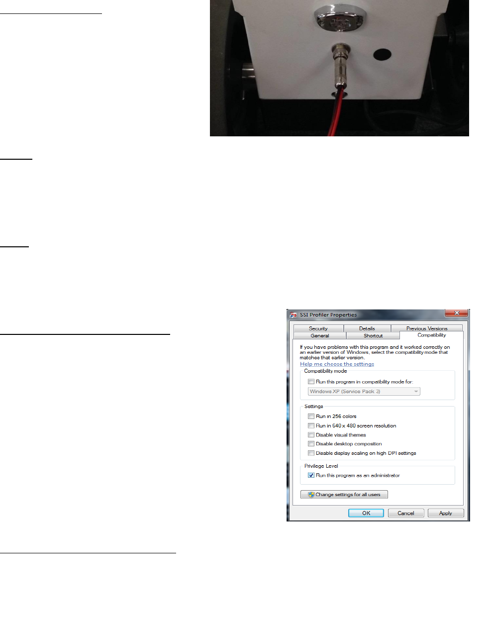
Charging the Battery
To charge the WalkPro insert the leads
into their corresponding ports on the rear
of the WalkPro. The light of the charger
should turn from green to red to signify
charging. When the battery is fully
charged, the LED on the charger will turn
green.
Cables
The walking profiler has cables for the 9-pin data cable (which can also be a usb cable on some
models), power cable for the Toughbook and an ethernet cable for front arm laser models. The
Toughbook power cable does not need to be connected to collect. If the Toughbook power cable
is connected, the battery life of the walking profiler will be reduced.
Lights
The lights on the WalkPro are turned on by flipping the switch on the housing of the WalkPro. The
lights can only turn on when the power switch is in the on position.
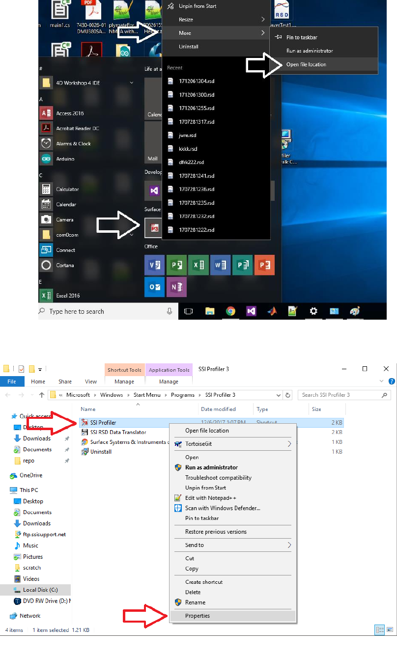
Run as Administrator (Windows 7)
Front arm laser models with ethernet connection require
Profiler to be run as Administrator. Go to the Desktop,
right click on the SSI Profiler icon and select the
“Compatibility” tab. At the bottom of the window under
“Privilege Level”, select the check box for “Run this
program as an administrator.”
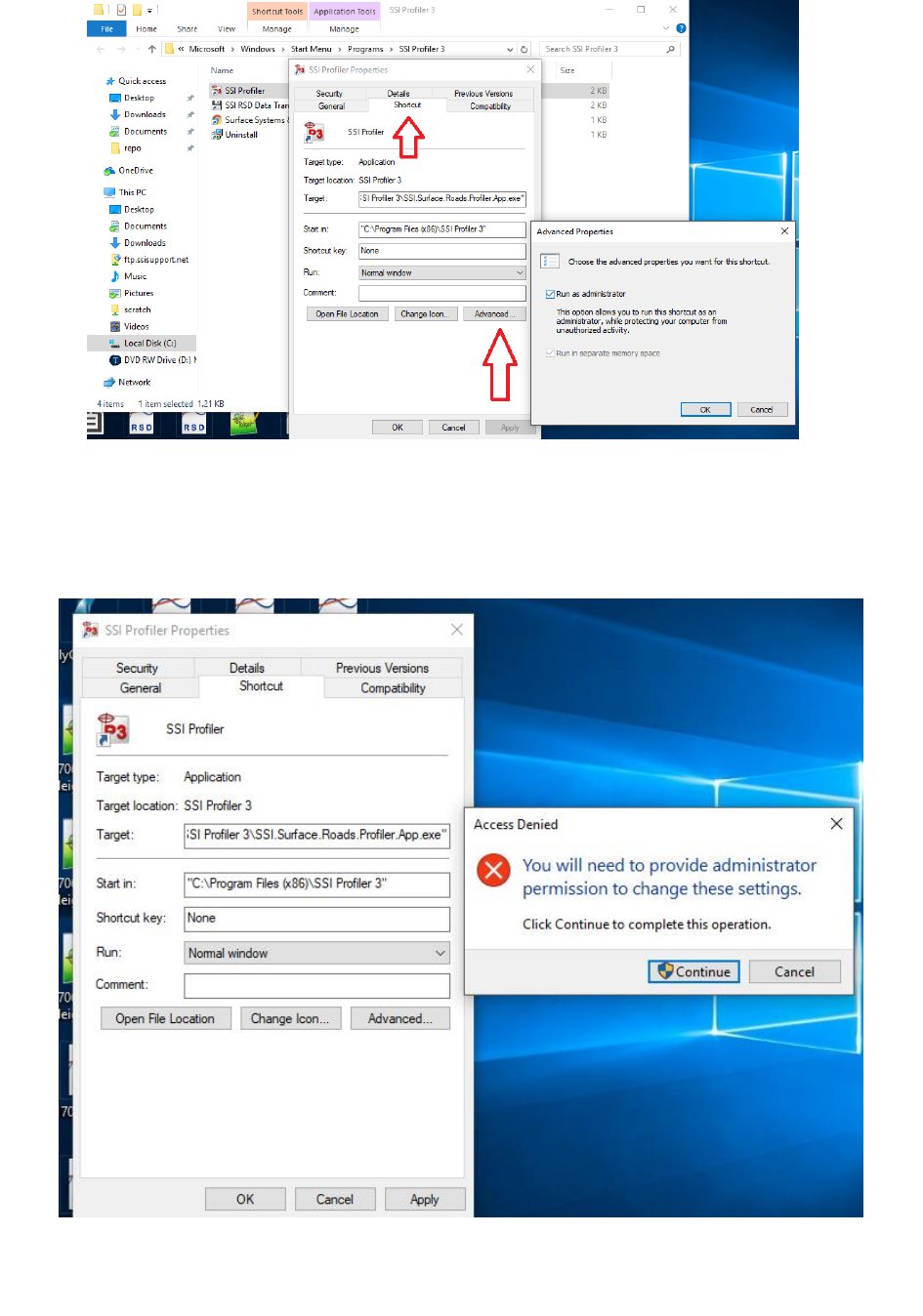
Run as Administrator (Windows 10)
Front arm laser models with ethernet connection require Profiler to be run as Administrator.
Right click on the Profiler V3 icon ‘P3’, go to More>Open File Location.
Right click on SSI Profiler shortcut, go to properties
In Shortcut tab go to Advanced... Check ‘Run as Administrator’ and then ‘ok’.
Figure 1: Configuration for charging the walking profiler.
Figure 2: Compatibility window for running Profiler
software as an administrator in Windows 7.
3
Figure 4: Selecting ‘Properties’ from drop down menu.
Figure 3: Searching for Profiler V3 program file.
4
Click ‘Continue’, in Access Denied window for Profiler to run as Administrator every time
opened.
Figure 5: Check ‘Run as Administrator’ in the Short Cut tab.
Figure 6: Click ‘OK’ and ‘Continue’ to confirm and run Profiler as Administrator.
5
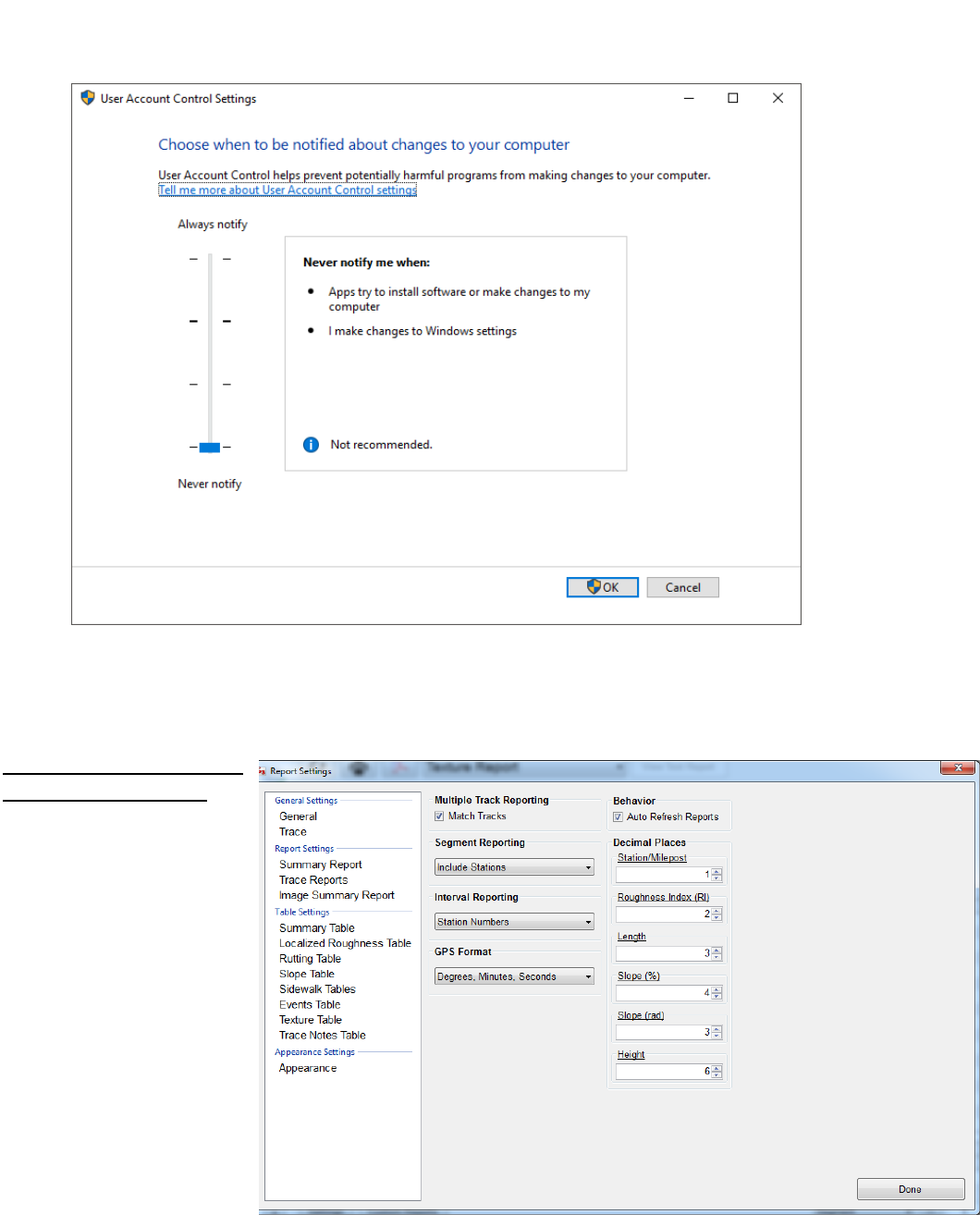
After setting Profiler V3 to run as Administrator, a popup with appear every time you open
the program. To get rid of the popup search "user account control" and set to "never notify"
(this is Optional)
Note: The settings.xml file goes in C:\Users\SSI PROFILER\AppData\Roaming\SSI\SSI.Surface.Roads.UDP.LaserRec
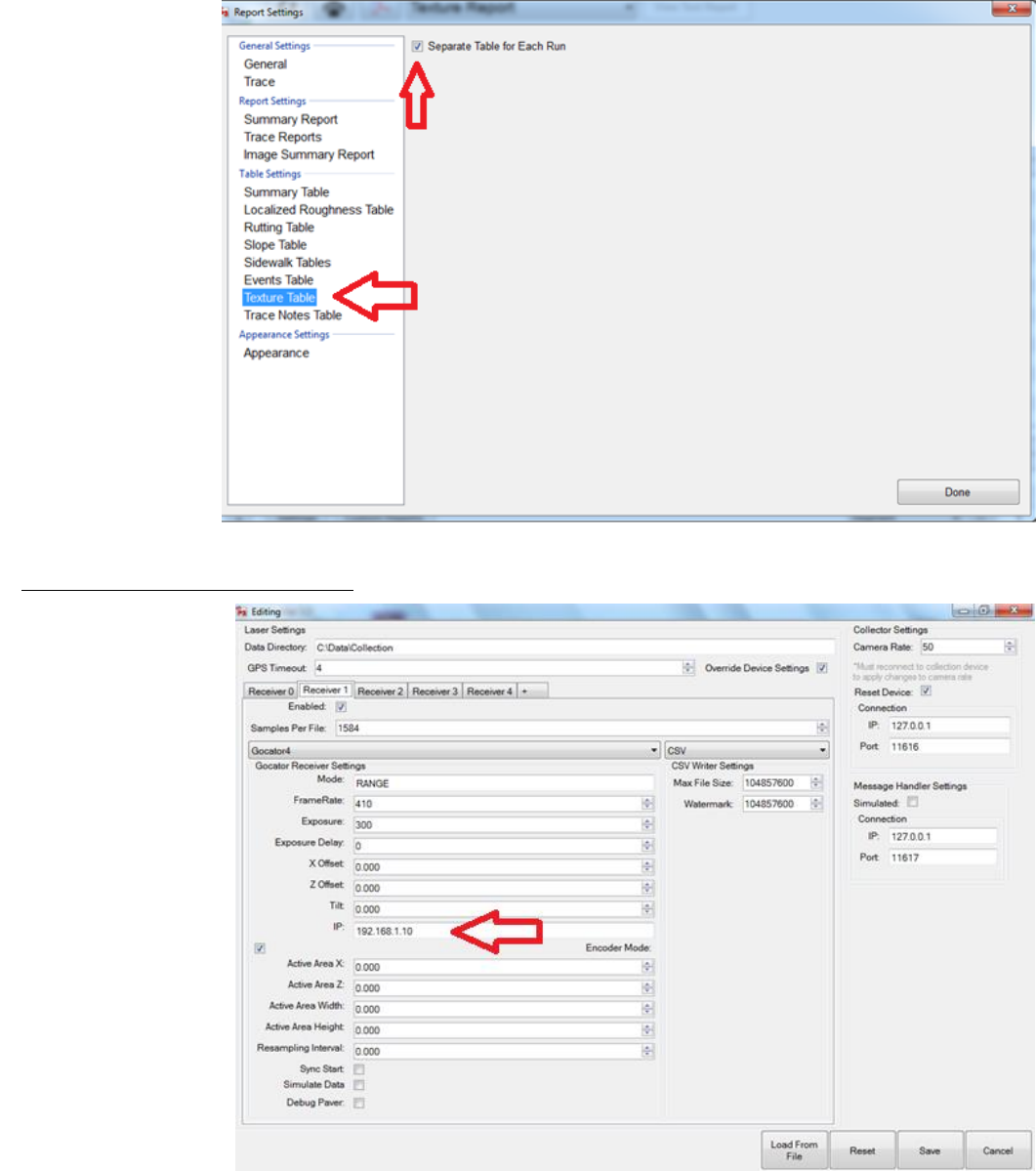
Texture Table Settings
(Systems with a Laser)
It’s recommended when
using the texture table to
change the decimal paces
to around 6. Go to Report
Engin>Settings>General
and change it to 6.
Figure 7: Window for disactivating notification of changes to computer.
Figure 8: General
Settings Window
6
After changing the
decimal places,
click on “Texture
Table” and check
the “Separate
Table for Each Run”
check box.
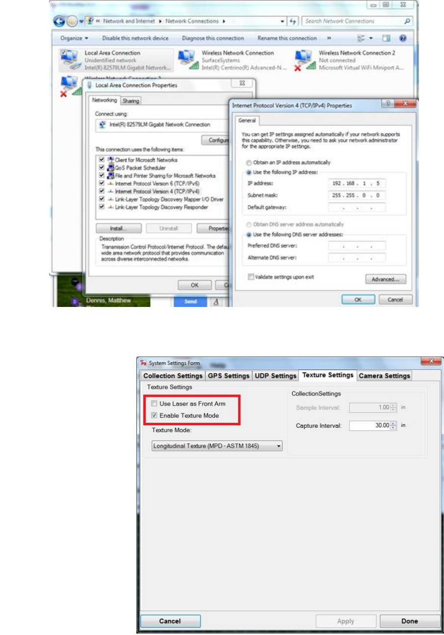
UDP Settings Systems with a Laser
For WalkPro systems
with a laser, make
sure that it has the IP
address
192.168.1.10. This
change can be made
under System
Settings>UDP
Settings>Advanced
Settings. Make sure
all the settings are
the same as in figure
10.
Figure 9: ‘Texture
Table’ selected and
‘Separate Table for
Each Run’ box
checked.
Figure 10: UDP
settings
7
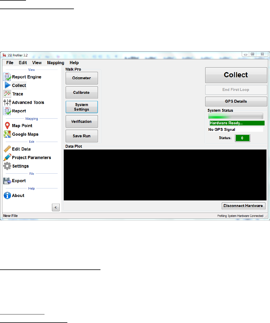
Toughbook operator computers should already be set up with the correct IP address. In any case
this can be done ‘Local Area Connection Properties’.
Dot lasers only work with
Longitudinal Texture
mode. Go to System
Settings>Texture settings
and check the “Enable
Texture Mode” box. Do
not enable the “Use Laser
as Front Arm” box.
Figure 11: IP Settings for operator Toughbook Computer.
Figure 12: Texture
Setting Window
for systems with
dot lasers.
8
Collect
Opening Profiler Software
Open the Profiler software by selecting the Profiler icon on the desktop, or through the folder
destination of MyComputer>C:\ProgramFiles\SSIProfiler3 and selecting the
‘SSI.Surface.Roads.Profiler.App.exe’ file. The software will only detect the hardware if the
electronics are powered on and the computer is connected to the device through the DB-9 serial
port or the proper usb cable.
Hardware Detected and Discovered
Once hardware is properly connected and set up, the Profiler program will recognize the hardware
once the Collect window is opened. When the hardware is found, “Profiling System Hardware
Connected” will be displayed at the bottom right corner of the window.
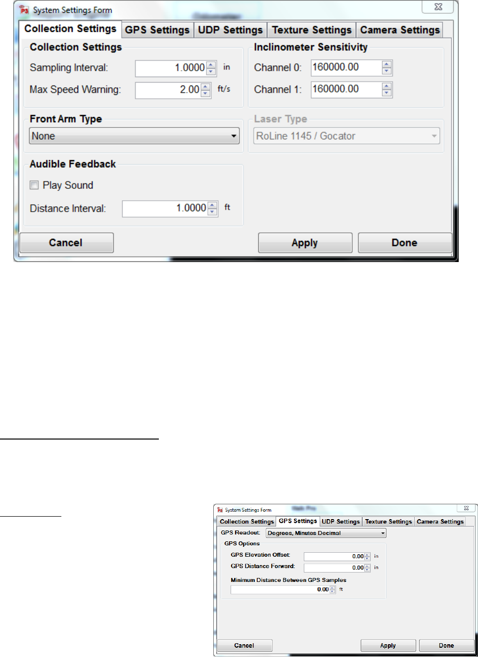
System Settings
Inclinometer Sensitivity
Under System setting there are text boxes to enter the inclinometer sensitivity. Before performing
the height calibration make sure the inclinometer sensitivity is set up correctly. Enter the same
number in Channel 0 and Channel 1 for the CS8800. For the CS8850 Sidewalk Profiler there are
different numbers for each channel. You can find your inclinometer sensitivity from the
documentation provided by your SSI Representative. The inclinometer sensitivity is based on the
scaling factor of the inclinometer.
Figure 13: Main Profiler Software collection window for the WalkPro with Systems Setting
button highlighted as next setup procedure.
9
The sampling interval should be set at one inch unless directed by a SSI Representative. The one-
inch sampling interval allows the CS8800 to be a Class I profiler for use in comparison with high
speed inertial systems.
The maximum speed warning can be adjusted based on the type of work being collected. As the
collection speed increases the accuracy of the system decreases. For optimal results, collect data
at one to 1.2 foot per second. Do not exceed two feet per second.
Front Arm Setting (If Applicable)
Depending on the type of front arm the operator should set the type of front arm being used. The
parameters will be entered in the Collect window under System Settings and Collection Settings.
There are no calibrations for the laser front arm.
GPS Settings
The CS8800 operator can select the type of
GPS string to display in the Collect
Window, and enter the parameters of the
GPS antenna location for more accurate
GPS positioning. The minimum GPS
sampling can be set to the default value of
0.00 for the maximum amount of samples.
Figure 15: The GPS Settings
Figure 14: Collection Settings tab of a WalkPro system with same
Inclinometer Sensitivity value in Channel 0 and Channel 1
10
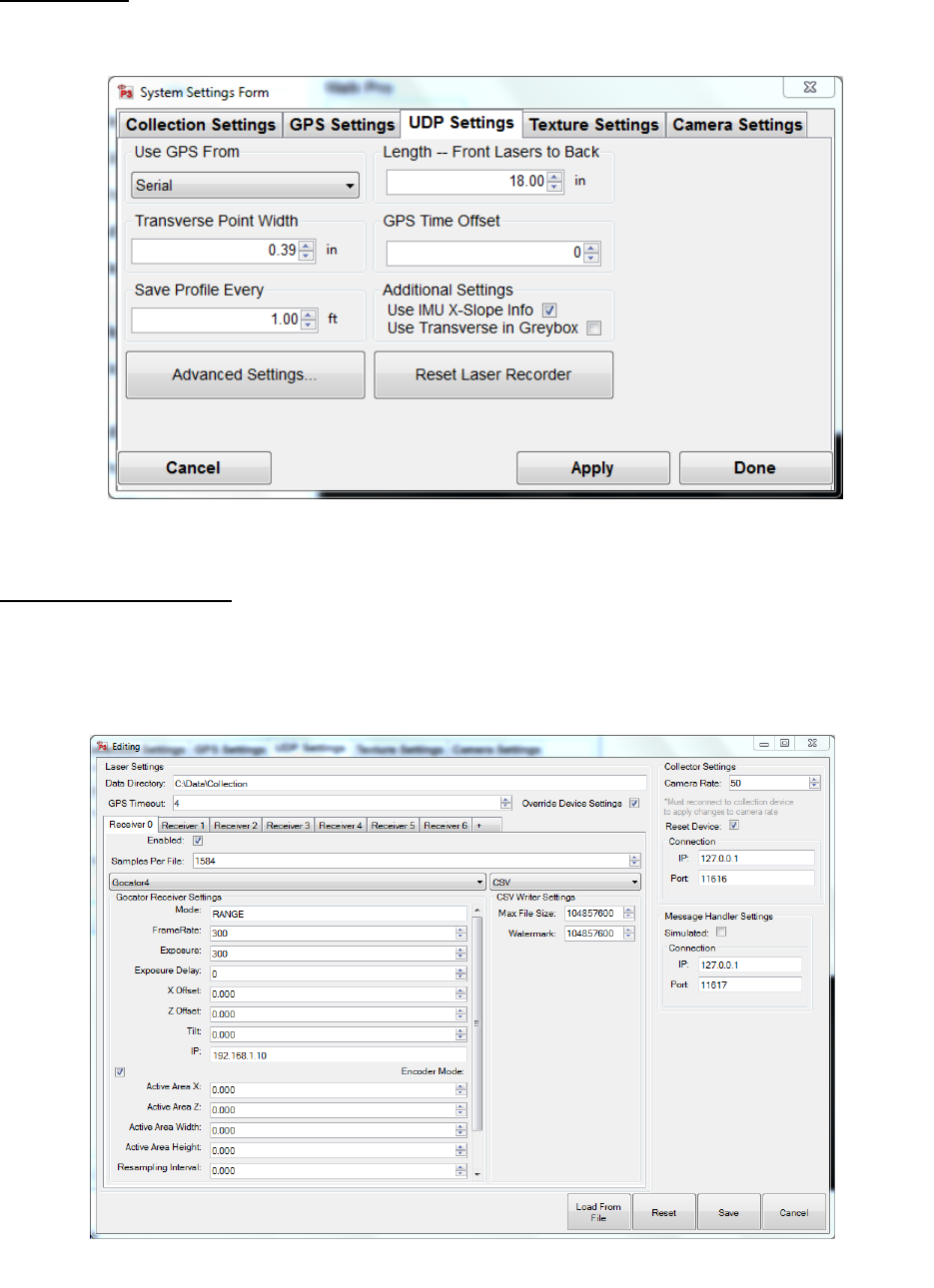
UDP Settings
Chose the appropriate UDP setting according to the configuration of your system. For devices with
a front arm laser, use “The Advanced setting” to configure the particular laser.
UDP Advanced Settings
Under Advanced Setting, make sure to follow the above image. The tab for “Receiver 0” should
be active and enabled. Make sure to select “Gocator 4” above the Gocator Receiver Settings and
take particular care in copying the correct inputs for Mode, FrameRate, Exposure, and the IP
address.
Figure 16: UDP Settings window.
Figure 17: UDP Advanced Settings window.
11
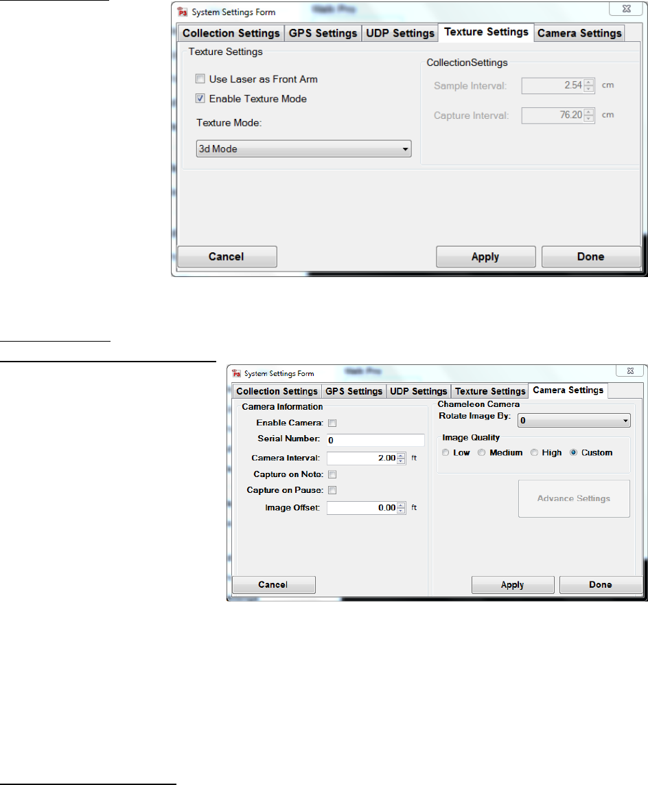
Texture Settings
Under the Texture
Setting window, make
sure to select the
“Enable Texture Mode”
checkbox. SSI
recommends the
Texture Mode set to
“3d Mode” for most
applications.
Camera Settings
How to Begin Using the Camera
Install the Flycap2Viewer driver
located on the disk supplied by
SSI (or already installed on the
computer). The correct driver
depends on if the computer is
32 or 64 bit. To check this, open
the start menu and right click on
My Computer (or My PC) and
choose ‘Properties’. On this
window find the System Type
and view if the system is 32 or
64 bit. If the computer is 32-bit,
install the x86 flycap2viewer. If
the system is 64-bit, install the
x64 flycap2viewer. Once the driver is installed, plug in the Chameleon Camera to the computer’s
USB port and the camera’s back cover. The computer will sound two pings and install the driver
software for the camera. Once finished, a notification window will appear in the bottom right of
the screen to say that a Chameleon camera is connected. Now the camera can be enabled in the
Profiler V3 program.
Enabling Camera Settings
Once the profiling system is connected and the Collect tab is open, the operator can enable the
camera. At this time make sure the flycap2viewer driver is installed and the camera is connected.
Open the collect window and once the hardware is found, select System Settings. Under the
system settings window, select the Camera Settings tab. To enable the camera feature, select the
check box under the Camera Settings Tab. The camera interval is the distance between each
picture. This can be set to any interval, however, the more pictures taken results in more data
saved to the file and more time that post-processing will take. If the camera is not mounted
Figure 19: Camera Settings window
Figure 18: Texture
Settings window.
12
upright, enter the correct rotation angle in degrees, selecting one of the four options. The camera
is focused on the physical lens. Enter the serial number of the camera which is on the sticker on
the back panel of the camera. Once apply is selected the camera will be found in under one minute
for the first use. Once the settings are saved, the serial number will fade out.
If the camera image preview is not in color: Under Collect Window > System Settings > Advanced
Camera Settings > Standard Video Mode, select the button for the resolution and pixel type to be
Y8 and 1280 x 960. The frame rate should be at 15 Hz. This will make the camera take color pictures
(as seen in the preview window also). Also make sure that the pixel type is Raw 8 and the mode is
‘0’ under the custom video modes tab.
The image preview should appear in the Collect window in color and at the correct orientation. If
not, change the settings to the appropriate orientation or open the Advanced Settings.
To reduce the size of the image, change the resolution of the camera medium or low. This will
decrease the processing time and RSD file size. The Advanced Options can be changed by the user
under Custom Mode.
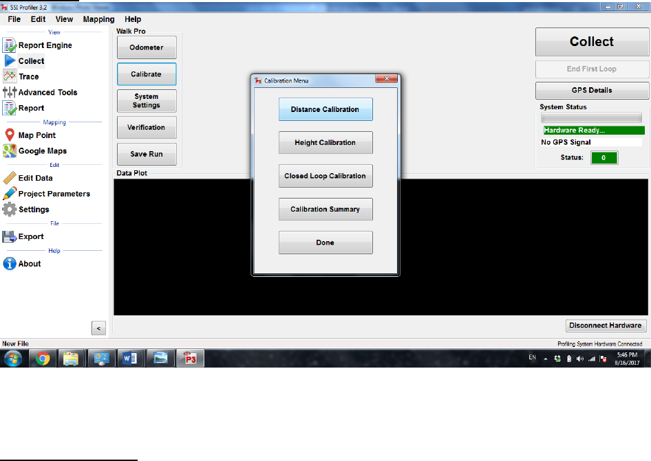
Calibration
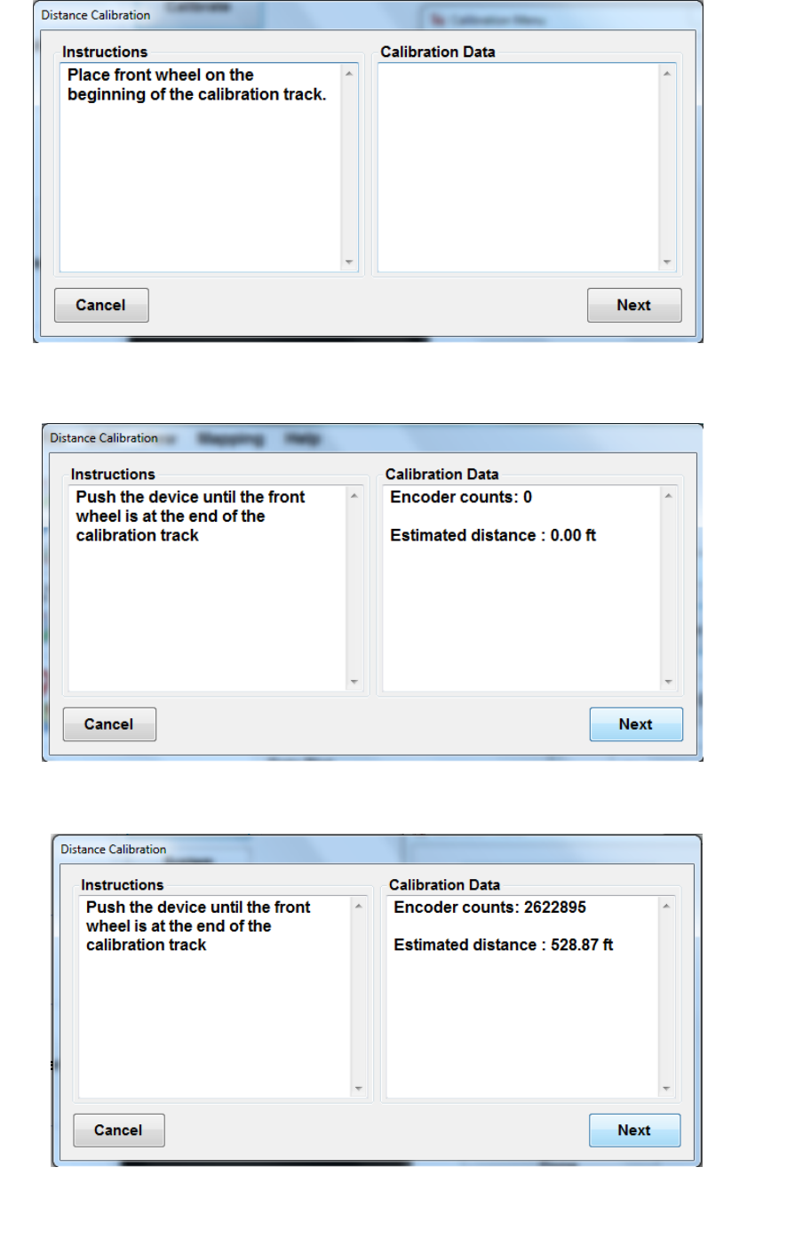
Distance Calibration
Prepare a test track by measuring out 528 ft (160 meters) with a rolling wheel measuring device
in a marked and straight path. Once the test track is prepared, start the calibration procedures
through the Calibrate icon in the Collect window. Select Distance Calibration and follow the steps
precisely to complete a successful calibration.
Figure 20: The Calibration menu appears after the “Calibrate” icon is selected.
13
Figure 21: The initial window of the distance calibration. Once the walking
profiler’s front wheel is on the beginning of the track, select next.
Figure 22: Follow the instructions and push the device until the front wheel
is at the end of the calibration track.
Figure 23: Calibration window with front arm at the end of the track. The estimated
distance can be ignored as it will be overwritten at the end of the calibration procedure.
14
Height Calibration
Before performing the height calibration make sure the inclinometer sensitivity is set up correctly
under System Settings. Enter the same number in Channel 0 and Channel 1. You can find your
inclinometer sensitivity from documentation from your SSI Representative. The inclinometer
sensitivity is based on the scaling factor of the inclinometer.
To perform a height calibration, the walking profiler needs to be placed on a level surface. Mark
the locations of the main wheels on the ground and begin the calibration process. These wheels
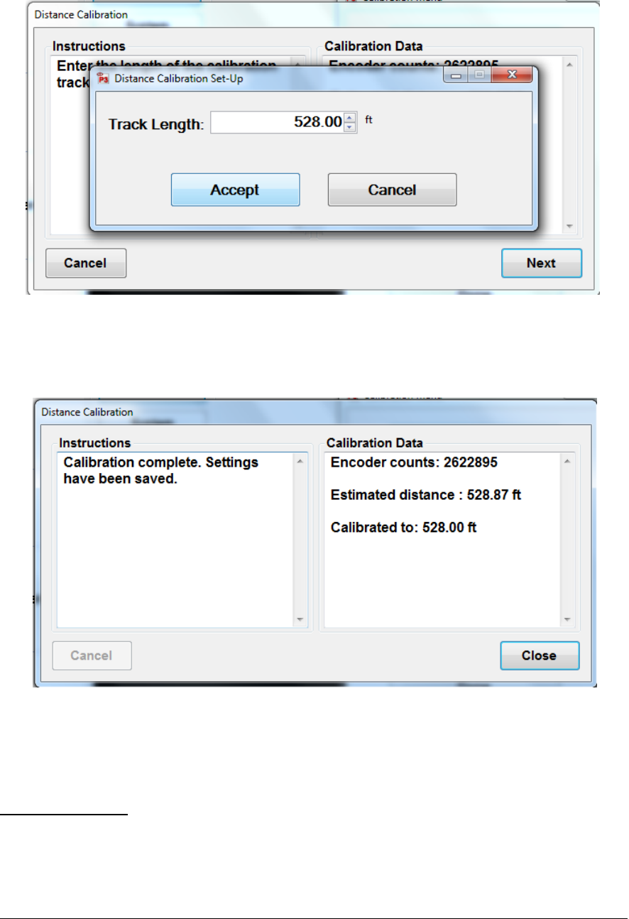
Figure 24: This is the window where the operator enters how long the calibration
track is. The units can be changed by clicking on the feet (ft) and choosing the
appropriate units. After the length of the track has been entered, select accept.
Figure 25: This window shows the number of encoder counts, the length of the
track that was entered in the previous window and the estimated distance traveled
based on the last calibration.
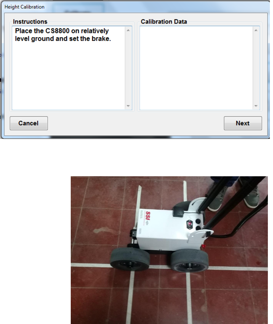
15
do not move along the body of the walking profiler, so they are a good reference point. While the
inclinometer is calibrating, do not touch or move the walking profiler.
Once the first step is complete, rotate the walking profiler 180 degrees so that the wheels switch
positions and resume the calibrations. Last, return the device to its initial position on the marks.
These steps are listed in the procedures while performing the height calibration. Follow the images
and instructions below.
The position of the
wheels must be marked
in a manner similar to
the image. To begin the
calibration, the surface
must be close to level.
Figure 26: The first window of the height calibration. This window instructs the operator to
place the walking profiler on level ground with the brake applied.
Figure 27: First Step
to Height Calibration
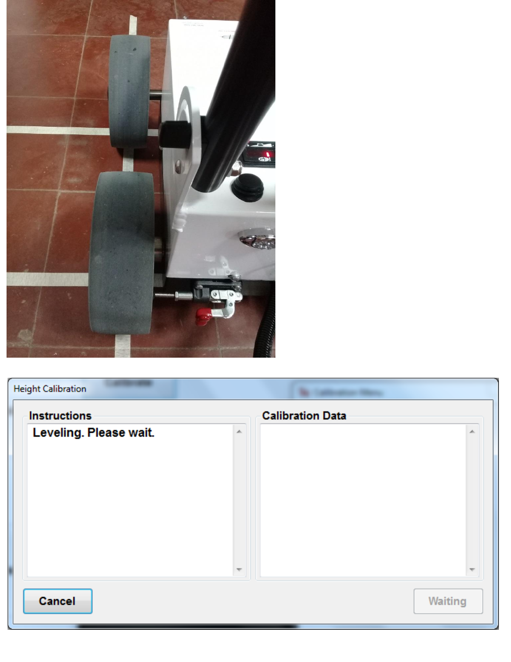
16
Make sure the wheel’s axels align with
the markings on the floor by looking from
above down at the axel. Look that the
axels align with both marking, and that
the wheels are exactly above the
intersecting points of the markings.
Figure 28: Align wheels
and axels with marks on
the floor
Figure 29: The software will briefly flash the “Leveling” window begore continuing the calibration.
17
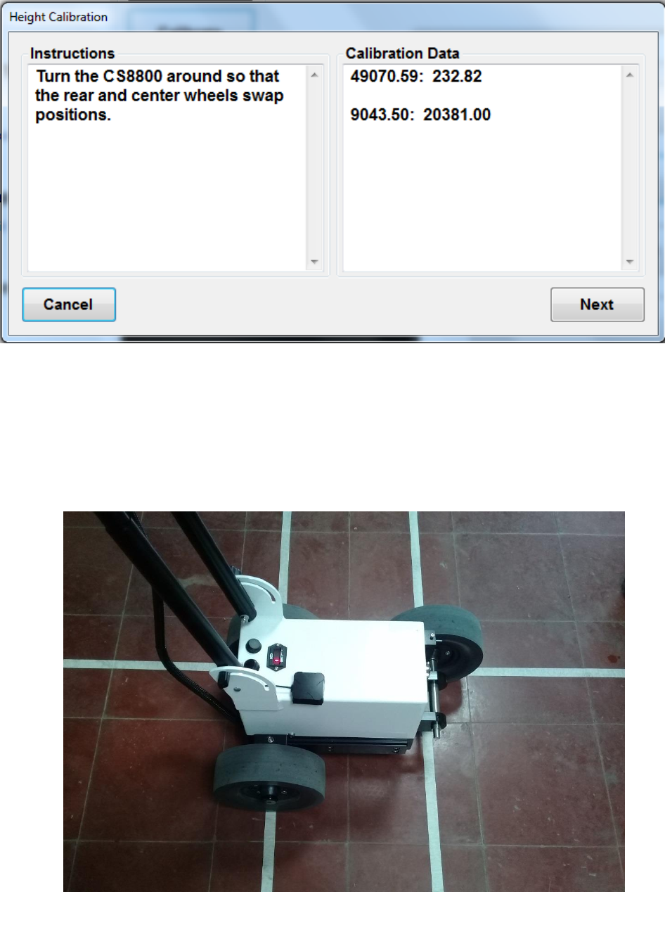
After the first phase of the height calibration, the walking profiler must be turned around 180
degrees and have its left rear wheel switch positions with the left front wheel. The wheels must
interchange contact points.
After the first phase of the calibration, rotate the walking profiler 180 degrees so that it is facing
the other direction. Line up the wheels on the same marks that were made in phase one; the
back wheel has switched positions with the front wheel. Finish the calibration procedures given
by the program. The points of contact of between wheels and floor should now be
interchanged.
Figure 30: Next step Height Calibration
Figure 31: WalkPro device rotated 180 degrees.
18
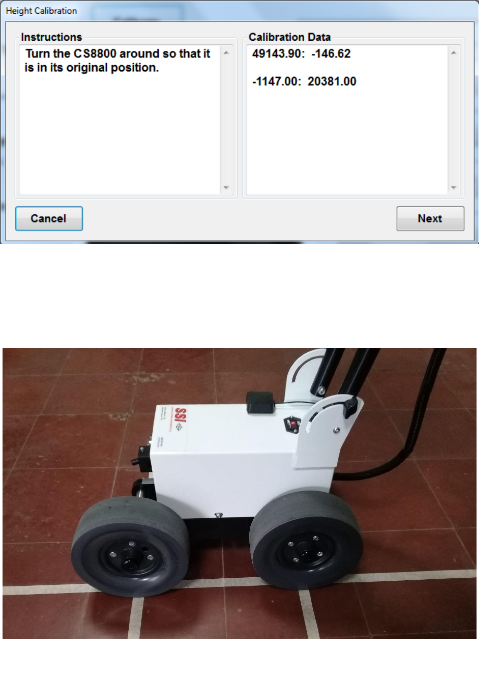
This last step of the height calibration will only appear if the system hasn’t been recently calibrated.
If the device has valid height calibration settings, the calibration routine will stop after rotating the
system 180 degrees and pressing next.
Figure 32: Window instructing to turn the devices around so that it’s in the original position.
Figure 33: The system turned back to it’s original position.
19
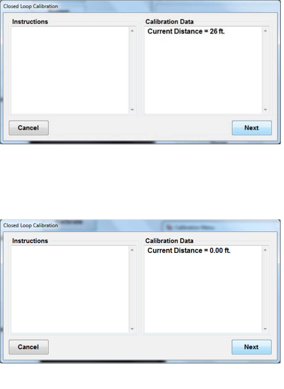
Profile Slope Calibration (Closed Loop Calibration) - Optional
This calibration allows the system to determine the inclinometer drift and compensate for it. The
closed loop calibration is not required for operation of the CS8800. By compensating for the drift
the elevation profile will be more accurately represented. The calibration is called a closed-loop
calibration because the operation is performed down and back along the calibration track. A
distance of 20ft-25ft is recommended for the closed loop calibration (20ft is the minimun).
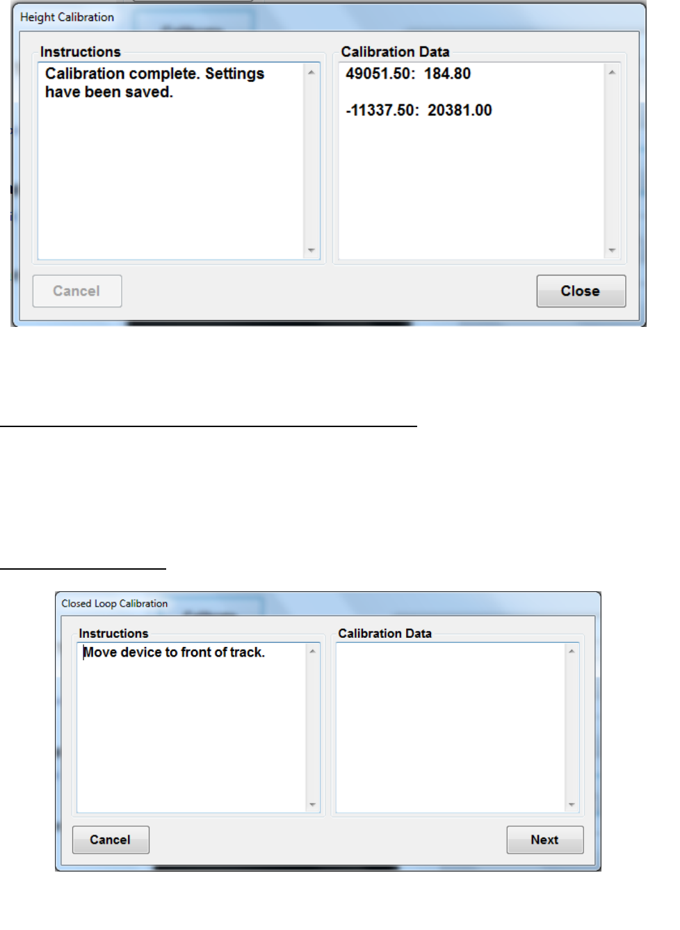
Calibration Instructions:
Place system laser at start of track.
Figure 35: 1st window of the Profile Slope Calibration. The initial negative distance indicates the
length between the laser and back wheel. Proceed to push system to end of track.
Figure 34: After a successful calibration, the settings will be saved. Select close to
proceed to the next procedure.
20
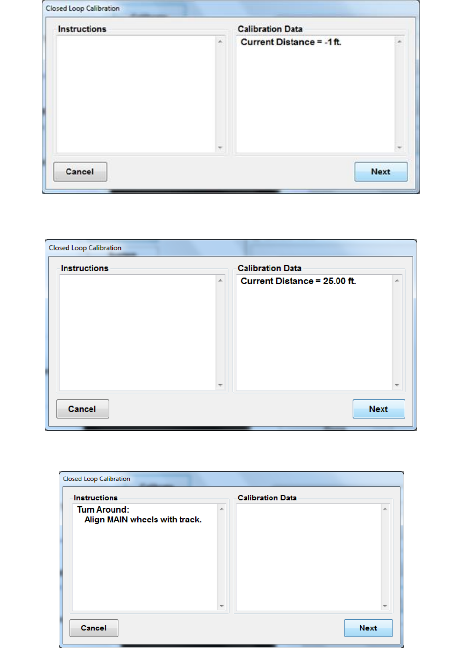
Figure 36: 2nd window of the Profile Slope Calibration. The initial negative distance indicates the
length between the front and back wheel. Proceed to push system to end of track.
Figure 37: Profile Slope Calibration widow after device has been pushed for 25 ft along a
straight calibration path. Closed loop calibrations can be no shorter than 20ft.
Figure 38: Window indicating operator to come back over the same calibration line
21
With the system facing the opposite direction and laser at the end of the track, where the back
wheel ended, push system back to initial starting point. The main wheels should go over the same
line. The distance traveled will be reversed. Stop when the onscreen “Current Distance” shows
0.00 feet.
Figure 39: Window starting the second half of the closed loop calibration. Push device back to
the start of the original track.
Figure 40: Window at the end of the second half of the calibration routine when the device has
reached the starting point of the initial track.
22
GPS Reporting Notes
If WalkPro is equipped with 5 Hertz (Hz) GPS, the coordinates of the profile will be included with
the data. The GPS system is maintenance free and does not require any set up as long as the
antenna is fixed to the WalkPro housing. The reporting interval of the GPS coordinates can be
adjusted within Profiler V3. Navigate to the Report Options tab under Settings. Select the icon
labeled “Customize Reporting Intervals” and enter the appropriate distance between GPS
coordinates.
Figure 42: Last close loop calibration window indication a completed routine.
Figure 41:Calibration window calculating results
23
Create A New Job Folder on the Hard Drive For Organization
Prior to starting a profile job, it is recommended to organize the files into a folder where all of the
files can be easily accessed. Each job should have its own folder. To create a new folder right click
within windows explorer and select New>Folder.
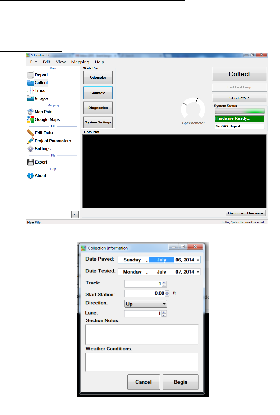
Collecting Data
Figure 43: The main collection window for the walking profiler.
Figure 44: First window after pressing the “Collect” button.

24
Closed Loop Collections and Slope Compensation
Closed loop collections are not mandatory to operate the WalkPro. The operator has the right
to only run open loop collections (one collection direction).
Closed loop collections eliminate inclinometer drift by subtracting the elevation changes from
sequential samples through the profile. A closed loop collection collects one run up and the second
run down the collection path. A slope compensation value is determined from the first closed loop
collection and is used in the subsequent collections of the WalkPro as long as the device hardware
is not disconnected. If the hardware is disconnected the slope compensation value is deleted and
the operator must perform another closed loop collection to determine the drift coefficient.
The red lever arm wheel should follow the same path for both collection directions.
Every time the hardware is disconnected the slope compensation value is lost and another closed
loop collection is required to replace the drift coefficient.
To collect a closed loop collection begin the collection by connecting the WalkPro hardware and
selecting Collect icon to input the collection parameters. Start the collection with the front left
wheel (lever wheel) on the starting position. Select “OK” to begin collecting. Once the collection
device’s rear left wheel is over the end point select “End First Loop” below “Stop Collecting” (End
First Loop is a closed loop collection; Stop Collecting is an open loop collection). Once the operator
selects “End First Loop” the WalkPro should be turned 180 degrees so the lever wheel is on the
same path as run one. The operator will select “Start Second Run” when in the start collection
position. Continue beginning point of run one and end the collection by selecting “Stop.” At this
time the program will determine a drift coefficient for the current hardware connection.
If the second loop is not approximately the same length as the first loop (1 foot tolerance) the
program will make the collections into open loop runs.
The physical procedure for closed loop collections is shown below. Begin at a point A and end at
point B, then turn around to begin at point B to end at point A. The exact path of run 1 is followed
until the collection is ended at point A. Do no drastically lift the wheels of the walking profiler
while reversing its direction. Execute multiple “Y” turns to rotate the walking profiler 180 degrees.
Begin the collection of run one at point A with the axle of the front measurement wheel centered
on the starting line. End run 1 at the ending station (point B) with the left rear wheel centered over
the end line (the wheel that the brake acts on). This ending position may be marked to find the
same point to start run two. Begin run two with the measurement wheel (wheel on the lever arm)
centered on the marked line showing the end of run one. Run two ends at point A with the left
rear wheel over the initial starting point.
Point B
Point A
Run 1
Run 2
Figure 45: Collection procedure for a closed loop collection
25
The collection speed should not exceed one foot
per second to have the most accurate profile
collections. The speed limit is denoted by the red
area of the speedometer. The operator is able to
change the warning speed at their discretion. As the
collection speed increases the accuracy of the
WalkPro decreases.
It is not recommended to collect WalkPro profiles
faster than 4 feet per second. For the most
accurate profiles set the speedometer for a
maximum speed of 1 foot per second.
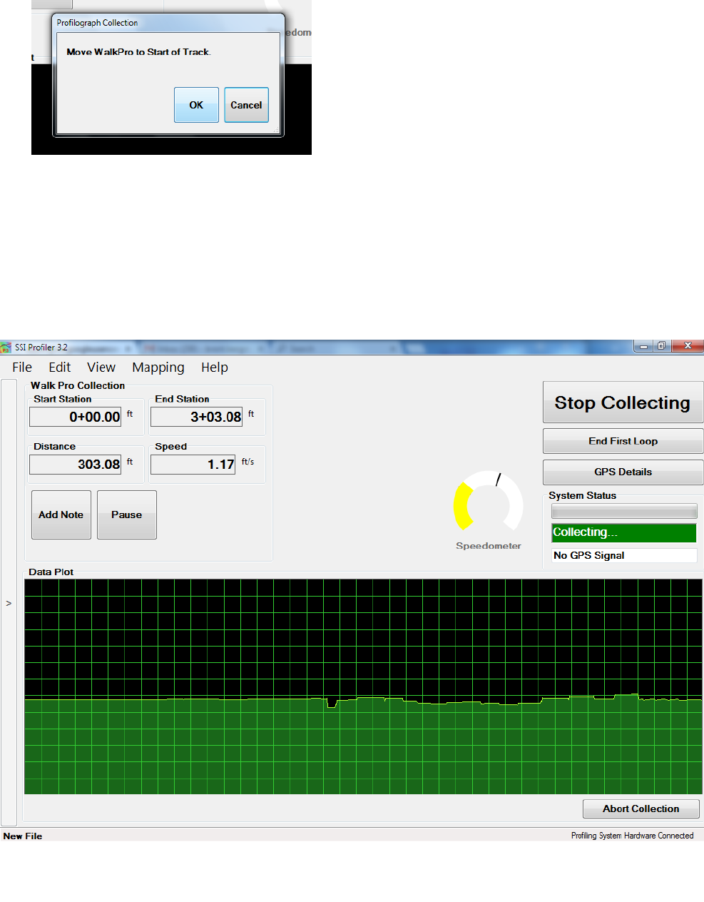
Figure 46: Start Collection.
To start the collection, move the
walking profiler to the beginning of
the track. Once OK is selected, data
collection will begin.
Figure 47: The collection window. It shows the initial options to stop the open
loop collection or end the first loop of a closed loop collection.
26
When the walking profiler is in place to start the second leg of the closed loop, select “Start
Second Run.” Once the front left wheel is on the starting mark the operator may select “Start
Second Run” of the closed loop collection.
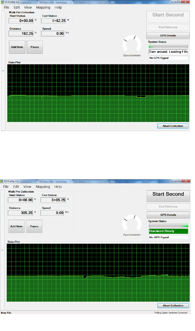
Figure 48: Window at the end of the first part of the closed loop.
Figure 49: Begin Second Loop window
27
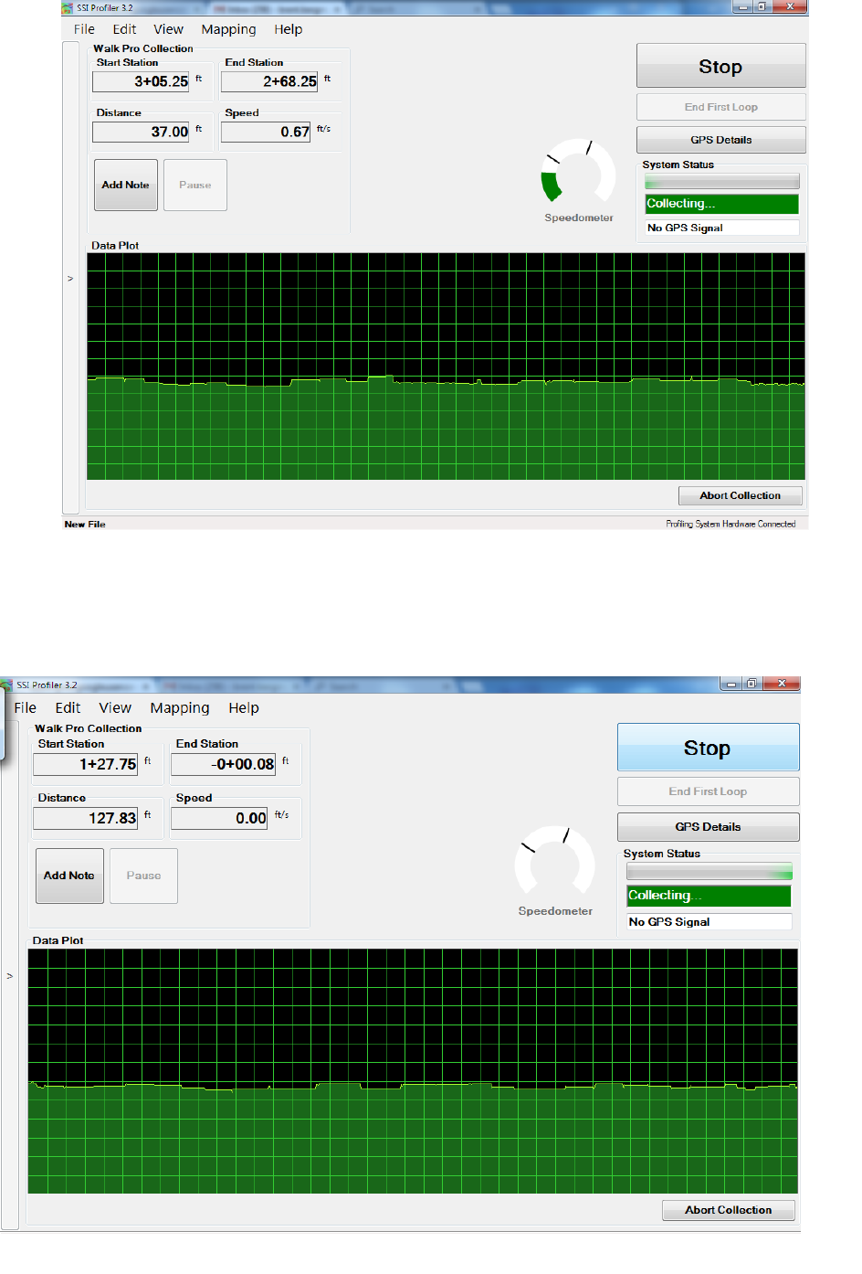
Figure 50: Once the second run is started the option to stop collecting appears.
During the second leg of collection, the end station will decrease toward zero; the
starting station for the first loop.
Figure 51: End of Second Loop for Closed Loop Collection
28
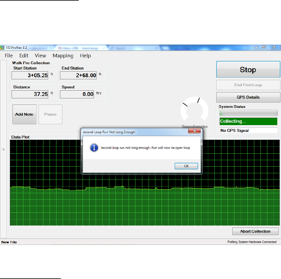
Closed Loop Requirements
If the second leg of the closed loop collection is not as long as the first leg the Profiler program will
give the operator an error. The tolerance for this error is one foot. The ending station of the second
loop must accurately match the beginning station of loop one for the slope compensation feature
to function.
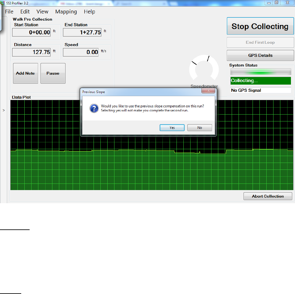
Slope Compensation
After the operator has collected a valid closed loop run the WalkPro software will save the slope
compensation value until the hardware is disconnected. To use the slope compensation feature
with open run collections, select “Yes” after an open loop collection. The slope compensation
allows one direction open loop collections to be closed loop collections. Either method, closed
loop or slope compensation, will produce accurate profiles without inclinometer drift. The slope
compensation is much faster and more efficient and will reduce the number of runs collected by
the operator.
For instructions on performing a closed loop collection, see the closed loop section above.
Figure 52: Second Loop Length for Closed Loop is Invalid
29
Add Note
Adding notes is a valuable tool when pausing or explaining information that is not included in the
profile data. This can be information on manholes, drainage structure, bridge decks or any other
obstruction. Adding notes assures the operator that the data will be able to be deciphered at a
later date, and any questions can be answered. Notes, also known as events, can be changed or
edited in post processing under the Edit Data>Edit Events tab in Profiler V3.
Pauses
Pausing is allowed for certain obstructions in the profiling path. These are for instance, drainage
structures, bridge decks and manholes. Review the overseeing agency’s specifications for paused
and excluded data. Pausing the data run still collects the distance traveled, but the height data is
omitted. The trace will still show the trace of the paused section. If the operator decides to review
the paused sections, these sections can be analyzed alone, with the rest of the data, or excluded.
When the paused sections are excluded, the data within the paused section will not affect the
localized roughness or ride value calculations. This option can be found in General Settings within
the drop-down menu under the label Pause Section Analysis.
New pauses, adjustments to the run up/out data, and stationing changes can be made after the
data has been collected. To adjust these settings, navigate to the Edit Data section under the Edit
tab.
Figure 53: Prompt to Use Slope Compensation on an Open Loop Collection
30
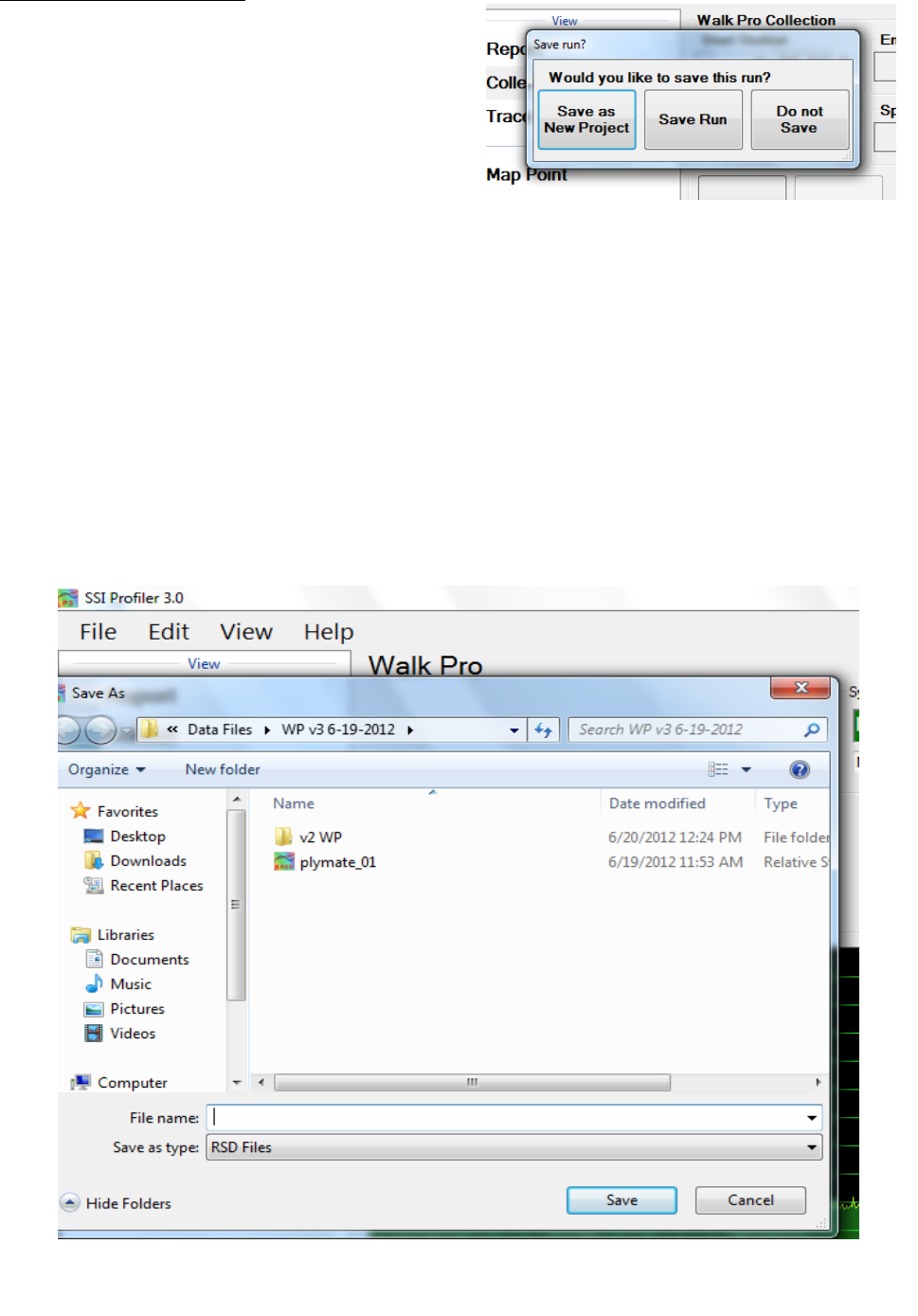
Saving the New Collection
After collection of the data the Profiler program will
ask the operator to Save as New Project, Save Run,
or Do Not Save. The options of Save as New Project
and Save Run will open windows explorer to choose
a folder destination for the new file. If do not save
is chosen, the program will keep the last collection,
but it will not be saved. To save the collection after
selecting do not save, open the file>Save As in the
menu bar.
When there is unsaved data or changes in Profiler V3, the file name in the lower left corner will
have an asterisk (*) after the file name.
The save as new feature can be used if a new file was not created before collection. If the data was
collected under an old file name and the operator does not want the recent data to be saved under
this old file, choose Save As New. If the operator created a new file prior to collection Save As New
and Save Run will perform the same function.
Save the file by selecting File>Save or File> Save As. This will allow the operator to save the
collection data.
Figure 55: Windows Explorer to save the collection
Figure 54: Saving Options after a collection
31
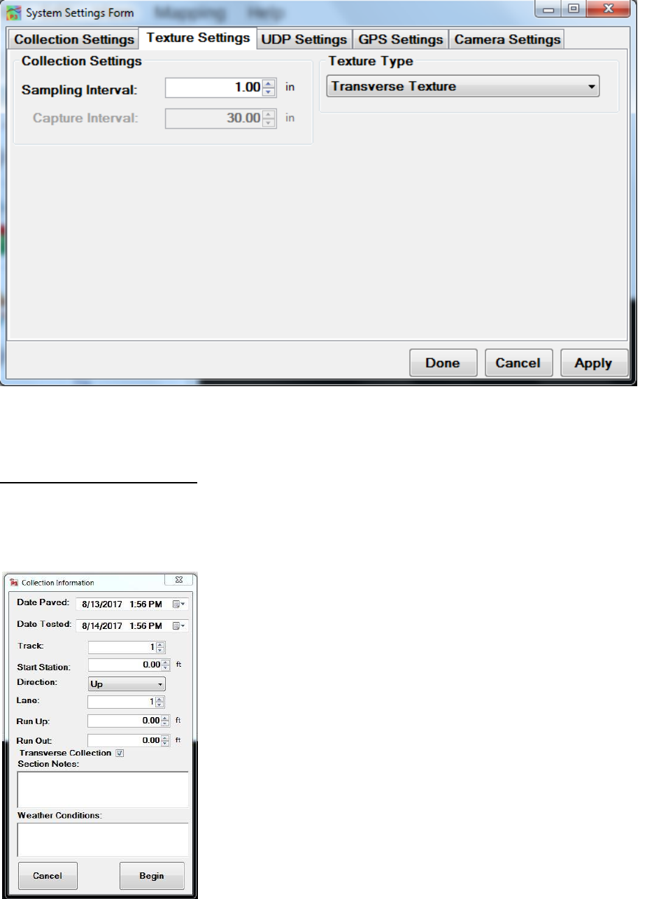
Texture Measurement
Using the laser front arm the WalkPro can collect high frequency elevation samples to be used to
calculate texture or Mean Profile Depth (MPD). The collection procedure is the same as the
regular WalkPro collections, however there are new parameters that need to be entered prior to
collection such as texture sampling interval and laser front arm type. The collection program
uses SSI’s Laser Recorder program that has the ability to collect a high amount of laser samples in
different modes. Under Collect>System Settings>Texture Settings the operator can choose one of
three texture modes: Longitudinal, Transverse and 3D Modes. The sampling interval is the length
of the texture sample while the capture interval is the length between texture patches.
• Longitudinal Texture Mode
Collects longitudinal texture along a thin line, only using the center elevation
readings of the laser. A four-inch (10.16 cm) strip is used to calculate the texture
value.
• Transverse Texture Mode
Collects transverse texture at the specified sampling interval.
• 3D Texture Mode
o Full and continuous texture profile at 1mm x 1mm resolution.
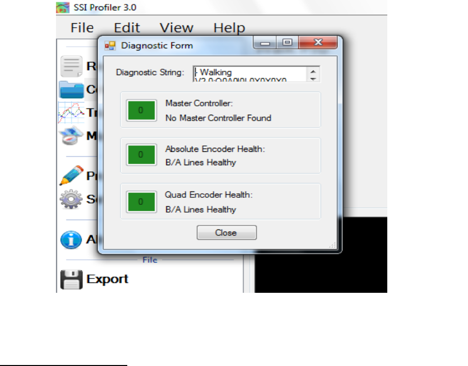
Figure 56: The diagnostics window is shown above with all of the components
green and operational.
32
Transverse Profile Collection
The WalkPro CS8800 is able to collect transverse profiles with no change in hardware. In order to
complete this operation, the user must select the check box under the run out input of the
Collection Parameters window (appearing after clicking on the Collect icon). The transverse
collection procedure is similar to the longitudinal collection and the calibrations are the same.
After selecting the ‘Collect’ icon at the top right corner of the
Collect window the user is presented with the Collection
Parameters window. To collect transverse runs select the checkbox
below the run out input. After selecting begin the operator will be
asked if the collection type is desired to be transverse. Before
proceeding the CS8800 should be near the starting point of the
collection. The collection will begin after the SSI Profiler program
confirms the CS8800 is at the edge of the collection track, or path,
and the user enters the starting station and station direction.
Figure 57: Texture setting tab under system setting.
Figure 58: First Collection window after pressing collect.
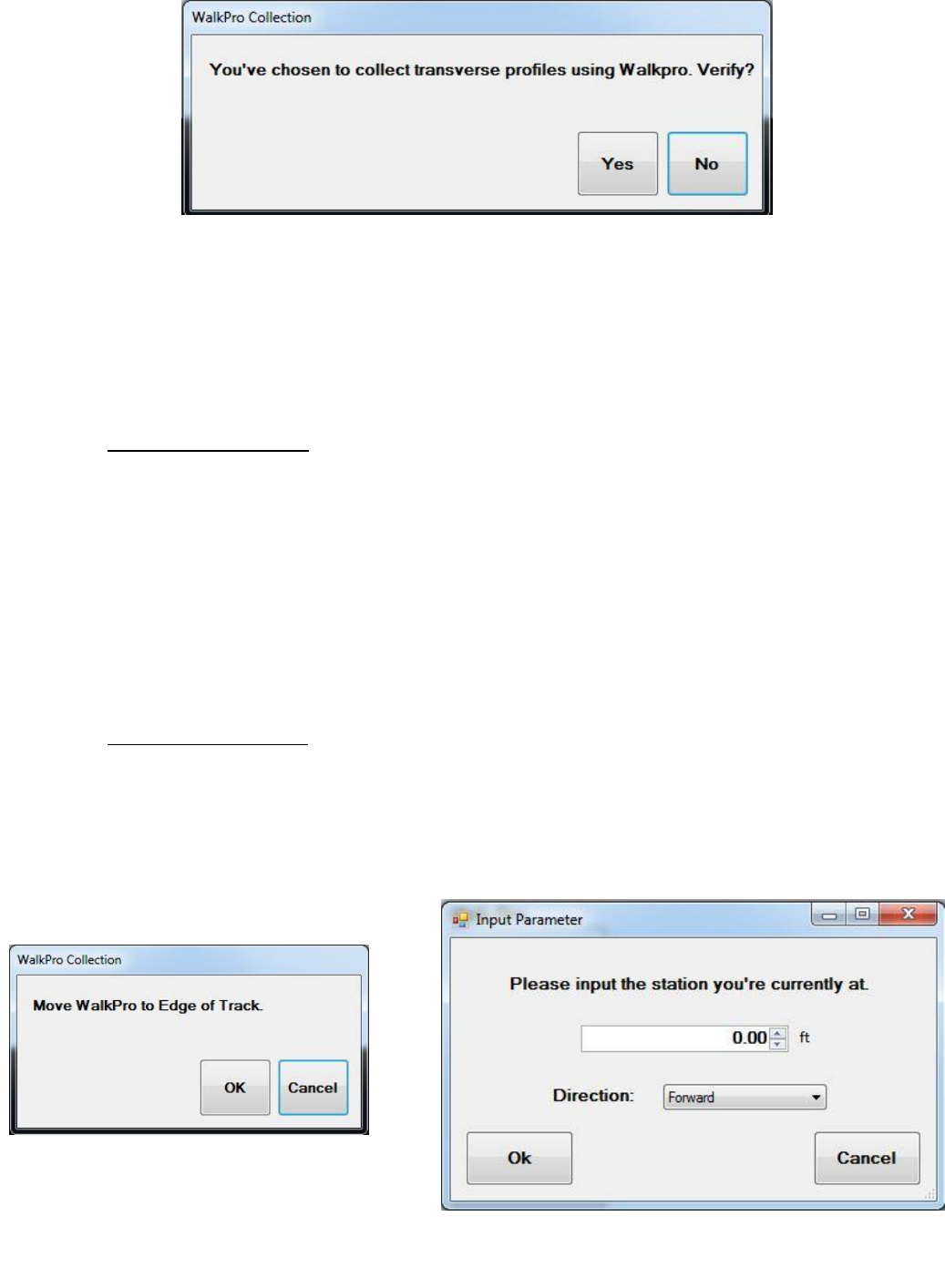
33
The transverse data will be displayed within the collection screen along with the distance
traveled, speed and station position. To end the collection, select the icon at the top right of the
window, ‘Stop Transverse’.
At the end of the collection the SSI Profiler program will ask if more transverse profiles will be
collected. If no other collections will be made the previous collection will be saved.
Data Saving Option A:
If additional transverse data will be collected the program will ask how to save the
additional runs. The user may save the additional runs to the currently open RSD file. The
SSI program will automatically categorize the collections as sequential Run 1, Run 2, etc.
If another transverse collection will be saved to the current RSD file, the user shall move
the CS8800 to the edge of the collection track when prompted by the software. The
collection will start once the user selects OK under the, ‘Move WalkPro to Edge of Track’
window. Additional transverse collections will be terminated the same way as previous
runs. Additional collections may be saved under one RSD file. SSI recommends a
maximum of twelve collections under one RSD file.
Data Saving Option B:
The user may save each transverse collection as an independent RSD file. This is the
preferred collection method when post-processing will be performed. After each
collection the operator shall decline to collect additional transverse collections and will
save each file as a new RSD file. Once the user is ready for another collection, it is
recommended to create a new file. A new RSD file can be created through File>New or
CTRL+N.
Figure 59: Verification window for collecting transverse profiles.
Figure 60: First
Collection window for
Transverse profiler.
Figure 61: Window indicating operator
to input start station and direction of
travel.
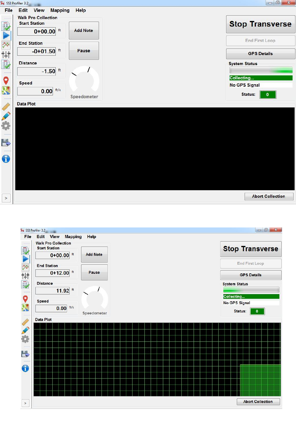
34
Figure 62: First Collection window after pressing collect.
Figure 63: Collection window while profiling
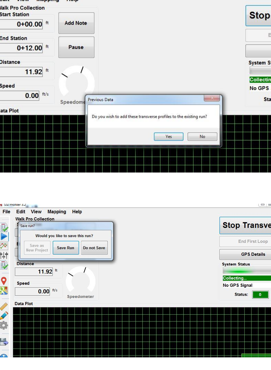
35
Figure 64 : Window asking for another transverse profile. Pressing “No”
will lead to figure 55. Pressing “Yes” will lead to figure 57.
Figure 65: Save run window.
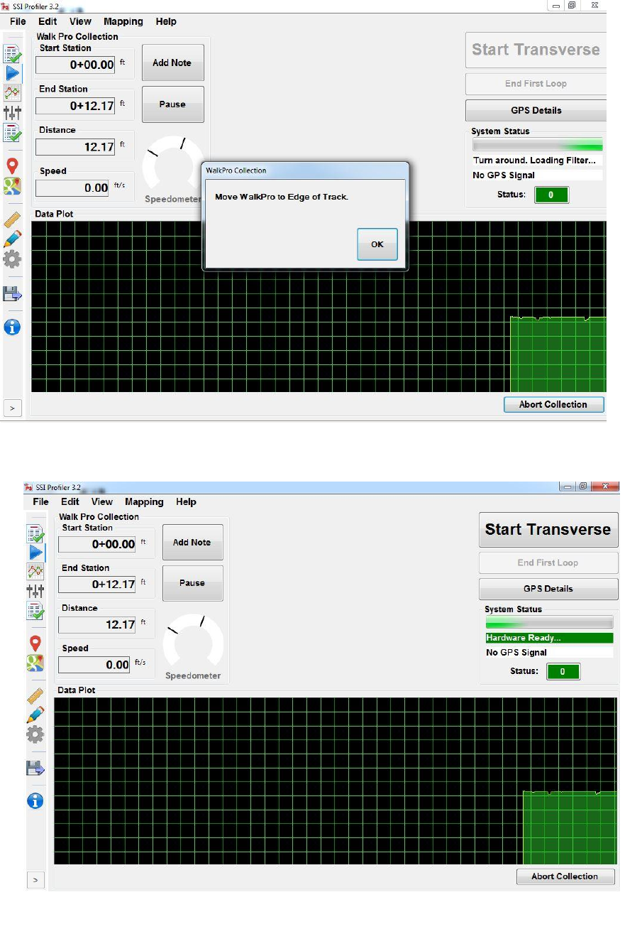
36
Figure 66: Window after selecting “Yes” to figure 54 for collecting another profile.
Figure 67: Collecting another transverse profile.
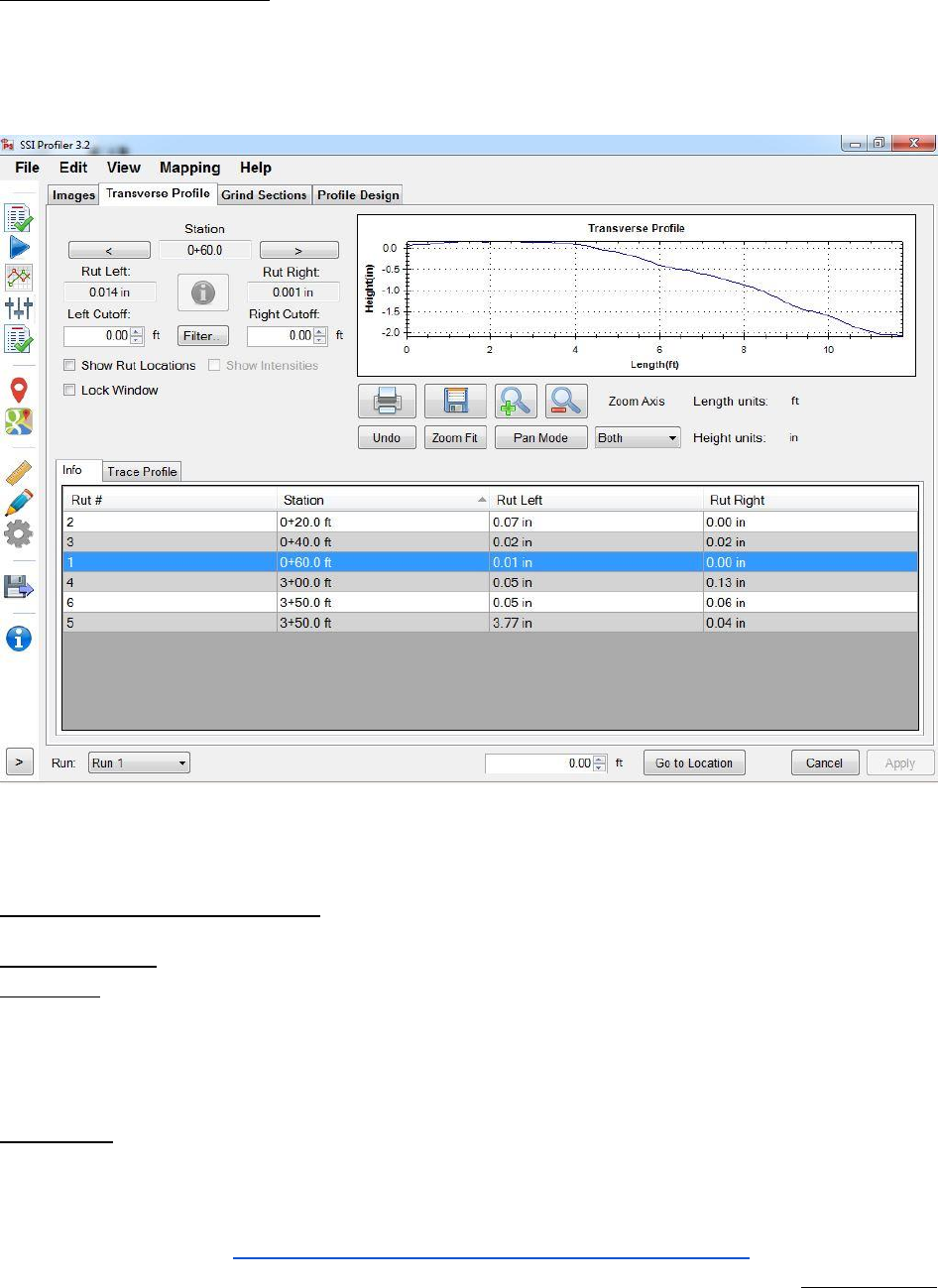
37
Viewing Transverse Profiles
The transverse collections will be available for viewing under the Advanced Tools section of SSI
Profiler. The tab will be labeled, ‘Transverse Profile’. Within this window the user may review the
elevation trace, longitudinal station, and rut depth. Each transverse profile can be edited under
this window by cropping either side of the collection.
Reporting and Exporting
1.0- File Tab
1.1. - New
Selecting New creates a new project file to be saved on the operator’s computer or external device.
The file will open automatically and the bottom left corner of the program will display “New File.”
If data has been collected with this file, the name will be displayed with as asterisk as “New File*.”
1.2. – Open
Opens a project file previously saved on the operating computer or connected external device.
Profiler V3 creates RSD type files. The RHD file type from the previous version of Profiler can also
be opened Profiler V3. If your file is in another format, use the appropriate translators found on
the support website (http://www.smoothroad.com/support/download.asp) or contact S.S.I.
Customer Support. The only two file formats used in the Profiler V3 program are RHD and RSD.
Profiler V3 only collects data in the RSD format.
Figure 68: Transverse profile viewing window.
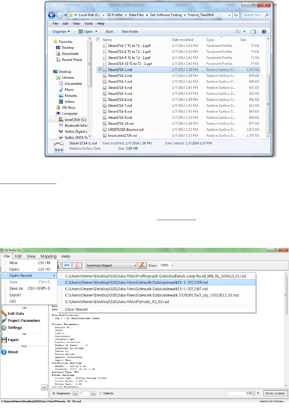
38
1.3. - Open Recent
Opens recently viewed or created project files. Files will only be available if they are saved on the
operating computer or connected external device. The Open Recent feature is a shortcut to find
current profiling data. It is also possible to use the File>Open tool to open saved data. The only
two file formats used in the Profiler V3 program are RHD and RSD. Files can only be saved in RSD.
The default file to be searched for in Window’s Explorer can be changed under General Settings
and the “Default File Type.”
Figure 69: Opening a data file in the Profiler V3 program.
Figure 70: The Open Recent feature
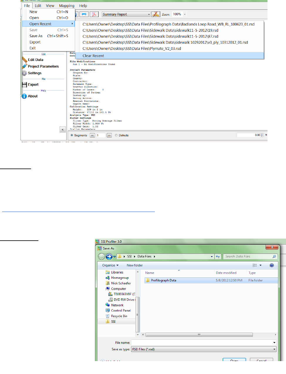
39
Clear Recent
Clear Recent deletes the history of previously viewed RHD and RSD files. Once the history is cleared
it cannot be reversed. The operator must navigate to File>Open to view saved files.
1.4. – Save
Save allows the operator to save the current file in RSD format on the operating computer or
connected external device. If ‘Save’ is selected while an unsaved file is open, the operator will be
prompted to choose a file name and folder destination to save the current file. The file will be
saved in SSI´s patented RSD format. If another format is required, visit the SSI support website
(http://www.smoothroad.com/support/download.asp) to download the latest translators or
contact SSI Customer Support.
1.5. - Save As
When Save As is selected, the
operator will be prompted to
choose a file name and folder
destination in which to save the
current file. The file will be
saved in SSI´s patented RSD
format. If another format is
required, visit the SSI support
website
Figure 71: The clear recent feature
Figure 72: Saving a file through Save As in RSD format.
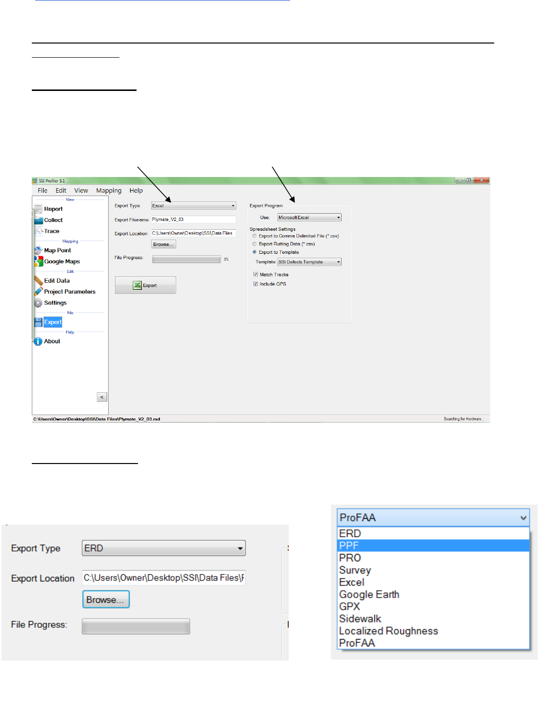
40
(http://www.smoothroad.com/support/download.asp) to download the latest translators or
contact SSI Customer Support.
Note: Save and Save As are only available after data has been collected or if changes are made
to preexisting file.
1.6. - Exporting
Exporting allows the operator to create files in ERD, PPF, PRO, Survey, GPS Matching, and Excel
formats. The settings for each export feature are described below. For each of the exporting
formats, a folder destination is required. The Export feature can be found in the shortcut bar on
the left hand side of the Profiler V3 window and in File>Export.
1.6.1. Export Location
To select the folder destination, select ‘Browse’ and navigate through Windows Explorer to the
desired folder. Once the folder destination is reached and selected, left click on ‘OK’ at the bottom
of the window to save the folder location.
Figure 73: The export window for exporting the data into Excel format.
Figure 74: Selecting a location to save the exported file.
Figure 75: The export type drop down menu
Export type drop down menu Stationing Extraction
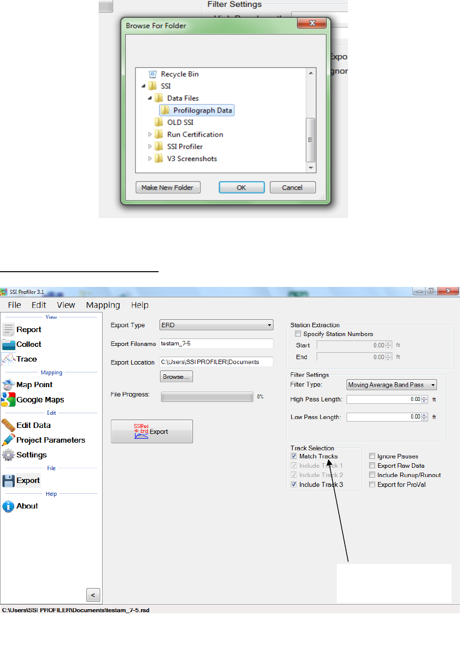
41
1.6.2. – Exporting to ERD Format
Figure 76: The export folder location selection
Figure 77: The ERD format export window with match tracks selected.
Match Tracks is
selected

42
Station Extraction
The operator has the option export only certain sections of the data, based on the stationing set
within the profiling data. To use this feature, select the check box near “Specify Station Numbers.”
When the box is selected, the operator will be able to adjust the stationing numbers. The ‘Start’
stationing is the initial stationing where the exported file will begin, while the ‘End’ stationing is
the point where the exported file will finish. These values can be adjusted by typing values into
the box or by using the arrow keys to the right of the box.
Filter Settings—High & low pass length
The exported data file can have additional filters applied while being processed into the chosen
format. To not filter the data, leave the filter lengths at the default value of 0.00 feet.
Moving Average High Pass Filter
A high pass filter will remove any trend that is shorter than the selected length. Typical range of
length for this filter is one hundred feet (100 ft.) through two hundred feet (200 ft.).
Moving Average Band Pass Filter
This filter only allows the desired frequency of data to be shown. Adding this filter will adapt the
profile trace to remove the high frequency motions. Moving average filters are typically used for
short data runs less than two hundred feet (200 ft.).
Butterworth High Pass Filter
High pass filters allow the high frequency characteristics of the data plot to pass through while
blocking the lower frequency attributes of the data run. Butterworth filters do not introduce a
phase shift into the plot like moving average filters. Butterworth filters are traditionally used for
longer data runs over two hundred feet.
Butterworth Band Pass Filter
This filter will perform both a high pass and low pass Butterworth filter operation on the data. The
result is a run that has frequencies within the lower and upper bounds. Butterworth filters do not
introduce a phase shift into the plot like moving average filters. Butterworth filters are traditionally
used for longer data runs over two hundred feet.
Include Run Up – Run Up Data
Some High-Speed Profiling data files have Run Up and/or Run out data associated with them,
depending on the practice used to collect the data. If this data exists in the data file, it will be
included in the exported file if this box is selected. Run Up and Run out is used to allow the
electronics to settle on the accurate profile.
Run Up data exists in HSP data files if the operator selected a Run Up and/or Run out distance in
the initial stages of setting up a collection. In the HSP collection software, the Run Up and Run out
settings are found on the last window before performing a collection. Use run up and run out to
stabilize the electronics before the starting location is reached.
Export Raw Data
Selecting the Export Raw Data check box assures the operator that only unfiltered data collected
from the profile will be exported into the chosen file.
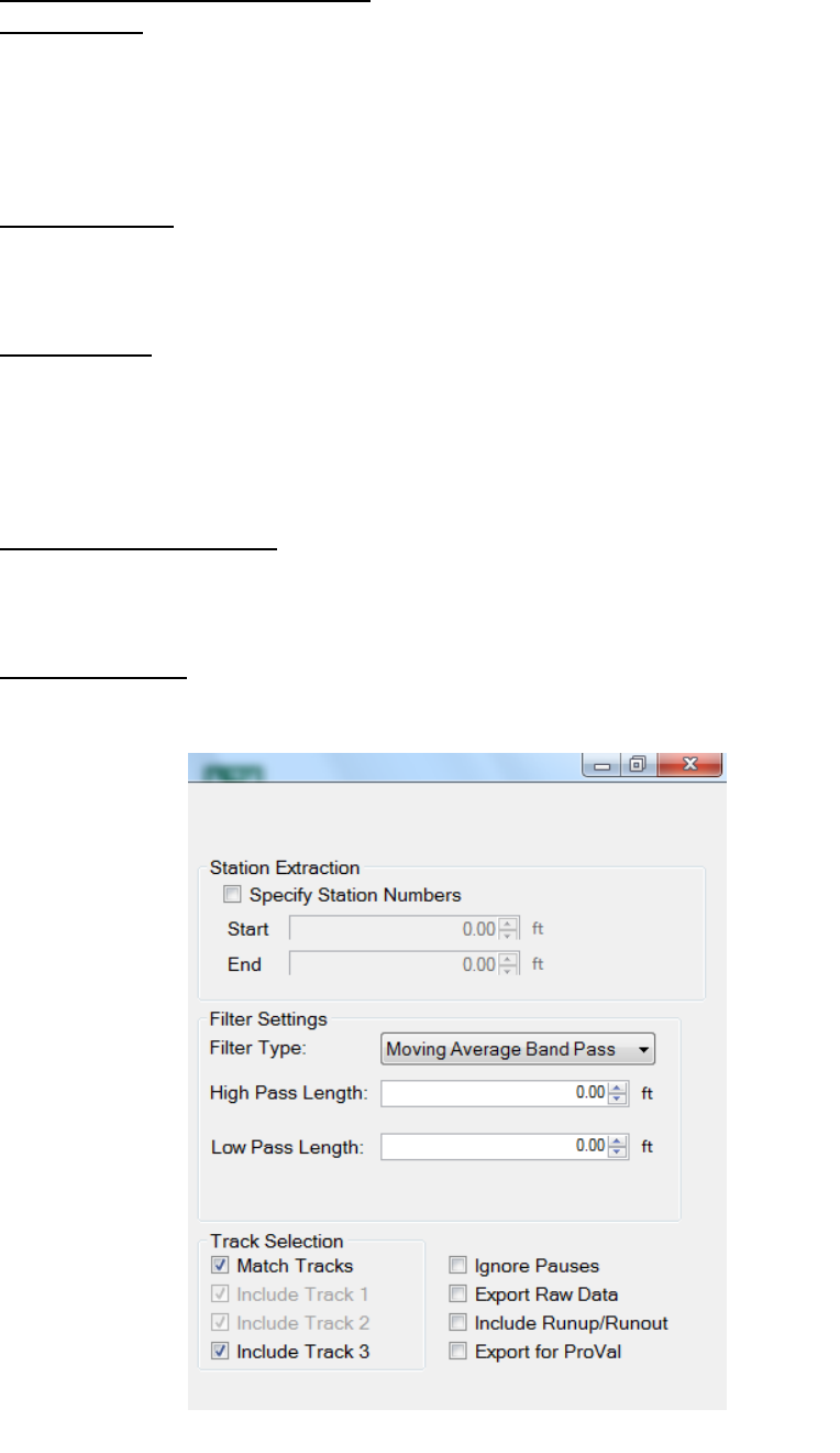
43
Match Tracks and Choosing Tracks
Match Tracks
Selecting ‘Match Tracks’ exports all of the tracks associated with the lane file. For the three laser
systems, this includes Track 1, 2 and the center trace. For Profilograph files, the tracks are matched
based on the settings entered prior to profiling. The label of the track number and stationing
cannot be changed after collection.
Choosing Tracks
The tracks that are exported are checked under “Track Selection.” If Match Tracks is selected the
user cannot deselect track 1 or 2.
Ignore Pauses
Pauses are useful when an obstruction comes into the profiling path or when a section of
pavement is not to be profiled. When Pause is activated, the stationing remains constant and
under the same file. Pauses can either be omitted or included in reports and exported files of
Profiler V3 software. To omit pauses from the exported file, select the check box, “Ignore Pauses.”
Include Run Up/ Run out
When this option is selected, the Run Up and Run out data collected during the collection will be
included in the export data.
Export for ProVal
When the user exports an ERD file for use in ProVal, it changes the file’s default filters and settings
to more accurately match the values in ProVal.
Figure 78: The ERD export window settings
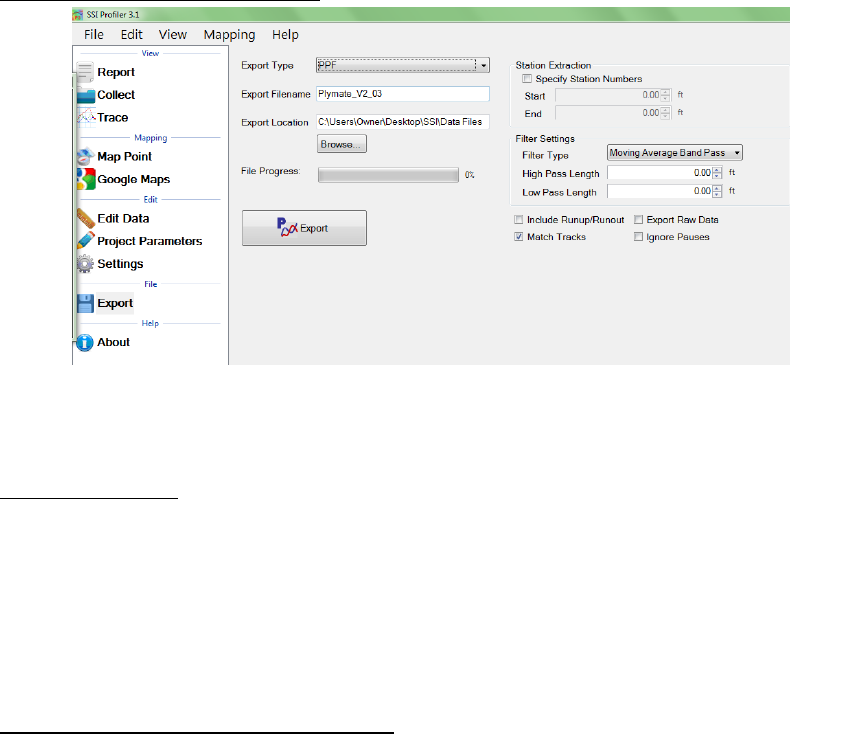
44
1.6.3. – Exporting to PPF Format
Station Extraction
The operator has the option to export only certain sections of the data, based on the stationing
set within the profiling data. To use this feature, select the check box near “Specify Station
Numbers.” When the box is selected, the operator will be able to adjust the stationing numbers.
The ‘Start’ stationing is the initial stationing where the exported file will begin, while the ‘End’
stationing is the point where the exported file will finish. The start and end stationing can be
adjusted by typing values into the box or by using the arrow keys to the right of the box.
Filter Settings—High & Low Pass Length
The exported data file can have an additional filter applied while being processed into the chosen
format. To not filter the data, leave the filter lengths at the default value of 0.00 feet.
Moving Average High Pass Filter
A high pass filter will remove any trend that is shorter than the selected length. Typical range of
length for this filter is one hundred feet (100 ft.) through two hundred feet (200 ft.).
Moving Average Band Pass Filter
This filter only allows the desired frequency of data to be shown. Adding this filter will adapt the
profile trace to remove the high frequency motions. Moving average filters are typically used for
short data runs less than two hundred feet (200 ft.).
Butterworth High Pass Filter
High pass filters allow the high frequency characteristics of the data plot to pass through while
blocking the lower frequency attributes of the data run. Butterworth filters do not introduce a
phase shift into the plot like moving average filters. Butterworth filters are traditionally used for
longer data runs over two hundred feet.
Butterworth Band Pass Filter
This filter will perform both a high pass and low pass Butterworth filter operation on the data. The
result is a run that has frequencies within the lower and upper bounds. Butterworth filters do not
Figure 79: The PPF export window
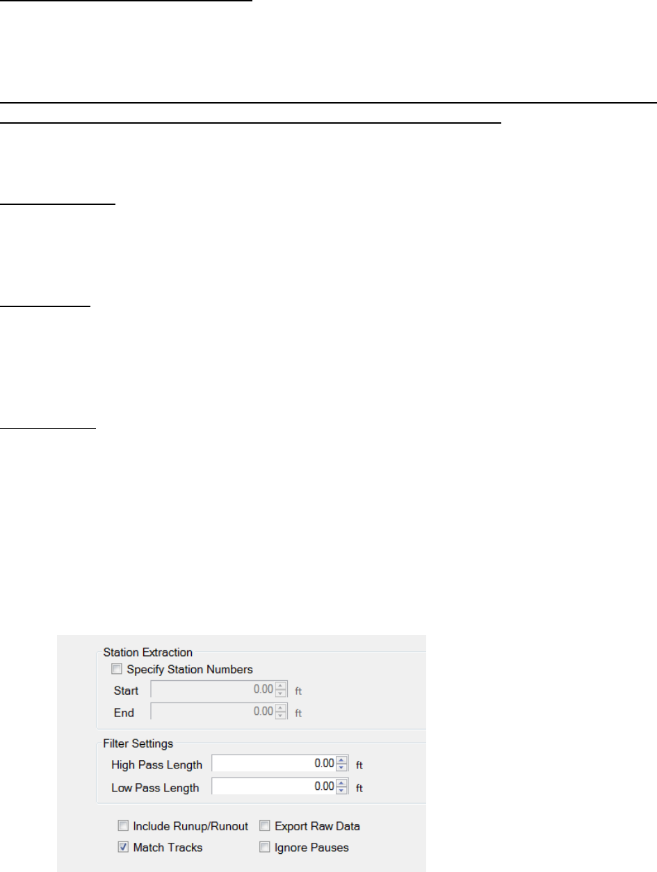
45
introduce a phase shift into the plot like moving average filters. Butterworth filters are traditionally
used for longer data runs over two hundred feet.
Include Run Up and/or Run out Data
Some High Speed Profiling data files have Run Up and/or Run out data associated with them,
depending on the practice used to collect the data. If this data exists in the data file, it will be
included in the exported file if this box is selected.
Run Up data only exists in HSP (High Speed Profiler) data files if the operator selected a Run Up
and/or Run out distance in the initial stages of setting up a collection. In the HSP collection
software, the Run Up and Run out settings are found on the last window before performing a
collection.
Export Raw Data
Selecting the Export Raw Data check box assures the operator that only unfiltered data collected
from the profile will be exported into the chosen file. The file is adjusted so that the elevations
begin at zero.
Match Tracks
Selecting ‘Match Tracks’ exports all of the tracks associated with the lane file. For the three laser
systems, this includes Track 1, 2 and the center trace (track 3). For the Profilograph files, the tracks
are matched based on settings entered prior to profiling. The stationing and number label assigned
to the track are settings that cannot be changed after collection.
Ignore Pauses
Pauses are used when an obstruction comes into the profiling path or when a section of pavement
is not to be included in the calculation of ride values and localized roughness. While Pause is
activated, the program will continue to collect stationing date, but will not collect height data.
Pauses can either be omitted or included in reports and exported files. To omit pauses from the
exported file, select the check box, “Ignore Pauses.”
To import into ProVal the best method is to include pauses. The pauses of the rsd file will turn into
a leave-out section within ProVal. If pauses are not included during export, it will result in two PPF
files for the same track. There will be one more PPF file than the number of pauses.
Figure 80: The
optional settings
when exporting
in PPF format.
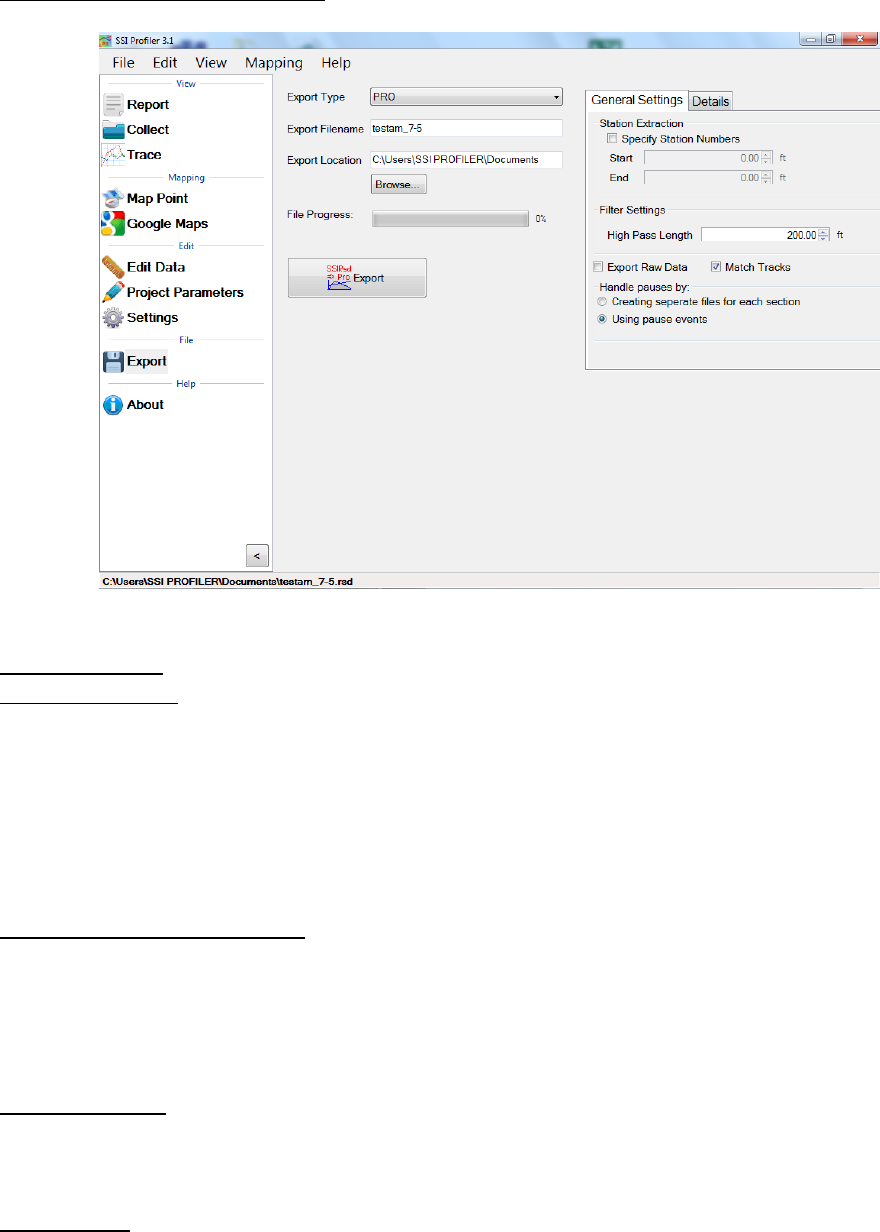
46
1.6.4. – Exporting to PRO Format
General Settings
Station Extraction
The operator has the option to only export only certain sections of the data, based on the
stationing set within the profiling data. To use this feature, select the check box near “Specify
Station Numbers.” When the box is selected, the operator will be able to adjust the stationing
numbers. The ‘Start’ stationing is the initial stationing where the exported file will begin, while the
‘End’ stationing is the point where the exported file will finish. These values can be adjusted by
typing values into the box or by using the arrow keys to the right of the box.
Filter Settings-high pass length
It is an option to change the High pass filter length when exporting files to PRO format. A High Pass
Filter removes all of the data trends below the filter length. The default length of the High Pass
Filter is 200 feet. In order to export the data without filtering, the ‘Export Raw Data’ check box
must be selected. See ‘Export Raw Data’ below.
Export Raw Data
Selecting the Export Raw Data check box assures the operator that only unfiltered data collected
from the profile will be exported into the chosen file.
Match Tracks
Selecting ‘Match Tracks’ exports all of the tracks associated with the lane file. For the three laser
systems, this includes Track 1, 2 and the center trace. For the Profilograph files, the tracks are
matched based on settings entered prior to profiling. The label of the track cannot be changed
after collection.
Figure 81: The export window when PRO format is selected.
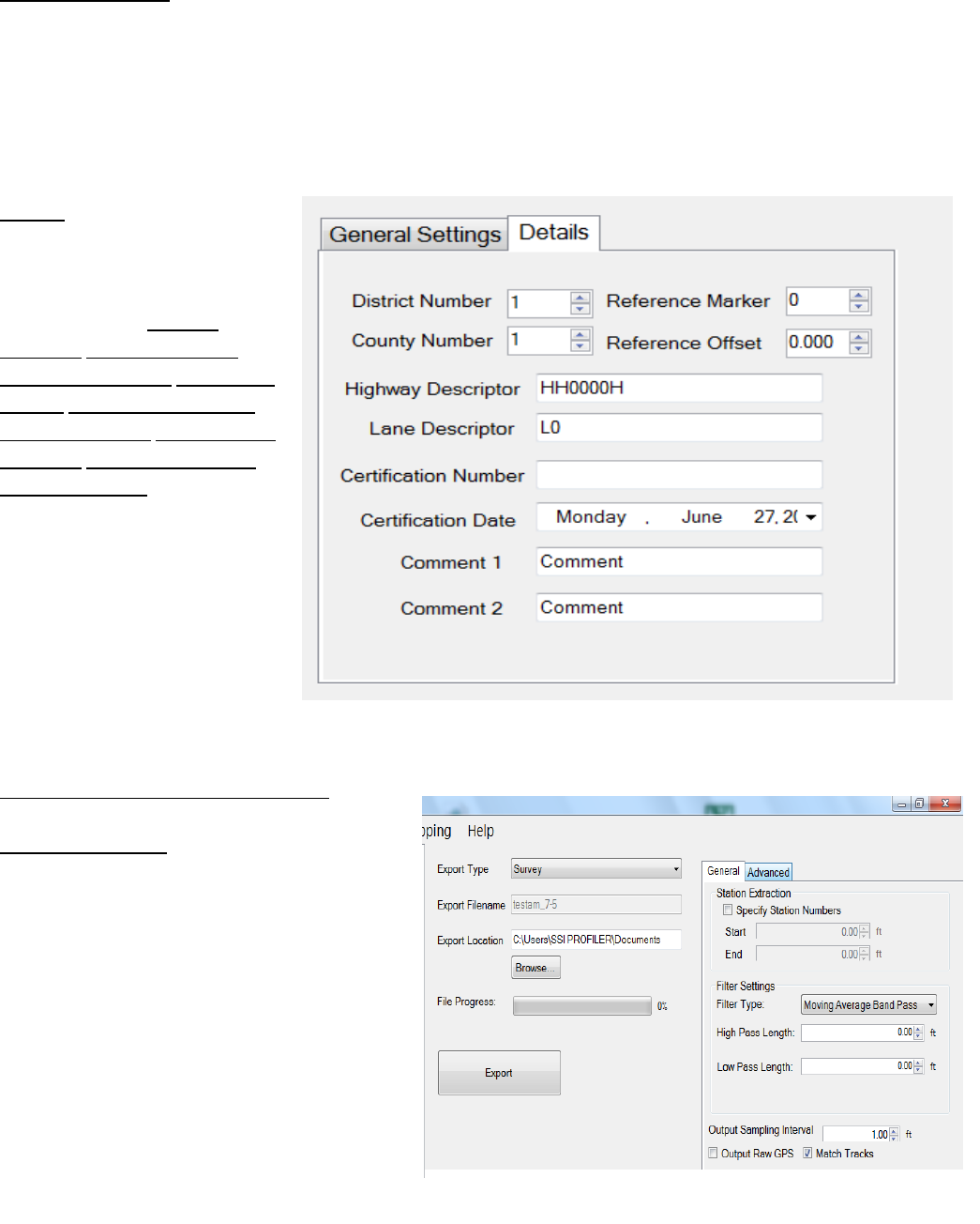
47
Handle Pauses By:
The paused sections within the collected data can be exported in two ways. Separate files can be
created for each segment or the file can be exported with the paused sections included in one file.
The difference in these two options is that creating separate file for each segment exports multiple
files into the folder location, and the option of “Using pause events” exports one file to the folder
location including all of the data. If the pauses were used to omit data because of pavement
anomalies, use the option of ignoring the pauses.
Details
The details section of PRO
exporting is the job specific
information that is saved with
the file, such as District
Number, County Number,
Reference Marker, Reference
Offset, Highway Descriptor,
Lane Descriptor, Certification
Number, Certification Date,
and Comments. This
information is then saved with
the PRO file to be displayed
when the file is opened or
printed using another
program.
1.6.5. – Exporting to Survey Format
Station Extraction
The operator has the option to only export
certain sections of the data, based on the
stationing set within the profiling data. To
use this feature, select the check box near
“Specify Station Numbers.” When the box is
selected, the operator will be able to adjust
the stationing numbers. The ‘Start’
stationing is the initial stationing where the
exported file will begin, while the ‘End’
stationing is the point where the exported
file will finish. These values can be adjusted
by typing values into the box or by using the
arrow keys to the right of the box.
Figure 82: The Details tab contains information about the project.
Figure 83: The window for exporting in Survey format
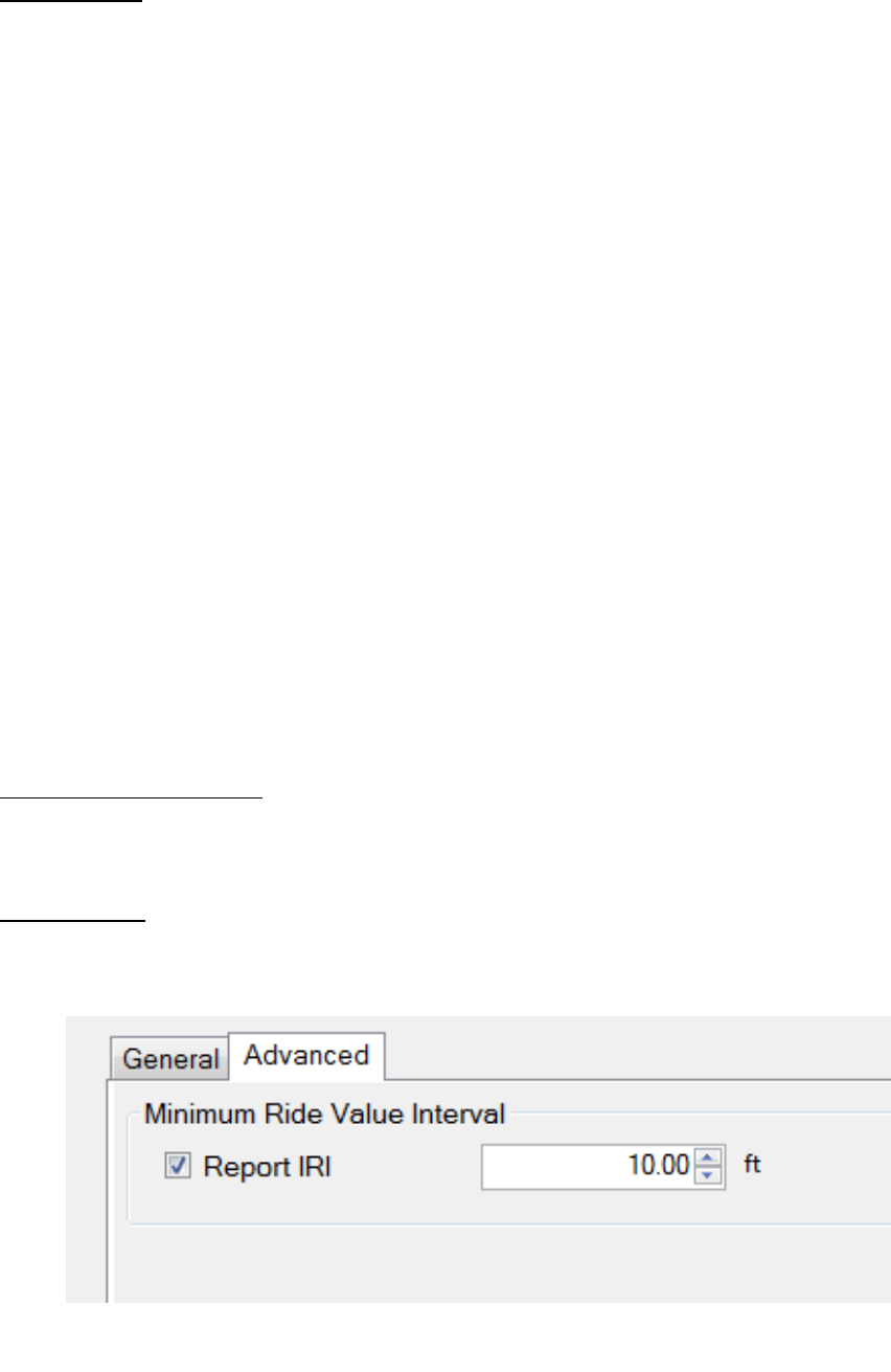
48
Filter Settings
A High and Low Pass filters are optional when exporting to survey format. The exported data file
can have an additional filter applied while being processed into the chosen format. To not filter
the data, leave the filter lengths at the default value of 0.00 feet.
Moving Average High Pass Filter
A high pass filter will remove any trend that is shorter than the selected length. Typical range of
length for this filter is one hundred feet (100 ft.) through two hundred feet (200 ft.).
Moving Average Band Pass Filter
This filter only allows the desired frequency of data to be shown. Adding this filter will adapt the
profile trace to remove the high frequency motions. Moving average filters are typically used for
short data runs less than two hundred feet (200 ft.).
Butterworth High Pass Filter
High pass filters allow the high frequency characteristics of the data plot to pass through while
blocking the lower frequency attributes of the data run.. Butterworth filters do not introduce a
phase shift into the plot like moving average filters. Butterworth filters are traditionally used for
longer data runs over two hundred feet.
Butterworth Band Pass Filter
This filter will perform both a high pass and low pass Butterworth filter operation on the data. The
result is a run that has frequencies within the lower and upper bounds. Butterworth filters do not
introduce a phase shift into the plot like moving average filters. Butterworth filters are traditionally
used for longer data runs over two hundred feet.
Output Sampling Interval
The sampling interval is the distance between readings of the SSI survey system. The default length
of this interval is 1 foot. This feature allows other intervals to be implemented, depending on the
accuracy specifications required in the surveying program.
Advanced Tab
The user has the option to report the IRI ride value every interval. The figure below is set to ten
feet; meaning the IRI will be displayed every ten feet of the profile.
Figure 84: The Advanced Options of the Survey format
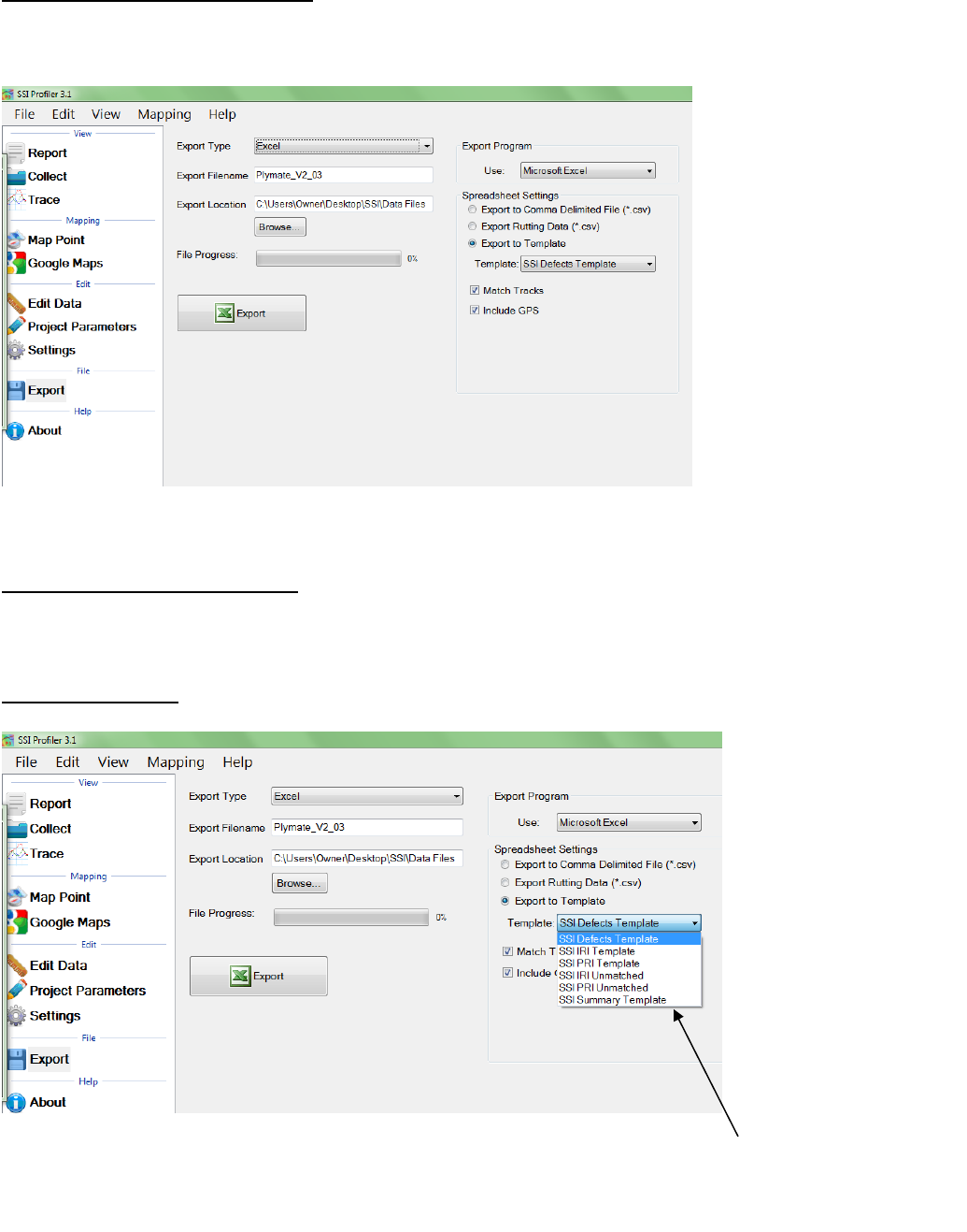
49
1.6.6. – Exporting to Excel Format
Exporting the profile data to excel gives the operator versatility and efficiency when an adjustable
numerical printout is needed.
Export to Comma Delimited File
The Comma Delimited file shows the track number, segment number, start and end stationing and
the ride number selected in the Analysis Parameters.
Export to Template
To choose a SSI Excel Template, select “Export to Template.”
Figure 85: Exporting the data into Microsoft Excel format
Figure 86: The types of excel formats are listed in the drop-down menu.
Types of excel formats to
export the collected data
into.
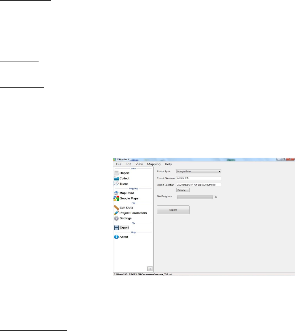
50
Defects Template
The Defects Template shows the locations and heights of the defects and information about the
file in spreadsheet form.
IRI Template
The IRI Template gives information on the IRI statistics along with the defect locations and heights.
PRI Template
The PRI Template lists the PRI for each track along with the bump heights, locations and settings.
IRI Unmatched
The IRI Unmatched Template shows the calculated IRI for each track along with the defect heights,
defect locations and settings.
PRI Unmatched
The PRI Unmatched Template shows the calculated PRI for each track along with the bump heights,
locations and settings in spreadsheet form.
1.6.7. – Exporting to Google Earth
The export to Google Earth feature
allows operators with Google Earth
installed on their computers to view
the test data in the real environment.
The view of the Google Earth feature
shows the project area with the
traces superimposed into the
window. The user may view the traces
and project from any view or angle.
For this feature to be used, the
operating computer must have
Google Earth installed.
The user may then use Google Earth
to view the profile trace in their
computer, tablet or smart phone as
long as the device has Google Earth installed. The .kmz file can be emailed to the device or sent
via Bluetooth if your Toughbook is equipped.
1.6.8. – Exporting GPX
The GPS coordinates can be exported into a format that describes the locations of the defect
stations. The GPS coordinates of the defect can be viewed through the defect start station, defect
end station or the defect peak station. Specific runs can be chosen to retrieve the GPS coordinates
by adjusting the drop down menu under the title, “Select Run to Export.”
Figure 87: Google Earth
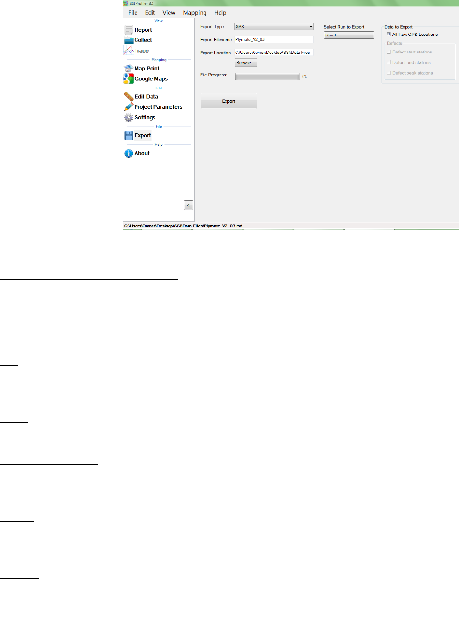
51
Under the title of Data
to Export there are
multiple check boxes. In
order to export the
defect’s GPS
coordinates, the All Raw
GPS locations check box
must not be checked.
Once the All Raw GPS
Locations box is
deselected, the options
to export the defect
stationing GPS
coordinates become
available.
1.6.9 – Exporting to Sidewalk Format
This option is only to be used with files collected with the SSI Sidewalk Profiler (CS-8850). The
sidewalk format has all of the information of the collection exported into GIS compatible file types.
These files types and the corresponding information within them are:
File Type
ngd
Ngd format contains synchronized distance, time, and gyroscopic data for a specified collection
interval.
pxyzd
This format is the three dimensional profile derived from the travel grade and gyroscope.
pxyzdg and pxyzdinc
These formats are the same as the format pxyzd, except these two formats do not have column
headers for the data.
rmpslp
Rmpslp is the ramp and running slope exceptions. The column headers are travel distance, marker
distance, time, ramp type, and casename.
rmpslpg
Rmpslpg contains the same data as the file rmpslp, except rmpslpg does not have column headers.
This format contains travel distance, marker distance, time, ramp type, and casename.
rmpslpg_ls
Rmpslpg_ls is a line segment version of rmpslpg without column headers.
Figure 88: The export window when the GPX format is selected.
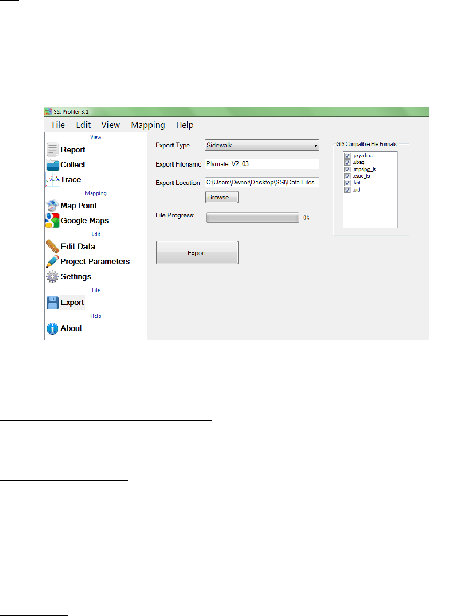
52
uba
This file contains the bump height and bevel slope data. The column headers are; travel distance,
bump type, bump height [inches], bevel slope, and the casename.
ubag
Ubag contains the same data as uba, but ubag does not have column headers for the data. This
format contains travel distance, bump type, bump height [inches], bevel slope, and the casename.
1.6.10 – Exporting to Localized Roughness
The localized roughness export feature allows the user to create an excel spreadsheet of the
localized roughness, or defects, for the collected data.
Specify Station Numbers
If the users desires to only export a section of the collection, select this check box and enter the
start and end stationing of the soon to be exported section. If the specify station numbers is not
selected, the entire collection will be exported.
GPS Reporting
To choose the type of GPS format to be used in the export select Northing/Easting, Decimal
Degrees, or NMEA Format from the drop down list.
Lane Settings
The user may change the lane number that is currently in the collection file by selecting this check
box and entering the correct lane number. To change the lane number, deselect the check box and
change the lane number in the input location.
Figure 89: The Sidewalk Export Window.
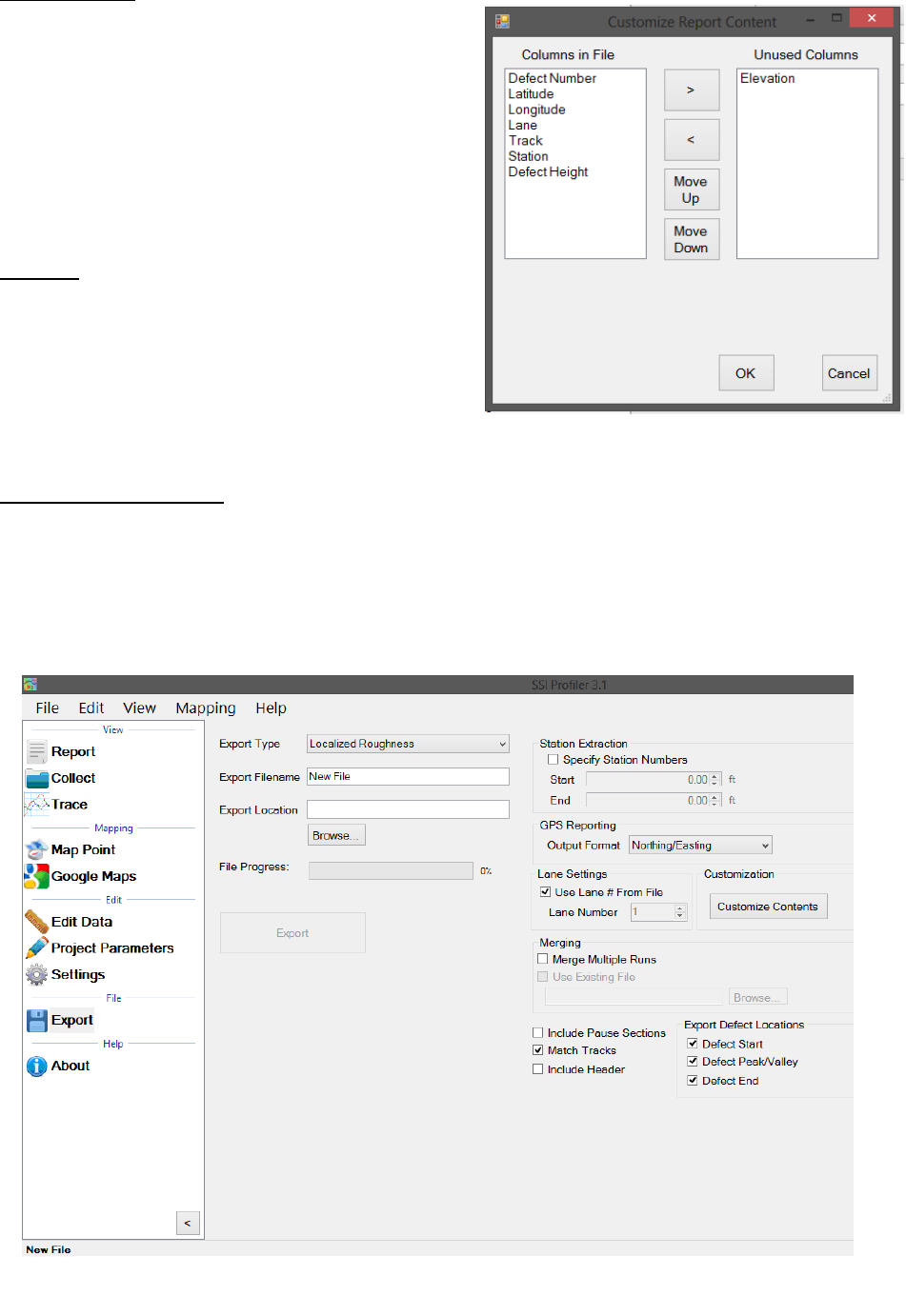
53
Customization
The user may add, move and remove columns from
the Excel spreadsheet format. To do this, open the
“Customize Contents” window and use the arrow
keys, move up and move down to change the order
of the included columns in the spreadsheet. The
columns types at the top of the “Columns in File”
side the left-most columns in the exported Excel
file.
Merging
Merge multiple runs check box allows the user to
include multiple collection runs in the spreadsheet.
Runs that are saved in a separate file can be
opened and exported alongside the current file by
selecting “Use Existing File” and browsing to enter
the location of the file.
Export Defect Locations
Use the check boxes to select whether the program will export the start, peak and end of the
defect in the spreadsheet.
The use will have the options to match tracks 1 and 2, include the paused sections, and include
the header information. When paused sections are included the defects within the paused
sections will be listed.
Figure 91: The Localized Roughness Export Template
Figure 90: The Customize Window
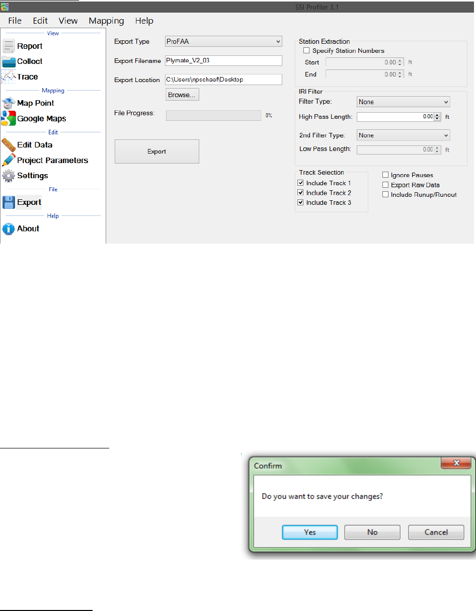
54
1.6.11 – ProFAA
ProFAA is the format used for the Federal Aviation Administration (FAA) profiling program. This is
the program that uses the Boeing Bump test method.
The user can enable high and low pass filters, change the start and end stationing, including the
pauses and exclude specific tracks from the exported data.
Exporting raw data will force the data through a linear regression filter and have the data begin
and end at zero elevation. The Run Up and Run out data can be included by selecting the check
box.
1.7. – Exiting Program
To exit the Profiler V3 program, save current
project and click the red “X” at the top right
corner or navigate to the File tab and select Exit.
If the current project is not saved when the
program is terminated, Profiler V3 will ask if the
operator would like to save the current project.
To save and exit the program, select “Yes.” If
you do not wish to exit to program, select cancel
and the program will remain open.
1.8. – Shortcut Bar
The Shortcut Bar is located at the left side of the main window. The shortcut bar is used to navigate
around the profiler program without using the menu bar.
Figure 93: Exiting the program- Saving
Figure 92: ProFAA Matching
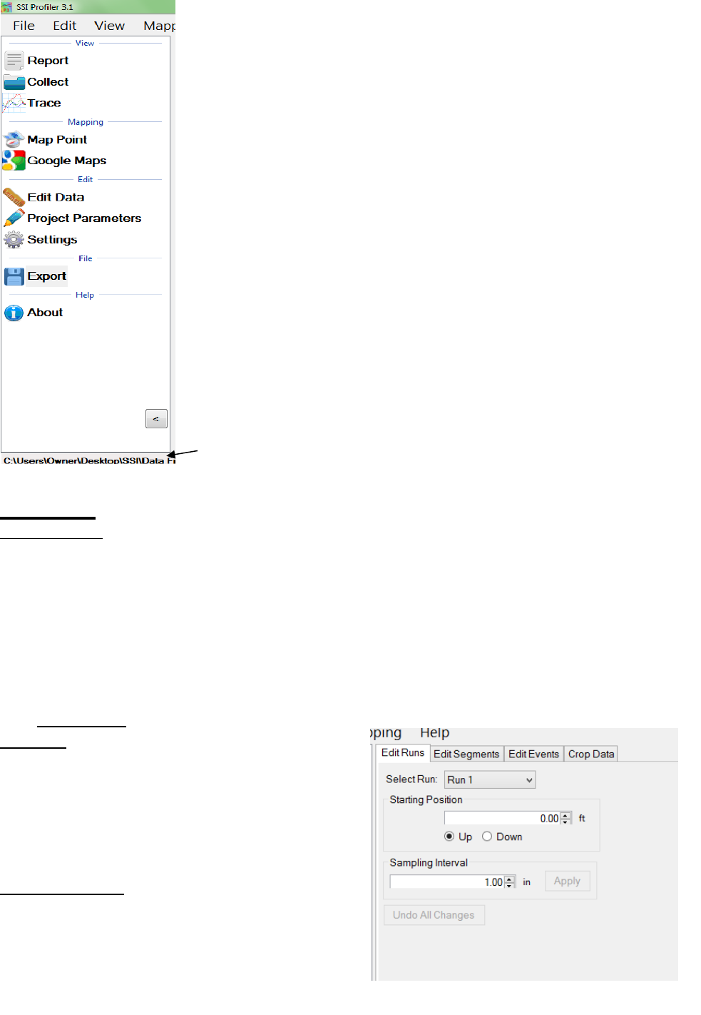
55
The shortcut bar can be hidden by selecting the arrow at the bottom of
the window. The direction that the arrow is pointing is the direction
that the shortcut bar will move. It will either become hidden, or
reappear.
2.0. - Edit
2.1 – Edit Data
Note: Any edit to the data will be described in the report header under File Modifications.
The edit data feature allows the user to adjust the starting station, insert pauses, or add events.
All of this can be done in post processing, after a collection has been completed. To edit the
collection:
1) Open the tab that has the information that needs adjustment. (Edit, Runs, Segments, Events)
2) Select the run that needs to be adjusted from the drop-down menu.
3) Change the parameter of starting position, run direction, and amount of Run Up or Run out
data
4) Select apply.
Edit Runs
Under Edit Runs the user can adjust the starting
position and change the Run Up or Run out lengths.
If the data was collected in the wrong station
direction, this can also be reversed by changing the
bullet selection to “Up” or “Down.”
Sampling Interval
The sampling interval is the distance between
readings of the electronics of the profiling system
(DMI, lasers, etc). This is usually set to 1 inch to
exceed AASHTO m328 and ASTM specifications.
Figure 94: The
shortcut bar
with all of the
frequently used
windows
Hide the shortcut
bar by selecting
the Hide Icon
Figure 95: The Edit Run Options
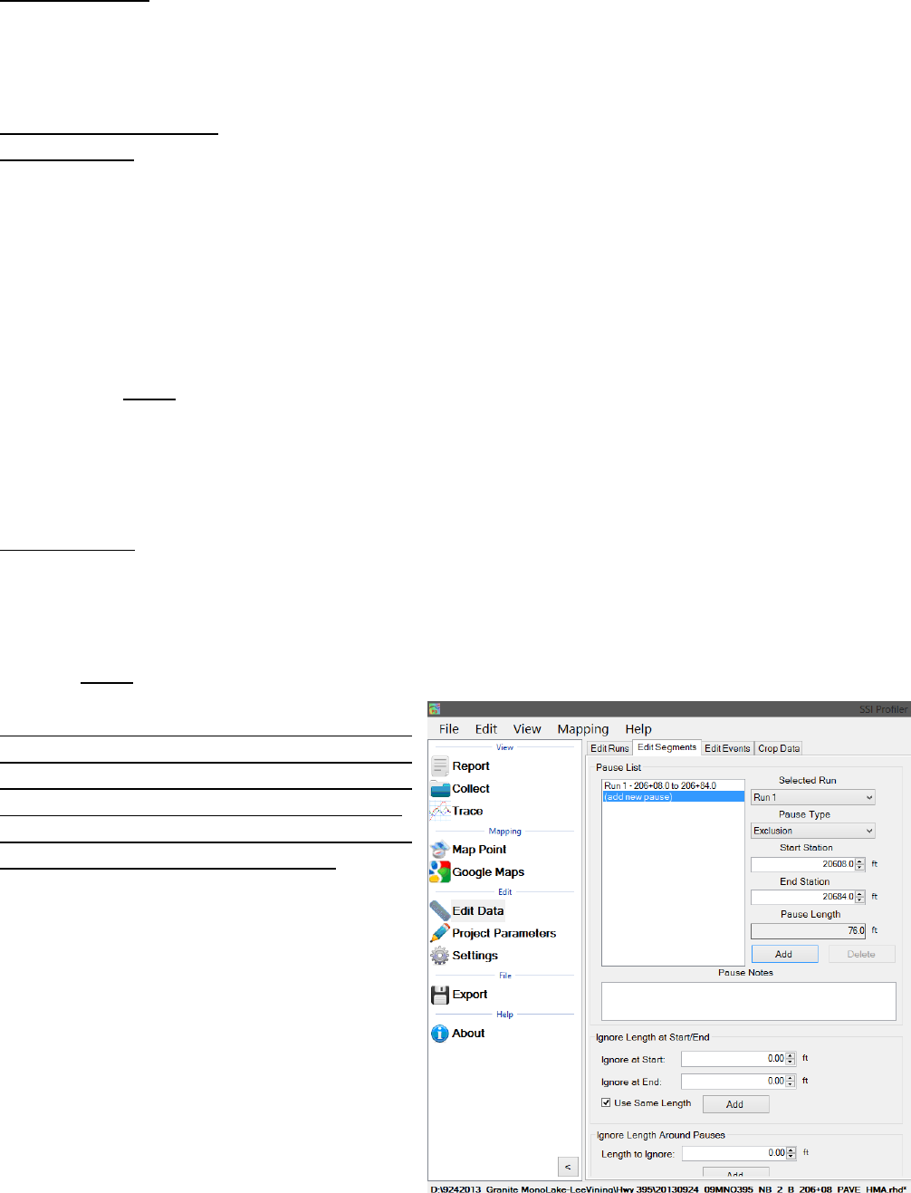
56
Edit Segments
The Edit Segment feature allows the user to add pauses to the collection or to ignore a certain
distance of collected data at the beginning or end of the run. The data will not be included in
calculation of the PRI.
Adding & Editing Pauses
To add a pause
1) New Pause will be added above the highlighted blue bar “(add new pause).”
2) Select the run number to add the pause to from the drop down menu.
3) Select the pause type (Exclusion, Bridge, Intersection)
4) Enter the start station for the pause
5) Enter the end station for the pause
(The pause length will be updated automatically)
6) Select Add. The pause stations will appear in the Pause List.
7) The user will now be able to add Pause Notes.
a. Select Apply to save the pause note.
Note: A pause will not be added unless the Start Station is different than the End Station.
The pause can be edited at any time. Any pause or edit made after collection will be displayed
in the report header under file modifications.
To Edit a pause
1) Select the paused section to be edited in the Paused list. It is selected when the blue bar is
highlighting the pause title (Ex. “Run 1 - 0+00.0 to 0+010.0”)
2) Change the stationing.
3) Select Save to set the changes.
4) Select Apply for the changes to take effect
Note: The run(s) that the pause is applied to
cannot be changed through Edit Run. Please
create a new Pause to change the pauses of a
run. See directions above to create a pause.
If the pause is going to be deleted, select the
Delete icon to remove it from the list.
Figure 96: Adding or removing
pauses from the collection

57
Pause Definition
When the collection system is paused, height data is omitted but the distance is still collected.
When the paused sections are excluded the height values are not included in the calculation of
localized roughness or ride values.
Pause Notes
To explain the reason for the pause or the location, enter the information in the pause notes. This
information will appear in the track notes of the trace reports.
Pause List
The Pause List shows all of the paused sections of the selected runs. The runs are selected from
the drop down menu of “Add Pause to Run.”
Start Station
The Start Station in the stationing where the pause is to begin.
End Station
The End Station is the stationing where the pause will stop, and collection will resume.
Save Pause Icon
When the operator selects a created pause in the Pause List by left clicking on it and highlighting
it blue, the two options of Save and Delete appear in the middle of the window. To save the
selected pause in the Pause List, left click Save.
Ignore Length at Start/End
This feature ignores a distance at the start and end of a collection by adding a pause at these
locations. If the “Use Same Length” box is not selected, the ignored distance at start and end will
be the same.
Ignore Length Around Pauses
This feature increases the pause length around the pause by adding longitudinal length to the
pauses. This length will be automatically added to all of the pauses in the Pause List.
Use Same Length
When the Use Same Length check box is selected, the runs will be trimmed to the same length.
Edit Events
Edit Events allows the user to input events that were not added during collection, or to delete
saved events. The events can have information associated with them that is inputted into the text
box. The types of events for walking profilers (Sidewalk) are Height and Width obstruction. High
speed and Profilograph systems should use the “Default” Event Type.
To add an Event
1) Select the run to add the event to,
2) Select New Event,
3) Change the Stationing to the correct point location
4) Adjust the Event type to explain the event.
5) Under notes, add information about the event. (Start Structure, manhole, drainage, etc.)
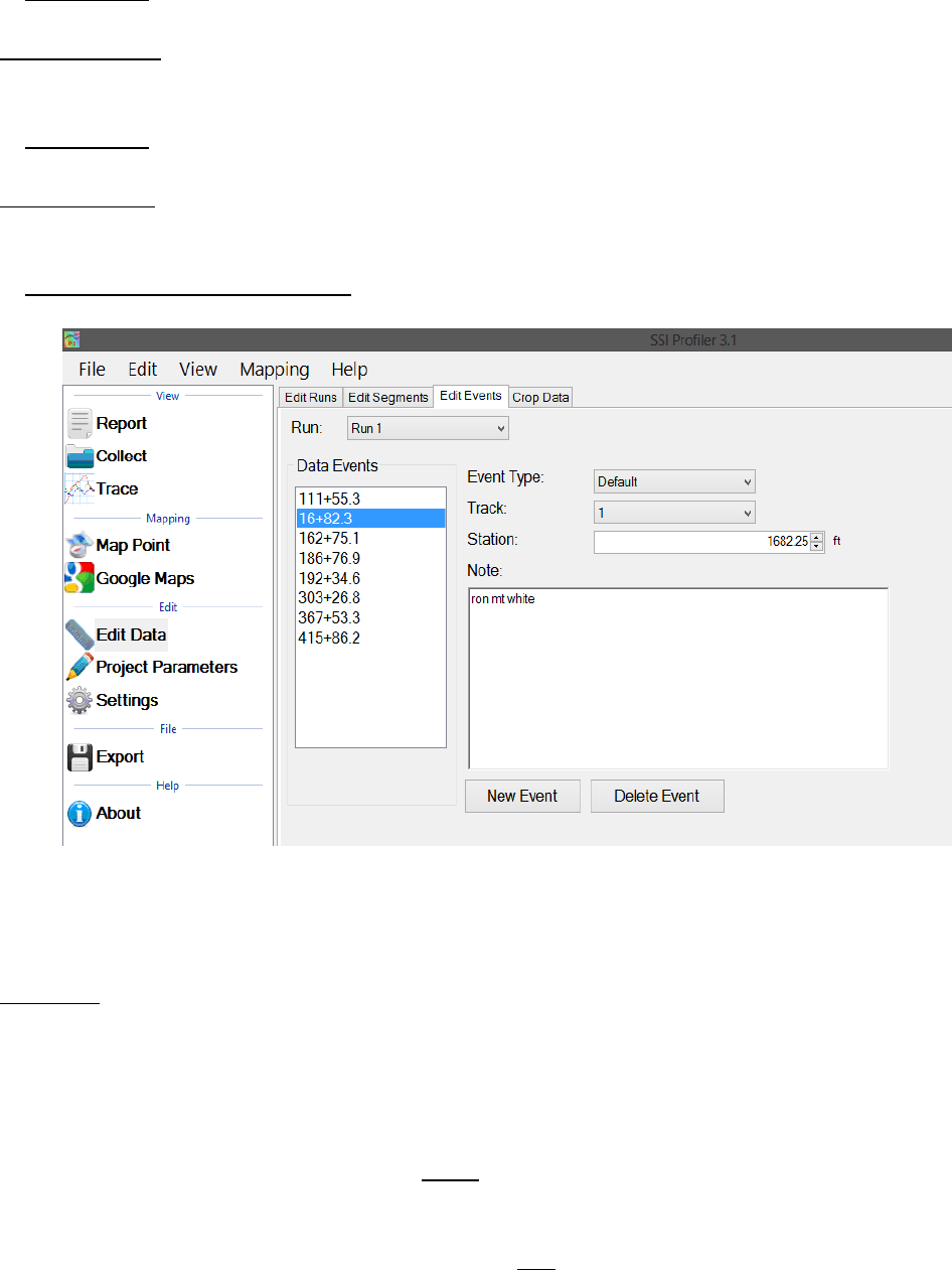
58
6) Select Apply
Editing an Event
1) Select the event in the Data Events list to highlight it blue.
2) While highlighted, the event stationing, type or notes can be changed
3) Select Apply
Deleting Events
1) Select the event in the Data Events list
2) Select Delete to remove the event.
3) Select Apply to save the changes
Crop Data
The Crop Data tool allows the user to trim the collections before analysis and reporting. If any
changes are made to the file, the information that was changed will be described in the report
header under File Modifications.
To crop the collection, change the distances for the run up and/or run out distances. When the
lengths are at the desired distances, select Apply.
To reset the run up and run out to the original lengths select the rest icon next to run out. This icon
will become available once a change has been made and Apply has been selected.
Figure 97: Edit Events Tab
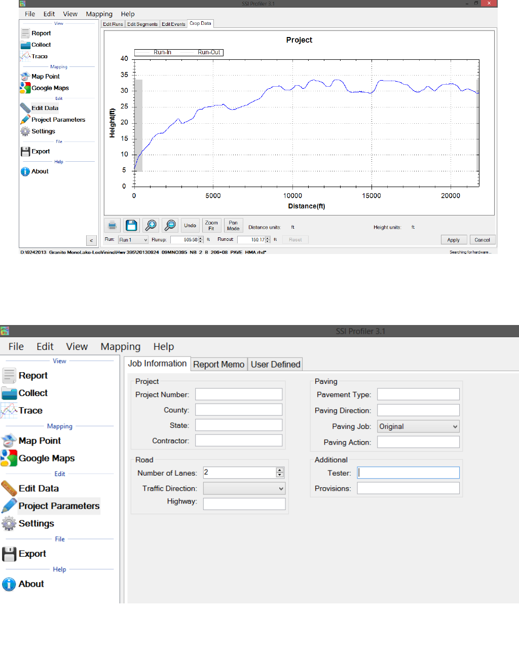
59
Figure 99: The Project Parameters window
Figure 98: The Crop Data Tool

60
2.2 - Project Parameters
The Project Parameters section is the location where the job information is inputted. This
information appears on the header of the reports and the exported excel templates. Before
leaving the Project Parameters window, always select ‘Apply’ if changes were made.
2.2.1. - Job Information
The job specific criteria listed below are descriptive information about the project. Review the
contract to enter the required information into the sections listed below. These sections can be
edited at any time within Profiler V3.
Project
Project Number
The Project Number is unique to each project. This is to be determined by the State, Federal DOT
or by the contractor. This information will be listed in the project contract.
County
This location is reserved to list the county where the profiling is taking place.
State
The state in which the profiling is taking place and the job is located.
Contractor
This section is for the name of the paving company or for the company operating the profiler.
Road
Traffic Direction
The traffic direction of the lane to be profiled.
Number of Lanes
The number of lanes of the project. This section can be changed by inputting values directly or by
using the arrow keys. Traditionally, the number of lanes is the number of lanes travelling in the
same direction for main line freeways. Use a classification system that can be understood during
post-collection analysis.
Paving
Pavement Type
Input the type of pavement here. Enter pavement types such as Cold–in–Place Asphalt, HMA,
JPCP, CRCP, Open Grade etc.
Paving Direction
Enter the direction of the paver when placing the pavement.
Paving Job
Specify the type of paving job, either corrected or original.
Paving Action
Under paving action list any further information about the paving process.
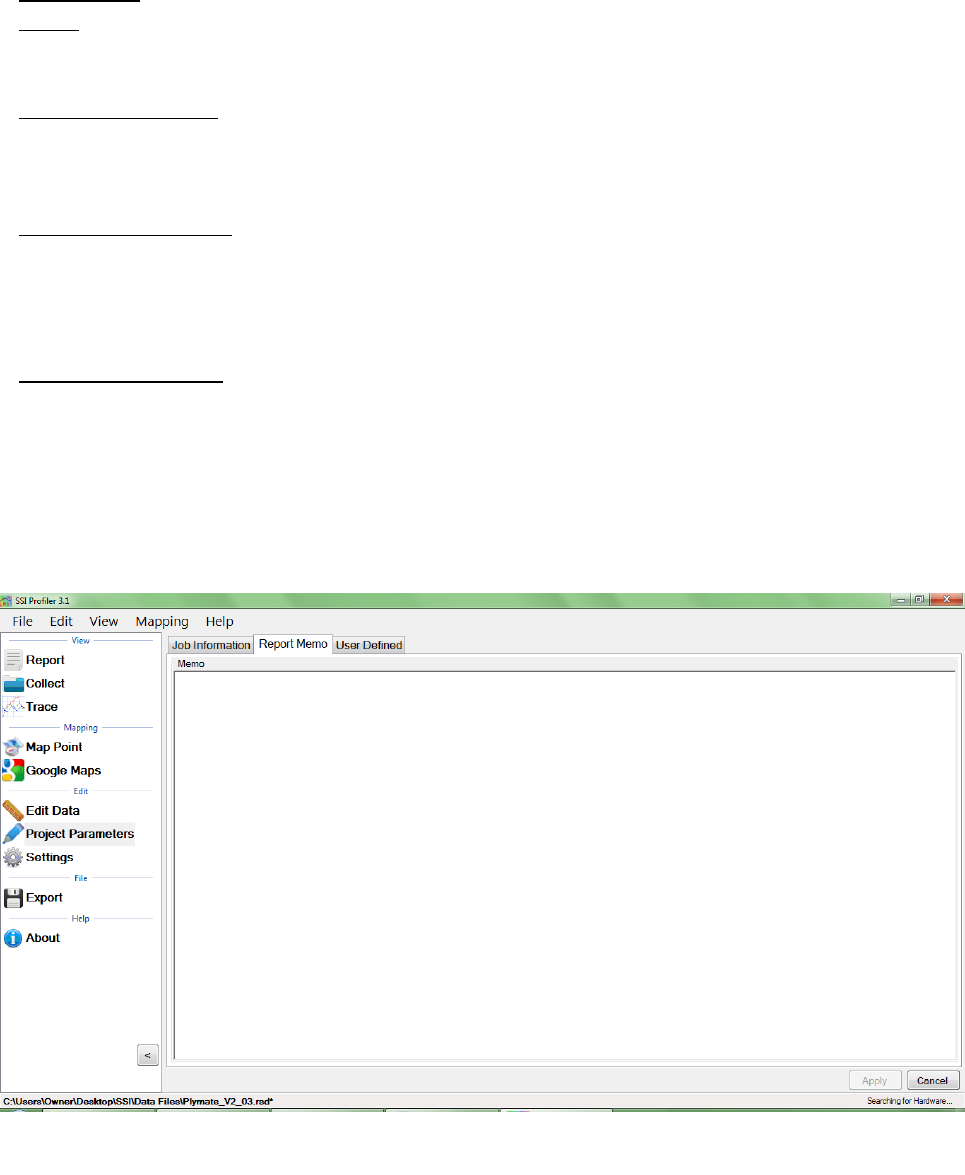
61
Additional
Tester
The individual operating the profiling equipment over the pavement surface.
Provisions/Weather
The weather at the time of profiling the pavement. Such as: Cold, Hot, Overcast, Morning,
Afternoon, Evening, etc.
2.2.2. - Report Memo
Report Memo is a section available for inputting large amounts of text to be saved along with the
data file. Anything from reminders to stationing can be inputted into the Report Memo and not
influence the data.
2.2.3. - User Defined
Additional parameters can be stored in the data file as desired by the operator. Consult the
contract for any additional user defined parameters that may be required for the profile data files.
Add new parameters by selecting ‘Add’ at the bottom of the window. The parameters are entered
by double-left clicking on the ‘Key’ column and typing in the required information.
Figure 100: The Report Memo window
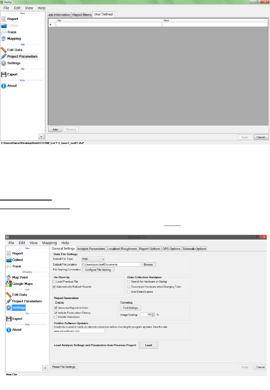
62
2.2. - Settings
2.2.1. – General Settings
The default file preferences and settings for report generation can be changed under the
“Settings”. Whenever a change is made, always select the Apply icon in the lower right corner.
Figure 102: The General Settings window
Figure 101: The User Defined window

63
Section 1 – Units
Default File Type (RSD, RHD)
The drop down menu can be used to select the type of file to be used in Profiler V3. Both RHD and
RSD files can be imported into the program at any time. The default file type is the file format that
will be used automatically when files are opened. Profiler V3 only saves in the RSD format.
Default File Location
The default file location is the folder on the computer or external device that Profiler will search
for the default file type. This folder can be changed through the Browse icon. If a location is used
to open a file, the program will use this location to open files for future attempts. This feature
saves time when opening files when the program opens directly to the file location. Select Apply
after a folder is chosen.
Default File Name
The file name can be chosen to have a name based on parameters of the program or by using a
pre-loaded template. The parameters can be chosen from the list of (multiple can be chosen):
Contractor, Country, Tester, etc. When a template is selected there will be a preview at the bottom
of the window. Select OK and Apply to set this configuration as the default file name.
Creating a New Template
Create a New Template by selecting the “New Template” icon on the right side of the window.
Select the template’s name to rename it and append parameters to it. The template will be used
as long as it is selected when OK is selected at the bottom right corner when exiting the Default
File Name tool.
User Defined Parameter
To create parameters that are specific to the job, type a new parameter name into the User Defined
Parameter text box and select “Add User Defined Parameter.” The bracketed variable will appear
in the filename preview. To add information to the user defined parameter, open Project
Parameters and the User Defined Tab. The name of the parameter will be under the Key column.
Under the Value column, enter the information that is needed in the filename.
Changing the Template Name
The template’s name can be changed by changing the characters under Template Name. Once a
change is made, the Rename icon will be available. Select OK or Apply to save the changes.
Adding Parameters to the Template
When adding parameters to the template they will only be added to the right end of the template,
as seen in the naming preview.
Select Apply after changes are made to the template.
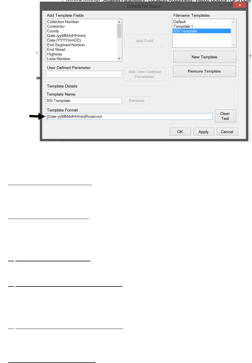
64
On Startup
Load Previous File on Startup
If this box is selected, the file that was open when profiler closed last will be reopened when the
program is started. A report of this file will be generated when the program is opened.
Load Previous File’s Settings
The user may choose a previous file to save time if entering the same analysis parameters or
project parameters under “Settings.” To load a previous file’s setting’s, choose the file under
General Settings or start a new file and choose one of the three options.
1) Use Last File’s Parameters
This option will use the last file’s settings under the localized roughness and project parameters.
2) Choose from a Previous File (Browse)
When this option is chosen a window explorer window will appear and the user may select a file
that is saved on the computer to import the saved file’s parameters under analysis and project
parameters.
3) Set File Parameters after Collection
By choosing this option the user will not import a previously collected file, but will instead
manually set the parameters after the collection has finished.
Automatically Refresh Reports
The reports will automatically refresh when the operator navigates to the report window from
another tab. When the user makes a change of report type within the report window, the refresh
button will have to be selected manually.
Figure 103: The custom file naming convention window
Preview

65
Data Collection Hardware
Search for Hardware on Startup
If this option is selected, the program will search for hardware, and if available, will connect to it
upon opening the program.
Disconnect Hardware When Changing Tabs
If this feature is checked the program will disconnect from the hardware when the operator leaves
the collect tab.
Auto Detect Lasers
This feature will use the health string to determine the type of laser that is connected to the
system. This is not an end-all solution. Please check the laser type in the System Settings under
the collection window prior to any data collection or perform a height verification.
Report Generation
Generate Reports in Color
If the reports are generated in color, the defect types will be more visible. On the trace reports
dips will appear be highlighted blue and bumps will be highlighted red.
Include the Footer
If the footer is included, the file name and the page number will be printed at the bottom of each
page for the report. Select the check box to apply this feature.
Enable Animations
When enable animations is selected, the windows within Profiler V3 will slide across the screen
whenever the operator moves from one section to another (Reports to Collect). This feature does
not affect the functionality of the program, but adds an aesthetic behavior when changing
windows.
Formatting
Font Settings
The font of the reports can be changed by selecting the Font Settings icon under formatting. This
allows the user to make the size of the font smaller or in a readable font. The image scaling allows
the user to print off less pages if the scaling factor is increased. The window that appears can also
change the font to a strike-through or an underline.
Image Scaling
The default for this value is 100%. When image scaling is set to a percentage greater than 100%, it
acts the same way as the zoom function. The size of the traces within the reports will increase in
size.
Profiler Software Update
Profiler V3 will check the internet connection by attempting to connect to the website listed under
this location. If the internet connection is found, the updates will be available for download from
the SSI server.

66
2.2.2. – Analysis Parameters (Ride Values)
Changing the units alters the specifications for defects and the ride numbers.
Section 1 – Units
Profiling Units
English
Selecting English units sets the segment length at 528 feet. English units use inches for the height
of the defects and counts for roughness settings, while using feet for scallop width and filter
lengths. After every adjustment of units, select apply in the lower right corner to save changes.
Metric Meters
In the Metric Meters setting, the blanking band, scallop height and scallop resolution are all in
centimeters. The rest of the measurements for scallop width and filter lengths are in meters. The
Metric Meters and Metric Centimeters settings have the same units of centimeters for height and
meters for length for all sections of defects and roughness. After every adjustment of units, select
apply in the lower right corner to save changes.
Metric Centimeters
In the Metric Centimeters setting, the blanking band, scallop height and scallop resolution are all
in centimeters. The rest of the measurements for scallop width and filter lengths are in meters.
The Metric Meters and Metric Centimeters settings have the same units of centimeters for height
and meters for length for all sections of defects and roughness. After every adjustment of units,
select apply in the lower right corner to save changes.
Metric Millimeters
In the Metric Millimeters setting, the blanking band, scallop height and scallop resolution are all
in millimeters. The rest of the measurements for scallop width and filter lengths are in meters.
After every adjustment of units, select apply in the lower right corner to save changes.
CA Bridge
The CA Bridge setting is based off of the specification of the California Bridge Profilograph, which
is twelve feet long instead of the California Profilograph 25 foot length. The CA Bridge setting is in
English units and has a segment length of 100 feet. After every adjustment of units, select apply
in the lower right corner to save changes.
CA Bridge Metric
This setting is for simulation of the 12 foot frame of the Bridge Profilograph. The Bridge Metric
setting is the metric version of the CA Bridge Profilograph. Its segment length is 90 meters and
the defects and counts for roughness are in millimeters and meters. After every adjustment of
units, select apply in the lower right corner to save changes.
Section 2 - Segment Settings
Segment Length
Segment length is the interval of profiling that is used to calculate ride values. Traditionally the
distance used for segment length is one-tenth of a mile, or 528 feet (160 meters).
This section is adjusted by using the arrow keys or double-left clicking in the box to type the
segment length.
Merge Last Segment if it is less than
If the last segment is a short length, the last segment can be merged into the second-to-last
segment. This will prevent large ride values from short distances. Only use if your specification
does not require a specific segment length for pay incentives. The last segment length will be
changed if this feature is used.

67
Paused Sections Drop Down Menu
Exclude Paused Sections
When Exclude Pause Sections is selected, the paused sections created during collection or through
the Segment Adjustment window will not be included in the report or the calculation of the ride
values.
Include Paused Sections
When Include Paused Sections is selected, the paused sections are included with the actual
collection when calculating the ride values. The report will show the paused sections in the
segment summary and the trace view.
Paused Sections Only
When Include Paused Sections only is selected from the drop down menu, only the paused
sections created during collection or through the Segment Adjustment Window will be displayed
in reports and used to calculate ride values and counts for roughness.
Section 3 - Analysis Type
IRI
The International Roughness Index is a universal ride index calculation which is universal or roads
around the world from concrete and asphalt surfaces. The profile is analyzed using a quarter-car
simulation that is weighted towards the frequencies of body and vehicle bounce; the most
uncomfortable riding conditions.
To calculate IRI in Profiler V3, select IRI from the drop down menu, then adjust the filter settings if
necessary according to the contract specifications. View the report under the Report Tab to
observe IRI.
𝑰𝑹𝑰 = 𝑺𝒕𝒂𝒏𝒅𝒂𝒓𝒊𝒛𝒆𝒅 𝑽𝒆𝒉𝒊𝒄𝒍𝒆′𝒔 𝑨𝒄𝒄𝒖𝒎𝒖𝒍𝒂𝒕𝒆𝒅 𝑺𝒖𝒔𝒑𝒆𝒏𝒔𝒊𝒐𝒏 𝑴𝒐𝒕𝒊𝒐𝒏
𝑫𝒊𝒔𝒕𝒂𝒏𝒄𝒆 𝑻𝒓𝒂𝒗𝒆𝒍𝒆𝒅
PRI
The Profile Ride Index is a simple calculation to classify the smoothness of a road profile against
other roads. The formula for this calculation is:
English Units:
𝟓𝟐𝟖𝟎 𝒇𝒕 × (𝑻𝒐𝒕𝒂𝒍 𝑹𝒐𝒖𝒈𝒉𝒏𝒆𝒔𝒔 𝒊𝒏 𝒊𝒏𝒄𝒉𝒆𝒔 𝒊𝒏 𝑺𝒆𝒈𝒎𝒆𝒏𝒕)(𝑺𝒆𝒈𝒎𝒆𝒏𝒕 𝑳𝒆𝒏𝒈𝒕𝒉 [𝒇𝒕])
⁄
Metric Units:
𝟏𝟎𝟎𝟎 𝒎 × (𝑻𝒐𝒕𝒂𝒍 𝑹𝒐𝒖𝒈𝒉𝒏𝒆𝒔𝒔 𝒊𝒏 𝒎, 𝒄𝒎,𝒐𝒓 𝒎𝒎 𝒊𝒏 𝒔𝒆𝒈𝒎𝒆𝒏𝒕) (𝑺𝒆𝒈𝒎𝒆𝒏𝒕 𝑳𝒆𝒏𝒈𝒕𝒉 [𝒎])
⁄
To calculate the PRI in Profiler V3, select PRI from the Analysis Type drop down menu and set the
defect settings. Once the defect settings are correct, select Apply and then view a report to
observe the PRI ride values.
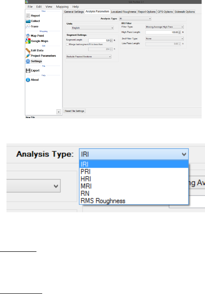
68
PRI Parameters
Note that the PRI Parameters are only for the calculation of the Profile Ride Index (PRI). Blanking
Band, and Scallops have no connection to the manner in which defects are found. For defect
settings, see Localized Roughness.
Scallop Definition
Scallops are the deviations of the profile trace from the limit of the localized roughness line. If the
trace exceeds the defect height but the minimum width of the scallop is not reached, the deviation
is not included as a defect. Although the defect is not included in the Ride Values, the deviation is
still exceeding the defect height parameter which adds counts for roughness.
Figure 104: The IRI Analysis Parameters window
Figure 105: The Analysis type drop down menu displaying all of
the Ride Values options
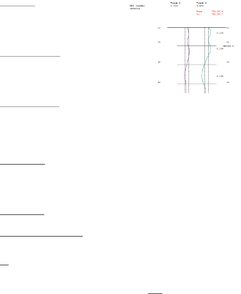
69
Blanking Band
The blanking band is a null area that classifies the
height of all sections of the trace within its borders
as zero. Therefore, a trace that remains within the
borders of the blanking band would have zero
counts for roughness and a PRI of zero.
Minimum Scallop Height
The minimum scallop height is the minimum height
that is seen to be a deviation from the null line.
Frequently, the value for minimum scallop height is
0.035 or 0.9mm, which is the default value for the
Profiler V3 program.
Minimum Scallop Width
The minimum scallop width is traditionally 2 feet (0.61
meters). Review the Department of Transportation
smoothness specification that pertains to the project. The minimum scallop distance is the
minimum longitudinal length (the direction of traffic) that is used to find the deviations of the
profile off of the null line or blanking band. The setting of 2 feet or 0.61 meters is the default
setting for Profiler V3.
Scallop Resolution
The scallop resolution is the accuracy of the height measurement of the profiler. Current
equipment is accurate to 0.01 inches, the default value for Profiler V3 software. A resolution of
one-hundredth of an inch means that the scallop heights will always be rounded to the hundredth
decimal. Consult the recent smoothness specification released by the overseeing agency to
confirm the scallop resolution value.
Reset File Settings
Selecting this icon brings all values in Settings to their default program values.
Minimum Scallop Height Inclusive
When this box is selected, the minimum scallop height will be included as a scallop. Meaning, if
the minimum scallop height is 0.035, 0.035 will be the minimum instead of 0.0351.
HRI
The Half Car Ride Index (HRI) is found by applying IRI to an average of two profiles. HRI uses a half
car simulation, unlike IRI which uses a quarter car simulation. To calculate the HRI in Profiler V3,
select HRI from the Analysis Type drop down menu and verify the settings of filter length based on
the project specifications. Once the filters are correct, select Apply to save the settings. To view
the calculated HRI, view one of the reports under View>Report.
Figure 106: An example of
the blanking band in the
trace report.
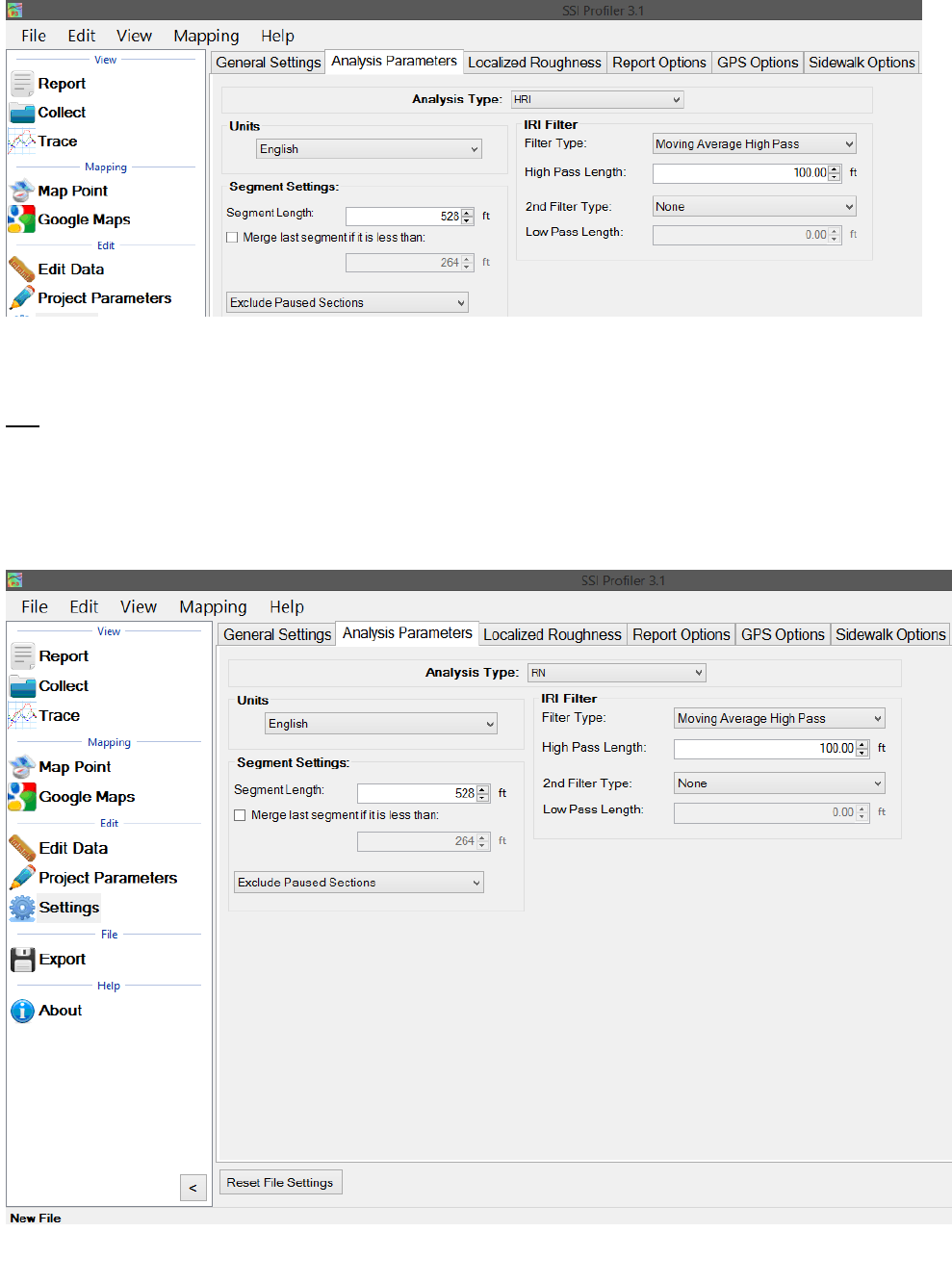
70
RN
The Ride Number (RN) can be calculated in Profiler V3 by selecting RN from the Analysis Type drop
down menu and verifying the settings of filter length based on the project specifications. Once the
filters are correct, select Apply to save the settings. To view the calculated RN values, view one of
the reports under View>Report.
Figure 107: The HRI analysis window with the available filter settings.
Figure 108: The RN analysis window with the filter options shown.
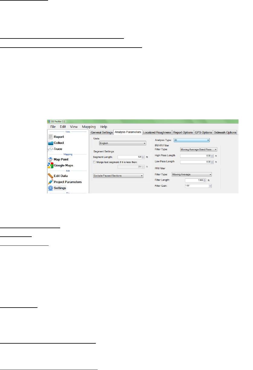
71
RMS Roughness
The RMS roughness is another ride value method that is calculated by the profile height over a
base length of 25 feet. This is how RMS roughness gets the units of inches.
2.2.3. – Analysis Parameters: Filters
Section 1 - IRI/HRI Filter----Same for IRI,HRI, RN
High Pass Filter – The High Pass Filter will remove any trend in the data that is less than the chosen
length. The length can be selected by typing the value in the box or by using the arrows to adjust
the input.
Low Pass Filter – The Low Pass Filter will remove any trend in the data that is greater than the
chosen length. The length can be selected by typing the value in the box or by using the arrows to
adjust the input.
Section 2 - PRI Filter
Filter Type
Moving Average
A Moving Average Filter of length 1.90 feet can be chosen by the operator, depending on the
contract specification. The use of the moving average filter was developed by the Kansas
Department of Transportation.
Kansas Department of Transportation (see Report No. K-TRAN: KSU-9302 “An Automated System
for Determination of Pavement Profile Index and Location of Bumps for Grinding from the
Profilograph Traces.)
Butterworth
The third order Butterworth filter has a default length of 2.0 feet. The Butterworth filter is not
required for updated profiling specifications. The Butterworth filter was used for the original
automated Profilograph systems.
Moving Average High Pass Filter
A high pass filter will remove any trend that is shorter than the selected length. Typical range of
length for this filter is one hundred feet (100 ft.) through two hundred feet (200 ft.).
Moving Average Band Pass Filter
This filter only allows the desired frequency of data to be shown. Adding this filter will adapt the
profile trace to remove the high frequency motions. Moving average filters are typically used for
short data runs less than two hundred feet (200 ft.).
Figure 109: The filters within the IRI analysis parameter window
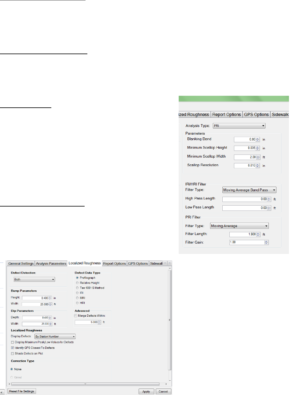
72
Butterworth High Pass Filter
High pass filters allow the high frequency characteristics of the data plot to pass through while
blocking the lower frequency attributes of the data run. Butterworth filters do not introduce a
phase shift into the plot like moving average filters. Butterworth filters are traditionally used for
longer data runs over two hundred feet.
Butterworth Band Pass Filter
This filter will perform both a high pass and low pass Butterworth filter operation on the data. The
result is a run that has frequencies within the lower and upper bounds. Butterworth filters do not
introduce a phase shift into the plot like moving average filters. Butterworth filters are traditionally
used for longer data runs over two hundred feet.
Filter Gain—1.00
The filter gain is to only be used when adjustments are
necessary while comparing different profiling systems. The
filter gain does not need to be used in normal profiling
environments. When comparing high speed profiling
systems to other Profilograph systems, the filter gain may
be used to change the output of the data files so they are
more accurate. A filter gain setting of 1.00 does not affect
the collected data. For typical profiling use the default
setting of 1.
2.2.4. –Localized Roughness
Localized roughness refers to the bumps and dips that
occur over a distance (longitudinal distance is the width of
the bump).
Figure 111: The
Localized Roughness
window with the
defect settings.
Figure 110: The filters for PRI
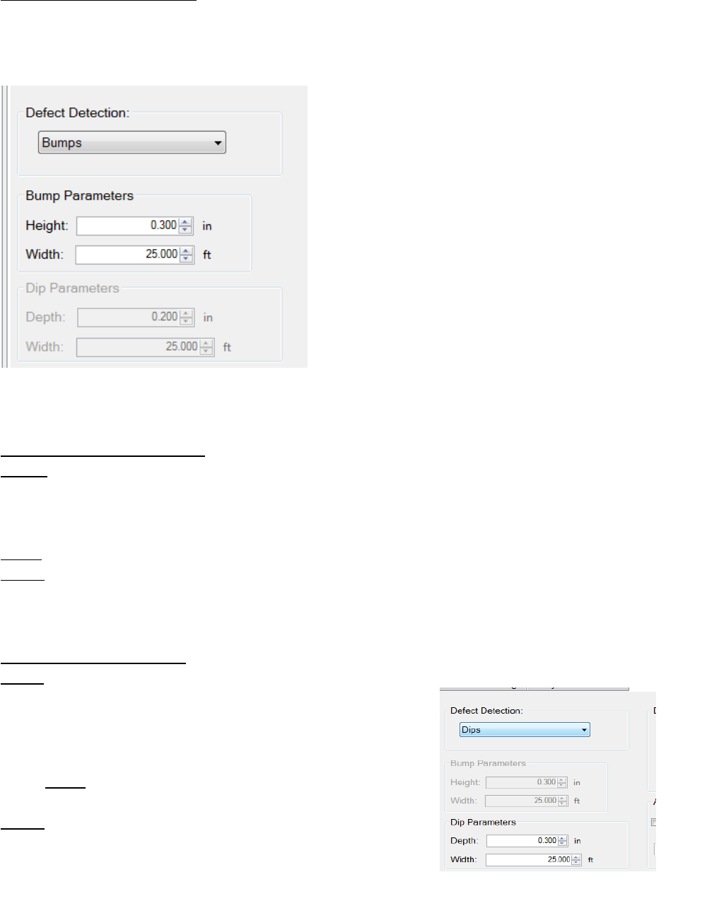
73
Section 1 - Defect Detection
The operator may choose the type of defect detection to implement in Profiler V3. The options to
choose from are Bumps, Dips, Both, and None. To select the type, use the drop down menu labeled
Defect Detection. No filters are associated with localized roughness. “Both” is selected by default.
If only one defect type is chosen, be sure to change
the correct settings. Do not change the dip
parameters instead of the bump parameters by
mistake. The report section of Profiler V3 can be
used to review the settings and traces of the
collection.
Section 2 - Bump Parameters
Height
Bump height is the maximum distance that a profile may deviate within the width of the bump.
The width of the bump is the length of a Profilograph, or 25 feet (7.62 meters). A typical value for
bump height is 0.3 inches. When the settings are changed for the bump parameters, always select
Apply to save changes.
Width
The width of a bump is based on the length of a Profilograph; 25 feet or 7.62 meters. This is the
default value for the Profiler software.
Section 3 - Dip Parameters
Depth
The depth of a dip is the maximum distance a profile trace may
deviate within the width of the dip (25 ft or 7.62 m). The
default value for dip height is 0.4 inches or 10.2 millimeters.
When the settings are changed for the dip parameters, always
select Apply to save changes.
Width
The width of a dip is based on the length of a Profilograph; 25
feet or 7.62 meters. This is the default value for the Profiler V3
software.
Figure 112: When only bumps are selected from the drop-
down menu, the dip parameters become unavailable.
Figure 113: Only dips selected.
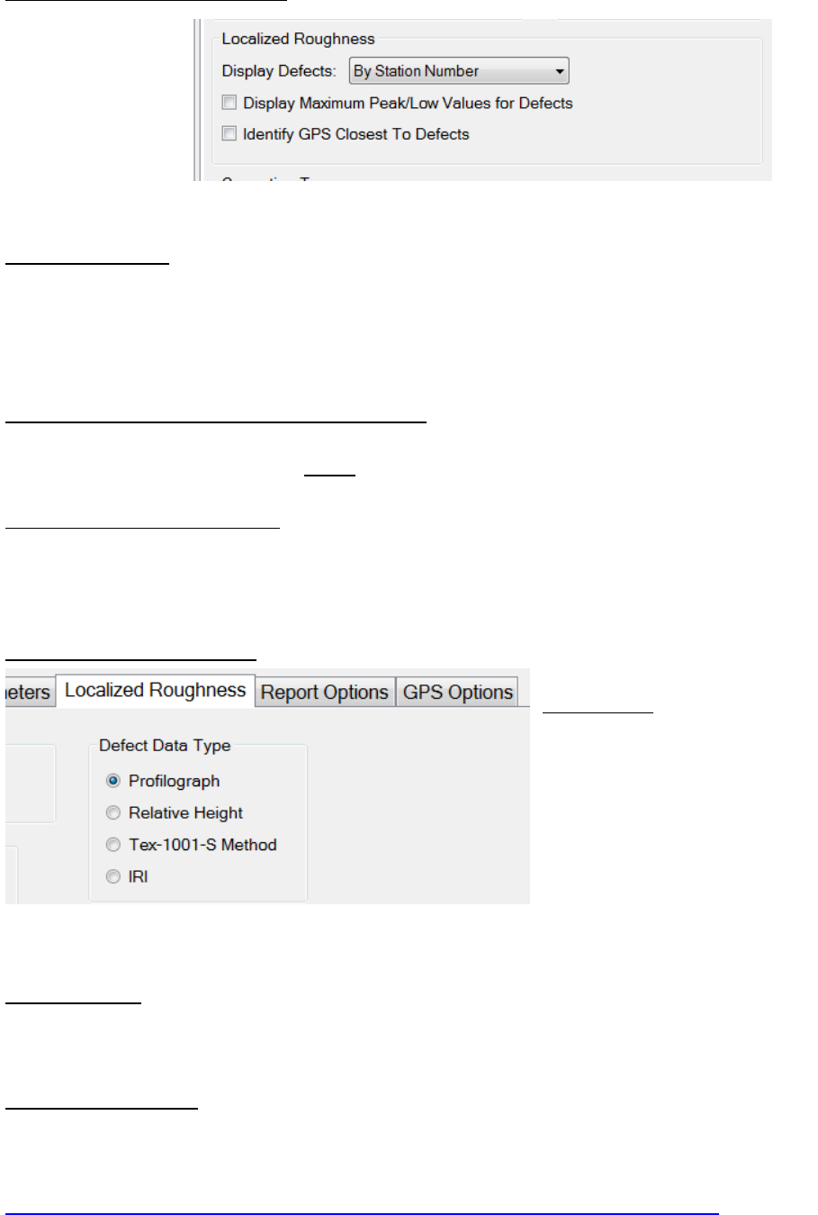
74
Section 4 - Localized Roughness
Display Defects By:
The operator has the option to display defects by the station number or by the track in the report.
To modify this setting, choose the desired display setting then select apply to save the changes.
When displaying the defects by track, the defects are split up into their respective tracks. When
the defects are organized by stationing they are listed in the same classification.
Display Maximum Peak/Low Values for Defects
Selecting this check box shows the peak values for the defects when viewing the summary report.
When altering the settings, select Apply to save the changes.
Identify GPS Closest to Defects
To show the closest GPS reading to each defect, select this check box. When viewing the summary,
the GPS coordinates will be in the table with Defect Type, Track, Segment, and Stationing of the
defect.
Section 5 - Defect Data Type
Profilograph
The Profilograph defect data type is
the most common method used to
find defects. The settings are the
same as described above in Analysis
Parameters, defect detection, bump
parameters and dip parameters.
Relative Height
Relative Height defect data type finds the defects of the profiled surface through the local
differences in the trace. The settings required to be inputted within the Localized Roughness tab
of the Settings Window are the bump and/or dip parameters.
Texas-1001-S Method
The Texas 1001-S Method is used mainly by the Texas DOT for profiling with inertial profilers. The
procedures and information for this test method can be found on the Texas DOT website; a direct
link is below.
ftp://ftp.dot.state.tx.us/pub/txdot-info/cst/TMS/1000-S_series/pdfs/spe1001.pdf
Figure 114: The localized roughness settings for displaying defects
Figure 115: The types of testing available to find the defects in the data.
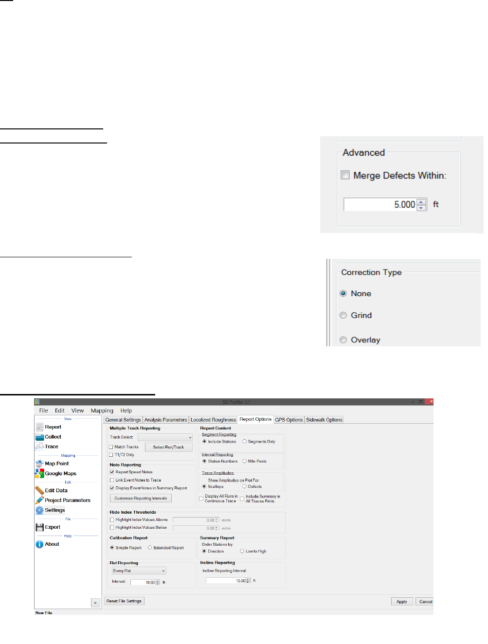
75
The Texas-1001-S method detects localized roughness (defects) of the profiled surface by applying
the base length and the threshold values saved in the Settings Window.
IRI
When IRI Defect Data type is selected, the IRI calculation will be used to find the road’s defects
(localized roughness) of the profiled surface. If this setting is selected the IRI ride value will not be
shown in the summary. To list the IRI ride values on the reports, select the analysis type to be IRI
in the Analysis Parameters tab. The ride interval is set (usually to 25 feet, in English units) and is
used as a sliding guide across the profile. When the summation of the profile’s IRI exceeds the
threshold, the entire continuous length which exceeds the threshold will be an area of localized
roughness.
Section 6 – Advanced
Merge Defects within:
The operator is able to merge multiple defects into one defect to
eliminate high frequency grinding patterns. The action of merging
defects does not affect the ride values or the defect heights.
Merging adjusts the start and end stationing of two defects into
one length. The default value of the merge defects tool is 5 feet.
To use this feature, select the check box next to “Merge Defects
Within.”
Section 7 – Correction Type
When PRI is selected as the Analysis Type, the correction type
may be chosen. The three options for Correction Type are None,
Grind, and Overlay. When IRI, HRI, or RN are selected as the
Analysis Type, the only Correction Type option is to select None.
When modifications are made to the settings, select ‘Apply’ to
save the changes.
2.2.5. - Report Options
Figure 117: Correction Types
Figure 118: The report options window.
Figure 116: Merge Defects
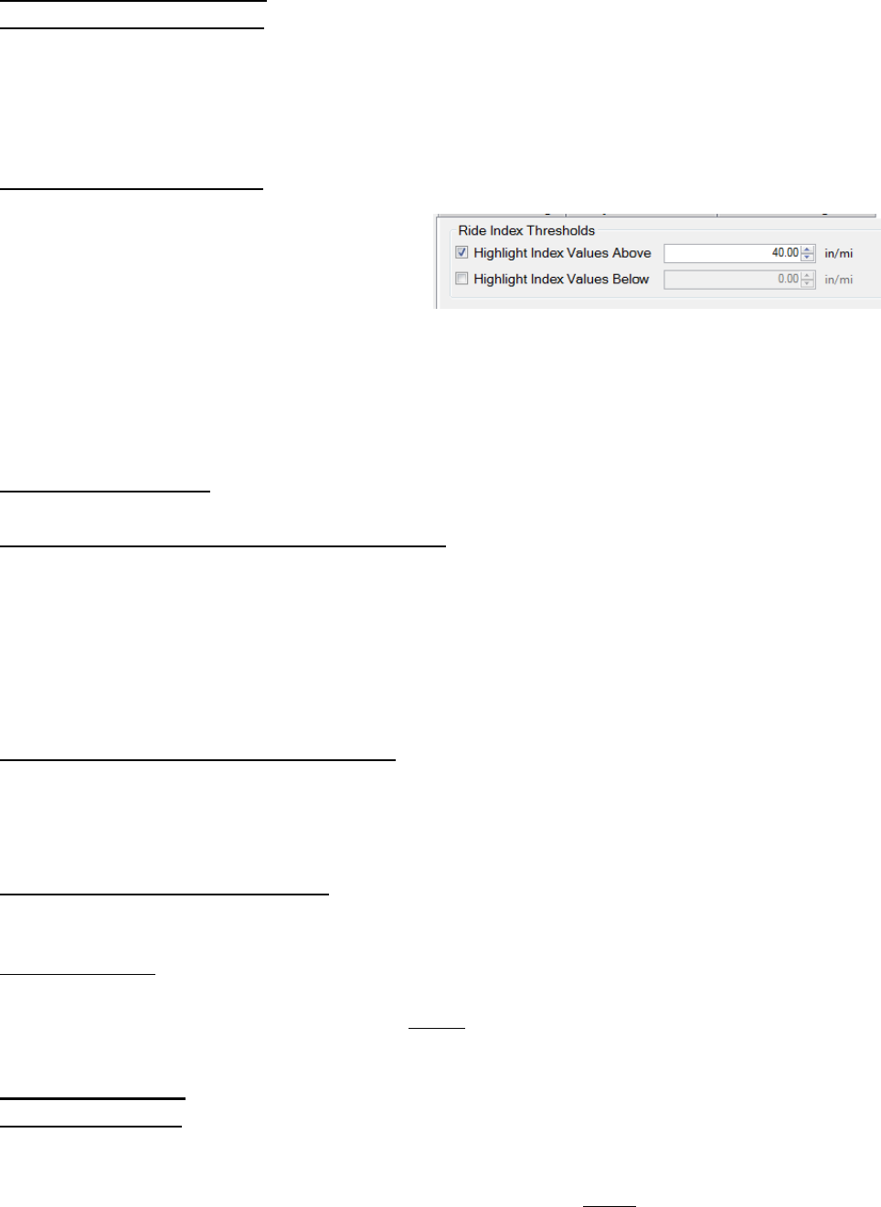
76
Ride Index Thresholds
Highlight Index Values Above
The operator may choose the threshold in which to highlight a certain interval of ride index values
above a number. The highlight color is red and can be seen in the summary table of the reports.
Only the segment ride values are highlighted, not the total ride values. This is convenient for
comparing segment ride indexes to determine where grinding should be done.
Highlight Index Values Below
The operator may choose the threshold to
highlight a certain interval of ride index values
below a chosen number. The highlight color
will be green and it is seen in the summary
table of the reports. Only the segment ride
values are highlighted, not the total ride
values. This is convenient for comparing
segment ride indexes to determine where
grinding should be done.
Trace Amplitudes
This section relates to the amplitudes of the collected data relative to the trace.
Show Amplitudes on trace for Scallops or Defects
The operator has the option of showing the amplitudes for either the scallops or the defects on
the plot. When comparing the reports to the SSI spreadsheet defects templates, the operators
should choose to show only the defect heights. Scallops are the deviations of the trace outside of
the centerline or blanking band. The defect heights will also be shown when scallops are selected,
however there will be more labels on the deviations. Therefore, it is acceptable to leave the
amplitudes on scallops.
Display All Runs in Continuous Trace Report
When this box is selected, all runs within the file will be displayed within the continuous trace. The
organization of the runs and tracks is always the same when this option is selected. If Run 1 will
come first, then Run 2. Track 1 will always be the left-most trace on the report.
Include Summary in All Traces Prints
The summary header will be included in the All Traces report when this feature is selected.
Incline Reporting
To adjust the frequency that Profiler V3 displays the incline data from the inclinometer, change
this setting. If there are changes made, select Apply.
Note Reporting
Report Speed Notes
To have the speed notes included in the printed report, the check box to the left of “Report Speed
Notes” should be selected. To change the interval which the notes are reported, select the
“Customize Reporting Intervals” icon. If changes are made, select Apply.
Figure 119: Highlighting IRI values over a
threshold

77
Report GPS Notes
To have the GPS notes included in the report, select this box. If this box is not selected, the GPS
notes will not be shown at the bottom of the report.
Customize Reporting Intervals
The reporting intervals are the distances traveled while collecting data to between a GPS, Speed
or Incline note on the report. A new note will be shown each time the distance of the interval is
traveled. The types of intervals that can be adjusted are:
Maximum GPS Note Reporting Interval
Minimum Speed Not Reporting Interval
Minimum Incline Reporting Interval
In the case that the report becomes cluttered with the report notes, the operator may increase
the reporting intervals to simplify the printout.
Segment Reporting
The operator can choose to Include Stations and Segments Only. To include station and segment
numbers in the continuous trace report select “Include Stations.” To only display the segment
numbers select “Segments Only.”
Report Type
This section changes parameters that appear on the reports.
Station Numbers – The Default Setting
When Station Numbers is selected, the segment stationing will be giving in the form of station
numbers. Such as: ‘Track 1 Segment 1 Station: 0+00.0 to 5+28.0.’ In order to save changes made
to the Report Type, always select Apply after making any changes.
Mile Posts
When Mile Posts are selected, the segment position will be given in terms of miles. This number
will be in decimal form. Such as: ‘Track 1 Segment 1 Station: 0.0 to 0.10.” In order to save changes
made to the Report Type, always select Apply after making any changes.
Summary Report – Order Stations By:
Direction
The summary report will be organized by the direction of the profiling motion. The stationing
direction will not be relevant.
Low to High
The stationing in the reports will be displayed from low to high numbers when the low to high
feature is selected.
Calibration Report
Simple Report
The simple report contains information about the software version and the calibration summary.
The included calibrations are the accelerometer calibration constants, distance calibration counts,
and inclinometer calibration settings.
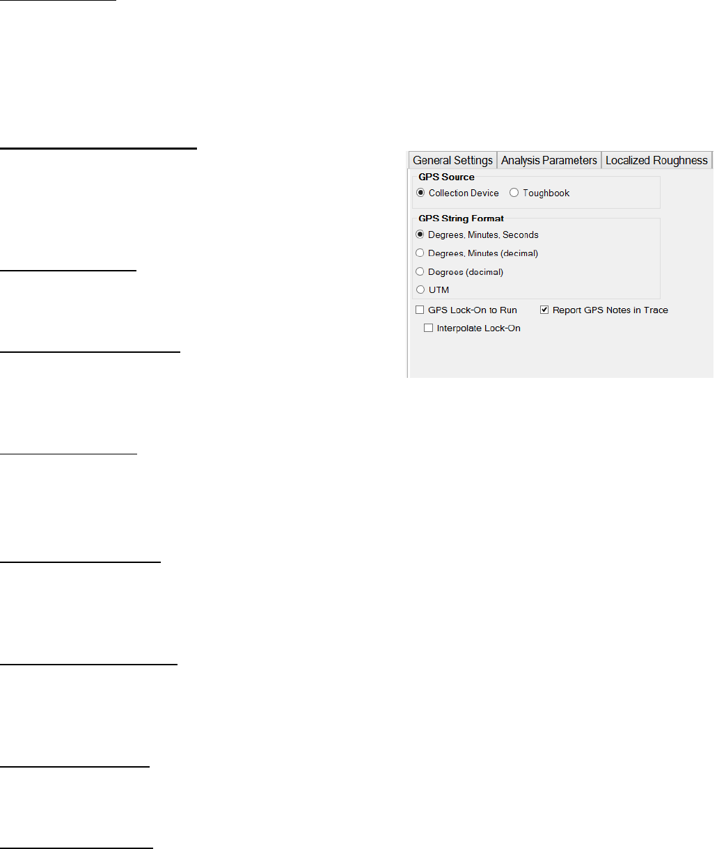
78
Extended Report
The extended report has the calibration and the verification data from the last verification
procedures. The verifications for the inclinometer, height sensor, and the bounce test are all
included along with the calibrations for the accelerometer, inclinometer, and distance encoder. To
review the calibration report, select the Report tab and select the Calibration Report from the drop
down menu.
2.2.6. – GPS Options
The operator has the option to choose the type of GPS to
use for collection. If a survey system is being used, use the
GPS supplied with the collection device.
GPS Lock-On to Run
The GPS signal will reference the GPS coordinates of the
collection while the system is in motion.
Report GPS Notes in Trace
To report GPS notes in the trace select this box. The GPS
notes will be at the bottom of the trace with carrots and
numbers signifying where the note it located.
Interpolate Lock-On
When between GPS points, the interpolation give the user a more accurate current location. The
interpolation uses the two nearest GPS points and the position given by the profiler distance to
give a location between the GPS points.
Sidewalk Options
When using a SSI Sidewalk Profiler, the sidewalk parameters can be changed in the Settings under
the Sidewalk Options tab. The non-conforming parameters of the collected surface will be
displayed in the report. At this location the user may change:
Maximum Running Grade
Maximum running grade is the maximum value that the running grade cannot exceed. If this value
is exceeded, the sidewalk report will list the sections of non-conforming sidewalk sections by GPS
and stationing.
Running Grade Cutoff
Running grade cutoff is the value that is the maximum output allowed in the reports. Values over
this threshold will be displayed as this maximum value in the report.
Maximum Cross Slope
Maximum cross slope is the value that is the maximum output allowed in the report. If this value
is exceeded, the cross slope report will list the non-conforming sidewalk sections.
Figure 120: The GPS options tab
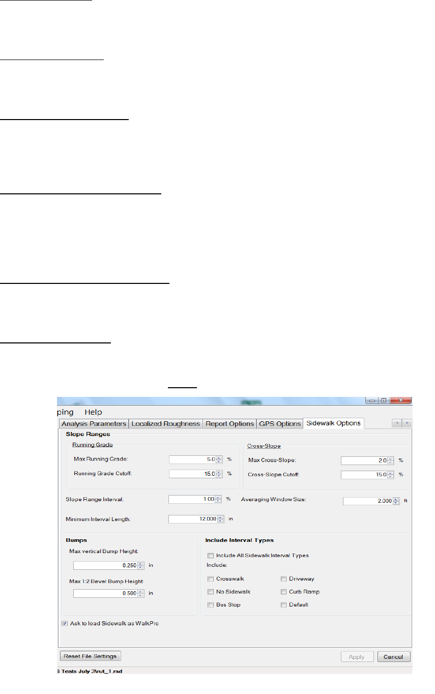
79
Cross Slope Cutoff
Cross slope cutoff is the value that is the maximum output allowed in the reports. Values over this
threshold will be displayed as this maximum value in the report.
Slope Range Interval
Slope range interval is size of the percentage range that the user desired to report running grade
and cross slope.
Minimum Interval Length
Minimum length is the shortest distance or length that can be reported for a given running grade
or cross slope range. Most sidewalks will have a reporting distance of 24 inches based off of a
wheelchair.
Maximum Vertical Bump Height
Maximum vertical bump height is the maximum deviation from the running height. The height is
measured from sharp peaks for relatively short distances. Bumps are characterized by a length to
height ratio of 1:2. All bumps that are over this ratio are classified under this maximum bump
height.
Maximum 1:2 Bevel Bump Height
Maximum bevel bump height applies to bumps that have a height less than the length to height
ratio of 1:2.
Include Interval Types
To include an interval type that will be used during collection select the options individually. To
include all interval types, select the check box to the left of, “Include All Sidewalk Interval Types.”
When a setting is changed, select Apply to save the changes.
Figure 121: The Sidewalk Options
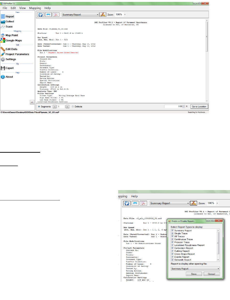
80
3. 0 – View
3.1. - Report
Refresh
It is required to refresh the Report window whenever a change is made to the Project Parameters,
Settings, or Report Options. The refresh icon is located at the top left of the Report window. Select
the refresh button and verify that the information is accurate before printing.
Enable of Disable Reports
This feature allows the user to select the type of
reports that appear in the drop down menu. To
have a report not be displayed in the drop down
menu, deselect the check box.
At the bottom of the Enable or Disable Window
the user may choose which report type is opened
by defa.ult with a new file. In the connecting
figure, the summary report is the file that will be
shown when a file is opened.
Figure 122: The summary header of a single trace report.
Figure 123: Enable and Disable Reports
Window
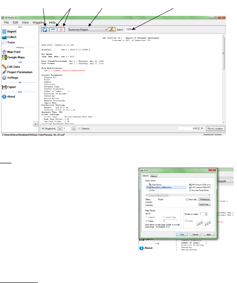
81
Print
To print a report, select the Print Icon in the Report
window or select CTRL+P on the keyboard. The print
window will appear. Within the window, select the printer
to be used and verify that the printer settings are correct.
When ‘Print’ is selected, the document will be sent to the
printer.
If more printing options are needed, select the
‘Preferences’ icon. This icon will open a window that is
printer specific that contains information about the
orientation, paper size, and image quality.
The Adobe Symbol between the Printer symbol and the
report type will print the report to PDF format if the
Broadgun PDF printer is installed.
Report Options
The Report Options available in Profiler V3 are Summary Report, Single Trace, All Trace,
Continuous Trace, Proscan Trace, Defects Report, Calibration Report, Rutting Report, Cross-Slope
Report, Text Report, and QA Suite Report.
Figure 124: The tool bar for the report window
Figure 125: Printing Options Window
Refresh Icon Print Icons Drop Down Report Menu Zoom Ratio
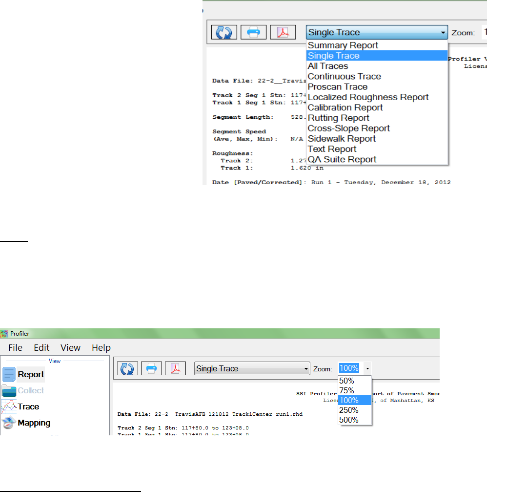
82
Unless directed by the overseeing
agency, the frequently used reports are
Summary Report, Single Trace,
Continuous Trace and Calibration Report.
These reports are commonly used due to
the information provided within them.
All of these reports have the locations of
defects and the information entered in
Project Parameters and Localized
Roughness.
Zoom
The zoom feature is used to adjust the size of the Report window. To change the view of the Report
window, left click on the Zoom box or on the arrow to the right of the box. Selecting the arrow
will only allow the window to change to the preset values of 50%, 75%, 100%, 250% and 500%. If
the operator chooses to left click within the zoom box, the keyboard can be used to type in the
desired zoom percentage. After the zoom percentage is entered, select ‘Enter.’
View by Segments or Defects
By selecting Segments (the default setting) the operator may navigate through the segments of
the file by typing in the segment number and selecting ‘Enter’, or by using the arrow keys to the
right of the box. When Defects are selected, the same procedure is used to navigate throughout
the file to the defect locations. This is a shortcut for moving throughout segments and finding
defects while in the Single Trace report option.
If the operator is not in Single Trace while using this feature, the program will adapt and open
Single Trace when the Report window generates.
Figure 126: The drop-down menu for the report options
Figure 127: The built in zoom ratios
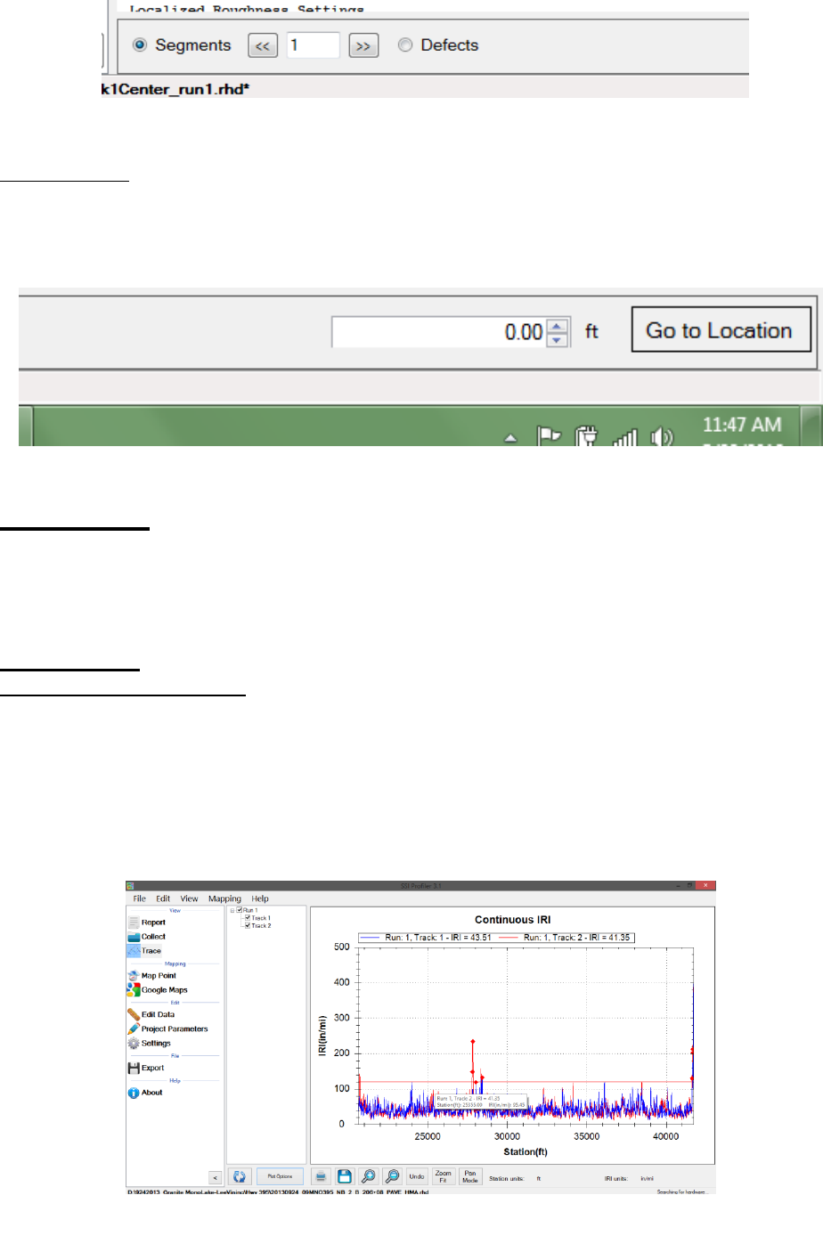
83
Go to Location
The Go to Location Feature moves the report window to the position of the profile (a distance)
entered in the box. By entering the station number in decimal form and selecting ‘Go to Location’
the segment containing the entered station number will be displayed in the Report window.
3.2 – Collect
To collect data the operator should select the Collect Icon when the hardware is attached. Once
the hardware is found, the data collection may begin. See the Collection section of this manual for
procedures to perform prior and during a collection.
3.3. – Trace
Choosing Tracks for Plotting
To choose tracks for plotting in the trace window, select the check box next to the desired tracks.
Once all of the necessary tracks are checked, select the refresh icon to view the tracks within the
plot. Whenever a change is made by deselecting a track or checking a new track, select the refresh
icon to have it appear in the trace. If the refresh icon is not selected, the trace will not update and
the changes will not be shown. Review the legend to verify that all of the selected tracks are shown
in the plot.
Figure 128: The segment or defect navigator
Figure 129: Go to Location Feature
Figure 130: An example of the profile trace
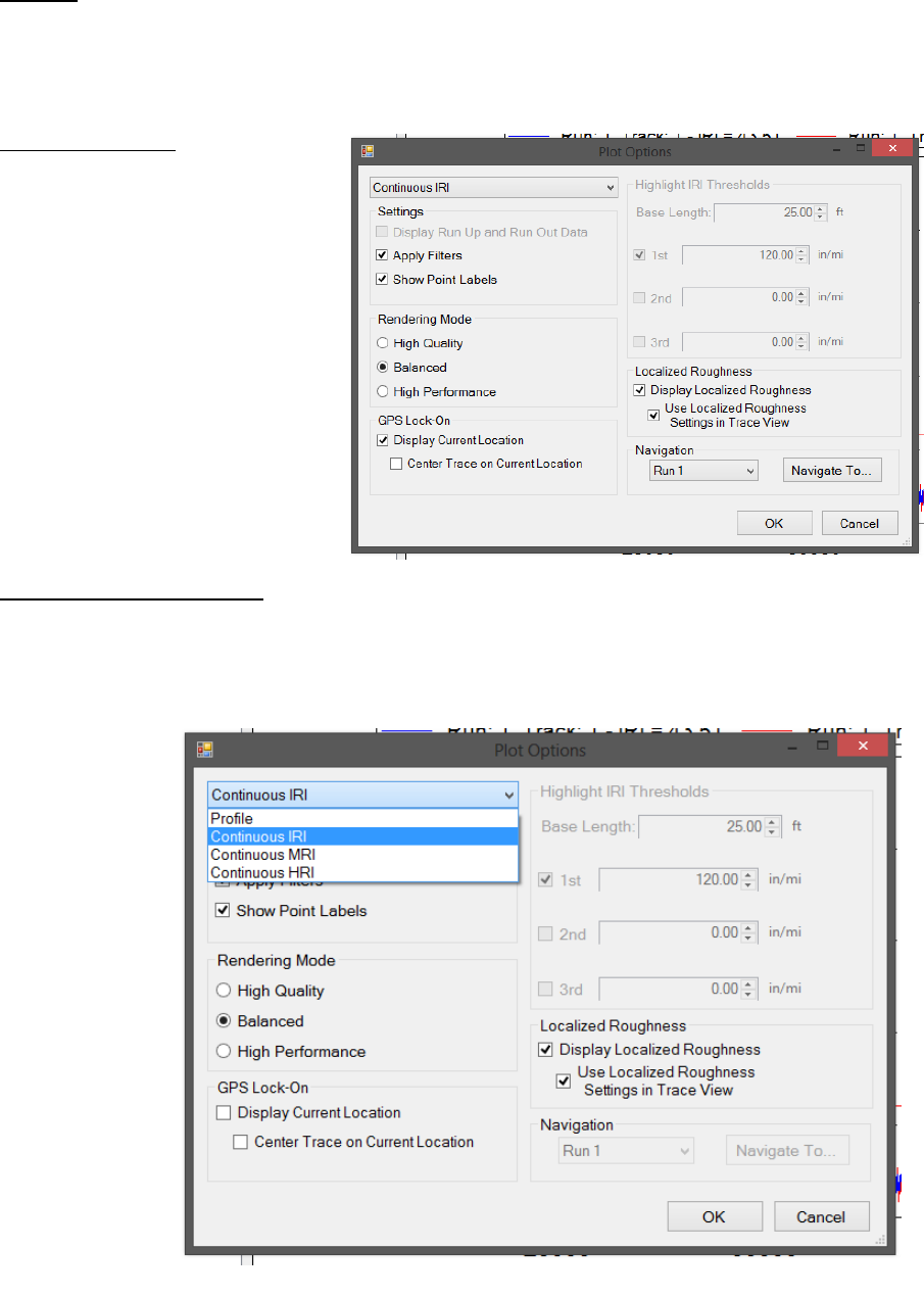
84
Refresh
It is required to refresh the Trace window whenever a change is made to the track selections. The
refresh icon is located at the bottom left of the Trace window. Select the refresh button and verify
that the trace is accurate before a print is made.
Plot Options Icon
Profile/Continuous IRI
The drop down menu allows the user to select options of Profile and Continuous IRI, MRI or HRI.
When Continuous IRI is selected, the operator may not choose the option to include Run Up and
Run out data.
Figure 131: The plot
options window
Figure 132: Plot Options Window
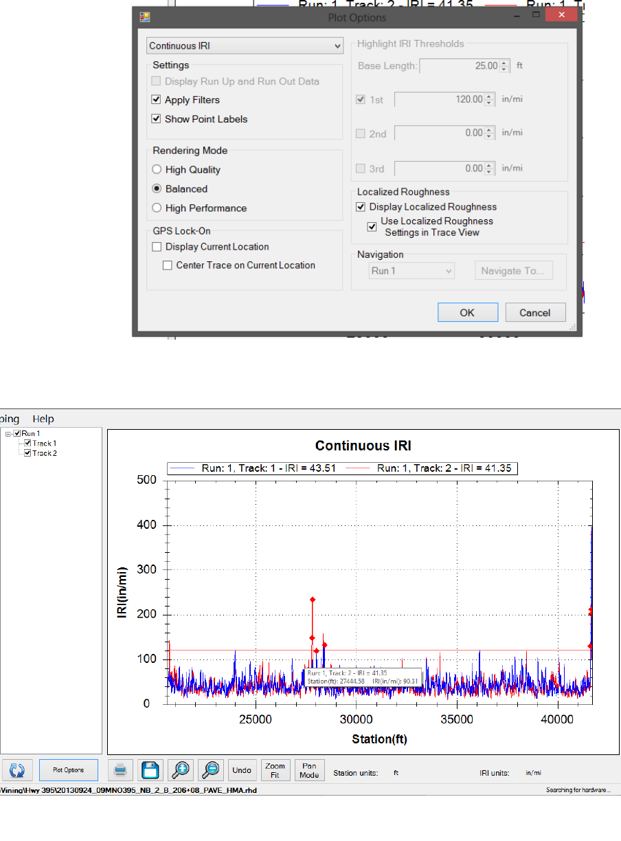
85
Figure 125: The Continuous IRI Plot
options window.
Figure 134: The plot of the Continuous IRI trace
Figure 133: Continuous IRI Window.
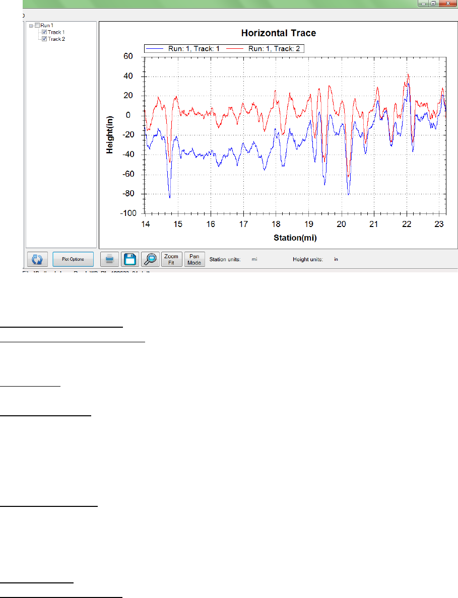
86
Plot Options Settings
Display Run in/ Run out Data
Many High Speed Profiler data files have Run in and/or Run out data associated with them. To
include this data in the trace, select the check box next to “Display Run Up and Run out Data.”
Apply filters
To apply the filters select the check box “Apply Filters.”
Show Point Labels
Showing point labels allows the user to move the cursor over the profile to find the stationing and
height at a certain point of the plot. When the cursor stays over a point for one second, a dialogue
box appears that gives information on station number and height at the cursors current position.
The units of the stationing and height are the same as the units of the axes.
Rendering Mode
Under the Rendering Mode section the operator can choose the type of rendering to increase the
speed or increase the quality when refreshing the graph. When using the high quality rendering,
the time it takes to refresh will be longer, however the resolution of the trace will be optimum.
GPS Lock-On
Display Current Location
This feature will display a vertical line at the vehicle’s current GPS location. This vertical line will
move through the trace as the vehicle moves, allowing the user to locate the points of localized
roughness.
Figure 135: The plot of the profile trace
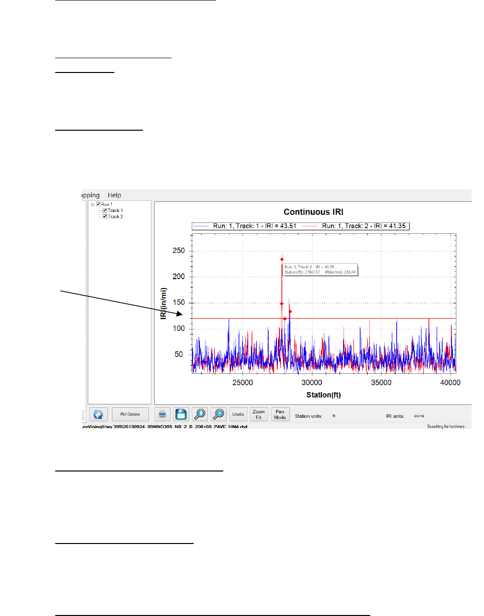
87
Center Trace on Current Location
Then this box is checked, the trace will pan with the motion of the vehicle so that the current
location is always in the center of the window.
Highlight IRI Thresholds
Base Length
The base length is the length of the California Profilograph or 25 feet. It will be the basis of the IRI
localized roughness calculations.
1st, 2nd, 3rd [in/mi]
Three separate thresholds can be set to depict which plots exceed the thresholds on the graph.
These thresholds will be plotted as a horizontal line across the trace graph at the IRI values of the
threshold in inches per mile.
Localized Roughness in Trace View
Be aware that when using the localized roughness, the defects can appear below the threshold
line. This is because the localized roughness is based off of a 25-foot length and not the entire
profile.
Display Localized Roughness
When this box is selected the trace view will have the localized roughness location marked with a
diamond. If the user places the cursor over the red diamond, the information about the localized
roughness will be displayed.
Use Localized Roughness Settings in Trace View (Recommended)
By selecting this box the IRI Localized Roughness threshold established under the Settings and
Localized Roughness Tab will be used to find and display the localized roughness in Trace View. If
Figure 136: The Continuous IRI trace with the localized roughness diamonds
shown
Threshold
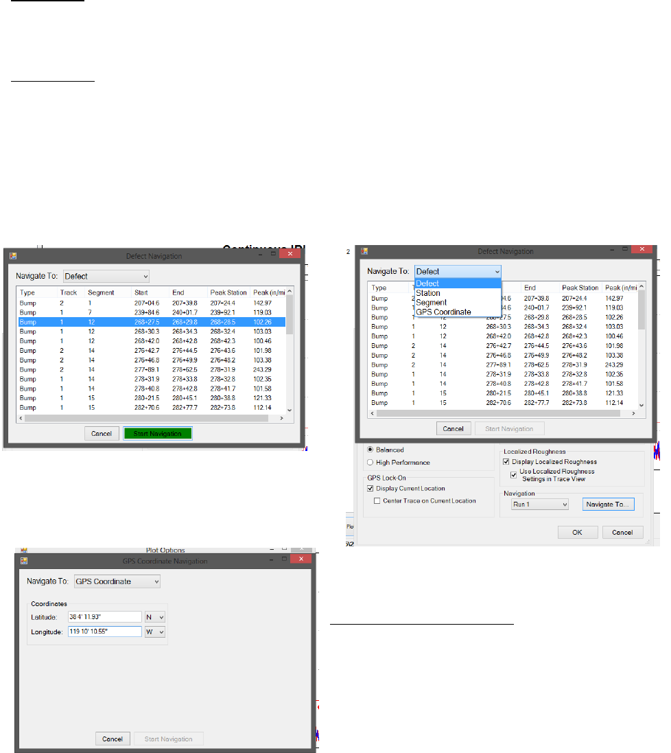
88
the other thresholds are used, the number of defects displayed in the trace may be different than
the number in the report. This selection displays the same localized roughness as in the report.
Navigation
In order to use the Navigation feature in Trace View the GPS must be connected and you must
select the “Display Current Location” check box under GPS Lock-On in the Plot Options Window.
To Navigate:
1) Select the run that the desired point of localized roughness, segment, station or GPS
coordinate is found in under the Plot Options Menu.
2) Select Navigate To…
3) Use the drop down menu to select the type of location: defect (localized roughness),
segment, station, or GPS coordinate.
4) Select a location from the list and then select the green “Start Navigation” icon
GPS Coordinate Navigation
To navigate to a GPS coordinate, type in the GPS
coordinates for longitude and latitude.
Figure 138: The Trace Navigation Options
Figure 137: A Location selected and ready to
start navigation
Figure 139: Navigate to GPS Coordinate
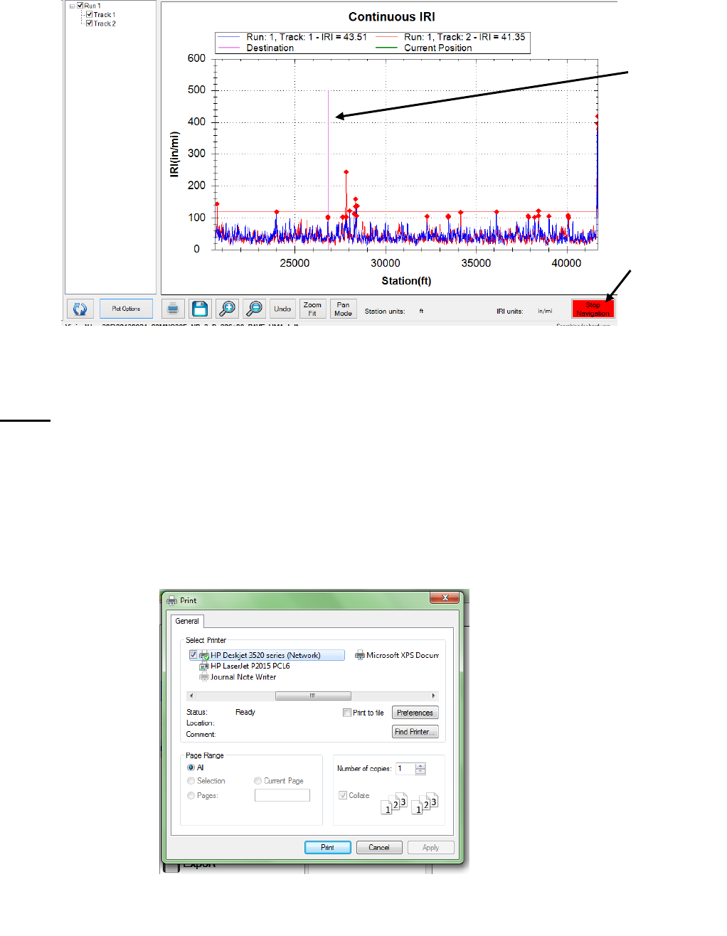
89
Print
To print the trace, select the Print Icon in the window or select CTRL+P on the keyboard. The print
window will appear at this time. Within the window, select the printer to be used and verify that
the printer settings are correct. When ‘Print’ is selected, the document will be sent to the printer.
If more printing options are needed, select the ‘Preferences’ icon. This icon will open a window
that is printer specific containing information about the orientation, paper size, and image quality.
Figure 141: The Print window that appears after the print icon is selected
Figure 140: The Navigation started. The pink line is the destination
Destination
Stop
Navigation
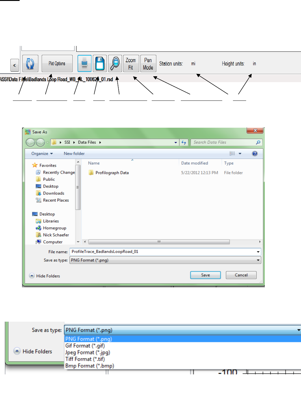
90
Save
When the Save icon is selected, the user is able to save the trace as an image in png, gif, jpeg, tiff,
and bmp format. The image can be saved on the operating computer or on a connected external
device.
Figure 142: The tool bar for the trace window
Figure 143: Windows explorer to save a picture of the graph.
Figure 144: Available picture formats to save the trace graph
Refresh Plot Options Print Save Zoom Previous Zoom Fit Pan/Zoom Mode Units

91
Zoom
To zoom in the trace window, verify that the Pan/Zoom Mode icon displays ‘Pan Mode.’ To zoom
in on the plot, left click and hold while dragging the cursor over the area to be blown up. While
dragging the cursor, a dotted box will appear. This dotted box contains the area of the plot that
will be blown up, by being fit to the size of the plot window.
Zoom Previous Icon
When Zoom Previous is selected, the last ‘zoom in’ action is undone.
Zoom Fit Icon
To return to the original aspect ratio, also known as the home view, select Zoom Fit.
Pan/Zoom Mode Icon
The Pan/Zoom Mode icon has two functions. When Pan Mode is displayed, the cursor may be
used to zoom in on the plot. To zoom in on the plot, hold down the left mouse button and move
the cursor over the plot area to be blown up. The dashed box contains the area that will be
enlarged.
When Zoom Mode is displayed, the operator may use the cursor to pan across the plot area. The
pan mode allows the user to navigate through the plot area without changing the aspect ratio, or
zooming out.
Units for Height and Station
The units for height (y-axis) and stationing (x-axis) can be changed by left clicking upon the current
units and selecting the necessary units from the dialogue box that appears. The units available are
mils, inches, feet, yard, miles, millimeters, centimeters, meters, and kilometers. The units scale the
plot area.
4.0. – Mapping
The Profiler V3 program has two separate mapping programs to choose from. Map Point can be
used to travel to the point of defects or other points of interest on the run path. For this reason,
Map Point requires a connected GPS device to function. Google Maps can be used to show the real
world location of the event, segment, and collection path. Both of these features are used after a
collection has been completed with GPS coordinates.
4.1. – Map Point
Map Point is used to navigate to points of interest along the path of collection.
The Map Point feature can be used to navigate to defects in the profile based on the GPS
coordinates. Map Point can be used in trace view or through the compass and distance readout
on the Map Point window. To navigate to a defect using Mapping:
1) Open a file in SSI Profiler with defects
2) Open the Mapping window through the shortcut bar or through View>Mapping.
3) At the top, select a run and click on the “Navigate To” icon.
4) The user may choose to navigate to a defect, station, segment, or a specific GPS
coordinate. Choose the option from the drop down menu. Select a location and click on the green
Start Navigation icon.
5) Follow the instructions of the mapping to get to the destination.
Note: A GPS signal and a collection using GPS is required to use Mapping feature.
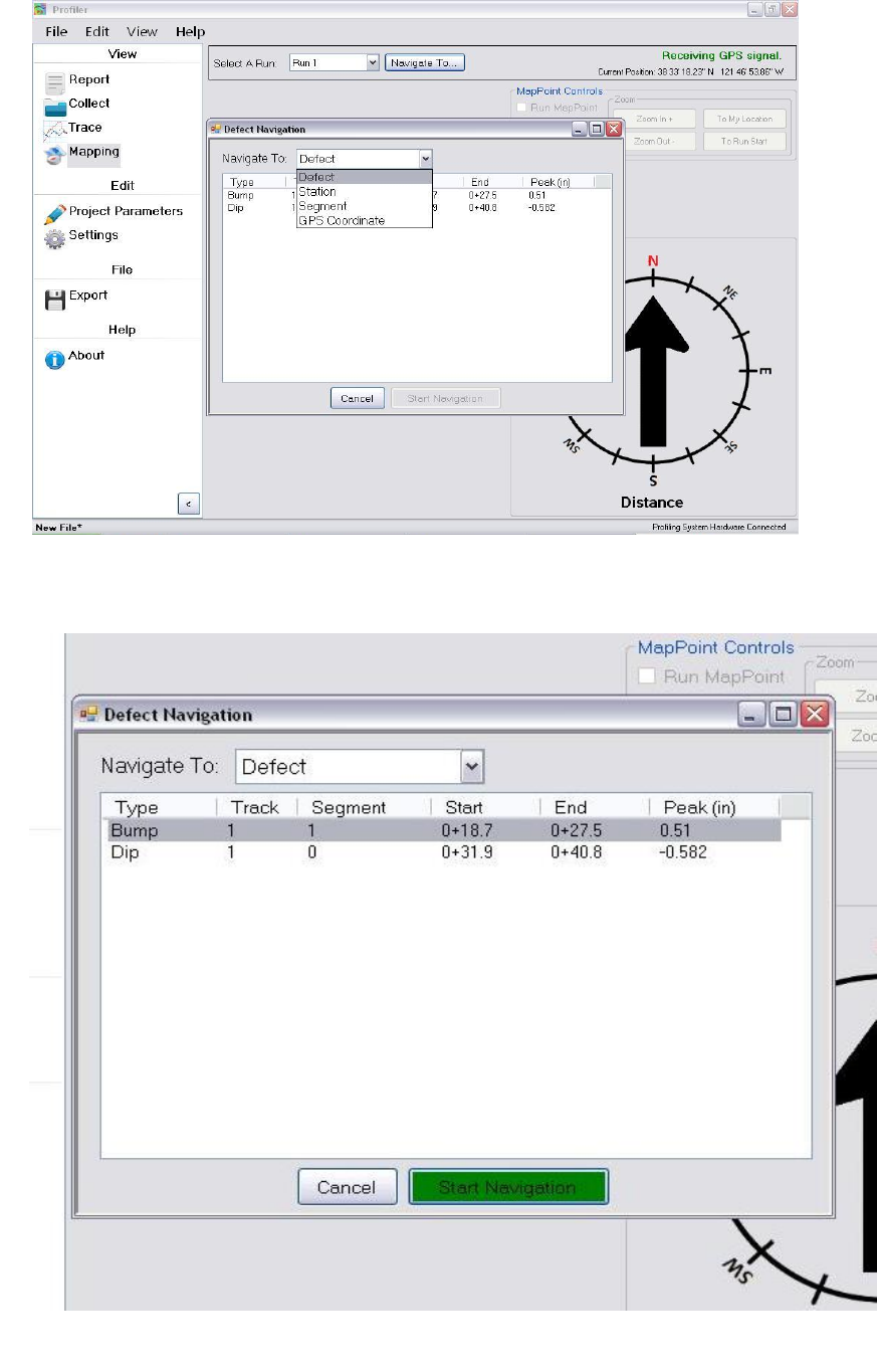
92
Figure 145: The drop-down menu for Mapping. Run being navigated along Run1
Figure 146: A bump is selected in Mapping
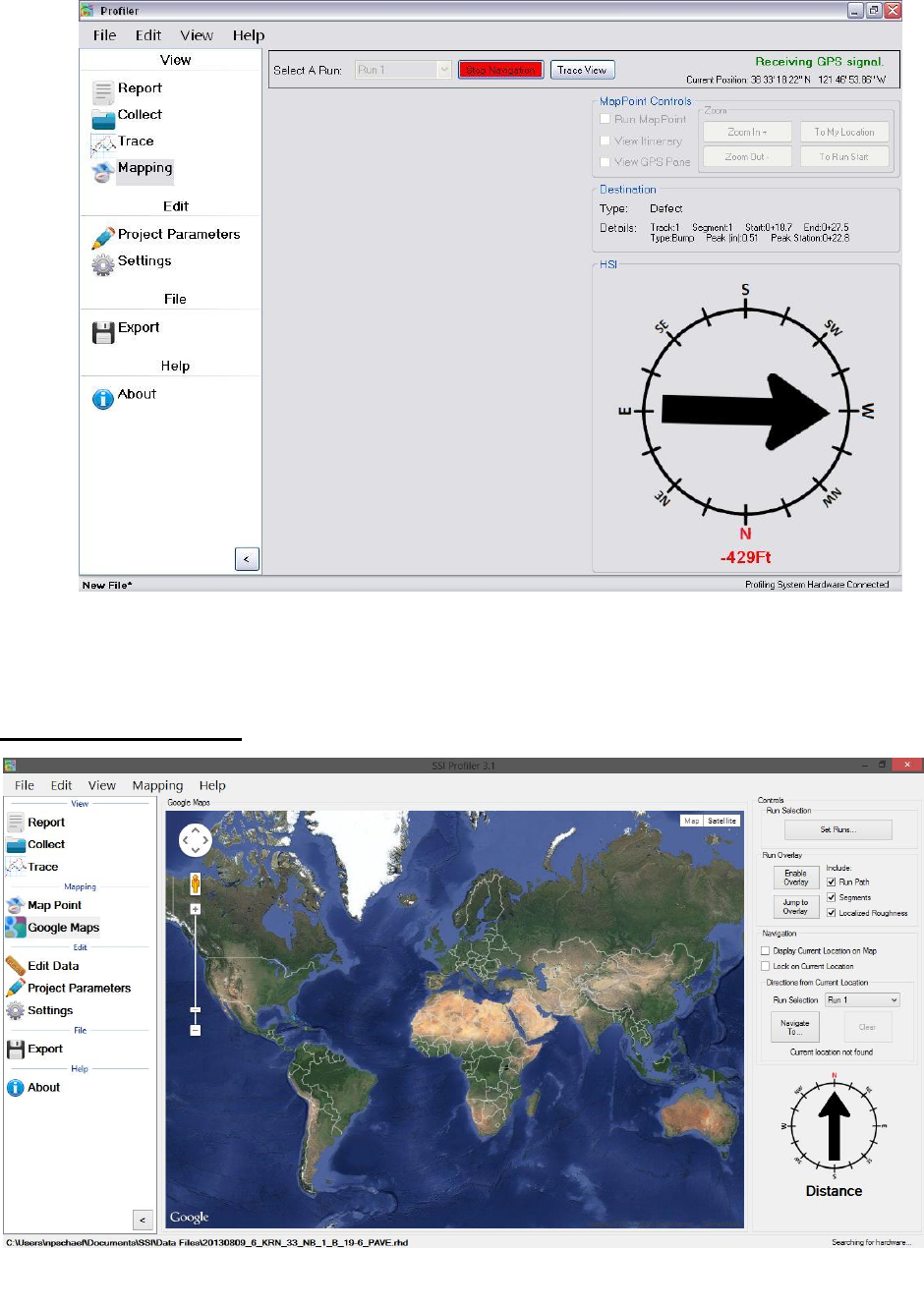
93
4.1 – Google Maps
Figure 148: Initial Google Maps Screen
Figure 147: Navigation to a point in Mapping

94
Google Maps can be used to show the location of the run path, segments, and localized roughness.
Google Maps can also be used within Profiler V3 to navigate to defects, the start of the run or the
end of the run.
To view the location of the collection without any collection information displayed:
1) To begin, select the Google Maps icon in the shortcut bar.
2) The world view will be the initial view in the window.
3) The right side of the window has the controls section. Choose the run number of the
collection to be viewed in the map.
4) Select Jump to Overlay or “Navigate To…” and select an event.
To view the Run Path, Segments, and Localized Roughness:
1) Select their corresponding check boxes of the parameters. If one parameter is not desired,
do not select its check box
2) Select the “Enable Overlay” icon.
3) Select Jump to Run
4) If the push-pin is selected, the statistics and information for that location will be displayed.
For Localized Roughness: Red Pin is Track 1, Blue Pin is Track 2, Green Pin is Track 3.
To deselect a track to not show it on the map, select the “Set Runs” icon and uncheck the box next
to the unwanted track.
Once the run is displayed in Google Maps, use the scrolling and cursor to navigate through the run.
The run path, segments and localized roughness are shown if their respective box is selected.
These features can be shown if the box is checked reading, “Disable Overlay.”
Display Current Location on Map
If this check box is selected, the current location of the profiler is marked by a large green arrow
in the map window.
Lock on Current Location
If the check box for “Lock on Current Location” is selected, the location of the profiling system will
remain in the center of the map window.
Directions from Current Location
The V3 program will navigate to the start or end of the run and any defects found during collection.
Select the destination from the drop down menu and select the calculate icon. The route will
appear as a black line from your current location to the “B” landmark.
To navigate to an event, pause, segment, or defect, select the correct run number and hen the
“Navigate To” icon. If GPS is connected the program will ask the user where to be navigated to.
Once the location is selected Profiler will direct the device to the location.
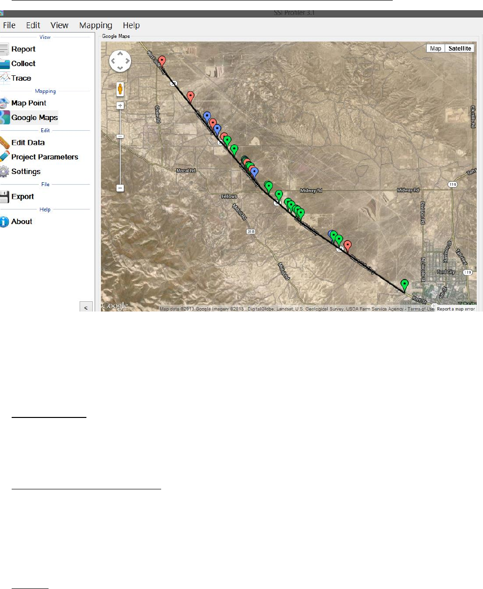
95
Note: GPS must be connected to use the Google Maps and Map Point features.
5.0 – About
The About section has information concerning Profiler V3 software and its licenses. The software
version, copyright and license can all be found in the ‘About’ window. Additionally, third party
software licenses are listed in the About window.
Profiler V3 License Information
The computer’s Profiler V3 license information can be viewed in the About window. The details
will display all of the additional features and collection devices attributed to the license.
The update icon will allow the operator to choose an installation file from the computer to update
the Profiler V3 software.
Manual
The manual can be found under the Help Tab or on the About Section window. Otherwise, the
manual is save to the Desktop or in the “Manuals” folder under C:\Program Files (x86)\SSI Profiler
3\Manuals.
Figure 149: Google Maps showing the localized roughness
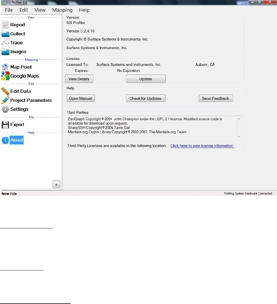
96
Check for Updates
The operator can manually check for updates through Help>Check For Updates. By default, the
program will check for updates every time it is opened. To not check for updates at each opening,
deselect the check box in this window.
Send Feedback
If SSI should be informed of issues or advancements of the software, please send us feedback so
we can improve our services.
Third Party Components
The Third Party Components of Profiler V3 are:
ZedGraph Copyright © 2004 John Champion under the LGPL 2.1 license.
Modified source code is available for download at:
http://www.smoothroad.com/support/download.asp.
SharpSSH Copyright © 2006 Tamir Gal
Mentalis.org Crypto Library Copyright © 2002-2007. The Mentalis.org Team
Full copies of all third party licenses can be found in the Licenses folder located inside the Profiler
V3 installation directory.
Figure 150: The About Window
97
Troubleshooting
CS8800 Profiling System Software. For technical support for the CS8800 electronics or software,
contact SSI by email at support@smoothroad.com or telephone at:
(785) 539-6305 (Kansas, USA)
or
(530) 885-1482 (California, USA).
Necessary software updates and periodic version upgrades can be downloaded the Profiler V3
program when internet access is available. If there is an update, the program will ask the operator
to install the current version.
For customer specific downloads, visit the SSI website at: SSI Download Site. Contact SSI customer
support for a user ID and password, or for further assistance.
CS8800 Profiling System Hardware. For hardware or spare parts, contact James Cox & Associates
office in Auburn, California at (530) 885-1482 or by email at:
mchadd@smoothroad.com. Operators can also contact SSI by email at
support@smoothroad.com or telephone at (785)539-6305 (Kansas, USA) or (415)383-0570
(California, USA).
Panasonic Toughbook Computer. For technical support for Panasonic Toughbook computers,
contact Panasonic Technical Support at 1-800-Laptop 5 (800- 527-8675) or go to the this link:
Panasonic Toughbook Support.
Paper Supplies or Printer Servicing. For printer paper supplies or printer servicing, contact SSI
Customer Support.
No GPS Signal
Check the connections of the GPS antenna. If the location of the antenna is beneath the Toughbook
stand or if the profiler is in an area of low reception, the GPS position may not be found. Review
the GPS settings under Settings to see if collection device is selected. Under the Collect tab, select
the GPS icon to view the number of satellites and signal information.
Will Not Find Hardware
The electronics will not be found if the system does not have sufficient power or if it is not
connected to the computer.
1) Check that the system has power
2) Check the integrity of the cables. Have special attention to the DB-9 serial cable.
Abnormal Collection Results
If the system returns multiple defects or localized roughness and high ride numbers, review the
calibration information. As needed, recalibrate the absolute encoder, distance, and height sensor.
Battery is Not Charging
1) Check the charger for a red LED
2) Turn off the power to the CS8800 and turn it back on after 3 seconds. This will refresh the
battery gauge
3) A pin or a wire is not making connection for power within the device.
