SciPy Reference Guide
User Manual:
Open the PDF directly: View PDF ![]() .
.
Page Count: 1229 [warning: Documents this large are best viewed by clicking the View PDF Link!]
- SciPy Tutorial
- Introduction
- Basic functions
- Special functions (scipy.special)
- Integration (scipy.integrate)
- Optimization (scipy.optimize)
- Interpolation (scipy.interpolate)
- Fourier Transforms (scipy.fftpack)
- Signal Processing (scipy.signal)
- Linear Algebra (scipy.linalg)
- Sparse Eigenvalue Problems with ARPACK
- Compressed Sparse Graph Routines scipy.sparse.csgraph
- Spatial data structures and algorithms (scipy.spatial)
- Statistics (scipy.stats)
- Multidimensional image processing (scipy.ndimage)
- File IO (scipy.io)
- Weave (scipy.weave)
- Contributing to SciPy
- API - importing from Scipy
- Release Notes
- Reference
- Clustering package (scipy.cluster)
- K-means clustering and vector quantization (scipy.cluster.vq)
- Hierarchical clustering (scipy.cluster.hierarchy)
- Constants (scipy.constants)
- Discrete Fourier transforms (scipy.fftpack)
- Integration and ODEs (scipy.integrate)
- Interpolation (scipy.interpolate)
- Input and output (scipy.io)
- Linear algebra (scipy.linalg)
- Low-level BLAS functions
- Finding functions
- All functions
- Low-level LAPACK functions
- Finding functions
- All functions
- Interpolative matrix decomposition (scipy.linalg.interpolative)
- Miscellaneous routines (scipy.misc)
- Multi-dimensional image processing (scipy.ndimage)
- Orthogonal distance regression (scipy.odr)
- Optimization and root finding (scipy.optimize)
- Nonlinear solvers
- Signal processing (scipy.signal)
- Sparse matrices (scipy.sparse)
- Sparse linear algebra (scipy.sparse.linalg)
- Compressed Sparse Graph Routines (scipy.sparse.csgraph)
- Spatial algorithms and data structures (scipy.spatial)
- Distance computations (scipy.spatial.distance)
- Special functions (scipy.special)
- Statistical functions (scipy.stats)
- Statistical functions for masked arrays (scipy.stats.mstats)
- C/C++ integration (scipy.weave)
- Bibliography
- Index

SciPy Reference Guide
Release 0.13.0
Written by the SciPy community
October 21, 2013

CONTENTS
1 SciPy Tutorial 3
1.1 Introduction ............................................... 3
1.2 Basic functions .............................................. 5
1.3 Special functions (scipy.special)................................. 9
1.4 Integration (scipy.integrate)................................... 11
1.5 Optimization (scipy.optimize)................................... 16
1.6 Interpolation (scipy.interpolate)................................ 29
1.7 Fourier Transforms (scipy.fftpack)................................ 41
1.8 Signal Processing (scipy.signal).................................. 44
1.9 Linear Algebra (scipy.linalg)................................... 52
1.10 Sparse Eigenvalue Problems with ARPACK ............................... 65
1.11 Compressed Sparse Graph Routines scipy.sparse.csgraph .................. 68
1.12 Spatial data structures and algorithms (scipy.spatial)...................... 71
1.13 Statistics (scipy.stats)....................................... 77
1.14 Multidimensional image processing (scipy.ndimage)....................... 96
1.15 File IO (scipy.io)........................................... 117
1.16 Weave (scipy.weave)........................................ 123
2 Contributing to SciPy 159
2.1 Contributing new code .......................................... 159
2.2 Contributing by helping maintain existing code ............................. 160
2.3 Other ways to contribute ......................................... 161
2.4 Recommended development setup .................................... 161
2.5 SciPy structure .............................................. 162
2.6 Useful links, FAQ, checklist ....................................... 162
3 API - importing from Scipy 165
3.1 Guidelines for importing functions from Scipy ............................. 165
3.2 API definition .............................................. 166
4 Release Notes 169
4.1 SciPy 0.13.0 Release Notes ....................................... 169
4.2 SciPy 0.12.0 Release Notes ....................................... 176
4.3 SciPy 0.11.0 Release Notes ....................................... 181
4.4 SciPy 0.10.0 Release Notes ....................................... 187
4.5 SciPy 0.9.0 Release Notes ........................................ 191
4.6 SciPy 0.8.0 Release Notes ........................................ 195
4.7 SciPy 0.7.2 Release Notes ........................................ 199
4.8 SciPy 0.7.1 Release Notes ........................................ 199
i

4.9 SciPy 0.7.0 Release Notes ........................................ 201
5 Reference 207
5.1 Clustering package (scipy.cluster)................................ 207
5.2 K-means clustering and vector quantization (scipy.cluster.vq)................. 207
5.3 Hierarchical clustering (scipy.cluster.hierarchy)...................... 211
5.4 Constants (scipy.constants).................................... 226
5.5 Discrete Fourier transforms (scipy.fftpack)............................ 241
5.6 Integration and ODEs (scipy.integrate)............................. 255
5.7 Interpolation (scipy.interpolate)................................ 273
5.8 Input and output (scipy.io)...................................... 320
5.9 Linear algebra (scipy.linalg)................................... 331
5.10 Low-level BLAS functions ........................................ 373
5.11 Finding functions ............................................. 373
5.12 All functions ............................................... 373
5.13 Low-level LAPACK functions ...................................... 398
5.14 Finding functions ............................................. 398
5.15 All functions ............................................... 398
5.16 Interpolative matrix decomposition (scipy.linalg.interpolative)............. 448
5.17 Miscellaneous routines (scipy.misc)................................ 457
5.18 Multi-dimensional image processing (scipy.ndimage)....................... 466
5.19 Orthogonal distance regression (scipy.odr)............................. 520
5.20 Optimization and root finding (scipy.optimize).......................... 530
5.21 Nonlinear solvers ............................................. 593
5.22 Signal processing (scipy.signal).................................. 595
5.23 Sparse matrices (scipy.sparse)................................... 692
5.24 Sparse linear algebra (scipy.sparse.linalg).......................... 784
5.25 Compressed Sparse Graph Routines (scipy.sparse.csgraph).................. 809
5.26 Spatial algorithms and data structures (scipy.spatial)...................... 819
5.27 Distance computations (scipy.spatial.distance)....................... 853
5.28 Special functions (scipy.special)................................. 867
5.29 Statistical functions (scipy.stats)................................. 897
5.30 Statistical functions for masked arrays (scipy.stats.mstats).................. 1162
5.31 C/C++ integration (scipy.weave).................................. 1188
Bibliography 1193
Index 1205
ii

SciPy Reference Guide, Release 0.13.0
Release 0.13.0
Date October 21, 2013
SciPy (pronounced “Sigh Pie”) is open-source software for mathematics, science, and engineering.
CONTENTS 1

SciPy Reference Guide, Release 0.13.0
2 CONTENTS

CHAPTER
ONE
SCIPY TUTORIAL
1.1 Introduction
Contents
•Introduction
–SciPy Organization
–Finding Documentation
SciPy is a collection of mathematical algorithms and convenience functions built on the Numpy extension of Python. It
adds significant power to the interactive Python session by providing the user with high-level commands and classes for
manipulating and visualizing data. With SciPy an interactive Python session becomes a data-processing and system-
prototyping environment rivaling sytems such as MATLAB, IDL, Octave, R-Lab, and SciLab.
The additional benefit of basing SciPy on Python is that this also makes a powerful programming language available
for use in developing sophisticated programs and specialized applications. Scientific applications using SciPy benefit
from the development of additional modules in numerous niche’s of the software landscape by developers across the
world. Everything from parallel programming to web and data-base subroutines and classes have been made available
to the Python programmer. All of this power is available in addition to the mathematical libraries in SciPy.
This tutorial will acquaint the first-time user of SciPy with some of its most important features. It assumes that the
user has already installed the SciPy package. Some general Python facility is also assumed, such as could be acquired
by working through the Python distribution’s Tutorial. For further introductory help the user is directed to the Numpy
documentation.
For brevity and convenience, we will often assume that the main packages (numpy, scipy, and matplotlib) have been
imported as:
>>> import numpy as np
>>> import scipy as sp
>>> import matplotlib as mpl
>>> import matplotlib.pyplot as plt
These are the import conventions that our community has adopted after discussion on public mailing lists. You will
see these conventions used throughout NumPy and SciPy source code and documentation. While we obviously don’t
require you to follow these conventions in your own code, it is highly recommended.
1.1.1 SciPy Organization
SciPy is organized into subpackages covering different scientific computing domains. These are summarized in the
following table:
3

SciPy Reference Guide, Release 0.13.0
Subpackage Description
cluster Clustering algorithms
constants Physical and mathematical constants
fftpack Fast Fourier Transform routines
integrate Integration and ordinary differential equation solvers
interpolate Interpolation and smoothing splines
io Input and Output
linalg Linear algebra
ndimage N-dimensional image processing
odr Orthogonal distance regression
optimize Optimization and root-finding routines
signal Signal processing
sparse Sparse matrices and associated routines
spatial Spatial data structures and algorithms
special Special functions
stats Statistical distributions and functions
weave C/C++ integration
Scipy sub-packages need to be imported separately, for example:
>>> from scipy import linalg, optimize
Because of their ubiquitousness, some of the functions in these subpackages are also made available in the scipy
namespace to ease their use in interactive sessions and programs. In addition, many basic array functions from numpy
are also available at the top-level of the scipy package. Before looking at the sub-packages individually, we will first
look at some of these common functions.
1.1.2 Finding Documentation
SciPy and NumPy have documentation versions in both HTML and PDF format available at http://docs.scipy.org/, that
cover nearly all available functionality. However, this documentation is still work-in-progress and some parts may be
incomplete or sparse. As we are a volunteer organization and depend on the community for growth, your participation
- everything from providing feedback to improving the documentation and code - is welcome and actively encouraged.
Python’s documentation strings are used in SciPy for on-line documentation. There are two methods for reading
them and getting help. One is Python’s command help in the pydoc module. Entering this command with no
arguments (i.e. >>> help ) launches an interactive help session that allows searching through the keywords and
modules available to all of Python. Secondly, running the command help(obj) with an object as the argument displays
that object’s calling signature, and documentation string.
The pydoc method of help is sophisticated but uses a pager to display the text. Sometimes this can interfere with
the terminal you are running the interactive session within. A scipy-specific help system is also available under the
command sp.info. The signature and documentation string for the object passed to the help command are printed
to standard output (or to a writeable object passed as the third argument). The second keyword argument of sp.info
defines the maximum width of the line for printing. If a module is passed as the argument to help than a list of the
functions and classes defined in that module is printed. For example:
>>> sp.info(optimize.fmin)
fmin(func, x0, args=(), xtol=0.0001, ftol=0.0001, maxiter=None, maxfun=None,
full_output=0, disp=1, retall=0, callback=None)
Minimize a function using the downhill simplex algorithm.
Parameters
----------
func : callable func(x,*args)
4 Chapter 1. SciPy Tutorial

SciPy Reference Guide, Release 0.13.0
The objective function to be minimized.
x0 : ndarray
Initial guess.
args : tuple
Extra arguments passed to func, i.e. ‘‘f(x,*args)‘‘.
callback : callable
Called after each iteration, as callback(xk), where xk is the
current parameter vector.
Returns
-------
xopt : ndarray
Parameter that minimizes function.
fopt : float
Value of function at minimum: ‘‘fopt = func(xopt)‘‘.
iter : int
Number of iterations performed.
funcalls : int
Number of function calls made.
warnflag : int
1 : Maximum number of function evaluations made.
2 : Maximum number of iterations reached.
allvecs : list
Solution at each iteration.
Other parameters
----------------
xtol : float
Relative error in xopt acceptable for convergence.
ftol : number
Relative error in func(xopt) acceptable for convergence.
maxiter : int
Maximum number of iterations to perform.
maxfun : number
Maximum number of function evaluations to make.
full_output : bool
Set to True if fopt and warnflag outputs are desired.
disp : bool
Set to True to print convergence messages.
retall : bool
Set to True to return list of solutions at each iteration.
Notes
-----
Uses a Nelder-Mead simplex algorithm to find the minimum of function of
one or more variables.
Another useful command is source. When given a function written in Python as an argument, it prints out a listing
of the source code for that function. This can be helpful in learning about an algorithm or understanding exactly what
a function is doing with its arguments. Also don’t forget about the Python command dir which can be used to look
at the namespace of a module or package.
1.2 Basic functions
1.2. Basic functions 5

SciPy Reference Guide, Release 0.13.0
Contents
•Basic functions
–Interaction with Numpy
*Index Tricks
*Shape manipulation
*Polynomials
*Vectorizing functions (vectorize)
*Type handling
*Other useful functions
1.2.1 Interaction with Numpy
Scipy builds on Numpy, and for all basic array handling needs you can use Numpy functions:
>>> import numpy as np
>>> np.some_function()
Rather than giving a detailed description of each of these functions (which is available in the Numpy Reference Guide
or by using the help,info and source commands), this tutorial will discuss some of the more useful commands
which require a little introduction to use to their full potential.
To use functions from some of the Scipy modules, you can do:
>>> from scipy import some_module
>>> some_module.some_function()
The top level of scipy also contains functions from numpy and numpy.lib.scimath. However, it is better to
use them directly from the numpy module instead.
Index Tricks
There are some class instances that make special use of the slicing functionality to provide efficient means for array
construction. This part will discuss the operation of np.mgrid ,np.ogrid ,np.r_ , and np.c_ for quickly
constructing arrays.
For example, rather than writing something like the following
>>> concatenate(([3],[0]*5,arange(-1,1.002,2/9.0)))
with the r_ command one can enter this as
>>> r_[3,[0]*5,-1:1:10j]
which can ease typing and make for more readable code. Notice how objects are concatenated, and the slicing syntax
is (ab)used to construct ranges. The other term that deserves a little explanation is the use of the complex number
10j as the step size in the slicing syntax. This non-standard use allows the number to be interpreted as the number of
points to produce in the range rather than as a step size (note we would have used the long integer notation, 10L, but
this notation may go away in Python as the integers become unified). This non-standard usage may be unsightly to
some, but it gives the user the ability to quickly construct complicated vectors in a very readable fashion. When the
number of points is specified in this way, the end- point is inclusive.
The “r” stands for row concatenation because if the objects between commas are 2 dimensional arrays, they are stacked
by rows (and thus must have commensurate columns). There is an equivalent command c_ that stacks 2d arrays by
columns but works identically to r_ for 1d arrays.
6 Chapter 1. SciPy Tutorial

SciPy Reference Guide, Release 0.13.0
Another very useful class instance which makes use of extended slicing notation is the function mgrid. In the simplest
case, this function can be used to construct 1d ranges as a convenient substitute for arange. It also allows the use of
complex-numbers in the step-size to indicate the number of points to place between the (inclusive) end-points. The real
purpose of this function however is to produce N, N-d arrays which provide coordinate arrays for an N-dimensional
volume. The easiest way to understand this is with an example of its usage:
>>> mgrid[0:5,0:5]
array([[[0, 0, 0, 0, 0],
[1, 1, 1, 1, 1],
[2, 2, 2, 2, 2],
[3, 3, 3, 3, 3],
[4, 4, 4, 4, 4]],
[[0, 1, 2, 3, 4],
[0, 1, 2, 3, 4],
[0, 1, 2, 3, 4],
[0, 1, 2, 3, 4],
[0, 1, 2, 3, 4]]])
>>> mgrid[0:5:4j,0:5:4j]
array([[[ 0. , 0. , 0. , 0. ],
[ 1.6667, 1.6667, 1.6667, 1.6667],
[ 3.3333, 3.3333, 3.3333, 3.3333],
[ 5. , 5. , 5. , 5. ]],
[[ 0. , 1.6667, 3.3333, 5. ],
[ 0. , 1.6667, 3.3333, 5. ],
[ 0. , 1.6667, 3.3333, 5. ],
[ 0. , 1.6667, 3.3333, 5. ]]])
Having meshed arrays like this is sometimes very useful. However, it is not always needed just to evaluate some N-
dimensional function over a grid due to the array-broadcasting rules of Numpy and SciPy. If this is the only purpose for
generating a meshgrid, you should instead use the function ogrid which generates an “open” grid using newaxis
judiciously to create N, N-d arrays where only one dimension in each array has length greater than 1. This will save
memory and create the same result if the only purpose for the meshgrid is to generate sample points for evaluation of
an N-d function.
Shape manipulation
In this category of functions are routines for squeezing out length- one dimensions from N-dimensional arrays, ensur-
ing that an array is at least 1-, 2-, or 3-dimensional, and stacking (concatenating) arrays by rows, columns, and “pages
“(in the third dimension). Routines for splitting arrays (roughly the opposite of stacking arrays) are also available.
Polynomials
There are two (interchangeable) ways to deal with 1-d polynomials in SciPy. The first is to use the poly1d class from
Numpy. This class accepts coefficients or polynomial roots to initialize a polynomial. The polynomial object can then
be manipulated in algebraic expressions, integrated, differentiated, and evaluated. It even prints like a polynomial:
>>> p=poly1d([3,4,5])
>>> print p
2
3x+4x+5
>>> print p*p
432
9x+24x+46x+40x+25
>>> print p.integ(k=6)
3 2
x+2x+5x+6
1.2. Basic functions 7

SciPy Reference Guide, Release 0.13.0
>>> print p.deriv()
6x+4
>>> p([4,5])
array([ 69, 100])
The other way to handle polynomials is as an array of coefficients with the first element of the array giving the
coefficient of the highest power. There are explicit functions to add, subtract, multiply, divide, integrate, differentiate,
and evaluate polynomials represented as sequences of coefficients.
Vectorizing functions (vectorize)
One of the features that NumPy provides is a class vectorize to convert an ordinary Python function which accepts
scalars and returns scalars into a “vectorized-function” with the same broadcasting rules as other Numpy functions
(i.e. the Universal functions, or ufuncs). For example, suppose you have a Python function named addsubtract
defined as:
>>> def addsubtract(a,b):
... if a>b:
... return a-b
... else:
... return a+b
which defines a function of two scalar variables and returns a scalar result. The class vectorize can be used to “vectorize
“this function so that
>>> vec_addsubtract =vectorize(addsubtract)
returns a function which takes array arguments and returns an array result:
>>> vec_addsubtract([0,3,6,9],[1,3,5,7])
array([1, 6, 1, 2])
This particular function could have been written in vector form without the use of vectorize . But, what if the
function you have written is the result of some optimization or integration routine. Such functions can likely only be
vectorized using vectorize.
Type handling
Note the difference between np.iscomplex/np.isreal and np.iscomplexobj/np.isrealobj. The for-
mer command is array based and returns byte arrays of ones and zeros providing the result of the element-wise test.
The latter command is object based and returns a scalar describing the result of the test on the entire object.
Often it is required to get just the real and/or imaginary part of a complex number. While complex numbers and arrays
have attributes that return those values, if one is not sure whether or not the object will be complex-valued, it is better
to use the functional forms np.real and np.imag . These functions succeed for anything that can be turned into
a Numpy array. Consider also the function np.real_if_close which transforms a complex-valued number with
tiny imaginary part into a real number.
Occasionally the need to check whether or not a number is a scalar (Python (long)int, Python float, Python complex,
or rank-0 array) occurs in coding. This functionality is provided in the convenient function np.isscalar which
returns a 1 or a 0.
Finally, ensuring that objects are a certain Numpy type occurs often enough that it has been given a convenient interface
in SciPy through the use of the np.cast dictionary. The dictionary is keyed by the type it is desired to cast to and
the dictionary stores functions to perform the casting. Thus, np.cast[’f’](d) returns an array of np.float32
from d. This function is also useful as an easy way to get a scalar of a certain type:
8 Chapter 1. SciPy Tutorial

SciPy Reference Guide, Release 0.13.0
>>> np.cast[’f’](np.pi)
array(3.1415927410125732, dtype=float32)
Other useful functions
There are also several other useful functions which should be mentioned. For doing phase processing, the functions
angle, and unwrap are useful. Also, the linspace and logspace functions return equally spaced samples in a
linear or log scale. Finally, it’s useful to be aware of the indexing capabilities of Numpy. Mention should be made of
the function select which extends the functionality of where to include multiple conditions and multiple choices.
The calling convention is select(condlist,choicelist,default=0). select is a vectorized form of
the multiple if-statement. It allows rapid construction of a function which returns an array of results based on a list
of conditions. Each element of the return array is taken from the array in a choicelist corresponding to the first
condition in condlist that is true. For example
>>> x=r_[-2:3]
>>> x
array([-2, -1, 0, 1, 2])
>>> np.select([x >3,x>= 0],[0,x+2])
array([0, 0, 2, 3, 4])
Some additional useful functions can also be found in the module scipy.misc. For example the factorial and
comb functions compute n!and n!/k!(n−k)! using either exact integer arithmetic (thanks to Python’s Long integer
object), or by using floating-point precision and the gamma function. Another function returns a common image used
in image processing: lena.
Finally, two functions are provided that are useful for approximating derivatives of functions using discrete-differences.
The function central_diff_weights returns weighting coefficients for an equally-spaced N-point approxima-
tion to the derivative of order o. These weights must be multiplied by the function corresponding to these points and
the results added to obtain the derivative approximation. This function is intended for use when only samples of the
function are avaiable. When the function is an object that can be handed to a routine and evaluated, the function
derivative can be used to automatically evaluate the object at the correct points to obtain an N-point approxima-
tion to the o-th derivative at a given point.
1.3 Special functions (scipy.special)
The main feature of the scipy.special package is the definition of numerous special functions of mathematical
physics. Available functions include airy, elliptic, bessel, gamma, beta, hypergeometric, parabolic cylinder, mathieu,
spheroidal wave, struve, and kelvin. There are also some low-level stats functions that are not intended for general
use as an easier interface to these functions is provided by the stats module. Most of these functions can take array
arguments and return array results following the same broadcasting rules as other math functions in Numerical Python.
Many of these functions also accept complex numbers as input. For a complete list of the available functions with a
one-line description type >>> help(special). Each function also has its own documentation accessible using
help. If you don’t see a function you need, consider writing it and contributing it to the library. You can write the
function in either C, Fortran, or Python. Look in the source code of the library for examples of each of these kinds of
functions.
1.3. Special functions (scipy.special) 9
SciPy Reference Guide, Release 0.13.0
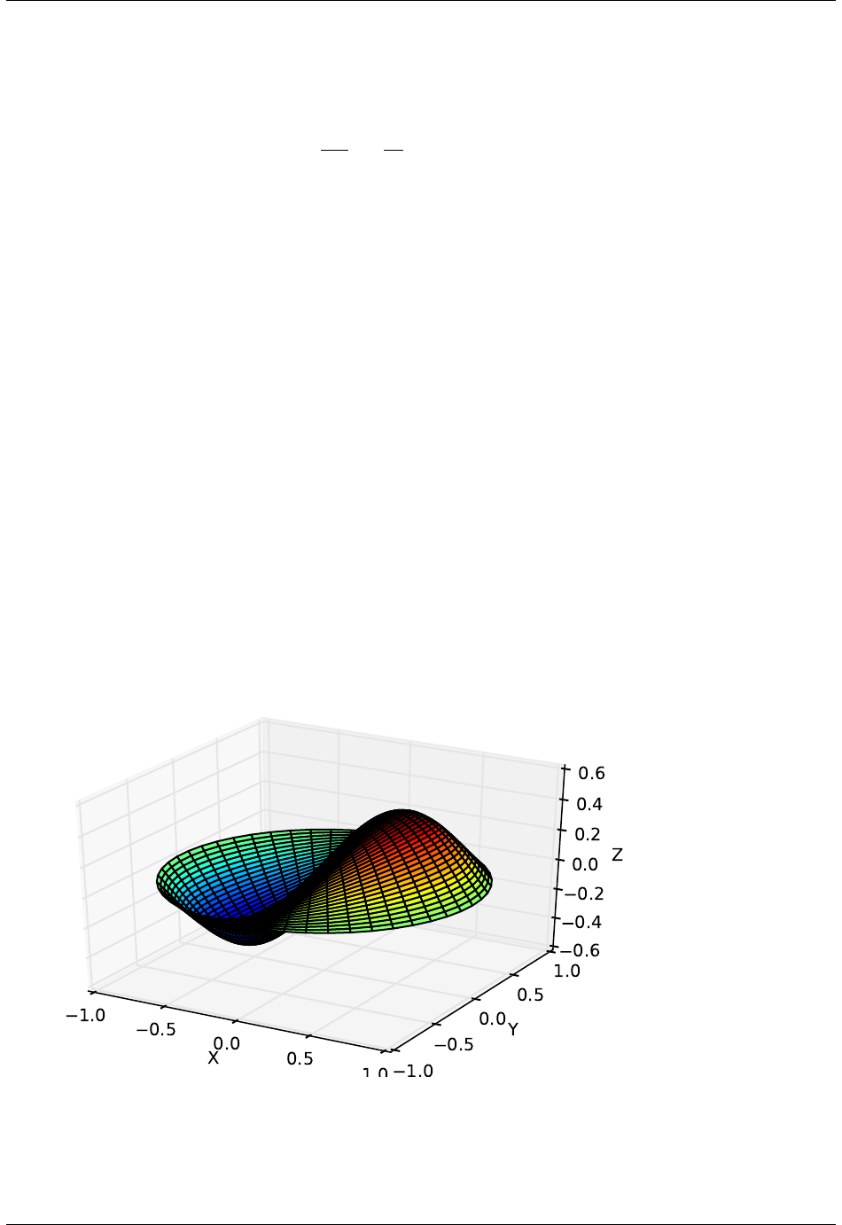
1.3.1 Bessel functions of real order(jn,jn_zeros)
Bessel functions are a family of solutions to Bessel’s differential equation with real or complex order alpha:
x2d2y
dx2+xdy
dx + (x2−α2)y= 0
Among other uses, these functions arise in wave propagation problems such as the vibrational modes of a thin drum
head. Here is an example of a circular drum head anchored at the edge:
>>> from scipy import *
>>> from scipy.special import jn, jn_zeros
>>> def drumhead_height(n, k, distance, angle, t):
... nth_zero =jn_zeros(n, k)
... return cos(t)*cos(n*angle)*jn(n, distance*nth_zero)
>>> theta =r_[0:2*pi:50j]
>>> radius =r_[0:1:50j]
>>> x=array([r*cos(theta) for rin radius])
>>> y=array([r*sin(theta) for rin radius])
>>> z=array([drumhead_height(1,1, r, theta, 0.5)for rin radius])
>>> import pylab
>>> from mpl_toolkits.mplot3d import Axes3D
>>> from matplotlib import cm
>>> fig =pylab.figure()
>>> ax =Axes3D(fig)
>>> ax.plot_surface(x, y, z, rstride=1, cstride=1, cmap=cm.jet)
>>> ax.set_xlabel(’X’)
>>> ax.set_ylabel(’Y’)
>>> ax.set_zlabel(’Z’)
>>> pylab.show()
10 Chapter 1. SciPy Tutorial

SciPy Reference Guide, Release 0.13.0
1.4 Integration (scipy.integrate)
The scipy.integrate sub-package provides several integration techniques including an ordinary differential
equation integrator. An overview of the module is provided by the help command:
>>> help(integrate)
Methods for Integrating Functions given function object.
quad -- General purpose integration.
dblquad -- General purpose double integration.
tplquad -- General purpose triple integration.
fixed_quad -- Integrate func(x) using Gaussian quadrature of order n.
quadrature -- Integrate with given tolerance using Gaussian quadrature.
romberg -- Integrate func using Romberg integration.
Methods for Integrating Functions given fixed samples.
trapz -- Use trapezoidal rule to compute integral from samples.
cumtrapz -- Use trapezoidal rule to cumulatively compute integral.
simps -- Use Simpson’s rule to compute integral from samples.
romb -- Use Romberg Integration to compute integral from
(2**k + 1) evenly-spaced samples.
See the special module’s orthogonal polynomials (special) for Gaussian
quadrature roots and weights for other weighting factors and regions.
Interface to numerical integrators of ODE systems.
odeint -- General integration of ordinary differential equations.
ode -- Integrate ODE using VODE and ZVODE routines.
1.4.1 General integration (quad)
The function quad is provided to integrate a function of one variable between two points. The points can be ±∞ (±
inf) to indicate infinite limits. For example, suppose you wish to integrate a bessel function jv(2.5,x) along the
interval [0,4.5].
I=Z4.5
0
J2.5(x)dx.
This could be computed using quad:
>>> result =integrate.quad(lambda x: special.jv(2.5,x), 0,4.5)
>>> print result
(1.1178179380783249, 7.8663172481899801e-09)
>>> I=sqrt(2/pi)*(18.0/27*sqrt(2)*cos(4.5)-4.0/27*sqrt(2)*sin(4.5)+
sqrt(2*pi)*special.fresnel(3/sqrt(pi))[0])
>>> print I
1.117817938088701
>>> print abs(result[0]-I)
1.03761443881e-11
The first argument to quad is a “callable” Python object (i.e a function, method, or class instance). Notice the use of a
lambda- function in this case as the argument. The next two arguments are the limits of integration. The return value
1.4. Integration (scipy.integrate) 11

SciPy Reference Guide, Release 0.13.0
is a tuple, with the first element holding the estimated value of the integral and the second element holding an upper
bound on the error. Notice, that in this case, the true value of this integral is
I=r2
π18
27√2 cos (4.5) −4
27√2 sin (4.5) + √2πSi 3
√π,
where
Si (x) = Zx
0
sin π
2t2dt.
is the Fresnel sine integral. Note that the numerically-computed integral is within 1.04 ×10⁻¹¹ of the exact result —
well below the reported error bound.
If the function to integrate takes additional parameters, the can be provided in the args argument. Suppose that the
following integral shall be calculated:
I(a, b) = Z1
0
ax2+b dx.
This integral can be evaluated by using the following code:
>>> from scipy.integrate import quad
>>> def integrand(x, a, b):
... return a*x+b
>>> a=2
>>> b=1
>>> I=quad(integrand, 0,1, args=(a,b))
>>> I=(2.0,2.220446049250313e-14)
Infinite inputs are also allowed in quad by using ±inf as one of the arguments. For example, suppose that a
numerical value for the exponential integral:
En(x) = Z∞
1
e−xt
tndt.
is desired (and the fact that this integral can be computed as special.expn(n,x) is forgotten). The functionality
of the function special.expn can be replicated by defining a new function vec_expint based on the routine
quad:
>>> from scipy.integrate import quad
>>> def integrand(t,n,x):
... return exp(-x*t) /t**n
>>> def expint(n,x):
... return quad(integrand, 1, Inf, args=(n, x))[0]
>>> vec_expint =vectorize(expint)
>>> vec_expint(3,arange(1.0,4.0,0.5))
array([ 0.1097, 0.0567, 0.0301, 0.0163, 0.0089, 0.0049])
>>> special.expn(3,arange(1.0,4.0,0.5))
array([ 0.1097, 0.0567, 0.0301, 0.0163, 0.0089, 0.0049])
The function which is integrated can even use the quad argument (though the error bound may underestimate the error
due to possible numerical error in the integrand from the use of quad ). The integral in this case is
In=Z∞
0Z∞
1
e−xt
tndt dx =1
n.
12 Chapter 1. SciPy Tutorial

SciPy Reference Guide, Release 0.13.0
>>> result =quad(lambda x: expint(3, x), 0, inf)
>>> print result
(0.33333333324560266, 2.8548934485373678e-09)
>>> I3 =1.0/3.0
>>> print I3
0.333333333333
>>> print I3 -result[0]
8.77306560731e-11
This last example shows that multiple integration can be handled using repeated calls to quad.
1.4.2 General multiple integration (dblquad,tplquad,nquad)
The mechanics for double and triple integration have been wrapped up into the functions dblquad and tplquad.
These functions take the function to integrate and four, or six arguments, respecively. The limits of all inner integrals
need to be defined as functions.
An example of using double integration to compute several values of Inis shown below:
>>> from scipy.integrate import quad, dblquad
>>> def I(n):
... return dblquad(lambda t, x: exp(-x*t)/t**n, 0, Inf, lambda x: 1,lambda x: Inf)
>>> print I(4)
(0.25000000000435768, 1.0518245707751597e-09)
>>> print I(3)
(0.33333333325010883, 2.8604069919261191e-09)
>>> print I(2)
(0.49999999999857514, 1.8855523253868967e-09)
As example for non-constant limits consider the integral
I=Z1/2
y=0 Z1−2y
x=0
xy dx dy =1
96.
This integral can be evaluated using the expression below (Note the use of the non-constant lambda functions for the
upper limit of the inner integral):
>>> from scipy.integrate import dblquad
>>> area =dblquad(lambda x, y: x*y, 0,0.5,lambda x: 0,lambda x: 1-2*x)
>>> area
(0.010416666666666668, 1.1564823173178715e-16)
For n-fold integration, scipy provides the function nquad. The integration bounds are an iterable object: either a
list of constant bounds, or a list of functions for the non-constant integration bounds. The order of integration (and
therefore the bounds) is from the innermost integral to the outermost one.
The integral from above
In=Z∞
0Z∞
1
e−xt
tndt dx =1
n
can be calculated as
1.4. Integration (scipy.integrate) 13

SciPy Reference Guide, Release 0.13.0
>>> from scipy import integrate
>>> N=5
>>> def f(t, x):
>>> return np.exp(-x*t) /t**N
>>> integrate.nquad(f, [[1, np.inf],[0, np.inf]])
(0.20000000000002294, 1.2239614263187945e-08)
Note that the order of arguments for fmust match the order of the integration bounds; i.e. the inner integral with
respect to tis on the interval [1,∞]and the outer integral with respect to xis on the interval [0,∞].
Non-constant integration bounds can be treated in a similar manner; the example from above
I=Z1/2
y=0 Z1−2y
x=0
xy dx dy =1
96.
can be evaluated by means of
>>> from scipy import integrate
>>> def f(x,y):
>>> return x*y
>>> def bounds_y():
>>> return [0,0.5]
>>> def bounds_x(y):
>>> return [0,1-2*y]
>>> integrate.nquad(f, [bounds_x, bounds_y])
(0.010416666666666668, 4.101620128472366e-16)
which is the same result as before.
1.4.3 Gaussian quadrature
A few functions are also provided in order to perform simple Gaussian quadrature over a fixed interval. The first
is fixed_quad which performs fixed-order Gaussian quadrature. The second function is quadrature which
performs Gaussian quadrature of multiple orders until the difference in the integral estimate is beneath some tolerance
supplied by the user. These functions both use the module special.orthogonal which can calculate the roots
and quadrature weights of a large variety of orthogonal polynomials (the polynomials themselves are available as
special functions returning instances of the polynomial class — e.g. special.legendre).
1.4.4 Romberg Integration
Romberg’s method [WPR] is another method for numerically evaluating an integral. See the help function for
romberg for further details.
1.4.5 Integrating using Samples
If the samples are equally-spaced and the number of samples available is 2k+ 1 for some integer k, then Romberg
romb integration can be used to obtain high-precision estimates of the integral using the available samples. Romberg
integration uses the trapezoid rule at step-sizes related by a power of two and then performs Richardson extrapolation
on these estimates to approximate the integral with a higher-degree of accuracy.
In case of arbitrary spaced samples, the two functions trapz (defined in numpy [NPT]) and simps are available.
They are using Newton-Coates formulas of order 1 and 2 respectively to perform integration. The trapezoidal rule
approximates the function as a straight line between adjacent points, while Simpson’s rule approximates the function
between three adjacent points as a parabola.
14 Chapter 1. SciPy Tutorial

SciPy Reference Guide, Release 0.13.0
For an odd number of samples that are equally spaced Simpson’s rule is exact if the function is a polynomial of order
3 or less. If the samples are not equally spaced, then the result is exact only if the function is a polynomial of order 2
or less.
>>> from scipy.integrate import simps
>>> import numpy as np
>>> def f(x):
... return x**2
>>> def f2(x):
... return x**3
>>> x=np.array([1,3,4])
>>> y1 =f1(x)
>>> I1 =integrate.simps(y1,x)
>>> print(I1)
21.0
This corresponds exactly to
Z4
1
x2dx = 21,
whereas integrating the second function
>>> y2 =f2(x)
>>> I2 =integrate.simps(y2,x)
>>> print(I2)
61.5
does not correspond to
Z4
1
x3dx = 63.75
because the order of the polynomial in f2 is larger than two.
1.4.6 Ordinary differential equations (odeint)
Integrating a set of ordinary differential equations (ODEs) given initial conditions is another useful example. The
function odeint is available in SciPy for integrating a first-order vector differential equation:
dy
dt =f(y, t),
given initial conditions y(0) = y0, where yis a length Nvector and fis a mapping from RNto RN.A higher-order
ordinary differential equation can always be reduced to a differential equation of this type by introducing intermediate
derivatives into the yvector.
For example suppose it is desired to find the solution to the following second-order differential equation:
d2w
dz2−zw(z) = 0
with initial conditions w(0) = 1
3
√32Γ(2
3)and dw
dz z=0 =−1
3
√3Γ(1
3).It is known that the solution to this differential
equation with these boundary conditions is the Airy function
w=Ai (z),
which gives a means to check the integrator using special.airy.
1.4. Integration (scipy.integrate) 15

SciPy Reference Guide, Release 0.13.0
First, convert this ODE into standard form by setting y=dw
dz , wand t=z. Thus, the differential equation becomes
dy
dt =ty1
y0=0t
1 0 y0
y1=0t
1 0 y.
In other words,
f(y, t) = A(t)y.
As an interesting reminder, if A(t)commutes with Rt
0A(τ)dτ under matrix multiplication, then this linear differen-
tial equation has an exact solution using the matrix exponential:
y(t) = exp Zt
0
A(τ)dτy(0) ,
However, in this case, A(t)and its integral do not commute.
There are many optional inputs and outputs available when using odeint which can help tune the solver. These ad-
ditional inputs and outputs are not needed much of the time, however, and the three required input arguments and
the output solution suffice. The required inputs are the function defining the derivative, fprime, the initial conditions
vector, y0, and the time points to obtain a solution, t, (with the initial value point as the first element of this sequence).
The output to odeint is a matrix where each row contains the solution vector at each requested time point (thus, the
initial conditions are given in the first output row).
The following example illustrates the use of odeint including the usage of the Dfun option which allows the user to
specify a gradient (with respect to y) of the function, f(y, t).
>>> from scipy.integrate import odeint
>>> from scipy.special import gamma, airy
>>> y1_0 =1.0/3**(2.0/3.0)/gamma(2.0/3.0)
>>> y0_0 = -1.0/3**(1.0/3.0)/gamma(1.0/3.0)
>>> y0 =[y0_0, y1_0]
>>> def func(y, t):
... return [t*y[1],y[0]]
>>> def gradient(y,t):
... return [[0,t],[1,0]]
>>> x=arange(0,4.0,0.01)
>>> t=x
>>> ychk =airy(x)[0]
>>> y=odeint(func, y0, t)
>>> y2 =odeint(func, y0, t, Dfun=gradient)
>>> print ychk[:36:6]
[ 0.355028 0.339511 0.324068 0.308763 0.293658 0.278806]
>>> print y[:36:6,1]
[ 0.355028 0.339511 0.324067 0.308763 0.293658 0.278806]
>>> print y2[:36:6,1]
[ 0.355028 0.339511 0.324067 0.308763 0.293658 0.278806]
References
1.5 Optimization (scipy.optimize)
The scipy.optimize package provides several commonly used optimization algorithms. A detailed listing is
available: scipy.optimize (can also be found by help(scipy.optimize)).
16 Chapter 1. SciPy Tutorial

SciPy Reference Guide, Release 0.13.0
The module contains:
1. Unconstrained and constrained minimization of multivariate scalar functions (minimize) using a variety of
algorithms (e.g. BFGS, Nelder-Mead simplex, Newton Conjugate Gradient, COBYLA or SLSQP)
2. Global (brute-force) optimization routines (e.g., anneal,basinhopping)
3. Least-squares minimization (leastsq) and curve fitting (curve_fit) algorithms
4. Scalar univariate functions minimizers (minimize_scalar) and root finders (newton)
5. Multivariate equation system solvers (root) using a variety of algorithms (e.g. hybrid Powell, Levenberg-
Marquardt or large-scale methods such as Newton-Krylov).
Below, several examples demonstrate their basic usage.
1.5.1 Unconstrained minimization of multivariate scalar functions (minimize)
The minimize function provides a common interface to unconstrained and constrained minimization algorithms for
multivariate scalar functions in scipy.optimize. To demonstrate the minimization function consider the problem
of minimizing the Rosenbrock function of Nvariables:
f(x) =
N−1
X
i=1
100 xi−x2
i−12+ (1 −xi−1)2.
The minimum value of this function is 0 which is achieved when xi= 1.
Note that the Rosenbrock function and its derivatives are included in scipy.optimize. The implementations
shown in the following sections provide examples of how to define an objective function as well as its jacobian and
hessian functions.
Nelder-Mead Simplex algorithm (method=’Nelder-Mead’)
In the example below, the minimize routine is used with the Nelder-Mead simplex algorithm (selected through the
method parameter):
>>> import numpy as np
>>> from scipy.optimize import minimize
>>> def rosen(x):
... """The Rosenbrock function"""
... return sum(100.0*(x[1:]-x[:-1]**2.0)**2.0 +(1-x[:-1])**2.0)
>>> x0 =np.array([1.3,0.7,0.8,1.9,1.2])
>>> res =minimize(rosen, x0, method=’nelder-mead’,
... options={’xtol’:1e-8,’disp’:True})
Optimization terminated successfully.
Current function value: 0.000000
Iterations: 339
Function evaluations: 571
>>> print(res.x)
[ 1. 1. 1. 1. 1.]
The simplex algorithm is probably the simplest way to minimize a fairly well-behaved function. It requires only
function evaluations and is a good choice for simple minimization problems. However, because it does not use any
gradient evaluations, it may take longer to find the minimum.
1.5. Optimization (scipy.optimize) 17

SciPy Reference Guide, Release 0.13.0
Another optimization algorithm that needs only function calls to find the minimum is Powell‘s method available by
setting method=’powell’ in minimize.
Broyden-Fletcher-Goldfarb-Shanno algorithm (method=’BFGS’)
In order to converge more quickly to the solution, this routine uses the gradient of the objective function. If the gradient
is not given by the user, then it is estimated using first-differences. The Broyden-Fletcher-Goldfarb-Shanno (BFGS)
method typically requires fewer function calls than the simplex algorithm even when the gradient must be estimated.
To demonstrate this algorithm, the Rosenbrock function is again used. The gradient of the Rosenbrock function is the
vector:
∂f
∂xj
=
N
X
i=1
200 xi−x2
i−1(δi,j −2xi−1δi−1,j )−2 (1 −xi−1)δi−1,j .
= 200 xj−x2
j−1−400xjxj+1 −x2
j−2 (1 −xj).
This expression is valid for the interior derivatives. Special cases are
∂f
∂x0
=−400x0x1−x2
0−2 (1 −x0),
∂f
∂xN−1
= 200 xN−1−x2
N−2.
A Python function which computes this gradient is constructed by the code-segment:
>>> def rosen_der(x):
... xm =x[1:-1]
... xm_m1 =x[:-2]
... xm_p1 =x[2:]
... der =np.zeros_like(x)
... der[1:-1]=200*(xm-xm_m1**2)-400*(xm_p1 -xm**2)*xm -2*(1-xm)
... der[0]= -400*x[0]*(x[1]-x[0]**2)-2*(1-x[0])
... der[-1]=200*(x[-1]-x[-2]**2)
... return der
This gradient information is specified in the minimize function through the jac parameter as illustrated below.
>>> res =minimize(rosen, x0, method=’BFGS’, jac=rosen_der,
... options={’disp’:True})
Optimization terminated successfully.
Current function value: 0.000000
Iterations: 51
Function evaluations: 63
Gradient evaluations: 63
>>> print(res.x)
[ 1. 1. 1. 1. 1.]
Newton-Conjugate-Gradient algorithm (method=’Newton-CG’)
The method which requires the fewest function calls and is therefore often the fastest method to minimize functions
of many variables uses the Newton-Conjugate Gradient algorithm. This method is a modified Newton’s method and
uses a conjugate gradient algorithm to (approximately) invert the local Hessian. Newton’s method is based on fitting
the function locally to a quadratic form:
f(x)≈f(x0) + ∇f(x0)·(x−x0) + 1
2(x−x0)TH(x0) (x−x0).
18 Chapter 1. SciPy Tutorial

SciPy Reference Guide, Release 0.13.0
where H(x0)is a matrix of second-derivatives (the Hessian). If the Hessian is positive definite then the local minimum
of this function can be found by setting the gradient of the quadratic form to zero, resulting in
xopt =x0−H−1∇f.
The inverse of the Hessian is evaluated using the conjugate-gradient method. An example of employing this method
to minimizing the Rosenbrock function is given below. To take full advantage of the Newton-CG method, a function
which computes the Hessian must be provided. The Hessian matrix itself does not need to be constructed, only a
vector which is the product of the Hessian with an arbitrary vector needs to be available to the minimization routine.
As a result, the user can provide either a function to compute the Hessian matrix, or a function to compute the product
of the Hessian with an arbitrary vector.
Full Hessian example:
The Hessian of the Rosenbrock function is
Hij =∂2f
∂xi∂xj
= 200 (δi,j −2xi−1δi−1,j )−400xi(δi+1,j −2xiδi,j )−400δi,j xi+1 −x2
i+ 2δi,j ,
=202 + 1200x2
i−400xi+1δi,j −400xiδi+1,j −400xi−1δi−1,j ,
if i, j ∈[1, N −2] with i, j ∈[0, N −1] defining the N×Nmatrix. Other non-zero entries of the matrix are
∂2f
∂x2
0
= 1200x2
0−400x1+ 2,
∂2f
∂x0∂x1
=∂2f
∂x1∂x0
=−400x0,
∂2f
∂xN−1∂xN−2
=∂2f
∂xN−2∂xN−1
=−400xN−2,
∂2f
∂x2
N−1
= 200.
For example, the Hessian when N= 5 is
H=
1200x2
0−400x1+ 2 −400x00 0 0
−400x0202 + 1200x2
1−400x2−400x10 0
0−400x1202 + 1200x2
2−400x3−400x20
0−400x2202 + 1200x2
3−400x4−400x3
0 0 0 −400x3200
.
The code which computes this Hessian along with the code to minimize the function using Newton-CG method is
shown in the following example:
>>> def rosen_hess(x):
... x=np.asarray(x)
... H=np.diag(-400*x[:-1],1)-np.diag(400*x[:-1],-1)
... diagonal =np.zeros_like(x)
... diagonal[0]=1200*x[0]**2-400*x[1]+2
... diagonal[-1]=200
... diagonal[1:-1]=202 +1200*x[1:-1]**2-400*x[2:]
... H=H+np.diag(diagonal)
... return H
>>> res =minimize(rosen, x0, method=’Newton-CG’,
... jac=rosen_der, hess=rosen_hess,
... options={’avextol’:1e-8,’disp’:True})
Optimization terminated successfully.
Current function value: 0.000000
1.5. Optimization (scipy.optimize) 19

SciPy Reference Guide, Release 0.13.0
Iterations: 19
Function evaluations: 22
Gradient evaluations: 19
Hessian evaluations: 19
>>> print(res.x)
[ 1. 1. 1. 1. 1.]
Hessian product example:
For larger minimization problems, storing the entire Hessian matrix can consume considerable time and memory. The
Newton-CG algorithm only needs the product of the Hessian times an arbitrary vector. As a result, the user can supply
code to compute this product rather than the full Hessian by giving a hess function which take the minimization
vector as the first argument and the arbitrary vector as the second argument (along with extra arguments passed to the
function to be minimized). If possible, using Newton-CG with the Hessian product option is probably the fastest way
to minimize the function.
In this case, the product of the Rosenbrock Hessian with an arbitrary vector is not difficult to compute. If pis the
arbitrary vector, then H(x)phas elements:
H(x)p=
1200x2
0−400x1+ 2p0−400x0p1
.
.
.
−400xi−1pi−1+202 + 1200x2
i−400xi+1pi−400xipi+1
.
.
.
−400xN−2pN−2+ 200pN−1
.
Code which makes use of this Hessian product to minimize the Rosenbrock function using minimize follows:
>>> def rosen_hess_p(x,p):
... x=np.asarray(x)
... Hp =np.zeros_like(x)
... Hp[0]=(1200*x[0]**2-400*x[1]+2)*p[0]-400*x[0]*p[1]
... Hp[1:-1]= -400*x[:-2]*p[:-2]+(202+1200*x[1:-1]**2-400*x[2:])*p[1:-1] \
... -400*x[1:-1]*p[2:]
... Hp[-1]= -400*x[-2]*p[-2]+200*p[-1]
... return Hp
>>> res =minimize(rosen, x0, method=’Newton-CG’,
... jac=rosen_der, hess=rosen_hess_p,
... options={’avextol’:1e-8,’disp’:True})
Optimization terminated successfully.
Current function value: 0.000000
Iterations: 20
Function evaluations: 23
Gradient evaluations: 20
Hessian evaluations: 44
>>> print(res.x)
[ 1. 1. 1. 1. 1.]
1.5.2 Constrained minimization of multivariate scalar functions (minimize)
The minimize function also provides an interface to several constrained minimization algorithm. As an example,
the Sequential Least SQuares Programming optimization algorithm (SLSQP) will be considered here. This algorithm
20 Chapter 1. SciPy Tutorial

SciPy Reference Guide, Release 0.13.0
allows to deal with constrained minimization problems of the form:
min F(x)
subject to Cj(X) = 0, j = 1, ..., MEQ
Cj(x)≥0, j =MEQ + 1, ..., M
XL ≤x≤XU, I = 1, ..., N.
As an example, let us consider the problem of maximizing the function:
f(x, y)=2xy + 2x−x2−2y2
subject to an equality and an inequality constraints defined as:
x3−y= 0
y−1≥0
The objective function and its derivative are defined as follows.
>>> def func(x, sign=1.0):
... """ Objective function """
... return sign*(2*x[0]*x[1]+2*x[0]-x[0]**2-2*x[1]**2)
>>> def func_deriv(x, sign=1.0):
... """ Derivative of objective function """
... dfdx0 =sign*(-2*x[0]+2*x[1]+2)
... dfdx1 =sign*(2*x[0]-4*x[1])
... return np.array([ dfdx0, dfdx1 ])
Note that since minimize only minimizes functions, the sign parameter is introduced to multiply the objective
function (and its derivative by -1) in order to perform a maximization.
Then constraints are defined as a sequence of dictionaries, with keys type,fun and jac.
>>> cons =({’type’:’eq’,
... ’fun’ :lambda x: np.array([x[0]**3-x[1]]),
... ’jac’ :lambda x: np.array([3.0*(x[0]**2.0), -1.0])},
... {’type’:’ineq’,
... ’fun’ :lambda x: np.array([x[1]-1]),
... ’jac’ :lambda x: np.array([0.0,1.0])})
Now an unconstrained optimization can be performed as:
>>> res =minimize(func, [-1.0,1.0], args=(-1.0,), jac=func_deriv,
... method=’SLSQP’, options={’disp’:True})
Optimization terminated successfully. (Exit mode 0)
Current function value: -2.0
Iterations: 4
Function evaluations: 5
Gradient evaluations: 4
>>> print(res.x)
[ 2. 1.]
and a constrained optimization as:
>>> res =minimize(func, [-1.0,1.0], args=(-1.0,), jac=func_deriv,
... constraints=cons, method=’SLSQP’, options={’disp’:True})
Optimization terminated successfully. (Exit mode 0)
Current function value: -1.00000018311
Iterations: 9
1.5. Optimization (scipy.optimize) 21

SciPy Reference Guide, Release 0.13.0
Function evaluations: 14
Gradient evaluations: 9
>>> print(res.x)
[ 1.00000009 1. ]
1.5.3 Least-square fitting (leastsq)
All of the previously-explained minimization procedures can be used to solve a least-squares problem provided the
appropriate objective function is constructed. For example, suppose it is desired to fit a set of data {xi,yi}to a known
model, y=f(x,p)where pis a vector of parameters for the model that need to be found. A common method for
determining which parameter vector gives the best fit to the data is to minimize the sum of squares of the residuals.
The residual is usually defined for each observed data-point as
ei(p,yi,xi) = kyi−f(xi,p)k.
An objective function to pass to any of the previous minization algorithms to obtain a least-squares fit is.
J(p) =
N−1
X
i=0
e2
i(p).
The leastsq algorithm performs this squaring and summing of the residuals automatically. It takes as an input
argument the vector function e(p)and returns the value of pwhich minimizes J(p) = eTedirectly. The user is also
encouraged to provide the Jacobian matrix of the function (with derivatives down the columns or across the rows). If
the Jacobian is not provided, it is estimated.
An example should clarify the usage. Suppose it is believed some measured data follow a sinusoidal pattern
yi=Asin (2πkxi+θ)
where the parameters A, k , and θare unknown. The residual vector is
ei=|yi−Asin (2πkxi+θ)|.
By defining a function to compute the residuals and (selecting an appropriate starting position), the least-squares fit
routine can be used to find the best-fit parameters ˆ
A, ˆ
k, ˆ
θ. This is shown in the following example:
>>> from numpy import *
>>> x=arange(0,6e-2,6e-2/30)
>>> A,k,theta =10,1.0/3e-2, pi/6
>>> y_true =A*sin(2*pi*k*x+theta)
>>> y_meas =y_true +2*random.randn(len(x))
>>> def residuals(p, y, x):
... A,k,theta =p
... err =y-A*sin(2*pi*k*x+theta)
... return err
>>> def peval(x, p):
... return p[0]*sin(2*pi*p[1]*x+p[2])
>>> p0 =[8,1/2.3e-2, pi/3]
>>> print(array(p0))
[ 8. 43.4783 1.0472]
>>> from scipy.optimize import leastsq
>>> plsq =leastsq(residuals, p0, args=(y_meas, x))
>>> print(plsq[0])
[ 10.9437 33.3605 0.5834]
22 Chapter 1. SciPy Tutorial
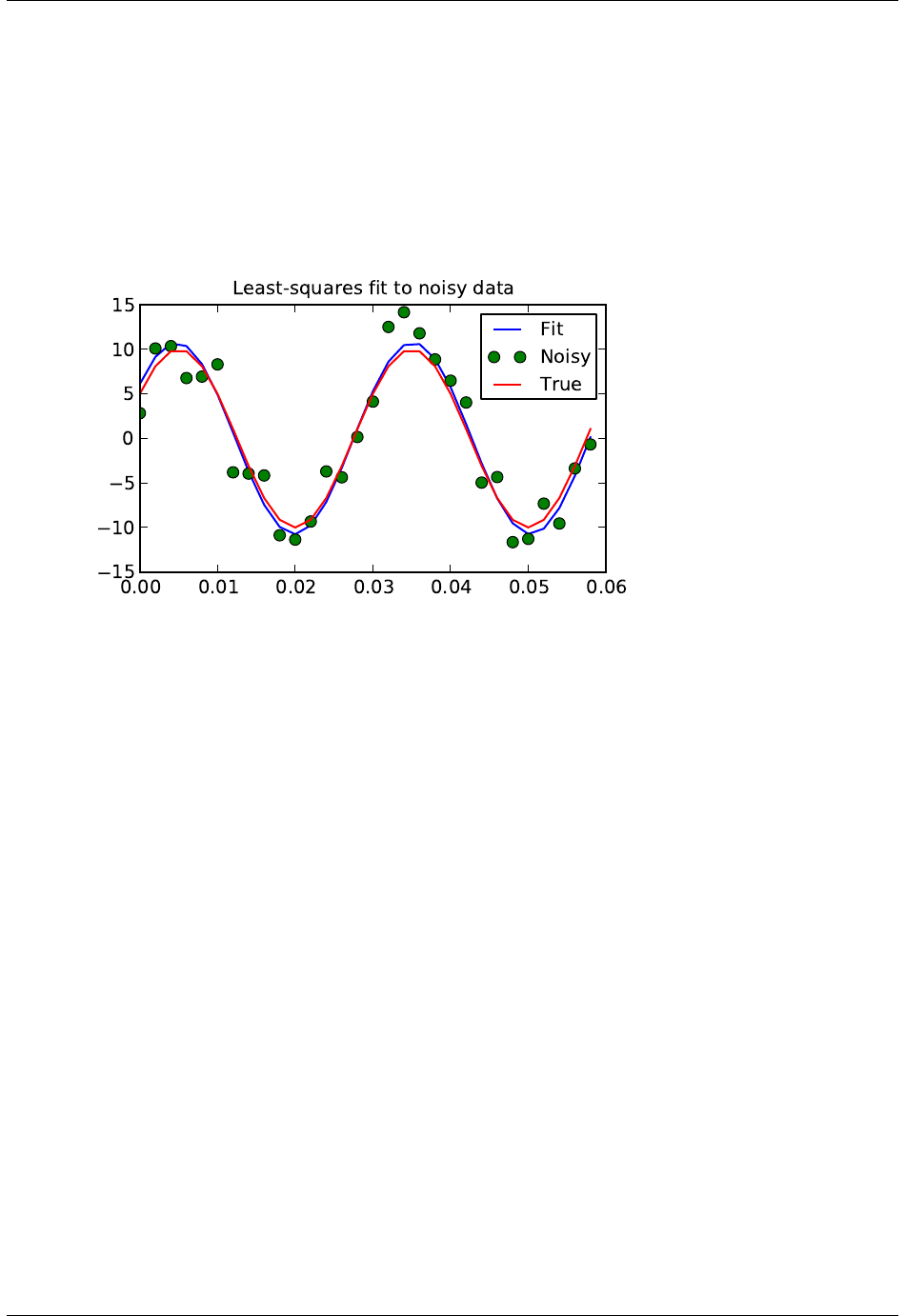
SciPy Reference Guide, Release 0.13.0
>>> print(array([A, k, theta]))
[ 10. 33.3333 0.5236]
>>> import matplotlib.pyplot as plt
>>> plt.plot(x,peval(x,plsq[0]),x,y_meas,’o’,x,y_true)
>>> plt.title(’Least-squares fit to noisy data’)
>>> plt.legend([’Fit’,’Noisy’,’True’])
>>> plt.show()
1.5.4 Univariate function minimizers (minimize_scalar)
Often only the minimum of an univariate function (i.e. a function that takes a scalar as input) is needed. In these
circumstances, other optimization techniques have been developed that can work faster. These are accessible from the
minimize_scalar function which proposes several algorithms.
Unconstrained minimization (method=’brent’)
There are actually two methods that can be used to minimize an univariate function: brent and golden, but
golden is included only for academic purposes and should rarely be used. These can be respectively selected through
the method parameter in minimize_scalar. The brent method uses Brent’s algorithm for locating a minimum.
Optimally a bracket (the bs parameter) should be given which contains the minimum desired. A bracket is a triple
(a, b, c)such that f(a)> f (b)< f (c)and a<b<c. If this is not given, then alternatively two starting points can
be chosen and a bracket will be found from these points using a simple marching algorithm. If these two starting points
are not provided 0and 1will be used (this may not be the right choice for your function and result in an unexpected
minimum being returned).
Here is an example:
>>> from scipy.optimize import minimize_scalar
>>> f=lambda x: (x -2)*(x +1)**2
>>> res =minimize_scalar(f, method=’brent’)
>>> print(res.x)
1.0
1.5. Optimization (scipy.optimize) 23

SciPy Reference Guide, Release 0.13.0
Bounded minimization (method=’bounded’)
Very often, there are constraints that can be placed on the solution space before minimization occurs. The bounded
method in minimize_scalar is an example of a constrained minimization procedure that provides a rudimentary
interval constraint for scalar functions. The interval constraint allows the minimization to occur only between two
fixed endpoints, specified using the mandatory bs parameter.
For example, to find the minimum of J1(x)near x= 5 ,minimize_scalar can be called using the interval [4,7]
as a constraint. The result is xmin = 5.3314 :
>>> from scipy.special import j1
>>> res =minimize_scalar(j1, bs=(4,7), method=’bounded’)
>>> print(res.x)
5.33144184241
1.5.5 Root finding
Scalar functions
If one has a single-variable equation, there are four different root finding algorithms that can be tried. Each of these
algorithms requires the endpoints of an interval in which a root is expected (because the function changes signs). In
general brentq is the best choice, but the other methods may be useful in certain circumstances or for academic
purposes.
Fixed-point solving
A problem closely related to finding the zeros of a function is the problem of finding a fixed-point of a function. A
fixed point of a function is the point at which evaluation of the function returns the point: g(x) = x. Clearly the fixed
point of gis the root of f(x) = g(x)−x. Equivalently, the root of fis the fixed_point of g(x) = f(x) + x. The
routine fixed_point provides a simple iterative method using Aitkens sequence acceleration to estimate the fixed
point of ggiven a starting point.
Sets of equations
Finding a root of a set of non-linear equations can be achieve using the root function. Several methods are available,
amongst which hybr (the default) and lm which respectively use the hybrid method of Powell and the Levenberg-
Marquardt method from MINPACK.
The following example considers the single-variable transcendental equation
x+ 2 cos (x) = 0,
a root of which can be found as follows:
>>> import numpy as np
>>> from scipy.optimize import root
>>> def func(x):
... return x+2*np.cos(x)
>>> sol =root(func, 0.3)
>>> sol.x
array([-1.02986653])
>>> sol.fun
array([ -6.66133815e-16])
24 Chapter 1. SciPy Tutorial

SciPy Reference Guide, Release 0.13.0
Consider now a set of non-linear equations
x0cos (x1)=4,
x0x1−x1= 5.
We define the objective function so that it also returns the Jacobian and indicate this by setting the jac parameter to
True. Also, the Levenberg-Marquardt solver is used here.
>>> def func2(x):
... f=[x[0]*np.cos(x[1]) -4,
... x[1]*x[0]-x[1]-5]
... df =np.array([[np.cos(x[1]), -x[0]*np.sin(x[1])],
... [x[1], x[0]-1]])
... return f, df
>>> sol =root(func2, [1,1], jac=True, method=’lm’)
>>> sol.x
array([ 6.50409711, 0.90841421])
Root finding for large problems
Methods hybr and lm in root cannot deal with a very large number of variables (N), as they need to calculate and
invert a dense NxNJacobian matrix on every Newton step. This becomes rather inefficient when Ngrows.
Consider for instance the following problem: we need to solve the following integrodifferential equation on the square
[0,1] ×[0,1]:
(∂2
x+∂2
y)P+ 5 Z1
0Z1
0
cosh(P)dx dy2
= 0
with the boundary condition P(x, 1) = 1 on the upper edge and P= 0 elsewhere on the boundary of the square. This
can be done by approximating the continuous function Pby its values on a grid, Pn,m ≈P(nh, mh), with a small
grid spacing h. The derivatives and integrals can then be approximated; for instance ∂2
xP(x, y)≈(P(x+h, y)−
2P(x, y) + P(x−h, y))/h2. The problem is then equivalent to finding the root of some function residual(P),
where Pis a vector of length NxNy.
Now, because NxNycan be large, methods hybr or lm in root will take a long time to solve this problem. The
solution can however be found using one of the large-scale solvers, for example krylov,broyden2, or anderson.
These use what is known as the inexact Newton method, which instead of computing the Jacobian matrix exactly, forms
an approximation for it.
The problem we have can now be solved as follows:
import numpy as np
from scipy.optimize import root
from numpy import cosh, zeros_like, mgrid, zeros
# parameters
nx, ny =75,75
hx, hy =1./(nx-1), 1./(ny-1)
P_left, P_right =0,0
P_top, P_bottom =1,0
def residual(P):
d2x =zeros_like(P)
d2y =zeros_like(P)
1.5. Optimization (scipy.optimize) 25
SciPy Reference Guide, Release 0.13.0
d2x[1:-1]=(P[2:] -2*P[1:-1]+P[:-2]) /hx/hx
d2x[0]=(P[1]-2*P[0]+P_left)/hx/hx
d2x[-1]=(P_right -2*P[-1]+P[-2])/hx/hx
d2y[:,1:-1]=(P[:,2:] -2*P[:,1:-1]+P[:,:-2])/hy/hy
d2y[:,0]=(P[:,1]-2*P[:,0]+P_bottom)/hy/hy
d2y[:,-1]=(P_top -2*P[:,-1]+P[:,-2])/hy/hy
return d2x +d2y +5*cosh(P).mean()**2
# solve
guess =zeros((nx, ny), float)
sol =root(residual, guess, method=’krylov’, options={’disp’:True})
#sol = root(residual, guess, method=’broyden2’, options={’disp’: True, ’max_rank’: 50})
#sol = root(residual, guess, method=’anderson’, options={’disp’: True, ’M’: 10})
print(’Residual: %g’%abs(residual(sol.x)).max())
# visualize
import matplotlib.pyplot as plt
x,y=mgrid[0:1:(nx*1j), 0:1:(ny*1j)]
plt.pcolor(x, y, sol.x)
plt.colorbar()
plt.show()
Still too slow? Preconditioning.
When looking for the zero of the functions fi(x)=0,i = 1, 2, ..., N, the krylov solver spends most of its time
inverting the Jacobian matrix,
Jij =∂fi
∂xj
.
If you have an approximation for the inverse matrix M≈J−1, you can use it for preconditioning the linear inversion
problem. The idea is that instead of solving Js=yone solves MJs=My: since matrix MJ is “closer” to the
identity matrix than Jis, the equation should be easier for the Krylov method to deal with.
26 Chapter 1. SciPy Tutorial

SciPy Reference Guide, Release 0.13.0
The matrix Mcan be passed to root with method krylov as an op-
tion options[’jac_options’][’inner_M’]. It can be a (sparse) matrix or a
scipy.sparse.linalg.LinearOperator instance.
For the problem in the previous section, we note that the function to solve consists of two parts: the first one is
application of the Laplace operator, [∂2
x+∂2
y]P, and the second is the integral. We can actually easily compute the
Jacobian corresponding to the Laplace operator part: we know that in one dimension
∂2
x≈1
h2
x
−2 1 0 0 ···
1−210···
0 1 −2 1 ···
. . .
=h−2
xL
so that the whole 2-D operator is represented by
J1=∂2
x+∂2
y'h−2
xL⊗I+h−2
yI⊗L
The matrix J2of the Jacobian corresponding to the integral is more difficult to calculate, and since all of it entries
are nonzero, it will be difficult to invert. J1on the other hand is a relatively simple matrix, and can be inverted by
scipy.sparse.linalg.splu (or the inverse can be approximated by scipy.sparse.linalg.spilu).
So we are content to take M≈J−1
1and hope for the best.
In the example below, we use the preconditioner M=J−1
1.
import numpy as np
from scipy.optimize import root
from scipy.sparse import spdiags, kron
from scipy.sparse.linalg import spilu, LinearOperator
from numpy import cosh, zeros_like, mgrid, zeros, eye
# parameters
nx, ny =75,75
hx, hy =1./(nx-1), 1./(ny-1)
P_left, P_right =0,0
P_top, P_bottom =1,0
def get_preconditioner():
"""Compute the preconditioner M"""
diags_x =zeros((3, nx))
diags_x[0,:] =1/hx/hx
diags_x[1,:] = -2/hx/hx
diags_x[2,:] =1/hx/hx
Lx =spdiags(diags_x, [-1,0,1], nx, nx)
diags_y =zeros((3, ny))
diags_y[0,:] =1/hy/hy
diags_y[1,:] = -2/hy/hy
diags_y[2,:] =1/hy/hy
Ly =spdiags(diags_y, [-1,0,1], ny, ny)
J1 =kron(Lx, eye(ny)) +kron(eye(nx), Ly)
# Now we have the matrix ‘J_1‘. We need to find its inverse ‘M‘ --
# however, since an approximate inverse is enough, we can use
# the *incomplete LU*decomposition
J1_ilu =spilu(J1)
1.5. Optimization (scipy.optimize) 27

SciPy Reference Guide, Release 0.13.0
# This returns an object with a method .solve() that evaluates
# the corresponding matrix-vector product. We need to wrap it into
# a LinearOperator before it can be passed to the Krylov methods:
M=LinearOperator(shape=(nx*ny, nx*ny), matvec=J1_ilu.solve)
return M
def solve(preconditioning=True):
"""Compute the solution"""
count =[0]
def residual(P):
count[0]+= 1
d2x =zeros_like(P)
d2y =zeros_like(P)
d2x[1:-1]=(P[2:] -2*P[1:-1]+P[:-2])/hx/hx
d2x[0]=(P[1]-2*P[0]+P_left)/hx/hx
d2x[-1]=(P_right -2*P[-1]+P[-2])/hx/hx
d2y[:,1:-1]=(P[:,2:] -2*P[:,1:-1]+P[:,:-2])/hy/hy
d2y[:,0]=(P[:,1]-2*P[:,0]+P_bottom)/hy/hy
d2y[:,-1]=(P_top -2*P[:,-1]+P[:,-2])/hy/hy
return d2x +d2y +5*cosh(P).mean()**2
# preconditioner
if preconditioning:
M=get_preconditioner()
else:
M=None
# solve
guess =zeros((nx, ny), float)
sol =root(residual, guess, method=’krylov’,
options={’disp’:True,
’jac_options’: {’inner_M’: M}})
print ’Residual’,abs(residual(sol.x)).max()
print ’Evaluations’, count[0]
return sol.x
def main():
sol =solve(preconditioning=True)
# visualize
import matplotlib.pyplot as plt
x,y=mgrid[0:1:(nx*1j), 0:1:(ny*1j)]
plt.clf()
plt.pcolor(x, y, sol)
plt.clim(0,1)
plt.colorbar()
plt.show()
if __name__ == "__main__":
main()
28 Chapter 1. SciPy Tutorial

SciPy Reference Guide, Release 0.13.0
Resulting run, first without preconditioning:
0: |F(x)| = 803.614; step 1; tol 0.000257947
1: |F(x)| = 345.912; step 1; tol 0.166755
2: |F(x)| = 139.159; step 1; tol 0.145657
3: |F(x)| = 27.3682; step 1; tol 0.0348109
4: |F(x)| = 1.03303; step 1; tol 0.00128227
5: |F(x)| = 0.0406634; step 1; tol 0.00139451
6: |F(x)| = 0.00344341; step 1; tol 0.00645373
7: |F(x)| = 0.000153671; step 1; tol 0.00179246
8: |F(x)| = 6.7424e-06; step 1; tol 0.00173256
Residual 3.57078908664e-07
Evaluations 317
and then with preconditioning:
0: |F(x)| = 136.993; step 1; tol 7.49599e-06
1: |F(x)| = 4.80983; step 1; tol 0.00110945
2: |F(x)| = 0.195942; step 1; tol 0.00149362
3: |F(x)| = 0.000563597; step 1; tol 7.44604e-06
4: |F(x)| = 1.00698e-09; step 1; tol 2.87308e-12
Residual 9.29603061195e-11
Evaluations 77
Using a preconditioner reduced the number of evaluations of the residual function by a factor of 4. For problems
where the residual is expensive to compute, good preconditioning can be crucial — it can even decide whether the
problem is solvable in practice or not.
Preconditioning is an art, science, and industry. Here, we were lucky in making a simple choice that worked reasonably
well, but there is a lot more depth to this topic than is shown here.
References
Some further reading and related software:
1.6 Interpolation (scipy.interpolate)
Contents
•Interpolation (scipy.interpolate)
–1-D interpolation (interp1d)
–Multivariate data interpolation (griddata)
–Spline interpolation
*Spline interpolation in 1-d: Procedural (interpolate.splXXX)
*Spline interpolation in 1-d: Object-oriented (UnivariateSpline)
*Two-dimensional spline representation: Procedural (bisplrep)
*Two-dimensional spline representation: Object-oriented (BivariateSpline)
–Using radial basis functions for smoothing/interpolation
*1-d Example
*2-d Example
There are several general interpolation facilities available in SciPy, for data in 1, 2, and higher dimensions:
• A class representing an interpolant (interp1d) in 1-D, offering several interpolation methods.
1.6. Interpolation (scipy.interpolate) 29
SciPy Reference Guide, Release 0.13.0
• Convenience function griddata offering a simple interface to interpolation in N dimensions (N = 1, 2, 3, 4,
...). Object-oriented interface for the underlying routines is also available.
• Functions for 1- and 2-dimensional (smoothed) cubic-spline interpolation, based on the FORTRAN library
FITPACK. There are both procedural and object-oriented interfaces for the FITPACK library.
• Interpolation using Radial Basis Functions.
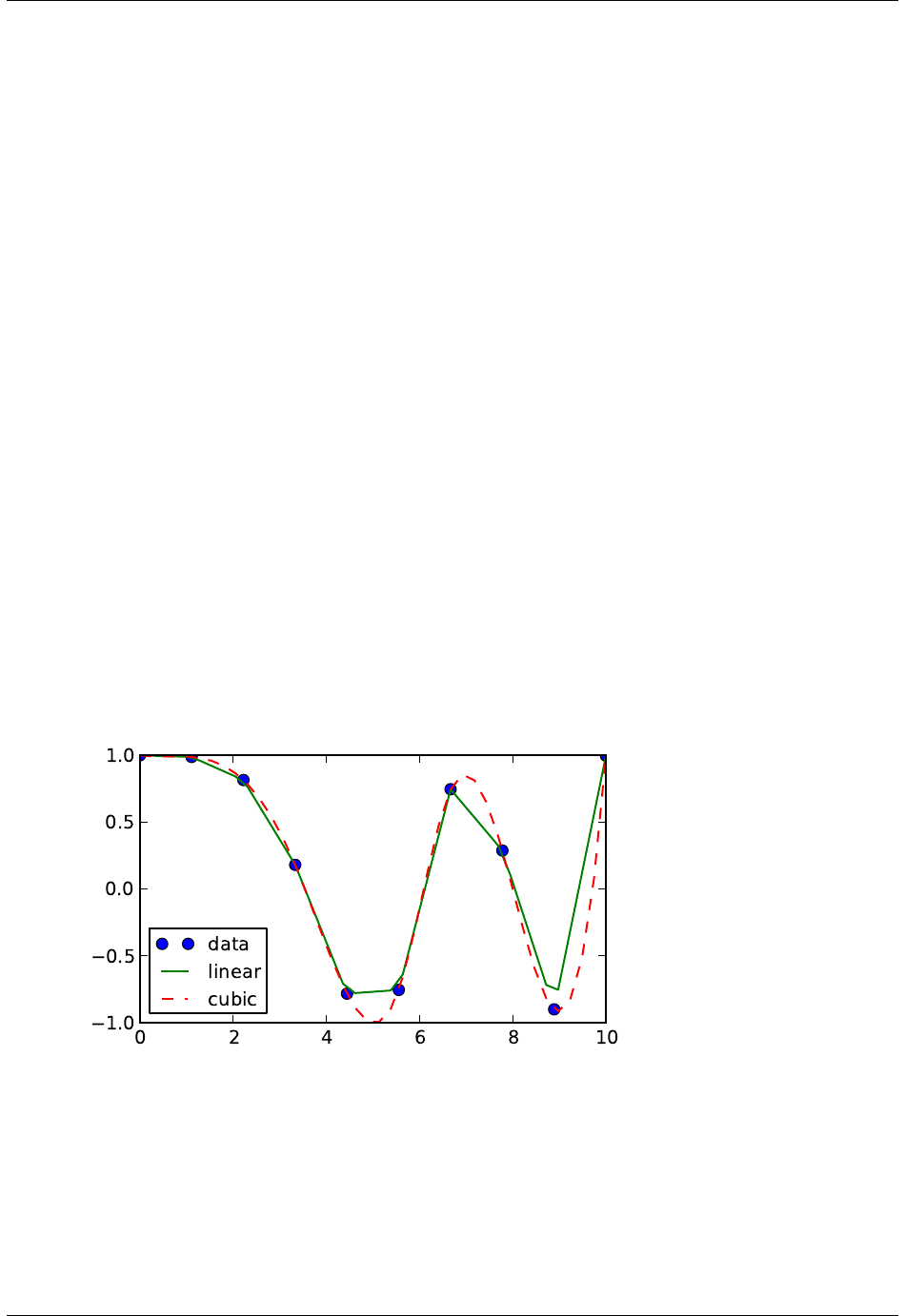
1.6.1 1-D interpolation (interp1d)
The interp1d class in scipy.interpolate is a convenient method to create a function based on fixed data points which can
be evaluated anywhere within the domain defined by the given data using linear interpolation. An instance of this class
is created by passing the 1-d vectors comprising the data. The instance of this class defines a __call__ method and
can therefore by treated like a function which interpolates between known data values to obtain unknown values (it
also has a docstring for help). Behavior at the boundary can be specified at instantiation time. The following example
demonstrates its use, for linear and cubic spline interpolation:
>>> from scipy.interpolate import interp1d
>>> x=np.linspace(0,10,10)
>>> y=np.cos(-x**2/8.0)
>>> f=interp1d(x, y)
>>> f2 =interp1d(x, y, kind=’cubic’)
>>> xnew =np.linspace(0,10,40)
>>> import matplotlib.pyplot as plt
>>> plt.plot(x,y,’o’,xnew,f(xnew),’-’, xnew, f2(xnew),’--’)
>>> plt.legend([’data’,’linear’,’cubic’], loc=’best’)
>>> plt.show()
1.6.2 Multivariate data interpolation (griddata)
Suppose you have multidimensional data, for instance for an underlying function f(x, y) you only know the values at
points (x[i], y[i]) that do not form a regular grid.
Suppose we want to interpolate the 2-D function
30 Chapter 1. SciPy Tutorial

SciPy Reference Guide, Release 0.13.0
>>> def func(x, y):
>>> return x*(1-x)*np.cos(4*np.pi*x) *np.sin(4*np.pi*y**2)**2
on a grid in [0, 1]x[0, 1]
>>> grid_x, grid_y =np.mgrid[0:1:100j,0:1:200j]
but we only know its values at 1000 data points:
>>> points =np.random.rand(1000,2)
>>> values =func(points[:,0], points[:,1])
This can be done with griddata – below we try out all of the interpolation methods:
>>> from scipy.interpolate import griddata
>>> grid_z0 =griddata(points, values, (grid_x, grid_y), method=’nearest’)
>>> grid_z1 =griddata(points, values, (grid_x, grid_y), method=’linear’)
>>> grid_z2 =griddata(points, values, (grid_x, grid_y), method=’cubic’)
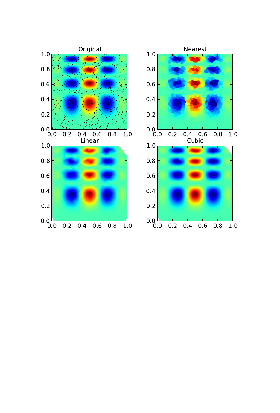
One can see that the exact result is reproduced by all of the methods to some degree, but for this smooth function the
piecewise cubic interpolant gives the best results:
>>> import matplotlib.pyplot as plt
>>> plt.subplot(221)
>>> plt.imshow(func(grid_x, grid_y).T, extent=(0,1,0,1), origin=’lower’)
>>> plt.plot(points[:,0], points[:,1], ’k.’, ms=1)
>>> plt.title(’Original’)
>>> plt.subplot(222)
>>> plt.imshow(grid_z0.T, extent=(0,1,0,1), origin=’lower’)
>>> plt.title(’Nearest’)
>>> plt.subplot(223)
>>> plt.imshow(grid_z1.T, extent=(0,1,0,1), origin=’lower’)
>>> plt.title(’Linear’)
>>> plt.subplot(224)
>>> plt.imshow(grid_z2.T, extent=(0,1,0,1), origin=’lower’)
>>> plt.title(’Cubic’)
>>> plt.gcf().set_size_inches(6,6)
>>> plt.show()
1.6. Interpolation (scipy.interpolate) 31
SciPy Reference Guide, Release 0.13.0
1.6.3 Spline interpolation
Spline interpolation in 1-d: Procedural (interpolate.splXXX)
Spline interpolation requires two essential steps: (1) a spline representation of the curve is computed, and (2) the spline
is evaluated at the desired points. In order to find the spline representation, there are two different ways to represent
a curve and obtain (smoothing) spline coefficients: directly and parametrically. The direct method finds the spline
representation of a curve in a two- dimensional plane using the function splrep. The first two arguments are the
only ones required, and these provide the xand ycomponents of the curve. The normal output is a 3-tuple, (t, c, k),
containing the knot-points, t, the coefficients cand the order kof the spline. The default spline order is cubic, but this
can be changed with the input keyword, k.
For curves in N-dimensional space the function splprep allows defining the curve parametrically. For this function
only 1 input argument is required. This input is a list of N-arrays representing the curve in N-dimensional space. The
length of each array is the number of curve points, and each array provides one component of the N-dimensional data
point. The parameter variable is given with the keword argument, u, which defaults to an equally-spaced monotonic
32 Chapter 1. SciPy Tutorial
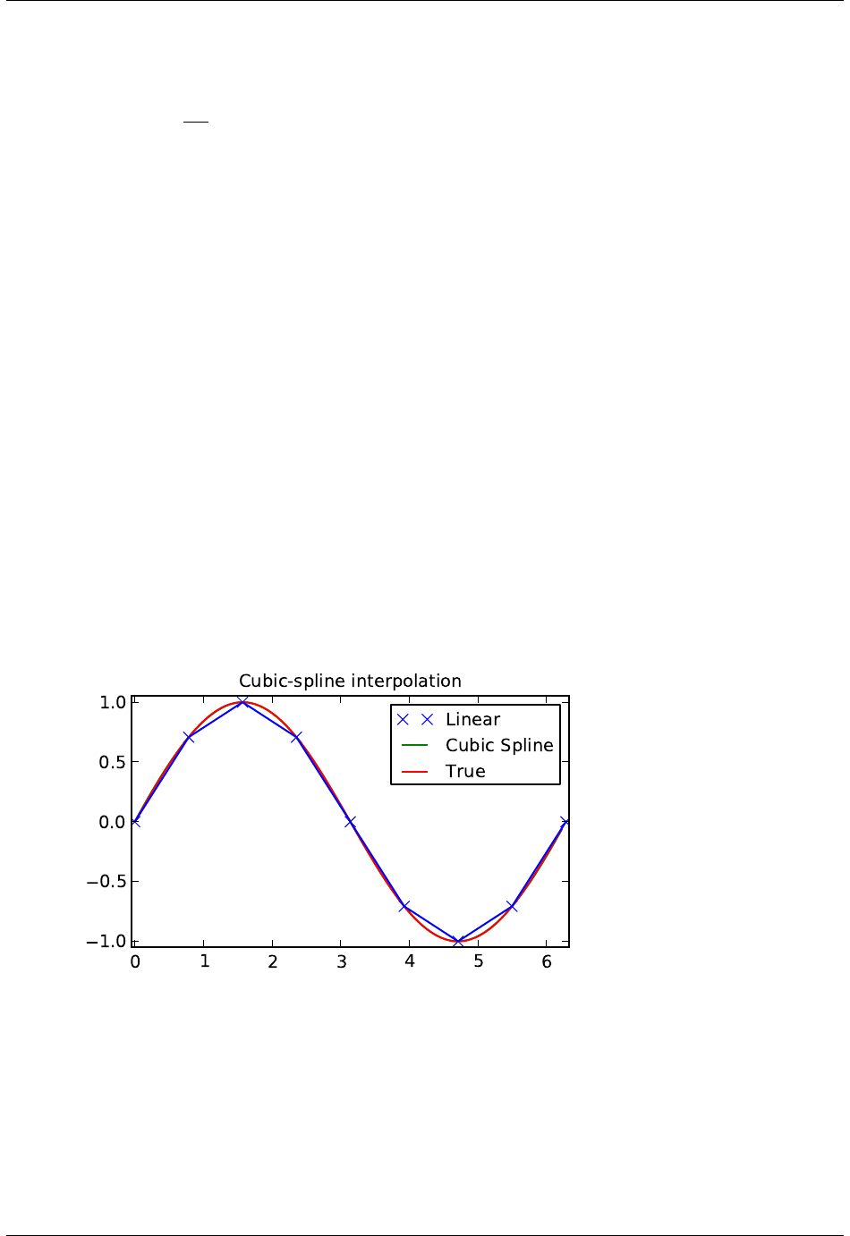
SciPy Reference Guide, Release 0.13.0
sequence between 0and 1. The default output consists of two objects: a 3-tuple, (t, c, k), containing the spline
representation and the parameter variable u.
The keyword argument, s, is used to specify the amount of smoothing to perform during the spline fit. The default
value of sis s=m−√2mwhere mis the number of data-points being fit. Therefore, if no smoothing is desired a
value of s= 0 should be passed to the routines.
Once the spline representation of the data has been determined, functions are available for evaluating the spline
(splev) and its derivatives (splev,spalde) at any point and the integral of the spline between any two points
(splint). In addition, for cubic splines ( k= 3 ) with 8 or more knots, the roots of the spline can be estimated (
sproot). These functions are demonstrated in the example that follows.
>>> import numpy as np
>>> import matplotlib.pyplot as plt
>>> from scipy import interpolate
Cubic-spline
>>> x=np.arange(0,2*np.pi+np.pi/4,2*np.pi/8)
>>> y=np.sin(x)
>>> tck =interpolate.splrep(x,y,s=0)
>>> xnew =np.arange(0,2*np.pi,np.pi/50)
>>> ynew =interpolate.splev(xnew,tck,der=0)
>>> plt.figure()
>>> plt.plot(x,y,’x’,xnew,ynew,xnew,np.sin(xnew),x,y,’b’)
>>> plt.legend([’Linear’,’Cubic Spline’,’True’])
>>> plt.axis([-0.05,6.33,-1.05,1.05])
>>> plt.title(’Cubic-spline interpolation’)
>>> plt.show()
Derivative of spline
>>> yder =interpolate.splev(xnew,tck,der=1)
>>> plt.figure()
>>> plt.plot(xnew,yder,xnew,np.cos(xnew),’--’)
>>> plt.legend([’Cubic Spline’,’True’])
>>> plt.axis([-0.05,6.33,-1.05,1.05])
>>> plt.title(’Derivative estimation from spline’)
1.6. Interpolation (scipy.interpolate) 33
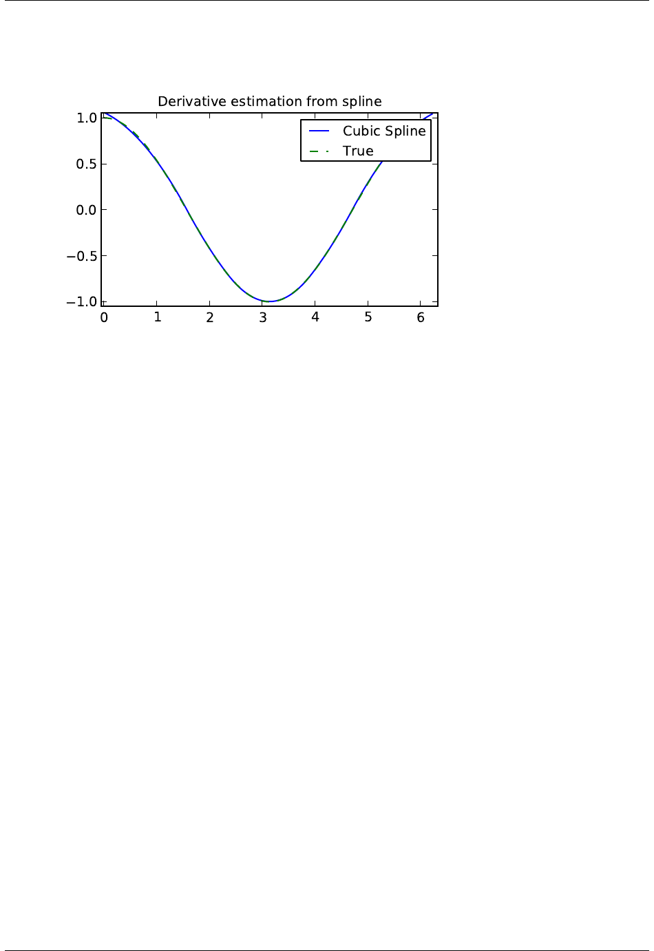
SciPy Reference Guide, Release 0.13.0
>>> plt.show()
Integral of spline
>>> def integ(x,tck,constant=-1):
>>> x=np.atleast_1d(x)
>>> out =np.zeros(x.shape, dtype=x.dtype)
>>> for nin xrange(len(out)):
>>> out[n] =interpolate.splint(0,x[n],tck)
>>> out += constant
>>> return out
>>>
>>> yint =integ(xnew,tck)
>>> plt.figure()
>>> plt.plot(xnew,yint,xnew,-np.cos(xnew),’--’)
>>> plt.legend([’Cubic Spline’,’True’])
>>> plt.axis([-0.05,6.33,-1.05,1.05])
>>> plt.title(’Integral estimation from spline’)
>>> plt.show()
34 Chapter 1. SciPy Tutorial
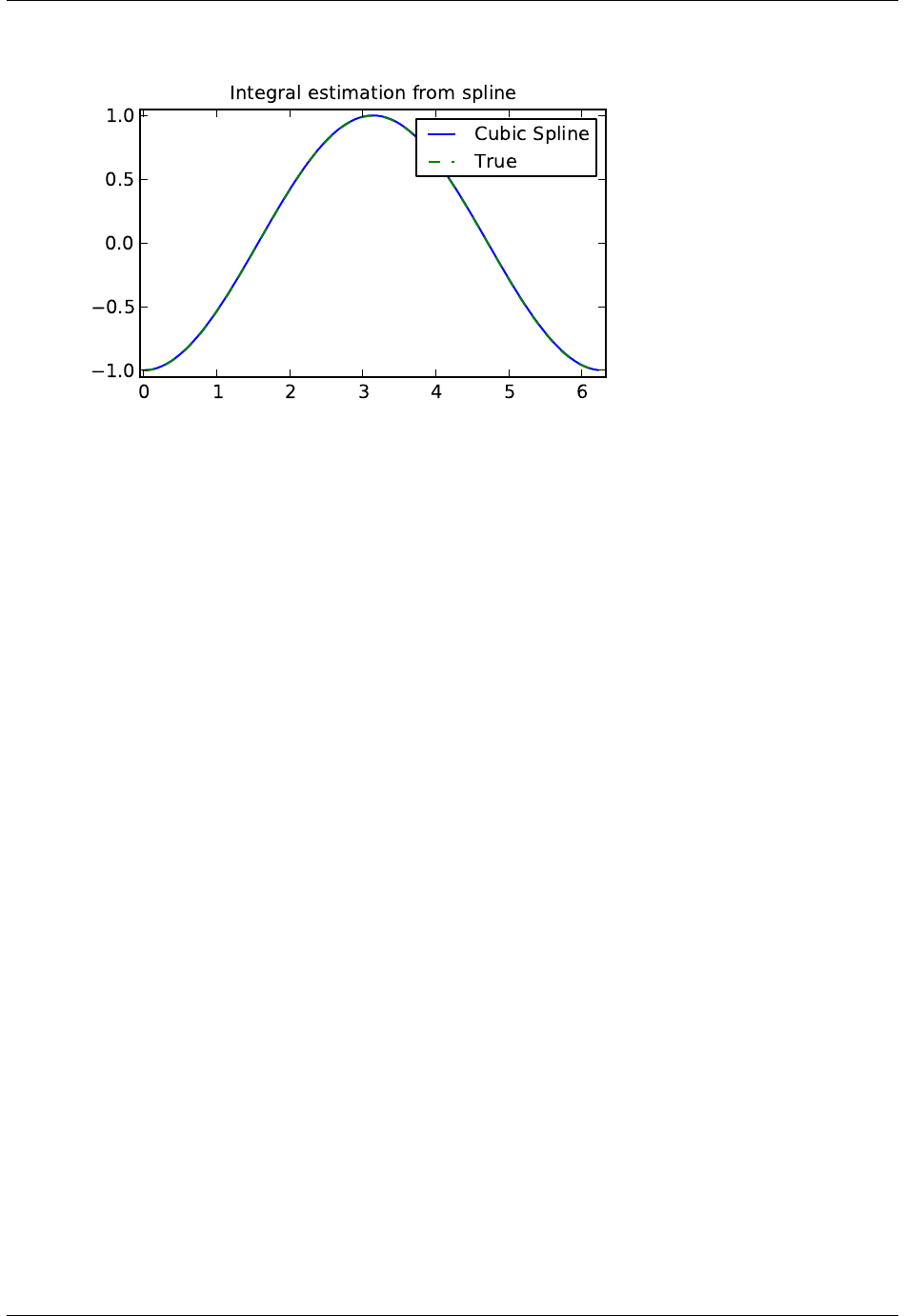
SciPy Reference Guide, Release 0.13.0
Roots of spline
>>> print(interpolate.sproot(tck))
[ 0. 3.1416]
Parametric spline
>>> t=np.arange(0,1.1,.1)
>>> x=np.sin(2*np.pi*t)
>>> y=np.cos(2*np.pi*t)
>>> tck,u =interpolate.splprep([x,y],s=0)
>>> unew =np.arange(0,1.01,0.01)
>>> out =interpolate.splev(unew,tck)
>>> plt.figure()
>>> plt.plot(x,y,’x’,out[0],out[1],np.sin(2*np.pi*unew),np.cos(2*np.pi*unew),x,y,’b’)
>>> plt.legend([’Linear’,’Cubic Spline’,’True’])
>>> plt.axis([-1.05,1.05,-1.05,1.05])
>>> plt.title(’Spline of parametrically-defined curve’)
>>> plt.show()
1.6. Interpolation (scipy.interpolate) 35
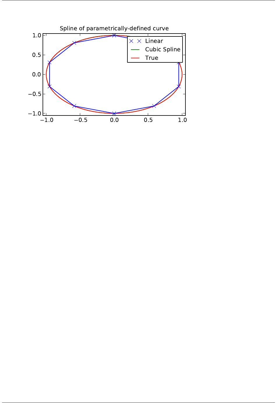
SciPy Reference Guide, Release 0.13.0
Spline interpolation in 1-d: Object-oriented (UnivariateSpline)
The spline-fitting capabilities described above are also available via an objected-oriented interface. The one dimen-
sional splines are objects of the UnivariateSpline class, and are created with the xand ycomponents of the
curve provided as arguments to the constructor. The class defines __call__, allowing the object to be called with the
x-axis values at which the spline should be evaluated, returning the interpolated y-values. This is shown in the ex-
ample below for the subclass InterpolatedUnivariateSpline. The methods integral,derivatives,
and roots methods are also available on UnivariateSpline objects, allowing definite integrals, derivatives, and
roots to be computed for the spline.
The UnivariateSpline class can also be used to smooth data by providing a non-zero value of the smoothing parameter
s, with the same meaning as the skeyword of the splrep function described above. This results in a spline that
has fewer knots than the number of data points, and hence is no longer strictly an interpolating spline, but rather a
smoothing spline. If this is not desired, the InterpolatedUnivariateSpline class is available. It is a subclass
of UnivariateSpline that always passes through all points (equivalent to forcing the smoothing parameter to 0).
This class is demonstrated in the example below.
The LSQUnivarateSpline is the other subclass of UnivarateSpline. It allows the user to specify the number and location
of internal knots as explicitly with the parameter t. This allows creation of customized splines with non-linear spacing,
to interpolate in some domains and smooth in others, or change the character of the spline.
>>> import numpy as np
>>> import matplotlib.pyplot as plt
>>> from scipy import interpolate
InterpolatedUnivariateSpline
>>> x=np.arange(0,2*np.pi+np.pi/4,2*np.pi/8)
>>> y=np.sin(x)
>>> s=interpolate.InterpolatedUnivariateSpline(x,y)
>>> xnew =np.arange(0,2*np.pi,np.pi/50)
>>> ynew =s(xnew)
>>> plt.figure()
>>> plt.plot(x,y,’x’,xnew,ynew,xnew,np.sin(xnew),x,y,’b’)
>>> plt.legend([’Linear’,’InterpolatedUnivariateSpline’,’True’])
>>> plt.axis([-0.05,6.33,-1.05,1.05])
36 Chapter 1. SciPy Tutorial
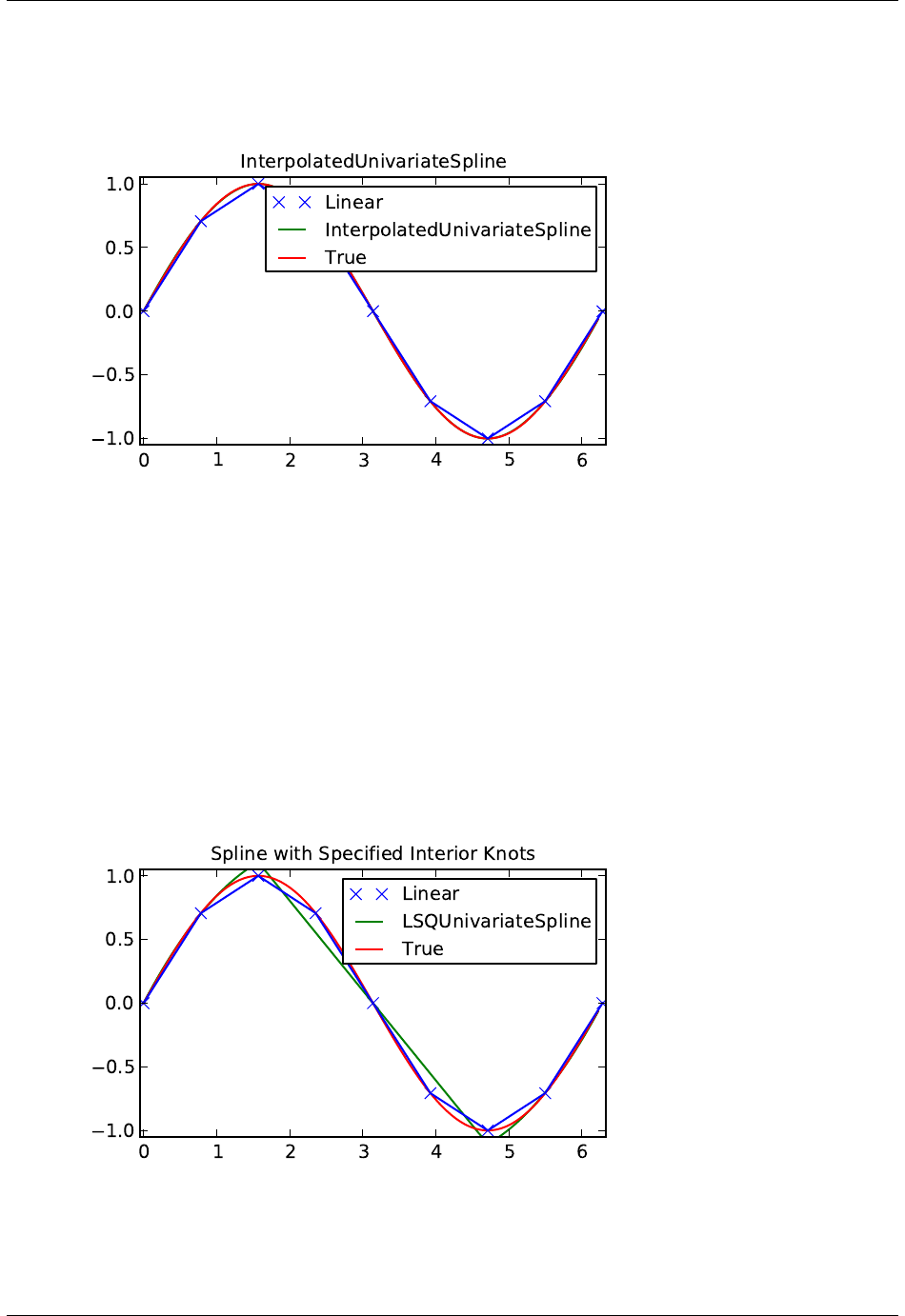
SciPy Reference Guide, Release 0.13.0
>>> plt.title(’InterpolatedUnivariateSpline’)
>>> plt.show()
LSQUnivarateSpline with non-uniform knots
>>> t=[np.pi/2-.1,np.pi/2+.1,3*np.pi/2-.1,3*np.pi/2+.1]
>>> s=interpolate.LSQUnivariateSpline(x,y,t,k=2)
>>> ynew =s(xnew)
>>> plt.figure()
>>> plt.plot(x,y,’x’,xnew,ynew,xnew,np.sin(xnew),x,y,’b’)
>>> plt.legend([’Linear’,’LSQUnivariateSpline’,’True’])
>>> plt.axis([-0.05,6.33,-1.05,1.05])
>>> plt.title(’Spline with Specified Interior Knots’)
>>> plt.show()
1.6. Interpolation (scipy.interpolate) 37
SciPy Reference Guide, Release 0.13.0
Two-dimensional spline representation: Procedural (bisplrep)
For (smooth) spline-fitting to a two dimensional surface, the function bisplrep is available. This function takes as
required inputs the 1-D arrays x,y, and zwhich represent points on the surface z=f(x, y).The default output is a
list [tx, ty, c, kx, ky]whose entries represent respectively, the components of the knot positions, the coefficients of the
spline, and the order of the spline in each coordinate. It is convenient to hold this list in a single object, tck, so that
it can be passed easily to the function bisplev. The keyword, s, can be used to change the amount of smoothing
performed on the data while determining the appropriate spline. The default value is s=m−√2mwhere mis the
number of data points in the x, y, and zvectors. As a result, if no smoothing is desired, then s= 0 should be passed to
bisplrep .
To evaluate the two-dimensional spline and it’s partial derivatives (up to the order of the spline), the function bisplev
is required. This function takes as the first two arguments two 1-D arrays whose cross-product specifies the domain
over which to evaluate the spline. The third argument is the tck list returned from bisplrep. If desired, the fourth
and fifth arguments provide the orders of the partial derivative in the xand ydirection respectively.
It is important to note that two dimensional interpolation should not be used to find the spline representation of
images. The algorithm used is not amenable to large numbers of input points. The signal processing toolbox contains
more appropriate algorithms for finding the spline representation of an image. The two dimensional interpolation
commands are intended for use when interpolating a two dimensional function as shown in the example that follows.
This example uses the mgrid command in SciPy which is useful for defining a “mesh-grid “in many dimensions.
(See also the ogrid command if the full-mesh is not needed). The number of output arguments and the number of
dimensions of each argument is determined by the number of indexing objects passed in mgrid.
>>> import numpy as np
>>> from scipy import interpolate
>>> import matplotlib.pyplot as plt
Define function over sparse 20x20 grid
>>> x,y =np.mgrid[-1:1:20j,-1:1:20j]
>>> z=(x+y)*np.exp(-6.0*(x*x+y*y))
>>> plt.figure()
>>> plt.pcolor(x,y,z)
>>> plt.colorbar()
>>> plt.title("Sparsely sampled function.")
>>> plt.show()
38 Chapter 1. SciPy Tutorial
SciPy Reference Guide, Release 0.13.0
Interpolate function over new 70x70 grid
>>> xnew,ynew =np.mgrid[-1:1:70j,-1:1:70j]
>>> tck =interpolate.bisplrep(x,y,z,s=0)
>>> znew =interpolate.bisplev(xnew[:,0],ynew[0,:],tck)
>>> plt.figure()
>>> plt.pcolor(xnew,ynew,znew)
>>> plt.colorbar()
>>> plt.title("Interpolated function.")
>>> plt.show()
Two-dimensional spline representation: Object-oriented (BivariateSpline)
The BivariateSpline class is the 2-dimensional analog of the UnivariateSpline class. It and its subclasses
implement the FITPACK functions described above in an object oriented fashion, allowing objects to be instantiated
that can be called to compute the spline value by passing in the two coordinates as the two arguments.
1.6.4 Using radial basis functions for smoothing/interpolation
Radial basis functions can be used for smoothing/interpolating scattered data in n-dimensions, but should be used with
caution for extrapolation outside of the observed data range.
1-d Example
This example compares the usage of the Rbf and UnivariateSpline classes from the scipy.interpolate module.
>>> import numpy as np
>>> from scipy.interpolate import Rbf, InterpolatedUnivariateSpline
>>> import matplotlib.pyplot as plt
>>> # setup data
>>> x=np.linspace(0,10,9)
>>> y=np.sin(x)
>>> xi =np.linspace(0,10,101)
1.6. Interpolation (scipy.interpolate) 39
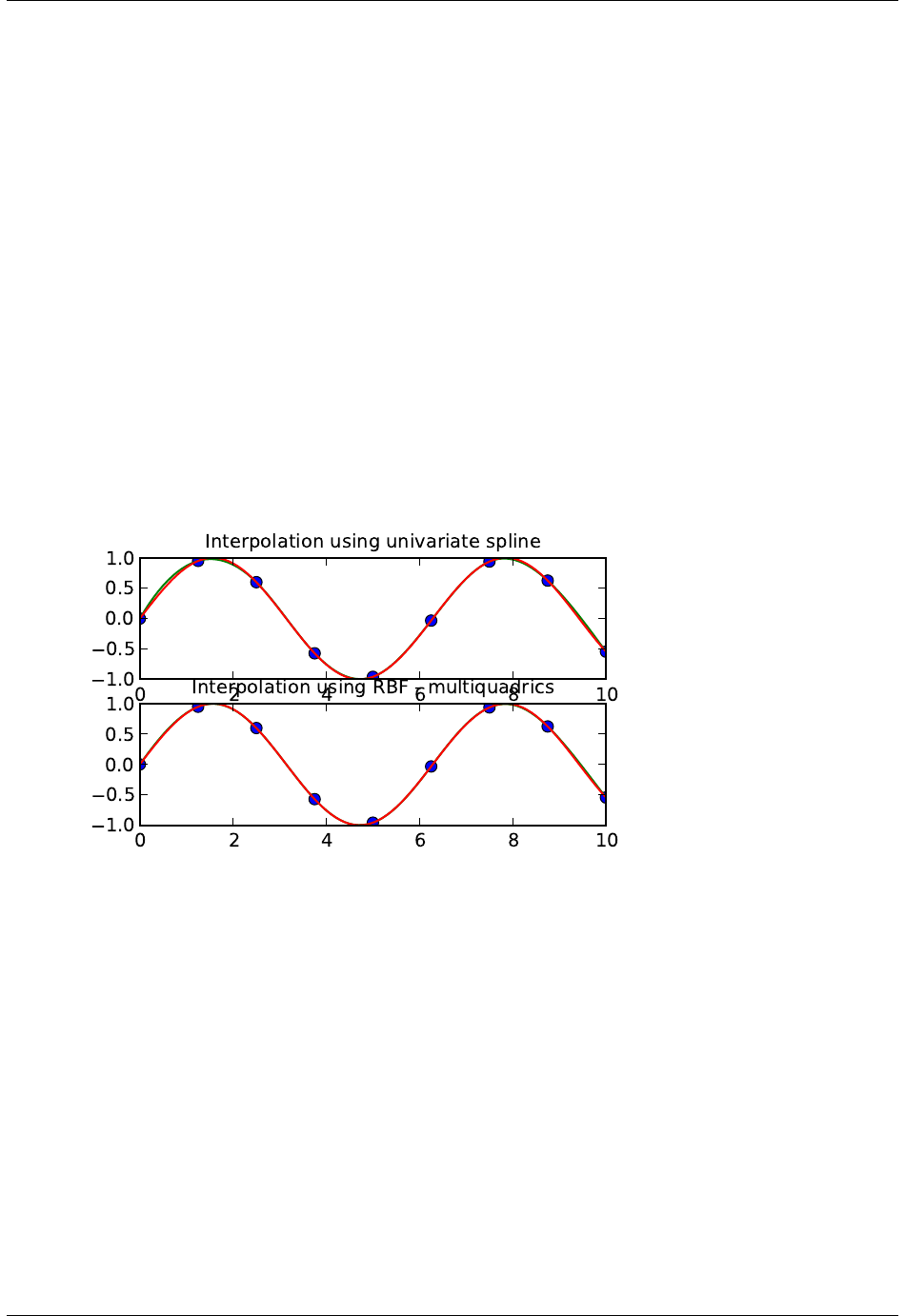
SciPy Reference Guide, Release 0.13.0
>>> # use fitpack2 method
>>> ius =InterpolatedUnivariateSpline(x, y)
>>> yi =ius(xi)
>>> plt.subplot(2,1,1)
>>> plt.plot(x, y, ’bo’)
>>> plt.plot(xi, yi, ’g’)
>>> plt.plot(xi, np.sin(xi), ’r’)
>>> plt.title(’Interpolation using univariate spline’)
>>> # use RBF method
>>> rbf =Rbf(x, y)
>>> fi =rbf(xi)
>>> plt.subplot(2,1,2)
>>> plt.plot(x, y, ’bo’)
>>> plt.plot(xi, fi, ’g’)
>>> plt.plot(xi, np.sin(xi), ’r’)
>>> plt.title(’Interpolation using RBF - multiquadrics’)
>>> plt.show()
2-d Example
This example shows how to interpolate scattered 2d data.
>>> import numpy as np
>>> from scipy.interpolate import Rbf
>>> import matplotlib.pyplot as plt
>>> from matplotlib import cm
>>> # 2-d tests - setup scattered data
>>> x=np.random.rand(100)*4.0-2.0
>>> y=np.random.rand(100)*4.0-2.0
>>> z=x*np.exp(-x**2-y**2)
>>> ti =np.linspace(-2.0,2.0,100)
>>> XI, YI =np.meshgrid(ti, ti)
40 Chapter 1. SciPy Tutorial
SciPy Reference Guide, Release 0.13.0
>>> # use RBF
>>> rbf =Rbf(x, y, z, epsilon=2)
>>> ZI =rbf(XI, YI)
>>> # plot the result
>>> n=plt.normalize(-2.,2.)
>>> plt.subplot(1,1,1)
>>> plt.pcolor(XI, YI, ZI, cmap=cm.jet)
>>> plt.scatter(x, y, 100, z, cmap=cm.jet)
>>> plt.title(’RBF interpolation - multiquadrics’)
>>> plt.xlim(-2,2)
>>> plt.ylim(-2,2)
>>> plt.colorbar()
1.7 Fourier Transforms (scipy.fftpack)
Warning: This is currently a stub page
1.7. Fourier Transforms (scipy.fftpack) 41

SciPy Reference Guide, Release 0.13.0
Contents
•Fourier Transforms (scipy.fftpack)
–Fast Fourier transforms
–One dimensional discrete Fourier transforms
–Two and n dimensional discrete Fourier transforms
–Discrete Cosine Transforms
*type I
*type II
*type III
–Discrete Sine Transforms
*type I
*type II
*type III
*References
–FFT convolution
–Cache Destruction
Fourier analysis is fundamentally a method for expressing a function as a sum of periodic components, and for recover-
ing the signal from those components. When both the function and its Fourier transform are replaced with discretized
counterparts, it is called the discrete Fourier transform (DFT). The DFT has become a mainstay of numerical com-
puting in part because of a very fast algorithm for computing it, called the Fast Fourier Transform (FFT), which was
known to Gauss (1805) and was brought to light in its current form by Cooley and Tukey [CT]. Press et al. [NR]
provide an accessible introduction to Fourier analysis and its applications.
1.7.1 Fast Fourier transforms
1.7.2 One dimensional discrete Fourier transforms
fft, ifft, rfft, irfft
1.7.3 Two and n dimensional discrete Fourier transforms
fft in more than one dimension
1.7.4 Discrete Cosine Transforms
Return the Discrete Cosine Transform [Mak] of arbitrary type sequence x.
For a single dimension array x,dct(x, norm=’ortho’) is equal to MATLAB dct(x).
There are theoretically 8 types of the DCT [WPC], only the first 3 types are implemented in scipy. ‘The’ DCT generally
refers to DCT type 2, and ‘the’ Inverse DCT generally refers to DCT type 3.
type I
There are several definitions of the DCT-I; we use the following (for norm=None):
yk=x0+ (−1)kxN−1+ 2
N−2
X
n=1
xncos πnk
N−1,0≤k < N.
42 Chapter 1. SciPy Tutorial

SciPy Reference Guide, Release 0.13.0
Only None is supported as normalization mode for DCT-I. Note also that the DCT-I is only supported for input size >
1
type II
There are several definitions of the DCT-II; we use the following (for norm=None):
yk= 2
N−1
X
n=0
xncos π(2n+ 1)k
2N0≤k < N.
If norm=’ortho’,ykis multiplied by a scaling factor f:
f=(p1/(4N),if k= 0
p1/(2N),otherwise
Which makes the corresponding matrix of coefficients orthonormal (OO’ = Id).
type III
There are several definitions of the DCT-III, we use the following (for norm=None):
yk=x0+ 2
N−1
X
n=1
xncos πn(2k+ 1)
2N0≤k < N,
or, for norm=’ortho’:
yk=x0
√N+1
√N
N−1
X
n=1
xncos πn(2k+ 1)
2N0≤k < N.
The (unnormalized) DCT-III is the inverse of the (unnormalized) DCT-II, up to a factor 2N. The orthonormalized
DCT-III is exactly the inverse of the orthonormalized DCT-II.
1.7.5 Discrete Sine Transforms
Return the Discrete Sine Transform [Mak] of arbitrary type sequence x.
There are theoretically 8 types of the DST for different combinations of even/odd boundary conditions and boundary
off sets [WPS], only the first 3 types are implemented in scipy.
type I
There are several definitions of the DST-I; we use the following for norm=None. DST-I assumes the input is odd
around n=-1 and n=N.
yk= 2
N−1
X
n=0
xnsin π(n+ 1)(k+ 1)
N+ 1 ,0≤k < N.
Only None is supported as normalization mode for DST-I. Note also that the DCT-I is only supported for input size >
1. The (unnormalized) DCT-I is its own inverse, up to a factor 2(N+1).
1.7. Fourier Transforms (scipy.fftpack) 43

SciPy Reference Guide, Release 0.13.0
type II
There are several definitions of the DST-II; we use the following (for norm=None). DST-II assumes the input is odd
around n=-1/2 and even around n=N
yk= 2
N−1
X
n=0
xnsin π(n+ 1/2)(k+ 1)
N,0≤k < N.
type III
There are several definitions of the DST-III, we use the following (for norm=None). DST-III assumes the input is
odd around n=-1 and even around n=N-1
yk= (−1)kxN−1+ 2
N−2
X
n=0
xnsin π(n+ 1)(k+ 1/2)
N,0≤k < N.
The (unnormalized) DCT-III is the inverse of the (unnormalized) DCT-II, up to a factor 2N.
References
1.7.6 FFT convolution
scipy.fftpack.convolve performs a convolution of two one-dimensional arrays in frequency domain.
1.7.7 Cache Destruction
To accelerate repeat transforms on arrays of the same shape and dtype, scipy.fftpack keeps a cache of the prime
factorization of length of the array and pre-computed trigonometric functions. These caches can be destroyed by
calling the appropriate function in scipy.fftpack._fftpack. dst(type=1) and idst(type=1) share a cache (*dst1_cache).
As do dst(type=2), dst(type=3), idst(type=3), and idst(type=3) (*dst2_cache).
1.8 Signal Processing (scipy.signal)
The signal processing toolbox currently contains some filtering functions, a limited set of filter design tools, and a few
B-spline interpolation algorithms for one- and two-dimensional data. While the B-spline algorithms could technically
be placed under the interpolation category, they are included here because they only work with equally-spaced data and
make heavy use of filter-theory and transfer-function formalism to provide a fast B-spline transform. To understand
this section you will need to understand that a signal in SciPy is an array of real or complex numbers.
1.8.1 B-splines
A B-spline is an approximation of a continuous function over a finite- domain in terms of B-spline coefficients and knot
points. If the knot- points are equally spaced with spacing ∆x, then the B-spline approximation to a 1-dimensional
function is the finite-basis expansion.
y(x)≈X
j
cjβox
∆x−j.
44 Chapter 1. SciPy Tutorial

SciPy Reference Guide, Release 0.13.0
In two dimensions with knot-spacing ∆xand ∆y, the function representation is
z(x, y)≈X
jX
k
cjkβox
∆x−jβoy
∆y−k.
In these expressions, βo(·)is the space-limited B-spline basis function of order, o. The requirement of equally-
spaced knot-points and equally-spaced data points, allows the development of fast (inverse-filtering) algorithms for
determining the coefficients, cj, from sample-values, yn. Unlike the general spline interpolation algorithms, these
algorithms can quickly find the spline coefficients for large images.
The advantage of representing a set of samples via B-spline basis functions is that continuous-domain operators
(derivatives, re- sampling, integral, etc.) which assume that the data samples are drawn from an underlying con-
tinuous function can be computed with relative ease from the spline coefficients. For example, the second-derivative
of a spline is
y00 (x) = 1
∆x2X
j
cjβo00 x
∆x−j.
Using the property of B-splines that
d2βo(w)
dw2=βo−2(w+ 1) −2βo−2(w) + βo−2(w−1)
it can be seen that
y00 (x) = 1
∆x2X
j
cjhβo−2x
∆x−j+ 1−2βo−2x
∆x−j+βo−2x
∆x−j−1i.
If o= 3 , then at the sample points,
∆x2y0(x)|x=n∆x=X
j
cjδn−j+1 −2cjδn−j+cjδn−j−1,
=cn+1 −2cn+cn−1.
Thus, the second-derivative signal can be easily calculated from the spline fit. if desired, smoothing splines can be
found to make the second-derivative less sensitive to random-errors.
The savvy reader will have already noticed that the data samples are related to the knot coefficients via a convolution
operator, so that simple convolution with the sampled B-spline function recovers the original data from the spline coef-
ficients. The output of convolutions can change depending on how boundaries are handled (this becomes increasingly
more important as the number of dimensions in the data- set increases). The algorithms relating to B-splines in the
signal- processing sub package assume mirror-symmetric boundary conditions. Thus, spline coefficients are computed
based on that assumption, and data-samples can be recovered exactly from the spline coefficients by assuming them
to be mirror-symmetric also.
Currently the package provides functions for determining second- and third-order cubic spline coefficients
from equally spaced samples in one- and two-dimensions (signal.qspline1d,signal.qspline2d,
signal.cspline1d,signal.cspline2d). The package also supplies a function ( signal.bspline ) for
evaluating the bspline basis function, βo(x)for arbitrary order and x. For large o, the B-spline basis function can be
approximated well by a zero-mean Gaussian function with standard-deviation equal to σo= (o+ 1) /12 :
βo(x)≈1
p2πσ2
o
exp −x2
2σo.
A function to compute this Gaussian for arbitrary xand ois also available ( signal.gauss_spline ). The
following code and Figure uses spline-filtering to compute an edge-image (the second-derivative of a smoothed
spline) of Lena’s face which is an array returned by the command lena. The command signal.sepfir2d
was used to apply a separable two-dimensional FIR filter with mirror- symmetric boundary conditions to the spline
coefficients. This function is ideally suited for reconstructing samples from spline coefficients and is faster than
signal.convolve2d which convolves arbitrary two-dimensional filters and allows for choosing mirror-symmetric
boundary conditions.
1.8. Signal Processing (scipy.signal) 45
SciPy Reference Guide, Release 0.13.0
>>> from numpy import *
>>> from scipy import signal, misc
>>> import matplotlib.pyplot as plt
>>> image =misc.lena().astype(float32)
>>> derfilt =array([1.0,-2,1.0],float32)
>>> ck =signal.cspline2d(image,8.0)
>>> deriv =signal.sepfir2d(ck, derfilt, [1]) +\
>>> signal.sepfir2d(ck, [1], derfilt)
Alternatively we could have done:
laplacian =array([[0,1,0],[1,-4,1],[0,1,0]],float32)
deriv2 =signal.convolve2d(ck,laplacian,mode=’same’,boundary=’symm’)
>>> plt.figure()
>>> plt.imshow(image)
>>> plt.gray()
>>> plt.title(’Original image’)
>>> plt.show()
>>> plt.figure()
>>> plt.imshow(deriv)
>>> plt.gray()
>>> plt.title(’Output of spline edge filter’)
>>> plt.show()
46 Chapter 1. SciPy Tutorial
SciPy Reference Guide, Release 0.13.0
1.8.2 Filtering
Filtering is a generic name for any system that modifies an input signal in some way. In SciPy a signal can be thought
of as a Numpy array. There are different kinds of filters for different kinds of operations. There are two broad kinds
of filtering operations: linear and non-linear. Linear filters can always be reduced to multiplication of the flattened
Numpy array by an appropriate matrix resulting in another flattened Numpy array. Of course, this is not usually the
best way to compute the filter as the matrices and vectors involved may be huge. For example filtering a 512 ×512
image with this method would require multiplication of a 5122×5122matrix with a 5122vector. Just trying to store the
5122×5122matrix using a standard Numpy array would require 68,719,476,736 elements. At 4 bytes per element
this would require 256GB of memory. In most applications most of the elements of this matrix are zero and a different
method for computing the output of the filter is employed.
Convolution/Correlation
Many linear filters also have the property of shift-invariance. This means that the filtering operation is the same at
different locations in the signal and it implies that the filtering matrix can be constructed from knowledge of one row
(or column) of the matrix alone. In this case, the matrix multiplication can be accomplished using Fourier transforms.
Let x[n]define a one-dimensional signal indexed by the integer n. Full convolution of two one-dimensional signals
can be expressed as
y[n] = ∞
X
k=−∞
x[k]h[n−k].
This equation can only be implemented directly if we limit the sequences to finite support sequences that can be stored
in a computer, choose n= 0 to be the starting point of both sequences, let K+ 1 be that value for which y[n] = 0
for all n>K+ 1 and M+ 1 be that value for which x[n] = 0 for all n>M+ 1 , then the discrete convolution
expression is
y[n] =
min(n,K)
X
k=max(n−M,0)
x[k]h[n−k].
1.8. Signal Processing (scipy.signal) 47

SciPy Reference Guide, Release 0.13.0
For convenience assume K≥M. Then, more explicitly the output of this operation is
y[0] = x[0] h[0]
y[1] = x[0] h[1] + x[1] h[0]
y[2] = x[0] h[2] + x[1] h[1] + x[2] h[0]
.
.
..
.
..
.
.
y[M] = x[0] h[M] + x[1] h[M−1] + ··· +x[M]h[0]
y[M+ 1] = x[1] h[M] + x[2] h[M−1] + ··· +x[M+ 1] h[0]
.
.
..
.
..
.
.
y[K] = x[K−M]h[M] + ··· +x[K]h[0]
y[K+ 1] = x[K+ 1 −M]h[M] + ··· +x[K]h[1]
.
.
..
.
..
.
.
y[K+M−1] = x[K−1] h[M] + x[K]h[M−1]
y[K+M] = x[K]h[M].
Thus, the full discrete convolution of two finite sequences of lengths K+ 1 and M+ 1 respectively results in a finite
sequence of length K+M+ 1 = (K+ 1) + (M+ 1) −1.
One dimensional convolution is implemented in SciPy with the function signal.convolve . This function takes
as inputs the signals x, h , and an optional flag and returns the signal y. The optional flag allows for specification of
which part of the output signal to return. The default value of ‘full’ returns the entire signal. If the flag has a value of
‘same’ then only the middle Kvalues are returned starting at yM−1
2so that the output has the same length as the
largest input. If the flag has a value of ‘valid’ then only the middle K−M+ 1 = (K+ 1) −(M+ 1) + 1 output
values are returned where zdepends on all of the values of the smallest input from h[0] to h[M].In other words only
the values y[M]to y[K]inclusive are returned.
This same function signal.convolve can actually take N-dimensional arrays as inputs and will return the N
-dimensional convolution of the two arrays. The same input flags are available for that case as well.
Correlation is very similar to convolution except for the minus sign becomes a plus sign. Thus
w[n] = ∞
X
k=−∞
y[k]x[n+k]
is the (cross) correlation of the signals yand x. For finite-length signals with y[n] = 0 outside of the range [0, K]and
x[n] = 0 outside of the range [0, M ],the summation can simplify to
w[n] =
min(K,M−n)
X
k=max(0,−n)
y[k]x[n+k].
48 Chapter 1. SciPy Tutorial

SciPy Reference Guide, Release 0.13.0
Assuming again that K≥Mthis is
w[−K] = y[K]x[0]
w[−K+ 1] = y[K−1] x[0] + y[K]x[1]
.
.
..
.
..
.
.
w[M−K] = y[K−M]x[0] + y[K−M+ 1] x[1] + ··· +y[K]x[M]
w[M−K+ 1] = y[K−M−1] x[0] + ··· +y[K−1] x[M]
.
.
..
.
..
.
.
w[−1] = y[1] x[0] + y[2] x[1] + ··· +y[M+ 1] x[M]
w[0] = y[0] x[0] + y[1] x[1] + ··· +y[M]x[M]
w[1] = y[0] x[1] + y[1] x[2] + ··· +y[M−1] x[M]
w[2] = y[0] x[2] + y[1] x[3] + ··· +y[M−2] x[M]
.
.
..
.
..
.
.
w[M−1] = y[0] x[M−1] + y[1] x[M]
w[M] = y[0] x[M].
The SciPy function signal.correlate implements this operation. Equivalent flags are available for this operation
to return the full K+M+1 length sequence (‘full’) or a sequence with the same size as the largest sequence starting at
w−K+M−1
2(‘same’) or a sequence where the values depend on all the values of the smallest sequence (‘valid’).
This final option returns the K−M+ 1 values w[M−K]to w[0] inclusive.
The function signal.correlate can also take arbitrary N-dimensional arrays as input and return the N-
dimensional convolution of the two arrays on output.
When N= 2,signal.correlate and/or signal.convolve can be used to construct arbitrary image filters
to perform actions such as blurring, enhancing, and edge-detection for an image.
Convolution is mainly used for filtering when one of the signals is much smaller than the other ( KM), otherwise
linear filtering is more easily accomplished in the frequency domain (see Fourier Transforms).
Difference-equation filtering
A general class of linear one-dimensional filters (that includes convolution filters) are filters described by the difference
equation
N
X
k=0
aky[n−k] =
M
X
k=0
bkx[n−k]
where x[n]is the input sequence and y[n]is the output sequence. If we assume initial rest so that y[n] = 0 for n < 0
, then this kind of filter can be implemented using convolution. However, the convolution filter sequence h[n]could
be infinite if ak6= 0 for k≥1.In addition, this general class of linear filter allows initial conditions to be placed on
y[n]for n < 0resulting in a filter that cannot be expressed using convolution.
The difference equation filter can be thought of as finding y[n]recursively in terms of it’s previous values
a0y[n] = −a1y[n−1] − ··· − aNy[n−N] + ··· +b0x[n] + ··· +bMx[n−M].
Often a0= 1 is chosen for normalization. The implementation in SciPy of this general difference equation filter is
a little more complicated then would be implied by the previous equation. It is implemented so that only one signal
1.8. Signal Processing (scipy.signal) 49

SciPy Reference Guide, Release 0.13.0
needs to be delayed. The actual implementation equations are (assuming a0= 1 ).
y[n] = b0x[n] + z0[n−1]
z0[n] = b1x[n] + z1[n−1] −a1y[n]
z1[n] = b2x[n] + z2[n−1] −a2y[n]
.
.
..
.
..
.
.
zK−2[n] = bK−1x[n] + zK−1[n−1] −aK−1y[n]
zK−1[n] = bKx[n]−aKy[n],
where K= max (N, M).Note that bK= 0 if K > M and aK= 0 if K > N. In this way, the output at time n
depends only on the input at time nand the value of z0at the previous time. This can always be calculated as long as
the Kvalues z0[n−1] . . . zK−1[n−1] are computed and stored at each time step.
The difference-equation filter is called using the command signal.lfilter in SciPy. This command takes as
inputs the vector b, the vector, a, a signal xand returns the vector y(the same length as x) computed using the
equation given above. If xis N-dimensional, then the filter is computed along the axis provided. If, desired, initial
conditions providing the values of z0[−1] to zK−1[−1] can be provided or else it will be assumed that they are all
zero. If initial conditions are provided, then the final conditions on the intermediate variables are also returned. These
could be used, for example, to restart the calculation in the same state.
Sometimes it is more convenient to express the initial conditions in terms of the signals x[n]and y[n].In other words,
perhaps you have the values of x[−M]to x[−1] and the values of y[−N]to y[−1] and would like to determine what
values of zm[−1] should be delivered as initial conditions to the difference-equation filter. It is not difficult to show
that for 0≤m < K,
zm[n] =
K−m−1
X
p=0
(bm+p+1x[n−p]−am+p+1y[n−p]) .
Using this formula we can find the intial condition vector z0[−1] to zK−1[−1] given initial conditions on y(and x).
The command signal.lfiltic performs this function.
Other filters
The signal processing package provides many more filters as well.
Median Filter
A median filter is commonly applied when noise is markedly non-Gaussian or when it is desired to preserve edges. The
median filter works by sorting all of the array pixel values in a rectangular region surrounding the point of interest.
The sample median of this list of neighborhood pixel values is used as the value for the output array. The sample
median is the middle array value in a sorted list of neighborhood values. If there are an even number of elements in the
neighborhood, then the average of the middle two values is used as the median. A general purpose median filter that
works on N-dimensional arrays is signal.medfilt . A specialized version that works only for two-dimensional
arrays is available as signal.medfilt2d .
Order Filter
A median filter is a specific example of a more general class of filters called order filters. To compute the output
at a particular pixel, all order filters use the array values in a region surrounding that pixel. These array values are
sorted and then one of them is selected as the output value. For the median filter, the sample median of the list of
array values is used as the output. A general order filter allows the user to select which of the sorted values will be
used as the output. So, for example one could choose to pick the maximum in the list or the minimum. The order
filter takes an additional argument besides the input array and the region mask that specifies which of the elements
in the sorted list of neighbor array values should be used as the output. The command to perform an order filter is
signal.order_filter .
50 Chapter 1. SciPy Tutorial

SciPy Reference Guide, Release 0.13.0
Wiener filter
The Wiener filter is a simple deblurring filter for denoising images. This is not the Wiener filter commonly described
in image reconstruction problems but instead it is a simple, local-mean filter. Let xbe the input signal, then the output
is
y=(σ2
σ2
xmx+1−σ2
σ2
xx σ2
x≥σ2,
mxσ2
x< σ2,
where mxis the local estimate of the mean and σ2
xis the local estimate of the variance. The window for these estimates
is an optional input parameter (default is 3×3). The parameter σ2is a threshold noise parameter. If σis not given
then it is estimated as the average of the local variances.
Hilbert filter
The Hilbert transform constructs the complex-valued analytic signal from a real signal. For example if x= cos ωn
then y=hilbert (x)would return (except near the edges) y= exp (jωn).In the frequency domain, the hilbert
transform performs
Y=X·H
where His 2 for positive frequencies, 0for negative frequencies and 1for zero-frequencies.
1.8.3 Least-Squares Spectral Analysis
Least-squares spectral analysis (LSSA) is a method of estimating a frequency spectrum, based on a least squares fit
of sinusoids to data samples, similar to Fourier analysis. Fourier analysis, the most used spectral method in science,
generally boosts long-periodic noise in long gapped records; LSSA mitigates such problems.
Lomb-Scargle Periodograms (lombscargle)
The Lomb-Scargle method performs spectral analysis on unevenly sampled data and is known to be a powerful way
to find, and test the significance of, weak periodic signals.
For a time series comprising Ntmeasurements Xj≡X(tj)sampled at times tjwhere (j= 1, . . . , Nt), assumed
to have been scaled and shifted such that its mean is zero and its variance is unity, the normalized Lomb-Scargle
periodogram at frequency fis
Pn(f)1
2
hPNt
jXjcos ω(tj−τ)i2
PNt
jcos2ω(tj−τ)+hPNt
jXjsin ω(tj−τ)i2
PNt
jsin2ω(tj−τ)
.
Here, ω≡2πf is the angular frequency. The frequency dependent time offset τis given by
tan 2ωτ =PNt
jsin 2ωtj
PNt
jcos 2ωtj
.
The lombscargle function calculates the periodogram using a slightly modified algorithm due to Townsend 1which
allows the periodogram to be calculated using only a single pass through the input arrays for each frequency.
The equation is refactored as:
Pn(f) = 1
2(cτXC +sτXS)2
c2
τCC + 2cτsτCS +s2
τSS +(cτXS −sτXC)2
c2
τSS −2cτsτCS +s2
τCC
1R.H.D. Townsend, “Fast calculation of the Lomb-Scargle periodogram using graphics processing units.”, The Astrophysical Journal Supple-
ment Series, vol 191, pp. 247-253, 2010
1.8. Signal Processing (scipy.signal) 51

SciPy Reference Guide, Release 0.13.0
and
tan 2ωτ =2CS
CC −SS .
Here,
cτ= cos ωτ, sτ= sin ωτ
while the sums are
XC =
Nt
X
j
Xjcos ωtj
XS =
Nt
X
j
Xjsin ωtj
CC =
Nt
X
j
cos2ωtj
SS =
Nt
X
j
sin2ωtj
CS =
Nt
X
j
cos ωtjsin ωtj.
This requires Nf(2Nt+ 3) trigonometric function evaluations giving a factor of ∼2speed increase over the straight-
forward implementation.
References
Some further reading and related software:
1.9 Linear Algebra (scipy.linalg)
When SciPy is built using the optimized ATLAS LAPACK and BLAS libraries, it has very fast linear algebra capabil-
ities. If you dig deep enough, all of the raw lapack and blas libraries are available for your use for even more speed.
In this section, some easier-to-use interfaces to these routines are described.
All of these linear algebra routines expect an object that can be converted into a 2-dimensional array. The output of
these routines is also a two-dimensional array.
scipy.linalg contains all the functions in numpy.linalg. plus some other more advanced ones not contained
in numpy.linalg
Another advantage of using scipy.linalg over numpy.linalg is that it is always compiled with
BLAS/LAPACK support, while for numpy this is optional. Therefore, the scipy version might be faster depending
on how numpy was installed.
Therefore, unless you don’t want to add scipy as a dependency to your numpy program, use scipy.linalg
instead of numpy.linalg
1.9.1 numpy.matrix vs 2D numpy.ndarray
The classes that represent matrices, and basic operations such as matrix multiplications and transpose are a part of
numpy. For convenience, we summarize the differences between numpy.matrix and numpy.ndarray here.
52 Chapter 1. SciPy Tutorial

SciPy Reference Guide, Release 0.13.0
numpy.matrix is matrix class that has a more convenient interface than numpy.ndarray for matrix operations.
This class supports for example MATLAB-like creation syntax via the, has matrix multiplication as default for the *
operator, and contains Iand Tmembers that serve as shortcuts for inverse and transpose:
>>> import numpy as np
>>> A=np.mat(’[1 2;3 4]’)
>>> A
matrix([[1, 2],
[3, 4]])
>>> A.I
matrix([[-2. , 1. ],
[ 1.5, -0.5]])
>>> b=np.mat(’[5 6]’)
>>> b
matrix([[5, 6]])
>>> b.T
matrix([[5],
[6]])
>>> A*b.T
matrix([[17],
[39]])
Despite its convenience, the use of the numpy.matrix class is discouraged, since it adds nothing that cannot be
accomplished with 2D numpy.ndarray objects, and may lead to a confusion of which class is being used. For
example, the above code can be rewritten as:
>>> import numpy as np
>>> from scipy import linalg
>>> A=np.array([[1,2],[3,4]])
>>> A
array([[1, 2],
[3, 4]])
>>> linalg.inv(A)
array([[-2. , 1. ],
[ 1.5, -0.5]])
>>> b=np.array([[5,6]]) #2D array
>>> b
array([[5, 6]])
>>> b.T
array([[5],
[6]])
>>> A*b#not matrix multiplication!
array([[ 5, 12],
[15, 24]])
>>> A.dot(b.T) #matrix multiplication
array([[17],
[39]])
>>> b=np.array([5,6]) #1D array
>>> b
array([5, 6])
>>> b.T#not matrix transpose!
array([5, 6])
>>> A.dot(b) #does not matter for multiplication
array([17, 39])
scipy.linalg operations can be applied equally to numpy.matrix or to 2D numpy.ndarray objects.
1.9. Linear Algebra (scipy.linalg) 53

SciPy Reference Guide, Release 0.13.0
1.9.2 Basic routines
Finding Inverse
The inverse of a matrix Ais the matrix Bsuch that AB =Iwhere Iis the identity matrix consisting of ones down
the main diagonal. Usually Bis denoted B=A−1. In SciPy, the matrix inverse of the Numpy array, A, is obtained
using linalg.inv (A) , or using A.I if Ais a Matrix. For example, let
A=
135
251
238
then
A−1=1
25
−37 9 22
14 2 −9
4−3 1
=
−1.48 0.36 0.88
0.56 0.08 −0.36
0.16 −0.12 0.04
.
The following example demonstrates this computation in SciPy
>>> import numpy as np
>>> from scipy import linalg
>>> A=np.array([[1,2],[3,4]])
array([[1, 2],
[3, 4]])
>>> linalg.inv(A)
array([[-2. , 1. ],
[ 1.5, -0.5]])
>>> A.dot(linalg.inv(A)) #double check
array([[ 1.00000000e+00, 0.00000000e+00],
[ 4.44089210e-16, 1.00000000e+00]])
Solving linear system
Solving linear systems of equations is straightforward using the scipy command linalg.solve. This command
expects an input matrix and a right-hand-side vector. The solution vector is then computed. An option for entering a
symmetrix matrix is offered which can speed up the processing when applicable. As an example, suppose it is desired
to solve the following simultaneous equations:
x+ 3y+ 5z= 10
2x+ 5y+z= 8
2x+ 3y+ 8z= 3
We could find the solution vector using a matrix inverse:
x
y
z
=
135
251
238
−1
10
8
3
=1
25
−232
129
19
=
−9.28
5.16
0.76
.
However, it is better to use the linalg.solve command which can be faster and more numerically stable. In this case it
however gives the same answer as shown in the following example:
>>> import numpy as np
>>> from scipy import linalg
>>> A=np.array([[1,2],[3,4]])
>>> A
array([[1, 2],
54 Chapter 1. SciPy Tutorial

SciPy Reference Guide, Release 0.13.0
[3, 4]])
>>> b=np.array([[5],[6]])
>>> b
array([[5],
[6]])
>>> linalg.inv(A).dot(b) #slow
array([[-4. ],
[ 4.5]]
>>> A.dot(linalg.inv(A).dot(b))-b#check
array([[ 8.88178420e-16],
[ 2.66453526e-15]])
>>> np.linalg.solve(A,b) #fast
array([[-4. ],
[ 4.5]])
>>> A.dot(np.linalg.solve(A,b))-b#check
array([[ 0.],
[ 0.]])
Finding Determinant
The determinant of a square matrix Ais often denoted |A|and is a quantity often used in linear algebra. Suppose aij
are the elements of the matrix Aand let Mij =|Aij |be the determinant of the matrix left by removing the ith row
and jth column from A. Then for any row i,
|A|=X
j
(−1)i+jaij Mij .
This is a recursive way to define the determinant where the base case is defined by accepting that the determinant of a
1×1matrix is the only matrix element. In SciPy the determinant can be calculated with linalg.det . For example,
the determinant of
A=
135
251
238
is
|A|= 1
5 1
3 8 −3
2 1
2 8
+ 5
2 5
2 3
= 1 (5 ·8−3·1) −3 (2 ·8−2·1) + 5 (2 ·3−2·5) = −25.
In SciPy this is computed as shown in this example:
>>> import numpy as np
>>> from scipy import linalg
>>> A=np.array([[1,2],[3,4]])
>>> A
array([[1, 2],
[3, 4]])
>>> linalg.det(A)
-2.0
Computing norms
Matrix and vector norms can also be computed with SciPy. A wide range of norm definitions are available using
different parameters to the order argument of linalg.norm . This function takes a rank-1 (vectors) or a rank-2
1.9. Linear Algebra (scipy.linalg) 55

SciPy Reference Guide, Release 0.13.0
(matrices) array and an optional order argument (default is 2). Based on these inputs a vector or matrix norm of the
requested order is computed.
For vector x, the order parameter can be any real number including inf or -inf. The computed norm is
kxk=
max |xi|ord =inf
min |xi|ord =−inf
Pi|xi|ord1/ord
|ord|<∞.
For matrix Athe only valid values for norm are ±2,±1,±inf, and ‘fro’ (or ‘f’) Thus,
kAk=
maxiPj|aij |ord =inf
miniPj|aij |ord =−inf
maxjPi|aij |ord = 1
minjPi|aij |ord =−1
max σiord = 2
min σiord =−2
ptrace (AHA)ord =’fro’
where σiare the singular values of A.
Examples:
>>> import numpy as np
>>> from scipy import linalg
>>> A=np.array([[1,2],[3,4]])
>>> A
array([[1, 2],
[3, 4]])
>>> linalg.norm(A)
5.4772255750516612
>>> linalg.norm(A,’fro’)# frobenius norm is the default
5.4772255750516612
>>> linalg.norm(A,1)# L1 norm (max column sum)
6
>>> linalg.norm(A,-1)
4
>>> linalg.norm(A,inf) # L inf norm (max row sum)
7
Solving linear least-squares problems and pseudo-inverses
Linear least-squares problems occur in many branches of applied mathematics. In this problem a set of linear scaling
coefficients is sought that allow a model to fit data. In particular it is assumed that data yiis related to data xithrough
a set of coefficients cjand model functions fj(xi)via the model
yi=X
j
cjfj(xi) + i
where irepresents uncertainty in the data. The strategy of least squares is to pick the coefficients cjto minimize
J(c) = X
i
yi−X
j
cjfj(xi)
2
.
Theoretically, a global minimum will occur when
∂J
∂c∗
n
=0=X
i
yi−X
j
cjfj(xi)
(−f∗
n(xi))
56 Chapter 1. SciPy Tutorial

SciPy Reference Guide, Release 0.13.0
or
X
j
cjX
i
fj(xi)f∗
n(xi) = X
i
yif∗
n(xi)
AHAc =AHy
where
{A}ij =fj(xi).
When AHAis invertible, then
c=AHA−1AHy=A†y
where A†is called the pseudo-inverse of A.Notice that using this definition of Athe model can be written
y=Ac +.
The command linalg.lstsq will solve the linear least squares problem for cgiven Aand y. In addition
linalg.pinv or linalg.pinv2 (uses a different method based on singular value decomposition) will find A†
given A.
The following example and figure demonstrate the use of linalg.lstsq and linalg.pinv for solving a data-
fitting problem. The data shown below were generated using the model:
yi=c1e−xi+c2xi
where xi= 0.1ifor i= 1 . . . 10 ,c1= 5 , and c2= 4.Noise is added to yiand the coefficients c1and c2are estimated
using linear least squares.
>>> from numpy import *
>>> from scipy import linalg
>>> import matplotlib.pyplot as plt
>>> c1,c2=5.0,2.0
>>> i=r_[1:11]
>>> xi =0.1*i
>>> yi =c1*exp(-xi)+c2*xi
>>> zi =yi +0.05*max(yi)*random.randn(len(yi))
>>> A=c_[exp(-xi)[:,newaxis],xi[:,newaxis]]
>>> c,resid,rank,sigma =linalg.lstsq(A,zi)
>>> xi2 =r_[0.1:1.0:100j]
>>> yi2 =c[0]*exp(-xi2) +c[1]*xi2
>>> plt.plot(xi,zi,’x’,xi2,yi2)
>>> plt.axis([0,1.1,3.0,5.5])
>>> plt.xlabel(’$x_i$’)
>>> plt.title(’Data fitting with linalg.lstsq’)
>>> plt.show()
1.9. Linear Algebra (scipy.linalg) 57
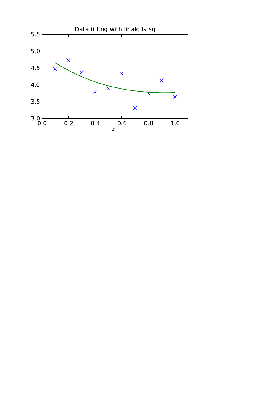
SciPy Reference Guide, Release 0.13.0
Generalized inverse
The generalized inverse is calculated using the command linalg.pinv or linalg.pinv2. These two commands
differ in how they compute the generalized inverse. The first uses the linalg.lstsq algorithm while the second uses
singular value decomposition. Let Abe an M×Nmatrix, then if M > N the generalized inverse is
A†=AHA−1AH
while if M < N matrix the generalized inverse is
A#=AHAAH−1.
In both cases for M=N, then
A†=A#=A−1
as long as Ais invertible.
1.9.3 Decompositions
In many applications it is useful to decompose a matrix using other representations. There are several decompositions
supported by SciPy.
Eigenvalues and eigenvectors
The eigenvalue-eigenvector problem is one of the most commonly employed linear algebra operations. In one popular
form, the eigenvalue-eigenvector problem is to find for some square matrix Ascalars λand corresponding vectors v
such that
Av =λv.
For an N×Nmatrix, there are N(not necessarily distinct) eigenvalues — roots of the (characteristic) polynomial
|A−λI|= 0.
The eigenvectors, v, are also sometimes called right eigenvectors to distinguish them from another set of left eigen-
vectors that satisfy
vH
LA=λvH
L
58 Chapter 1. SciPy Tutorial

SciPy Reference Guide, Release 0.13.0
or
AHvL=λ∗vL.
With it’s default optional arguments, the command linalg.eig returns λand v.However, it can also return vLand
just λby itself ( linalg.eigvals returns just λas well).
In addtion, linalg.eig can also solve the more general eigenvalue problem
Av =λBv
AHvL=λ∗BHvL
for square matrices Aand B.The standard eigenvalue problem is an example of the general eigenvalue problem for
B=I.When a generalized eigenvalue problem can be solved, then it provides a decomposition of Aas
A=BVΛV−1
where Vis the collection of eigenvectors into columns and Λis a diagonal matrix of eigenvalues.
By definition, eigenvectors are only defined up to a constant scale factor. In SciPy, the scaling factor for the eigenvec-
tors is chosen so that kvk2=Piv2
i= 1.
As an example, consider finding the eigenvalues and eigenvectors of the matrix
A=
152
241
362
.
The characteristic polynomial is
|A−λI|= (1 −λ) [(4 −λ) (2 −λ)−6] −
5 [2 (2 −λ)−3] + 2 [12 −3 (4 −λ)]
=−λ3+ 7λ2+ 8λ−3.
The roots of this polynomial are the eigenvalues of A:
λ1= 7.9579
λ2=−1.2577
λ3= 0.2997.
The eigenvectors corresponding to each eigenvalue can be found using the original equation. The eigenvectors associ-
ated with these eigenvalues can then be found.
>>> import numpy as np
>>> from scipy import linalg
>>> A=np.array([[1,2],[3,4]])
>>> la,v =linalg.eig(A)
>>> l1,l2 =la
>>> print l1, l2 #eigenvalues
(-0.372281323269+0j) (5.37228132327+0j)
>>> print v[:,0]#first eigenvector
[-0.82456484 0.56576746]
>>> print v[:,1]#second eigenvector
[-0.41597356 -0.90937671]
>>> print np.sum(abs(v**2),axis=0)#eigenvectors are unitary
[ 1. 1. ]
>>> v1 =np.array(v[:,0]).T
>>> print linalg.norm(A.dot(v1)-l1*v1) #check the computation
3.23682852457e-16
1.9. Linear Algebra (scipy.linalg) 59

SciPy Reference Guide, Release 0.13.0
Singular value decomposition
Singular Value Decompostion (SVD) can be thought of as an extension of the eigenvalue problem to matrices that are
not square. Let Abe an M×Nmatrix with Mand Narbitrary. The matrices AHAand AAHare square hermitian
matrices 2of size N×Nand M×Mrespectively. It is known that the eigenvalues of square hermitian matrices are
real and non-negative. In addtion, there are at most min (M, N)identical non-zero eigenvalues of AHAand AAH.
Define these positive eigenvalues as σ2
i.The square-root of these are called singular values of A.The eigenvectors of
AHAare collected by columns into an N×Nunitary 3matrix Vwhile the eigenvectors of AAHare collected by
columns in the unitary matrix U, the singular values are collected in an M×Nzero matrix Σwith main diagonal
entries set to the singular values. Then
A=UΣVH
is the singular-value decomposition of A.Every matrix has a singular value decomposition. Sometimes, the singular
values are called the spectrum of A.The command linalg.svd will return U,VH, and σias an array of the
singular values. To obtain the matrix Σuse linalg.diagsvd. The following example illustrates the use of
linalg.svd .
>>> import numpy as np
>>> from scipy import linalg
>>> A=np.array([[1,2,3],[4,5,6]])
>>> A
array([[1, 2, 3],
[4, 5, 6]])
>>> M,N =A.shape
>>> U,s,Vh =linalg.svd(A)
>>> Sig =linalg.diagsvd(s,M,N)
>>> U, Vh =U, Vh
>>> U
array([[-0.3863177 , -0.92236578],
[-0.92236578, 0.3863177 ]])
>>> Sig
array([[ 9.508032 , 0. , 0. ],
[ 0. , 0.77286964, 0. ]])
>>> Vh
array([[-0.42866713, -0.56630692, -0.7039467 ],
[ 0.80596391, 0.11238241, -0.58119908],
[ 0.40824829, -0.81649658, 0.40824829]])
>>> U.dot(Sig.dot(Vh)) #check computation
array([[ 1., 2., 3.],
[ 4., 5., 6.]])
LU decomposition
The LU decompostion finds a representation for the M×Nmatrix Aas
A=PLU
where Pis an M×Mpermutation matrix (a permutation of the rows of the identity matrix), Lis in M×Klower
triangular or trapezoidal matrix ( K= min (M, N)) with unit-diagonal, and Uis an upper triangular or trapezoidal
matrix. The SciPy command for this decomposition is linalg.lu .
Such a decomposition is often useful for solving many simultaneous equations where the left-hand-side does not
change but the right hand side does. For example, suppose we are going to solve
Axi=bi
2A hermitian matrix Dsatisfies DH=D.
3A unitary matrix Dsatisfies DHD=I=DDHso that D−1=DH
.
60 Chapter 1. SciPy Tutorial

SciPy Reference Guide, Release 0.13.0
for many different bi. The LU decomposition allows this to be written as
PLUxi=bi.
Because Lis lower-triangular, the equation can be solved for Uxiand finally xivery rapidly using forward- and
back-substitution. An initial time spent factoring Aallows for very rapid solution of similar systems of equa-
tions in the future. If the intent for performing LU decomposition is for solving linear systems then the command
linalg.lu_factor should be used followed by repeated applications of the command linalg.lu_solve to
solve the system for each new right-hand-side.
Cholesky decomposition
Cholesky decomposition is a special case of LU decomposition applicable to Hermitian positive definite matrices.
When A=AHand xHAx ≥0for all x, then decompositions of Acan be found so that
A=UHU
A=LLH
where Lis lower-triangular and Uis upper triangular. Notice that L=UH.The command linagl.cholesky
computes the cholesky factorization. For using cholesky factorization to solve systems of equations there are also
linalg.cho_factor and linalg.cho_solve routines that work similarly to their LU decomposition coun-
terparts.
QR decomposition
The QR decomposition (sometimes called a polar decomposition) works for any M×Narray and finds an M×M
unitary matrix Qand an M×Nupper-trapezoidal matrix Rsuch that
A=QR.
Notice that if the SVD of Ais known then the QR decomposition can be found
A=UΣVH=QR
implies that Q=Uand R=ΣVH.Note, however, that in SciPy independent algorithms are used to find QR and
SVD decompositions. The command for QR decomposition is linalg.qr .
Schur decomposition
For a square N×Nmatrix, A, the Schur decomposition finds (not-necessarily unique) matrices Tand Zsuch that
A=ZTZH
where Zis a unitary matrix and Tis either upper-triangular or quasi-upper triangular depending on whether or not a
real schur form or complex schur form is requested. For a real schur form both Tand Zare real-valued when Ais
real-valued. When Ais a real-valued matrix the real schur form is only quasi-upper triangular because 2×2blocks
extrude from the main diagonal corresponding to any complex- valued eigenvalues. The command linalg.schur
finds the Schur decomposition while the command linalg.rsf2csf converts Tand Zfrom a real Schur form to
a complex Schur form. The Schur form is especially useful in calculating functions of matrices.
The following example illustrates the schur decomposition:
1.9. Linear Algebra (scipy.linalg) 61

SciPy Reference Guide, Release 0.13.0
>>> from scipy import linalg
>>> A=mat(’[132;145;236]’)
>>> T,Z =linalg.schur(A)
>>> T1,Z1 =linalg.schur(A,’complex’)
>>> T2,Z2 =linalg.rsf2csf(T,Z)
>>> print T
[[ 9.90012467 1.78947961 -0.65498528]
[ 0. 0.54993766 -1.57754789]
[ 0. 0.51260928 0.54993766]]
>>> print T2
[[ 9.90012467 +0.00000000e+00j -0.32436598 +1.55463542e+00j
-0.88619748 +5.69027615e-01j]
[ 0.00000000 +0.00000000e+00j 0.54993766 +8.99258408e-01j
1.06493862 +1.37016050e-17j]
[ 0.00000000 +0.00000000e+00j 0.00000000 +0.00000000e+00j
0.54993766 -8.99258408e-01j]]
>>> print abs(T1-T2) # different
[[ 1.24357637e-14 2.09205364e+00 6.56028192e-01]
[ 0.00000000e+00 4.00296604e-16 1.83223097e+00]
[ 0.00000000e+00 0.00000000e+00 4.57756680e-16]]
>>> print abs(Z1-Z2) # different
[[ 0.06833781 1.10591375 0.23662249]
[ 0.11857169 0.5585604 0.29617525]
[ 0.12624999 0.75656818 0.22975038]]
>>> T,Z,T1,Z1,T2,Z2 =map(mat,(T,Z,T1,Z1,T2,Z2))
>>> print abs(A-Z*T*Z.H) # same
[[ 1.11022302e-16 4.44089210e-16 4.44089210e-16]
[ 4.44089210e-16 1.33226763e-15 8.88178420e-16]
[ 8.88178420e-16 4.44089210e-16 2.66453526e-15]]
>>> print abs(A-Z1*T1*Z1.H) # same
[[ 1.00043248e-15 2.22301403e-15 5.55749485e-15]
[ 2.88899660e-15 8.44927041e-15 9.77322008e-15]
[ 3.11291538e-15 1.15463228e-14 1.15464861e-14]]
>>> print abs(A-Z2*T2*Z2.H) # same
[[ 3.34058710e-16 8.88611201e-16 4.18773089e-18]
[ 1.48694940e-16 8.95109973e-16 8.92966151e-16]
[ 1.33228956e-15 1.33582317e-15 3.55373104e-15]]
Interpolative Decomposition
scipy.linalg.interpolative contains routines for computing the interpolative decomposition (ID) of a ma-
trix. For a matrix A∈Cm×nof rank k≤min{m, n}this is a factorization
AΠ = AΠ1AΠ2=AΠ1I T ,
where Π = [Π1,Π2]is a permutation matrix with Π1∈ {0,1}n×k, i.e., AΠ2=AΠ1T. This can equivalently be
written as A=BP , where B=AΠ1and P= [I, T ]ΠTare the skeleton and interpolation matrices, respectively.
See Also
scipy.linalg.interpolative — for more information.
62 Chapter 1. SciPy Tutorial

SciPy Reference Guide, Release 0.13.0
1.9.4 Matrix Functions
Consider the function f(x)with Taylor series expansion
f(x) = ∞
X
k=0
f(k)(0)
k!xk.
A matrix function can be defined using this Taylor series for the square matrix Aas
f(A) = ∞
X
k=0
f(k)(0)
k!Ak.
While, this serves as a useful representation of a matrix function, it is rarely the best way to calculate a matrix function.
Exponential and logarithm functions
The matrix exponential is one of the more common matrix functions. It can be defined for square matrices as
eA=∞
X
k=0
1
k!Ak.
The command linalg.expm3 uses this Taylor series definition to compute the matrix exponential. Due to poor
convergence properties it is not often used.
Another method to compute the matrix exponential is to find an eigenvalue decomposition of A:
A=VΛV−1
and note that
eA=VeΛV−1
where the matrix exponential of the diagonal matrix Λis just the exponential of its elements. This method is imple-
mented in linalg.expm2 .
The preferred method for implementing the matrix exponential is to use scaling and a Padé approximation for ex.
This algorithm is implemented as linalg.expm .
The inverse of the matrix exponential is the matrix logarithm defined as the inverse of the matrix exponential.
A≡exp (log (A)) .
The matrix logarithm can be obtained with linalg.logm .
Trigonometric functions
The trigonometric functions sin ,cos , and tan are implemented for matrices in linalg.sinm,linalg.cosm,
and linalg.tanm respectively. The matrix sin and cosine can be defined using Euler’s identity as
sin (A) = ejA−e−jA
2j
cos (A) = ejA+e−jA
2.
The tangent is
tan (x) = sin (x)
cos (x)= [cos (x)]−1sin (x)
and so the matrix tangent is defined as
[cos (A)]−1sin (A).
1.9. Linear Algebra (scipy.linalg) 63

SciPy Reference Guide, Release 0.13.0
Hyperbolic trigonometric functions
The hyperbolic trigonemetric functions sinh ,cosh , and tanh can also be defined for matrices using the familiar
definitions:
sinh (A) = eA−e−A
2
cosh (A) = eA+e−A
2
tanh (A) = [cosh (A)]−1sinh (A).
These matrix functions can be found using linalg.sinhm,linalg.coshm , and linalg.tanhm.
Arbitrary function
Finally, any arbitrary function that takes one complex number and returns a complex number can be called as a matrix
function using the command linalg.funm. This command takes the matrix and an arbitrary Python function. It
then implements an algorithm from Golub and Van Loan’s book “Matrix Computations “to compute function applied
to the matrix using a Schur decomposition. Note that the function needs to accept complex numbers as input in order
to work with this algorithm. For example the following code computes the zeroth-order Bessel function applied to a
matrix.
>>> from scipy import special, random, linalg
>>> A=random.rand(3,3)
>>> B=linalg.funm(A,lambda x: special.jv(0,x))
>>> print A
[[ 0.72578091 0.34105276 0.79570345]
[ 0.65767207 0.73855618 0.541453 ]
[ 0.78397086 0.68043507 0.4837898 ]]
>>> print B
[[ 0.72599893 -0.20545711 -0.22721101]
[-0.27426769 0.77255139 -0.23422637]
[-0.27612103 -0.21754832 0.7556849 ]]
>>> print linalg.eigvals(A)
[ 1.91262611+0.j 0.21846476+0.j -0.18296399+0.j]
>>> print special.jv(0, linalg.eigvals(A))
[ 0.27448286+0.j 0.98810383+0.j 0.99164854+0.j]
>>> print linalg.eigvals(B)
[ 0.27448286+0.j 0.98810383+0.j 0.99164854+0.j]
Note how, by virtue of how matrix analytic functions are defined, the Bessel function has acted on the matrix eigen-
values.
1.9.5 Special matrices
SciPy and NumPy provide several functions for creating special matrices that are frequently used in engineering and
science.
64 Chapter 1. SciPy Tutorial

SciPy Reference Guide, Release 0.13.0
Type Function Description
block diagonal scipy.linalg.block_diag Create a block diagonal matrix from the provided arrays.
circulant scipy.linalg.circulant Construct a circulant matrix.
companion scipy.linalg.companion Create a companion matrix.
Hadamard scipy.linalg.hadamard Construct a Hadamard matrix.
Hankel scipy.linalg.hankel Construct a Hankel matrix.
Hilbert scipy.linalg.hilbert Construct a Hilbert matrix.
Inverse Hilbert scipy.linalg.invhilbert Construct the inverse of a Hilbert matrix.
Leslie scipy.linalg.leslie Create a Leslie matrix.
Pascal scipy.linalg.pascal Create a Pascal matrix.
Toeplitz scipy.linalg.toeplitz Construct a Toeplitz matrix.
Van der Monde numpy.vander Generate a Van der Monde matrix.
For examples of the use of these functions, see their respective docstrings.
1.10 Sparse Eigenvalue Problems with ARPACK
1.10.1 Introduction
ARPACK is a Fortran package which provides routines for quickly finding a few eigenvalues/eigenvectors of large
sparse matrices. In order to find these solutions, it requires only left-multiplication by the matrix in question. This
operation is performed through a reverse-communication interface. The result of this structure is that ARPACK is able
to find eigenvalues and eigenvectors of any linear function mapping a vector to a vector.
All of the functionality provided in ARPACK is contained within the two high-level interfaces
scipy.sparse.linalg.eigs and scipy.sparse.linalg.eigsh.eigs provides interfaces to
find the eigenvalues/vectors of real or complex nonsymmetric square matrices, while eigsh provides interfaces for
real-symmetric or complex-hermitian matrices.
1.10.2 Basic Functionality
ARPACK can solve either standard eigenvalue problems of the form
Ax=λx
or general eigenvalue problems of the form
Ax=λMx
The power of ARPACK is that it can compute only a specified subset of eigenvalue/eigenvector pairs. This is accom-
plished through the keyword which. The following values of which are available:
•which = ’LM’ : Eigenvalues with largest magnitude (eigs,eigsh), that is, largest eigenvalues in the
euclidean norm of complex numbers.
•which = ’SM’ : Eigenvalues with smallest magnitude (eigs,eigsh), that is, smallest eigenvalues in the
euclidean norm of complex numbers.
•which = ’LR’ : Eigenvalues with largest real part (eigs)
•which = ’SR’ : Eigenvalues with smallest real part (eigs)
•which = ’LI’ : Eigenvalues with largest imaginary part (eigs)
1.10. Sparse Eigenvalue Problems with ARPACK 65

SciPy Reference Guide, Release 0.13.0
•which = ’SI’ : Eigenvalues with smallest imaginary part (eigs)
•which = ’LA’ : Eigenvalues with largest algebraic value (eigsh), that is, largest eigenvalues inclusive of
any negative sign.
•which = ’SA’ : Eigenvalues with smallest algebraic value (eigsh), that is, smallest eigenvalues inclusive
of any negative sign.
•which = ’BE’ : Eigenvalues from both ends of the spectrum (eigsh)
Note that ARPACK is generally better at finding extremal eigenvalues: that is, eigenvalues with large magnitudes. In
particular, using which = ’SM’ may lead to slow execution time and/or anomalous results. A better approach is to
use shift-invert mode.
1.10.3 Shift-Invert Mode
Shift invert mode relies on the following observation. For the generalized eigenvalue problem
Ax=λMx
it can be shown that
(A−σM)−1Mx=νx
where
ν=1
λ−σ
1.10.4 Examples
Imagine you’d like to find the smallest and largest eigenvalues and the corresponding eigenvectors for a
large matrix. ARPACK can handle many forms of input: dense matrices such as numpy.ndarray in-
stances, sparse matrices such as scipy.sparse.csr_matrix, or a general linear operator derived from
scipy.sparse.linalg.LinearOperator. For this example, for simplicity, we’ll construct a symmetric,
positive-definite matrix.
>>> import numpy as np
>>> from scipy.linalg import eigh
>>> from scipy.sparse.linalg import eigsh
>>> np.set_printoptions(suppress=True)
>>>
>>> np.random.seed(0)
>>> X=np.random.random((100,100)) -0.5
>>> X=np.dot(X, X.T) #create a symmetric matrix
We now have a symmetric matrix Xwith which to test the routines. First compute a standard eigenvalue decomposition
using eigh:
>>> evals_all, evecs_all =eigh(X)
As the dimension of Xgrows, this routine becomes very slow. Especially if only a few eigenvectors and eigenvalues
are needed, ARPACK can be a better option. First let’s compute the largest eigenvalues (which = ’LM’) of Xand
compare them to the known results:
66 Chapter 1. SciPy Tutorial

SciPy Reference Guide, Release 0.13.0
>>> evals_large, evecs_large =eigsh(X, 3, which=’LM’)
>>> print evals_all[-3:]
[ 29.1446102 30.05821805 31.19467646]
>>> print evals_large
[ 29.1446102 30.05821805 31.19467646]
>>> print np.dot(evecs_large.T, evecs_all[:,-3:])
[[-1. 0. 0.]
[ 0. 1. 0.]
[-0. 0. -1.]]
The results are as expected. ARPACK recovers the desired eigenvalues, and they match the previously known results.
Furthermore, the eigenvectors are orthogonal, as we’d expect. Now let’s attempt to solve for the eigenvalues with
smallest magnitude:
>>> evals_small, evecs_small =eigsh(X, 3, which=’SM’)
scipy.sparse.linalg.eigen.arpack.arpack.ArpackNoConvergence:
ARPACK error -1: No convergence (1001 iterations, 0/3 eigenvectors converged)
Oops. We see that as mentioned above, ARPACK is not quite as adept at finding small eigenvalues. There are a few
ways this problem can be addressed. We could increase the tolerance (tol) to lead to faster convergence:
>>> evals_small, evecs_small =eigsh(X, 3, which=’SM’, tol=1E-2)
>>> print evals_all[:3]
[ 0.0003783 0.00122714 0.00715878]
>>> print evals_small
[ 0.00037831 0.00122714 0.00715881]
>>> print np.dot(evecs_small.T, evecs_all[:,:3])
[[ 0.99999999 0.00000024 -0.00000049]
[-0.00000023 0.99999999 0.00000056]
[ 0.00000031 -0.00000037 0.99999852]]
This works, but we lose the precision in the results. Another option is to increase the maximum number of iterations
(maxiter) from 1000 to 5000:
>>> evals_small, evecs_small =eigsh(X, 3, which=’SM’, maxiter=5000)
>>> print evals_all[:3]
[ 0.0003783 0.00122714 0.00715878]
>>> print evals_small
[ 0.0003783 0.00122714 0.00715878]
>>> print np.dot(evecs_small.T, evecs_all[:,:3])
[[ 1. 0. 0.]
[-0. 1. 0.]
[ 0. 0. -1.]]
We get the results we’d hoped for, but the computation time is much longer. Fortunately, ARPACK contains a mode that
allows quick determination of non-external eigenvalues: shift-invert mode. As mentioned above, this mode involves
transforming the eigenvalue problem to an equivalent problem with different eigenvalues. In this case, we hope to find
eigenvalues near zero, so we’ll choose sigma = 0. The transformed eigenvalues will then satisfy ν= 1/(σ−λ) =
1/λ, so our small eigenvalues λbecome large eigenvalues ν.
>>> evals_small, evecs_small =eigsh(X, 3, sigma=0, which=’LM’)
>>> print evals_all[:3]
[ 0.0003783 0.00122714 0.00715878]
>>> print evals_small
[ 0.0003783 0.00122714 0.00715878]
>>> print np.dot(evecs_small.T, evecs_all[:,:3])
[[ 1. 0. 0.]
[ 0. -1. -0.]
[-0. -0. 1.]]
1.10. Sparse Eigenvalue Problems with ARPACK 67

SciPy Reference Guide, Release 0.13.0
We get the results we were hoping for, with much less computational time. Note that the transformation from ν→λ
takes place entirely in the background. The user need not worry about the details.
The shift-invert mode provides more than just a fast way to obtain a few small eigenvalues. Say you desire to find
internal eigenvalues and eigenvectors, e.g. those nearest to λ= 1. Simply set sigma = 1 and ARPACK takes care
of the rest:
>>> evals_mid, evecs_mid =eigsh(X, 3, sigma=1, which=’LM’)
>>> i_sort =np.argsort(abs(1. /(1-evals_all)))[-3:]
>>> print evals_all[i_sort]
[ 1.16577199 0.85081388 1.06642272]
>>> print evals_mid
[ 0.85081388 1.06642272 1.16577199]
>>> print np.dot(evecs_mid.T, evecs_all[:,i_sort])
[[-0. 1. 0.]
[-0. -0. 1.]
[ 1. 0. 0.]]
The eigenvalues come out in a different order, but they’re all there. Note that the shift-invert mode requires
the internal solution of a matrix inverse. This is taken care of automatically by eigsh and eigs, but the
operation can also be specified by the user. See the docstring of scipy.sparse.linalg.eigsh and
scipy.sparse.linalg.eigs for details.
1.10.5 References
1.11 Compressed Sparse Graph Routines scipy.sparse.csgraph
1.11.1 Example: Word Ladders
AWord Ladder is a word game invented by Lewis Carroll in which players find paths between words by switching
one letter at a time. For example, one can link “ape” and “man” in the following way:
ape →apt →ait →bit →big →bag →mag →man
Note that each step involves changing just one letter of the word. This is just one possible path from “ape” to “man”,
but is it the shortest possible path? If we desire to find the shortest word ladder path between two given words, the
sparse graph submodule can help.
First we need a list of valid words. Many operating systems have such a list built-in. For example, on linux, a word
list can often be found at one of the following locations:
/usr/share/dict
/var/lib/dict
Another easy source for words are the scrabble word lists available at various sites around the internet (search with
your favorite search engine). We’ll first create this list. The system word lists consist of a file with one word per line.
The following should be modified to use the particular word list you have available:
>>> word_list =open(’/usr/share/dict/words’).readlines()
>>> word_list =map(str.strip, word_list)
We want to look at words of length 3, so let’s select just those words of the correct length. We’ll also eliminate words
which start with upper-case (proper nouns) or contain non alpha-numeric characters like apostrophes and hyphens.
Finally, we’ll make sure everything is lower-case for comparison later:
68 Chapter 1. SciPy Tutorial

SciPy Reference Guide, Release 0.13.0
>>> word_list =[word for word in word_list if len(word) == 3]
>>> word_list =[word for word in word_list if word[0].islower()]
>>> word_list =[word for word in word_list if word.isalpha()]
>>> word_list =map(str.lower, word_list)
>>> len(word_list)
586
Now we have a list of 586 valid three-letter words (the exact number may change depending on the particular list
used). Each of these words will become a node in our graph, and we will create edges connecting the nodes associated
with each pair of words which differs by only one letter.
There are efficient ways to do this, and inefficient ways to do this. To do this as efficiently as possible, we’re going to
use some sophisticated numpy array manipulation:
>>> import numpy as np
>>> word_list =np.asarray(word_list)
>>> word_list.dtype
dtype(’|S3’)
>>> word_list.sort() # sort for quick searching later
We have an array where each entry is three bytes. We’d like to find all pairs where exactly one byte is different. We’ll
start by converting each word to a three-dimensional vector:
>>> word_bytes =np.ndarray((word_list.size, word_list.itemsize),
... dtype=’int8’,
... buffer=word_list.data)
>>> word_bytes.shape
(586, 3)
Now we’ll use the Hamming distance between each point to determine which pairs of words are connected. The
Hamming distance measures the fraction of entries between two vectors which differ: any two words with a hamming
distance equal to 1/N, where Nis the number of letters, are connected in the word ladder:
>>> from scipy.spatial.distance import pdist, squareform
>>> from scipy.sparse import csr_matrix
>>> hamming_dist =pdist(word_bytes, metric=’hamming’)
>>> graph =csr_matrix(squareform(hamming_dist <1.5 /word_list.itemsize))
When comparing the distances, we don’t use an equality because this can be unstable for floating point values. The
inequality produces the desired result as long as no two entries of the word list are identical. Now that our graph is set
up, we’ll use a shortest path search to find the path between any two words in the graph:
>>> i1 =word_list.searchsorted(’ape’)
>>> i2 =word_list.searchsorted(’man’)
>>> word_list[i1]
’ape’
>>> word_list[i2]
’man’
We need to check that these match, because if the words are not in the list that will not be the case. Now all we need
is to find the shortest path between these two indices in the graph. We’ll use dijkstra’s algorithm, because it allows us
to find the path for just one node:
>>> from scipy.sparse.csgraph import dijkstra
>>> distances, predecessors =dijkstra(graph, indices=i1,
... return_predecessors=True)
>>> print distances[i2]
5.0
1.11. Compressed Sparse Graph Routines scipy.sparse.csgraph 69

SciPy Reference Guide, Release 0.13.0
So we see that the shortest path between ‘ape’ and ‘man’ contains only five steps. We can use the predecessors returned
by the algorithm to reconstruct this path:
>>> path =[]
>>> i=i2
>>> while i!= i1:
>>> path.append(word_list[i])
>>> i=predecessors[i]
>>> path.append(word_list[i1])
>>> print path[::-1]
[’ape’, ’apt’, ’opt’, ’oat’, ’mat’, ’man’]
This is three fewer links than our initial example: the path from ape to man is only five steps.
Using other tools in the module, we can answer other questions. For example, are there three-letter words which are
not linked in a word ladder? This is a question of connected components in the graph:
>>> from scipy.sparse.csgraph import connected_components
>>> N_components, component_list =connected_components(graph)
>>> print N_components
15
In this particular sample of three-letter words, there are 15 connected components: that is, 15 distinct sets of words with
no paths between the sets. How many words are in each of these sets? We can learn this from the list of components:
>>> [np.sum(component_list == i) for iin range(15)]
[571, 1, 1, 1, 2, 1, 1, 1, 1, 1, 1, 1, 1, 1, 1]
There is one large connected set, and 14 smaller ones. Let’s look at the words in the smaller ones:
>>> [list(word_list[np.where(component_list == i)]) for iin range(1,15)]
[[’aha’],
[’chi’],
[’ebb’],
[’ems’, ’emu’],
[’gnu’],
[’ism’],
[’khz’],
[’nth’],
[’ova’],
[’qua’],
[’ugh’],
[’ups’],
[’urn’],
[’use’]]
These are all the three-letter words which do not connect to others via a word ladder.
We might also be curious about which words are maximally separated. Which two words take the most links to
connect? We can determine this by computing the matrix of all shortest paths. Note that by convention, the distance
between two non-connected points is reported to be infinity, so we’ll need to remove these before finding the maximum:
>>> distances, predecessors =dijkstra(graph, return_predecessors=True)
>>> np.max(distances[~np.isinf(distances)])
13.0
So there is at least one pair of words which takes 13 steps to get from one to the other! Let’s determine which these
are:
>>> i1, i2 =np.where(distances == 13)
>>> zip(word_list[i1], word_list[i2])
70 Chapter 1. SciPy Tutorial

SciPy Reference Guide, Release 0.13.0
[(’imp’, ’ohm’),
(’imp’, ’ohs’),
(’ohm’, ’imp’),
(’ohm’, ’ump’),
(’ohs’, ’imp’),
(’ohs’, ’ump’),
(’ump’, ’ohm’),
(’ump’, ’ohs’)]
We see that there are two pairs of words which are maximally separated from each other: ‘imp’ and ‘ump’ on one
hand, and ‘ohm’ and ‘ohs’ on the other hand. We can find the connecting list in the same way as above:
>>> path =[]
>>> i=i2[0]
>>> while i!= i1[0]:
>>> path.append(word_list[i])
>>> i=predecessors[i1[0], i]
>>> path.append(word_list[i1[0]])
>>> print path[::-1]
[’imp’, ’amp’, ’asp’, ’ask’, ’ark’, ’are’, ’aye’, ’rye’, ’roe’, ’woe’, ’woo’, ’who’, ’oho’, ’ohm’]
This gives us the path we desired to see.
Word ladders are just one potential application of scipy’s fast graph algorithms for sparse matrices. Graph theory
makes appearances in many areas of mathematics, data analysis, and machine learning. The sparse graph tools are
flexible enough to handle many of these situations.
1.12 Spatial data structures and algorithms (scipy.spatial)
scipy.spatial can compute triangulations, Voronoi diagrams, and convex hulls of a set of points, by leveraging
the Qhull library.
Moreover, it contains KDTree implementations for nearest-neighbor point queries, and utilities for distance compu-
tations in various metrics.
1.12.1 Delaunay triangulations
The Delaunay triangulation is a subdivision of a set of points into a non-overlapping set of triangles, such that no point
is inside the circumcircle of any triangle. In practice, such triangulations tend to avoid triangles with small angles.
Delaunay triangulation can be computed using scipy.spatial as follows:
>>> from scipy.spatial import Delaunay
>>> points =np.array([[0,0], [0,1.1], [1,0], [1,1]])
>>> tri =Delaunay(points)
We can visualize it:
>>> import matplotlib.pyplot as plt
>>> plt.triplot(points[:,0], points[:,1], tri.simplices.copy())
>>> plt.plot(points[:,0], points[:,1], ’o’)
And add some further decorations:
>>> for j, p in enumerate(points):
... plt.text(p[0]-0.03, p[1]+0.03, j, ha=’right’)# label the points
1.12. Spatial data structures and algorithms (scipy.spatial) 71
SciPy Reference Guide, Release 0.13.0
>>> for j, s in enumerate(tri.simplices):
... p=points[s].mean(axis=0)
... plt.text(p[0], p[1], ’#%d’%j, ha=’center’)# label triangles
>>> plt.xlim(-0.5,1.5); plt.ylim(-0.5,1.5)
>>> plt.show()
The structure of the triangulation is encoded in the following way: the simplices attribute contains the indices of
the points in the points array that make up the triangle. For instance:
>>> i=1
>>> tri.simplices[i,:]
array([3, 1, 0], dtype=int32)
>>> points[tri.simplices[i,:]]
array([[ 1. , 1. ],
[ 0. , 1.1],
[ 0. , 0. ]])
Moreover, neighboring triangles can also be found out:
>>> tri.neighbors[i]
array([-1, 0, -1], dtype=int32)
What this tells us is that this triangle has triangle #0 as a neighbor, but no other neighbors. Moreover, it tells us that
neighbor 0 is opposite the vertex 1 of the triangle:
>>> points[tri.simplices[i, 1]]
array([ 0. , 1.1])
Indeed, from the figure we see that this is the case.
Qhull can also perform tesselations to simplices also for higher-dimensional point sets (for instance, subdivision into
tetrahedra in 3-D).
Coplanar points
It is important to note that not all points necessarily appear as vertices of the triangulation, due to numerical precision
issues in forming the triangulation. Consider the above with a duplicated point:
72 Chapter 1. SciPy Tutorial

SciPy Reference Guide, Release 0.13.0
>>> points =np.array([[0,0], [0,1], [1,0], [1,1], [1,1]])
>>> tri =Delaunay(points)
>>> np.unique(tri.simplices.ravel())
array([0, 1, 2, 3], dtype=int32)
Observe that point #4, which is a duplicate, does not occur as a vertex of the triangulation. That this happened is
recorded:
>>> tri.coplanar
array([[4, 0, 3]], dtype=int32)
This means that point 4 resides near triangle 0 and vertex 3, but is not included in the triangulation.
Note that such degeneracies can occur not only because of duplicated points, but also for more complicated geometrical
reasons, even in point sets that at first sight seem well-behaved.
However, Qhull has the “QJ” option, which instructs it to perturb the input data randomly until degeneracies are
resolved:
>>> tri =Delaunay(points, qhull_options="QJ Pp")
>>> points[tri.simplices]
array([[[1, 1],
[1, 0],
[0, 0]],
[[1, 1],
[1, 1],
[1, 0]],
[[0, 1],
[1, 1],
[0, 0]],
[[0, 1],
[1, 1],
[1, 1]]])
Two new triangles appeared. However, we see that they are degenerate and have zero area.
1.12.2 Convex hulls
Convex hull is the smallest convex object containing all points in a given point set.
These can be computed via the Qhull wrappers in scipy.spatial as follows:
>>> from scipy.spatial import ConvexHull
>>> points =np.random.rand(30,2)# 30 random points in 2-D
>>> hull =ConvexHull(points)
The convex hull is represented as a set of N-1 dimensional simplices, which in 2-D means line segments. The storage
scheme is exactly the same as for the simplices in the Delaunay triangulation discussed above.
We can illustrate the above result:
>>> import matplotlib.pyplot as plt
>>> plt.plot(points[:,0], points[:,1], ’o’)
>>> for simplex in hull.simplices:
>>> plt.plot(points[simplex,0], points[simplex,1], ’k-’)
>>> plt.show()
1.12. Spatial data structures and algorithms (scipy.spatial) 73
SciPy Reference Guide, Release 0.13.0
The same can be achieved with scipy.spatial.convex_hull_plot_2d.
1.12.3 Voronoi diagrams
A Voronoi diagram is a subdivision of the space into the nearest neighborhoods of a given set of points.
There are two ways to approach this object using scipy.spatial. First, one can use the KDTree to answer the
question “which of the points is closest to this one”, and define the regions that way:
>>> from scipy.spatial import KDTree
>>> points =np.array([[0,0], [0,1], [0,2], [1,0], [1,1], [1,2],
... [2,0], [2,1], [2,2]])
>>> tree =KDTree(points)
>>> tree.query([0.1,0.1])
(0.14142135623730953, 0)
So the point (0.1, 0.1) belongs to region 0. In color:
>>> x=np.linspace(-0.5,2.5,31)
>>> y=np.linspace(-0.5,2.5,33)
>>> xx, yy =np.meshgrid(x, y)
>>> xy =np.c_[xx.ravel(), yy.ravel()]
>>> import matplotlib.pyplot as plt
>>> plt.pcolor(x, y, tree.query(xy)[1].reshape(33,31))
>>> plt.plot(points[:,0], points[:,1], ’ko’)
>>> plt.show()
74 Chapter 1. SciPy Tutorial
SciPy Reference Guide, Release 0.13.0
This does not, however, give the Voronoi diagram as a geometrical object.
The representation in terms of lines and points can be again obtained via the Qhull wrappers in scipy.spatial:
>>> from scipy.spatial import Voronoi
>>> vor =Voronoi(points)
>>> vor.vertices
array([[ 0.5, 0.5],
[ 1.5, 0.5],
[ 0.5, 1.5],
[ 1.5, 1.5]])
The Voronoi vertices denote the set of points forming the polygonal edges of the Voronoi regions. In this case, there
are 9 different regions:
>>> vor.regions
[[-1, 0], [-1, 1], [1, -1, 0], [3, -1, 2], [-1, 3], [-1, 2], [3, 1, 0, 2], [2, -1, 0], [3, -1, 1]]
Negative value -1 again indicates a point at infinity. Indeed, only one of the regions, [3, 1, 0, 2], is bounded.
Note here that due to similar numerical precision issues as in Delaunay triangulation above, there may be fewer
Voronoi regions than input points.
The ridges (lines in 2-D) separating the regions are described as a similar collection of simplices as the convex hull
pieces:
>>> vor.ridge_vertices
[[-1, 0], [-1, 0], [-1, 1], [-1, 1], [0, 1], [-1, 3], [-1, 2], [2, 3], [-1, 3], [-1, 2], [0, 2], [1, 3]]
These numbers indicate indices of the Voronoi vertices making up the line segments. -1 is again a point at infinity —
only four of the 12 lines is a bounded line segment while the others extend to infinity.
The Voronoi ridges are perpendicular to lines drawn between the input points. Which two points each ridge corre-
sponds to is also recorded:
>>> vor.ridge_points
array([[0, 3],
[0, 1],
[6, 3],
[6, 7],
[3, 4],
1.12. Spatial data structures and algorithms (scipy.spatial) 75
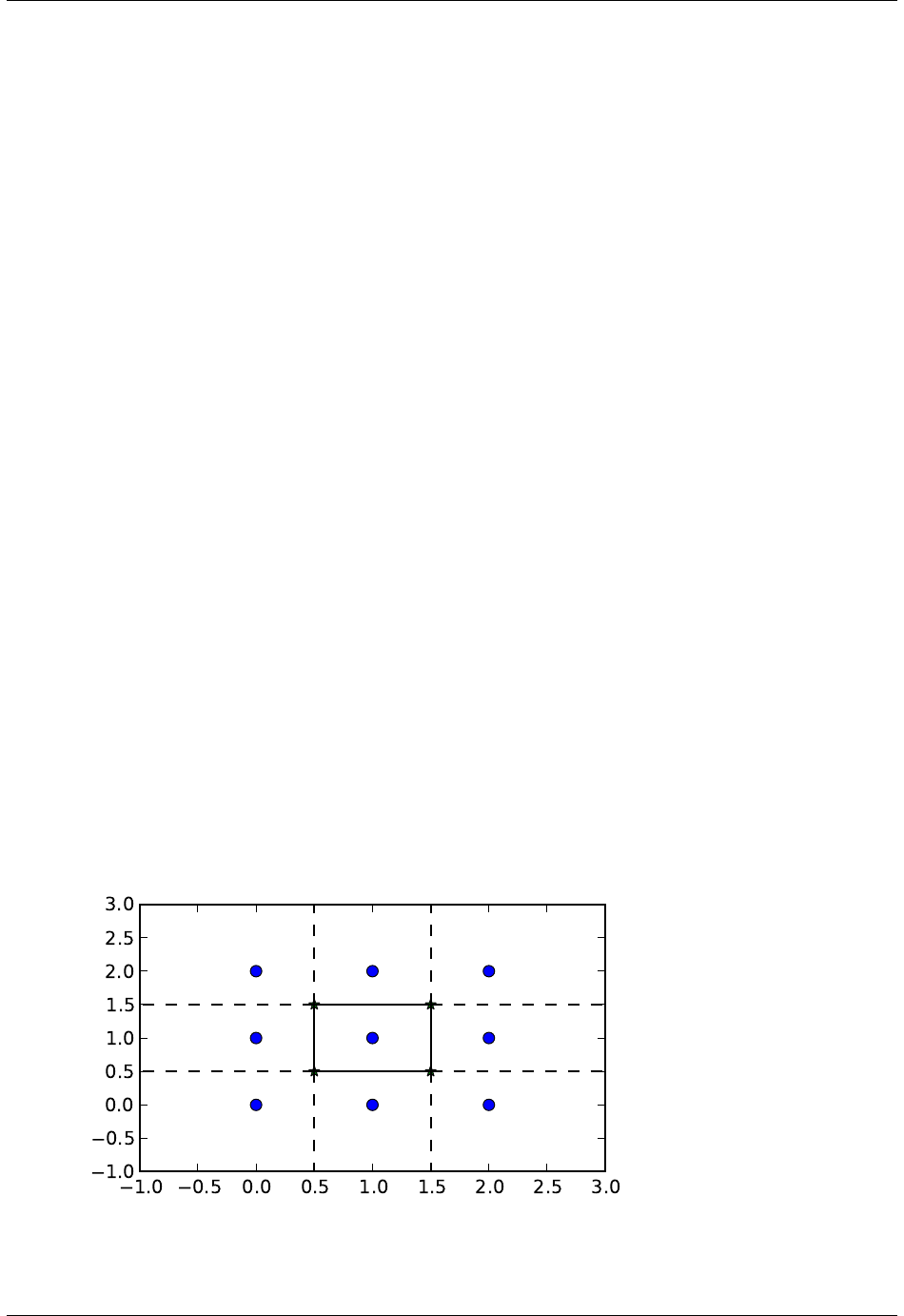
SciPy Reference Guide, Release 0.13.0
[5, 8],
[5, 2],
[5, 4],
[8, 7],
[2, 1],
[4, 1],
[4, 7]], dtype=int32)
This information, taken together, is enough to construct the full diagram.
We can plot it as follows. First the points and the Voronoi vertices:
>>> plt.plot(points[:,0], points[:,1], ’o’)
>>> plt.plot(vor.vertices[:,0], vor.vertices[:,1], ’*’)
>>> plt.xlim(-1,3); plt.ylim(-1,3)
Plotting the finite line segments goes as for the convex hull, but now we have to guard for the infinite edges:
>>> for simplex in vor.ridge_vertices:
>>> simplex =np.asarray(simplex)
>>> if np.all(simplex >= 0):
>>> plt.plot(vor.vertices[simplex,0], vor.vertices[simplex,1], ’k-’)
The ridges extending to infinity require a bit more care:
>>> center =points.mean(axis=0)
>>> for pointidx, simplex in zip(vor.ridge_points, vor.ridge_vertices):
>>> simplex =np.asarray(simplex)
>>> if np.any(simplex <0):
>>> i=simplex[simplex >= 0][0]# finite end Voronoi vertex
>>> t=points[pointidx[1]] -points[pointidx[0]] # tangent
>>> t/= np.linalg.norm(t)
>>> n=np.array([-t[1], t[0]]) # normal
>>> midpoint =points[pointidx].mean(axis=0)
>>> far_point =vor.vertices[i] +np.sign(np.dot(midpoint -center, n)) *n*100
>>> plt.plot([vor.vertices[i,0], far_point[0]],
... [vor.vertices[i,1], far_point[1]], ’k--’)
>>> plt.show()
76 Chapter 1. SciPy Tutorial

SciPy Reference Guide, Release 0.13.0
This plot can also be created using scipy.spatial.voronoi_plot_2d.
1.13 Statistics (scipy.stats)
1.13.1 Introduction
In this tutorial we discuss many, but certainly not all, features of scipy.stats. The intention here is to provide a
user with a working knowledge of this package. We refer to the reference manual for further details.
Note: This documentation is work in progress.
1.13.2 Random Variables
There are two general distribution classes that have been implemented for encapsulating continuous random variables
and discrete random variables . Over 80 continuous random variables (RVs) and 10 discrete random variables have
been implemented using these classes. Besides this, new routines and distributions can easily added by the end user.
(If you create one, please contribute it).
All of the statistics functions are located in the sub-package scipy.stats and a fairly complete listing of these
functions can be obtained using info(stats). The list of the random variables available can also be obtained from
the docstring for the stats sub-package.
In the discussion below we mostly focus on continuous RVs. Nearly all applies to discrete variables also, but we point
out some differences here: Specific Points for Discrete Distributions.
Getting Help
First of all, all distributions are accompanied with help functions. To obtain just some basic information we can call
>>> from scipy import stats
>>> from scipy.stats import norm
>>> print norm.__doc__
To find the support, i.e., upper and lower bound of the distribution, call:
>>> print ’bounds of distribution lower: %s, upper: %s’%(norm.a,norm.b)
bounds of distribution lower: -inf, upper: inf
We can list all methods and properties of the distribution with dir(norm). As it turns out, some of the methods
are private methods although they are not named as such (their name does not start with a leading underscore), for
example veccdf, are only available for internal calculation.
To obtain the real main methods, we list the methods of the frozen distribution. (We explain the meaning of a frozen
distribution below).
>>> rv =norm()
>>> dir(rv) #reformatted
[’__class__’, ’__delattr__’, ’__dict__’, ’__doc__’, ’__getattribute__’,
’__hash__’, ’__init__’, ’__module__’, ’__new__’, ’__reduce__’, ’__reduce_ex__’,
’__repr__’, ’__setattr__’, ’__str__’, ’__weakref__’, ’args’, ’cdf’, ’dist’,
’entropy’, ’isf’, ’kwds’, ’moment’, ’pdf’, ’pmf’, ’ppf’, ’rvs’, ’sf’, ’stats’]
Finally, we can obtain the list of available distribution through introspection:
1.13. Statistics (scipy.stats) 77

SciPy Reference Guide, Release 0.13.0
>>> import warnings
>>> warnings.simplefilter(’ignore’,DeprecationWarning)
>>> dist_continu =[d for din dir(stats) if
... isinstance(getattr(stats,d), stats.rv_continuous)]
>>> dist_discrete =[d for din dir(stats) if
... isinstance(getattr(stats,d), stats.rv_discrete)]
>>> print ’number of continuous distributions:’,len(dist_continu)
number of continuous distributions: 84
>>> print ’number of discrete distributions: ’,len(dist_discrete)
number of discrete distributions: 12
Common Methods
The main public methods for continuous RVs are:
• rvs: Random Variates
• pdf: Probability Density Function
• cdf: Cumulative Distribution Function
• sf: Survival Function (1-CDF)
• ppf: Percent Point Function (Inverse of CDF)
• isf: Inverse Survival Function (Inverse of SF)
• stats: Return mean, variance, (Fisher’s) skew, or (Fisher’s) kurtosis
• moment: non-central moments of the distribution
Let’s take a normal RV as an example.
>>> norm.cdf(0)
0.5
To compute the cdf at a number of points, we can pass a list or a numpy array.
>>> norm.cdf([-1.,0,1])
array([ 0.15865525, 0.5 , 0.84134475])
>>> import numpy as np
>>> norm.cdf(np.array([-1.,0,1]))
array([ 0.15865525, 0.5 , 0.84134475])
Thus, the basic methods such as pdf,cdf, and so on are vectorized with np.vectorize.
Other generally useful methods are supported too:
>>> norm.mean(), norm.std(), norm.var()
(0.0, 1.0, 1.0)
>>> norm.stats(moments ="mv")
(array(0.0), array(1.0))
To find the median of a distribution we can use the percent point function ppf, which is the inverse of the cdf:
>>> norm.ppf(0.5)
0.0
To generate a set of random variates:
>>> norm.rvs(size=5)
array([-0.35687759, 1.34347647, -0.11710531, -1.00725181, -0.51275702])
78 Chapter 1. SciPy Tutorial

SciPy Reference Guide, Release 0.13.0
Don’t think that norm.rvs(5) generates 5 variates:
>>> norm.rvs(5)
7.131624370075814
This brings us, in fact, to the topic of the next subsection.
Shifting and Scaling
All continuous distributions take loc and scale as keyword parameters to adjust the location and scale of the
distribution, e.g. for the standard normal distribution the location is the mean and the scale is the standard deviation.
>>> norm.stats(loc =3, scale =4, moments ="mv")
(array(3.0), array(16.0))
In general the standardized distribution for a random variable Xis obtained through the transformation (X - loc)
/ scale. The default values are loc = 0 and scale = 1.
Smart use of loc and scale can help modify the standard distributions in many ways. To illustrate the scaling
further, the cdf of an exponentially distributed RV with mean 1/λ is given by
F(x) = 1 −exp(−λx)
By applying the scaling rule above, it can be seen that by taking scale = 1./lambda we get the proper scale.
>>> from scipy.stats import expon
>>> expon.mean(scale =3.)
3.0
The uniform distribution is also interesting:
>>> from scipy.stats import uniform
>>> uniform.cdf([0,1,2,3,4,5], loc =1, scale =4)
array([ 0. , 0. , 0.25, 0.5 , 0.75, 1. ])
Finally, recall from the previous paragraph that we are left with the problem of the meaning of norm.rvs(5). As it
turns out, calling a distribution like this, the first argument, i.e., the 5, gets passed to set the loc parameter. Let’s see:
>>> np.mean(norm.rvs(5, size=500))
4.983550784784704
Thus, to explain the output of the example of the last section: norm.rvs(5)‘ generates a normally
distributed random variate with mean ‘‘loc=5.
I prefer to set the loc and scale parameter explicitly, by passing the values as keywords rather than as arguments.
This is less of a hassle as it may seem. We clarify this below when we explain the topic of freezing a RV.
Shape Parameters
While a general continuous random variable can be shifted and scaled with the loc and scale parameters, some
distributions require additional shape parameters. For instance, the gamma distribution, with density
γ(x, n) = λ(λx)n−1
Γ(n)e−λx ,
requires the shape parameter n. Observe that setting λcan be obtained by setting the scale keyword to 1/λ.
Let’s check the number and name of the shape parameters of the gamma distribution. (We know from the above that
this should be 1.)
1.13. Statistics (scipy.stats) 79

SciPy Reference Guide, Release 0.13.0
>>> from scipy.stats import gamma
>>> gamma.numargs
1
>>> gamma.shapes
’a’
Now we set the value of the shape variable to 1 to obtain the exponential distribution, so that we compare easily
whether we get the results we expect.
>>> gamma(1, scale=2.).stats(moments="mv")
(array(2.0), array(4.0))
Notice that we can also specify shape parameters as keywords:
>>> gamma(a=1, scale=2.).stats(moments="mv")
(array(2.0), array(4.0))
Freezing a Distribution
Passing the loc and scale keywords time and again can become quite bothersome. The concept of freezing a RV is
used to solve such problems.
>>> rv =gamma(1, scale=2.)
By using rv we no longer have to include the scale or the shape parameters anymore. Thus, distributions can be used
in one of two ways, either by passing all distribution parameters to each method call (such as we did earlier) or by
freezing the parameters for the instance of the distribution. Let us check this:
>>> rv.mean(), rv.std()
(2.0, 2.0)
This is indeed what we should get.
Broadcasting
The basic methods pdf and so on satisfy the usual numpy broadcasting rules. For example, we can calculate the
critical values for the upper tail of the t distribution for different probabilites and degrees of freedom.
>>> stats.t.isf([0.1,0.05,0.01], [[10], [11]])
array([[ 1.37218364, 1.81246112, 2.76376946],
[ 1.36343032, 1.79588482, 2.71807918]])
Here, the first row are the critical values for 10 degrees of freedom and the second row for 11 degrees of freedom
(d.o.f.). Thus, the broadcasting rules give the same result of calling isf twice:
>>> stats.t.isf([0.1,0.05,0.01], 10)
array([ 1.37218364, 1.81246112, 2.76376946])
>>> stats.t.isf([0.1,0.05,0.01], 11)
array([ 1.36343032, 1.79588482, 2.71807918])
If the array with probabilities, i.e, [0.1, 0.05, 0.01] and the array of degrees of freedom i.e., [10, 11,
12], have the same array shape, then element wise matching is used. As an example, we can obtain the 10% tail for
10 d.o.f., the 5% tail for 11 d.o.f. and the 1% tail for 12 d.o.f. by calling
>>> stats.t.isf([0.1,0.05,0.01], [10,11,12])
array([ 1.37218364, 1.79588482, 2.68099799])
80 Chapter 1. SciPy Tutorial

SciPy Reference Guide, Release 0.13.0
Specific Points for Discrete Distributions
Discrete distribution have mostly the same basic methods as the continuous distributions. However pdf is replaced
the probability mass function pmf, no estimation methods, such as fit, are available, and scale is not a valid keyword
parameter. The location parameter, keyword loc can still be used to shift the distribution.
The computation of the cdf requires some extra attention. In the case of continuous distribution the cumulative distri-
bution function is in most standard cases strictly monotonic increasing in the bounds (a,b) and has therefore a unique
inverse. The cdf of a discrete distribution, however, is a step function, hence the inverse cdf, i.e., the percent point
function, requires a different definition:
ppf(q) = min{x : cdf(x) >= q, x integer}
For further info, see the docs here.
We can look at the hypergeometric distribution as an example
>>> from scipy.stats import hypergeom
>>> [M, n, N] =[20,7,12]
If we use the cdf at some integer points and then evaluate the ppf at those cdf values, we get the initial integers back,
for example
>>> x=np.arange(4)*2
>>> x
array([0, 2, 4, 6])
>>> prb =hypergeom.cdf(x, M, n, N)
>>> prb
array([ 0.0001031991744066, 0.0521155830753351, 0.6083591331269301,
0.9897832817337386])
>>> hypergeom.ppf(prb, M, n, N)
array([ 0., 2., 4., 6.])
If we use values that are not at the kinks of the cdf step function, we get the next higher integer back:
>>> hypergeom.ppf(prb+1e-8, M, n, N)
array([ 1., 3., 5., 7.])
>>> hypergeom.ppf(prb-1e-8, M, n, N)
array([ 0., 2., 4., 6.])
Fitting Distributions
The main additional methods of the not frozen distribution are related to the estimation of distribution parameters:
•fit: maximum likelihood estimation of distribution parameters, including location
and scale
• fit_loc_scale: estimation of location and scale when shape parameters are given
• nnlf: negative log likelihood function
• expect: Calculate the expectation of a function against the pdf or pmf
Performance Issues and Cautionary Remarks
The performance of the individual methods, in terms of speed, varies widely by distribution and method. The results of
a method are obtained in one of two ways: either by explicit calculation, or by a generic algorithm that is independent
of the specific distribution.
1.13. Statistics (scipy.stats) 81

SciPy Reference Guide, Release 0.13.0
Explicit calculation, on the one hand, requires that the method is directly specified for the given distribution, either
through analytic formulas or through special functions in scipy.special or numpy.random for rvs. These are
usually relatively fast calculations.
The generic methods, on the other hand, are used if the distribution does not specify any explicit calcula-
tion. To define a distribution, only one of pdf or cdf is necessary; all other methods can be derived using nu-
meric integration and root finding. However, these indirect methods can be very slow. As an example, rgh =
stats.gausshyper.rvs(0.5, 2, 2, 2, size=100) creates random variables in a very indirect way and
takes about 19 seconds for 100 random variables on my computer, while one million random variables from the
standard normal or from the t distribution take just above one second.
Remaining Issues
The distributions in scipy.stats have recently been corrected and improved and gained a considerable test suite,
however a few issues remain:
• skew and kurtosis, 3rd and 4th moments and entropy are not thoroughly tested and some coarse testing indicates
that there are still some incorrect results left.
• the distributions have been tested over some range of parameters, however in some corner ranges, a few incorrect
results may remain.
• the maximum likelihood estimation in fit does not work with default starting parameters for all distributions
and the user needs to supply good starting parameters. Also, for some distribution using a maximum likelihood
estimator might inherently not be the best choice.
1.13.3 Building Specific Distributions
The next examples shows how to build your own distributions. Further examples show the usage of the distributions
and some statistical tests.
Making a Continuous Distribution, i.e., Subclassing rv_continuous
Making continuous distributions is fairly simple.
>>> from scipy import stats
>>> class deterministic_gen(stats.rv_continuous):
... def _cdf(self, x ):
... return np.where(x<0,0.,1.)
... def _stats(self):
... return 0.,0.,0.,0.
>>> deterministic =deterministic_gen(name="deterministic")
>>> deterministic.cdf(np.arange(-3,3,0.5))
array([ 0., 0., 0., 0., 0., 0., 1., 1., 1., 1., 1., 1.])
Interestingly, the pdf is now computed automatically:
>>> deterministic.pdf(np.arange(-3,3,0.5))
array([ 0.00000000e+00, 0.00000000e+00, 0.00000000e+00,
0.00000000e+00, 0.00000000e+00, 0.00000000e+00,
5.83333333e+04, 4.16333634e-12, 4.16333634e-12,
4.16333634e-12, 4.16333634e-12, 4.16333634e-12])
82 Chapter 1. SciPy Tutorial

SciPy Reference Guide, Release 0.13.0
Be aware of the performance issues mentions in Performance Issues and Cautionary Remarks. The computation of
unspecified common methods can become very slow, since only general methods are called which, by their very nature,
cannot use any specific information about the distribution. Thus, as a cautionary example:
>>> from scipy.integrate import quad
>>> quad(deterministic.pdf, -1e-1,1e-1)
(4.163336342344337e-13, 0.0)
But this is not correct: the integral over this pdf should be 1. Let’s make the integration interval smaller:
>>> quad(deterministic.pdf, -1e-3,1e-3)# warning removed
(1.000076872229173, 0.0010625571718182458)
This looks better. However, the problem originated from the fact that the pdf is not specified in the class definition of
the deterministic distribution.
Subclassing rv_discrete
In the following we use stats.rv_discrete to generate a discrete distribution that has the probabilities of the
truncated normal for the intervals centered around the integers.
General Info
From the docstring of rv_discrete, i.e.,
>>> from scipy.stats import rv_discrete
>>> help(rv_discrete)
we learn that:
“You can construct an aribtrary discrete rv where P{X=xk} = pk by passing to the rv_discrete initialization
method (through the values= keyword) a tuple of sequences (xk, pk) which describes only those values of X
(xk) that occur with nonzero probability (pk).”
Next to this, there are some further requirements for this approach to work:
• The keyword name is required.
• The support points of the distribution xk have to be integers.
• The number of significant digits (decimals) needs to be specified.
In fact, if the last two requirements are not satisfied an exception may be raised or the resulting numbers may be
incorrect.
An Example
Let’s do the work. First
>>> npoints =20 # number of integer support points of the distribution minus 1
>>> npointsh =npoints /2
>>> npointsf =float(npoints)
>>> nbound =4# bounds for the truncated normal
>>> normbound =(1+1/npointsf) *nbound # actual bounds of truncated normal
>>> grid =np.arange(-npointsh, npointsh+2,1)# integer grid
>>> gridlimitsnorm =(grid-0.5)/npointsh *nbound # bin limits for the truncnorm
>>> gridlimits =grid -0.5 # used later in the analysis
>>> grid =grid[:-1]
>>> probs =np.diff(stats.truncnorm.cdf(gridlimitsnorm, -normbound, normbound))
>>> gridint =grid
And finally we can subclass rv_discrete:
1.13. Statistics (scipy.stats) 83

SciPy Reference Guide, Release 0.13.0
>>> normdiscrete =stats.rv_discrete(values=(gridint,
... np.round(probs, decimals=7)), name=’normdiscrete’)
Now that we have defined the distribution, we have access to all common methods of discrete distributions.
>>> print ’mean = %6.4f, variance = %6.4f, skew = %6.4f, kurtosis = %6.4f’%\
... normdiscrete.stats(moments =’mvsk’)
mean = -0.0000, variance = 6.3302, skew = 0.0000, kurtosis = -0.0076
>>> nd_std =np.sqrt(normdiscrete.stats(moments=’v’))
Testing the Implementation
Let’s generate a random sample and compare observed frequencies with the probabilities.
>>> n_sample =500
>>> np.random.seed(87655678)# fix the seed for replicability
>>> rvs =normdiscrete.rvs(size=n_sample)
>>> rvsnd =rvs
>>> f,l=np.histogram(rvs, bins=gridlimits)
>>> sfreq =np.vstack([gridint, f, probs*n_sample]).T
>>> print sfreq
[[ -1.00000000e+01 0.00000000e+00 2.95019349e-02]
[ -9.00000000e+00 0.00000000e+00 1.32294142e-01]
[ -8.00000000e+00 0.00000000e+00 5.06497902e-01]
[ -7.00000000e+00 2.00000000e+00 1.65568919e+00]
[ -6.00000000e+00 1.00000000e+00 4.62125309e+00]
[ -5.00000000e+00 9.00000000e+00 1.10137298e+01]
[ -4.00000000e+00 2.60000000e+01 2.24137683e+01]
[ -3.00000000e+00 3.70000000e+01 3.89503370e+01]
[ -2.00000000e+00 5.10000000e+01 5.78004747e+01]
[ -1.00000000e+00 7.10000000e+01 7.32455414e+01]
[ 0.00000000e+00 7.40000000e+01 7.92618251e+01]
[ 1.00000000e+00 8.90000000e+01 7.32455414e+01]
[ 2.00000000e+00 5.50000000e+01 5.78004747e+01]
[ 3.00000000e+00 5.00000000e+01 3.89503370e+01]
[ 4.00000000e+00 1.70000000e+01 2.24137683e+01]
[ 5.00000000e+00 1.10000000e+01 1.10137298e+01]
[ 6.00000000e+00 4.00000000e+00 4.62125309e+00]
[ 7.00000000e+00 3.00000000e+00 1.65568919e+00]
[ 8.00000000e+00 0.00000000e+00 5.06497902e-01]
[ 9.00000000e+00 0.00000000e+00 1.32294142e-01]
[ 1.00000000e+01 0.00000000e+00 2.95019349e-02]]
84 Chapter 1. SciPy Tutorial
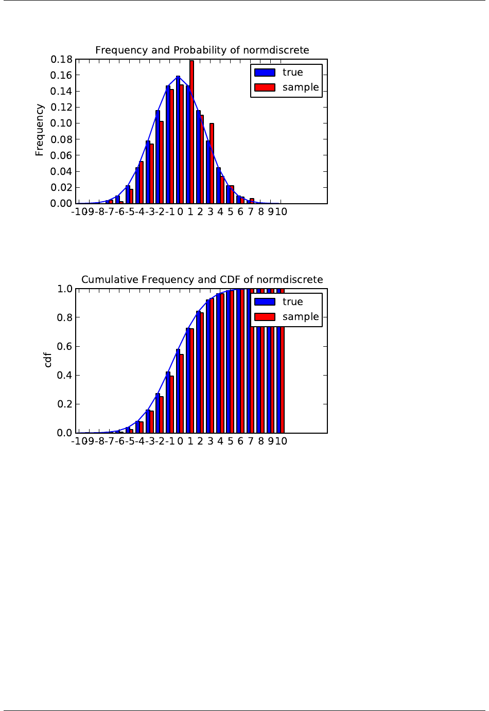
SciPy Reference Guide, Release 0.13.0
Next, we can test, whether our sample was generated by our normdiscrete distribution. This also verifies whether the
random numbers are generated correctly.
The chisquare test requires that there are a minimum number of observations in each bin. We combine the tail bins
into larger bins so that they contain enough observations.
>>> f2 =np.hstack([f[:5].sum(), f[5:-5], f[-5:].sum()])
>>> p2 =np.hstack([probs[:5].sum(), probs[5:-5], probs[-5:].sum()])
>>> ch2, pval =stats.chisquare(f2, p2*n_sample)
>>> print ’chisquare for normdiscrete: chi2 = %6.3f pvalue = %6.4f’%(ch2, pval)
chisquare for normdiscrete: chi2 = 12.466 pvalue = 0.4090
The pvalue in this case is high, so we can be quite confident that our random sample was actually generated by the
distribution.
1.13. Statistics (scipy.stats) 85

SciPy Reference Guide, Release 0.13.0
1.13.4 Analysing One Sample
First, we create some random variables. We set a seed so that in each run we get identical results to look at. As an
example we take a sample from the Student t distribution:
>>> np.random.seed(282629734)
>>> x=stats.t.rvs(10, size=1000)
Here, we set the required shape parameter of the t distribution, which in statistics corresponds to the degrees of
freedom, to 10. Using size=1000 means that our sample consists of 1000 independently drawn (pseudo) random
numbers. Since we did not specify the keyword arguments loc and scale, those are set to their default values zero and
one.
Descriptive Statistics
xis a numpy array, and we have direct access to all array methods, e.g.
>>> print x.max(), x.min() # equivalent to np.max(x), np.min(x)
5.26327732981 -3.78975572422
>>> print x.mean(), x.var() # equivalent to np.mean(x), np.var(x)
0.0140610663985 1.28899386208
How do the some sample properties compare to their theoretical counterparts?
>>> m,v,s,k=stats.t.stats(10, moments=’mvsk’)
>>> n, (smin, smax), sm, sv, ss, sk =stats.describe(x)
>>> print ’distribution:’,
distribution:
>>> sstr =’mean = %6.4f, variance = %6.4f, skew = %6.4f, kurtosis = %6.4f’
>>> print sstr %(m, v, s ,k)
mean = 0.0000, variance = 1.2500, skew = 0.0000, kurtosis = 1.0000
>>> print ’sample: ’,
sample:
>>> print sstr %(sm, sv, ss, sk)
mean = 0.0141, variance = 1.2903, skew = 0.2165, kurtosis = 1.0556
Note: stats.describe uses the unbiased estimator for the variance, while np.var is the biased estimator.
For our sample the sample statistics differ a by a small amount from their theoretical counterparts.
T-test and KS-test
We can use the t-test to test whether the mean of our sample differs in a statistcally significant way from the theoretical
expectation.
>>> print ’t-statistic = %6.3f pvalue = %6.4f’%stats.ttest_1samp(x, m)
t-statistic = 0.391 pvalue = 0.6955
The pvalue is 0.7, this means that with an alpha error of, for example, 10%, we cannot reject the hypothesis that the
sample mean is equal to zero, the expectation of the standard t-distribution.
As an exercise, we can calculate our ttest also directly without using the provided function, which should give us the
same answer, and so it does:
>>> tt =(sm-m)/np.sqrt(sv/float(n)) # t-statistic for mean
>>> pval =stats.t.sf(np.abs(tt), n-1)*2# two-sided pvalue = Prob(abs(t)>tt)
86 Chapter 1. SciPy Tutorial

SciPy Reference Guide, Release 0.13.0
>>> print ’t-statistic = %6.3f pvalue = %6.4f’%(tt, pval)
t-statistic = 0.391 pvalue = 0.6955
The Kolmogorov-Smirnov test can be used to test the hypothesis that the sample comes from the standard t-distribution
>>> print ’KS-statistic D = %6.3f pvalue = %6.4f’%stats.kstest(x, ’t’, (10,))
KS-statistic D = 0.016 pvalue = 0.9606
Again the p-value is high enough that we cannot reject the hypothesis that the random sample really is distributed
according to the t-distribution. In real applications, we don’t know what the underlying distribution is. If we perform
the Kolmogorov-Smirnov test of our sample against the standard normal distribution, then we also cannot reject the
hypothesis that our sample was generated by the normal distribution given that in this example the p-value is almost
40%.
>>> print ’KS-statistic D = %6.3f pvalue = %6.4f’%stats.kstest(x,’norm’)
KS-statistic D = 0.028 pvalue = 0.3949
However, the standard normal distribution has a variance of 1, while our sample has a variance of 1.29. If we stan-
dardize our sample and test it against the normal distribution, then the p-value is again large enough that we cannot
reject the hypothesis that the sample came form the normal distribution.
>>> d, pval =stats.kstest((x-x.mean())/x.std(), ’norm’)
>>> print ’KS-statistic D = %6.3f pvalue = %6.4f’%(d, pval)
KS-statistic D = 0.032 pvalue = 0.2402
Note: The Kolmogorov-Smirnov test assumes that we test against a distribution with given parameters, since in the
last case we estimated mean and variance, this assumption is violated, and the distribution of the test statistic on which
the p-value is based, is not correct.
Tails of the distribution
Finally, we can check the upper tail of the distribution. We can use the percent point function ppf, which is the inverse
of the cdf function, to obtain the critical values, or, more directly, we can use the inverse of the survival function
>>> crit01, crit05, crit10 =stats.t.ppf([1-0.01,1-0.05,1-0.10], 10)
>>> print ’critical values from ppf at 1%%, 5%% and 10%% %8.4f %8.4f %8.4f’%(crit01, crit05, crit10)
critical values from ppf at 1%, 5% and 10% 2.7638 1.8125 1.3722
>>> print ’critical values from isf at 1%%, 5%% and 10%% %8.4f %8.4f %8.4f’%tuple(stats.t.isf([0.01,0.05,0.10],10))
critical values from isf at 1%, 5% and 10% 2.7638 1.8125 1.3722
>>> freq01 =np.sum(x>crit01) /float(n) *100
>>> freq05 =np.sum(x>crit05) /float(n) *100
>>> freq10 =np.sum(x>crit10) /float(n) *100
>>> print ’sample %%-frequency at 1%%, 5%% and 10%% tail %8.4f %8.4f %8.4f’%(freq01, freq05, freq10)
sample %-frequency at 1%, 5% and 10% tail 1.4000 5.8000 10.5000
In all three cases, our sample has more weight in the top tail than the underlying distribution. We can briefly check
a larger sample to see if we get a closer match. In this case the empirical frequency is quite close to the theoretical
probability, but if we repeat this several times the fluctuations are still pretty large.
>>> freq05l =np.sum(stats.t.rvs(10, size=10000)>crit05) /10000.0 *100
>>> print ’larger sample %%-frequency at 5%% tail %8.4f’%freq05l
larger sample %-frequency at 5% tail 4.8000
We can also compare it with the tail of the normal distribution, which has less weight in the tails:
1.13. Statistics (scipy.stats) 87

SciPy Reference Guide, Release 0.13.0
>>> print ’tail prob. of normal at 1%%, 5%% and 10%% %8.4f %8.4f %8.4f’%\
... tuple(stats.norm.sf([crit01, crit05, crit10])*100)
tail prob. of normal at 1%, 5% and 10% 0.2857 3.4957 8.5003
The chisquare test can be used to test, whether for a finite number of bins, the observed frequencies differ significantly
from the probabilites of the hypothesized distribution.
>>> quantiles =[0.0,0.01,0.05,0.1,1-0.10,1-0.05,1-0.01,1.0]
>>> crit =stats.t.ppf(quantiles, 10)
>>> print crit
[ -Inf -2.76376946 -1.81246112 -1.37218364 1.37218364 1.81246112
2.76376946 Inf]
>>> n_sample =x.size
>>> freqcount =np.histogram(x, bins=crit)[0]
>>> tprob =np.diff(quantiles)
>>> nprob =np.diff(stats.norm.cdf(crit))
>>> tch, tpval =stats.chisquare(freqcount, tprob*n_sample)
>>> nch, npval =stats.chisquare(freqcount, nprob*n_sample)
>>> print ’chisquare for t: chi2 = %6.3f pvalue = %6.4f’%(tch, tpval)
chisquare for t: chi2 = 2.300 pvalue = 0.8901
>>> print ’chisquare for normal: chi2 = %6.3f pvalue = %6.4f’%(nch, npval)
chisquare for normal: chi2 = 64.605 pvalue = 0.0000
We see that the standard normal distribution is clearly rejected while the standard t-distribution cannot be rejected.
Since the variance of our sample differs from both standard distribution, we can again redo the test taking the estimate
for scale and location into account.
The fit method of the distributions can be used to estimate the parameters of the distribution, and the test is repeated
using probabilites of the estimated distribution.
>>> tdof, tloc, tscale =stats.t.fit(x)
>>> nloc, nscale =stats.norm.fit(x)
>>> tprob =np.diff(stats.t.cdf(crit, tdof, loc=tloc, scale=tscale))
>>> nprob =np.diff(stats.norm.cdf(crit, loc=nloc, scale=nscale))
>>> tch, tpval =stats.chisquare(freqcount, tprob*n_sample)
>>> nch, npval =stats.chisquare(freqcount, nprob*n_sample)
>>> print ’chisquare for t: chi2 = %6.3f pvalue = %6.4f’%(tch, tpval)
chisquare for t: chi2 = 1.577 pvalue = 0.9542
>>> print ’chisquare for normal: chi2 = %6.3f pvalue = %6.4f’%(nch, npval)
chisquare for normal: chi2 = 11.084 pvalue = 0.0858
Taking account of the estimated parameters, we can still reject the hypothesis that our sample came from a normal
distribution (at the 5% level), but again, with a p-value of 0.95, we cannot reject the t distribution.
Special tests for normal distributions
Since the normal distribution is the most common distribution in statistics, there are several additional functions
available to test whether a sample could have been drawn from a normal distribution
First we can test if skew and kurtosis of our sample differ significantly from those of a normal distribution:
>>> print ’normal skewtest teststat = %6.3f pvalue = %6.4f’%stats.skewtest(x)
normal skewtest teststat = 2.785 pvalue = 0.0054
>>> print ’normal kurtosistest teststat = %6.3f pvalue = %6.4f’%stats.kurtosistest(x)
normal kurtosistest teststat = 4.757 pvalue = 0.0000
These two tests are combined in the normality test
88 Chapter 1. SciPy Tutorial

SciPy Reference Guide, Release 0.13.0
>>> print ’normaltest teststat = %6.3f pvalue = %6.4f’%stats.normaltest(x)
normaltest teststat = 30.379 pvalue = 0.0000
In all three tests the p-values are very low and we can reject the hypothesis that the our sample has skew and kurtosis
of the normal distribution.
Since skew and kurtosis of our sample are based on central moments, we get exactly the same results if we test the
standardized sample:
>>> print ’normaltest teststat = %6.3f pvalue = %6.4f’%\
... stats.normaltest((x-x.mean())/x.std())
normaltest teststat = 30.379 pvalue = 0.0000
Because normality is rejected so strongly, we can check whether the normaltest gives reasonable results for other
cases:
>>> print ’normaltest teststat = %6.3f pvalue = %6.4f’%stats.normaltest(stats.t.rvs(10, size=100))
normaltest teststat = 4.698 pvalue = 0.0955
>>> print ’normaltest teststat = %6.3f pvalue = %6.4f’%stats.normaltest(stats.norm.rvs(size=1000))
normaltest teststat = 0.613 pvalue = 0.7361
When testing for normality of a small sample of t-distributed observations and a large sample of normal distributed
observation, then in neither case can we reject the null hypothesis that the sample comes from a normal distribution.
In the first case this is because the test is not powerful enough to distinguish a t and a normally distributed random
variable in a small sample.
1.13.5 Comparing two samples
In the following, we are given two samples, which can come either from the same or from different distribution, and
we want to test whether these samples have the same statistical properties.
Comparing means
Test with sample with identical means:
>>> rvs1 =stats.norm.rvs(loc=5, scale=10, size=500)
>>> rvs2 =stats.norm.rvs(loc=5, scale=10, size=500)
>>> stats.ttest_ind(rvs1, rvs2)
(-0.54890361750888583, 0.5831943748663857)
Test with sample with different means:
>>> rvs3 =stats.norm.rvs(loc=8, scale=10, size=500)
>>> stats.ttest_ind(rvs1, rvs3)
(-4.5334142901750321, 6.507128186505895e-006)
Kolmogorov-Smirnov test for two samples ks_2samp
For the example where both samples are drawn from the same distribution, we cannot reject the null hypothesis since
the pvalue is high
>>> stats.ks_2samp(rvs1, rvs2)
(0.025999999999999995, 0.99541195173064878)
In the second example, with different location, i.e. means, we can reject the null hypothesis since the pvalue is below
1%
1.13. Statistics (scipy.stats) 89
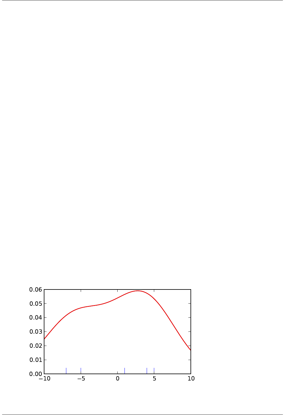
SciPy Reference Guide, Release 0.13.0
>>> stats.ks_2samp(rvs1, rvs3)
(0.11399999999999999, 0.0027132103661283141)
1.13.6 Kernel Density Estimation
A common task in statistics is to estimate the probability density function (PDF) of a random variable from a set
of data samples. This task is called density estimation. The most well-known tool to do this is the histogram. A
histogram is a useful tool for visualization (mainly because everyone understands it), but doesn’t use the available data
very efficiently. Kernel density estimation (KDE) is a more efficient tool for the same task. The gaussian_kde
estimator can be used to estimate the PDF of univariate as well as multivariate data. It works best if the data is
unimodal.
Univariate estimation
We start with a minimal amount of data in order to see how gaussian_kde works, and what the different options
for bandwidth selection do. The data sampled from the PDF is show as blue dashes at the bottom of the figure (this is
called a rug plot):
>>> from scipy import stats
>>> import matplotlib.pyplot as plt
>>> x1 =np.array([-7,-5,1,4,5], dtype=np.float)
>>> kde1 =stats.gaussian_kde(x1)
>>> kde2 =stats.gaussian_kde(x1, bw_method=’silverman’)
>>> fig =plt.figure()
>>> ax =fig.add_subplot(111)
>>> ax.plot(x1, np.zeros(x1.shape), ’b+’, ms=20)# rug plot
>>> x_eval =np.linspace(-10,10, num=200)
>>> ax.plot(x_eval, kde1(x_eval), ’k-’, label="Scott’s Rule")
>>> ax.plot(x_eval, kde1(x_eval), ’r-’, label="Silverman’s Rule")
>>> plt.show()
90 Chapter 1. SciPy Tutorial
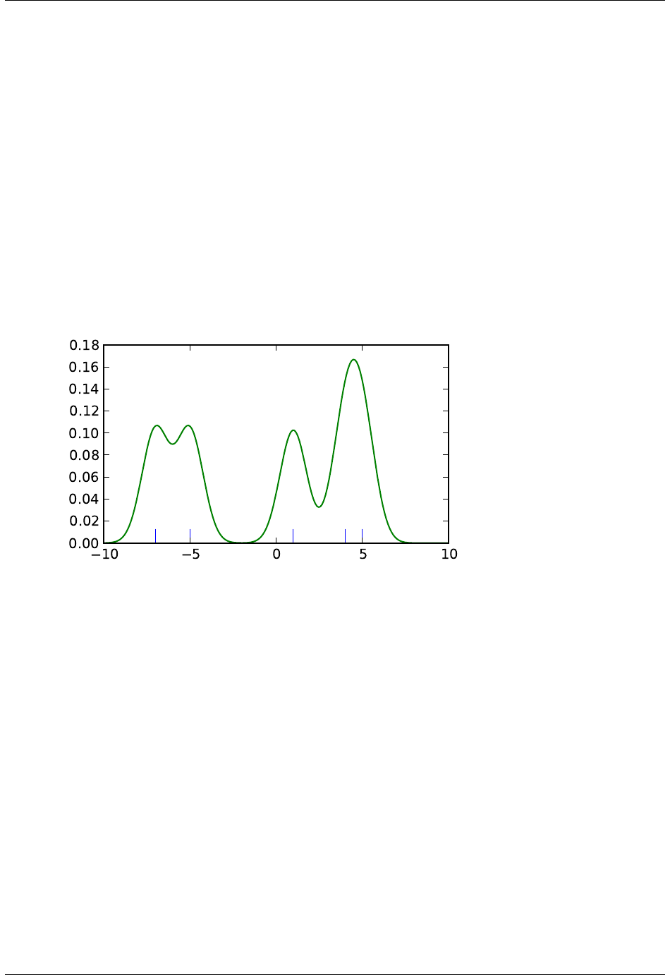
SciPy Reference Guide, Release 0.13.0
We see that there is very little difference between Scott’s Rule and Silverman’s Rule, and that the bandwidth selection
with a limited amount of data is probably a bit too wide. We can define our own bandwidth function to get a less
smoothed out result.
>>> def my_kde_bandwidth(obj, fac=1./5):
... """We use Scott’s Rule, multiplied by a constant factor."""
... return np.power(obj.n, -1./(obj.d+4)) *fac
>>> fig =plt.figure()
>>> ax =fig.add_subplot(111)
>>> ax.plot(x1, np.zeros(x1.shape), ’b+’, ms=20)# rug plot
>>> kde3 =stats.gaussian_kde(x1, bw_method=my_kde_bandwidth)
>>> ax.plot(x_eval, kde3(x_eval), ’g-’, label="With smaller BW")
>>> plt.show()
We see that if we set bandwidth to be very narrow, the obtained estimate for the probability density function (PDF) is
simply the sum of Gaussians around each data point.
We now take a more realistic example, and look at the difference between the two available bandwidth selection rules.
Those rules are known to work well for (close to) normal distributions, but even for unimodal distributions that are
quite strongly non-normal they work reasonably well. As a non-normal distribution we take a Student’s T distribution
with 5 degrees of freedom.
import numpy as np
import matplotlib.pyplot as plt
from scipy import stats
np.random.seed(12456)
x1 =np.random.normal(size=200)# random data, normal distribution
xs =np.linspace(x1.min()-1, x1.max()+1,200)
kde1 =stats.gaussian_kde(x1)
kde2 =stats.gaussian_kde(x1, bw_method=’silverman’)
fig =plt.figure(figsize=(8,6))
1.13. Statistics (scipy.stats) 91

SciPy Reference Guide, Release 0.13.0
ax1 =fig.add_subplot(211)
ax1.plot(x1, np.zeros(x1.shape), ’b+’, ms=12)# rug plot
ax1.plot(xs, kde1(xs), ’k-’, label="Scott’s Rule")
ax1.plot(xs, kde2(xs), ’b-’, label="Silverman’s Rule")
ax1.plot(xs, stats.norm.pdf(xs), ’r--’, label="True PDF")
ax1.set_xlabel(’x’)
ax1.set_ylabel(’Density’)
ax1.set_title("Normal (top) and Student’s T$_{df=5}$ (bottom) distributions")
ax1.legend(loc=1)
x2 =stats.t.rvs(5, size=200)# random data, T distribution
xs =np.linspace(x2.min() -1, x2.max() +1,200)
kde3 =stats.gaussian_kde(x2)
kde4 =stats.gaussian_kde(x2, bw_method=’silverman’)
ax2 =fig.add_subplot(212)
ax2.plot(x2, np.zeros(x2.shape), ’b+’, ms=12)# rug plot
ax2.plot(xs, kde3(xs), ’k-’, label="Scott’s Rule")
ax2.plot(xs, kde4(xs), ’b-’, label="Silverman’s Rule")
ax2.plot(xs, stats.t.pdf(xs, 5), ’r--’, label="True PDF")
ax2.set_xlabel(’x’)
ax2.set_ylabel(’Density’)
plt.show()
92 Chapter 1. SciPy Tutorial
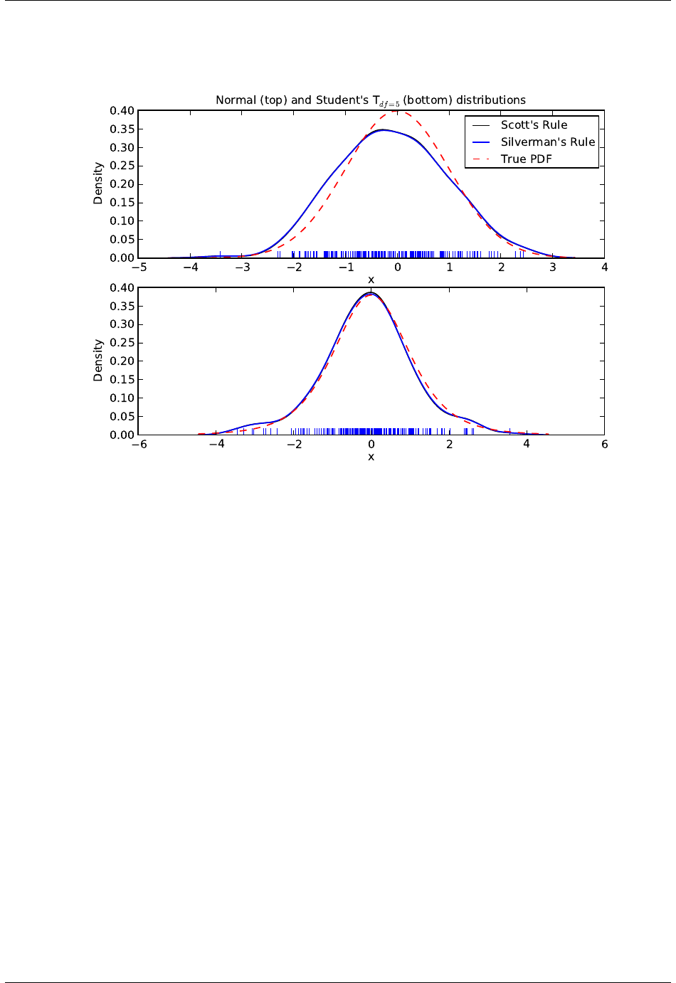
SciPy Reference Guide, Release 0.13.0
We now take a look at a bimodal distribution with one wider and one narrower Gaussian feature. We expect that this
will be a more difficult density to approximate, due to the different bandwidths required to accurately resolve each
feature.
>>> from functools import partial
>>> loc1, scale1, size1 =(-2,1,175)
>>> loc2, scale2, size2 =(2,0.2,50)
>>> x2 =np.concatenate([np.random.normal(loc=loc1, scale=scale1, size=size1),
... np.random.normal(loc=loc2, scale=scale2, size=size2)])
>>> x_eval =np.linspace(x2.min() -1, x2.max() +1,500)
>>> kde =stats.gaussian_kde(x2)
>>> kde2 =stats.gaussian_kde(x2, bw_method=’silverman’)
>>> kde3 =stats.gaussian_kde(x2, bw_method=partial(my_kde_bandwidth, fac=0.2))
>>> kde4 =stats.gaussian_kde(x2, bw_method=partial(my_kde_bandwidth, fac=0.5))
>>> pdf =stats.norm.pdf
>>> bimodal_pdf =pdf(x_eval, loc=loc1, scale=scale1) *float(size1) /x2.size +\
... pdf(x_eval, loc=loc2, scale=scale2) *float(size2) /x2.size
>>> fig =plt.figure(figsize=(8,6))
>>> ax =fig.add_subplot(111)
1.13. Statistics (scipy.stats) 93
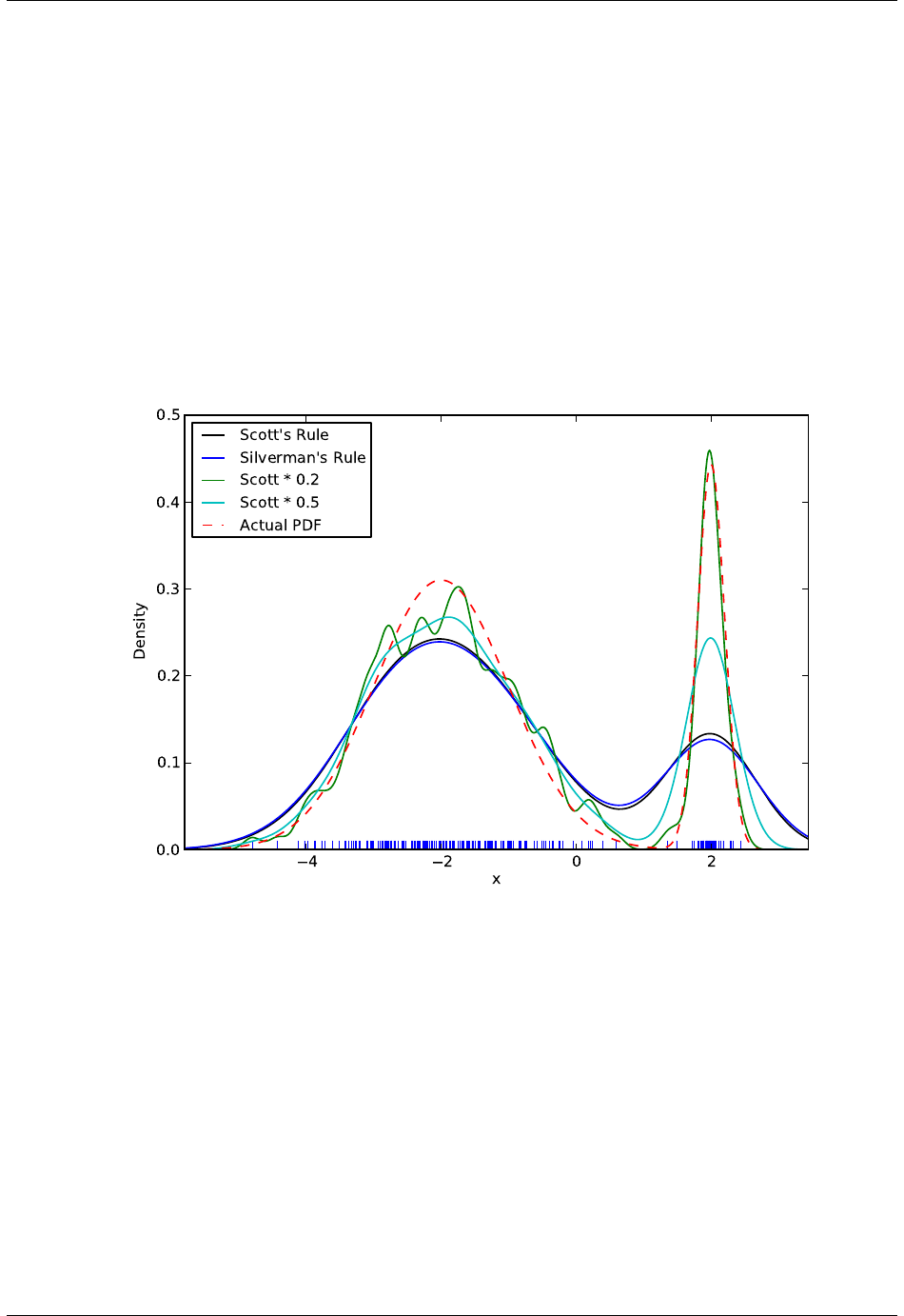
SciPy Reference Guide, Release 0.13.0
>>> ax.plot(x2, np.zeros(x2.shape), ’b+’, ms=12)
>>> ax.plot(x_eval, kde(x_eval), ’k-’, label="Scott’s Rule")
>>> ax.plot(x_eval, kde2(x_eval), ’b-’, label="Silverman’s Rule")
>>> ax.plot(x_eval, kde3(x_eval), ’g-’, label="Scott *0.2")
>>> ax.plot(x_eval, kde4(x_eval), ’c-’, label="Scott *0.5")
>>> ax.plot(x_eval, bimodal_pdf, ’r--’, label="Actual PDF")
>>> ax.set_xlim([x_eval.min(), x_eval.max()])
>>> ax.legend(loc=2)
>>> ax.set_xlabel(’x’)
>>> ax.set_ylabel(’Density’)
>>> plt.show()
As expected, the KDE is not as close to the true PDF as we would like due to the different characteristic size of the
two features of the bimodal distribution. By halving the default bandwidth (Scott *0.5) we can do somewhat
better, while using a factor 5 smaller bandwidth than the default doesn’t smooth enough. What we really need though
in this case is a non-uniform (adaptive) bandwidth.
Multivariate estimation
With gaussian_kde we can perform multivariate as well as univariate estimation. We demonstrate the bivariate
case. First we generate some random data with a model in which the two variates are correlated.
>>> def measure(n):
... """Measurement model, return two coupled measurements."""
94 Chapter 1. SciPy Tutorial

SciPy Reference Guide, Release 0.13.0
... m1 =np.random.normal(size=n)
... m2 =np.random.normal(scale=0.5, size=n)
... return m1+m2, m1-m2
>>> m1, m2 =measure(2000)
>>> xmin =m1.min()
>>> xmax =m1.max()
>>> ymin =m2.min()
>>> ymax =m2.max()
Then we apply the KDE to the data:
>>> X,Y=np.mgrid[xmin:xmax:100j, ymin:ymax:100j]
>>> positions =np.vstack([X.ravel(), Y.ravel()])
>>> values =np.vstack([m1, m2])
>>> kernel =stats.gaussian_kde(values)
>>> Z=np.reshape(kernel.evaluate(positions).T, X.shape)
Finally we plot the estimated bivariate distribution as a colormap, and plot the individual data points on top.
>>> fig =plt.figure(figsize=(8,6))
>>> ax =fig.add_subplot(111)
>>> ax.imshow(np.rot90(Z), cmap=plt.cm.gist_earth_r,
... extent=[xmin, xmax, ymin, ymax])
>>> ax.plot(m1, m2, ’k.’, markersize=2)
>>> ax.set_xlim([xmin, xmax])
>>> ax.set_ylim([ymin, ymax])
>>> plt.show()
1.13. Statistics (scipy.stats) 95
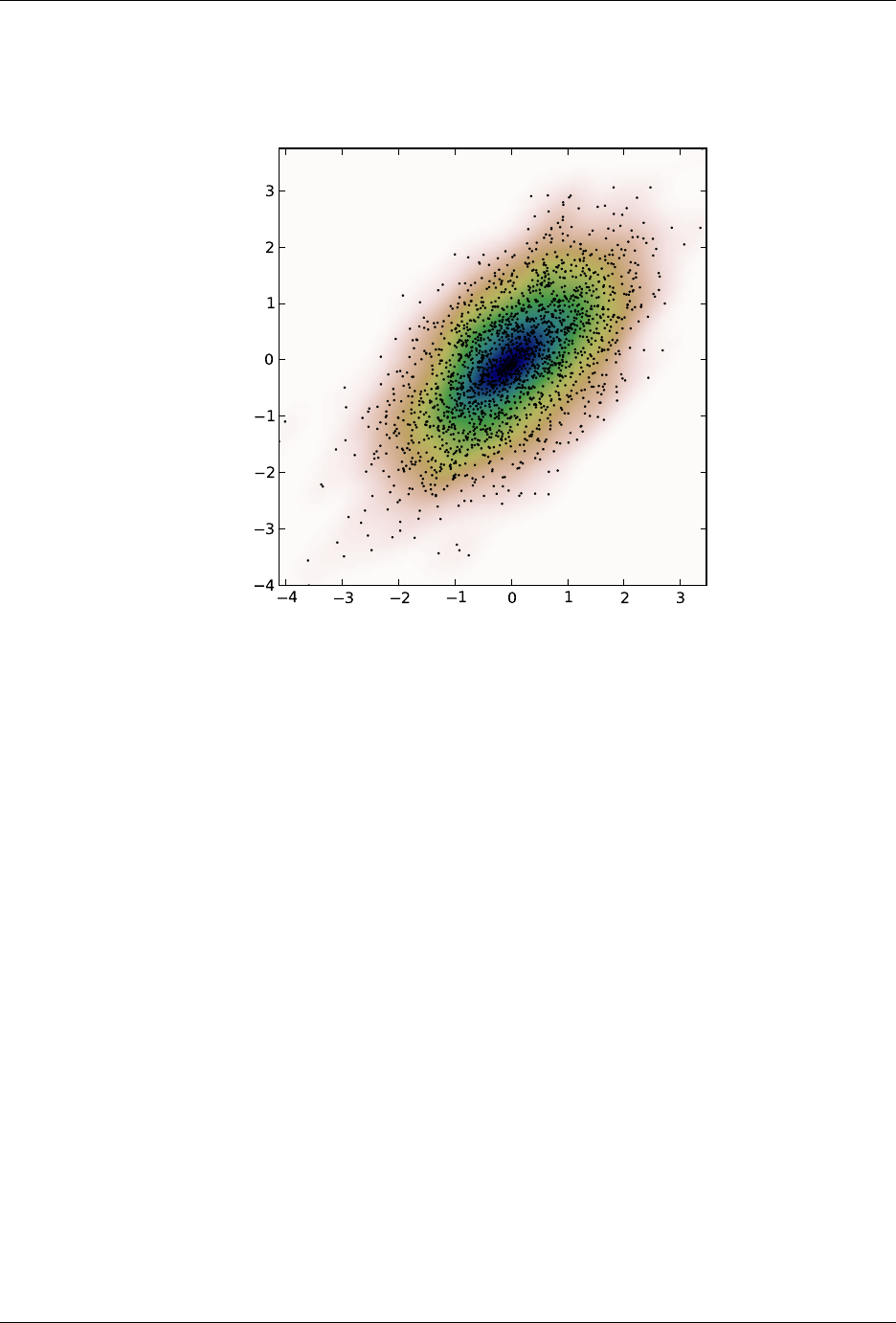
SciPy Reference Guide, Release 0.13.0
1.14 Multidimensional image processing (scipy.ndimage)
1.14.1 Introduction
Image processing and analysis are generally seen as operations on two-dimensional arrays of values. There are how-
ever a number of fields where images of higher dimensionality must be analyzed. Good examples of these are medical
imaging and biological imaging. numpy is suited very well for this type of applications due its inherent multidimen-
sional nature. The scipy.ndimage packages provides a number of general image processing and analysis functions
that are designed to operate with arrays of arbitrary dimensionality. The packages currently includes functions for lin-
ear and non-linear filtering, binary morphology, B-spline interpolation, and object measurements.
1.14.2 Properties shared by all functions
All functions share some common properties. Notably, all functions allow the specification of an output array with the
output argument. With this argument you can specify an array that will be changed in-place with the result with the
operation. In this case the result is not returned. Usually, using the output argument is more efficient, since an existing
array is used to store the result.
The type of arrays returned is dependent on the type of operation, but it is in most cases equal to the type of the input.
If, however, the output argument is used, the type of the result is equal to the type of the specified output argument.
96 Chapter 1. SciPy Tutorial

SciPy Reference Guide, Release 0.13.0
If no output argument is given, it is still possible to specify what the result of the output should be. This is done by
simply assigning the desired numpy type object to the output argument. For example:
>>> correlate(np.arange(10), [1,2.5])
array([ 0, 2, 6, 9, 13, 16, 20, 23, 27, 30])
>>> correlate(np.arange(10), [1,2.5], output=np.float64)
array([ 0. , 2.5, 6. , 9.5, 13. , 16.5, 20. , 23.5, 27. , 30.5])
1.14.3 Filter functions
The functions described in this section all perform some type of spatial filtering of the the input array: the elements
in the output are some function of the values in the neighborhood of the corresponding input element. We refer to
this neighborhood of elements as the filter kernel, which is often rectangular in shape but may also have an arbitrary
footprint. Many of the functions described below allow you to define the footprint of the kernel, by passing a mask
through the footprint parameter. For example a cross shaped kernel can be defined as follows:
>>> footprint =array([[0,1,0],[1,1,1],[0,1,0]])
>>> footprint
array([[0, 1, 0],
[1, 1, 1],
[0, 1, 0]])
Usually the origin of the kernel is at the center calculated by dividing the dimensions of the kernel shape by two.
For instance, the origin of a one-dimensional kernel of length three is at the second element. Take for example the
correlation of a one-dimensional array with a filter of length 3 consisting of ones:
>>> a=[0,0,0,1,0,0,0]
>>> correlate1d(a, [1,1,1])
array([0, 0, 1, 1, 1, 0, 0])
Sometimes it is convenient to choose a different origin for the kernel. For this reason most functions support the origin
parameter which gives the origin of the filter relative to its center. For example:
>>> a=[0,0,0,1,0,0,0]
>>> correlate1d(a, [1,1,1], origin = -1)
array([0 1 1 1 0 0 0])
The effect is a shift of the result towards the left. This feature will not be needed very often, but it may be useful
especially for filters that have an even size. A good example is the calculation of backward and forward differences:
>>> a=[0,0,1,1,1,0,0]
>>> correlate1d(a, [-1,1]) # backward difference
array([ 0 0 1 0 0 -1 0])
>>> correlate1d(a, [-1,1], origin = -1)# forward difference
array([ 0 1 0 0 -1 0 0])
We could also have calculated the forward difference as follows:
>>> correlate1d(a, [0,-1,1])
array([ 0 1 0 0 -1 0 0])
However, using the origin parameter instead of a larger kernel is more efficient. For multidimensional kernels origin
can be a number, in which case the origin is assumed to be equal along all axes, or a sequence giving the origin along
each axis.
Since the output elements are a function of elements in the neighborhood of the input elements, the borders of the
array need to be dealt with appropriately by providing the values outside the borders. This is done by assuming that
the arrays are extended beyond their boundaries according certain boundary conditions. In the functions described
1.14. Multidimensional image processing (scipy.ndimage) 97

SciPy Reference Guide, Release 0.13.0
below, the boundary conditions can be selected using the mode parameter which must be a string with the name of the
boundary condition. Following boundary conditions are currently supported:
“nearest” Use the value at the boundary [1 2 3]->[1 1 2 3 3]
“wrap” Periodically replicate the array [1 2 3]->[3 1 2 3 1]
“reflect” Reflect the array at the boundary [1 2 3]->[1 1 2 3 3]
“constant” Use a constant value, default is 0.0 [1 2 3]->[0 1 2 3 0]
The “constant” mode is special since it needs an additional parameter to specify the constant value that should be used.
Note: The easiest way to implement such boundary conditions would be to copy the data to a larger array and extend
the data at the borders according to the boundary conditions. For large arrays and large filter kernels, this would be
very memory consuming, and the functions described below therefore use a different approach that does not require
allocating large temporary buffers.
Correlation and convolution
The correlate1d function calculates a one-dimensional correlation along the given axis. The lines of the ar-
ray along the given axis are correlated with the given weights. The weights parameter must be a one-dimensional
sequences of numbers.
The function correlate implements multidimensional correlation of the input array with a given kernel.
The convolve1d function calculates a one-dimensional convolution along the given axis. The lines of the
array along the given axis are convoluted with the given weights. The weights parameter must be a one-
dimensional sequences of numbers.
Note: A convolution is essentially a correlation after mirroring the kernel. As a result, the origin parameter
behaves differently than in the case of a correlation: the result is shifted in the opposite directions.
The function convolve implements multidimensional convolution of the input array with a given kernel.
Note: A convolution is essentially a correlation after mirroring the kernel. As a result, the origin parameter
behaves differently than in the case of a correlation: the results is shifted in the opposite direction.
Smoothing filters
The gaussian_filter1d function implements a one-dimensional Gaussian filter. The standard-deviation
of the Gaussian filter is passed through the parameter sigma. Setting order = 0 corresponds to convolution with
a Gaussian kernel. An order of 1, 2, or 3 corresponds to convolution with the first, second or third derivatives of
a Gaussian. Higher order derivatives are not implemented.
The gaussian_filter function implements a multidimensional Gaussian filter. The standard-deviations of
the Gaussian filter along each axis are passed through the parameter sigma as a sequence or numbers. If sigma
is not a sequence but a single number, the standard deviation of the filter is equal along all directions. The order
of the filter can be specified separately for each axis. An order of 0 corresponds to convolution with a Gaussian
kernel. An order of 1, 2, or 3 corresponds to convolution with the first, second or third derivatives of a Gaussian.
Higher order derivatives are not implemented. The order parameter must be a number, to specify the same order
for all axes, or a sequence of numbers to specify a different order for each axis.
Note: The multidimensional filter is implemented as a sequence of one-dimensional Gaussian filters. The
intermediate arrays are stored in the same data type as the output. Therefore, for output types with a lower
precision, the results may be imprecise because intermediate results may be stored with insufficient precision.
This can be prevented by specifying a more precise output type.
98 Chapter 1. SciPy Tutorial

SciPy Reference Guide, Release 0.13.0
The uniform_filter1d function calculates a one-dimensional uniform filter of the given size along the
given axis.
The uniform_filter implements a multidimensional uniform filter. The sizes of the uniform filter are given
for each axis as a sequence of integers by the size parameter. If size is not a sequence, but a single number, the
sizes along all axis are assumed to be equal.
Note: The multidimensional filter is implemented as a sequence of one-dimensional uniform filters. The
intermediate arrays are stored in the same data type as the output. Therefore, for output types with a lower
precision, the results may be imprecise because intermediate results may be stored with insufficient precision.
This can be prevented by specifying a more precise output type.
Filters based on order statistics
The minimum_filter1d function calculates a one-dimensional minimum filter of given size along the given
axis.
The maximum_filter1d function calculates a one-dimensional maximum filter of given size along the given
axis.
The minimum_filter function calculates a multidimensional minimum filter. Either the sizes of a rectangu-
lar kernel or the footprint of the kernel must be provided. The size parameter, if provided, must be a sequence of
sizes or a single number in which case the size of the filter is assumed to be equal along each axis. The footprint,
if provided, must be an array that defines the shape of the kernel by its non-zero elements.
The maximum_filter function calculates a multidimensional maximum filter. Either the sizes of a rectangu-
lar kernel or the footprint of the kernel must be provided. The size parameter, if provided, must be a sequence of
sizes or a single number in which case the size of the filter is assumed to be equal along each axis. The footprint,
if provided, must be an array that defines the shape of the kernel by its non-zero elements.
The rank_filter function calculates a multidimensional rank filter. The rank may be less then zero, i.e.,
rank = -1 indicates the largest element. Either the sizes of a rectangular kernel or the footprint of the kernel must
be provided. The size parameter, if provided, must be a sequence of sizes or a single number in which case the
size of the filter is assumed to be equal along each axis. The footprint, if provided, must be an array that defines
the shape of the kernel by its non-zero elements.
The percentile_filter function calculates a multidimensional percentile filter. The percentile may be
less then zero, i.e., percentile = -20 equals percentile = 80. Either the sizes of a rectangular kernel or the
footprint of the kernel must be provided. The size parameter, if provided, must be a sequence of sizes or a single
number in which case the size of the filter is assumed to be equal along each axis. The footprint, if provided,
must be an array that defines the shape of the kernel by its non-zero elements.
The median_filter function calculates a multidimensional median filter. Either the sizes of a rectangular
kernel or the footprint of the kernel must be provided. The size parameter, if provided, must be a sequence of
sizes or a single number in which case the size of the filter is assumed to be equal along each axis. The footprint
if provided, must be an array that defines the shape of the kernel by its non-zero elements.
Derivatives
Derivative filters can be constructed in several ways. The function gaussian_filter1d described in Smoothing
filters can be used to calculate derivatives along a given axis using the order parameter. Other derivative filters are the
Prewitt and Sobel filters:
The prewitt function calculates a derivative along the given axis.
The sobel function calculates a derivative along the given axis.
The Laplace filter is calculated by the sum of the second derivatives along all axes. Thus, different Laplace filters
can be constructed using different second derivative functions. Therefore we provide a general function that takes a
function argument to calculate the second derivative along a given direction and to construct the Laplace filter:
1.14. Multidimensional image processing (scipy.ndimage) 99

SciPy Reference Guide, Release 0.13.0
The function generic_laplace calculates a laplace filter using the function passed through derivative2
to calculate second derivatives. The function derivative2 should have the following signature:
derivative2(input, axis, output, mode, cval, *extra_arguments, **extra_keywords)
It should calculate the second derivative along the dimension axis. If output is not None it should use that for
the output and return None, otherwise it should return the result. mode,cval have the usual meaning.
The extra_arguments and extra_keywords arguments can be used to pass a tuple of extra arguments and a dic-
tionary of named arguments that are passed to derivative2 at each call.
For example:
>>> def d2(input, axis, output, mode, cval):
... return correlate1d(input, [1,-2,1], axis, output, mode, cval, 0)
...
>>> a=zeros((5,5))
>>> a[2,2]=1
>>> generic_laplace(a, d2)
array([[ 0., 0., 0., 0., 0.],
[ 0., 0., 1., 0., 0.],
[ 0., 1., -4., 1., 0.],
[ 0., 0., 1., 0., 0.],
[ 0., 0., 0., 0., 0.]])
To demonstrate the use of the extra_arguments argument we could do:
>>> def d2(input, axis, output, mode, cval, weights):
... return correlate1d(input, weights, axis, output, mode, cval, 0,)
...
>>> a=zeros((5,5))
>>> a[2,2]=1
>>> generic_laplace(a, d2, extra_arguments =([1,-2,1],))
array([[ 0., 0., 0., 0., 0.],
[ 0., 0., 1., 0., 0.],
[ 0., 1., -4., 1., 0.],
[ 0., 0., 1., 0., 0.],
[ 0., 0., 0., 0., 0.]])
or:
>>> generic_laplace(a, d2, extra_keywords ={’weights’: [1,-2,1]})
array([[ 0., 0., 0., 0., 0.],
[ 0., 0., 1., 0., 0.],
[ 0., 1., -4., 1., 0.],
[ 0., 0., 1., 0., 0.],
[ 0., 0., 0., 0., 0.]])
The following two functions are implemented using generic_laplace by providing appropriate functions for the
second derivative function:
The function laplace calculates the Laplace using discrete differentiation for the second derivative (i.e. con-
volution with [1, -2, 1]).
The function gaussian_laplace calculates the Laplace using gaussian_filter to calculate the second
derivatives. The standard-deviations of the Gaussian filter along each axis are passed through the parameter
sigma as a sequence or numbers. If sigma is not a sequence but a single number, the standard deviation of the
filter is equal along all directions.
The gradient magnitude is defined as the square root of the sum of the squares of the gradients in all directions. Similar
to the generic Laplace function there is a generic_gradient_magnitude function that calculated the gradient
magnitude of an array:
The function generic_gradient_magnitude calculates a gradient magnitude using the function passed
through derivative to calculate first derivatives. The function derivative should have the following
100 Chapter 1. SciPy Tutorial

SciPy Reference Guide, Release 0.13.0
signature:
derivative(input, axis, output, mode, cval, *extra_arguments, **extra_keywords)
It should calculate the derivative along the dimension axis. If output is not None it should use that for the output
and return None, otherwise it should return the result. mode,cval have the usual meaning.
The extra_arguments and extra_keywords arguments can be used to pass a tuple of extra arguments and a dic-
tionary of named arguments that are passed to derivative at each call.
For example, the sobel function fits the required signature:
>>> a=zeros((5,5))
>>> a[2,2]=1
>>> generic_gradient_magnitude(a, sobel)
array([[ 0. , 0. , 0. , 0. , 0. ],
[ 0. , 1.41421356, 2. , 1.41421356, 0. ],
[ 0. , 2. , 0. , 2. , 0. ],
[ 0. , 1.41421356, 2. , 1.41421356, 0. ],
[ 0. , 0. , 0. , 0. , 0. ]])
See the documentation of generic_laplace for examples of using the extra_arguments and extra_keywords
arguments.
The sobel and prewitt functions fit the required signature and can therefore directly be used with
generic_gradient_magnitude. The following function implements the gradient magnitude using Gaussian
derivatives:
The function gaussian_gradient_magnitude calculates the gradient magnitude using
gaussian_filter to calculate the first derivatives. The standard-deviations of the Gaussian filter
along each axis are passed through the parameter sigma as a sequence or numbers. If sigma is not a sequence
but a single number, the standard deviation of the filter is equal along all directions.
Generic filter functions
To implement filter functions, generic functions can be used that accept a callable object that implements the filtering
operation. The iteration over the input and output arrays is handled by these generic functions, along with such
details as the implementation of the boundary conditions. Only a callable object implementing a callback function
that does the actual filtering work must be provided. The callback function can also be written in C and passed using
aPyCObject (see Extending ndimage in C for more information).
The generic_filter1d function implements a generic one-dimensional filter function, where the actual
filtering operation must be supplied as a python function (or other callable object). The generic_filter1d
function iterates over the lines of an array and calls function at each line. The arguments that are passed to
function are one-dimensional arrays of the tFloat64 type. The first contains the values of the current line.
It is extended at the beginning end the end, according to the filter_size and origin arguments. The second array
should be modified in-place to provide the output values of the line. For example consider a correlation along
one dimension:
>>> a=arange(12).reshape(3,4)
>>> correlate1d(a, [1,2,3])
array([[ 3, 8, 14, 17],
[27, 32, 38, 41],
[51, 56, 62, 65]])
The same operation can be implemented using generic_filter1d as follows:
>>> def fnc(iline, oline):
... oline[...]=iline[:-2]+2*iline[1:-1]+3*iline[2:]
...
>>> generic_filter1d(a, fnc, 3)
array([[ 3, 8, 14, 17],
1.14. Multidimensional image processing (scipy.ndimage) 101

SciPy Reference Guide, Release 0.13.0
[27, 32, 38, 41],
[51, 56, 62, 65]])
Here the origin of the kernel was (by default) assumed to be in the middle of the filter of length 3. Therefore,
each input line was extended by one value at the beginning and at the end, before the function was called.
Optionally extra arguments can be defined and passed to the filter function. The extra_arguments and ex-
tra_keywords arguments can be used to pass a tuple of extra arguments and/or a dictionary of named arguments
that are passed to derivative at each call. For example, we can pass the parameters of our filter as an argument:
>>> def fnc(iline, oline, a, b):
... oline[...]=iline[:-2]+a*iline[1:-1]+b*iline[2:]
...
>>> generic_filter1d(a, fnc, 3, extra_arguments =(2,3))
array([[ 3, 8, 14, 17],
[27, 32, 38, 41],
[51, 56, 62, 65]])
or:
>>> generic_filter1d(a, fnc, 3, extra_keywords ={’a’:2,’b’:3})
array([[ 3, 8, 14, 17],
[27, 32, 38, 41],
[51, 56, 62, 65]])
The generic_filter function implements a generic filter function, where the actual filtering operation must
be supplied as a python function (or other callable object). The generic_filter function iterates over the
array and calls function at each element. The argument of function is a one-dimensional array of the
tFloat64 type, that contains the values around the current element that are within the footprint of the filter.
The function should return a single value that can be converted to a double precision number. For example
consider a correlation:
>>> a=arange(12).reshape(3,4)
>>> correlate(a, [[1,0], [0,3]])
array([[ 0, 3, 7, 11],
[12, 15, 19, 23],
[28, 31, 35, 39]])
The same operation can be implemented using generic_filter as follows:
>>> def fnc(buffer):
... return (buffer *array([1,3])).sum()
...
>>> generic_filter(a, fnc, footprint =[[1,0], [0,1]])
array([[ 0 3 7 11],
[12 15 19 23],
[28 31 35 39]])
Here a kernel footprint was specified that contains only two elements. Therefore the filter function receives a
buffer of length equal to two, which was multiplied with the proper weights and the result summed.
When calling generic_filter, either the sizes of a rectangular kernel or the footprint of the kernel must be
provided. The size parameter, if provided, must be a sequence of sizes or a single number in which case the size
of the filter is assumed to be equal along each axis. The footprint, if provided, must be an array that defines the
shape of the kernel by its non-zero elements.
Optionally extra arguments can be defined and passed to the filter function. The extra_arguments and ex-
tra_keywords arguments can be used to pass a tuple of extra arguments and/or a dictionary of named arguments
that are passed to derivative at each call. For example, we can pass the parameters of our filter as an argument:
>>> def fnc(buffer, weights):
... weights =asarray(weights)
... return (buffer *weights).sum()
...
102 Chapter 1. SciPy Tutorial

SciPy Reference Guide, Release 0.13.0
>>> generic_filter(a, fnc, footprint =[[1,0], [0,1]], extra_arguments =([1,3],))
array([[ 0, 3, 7, 11],
[12, 15, 19, 23],
[28, 31, 35, 39]])
or:
>>> generic_filter(a, fnc, footprint =[[1,0], [0,1]], extra_keywords={’weights’: [1,3]})
array([[ 0, 3, 7, 11],
[12, 15, 19, 23],
[28, 31, 35, 39]])
These functions iterate over the lines or elements starting at the last axis, i.e. the last index changes the fastest. This
order of iteration is guaranteed for the case that it is important to adapt the filter depending on spatial location. Here
is an example of using a class that implements the filter and keeps track of the current coordinates while iterating.
It performs the same filter operation as described above for generic_filter, but additionally prints the current
coordinates:
>>> a=arange(12).reshape(3,4)
>>>
>>> class fnc_class:
... def __init__(self, shape):
... # store the shape:
... self.shape =shape
... # initialize the coordinates:
... self.coordinates =[0]*len(shape)
...
... def filter(self,buffer):
... result =(buffer *array([1,3])).sum()
... print self.coordinates
... # calculate the next coordinates:
... axes =range(len(self.shape))
... axes.reverse()
... for jj in axes:
... if self.coordinates[jj] <self.shape[jj] -1:
... self.coordinates[jj] += 1
... break
... else:
... self.coordinates[jj] =0
... return result
...
>>> fnc =fnc_class(shape =(3,4))
>>> generic_filter(a, fnc.filter, footprint =[[1,0], [0,1]])
[0, 0]
[0, 1]
[0, 2]
[0, 3]
[1, 0]
[1, 1]
[1, 2]
[1, 3]
[2, 0]
[2, 1]
[2, 2]
[2, 3]
array([[ 0, 3, 7, 11],
[12, 15, 19, 23],
[28, 31, 35, 39]])
1.14. Multidimensional image processing (scipy.ndimage) 103

SciPy Reference Guide, Release 0.13.0
For the generic_filter1d function the same approach works, except that this function does not iterate over the
axis that is being filtered. The example for generic_filter1d then becomes this:
>>> a=arange(12).reshape(3,4)
>>>
>>> class fnc1d_class:
... def __init__(self, shape, axis = -1):
... # store the filter axis:
... self.axis =axis
... # store the shape:
... self.shape =shape
... # initialize the coordinates:
... self.coordinates =[0]*len(shape)
...
... def filter(self, iline, oline):
... oline[...]=iline[:-2]+2*iline[1:-1]+3*iline[2:]
... print self.coordinates
... # calculate the next coordinates:
... axes =range(len(self.shape))
... # skip the filter axis:
... del axes[self.axis]
... axes.reverse()
... for jj in axes:
... if self.coordinates[jj] <self.shape[jj] -1:
... self.coordinates[jj] += 1
... break
... else:
... self.coordinates[jj] =0
...
>>> fnc =fnc1d_class(shape =(3,4))
>>> generic_filter1d(a, fnc.filter, 3)
[0, 0]
[1, 0]
[2, 0]
array([[ 3, 8, 14, 17],
[27, 32, 38, 41],
[51, 56, 62, 65]])
Fourier domain filters
The functions described in this section perform filtering operations in the Fourier domain. Thus, the input array
of such a function should be compatible with an inverse Fourier transform function, such as the functions from the
numpy.fft module. We therefore have to deal with arrays that may be the result of a real or a complex Fourier
transform. In the case of a real Fourier transform only half of the of the symmetric complex transform is stored.
Additionally, it needs to be known what the length of the axis was that was transformed by the real fft. The functions
described here provide a parameter nthat in the case of a real transform must be equal to the length of the real
transform axis before transformation. If this parameter is less than zero, it is assumed that the input array was the
result of a complex Fourier transform. The parameter axis can be used to indicate along which axis the real transform
was executed.
The fourier_shift function multiplies the input array with the multidimensional Fourier transform of a
shift operation for the given shift. The shift parameter is a sequences of shifts for each dimension, or a single
value for all dimensions.
The fourier_gaussian function multiplies the input array with the multidimensional Fourier transform of
a Gaussian filter with given standard-deviations sigma. The sigma parameter is a sequences of values for each
dimension, or a single value for all dimensions.
104 Chapter 1. SciPy Tutorial

SciPy Reference Guide, Release 0.13.0
The fourier_uniform function multiplies the input array with the multidimensional Fourier transform of a
uniform filter with given sizes size. The size parameter is a sequences of values for each dimension, or a single
value for all dimensions.
The fourier_ellipsoid function multiplies the input array with the multidimensional Fourier transform of
a elliptically shaped filter with given sizes size. The size parameter is a sequences of values for each dimension,
or a single value for all dimensions. This function is only implemented for dimensions 1, 2, and 3.
1.14.4 Interpolation functions
This section describes various interpolation functions that are based on B-spline theory. A good introduction to B-
splines can be found in: M. Unser, “Splines: A Perfect Fit for Signal and Image Processing,” IEEE Signal Processing
Magazine, vol. 16, no. 6, pp. 22-38, November 1999.
Spline pre-filters
Interpolation using splines of an order larger than 1 requires a pre- filtering step. The interpolation functions described
in section Interpolation functions apply pre-filtering by calling spline_filter, but they can be instructed not to
do this by setting the prefilter keyword equal to False. This is useful if more than one interpolation operation is done
on the same array. In this case it is more efficient to do the pre-filtering only once and use a prefiltered array as the
input of the interpolation functions. The following two functions implement the pre-filtering:
The spline_filter1d function calculates a one-dimensional spline filter along the given axis. An output
array can optionally be provided. The order of the spline must be larger then 1 and less than 6.
The spline_filter function calculates a multidimensional spline filter.
Note: The multidimensional filter is implemented as a sequence of one-dimensional spline filters. The inter-
mediate arrays are stored in the same data type as the output. Therefore, if an output with a limited precision is
requested, the results may be imprecise because intermediate results may be stored with insufficient precision.
This can be prevented by specifying a output type of high precision.
Interpolation functions
Following functions all employ spline interpolation to effect some type of geometric transformation of the input array.
This requires a mapping of the output coordinates to the input coordinates, and therefore the possibility arises that input
values outside the boundaries are needed. This problem is solved in the same way as described in Filter functions for
the multidimensional filter functions. Therefore these functions all support a mode parameter that determines how the
boundaries are handled, and a cval parameter that gives a constant value in case that the ‘constant’ mode is used.
The geometric_transform function applies an arbitrary geometric transform to the input. The given map-
ping function is called at each point in the output to find the corresponding coordinates in the input. mapping
must be a callable object that accepts a tuple of length equal to the output array rank and returns the correspond-
ing input coordinates as a tuple of length equal to the input array rank. The output shape and output type can
optionally be provided. If not given they are equal to the input shape and type.
For example:
>>> a=arange(12).reshape(4,3).astype(np.float64)
>>> def shift_func(output_coordinates):
... return (output_coordinates[0]-0.5, output_coordinates[1]-0.5)
...
>>> geometric_transform(a, shift_func)
array([[ 0. , 0. , 0. ],
[ 0. , 1.3625, 2.7375],
1.14. Multidimensional image processing (scipy.ndimage) 105

SciPy Reference Guide, Release 0.13.0
[ 0. , 4.8125, 6.1875],
[ 0. , 8.2625, 9.6375]])
Optionally extra arguments can be defined and passed to the filter function. The extra_arguments and ex-
tra_keywords arguments can be used to pass a tuple of extra arguments and/or a dictionary of named arguments
that are passed to derivative at each call. For example, we can pass the shifts in our example as arguments:
>>> def shift_func(output_coordinates, s0, s1):
... return (output_coordinates[0]-s0, output_coordinates[1]-s1)
...
>>> geometric_transform(a, shift_func, extra_arguments =(0.5,0.5))
array([[ 0. , 0. , 0. ],
[ 0. , 1.3625, 2.7375],
[ 0. , 4.8125, 6.1875],
[ 0. , 8.2625, 9.6375]])
or:
>>> geometric_transform(a, shift_func, extra_keywords ={’s0’:0.5,’s1’:0.5})
array([[ 0. , 0. , 0. ],
[ 0. , 1.3625, 2.7375],
[ 0. , 4.8125, 6.1875],
[ 0. , 8.2625, 9.6375]])
Note: The mapping function can also be written in C and passed using a PyCObject. See Extending ndimage
in C for more information.
The function map_coordinates applies an arbitrary coordinate transformation using the given array of
coordinates. The shape of the output is derived from that of the coordinate array by dropping the first axis. The
parameter coordinates is used to find for each point in the output the corresponding coordinates in the input.
The values of coordinates along the first axis are the coordinates in the input array at which the output value is
found. (See also the numarray coordinates function.) Since the coordinates may be non- integer coordinates,
the value of the input at these coordinates is determined by spline interpolation of the requested order. Here is
an example that interpolates a 2D array at (0.5, 0.5) and (1, 2):
>>> a=arange(12).reshape(4,3).astype(np.float64)
>>> a
array([[ 0., 1., 2.],
[ 3., 4., 5.],
[ 6., 7., 8.],
[ 9., 10., 11.]])
>>> map_coordinates(a, [[0.5,2], [0.5,1]])
array([ 1.3625 7. ])
The affine_transform function applies an affine transformation to the input array. The given transforma-
tion matrix and offset are used to find for each point in the output the corresponding coordinates in the input. The
value of the input at the calculated coordinates is determined by spline interpolation of the requested order. The
transformation matrix must be two-dimensional or can also be given as a one-dimensional sequence or array. In
the latter case, it is assumed that the matrix is diagonal. A more efficient interpolation algorithm is then applied
that exploits the separability of the problem. The output shape and output type can optionally be provided. If
not given they are equal to the input shape and type.
The shift function returns a shifted version of the input, using spline interpolation of the requested order.
The zoom function returns a rescaled version of the input, using spline interpolation of the requested order.
The rotate function returns the input array rotated in the plane defined by the two axes given by the parameter
axes, using spline interpolation of the requested order. The angle must be given in degrees. If reshape is true,
then the size of the output array is adapted to contain the rotated input.
106 Chapter 1. SciPy Tutorial

SciPy Reference Guide, Release 0.13.0
1.14.5 Morphology
Binary morphology
Binary morphology (need something to put here).
The generate_binary_structure functions generates a binary structuring element for use in binary
morphology operations. The rank of the structure must be provided. The size of the structure that is returned is
equal to three in each direction. The value of each element is equal to one if the square of the Euclidean distance
from the element to the center is less or equal to connectivity. For instance, two dimensional 4-connected and
8-connected structures are generated as follows:
>>> generate_binary_structure(2,1)
array([[False, True, False],
[ True, True, True],
[False, True, False]], dtype=bool)
>>> generate_binary_structure(2,2)
array([[ True, True, True],
[ True, True, True],
[ True, True, True]], dtype=bool)
Most binary morphology functions can be expressed in terms of the basic operations erosion and dilation:
The binary_erosion function implements binary erosion of arrays of arbitrary rank with the given struc-
turing element. The origin parameter controls the placement of the structuring element as described in Filter
functions. If no structuring element is provided, an element with connectivity equal to one is generated using
generate_binary_structure. The border_value parameter gives the value of the array outside bound-
aries. The erosion is repeated iterations times. If iterations is less than one, the erosion is repeated until the result
does not change anymore. If a mask array is given, only those elements with a true value at the corresponding
mask element are modified at each iteration.
The binary_dilation function implements binary dilation of arrays of arbitrary rank with the given struc-
turing element. The origin parameter controls the placement of the structuring element as described in Filter
functions. If no structuring element is provided, an element with connectivity equal to one is generated using
generate_binary_structure. The border_value parameter gives the value of the array outside bound-
aries. The dilation is repeated iterations times. If iterations is less than one, the dilation is repeated until the
result does not change anymore. If a mask array is given, only those elements with a true value at the corre-
sponding mask element are modified at each iteration.
Here is an example of using binary_dilation to find all elements that touch the border, by repeatedly
dilating an empty array from the border using the data array as the mask:
>>> struct =array([[0,1,0], [1,1,1], [0,1,0]])
>>> a=array([[1,0,0,0,0], [1,1,0,1,0], [0,0,1,1,0], [0,0,0,0,0]])
>>> a
array([[1, 0, 0, 0, 0],
[1, 1, 0, 1, 0],
[0, 0, 1, 1, 0],
[0, 0, 0, 0, 0]])
>>> binary_dilation(zeros(a.shape), struct, -1, a, border_value=1)
array([[ True, False, False, False, False],
[ True, True, False, False, False],
[False, False, False, False, False],
[False, False, False, False, False]], dtype=bool)
The binary_erosion and binary_dilation functions both have an iterations parameter which allows the
erosion or dilation to be repeated a number of times. Repeating an erosion or a dilation with a given structure ntimes
is equivalent to an erosion or a dilation with a structure that is n-1 times dilated with itself. A function is provided that
allows the calculation of a structure that is dilated a number of times with itself:
1.14. Multidimensional image processing (scipy.ndimage) 107

SciPy Reference Guide, Release 0.13.0
The iterate_structure function returns a structure by dilation of the input structure iteration - 1 times
with itself. For instance:
>>> struct =generate_binary_structure(2,1)
>>> struct
array([[False, True, False],
[ True, True, True],
[False, True, False]], dtype=bool)
>>> iterate_structure(struct, 2)
array([[False, False, True, False, False],
[False, True, True, True, False],
[ True, True, True, True, True],
[False, True, True, True, False],
[False, False, True, False, False]], dtype=bool)
If the origin of the original structure is equal to 0, then it is also equal to 0 for the iterated structure. If not,
the origin must also be adapted if the equivalent of the iterations erosions or dilations must be achieved with
the iterated structure. The adapted origin is simply obtained by multiplying with the number of iterations. For
convenience the iterate_structure also returns the adapted origin if the origin parameter is not None:
>>> iterate_structure(struct, 2,-1)
(array([[False, False, True, False, False],
[False, True, True, True, False],
[ True, True, True, True, True],
[False, True, True, True, False],
[False, False, True, False, False]], dtype=bool), [-2, -2])
Other morphology operations can be defined in terms of erosion and d dilation. Following functions provide a few of
these operations for convenience:
The binary_opening function implements binary opening of arrays of arbitrary rank with the given struc-
turing element. Binary opening is equivalent to a binary erosion followed by a binary dilation with the same
structuring element. The origin parameter controls the placement of the structuring element as described in Fil-
ter functions. If no structuring element is provided, an element with connectivity equal to one is generated using
generate_binary_structure. The iterations parameter gives the number of erosions that is performed
followed by the same number of dilations.
The binary_closing function implements binary closing of arrays of arbitrary rank with the given struc-
turing element. Binary closing is equivalent to a binary dilation followed by a binary erosion with the same
structuring element. The origin parameter controls the placement of the structuring element as described in Fil-
ter functions. If no structuring element is provided, an element with connectivity equal to one is generated using
generate_binary_structure. The iterations parameter gives the number of dilations that is performed
followed by the same number of erosions.
The binary_fill_holes function is used to close holes in objects in a binary image, where the structure
defines the connectivity of the holes. The origin parameter controls the placement of the structuring element as
described in Filter functions. If no structuring element is provided, an element with connectivity equal to one is
generated using generate_binary_structure.
The binary_hit_or_miss function implements a binary hit-or-miss transform of arrays of arbitrary rank
with the given structuring elements. The hit-or-miss transform is calculated by erosion of the input with
the first structure, erosion of the logical not of the input with the second structure, followed by the logi-
cal and of these two erosions. The origin parameters control the placement of the structuring elements as
described in Filter functions. If origin2 equals None it is set equal to the origin1 parameter. If the first
structuring element is not provided, a structuring element with connectivity equal to one is generated using
generate_binary_structure, if structure2 is not provided, it is set equal to the logical not of struc-
ture1.
108 Chapter 1. SciPy Tutorial

SciPy Reference Guide, Release 0.13.0
Grey-scale morphology
Grey-scale morphology operations are the equivalents of binary morphology operations that operate on arrays with
arbitrary values. Below we describe the grey-scale equivalents of erosion, dilation, opening and closing. These
operations are implemented in a similar fashion as the filters described in Filter functions, and we refer to this section
for the description of filter kernels and footprints, and the handling of array borders. The grey-scale morphology
operations optionally take a structure parameter that gives the values of the structuring element. If this parameter
is not given the structuring element is assumed to be flat with a value equal to zero. The shape of the structure
can optionally be defined by the footprint parameter. If this parameter is not given, the structure is assumed to be
rectangular, with sizes equal to the dimensions of the structure array, or by the size parameter if structure is not given.
The size parameter is only used if both structure and footprint are not given, in which case the structuring element
is assumed to be rectangular and flat with the dimensions given by size. The size parameter, if provided, must be a
sequence of sizes or a single number in which case the size of the filter is assumed to be equal along each axis. The
footprint parameter, if provided, must be an array that defines the shape of the kernel by its non-zero elements.
Similar to binary erosion and dilation there are operations for grey-scale erosion and dilation:
The grey_erosion function calculates a multidimensional grey- scale erosion.
The grey_dilation function calculates a multidimensional grey- scale dilation.
Grey-scale opening and closing operations can be defined similar to their binary counterparts:
The grey_opening function implements grey-scale opening of arrays of arbitrary rank. Grey-scale opening
is equivalent to a grey-scale erosion followed by a grey-scale dilation.
The grey_closing function implements grey-scale closing of arrays of arbitrary rank. Grey-scale opening
is equivalent to a grey-scale dilation followed by a grey-scale erosion.
The morphological_gradient function implements a grey-scale morphological gradient of arrays of
arbitrary rank. The grey-scale morphological gradient is equal to the difference of a grey-scale dilation and a
grey-scale erosion.
The morphological_laplace function implements a grey-scale morphological laplace of arrays of arbi-
trary rank. The grey-scale morphological laplace is equal to the sum of a grey-scale dilation and a grey-scale
erosion minus twice the input.
The white_tophat function implements a white top-hat filter of arrays of arbitrary rank. The white top-hat
is equal to the difference of the input and a grey-scale opening.
The black_tophat function implements a black top-hat filter of arrays of arbitrary rank. The black top-hat
is equal to the difference of the a grey-scale closing and the input.
1.14.6 Distance transforms
Distance transforms are used to calculate the minimum distance from each element of an object to the background.
The following functions implement distance transforms for three different distance metrics: Euclidean, City Block,
and Chessboard distances.
The function distance_transform_cdt uses a chamfer type algorithm to calculate the distance trans-
form of the input, by replacing each object element (defined by values larger than zero) with the shortest dis-
tance to the background (all non-object elements). The structure determines the type of chamfering that is
done. If the structure is equal to ‘cityblock’ a structure is generated using generate_binary_structure
with a squared distance equal to 1. If the structure is equal to ‘chessboard’, a structure is generated using
generate_binary_structure with a squared distance equal to the rank of the array. These choices cor-
respond to the common interpretations of the cityblock and the chessboard distancemetrics in two dimensions.
In addition to the distance transform, the feature transform can be calculated. In this case the index of the closest
background element is returned along the first axis of the result. The return_distances, and return_indices flags
can be used to indicate if the distance transform, the feature transform, or both must be returned.
The distances and indices arguments can be used to give optional output arrays that must be of the correct size
and type (both Int32).
1.14. Multidimensional image processing (scipy.ndimage) 109

SciPy Reference Guide, Release 0.13.0
The basics of the algorithm used to implement this function is described in: G. Borgefors, “Distance transfor-
mations in arbitrary dimensions.”, Computer Vision, Graphics, and Image Processing, 27:321-345, 1984.
The function distance_transform_edt calculates the exact euclidean distance transform of the input, by
replacing each object element (defined by values larger than zero) with the shortest euclidean distance to the
background (all non-object elements).
In addition to the distance transform, the feature transform can be calculated. In this case the index of the closest
background element is returned along the first axis of the result. The return_distances, and return_indices flags
can be used to indicate if the distance transform, the feature transform, or both must be returned.
Optionally the sampling along each axis can be given by the sampling parameter which should be a sequence of
length equal to the input rank, or a single number in which the sampling is assumed to be equal along all axes.
The distances and indices arguments can be used to give optional output arrays that must be of the correct size
and type (Float64 and Int32).
The algorithm used to implement this function is described in: C. R. Maurer, Jr., R. Qi, and V. Raghavan, “A lin-
ear time algorithm for computing exact euclidean distance transforms of binary images in arbitrary dimensions.
IEEE Trans. PAMI 25, 265-270, 2003.
The function distance_transform_bf uses a brute-force algorithm to calculate the distance transform of
the input, by replacing each object element (defined by values larger than zero) with the shortest distance to the
background (all non-object elements). The metric must be one of “euclidean”, “cityblock”, or “chessboard”.
In addition to the distance transform, the feature transform can be calculated. In this case the index of the closest
background element is returned along the first axis of the result. The return_distances, and return_indices flags
can be used to indicate if the distance transform, the feature transform, or both must be returned.
Optionally the sampling along each axis can be given by the sampling parameter which should be a sequence of
length equal to the input rank, or a single number in which the sampling is assumed to be equal along all axes.
This parameter is only used in the case of the euclidean distance transform.
The distances and indices arguments can be used to give optional output arrays that must be of the correct size
and type (Float64 and Int32).
Note: This function uses a slow brute-force algorithm, the function distance_transform_cdt
can be used to more efficiently calculate cityblock and chessboard distance transforms. The function
distance_transform_edt can be used to more efficiently calculate the exact euclidean distance trans-
form.
1.14.7 Segmentation and labeling
Segmentation is the process of separating objects of interest from the background. The most simple approach is
probably intensity thresholding, which is easily done with numpy functions:
>>> a=array([[1,2,2,1,1,0],
... [0,2,3,1,2,0],
... [1,1,1,3,3,2],
... [1,1,1,1,2,1]])
>>> where(a >1,1,0)
array([[0, 1, 1, 0, 0, 0],
[0, 1, 1, 0, 1, 0],
[0, 0, 0, 1, 1, 1],
[0, 0, 0, 0, 1, 0]])
The result is a binary image, in which the individual objects still need to be identified and labeled. The function
label generates an array where each object is assigned a unique number:
The label function generates an array where the objects in the input are labeled with an integer index. It returns
a tuple consisting of the array of object labels and the number of objects found, unless the output parameter is
given, in which case only the number of objects is returned. The connectivity of the objects is defined by a
structuring element. For instance, in two dimensions using a four-connected structuring element gives:
110 Chapter 1. SciPy Tutorial

SciPy Reference Guide, Release 0.13.0
>>> a=array([[0,1,1,0,0,0],[0,1,1,0,1,0],[0,0,0,1,1,1],[0,0,0,0,1,0]])
>>> s=[[0,1,0], [1,1,1], [0,1,0]]
>>> label(a, s)
(array([[0, 1, 1, 0, 0, 0],
[0, 1, 1, 0, 2, 0],
[0, 0, 0, 2, 2, 2],
[0, 0, 0, 0, 2, 0]]), 2)
These two objects are not connected because there is no way in which we can place the structuring element such
that it overlaps with both objects. However, an 8-connected structuring element results in only a single object:
>>> a=array([[0,1,1,0,0,0],[0,1,1,0,1,0],[0,0,0,1,1,1],[0,0,0,0,1,0]])
>>> s=[[1,1,1], [1,1,1], [1,1,1]]
>>> label(a, s)[0]
array([[0, 1, 1, 0, 0, 0],
[0, 1, 1, 0, 1, 0],
[0, 0, 0, 1, 1, 1],
[0, 0, 0, 0, 1, 0]])
If no structuring element is provided, one is generated by calling generate_binary_structure (see
Binary morphology) using a connectivity of one (which in 2D is the 4-connected structure of the first example).
The input can be of any type, any value not equal to zero is taken to be part of an object. This is useful if you
need to ‘re-label’ an array of object indices, for instance after removing unwanted objects. Just apply the label
function again to the index array. For instance:
>>> l,n=label([1,0,1,0,1])
>>> l
array([1 0 2 0 3])
>>> l=where(l != 2,l,0)
>>> l
array([1 0 0 0 3])
>>> label(l)[0]
array([1 0 0 0 2])
Note: The structuring element used by label is assumed to be symmetric.
There is a large number of other approaches for segmentation, for instance from an estimation of the borders of
the objects that can be obtained for instance by derivative filters. One such an approach is watershed segmentation.
The function watershed_ift generates an array where each object is assigned a unique label, from an array that
localizes the object borders, generated for instance by a gradient magnitude filter. It uses an array containing initial
markers for the objects:
The watershed_ift function applies a watershed from markers algorithm, using an Iterative Forest Trans-
form, as described in: P. Felkel, R. Wegenkittl, and M. Bruckschwaiger, “Implementation and Complexity of the
Watershed-from-Markers Algorithm Computed as a Minimal Cost Forest.”, Eurographics 2001, pp. C:26-35.
The inputs of this function are the array to which the transform is applied, and an array of markers that designate
the objects by a unique label, where any non-zero value is a marker. For instance:
>>> input =array([[0,0,0,0,0,0,0],
... [0,1,1,1,1,1,0],
... [0,1,0,0,0,1,0],
... [0,1,0,0,0,1,0],
... [0,1,0,0,0,1,0],
... [0,1,1,1,1,1,0],
... [0,0,0,0,0,0,0]], np.uint8)
>>> markers =array([[1,0,0,0,0,0,0],
... [0,0,0,0,0,0,0],
... [0,0,0,0,0,0,0],
... [0,0,0,2,0,0,0],
1.14. Multidimensional image processing (scipy.ndimage) 111

SciPy Reference Guide, Release 0.13.0
... [0,0,0,0,0,0,0],
... [0,0,0,0,0,0,0],
... [0,0,0,0,0,0,0]], np.int8)
>>> watershed_ift(input, markers)
array([[1, 1, 1, 1, 1, 1, 1],
[1, 1, 2, 2, 2, 1, 1],
[1, 2, 2, 2, 2, 2, 1],
[1, 2, 2, 2, 2, 2, 1],
[1, 2, 2, 2, 2, 2, 1],
[1, 1, 2, 2, 2, 1, 1],
[1, 1, 1, 1, 1, 1, 1]], dtype=int8)
Here two markers were used to designate an object (marker = 2) and the background (marker = 1). The order
in which these are processed is arbitrary: moving the marker for the background to the lower right corner of the
array yields a different result:
>>> markers =array([[0,0,0,0,0,0,0],
... [0,0,0,0,0,0,0],
... [0,0,0,0,0,0,0],
... [0,0,0,2,0,0,0],
... [0,0,0,0,0,0,0],
... [0,0,0,0,0,0,0],
... [0,0,0,0,0,0,1]], np.int8)
>>> watershed_ift(input, markers)
array([[1, 1, 1, 1, 1, 1, 1],
[1, 1, 1, 1, 1, 1, 1],
[1, 1, 2, 2, 2, 1, 1],
[1, 1, 2, 2, 2, 1, 1],
[1, 1, 2, 2, 2, 1, 1],
[1, 1, 1, 1, 1, 1, 1],
[1, 1, 1, 1, 1, 1, 1]], dtype=int8)
The result is that the object (marker = 2) is smaller because the second marker was processed earlier. This
may not be the desired effect if the first marker was supposed to designate a background object. Therefore
watershed_ift treats markers with a negative value explicitly as background markers and processes them
after the normal markers. For instance, replacing the first marker by a negative marker gives a result similar to
the first example:
>>> markers =array([[0,0,0,0,0,0,0],
... [0,0,0,0,0,0,0],
... [0,0,0,0,0,0,0],
... [0,0,0,2,0,0,0],
... [0,0,0,0,0,0,0],
... [0,0,0,0,0,0,0],
... [0,0,0,0,0,0,-1]], np.int8)
>>> watershed_ift(input, markers)
array([[-1, -1, -1, -1, -1, -1, -1],
[-1, -1, 2, 2, 2, -1, -1],
[-1, 2, 2, 2, 2, 2, -1],
[-1, 2, 2, 2, 2, 2, -1],
[-1, 2, 2, 2, 2, 2, -1],
[-1, -1, 2, 2, 2, -1, -1],
[-1, -1, -1, -1, -1, -1, -1]], dtype=int8)
The connectivity of the objects is defined by a structuring element. If no structuring element is provided, one
is generated by calling generate_binary_structure (see Binary morphology) using a connectivity of
one (which in 2D is a 4-connected structure.) For example, using an 8-connected structure with the last example
yields a different object:
112 Chapter 1. SciPy Tutorial

SciPy Reference Guide, Release 0.13.0
>>> watershed_ift(input, markers,
... structure =[[1,1,1], [1,1,1], [1,1,1]])
array([[-1, -1, -1, -1, -1, -1, -1],
[-1, 2, 2, 2, 2, 2, -1],
[-1, 2, 2, 2, 2, 2, -1],
[-1, 2, 2, 2, 2, 2, -1],
[-1, 2, 2, 2, 2, 2, -1],
[-1, 2, 2, 2, 2, 2, -1],
[-1, -1, -1, -1, -1, -1, -1]], dtype=int8)
Note: The implementation of watershed_ift limits the data types of the input to UInt8 and UInt16.
1.14.8 Object measurements
Given an array of labeled objects, the properties of the individual objects can be measured. The find_objects
function can be used to generate a list of slices that for each object, give the smallest sub-array that fully contains the
object:
The find_objects function finds all objects in a labeled array and returns a list of slices that correspond to
the smallest regions in the array that contains the object. For instance:
>>> a=array([[0,1,1,0,0,0],[0,1,1,0,1,0],[0,0,0,1,1,1],[0,0,0,0,1,0]])
>>> l,n=label(a)
>>> f=find_objects(l)
>>> a[f[0]]
array([[1 1],
[1 1]])
>>> a[f[1]]
array([[0, 1, 0],
[1, 1, 1],
[0, 1, 0]])
find_objects returns slices for all objects, unless the max_label parameter is larger then zero, in which case
only the first max_label objects are returned. If an index is missing in the label array, None is return instead of
a slice. For example:
>>> find_objects([1,0,3,4], max_label =3)
[(slice(0, 1, None),), None, (slice(2, 3, None),)]
The list of slices generated by find_objects is useful to find the position and dimensions of the objects in the
array, but can also be used to perform measurements on the individual objects. Say we want to find the sum of the
intensities of an object in image:
>>> image =arange(4*6).reshape(4,6)
>>> mask =array([[0,1,1,0,0,0],[0,1,1,0,1,0],[0,0,0,1,1,1],[0,0,0,0,1,0]])
>>> labels =label(mask)[0]
>>> slices =find_objects(labels)
Then we can calculate the sum of the elements in the second object:
>>> where(labels[slices[1]] == 2, image[slices[1]], 0).sum()
80
That is however not particularly efficient, and may also be more complicated for other types of measurements. There-
fore a few measurements functions are defined that accept the array of object labels and the index of the object to be
measured. For instance calculating the sum of the intensities can be done by:
1.14. Multidimensional image processing (scipy.ndimage) 113

SciPy Reference Guide, Release 0.13.0
>>> sum(image, labels, 2)
80
For large arrays and small objects it is more efficient to call the measurement functions after slicing the array:
>>> sum(image[slices[1]], labels[slices[1]], 2)
80
Alternatively, we can do the measurements for a number of labels with a single function call, returning a list of results.
For instance, to measure the sum of the values of the background and the second object in our example we give a list
of labels:
>>> sum(image, labels, [0,2])
array([178.0, 80.0])
The measurement functions described below all support the index parameter to indicate which object(s) should be
measured. The default value of index is None. This indicates that all elements where the label is larger than zero
should be treated as a single object and measured. Thus, in this case the labels array is treated as a mask defined by
the elements that are larger than zero. If index is a number or a sequence of numbers it gives the labels of the objects
that are measured. If index is a sequence, a list of the results is returned. Functions that return more than one result,
return their result as a tuple if index is a single number, or as a tuple of lists, if index is a sequence.
The sum function calculates the sum of the elements of the object with label(s) given by index, using the labels
array for the object labels. If index is None, all elements with a non-zero label value are treated as a single
object. If label is None, all elements of input are used in the calculation.
The mean function calculates the mean of the elements of the object with label(s) given by index, using the
labels array for the object labels. If index is None, all elements with a non-zero label value are treated as a
single object. If label is None, all elements of input are used in the calculation.
The variance function calculates the variance of the elements of the object with label(s) given by index, using
the labels array for the object labels. If index is None, all elements with a non-zero label value are treated as a
single object. If label is None, all elements of input are used in the calculation.
The standard_deviation function calculates the standard deviation of the elements of the object with
label(s) given by index, using the labels array for the object labels. If index is None, all elements with a non-
zero label value are treated as a single object. If label is None, all elements of input are used in the calculation.
The minimum function calculates the minimum of the elements of the object with label(s) given by index, using
the labels array for the object labels. If index is None, all elements with a non-zero label value are treated as a
single object. If label is None, all elements of input are used in the calculation.
The maximum function calculates the maximum of the elements of the object with label(s) given by index, using
the labels array for the object labels. If index is None, all elements with a non-zero label value are treated as a
single object. If label is None, all elements of input are used in the calculation.
The minimum_position function calculates the position of the minimum of the elements of the object with
label(s) given by index, using the labels array for the object labels. If index is None, all elements with a non-zero
label value are treated as a single object. If label is None, all elements of input are used in the calculation.
The maximum_position function calculates the position of the maximum of the elements of the object with
label(s) given by index, using the labels array for the object labels. If index is None, all elements with a non-zero
label value are treated as a single object. If label is None, all elements of input are used in the calculation.
The extrema function calculates the minimum, the maximum, and their positions, of the elements of the
object with label(s) given by index, using the labels array for the object labels. If index is None, all elements
with a non-zero label value are treated as a single object. If label is None, all elements of input are used in
the calculation. The result is a tuple giving the minimum, the maximum, the position of the minimum and the
postition of the maximum. The result is the same as a tuple formed by the results of the functions minimum,
maximum,minimum_position, and maximum_position that are described above.
The center_of_mass function calculates the center of mass of the of the object with label(s) given by index,
using the labels array for the object labels. If index is None, all elements with a non-zero label value are treated
as a single object. If label is None, all elements of input are used in the calculation.
114 Chapter 1. SciPy Tutorial

SciPy Reference Guide, Release 0.13.0
The histogram function calculates a histogram of the of the object with label(s) given by index, using the
labels array for the object labels. If index is None, all elements with a non-zero label value are treated as a
single object. If label is None, all elements of input are used in the calculation. Histograms are defined by their
minimum (min), maximum (max) and the number of bins (bins). They are returned as one-dimensional arrays
of type Int32.
1.14.9 Extending ndimage in C
A few functions in the scipy.ndimage take a call-back argument. This can be a python function, but also a
PyCObject containing a pointer to a C function. To use this feature, you must write your own C extension that
defines the function, and define a Python function that returns a PyCObject containing a pointer to this function.
An example of a function that supports this is geometric_transform (see Interpolation functions). You can pass
it a python callable object that defines a mapping from all output coordinates to corresponding coordinates in the input
array. This mapping function can also be a C function, which generally will be much more efficient, since the overhead
of calling a python function at each element is avoided.
For example to implement a simple shift function we define the following function:
static int
_shift_function(int *output_coordinates, double*input_coordinates,
int output_rank, int input_rank, void *callback_data)
{
int ii;
/*get the shift from the callback data pointer: */
double shift =*(double*)callback_data;
/*calculate the coordinates: */
for(ii =0;ii<irank; ii++)
icoor[ii] =ocoor[ii] -shift;
/*return OK status: */
return 1;
}
This function is called at every element of the output array, passing the current coordinates in the output_coordinates
array. On return, the input_coordinates array must contain the coordinates at which the input is interpolated. The ranks
of the input and output array are passed through output_rank and input_rank. The value of the shift is passed through
the callback_data argument, which is a pointer to void. The function returns an error status, in this case always 1,
since no error can occur.
A pointer to this function and a pointer to the shift value must be passed to geometric_transform. Both are
passed by a single PyCObject which is created by the following python extension function:
static PyObject *
py_shift_function(PyObject *obj, PyObject *args)
{
double shift =0.0;
if (!PyArg_ParseTuple(args, "d",&shift)) {
PyErr_SetString(PyExc_RuntimeError, "invalid parameters");
return NULL;
}else {
/*assign the shift to a dynamically allocated location: */
double *cdata =(double*)malloc(sizeof(double));
*cdata =shift;
/*wrap function and callback_data in a CObject: */
return PyCObject_FromVoidPtrAndDesc(_shift_function, cdata,
_destructor);
}
}
1.14. Multidimensional image processing (scipy.ndimage) 115

SciPy Reference Guide, Release 0.13.0
The value of the shift is obtained and then assigned to a dynamically allocated memory location. Both this data pointer
and the function pointer are then wrapped in a PyCObject, which is returned. Additionally, a pointer to a destructor
function is given, that will free the memory we allocated for the shift value when the PyCObject is destroyed. This
destructor is very simple:
static void
_destructor(void*cobject, void *cdata)
{
if (cdata)
free(cdata);
}
To use these functions, an extension module is built:
static PyMethodDef methods[] ={
{"shift_function", (PyCFunction)py_shift_function, METH_VARARGS, ""},
{NULL,NULL,0,NULL}
};
void
initexample(void)
{
Py_InitModule("example", methods);
}
This extension can then be used in Python, for example:
>>> import example
>>> array =arange(12).reshape=(4,3).astype(np.float64)
>>> fnc =example.shift_function(0.5)
>>> geometric_transform(array, fnc)
array([[ 0. 0. 0. ],
[ 0. 1.3625 2.7375],
[ 0. 4.8125 6.1875],
[ 0. 8.2625 9.6375]])
C callback functions for use with ndimage functions must all be written according to this scheme. The next section
lists the ndimage functions that acccept a C callback function and gives the prototype of the callback function.
1.14.10 Functions that support C callback functions
The ndimage functions that support C callback functions are described here. Obviously, the prototype of the func-
tion that is provided to these functions must match exactly that what they expect. Therefore we give here the pro-
totypes of the callback functions. All these callback functions accept a void callback_data pointer that must be
wrapped in a PyCObject using the Python PyCObject_FromVoidPtrAndDesc function, which can also ac-
cept a pointer to a destructor function to free any memory allocated for callback_data. If callback_data is not needed,
PyCObject_FromVoidPtr may be used instead. The callback functions must return an integer error status that is
equal to zero if something went wrong, or 1 otherwise. If an error occurs, you should normally set the python error
status with an informative message before returning, otherwise, a default error message is set by the calling function.
The function generic_filter (see Generic filter functions) accepts a callback function with the following proto-
type:
The calling function iterates over the elements of the input and output arrays, calling the callback function at
each element. The elements within the footprint of the filter at the current element are passed through the buffer
parameter, and the number of elements within the footprint through filter_size. The calculated valued should be
returned in the return_value argument.
116 Chapter 1. SciPy Tutorial

SciPy Reference Guide, Release 0.13.0
The function generic_filter1d (see Generic filter functions) accepts a callback function with the following
prototype:
The calling function iterates over the lines of the input and output arrays, calling the callback function at each
line. The current line is extended according to the border conditions set by the calling function, and the result is
copied into the array that is passed through the input_line array. The length of the input line (after extension) is
passed through input_length. The callback function should apply the 1D filter and store the result in the array
passed through output_line. The length of the output line is passed through output_length.
The function geometric_transform (see Interpolation functions) expects a function with the following proto-
type:
The calling function iterates over the elements of the output array, calling the callback function at each element.
The coordinates of the current output element are passed through output_coordinates. The callback function
must return the coordinates at which the input must be interpolated in input_coordinates. The rank of the input
and output arrays are given by input_rank and output_rank respectively.
1.15 File IO (scipy.io)
See Also
numpy-reference.routines.io (in numpy)
1.15.1 MATLAB files
loadmat(file_name[, mdict, appendmat]) Load MATLAB file
savemat(file_name, mdict[, appendmat, ...]) Save a dictionary of names and arrays into a MATLAB-style .mat file.
whosmat(file_name[, appendmat]) List variables inside a MATLAB file
The basic functions
We’ll start by importing scipy.io and calling it sio for convenience:
>>> import scipy.io as sio
If you are using IPython, try tab completing on sio. Among the many options, you will find:
sio.loadmat
sio.savemat
sio.whosmat
These are the high-level functions you will most likely use when working with MATLAB files. You’ll also find:
sio.matlab
This is the package from which loadmat,savemat and whosmat are imported. Within sio.matlab, you will
find the mio module This module contains the machinery that loadmat and savemat use. From time to time you
may find yourself re-using this machinery.
How do I start?
You may have a .mat file that you want to read into Scipy. Or, you want to pass some variables from Scipy / Numpy
into MATLAB.
1.15. File IO (scipy.io) 117

SciPy Reference Guide, Release 0.13.0
To save us using a MATLAB license, let’s start in Octave. Octave has MATLAB-compatible save and load functions.
Start Octave (octave at the command line for me):
octave:1>a=1:12
a =
123456789101112
octave:2>a=reshape(a, [134])
a =
ans(:,:,1) =
123
ans(:,:,2) =
456
ans(:,:,3) =
789
ans(:,:,4) =
10 11 12
octave:3>save -6octave_a.mat a % MATLAB 6 compatible
octave:4>ls octave_a.mat
octave_a.mat
Now, to Python:
>>> mat_contents =sio.loadmat(’octave_a.mat’)
>>> mat_contents
{’a’: array([[[ 1., 4., 7., 10.],
[ 2., 5., 8., 11.],
[ 3., 6., 9., 12.]]]),
’__version__’: ’1.0’,
’__header__’: ’MATLAB 5.0 MAT-file, written by
Octave 3.6.3, 2013-02-17 21:02:11 UTC’,
’__globals__’: []}
>>> oct_a =mat_contents[’a’]
>>> oct_a
array([[[ 1., 4., 7., 10.],
[ 2., 5., 8., 11.],
[ 3., 6., 9., 12.]]])
>>> oct_a.shape
(1, 3, 4)
Now let’s try the other way round:
>>> import numpy as np
>>> vect =np.arange(10)
>>> vect.shape
(10,)
>>> sio.savemat(’np_vector.mat’, {’vect’:vect})
Then back to Octave:
118 Chapter 1. SciPy Tutorial

SciPy Reference Guide, Release 0.13.0
octave:8>load np_vector.mat
octave:9>vect
vect =
0123456789
octave:10>size(vect)
ans =
1 10
If you want to inspect the contents of a MATLAB file without reading the data into memory, use the whosmat
command:
>>> sio.whosmat(’octave_a.mat’)
[(’a’, (1, 3, 4), ’double’)]
whosmat returns a list of tuples, one for each array (or other object) in the file. Each tuple contains the name, shape
and data type of the array.
MATLAB structs
MATLAB structs are a little bit like Python dicts, except the field names must be strings. Any MATLAB object can be
a value of a field. As for all objects in MATLAB, structs are in fact arrays of structs, where a single struct is an array
of shape (1, 1).
octave:11>my_struct = struct(’field1’,1,’field2’,2)
my_struct =
{
field1 = 1
field2 = 2
}
octave:12>save -6octave_struct.mat my_struct
We can load this in Python:
>>> mat_contents =sio.loadmat(’octave_struct.mat’)
>>> mat_contents
{’my_struct’: array([[([[1.0]], [[2.0]])]],
dtype=[(’field1’, ’O’), (’field2’, ’O’)]), ’__version__’: ’1.0’, ’__header__’: ’MATLAB 5.0 MAT-file, written by Octave 3.6.3, 2013-02-17 21:23:14 UTC’, ’__globals__’: []}
>>> oct_struct =mat_contents[’my_struct’]
>>> oct_struct.shape
(1, 1)
>>> val =oct_struct[0,0]
>>> val
([[1.0]], [[2.0]])
>>> val[’field1’]
array([[ 1.]])
>>> val[’field2’]
array([[ 2.]])
>>> val.dtype
dtype([(’field1’, ’O’), (’field2’, ’O’)])
In versions of Scipy from 0.12.0, MATLAB structs come back as numpy structured arrays, with fields named for the
struct fields. You can see the field names in the dtype output above. Note also:
1.15. File IO (scipy.io) 119

SciPy Reference Guide, Release 0.13.0
>>> val =oct_struct[0,0]
and:
octave:13>size(my_struct)
ans =
1 1
So, in MATLAB, the struct array must be at least 2D, and we replicate that when we read into Scipy. If you want all
length 1 dimensions squeezed out, try this:
>>> mat_contents =sio.loadmat(’octave_struct.mat’, squeeze_me=True)
>>> oct_struct =mat_contents[’my_struct’]
>>> oct_struct.shape
()
Sometimes, it’s more convenient to load the MATLAB structs as python objects rather than numpy structured ar-
rays - it can make the access syntax in python a bit more similar to that in MATLAB. In order to do this, use the
struct_as_record=False parameter setting to loadmat.
>>> mat_contents =sio.loadmat(’octave_struct.mat’, struct_as_record=False)
>>> oct_struct =mat_contents[’my_struct’]
>>> oct_struct[0,0].field1
array([[ 1.]])
struct_as_record=False works nicely with squeeze_me:
>>> mat_contents =sio.loadmat(’octave_struct.mat’, struct_as_record=False, squeeze_me=True)
>>> oct_struct =mat_contents[’my_struct’]
>>> oct_struct.shape # but no - it’s a scalar
Traceback (most recent call last):
File "<stdin>", line 1, in <module>
AttributeError: ’mat_struct’ object has no attribute ’shape’
>>> type(oct_struct)
<class ’scipy.io.matlab.mio5_params.mat_struct’>
>>> oct_struct.field1
1.0
Saving struct arrays can be done in various ways. One simple method is to use dicts:
>>> a_dict ={’field1’:0.5,’field2’:’a string’}
>>> sio.savemat(’saved_struct.mat’, {’a_dict’: a_dict})
loaded as:
octave:21>load saved_struct
octave:22>a_dict
a_dict =
scalar structure containing the fields:
field2 = a string
field1 = 0.50000
You can also save structs back again to MATLAB (or Octave in our case) like this:
>>> dt =[(’f1’,’f8’), (’f2’,’S10’)]
>>> arr =np.zeros((2,), dtype=dt)
>>> arr
120 Chapter 1. SciPy Tutorial

SciPy Reference Guide, Release 0.13.0
array([(0.0, ’’), (0.0, ’’)],
dtype=[(’f1’, ’<f8’), (’f2’, ’S10’)])
>>> arr[0][’f1’]=0.5
>>> arr[0][’f2’]=’python’
>>> arr[1][’f1’]=99
>>> arr[1][’f2’]=’not perl’
>>> sio.savemat(’np_struct_arr.mat’, {’arr’: arr})
MATLAB cell arrays
Cell arrays in MATLAB are rather like python lists, in the sense that the elements in the arrays can contain any type
of MATLAB object. In fact they are most similar to numpy object arrays, and that is how we load them into numpy.
octave:14>my_cells = {1, [2,3]}
my_cells =
{
[1,1] = 1
[1,2] =
2 3
}
octave:15>save -6octave_cells.mat my_cells
Back to Python:
>>> mat_contents =sio.loadmat(’octave_cells.mat’)
>>> oct_cells =mat_contents[’my_cells’]
>>> print(oct_cells.dtype)
object
>>> val =oct_cells[0,0]
>>> val
array([[ 1.]])
>>> print(val.dtype)
float64
Saving to a MATLAB cell array just involves making a numpy object array:
>>> obj_arr =np.zeros((2,), dtype=np.object)
>>> obj_arr[0]=1
>>> obj_arr[1]=’a string’
>>> obj_arr
array([1, ’a string’], dtype=object)
>>> sio.savemat(’np_cells.mat’, {’obj_arr’:obj_arr})
octave:16>load np_cells.mat
octave:17>obj_arr
obj_arr =
{
[1,1]=1
[2,1] = a string
}
1.15.2 IDL files
1.15. File IO (scipy.io) 121

SciPy Reference Guide, Release 0.13.0
readsav(file_name[, idict, python_dict, ...]) Read an IDL .sav file
1.15.3 Matrix Market files
mminfo(source) Queries the contents of the Matrix Market file ‘filename’ to
mmread(source) Reads the contents of a Matrix Market file ‘filename’ into a matrix.
mmwrite(target, a[, comment, field, precision]) Writes the sparse or dense matrix A to a Matrix Market formatted file.
1.15.4 Wav sound files (scipy.io.wavfile)
read(filename[, mmap]) Return the sample rate (in samples/sec) and data from a WAV file
write(filename, rate, data) Write a numpy array as a WAV file
1.15.5 Arff files (scipy.io.arff)
Module to read ARFF files, which are the standard data format for WEKA.
ARFF is a text file format which support numerical, string and data values. The format can also represent missing data
and sparse data.
See the WEKA website for more details about arff format and available datasets.
Examples
>>> from scipy.io import arff
>>> from cStringIO import StringIO
>>> content ="""
... @relation foo
... @attribute width numeric
... @attribute height numeric
... @attribute color {red,green,blue,yellow,black}
... @data
... 5.0,3.25,blue
... 4.5,3.75,green
... 3.0,4.00,red
... """
>>> f=StringIO(content)
>>> data, meta =arff.loadarff(f)
>>> data
array([(5.0, 3.25, ’blue’), (4.5, 3.75, ’green’), (3.0, 4.0, ’red’)],
dtype=[(’width’, ’<f8’), (’height’, ’<f8’), (’color’, ’|S6’)])
>>> meta
Dataset: foo
width’s type is numeric
height’s type is numeric
color’s type is nominal, range is (’red’, ’green’, ’blue’, ’yellow’, ’black’)
loadarff(f) Read an arff file.
122 Chapter 1. SciPy Tutorial


SciPy Reference Guide, Release 0.13.0
Contents
•Weave (scipy.weave)
–Outline
–Introduction
–Requirements
–Installation
–Testing
*Testing Notes:
–Benchmarks
–Inline
*More with printf
*More examples
·Binary search
·Dictionary Sort
·NumPy – cast/copy/transpose
·wxPython
*Keyword Option
*Inline Arguments
*Distutils keywords
·Keyword Option Examples
·Returning Values
·The issue with locals()
·A quick look at the code
*Technical Details
*Passing Variables in/out of the C/C++ code
*Type Conversions
·NumPy Argument Conversion
·String, List, Tuple, and Dictionary Conversion
·File Conversion
·Callable, Instance, and Module Conversion
·Customizing Conversions
*The Catalog
·Function Storage
·Catalog search paths and the PYTHONCOMPILED variable
–Blitz
*Requirements
*Limitations
*NumPy efficiency issues: What compilation buys you
*The Tools
·Parser
·Blitz and NumPy
*Type definitions and coersion
*Cataloging Compiled Functions
*Checking Array Sizes
*Creating the Extension Module
–Extension Modules
*A Simple Example
*Fibonacci Example
–Customizing Type Conversions – Type Factories
–Things I wish weave did
124 Chapter 1. SciPy Tutorial

SciPy Reference Guide, Release 0.13.0
1.16.2 Introduction
The scipy.weave (below just weave) package provides tools for including C/C++ code within in Python code.
This offers both another level of optimization to those who need it, and an easy way to modify and extend any supported
extension libraries such as wxPython and hopefully VTK soon. Inlining C/C++ code within Python generally results
in speed ups of 1.5x to 30x speed-up over algorithms written in pure Python (However, it is also possible to slow things
down...). Generally algorithms that require a large number of calls to the Python API don’t benefit as much from the
conversion to C/C++ as algorithms that have inner loops completely convertable to C.
There are three basic ways to use weave. The weave.inline() function executes C code directly within Python,
and weave.blitz() translates Python NumPy expressions to C++ for fast execution. blitz() was the original
reason weave was built. For those interested in building extension libraries, the ext_tools module provides classes
for building extension modules within Python.
Most of weave’s functionality should work on Windows and Unix, although some of its functionality requires gcc
or a similarly modern C++ compiler that handles templates well. Up to now, most testing has been done on Windows
2000 with Microsoft’s C++ compiler (MSVC) and with gcc (mingw32 2.95.2 and 2.95.3-6). All tests also pass on
Linux (RH 7.1 with gcc 2.96), and I’ve had reports that it works on Debian also (thanks Pearu).
The inline and blitz provide new functionality to Python (although I’ve recently learned about the PyInline
project which may offer similar functionality to inline). On the other hand, tools for building Python extension
modules already exists (SWIG, SIP, pycpp, CXX, and others). As of yet, I’m not sure where weave fits in this
spectrum. It is closest in flavor to CXX in that it makes creating new C/C++ extension modules pretty easy. However,
if you’re wrapping a gaggle of legacy functions or classes, SWIG and friends are definitely the better choice. weave
is set up so that you can customize how Python types are converted to C types in weave. This is great for inline(),
but, for wrapping legacy code, it is more flexible to specify things the other way around – that is how C types map to
Python types. This weave does not do. I guess it would be possible to build such a tool on top of weave, but with
good tools like SWIG around, I’m not sure the effort produces any new capabilities. Things like function overloading
are probably easily implemented in weave and it might be easier to mix Python/C code in function calls, but nothing
beyond this comes to mind. So, if you’re developing new extension modules or optimizing Python functions in C,
weave.ext_tools() might be the tool for you. If you’re wrapping legacy code, stick with SWIG.
The next several sections give the basics of how to use weave. We’ll discuss what’s happening under the covers in
more detail later on. Serious users will need to at least look at the type conversion section to understand how Python
variables map to C/C++ types and how to customize this behavior. One other note. If you don’t know C or C++ then
these docs are probably of very little help to you. Further, it’d be helpful if you know something about writing Python
extensions. weave does quite a bit for you, but for anything complex, you’ll need to do some conversions, reference
counting, etc.
Note: weave is actually part of the SciPy package. However, it also works fine as a standalone package (you can
install from scipy/weave with python setup.py install). The examples here are given as if it is used as
a stand alone package. If you are using from within scipy, you can use from scipy import weave and the
examples will work identically.
1.16.3 Requirements
• Python
I use 2.1.1. Probably 2.0 or higher should work.
• C++ compiler
weave uses distutils to actually build extension modules, so it uses whatever compiler was originally
used to build Python. weave itself requires a C++ compiler. If you used a C++ compiler to build Python, your
probably fine.
1.16. Weave (scipy.weave) 125

SciPy Reference Guide, Release 0.13.0
On Unix gcc is the preferred choice because I’ve done a little testing with it. All testing has been done with gcc,
but I expect the majority of compilers should work for inline and ext_tools. The one issue I’m not sure
about is that I’ve hard coded things so that compilations are linked with the stdc++ library. Is this standard
across Unix compilers, or is this a gcc-ism?
For blitz(), you’ll need a reasonably recent version of gcc. 2.95.2 works on windows and 2.96 looks fine on
Linux. Other versions are likely to work. Its likely that KAI’s C++ compiler and maybe some others will work,
but I haven’t tried. My advice is to use gcc for now unless your willing to tinker with the code some.
On Windows, either MSVC or gcc (mingw32) should work. Again, you’ll need gcc for blitz() as the MSVC
compiler doesn’t handle templates well.
I have not tried Cygwin, so please report success if it works for you.
• NumPy
The python NumPy module is required for blitz() to work and for numpy.distutils which is used by weave.
1.16.4 Installation
There are currently two ways to get weave. First, weave is part of SciPy and installed automatically (as a sub-
package) whenever SciPy is installed. Second, since weave is useful outside of the scientific community, it has been
setup so that it can be used as a stand-alone module.
The stand-alone version can be downloaded from here. Instructions for installing should be found there as well.
setup.py file to simplify installation.
1.16.5 Testing
Once weave is installed, fire up python and run its unit tests.
>>> import weave
>>> weave.test()
runs long time... spews tons of output and a few warnings
.
.
.
..............................................................
................................................................
..................................................
----------------------------------------------------------------------
Ran 184 tests in 158.418s
OK
>>>
This takes a while, usually several minutes. On Unix with remote file systems, I’ve had it take 15 or so minutes. In the
end, it should run about 180 tests and spew some speed results along the way. If you get errors, they’ll be reported at
the end of the output. Please report errors that you find. Some tests are known to fail at this point.
If you only want to test a single module of the package, you can do this by running test() for that specific module.
>>> import weave.scalar_spec
>>> weave.scalar_spec.test()
.......
----------------------------------------------------------------------
Ran 7 tests in 23.284s
126 Chapter 1. SciPy Tutorial

SciPy Reference Guide, Release 0.13.0
Testing Notes:
• Windows 1
I’ve had some test fail on windows machines where I have msvc, gcc-2.95.2 (in c:gcc-2.95.2), and gcc-2.95.3-6
(in c:gcc) all installed. My environment has c:gcc in the path and does not have c:gcc-2.95.2 in the path. The test
process runs very smoothly until the end where several test using gcc fail with cpp0 not found by g++. If I check
os.system(‘gcc -v’) before running tests, I get gcc-2.95.3-6. If I check after running tests (and after failure), I
get gcc-2.95.2. ??huh??. The os.environ[’PATH’] still has c:gcc first in it and is not corrupted (msvc/distutils
messes with the environment variables, so we have to undo its work in some places). If anyone else sees this, let
me know - - it may just be an quirk on my machine (unlikely). Testing with the gcc- 2.95.2 installation always
works.
• Windows 2
If you run the tests from PythonWin or some other GUI tool, you’ll get a ton of DOS windows popping up
periodically as weave spawns the compiler multiple times. Very annoying. Anyone know how to fix this?
• wxPython
wxPython tests are not enabled by default because importing wxPython on a Unix machine without access to a
X-term will cause the program to exit. Anyone know of a safe way to detect whether wxPython can be imported
and whether a display exists on a machine?
1.16.6 Benchmarks
This section has not been updated from old scipy weave and Numeric....
This section has a few benchmarks – thats all people want to see anyway right? These are mostly taken from running
files in the weave/example directory and also from the test scripts. Without more information about what the test
actually do, their value is limited. Still, their here for the curious. Look at the example scripts for more specifics about
what problem was actually solved by each run. These examples are run under windows 2000 using Microsoft Visual
C++ and python2.1 on a 850 MHz PIII laptop with 320 MB of RAM. Speed up is the improvement (degredation)
factor of weave compared to conventional Python functions. The blitz() comparisons are shown compared to
NumPy.
Table 1.7: inline and ext_tools
Algorithm Speed up
binary search 1.50
fibonacci (recursive) 82.10
fibonacci (loop) 9.17
return None 0.14
map 1.20
dictionary sort 2.54
vector quantization 37.40
Table 1.8: blitz – double precision
Algorithm Speed up
a = b + c 512x512 3.05
a = b + c + d 512x512 4.59
5 pt avg. filter, 2D Image 512x512 9.01
Electromagnetics (FDTD) 100x100x100 8.61
The benchmarks shown blitz in the best possible light. NumPy (at least on my machine) is significantly worse for
double precision than it is for single precision calculations. If your interested in single precision results, you can pretty
much divide the double precision speed up by 3 and you’ll be close.
1.16. Weave (scipy.weave) 127

SciPy Reference Guide, Release 0.13.0
1.16.7 Inline
inline() compiles and executes C/C++ code on the fly. Variables in the local and global Python scope are also
available in the C/C++ code. Values are passed to the C/C++ code by assignment much like variables are passed into
a standard Python function. Values are returned from the C/C++ code through a special argument called return_val.
Also, the contents of mutable objects can be changed within the C/C++ code and the changes remain after the C code
exits and returns to Python. (more on this later)
Here’s a trivial printf example using inline():
>>> import weave
>>> a=1
>>> weave.inline(’printf("%d\\n",a);’,[’a’])
1
In this, its most basic form, inline(c_code, var_list) requires two arguments. c_code is a string of valid
C/C++ code. var_list is a list of variable names that are passed from Python into C/C++. Here we have a simple
printf statement that writes the Python variable ato the screen. The first time you run this, there will be a pause
while the code is written to a .cpp file, compiled into an extension module, loaded into Python, cataloged for future
use, and executed. On windows (850 MHz PIII), this takes about 1.5 seconds when using Microsoft’s C++ compiler
(MSVC) and 6-12 seconds using gcc (mingw32 2.95.2). All subsequent executions of the code will happen very
quickly because the code only needs to be compiled once. If you kill and restart the interpreter and then execute the
same code fragment again, there will be a much shorter delay in the fractions of seconds range. This is because weave
stores a catalog of all previously compiled functions in an on disk cache. When it sees a string that has been compiled,
it loads the already compiled module and executes the appropriate function.
Note: If you try the printf example in a GUI shell such as IDLE, PythonWin, PyShell, etc., you’re unlikely to
see the output. This is because the C code is writing to stdout, instead of to the GUI window. This doesn’t mean that
inline doesn’t work in these environments – it only means that standard out in C is not the same as the standard out for
Python in these cases. Non input/output functions will work as expected.
Although effort has been made to reduce the overhead associated with calling inline, it is still less efficient for simple
code snippets than using equivalent Python code. The simple printf example is actually slower by 30% or so
than using Python print statement. And, it is not difficult to create code fragments that are 8-10 times slower
using inline than equivalent Python. However, for more complicated algorithms, the speedup can be worthwhile –
anywhere from 1.5-30 times faster. Algorithms that have to manipulate Python objects (sorting a list) usually only see
a factor of 2 or so improvement. Algorithms that are highly computational or manipulate NumPy arrays can see much
larger improvements. The examples/vq.py file shows a factor of 30 or more improvement on the vector quantization
algorithm that is used heavily in information theory and classification problems.
More with printf
MSVC users will actually see a bit of compiler output that distutils does not suppress the first time the code executes:
>>> weave.inline(r’printf("%d\n",a);’,[’a’])
sc_e013937dbc8c647ac62438874e5795131.cpp
Creating library C:\DOCUME~1\eric\LOCALS~1\Temp\python21_compiled\temp
\Release\sc_e013937dbc8c647ac62438874e5795131.lib and
object C:\DOCUME~1\eric\LOCALS~1\Temp\python21_compiled\temp\Release\sc_e013937dbc8c647ac62438874e5795131.exp
1
Nothing bad is happening, its just a bit annoying. * Anyone know how to turn this off?*
This example also demonstrates using ‘raw strings’. The rpreceeding the code string in the last example denotes
that this is a ‘raw string’. In raw strings, the backslash character is not interpreted as an escape character, and so it
isn’t necessary to use a double backslash to indicate that the ‘n’ is meant to be interpreted in the C printf statement
128 Chapter 1. SciPy Tutorial

SciPy Reference Guide, Release 0.13.0
instead of by Python. If your C code contains a lot of strings and control characters, raw strings might make things
easier. Most of the time, however, standard strings work just as well.
The printf statement in these examples is formatted to print out integers. What happens if ais a string? inline
will happily, compile a new version of the code to accept strings as input, and execute the code. The result?
>>> a=’string’
>>> weave.inline(r’printf("%d\n",a);’,[’a’])
32956972
In this case, the result is non-sensical, but also non-fatal. In other situations, it might produce a compile time error
because ais required to be an integer at some point in the code, or it could produce a segmentation fault. Its possible
to protect against passing inline arguments of the wrong data type by using asserts in Python.
>>> a=’string’
>>> def protected_printf(a):
... assert(type(a) == type(1))
... weave.inline(r’printf("%d\n",a);’,[’a’])
>>> protected_printf(1)
1
>>> protected_printf(’string’)
AssertError...
For printing strings, the format statement needs to be changed. Also, weave doesn’t convert strings to char*. Instead
it uses CXX Py::String type, so you have to do a little more work. Here we convert it to a C++ std::string and then ask
cor the char* version.
>>> a=’string’
>>> weave.inline(r’printf("%s\n",std::string(a).c_str());’,[’a’])
string
XXX
This is a little convoluted. Perhaps strings should convert to std::string objects instead of CXX objects. Or
maybe to char*.
As in this case, C/C++ code fragments often have to change to accept different types. For the given printing task,
however, C++ streams provide a way of a single statement that works for integers and strings. By default, the stream
objects live in the std (standard) namespace and thus require the use of std::.
>>> weave.inline(’std::cout << a << std::endl;’,[’a’])
1
>>> a=’string’
>>> weave.inline(’std::cout << a << std::endl;’,[’a’])
string
Examples using printf and cout are included in examples/print_example.py.
More examples
This section shows several more advanced uses of inline. It includes a few algorithms from the Python Cookbook
that have been re-written in inline C to improve speed as well as a couple examples using NumPy and wxPython.
Binary search
Lets look at the example of searching a sorted list of integers for a value. For inspiration, we’ll use Kalle Svensson’s
binary_search() algorithm from the Python Cookbook. His recipe follows:
1.16. Weave (scipy.weave) 129

SciPy Reference Guide, Release 0.13.0
def binary_search(seq, t):
min =0;max =len(seq) -1
while 1:
if max <min:
return -1
m=(min +max)/2
if seq[m] <t:
min =m+1
elif seq[m] >t:
max =m-1
else:
return m
This Python version works for arbitrary Python data types. The C version below is specialized to handle integer values.
There is a little type checking done in Python to assure that we’re working with the correct data types before heading
into C. The variables seq and tdon’t need to be declared beacuse weave handles converting and declaring them in
the C code. All other temporary variables such as min, max, etc. must be declared – it is C after all. Here’s the new
mixed Python/C function:
def c_int_binary_search(seq,t):
# do a little type checking in Python
assert(type(t) == type(1))
assert(type(seq) == type([]))
# now the C code
code ="""
#line 29 "binary_search.py"
int val, m, min = 0;
int max = seq.length() - 1;
PyObject *py_val;
for(;;)
{
if (max < min )
{
return_val = Py::new_reference_to(Py::Int(-1));
break;
}
m = (min + max) /2;
val = py_to_int(PyList_GetItem(seq.ptr(),m),"val");
if (val < t)
min = m + 1;
else if (val > t)
max = m - 1;
else
{
return_val = Py::new_reference_to(Py::Int(m));
break;
}
}
"""
return inline(code,[’seq’,’t’])
We have two variables seq and tpassed in. tis guaranteed (by the assert) to be an integer. Python integers are
converted to C int types in the transition from Python to C. seq is a Python list. By default, it is translated to a CXX
list object. Full documentation for the CXX library can be found at its website. The basics are that the CXX provides
C++ class equivalents for Python objects that simplify, or at least object orientify, working with Python objects in
C/C++. For example, seq.length() returns the length of the list. A little more about CXX and its class methods,
etc. is in the Type Conversions section.
130 Chapter 1. SciPy Tutorial

SciPy Reference Guide, Release 0.13.0
Note: CXX uses templates and therefore may be a little less portable than another alternative by Gordan McMillan
called SCXX which was inspired by CXX. It doesn’t use templates so it should compile faster and be more portable.
SCXX has a few less features, but it appears to me that it would mesh with the needs of weave quite well. Hopefully
xxx_spec files will be written for SCXX in the future, and we’ll be able to compare on a more empirical basis. Both
sets of spec files will probably stick around, it just a question of which becomes the default.
Most of the algorithm above looks similar in C to the original Python code. There are two main differences. The first is
the setting of return_val instead of directly returning from the C code with a return statement. return_val
is an automatically defined variable of type PyObject*that is returned from the C code back to Python. You’ll
have to handle reference counting issues when setting this variable. In this example, CXX classes and functions
handle the dirty work. All CXX functions and classes live in the namespace Py::. The following code con-
verts the integer mto a CXX Int() object and then to a PyObject*with an incremented reference count using
Py::new_reference_to().
return_val = Py::new_reference_to(Py::Int(m));
The second big differences shows up in the retrieval of integer values from the Python list. The simple Python seq[i]
call balloons into a C Python API call to grab the value out of the list and then a separate call to py_to_int() that
converts the PyObject* to an integer. py_to_int() includes both a NULL cheack and a PyInt_Check() call as
well as the conversion call. If either of the checks fail, an exception is raised. The entire C++ code block is executed
with in a try/catch block that handles exceptions much like Python does. This removes the need for most error
checking code.
It is worth note that CXX lists do have indexing operators that result in code that looks much like Python. However,
the overhead in using them appears to be relatively high, so the standard Python API was used on the seq.ptr()
which is the underlying PyObject*of the List object.
The #line directive that is the first line of the C code block isn’t necessary, but it’s nice for debugging. If the
compilation fails because of the syntax error in the code, the error will be reported as an error in the Python file
“binary_search.py” with an offset from the given line number (29 here).
So what was all our effort worth in terms of efficiency? Well not a lot in this case. The examples/binary_search.py file
runs both Python and C versions of the functions As well as using the standard bisect module. If we run it on a 1
million element list and run the search 3000 times (for 0- 2999), here are the results we get:
C:\home\ej\wrk\scipy\weave\examples> python binary_search.py
Binary search for 3000 items in 1000000 length list of integers:
speed in python: 0.159999966621
speed of bisect: 0.121000051498
speed up: 1.32
speed in c: 0.110000014305
speed up: 1.45
speed in c(no asserts): 0.0900000333786
speed up: 1.78
So, we get roughly a 50-75% improvement depending on whether we use the Python asserts in our C version. If
we move down to searching a 10000 element list, the advantage evaporates. Even smaller lists might result in the
Python version being faster. I’d like to say that moving to NumPy lists (and getting rid of the GetItem() call) offers a
substantial speed up, but my preliminary efforts didn’t produce one. I think the log(N) algorithm is to blame. Because
the algorithm is nice, there just isn’t much time spent computing things, so moving to C isn’t that big of a win. If
there are ways to reduce conversion overhead of values, this may improve the C/Python speed up. Anyone have other
explanations or faster code, please let me know.
1.16. Weave (scipy.weave) 131

SciPy Reference Guide, Release 0.13.0
Dictionary Sort
The demo in examples/dict_sort.py is another example from the Python CookBook. This submission, by Alex Martelli,
demonstrates how to return the values from a dictionary sorted by their keys:
def sortedDictValues3(adict):
keys =adict.keys()
keys.sort()
return map(adict.get, keys)
Alex provides 3 algorithms and this is the 3rd and fastest of the set. The C version of this same algorithm follows:
def c_sort(adict):
assert(type(adict) == type({}))
code ="""
#line 21 "dict_sort.py"
Py::List keys = adict.keys();
Py::List items(keys.length()); keys.sort();
PyObject*item = NULL;
for(int i = 0; i < keys.length();i++)
{
item = PyList_GET_ITEM(keys.ptr(),i);
item = PyDict_GetItem(adict.ptr(),item);
Py_XINCREF(item);
PyList_SetItem(items.ptr(),i,item);
}
return_val = Py::new_reference_to(items);
"""
return inline_tools.inline(code,[’adict’],verbose=1)
Like the original Python function, the C++ version can handle any Python dictionary regardless of the key/value pair
types. It uses CXX objects for the most part to declare python types in C++, but uses Python API calls to manipulate
their contents. Again, this choice is made for speed. The C++ version, while more complicated, is about a factor of 2
faster than Python.
C:\home\ej\wrk\scipy\weave\examples> python dict_sort.py
Dict sort of 1000 items for 300 iterations:
speed in python: 0.319999933243
[0, 1, 2, 3, 4]
speed in c: 0.151000022888
speed up: 2.12
[0, 1, 2, 3, 4]
NumPy – cast/copy/transpose
CastCopyTranspose is a function called quite heavily by Linear Algebra routines in the NumPy library. Its needed
in part because of the row-major memory layout of multi-demensional Python (and C) arrays vs. the col-major order
of the underlying Fortran algorithms. For small matrices (say 100x100 or less), a significant portion of the common
routines such as LU decompisition or singular value decompostion are spent in this setup routine. This shouldn’t
happen. Here is the Python version of the function using standard NumPy operations.
def _castCopyAndTranspose(type, array):
if a.typecode() == type:
cast_array =copy.copy(NumPy.transpose(a))
else:
cast_array =copy.copy(NumPy.transpose(a).astype(type))
return cast_array
And the following is a inline C version of the same function:
132 Chapter 1. SciPy Tutorial

SciPy Reference Guide, Release 0.13.0
from weave.blitz_tools import blitz_type_factories
from weave import scalar_spec
from weave import inline
def _cast_copy_transpose(type,a_2d):
assert(len(shape(a_2d)) == 2)
new_array =zeros(shape(a_2d),type)
NumPy_type =scalar_spec.NumPy_to_blitz_type_mapping[type]
code =\
"""
for(int i = 0;i < _Na_2d[0]; i++)
for(int j = 0; j < _Na_2d[1]; j++)
new_array(i,j) = (%s) a_2d(j,i);
""" %NumPy_type
inline(code,[’new_array’,’a_2d’],
type_factories =blitz_type_factories,compiler=’gcc’)
return new_array
This example uses blitz++ arrays instead of the standard representation of NumPy arrays so that indexing is simplier
to write. This is accomplished by passing in the blitz++ “type factories” to override the standard Python to C++ type
conversions. Blitz++ arrays allow you to write clean, fast code, but they also are sloooow to compile (20 seconds
or more for this snippet). This is why they aren’t the default type used for Numeric arrays (and also because most
compilers can’t compile blitz arrays...). inline() is also forced to use ‘gcc’ as the compiler because the default
compiler on Windows (MSVC) will not compile blitz code. (‘gcc’ I think will use the standard compiler on Unix
machine instead of explicitly forcing gcc (check this)) Comparisons of the Python vs inline C++ code show a factor
of 3 speed up. Also shown are the results of an “inplace” transpose routine that can be used if the output of the
linear algebra routine can overwrite the original matrix (this is often appropriate). This provides another factor of 2
improvement.
#C:\home\ej\wrk\scipy\weave\examples> python cast_copy_transpose.py
# Cast/Copy/Transposing (150,150)array 1 times
# speed in python: 0.870999932289
# speed in c: 0.25
# speed up: 3.48
# inplace transpose c: 0.129999995232
# speed up: 6.70
wxPython
inline knows how to handle wxPython objects. Thats nice in and of itself, but it also demonstrates that the type
conversion mechanism is reasonably flexible. Chances are, it won’t take a ton of effort to support special types you
might have. The examples/wx_example.py borrows the scrolled window example from the wxPython demo, accept
that it mixes inline C code in the middle of the drawing function.
def DoDrawing(self, dc):
red =wxNamedColour("RED");
blue =wxNamedColour("BLUE");
grey_brush =wxLIGHT_GREY_BRUSH;
code =\
"""
#line 108 "wx_example.py"
dc->BeginDrawing();
dc->SetPen(wxPen(*red,4,wxSOLID));
dc->DrawRectangle(5,5,50,50);
dc->SetBrush(*grey_brush);
dc->SetPen(wxPen(*blue,4,wxSOLID));
dc->DrawRectangle(15, 15, 50, 50);
"""
1.16. Weave (scipy.weave) 133

SciPy Reference Guide, Release 0.13.0
inline(code,[’dc’,’red’,’blue’,’grey_brush’])
dc.SetFont(wxFont(14, wxSWISS, wxNORMAL, wxNORMAL))
dc.SetTextForeground(wxColour(0xFF,0x20,0xFF))
te =dc.GetTextExtent("Hello World")
dc.DrawText("Hello World",60,65)
dc.SetPen(wxPen(wxNamedColour(’VIOLET’), 4))
dc.DrawLine(5,65+te[1], 60+te[0], 65+te[1])
...
Here, some of the Python calls to wx objects were just converted to C++ calls. There isn’t any benefit, it just demon-
strates the capabilities. You might want to use this if you have a computationally intensive loop in your drawing code
that you want to speed up. On windows, you’ll have to use the MSVC compiler if you use the standard wxPython
DLLs distributed by Robin Dunn. Thats because MSVC and gcc, while binary compatible in C, are not binary com-
patible for C++. In fact, its probably best, no matter what platform you’re on, to specify that inline use the same
compiler that was used to build wxPython to be on the safe side. There isn’t currently a way to learn this info from the
library – you just have to know. Also, at least on the windows platform, you’ll need to install the wxWindows libraries
and link to them. I think there is a way around this, but I haven’t found it yet – I get some linking errors dealing with
wxString. One final note. You’ll probably have to tweak weave/wx_spec.py or weave/wx_info.py for your machine’s
configuration to point at the correct directories etc. There. That should sufficiently scare people into not even looking
at this... :)
Keyword Option
The basic definition of the inline() function has a slew of optional variables. It also takes keyword arguments that
are passed to distutils as compiler options. The following is a formatted cut/paste of the argument section of
inline’s doc-string. It explains all of the variables. Some examples using various options will follow.
def inline(code,arg_names,local_dict = None, global_dict = None,
force = 0,
compiler=’’,
verbose = 0,
support_code = None,
customize=None,
type_factories = None,
auto_downcast=1,
**kw):
inline has quite a few options as listed below. Also, the keyword arguments for distutils extension modules are
accepted to specify extra information needed for compiling.
Inline Arguments
code string. A string of valid C++ code. It should not specify a return statement. Instead it should assign results that
need to be returned to Python in the return_val. arg_names list of strings. A list of Python variable names that should
be transferred from Python into the C/C++ code. local_dict optional. dictionary. If specified, it is a dictionary of
values that should be used as the local scope for the C/C++ code. If local_dict is not specified the local dictionary of
the calling function is used. global_dict optional. dictionary. If specified, it is a dictionary of values that should be
used as the global scope for the C/C++ code. If global_dict is not specified the global dictionary of the calling function
is used. force optional. 0 or 1. default 0. If 1, the C++ code is compiled every time inline is called. This is really only
useful for debugging, and probably only useful if you’re editing support_code a lot. compiler optional. string. The
name of compiler to use when compiling. On windows, it understands ‘msvc’ and ‘gcc’ as well as all the compiler
names understood by distutils. On Unix, it’ll only understand the values understoof by distutils. (I should add ‘gcc’
though to this).
134 Chapter 1. SciPy Tutorial

SciPy Reference Guide, Release 0.13.0
On windows, the compiler defaults to the Microsoft C++ compiler. If this isn’t available, it looks for mingw32 (the
gcc compiler).
On Unix, it’ll probably use the same compiler that was used when compiling Python. Cygwin’s behavior should be
similar.
verbose optional. 0,1, or 2. defualt 0. Speficies how much much information is printed during the compile phase
of inlining code. 0 is silent (except on windows with msvc where it still prints some garbage). 1 informs you when
compiling starts, finishes, and how long it took. 2 prints out the command lines for the compilation process and can
be useful if you’re having problems getting code to work. Its handy for finding the name of the .cpp file if you need
to examine it. verbose has no affect if the compilation isn’t necessary. support_code optional. string. A string of
valid C++ code declaring extra code that might be needed by your compiled function. This could be declarations of
functions, classes, or structures. customize optional. base_info.custom_info object. An alternative way to specifiy
support_code, headers, etc. needed by the function see the weave.base_info module for more details. (not sure this’ll
be used much). type_factories optional. list of type specification factories. These guys are what convert Python data
types to C/C++ data types. If you’d like to use a different set of type conversions than the default, specify them here.
Look in the type conversions section of the main documentation for examples. auto_downcast optional. 0 or 1. default
1. This only affects functions that have Numeric arrays as input variables. Setting this to 1 will cause all floating point
values to be cast as float instead of double if all the NumPy arrays are of type float. If even one of the arrays has type
double or double complex, all variables maintain there standard types.
Distutils keywords
inline() also accepts a number of distutils keywords for controlling how the code is compiled. The following
descriptions have been copied from Greg Ward’s distutils.extension.Extension class doc- strings for
convenience: sources [string] list of source filenames, relative to the distribution root (where the setup script lives), in
Unix form (slash- separated) for portability. Source files may be C, C++, SWIG (.i), platform- specific resource files,
or whatever else is recognized by the “build_ext” command as source for a Python extension. Note: The module_path
file is always appended to the front of this list include_dirs [string] list of directories to search for C/C++ header files
(in Unix form for portability) define_macros [(name : string, value : string|None)] list of macros to define; each macro
is defined using a 2-tuple, where ‘value’ is either the string to define it to or None to define it without a particular value
(equivalent of “#define FOO” in source or -DFOO on Unix C compiler command line) undef_macros [string] list of
macros to undefine explicitly library_dirs [string] list of directories to search for C/C++ libraries at link time libraries
[string] list of library names (not filenames or paths) to link against runtime_library_dirs [string] list of directories to
search for C/C++ libraries at run time (for shared extensions, this is when the extension is loaded) extra_objects [string]
list of extra files to link with (eg. object files not implied by ‘sources’, static library that must be explicitly specified,
binary resource files, etc.) extra_compile_args [string] any extra platform- and compiler-specific information to use
when compiling the source files in ‘sources’. For platforms and compilers where “command line” makes sense, this is
typically a list of command-line arguments, but for other platforms it could be anything. extra_link_args [string] any
extra platform- and compiler-specific information to use when linking object files together to create the extension (or
to create a new static Python interpreter). Similar interpretation as for ‘extra_compile_args’. export_symbols [string]
list of symbols to be exported from a shared extension. Not used on all platforms, and not generally necessary for
Python extensions, which typically export exactly one symbol: “init” + extension_name.
Keyword Option Examples
We’ll walk through several examples here to demonstrate the behavior of inline and also how the various arguments
are used. In the simplest (most) cases, code and arg_names are the only arguments that need to be specified. Here’s
a simple example run on Windows machine that has Microsoft VC++ installed.
>>> from weave import inline
>>> a=’string’
>>> code ="""
... int l = a.length();
... return_val = Py::new_reference_to(Py::Int(l));
1.16. Weave (scipy.weave) 135

SciPy Reference Guide, Release 0.13.0
... """
>>> inline(code,[’a’])
sc_86e98826b65b047ffd2cd5f479c627f12.cpp
Creating
library C:\DOCUME~1\eric\LOCALS~1\Temp\python21_compiled\temp\Release\sc_86e98826b65b047ffd2cd5f479c627f12.lib
and object C:\DOCUME~1\eric\LOCALS~1\Temp\python21_compiled\temp\Release\sc_86e98826b65b047ff
d2cd5f479c627f12.exp
6
>>> inline(code,[’a’])
6
When inline is first run, you’ll notice that pause and some trash printed to the screen. The “trash” is actually part of
the compiler’s output that distutils does not supress. The name of the extension file, sc_bighonkingnumber.cpp,
is generated from the SHA-256 check sum of the C/C++ code fragment. On Unix or windows machines with only gcc
installed, the trash will not appear. On the second call, the code fragment is not compiled since it already exists, and
only the answer is returned. Now kill the interpreter and restart, and run the same code with a different string.
>>> from weave import inline
>>> a=’a longer string’
>>> code ="""
... int l = a.length();
... return_val = Py::new_reference_to(Py::Int(l));
... """
>>> inline(code,[’a’])
15
Notice this time, inline() did not recompile the code because it found the compiled function in the persistent
catalog of functions. There is a short pause as it looks up and loads the function, but it is much shorter than compiling
would require.
You can specify the local and global dictionaries if you’d like (much like exec or eval() in Python), but if they
aren’t specified, the “expected” ones are used – i.e. the ones from the function that called inline(). This is
accomplished through a little call frame trickery. Here is an example where the local_dict is specified using the same
code example from above:
>>> a=’a longer string’
>>> b=’an even longer string’
>>> my_dict ={’a’:b}
>>> inline(code,[’a’])
15
>>> inline(code,[’a’],my_dict)
21
Everytime, the code is changed, inline does a recompile. However, changing any of the other options in inline
does not force a recompile. The force option was added so that one could force a recompile when tinkering with
other variables. In practice, it is just as easy to change the code by a single character (like adding a space some place)
to force the recompile.
Note: It also might be nice to add some methods for purging the cache and on disk catalogs.
I use verbose sometimes for debugging. When set to 2, it’ll output all the information (including the name of
the .cpp file) that you’d expect from running a make file. This is nice if you need to examine the generated code to
see where things are going haywire. Note that error messages from failed compiles are printed to the screen even if
verbose is set to 0.
The following example demonstrates using gcc instead of the standard msvc compiler on windows using same code
fragment as above. Because the example has already been compiled, the force=1 flag is needed to make inline()
136 Chapter 1. SciPy Tutorial

SciPy Reference Guide, Release 0.13.0
ignore the previously compiled version and recompile using gcc. The verbose flag is added to show what is printed
out:
>>>inline(code,[’a’],compiler=’gcc’,verbose=2,force=1)
running build_ext
building ’sc_86e98826b65b047ffd2cd5f479c627f13’ extension
c:\gcc-2.95.2\bin\g++.exe -mno-cygwin -mdll -O2 -w -Wstrict-prototypes -IC:
\home\ej\wrk\scipy\weave -IC:\Python21\Include -c C:\DOCUME~1\eric\LOCAL
S~1\Temp\python21_compiled\sc_86e98826b65b047ffd2cd5f479c627f13.cpp
-o C:\DOCUME~1\eric\LOCALS~1\Temp\python21_compiled\temp\Release\sc_86e98826b65b04ffd2cd5f479c627f13.o
skipping C:\home\ej\wrk\scipy\weave\CXX\cxxextensions.c
(C:\DOCUME~1\eric\LOCALS~1\Temp\python21_compiled\temp\Release\cxxextensions.o up-to-date)
skipping C:\home\ej\wrk\scipy\weave\CXX\cxxsupport.cxx
(C:\DOCUME~1\eric\LOCALS~1\Temp\python21_compiled\temp\Release\cxxsupport.o up-to-date)
skipping C:\home\ej\wrk\scipy\weave\CXX\IndirectPythonInterface.cxx
(C:\DOCUME~1\eric\LOCALS~1\Temp\python21_compiled\temp\Release\indirectpythoninterface.o up-to-date)
skipping C:\home\ej\wrk\scipy\weave\CXX\cxx_extensions.cxx
(C:\DOCUME~1\eric\LOCALS~1\Temp\python21_compiled\temp\Release\cxx_extensions.o
up-to-date)
writing C:\DOCUME~1\eric\LOCALS~1\Temp\python21_compiled\temp\Release\sc_86e98826b65b047ffd2cd5f479c627f13.def
c:\gcc-2.95.2\bin\dllwrap.exe --driver-name g++ -mno-cygwin
-mdll -static --output-lib
C:\DOCUME~1\eric\LOCALS~1\Temp\python21_compiled\temp\Release\libsc_86e98826b65b047ffd2cd5f479c627f13.a --def
C:\DOCUME~1\eric\LOCALS~1\Temp\python21_compiled\temp\Release\sc_86e98826b65b047ffd2cd5f479c627f13.def
-sC:\DOCUME~1\eric\LOCALS~1\Temp\python21_compiled\temp\Release\sc_86e98826b65b047ffd2cd5f479c627f13.o
C:\DOCUME~1\eric\LOCALS~1\Temp\python21_compiled\temp\Release\cxxextensions.o
C:\DOCUME~1\eric\LOCALS~1\Temp\python21_compiled\temp\Release\cxxsupport.o
C:\DOCUME~1\eric\LOCALS~1\Temp\python21_compiled\temp\Release\indirectpythoninterface.o
C:\DOCUME~1\eric\LOCALS~1\Temp\python21_compiled\temp\Release\cxx_extensions.o -LC:\Python21\libs
-lpython21 -o
C:\DOCUME~1\eric\LOCALS~1\Temp\python21_compiled\sc_86e98826b65b047ffd2cd5f479c627f13.pyd
15
That’s quite a bit of output. verbose=1 just prints the compile time.
>>>inline(code,[’a’],compiler=’gcc’,verbose=1,force=1)
Compiling code...
finished compiling (sec): 6.00800001621
15
Note: I’ve only used the compiler option for switching between ‘msvc’ and ‘gcc’ on windows. It may have use on
Unix also, but I don’t know yet.
The support_code argument is likely to be used a lot. It allows you to specify extra code fragments such as
function, structure or class definitions that you want to use in the code string. Note that changes to support_code
do not force a recompile. The catalog only relies on code (for performance reasons) to determine whether recompiling
is necessary. So, if you make a change to support_code, you’ll need to alter code in some way or use the force
argument to get the code to recompile. I usually just add some inocuous whitespace to the end of one of the lines in
code somewhere. Here’s an example of defining a separate method for calculating the string length:
>>> from weave import inline
>>> a=’a longer string’
>>> support_code ="""
... PyObject*length(Py::String a)
... {
... int l = a.length();
... return Py::new_reference_to(Py::Int(l));
... }
1.16. Weave (scipy.weave) 137

SciPy Reference Guide, Release 0.13.0
... """
>>> inline("return_val = length(a);",[’a’],
... support_code =support_code)
15
customize is a left over from a previous way of specifying compiler options. It is a custom_info object that can
specify quite a bit of information about how a file is compiled. These info objects are the standard way of defining
compile information for type conversion classes. However, I don’t think they are as handy here, especially since we’ve
exposed all the keyword arguments that distutils can handle. Between these keywords, and the support_code
option, I think customize may be obsolete. We’ll see if anyone cares to use it. If not, it’ll get axed in the next
version.
The type_factories variable is important to people who want to customize the way arguments are converted
from Python to C. We’ll talk about this in the next chapter xx of this document when we discuss type conversions.
auto_downcast handles one of the big type conversion issues that is common when using NumPy arrays in con-
junction with Python scalar values. If you have an array of single precision values and multiply that array by a Python
scalar, the result is upcast to a double precision array because the scalar value is double precision. This is not usu-
ally the desired behavior because it can double your memory usage. auto_downcast goes some distance towards
changing the casting precedence of arrays and scalars. If your only using single precision arrays, it will automatically
downcast all scalar values from double to single precision when they are passed into the C++ code. This is the default
behavior. If you want all values to keep there default type, set auto_downcast to 0.
Returning Values
Python variables in the local and global scope transfer seemlessly from Python into the C++ snippets. And, if inline
were to completely live up to its name, any modifications to variables in the C++ code would be reflected in the Python
variables when control was passed back to Python. For example, the desired behavior would be something like:
# THIS DOES NOT WORK
>>> a = 1
>>> weave.inline("a++;",[’a’])
>>> a
2
Instead you get:
>>> a=1
>>> weave.inline("a++;",[’a’])
>>> a
1
Variables are passed into C++ as if you are calling a Python function. Python’s calling convention is sometimes called
“pass by assignment”. This means its as if a c_a = a assignment is made right before inline call is made and the
c_a variable is used within the C++ code. Thus, any changes made to c_a are not reflected in Python’s avariable.
Things do get a little more confusing, however, when looking at variables with mutable types. Changes made in C++
to the contents of mutable types are reflected in the Python variables.
>>> a=[1,2]
>>> weave.inline("PyList_SetItem(a.ptr(),0,PyInt_FromLong(3));",[’a’])
>>> print a
[3, 2]
So modifications to the contents of mutable types in C++ are seen when control is returned to Python. Modifications
to immutable types such as tuples, strings, and numbers do not alter the Python variables. If you need to make changes
to an immutable variable, you’ll need to assign the new value to the “magic” variable return_val in C++. This
value is returned by the inline() function:
138 Chapter 1. SciPy Tutorial

SciPy Reference Guide, Release 0.13.0
>>> a=1
>>> a=weave.inline("return_val = Py::new_reference_to(Py::Int(a+1));",[’a’])
>>> a
2
The return_val variable can also be used to return newly created values. This is possible by returning a tuple. The
following trivial example illustrates how this can be done:
# python version
def multi_return():
return 1,’2nd’
# C version.
def c_multi_return():
code ="""
py::tuple results(2);
results[0] = 1;
results[1] = "2nd";
return_val = results;
"""
return inline_tools.inline(code)
The example is available in examples/tuple_return.py. It also has the dubious honor of demonstrating how
much inline() can slow things down. The C version here is about 7-10 times slower than the Python version. Of
course, something so trivial has no reason to be written in C anyway.
The issue with locals() inline passes the locals() and globals() dictionaries from Python into the
C++ function from the calling function. It extracts the variables that are used in the C++ code from these dictionaries,
converts then to C++ variables, and then calculates using them. It seems like it would be trivial, then, after the
calculations were finished to then insert the new values back into the locals() and globals() dictionaries so
that the modified values were reflected in Python. Unfortunately, as pointed out by the Python manual, the locals()
dictionary is not writable.
I suspect locals() is not writable because there are some optimizations done to speed lookups of the local names-
pace. I’m guessing local lookups don’t always look at a dictionary to find values. Can someone “in the know” confirm
or correct this? Another thing I’d like to know is whether there is a way to write to the local namespace of another
stack frame from C/C++. If so, it would be possible to have some clean up code in compiled functions that wrote
final values of variables in C++ back to the correct Python stack frame. I think this goes a long way toward making
inline truely live up to its name. I don’t think we’ll get to the point of creating variables in Python for variables
created in C – although I suppose with a C/C++ parser you could do that also.
A quick look at the code
weave generates a C++ file holding an extension function for each inline code snippet. These file names are
generated using from the SHA-256 signature of the code snippet and saved to a location specified by the PYTHON-
COMPILED environment variable (discussed later). The cpp files are generally about 200-400 lines long and include
quite a few functions to support type conversions, etc. However, the actual compiled function is pretty simple. Below
is the familiar printf example:
>>> import weave
>>> a=1
>>> weave.inline(’printf("%d\\n",a);’,[’a’])
1
And here is the extension function generated by inline:
1.16. Weave (scipy.weave) 139

SciPy Reference Guide, Release 0.13.0
static PyObject*compiled_func(PyObject*self, PyObject*args)
{
py::object return_val;
int exception_occured = 0;
PyObject *py__locals = NULL;
PyObject *py__globals = NULL;
PyObject *py_a;
py_a = NULL;
if(!PyArg_ParseTuple(args,"OO:compiled_func",&py__locals,&py__globals))
return NULL;
try
{
PyObject*raw_locals = py_to_raw_dict(py__locals,"_locals");
PyObject*raw_globals = py_to_raw_dict(py__globals,"_globals");
/*argument conversion code */
py_a = get_variable("a",raw_locals,raw_globals);
int a = convert_to_int(py_a,"a");
/*inline code */
/*NDARRAY API VERSION 90907 */
printf("%d\n",a); /*I would like to fill in changed locals and globals here...*/
}
catch(...)
{
return_val = py::object();
exception_occured = 1;
}
/*cleanup code */
if(!(PyObject*)return_val && !exception_occured)
{
return_val = Py_None;
}
return return_val.disown();
}
Every inline function takes exactly two arguments – the local and global dictionaries for the current scope. All variable
values are looked up out of these dictionaries. The lookups, along with all inline code execution, are done within
a C++ try block. If the variables aren’t found, or there is an error converting a Python variable to the appropriate
type in C++, an exception is raised. The C++ exception is automatically converted to a Python exception by SCXX
and returned to Python. The py_to_int() function illustrates how the conversions and exception handling works.
py_to_int first checks that the given PyObject* pointer is not NULL and is a Python integer. If all is well, it calls the
Python API to convert the value to an int. Otherwise, it calls handle_bad_type() which gathers information
about what went wrong and then raises a SCXX TypeError which returns to Python as a TypeError.
int py_to_int(PyObject*py_obj,char*name)
{
if (!py_obj || !PyInt_Check(py_obj))
handle_bad_type(py_obj,"int", name);
return (int) PyInt_AsLong(py_obj);
}
void handle_bad_type(PyObject*py_obj, char*good_type, char*var_name)
{
char msg[500];
sprintf(msg,"received ’%s’ type instead of ’%s’ for variable ’%s’",
find_type(py_obj),good_type,var_name);
throw Py::TypeError(msg);
}
140 Chapter 1. SciPy Tutorial

SciPy Reference Guide, Release 0.13.0
char*find_type(PyObject*py_obj)
{
if(py_obj == NULL) return "C NULL value";
if(PyCallable_Check(py_obj)) return "callable";
if(PyString_Check(py_obj)) return "string";
if(PyInt_Check(py_obj)) return "int";
if(PyFloat_Check(py_obj)) return "float";
if(PyDict_Check(py_obj)) return "dict";
if(PyList_Check(py_obj)) return "list";
if(PyTuple_Check(py_obj)) return "tuple";
if(PyFile_Check(py_obj)) return "file";
if(PyModule_Check(py_obj)) return "module";
//should probably do more interagation (and thinking) on these.
if(PyCallable_Check(py_obj) && PyInstance_Check(py_obj)) return "callable";
if(PyInstance_Check(py_obj)) return "instance";
if(PyCallable_Check(py_obj)) return "callable";
return "unknown type";
}
Since the inline is also executed within the try/catch block, you can use CXX exceptions within your code. It
is usually a bad idea to directly return from your code, even if an error occurs. This skips the clean up section of
the extension function. In this simple example, there isn’t any clean up code, but in more complicated examples, there
may be some reference counting that needs to be taken care of here on converted variables. To avoid this, either uses
exceptions or set return_val to NULL and use if/then’s to skip code after errors.
Technical Details
There are several main steps to using C/C++ code within Python:
1. Type conversion
2. Generating C/C++ code
3. Compile the code to an extension module
4. Catalog (and cache) the function for future use
Items 1 and 2 above are related, but most easily discussed separately. Type conversions are customizable by the user if
needed. Understanding them is pretty important for anything beyond trivial uses of inline. Generating the C/C++
code is handled by ext_function and ext_module classes and . For the most part, compiling the code is handled
by distutils. Some customizations were needed, but they were relatively minor and do not require changes to distutils
itself. Cataloging is pretty simple in concept, but surprisingly required the most code to implement (and still likely
needs some work). So, this section covers items 1 and 4 from the list. Item 2 is covered later in the chapter covering
the ext_tools module, and distutils is covered by a completely separate document xxx.
Passing Variables in/out of the C/C++ code
Note: Passing variables into the C code is pretty straight forward, but there are subtlties to how variable modifications
in C are returned to Python. see Returning Values for a more thorough discussion of this issue.
Type Conversions
1.16. Weave (scipy.weave) 141

SciPy Reference Guide, Release 0.13.0
Note: Maybe xxx_converter instead of xxx_specification is a more descriptive name. Might change in
future version?
By default, inline() makes the following type conversions between Python and C++ types.
Table 1.9: Default Data Type Conver-
sions
Python C++
int int
float double
complex std::complex
string py::string
list py::list
dict py::dict
tuple py::tuple
file FILE*
callable py::object
instance py::object
numpy.ndarray PyArrayObject*
wxXXX wxXXX*
The Py:: namespace is defined by the SCXX library which has C++ class equivalents for many Python types. std::
is the namespace of the standard library in C++.
Note:
• I haven’t figured out how to handle long int yet (I think they are currenlty converted to int - - check this).
• Hopefully VTK will be added to the list soon
Python to C++ conversions fill in code in several locations in the generated inline extension function. Below is the
basic template for the function. This is actually the exact code that is generated by calling weave.inline("").
The /*inline code */section is filled with the code passed to the inline() function call. The
/*argument conversion code*/and /*cleanup code */sections are filled with code that handles
conversion from Python to C++ types and code that deallocates memory or manipulates reference counts before the
function returns. The following sections demonstrate how these two areas are filled in by the default conversion meth-
ods. * Note: I’m not sure I have reference counting correct on a few of these. The only thing I increase/decrease the
ref count on is NumPy arrays. If you see an issue, please let me know.
NumPy Argument Conversion
Integer, floating point, and complex arguments are handled in a very similar fashion. Consider the following inline
function that has a single integer variable passed in:
>>> a=1
>>> inline("",[’a’])
The argument conversion code inserted for ais:
/*argument conversion code */
int a = py_to_int (get_variable("a",raw_locals,raw_globals),"a");
get_variable() reads the variable afrom the local and global namespaces. py_to_int() has the following
form:
142 Chapter 1. SciPy Tutorial

SciPy Reference Guide, Release 0.13.0
static int py_to_int(PyObject*py_obj,char*name)
{
if (!py_obj || !PyInt_Check(py_obj))
handle_bad_type(py_obj,"int", name);
return (int) PyInt_AsLong(py_obj);
}
Similarly, the float and complex conversion routines look like:
static double py_to_float(PyObject*py_obj,char*name)
{
if (!py_obj || !PyFloat_Check(py_obj))
handle_bad_type(py_obj,"float", name);
return PyFloat_AsDouble(py_obj);
}
static std::complex py_to_complex(PyObject*py_obj,char*name)
{
if (!py_obj || !PyComplex_Check(py_obj))
handle_bad_type(py_obj,"complex", name);
return std::complex(PyComplex_RealAsDouble(py_obj),
PyComplex_ImagAsDouble(py_obj));
}
NumPy conversions do not require any clean up code.
String, List, Tuple, and Dictionary Conversion
Strings, Lists, Tuples and Dictionary conversions are all converted to SCXX types by default. For the following code,
>>> a=[1]
>>> inline("",[’a’])
The argument conversion code inserted for ais:
/*argument conversion code */
Py::List a = py_to_list(get_variable("a",raw_locals,raw_globals),"a");
get_variable() reads the variable afrom the local and global namespaces. py_to_list() and its friends
have the following form:
static Py::List py_to_list(PyObject*py_obj,char*name)
{
if (!py_obj || !PyList_Check(py_obj))
handle_bad_type(py_obj,"list", name);
return Py::List(py_obj);
}
static Py::String py_to_string(PyObject*py_obj,char*name)
{
if (!PyString_Check(py_obj))
handle_bad_type(py_obj,"string", name);
return Py::String(py_obj);
}
static Py::Dict py_to_dict(PyObject*py_obj,char*name)
{
if (!py_obj || !PyDict_Check(py_obj))
handle_bad_type(py_obj,"dict", name);
return Py::Dict(py_obj);
1.16. Weave (scipy.weave) 143

SciPy Reference Guide, Release 0.13.0
}
static Py::Tuple py_to_tuple(PyObject*py_obj,char*name)
{
if (!py_obj || !PyTuple_Check(py_obj))
handle_bad_type(py_obj,"tuple", name);
return Py::Tuple(py_obj);
}
SCXX handles reference counts on for strings, lists, tuples, and dictionaries, so clean up code isn’t necessary.
File Conversion
For the following code,
>>> a=open("bob",’w’)
>>> inline("",[’a’])
The argument conversion code is:
/*argument conversion code */
PyObject*py_a = get_variable("a",raw_locals,raw_globals);
FILE*a = py_to_file(py_a,"a");
get_variable() reads the variable afrom the local and global namespaces. py_to_file() converts PyObject*
to a FILE* and increments the reference count of the PyObject*:
FILE*py_to_file(PyObject*py_obj, char*name)
{
if (!py_obj || !PyFile_Check(py_obj))
handle_bad_type(py_obj,"file", name);
Py_INCREF(py_obj);
return PyFile_AsFile(py_obj);
}
Because the PyObject* was incremented, the clean up code needs to decrement the counter
/*cleanup code */
Py_XDECREF(py_a);
Its important to understand that file conversion only works on actual files – i.e. ones created using the open()
command in Python. It does not support converting arbitrary objects that support the file interface into C FILE*
pointers. This can affect many things. For example, in initial printf() examples, one might be tempted to solve the
problem of C and Python IDE’s (PythonWin, PyCrust, etc.) writing to different stdout and stderr by using fprintf()
and passing in sys.stdout and sys.stderr. For example, instead of
>>> weave.inline(’printf("hello\\n");’)
You might try:
>>> buf =sys.stdout
>>> weave.inline(’fprintf(buf,"hello\\n");’,[’buf’])
This will work as expected from a standard python interpreter, but in PythonWin, the following occurs:
>>> buf =sys.stdout
>>> weave.inline(’fprintf(buf,"hello\\n");’,[’buf’])
144 Chapter 1. SciPy Tutorial

SciPy Reference Guide, Release 0.13.0
The traceback tells us that inline() was unable to convert ‘buf’ to a C++ type (If instance conversion was imple-
mented, the error would have occurred at runtime instead). Why is this? Let’s look at what the buf object really
is:
>>> buf
pywin.framework.interact.InteractiveView instance at 00EAD014
PythonWin has reassigned sys.stdout to a special object that implements the Python file interface. This works
great in Python, but since the special object doesn’t have a FILE* pointer underlying it, fprintf doesn’t know what
to do with it (well this will be the problem when instance conversion is implemented...).
Callable, Instance, and Module Conversion
Note: Need to look into how ref counts should be handled. Also, Instance and Module conversion are not currently
implemented.
>>> def a():
pass
>>> inline("",[’a’])
Callable and instance variables are converted to PyObject*. Nothing is done to their reference counts.
/*argument conversion code */
PyObject*a = py_to_callable(get_variable("a",raw_locals,raw_globals),"a");
get_variable() reads the variable afrom the local and global namespaces. The py_to_callable() and
py_to_instance() don’t currently increment the ref count.
PyObject*py_to_callable(PyObject*py_obj, char*name)
{
if (!py_obj || !PyCallable_Check(py_obj))
handle_bad_type(py_obj,"callable", name);
return py_obj;
}
PyObject*py_to_instance(PyObject*py_obj, char*name)
{
if (!py_obj || !PyFile_Check(py_obj))
handle_bad_type(py_obj,"instance", name);
return py_obj;
}
There is no cleanup code for callables, modules, or instances.
Customizing Conversions
Converting from Python to C++ types is handled by xxx_specification classes. A type specification class
actually serve in two related but different roles. The first is in determining whether a Python variable that needs to be
converted should be represented by the given class. The second is as a code generator that generates C++ code needed
to convert from Python to C++ types for a specific variable.
When
>>> a=1
>>> weave.inline(’printf("%d",a);’,[’a’])
is called for the first time, the code snippet has to be compiled. In this process, the variable ‘a’ is tested against a
list of type specifications (the default list is stored in weave/ext_tools.py). The first specification in the list is used to
represent the variable.
1.16. Weave (scipy.weave) 145

SciPy Reference Guide, Release 0.13.0
Examples of xxx_specification are scattered throughout numerous “xxx_spec.py” files in the weave pack-
age. Closely related to the xxx_specification classes are yyy_info classes. These classes contain compiler,
header, and support code information necessary for including a certain set of capabilities (such as blitz++ or CXX
support) in a compiled module. xxx_specification classes have one or more yyy_info classes associated
with them. If you’d like to define your own set of type specifications, the current best route is to examine some of the
existing spec and info files. Maybe looking over sequence_spec.py and cxx_info.py are a good place to start. After
defining specification classes, you’ll need to pass them into inline using the type_factories argument. A
lot of times you may just want to change how a specific variable type is represented. Say you’d rather have Python
strings converted to std::string or maybe char*instead of using the CXX string object, but would like all other
type conversions to have default behavior. This requires that a new specification class that handles strings is written
and then prepended to a list of the default type specifications. Since it is closer to the front of the list, it effectively
overrides the default string specification. The following code demonstrates how this is done: ...
The Catalog
catalog.py has a class called catalog that helps keep track of previously compiled functions. This prevents
inline() and related functions from having to compile functions everytime they are called. Instead, catalog will
check an in memory cache to see if the function has already been loaded into python. If it hasn’t, then it starts searching
through persisent catalogs on disk to see if it finds an entry for the given function. By saving information about
compiled functions to disk, it isn’t necessary to re-compile functions everytime you stop and restart the interpreter.
Functions are compiled once and stored for future use.
When inline(cpp_code) is called the following things happen:
1. A fast local cache of functions is checked for the last function called for cpp_code. If an entry for cpp_code
doesn’t exist in the cache or the cached function call fails (perhaps because the function doesn’t have compatible
types) then the next step is to check the catalog.
2. The catalog class also keeps an in-memory cache with a list of all the functions compiled for cpp_code. If
cpp_code has ever been called, then this cache will be present (loaded from disk). If the cache isn’t present,
then it is loaded from disk.
If the cache is present, each function in the cache is called until one is found that was compiled for the correct
argument types. If none of the functions work, a new function is compiled with the given argument types. This
function is written to the on-disk catalog as well as into the in-memory cache.
3. When a lookup for cpp_code fails, the catalog looks through the on-disk function catalogs for the en-
tries. The PYTHONCOMPILED variable determines where to search for these catalogs and in what order.
If PYTHONCOMPILED is not present several platform dependent locations are searched. All functions found
for cpp_code in the path are loaded into the in-memory cache with functions found earlier in the search path
closer to the front of the call list.
If the function isn’t found in the on-disk catalog, then the function is compiled, written to the first writable
directory in the PYTHONCOMPILED path, and also loaded into the in-memory cache.
Function Storage
Function caches are stored as dictionaries where the key is the entire C++ code string and the value is either a single
function (as in the “level 1” cache) or a list of functions (as in the main catalog cache). On disk catalogs are stored in
the same manor using standard Python shelves.
Early on, there was a question as to whether md5 checksums of the C++ code strings should be used instead of the
actual code strings. I think this is the route inline Perl took. Some (admittedly quick) tests of the md5 vs. the entire
string showed that using the entire string was at least a factor of 3 or 4 faster for Python. I think this is because it is
more time consuming to compute the md5 value than it is to do look-ups of long strings in the dictionary. Look at the
examples/md5_speed.py file for the test run.
146 Chapter 1. SciPy Tutorial

SciPy Reference Guide, Release 0.13.0
Catalog search paths and the PYTHONCOMPILED variable
The default location for catalog files on Unix is is ~/.pythonXX_compiled where XX is version of Python being used.
If this directory doesn’t exist, it is created the first time a catalog is used. The directory must be writable. If, for any
reason it isn’t, then the catalog attempts to create a directory based on your user id in the /tmp directory. The directory
permissions are set so that only you have access to the directory. If this fails, I think you’re out of luck. I don’t think
either of these should ever fail though. On Windows, a directory called pythonXX_compiled is created in the user’s
temporary directory.
The actual catalog file that lives in this directory is a Python shelf with a platform specific name such as
“nt21compiled_catalog” so that multiple OSes can share the same file systems without trampling on each other. Along
with the catalog file, the .cpp and .so or .pyd files created by inline will live in this directory. The catalog file simply
contains keys which are the C++ code strings with values that are lists of functions. The function lists point at func-
tions within these compiled modules. Each function in the lists executes the same C++ code string, but compiled for
different input variables.
You can use the PYTHONCOMPILED environment variable to specify alternative locations for compiled functions.
On Unix this is a colon (‘:’) separated list of directories. On windows, it is a (‘;’) separated list of directories. These
directories will be searched prior to the default directory for a compiled function catalog. Also, the first writable
directory in the list is where all new compiled function catalogs, .cpp and .so or .pyd files are written. Relative
directory paths (‘.’ and ‘..’) should work fine in the PYTHONCOMPILED variable as should environement variables.
There is a “special” path variable called MODULE that can be placed in the PYTHONCOMPILED variable. It
specifies that the compiled catalog should reside in the same directory as the module that called it. This is useful if an
admin wants to build a lot of compiled functions during the build of a package and then install them in site-packages
along with the package. User’s who specify MODULE in their PYTHONCOMPILED variable will have access to
these compiled functions. Note, however, that if they call the function with a set of argument types that it hasn’t
previously been built for, the new function will be stored in their default directory (or some other writable directory in
the PYTHONCOMPILED path) because the user will not have write access to the site-packages directory.
An example of using the PYTHONCOMPILED path on bash follows:
PYTHONCOMPILED=MODULE:/some/path;export PYTHONCOMPILED;
If you are using python21 on linux, and the module bob.py in site-packages has a compiled function in it, then the
catalog search order when calling that function for the first time in a python session would be:
/usr/lib/python21/site-packages/linuxpython_compiled
/some/path/linuxpython_compiled
~/.python21_compiled/linuxpython_compiled
The default location is always included in the search path.
Note: hmmm. see a possible problem here. I should probably make a sub- directory such as /usr/lib/python21/site-
packages/python21_compiled/linuxpython_compiled so that library files compiled with python21 are tried to link with
python22 files in some strange scenarios. Need to check this.
The in-module cache (in weave.inline_tools reduces the overhead of calling inline functions by about a factor
of 2. It can be reduced a little more for type loop calls where the same function is called over and over again if the
cache was a single value instead of a dictionary, but the benefit is very small (less than 5%) and the utility is quite a bit
less. So, we’ll stick with a dictionary as the cache.
1.16.8 Blitz
Note: most of this section is lifted from old documentation. It should be pretty accurate, but there may be a few
discrepancies.
1.16. Weave (scipy.weave) 147

SciPy Reference Guide, Release 0.13.0
weave.blitz() compiles NumPy Python expressions for fast execution. For most applications, compiled expres-
sions should provide a factor of 2-10 speed-up over NumPy arrays. Using compiled expressions is meant to be as
unobtrusive as possible and works much like pythons exec statement. As an example, the following code fragment
takes a 5 point average of the 512x512 2d image, b, and stores it in array, a:
from scipy import *# or from NumPy import *
a=ones((512,512), Float64)
b=ones((512,512), Float64)
# ...do some stuff to fill in b...
# now average
a[1:-1,1:-1]=(b[1:-1,1:-1]+b[2:,1:-1]+b[:-2,1:-1] \
+b[1:-1,2:] +b[1:-1,:-2]) /5.
To compile the expression, convert the expression to a string by putting quotes around it and then use weave.blitz:
import weave
expr ="a[1:-1,1:-1] = (b[1:-1,1:-1] + b[2:,1:-1] + b[:-2,1:-1]" \
"+ b[1:-1,2:] + b[1:-1,:-2]) / 5."
weave.blitz(expr)
The first time weave.blitz is run for a given expression and set of arguements, C++ code that accomplishes the
exact same task as the Python expression is generated and compiled to an extension module. This can take up to a
couple of minutes depending on the complexity of the function. Subsequent calls to the function are very fast. Futher,
the generated module is saved between program executions so that the compilation is only done once for a given
expression and associated set of array types. If the given expression is executed with a new set of array types, the
code most be compiled again. This does not overwrite the previously compiled function – both of them are saved and
available for exectution.
The following table compares the run times for standard NumPy code and compiled code for the 5 point averaging.
Method Run Time (seconds) Standard NumPy 0.46349 blitz (1st time compiling) 78.95526 blitz (subsequent calls)
0.05843 (factor of 8 speedup)
These numbers are for a 512x512 double precision image run on a 400 MHz Celeron processor under RedHat Linux
6.2.
Because of the slow compile times, its probably most effective to develop algorithms as you usually do using the
capabilities of scipy or the NumPy module. Once the algorithm is perfected, put quotes around it and execute it using
weave.blitz. This provides the standard rapid prototyping strengths of Python and results in algorithms that run
close to that of hand coded C or Fortran.
Requirements
Currently, the weave.blitz has only been tested under Linux with gcc-2.95-3 and on Windows with Mingw32
(2.95.2). Its compiler requirements are pretty heavy duty (see the blitz++ home page), so it won’t work with just any
compiler. Particularly MSVC++ isn’t up to snuff. A number of other compilers such as KAI++ will also work, but my
suspicions are that gcc will get the most use.
Limitations
1. Currently, weave.blitz handles all standard mathematical operators except for the ** power operator. The
built-in trigonmetric, log, floor/ceil, and fabs functions might work (but haven’t been tested). It also handles all
types of array indexing supported by the NumPy module. numarray’s NumPy compatible array indexing modes
are likewise supported, but numarray’s enhanced (array based) indexing modes are not supported.
148 Chapter 1. SciPy Tutorial

SciPy Reference Guide, Release 0.13.0
weave.blitz does not currently support operations that use array broadcasting, nor have any of the special
purpose functions in NumPy such as take, compress, etc. been implemented. Note that there are no obvious
reasons why most of this functionality cannot be added to scipy.weave, so it will likely trickle into future
versions. Using slice() objects directly instead of start:stop:step is also not supported.
2. Currently Python only works on expressions that include assignment such as
>>> result =b+c+d
This means that the result array must exist before calling weave.blitz. Future versions will allow the
following:
>>> result =weave.blitz_eval("b+c+d")
3. weave.blitz works best when algorithms can be expressed in a “vectorized” form. Algorithms that have a
large number of if/thens and other conditions are better hand-written in C or Fortran. Further, the restrictions
imposed by requiring vectorized expressions sometimes preclude the use of more efficient data structures or
algorithms. For maximum speed in these cases, hand-coded C or Fortran code is the only way to go.
4. weave.blitz can produce different results than NumPy in certain situations. It can happen when the array
receiving the results of a calculation is also used during the calculation. The NumPy behavior is to carry out the
entire calculation on the right hand side of an equation and store it in a temporary array. This temprorary array is
assigned to the array on the left hand side of the equation. blitz, on the other hand, does a “running” calculation
of the array elements assigning values from the right hand side to the elements on the left hand side immediately
after they are calculated. Here is an example, provided by Prabhu Ramachandran, where this happens:
# 4 point average.
>>> expr = "u[1:-1, 1:-1] = (u[0:-2, 1:-1] + u[2:, 1:-1] + \
... "u[1:-1,0:-2] + u[1:-1, 2:])*0.25"
>>> u = zeros((5, 5), ’d’); u[0,:] = 100
>>> exec (expr)
>>> u
array([[ 100., 100., 100., 100., 100.],
[ 0., 25., 25., 25., 0.],
[ 0., 0., 0., 0., 0.],
[ 0., 0., 0., 0., 0.],
[ 0., 0., 0., 0., 0.]])
>>> u = zeros((5, 5), ’d’); u[0,:] = 100
>>> weave.blitz (expr)
>>> u
array([[ 100. , 100. , 100. , 100. , 100. ],
[ 0. , 25. , 31.25 , 32.8125 , 0. ],
[ 0. , 6.25 , 9.375 , 10.546875 , 0. ],
[ 0. , 1.5625 , 2.734375 , 3.3203125, 0. ],
[ 0. , 0. , 0. , 0. , 0. ]])
You can prevent this behavior by using a temporary array.
>>> u=zeros((5,5), ’d’); u[0,:] =100
>>> temp =zeros((4,4), ’d’);
>>> expr ="temp = (u[0:-2, 1:-1] + u[2:, 1:-1] + "\
... "u[1:-1,0:-2] + u[1:-1, 2:])*0.25;"\
... "u[1:-1,1:-1] = temp"
>>> weave.blitz (expr)
>>> u
array([[ 100., 100., 100., 100., 100.],
[ 0., 25., 25., 25., 0.],
[ 0., 0., 0., 0., 0.],
1.16. Weave (scipy.weave) 149

SciPy Reference Guide, Release 0.13.0
[ 0., 0., 0., 0., 0.],
[ 0., 0., 0., 0., 0.]])
5. One other point deserves mention lest people be confused. weave.blitz is not a general purpose Python->C
compiler. It only works for expressions that contain NumPy arrays and/or Python scalar values. This focused
scope concentrates effort on the compuationally intensive regions of the program and sidesteps the difficult
issues associated with a general purpose Python->C compiler.
NumPy efficiency issues: What compilation buys you
Some might wonder why compiling NumPy expressions to C++ is beneficial since operations on NumPy array op-
erations are already executed within C loops. The problem is that anything other than the simplest expression are
executed in less than optimal fashion. Consider the following NumPy expression:
a=1.2 *b+c*d
When NumPy calculates the value for the 2d array, a, it does the following steps:
temp1 =1.2 *b
temp2 =c*d
a=temp1 +temp2
Two things to note. Since cis an (perhaps large) array, a large temporary array must be created to store the results of
1.2 *b. The same is true for temp2. Allocation is slow. The second thing is that we have 3 loops executing, one
to calculate temp1, one for temp2 and one for adding them up. A C loop for the same problem might look like:
for(int i = 0; i < M; i++)
for(int j = 0; j < N; j++)
a[i,j] = 1.2 *b[i,j] + c[i,j] *d[i,j]
Here, the 3 loops have been fused into a single loop and there is no longer a need for a temporary array. This provides
a significant speed improvement over the above example (write me and tell me what you get).
So, converting NumPy expressions into C/C++ loops that fuse the loops and eliminate temporary arrays can provide big
gains. The goal, then, is to convert NumPy expression to C/C++ loops, compile them in an extension module, and then
call the compiled extension function. The good news is that there is an obvious correspondence between the NumPy
expression above and the C loop. The bad news is that NumPy is generally much more powerful than this simple
example illustrates and handling all possible indexing possibilities results in loops that are less than straightforward to
write. (Take a peek at NumPy for confirmation). Luckily, there are several available tools that simplify the process.
The Tools
weave.blitz relies heavily on several remarkable tools. On the Python side, the main facilitators are Jermey
Hylton’s parser module and Travis Oliphant’s NumPy module. On the compiled language side, Todd Veldhuizen’s
blitz++ array library, written in C++ (shhhh. don’t tell David Beazley), does the heavy lifting. Don’t assume that,
because it’s C++, it’s much slower than C or Fortran. Blitz++ uses a jaw dropping array of template techniques
(metaprogramming, template expression, etc) to convert innocent-looking and readable C++ expressions into to code
that usually executes within a few percentage points of Fortran code for the same problem. This is good. Unfortunately
all the template raz-ma-taz is very expensive to compile, so the 200 line extension modules often take 2 or more
minutes to compile. This isn’t so good. weave.blitz works to minimize this issue by remembering where compiled
modules live and reusing them instead of re-compiling every time a program is re-run.
Parser
Tearing NumPy expressions apart, examining the pieces, and then rebuilding them as C++ (blitz) expressions requires
a parser of some sort. I can imagine someone attacking this problem with regular expressions, but it’d likely be ugly
150 Chapter 1. SciPy Tutorial

SciPy Reference Guide, Release 0.13.0
and fragile. Amazingly, Python solves this problem for us. It actually exposes its parsing engine to the world through
the parser module. The following fragment creates an Abstract Syntax Tree (AST) object for the expression and
then converts to a (rather unpleasant looking) deeply nested list representation of the tree.
>>> import parser
>>> import scipy.weave.misc
>>> ast =parser.suite("a = b *c + d")
>>> ast_list =ast.tolist()
>>> sym_list =scipy.weave.misc.translate_symbols(ast_list)
>>> pprint.pprint(sym_list)
[’file_input’,
[’stmt’,
[’simple_stmt’,
[’small_stmt’,
[’expr_stmt’,
[’testlist’,
[’test’,
[’and_test’,
[’not_test’,
[’comparison’,
[’expr’,
[’xor_expr’,
[’and_expr’,
[’shift_expr’,
[’arith_expr’,
[’term’,
[’factor’, [’power’, [’atom’, [’NAME’, ’a’]]]]]]]]]]]]]]],
[’EQUAL’, ’=’],
[’testlist’,
[’test’,
[’and_test’,
[’not_test’,
[’comparison’,
[’expr’,
[’xor_expr’,
[’and_expr’,
[’shift_expr’,
[’arith_expr’,
[’term’,
[’factor’, [’power’, [’atom’, [’NAME’, ’b’]]]],
[’STAR’, ’*’],
[’factor’, [’power’, [’atom’, [’NAME’, ’c’]]]]],
[’PLUS’, ’+’],
[’term’,
[’factor’, [’power’, [’atom’, [’NAME’, ’d’]]]]]]]]]]]]]]]]],
[’NEWLINE’, ’’]]],
[’ENDMARKER’, ’’]]
Despite its looks, with some tools developed by Jermey H., it’s possible to search these trees for specific patterns
(sub-trees), extract the sub-tree, manipulate them converting python specific code fragments to blitz code fragments,
and then re-insert it in the parse tree. The parser module documentation has some details on how to do this. Traversing
the new blitzified tree, writing out the terminal symbols as you go, creates our new blitz++ expression string.
Blitz and NumPy
The other nice discovery in the project is that the data structure used for NumPy arrays and blitz arrays is nearly
identical. NumPy stores “strides” as byte offsets and blitz stores them as element offsets, but other than that, they are
the same. Further, most of the concept and capabilities of the two libraries are remarkably similar. It is satisfying that
two completely different implementations solved the problem with similar basic architectures. It is also fortuitous.
1.16. Weave (scipy.weave) 151

SciPy Reference Guide, Release 0.13.0
The work involved in converting NumPy expressions to blitz expressions was greatly diminished. As an example,
consider the code for slicing an array in Python with a stride:
>>> a=b[0:4:2]+c
>>> a
[0,2,4]
In Blitz it is as follows:
Array<2,int> b(10);
Array<2,int> c(3);
// ...
Array<2,int> a = b(Range(0,3,2)) + c;
Here the range object works exactly like Python slice objects with the exception that the top index (3) is inclusive
where as Python’s (4) is exclusive. Other differences include the type declarations in C++ and parentheses instead of
brackets for indexing arrays. Currently, weave.blitz handles the inclusive/exclusive issue by subtracting one from
upper indices during the translation. An alternative that is likely more robust/maintainable in the long run is to write a
PyRange class that behaves like Python’s range. This is likely very easy.
The stock blitz also doesn’t handle negative indices in ranges. The current implementation of the blitz() has a
partial solution to this problem. It calculates and index that starts with a ‘-‘ sign by subtracting it from the maximum
index in the array so that:
upper index limit
/-----\
b[:-1] -> b(Range(0,Nb[0]-1-1))
This approach fails, however, when the top index is calculated from other values. In the following scenario, if i+j
evaluates to a negative value, the compiled code will produce incorrect results and could even core-dump. Right now,
all calculated indices are assumed to be positive.
b[:i-j] -> b(Range(0,i+j))
A solution is to calculate all indices up front using if/then to handle the +/- cases. This is a little work and results in
more code, so it hasn’t been done. I’m holding out to see if blitz++ can be modified to handle negative indexing, but
haven’t looked into how much effort is involved yet. While it needs fixin’, I don’t think there is a ton of code where
this is an issue.
The actual translation of the Python expressions to blitz expressions is currently a two part process. First, all x:y:z
slicing expression are removed from the AST, converted to slice(x,y,z) and re-inserted into the tree. Any math needed
on these expressions (subtracting from the maximum index, etc.) are also preformed here. _beg and _end are used as
special variables that are defined as blitz::fromBegin and blitz::toEnd.
a[i+j:i+j+1,:] =b[2:3,:]
becomes a more verbose:
a[slice(i+j,i+j+1),slice(_beg,_end)] =b[slice(2,3),slice(_beg,_end)]
The second part does a simple string search/replace to convert to a blitz expression with the following translations:
slice(_beg,_end) -> _all # not strictly needed, but cuts down on code.
slice -> blitz::Range
[ -> (
] -> )
_stp -> 1
_all is defined in the compiled function as blitz::Range.all(). These translations could of course happen
directly in the syntax tree. But the string replacement is slightly easier. Note that namespaces are maintained in the
152 Chapter 1. SciPy Tutorial

SciPy Reference Guide, Release 0.13.0
C++ code to lessen the likelihood of name clashes. Currently no effort is made to detect name clashes. A good rule of
thumb is don’t use values that start with ‘_’ or ‘py_’ in compiled expressions and you’ll be fine.
Type definitions and coersion
So far we’ve glossed over the dynamic vs. static typing issue between Python and C++. In Python, the type of value
that a variable holds can change through the course of program execution. C/C++, on the other hand, forces you to
declare the type of value a variables will hold prior at compile time. weave.blitz handles this issue by examining
the types of the variables in the expression being executed, and compiling a function for those explicit types. For
example:
a=ones((5,5),Float32)
b=ones((5,5),Float32)
weave.blitz("a=a+b")
When compiling this expression to C++, weave.blitz sees that the values for a and b in the local scope have type
Float32, or ‘float’ on a 32 bit architecture. As a result, it compiles the function using the float type (no attempt has
been made to deal with 64 bit issues).
What happens if you call a compiled function with array types that are different than the ones for which it was
originally compiled? No biggie, you’ll just have to wait on it to compile a new version for your new types. This
doesn’t overwrite the old functions, as they are still accessible. See the catalog section in the inline() documentation
to see how this is handled. Suffice to say, the mechanism is transparent to the user and behaves like dynamic typing
with the occasional wait for compiling newly typed functions.
When working with combined scalar/array operations, the type of the array is always used. This is similar to the saves-
pace flag that was recently added to NumPy. This prevents issues with the following expression perhaps unexpectedly
being calculated at a higher (more expensive) precision that can occur in Python:
>>> a=array((1,2,3),typecode =Float32)
>>> b=a*2.1 # results in b being a Float64 array.
In this example,
>>> a=ones((5,5),Float32)
>>> b=ones((5,5),Float32)
>>> weave.blitz("b = a *2.1")
the 2.1 is cast down to a float before carrying out the operation. If you really want to force the calculation to be a
double, define aand bas double arrays.
One other point of note. Currently, you must include both the right hand side and left hand side (assignment side)
of your equation in the compiled expression. Also, the array being assigned to must be created prior to calling
weave.blitz. I’m pretty sure this is easily changed so that a compiled_eval expression can be defined, but no
effort has been made to allocate new arrays (and decern their type) on the fly.
Cataloging Compiled Functions
See The Catalog section in the weave.inline() documentation.
Checking Array Sizes
Surprisingly, one of the big initial problems with compiled code was making sure all the arrays in an operation were
of compatible type. The following case is trivially easy:
1.16. Weave (scipy.weave) 153

SciPy Reference Guide, Release 0.13.0
a=b+c
It only requires that arrays a,b, and chave the same shape. However, expressions like:
a[i+j:i+j+1,:] =b[2:3,:] +c
are not so trivial. Since slicing is involved, the size of the slices, not the input arrays, must be checked. Broadcasting
complicates things further because arrays and slices with different dimensions and shapes may be compatible for math
operations (broadcasting isn’t yet supported by weave.blitz). Reductions have a similar effect as their results are
different shapes than their input operand. The binary operators in NumPy compare the shapes of their two operands just
before they operate on them. This is possible because NumPy treats each operation independently. The intermediate
(temporary) arrays created during sub-operations in an expression are tested for the correct shape before they are
combined by another operation. Because weave.blitz fuses all operations into a single loop, this isn’t possible.
The shape comparisons must be done and guaranteed compatible before evaluating the expression.
The solution chosen converts input arrays to “dummy arrays” that only represent the dimensions of the arrays, not the
data. Binary operations on dummy arrays check that input array sizes are comptible and return a dummy array with
the size correct size. Evaluating an expression of dummy arrays traces the changing array sizes through all operations
and fails if incompatible array sizes are ever found.
The machinery for this is housed in weave.size_check. It basically involves writing a new class (dummy array)
and overloading its math operators to calculate the new sizes correctly. All the code is in Python and there is a fair
amount of logic (mainly to handle indexing and slicing) so the operation does impose some overhead. For large arrays
(ie. 50x50x50), the overhead is negligible compared to evaluating the actual expression. For small arrays (ie. 16x16),
the overhead imposed for checking the shapes with this method can cause the weave.blitz to be slower than
evaluating the expression in Python.
What can be done to reduce the overhead? (1) The size checking code could be moved into C. This would likely
remove most of the overhead penalty compared to NumPy (although there is also some calling overhead), but no effort
has been made to do this. (2) You can also call weave.blitz with check_size=0 and the size checking isn’t
done. However, if the sizes aren’t compatible, it can cause a core-dump. So, foregoing size_checking isn’t advisable
until your code is well debugged.
Creating the Extension Module
weave.blitz uses the same machinery as weave.inline to build the extension module. The only difference is
the code included in the function is automatically generated from the NumPy array expression instead of supplied by
the user.
1.16.9 Extension Modules
weave.inline and weave.blitz are high level tools that generate extension modules automatically. Under
the covers, they use several classes from weave.ext_tools to help generate the extension module. The main two
classes are ext_module and ext_function (I’d like to add ext_class and ext_method also). These classes
simplify the process of generating extension modules by handling most of the “boiler plate” code automatically.
Note: inline actually sub-classes weave.ext_tools.ext_function to generate slightly different code
than the standard ext_function. The main difference is that the standard class converts function arguments to C
types, while inline always has two arguments, the local and global dicts, and the grabs the variables that need to be
convereted to C from these.
154 Chapter 1. SciPy Tutorial

SciPy Reference Guide, Release 0.13.0
A Simple Example
The following simple example demonstrates how to build an extension module within a Python function:
# examples/increment_example.py
from weave import ext_tools
def build_increment_ext():
""" Build a simple extension with functions that increment numbers.
The extension will be built in the local directory.
"""
mod =ext_tools.ext_module(’increment_ext’)
a=1# effectively a type declaration for ’a’ in the
# following functions.
ext_code ="return_val = Py::new_reference_to(Py::Int(a+1));"
func =ext_tools.ext_function(’increment’,ext_code,[’a’])
mod.add_function(func)
ext_code ="return_val = Py::new_reference_to(Py::Int(a+2));"
func =ext_tools.ext_function(’increment_by_2’,ext_code,[’a’])
mod.add_function(func)
mod.compile()
The function build_increment_ext() creates an extension module named increment_ext and compiles
it to a shared library (.so or .pyd) that can be loaded into Python.. increment_ext contains two functions,
increment and increment_by_2. The first line of build_increment_ext(),
mod = ext_tools.ext_module(‘increment_ext’)
creates an ext_module instance that is ready to have ext_function instances added to it. ext_function
instances are created much with a calling convention similar to weave.inline(). The most common call includes
a C/C++ code snippet and a list of the arguments for the function. The following:
ext_code ="return_val = Py::new_reference_to(Py::Int(a+1));"
func =ext_tools.ext_function(’increment’,ext_code,[’a’])
creates a C/C++ extension function that is equivalent to the following Python function:
def increment(a):
return a+1
A second method is also added to the module and then,
mod.compile()
is called to build the extension module. By default, the module is created in the current working directory. This exam-
ple is available in the examples/increment_example.py file found in the weave directory. At the bottom of
the file in the module’s “main” program, an attempt to import increment_ext without building it is made. If this
fails (the module doesn’t exist in the PYTHONPATH), the module is built by calling build_increment_ext().
This approach only takes the time-consuming (a few seconds for this example) process of building the module if it
hasn’t been built before.
if __name__ == "__main__":
try:
import increment_ext
except ImportError:
build_increment_ext()
1.16. Weave (scipy.weave) 155

SciPy Reference Guide, Release 0.13.0
import increment_ext
a=1
print ’a, a+1:’, a, increment_ext.increment(a)
print ’a, a+2:’, a, increment_ext.increment_by_2(a)
Note: If we were willing to always pay the penalty of building the C++ code for a module, we could store
the SHA-256 checksum of the C++ code along with some information about the compiler, platform, etc. Then,
ext_module.compile() could try importing the module before it actually compiles it, check the SHA-256 check-
sum and other meta-data in the imported module with the meta-data of the code it just produced and only compile the
code if the module didn’t exist or the meta-data didn’t match. This would reduce the above code to:
if __name__ == "__main__":
build_increment_ext()
a=1
print ’a, a+1:’, a, increment_ext.increment(a)
print ’a, a+2:’, a, increment_ext.increment_by_2(a)
Note: There would always be the overhead of building the C++ code, but it would only actually compile the code
once. You pay a little in overhead and get cleaner “import” code. Needs some thought.
If you run increment_example.py from the command line, you get the following:
[eric@n0]$ python increment_example.py
a, a+1: 1 2
a, a+2: 1 3
If the module didn’t exist before it was run, the module is created. If it did exist, it is just imported and used.
Fibonacci Example
examples/fibonacci.py provides a little more complex example of how to use ext_tools. Fibonacci num-
bers are a series of numbers where each number in the series is the sum of the previous two: 1, 1, 2, 3, 5, 8, etc. Here,
the first two numbers in the series are taken to be 1. One approach to calculating Fibonacci numbers uses recursive
function calls. In Python, it might be written as:
def fib(a):
if a<= 2:
return 1
else:
return fib(a-2)+fib(a-1)
In C, the same function would look something like this:
int fib(int a)
{
if(a <= 2)
return 1;
else
return fib(a-2) + fib(a-1);
}
Recursion is much faster in C than in Python, so it would be beneficial to use the C version for fibonacci number
calculations instead of the Python version. We need an extension function that calls this C function to do this. This
156 Chapter 1. SciPy Tutorial

SciPy Reference Guide, Release 0.13.0
is possible by including the above code snippet as “support code” and then calling it from the extension function.
Support code snippets (usually structure definitions, helper functions and the like) are inserted into the extension
module C/C++ file before the extension function code. Here is how to build the C version of the fibonacci number
generator:
def build_fibonacci():
""" Builds an extension module with fibonacci calculators.
"""
mod =ext_tools.ext_module(’fibonacci_ext’)
a=1# this is effectively a type declaration
# recursive fibonacci in C
fib_code ="""
int fib1(int a)
{
if(a <= 2)
return 1;
else
return fib1(a-2) + fib1(a-1);
}
"""
ext_code ="""
int val = fib1(a);
return_val = Py::new_reference_to(Py::Int(val));
"""
fib =ext_tools.ext_function(’fib’,ext_code,[’a’])
fib.customize.add_support_code(fib_code)
mod.add_function(fib)
mod.compile()
XXX More about custom_info, and what xxx_info instances are good for.
Note: recursion is not the fastest way to calculate fibonacci numbers, but this approach serves nicely for this example.
1.16.10 Customizing Type Conversions – Type Factories
not written
1.16.11 Things I wish weave did
It is possible to get name clashes if you uses a variable name that is already defined in a header automatically included
(such as stdio.h) For instance, if you try to pass in a variable named stdout, you’ll get a cryptic error report due
to the fact that stdio.h also defines the name. weave should probably try and handle this in some way. Other
things...
1.16. Weave (scipy.weave) 157

SciPy Reference Guide, Release 0.13.0
158 Chapter 1. SciPy Tutorial

CHAPTER
TWO
CONTRIBUTING TO SCIPY
This document aims to give an overview of how to contribute to SciPy. It tries to answer commonly asked questions,
and provide some insight into how the community process works in practice. Readers who are familiar with the SciPy
community and are experienced Python coders may want to jump straight to the git workflow documentation.
Note: You may want to check the latest version of this guide, which is available at:
https://github.com/scipy/scipy/blob/master/HACKING.rst.txt
2.1 Contributing new code
If you have been working with the scientific Python toolstack for a while, you probably have some code lying around
of which you think “this could be useful for others too”. Perhaps it’s a good idea then to contribute it to SciPy or
another open source project. The first question to ask is then, where does this code belong? That question is hard
to answer here, so we start with a more specific one: what code is suitable for putting into SciPy? Almost all of
the new code added to scipy has in common that it’s potentially useful in multiple scientific domains and it fits in
the scope of existing scipy submodules. In principle new submodules can be added too, but this is far less common.
For code that is specific to a single application, there may be an existing project that can use the code. Some scikits
(scikit-learn,scikits-image,statsmodels, etc.) are good examples here; they have a narrower focus and because of that
more domain-specific code than SciPy.
Now if you have code that you would like to see included in SciPy, how do you go about it? After checking that your
code can be distributed in SciPy under a compatible license (see FAQ for details), the first step is to discuss on the
scipy-dev mailing list. All new features, as well as changes to existing code, are discussed and decided on there. You
can, and probably should, already start this discussion before your code is finished.
Assuming the outcome of the discussion on the mailing list is positive and you have a function or piece of code that
does what you need it to do, what next? Before code is added to SciPy, it at least has to have good documentation, unit
tests and correct code style.
1. Unit tests In principle you should aim to create unit tests that exercise all the code that you are adding.
This gives some degree of confidence that your code runs correctly, also on Python versions and
hardware or OSes that you don’t have available yourself. An extensive description of how to
write unit tests is given in the NumPy testing guidelines.
2. Documentation
Clear and complete documentation is essential in order for users to be able to find and under-
stand the code. Documentation for individual functions and classes – which includes at least a
basic description, type and meaning of all parameters and returns values, and usage examples in
doctest format – is put in docstrings. Those docstrings can be read within the interpreter, and
are compiled into a reference guide in html and pdf format. Higher-level documentation for key
159

SciPy Reference Guide, Release 0.13.0
(areas of) functionality is provided in tutorial format and/or in module docstrings. A guide on
how to write documentation is given in how to document.
3. Code style Uniformity of style in which code is written is important to others trying to understand the code.
SciPy follows the standard Python guidelines for code style, PEP8. In order to check that your
code conforms to PEP8, you can use the pep8 package style checker. Most IDEs and text editors
have settings that can help you follow PEP8, for example by translating tabs by four spaces.
Using pyflakes to check your code is also a good idea.
At the end of this document a checklist is given that may help to check if your code fulfills all requirements for
inclusion in SciPy.
Another question you may have is: where exactly do I put my code? To answer this, it is useful to understand
how the SciPy public API (application programming interface) is defined. For most modules the API is two levels
deep, which means your new function should appear as scipy.submodule.my_new_func.my_new_func
can be put in an existing or new file under /scipy/<submodule>/, its name is added to the __all__
list in that file (which lists all public functions in the file), and those public functions are then imported in
/scipy/<submodule>/__init__.py. Any private functions/classes should have a leading underscore (_) in
their name. A more detailed description of what the public API of SciPy is, is given in SciPy API.
Once you think your code is ready for inclusion in SciPy, you can send a pull request (PR) on Github. We won’t
go into the details of how to work with git here, this is described well in the git workflow section of the NumPy
documentation and on the Github help pages. When you send the PR for a new feature, be sure to also mention this on
the scipy-dev mailing list. This can prompt interested people to help review your PR. Assuming that you already got
positive feedback before on the general idea of your code/feature, the purpose of the code review is to ensure that the
code is correct, efficient and meets the requirements outlined above. In many cases the code review happens relatively
quickly, but it’s possible that it stalls. If you have addressed all feedback already given, it’s perfectly fine to ask on the
mailing list again for review (after a reasonable amount of time, say a couple of weeks, has passed). Once the review
is completed, the PR is merged into the “master” branch of SciPy.
The above describes the requirements and process for adding code to SciPy. It doesn’t yet answer the question though
how decisions are made exactly. The basic answer is: decisions are made by consensus, by everyone who chooses
to participate in the discussion on the mailing list. This includes developers, other users and yourself. Aiming for
consensus in the discussion is important – SciPy is a project by and for the scientific Python community. In those rare
cases that agreement cannot be reached, the maintainers of the module in question can decide the issue.
2.2 Contributing by helping maintain existing code
The previous section talked specifically about adding new functionality to SciPy. A large part of that discussion also
applies to maintenance of existing code. Maintenance means fixing bugs, improving code quality or style, documenting
existing functionality better, adding missing unit tests, keeping build scripts up-to-date, etc. The SciPy issue list
contains all reported bugs, build/documentation issues, etc. Fixing issues helps improve the overall quality of SciPy,
and is also a good way of getting familiar with the project. You may also want to fix a bug because you ran into it and
need the function in question to work correctly.
The discussion on code style and unit testing above applies equally to bug fixes. It is usually best to start by writing a
unit test that shows the problem, i.e. it should pass but doesn’t. Once you have that, you can fix the code so that the
test does pass. That should be enough to send a PR for this issue. Unlike when adding new code, discussing this on
the mailing list may not be necessary - if the old behavior of the code is clearly incorrect, no one will object to having
it fixed. It may be necessary to add some warning or deprecation message for the changed behavior. This should be
part of the review process.
160 Chapter 2. Contributing to SciPy

SciPy Reference Guide, Release 0.13.0
2.3 Other ways to contribute
There are many ways to contribute other than contributing code. Participating in discussions on the scipy-user and
scipy-dev mailing lists is a contribution in itself. The scipy.org website contains a lot of information on the SciPy
community and can always use a new pair of hands. A redesign of this website is ongoing, see scipy.github.com. The
redesigned website is a static site based on Sphinx, the sources for it are also on Github at scipy.org-new.
The SciPy documentation is constantly being improved by many developers and users. You can contribute by sending
a PR on Github that improves the documentation, but there’s also a documentation wiki that is very convenient for
making edits to docstrings (and doesn’t require git knowledge). Anyone can register a username on that wiki, ask on
the scipy-dev mailing list for edit rights and make edits. The documentation there is updated every day with the latest
changes in the SciPy master branch, and wiki edits are regularly reviewed and merged into master. Another advantage
of the documentation wiki is that you can immediately see how the reStructuredText (reST) of docstrings and other
docs is rendered as html, so you can easily catch formatting errors.
Code that doesn’t belong in SciPy itself or in another package but helps users accomplish a certain task is valuable.
SciPy Central is the place to share this type of code (snippets, examples, plotting code, etc.).
2.4 Recommended development setup
Since Scipy contains parts written in C, C++, and Fortran that need to be compiled before use, make sure you have
the necessary compilers and Python development headers installed. Having compiled code also means that importing
Scipy from the development sources needs some additional steps, which are explained below.
First fork a copy of the main Scipy repository in Github onto your own account and then create your local repository
via:
$ git clone git@github.com:YOURUSERNAME/scipy.git scipy
$ cd scipy
$ git remote add upstream git://github.com/scipy/scipy.git
To build the development version of Scipy and run tests, spawn interactive shells with the Python import paths properly
set up etc., do one of:
$ python runtests.py -v
$ python runtests.py -v -s optimize
$ python runtests.py -v -t scipy/special/tests/test_basic.py:test_xlogy
$ python runtests.py --ipython
$ python runtests.py --python somescript.py
This builds Scipy first, so the first time it may take some time. If you specify -n, the tests are run against the version
of Scipy (if any) found on current PYTHONPATH.
You may want to set up an in-place build so that changes made to .py files have effect without rebuild. First, run:
$ python setup.py build_ext -i
Then you need to point your PYTHONPATH environment variable to this directory. Some IDEs (Spyder for example)
have utilities to manage PYTHONPATH. On Linux and OSX, you can run the command:
$ export PYTHONPATH=$PWD
and on Windows
$ set PYTHONPATH=/path/to/scipy
2.3. Other ways to contribute 161

SciPy Reference Guide, Release 0.13.0
Now editing a Python source file in SciPy allows you to immediately test and use your changes (in .py files), by
simply restarting the interpreter.
Another good approach is to install Scipy normally in an isolated test environment using virtualenv, and work from
there (see FAQ below).
2.5 SciPy structure
All SciPy modules should follow the following conventions. In the following, a SciPy module is defined as a Python
package, say yyy, that is located in the scipy/ directory.
• Ideally, each SciPy module should be as self-contained as possible. That is, it should have minimal dependencies
on other packages or modules. Even dependencies on other SciPy modules should be kept to a minimum. A
dependency on NumPy is of course assumed.
• Directory yyy/ contains:
–A file setup.py that defines configuration(parent_package=”,top_path=None) func-
tion for numpy.distutils.
–A directory tests/ that contains files test_<name>.py corresponding to modules
yyy/<name>{.py,.so,/}.
–A directory benchmarks/ that contains files bench_<name>.py corresponding to modules
yyy/<name>{.py,.so,/}.
• Private modules should be prefixed with an underscore _, for instance yyy/_somemodule.py.
• User-visible functions should have good documentation following the Numpy documentation style, see how to
document
• The __init__.py of the module should contain the main reference documentation in its docstring. This is
connected to the Sphinx documentation under doc/ via Sphinx’s automodule directive.
The reference documentation should first give a categorized list of the contents of the module using
autosummary:: directives, and after that explain points essential for understanding the use of the module.
Tutorial-style documentation with extensive examples should be separate, and put under
doc/source/tutorial/
See the existing Scipy submodules for guidance.
For further details on Numpy distutils, see:
https://github.com/numpy/numpy/blob/master/doc/DISTUTILS.rst.txt
2.6 Useful links, FAQ, checklist
2.6.1 Checklist before submitting a PR
• Are there unit tests with good code coverage?
• Do all public function have docstrings including examples?
• Is the code style correct (PEP8, pyflakes)
• Is the new functionality tagged with .. versionadded:: X.Y.Z (with X.Y.Z the version number of
the next release - can be found in setup.py)?
162 Chapter 2. Contributing to SciPy

SciPy Reference Guide, Release 0.13.0
• Is the new functionality mentioned in the release notes of the next release?
• Is the new functionality added to the reference guide?
• In case of larger additions, is there a tutorial or more extensive module-level description?
• In case compiled code is added, is it integrated correctly via setup.py (and preferably also Bento configuration
files - bento.info and bscript)?
• If you are a first-time contributor, did you add yourself to THANKS.txt? Please note that this is perfectly normal
and desirable - the aim is to give every single contributor credit, and if you don’t add yourself it’s simply extra
work for the reviewer (or worse, the reviewer may forget).
• Did you check that the code can be distributed under a BSD license?
2.6.2 Useful SciPy documents
• The how to document guidelines
• NumPy/SciPy testing guidelines
•SciPy API
• SciPy maintainers
• NumPy/SciPy git workflow
2.6.3 FAQ
I based my code on existing Matlab/R/... code I found online, is this OK?
It depends. SciPy is distributed under a BSD license, so if the code that you based your code on is also BSD licensed
or has a BSD-compatible license (MIT, Apache, ...) then it’s OK. Code which is GPL-licensed, has no clear license,
requires citation or is free for academic use only can’t be included in SciPy. Therefore if you copied existing code with
such a license or made a direct translation to Python of it, your code can’t be included. See also license compatibility.
Why is SciPy under the BSD license and not, say, the GPL?
Like Python, SciPy uses a “permissive” open source license, which allows proprietary re-use. While this allows
companies to use and modify the software without giving anything back, it is felt that the larger user base results in
more contributions overall, and companies often publish their modifications anyway, without being required to. See
John Hunter’s BSD pitch.
How do I set up a development version of SciPy in parallel to a released version that I use to do my job/research?
One simple way to achieve this is to install the released version in site-packages, by using a binary installer or pip for
example, and set up the development version in a virtualenv. First install virtualenv (optionally use virtualenvwrapper),
then create your virtualenv (named scipy-dev here) with:
$ virtualenv scipy-dev
Now, whenever you want to switch to the virtual environment, you can use the command source
scipy-dev/bin/activate, and deactivate to exit from the virtual environment and back to your previ-
ous shell. With scipy-dev activated, install first Scipy’s dependencies:
$ pip install Numpy Nose Cython
After that, you can install a development version of Scipy, for example via:
$ python setup.py install
2.6. Useful links, FAQ, checklist 163

SciPy Reference Guide, Release 0.13.0
The installation goes to the virtual environment.
Can I use a programming language other than Python to speed up my code?
Yes. The languages used in SciPy are Python, Cython, C, C++ and Fortran. All of these have their pros and cons.
If Python really doesn’t offer enough performance, one of those languages can be used. Important concerns when
using compiled languages are maintainability and portability. For maintainability, Cython is clearly preferred over
C/C++/Fortran. Cython and C are more portable than C++/Fortran. A lot of the existing C and Fortran code in SciPy
is older, battle-tested code that was only wrapped in (but not specifically written for) Python/SciPy. Therefore the
basic advice is: use Cython. If there’s specific reasons why C/C++/Fortran should be preferred, please discuss those
reasons first.
How do I debug code written in C/C++/Fortran inside Scipy?
The easiest way to do this is to first write a Python script that invokes the C code whose execution you want to debug.
For instance mytest.py:
from scipy.special import hyp2f1
print(hyp2f1(5.0,1.0,-1.8,0.95))
Now, you can run:
gdb --args python runtests.py -g --python mytest.py
If you didn’t compile with debug symbols enabled before, remove the build directory first. While in the debugger:
(gdb) break cephes_hyp2f1
(gdb) run
The execution will now stop at the corresponding C function and you can step through it as usual. Instead of
plain gdb you can of course use your favourite alternative debugger; run it on the python binary with arguments
runtests.py -g --python mytest.py.
164 Chapter 2. Contributing to SciPy

CHAPTER
THREE
API - IMPORTING FROM SCIPY
In Python the distinction between what is the public API of a library and what are private implementation details is
not always clear. Unlike in other languages like Java, it is possible in Python to access “private” function or objects.
Occasionally this may be convenient, but be aware that if you do so your code may break without warning in future
releases. Some widely understood rules for what is and isn’t public in Python are:
• Methods / functions / classes and module attributes whose names begin with a leading underscore are private.
• If a class name begins with a leading underscore none of its members are public, whether or not they begin with
a leading underscore.
• If a module name in a package begins with a leading underscore none of its members are public, whether or not
they begin with a leading underscore.
• If a module or package defines __all__ that authoritatively defines the public interface.
• If a module or package doesn’t define __all__ then all names that don’t start with a leading underscore are
public.
Note: Reading the above guidelines one could draw the conclusion that every private module or object starts with
an underscore. This is not the case; the presence of underscores do mark something as private, but the absence of
underscores do not mark something as public.
In Scipy there are modules whose names don’t start with an underscore, but that should be considered private. To
clarify which modules these are we define below what the public API is for Scipy, and give some recommendations
for how to import modules/functions/objects from Scipy.
3.1 Guidelines for importing functions from Scipy
The scipy namespace itself only contains functions imported from numpy. These functions still exist for backwards
compatibility, but should be imported from numpy directly.
Everything in the namespaces of scipy submodules is public. In general, it is recommended to import functions from
submodule namespaces. For example, the function curve_fit (defined in scipy/optimize/minpack.py) should be
imported like this:
from scipy import optimize
result =optimize.curve_fit(...)
This form of importing submodules is preferred for all submodules except scipy.io (because io is also the name
of a module in the Python stdlib):
165

SciPy Reference Guide, Release 0.13.0
from scipy import interpolate
from scipy import integrate
import scipy.io as spio
In some cases, the public API is one level deeper. For example the scipy.sparse.linalg module is public, and
the functions it contains are not available in the scipy.sparse namespace. Sometimes it may result in more easily
understandable code if functions are imported from one level deeper. For example, in the following it is immediately
clear that lomax is a distribution if the second form is chosen:
# first form
from scipy import stats
stats.lomax(...)
# second form
from scipy.stats import distributions
distributions.lomax(...)
In that case the second form can be chosen, if it is documented in the next section that the submodule in question is
public.
3.2 API definition
Every submodule listed below is public. That means that these submodules are unlikely to be renamed or changed
in an incompatible way, and if that is necessary a deprecation warning will be raised for one Scipy release before the
change is made.
• scipy.cluster
–vq
–hierarchy
• scipy.constants
• scipy.fftpack
• scipy.integrate
• scipy.interpolate
• scipy.io
–arff
–harwell_boeing
–idl
–matlab
–netcdf
–wavfile
• scipy.linalg
–scipy.linalg.blas
–scipy.linalg.lapack
–scipy.linalg.interpolative
• scipy.misc
166 Chapter 3. API - importing from Scipy

SciPy Reference Guide, Release 0.13.0
• scipy.ndimage
• scipy.odr
• scipy.optimize
• scipy.signal
• scipy.sparse
–linalg
–csgraph
• scipy.spatial
–distance
• scipy.special
• scipy.stats
–distributions
–mstats
• scipy.weave
3.2. API definition 167

SciPy Reference Guide, Release 0.13.0
168 Chapter 3. API - importing from Scipy

CHAPTER
FOUR
RELEASE NOTES
4.1 SciPy 0.13.0 Release Notes
169

SciPy Reference Guide, Release 0.13.0
Contents
•SciPy 0.13.0 Release Notes
–New features
*scipy.integrate improvements
·N-dimensional numerical integration
·dopri*improvements
*scipy.linalg improvements
·Interpolative decompositions
·Polar decomposition
·BLAS level 3 functions
·Matrix functions
*scipy.optimize improvements
·Trust-region unconstrained minimization algorithms
*scipy.sparse improvements
·Boolean comparisons and sparse matrices
·CSR and CSC fancy indexing
*scipy.sparse.linalg improvements
*scipy.spatial improvements
*scipy.signal improvements
*scipy.special improvements
*scipy.io improvements
·Unformatted Fortran file reader
·scipy.io.wavfile enhancements
*scipy.interpolate improvements
·B-spline derivatives and antiderivatives
*scipy.stats improvements
–Deprecated features
*expm2 and expm3
*scipy.stats functions
–Backwards incompatible changes
*LIL matrix assignment
*Deprecated radon function removed
*Removed deprecated keywords xa and xb from stats.distributions
*Changes to MATLAB file readers / writers
–Other changes
–Authors
SciPy 0.13.0 is the culmination of 7 months of hard work. It contains many new features, numerous bug-fixes,
improved test coverage and better documentation. There have been a number of deprecations and API changes in
this release, which are documented below. All users are encouraged to upgrade to this release, as there are a large
number of bug-fixes and optimizations. Moreover, our development attention will now shift to bug-fix releases on the
0.13.x branch, and on adding new features on the master branch.
This release requires Python 2.6, 2.7 or 3.1-3.3 and NumPy 1.5.1 or greater. Highlights of this release are:
• support for fancy indexing and boolean comparisons with sparse matrices
• interpolative decompositions and matrix functions in the linalg module
• two new trust-region solvers for unconstrained minimization
170 Chapter 4. Release Notes

SciPy Reference Guide, Release 0.13.0
4.1.1 New features
scipy.integrate improvements
N-dimensional numerical integration
A new function scipy.integrate.nquad, which provides N-dimensional integration functionality with a more
flexible interface than dblquad and tplquad, has been added.
dopri*improvements
The intermediate results from the dopri family of ODE solvers can now be accessed by a solout callback function.
scipy.linalg improvements
Interpolative decompositions
Scipy now includes a new module scipy.linalg.interpolative containing routines for computing interpola-
tive matrix decompositions (ID). This feature is based on the ID software package by P.G. Martinsson, V. Rokhlin, Y.
Shkolnisky, and M. Tygert, previously adapted for Python in the PymatrixId package by K.L. Ho.
Polar decomposition
A new function scipy.linalg.polar, to compute the polar decomposition of a matrix, was added.
BLAS level 3 functions
The BLAS functions symm,syrk,syr2k,hemm,herk and her2k are now wrapped in scipy.linalg.
Matrix functions
Several matrix function algorithms have been implemented or updated following detailed descriptions in recent pa-
pers of Nick Higham and his co-authors. These include the matrix square root (sqrtm), the matrix logarithm
(logm), the matrix exponential (expm) and its Frechet derivative (expm_frechet), and fractional matrix powers
(fractional_matrix_power).
scipy.optimize improvements
Trust-region unconstrained minimization algorithms
The minimize function gained two trust-region solvers for unconstrained minimization: dogleg and trust-ncg.
scipy.sparse improvements
Boolean comparisons and sparse matrices
All sparse matrix types now support boolean data, and boolean operations. Two sparse matrices Aand Bcan be com-
pared in all the expected ways A < B,A >= B,A != B, producing similar results as dense Numpy arrays. Comparisons
with dense matrices and scalars are also supported.
CSR and CSC fancy indexing
Compressed sparse row and column sparse matrix types now support fancy indexing with boolean matrices, slices,
and lists. So where A is a (CSC or CSR) sparse matrix, you can do things like:
4.1. SciPy 0.13.0 Release Notes 171

SciPy Reference Guide, Release 0.13.0
>>> A[A >0.5]=1# since Boolean sparse matrices work
>>> A[:2, :3]=2
>>> A[[1,2], 2]=3
scipy.sparse.linalg improvements
The new function onenormest provides a lower bound of the 1-norm of a linear operator and has been implemented
according to Higham and Tisseur (2000). This function is not only useful for sparse matrices, but can also be used to
estimate the norm of products or powers of dense matrices without explictly building the intermediate matrix.
The multiplicative action of the matrix exponential of a linear operator (expm_multiply) has been implemented
following the description in Al-Mohy and Higham (2011).
Abstract linear operators (scipy.sparse.linalg.LinearOperator) can now be multiplied, added to each
other, and exponentiated, producing new linear operators. This enables easier construction of composite linear opera-
tions.
scipy.spatial improvements
The vertices of a ConvexHull can now be accessed via the vertices attribute, which gives proper orientation in 2-D.
scipy.signal improvements
The cosine window function scipy.signal.cosine was added.
scipy.special improvements
New functions scipy.special.xlogy and scipy.special.xlog1py were added. These functions can
simplify and speed up code that has to calculate x*log(y) and give 0 when x == 0.
scipy.io improvements
Unformatted Fortran file reader
The new class scipy.io.FortranFile facilitates reading unformatted sequential files written by Fortran code.
scipy.io.wavfile enhancements
scipy.io.wavfile.write now accepts a file buffer. Previously it only accepted a filename.
scipy.io.wavfile.read and scipy.io.wavfile.write can now handle floating point WAV files.
scipy.interpolate improvements
B-spline derivatives and antiderivatives
scipy.interpolate.splder and scipy.interpolate.splantider functions for comput-
ing B-splines that represent derivatives and antiderivatives of B-splines were added. These functions
are also available in the class-based FITPACK interface as UnivariateSpline.derivative and
UnivariateSpline.antiderivative.
172 Chapter 4. Release Notes

SciPy Reference Guide, Release 0.13.0
scipy.stats improvements
Distributions now allow using keyword parameters in addition to positional parameters in all methods.
The function scipy.stats.power_divergence has been added for the Cressie-Read power divergence statistic
and goodness of fit test. Included in this family of statistics is the “G-test” (http://en.wikipedia.org/wiki/G-test).
scipy.stats.mood now accepts multidimensional input.
An option was added to scipy.stats.wilcoxon for continuity correction.
scipy.stats.chisquare now has an axis argument.
scipy.stats.mstats.chisquare now has axis and ddof arguments.
4.1.2 Deprecated features
expm2 and expm3
The matrix exponential functions scipy.linalg.expm2 and scipy.linalg.expm3 are deprecated. All users
should use the numerically more robust scipy.linalg.expm function instead.
scipy.stats functions
scipy.stats.oneway is deprecated; scipy.stats.f_oneway should be used instead.
scipy.stats.glm is deprecated. scipy.stats.ttest_ind is an equivalent function; more full-featured
general (and generalized) linear model implementations can be found in statsmodels.
scipy.stats.cmedian is deprecated; numpy.median should be used instead.
4.1.3 Backwards incompatible changes
LIL matrix assignment
Assigning values to LIL matrices with two index arrays now works similarly as assigning into ndarrays:
>>> x=lil_matrix((3,3))
>>> x[[0,1,2],[0,1,2]]=[0,1,2]
>>> x.todense()
matrix([[ 0., 0., 0.],
[ 0., 1., 0.],
[ 0., 0., 2.]])
rather than giving the result:
>>> x.todense()
matrix([[ 0., 1., 2.],
[ 0., 1., 2.],
[ 0., 1., 2.]])
Users relying on the previous behavior will need to revisit their code. The previous behavior is obtained by
‘‘x[numpy.ix_([0,1,2],[0,1,2])] = ...‘.
4.1. SciPy 0.13.0 Release Notes 173

SciPy Reference Guide, Release 0.13.0
Deprecated radon function removed
The misc.radon function, which was deprecated in scipy 0.11.0, has been removed. Users can find a more full-
featured radon function in scikit-image.
Removed deprecated keywords xa and xb from stats.distributions
The keywords xa and xb, which were deprecated since 0.11.0, have been removed from the distributions in
scipy.stats.
Changes to MATLAB file readers / writers
The major change is that 1D arrays in numpy now become row vectors (shape 1, N) when saved to a MATLAB 5 format
file. Previously 1D arrays saved as column vectors (N, 1). This is to harmonize the behavior of writing MATLAB 4
and 5 formats, and adapt to the defaults of numpy and MATLAB - for example np.atleast_2d returns 1D arrays
as row vectors.
Trying to save arrays of greater than 2 dimensions in MATLAB 4 format now raises an error instead of silently
reshaping the array as 2D.
scipy.io.loadmat(’afile’) used to look for afile on the Python system path (sys.path); now loadmat
only looks in the current directory for a relative path filename.
4.1.4 Other changes
Security fix: scipy.weave previously used temporary directories in an insecure manner under certain circum-
stances.
Cython is now required to build unreleased versions of scipy. The C files generated from Cython sources are not
included in the git repo anymore. They are however still shipped in source releases.
The code base received a fairly large PEP8 cleanup. A tox pep8 command has been added; new code should pass
this test command.
Scipy cannot be compiled with gfortran 4.1 anymore (at least on RH5), likely due to that compiler version not sup-
porting entry constructs well.
4.1.5 Authors
This release contains work by the following people (contributed at least one patch to this release, names in alphabetical
order):
• Jorge Cañardo Alastuey +
• Tom Aldcroft +
• Max Bolingbroke +
• Joseph Jon Booker +
• François Boulogne
• Matthew Brett
• Christian Brodbeck +
• Per Brodtkorb +
174 Chapter 4. Release Notes

SciPy Reference Guide, Release 0.13.0
• Christian Brueffer +
• Lars Buitinck
• Evgeni Burovski +
• Tim Cera
• Lawrence Chan +
• David Cournapeau
• Drazen Lucanin +
• Alexander J. Dunlap +
• endolith
• André Gaul +
• Christoph Gohlke
• Ralf Gommers
• Alex Griffing +
• Blake Griffith +
• Charles Harris
• Bob Helmbold +
• Andreas Hilboll
• Kat Huang +
• Oleksandr (Sasha) Huziy +
• Gert-Ludwig Ingold +
• Thouis (Ray) Jones
• Juan Luis Cano Rodríguez +
• Robert Kern
• Andreas Kloeckner +
• Sytse Knypstra +
• Gustav Larsson +
• Denis Laxalde
• Christopher Lee
• Tim Leslie
• Wendy Liu +
• Clemens Novak +
• Takuya Oshima +
• Josef Perktold
• Illia Polosukhin +
• Przemek Porebski +
• Steve Richardson +
4.1. SciPy 0.13.0 Release Notes 175

SciPy Reference Guide, Release 0.13.0
• Branden Rolston +
• Skipper Seabold
• Fazlul Shahriar
• Leo Singer +
• Rohit Sivaprasad +
• Daniel B. Smith +
• Julian Taylor
• Louis Thibault +
• Tomas Tomecek +
• John Travers
• Richard Tsai +
• Jacob Vanderplas
• Patrick Varilly
• Pauli Virtanen
• Stefan van der Walt
• Warren Weckesser
• Pedro Werneck +
• Nils Werner +
• Michael Wimmer +
• Nathan Woods +
• Tony S. Yu +
A total of 65 people contributed to this release. People with a “+” by their names contributed a patch for the first time.
4.2 SciPy 0.12.0 Release Notes
176 Chapter 4. Release Notes

SciPy Reference Guide, Release 0.13.0
Contents
•SciPy 0.12.0 Release Notes
–New features
*scipy.spatial improvements
·cKDTree feature-complete
·Voronoi diagrams and convex hulls
·Delaunay improvements
*Spectral estimators (scipy.signal)
*scipy.optimize improvements
·Callback functions in L-BFGS-B and TNC
·Basin hopping global optimization (scipy.optimize.basinhopping)
*scipy.special improvements
·Revised complex error functions
·Faster orthogonal polynomials
*scipy.sparse.linalg features
*Listing Matlab(R) file contents in scipy.io
*Documented BLAS and LAPACK low-level interfaces (scipy.linalg)
*Polynomial interpolation improvements (scipy.interpolate)
–Deprecated features
*scipy.lib.lapack
*fblas and cblas
–Backwards incompatible changes
*Removal of scipy.io.save_as_module
–Other changes
–Authors
SciPy 0.12.0 is the culmination of 7 months of hard work. It contains many new features, numerous bug-fixes,
improved test coverage and better documentation. There have been a number of deprecations and API changes in
this release, which are documented below. All users are encouraged to upgrade to this release, as there are a large
number of bug-fixes and optimizations. Moreover, our development attention will now shift to bug-fix releases on the
0.12.x branch, and on adding new features on the master branch.
Some of the highlights of this release are:
• Completed QHull wrappers in scipy.spatial.
• cKDTree now a drop-in replacement for KDTree.
• A new global optimizer, basinhopping.
• Support for Python 2 and Python 3 from the same code base (no more 2to3).
This release requires Python 2.6, 2.7 or 3.1-3.3 and NumPy 1.5.1 or greater. Support for Python 2.4 and 2.5 has been
dropped as of this release.
4.2.1 New features
scipy.spatial improvements
cKDTree feature-complete
Cython version of KDTree, cKDTree, is now feature-complete. Most operations (construction, query,
query_ball_point, query_pairs, count_neighbors and sparse_distance_matrix) are between 200 and 1000 times faster
in cKDTree than in KDTree. With very minor caveats, cKDTree has exactly the same interface as KDTree, and can be
used as a drop-in replacement.
4.2. SciPy 0.12.0 Release Notes 177

SciPy Reference Guide, Release 0.13.0
Voronoi diagrams and convex hulls
scipy.spatial now contains functionality for computing Voronoi diagrams and convex hulls using the Qhull
library. (Delaunay triangulation was available since Scipy 0.9.0.)
Delaunay improvements
It’s now possible to pass in custom Qhull options in Delaunay triangulation. Coplanar points are now also recorded, if
present. Incremental construction of Delaunay triangulations is now also possible.
Spectral estimators (scipy.signal)
The functions scipy.signal.periodogram and scipy.signal.welch were added, providing DFT-based
spectral estimators.
scipy.optimize improvements
Callback functions in L-BFGS-B and TNC
A callback mechanism was added to L-BFGS-B and TNC minimization solvers.
Basin hopping global optimization (scipy.optimize.basinhopping)
A new global optimization algorithm. Basinhopping is designed to efficiently find the global minimum of a smooth
function.
scipy.special improvements
Revised complex error functions
The computation of special functions related to the error function now uses a new Faddeeva library from MIT which
increases their numerical precision. The scaled and imaginary error functions erfcx and erfi were also added, and
the Dawson integral dawsn can now be evaluated for a complex argument.
Faster orthogonal polynomials
Evaluation of orthogonal polynomials (the eval_*routines) in now faster in scipy.special, and their out=
argument functions properly.
scipy.sparse.linalg features
• In scipy.sparse.linalg.spsolve, the bargument can now be either a vector or a matrix.
•scipy.sparse.linalg.inv was added. This uses spsolve to compute a sparse matrix inverse.
•scipy.sparse.linalg.expm was added. This computes the exponential of a sparse matrix using a similar
algorithm to the existing dense array implementation in scipy.linalg.expm.
Listing Matlab(R) file contents in scipy.io
A new function whosmat is available in scipy.io for inspecting contents of MAT files without reading them to
memory.
178 Chapter 4. Release Notes

SciPy Reference Guide, Release 0.13.0
Documented BLAS and LAPACK low-level interfaces (scipy.linalg)
The modules scipy.linalg.blas and scipy.linalg.lapack can be used to access low-level BLAS and
LAPACK functions.
Polynomial interpolation improvements (scipy.interpolate)
The barycentric, Krogh, piecewise and pchip polynomial interpolators in scipy.interpolate accept now an
axis argument.
4.2.2 Deprecated features
scipy.lib.lapack
The module scipy.lib.lapack is deprecated. You can use scipy.linalg.lapack instead. The module
scipy.lib.blas was deprecated earlier in Scipy 0.10.0.
fblas and cblas
Accessing the modules scipy.linalg.fblas,cblas,flapack,clapack is deprecated. Instead, use the modules
scipy.linalg.lapack and scipy.linalg.blas.
4.2.3 Backwards incompatible changes
Removal of scipy.io.save_as_module
The function scipy.io.save_as_module was deprecated in Scipy 0.11.0, and is now removed.
Its private support modules scipy.io.dumbdbm_patched and scipy.io.dumb_shelve are also removed.
4.2.4 Other changes
4.2.5 Authors
• Anton Akhmerov +
• Alexander Eberspächer +
• Anne Archibald
• Jisk Attema +
• K.-Michael Aye +
• bemasc +
• Sebastian Berg +
• François Boulogne +
• Matthew Brett
• Lars Buitinck
• Steven Byrnes +
4.2. SciPy 0.12.0 Release Notes 179

SciPy Reference Guide, Release 0.13.0
• Tim Cera +
• Christian +
• Keith Clawson +
• David Cournapeau
• Nathan Crock +
• endolith
• Bradley M. Froehle +
• Matthew R Goodman
• Christoph Gohlke
• Ralf Gommers
• Robert David Grant +
• Yaroslav Halchenko
• Charles Harris
• Jonathan Helmus
• Andreas Hilboll
• Hugo +
• Oleksandr Huziy
• Jeroen Demeyer +
• Johannes Schönberger +
• Steven G. Johnson +
• Chris Jordan-Squire
• Jonathan Taylor +
• Niklas Kroeger +
• Jerome Kieffer +
• kingson +
• Josh Lawrence
• Denis Laxalde
• Alex Leach +
• Tim Leslie
• Richard Lindsley +
• Lorenzo Luengo +
• Stephen McQuay +
• MinRK
• Sturla Molden +
• Eric Moore +
• mszep +
180 Chapter 4. Release Notes

SciPy Reference Guide, Release 0.13.0
• Matt Newville +
• Vlad Niculae
• Travis Oliphant
• David Parker +
• Fabian Pedregosa
• Josef Perktold
• Zach Ploskey +
• Alex Reinhart +
• Gilles Rochefort +
• Ciro Duran Santillli +
• Jan Schlueter +
• Jonathan Scholz +
• Anthony Scopatz
• Skipper Seabold
• Fabrice Silva +
• Scott Sinclair
• Jacob Stevenson +
• Sturla Molden +
• Julian Taylor +
• thorstenkranz +
• John Travers +
• True Price +
• Nicky van Foreest
• Jacob Vanderplas
• Patrick Varilly
• Daniel Velkov +
• Pauli Virtanen
• Stefan van der Walt
• Warren Weckesser
A total of 75 people contributed to this release. People with a “+” by their names contributed a patch for the first time.
4.3 SciPy 0.11.0 Release Notes
4.3. SciPy 0.11.0 Release Notes 181

SciPy Reference Guide, Release 0.13.0
Contents
•SciPy 0.11.0 Release Notes
–New features
*Sparse Graph Submodule
*scipy.optimize improvements
·Unified interfaces to minimizers
·Unified interface to root finding algorithms
*scipy.linalg improvements
·New matrix equation solvers
·QZ and QR Decomposition
·Pascal matrices
*Sparse matrix construction and operations
*LSMR iterative solver
*Discrete Sine Transform
*scipy.interpolate improvements
*Binned statistics (scipy.stats)
–Deprecated features
–Backwards incompatible changes
*Removal of scipy.maxentropy
*Minor change in behavior of splev
*Behavior of scipy.integrate.complex_ode
*Minor change in behavior of T-tests
–Other changes
–Authors
SciPy 0.11.0 is the culmination of 8 months of hard work. It contains many new features, numerous bug-fixes,
improved test coverage and better documentation. Highlights of this release are:
• A new module has been added which provides a number of common sparse graph algorithms.
• New unified interfaces to the existing optimization and root finding functions have been added.
All users are encouraged to upgrade to this release, as there are a large number of bug-fixes and optimizations. Our
development attention will now shift to bug-fix releases on the 0.11.x branch, and on adding new features on the master
branch.
This release requires Python 2.4-2.7 or 3.1-3.2 and NumPy 1.5.1 or greater.
4.3.1 New features
Sparse Graph Submodule
The new submodule scipy.sparse.csgraph implements a number of efficient graph algorithms for graphs
stored as sparse adjacency matrices. Available routines are:
•connected_components - determine connected components of a graph
•laplacian - compute the laplacian of a graph
•shortest_path - compute the shortest path between points on a positive graph
•dijkstra - use Dijkstra’s algorithm for shortest path
•floyd_warshall - use the Floyd-Warshall algorithm for shortest path
•breadth_first_order - compute a breadth-first order of nodes
182 Chapter 4. Release Notes

SciPy Reference Guide, Release 0.13.0
•depth_first_order - compute a depth-first order of nodes
•breadth_first_tree - construct the breadth-first tree from a given node
•depth_first_tree - construct a depth-first tree from a given node
•minimum_spanning_tree - construct the minimum spanning tree of a graph
scipy.optimize improvements
The optimize module has received a lot of attention this release. In addition to added tests, documentation improve-
ments, bug fixes and code clean-up, the following improvements were made:
• A unified interface to minimizers of univariate and multivariate functions has been added.
• A unified interface to root finding algorithms for multivariate functions has been added.
• The L-BFGS-B algorithm has been updated to version 3.0.
Unified interfaces to minimizers
Two new functions scipy.optimize.minimize and scipy.optimize.minimize_scalar were added
to provide a common interface to minimizers of multivariate and univariate functions respectively. For multivari-
ate functions, scipy.optimize.minimize provides an interface to methods for unconstrained optimization
(fmin,fmin_powell,fmin_cg,fmin_ncg,fmin_bfgs and anneal) or constrained optimization (fmin_l_bfgs_b,fmin_tnc,
fmin_cobyla and fmin_slsqp). For univariate functions, scipy.optimize.minimize_scalar provides an in-
terface to methods for unconstrained and bounded optimization (brent,golden,fminbound). This allows for easier
comparing and switching between solvers.
Unified interface to root finding algorithms
The new function scipy.optimize.root provides a common interface to root finding algorithms for multivariate
functions, embeding fsolve,leastsq and nonlin solvers.
scipy.linalg improvements
New matrix equation solvers
Solvers for the Sylvester equation (scipy.linalg.solve_sylvester, discrete and continuous Lya-
punov equations (scipy.linalg.solve_lyapunov,scipy.linalg.solve_discrete_lyapunov)
and discrete and continuous algebraic Riccati equations (scipy.linalg.solve_continuous_are,
scipy.linalg.solve_discrete_are) have been added to scipy.linalg. These solvers are often used in
the field of linear control theory.
QZ and QR Decomposition
It is now possible to calculate the QZ, or Generalized Schur, decomposition using scipy.linalg.qz. This func-
tion wraps the LAPACK routines sgges, dgges, cgges, and zgges.
The function scipy.linalg.qr_multiply, which allows efficient computation of the matrix product of Q (from
a QR decompostion) and a vector, has been added.
Pascal matrices
A function for creating Pascal matrices, scipy.linalg.pascal, was added.
4.3. SciPy 0.11.0 Release Notes 183

SciPy Reference Guide, Release 0.13.0
Sparse matrix construction and operations
Two new functions, scipy.sparse.diags and scipy.sparse.block_diag, were added to easily construct
diagonal and block-diagonal sparse matrices respectively.
scipy.sparse.csc_matrix and csr_matrix now support the operations sin,tan,arcsin,arctan,
sinh,tanh,arcsinh,arctanh,rint,sign,expm1,log1p,deg2rad,rad2deg,floor,ceil and
trunc. Previously, these operations had to be performed by operating on the matrices’ data attribute.
LSMR iterative solver
LSMR, an iterative method for solving (sparse) linear and linear least-squares systems, was added as
scipy.sparse.linalg.lsmr.
Discrete Sine Transform
Bindings for the discrete sine transform functions have been added to scipy.fftpack.
scipy.interpolate improvements
For interpolation in spherical coordinates, the three classes scipy.interpolate.SmoothSphereBivariateSpline,
scipy.interpolate.LSQSphereBivariateSpline, and scipy.interpolate.RectSphereBivariateSpline
have been added.
Binned statistics (scipy.stats)
The stats module has gained functions to do binned statistics, which are a generalization of histograms, in 1-D, 2-D
and multiple dimensions: scipy.stats.binned_statistic,scipy.stats.binned_statistic_2d
and scipy.stats.binned_statistic_dd.
4.3.2 Deprecated features
scipy.sparse.cs_graph_components has been made a part of the sparse graph submodule, and renamed to
scipy.sparse.csgraph.connected_components. Calling the former routine will result in a deprecation
warning.
scipy.misc.radon has been deprecated. A more full-featured radon transform can be found in scikits-image.
scipy.io.save_as_module has been deprecated. A better way to save multiple Numpy arrays is the
numpy.savez function.
The xa and xb parameters for all distributions in scipy.stats.distributions already weren’t used; they have
now been deprecated.
4.3.3 Backwards incompatible changes
Removal of scipy.maxentropy
The scipy.maxentropy module, which was deprecated in the 0.10.0 release, has been removed. Logistic regres-
sion in scikits.learn is a good and modern alternative for this functionality.
184 Chapter 4. Release Notes

SciPy Reference Guide, Release 0.13.0
Minor change in behavior of splev
The spline evaluation function now behaves similarly to interp1d for size-1 arrays. Previous behavior:
>>> from scipy.interpolate import splev, splrep, interp1d
>>> x=[1,2,3,4,5]
>>> y=[4,5,6,7,8]
>>> tck =splrep(x, y)
>>> splev([1], tck)
4.
>>> splev(1, tck)
4.
Corrected behavior:
>>> splev([1], tck)
array([ 4.])
>>> splev(1, tck)
array(4.)
This affects also the UnivariateSpline classes.
Behavior of scipy.integrate.complex_ode
The behavior of the yattribute of complex_ode is changed. Previously, it expressed the complex-valued solution
in the form:
z=ode.y[::2]+1j *ode.y[1::2]
Now, it is directly the complex-valued solution:
z=ode.y
Minor change in behavior of T-tests
The T-tests scipy.stats.ttest_ind,scipy.stats.ttest_rel and scipy.stats.ttest_1samp
have been changed so that 0 / 0 now returns NaN instead of 1.
4.3.4 Other changes
The SuperLU sources in scipy.sparse.linalg have been updated to version 4.3 from upstream.
The function scipy.signal.bode, which calculates magnitude and phase data for a continuous-time system, has
been added.
The two-sample T-test scipy.stats.ttest_ind gained an option to compare samples with unequal variances,
i.e. Welch’s T-test.
scipy.misc.logsumexp now takes an optional axis keyword argument.
4.3.5 Authors
This release contains work by the following people (contributed at least one patch to this release, names in alphabetical
order):
• Jeff Armstrong
4.3. SciPy 0.11.0 Release Notes 185

SciPy Reference Guide, Release 0.13.0
• Chad Baker
• Brandon Beacher +
• behrisch +
• borishim +
• Matthew Brett
• Lars Buitinck
• Luis Pedro Coelho +
• Johann Cohen-Tanugi
• David Cournapeau
• dougal +
• Ali Ebrahim +
• endolith +
• Bjørn Forsman +
• Robert Gantner +
• Sebastian Gassner +
• Christoph Gohlke
• Ralf Gommers
• Yaroslav Halchenko
• Charles Harris
• Jonathan Helmus +
• Andreas Hilboll +
• Marc Honnorat +
• Jonathan Hunt +
• Maxim Ivanov +
• Thouis (Ray) Jones
• Christopher Kuster +
• Josh Lawrence +
• Denis Laxalde +
• Travis Oliphant
• Joonas Paalasmaa +
• Fabian Pedregosa
• Josef Perktold
• Gavin Price +
• Jim Radford +
• Andrew Schein +
• Skipper Seabold
186 Chapter 4. Release Notes

SciPy Reference Guide, Release 0.13.0
• Jacob Silterra +
• Scott Sinclair
• Alexis Tabary +
• Martin Teichmann
• Matt Terry +
• Nicky van Foreest +
• Jacob Vanderplas
• Patrick Varilly +
• Pauli Virtanen
• Nils Wagner +
• Darryl Wally +
• Stefan van der Walt
• Liming Wang +
• David Warde-Farley +
• Warren Weckesser
• Sebastian Werk +
• Mike Wimmer +
• Tony S Yu +
A total of 55 people contributed to this release. People with a “+” by their names contributed a patch for the first time.
4.4 SciPy 0.10.0 Release Notes
Contents
•SciPy 0.10.0 Release Notes
–New features
*Bento: new optional build system
*Generalized and shift-invert eigenvalue problems in scipy.sparse.linalg
*Discrete-Time Linear Systems (scipy.signal)
*Enhancements to scipy.signal
*Additional decomposition options (scipy.linalg)
*Additional special matrices (scipy.linalg)
*Enhancements to scipy.stats
*Basic support for Harwell-Boeing file format for sparse matrices
–Deprecated features
*scipy.maxentropy
*scipy.lib.blas
*Numscons build system
–Backwards-incompatible changes
–Other changes
–Authors
4.4. SciPy 0.10.0 Release Notes 187

SciPy Reference Guide, Release 0.13.0
SciPy 0.10.0 is the culmination of 8 months of hard work. It contains many new features, numerous bug-fixes,
improved test coverage and better documentation. There have been a limited number of deprecations and backwards-
incompatible changes in this release, which are documented below. All users are encouraged to upgrade to this release,
as there are a large number of bug-fixes and optimizations. Moreover, our development attention will now shift to bug-
fix releases on the 0.10.x branch, and on adding new features on the development master branch.
Release highlights:
• Support for Bento as optional build system.
• Support for generalized eigenvalue problems, and all shift-invert modes available in ARPACK.
This release requires Python 2.4-2.7 or 3.1- and NumPy 1.5 or greater.
4.4.1 New features
Bento: new optional build system
Scipy can now be built with Bento. Bento has some nice features like parallel builds and partial rebuilds, that are not
possible with the default build system (distutils). For usage instructions see BENTO_BUILD.txt in the scipy top-level
directory.
Currently Scipy has three build systems, distutils, numscons and bento. Numscons is deprecated and is planned and
will likely be removed in the next release.
Generalized and shift-invert eigenvalue problems in scipy.sparse.linalg
The sparse eigenvalue problem solver functions scipy.sparse.eigs/eigh now support generalized eigenvalue
problems, and all shift-invert modes available in ARPACK.
Discrete-Time Linear Systems (scipy.signal)
Support for simulating discrete-time linear systems, including scipy.signal.dlsim,
scipy.signal.dimpulse, and scipy.signal.dstep, has been added to SciPy. Conver-
sion of linear systems from continuous-time to discrete-time representations is also present via the
scipy.signal.cont2discrete function.
Enhancements to scipy.signal
A Lomb-Scargle periodogram can now be computed with the new function scipy.signal.lombscargle.
The forward-backward filter function scipy.signal.filtfilt can now filter the data in a given axis of an n-
dimensional numpy array. (Previously it only handled a 1-dimensional array.) Options have been added to allow more
control over how the data is extended before filtering.
FIR filter design with scipy.signal.firwin2 now has options to create filters of type III (zero at zero and
Nyquist frequencies) and IV (zero at zero frequency).
Additional decomposition options (scipy.linalg)
A sort keyword has been added to the Schur decomposition routine (scipy.linalg.schur) to allow the sorting
of eigenvalues in the resultant Schur form.
188 Chapter 4. Release Notes

SciPy Reference Guide, Release 0.13.0
Additional special matrices (scipy.linalg)
The functions hilbert and invhilbert were added to scipy.linalg.
Enhancements to scipy.stats
• The one-sided form of Fisher’s exact test is now also implemented in stats.fisher_exact.
• The function stats.chi2_contingency for computing the chi-square test of independence of factors in a
contingency table has been added, along with the related utility functions stats.contingency.margins
and stats.contingency.expected_freq.
Basic support for Harwell-Boeing file format for sparse matrices
Both read and write are support through a simple function-based API, as well as a more complete API to control
number format. The functions may be found in scipy.sparse.io.
The following features are supported:
• Read and write sparse matrices in the CSC format
• Only real, symmetric, assembled matrix are supported (RUA format)
4.4.2 Deprecated features
scipy.maxentropy
The maxentropy module is unmaintained, rarely used and has not been functioning well for several releases. There-
fore it has been deprecated for this release, and will be removed for scipy 0.11. Logistic regression in scikits.learn
is a good alternative for this functionality. The scipy.maxentropy.logsumexp function has been moved to
scipy.misc.
scipy.lib.blas
There are similar BLAS wrappers in scipy.linalg and scipy.lib. These have now been consolidated as
scipy.linalg.blas, and scipy.lib.blas is deprecated.
Numscons build system
The numscons build system is being replaced by Bento, and will be removed in one of the next scipy releases.
4.4.3 Backwards-incompatible changes
The deprecated name invnorm was removed from scipy.stats.distributions, this distribution is available
as invgauss.
The following deprecated nonlinear solvers from scipy.optimize have been removed:
4.4. SciPy 0.10.0 Release Notes 189

SciPy Reference Guide, Release 0.13.0
- ‘‘broyden_modified‘‘ (bad performance)
- ‘‘broyden1_modified‘‘ (bad performance)
- ‘‘broyden_generalized‘‘ (equivalent to ‘‘anderson‘‘)
- ‘‘anderson2‘‘ (equivalent to ‘‘anderson‘‘)
- ‘‘broyden3‘‘ (obsoleted by new limited-memory broyden methods)
- ‘‘vackar‘‘ (renamed to ‘‘diagbroyden‘‘)
4.4.4 Other changes
scipy.constants has been updated with the CODATA 2010 constants.
__all__ dicts have been added to all modules, which has cleaned up the namespaces (particularly useful for inter-
active work).
An API section has been added to the documentation, giving recommended import guidelines and specifying which
submodules are public and which aren’t.
4.4.5 Authors
This release contains work by the following people (contributed at least one patch to this release, names in alphabetical
order):
• Jeff Armstrong +
• Matthew Brett
• Lars Buitinck +
• David Cournapeau
• FI$H 2000 +
• Michael McNeil Forbes +
• Matty G +
• Christoph Gohlke
• Ralf Gommers
• Yaroslav Halchenko
• Charles Harris
• Thouis (Ray) Jones +
• Chris Jordan-Squire +
• Robert Kern
• Chris Lasher +
• Wes McKinney +
• Travis Oliphant
• Fabian Pedregosa
• Josef Perktold
• Thomas Robitaille +
• Pim Schellart +
190 Chapter 4. Release Notes

SciPy Reference Guide, Release 0.13.0
• Anthony Scopatz +
• Skipper Seabold +
• Fazlul Shahriar +
• David Simcha +
• Scott Sinclair +
• Andrey Smirnov +
• Collin RM Stocks +
• Martin Teichmann +
• Jake Vanderplas +
• Gaël Varoquaux +
• Pauli Virtanen
• Stefan van der Walt
• Warren Weckesser
• Mark Wiebe +
A total of 35 people contributed to this release. People with a “+” by their names contributed a patch for the first time.
4.5 SciPy 0.9.0 Release Notes
Contents
•SciPy 0.9.0 Release Notes
–Python 3
–Scipy source code location to be changed
–New features
*Delaunay tesselations (scipy.spatial)
*N-dimensional interpolation (scipy.interpolate)
*Nonlinear equation solvers (scipy.optimize)
*New linear algebra routines (scipy.linalg)
*Improved FIR filter design functions (scipy.signal)
*Improved statistical tests (scipy.stats)
–Deprecated features
*Obsolete nonlinear solvers (in scipy.optimize)
–Removed features
*Old correlate/convolve behavior (in scipy.signal)
*scipy.stats
*scipy.sparse
*scipy.sparse.linalg.arpack.speigs
–Other changes
*ARPACK interface changes
SciPy 0.9.0 is the culmination of 6 months of hard work. It contains many new features, numerous bug-fixes, improved
test coverage and better documentation. There have been a number of deprecations and API changes in this release,
4.5. SciPy 0.9.0 Release Notes 191

SciPy Reference Guide, Release 0.13.0
which are documented below. All users are encouraged to upgrade to this release, as there are a large number of bug-
fixes and optimizations. Moreover, our development attention will now shift to bug-fix releases on the 0.9.x branch,
and on adding new features on the development trunk.
This release requires Python 2.4 - 2.7 or 3.1 - and NumPy 1.5 or greater.
Please note that SciPy is still considered to have “Beta” status, as we work toward a SciPy 1.0.0 release. The 1.0.0
release will mark a major milestone in the development of SciPy, after which changing the package structure or API
will be much more difficult. Whilst these pre-1.0 releases are considered to have “Beta” status, we are committed to
making them as bug-free as possible.
However, until the 1.0 release, we are aggressively reviewing and refining the functionality, organization, and interface.
This is being done in an effort to make the package as coherent, intuitive, and useful as possible. To achieve this, we
need help from the community of users. Specifically, we need feedback regarding all aspects of the project - everything
- from which algorithms we implement, to details about our function’s call signatures.
4.5.1 Python 3
Scipy 0.9.0 is the first SciPy release to support Python 3. The only module that is not yet ported is scipy.weave.
4.5.2 Scipy source code location to be changed
Soon after this release, Scipy will stop using SVN as the version control system, and move to Git. The development
source code for Scipy can from then on be found at
http://github.com/scipy/scipy
4.5.3 New features
Delaunay tesselations (scipy.spatial)
Scipy now includes routines for computing Delaunay tesselations in N dimensions, powered by the Qhull computa-
tional geometry library. Such calculations can now make use of the new scipy.spatial.Delaunay interface.
N-dimensional interpolation (scipy.interpolate)
Support for scattered data interpolation is now significantly improved. This version includes a
scipy.interpolate.griddata function that can perform linear and nearest-neighbour interpolation for
N-dimensional scattered data, in addition to cubic spline (C1-smooth) interpolation in 2D and 1D. An object-oriented
interface to each interpolator type is also available.
Nonlinear equation solvers (scipy.optimize)
Scipy includes new routines for large-scale nonlinear equation solving in scipy.optimize. The following methods
are implemented:
• Newton-Krylov (scipy.optimize.newton_krylov)
• (Generalized) secant methods:
–Limited-memory Broyden methods (scipy.optimize.broyden1,
scipy.optimize.broyden2)
–Anderson method (scipy.optimize.anderson)
192 Chapter 4. Release Notes

SciPy Reference Guide, Release 0.13.0
• Simple iterations (scipy.optimize.diagbroyden,scipy.optimize.excitingmixing,
scipy.optimize.linearmixing)
The scipy.optimize.nonlin module was completely rewritten, and some of the functions were deprecated (see
above).
New linear algebra routines (scipy.linalg)
Scipy now contains routines for effectively solving triangular equation systems
(scipy.linalg.solve_triangular).
Improved FIR filter design functions (scipy.signal)
The function scipy.signal.firwin was enhanced to allow the design of highpass, bandpass, bandstop and
multi-band FIR filters.
The function scipy.signal.firwin2 was added. This function uses the window method to create a linear phase
FIR filter with an arbitrary frequency response.
The functions scipy.signal.kaiser_atten and scipy.signal.kaiser_beta were added.
Improved statistical tests (scipy.stats)
A new function scipy.stats.fisher_exact was added, that provides Fisher’s exact test for 2x2 contingency
tables.
The function scipy.stats.kendalltau was rewritten to make it much faster (O(n log(n)) vs O(n^2)).
4.5.4 Deprecated features
Obsolete nonlinear solvers (in scipy.optimize)
The following nonlinear solvers from scipy.optimize are deprecated:
•broyden_modified (bad performance)
•broyden1_modified (bad performance)
•broyden_generalized (equivalent to anderson)
•anderson2 (equivalent to anderson)
•broyden3 (obsoleted by new limited-memory broyden methods)
•vackar (renamed to diagbroyden)
4.5.5 Removed features
The deprecated modules helpmod,pexec and ppimport were removed from scipy.misc.
The output_type keyword in many scipy.ndimage interpolation functions has been removed.
The econ keyword in scipy.linalg.qr has been removed. The same functionality is still available by specifying
mode=’economic’.
4.5. SciPy 0.9.0 Release Notes 193

SciPy Reference Guide, Release 0.13.0
Old correlate/convolve behavior (in scipy.signal)
The old behavior for scipy.signal.convolve,scipy.signal.convolve2d,
scipy.signal.correlate and scipy.signal.correlate2d was deprecated in 0.8.0 and has now
been removed. Convolve and correlate used to swap their arguments if the second argument has dimensions larger
than the first one, and the mode was relative to the input with the largest dimension. The current behavior is to never
swap the inputs, which is what most people expect, and is how correlation is usually defined.
scipy.stats
Many functions in scipy.stats that are either available from numpy or have been superseded, and have been
deprecated since version 0.7, have been removed: std,var,mean,median,cov,corrcoef,z,zs,stderr,samplestd,
samplevar,pdfapprox,pdf_moments and erfc. These changes are mirrored in scipy.stats.mstats.
scipy.sparse
Several methods of the sparse matrix classes in scipy.sparse which had been deprecated since version 0.7 were
removed: save,rowcol,getdata,listprint,ensure_sorted_indices,matvec,matmat and rmatvec.
The functions spkron,speye,spidentity,lil_eye and lil_diags were removed from scipy.sparse.
The first three functions are still available as scipy.sparse.kron,scipy.sparse.eye and
scipy.sparse.identity.
The dims and nzmax keywords were removed from the sparse matrix constructor. The colind and rowind attributes
were removed from CSR and CSC matrices respectively.
scipy.sparse.linalg.arpack.speigs
A duplicated interface to the ARPACK library was removed.
4.5.6 Other changes
ARPACK interface changes
The interface to the ARPACK eigenvalue routines in scipy.sparse.linalg was changed for more robustness.
The eigenvalue and SVD routines now raise ArpackNoConvergence if the eigenvalue iteration fails to converge.
If partially converged results are desired, they can be accessed as follows:
import numpy as np
from scipy.sparse.linalg import eigs, ArpackNoConvergence
m=np.random.randn(30,30)
try:
w,v=eigs(m, 6)
except ArpackNoConvergence, err:
partially_converged_w =err.eigenvalues
partially_converged_v =err.eigenvectors
Several bugs were also fixed.
The routines were moreover renamed as follows:
• eigen –> eigs
194 Chapter 4. Release Notes

SciPy Reference Guide, Release 0.13.0
• eigen_symmetric –> eigsh
• svd –> svds
4.6 SciPy 0.8.0 Release Notes
Contents
•SciPy 0.8.0 Release Notes
–Python 3
–Major documentation improvements
–Deprecated features
*Swapping inputs for correlation functions (scipy.signal)
*Obsolete code deprecated (scipy.misc)
*Additional deprecations
–New features
*DCT support (scipy.fftpack)
*Single precision support for fft functions (scipy.fftpack)
*Correlation functions now implement the usual definition (scipy.signal)
*Additions and modification to LTI functions (scipy.signal)
*Improved waveform generators (scipy.signal)
*New functions and other changes in scipy.linalg
*New function and changes in scipy.optimize
*New sparse least squares solver
*ARPACK-based sparse SVD
*Alternative behavior available for scipy.constants.find
*Incomplete sparse LU decompositions
*Faster matlab file reader and default behavior change
*Faster evaluation of orthogonal polynomials
*Lambert W function
*Improved hypergeometric 2F1 function
*More flexible interface for Radial basis function interpolation
–Removed features
*scipy.io
SciPy 0.8.0 is the culmination of 17 months of hard work. It contains many new features, numerous bug-fixes,
improved test coverage and better documentation. There have been a number of deprecations and API changes in
this release, which are documented below. All users are encouraged to upgrade to this release, as there are a large
number of bug-fixes and optimizations. Moreover, our development attention will now shift to bug-fix releases on the
0.8.x branch, and on adding new features on the development trunk. This release requires Python 2.4 - 2.6 and NumPy
1.4.1 or greater.
Please note that SciPy is still considered to have “Beta” status, as we work toward a SciPy 1.0.0 release. The 1.0.0
release will mark a major milestone in the development of SciPy, after which changing the package structure or API
will be much more difficult. Whilst these pre-1.0 releases are considered to have “Beta” status, we are committed to
making them as bug-free as possible.
However, until the 1.0 release, we are aggressively reviewing and refining the functionality, organization, and interface.
This is being done in an effort to make the package as coherent, intuitive, and useful as possible. To achieve this, we
need help from the community of users. Specifically, we need feedback regarding all aspects of the project - everything
- from which algorithms we implement, to details about our function’s call signatures.
4.6. SciPy 0.8.0 Release Notes 195

SciPy Reference Guide, Release 0.13.0
4.6.1 Python 3
Python 3 compatibility is planned and is currently technically feasible, since Numpy has been ported. However, since
the Python 3 compatible Numpy 1.5 has not been released yet, support for Python 3 in Scipy is not yet included in
Scipy 0.8. SciPy 0.9, planned for fall 2010, will very likely include experimental support for Python 3.
4.6.2 Major documentation improvements
SciPy documentation is greatly improved.
4.6.3 Deprecated features
Swapping inputs for correlation functions (scipy.signal)
Concern correlate, correlate2d, convolve and convolve2d. If the second input is larger than the first input, the inputs
are swapped before calling the underlying computation routine. This behavior is deprecated, and will be removed in
scipy 0.9.0.
Obsolete code deprecated (scipy.misc)
The modules helpmod,ppimport and pexec from scipy.misc are deprecated. They will be removed from SciPy in
version 0.9.
Additional deprecations
• linalg: The function solveh_banded currently returns a tuple containing the Cholesky factorization and the
solution to the linear system. In SciPy 0.9, the return value will be just the solution.
• The function constants.codata.find will generate a DeprecationWarning. In Scipy version 0.8.0, the keyword
argument ‘disp’ was added to the function, with the default value ‘True’. In 0.9.0, the default will be ‘False’.
• The qshape keyword argument of signal.chirp is deprecated. Use the argument vertex_zero instead.
• Passing the coefficients of a polynomial as the argument f0 to signal.chirp is deprecated. Use the function
signal.sweep_poly instead.
• The io.recaster module has been deprecated and will be removed in 0.9.0.
4.6.4 New features
DCT support (scipy.fftpack)
New realtransforms have been added, namely dct and idct for Discrete Cosine Transform; type I, II and III are available.
Single precision support for fft functions (scipy.fftpack)
fft functions can now handle single precision inputs as well: fft(x) will return a single precision array if x is single
precision.
At the moment, for FFT sizes that are not composites of 2, 3, and 5, the transform is computed internally in double
precision to avoid rounding error in FFTPACK.
196 Chapter 4. Release Notes

SciPy Reference Guide, Release 0.13.0
Correlation functions now implement the usual definition (scipy.signal)
The outputs should now correspond to their matlab and R counterparts, and do what most people expect if the
old_behavior=False argument is passed:
• correlate, convolve and their 2d counterparts do not swap their inputs depending on their relative shape anymore;
• correlation functions now conjugate their second argument while computing the slided sum-products, which
correspond to the usual definition of correlation.
Additions and modification to LTI functions (scipy.signal)
• The functions impulse2 and step2 were added to scipy.signal. They use the function
scipy.signal.lsim2 to compute the impulse and step response of a system, respectively.
• The function scipy.signal.lsim2 was changed to pass any additional keyword arguments to the ODE
solver.
Improved waveform generators (scipy.signal)
Several improvements to the chirp function in scipy.signal were made:
• The waveform generated when method=”logarithmic” was corrected; it now generates a waveform that is also
known as an “exponential” or “geometric” chirp. (See http://en.wikipedia.org/wiki/Chirp.)
• A new chirp method, “hyperbolic”, was added.
• Instead of the keyword qshape,chirp now uses the keyword vertex_zero, a boolean.
•chirp no longer handles an arbitrary polynomial. This functionality has been moved to a new function,
sweep_poly.
A new function, sweep_poly, was added.
New functions and other changes in scipy.linalg
The functions cho_solve_banded,circulant,companion,hadamard and leslie were added to scipy.linalg.
The function block_diag was enhanced to accept scalar and 1D arguments, along with the usual 2D arguments.
New function and changes in scipy.optimize
The curve_fit function has been added; it takes a function and uses non-linear least squares to fit that to the provided
data.
The leastsq and fsolve functions now return an array of size one instead of a scalar when solving for a single parameter.
New sparse least squares solver
The lsqr function was added to scipy.sparse.This routine finds a least-squares solution to a large, sparse, linear
system of equations.
4.6. SciPy 0.8.0 Release Notes 197

SciPy Reference Guide, Release 0.13.0
ARPACK-based sparse SVD
A naive implementation of SVD for sparse matrices is available in scipy.sparse.linalg.eigen.arpack. It is based on
using an symmetric solver on <A, A>, and as such may not be very precise.
Alternative behavior available for scipy.constants.find
The keyword argument disp was added to the function scipy.constants.find, with the default value True.
When disp is True, the behavior is the same as in Scipy version 0.7. When False, the function returns the list of keys
instead of printing them. (In SciPy version 0.9, the default will be reversed.)
Incomplete sparse LU decompositions
Scipy now wraps SuperLU version 4.0, which supports incomplete sparse LU decompositions. These can be accessed
via scipy.sparse.linalg.spilu. Upgrade to SuperLU 4.0 also fixes some known bugs.
Faster matlab file reader and default behavior change
We’ve rewritten the matlab file reader in Cython and it should now read matlab files at around the same speed that
Matlab does.
The reader reads matlab named and anonymous functions, but it can’t write them.
Until scipy 0.8.0 we have returned arrays of matlab structs as numpy object arrays, where the objects have attributes
named for the struct fields. As of 0.8.0, we return matlab structs as numpy structured arrays. You can get the older
behavior by using the optional struct_as_record=False keyword argument to scipy.io.loadmat and
friends.
There is an inconsistency in the matlab file writer, in that it writes numpy 1D arrays as column vectors in matlab 5
files, and row vectors in matlab 4 files. We will change this in the next version, so both write row vectors. There is
aFutureWarning when calling the writer to warn of this change; for now we suggest using the oned_as=’row’
keyword argument to scipy.io.savemat and friends.
Faster evaluation of orthogonal polynomials
Values of orthogonal polynomials can be evaluated with new vectorized functions in scipy.special:
eval_legendre,eval_chebyt,eval_chebyu,eval_chebyc,eval_chebys,eval_jacobi,eval_laguerre,eval_genlaguerre,
eval_hermite,eval_hermitenorm,eval_gegenbauer,eval_sh_legendre,eval_sh_chebyt,eval_sh_chebyu,
eval_sh_jacobi. This is faster than constructing the full coefficient representation of the polynomials, which
was previously the only available way.
Note that the previous orthogonal polynomial routines will now also invoke this feature, when possible.
Lambert W function
scipy.special.lambertw can now be used for evaluating the Lambert W function.
Improved hypergeometric 2F1 function
Implementation of scipy.special.hyp2f1 for real parameters was revised. The new version should produce
accurate values for all real parameters.
198 Chapter 4. Release Notes

SciPy Reference Guide, Release 0.13.0
More flexible interface for Radial basis function interpolation
The scipy.interpolate.Rbf class now accepts a callable as input for the “function” argument, in addition to
the built-in radial basis functions which can be selected with a string argument.
4.6.5 Removed features
scipy.stsci: the package was removed
The module scipy.misc.limits was removed.
The IO code in both NumPy and SciPy is being extensively reworked. NumPy will be where basic code for reading
and writing NumPy arrays is located, while SciPy will house file readers and writers for various data formats (data,
audio, video, images, matlab, etc.).
Several functions in scipy.io are removed in the 0.8.0 release including: npfile,save,load,create_module,cre-
ate_shelf,objload,objsave,fopen,read_array,write_array,fread,fwrite,bswap,packbits,unpackbits, and con-
vert_objectarray. Some of these functions have been replaced by NumPy’s raw reading and writing capabilities,
memory-mapping capabilities, or array methods. Others have been moved from SciPy to NumPy, since basic array
reading and writing capability is now handled by NumPy.
4.7 SciPy 0.7.2 Release Notes
Contents
•SciPy 0.7.2 Release Notes
SciPy 0.7.2 is a bug-fix release with no new features compared to 0.7.1. The only change is that all C sources from
Cython code have been regenerated with Cython 0.12.1. This fixes the incompatibility between binaries of SciPy 0.7.1
and NumPy 1.4.
4.8 SciPy 0.7.1 Release Notes
Contents
•SciPy 0.7.1 Release Notes
–scipy.io
–scipy.odr
–scipy.signal
–scipy.sparse
–scipy.special
–scipy.stats
–Windows binaries for python 2.6
–Universal build for scipy
SciPy 0.7.1 is a bug-fix release with no new features compared to 0.7.0.
Bugs fixed:
• Several fixes in Matlab file IO
4.7. SciPy 0.7.2 Release Notes 199

SciPy Reference Guide, Release 0.13.0
Bugs fixed:
• Work around a failure with Python 2.6
Memory leak in lfilter have been fixed, as well as support for array object
Bugs fixed:
• #880, #925: lfilter fixes
• #871: bicgstab fails on Win32
Bugs fixed:
• #883: scipy.io.mmread with scipy.sparse.lil_matrix broken
• lil_matrix and csc_matrix reject now unexpected sequences, cf. http://thread.gmane.org/gmane.comp.python.scientific.user/19996
Several bugs of varying severity were fixed in the special functions:
• #503, #640: iv: problems at large arguments fixed by new implementation
• #623: jv: fix errors at large arguments
• #679: struve: fix wrong output for v < 0
• #803: pbdv produces invalid output
• #804: lqmn: fix crashes on some input
• #823: betainc: fix documentation
• #834: exp1 strange behavior near negative integer values
• #852: jn_zeros: more accurate results for large s, also in jnp/yn/ynp_zeros
• #853: jv, yv, iv: invalid results for non-integer v < 0, complex x
• #854: jv, yv, iv, kv: return nan more consistently when out-of-domain
• #927: ellipj: fix segfault on Windows
• #946: ellpj: fix segfault on Mac OS X/python 2.6 combination.
• ive, jve, yve, kv, kve: with real-valued input, return nan for out-of-domain instead of returning only the real part
of the result.
Also, when scipy.special.errprint(1) has been enabled, warning messages are now issued as Python warn-
ings instead of printing them to stderr.
• linregress, mannwhitneyu, describe: errors fixed
• kstwobign, norm, expon, exponweib, exponpow, frechet, genexpon, rdist, truncexpon, planck: improvements to
numerical accuracy in distributions
4.8.1 Windows binaries for python 2.6
python 2.6 binaries for windows are now included. The binary for python 2.5 requires numpy 1.2.0 or above, and and
the one for python 2.6 requires numpy 1.3.0 or above.
4.8.2 Universal build for scipy
Mac OS X binary installer is now a proper universal build, and does not depend on gfortran anymore (libgfortran is
statically linked). The python 2.5 version of scipy requires numpy 1.2.0 or above, the python 2.6 version requires
numpy 1.3.0 or above.
200 Chapter 4. Release Notes

SciPy Reference Guide, Release 0.13.0
4.9 SciPy 0.7.0 Release Notes
Contents
•SciPy 0.7.0 Release Notes
–Python 2.6 and 3.0
–Major documentation improvements
–Running Tests
–Building SciPy
–Sandbox Removed
–Sparse Matrices
–Statistics package
–Reworking of IO package
–New Hierarchical Clustering module
–New Spatial package
–Reworked fftpack package
–New Constants package
–New Radial Basis Function module
–New complex ODE integrator
–New generalized symmetric and hermitian eigenvalue problem solver
–Bug fixes in the interpolation package
–Weave clean up
–Known problems
SciPy 0.7.0 is the culmination of 16 months of hard work. It contains many new features, numerous bug-fixes,
improved test coverage and better documentation. There have been a number of deprecations and API changes in
this release, which are documented below. All users are encouraged to upgrade to this release, as there are a large
number of bug-fixes and optimizations. Moreover, our development attention will now shift to bug-fix releases on
the 0.7.x branch, and on adding new features on the development trunk. This release requires Python 2.4 or 2.5 and
NumPy 1.2 or greater.
Please note that SciPy is still considered to have “Beta” status, as we work toward a SciPy 1.0.0 release. The 1.0.0
release will mark a major milestone in the development of SciPy, after which changing the package structure or API
will be much more difficult. Whilst these pre-1.0 releases are considered to have “Beta” status, we are committed to
making them as bug-free as possible. For example, in addition to fixing numerous bugs in this release, we have also
doubled the number of unit tests since the last release.
However, until the 1.0 release, we are aggressively reviewing and refining the functionality, organization, and interface.
This is being done in an effort to make the package as coherent, intuitive, and useful as possible. To achieve this, we
need help from the community of users. Specifically, we need feedback regarding all aspects of the project - everything
- from which algorithms we implement, to details about our function’s call signatures.
Over the last year, we have seen a rapid increase in community involvement, and numerous infrastructure improve-
ments to lower the barrier to contributions (e.g., more explicit coding standards, improved testing infrastructure, better
documentation tools). Over the next year, we hope to see this trend continue and invite everyone to become more
involved.
4.9.1 Python 2.6 and 3.0
A significant amount of work has gone into making SciPy compatible with Python 2.6; however, there are still some
issues in this regard. The main issue with 2.6 support is NumPy. On UNIX (including Mac OS X), NumPy 1.2.1
mostly works, with a few caveats. On Windows, there are problems related to the compilation process. The upcoming
4.9. SciPy 0.7.0 Release Notes 201

SciPy Reference Guide, Release 0.13.0
NumPy 1.3 release will fix these problems. Any remaining issues with 2.6 support for SciPy 0.7 will be addressed in
a bug-fix release.
Python 3.0 is not supported at all; it requires NumPy to be ported to Python 3.0. This requires immense effort, since a
lot of C code has to be ported. The transition to 3.0 is still under consideration; currently, we don’t have any timeline
or roadmap for this transition.
4.9.2 Major documentation improvements
SciPy documentation is greatly improved; you can view a HTML reference manual online or download it as a PDF
file. The new reference guide was built using the popular Sphinx tool.
This release also includes an updated tutorial, which hadn’t been available since SciPy was ported to NumPy in
2005. Though not comprehensive, the tutorial shows how to use several essential parts of Scipy. It also includes the
ndimage documentation from the numarray manual.
Nevertheless, more effort is needed on the documentation front. Luckily, contributing to Scipy documentation is now
easier than before: if you find that a part of it requires improvements, and want to help us out, please register a user
name in our web-based documentation editor at http://docs.scipy.org/ and correct the issues.
4.9.3 Running Tests
NumPy 1.2 introduced a new testing framework based on nose. Starting with this release, SciPy now uses the new
NumPy test framework as well. Taking advantage of the new testing framework requires nose version 0.10, or later.
One major advantage of the new framework is that it greatly simplifies writing unit tests - which has all ready paid off,
given the rapid increase in tests. To run the full test suite:
>>> import scipy
>>> scipy.test(’full’)
For more information, please see The NumPy/SciPy Testing Guide.
We have also greatly improved our test coverage. There were just over 2,000 unit tests in the 0.6.0 release; this release
nearly doubles that number, with just over 4,000 unit tests.
4.9.4 Building SciPy
Support for NumScons has been added. NumScons is a tentative new build system for NumPy/SciPy, using SCons at
its core.
SCons is a next-generation build system, intended to replace the venerable Make with the integrated functionality
of autoconf/automake and ccache. Scons is written in Python and its configuration files are Python scripts.
NumScons is meant to replace NumPy’s custom version of distutils providing more advanced functionality, such
as autoconf, improved fortran support, more tools, and support for numpy.distutils/scons cooperation.
4.9.5 Sandbox Removed
While porting SciPy to NumPy in 2005, several packages and modules were moved into scipy.sandbox. The
sandbox was a staging ground for packages that were undergoing rapid development and whose APIs were in flux. It
was also a place where broken code could live. The sandbox has served its purpose well, but was starting to create
confusion. Thus scipy.sandbox was removed. Most of the code was moved into scipy, some code was made
into a scikit, and the remaining code was just deleted, as the functionality had been replaced by other code.
202 Chapter 4. Release Notes

SciPy Reference Guide, Release 0.13.0
4.9.6 Sparse Matrices
Sparse matrices have seen extensive improvements. There is now support for integer dtypes such int8,uint32, etc.
Two new sparse formats were added:
• new class dia_matrix : the sparse DIAgonal format
• new class bsr_matrix : the Block CSR format
Several new sparse matrix construction functions were added:
•sparse.kron : sparse Kronecker product
•sparse.bmat : sparse version of numpy.bmat
•sparse.vstack : sparse version of numpy.vstack
•sparse.hstack : sparse version of numpy.hstack
Extraction of submatrices and nonzero values have been added:
•sparse.tril : extract lower triangle
•sparse.triu : extract upper triangle
•sparse.find : nonzero values and their indices
csr_matrix and csc_matrix now support slicing and fancy indexing (e.g., A[1:3, 4:7] and
A[[3,2,6,8],:]). Conversions among all sparse formats are now possible:
• using member functions such as .tocsr() and .tolil()
• using the .asformat() member function, e.g. A.asformat(’csr’)
• using constructors A = lil_matrix([[1,2]]); B = csr_matrix(A)
All sparse constructors now accept dense matrices and lists of lists. For example:
•A = csr_matrix( rand(3,3) ) and B = lil_matrix( [[1,2],[3,4]] )
The handling of diagonals in the spdiags function has been changed. It now agrees with the MATLAB(TM) function
of the same name.
Numerous efficiency improvements to format conversions and sparse matrix arithmetic have been made. Finally, this
release contains numerous bugfixes.
4.9.7 Statistics package
Statistical functions for masked arrays have been added, and are accessible through scipy.stats.mstats. The
functions are similar to their counterparts in scipy.stats but they have not yet been verified for identical interfaces
and algorithms.
Several bugs were fixed for statistical functions, of those, kstest and percentileofscore gained new keyword
arguments.
Added deprecation warning for mean,median,var,std,cov, and corrcoef. These functions should
be replaced by their numpy counterparts. Note, however, that some of the default options differ between the
scipy.stats and numpy versions of these functions.
Numerous bug fixes to stats.distributions: all generic methods now work correctly, several methods in
individual distributions were corrected. However, a few issues remain with higher moments (skew,kurtosis)
and entropy. The maximum likelihood estimator, fit, does not work out-of-the-box for some distributions - in
some cases, starting values have to be carefully chosen, in other cases, the generic implementation of the maximum
likelihood method might not be the numerically appropriate estimation method.
4.9. SciPy 0.7.0 Release Notes 203

SciPy Reference Guide, Release 0.13.0
We expect more bugfixes, increases in numerical precision and enhancements in the next release of scipy.
4.9.8 Reworking of IO package
The IO code in both NumPy and SciPy is being extensively reworked. NumPy will be where basic code for reading
and writing NumPy arrays is located, while SciPy will house file readers and writers for various data formats (data,
audio, video, images, matlab, etc.).
Several functions in scipy.io have been deprecated and will be removed in the 0.8.0 release including
npfile,save,load,create_module,create_shelf,objload,objsave,fopen,read_array,
write_array,fread,fwrite,bswap,packbits,unpackbits, and convert_objectarray. Some
of these functions have been replaced by NumPy’s raw reading and writing capabilities, memory-mapping capabili-
ties, or array methods. Others have been moved from SciPy to NumPy, since basic array reading and writing capability
is now handled by NumPy.
The Matlab (TM) file readers/writers have a number of improvements:
• default version 5
• v5 writers for structures, cell arrays, and objects
• v5 readers/writers for function handles and 64-bit integers
• new struct_as_record keyword argument to loadmat, which loads struct arrays in matlab as record arrays in
numpy
• string arrays have dtype=’U...’ instead of dtype=object
•loadmat no longer squeezes singleton dimensions, i.e. squeeze_me=False by default
4.9.9 New Hierarchical Clustering module
This module adds new hierarchical clustering functionality to the scipy.cluster package. The function inter-
faces are similar to the functions provided MATLAB(TM)’s Statistics Toolbox to help facilitate easier migration to
the NumPy/SciPy framework. Linkage methods implemented include single, complete, average, weighted, centroid,
median, and ward.
In addition, several functions are provided for computing inconsistency statistics, cophenetic distance, and maximum
distance between descendants. The fcluster and fclusterdata functions transform a hierarchical clustering
into a set of flat clusters. Since these flat clusters are generated by cutting the tree into a forest of trees, the leaders
function takes a linkage and a flat clustering, and finds the root of each tree in the forest. The ClusterNode class
represents a hierarchical clusterings as a field-navigable tree object. to_tree converts a matrix-encoded hierarchical
clustering to a ClusterNode object. Routines for converting between MATLAB and SciPy linkage encodings are
provided. Finally, a dendrogram function plots hierarchical clusterings as a dendrogram, using matplotlib.
4.9.10 New Spatial package
The new spatial package contains a collection of spatial algorithms and data structures, useful for spatial statistics and
clustering applications. It includes rapidly compiled code for computing exact and approximate nearest neighbors, as
well as a pure-python kd-tree with the same interface, but that supports annotation and a variety of other algorithms.
The API for both modules may change somewhat, as user requirements become clearer.
It also includes a distance module, containing a collection of distance and dissimilarity functions for computing
distances between vectors, which is useful for spatial statistics, clustering, and kd-trees. Distance and dissimilar-
ity functions provided include Bray-Curtis, Canberra, Chebyshev, City Block, Cosine, Dice, Euclidean, Hamming,
204 Chapter 4. Release Notes

SciPy Reference Guide, Release 0.13.0
Jaccard, Kulsinski, Mahalanobis, Matching, Minkowski, Rogers-Tanimoto, Russell-Rao, Squared Euclidean, Stan-
dardized Euclidean, Sokal-Michener, Sokal-Sneath, and Yule.
The pdist function computes pairwise distance between all unordered pairs of vectors in a set of vectors. The cdist
computes the distance on all pairs of vectors in the Cartesian product of two sets of vectors. Pairwise distance matrices
are stored in condensed form; only the upper triangular is stored. squareform converts distance matrices between
square and condensed forms.
4.9.11 Reworked fftpack package
FFTW2, FFTW3, MKL and DJBFFT wrappers have been removed. Only (NETLIB) fftpack remains. By focusing on
one backend, we hope to add new features - like float32 support - more easily.
4.9.12 New Constants package
scipy.constants provides a collection of physical constants and conversion factors. These constants are
taken from CODATA Recommended Values of the Fundamental Physical Constants: 2002. They may be found at
physics.nist.gov/constants. The values are stored in the dictionary physical_constants as a tuple containing the value,
the units, and the relative precision - in that order. All constants are in SI units, unless otherwise stated. Several helper
functions are provided.
4.9.13 New Radial Basis Function module
scipy.interpolate now contains a Radial Basis Function module. Radial basis functions can be used for
smoothing/interpolating scattered data in n-dimensions, but should be used with caution for extrapolation outside
of the observed data range.
4.9.14 New complex ODE integrator
scipy.integrate.ode now contains a wrapper for the ZVODE complex-valued ordinary differential equation
solver (by Peter N. Brown, Alan C. Hindmarsh, and George D. Byrne).
4.9.15 New generalized symmetric and hermitian eigenvalue problem solver
scipy.linalg.eigh now contains wrappers for more LAPACK symmetric and hermitian eigenvalue problem
solvers. Users can now solve generalized problems, select a range of eigenvalues only, and choose to use a faster algo-
rithm at the expense of increased memory usage. The signature of the scipy.linalg.eigh changed accordingly.
4.9.16 Bug fixes in the interpolation package
The shape of return values from scipy.interpolate.interp1d used to be incorrect, if interpolated data
had more than 2 dimensions and the axis keyword was set to a non-default value. This has been fixed. Moreover,
interp1d returns now a scalar (0D-array) if the input is a scalar. Users of scipy.interpolate.interp1d
may need to revise their code if it relies on the previous behavior.
4.9.17 Weave clean up
There were numerous improvements to scipy.weave.blitz++ was relicensed by the author to be compatible
with the SciPy license. wx_spec.py was removed.
4.9. SciPy 0.7.0 Release Notes 205

SciPy Reference Guide, Release 0.13.0
4.9.18 Known problems
Here are known problems with scipy 0.7.0:
• weave test failures on windows: those are known, and are being revised.
• weave test failure with gcc 4.3 (std::labs): this is a gcc 4.3 bug. A workaround is to add #include <cstdlib> in
scipy/weave/blitz/blitz/funcs.h (line 27). You can make the change in the installed scipy (in site-packages).
206 Chapter 4. Release Notes

CHAPTER
FIVE
REFERENCE
5.1 Clustering package (scipy.cluster)
scipy.cluster.vq
Clustering algorithms are useful in information theory, target detection, communications, compression, and other
areas. The vq module only supports vector quantization and the k-means algorithms.
scipy.cluster.hierarchy
The hierarchy module provides functions for hierarchical and agglomerative clustering. Its features include gener-
ating hierarchical clusters from distance matrices, computing distance matrices from observation vectors, calculating
statistics on clusters, cutting linkages to generate flat clusters, and visualizing clusters with dendrograms.
5.2 K-means clustering and vector quantization
(scipy.cluster.vq)
Provides routines for k-means clustering, generating code books from k-means models, and quantizing vectors by
comparing them with centroids in a code book.
whiten(obs) Normalize a group of observations on a per feature basis.
vq(obs, code_book) Assign codes from a code book to observations.
kmeans(obs, k_or_guess[, iter, thresh]) Performs k-means on a set of observation vectors forming k clusters.
kmeans2(data, k[, iter, thresh, minit, missing]) Classify a set of observations into k clusters using the k-means algorithm.
scipy.cluster.vq.whiten(obs)
Normalize a group of observations on a per feature basis.
Before running k-means, it is beneficial to rescale each feature dimension of the observation set with whitening.
Each feature is divided by its standard deviation across all observations to give it unit variance.
Parameters obs : ndarray
Each row of the array is an observation. The columns are the features seen during each
observation.
>>> # f0 f1 f2
>>> obs =[[ 1.,1.,1.], #o0
... [2.,2.,2.], #o1
... [3.,3.,3.], #o2
... [4.,4.,4.]]) #o3
207

SciPy Reference Guide, Release 0.13.0
Returns result : ndarray
Contains the values in obs scaled by the standard deviation of each column.
Examples
>>> from scipy.cluster.vq import whiten
>>> features =np.array([[1.9,2.3,1.7],
... [1.5,2.5,2.2],
... [0.8,0.6,1.7,]])
>>> whiten(features)
array([[ 4.17944278, 2.69811351, 7.21248917],
[ 3.29956009, 2.93273208, 9.33380951],
[ 1.75976538, 0.7038557 , 7.21248917]])
scipy.cluster.vq.vq(obs,code_book)
Assign codes from a code book to observations.
Assigns a code from a code book to each observation. Each observation vector in the ‘M’ by ‘N’ obs array is
compared with the centroids in the code book and assigned the code of the closest centroid.
The features in obs should have unit variance, which can be acheived by passing them through the whiten
function. The code book can be created with the k-means algorithm or a different encoding algorithm.
Parameters obs : ndarray
Each row of the ‘N’ x ‘M’ array is an observation. The columns are the “features” seen
during each observation. The features must be whitened first using the whiten function
or something equivalent.
code_book : ndarray
The code book is usually generated using the k-means algorithm. Each row of the array
holds a different code, and the columns are the features of the code.
>>> # f0 f1 f2 f3
>>> code_book =[
... [1.,2.,3.,4.], #c0
... [1.,2.,3.,4.], #c1
... [1.,2.,3.,4.]]) #c2
Returns code : ndarray
A length N array holding the code book index for each observation.
dist : ndarray
The distortion (distance) between the observation and its nearest code.
Notes
This currently forces 32-bit math precision for speed. Anyone know of a situation where this undermines the
accuracy of the algorithm?
Examples
>>> from numpy import array
>>> from scipy.cluster.vq import vq
>>> code_book =array([[1.,1.,1.],
... [2.,2.,2.]])
>>> features =array([[ 1.9,2.3,1.7],
... [1.5,2.5,2.2],
... [0.8,0.6,1.7]])
>>> vq(features,code_book)
(array([1, 1, 0],’i’), array([ 0.43588989, 0.73484692, 0.83066239]))
208 Chapter 5. Reference

SciPy Reference Guide, Release 0.13.0
scipy.cluster.vq.kmeans(obs,k_or_guess,iter=20,thresh=1e-05)
Performs k-means on a set of observation vectors forming k clusters.
The k-means algorithm adjusts the centroids until sufficient progress cannot be made, i.e. the change in distor-
tion since the last iteration is less than some threshold. This yields a code book mapping centroids to codes and
vice versa.
Distortion is defined as the sum of the squared differences between the observations and the corresponding
centroid.
Parameters obs : ndarray
Each row of the M by N array is an observation vector. The columns are the features
seen during each observation. The features must be whitened first with the whiten
function.
k_or_guess : int or ndarray
The number of centroids to generate. A code is assigned to each centroid, which is also
the row index of the centroid in the code_book matrix generated.
The initial k centroids are chosen by randomly selecting observations from the obser-
vation matrix. Alternatively, passing a k by N array specifies the initial k centroids.
iter : int, optional
The number of times to run k-means, returning the codebook with the lowest distor-
tion. This argument is ignored if initial centroids are specified with an array for the
k_or_guess parameter. This parameter does not represent the number of iterations
of the k-means algorithm.
thresh : float, optional
Terminates the k-means algorithm if the change in distortion since the last k-means
iteration is less than or equal to thresh.
Returns codebook : ndarray
A k by N array of k centroids. The i’th centroid codebook[i] is represented with the
code i. The centroids and codes generated represent the lowest distortion seen, not
necessarily the globally minimal distortion.
distortion : float
The distortion between the observations passed and the centroids generated.
See Also
kmeans2 a different implementation of k-means clustering with more methods for generating initial cen-
troids but without using a distortion change threshold as a stopping criterion.
whiten must be called prior to passing an observation matrix to kmeans.
Examples
>>> from numpy import array
>>> from scipy.cluster.vq import vq, kmeans, whiten
>>> features =array([[ 1.9,2.3],
... [1.5,2.5],
... [0.8,0.6],
... [0.4,1.8],
... [0.1,0.1],
... [0.2,1.8],
... [2.0,0.5],
... [0.3,1.5],
... [1.0,1.0]])
>>> whitened =whiten(features)
>>> book =array((whitened[0],whitened[2]))
>>> kmeans(whitened,book)
5.2. K-means clustering and vector quantization (scipy.cluster.vq) 209

SciPy Reference Guide, Release 0.13.0
(array([[ 2.3110306 , 2.86287398],
[ 0.93218041, 1.24398691]]), 0.85684700941625547)
>>> from numpy import random
>>> random.seed((1000,2000))
>>> codes =3
>>> kmeans(whitened,codes)
(array([[ 2.3110306 , 2.86287398],
[ 1.32544402, 0.65607529],
[ 0.40782893, 2.02786907]]), 0.5196582527686241)
scipy.cluster.vq.kmeans2(data,k,iter=10,thresh=1e-05,minit=’random’,missing=’warn’)
Classify a set of observations into k clusters using the k-means algorithm.
The algorithm attempts to minimize the Euclidian distance between observations and centroids. Several initial-
ization methods are included.
Parameters data : ndarray
A ‘M’ by ‘N’ array of ‘M’ observations in ‘N’ dimensions or a length ‘M’ array of ‘M’
one-dimensional observations.
k: int or ndarray
The number of clusters to form as well as the number of centroids to generate. If minit
initialization string is ‘matrix’, or if a ndarray is given instead, it is interpreted as initial
cluster to use instead.
iter : int
Number of iterations of the k-means algrithm to run. Note that this differs in meaning
from the iters parameter to the kmeans function.
thresh : float
(not used yet)
minit : string
Method for initialization. Available methods are ‘random’, ‘points’, ‘uniform’, and
‘matrix’:
‘random’: generate k centroids from a Gaussian with mean and variance estimated
from the data.
‘points’: choose k observations (rows) at random from data for the initial centroids.
‘uniform’: generate k observations from the data from a uniform distribution defined
by the data set (unsupported).
‘matrix’: interpret the k parameter as a k by M (or length k array for one-dimensional
data) array of initial centroids.
Returns centroid : ndarray
A ‘k’ by ‘N’ array of centroids found at the last iteration of k-means.
label : ndarray
label[i] is the code or index of the centroid the i’th observation is closest to.
5.2.1 Background information
The k-means algorithm takes as input the number of clusters to generate, k, and a set of observation vectors to cluster.
It returns a set of centroids, one for each of the k clusters. An observation vector is classified with the cluster number
or centroid index of the centroid closest to it.
A vector v belongs to cluster i if it is closer to centroid i than any other centroids. If v belongs to i, we say centroid i is
the dominating centroid of v. The k-means algorithm tries to minimize distortion, which is defined as the sum of the
squared distances between each observation vector and its dominating centroid. Each step of the k-means algorithm
refines the choices of centroids to reduce distortion. The change in distortion is used as a stopping criterion: when
210 Chapter 5. Reference

SciPy Reference Guide, Release 0.13.0
the change is lower than a threshold, the k-means algorithm is not making sufficient progress and terminates. One can
also define a maximum number of iterations.
Since vector quantization is a natural application for k-means, information theory terminology is often used. The
centroid index or cluster index is also referred to as a “code” and the table mapping codes to centroids and vice
versa is often referred as a “code book”. The result of k-means, a set of centroids, can be used to quantize vectors.
Quantization aims to find an encoding of vectors that reduces the expected distortion.
All routines expect obs to be a M by N array where the rows are the observation vectors. The codebook is a k by N
array where the i’th row is the centroid of code word i. The observation vectors and centroids have the same feature
dimension.
As an example, suppose we wish to compress a 24-bit color image (each pixel is represented by one byte for red, one
for blue, and one for green) before sending it over the web. By using a smaller 8-bit encoding, we can reduce the
amount of data by two thirds. Ideally, the colors for each of the 256 possible 8-bit encoding values should be chosen
to minimize distortion of the color. Running k-means with k=256 generates a code book of 256 codes, which fills up
all possible 8-bit sequences. Instead of sending a 3-byte value for each pixel, the 8-bit centroid index (or code word)
of the dominating centroid is transmitted. The code book is also sent over the wire so each 8-bit code can be translated
back to a 24-bit pixel value representation. If the image of interest was of an ocean, we would expect many 24-bit
blues to be represented by 8-bit codes. If it was an image of a human face, more flesh tone colors would be represented
in the code book.
5.3 Hierarchical clustering (scipy.cluster.hierarchy)
These functions cut hierarchical clusterings into flat clusterings or find the roots of the forest formed by a cut by
providing the flat cluster ids of each observation.
fcluster(Z, t[, criterion, depth, R, monocrit]) Forms flat clusters from the hierarchical clustering defined by
fclusterdata(X, t[, criterion, metric, ...]) Cluster observation data using a given metric.
leaders(Z, T) Returns the root nodes in a hierarchical clustering.
scipy.cluster.hierarchy.fcluster(Z,t,criterion=’inconsistent’,depth=2,R=None,mon-
ocrit=None)
Forms flat clusters from the hierarchical clustering defined by the linkage matrix Z.
Parameters Z: ndarray
The hierarchical clustering encoded with the matrix returned by the linkage func-
tion.
t: float
The threshold to apply when forming flat clusters.
criterion : str, optional
The criterion to use in forming flat clusters. This can be any of the following values:
inconsistent
[If a cluster node and all its] descendants have an inconsistent value
less than or equal to tthen all its leaf descendants belong to the same
flat cluster. When no non-singleton cluster meets this criterion, every
node is assigned to its own cluster. (Default)
distance [Forms flat clusters so that the original] observations in each flat clus-
ter have no greater a cophenetic distance than t.
maxclust [Finds a minimum threshold rso that] the cophenetic distance be-
tween any two original observations in the same flat cluster is no more
than rand no more than tflat clusters are formed.
monocrit [Forms a flat cluster from a cluster node c] with index i when
monocrit[j] <= t.
5.3. Hierarchical clustering (scipy.cluster.hierarchy) 211

SciPy Reference Guide, Release 0.13.0
For example, to threshold on the maximum mean distance as com-
puted in the inconsistency matrix R with a threshold of 0.8 do:
MR = maxRstat(Z, R, 3)
cluster(Z, t=0.8, criterion=’monocrit’, monocrit=MR)
maxclust_monocrit
[Forms a flat cluster from a] non-singleton cluster node cwhen
monocrit[i] <= r for all cluster indices ibelow and including
c.ris minimized such that no more than tflat clusters are formed.
monocrit must be monotonic. For example, to minimize the thresh-
old t on maximum inconsistency values so that no more than 3 flat
clusters are formed, do:
MI = maxinconsts(Z, R)
cluster(Z, t=3, criterion=’maxclust_monocrit’, monocrit=MI)
depth : int, optional
The maximum depth to perform the inconsistency calculation. It has no meaning for
the other criteria. Default is 2.
R: ndarray, optional
The inconsistency matrix to use for the ‘inconsistent’ criterion. This matrix is com-
puted if not provided.
monocrit : ndarray, optional
An array of length n-1. monocrit[i] is the statistics upon which non-singleton i is
thresholded. The monocrit vector must be monotonic, i.e. given a node c with index i,
for all node indices j corresponding to nodes below c, monocrit[i] >= monocrit[j].
Returns fcluster : ndarray
An array of length n. T[i] is the flat cluster number to which original observation i
belongs.
scipy.cluster.hierarchy.fclusterdata(X,t,criterion=’inconsistent’,metric=’euclidean’,
depth=2,method=’single’,R=None)
Cluster observation data using a given metric.
Clusters the original observations in the n-by-m data matrix X (n observations in m dimensions), using the
euclidean distance metric to calculate distances between original observations, performs hierarchical clustering
using the single linkage algorithm, and forms flat clusters using the inconsistency method with tas the cut-off
threshold.
A one-dimensional array T of length n is returned. T[i] is the index of the flat cluster to which the original
observation i belongs.
Parameters X: (N, M) ndarray
N by M data matrix with N observations in M dimensions.
t: float
The threshold to apply when forming flat clusters.
criterion : str, optional
Specifies the criterion for forming flat clusters. Valid values are ‘inconsistent’ (de-
fault), ‘distance’, or ‘maxclust’ cluster formation algorithms. See fcluster for
descriptions.
metric : str, optional
The distance metric for calculating pairwise distances. See distance.pdist for
descriptions and linkage to verify compatibility with the linkage method.
depth : int, optional
The maximum depth for the inconsistency calculation. See inconsistent for
more information.
method : str, optional
The linkage method to use (single, complete, average, weighted, median centroid,
ward). See linkage for more information. Default is “single”.
212 Chapter 5. Reference

SciPy Reference Guide, Release 0.13.0
R: ndarray, optional
The inconsistency matrix. It will be computed if necessary if it is not passed.
Returns fclusterdata : ndarray
A vector of length n. T[i] is the flat cluster number to which original observation i
belongs.
Notes
This function is similar to the MATLAB function clusterdata.
scipy.cluster.hierarchy.leaders(Z,T)
Returns the root nodes in a hierarchical clustering.
Returns the root nodes in a hierarchical clustering corresponding to a cut defined by a flat cluster assignment
vector T. See the fcluster function for more information on the format of T.
For each flat cluster jof the kflat clusters represented in the n-sized flat cluster assignment vector T, this
function finds the lowest cluster node iin the linkage tree Z such that:
•leaf descendents belong only to flat cluster j (i.e. T[p]==j for all pin S(i)where S(i)is the set of leaf
ids of leaf nodes descendent with cluster node i)
•there does not exist a leaf that is not descendent with ithat also belongs to cluster j(i.e. T[q]!=j for
all qnot in S(i)). If this condition is violated, Tis not a valid cluster assignment vector, and an exception
will be thrown.
Parameters Z: ndarray
The hierarchical clustering encoded as a matrix. See linkage for more information.
T: ndarray
The flat cluster assignment vector.
Returns L: ndarray
The leader linkage node id’s stored as a k-element 1-D array where kis the number
of flat clusters found in T.
L[j]=i is the linkage cluster node id that is the leader of flat cluster with id M[j].
If i<n,icorresponds to an original observation, otherwise it corresponds to a
non-singleton cluster.
For example: if L[3]=2 and M[3]=8, the flat cluster with id 8’s leader is linkage
node 2.
M: ndarray
The leader linkage node id’s stored as a k-element 1-D array where kis the number
of flat clusters found in T. This allows the set of flat cluster ids to be any arbitrary set
of kintegers.
These are routines for agglomerative clustering.
linkage(y[, method, metric]) Performs hierarchical/agglomerative clustering on the condensed distance matrix y.
single(y) Performs single/min/nearest linkage on the condensed distance matrix y
complete(y) Performs complete/max/farthest point linkage on a condensed distance matrix
average(y) Performs average/UPGMA linkage on a condensed distance matrix
weighted(y) Performs weighted/WPGMA linkage on the condensed distance matrix.
centroid(y) Performs centroid/UPGMC linkage.
median(y) Performs median/WPGMC linkage.
ward(y) Performs Ward’s linkage on a condensed or redundant distance matrix.
scipy.cluster.hierarchy.linkage(y,method=’single’,metric=’euclidean’)
Performs hierarchical/agglomerative clustering on the condensed distance matrix y.
5.3. Hierarchical clustering (scipy.cluster.hierarchy) 213

SciPy Reference Guide, Release 0.13.0
y must be a n
2sized vector where n is the number of original observations paired in the distance matrix. The
behavior of this function is very similar to the MATLAB linkage function.
A 4 by (n−1) matrix Zis returned. At the i-th iteration, clusters with indices Z[i, 0] and Z[i, 1]
are combined to form cluster n+i. A cluster with an index less than ncorresponds to one of the noriginal
observations. The distance between clusters Z[i, 0] and Z[i, 1] is given by Z[i, 2]. The fourth value
Z[i, 3] represents the number of original observations in the newly formed cluster.
The following linkage methods are used to compute the distance d(s, t)between two clusters sand t. The
algorithm begins with a forest of clusters that have yet to be used in the hierarchy being formed. When two
clusters sand tfrom this forest are combined into a single cluster u,sand tare removed from the forest, and u
is added to the forest. When only one cluster remains in the forest, the algorithm stops, and this cluster becomes
the root.
A distance matrix is maintained at each iteration. The d[i,j] entry corresponds to the distance between cluster
iand jin the original forest.
At each iteration, the algorithm must update the distance matrix to reflect the distance of the newly formed
cluster u with the remaining clusters in the forest.
Suppose there are |u|original observations u[0], . . . , u[|u| − 1] in cluster uand |v|original objects
v[0], . . . , v[|v| − 1] in cluster v. Recall sand tare combined to form cluster u. Let vbe any remaining cluster
in the forest that is not u.
The following are methods for calculating the distance between the newly formed cluster uand each v.
•method=’single’ assigns
d(u, v) = min(dist(u[i], v[j]))
for all points iin cluster uand jin cluster v. This is also known as the Nearest Point Algorithm.
•method=’complete’ assigns
d(u, v) = max(dist(u[i], v[j]))
for all points iin cluster u and jin cluster v. This is also known by the Farthest Point Algorithm or Voor
Hees Algorithm.
•method=’average’ assigns
d(u, v) = X
ij
d(u[i], v[j])
(|u|∗|v|)
for all points iand jwhere |u|and |v|are the cardinalities of clusters uand v, respectively. This is also
called the UPGMA algorithm. This is called UPGMA.
•method=’weighted’ assigns
d(u, v)=(dist(s, v) + dist(t, v))/2
where cluster u was formed with cluster s and t and v is a remaining cluster in the forest. (also called
WPGMA)
214 Chapter 5. Reference

SciPy Reference Guide, Release 0.13.0
•method=’centroid’ assigns
dist(s, t) = ||cs−ct||2
where csand ctare the centroids of clusters sand t, respectively. When two clusters sand tare combined
into a new cluster u, the new centroid is computed over all the original objects in clusters sand t. The
distance then becomes the Euclidean distance between the centroid of uand the centroid of a remaining
cluster vin the forest. This is also known as the UPGMC algorithm.
•method=’median’ assigns math:d(s,t) like the centroid method. When two clusters sand tare com-
bined into a new cluster u, the average of centroids s and t give the new centroid u. This is also known as
the WPGMC algorithm.
•method=’ward’ uses the Ward variance minimization algorithm. The new entry d(u, v)is computed as
follows,
d(u, v) = r|v|+|s|
Td(v, s)2+|v|+|t|
Td(v, t)2+|v|
Td(s, t)2
where uis the newly joined cluster consisting of clusters sand t,vis an unused cluster in the forest,
T=|v|+|s|+|t|, and | ∗ | is the cardinality of its argument. This is also known as the incremental
algorithm.
Warning: When the minimum distance pair in the forest is chosen, there may be two or more pairs with the same
minimum distance. This implementation may chose a different minimum than the MATLAB version.
Parameters y: ndarray
A condensed or redundant distance matrix. A condensed distance matrix is a flat array
containing the upper triangular of the distance matrix. This is the form that pdist
returns. Alternatively, a collection of mobservation vectors in n dimensions may be
passed as an mby narray.
method : str, optional
The linkage algorithm to use. See the Linkage Methods section below for full
descriptions.
metric : str, optional
The distance metric to use. See the distance.pdist function for a list of valid
distance metrics.
Returns Z: ndarray
The hierarchical clustering encoded as a linkage matrix.
scipy.cluster.hierarchy.single(y)
Performs single/min/nearest linkage on the condensed distance matrix y
Parameters y: ndarray
The upper triangular of the distance matrix. The result of pdist is returned in this
form.
Returns Z: ndarray
The linkage matrix.
See Also
linkage for advanced creation of hierarchical clusterings.
scipy.cluster.hierarchy.complete(y)
Performs complete/max/farthest point linkage on a condensed distance matrix
Parameters y: ndarray
5.3. Hierarchical clustering (scipy.cluster.hierarchy) 215

SciPy Reference Guide, Release 0.13.0
The upper triangular of the distance matrix. The result of pdist is returned in this
form.
Returns Z: ndarray
A linkage matrix containing the hierarchical clustering. See the linkage function
documentation for more information on its structure.
See Also
linkage
scipy.cluster.hierarchy.average(y)
Performs average/UPGMA linkage on a condensed distance matrix
Parameters y: ndarray
The upper triangular of the distance matrix. The result of pdist is returned in this
form.
Returns Z: ndarray
A linkage matrix containing the hierarchical clustering. See the linkage function
documentation for more information on its structure.
See Also
linkage for advanced creation of hierarchical clusterings.
scipy.cluster.hierarchy.weighted(y)
Performs weighted/WPGMA linkage on the condensed distance matrix.
See linkage for more information on the return structure and algorithm.
Parameters y: ndarray
The upper triangular of the distance matrix. The result of pdist is returned in this
form.
Returns Z: ndarray
A linkage matrix containing the hierarchical clustering. See the linkage function
documentation for more information on its structure.
See Also
linkage for advanced creation of hierarchical clusterings.
scipy.cluster.hierarchy.centroid(y)
Performs centroid/UPGMC linkage.
See linkage for more information on the return structure and algorithm.
The following are common calling conventions:
1.Z = centroid(y)
Performs centroid/UPGMC linkage on the condensed distance matrix y. See linkage for more infor-
mation on the return structure and algorithm.
2.Z = centroid(X)
Performs centroid/UPGMC linkage on the observation matrix Xusing Euclidean distance as the distance
metric. See linkage for more information on the return structure and algorithm.
Parameters Q: ndarray
216 Chapter 5. Reference

SciPy Reference Guide, Release 0.13.0
A condensed or redundant distance matrix. A condensed distance matrix is a flat array
containing the upper triangular of the distance matrix. This is the form that pdist
returns. Alternatively, a collection of m observation vectors in n dimensions may be
passed as a m by n array.
Returns Z: ndarray
A linkage matrix containing the hierarchical clustering. See the linkage function
documentation for more information on its structure.
See Also
linkage for advanced creation of hierarchical clusterings.
scipy.cluster.hierarchy.median(y)
Performs median/WPGMC linkage.
See linkage for more information on the return structure and algorithm.
The following are common calling conventions:
1.Z = median(y)
Performs median/WPGMC linkage on the condensed distance matrix y. See linkage for more
information on the return structure and algorithm.
2.Z = median(X)
Performs median/WPGMC linkage on the observation matrix Xusing Euclidean distance as the
distance metric. See linkage for more information on the return structure and algorithm.
Parameters Q: ndarray
A condensed or redundant distance matrix. A condensed distance matrix is a flat array
containing the upper triangular of the distance matrix. This is the form that pdist
returns. Alternatively, a collection of m observation vectors in n dimensions may be
passed as a m by n array.
Returns Z: ndarray
The hierarchical clustering encoded as a linkage matrix.
See Also
linkage for advanced creation of hierarchical clusterings.
scipy.cluster.hierarchy.ward(y)
Performs Ward’s linkage on a condensed or redundant distance matrix.
See linkage for more information on the return structure and algorithm.
The following are common calling conventions:
1.Z = ward(y) Performs Ward’s linkage on the condensed distance matrix Z. See linkage for more
information on the return structure and algorithm.
2.Z = ward(X) Performs Ward’s linkage on the observation matrix Xusing Euclidean distance as the
distance metric. See linkage for more information on the return structure and algorithm.
Parameters Q: ndarray
A condensed or redundant distance matrix. A condensed distance matrix is a flat array
containing the upper triangular of the distance matrix. This is the form that pdist
returns. Alternatively, a collection of m observation vectors in n dimensions may be
passed as a m by n array.
Returns Z: ndarray
The hierarchical clustering encoded as a linkage matrix.
5.3. Hierarchical clustering (scipy.cluster.hierarchy) 217

SciPy Reference Guide, Release 0.13.0
See Also
linkage for advanced creation of hierarchical clusterings.
These routines compute statistics on hierarchies.
cophenet(Z[, Y]) Calculates the cophenetic distances between each observation in
from_mlab_linkage(Z) Converts a linkage matrix generated by MATLAB(TM) to a new
inconsistent(Z[, d]) Calculates inconsistency statistics on a linkage.
maxinconsts(Z, R) Returns the maximum inconsistency coefficient for each non-singleton cluster and its descendents.
maxdists(Z) Returns the maximum distance between any non-singleton cluster.
maxRstat(Z, R, i) Returns the maximum statistic for each non-singleton cluster and its descendents.
to_mlab_linkage(Z) Converts a linkage matrix to a MATLAB(TM) compatible one.
scipy.cluster.hierarchy.cophenet(Z,Y=None)
Calculates the cophenetic distances between each observation in the hierarchical clustering defined by the
linkage Z.
Suppose pand qare original observations in disjoint clusters sand t, respectively and sand tare joined by
a direct parent cluster u. The cophenetic distance between observations iand jis simply the distance between
clusters sand t.
Parameters Z: ndarray
The hierarchical clustering encoded as an array (see linkage function).
Y: ndarray (optional)
Calculates the cophenetic correlation coefficient cof a hierarchical clustering defined
by the linkage matrix Zof a set of nobservations in mdimensions. Yis the condensed
distance matrix from which Zwas generated.
Returns c: ndarray
The cophentic correlation distance (if yis passed).
d: ndarray
The cophenetic distance matrix in condensed form. The ij th entry is the cophenetic
distance between original observations iand j.
scipy.cluster.hierarchy.from_mlab_linkage(Z)
Converts a linkage matrix generated by MATLAB(TM) to a new linkage matrix compatible with this module.
The conversion does two things:
•the indices are converted from 1..N to 0..(N-1) form, and
•a fourth column Z[:,3] is added where Z[i,3] is represents the number of original observations (leaves) in
the non-singleton cluster i.
This function is useful when loading in linkages from legacy data files generated by MATLAB.
Parameters Z: ndarray
A linkage matrix generated by MATLAB(TM).
Returns ZS : ndarray
A linkage matrix compatible with this library.
scipy.cluster.hierarchy.inconsistent(Z,d=2)
Calculates inconsistency statistics on a linkage.
Note: This function behaves similarly to the MATLAB(TM) inconsistent function.
Parameters Z: ndarray
The (n−1) by 4 matrix encoding the linkage (hierarchical clustering). See linkage
documentation for more information on its form.
218 Chapter 5. Reference

SciPy Reference Guide, Release 0.13.0
d: int, optional
The number of links up to dlevels below each non-singleton cluster.
Returns R: ndarray
A(n−1) by 5 matrix where the i‘th row contains the link statistics for the non-
singleton cluster i. The link statistics are computed over the link heights for links d
levels below the cluster i.R[i,0] and R[i,1] are the mean and standard devia-
tion of the link heights, respectively; R[i,2] is the number of links included in the
calculation; and R[i,3] is the inconsistency coefficient,
Z[i,2]−R[i,0]
R[i, 1]
scipy.cluster.hierarchy.maxinconsts(Z,R)
Returns the maximum inconsistency coefficient for each non-singleton cluster and its descendents.
Parameters Z: ndarray
The hierarchical clustering encoded as a matrix. See linkage for more information.
R: ndarray
The inconsistency matrix.
Returns MI : ndarray
A monotonic (n-1)-sized numpy array of doubles.
scipy.cluster.hierarchy.maxdists(Z)
Returns the maximum distance between any non-singleton cluster.
Parameters Z: ndarray
The hierarchical clustering encoded as a matrix. See linkage for more information.
Returns maxdists : ndarray
A(n-1) sized numpy array of doubles; MD[i] represents the maximum distance
between any cluster (including singletons) below and including the node with index
i. More specifically, MD[i] = Z[Q(i)-n, 2].max() where Q(i) is the set of
all node indices below and including node i.
scipy.cluster.hierarchy.maxRstat(Z,R,i)
Returns the maximum statistic for each non-singleton cluster and its descendents.
Parameters Z: array_like
The hierarchical clustering encoded as a matrix. See linkage for more information.
R: array_like
The inconsistency matrix.
i: int
The column of Rto use as the statistic.
Returns MR : ndarray
Calculates the maximum statistic for the i’th column of the inconsistency matrix R
for each non-singleton cluster node. MR[j] is the maximum over R[Q(j)-n, i]
where Q(j) the set of all node ids corresponding to nodes below and including j.
scipy.cluster.hierarchy.to_mlab_linkage(Z)
Converts a linkage matrix to a MATLAB(TM) compatible one.
Converts a linkage matrix Zgenerated by the linkage function of this module to a MATLAB(TM) compatible
one. The return linkage matrix has the last column removed and the cluster indices are converted to 1..N
indexing.
Parameters Z: ndarray
A linkage matrix generated by this library.
Returns to_mlab_linkage : ndarray
5.3. Hierarchical clustering (scipy.cluster.hierarchy) 219

SciPy Reference Guide, Release 0.13.0
A linkage matrix compatible with MATLAB(TM)’s hierarchical clustering functions.
The return linkage matrix has the last column removed and the cluster indices are
converted to 1..N indexing.
Routines for visualizing flat clusters.
dendrogram(Z[, p, truncate_mode, ...]) Plots the hierarchical clustering as a dendrogram.
scipy.cluster.hierarchy.dendrogram(Z,p=30,truncate_mode=None,color_threshold=None,
get_leaves=True,orientation=’top’,la-
bels=None,count_sort=False,distance_sort=False,
show_leaf_counts=True,no_plot=False,
no_labels=False,color_list=None,leaf_font_size=None,
leaf_rotation=None,leaf_label_func=None,
no_leaves=False,show_contracted=False,
link_color_func=None)
Plots the hierarchical clustering as a dendrogram.
The dendrogram illustrates how each cluster is composed by drawing a U-shaped link between a non-singleton
cluster and its children. The height of the top of the U-link is the distance between its children clusters. It is
also the cophenetic distance between original observations in the two children clusters. It is expected that the
distances in Z[:,2] be monotonic, otherwise crossings appear in the dendrogram.
Parameters Z: ndarray
The linkage matrix encoding the hierarchical clustering to render as a dendrogram.
See the linkage function for more information on the format of Z.
p: int, optional
The pparameter for truncate_mode.
truncate_mode : str, optional
The dendrogram can be hard to read when the original observation matrix from which
the linkage is derived is large. Truncation is used to condense the dendrogram. There
are several modes:
None/’none’: no truncation is performed (Default)
‘lastp’: the last pnon-singleton formed in the linkage
are the only non-leaf nodes in the linkage; they correspond to to rows
Z[n-p-2:end] in Z. All other non-singleton clusters are contracted
into leaf nodes.
‘mlab’: This corresponds to MATLAB(TM) behavior. (not
implemented yet)
‘level’/’mtica’: no more than plevels of the
dendrogram tree are displayed. This corresponds to Mathematica(TM)
behavior.
color_threshold : double, optional
For brevity, let tbe the color_threshold. Colors all the descendent links below
a cluster node kthe same color if kis the first node below the cut threshold t. All links
connecting nodes with distances greater than or equal to the threshold are colored blue.
If tis less than or equal to zero, all nodes are colored blue. If color_threshold
is None or ‘default’, corresponding with MATLAB(TM) behavior, the threshold is set
to 0.7*max(Z[:,2]).
get_leaves : bool, optional
Includes a list R[’leaves’]=H in the result dictionary. For each i,H[i] == j,
cluster node jappears in position iin the left-to-right traversal of the leaves, where
j < 2n−1and i<n.
orientation : str, optional
The direction to plot the dendrogram, which can be any of the following strings:
220 Chapter 5. Reference

SciPy Reference Guide, Release 0.13.0
‘top’ plots the root at the top, and plot descendent
links going downwards. (default).
‘bottom’- plots the root at the bottom, and plot descendent
links going upwards.
‘left’- plots the root at the left, and plot descendent
links going right.
‘right’- plots the root at the right, and plot descendent
links going left.
labels : ndarray, optional
By default labels is None so the index of the original observation is used to label
the leaf nodes. Otherwise, this is an n-sized list (or tuple). The labels[i] value is
the text to put under the ith leaf node only if it corresponds to an original observation
and not a non-singleton cluster.
count_sort : str or bool, optional
For each node n, the order (visually, from left-to-right) n’s two descendent links are
plotted is determined by this parameter, which can be any of the following values:
False: nothing is done.
‘ascending’/True: the child with the minimum number of
original objects in its cluster is plotted first.
‘descendent’: the child with the maximum number of
original objects in its cluster is plotted first.
Note distance_sort and count_sort cannot both be True.
distance_sort : str or bool, optional
For each node n, the order (visually, from left-to-right) n’s two descendent links are
plotted is determined by this parameter, which can be any of the following values:
False: nothing is done.
‘ascending’/True: the child with the minimum distance
between its direct descendents is plotted first.
‘descending’: the child with the maximum distance
between its direct descendents is plotted first.
Note distance_sort and count_sort cannot both be True.
show_leaf_counts : bool, optional
When True, leaf nodes representing k > 1original observation are labeled with the
number of observations they contain in parentheses.
no_plot : bool, optional
When True, the final rendering is not performed. This is useful if only the data struc-
tures computed for the rendering are needed or if matplotlib is not available.
no_labels : bool, optional
When True, no labels appear next to the leaf nodes in the rendering of the dendrogram.
leaf_label_rotation : double, optional
Specifies the angle (in degrees) to rotate the leaf labels. When unspecified, the rotation
based on the number of nodes in the dendrogram. (Default=0)
leaf_font_size : int, optional
Specifies the font size (in points) of the leaf labels. When unspecified, the size based
on the number of nodes in the dendrogram.
leaf_label_func : lambda or function, optional
When leaf_label_func is a callable function, for each leaf with cluster index k <
2n−1. The function is expected to return a string with the label for the leaf.
Indices k < n correspond to original observations while indices k≥ncorrespond to
non-singleton clusters.
For example, to label singletons with their node id and non-singletons with their id,
count, and inconsistency coefficient, simply do:
5.3. Hierarchical clustering (scipy.cluster.hierarchy) 221

SciPy Reference Guide, Release 0.13.0
>>> # First define the leaf label function.
>>> def llf(id):
... if id <n:
... return str(id)
... else:
>>> return ’[%d %d %1.2f]’ %(id, count, R[n-id,3])
>>>
>>> # The text for the leaf nodes is going to be big so force
>>> # a rotation of 90 degrees.
>>> dendrogram(Z, leaf_label_func=llf, leaf_rotation=90)
show_contracted : bool
When True the heights of non-singleton nodes contracted into a leaf node are plotted
as crosses along the link connecting that leaf node. This really is only useful when
truncation is used (see truncate_mode parameter).
link_color_func : lambda/function
When a callable function, link_color_function is called with each non-singleton id
corresponding to each U-shaped link it will paint. The function is expected to return
the color to paint the link, encoded as a matplotlib color string code. For example:
>>> dendrogram(Z, link_color_func=lambda k: colors[k])
colors the direct links below each untruncated non-singleton node kusing
colors[k].
Returns R: dict
A dictionary of data structures computed to render the dendrogram. Its has the fol-
lowing keys:
‘icoords’: a list of lists [I1, I2, ..., Ip] where
Ik is a list of 4 independent variable coordinates corresponding to
the line that represents the k’th link painted.
‘dcoords’: a list of lists [I2, I2, ..., Ip] where
Ik is a list of 4 independent variable coordinates corresponding to
the line that represents the k’th link painted.
‘ivl’: a list of labels corresponding to the leaf nodes.
‘leaves’: for each i, H[i] == j, cluster node
jappears in position iin the left-to-right traversal of the leaves,
where j < 2n−1and i<n. If jis less than n, the ith leaf node
corresponds to an original observation. Otherwise, it corresponds
to a non-singleton cluster.
These are data structures and routines for representing hierarchies as tree objects.
ClusterNode(id[, left, right, dist, count]) A tree node class for representing a cluster.
leaves_list(Z) Returns a list of leaf node ids
to_tree(Z[, rd]) Converts a hierarchical clustering encoded in the matrix Z(by
class scipy.cluster.hierarchy.ClusterNode(id,left=None,right=None,dist=0,count=1)
A tree node class for representing a cluster.
Leaf nodes correspond to original observations, while non-leaf nodes correspond to non-singleton clusters.
The to_tree function converts a matrix returned by the linkage function into an easy-to-use tree representation.
See Also
to_tree for converting a linkage matrix Zinto a tree object.
222 Chapter 5. Reference

SciPy Reference Guide, Release 0.13.0
Methods
get_count() The number of leaf nodes (original observations) belonging to the cluster node nd.
get_id() The identifier of the target node.
get_left() Return a reference to the left child tree object.
get_right() Returns a reference to the right child tree object.
is_leaf() Returns True if the target node is a leaf.
pre_order([func]) Performs pre-order traversal without recursive function calls.
ClusterNode.get_count()
The number of leaf nodes (original observations) belonging to the cluster node nd. If the target node is a
leaf, 1 is returned.
Returns get_count : int
The number of leaf nodes below the target node.
ClusterNode.get_id()
The identifier of the target node.
For 0<=i<n,icorresponds to original observation i. For n <= i < 2n-1,icorresponds to
non-singleton cluster formed at iteration i-n.
Returns id : int
The identifier of the target node.
ClusterNode.get_left()
Return a reference to the left child tree object.
Returns left : ClusterNode
The left child of the target node. If the node is a leaf, None is returned.
ClusterNode.get_right()
Returns a reference to the right child tree object.
Returns right : ClusterNode
The left child of the target node. If the node is a leaf, None is returned.
ClusterNode.is_leaf()
Returns True if the target node is a leaf.
Returns leafness : bool
True if the target node is a leaf node.
ClusterNode.pre_order(func=<function <lambda> at 0x5336cf8>)
Performs pre-order traversal without recursive function calls.
When a leaf node is first encountered, func is called with the leaf node as its argument, and its result is
appended to the list.
For example, the statement:
ids =root.pre_order(lambda x: x.id)
returns a list of the node ids corresponding to the leaf nodes of the tree as they appear from left to right.
Parameters func : function
Applied to each leaf ClusterNode object in the pre-order traversal. Given the
i’th leaf node in the pre-ordeR traversal n[i], the result of func(n[i]) is stored
in L[i]. If not provided, the index of the original observation to which the node
corresponds is used.
5.3. Hierarchical clustering (scipy.cluster.hierarchy) 223

SciPy Reference Guide, Release 0.13.0
Returns L: list
The pre-order traversal.
scipy.cluster.hierarchy.leaves_list(Z)
Returns a list of leaf node ids
The return corresponds to the observation vector index as it appears in the tree from left to right. Z is a linkage
matrix.
Parameters Z: ndarray
The hierarchical clustering encoded as a matrix. Zis a linkage matrix. See linkage
for more information.
Returns leaves_list : ndarray
The list of leaf node ids.
scipy.cluster.hierarchy.to_tree(Z,rd=False)
Converts a hierarchical clustering encoded in the matrix Z(by linkage) into an easy-to-use tree object.
The reference r to the root ClusterNode object is returned.
Each ClusterNode object has a left, right, dist, id, and count attribute. The left and right attributes point to
ClusterNode objects that were combined to generate the cluster. If both are None then the ClusterNode object
is a leaf node, its count must be 1, and its distance is meaningless but set to 0.
Note: This function is provided for the convenience of the library user. ClusterNodes are not used as input to
any of the functions in this library.
Parameters Z: ndarray
The linkage matrix in proper form (see the linkage function documentation).
rd : bool, optional
When False, a reference to the root ClusterNode object is returned. Otherwise, a tuple
(r,d) is returned. ris a reference to the root node while dis a dictionary mapping clus-
ter ids to ClusterNode references. If a cluster id is less than n, then it corresponds to a
singleton cluster (leaf node). See linkage for more information on the assignment
of cluster ids to clusters.
Returns L: list
The pre-order traversal.
These are predicates for checking the validity of linkage and inconsistency matrices as well as for checking isomor-
phism of two flat cluster assignments.
is_valid_im(R[, warning, throw, name]) Returns True if the inconsistency matrix passed is valid.
is_valid_linkage(Z[, warning, throw, name]) Checks the validity of a linkage matrix.
is_isomorphic(T1, T2) Determines if two different cluster assignments are equivalent.
is_monotonic(Z) Returns True if the linkage passed is monotonic.
correspond(Z, Y) Checks for correspondence between linkage and condensed distance matrices
num_obs_linkage(Z) Returns the number of original observations of the linkage matrix passed.
scipy.cluster.hierarchy.is_valid_im(R,warning=False,throw=False,name=None)
Returns True if the inconsistency matrix passed is valid.
It must be a nby 4 numpy array of doubles. The standard deviations R[:,1] must be nonnegative. The link
counts R[:,2] must be positive and no greater than n−1.
Parameters R: ndarray
The inconsistency matrix to check for validity.
warning : bool, optional
When True, issues a Python warning if the linkage matrix passed is invalid.
224 Chapter 5. Reference

SciPy Reference Guide, Release 0.13.0
throw : bool, optional
When True, throws a Python exception if the linkage matrix passed is invalid.
name : str, optional
This string refers to the variable name of the invalid linkage matrix.
Returns b: bool
True if the inconsistency matrix is valid.
scipy.cluster.hierarchy.is_valid_linkage(Z,warning=False,throw=False,name=None)
Checks the validity of a linkage matrix.
A linkage matrix is valid if it is a two dimensional ndarray (type double) with nrows and 4 columns. The first
two columns must contain indices between 0 and 2n−1. For a given row i,0≤Z[i,0]≤i+n−1and
0≤Z[i, 1] ≤i+n−1(i.e. a cluster cannot join another cluster unless the cluster being joined has been
generated.)
Parameters Z: array_like
Linkage matrix.
warning : bool, optional
When True, issues a Python warning if the linkage matrix passed is invalid.
throw : bool, optional
When True, throws a Python exception if the linkage matrix passed is invalid.
name : str, optional
This string refers to the variable name of the invalid linkage matrix.
Returns b: bool
True iff the inconsistency matrix is valid.
scipy.cluster.hierarchy.is_isomorphic(T1,T2)
Determines if two different cluster assignments are equivalent.
Parameters T1 : array_like
An assignment of singleton cluster ids to flat cluster ids.
T2 : array_like
An assignment of singleton cluster ids to flat cluster ids.
Returns b: bool
Whether the flat cluster assignments T1 and T2 are equivalent.
scipy.cluster.hierarchy.is_monotonic(Z)
Returns True if the linkage passed is monotonic.
The linkage is monotonic if for every cluster sand tjoined, the distance between them is no less than the
distance between any previously joined clusters.
Parameters Z: ndarray
The linkage matrix to check for monotonicity.
Returns b: bool
A boolean indicating whether the linkage is monotonic.
scipy.cluster.hierarchy.correspond(Z,Y)
Checks for correspondence between linkage and condensed distance matrices
They must have the same number of original observations for the check to succeed.
This function is useful as a sanity check in algorithms that make extensive use of linkage and distance matrices
that must correspond to the same set of original observations.
Parameters Z: array_like
The linkage matrix to check for correspondence.
Y: array_like
The condensed distance matrix to check for correspondence.
Returns b: bool
5.3. Hierarchical clustering (scipy.cluster.hierarchy) 225

SciPy Reference Guide, Release 0.13.0
A boolean indicating whether the linkage matrix and distance matrix could possibly
correspond to one another.
scipy.cluster.hierarchy.num_obs_linkage(Z)
Returns the number of original observations of the linkage matrix passed.
Parameters Z: ndarray
The linkage matrix on which to perform the operation.
Returns n: int
The number of original observations in the linkage.
Utility routines for plotting:
set_link_color_palette(palette) Set list of matplotlib color codes for dendrogram color_threshold.
scipy.cluster.hierarchy.set_link_color_palette(palette)
Set list of matplotlib color codes for dendrogram color_threshold.
Parameters palette : list
A list of matplotlib color codes. The order of the color codes is the order in which the
colors are cycled through when color thresholding in the dendrogram.
5.3.1 References
• MATLAB and MathWorks are registered trademarks of The MathWorks, Inc.
• Mathematica is a registered trademark of The Wolfram Research, Inc.
5.4 Constants (scipy.constants)
Physical and mathematical constants and units.
5.4.1 Mathematical constants
pi Pi
golden Golden ratio
226 Chapter 5. Reference

SciPy Reference Guide, Release 0.13.0
5.4.2 Physical constants
cspeed of light in vacuum
mu_0 the magnetic constant µ0
epsilon_0 the electric constant (vacuum permittivity), 0
hthe Planck constant h
hbar ¯h=h/(2π)
GNewtonian constant of gravitation
gstandard acceleration of gravity
eelementary charge
Rmolar gas constant
alpha fine-structure constant
N_A Avogadro constant
kBoltzmann constant
sigma Stefan-Boltzmann constant σ
Wien Wien displacement law constant
Rydberg Rydberg constant
m_e electron mass
m_p proton mass
m_n neutron mass
Constants database
In addition to the above variables, scipy.constants also contains the 2010 CODATA recommended values [CO-
DATA2010] database containing more physical constants.
value(key) Value in physical_constants indexed by key
unit(key) Unit in physical_constants indexed by key
precision(key) Relative precision in physical_constants indexed by key
find([sub, disp]) Return list of codata.physical_constant keys containing a given string.
ConstantWarning Accessing a constant no longer in current CODATA data set
scipy.constants.value(key)
Value in physical_constants indexed by key
Parameters key : Python string or unicode
Key in dictionary physical_constants
Returns value : float
Value in physical_constants corresponding to key
See Also
codata Contains the description of physical_constants, which, as a dictionary literal object, does
not itself possess a docstring.
Examples
>>> from scipy.constants import codata
>>> codata.value(’elementary charge’)
1.602176487e-019
scipy.constants.unit(key)
Unit in physical_constants indexed by key
5.4. Constants (scipy.constants) 227

SciPy Reference Guide, Release 0.13.0
Parameters key : Python string or unicode
Key in dictionary physical_constants
Returns unit : Python string
Unit in physical_constants corresponding to key
See Also
codata Contains the description of physical_constants, which, as a dictionary literal object, does
not itself possess a docstring.
Examples
>>> from scipy.constants import codata
>>> codata.unit(u’proton mass’)
’kg’
scipy.constants.precision(key)
Relative precision in physical_constants indexed by key
Parameters key : Python string or unicode
Key in dictionary physical_constants
Returns prec : float
Relative precision in physical_constants corresponding to key
See Also
codata Contains the description of physical_constants, which, as a dictionary literal object, does
not itself possess a docstring.
Examples
>>> from scipy.constants import codata
>>> codata.precision(u’proton mass’)
4.96226989798e-08
scipy.constants.find(sub=None,disp=False)
Return list of codata.physical_constant keys containing a given string.
Parameters sub : str, unicode
Sub-string to search keys for. By default, return all keys.
disp : bool
If True, print the keys that are found, and return None. Otherwise, return the list of
keys without printing anything.
Returns keys : list or None
If disp is False, the list of keys is returned. Otherwise, None is returned.
See Also
codata Contains the description of physical_constants, which, as a dictionary literal object, does
not itself possess a docstring.
exception scipy.constants.ConstantWarning
Accessing a constant no longer in current CODATA data set
scipy.constants.physical_constants
Dictionary of physical constants, of the format physical_constants[name] = (value, unit,
uncertainty).
Available constants:
228 Chapter 5. Reference

SciPy Reference Guide, Release 0.13.0
alpha particle mass 6.64465675e-27 kg
alpha particle mass energy equivalent 5.97191967e-10 J
alpha particle mass energy equivalent in MeV 3727.37924 MeV
alpha particle mass in u 4.00150617913 u
alpha particle molar mass 0.00400150617912 kg mol^-1
alpha particle-electron mass ratio 7294.2995361
alpha particle-proton mass ratio 3.97259968933
Angstrom star 1.00001495e-10 m
atomic mass constant 1.660538921e-27 kg
atomic mass constant energy equivalent 1.492417954e-10 J
atomic mass constant energy equivalent in MeV 931.494061 MeV
atomic mass unit-electron volt relationship 931494061.0 eV
atomic mass unit-hartree relationship 34231776.845 E_h
atomic mass unit-hertz relationship 2.2523427168e+23 Hz
atomic mass unit-inverse meter relationship 7.5130066042e+14 m^-1
atomic mass unit-joule relationship 1.492417954e-10 J
atomic mass unit-kelvin relationship 1.08095408e+13 K
atomic mass unit-kilogram relationship 1.660538921e-27 kg
atomic unit of 1st hyperpolarizability 3.206361449e-53 C^3 m^3 J^-2
atomic unit of 2nd hyperpolarizability 6.23538054e-65 C^4 m^4 J^-3
atomic unit of action 1.054571726e-34 J s
atomic unit of charge 1.602176565e-19 C
atomic unit of charge density 1.081202338e+12 C m^-3
atomic unit of current 0.00662361795 A
atomic unit of electric dipole mom. 8.47835326e-30 C m
atomic unit of electric field 5.14220652e+11 V m^-1
atomic unit of electric field gradient 9.717362e+21 V m^-2
atomic unit of electric polarizability 1.6487772754e-41 C^2 m^2 J^-1
atomic unit of electric potential 27.21138505 V
atomic unit of electric quadrupole mom. 4.486551331e-40 C m^2
atomic unit of energy 4.35974434e-18 J
atomic unit of force 8.23872278e-08 N
atomic unit of length 5.2917721092e-11 m
atomic unit of mag. dipole mom. 1.854801936e-23 J T^-1
atomic unit of mag. flux density 235051.7464 T
atomic unit of magnetizability 7.891036607e-29 J T^-2
atomic unit of mass 9.10938291e-31 kg
atomic unit of mom.um 1.99285174e-24 kg m s^-1
atomic unit of permittivity 1.11265005605e-10 F m^-1
atomic unit of time 2.4188843265e-17 s
atomic unit of velocity 2187691.26379 m s^-1
Avogadro constant 6.02214129e+23 mol^-1
Bohr magneton 9.27400968e-24 J T^-1
Bohr magneton in eV/T 5.7883818066e-05 eV T^-1
Bohr magneton in Hz/T 13996245550.0 Hz T^-1
Bohr magneton in inverse meters per tesla 46.6864498 m^-1 T^-1
Bohr magneton in K/T 0.67171388 K T^-1
Bohr radius 5.2917721092e-11 m
Boltzmann constant 1.3806488e-23 J K^-1
Boltzmann constant in eV/K 8.6173324e-05 eV K^-1
Continued on next page
5.4. Constants (scipy.constants) 229

SciPy Reference Guide, Release 0.13.0
Table 5.11 – continued from previous page
Boltzmann constant in Hz/K 20836618000.0 Hz K^-1
Boltzmann constant in inverse meters per kelvin 69.503476 m^-1 K^-1
characteristic impedance of vacuum 376.730313462 ohm
classical electron radius 2.8179403267e-15 m
Compton wavelength 2.4263102389e-12 m
Compton wavelength over 2 pi 3.86159268e-13 m
conductance quantum 7.7480917346e-05 S
conventional value of Josephson constant 4.835979e+14 Hz V^-1
conventional value of von Klitzing constant 25812.807 ohm
Cu x unit 1.00207697e-13 m
deuteron g factor 0.8574382308
deuteron mag. mom. 4.33073489e-27 J T^-1
deuteron mag. mom. to Bohr magneton ratio 0.0004669754556
deuteron mag. mom. to nuclear magneton ratio 0.8574382308
deuteron mass 3.34358348e-27 kg
deuteron mass energy equivalent 3.00506297e-10 J
deuteron mass energy equivalent in MeV 1875.612859 MeV
deuteron mass in u 2.01355321271 u
deuteron molar mass 0.00201355321271 kg mol^-1
deuteron rms charge radius 2.1424e-15 m
deuteron-electron mag. mom. ratio -0.0004664345537
deuteron-electron mass ratio 3670.4829652
deuteron-neutron mag. mom. ratio -0.44820652
deuteron-proton mag. mom. ratio 0.307012207
deuteron-proton mass ratio 1.99900750097
electric constant 8.85418781762e-12 F m^-1
electron charge to mass quotient -1.758820088e+11 C kg^-1
electron g factor -2.00231930436
electron gyromag. ratio 1.760859708e+11 s^-1 T^-1
electron gyromag. ratio over 2 pi 28024.95266 MHz T^-1
electron mag. mom. -9.2847643e-24 J T^-1
electron mag. mom. anomaly 0.00115965218076
electron mag. mom. to Bohr magneton ratio -1.00115965218
electron mag. mom. to nuclear magneton ratio -1838.2819709
electron mass 9.10938291e-31 kg
electron mass energy equivalent 8.18710506e-14 J
electron mass energy equivalent in MeV 0.510998928 MeV
electron mass in u 0.00054857990946 u
electron molar mass 5.4857990946e-07 kg mol^-1
electron to alpha particle mass ratio 0.000137093355578
electron to shielded helion mag. mom. ratio 864.058257
electron to shielded proton mag. mom. ratio -658.2275971
electron volt 1.602176565e-19 J
electron volt-atomic mass unit relationship 1.07354415e-09 u
electron volt-hartree relationship 0.03674932379 E_h
electron volt-hertz relationship 2.417989348e+14 Hz
electron volt-inverse meter relationship 806554.429 m^-1
electron volt-joule relationship 1.602176565e-19 J
electron volt-kelvin relationship 11604.519 K
electron volt-kilogram relationship 1.782661845e-36 kg
Continued on next page
230 Chapter 5. Reference

SciPy Reference Guide, Release 0.13.0
Table 5.11 – continued from previous page
electron-deuteron mag. mom. ratio -2143.923498
electron-deuteron mass ratio 0.00027244371095
electron-helion mass ratio 0.00018195430761
electron-muon mag. mom. ratio 206.7669896
electron-muon mass ratio 0.00483633166
electron-neutron mag. mom. ratio 960.9205
electron-neutron mass ratio 0.00054386734461
electron-proton mag. mom. ratio -658.2106848
electron-proton mass ratio 0.00054461702178
electron-tau mass ratio 0.000287592
electron-triton mass ratio 0.00018192000653
elementary charge 1.602176565e-19 C
elementary charge over h 2.417989348e+14 A J^-1
Faraday constant 96485.3365 C mol^-1
Faraday constant for conventional electric current 96485.3321 C_90 mol^-1
Fermi coupling constant 1.166364e-05 GeV^-2
fine-structure constant 0.0072973525698
first radiation constant 3.74177153e-16 W m^2
first radiation constant for spectral radiance 1.191042869e-16 W m^2 sr^-1
Hartree energy 4.35974434e-18 J
Hartree energy in eV 27.21138505 eV
hartree-atomic mass unit relationship 2.9212623246e-08 u
hartree-electron volt relationship 27.21138505 eV
hartree-hertz relationship 6.57968392073e+15 Hz
hartree-inverse meter relationship 21947463.1371 m^-1
hartree-joule relationship 4.35974434e-18 J
hartree-kelvin relationship 315775.04 K
hartree-kilogram relationship 4.85086979e-35 kg
helion g factor -4.255250613
helion mag. mom. -1.074617486e-26 J T^-1
helion mag. mom. to Bohr magneton ratio -0.001158740958
helion mag. mom. to nuclear magneton ratio -2.127625306
helion mass 5.00641234e-27 kg
helion mass energy equivalent 4.49953902e-10 J
helion mass energy equivalent in MeV 2808.391482 MeV
helion mass in u 3.0149322468 u
helion molar mass 0.0030149322468 kg mol^-1
helion-electron mass ratio 5495.8852754
helion-proton mass ratio 2.9931526707
hertz-atomic mass unit relationship 4.4398216689e-24 u
hertz-electron volt relationship 4.135667516e-15 eV
hertz-hartree relationship 1.519829846e-16 E_h
hertz-inverse meter relationship 3.33564095198e-09 m^-1
hertz-joule relationship 6.62606957e-34 J
hertz-kelvin relationship 4.7992434e-11 K
hertz-kilogram relationship 7.37249668e-51 kg
inverse fine-structure constant 137.035999074
inverse meter-atomic mass unit relationship 1.3310250512e-15 u
inverse meter-electron volt relationship 1.23984193e-06 eV
inverse meter-hartree relationship 4.55633525276e-08 E_h
Continued on next page
5.4. Constants (scipy.constants) 231

SciPy Reference Guide, Release 0.13.0
Table 5.11 – continued from previous page
inverse meter-hertz relationship 299792458.0 Hz
inverse meter-joule relationship 1.986445684e-25 J
inverse meter-kelvin relationship 0.01438777 K
inverse meter-kilogram relationship 2.210218902e-42 kg
inverse of conductance quantum 12906.4037217 ohm
Josephson constant 4.8359787e+14 Hz V^-1
joule-atomic mass unit relationship 6700535850.0 u
joule-electron volt relationship 6.24150934e+18 eV
joule-hartree relationship 2.29371248e+17 E_h
joule-hertz relationship 1.509190311e+33 Hz
joule-inverse meter relationship 5.03411701e+24 m^-1
joule-kelvin relationship 7.2429716e+22 K
joule-kilogram relationship 1.11265005605e-17 kg
kelvin-atomic mass unit relationship 9.2510868e-14 u
kelvin-electron volt relationship 8.6173324e-05 eV
kelvin-hartree relationship 3.1668114e-06 E_h
kelvin-hertz relationship 20836618000.0 Hz
kelvin-inverse meter relationship 69.503476 m^-1
kelvin-joule relationship 1.3806488e-23 J
kelvin-kilogram relationship 1.536179e-40 kg
kilogram-atomic mass unit relationship 6.02214129e+26 u
kilogram-electron volt relationship 5.60958885e+35 eV
kilogram-hartree relationship 2.061485968e+34 E_h
kilogram-hertz relationship 1.356392608e+50 Hz
kilogram-inverse meter relationship 4.52443873e+41 m^-1
kilogram-joule relationship 8.98755178737e+16 J
kilogram-kelvin relationship 6.5096582e+39 K
lattice parameter of silicon 5.431020504e-10 m
Loschmidt constant (273.15 K, 100 kPa) 2.6516462e+25 m^-3
Loschmidt constant (273.15 K, 101.325 kPa) 2.6867805e+25 m^-3
mag. constant 1.25663706144e-06 N A^-2
mag. flux quantum 2.067833758e-15 Wb
Mo x unit 1.00209952e-13 m
molar gas constant 8.3144621 J mol^-1 K^-1
molar mass constant 0.001 kg mol^-1
molar mass of carbon-12 0.012 kg mol^-1
molar Planck constant 3.9903127176e-10 J s mol^-1
molar Planck constant times c 0.119626565779 J m mol^-1
molar volume of ideal gas (273.15 K, 100 kPa) 0.022710953 m^3 mol^-1
molar volume of ideal gas (273.15 K, 101.325 kPa) 0.022413968 m^3 mol^-1
molar volume of silicon 1.205883301e-05 m^3 mol^-1
muon Compton wavelength 1.173444103e-14 m
muon Compton wavelength over 2 pi 1.867594294e-15 m
muon g factor -2.0023318418
muon mag. mom. -4.49044807e-26 J T^-1
muon mag. mom. anomaly 0.00116592091
muon mag. mom. to Bohr magneton ratio -0.00484197044
muon mag. mom. to nuclear magneton ratio -8.89059697
muon mass 1.883531475e-28 kg
muon mass energy equivalent 1.692833667e-11 J
Continued on next page
232 Chapter 5. Reference

SciPy Reference Guide, Release 0.13.0
Table 5.11 – continued from previous page
muon mass energy equivalent in MeV 105.6583715 MeV
muon mass in u 0.1134289267 u
muon molar mass 0.0001134289267 kg mol^-1
muon-electron mass ratio 206.7682843
muon-neutron mass ratio 0.1124545177
muon-proton mag. mom. ratio -3.183345107
muon-proton mass ratio 0.1126095272
muon-tau mass ratio 0.0594649
natural unit of action 1.054571726e-34 J s
natural unit of action in eV s 6.58211928e-16 eV s
natural unit of energy 8.18710506e-14 J
natural unit of energy in MeV 0.510998928 MeV
natural unit of length 3.86159268e-13 m
natural unit of mass 9.10938291e-31 kg
natural unit of mom.um 2.73092429e-22 kg m s^-1
natural unit of mom.um in MeV/c 0.510998928 MeV/c
natural unit of time 1.28808866833e-21 s
natural unit of velocity 299792458.0 m s^-1
neutron Compton wavelength 1.3195909068e-15 m
neutron Compton wavelength over 2 pi 2.1001941568e-16 m
neutron g factor -3.82608545
neutron gyromag. ratio 183247179.0 s^-1 T^-1
neutron gyromag. ratio over 2 pi 29.1646943 MHz T^-1
neutron mag. mom. -9.6623647e-27 J T^-1
neutron mag. mom. to Bohr magneton ratio -0.00104187563
neutron mag. mom. to nuclear magneton ratio -1.91304272
neutron mass 1.674927351e-27 kg
neutron mass energy equivalent 1.505349631e-10 J
neutron mass energy equivalent in MeV 939.565379 MeV
neutron mass in u 1.008664916 u
neutron molar mass 0.001008664916 kg mol^-1
neutron to shielded proton mag. mom. ratio -0.68499694
neutron-electron mag. mom. ratio 0.00104066882
neutron-electron mass ratio 1838.6836605
neutron-muon mass ratio 8.892484
neutron-proton mag. mom. ratio -0.68497934
neutron-proton mass difference 2.30557392e-30
neutron-proton mass difference energy equivalent 2.0721465e-13
neutron-proton mass difference energy equivalent in MeV 1.29333217
neutron-proton mass difference in u 0.00138844919
neutron-proton mass ratio 1.00137841917
neutron-tau mass ratio 0.52879
Newtonian constant of gravitation 6.67384e-11 m^3 kg^-1 s^-2
Newtonian constant of gravitation over h-bar c 6.70837e-39 (GeV/c^2)^-2
nuclear magneton 5.05078353e-27 J T^-1
nuclear magneton in eV/T 3.1524512605e-08 eV T^-1
nuclear magneton in inverse meters per tesla 0.02542623527 m^-1 T^-1
nuclear magneton in K/T 0.00036582682 K T^-1
nuclear magneton in MHz/T 7.62259357 MHz T^-1
Planck constant 6.62606957e-34 J s
Continued on next page
5.4. Constants (scipy.constants) 233

SciPy Reference Guide, Release 0.13.0
Table 5.11 – continued from previous page
Planck constant in eV s 4.135667516e-15 eV s
Planck constant over 2 pi 1.054571726e-34 J s
Planck constant over 2 pi in eV s 6.58211928e-16 eV s
Planck constant over 2 pi times c in MeV fm 197.3269718 MeV fm
Planck length 1.616199e-35 m
Planck mass 2.17651e-08 kg
Planck mass energy equivalent in GeV 1.220932e+19 GeV
Planck temperature 1.416833e+32 K
Planck time 5.39106e-44 s
proton charge to mass quotient 95788335.8 C kg^-1
proton Compton wavelength 1.32140985623e-15 m
proton Compton wavelength over 2 pi 2.1030891047e-16 m
proton g factor 5.585694713
proton gyromag. ratio 267522200.5 s^-1 T^-1
proton gyromag. ratio over 2 pi 42.5774806 MHz T^-1
proton mag. mom. 1.410606743e-26 J T^-1
proton mag. mom. to Bohr magneton ratio 0.00152103221
proton mag. mom. to nuclear magneton ratio 2.792847356
proton mag. shielding correction 2.5694e-05
proton mass 1.672621777e-27 kg
proton mass energy equivalent 1.503277484e-10 J
proton mass energy equivalent in MeV 938.272046 MeV
proton mass in u 1.00727646681 u
proton molar mass 0.00100727646681 kg mol^-1
proton rms charge radius 8.775e-16 m
proton-electron mass ratio 1836.15267245
proton-muon mass ratio 8.88024331
proton-neutron mag. mom. ratio -1.45989806
proton-neutron mass ratio 0.99862347826
proton-tau mass ratio 0.528063
quantum of circulation 0.0003636947552 m^2 s^-1
quantum of circulation times 2 0.0007273895104 m^2 s^-1
Rydberg constant 10973731.5685 m^-1
Rydberg constant times c in Hz 3.28984196036e+15 Hz
Rydberg constant times hc in eV 13.60569253 eV
Rydberg constant times hc in J 2.179872171e-18 J
Sackur-Tetrode constant (1 K, 100 kPa) -1.1517078
Sackur-Tetrode constant (1 K, 101.325 kPa) -1.1648708
second radiation constant 0.01438777 m K
shielded helion gyromag. ratio 203789465.9 s^-1 T^-1
shielded helion gyromag. ratio over 2 pi 32.43410084 MHz T^-1
shielded helion mag. mom. -1.074553044e-26 J T^-1
shielded helion mag. mom. to Bohr magneton ratio -0.001158671471
shielded helion mag. mom. to nuclear magneton ratio -2.127497718
shielded helion to proton mag. mom. ratio -0.761766558
shielded helion to shielded proton mag. mom. ratio -0.7617861313
shielded proton gyromag. ratio 267515326.8 s^-1 T^-1
shielded proton gyromag. ratio over 2 pi 42.5763866 MHz T^-1
shielded proton mag. mom. 1.410570499e-26 J T^-1
shielded proton mag. mom. to Bohr magneton ratio 0.001520993128
Continued on next page
234 Chapter 5. Reference

SciPy Reference Guide, Release 0.13.0
Table 5.11 – continued from previous page
shielded proton mag. mom. to nuclear magneton ratio 2.792775598
speed of light in vacuum 299792458.0 m s^-1
standard acceleration of gravity 9.80665 m s^-2
standard atmosphere 101325.0 Pa
standard-state pressure 100000.0 Pa
Stefan-Boltzmann constant 5.670373e-08 W m^-2 K^-4
tau Compton wavelength 6.97787e-16 m
tau Compton wavelength over 2 pi 1.11056e-16 m
tau mass 3.16747e-27 kg
tau mass energy equivalent 2.84678e-10 J
tau mass energy equivalent in MeV 1776.82 MeV
tau mass in u 1.90749 u
tau molar mass 0.00190749 kg mol^-1
tau-electron mass ratio 3477.15
tau-muon mass ratio 16.8167
tau-neutron mass ratio 1.89111
tau-proton mass ratio 1.89372
Thomson cross section 6.652458734e-29 m^2
triton g factor 5.957924896
triton mag. mom. 1.504609447e-26 J T^-1
triton mag. mom. to Bohr magneton ratio 0.001622393657
triton mag. mom. to nuclear magneton ratio 2.978962448
triton mass 5.0073563e-27 kg
triton mass energy equivalent 4.50038741e-10 J
triton mass energy equivalent in MeV 2808.921005 MeV
triton mass in u 3.0155007134 u
triton molar mass 0.0030155007134 kg mol^-1
triton-electron mass ratio 5496.9215267
triton-proton mass ratio 2.9937170308
unified atomic mass unit 1.660538921e-27 kg
von Klitzing constant 25812.8074434 ohm
weak mixing angle 0.2223
Wien frequency displacement law constant 58789254000.0 Hz K^-1
Wien wavelength displacement law constant 0.0028977721 m K
{220} lattice spacing of silicon 1.920155714e-10 m
5.4. Constants (scipy.constants) 235

SciPy Reference Guide, Release 0.13.0
5.4.3 Units
SI prefixes
yotta 1024
zetta 1021
exa 1018
peta 1015
tera 1012
giga 109
mega 106
kilo 103
hecto 102
deka 101
deci 10−1
centi 10−2
milli 10−3
micro 10−6
nano 10−9
pico 10−12
femto 10−15
atto 10−18
zepto 10−21
Binary prefixes
kibi 210
mebi 220
gibi 230
tebi 240
pebi 250
exbi 260
zebi 270
yobi 280
Weight
gram 10−3kg
metric_ton 103kg
grain one grain in kg
lb one pound (avoirdupous) in kg
oz one ounce in kg
stone one stone in kg
grain one grain in kg
long_ton one long ton in kg
short_ton one short ton in kg
troy_ounce one Troy ounce in kg
troy_pound one Troy pound in kg
carat one carat in kg
m_u atomic mass constant (in kg)
236 Chapter 5. Reference

SciPy Reference Guide, Release 0.13.0
Angle
degree degree in radians
arcmin arc minute in radians
arcsec arc second in radians
Time
minute one minute in seconds
hour one hour in seconds
day one day in seconds
week one week in seconds
year one year (365 days) in seconds
Julian_year one Julian year (365.25 days) in seconds
Length
inch one inch in meters
foot one foot in meters
yard one yard in meters
mile one mile in meters
mil one mil in meters
pt one point in meters
survey_foot one survey foot in meters
survey_mile one survey mile in meters
nautical_mile one nautical mile in meters
fermi one Fermi in meters
angstrom one Angstrom in meters
micron one micron in meters
au one astronomical unit in meters
light_year one light year in meters
parsec one parsec in meters
Pressure
atm standard atmosphere in pascals
bar one bar in pascals
torr one torr (mmHg) in pascals
psi one psi in pascals
Area
hectare one hectare in square meters
acre one acre in square meters
5.4. Constants (scipy.constants) 237

SciPy Reference Guide, Release 0.13.0
Volume
liter one liter in cubic meters
gallon one gallon (US) in cubic meters
gallon_imp one gallon (UK) in cubic meters
fluid_ounce one fluid ounce (US) in cubic meters
fluid_ounce_imp one fluid ounce (UK) in cubic meters
bbl one barrel in cubic meters
Speed
kmh kilometers per hour in meters per second
mph miles per hour in meters per second
mach one Mach (approx., at 15 C, 1 atm) in meters per second
knot one knot in meters per second
Temperature
zero_Celsius zero of Celsius scale in Kelvin
degree_Fahrenheit one Fahrenheit (only differences) in Kelvins
C2K(C) Convert Celsius to Kelvin
K2C(K) Convert Kelvin to Celsius
F2C(F) Convert Fahrenheit to Celsius
C2F(C) Convert Celsius to Fahrenheit
F2K(F) Convert Fahrenheit to Kelvin
K2F(K) Convert Kelvin to Fahrenheit
scipy.constants.C2K(C)
Convert Celsius to Kelvin
Parameters C: array_like
Celsius temperature(s) to be converted.
Returns K: float or array of floats
Equivalent Kelvin temperature(s).
Notes
Computes K = C + zero_Celsius where zero_Celsius = 273.15, i.e., (the absolute value of) temper-
ature “absolute zero” as measured in Celsius.
Examples
>>> from scipy.constants.constants import C2K
>>> C2K(_np.array([-40,40.0]))
array([ 233.15, 313.15])
scipy.constants.K2C(K)
Convert Kelvin to Celsius
Parameters K: array_like
Kelvin temperature(s) to be converted.
Returns C: float or array of floats
238 Chapter 5. Reference

SciPy Reference Guide, Release 0.13.0
Equivalent Celsius temperature(s).
Notes
Computes C = K - zero_Celsius where zero_Celsius = 273.15, i.e., (the absolute value of) temper-
ature “absolute zero” as measured in Celsius.
Examples
>>> from scipy.constants.constants import K2C
>>> K2C(_np.array([233.15,313.15]))
array([-40., 40.])
scipy.constants.F2C(F)
Convert Fahrenheit to Celsius
Parameters F: array_like
Fahrenheit temperature(s) to be converted.
Returns C: float or array of floats
Equivalent Celsius temperature(s).
Notes
Computes C = (F - 32) / 1.8.
Examples
>>> from scipy.constants.constants import F2C
>>> F2C(_np.array([-40,40.0]))
array([-40. , 4.44444444])
scipy.constants.C2F(C)
Convert Celsius to Fahrenheit
Parameters C: array_like
Celsius temperature(s) to be converted.
Returns F: float or array of floats
Equivalent Fahrenheit temperature(s).
Notes
Computes F = 1.8 *C + 32.
Examples
>>> from scipy.constants.constants import C2F
>>> C2F(_np.array([-40,40.0]))
array([ -40., 104.])
scipy.constants.F2K(F)
Convert Fahrenheit to Kelvin
Parameters F: array_like
Fahrenheit temperature(s) to be converted.
Returns K: float or array of floats
Equivalent Kelvin temperature(s).
Notes
Computes K = (F - 32)/1.8 + zero_Celsius where zero_Celsius = 273.15, i.e., (the absolute
value of) temperature “absolute zero” as measured in Celsius.
5.4. Constants (scipy.constants) 239

SciPy Reference Guide, Release 0.13.0
Examples
>>> from scipy.constants.constants import F2K
>>> F2K(_np.array([-40,104]))
array([ 233.15, 313.15])
scipy.constants.K2F(K)
Convert Kelvin to Fahrenheit
Parameters K: array_like
Kelvin temperature(s) to be converted.
Returns F: float or array of floats
Equivalent Fahrenheit temperature(s).
Notes
Computes F = 1.8 *(K - zero_Celsius) + 32 where zero_Celsius = 273.15, i.e., (the abso-
lute value of) temperature “absolute zero” as measured in Celsius.
Examples
>>> from scipy.constants.constants import K2F
>>> K2F(_np.array([233.15,313.15]))
array([ -40., 104.])
Energy
eV one electron volt in Joules
calorie one calorie (thermochemical) in Joules
calorie_IT one calorie (International Steam Table calorie, 1956) in Joules
erg one erg in Joules
Btu one British thermal unit (International Steam Table) in Joules
Btu_th one British thermal unit (thermochemical) in Joules
ton_TNT one ton of TNT in Joules
Power
hp one horsepower in watts
Force
dyn one dyne in newtons
lbf one pound force in newtons
kgf one kilogram force in newtons
Optics
lambda2nu(lambda_) Convert wavelength to optical frequency
nu2lambda(nu) Convert optical frequency to wavelength.
240 Chapter 5. Reference

SciPy Reference Guide, Release 0.13.0
scipy.constants.lambda2nu(lambda_)
Convert wavelength to optical frequency
Parameters lambda : array_like
Wavelength(s) to be converted.
Returns nu : float or array of floats
Equivalent optical frequency.
Notes
Computes nu = c / lambda where c = 299792458.0, i.e., the (vacuum) speed of light in meters/second.
Examples
>>> from scipy.constants.constants import lambda2nu
>>> lambda2nu(_np.array((1, speed_of_light)))
array([ 2.99792458e+08, 1.00000000e+00])
scipy.constants.nu2lambda(nu)
Convert optical frequency to wavelength.
Parameters nu : array_like
Optical frequency to be converted.
Returns lambda : float or array of floats
Equivalent wavelength(s).
Notes
Computes lambda = c / nu where c = 299792458.0, i.e., the (vacuum) speed of light in meters/second.
Examples
>>> from scipy.constants.constants import nu2lambda
>>> nu2lambda(_np.array((1, speed_of_light)))
array([ 2.99792458e+08, 1.00000000e+00])
5.4.4 References
5.5 Discrete Fourier transforms (scipy.fftpack)
5.5.1 Fast Fourier Transforms (FFTs)
fft(x[, n, axis, overwrite_x]) Return discrete Fourier transform of real or complex sequence.
ifft(x[, n, axis, overwrite_x]) Return discrete inverse Fourier transform of real or complex sequence.
fft2(x[, shape, axes, overwrite_x]) 2-D discrete Fourier transform.
ifft2(x[, shape, axes, overwrite_x]) 2-D discrete inverse Fourier transform of real or complex sequence.
fftn(x[, shape, axes, overwrite_x]) Return multidimensional discrete Fourier transform.
ifftn(x[, shape, axes, overwrite_x]) Return inverse multi-dimensional discrete Fourier transform of
rfft(x[, n, axis, overwrite_x]) Discrete Fourier transform of a real sequence.
irfft(x[, n, axis, overwrite_x]) Return inverse discrete Fourier transform of real sequence x.
dct(x[, type, n, axis, norm, overwrite_x]) Return the Discrete Cosine Transform of arbitrary type sequence x.
idct(x[, type, n, axis, norm, overwrite_x]) Return the Inverse Discrete Cosine Transform of an arbitrary type sequence.
5.5. Discrete Fourier transforms (scipy.fftpack) 241

SciPy Reference Guide, Release 0.13.0
scipy.fftpack.fft(x,n=None,axis=-1,overwrite_x=0)
Return discrete Fourier transform of real or complex sequence.
The returned complex array contains y(0), y(1),..., y(n-1) where
y(j) = (x *exp(-2*pi*sqrt(-1)*j*np.arange(n)/n)).sum().
Parameters x: array_like
Array to Fourier transform.
n: int, optional
Length of the Fourier transform. If n < x.shape[axis],xis truncated.
If n > x.shape[axis],xis zero-padded. The default results in n =
x.shape[axis].
axis : int, optional
Axis along which the fft’s are computed; the default is over the last axis (i.e.,
axis=-1).
overwrite_x : bool, optional
If True the contents of xcan be destroyed; the default is False.
Returns z: complex ndarray
with the elements:
[y(0),y(1),..,y(n/2),y(1-n/2),...,y(-1)] if n is even
[y(0),y(1),..,y((n-1)/2),y(-(n-1)/2),...,y(-1)] if n is odd
where:
y(j) = sum[k=0..n-1] x[k] *exp(-sqrt(-1)*j*k*2*pi/n), j = 0..n-1
Note that y(-j) = y(n-j).conjugate().
See Also
ifft Inverse FFT
rfft FFT of a real sequence
Notes
The packing of the result is “standard”: If A = fft(a, n), then A[0] contains the zero-frequency term,
A[1:n/2] contains the positive-frequency terms, and A[n/2:] contains the negative-frequency terms, in
order of decreasingly negative frequency. So for an 8-point transform, the frequencies of the result are [0, 1, 2,
3, -4, -3, -2, -1]. To rearrange the fft output so that the zero-frequency component is centered, like [-4, -3, -2, -1,
0, 1, 2, 3], use fftshift.
For neven, A[n/2] contains the sum of the positive and negative-frequency terms. For neven and xreal,
A[n/2] will always be real.
This function is most efficient when nis a power of two.
Examples
>>> from scipy.fftpack import fft, ifft
>>> x=np.arange(5)
>>> np.allclose(fft(ifft(x)), x, atol=1e-15)# within numerical accuracy.
True
scipy.fftpack.ifft(x,n=None,axis=-1,overwrite_x=0)
Return discrete inverse Fourier transform of real or complex sequence.
The returned complex array contains y(0), y(1),..., y(n-1) where
y(j) = (x *exp(2*pi*sqrt(-1)*j*np.arange(n)/n)).mean().
242 Chapter 5. Reference

SciPy Reference Guide, Release 0.13.0
Parameters x: array_like
Transformed data to invert.
n: int, optional
Length of the inverse Fourier transform. If n < x.shape[axis],xis trun-
cated. If n > x.shape[axis],xis zero-padded. The default results in n =
x.shape[axis].
axis : int, optional
Axis along which the ifft’s are computed; the default is over the last axis (i.e.,
axis=-1).
overwrite_x : bool, optional
If True the contents of xcan be destroyed; the default is False.
scipy.fftpack.fft2(x,shape=None,axes=(-2,-1),overwrite_x=0)
2-D discrete Fourier transform.
Return the two-dimensional discrete Fourier transform of the 2-D argument x.
See Also
fftn for detailed information.
scipy.fftpack.ifft2(x,shape=None,axes=(-2,-1),overwrite_x=0)
2-D discrete inverse Fourier transform of real or complex sequence.
Return inverse two-dimensional discrete Fourier transform of arbitrary type sequence x.
See ifft for more information.
See Also
fft2,ifft
scipy.fftpack.fftn(x,shape=None,axes=None,overwrite_x=0)
Return multidimensional discrete Fourier transform.
The returned array contains:
y[j_1,..,j_d] = sum[k_1=0..n_1-1, ..., k_d=0..n_d-1]
x[k_1,..,k_d] *prod[i=1..d] exp(-sqrt(-1)*2*pi/n_i *j_i *k_i)
where d = len(x.shape) and n = x.shape. Note that y[..., -j_i, ...] = y[..., n_i-j_i,
...].conjugate().
Parameters x: array_like
The (n-dimensional) array to transform.
shape : tuple of ints, optional
The shape of the result. If both shape and axes (see below) are None,
shape is x.shape; if shape is None but axes is not None, then shape is
scipy.take(x.shape, axes, axis=0). If shape[i] > x.shape[i],
the i-th dimension is padded with zeros. If shape[i] < x.shape[i], the i-th
dimension is truncated to length shape[i].
axes : array_like of ints, optional
The axes of x(yif shape is not None) along which the transform is applied.
overwrite_x : bool, optional
If True, the contents of xcan be destroyed. Default is False.
Returns y: complex-valued n-dimensional numpy array
The (n-dimensional) DFT of the input array.
5.5. Discrete Fourier transforms (scipy.fftpack) 243

SciPy Reference Guide, Release 0.13.0
See Also
ifftn
Examples
>>> y=(-np.arange(16), 8-np.arange(16), np.arange(16))
>>> np.allclose(y, fftn(ifftn(y)))
True
scipy.fftpack.ifftn(x,shape=None,axes=None,overwrite_x=0)
Return inverse multi-dimensional discrete Fourier transform of arbitrary type sequence x.
The returned array contains:
y[j_1,..,j_d] = 1/p *sum[k_1=0..n_1-1, ..., k_d=0..n_d-1]
x[k_1,..,k_d] *prod[i=1..d] exp(sqrt(-1)*2*pi/n_i *j_i *k_i)
where d = len(x.shape),n = x.shape, and p = prod[i=1..d] n_i.
For description of parameters see fftn.
See Also
fftn for detailed information.
scipy.fftpack.rfft(x,n=None,axis=-1,overwrite_x=0)
Discrete Fourier transform of a real sequence.
The returned real arrays contains:
[y(0),Re(y(1)),Im(y(1)),...,Re(y(n/2))] if n is even
[y(0),Re(y(1)),Im(y(1)),...,Re(y(n/2)),Im(y(n/2))] if n is odd
where
y(j) = sum[k=0..n-1] x[k] *exp(-sqrt(-1)*j*k*2*pi/n)
j = 0..n-1
Note that y(-j) == y(n-j).conjugate().
Parameters x: array_like, real-valued
The data to transform.
n: int, optional
Defines the length of the Fourier transform. If nis not specified (the default)
then n = x.shape[axis]. If n < x.shape[axis],xis truncated, if n >
x.shape[axis],xis zero-padded.
axis : int, optional
The axis along which the transform is applied. The default is the last axis.
overwrite_x : bool, optional
If set to true, the contents of xcan be overwritten. Default is False.
See Also
fft,irfft,scipy.fftpack.basic
Notes
Within numerical accuracy, y == rfft(irfft(y)).
244 Chapter 5. Reference

SciPy Reference Guide, Release 0.13.0
scipy.fftpack.irfft(x,n=None,axis=-1,overwrite_x=0)
Return inverse discrete Fourier transform of real sequence x.
The contents of x is interpreted as the output of the rfft(..) function.
Parameters x: array_like
Transformed data to invert.
n: int, optional
Length of the inverse Fourier transform. If n < x.shape[axis], x is truncated. If n >
x.shape[axis], x is zero-padded. The default results in n = x.shape[axis].
axis : int, optional
Axis along which the ifft’s are computed; the default is over the last axis (i.e., axis=-1).
overwrite_x : bool, optional
If True the contents of xcan be destroyed; the default is False.
Returns irfft : ndarray of floats
The inverse discrete Fourier transform.
See Also
rfft,ifft
Notes
The returned real array contains:
[y(0),y(1),...,y(n-1)]
where for n is even:
y(j) = 1/n (sum[k=1..n/2-1] (x[2*k-1]+sqrt(-1)*x[2*k])
*exp(sqrt(-1)*j*k*2*pi/n)
+ c.c. + x[0] + (-1)**(j) x[n-1])
and for n is odd:
y(j) = 1/n (sum[k=1..(n-1)/2] (x[2*k-1]+sqrt(-1)*x[2*k])
*exp(sqrt(-1)*j*k*2*pi/n)
+ c.c. + x[0])
c.c. denotes complex conjugate of preceeding expression.
For details on input parameters, see rfft.
scipy.fftpack.dct(x,type=2,n=None,axis=-1,norm=None,overwrite_x=0)
Return the Discrete Cosine Transform of arbitrary type sequence x.
Parameters x: array_like
The input array.
type : {1, 2, 3}, optional
Type of the DCT (see Notes). Default type is 2.
n: int, optional
Length of the transform.
axis : int, optional
Axis over which to compute the transform.
norm : {None, ‘ortho’}, optional
Normalization mode (see Notes). Default is None.
overwrite_x : bool, optional
If True the contents of x can be destroyed. (default=False)
Returns y: ndarray of real
The transformed input array.
5.5. Discrete Fourier transforms (scipy.fftpack) 245

SciPy Reference Guide, Release 0.13.0
See Also
idct
Notes
For a single dimension array x,dct(x, norm=’ortho’) is equal to MATLAB dct(x).
There are theoretically 8 types of the DCT, only the first 3 types are implemented in scipy. ‘The’ DCT generally
refers to DCT type 2, and ‘the’ Inverse DCT generally refers to DCT type 3.
type I
There are several definitions of the DCT-I; we use the following (for norm=None):
N-2
y[k] = x[0] + (-1)**k x[N-1] + 2 *sum x[n]*cos(pi*k*n/(N-1))
n=1
Only None is supported as normalization mode for DCT-I. Note also that the DCT-I is only supported for input
size > 1
type II
There are several definitions of the DCT-II; we use the following (for norm=None):
N-1
y[k] = 2*sum x[n]*cos(pi*k*(2n+1)/(2*N)), 0 <= k < N.
n=0
If norm=’ortho’,y[k] is multiplied by a scaling factor f:
f = sqrt(1/(4*N)) if k = 0,
f = sqrt(1/(2*N)) otherwise.
Which makes the corresponding matrix of coefficients orthonormal (OO’ = Id).
type III
There are several definitions, we use the following (for norm=None):
N-1
y[k] = x[0] + 2 *sum x[n]*cos(pi*(k+0.5)*n/N), 0 <= k < N.
n=1
or, for norm=’ortho’ and 0 <= k < N:
N-1
y[k] = x[0] / sqrt(N) + sqrt(1/N) *sum x[n]*cos(pi*(k+0.5)*n/N)
n=1
The (unnormalized) DCT-III is the inverse of the (unnormalized) DCT-II, up to a factor 2N. The orthonormalized
DCT-III is exactly the inverse of the orthonormalized DCT-II.
References
[R29],[R30]
scipy.fftpack.idct(x,type=2,n=None,axis=-1,norm=None,overwrite_x=0)
Return the Inverse Discrete Cosine Transform of an arbitrary type sequence.
Parameters x: array_like
The input array.
type : {1, 2, 3}, optional
246 Chapter 5. Reference

SciPy Reference Guide, Release 0.13.0
Type of the DCT (see Notes). Default type is 2.
n: int, optional
Length of the transform.
axis : int, optional
Axis over which to compute the transform.
norm : {None, ‘ortho’}, optional
Normalization mode (see Notes). Default is None.
overwrite_x : bool, optional
If True the contents of x can be destroyed. (default=False)
Returns idct : ndarray of real
The transformed input array.
See Also
dct
Notes
For a single dimension array x,idct(x, norm=’ortho’) is equal to MATLAB idct(x).
‘The’ IDCT is the IDCT of type 2, which is the same as DCT of type 3.
IDCT of type 1 is the DCT of type 1, IDCT of type 2 is the DCT of type 3, and IDCT of type 3 is the DCT of
type 2. For the definition of these types, see dct.
5.5.2 Differential and pseudo-differential operators
diff(x[, order, period, _cache]) Return k-th derivative (or integral) of a periodic sequence x.
tilbert(x, h[, period, _cache]) Return h-Tilbert transform of a periodic sequence x.
itilbert(x, h[, period, _cache]) Return inverse h-Tilbert transform of a periodic sequence x.
hilbert(x[, _cache]) Return Hilbert transform of a periodic sequence x.
ihilbert(x) Return inverse Hilbert transform of a periodic sequence x.
cs_diff(x, a, b[, period, _cache]) Return (a,b)-cosh/sinh pseudo-derivative of a periodic sequence.
sc_diff(x, a, b[, period, _cache]) Return (a,b)-sinh/cosh pseudo-derivative of a periodic sequence x.
ss_diff(x, a, b[, period, _cache]) Return (a,b)-sinh/sinh pseudo-derivative of a periodic sequence x.
cc_diff(x, a, b[, period, _cache]) Return (a,b)-cosh/cosh pseudo-derivative of a periodic sequence.
shift(x, a[, period, _cache]) Shift periodic sequence x by a: y(u) = x(u+a).
scipy.fftpack.diff(x,order=1,period=None,_cache={})
Return k-th derivative (or integral) of a periodic sequence x.
If x_j and y_j are Fourier coefficients of periodic functions x and y, respectively, then:
y_j = pow(sqrt(-1)*j*2*pi/period, order) *x_j
y_0 = 0 if order is not 0.
Parameters x: array_like
Input array.
order : int, optional
The order of differentiation. Default order is 1. If order is negative, then integration is
carried out under the assumption that x_0 == 0.
period : float, optional
The assumed period of the sequence. Default is 2*pi.
5.5. Discrete Fourier transforms (scipy.fftpack) 247

SciPy Reference Guide, Release 0.13.0
Notes
If sum(x, axis=0) = 0 then diff(diff(x, k), -k) == x (within numerical accuracy).
For odd order and even len(x), the Nyquist mode is taken zero.
scipy.fftpack.tilbert(x,h,period=None,_cache={})
Return h-Tilbert transform of a periodic sequence x.
If x_j and y_j are Fourier coefficients of periodic functions x and y, respectively, then:
y_j =sqrt(-1)*coth(j*h*2*pi/period) *x_j
y_0 =0
Parameters x: array_like
The input array to transform.
h: float
Defines the parameter of the Tilbert transform.
period : float, optional
The assumed period of the sequence. Default period is 2*pi.
Returns tilbert : ndarray
The result of the transform.
Notes
If sum(x, axis=0) == 0 and n = len(x) is odd then tilbert(itilbert(x)) == x.
If 2*pi *h / period is approximately 10 or larger, then numerically tilbert == hilbert (the-
oretically oo-Tilbert == Hilbert).
For even len(x), the Nyquist mode of xis taken zero.
scipy.fftpack.itilbert(x,h,period=None,_cache={})
Return inverse h-Tilbert transform of a periodic sequence x.
If x_j and y_j are Fourier coefficients of periodic functions x and y, respectively, then:
y_j = -sqrt(-1)*tanh(j*h*2*pi/period) *x_j
y_0 =0
For more details, see tilbert.
scipy.fftpack.hilbert(x,_cache={})
Return Hilbert transform of a periodic sequence x.
If x_j and y_j are Fourier coefficients of periodic functions x and y, respectively, then:
y_j =sqrt(-1)*sign(j) *x_j
y_0 =0
Parameters x: array_like
The input array, should be periodic.
_cache : dict, optional
Dictionary that contains the kernel used to do a convolution with.
Returns y: ndarray
The transformed input.
248 Chapter 5. Reference

SciPy Reference Guide, Release 0.13.0
Notes
If sum(x, axis=0) == 0 then hilbert(ihilbert(x)) == x.
For even len(x), the Nyquist mode of x is taken zero.
The sign of the returned transform does not have a factor -1 that is more often than not found in the definition
of the Hilbert transform. Note also that scipy.signal.hilbert does have an extra -1 factor compared to
this function.
scipy.fftpack.ihilbert(x)
Return inverse Hilbert transform of a periodic sequence x.
If x_j and y_j are Fourier coefficients of periodic functions x and y, respectively, then:
y_j = -sqrt(-1)*sign(j) *x_j
y_0 =0
scipy.fftpack.cs_diff(x,a,b,period=None,_cache={})
Return (a,b)-cosh/sinh pseudo-derivative of a periodic sequence.
If x_j and y_j are Fourier coefficients of periodic functions x and y, respectively, then:
y_j = -sqrt(-1)*cosh(j*a*2*pi/period)/sinh(j*b*2*pi/period) *x_j
y_0 =0
Parameters x: array_like
The array to take the pseudo-derivative from.
a, b : float
Defines the parameters of the cosh/sinh pseudo-differential operator.
period : float, optional
The period of the sequence. Default period is 2*pi.
Returns cs_diff : ndarray
Pseudo-derivative of periodic sequence x.
Notes
For even len(x), the Nyquist mode of xis taken as zero.
scipy.fftpack.sc_diff(x,a,b,period=None,_cache={})
Return (a,b)-sinh/cosh pseudo-derivative of a periodic sequence x.
If x_j and y_j are Fourier coefficients of periodic functions x and y, respectively, then:
y_j =sqrt(-1)*sinh(j*a*2*pi/period)/cosh(j*b*2*pi/period) *x_j
y_0 =0
Parameters x: array_like
Input array.
a,b : float
Defines the parameters of the sinh/cosh pseudo-differential operator.
period : float, optional
The period of the sequence x. Default is 2*pi.
Notes
sc_diff(cs_diff(x,a,b),b,a) == x For even len(x), the Nyquist mode of x is taken as zero.
5.5. Discrete Fourier transforms (scipy.fftpack) 249

SciPy Reference Guide, Release 0.13.0
scipy.fftpack.ss_diff(x,a,b,period=None,_cache={})
Return (a,b)-sinh/sinh pseudo-derivative of a periodic sequence x.
If x_j and y_j are Fourier coefficients of periodic functions x and y, respectively, then:
y_j =sinh(j*a*2*pi/period)/sinh(j*b*2*pi/period) *x_j
y_0 =a/b*x_0
Parameters x: array_like
The array to take the pseudo-derivative from.
a,b
Defines the parameters of the sinh/sinh pseudo-differential operator.
period : float, optional
The period of the sequence x. Default is 2*pi.
Notes
ss_diff(ss_diff(x,a,b),b,a) == x
scipy.fftpack.cc_diff(x,a,b,period=None,_cache={})
Return (a,b)-cosh/cosh pseudo-derivative of a periodic sequence.
If x_j and y_j are Fourier coefficients of periodic functions x and y, respectively, then:
y_j =cosh(j*a*2*pi/period)/cosh(j*b*2*pi/period) *x_j
Parameters x: array_like
The array to take the pseudo-derivative from.
a,b : float
Defines the parameters of the sinh/sinh pseudo-differential operator.
period : float, optional
The period of the sequence x. Default is 2*pi.
Returns cc_diff : ndarray
Pseudo-derivative of periodic sequence x.
Notes
cc_diff(cc_diff(x,a,b),b,a) == x
scipy.fftpack.shift(x,a,period=None,_cache={})
Shift periodic sequence x by a: y(u) = x(u+a).
If x_j and y_j are Fourier coefficients of periodic functions x and y, respectively, then:
y_j =exp(j*a*2*pi/period*sqrt(-1)) *x_f
Parameters x: array_like
The array to take the pseudo-derivative from.
a: float
Defines the parameters of the sinh/sinh pseudo-differential
period : float, optional
The period of the sequences x and y. Default period is 2*pi.
Continued on next page
250 Chapter 5. Reference

SciPy Reference Guide, Release 0.13.0
Table 5.16 – continued from previous page
5.5.3 Helper functions
fftshift(x[, axes]) Shift the zero-frequency component to the center of the spectrum.
ifftshift(x[, axes]) The inverse of fftshift.
fftfreq(n[, d]) Return the Discrete Fourier Transform sample frequencies.
rfftfreq(n[, d]) DFT sample frequencies (for usage with rfft, irfft).
scipy.fftpack.fftshift(x,axes=None)
Shift the zero-frequency component to the center of the spectrum.
This function swaps half-spaces for all axes listed (defaults to all). Note that y[0] is the Nyquist component
only if len(x) is even.
Parameters x: array_like
Input array.
axes : int or shape tuple, optional
Axes over which to shift. Default is None, which shifts all axes.
Returns y: ndarray
The shifted array.
See Also
ifftshift The inverse of fftshift.
Examples
>>> freqs =np.fft.fftfreq(10,0.1)
>>> freqs
array([ 0., 1., 2., 3., 4., -5., -4., -3., -2., -1.])
>>> np.fft.fftshift(freqs)
array([-5., -4., -3., -2., -1., 0., 1., 2., 3., 4.])
Shift the zero-frequency component only along the second axis:
>>> freqs =np.fft.fftfreq(9, d=1./9).reshape(3,3)
>>> freqs
array([[ 0., 1., 2.],
[ 3., 4., -4.],
[-3., -2., -1.]])
>>> np.fft.fftshift(freqs, axes=(1,))
array([[ 2., 0., 1.],
[-4., 3., 4.],
[-1., -3., -2.]])
scipy.fftpack.ifftshift(x,axes=None)
The inverse of fftshift.
Parameters x: array_like
Input array.
axes : int or shape tuple, optional
Axes over which to calculate. Defaults to None, which shifts all axes.
Returns y: ndarray
The shifted array.
5.5. Discrete Fourier transforms (scipy.fftpack) 251

SciPy Reference Guide, Release 0.13.0
See Also
fftshift Shift zero-frequency component to the center of the spectrum.
Examples
>>> freqs =np.fft.fftfreq(9, d=1./9).reshape(3,3)
>>> freqs
array([[ 0., 1., 2.],
[ 3., 4., -4.],
[-3., -2., -1.]])
>>> np.fft.ifftshift(np.fft.fftshift(freqs))
array([[ 0., 1., 2.],
[ 3., 4., -4.],
[-3., -2., -1.]])
scipy.fftpack.fftfreq(n,d=1.0)
Return the Discrete Fourier Transform sample frequencies.
The returned float array contains the frequency bins in cycles/unit (with zero at the start) given a window length
nand a sample spacing d:
f = [0, 1, ..., n/2-1, -n/2, ..., -1] / (d*n) if n is even
f = [0, 1, ..., (n-1)/2, -(n-1)/2, ..., -1] / (d*n) if n is odd
Parameters n: int
Window length.
d: scalar
Sample spacing.
Returns out : ndarray
The array of length n, containing the sample frequencies.
Examples
>>> signal =np.array([-2,8,6,4,1,0,3,5], dtype=float)
>>> fourier =np.fft.fft(signal)
>>> n=signal.size
>>> timestep =0.1
>>> freq =np.fft.fftfreq(n, d=timestep)
>>> freq
array([ 0. , 1.25, 2.5 , 3.75, -5. , -3.75, -2.5 , -1.25])
scipy.fftpack.rfftfreq(n,d=1.0)
DFT sample frequencies (for usage with rfft, irfft).
The returned float array contains the frequency bins in cycles/unit (with zero at the start) given a window length
nand a sample spacing d:
f = [0,1,1,2,2,...,n/2-1,n/2-1,n/2]/(d*n) if n is even
f = [0,1,1,2,2,...,n/2-1,n/2-1,n/2,n/2]/(d*n) if n is odd
Parameters n: int
Window length.
d: scalar, optional
Sample spacing. Default is 1.
Returns out : ndarray
The array of length n, containing the sample frequencies.
252 Chapter 5. Reference

SciPy Reference Guide, Release 0.13.0
Examples
>>> from scipy import fftpack
>>> sig =np.array([-2,8,6,4,1,0,3,5], dtype=float)
>>> sig_fft =fftpack.rfft(sig)
>>> n=sig_fft.size
>>> timestep =0.1
>>> freq =fftpack.rfftfreq(n, d=timestep)
>>> freq
array([ 0. , 1.25, 1.25, 2.5 , 2.5 , 3.75, 3.75, 5. ])
5.5.4 Convolutions (scipy.fftpack.convolve)
convolve convolve - Function signature:
convolve_z convolve_z - Function signature:
init_convolution_kernel init_convolution_kernel - Function signature:
destroy_convolve_cache destroy_convolve_cache - Function signature:
scipy.fftpack.convolve.convolve = <fortran object>
convolve - Function signature:
y = convolve(x,omega,[swap_real_imag,overwrite_x])
Required arguments:
x : input rank-1 array(‘d’) with bounds (n) omega : input rank-1 array(‘d’) with bounds (n)
Optional arguments:
overwrite_x := 0 input int swap_real_imag := 0 input int
Return objects:
y : rank-1 array(‘d’) with bounds (n) and x storage
scipy.fftpack.convolve.convolve_z = <fortran object>
convolve_z - Function signature:
y = convolve_z(x,omega_real,omega_imag,[overwrite_x])
Required arguments:
x : input rank-1 array(‘d’) with bounds (n) omega_real : input rank-1 array(‘d’) with bounds (n)
omega_imag : input rank-1 array(‘d’) with bounds (n)
Optional arguments:
overwrite_x := 0 input int
Return objects:
y : rank-1 array(‘d’) with bounds (n) and x storage
scipy.fftpack.convolve.init_convolution_kernel = <fortran object>
init_convolution_kernel - Function signature:
omega = init_convolution_kernel(n,kernel_func,[d,zero_nyquist,kernel_func_extra_args])
Required arguments:
n : input int kernel_func : call-back function
5.5. Discrete Fourier transforms (scipy.fftpack) 253

SciPy Reference Guide, Release 0.13.0
Optional arguments:
d := 0 input int kernel_func_extra_args := () input tuple zero_nyquist := d%2 input int
Return objects:
omega : rank-1 array(‘d’) with bounds (n)
Call-back functions:
def kernel_func(k): return kernel_func Required arguments:
k : input int
Return objects:
kernel_func : float
scipy.fftpack.convolve.destroy_convolve_cache = <fortran object>
destroy_convolve_cache - Function signature: destroy_convolve_cache()
5.5.5 Other (scipy.fftpack._fftpack)
drfft drfft - Function signature:
zfft zfft - Function signature:
zrfft zrfft - Function signature:
zfftnd zfftnd - Function signature:
destroy_drfft_cache destroy_drfft_cache - Function signature:
destroy_zfft_cache destroy_zfft_cache - Function signature:
destroy_zfftnd_cache destroy_zfftnd_cache - Function signature:
scipy.fftpack._fftpack.drfft = <fortran object>
drfft - Function signature:
y = drfft(x,[n,direction,normalize,overwrite_x])
Required arguments:
x : input rank-1 array(‘d’) with bounds (*)
Optional arguments:
overwrite_x := 0 input int n := size(x) input int direction := 1 input int normalize := (direction<0)
input int
Return objects:
y : rank-1 array(‘d’) with bounds (*) and x storage
scipy.fftpack._fftpack.zfft = <fortran object>
zfft - Function signature:
y = zfft(x,[n,direction,normalize,overwrite_x])
Required arguments:
x : input rank-1 array(‘D’) with bounds (*)
Optional arguments:
overwrite_x := 0 input int n := size(x) input int direction := 1 input int normalize := (direction<0)
input int
Return objects:
y : rank-1 array(‘D’) with bounds (*) and x storage
254 Chapter 5. Reference

SciPy Reference Guide, Release 0.13.0
scipy.fftpack._fftpack.zrfft = <fortran object>
zrfft - Function signature:
y = zrfft(x,[n,direction,normalize,overwrite_x])
Required arguments:
x : input rank-1 array(‘D’) with bounds (*)
Optional arguments:
overwrite_x := 1 input int n := size(x) input int direction := 1 input int normalize := (direction<0)
input int
Return objects:
y : rank-1 array(‘D’) with bounds (*) and x storage
scipy.fftpack._fftpack.zfftnd = <fortran object>
zfftnd - Function signature:
y = zfftnd(x,[s,direction,normalize,overwrite_x])
Required arguments:
x : input rank-1 array(‘D’) with bounds (*)
Optional arguments:
overwrite_x := 0 input int s := old_shape(x,j++) input rank-1 array(‘i’) with bounds (r) direction
:= 1 input int normalize := (direction<0) input int
Return objects:
y : rank-1 array(‘D’) with bounds (*) and x storage
scipy.fftpack._fftpack.destroy_drfft_cache = <fortran object>
destroy_drfft_cache - Function signature: destroy_drfft_cache()
scipy.fftpack._fftpack.destroy_zfft_cache = <fortran object>
destroy_zfft_cache - Function signature: destroy_zfft_cache()
scipy.fftpack._fftpack.destroy_zfftnd_cache = <fortran object>
destroy_zfftnd_cache - Function signature: destroy_zfftnd_cache()
5.6 Integration and ODEs (scipy.integrate)
5.6.1 Integrating functions, given function object
quad(func, a, b[, args, full_output, ...]) Compute a definite integral.
dblquad(func, a, b, gfun, hfun[, args, ...]) Compute a double integral.
tplquad(func, a, b, gfun, hfun, qfun, rfun) Compute a triple (definite) integral.
nquad(func, ranges[, args, opts]) Integration over multiple variables.
fixed_quad(func, a, b[, args, n]) Compute a definite integral using fixed-order Gaussian quadrature.
quadrature(func, a, b[, args, tol, rtol, ...]) Compute a definite integral using fixed-tolerance Gaussian quadrature.
romberg(function, a, b[, args, tol, rtol, ...]) Romberg integration of a callable function or method.
scipy.integrate.quad(func,a,b,args=(),full_output=0,epsabs=1.49e-08,epsrel=1.49e-08,limit=50,
points=None,weight=None,wvar=None,wopts=None,maxp1=50,limlst=50)
Compute a definite integral.
5.6. Integration and ODEs (scipy.integrate) 255

SciPy Reference Guide, Release 0.13.0
Integrate func from ato b(possibly infinite interval) using a technique from the Fortran library QUADPACK.
Run scipy.integrate.quad_explain() for more information on the more esoteric inputs and outputs.
Parameters func : function
A Python function or method to integrate. If func takes many arguments, it is inte-
grated along the axis corresponding to the first argument.
a: float
Lower limit of integration (use -numpy.inf for -infinity).
b: float
Upper limit of integration (use numpy.inf for +infinity).
args : tuple, optional
Extra arguments to pass to func.
full_output : int, optional
Non-zero to return a dictionary of integration information. If non-zero, warning mes-
sages are also suppressed and the message is appended to the output tuple.
Returns y: float
The integral of func from ato b.
abserr : float
An estimate of the absolute error in the result.
infodict : dict
A dictionary containing additional information. Run scipy.integrate.quad_explain()
for more information.
message :
A convergence message.
explain :
Appended only with ‘cos’ or ‘sin’ weighting and infinite integration limits, it contains
an explanation of the codes in infodict[’ierlst’]
Other Parameters
epsabs : float or int, optional
Absolute error tolerance.
epsrel : float or int, optional
Relative error tolerance.
limit : float or int, optional
An upper bound on the number of subintervals used in the adaptive algorithm.
points : (sequence of floats,ints), optional
A sequence of break points in the bounded integration interval where local difficulties
of the integrand may occur (e.g., singularities, discontinuities). The sequence does
not have to be sorted.
weight : float or int, optional
String indicating weighting function.
wvar : optional
Variables for use with weighting functions.
wopts : optional
Optional input for reusing Chebyshev moments.
maxp1 : float or int, optional
An upper bound on the number of Chebyshev moments.
limlst : int, optional
Upper bound on the number of cylces (>=3) for use with a sinusoidal weighting and
an infinite end-point.
See Also
dblquad double integral
tplquad triple integral
256 Chapter 5. Reference

SciPy Reference Guide, Release 0.13.0
nquad n-dimensional integrals (uses quad recursively)
fixed_quadfixed-order Gaussian quadrature
quadratureadaptive Gaussian quadrature
odeint ODE integrator
ode ODE integrator
simps integrator for sampled data
romb integrator for sampled data
scipy.special
for coefficients and roots of orthogonal polynomials
Examples
Calculate R4
0x2dx and compare with an analytic result
>>> from scipy import integrate
>>> x2 =lambda x: x**2
>>> integrate.quad(x2, 0,4)
(21.333333333333332, 2.3684757858670003e-13)
>>> print(4**3/3.)# analytical result
21.3333333333
Calculate R∞
0e−xdx
>>> invexp =lambda x: np.exp(-x)
>>> integrate.quad(invexp, 0, np.inf)
(1.0, 5.842605999138044e-11)
>>> f=lambda x,a : a*x
>>> y, err =integrate.quad(f, 0,1, args=(1,))
>>> y
0.5
>>> y, err =integrate.quad(f, 0,1, args=(3,))
>>> y
1.5
scipy.integrate.dblquad(func,a,b,gfun,hfun,args=(),epsabs=1.49e-08,epsrel=1.49e-08)
Compute a double integral.
Return the double (definite) integral of func(y, x) from x = a..b and y = gfun(x)..hfun(x).
Parameters func : callable
A Python function or method of at least two variables: y must be the first argument
and x the second argument.
(a,b) : tuple
The limits of integration in x: a<b
gfun : callable
The lower boundary curve in y which is a function taking a single floating point argu-
ment (x) and returning a floating point result: a lambda function can be useful here.
hfun : callable
The upper boundary curve in y (same requirements as gfun).
args : sequence, optional
Extra arguments to pass to func.
epsabs : float, optional
5.6. Integration and ODEs (scipy.integrate) 257

SciPy Reference Guide, Release 0.13.0
Absolute tolerance passed directly to the inner 1-D quadrature integration. Default is
1.49e-8.
epsrel : float
Relative tolerance of the inner 1-D integrals. Default is 1.49e-8.
Returns y: float
The resultant integral.
abserr : float
An estimate of the error.
See Also
quad single integral
tplquad triple integral
nquad N-dimensional integrals
fixed_quadfixed-order Gaussian quadrature
quadratureadaptive Gaussian quadrature
odeint ODE integrator
ode ODE integrator
simps integrator for sampled data
romb integrator for sampled data
scipy.special
for coefficients and roots of orthogonal polynomials
scipy.integrate.tplquad(func,a,b,gfun,hfun,qfun,rfun,args=(),epsabs=1.49e-08,epsrel=1.49e-
08)
Compute a triple (definite) integral.
Return the triple integral of func(z, y, x) from x = a..b,y = gfun(x)..hfun(x), and z =
qfun(x,y)..rfun(x,y).
Parameters func : function
A Python function or method of at least three variables in the order (z, y, x).
(a,b) : tuple
The limits of integration in x: a<b
gfun : function
The lower boundary curve in y which is a function taking a single floating point argu-
ment (x) and returning a floating point result: a lambda function can be useful here.
hfun : function
The upper boundary curve in y (same requirements as gfun).
qfun : function
The lower boundary surface in z. It must be a function that takes two floats in the
order (x, y) and returns a float.
rfun : function
The upper boundary surface in z. (Same requirements as qfun.)
args : Arguments
Extra arguments to pass to func.
epsabs : float, optional
Absolute tolerance passed directly to the innermost 1-D quadrature integration. De-
fault is 1.49e-8.
epsrel : float, optional
Relative tolerance of the innermost 1-D integrals. Default is 1.49e-8.
258 Chapter 5. Reference

SciPy Reference Guide, Release 0.13.0
Returns y: float
The resultant integral.
abserr : float
An estimate of the error.
See Also
quad Adaptive quadrature using QUADPACK
quadratureAdaptive Gaussian quadrature
fixed_quadFixed-order Gaussian quadrature
dblquad Double integrals
nquad N-dimensional integrals
romb Integrators for sampled data
simps Integrators for sampled data
ode ODE integrators
odeint ODE integrators
scipy.special
For coefficients and roots of orthogonal polynomials
scipy.integrate.nquad(func,ranges,args=None,opts=None)
Integration over multiple variables.
Wraps quad to enable integration over multiple variables. Various options allow improved integration of dis-
continuous functions, as well as the use of weighted integration, and generally finer control of the integration
process.
Parameters func : callable
The function to be integrated. Has arguments of x0, ... xn,t0, tm, where
integration is carried out over x0, ... xn, which must be floats. Function signa-
ture should be func(x0, x1, ..., xn, t0, t1, ..., tm). Integration
is carried out in order. That is, integration over x0 is the innermost integral, and xn
is the outermost.
ranges : iterable object
Each element of ranges may be either a sequence of 2 numbers, or else a callable that
returns such a sequence. ranges[0] corresponds to integration over x0, and so on.
If an element of ranges is a callable, then it will be called with all of the integration
arguments available. e.g. if func = f(x0, x1, x2), then ranges[0] may be
defined as either (a, b) or else as (a, b) = range0(x1, x2).
args : iterable object, optional
Additional arguments t0, ..., tn, required by func.
opts : iterable object or dict, optional
Options to be passed to quad. May be empty, a dict, or a sequence of dicts or func-
tions that return a dict. If empty, the default options from scipy.integrate.quadare
used. If a dict, the same options are used for all levels of integraion. If a sequence,
then each element of the sequence corresponds to a particular integration. e.g. opts[0]
corresponds to integration over x0, and so on. The available options together with
their default values are:
•epsabs = 1.49e-08
•epsrel = 1.49e-08
•limit = 50
•points = None
5.6. Integration and ODEs (scipy.integrate) 259

SciPy Reference Guide, Release 0.13.0
•weight = None
•wvar = None
•wopts = None
The full_output option from quad is unavailable, due to the complexity of han-
dling the large amount of data such an option would return for this kind of nested
integration. For more information on these options, see quad and quad_explain.
Returns result : float
The result of the integration.
abserr : float
The maximum of the estimates of the absolute error in the various integration results.
See Also
quad 1-dimensional numerical integration
dblquad,tplquad
fixed_quadfixed-order Gaussian quadrature
quadratureadaptive Gaussian quadrature
Examples
>>> from scipy import integrate
>>> func =lambda x0,x1,x2,x3 : x0**2+x1*x2 -x3**3+np.sin(x0) +(
... 1if (x0-.2*x3-.5-.25*x1>0)else 0)
>>> points =[[lambda (x1,x2,x3) : 0.2*x3 +0.5 +0.25*x1], [], [], []]
>>> def opts0(*args, **kwargs):
... return {’points’:[0.2*args[2]+0.5 +0.25*args[0]]}
>>> integrate.nquad(func, [[0,1], [-1,1], [.13,.8], [-.15,1]],
... opts=[opts0,{},{},{}])
(1.5267454070738633, 2.9437360001402324e-14)
>>> scale = .1
>>> def func2(x0, x1, x2, x3, t0, t1):
... return x0*x1*x3**2+np.sin(x2) +1+(1if x0+t1*x1-t0>0else 0)
>>> def lim0(x1, x2, x3, t0, t1):
... return [scale *(x1**2+x2 +np.cos(x3)*t0*t1 +1)-1,
... scale *(x1**2+x2 +np.cos(x3)*t0*t1 +1)+1]
>>> def lim1(x2, x3, t0, t1):
... return [scale *(t0*x2 +t1*x3) -1,
... scale *(t0*x2 +t1*x3) +1]
>>> def lim2(x3, t0, t1):
... return [scale *(x3 +t0**2*t1**3)-1,
... scale *(x3 +t0**2*t1**3)+1]
>>> def lim3(t0, t1):
... return [scale *(t0+t1) -1, scale *(t0+t1) +1]
>>> def opts0(x1, x2, x3, t0, t1):
... return {’points’ : [t0 -t1*x1]}
>>> def opts1(x2, x3, t0, t1):
... return {}
>>> def opts2(x3, t0, t1):
... return {}
>>> def opts3(t0, t1):
... return {}
>>> integrate.nquad(func2, [lim0, lim1, lim2, lim3], args=(0,0),
opts=[opts0, opts1, opts2, opts3])
(25.066666666666666, 2.7829590483937256e-13)
260 Chapter 5. Reference

SciPy Reference Guide, Release 0.13.0
scipy.integrate.fixed_quad(func,a,b,args=(),n=5)
Compute a definite integral using fixed-order Gaussian quadrature.
Integrate func from ato busing Gaussian quadrature of order n.
Parameters func : callable
A Python function or method to integrate (must accept vector inputs).
a: float
Lower limit of integration.
b: float
Upper limit of integration.
args : tuple, optional
Extra arguments to pass to function, if any.
n: int, optional
Order of quadrature integration. Default is 5.
Returns val : float
Gaussian quadrature approximation to the integral
See Also
quad adaptive quadrature using QUADPACK
dblquad double integrals
tplquad triple integrals
romberg adaptive Romberg quadrature
quadratureadaptive Gaussian quadrature
romb integrators for sampled data
simps integrators for sampled data
cumtrapz cumulative integration for sampled data
ode ODE integrator
odeint ODE integrator
scipy.integrate.quadrature(func,a,b,args=(),tol=1.49e-08,rtol=1.49e-08,maxiter=50,
vec_func=True)
Compute a definite integral using fixed-tolerance Gaussian quadrature.
Integrate func from ato busing Gaussian quadrature with absolute tolerance tol.
Parameters func : function
A Python function or method to integrate.
a: float
Lower limit of integration.
b: float
Upper limit of integration.
args : tuple, optional
Extra arguments to pass to function.
tol, rol : float, optional
Iteration stops when error between last two iterates is less than tol OR the relative
change is less than rtol.
maxiter : int, optional
Maximum number of iterations.
vec_func : bool, optional
5.6. Integration and ODEs (scipy.integrate) 261

SciPy Reference Guide, Release 0.13.0
True or False if func handles arrays as arguments (is a “vector” function). Default is
True.
Returns val : float
Gaussian quadrature approximation (within tolerance) to integral.
err : float
Difference between last two estimates of the integral.
See Also
romberg adaptive Romberg quadrature
fixed_quadfixed-order Gaussian quadrature
quad adaptive quadrature using QUADPACK
dblquad double integrals
tplquad triple integrals
romb integrator for sampled data
simps integrator for sampled data
cumtrapz cumulative integration for sampled data
ode ODE integrator
odeint ODE integrator
scipy.integrate.romberg(function,a,b,args=(),tol=1.48e-08,rtol=1.48e-08,show=False,div-
max=10,vec_func=False)
Romberg integration of a callable function or method.
Returns the integral of function (a function of one variable) over the interval (a,b).
If show is 1, the triangular array of the intermediate results will be printed. If vec_func is True (default is False),
then function is assumed to support vector arguments.
Parameters function : callable
Function to be integrated.
a: float
Lower limit of integration.
b: float
Upper limit of integration.
Returns results : float
Result of the integration.
Other Parameters
args : tuple, optional
Extra arguments to pass to function. Each element of args will be passed as a single
argument to func. Default is to pass no extra arguments.
tol, rtol : float, optional
The desired absolute and relative tolerances. Defaults are 1.48e-8.
show : bool, optional
Whether to print the results. Default is False.
divmax : int, optional
Maximum order of extrapolation. Default is 10.
vec_func : bool, optional
Whether func handles arrays as arguments (i.e whether it is a “vector” function). De-
fault is False.
262 Chapter 5. Reference

SciPy Reference Guide, Release 0.13.0
See Also
fixed_quadFixed-order Gaussian quadrature.
quad Adaptive quadrature using QUADPACK.
dblquad Double integrals.
tplquad Triple integrals.
romb Integrators for sampled data.
simps Integrators for sampled data.
cumtrapz Cumulative integration for sampled data.
ode ODE integrator.
odeint ODE integrator.
References
[R31]
Examples
Integrate a gaussian from 0 to 1 and compare to the error function.
>>> from scipy import integrate
>>> from scipy.special import erf
>>> gaussian =lambda x: 1/np.sqrt(np.pi) *np.exp(-x**2)
>>> result =integrate.romberg(gaussian, 0,1, show=True)
Romberg integration of <function vfunc at ...> from [0, 1]
Steps StepSize Results
1 1.000000 0.385872
2 0.500000 0.412631 0.421551
4 0.250000 0.419184 0.421368 0.421356
8 0.125000 0.420810 0.421352 0.421350 0.421350
16 0.062500 0.421215 0.421350 0.421350 0.421350 0.421350
32 0.031250 0.421317 0.421350 0.421350 0.421350 0.421350 0.421350
The final result is 0.421350396475 after 33 function evaluations.
>>> print("%g %g"%(2*result, erf(1)))
0.842701 0.842701
5.6.2 Integrating functions, given fixed samples
cumtrapz(y[, x, dx, axis, initial]) Cumulatively integrate y(x) using the composite trapezoidal rule.
simps(y[, x, dx, axis, even]) Integrate y(x) using samples along the given axis and the composite
romb(y[, dx, axis, show]) Romberg integration using samples of a function.
scipy.integrate.cumtrapz(y,x=None,dx=1.0,axis=-1,initial=None)
Cumulatively integrate y(x) using the composite trapezoidal rule.
Parameters y: array_like
Values to integrate.
x: array_like, optional
5.6. Integration and ODEs (scipy.integrate) 263

SciPy Reference Guide, Release 0.13.0
The coordinate to integrate along. If None (default), use spacing dx between consec-
utive elements in y.
dx : int, optional
Spacing between elements of y. Only used if xis None.
axis : int, optional
Specifies the axis to cumulate. Default is -1 (last axis).
initial : scalar, optional
If given, uses this value as the first value in the returned result. Typically this value
should be 0. Default is None, which means no value at x[0] is returned and res has
one element less than yalong the axis of integration.
Returns res : ndarray
The result of cumulative integration of yalong axis. If initial is None, the shape is
such that the axis of integration has one less value than y. If initial is given, the shape
is equal to that of y.
See Also
numpy.cumsum,numpy.cumprod
quad adaptive quadrature using QUADPACK
romberg adaptive Romberg quadrature
quadratureadaptive Gaussian quadrature
fixed_quadfixed-order Gaussian quadrature
dblquad double integrals
tplquad triple integrals
romb integrators for sampled data
ode ODE integrators
odeint ODE integrators
Examples
>>> from scipy import integrate
>>> import matplotlib.pyplot as plt
>>> x=np.linspace(-2,2, num=20)
>>> y=x
>>> y_int =integrate.cumtrapz(y, x, initial=0)
>>> plt.plot(x, y_int, ’ro’, x, y[0]+0.5 *x**2,’b-’)
>>> plt.show()
264 Chapter 5. Reference
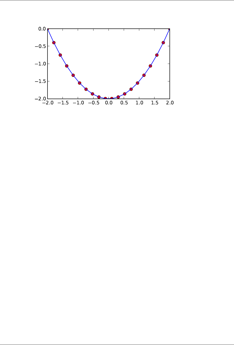
SciPy Reference Guide, Release 0.13.0
scipy.integrate.simps(y,x=None,dx=1,axis=-1,even=’avg’)
Integrate y(x) using samples along the given axis and the composite Simpson’s rule. If x is None, spacing of dx
is assumed.
If there are an even number of samples, N, then there are an odd number of intervals (N-1), but Simpson’s rule
requires an even number of intervals. The parameter ‘even’ controls how this is handled.
Parameters y: array_like
Array to be integrated.
x: array_like, optional
If given, the points at which yis sampled.
dx : int, optional
Spacing of integration points along axis of y. Only used when xis None. Default is 1.
axis : int, optional
Axis along which to integrate. Default is the last axis.
even : {‘avg’, ‘first’, ‘str’}, optional
‘avg’ [Average two results:1) use the first N-2 intervals with] a trapezoidal
rule on the last interval and 2) use the last N-2 intervals with a trape-
zoidal rule on the first interval.
‘first’ [Use Simpson’s rule for the first N-2 intervals with] a trapezoidal rule
on the last interval.
‘last’ [Use Simpson’s rule for the last N-2 intervals with a] trapezoidal rule
on the first interval.
See Also
quad adaptive quadrature using QUADPACK
romberg adaptive Romberg quadrature
quadratureadaptive Gaussian quadrature
fixed_quadfixed-order Gaussian quadrature
dblquad double integrals
tplquad triple integrals
romb integrators for sampled data
5.6. Integration and ODEs (scipy.integrate) 265

SciPy Reference Guide, Release 0.13.0
cumtrapz cumulative integration for sampled data
ode ODE integrators
odeint ODE integrators
Notes
For an odd number of samples that are equally spaced the result is exact if the function is a polynomial of order
3 or less. If the samples are not equally spaced, then the result is exact only if the function is a polynomial of
order 2 or less.
scipy.integrate.romb(y,dx=1.0,axis=-1,show=False)
Romberg integration using samples of a function.
Parameters y: array_like
A vector of 2**k+1equally-spaced samples of a function.
dx : array_like, optional
The sample spacing. Default is 1.
axis : int, optional
The axis along which to integrate. Default is -1 (last axis).
show : bool, optional
When yis a single 1-D array, then if this argument is True print the table showing
Richardson extrapolation from the samples. Default is False.
Returns romb : ndarray
The integrated result for axis.
See Also
quad adaptive quadrature using QUADPACK
romberg adaptive Romberg quadrature
quadratureadaptive Gaussian quadrature
fixed_quadfixed-order Gaussian quadrature
dblquad double integrals
tplquad triple integrals
simps integrators for sampled data
cumtrapz cumulative integration for sampled data
ode ODE integrators
odeint ODE integrators
See Also
scipy.special for orthogonal polynomials (special) for Gaussian quadrature roots and weights for other weight-
ing factors and regions.
5.6.3 Integrators of ODE systems
odeint(func, y0, t[, args, Dfun, col_deriv, ...]) Integrate a system of ordinary differential equations.
ode(f[, jac]) A generic interface class to numeric integrators.
complex_ode(f[, jac]) A wrapper of ode for complex systems.
266 Chapter 5. Reference

SciPy Reference Guide, Release 0.13.0
scipy.integrate.odeint(func,y0,t,args=(),Dfun=None,col_deriv=0,full_output=0,ml=None,
mu=None,rtol=None,atol=None,tcrit=None,h0=0.0,hmax=0.0,
hmin=0.0,ixpr=0,mxstep=0,mxhnil=0,mxordn=12,mxords=5,print-
messg=0)
Integrate a system of ordinary differential equations.
Solve a system of ordinary differential equations using lsoda from the FORTRAN library odepack.
Solves the initial value problem for stiff or non-stiff systems of first order ode-s:
dy/dt =func(y,t0,...)
where y can be a vector.
Parameters func : callable(y, t0, ...)
Computes the derivative of y at t0.
y0 : array
Initial condition on y (can be a vector).
t: array
A sequence of time points for which to solve for y. The initial value point should be
the first element of this sequence.
args : tuple, optional
Extra arguments to pass to function.
Dfun : callable(y, t0, ...)
Gradient (Jacobian) of func.
col_deriv : bool, optional
True if Dfun defines derivatives down columns (faster), otherwise Dfun should define
derivatives across rows.
full_output : bool, optional
True if to return a dictionary of optional outputs as the second output
printmessg : bool, optional
Whether to print the convergence message
Returns y: array, shape (len(t), len(y0))
Array containing the value of y for each desired time in t, with the initial value y0 in
the first row.
infodict : dict, only returned if full_output == True
Dictionary containing additional output information
key meaning
‘hu’ vector of step sizes successfully used for each time step.
‘tcur’ vector with the value of t reached for each time step. (will always be at
least as large as the input times).
‘tolsf’ vector of tolerance scale factors, greater than 1.0, computed when a
request for too much accuracy was detected.
‘tsw’ value of t at the time of the last method switch (given for each time step)
‘nst’ cumulative number of time steps
‘nfe’ cumulative number of function evaluations for each time step
‘nje’ cumulative number of jacobian evaluations for each time step
‘nqu’ a vector of method orders for each successful step.
‘imxer’ index of the component of largest magnitude in the weighted local error
vector (e / ewt) on an error return, -1 otherwise.
‘lenrw’ the length of the double work array required.
‘leniw’ the length of integer work array required.
‘mused’a vector of method indicators for each successful time step: 1: adams
(nonstiff), 2: bdf (stiff)
Other Parameters
ml, mu : int, optional
5.6. Integration and ODEs (scipy.integrate) 267

SciPy Reference Guide, Release 0.13.0
If either of these are not None or non-negative, then the Jacobian is assumed to be
banded. These give the number of lower and upper non-zero diagonals in this banded
matrix. For the banded case, Dfun should return a matrix whose columns contain the
non-zero bands (starting with the lowest diagonal). Thus, the return matrix from Dfun
should have shape len(y0) *(ml + mu + 1) when ml >=0 or mu >=0.
rtol, atol : float, optional
The input parameters rtol and atol determine the error control performed by the solver.
The solver will control the vector, e, of estimated local errors in y, according to an
inequality of the form max-norm of (e / ewt) <= 1, where ewt is a vector
of positive error weights computed as ewt = rtol *abs(y) + atol. rtol
and atol can be either vectors the same length as y or scalars. Defaults to 1.49012e-8.
tcrit : ndarray, optional
Vector of critical points (e.g. singularities) where integration care should be taken.
h0 : float, (0: solver-determined), optional
The step size to be attempted on the first step.
hmax : float, (0: solver-determined), optional
The maximum absolute step size allowed.
hmin : float, (0: solver-determined), optional
The minimum absolute step size allowed.
ixpr : bool, optional
Whether to generate extra printing at method switches.
mxstep : int, (0: solver-determined), optional
Maximum number of (internally defined) steps allowed for each integration point in t.
mxhnil : int, (0: solver-determined), optional
Maximum number of messages printed.
mxordn : int, (0: solver-determined), optional
Maximum order to be allowed for the non-stiff (Adams) method.
mxords : int, (0: solver-determined), optional
Maximum order to be allowed for the stiff (BDF) method.
See Also
ode a more object-oriented integrator based on VODE.
quad for finding the area under a curve.
class scipy.integrate.ode(f,jac=None)
A generic interface class to numeric integrators.
Solve an equation system y0(t) = f(t, y)with (optional) jac = df/dy.
Parameters f: callable f(t, y, *f_args)
Rhs of the equation. t is a scalar, y.shape == (n,).f_args is set by calling
set_f_params(*args).fshould return a scalar, array or list (not a tuple).
jac : callable jac(t, y, *jac_args)
Jacobian of the rhs, jac[i,j] = d f[i] / d y[j].jac_args is set by call-
ing set_f_params(*args).
See Also
odeint an integrator with a simpler interface based on lsoda from ODEPACK
quad for finding the area under a curve
268 Chapter 5. Reference

SciPy Reference Guide, Release 0.13.0
Notes
Available integrators are listed below. They can be selected using the set_integrator method.
“vode”
Real-valued Variable-coefficient Ordinary Differential Equation solver, with fixed-leading-coefficient im-
plementation. It provides implicit Adams method (for non-stiff problems) and a method based on back-
ward differentiation formulas (BDF) (for stiff problems).
Source: http://www.netlib.org/ode/vode.f
Warning: This integrator is not re-entrant. You cannot have two ode instances using the “vode”
integrator at the same time.
This integrator accepts the following parameters in set_integrator method of the ode class:
•atol : float or sequence absolute tolerance for solution
•rtol : float or sequence relative tolerance for solution
•lband : None or int
•rband : None or int Jacobian band width, jac[i,j] != 0 for i-lband <= j <= i+rband. Setting these
requires your jac routine to return the jacobian in packed format, jac_packed[i-j+lband, j] = jac[i,j].
•method: ‘adams’ or ‘bdf’ Which solver to use, Adams (non-stiff) or BDF (stiff)
•with_jacobian : bool Whether to use the jacobian
•nsteps : int Maximum number of (internally defined) steps allowed during one call to the solver.
•first_step : float
•min_step : float
•max_step : float Limits for the step sizes used by the integrator.
•order : int Maximum order used by the integrator, order <= 12 for Adams, <= 5 for BDF.
“zvode”
Complex-valued Variable-coefficient Ordinary Differential Equation solver, with fixed-leading-coefficient
implementation. It provides implicit Adams method (for non-stiff problems) and a method based on
backward differentiation formulas (BDF) (for stiff problems).
Source: http://www.netlib.org/ode/zvode.f
Warning: This integrator is not re-entrant. You cannot have two ode instances using the “zvode”
integrator at the same time.
This integrator accepts the same parameters in set_integrator as the “vode” solver.
Note: When using ZVODE for a stiff system, it should only be used for the case in which the function
f is analytic, that is, when each f(i) is an analytic function of each y(j). Analyticity means that the partial
derivative df(i)/dy(j) is a unique complex number, and this fact is critical in the way ZVODE solves the
dense or banded linear systems that arise in the stiff case. For a complex stiff ODE system in which f is
not analytic, ZVODE is likely to have convergence failures, and for this problem one should instead use
DVODE on the equivalent real system (in the real and imaginary parts of y).
“lsoda”
Real-valued Variable-coefficient Ordinary Differential Equation solver, with fixed-leading-coefficient im-
plementation. It provides automatic method switching between implicit Adams method (for non-stiff
problems) and a method based on backward differentiation formulas (BDF) (for stiff problems).
Source: http://www.netlib.org/odepack
Warning: This integrator is not re-entrant. You cannot have two ode instances using the “lsoda”
integrator at the same time.
This integrator accepts the following parameters in set_integrator method of the ode class:
•atol : float or sequence absolute tolerance for solution
5.6. Integration and ODEs (scipy.integrate) 269

SciPy Reference Guide, Release 0.13.0
•rtol : float or sequence relative tolerance for solution
•lband : None or int
•rband : None or int Jacobian band width, jac[i,j] != 0 for i-lband <= j <= i+rband. Setting these
requires your jac routine to return the jacobian in packed format, jac_packed[i-j+lband, j] = jac[i,j].
•with_jacobian : bool Whether to use the jacobian
•nsteps : int Maximum number of (internally defined) steps allowed during one call to the solver.
•first_step : float
•min_step : float
•max_step : float Limits for the step sizes used by the integrator.
•max_order_ns : int Maximum order used in the nonstiff case (default 12).
•max_order_s : int Maximum order used in the stiff case (default 5).
•max_hnil : int Maximum number of messages reporting too small step size (t + h = t) (default 0)
•ixpr : int Whether to generate extra printing at method switches (default False).
“dopri5”
This is an explicit runge-kutta method of order (4)5 due to Dormand & Prince (with stepsize control and
dense output).
Authors:
E. Hairer and G. Wanner Universite de Geneve, Dept. de Mathematiques CH-1211 Geneve 24,
Switzerland e-mail: ernst.hairer@math.unige.ch,gerhard.wanner@math.unige.ch
This code is described in [HNW93].
This integrator accepts the following parameters in set_integrator() method of the ode class:
•atol : float or sequence absolute tolerance for solution
•rtol : float or sequence relative tolerance for solution
•nsteps : int Maximum number of (internally defined) steps allowed during one call to the solver.
•first_step : float
•max_step : float
•safety : float Safety factor on new step selection (default 0.9)
•ifactor : float
•dfactor : float Maximum factor to increase/decrease step size by in one step
•beta : float Beta parameter for stabilised step size control.
•verbosity : int Switch for printing messages (< 0 for no messages).
“dop853”
This is an explicit runge-kutta method of order 8(5,3) due to Dormand & Prince (with stepsize control and
dense output).
Options and references the same as “dopri5”.
References
[HNW93]
Examples
A problem to integrate and the corresponding jacobian:
>>> from scipy.integrate import ode
>>>
>>> y0, t0 =[1.0j,2.0], 0
>>>
>>> def f(t, y, arg1):
>>> return [1j*arg1*y[0]+y[1], -arg1*y[1]**2]
>>> def jac(t, y, arg1):
>>> return [[1j*arg1, 1], [0,-arg1*2*y[1]]]
The integration:
270 Chapter 5. Reference

SciPy Reference Guide, Release 0.13.0
>>> r=ode(f, jac).set_integrator(’zvode’, method=’bdf’, with_jacobian=True)
>>> r.set_initial_value(y0, t0).set_f_params(2.0).set_jac_params(2.0)
>>> t1 =10
>>> dt =1
>>> while r.successful() and r.t<t1:
>>> r.integrate(r.t+dt)
>>> print("%g %g"%(r.t, r.y))
Attributes
t (float) Current time.
y (ndarray) Current variable values.
Methods
integrate(t[, step, relax]) Find y=y(t), set y as an initial condition, and return y.
set_f_params(*args) Set extra parameters for user-supplied function f.
set_initial_value(y[, t]) Set initial conditions y(t) = y.
set_integrator(name, **integrator_params) Set integrator by name.
set_jac_params(*args) Set extra parameters for user-supplied function jac.
set_solout(solout) Set callable to be called at every successful integration step.
successful() Check if integration was successful.
ode.integrate(t,step=0,relax=0)
Find y=y(t), set y as an initial condition, and return y.
ode.set_f_params(*args)
Set extra parameters for user-supplied function f.
ode.set_initial_value(y,t=0.0)
Set initial conditions y(t) = y.
ode.set_integrator(name,**integrator_params)
Set integrator by name.
Parameters name : str
Name of the integrator.
integrator_params :
Additional parameters for the integrator.
ode.set_jac_params(*args)
Set extra parameters for user-supplied function jac.
ode.set_solout(solout)
Set callable to be called at every successful integration step.
Parameters solout : callable
solout(t, y) is called at each internal integrator step, t is a scalar providing
the current independent position y is the current soloution y.shape == (n,)
solout should return -1 to stop integration otherwise it should return None or 0
ode.successful()
Check if integration was successful.
class scipy.integrate.complex_ode(f,jac=None)
A wrapper of ode for complex systems.
5.6. Integration and ODEs (scipy.integrate) 271

SciPy Reference Guide, Release 0.13.0
This functions similarly as ode, but re-maps a complex-valued equation system to a real-valued one before
using the integrators.
Parameters f: callable f(t, y, *f_args)
Rhs of the equation. t is a scalar, y.shape == (n,).f_args is set by calling
set_f_params(*args).
jac : callable jac(t, y, *jac_args)
Jacobian of the rhs, jac[i,j] = d f[i] / d y[j].jac_args is set by call-
ing set_f_params(*args).
Examples
For usage examples, see ode.
Attributes
t (float) Current time.
y (ndarray) Current variable values.
Methods
integrate(t[, step, relax]) Find y=y(t), set y as an initial condition, and return y.
set_f_params(*args) Set extra parameters for user-supplied function f.
set_initial_value(y[, t]) Set initial conditions y(t) = y.
set_integrator(name, **integrator_params) Set integrator by name.
set_jac_params(*args) Set extra parameters for user-supplied function jac.
set_solout(solout) Set callable to be called at every successful integration step.
successful() Check if integration was successful.
complex_ode.integrate(t,step=0,relax=0)
Find y=y(t), set y as an initial condition, and return y.
complex_ode.set_f_params(*args)
Set extra parameters for user-supplied function f.
complex_ode.set_initial_value(y,t=0.0)
Set initial conditions y(t) = y.
complex_ode.set_integrator(name,**integrator_params)
Set integrator by name.
Parameters name : str
Name of the integrator
integrator_params :
Additional parameters for the integrator.
complex_ode.set_jac_params(*args)
Set extra parameters for user-supplied function jac.
complex_ode.set_solout(solout)
Set callable to be called at every successful integration step.
Parameters solout : callable
solout(t, y) is called at each internal integrator step, t is a scalar providing
the current independent position y is the current soloution y.shape == (n,)
solout should return -1 to stop integration otherwise it should return None or 0
complex_ode.successful()
Check if integration was successful.
272 Chapter 5. Reference

SciPy Reference Guide, Release 0.13.0
5.7 Interpolation (scipy.interpolate)
Sub-package for objects used in interpolation.
As listed below, this sub-package contains spline functions and classes, one-dimensional and multi-dimensional (uni-
variate and multivariate) interpolation classes, Lagrange and Taylor polynomial interpolators, and wrappers for FIT-
PACK and DFITPACK functions.
5.7.1 Univariate interpolation
interp1d(x, y[, kind, axis, copy, ...]) Interpolate a 1-D function.
BarycentricInterpolator(xi[, yi, axis]) The interpolating polynomial for a set of points
KroghInterpolator(xi, yi[, axis]) Interpolating polynomial for a set of points.
PiecewisePolynomial(xi, yi[, orders, ...]) Piecewise polynomial curve specified by points and derivatives
PchipInterpolator(x, y[, axis]) PCHIP 1-d monotonic cubic interpolation
barycentric_interpolate(xi, yi, x[, axis]) Convenience function for polynomial interpolation.
krogh_interpolate(xi, yi, x[, der, axis]) Convenience function for polynomial interpolation.
piecewise_polynomial_interpolate(xi, yi, x) Convenience function for piecewise polynomial interpolation.
pchip_interpolate(xi, yi, x[, der, axis]) Convenience function for pchip interpolation.
class scipy.interpolate.interp1d(x,y,kind=’linear’,axis=-1,copy=True,bounds_error=True,
fill_value=np.nan)
Interpolate a 1-D function.
xand yare arrays of values used to approximate some function f: y = f(x). This class returns a function
whose call method uses interpolation to find the value of new points.
Parameters x: (N,) array_like
A 1-D array of monotonically increasing real values.
y: (...,N,...) array_like
A N-D array of real values. The length of yalong the interpolation axis must be equal
to the length of x.
kind : str or int, optional
Specifies the kind of interpolation as a string (‘linear’, ‘nearest’, ‘zero’, ‘slinear’,
‘quadratic, ‘cubic’ where ‘slinear’, ‘quadratic’ and ‘cubic’ refer to a spline interpola-
tion of first, second or third order) or as an integer specifying the order of the spline
interpolator to use. Default is ‘linear’.
axis : int, optional
Specifies the axis of yalong which to interpolate. Interpolation defaults to the last axis
of y.
copy : bool, optional
If True, the class makes internal copies of x and y. If False, references to xand yare
used. The default is to copy.
bounds_error : bool, optional
If True, a ValueError is raised any time interpolation is attempted on a value outside
of the range of x (where extrapolation is necessary). If False, out of bounds values are
assigned fill_value. By default, an error is raised.
fill_value : float, optional
If provided, then this value will be used to fill in for requested points outside of the
data range. If not provided, then the default is NaN.
5.7. Interpolation (scipy.interpolate) 273

SciPy Reference Guide, Release 0.13.0
See Also
UnivariateSpline
A more recent wrapper of the FITPACK routines.
splrep,splev,interp2d
Examples
>>> from scipy import interpolate
>>> x=np.arange(0,10)
>>> y=np.exp(-x/3.0)
>>> f=interpolate.interp1d(x, y)
>>> xnew =np.arange(0,9,0.1)
>>> ynew =f(xnew) # use interpolation function returned by ‘interp1d‘
>>> plt.plot(x, y, ’o’, xnew, ynew, ’-’)
>>> plt.show()
Methods
__call__(x) Evaluate the interpolant
interp1d.__call__(x)
Evaluate the interpolant
Parameters x: array-like
Points to evaluate the interpolant at.
Returns y: array-like
Interpolated values. Shape is determined by replacing the interpolation axis in
the original array with the shape of x.
class scipy.interpolate.BarycentricInterpolator(xi,yi=None,axis=0)
The interpolating polynomial for a set of points
Constructs a polynomial that passes through a given set of points. Allows evaluation of the polynomial, efficient
changing of the y values to be interpolated, and updating by adding more x values. For reasons of numerical
stability, this function does not compute the coefficients of the polynomial.
The values yi need to be provided before the function is evaluated, but none of the preprocessing depends on
them, so rapid updates are possible.
Parameters xi : array-like
1-d array of x coordinates of the points the polynomial should pass through
yi : array-like
The y coordinates of the points the polynomial should pass through. If None, the y
values will be supplied later via the set_y method.
axis : int, optional
Axis in the yi array corresponding to the x-coordinate values.
Notes
This class uses a “barycentric interpolation” method that treats the problem as a special case of rational function
interpolation. This algorithm is quite stable, numerically, but even in a world of exact computation, unless the
x coordinates are chosen very carefully - Chebyshev zeros (e.g. cos(i*pi/n)) are a good choice - polynomial
interpolation itself is a very ill-conditioned process due to the Runge phenomenon.
Based on Berrut and Trefethen 2004, “Barycentric Lagrange Interpolation”.
274 Chapter 5. Reference

SciPy Reference Guide, Release 0.13.0
Methods
__call__(x) Evaluate the interpolating polynomial at the points x
add_xi(xi[, yi]) Add more x values to the set to be interpolated
set_yi(yi[, axis]) Update the y values to be interpolated
BarycentricInterpolator.__call__(x)
Evaluate the interpolating polynomial at the points x
Parameters x: array-like
Points to evaluate the interpolant at.
Returns y: array-like
Interpolated values. Shape is determined by replacing the interpolation axis in
the original array with the shape of x.
Notes
Currently the code computes an outer product between x and the weights, that is, it constructs an interme-
diate array of size N by len(x), where N is the degree of the polynomial.
BarycentricInterpolator.add_xi(xi,yi=None)
Add more x values to the set to be interpolated
The barycentric interpolation algorithm allows easy updating by adding more points for the polynomial
to pass through.
Parameters xi : array_like
The x coordinates of the points that the polynomial should pass through.
yi : array_like, optional
The y coordinates of the points the polynomial should pass through. Should have
shape (xi.size, R); if R > 1 then the polynomial is vector-valued. If yi is
not given, the y values will be supplied later. yi should be given if and only if the
interpolator has y values specified.
BarycentricInterpolator.set_yi(yi,axis=None)
Update the y values to be interpolated
The barycentric interpolation algorithm requires the calculation of weights, but these depend only on the
xi. The yi can be changed at any time.
Parameters yi : array_like
The y coordinates of the points the polynomial should pass through. If None, the
y values will be supplied later.
axis : int, optional
Axis in the yi array corresponding to the x-coordinate values.
class scipy.interpolate.KroghInterpolator(xi,yi,axis=0)
Interpolating polynomial for a set of points.
The polynomial passes through all the pairs (xi,yi). One may additionally specify a number of derivatives at
each point xi; this is done by repeating the value xi and specifying the derivatives as successive yi values.
Allows evaluation of the polynomial and all its derivatives. For reasons of numerical stability, this function does
not compute the coefficients of the polynomial, although they can be obtained by evaluating all the derivatives.
Parameters xi : array-like, length N
Known x-coordinates. Must be sorted in increasing order.
yi : array-like
5.7. Interpolation (scipy.interpolate) 275

SciPy Reference Guide, Release 0.13.0
Known y-coordinates. When an xi occurs two or more times in a row, the correspond-
ing yi’s represent derivative values.
axis : int, optional
Axis in the yi array corresponding to the x-coordinate values.
Notes
Be aware that the algorithms implemented here are not necessarily the most numerically stable known. More-
over, even in a world of exact computation, unless the x coordinates are chosen very carefully - Chebyshev
zeros (e.g. cos(i*pi/n)) are a good choice - polynomial interpolation itself is a very ill-conditioned process due
to the Runge phenomenon. In general, even with well-chosen x values, degrees higher than about thirty cause
problems with numerical instability in this code.
Based on [R33].
References
[R33]
Examples
To produce a polynomial that is zero at 0 and 1 and has derivative 2 at 0, call
>>> KroghInterpolator([0,0,1],[0,2,0])
This constructs the quadratic 2*X**2-2*X. The derivative condition is indicated by the repeated zero in the xi
array; the corresponding yi values are 0, the function value, and 2, the derivative value.
For another example, given xi, yi, and a derivative ypi for each point, appropriate arrays can be constructed as:
>>> xi_k, yi_k =np.repeat(xi, 2), np.ravel(np.dstack((yi,ypi)))
>>> KroghInterpolator(xi_k, yi_k)
To produce a vector-valued polynomial, supply a higher-dimensional array for yi:
>>> KroghInterpolator([0,1],[[2,3],[4,5]])
This constructs a linear polynomial giving (2,3) at 0 and (4,5) at 1.
Methods
__call__(x) Evaluate the interpolant
derivative(x[, der]) Evaluate one derivative of the polynomial at the point x
derivatives(x[, der]) Evaluate many derivatives of the polynomial at the point x
KroghInterpolator.__call__(x)
Evaluate the interpolant
Parameters x: array-like
Points to evaluate the interpolant at.
Returns y: array-like
Interpolated values. Shape is determined by replacing the interpolation axis in
the original array with the shape of x.
KroghInterpolator.derivative(x,der=1)
Evaluate one derivative of the polynomial at the point x
Parameters x: array-like
Point or points at which to evaluate the derivatives
276 Chapter 5. Reference

SciPy Reference Guide, Release 0.13.0
der : integer, optional
Which derivative to extract. This number includes the function value as 0th
derivative.
Returns d: ndarray
Derivative interpolated at the x-points. Shape of d is determined by replacing the
interpolation axis in the original array with the shape of x.
Notes
This is computed by evaluating all derivatives up to the desired one (using self.derivatives()) and then
discarding the rest.
KroghInterpolator.derivatives(x,der=None)
Evaluate many derivatives of the polynomial at the point x
Produce an array of all derivative values at the point x.
Parameters x: array-like
Point or points at which to evaluate the derivatives
der : None or integer
How many derivatives to extract; None for all potentially nonzero derivatives
(that is a number equal to the number of points). This number includes the func-
tion value as 0th derivative.
Returns d: ndarray
Array with derivatives; d[j] contains the j-th derivative. Shape of d[j] is deter-
mined by replacing the interpolation axis in the original array with the shape of
x.
Examples
>>> KroghInterpolator([0,0,0],[1,2,3]).derivatives(0)
array([1.0,2.0,3.0])
>>> KroghInterpolator([0,0,0],[1,2,3]).derivatives([0,0])
array([[1.0,1.0],
[2.0,2.0],
[3.0,3.0]])
class scipy.interpolate.PiecewisePolynomial(xi,yi,orders=None,direction=None,axis=0)
Piecewise polynomial curve specified by points and derivatives
This class represents a curve that is a piecewise polynomial. It passes through a list of points and has specified
derivatives at each point. The degree of the polynomial may vary from segment to segment, as may the number
of derivatives available. The degree should not exceed about thirty.
Appending points to the end of the curve is efficient.
Parameters xi : array-like
a sorted 1-d array of x-coordinates
yi : array-like or list of array-likes
yi[i][j] is the j-th derivative known at xi[i] (for axis=0)
orders : list of integers, or integer
a list of polynomial orders, or a single universal order
direction : {None, 1, -1}
indicates whether the xi are increasing or decreasing +1 indicates increasing -1 indi-
cates decreasing None indicates that it should be deduced from the first two xi
axis : int, optional
Axis in the yi array corresponding to the x-coordinate values.
5.7. Interpolation (scipy.interpolate) 277

SciPy Reference Guide, Release 0.13.0
Notes
If orders is None, or orders[i] is None, then the degree of the polynomial segment is exactly the degree required
to match all i available derivatives at both endpoints. If orders[i] is not None, then some derivatives will be
ignored. The code will try to use an equal number of derivatives from each end; if the total number of derivatives
needed is odd, it will prefer the rightmost endpoint. If not enough derivatives are available, an exception is raised.
Methods
__call__(x) Evaluate the interpolant
append(xi, yi[, order]) Append a single point with derivatives to the PiecewisePolynomial
derivative(x[, der]) Evaluate one derivative of the polynomial at the point x
derivatives(x[, der]) Evaluate many derivatives of the polynomial at the point x
extend(xi, yi[, orders]) Extend the PiecewisePolynomial by a list of points
PiecewisePolynomial.__call__(x)
Evaluate the interpolant
Parameters x: array-like
Points to evaluate the interpolant at.
Returns y: array-like
Interpolated values. Shape is determined by replacing the interpolation axis in
the original array with the shape of x.
PiecewisePolynomial.append(xi,yi,order=None)
Append a single point with derivatives to the PiecewisePolynomial
Parameters xi : float
Input
yi : array_like
yi is the list of derivatives known at xi
order : integer or None
a polynomial order, or instructions to use the highest possible order
PiecewisePolynomial.derivative(x,der=1)
Evaluate one derivative of the polynomial at the point x
Parameters x: array-like
Point or points at which to evaluate the derivatives
der : integer, optional
Which derivative to extract. This number includes the function value as 0th
derivative.
Returns d: ndarray
Derivative interpolated at the x-points. Shape of d is determined by replacing the
interpolation axis in the original array with the shape of x.
Notes
This is computed by evaluating all derivatives up to the desired one (using self.derivatives()) and then
discarding the rest.
PiecewisePolynomial.derivatives(x,der=None)
Evaluate many derivatives of the polynomial at the point x
Produce an array of all derivative values at the point x.
Parameters x: array-like
Point or points at which to evaluate the derivatives
278 Chapter 5. Reference

SciPy Reference Guide, Release 0.13.0
der : None or integer
How many derivatives to extract; None for all potentially nonzero derivatives
(that is a number equal to the number of points). This number includes the func-
tion value as 0th derivative.
Returns d: ndarray
Array with derivatives; d[j] contains the j-th derivative. Shape of d[j] is deter-
mined by replacing the interpolation axis in the original array with the shape of
x.
Examples
>>> KroghInterpolator([0,0,0],[1,2,3]).derivatives(0)
array([1.0,2.0,3.0])
>>> KroghInterpolator([0,0,0],[1,2,3]).derivatives([0,0])
array([[1.0,1.0],
[2.0,2.0],
[3.0,3.0]])
PiecewisePolynomial.extend(xi,yi,orders=None)
Extend the PiecewisePolynomial by a list of points
Parameters xi : array_like
A sorted list of x-coordinates.
yi : list of lists of length N1
yi[i] (if axis == 0) is the list of derivatives known at xi[i].
orders : int or list of ints
A list of polynomial orders, or a single universal order.
direction : {None, 1, -1}
Indicates whether the xi are increasing or decreasing.
+1 indicates increasing
-1 indicates decreasing
None indicates that it should be deduced from the first two xi.
class scipy.interpolate.PchipInterpolator(x,y,axis=0)
PCHIP 1-d monotonic cubic interpolation
x and y are arrays of values used to approximate some function f, with y = f(x). The interpolant uses
monotonic cubic splines to find the value of new points.
Parameters x: ndarray
A 1-D array of monotonically increasing real values. xcannot include duplicate values
(otherwise f is overspecified)
y: ndarray
A 1-D array of real values. y‘s length along the interpolation axis must be equal to the
length of x.
axis : int, optional
Axis in the yi array corresponding to the x-coordinate values.
Notes
Assumes x is sorted in monotonic order (e.g. x[1] > x[0]).
Methods
__call__(x) Evaluate the interpolant
append(xi, yi[, order]) Append a single point with derivatives to the PiecewisePolynomial
Continued on next page
5.7. Interpolation (scipy.interpolate) 279

SciPy Reference Guide, Release 0.13.0
Table 5.29 – continued from previous page
derivative(x[, der]) Evaluate one derivative of the polynomial at the point x
derivatives(x[, der]) Evaluate many derivatives of the polynomial at the point x
extend(xi, yi[, orders]) Extend the PiecewisePolynomial by a list of points
PchipInterpolator.__call__(x)
Evaluate the interpolant
Parameters x: array-like
Points to evaluate the interpolant at.
Returns y: array-like
Interpolated values. Shape is determined by replacing the interpolation axis in
the original array with the shape of x.
PchipInterpolator.append(xi,yi,order=None)
Append a single point with derivatives to the PiecewisePolynomial
Parameters xi : float
Input
yi : array_like
yi is the list of derivatives known at xi
order : integer or None
a polynomial order, or instructions to use the highest possible order
PchipInterpolator.derivative(x,der=1)
Evaluate one derivative of the polynomial at the point x
Parameters x: array-like
Point or points at which to evaluate the derivatives
der : integer, optional
Which derivative to extract. This number includes the function value as 0th
derivative.
Returns d: ndarray
Derivative interpolated at the x-points. Shape of d is determined by replacing the
interpolation axis in the original array with the shape of x.
Notes
This is computed by evaluating all derivatives up to the desired one (using self.derivatives()) and then
discarding the rest.
PchipInterpolator.derivatives(x,der=None)
Evaluate many derivatives of the polynomial at the point x
Produce an array of all derivative values at the point x.
Parameters x: array-like
Point or points at which to evaluate the derivatives
der : None or integer
How many derivatives to extract; None for all potentially nonzero derivatives
(that is a number equal to the number of points). This number includes the func-
tion value as 0th derivative.
Returns d: ndarray
Array with derivatives; d[j] contains the j-th derivative. Shape of d[j] is deter-
mined by replacing the interpolation axis in the original array with the shape of
x.
280 Chapter 5. Reference

SciPy Reference Guide, Release 0.13.0
Examples
>>> KroghInterpolator([0,0,0],[1,2,3]).derivatives(0)
array([1.0,2.0,3.0])
>>> KroghInterpolator([0,0,0],[1,2,3]).derivatives([0,0])
array([[1.0,1.0],
[2.0,2.0],
[3.0,3.0]])
PchipInterpolator.extend(xi,yi,orders=None)
Extend the PiecewisePolynomial by a list of points
Parameters xi : array_like
A sorted list of x-coordinates.
yi : list of lists of length N1
yi[i] (if axis == 0) is the list of derivatives known at xi[i].
orders : int or list of ints
A list of polynomial orders, or a single universal order.
direction : {None, 1, -1}
Indicates whether the xi are increasing or decreasing.
+1 indicates increasing
-1 indicates decreasing
None indicates that it should be deduced from the first two xi.
scipy.interpolate.barycentric_interpolate(xi,yi,x,axis=0)
Convenience function for polynomial interpolation.
Constructs a polynomial that passes through a given set of points, then evaluates the polynomial. For reasons of
numerical stability, this function does not compute the coefficients of the polynomial.
This function uses a “barycentric interpolation” method that treats the problem as a special case of rational
function interpolation. This algorithm is quite stable, numerically, but even in a world of exact computation,
unless the xcoordinates are chosen very carefully - Chebyshev zeros (e.g. cos(i*pi/n)) are a good choice -
polynomial interpolation itself is a very ill-conditioned process due to the Runge phenomenon.
Parameters xi : array_like
1-d array of x coordinates of the points the polynomial should pass through
yi : array_like
The y coordinates of the points the polynomial should pass through.
x: scalar or array_like
Points to evaluate the interpolator at.
axis : int, optional
Axis in the yi array corresponding to the x-coordinate values.
Returns y: scalar or array_like
Interpolated values. Shape is determined by replacing the interpolation axis in the
original array with the shape of x.
See Also
BarycentricInterpolator
Notes
Construction of the interpolation weights is a relatively slow process. If you want to call this many times with
the same xi (but possibly varying yi or x) you should use the class BarycentricInterpolator. This is
what this function uses internally.
scipy.interpolate.krogh_interpolate(xi,yi,x,der=0,axis=0)
Convenience function for polynomial interpolation.
5.7. Interpolation (scipy.interpolate) 281

SciPy Reference Guide, Release 0.13.0
See KroghInterpolator for more details.
Parameters xi : array_like
Known x-coordinates.
yi : array_like
Known y-coordinates, of shape (xi.size, R). Interpreted as vectors of length R,
or scalars if R=1.
x: array_like
Point or points at which to evaluate the derivatives.
der : int or list
How many derivatives to extract; None for all potentially nonzero derivatives (that is a
number equal to the number of points), or a list of derivatives to extract. This number
includes the function value as 0th derivative.
axis : int, optional
Axis in the yi array corresponding to the x-coordinate values.
Returns d: ndarray
If the interpolator’s values are R-dimensional then the returned array will be the num-
ber of derivatives by N by R. If xis a scalar, the middle dimension will be dropped; if
the yi are scalars then the last dimension will be dropped.
See Also
KroghInterpolator
Notes
Construction of the interpolating polynomial is a relatively expensive process. If you want to evaluate it repeat-
edly consider using the class KroghInterpolator (which is what this function uses).
scipy.interpolate.piecewise_polynomial_interpolate(xi,yi,x,orders=None,der=0,
axis=0)
Convenience function for piecewise polynomial interpolation.
Parameters xi : array_like
A sorted list of x-coordinates.
yi : list of lists
yi[i] is the list of derivatives known at xi[i].
x: scalar or array_like
Coordinates at which to evalualte the polynomial.
orders : int or list of ints, optional
A list of polynomial orders, or a single universal order.
der : int or list
How many derivatives to extract; None for all potentially nonzero derivatives (that is a
number equal to the number of points), or a list of derivatives to extract. This number
includes the function value as 0th derivative.
axis : int, optional
Axis in the yi array corresponding to the x-coordinate values.
Returns y: ndarray
Interpolated values or derivatives. If multiple derivatives were requested, these are
given along the first axis.
See Also
PiecewisePolynomial
282 Chapter 5. Reference

SciPy Reference Guide, Release 0.13.0
Notes
If orders is None, or orders[i] is None, then the degree of the polynomial segment is exactly the degree
required to match all i available derivatives at both endpoints. If orders[i] is not None, then some derivatives
will be ignored. The code will try to use an equal number of derivatives from each end; if the total number of
derivatives needed is odd, it will prefer the rightmost endpoint. If not enough derivatives are available, an
exception is raised.
Construction of these piecewise polynomials can be an expensive process; if you repeatedly evaluate the same
polynomial, consider using the class PiecewisePolynomial (which is what this function does).
scipy.interpolate.pchip_interpolate(xi,yi,x,der=0,axis=0)
Convenience function for pchip interpolation.
See PchipInterpolator for details.
Parameters xi : array_like
A sorted list of x-coordinates, of length N.
yi : list of lists
yi[i] is the list of derivatives known at xi[i]. Of length N.
x: scalar or array_like
Of length M.
der : integer or list
How many derivatives to extract; None for all potentially nonzero derivatives (that is a
number equal to the number of points), or a list of derivatives to extract. This number
includes the function value as 0th derivative.
axis : int, optional
Axis in the yi array corresponding to the x-coordinate values.
Returns y: scalar or array_like
The result, of length R or length M or M by R,
See Also
PchipInterpolator
5.7.2 Multivariate interpolation
Unstructured data:
griddata(points, values, xi[, method, ...]) Interpolate unstructured N-dimensional data.
LinearNDInterpolator(points, values[, ...]) Piecewise linear interpolant in N dimensions.
NearestNDInterpolator(points, values) Nearest-neighbour interpolation in N dimensions.
CloughTocher2DInterpolator(points, values[, tol]) Piecewise cubic, C1 smooth, curvature-minimizing interpolant in 2D.
Rbf(*args) A class for radial basis function approximation/interpolation of n-dimensional scattered data.
interp2d(x, y, z[, kind, copy, ...]) Interpolate over a 2-D grid.
scipy.interpolate.griddata(points,values,xi,method=’linear’,fill_value=nan)
Interpolate unstructured N-dimensional data. New in version 0.9.
Parameters points : ndarray of floats, shape (N, ndim)
Data point coordinates. Can either be an array of size (N, ndim), or a tuple of ndim
arrays.
values : ndarray of float or complex, shape (N,)
Data values.
xi : ndarray of float, shape (M, ndim)
Points at which to interpolate data.
5.7. Interpolation (scipy.interpolate) 283

SciPy Reference Guide, Release 0.13.0
method : {‘linear’, ‘nearest’, ‘cubic’}, optional
Method of interpolation. One of
nearest return the value at the data point closest to the point of interpolation.
See NearestNDInterpolator for more details.
linear tesselate the input point set to n-dimensional simplices, and interpolate
linearly on each simplex. See LinearNDInterpolator for more
details.
cubic (1-D) return the value determined from a cubic spline.
cubic (2-D) return the value determined from a piecewise cubic, continuously dif-
ferentiable (C1), and approximately curvature-minimizing polynomial
surface. See CloughTocher2DInterpolator for more details.
fill_value : float, optional
Value used to fill in for requested points outside of the convex hull of the input points.
If not provided, then the default is nan. This option has no effect for the ‘nearest’
method.
Examples
Suppose we want to interpolate the 2-D function
>>> def func(x, y):
>>> return x*(1-x)*np.cos(4*np.pi*x) *np.sin(4*np.pi*y**2)**2
on a grid in [0, 1]x[0, 1]
>>> grid_x, grid_y =np.mgrid[0:1:100j,0:1:200j]
but we only know its values at 1000 data points:
>>> points =np.random.rand(1000,2)
>>> values =func(points[:,0], points[:,1])
This can be done with griddata – below we try out all of the interpolation methods:
>>> from scipy.interpolate import griddata
>>> grid_z0 =griddata(points, values, (grid_x, grid_y), method=’nearest’)
>>> grid_z1 =griddata(points, values, (grid_x, grid_y), method=’linear’)
>>> grid_z2 =griddata(points, values, (grid_x, grid_y), method=’cubic’)
One can see that the exact result is reproduced by all of the methods to some degree, but for this smooth function
the piecewise cubic interpolant gives the best results:
>>> import matplotlib.pyplot as plt
>>> plt.subplot(221)
>>> plt.imshow(func(grid_x, grid_y).T, extent=(0,1,0,1), origin=’lower’)
>>> plt.plot(points[:,0], points[:,1], ’k.’, ms=1)
>>> plt.title(’Original’)
>>> plt.subplot(222)
>>> plt.imshow(grid_z0.T, extent=(0,1,0,1), origin=’lower’)
>>> plt.title(’Nearest’)
>>> plt.subplot(223)
>>> plt.imshow(grid_z1.T, extent=(0,1,0,1), origin=’lower’)
>>> plt.title(’Linear’)
>>> plt.subplot(224)
>>> plt.imshow(grid_z2.T, extent=(0,1,0,1), origin=’lower’)
>>> plt.title(’Cubic’)
>>> plt.gcf().set_size_inches(6,6)
>>> plt.show()
284 Chapter 5. Reference
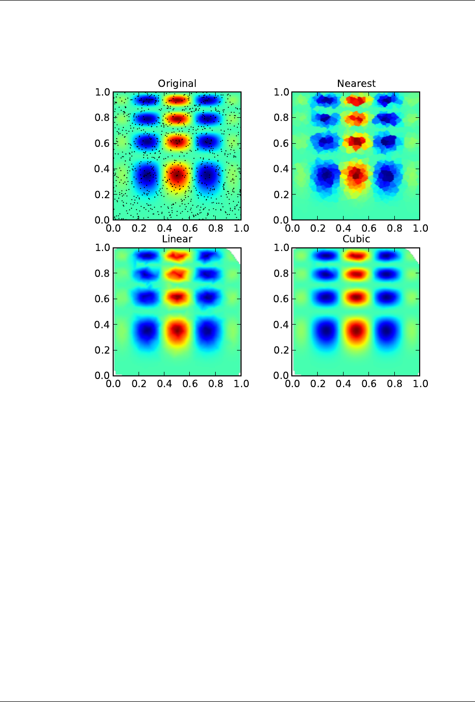
SciPy Reference Guide, Release 0.13.0
class scipy.interpolate.LinearNDInterpolator(points,values,fill_value=np.nan)
Piecewise linear interpolant in N dimensions. New in version 0.9.
Parameters points : ndarray of floats, shape (npoints, ndims); or Delaunay
Data point coordinates, or a precomputed Delaunay triangulation.
values : ndarray of float or complex, shape (npoints, ...)
Data values.
fill_value : float, optional
Value used to fill in for requested points outside of the convex hull of the input points.
If not provided, then the default is nan.
Notes
The interpolant is constructed by triangulating the input data with Qhull [R34], and on each triangle performing
linear barycentric interpolation.
References
[R34]
5.7. Interpolation (scipy.interpolate) 285

SciPy Reference Guide, Release 0.13.0
Methods
__call__(xi) Evaluate interpolator at given points.
LinearNDInterpolator.__call__(xi)
Evaluate interpolator at given points.
Parameters xi : ndarray of float, shape (..., ndim)
Points where to interpolate data at.
class scipy.interpolate.NearestNDInterpolator(points,values)
Nearest-neighbour interpolation in N dimensions. New in version 0.9.
Parameters points : (Npoints, Ndims) ndarray of floats
Data point coordinates.
values : (Npoints,) ndarray of float or complex
Data values.
Notes
Uses scipy.spatial.cKDTree
Methods
__call__(*args) Evaluate interpolator at given points.
NearestNDInterpolator.__call__(*args)
Evaluate interpolator at given points.
Parameters xi : ndarray of float, shape (..., ndim)
Points where to interpolate data at.
class scipy.interpolate.CloughTocher2DInterpolator(points,values,tol=1e-6)
Piecewise cubic, C1 smooth, curvature-minimizing interpolant in 2D. New in version 0.9.
Parameters points : ndarray of floats, shape (npoints, ndims); or Delaunay
Data point coordinates, or a precomputed Delaunay triangulation.
values : ndarray of float or complex, shape (npoints, ...)
Data values.
fill_value : float, optional
Value used to fill in for requested points outside of the convex hull of the input points.
If not provided, then the default is nan.
tol : float, optional
Absolute/relative tolerance for gradient estimation.
maxiter : int, optional
Maximum number of iterations in gradient estimation.
Notes
The interpolant is constructed by triangulating the input data with Qhull [R32], and constructing a piecewise
cubic interpolating Bezier polynomial on each triangle, using a Clough-Tocher scheme [CT]. The interpolant is
guaranteed to be continuously differentiable.
The gradients of the interpolant are chosen so that the curvature of the interpolating surface is approxima-
tively minimized. The gradients necessary for this are estimated using the global algorithm described in [Niel-
son83,Renka84]_.
286 Chapter 5. Reference

SciPy Reference Guide, Release 0.13.0
References
[R32],[CT],[Nielson83],[Renka84]
Methods
__call__(xi) Evaluate interpolator at given points.
CloughTocher2DInterpolator.__call__(xi)
Evaluate interpolator at given points.
Parameters xi : ndarray of float, shape (..., ndim)
Points where to interpolate data at.
class scipy.interpolate.Rbf(*args)
A class for radial basis function approximation/interpolation of n-dimensional scattered data.
Parameters *args : arrays
x, y, z, ..., d, where x, y, z, ... are the coordinates of the nodes and d is the array of
values at the nodes
function : str or callable, optional
The radial basis function, based on the radius, r, given by the norm (default is Eu-
clidean distance); the default is ‘multiquadric’:
’multiquadric’: sqrt((r/self.epsilon)**2 + 1)
’inverse’: 1.0/sqrt((r/self.epsilon)**2 + 1)
’gaussian’: exp(-(r/self.epsilon)**2)
’linear’: r
’cubic’: r**3
’quintic’: r**5
’thin_plate’: r**2*log(r)
If callable, then it must take 2 arguments (self, r). The epsilon parameter will be
available as self.epsilon. Other keyword arguments passed in will be available as
well.
epsilon : float, optional
Adjustable constant for gaussian or multiquadrics functions - defaults to approximate
average distance between nodes (which is a good start).
smooth : float, optional
Values greater than zero increase the smoothness of the approximation. 0 is for inter-
polation (default), the function will always go through the nodal points in this case.
norm : callable, optional
A function that returns the ‘distance’ between two points, with inputs as arrays of
positions (x, y, z, ...), and an output as an array of distance. E.g, the default:
def euclidean_norm(x1, x2):
return sqrt( ((x1 -x2)**2).sum(axis=0) )
which is called with x1=x1[ndims,newaxis,:] and x2=x2[ndims,:,newaxis] such that
the result is a matrix of the distances from each point in x1 to each point in x2.
Examples
>>> rbfi =Rbf(x, y, z, d) # radial basis function interpolator instance
>>> di =rbfi(xi, yi, zi) # interpolated values
Methods
5.7. Interpolation (scipy.interpolate) 287

SciPy Reference Guide, Release 0.13.0
__call__(*args)
Rbf.__call__(*args)
class scipy.interpolate.interp2d(x,y,z,kind=’linear’,copy=True,bounds_error=False,
fill_value=nan)
Interpolate over a 2-D grid.
x,yand zare arrays of values used to approximate some function f: z = f(x, y). This class returns a
function whose call method uses spline interpolation to find the value of new points.
If xand yrepresent a regular grid, consider using RectBivariateSpline.
Parameters x, y : array_like
Arrays defining the data point coordinates.
If the points lie on a regular grid, xcan specify the column coordinates and ythe row
coordinates, for example:
>>> x=[0,1,2]; y =[0,3];z=[[1,2,3], [4,5,6]]
Otherwise, xand ymust specify the full coordinates for each point, for example:
>>> x=[0,1,2,0,1,2]; y =[0,0,0,3,3,3];z=[1,2,3,4,5,6]
If xand yare multi-dimensional, they are flattened before use.
z: array_like
The values of the function to interpolate at the data points. If zis a multi-dimensional
array, it is flattened before use. The length of a flattened zarray is either len(x)*len(y)
if xand yspecify the column and row coordinates or len(z) == len(x) ==
len(y) if xand yspecify coordinates for each point.
kind : {‘linear’, ‘cubic’, ‘quintic’}, optional
The kind of spline interpolation to use. Default is ‘linear’.
copy : bool, optional
If True, the class makes internal copies of x, y and z. If False, references may be used.
The default is to copy.
bounds_error : bool, optional
If True, when interpolated values are requested outside of the domain of the input data
(x,y), a ValueError is raised. If False, then fill_value is used.
fill_value : number, optional
If provided, the value to use for points outside of the interpolation domain. If omitted
(None), values outside the domain are extrapolated.
See Also
RectBivariateSpline
Much faster 2D interpolation if your input data is on a grid
bisplrep,bisplev
BivariateSpline
a more recent wrapper of the FITPACK routines
interp1d one dimension version of this function
288 Chapter 5. Reference

SciPy Reference Guide, Release 0.13.0
Notes
The minimum number of data points required along the interpolation axis is (k+1)**2, with k=1 for linear,
k=3 for cubic and k=5 for quintic interpolation.
The interpolator is constructed by bisplrep, with a smoothing factor of 0. If more control over smoothing is
needed, bisplrep should be used directly.
Examples
Construct a 2-D grid and interpolate on it:
>>> from scipy import interpolate
>>> x=np.arange(-5.01,5.01,0.25)
>>> y=np.arange(-5.01,5.01,0.25)
>>> xx, yy =np.meshgrid(x, y)
>>> z=np.sin(xx**2+yy**2)
>>> f=interpolate.interp2d(x, y, z, kind=’cubic’)
Now use the obtained interpolation function and plot the result:
>>> xnew =np.arange(-5.01,5.01,1e-2)
>>> ynew =np.arange(-5.01,5.01,1e-2)
>>> znew =f(xnew, ynew)
>>> plt.plot(x, z[:, 0], ’ro-’, xnew, znew[:, 0], ’b-’)
>>> plt.show()
Methods
__call__(x, y[, dx, dy]) Interpolate the function.
interp2d.__call__(x,y,dx=0,dy=0)
Interpolate the function.
Parameters x: 1D array
x-coordinates of the mesh on which to interpolate.
y: 1D array
y-coordinates of the mesh on which to interpolate.
dx : int >= 0, < kx
Order of partial derivatives in x.
dy : int >= 0, < ky
Order of partial derivatives in y.
Returns z: 2D array with shape (len(y), len(x))
The interpolated values.
For data on a grid:
RectBivariateSpline(x, y, z[, bbox, kx, ky, s]) Bivariate spline approximation over a rectangular mesh.
See Also
scipy.ndimage.map_coordinates
5.7.3 1-D Splines
5.7. Interpolation (scipy.interpolate) 289

SciPy Reference Guide, Release 0.13.0
UnivariateSpline(x, y[, w, bbox, k, s]) One-dimensional smoothing spline fit to a given set of data points.
InterpolatedUnivariateSpline(x, y[, w, bbox, k]) One-dimensional interpolating spline for a given set of data points.
LSQUnivariateSpline(x, y, t[, w, bbox, k]) One-dimensional spline with explicit internal knots.
class scipy.interpolate.UnivariateSpline(x, y, w=None, bbox=[None, None], k=3, s=None)
One-dimensional smoothing spline fit to a given set of data points.
Fits a spline y=s(x) of degree kto the provided x,ydata. sspecifies the number of knots by specifying a
smoothing condition.
Parameters x: (N,) array_like
1-D array of independent input data. Must be increasing.
y: (N,) array_like
1-D array of dependent input data, of the same length as x.
w: (N,) array_like, optional
Weights for spline fitting. Must be positive. If None (default), weights are all equal.
bbox : (2,) array_like, optional
2-sequence specifying the boundary of the approximation interval. If None (default),
bbox=[x[0], x[-1]].
k: int, optional
Degree of the smoothing spline. Must be <= 5.
s: float or None, optional
Positive smoothing factor used to choose the number of knots. Number of knots will
be increased until the smoothing condition is satisfied:
sum((w[i]*(y[i]-s(x[i])))**2,axis=0) <= s
If None (default), s=len(w) which should be a good value if 1/w[i] is an estimate of
the standard deviation of y[i]. If 0, spline will interpolate through all data points.
See Also
InterpolatedUnivariateSpline
Subclass with smoothing forced to 0
LSQUnivariateSpline
Subclass in which knots are user-selected instead of being set by smoothing condition
splrep An older, non object-oriented wrapping of FITPACK
splev,sproot,splint,spalde
BivariateSpline
A similar class for two-dimensional spline interpolation
Notes
The number of data points must be larger than the spline degree k.
Examples
>>> from numpy import linspace,exp
>>> from numpy.random import randn
>>> import matplotlib.pyplot as plt
>>> from scipy.interpolate import UnivariateSpline
>>> x=linspace(-3,3,100)
>>> y=exp(-x**2)+randn(100)/10
>>> s=UnivariateSpline(x, y, s=1)
>>> xs =linspace(-3,3,1000)
290 Chapter 5. Reference

SciPy Reference Guide, Release 0.13.0
>>> ys =s(xs)
>>> plt.plot(x, y, ’.-’)
>>> plt.plot(xs, ys)
>>> plt.show()
xs,ys is now a smoothed, super-sampled version of the noisy gaussian x,y.
Methods
__call__(x[, nu]) Evaluate spline (or its nu-th derivative) at positions x.
antiderivative([n]) Construct a new spline representing the antiderivative of this spline.
derivative([n]) Construct a new spline representing the derivative of this spline.
derivatives(x) Return all derivatives of the spline at the point x.
get_coeffs() Return spline coefficients.
get_knots() Return positions of (boundary and interior) knots of the spline.
get_residual() Return weighted sum of squared residuals of the spline
integral(a, b) Return definite integral of the spline between two given points.
roots() Return the zeros of the spline.
set_smoothing_factor(s) Continue spline computation with the given smoothing
UnivariateSpline.__call__(x,nu=0)
Evaluate spline (or its nu-th derivative) at positions x.
Note: x can be unordered but the evaluation is more efficient if x is (partially) ordered.
UnivariateSpline.antiderivative(n=1)
Construct a new spline representing the antiderivative of this spline. New in version 0.13.0.
Parameters n: int, optional
Order of antiderivative to evaluate. Default: 1
Returns spline : UnivariateSpline
Spline of order k2=k+n representing the antiderivative of this spline.
See Also
splantider,derivative
Examples
>>> from scipy.interpolate import UnivariateSpline
>>> x=np.linspace(0, np.pi/2,70)
>>> y=1/np.sqrt(1-0.8*np.sin(x)**2)
>>> spl =UnivariateSpline(x, y, s=0)
The derivative is the inverse operation of the antiderivative, although some floating point error accumu-
lates:
>>> spl(1.7), spl.antiderivative().derivative()(1.7)
(array(2.1565429877197317), array(2.1565429877201865))
Antiderivative can be used to evaluate definite integrals:
>>> ispl =spl.antiderivative()
>>> ispl(np.pi/2)-ispl(0)
2.2572053588768486
This is indeed an approximation to the complete elliptic integral K(m) = Rπ/2
0[1 −msin2x]−1/2dx:
5.7. Interpolation (scipy.interpolate) 291

SciPy Reference Guide, Release 0.13.0
>>> from scipy.special import ellipk
>>> ellipk(0.8)
2.2572053268208538
UnivariateSpline.derivative(n=1)
Construct a new spline representing the derivative of this spline. New in version 0.13.0.
Parameters n: int, optional
Order of derivative to evaluate. Default: 1
Returns spline : UnivariateSpline
Spline of order k2=k-n representing the derivative of this spline.
See Also
splder,antiderivative
Examples
This can be used for finding maxima of a curve:
>>> from scipy.interpolate import UnivariateSpline
>>> x=np.linspace(0,10,70)
>>> y=np.sin(x)
>>> spl =UnivariateSpline(x, y, k=4, s=0)
Now, differentiate the spline and find the zeros of the derivative. (NB: sproot only works for order 3
splines, so we fit an order 4 spline):
>>> spl.derivative().roots() /np.pi
array([ 0.50000001, 1.5 , 2.49999998])
This agrees well with roots π/2 + nπ of cos(x) = sin’(x).
UnivariateSpline.derivatives(x)
Return all derivatives of the spline at the point x.
UnivariateSpline.get_coeffs()
Return spline coefficients.
UnivariateSpline.get_knots()
Return positions of (boundary and interior) knots of the spline.
UnivariateSpline.get_residual()
Return weighted sum of squared residuals of the spline approximation: sum((w[i] *
(y[i]-s(x[i])))**2, axis=0).
UnivariateSpline.integral(a,b)
Return definite integral of the spline between two given points.
UnivariateSpline.roots()
Return the zeros of the spline.
Restriction: only cubic splines are supported by fitpack.
UnivariateSpline.set_smoothing_factor(s)
Continue spline computation with the given smoothing factor s and with the knots found at the last call.
class scipy.interpolate.InterpolatedUnivariateSpline(x, y, w=None, bbox=[None, None],
k=3)
One-dimensional interpolating spline for a given set of data points.
Fits a spline y=s(x) of degree kto the provided x,ydata. Spline function passes through all provided points.
Equivalent to UnivariateSpline with s=0.
292 Chapter 5. Reference

SciPy Reference Guide, Release 0.13.0
Parameters x: (N,) array_like
Input dimension of data points – must be increasing
y: (N,) array_like
input dimension of data points
w: (N,) array_like, optional
Weights for spline fitting. Must be positive. If None (default), weights are all equal.
bbox : (2,) array_like, optional
2-sequence specifying the boundary of the approximation interval. If None (default),
bbox=[x[0],x[-1]].
k: int, optional
Degree of the smoothing spline. Must be 1 <= k<= 5.
See Also
UnivariateSpline
Superclass – allows knots to be selected by a smoothing condition
LSQUnivariateSpline
spline for which knots are user-selected
splrep An older, non object-oriented wrapping of FITPACK
splev,sproot,splint,spalde
BivariateSpline
A similar class for two-dimensional spline interpolation
Notes
The number of data points must be larger than the spline degree k.
Examples
>>> from numpy import linspace,exp
>>> from numpy.random import randn
>>> from scipy.interpolate import InterpolatedUnivariateSpline
>>> import matplotlib.pyplot as plt
>>> x=linspace(-3,3,100)
>>> y=exp(-x**2)+randn(100)/10
>>> s=InterpolatedUnivariateSpline(x, y)
>>> xs =linspace(-3,3,1000)
>>> ys =s(xs)
>>> plt.plot(x, y, ’.-’)
>>> plt.plot(xs, ys)
>>> plt.show()
xs,ys is now a smoothed, super-sampled version of the noisy gaussian x,y
Methods
__call__(x[, nu]) Evaluate spline (or its nu-th derivative) at positions x.
antiderivative([n]) Construct a new spline representing the antiderivative of this spline.
derivative([n]) Construct a new spline representing the derivative of this spline.
derivatives(x) Return all derivatives of the spline at the point x.
get_coeffs() Return spline coefficients.
get_knots() Return positions of (boundary and interior) knots of the spline.
get_residual() Return weighted sum of squared residuals of the spline
Continued on next page
5.7. Interpolation (scipy.interpolate) 293

SciPy Reference Guide, Release 0.13.0
Table 5.39 – continued from previous page
integral(a, b) Return definite integral of the spline between two given points.
roots() Return the zeros of the spline.
set_smoothing_factor(s) Continue spline computation with the given smoothing
InterpolatedUnivariateSpline.__call__(x,nu=0)
Evaluate spline (or its nu-th derivative) at positions x.
Note: x can be unordered but the evaluation is more efficient if x is (partially) ordered.
InterpolatedUnivariateSpline.antiderivative(n=1)
Construct a new spline representing the antiderivative of this spline. New in version 0.13.0.
Parameters n: int, optional
Order of antiderivative to evaluate. Default: 1
Returns spline : UnivariateSpline
Spline of order k2=k+n representing the antiderivative of this spline.
See Also
splantider,derivative
Examples
>>> from scipy.interpolate import UnivariateSpline
>>> x=np.linspace(0, np.pi/2,70)
>>> y=1/np.sqrt(1-0.8*np.sin(x)**2)
>>> spl =UnivariateSpline(x, y, s=0)
The derivative is the inverse operation of the antiderivative, although some floating point error accumu-
lates:
>>> spl(1.7), spl.antiderivative().derivative()(1.7)
(array(2.1565429877197317), array(2.1565429877201865))
Antiderivative can be used to evaluate definite integrals:
>>> ispl =spl.antiderivative()
>>> ispl(np.pi/2)-ispl(0)
2.2572053588768486
This is indeed an approximation to the complete elliptic integral K(m) = Rπ/2
0[1 −msin2x]−1/2dx:
>>> from scipy.special import ellipk
>>> ellipk(0.8)
2.2572053268208538
InterpolatedUnivariateSpline.derivative(n=1)
Construct a new spline representing the derivative of this spline. New in version 0.13.0.
Parameters n: int, optional
Order of derivative to evaluate. Default: 1
Returns spline : UnivariateSpline
Spline of order k2=k-n representing the derivative of this spline.
See Also
splder,antiderivative
294 Chapter 5. Reference

SciPy Reference Guide, Release 0.13.0
Examples
This can be used for finding maxima of a curve:
>>> from scipy.interpolate import UnivariateSpline
>>> x=np.linspace(0,10,70)
>>> y=np.sin(x)
>>> spl =UnivariateSpline(x, y, k=4, s=0)
Now, differentiate the spline and find the zeros of the derivative. (NB: sproot only works for order 3
splines, so we fit an order 4 spline):
>>> spl.derivative().roots() /np.pi
array([ 0.50000001, 1.5 , 2.49999998])
This agrees well with roots π/2 + nπ of cos(x) = sin’(x).
InterpolatedUnivariateSpline.derivatives(x)
Return all derivatives of the spline at the point x.
InterpolatedUnivariateSpline.get_coeffs()
Return spline coefficients.
InterpolatedUnivariateSpline.get_knots()
Return positions of (boundary and interior) knots of the spline.
InterpolatedUnivariateSpline.get_residual()
Return weighted sum of squared residuals of the spline approximation: sum((w[i] *
(y[i]-s(x[i])))**2, axis=0).
InterpolatedUnivariateSpline.integral(a,b)
Return definite integral of the spline between two given points.
InterpolatedUnivariateSpline.roots()
Return the zeros of the spline.
Restriction: only cubic splines are supported by fitpack.
InterpolatedUnivariateSpline.set_smoothing_factor(s)
Continue spline computation with the given smoothing factor s and with the knots found at the last call.
class scipy.interpolate.LSQUnivariateSpline(x, y, t, w=None, bbox=[None, None], k=3)
One-dimensional spline with explicit internal knots.
Fits a spline y=s(x) of degree kto the provided x,ydata. tspecifies the internal knots of the spline
Parameters x: (N,) array_like
Input dimension of data points – must be increasing
y: (N,) array_like
Input dimension of data points
t: (M,) array_like
interior knots of the spline. Must be in ascending order and bbox[0]<t[0]<...<t[-
1]<bbox[-1]
w: (N,) array_like, optional
weights for spline fitting. Must be positive. If None (default), weights are all equal.
bbox : (2,) array_like, optional
2-sequence specifying the boundary of the approximation interval. If None (default),
bbox=[x[0],x[-1]].
k: int, optional
Degree of the smoothing spline. Must be 1 <= k<= 5.
Raises ValueError
5.7. Interpolation (scipy.interpolate) 295

SciPy Reference Guide, Release 0.13.0
If the interior knots do not satisfy the Schoenberg-Whitney conditions
See Also
UnivariateSpline
Superclass – knots are specified by setting a smoothing condition
InterpolatedUnivariateSpline
spline passing through all points
splrep An older, non object-oriented wrapping of FITPACK
splev,sproot,splint,spalde
BivariateSpline
A similar class for two-dimensional spline interpolation
Notes
The number of data points must be larger than the spline degree k.
Examples
>>> from numpy import linspace,exp
>>> from numpy.random import randn
>>> from scipy.interpolate import LSQUnivariateSpline
>>> import matplotlib.pyplot as plt
>>> x=linspace(-3,3,100)
>>> y=exp(-x**2)+randn(100)/10
>>> t=[-1,0,1]
>>> s=LSQUnivariateSpline(x,y,t)
>>> xs =linspace(-3,3,1000)
>>> ys =s(xs)
>>> plt.plot(x, y, ’.-’)
>>> plt.plot(xs, ys)
>>> plt.show()
xs,ys is now a smoothed, super-sampled version of the noisy gaussian x,y with knots [-3,-1,0,1,3]
Methods
__call__(x[, nu]) Evaluate spline (or its nu-th derivative) at positions x.
antiderivative([n]) Construct a new spline representing the antiderivative of this spline.
derivative([n]) Construct a new spline representing the derivative of this spline.
derivatives(x) Return all derivatives of the spline at the point x.
get_coeffs() Return spline coefficients.
get_knots() Return positions of (boundary and interior) knots of the spline.
get_residual() Return weighted sum of squared residuals of the spline
integral(a, b) Return definite integral of the spline between two given points.
roots() Return the zeros of the spline.
set_smoothing_factor(s) Continue spline computation with the given smoothing
LSQUnivariateSpline.__call__(x,nu=0)
Evaluate spline (or its nu-th derivative) at positions x.
Note: x can be unordered but the evaluation is more efficient if x is (partially) ordered.
LSQUnivariateSpline.antiderivative(n=1)
296 Chapter 5. Reference

SciPy Reference Guide, Release 0.13.0
Construct a new spline representing the antiderivative of this spline. New in version 0.13.0.
Parameters n: int, optional
Order of antiderivative to evaluate. Default: 1
Returns spline : UnivariateSpline
Spline of order k2=k+n representing the antiderivative of this spline.
See Also
splantider,derivative
Examples
>>> from scipy.interpolate import UnivariateSpline
>>> x=np.linspace(0, np.pi/2,70)
>>> y=1/np.sqrt(1-0.8*np.sin(x)**2)
>>> spl =UnivariateSpline(x, y, s=0)
The derivative is the inverse operation of the antiderivative, although some floating point error accumu-
lates:
>>> spl(1.7), spl.antiderivative().derivative()(1.7)
(array(2.1565429877197317), array(2.1565429877201865))
Antiderivative can be used to evaluate definite integrals:
>>> ispl =spl.antiderivative()
>>> ispl(np.pi/2)-ispl(0)
2.2572053588768486
This is indeed an approximation to the complete elliptic integral K(m) = Rπ/2
0[1 −msin2x]−1/2dx:
>>> from scipy.special import ellipk
>>> ellipk(0.8)
2.2572053268208538
LSQUnivariateSpline.derivative(n=1)
Construct a new spline representing the derivative of this spline. New in version 0.13.0.
Parameters n: int, optional
Order of derivative to evaluate. Default: 1
Returns spline : UnivariateSpline
Spline of order k2=k-n representing the derivative of this spline.
See Also
splder,antiderivative
Examples
This can be used for finding maxima of a curve:
>>> from scipy.interpolate import UnivariateSpline
>>> x=np.linspace(0,10,70)
>>> y=np.sin(x)
>>> spl =UnivariateSpline(x, y, k=4, s=0)
Now, differentiate the spline and find the zeros of the derivative. (NB: sproot only works for order 3
splines, so we fit an order 4 spline):
5.7. Interpolation (scipy.interpolate) 297

SciPy Reference Guide, Release 0.13.0
>>> spl.derivative().roots() /np.pi
array([ 0.50000001, 1.5 , 2.49999998])
This agrees well with roots π/2 + nπ of cos(x) = sin’(x).
LSQUnivariateSpline.derivatives(x)
Return all derivatives of the spline at the point x.
LSQUnivariateSpline.get_coeffs()
Return spline coefficients.
LSQUnivariateSpline.get_knots()
Return positions of (boundary and interior) knots of the spline.
LSQUnivariateSpline.get_residual()
Return weighted sum of squared residuals of the spline approximation: sum((w[i] *
(y[i]-s(x[i])))**2, axis=0).
LSQUnivariateSpline.integral(a,b)
Return definite integral of the spline between two given points.
LSQUnivariateSpline.roots()
Return the zeros of the spline.
Restriction: only cubic splines are supported by fitpack.
LSQUnivariateSpline.set_smoothing_factor(s)
Continue spline computation with the given smoothing factor s and with the knots found at the last call.
The above univariate spline classes have the following methods:
UnivariateSpline.__call__(x[, nu]) Evaluate spline (or its nu-th derivative) at positions x.
UnivariateSpline.derivatives(x) Return all derivatives of the spline at the point x.
UnivariateSpline.integral(a, b) Return definite integral of the spline between two given points.
UnivariateSpline.roots() Return the zeros of the spline.
UnivariateSpline.derivative([n]) Construct a new spline representing the derivative of this spline.
UnivariateSpline.antiderivative([n]) Construct a new spline representing the antiderivative of this spline.
UnivariateSpline.get_coeffs() Return spline coefficients.
UnivariateSpline.get_knots() Return positions of (boundary and interior) knots of the spline.
UnivariateSpline.get_residual() Return weighted sum of squared residuals of the spline
UnivariateSpline.set_smoothing_factor(s) Continue spline computation with the given smoothing
Functional interface to FITPACK functions:
splrep(x, y[, w, xb, xe, k, task, s, t, ...]) Find the B-spline representation of 1-D curve.
splprep(x[, w, u, ub, ue, k, task, s, t, ...]) Find the B-spline representation of an N-dimensional curve.
splev(x, tck[, der, ext]) Evaluate a B-spline or its derivatives.
splint(a, b, tck[, full_output]) Evaluate the definite integral of a B-spline.
sproot(tck[, mest]) Find the roots of a cubic B-spline.
spalde(x, tck) Evaluate all derivatives of a B-spline.
splder(tck[, n]) Compute the spline representation of the derivative of a given spline ..
splantider(tck[, n]) Compute the spline for the antiderivative (integral) of a given spline.
bisplrep(x, y, z[, w, xb, xe, yb, ye, kx, ...]) Find a bivariate B-spline representation of a surface.
bisplev(x, y, tck[, dx, dy]) Evaluate a bivariate B-spline and its derivatives.
298 Chapter 5. Reference

SciPy Reference Guide, Release 0.13.0
scipy.interpolate.splrep(x,y,w=None,xb=None,xe=None,k=3,task=0,s=None,t=None,
full_output=0,per=0,quiet=1)
Find the B-spline representation of 1-D curve.
Given the set of data points (x[i], y[i]) determine a smooth spline approximation of degree k on the
interval xb <= x <= xe.
Parameters x, y : array_like
The data points defining a curve y = f(x).
w: array_like
Strictly positive rank-1 array of weights the same length as x and y. The weights
are used in computing the weighted least-squares spline fit. If the errors in the y
values have standard-deviation given by the vector d, then w should be 1/d. Default is
ones(len(x)).
xb, xe : float
The interval to fit. If None, these default to x[0] and x[-1] respectively.
k: int
The order of the spline fit. It is recommended to use cubic splines. Even order splines
should be avoided especially with small s values. 1 <= k <= 5
task : {1, 0, -1}
If task==0 find t and c for a given smoothing factor, s.
If task==1 find t and c for another value of the smoothing factor, s. There must have
been a previous call with task=0 or task=1 for the same set of data (t will be stored an
used internally)
If task=-1 find the weighted least square spline for a given set of knots, t. These should
be interior knots as knots on the ends will be added automatically.
s: float
A smoothing condition. The amount of smoothness is determined by satisfying the
conditions: sum((w * (y - g))**2,axis=0) <= s where g(x) is the smoothed interpola-
tion of (x,y). The user can use s to control the tradeoff between closeness and smooth-
ness of fit. Larger s means more smoothing while smaller values of s indicate less
smoothing. Recommended values of s depend on the weights, w. If the weights rep-
resent the inverse of the standard-deviation of y, then a good s value should be found
in the range (m-sqrt(2*m),m+sqrt(2*m)) where m is the number of datapoints in x, y,
and w. default : s=m-sqrt(2*m) if weights are supplied. s = 0.0 (interpolating) if no
weights are supplied.
t: int
The knots needed for task=-1. If given then task is automatically set to -1.
full_output : bool
If non-zero, then return optional outputs.
per : bool
If non-zero, data points are considered periodic with period x[m-1] - x[0] and a smooth
periodic spline approximation is returned. Values of y[m-1] and w[m-1] are not used.
quiet : bool
Non-zero to suppress messages.
Returns tck : tuple
(t,c,k) a tuple containing the vector of knots, the B-spline coefficients, and the degree
of the spline.
fp : array, optional
The weighted sum of squared residuals of the spline approximation.
ier : int, optional
An integer flag about splrep success. Success is indicated if ier<=0. If ier in [1,2,3]
an error occurred but was not raised. Otherwise an error is raised.
msg : str, optional
A message corresponding to the integer flag, ier.
5.7. Interpolation (scipy.interpolate) 299

SciPy Reference Guide, Release 0.13.0
See Also
UnivariateSpline,BivariateSpline,splprep,splev,sproot,spalde,splint,
bisplrep,bisplev
Notes
See splev for evaluation of the spline and its derivatives. Uses the FORTRAN routine curfit from FITPACK.
References
Based on algorithms described in [1], [2], [3], and [4]:
[R52],[R53],[R54],[R55]
Examples
>>> x=linspace(0,10,10)
>>> y=sin(x)
>>> tck =splrep(x, y)
>>> x2 =linspace(0,10,200)
>>> y2 =splev(x2, tck)
>>> plot(x, y, ’o’, x2, y2)
scipy.interpolate.splprep(x,w=None,u=None,ub=None,ue=None,k=3,task=0,s=None,
t=None,full_output=0,nest=None,per=0,quiet=1)
Find the B-spline representation of an N-dimensional curve.
Given a list of N rank-1 arrays, x, which represent a curve in N-dimensional space parametrized by u, find a
smooth approximating spline curve g(u). Uses the FORTRAN routine parcur from FITPACK.
Parameters x: array_like
A list of sample vector arrays representing the curve.
w: array_like
Strictly positive rank-1 array of weights the same length as x[0]. The weights are
used in computing the weighted least-squares spline fit. If the errors in the xval-
ues have standard-deviation given by the vector d, then wshould be 1/d. Default is
ones(len(x[0])).
u: array_like, optional
An array of parameter values. If not given, these values are calculated automatically
as M = len(x[0]), where
v[0] = 0
v[i] = v[i-1] + distance(x[i],x[i-1])
u[i] = v[i] / v[M-1]
ub, ue : int, optional
The end-points of the parameters interval. Defaults to u[0] and u[-1].
k: int, optional
Degree of the spline. Cubic splines are recommended. Even values of kshould be
avoided especially with a small s-value. 1<=k<=5, default is 3.
task : int, optional
If task==0 (default), find t and c for a given smoothing factor, s. If task==1, find t
and c for another value of the smoothing factor, s. There must have been a previous
call with task=0 or task=1 for the same set of data. If task=-1 find the weighted least
square spline for a given set of knots, t.
s: float, optional
A smoothing condition. The amount of smoothness is determined by satisfying
the conditions: sum((w *(y - g))**2,axis=0) <= s, where g(x) is the
smoothed interpolation of (x,y). The user can use sto control the trade-off between
300 Chapter 5. Reference

SciPy Reference Guide, Release 0.13.0
closeness and smoothness of fit. Larger smeans more smoothing while smaller val-
ues of sindicate less smoothing. Recommended values of sdepend on the weights,
w. If the weights represent the inverse of the standard-deviation of y, then a good s
value should be found in the range (m-sqrt(2*m),m+sqrt(2*m)), where m is
the number of data points in x, y, and w.
t: int, optional
The knots needed for task=-1.
full_output : int, optional
If non-zero, then return optional outputs.
nest : int, optional
An over-estimate of the total number of knots of the spline to help in determining the
storage space. By default nest=m/2. Always large enough is nest=m+k+1.
per : int, optional
If non-zero, data points are considered periodic with period x[m-1] - x[0] and a
smooth periodic spline approximation is returned. Values of y[m-1] and w[m-1]
are not used.
quiet : int, optional
Non-zero to suppress messages.
Returns tck : tuple
A tuple (t,c,k) containing the vector of knots, the B-spline coefficients, and the degree
of the spline.
u: array
An array of the values of the parameter.
fp : float
The weighted sum of squared residuals of the spline approximation.
ier : int
An integer flag about splrep success. Success is indicated if ier<=0. If ier in [1,2,3]
an error occurred but was not raised. Otherwise an error is raised.
msg : str
A message corresponding to the integer flag, ier.
See Also
splrep,splev,sproot,spalde,splint,bisplrep,bisplev,UnivariateSpline,
BivariateSpline
Notes
See splev for evaluation of the spline and its derivatives.
References
[R49],[R50],[R51]
scipy.interpolate.splev(x,tck,der=0,ext=0)
Evaluate a B-spline or its derivatives.
Given the knots and coefficients of a B-spline representation, evaluate the value of the smoothing polynomial
and its derivatives. This is a wrapper around the FORTRAN routines splev and splder of FITPACK.
Parameters x: array_like
A 1-D array of points at which to return the value of the smoothed spline or its deriva-
tives. If tck was returned from splprep, then the parameter values, u should be
given.
tck : tuple
A sequence of length 3 returned by splrep or splprep containing the knots, co-
efficients, and degree of the spline.
5.7. Interpolation (scipy.interpolate) 301

SciPy Reference Guide, Release 0.13.0
der : int
The order of derivative of the spline to compute (must be less than or equal to k).
ext : int
Controls the value returned for elements of xnot in the interval defined by the knot
sequence.
•if ext=0, return the extrapolated value.
•if ext=1, return 0
•if ext=2, raise a ValueError
The default value is 0.
Returns y: ndarray or list of ndarrays
An array of values representing the spline function evaluated at the points in x. If
tck was returned from splrep, then this is a list of arrays representing the curve in
N-dimensional space.
See Also
splprep,splrep,sproot,spalde,splint,bisplrep,bisplev
References
[R44],[R45],[R46]
scipy.interpolate.splint(a,b,tck,full_output=0)
Evaluate the definite integral of a B-spline.
Given the knots and coefficients of a B-spline, evaluate the definite integral of the smoothing polynomial be-
tween two given points.
Parameters a, b : float
The end-points of the integration interval.
tck : tuple
A tuple (t,c,k) containing the vector of knots, the B-spline coefficients, and the degree
of the spline (see splev).
full_output : int, optional
Non-zero to return optional output.
Returns integral : float
The resulting integral.
wrk : ndarray
An array containing the integrals of the normalized B-splines defined on the set of
knots.
See Also
splprep,splrep,sproot,spalde,splev,bisplrep,bisplev,UnivariateSpline,
BivariateSpline
References
[R47],[R48]
scipy.interpolate.sproot(tck,mest=10)
Find the roots of a cubic B-spline.
Given the knots (>=8) and coefficients of a cubic B-spline return the roots of the spline.
Parameters tck : tuple
A tuple (t,c,k) containing the vector of knots, the B-spline coefficients, and the degree
of the spline. The number of knots must be >= 8, and the degree must be 3. The knots
must be a montonically increasing sequence.
302 Chapter 5. Reference

SciPy Reference Guide, Release 0.13.0
mest : int
An estimate of the number of zeros (Default is 10).
Returns zeros : ndarray
An array giving the roots of the spline.
See Also
splprep,splrep,splint,spalde,splev,bisplrep,bisplev,UnivariateSpline,
BivariateSpline
References
[R56],[R57],[R58]
scipy.interpolate.spalde(x,tck)
Evaluate all derivatives of a B-spline.
Given the knots and coefficients of a cubic B-spline compute all derivatives up to order k at a point (or set of
points).
Parameters x: array_like
A point or a set of points at which to evaluate the derivatives. Note that t(k) <= x
<= t(n-k+1) must hold for each x.
tck : tuple
A tuple (t,c,k) containing the vector of knots, the B-spline coefficients, and the degree
of the spline.
Returns results : {ndarray, list of ndarrays}
An array (or a list of arrays) containing all derivatives up to order k inclusive for each
point x.
See Also
splprep,splrep,splint,sproot,splev,bisplrep,bisplev,UnivariateSpline,
BivariateSpline
References
[R41],[R42],[R43]
scipy.interpolate.splder(tck,n=1)
Compute the spline representation of the derivative of a given spline New in version 0.13.0.
Parameters tck : tuple of (t, c, k)
Spline whose derivative to compute
n: int, optional
Order of derivative to evaluate. Default: 1
Returns tck_der : tuple of (t2, c2, k2)
Spline of order k2=k-n representing the derivative of the input spline.
See Also
splantider,splev,spalde
Examples
This can be used for finding maxima of a curve:
>>> from scipy.interpolate import splrep, splder, sproot
>>> x=np.linspace(0,10,70)
>>> y=np.sin(x)
>>> spl =splrep(x, y, k=4)
5.7. Interpolation (scipy.interpolate) 303

SciPy Reference Guide, Release 0.13.0
Now, differentiate the spline and find the zeros of the derivative. (NB: sproot only works for order 3 splines,
so we fit an order 4 spline):
>>> dspl =splder(spl)
>>> sproot(dspl) /np.pi
array([ 0.50000001, 1.5 , 2.49999998])
This agrees well with roots π/2 + nπ of cos(x) = sin0(x).
scipy.interpolate.splantider(tck,n=1)
Compute the spline for the antiderivative (integral) of a given spline. New in version 0.13.0.
Parameters tck : tuple of (t, c, k)
Spline whose antiderivative to compute
n: int, optional
Order of antiderivative to evaluate. Default: 1
Returns tck_ader : tuple of (t2, c2, k2)
Spline of order k2=k+n representing the antiderivative of the input spline.
See Also
splder,splev,spalde
Notes
The splder function is the inverse operation of this function. Namely, splder(splantider(tck)) is
identical to tck, modulo rounding error.
Examples
>>> from scipy.interpolate import splrep, splder, splantider, splev
>>> x=np.linspace(0, np.pi/2,70)
>>> y=1/np.sqrt(1-0.8*np.sin(x)**2)
>>> spl =splrep(x, y)
The derivative is the inverse operation of the antiderivative, although some floating point error accumulates:
>>> splev(1.7, spl), splev(1.7, splder(splantider(spl)))
(array(2.1565429877197317), array(2.1565429877201865))
Antiderivative can be used to evaluate definite integrals:
>>> ispl =splantider(spl)
>>> splev(np.pi/2, ispl) -splev(0, ispl)
2.2572053588768486
This is indeed an approximation to the complete elliptic integral K(m) = Rπ/2
0[1 −msin2x]−1/2dx:
>>> from scipy.special import ellipk
>>> ellipk(0.8)
2.2572053268208538
scipy.interpolate.bisplrep(x,y,z,w=None,xb=None,xe=None,yb=None,ye=None,kx=3,ky=3,
task=0,s=None,eps=1e-16,tx=None,ty=None,full_output=0,nx-
est=None,nyest=None,quiet=1)
Find a bivariate B-spline representation of a surface.
Given a set of data points (x[i], y[i], z[i]) representing a surface z=f(x,y), compute a B-spline representation of
the surface. Based on the routine SURFIT from FITPACK.
Parameters x, y, z : ndarray
304 Chapter 5. Reference

SciPy Reference Guide, Release 0.13.0
Rank-1 arrays of data points.
w: ndarray, optional
Rank-1 array of weights. By default w=np.ones(len(x)).
xb, xe : float, optional
End points of approximation interval in x. By default xb = x.min(),
xe=x.max().
yb, ye : float, optional
End points of approximation interval in y. By default yb=y.min(), ye =
y.max().
kx, ky : int, optional
The degrees of the spline (1 <= kx, ky <= 5). Third order (kx=ky=3) is recommended.
task : int, optional
If task=0, find knots in x and y and coefficients for a given smoothing factor, s. If
task=1, find knots and coefficients for another value of the smoothing factor, s. bis-
plrep must have been previously called with task=0 or task=1. If task=-1, find coeffi-
cients for a given set of knots tx, ty.
s: float, optional
A non-negative smoothing factor. If weights correspond to the inverse of the standard-
deviation of the errors in z, then a good s-value should be found in the range
(m-sqrt(2*m),m+sqrt(2*m)) where m=len(x).
eps : float, optional
A threshold for determining the effective rank of an over-determined linear system of
equations (0 < eps < 1). eps is not likely to need changing.
tx, ty : ndarray, optional
Rank-1 arrays of the knots of the spline for task=-1
full_output : int, optional
Non-zero to return optional outputs.
nxest, nyest : int, optional
Over-estimates of the total number of knots. If None
then nxest = max(kx+sqrt(m/2),2*kx+3),nyest =
max(ky+sqrt(m/2),2*ky+3).
quiet : int, optional
Non-zero to suppress printing of messages.
Returns tck : array_like
A list [tx, ty, c, kx, ky] containing the knots (tx, ty) and coefficients (c) of the bivariate
B-spline representation of the surface along with the degree of the spline.
fp : ndarray
The weighted sum of squared residuals of the spline approximation.
ier : int
An integer flag about splrep success. Success is indicated if ier<=0. If ier in [1,2,3]
an error occurred but was not raised. Otherwise an error is raised.
msg : str
A message corresponding to the integer flag, ier.
See Also
splprep,splrep,splint,sproot,splev,UnivariateSpline,BivariateSpline
Notes
See bisplev to evaluate the value of the B-spline given its tck representation.
References
[R38],[R39],[R40]
5.7. Interpolation (scipy.interpolate) 305

SciPy Reference Guide, Release 0.13.0
scipy.interpolate.bisplev(x,y,tck,dx=0,dy=0)
Evaluate a bivariate B-spline and its derivatives.
Return a rank-2 array of spline function values (or spline derivative values) at points given by the cross-product
of the rank-1 arrays xand y. In special cases, return an array or just a float if either xor yor both are floats.
Based on BISPEV from FITPACK.
Parameters x, y : ndarray
Rank-1 arrays specifying the domain over which to evaluate the spline or its derivative.
tck : tuple
A sequence of length 5 returned by bisplrep containing the knot locations, the
coefficients, and the degree of the spline: [tx, ty, c, kx, ky].
dx, dy : int, optional
The orders of the partial derivatives in xand yrespectively.
Returns vals : ndarray
The B-spline or its derivative evaluated over the set formed by the cross-product of x
and y.
See Also
splprep,splrep,splint,sproot,splev,UnivariateSpline,BivariateSpline
Notes
See bisplrep to generate the tck representation.
References
[R35],[R36],[R37]
5.7.4 2-D Splines
For data on a grid:
RectBivariateSpline(x, y, z[, bbox, kx, ky, s]) Bivariate spline approximation over a rectangular mesh.
RectSphereBivariateSpline(u, v, r[, s, ...]) Bivariate spline approximation over a rectangular mesh on a sphere.
class scipy.interpolate.RectBivariateSpline(x, y, z, bbox=[None, None, None, None], kx=3,
ky=3, s=0)
Bivariate spline approximation over a rectangular mesh.
Can be used for both smoothing and interpolating data.
Parameters x,y : array_like
1-D arrays of coordinates in strictly ascending order.
z: array_like
2-D array of data with shape (x.size,y.size).
bbox : array_like, optional
Sequence of length 4 specifying the boundary of the rectangular ap-
proximation domain. By default, bbox=[min(x,tx),max(x,tx),
min(y,ty),max(y,ty)].
kx, ky : ints, optional
Degrees of the bivariate spline. Default is 3.
s: float, optional
Positive smoothing factor defined for estimation condition:
sum((w[i]*(z[i]-s(x[i], y[i])))**2, axis=0) <= s Default
306 Chapter 5. Reference

SciPy Reference Guide, Release 0.13.0
is s=0, which is for interpolation.
See Also
SmoothBivariateSpline
a smoothing bivariate spline for scattered data
bisplrep an older wrapping of FITPACK
bisplev an older wrapping of FITPACK
UnivariateSpline
a similar class for univariate spline interpolation
Methods
__call__(x, y[, mth]) Evaluate spline at the grid points defined by the coordinate arrays
ev(xi, yi) Evaluate spline at points (x[i], y[i]), i=0,...,len(x)-1
get_coeffs() Return spline coefficients.
get_knots() Return a tuple (tx,ty) where tx,ty contain knots positions of the spline with respect to x-, y-variable, respectively.
get_residual() Return weighted sum of squared residuals of the spline
integral(xa, xb, ya, yb) Evaluate the integral of the spline over area [xa,xb] x [ya,yb].
RectBivariateSpline.__call__(x,y,mth=’array’)
Evaluate spline at the grid points defined by the coordinate arrays x,y.
RectBivariateSpline.ev(xi,yi)
Evaluate spline at points (x[i], y[i]), i=0,...,len(x)-1
RectBivariateSpline.get_coeffs()
Return spline coefficients.
RectBivariateSpline.get_knots()
Return a tuple (tx,ty) where tx,ty contain knots positions of the spline with respect to x-, y-variable,
respectively. The position of interior and additional knots are given as
t[k+1:-k-1] and t[:k+1]=b, t[-k-1:]=e, respectively.
RectBivariateSpline.get_residual()
Return weighted sum of squared residuals of the spline approximation: sum ((w[i]*(z[i]-
s(x[i],y[i])))**2,axis=0)
RectBivariateSpline.integral(xa,xb,ya,yb)
Evaluate the integral of the spline over area [xa,xb] x [ya,yb].
Parameters xa, xb : float
The end-points of the x integration interval.
ya, yb : float
The end-points of the y integration interval.
Returns integ : float
The value of the resulting integral.
class scipy.interpolate.RectSphereBivariateSpline(u,v,r,s=0.0,pole_continuity=False,
pole_values=None,pole_exact=False,
pole_flat=False)
Bivariate spline approximation over a rectangular mesh on a sphere.
Can be used for smoothing data. New in version 0.11.0.
Parameters u: array_like
5.7. Interpolation (scipy.interpolate) 307

SciPy Reference Guide, Release 0.13.0
1-D array of latitude coordinates in strictly ascending order. Coordinates must be
given in radians and lie within the interval (0, pi).
v: array_like
1-D array of longitude coordinates in strictly ascending order. Coordinates must be
given in radians, and must lie within (0, 2pi).
r: array_like
2-D array of data with shape (u.size, v.size).
s: float, optional
Positive smoothing factor defined for estimation condition (s=0 is for interpolation).
pole_continuity : bool or (bool, bool), optional
Order of continuity at the poles u=0 (pole_continuity[0]) and u=pi
(pole_continuity[1]). The order of continuity at the pole will be 1 or 0 when
this is True or False, respectively. Defaults to False.
pole_values : float or (float, float), optional
Data values at the poles u=0 and u=pi. Either the whole parameter or each individual
element can be None. Defaults to None.
pole_exact : bool or (bool, bool), optional
Data value exactness at the poles u=0 and u=pi. If True, the value is considered to
be the right function value, and it will be fitted exactly. If False, the value will be
considered to be a data value just like the other data values. Defaults to False.
pole_flat : bool or (bool, bool), optional
For the poles at u=0 and u=pi, specify whether or not the approximation has vanish-
ing derivatives. Defaults to False.
See Also
RectBivariateSpline
bivariate spline approximation over a rectangular mesh
Notes
Currently, only the smoothing spline approximation (iopt[0] = 0 and iopt[0] = 1 in the FITPACK
routine) is supported. The exact least-squares spline approximation is not implemented yet.
When actually performing the interpolation, the requested vvalues must lie within the same length 2pi interval
that the original vvalues were chosen from.
For more information, see the FITPACK site about this function.
Examples
Suppose we have global data on a coarse grid
>>> lats =np.linspace(10,170,9)*np.pi /180.
>>> lons =np.linspace(0,350,18)*np.pi /180.
>>> data =np.dot(np.atleast_2d(90. -np.linspace(-80.,80.,18)).T,
np.atleast_2d(180. - np.abs(np.linspace(0., 350., 9)))).T
We want to interpolate it to a global one-degree grid
>>> new_lats =np.linspace(1,180,180)*np.pi /180
>>> new_lons =np.linspace(1,360,360)*np.pi /180
>>> new_lats, new_lons =np.meshgrid(new_lats, new_lons)
We need to set up the interpolator object
>>> from scipy.interpolate import RectSphereBivariateSpline
>>> lut =RectSphereBivariateSpline(lats, lons, data)
308 Chapter 5. Reference

SciPy Reference Guide, Release 0.13.0
Finally we interpolate the data. The RectSphereBivariateSpline object only takes 1-D arrays as input,
therefore we need to do some reshaping.
>>> data_interp =lut.ev(new_lats.ravel(),
... new_lons.ravel()).reshape((360,180)).T
Looking at the original and the interpolated data, one can see that the interpolant reproduces the original data
very well:
>>> fig =plt.figure()
>>> ax1 =fig.add_subplot(211)
>>> ax1.imshow(data, interpolation=’nearest’)
>>> ax2 =fig.add_subplot(212)
>>> ax2.imshow(data_interp, interpolation=’nearest’)
>>> plt.show()
Chosing the optimal value of scan be a delicate task. Recommended values for sdepend on the accuracy of
the data values. If the user has an idea of the statistical errors on the data, she can also find a proper estimate
for s. By assuming that, if she specifies the right s, the interpolator will use a spline f(u,v) which exactly
reproduces the function underlying the data, she can evaluate sum((r(i,j)-s(u(i),v(j)))**2) to find
a good estimate for this s. For example, if she knows that the statistical errors on her r(i,j)-values are not
greater than 0.1, she may expect that a good sshould have a value not larger than u.size *v.size *
(0.1)**2.
If nothing is known about the statistical error in r(i,j),smust be determined by trial and error. The best is
then to start with a very large value of s(to determine the least-squares polynomial and the corresponding upper
bound fp0 for s) and then to progressively decrease the value of s(say by a factor 10 in the beginning, i.e. s
= fp0 / 10, fp0 / 100, ... and more carefully as the approximation shows more detail) to obtain
closer fits.
The interpolation results for different values of sgive some insight into this process:
>>> fig2 =plt.figure()
>>> s=[3e9,2e9,1e9,1e8]
>>> for ii in xrange(len(s)):
>>> lut =RectSphereBivariateSpline(lats, lons, data, s=s[ii])
>>> data_interp =lut.ev(new_lats.ravel(),
... new_lons.ravel()).reshape((360,180)).T
>>> ax =fig2.add_subplot(2,2, ii+1)
>>> ax.imshow(data_interp, interpolation=’nearest’)
>>> ax.set_title("s = %g"%s[ii])
>>> plt.show()
Methods
__call__(theta, phi) Evaluate the spline at the grid ponts defined by the coordinate
ev(thetai, phii) Evaluate the spline at the points (theta[i], phi[i]),
get_coeffs() Return spline coefficients.
get_knots() Return a tuple (tx,ty) where tx,ty contain knots positions of the spline with respect to x-, y-variable, respectively.
get_residual() Return weighted sum of squared residuals of the spline
RectSphereBivariateSpline.__call__(theta,phi)
Evaluate the spline at the grid ponts defined by the coordinate arrays theta, phi.
RectSphereBivariateSpline.ev(thetai,phii)
Evaluate the spline at the points (theta[i], phi[i]), i=0,...,len(theta)-1
RectSphereBivariateSpline.get_coeffs()
5.7. Interpolation (scipy.interpolate) 309

SciPy Reference Guide, Release 0.13.0
Return spline coefficients.
RectSphereBivariateSpline.get_knots()
Return a tuple (tx,ty) where tx,ty contain knots positions of the spline with respect to x-, y-variable,
respectively. The position of interior and additional knots are given as
t[k+1:-k-1] and t[:k+1]=b, t[-k-1:]=e, respectively.
RectSphereBivariateSpline.get_residual()
Return weighted sum of squared residuals of the spline approximation: sum ((w[i]*(z[i]-
s(x[i],y[i])))**2,axis=0)
For unstructured data:
BivariateSpline Base class for bivariate splines.
SmoothBivariateSpline(x, y, z[, w, bbox, ...]) Smooth bivariate spline approximation.
SmoothSphereBivariateSpline(theta, phi, r[, ...]) Smooth bivariate spline approximation in spherical coordinates.
LSQBivariateSpline(x, y, z, tx, ty[, w, ...]) Weighted least-squares bivariate spline approximation.
LSQSphereBivariateSpline(theta, phi, r, tt, tp) Weighted least-squares bivariate spline approximation in spherical coordinates.
class scipy.interpolate.BivariateSpline
Base class for bivariate splines.
This describes a spline s(x, y) of degrees kx and ky on the rectangle [xb, xe] *[yb, ye] calculated
from a given set of data points (x, y, z).
This class is meant to be subclassed, not instantiated directly. To construct these splines, call either
SmoothBivariateSpline or LSQBivariateSpline.
See Also
UnivariateSpline
a similar class for univariate spline interpolation
SmoothBivariateSpline
to create a BivariateSpline through the given points
LSQBivariateSpline
to create a BivariateSpline using weighted least-squares fitting
SphereBivariateSpline
bivariate spline interpolation in spherical cooridinates
bisplrep older wrapping of FITPACK
bisplev older wrapping of FITPACK
Methods
__call__(x, y[, mth]) Evaluate spline at the grid points defined by the coordinate arrays
ev(xi, yi) Evaluate spline at points (x[i], y[i]), i=0,...,len(x)-1
get_coeffs() Return spline coefficients.
get_knots() Return a tuple (tx,ty) where tx,ty contain knots positions of the spline with respect to x-, y-variable, respectively.
get_residual() Return weighted sum of squared residuals of the spline
integral(xa, xb, ya, yb) Evaluate the integral of the spline over area [xa,xb] x [ya,yb].
BivariateSpline.__call__(x,y,mth=’array’)
Evaluate spline at the grid points defined by the coordinate arrays x,y.
310 Chapter 5. Reference

SciPy Reference Guide, Release 0.13.0
BivariateSpline.ev(xi,yi)
Evaluate spline at points (x[i], y[i]), i=0,...,len(x)-1
BivariateSpline.get_coeffs()
Return spline coefficients.
BivariateSpline.get_knots()
Return a tuple (tx,ty) where tx,ty contain knots positions of the spline with respect to x-, y-variable,
respectively. The position of interior and additional knots are given as
t[k+1:-k-1] and t[:k+1]=b, t[-k-1:]=e, respectively.
BivariateSpline.get_residual()
Return weighted sum of squared residuals of the spline approximation: sum ((w[i]*(z[i]-
s(x[i],y[i])))**2,axis=0)
BivariateSpline.integral(xa,xb,ya,yb)
Evaluate the integral of the spline over area [xa,xb] x [ya,yb].
Parameters xa, xb : float
The end-points of the x integration interval.
ya, yb : float
The end-points of the y integration interval.
Returns integ : float
The value of the resulting integral.
class scipy.interpolate.SmoothBivariateSpline(x, y, z, w=None, bbox=[None, None, None,
None], kx=3, ky=3, s=None, eps=None)
Smooth bivariate spline approximation.
Parameters x, y, z : array_like
1-D sequences of data points (order is not important).
w: array_like, optional
Positive 1-D sequence of weights, of same length as x,yand z.
bbox : array_like, optional
Sequence of length 4 specifying the boundary of the rectangular ap-
proximation domain. By default, bbox=[min(x,tx),max(x,tx),
min(y,ty),max(y,ty)].
kx, ky : ints, optional
Degrees of the bivariate spline. Default is 3.
s: float, optional
Positive smoothing factor defined for estimation condition:
sum((w[i]*(z[i]-s(x[i], y[i])))**2, axis=0) <= s Default
s=len(w) which should be a good value if 1/w[i] is an estimate of the standard
deviation of z[i].
eps : float, optional
A threshold for determining the effective rank of an over-determined linear system of
equations. eps should have a value between 0 and 1, the default is 1e-16.
See Also
bisplrep an older wrapping of FITPACK
bisplev an older wrapping of FITPACK
UnivariateSpline
a similar class for univariate spline interpolation
LSQUnivariateSpline
to create a BivariateSpline using weighted
5.7. Interpolation (scipy.interpolate) 311

SciPy Reference Guide, Release 0.13.0
Notes
The length of x,yand zshould be at least (kx+1) *(ky+1).
Methods
__call__(x, y[, mth]) Evaluate spline at the grid points defined by the coordinate arrays
ev(xi, yi) Evaluate spline at points (x[i], y[i]), i=0,...,len(x)-1
get_coeffs() Return spline coefficients.
get_knots() Return a tuple (tx,ty) where tx,ty contain knots positions of the spline with respect to x-, y-variable, respectively.
get_residual() Return weighted sum of squared residuals of the spline
integral(xa, xb, ya, yb) Evaluate the integral of the spline over area [xa,xb] x [ya,yb].
SmoothBivariateSpline.__call__(x,y,mth=’array’)
Evaluate spline at the grid points defined by the coordinate arrays x,y.
SmoothBivariateSpline.ev(xi,yi)
Evaluate spline at points (x[i], y[i]), i=0,...,len(x)-1
SmoothBivariateSpline.get_coeffs()
Return spline coefficients.
SmoothBivariateSpline.get_knots()
Return a tuple (tx,ty) where tx,ty contain knots positions of the spline with respect to x-, y-variable,
respectively. The position of interior and additional knots are given as
t[k+1:-k-1] and t[:k+1]=b, t[-k-1:]=e, respectively.
SmoothBivariateSpline.get_residual()
Return weighted sum of squared residuals of the spline approximation: sum ((w[i]*(z[i]-
s(x[i],y[i])))**2,axis=0)
SmoothBivariateSpline.integral(xa,xb,ya,yb)
Evaluate the integral of the spline over area [xa,xb] x [ya,yb].
Parameters xa, xb : float
The end-points of the x integration interval.
ya, yb : float
The end-points of the y integration interval.
Returns integ : float
The value of the resulting integral.
class scipy.interpolate.SmoothSphereBivariateSpline(theta,phi,r,w=None,s=0.0,
eps=1e-16)
Smooth bivariate spline approximation in spherical coordinates. New in version 0.11.0.
Parameters theta, phi, r : array_like
1-D sequences of data points (order is not important). Coordinates must be given in
radians. Theta must lie within the interval (0, pi), and phi must lie within the interval
(0, 2pi).
w: array_like, optional
Positive 1-D sequence of weights.
s: float, optional
Positive smoothing factor defined for estimation condition: sum((w(i)*(r(i) -
s(theta(i), phi(i))))**2, axis=0) <= s Default s=len(w) which
should be a good value if 1/w[i] is an estimate of the standard deviation of r[i].
eps : float, optional
312 Chapter 5. Reference

SciPy Reference Guide, Release 0.13.0
A threshold for determining the effective rank of an over-determined linear system of
equations. eps should have a value between 0 and 1, the default is 1e-16.
Notes
For more information, see the FITPACK site about this function.
Examples
Suppose we have global data on a coarse grid (the input data does not have to be on a grid):
>>> theta =np.linspace(0., np.pi, 7)
>>> phi =np.linspace(0.,2*np.pi, 9)
>>> data =np.empty((theta.shape[0], phi.shape[0]))
>>> data[:,0], data[0,:], data[-1,:] =0.,0.,0.
>>> data[1:-1,1], data[1:-1,-1]=1.,1.
>>> data[1,1:-1], data[-2,1:-1]=1.,1.
>>> data[2:-2,2], data[2:-2,-2]=2.,2.
>>> data[2,2:-2], data[-3,2:-2]=2.,2.
>>> data[3,3:-2]=3.
>>> data =np.roll(data, 4,1)
We need to set up the interpolator object
>>> lats, lons =np.meshgrid(theta, phi)
>>> from scipy.interpolate import SmoothSphereBivariateSpline
>>> lut =SmoothSphereBivariateSpline(lats.ravel(), lons.ravel(),
data.T.ravel(),s=3.5)
As a first test, we’ll see what the algorithm returns when run on the input coordinates
>>> data_orig =lut(theta, phi)
Finally we interpolate the data to a finer grid
>>> fine_lats =np.linspace(0., np.pi, 70)
>>> fine_lons =np.linspace(0.,2*np.pi, 90)
>>> data_smth =lut(fine_lats, fine_lons)
>>> fig =plt.figure()
>>> ax1 =fig.add_subplot(131)
>>> ax1.imshow(data, interpolation=’nearest’)
>>> ax2 =fig.add_subplot(132)
>>> ax2.imshow(data_orig, interpolation=’nearest’)
>>> ax3 =fig.add_subplot(133)
>>> ax3.imshow(data_smth, interpolation=’nearest’)
>>> plt.show()
Methods
__call__(theta, phi) Evaluate the spline at the grid ponts defined by the coordinate
ev(thetai, phii) Evaluate the spline at the points (theta[i], phi[i]),
get_coeffs() Return spline coefficients.
get_knots() Return a tuple (tx,ty) where tx,ty contain knots positions of the spline with respect to x-, y-variable, respectively.
get_residual() Return weighted sum of squared residuals of the spline
5.7. Interpolation (scipy.interpolate) 313

SciPy Reference Guide, Release 0.13.0
SmoothSphereBivariateSpline.__call__(theta,phi)
Evaluate the spline at the grid ponts defined by the coordinate arrays theta, phi.
SmoothSphereBivariateSpline.ev(thetai,phii)
Evaluate the spline at the points (theta[i], phi[i]), i=0,...,len(theta)-1
SmoothSphereBivariateSpline.get_coeffs()
Return spline coefficients.
SmoothSphereBivariateSpline.get_knots()
Return a tuple (tx,ty) where tx,ty contain knots positions of the spline with respect to x-, y-variable,
respectively. The position of interior and additional knots are given as
t[k+1:-k-1] and t[:k+1]=b, t[-k-1:]=e, respectively.
SmoothSphereBivariateSpline.get_residual()
Return weighted sum of squared residuals of the spline approximation: sum ((w[i]*(z[i]-
s(x[i],y[i])))**2,axis=0)
class scipy.interpolate.LSQBivariateSpline(x, y, z, tx, ty, w=None, bbox=[None, None, None,
None], kx=3, ky=3, eps=None)
Weighted least-squares bivariate spline approximation.
Parameters x, y, z : array_like
1-D sequences of data points (order is not important).
tx, ty : array_like
Strictly ordered 1-D sequences of knots coordinates.
w: array_like, optional
Positive 1-D array of weights, of the same length as x,yand z.
bbox : (4,) array_like, optional
Sequence of length 4 specifying the boundary of the rectangular ap-
proximation domain. By default, bbox=[min(x,tx),max(x,tx),
min(y,ty),max(y,ty)].
kx, ky : ints, optional
Degrees of the bivariate spline. Default is 3.
s: float, optional
Positive smoothing factor defined for estimation condition:
sum((w[i]*(z[i]-s(x[i], y[i])))**2, axis=0) <= s Default
s=len(w) which should be a good value if 1/w[i] is an estimate of the standard
deviation of z[i].
eps : float, optional
A threshold for determining the effective rank of an over-determined linear system of
equations. eps should have a value between 0 and 1, the default is 1e-16.
See Also
bisplrep an older wrapping of FITPACK
bisplev an older wrapping of FITPACK
UnivariateSpline
a similar class for univariate spline interpolation
SmoothBivariateSpline
create a smoothing BivariateSpline
Notes
The length of x,yand zshould be at least (kx+1) *(ky+1).
314 Chapter 5. Reference

SciPy Reference Guide, Release 0.13.0
Methods
__call__(x, y[, mth]) Evaluate spline at the grid points defined by the coordinate arrays
ev(xi, yi) Evaluate spline at points (x[i], y[i]), i=0,...,len(x)-1
get_coeffs() Return spline coefficients.
get_knots() Return a tuple (tx,ty) where tx,ty contain knots positions of the spline with respect to x-, y-variable, respectively.
get_residual() Return weighted sum of squared residuals of the spline
integral(xa, xb, ya, yb) Evaluate the integral of the spline over area [xa,xb] x [ya,yb].
LSQBivariateSpline.__call__(x,y,mth=’array’)
Evaluate spline at the grid points defined by the coordinate arrays x,y.
LSQBivariateSpline.ev(xi,yi)
Evaluate spline at points (x[i], y[i]), i=0,...,len(x)-1
LSQBivariateSpline.get_coeffs()
Return spline coefficients.
LSQBivariateSpline.get_knots()
Return a tuple (tx,ty) where tx,ty contain knots positions of the spline with respect to x-, y-variable,
respectively. The position of interior and additional knots are given as
t[k+1:-k-1] and t[:k+1]=b, t[-k-1:]=e, respectively.
LSQBivariateSpline.get_residual()
Return weighted sum of squared residuals of the spline approximation: sum ((w[i]*(z[i]-
s(x[i],y[i])))**2,axis=0)
LSQBivariateSpline.integral(xa,xb,ya,yb)
Evaluate the integral of the spline over area [xa,xb] x [ya,yb].
Parameters xa, xb : float
The end-points of the x integration interval.
ya, yb : float
The end-points of the y integration interval.
Returns integ : float
The value of the resulting integral.
class scipy.interpolate.LSQSphereBivariateSpline(theta,phi,r,tt,tp,w=None,eps=1e-16)
Weighted least-squares bivariate spline approximation in spherical coordinates. New in version 0.11.0.
Parameters theta, phi, r : array_like
1-D sequences of data points (order is not important). Coordinates must be given in
radians. Theta must lie within the interval (0, pi), and phi must lie within the interval
(0, 2pi).
tt, tp : array_like
Strictly ordered 1-D sequences of knots coordinates. Coordinates must satisfy 0 <
tt[i] < pi,0 < tp[i] < 2*pi.
w: array_like, optional
Positive 1-D sequence of weights, of the same length as theta,phi and r.
eps : float, optional
A threshold for determining the effective rank of an over-determined linear system of
equations. eps should have a value between 0 and 1, the default is 1e-16.
Notes
For more information, see the FITPACK site about this function.
5.7. Interpolation (scipy.interpolate) 315

SciPy Reference Guide, Release 0.13.0
Examples
Suppose we have global data on a coarse grid (the input data does not have to be on a grid):
>>> theta =np.linspace(0., np.pi, 7)
>>> phi =np.linspace(0.,2*np.pi, 9)
>>> data =np.empty((theta.shape[0], phi.shape[0]))
>>> data[:,0], data[0,:], data[-1,:] =0.,0.,0.
>>> data[1:-1,1], data[1:-1,-1]=1.,1.
>>> data[1,1:-1], data[-2,1:-1]=1.,1.
>>> data[2:-2,2], data[2:-2,-2]=2.,2.
>>> data[2,2:-2], data[-3,2:-2]=2.,2.
>>> data[3,3:-2]=3.
>>> data =np.roll(data, 4,1)
We need to set up the interpolator object. Here, we must also specify the coordinates of the knots to use.
>>> lats, lons =np.meshgrid(theta, phi)
>>> knotst, knotsp =theta.copy(), phi.copy()
>>> knotst[0]+= .0001
>>> knotst[-1]-= .0001
>>> knotsp[0]+= .0001
>>> knotsp[-1]-= .0001
>>> from scipy.interpolate import LSQSphereBivariateSpline
>>> lut =LSQSphereBivariateSpline(lats.ravel(), lons.ravel(),
data.T.ravel(),knotst,knotsp)
As a first test, we’ll see what the algorithm returns when run on the input coordinates
>>> data_orig =lut(theta, phi)
Finally we interpolate the data to a finer grid
>>> fine_lats =np.linspace(0., np.pi, 70)
>>> fine_lons =np.linspace(0.,2*np.pi, 90)
>>> data_lsq =lut(fine_lats, fine_lons)
>>> fig =plt.figure()
>>> ax1 =fig.add_subplot(131)
>>> ax1.imshow(data, interpolation=’nearest’)
>>> ax2 =fig.add_subplot(132)
>>> ax2.imshow(data_orig, interpolation=’nearest’)
>>> ax3 =fig.add_subplot(133)
>>> ax3.imshow(data_lsq, interpolation=’nearest’)
>>> plt.show()
Methods
__call__(theta, phi) Evaluate the spline at the grid ponts defined by the coordinate
ev(thetai, phii) Evaluate the spline at the points (theta[i], phi[i]),
get_coeffs() Return spline coefficients.
get_knots() Return a tuple (tx,ty) where tx,ty contain knots positions of the spline with respect to x-, y-variable, respectively.
get_residual() Return weighted sum of squared residuals of the spline
LSQSphereBivariateSpline.__call__(theta,phi)
Evaluate the spline at the grid ponts defined by the coordinate arrays theta, phi.
316 Chapter 5. Reference

SciPy Reference Guide, Release 0.13.0
LSQSphereBivariateSpline.ev(thetai,phii)
Evaluate the spline at the points (theta[i], phi[i]), i=0,...,len(theta)-1
LSQSphereBivariateSpline.get_coeffs()
Return spline coefficients.
LSQSphereBivariateSpline.get_knots()
Return a tuple (tx,ty) where tx,ty contain knots positions of the spline with respect to x-, y-variable,
respectively. The position of interior and additional knots are given as
t[k+1:-k-1] and t[:k+1]=b, t[-k-1:]=e, respectively.
LSQSphereBivariateSpline.get_residual()
Return weighted sum of squared residuals of the spline approximation: sum ((w[i]*(z[i]-
s(x[i],y[i])))**2,axis=0)
Low-level interface to FITPACK functions:
bisplrep(x, y, z[, w, xb, xe, yb, ye, kx, ...]) Find a bivariate B-spline representation of a surface.
bisplev(x, y, tck[, dx, dy]) Evaluate a bivariate B-spline and its derivatives.
scipy.interpolate.bisplrep(x,y,z,w=None,xb=None,xe=None,yb=None,ye=None,kx=3,ky=3,
task=0,s=None,eps=1e-16,tx=None,ty=None,full_output=0,nx-
est=None,nyest=None,quiet=1)
Find a bivariate B-spline representation of a surface.
Given a set of data points (x[i], y[i], z[i]) representing a surface z=f(x,y), compute a B-spline representation of
the surface. Based on the routine SURFIT from FITPACK.
Parameters x, y, z : ndarray
Rank-1 arrays of data points.
w: ndarray, optional
Rank-1 array of weights. By default w=np.ones(len(x)).
xb, xe : float, optional
End points of approximation interval in x. By default xb = x.min(),
xe=x.max().
yb, ye : float, optional
End points of approximation interval in y. By default yb=y.min(), ye =
y.max().
kx, ky : int, optional
The degrees of the spline (1 <= kx, ky <= 5). Third order (kx=ky=3) is recommended.
task : int, optional
If task=0, find knots in x and y and coefficients for a given smoothing factor, s. If
task=1, find knots and coefficients for another value of the smoothing factor, s. bis-
plrep must have been previously called with task=0 or task=1. If task=-1, find coeffi-
cients for a given set of knots tx, ty.
s: float, optional
A non-negative smoothing factor. If weights correspond to the inverse of the standard-
deviation of the errors in z, then a good s-value should be found in the range
(m-sqrt(2*m),m+sqrt(2*m)) where m=len(x).
eps : float, optional
A threshold for determining the effective rank of an over-determined linear system of
equations (0 < eps < 1). eps is not likely to need changing.
tx, ty : ndarray, optional
Rank-1 arrays of the knots of the spline for task=-1
full_output : int, optional
Non-zero to return optional outputs.
5.7. Interpolation (scipy.interpolate) 317

SciPy Reference Guide, Release 0.13.0
nxest, nyest : int, optional
Over-estimates of the total number of knots. If None
then nxest = max(kx+sqrt(m/2),2*kx+3),nyest =
max(ky+sqrt(m/2),2*ky+3).
quiet : int, optional
Non-zero to suppress printing of messages.
Returns tck : array_like
A list [tx, ty, c, kx, ky] containing the knots (tx, ty) and coefficients (c) of the bivariate
B-spline representation of the surface along with the degree of the spline.
fp : ndarray
The weighted sum of squared residuals of the spline approximation.
ier : int
An integer flag about splrep success. Success is indicated if ier<=0. If ier in [1,2,3]
an error occurred but was not raised. Otherwise an error is raised.
msg : str
A message corresponding to the integer flag, ier.
See Also
splprep,splrep,splint,sproot,splev,UnivariateSpline,BivariateSpline
Notes
See bisplev to evaluate the value of the B-spline given its tck representation.
References
[R38],[R39],[R40]
scipy.interpolate.bisplev(x,y,tck,dx=0,dy=0)
Evaluate a bivariate B-spline and its derivatives.
Return a rank-2 array of spline function values (or spline derivative values) at points given by the cross-product
of the rank-1 arrays xand y. In special cases, return an array or just a float if either xor yor both are floats.
Based on BISPEV from FITPACK.
Parameters x, y : ndarray
Rank-1 arrays specifying the domain over which to evaluate the spline or its derivative.
tck : tuple
A sequence of length 5 returned by bisplrep containing the knot locations, the
coefficients, and the degree of the spline: [tx, ty, c, kx, ky].
dx, dy : int, optional
The orders of the partial derivatives in xand yrespectively.
Returns vals : ndarray
The B-spline or its derivative evaluated over the set formed by the cross-product of x
and y.
See Also
splprep,splrep,splint,sproot,splev,UnivariateSpline,BivariateSpline
Notes
See bisplrep to generate the tck representation.
References
[R35],[R36],[R37]
318 Chapter 5. Reference

SciPy Reference Guide, Release 0.13.0
5.7.5 Additional tools
lagrange(x, w) Return a Lagrange interpolating polynomial.
approximate_taylor_polynomial(f, x, degree, ...) Estimate the Taylor polynomial of f at x by polynomial fitting.
scipy.interpolate.lagrange(x,w)
Return a Lagrange interpolating polynomial.
Given two 1-D arrays xand w, returns the Lagrange interpolating polynomial through the points (x, w).
Warning: This implementation is numerically unstable. Do not expect to be able to use more than about 20
points even if they are chosen optimally.
Parameters x: array_like
xrepresents the x-coordinates of a set of datapoints.
w: array_like
wrepresents the y-coordinates of a set of datapoints, i.e. f(x).
Returns lagrange : numpy.poly1d instance
The Lagrange interpolating polynomial.
scipy.interpolate.approximate_taylor_polynomial(f,x,degree,scale,order=None)
Estimate the Taylor polynomial of f at x by polynomial fitting.
Parameters f: callable
The function whose Taylor polynomial is sought. Should accept a vector of xvalues.
x: scalar
The point at which the polynomial is to be evaluated.
degree : int
The degree of the Taylor polynomial
scale : scalar
The width of the interval to use to evaluate the Taylor polynomial. Function values
spread over a range this wide are used to fit the polynomial. Must be chosen carefully.
order : int or None, optional
The order of the polynomial to be used in the fitting; fwill be evaluated order+1
times. If None, use degree.
Returns p: poly1d instance
The Taylor polynomial (translated to the origin, so that for example p(0)=f(x)).
Notes
The appropriate choice of “scale” is a trade-off; too large and the function differs from its Taylor polynomial too
much to get a good answer, too small and round-off errors overwhelm the higher-order terms. The algorithm
used becomes numerically unstable around order 30 even under ideal circumstances.
Choosing order somewhat larger than degree may improve the higher-order terms.
See Also
scipy.ndimage.map_coordinates,scipy.ndimage.spline_filter,
scipy.signal.resample,scipy.signal.bspline,scipy.signal.gauss_spline,
scipy.signal.qspline1d,scipy.signal.cspline1d,scipy.signal.qspline1d_eval,
scipy.signal.cspline1d_eval,scipy.signal.qspline2d,scipy.signal.cspline2d.
5.7. Interpolation (scipy.interpolate) 319

SciPy Reference Guide, Release 0.13.0
5.8 Input and output (scipy.io)
SciPy has many modules, classes, and functions available to read data from and write data to a variety of file formats.
See Also
numpy-reference.routines.io (in Numpy)
5.8.1 MATLAB® files
loadmat(file_name[, mdict, appendmat]) Load MATLAB file
savemat(file_name, mdict[, appendmat, ...]) Save a dictionary of names and arrays into a MATLAB-style .mat file.
whosmat(file_name[, appendmat]) List variables inside a MATLAB file
scipy.io.loadmat(file_name,mdict=None,appendmat=True,**kwargs)
Load MATLAB file
Parameters file_name : str
Name of the mat file (do not need .mat extension if appendmat==True) Can also pass
open file-like object.
m_dict : dict, optional
Dictionary in which to insert matfile variables.
appendmat : bool, optional
True to append the .mat extension to the end of the given filename, if not already
present.
byte_order : str or None, optional
None by default, implying byte order guessed from mat file. Otherwise can be one of
(‘native’, ‘=’, ‘little’, ‘<’, ‘BIG’, ‘>’).
mat_dtype : bool, optional
If True, return arrays in same dtype as would be loaded into MATLAB (instead of the
dtype with which they are saved).
squeeze_me : bool, optional
Whether to squeeze unit matrix dimensions or not.
chars_as_strings : bool, optional
Whether to convert char arrays to string arrays.
matlab_compatible : bool, optional
Returns matrices as would be loaded by MATLAB (implies squeeze_me=False,
chars_as_strings=False, mat_dtype=True, struct_as_record=True).
struct_as_record : bool, optional
Whether to load MATLAB structs as numpy record arrays, or as old-style numpy
arrays with dtype=object. Setting this flag to False replicates the behavior of scipy
version 0.7.x (returning numpy object arrays). The default setting is True, because it
allows easier round-trip load and save of MATLAB files.
variable_names : None or sequence
If None (the default) - read all variables in file. Otherwise variable_names should be
a sequence of strings, giving names of the matlab variables to read from the file. The
reader will skip any variable with a name not in this sequence, possibly saving some
read processing.
Returns mat_dict : dict
dictionary with variable names as keys, and loaded matrices as values
320 Chapter 5. Reference

SciPy Reference Guide, Release 0.13.0
Notes
v4 (Level 1.0), v6 and v7 to 7.2 matfiles are supported.
You will need an HDF5 python library to read matlab 7.3 format mat files. Because scipy does not supply one,
we do not implement the HDF5 / 7.3 interface here.
scipy.io.savemat(file_name,mdict,appendmat=True,format=‘5’,long_field_names=False,
do_compression=False,oned_as=’row’)
Save a dictionary of names and arrays into a MATLAB-style .mat file.
This saves the array objects in the given dictionary to a MATLAB- style .mat file.
Parameters file_name : str or file-like object
Name of the .mat file (.mat extension not needed if appendmat == True). Can
also pass open file_like object.
mdict : dict
Dictionary from which to save matfile variables.
appendmat : bool, optional
True (the default) to append the .mat extension to the end of the given filename, if not
already present.
format : {‘5’, ‘4’}, string, optional
‘5’ (the default) for MATLAB 5 and up (to 7.2), ‘4’ for MATLAB 4 .mat files
long_field_names : bool, optional
False (the default) - maximum field name length in a structure is 31 characters which
is the documented maximum length. True - maximum field name length in a structure
is 63 characters which works for MATLAB 7.6+
do_compression : bool, optional
Whether or not to compress matrices on write. Default is False.
oned_as : {‘row’, ‘column’}, optional
If ‘column’, write 1-D numpy arrays as column vectors. If ‘row’, write 1-D numpy
arrays as row vectors.
See Also
mio4.MatFile4Writer,mio5.MatFile5Writer
scipy.io.whosmat(file_name,appendmat=True,**kwargs)
List variables inside a MATLAB file New in version 0.12.0.
Parameters file_name : str
Name of the mat file (do not need .mat extension if appendmat==True) Can also pass
open file-like object.
appendmat : bool, optional
True to append the .mat extension to the end of the given filename, if not already
present.
byte_order : str or None, optional
None by default, implying byte order guessed from mat file. Otherwise can be one of
(‘native’, ‘=’, ‘little’, ‘<’, ‘BIG’, ‘>’).
mat_dtype : bool, optional
If True, return arrays in same dtype as would be loaded into MATLAB (instead of the
dtype with which they are saved).
squeeze_me : bool, optional
Whether to squeeze unit matrix dimensions or not.
chars_as_strings : bool, optional
Whether to convert char arrays to string arrays.
matlab_compatible : bool, optional
5.8. Input and output (scipy.io) 321

SciPy Reference Guide, Release 0.13.0
Returns matrices as would be loaded by MATLAB (implies squeeze_me=False,
chars_as_strings=False, mat_dtype=True, struct_as_record=True).
struct_as_record : bool, optional
Whether to load MATLAB structs as numpy record arrays, or as old-style numpy
arrays with dtype=object. Setting this flag to False replicates the behavior of scipy
version 0.7.x (returning numpy object arrays). The default setting is True, because it
allows easier round-trip load and save of MATLAB files.
Returns variables : list of tuples
A list of tuples, where each tuple holds the matrix name (a string), its shape (tuple of
ints), and its data class (a string). Possible data classes are: int8, uint8, int16, uint16,
int32, uint32, int64, uint64, single, double, cell, struct, object, char, sparse, function,
opaque, logical, unknown.
Notes
v4 (Level 1.0), v6 and v7 to 7.2 matfiles are supported.
You will need an HDF5 python library to read matlab 7.3 format mat files. Because scipy does not supply one,
we do not implement the HDF5 / 7.3 interface here.
5.8.2 IDL® files
readsav(file_name[, idict, python_dict, ...]) Read an IDL .sav file
scipy.io.readsav(file_name,idict=None,python_dict=False,uncompressed_file_name=None,ver-
bose=False)
Read an IDL .sav file
Parameters file_name : str
Name of the IDL save file.
idict : dict, optional
Dictionary in which to insert .sav file variables
python_dict : bool, optional
By default, the object return is not a Python dictionary, but a case-insensitive dic-
tionary with item, attribute, and call access to variables. To get a standard Python
dictionary, set this option to True.
uncompressed_file_name : str, optional
This option only has an effect for .sav files written with the /compress option. If a
file name is specified, compressed .sav files are uncompressed to this file. Otherwise,
readsav will use the tempfile module to determine a temporary filename automat-
ically, and will remove the temporary file upon successfully reading it in.
verbose : bool, optional
Whether to print out information about the save file, including the records read, and
available variables.
Returns idl_dict : AttrDict or dict
If python_dict is set to False (default), this function returns a case-insensitive dictio-
nary with item, attribute, and call access to variables. If python_dict is set to True,
this function returns a Python dictionary with all variable names in lowercase. If idict
was specified, then variables are written to the dictionary specified, and the updated
dictionary is returned.
5.8.3 Matrix Market files
322 Chapter 5. Reference

SciPy Reference Guide, Release 0.13.0
mminfo(source) Queries the contents of the Matrix Market file ‘filename’ to
mmread(source) Reads the contents of a Matrix Market file ‘filename’ into a matrix.
mmwrite(target, a[, comment, field, precision]) Writes the sparse or dense matrix A to a Matrix Market formatted file.
scipy.io.mminfo(source)
Queries the contents of the Matrix Market file ‘filename’ to extract size and storage information.
Parameters source : file
Matrix Market filename (extension .mtx) or open file object
Returns rows,cols : int
Number of matrix rows and columns
entries : int
Number of non-zero entries of a sparse matrix or rows*cols for a dense matrix
format : str
Either ‘coordinate’ or ‘array’.
field : str
Either ‘real’, ‘complex’, ‘pattern’, or ‘integer’.
symm : str
Either ‘general’, ‘symmetric’, ‘skew-symmetric’, or ‘hermitian’.
scipy.io.mmread(source)
Reads the contents of a Matrix Market file ‘filename’ into a matrix.
Parameters source : file
Matrix Market filename (extensions .mtx, .mtz.gz) or open file object.
Returns a:
Sparse or full matrix
scipy.io.mmwrite(target,a,comment=’‘,field=None,precision=None)
Writes the sparse or dense matrix A to a Matrix Market formatted file.
Parameters target : file
Matrix Market filename (extension .mtx) or open file object
a: array like
Sparse or full matrix
comment : str, optional
comments to be prepended to the Matrix Market file
field : str, optional
Either ‘real’, ‘complex’, ‘pattern’, or ‘integer’.
precision : int, optional
Number of digits to display for real or complex values.
5.8.4 Unformatted Fortran files
FortranFile(filename[, mode, header_dtype]) A file object for unformatted sequential files from Fortran code.
class scipy.io.FortranFile(filename,mode=’r’,header_dtype=<type ‘numpy.uint32’>)
A file object for unformatted sequential files from Fortran code.
Parameters filename: file or str
Open file object or filename.
mode : {‘r’, ‘w’}, optional
Read-write mode, default is ‘r’.
5.8. Input and output (scipy.io) 323

SciPy Reference Guide, Release 0.13.0
header_dtype : data-type
Data type of the header. Size and endiness must match the input/output file.
Notes
These files are broken up into records of unspecified types. The size of each record is given at the start (although
the size of this header is not standard) and the data is written onto disk without any formatting. Fortran compilers
supporting the BACKSPACE statement will write a second copy of the size to facilitate backwards seeking.
This class only supports files written with both sizes for the record. It also does not support the subrecords used
in Intel and gfortran compilers for records which are greater than 2GB with a 4-byte header.
An example of an unformatted sequential file in Fortran would be written as:
OPEN(1, FILE=myfilename, FORM=’unformatted’)
WRITE(1) myvariable
Since this is a non-standard file format, whose contents depend on the compiler and the endianness of the
machine, caution is advised. Files from gfortran 4.8.0 and gfortran 4.1.2 on x86_64 are known to work.
Consider using Fortran direct-access files or files from the newer Stream I/O, which can be easily read by
numpy.fromfile.
Examples
To create an unformatted sequential Fortran file:
>>> from scipy.io import FortranFile
>>> f=FortranFile(’test.unf’,’w’)
>>> f.write_record(np.array([1,2,3,4,5],dtype=np.int32))
>>> f.write_record(np.linspace(0,1,20).reshape((5,-1)))
>>> f.close()
To read this file:
>>> from scipy.io import FortranFile
>>> f=FortranFile(’test.unf’,’r’)
>>> print(f.read_ints(dtype=np.int32))
[12345]
>>> print(f.read_reals(dtype=np.float).reshape((5,-1)))
[[ 0. 0.05263158 0.10526316 0.15789474]
[ 0.21052632 0.26315789 0.31578947 0.36842105]
[ 0.42105263 0.47368421 0.52631579 0.57894737]
[ 0.63157895 0.68421053 0.73684211 0.78947368]
[ 0.84210526 0.89473684 0.94736842 1. ]]
>>> f.close()
Methods
close() Closes the file.
read_ints([dtype]) Reads a record of a given type from the file, defaulting to an integer
read_reals([dtype]) Reads a record of a given type from the file, defaulting to a floating
read_record([dtype]) Reads a record of a given type from the file.
write_record(s) Write a record (including sizes) to the file.
FortranFile.close()
Closes the file. It is unsupported to call any other methods off this object after closing it. Note that this
324 Chapter 5. Reference

SciPy Reference Guide, Release 0.13.0
class supports the ‘with’ statement in modern versions of Python, to call this automatically
FortranFile.read_ints(dtype=’i4’)
Reads a record of a given type from the file, defaulting to an integer type (INTEGER*4 in Fortran)
Parameters dtype : data-type
Data type specifying the size and endiness of the data.
Returns data : ndarray
A one-dimensional array object.
See Also
read_reals,read_record
FortranFile.read_reals(dtype=’f8’)
Reads a record of a given type from the file, defaulting to a floating point number (real*8 in Fortran)
Parameters dtype : data-type
Data type specifying the size and endiness of the data.
Returns data : ndarray
A one-dimensional array object.
See Also
read_ints,read_record
FortranFile.read_record(dtype=None)
Reads a record of a given type from the file.
Parameters dtype : data-type
Data type specifying the size and endiness of the data.
Returns data : ndarray
A one-dimensional array object.
See Also
read_reals,read_ints
Notes
If the record contains a multi-dimensional array, calling reshape or resize will restructure the array to the
correct size. Since Fortran multidimensional arrays are stored in column-major format, this may have
some non-intuitive consequences. If the variable was declared as ‘INTEGER var(5,4)’, for example, var
could be read with ‘read_record(dtype=np.integer).reshape( (4,5) )’ since Python uses row-major ordering
of indices.
One can transpose to obtain the indices in the same order as in Fortran.
FortranFile.write_record(s)
Write a record (including sizes) to the file.
Parameters s: array_like
The data to write.
5.8.5 Wav sound files (scipy.io.wavfile)
read(filename[, mmap]) Return the sample rate (in samples/sec) and data from a WAV file
write(filename, rate, data) Write a numpy array as a WAV file
5.8. Input and output (scipy.io) 325

SciPy Reference Guide, Release 0.13.0
scipy.io.wavfile.read(filename,mmap=False)
Return the sample rate (in samples/sec) and data from a WAV file
Parameters filename : string or open file handle
Input wav file.
mmap : bool, optional
Whether to read data as memory mapped. Only to be used on real files (Default: False)
New in version 0.12.0.
Returns rate : int
Sample rate of wav file
data : numpy array
Data read from wav file
Notes
•The file can be an open file or a filename.
•The returned sample rate is a Python integer
•The data is returned as a numpy array with a data-type determined from the file.
scipy.io.wavfile.write(filename,rate,data)
Write a numpy array as a WAV file
Parameters filename : string or open file handle
Output wav file
rate : int
The sample rate (in samples/sec).
data : ndarray
A 1-D or 2-D numpy array of either integer or float data-type.
Notes
•The file can be an open file or a filename.
•Writes a simple uncompressed WAV file.
•The bits-per-sample will be determined by the data-type.
•To write multiple-channels, use a 2-D array of shape (Nsamples, Nchannels).
5.8.6 Arff files (scipy.io.arff)
loadarff(f) Read an arff file.
scipy.io.arff.loadarff(f)
Read an arff file.
The data is returned as a record array, which can be accessed much like a dictionary of numpy arrays. For
example, if one of the attributes is called ‘pressure’, then its first 10 data points can be accessed from the data
record array like so: data[’pressure’][0:10]
Parameters f: file-like or str
File-like object to read from, or filename to open.
Returns data : record array
The data of the arff file, accessible by attribute names.
meta :MetaData
326 Chapter 5. Reference

SciPy Reference Guide, Release 0.13.0
Contains information about the arff file such as name and type of attributes, the rela-
tion (name of the dataset), etc...
Raises ‘ParseArffError‘
This is raised if the given file is not ARFF-formatted.
NotImplementedError
The ARFF file has an attribute which is not supported yet.
Notes
This function should be able to read most arff files. Not implemented functionality include:
•date type attributes
•string type attributes
It can read files with numeric and nominal attributes. It cannot read files with sparse data ({} in the file).
However, this function can read files with missing data (? in the file), representing the data points as NaNs.
5.8.7 Netcdf (scipy.io.netcdf)
netcdf_file(filename[, mode, mmap, version]) A file object for NetCDF data.
netcdf_variable(data, typecode, size, shape, ...) A data object for the netcdf module.
class scipy.io.netcdf.netcdf_file(filename,mode=’r’,mmap=None,version=1)
A file object for NetCDF data.
Anetcdf_file object has two standard attributes: dimensions and variables. The values of both are dic-
tionaries, mapping dimension names to their associated lengths and variable names to variables, respectively.
Application programs should never modify these dictionaries.
All other attributes correspond to global attributes defined in the NetCDF file. Global file attributes are created
by assigning to an attribute of the netcdf_file object.
Parameters filename : string or file-like
string -> filename
mode : {‘r’, ‘w’}, optional
read-write mode, default is ‘r’
mmap : None or bool, optional
Whether to mmap filename when reading. Default is True when filename is a file
name, False when filename is a file-like object
version : {1, 2}, optional
version of netcdf to read / write, where 1 means Classic format and 2 means 64-bit
offset format. Default is 1. See here for more info.
Notes
The major advantage of this module over other modules is that it doesn’t require the code to be linked to the
NetCDF libraries. This module is derived from pupynere.
NetCDF files are a self-describing binary data format. The file contains metadata that describes the dimensions
and variables in the file. More details about NetCDF files can be found here. There are three main sections to a
NetCDF data structure:
1.Dimensions
2.Variables
3.Attributes
5.8. Input and output (scipy.io) 327

SciPy Reference Guide, Release 0.13.0
The dimensions section records the name and length of each dimension used by the variables. The variables
would then indicate which dimensions it uses and any attributes such as data units, along with containing the
data values for the variable. It is good practice to include a variable that is the same name as a dimension to
provide the values for that axes. Lastly, the attributes section would contain additional information such as the
name of the file creator or the instrument used to collect the data.
When writing data to a NetCDF file, there is often the need to indicate the ‘record dimension’. A record
dimension is the unbounded dimension for a variable. For example, a temperature variable may have dimensions
of latitude, longitude and time. If one wants to add more temperature data to the NetCDF file as time progresses,
then the temperature variable should have the time dimension flagged as the record dimension.
In addition, the NetCDF file header contains the position of the data in the file, so access can be done in an
efficient manner without loading unnecessary data into memory. It uses the mmap module to create Numpy
arrays mapped to the data on disk, for the same purpose.
Examples
To create a NetCDF file:
>>> from scipy.io import netcdf
>>> f=netcdf.netcdf_file(’simple.nc’,’w’)
>>> f.history =’Created for a test’
>>> f.createDimension(’time’,10)
>>> time =f.createVariable(’time’,’i’, (’time’,))
>>> time[:] =np.arange(10)
>>> time.units =’days since 2008-01-01’
>>> f.close()
Note the assignment of range(10) to time[:]. Exposing the slice of the time variable allows for the data
to be set in the object, rather than letting range(10) overwrite the time variable.
To read the NetCDF file we just created:
>>> from scipy.io import netcdf
>>> f=netcdf.netcdf_file(’simple.nc’,’r’)
>>> print(f.history)
Created for a test
>>> time =f.variables[’time’]
>>> print(time.units)
days since 2008-01-01
>>> print(time.shape)
(10,)
>>> print(time[-1])
9
>>> f.close()
A NetCDF file can also be used as context manager:
>>> from scipy.io import netcdf
>>> with netcdf.netcdf_file(’simple.nc’,’r’)as f:
>>> print(f.history)
Created for a test
Methods
close() Closes the NetCDF file.
createDimension(name, length) Adds a dimension to the Dimension section of the NetCDF data structure.
createVariable(name, type, dimensions) Create an empty variable for the netcdf_file object, specifying its data type and the dimensions it uses.
Continued on next page
328 Chapter 5. Reference

SciPy Reference Guide, Release 0.13.0
Table 5.62 – continued from previous page
flush() Perform a sync-to-disk flush if the netcdf_file object is in write mode.
sync() Perform a sync-to-disk flush if the netcdf_file object is in write mode.
netcdf_file.close()
Closes the NetCDF file.
netcdf_file.createDimension(name,length)
Adds a dimension to the Dimension section of the NetCDF data structure.
Note that this function merely adds a new dimension that the variables can reference. The values for
the dimension, if desired, should be added as a variable using createVariable, referring to this
dimension.
Parameters name : str
Name of the dimension (Eg, ‘lat’ or ‘time’).
length : int
Length of the dimension.
See Also
createVariable
netcdf_file.createVariable(name,type,dimensions)
Create an empty variable for the netcdf_file object, specifying its data type and the dimensions it
uses.
Parameters name : str
Name of the new variable.
type : dtype or str
Data type of the variable.
dimensions : sequence of str
List of the dimension names used by the variable, in the desired order.
Returns variable : netcdf_variable
The newly created netcdf_variable object. This object has also been added
to the netcdf_file object as well.
See Also
createDimension
Notes
Any dimensions to be used by the variable should already exist in the NetCDF data structure or should be
created by createDimension prior to creating the NetCDF variable.
netcdf_file.flush()
Perform a sync-to-disk flush if the netcdf_file object is in write mode.
See Also
sync Identical function
netcdf_file.sync()
Perform a sync-to-disk flush if the netcdf_file object is in write mode.
5.8. Input and output (scipy.io) 329

SciPy Reference Guide, Release 0.13.0
See Also
sync Identical function
class scipy.io.netcdf.netcdf_variable(data,typecode,size,shape,dimensions,at-
tributes=None)
A data object for the netcdf module.
netcdf_variable objects are constructed by calling the method netcdf_file.createVariable on
the netcdf_file object. netcdf_variable objects behave much like array objects defined in numpy,
except that their data resides in a file. Data is read by indexing and written by assigning to an indexed sub-
set; the entire array can be accessed by the index [:] or (for scalars) by using the methods getValue and
assignValue.netcdf_variable objects also have attribute shape with the same meaning as for arrays,
but the shape cannot be modified. There is another read-only attribute dimensions, whose value is the tuple of
dimension names.
All other attributes correspond to variable attributes defined in the NetCDF file. Variable attributes are created
by assigning to an attribute of the netcdf_variable object.
Parameters data : array_like
The data array that holds the values for the variable. Typically, this is initialized as
empty, but with the proper shape.
typecode : dtype character code
Desired data-type for the data array.
size : int
Desired element size for the data array.
shape : sequence of ints
The shape of the array. This should match the lengths of the variable’s dimensions.
dimensions : sequence of strings
The names of the dimensions used by the variable. Must be in the same order of the
dimension lengths given by shape.
attributes : dict, optional
Attribute values (any type) keyed by string names. These attributes become attributes
for the netcdf_variable object.
See Also
isrec,shape
Attributes
dimensions (list of str) List of names of dimensions used by the variable object.
isrec, shape Properties
Methods
assignValue(value) Assign a scalar value to a netcdf_variable of length one.
getValue() Retrieve a scalar value from a netcdf_variable of length one.
itemsize() Return the itemsize of the variable.
typecode() Return the typecode of the variable.
netcdf_variable.assignValue(value)
Assign a scalar value to a netcdf_variable of length one.
Parameters value : scalar
Scalar value (of compatible type) to assign to a length-one netcdf variable. This
value will be written to file.
330 Chapter 5. Reference

SciPy Reference Guide, Release 0.13.0
Raises ValueError
If the input is not a scalar, or if the destination is not a length-one netcdf variable.
netcdf_variable.getValue()
Retrieve a scalar value from a netcdf_variable of length one.
Raises ValueError
If the netcdf variable is an array of length greater than one, this exception will be
raised.
netcdf_variable.itemsize()
Return the itemsize of the variable.
Returns itemsize : int
The element size of the variable (eg, 8 for float64).
netcdf_variable.typecode()
Return the typecode of the variable.
Returns typecode : char
The character typecode of the variable (eg, ‘i’ for int).
5.9 Linear algebra (scipy.linalg)
Linear algebra functions.
See Also
numpy.linalg for more linear algebra functions. Note that although scipy.linalg imports most of them,
identically named functions from scipy.linalg may offer more or slightly differing functionality.
5.9.1 Basics
inv(a[, overwrite_a, check_finite]) Compute the inverse of a matrix.
solve(a, b[, sym_pos, lower, overwrite_a, ...]) Solve the equation ax=bfor x.
solve_banded(l_and_u, ab, b[, overwrite_ab, ...]) Solve the equation a x = b for x, assuming a is banded matrix.
solveh_banded(ab, b[, overwrite_ab, ...]) Solve equation a x = b.
solve_triangular(a, b[, trans, lower, ...]) Solve the equation ax=bfor x, assuming a is a triangular matrix.
det(a[, overwrite_a, check_finite]) Compute the determinant of a matrix
norm(a[, ord]) Matrix or vector norm.
lstsq(a, b[, cond, overwrite_a, ...]) Compute least-squares solution to equation Ax = b.
pinv(a[, cond, rcond, return_rank, check_finite]) Compute the (Moore-Penrose) pseudo-inverse of a matrix.
pinv2(a[, cond, rcond, return_rank, ...]) Compute the (Moore-Penrose) pseudo-inverse of a matrix.
pinvh(a[, cond, rcond, lower, return_rank, ...]) Compute the (Moore-Penrose) pseudo-inverse of a Hermitian matrix.
kron(a, b) Kronecker product.
tril(m[, k]) Make a copy of a matrix with elements above the k-th diagonal zeroed.
triu(m[, k]) Make a copy of a matrix with elements below the k-th diagonal zeroed.
scipy.linalg.inv(a,overwrite_a=False,check_finite=True)
Compute the inverse of a matrix.
Parameters a: array_like
Square matrix to be inverted.
overwrite_a : bool, optional
5.9. Linear algebra (scipy.linalg) 331

SciPy Reference Guide, Release 0.13.0
Discard data in a(may improve performance). Default is False.
check_finite : boolean, optional
Whether to check that the input matrix contains only finite numbers. Disabling may
give a performance gain, but may result in problems (crashes, non-termination) if the
inputs do contain infinities or NaNs.
Returns ainv : ndarray
Inverse of the matrix a.
Raises LinAlgError :
If ais singular.
ValueError :
If ais not square, or not 2-dimensional.
Examples
>>> a=np.array([[1.,2.], [3.,4.]])
>>> sp.linalg.inv(a)
array([[-2. , 1. ],
[ 1.5, -0.5]])
>>> np.dot(a, sp.linalg.inv(a))
array([[ 1., 0.],
[ 0., 1.]])
scipy.linalg.solve(a,b,sym_pos=False,lower=False,overwrite_a=False,overwrite_b=False,de-
bug=False,check_finite=True)
Solve the equation ax=bfor x.
Parameters a: (M, M) array_like
A square matrix.
b: (M,) or (M, N) array_like
Right-hand side matrix in ax=b.
sym_pos : bool
Assume ais symmetric and positive definite.
lower : boolean
Use only data contained in the lower triangle of a, if sym_pos is true. Default is to use
upper triangle.
overwrite_a : bool
Allow overwriting data in a(may enhance performance). Default is False.
overwrite_b : bool
Allow overwriting data in b(may enhance performance). Default is False.
check_finite : boolean, optional
Whether to check that the input matrices contain only finite numbers. Disabling may
give a performance gain, but may result in problems (crashes, non-termination) if the
inputs do contain infinities or NaNs.
Returns x: (M,) or (M, N) ndarray
Solution to the system ax=b. Shape of the return matches the shape of b.
Raises LinAlgError
If ais singular.
Examples
Given aand b, solve for x:
>>> a=np.array([[3,2,0],[1,-1,0],[0,5,1]])
>>> b=np.array([2,4,-1])
>>> x=linalg.solve(a,b)
>>> x
array([ 2., -2., 9.])
332 Chapter 5. Reference

SciPy Reference Guide, Release 0.13.0
>>> np.dot(a, x) == b
array([ True, True, True], dtype=bool)
scipy.linalg.solve_banded(l_and_u,ab,b,overwrite_ab=False,overwrite_b=False,debug=False,
check_finite=True)
Solve the equation a x = b for x, assuming a is banded matrix.
The matrix a is stored in ab using the matrix diagonal ordered form:
ab[u +i-j, j] == a[i,j]
Example of ab (shape of a is (6,6), u=1, l=2):
*a01 a12 a23 a34 a45
a00 a11 a22 a33 a44 a55
a10 a21 a32 a43 a54 *
a20 a31 a42 a53 * *
Parameters (l, u) : (integer, integer)
Number of non-zero lower and upper diagonals
ab : (l+u+ 1, M) array_like
Banded matrix
b: (M,) or (M, K) array_like
Right-hand side
overwrite_ab : boolean, optional
Discard data in ab (may enhance performance)
overwrite_b : boolean, optional
Discard data in b(may enhance performance)
check_finite : boolean, optional
Whether to check that the input matrices contain only finite numbers. Disabling may
give a performance gain, but may result in problems (crashes, non-termination) if the
inputs do contain infinities or NaNs.
Returns x: (M,) or (M, K) ndarray
The solution to the system a x = b. Returned shape depends on the shape of b.
scipy.linalg.solveh_banded(ab,b,overwrite_ab=False,overwrite_b=False,lower=False,
check_finite=True)
Solve equation a x = b. a is Hermitian positive-definite banded matrix.
The matrix a is stored in ab either in lower diagonal or upper diagonal ordered form:
ab[u + i - j, j] == a[i,j] (if upper form; i <= j) ab[ i - j, j] == a[i,j] (if lower form; i >= j)
Example of ab (shape of a is (6,6), u=2):
upper form:
* * a02 a13 a24 a35
*a01 a12 a23 a34 a45
a00 a11 a22 a33 a44 a55
lower form:
a00 a11 a22 a33 a44 a55
a10 a21 a32 a43 a54 *
a20 a31 a42 a53 * *
Cells marked with * are not used.
Parameters ab : (u+ 1, M) array_like
Banded matrix
5.9. Linear algebra (scipy.linalg) 333

SciPy Reference Guide, Release 0.13.0
b: (M,) or (M, K) array_like
Right-hand side
overwrite_ab : bool, optional
Discard data in ab (may enhance performance)
overwrite_b : bool, optional
Discard data in b(may enhance performance)
lower : bool, optional
Is the matrix in the lower form. (Default is upper form)
check_finite : boolean, optional
Whether to check that the input matrices contain only finite numbers. Disabling may
give a performance gain, but may result in problems (crashes, non-termination) if the
inputs do contain infinities or NaNs.
Returns x: (M,) or (M, K) ndarray
The solution to the system a x = b. Shape of return matches shape of b.
scipy.linalg.solve_triangular(a,b,trans=0,lower=False,unit_diagonal=False,over-
write_b=False,debug=False,check_finite=True)
Solve the equation ax=bfor x, assuming a is a triangular matrix.
Parameters a: (M, M) array_like
A triangular matrix
b: (M,) or (M, N) array_like
Right-hand side matrix in ax=b
lower : boolean
Use only data contained in the lower triangle of a. Default is to use upper triangle.
trans : {0, 1, 2, ‘N’, ‘T’, ‘C’}, optional
Type of system to solve:
trans system
0 or ‘N’ a x = b
1 or ‘T’ a^T x = b
2 or ‘C’ a^H x = b
unit_diagonal : bool, optional
If True, diagonal elements of aare assumed to be 1 and will not be referenced.
overwrite_b : bool, optional
Allow overwriting data in b(may enhance performance)
check_finite : bool, optional
Whether to check that the input matrices contain only finite numbers. Disabling may
give a performance gain, but may result in problems (crashes, non-termination) if the
inputs do contain infinities or NaNs.
Returns x: (M,) or (M, N) ndarray
Solution to the system ax=b. Shape of return matches b.
Raises LinAlgError
If ais singular
Notes
New in version 0.9.0.
scipy.linalg.det(a,overwrite_a=False,check_finite=True)
Compute the determinant of a matrix
The determinant of a square matrix is a value derived arithmetically from the coefficients of the matrix.
The determinant for a 3x3 matrix, for example, is computed as follows:
334 Chapter 5. Reference

SciPy Reference Guide, Release 0.13.0
abc
d e f = A
ghi
det(A) = a*e*i+b*f*g+c*d*h-c*e*g-b*d*i-a*f*h
Parameters a: (M, M) array_like
A square matrix.
overwrite_a : bool
Allow overwriting data in a (may enhance performance).
check_finite : boolean, optional
Whether to check that the input matrix contains only finite numbers. Disabling may
give a performance gain, but may result in problems (crashes, non-termination) if the
inputs do contain infinities or NaNs.
Returns det : float or complex
Determinant of a.
Notes
The determinant is computed via LU factorization, LAPACK routine z/dgetrf.
Examples
>>> a=np.array([[1,2,3],[4,5,6],[7,8,9]])
>>> linalg.det(a)
0.0
>>> a=np.array([[0,2,3],[4,5,6],[7,8,9]])
>>> linalg.det(a)
3.0
scipy.linalg.norm(a,ord=None)
Matrix or vector norm.
This function is able to return one of seven different matrix norms, or one of an infinite number of vector norms
(described below), depending on the value of the ord parameter.
Parameters x: {(M,), (M, N)} array_like
Input array.
ord : {non-zero int, inf, -inf, ‘fro’}, optional
Order of the norm (see table under Notes). inf means numpy’s inf object.
Returns n: float
Norm of the matrix or vector.
Notes
For values of ord <= 0, the result is, strictly speaking, not a mathematical ‘norm’, but it may still be useful
for various numerical purposes.
The following norms can be calculated:
5.9. Linear algebra (scipy.linalg) 335

SciPy Reference Guide, Release 0.13.0
ord norm for matrices norm for vectors
None Frobenius norm 2-norm
‘fro’ Frobenius norm –
inf max(sum(abs(x), axis=1)) max(abs(x))
-inf min(sum(abs(x), axis=1)) min(abs(x))
0 – sum(x != 0)
1 max(sum(abs(x), axis=0)) as below
-1 min(sum(abs(x), axis=0)) as below
2 2-norm (largest sing. value) as below
-2 smallest singular value as below
other – sum(abs(x)**ord)**(1./ord)
The Frobenius norm is given by [R63]:
||A||F= [Pi,j abs(ai,j )2]1/2
References
[R63]
Examples
>>> from numpy import linalg as LA
>>> a=np.arange(9)-4
>>> a
array([-4, -3, -2, -1, 0, 1, 2, 3, 4])
>>> b=a.reshape((3,3))
>>> b
array([[-4, -3, -2],
[-1, 0, 1],
[ 2, 3, 4]])
>>> LA.norm(a)
7.745966692414834
>>> LA.norm(b)
7.745966692414834
>>> LA.norm(b, ’fro’)
7.745966692414834
>>> LA.norm(a, np.inf)
4
>>> LA.norm(b, np.inf)
9
>>> LA.norm(a, -np.inf)
0
>>> LA.norm(b, -np.inf)
2
>>> LA.norm(a, 1)
20
>>> LA.norm(b, 1)
7
>>> LA.norm(a, -1)
-4.6566128774142013e-010
>>> LA.norm(b, -1)
6
>>> LA.norm(a, 2)
7.745966692414834
>>> LA.norm(b, 2)
7.3484692283495345
336 Chapter 5. Reference

SciPy Reference Guide, Release 0.13.0
>>> LA.norm(a, -2)
nan
>>> LA.norm(b, -2)
1.8570331885190563e-016
>>> LA.norm(a, 3)
5.8480354764257312
>>> LA.norm(a, -3)
nan
scipy.linalg.lstsq(a,b,cond=None,overwrite_a=False,overwrite_b=False,check_finite=True)
Compute least-squares solution to equation Ax = b.
Compute a vector x such that the 2-norm |b - A x| is minimized.
Parameters a: (M, N) array_like
Left hand side matrix (2-D array).
b: (M,) or (M, K) array_like
Right hand side matrix or vector (1-D or 2-D array).
cond : float, optional
Cutoff for ‘small’ singular values; used to determine effective rank of a. Singular
values smaller than rcond *largest_singular_value are considered zero.
overwrite_a : bool, optional
Discard data in a(may enhance performance). Default is False.
overwrite_b : bool, optional
Discard data in b(may enhance performance). Default is False.
check_finite : boolean, optional
Whether to check that the input matrices contain only finite numbers. Disabling may
give a performance gain, but may result in problems (crashes, non-termination) if the
inputs do contain infinities or NaNs.
Returns x: (N,) or (N, K) ndarray
Least-squares solution. Return shape matches shape of b.
residues : () or (1,) or (K,) ndarray
Sums of residues, squared 2-norm for each column in b-ax. If rank of matrix a
is < N or > M this is an empty array. If b was 1-D, this is an (1,) shape array, otherwise
the shape is (K,).
rank : int
Effective rank of matrix a.
s: (min(M,N),) ndarray
Singular values of a. The condition number of a is abs(s[0]/s[-1]).
Raises LinAlgError :
If computation does not converge.
See Also
optimize.nnls
linear least squares with non-negativity constraint
scipy.linalg.pinv(a,cond=None,rcond=None,return_rank=False,check_finite=True)
Compute the (Moore-Penrose) pseudo-inverse of a matrix.
Calculate a generalized inverse of a matrix using a least-squares solver.
Parameters a: (M, N) array_like
Matrix to be pseudo-inverted.
cond, rcond : float, optional
Cutoff for ‘small’ singular values in the least-squares solver. Singular values smaller
than rcond *largest_singular_value are considered zero.
5.9. Linear algebra (scipy.linalg) 337

SciPy Reference Guide, Release 0.13.0
return_rank : bool, optional
if True, return the effective rank of the matrix
check_finite : boolean, optional
Whether to check that the input matrix contains only finite numbers. Disabling may
give a performance gain, but may result in problems (crashes, non-termination) if the
inputs do contain infinities or NaNs.
Returns B: (N, M) ndarray
The pseudo-inverse of matrix a.
rank : int
The effective rank of the matrix. Returned if return_rank == True
Raises LinAlgError
If computation does not converge.
Examples
>>> a=np.random.randn(9,6)
>>> B=linalg.pinv(a)
>>> np.allclose(a, dot(a, dot(B, a)))
True
>>> np.allclose(B, dot(B, dot(a, B)))
True
scipy.linalg.pinv2(a,cond=None,rcond=None,return_rank=False,check_finite=True)
Compute the (Moore-Penrose) pseudo-inverse of a matrix.
Calculate a generalized inverse of a matrix using its singular-value decomposition and including all ‘large’
singular values.
Parameters a: (M, N) array_like
Matrix to be pseudo-inverted.
cond, rcond : float or None
Cutoff for ‘small’ singular values. Singular values smaller than
rcond*largest_singular_value are considered zero. If None or -1,
suitable machine precision is used.
return_rank : bool, optional
if True, return the effective rank of the matrix
check_finite : boolean, optional
Whether to check that the input matrix contains only finite numbers. Disabling may
give a performance gain, but may result in problems (crashes, non-termination) if the
inputs do contain infinities or NaNs.
Returns B: (N, M) ndarray
The pseudo-inverse of matrix a.
rank : int
The effective rank of the matrix. Returned if return_rank == True
Raises LinAlgError
If SVD computation does not converge.
Examples
>>> a=np.random.randn(9,6)
>>> B=linalg.pinv2(a)
>>> np.allclose(a, dot(a, dot(B, a)))
True
>>> np.allclose(B, dot(B, dot(a, B)))
True
338 Chapter 5. Reference

SciPy Reference Guide, Release 0.13.0
scipy.linalg.pinvh(a,cond=None,rcond=None,lower=True,return_rank=False,check_finite=True)
Compute the (Moore-Penrose) pseudo-inverse of a Hermitian matrix.
Calculate a generalized inverse of a Hermitian or real symmetric matrix using its eigenvalue decomposition and
including all eigenvalues with ‘large’ absolute value.
Parameters a: (N, N) array_like
Real symmetric or complex hermetian matrix to be pseudo-inverted
cond, rcond : float or None
Cutoff for ‘small’ eigenvalues. Singular values smaller than rcond *
largest_eigenvalue are considered zero.
If None or -1, suitable machine precision is used.
lower : bool
Whether the pertinent array data is taken from the lower or upper triangle of a. (De-
fault: lower)
return_rank : bool, optional
if True, return the effective rank of the matrix
check_finite : boolean, optional
Whether to check that the input matrix contains only finite numbers. Disabling may
give a performance gain, but may result in problems (crashes, non-termination) if the
inputs do contain infinities or NaNs.
Returns B: (N, N) ndarray
The pseudo-inverse of matrix a.
rank : int
The effective rank of the matrix. Returned if return_rank == True
Raises LinAlgError
If eigenvalue does not converge
Examples
>>> from numpy import *
>>> a=random.randn(9,6)
>>> a=np.dot(a, a.T)
>>> B=pinvh(a)
>>> allclose(a, dot(a, dot(B, a)))
True
>>> allclose(B, dot(B, dot(a, B)))
True
scipy.linalg.kron(a,b)
Kronecker product.
The result is the block matrix:
a[0,0]*b a[0,1]*b ... a[0,-1]*b
a[1,0]*b a[1,1]*b ... a[1,-1]*b
...
a[-1,0]*b a[-1,1]*b ... a[-1,-1]*b
Parameters a: (M, N) ndarray
Input array
b: (P, Q) ndarray
Input array
Returns A: (M*P, N*Q) ndarray
Kronecker product of aand b.
5.9. Linear algebra (scipy.linalg) 339

SciPy Reference Guide, Release 0.13.0
Examples
>>> from numpy import array
>>> from scipy.linalg import kron
>>> kron(array([[1,2],[3,4]]), array([[1,1,1]]))
array([[1, 1, 1, 2, 2, 2],
[3, 3, 3, 4, 4, 4]])
scipy.linalg.tril(m,k=0)
Make a copy of a matrix with elements above the k-th diagonal zeroed.
Parameters m: array_like
Matrix whose elements to return
k: integer
Diagonal above which to zero elements. k== 0 is the main diagonal, k< 0 subdiagonal
and k> 0 superdiagonal.
Returns tril : ndarray
Return is the same shape and type as m.
Examples
>>> from scipy.linalg import tril
>>> tril([[1,2,3],[4,5,6],[7,8,9],[10,11,12]], -1)
array([[ 0, 0, 0],
[ 4, 0, 0],
[ 7, 8, 0],
[10, 11, 12]])
scipy.linalg.triu(m,k=0)
Make a copy of a matrix with elements below the k-th diagonal zeroed.
Parameters m: array_like
Matrix whose elements to return
k: int, optional
Diagonal below which to zero elements. k== 0 is the main diagonal, k< 0 subdiagonal
and k> 0 superdiagonal.
Returns triu : ndarray
Return matrix with zeroed elements below the k-th diagonal and has same shape and
type as m.
Examples
>>> from scipy.linalg import triu
>>> triu([[1,2,3],[4,5,6],[7,8,9],[10,11,12]], -1)
array([[ 1, 2, 3],
[ 4, 5, 6],
[ 0, 8, 9],
[ 0, 0, 12]])
5.9.2 Eigenvalue Problems
eig(a[, b, left, right, overwrite_a, ...]) Solve an ordinary or generalized eigenvalue problem of a square matrix.
eigvals(a[, b, overwrite_a, check_finite]) Compute eigenvalues from an ordinary or generalized eigenvalue problem.
eigh(a[, b, lower, eigvals_only, ...]) Solve an ordinary or generalized eigenvalue problem for a complex
eigvalsh(a[, b, lower, overwrite_a, ...]) Solve an ordinary or generalized eigenvalue problem for a complex
Continued on next page
340 Chapter 5. Reference

SciPy Reference Guide, Release 0.13.0
Table 5.65 – continued from previous page
eig_banded(a_band[, lower, eigvals_only, ...]) Solve real symmetric or complex hermitian band matrix eigenvalue problem.
eigvals_banded(a_band[, lower, ...]) Solve real symmetric or complex hermitian band matrix eigenvalue problem.
scipy.linalg.eig(a,b=None,left=False,right=True,overwrite_a=False,overwrite_b=False,
check_finite=True)
Solve an ordinary or generalized eigenvalue problem of a square matrix.
Find eigenvalues w and right or left eigenvectors of a general matrix:
a vr[:,i] = w[i] b vr[:,i]
a.H vl[:,i] = w[i].conj() b.H vl[:,i]
where .H is the Hermitian conjugation.
Parameters a: (M, M) array_like
A complex or real matrix whose eigenvalues and eigenvectors will be computed.
b: (M, M) array_like, optional
Right-hand side matrix in a generalized eigenvalue problem. Default is None, identity
matrix is assumed.
left : bool, optional
Whether to calculate and return left eigenvectors. Default is False.
right : bool, optional
Whether to calculate and return right eigenvectors. Default is True.
overwrite_a : bool, optional
Whether to overwrite a; may improve performance. Default is False.
overwrite_b : bool, optional
Whether to overwrite b; may improve performance. Default is False.
check_finite : boolean, optional
Whether to check that the input matrices contain only finite numbers. Disabling may
give a performance gain, but may result in problems (crashes, non-termination) if the
inputs do contain infinities or NaNs.
Returns w: (M,) double or complex ndarray
The eigenvalues, each repeated according to its multiplicity.
vl : (M, M) double or complex ndarray
The normalized left eigenvector corresponding to the eigenvalue w[i] is the column
v[:,i]. Only returned if left=True.
vr : (M, M) double or complex ndarray
The normalized right eigenvector corresponding to the eigenvalue w[i] is the column
vr[:,i]. Only returned if right=True.
Raises LinAlgError
If eigenvalue computation does not converge.
See Also
eigh Eigenvalues and right eigenvectors for symmetric/Hermitian arrays.
scipy.linalg.eigvals(a,b=None,overwrite_a=False,check_finite=True)
Compute eigenvalues from an ordinary or generalized eigenvalue problem.
Find eigenvalues of a general matrix:
a vr[:,i] = w[i] b vr[:,i]
Parameters a: (M, M) array_like
A complex or real matrix whose eigenvalues and eigenvectors will be computed.
5.9. Linear algebra (scipy.linalg) 341

SciPy Reference Guide, Release 0.13.0
b: (M, M) array_like, optional
Right-hand side matrix in a generalized eigenvalue problem. If omitted, identity ma-
trix is assumed.
overwrite_a : boolean, optional
Whether to overwrite data in a (may improve performance)
check_finite : boolean, optional
Whether to check that the input matrices contain only finite numbers. Disabling may
give a performance gain, but may result in problems (crashes, non-termination) if the
inputs do contain infinities or NaNs.
Returns w: (M,) double or complex ndarray
The eigenvalues, each repeated according to its multiplicity, but not in any specific
order.
Raises LinAlgError
If eigenvalue computation does not converge
See Also
eigvalsh eigenvalues of symmetric or Hermitian arrays,
eig eigenvalues and right eigenvectors of general arrays.
eigh eigenvalues and eigenvectors of symmetric/Hermitian arrays.
scipy.linalg.eigh(a,b=None,lower=True,eigvals_only=False,overwrite_a=False,over-
write_b=False,turbo=True,eigvals=None,type=1,check_finite=True)
Solve an ordinary or generalized eigenvalue problem for a complex Hermitian or real symmetric matrix.
Find eigenvalues w and optionally eigenvectors v of matrix a, where bis positive definite:
a v[:,i] = w[i] b v[:,i]
v[i,:].conj() a v[:,i] = w[i]
v[i,:].conj() b v[:,i] = 1
Parameters a: (M, M) array_like
A complex Hermitian or real symmetric matrix whose eigenvalues and eigenvectors
will be computed.
b: (M, M) array_like, optional
A complex Hermitian or real symmetric definite positive matrix in. If omitted, identity
matrix is assumed.
lower : bool, optional
Whether the pertinent array data is taken from the lower or upper triangle of a. (De-
fault: lower)
eigvals_only : bool, optional
Whether to calculate only eigenvalues and no eigenvectors. (Default: both are calcu-
lated)
turbo : bool, optional
Use divide and conquer algorithm (faster but expensive in memory, only for general-
ized eigenvalue problem and if eigvals=None)
eigvals : tuple (lo, hi), optional
Indexes of the smallest and largest (in ascending order) eigenvalues and corresponding
eigenvectors to be returned: 0 <= lo <= hi <= M-1. If omitted, all eigenvalues and
eigenvectors are returned.
type : int, optional
Specifies the problem type to be solved:
342 Chapter 5. Reference

SciPy Reference Guide, Release 0.13.0
type = 1: a v[:,i] = w[i] b v[:,i]
type = 2: a b v[:,i] = w[i] v[:,i]
type = 3: b a v[:,i] = w[i] v[:,i]
overwrite_a : bool, optional
Whether to overwrite data in a(may improve performance)
overwrite_b : bool, optional
Whether to overwrite data in b(may improve performance)
check_finite : boolean, optional
Whether to check that the input matrices contain only finite numbers. Disabling may
give a performance gain, but may result in problems (crashes, non-termination) if the
inputs do contain infinities or NaNs.
Returns w: (N,) float ndarray
The N (1<=N<=M) selected eigenvalues, in ascending order, each repeated according
to its multiplicity.
v: (M, N) complex ndarray
(if eigvals_only == False)
The normalized selected eigenvector corresponding to the eigenvalue w[i] is the col-
umn v[:,i].
Normalization:
type 1 and 3: v.conj() a v = w
type 2: inv(v).conj() a inv(v) = w
type = 1 or 2: v.conj() b v = I
type = 3: v.conj() inv(b) v = I
Raises LinAlgError :
If eigenvalue computation does not converge, an error occurred, or b matrix is not
definite positive. Note that if input matrices are not symmetric or hermitian, no error
is reported but results will be wrong.
See Also
eig eigenvalues and right eigenvectors for non-symmetric arrays
scipy.linalg.eigvalsh(a,b=None,lower=True,overwrite_a=False,overwrite_b=False,turbo=True,
eigvals=None,type=1,check_finite=True)
Solve an ordinary or generalized eigenvalue problem for a complex Hermitian or real symmetric matrix.
Find eigenvalues w of matrix a, where b is positive definite:
a v[:,i] = w[i] b v[:,i]
v[i,:].conj() a v[:,i] = w[i]
v[i,:].conj() b v[:,i] = 1
Parameters a: (M, M) array_like
A complex Hermitian or real symmetric matrix whose eigenvalues and eigenvectors
will be computed.
b: (M, M) array_like, optional
A complex Hermitian or real symmetric definite positive matrix in. If omitted, identity
matrix is assumed.
lower : bool, optional
Whether the pertinent array data is taken from the lower or upper triangle of a. (De-
fault: lower)
turbo : bool, optional
Use divide and conquer algorithm (faster but expensive in memory, only for general-
ized eigenvalue problem and if eigvals=None)
eigvals : tuple (lo, hi), optional
5.9. Linear algebra (scipy.linalg) 343

SciPy Reference Guide, Release 0.13.0
Indexes of the smallest and largest (in ascending order) eigenvalues and corresponding
eigenvectors to be returned: 0 <= lo < hi <= M-1. If omitted, all eigenvalues and
eigenvectors are returned.
type : integer, optional
Specifies the problem type to be solved:
type = 1: a v[:,i] = w[i] b v[:,i]
type = 2: a b v[:,i] = w[i] v[:,i]
type = 3: b a v[:,i] = w[i] v[:,i]
overwrite_a : bool, optional
Whether to overwrite data in a(may improve performance)
overwrite_b : bool, optional
Whether to overwrite data in b(may improve performance)
check_finite : boolean, optional
Whether to check that the input matrices contain only finite numbers. Disabling may
give a performance gain, but may result in problems (crashes, non-termination) if the
inputs do contain infinities or NaNs.
Returns w: (N,) float ndarray
The N (1<=N<=M) selected eigenvalues, in ascending order, each repeated according
to its multiplicity.
Raises LinAlgError :
If eigenvalue computation does not converge, an error occurred, or b matrix is not
definite positive. Note that if input matrices are not symmetric or hermitian, no error
is reported but results will be wrong.
See Also
eigvals eigenvalues of general arrays
eigh eigenvalues and right eigenvectors for symmetric/Hermitian arrays
eig eigenvalues and right eigenvectors for non-symmetric arrays
scipy.linalg.eig_banded(a_band,lower=False,eigvals_only=False,overwrite_a_band=False,se-
lect=’a’,select_range=None,max_ev=0,check_finite=True)
Solve real symmetric or complex hermitian band matrix eigenvalue problem.
Find eigenvalues w and optionally right eigenvectors v of a:
a v[:,i] = w[i] v[:,i]
v.H v = identity
The matrix a is stored in a_band either in lower diagonal or upper diagonal ordered form:
a_band[u + i - j, j] == a[i,j] (if upper form; i <= j) a_band[ i - j, j] == a[i,j] (if lower form; i >= j)
where u is the number of bands above the diagonal.
Example of a_band (shape of a is (6,6), u=2):
upper form:
* * a02 a13 a24 a35
*a01 a12 a23 a34 a45
a00 a11 a22 a33 a44 a55
lower form:
a00 a11 a22 a33 a44 a55
a10 a21 a32 a43 a54 *
a20 a31 a42 a53 * *
Cells marked with * are not used.
344 Chapter 5. Reference

SciPy Reference Guide, Release 0.13.0
Parameters a_band : (u+1, M) array_like
The bands of the M by M matrix a.
lower : bool, optional
Is the matrix in the lower form. (Default is upper form)
eigvals_only : bool, optional
Compute only the eigenvalues and no eigenvectors. (Default: calculate also eigenvec-
tors)
overwrite_a_band : bool, optional
Discard data in a_band (may enhance performance)
select : {‘a’, ‘v’, ‘i’}, optional
Which eigenvalues to calculate
select calculated
‘a’ All eigenvalues
‘v’ Eigenvalues in the interval (min, max]
‘i’ Eigenvalues with indices min <= i <= max
select_range : (min, max), optional
Range of selected eigenvalues
max_ev : int, optional
For select==’v’, maximum number of eigenvalues expected. For other values of select,
has no meaning.
In doubt, leave this parameter untouched.
check_finite : boolean, optional
Whether to check that the input matrix contains only finite numbers. Disabling may
give a performance gain, but may result in problems (crashes, non-termination) if the
inputs do contain infinities or NaNs.
Returns w: (M,) ndarray
The eigenvalues, in ascending order, each repeated according to its multiplicity.
v: (M, M) float or complex ndarray
The normalized eigenvector corresponding to the eigenvalue w[i] is the column v[:,i].
Raises LinAlgError if eigenvalue computation does not converge
scipy.linalg.eigvals_banded(a_band,lower=False,overwrite_a_band=False,select=’a’,se-
lect_range=None,check_finite=True)
Solve real symmetric or complex hermitian band matrix eigenvalue problem.
Find eigenvalues w of a:
a v[:,i] = w[i] v[:,i]
v.H v = identity
The matrix a is stored in a_band either in lower diagonal or upper diagonal ordered form:
a_band[u + i - j, j] == a[i,j] (if upper form; i <= j) a_band[ i - j, j] == a[i,j] (if lower form; i >= j)
where u is the number of bands above the diagonal.
Example of a_band (shape of a is (6,6), u=2):
upper form:
* * a02 a13 a24 a35
*a01 a12 a23 a34 a45
a00 a11 a22 a33 a44 a55
lower form:
a00 a11 a22 a33 a44 a55
a10 a21 a32 a43 a54 *
a20 a31 a42 a53 * *
Cells marked with * are not used.
5.9. Linear algebra (scipy.linalg) 345

SciPy Reference Guide, Release 0.13.0
Parameters a_band : (u+1, M) array_like
The bands of the M by M matrix a.
lower : boolean
Is the matrix in the lower form. (Default is upper form)
overwrite_a_band:
Discard data in a_band (may enhance performance)
select : {‘a’, ‘v’, ‘i’}
Which eigenvalues to calculate
select calculated
‘a’ All eigenvalues
‘v’ Eigenvalues in the interval (min, max]
‘i’ Eigenvalues with indices min <= i <= max
select_range : (min, max)
Range of selected eigenvalues
check_finite : boolean, optional
Whether to check that the input matrix contains only finite numbers. Disabling may
give a performance gain, but may result in problems (crashes, non-termination) if the
inputs do contain infinities or NaNs.
Returns w: (M,) ndarray
The eigenvalues, in ascending order, each repeated according to its multiplicity.
Raises LinAlgError if eigenvalue computation does not converge
See Also
eig_bandedeigenvalues and right eigenvectors for symmetric/Hermitian band matrices
eigvals eigenvalues of general arrays
eigh eigenvalues and right eigenvectors for symmetric/Hermitian arrays
eig eigenvalues and right eigenvectors for non-symmetric arrays
5.9.3 Decompositions
lu(a[, permute_l, overwrite_a, check_finite]) Compute pivoted LU decompostion of a matrix.
lu_factor(a[, overwrite_a, check_finite]) Compute pivoted LU decomposition of a matrix.
lu_solve(lu_and_piv, b[, trans, ...]) Solve an equation system, a x = b, given the LU factorization of a
svd(a[, full_matrices, compute_uv, ...]) Singular Value Decomposition.
svdvals(a[, overwrite_a, check_finite]) Compute singular values of a matrix.
diagsvd(s, M, N) Construct the sigma matrix in SVD from singular values and size M, N.
orth(A) Construct an orthonormal basis for the range of A using SVD
cholesky(a[, lower, overwrite_a, check_finite]) Compute the Cholesky decomposition of a matrix.
cholesky_banded(ab[, overwrite_ab, lower, ...]) Cholesky decompose a banded Hermitian positive-definite matrix
cho_factor(a[, lower, overwrite_a, check_finite]) Compute the Cholesky decomposition of a matrix, to use in cho_solve
cho_solve(c_and_lower, b[, overwrite_b, ...]) Solve the linear equations A x = b, given the Cholesky factorization of A.
cho_solve_banded(cb_and_lower, b[, ...]) Solve the linear equations A x = b, given the Cholesky factorization of A.
polar(a[, side]) Compute the polar decomposition.
qr(a[, overwrite_a, lwork, mode, pivoting, ...]) Compute QR decomposition of a matrix.
qr_multiply(a, c[, mode, pivoting, ...]) Calculate the QR decomposition and multiply Q with a matrix.
qz(A, B[, output, lwork, sort, overwrite_a, ...]) QZ decompostion for generalized eigenvalues of a pair of matrices.
schur(a[, output, lwork, overwrite_a, sort, ...]) Compute Schur decomposition of a matrix.
rsf2csf(T, Z[, check_finite]) Convert real Schur form to complex Schur form.
hessenberg(a[, calc_q, overwrite_a, ...]) Compute Hessenberg form of a matrix.
346 Chapter 5. Reference

SciPy Reference Guide, Release 0.13.0
scipy.linalg.lu(a,permute_l=False,overwrite_a=False,check_finite=True)
Compute pivoted LU decompostion of a matrix.
The decomposition is:
A=PLU
where P is a permutation matrix, L lower triangular with unit diagonal elements, and U upper triangular.
Parameters a: (M, N) array_like
Array to decompose
permute_l : bool
Perform the multiplication P*L (Default: do not permute)
overwrite_a : bool
Whether to overwrite data in a (may improve performance)
check_finite : boolean, optional
Whether to check that the input matrix contains only finite numbers. Disabling may
give a performance gain, but may result in problems (crashes, non-termination) if the
inputs do contain infinities or NaNs.
Returns (If permute_l == False)
p: (M, M) ndarray
Permutation matrix
l: (M, K) ndarray
Lower triangular or trapezoidal matrix with unit diagonal. K = min(M, N)
u: (K, N) ndarray
Upper triangular or trapezoidal matrix
(If permute_l == True)
pl : (M, K) ndarray
Permuted L matrix. K = min(M, N)
u: (K, N) ndarray
Upper triangular or trapezoidal matrix
Notes
This is a LU factorization routine written for Scipy.
scipy.linalg.lu_factor(a,overwrite_a=False,check_finite=True)
Compute pivoted LU decomposition of a matrix.
The decomposition is:
A=PLU
where P is a permutation matrix, L lower triangular with unit diagonal elements, and U upper triangular.
Parameters a: (M, M) array_like
Matrix to decompose
overwrite_a : boolean
Whether to overwrite data in A (may increase performance)
check_finite : boolean, optional
Whether to check that the input matrix contains only finite numbers. Disabling may
give a performance gain, but may result in problems (crashes, non-termination) if the
inputs do contain infinities or NaNs.
Returns lu : (N, N) ndarray
Matrix containing U in its upper triangle, and L in its lower triangle. The unit diagonal
elements of L are not stored.
piv : (N,) ndarray
Pivot indices representing the permutation matrix P: row i of matrix was interchanged
with row piv[i].
5.9. Linear algebra (scipy.linalg) 347

SciPy Reference Guide, Release 0.13.0
See Also
lu_solve solve an equation system using the LU factorization of a matrix
Notes
This is a wrapper to the *GETRF routines from LAPACK.
scipy.linalg.lu_solve(lu_and_piv,b,trans=0,overwrite_b=False,check_finite=True)
Solve an equation system, a x = b, given the LU factorization of a
Parameters (lu, piv)
Factorization of the coefficient matrix a, as given by lu_factor
b: array
Right-hand side
trans : {0, 1, 2}
Type of system to solve:
trans system
0 ax=b
1 a^T x = b
2 a^H x = b
check_finite : boolean, optional
Whether to check that the input matrices contain only finite numbers. Disabling may
give a performance gain, but may result in problems (crashes, non-termination) if the
inputs do contain infinities or NaNs.
Returns x: array
Solution to the system
See Also
lu_factor LU factorize a matrix
scipy.linalg.svd(a,full_matrices=True,compute_uv=True,overwrite_a=False,check_finite=True)
Singular Value Decomposition.
Factorizes the matrix a into two unitary matrices U and Vh, and a 1-D array s of singular values (real, non-
negative) such that a == U*S*Vh, where S is a suitably shaped matrix of zeros with main diagonal s.
Parameters a: (M, N) array_like
Matrix to decompose.
full_matrices : bool, optional
If True, Uand Vh are of shape (M,M),(N,N). If False, the shapes are (M,K) and
(K,N), where K = min(M,N).
compute_uv : bool, optional
Whether to compute also Uand Vh in addition to s. Default is True.
overwrite_a : bool, optional
Whether to overwrite a; may improve performance. Default is False.
check_finite : boolean, optional
Whether to check that the input matrix contains only finite numbers. Disabling may
give a performance gain, but may result in problems (crashes, non-termination) if the
inputs do contain infinities or NaNs.
Returns U: ndarray
Unitary matrix having left singular vectors as columns. Of shape (M,M) or (M,K),
depending on full_matrices.
s: ndarray
The singular values, sorted in non-increasing order. Of shape (K,), with K =
min(M, N).
348 Chapter 5. Reference

SciPy Reference Guide, Release 0.13.0
Vh : ndarray
Unitary matrix having right singular vectors as rows. Of shape (N,N) or (K,N)
depending on full_matrices.
For compute_uv = False, only sis returned.
Raises LinAlgError
If SVD computation does not converge.
See Also
svdvals Compute singular values of a matrix.
diagsvd Construct the Sigma matrix, given the vector s.
Examples
>>> from scipy import linalg
>>> a=np.random.randn(9,6)+1.j*np.random.randn(9,6)
>>> U, s, Vh =linalg.svd(a)
>>> U.shape, Vh.shape, s.shape
((9, 9), (6, 6), (6,))
>>> U, s, Vh =linalg.svd(a, full_matrices=False)
>>> U.shape, Vh.shape, s.shape
((9, 6), (6, 6), (6,))
>>> S=linalg.diagsvd(s, 6,6)
>>> np.allclose(a, np.dot(U, np.dot(S, Vh)))
True
>>> s2 =linalg.svd(a, compute_uv=False)
>>> np.allclose(s, s2)
True
scipy.linalg.svdvals(a,overwrite_a=False,check_finite=True)
Compute singular values of a matrix.
Parameters a: (M, N) array_like
Matrix to decompose.
overwrite_a : bool, optional
Whether to overwrite a; may improve performance. Default is False.
check_finite : boolean, optional
Whether to check that the input matrix contains only finite numbers. Disabling may
give a performance gain, but may result in problems (crashes, non-termination) if the
inputs do contain infinities or NaNs.
Returns s: (min(M, N),) ndarray
The singular values, sorted in decreasing order.
Raises LinAlgError
If SVD computation does not converge.
See Also
svd Compute the full singular value decomposition of a matrix.
diagsvd Construct the Sigma matrix, given the vector s.
scipy.linalg.diagsvd(s,M,N)
Construct the sigma matrix in SVD from singular values and size M, N.
Parameters s: (M,) or (N,) array_like
Singular values
5.9. Linear algebra (scipy.linalg) 349

SciPy Reference Guide, Release 0.13.0
M: int
Size of the matrix whose singular values are s.
N: int
Size of the matrix whose singular values are s.
Returns S: (M, N) ndarray
The S-matrix in the singular value decomposition
scipy.linalg.orth(A)
Construct an orthonormal basis for the range of A using SVD
Parameters A: (M, N) ndarray
Input array
Returns Q: (M, K) ndarray
Orthonormal basis for the range of A. K = effective rank of A, as determined by
automatic cutoff
See Also
svd Singular value decomposition of a matrix
scipy.linalg.cholesky(a,lower=False,overwrite_a=False,check_finite=True)
Compute the Cholesky decomposition of a matrix.
Returns the Cholesky decomposition, A=LL∗or A=U∗Uof a Hermitian positive-definite matrix A.
Parameters a: (M, M) array_like
Matrix to be decomposed
lower : bool
Whether to compute the upper or lower triangular Cholesky factorization. Default is
upper-triangular.
overwrite_a : bool
Whether to overwrite data in a(may improve performance).
check_finite : boolean, optional
Whether to check that the input matrix contains only finite numbers. Disabling may
give a performance gain, but may result in problems (crashes, non-termination) if the
inputs do contain infinities or NaNs.
Returns c: (M, M) ndarray
Upper- or lower-triangular Cholesky factor of a.
Raises LinAlgError : if decomposition fails.
Examples
>>> from scipy import array, linalg, dot
>>> a=array([[1,-2j],[2j,5]])
>>> L=linalg.cholesky(a, lower=True)
>>> L
array([[ 1.+0.j, 0.+0.j],
[ 0.+2.j, 1.+0.j]])
>>> dot(L, L.T.conj())
array([[ 1.+0.j, 0.-2.j],
[ 0.+2.j, 5.+0.j]])
scipy.linalg.cholesky_banded(ab,overwrite_ab=False,lower=False,check_finite=True)
Cholesky decompose a banded Hermitian positive-definite matrix
The matrix a is stored in ab either in lower diagonal or upper diagonal ordered form:
ab[u + i - j, j] == a[i,j] (if upper form; i <= j) ab[ i - j, j] == a[i,j] (if lower form; i >= j)
350 Chapter 5. Reference

SciPy Reference Guide, Release 0.13.0
Example of ab (shape of a is (6,6), u=2):
upper form:
* * a02 a13 a24 a35
*a01 a12 a23 a34 a45
a00 a11 a22 a33 a44 a55
lower form:
a00 a11 a22 a33 a44 a55
a10 a21 a32 a43 a54 *
a20 a31 a42 a53 * *
Parameters ab : (u + 1, M) array_like
Banded matrix
overwrite_ab : boolean
Discard data in ab (may enhance performance)
lower : boolean
Is the matrix in the lower form. (Default is upper form)
check_finite : boolean, optional
Whether to check that the input matrix contains only finite numbers. Disabling may
give a performance gain, but may result in problems (crashes, non-termination) if the
inputs do contain infinities or NaNs.
Returns c: (u + 1, M) ndarray
Cholesky factorization of a, in the same banded format as ab
scipy.linalg.cho_factor(a,lower=False,overwrite_a=False,check_finite=True)
Compute the Cholesky decomposition of a matrix, to use in cho_solve
Returns a matrix containing the Cholesky decomposition, A=LL*or A=U*Uof a Hermitian positive-
definite matrix a. The return value can be directly used as the first parameter to cho_solve.
Warning: The returned matrix also contains random data in the entries not used by the Cholesky decom-
position. If you need to zero these entries, use the function cholesky instead.
Parameters a: (M, M) array_like
Matrix to be decomposed
lower : boolean
Whether to compute the upper or lower triangular Cholesky factorization (Default:
upper-triangular)
overwrite_a : boolean
Whether to overwrite data in a (may improve performance)
check_finite : boolean, optional
Whether to check that the input matrix contains only finite numbers. Disabling may
give a performance gain, but may result in problems (crashes, non-termination) if the
inputs do contain infinities or NaNs.
Returns c: (M, M) ndarray
Matrix whose upper or lower triangle contains the Cholesky factor of a. Other parts
of the matrix contain random data.
lower : boolean
Flag indicating whether the factor is in the lower or upper triangle
Raises LinAlgError
Raised if decomposition fails.
5.9. Linear algebra (scipy.linalg) 351

SciPy Reference Guide, Release 0.13.0
See Also
cho_solve Solve a linear set equations using the Cholesky factorization of a matrix.
scipy.linalg.cho_solve(c_and_lower,b,overwrite_b=False,check_finite=True)
Solve the linear equations A x = b, given the Cholesky factorization of A.
Parameters (c, lower) : tuple, (array, bool)
Cholesky factorization of a, as given by cho_factor
b: array
Right-hand side
check_finite : boolean, optional
Whether to check that the input matrices contain only finite numbers. Disabling may
give a performance gain, but may result in problems (crashes, non-termination) if the
inputs do contain infinities or NaNs.
Returns x: array
The solution to the system A x = b
See Also
cho_factorCholesky factorization of a matrix
scipy.linalg.cho_solve_banded(cb_and_lower,b,overwrite_b=False,check_finite=True)
Solve the linear equations A x = b, given the Cholesky factorization of A.
Parameters (cb, lower) : tuple, (array, bool)
cb is the Cholesky factorization of A, as given by cholesky_banded. lower must be
the same value that was given to cholesky_banded.
b: array
Right-hand side
overwrite_b : bool
If True, the function will overwrite the values in b.
check_finite : boolean, optional
Whether to check that the input matrices contain only finite numbers. Disabling may
give a performance gain, but may result in problems (crashes, non-termination) if the
inputs do contain infinities or NaNs.
Returns x: array
The solution to the system A x = b
See Also
cholesky_banded
Cholesky factorization of a banded matrix
Notes
New in version 0.8.0.
scipy.linalg.polar(a,side=’right’)
Compute the polar decomposition.
Returns the factors of the polar decomposition [R64] uand psuch that a = up (if side is “right”) or a = pu
(if side is “left”), where pis positive semidefinite. Depending on the shape of a, either the rows or columns of
uare orthonormal. When ais a square array, uis a square unitary array. When ais not square, the “canonical
polar decomposition” [R65] is computed.
Parameters a: (m, n) array_like
The array to be factored.
side : string, optional
352 Chapter 5. Reference

SciPy Reference Guide, Release 0.13.0
Determines whether a right or left polar decomposition is computed. If side is “right”,
then a = up. If side is “left”, then a = pu. The default is “right”.
Returns u: (m, n) ndarray
If ais square, then uis unitary. If m > n, then the columns of aare orthonormal, and
if m < n, then the rows of uare orthonormal.
p: ndarray
pis Hermitian positive semidefinite. If ais nonsingular, pis positive definite. The
shape of pis (n, n) or (m, m), depending on whether side is “right” or “left”, respec-
tively.
References
[R64],[R65]
Examples
>>> a=np.array([[1,-1], [2,4]])
>>> u,p=polar(a)
>>> u
array([[ 0.85749293, -0.51449576],
[ 0.51449576, 0.85749293]])
>>> p
array([[ 1.88648444, 1.2004901 ],
[ 1.2004901 , 3.94446746]])
A non-square example, with m < n:
>>> b=np.array([[0.5,1,2], [1.5,3,4]])
>>> u,p=polar(b)
>>> u
array([[-0.21196618, -0.42393237, 0.88054056],
[ 0.39378971, 0.78757942, 0.4739708 ]])
>>> p
array([[ 0.48470147, 0.96940295, 1.15122648],
[ 0.96940295, 1.9388059 , 2.30245295],
[ 1.15122648, 2.30245295, 3.65696431]])
>>> u.dot(p) # Verify the decomposition.
array([[ 0.5, 1. , 2. ],
[ 1.5, 3. , 4. ]])
>>> u.dot(u.T) # The rows of u are orthonormal.
array([[ 1.00000000e+00, -2.07353665e-17],
[ -2.07353665e-17, 1.00000000e+00]])
Another non-square example, with m > n:
>>> c=b.T
>>> u,p=polar(c)
>>> u
array([[-0.21196618, 0.39378971],
[-0.42393237, 0.78757942],
[ 0.88054056, 0.4739708 ]])
>>> p
array([[ 1.23116567, 1.93241587],
[ 1.93241587, 4.84930602]])
>>> u.dot(p) # Verify the decomposition.
array([[ 0.5, 1.5],
[ 1. , 3. ],
[ 2. , 4. ]])
>>> u.T.dot(u) # The columns of u are orthonormal.
5.9. Linear algebra (scipy.linalg) 353

SciPy Reference Guide, Release 0.13.0
array([[ 1.00000000e+00, -1.26363763e-16],
[ -1.26363763e-16, 1.00000000e+00]])
scipy.linalg.qr(a,overwrite_a=False,lwork=None,mode=’full’,pivoting=False,check_finite=True)
Compute QR decomposition of a matrix.
Calculate the decomposition A=QRwhere Q is unitary/orthogonal and R upper triangular.
Parameters a: (M, N) array_like
Matrix to be decomposed
overwrite_a : bool, optional
Whether data in a is overwritten (may improve performance)
lwork : int, optional
Work array size, lwork >= a.shape[1]. If None or -1, an optimal size is computed.
mode : {‘full’, ‘r’, ‘economic’, ‘raw’}, optional
Determines what information is to be returned: either both Q and R (‘full’, default),
only R (‘r’) or both Q and R but computed in economy-size (‘economic’, see Notes).
The final option ‘raw’ (added in Scipy 0.11) makes the function return two matrices
(Q, TAU) in the internal format used by LAPACK.
pivoting : bool, optional
Whether or not factorization should include pivoting for rank-revealing qr decompo-
sition. If pivoting, compute the decomposition AP=QRas above, but where P is
chosen such that the diagonal of R is non-increasing.
check_finite : boolean, optional
Whether to check that the input matrix contains only finite numbers. Disabling may
give a performance gain, but may result in problems (crashes, non-termination) if the
inputs do contain infinities or NaNs.
Returns Q: float or complex ndarray
Of shape (M, M), or (M, K) for mode=’economic’. Not returned if mode=’r’.
R: float or complex ndarray
Of shape (M, N), or (K, N) for mode=’economic’.K = min(M, N).
P: int ndarray
Of shape (N,) for pivoting=True. Not returned if pivoting=False.
Raises LinAlgError
Raised if decomposition fails
Notes
This is an interface to the LAPACK routines dgeqrf, zgeqrf, dorgqr, zungqr, dgeqp3, and zgeqp3.
If mode=economic, the shapes of Q and R are (M, K) and (K, N) instead of (M,M) and (M,N), with
K=min(M,N).
Examples
>>> from scipy import random, linalg, dot, diag, all, allclose
>>> a=random.randn(9,6)
>>> q,r=linalg.qr(a)
>>> allclose(a, np.dot(q, r))
True
>>> q.shape, r.shape
((9, 9), (9, 6))
>>> r2 =linalg.qr(a, mode=’r’)
>>> allclose(r, r2)
True
354 Chapter 5. Reference

SciPy Reference Guide, Release 0.13.0
>>> q3, r3 =linalg.qr(a, mode=’economic’)
>>> q3.shape, r3.shape
((9, 6), (6, 6))
>>> q4, r4, p4 =linalg.qr(a, pivoting=True)
>>> d=abs(diag(r4))
>>> all(d[1:] <= d[:-1])
True
>>> allclose(a[:, p4], dot(q4, r4))
True
>>> q4.shape, r4.shape, p4.shape
((9, 9), (9, 6), (6,))
>>> q5, r5, p5 =linalg.qr(a, mode=’economic’, pivoting=True)
>>> q5.shape, r5.shape, p5.shape
((9, 6), (6, 6), (6,))
scipy.linalg.qr_multiply(a,c,mode=’right’,pivoting=False,conjugate=False,overwrite_a=False,
overwrite_c=False)
Calculate the QR decomposition and multiply Q with a matrix.
Calculate the decomposition A=QRwhere Q is unitary/orthogonal and R upper triangular. Multiply Q with
a vector or a matrix c. New in version 0.11.0.
Parameters a: ndarray, shape (M, N)
Matrix to be decomposed
c: ndarray, one- or two-dimensional
calculate the product of c and q, depending on the mode:
mode : {‘left’, ‘right’}, optional
dot(Q, c) is returned if mode is ‘left’, dot(c, Q) is returned if mode is
‘right’. The shape of c must be appropriate for the matrix multiplications, if mode is
‘left’, min(a.shape) == c.shape[0], if mode is ‘right’, a.shape[0] ==
c.shape[1].
pivoting : bool, optional
Whether or not factorization should include pivoting for rank-revealing qr decompo-
sition, see the documentation of qr.
conjugate : bool, optional
Whether Q should be complex-conjugated. This might be faster than explicit conju-
gation.
overwrite_a : bool, optional
Whether data in a is overwritten (may improve performance)
overwrite_c : bool, optional
Whether data in c is overwritten (may improve performance). If this is used, c must
be big enough to keep the result, i.e. c.shape[0] = a.shape[0] if mode is ‘left’.
Returns CQ : float or complex ndarray
the product of Q and c, as defined in mode
R: float or complex ndarray
Of shape (K, N), K = min(M, N).
P: ndarray of ints
Of shape (N,) for pivoting=True. Not returned if pivoting=False.
Raises LinAlgError
Raised if decomposition fails
Notes
This is an interface to the LAPACK routines dgeqrf, zgeqrf, dormqr, zunmqr, dgeqp3, and zgeqp3.
5.9. Linear algebra (scipy.linalg) 355

SciPy Reference Guide, Release 0.13.0
scipy.linalg.qz(A,B,output=’real’,lwork=None,sort=None,overwrite_a=False,overwrite_b=False,
check_finite=True)
QZ decompostion for generalized eigenvalues of a pair of matrices.
The QZ, or generalized Schur, decomposition for a pair of N x N nonsymmetric matrices (A,B) is:
(A,B) = (Q*AA*Z’, Q*BB*Z’)
where AA, BB is in generalized Schur form if BB is upper-triangular with non-negative diagonal and AA is
upper-triangular, or for real QZ decomposition (output=’real’) block upper triangular with 1x1 and 2x2
blocks. In this case, the 1x1 blocks correspond to real generalized eigenvalues and 2x2 blocks are ‘standardized’
by making the corresponding elements of BB have the form:
[a0]
[0b]
and the pair of corresponding 2x2 blocks in AA and BB will have a complex conjugate pair of generalized
eigenvalues. If (output=’complex’) or A and B are complex matrices, Z’ denotes the conjugate-transpose
of Z. Q and Z are unitary matrices. New in version 0.11.0.
Parameters A: (N, N) array_like
2d array to decompose
B: (N, N) array_like
2d array to decompose
output : str {‘real’,’complex’}
Construct the real or complex QZ decomposition for real matrices. Default is ‘real’.
lwork : int, optional
Work array size. If None or -1, it is automatically computed.
sort : {None, callable, ‘lhp’, ‘rhp’, ‘iuc’, ‘ouc’}, optional
NOTE: THIS INPUT IS DISABLED FOR NOW, IT DOESN’T WORK WELL ON
WINDOWS.
Specifies whether the upper eigenvalues should be sorted. A callable may be passed
that, given a eigenvalue, returns a boolean denoting whether the eigenvalue should be
sorted to the top-left (True). For real matrix pairs, the sort function takes three real
arguments (alphar, alphai, beta). The eigenvalue x = (alphar + alphai*1j)/beta. For
complex matrix pairs or output=’complex’, the sort function takes two complex argu-
ments (alpha, beta). The eigenvalue x = (alpha/beta). Alternatively, string parameters
may be used:
•‘lhp’ Left-hand plane (x.real < 0.0)
•‘rhp’ Right-hand plane (x.real > 0.0)
•‘iuc’ Inside the unit circle (x*x.conjugate() <= 1.0)
•‘ouc’ Outside the unit circle (x*x.conjugate() > 1.0)
Defaults to None (no sorting).
check_finite : boolean
If true checks the elements of Aand Bare finite numbers. If false does no checking
and passes matrix through to underlying algorithm.
Returns AA : (N, N) ndarray
Generalized Schur form of A.
BB : (N, N) ndarray
Generalized Schur form of B.
Q: (N, N) ndarray
The left Schur vectors.
Z: (N, N) ndarray
The right Schur vectors.
sdim : int, optional
If sorting was requested, a fifth return value will contain the number of eigenvalues
for which the sort condition was True.
356 Chapter 5. Reference

SciPy Reference Guide, Release 0.13.0
Notes
Q is transposed versus the equivalent function in Matlab.
Examples
>>> from scipy import linalg
>>> np.random.seed(1234)
>>> A=np.arange(9).reshape((3,3))
>>> B=np.random.randn(3,3)
>>> AA, BB, Q, Z =linalg.qz(A, B)
>>> AA
array([[-13.40928183, -4.62471562, 1.09215523],
[ 0. , 0. , 1.22805978],
[ 0. , 0. , 0.31973817]])
>>> BB
array([[ 0.33362547, -1.37393632, 0.02179805],
[ 0. , 1.68144922, 0.74683866],
[ 0. , 0. , 0.9258294 ]])
>>> Q
array([[ 0.14134727, -0.97562773, 0.16784365],
[ 0.49835904, -0.07636948, -0.86360059],
[ 0.85537081, 0.20571399, 0.47541828]])
>>> Z
array([[-0.24900855, -0.51772687, 0.81850696],
[-0.79813178, 0.58842606, 0.12938478],
[-0.54861681, -0.6210585 , -0.55973739]])
scipy.linalg.schur(a,output=’real’,lwork=None,overwrite_a=False,sort=None,
check_finite=True)
Compute Schur decomposition of a matrix.
The Schur decomposition is:
A=ZTZ^H
where Z is unitary and T is either upper-triangular, or for real Schur decomposition (output=’real’), quasi-upper
triangular. In the quasi-triangular form, 2x2 blocks describing complex-valued eigenvalue pairs may extrude
from the diagonal.
Parameters a: (M, M) array_like
Matrix to decompose
output : {‘real’, ‘complex’}, optional
Construct the real or complex Schur decomposition (for real matrices).
lwork : int, optional
Work array size. If None or -1, it is automatically computed.
overwrite_a : bool, optional
Whether to overwrite data in a (may improve performance).
sort : {None, callable, ‘lhp’, ‘rhp’, ‘iuc’, ‘ouc’}, optional
Specifies whether the upper eigenvalues should be sorted. A callable may be passed
that, given a eigenvalue, returns a boolean denoting whether the eigenvalue should be
sorted to the top-left (True). Alternatively, string parameters may be used:
’lhp’ Left-hand plane (x.real < 0.0)
’rhp’ Right-hand plane (x.real > 0.0)
’iuc’ Inside the unit circle (x*x.conjugate() <= 1.0)
’ouc’ Outside the unit circle (x*x.conjugate() > 1.0)
Defaults to None (no sorting).
5.9. Linear algebra (scipy.linalg) 357

SciPy Reference Guide, Release 0.13.0
check_finite : boolean, optional
Whether to check that the input matrix contains only finite numbers. Disabling may
give a performance gain, but may result in problems (crashes, non-termination) if the
inputs do contain infinities or NaNs.
Returns T: (M, M) ndarray
Schur form of A. It is real-valued for the real Schur decomposition.
Z: (M, M) ndarray
An unitary Schur transformation matrix for A. It is real-valued for the real Schur
decomposition.
sdim : int
If and only if sorting was requested, a third return value will contain the number of
eigenvalues satisfying the sort condition.
Raises LinAlgError
Error raised under three conditions:
1.The algorithm failed due to a failure of the QR algorithm to compute all eigenval-
ues
2.If eigenvalue sorting was requested, the eigenvalues could not be reordered due to
a failure to separate eigenvalues, usually because of poor conditioning
3.If eigenvalue sorting was requested, roundoff errors caused the leading eigenval-
ues to no longer satisfy the sorting condition
See Also
rsf2csf Convert real Schur form to complex Schur form
scipy.linalg.rsf2csf(T,Z,check_finite=True)
Convert real Schur form to complex Schur form.
Convert a quasi-diagonal real-valued Schur form to the upper triangular complex-valued Schur form.
Parameters T: (M, M) array_like
Real Schur form of the original matrix
Z: (M, M) array_like
Schur transformation matrix
check_finite : boolean, optional
Whether to check that the input matrices contain only finite numbers. Disabling may
give a performance gain, but may result in problems (crashes, non-termination) if the
inputs do contain infinities or NaNs.
Returns T: (M, M) ndarray
Complex Schur form of the original matrix
Z: (M, M) ndarray
Schur transformation matrix corresponding to the complex form
See Also
schur Schur decompose a matrix
scipy.linalg.hessenberg(a,calc_q=False,overwrite_a=False,check_finite=True)
Compute Hessenberg form of a matrix.
The Hessenberg decomposition is:
A=QHQ^H
where Qis unitary/orthogonal and Hhas only zero elements below the first sub-diagonal.
Parameters a: (M, M) array_like
Matrix to bring into Hessenberg form.
358 Chapter 5. Reference

SciPy Reference Guide, Release 0.13.0
calc_q : bool, optional
Whether to compute the transformation matrix. Default is False.
overwrite_a : bool, optional
Whether to overwrite a; may improve performance. Default is False.
check_finite : boolean, optional
Whether to check that the input matrix contains only finite numbers. Disabling may
give a performance gain, but may result in problems (crashes, non-termination) if the
inputs do contain infinities or NaNs.
Returns H: (M, M) ndarray
Hessenberg form of a.
Q: (M, M) ndarray
Unitary/orthogonal similarity transformation matrix A=QHQ^H. Only returned
if calc_q=True.
See Also
scipy.linalg.interpolative – Interpolative matrix decompositions
5.9.4 Matrix Functions
expm(A[, q]) Compute the matrix exponential using Pade approximation.
logm(A[, disp]) Compute matrix logarithm.
cosm(A) Compute the matrix cosine.
sinm(A) Compute the matrix sine.
tanm(A) Compute the matrix tangent.
coshm(A) Compute the hyperbolic matrix cosine.
sinhm(A) Compute the hyperbolic matrix sine.
tanhm(A) Compute the hyperbolic matrix tangent.
signm(a[, disp]) Matrix sign function.
sqrtm(A[, disp, blocksize]) Matrix square root.
funm(A, func[, disp]) Evaluate a matrix function specified by a callable.
expm_frechet(A, E[, method, compute_expm, ...]) Frechet derivative of the matrix exponential of A in the direction E.
fractional_matrix_power(A, t)
scipy.linalg.expm(A,q=None)
Compute the matrix exponential using Pade approximation.
Parameters A: (N, N) array_like
Matrix to be exponentiated
Returns expm : (N, N) ndarray
Matrix exponential of A
References
N. J. Higham, “The Scaling and Squaring Method for the Matrix Exponential Revisited”, SIAM. J. Matrix Anal.
& Appl. 26, 1179 (2005).
scipy.linalg.logm(A,disp=True)
Compute matrix logarithm.
The matrix logarithm is the inverse of expm: expm(logm(A)) == A
Parameters A: (N, N) array_like
Matrix whose logarithm to evaluate
5.9. Linear algebra (scipy.linalg) 359

SciPy Reference Guide, Release 0.13.0
disp : bool, optional
Print warning if error in the result is estimated large instead of returning estimated
error. (Default: True)
Returns logm : (N, N) ndarray
Matrix logarithm of A
errest : float
(if disp == False)
1-norm of the estimated error, ||err||_1 / ||A||_1
scipy.linalg.cosm(A)
Compute the matrix cosine.
This routine uses expm to compute the matrix exponentials.
Parameters A: (N, N) array_like
Input array
Returns cosm : (N, N) ndarray
Matrix cosine of A
scipy.linalg.sinm(A)
Compute the matrix sine.
This routine uses expm to compute the matrix exponentials.
Parameters A: (N, N) array_like
Input array.
Returns sinm : (N, N) ndarray
Matrix cosine of A
scipy.linalg.tanm(A)
Compute the matrix tangent.
This routine uses expm to compute the matrix exponentials.
Parameters A: (N, N) array_like
Input array.
Returns tanm : (N, N) ndarray
Matrix tangent of A
scipy.linalg.coshm(A)
Compute the hyperbolic matrix cosine.
This routine uses expm to compute the matrix exponentials.
Parameters A: (N, N) array_like
Input array.
Returns coshm : (N, N) ndarray
Hyperbolic matrix cosine of A
scipy.linalg.sinhm(A)
Compute the hyperbolic matrix sine.
This routine uses expm to compute the matrix exponentials.
Parameters A: (N, N) array_like
Input array.
Returns sinhm : (N, N) ndarray
Hyperbolic matrix sine of A
360 Chapter 5. Reference

SciPy Reference Guide, Release 0.13.0
scipy.linalg.tanhm(A)
Compute the hyperbolic matrix tangent.
This routine uses expm to compute the matrix exponentials.
Parameters A: (N, N) array_like
Input array
Returns tanhm : (N, N) ndarray
Hyperbolic matrix tangent of A
scipy.linalg.signm(a,disp=True)
Matrix sign function.
Extension of the scalar sign(x) to matrices.
Parameters A: (N, N) array_like
Matrix at which to evaluate the sign function
disp : bool, optional
Print warning if error in the result is estimated large instead of returning estimated
error. (Default: True)
Returns signm : (N, N) ndarray
Value of the sign function at A
errest : float
(if disp == False)
1-norm of the estimated error, ||err||_1 / ||A||_1
Examples
>>> from scipy.linalg import signm, eigvals
>>> a=[[1,2,3], [1,2,1], [1,1,1]]
>>> eigvals(a)
array([ 4.12488542+0.j, -0.76155718+0.j, 0.63667176+0.j])
>>> eigvals(signm(a))
array([-1.+0.j, 1.+0.j, 1.+0.j])
scipy.linalg.sqrtm(A,disp=True,blocksize=64)
Matrix square root.
Parameters A: (N, N) array_like
Matrix whose square root to evaluate
disp : bool, optional
Print warning if error in the result is estimated large instead of returning estimated
error. (Default: True)
blocksize : integer, optional
If the blocksize is not degenerate with respect to the size of the input array, then use a
blocked algorithm. (Default: 64)
Returns sqrtm : (N, N) ndarray
Value of the sqrt function at A
errest : float
(if disp == False)
Frobenius norm of the estimated error, ||err||_F / ||A||_F
References
[R66]
scipy.linalg.funm(A,func,disp=True)
Evaluate a matrix function specified by a callable.
5.9. Linear algebra (scipy.linalg) 361

SciPy Reference Guide, Release 0.13.0
Returns the value of matrix-valued function fat A. The function fis an extension of the scalar-valued function
func to matrices.
Parameters A: (N, N) array_like
Matrix at which to evaluate the function
func : callable
Callable object that evaluates a scalar function f. Must be vectorized (eg. using vec-
torize).
disp : bool, optional
Print warning if error in the result is estimated large instead of returning estimated
error. (Default: True)
Returns funm : (N, N) ndarray
Value of the matrix function specified by func evaluated at A
errest : float
(if disp == False)
1-norm of the estimated error, ||err||_1 / ||A||_1
scipy.linalg.expm_frechet(A,E,method=’SPS’,compute_expm=True,check_finite=True)
Frechet derivative of the matrix exponential of A in the direction E. New in version 0.13.0.
Parameters A: (N, N) array_like
Matrix of which to take the matrix exponential.
E: (N, N) array_like
Matrix direction in which to take the Frechet derivative.
method : str, optional
Choice of algorithm. Should be one of
•SPS
•blockEnlarge
compute_expm : bool, optional
Whether to compute also expm_A in addition to expm_frechet_AE. Default is True.
check_finite : boolean, optional
Whether to check that the input matrix contains only finite numbers. Disabling may
give a performance gain, but may result in problems (crashes, non-termination) if the
inputs do contain infinities or NaNs.
Returns expm_A : ndarray
Matrix exponential of A.
expm_frechet_AE : ndarray
Frechet derivative of the matrix exponential of A in the direction E.
For compute_expm = False, only expm_frechet_AE is returned.
See Also
expm Compute the exponential of a matrix.
Notes
This section describes the available implementations that can be selected by the method parameter. The default
method is SPS.
Method blockEnlarge is a naive algorithm.
Method SPS is Scaling-Pade-Squaring [R60]. It is a sophisticated implementation which should take only about
3/8 as much time as the naive implementation. The asymptotics are the same.
References
[R60]
362 Chapter 5. Reference

SciPy Reference Guide, Release 0.13.0
Examples
>>> import scipy.linalg
>>> A=np.random.randn(3,3)
>>> E=np.random.randn(3,3)
>>> expm_A, expm_frechet_AE =scipy.linalg.expm_frechet(A, E)
>>> expm_A.shape, expm_frechet_AE.shape
((3, 3), (3, 3))
>>> import scipy.linalg
>>> A=np.random.randn(3,3)
>>> E=np.random.randn(3,3)
>>> expm_A, expm_frechet_AE =scipy.linalg.expm_frechet(A, E)
>>> M=np.zeros((6,6))
>>> M[:3, :3]=A; M[:3,3:] =E; M[3:, 3:] =A
>>> expm_M =scipy.linalg.expm(M)
>>> np.allclose(expm_A, expm_M[:3, :3])
True
>>> np.allclose(expm_frechet_AE, expm_M[:3,3:])
True
scipy.linalg.fractional_matrix_power(A,t)
5.9.5 Matrix Equation Solvers
solve_sylvester(a, b, q) Computes a solution (X) to the Sylvester equation (AX + XB = Q).
solve_continuous_are(a, b, q, r) Solves the continuous algebraic Riccati equation, or CARE, defined
solve_discrete_are(a, b, q, r) Solves the disctrete algebraic Riccati equation, or DARE, defined as
solve_discrete_lyapunov(a, q) Solves the Discrete Lyapunov Equation (A’XA-X=-Q) directly.
solve_lyapunov(a, q) Solves the continuous Lyapunov equation (AX + XA^H = Q) given the values
scipy.linalg.solve_sylvester(a,b,q)
Computes a solution (X) to the Sylvester equation (AX + XB = Q). New in version 0.11.0.
Parameters a: (M, M) array_like
Leading matrix of the Sylvester equation
b: (N, N) array_like
Trailing matrix of the Sylvester equation
q: (M, N) array_like
Right-hand side
Returns x: (M, N) ndarray
The solution to the Sylvester equation.
Raises LinAlgError
If solution was not found
Notes
Computes a solution to the Sylvester matrix equation via the Bartels- Stewart algorithm. The A and B matri-
ces first undergo Schur decompositions. The resulting matrices are used to construct an alternative Sylvester
equation (RY + YS^T = F) where the R and S matrices are in quasi-triangular form (or, when R, S or F are
complex, triangular form). The simplified equation is then solved using *TRSYL from LAPACK directly.
scipy.linalg.solve_continuous_are(a,b,q,r)
Solves the continuous algebraic Riccati equation, or CARE, defined as (A’X + XA - XBR^-1B’X+Q=0) directly
5.9. Linear algebra (scipy.linalg) 363

SciPy Reference Guide, Release 0.13.0
using a Schur decomposition method. New in version 0.11.0.
Parameters a: (M, M) array_like
Input
b: (M, N) array_like
Input
q: (M, M) array_like
Input
r: (N, N) array_like
Non-singular, square matrix
Returns x: (M, M) ndarray
Solution to the continuous algebraic Riccati equation
See Also
solve_discrete_are
Solves the discrete algebraic Riccati equation
Notes
Method taken from: Laub, “A Schur Method for Solving Algebraic Riccati Equations.”
U.S. Energy Research and Development Agency under contract ERDA-E(49-18)-2087.
http://dspace.mit.edu/bitstream/handle/1721.1/1301/R-0859-05666488.pdf
scipy.linalg.solve_discrete_are(a,b,q,r)
Solves the disctrete algebraic Riccati equation, or DARE, defined as (X = A’XA-(A’XB)(R+B’XB)^-
1(B’XA)+Q), directly using a Schur decomposition method. New in version 0.11.0.
Parameters a: (M, M) array_like
Non-singular, square matrix
b: (M, N) array_like
Input
q: (M, M) array_like
Input
r: (N, N) array_like
Non-singular, square matrix
Returns x: ndarray
Solution to the continuous Lyapunov equation
See Also
solve_continuous_are
Solves the continuous algebraic Riccati equation
Notes
Method taken from: Laub, “A Schur Method for Solving Algebraic Riccati Equations.”
U.S. Energy Research and Development Agency under contract ERDA-E(49-18)-2087.
http://dspace.mit.edu/bitstream/handle/1721.1/1301/R-0859-05666488.pdf
scipy.linalg.solve_discrete_lyapunov(a,q)
Solves the Discrete Lyapunov Equation (A’XA-X=-Q) directly. New in version 0.11.0.
Parameters a: (M, M) array_like
A square matrix
q: (M, M) array_like
Right-hand side square matrix
Returns x: ndarray
Solution to the continuous Lyapunov equation
364 Chapter 5. Reference

SciPy Reference Guide, Release 0.13.0
Notes
Algorithm is based on a direct analytical solution from: Hamilton, James D. Time Series Analysis, Prince-
ton: Princeton University Press, 1994. 265. Print. http://www.scribd.com/doc/20577138/Hamilton-1994-Time-
Series-Analysis
scipy.linalg.solve_lyapunov(a,q)
Solves the continuous Lyapunov equation (AX + XA^H = Q) given the values of A and Q using the Bartels-
Stewart algorithm. New in version 0.11.0.
Parameters a: array_like
A square matrix
q: array_like
Right-hand side square matrix
Returns x: array_like
Solution to the continuous Lyapunov equation
See Also
solve_sylvester
computes the solution to the Sylvester equation
Notes
Because the continuous Lyapunov equation is just a special form of the Sylvester equation, this solver relies
entirely on solve_sylvester for a solution.
5.9.6 Special Matrices
block_diag(*arrs) Create a block diagonal matrix from provided arrays.
circulant(c) Construct a circulant matrix.
companion(a) Create a companion matrix.
hadamard(n[, dtype]) Construct a Hadamard matrix.
hankel(c[, r]) Construct a Hankel matrix.
hilbert(n) Create a Hilbert matrix of order n.
invhilbert(n[, exact]) Compute the inverse of the Hilbert matrix of order n.
leslie(f, s) Create a Leslie matrix.
pascal(n[, kind, exact]) Returns the n x n Pascal matrix.
toeplitz(c[, r]) Construct a Toeplitz matrix.
tri(N[, M, k, dtype]) Construct (N, M) matrix filled with ones at and below the k-th diagonal.
scipy.linalg.block_diag(*arrs)
Create a block diagonal matrix from provided arrays.
Given the inputs A,Band C, the output will have these arrays arranged on the diagonal:
[[A, 0,0],
[0,B,0],
[0,0, C]]
Parameters A, B, C, ... : array_like, up to 2-D
Input arrays. A 1-D array or array_like sequence of length n‘is treated as a 2-D array
with shape ‘‘(1,n)‘.
Returns D: ndarray
Array with A,B,C, ... on the diagonal. Dhas the same dtype as A.
5.9. Linear algebra (scipy.linalg) 365

SciPy Reference Guide, Release 0.13.0
Notes
If all the input arrays are square, the output is known as a block diagonal matrix.
Examples
>>> from scipy.linalg import block_diag
>>> A=[[1,0],
... [0,1]]
>>> B=[[3,4,5],
... [6,7,8]]
>>> C=[[7]]
>>> block_diag(A, B, C)
[[100000]
[010000]
[003450]
[006780]
[000007]]
>>> block_diag(1.0, [2,3], [[4,5], [6,7]])
array([[ 1., 0., 0., 0., 0.],
[ 0., 2., 3., 0., 0.],
[ 0., 0., 0., 4., 5.],
[ 0., 0., 0., 6., 7.]])
scipy.linalg.circulant(c)
Construct a circulant matrix.
Parameters c: (N,) array_like
1-D array, the first column of the matrix.
Returns A: (N, N) ndarray
A circulant matrix whose first column is c.
See Also
toeplitz Toeplitz matrix
hankel Hankel matrix
Notes
New in version 0.8.0.
Examples
>>> from scipy.linalg import circulant
>>> circulant([1,2,3])
array([[1, 3, 2],
[2, 1, 3],
[3, 2, 1]])
scipy.linalg.companion(a)
Create a companion matrix.
Create the companion matrix [R59] associated with the polynomial whose coefficients are given in a.
Parameters a: (N,) array_like
1-D array of polynomial coefficients. The length of amust be at least two, and a[0]
must not be zero.
Returns c: (N-1, N-1) ndarray
The first row of cis -a[1:]/a[0], and the first sub-diagonal is all ones. The data-
type of the array is the same as the data-type of 1.0*a[0].
366 Chapter 5. Reference

SciPy Reference Guide, Release 0.13.0
Raises ValueError
If any of the following are true: a) a.ndim != 1; b) a.size < 2; c) a[0] ==
0.
Notes
New in version 0.8.0.
References
[R59]
Examples
>>> from scipy.linalg import companion
>>> companion([1,-10,31,-30])
array([[ 10., -31., 30.],
[ 1., 0., 0.],
[ 0., 1., 0.]])
scipy.linalg.hadamard(n,dtype=<type ‘int’>)
Construct a Hadamard matrix.
Constructs an n-by-n Hadamard matrix, using Sylvester’s construction. nmust be a power of 2.
Parameters n: int
The order of the matrix. nmust be a power of 2.
dtype : numpy dtype
The data type of the array to be constructed.
Returns H: (n, n) ndarray
The Hadamard matrix.
Notes
New in version 0.8.0.
Examples
>>> from scipy.linalg import hadamard
>>> hadamard(2, dtype=complex)
array([[ 1.+0.j, 1.+0.j],
[ 1.+0.j, -1.-0.j]])
>>> hadamard(4)
array([[ 1, 1, 1, 1],
[ 1, -1, 1, -1],
[ 1, 1, -1, -1],
[ 1, -1, -1, 1]])
scipy.linalg.hankel(c,r=None)
Construct a Hankel matrix.
The Hankel matrix has constant anti-diagonals, with cas its first column and ras its last row. If ris not given,
then r = zeros_like(c) is assumed.
Parameters c: array_like
First column of the matrix. Whatever the actual shape of c, it will be converted to a
1-D array.
r: array_like
5.9. Linear algebra (scipy.linalg) 367

SciPy Reference Guide, Release 0.13.0
Last row of the matrix. If None, r = zeros_like(c) is assumed. r[0] is ignored;
the last row of the returned matrix is [c[-1], r[1:]]. Whatever the actual shape
of r, it will be converted to a 1-D array.
Returns A: (len(c), len(r)) ndarray
The Hankel matrix. Dtype is the same as (c[0] + r[0]).dtype.
See Also
toeplitz Toeplitz matrix
circulant circulant matrix
Examples
>>> from scipy.linalg import hankel
>>> hankel([1,17,99])
array([[ 1, 17, 99],
[17, 99, 0],
[99, 0, 0]])
>>> hankel([1,2,3,4], [4,7,7,8,9])
array([[1, 2, 3, 4, 7],
[2, 3, 4, 7, 7],
[3, 4, 7, 7, 8],
[4, 7, 7, 8, 9]])
scipy.linalg.hilbert(n)
Create a Hilbert matrix of order n.
Returns the nby narray with entries h[i,j] = 1 / (i + j + 1).
Parameters n: int
The size of the array to create.
Returns h: (n, n) ndarray
The Hilbert matrix.
See Also
invhilbertCompute the inverse of a Hilbert matrix.
Notes
New in version 0.10.0.
Examples
>>> from scipy.linalg import hilbert
>>> hilbert(3)
array([[ 1. , 0.5 , 0.33333333],
[ 0.5 , 0.33333333, 0.25 ],
[ 0.33333333, 0.25 , 0.2 ]])
scipy.linalg.invhilbert(n,exact=False)
Compute the inverse of the Hilbert matrix of order n.
The entries in the inverse of a Hilbert matrix are integers. When nis greater than 14, some entries in the inverse
exceed the upper limit of 64 bit integers. The exact argument provides two options for dealing with these large
integers.
Parameters n: int
The order of the Hilbert matrix.
exact : bool
368 Chapter 5. Reference

SciPy Reference Guide, Release 0.13.0
If False, the data type of the array that is returned is np.float64, and the array is an
approximation of the inverse. If True, the array is the exact integer inverse array. To
represent the exact inverse when n > 14, the returned array is an object array of long
integers. For n <= 14, the exact inverse is returned as an array with data type np.int64.
Returns invh : (n, n) ndarray
The data type of the array is np.float64 if exact is False. If exact is True, the data type
is either np.int64 (for n <= 14) or object (for n > 14). In the latter case, the objects in
the array will be long integers.
See Also
hilbert Create a Hilbert matrix.
Notes
New in version 0.10.0.
Examples
>>> from scipy.linalg import invhilbert
>>> invhilbert(4)
array([[ 16., -120., 240., -140.],
[ -120., 1200., -2700., 1680.],
[ 240., -2700., 6480., -4200.],
[ -140., 1680., -4200., 2800.]])
>>> invhilbert(4, exact=True)
array([[ 16, -120, 240, -140],
[ -120, 1200, -2700, 1680],
[ 240, -2700, 6480, -4200],
[ -140, 1680, -4200, 2800]], dtype=int64)
>>> invhilbert(16)[7,7]
4.2475099528537506e+19
>>> invhilbert(16, exact=True)[7,7]
42475099528537378560L
scipy.linalg.leslie(f,s)
Create a Leslie matrix.
Given the length n array of fecundity coefficients fand the length n-1 array of survival coefficents s, return the
associated Leslie matrix.
Parameters f: (N,) array_like
The “fecundity” coefficients.
s: (N-1,) array_like
The “survival” coefficients, has to be 1-D. The length of smust be one less than the
length of f, and it must be at least 1.
Returns L: (N, N) ndarray
The array is zero except for the first row, which is f, and the first sub-diagonal, which
is s. The data-type of the array will be the data-type of f[0]+s[0].
Notes
New in version 0.8.0. The Leslie matrix is used to model discrete-time, age-structured population growth [R61]
[R62]. In a population with nage classes, two sets of parameters define a Leslie matrix: the n“fecundity
coefficients”, which give the number of offspring per-capita produced by each age class, and the n- 1 “survival
coefficients”, which give the per-capita survival rate of each age class.
5.9. Linear algebra (scipy.linalg) 369

SciPy Reference Guide, Release 0.13.0
References
[R61],[R62]
Examples
>>> from scipy.linalg import leslie
>>> leslie([0.1,2.0,1.0,0.1], [0.2,0.8,0.7])
array([[ 0.1, 2. , 1. , 0.1],
[ 0.2, 0. , 0. , 0. ],
[ 0. , 0.8, 0. , 0. ],
[ 0. , 0. , 0.7, 0. ]])
scipy.linalg.pascal(n,kind=’symmetric’,exact=True)
Returns the n x n Pascal matrix.
The Pascal matrix is a matrix containing the binomial coefficients as its elements. New in version 0.11.0.
Parameters n: int
The size of the matrix to create; that is, the result is an n x n matrix.
kind : str, optional
Must be one of ‘symmetric’, ‘lower’, or ‘upper’. Default is ‘symmetric’.
exact : bool, optional
If exact is True, the result is either an array of type numpy.uint64 (if n <= 35) or an
object array of Python long integers. If exact is False, the coefficients in the matrix
are computed using scipy.misc.comb with exact=False. The result will be a
floating point array, and the values in the array will not be the exact coefficients, but
this version is much faster than exact=True.
Returns p: (n, n) ndarray
The Pascal matrix.
Notes
See http://en.wikipedia.org/wiki/Pascal_matrix for more information about Pascal matrices.
Examples
>>> from scipy.linalg import pascal
>>> pascal(4)
array([[ 1, 1, 1, 1],
[ 1, 2, 3, 4],
[ 1, 3, 6, 10],
[ 1, 4, 10, 20]], dtype=uint64)
>>> pascal(4, kind=’lower’)
array([[1, 0, 0, 0],
[1, 1, 0, 0],
[1, 2, 1, 0],
[1, 3, 3, 1]], dtype=uint64)
>>> pascal(50)[-1,-1]
25477612258980856902730428600L
>>> from scipy.misc import comb
>>> comb(98,49, exact=True)
25477612258980856902730428600L
scipy.linalg.toeplitz(c,r=None)
Construct a Toeplitz matrix.
The Toeplitz matrix has constant diagonals, with c as its first column and r as its first row. If r is not given, r
== conjugate(c) is assumed.
370 Chapter 5. Reference

SciPy Reference Guide, Release 0.13.0
Parameters c: array_like
First column of the matrix. Whatever the actual shape of c, it will be converted to a
1-D array.
r: array_like
First row of the matrix. If None, r = conjugate(c) is assumed; in this case, if
c[0] is real, the result is a Hermitian matrix. r[0] is ignored; the first row of the returned
matrix is [c[0], r[1:]]. Whatever the actual shape of r, it will be converted to a
1-D array.
Returns A: (len(c), len(r)) ndarray
The Toeplitz matrix. Dtype is the same as (c[0] + r[0]).dtype.
See Also
circulant circulant matrix
hankel Hankel matrix
Notes
The behavior when cor ris a scalar, or when cis complex and ris None, was changed in version 0.8.0. The
behavior in previous versions was undocumented and is no longer supported.
Examples
>>> from scipy.linalg import toeplitz
>>> toeplitz([1,2,3], [1,4,5,6])
array([[1, 4, 5, 6],
[2, 1, 4, 5],
[3, 2, 1, 4]])
>>> toeplitz([1.0,2+3j,4-1j])
array([[ 1.+0.j, 2.-3.j, 4.+1.j],
[ 2.+3.j, 1.+0.j, 2.-3.j],
[ 4.-1.j, 2.+3.j, 1.+0.j]])
scipy.linalg.tri(N,M=None,k=0,dtype=None)
Construct (N, M) matrix filled with ones at and below the k-th diagonal.
The matrix has A[i,j] == 1 for i <= j + k
Parameters N: integer
The size of the first dimension of the matrix.
M: integer or None
The size of the second dimension of the matrix. If Mis None, M=Nis assumed.
k: integer
Number of subdiagonal below which matrix is filled with ones. k= 0 is the main
diagonal, k< 0 subdiagonal and k> 0 superdiagonal.
dtype : dtype
Data type of the matrix.
Returns tri : (N, M) ndarray
Tri matrix.
Examples
>>> from scipy.linalg import tri
>>> tri(3,5,2, dtype=int)
array([[1, 1, 1, 0, 0],
[1, 1, 1, 1, 0],
[1, 1, 1, 1, 1]])
>>> tri(3,5,-1, dtype=int)
5.9. Linear algebra (scipy.linalg) 371

SciPy Reference Guide, Release 0.13.0
array([[0, 0, 0, 0, 0],
[1, 0, 0, 0, 0],
[1, 1, 0, 0, 0]])
5.9.7 Low-level routines
get_blas_funcs(names[, arrays, dtype]) Return available BLAS function objects from names.
get_lapack_funcs(names[, arrays, dtype]) Return available LAPACK function objects from names.
find_best_blas_type([arrays, dtype]) Find best-matching BLAS/LAPACK type.
scipy.linalg.get_blas_funcs(names,arrays=(),dtype=None)
Return available BLAS function objects from names.
Arrays are used to determine the optimal prefix of BLAS routines.
Parameters names : str or sequence of str
Name(s) of BLAS functions withouth type prefix.
arrays : sequency of ndarrays, optional
Arrays can be given to determine optiomal prefix of BLAS routines. If not given,
double-precision routines will be used, otherwise the most generic type in arrays will
be used.
dtype : str or dtype, optional
Data-type specifier. Not used if arrays is non-empty.
Returns funcs : list
List containing the found function(s).
Notes
This routines automatically chooses between Fortran/C interfaces. Fortran code is used whenever possible for
arrays with column major order. In all other cases, C code is preferred.
In BLAS, the naming convention is that all functions start with a type prefix, which depends on the type of
the principal matrix. These can be one of {‘s’, ‘d’, ‘c’, ‘z’} for the numpy types {float32, float64, complex64,
complex128} respectively. The code and the dtype are stored in attributes typecode and dtype of the returned
functions.
scipy.linalg.get_lapack_funcs(names,arrays=(),dtype=None)
Return available LAPACK function objects from names.
Arrays are used to determine the optimal prefix of LAPACK routines.
Parameters names : str or sequence of str
Name(s) of LAPACK functions withouth type prefix.
arrays : sequency of ndarrays, optional
Arrays can be given to determine optiomal prefix of LAPACK routines. If not given,
double-precision routines will be used, otherwise the most generic type in arrays will
be used.
dtype : str or dtype, optional
Data-type specifier. Not used if arrays is non-empty.
Returns funcs : list
List containing the found function(s).
372 Chapter 5. Reference

SciPy Reference Guide, Release 0.13.0
Notes
This routines automatically chooses between Fortran/C interfaces. Fortran code is used whenever possible for
arrays with column major order. In all other cases, C code is preferred.
In LAPACK, the naming convention is that all functions start with a type prefix, which depends on the type of
the principal matrix. These can be one of {‘s’, ‘d’, ‘c’, ‘z’} for the numpy types {float32, float64, complex64,
complex128} respectevely, and are stored in attribute typecode of the returned functions.
scipy.linalg.find_best_blas_type(arrays=(),dtype=None)
Find best-matching BLAS/LAPACK type.
Arrays are used to determine the optimal prefix of BLAS routines.
Parameters arrays : sequency of ndarrays, optional
Arrays can be given to determine optiomal prefix of BLAS routines. If not given,
double-precision routines will be used, otherwise the most generic type in arrays will
be used.
dtype : str or dtype, optional
Data-type specifier. Not used if arrays is non-empty.
Returns prefix : str
BLAS/LAPACK prefix character.
dtype : dtype
Inferred Numpy data type.
prefer_fortran : bool
Whether to prefer Fortran order routines over C order.
See Also
scipy.linalg.blas – Low-level BLAS functions
scipy.linalg.lapack – Low-level LAPACK functions
5.10 Low-level BLAS functions
This module contains low-level functions from the BLAS library. New in version 0.12.0.
Warning: These functions do little to no error checking. It is possible to cause crashes by mis-using them, so
prefer using the higher-level routines in scipy.linalg.
5.11 Finding functions
get_blas_funcs(names[, arrays, dtype]) Return available BLAS function objects from names.
find_best_blas_type([arrays, dtype]) Find best-matching BLAS/LAPACK type.
5.12 All functions
caxpy caxpy - Function signature:
ccopy ccopy - Function signature:
cdotc cdotc - Function signature:
Continued on next page
5.12. All functions 373

SciPy Reference Guide, Release 0.13.0
Table 5.72 – continued from previous page
cdotu cdotu - Function signature:
cgemm cgemm - Function signature:
cgemv cgemv - Function signature:
cgerc cgerc - Function signature:
cgeru cgeru - Function signature:
chemm chemm - Function signature:
chemv chemv - Function signature:
cherk cherk - Function signature:
cher2k cher2k - Function signature:
crotg crotg - Function signature:
cscal cscal - Function signature:
csrot csrot - Function signature:
csscal csscal - Function signature:
csymm csymm - Function signature:
csyrk csyrk - Function signature:
csyr2k csyr2k - Function signature:
cswap cswap - Function signature:
ctrmv ctrmv - Function signature:
dasum dasum - Function signature:
daxpy daxpy - Function signature:
dcopy dcopy - Function signature:
ddot ddot - Function signature:
dgemm dgemm - Function signature:
dgemv dgemv - Function signature:
dger dger - Function signature:
dnrm2 dnrm2 - Function signature:
drot drot - Function signature:
drotg drotg - Function signature:
drotm drotm - Function signature:
drotmg drotmg - Function signature:
dscal dscal - Function signature:
dswap dswap - Function signature:
dsymm dsymm - Function signature:
dsymv dsymv - Function signature:
dsyrk dsyrk - Function signature:
dsyr2k dsyr2k - Function signature:
dtrmv dtrmv - Function signature:
dzasum dzasum - Function signature:
dznrm2 dznrm2 - Function signature:
icamax icamax - Function signature:
idamax idamax - Function signature:
isamax isamax - Function signature:
izamax izamax - Function signature:
sasum sasum - Function signature:
saxpy saxpy - Function signature:
scasum scasum - Function signature:
scnrm2 scnrm2 - Function signature:
scopy scopy - Function signature:
sdot sdot - Function signature:
sgemm sgemm - Function signature:
Continued on next page
374 Chapter 5. Reference

SciPy Reference Guide, Release 0.13.0
Table 5.72 – continued from previous page
sgemv sgemv - Function signature:
sger sger - Function signature:
snrm2 snrm2 - Function signature:
srot srot - Function signature:
srotg srotg - Function signature:
srotm srotm - Function signature:
srotmg srotmg - Function signature:
sscal sscal - Function signature:
sswap sswap - Function signature:
ssymm ssymm - Function signature:
ssymv ssymv - Function signature:
ssyrk ssyrk - Function signature:
ssyr2k ssyr2k - Function signature:
strmv strmv - Function signature:
zaxpy zaxpy - Function signature:
zcopy zcopy - Function signature:
zdotc zdotc - Function signature:
zdotu zdotu - Function signature:
zdrot zdrot - Function signature:
zdscal zdscal - Function signature:
zgemm zgemm - Function signature:
zgemv zgemv - Function signature:
zgerc zgerc - Function signature:
zgeru zgeru - Function signature:
zhemm zhemm - Function signature:
zhemv zhemv - Function signature:
zherk zherk - Function signature:
zher2k zher2k - Function signature:
zrotg zrotg - Function signature:
zscal zscal - Function signature:
zsymm zsymm - Function signature:
zsyrk zsyrk - Function signature:
zsyr2k zsyr2k - Function signature:
zswap zswap - Function signature:
ztrmv ztrmv - Function signature:
scipy.linalg.blas.caxpy = <fortran object>
caxpy - Function signature:
z = caxpy(x,y,[n,a,offx,incx,offy,incy])
Required arguments:
x : input rank-1 array(‘F’) with bounds (*) y : input rank-1 array(‘F’) with bounds (*)
Optional arguments:
n := (len(x)-offx)/abs(incx) input int a := (1.0, 0.0) input complex offx := 0 input int incx := 1
input int offy := 0 input int incy := 1 input int
Return objects:
z : rank-1 array(‘F’) with bounds (*) and y storage
scipy.linalg.blas.ccopy = <fortran object>
5.12. All functions 375

SciPy Reference Guide, Release 0.13.0
ccopy - Function signature:
y = ccopy(x,y,[n,offx,incx,offy,incy])
Required arguments:
x : input rank-1 array(‘F’) with bounds (*) y : input rank-1 array(‘F’) with bounds (*)
Optional arguments:
n := (len(x)-offx)/abs(incx) input int offx := 0 input int incx := 1 input int offy := 0 input int incy
:= 1 input int
Return objects:
y : rank-1 array(‘F’) with bounds (*)
scipy.linalg.blas.cdotc = <fortran cdotc>
cdotc - Function signature:
xy = cdotc(x,y,[n,offx,incx,offy,incy])
Required arguments:
x : input rank-1 array(‘F’) with bounds (*) y : input rank-1 array(‘F’) with bounds (*)
Optional arguments:
n := (len(x)-offx)/abs(incx) input int offx := 0 input int incx := 1 input int offy := 0 input int incy
:= 1 input int
Return objects:
xy : complex
scipy.linalg.blas.cdotu = <fortran cdotu>
cdotu - Function signature:
xy = cdotu(x,y,[n,offx,incx,offy,incy])
Required arguments:
x : input rank-1 array(‘F’) with bounds (*) y : input rank-1 array(‘F’) with bounds (*)
Optional arguments:
n := (len(x)-offx)/abs(incx) input int offx := 0 input int incx := 1 input int offy := 0 input int incy
:= 1 input int
Return objects:
xy : complex
scipy.linalg.blas.cgemm = <fortran object>
cgemm - Function signature:
c = cgemm(alpha,a,b,[beta,c,trans_a,trans_b,overwrite_c])
Required arguments:
alpha : input complex a : input rank-2 array(‘F’) with bounds (lda,ka) b : input rank-2 array(‘F’)
with bounds (ldb,kb)
Optional arguments:
beta := (0.0, 0.0) input complex c : input rank-2 array(‘F’) with bounds (m,n) overwrite_c := 0
input int trans_a := 0 input int trans_b := 0 input int
Return objects:
c : rank-2 array(‘F’) with bounds (m,n)
376 Chapter 5. Reference

SciPy Reference Guide, Release 0.13.0
scipy.linalg.blas.cgemv = <fortran object>
cgemv - Function signature:
y = cgemv(alpha,a,x,[beta,y,offx,incx,offy,incy,trans,overwrite_y])
Required arguments:
alpha : input complex a : input rank-2 array(‘F’) with bounds (m,n) x : input rank-1 array(‘F’)
with bounds (*)
Optional arguments:
beta := (0.0, 0.0) input complex y : input rank-1 array(‘F’) with bounds (ly) overwrite_y := 0
input int offx := 0 input int incx := 1 input int offy := 0 input int incy := 1 input int trans := 0
input int
Return objects:
y : rank-1 array(‘F’) with bounds (ly)
scipy.linalg.blas.cgerc = <fortran object>
cgerc - Function signature:
a = cgerc(alpha,x,y,[incx,incy,a,overwrite_x,overwrite_y,overwrite_a])
Required arguments:
alpha : input complex x : input rank-1 array(‘F’) with bounds (m) y : input rank-1 array(‘F’)
with bounds (n)
Optional arguments:
overwrite_x := 1 input int incx := 1 input int overwrite_y := 1 input int incy := 1 input int a :=
(0.0,0.0) input rank-2 array(‘F’) with bounds (m,n) overwrite_a := 0 input int
Return objects:
a : rank-2 array(‘F’) with bounds (m,n)
scipy.linalg.blas.cgeru = <fortran object>
cgeru - Function signature:
a = cgeru(alpha,x,y,[incx,incy,a,overwrite_x,overwrite_y,overwrite_a])
Required arguments:
alpha : input complex x : input rank-1 array(‘F’) with bounds (m) y : input rank-1 array(‘F’)
with bounds (n)
Optional arguments:
overwrite_x := 1 input int incx := 1 input int overwrite_y := 1 input int incy := 1 input int a :=
(0.0,0.0) input rank-2 array(‘F’) with bounds (m,n) overwrite_a := 0 input int
Return objects:
a : rank-2 array(‘F’) with bounds (m,n)
scipy.linalg.blas.chemm = <fortran object>
chemm - Function signature:
c = chemm(alpha,a,b,[beta,c,side,lower,overwrite_c])
Required arguments:
alpha : input complex a : input rank-2 array(‘F’) with bounds (lda,ka) b : input rank-2 array(‘F’)
with bounds (ldb,kb)
5.12. All functions 377

SciPy Reference Guide, Release 0.13.0
Optional arguments:
beta := (0.0, 0.0) input complex c : input rank-2 array(‘F’) with bounds (m,n) overwrite_c := 0
input int side := 0 input int lower := 0 input int
Return objects:
c : rank-2 array(‘F’) with bounds (m,n)
scipy.linalg.blas.chemv = <fortran object>
chemv - Function signature:
y = chemv(alpha,a,x,[beta,y,offx,incx,offy,incy,lower,overwrite_y])
Required arguments:
alpha : input complex a : input rank-2 array(‘F’) with bounds (n,n) x : input rank-1 array(‘F’)
with bounds (*)
Optional arguments:
beta := (0.0, 0.0) input complex y : input rank-1 array(‘F’) with bounds (ly) overwrite_y := 0
input int offx := 0 input int incx := 1 input int offy := 0 input int incy := 1 input int lower := 0
input int
Return objects:
y : rank-1 array(‘F’) with bounds (ly)
scipy.linalg.blas.cherk = <fortran object>
cherk - Function signature:
c = cherk(alpha,a,[beta,c,trans,lower,overwrite_c])
Required arguments:
alpha : input complex a : input rank-2 array(‘F’) with bounds (lda,ka)
Optional arguments:
beta := (0.0, 0.0) input complex c : input rank-2 array(‘F’) with bounds (n,n) overwrite_c := 0
input int trans := 0 input int lower := 0 input int
Return objects:
c : rank-2 array(‘F’) with bounds (n,n)
scipy.linalg.blas.cher2k = <fortran object>
cher2k - Function signature:
c = cher2k(alpha,a,b,[beta,c,trans,lower,overwrite_c])
Required arguments:
alpha : input complex a : input rank-2 array(‘F’) with bounds (lda,ka) b : input rank-2 array(‘F’)
with bounds (ldb,kb)
Optional arguments:
beta := (0.0, 0.0) input complex c : input rank-2 array(‘F’) with bounds (n,n) overwrite_c := 0
input int trans := 0 input int lower := 0 input int
Return objects:
c : rank-2 array(‘F’) with bounds (n,n)
scipy.linalg.blas.crotg = <fortran object>
crotg - Function signature:
c,s = crotg(a,b)
378 Chapter 5. Reference

SciPy Reference Guide, Release 0.13.0
Required arguments:
a : input complex b : input complex
Return objects:
c : complex s : complex
scipy.linalg.blas.cscal = <fortran object>
cscal - Function signature:
x = cscal(a,x,[n,offx,incx])
Required arguments:
a : input complex x : input rank-1 array(‘F’) with bounds (*)
Optional arguments:
n := (len(x)-offx)/abs(incx) input int offx := 0 input int incx := 1 input int
Return objects:
x : rank-1 array(‘F’) with bounds (*)
scipy.linalg.blas.csrot = <fortran object>
csrot - Function signature:
x,y = csrot(x,y,c,s,[n,offx,incx,offy,incy,overwrite_x,overwrite_y])
Required arguments:
x : input rank-1 array(‘F’) with bounds (*) y : input rank-1 array(‘F’) with bounds (*) c : input
float s : input float
Optional arguments:
n := (len(x)-offx)/abs(incx) input int overwrite_x := 0 input int offx := 0 input int incx := 1 input
int overwrite_y := 0 input int offy := 0 input int incy := 1 input int
Return objects:
x : rank-1 array(‘F’) with bounds (*) y : rank-1 array(‘F’) with bounds (*)
scipy.linalg.blas.csscal = <fortran object>
csscal - Function signature:
x = csscal(a,x,[n,offx,incx,overwrite_x])
Required arguments:
a : input float x : input rank-1 array(‘F’) with bounds (*)
Optional arguments:
n := (len(x)-offx)/abs(incx) input int overwrite_x := 0 input int offx := 0 input int incx := 1 input
int
Return objects:
x : rank-1 array(‘F’) with bounds (*)
scipy.linalg.blas.csymm = <fortran object>
csymm - Function signature:
c = csymm(alpha,a,b,[beta,c,side,lower,overwrite_c])
Required arguments:
alpha : input complex a : input rank-2 array(‘F’) with bounds (lda,ka) b : input rank-2 array(‘F’)
with bounds (ldb,kb)
5.12. All functions 379

SciPy Reference Guide, Release 0.13.0
Optional arguments:
beta := (0.0, 0.0) input complex c : input rank-2 array(‘F’) with bounds (m,n) overwrite_c := 0
input int side := 0 input int lower := 0 input int
Return objects:
c : rank-2 array(‘F’) with bounds (m,n)
scipy.linalg.blas.csyrk = <fortran object>
csyrk - Function signature:
c = csyrk(alpha,a,[beta,c,trans,lower,overwrite_c])
Required arguments:
alpha : input complex a : input rank-2 array(‘F’) with bounds (lda,ka)
Optional arguments:
beta := (0.0, 0.0) input complex c : input rank-2 array(‘F’) with bounds (n,n) overwrite_c := 0
input int trans := 0 input int lower := 0 input int
Return objects:
c : rank-2 array(‘F’) with bounds (n,n)
scipy.linalg.blas.csyr2k = <fortran object>
csyr2k - Function signature:
c = csyr2k(alpha,a,b,[beta,c,trans,lower,overwrite_c])
Required arguments:
alpha : input complex a : input rank-2 array(‘F’) with bounds (lda,ka) b : input rank-2 array(‘F’)
with bounds (ldb,kb)
Optional arguments:
beta := (0.0, 0.0) input complex c : input rank-2 array(‘F’) with bounds (n,n) overwrite_c := 0
input int trans := 0 input int lower := 0 input int
Return objects:
c : rank-2 array(‘F’) with bounds (n,n)
scipy.linalg.blas.cswap = <fortran object>
cswap - Function signature:
x,y = cswap(x,y,[n,offx,incx,offy,incy])
Required arguments:
x : input rank-1 array(‘F’) with bounds (*) y : input rank-1 array(‘F’) with bounds (*)
Optional arguments:
n := (len(x)-offx)/abs(incx) input int offx := 0 input int incx := 1 input int offy := 0 input int incy
:= 1 input int
Return objects:
x : rank-1 array(‘F’) with bounds (*) y : rank-1 array(‘F’) with bounds (*)
scipy.linalg.blas.ctrmv = <fortran object>
ctrmv - Function signature:
x = ctrmv(a,x,[offx,incx,lower,trans,unitdiag,overwrite_x])
380 Chapter 5. Reference

SciPy Reference Guide, Release 0.13.0
Required arguments:
a : input rank-2 array(‘F’) with bounds (n,n) x : input rank-1 array(‘F’) with bounds (*)
Optional arguments:
overwrite_x := 0 input int offx := 0 input int incx := 1 input int lower := 0 input int trans := 0
input int unitdiag := 0 input int
Return objects:
x : rank-1 array(‘F’) with bounds (*)
scipy.linalg.blas.dasum = <fortran dasum>
dasum - Function signature:
s = dasum(x,[n,offx,incx])
Required arguments:
x : input rank-1 array(‘d’) with bounds (*)
Optional arguments:
n := (len(x)-offx)/abs(incx) input int offx := 0 input int incx := 1 input int
Return objects:
s : float
scipy.linalg.blas.daxpy = <fortran object>
daxpy - Function signature:
z = daxpy(x,y,[n,a,offx,incx,offy,incy])
Required arguments:
x : input rank-1 array(‘d’) with bounds (*) y : input rank-1 array(‘d’) with bounds (*)
Optional arguments:
n := (len(x)-offx)/abs(incx) input int a := 1.0 input float offx := 0 input int incx := 1 input int offy
:= 0 input int incy := 1 input int
Return objects:
z : rank-1 array(‘d’) with bounds (*) and y storage
scipy.linalg.blas.dcopy = <fortran object>
dcopy - Function signature:
y = dcopy(x,y,[n,offx,incx,offy,incy])
Required arguments:
x : input rank-1 array(‘d’) with bounds (*) y : input rank-1 array(‘d’) with bounds (*)
Optional arguments:
n := (len(x)-offx)/abs(incx) input int offx := 0 input int incx := 1 input int offy := 0 input int incy
:= 1 input int
Return objects:
y : rank-1 array(‘d’) with bounds (*)
scipy.linalg.blas.ddot = <fortran ddot>
ddot - Function signature:
xy = ddot(x,y,[n,offx,incx,offy,incy])
5.12. All functions 381

SciPy Reference Guide, Release 0.13.0
Required arguments:
x : input rank-1 array(‘d’) with bounds (*) y : input rank-1 array(‘d’) with bounds (*)
Optional arguments:
n := (len(x)-offx)/abs(incx) input int offx := 0 input int incx := 1 input int offy := 0 input int incy
:= 1 input int
Return objects:
xy : float
scipy.linalg.blas.dgemm = <fortran object>
dgemm - Function signature:
c = dgemm(alpha,a,b,[beta,c,trans_a,trans_b,overwrite_c])
Required arguments:
alpha : input float a : input rank-2 array(‘d’) with bounds (lda,ka) b : input rank-2 array(‘d’) with
bounds (ldb,kb)
Optional arguments:
beta := 0.0 input float c : input rank-2 array(‘d’) with bounds (m,n) overwrite_c := 0 input int
trans_a := 0 input int trans_b := 0 input int
Return objects:
c : rank-2 array(‘d’) with bounds (m,n)
scipy.linalg.blas.dgemv = <fortran object>
dgemv - Function signature:
y = dgemv(alpha,a,x,[beta,y,offx,incx,offy,incy,trans,overwrite_y])
Required arguments:
alpha : input float a : input rank-2 array(‘d’) with bounds (m,n) x : input rank-1 array(‘d’) with
bounds (*)
Optional arguments:
beta := 0.0 input float y : input rank-1 array(‘d’) with bounds (ly) overwrite_y := 0 input int offx
:= 0 input int incx := 1 input int offy := 0 input int incy := 1 input int trans := 0 input int
Return objects:
y : rank-1 array(‘d’) with bounds (ly)
scipy.linalg.blas.dger = <fortran object>
dger - Function signature:
a = dger(alpha,x,y,[incx,incy,a,overwrite_x,overwrite_y,overwrite_a])
Required arguments:
alpha : input float x : input rank-1 array(‘d’) with bounds (m) y : input rank-1 array(‘d’) with
bounds (n)
Optional arguments:
overwrite_x := 1 input int incx := 1 input int overwrite_y := 1 input int incy := 1 input int a := 0.0
input rank-2 array(‘d’) with bounds (m,n) overwrite_a := 0 input int
Return objects:
a : rank-2 array(‘d’) with bounds (m,n)
scipy.linalg.blas.dnrm2 = <fortran dnrm2>
382 Chapter 5. Reference

SciPy Reference Guide, Release 0.13.0
dnrm2 - Function signature:
n2 = dnrm2(x,[n,offx,incx])
Required arguments:
x : input rank-1 array(‘d’) with bounds (*)
Optional arguments:
n := (len(x)-offx)/abs(incx) input int offx := 0 input int incx := 1 input int
Return objects:
n2 : float
scipy.linalg.blas.drot = <fortran object>
drot - Function signature:
x,y = drot(x,y,c,s,[n,offx,incx,offy,incy,overwrite_x,overwrite_y])
Required arguments:
x : input rank-1 array(‘d’) with bounds (*) y : input rank-1 array(‘d’) with bounds (*) c : input
float s : input float
Optional arguments:
n := (len(x)-offx)/abs(incx) input int overwrite_x := 0 input int offx := 0 input int incx := 1 input
int overwrite_y := 0 input int offy := 0 input int incy := 1 input int
Return objects:
x : rank-1 array(‘d’) with bounds (*) y : rank-1 array(‘d’) with bounds (*)
scipy.linalg.blas.drotg = <fortran object>
drotg - Function signature:
c,s = drotg(a,b)
Required arguments:
a : input float b : input float
Return objects:
c : float s : float
scipy.linalg.blas.drotm = <fortran object>
drotm - Function signature:
x,y = drotm(x,y,param,[n,offx,incx,offy,incy,overwrite_x,overwrite_y])
Required arguments:
x : input rank-1 array(‘d’) with bounds (*) y : input rank-1 array(‘d’) with bounds (*) param :
input rank-1 array(‘d’) with bounds (5)
Optional arguments:
n := (len(x)-offx)/abs(incx) input int overwrite_x := 0 input int offx := 0 input int incx := 1 input
int overwrite_y := 0 input int offy := 0 input int incy := 1 input int
Return objects:
x : rank-1 array(‘d’) with bounds (*) y : rank-1 array(‘d’) with bounds (*)
scipy.linalg.blas.drotmg = <fortran object>
drotmg - Function signature:
param = drotmg(d1,d2,x1,y1)
5.12. All functions 383

SciPy Reference Guide, Release 0.13.0
Required arguments:
d1 : input float d2 : input float x1 : input float y1 : input float
Return objects:
param : rank-1 array(‘d’) with bounds (5)
scipy.linalg.blas.dscal = <fortran object>
dscal - Function signature:
x = dscal(a,x,[n,offx,incx])
Required arguments:
a : input float x : input rank-1 array(‘d’) with bounds (*)
Optional arguments:
n := (len(x)-offx)/abs(incx) input int offx := 0 input int incx := 1 input int
Return objects:
x : rank-1 array(‘d’) with bounds (*)
scipy.linalg.blas.dswap = <fortran object>
dswap - Function signature:
x,y = dswap(x,y,[n,offx,incx,offy,incy])
Required arguments:
x : input rank-1 array(‘d’) with bounds (*) y : input rank-1 array(‘d’) with bounds (*)
Optional arguments:
n := (len(x)-offx)/abs(incx) input int offx := 0 input int incx := 1 input int offy := 0 input int incy
:= 1 input int
Return objects:
x : rank-1 array(‘d’) with bounds (*) y : rank-1 array(‘d’) with bounds (*)
scipy.linalg.blas.dsymm = <fortran object>
dsymm - Function signature:
c = dsymm(alpha,a,b,[beta,c,side,lower,overwrite_c])
Required arguments:
alpha : input float a : input rank-2 array(‘d’) with bounds (lda,ka) b : input rank-2 array(‘d’) with
bounds (ldb,kb)
Optional arguments:
beta := 0.0 input float c : input rank-2 array(‘d’) with bounds (m,n) overwrite_c := 0 input int
side := 0 input int lower := 0 input int
Return objects:
c : rank-2 array(‘d’) with bounds (m,n)
scipy.linalg.blas.dsymv = <fortran object>
dsymv - Function signature:
y = dsymv(alpha,a,x,[beta,y,offx,incx,offy,incy,lower,overwrite_y])
Required arguments:
alpha : input float a : input rank-2 array(‘d’) with bounds (n,n) x : input rank-1 array(‘d’) with
bounds (*)
384 Chapter 5. Reference

SciPy Reference Guide, Release 0.13.0
Optional arguments:
beta := 0.0 input float y : input rank-1 array(‘d’) with bounds (ly) overwrite_y := 0 input int offx
:= 0 input int incx := 1 input int offy := 0 input int incy := 1 input int lower := 0 input int
Return objects:
y : rank-1 array(‘d’) with bounds (ly)
scipy.linalg.blas.dsyrk = <fortran object>
dsyrk - Function signature:
c = dsyrk(alpha,a,[beta,c,trans,lower,overwrite_c])
Required arguments:
alpha : input float a : input rank-2 array(‘d’) with bounds (lda,ka)
Optional arguments:
beta := 0.0 input float c : input rank-2 array(‘d’) with bounds (n,n) overwrite_c := 0 input int
trans := 0 input int lower := 0 input int
Return objects:
c : rank-2 array(‘d’) with bounds (n,n)
scipy.linalg.blas.dsyr2k = <fortran object>
dsyr2k - Function signature:
c = dsyr2k(alpha,a,b,[beta,c,trans,lower,overwrite_c])
Required arguments:
alpha : input float a : input rank-2 array(‘d’) with bounds (lda,ka) b : input rank-2 array(‘d’) with
bounds (ldb,kb)
Optional arguments:
beta := 0.0 input float c : input rank-2 array(‘d’) with bounds (n,n) overwrite_c := 0 input int
trans := 0 input int lower := 0 input int
Return objects:
c : rank-2 array(‘d’) with bounds (n,n)
scipy.linalg.blas.dtrmv = <fortran object>
dtrmv - Function signature:
x = dtrmv(a,x,[offx,incx,lower,trans,unitdiag,overwrite_x])
Required arguments:
a : input rank-2 array(‘d’) with bounds (n,n) x : input rank-1 array(‘d’) with bounds (*)
Optional arguments:
overwrite_x := 0 input int offx := 0 input int incx := 1 input int lower := 0 input int trans := 0
input int unitdiag := 0 input int
Return objects:
x : rank-1 array(‘d’) with bounds (*)
scipy.linalg.blas.dzasum = <fortran dzasum>
dzasum - Function signature:
s = dzasum(x,[n,offx,incx])
5.12. All functions 385

SciPy Reference Guide, Release 0.13.0
Required arguments:
x : input rank-1 array(‘D’) with bounds (*)
Optional arguments:
n := (len(x)-offx)/abs(incx) input int offx := 0 input int incx := 1 input int
Return objects:
s : float
scipy.linalg.blas.dznrm2 = <fortran dznrm2>
dznrm2 - Function signature:
n2 = dznrm2(x,[n,offx,incx])
Required arguments:
x : input rank-1 array(‘D’) with bounds (*)
Optional arguments:
n := (len(x)-offx)/abs(incx) input int offx := 0 input int incx := 1 input int
Return objects:
n2 : float
scipy.linalg.blas.icamax = <fortran object>
icamax - Function signature:
k = icamax(x,[n,offx,incx])
Required arguments:
x : input rank-1 array(‘F’) with bounds (*)
Optional arguments:
n := (len(x)-offx)/abs(incx) input int offx := 0 input int incx := 1 input int
Return objects:
k : int
scipy.linalg.blas.idamax = <fortran object>
idamax - Function signature:
k = idamax(x,[n,offx,incx])
Required arguments:
x : input rank-1 array(‘d’) with bounds (*)
Optional arguments:
n := (len(x)-offx)/abs(incx) input int offx := 0 input int incx := 1 input int
Return objects:
k : int
scipy.linalg.blas.isamax = <fortran object>
isamax - Function signature:
k = isamax(x,[n,offx,incx])
Required arguments:
x : input rank-1 array(‘f’) with bounds (*)
386 Chapter 5. Reference

SciPy Reference Guide, Release 0.13.0
Optional arguments:
n := (len(x)-offx)/abs(incx) input int offx := 0 input int incx := 1 input int
Return objects:
k : int
scipy.linalg.blas.izamax = <fortran object>
izamax - Function signature:
k = izamax(x,[n,offx,incx])
Required arguments:
x : input rank-1 array(‘D’) with bounds (*)
Optional arguments:
n := (len(x)-offx)/abs(incx) input int offx := 0 input int incx := 1 input int
Return objects:
k : int
scipy.linalg.blas.sasum = <fortran sasum>
sasum - Function signature:
s = sasum(x,[n,offx,incx])
Required arguments:
x : input rank-1 array(‘f’) with bounds (*)
Optional arguments:
n := (len(x)-offx)/abs(incx) input int offx := 0 input int incx := 1 input int
Return objects:
s : float
scipy.linalg.blas.saxpy = <fortran object>
saxpy - Function signature:
z = saxpy(x,y,[n,a,offx,incx,offy,incy])
Required arguments:
x : input rank-1 array(‘f’) with bounds (*) y : input rank-1 array(‘f’) with bounds (*)
Optional arguments:
n := (len(x)-offx)/abs(incx) input int a := 1.0 input float offx := 0 input int incx := 1 input int offy
:= 0 input int incy := 1 input int
Return objects:
z : rank-1 array(‘f’) with bounds (*) and y storage
scipy.linalg.blas.scasum = <fortran scasum>
scasum - Function signature:
s = scasum(x,[n,offx,incx])
Required arguments:
x : input rank-1 array(‘F’) with bounds (*)
Optional arguments:
n := (len(x)-offx)/abs(incx) input int offx := 0 input int incx := 1 input int
5.12. All functions 387

SciPy Reference Guide, Release 0.13.0
Return objects:
s : float
scipy.linalg.blas.scnrm2 = <fortran scnrm2>
scnrm2 - Function signature:
n2 = scnrm2(x,[n,offx,incx])
Required arguments:
x : input rank-1 array(‘F’) with bounds (*)
Optional arguments:
n := (len(x)-offx)/abs(incx) input int offx := 0 input int incx := 1 input int
Return objects:
n2 : float
scipy.linalg.blas.scopy = <fortran object>
scopy - Function signature:
y = scopy(x,y,[n,offx,incx,offy,incy])
Required arguments:
x : input rank-1 array(‘f’) with bounds (*) y : input rank-1 array(‘f’) with bounds (*)
Optional arguments:
n := (len(x)-offx)/abs(incx) input int offx := 0 input int incx := 1 input int offy := 0 input int incy
:= 1 input int
Return objects:
y : rank-1 array(‘f’) with bounds (*)
scipy.linalg.blas.sdot = <fortran sdot>
sdot - Function signature:
xy = sdot(x,y,[n,offx,incx,offy,incy])
Required arguments:
x : input rank-1 array(‘f’) with bounds (*) y : input rank-1 array(‘f’) with bounds (*)
Optional arguments:
n := (len(x)-offx)/abs(incx) input int offx := 0 input int incx := 1 input int offy := 0 input int incy
:= 1 input int
Return objects:
xy : float
scipy.linalg.blas.sgemm = <fortran object>
sgemm - Function signature:
c = sgemm(alpha,a,b,[beta,c,trans_a,trans_b,overwrite_c])
Required arguments:
alpha : input float a : input rank-2 array(‘f’) with bounds (lda,ka) b : input rank-2 array(‘f’) with
bounds (ldb,kb)
Optional arguments:
beta := 0.0 input float c : input rank-2 array(‘f’) with bounds (m,n) overwrite_c := 0 input int
trans_a := 0 input int trans_b := 0 input int
388 Chapter 5. Reference

SciPy Reference Guide, Release 0.13.0
Return objects:
c : rank-2 array(‘f’) with bounds (m,n)
scipy.linalg.blas.sgemv = <fortran object>
sgemv - Function signature:
y = sgemv(alpha,a,x,[beta,y,offx,incx,offy,incy,trans,overwrite_y])
Required arguments:
alpha : input float a : input rank-2 array(‘f’) with bounds (m,n) x : input rank-1 array(‘f’) with
bounds (*)
Optional arguments:
beta := 0.0 input float y : input rank-1 array(‘f’) with bounds (ly) overwrite_y := 0 input int offx
:= 0 input int incx := 1 input int offy := 0 input int incy := 1 input int trans := 0 input int
Return objects:
y : rank-1 array(‘f’) with bounds (ly)
scipy.linalg.blas.sger = <fortran object>
sger - Function signature:
a = sger(alpha,x,y,[incx,incy,a,overwrite_x,overwrite_y,overwrite_a])
Required arguments:
alpha : input float x : input rank-1 array(‘f’) with bounds (m) y : input rank-1 array(‘f’) with
bounds (n)
Optional arguments:
overwrite_x := 1 input int incx := 1 input int overwrite_y := 1 input int incy := 1 input int a := 0.0
input rank-2 array(‘f’) with bounds (m,n) overwrite_a := 0 input int
Return objects:
a : rank-2 array(‘f’) with bounds (m,n)
scipy.linalg.blas.snrm2 = <fortran snrm2>
snrm2 - Function signature:
n2 = snrm2(x,[n,offx,incx])
Required arguments:
x : input rank-1 array(‘f’) with bounds (*)
Optional arguments:
n := (len(x)-offx)/abs(incx) input int offx := 0 input int incx := 1 input int
Return objects:
n2 : float
scipy.linalg.blas.srot = <fortran object>
srot - Function signature:
x,y = srot(x,y,c,s,[n,offx,incx,offy,incy,overwrite_x,overwrite_y])
Required arguments:
x : input rank-1 array(‘f’) with bounds (*) y : input rank-1 array(‘f’) with bounds (*) c : input
float s : input float
5.12. All functions 389

SciPy Reference Guide, Release 0.13.0
Optional arguments:
n := (len(x)-offx)/abs(incx) input int overwrite_x := 0 input int offx := 0 input int incx := 1 input
int overwrite_y := 0 input int offy := 0 input int incy := 1 input int
Return objects:
x : rank-1 array(‘f’) with bounds (*) y : rank-1 array(‘f’) with bounds (*)
scipy.linalg.blas.srotg = <fortran object>
srotg - Function signature:
c,s = srotg(a,b)
Required arguments:
a : input float b : input float
Return objects:
c : float s : float
scipy.linalg.blas.srotm = <fortran object>
srotm - Function signature:
x,y = srotm(x,y,param,[n,offx,incx,offy,incy,overwrite_x,overwrite_y])
Required arguments:
x : input rank-1 array(‘f’) with bounds (*) y : input rank-1 array(‘f’) with bounds (*) param :
input rank-1 array(‘f’) with bounds (5)
Optional arguments:
n := (len(x)-offx)/abs(incx) input int overwrite_x := 0 input int offx := 0 input int incx := 1 input
int overwrite_y := 0 input int offy := 0 input int incy := 1 input int
Return objects:
x : rank-1 array(‘f’) with bounds (*) y : rank-1 array(‘f’) with bounds (*)
scipy.linalg.blas.srotmg = <fortran object>
srotmg - Function signature:
param = srotmg(d1,d2,x1,y1)
Required arguments:
d1 : input float d2 : input float x1 : input float y1 : input float
Return objects:
param : rank-1 array(‘f’) with bounds (5)
scipy.linalg.blas.sscal = <fortran object>
sscal - Function signature:
x = sscal(a,x,[n,offx,incx])
Required arguments:
a : input float x : input rank-1 array(‘f’) with bounds (*)
Optional arguments:
n := (len(x)-offx)/abs(incx) input int offx := 0 input int incx := 1 input int
Return objects:
x : rank-1 array(‘f’) with bounds (*)
390 Chapter 5. Reference

SciPy Reference Guide, Release 0.13.0
scipy.linalg.blas.sswap = <fortran object>
sswap - Function signature:
x,y = sswap(x,y,[n,offx,incx,offy,incy])
Required arguments:
x : input rank-1 array(‘f’) with bounds (*) y : input rank-1 array(‘f’) with bounds (*)
Optional arguments:
n := (len(x)-offx)/abs(incx) input int offx := 0 input int incx := 1 input int offy := 0 input int incy
:= 1 input int
Return objects:
x : rank-1 array(‘f’) with bounds (*) y : rank-1 array(‘f’) with bounds (*)
scipy.linalg.blas.ssymm = <fortran object>
ssymm - Function signature:
c = ssymm(alpha,a,b,[beta,c,side,lower,overwrite_c])
Required arguments:
alpha : input float a : input rank-2 array(‘f’) with bounds (lda,ka) b : input rank-2 array(‘f’) with
bounds (ldb,kb)
Optional arguments:
beta := 0.0 input float c : input rank-2 array(‘f’) with bounds (m,n) overwrite_c := 0 input int side
:= 0 input int lower := 0 input int
Return objects:
c : rank-2 array(‘f’) with bounds (m,n)
scipy.linalg.blas.ssymv = <fortran object>
ssymv - Function signature:
y = ssymv(alpha,a,x,[beta,y,offx,incx,offy,incy,lower,overwrite_y])
Required arguments:
alpha : input float a : input rank-2 array(‘f’) with bounds (n,n) x : input rank-1 array(‘f’) with
bounds (*)
Optional arguments:
beta := 0.0 input float y : input rank-1 array(‘f’) with bounds (ly) overwrite_y := 0 input int offx
:= 0 input int incx := 1 input int offy := 0 input int incy := 1 input int lower := 0 input int
Return objects:
y : rank-1 array(‘f’) with bounds (ly)
scipy.linalg.blas.ssyrk = <fortran object>
ssyrk - Function signature:
c = ssyrk(alpha,a,[beta,c,trans,lower,overwrite_c])
Required arguments:
alpha : input float a : input rank-2 array(‘f’) with bounds (lda,ka)
Optional arguments:
beta := 0.0 input float c : input rank-2 array(‘f’) with bounds (n,n) overwrite_c := 0 input int trans
:= 0 input int lower := 0 input int
5.12. All functions 391

SciPy Reference Guide, Release 0.13.0
Return objects:
c : rank-2 array(‘f’) with bounds (n,n)
scipy.linalg.blas.ssyr2k = <fortran object>
ssyr2k - Function signature:
c = ssyr2k(alpha,a,b,[beta,c,trans,lower,overwrite_c])
Required arguments:
alpha : input float a : input rank-2 array(‘f’) with bounds (lda,ka) b : input rank-2 array(‘f’) with
bounds (ldb,kb)
Optional arguments:
beta := 0.0 input float c : input rank-2 array(‘f’) with bounds (n,n) overwrite_c := 0 input int trans
:= 0 input int lower := 0 input int
Return objects:
c : rank-2 array(‘f’) with bounds (n,n)
scipy.linalg.blas.strmv = <fortran object>
strmv - Function signature:
x = strmv(a,x,[offx,incx,lower,trans,unitdiag,overwrite_x])
Required arguments:
a : input rank-2 array(‘f’) with bounds (n,n) x : input rank-1 array(‘f’) with bounds (*)
Optional arguments:
overwrite_x := 0 input int offx := 0 input int incx := 1 input int lower := 0 input int trans := 0
input int unitdiag := 0 input int
Return objects:
x : rank-1 array(‘f’) with bounds (*)
scipy.linalg.blas.zaxpy = <fortran object>
zaxpy - Function signature:
z = zaxpy(x,y,[n,a,offx,incx,offy,incy])
Required arguments:
x : input rank-1 array(‘D’) with bounds (*) y : input rank-1 array(‘D’) with bounds (*)
Optional arguments:
n := (len(x)-offx)/abs(incx) input int a := (1.0, 0.0) input complex offx := 0 input int incx := 1
input int offy := 0 input int incy := 1 input int
Return objects:
z : rank-1 array(‘D’) with bounds (*) and y storage
scipy.linalg.blas.zcopy = <fortran object>
zcopy - Function signature:
y = zcopy(x,y,[n,offx,incx,offy,incy])
Required arguments:
x : input rank-1 array(‘D’) with bounds (*) y : input rank-1 array(‘D’) with bounds (*)
392 Chapter 5. Reference

SciPy Reference Guide, Release 0.13.0
Optional arguments:
n := (len(x)-offx)/abs(incx) input int offx := 0 input int incx := 1 input int offy := 0 input int incy
:= 1 input int
Return objects:
y : rank-1 array(‘D’) with bounds (*)
scipy.linalg.blas.zdotc = <fortran zdotc>
zdotc - Function signature:
xy = zdotc(x,y,[n,offx,incx,offy,incy])
Required arguments:
x : input rank-1 array(‘D’) with bounds (*) y : input rank-1 array(‘D’) with bounds (*)
Optional arguments:
n := (len(x)-offx)/abs(incx) input int offx := 0 input int incx := 1 input int offy := 0 input int incy
:= 1 input int
Return objects:
xy : complex
scipy.linalg.blas.zdotu = <fortran zdotu>
zdotu - Function signature:
xy = zdotu(x,y,[n,offx,incx,offy,incy])
Required arguments:
x : input rank-1 array(‘D’) with bounds (*) y : input rank-1 array(‘D’) with bounds (*)
Optional arguments:
n := (len(x)-offx)/abs(incx) input int offx := 0 input int incx := 1 input int offy := 0 input int incy
:= 1 input int
Return objects:
xy : complex
scipy.linalg.blas.zdrot = <fortran object>
zdrot - Function signature:
x,y = zdrot(x,y,c,s,[n,offx,incx,offy,incy,overwrite_x,overwrite_y])
Required arguments:
x : input rank-1 array(‘D’) with bounds (*) y : input rank-1 array(‘D’) with bounds (*) c : input
float s : input float
Optional arguments:
n := (len(x)-offx)/abs(incx) input int overwrite_x := 0 input int offx := 0 input int incx := 1 input
int overwrite_y := 0 input int offy := 0 input int incy := 1 input int
Return objects:
x : rank-1 array(‘D’) with bounds (*) y : rank-1 array(‘D’) with bounds (*)
scipy.linalg.blas.zdscal = <fortran object>
zdscal - Function signature:
x = zdscal(a,x,[n,offx,incx,overwrite_x])
5.12. All functions 393

SciPy Reference Guide, Release 0.13.0
Required arguments:
a : input float x : input rank-1 array(‘D’) with bounds (*)
Optional arguments:
n := (len(x)-offx)/abs(incx) input int overwrite_x := 0 input int offx := 0 input int incx := 1 input
int
Return objects:
x : rank-1 array(‘D’) with bounds (*)
scipy.linalg.blas.zgemm = <fortran object>
zgemm - Function signature:
c = zgemm(alpha,a,b,[beta,c,trans_a,trans_b,overwrite_c])
Required arguments:
alpha : input complex a : input rank-2 array(‘D’) with bounds (lda,ka) b : input rank-2 array(‘D’)
with bounds (ldb,kb)
Optional arguments:
beta := (0.0, 0.0) input complex c : input rank-2 array(‘D’) with bounds (m,n) overwrite_c := 0
input int trans_a := 0 input int trans_b := 0 input int
Return objects:
c : rank-2 array(‘D’) with bounds (m,n)
scipy.linalg.blas.zgemv = <fortran object>
zgemv - Function signature:
y = zgemv(alpha,a,x,[beta,y,offx,incx,offy,incy,trans,overwrite_y])
Required arguments:
alpha : input complex a : input rank-2 array(‘D’) with bounds (m,n) x : input rank-1 array(‘D’)
with bounds (*)
Optional arguments:
beta := (0.0, 0.0) input complex y : input rank-1 array(‘D’) with bounds (ly) overwrite_y := 0
input int offx := 0 input int incx := 1 input int offy := 0 input int incy := 1 input int trans := 0
input int
Return objects:
y : rank-1 array(‘D’) with bounds (ly)
scipy.linalg.blas.zgerc = <fortran object>
zgerc - Function signature:
a = zgerc(alpha,x,y,[incx,incy,a,overwrite_x,overwrite_y,overwrite_a])
Required arguments:
alpha : input complex x : input rank-1 array(‘D’) with bounds (m) y : input rank-1 array(‘D’)
with bounds (n)
Optional arguments:
overwrite_x := 1 input int incx := 1 input int overwrite_y := 1 input int incy := 1 input int a :=
(0.0,0.0) input rank-2 array(‘D’) with bounds (m,n) overwrite_a := 0 input int
Return objects:
a : rank-2 array(‘D’) with bounds (m,n)
394 Chapter 5. Reference

SciPy Reference Guide, Release 0.13.0
scipy.linalg.blas.zgeru = <fortran object>
zgeru - Function signature:
a = zgeru(alpha,x,y,[incx,incy,a,overwrite_x,overwrite_y,overwrite_a])
Required arguments:
alpha : input complex x : input rank-1 array(‘D’) with bounds (m) y : input rank-1 array(‘D’)
with bounds (n)
Optional arguments:
overwrite_x := 1 input int incx := 1 input int overwrite_y := 1 input int incy := 1 input int a :=
(0.0,0.0) input rank-2 array(‘D’) with bounds (m,n) overwrite_a := 0 input int
Return objects:
a : rank-2 array(‘D’) with bounds (m,n)
scipy.linalg.blas.zhemm = <fortran object>
zhemm - Function signature:
c = zhemm(alpha,a,b,[beta,c,side,lower,overwrite_c])
Required arguments:
alpha : input complex a : input rank-2 array(‘D’) with bounds (lda,ka) b : input rank-2 array(‘D’)
with bounds (ldb,kb)
Optional arguments:
beta := (0.0, 0.0) input complex c : input rank-2 array(‘D’) with bounds (m,n) overwrite_c := 0
input int side := 0 input int lower := 0 input int
Return objects:
c : rank-2 array(‘D’) with bounds (m,n)
scipy.linalg.blas.zhemv = <fortran object>
zhemv - Function signature:
y = zhemv(alpha,a,x,[beta,y,offx,incx,offy,incy,lower,overwrite_y])
Required arguments:
alpha : input complex a : input rank-2 array(‘D’) with bounds (n,n) x : input rank-1 array(‘D’)
with bounds (*)
Optional arguments:
beta := (0.0, 0.0) input complex y : input rank-1 array(‘D’) with bounds (ly) overwrite_y := 0
input int offx := 0 input int incx := 1 input int offy := 0 input int incy := 1 input int lower := 0
input int
Return objects:
y : rank-1 array(‘D’) with bounds (ly)
scipy.linalg.blas.zherk = <fortran object>
zherk - Function signature:
c = zherk(alpha,a,[beta,c,trans,lower,overwrite_c])
Required arguments:
alpha : input complex a : input rank-2 array(‘D’) with bounds (lda,ka)
5.12. All functions 395

SciPy Reference Guide, Release 0.13.0
Optional arguments:
beta := (0.0, 0.0) input complex c : input rank-2 array(‘D’) with bounds (n,n) overwrite_c := 0
input int trans := 0 input int lower := 0 input int
Return objects:
c : rank-2 array(‘D’) with bounds (n,n)
scipy.linalg.blas.zher2k = <fortran object>
zher2k - Function signature:
c = zher2k(alpha,a,b,[beta,c,trans,lower,overwrite_c])
Required arguments:
alpha : input complex a : input rank-2 array(‘D’) with bounds (lda,ka) b : input rank-2 array(‘D’)
with bounds (ldb,kb)
Optional arguments:
beta := (0.0, 0.0) input complex c : input rank-2 array(‘D’) with bounds (n,n) overwrite_c := 0
input int trans := 0 input int lower := 0 input int
Return objects:
c : rank-2 array(‘D’) with bounds (n,n)
scipy.linalg.blas.zrotg = <fortran object>
zrotg - Function signature:
c,s = zrotg(a,b)
Required arguments:
a : input complex b : input complex
Return objects:
c : complex s : complex
scipy.linalg.blas.zscal = <fortran object>
zscal - Function signature:
x = zscal(a,x,[n,offx,incx])
Required arguments:
a : input complex x : input rank-1 array(‘D’) with bounds (*)
Optional arguments:
n := (len(x)-offx)/abs(incx) input int offx := 0 input int incx := 1 input int
Return objects:
x : rank-1 array(‘D’) with bounds (*)
scipy.linalg.blas.zsymm = <fortran object>
zsymm - Function signature:
c = zsymm(alpha,a,b,[beta,c,side,lower,overwrite_c])
Required arguments:
alpha : input complex a : input rank-2 array(‘D’) with bounds (lda,ka) b : input rank-2 array(‘D’)
with bounds (ldb,kb)
396 Chapter 5. Reference

SciPy Reference Guide, Release 0.13.0
Optional arguments:
beta := (0.0, 0.0) input complex c : input rank-2 array(‘D’) with bounds (m,n) overwrite_c := 0
input int side := 0 input int lower := 0 input int
Return objects:
c : rank-2 array(‘D’) with bounds (m,n)
scipy.linalg.blas.zsyrk = <fortran object>
zsyrk - Function signature:
c = zsyrk(alpha,a,[beta,c,trans,lower,overwrite_c])
Required arguments:
alpha : input complex a : input rank-2 array(‘D’) with bounds (lda,ka)
Optional arguments:
beta := (0.0, 0.0) input complex c : input rank-2 array(‘D’) with bounds (n,n) overwrite_c := 0
input int trans := 0 input int lower := 0 input int
Return objects:
c : rank-2 array(‘D’) with bounds (n,n)
scipy.linalg.blas.zsyr2k = <fortran object>
zsyr2k - Function signature:
c = zsyr2k(alpha,a,b,[beta,c,trans,lower,overwrite_c])
Required arguments:
alpha : input complex a : input rank-2 array(‘D’) with bounds (lda,ka) b : input rank-2 array(‘D’)
with bounds (ldb,kb)
Optional arguments:
beta := (0.0, 0.0) input complex c : input rank-2 array(‘D’) with bounds (n,n) overwrite_c := 0
input int trans := 0 input int lower := 0 input int
Return objects:
c : rank-2 array(‘D’) with bounds (n,n)
scipy.linalg.blas.zswap = <fortran object>
zswap - Function signature:
x,y = zswap(x,y,[n,offx,incx,offy,incy])
Required arguments:
x : input rank-1 array(‘D’) with bounds (*) y : input rank-1 array(‘D’) with bounds (*)
Optional arguments:
n := (len(x)-offx)/abs(incx) input int offx := 0 input int incx := 1 input int offy := 0 input int incy
:= 1 input int
Return objects:
x : rank-1 array(‘D’) with bounds (*) y : rank-1 array(‘D’) with bounds (*)
scipy.linalg.blas.ztrmv = <fortran object>
ztrmv - Function signature:
x = ztrmv(a,x,[offx,incx,lower,trans,unitdiag,overwrite_x])
5.12. All functions 397

SciPy Reference Guide, Release 0.13.0
Required arguments:
a : input rank-2 array(‘D’) with bounds (n,n) x : input rank-1 array(‘D’) with bounds (*)
Optional arguments:
overwrite_x := 0 input int offx := 0 input int incx := 1 input int lower := 0 input int trans := 0
input int unitdiag := 0 input int
Return objects:
x : rank-1 array(‘D’) with bounds (*)
5.13 Low-level LAPACK functions
This module contains low-level functions from the LAPACK library. New in version 0.12.0.
Warning: These functions do little to no error checking. It is possible to cause crashes by mis-using them, so
prefer using the higher-level routines in scipy.linalg.
5.14 Finding functions
get_lapack_funcs(names[, arrays, dtype]) Return available LAPACK function objects from names.
5.15 All functions
cgbsv cgbsv - Function signature:
cgbtrf cgbtrf - Function signature:
cgbtrs cgbtrs - Function signature:
cgebal cgebal - Function signature:
cgees cgees - Function signature:
cgeev cgeev - Function signature:
cgegv cgegv - Function signature:
cgehrd cgehrd - Function signature:
cgelss cgelss - Function signature:
cgeqp3 cgeqp3 - Function signature:
cgeqrf cgeqrf - Function signature:
cgerqf cgerqf - Function signature:
cgesdd cgesdd - Function signature:
cgesv cgesv - Function signature:
cgetrf cgetrf - Function signature:
cgetri cgetri - Function signature:
cgetrs cgetrs - Function signature:
cgges cgges - Function signature:
cggev cggev - Function signature:
chbevd chbevd - Function signature:
chbevx chbevx - Function signature:
cheev cheev - Function signature:
cheevd cheevd - Function signature:
cheevr cheevr - Function signature:
Continued on next page
398 Chapter 5. Reference

SciPy Reference Guide, Release 0.13.0
Table 5.74 – continued from previous page
chegv chegv - Function signature:
chegvd chegvd - Function signature:
chegvx chegvx - Function signature:
claswp claswp - Function signature:
clauum clauum - Function signature:
cpbsv cpbsv - Function signature:
cpbtrf cpbtrf - Function signature:
cpbtrs cpbtrs - Function signature:
cposv cposv - Function signature:
cpotrf cpotrf - Function signature:
cpotri cpotri - Function signature:
cpotrs cpotrs - Function signature:
ctrsyl ctrsyl - Function signature:
ctrtri ctrtri - Function signature:
ctrtrs ctrtrs - Function signature:
cungqr cungqr - Function signature:
cungrq cungrq - Function signature:
cunmqr cunmqr - Function signature:
dgbsv dgbsv - Function signature:
dgbtrf dgbtrf - Function signature:
dgbtrs dgbtrs - Function signature:
dgebal dgebal - Function signature:
dgees dgees - Function signature:
dgeev dgeev - Function signature:
dgegv dgegv - Function signature:
dgehrd dgehrd - Function signature:
dgelss dgelss - Function signature:
dgeqp3 dgeqp3 - Function signature:
dgeqrf dgeqrf - Function signature:
dgerqf dgerqf - Function signature:
dgesdd dgesdd - Function signature:
dgesv dgesv - Function signature:
dgetrf dgetrf - Function signature:
dgetri dgetri - Function signature:
dgetrs dgetrs - Function signature:
dgges dgges - Function signature:
dggev dggev - Function signature:
dlamch dlamch - Function signature:
dlaswp dlaswp - Function signature:
dlauum dlauum - Function signature:
dorgqr dorgqr - Function signature:
dorgrq dorgrq - Function signature:
dormqr dormqr - Function signature:
dpbsv dpbsv - Function signature:
dpbtrf dpbtrf - Function signature:
dpbtrs dpbtrs - Function signature:
dposv dposv - Function signature:
dpotrf dpotrf - Function signature:
dpotri dpotri - Function signature:
dpotrs dpotrs - Function signature:
Continued on next page
5.15. All functions 399

SciPy Reference Guide, Release 0.13.0
Table 5.74 – continued from previous page
dsbev dsbev - Function signature:
dsbevd dsbevd - Function signature:
dsbevx dsbevx - Function signature:
dsyev dsyev - Function signature:
dsyevd dsyevd - Function signature:
dsyevr dsyevr - Function signature:
dsygv dsygv - Function signature:
dsygvd dsygvd - Function signature:
dsygvx dsygvx - Function signature:
dtrsyl dtrsyl - Function signature:
dtrtri dtrtri - Function signature:
dtrtrs dtrtrs - Function signature:
sgbsv sgbsv - Function signature:
sgbtrf sgbtrf - Function signature:
sgbtrs sgbtrs - Function signature:
sgebal sgebal - Function signature:
sgees sgees - Function signature:
sgeev sgeev - Function signature:
sgegv sgegv - Function signature:
sgehrd sgehrd - Function signature:
sgelss sgelss - Function signature:
sgeqp3 sgeqp3 - Function signature:
sgeqrf sgeqrf - Function signature:
sgerqf sgerqf - Function signature:
sgesdd sgesdd - Function signature:
sgesv sgesv - Function signature:
sgetrf sgetrf - Function signature:
sgetri sgetri - Function signature:
sgetrs sgetrs - Function signature:
sgges sgges - Function signature:
sggev sggev - Function signature:
slamch slamch - Function signature:
slaswp slaswp - Function signature:
slauum slauum - Function signature:
sorgqr sorgqr - Function signature:
sorgrq sorgrq - Function signature:
sormqr sormqr - Function signature:
spbsv spbsv - Function signature:
spbtrf spbtrf - Function signature:
spbtrs spbtrs - Function signature:
sposv sposv - Function signature:
spotrf spotrf - Function signature:
spotri spotri - Function signature:
spotrs spotrs - Function signature:
ssbev ssbev - Function signature:
ssbevd ssbevd - Function signature:
ssbevx ssbevx - Function signature:
ssyev ssyev - Function signature:
ssyevd ssyevd - Function signature:
ssyevr ssyevr - Function signature:
Continued on next page
400 Chapter 5. Reference

SciPy Reference Guide, Release 0.13.0
Table 5.74 – continued from previous page
ssygv ssygv - Function signature:
ssygvd ssygvd - Function signature:
ssygvx ssygvx - Function signature:
strsyl strsyl - Function signature:
strtri strtri - Function signature:
strtrs strtrs - Function signature:
zgbsv zgbsv - Function signature:
zgbtrf zgbtrf - Function signature:
zgbtrs zgbtrs - Function signature:
zgebal zgebal - Function signature:
zgees zgees - Function signature:
zgeev zgeev - Function signature:
zgegv zgegv - Function signature:
zgehrd zgehrd - Function signature:
zgelss zgelss - Function signature:
zgeqp3 zgeqp3 - Function signature:
zgeqrf zgeqrf - Function signature:
zgerqf zgerqf - Function signature:
zgesdd zgesdd - Function signature:
zgesv zgesv - Function signature:
zgetrf zgetrf - Function signature:
zgetri zgetri - Function signature:
zgetrs zgetrs - Function signature:
zgges zgges - Function signature:
zggev zggev - Function signature:
zhbevd zhbevd - Function signature:
zhbevx zhbevx - Function signature:
zheev zheev - Function signature:
zheevd zheevd - Function signature:
zheevr zheevr - Function signature:
zhegv zhegv - Function signature:
zhegvd zhegvd - Function signature:
zhegvx zhegvx - Function signature:
zlaswp zlaswp - Function signature:
zlauum zlauum - Function signature:
zpbsv zpbsv - Function signature:
zpbtrf zpbtrf - Function signature:
zpbtrs zpbtrs - Function signature:
zposv zposv - Function signature:
zpotrf zpotrf - Function signature:
zpotri zpotri - Function signature:
zpotrs zpotrs - Function signature:
ztrsyl ztrsyl - Function signature:
ztrtri ztrtri - Function signature:
ztrtrs ztrtrs - Function signature:
zungqr zungqr - Function signature:
zungrq zungrq - Function signature:
zunmqr zunmqr - Function signature:
scipy.linalg.lapack.cgbsv = <fortran object>
5.15. All functions 401

SciPy Reference Guide, Release 0.13.0
cgbsv - Function signature:
lub,piv,x,info = cgbsv(kl,ku,ab,b,[overwrite_ab,overwrite_b])
Required arguments:
kl : input int ku : input int ab : input rank-2 array(‘F’) with bounds (2*kl+ku+1,n) b : input
rank-2 array(‘F’) with bounds (n,nrhs)
Optional arguments:
overwrite_ab := 0 input int overwrite_b := 0 input int
Return objects:
lub : rank-2 array(‘F’) with bounds (2*kl+ku+1,n) and ab storage piv : rank-1 array(‘i’) with
bounds (n) x : rank-2 array(‘F’) with bounds (n,nrhs) and b storage info : int
scipy.linalg.lapack.cgbtrf = <fortran object>
cgbtrf - Function signature:
lu,ipiv,info = cgbtrf(ab,kl,ku,[m,n,ldab,overwrite_ab])
Required arguments:
ab : input rank-2 array(‘F’) with bounds (ldab,*) kl : input int ku : input int
Optional arguments:
m := shape(ab,1) input int n := shape(ab,1) input int overwrite_ab := 0 input int ldab :=
shape(ab,0) input int
Return objects:
lu : rank-2 array(‘F’) with bounds (ldab,*) and ab storage ipiv : rank-1 array(‘i’) with bounds
(MIN(m,n)) info : int
scipy.linalg.lapack.cgbtrs = <fortran object>
cgbtrs - Function signature:
x,info = cgbtrs(ab,kl,ku,b,ipiv,[trans,n,ldab,ldb,overwrite_b])
Required arguments:
ab : input rank-2 array(‘F’) with bounds (ldab,*) kl : input int ku : input int b : input rank-2
array(‘F’) with bounds (ldb,*) ipiv : input rank-1 array(‘i’) with bounds (n)
Optional arguments:
overwrite_b := 0 input int trans := 0 input int n := shape(ab,1) input int ldab := shape(ab,0) input
int ldb := shape(b,0) input int
Return objects:
x : rank-2 array(‘F’) with bounds (ldb,*) and b storage info : int
scipy.linalg.lapack.cgebal = <fortran object>
cgebal - Function signature:
ba,lo,hi,pivscale,info = cgebal(a,[scale,permute,overwrite_a])
Required arguments:
a : input rank-2 array(‘F’) with bounds (m,n)
Optional arguments:
scale := 0 input int permute := 0 input int overwrite_a := 0 input int
Return objects:
ba : rank-2 array(‘F’) with bounds (m,n) and a storage lo : int hi : int pivscale : rank-1 array(‘f’)
with bounds (n) info : int
402 Chapter 5. Reference

SciPy Reference Guide, Release 0.13.0
scipy.linalg.lapack.cgees = <fortran object>
cgees - Function signature:
t,sdim,w,vs,work,info = cgees(cselect,a,[compute_v,sort_t,lwork,cselect_extra_args,overwrite_a])
Required arguments:
cselect : call-back function a : input rank-2 array(‘F’) with bounds (n,n)
Optional arguments:
compute_v := 1 input int sort_t := 0 input int cselect_extra_args := () input tuple overwrite_a :=
0 input int lwork := 3*n input int
Return objects:
t : rank-2 array(‘F’) with bounds (n,n) and a storage sdim : int w : rank-1 array(‘F’) with
bounds (n) vs : rank-2 array(‘F’) with bounds (ldvs,n) work : rank-1 array(‘F’) with bounds
(MAX(lwork,1)) info : int
Call-back functions:
def cselect(arg): return cselect Required arguments:
arg : input complex
Return objects:
cselect : int
scipy.linalg.lapack.cgeev = <fortran object>
cgeev - Function signature:
w,vl,vr,info = cgeev(a,[compute_vl,compute_vr,lwork,overwrite_a])
Required arguments:
a : input rank-2 array(‘F’) with bounds (n,n)
Optional arguments:
compute_vl := 1 input int compute_vr := 1 input int overwrite_a := 0 input int lwork := 2*n input
int
Return objects:
w : rank-1 array(‘F’) with bounds (n) vl : rank-2 array(‘F’) with bounds (ldvl,n) vr : rank-2
array(‘F’) with bounds (ldvr,n) info : int
scipy.linalg.lapack.cgegv = <fortran object>
cgegv - Function signature:
alpha,beta,vl,vr,info = cgegv(a,b,[compute_vl,compute_vr,lwork,overwrite_a,overwrite_b])
Required arguments:
a : input rank-2 array(‘F’) with bounds (n,n) b : input rank-2 array(‘F’) with bounds (n,n)
Optional arguments:
compute_vl := 1 input int compute_vr := 1 input int overwrite_a := 0 input int overwrite_b := 0
input int lwork := 2*n input int
Return objects:
alpha : rank-1 array(‘F’) with bounds (n) beta : rank-1 array(‘F’) with bounds (n) vl : rank-2
array(‘F’) with bounds (ldvl,n) vr : rank-2 array(‘F’) with bounds (ldvr,n) info : int
scipy.linalg.lapack.cgehrd = <fortran object>
5.15. All functions 403

SciPy Reference Guide, Release 0.13.0
cgehrd - Function signature:
ht,tau,info = cgehrd(a,[lo,hi,lwork,overwrite_a])
Required arguments:
a : input rank-2 array(‘F’) with bounds (n,n)
Optional arguments:
lo := 0 input int hi := n-1 input int overwrite_a := 0 input int lwork := MAX(n,1) input int
Return objects:
ht : rank-2 array(‘F’) with bounds (n,n) and a storage tau : rank-1 array(‘F’) with bounds (n - 1)
info : int
scipy.linalg.lapack.cgelss = <fortran object>
cgelss - Function signature:
v,x,s,rank,work,info = cgelss(a,b,[cond,lwork,overwrite_a,overwrite_b])
Required arguments:
a : input rank-2 array(‘F’) with bounds (m,n) b : input rank-2 array(‘F’) with bounds
(maxmn,nrhs)
Optional arguments:
overwrite_a := 0 input int overwrite_b := 0 input int cond := -1.0 input float lwork :=
2*minmn+MAX(maxmn,nrhs) input int
Return objects:
v : rank-2 array(‘F’) with bounds (m,n) and a storage x : rank-2 array(‘F’) with bounds
(maxmn,nrhs) and b storage s : rank-1 array(‘f’) with bounds (minmn) rank : int work : rank-1
array(‘F’) with bounds (MAX(lwork,1)) info : int
scipy.linalg.lapack.cgeqp3 = <fortran object>
cgeqp3 - Function signature:
qr,jpvt,tau,work,info = cgeqp3(a,[lwork,overwrite_a])
Required arguments:
a : input rank-2 array(‘F’) with bounds (m,n)
Optional arguments:
overwrite_a := 0 input int lwork := 3*(n+1) input int
Return objects:
qr : rank-2 array(‘F’) with bounds (m,n) and a storage jpvt : rank-1 array(‘i’) with bounds (n) tau :
rank-1 array(‘F’) with bounds (MIN(m,n)) work : rank-1 array(‘F’) with bounds (MAX(lwork,1))
info : int
scipy.linalg.lapack.cgeqrf = <fortran object>
cgeqrf - Function signature:
qr,tau,work,info = cgeqrf(a,[lwork,overwrite_a])
Required arguments:
a : input rank-2 array(‘F’) with bounds (m,n)
Optional arguments:
overwrite_a := 0 input int lwork := 3*n input int
404 Chapter 5. Reference

SciPy Reference Guide, Release 0.13.0
Return objects:
qr : rank-2 array(‘F’) with bounds (m,n) and a storage tau : rank-1 array(‘F’) with bounds
(MIN(m,n)) work : rank-1 array(‘F’) with bounds (MAX(lwork,1)) info : int
scipy.linalg.lapack.cgerqf = <fortran object>
cgerqf - Function signature:
qr,tau,work,info = cgerqf(a,[lwork,overwrite_a])
Required arguments:
a : input rank-2 array(‘F’) with bounds (m,n)
Optional arguments:
overwrite_a := 0 input int lwork := 3*m input int
Return objects:
qr : rank-2 array(‘F’) with bounds (m,n) and a storage tau : rank-1 array(‘F’) with bounds
(MIN(m,n)) work : rank-1 array(‘F’) with bounds (MAX(lwork,1)) info : int
scipy.linalg.lapack.cgesdd = <fortran object>
cgesdd - Function signature:
u,s,vt,info = cgesdd(a,[compute_uv,full_matrices,lwork,overwrite_a])
Required arguments:
a : input rank-2 array(‘F’) with bounds (m,n)
Optional arguments:
overwrite_a := 0 input int compute_uv := 1 input int full_matrices := 1 input int lwork := (com-
pute_uv?2*minmn*minmn+MAX(m,n)+2*minmn:2*minmn+MAX(m,n)) input int
Return objects:
u : rank-2 array(‘F’) with bounds (u0,u1) s : rank-1 array(‘f’) with bounds (minmn) vt : rank-2
array(‘F’) with bounds (vt0,vt1) info : int
scipy.linalg.lapack.cgesv = <fortran object>
cgesv - Function signature:
lu,piv,x,info = cgesv(a,b,[overwrite_a,overwrite_b])
Required arguments:
a : input rank-2 array(‘F’) with bounds (n,n) b : input rank-2 array(‘F’) with bounds (n,nrhs)
Optional arguments:
overwrite_a := 0 input int overwrite_b := 0 input int
Return objects:
lu : rank-2 array(‘F’) with bounds (n,n) and a storage piv : rank-1 array(‘i’) with bounds (n) x :
rank-2 array(‘F’) with bounds (n,nrhs) and b storage info : int
scipy.linalg.lapack.cgetrf = <fortran object>
cgetrf - Function signature:
lu,piv,info = cgetrf(a,[overwrite_a])
Required arguments:
a : input rank-2 array(‘F’) with bounds (m,n)
5.15. All functions 405

SciPy Reference Guide, Release 0.13.0
Optional arguments:
overwrite_a := 0 input int
Return objects:
lu : rank-2 array(‘F’) with bounds (m,n) and a storage piv : rank-1 array(‘i’) with bounds
(MIN(m,n)) info : int
scipy.linalg.lapack.cgetri = <fortran object>
cgetri - Function signature:
inv_a,info = cgetri(lu,piv,[lwork,overwrite_lu])
Required arguments:
lu : input rank-2 array(‘F’) with bounds (n,n) piv : input rank-1 array(‘i’) with bounds (n)
Optional arguments:
overwrite_lu := 0 input int lwork := 3*n input int
Return objects:
inv_a : rank-2 array(‘F’) with bounds (n,n) and lu storage info : int
scipy.linalg.lapack.cgetrs = <fortran object>
cgetrs - Function signature:
x,info = cgetrs(lu,piv,b,[trans,overwrite_b])
Required arguments:
lu : input rank-2 array(‘F’) with bounds (n,n) piv : input rank-1 array(‘i’) with bounds (n) b :
input rank-2 array(‘F’) with bounds (n,nrhs)
Optional arguments:
overwrite_b := 0 input int trans := 0 input int
Return objects:
x : rank-2 array(‘F’) with bounds (n,nrhs) and b storage info : int
scipy.linalg.lapack.cgges = <fortran object>
cgges - Function signature:
a,b,sdim,alpha,beta,vsl,vsr,work,info = cgges(cselect,a,b,[jobvsl,jobvsr,sort_t,ldvsl,ldvsr,lwork,cselect_extra_args,overwrite_a,overwrite_b])
Required arguments:
cselect : call-back function a : input rank-2 array(‘F’) with bounds (lda,*) b : input rank-2
array(‘F’) with bounds (ldb,*)
Optional arguments:
jobvsl := 1 input int jobvsr := 1 input int sort_t := 0 input int cselect_extra_args := () input tuple
overwrite_a := 0 input int overwrite_b := 0 input int ldvsl := ((jobvsl==1)?n:1) input int ldvsr :=
((jobvsr==1)?n:1) input int lwork := 2*n input int
Return objects:
a : rank-2 array(‘F’) with bounds (lda,*) b : rank-2 array(‘F’) with bounds (ldb,*) sdim : int
alpha : rank-1 array(‘F’) with bounds (n) beta : rank-1 array(‘F’) with bounds (n) vsl : rank-
2 array(‘F’) with bounds (ldvsl,n) vsr : rank-2 array(‘F’) with bounds (ldvsr,n) work : rank-1
array(‘F’) with bounds (MAX(lwork,1)) info : int
Call-back functions:
def cselect(alpha,beta): return cselect Required arguments:
alpha : input complex beta : input complex
406 Chapter 5. Reference

SciPy Reference Guide, Release 0.13.0
Return objects:
cselect : int
scipy.linalg.lapack.cggev = <fortran object>
cggev - Function signature:
alpha,beta,vl,vr,work,info = cggev(a,b,[compute_vl,compute_vr,lwork,overwrite_a,overwrite_b])
Required arguments:
a : input rank-2 array(‘F’) with bounds (n,n) b : input rank-2 array(‘F’) with bounds (n,n)
Optional arguments:
compute_vl := 1 input int compute_vr := 1 input int overwrite_a := 0 input int overwrite_b := 0
input int lwork := 2*n input int
Return objects:
alpha : rank-1 array(‘F’) with bounds (n) beta : rank-1 array(‘F’) with bounds (n) vl : rank-2 ar-
ray(‘F’) with bounds (ldvl,n) vr : rank-2 array(‘F’) with bounds (ldvr,n) work : rank-1 array(‘F’)
with bounds (MAX(lwork,1)) info : int
scipy.linalg.lapack.chbevd = <fortran object>
chbevd - Function signature:
w,z,info = chbevd(ab,[compute_v,lower,ldab,lrwork,liwork,overwrite_ab])
Required arguments:
ab : input rank-2 array(‘F’) with bounds (ldab,*)
Optional arguments:
overwrite_ab := 1 input int compute_v := 1 input int lower := 0 input int ldab := shape(ab,0) input
int lrwork := (compute_v?1+5*n+2*n*n:n) input int liwork := (compute_v?3+5*n:1) input int
Return objects:
w : rank-1 array(‘f’) with bounds (n) z : rank-2 array(‘F’) with bounds (ldz,ldz) info : int
scipy.linalg.lapack.chbevx = <fortran object>
chbevx - Function signature:
w,z,m,ifail,info = chbevx(ab,vl,vu,il,iu,[ldab,compute_v,range,lower,abstol,mmax,overwrite_ab])
Required arguments:
ab : input rank-2 array(‘F’) with bounds (ldab,*) vl : input float vu : input float il : input int iu :
input int
Optional arguments:
overwrite_ab := 1 input int ldab := shape(ab,0) input int compute_v := 1 input int range := 0 input
int lower := 0 input int abstol := 0.0 input float mmax := (compute_v?(range==2?(iu-il+1):n):1)
input int
Return objects:
w : rank-1 array(‘f’) with bounds (n) z : rank-2 array(‘F’) with bounds (ldz,mmax) m : int ifail :
rank-1 array(‘i’) with bounds ((compute_v?n:1)) info : int
scipy.linalg.lapack.cheev = <fortran object>
cheev - Function signature:
w,v,info = cheev(a,[compute_v,lower,lwork,overwrite_a])
5.15. All functions 407

SciPy Reference Guide, Release 0.13.0
Required arguments:
a : input rank-2 array(‘F’) with bounds (n,n)
Optional arguments:
compute_v := 1 input int lower := 0 input int overwrite_a := 0 input int lwork := 2*n-1 input int
Return objects:
w : rank-1 array(‘f’) with bounds (n) v : rank-2 array(‘F’) with bounds (n,n) and a storage info :
int
scipy.linalg.lapack.cheevd = <fortran object>
cheevd - Function signature:
w,v,info = cheevd(a,[compute_v,lower,lwork,overwrite_a])
Required arguments:
a : input rank-2 array(‘F’) with bounds (n,n)
Optional arguments:
compute_v := 1 input int lower := 0 input int overwrite_a := 0 input int lwork := (com-
pute_v?2*n+n*n:n+1) input int
Return objects:
w : rank-1 array(‘f’) with bounds (n) v : rank-2 array(‘F’) with bounds (n,n) and a storage info :
int
scipy.linalg.lapack.cheevr = <fortran object>
cheevr - Function signature:
w,z,info = cheevr(a,[jobz,range,uplo,il,iu,lwork,overwrite_a])
Required arguments:
a : input rank-2 array(‘F’) with bounds (n,n)
Optional arguments:
jobz := ‘V’ input string(len=1) range := ‘A’ input string(len=1) uplo := ‘L’ input string(len=1)
overwrite_a := 0 input int il := 1 input int iu := n input int lwork := 18*n input int
Return objects:
w : rank-1 array(‘f’) with bounds (n) z : rank-2 array(‘F’) with bounds (n,m) info : int
scipy.linalg.lapack.chegv = <fortran object>
chegv - Function signature:
a,w,info = chegv(a,b,[itype,jobz,uplo,overwrite_a,overwrite_b])
Required arguments:
a : input rank-2 array(‘F’) with bounds (n,n) b : input rank-2 array(‘F’) with bounds (n,n)
Optional arguments:
itype := 1 input int jobz := ‘V’ input string(len=1) uplo := ‘L’ input string(len=1) overwrite_a :=
0 input int overwrite_b := 0 input int
Return objects:
a : rank-2 array(‘F’) with bounds (n,n) w : rank-1 array(‘f’) with bounds (n) info : int
scipy.linalg.lapack.chegvd = <fortran object>
408 Chapter 5. Reference

SciPy Reference Guide, Release 0.13.0
chegvd - Function signature:
a,w,info = chegvd(a,b,[itype,jobz,uplo,lwork,overwrite_a,overwrite_b])
Required arguments:
a : input rank-2 array(‘F’) with bounds (n,n) b : input rank-2 array(‘F’) with bounds (n,n)
Optional arguments:
itype := 1 input int jobz := ‘V’ input string(len=1) uplo := ‘L’ input string(len=1) overwrite_a :=
0 input int overwrite_b := 0 input int lwork := 2*n+n*n input int
Return objects:
a : rank-2 array(‘F’) with bounds (n,n) w : rank-1 array(‘f’) with bounds (n) info : int
scipy.linalg.lapack.chegvx = <fortran object>
chegvx - Function signature:
w,z,ifail,info = chegvx(a,b,iu,[itype,jobz,uplo,il,lwork,overwrite_a,overwrite_b])
Required arguments:
a : input rank-2 array(‘F’) with bounds (n,n) b : input rank-2 array(‘F’) with bounds (n,n) iu :
input int
Optional arguments:
itype := 1 input int jobz := ‘V’ input string(len=1) uplo := ‘L’ input string(len=1) overwrite_a :=
0 input int overwrite_b := 0 input int il := 1 input int lwork := 18*n-1 input int
Return objects:
w : rank-1 array(‘f’) with bounds (n) z : rank-2 array(‘F’) with bounds (n,m) ifail : rank-1
array(‘i’) with bounds (n) info : int
scipy.linalg.lapack.claswp = <fortran object>
claswp - Function signature:
a = claswp(a,piv,[k1,k2,off,inc,overwrite_a])
Required arguments:
a : input rank-2 array(‘F’) with bounds (nrows,n) piv : input rank-1 array(‘i’) with bounds (*)
Optional arguments:
overwrite_a := 0 input int k1 := 0 input int k2 := len(piv)-1 input int off := 0 input int inc := 1
input int
Return objects:
a : rank-2 array(‘F’) with bounds (nrows,n)
scipy.linalg.lapack.clauum = <fortran object>
clauum - Function signature:
a,info = clauum(c,[lower,overwrite_c])
Required arguments:
c : input rank-2 array(‘F’) with bounds (n,n)
Optional arguments:
overwrite_c := 0 input int lower := 0 input int
Return objects:
a : rank-2 array(‘F’) with bounds (n,n) and c storage info : int
5.15. All functions 409

SciPy Reference Guide, Release 0.13.0
scipy.linalg.lapack.cpbsv = <fortran object>
cpbsv - Function signature:
c,x,info = cpbsv(ab,b,[lower,ldab,overwrite_ab,overwrite_b])
Required arguments:
ab : input rank-2 array(‘F’) with bounds (ldab,n) b : input rank-2 array(‘F’) with bounds
(ldb,nrhs)
Optional arguments:
lower := 0 input int overwrite_ab := 0 input int ldab := shape(ab,0) input int overwrite_b := 0
input int
Return objects:
c : rank-2 array(‘F’) with bounds (ldab,n) and ab storage x : rank-2 array(‘F’) with bounds
(ldb,nrhs) and b storage info : int
scipy.linalg.lapack.cpbtrf = <fortran object>
cpbtrf - Function signature:
c,info = cpbtrf(ab,[lower,ldab,overwrite_ab])
Required arguments:
ab : input rank-2 array(‘F’) with bounds (ldab,n)
Optional arguments:
lower := 0 input int overwrite_ab := 0 input int ldab := shape(ab,0) input int
Return objects:
c : rank-2 array(‘F’) with bounds (ldab,n) and ab storage info : int
scipy.linalg.lapack.cpbtrs = <fortran object>
cpbtrs - Function signature:
x,info = cpbtrs(ab,b,[lower,ldab,overwrite_b])
Required arguments:
ab : input rank-2 array(‘F’) with bounds (ldab,n) b : input rank-2 array(‘F’) with bounds
(ldb,nrhs)
Optional arguments:
lower := 0 input int ldab := shape(ab,0) input int overwrite_b := 0 input int
Return objects:
x : rank-2 array(‘F’) with bounds (ldb,nrhs) and b storage info : int
scipy.linalg.lapack.cposv = <fortran object>
cposv - Function signature:
c,x,info = cposv(a,b,[lower,overwrite_a,overwrite_b])
Required arguments:
a : input rank-2 array(‘F’) with bounds (n,n) b : input rank-2 array(‘F’) with bounds (n,nrhs)
Optional arguments:
overwrite_a := 0 input int overwrite_b := 0 input int lower := 0 input int
410 Chapter 5. Reference

SciPy Reference Guide, Release 0.13.0
Return objects:
c : rank-2 array(‘F’) with bounds (n,n) and a storage x : rank-2 array(‘F’) with bounds (n,nrhs)
and b storage info : int
scipy.linalg.lapack.cpotrf = <fortran object>
cpotrf - Function signature:
c,info = cpotrf(a,[lower,clean,overwrite_a])
Required arguments:
a : input rank-2 array(‘F’) with bounds (n,n)
Optional arguments:
overwrite_a := 0 input int lower := 0 input int clean := 1 input int
Return objects:
c : rank-2 array(‘F’) with bounds (n,n) and a storage info : int
scipy.linalg.lapack.cpotri = <fortran object>
cpotri - Function signature:
inv_a,info = cpotri(c,[lower,overwrite_c])
Required arguments:
c : input rank-2 array(‘F’) with bounds (n,n)
Optional arguments:
overwrite_c := 0 input int lower := 0 input int
Return objects:
inv_a : rank-2 array(‘F’) with bounds (n,n) and c storage info : int
scipy.linalg.lapack.cpotrs = <fortran object>
cpotrs - Function signature:
x,info = cpotrs(c,b,[lower,overwrite_b])
Required arguments:
c : input rank-2 array(‘F’) with bounds (n,n) b : input rank-2 array(‘F’) with bounds (n,nrhs)
Optional arguments:
overwrite_b := 0 input int lower := 0 input int
Return objects:
x : rank-2 array(‘F’) with bounds (n,nrhs) and b storage info : int
scipy.linalg.lapack.ctrsyl = <fortran object>
ctrsyl - Function signature:
x,scale,info = ctrsyl(a,b,c,[trana,tranb,isgn,overwrite_c])
Required arguments:
a : input rank-2 array(‘F’) with bounds (m,m) b : input rank-2 array(‘F’) with bounds (n,n) c :
input rank-2 array(‘F’) with bounds (m,n)
Optional arguments:
trana := ‘N’ input string(len=1) tranb := ‘N’ input string(len=1) isgn := 1 input int overwrite_c :=
0 input int
5.15. All functions 411

SciPy Reference Guide, Release 0.13.0
Return objects:
x : rank-2 array(‘F’) with bounds (m,n) and c storage scale : float info : int
scipy.linalg.lapack.ctrtri = <fortran object>
ctrtri - Function signature:
inv_c,info = ctrtri(c,[lower,unitdiag,overwrite_c])
Required arguments:
c : input rank-2 array(‘F’) with bounds (n,n)
Optional arguments:
overwrite_c := 0 input int lower := 0 input int unitdiag := 0 input int
Return objects:
inv_c : rank-2 array(‘F’) with bounds (n,n) and c storage info : int
scipy.linalg.lapack.ctrtrs = <fortran object>
ctrtrs - Function signature:
x,info = ctrtrs(a,b,[lower,trans,unitdiag,lda,overwrite_b])
Required arguments:
a : input rank-2 array(‘F’) with bounds (lda,n) b : input rank-2 array(‘F’) with bounds (ldb,nrhs)
Optional arguments:
lower := 0 input int trans := 0 input int unitdiag := 0 input int lda := shape(a,0) input int over-
write_b := 0 input int
Return objects:
x : rank-2 array(‘F’) with bounds (ldb,nrhs) and b storage info : int
scipy.linalg.lapack.cungqr = <fortran object>
cungqr - Function signature:
q,work,info = cungqr(a,tau,[lwork,overwrite_a])
Required arguments:
a : input rank-2 array(‘F’) with bounds (m,n) tau : input rank-1 array(‘F’) with bounds (k)
Optional arguments:
overwrite_a := 0 input int lwork := 3*n input int
Return objects:
q : rank-2 array(‘F’) with bounds (m,n) and a storage work : rank-1 array(‘F’) with bounds
(MAX(lwork,1)) info : int
scipy.linalg.lapack.cungrq = <fortran object>
cungrq - Function signature:
q,work,info = cungrq(a,tau,[lwork,overwrite_a])
Required arguments:
a : input rank-2 array(‘F’) with bounds (m,n) tau : input rank-1 array(‘F’) with bounds (k)
Optional arguments:
overwrite_a := 0 input int lwork := 3*m input int
412 Chapter 5. Reference

SciPy Reference Guide, Release 0.13.0
Return objects:
q : rank-2 array(‘F’) with bounds (m,n) and a storage work : rank-1 array(‘F’) with bounds
(MAX(lwork,1)) info : int
scipy.linalg.lapack.cunmqr = <fortran object>
cunmqr - Function signature:
cq,work,info = cunmqr(side,trans,a,tau,c,lwork,[overwrite_c])
Required arguments:
side : input string(len=1) trans : input string(len=1) a : input rank-2 array(‘F’) with bounds
(lda,k) tau : input rank-1 array(‘F’) with bounds (k) c : input rank-2 array(‘F’) with bounds
(ldc,n) lwork : input int
Optional arguments:
overwrite_c := 0 input int
Return objects:
cq : rank-2 array(‘F’) with bounds (ldc,n) and c storage work : rank-1 array(‘F’) with bounds
(MAX(lwork,1)) info : int
scipy.linalg.lapack.dgbsv = <fortran object>
dgbsv - Function signature:
lub,piv,x,info = dgbsv(kl,ku,ab,b,[overwrite_ab,overwrite_b])
Required arguments:
kl : input int ku : input int ab : input rank-2 array(‘d’) with bounds (2*kl+ku+1,n) b : input
rank-2 array(‘d’) with bounds (n,nrhs)
Optional arguments:
overwrite_ab := 0 input int overwrite_b := 0 input int
Return objects:
lub : rank-2 array(‘d’) with bounds (2*kl+ku+1,n) and ab storage piv : rank-1 array(‘i’) with
bounds (n) x : rank-2 array(‘d’) with bounds (n,nrhs) and b storage info : int
scipy.linalg.lapack.dgbtrf = <fortran object>
dgbtrf - Function signature:
lu,ipiv,info = dgbtrf(ab,kl,ku,[m,n,ldab,overwrite_ab])
Required arguments:
ab : input rank-2 array(‘d’) with bounds (ldab,*) kl : input int ku : input int
Optional arguments:
m := shape(ab,1) input int n := shape(ab,1) input int overwrite_ab := 0 input int ldab :=
shape(ab,0) input int
Return objects:
lu : rank-2 array(‘d’) with bounds (ldab,*) and ab storage ipiv : rank-1 array(‘i’) with bounds
(MIN(m,n)) info : int
scipy.linalg.lapack.dgbtrs = <fortran object>
dgbtrs - Function signature:
x,info = dgbtrs(ab,kl,ku,b,ipiv,[trans,n,ldab,ldb,overwrite_b])
5.15. All functions 413

SciPy Reference Guide, Release 0.13.0
Required arguments:
ab : input rank-2 array(‘d’) with bounds (ldab,*) kl : input int ku : input int b : input rank-2
array(‘d’) with bounds (ldb,*) ipiv : input rank-1 array(‘i’) with bounds (n)
Optional arguments:
overwrite_b := 0 input int trans := 0 input int n := shape(ab,1) input int ldab := shape(ab,0) input
int ldb := shape(b,0) input int
Return objects:
x : rank-2 array(‘d’) with bounds (ldb,*) and b storage info : int
scipy.linalg.lapack.dgebal = <fortran object>
dgebal - Function signature:
ba,lo,hi,pivscale,info = dgebal(a,[scale,permute,overwrite_a])
Required arguments:
a : input rank-2 array(‘d’) with bounds (m,n)
Optional arguments:
scale := 0 input int permute := 0 input int overwrite_a := 0 input int
Return objects:
ba : rank-2 array(‘d’) with bounds (m,n) and a storage lo : int hi : int pivscale : rank-1 array(‘d’)
with bounds (n) info : int
scipy.linalg.lapack.dgees = <fortran object>
dgees - Function signature:
t,sdim,wr,wi,vs,work,info = dgees(dselect,a,[compute_v,sort_t,lwork,dselect_extra_args,overwrite_a])
Required arguments:
dselect : call-back function a : input rank-2 array(‘d’) with bounds (n,n)
Optional arguments:
compute_v := 1 input int sort_t := 0 input int dselect_extra_args := () input tuple overwrite_a :=
0 input int lwork := 3*n input int
Return objects:
t : rank-2 array(‘d’) with bounds (n,n) and a storage sdim : int wr : rank-1 array(‘d’) with bounds
(n) wi : rank-1 array(‘d’) with bounds (n) vs : rank-2 array(‘d’) with bounds (ldvs,n) work :
rank-1 array(‘d’) with bounds (MAX(lwork,1)) info : int
Call-back functions:
def dselect(arg1,arg2): return dselect Required arguments:
arg1 : input float arg2 : input float
Return objects:
dselect : int
scipy.linalg.lapack.dgeev = <fortran object>
dgeev - Function signature:
wr,wi,vl,vr,info = dgeev(a,[compute_vl,compute_vr,lwork,overwrite_a])
Required arguments:
a : input rank-2 array(‘d’) with bounds (n,n)
414 Chapter 5. Reference

SciPy Reference Guide, Release 0.13.0
Optional arguments:
compute_vl := 1 input int compute_vr := 1 input int overwrite_a := 0 input int lwork := 4*n input
int
Return objects:
wr : rank-1 array(‘d’) with bounds (n) wi : rank-1 array(‘d’) with bounds (n) vl : rank-2 array(‘d’)
with bounds (ldvl,n) vr : rank-2 array(‘d’) with bounds (ldvr,n) info : int
scipy.linalg.lapack.dgegv = <fortran object>
dgegv - Function signature:
alphar,alphai,beta,vl,vr,info = dgegv(a,b,[compute_vl,compute_vr,lwork,overwrite_a,overwrite_b])
Required arguments:
a : input rank-2 array(‘d’) with bounds (n,n) b : input rank-2 array(‘d’) with bounds (n,n)
Optional arguments:
compute_vl := 1 input int compute_vr := 1 input int overwrite_a := 0 input int overwrite_b := 0
input int lwork := 8*n input int
Return objects:
alphar : rank-1 array(‘d’) with bounds (n) alphai : rank-1 array(‘d’) with bounds (n) beta : rank-1
array(‘d’) with bounds (n) vl : rank-2 array(‘d’) with bounds (ldvl,n) vr : rank-2 array(‘d’) with
bounds (ldvr,n) info : int
scipy.linalg.lapack.dgehrd = <fortran object>
dgehrd - Function signature:
ht,tau,info = dgehrd(a,[lo,hi,lwork,overwrite_a])
Required arguments:
a : input rank-2 array(‘d’) with bounds (n,n)
Optional arguments:
lo := 0 input int hi := n-1 input int overwrite_a := 0 input int lwork := MAX(n,1) input int
Return objects:
ht : rank-2 array(‘d’) with bounds (n,n) and a storage tau : rank-1 array(‘d’) with bounds (n - 1)
info : int
scipy.linalg.lapack.dgelss = <fortran object>
dgelss - Function signature:
v,x,s,rank,work,info = dgelss(a,b,[cond,lwork,overwrite_a,overwrite_b])
Required arguments:
a : input rank-2 array(‘d’) with bounds (m,n) b : input rank-2 array(‘d’) with bounds
(maxmn,nrhs)
Optional arguments:
overwrite_a := 0 input int overwrite_b := 0 input int cond := -1.0 input float lwork :=
3*minmn+MAX(2*minmn,MAX(maxmn,nrhs)) input int
Return objects:
v : rank-2 array(‘d’) with bounds (m,n) and a storage x : rank-2 array(‘d’) with bounds
(maxmn,nrhs) and b storage s : rank-1 array(‘d’) with bounds (minmn) rank : int work : rank-1
array(‘d’) with bounds (MAX(lwork,1)) info : int
5.15. All functions 415

SciPy Reference Guide, Release 0.13.0
scipy.linalg.lapack.dgeqp3 = <fortran object>
dgeqp3 - Function signature:
qr,jpvt,tau,work,info = dgeqp3(a,[lwork,overwrite_a])
Required arguments:
a : input rank-2 array(‘d’) with bounds (m,n)
Optional arguments:
overwrite_a := 0 input int lwork := 3*(n+1) input int
Return objects:
qr : rank-2 array(‘d’) with bounds (m,n) and a storage jpvt : rank-1 array(‘i’) with bounds (n) tau :
rank-1 array(‘d’) with bounds (MIN(m,n)) work : rank-1 array(‘d’) with bounds (MAX(lwork,1))
info : int
scipy.linalg.lapack.dgeqrf = <fortran object>
dgeqrf - Function signature:
qr,tau,work,info = dgeqrf(a,[lwork,overwrite_a])
Required arguments:
a : input rank-2 array(‘d’) with bounds (m,n)
Optional arguments:
overwrite_a := 0 input int lwork := 3*n input int
Return objects:
qr : rank-2 array(‘d’) with bounds (m,n) and a storage tau : rank-1 array(‘d’) with bounds
(MIN(m,n)) work : rank-1 array(‘d’) with bounds (MAX(lwork,1)) info : int
scipy.linalg.lapack.dgerqf = <fortran object>
dgerqf - Function signature:
qr,tau,work,info = dgerqf(a,[lwork,overwrite_a])
Required arguments:
a : input rank-2 array(‘d’) with bounds (m,n)
Optional arguments:
overwrite_a := 0 input int lwork := 3*m input int
Return objects:
qr : rank-2 array(‘d’) with bounds (m,n) and a storage tau : rank-1 array(‘d’) with bounds
(MIN(m,n)) work : rank-1 array(‘d’) with bounds (MAX(lwork,1)) info : int
scipy.linalg.lapack.dgesdd = <fortran object>
dgesdd - Function signature:
u,s,vt,info = dgesdd(a,[compute_uv,full_matrices,lwork,overwrite_a])
Required arguments:
a : input rank-2 array(‘d’) with bounds (m,n)
Optional arguments:
overwrite_a := 0 input int compute_uv := 1 input int full_matrices := 1 input int lwork := (com-
pute_uv?4*minmn*minmn+MAX(m,n)+9*minmn:MAX(14*minmn+4,10*minmn+2+25*(25+8))+MAX(m,n))
input int
416 Chapter 5. Reference

SciPy Reference Guide, Release 0.13.0
Return objects:
u : rank-2 array(‘d’) with bounds (u0,u1) s : rank-1 array(‘d’) with bounds (minmn) vt : rank-2
array(‘d’) with bounds (vt0,vt1) info : int
scipy.linalg.lapack.dgesv = <fortran object>
dgesv - Function signature:
lu,piv,x,info = dgesv(a,b,[overwrite_a,overwrite_b])
Required arguments:
a : input rank-2 array(‘d’) with bounds (n,n) b : input rank-2 array(‘d’) with bounds (n,nrhs)
Optional arguments:
overwrite_a := 0 input int overwrite_b := 0 input int
Return objects:
lu : rank-2 array(‘d’) with bounds (n,n) and a storage piv : rank-1 array(‘i’) with bounds (n) x :
rank-2 array(‘d’) with bounds (n,nrhs) and b storage info : int
scipy.linalg.lapack.dgetrf = <fortran object>
dgetrf - Function signature:
lu,piv,info = dgetrf(a,[overwrite_a])
Required arguments:
a : input rank-2 array(‘d’) with bounds (m,n)
Optional arguments:
overwrite_a := 0 input int
Return objects:
lu : rank-2 array(‘d’) with bounds (m,n) and a storage piv : rank-1 array(‘i’) with bounds
(MIN(m,n)) info : int
scipy.linalg.lapack.dgetri = <fortran object>
dgetri - Function signature:
inv_a,info = dgetri(lu,piv,[lwork,overwrite_lu])
Required arguments:
lu : input rank-2 array(‘d’) with bounds (n,n) piv : input rank-1 array(‘i’) with bounds (n)
Optional arguments:
overwrite_lu := 0 input int lwork := 3*n input int
Return objects:
inv_a : rank-2 array(‘d’) with bounds (n,n) and lu storage info : int
scipy.linalg.lapack.dgetrs = <fortran object>
dgetrs - Function signature:
x,info = dgetrs(lu,piv,b,[trans,overwrite_b])
Required arguments:
lu : input rank-2 array(‘d’) with bounds (n,n) piv : input rank-1 array(‘i’) with bounds (n) b :
input rank-2 array(‘d’) with bounds (n,nrhs)
Optional arguments:
overwrite_b := 0 input int trans := 0 input int
5.15. All functions 417

SciPy Reference Guide, Release 0.13.0
Return objects:
x : rank-2 array(‘d’) with bounds (n,nrhs) and b storage info : int
scipy.linalg.lapack.dgges = <fortran object>
dgges - Function signature:
a,b,sdim,alphar,alphai,beta,vsl,vsr,work,info = dgges(dselect,a,b,[jobvsl,jobvsr,sort_t,ldvsl,ldvsr,lwork,dselect_extra_args,overwrite_a,overwrite_b])
Required arguments:
dselect : call-back function a : input rank-2 array(‘d’) with bounds (lda,*) b : input rank-2
array(‘d’) with bounds (ldb,*)
Optional arguments:
jobvsl := 1 input int jobvsr := 1 input int sort_t := 0 input int dselect_extra_args := () input tuple
overwrite_a := 0 input int overwrite_b := 0 input int ldvsl := ((jobvsl==1)?n:1) input int ldvsr :=
((jobvsr==1)?n:1) input int lwork := 8*n+16 input int
Return objects:
a : rank-2 array(‘d’) with bounds (lda,*) b : rank-2 array(‘d’) with bounds (ldb,*) sdim : int
alphar : rank-1 array(‘d’) with bounds (n) alphai : rank-1 array(‘d’) with bounds (n) beta : rank-1
array(‘d’) with bounds (n) vsl : rank-2 array(‘d’) with bounds (ldvsl,n) vsr : rank-2 array(‘d’)
with bounds (ldvsr,n) work : rank-1 array(‘d’) with bounds (MAX(lwork,1)) info : int
Call-back functions:
def dselect(alphar,alphai,beta): return dselect Required arguments:
alphar : input float alphai : input float beta : input float
Return objects:
dselect : int
scipy.linalg.lapack.dggev = <fortran object>
dggev - Function signature:
alphar,alphai,beta,vl,vr,work,info = dggev(a,b,[compute_vl,compute_vr,lwork,overwrite_a,overwrite_b])
Required arguments:
a : input rank-2 array(‘d’) with bounds (n,n) b : input rank-2 array(‘d’) with bounds (n,n)
Optional arguments:
compute_vl := 1 input int compute_vr := 1 input int overwrite_a := 0 input int overwrite_b := 0
input int lwork := 8*n input int
Return objects:
alphar : rank-1 array(‘d’) with bounds (n) alphai : rank-1 array(‘d’) with bounds (n) beta : rank-1
array(‘d’) with bounds (n) vl : rank-2 array(‘d’) with bounds (ldvl,n) vr : rank-2 array(‘d’) with
bounds (ldvr,n) work : rank-1 array(‘d’) with bounds (MAX(lwork,1)) info : int
scipy.linalg.lapack.dlamch = <fortran dlamch>
dlamch - Function signature:
dlamch = dlamch(cmach)
Required arguments:
cmach : input string(len=1)
Return objects:
dlamch : float
418 Chapter 5. Reference

SciPy Reference Guide, Release 0.13.0
scipy.linalg.lapack.dlaswp = <fortran object>
dlaswp - Function signature:
a = dlaswp(a,piv,[k1,k2,off,inc,overwrite_a])
Required arguments:
a : input rank-2 array(‘d’) with bounds (nrows,n) piv : input rank-1 array(‘i’) with bounds (*)
Optional arguments:
overwrite_a := 0 input int k1 := 0 input int k2 := len(piv)-1 input int off := 0 input int inc := 1
input int
Return objects:
a : rank-2 array(‘d’) with bounds (nrows,n)
scipy.linalg.lapack.dlauum = <fortran object>
dlauum - Function signature:
a,info = dlauum(c,[lower,overwrite_c])
Required arguments:
c : input rank-2 array(‘d’) with bounds (n,n)
Optional arguments:
overwrite_c := 0 input int lower := 0 input int
Return objects:
a : rank-2 array(‘d’) with bounds (n,n) and c storage info : int
scipy.linalg.lapack.dorgqr = <fortran object>
dorgqr - Function signature:
q,work,info = dorgqr(a,tau,[lwork,overwrite_a])
Required arguments:
a : input rank-2 array(‘d’) with bounds (m,n) tau : input rank-1 array(‘d’) with bounds (k)
Optional arguments:
overwrite_a := 0 input int lwork := 3*n input int
Return objects:
q : rank-2 array(‘d’) with bounds (m,n) and a storage work : rank-1 array(‘d’) with bounds
(MAX(lwork,1)) info : int
scipy.linalg.lapack.dorgrq = <fortran object>
dorgrq - Function signature:
q,work,info = dorgrq(a,tau,[lwork,overwrite_a])
Required arguments:
a : input rank-2 array(‘d’) with bounds (m,n) tau : input rank-1 array(‘d’) with bounds (k)
Optional arguments:
overwrite_a := 0 input int lwork := 3*m input int
Return objects:
q : rank-2 array(‘d’) with bounds (m,n) and a storage work : rank-1 array(‘d’) with bounds
(MAX(lwork,1)) info : int
5.15. All functions 419

SciPy Reference Guide, Release 0.13.0
scipy.linalg.lapack.dormqr = <fortran object>
dormqr - Function signature:
cq,work,info = dormqr(side,trans,a,tau,c,lwork,[overwrite_c])
Required arguments:
side : input string(len=1) trans : input string(len=1) a : input rank-2 array(‘d’) with bounds (lda,k)
tau : input rank-1 array(‘d’) with bounds (k) c : input rank-2 array(‘d’) with bounds (ldc,n) lwork
: input int
Optional arguments:
overwrite_c := 0 input int
Return objects:
cq : rank-2 array(‘d’) with bounds (ldc,n) and c storage work : rank-1 array(‘d’) with bounds
(MAX(lwork,1)) info : int
scipy.linalg.lapack.dpbsv = <fortran object>
dpbsv - Function signature:
c,x,info = dpbsv(ab,b,[lower,ldab,overwrite_ab,overwrite_b])
Required arguments:
ab : input rank-2 array(‘d’) with bounds (ldab,n) b : input rank-2 array(‘d’) with bounds
(ldb,nrhs)
Optional arguments:
lower := 0 input int overwrite_ab := 0 input int ldab := shape(ab,0) input int overwrite_b := 0
input int
Return objects:
c : rank-2 array(‘d’) with bounds (ldab,n) and ab storage x : rank-2 array(‘d’) with bounds
(ldb,nrhs) and b storage info : int
scipy.linalg.lapack.dpbtrf = <fortran object>
dpbtrf - Function signature:
c,info = dpbtrf(ab,[lower,ldab,overwrite_ab])
Required arguments:
ab : input rank-2 array(‘d’) with bounds (ldab,n)
Optional arguments:
lower := 0 input int overwrite_ab := 0 input int ldab := shape(ab,0) input int
Return objects:
c : rank-2 array(‘d’) with bounds (ldab,n) and ab storage info : int
scipy.linalg.lapack.dpbtrs = <fortran object>
dpbtrs - Function signature:
x,info = dpbtrs(ab,b,[lower,ldab,overwrite_b])
Required arguments:
ab : input rank-2 array(‘d’) with bounds (ldab,n) b : input rank-2 array(‘d’) with bounds
(ldb,nrhs)
Optional arguments:
lower := 0 input int ldab := shape(ab,0) input int overwrite_b := 0 input int
420 Chapter 5. Reference

SciPy Reference Guide, Release 0.13.0
Return objects:
x : rank-2 array(‘d’) with bounds (ldb,nrhs) and b storage info : int
scipy.linalg.lapack.dposv = <fortran object>
dposv - Function signature:
c,x,info = dposv(a,b,[lower,overwrite_a,overwrite_b])
Required arguments:
a : input rank-2 array(‘d’) with bounds (n,n) b : input rank-2 array(‘d’) with bounds (n,nrhs)
Optional arguments:
overwrite_a := 0 input int overwrite_b := 0 input int lower := 0 input int
Return objects:
c : rank-2 array(‘d’) with bounds (n,n) and a storage x : rank-2 array(‘d’) with bounds (n,nrhs)
and b storage info : int
scipy.linalg.lapack.dpotrf = <fortran object>
dpotrf - Function signature:
c,info = dpotrf(a,[lower,clean,overwrite_a])
Required arguments:
a : input rank-2 array(‘d’) with bounds (n,n)
Optional arguments:
overwrite_a := 0 input int lower := 0 input int clean := 1 input int
Return objects:
c : rank-2 array(‘d’) with bounds (n,n) and a storage info : int
scipy.linalg.lapack.dpotri = <fortran object>
dpotri - Function signature:
inv_a,info = dpotri(c,[lower,overwrite_c])
Required arguments:
c : input rank-2 array(‘d’) with bounds (n,n)
Optional arguments:
overwrite_c := 0 input int lower := 0 input int
Return objects:
inv_a : rank-2 array(‘d’) with bounds (n,n) and c storage info : int
scipy.linalg.lapack.dpotrs = <fortran object>
dpotrs - Function signature:
x,info = dpotrs(c,b,[lower,overwrite_b])
Required arguments:
c : input rank-2 array(‘d’) with bounds (n,n) b : input rank-2 array(‘d’) with bounds (n,nrhs)
Optional arguments:
overwrite_b := 0 input int lower := 0 input int
Return objects:
x : rank-2 array(‘d’) with bounds (n,nrhs) and b storage info : int
5.15. All functions 421

SciPy Reference Guide, Release 0.13.0
scipy.linalg.lapack.dsbev = <fortran object>
dsbev - Function signature:
w,z,info = dsbev(ab,[compute_v,lower,ldab,overwrite_ab])
Required arguments:
ab : input rank-2 array(‘d’) with bounds (ldab,*)
Optional arguments:
overwrite_ab := 1 input int compute_v := 1 input int lower := 0 input int ldab := shape(ab,0) input
int
Return objects:
w : rank-1 array(‘d’) with bounds (n) z : rank-2 array(‘d’) with bounds (ldz,ldz) info : int
scipy.linalg.lapack.dsbevd = <fortran object>
dsbevd - Function signature:
w,z,info = dsbevd(ab,[compute_v,lower,ldab,liwork,overwrite_ab])
Required arguments:
ab : input rank-2 array(‘d’) with bounds (ldab,*)
Optional arguments:
overwrite_ab := 1 input int compute_v := 1 input int lower := 0 input int ldab := shape(ab,0) input
int liwork := (compute_v?3+5*n:1) input int
Return objects:
w : rank-1 array(‘d’) with bounds (n) z : rank-2 array(‘d’) with bounds (ldz,ldz) info : int
scipy.linalg.lapack.dsbevx = <fortran object>
dsbevx - Function signature:
w,z,m,ifail,info = dsbevx(ab,vl,vu,il,iu,[ldab,compute_v,range,lower,abstol,mmax,overwrite_ab])
Required arguments:
ab : input rank-2 array(‘d’) with bounds (ldab,*) vl : input float vu : input float il : input int iu :
input int
Optional arguments:
overwrite_ab := 1 input int ldab := shape(ab,0) input int compute_v := 1 input int range := 0 input
int lower := 0 input int abstol := 0.0 input float mmax := (compute_v?(range==2?(iu-il+1):n):1)
input int
Return objects:
w : rank-1 array(‘d’) with bounds (n) z : rank-2 array(‘d’) with bounds (ldz,mmax) m : int ifail :
rank-1 array(‘i’) with bounds ((compute_v?n:1)) info : int
scipy.linalg.lapack.dsyev = <fortran object>
dsyev - Function signature:
w,v,info = dsyev(a,[compute_v,lower,lwork,overwrite_a])
Required arguments:
a : input rank-2 array(‘d’) with bounds (n,n)
Optional arguments:
compute_v := 1 input int lower := 0 input int overwrite_a := 0 input int lwork := 3*n-1 input int
422 Chapter 5. Reference

SciPy Reference Guide, Release 0.13.0
Return objects:
w : rank-1 array(‘d’) with bounds (n) v : rank-2 array(‘d’) with bounds (n,n) and a storage info :
int
scipy.linalg.lapack.dsyevd = <fortran object>
dsyevd - Function signature:
w,v,info = dsyevd(a,[compute_v,lower,lwork,overwrite_a])
Required arguments:
a : input rank-2 array(‘d’) with bounds (n,n)
Optional arguments:
compute_v := 1 input int lower := 0 input int overwrite_a := 0 input int lwork := (com-
pute_v?1+6*n+2*n*n:2*n+1) input int
Return objects:
w : rank-1 array(‘d’) with bounds (n) v : rank-2 array(‘d’) with bounds (n,n) and a storage info :
int
scipy.linalg.lapack.dsyevr = <fortran object>
dsyevr - Function signature:
w,z,info = dsyevr(a,[jobz,range,uplo,il,iu,lwork,overwrite_a])
Required arguments:
a : input rank-2 array(‘d’) with bounds (n,n)
Optional arguments:
jobz := ‘V’ input string(len=1) range := ‘A’ input string(len=1) uplo := ‘L’ input string(len=1)
overwrite_a := 0 input int il := 1 input int iu := n input int lwork := 26*n input int
Return objects:
w : rank-1 array(‘d’) with bounds (n) z : rank-2 array(‘d’) with bounds (n,m) info : int
scipy.linalg.lapack.dsygv = <fortran object>
dsygv - Function signature:
a,w,info = dsygv(a,b,[itype,jobz,uplo,overwrite_a,overwrite_b])
Required arguments:
a : input rank-2 array(‘d’) with bounds (n,n) b : input rank-2 array(‘d’) with bounds (n,n)
Optional arguments:
itype := 1 input int jobz := ‘V’ input string(len=1) uplo := ‘L’ input string(len=1) overwrite_a :=
0 input int overwrite_b := 0 input int
Return objects:
a : rank-2 array(‘d’) with bounds (n,n) w : rank-1 array(‘d’) with bounds (n) info : int
scipy.linalg.lapack.dsygvd = <fortran object>
dsygvd - Function signature:
a,w,info = dsygvd(a,b,[itype,jobz,uplo,lwork,overwrite_a,overwrite_b])
Required arguments:
a : input rank-2 array(‘d’) with bounds (n,n) b : input rank-2 array(‘d’) with bounds (n,n)
5.15. All functions 423

SciPy Reference Guide, Release 0.13.0
Optional arguments:
itype := 1 input int jobz := ‘V’ input string(len=1) uplo := ‘L’ input string(len=1) overwrite_a :=
0 input int overwrite_b := 0 input int lwork := 1+6*n+2*n*n input int
Return objects:
a : rank-2 array(‘d’) with bounds (n,n) w : rank-1 array(‘d’) with bounds (n) info : int
scipy.linalg.lapack.dsygvx = <fortran object>
dsygvx - Function signature:
w,z,ifail,info = dsygvx(a,b,iu,[itype,jobz,uplo,il,lwork,overwrite_a,overwrite_b])
Required arguments:
a : input rank-2 array(‘d’) with bounds (n,n) b : input rank-2 array(‘d’) with bounds (n,n) iu :
input int
Optional arguments:
itype := 1 input int jobz := ‘V’ input string(len=1) uplo := ‘L’ input string(len=1) overwrite_a :=
0 input int overwrite_b := 0 input int il := 1 input int lwork := 8*n input int
Return objects:
w : rank-1 array(‘d’) with bounds (n) z : rank-2 array(‘d’) with bounds (n,m) ifail : rank-1
array(‘i’) with bounds (n) info : int
scipy.linalg.lapack.dtrsyl = <fortran object>
dtrsyl - Function signature:
x,scale,info = dtrsyl(a,b,c,[trana,tranb,isgn,overwrite_c])
Required arguments:
a : input rank-2 array(‘d’) with bounds (m,m) b : input rank-2 array(‘d’) with bounds (n,n) c :
input rank-2 array(‘d’) with bounds (m,n)
Optional arguments:
trana := ‘N’ input string(len=1) tranb := ‘N’ input string(len=1) isgn := 1 input int overwrite_c :=
0 input int
Return objects:
x : rank-2 array(‘d’) with bounds (m,n) and c storage scale : float info : int
scipy.linalg.lapack.dtrtri = <fortran object>
dtrtri - Function signature:
inv_c,info = dtrtri(c,[lower,unitdiag,overwrite_c])
Required arguments:
c : input rank-2 array(‘d’) with bounds (n,n)
Optional arguments:
overwrite_c := 0 input int lower := 0 input int unitdiag := 0 input int
Return objects:
inv_c : rank-2 array(‘d’) with bounds (n,n) and c storage info : int
scipy.linalg.lapack.dtrtrs = <fortran object>
dtrtrs - Function signature:
x,info = dtrtrs(a,b,[lower,trans,unitdiag,lda,overwrite_b])
424 Chapter 5. Reference

SciPy Reference Guide, Release 0.13.0
Required arguments:
a : input rank-2 array(‘d’) with bounds (lda,n) b : input rank-2 array(‘d’) with bounds (ldb,nrhs)
Optional arguments:
lower := 0 input int trans := 0 input int unitdiag := 0 input int lda := shape(a,0) input int over-
write_b := 0 input int
Return objects:
x : rank-2 array(‘d’) with bounds (ldb,nrhs) and b storage info : int
scipy.linalg.lapack.sgbsv = <fortran object>
sgbsv - Function signature:
lub,piv,x,info = sgbsv(kl,ku,ab,b,[overwrite_ab,overwrite_b])
Required arguments:
kl : input int ku : input int ab : input rank-2 array(‘f’) with bounds (2*kl+ku+1,n) b : input rank-2
array(‘f’) with bounds (n,nrhs)
Optional arguments:
overwrite_ab := 0 input int overwrite_b := 0 input int
Return objects:
lub : rank-2 array(‘f’) with bounds (2*kl+ku+1,n) and ab storage piv : rank-1 array(‘i’) with
bounds (n) x : rank-2 array(‘f’) with bounds (n,nrhs) and b storage info : int
scipy.linalg.lapack.sgbtrf = <fortran object>
sgbtrf - Function signature:
lu,ipiv,info = sgbtrf(ab,kl,ku,[m,n,ldab,overwrite_ab])
Required arguments:
ab : input rank-2 array(‘f’) with bounds (ldab,*) kl : input int ku : input int
Optional arguments:
m := shape(ab,1) input int n := shape(ab,1) input int overwrite_ab := 0 input int ldab :=
shape(ab,0) input int
Return objects:
lu : rank-2 array(‘f’) with bounds (ldab,*) and ab storage ipiv : rank-1 array(‘i’) with bounds
(MIN(m,n)) info : int
scipy.linalg.lapack.sgbtrs = <fortran object>
sgbtrs - Function signature:
x,info = sgbtrs(ab,kl,ku,b,ipiv,[trans,n,ldab,ldb,overwrite_b])
Required arguments:
ab : input rank-2 array(‘f’) with bounds (ldab,*) kl : input int ku : input int b : input rank-2
array(‘f’) with bounds (ldb,*) ipiv : input rank-1 array(‘i’) with bounds (n)
Optional arguments:
overwrite_b := 0 input int trans := 0 input int n := shape(ab,1) input int ldab := shape(ab,0) input
int ldb := shape(b,0) input int
Return objects:
x : rank-2 array(‘f’) with bounds (ldb,*) and b storage info : int
scipy.linalg.lapack.sgebal = <fortran object>
5.15. All functions 425

SciPy Reference Guide, Release 0.13.0
sgebal - Function signature:
ba,lo,hi,pivscale,info = sgebal(a,[scale,permute,overwrite_a])
Required arguments:
a : input rank-2 array(‘f’) with bounds (m,n)
Optional arguments:
scale := 0 input int permute := 0 input int overwrite_a := 0 input int
Return objects:
ba : rank-2 array(‘f’) with bounds (m,n) and a storage lo : int hi : int pivscale : rank-1 array(‘f’)
with bounds (n) info : int
scipy.linalg.lapack.sgees = <fortran object>
sgees - Function signature:
t,sdim,wr,wi,vs,work,info = sgees(sselect,a,[compute_v,sort_t,lwork,sselect_extra_args,overwrite_a])
Required arguments:
sselect : call-back function a : input rank-2 array(‘f’) with bounds (n,n)
Optional arguments:
compute_v := 1 input int sort_t := 0 input int sselect_extra_args := () input tuple overwrite_a :=
0 input int lwork := 3*n input int
Return objects:
t : rank-2 array(‘f’) with bounds (n,n) and a storage sdim : int wr : rank-1 array(‘f’) with bounds
(n) wi : rank-1 array(‘f’) with bounds (n) vs : rank-2 array(‘f’) with bounds (ldvs,n) work :
rank-1 array(‘f’) with bounds (MAX(lwork,1)) info : int
Call-back functions:
def sselect(arg1,arg2): return sselect Required arguments:
arg1 : input float arg2 : input float
Return objects:
sselect : int
scipy.linalg.lapack.sgeev = <fortran object>
sgeev - Function signature:
wr,wi,vl,vr,info = sgeev(a,[compute_vl,compute_vr,lwork,overwrite_a])
Required arguments:
a : input rank-2 array(‘f’) with bounds (n,n)
Optional arguments:
compute_vl := 1 input int compute_vr := 1 input int overwrite_a := 0 input int lwork := 4*n input
int
Return objects:
wr : rank-1 array(‘f’) with bounds (n) wi : rank-1 array(‘f’) with bounds (n) vl : rank-2 array(‘f’)
with bounds (ldvl,n) vr : rank-2 array(‘f’) with bounds (ldvr,n) info : int
scipy.linalg.lapack.sgegv = <fortran object>
sgegv - Function signature:
alphar,alphai,beta,vl,vr,info = sgegv(a,b,[compute_vl,compute_vr,lwork,overwrite_a,overwrite_b])
426 Chapter 5. Reference

SciPy Reference Guide, Release 0.13.0
Required arguments:
a : input rank-2 array(‘f’) with bounds (n,n) b : input rank-2 array(‘f’) with bounds (n,n)
Optional arguments:
compute_vl := 1 input int compute_vr := 1 input int overwrite_a := 0 input int overwrite_b := 0
input int lwork := 8*n input int
Return objects:
alphar : rank-1 array(‘f’) with bounds (n) alphai : rank-1 array(‘f’) with bounds (n) beta : rank-1
array(‘f’) with bounds (n) vl : rank-2 array(‘f’) with bounds (ldvl,n) vr : rank-2 array(‘f’) with
bounds (ldvr,n) info : int
scipy.linalg.lapack.sgehrd = <fortran object>
sgehrd - Function signature:
ht,tau,info = sgehrd(a,[lo,hi,lwork,overwrite_a])
Required arguments:
a : input rank-2 array(‘f’) with bounds (n,n)
Optional arguments:
lo := 0 input int hi := n-1 input int overwrite_a := 0 input int lwork := MAX(n,1) input int
Return objects:
ht : rank-2 array(‘f’) with bounds (n,n) and a storage tau : rank-1 array(‘f’) with bounds (n - 1)
info : int
scipy.linalg.lapack.sgelss = <fortran object>
sgelss - Function signature:
v,x,s,rank,work,info = sgelss(a,b,[cond,lwork,overwrite_a,overwrite_b])
Required arguments:
a : input rank-2 array(‘f’) with bounds (m,n) b : input rank-2 array(‘f’) with bounds
(maxmn,nrhs)
Optional arguments:
overwrite_a := 0 input int overwrite_b := 0 input int cond := -1.0 input float lwork :=
3*minmn+MAX(2*minmn,MAX(maxmn,nrhs)) input int
Return objects:
v : rank-2 array(‘f’) with bounds (m,n) and a storage x : rank-2 array(‘f’) with bounds
(maxmn,nrhs) and b storage s : rank-1 array(‘f’) with bounds (minmn) rank : int work : rank-1
array(‘f’) with bounds (MAX(lwork,1)) info : int
scipy.linalg.lapack.sgeqp3 = <fortran object>
sgeqp3 - Function signature:
qr,jpvt,tau,work,info = sgeqp3(a,[lwork,overwrite_a])
Required arguments:
a : input rank-2 array(‘f’) with bounds (m,n)
Optional arguments:
overwrite_a := 0 input int lwork := 3*(n+1) input int
Return objects:
qr : rank-2 array(‘f’) with bounds (m,n) and a storage jpvt : rank-1 array(‘i’) with bounds (n) tau :
5.15. All functions 427

SciPy Reference Guide, Release 0.13.0
rank-1 array(‘f’) with bounds (MIN(m,n)) work : rank-1 array(‘f’) with bounds (MAX(lwork,1))
info : int
scipy.linalg.lapack.sgeqrf = <fortran object>
sgeqrf - Function signature:
qr,tau,work,info = sgeqrf(a,[lwork,overwrite_a])
Required arguments:
a : input rank-2 array(‘f’) with bounds (m,n)
Optional arguments:
overwrite_a := 0 input int lwork := 3*n input int
Return objects:
qr : rank-2 array(‘f’) with bounds (m,n) and a storage tau : rank-1 array(‘f’) with bounds
(MIN(m,n)) work : rank-1 array(‘f’) with bounds (MAX(lwork,1)) info : int
scipy.linalg.lapack.sgerqf = <fortran object>
sgerqf - Function signature:
qr,tau,work,info = sgerqf(a,[lwork,overwrite_a])
Required arguments:
a : input rank-2 array(‘f’) with bounds (m,n)
Optional arguments:
overwrite_a := 0 input int lwork := 3*m input int
Return objects:
qr : rank-2 array(‘f’) with bounds (m,n) and a storage tau : rank-1 array(‘f’) with bounds
(MIN(m,n)) work : rank-1 array(‘f’) with bounds (MAX(lwork,1)) info : int
scipy.linalg.lapack.sgesdd = <fortran object>
sgesdd - Function signature:
u,s,vt,info = sgesdd(a,[compute_uv,full_matrices,lwork,overwrite_a])
Required arguments:
a : input rank-2 array(‘f’) with bounds (m,n)
Optional arguments:
overwrite_a := 0 input int compute_uv := 1 input int full_matrices := 1 input int lwork := (com-
pute_uv?4*minmn*minmn+MAX(m,n)+9*minmn:MAX(14*minmn+4,10*minmn+2+25*(25+8))+MAX(m,n))
input int
Return objects:
u : rank-2 array(‘f’) with bounds (u0,u1) s : rank-1 array(‘f’) with bounds (minmn) vt : rank-2
array(‘f’) with bounds (vt0,vt1) info : int
scipy.linalg.lapack.sgesv = <fortran object>
sgesv - Function signature:
lu,piv,x,info = sgesv(a,b,[overwrite_a,overwrite_b])
Required arguments:
a : input rank-2 array(‘f’) with bounds (n,n) b : input rank-2 array(‘f’) with bounds (n,nrhs)
428 Chapter 5. Reference

SciPy Reference Guide, Release 0.13.0
Optional arguments:
overwrite_a := 0 input int overwrite_b := 0 input int
Return objects:
lu : rank-2 array(‘f’) with bounds (n,n) and a storage piv : rank-1 array(‘i’) with bounds (n) x :
rank-2 array(‘f’) with bounds (n,nrhs) and b storage info : int
scipy.linalg.lapack.sgetrf = <fortran object>
sgetrf - Function signature:
lu,piv,info = sgetrf(a,[overwrite_a])
Required arguments:
a : input rank-2 array(‘f’) with bounds (m,n)
Optional arguments:
overwrite_a := 0 input int
Return objects:
lu : rank-2 array(‘f’) with bounds (m,n) and a storage piv : rank-1 array(‘i’) with bounds
(MIN(m,n)) info : int
scipy.linalg.lapack.sgetri = <fortran object>
sgetri - Function signature:
inv_a,info = sgetri(lu,piv,[lwork,overwrite_lu])
Required arguments:
lu : input rank-2 array(‘f’) with bounds (n,n) piv : input rank-1 array(‘i’) with bounds (n)
Optional arguments:
overwrite_lu := 0 input int lwork := 3*n input int
Return objects:
inv_a : rank-2 array(‘f’) with bounds (n,n) and lu storage info : int
scipy.linalg.lapack.sgetrs = <fortran object>
sgetrs - Function signature:
x,info = sgetrs(lu,piv,b,[trans,overwrite_b])
Required arguments:
lu : input rank-2 array(‘f’) with bounds (n,n) piv : input rank-1 array(‘i’) with bounds (n) b :
input rank-2 array(‘f’) with bounds (n,nrhs)
Optional arguments:
overwrite_b := 0 input int trans := 0 input int
Return objects:
x : rank-2 array(‘f’) with bounds (n,nrhs) and b storage info : int
scipy.linalg.lapack.sgges = <fortran object>
sgges - Function signature:
a,b,sdim,alphar,alphai,beta,vsl,vsr,work,info = sgges(sselect,a,b,[jobvsl,jobvsr,sort_t,ldvsl,ldvsr,lwork,sselect_extra_args,overwrite_a,overwrite_b])
Required arguments:
sselect : call-back function a : input rank-2 array(‘f’) with bounds (lda,*) b : input rank-2
array(‘f’) with bounds (ldb,*)
5.15. All functions 429

SciPy Reference Guide, Release 0.13.0
Optional arguments:
jobvsl := 1 input int jobvsr := 1 input int sort_t := 0 input int sselect_extra_args := () input tuple
overwrite_a := 0 input int overwrite_b := 0 input int ldvsl := ((jobvsl==1)?n:1) input int ldvsr :=
((jobvsr==1)?n:1) input int lwork := 8*n+16 input int
Return objects:
a : rank-2 array(‘f’) with bounds (lda,*) b : rank-2 array(‘f’) with bounds (ldb,*) sdim : int
alphar : rank-1 array(‘f’) with bounds (n) alphai : rank-1 array(‘f’) with bounds (n) beta : rank-1
array(‘f’) with bounds (n) vsl : rank-2 array(‘f’) with bounds (ldvsl,n) vsr : rank-2 array(‘f’) with
bounds (ldvsr,n) work : rank-1 array(‘f’) with bounds (MAX(lwork,1)) info : int
Call-back functions:
def sselect(alphar,alphai,beta): return sselect Required arguments:
alphar : input float alphai : input float beta : input float
Return objects:
sselect : int
scipy.linalg.lapack.sggev = <fortran object>
sggev - Function signature:
alphar,alphai,beta,vl,vr,work,info = sggev(a,b,[compute_vl,compute_vr,lwork,overwrite_a,overwrite_b])
Required arguments:
a : input rank-2 array(‘f’) with bounds (n,n) b : input rank-2 array(‘f’) with bounds (n,n)
Optional arguments:
compute_vl := 1 input int compute_vr := 1 input int overwrite_a := 0 input int overwrite_b := 0
input int lwork := 8*n input int
Return objects:
alphar : rank-1 array(‘f’) with bounds (n) alphai : rank-1 array(‘f’) with bounds (n) beta : rank-1
array(‘f’) with bounds (n) vl : rank-2 array(‘f’) with bounds (ldvl,n) vr : rank-2 array(‘f’) with
bounds (ldvr,n) work : rank-1 array(‘f’) with bounds (MAX(lwork,1)) info : int
scipy.linalg.lapack.slamch = <fortran slamch>
slamch - Function signature:
slamch = slamch(cmach)
Required arguments:
cmach : input string(len=1)
Return objects:
slamch : float
scipy.linalg.lapack.slaswp = <fortran object>
slaswp - Function signature:
a = slaswp(a,piv,[k1,k2,off,inc,overwrite_a])
Required arguments:
a : input rank-2 array(‘f’) with bounds (nrows,n) piv : input rank-1 array(‘i’) with bounds (*)
Optional arguments:
overwrite_a := 0 input int k1 := 0 input int k2 := len(piv)-1 input int off := 0 input int inc := 1
input int
430 Chapter 5. Reference

SciPy Reference Guide, Release 0.13.0
Return objects:
a : rank-2 array(‘f’) with bounds (nrows,n)
scipy.linalg.lapack.slauum = <fortran object>
slauum - Function signature:
a,info = slauum(c,[lower,overwrite_c])
Required arguments:
c : input rank-2 array(‘f’) with bounds (n,n)
Optional arguments:
overwrite_c := 0 input int lower := 0 input int
Return objects:
a : rank-2 array(‘f’) with bounds (n,n) and c storage info : int
scipy.linalg.lapack.sorgqr = <fortran object>
sorgqr - Function signature:
q,work,info = sorgqr(a,tau,[lwork,overwrite_a])
Required arguments:
a : input rank-2 array(‘f’) with bounds (m,n) tau : input rank-1 array(‘f’) with bounds (k)
Optional arguments:
overwrite_a := 0 input int lwork := 3*n input int
Return objects:
q : rank-2 array(‘f’) with bounds (m,n) and a storage work : rank-1 array(‘f’) with bounds
(MAX(lwork,1)) info : int
scipy.linalg.lapack.sorgrq = <fortran object>
sorgrq - Function signature:
q,work,info = sorgrq(a,tau,[lwork,overwrite_a])
Required arguments:
a : input rank-2 array(‘f’) with bounds (m,n) tau : input rank-1 array(‘f’) with bounds (k)
Optional arguments:
overwrite_a := 0 input int lwork := 3*m input int
Return objects:
q : rank-2 array(‘f’) with bounds (m,n) and a storage work : rank-1 array(‘f’) with bounds
(MAX(lwork,1)) info : int
scipy.linalg.lapack.sormqr = <fortran object>
sormqr - Function signature:
cq,work,info = sormqr(side,trans,a,tau,c,lwork,[overwrite_c])
Required arguments:
side : input string(len=1) trans : input string(len=1) a : input rank-2 array(‘f’) with bounds (lda,k)
tau : input rank-1 array(‘f’) with bounds (k) c : input rank-2 array(‘f’) with bounds (ldc,n) lwork
: input int
Optional arguments:
overwrite_c := 0 input int
5.15. All functions 431

SciPy Reference Guide, Release 0.13.0
Return objects:
cq : rank-2 array(‘f’) with bounds (ldc,n) and c storage work : rank-1 array(‘f’) with bounds
(MAX(lwork,1)) info : int
scipy.linalg.lapack.spbsv = <fortran object>
spbsv - Function signature:
c,x,info = spbsv(ab,b,[lower,ldab,overwrite_ab,overwrite_b])
Required arguments:
ab : input rank-2 array(‘f’) with bounds (ldab,n) b : input rank-2 array(‘f’) with bounds (ldb,nrhs)
Optional arguments:
lower := 0 input int overwrite_ab := 0 input int ldab := shape(ab,0) input int overwrite_b := 0
input int
Return objects:
c : rank-2 array(‘f’) with bounds (ldab,n) and ab storage x : rank-2 array(‘f’) with bounds
(ldb,nrhs) and b storage info : int
scipy.linalg.lapack.spbtrf = <fortran object>
spbtrf - Function signature:
c,info = spbtrf(ab,[lower,ldab,overwrite_ab])
Required arguments:
ab : input rank-2 array(‘f’) with bounds (ldab,n)
Optional arguments:
lower := 0 input int overwrite_ab := 0 input int ldab := shape(ab,0) input int
Return objects:
c : rank-2 array(‘f’) with bounds (ldab,n) and ab storage info : int
scipy.linalg.lapack.spbtrs = <fortran object>
spbtrs - Function signature:
x,info = spbtrs(ab,b,[lower,ldab,overwrite_b])
Required arguments:
ab : input rank-2 array(‘f’) with bounds (ldab,n) b : input rank-2 array(‘f’) with bounds (ldb,nrhs)
Optional arguments:
lower := 0 input int ldab := shape(ab,0) input int overwrite_b := 0 input int
Return objects:
x : rank-2 array(‘f’) with bounds (ldb,nrhs) and b storage info : int
scipy.linalg.lapack.sposv = <fortran object>
sposv - Function signature:
c,x,info = sposv(a,b,[lower,overwrite_a,overwrite_b])
Required arguments:
a : input rank-2 array(‘f’) with bounds (n,n) b : input rank-2 array(‘f’) with bounds (n,nrhs)
Optional arguments:
overwrite_a := 0 input int overwrite_b := 0 input int lower := 0 input int
432 Chapter 5. Reference

SciPy Reference Guide, Release 0.13.0
Return objects:
c : rank-2 array(‘f’) with bounds (n,n) and a storage x : rank-2 array(‘f’) with bounds (n,nrhs)
and b storage info : int
scipy.linalg.lapack.spotrf = <fortran object>
spotrf - Function signature:
c,info = spotrf(a,[lower,clean,overwrite_a])
Required arguments:
a : input rank-2 array(‘f’) with bounds (n,n)
Optional arguments:
overwrite_a := 0 input int lower := 0 input int clean := 1 input int
Return objects:
c : rank-2 array(‘f’) with bounds (n,n) and a storage info : int
scipy.linalg.lapack.spotri = <fortran object>
spotri - Function signature:
inv_a,info = spotri(c,[lower,overwrite_c])
Required arguments:
c : input rank-2 array(‘f’) with bounds (n,n)
Optional arguments:
overwrite_c := 0 input int lower := 0 input int
Return objects:
inv_a : rank-2 array(‘f’) with bounds (n,n) and c storage info : int
scipy.linalg.lapack.spotrs = <fortran object>
spotrs - Function signature:
x,info = spotrs(c,b,[lower,overwrite_b])
Required arguments:
c : input rank-2 array(‘f’) with bounds (n,n) b : input rank-2 array(‘f’) with bounds (n,nrhs)
Optional arguments:
overwrite_b := 0 input int lower := 0 input int
Return objects:
x : rank-2 array(‘f’) with bounds (n,nrhs) and b storage info : int
scipy.linalg.lapack.ssbev = <fortran object>
ssbev - Function signature:
w,z,info = ssbev(ab,[compute_v,lower,ldab,overwrite_ab])
Required arguments:
ab : input rank-2 array(‘f’) with bounds (ldab,*)
Optional arguments:
overwrite_ab := 1 input int compute_v := 1 input int lower := 0 input int ldab := shape(ab,0) input
int
Return objects:
w : rank-1 array(‘f’) with bounds (n) z : rank-2 array(‘f’) with bounds (ldz,ldz) info : int
5.15. All functions 433

SciPy Reference Guide, Release 0.13.0
scipy.linalg.lapack.ssbevd = <fortran object>
ssbevd - Function signature:
w,z,info = ssbevd(ab,[compute_v,lower,ldab,liwork,overwrite_ab])
Required arguments:
ab : input rank-2 array(‘f’) with bounds (ldab,*)
Optional arguments:
overwrite_ab := 1 input int compute_v := 1 input int lower := 0 input int ldab := shape(ab,0) input
int liwork := (compute_v?3+5*n:1) input int
Return objects:
w : rank-1 array(‘f’) with bounds (n) z : rank-2 array(‘f’) with bounds (ldz,ldz) info : int
scipy.linalg.lapack.ssbevx = <fortran object>
ssbevx - Function signature:
w,z,m,ifail,info = ssbevx(ab,vl,vu,il,iu,[ldab,compute_v,range,lower,abstol,mmax,overwrite_ab])
Required arguments:
ab : input rank-2 array(‘f’) with bounds (ldab,*) vl : input float vu : input float il : input int iu :
input int
Optional arguments:
overwrite_ab := 1 input int ldab := shape(ab,0) input int compute_v := 1 input int range := 0 input
int lower := 0 input int abstol := 0.0 input float mmax := (compute_v?(range==2?(iu-il+1):n):1)
input int
Return objects:
w : rank-1 array(‘f’) with bounds (n) z : rank-2 array(‘f’) with bounds (ldz,mmax) m : int ifail :
rank-1 array(‘i’) with bounds ((compute_v?n:1)) info : int
scipy.linalg.lapack.ssyev = <fortran object>
ssyev - Function signature:
w,v,info = ssyev(a,[compute_v,lower,lwork,overwrite_a])
Required arguments:
a : input rank-2 array(‘f’) with bounds (n,n)
Optional arguments:
compute_v := 1 input int lower := 0 input int overwrite_a := 0 input int lwork := 3*n-1 input int
Return objects:
w : rank-1 array(‘f’) with bounds (n) v : rank-2 array(‘f’) with bounds (n,n) and a storage info :
int
scipy.linalg.lapack.ssyevd = <fortran object>
ssyevd - Function signature:
w,v,info = ssyevd(a,[compute_v,lower,lwork,overwrite_a])
Required arguments:
a : input rank-2 array(‘f’) with bounds (n,n)
Optional arguments:
compute_v := 1 input int lower := 0 input int overwrite_a := 0 input int lwork := (com-
pute_v?1+6*n+2*n*n:2*n+1) input int
434 Chapter 5. Reference

SciPy Reference Guide, Release 0.13.0
Return objects:
w : rank-1 array(‘f’) with bounds (n) v : rank-2 array(‘f’) with bounds (n,n) and a storage info :
int
scipy.linalg.lapack.ssyevr = <fortran object>
ssyevr - Function signature:
w,z,info = ssyevr(a,[jobz,range,uplo,il,iu,lwork,overwrite_a])
Required arguments:
a : input rank-2 array(‘f’) with bounds (n,n)
Optional arguments:
jobz := ‘V’ input string(len=1) range := ‘A’ input string(len=1) uplo := ‘L’ input string(len=1)
overwrite_a := 0 input int il := 1 input int iu := n input int lwork := 26*n input int
Return objects:
w : rank-1 array(‘f’) with bounds (n) z : rank-2 array(‘f’) with bounds (n,m) info : int
scipy.linalg.lapack.ssygv = <fortran object>
ssygv - Function signature:
a,w,info = ssygv(a,b,[itype,jobz,uplo,overwrite_a,overwrite_b])
Required arguments:
a : input rank-2 array(‘f’) with bounds (n,n) b : input rank-2 array(‘f’) with bounds (n,n)
Optional arguments:
itype := 1 input int jobz := ‘V’ input string(len=1) uplo := ‘L’ input string(len=1) overwrite_a :=
0 input int overwrite_b := 0 input int
Return objects:
a : rank-2 array(‘f’) with bounds (n,n) w : rank-1 array(‘f’) with bounds (n) info : int
scipy.linalg.lapack.ssygvd = <fortran object>
ssygvd - Function signature:
a,w,info = ssygvd(a,b,[itype,jobz,uplo,lwork,overwrite_a,overwrite_b])
Required arguments:
a : input rank-2 array(‘f’) with bounds (n,n) b : input rank-2 array(‘f’) with bounds (n,n)
Optional arguments:
itype := 1 input int jobz := ‘V’ input string(len=1) uplo := ‘L’ input string(len=1) overwrite_a :=
0 input int overwrite_b := 0 input int lwork := 1+6*n+2*n*n input int
Return objects:
a : rank-2 array(‘f’) with bounds (n,n) w : rank-1 array(‘f’) with bounds (n) info : int
scipy.linalg.lapack.ssygvx = <fortran object>
ssygvx - Function signature:
w,z,ifail,info = ssygvx(a,b,iu,[itype,jobz,uplo,il,lwork,overwrite_a,overwrite_b])
Required arguments:
a : input rank-2 array(‘f’) with bounds (n,n) b : input rank-2 array(‘f’) with bounds (n,n) iu :
input int
5.15. All functions 435

SciPy Reference Guide, Release 0.13.0
Optional arguments:
itype := 1 input int jobz := ‘V’ input string(len=1) uplo := ‘L’ input string(len=1) overwrite_a :=
0 input int overwrite_b := 0 input int il := 1 input int lwork := 8*n input int
Return objects:
w : rank-1 array(‘f’) with bounds (n) z : rank-2 array(‘f’) with bounds (n,m) ifail : rank-1
array(‘i’) with bounds (n) info : int
scipy.linalg.lapack.strsyl = <fortran object>
strsyl - Function signature:
x,scale,info = strsyl(a,b,c,[trana,tranb,isgn,overwrite_c])
Required arguments:
a : input rank-2 array(‘f’) with bounds (m,m) b : input rank-2 array(‘f’) with bounds (n,n) c :
input rank-2 array(‘f’) with bounds (m,n)
Optional arguments:
trana := ‘N’ input string(len=1) tranb := ‘N’ input string(len=1) isgn := 1 input int overwrite_c :=
0 input int
Return objects:
x : rank-2 array(‘f’) with bounds (m,n) and c storage scale : float info : int
scipy.linalg.lapack.strtri = <fortran object>
strtri - Function signature:
inv_c,info = strtri(c,[lower,unitdiag,overwrite_c])
Required arguments:
c : input rank-2 array(‘f’) with bounds (n,n)
Optional arguments:
overwrite_c := 0 input int lower := 0 input int unitdiag := 0 input int
Return objects:
inv_c : rank-2 array(‘f’) with bounds (n,n) and c storage info : int
scipy.linalg.lapack.strtrs = <fortran object>
strtrs - Function signature:
x,info = strtrs(a,b,[lower,trans,unitdiag,lda,overwrite_b])
Required arguments:
a : input rank-2 array(‘f’) with bounds (lda,n) b : input rank-2 array(‘f’) with bounds (ldb,nrhs)
Optional arguments:
lower := 0 input int trans := 0 input int unitdiag := 0 input int lda := shape(a,0) input int over-
write_b := 0 input int
Return objects:
x : rank-2 array(‘f’) with bounds (ldb,nrhs) and b storage info : int
scipy.linalg.lapack.zgbsv = <fortran object>
zgbsv - Function signature:
lub,piv,x,info = zgbsv(kl,ku,ab,b,[overwrite_ab,overwrite_b])
436 Chapter 5. Reference

SciPy Reference Guide, Release 0.13.0
Required arguments:
kl : input int ku : input int ab : input rank-2 array(‘D’) with bounds (2*kl+ku+1,n) b : input
rank-2 array(‘D’) with bounds (n,nrhs)
Optional arguments:
overwrite_ab := 0 input int overwrite_b := 0 input int
Return objects:
lub : rank-2 array(‘D’) with bounds (2*kl+ku+1,n) and ab storage piv : rank-1 array(‘i’) with
bounds (n) x : rank-2 array(‘D’) with bounds (n,nrhs) and b storage info : int
scipy.linalg.lapack.zgbtrf = <fortran object>
zgbtrf - Function signature:
lu,ipiv,info = zgbtrf(ab,kl,ku,[m,n,ldab,overwrite_ab])
Required arguments:
ab : input rank-2 array(‘D’) with bounds (ldab,*) kl : input int ku : input int
Optional arguments:
m := shape(ab,1) input int n := shape(ab,1) input int overwrite_ab := 0 input int ldab :=
shape(ab,0) input int
Return objects:
lu : rank-2 array(‘D’) with bounds (ldab,*) and ab storage ipiv : rank-1 array(‘i’) with bounds
(MIN(m,n)) info : int
scipy.linalg.lapack.zgbtrs = <fortran object>
zgbtrs - Function signature:
x,info = zgbtrs(ab,kl,ku,b,ipiv,[trans,n,ldab,ldb,overwrite_b])
Required arguments:
ab : input rank-2 array(‘D’) with bounds (ldab,*) kl : input int ku : input int b : input rank-2
array(‘D’) with bounds (ldb,*) ipiv : input rank-1 array(‘i’) with bounds (n)
Optional arguments:
overwrite_b := 0 input int trans := 0 input int n := shape(ab,1) input int ldab := shape(ab,0) input
int ldb := shape(b,0) input int
Return objects:
x : rank-2 array(‘D’) with bounds (ldb,*) and b storage info : int
scipy.linalg.lapack.zgebal = <fortran object>
zgebal - Function signature:
ba,lo,hi,pivscale,info = zgebal(a,[scale,permute,overwrite_a])
Required arguments:
a : input rank-2 array(‘D’) with bounds (m,n)
Optional arguments:
scale := 0 input int permute := 0 input int overwrite_a := 0 input int
Return objects:
ba : rank-2 array(‘D’) with bounds (m,n) and a storage lo : int hi : int pivscale : rank-1 array(‘d’)
with bounds (n) info : int
scipy.linalg.lapack.zgees = <fortran object>
5.15. All functions 437

SciPy Reference Guide, Release 0.13.0
zgees - Function signature:
t,sdim,w,vs,work,info = zgees(zselect,a,[compute_v,sort_t,lwork,zselect_extra_args,overwrite_a])
Required arguments:
zselect : call-back function a : input rank-2 array(‘D’) with bounds (n,n)
Optional arguments:
compute_v := 1 input int sort_t := 0 input int zselect_extra_args := () input tuple overwrite_a :=
0 input int lwork := 3*n input int
Return objects:
t : rank-2 array(‘D’) with bounds (n,n) and a storage sdim : int w : rank-1 array(‘D’) with
bounds (n) vs : rank-2 array(‘D’) with bounds (ldvs,n) work : rank-1 array(‘D’) with bounds
(MAX(lwork,1)) info : int
Call-back functions:
def zselect(arg): return zselect Required arguments:
arg : input complex
Return objects:
zselect : int
scipy.linalg.lapack.zgeev = <fortran object>
zgeev - Function signature:
w,vl,vr,info = zgeev(a,[compute_vl,compute_vr,lwork,overwrite_a])
Required arguments:
a : input rank-2 array(‘D’) with bounds (n,n)
Optional arguments:
compute_vl := 1 input int compute_vr := 1 input int overwrite_a := 0 input int lwork := 2*n input
int
Return objects:
w : rank-1 array(‘D’) with bounds (n) vl : rank-2 array(‘D’) with bounds (ldvl,n) vr : rank-2
array(‘D’) with bounds (ldvr,n) info : int
scipy.linalg.lapack.zgegv = <fortran object>
zgegv - Function signature:
alpha,beta,vl,vr,info = zgegv(a,b,[compute_vl,compute_vr,lwork,overwrite_a,overwrite_b])
Required arguments:
a : input rank-2 array(‘D’) with bounds (n,n) b : input rank-2 array(‘D’) with bounds (n,n)
Optional arguments:
compute_vl := 1 input int compute_vr := 1 input int overwrite_a := 0 input int overwrite_b := 0
input int lwork := 2*n input int
Return objects:
alpha : rank-1 array(‘D’) with bounds (n) beta : rank-1 array(‘D’) with bounds (n) vl : rank-2
array(‘D’) with bounds (ldvl,n) vr : rank-2 array(‘D’) with bounds (ldvr,n) info : int
scipy.linalg.lapack.zgehrd = <fortran object>
zgehrd - Function signature:
ht,tau,info = zgehrd(a,[lo,hi,lwork,overwrite_a])
438 Chapter 5. Reference

SciPy Reference Guide, Release 0.13.0
Required arguments:
a : input rank-2 array(‘D’) with bounds (n,n)
Optional arguments:
lo := 0 input int hi := n-1 input int overwrite_a := 0 input int lwork := MAX(n,1) input int
Return objects:
ht : rank-2 array(‘D’) with bounds (n,n) and a storage tau : rank-1 array(‘D’) with bounds (n - 1)
info : int
scipy.linalg.lapack.zgelss = <fortran object>
zgelss - Function signature:
v,x,s,rank,work,info = zgelss(a,b,[cond,lwork,overwrite_a,overwrite_b])
Required arguments:
a : input rank-2 array(‘D’) with bounds (m,n) b : input rank-2 array(‘D’) with bounds
(maxmn,nrhs)
Optional arguments:
overwrite_a := 0 input int overwrite_b := 0 input int cond := -1.0 input float lwork :=
2*minmn+MAX(maxmn,nrhs) input int
Return objects:
v : rank-2 array(‘D’) with bounds (m,n) and a storage x : rank-2 array(‘D’) with bounds
(maxmn,nrhs) and b storage s : rank-1 array(‘d’) with bounds (minmn) rank : int work : rank-1
array(‘D’) with bounds (MAX(lwork,1)) info : int
scipy.linalg.lapack.zgeqp3 = <fortran object>
zgeqp3 - Function signature:
qr,jpvt,tau,work,info = zgeqp3(a,[lwork,overwrite_a])
Required arguments:
a : input rank-2 array(‘D’) with bounds (m,n)
Optional arguments:
overwrite_a := 0 input int lwork := 3*(n+1) input int
Return objects:
qr : rank-2 array(‘D’) with bounds (m,n) and a storage jpvt : rank-1 array(‘i’) with bounds
(n) tau : rank-1 array(‘D’) with bounds (MIN(m,n)) work : rank-1 array(‘D’) with bounds
(MAX(lwork,1)) info : int
scipy.linalg.lapack.zgeqrf = <fortran object>
zgeqrf - Function signature:
qr,tau,work,info = zgeqrf(a,[lwork,overwrite_a])
Required arguments:
a : input rank-2 array(‘D’) with bounds (m,n)
Optional arguments:
overwrite_a := 0 input int lwork := 3*n input int
Return objects:
qr : rank-2 array(‘D’) with bounds (m,n) and a storage tau : rank-1 array(‘D’) with bounds
(MIN(m,n)) work : rank-1 array(‘D’) with bounds (MAX(lwork,1)) info : int
5.15. All functions 439

SciPy Reference Guide, Release 0.13.0
scipy.linalg.lapack.zgerqf = <fortran object>
zgerqf - Function signature:
qr,tau,work,info = zgerqf(a,[lwork,overwrite_a])
Required arguments:
a : input rank-2 array(‘D’) with bounds (m,n)
Optional arguments:
overwrite_a := 0 input int lwork := 3*m input int
Return objects:
qr : rank-2 array(‘D’) with bounds (m,n) and a storage tau : rank-1 array(‘D’) with bounds
(MIN(m,n)) work : rank-1 array(‘D’) with bounds (MAX(lwork,1)) info : int
scipy.linalg.lapack.zgesdd = <fortran object>
zgesdd - Function signature:
u,s,vt,info = zgesdd(a,[compute_uv,full_matrices,lwork,overwrite_a])
Required arguments:
a : input rank-2 array(‘D’) with bounds (m,n)
Optional arguments:
overwrite_a := 0 input int compute_uv := 1 input int full_matrices := 1 input int lwork := (com-
pute_uv?2*minmn*minmn+MAX(m,n)+2*minmn:2*minmn+MAX(m,n)) input int
Return objects:
u : rank-2 array(‘D’) with bounds (u0,u1) s : rank-1 array(‘d’) with bounds (minmn) vt : rank-2
array(‘D’) with bounds (vt0,vt1) info : int
scipy.linalg.lapack.zgesv = <fortran object>
zgesv - Function signature:
lu,piv,x,info = zgesv(a,b,[overwrite_a,overwrite_b])
Required arguments:
a : input rank-2 array(‘D’) with bounds (n,n) b : input rank-2 array(‘D’) with bounds (n,nrhs)
Optional arguments:
overwrite_a := 0 input int overwrite_b := 0 input int
Return objects:
lu : rank-2 array(‘D’) with bounds (n,n) and a storage piv : rank-1 array(‘i’) with bounds (n) x :
rank-2 array(‘D’) with bounds (n,nrhs) and b storage info : int
scipy.linalg.lapack.zgetrf = <fortran object>
zgetrf - Function signature:
lu,piv,info = zgetrf(a,[overwrite_a])
Required arguments:
a : input rank-2 array(‘D’) with bounds (m,n)
Optional arguments:
overwrite_a := 0 input int
440 Chapter 5. Reference

SciPy Reference Guide, Release 0.13.0
Return objects:
lu : rank-2 array(‘D’) with bounds (m,n) and a storage piv : rank-1 array(‘i’) with bounds
(MIN(m,n)) info : int
scipy.linalg.lapack.zgetri = <fortran object>
zgetri - Function signature:
inv_a,info = zgetri(lu,piv,[lwork,overwrite_lu])
Required arguments:
lu : input rank-2 array(‘D’) with bounds (n,n) piv : input rank-1 array(‘i’) with bounds (n)
Optional arguments:
overwrite_lu := 0 input int lwork := 3*n input int
Return objects:
inv_a : rank-2 array(‘D’) with bounds (n,n) and lu storage info : int
scipy.linalg.lapack.zgetrs = <fortran object>
zgetrs - Function signature:
x,info = zgetrs(lu,piv,b,[trans,overwrite_b])
Required arguments:
lu : input rank-2 array(‘D’) with bounds (n,n) piv : input rank-1 array(‘i’) with bounds (n) b :
input rank-2 array(‘D’) with bounds (n,nrhs)
Optional arguments:
overwrite_b := 0 input int trans := 0 input int
Return objects:
x : rank-2 array(‘D’) with bounds (n,nrhs) and b storage info : int
scipy.linalg.lapack.zgges = <fortran object>
zgges - Function signature:
a,b,sdim,alpha,beta,vsl,vsr,work,info = zgges(zselect,a,b,[jobvsl,jobvsr,sort_t,ldvsl,ldvsr,lwork,zselect_extra_args,overwrite_a,overwrite_b])
Required arguments:
zselect : call-back function a : input rank-2 array(‘D’) with bounds (lda,*) b : input rank-2
array(‘D’) with bounds (ldb,*)
Optional arguments:
jobvsl := 1 input int jobvsr := 1 input int sort_t := 0 input int zselect_extra_args := () input tuple
overwrite_a := 0 input int overwrite_b := 0 input int ldvsl := ((jobvsl==1)?n:1) input int ldvsr :=
((jobvsr==1)?n:1) input int lwork := 2*n input int
Return objects:
a : rank-2 array(‘D’) with bounds (lda,*) b : rank-2 array(‘D’) with bounds (ldb,*) sdim : int
alpha : rank-1 array(‘D’) with bounds (n) beta : rank-1 array(‘D’) with bounds (n) vsl : rank-
2 array(‘D’) with bounds (ldvsl,n) vsr : rank-2 array(‘D’) with bounds (ldvsr,n) work : rank-1
array(‘D’) with bounds (MAX(lwork,1)) info : int
Call-back functions:
def zselect(alpha,beta): return zselect Required arguments:
alpha : input complex beta : input complex
5.15. All functions 441

SciPy Reference Guide, Release 0.13.0
Return objects:
zselect : int
scipy.linalg.lapack.zggev = <fortran object>
zggev - Function signature:
alpha,beta,vl,vr,work,info = zggev(a,b,[compute_vl,compute_vr,lwork,overwrite_a,overwrite_b])
Required arguments:
a : input rank-2 array(‘D’) with bounds (n,n) b : input rank-2 array(‘D’) with bounds (n,n)
Optional arguments:
compute_vl := 1 input int compute_vr := 1 input int overwrite_a := 0 input int overwrite_b := 0
input int lwork := 2*n input int
Return objects:
alpha : rank-1 array(‘D’) with bounds (n) beta : rank-1 array(‘D’) with bounds (n) vl : rank-
2 array(‘D’) with bounds (ldvl,n) vr : rank-2 array(‘D’) with bounds (ldvr,n) work : rank-1
array(‘D’) with bounds (MAX(lwork,1)) info : int
scipy.linalg.lapack.zhbevd = <fortran object>
zhbevd - Function signature:
w,z,info = zhbevd(ab,[compute_v,lower,ldab,lrwork,liwork,overwrite_ab])
Required arguments:
ab : input rank-2 array(‘D’) with bounds (ldab,*)
Optional arguments:
overwrite_ab := 1 input int compute_v := 1 input int lower := 0 input int ldab := shape(ab,0) input
int lrwork := (compute_v?1+5*n+2*n*n:n) input int liwork := (compute_v?3+5*n:1) input int
Return objects:
w : rank-1 array(‘d’) with bounds (n) z : rank-2 array(‘D’) with bounds (ldz,ldz) info : int
scipy.linalg.lapack.zhbevx = <fortran object>
zhbevx - Function signature:
w,z,m,ifail,info = zhbevx(ab,vl,vu,il,iu,[ldab,compute_v,range,lower,abstol,mmax,overwrite_ab])
Required arguments:
ab : input rank-2 array(‘D’) with bounds (ldab,*) vl : input float vu : input float il : input int iu :
input int
Optional arguments:
overwrite_ab := 1 input int ldab := shape(ab,0) input int compute_v := 1 input int range := 0 input
int lower := 0 input int abstol := 0.0 input float mmax := (compute_v?(range==2?(iu-il+1):n):1)
input int
Return objects:
w : rank-1 array(‘d’) with bounds (n) z : rank-2 array(‘D’) with bounds (ldz,mmax) m : int ifail
: rank-1 array(‘i’) with bounds ((compute_v?n:1)) info : int
scipy.linalg.lapack.zheev = <fortran object>
zheev - Function signature:
w,v,info = zheev(a,[compute_v,lower,lwork,overwrite_a])
442 Chapter 5. Reference

SciPy Reference Guide, Release 0.13.0
Required arguments:
a : input rank-2 array(‘D’) with bounds (n,n)
Optional arguments:
compute_v := 1 input int lower := 0 input int overwrite_a := 0 input int lwork := 2*n-1 input int
Return objects:
w : rank-1 array(‘d’) with bounds (n) v : rank-2 array(‘D’) with bounds (n,n) and a storage info
: int
scipy.linalg.lapack.zheevd = <fortran object>
zheevd - Function signature:
w,v,info = zheevd(a,[compute_v,lower,lwork,overwrite_a])
Required arguments:
a : input rank-2 array(‘D’) with bounds (n,n)
Optional arguments:
compute_v := 1 input int lower := 0 input int overwrite_a := 0 input int lwork := (com-
pute_v?2*n+n*n:n+1) input int
Return objects:
w : rank-1 array(‘d’) with bounds (n) v : rank-2 array(‘D’) with bounds (n,n) and a storage info
: int
scipy.linalg.lapack.zheevr = <fortran object>
zheevr - Function signature:
w,z,info = zheevr(a,[jobz,range,uplo,il,iu,lwork,overwrite_a])
Required arguments:
a : input rank-2 array(‘D’) with bounds (n,n)
Optional arguments:
jobz := ‘V’ input string(len=1) range := ‘A’ input string(len=1) uplo := ‘L’ input string(len=1)
overwrite_a := 0 input int il := 1 input int iu := n input int lwork := 18*n input int
Return objects:
w : rank-1 array(‘d’) with bounds (n) z : rank-2 array(‘D’) with bounds (n,m) info : int
scipy.linalg.lapack.zhegv = <fortran object>
zhegv - Function signature:
a,w,info = zhegv(a,b,[itype,jobz,uplo,overwrite_a,overwrite_b])
Required arguments:
a : input rank-2 array(‘D’) with bounds (n,n) b : input rank-2 array(‘D’) with bounds (n,n)
Optional arguments:
itype := 1 input int jobz := ‘V’ input string(len=1) uplo := ‘L’ input string(len=1) overwrite_a :=
0 input int overwrite_b := 0 input int
Return objects:
a : rank-2 array(‘D’) with bounds (n,n) w : rank-1 array(‘d’) with bounds (n) info : int
scipy.linalg.lapack.zhegvd = <fortran object>
5.15. All functions 443

SciPy Reference Guide, Release 0.13.0
zhegvd - Function signature:
a,w,info = zhegvd(a,b,[itype,jobz,uplo,lwork,overwrite_a,overwrite_b])
Required arguments:
a : input rank-2 array(‘D’) with bounds (n,n) b : input rank-2 array(‘D’) with bounds (n,n)
Optional arguments:
itype := 1 input int jobz := ‘V’ input string(len=1) uplo := ‘L’ input string(len=1) overwrite_a :=
0 input int overwrite_b := 0 input int lwork := 2*n+n*n input int
Return objects:
a : rank-2 array(‘D’) with bounds (n,n) w : rank-1 array(‘d’) with bounds (n) info : int
scipy.linalg.lapack.zhegvx = <fortran object>
zhegvx - Function signature:
w,z,ifail,info = zhegvx(a,b,iu,[itype,jobz,uplo,il,lwork,overwrite_a,overwrite_b])
Required arguments:
a : input rank-2 array(‘D’) with bounds (n,n) b : input rank-2 array(‘D’) with bounds (n,n) iu :
input int
Optional arguments:
itype := 1 input int jobz := ‘V’ input string(len=1) uplo := ‘L’ input string(len=1) overwrite_a :=
0 input int overwrite_b := 0 input int il := 1 input int lwork := 18*n-1 input int
Return objects:
w : rank-1 array(‘d’) with bounds (n) z : rank-2 array(‘D’) with bounds (n,m) ifail : rank-1
array(‘i’) with bounds (n) info : int
scipy.linalg.lapack.zlaswp = <fortran object>
zlaswp - Function signature:
a = zlaswp(a,piv,[k1,k2,off,inc,overwrite_a])
Required arguments:
a : input rank-2 array(‘D’) with bounds (nrows,n) piv : input rank-1 array(‘i’) with bounds (*)
Optional arguments:
overwrite_a := 0 input int k1 := 0 input int k2 := len(piv)-1 input int off := 0 input int inc := 1
input int
Return objects:
a : rank-2 array(‘D’) with bounds (nrows,n)
scipy.linalg.lapack.zlauum = <fortran object>
zlauum - Function signature:
a,info = zlauum(c,[lower,overwrite_c])
Required arguments:
c : input rank-2 array(‘D’) with bounds (n,n)
Optional arguments:
overwrite_c := 0 input int lower := 0 input int
Return objects:
a : rank-2 array(‘D’) with bounds (n,n) and c storage info : int
444 Chapter 5. Reference

SciPy Reference Guide, Release 0.13.0
scipy.linalg.lapack.zpbsv = <fortran object>
zpbsv - Function signature:
c,x,info = zpbsv(ab,b,[lower,ldab,overwrite_ab,overwrite_b])
Required arguments:
ab : input rank-2 array(‘D’) with bounds (ldab,n) b : input rank-2 array(‘D’) with bounds
(ldb,nrhs)
Optional arguments:
lower := 0 input int overwrite_ab := 0 input int ldab := shape(ab,0) input int overwrite_b := 0
input int
Return objects:
c : rank-2 array(‘D’) with bounds (ldab,n) and ab storage x : rank-2 array(‘D’) with bounds
(ldb,nrhs) and b storage info : int
scipy.linalg.lapack.zpbtrf = <fortran object>
zpbtrf - Function signature:
c,info = zpbtrf(ab,[lower,ldab,overwrite_ab])
Required arguments:
ab : input rank-2 array(‘D’) with bounds (ldab,n)
Optional arguments:
lower := 0 input int overwrite_ab := 0 input int ldab := shape(ab,0) input int
Return objects:
c : rank-2 array(‘D’) with bounds (ldab,n) and ab storage info : int
scipy.linalg.lapack.zpbtrs = <fortran object>
zpbtrs - Function signature:
x,info = zpbtrs(ab,b,[lower,ldab,overwrite_b])
Required arguments:
ab : input rank-2 array(‘D’) with bounds (ldab,n) b : input rank-2 array(‘D’) with bounds
(ldb,nrhs)
Optional arguments:
lower := 0 input int ldab := shape(ab,0) input int overwrite_b := 0 input int
Return objects:
x : rank-2 array(‘D’) with bounds (ldb,nrhs) and b storage info : int
scipy.linalg.lapack.zposv = <fortran object>
zposv - Function signature:
c,x,info = zposv(a,b,[lower,overwrite_a,overwrite_b])
Required arguments:
a : input rank-2 array(‘D’) with bounds (n,n) b : input rank-2 array(‘D’) with bounds (n,nrhs)
Optional arguments:
overwrite_a := 0 input int overwrite_b := 0 input int lower := 0 input int
5.15. All functions 445

SciPy Reference Guide, Release 0.13.0
Return objects:
c : rank-2 array(‘D’) with bounds (n,n) and a storage x : rank-2 array(‘D’) with bounds (n,nrhs)
and b storage info : int
scipy.linalg.lapack.zpotrf = <fortran object>
zpotrf - Function signature:
c,info = zpotrf(a,[lower,clean,overwrite_a])
Required arguments:
a : input rank-2 array(‘D’) with bounds (n,n)
Optional arguments:
overwrite_a := 0 input int lower := 0 input int clean := 1 input int
Return objects:
c : rank-2 array(‘D’) with bounds (n,n) and a storage info : int
scipy.linalg.lapack.zpotri = <fortran object>
zpotri - Function signature:
inv_a,info = zpotri(c,[lower,overwrite_c])
Required arguments:
c : input rank-2 array(‘D’) with bounds (n,n)
Optional arguments:
overwrite_c := 0 input int lower := 0 input int
Return objects:
inv_a : rank-2 array(‘D’) with bounds (n,n) and c storage info : int
scipy.linalg.lapack.zpotrs = <fortran object>
zpotrs - Function signature:
x,info = zpotrs(c,b,[lower,overwrite_b])
Required arguments:
c : input rank-2 array(‘D’) with bounds (n,n) b : input rank-2 array(‘D’) with bounds (n,nrhs)
Optional arguments:
overwrite_b := 0 input int lower := 0 input int
Return objects:
x : rank-2 array(‘D’) with bounds (n,nrhs) and b storage info : int
scipy.linalg.lapack.ztrsyl = <fortran object>
ztrsyl - Function signature:
x,scale,info = ztrsyl(a,b,c,[trana,tranb,isgn,overwrite_c])
Required arguments:
a : input rank-2 array(‘D’) with bounds (m,m) b : input rank-2 array(‘D’) with bounds (n,n) c :
input rank-2 array(‘D’) with bounds (m,n)
Optional arguments:
trana := ‘N’ input string(len=1) tranb := ‘N’ input string(len=1) isgn := 1 input int overwrite_c :=
0 input int
446 Chapter 5. Reference

SciPy Reference Guide, Release 0.13.0
Return objects:
x : rank-2 array(‘D’) with bounds (m,n) and c storage scale : float info : int
scipy.linalg.lapack.ztrtri = <fortran object>
ztrtri - Function signature:
inv_c,info = ztrtri(c,[lower,unitdiag,overwrite_c])
Required arguments:
c : input rank-2 array(‘D’) with bounds (n,n)
Optional arguments:
overwrite_c := 0 input int lower := 0 input int unitdiag := 0 input int
Return objects:
inv_c : rank-2 array(‘D’) with bounds (n,n) and c storage info : int
scipy.linalg.lapack.ztrtrs = <fortran object>
ztrtrs - Function signature:
x,info = ztrtrs(a,b,[lower,trans,unitdiag,lda,overwrite_b])
Required arguments:
a : input rank-2 array(‘D’) with bounds (lda,n) b : input rank-2 array(‘D’) with bounds (ldb,nrhs)
Optional arguments:
lower := 0 input int trans := 0 input int unitdiag := 0 input int lda := shape(a,0) input int over-
write_b := 0 input int
Return objects:
x : rank-2 array(‘D’) with bounds (ldb,nrhs) and b storage info : int
scipy.linalg.lapack.zungqr = <fortran object>
zungqr - Function signature:
q,work,info = zungqr(a,tau,[lwork,overwrite_a])
Required arguments:
a : input rank-2 array(‘D’) with bounds (m,n) tau : input rank-1 array(‘D’) with bounds (k)
Optional arguments:
overwrite_a := 0 input int lwork := 3*n input int
Return objects:
q : rank-2 array(‘D’) with bounds (m,n) and a storage work : rank-1 array(‘D’) with bounds
(MAX(lwork,1)) info : int
scipy.linalg.lapack.zungrq = <fortran object>
zungrq - Function signature:
q,work,info = zungrq(a,tau,[lwork,overwrite_a])
Required arguments:
a : input rank-2 array(‘D’) with bounds (m,n) tau : input rank-1 array(‘D’) with bounds (k)
Optional arguments:
overwrite_a := 0 input int lwork := 3*m input int
5.15. All functions 447

SciPy Reference Guide, Release 0.13.0
Return objects:
q : rank-2 array(‘D’) with bounds (m,n) and a storage work : rank-1 array(‘D’) with bounds
(MAX(lwork,1)) info : int
scipy.linalg.lapack.zunmqr = <fortran object>
zunmqr - Function signature:
cq,work,info = zunmqr(side,trans,a,tau,c,lwork,[overwrite_c])
Required arguments:
side : input string(len=1) trans : input string(len=1) a : input rank-2 array(‘D’) with bounds
(lda,k) tau : input rank-1 array(‘D’) with bounds (k) c : input rank-2 array(‘D’) with bounds
(ldc,n) lwork : input int
Optional arguments:
overwrite_c := 0 input int
Return objects:
cq : rank-2 array(‘D’) with bounds (ldc,n) and c storage work : rank-1 array(‘D’) with bounds
(MAX(lwork,1)) info : int
5.16 Interpolative matrix decomposition (scipy.linalg.interpolative)
New in version 0.13. An interpolative decomposition (ID) of a matrix A∈Cm×nof rank k≤min{m, n}is a
factorization
AΠ = AΠ1AΠ2=AΠ1I T ,
where Π = [Π1,Π2]is a permutation matrix with Π1∈ {0,1}n×k, i.e., AΠ2=AΠ1T. This can equivalently be
written as A=BP , where B=AΠ1and P= [I, T ]ΠTare the skeleton and interpolation matrices, respectively.
If Adoes not have exact rank k, then there exists an approximation in the form of an ID such that A=BP +E,
where kEk ∼ σk+1 is on the order of the (k+ 1)-th largest singular value of A. Note that σk+1 is the best possible
error for a rank-kapproximation and, in fact, is achieved by the singular value decomposition (SVD) A≈U SV ∗,
where U∈Cm×kand V∈Cn×khave orthonormal columns and S= diag(σi)∈Ck×kis diagonal with nonnegative
entries. The principal advantages of using an ID over an SVD are that:
• it is cheaper to construct;
• it preserves the structure of A; and
• it is more efficient to compute with in light of the identity submatrix of P.
5.16.1 Routines
Main functionality:
interp_decomp(A, eps_or_k[, rand]) Compute ID of a matrix.
reconstruct_matrix_from_id(B, idx, proj) Reconstruct matrix from its ID.
reconstruct_interp_matrix(idx, proj) Reconstruct interpolation matrix from ID.
reconstruct_skel_matrix(A, k, idx) Reconstruct skeleton matrix from ID.
id_to_svd(B, idx, proj) Convert ID to SVD.
svd(A, eps_or_k[, rand]) Compute SVD of a matrix via an ID.
Continued on next page
448 Chapter 5. Reference

SciPy Reference Guide, Release 0.13.0
Table 5.75 – continued from previous page
estimate_spectral_norm(A[, its]) Estimate spectral norm of a matrix by the randomized power method.
estimate_spectral_norm_diff(A, B[, its]) Estimate spectral norm of the difference of two matrices by the randomized power method.
estimate_rank(A, eps) Estimate matrix rank to a specified relative precision using randomized methods.
scipy.linalg.interpolative.interp_decomp(A,eps_or_k,rand=True)
Compute ID of a matrix.
An ID of a matrix Ais a factorization defined by a rank k, a column index array idx, and interpolation coefficients
proj such that:
numpy.dot(A[:,idx[:k]], proj) =A[:,idx[k:]]
The original matrix can then be reconstructed as:
numpy.hstack([A[:,idx[:k]],
numpy.dot(A[:,idx[:k]], proj)]
)[:,numpy.argsort(idx)]
or via the routine reconstruct_matrix_from_id. This can equivalently be written as:
numpy.dot(A[:,idx[:k]],
numpy.hstack([numpy.eye(k), proj])
)[:,np.argsort(idx)]
in terms of the skeleton and interpolation matrices:
B=A[:,idx[:k]]
and:
P=numpy.hstack([numpy.eye(k), proj])[:,np.argsort(idx)]
respectively. See also reconstruct_interp_matrix and reconstruct_skel_matrix.
The ID can be computed to any relative precision or rank (depending on the value of eps_or_k). If a precision
is specified (eps_or_k < 1), then this function has the output signature:
k, idx, proj =interp_decomp(A, eps_or_k)
Otherwise, if a rank is specified (eps_or_k >= 1), then the output signature is:
idx, proj =interp_decomp(A, eps_or_k)
Parameters A:numpy.ndarray or scipy.sparse.linalg.LinearOperator with
rmatvec
Matrix to be factored
eps_or_k : float or int
Relative error (if eps_or_k < 1) or rank (if eps_or_k >= 1) of approximation.
rand : bool, optional
Whether to use random sampling if Ais of type numpy.ndarray
(randomized algorithms are always used if Ais of type
scipy.sparse.linalg.LinearOperator).
Returns k: int
Rank required to achieve specified relative precision if eps_or_k < 1.
idx :numpy.ndarray
Column index array.
proj :numpy.ndarray
5.16. Interpolative matrix decomposition (scipy.linalg.interpolative) 449

SciPy Reference Guide, Release 0.13.0
Interpolation coefficients.
scipy.linalg.interpolative.reconstruct_matrix_from_id(B,idx,proj)
Reconstruct matrix from its ID.
A matrix Awith skeleton matrix Band ID indices and coefficients idx and proj, respectively, can be reconstructed
as:
numpy.hstack([B, numpy.dot(B, proj)])[:,numpy.argsort(idx)]
See also reconstruct_interp_matrix and reconstruct_skel_matrix.
Parameters B:numpy.ndarray
Skeleton matrix.
idx :numpy.ndarray
Column index array.
proj :numpy.ndarray
Interpolation coefficients.
Returns numpy.ndarray
Reconstructed matrix.
scipy.linalg.interpolative.reconstruct_interp_matrix(idx,proj)
Reconstruct interpolation matrix from ID.
The interpolation matrix can be reconstructed from the ID indices and coefficients idx and proj, respectively, as:
P=numpy.hstack([numpy.eye(proj.shape[0]), proj])[:,numpy.argsort(idx)]
The original matrix can then be reconstructed from its skeleton matrix Bvia:
numpy.dot(B, P)
See also reconstruct_matrix_from_id and reconstruct_skel_matrix.
Parameters idx :numpy.ndarray
Column index array.
proj :numpy.ndarray
Interpolation coefficients.
Returns numpy.ndarray
Interpolation matrix.
scipy.linalg.interpolative.reconstruct_skel_matrix(A,k,idx)
Reconstruct skeleton matrix from ID.
The skeleton matrix can be reconstructed from the original matrix Aand its ID rank and indices kand idx,
respectively, as:
B=A[:,idx[:k]]
The original matrix can then be reconstructed via:
numpy.hstack([B, numpy.dot(B, proj)])[:,numpy.argsort(idx)]
See also reconstruct_matrix_from_id and reconstruct_interp_matrix.
Parameters A:numpy.ndarray
Original matrix.
k: int
Rank of ID.
idx :numpy.ndarray
Column index array.
450 Chapter 5. Reference

SciPy Reference Guide, Release 0.13.0
Returns numpy.ndarray
Skeleton matrix.
scipy.linalg.interpolative.id_to_svd(B,idx,proj)
Convert ID to SVD.
The SVD reconstruction of a matrix with skeleton matrix Band ID indices and coefficients idx and proj, respec-
tively, is:
U,S,V=id_to_svd(B, idx, proj)
A=numpy.dot(U, numpy.dot(numpy.diag(S), V.conj().T))
See also svd.
Parameters B:numpy.ndarray
Skeleton matrix.
idx :numpy.ndarray
Column index array.
proj :numpy.ndarray
Interpolation coefficients.
Returns U:numpy.ndarray
Left singular vectors.
S:numpy.ndarray
Singular values.
V:numpy.ndarray
Right singular vectors.
scipy.linalg.interpolative.svd(A,eps_or_k,rand=True)
Compute SVD of a matrix via an ID.
An SVD of a matrix Ais a factorization:
A=numpy.dot(U, numpy.dot(numpy.diag(S), V.conj().T))
where Uand Vhave orthonormal columns and Sis nonnegative.
The SVD can be computed to any relative precision or rank (depending on the value of eps_or_k).
See also interp_decomp and id_to_svd.
Parameters A:numpy.ndarray or scipy.sparse.linalg.LinearOperator
Matrix to be factored, given as either a numpy.ndarray or a
scipy.sparse.linalg.LinearOperator with the matvec and rmatvec
methods (to apply the matrix and its adjoint).
eps_or_k : float or int
Relative error (if eps_or_k < 1) or rank (if eps_or_k >= 1) of approximation.
rand : bool, optional
Whether to use random sampling if Ais of type numpy.ndarray
(randomized algorithms are always used if Ais of type
scipy.sparse.linalg.LinearOperator).
Returns U:numpy.ndarray
Left singular vectors.
S:numpy.ndarray
Singular values.
V:numpy.ndarray
Right singular vectors.
scipy.linalg.interpolative.estimate_spectral_norm(A,its=20)
Estimate spectral norm of a matrix by the randomized power method.
5.16. Interpolative matrix decomposition (scipy.linalg.interpolative) 451

SciPy Reference Guide, Release 0.13.0
Parameters A:scipy.sparse.linalg.LinearOperator
Matrix given as a scipy.sparse.linalg.LinearOperator with the matvec
and rmatvec methods (to apply the matrix and its adjoint).
its : int
Number of power method iterations.
Returns float
Spectral norm estimate.
scipy.linalg.interpolative.estimate_spectral_norm_diff(A,B,its=20)
Estimate spectral norm of the difference of two matrices by the randomized power method.
Parameters A:scipy.sparse.linalg.LinearOperator
First matrix given as a scipy.sparse.linalg.LinearOperator with the
matvec and rmatvec methods (to apply the matrix and its adjoint).
B:scipy.sparse.linalg.LinearOperator
Second matrix given as a scipy.sparse.linalg.LinearOperator with the
matvec and rmatvec methods (to apply the matrix and its adjoint).
its : int
Number of power method iterations.
Returns float
Spectral norm estimate of matrix difference.
scipy.linalg.interpolative.estimate_rank(A,eps)
Estimate matrix rank to a specified relative precision using randomized methods.
The matrix Acan be given as either a numpy.ndarray or a
scipy.sparse.linalg.LinearOperator, with different algorithms used for each case. If Ais
of type numpy.ndarray, then the output rank is typically about 8 higher than the actual numerical rank.
Parameters A:numpy.ndarray or scipy.sparse.linalg.LinearOperator
Matrix whose rank is to be estimated, given as either a numpy.ndarray or a
scipy.sparse.linalg.LinearOperator with the rmatvec method (to ap-
ply the matrix adjoint).
eps : float
Relative error for numerical rank definition.
Returns int
Estimated matrix rank.
Support functions:
seed([seed]) Seed the internal random number generator used in this ID package.
rand(*shape) Generate standard uniform pseudorandom numbers via a very efficient lagged
scipy.linalg.interpolative.seed(seed=None)
Seed the internal random number generator used in this ID package.
The generator is a lagged Fibonacci method with 55-element internal state.
Parameters seed : int, sequence, ‘default’, optional
If ‘default’, the random seed is reset to a default value.
If seed is a sequence containing 55 floating-point numbers in range [0,1], these are
used to set the internal state of the generator.
If the value is an integer, the internal state is obtained from
numpy.random.RandomState (MT19937) with the integer used as the
initial seed.
If seed is omitted (None), numpy.random is used to initialize the generator.
452 Chapter 5. Reference

SciPy Reference Guide, Release 0.13.0
scipy.linalg.interpolative.rand(*shape)
Generate standard uniform pseudorandom numbers via a very efficient lagged Fibonacci method.
This routine is used for all random number generation in this package and can affect ID and SVD results.
Parameters shape
Shape of output array
5.16.2 References
This module uses the ID software package [R294] by Martinsson, Rokhlin, Shkolnisky, and Tygert, which is a Fortran
library for computing IDs using various algorithms, including the rank-revealing QR approach of [R295] and the more
recent randomized methods described in [R296],[R297], and [R298]. This module exposes its functionality in a way
convenient for Python users. Note that this module does not add any functionality beyond that of organizing a simpler
and more consistent interface.
We advise the user to consult also the documentation for the ID package.
5.16.3 Tutorial
Initializing
The first step is to import scipy.linalg.interpolative by issuing the command:
>>> import scipy.linalg.interpolative as sli
Now let’s build a matrix. For this, we consider a Hilbert matrix, which is well know to have low rank:
>>> from scipy.linalg import hilbert
>>> n=1000
>>> A=hilbert(n)
We can also do this explicitly via:
>>> import numpy as np
>>> n=1000
>>> A=np.empty((n, n), order=’F’)
>>> for jin range(n):
>>> for iin range(m):
>>> A[i,j] =1. /(i +j+1)
Note the use of the flag order=’F’ in numpy.empty. This instantiates the matrix in Fortran-contiguous order and
is important for avoiding data copying when passing to the backend.
We then define multiplication routines for the matrix by regarding it as a
scipy.sparse.linalg.LinearOperator:
>>> from scipy.sparse.linalg import aslinearoperator
>>> L=aslinearoperator(A)
This automatically sets up methods describing the action of the matrix and its adjoint on a vector.
5.16. Interpolative matrix decomposition (scipy.linalg.interpolative) 453

SciPy Reference Guide, Release 0.13.0
Computing an ID
We have several choices of algorithm to compute an ID. These fall largely according to two dichotomies:
1. how the matrix is represented, i.e., via its entries or via its action on a vector; and
2. whether to approximate it to a fixed relative precision or to a fixed rank.
We step through each choice in turn below.
In all cases, the ID is represented by three parameters:
1. a rank k;
2. an index array idx; and
3. interpolation coefficients proj.
The ID is specified by the relation np.dot(A[:,idx[:k]], proj) == A[:,idx[k:]].
From matrix entries
We first consider a matrix given in terms of its entries.
To compute an ID to a fixed precision, type:
>>> k, idx, proj =sli.interp_decomp(A, eps)
where eps < 1 is the desired precision.
To compute an ID to a fixed rank, use:
>>> idx, proj =sli.interp_decomp(A, k)
where k >= 1 is the desired rank.
Both algorithms use random sampling and are usually faster than the corresponding older, deterministic algorithms,
which can be accessed via the commands:
>>> k, idx, proj =sli.interp_decomp(A, eps, rand=False)
and:
>>> idx, proj =sli.interp_decomp(A, k, rand=False)
respectively.
From matrix action
Now consider a matrix given in terms of its action on a vector as a scipy.sparse.linalg.LinearOperator.
To compute an ID to a fixed precision, type:
>>> k, idx, proj =sli.interp_decomp(L, eps)
To compute an ID to a fixed rank, use:
>>> idx, proj =sli.interp_decomp(L, k)
These algorithms are randomized.
454 Chapter 5. Reference

SciPy Reference Guide, Release 0.13.0
Reconstructing an ID
The ID routines above do not output the skeleton and interpolation matrices explicitly but instead return the relevant
information in a more compact (and sometimes more useful) form. To build these matrices, write:
>>> B=sli.reconstruct_skel_matrix(A, k, idx)
for the skeleton matrix and:
>>> P=sli.reconstruct_interp_matrix(idx, proj)
for the interpolation matrix. The ID approximation can then be computed as:
>>> C=np.dot(B, P)
This can also be constructed directly using:
>>> C=sli.reconstruct_matrix_from_id(B, idx, proj)
without having to first compute P.
Alternatively, this can be done explicitly as well using:
>>> B=A[:,idx[:k]]
>>> P=np.hstack([np.eye(k), proj])[:,np.argsort(idx)]
>>> C=np.dot(B, P)
Computing an SVD
An ID can be converted to an SVD via the command:
>>> U,S,V=sli.id_to_svd(B, idx, proj)
The SVD approximation is then:
>>> C=np.dot(U, np.dot(np.diag(S), np.dot(V.conj().T)))
The SVD can also be computed “fresh” by combining both the ID and conversion steps into one command. Following
the various ID algorithms above, there are correspondingly various SVD algorithms that one can employ.
From matrix entries
We consider first SVD algorithms for a matrix given in terms of its entries.
To compute an SVD to a fixed precision, type:
>>> U,S,V=sli.svd(A, eps)
To compute an SVD to a fixed rank, use:
>>> U,S,V=sli.svd(A, k)
Both algorithms use random sampling; for the determinstic versions, issue the keyword rand=False as above.
5.16. Interpolative matrix decomposition (scipy.linalg.interpolative) 455

SciPy Reference Guide, Release 0.13.0
From matrix action
Now consider a matrix given in terms of its action on a vector.
To compute an SVD to a fixed precision, type:
>>> U,S,V=sli.svd(L, eps)
To compute an SVD to a fixed rank, use:
>>> U,S,V=sli.svd(L, k)
Utility routines
Several utility routines are also available.
To estimate the spectral norm of a matrix, use:
>>> snorm =sli.estimate_spectral_norm(A)
This algorithm is based on the randomized power method and thus requires only matrix-vector products. The num-
ber of iterations to take can be set using the keyword its (default: its=20). The matrix is interpreted as a
scipy.sparse.linalg.LinearOperator, but it is also valid to supply it as a numpy.ndarray, in which
case it is trivially converted using scipy.sparse.linalg.aslinearoperator.
The same algorithm can also estimate the spectral norm of the difference of two matrices A1 and A2 as follows:
>>> diff =sli.estimate_spectral_norm_diff(A1, A2)
This is often useful for checking the accuracy of a matrix approximation.
Some routines in scipy.linalg.interpolative require estimating the rank of a matrix as well. This can be
done with either:
>>> k=sli.estimate_rank(A, eps)
or:
>>> k=sli.estimate_rank(L, eps)
depending on the representation. The parameter eps controls the definition of the numerical rank.
Finally, the random number generation required for all randomized routines can be controlled via
scipy.linalg.interpolative.seed. To reset the seed values to their original values, use:
>>> sli.seed(’default’)
To specify the seed values, use:
>>> sli.seed(s)
456 Chapter 5. Reference

SciPy Reference Guide, Release 0.13.0
where smust be an integer or array of 55 floats. If an integer, the array of floats is obtained by using
np.random.rand with the given integer seed.
To simply generate some random numbers, type:
>>> sli.rand(n)
where nis the number of random numbers to generate.
Remarks
The above functions all automatically detect the appropriate interface and work with both real and complex data types,
passing input arguments to the proper backend routine.
5.17 Miscellaneous routines (scipy.misc)
Various utilities that don’t have another home.
Note that the Python Imaging Library (PIL) is not a dependency of SciPy and therefore the pilutil module is not
available on systems that don’t have PIL installed.
bytescale(data[, cmin, cmax, high, low]) Byte scales an array (image).
central_diff_weights(Np[, ndiv]) Return weights for an Np-point central derivative.
comb(N, k[, exact]) The number of combinations of N things taken k at a time.
derivative(func, x0[, dx, n, args, order]) Find the n-th derivative of a function at a point.
factorial(n[, exact]) The factorial function, n! = special.gamma(n+1).
factorial2(n[, exact]) Double factorial.
factorialk(n, k[, exact]) n(!!...!) = multifactorial of order k
fromimage(im[, flatten]) Return a copy of a PIL image as a numpy array.
imfilter(arr, ftype) Simple filtering of an image.
imread(name[, flatten]) Read an image file from a filename.
imresize(arr, size[, interp, mode]) Resize an image.
imrotate(arr, angle[, interp]) Rotate an image counter-clockwise by angle degrees.
imsave(name, arr) Save an array as an image.
imshow(arr) Simple showing of an image through an external viewer.
info([object, maxwidth, output, toplevel]) Get help information for a function, class, or module.
lena() Get classic image processing example image, Lena, at 8-bit grayscale
logsumexp(a[, axis, b]) Compute the log of the sum of exponentials of input elements.
pade(an, m) Return Pade approximation to a polynomial as the ratio of two polynomials.
toimage(arr[, high, low, cmin, cmax, pal, ...]) Takes a numpy array and returns a PIL image.
who([vardict]) Print the Numpy arrays in the given dictionary.
scipy.misc.bytescale(data,cmin=None,cmax=None,high=255,low=0)
Byte scales an array (image).
Byte scaling means converting the input image to uint8 dtype and scaling the range to (low, high) (default
0-255). If the input image already has dtype uint8, no scaling is done.
Parameters data : ndarray
PIL image data array.
cmin : scalar, optional
Bias scaling of small values. Default is data.min().
5.17. Miscellaneous routines (scipy.misc) 457

SciPy Reference Guide, Release 0.13.0
cmax : scalar, optional
Bias scaling of large values. Default is data.max().
high : scalar, optional
Scale max value to high. Default is 255.
low : scalar, optional
Scale min value to low. Default is 0.
Returns img_array : uint8 ndarray
The byte-scaled array.
Examples
>>> img =array([[ 91.06794177,3.39058326,84.4221549 ],
[ 73.88003259, 80.91433048, 4.88878881],
[ 51.53875334, 34.45808177, 27.5873488 ]])
>>> bytescale(img)
array([[255, 0, 236],
[205, 225, 4],
[140, 90, 70]], dtype=uint8)
>>> bytescale(img, high=200, low=100)
array([[200, 100, 192],
[180, 188, 102],
[155, 135, 128]], dtype=uint8)
>>> bytescale(img, cmin=0, cmax=255)
array([[91, 3, 84],
[74, 81, 5],
[52, 34, 28]], dtype=uint8)
scipy.misc.central_diff_weights(Np,ndiv=1)
Return weights for an Np-point central derivative.
Assumes equally-spaced function points.
If weights are in the vector w, then derivative is w[0] * f(x-ho*dx) + ... + w[-1] * f(x+h0*dx)
Parameters Np : int
Number of points for the central derivative.
ndiv : int, optional
Number of divisions. Default is 1.
Notes
Can be inaccurate for large number of points.
scipy.misc.comb(N,k,exact=0)
The number of combinations of N things taken k at a time.
This is often expressed as “N choose k”.
Parameters N: int, ndarray
Number of things.
k: int, ndarray
Number of elements taken.
exact : int, optional
If exact is 0, then floating point precision is used, otherwise exact long integer is
computed.
Returns val : int, ndarray
The total number of combinations.
458 Chapter 5. Reference

SciPy Reference Guide, Release 0.13.0
Notes
•Array arguments accepted only for exact=0 case.
•If k > N, N < 0, or k < 0, then a 0 is returned.
Examples
>>> k=np.array([3,4])
>>> n=np.array([10,10])
>>> sc.comb(n, k, exact=False)
array([ 120., 210.])
>>> sc.comb(10,3, exact=True)
120L
scipy.misc.derivative(func,x0,dx=1.0,n=1,args=(),order=3)
Find the n-th derivative of a function at a point.
Given a function, use a central difference formula with spacing dx to compute the n-th derivative at x0.
Parameters func : function
Input function.
x0 : float
The point at which n-th derivative is found.
dx : int, optional
Spacing.
n: int, optional
Order of the derivative. Default is 1.
args : tuple, optional
Arguments
order : int, optional
Number of points to use, must be odd.
Notes
Decreasing the step size too small can result in round-off error.
Examples
>>> def f(x):
... return x**3+x**2
...
>>> derivative(f, 1.0, dx=1e-6)
4.9999999999217337
scipy.misc.factorial(n,exact=0)
The factorial function, n! = special.gamma(n+1).
If exact is 0, then floating point precision is used, otherwise exact long integer is computed.
•Array argument accepted only for exact=0 case.
•If n<0, the return value is 0.
Parameters n: int or array_like of ints
Calculate n!. Arrays are only supported with exact set to False. If n<0, the return
value is 0.
exact : bool, optional
The result can be approximated rapidly using the gamma-formula above. If exact is
set to True, calculate the answer exactly using integer arithmetic. Default is False.
5.17. Miscellaneous routines (scipy.misc) 459

SciPy Reference Guide, Release 0.13.0
Returns nf : float or int
Factorial of n, as an integer or a float depending on exact.
Examples
>>> arr =np.array([3,4,5])
>>> sc.factorial(arr, exact=False)
array([ 6., 24., 120.])
>>> sc.factorial(5, exact=True)
120L
scipy.misc.factorial2(n,exact=False)
Double factorial.
This is the factorial with every second value skipped, i.e., 7!! = 7 *5*3*1. It can be approximated
numerically as:
n!! = special.gamma(n/2+1)*2**((m+1)/2)/sqrt(pi) n odd
= 2**(n/2) *(n/2)! n even
Parameters n: int or array_like
Calculate n!!. Arrays are only supported with exact set to False. If n<0, the
return value is 0.
exact : bool, optional
The result can be approximated rapidly using the gamma-formula above (default). If
exact is set to True, calculate the answer exactly using integer arithmetic.
Returns nff : float or int
Double factorial of n, as an int or a float depending on exact.
Examples
>>> factorial2(7, exact=False)
array(105.00000000000001)
>>> factorial2(7, exact=True)
105L
scipy.misc.factorialk(n,k,exact=1)
n(!!...!) = multifactorial of order k k times
Parameters n: int, array_like
Calculate multifactorial. Arrays are only supported with exact set to False. If n< 0,
the return value is 0.
exact : bool, optional
If exact is set to True, calculate the answer exactly using integer arithmetic.
Returns val : int
Multi factorial of n.
Raises NotImplementedError
Raises when exact is False
Examples
>>> sc.factorialk(5,1, exact=True)
120L
>>> sc.factorialk(5,3, exact=True)
10L
scipy.misc.fromimage(im,flatten=0)
Return a copy of a PIL image as a numpy array.
460 Chapter 5. Reference

SciPy Reference Guide, Release 0.13.0
Parameters im : PIL image
Input image.
flatten : bool
If true, convert the output to grey-scale.
Returns fromimage : ndarray
The different colour bands/channels are stored in the third dimension, such that a
grey-image is MxN, an RGB-image MxNx3 and an RGBA-image MxNx4.
scipy.misc.imfilter(arr,ftype)
Simple filtering of an image.
Parameters arr : ndarray
The array of Image in which the filter is to be applied.
ftype : str
The filter that has to be applied. Legal values are: ‘blur’, ‘contour’, ‘de-
tail’, ‘edge_enhance’, ‘edge_enhance_more’, ‘emboss’, ‘find_edges’, ‘smooth’,
‘smooth_more’, ‘sharpen’.
Returns imfilter : ndarray
The array with filter applied.
Raises ValueError
Unknown filter type. If the filter you are trying to apply is unsupported.
scipy.misc.imread(name,flatten=0)
Read an image file from a filename.
Parameters name : str
The file name to be read.
flatten : bool, optional
If True, flattens the color layers into a single gray-scale layer.
Returns imread : ndarray
The array obtained by reading image from file name.
Notes
The image is flattened by calling convert(‘F’) on the resulting image object.
scipy.misc.imresize(arr,size,interp=’bilinear’,mode=None)
Resize an image.
Parameters arr : ndarray
The array of image to be resized.
size : int, float or tuple
•int - Percentage of current size.
•float - Fraction of current size.
•tuple - Size of the output image.
interp : str
Interpolation to use for re-sizing (‘nearest’, ‘bilinear’, ‘bicubic’ or ‘cubic’).
mode : str
The PIL image mode (‘P’, ‘L’, etc.).
Returns imresize : ndarray
The resized array of image.
scipy.misc.imrotate(arr,angle,interp=’bilinear’)
Rotate an image counter-clockwise by angle degrees.
Parameters arr : ndarray
Input array of image to be rotated.
angle : float
5.17. Miscellaneous routines (scipy.misc) 461

SciPy Reference Guide, Release 0.13.0
The angle of rotation.
interp : str, optional
Interpolation
•‘nearest’ : for nearest neighbor
•‘bilinear’ : for bilinear
•‘cubic’ : cubic
•‘bicubic’ : for bicubic
Returns imrotate : ndarray
The rotated array of image.
scipy.misc.imsave(name,arr)
Save an array as an image.
Parameters name : str
Output filename.
arr : ndarray, MxN or MxNx3 or MxNx4
Array containing image values. If the shape is MxN, the array represents a grey-level
image. Shape MxNx3 stores the red, green and blue bands along the last dimension.
An alpha layer may be included, specified as the last colour band of an MxNx4 array.
Examples
Construct an array of gradient intensity values and save to file:
>>> x=np.zeros((255,255))
>>> x=np.zeros((255,255), dtype=np.uint8)
>>> x[:] =np.arange(255)
>>> imsave(’/tmp/gradient.png’, x)
Construct an array with three colour bands (R, G, B) and store to file:
>>> rgb =np.zeros((255,255,3), dtype=np.uint8)
>>> rgb[...,0]=np.arange(255)
>>> rgb[...,1]=55
>>> rgb[...,2]=1-np.arange(255)
>>> imsave(’/tmp/rgb_gradient.png’, rgb)
scipy.misc.imshow(arr)
Simple showing of an image through an external viewer.
Uses the image viewer specified by the environment variable SCIPY_PIL_IMAGE_VIEWER, or if that is not
defined then see, to view a temporary file generated from array data.
Parameters arr : ndarray
Array of image data to show.
Returns None
Examples
>>> a=np.tile(np.arange(255), (255,1))
>>> from scipy import misc
>>> misc.pilutil.imshow(a)
scipy.misc.info(object=None,maxwidth=76,output=<open file ‘<stdout>’,mode ‘w’ at
0x2b6ae5624150>,toplevel=’scipy’)
Get help information for a function, class, or module.
Parameters object : object or str, optional
462 Chapter 5. Reference

SciPy Reference Guide, Release 0.13.0
Input object or name to get information about. If object is a numpy object, its docstring
is given. If it is a string, available modules are searched for matching objects. If None,
information about info itself is returned.
maxwidth : int, optional
Printing width.
output : file like object, optional
File like object that the output is written to, default is stdout. The object has to be
opened in ‘w’ or ‘a’ mode.
toplevel : str, optional
Start search at this level.
See Also
source,lookfor
Notes
When used interactively with an object, np.info(obj) is equivalent to help(obj) on the Python prompt
or obj? on the IPython prompt.
Examples
>>> np.info(np.polyval)
polyval(p, x)
Evaluate the polynomial p at x.
...
When using a string for object it is possible to get multiple results.
>>> np.info(’fft’)
*** Found in numpy ***
Core FFT routines
...
*** Found in numpy.fft ***
fft(a, n=None, axis=-1)
...
*** Repeat reference found in numpy.fft.fftpack ***
*** Total of 3 references found. ***
scipy.misc.lena()
Get classic image processing example image, Lena, at 8-bit grayscale bit-depth, 512 x 512 size.
Parameters None
Returns lena : ndarray
Lena image
Examples
>>> import scipy.misc
>>> lena =scipy.misc.lena()
>>> lena.shape
(512, 512)
>>> lena.max()
245
>>> lena.dtype
dtype(’int32’)
>>> import matplotlib.pyplot as plt
>>> plt.gray()
5.17. Miscellaneous routines (scipy.misc) 463
SciPy Reference Guide, Release 0.13.0
>>> plt.imshow(lena)
>>> plt.show()
scipy.misc.logsumexp(a,axis=None,b=None)
Compute the log of the sum of exponentials of input elements.
Parameters a: array_like
Input array.
axis : int, optional
Axis over which the sum is taken. By default axis is None, and all elements are
summed. New in version 0.11.0.
b: array-like, optional
Scaling factor for exp(a) must be of the same shape as aor broadcastable to a. New
in version 0.12.0.
Returns res : ndarray
The result, np.log(np.sum(np.exp(a))) calculated in a numerically more
stable way. If bis given then np.log(np.sum(b*np.exp(a))) is returned.
See Also
numpy.logaddexp,numpy.logaddexp2
Notes
Numpy has a logaddexp function which is very similar to logsumexp, but only handles two arguments. lo-
gaddexp.reduce is similar to this function, but may be less stable.
Examples
>>> from scipy.misc import logsumexp
>>> a=np.arange(10)
>>> np.log(np.sum(np.exp(a)))
9.4586297444267107
>>> logsumexp(a)
9.4586297444267107
With weights
464 Chapter 5. Reference

SciPy Reference Guide, Release 0.13.0
>>> a=np.arange(10)
>>> b=np.arange(10,0,-1)
>>> logsumexp(a, b=b)
9.9170178533034665
>>> np.log(np.sum(b*np.exp(a)))
9.9170178533034647
scipy.misc.pade(an,m)
Return Pade approximation to a polynomial as the ratio of two polynomials.
Parameters an : (N,) array_like
Taylor series coefficients.
m: int
The order of the returned approximating polynomials.
Returns p, q : Polynomial class
The pade approximation of the polynomial defined by an is p(x)/q(x).
Examples
>>> from scipy import misc
>>> e_exp =[1.0,1.0,1.0/2.0,1.0/6.0,1.0/24.0,1.0/120.0]
>>> p,q=misc.pade(e_exp, 2)
>>> e_exp.reverse()
>>> e_poly =np.poly1d(e_exp)
Compare e_poly(x) and the pade approximation p(x)/q(x)
>>> e_poly(1)
2.7166666666666668
>>> p(1)/q(1)
2.7179487179487181
scipy.misc.toimage(arr,high=255,low=0,cmin=None,cmax=None,pal=None,mode=None,chan-
nel_axis=None)
Takes a numpy array and returns a PIL image.
The mode of the PIL image depends on the array shape and the pal and mode keywords.
For 2-D arrays, if pal is a valid (N,3) byte-array giving the RGB values (from 0 to 255) then mode=’P’,
otherwise mode=’L’, unless mode is given as ‘F’ or ‘I’ in which case a float and/or integer array is made.
Notes
For 3-D arrays, the channel_axis argument tells which dimension of the array holds the channel data.
For 3-D arrays if one of the dimensions is 3, the mode is ‘RGB’ by default or ‘YCbCr’ if selected.
The numpy array must be either 2 dimensional or 3 dimensional.
scipy.misc.who(vardict=None)
Print the Numpy arrays in the given dictionary.
If there is no dictionary passed in or vardict is None then returns Numpy arrays in the globals() dictionary (all
Numpy arrays in the namespace).
Parameters vardict : dict, optional
A dictionary possibly containing ndarrays. Default is globals().
Returns out : None
Returns ‘None’.
5.17. Miscellaneous routines (scipy.misc) 465

SciPy Reference Guide, Release 0.13.0
Notes
Prints out the name, shape, bytes and type of all of the ndarrays present in vardict.
Examples
>>> a=np.arange(10)
>>> b=np.ones(20)
>>> np.who()
Name Shape Bytes Type
===========================================================
a 10 40 int32
b 20 160 float64
Upper bound on total bytes = 200
>>> d={’x’: np.arange(2.0), ’y’: np.arange(3.0), ’txt’:’Some str’,
... ’idx’:5}
>>> np.who(d)
Name Shape Bytes Type
===========================================================
y 3 24 float64
x 2 16 float64
Upper bound on total bytes = 40
5.18 Multi-dimensional image processing (scipy.ndimage)
This package contains various functions for multi-dimensional image processing.
5.18.1 Filters scipy.ndimage.filters
convolve(input, weights[, output, mode, ...]) Multidimensional convolution.
convolve1d(input, weights[, axis, output, ...]) Calculate a one-dimensional convolution along the given axis.
correlate(input, weights[, output, mode, ...]) Multi-dimensional correlation.
correlate1d(input, weights[, axis, output, ...]) Calculate a one-dimensional correlation along the given axis.
gaussian_filter(input, sigma[, order, ...]) Multidimensional Gaussian filter.
gaussian_filter1d(input, sigma[, axis, ...]) One-dimensional Gaussian filter.
gaussian_gradient_magnitude(input, sigma[, ...]) Multidimensional gradient magnitude using Gaussian derivatives.
gaussian_laplace(input, sigma[, output, ...]) Multidimensional Laplace filter using gaussian second derivatives.
generic_filter(input, function[, size, ...]) Calculates a multi-dimensional filter using the given function.
generic_filter1d(input, function, filter_size) Calculate a one-dimensional filter along the given axis.
generic_gradient_magnitude(input, derivative) Gradient magnitude using a provided gradient function.
generic_laplace(input, derivative2[, ...]) N-dimensional Laplace filter using a provided second derivative function
laplace(input[, output, mode, cval]) N-dimensional Laplace filter based on approximate second derivatives.
maximum_filter(input[, size, footprint, ...]) Calculates a multi-dimensional maximum filter.
maximum_filter1d(input, size[, axis, ...]) Calculate a one-dimensional maximum filter along the given axis.
median_filter(input[, size, footprint, ...]) Calculates a multidimensional median filter.
minimum_filter(input[, size, footprint, ...]) Calculates a multi-dimensional minimum filter.
minimum_filter1d(input, size[, axis, ...]) Calculate a one-dimensional minimum filter along the given axis.
percentile_filter(input, percentile[, size, ...]) Calculates a multi-dimensional percentile filter.
prewitt(input[, axis, output, mode, cval]) Calculate a Prewitt filter.
rank_filter(input, rank[, size, footprint, ...]) Calculates a multi-dimensional rank filter.
Continued on next page
466 Chapter 5. Reference

SciPy Reference Guide, Release 0.13.0
Table 5.78 – continued from previous page
sobel(input[, axis, output, mode, cval]) Calculate a Sobel filter.
uniform_filter(input[, size, output, mode, ...]) Multi-dimensional uniform filter.
uniform_filter1d(input, size[, axis, ...]) Calculate a one-dimensional uniform filter along the given axis.
scipy.ndimage.filters.convolve(input,weights,output=None,mode=’reflect’,cval=0.0,ori-
gin=0)
Multidimensional convolution.
The array is convolved with the given kernel.
Parameters input : array_like
Input array to filter.
weights : array_like
Array of weights, same number of dimensions as input
output : ndarray, optional
The output parameter passes an array in which to store the filter output.
mode : {‘reflect’,’constant’,’nearest’,’mirror’, ‘wrap’}, optional
the mode parameter determines how the array borders are handled. For ‘constant’
mode, values beyond borders are set to be cval. Default is ‘reflect’.
cval : scalar, optional
Value to fill past edges of input if mode is ‘constant’. Default is 0.0
origin : array_like, optional
The origin parameter controls the placement of the filter. Default is 0.
Returns result : ndarray
The result of convolution of input with weights.
See Also
correlate Correlate an image with a kernel.
Notes
Each value in result is Ci=PjIi+j−kWj, where W is the weights kernel, j is the n-D spatial index over W, I
is the input and k is the coordinate of the center of W, specified by origin in the input parameters.
Examples
Perhaps the simplest case to understand is mode=’constant’, cval=0.0, because in this case borders
(i.e. where the weights kernel, centered on any one value, extends beyond an edge of input.
>>> a=np.array([[1,2,0,0],
.... [5, 3, 0, 4],
.... [0, 0, 0, 7],
.... [9, 3, 0, 0]])
>>> k=np.array([[1,1,1],[1,1,0],[1,0,0]])
>>> from scipy import ndimage
>>> ndimage.convolve(a, k, mode=’constant’, cval=0.0)
array([[11, 10, 7, 4],
[10, 3, 11, 11],
[15, 12, 14, 7],
[12, 3, 7, 0]])
Setting cval=1.0 is equivalent to padding the outer edge of input with 1.0’s (and then extracting only the
original region of the result).
5.18. Multi-dimensional image processing (scipy.ndimage) 467

SciPy Reference Guide, Release 0.13.0
>>> ndimage.convolve(a, k, mode=’constant’, cval=1.0)
array([[13, 11, 8, 7],
[11, 3, 11, 14],
[16, 12, 14, 10],
[15, 6, 10, 5]])
With mode=’reflect’ (the default), outer values are reflected at the edge of input to fill in missing values.
>>> b=np.array([[2,0,0],
[1, 0, 0],
[0, 0, 0]])
>>> k=np.array([[0,1,0],[0,1,0],[0,1,0]])
>>> ndimage.convolve(b, k, mode=’reflect’)
array([[5, 0, 0],
[3, 0, 0],
[1, 0, 0]])
This includes diagonally at the corners.
>>> k=np.array([[1,0,0],[0,1,0],[0,0,1]])
>>> ndimage.convolve(b, k)
array([[4, 2, 0],
[3, 2, 0],
[1, 1, 0]])
With mode=’nearest’, the single nearest value in to an edge in input is repeated as many times as needed
to match the overlapping weights.
>>> c=np.array([[2,0,1],
[1, 0, 0],
[0, 0, 0]])
>>> k=np.array([[0,1,0],
[0, 1, 0],
[0, 1, 0],
[0, 1, 0],
[0, 1, 0]])
>>> ndimage.convolve(c, k, mode=’nearest’)
array([[7, 0, 3],
[5, 0, 2],
[3, 0, 1]])
scipy.ndimage.filters.convolve1d(input,weights,axis=-1,output=None,mode=’reflect’,
cval=0.0,origin=0)
Calculate a one-dimensional convolution along the given axis.
The lines of the array along the given axis are convolved with the given weights.
Parameters input : array_like
Input array to filter.
weights : ndarray
One-dimensional sequence of numbers.
axis : int, optional
The axis of input along which to calculate. Default is -1.
output : array, optional
The output parameter passes an array in which to store the filter output.
mode : {‘reflect’, ‘constant’, ‘nearest’, ‘mirror’, ‘wrap’}, optional
The mode parameter determines how the array borders are handled, where cval is the
value when mode is equal to ‘constant’. Default is ‘reflect’
cval : scalar, optional
468 Chapter 5. Reference

SciPy Reference Guide, Release 0.13.0
Value to fill past edges of input if mode is ‘constant’. Default is 0.0
origin : scalar, optional
The origin parameter controls the placement of the filter. Default 0.0.
Returns convolve1d : ndarray
Convolved array with same shape as input
scipy.ndimage.filters.correlate(input,weights,output=None,mode=’reflect’,cval=0.0,ori-
gin=0)
Multi-dimensional correlation.
The array is correlated with the given kernel.
Parameters input : array-like
input array to filter
weights : ndarray
array of weights, same number of dimensions as input
output : array, optional
The output parameter passes an array in which to store the filter output.
mode : {‘reflect’,’constant’,’nearest’,’mirror’, ‘wrap’}, optional
The mode parameter determines how the array borders are handled, where cval is
the value when mode is equal to ‘constant’. Default is ‘reflect’
cval : scalar, optional
Value to fill past edges of input if mode is ‘constant’. Default is 0.0
origin : scalar, optional
The origin parameter controls the placement of the filter. Default 0
See Also
convolve Convolve an image with a kernel.
scipy.ndimage.filters.correlate1d(input,weights,axis=-1,output=None,mode=’reflect’,
cval=0.0,origin=0)
Calculate a one-dimensional correlation along the given axis.
The lines of the array along the given axis are correlated with the given weights.
Parameters input : array_like
Input array to filter.
weights : array
One-dimensional sequence of numbers.
axis : int, optional
The axis of input along which to calculate. Default is -1.
output : array, optional
The output parameter passes an array in which to store the filter output.
mode : {‘reflect’, ‘constant’, ‘nearest’, ‘mirror’, ‘wrap’}, optional
The mode parameter determines how the array borders are handled, where cval is the
value when mode is equal to ‘constant’. Default is ‘reflect’
cval : scalar, optional
Value to fill past edges of input if mode is ‘constant’. Default is 0.0
origin : scalar, optional
The origin parameter controls the placement of the filter. Default 0.0.
scipy.ndimage.filters.gaussian_filter(input,sigma,order=0,output=None,mode=’reflect’,
cval=0.0)
Multidimensional Gaussian filter.
Parameters input : array_like
Input array to filter.
sigma : scalar or sequence of scalars
5.18. Multi-dimensional image processing (scipy.ndimage) 469

SciPy Reference Guide, Release 0.13.0
Standard deviation for Gaussian kernel. The standard deviations of the Gaussian filter
are given for each axis as a sequence, or as a single number, in which case it is equal
for all axes.
order : {0, 1, 2, 3} or sequence from same set, optional
The order of the filter along each axis is given as a sequence of integers, or as a single
number. An order of 0 corresponds to convolution with a Gaussian kernel. An order
of 1, 2, or 3 corresponds to convolution with the first, second or third derivatives of a
Gaussian. Higher order derivatives are not implemented
output : array, optional
The output parameter passes an array in which to store the filter output.
mode : {‘reflect’, ‘constant’, ‘nearest’, ‘mirror’, ‘wrap’}, optional
The mode parameter determines how the array borders are handled, where cval is the
value when mode is equal to ‘constant’. Default is ‘reflect’
cval : scalar, optional
Value to fill past edges of input if mode is ‘constant’. Default is 0.0
Returns gaussian_filter : ndarray
Returned array of same shape as input.
Notes
The multidimensional filter is implemented as a sequence of one-dimensional convolution filters. The interme-
diate arrays are stored in the same data type as the output. Therefore, for output types with a limited precision,
the results may be imprecise because intermediate results may be stored with insufficient precision.
scipy.ndimage.filters.gaussian_filter1d(input,sigma,axis=-1,order=0,output=None,
mode=’reflect’,cval=0.0)
One-dimensional Gaussian filter.
Parameters input : array_like
Input array to filter.
sigma : scalar
standard deviation for Gaussian kernel
axis : int, optional
The axis of input along which to calculate. Default is -1.
order : {0, 1, 2, 3}, optional
An order of 0 corresponds to convolution with a Gaussian kernel. An order of 1, 2, or
3 corresponds to convolution with the first, second or third derivatives of a Gaussian.
Higher order derivatives are not implemented
output : array, optional
The output parameter passes an array in which to store the filter output.
mode : {‘reflect’, ‘constant’, ‘nearest’, ‘mirror’, ‘wrap’}, optional
The mode parameter determines how the array borders are handled, where cval is the
value when mode is equal to ‘constant’. Default is ‘reflect’
cval : scalar, optional
Value to fill past edges of input if mode is ‘constant’. Default is 0.0
Returns gaussian_filter1d : ndarray
scipy.ndimage.filters.gaussian_gradient_magnitude(input,sigma,output=None,
mode=’reflect’,cval=0.0)
Multidimensional gradient magnitude using Gaussian derivatives.
Parameters input : array_like
Input array to filter.
sigma : scalar or sequence of scalars
The standard deviations of the Gaussian filter are given for each axis as a sequence, or
as a single number, in which case it is equal for all axes..
output : array, optional
470 Chapter 5. Reference

SciPy Reference Guide, Release 0.13.0
The output parameter passes an array in which to store the filter output.
mode : {‘reflect’, ‘constant’, ‘nearest’, ‘mirror’, ‘wrap’}, optional
The mode parameter determines how the array borders are handled, where cval is the
value when mode is equal to ‘constant’. Default is ‘reflect’
cval : scalar, optional
Value to fill past edges of input if mode is ‘constant’. Default is 0.0
scipy.ndimage.filters.gaussian_laplace(input,sigma,output=None,mode=’reflect’,
cval=0.0)
Multidimensional Laplace filter using gaussian second derivatives.
Parameters input : array_like
Input array to filter.
sigma : scalar or sequence of scalars
The standard deviations of the Gaussian filter are given for each axis as a sequence, or
as a single number, in which case it is equal for all axes.
output : array, optional
The output parameter passes an array in which to store the filter output.
mode : {‘reflect’, ‘constant’, ‘nearest’, ‘mirror’, ‘wrap’}, optional
The mode parameter determines how the array borders are handled, where cval is the
value when mode is equal to ‘constant’. Default is ‘reflect’
cval : scalar, optional
Value to fill past edges of input if mode is ‘constant’. Default is 0.0
scipy.ndimage.filters.generic_filter(input,function,size=None,footprint=None,out-
put=None,mode=’reflect’,cval=0.0,origin=0,ex-
tra_arguments=(),extra_keywords=None)
Calculates a multi-dimensional filter using the given function.
At each element the provided function is called. The input values within the filter footprint at that element are
passed to the function as a 1D array of double values.
Parameters input : array_like
Input array to filter.
function : callable
Function to apply at each element.
size : scalar or tuple, optional
See footprint, below
footprint : array, optional
Either size or footprint must be defined. size gives the shape that is taken from the
input array, at every element position, to define the input to the filter function. foot-
print is a boolean array that specifies (implicitly) a shape, but also which of the el-
ements within this shape will get passed to the filter function. Thus size=(n,m)
is equivalent to footprint=np.ones((n,m)). We adjust size to the number of
dimensions of the input array, so that, if the input array is shape (10,10,10), and size
is 2, then the actual size used is (2,2,2).
output : array, optional
The output parameter passes an array in which to store the filter output.
mode : {‘reflect’, ‘constant’, ‘nearest’, ‘mirror’, ‘wrap’}, optional
The mode parameter determines how the array borders are handled, where cval is the
value when mode is equal to ‘constant’. Default is ‘reflect’
cval : scalar, optional
Value to fill past edges of input if mode is ‘constant’. Default is 0.0
origin : scalar, optional
The origin parameter controls the placement of the filter. Default 0.0.
extra_arguments : sequence, optional
Sequence of extra positional arguments to pass to passed function
5.18. Multi-dimensional image processing (scipy.ndimage) 471

SciPy Reference Guide, Release 0.13.0
extra_keywords : dict, optional
dict of extra keyword arguments to pass to passed function
scipy.ndimage.filters.generic_filter1d(input,function,filter_size,axis=-1,out-
put=None,mode=’reflect’,cval=0.0,origin=0,
extra_arguments=(),extra_keywords=None)
Calculate a one-dimensional filter along the given axis.
generic_filter1d iterates over the lines of the array, calling the given function at each line. The arguments
of the line are the input line, and the output line. The input and output lines are 1D double arrays. The input line
is extended appropriately according to the filter size and origin. The output line must be modified in-place with
the result.
Parameters input : array_like
Input array to filter.
function : callable
Function to apply along given axis.
filter_size : scalar
Length of the filter.
axis : int, optional
The axis of input along which to calculate. Default is -1.
output : array, optional
The output parameter passes an array in which to store the filter output.
mode : {‘reflect’, ‘constant’, ‘nearest’, ‘mirror’, ‘wrap’}, optional
The mode parameter determines how the array borders are handled, where cval is the
value when mode is equal to ‘constant’. Default is ‘reflect’
cval : scalar, optional
Value to fill past edges of input if mode is ‘constant’. Default is 0.0
origin : scalar, optional
The origin parameter controls the placement of the filter. Default 0.0.
extra_arguments : sequence, optional
Sequence of extra positional arguments to pass to passed function
extra_keywords : dict, optional
dict of extra keyword arguments to pass to passed function
scipy.ndimage.filters.generic_gradient_magnitude(input,derivative,output=None,
mode=’reflect’,cval=0.0,
extra_arguments=(),ex-
tra_keywords=None)
Gradient magnitude using a provided gradient function.
Parameters input : array_like
Input array to filter.
derivative : callable
Callable with the following signature:
derivative(input, axis, output, mode, cval,
*extra_arguments, **extra_keywords)
See extra_arguments,extra_keywords below. derivative can assume that input and
output are ndarrays. Note that the output from derivative is modified inplace; be
careful to copy important inputs before returning them.
output : array, optional
The output parameter passes an array in which to store the filter output.
mode : {‘reflect’, ‘constant’, ‘nearest’, ‘mirror’, ‘wrap’}, optional
The mode parameter determines how the array borders are handled, where cval is the
value when mode is equal to ‘constant’. Default is ‘reflect’
cval : scalar, optional
472 Chapter 5. Reference

SciPy Reference Guide, Release 0.13.0
Value to fill past edges of input if mode is ‘constant’. Default is 0.0
extra_keywords : dict, optional
dict of extra keyword arguments to pass to passed function
extra_arguments : sequence, optional
Sequence of extra positional arguments to pass to passed function
scipy.ndimage.filters.generic_laplace(input,derivative2,output=None,mode=’reflect’,
cval=0.0,extra_arguments=(),ex-
tra_keywords=None)
N-dimensional Laplace filter using a provided second derivative function
Parameters input : array_like
Input array to filter.
derivative2 : callable
Callable with the following signature:
derivative2(input, axis, output, mode, cval,
*extra_arguments, **extra_keywords)
See extra_arguments,extra_keywords below.
output : array, optional
The output parameter passes an array in which to store the filter output.
mode : {‘reflect’, ‘constant’, ‘nearest’, ‘mirror’, ‘wrap’}, optional
The mode parameter determines how the array borders are handled, where cval is the
value when mode is equal to ‘constant’. Default is ‘reflect’
cval : scalar, optional
Value to fill past edges of input if mode is ‘constant’. Default is 0.0
extra_keywords : dict, optional
dict of extra keyword arguments to pass to passed function
extra_arguments : sequence, optional
Sequence of extra positional arguments to pass to passed function
scipy.ndimage.filters.laplace(input,output=None,mode=’reflect’,cval=0.0)
N-dimensional Laplace filter based on approximate second derivatives.
Parameters input : array_like
Input array to filter.
output : array, optional
The output parameter passes an array in which to store the filter output.
mode : {‘reflect’, ‘constant’, ‘nearest’, ‘mirror’, ‘wrap’}, optional
The mode parameter determines how the array borders are handled, where cval is the
value when mode is equal to ‘constant’. Default is ‘reflect’
cval : scalar, optional
Value to fill past edges of input if mode is ‘constant’. Default is 0.0
scipy.ndimage.filters.maximum_filter(input,size=None,footprint=None,output=None,
mode=’reflect’,cval=0.0,origin=0)
Calculates a multi-dimensional maximum filter.
Parameters input : array_like
Input array to filter.
size : scalar or tuple, optional
See footprint, below
footprint : array, optional
Either size or footprint must be defined. size gives the shape that is taken from the
input array, at every element position, to define the input to the filter function. foot-
print is a boolean array that specifies (implicitly) a shape, but also which of the el-
ements within this shape will get passed to the filter function. Thus size=(n,m)
5.18. Multi-dimensional image processing (scipy.ndimage) 473

SciPy Reference Guide, Release 0.13.0
is equivalent to footprint=np.ones((n,m)). We adjust size to the number of
dimensions of the input array, so that, if the input array is shape (10,10,10), and size
is 2, then the actual size used is (2,2,2).
output : array, optional
The output parameter passes an array in which to store the filter output.
mode : {‘reflect’, ‘constant’, ‘nearest’, ‘mirror’, ‘wrap’}, optional
The mode parameter determines how the array borders are handled, where cval is the
value when mode is equal to ‘constant’. Default is ‘reflect’
cval : scalar, optional
Value to fill past edges of input if mode is ‘constant’. Default is 0.0
origin : scalar, optional
The origin parameter controls the placement of the filter. Default 0.0.
scipy.ndimage.filters.maximum_filter1d(input,size,axis=-1,output=None,mode=’reflect’,
cval=0.0,origin=0)
Calculate a one-dimensional maximum filter along the given axis.
The lines of the array along the given axis are filtered with a maximum filter of given size.
Parameters input : array_like
Input array to filter.
size : int
Length along which to calculate the 1-D maximum.
axis : int, optional
The axis of input along which to calculate. Default is -1.
output : array, optional
The output parameter passes an array in which to store the filter output.
mode : {‘reflect’, ‘constant’, ‘nearest’, ‘mirror’, ‘wrap’}, optional
The mode parameter determines how the array borders are handled, where cval is the
value when mode is equal to ‘constant’. Default is ‘reflect’
cval : scalar, optional
Value to fill past edges of input if mode is ‘constant’. Default is 0.0
origin : scalar, optional
The origin parameter controls the placement of the filter. Default 0.0.
scipy.ndimage.filters.median_filter(input,size=None,footprint=None,output=None,
mode=’reflect’,cval=0.0,origin=0)
Calculates a multidimensional median filter.
Parameters input : array_like
Input array to filter.
size : scalar or tuple, optional
See footprint, below
footprint : array, optional
Either size or footprint must be defined. size gives the shape that is taken from the
input array, at every element position, to define the input to the filter function. foot-
print is a boolean array that specifies (implicitly) a shape, but also which of the el-
ements within this shape will get passed to the filter function. Thus size=(n,m)
is equivalent to footprint=np.ones((n,m)). We adjust size to the number of
dimensions of the input array, so that, if the input array is shape (10,10,10), and size
is 2, then the actual size used is (2,2,2).
output : array, optional
The output parameter passes an array in which to store the filter output.
mode : {‘reflect’, ‘constant’, ‘nearest’, ‘mirror’, ‘wrap’}, optional
The mode parameter determines how the array borders are handled, where cval is the
value when mode is equal to ‘constant’. Default is ‘reflect’
cval : scalar, optional
474 Chapter 5. Reference

SciPy Reference Guide, Release 0.13.0
Value to fill past edges of input if mode is ‘constant’. Default is 0.0
origin : scalar, optional
The origin parameter controls the placement of the filter. Default 0.0.
Returns median_filter : ndarray
Return of same shape as input.
scipy.ndimage.filters.minimum_filter(input,size=None,footprint=None,output=None,
mode=’reflect’,cval=0.0,origin=0)
Calculates a multi-dimensional minimum filter.
Parameters input : array_like
Input array to filter.
size : scalar or tuple, optional
See footprint, below
footprint : array, optional
Either size or footprint must be defined. size gives the shape that is taken from the
input array, at every element position, to define the input to the filter function. foot-
print is a boolean array that specifies (implicitly) a shape, but also which of the el-
ements within this shape will get passed to the filter function. Thus size=(n,m)
is equivalent to footprint=np.ones((n,m)). We adjust size to the number of
dimensions of the input array, so that, if the input array is shape (10,10,10), and size
is 2, then the actual size used is (2,2,2).
output : array, optional
The output parameter passes an array in which to store the filter output.
mode : {‘reflect’, ‘constant’, ‘nearest’, ‘mirror’, ‘wrap’}, optional
The mode parameter determines how the array borders are handled, where cval is the
value when mode is equal to ‘constant’. Default is ‘reflect’
cval : scalar, optional
Value to fill past edges of input if mode is ‘constant’. Default is 0.0
origin : scalar, optional
The origin parameter controls the placement of the filter. Default 0.0.
scipy.ndimage.filters.minimum_filter1d(input,size,axis=-1,output=None,mode=’reflect’,
cval=0.0,origin=0)
Calculate a one-dimensional minimum filter along the given axis.
The lines of the array along the given axis are filtered with a minimum filter of given size.
Parameters input : array_like
Input array to filter.
size : int
length along which to calculate 1D minimum
axis : int, optional
The axis of input along which to calculate. Default is -1.
output : array, optional
The output parameter passes an array in which to store the filter output.
mode : {‘reflect’, ‘constant’, ‘nearest’, ‘mirror’, ‘wrap’}, optional
The mode parameter determines how the array borders are handled, where cval is the
value when mode is equal to ‘constant’. Default is ‘reflect’
cval : scalar, optional
Value to fill past edges of input if mode is ‘constant’. Default is 0.0
origin : scalar, optional
The origin parameter controls the placement of the filter. Default 0.0.
scipy.ndimage.filters.percentile_filter(input,percentile,size=None,footprint=None,out-
put=None,mode=’reflect’,cval=0.0,origin=0)
Calculates a multi-dimensional percentile filter.
5.18. Multi-dimensional image processing (scipy.ndimage) 475

SciPy Reference Guide, Release 0.13.0
Parameters input : array_like
Input array to filter.
percentile : scalar
The percentile parameter may be less then zero, i.e., percentile = -20 equals percentile
= 80
size : scalar or tuple, optional
See footprint, below
footprint : array, optional
Either size or footprint must be defined. size gives the shape that is taken from the
input array, at every element position, to define the input to the filter function. foot-
print is a boolean array that specifies (implicitly) a shape, but also which of the el-
ements within this shape will get passed to the filter function. Thus size=(n,m)
is equivalent to footprint=np.ones((n,m)). We adjust size to the number of
dimensions of the input array, so that, if the input array is shape (10,10,10), and size
is 2, then the actual size used is (2,2,2).
output : array, optional
The output parameter passes an array in which to store the filter output.
mode : {‘reflect’, ‘constant’, ‘nearest’, ‘mirror’, ‘wrap’}, optional
The mode parameter determines how the array borders are handled, where cval is the
value when mode is equal to ‘constant’. Default is ‘reflect’
cval : scalar, optional
Value to fill past edges of input if mode is ‘constant’. Default is 0.0
origin : scalar, optional
The origin parameter controls the placement of the filter. Default 0.0.
scipy.ndimage.filters.prewitt(input,axis=-1,output=None,mode=’reflect’,cval=0.0)
Calculate a Prewitt filter.
Parameters input : array_like
Input array to filter.
axis : int, optional
The axis of input along which to calculate. Default is -1.
output : array, optional
The output parameter passes an array in which to store the filter output.
mode : {‘reflect’, ‘constant’, ‘nearest’, ‘mirror’, ‘wrap’}, optional
The mode parameter determines how the array borders are handled, where cval is the
value when mode is equal to ‘constant’. Default is ‘reflect’
cval : scalar, optional
Value to fill past edges of input if mode is ‘constant’. Default is 0.0
scipy.ndimage.filters.rank_filter(input,rank,size=None,footprint=None,output=None,
mode=’reflect’,cval=0.0,origin=0)
Calculates a multi-dimensional rank filter.
Parameters input : array_like
Input array to filter.
rank : integer
The rank parameter may be less then zero, i.e., rank = -1 indicates the largest element.
size : scalar or tuple, optional
See footprint, below
footprint : array, optional
Either size or footprint must be defined. size gives the shape that is taken from the
input array, at every element position, to define the input to the filter function. foot-
print is a boolean array that specifies (implicitly) a shape, but also which of the el-
ements within this shape will get passed to the filter function. Thus size=(n,m)
is equivalent to footprint=np.ones((n,m)). We adjust size to the number of
476 Chapter 5. Reference

SciPy Reference Guide, Release 0.13.0
dimensions of the input array, so that, if the input array is shape (10,10,10), and size
is 2, then the actual size used is (2,2,2).
output : array, optional
The output parameter passes an array in which to store the filter output.
mode : {‘reflect’, ‘constant’, ‘nearest’, ‘mirror’, ‘wrap’}, optional
The mode parameter determines how the array borders are handled, where cval is the
value when mode is equal to ‘constant’. Default is ‘reflect’
cval : scalar, optional
Value to fill past edges of input if mode is ‘constant’. Default is 0.0
origin : scalar, optional
The origin parameter controls the placement of the filter. Default 0.0.
scipy.ndimage.filters.sobel(input,axis=-1,output=None,mode=’reflect’,cval=0.0)
Calculate a Sobel filter.
Parameters input : array_like
Input array to filter.
axis : int, optional
The axis of input along which to calculate. Default is -1.
output : array, optional
The output parameter passes an array in which to store the filter output.
mode : {‘reflect’, ‘constant’, ‘nearest’, ‘mirror’, ‘wrap’}, optional
The mode parameter determines how the array borders are handled, where cval is the
value when mode is equal to ‘constant’. Default is ‘reflect’
cval : scalar, optional
Value to fill past edges of input if mode is ‘constant’. Default is 0.0
scipy.ndimage.filters.uniform_filter(input,size=3,output=None,mode=’reflect’,cval=0.0,
origin=0)
Multi-dimensional uniform filter.
Parameters input : array_like
Input array to filter.
size : int or sequence of ints
The sizes of the uniform filter are given for each axis as a sequence, or as a single
number, in which case the size is equal for all axes.
output : array, optional
The output parameter passes an array in which to store the filter output.
mode : {‘reflect’, ‘constant’, ‘nearest’, ‘mirror’, ‘wrap’}, optional
The mode parameter determines how the array borders are handled, where cval is the
value when mode is equal to ‘constant’. Default is ‘reflect’
cval : scalar, optional
Value to fill past edges of input if mode is ‘constant’. Default is 0.0
origin : scalar, optional
The origin parameter controls the placement of the filter. Default 0.0.
Notes
The multi-dimensional filter is implemented as a sequence of one-dimensional uniform filters. The intermediate
arrays are stored in the same data type as the output. Therefore, for output types with a limited precision, the
results may be imprecise because intermediate results may be stored with insufficient precision.
scipy.ndimage.filters.uniform_filter1d(input,size,axis=-1,output=None,mode=’reflect’,
cval=0.0,origin=0)
Calculate a one-dimensional uniform filter along the given axis.
The lines of the array along the given axis are filtered with a uniform filter of given size.
5.18. Multi-dimensional image processing (scipy.ndimage) 477

SciPy Reference Guide, Release 0.13.0
Parameters input : array_like
Input array to filter.
size : integer
length of uniform filter
axis : int, optional
The axis of input along which to calculate. Default is -1.
output : array, optional
The output parameter passes an array in which to store the filter output.
mode : {‘reflect’, ‘constant’, ‘nearest’, ‘mirror’, ‘wrap’}, optional
The mode parameter determines how the array borders are handled, where cval is the
value when mode is equal to ‘constant’. Default is ‘reflect’
cval : scalar, optional
Value to fill past edges of input if mode is ‘constant’. Default is 0.0
origin : scalar, optional
The origin parameter controls the placement of the filter. Default 0.0.
5.18.2 Fourier filters scipy.ndimage.fourier
fourier_ellipsoid(input, size[, n, axis, output]) Multi-dimensional ellipsoid fourier filter.
fourier_gaussian(input, sigma[, n, axis, output]) Multi-dimensional Gaussian fourier filter.
fourier_shift(input, shift[, n, axis, output]) Multi-dimensional fourier shift filter.
fourier_uniform(input, size[, n, axis, output]) Multi-dimensional uniform fourier filter.
scipy.ndimage.fourier.fourier_ellipsoid(input,size,n=-1,axis=-1,output=None)
Multi-dimensional ellipsoid fourier filter.
The array is multiplied with the fourier transform of a ellipsoid of given sizes.
Parameters input : array_like
The input array.
size : float or sequence
The size of the box used for filtering. If a float, size is the same for all axes. If a
sequence, size has to contain one value for each axis.
n: int, optional
If nis negative (default), then the input is assumed to be the result of a complex fft. If
nis larger than or equal to zero, the input is assumed to be the result of a real fft, and n
gives the length of the array before transformation along the real transform direction.
axis : int, optional
The axis of the real transform.
output : ndarray, optional
If given, the result of filtering the input is placed in this array. None is returned in this
case.
Returns fourier_ellipsoid : ndarray or None
The filtered input. If output is given as a parameter, None is returned.
Notes
This function is implemented for arrays of rank 1, 2, or 3.
scipy.ndimage.fourier.fourier_gaussian(input,sigma,n=-1,axis=-1,output=None)
Multi-dimensional Gaussian fourier filter.
The array is multiplied with the fourier transform of a Gaussian kernel.
Parameters input : array_like
478 Chapter 5. Reference

SciPy Reference Guide, Release 0.13.0
The input array.
sigma : float or sequence
The sigma of the Gaussian kernel. If a float, sigma is the same for all axes. If a
sequence, sigma has to contain one value for each axis.
n: int, optional
If nis negative (default), then the input is assumed to be the result of a complex fft. If
nis larger than or equal to zero, the input is assumed to be the result of a real fft, and n
gives the length of the array before transformation along the real transform direction.
axis : int, optional
The axis of the real transform.
output : ndarray, optional
If given, the result of filtering the input is placed in this array. None is returned in this
case.
Returns fourier_gaussian : ndarray or None
The filtered input. If output is given as a parameter, None is returned.
scipy.ndimage.fourier.fourier_shift(input,shift,n=-1,axis=-1,output=None)
Multi-dimensional fourier shift filter.
The array is multiplied with the fourier transform of a shift operation.
Parameters input : array_like
The input array.
shift : float or sequence
The size of the box used for filtering. If a float, shift is the same for all axes. If a
sequence, shift has to contain one value for each axis.
n: int, optional
If nis negative (default), then the input is assumed to be the result of a complex fft. If
nis larger than or equal to zero, the input is assumed to be the result of a real fft, and n
gives the length of the array before transformation along the real transform direction.
axis : int, optional
The axis of the real transform.
output : ndarray, optional
If given, the result of shifting the input is placed in this array. None is returned in this
case.
Returns fourier_shift : ndarray or None
The shifted input. If output is given as a parameter, None is returned.
scipy.ndimage.fourier.fourier_uniform(input,size,n=-1,axis=-1,output=None)
Multi-dimensional uniform fourier filter.
The array is multiplied with the fourier transform of a box of given size.
Parameters input : array_like
The input array.
size : float or sequence
The size of the box used for filtering. If a float, size is the same for all axes. If a
sequence, size has to contain one value for each axis.
n: int, optional
If nis negative (default), then the input is assumed to be the result of a complex fft. If
nis larger than or equal to zero, the input is assumed to be the result of a real fft, and n
gives the length of the array before transformation along the real transform direction.
axis : int, optional
The axis of the real transform.
output : ndarray, optional
If given, the result of filtering the input is placed in this array. None is returned in this
case.
5.18. Multi-dimensional image processing (scipy.ndimage) 479

SciPy Reference Guide, Release 0.13.0
Returns fourier_uniform : ndarray or None
The filtered input. If output is given as a parameter, None is returned.
5.18.3 Interpolation scipy.ndimage.interpolation
affine_transform(input, matrix[, offset, ...]) Apply an affine transformation.
geometric_transform(input, mapping[, ...]) Apply an arbritrary geometric transform.
map_coordinates(input, coordinates[, ...]) Map the input array to new coordinates by interpolation.
rotate(input, angle[, axes, reshape, ...]) Rotate an array.
shift(input, shift[, output, order, mode, ...]) Shift an array.
spline_filter(input[, order, output]) Multi-dimensional spline filter.
spline_filter1d(input[, order, axis, output]) Calculates a one-dimensional spline filter along the given axis.
zoom(input, zoom[, output, order, mode, ...]) Zoom an array.
scipy.ndimage.interpolation.affine_transform(input,matrix,offset=0.0,out-
put_shape=None,output=None,or-
der=3,mode=’constant’,cval=0.0,
prefilter=True)
Apply an affine transformation.
The given matrix and offset are used to find for each point in the output the corresponding coordinates in the input
by an affine transformation. The value of the input at those coordinates is determined by spline interpolation of
the requested order. Points outside the boundaries of the input are filled according to the given mode.
Parameters input : ndarray
The input array.
matrix : ndarray
The matrix must be two-dimensional or can also be given as a one-dimensional se-
quence or array. In the latter case, it is assumed that the matrix is diagonal. A more
efficient algorithms is then applied that exploits the separability of the problem.
offset : float or sequence, optional
The offset into the array where the transform is applied. If a float, offset is the same
for each axis. If a sequence, offset should contain one value for each axis.
output_shape : tuple of ints, optional
Shape tuple.
output : ndarray or dtype, optional
The array in which to place the output, or the dtype of the returned array.
order : int, optional
The order of the spline interpolation, default is 3. The order has to be in the range 0-5.
mode : str, optional
Points outside the boundaries of the input are filled according to the given mode (‘con-
stant’, ‘nearest’, ‘reflect’ or ‘wrap’). Default is ‘constant’.
cval : scalar, optional
Value used for points outside the boundaries of the input if mode=’constant’.
Default is 0.0
prefilter : bool, optional
The parameter prefilter determines if the input is pre-filtered with spline_filter
before interpolation (necessary for spline interpolation of order > 1). If False, it is
assumed that the input is already filtered. Default is True.
Returns affine_transform : ndarray or None
The transformed input. If output is given as a parameter, None is returned.
480 Chapter 5. Reference

SciPy Reference Guide, Release 0.13.0
scipy.ndimage.interpolation.geometric_transform(input,mapping,output_shape=None,
output=None,order=3,
mode=’constant’,cval=0.0,pre-
filter=True,extra_arguments=(),
extra_keywords={})
Apply an arbritrary geometric transform.
The given mapping function is used to find, for each point in the output, the corresponding coordinates in the
input. The value of the input at those coordinates is determined by spline interpolation of the requested order.
Parameters input : array_like
The input array.
mapping : callable
A callable object that accepts a tuple of length equal to the output array rank, and
returns the corresponding input coordinates as a tuple of length equal to the input
array rank.
output_shape : tuple of ints
Shape tuple.
output : ndarray or dtype, optional
The array in which to place the output, or the dtype of the returned array.
order : int, optional
The order of the spline interpolation, default is 3. The order has to be in the range 0-5.
mode : str, optional
Points outside the boundaries of the input are filled according to the given mode (‘con-
stant’, ‘nearest’, ‘reflect’ or ‘wrap’). Default is ‘constant’.
cval : scalar, optional
Value used for points outside the boundaries of the input if mode=’constant’.
Default is 0.0
prefilter : bool, optional
The parameter prefilter determines if the input is pre-filtered with spline_filter
before interpolation (necessary for spline interpolation of order > 1). If False, it is
assumed that the input is already filtered. Default is True.
extra_arguments : tuple, optional
Extra arguments passed to mapping.
extra_keywords : dict, optional
Extra keywords passed to mapping.
Returns return_value : ndarray or None
The filtered input. If output is given as a parameter, None is returned.
See Also
map_coordinates,affine_transform,spline_filter1d
Examples
>>> a=np.arange(12.).reshape((4,3))
>>> def shift_func(output_coords):
... return (output_coords[0]-0.5, output_coords[1]-0.5)
...
>>> sp.ndimage.geometric_transform(a, shift_func)
array([[ 0. , 0. , 0. ],
[ 0. , 1.362, 2.738],
[ 0. , 4.812, 6.187],
[ 0. , 8.263, 9.637]])
5.18. Multi-dimensional image processing (scipy.ndimage) 481

SciPy Reference Guide, Release 0.13.0
scipy.ndimage.interpolation.map_coordinates(input,coordinates,output=None,order=3,
mode=’constant’,cval=0.0,prefilter=True)
Map the input array to new coordinates by interpolation.
The array of coordinates is used to find, for each point in the output, the corresponding coordinates in the input.
The value of the input at those coordinates is determined by spline interpolation of the requested order.
The shape of the output is derived from that of the coordinate array by dropping the first axis. The values of the
array along the first axis are the coordinates in the input array at which the output value is found.
Parameters input : ndarray
The input array.
coordinates : array_like
The coordinates at which input is evaluated.
output : ndarray or dtype, optional
The array in which to place the output, or the dtype of the returned array.
order : int, optional
The order of the spline interpolation, default is 3. The order has to be in the range 0-5.
mode : str, optional
Points outside the boundaries of the input are filled according to the given mode (‘con-
stant’, ‘nearest’, ‘reflect’ or ‘wrap’). Default is ‘constant’.
cval : scalar, optional
Value used for points outside the boundaries of the input if mode=’constant’.
Default is 0.0
prefilter : bool, optional
The parameter prefilter determines if the input is pre-filtered with spline_filter
before interpolation (necessary for spline interpolation of order > 1). If False, it is
assumed that the input is already filtered. Default is True.
Returns map_coordinates : ndarray
The result of transforming the input. The shape of the output is derived from that of
coordinates by dropping the first axis.
See Also
spline_filter,geometric_transform,scipy.interpolate
Examples
>>> from scipy import ndimage
>>> a=np.arange(12.).reshape((4,3))
>>> a
array([[ 0., 1., 2.],
[ 3., 4., 5.],
[ 6., 7., 8.],
[ 9., 10., 11.]])
>>> ndimage.map_coordinates(a, [[0.5,2], [0.5,1]], order=1)
[ 2. 7.]
Above, the interpolated value of a[0.5, 0.5] gives output[0], while a[2, 1] is output[1].
>>> inds =np.array([[0.5,2], [0.5,4]])
>>> ndimage.map_coordinates(a, inds, order=1, cval=-33.3)
array([ 2. , -33.3])
>>> ndimage.map_coordinates(a, inds, order=1, mode=’nearest’)
array([ 2., 8.])
>>> ndimage.map_coordinates(a, inds, order=1, cval=0, output=bool)
array([ True, False], dtype=bool
482 Chapter 5. Reference

SciPy Reference Guide, Release 0.13.0
scipy.ndimage.interpolation.rotate(input,angle,axes=(1,0),reshape=True,output=None,or-
der=3,mode=’constant’,cval=0.0,prefilter=True)
Rotate an array.
The array is rotated in the plane defined by the two axes given by the axes parameter using spline interpolation
of the requested order.
Parameters input : ndarray
The input array.
angle : float
The rotation angle in degrees.
axes : tuple of 2 ints, optional
The two axes that define the plane of rotation. Default is the first two axes.
reshape : bool, optional
If reshape is true, the output shape is adapted so that the input array is contained
completely in the output. Default is True.
output : ndarray or dtype, optional
The array in which to place the output, or the dtype of the returned array.
order : int, optional
The order of the spline interpolation, default is 3. The order has to be in the range 0-5.
mode : str, optional
Points outside the boundaries of the input are filled according to the given mode (‘con-
stant’, ‘nearest’, ‘reflect’ or ‘wrap’). Default is ‘constant’.
cval : scalar, optional
Value used for points outside the boundaries of the input if mode=’constant’.
Default is 0.0
prefilter : bool, optional
The parameter prefilter determines if the input is pre-filtered with spline_filter
before interpolation (necessary for spline interpolation of order > 1). If False, it is
assumed that the input is already filtered. Default is True.
Returns rotate : ndarray or None
The rotated input. If output is given as a parameter, None is returned.
scipy.ndimage.interpolation.shift(input,shift,output=None,order=3,mode=’constant’,
cval=0.0,prefilter=True)
Shift an array.
The array is shifted using spline interpolation of the requested order. Points outside the boundaries of the input
are filled according to the given mode.
Parameters input : ndarray
The input array.
shift : float or sequence, optional
The shift along the axes. If a float, shift is the same for each axis. If a sequence,
shift should contain one value for each axis.
output : ndarray or dtype, optional
The array in which to place the output, or the dtype of the returned array.
order : int, optional
The order of the spline interpolation, default is 3. The order has to be in the range 0-5.
mode : str, optional
Points outside the boundaries of the input are filled according to the given mode (‘con-
stant’, ‘nearest’, ‘reflect’ or ‘wrap’). Default is ‘constant’.
cval : scalar, optional
Value used for points outside the boundaries of the input if mode=’constant’.
Default is 0.0
prefilter : bool, optional
5.18. Multi-dimensional image processing (scipy.ndimage) 483

SciPy Reference Guide, Release 0.13.0
The parameter prefilter determines if the input is pre-filtered with spline_filter
before interpolation (necessary for spline interpolation of order > 1). If False, it is
assumed that the input is already filtered. Default is True.
Returns shift : ndarray or None
The shifted input. If output is given as a parameter, None is returned.
scipy.ndimage.interpolation.spline_filter(input,order=3,output=<type
‘numpy.float64’>)
Multi-dimensional spline filter.
For more details, see spline_filter1d.
See Also
spline_filter1d
Notes
The multi-dimensional filter is implemented as a sequence of one-dimensional spline filters. The intermediate
arrays are stored in the same data type as the output. Therefore, for output types with a limited precision, the
results may be imprecise because intermediate results may be stored with insufficient precision.
scipy.ndimage.interpolation.spline_filter1d(input,order=3,axis=-1,output=<type
‘numpy.float64’>)
Calculates a one-dimensional spline filter along the given axis.
The lines of the array along the given axis are filtered by a spline filter. The order of the spline must be >= 2 and
<= 5.
Parameters input : array_like
The input array.
order : int, optional
The order of the spline, default is 3.
axis : int, optional
The axis along which the spline filter is applied. Default is the last axis.
output : ndarray or dtype, optional
The array in which to place the output, or the dtype of the returned array. Default is
numpy.float64.
Returns spline_filter1d : ndarray or None
The filtered input. If output is given as a parameter, None is returned.
scipy.ndimage.interpolation.zoom(input,zoom,output=None,order=3,mode=’constant’,
cval=0.0,prefilter=True)
Zoom an array.
The array is zoomed using spline interpolation of the requested order.
Parameters input : ndarray
The input array.
zoom : float or sequence, optional
The zoom factor along the axes. If a float, zoom is the same for each axis. If a
sequence, zoom should contain one value for each axis.
output : ndarray or dtype, optional
The array in which to place the output, or the dtype of the returned array.
order : int, optional
The order of the spline interpolation, default is 3. The order has to be in the range 0-5.
mode : str, optional
Points outside the boundaries of the input are filled according to the given mode (‘con-
stant’, ‘nearest’, ‘reflect’ or ‘wrap’). Default is ‘constant’.
cval : scalar, optional
484 Chapter 5. Reference

SciPy Reference Guide, Release 0.13.0
Value used for points outside the boundaries of the input if mode=’constant’.
Default is 0.0
prefilter : bool, optional
The parameter prefilter determines if the input is pre-filtered with spline_filter
before interpolation (necessary for spline interpolation of order > 1). If False, it is
assumed that the input is already filtered. Default is True.
Returns zoom : ndarray or None
The zoomed input. If output is given as a parameter, None is returned.
5.18.4 Measurements scipy.ndimage.measurements
center_of_mass(input[, labels, index]) Calculate the center of mass of the values of an array at labels.
extrema(input[, labels, index]) Calculate the minimums and maximums of the values of an array at labels, along with their positions.
find_objects(input[, max_label]) Find objects in a labeled array.
histogram(input, min, max, bins[, labels, index]) Calculate the histogram of the values of an array, optionally at labels.
label(input[, structure, output]) Label features in an array.
labeled_comprehension(input, labels, index, ...) Roughly equivalent to [func(input[labels == i]) for i in index].
maximum(input[, labels, index]) Calculate the maximum of the values of an array over labeled regions.
maximum_position(input[, labels, index]) Find the positions of the maximums of the values of an array at labels.
mean(input[, labels, index]) Calculate the mean of the values of an array at labels.
minimum(input[, labels, index]) Calculate the minimum of the values of an array over labeled regions.
minimum_position(input[, labels, index]) Find the positions of the minimums of the values of an array at labels.
standard_deviation(input[, labels, index]) Calculate the standard deviation of the values of an n-D image array,
sum(input[, labels, index]) Calculate the sum of the values of the array.
variance(input[, labels, index]) Calculate the variance of the values of an n-D image array, optionally at
watershed_ift(input, markers[, structure, ...]) Apply watershed from markers using an iterative forest transform algorithm.
scipy.ndimage.measurements.center_of_mass(input,labels=None,index=None)
Calculate the center of mass of the values of an array at labels.
Parameters input : ndarray
Data from which to calculate center-of-mass.
labels : ndarray, optional
Labels for objects in input, as generated by ndimage.label. Only used with index.
Dimensions must be the same as input.
index : int or sequence of ints, optional
Labels for which to calculate centers-of-mass. If not specified, all labels greater than
zero are used. Only used with labels.
Returns center_of_mass : tuple, or list of tuples
Coordinates of centers-of-mass.
Examples
>>> a=np.array(([0,0,0,0],
[0,1,1,0],
[0,1,1,0],
[0,1,1,0]))
>>> from scipy import ndimage
>>> ndimage.measurements.center_of_mass(a)
(2.0, 1.5)
Calculation of multiple objects in an image
5.18. Multi-dimensional image processing (scipy.ndimage) 485

SciPy Reference Guide, Release 0.13.0
>>> b=np.array(([0,1,1,0],
[0,1,0,0],
[0,0,0,0],
[0,0,1,1],
[0,0,1,1]))
>>> lbl =ndimage.label(b)[0]
>>> ndimage.measurements.center_of_mass(b, lbl, [1,2])
[(0.33333333333333331, 1.3333333333333333), (3.5, 2.5)]
scipy.ndimage.measurements.extrema(input,labels=None,index=None)
Calculate the minimums and maximums of the values of an array at labels, along with their positions.
Parameters input : ndarray
Nd-image data to process.
labels : ndarray, optional
Labels of features in input. If not None, must be same shape as input.
index : int or sequence of ints, optional
Labels to include in output. If None (default), all values where non-zero labels are
used.
Returns minimums, maximums : int or ndarray
Values of minimums and maximums in each feature.
min_positions, max_positions : tuple or list of tuples
Each tuple gives the n-D coordinates of the corresponding minimum or maximum.
See Also
maximum,minimum,maximum_position,minimum_position,center_of_mass
Examples
>>> a=np.array([[1,2,0,0],
[5, 3, 0, 4],
[0, 0, 0, 7],
[9, 3, 0, 0]])
>>> from scipy import ndimage
>>> ndimage.extrema(a)
(0, 9, (0, 2), (3, 0))
Features to process can be specified using labels and index:
>>> lbl, nlbl =ndimage.label(a)
>>> ndimage.extrema(a, lbl, index=np.arange(1, nlbl+1))
(array([1, 4, 3]),
array([5, 7, 9]),
[(0.0, 0.0), (1.0, 3.0), (3.0, 1.0)],
[(1.0, 0.0), (2.0, 3.0), (3.0, 0.0)])
If no index is given, non-zero labels are processed:
>>> ndimage.extrema(a, lbl)
(1, 9, (0, 0), (3, 0))
scipy.ndimage.measurements.find_objects(input,max_label=0)
Find objects in a labeled array.
Parameters input : ndarray of ints
Array containing objects defined by different labels.
max_label : int, optional
486 Chapter 5. Reference

SciPy Reference Guide, Release 0.13.0
Maximum label to be searched for in input. If max_label is not given, the positions of
all objects are returned.
Returns object_slices : list of tuples
A list of tuples, with each tuple containing N slices (with N the dimension of the input
array). Slices correspond to the minimal parallelepiped that contains the object. If a
number is missing, None is returned instead of a slice.
See Also
label,center_of_mass
Notes
This function is very useful for isolating a volume of interest inside a 3-D array, that cannot be “seen through”.
Examples
>>> a=np.zeros((6,6), dtype=np.int)
>>> a[2:4,2:4]=1
>>> a[4,4]=1
>>> a[:2, :3]=2
>>> a[0,5]=3
>>> a
array([[2, 2, 2, 0, 0, 3],
[2, 2, 2, 0, 0, 0],
[0, 0, 1, 1, 0, 0],
[0, 0, 1, 1, 0, 0],
[0, 0, 0, 0, 1, 0],
[0, 0, 0, 0, 0, 0]])
>>> ndimage.find_objects(a)
[(slice(2, 5, None), slice(2, 5, None)), (slice(0, 2, None), slice(0, 3, None)), (slice(0, 1, None), slice(5, 6, None))]
>>> ndimage.find_objects(a, max_label=2)
[(slice(2, 5, None), slice(2, 5, None)), (slice(0, 2, None), slice(0, 3, None))]
>>> ndimage.find_objects(a == 1, max_label=2)
[(slice(2, 5, None), slice(2, 5, None)), None]
>>> loc =ndimage.find_objects(a)[0]
>>> a[loc]
array([[1, 1, 0]
[1, 1, 0]
[0, 0, 1]])
scipy.ndimage.measurements.histogram(input,min,max,bins,labels=None,index=None)
Calculate the histogram of the values of an array, optionally at labels.
Histogram calculates the frequency of values in an array within bins determined by min,max, and bins. The
labels and index keywords can limit the scope of the histogram to specified sub-regions within the array.
Parameters input : array_like
Data for which to calculate histogram.
min, max : int
Minimum and maximum values of range of histogram bins.
bins : int
Number of bins.
labels : array_like, optional
Labels for objects in input. If not None, must be same shape as input.
index : int or sequence of ints, optional
Label or labels for which to calculate histogram. If None, all values where label is
greater than zero are used
5.18. Multi-dimensional image processing (scipy.ndimage) 487

SciPy Reference Guide, Release 0.13.0
Returns hist : ndarray
Histogram counts.
Examples
>>> a=np.array([[ 0. ,0.2146,0.5962,0. ],
[ 0. , 0.7778, 0. , 0. ],
[ 0. , 0. , 0. , 0. ],
[ 0. , 0. , 0.7181, 0.2787],
[ 0. , 0. , 0.6573, 0.3094]])
>>> from scipy import ndimage
>>> ndimage.measurements.histogram(a, 0,1,10)
array([13, 0, 2, 1, 0, 1, 1, 2, 0, 0])
With labels and no indices, non-zero elements are counted:
>>> lbl, nlbl =ndimage.label(a)
>>> ndimage.measurements.histogram(a, 0,1,10, lbl)
array([0, 0, 2, 1, 0, 1, 1, 2, 0, 0])
Indices can be used to count only certain objects:
>>> ndimage.measurements.histogram(a, 0,1,10, lbl, 2)
array([0, 0, 1, 1, 0, 0, 1, 1, 0, 0])
scipy.ndimage.measurements.label(input,structure=None,output=None)
Label features in an array.
Parameters input : array_like
An array-like object to be labeled. Any non-zero values in input are counted as fea-
tures and zero values are considered the background.
structure : array_like, optional
A structuring element that defines feature connections. structure must be symmetric.
If no structuring element is provided, one is automatically generated with a squared
connectivity equal to one. That is, for a 2-D input array, the default structuring element
is:
[[0,1,0],
[1,1,1],
[0,1,0]]
output : (None, data-type, array_like), optional
If output is a data type, it specifies the type of the resulting labeled feature array If
output is an array-like object, then output will be updated with the labeled features
from this function. This function can operate in-place, by passing output=input. Note
that the output must be able to store the largest label, or this function will raise an
Exception.
Returns label : ndarray or int
An integer ndarray where each unique feature in input has a unique label in the re-
turned array.
num_features : int
How many objects were found.
If output is None, this function returns a tuple of (labeled_array,num_features).
If output is a ndarray, then it will be updated with values in labeled_array and only
num_features will be returned by this function.
488 Chapter 5. Reference

SciPy Reference Guide, Release 0.13.0
See Also
find_objects
generate a list of slices for the labeled features (or objects); useful for finding features’ position
or dimensions
Examples
Create an image with some features, then label it using the default (cross-shaped) structuring element:
>>> a=np.array([[0,0,1,1,0,0],
... [0,0,0,1,0,0],
... [1,1,0,0,1,0],
... [0,0,0,1,0,0]])
>>> labeled_array, num_features =label(a)
Each of the 4 features are labeled with a different integer:
>>> print(num_features)
4
>>> print(labeled_array)
array([[0, 0, 1, 1, 0, 0],
[0, 0, 0, 1, 0, 0],
[2, 2, 0, 0, 3, 0],
[0, 0, 0, 4, 0, 0]])
Generate a structuring element that will consider features connected even if they touch diagonally:
>>> s=generate_binary_structure(2,2)
or,
>>> s=[[1,1,1],
[1,1,1],
[1,1,1]]
Label the image using the new structuring element:
>>> labeled_array, num_features =label(a, structure=s)
Show the 2 labeled features (note that features 1, 3, and 4 from above are now considered a single feature):
>>> print(num_features)
2
>>> print(labeled_array)
array([[0, 0, 1, 1, 0, 0],
[0, 0, 0, 1, 0, 0],
[2, 2, 0, 0, 1, 0],
[0, 0, 0, 1, 0, 0]])
scipy.ndimage.measurements.labeled_comprehension(input,labels,index,func,out_dtype,
default,pass_positions=False)
Roughly equivalent to [func(input[labels == i]) for i in index].
Sequentially applies an arbitrary function (that works on array_like input) to subsets of an n-D image array
specified by labels and index. The option exists to provide the function with positional parameters as the second
argument.
Parameters input : array_like
Data from which to select labels to process.
labels : array_like or None
5.18. Multi-dimensional image processing (scipy.ndimage) 489

SciPy Reference Guide, Release 0.13.0
Labels to objects in input. If not None, array must be same shape as input. If None,
func is applied to raveled input.
index : int, sequence of ints or None
Subset of labels to which to apply func. If a scalar, a single value is returned. If None,
func is applied to all non-zero values of labels.
func : callable
Python function to apply to labels from input.
out_dtype : dtype
Dtype to use for result.
default : int, float or None
Default return value when a element of index does not exist in labels.
pass_positions : bool, optional
If True, pass linear indices to func as a second argument. Default is False.
Returns result : ndarray
Result of applying func to each of labels to input in index.
Examples
>>> a=np.array([[1,2,0,0],
[5, 3, 0, 4],
[0, 0, 0, 7],
[9, 3, 0, 0]])
>>> from scipy import ndimage
>>> lbl, nlbl =ndimage.label(a)
>>> lbls =np.arange(1, nlbl+1)
>>> ndimage.labeled_comprehension(a, lbl, lbls, np.mean, float,0)
array([ 2.75, 5.5 , 6. ])
Falling back to default:
>>> lbls =np.arange(1, nlbl+2)
>>> ndimage.labeled_comprehension(a, lbl, lbls, np.mean, float,-1)
array([ 2.75, 5.5 , 6. , -1. ])
Passing positions:
>>> def fn(val, pos):
... print("fn says: %s :%s"%(val, pos))
... return (val.sum()) if (pos.sum() %2== 0)else (-val.sum())
...
>>> ndimage.labeled_comprehension(a, lbl, lbls, fn, float,0,True)
fn says: [1 2 5 3] : [0 1 4 5]
fn says: [4 7] : [7 11]
fn says: [9 3] : [12 13]
array([ 11., 11., -12.])
scipy.ndimage.measurements.maximum(input,labels=None,index=None)
Calculate the maximum of the values of an array over labeled regions.
Parameters input : array_like
Array_like of values. For each region specified by labels, the maximal values of input
over the region is computed.
labels : array_like, optional
An array of integers marking different regions over which the maximum value of input
is to be computed. labels must have the same shape as input. If labels is not specified,
the maximum over the whole array is returned.
index : array_like, optional
490 Chapter 5. Reference

SciPy Reference Guide, Release 0.13.0
A list of region labels that are taken into account for computing the maxima. If index
is None, the maximum over all elements where labels is non-zero is returned.
Returns output : float or list of floats
List of maxima of input over the regions determined by labels and whose index is in
index. If index or labels are not specified, a float is returned: the maximal value of
input if labels is None, and the maximal value of elements where labels is greater than
zero if index is None.
See Also
label,minimum,median,maximum_position,extrema,sum,mean,variance,
standard_deviation
Notes
The function returns a Python list and not a Numpy array, use np.array to convert the list to an array.
Examples
>>> a=np.arange(16).reshape((4,4))
>>> a
array([[ 0, 1, 2, 3],
[ 4, 5, 6, 7],
[ 8, 9, 10, 11],
[12, 13, 14, 15]])
>>> labels =np.zeros_like(a)
>>> labels[:2,:2]=1
>>> labels[2:, 1:3]=2
>>> labels
array([[1, 1, 0, 0],
[1, 1, 0, 0],
[0, 2, 2, 0],
[0, 2, 2, 0]])
>>> from scipy import ndimage
>>> ndimage.maximum(a)
15.0
>>> ndimage.maximum(a, labels=labels, index=[1,2])
[5.0, 14.0]
>>> ndimage.maximum(a, labels=labels)
14.0
>>> b=np.array([[1,2,0,0],
[5, 3, 0, 4],
[0, 0, 0, 7],
[9, 3, 0, 0]])
>>> labels, labels_nb =ndimage.label(b)
>>> labels
array([[1, 1, 0, 0],
[1, 1, 0, 2],
[0, 0, 0, 2],
[3, 3, 0, 0]])
>>> ndimage.maximum(b, labels=labels, index=np.arange(1, labels_nb +1))
[5.0, 7.0, 9.0]
scipy.ndimage.measurements.maximum_position(input,labels=None,index=None)
Find the positions of the maximums of the values of an array at labels.
For each region specified by labels, the position of the maximum value of input within the region is returned.
Parameters input : array_like
5.18. Multi-dimensional image processing (scipy.ndimage) 491

SciPy Reference Guide, Release 0.13.0
Array_like of values.
labels : array_like, optional
An array of integers marking different regions over which the position of the max-
imum value of input is to be computed. labels must have the same shape as input.
If labels is not specified, the location of the first maximum over the whole array is
returned.
The labels argument only works when index is specified.
index : array_like, optional
A list of region labels that are taken into account for finding the location of the max-
ima. If index is None, the first maximum over all elements where labels is non-zero is
returned.
The index argument only works when labels is specified.
Returns output : list of tuples of floats
List of tuples of floats that specify the location of maxima of input over the regions
determined by labels and whose index is in index.
If index or labels are not specified, a tuple of floats is returned specifying the location
of the first maximal value of input.
See Also
label,minimum,median,maximum_position,extrema,sum,mean,variance,
standard_deviation
scipy.ndimage.measurements.mean(input,labels=None,index=None)
Calculate the mean of the values of an array at labels.
Parameters input : array_like
Array on which to compute the mean of elements over distinct regions.
labels : array_like, optional
Array of labels of same shape, or broadcastable to the same shape as input. All ele-
ments sharing the same label form one region over which the mean of the elements is
computed.
index : int or sequence of ints, optional
Labels of the objects over which the mean is to be computed. Default is None, in
which case the mean for all values where label is greater than 0 is calculated.
Returns out : list
Sequence of same length as index, with the mean of the different regions labeled by
the labels in index.
See Also
ndimage.variance,ndimage.standard_deviation,ndimage.minimum,
ndimage.maximum,ndimage.sum,ndimage.label
Examples
>>> a=np.arange(25).reshape((5,5))
>>> labels =np.zeros_like(a)
>>> labels[3:5,3:5]=1
>>> index =np.unique(labels)
>>> labels
array([[0, 0, 0, 0, 0],
[0, 0, 0, 0, 0],
[0, 0, 0, 0, 0],
[0, 0, 0, 1, 1],
[0, 0, 0, 1, 1]])
>>> index
492 Chapter 5. Reference

SciPy Reference Guide, Release 0.13.0
array([0, 1])
>>> ndimage.mean(a, labels=labels, index=index)
[10.285714285714286, 21.0]
scipy.ndimage.measurements.minimum(input,labels=None,index=None)
Calculate the minimum of the values of an array over labeled regions.
Parameters input : array_like
Array_like of values. For each region specified by labels, the minimal values of input
over the region is computed.
labels : array_like, optional
An array_like of integers marking different regions over which the minimum value of
input is to be computed. labels must have the same shape as input. If labels is not
specified, the minimum over the whole array is returned.
index : array_like, optional
A list of region labels that are taken into account for computing the minima. If index
is None, the minimum over all elements where labels is non-zero is returned.
Returns minimum : float or list of floats
List of minima of input over the regions determined by labels and whose index is in
index. If index or labels are not specified, a float is returned: the minimal value of
input if labels is None, and the minimal value of elements where labels is greater than
zero if index is None.
See Also
label,maximum,median,minimum_position,extrema,sum,mean,variance,
standard_deviation
Notes
The function returns a Python list and not a Numpy array, use np.array to convert the list to an array.
Examples
>>> a=np.array([[1,2,0,0],
... [5,3,0,4],
... [0,0,0,7],
... [9,3,0,0]])
>>> labels, labels_nb =ndimage.label(a)
>>> labels
array([[1, 1, 0, 0],
[1, 1, 0, 2],
[0, 0, 0, 2],
[3, 3, 0, 0]])
>>> ndimage.minimum(a, labels=labels, index=np.arange(1, labels_nb +1))
[1.0, 4.0, 3.0]
>>> ndimage.minimum(a)
0.0
>>> ndimage.minimum(a, labels=labels)
1.0
scipy.ndimage.measurements.minimum_position(input,labels=None,index=None)
Find the positions of the minimums of the values of an array at labels.
Parameters input : array_like
Array_like of values.
labels : array_like, optional
5.18. Multi-dimensional image processing (scipy.ndimage) 493

SciPy Reference Guide, Release 0.13.0
An array of integers marking different regions over which the position of the minimum
value of input is to be computed. labels must have the same shape as input. If labels
is not specified, the location of the first minimum over the whole array is returned.
The labels argument only works when index is specified.
index : array_like, optional
A list of region labels that are taken into account for finding the location of the minima.
If index is None, the first minimum over all elements where labels is non-zero is
returned.
The index argument only works when labels is specified.
Returns output : list of tuples of floats
Tuple of floats or list of tuples of floats that specify the location of minima of input
over the regions determined by labels and whose index is in index.
If index or labels are not specified, a tuple of floats is returned specifying the location
of the first minimal value of input.
See Also
label,minimum,median,maximum_position,extrema,sum,mean,variance,
standard_deviation
scipy.ndimage.measurements.standard_deviation(input,labels=None,index=None)
Calculate the standard deviation of the values of an n-D image array, optionally at specified sub-regions.
Parameters input : array_like
Nd-image data to process.
labels : array_like, optional
Labels to identify sub-regions in input. If not None, must be same shape as input.
index : int or sequence of ints, optional
labels to include in output. If None (default), all values where labels is non-zero are
used.
Returns standard_deviation : float or ndarray
Values of standard deviation, for each sub-region if labels and index are specified.
See Also
label,variance,maximum,minimum,extrema
Examples
>>> a=np.array([[1,2,0,0],
[5, 3, 0, 4],
[0, 0, 0, 7],
[9, 3, 0, 0]])
>>> from scipy import ndimage
>>> ndimage.standard_deviation(a)
2.7585095613392387
Features to process can be specified using labels and index:
>>> lbl, nlbl =ndimage.label(a)
>>> ndimage.standard_deviation(a, lbl, index=np.arange(1, nlbl+1))
array([ 1.479, 1.5 , 3. ])
If no index is given, non-zero labels are processed:
>>> ndimage.standard_deviation(a, lbl)
2.4874685927665499
494 Chapter 5. Reference

SciPy Reference Guide, Release 0.13.0
scipy.ndimage.measurements.sum(input,labels=None,index=None)
Calculate the sum of the values of the array.
Parameters input : array_like
Values of input inside the regions defined by labels are summed together.
labels : array_like of ints, optional
Assign labels to the values of the array. Has to have the same shape as input.
index : array_like, optional
A single label number or a sequence of label numbers of the objects to be measured.
Returns sum : list
A list of the sums of the values of input inside the regions defined by labels.
See Also
mean,median
Examples
>>> input =[0,1,2,3]
>>> labels =[1,1,2,2]
>>> sum(input, labels, index=[1,2])
[1.0, 5.0]
scipy.ndimage.measurements.variance(input,labels=None,index=None)
Calculate the variance of the values of an n-D image array, optionally at specified sub-regions.
Parameters input : array_like
Nd-image data to process.
labels : array_like, optional
Labels defining sub-regions in input. If not None, must be same shape as input.
index : int or sequence of ints, optional
labels to include in output. If None (default), all values where labels is non-zero are
used.
Returns variance : float or ndarray
Values of variance, for each sub-region if labels and index are specified.
See Also
label,standard_deviation,maximum,minimum,extrema
Examples
>>> a=np.array([[1,2,0,0],
[5, 3, 0, 4],
[0, 0, 0, 7],
[9, 3, 0, 0]])
>>> from scipy import ndimage
>>> ndimage.variance(a)
7.609375
Features to process can be specified using labels and index:
>>> lbl, nlbl =ndimage.label(a)
>>> ndimage.variance(a, lbl, index=np.arange(1, nlbl+1))
array([ 2.1875, 2.25 , 9. ])
If no index is given, all non-zero labels are processed:
5.18. Multi-dimensional image processing (scipy.ndimage) 495

SciPy Reference Guide, Release 0.13.0
>>> ndimage.variance(a, lbl)
6.1875
scipy.ndimage.measurements.watershed_ift(input,markers,structure=None,output=None)
Apply watershed from markers using an iterative forest transform algorithm.
Parameters input : array_like
Input.
markers : array_like
Markers are points within each watershed that form the beginning of the process.
Negative markers are considered background markers which are processed after the
other markers.
structure : structure element, optional
A structuring element defining the connectivity of the object can be provided. If None,
an element is generated with a squared connectivity equal to one.
out : ndarray
An output array can optionally be provided. The same shape as input.
Returns watershed_ift : ndarray
Output. Same shape as input.
5.18.5 Morphology scipy.ndimage.morphology
binary_closing(input[, structure, ...]) Multi-dimensional binary closing with the given structuring element.
binary_dilation(input[, structure, ...]) Multi-dimensional binary dilation with the given structuring element.
binary_erosion(input[, structure, ...]) Multi-dimensional binary erosion with a given structuring element.
binary_fill_holes(input[, structure, ...]) Fill the holes in binary objects.
binary_hit_or_miss(input[, structure1, ...]) Multi-dimensional binary hit-or-miss transform.
binary_opening(input[, structure, ...]) Multi-dimensional binary opening with the given structuring element.
binary_propagation(input[, structure, mask, ...]) Multi-dimensional binary propagation with the given structuring element.
black_tophat(input[, size, footprint, ...]) Multi-dimensional black tophat filter.
distance_transform_bf(input[, metric, ...]) Distance transform function by a brute force algorithm.
distance_transform_cdt(input[, metric, ...]) Distance transform for chamfer type of transforms.
distance_transform_edt(input[, sampling, ...]) Exact euclidean distance transform.
generate_binary_structure(rank, connectivity) Generate a binary structure for binary morphological operations.
grey_closing(input[, size, footprint, ...]) Multi-dimensional greyscale closing.
grey_dilation(input[, size, footprint, ...]) Calculate a greyscale dilation, using either a structuring element, or a footprint corresponding to a flat structuring element.
grey_erosion(input[, size, footprint, ...]) Calculate a greyscale erosion, using either a structuring element, or a footprint corresponding to a flat structuring element.
grey_opening(input[, size, footprint, ...]) Multi-dimensional greyscale opening.
iterate_structure(structure, iterations[, ...]) Iterate a structure by dilating it with itself.
morphological_gradient(input[, size, ...]) Multi-dimensional morphological gradient.
morphological_laplace(input[, size, ...]) Multi-dimensional morphological laplace.
white_tophat(input[, size, footprint, ...]) Multi-dimensional white tophat filter.
scipy.ndimage.morphology.binary_closing(input,structure=None,iterations=1,output=None,
origin=0)
Multi-dimensional binary closing with the given structuring element.
The closing of an input image by a structuring element is the erosion of the dilation of the image by the struc-
turing element.
Parameters input : array_like
Binary array_like to be closed. Non-zero (True) elements form the subset to be closed.
structure : array_like, optional
496 Chapter 5. Reference

SciPy Reference Guide, Release 0.13.0
Structuring element used for the closing. Non-zero elements are considered True. If
no structuring element is provided an element is generated with a square connectivity
equal to one (i.e., only nearest neighbors are connected to the center, diagonally-
connected elements are not considered neighbors).
iterations : {int, float}, optional
The dilation step of the closing, then the erosion step are each repeated iterations
times (one, by default). If iterations is less than 1, each operations is repeated until
the result does not change anymore.
output : ndarray, optional
Array of the same shape as input, into which the output is placed. By default, a new
array is created.
origin : int or tuple of ints, optional
Placement of the filter, by default 0.
Returns binary_closing : ndarray of bools
Closing of the input by the structuring element.
See Also
grey_closing,binary_opening,binary_dilation,binary_erosion,
generate_binary_structure
Notes
Closing [R67] is a mathematical morphology operation [R68] that consists in the succession of a dilation and an
erosion of the input with the same structuring element. Closing therefore fills holes smaller than the structuring
element.
Together with opening (binary_opening), closing can be used for noise removal.
References
[R67],[R68]
Examples
>>> a=np.zeros((5,5), dtype=np.int)
>>> a[1:-1,1:-1]=1; a[2,2]=0
>>> a
array([[0, 0, 0, 0, 0],
[0, 1, 1, 1, 0],
[0, 1, 0, 1, 0],
[0, 1, 1, 1, 0],
[0, 0, 0, 0, 0]])
>>> # Closing removes small holes
>>> ndimage.binary_closing(a).astype(np.int)
array([[0, 0, 0, 0, 0],
[0, 1, 1, 1, 0],
[0, 1, 1, 1, 0],
[0, 1, 1, 1, 0],
[0, 0, 0, 0, 0]])
>>> # Closing is the erosion of the dilation of the input
>>> ndimage.binary_dilation(a).astype(np.int)
array([[0, 1, 1, 1, 0],
[1, 1, 1, 1, 1],
[1, 1, 1, 1, 1],
[1, 1, 1, 1, 1],
[0, 1, 1, 1, 0]])
>>> ndimage.binary_erosion(ndimage.binary_dilation(a)).astype(np.int)
array([[0, 0, 0, 0, 0],
5.18. Multi-dimensional image processing (scipy.ndimage) 497

SciPy Reference Guide, Release 0.13.0
[0, 1, 1, 1, 0],
[0, 1, 1, 1, 0],
[0, 1, 1, 1, 0],
[0, 0, 0, 0, 0]])
>>> a=np.zeros((7,7), dtype=np.int)
>>> a[1:6,2:5]=1; a[1:3,3]=0
>>> a
array([[0, 0, 0, 0, 0, 0, 0],
[0, 0, 1, 0, 1, 0, 0],
[0, 0, 1, 0, 1, 0, 0],
[0, 0, 1, 1, 1, 0, 0],
[0, 0, 1, 1, 1, 0, 0],
[0, 0, 1, 1, 1, 0, 0],
[0, 0, 0, 0, 0, 0, 0]])
>>> # In addition to removing holes, closing can also
>>> # coarsen boundaries with fine hollows.
>>> ndimage.binary_closing(a).astype(np.int)
array([[0, 0, 0, 0, 0, 0, 0],
[0, 0, 1, 0, 1, 0, 0],
[0, 0, 1, 1, 1, 0, 0],
[0, 0, 1, 1, 1, 0, 0],
[0, 0, 1, 1, 1, 0, 0],
[0, 0, 1, 1, 1, 0, 0],
[0, 0, 0, 0, 0, 0, 0]])
>>> ndimage.binary_closing(a, structure=np.ones((2,2))).astype(np.int)
array([[0, 0, 0, 0, 0, 0, 0],
[0, 0, 1, 1, 1, 0, 0],
[0, 0, 1, 1, 1, 0, 0],
[0, 0, 1, 1, 1, 0, 0],
[0, 0, 1, 1, 1, 0, 0],
[0, 0, 1, 1, 1, 0, 0],
[0, 0, 0, 0, 0, 0, 0]])
scipy.ndimage.morphology.binary_dilation(input,structure=None,iterations=1,mask=None,
output=None,border_value=0,origin=0,
brute_force=False)
Multi-dimensional binary dilation with the given structuring element.
Parameters input : array_like
Binary array_like to be dilated. Non-zero (True) elements form the subset to be di-
lated.
structure : array_like, optional
Structuring element used for the dilation. Non-zero elements are considered True. If
no structuring element is provided an element is generated with a square connectivity
equal to one.
iterations : {int, float}, optional
The dilation is repeated iterations times (one, by default). If iterations is less than 1,
the dilation is repeated until the result does not change anymore.
mask : array_like, optional
If a mask is given, only those elements with a True value at the corresponding mask
element are modified at each iteration.
output : ndarray, optional
Array of the same shape as input, into which the output is placed. By default, a new
array is created.
origin : int or tuple of ints, optional
Placement of the filter, by default 0.
498 Chapter 5. Reference

SciPy Reference Guide, Release 0.13.0
border_value : int (cast to 0 or 1)
Value at the border in the output array.
Returns binary_dilation : ndarray of bools
Dilation of the input by the structuring element.
See Also
grey_dilation,binary_erosion,binary_closing,binary_opening,
generate_binary_structure
Notes
Dilation [R69] is a mathematical morphology operation [R70] that uses a structuring element for expanding the
shapes in an image. The binary dilation of an image by a structuring element is the locus of the points covered
by the structuring element, when its center lies within the non-zero points of the image.
References
[R69],[R70]
Examples
>>> a=np.zeros((5,5))
>>> a[2,2]=1
>>> a
array([[ 0., 0., 0., 0., 0.],
[ 0., 0., 0., 0., 0.],
[ 0., 0., 1., 0., 0.],
[ 0., 0., 0., 0., 0.],
[ 0., 0., 0., 0., 0.]])
>>> ndimage.binary_dilation(a)
array([[False, False, False, False, False],
[False, False, True, False, False],
[False, True, True, True, False],
[False, False, True, False, False],
[False, False, False, False, False]], dtype=bool)
>>> ndimage.binary_dilation(a).astype(a.dtype)
array([[ 0., 0., 0., 0., 0.],
[ 0., 0., 1., 0., 0.],
[ 0., 1., 1., 1., 0.],
[ 0., 0., 1., 0., 0.],
[ 0., 0., 0., 0., 0.]])
>>> # 3x3 structuring element with connectivity 1, used by default
>>> struct1 =ndimage.generate_binary_structure(2,1)
>>> struct1
array([[False, True, False],
[ True, True, True],
[False, True, False]], dtype=bool)
>>> # 3x3 structuring element with connectivity 2
>>> struct2 =ndimage.generate_binary_structure(2,2)
>>> struct2
array([[ True, True, True],
[ True, True, True],
[ True, True, True]], dtype=bool)
>>> ndimage.binary_dilation(a, structure=struct1).astype(a.dtype)
array([[ 0., 0., 0., 0., 0.],
[ 0., 0., 1., 0., 0.],
[ 0., 1., 1., 1., 0.],
[ 0., 0., 1., 0., 0.],
5.18. Multi-dimensional image processing (scipy.ndimage) 499

SciPy Reference Guide, Release 0.13.0
[ 0., 0., 0., 0., 0.]])
>>> ndimage.binary_dilation(a, structure=struct2).astype(a.dtype)
array([[ 0., 0., 0., 0., 0.],
[ 0., 1., 1., 1., 0.],
[ 0., 1., 1., 1., 0.],
[ 0., 1., 1., 1., 0.],
[ 0., 0., 0., 0., 0.]])
>>> ndimage.binary_dilation(a, structure=struct1,\
... iterations=2).astype(a.dtype)
array([[ 0., 0., 1., 0., 0.],
[ 0., 1., 1., 1., 0.],
[ 1., 1., 1., 1., 1.],
[ 0., 1., 1., 1., 0.],
[ 0., 0., 1., 0., 0.]])
scipy.ndimage.morphology.binary_erosion(input,structure=None,iterations=1,mask=None,
output=None,border_value=0,origin=0,
brute_force=False)
Multi-dimensional binary erosion with a given structuring element.
Binary erosion is a mathematical morphology operation used for image processing.
Parameters input : array_like
Binary image to be eroded. Non-zero (True) elements form the subset to be eroded.
structure : array_like, optional
Structuring element used for the erosion. Non-zero elements are considered True. If
no structuring element is provided, an element is generated with a square connectivity
equal to one.
iterations : {int, float}, optional
The erosion is repeated iterations times (one, by default). If iterations is less than 1,
the erosion is repeated until the result does not change anymore.
mask : array_like, optional
If a mask is given, only those elements with a True value at the corresponding mask
element are modified at each iteration.
output : ndarray, optional
Array of the same shape as input, into which the output is placed. By default, a new
array is created.
origin : int or tuple of ints, optional
Placement of the filter, by default 0.
border_value : int (cast to 0 or 1)
Value at the border in the output array.
Returns binary_erosion : ndarray of bools
Erosion of the input by the structuring element.
See Also
grey_erosion,binary_dilation,binary_closing,binary_opening,
generate_binary_structure
Notes
Erosion [R71] is a mathematical morphology operation [R72] that uses a structuring element for shrinking the
shapes in an image. The binary erosion of an image by a structuring element is the locus of the points where
a superimposition of the structuring element centered on the point is entirely contained in the set of non-zero
elements of the image.
500 Chapter 5. Reference

SciPy Reference Guide, Release 0.13.0
References
[R71],[R72]
Examples
>>> a=np.zeros((7,7), dtype=np.int)
>>> a[1:6,2:5]=1
>>> a
array([[0, 0, 0, 0, 0, 0, 0],
[0, 0, 1, 1, 1, 0, 0],
[0, 0, 1, 1, 1, 0, 0],
[0, 0, 1, 1, 1, 0, 0],
[0, 0, 1, 1, 1, 0, 0],
[0, 0, 1, 1, 1, 0, 0],
[0, 0, 0, 0, 0, 0, 0]])
>>> ndimage.binary_erosion(a).astype(a.dtype)
array([[0, 0, 0, 0, 0, 0, 0],
[0, 0, 0, 0, 0, 0, 0],
[0, 0, 0, 1, 0, 0, 0],
[0, 0, 0, 1, 0, 0, 0],
[0, 0, 0, 1, 0, 0, 0],
[0, 0, 0, 0, 0, 0, 0],
[0, 0, 0, 0, 0, 0, 0]])
>>> #Erosion removes objects smaller than the structure
>>> ndimage.binary_erosion(a, structure=np.ones((5,5))).astype(a.dtype)
array([[0, 0, 0, 0, 0, 0, 0],
[0, 0, 0, 0, 0, 0, 0],
[0, 0, 0, 0, 0, 0, 0],
[0, 0, 0, 0, 0, 0, 0],
[0, 0, 0, 0, 0, 0, 0],
[0, 0, 0, 0, 0, 0, 0],
[0, 0, 0, 0, 0, 0, 0]])
scipy.ndimage.morphology.binary_fill_holes(input,structure=None,output=None,ori-
gin=0)
Fill the holes in binary objects.
Parameters input : array_like
n-dimensional binary array with holes to be filled
structure : array_like, optional
Structuring element used in the computation; large-size elements make computations
faster but may miss holes separated from the background by thin regions. The default
element (with a square connectivity equal to one) yields the intuitive result where all
holes in the input have been filled.
output : ndarray, optional
Array of the same shape as input, into which the output is placed. By default, a new
array is created.
origin : int, tuple of ints, optional
Position of the structuring element.
Returns out : ndarray
Transformation of the initial image input where holes have been filled.
See Also
binary_dilation,binary_propagation,label
5.18. Multi-dimensional image processing (scipy.ndimage) 501

SciPy Reference Guide, Release 0.13.0
Notes
The algorithm used in this function consists in invading the complementary of the shapes in input from the outer
boundary of the image, using binary dilations. Holes are not connected to the boundary and are therefore not
invaded. The result is the complementary subset of the invaded region.
References
[R73]
Examples
>>> a=np.zeros((5,5), dtype=int)
>>> a[1:4,1:4]=1
>>> a[2,2]=0
>>> a
array([[0, 0, 0, 0, 0],
[0, 1, 1, 1, 0],
[0, 1, 0, 1, 0],
[0, 1, 1, 1, 0],
[0, 0, 0, 0, 0]])
>>> ndimage.binary_fill_holes(a).astype(int)
array([[0, 0, 0, 0, 0],
[0, 1, 1, 1, 0],
[0, 1, 1, 1, 0],
[0, 1, 1, 1, 0],
[0, 0, 0, 0, 0]])
>>> # Too big structuring element
>>> ndimage.binary_fill_holes(a, structure=np.ones((5,5))).astype(int)
array([[0, 0, 0, 0, 0],
[0, 1, 1, 1, 0],
[0, 1, 0, 1, 0],
[0, 1, 1, 1, 0],
[0, 0, 0, 0, 0]])
scipy.ndimage.morphology.binary_hit_or_miss(input,structure1=None,structure2=None,
output=None,origin1=0,origin2=None)
Multi-dimensional binary hit-or-miss transform.
The hit-or-miss transform finds the locations of a given pattern inside the input image.
Parameters input : array_like (cast to booleans)
Binary image where a pattern is to be detected.
structure1 : array_like (cast to booleans), optional
Part of the structuring element to be fitted to the foreground (non-zero elements) of
input. If no value is provided, a structure of square connectivity 1 is chosen.
structure2 : array_like (cast to booleans), optional
Second part of the structuring element that has to miss completely the foreground. If
no value is provided, the complementary of structure1 is taken.
output : ndarray, optional
Array of the same shape as input, into which the output is placed. By default, a new
array is created.
origin1 : int or tuple of ints, optional
Placement of the first part of the structuring element structure1, by default 0 for a
centered structure.
origin2 : int or tuple of ints, optional
Placement of the second part of the structuring element structure2, by default 0 for a
centered structure. If a value is provided for origin1 and not for origin2, then origin2
is set to origin1.
502 Chapter 5. Reference

SciPy Reference Guide, Release 0.13.0
Returns binary_hit_or_miss : ndarray
Hit-or-miss transform of input with the given structuring element (structure1,struc-
ture2).
See Also
ndimage.morphology,binary_erosion
References
[R74]
Examples
>>> a=np.zeros((7,7), dtype=np.int)
>>> a[1,1]=1; a[2:4,2:4]=1; a[4:6,4:6]=1
>>> a
array([[0, 0, 0, 0, 0, 0, 0],
[0, 1, 0, 0, 0, 0, 0],
[0, 0, 1, 1, 0, 0, 0],
[0, 0, 1, 1, 0, 0, 0],
[0, 0, 0, 0, 1, 1, 0],
[0, 0, 0, 0, 1, 1, 0],
[0, 0, 0, 0, 0, 0, 0]])
>>> structure1 =np.array([[1,0,0], [0,1,1], [0,1,1]])
>>> structure1
array([[1, 0, 0],
[0, 1, 1],
[0, 1, 1]])
>>> # Find the matches of structure1 in the array a
>>> ndimage.binary_hit_or_miss(a, structure1=structure1).astype(np.int)
array([[0, 0, 0, 0, 0, 0, 0],
[0, 0, 0, 0, 0, 0, 0],
[0, 0, 1, 0, 0, 0, 0],
[0, 0, 0, 0, 0, 0, 0],
[0, 0, 0, 0, 1, 0, 0],
[0, 0, 0, 0, 0, 0, 0],
[0, 0, 0, 0, 0, 0, 0]])
>>> # Change the origin of the filter
>>> # origin1=1 is equivalent to origin1=(1,1) here
>>> ndimage.binary_hit_or_miss(a, structure1=structure1,\
... origin1=1).astype(np.int)
array([[0, 0, 0, 0, 0, 0, 0],
[0, 0, 0, 0, 0, 0, 0],
[0, 0, 0, 0, 0, 0, 0],
[0, 0, 0, 1, 0, 0, 0],
[0, 0, 0, 0, 0, 0, 0],
[0, 0, 0, 0, 0, 1, 0],
[0, 0, 0, 0, 0, 0, 0]])
scipy.ndimage.morphology.binary_opening(input,structure=None,iterations=1,output=None,
origin=0)
Multi-dimensional binary opening with the given structuring element.
The opening of an input image by a structuring element is the dilation of the erosion of the image by the
structuring element.
Parameters input : array_like
Binary array_like to be opened. Non-zero (True) elements form the subset to be
opened.
5.18. Multi-dimensional image processing (scipy.ndimage) 503

SciPy Reference Guide, Release 0.13.0
structure : array_like, optional
Structuring element used for the opening. Non-zero elements are considered True. If
no structuring element is provided an element is generated with a square connectivity
equal to one (i.e., only nearest neighbors are connected to the center, diagonally-
connected elements are not considered neighbors).
iterations : {int, float}, optional
The erosion step of the opening, then the dilation step are each repeated iterations
times (one, by default). If iterations is less than 1, each operation is repeated until the
result does not change anymore.
output : ndarray, optional
Array of the same shape as input, into which the output is placed. By default, a new
array is created.
origin : int or tuple of ints, optional
Placement of the filter, by default 0.
Returns binary_opening : ndarray of bools
Opening of the input by the structuring element.
See Also
grey_opening,binary_closing,binary_erosion,binary_dilation,
generate_binary_structure
Notes
Opening [R75] is a mathematical morphology operation [R76] that consists in the succession of an erosion and
a dilation of the input with the same structuring element. Opening therefore removes objects smaller than the
structuring element.
Together with closing (binary_closing), opening can be used for noise removal.
References
[R75],[R76]
Examples
>>> a=np.zeros((5,5), dtype=np.int)
>>> a[1:4,1:4]=1; a[4,4]=1
>>> a
array([[0, 0, 0, 0, 0],
[0, 1, 1, 1, 0],
[0, 1, 1, 1, 0],
[0, 1, 1, 1, 0],
[0, 0, 0, 0, 1]])
>>> # Opening removes small objects
>>> ndimage.binary_opening(a, structure=np.ones((3,3))).astype(np.int)
array([[0, 0, 0, 0, 0],
[0, 1, 1, 1, 0],
[0, 1, 1, 1, 0],
[0, 1, 1, 1, 0],
[0, 0, 0, 0, 0]])
>>> # Opening can also smooth corners
>>> ndimage.binary_opening(a).astype(np.int)
array([[0, 0, 0, 0, 0],
[0, 0, 1, 0, 0],
[0, 1, 1, 1, 0],
[0, 0, 1, 0, 0],
[0, 0, 0, 0, 0]])
504 Chapter 5. Reference

SciPy Reference Guide, Release 0.13.0
>>> # Opening is the dilation of the erosion of the input
>>> ndimage.binary_erosion(a).astype(np.int)
array([[0, 0, 0, 0, 0],
[0, 0, 0, 0, 0],
[0, 0, 1, 0, 0],
[0, 0, 0, 0, 0],
[0, 0, 0, 0, 0]])
>>> ndimage.binary_dilation(ndimage.binary_erosion(a)).astype(np.int)
array([[0, 0, 0, 0, 0],
[0, 0, 1, 0, 0],
[0, 1, 1, 1, 0],
[0, 0, 1, 0, 0],
[0, 0, 0, 0, 0]])
scipy.ndimage.morphology.binary_propagation(input,structure=None,mask=None,out-
put=None,border_value=0,origin=0)
Multi-dimensional binary propagation with the given structuring element.
Parameters input : array_like
Binary image to be propagated inside mask.
structure : array_like
Structuring element used in the successive dilations. The output may depend on the
structuring element, especially if mask has several connex components. If no structur-
ing element is provided, an element is generated with a squared connectivity equal to
one.
mask : array_like
Binary mask defining the region into which input is allowed to propagate.
output : ndarray, optional
Array of the same shape as input, into which the output is placed. By default, a new
array is created.
origin : int or tuple of ints, optional
Placement of the filter, by default 0.
Returns binary_propagation : ndarray
Binary propagation of input inside mask.
Notes
This function is functionally equivalent to calling binary_dilation with the number of iterations less then one:
iterative dilation until the result does not change anymore.
The succession of an erosion and propagation inside the original image can be used instead of an opening for
deleting small objects while keeping the contours of larger objects untouched.
References
[R77],[R78]
Examples
>>> input =np.zeros((8,8), dtype=np.int)
>>> input[2,2]=1
>>> mask =np.zeros((8,8), dtype=np.int)
>>> mask[1:4,1:4]=mask[4,4]=mask[6:8,6:8]=1
>>> input
array([[0, 0, 0, 0, 0, 0, 0, 0],
[0, 0, 0, 0, 0, 0, 0, 0],
[0, 0, 1, 0, 0, 0, 0, 0],
[0, 0, 0, 0, 0, 0, 0, 0],
5.18. Multi-dimensional image processing (scipy.ndimage) 505

SciPy Reference Guide, Release 0.13.0
[0, 0, 0, 0, 0, 0, 0, 0],
[0, 0, 0, 0, 0, 0, 0, 0],
[0, 0, 0, 0, 0, 0, 0, 0],
[0, 0, 0, 0, 0, 0, 0, 0]])
>>> mask
array([[0, 0, 0, 0, 0, 0, 0, 0],
[0, 1, 1, 1, 0, 0, 0, 0],
[0, 1, 1, 1, 0, 0, 0, 0],
[0, 1, 1, 1, 0, 0, 0, 0],
[0, 0, 0, 0, 1, 0, 0, 0],
[0, 0, 0, 0, 0, 0, 0, 0],
[0, 0, 0, 0, 0, 0, 1, 1],
[0, 0, 0, 0, 0, 0, 1, 1]])
>>> ndimage.binary_propagation(input, mask=mask).astype(np.int)
array([[0, 0, 0, 0, 0, 0, 0, 0],
[0, 1, 1, 1, 0, 0, 0, 0],
[0, 1, 1, 1, 0, 0, 0, 0],
[0, 1, 1, 1, 0, 0, 0, 0],
[0, 0, 0, 0, 0, 0, 0, 0],
[0, 0, 0, 0, 0, 0, 0, 0],
[0, 0, 0, 0, 0, 0, 0, 0],
[0, 0, 0, 0, 0, 0, 0, 0]])
>>> ndimage.binary_propagation(input, mask=mask,\
... structure=np.ones((3,3))).astype(np.int)
array([[0, 0, 0, 0, 0, 0, 0, 0],
[0, 1, 1, 1, 0, 0, 0, 0],
[0, 1, 1, 1, 0, 0, 0, 0],
[0, 1, 1, 1, 0, 0, 0, 0],
[0, 0, 0, 0, 1, 0, 0, 0],
[0, 0, 0, 0, 0, 0, 0, 0],
[0, 0, 0, 0, 0, 0, 0, 0],
[0, 0, 0, 0, 0, 0, 0, 0]])
>>> # Comparison between opening and erosion+propagation
>>> a=np.zeros((6,6), dtype=np.int)
>>> a[2:5,2:5]=1; a[0,0]=1; a[5,5]=1
>>> a
array([[1, 0, 0, 0, 0, 0],
[0, 0, 0, 0, 0, 0],
[0, 0, 1, 1, 1, 0],
[0, 0, 1, 1, 1, 0],
[0, 0, 1, 1, 1, 0],
[0, 0, 0, 0, 0, 1]])
>>> ndimage.binary_opening(a).astype(np.int)
array([[0, 0, 0, 0, 0, 0],
[0, 0, 0, 0, 0, 0],
[0, 0, 0, 1, 0, 0],
[0, 0, 1, 1, 1, 0],
[0, 0, 0, 1, 0, 0],
[0, 0, 0, 0, 0, 0]])
>>> b=ndimage.binary_erosion(a)
>>> b.astype(int)
array([[0, 0, 0, 0, 0, 0],
[0, 0, 0, 0, 0, 0],
[0, 0, 0, 0, 0, 0],
[0, 0, 0, 1, 0, 0],
[0, 0, 0, 0, 0, 0],
[0, 0, 0, 0, 0, 0]])
506 Chapter 5. Reference

SciPy Reference Guide, Release 0.13.0
>>> ndimage.binary_propagation(b, mask=a).astype(np.int)
array([[0, 0, 0, 0, 0, 0],
[0, 0, 0, 0, 0, 0],
[0, 0, 1, 1, 1, 0],
[0, 0, 1, 1, 1, 0],
[0, 0, 1, 1, 1, 0],
[0, 0, 0, 0, 0, 0]])
scipy.ndimage.morphology.black_tophat(input,size=None,footprint=None,structure=None,
output=None,mode=’reflect’,cval=0.0,origin=0)
Multi-dimensional black tophat filter.
Parameters input : array_like
Input.
size : tuple of ints
Shape of a flat and full structuring element used for the filter. Optional if footprint or
structure is provided.
footprint : array of ints, optional
Positions of non-infinite elements of a flat structuring element used for the black
tophat filter.
structure : array of ints, optional
Structuring element used for the filter. structure may be a non-flat structuring element.
output : array, optional
An array used for storing the output of the filter may be provided.
mode : {‘reflect’, ‘constant’, ‘nearest’, ‘mirror’, ‘wrap’}, optional
The mode parameter determines how the array borders are handled, where cval is the
value when mode is equal to ‘constant’. Default is ‘reflect’
cval : scalar, optional
Value to fill past edges of input if mode is ‘constant’. Default is 0.0.
origin : scalar, optional
The origin parameter controls the placement of the filter. Default 0
Returns black_tophat : ndarray
Result of the filter of input with structure.
See Also
white_tophat,grey_opening,grey_closing
scipy.ndimage.morphology.distance_transform_bf(input,metric=’euclidean’,sam-
pling=None,return_distances=True,
return_indices=False,distances=None,
indices=None)
Distance transform function by a brute force algorithm.
This function calculates the distance transform of the input, by replacing each background element (zero values),
with its shortest distance to the foreground (any element non-zero).
In addition to the distance transform, the feature transform can be calculated. In this case the index of the closest
background element is returned along the first axis of the result.
Parameters input : array_like
Input
metric : str, optional
Three types of distance metric are supported: ‘euclidean’, ‘taxicab’ and ‘chessboard’.
sampling : {int, sequence of ints}, optional
This parameter is only used in the case of the euclidean metric distance transform.
5.18. Multi-dimensional image processing (scipy.ndimage) 507

SciPy Reference Guide, Release 0.13.0
The sampling along each axis can be given by the sampling parameter which should be
a sequence of length equal to the input rank, or a single number in which the sampling
is assumed to be equal along all axes.
return_distances : bool, optional
The return_distances flag can be used to indicate if the distance transform is returned.
The default is True.
return_indices : bool, optional
The return_indices flags can be used to indicate if the feature transform is returned.
The default is False.
distances : float64 ndarray, optional
Optional output array to hold distances (if return_distances is True).
indices : int64 ndarray, optional
Optional output array to hold indices (if return_indices is True).
Returns distances : ndarray
Distance array if return_distances is True.
indices : ndarray
Indices array if return_indices is True.
Notes
This function employs a slow brute force algorithm, see also the function distance_transform_cdt for more
efficient taxicab and chessboard algorithms.
scipy.ndimage.morphology.distance_transform_cdt(input,metric=’chessboard’,
return_distances=True,re-
turn_indices=False,distances=None,
indices=None)
Distance transform for chamfer type of transforms.
Parameters input : array_like
Input
metric : {‘chessboard’, ‘taxicab’}, optional
The metric determines the type of chamfering that is done. If the metric is equal
to ‘taxicab’ a structure is generated using generate_binary_structure with a squared
distance equal to 1. If the metric is equal to ‘chessboard’, a metric is generated us-
ing generate_binary_structure with a squared distance equal to the rank of the ar-
ray. These choices correspond to the common interpretations of the ‘taxicab’ and the
‘chessboard’ distance metrics in two dimensions.
The default for metric is ‘chessboard’.
return_distances, return_indices : bool, optional
The return_distances, and return_indices flags can be used to indicate if the distance
transform, the feature transform, or both must be returned.
If the feature transform is returned (return_indices=True), the index of the
closest background element is returned along the first axis of the result.
The return_distances default is True, and the return_indices default is False.
distances, indices : ndarrays of int32, optional
The distances and indices arguments can be used to give optional output arrays that
must be the same shape as input.
scipy.ndimage.morphology.distance_transform_edt(input,sampling=None,re-
turn_distances=True,re-
turn_indices=False,distances=None,
indices=None)
Exact euclidean distance transform.
In addition to the distance transform, the feature transform can be calculated. In this case the index of the closest
background element is returned along the first axis of the result.
508 Chapter 5. Reference

SciPy Reference Guide, Release 0.13.0
Parameters input : array_like
Input data to transform. Can be any type but will be converted into binary: 1 wherever
input equates to True, 0 elsewhere.
sampling : float or int, or sequence of same, optional
Spacing of elements along each dimension. If a sequence, must be of length equal
to the input rank; if a single number, this is used for all axes. If not specified, a grid
spacing of unity is implied.
return_distances : bool, optional
Whether to return distance matrix. At least one of return_distances/return_indices
must be True. Default is True.
return_indices : bool, optional
Whether to return indices matrix. Default is False.
distance : ndarray, optional
Used for output of distance array, must be of type float64.
indices : ndarray, optional
Used for output of indices, must be of type int32.
Returns distance_transform_edt : ndarray or list of ndarrays
Either distance matrix, index matrix, or a list of the two, depending on return_x flags
and distance and indices input parameters.
Notes
The euclidean distance transform gives values of the euclidean distance:
n
y_i = sqrt(sum (x[i]-b[i])**2)
i
where b[i] is the background point (value 0) with the smallest Euclidean distance to input points x[i], and n is
the number of dimensions.
Examples
>>> a=np.array(([0,1,1,1,1],
[0,0,1,1,1],
[0,1,1,1,1],
[0,1,1,1,0],
[0,1,1,0,0]))
>>> from scipy import ndimage
>>> ndimage.distance_transform_edt(a)
array([[ 0. , 1. , 1.4142, 2.2361, 3. ],
[ 0. , 0. , 1. , 2. , 2. ],
[ 0. , 1. , 1.4142, 1.4142, 1. ],
[ 0. , 1. , 1.4142, 1. , 0. ],
[ 0. , 1. , 1. , 0. , 0. ]])
With a sampling of 2 units along x, 1 along y:
>>> ndimage.distance_transform_edt(a, sampling=[2,1])
array([[ 0. , 1. , 2. , 2.8284, 3.6056],
[ 0. , 0. , 1. , 2. , 3. ],
[ 0. , 1. , 2. , 2.2361, 2. ],
[ 0. , 1. , 2. , 1. , 0. ],
[ 0. , 1. , 1. , 0. , 0. ]])
Asking for indices as well:
5.18. Multi-dimensional image processing (scipy.ndimage) 509

SciPy Reference Guide, Release 0.13.0
>>> edt, inds =ndimage.distance_transform_edt(a, return_indices=True)
>>> inds
array([[[0, 0, 1, 1, 3],
[1, 1, 1, 1, 3],
[2, 2, 1, 3, 3],
[3, 3, 4, 4, 3],
[4, 4, 4, 4, 4]],
[[0, 0, 1, 1, 4],
[0, 1, 1, 1, 4],
[0, 0, 1, 4, 4],
[0, 0, 3, 3, 4],
[0, 0, 3, 3, 4]]])
With arrays provided for inplace outputs:
>>> indices =np.zeros(((np.rank(a),) +a.shape), dtype=np.int32)
>>> ndimage.distance_transform_edt(a, return_indices=True, indices=indices)
array([[ 0. , 1. , 1.4142, 2.2361, 3. ],
[ 0. , 0. , 1. , 2. , 2. ],
[ 0. , 1. , 1.4142, 1.4142, 1. ],
[ 0. , 1. , 1.4142, 1. , 0. ],
[ 0. , 1. , 1. , 0. , 0. ]])
>>> indices
array([[[0, 0, 1, 1, 3],
[1, 1, 1, 1, 3],
[2, 2, 1, 3, 3],
[3, 3, 4, 4, 3],
[4, 4, 4, 4, 4]],
[[0, 0, 1, 1, 4],
[0, 1, 1, 1, 4],
[0, 0, 1, 4, 4],
[0, 0, 3, 3, 4],
[0, 0, 3, 3, 4]]])
scipy.ndimage.morphology.generate_binary_structure(rank,connectivity)
Generate a binary structure for binary morphological operations.
Parameters rank : int
Number of dimensions of the array to which the structuring element will be applied,
as returned by np.ndim.
connectivity : int
connectivity determines which elements of the output array belong to the structure, i.e.
are considered as neighbors of the central element. Elements up to a squared distance
of connectivity from the center are considered neighbors. connectivity may range from
1 (no diagonal elements are neighbors) to rank (all elements are neighbors).
Returns output : ndarray of bools
Structuring element which may be used for binary morphological operations, with
rank dimensions and all dimensions equal to 3.
See Also
iterate_structure,binary_dilation,binary_erosion
Notes
generate_binary_structure can only create structuring elements with dimensions equal to 3, i.e. min-
imal dimensions. For larger structuring elements, that are useful e.g. for eroding large objects, one may either
use iterate_structure, or create directly custom arrays with numpy functions such as numpy.ones.
510 Chapter 5. Reference

SciPy Reference Guide, Release 0.13.0
Examples
>>> struct =ndimage.generate_binary_structure(2,1)
>>> struct
array([[False, True, False],
[ True, True, True],
[False, True, False]], dtype=bool)
>>> a=np.zeros((5,5))
>>> a[2,2]=1
>>> a
array([[ 0., 0., 0., 0., 0.],
[ 0., 0., 0., 0., 0.],
[ 0., 0., 1., 0., 0.],
[ 0., 0., 0., 0., 0.],
[ 0., 0., 0., 0., 0.]])
>>> b=ndimage.binary_dilation(a, structure=struct).astype(a.dtype)
>>> b
array([[ 0., 0., 0., 0., 0.],
[ 0., 0., 1., 0., 0.],
[ 0., 1., 1., 1., 0.],
[ 0., 0., 1., 0., 0.],
[ 0., 0., 0., 0., 0.]])
>>> ndimage.binary_dilation(b, structure=struct).astype(a.dtype)
array([[ 0., 0., 1., 0., 0.],
[ 0., 1., 1., 1., 0.],
[ 1., 1., 1., 1., 1.],
[ 0., 1., 1., 1., 0.],
[ 0., 0., 1., 0., 0.]])
>>> struct =ndimage.generate_binary_structure(2,2)
>>> struct
array([[ True, True, True],
[ True, True, True],
[ True, True, True]], dtype=bool)
>>> struct =ndimage.generate_binary_structure(3,1)
>>> struct # no diagonal elements
array([[[False, False, False],
[False, True, False],
[False, False, False]],
[[False, True, False],
[ True, True, True],
[False, True, False]],
[[False, False, False],
[False, True, False],
[False, False, False]]], dtype=bool)
scipy.ndimage.morphology.grey_closing(input,size=None,footprint=None,structure=None,
output=None,mode=’reflect’,cval=0.0,origin=0)
Multi-dimensional greyscale closing.
A greyscale closing consists in the succession of a greyscale dilation, and a greyscale erosion.
Parameters input : array_like
Array over which the grayscale closing is to be computed.
size : tuple of ints
Shape of a flat and full structuring element used for the grayscale closing. Optional if
footprint or structure is provided.
footprint : array of ints, optional
Positions of non-infinite elements of a flat structuring element used for the grayscale
closing.
5.18. Multi-dimensional image processing (scipy.ndimage) 511

SciPy Reference Guide, Release 0.13.0
structure : array of ints, optional
Structuring element used for the grayscale closing. structure may be a non-flat struc-
turing element.
output : array, optional
An array used for storing the ouput of the closing may be provided.
mode : {‘reflect’, ‘constant’, ‘nearest’, ‘mirror’, ‘wrap’}, optional
The mode parameter determines how the array borders are handled, where cval is the
value when mode is equal to ‘constant’. Default is ‘reflect’
cval : scalar, optional
Value to fill past edges of input if mode is ‘constant’. Default is 0.0.
origin : scalar, optional
The origin parameter controls the placement of the filter. Default 0
Returns grey_closing : ndarray
Result of the grayscale closing of input with structure.
See Also
binary_closing,grey_dilation,grey_erosion,grey_opening,
generate_binary_structure
Notes
The action of a grayscale closing with a flat structuring element amounts to smoothen deep local minima,
whereas binary closing fills small holes.
References
[R79]
Examples
>>> a=np.arange(36).reshape((6,6))
>>> a[3,3]=0
>>> a
array([[ 0, 1, 2, 3, 4, 5],
[ 6, 7, 8, 9, 10, 11],
[12, 13, 14, 15, 16, 17],
[18, 19, 20, 0, 22, 23],
[24, 25, 26, 27, 28, 29],
[30, 31, 32, 33, 34, 35]])
>>> ndimage.grey_closing(a, size=(3,3))
array([[ 7, 7, 8, 9, 10, 11],
[ 7, 7, 8, 9, 10, 11],
[13, 13, 14, 15, 16, 17],
[19, 19, 20, 20, 22, 23],
[25, 25, 26, 27, 28, 29],
[31, 31, 32, 33, 34, 35]])
>>> # Note that the local minimum a[3,3] has disappeared
scipy.ndimage.morphology.grey_dilation(input,size=None,footprint=None,structure=None,
output=None,mode=’reflect’,cval=0.0,origin=0)
Calculate a greyscale dilation, using either a structuring element, or a footprint corresponding to a flat structuring
element.
Grayscale dilation is a mathematical morphology operation. For the simple case of a full and flat structuring
element, it can be viewed as a maximum filter over a sliding window.
Parameters input : array_like
Array over which the grayscale dilation is to be computed.
512 Chapter 5. Reference

SciPy Reference Guide, Release 0.13.0
size : tuple of ints
Shape of a flat and full structuring element used for the grayscale dilation. Optional if
footprint or structure is provided.
footprint : array of ints, optional
Positions of non-infinite elements of a flat structuring element used for the grayscale
dilation. Non-zero values give the set of neighbors of the center over which the maxi-
mum is chosen.
structure : array of ints, optional
Structuring element used for the grayscale dilation. structure may be a non-flat struc-
turing element.
output : array, optional
An array used for storing the ouput of the dilation may be provided.
mode : {‘reflect’,’constant’,’nearest’,’mirror’, ‘wrap’}, optional
The mode parameter determines how the array borders are handled, where cval is the
value when mode is equal to ‘constant’. Default is ‘reflect’
cval : scalar, optional
Value to fill past edges of input if mode is ‘constant’. Default is 0.0.
origin : scalar, optional
The origin parameter controls the placement of the filter. Default 0
Returns grey_dilation : ndarray
Grayscale dilation of input.
See Also
binary_dilation,grey_erosion,grey_closing,grey_opening,
generate_binary_structure,ndimage.maximum_filter
Notes
The grayscale dilation of an image input by a structuring element s defined over a domain E is given by:
(input+s)(x) = max {input(y) + s(x-y), for y in E}
In particular, for structuring elements defined as s(y) = 0 for y in E, the grayscale dilation computes the maximum
of the input image inside a sliding window defined by E.
Grayscale dilation [R80] is a mathematical morphology operation [R81].
References
[R80],[R81]
Examples
>>> a=np.zeros((7,7), dtype=np.int)
>>> a[2:5,2:5]=1
>>> a[4,4]=2; a[2,3]=3
>>> a
array([[0, 0, 0, 0, 0, 0, 0],
[0, 0, 0, 0, 0, 0, 0],
[0, 0, 1, 3, 1, 0, 0],
[0, 0, 1, 1, 1, 0, 0],
[0, 0, 1, 1, 2, 0, 0],
[0, 0, 0, 0, 0, 0, 0],
[0, 0, 0, 0, 0, 0, 0]])
>>> ndimage.grey_dilation(a, size=(3,3))
array([[0, 0, 0, 0, 0, 0, 0],
[0, 1, 3, 3, 3, 1, 0],
[0, 1, 3, 3, 3, 1, 0],
5.18. Multi-dimensional image processing (scipy.ndimage) 513

SciPy Reference Guide, Release 0.13.0
[0, 1, 3, 3, 3, 2, 0],
[0, 1, 1, 2, 2, 2, 0],
[0, 1, 1, 2, 2, 2, 0],
[0, 0, 0, 0, 0, 0, 0]])
>>> ndimage.grey_dilation(a, footprint=np.ones((3,3)))
array([[0, 0, 0, 0, 0, 0, 0],
[0, 1, 3, 3, 3, 1, 0],
[0, 1, 3, 3, 3, 1, 0],
[0, 1, 3, 3, 3, 2, 0],
[0, 1, 1, 2, 2, 2, 0],
[0, 1, 1, 2, 2, 2, 0],
[0, 0, 0, 0, 0, 0, 0]])
>>> s=ndimage.generate_binary_structure(2,1)
>>> s
array([[False, True, False],
[ True, True, True],
[False, True, False]], dtype=bool)
>>> ndimage.grey_dilation(a, footprint=s)
array([[0, 0, 0, 0, 0, 0, 0],
[0, 0, 1, 3, 1, 0, 0],
[0, 1, 3, 3, 3, 1, 0],
[0, 1, 1, 3, 2, 1, 0],
[0, 1, 1, 2, 2, 2, 0],
[0, 0, 1, 1, 2, 0, 0],
[0, 0, 0, 0, 0, 0, 0]])
>>> ndimage.grey_dilation(a, size=(3,3), structure=np.ones((3,3)))
array([[1, 1, 1, 1, 1, 1, 1],
[1, 2, 4, 4, 4, 2, 1],
[1, 2, 4, 4, 4, 2, 1],
[1, 2, 4, 4, 4, 3, 1],
[1, 2, 2, 3, 3, 3, 1],
[1, 2, 2, 3, 3, 3, 1],
[1, 1, 1, 1, 1, 1, 1]])
scipy.ndimage.morphology.grey_erosion(input,size=None,footprint=None,structure=None,
output=None,mode=’reflect’,cval=0.0,origin=0)
Calculate a greyscale erosion, using either a structuring element, or a footprint corresponding to a flat structuring
element.
Grayscale erosion is a mathematical morphology operation. For the simple case of a full and flat structuring
element, it can be viewed as a minimum filter over a sliding window.
Parameters input : array_like
Array over which the grayscale erosion is to be computed.
size : tuple of ints
Shape of a flat and full structuring element used for the grayscale erosion. Optional if
footprint or structure is provided.
footprint : array of ints, optional
Positions of non-infinite elements of a flat structuring element used for the grayscale
erosion. Non-zero values give the set of neighbors of the center over which the mini-
mum is chosen.
structure : array of ints, optional
Structuring element used for the grayscale erosion. structure may be a non-flat struc-
turing element.
output : array, optional
An array used for storing the ouput of the erosion may be provided.
mode : {‘reflect’,’constant’,’nearest’,’mirror’, ‘wrap’}, optional
514 Chapter 5. Reference

SciPy Reference Guide, Release 0.13.0
The mode parameter determines how the array borders are handled, where cval is the
value when mode is equal to ‘constant’. Default is ‘reflect’
cval : scalar, optional
Value to fill past edges of input if mode is ‘constant’. Default is 0.0.
origin : scalar, optional
The origin parameter controls the placement of the filter. Default 0
Returns output : ndarray
Grayscale erosion of input.
See Also
binary_erosion,grey_dilation,grey_opening,grey_closing,
generate_binary_structure,ndimage.minimum_filter
Notes
The grayscale erosion of an image input by a structuring element s defined over a domain E is given by:
(input+s)(x) = min {input(y) - s(x-y), for y in E}
In particular, for structuring elements defined as s(y) = 0 for y in E, the grayscale erosion computes the minimum
of the input image inside a sliding window defined by E.
Grayscale erosion [R82] is a mathematical morphology operation [R83].
References
[R82],[R83]
Examples
>>> a=np.zeros((7,7), dtype=np.int)
>>> a[1:6,1:6]=3
>>> a[4,4]=2; a[2,3]=1
>>> a
array([[0, 0, 0, 0, 0, 0, 0],
[0, 3, 3, 3, 3, 3, 0],
[0, 3, 3, 1, 3, 3, 0],
[0, 3, 3, 3, 3, 3, 0],
[0, 3, 3, 3, 2, 3, 0],
[0, 3, 3, 3, 3, 3, 0],
[0, 0, 0, 0, 0, 0, 0]])
>>> ndimage.grey_erosion(a, size=(3,3))
array([[0, 0, 0, 0, 0, 0, 0],
[0, 0, 0, 0, 0, 0, 0],
[0, 0, 1, 1, 1, 0, 0],
[0, 0, 1, 1, 1, 0, 0],
[0, 0, 3, 2, 2, 0, 0],
[0, 0, 0, 0, 0, 0, 0],
[0, 0, 0, 0, 0, 0, 0]])
>>> footprint =ndimage.generate_binary_structure(2,1)
>>> footprint
array([[False, True, False],
[ True, True, True],
[False, True, False]], dtype=bool)
>>> # Diagonally-connected elements are not considered neighbors
>>> ndimage.grey_erosion(a, size=(3,3), footprint=footprint)
array([[0, 0, 0, 0, 0, 0, 0],
[0, 0, 0, 0, 0, 0, 0],
[0, 0, 1, 1, 1, 0, 0],
5.18. Multi-dimensional image processing (scipy.ndimage) 515

SciPy Reference Guide, Release 0.13.0
[0, 0, 3, 1, 2, 0, 0],
[0, 0, 3, 2, 2, 0, 0],
[0, 0, 0, 0, 0, 0, 0],
[0, 0, 0, 0, 0, 0, 0]])
scipy.ndimage.morphology.grey_opening(input,size=None,footprint=None,structure=None,
output=None,mode=’reflect’,cval=0.0,origin=0)
Multi-dimensional greyscale opening.
A greyscale opening consists in the succession of a greyscale erosion, and a greyscale dilation.
Parameters input : array_like
Array over which the grayscale opening is to be computed.
size : tuple of ints
Shape of a flat and full structuring element used for the grayscale opening. Optional
if footprint or structure is provided.
footprint : array of ints, optional
Positions of non-infinite elements of a flat structuring element used for the grayscale
opening.
structure : array of ints, optional
Structuring element used for the grayscale opening. structure may be a non-flat struc-
turing element.
output : array, optional
An array used for storing the ouput of the opening may be provided.
mode : {‘reflect’, ‘constant’, ‘nearest’, ‘mirror’, ‘wrap’}, optional
The mode parameter determines how the array borders are handled, where cval is the
value when mode is equal to ‘constant’. Default is ‘reflect’
cval : scalar, optional
Value to fill past edges of input if mode is ‘constant’. Default is 0.0.
origin : scalar, optional
The origin parameter controls the placement of the filter. Default 0
Returns grey_opening : ndarray
Result of the grayscale opening of input with structure.
See Also
binary_opening,grey_dilation,grey_erosion,grey_closing,
generate_binary_structure
Notes
The action of a grayscale opening with a flat structuring element amounts to smoothen high local maxima,
whereas binary opening erases small objects.
References
[R84]
Examples
>>> a=np.arange(36).reshape((6,6))
>>> a[3,3]=50
>>> a
array([[ 0, 1, 2, 3, 4, 5],
[ 6, 7, 8, 9, 10, 11],
[12, 13, 14, 15, 16, 17],
[18, 19, 20, 50, 22, 23],
[24, 25, 26, 27, 28, 29],
516 Chapter 5. Reference

SciPy Reference Guide, Release 0.13.0
[30, 31, 32, 33, 34, 35]])
>>> ndimage.grey_opening(a, size=(3,3))
array([[ 0, 1, 2, 3, 4, 4],
[ 6, 7, 8, 9, 10, 10],
[12, 13, 14, 15, 16, 16],
[18, 19, 20, 22, 22, 22],
[24, 25, 26, 27, 28, 28],
[24, 25, 26, 27, 28, 28]])
>>> # Note that the local maximum a[3,3] has disappeared
scipy.ndimage.morphology.iterate_structure(structure,iterations,origin=None)
Iterate a structure by dilating it with itself.
Parameters structure : array_like
Structuring element (an array of bools, for example), to be dilated with itself.
iterations : int
number of dilations performed on the structure with itself
origin : optional
If origin is None, only the iterated structure is returned. If not, a tuple of the iterated
structure and the modified origin is returned.
Returns iterate_structure : ndarray of bools
A new structuring element obtained by dilating structure (iterations - 1) times with
itself.
See Also
generate_binary_structure
Examples
>>> struct =ndimage.generate_binary_structure(2,1)
>>> struct.astype(int)
array([[0, 1, 0],
[1, 1, 1],
[0, 1, 0]])
>>> ndimage.iterate_structure(struct, 2).astype(int)
array([[0, 0, 1, 0, 0],
[0, 1, 1, 1, 0],
[1, 1, 1, 1, 1],
[0, 1, 1, 1, 0],
[0, 0, 1, 0, 0]])
>>> ndimage.iterate_structure(struct, 3).astype(int)
array([[0, 0, 0, 1, 0, 0, 0],
[0, 0, 1, 1, 1, 0, 0],
[0, 1, 1, 1, 1, 1, 0],
[1, 1, 1, 1, 1, 1, 1],
[0, 1, 1, 1, 1, 1, 0],
[0, 0, 1, 1, 1, 0, 0],
[0, 0, 0, 1, 0, 0, 0]])
scipy.ndimage.morphology.morphological_gradient(input,size=None,footprint=None,
structure=None,output=None,
mode=’reflect’,cval=0.0,origin=0)
Multi-dimensional morphological gradient.
The morphological gradient is calculated as the difference between a dilation and an erosion of the input with a
given structuring element.
Parameters input : array_like
5.18. Multi-dimensional image processing (scipy.ndimage) 517

SciPy Reference Guide, Release 0.13.0
Array over which to compute the morphlogical gradient.
size : tuple of ints
Shape of a flat and full structuring element used for the mathematical morphology
operations. Optional if footprint or structure is provided. A larger size yields a more
blurred gradient.
footprint : array of ints, optional
Positions of non-infinite elements of a flat structuring element used for the morphol-
ogy operations. Larger footprints give a more blurred morphological gradient.
structure : array of ints, optional
Structuring element used for the morphology operations. structure may be a non-flat
structuring element.
output : array, optional
An array used for storing the ouput of the morphological gradient may be provided.
mode : {‘reflect’, ‘constant’, ‘nearest’, ‘mirror’, ‘wrap’}, optional
The mode parameter determines how the array borders are handled, where cval is the
value when mode is equal to ‘constant’. Default is ‘reflect’
cval : scalar, optional
Value to fill past edges of input if mode is ‘constant’. Default is 0.0.
origin : scalar, optional
The origin parameter controls the placement of the filter. Default 0
Returns morphological_gradient : ndarray
Morphological gradient of input.
See Also
grey_dilation,grey_erosion,ndimage.gaussian_gradient_magnitude
Notes
For a flat structuring element, the morphological gradient computed at a given point corresponds to the maximal
difference between elements of the input among the elements covered by the structuring element centered on
the point.
References
[R85]
Examples
>>> a=np.zeros((7,7), dtype=np.int)
>>> a[2:5,2:5]=1
>>> ndimage.morphological_gradient(a, size=(3,3))
array([[0, 0, 0, 0, 0, 0, 0],
[0, 1, 1, 1, 1, 1, 0],
[0, 1, 1, 1, 1, 1, 0],
[0, 1, 1, 0, 1, 1, 0],
[0, 1, 1, 1, 1, 1, 0],
[0, 1, 1, 1, 1, 1, 0],
[0, 0, 0, 0, 0, 0, 0]])
>>> # The morphological gradient is computed as the difference
>>> # between a dilation and an erosion
>>> ndimage.grey_dilation(a, size=(3,3)) -\
... ndimage.grey_erosion(a, size=(3,3))
array([[0, 0, 0, 0, 0, 0, 0],
[0, 1, 1, 1, 1, 1, 0],
[0, 1, 1, 1, 1, 1, 0],
[0, 1, 1, 0, 1, 1, 0],
[0, 1, 1, 1, 1, 1, 0],
518 Chapter 5. Reference

SciPy Reference Guide, Release 0.13.0
[0, 1, 1, 1, 1, 1, 0],
[0, 0, 0, 0, 0, 0, 0]])
>>> a=np.zeros((7,7), dtype=np.int)
>>> a[2:5,2:5]=1
>>> a[4,4]=2; a[2,3]=3
>>> a
array([[0, 0, 0, 0, 0, 0, 0],
[0, 0, 0, 0, 0, 0, 0],
[0, 0, 1, 3, 1, 0, 0],
[0, 0, 1, 1, 1, 0, 0],
[0, 0, 1, 1, 2, 0, 0],
[0, 0, 0, 0, 0, 0, 0],
[0, 0, 0, 0, 0, 0, 0]])
>>> ndimage.morphological_gradient(a, size=(3,3))
array([[0, 0, 0, 0, 0, 0, 0],
[0, 1, 3, 3, 3, 1, 0],
[0, 1, 3, 3, 3, 1, 0],
[0, 1, 3, 2, 3, 2, 0],
[0, 1, 1, 2, 2, 2, 0],
[0, 1, 1, 2, 2, 2, 0],
[0, 0, 0, 0, 0, 0, 0]])
scipy.ndimage.morphology.morphological_laplace(input,size=None,footprint=None,
structure=None,output=None,
mode=’reflect’,cval=0.0,origin=0)
Multi-dimensional morphological laplace.
Parameters input : array_like
Input.
size : int or sequence of ints, optional
See structure.
footprint : bool or ndarray, optional
See structure.
structure : structure
Either size,footprint, or the structure must be provided.
output : ndarray
An output array can optionally be provided.
mode : {‘reflect’,’constant’,’nearest’,’mirror’, ‘wrap’}, optional
The mode parameter determines how the array borders are handled. For ‘constant’
mode, values beyond borders are set to be cval. Default is ‘reflect’.
cval : scalar, optional
Value to fill past edges of input if mode is ‘constant’. Default is 0.0
origin : origin
The origin parameter controls the placement of the filter.
Returns morphological_laplace : ndarray
Output
scipy.ndimage.morphology.white_tophat(input,size=None,footprint=None,structure=None,
output=None,mode=’reflect’,cval=0.0,origin=0)
Multi-dimensional white tophat filter.
Parameters input : array_like
Input.
size : tuple of ints
Shape of a flat and full structuring element used for the filter. Optional if footprint or
structure is provided.
footprint : array of ints, optional
5.18. Multi-dimensional image processing (scipy.ndimage) 519

SciPy Reference Guide, Release 0.13.0
Positions of elements of a flat structuring element used for the white tophat filter.
structure : array of ints, optional
Structuring element used for the filter. structure may be a non-flat structuring element.
output : array, optional
An array used for storing the output of the filter may be provided.
mode : {‘reflect’, ‘constant’, ‘nearest’, ‘mirror’, ‘wrap’}, optional
The mode parameter determines how the array borders are handled, where cval is the
value when mode is equal to ‘constant’. Default is ‘reflect’
cval : scalar, optional
Value to fill past edges of input if mode is ‘constant’. Default is 0.0.
origin : scalar, optional
The origin parameter controls the placement of the filter. Default is 0.
Returns output : ndarray
Result of the filter of input with structure.
See Also
black_tophat
5.18.6 Utility
imread(fname[, flatten, mode]) Load an image from file.
scipy.ndimage.imread(fname,flatten=False,mode=None)
Load an image from file.
Parameters fname : str
Image file name, e.g. test.jpg.
flatten : bool, optional
If true, convert the output to grey-scale. Default is False.
mode : str, optional
mode to convert image to, e.g. RGB.
Returns img_array : ndarray
The different colour bands/channels are stored in the third dimension, such that a
grey-image is MxN, an RGB-image MxNx3 and an RGBA-image MxNx4.
Raises ImportError
If the Python Imaging Library (PIL) can not be imported.
5.19 Orthogonal distance regression (scipy.odr)
5.19.1 Package Content
Data(x[, y, we, wd, fix, meta]) The data to fit.
RealData(x[, y, sx, sy, covx, covy, fix, meta]) The data, with weightings as actual standard deviations and/or covariances.
Model(fcn[, fjacb, fjacd, extra_args, ...]) The Model class stores information about the function you wish to fit.
ODR(data, model[, beta0, delta0, ifixb, ...]) The ODR class gathers all information and coordinates the running of the
Output(output) The Output class stores the output of an ODR run.
odr(fcn, beta0, y, x[, we, wd, fjacb, ...]) Low-level function for ODR.
odr_error Exception indicating an error in fitting.
Continued on next page
520 Chapter 5. Reference

SciPy Reference Guide, Release 0.13.0
Table 5.84 – continued from previous page
odr_stop Exception stopping fitting.
class scipy.odr.Data(x,y=None,we=None,wd=None,fix=None,meta={})
The data to fit.
Parameters x: array_like
Input data for regression.
y: array_like, optional
Input data for regression.
we : array_like, optional
If we is a scalar, then that value is used for all data points (and all dimensions of
the response variable). If we is a rank-1 array of length q (the dimensionality of the
response variable), then this vector is the diagonal of the covariant weighting matrix
for all data points. If we is a rank-1 array of length n (the number of data points),
then the i’th element is the weight for the i’th response variable observation (single-
dimensional only). If we is a rank-2 array of shape (q, q), then this is the full covariant
weighting matrix broadcast to each observation. If we is a rank-2 array of shape (q, n),
then we[:,i] is the diagonal of the covariant weighting matrix for the i’th observation.
If we is a rank-3 array of shape (q, q, n), then we[:,:,i] is the full specification of
the covariant weighting matrix for each observation. If the fit is implicit, then only a
positive scalar value is used.
wd : array_like, optional
If wd is a scalar, then that value is used for all data points (and all dimensions of the
input variable). If wd = 0, then the covariant weighting matrix for each observation
is set to the identity matrix (so each dimension of each observation has the same
weight). If wd is a rank-1 array of length m (the dimensionality of the input variable),
then this vector is the diagonal of the covariant weighting matrix for all data points.
If wd is a rank-1 array of length n (the number of data points), then the i’th element
is the weight for the i’th input variable observation (single-dimensional only). If wd
is a rank-2 array of shape (m, m), then this is the full covariant weighting matrix
broadcast to each observation. If wd is a rank-2 array of shape (m, n), then wd[:,i]
is the diagonal of the covariant weighting matrix for the i’th observation. If wd is a
rank-3 array of shape (m, m, n), then wd[:,:,i] is the full specification of the covariant
weighting matrix for each observation.
fix : array_like of ints, optional
The fix argument is the same as ifixx in the class ODR. It is an array of integers with
the same shape as data.x that determines which input observations are treated as fixed.
One can use a sequence of length m (the dimensionality of the input observations) to
fix some dimensions for all observations. A value of 0 fixes the observation, a value >
0 makes it free.
meta : dict, optional
Free-form dictionary for metadata.
Notes
Each argument is attached to the member of the instance of the same name. The structures of xand yare
described in the Model class docstring. If yis an integer, then the Data instance can only be used to fit with
implicit models where the dimensionality of the response is equal to the specified value of y.
The we argument weights the effect a deviation in the response variable has on the fit. The wd argument weights
the effect a deviation in the input variable has on the fit. To handle multidimensional inputs and responses easily,
the structure of these arguments has the n’th dimensional axis first. These arguments heavily use the structured
arguments feature of ODRPACK to conveniently and flexibly support all options. See the ODRPACK User’s
5.19. Orthogonal distance regression (scipy.odr) 521

SciPy Reference Guide, Release 0.13.0
Guide for a full explanation of how these weights are used in the algorithm. Basically, a higher value of the
weight for a particular data point makes a deviation at that point more detrimental to the fit.
Methods
set_meta(**kwds) Update the metadata dictionary with the keywords and data provided by keywords.
Data.set_meta(**kwds)
Update the metadata dictionary with the keywords and data provided by keywords.
Examples
>>> data.set_meta(lab="Ph 7; Lab 26", title="Ag110 + Ag108 Decay")
class scipy.odr.RealData(x,y=None,sx=None,sy=None,covx=None,covy=None,fix=None,
meta={})
The data, with weightings as actual standard deviations and/or covariances.
Parameters x: array_like
x
y: array_like, optional
y
sx, sy : array_like, optional
Standard deviations of x.sx are standard deviations of xand are converted to weights
by
dividing 1.0 by their squares.
sy : array_like, optional
Standard deviations of y.sy are standard deviations of yand are converted to weights
by dividing 1.0 by their squares.
covx : array_like, optional
Covariance of x covx is an array of covariance matrices of xand are converted to
weights by performing a matrix inversion on each observation’s covariance matrix.
covy : array_like, optional
Covariance of y covy is an array of covariance matrices and are converted to weights
by performing a matrix inversion on each observation’s covariance matrix.
fix : array_like, optional
The argument and member fix is the same as Data.fix and ODR.ifixx: It is an array
of integers with the same shape as xthat determines which input observations are
treated as fixed. One can use a sequence of length m (the dimensionality of the input
observations) to fix some dimensions for all observations. A value of 0 fixes the
observation, a value > 0 makes it free.
meta : dict, optional
Free-form dictionary for metadata.
Notes
The weights wd and we are computed from provided values as follows:
sx and sy are converted to weights by dividing 1.0 by their squares. For example, wd =
1./numpy.power(‘sx‘, 2).
covx and covy are arrays of covariance matrices and are converted to weights by performing a matrix inversion
on each observation’s covariance matrix. For example, we[i] = numpy.linalg.inv(covy[i]).
These arguments follow the same structured argument conventions as wd and we only restricted by their natures:
sx and sy can’t be rank-3, but covx and covy can be.
522 Chapter 5. Reference

SciPy Reference Guide, Release 0.13.0
Only set either sx or covx (not both). Setting both will raise an exception. Same with sy and covy.
Methods
set_meta(**kwds) Update the metadata dictionary with the keywords and data provided by keywords.
RealData.set_meta(**kwds)
Update the metadata dictionary with the keywords and data provided by keywords.
Examples
>>> data.set_meta(lab="Ph 7; Lab 26", title="Ag110 + Ag108 Decay")
class scipy.odr.Model(fcn,fjacb=None,fjacd=None,extra_args=None,estimate=None,implicit=0,
meta=None)
The Model class stores information about the function you wish to fit.
It stores the function itself, at the least, and optionally stores functions which compute the Jacobians used
during fitting. Also, one can provide a function that will provide reasonable starting values for the fit parameters
possibly given the set of data.
Parameters fcn : function
fcn(beta, x) –> y
fjacb : function
Jacobian of fcn wrt the fit parameters beta.
fjacb(beta, x) –> @f_i(x,B)/@B_j
fjacd : function
Jacobian of fcn wrt the (possibly multidimensional) input variable.
fjacd(beta, x) –> @f_i(x,B)/@x_j
extra_args : tuple, optional
If specified, extra_args should be a tuple of extra arguments to pass to fcn,fjacb, and
fjacd. Each will be called by apply(fcn, (beta, x) + extra_args)
estimate : array_like of rank-1
Provides estimates of the fit parameters from the data
estimate(data) –> estbeta
implicit : boolean
If TRUE, specifies that the model is implicit; i.e fcn(beta, x) ~= 0 and there is no y
data to fit against
meta : dict, optional
freeform dictionary of metadata for the model
Notes
Note that the fcn,fjacb, and fjacd operate on NumPy arrays and return a NumPy array. The estimate object takes
an instance of the Data class.
Here are the rules for the shapes of the argument and return arrays of the callback functions:
xif the input data is single-dimensional, then xis rank-1 array; i.e. x = array([1, 2, 3,
...]); x.shape = (n,) If the input data is multi-dimensional, then xis a rank-2 ar-
ray; i.e., x = array([[1, 2, ...], [2, 4, ...]]); x.shape = (m, n). In
all cases, it has the same shape as the input data array passed to odr.mis the dimensionality of
the input data, nis the number of observations.
yif the response variable is single-dimensional, then yis a rank-1 array, i.e., y = array([2,
4, ...]); y.shape = (n,). If the response variable is multi-dimensional, then yis a
5.19. Orthogonal distance regression (scipy.odr) 523

SciPy Reference Guide, Release 0.13.0
rank-2 array, i.e., y = array([[2, 4, ...], [3, 6, ...]]); y.shape = (q,
n) where qis the dimensionality of the response variable.
beta rank-1 array of length pwhere pis the number of parameters; i.e. beta = array([B_1,
B_2, ..., B_p])
fjacb if the response variable is multi-dimensional, then the return array’s shape is (q, p, n) such that
fjacb(x,beta)[l,k,i] = d f_l(X,B)/d B_k evaluated at the i’th data point. If q
== 1, then the return array is only rank-2 and with shape (p, n).
fjacd as with fjacb, only the return array’s shape is (q, m, n) such that fjacd(x,beta)[l,j,i]
= d f_l(X,B)/d X_j at the i’th data point. If q == 1, then the return array’s shape is (m,
n). If m == 1, the shape is (q, n). If m==q==1, the shape is (n,).
Methods
set_meta(**kwds) Update the metadata dictionary with the keywords and data provided here.
Model.set_meta(**kwds)
Update the metadata dictionary with the keywords and data provided here.
Examples
set_meta(name=”Exponential”, equation=”y = a exp(b x) + c”)
class scipy.odr.ODR(data,model,beta0=None,delta0=None,ifixb=None,ifixx=None,job=None,
iprint=None,errfile=None,rptfile=None,ndigit=None,taufac=None,sstol=None,
partol=None,maxit=None,stpb=None,stpd=None,sclb=None,scld=None,
work=None,iwork=None)
The ODR class gathers all information and coordinates the running of the main fitting routine.
Members of instances of the ODR class have the same names as the arguments to the initialization routine.
Parameters data : Data class instance
instance of the Data class
model : Model class instance
instance of the Model class
Other Parameters
beta0 : array_like of rank-1
a rank-1 sequence of initial parameter values. Optional if model provides an “esti-
mate” function to estimate these values.
delta0 : array_like of floats of rank-1, optional
a (double-precision) float array to hold the initial values of the errors in the input
variables. Must be same shape as data.x
ifixb : array_like of ints of rank-1, optional
sequence of integers with the same length as beta0 that determines which parameters
are held fixed. A value of 0 fixes the parameter, a value > 0 makes the parameter free.
ifixx : array_like of ints with same shape as data.x, optional
an array of integers with the same shape as data.x that determines which input obser-
vations are treated as fixed. One can use a sequence of length m (the dimensionality
of the input observations) to fix some dimensions for all observations. A value of 0
fixes the observation, a value > 0 makes it free.
job : int, optional
an integer telling ODRPACK what tasks to perform. See p. 31 of the ODRPACK
User’s Guide if you absolutely must set the value here. Use the method set_job post-
initialization for a more readable interface.
iprint : int, optional
524 Chapter 5. Reference

SciPy Reference Guide, Release 0.13.0
an integer telling ODRPACK what to print. See pp. 33-34 of the ODRPACK User’s
Guide if you absolutely must set the value here. Use the method set_iprint post-
initialization for a more readable interface.
errfile : str, optional
string with the filename to print ODRPACK errors to. Do Not Open This File Yourself!
rptfile : str, optional
string with the filename to print ODRPACK summaries to. Do Not Open This File
Yourself!
ndigit : int, optional
integer specifying the number of reliable digits in the computation of the function.
taufac : float, optional
float specifying the initial trust region. The default value is 1. The initial trust region
is equal to taufac times the length of the first computed Gauss-Newton step. taufac
must be less than 1.
sstol : float, optional
float specifying the tolerance for convergence based on the relative change in the sum-
of-squares. The default value is eps**(1/2) where eps is the smallest value such that 1
+ eps > 1 for double precision computation on the machine. sstol must be less than 1.
partol : float, optional
float specifying the tolerance for convergence based on the relative change in the
estimated parameters. The default value is eps**(2/3) for explicit models and
eps**(1/3) for implicit models. partol must be less than 1.
maxit : int, optional
integer specifying the maximum number of iterations to perform. For first runs, maxit
is the total number of iterations performed and defaults to 50. For restarts, maxit is
the number of additional iterations to perform and defaults to 10.
stpb : array_like, optional
sequence (len(stpb) == len(beta0)) of relative step sizes to compute finite
difference derivatives wrt the parameters.
stpd : optional
array (stpd.shape == data.x.shape or stpd.shape == (m,)) of rela-
tive step sizes to compute finite difference derivatives wrt the input variable errors. If
stpd is a rank-1 array with length m (the dimensionality of the input variable), then
the values are broadcast to all observations.
sclb : array_like, optional
sequence (len(stpb) == len(beta0)) of scaling factors for the parameters.
The purpose of these scaling factors are to scale all of the parameters to around unity.
Normally appropriate scaling factors are computed if this argument is not specified.
Specify them yourself if the automatic procedure goes awry.
scld : array_like, optional
array (scld.shape == data.x.shape or scld.shape == (m,)) of scaling factors for the
errors in the input variables. Again, these factors are automatically computed if you
do not provide them. If scld.shape == (m,), then the scaling factors are broadcast to
all observations.
work : ndarray, optional
array to hold the double-valued working data for ODRPACK. When restarting, takes
the value of self.output.work.
iwork : ndarray, optional
array to hold the integer-valued working data for ODRPACK. When restarting, takes
the value of self.output.iwork.
5.19. Orthogonal distance regression (scipy.odr) 525

SciPy Reference Guide, Release 0.13.0
Attributes
data (Data) The data for this fit
model (Model) The model used in fit
out-
put
(Output) An instance if the Output class containing all of the returned data from an invocation of
ODR.run() or ODR.restart()
Methods
restart([iter]) Restarts the run with iter more iterations.
run() Run the fitting routine with all of the information given.
set_iprint([init, so_init, iter, so_iter, ...]) Set the iprint parameter for the printing of computation reports.
set_job([fit_type, deriv, var_calc, ...]) Sets the “job” parameter is a hopefully comprehensible way.
ODR.restart(iter=None)
Restarts the run with iter more iterations.
Parameters iter : int, optional
ODRPACK’s default for the number of new iterations is 10.
Returns output : Output instance
This object is also assigned to the attribute .output .
ODR.run()
Run the fitting routine with all of the information given.
Returns output : Output instance
This object is also assigned to the attribute .output .
ODR.set_iprint(init=None,so_init=None,iter=None,so_iter=None,iter_step=None,final=None,
so_final=None)
Set the iprint parameter for the printing of computation reports.
If any of the arguments are specified here, then they are set in the iprint member. If iprint is not set
manually or with this method, then ODRPACK defaults to no printing. If no filename is specified with the
member rptfile, then ODRPACK prints to stdout. One can tell ODRPACK to print to stdout in addition
to the specified filename by setting the so_* arguments to this function, but one cannot specify to print to
stdout but not a file since one can do that by not specifying a rptfile filename.
There are three reports: initialization, iteration, and final reports. They are represented by the arguments
init, iter, and final respectively. The permissible values are 0, 1, and 2 representing “no report”, “short
report”, and “long report” respectively.
The argument iter_step (0 <= iter_step <= 9) specifies how often to make the iteration report; the report
will be made for every iter_step’th iteration starting with iteration one. If iter_step == 0, then no iteration
report is made, regardless of the other arguments.
If the rptfile is None, then any so_* arguments supplied will raise an exception.
ODR.set_job(fit_type=None,deriv=None,var_calc=None,del_init=None,restart=None)
Sets the “job” parameter is a hopefully comprehensible way.
If an argument is not specified, then the value is left as is. The default value from class initialization is for
all of these options set to 0.
Parameters fit_type : {0, 1, 2} int
0 -> explicit ODR
1 -> implicit ODR
2 -> ordinary least-squares
deriv : {0, 1, 2, 3} int
526 Chapter 5. Reference

SciPy Reference Guide, Release 0.13.0
0 -> forward finite differences
1 -> central finite differences
2 -> user-supplied derivatives (Jacobians) with results
checked by ODRPACK
3 -> user-supplied derivatives, no checking
var_calc : {0, 1, 2} int
0 -> calculate asymptotic covariance matrix and fit
parameter uncertainties (V_B, s_B) using derivatives recomputed
at the final solution
1 -> calculate V_B and s_B using derivatives from last iteration
2 -> do not calculate V_B and s_B
del_init : {0, 1} int
0 -> initial input variable offsets set to 0
1 -> initial offsets provided by user in variable “work”
restart : {0, 1} int
0 -> fit is not a restart
1 -> fit is a restart
Notes
The permissible values are different from those given on pg. 31 of the ODRPACK User’s Guide only in
that one cannot specify numbers greater than the last value for each variable.
If one does not supply functions to compute the Jacobians, the fitting procedure will change deriv to 0,
finite differences, as a default. To initialize the input variable offsets by yourself, set del_init to 1 and put
the offsets into the “work” variable correctly.
class scipy.odr.Output(output)
The Output class stores the output of an ODR run.
Notes
Takes one argument for initialization, the return value from the function odr. The attributes listed as “optional”
above are only present if odr was run with full_output=1.
Attributes
beta (ndarray) Estimated parameter values, of shape (q,).
sd_beta (ndarray) Standard errors of the estimated parameters, of shape (p,).
cov_beta (ndarray) Covariance matrix of the estimated parameters, of shape (p,p).
delta (ndarray, optional) Array of estimated errors in input variables, of same shape as x.
eps (ndarray, optional) Array of estimated errors in response variables, of same shape as y.
xplus (ndarray, optional) Array of x + delta.
y (ndarray, optional) Array y = fcn(x + delta).
res_var (float, optional) Residual variance.
sum_sqare (float, optional) Sum of squares error.
sum_square_delta (float, optional) Sum of squares of delta error.
sum_square_eps (float, optional) Sum of squares of eps error.
inv_condnum (float, optional) Inverse condition number (cf. ODRPACK UG p. 77).
rel_error (float, optional) Relative error in function values computed within fcn.
work (ndarray, optional) Final work array.
work_ind (dict, optional) Indices into work for drawing out values (cf. ODRPACK UG p. 83).
info (int, optional) Reason for returning, as output by ODRPACK (cf. ODRPACK UG p. 38).
stopreason (list of str, optional) info interpreted into English.
5.19. Orthogonal distance regression (scipy.odr) 527

SciPy Reference Guide, Release 0.13.0
Methods
528 Chapter 5. Reference

SciPy Reference Guide, Release 0.13.0
pprint() Pretty-print important results.
Output.pprint()
Pretty-print important results.
scipy.odr.odr(fcn,beta0,y,x,we=None,wd=None,fjacb=None,fjacd=None,extra_args=None,
ifixx=None,ifixb=None,job=0,iprint=0,errfile=None,rptfile=None,ndigit=0,tau-
fac=0.0,sstol=-1.0,partol=-1.0,maxit=-1,stpb=None,stpd=None,sclb=None,
scld=None,work=None,iwork=None,full_output=0)
Low-level function for ODR.
See Also
ODR,Model,Data,RealData
Notes
This is a function performing the same operation as the ODR,Model and Data classes together. The parameters
of this function are explained in the class documentation.
exception scipy.odr.odr_error
Exception indicating an error in fitting.
This is raised by scipy.odr if an error occurs during fitting.
exception scipy.odr.odr_stop
Exception stopping fitting.
You can raise this exception in your objective function to tell scipy.odr to stop fitting.
5.19.2 Usage information
Introduction
Why Orthogonal Distance Regression (ODR)? Sometimes one has measurement errors in the explanatory (a.k.a.,
“independent”) variable(s), not just the response (a.k.a., “dependent”) variable(s). Ordinary Least Squares (OLS)
fitting procedures treat the data for explanatory variables as fixed, i.e., not subject to error of any kind. Furthermore,
OLS procedures require that the response variables be an explicit function of the explanatory variables; sometimes
making the equation explicit is impractical and/or introduces errors. ODR can handle both of these cases with ease,
and can even reduce to the OLS case if that is sufficient for the problem.
ODRPACK is a FORTRAN-77 library for performing ODR with possibly non-linear fitting functions. It uses a mod-
ified trust-region Levenberg-Marquardt-type algorithm [R318] to estimate the function parameters. The fitting func-
tions are provided by Python functions operating on NumPy arrays. The required derivatives may be provided by
Python functions as well, or may be estimated numerically. ODRPACK can do explicit or implicit ODR fits, or it
can do OLS. Input and output variables may be multi-dimensional. Weights can be provided to account for different
variances of the observations, and even covariances between dimensions of the variables.
The scipy.odr package offers an object-oriented interface to ODRPACK, in addition to the low-level odr function.
Additional background information about ODRPACK can be found in the ODRPACK User’s Guide, reading which is
recommended.
Basic usage
1. Define the function you want to fit against.:
5.19. Orthogonal distance regression (scipy.odr) 529

SciPy Reference Guide, Release 0.13.0
def f(B, x):
’’’Linear function y = m*x + b’’’
# B is a vector of the parameters.
# x is an array of the current x values.
# x is in the same format as the x passed to Data or RealData.
#
# Return an array in the same format as y passed to Data or RealData.
return B[0]*x+B[1]
2. Create a Model.:
linear =Model(f)
3. Create a Data or RealData instance.:
mydata =Data(x, y, wd=1./power(sx,2), we=1./power(sy,2))
or, when the actual covariances are known:
mydata =RealData(x, y, sx=sx, sy=sy)
4. Instantiate ODR with your data, model and initial parameter estimate.:
myodr =ODR(mydata, linear, beta0=[1.,2.])
5. Run the fit.:
myoutput =myodr.run()
6. Examine output.:
myoutput.pprint()
References
5.20 Optimization and root finding (scipy.optimize)
5.20.1 Optimization
General-purpose
minimize(fun, x0[, args, method, jac, hess, ...]) Minimization of scalar function of one or more variables.
fmin(func, x0[, args, xtol, ftol, maxiter, ...]) Minimize a function using the downhill simplex algorithm.
fmin_powell(func, x0[, args, xtol, ftol, ...]) Minimize a function using modified Powell’s method. This method
fmin_cg(f, x0[, fprime, args, gtol, norm, ...]) Minimize a function using a nonlinear conjugate gradient algorithm.
fmin_bfgs(f, x0[, fprime, args, gtol, norm, ...]) Minimize a function using the BFGS algorithm.
fmin_ncg(f, x0, fprime[, fhess_p, fhess, ...]) Unconstrained minimization of a function using the Newton-CG method.
leastsq(func, x0[, args, Dfun, full_output, ...]) Minimize the sum of squares of a set of equations.
scipy.optimize.minimize(fun,x0,args=(),method=’BFGS’,jac=None,hess=None,hessp=None,
bounds=None,constraints=(),tol=None,callback=None,options=None)
Minimization of scalar function of one or more variables. New in version 0.11.0.
Parameters fun : callable
Objective function.
530 Chapter 5. Reference

SciPy Reference Guide, Release 0.13.0
x0 : ndarray
Initial guess.
args : tuple, optional
Extra arguments passed to the objective function and its derivatives (Jacobian, Hes-
sian).
method : str, optional
Type of solver. Should be one of
•‘Nelder-Mead’
•‘Powell’
•‘CG’
•‘BFGS’
•‘Newton-CG’
•‘Anneal’
•‘L-BFGS-B’
•‘TNC’
•‘COBYLA’
•‘SLSQP’
•‘dogleg’
•‘trust-ncg’
jac : bool or callable, optional
Jacobian of objective function. Only for CG, BFGS, Newton-CG, dogleg, trust-ncg.
If jac is a Boolean and is True, fun is assumed to return the value of Jacobian along
with the objective function. If False, the Jacobian will be estimated numerically. jac
can also be a callable returning the Jacobian of the objective. In this case, it must
accept the same arguments as fun.
hess, hessp : callable, optional
Hessian of objective function or Hessian of objective function times an arbitrary vector
p. Only for Newton-CG, dogleg, trust-ncg. Only one of hessp or hess needs to be
given. If hess is provided, then hessp will be ignored. If neither hess nor hessp is
provided, then the hessian product will be approximated using finite differences on
jac.hessp must compute the Hessian times an arbitrary vector.
bounds : sequence, optional
Bounds for variables (only for L-BFGS-B, TNC and SLSQP). (min, max) pairs
for each element in x, defining the bounds on that parameter. Use None for one of
min or max when there is no bound in that direction.
constraints : dict or sequence of dict, optional
Constraints definition (only for COBYLA and SLSQP). Each constraint is defined in
a dictionary with fields:
type [str] Constraint type: ‘eq’ for equality, ‘ineq’ for inequality.
fun [callable] The function defining the constraint.
jac [callable, optional] The Jacobian of fun (only for SLSQP).
args [sequence, optional] Extra arguments to be passed to the function
and Jacobian.
Equality constraint means that the constraint function result is to be zero whereas
inequality means that it is to be non-negative. Note that COBYLA only supports
inequality constraints.
tol : float, optional
Tolerance for termination. For detailed control, use solver-specific options.
options : dict, optional
A dictionary of solver options. All methods accept the following generic options:
maxiter [int] Maximum number of iterations to perform.
disp [bool] Set to True to print convergence messages.
For method-specific options, see show_options(‘minimize’, method).
callback : callable, optional
5.20. Optimization and root finding (scipy.optimize) 531

SciPy Reference Guide, Release 0.13.0
Called after each iteration, as callback(xk), where xk is the current parameter
vector.
Returns res : Result
The optimization result represented as a Result object. Important attributes are: x
the solution array, success a Boolean flag indicating if the optimizer exited suc-
cessfully and message which describes the cause of the termination. See Result
for a description of other attributes.
See Also
minimize_scalar
Interface to minimization algorithms for scalar univariate functions.
Notes
This section describes the available solvers that can be selected by the ‘method’ parameter. The default method
is BFGS.
Unconstrained minimization
Method Nelder-Mead uses the Simplex algorithm [R93],[R94]. This algorithm has been successful in many
applications but other algorithms using the first and/or second derivatives information might be preferred for
their better performances and robustness in general.
Method Powell is a modification of Powell’s method [R95],[R96] which is a conjugate direction method. It
performs sequential one-dimensional minimizations along each vector of the directions set (direc field in op-
tions and info), which is updated at each iteration of the main minimization loop. The function need not be
differentiable, and no derivatives are taken.
Method CG uses a nonlinear conjugate gradient algorithm by Polak and Ribiere, a variant of the Fletcher-Reeves
method described in [R97] pp. 120-122. Only the first derivatives are used.
Method BFGS uses the quasi-Newton method of Broyden, Fletcher, Goldfarb, and Shanno (BFGS) [R97] pp.
136. It uses the first derivatives only. BFGS has proven good performance even for non-smooth optimizations.
This method also returns an approximation of the Hessian inverse, stored as hess_inv in the Result object.
Method Newton-CG uses a Newton-CG algorithm [R97] pp. 168 (also known as the truncated Newton method).
It uses a CG method to the compute the search direction. See also TNC method for a box-constrained minimiza-
tion with a similar algorithm.
Method Anneal uses simulated annealing, which is a probabilistic metaheuristic algorithm for global optimiza-
tion. It uses no derivative information from the function being optimized.
Method dogleg uses the dog-leg trust-region algorithm [R97] for unconstrained minimization. This algorithm
requires the gradient and Hessian; furthermore the Hessian is required to be positive definite.
Method trust-ncg uses the Newton conjugate gradient trust-region algorithm [R97] for unconstrained minimiza-
tion. This algorithm requires the gradient and either the Hessian or a function that computes the product of the
Hessian with a given vector.
Constrained minimization
Method L-BFGS-B uses the L-BFGS-B algorithm [R98],[R99] for bound constrained minimization.
Method TNC uses a truncated Newton algorithm [R97],[R100] to minimize a function with variables subject to
bounds. This algorithm uses gradient information; it is also called Newton Conjugate-Gradient. It differs from
the Newton-CG method described above as it wraps a C implementation and allows each variable to be given
upper and lower bounds.
Method COBYLA uses the Constrained Optimization BY Linear Approximation (COBYLA) method [R101],1,
1Powell M J D. Direct search algorithms for optimization calculations. 1998. Acta Numerica 7: 287-336.
532 Chapter 5. Reference

SciPy Reference Guide, Release 0.13.0
2. The algorithm is based on linear approximations to the objective function and each constraint. The method
wraps a FORTRAN implementation of the algorithm.
Method SLSQP uses Sequential Least SQuares Programming to minimize a function of several variables with
any combination of bounds, equality and inequality constraints. The method wraps the SLSQP Optimization
subroutine originally implemented by Dieter Kraft 3.
References
[R93],[R94],[R95],[R96],[R97],[R98],[R99],[R100],[R101],10,11,12
Examples
Let us consider the problem of minimizing the Rosenbrock function. This function (and its respective deriva-
tives) is implemented in rosen (resp. rosen_der,rosen_hess) in the scipy.optimize.
>>> from scipy.optimize import minimize, rosen, rosen_der
A simple application of the Nelder-Mead method is:
>>> x0 =[1.3,0.7,0.8,1.9,1.2]
>>> res =minimize(rosen, x0, method=’Nelder-Mead’)
>>> res.x
[ 1. 1. 1. 1. 1.]
Now using the BFGS algorithm, using the first derivative and a few options:
>>> res =minimize(rosen, x0, method=’BFGS’, jac=rosen_der,
... options={’gtol’:1e-6,’disp’:True})
Optimization terminated successfully.
Current function value: 0.000000
Iterations: 52
Function evaluations: 64
Gradient evaluations: 64
>>> res.x
[ 1. 1. 1. 1. 1.]
>>> print res.message
Optimization terminated successfully.
>>> res.hess
[[ 0.00749589 0.01255155 0.02396251 0.04750988 0.09495377]
[ 0.01255155 0.02510441 0.04794055 0.09502834 0.18996269]
[ 0.02396251 0.04794055 0.09631614 0.19092151 0.38165151]
[ 0.04750988 0.09502834 0.19092151 0.38341252 0.7664427 ]
[ 0.09495377 0.18996269 0.38165151 0.7664427 1.53713523]]
Next, consider a minimization problem with several constraints (namely Example 16.4 from [R97]). The objec-
tive function is:
>>> fun =lambda x: (x[0]-1)**2+(x[1]-2.5)**2
There are three constraints defined as:
>>> cons =({’type’:’ineq’,’fun’:lambda x: x[0]-2*x[1]+2},
... {’type’:’ineq’,’fun’:lambda x: -x[0]-2*x[1]+6},
... {’type’:’ineq’,’fun’:lambda x: -x[0]+2*x[1]+2})
And variables must be positive, hence the following bounds:
2Powell M J D. A view of algorithms for optimization without derivatives. 2007.Cambridge University Technical Report DAMTP 2007/NA03
3Kraft, D. A software package for sequential quadratic programming. 1988. Tech. Rep. DFVLR-FB 88-28, DLR German Aerospace Center –
Institute for Flight Mechanics, Koln, Germany.
5.20. Optimization and root finding (scipy.optimize) 533

SciPy Reference Guide, Release 0.13.0
>>> bnds =((0,None), (0,None))
The optimization problem is solved using the SLSQP method as:
>>> res =minimize(fun, (2,0), method=’SLSQP’, bounds=bnds,
... constraints=cons)
It should converge to the theoretical solution (1.4 ,1.7).
scipy.optimize.fmin(func,x0,args=(),xtol=0.0001,ftol=0.0001,maxiter=None,maxfun=None,
full_output=0,disp=1,retall=0,callback=None)
Minimize a function using the downhill simplex algorithm.
This algorithm only uses function values, not derivatives or second derivatives.
Parameters func : callable func(x,*args)
The objective function to be minimized.
x0 : ndarray
Initial guess.
args : tuple, optional
Extra arguments passed to func, i.e. f(x,*args).
callback : callable, optional
Called after each iteration, as callback(xk), where xk is the current parameter vector.
xtol : float, optional
Relative error in xopt acceptable for convergence.
ftol : number, optional
Relative error in func(xopt) acceptable for convergence.
maxiter : int, optional
Maximum number of iterations to perform.
maxfun : number, optional
Maximum number of function evaluations to make.
full_output : bool, optional
Set to True if fopt and warnflag outputs are desired.
disp : bool, optional
Set to True to print convergence messages.
retall : bool, optional
Set to True to return list of solutions at each iteration.
Returns xopt : ndarray
Parameter that minimizes function.
fopt : float
Value of function at minimum: fopt = func(xopt).
iter : int
Number of iterations performed.
funcalls : int
Number of function calls made.
warnflag : int
1 : Maximum number of function evaluations made. 2 : Maximum number of itera-
tions reached.
allvecs : list
Solution at each iteration.
See Also
minimize Interface to minimization algorithms for multivariate functions. See the ‘Nelder-Mead’ method
in particular.
534 Chapter 5. Reference

SciPy Reference Guide, Release 0.13.0
Notes
Uses a Nelder-Mead simplex algorithm to find the minimum of function of one or more variables.
This algorithm has a long history of successful use in applications. But it will usually be slower than an algorithm
that uses first or second derivative information. In practice it can have poor performance in high-dimensional
problems and is not robust to minimizing complicated functions. Additionally, there currently is no complete
theory describing when the algorithm will successfully converge to the minimum, or how fast it will if it does.
References
[R90],[R91]
scipy.optimize.fmin_powell(func,x0,args=(),xtol=0.0001,ftol=0.0001,maxiter=None,max-
fun=None,full_output=0,disp=1,retall=0,callback=None,di-
rec=None)
Minimize a function using modified Powell’s method. This method only uses function values, not derivatives.
Parameters func : callable f(x,*args)
Objective function to be minimized.
x0 : ndarray
Initial guess.
args : tuple, optional
Extra arguments passed to func.
callback : callable, optional
An optional user-supplied function, called after each iteration. Called as
callback(xk), where xk is the current parameter vector.
direc : ndarray, optional
Initial direction set.
xtol : float, optional
Line-search error tolerance.
ftol : float, optional
Relative error in func(xopt) acceptable for convergence.
maxiter : int, optional
Maximum number of iterations to perform.
maxfun : int, optional
Maximum number of function evaluations to make.
full_output : bool, optional
If True, fopt, xi, direc, iter, funcalls, and warnflag are returned.
disp : bool, optional
If True, print convergence messages.
retall : bool, optional
If True, return a list of the solution at each iteration.
Returns xopt : ndarray
Parameter which minimizes func.
fopt : number
Value of function at minimum: fopt = func(xopt).
direc : ndarray
Current direction set.
iter : int
Number of iterations.
funcalls : int
Number of function calls made.
warnflag : int
Integer warning flag:
1 : Maximum number of function evaluations. 2 : Maximum number
of iterations.
5.20. Optimization and root finding (scipy.optimize) 535

SciPy Reference Guide, Release 0.13.0
allvecs : list
List of solutions at each iteration.
See Also
minimize Interface to unconstrained minimization algorithms for multivariate functions. See the ‘Powell’
method in particular.
Notes
Uses a modification of Powell’s method to find the minimum of a function of N variables. Powell’s method is a
conjugate direction method.
The algorithm has two loops. The outer loop merely iterates over the inner loop. The inner loop minimizes over
each current direction in the direction set. At the end of the inner loop, if certain conditions are met, the direction
that gave the largest decrease is dropped and replaced with the difference between the current estiamted x and
the estimated x from the beginning of the inner-loop.
The technical conditions for replacing the direction of greatest increase amount to checking that
1.No further gain can be made along the direction of greatest increase from that iteration.
2.The direction of greatest increase accounted for a large sufficient fraction of the decrease in the function
value from that iteration of the inner loop.
References
Powell M.J.D. (1964) An efficient method for finding the minimum of a function of several variables without
calculating derivatives, Computer Journal, 7 (2):155-162.
Press W., Teukolsky S.A., Vetterling W.T., and Flannery B.P.: Numerical Recipes (any edition), Cambridge
University Press
scipy.optimize.fmin_cg(f,x0,fprime=None,args=(),gtol=1e-05,norm=inf,
epsilon=1.4901161193847656e-08,maxiter=None,full_output=0,disp=1,
retall=0,callback=None)
Minimize a function using a nonlinear conjugate gradient algorithm.
Parameters f: callable, f(x, *args)
Objective function to be minimized. Here xmust be a 1-D array of the variables
that are to be changed in the search for a minimum, and args are the other (fixed)
parameters of f.
x0 : ndarray
A user-supplied initial estimate of xopt, the optimal value of x. It must be a 1-D array
of values.
fprime : callable, fprime(x, *args), optional
A function that returns the gradient of fat x. Here xand args are as described above
for f. The returned value must be a 1-D array. Defaults to None, in which case the
gradient is approximated numerically (see epsilon, below).
args : tuple, optional
Parameter values passed to fand fprime. Must be supplied whenever additional fixed
parameters are needed to completely specify the functions fand fprime.
gtol : float, optional
Stop when the norm of the gradient is less than gtol.
norm : float, optional
Order to use for the norm of the gradient (-np.Inf is min, np.Inf is max).
epsilon : float or ndarray, optional
536 Chapter 5. Reference

SciPy Reference Guide, Release 0.13.0
Step size(s) to use when fprime is approximated numerically. Can be a scalar or a
1-D array. Defaults to sqrt(eps), with eps the floating point machine precision.
Usually sqrt(eps) is about 1.5e-8.
maxiter : int, optional
Maximum number of iterations to perform. Default is 200 *len(x0).
full_output : bool, optional
If True, return fopt,func_calls,grad_calls, and warnflag in addition to xopt. See the
Returns section below for additional information on optional return values.
disp : bool, optional
If True, return a convergence message, followed by xopt.
retall : bool, optional
If True, add to the returned values the results of each iteration.
callback : callable, optional
An optional user-supplied function, called after each iteration. Called as
callback(xk), where xk is the current value of x0.
Returns xopt : ndarray
Parameters which minimize f, i.e. f(xopt) == fopt.
fopt : float, optional
Minimum value found, f(xopt). Only returned if full_output is True.
func_calls : int, optional
The number of function_calls made. Only returned if full_output is True.
grad_calls : int, optional
The number of gradient calls made. Only returned if full_output is True.
warnflag : int, optional
Integer value with warning status, only returned if full_output is True.
0 : Success.
1 : The maximum number of iterations was exceeded.
2[Gradient and/or function calls were not changing. May indicate] that
precision was lost, i.e., the routine did not converge.
allvecs : list of ndarray, optional
List of arrays, containing the results at each iteration. Only returned if retall is True.
See Also
minimize common interface to all scipy.optimize algorithms for unconstrained and constrained mini-
mization of multivariate functions. It provides an alternative way to call fmin_cg, by specifying
method=’CG’.
Notes
This conjugate gradient algorithm is based on that of Polak and Ribiere [R92].
Conjugate gradient methods tend to work better when:
1.fhas a unique global minimizing point, and no local minima or other stationary points,
2.fis, at least locally, reasonably well approximated by a quadratic function of the variables,
3.fis continuous and has a continuous gradient,
4.fprime is not too large, e.g., has a norm less than 1000,
5.The initial guess, x0, is reasonably close to f‘s global minimizing point, xopt.
References
[R92]
5.20. Optimization and root finding (scipy.optimize) 537

SciPy Reference Guide, Release 0.13.0
Examples
Example 1: seek the minimum value of the expression a*u**2+b*u*v+c*v**2+d*u+e*v +
ffor given values of the parameters and an initial guess (u, v) = (0, 0).
>>> args =(2,3,7,8,9,10)# parameter values
>>> def f(x, *args):
... u,v=x
... a,b,c,d,e,f=args
... return a*u**2+b*u*v+c*v**2+d*u+e*v+f
>>> def gradf(x, *args):
... u,v=x
... a,b,c,d,e,f=args
... gu =2*a*u+b*v+d# u-component of the gradient
... gv =b*u+2*c*v+e# v-component of the gradient
... return np.asarray((gu, gv))
>>> x0 =np.asarray((0,0)) # Initial guess.
>>> from scipy import optimize
>>> res1 =optimize.fmin_cg(f, x0, fprime=gradf, args=args)
>>> print ’res1 = ’, res1
Optimization terminated successfully.
Current function value: 1.617021
Iterations: 2
Function evaluations: 5
Gradient evaluations: 5
res1 = [-1.80851064 -0.25531915]
Example 2: solve the same problem using the minimize function. (This myopts dictionary shows all of the
available options, although in practice only non-default values would be needed. The returned value will be a
dictionary.)
>>> opts ={’maxiter’ :None,# default value.
... ’disp’ :True,# non-default value.
... ’gtol’ :1e-5,# default value.
... ’norm’ : np.inf, # default value.
... ’eps’ :1.4901161193847656e-08}# default value.
>>> res2 =optimize.minimize(f, x0, jac=gradf, args=args,
... method=’CG’, options=opts)
Optimization terminated successfully.
Current function value: 1.617021
Iterations: 2
Function evaluations: 5
Gradient evaluations: 5
>>> res2.x# minimum found
array([-1.80851064 -0.25531915])
scipy.optimize.fmin_bfgs(f,x0,fprime=None,args=(),gtol=1e-05,norm=inf,
epsilon=1.4901161193847656e-08,maxiter=None,full_output=0,
disp=1,retall=0,callback=None)
Minimize a function using the BFGS algorithm.
Parameters f: callable f(x,*args)
Objective function to be minimized.
x0 : ndarray
Initial guess.
fprime : callable f’(x,*args), optional
Gradient of f.
args : tuple, optional
Extra arguments passed to f and fprime.
538 Chapter 5. Reference

SciPy Reference Guide, Release 0.13.0
gtol : float, optional
Gradient norm must be less than gtol before succesful termination.
norm : float, optional
Order of norm (Inf is max, -Inf is min)
epsilon : int or ndarray, optional
If fprime is approximated, use this value for the step size.
callback : callable, optional
An optional user-supplied function to call after each iteration. Called as callback(xk),
where xk is the current parameter vector.
maxiter : int, optional
Maximum number of iterations to perform.
full_output : bool, optional
If True,return fopt, func_calls, grad_calls, and warnflag in addition to xopt.
disp : bool, optional
Print convergence message if True.
retall : bool, optional
Return a list of results at each iteration if True.
Returns xopt : ndarray
Parameters which minimize f, i.e. f(xopt) == fopt.
fopt : float
Minimum value.
gopt : ndarray
Value of gradient at minimum, f’(xopt), which should be near 0.
Bopt : ndarray
Value of 1/f’‘(xopt), i.e. the inverse hessian matrix.
func_calls : int
Number of function_calls made.
grad_calls : int
Number of gradient calls made.
warnflag : integer
1 : Maximum number of iterations exceeded. 2 : Gradient and/or function calls not
changing.
allvecs : list
Results at each iteration. Only returned if retall is True.
See Also
minimize Interface to minimization algorithms for multivariate functions. See the ‘BFGS’ method in par-
ticular.
Notes
Optimize the function, f, whose gradient is given by fprime using the quasi-Newton method of Broyden,
Fletcher, Goldfarb, and Shanno (BFGS)
References
Wright, and Nocedal ‘Numerical Optimization’, 1999, pg. 198.
scipy.optimize.fmin_ncg(f,x0,fprime,fhess_p=None,fhess=None,args=(),avextol=1e-05,
epsilon=1.4901161193847656e-08,maxiter=None,full_output=0,disp=1,
retall=0,callback=None)
Unconstrained minimization of a function using the Newton-CG method.
Parameters f: callable f(x, *args)
Objective function to be minimized.
x0 : ndarray
5.20. Optimization and root finding (scipy.optimize) 539

SciPy Reference Guide, Release 0.13.0
Initial guess.
fprime : callable f’(x, *args)
Gradient of f.
fhess_p : callable fhess_p(x, p, *args), optional
Function which computes the Hessian of f times an arbitrary vector, p.
fhess : callable fhess(x, *args), optional
Function to compute the Hessian matrix of f.
args : tuple, optional
Extra arguments passed to f, fprime, fhess_p, and fhess (the same set of extra argu-
ments is supplied to all of these functions).
epsilon : float or ndarray, optional
If fhess is approximated, use this value for the step size.
callback : callable, optional
An optional user-supplied function which is called after each iteration. Called as
callback(xk), where xk is the current parameter vector.
avextol : float, optional
Convergence is assumed when the average relative error in the minimizer falls below
this amount.
maxiter : int, optional
Maximum number of iterations to perform.
full_output : bool, optional
If True, return the optional outputs.
disp : bool, optional
If True, print convergence message.
retall : bool, optional
If True, return a list of results at each iteration.
Returns xopt : ndarray
Parameters which minimize f, i.e. f(xopt) == fopt.
fopt : float
Value of the function at xopt, i.e. fopt = f(xopt).
fcalls : int
Number of function calls made.
gcalls : int
Number of gradient calls made.
hcalls : int
Number of hessian calls made.
warnflag : int
Warnings generated by the algorithm. 1 : Maximum number of iterations exceeded.
allvecs : list
The result at each iteration, if retall is True (see below).
See Also
minimize Interface to minimization algorithms for multivariate functions. See the ‘Newton-CG’ method in
particular.
Notes
Only one of fhess_p or fhess need to be given. If fhess is provided, then fhess_p will be ignored. If neither
fhess nor fhess_p is provided, then the hessian product will be approximated using finite differences on fprime.
fhess_p must compute the hessian times an arbitrary vector. If it is not given, finite-differences on fprime are
used to compute it.
Newton-CG methods are also called truncated Newton methods. This function differs from
scipy.optimize.fmin_tnc because
540 Chapter 5. Reference

SciPy Reference Guide, Release 0.13.0
1.scipy.optimize.fmin_ncg is written purely in python using numpy
and scipy while scipy.optimize.fmin_tnc calls a C function.
2.scipy.optimize.fmin_ncg is only for unconstrained minimization
while scipy.optimize.fmin_tnc is for unconstrained minimization or box constrained mini-
mization. (Box constraints give lower and upper bounds for each variable seperately.)
References
Wright & Nocedal, ‘Numerical Optimization’, 1999, pg. 140.
scipy.optimize.leastsq(func,x0,args=(),Dfun=None,full_output=0,col_deriv=0,ftol=1.49012e-
08,xtol=1.49012e-08,gtol=0.0,maxfev=0,epsfcn=None,factor=100,
diag=None)
Minimize the sum of squares of a set of equations.
x = arg min(sum(func(y)**2,axis=0))
y
Parameters func : callable
should take at least one (possibly length N vector) argument and returns M floating
point numbers.
x0 : ndarray
The starting estimate for the minimization.
args : tuple
Any extra arguments to func are placed in this tuple.
Dfun : callable
A function or method to compute the Jacobian of func with derivatives across the
rows. If this is None, the Jacobian will be estimated.
full_output : bool
non-zero to return all optional outputs.
col_deriv : bool
non-zero to specify that the Jacobian function computes derivatives down the columns
(faster, because there is no transpose operation).
ftol : float
Relative error desired in the sum of squares.
xtol : float
Relative error desired in the approximate solution.
gtol : float
Orthogonality desired between the function vector and the columns of the Jacobian.
maxfev : int
The maximum number of calls to the function. If zero, then 100*(N+1) is the maxi-
mum where N is the number of elements in x0.
epsfcn : float
A suitable step length for the forward-difference approximation of the Jacobian (for
Dfun=None). If epsfcn is less than the machine precision, it is assumed that the rela-
tive errors in the functions are of the order of the machine precision.
factor : float
A parameter determining the initial step bound (factor *|| diag *x||).
Should be in interval (0.1, 100).
diag : sequence
N positive entries that serve as a scale factors for the variables.
Returns x: ndarray
The solution (or the result of the last iteration for an unsuccessful call).
cov_x : ndarray
5.20. Optimization and root finding (scipy.optimize) 541

SciPy Reference Guide, Release 0.13.0
Uses the fjac and ipvt optional outputs to construct an estimate of the jacobian around
the solution. None if a singular matrix encountered (indicates very flat curvature in
some direction). This matrix must be multiplied by the residual variance to get the
covariance of the parameter estimates – see curve_fit.
infodict : dict
a dictionary of optional outputs with the key s:
nfev The number of function calls
fvec The function evaluated at the output
fjac A permutation of the R matrix of a QR factorization of the final ap-
proximate Jacobian matrix, stored column wise. Together with ipvt,
the covariance of the estimate can be approximated.
ipvt An integer array of length N which defines a permutation matrix, p,
such that fjac*p = q*r, where r is upper triangular with diagonal ele-
ments of nonincreasing magnitude. Column j of p is column ipvt(j) of
the identity matrix.
qtf The vector (transpose(q) * fvec).
mesg : str
A string message giving information about the cause of failure.
ier : int
An integer flag. If it is equal to 1, 2, 3 or 4, the solution was found. Otherwise, the
solution was not found. In either case, the optional output variable ‘mesg’ gives more
information.
Notes
“leastsq” is a wrapper around MINPACK’s lmdif and lmder algorithms.
cov_x is a Jacobian approximation to the Hessian of the least squares objective function. This approximation
assumes that the objective function is based on the difference between some observed target data (ydata) and a
(non-linear) function of the parameters f(xdata, params)
func(params) =ydata -f(xdata, params)
so that the objective function is
min sum((ydata - f(xdata, params))**2, axis=0)
params
Constrained (multivariate)
fmin_l_bfgs_b(func, x0[, fprime, args, ...]) Minimize a function func using the L-BFGS-B algorithm.
fmin_tnc(func, x0[, fprime, args, ...]) Minimize a function with variables subject to bounds, using
fmin_cobyla(func, x0, cons[, args, ...]) Minimize a function using the Constrained Optimization BY Linear
fmin_slsqp(func, x0[, eqcons, f_eqcons, ...]) Minimize a function using Sequential Least SQuares Programming
nnls(A, b) Solve argmin_x || Ax - b ||_2 for x>=0. This is a wrapper
scipy.optimize.fmin_l_bfgs_b(func,x0,fprime=None,args=(),approx_grad=0,bounds=None,
m=10,factr=10000000.0,pgtol=1e-05,epsilon=1e-08,iprint=-1,
maxfun=15000,maxiter=15000,disp=None,callback=None)
Minimize a function func using the L-BFGS-B algorithm.
Parameters func : callable f(x,*args)
Function to minimise.
x0 : ndarray
542 Chapter 5. Reference

SciPy Reference Guide, Release 0.13.0
Initial guess.
fprime : callable fprime(x,*args)
The gradient of func. If None, then func returns the function value and the gradient (f,
g = func(x, *args)), unless approx_grad is True in which case func returns
only f.
args : sequence
Arguments to pass to func and fprime.
approx_grad : bool
Whether to approximate the gradient numerically (in which case func returns only the
function value).
bounds : list
(min, max) pairs for each element in x, defining the bounds on that parameter.
Use None for one of min or max when there is no bound in that direction.
m: int
The maximum number of variable metric corrections used to define the limited mem-
ory matrix. (The limited memory BFGS method does not store the full hessian but
uses this many terms in an approximation to it.)
factr : float
The iteration stops when (f^k - f^{k+1})/max{|f^k|,|f^{k+1}|,1}
<= factr *eps, where eps is the machine precision, which is automatically
generated by the code. Typical values for factr are: 1e12 for low accuracy; 1e7 for
moderate accuracy; 10.0 for extremely high accuracy.
pgtol : float
The iteration will stop when max{|proj g_i | i = 1, ..., n} <=
pgtol where pg_i is the i-th component of the projected gradient.
epsilon : float
Step size used when approx_grad is True, for numerically calculating the gradient
iprint : int
Controls the frequency of output. iprint < 0 means no output; iprint ==
0means write messages to stdout; iprint > 1 in addition means write logging
information to a file named iterate.dat in the current working directory.
disp : int, optional
If zero, then no output. If a positive number, then this over-rides iprint (i.e., iprint gets
the value of disp).
maxfun : int
Maximum number of function evaluations.
maxiter : int
Maximum number of iterations.
callback : callable, optional
Called after each iteration, as callback(xk), where xk is the current parameter
vector.
Returns x: array_like
Estimated position of the minimum.
f: float
Value of func at the minimum.
d: dict
Information dictionary.
•d[’warnflag’] is
–0 if converged,
–1 if too many function evaluations or too many iterations,
–2 if stopped for another reason, given in d[’task’]
•d[’grad’] is the gradient at the minimum (should be 0 ish)
•d[’funcalls’] is the number of function calls made.
•d[’nit’] is the number of iterations.
5.20. Optimization and root finding (scipy.optimize) 543

SciPy Reference Guide, Release 0.13.0
See Also
minimize Interface to minimization algorithms for multivariate functions. See the ‘L-BFGS-B’ method in
particular.
Notes
License of L-BFGS-B (FORTRAN code):
The version included here (in fortran code) is 3.0 (released April 25, 2011). It was written by Ciyou Zhu,
Richard Byrd, and Jorge Nocedal <nocedal@ece.nwu.edu>. It carries the following condition for use:
This software is freely available, but we expect that all publications describing work using this software, or all
commercial products using it, quote at least one of the references given below. This software is released under
the BSD License.
References
•R. H. Byrd, P. Lu and J. Nocedal. A Limited Memory Algorithm for Bound Constrained Optimization,
(1995), SIAM Journal on Scientific and Statistical Computing, 16, 5, pp. 1190-1208.
•C. Zhu, R. H. Byrd and J. Nocedal. L-BFGS-B: Algorithm 778: L-BFGS-B, FORTRAN routines for
large scale bound constrained optimization (1997), ACM Transactions on Mathematical Software, 23, 4,
pp. 550 - 560.
•J.L. Morales and J. Nocedal. L-BFGS-B: Remark on Algorithm 778: L-BFGS-B, FORTRAN routines
for large scale bound constrained optimization (2011), ACM Transactions on Mathematical Software, 38,
1.
scipy.optimize.fmin_tnc(func,x0,fprime=None,args=(),approx_grad=0,bounds=None,
epsilon=1e-08,scale=None,offset=None,messages=15,maxCGit=-
1,maxfun=None,eta=-1,stepmx=0,accuracy=0,fmin=0,ftol=-1,
xtol=-1,pgtol=-1,rescale=-1,disp=None,callback=None)
Minimize a function with variables subject to bounds, using gradient information in a truncated Newton algo-
rithm. This method wraps a C implementation of the algorithm.
Parameters func : callable func(x, *args)
Function to minimize. Must do one of:
1.Return f and g, where f is the value of the function and g its gradient (a list of
floats).
2.Return the function value but supply gradient function seperately as fprime.
3.Return the function value and set approx_grad=True.
If the function returns None, the minimization is aborted.
x0 : array_like
Initial estimate of minimum.
fprime : callable fprime(x, *args)
Gradient of func. If None, then either func must return the function value and the
gradient (f,g = func(x, *args)) or approx_grad must be True.
args : tuple
Arguments to pass to function.
approx_grad : bool
If true, approximate the gradient numerically.
bounds : list
(min, max) pairs for each element in x0, defining the bounds on that parameter. Use
None or +/-inf for one of min or max when there is no bound in that direction.
epsilon : float
Used if approx_grad is True. The stepsize in a finite difference approximation for
fprime.
544 Chapter 5. Reference

SciPy Reference Guide, Release 0.13.0
scale : array_like
Scaling factors to apply to each variable. If None, the factors are up-low for interval
bounded variables and 1+|x| for the others. Defaults to None.
offset : array_like
Value to substract from each variable. If None, the offsets are (up+low)/2 for interval
bounded variables and x for the others.
messages :
Bit mask used to select messages display during minimization values defined in the
MSGS dict. Defaults to MGS_ALL.
disp : int
Integer interface to messages. 0 = no message, 5 = all messages
maxCGit : int
Maximum number of hessian*vector evaluations per main iteration. If max-
CGit == 0, the direction chosen is -gradient if maxCGit < 0, maxCGit is set to
max(1,min(50,n/2)). Defaults to -1.
maxfun : int
Maximum number of function evaluation. if None, maxfun is set to max(100,
10*len(x0)). Defaults to None.
eta : float
Severity of the line search. if < 0 or > 1, set to 0.25. Defaults to -1.
stepmx : float
Maximum step for the line search. May be increased during call. If too small, it will
be set to 10.0. Defaults to 0.
accuracy : float
Relative precision for finite difference calculations. If <= machine_precision, set to
sqrt(machine_precision). Defaults to 0.
fmin : float
Minimum function value estimate. Defaults to 0.
ftol : float
Precision goal for the value of f in the stoping criterion. If ftol < 0.0, ftol is set to 0.0
defaults to -1.
xtol : float
Precision goal for the value of x in the stopping criterion (after applying x scaling
factors). If xtol < 0.0, xtol is set to sqrt(machine_precision). Defaults to -1.
pgtol : float
Precision goal for the value of the projected gradient in the stopping criterion (after
applying x scaling factors). If pgtol < 0.0, pgtol is set to 1e-2 * sqrt(accuracy). Setting
it to 0.0 is not recommended. Defaults to -1.
rescale : float
Scaling factor (in log10) used to trigger f value rescaling. If 0, rescale at each iteration.
If a large value, never rescale. If < 0, rescale is set to 1.3.
callback : callable, optional
Called after each iteration, as callback(xk), where xk is the current parameter vector.
Returns x: ndarray
The solution.
nfeval : int
The number of function evaluations.
rc : int
Return code as defined in the RCSTRINGS dict.
See Also
minimize Interface to minimization algorithms for multivariate functions. See the ‘TNC’ method in partic-
ular.
5.20. Optimization and root finding (scipy.optimize) 545

SciPy Reference Guide, Release 0.13.0
Notes
The underlying algorithm is truncated Newton, also called Newton Conjugate-Gradient. This method differs
from scipy.optimize.fmin_ncg in that
1.It wraps a C implementation of the algorithm
2.It allows each variable to be given an upper and lower bound.
The algorithm incoporates the bound constraints by determining the descent direction as in an unconstrained
truncated Newton, but never taking a step-size large enough to leave the space of feasible x’s. The algorithm
keeps track of a set of currently active constraints, and ignores them when computing the minimum allowable
step size. (The x’s associated with the active constraint are kept fixed.) If the maximum allowable step size is
zero then a new constraint is added. At the end of each iteration one of the constraints may be deemed no longer
active and removed. A constraint is considered no longer active is if it is currently active but the gradient for
that variable points inward from the constraint. The specific constraint removed is the one associated with the
variable of largest index whose constraint is no longer active.
References
Wright S., Nocedal J. (2006), ‘Numerical Optimization’
Nash S.G. (1984), “Newton-Type Minimization Via the Lanczos Method”, SIAM Journal of Numerical Analysis
21, pp. 770-778
scipy.optimize.fmin_cobyla(func,x0,cons,args=(),consargs=None,rhobeg=1.0,rhoend=0.0001,
iprint=1,maxfun=1000,disp=None)
Minimize a function using the Constrained Optimization BY Linear Approximation (COBYLA) method. This
method wraps a FORTRAN implentation of the algorithm.
Parameters func : callable
Function to minimize. In the form func(x, *args).
x0 : ndarray
Initial guess.
cons : sequence
Constraint functions; must all be >=0 (a single function if only 1 constraint). Each
function takes the parameters xas its first argument.
args : tuple
Extra arguments to pass to function.
consargs : tuple
Extra arguments to pass to constraint functions (default of None means use same extra
arguments as those passed to func). Use () for no extra arguments.
rhobeg :
Reasonable initial changes to the variables.
rhoend :
Final accuracy in the optimization (not precisely guaranteed). This is a lower bound
on the size of the trust region.
iprint : {0, 1, 2, 3}
Controls the frequency of output; 0 implies no output. Deprecated.
disp : {0, 1, 2, 3}
Over-rides the iprint interface. Preferred.
maxfun : int
Maximum number of function evaluations.
Returns x: ndarray
The argument that minimises f.
546 Chapter 5. Reference

SciPy Reference Guide, Release 0.13.0
See Also
minimize Interface to minimization algorithms for multivariate functions. See the ‘COBYLA’ method in
particular.
Notes
This algorithm is based on linear approximations to the objective function and each constraint. We briefly
describe the algorithm.
Suppose the function is being minimized over k variables. At the jth iteration the algorithm has k+1 points v_1,
..., v_(k+1), an approximate solution x_j, and a radius RHO_j. (i.e. linear plus a constant) approximations to the
objective function and constraint functions such that their function values agree with the linear approximation
on the k+1 points v_1,.., v_(k+1). This gives a linear program to solve (where the linear approximations of the
constraint functions are constrained to be non-negative).
However the linear approximations are likely only good approximations near the current simplex, so the linear
program is given the further requirement that the solution, which will become x_(j+1), must be within RHO_j
from x_j. RHO_j only decreases, never increases. The initial RHO_j is rhobeg and the final RHO_j is rhoend.
In this way COBYLA’s iterations behave like a trust region algorithm.
Additionally, the linear program may be inconsistent, or the approximation may give poor improvement. For
details about how these issues are resolved, as well as how the points v_i are updated, refer to the source code
or the references below.
References
Powell M.J.D. (1994), “A direct search optimization method that models the objective and constraint functions
by linear interpolation.”, in Advances in Optimization and Numerical Analysis, eds. S. Gomez and J-P Hennart,
Kluwer Academic (Dordrecht), pp. 51-67
Powell M.J.D. (1998), “Direct search algorithms for optimization calculations”, Acta Numerica 7, 287-336
Powell M.J.D. (2007), “A view of algorithms for optimization without derivatives”, Cambridge University Tech-
nical Report DAMTP 2007/NA03
Examples
Minimize the objective function f(x,y) = x*y subject to the constraints x**2 + y**2 < 1 and y > 0:
>>> def objective(x):
... return x[0]*x[1]
...
>>> def constr1(x):
... return 1-(x[0]**2+x[1]**2)
...
>>> def constr2(x):
... return x[1]
...
>>> fmin_cobyla(objective, [0.0,0.1], [constr1, constr2], rhoend=1e-7)
Normal return from subroutine COBYLA
NFVALS = 64 F =-5.000000E-01 MAXCV = 1.998401E-14
X =-7.071069E-01 7.071067E-01
array([-0.70710685, 0.70710671])
The exact solution is (-sqrt(2)/2, sqrt(2)/2).
5.20. Optimization and root finding (scipy.optimize) 547

SciPy Reference Guide, Release 0.13.0
scipy.optimize.fmin_slsqp(func,x0,eqcons=[],f_eqcons=None,ieqcons=[],
f_ieqcons=None,bounds=[],fprime=None,fprime_eqcons=None,
fprime_ieqcons=None,args=(),iter=100,acc=1e-06,iprint=1,
disp=None,full_output=0,epsilon=1.4901161193847656e-08)
Minimize a function using Sequential Least SQuares Programming
Python interface function for the SLSQP Optimization subroutine originally implemented by Dieter Kraft.
Parameters func : callable f(x,*args)
Objective function.
x0 : 1-D ndarray of float
Initial guess for the independent variable(s).
eqcons : list
A list of functions of length n such that eqcons[j](x,*args) == 0.0 in a successfully
optimized problem.
f_eqcons : callable f(x,*args)
Returns a 1-D array in which each element must equal 0.0 in a successfully optimized
problem. If f_eqcons is specified, eqcons is ignored.
ieqcons : list
A list of functions of length n such that ieqcons[j](x,*args) >= 0.0 in a successfully
optimized problem.
f_ieqcons : callable f(x,*args)
Returns a 1-D ndarray in which each element must be greater or equal to 0.0 in a
successfully optimized problem. If f_ieqcons is specified, ieqcons is ignored.
bounds : list
A list of tuples specifying the lower and upper bound for each independent variable
[(xl0, xu0),(xl1, xu1),...]
fprime : callable f(x,*args)
A function that evaluates the partial derivatives of func.
fprime_eqcons : callable f(x,*args)
A function of the form f(x, *args) that returns the m by n array of equality constraint
normals. If not provided, the normals will be approximated. The array returned by
fprime_eqcons should be sized as ( len(eqcons), len(x0) ).
fprime_ieqcons : callable f(x,*args)
A function of the form f(x, *args) that returns the m by n array of inequality constraint
normals. If not provided, the normals will be approximated. The array returned by
fprime_ieqcons should be sized as ( len(ieqcons), len(x0) ).
args : sequence
Additional arguments passed to func and fprime.
iter : int
The maximum number of iterations.
acc : float
Requested accuracy.
iprint : int
The verbosity of fmin_slsqp :
•iprint <= 0 : Silent operation
•iprint == 1 : Print summary upon completion (default)
•iprint >= 2 : Print status of each iterate and summary
disp : int
Over-rides the iprint interface (preferred).
full_output : bool
If False, return only the minimizer of func (default). Otherwise, output final objective
function and summary information.
epsilon : float
The step size for finite-difference derivative estimates.
548 Chapter 5. Reference

SciPy Reference Guide, Release 0.13.0
Returns out : ndarray of float
The final minimizer of func.
fx : ndarray of float, if full_output is true
The final value of the objective function.
its : int, if full_output is true
The number of iterations.
imode : int, if full_output is true
The exit mode from the optimizer (see below).
smode : string, if full_output is true
Message describing the exit mode from the optimizer.
See Also
minimize Interface to minimization algorithms for multivariate functions. See the ‘SLSQP’ method in
particular.
Notes
Exit modes are defined as follows
-1 : Gradient evaluation required (g & a)
0 : Optimization terminated successfully.
1 : Function evaluation required (f & c)
2 : More equality constraints than independent variables
3 : More than 3*n iterations in LSQ subproblem
4 : Inequality constraints incompatible
5 : Singular matrix E in LSQ subproblem
6 : Singular matrix C in LSQ subproblem
7 : Rank-deficient equality constraint subproblem HFTI
8 : Positive directional derivative for linesearch
9 : Iteration limit exceeded
Examples
Examples are given in the tutorial.
scipy.optimize.nnls(A,b)
Solve argmin_x || Ax - b ||_2 for x>=0. This is a wrapper for a FORTAN non-negative least squares
solver.
Parameters A: ndarray
Matrix Aas shown above.
b: ndarray
Right-hand side vector.
Returns x: ndarray
Solution vector.
rnorm : float
The residual, || Ax-b ||_2.
Notes
The FORTRAN code was published in the book below. The algorithm is an active set method. It solves the
KKT (Karush-Kuhn-Tucker) conditions for the non-negative least squares problem.
References
Lawson C., Hanson R.J., (1987) Solving Least Squares Problems, SIAM
5.20. Optimization and root finding (scipy.optimize) 549

SciPy Reference Guide, Release 0.13.0
Global
anneal(func, x0[, args, schedule, ...]) Minimize a function using simulated annealing.
basinhopping(func, x0[, niter, T, stepsize, ...]) Find the global minimum of a function using the basin-hopping algorithm ..
brute(func, ranges[, args, Ns, full_output, ...]) Minimize a function over a given range by brute force.
scipy.optimize.anneal(func,x0,args=(),schedule=’fast’,full_output=0,T0=None,Tf=1e-12,max-
eval=None,maxaccept=None,maxiter=400,boltzmann=1.0,learn_rate=0.5,
feps=1e-06,quench=1.0,m=1.0,n=1.0,lower=-100,upper=100,dwell=50,
disp=True)
Minimize a function using simulated annealing.
Uses simulated annealing, a random algorithm that uses no derivative information from the function being
optimized. Other names for this family of approaches include: “Monte Carlo”, “Metropolis”, “Metropolis-
Hastings”, etc. They all involve (a) evaluating the objective function on a random set of points, (b) keeping
those that pass their randomized evaluation critera, (c) cooling (i.e., tightening) the evaluation critera, and (d)
repeating until their termination critera are met. In practice they have been used mainly in discrete rather than
in continuous optimization.
Available annealing schedules are ‘fast’, ‘cauchy’ and ‘boltzmann’.
Parameters func : callable
The objective function to be minimized. Must be in the form f(x, *args), where xis
the argument in the form of a 1-D array and args is a tuple of any additional fixed
parameters needed to completely specify the function.
x0: 1-D array
An initial guess at the optimizing argument of func.
args : tuple, optional
Any additional fixed parameters needed to completely specify the objective function.
schedule : str, optional
The annealing schedule to use. Must be one of ‘fast’, ‘cauchy’ or ‘boltzmann’. See
Notes.
full_output : bool, optional
If full_output, then return all values listed in the Returns section. Otherwise, return
just the xmin and status values.
T0 : float, optional
The initial “temperature”. If None, then estimate it as 1.2 times the largest cost-
function deviation over random points in the box-shaped region specified by the lower,
upper input parameters.
Tf : float, optional
Final goal temperature. Cease iterations if the temperature falls below Tf.
maxeval : int, optional
Cease iterations if the number of function evaluations exceeds maxeval.
maxaccept : int, optional
Cease iterations if the number of points accepted exceeds maxaccept. See Notes for
the probabilistic acceptance criteria used.
maxiter : int, optional
Cease iterations if the number of cooling iterations exceeds maxiter.
learn_rate : float, optional
Scale constant for tuning the probabilistc acceptance criteria.
boltzmann : float, optional
Boltzmann constant in the probabilistic acceptance criteria (increase for less stringent
criteria at each temperature).
feps : float, optional
550 Chapter 5. Reference

SciPy Reference Guide, Release 0.13.0
Cease iterations if the relative errors in the function value over the last four coolings
is below feps.
quench, m, n : floats, optional
Parameters to alter the fast simulated annealing schedule. See Notes.
lower, upper : floats or 1-D arrays, optional
Lower and upper bounds on the argument x. If floats are provided, they apply to all
components of x.
dwell : int, optional
The number of times to execute the inner loop at each value of the temperature. See
Notes.
disp : bool, optional
Print a descriptive convergence message if True.
Returns xmin : ndarray
The point where the lowest function value was found.
Jmin : float
The objective function value at xmin.
T: float
The temperature at termination of the iterations.
feval : int
Number of function evaluations used.
iters : int
Number of cooling iterations used.
accept : int
Number of tests accepted.
status : int
A code indicating the reason for termination:
•0 : Points no longer changing.
•1 : Cooled to final temperature.
•2 : Maximum function evaluations reached.
•3 : Maximum cooling iterations reached.
•4 : Maximum accepted query locations reached.
•5 : Final point not the minimum amongst encountered points.
See Also
basinhopping
another (more performant) global optimizer
brute brute-force global optimizer
Notes
Simulated annealing is a random algorithm which uses no derivative information from the function being opti-
mized. In practice it has been more useful in discrete optimization than continuous optimization, as there are
usually better algorithms for continuous optimization problems.
Some experimentation by trying the different temperature schedules and altering their parameters is likely re-
quired to obtain good performance.
The randomness in the algorithm comes from random sampling in numpy. To obtain the same results you can
call numpy.random.seed with the same seed immediately before calling anneal.
We give a brief description of how the three temperature schedules generate new points and vary their tem-
perature. Temperatures are only updated with iterations in the outer loop. The inner loop is over loop over
xrange(dwell), and new points are generated for every iteration in the inner loop. Whether the proposed
new points are accepted is probabilistic.
5.20. Optimization and root finding (scipy.optimize) 551

SciPy Reference Guide, Release 0.13.0
For readability, let ddenote the dimension of the inputs to func. Also, let x_old denote the previous state,
and kdenote the iteration number of the outer loop. All other variables not defined below are input variables to
anneal itself.
In the ‘fast’ schedule the updates are:
u ~ Uniform(0, 1, size = d)
y = sgn(u - 0.5) *T*((1 + 1/T)**abs(2*u - 1) - 1.0)
xc = y *(upper - lower)
x_new = x_old + xc
c=n*exp(-n *quench)
T_new = T0 *exp(-c *k**quench)
In the ‘cauchy’ schedule the updates are:
u ~ Uniform(-pi/2, pi/2, size=d)
xc = learn_rate *T*tan(u)
x_new = x_old + xc
T_new = T0 / (1 + k)
In the ‘boltzmann’ schedule the updates are:
std = minimum(sqrt(T) *ones(d), (upper - lower) / (3*learn_rate))
y ~ Normal(0, std, size = d)
x_new = x_old + learn_rate *y
T_new = T0 / log(1 + k)
References
[1] P. J. M. van Laarhoven and E. H. L. Aarts, “Simulated Annealing: Theory
and Applications”, Kluwer Academic Publishers, 1987.
[2] W.H. Press et al., “Numerical Recipies: The Art of Scientific Computing”,
Cambridge U. Press, 1987.
Examples
Example 1. We illustrate the use of anneal to seek the global minimum of a function of two variables that is
equal to the sum of a positive- definite quadratic and two deep “Gaussian-shaped” craters. Specifically, define
the objective function fas the sum of three other functions, f=f1+f2+f3. We suppose each of these
has a signature (z, *params), where z = (x, y),params, and the functions are as defined below.
>>> params =(2,3,7,8,9,10,44,-1,2,26,1,-2,0.5)
>>> def f1(z, *params):
... x,y=z
... a, b, c, d, e, f, g, h, i, j, k, l, scale =params
... return (a *x**2+b*x*y+c*y**2+d*x+e*y+f)
>>> def f2(z, *params):
... x,y=z
... a, b, c, d, e, f, g, h, i, j, k, l, scale =params
... return (-g*np.exp(-((x-h)**2+(y-i)**2)/scale))
>>> def f3(z, *params):
... x,y=z
552 Chapter 5. Reference

SciPy Reference Guide, Release 0.13.0
... a, b, c, d, e, f, g, h, i, j, k, l, scale =params
... return (-j*np.exp(-((x-k)**2+(y-l)**2)/scale))
>>> def f(z, *params):
... x,y=z
... a, b, c, d, e, f, g, h, i, j, k, l, scale =params
... return f1(z, *params) +f2(z, *params) +f3(z, *params)
>>> x0 =np.array([2.,2.]) # Initial guess.
>>> from scipy import optimize
>>> np.random.seed(555)# Seeded to allow replication.
>>> res =optimize.anneal(f, x0, args=params, schedule=’boltzmann’,
full_output=True, maxiter=500, lower=-10,
upper=10, dwell=250, disp=True)
Warning: Maximum number of iterations exceeded.
>>> res[0]# obtained minimum
array([-1.03914194, 1.81330654])
>>> res[1]# function value at minimum
-3.3817...
So this run settled on the point [-1.039, 1.813] with a minimum function value of about -3.382. The final
temperature was about 212. The run used 125301 function evaluations, 501 iterations (including the initial
guess as a iteration), and accepted 61162 points. The status flag of 3 also indicates that maxiter was reached.
This problem’s true global minimum lies near the point [-1.057, 1.808] and has a value of about -3.409. So these
anneal results are pretty good and could be used as the starting guess in a local optimizer to seek a more exact
local minimum.
Example 2. To minimize the same objective function using the minimize approach, we need to (a) convert the
options to an “options dictionary” using the keys prescribed for this method, (b) call the minimize function
with the name of the method (which in this case is ‘Anneal’), and (c) take account of the fact that the returned
value will be a Result object (i.e., a dictionary, as defined in optimize.py).
All of the allowable options for ‘Anneal’ when using the minimize approach are listed in the myopts dictio-
nary given below, although in practice only the non-default values would be needed. Some of their names differ
from those used in the anneal approach. We can proceed as follows:
>>> myopts ={
’schedule’ : ’boltzmann’, # Non-default value.
’maxfev’ : None, # Default, formerly ‘maxeval‘.
’maxiter’ : 500, # Non-default value.
’maxaccept’ : None, # Default value.
’ftol’ : 1e-6, # Default, formerly ‘feps‘.
’T0’ : None, # Default value.
’Tf’ : 1e-12, # Default value.
’boltzmann’ : 1.0, # Default value.
’learn_rate’ : 0.5, # Default value.
’quench’ : 1.0, # Default value.
’m’ : 1.0, # Default value.
’n’ : 1.0, # Default value.
’lower’ : -10, # Non-default value.
’upper’ : +10, # Non-default value.
’dwell’ : 250, # Non-default value.
’disp’ : True # Default value.
}
>>> from scipy import optimize
>>> np.random.seed(777)# Seeded to allow replication.
>>> res2 =optimize.minimize(f, x0, args=params, method=’Anneal’,
options=myopts)
5.20. Optimization and root finding (scipy.optimize) 553

SciPy Reference Guide, Release 0.13.0
Warning: Maximum number of iterations exceeded.
>>> res2
status: 3
success: False
accept: 61742
nfev: 125301
T: 214.20624873839623
fun: -3.4084065576676053
x: array([-1.05757366, 1.8071427 ])
message: ’Maximum cooling iterations reached’
nit: 501
scipy.optimize.basinhopping(func,x0,niter=100,T=1.0,stepsize=0.5,minimizer_kwargs=None,
take_step=None,accept_test=None,callback=None,interval=50,
disp=False,niter_success=None)
Find the global minimum of a function using the basin-hopping algorithm New in version 0.12.0.
Parameters func : callable f(x, *args)
Function to be optimized. args can be passed as an optional item in the dict
minimizer_kwargs
x0 : ndarray
Initial guess.
niter : integer, optional
The number of basin hopping iterations
T: float, optional
The “temperature” parameter for the accept or reject criterion. Higher “temperatures”
mean that larger jumps in function value will be accepted. For best results Tshould
be comparable to the separation (in function value) between local minima.
stepsize : float, optional
initial step size for use in the random displacement.
minimizer_kwargs : dict, optional
Extra keyword arguments to be passed to the minimizer
scipy.optimize.minimize() Some important options could be:
method [str] The minimization method (e.g. "L-BFGS-B")
args [tuple] Extra arguments passed to the objective function (func)
and its derivatives (Jacobian, Hessian).
take_step : callable take_step(x), optional
Replace the default step taking routine with this routine. The default step taking rou-
tine is a random displacement of the coordinates, but other step taking algorithms
may be better for some systems. take_step can optionally have the attribute
take_step.stepsize. If this attribute exists, then basinhopping will adjust
take_step.stepsize in order to try to optimize the global minimum search.
accept_test : callable, accept_test(f_new=f_new, x_new=x_new,
f_old=fold, x_old=x_old), optional
Define a test which will be used to judge whether or not to accept the step. This will
be used in addition to the Metropolis test based on “temperature” T. The acceptable
return values are True, False, or "force accept". If the latter, then this will
override any other tests in order to accept the step. This can be used, for example, to
forcefully escape from a local minimum that basinhopping is trapped in.
callback : callable, callback(x, f, accept), optional
A callback function which will be called for all minimum found. xand fare the
coordinates and function value of the trial minima, and accept is whether or not
that minima was accepted. This can be used, for example, to save the lowest N min-
ima found. Also, callback can be used to specify a user defined stop criterion by
optionally returning True to stop the basinhopping routine.
554 Chapter 5. Reference

SciPy Reference Guide, Release 0.13.0
interval : integer, optional
interval for how often to update the stepsize
disp : bool, optional
Set to True to print status messages
niter_success : integer, optional
Stop the run if the global minimum candidate remains the same for this number of
iterations.
Returns res : Result
The optimization result represented as a Result object. Important attributes are:
xthe solution array, fun the value of the function at the solution, and message
which describes the cause of the termination. See Result for a description of other
attributes.
See Also
minimize The local minimization function called once for each basinhopping step. minimizer_kwargs
is passed to this routine.
Notes
Basin-hopping is a stochastic algorithm which attempts to find the global minimum of a smooth scalar function
of one or more variables [R86] [R87] [R88] [R89]. The algorithm in its current form was described by David
Wales and Jonathan Doye [R87] http://www-wales.ch.cam.ac.uk/.
The algorithm is iterative with each cycle composed of the following features
1.random perturbation of the coordinates
2.local minimization
3.accept or reject the new coordinates based on the minimized function value
The acceptance test used here is the Metropolis criterion of standard Monte Carlo algorithms, although there are
many other possibilities [R88].
This global minimization method has been shown to be extremely efficient for a wide variety of problems in
physics and chemistry. It is particularly useful when the function has many minima separated by large barriers.
See the Cambridge Cluster Database http://www-wales.ch.cam.ac.uk/CCD.html for databases of molecular sys-
tems that have been optimized primarily using basin-hopping. This database includes minimization problems
exceeding 300 degrees of freedom.
See the free software program GMIN (http://www-wales.ch.cam.ac.uk/GMIN) for a Fortran implementation of
basin-hopping. This implementation has many different variations of the procedure described above, including
more advanced step taking algorithms and alternate acceptance criterion.
For stochastic global optimization there is no way to determine if the true global minimum has actually been
found. Instead, as a consistency check, the algorithm can be run from a number of different random starting
points to ensure the lowest minimum found in each example has converged to the global minimum. For this
reason basinhopping will by default simply run for the number of iterations niter and return the lowest
minimum found. It is left to the user to ensure that this is in fact the global minimum.
Choosing stepsize: This is a crucial parameter in basinhopping and depends on the problem being
solved. Ideally it should be comparable to the typical separation between local minima of the function being
optimized. basinhopping will, by default, adjust stepsize to find an optimal value, but this may take
many iterations. You will get quicker results if you set a sensible value for stepsize.
Choosing T: The parameter Tis the temperature used in the metropolis criterion. Basinhopping steps are ac-
cepted with probability 1if func(xnew) < func(xold), or otherwise with probability:
5.20. Optimization and root finding (scipy.optimize) 555

SciPy Reference Guide, Release 0.13.0
exp( -(func(xnew) -func(xold)) /T )
So, for best results, Tshould to be comparable to the typical difference in function value between between local
minima
References
[R86],[R87],[R88],[R89]
Examples
The following example is a one-dimensional minimization problem, with many local minima superimposed on
a parabola.
>>> func =lambda x: cos(14.5 *x-0.3)+(x +0.2)*x
>>> x0=[1.]
Basinhopping, internally, uses a local minimization algorithm. We will use the parameter
minimizer_kwargs to tell basinhopping which algorithm to use and how to set up that minimizer.
This parameter will be passed to scipy.optimize.minimize().
>>> minimizer_kwargs ={"method":"BFGS"}
>>> ret =basinhopping(func, x0, minimizer_kwargs=minimizer_kwargs,
... niter=200)
>>> print("global minimum: x = %.4f, f(x0) = %.4f"%(ret.x, ret.fun))
global minimum: x = -0.1951, f(x0) = -1.0009
Next consider a two-dimensional minimization problem. Also, this time we will use gradient information to
significantly speed up the search.
>>> def func2d(x):
... f=cos(14.5 *x[0]-0.3)+(x[1]+0.2)*x[1]+(x[0]+
... 0.2)*x[0]
... df =np.zeros(2)
... df[0]= -14.5 *sin(14.5 *x[0]-0.3)+2. *x[0]+0.2
... df[1]=2. *x[1]+0.2
... return f, df
We’ll also use a different local minimization algorithm. Also we must tell the minimizer that our function returns
both energy and gradient (jacobian)
>>> minimizer_kwargs ={"method":"L-BFGS-B","jac":True}
>>> x0 =[1.0,1.0]
>>> ret =basinhopping(func2d, x0, minimizer_kwargs=minimizer_kwargs,
... niter=200)
>>> print("global minimum: x = [%.4f,%.4f], f(x0) = %.4f"%(ret.x[0],
... ret.x[1],
... ret.fun))
global minimum: x = [-0.1951, -0.1000], f(x0) = -1.0109
Here is an example using a custom step taking routine. Imagine you want the first coordinate to take larger steps
then the rest of the coordinates. This can be implemented like so:
>>> class MyTakeStep(object):
... def __init__(self, stepsize=0.5):
... self.stepsize =stepsize
... def __call__(self, x):
... s=self.stepsize
... x[0]+= np.random.uniform(-2.*s, 2.*s)
556 Chapter 5. Reference

SciPy Reference Guide, Release 0.13.0
... x[1:] += np.random.uniform(-s, s, x[1:].shape)
... return x
Since MyTakeStep.stepsize exists basinhopping will adjust the magnitude of stepsize to optimize the
search. We’ll use the same 2-D function as before
>>> mytakestep =MyTakeStep()
>>> ret =basinhopping(func2d, x0, minimizer_kwargs=minimizer_kwargs,
... niter=200, take_step=mytakestep)
>>> print("global minimum: x = [%.4f,%.4f], f(x0) = %.4f"%(ret.x[0],
... ret.x[1],
... ret.fun))
global minimum: x = [-0.1951, -0.1000], f(x0) = -1.0109
Now let’s do an example using a custom callback function which prints the value of every minimum found
>>> def print_fun(x, f, accepted):
... print("at minima %.4f accepted %d"%(f, int(accepted)))
We’ll run it for only 10 basinhopping steps this time.
>>> np.random.seed(1)
>>> ret =basinhopping(func2d, x0, minimizer_kwargs=minimizer_kwargs,
... niter=10, callback=print_fun)
at minima 0.4159 accepted 1
at minima -0.9073 accepted 1
at minima -0.1021 accepted 1
at minima -0.1021 accepted 1
at minima 0.9102 accepted 1
at minima 0.9102 accepted 1
at minima 2.2945 accepted 0
at minima -0.1021 accepted 1
at minima -1.0109 accepted 1
at minima -1.0109 accepted 1
The minima at -1.0109 is actually the global minimum, found already on the 8th iteration.
Now let’s implement bounds on the problem using a custom accept_test:
>>> class MyBounds(object):
... def __init__(self, xmax=[1.1,1.1], xmin=[-1.1,-1.1] ):
... self.xmax =np.array(xmax)
... self.xmin =np.array(xmin)
... def __call__(self,**kwargs):
... x=kwargs["x_new"]
... tmax =bool(np.all(x <= self.xmax))
... tmin =bool(np.all(x >= self.xmin))
... return tmax and tmin
>>> mybounds =MyBounds()
>>> ret =basinhopping(func2d, x0, minimizer_kwargs=minimizer_kwargs,
... niter=10, accept_test=mybounds)
scipy.optimize.brute(func,ranges,args=(),Ns=20,full_output=0,finish=<function fmin at
0x45df5f0>,disp=False)
Minimize a function over a given range by brute force.
Uses the “brute force” method, i.e. computes the function’s value at each point of a multidimensional grid of
points, to find the global minimum of the function.
Parameters func : callable
5.20. Optimization and root finding (scipy.optimize) 557

SciPy Reference Guide, Release 0.13.0
The objective function to be minimized. Must be in the form f(x, *args), where
xis the argument in the form of a 1-D array and args is a tuple of any additional
fixed parameters needed to completely specify the function.
ranges : tuple
Each component of the ranges tuple must be either a “slice object” or a range tuple
of the form (low, high). The program uses these to create the grid of points on
which the objective function will be computed. See Note 2 for more detail.
args : tuple, optional
Any additional fixed parameters needed to completely specify the function.
Ns : int, optional
Number of grid points along the axes, if not otherwise specified. See Note2.
full_output : bool, optional
If True, return the evaluation grid and the objective function’s values on it.
finish : callable, optional
An optimization function that is called with the result of brute force minimization as
initial guess. finish should take the initial guess as positional argument, and take args,
full_output and disp as keyword arguments. Use None if no “polishing” function is to
be used. See Notes for more details.
disp : bool, optional
Set to True to print convergence messages.
Returns x0 : ndarray
A 1-D array containing the coordinates of a point at which the objective function had
its minimum value. (See Note 1 for which point is returned.)
fval : float
Function value at the point x0.
grid : tuple
Representation of the evaluation grid. It has the same length as x0. (Returned when
full_output is True.)
Jout : ndarray
Function values at each point of the evaluation grid, i.e.,Jout = func(*grid).
(Returned when full_output is True.)
See Also
anneal Another approach to seeking the global minimum of
multivariate,multimodal
Notes
Note 1: The program finds the gridpoint at which the lowest value of the objective function occurs. If finish is
None, that is the point returned. When the global minimum occurs within (or not very far outside) the grid’s
boundaries, and the grid is fine enough, that point will be in the neighborhood of the gobal minimum.
However, users often employ some other optimization program to “polish” the gridpoint values, i.e., to seek
a more precise (local) minimum near brute’s best gridpoint. The brute function’s finish option provides
a convenient way to do that. Any polishing program used must take brute’s output as its initial guess as a
positional argument, and take brute’s input values for args and full_output as keyword arguments, otherwise an
error will be raised.
brute assumes that the finish function returns a tuple in the form: (xmin, Jmin, ... ,
statuscode), where xmin is the minimizing value of the argument, Jmin is the minimum value of the
objective function, ”...” may be some other returned values (which are not used by brute), and statuscode
is the status code of the finish program.
558 Chapter 5. Reference

SciPy Reference Guide, Release 0.13.0
Note that when finish is not None, the values returned are those of the finish program, not the gridpoint ones.
Consequently, while brute confines its search to the input grid points, the finish program’s results usually will
not coincide with any gridpoint, and may fall outside the grid’s boundary.
Note 2: The grid of points is a numpy.mgrid object. For brute the ranges and Ns inputs have the following
effect. Each component of the ranges tuple can be either a slice object or a two-tuple giving a range of values,
such as (0, 5). If the component is a slice object, brute uses it directly. If the component is a two-tuple range,
brute internally converts it to a slice object that interpolates Ns points from its low-value to its high-value,
inclusive.
Examples
We illustrate the use of brute to seek the global minimum of a function of two variables that is given as the
sum of a positive-definite quadratic and two deep “Gaussian-shaped” craters. Specifically, define the objective
function fas the sum of three other functions, f=f1+f2+f3. We suppose each of these has a signature
(z, *params), where z = (x, y), and params and the functions are as defined below.
>>> params =(2,3,7,8,9,10,44,-1,2,26,1,-2,0.5)
>>> def f1(z, *params):
... x,y=z
... a, b, c, d, e, f, g, h, i, j, k, l, scale =params
... return (a *x**2+b*x*y+c*y**2+d*x+e*y+f)
>>> def f2(z, *params):
... x,y=z
... a, b, c, d, e, f, g, h, i, j, k, l, scale =params
... return (-g*np.exp(-((x-h)**2+(y-i)**2)/scale))
>>> def f3(z, *params):
... x,y=z
... a, b, c, d, e, f, g, h, i, j, k, l, scale =params
... return (-j*np.exp(-((x-k)**2+(y-l)**2)/scale))
>>> def f(z, *params):
... x,y=z
... a, b, c, d, e, f, g, h, i, j, k, l, scale =params
... return f1(z, *params) +f2(z, *params) +f3(z, *params)
Thus, the objective function may have local minima near the minimum of each of the three functions of which
it is composed. To use fmin to polish its gridpoint result, we may then continue as follows:
>>> rranges =(slice(-4,4,0.25), slice(-4,4,0.25))
>>> from scipy import optimize
>>> resbrute =optimize.brute(f, rranges, args=params, full_output=True,
finish=optimize.fmin)
>>> resbrute[0]# global minimum
array([-1.05665192, 1.80834843])
>>> resbrute[1]# function value at global minimum
-3.4085818767
Note that if finish had been set to None, we would have gotten the gridpoint [-1.0 1.75] where the rounded
function value is -2.892.
Scalar function minimizers
minimize_scalar(fun[, bracket, bounds, ...]) Minimization of scalar function of one variable.
Continued on next page
5.20. Optimization and root finding (scipy.optimize) 559

SciPy Reference Guide, Release 0.13.0
Table 5.93 – continued from previous page
fminbound(func, x1, x2[, args, xtol, ...]) Bounded minimization for scalar functions.
brent(func[, args, brack, tol, full_output, ...]) Given a function of one-variable and a possible bracketing interval, return the minimum of the function isolated to a fractional precision of tol.
golden(func[, args, brack, tol, full_output]) Return the minimum of a function of one variable.
bracket(func[, xa, xb, args, grow_limit, ...]) Bracket the minimum of the function.
scipy.optimize.minimize_scalar(fun,bracket=None,bounds=None,args=(),method=’brent’,
tol=None,options=None)
Minimization of scalar function of one variable. New in version 0.11.0.
Parameters fun : callable
Objective function. Scalar function, must return a scalar.
bracket : sequence, optional
For methods ‘brent’ and ‘golden’, bracket defines the bracketing interval and can
either have three items (a, b, c) so that a < b < c and fun(b) < fun(a), fun(c) or two
items aand cwhich are assumed to be a starting interval for a downhill bracket search
(see bracket); it doesn’t always mean that the obtained solution will satisfy a <= x
<= c.
bounds : sequence, optional
For method ‘bounded’, bounds is mandatory and must have two items corresponding
to the optimization bounds.
args : tuple, optional
Extra arguments passed to the objective function.
method : str, optional
Type of solver. Should be one of
•‘Brent’
•‘Bounded’
•‘Golden’
tol : float, optional
Tolerance for termination. For detailed control, use solver-specific options.
options : dict, optional
A dictionary of solver options.
xtol [float] Relative error in solution xopt acceptable for con-
vergence.
maxiter [int] Maximum number of iterations to perform.
disp [bool] Set to True to print convergence messages.
Returns res : Result
The optimization result represented as a Result object. Important attributes are: x
the solution array, success a Boolean flag indicating if the optimizer exited suc-
cessfully and message which describes the cause of the termination. See Result
for a description of other attributes.
See Also
minimize Interface to minimization algorithms for scalar multivariate functions.
Notes
This section describes the available solvers that can be selected by the ‘method’ parameter. The default method
is Brent.
Method Brent uses Brent’s algorithm to find a local minimum. The algorithm uses inverse parabolic interpolation
when possible to speed up convergence of the golden section method.
560 Chapter 5. Reference

SciPy Reference Guide, Release 0.13.0
Method Golden uses the golden section search technique. It uses analog of the bisection method to decrease the
bracketed interval. It is usually preferable to use the Brent method.
Method Bounded can perform bounded minimization. It uses the Brent method to find a local minimum in the
interval x1 < xopt < x2.
Examples
Consider the problem of minimizing the following function.
>>> def f(x):
... return (x -2)*x*(x +2)**2
Using the Brent method, we find the local minimum as:
>>> from scipy.optimize import minimize_scalar
>>> res =minimize_scalar(f)
>>> res.x
1.28077640403
Using the Bounded method, we find a local minimum with specified bounds as:
>>> res =minimize_scalar(f, bounds=(-3,-1), method=’bounded’)
>>> res.x
-2.0000002026
scipy.optimize.fminbound(func,x1,x2,args=(),xtol=1e-05,maxfun=500,full_output=0,disp=1)
Bounded minimization for scalar functions.
Parameters func : callable f(x,*args)
Objective function to be minimized (must accept and return scalars).
x1, x2 : float or array scalar
The optimization bounds.
args : tuple, optional
Extra arguments passed to function.
xtol : float, optional
The convergence tolerance.
maxfun : int, optional
Maximum number of function evaluations allowed.
full_output : bool, optional
If True, return optional outputs.
disp : int, optional
If non-zero, print messages.
0 : no message printing. 1 : non-convergence notification messages
only. 2 : print a message on convergence too. 3 : print iteration results.
Returns xopt : ndarray
Parameters (over given interval) which minimize the objective function.
fval : number
The function value at the minimum point.
ierr : int
An error flag (0 if converged, 1 if maximum number of function calls reached).
numfunc : int
The number of function calls made.
See Also
minimize_scalar
Interface to minimization algorithms for scalar univariate functions. See the ‘Bounded’ method
in particular.
5.20. Optimization and root finding (scipy.optimize) 561

SciPy Reference Guide, Release 0.13.0
Notes
Finds a local minimizer of the scalar function func in the interval x1 < xopt < x2 using Brent’s method. (See
brent for auto-bracketing).
scipy.optimize.brent(func,args=(),brack=None,tol=1.48e-08,full_output=0,maxiter=500)
Given a function of one-variable and a possible bracketing interval, return the minimum of the function isolated
to a fractional precision of tol.
Parameters func : callable f(x,*args)
Objective function.
args
Additional arguments (if present).
brack : tuple
Triple (a,b,c) where (a<b<c) and func(b) < func(a),func(c). If bracket consists of two
numbers (a,c) then they are assumed to be a starting interval for a downhill bracket
search (see bracket); it doesn’t always mean that the obtained solution will satisfy
a<=x<=c.
tol : float
Stop if between iteration change is less than tol.
full_output : bool
If True, return all output args (xmin, fval, iter, funcalls).
maxiter : int
Maximum number of iterations in solution.
Returns xmin : ndarray
Optimum point.
fval : float
Optimum value.
iter : int
Number of iterations.
funcalls : int
Number of objective function evaluations made.
See Also
minimize_scalar
Interface to minimization algorithms for scalar univariate functions. See the ‘Brent’ method in
particular.
Notes
Uses inverse parabolic interpolation when possible to speed up convergence of golden section method.
scipy.optimize.golden(func,args=(),brack=None,tol=1.4901161193847656e-08,full_output=0)
Return the minimum of a function of one variable.
Given a function of one variable and a possible bracketing interval, return the minimum of the function isolated
to a fractional precision of tol.
Parameters func : callable func(x,*args)
Objective function to minimize.
args : tuple
Additional arguments (if present), passed to func.
brack : tuple
Triple (a,b,c), where (a<b<c) and func(b) < func(a),func(c). If bracket consists of two
numbers (a, c), then they are assumed to be a starting interval for a downhill bracket
search (see bracket); it doesn’t always mean that obtained solution will satisfy
a<=x<=c.
562 Chapter 5. Reference

SciPy Reference Guide, Release 0.13.0
tol : float
x tolerance stop criterion
full_output : bool
If True, return optional outputs.
See Also
minimize_scalar
Interface to minimization algorithms for scalar univariate functions. See the ‘Golden’ method in
particular.
Notes
Uses analog of bisection method to decrease the bracketed interval.
scipy.optimize.bracket(func,xa=0.0,xb=1.0,args=(),grow_limit=110.0,maxiter=1000)
Bracket the minimum of the function.
Given a function and distinct initial points, search in the downhill direction (as defined by the initital points) and
return new points xa, xb, xc that bracket the minimum of the function f(xa) > f(xb) < f(xc). It doesn’t always
mean that obtained solution will satisfy xa<=x<=xb
Parameters func : callable f(x,*args)
Objective function to minimize.
xa, xb : float, optional
Bracketing interval. Defaults xa to 0.0, and xb to 1.0.
args : tuple, optional
Additional arguments (if present), passed to func.
grow_limit : float, optional
Maximum grow limit. Defaults to 110.0
maxiter : int, optional
Maximum number of iterations to perform. Defaults to 1000.
Returns xa, xb, xc : float
Bracket.
fa, fb, fc : float
Objective function values in bracket.
funcalls : int
Number of function evaluations made.
Rosenbrock function
rosen(x) The Rosenbrock function.
rosen_der(x) The derivative (i.e.
rosen_hess(x) The Hessian matrix of the Rosenbrock function.
rosen_hess_prod(x, p) Product of the Hessian matrix of the Rosenbrock function with a vector.
scipy.optimize.rosen(x)
The Rosenbrock function.
The function computed is:
sum(100.0*(x[1:] - x[:-1]**2.0)**2.0 + (1 - x[:-1])**2.0
Parameters x: array_like
1-D array of points at which the Rosenbrock function is to be computed.
5.20. Optimization and root finding (scipy.optimize) 563

SciPy Reference Guide, Release 0.13.0
Returns f: float
The value of the Rosenbrock function.
See Also
rosen_der,rosen_hess,rosen_hess_prod
scipy.optimize.rosen_der(x)
The derivative (i.e. gradient) of the Rosenbrock function.
Parameters x: array_like
1-D array of points at which the derivative is to be computed.
Returns rosen_der : (N,) ndarray
The gradient of the Rosenbrock function at x.
See Also
rosen,rosen_hess,rosen_hess_prod
scipy.optimize.rosen_hess(x)
The Hessian matrix of the Rosenbrock function.
Parameters x: array_like
1-D array of points at which the Hessian matrix is to be computed.
Returns rosen_hess : ndarray
The Hessian matrix of the Rosenbrock function at x.
See Also
rosen,rosen_der,rosen_hess_prod
scipy.optimize.rosen_hess_prod(x,p)
Product of the Hessian matrix of the Rosenbrock function with a vector.
Parameters x: array_like
1-D array of points at which the Hessian matrix is to be computed.
p: array_like
1-D array, the vector to be multiplied by the Hessian matrix.
Returns rosen_hess_prod : ndarray
The Hessian matrix of the Rosenbrock function at xmultiplied by the vector p.
See Also
rosen,rosen_der,rosen_hess
5.20.2 Fitting
curve_fit(f, xdata, ydata[, p0, sigma]) Use non-linear least squares to fit a function, f, to data.
scipy.optimize.curve_fit(f,xdata,ydata,p0=None,sigma=None,**kw)
Use non-linear least squares to fit a function, f, to data.
Assumes ydata = f(xdata, *params) + eps
Parameters f: callable
The model function, f(x, ...). It must take the independent variable as the first argument
and the parameters to fit as separate remaining arguments.
xdata : An N-length sequence or an (k,N)-shaped array
564 Chapter 5. Reference

SciPy Reference Guide, Release 0.13.0
for functions with k predictors. The independent variable where the data is measured.
ydata : N-length sequence
The dependent data — nominally f(xdata, ...)
p0 : None, scalar, or M-length sequence
Initial guess for the parameters. If None, then the initial values will all be 1 (if the
number of parameters for the function can be determined using introspection, other-
wise a ValueError is raised).
sigma : None or N-length sequence
If not None, this vector will be used as relative weights in the least-squares problem.
Returns popt : array
Optimal values for the parameters so that the sum of the squared error of f(xdata,
*popt) - ydata is minimized
pcov : 2d array
The estimated covariance of popt. The diagonals provide the variance of the parameter
estimate.
See Also
leastsq
Notes
The algorithm uses the Levenberg-Marquardt algorithm through leastsq. Additional keyword arguments are
passed directly to that algorithm.
Examples
>>> import numpy as np
>>> from scipy.optimize import curve_fit
>>> def func(x, a, b, c):
... return a*np.exp(-b*x) +c
>>> x=np.linspace(0,4,50)
>>> y=func(x, 2.5,1.3,0.5)
>>> yn =y+0.2*np.random.normal(size=len(x))
>>> popt, pcov =curve_fit(func, x, yn)
5.20.3 Root finding
Scalar functions
brentq(f, a, b[, args, xtol, rtol, maxiter, ...]) Find a root of a function in given interval.
brenth(f, a, b[, args, xtol, rtol, maxiter, ...]) Find root of f in [a,b].
ridder(f, a, b[, args, xtol, rtol, maxiter, ...]) Find a root of a function in an interval.
bisect(f, a, b[, args, xtol, rtol, maxiter, ...]) Find root of a function within an interval.
newton(func, x0[, fprime, args, tol, ...]) Find a zero using the Newton-Raphson or secant method.
scipy.optimize.brentq(f,a,b,args=(),xtol=1e-12,rtol=4.4408920985006262e-16,maxiter=100,
full_output=False,disp=True)
Find a root of a function in given interval.
Return float, a zero of fbetween aand b.fmust be a continuous function, and [a,b] must be a sign changing
interval.
5.20. Optimization and root finding (scipy.optimize) 565

SciPy Reference Guide, Release 0.13.0
Description: Uses the classic Brent (1973) method to find a zero of the function fon the sign changing interval [a
, b]. Generally considered the best of the rootfinding routines here. It is a safe version of the secant method that
uses inverse quadratic extrapolation. Brent’s method combines root bracketing, interval bisection, and inverse
quadratic interpolation. It is sometimes known as the van Wijngaarden-Deker-Brent method. Brent (1973)
claims convergence is guaranteed for functions computable within [a,b].
[Brent1973] provides the classic description of the algorithm. Another description can be found
in a recent edition of Numerical Recipes, including [PressEtal1992]. Another description is at
http://mathworld.wolfram.com/BrentsMethod.html. It should be easy to understand the algorithm just by read-
ing our code. Our code diverges a bit from standard presentations: we choose a different formula for the
extrapolation step.
Parameters f: function
Python function returning a number. f must be continuous, and f(a) and f(b) must have
opposite signs.
a: number
One end of the bracketing interval [a,b].
b: number
The other end of the bracketing interval [a,b].
xtol : number, optional
The routine converges when a root is known to lie within xtol of the value return.
Should be >= 0. The routine modifies this to take into account the relative precision
of doubles.
rtol : number, optional
The routine converges when a root is known to lie within rtol times the value returned
of the value returned. Should be >= 0. Defaults to np.finfo(float).eps *2.
maxiter : number, optional
if convergence is not achieved in maxiter iterations, and error is raised. Must be >= 0.
args : tuple, optional
containing extra arguments for the function f.fis called by apply(f,
(x)+args).
full_output : bool, optional
If full_output is False, the root is returned. If full_output is True, the return value is
(x, r), where xis the root, and ris a RootResults object.
disp : bool, optional
If True, raise RuntimeError if the algorithm didn’t converge.
Returns x0 : float
Zero of fbetween aand b.
r: RootResults (present if full_output = True)
Object containing information about the convergence. In particular, r.converged
is True if the routine converged.
See Also
multivariate
fmin,fmin_powell,fmin_cg,fmin_bfgs,fmin_ncg
nonlinear leastsq
constrained
fmin_l_bfgs_b,fmin_tnc,fmin_cobyla
global anneal,basinhopping,brute
local fminbound,brent,golden,bracket
n-dimensional
fsolve
566 Chapter 5. Reference

SciPy Reference Guide, Release 0.13.0
one-dimensional
brentq,brenth,ridder,bisect,newton
scalar fixed_point
Notes
fmust be continuous. f(a) and f(b) must have opposite signs.
References
[Brent1973],[PressEtal1992]
scipy.optimize.brenth(f,a,b,args=(),xtol=1e-12,rtol=4.4408920985006262e-16,maxiter=100,
full_output=False,disp=True)
Find root of f in [a,b].
A variation on the classic Brent routine to find a zero of the function f between the arguments a and b that uses
hyperbolic extrapolation instead of inverse quadratic extrapolation. There was a paper back in the 1980’s ... f(a)
and f(b) can not have the same signs. Generally on a par with the brent routine, but not as heavily tested. It is a
safe version of the secant method that uses hyperbolic extrapolation. The version here is by Chuck Harris.
Parameters f: function
Python function returning a number. f must be continuous, and f(a) and f(b) must have
opposite signs.
a: number
One end of the bracketing interval [a,b].
b: number
The other end of the bracketing interval [a,b].
xtol : number, optional
The routine converges when a root is known to lie within xtol of the value return.
Should be >= 0. The routine modifies this to take into account the relative precision
of doubles.
rtol : number, optional
The routine converges when a root is known to lie within rtol times the value returned
of the value returned. Should be >= 0. Defaults to np.finfo(float).eps *2.
maxiter : number, optional
if convergence is not achieved in maxiter iterations, and error is raised. Must be >= 0.
args : tuple, optional
containing extra arguments for the function f.fis called by apply(f,
(x)+args).
full_output : bool, optional
If full_output is False, the root is returned. If full_output is True, the return value is
(x, r), where xis the root, and ris a RootResults object.
disp : bool, optional
If True, raise RuntimeError if the algorithm didn’t converge.
Returns x0 : float
Zero of fbetween aand b.
r: RootResults (present if full_output = True)
Object containing information about the convergence. In particular, r.converged
is True if the routine converged.
See Also
fmin,fmin_powell,fmin_cg
leastsq nonlinear least squares minimizer
5.20. Optimization and root finding (scipy.optimize) 567

SciPy Reference Guide, Release 0.13.0
fmin_l_bfgs_b,fmin_tnc,fmin_cobyla,anneal,brute,fminbound,brent,golden,
bracket
fsolve n-dimensional root-finding
brentq,brenth,ridder,bisect,newton
fixed_point
scalar fixed-point finder
scipy.optimize.ridder(f,a,b,args=(),xtol=1e-12,rtol=4.4408920985006262e-16,maxiter=100,
full_output=False,disp=True)
Find a root of a function in an interval.
Parameters f: function
Python function returning a number. f must be continuous, and f(a) and f(b) must have
opposite signs.
a: number
One end of the bracketing interval [a,b].
b: number
The other end of the bracketing interval [a,b].
xtol : number, optional
The routine converges when a root is known to lie within xtol of the value return.
Should be >= 0. The routine modifies this to take into account the relative precision
of doubles.
rtol : number, optional
The routine converges when a root is known to lie within rtol times the value returned
of the value returned. Should be >= 0. Defaults to np.finfo(float).eps *2.
maxiter : number, optional
if convergence is not achieved in maxiter iterations, and error is raised. Must be >= 0.
args : tuple, optional
containing extra arguments for the function f.fis called by apply(f,
(x)+args).
full_output : bool, optional
If full_output is False, the root is returned. If full_output is True, the return value is
(x, r), where xis the root, and ris a RootResults object.
disp : bool, optional
If True, raise RuntimeError if the algorithm didn’t converge.
Returns x0 : float
Zero of fbetween aand b.
r: RootResults (present if full_output = True)
Object containing information about the convergence. In particular, r.converged
is True if the routine converged.
See Also
brentq,brenth,bisect,newton
fixed_point
scalar fixed-point finder
Notes
Uses [Ridders1979] method to find a zero of the function fbetween the arguments aand b. Ridders’ method
is faster than bisection, but not generally as fast as the Brent rountines. [Ridders1979] provides the classic
description and source of the algorithm. A description can also be found in any recent edition of Numerical
Recipes.
The routine used here diverges slightly from standard presentations in order to be a bit more careful of tolerance.
568 Chapter 5. Reference

SciPy Reference Guide, Release 0.13.0
References
[Ridders1979]
scipy.optimize.bisect(f,a,b,args=(),xtol=1e-12,rtol=4.4408920985006262e-16,maxiter=100,
full_output=False,disp=True)
Find root of a function within an interval.
Basic bisection routine to find a zero of the function fbetween the arguments aand b.f(a) and f(b) can not have
the same signs. Slow but sure.
Parameters f: function
Python function returning a number. fmust be continuous, and f(a) and f(b) must
have opposite signs.
a: number
One end of the bracketing interval [a,b].
b: number
The other end of the bracketing interval [a,b].
xtol : number, optional
The routine converges when a root is known to lie within xtol of the value return.
Should be >= 0. The routine modifies this to take into account the relative precision
of doubles.
rtol : number, optional
The routine converges when a root is known to lie within rtol times the value returned
of the value returned. Should be >= 0. Defaults to np.finfo(float).eps *2.
maxiter : number, optional
if convergence is not achieved in maxiter iterations, and error is raised. Must be >= 0.
args : tuple, optional
containing extra arguments for the function f.fis called by apply(f,
(x)+args).
full_output : bool, optional
If full_output is False, the root is returned. If full_output is True, the return value is
(x, r), where x is the root, and r is a RootResults object.
disp : bool, optional
If True, raise RuntimeError if the algorithm didn’t converge.
Returns x0 : float
Zero of fbetween aand b.
r: RootResults (present if full_output = True)
Object containing information about the convergence. In particular, r.converged
is True if the routine converged.
See Also
brentq,brenth,bisect,newton
fixed_point
scalar fixed-point finder
fsolve n-dimensional root-finding
scipy.optimize.newton(func,x0,fprime=None,args=(),tol=1.48e-08,maxiter=50,fprime2=None)
Find a zero using the Newton-Raphson or secant method.
Find a zero of the function func given a nearby starting point x0. The Newton-Raphson method is used if the
derivative fprime of func is provided, otherwise the secant method is used. If the second order derivate fprime2
of func is provided, parabolic Halley’s method is used.
Parameters func : function
5.20. Optimization and root finding (scipy.optimize) 569

SciPy Reference Guide, Release 0.13.0
The function whose zero is wanted. It must be a function of a single variable of the
form f(x,a,b,c...), where a,b,c... are extra arguments that can be passed in the args
parameter.
x0 : float
An initial estimate of the zero that should be somewhere near the actual zero.
fprime : function, optional
The derivative of the function when available and convenient. If it is None (default),
then the secant method is used.
args : tuple, optional
Extra arguments to be used in the function call.
tol : float, optional
The allowable error of the zero value.
maxiter : int, optional
Maximum number of iterations.
fprime2 : function, optional
The second order derivative of the function when available and convenient. If it is
None (default), then the normal Newton-Raphson or the secant method is used. If it
is given, parabolic Halley’s method is used.
Returns zero : float
Estimated location where function is zero.
See Also
brentq,brenth,ridder,bisect
fsolve find zeroes in n dimensions.
Notes
The convergence rate of the Newton-Raphson method is quadratic, the Halley method is cubic, and the secant
method is sub-quadratic. This means that if the function is well behaved the actual error in the estimated zero
is approximately the square (cube for Halley) of the requested tolerance up to roundoff error. However, the
stopping criterion used here is the step size and there is no guarantee that a zero has been found. Consequently
the result should be verified. Safer algorithms are brentq, brenth, ridder, and bisect, but they all require that the
root first be bracketed in an interval where the function changes sign. The brentq algorithm is recommended for
general use in one dimensional problems when such an interval has been found.
Fixed point finding:
fixed_point(func, x0[, args, xtol, maxiter]) Find a fixed point of the function.
scipy.optimize.fixed_point(func,x0,args=(),xtol=1e-08,maxiter=500)
Find a fixed point of the function.
Given a function of one or more variables and a starting point, find a fixed-point of the function: i.e. where
func(x0) == x0.
Parameters func : function
Function to evaluate.
x0 : array_like
Fixed point of function.
args : tuple, optional
Extra arguments to func.
xtol : float, optional
Convergence tolerance, defaults to 1e-08.
maxiter : int, optional
Maximum number of iterations, defaults to 500.
570 Chapter 5. Reference

SciPy Reference Guide, Release 0.13.0
Notes
Uses Steffensen’s Method using Aitken’s Del^2 convergence acceleration. See Burden, Faires, “Numerical
Analysis”, 5th edition, pg. 80
Examples
>>> from scipy import optimize
>>> def func(x, c1, c2):
.... return np.sqrt(c1/(x+c2))
>>> c1 =np.array([10,12.])
>>> c2 =np.array([3,5.])
>>> optimize.fixed_point(func, [1.2,1.3], args=(c1,c2))
array([ 1.4920333 , 1.37228132])
Multidimensional
General nonlinear solvers:
root(fun, x0[, args, method, jac, tol, ...]) Find a root of a vector function.
fsolve(func, x0[, args, fprime, ...]) Find the roots of a function.
broyden1(F, xin[, iter, alpha, ...]) Find a root of a function, using Broyden’s first Jacobian approximation.
broyden2(F, xin[, iter, alpha, ...]) Find a root of a function, using Broyden’s second Jacobian approximation.
scipy.optimize.root(fun,x0,args=(),method=’hybr’,jac=None,tol=None,callback=None,op-
tions=None)
Find a root of a vector function. New in version 0.11.0.
Parameters fun : callable
A vector function to find a root of.
x0 : ndarray
Initial guess.
args : tuple, optional
Extra arguments passed to the objective function and its Jacobian.
method : str, optional
Type of solver. Should be one of
•‘hybr’
•‘lm’
•‘broyden1’
•‘broyden2’
•‘anderson’
•‘linearmixing’
•‘diagbroyden’
•‘excitingmixing’
•‘krylov’
jac : bool or callable, optional
If jac is a Boolean and is True, fun is assumed to return the value of Jacobian along
with the objective function. If False, the Jacobian will be estimated numerically. jac
can also be a callable returning the Jacobian of fun. In this case, it must accept the
same arguments as fun.
tol : float, optional
Tolerance for termination. For detailed control, use solver-specific options.
callback : function, optional
5.20. Optimization and root finding (scipy.optimize) 571

SciPy Reference Guide, Release 0.13.0
Optional callback function. It is called on every iteration as callback(x, f)
where xis the current solution and fthe corresponding residual. For all methods but
‘hybr’ and ‘lm’.
options : dict, optional
A dictionary of solver options. E.g. xtol or maxiter, see show_options(’root’,
method) for details.
Returns sol : Result
The solution represented as a Result object. Important attributes are: xthe solution
array, success a Boolean flag indicating if the algorithm exited successfully and
message which describes the cause of the termination. See Result for a descrip-
tion of other attributes.
Notes
This section describes the available solvers that can be selected by the ‘method’ parameter. The default method
is hybr.
Method hybr uses a modification of the Powell hybrid method as implemented in MINPACK [R102].
Method lm solves the system of nonlinear equations in a least squares sense using a modification of the
Levenberg-Marquardt algorithm as implemented in MINPACK [R102].
Methods broyden1,broyden2,anderson,linearmixing,diagbroyden,excitingmixing,krylov are inexact Newton
methods, with backtracking or full line searches [R103]. Each method corresponds to a particular Jacobian
approximations. See nonlin for details.
•Method broyden1 uses Broyden’s first Jacobian approximation, it is known as Broyden’s good method.
•Method broyden2 uses Broyden’s second Jacobian approximation, it is known as Broyden’s bad method.
•Method anderson uses (extended) Anderson mixing.
•Method Krylov uses Krylov approximation for inverse Jacobian. It is suitable for large-scale problem.
•Method diagbroyden uses diagonal Broyden Jacobian approximation.
•Method linearmixing uses a scalar Jacobian approximation.
•Method excitingmixing uses a tuned diagonal Jacobian approximation.
Warning: The algorithms implemented for methods diagbroyden,linearmixing and excitingmixing may be
useful for specific problems, but whether they will work may depend strongly on the problem.
References
[R102],[R103]
Examples
The following functions define a system of nonlinear equations and its jacobian.
>>> def fun(x):
... return [x[0]+0.5 *(x[0]-x[1])**3-1.0,
... 0.5 *(x[1]-x[0])**3+x[1]]
>>> def jac(x):
... return np.array([[1+1.5 *(x[0]-x[1])**2,
... -1.5 *(x[0]-x[1])**2],
... [-1.5 *(x[1]-x[0])**2,
... 1+1.5 *(x[1]-x[0])**2]])
572 Chapter 5. Reference

SciPy Reference Guide, Release 0.13.0
A solution can be obtained as follows.
>>> from scipy import optimize
>>> sol =optimize.root(fun, [0,0], jac=jac, method=’hybr’)
>>> sol.x
array([ 0.8411639, 0.1588361])
scipy.optimize.fsolve(func,x0,args=(),fprime=None,full_output=0,col_deriv=0,xtol=1.49012e-
08,maxfev=0,band=None,epsfcn=None,factor=100,diag=None)
Find the roots of a function.
Return the roots of the (non-linear) equations defined by func(x) = 0 given a starting estimate.
Parameters func : callable f(x, *args)
A function that takes at least one (possibly vector) argument.
x0 : ndarray
The starting estimate for the roots of func(x) = 0.
args : tuple, optional
Any extra arguments to func.
fprime : callable(x), optional
A function to compute the Jacobian of func with derivatives across the rows. By
default, the Jacobian will be estimated.
full_output : bool, optional
If True, return optional outputs.
col_deriv : bool, optional
Specify whether the Jacobian function computes derivatives down the columns (faster,
because there is no transpose operation).
xtol : float
The calculation will terminate if the relative error between two consecutive iterates is
at most xtol.
maxfev : int, optional
The maximum number of calls to the function. If zero, then 100*(N+1) is the
maximum where N is the number of elements in x0.
band : tuple, optional
If set to a two-sequence containing the number of sub- and super-diagonals within
the band of the Jacobi matrix, the Jacobi matrix is considered banded (only for
fprime=None).
epsfcn : float, optional
A suitable step length for the forward-difference approximation of the Jacobian (for
fprime=None). If epsfcn is less than the machine precision, it is assumed that the
relative errors in the functions are of the order of the machine precision.
factor : float, optional
A parameter determining the initial step bound (factor *|| diag *x||).
Should be in the interval (0.1, 100).
diag : sequence, optional
N positive entries that serve as a scale factors for the variables.
Returns x: ndarray
The solution (or the result of the last iteration for an unsuccessful call).
infodict : dict
A dictionary of optional outputs with the keys:
nfev number of function calls
njev number of Jacobian calls
fvec function evaluated at the output
fjac the orthogonal matrix, q, produced by the QR factorization of the final
approximate Jacobian matrix, stored column wise
5.20. Optimization and root finding (scipy.optimize) 573

SciPy Reference Guide, Release 0.13.0
rupper triangular matrix produced by QR factorization of the same ma-
trix
qtf the vector (transpose(q) *fvec)
ier : int
An integer flag. Set to 1 if a solution was found, otherwise refer to mesg for more
information.
mesg : str
If no solution is found, mesg details the cause of failure.
See Also
root Interface to root finding algorithms for multivariate
functions.
Notes
fsolve is a wrapper around MINPACK’s hybrd and hybrj algorithms.
scipy.optimize.broyden1(F,xin,iter=None,alpha=None,reduction_method=’restart’,
max_rank=None,verbose=False,maxiter=None,f_tol=None,
f_rtol=None,x_tol=None,x_rtol=None,tol_norm=None,
line_search=’armijo’,callback=None,**kw)
Find a root of a function, using Broyden’s first Jacobian approximation.
This method is also known as “Broyden’s good method”.
Parameters F: function(x) -> f
Function whose root to find; should take and return an array-like object.
x0 : array_like
Initial guess for the solution
alpha : float, optional
Initial guess for the Jacobian is (-1/alpha).
reduction_method : str or tuple, optional
Method used in ensuring that the rank of the Broyden matrix stays low. Can either be
a string giving the name of the method, or a tuple of the form (method, param1,
param2, ...) that gives the name of the method and values for additional param-
eters.
Methods available:
•restart: drop all matrix columns. Has no extra parameters.
•simple: drop oldest matrix column. Has no extra parameters.
•svd: keep only the most significant SVD components. Takes an extra
parameter, to_retain‘, which determines the number of
SVD components to retain when rank reduction is done.
Default is ‘‘max_rank - 2.
max_rank : int, optional
Maximum rank for the Broyden matrix. Default is infinity (ie., no rank reduction).
iter : int, optional
Number of iterations to make. If omitted (default), make as many as required to meet
tolerances.
verbose : bool, optional
Print status to stdout on every iteration.
maxiter : int, optional
Maximum number of iterations to make. If more are needed to meet convergence,
NoConvergence is raised.
f_tol : float, optional
Absolute tolerance (in max-norm) for the residual. If omitted, default is 6e-6.
574 Chapter 5. Reference

SciPy Reference Guide, Release 0.13.0
f_rtol : float, optional
Relative tolerance for the residual. If omitted, not used.
x_tol : float, optional
Absolute minimum step size, as determined from the Jacobian approximation. If the
step size is smaller than this, optimization is terminated as successful. If omitted, not
used.
x_rtol : float, optional
Relative minimum step size. If omitted, not used.
tol_norm : function(vector) -> scalar, optional
Norm to use in convergence check. Default is the maximum norm.
line_search : {None, ‘armijo’ (default), ‘wolfe’}, optional
Which type of a line search to use to determine the step size in the direction given by
the Jacobian approximation. Defaults to ‘armijo’.
callback : function, optional
Optional callback function. It is called on every iteration as callback(x, f)
where xis the current solution and fthe corresponding residual.
Returns sol : ndarray
An array (of similar array type as x0) containing the final solution.
Raises NoConvergence
When a solution was not found.
Notes
This algorithm implements the inverse Jacobian Quasi-Newton update
H+=H+ (dx −Hdf)dx†H/(dx†Hdf)
which corresponds to Broyden’s first Jacobian update
J+=J+ (df −Jdx)dx†/dx†dx
References
[vR]
scipy.optimize.broyden2(F,xin,iter=None,alpha=None,reduction_method=’restart’,
max_rank=None,verbose=False,maxiter=None,f_tol=None,
f_rtol=None,x_tol=None,x_rtol=None,tol_norm=None,
line_search=’armijo’,callback=None,**kw)
Find a root of a function, using Broyden’s second Jacobian approximation.
This method is also known as “Broyden’s bad method”.
Parameters F: function(x) -> f
Function whose root to find; should take and return an array-like object.
x0 : array_like
Initial guess for the solution
alpha : float, optional
Initial guess for the Jacobian is (-1/alpha).
reduction_method : str or tuple, optional
Method used in ensuring that the rank of the Broyden matrix stays low. Can either be
a string giving the name of the method, or a tuple of the form (method, param1,
param2, ...) that gives the name of the method and values for additional param-
eters.
Methods available:
5.20. Optimization and root finding (scipy.optimize) 575

SciPy Reference Guide, Release 0.13.0
•restart: drop all matrix columns. Has no extra parameters.
•simple: drop oldest matrix column. Has no extra parameters.
•svd: keep only the most significant SVD components. Takes an extra
parameter, to_retain‘, which determines the number of
SVD components to retain when rank reduction is done.
Default is ‘‘max_rank - 2.
max_rank : int, optional
Maximum rank for the Broyden matrix. Default is infinity (ie., no rank reduction).
iter : int, optional
Number of iterations to make. If omitted (default), make as many as required to meet
tolerances.
verbose : bool, optional
Print status to stdout on every iteration.
maxiter : int, optional
Maximum number of iterations to make. If more are needed to meet convergence,
NoConvergence is raised.
f_tol : float, optional
Absolute tolerance (in max-norm) for the residual. If omitted, default is 6e-6.
f_rtol : float, optional
Relative tolerance for the residual. If omitted, not used.
x_tol : float, optional
Absolute minimum step size, as determined from the Jacobian approximation. If the
step size is smaller than this, optimization is terminated as successful. If omitted, not
used.
x_rtol : float, optional
Relative minimum step size. If omitted, not used.
tol_norm : function(vector) -> scalar, optional
Norm to use in convergence check. Default is the maximum norm.
line_search : {None, ‘armijo’ (default), ‘wolfe’}, optional
Which type of a line search to use to determine the step size in the direction given by
the Jacobian approximation. Defaults to ‘armijo’.
callback : function, optional
Optional callback function. It is called on every iteration as callback(x, f)
where xis the current solution and fthe corresponding residual.
Returns sol : ndarray
An array (of similar array type as x0) containing the final solution.
Raises NoConvergence
When a solution was not found.
Notes
This algorithm implements the inverse Jacobian Quasi-Newton update
H+=H+ (dx −Hdf)df†/(df†df)
corresponding to Broyden’s second method.
References
[vR]
Large-scale nonlinear solvers:
newton_krylov(F, xin[, iter, rdiff, method, ...]) Find a root of a function, using Krylov approximation for inverse Jacobian.
Continued on next page
576 Chapter 5. Reference

SciPy Reference Guide, Release 0.13.0
Table 5.99 – continued from previous page
anderson(F, xin[, iter, alpha, w0, M, ...]) Find a root of a function, using (extended) Anderson mixing.
scipy.optimize.newton_krylov(F,xin,iter=None,rdiff=None,method=’lgmres’,in-
ner_maxiter=20,inner_M=None,outer_k=10,verbose=False,
maxiter=None,f_tol=None,f_rtol=None,x_tol=None,
x_rtol=None,tol_norm=None,line_search=’armijo’,call-
back=None,**kw)
Find a root of a function, using Krylov approximation for inverse Jacobian.
This method is suitable for solving large-scale problems.
Parameters F: function(x) -> f
Function whose root to find; should take and return an array-like object.
x0 : array_like
Initial guess for the solution
rdiff : float, optional
Relative step size to use in numerical differentiation.
method : {‘lgmres’, ‘gmres’, ‘bicgstab’, ‘cgs’, ‘minres’} or function
Krylov method to use to approximate the Jacobian. Can be a string, or a function im-
plementing the same interface as the iterative solvers in scipy.sparse.linalg.
The default is scipy.sparse.linalg.lgmres.
inner_M : LinearOperator or InverseJacobian
Preconditioner for the inner Krylov iteration. Note that you can use also inverse Jaco-
bians as (adaptive) preconditioners. For example,
>>> jac =BroydenFirst()
>>> kjac =KrylovJacobian(inner_M=jac.inverse).
If the preconditioner has a method named ‘update’, it will be called as update(x,
f) after each nonlinear step, with xgiving the current point, and fthe current function
value.
inner_tol, inner_maxiter, ...
Parameters to pass on to the “inner” Krylov solver. See
scipy.sparse.linalg.gmres for details.
outer_k : int, optional
Size of the subspace kept across LGMRES nonlinear iterations. See
scipy.sparse.linalg.lgmres for details.
iter : int, optional
Number of iterations to make. If omitted (default), make as many as required to meet
tolerances.
verbose : bool, optional
Print status to stdout on every iteration.
maxiter : int, optional
Maximum number of iterations to make. If more are needed to meet convergence,
NoConvergence is raised.
f_tol : float, optional
Absolute tolerance (in max-norm) for the residual. If omitted, default is 6e-6.
f_rtol : float, optional
Relative tolerance for the residual. If omitted, not used.
x_tol : float, optional
Absolute minimum step size, as determined from the Jacobian approximation. If the
step size is smaller than this, optimization is terminated as successful. If omitted, not
used.
x_rtol : float, optional
Relative minimum step size. If omitted, not used.
5.20. Optimization and root finding (scipy.optimize) 577

SciPy Reference Guide, Release 0.13.0
tol_norm : function(vector) -> scalar, optional
Norm to use in convergence check. Default is the maximum norm.
line_search : {None, ‘armijo’ (default), ‘wolfe’}, optional
Which type of a line search to use to determine the step size in the direction given by
the Jacobian approximation. Defaults to ‘armijo’.
callback : function, optional
Optional callback function. It is called on every iteration as callback(x, f)
where xis the current solution and fthe corresponding residual.
Returns sol : ndarray
An array (of similar array type as x0) containing the final solution.
Raises NoConvergence
When a solution was not found.
See Also
scipy.sparse.linalg.gmres,scipy.sparse.linalg.lgmres
Notes
This function implements a Newton-Krylov solver. The basic idea is to compute the inverse of the Jacobian
with an iterative Krylov method. These methods require only evaluating the Jacobian-vector products, which
are conveniently approximated by numerical differentiation:
Jv ≈(f(x+ω∗v/|v|)−f(x))/ω
Due to the use of iterative matrix inverses, these methods can deal with large nonlinear problems.
Scipy’s scipy.sparse.linalg module offers a selection of Krylov solvers to choose from. The default
here is lgmres, which is a variant of restarted GMRES iteration that reuses some of the information obtained in
the previous Newton steps to invert Jacobians in subsequent steps.
For a review on Newton-Krylov methods, see for example [KK], and for the LGMRES sparse inverse method,
see [BJM].
References
[KK],[BJM]
scipy.optimize.anderson(F,xin,iter=None,alpha=None,w0=0.01,M=5,verbose=False,
maxiter=None,f_tol=None,f_rtol=None,x_tol=None,x_rtol=None,
tol_norm=None,line_search=’armijo’,callback=None,**kw)
Find a root of a function, using (extended) Anderson mixing.
The Jacobian is formed by for a ‘best’ solution in the space spanned by last Mvectors. As a result, only a MxM
matrix inversions and MxN multiplications are required. [Ey]
Parameters F: function(x) -> f
Function whose root to find; should take and return an array-like object.
x0 : array_like
Initial guess for the solution
alpha : float, optional
Initial guess for the Jacobian is (-1/alpha).
M: float, optional
Number of previous vectors to retain. Defaults to 5.
w0 : float, optional
Regularization parameter for numerical stability. Compared to unity, good values of
the order of 0.01.
iter : int, optional
578 Chapter 5. Reference

SciPy Reference Guide, Release 0.13.0
Number of iterations to make. If omitted (default), make as many as required to meet
tolerances.
verbose : bool, optional
Print status to stdout on every iteration.
maxiter : int, optional
Maximum number of iterations to make. If more are needed to meet convergence,
NoConvergence is raised.
f_tol : float, optional
Absolute tolerance (in max-norm) for the residual. If omitted, default is 6e-6.
f_rtol : float, optional
Relative tolerance for the residual. If omitted, not used.
x_tol : float, optional
Absolute minimum step size, as determined from the Jacobian approximation. If the
step size is smaller than this, optimization is terminated as successful. If omitted, not
used.
x_rtol : float, optional
Relative minimum step size. If omitted, not used.
tol_norm : function(vector) -> scalar, optional
Norm to use in convergence check. Default is the maximum norm.
line_search : {None, ‘armijo’ (default), ‘wolfe’}, optional
Which type of a line search to use to determine the step size in the direction given by
the Jacobian approximation. Defaults to ‘armijo’.
callback : function, optional
Optional callback function. It is called on every iteration as callback(x, f)
where xis the current solution and fthe corresponding residual.
Returns sol : ndarray
An array (of similar array type as x0) containing the final solution.
Raises NoConvergence
When a solution was not found.
References
[Ey]
Simple iterations:
excitingmixing(F, xin[, iter, alpha, ...]) Find a root of a function, using a tuned diagonal Jacobian approximation.
linearmixing(F, xin[, iter, alpha, verbose, ...]) Find a root of a function, using a scalar Jacobian approximation.
diagbroyden(F, xin[, iter, alpha, verbose, ...]) Find a root of a function, using diagonal Broyden Jacobian approximation.
scipy.optimize.excitingmixing(F,xin,iter=None,alpha=None,alphamax=1.0,verbose=False,
maxiter=None,f_tol=None,f_rtol=None,x_tol=None,
x_rtol=None,tol_norm=None,line_search=’armijo’,call-
back=None,**kw)
Find a root of a function, using a tuned diagonal Jacobian approximation.
The Jacobian matrix is diagonal and is tuned on each iteration.
Warning: This algorithm may be useful for specific problems, but whether it will work may depend strongly
on the problem.
Parameters F: function(x) -> f
Function whose root to find; should take and return an array-like object.
x0 : array_like
Initial guess for the solution
5.20. Optimization and root finding (scipy.optimize) 579

SciPy Reference Guide, Release 0.13.0
alpha : float, optional
Initial Jacobian approximation is (-1/alpha).
alphamax : float, optional
The entries of the diagonal Jacobian are kept in the range [alpha, alphamax].
iter : int, optional
Number of iterations to make. If omitted (default), make as many as required to meet
tolerances.
verbose : bool, optional
Print status to stdout on every iteration.
maxiter : int, optional
Maximum number of iterations to make. If more are needed to meet convergence,
NoConvergence is raised.
f_tol : float, optional
Absolute tolerance (in max-norm) for the residual. If omitted, default is 6e-6.
f_rtol : float, optional
Relative tolerance for the residual. If omitted, not used.
x_tol : float, optional
Absolute minimum step size, as determined from the Jacobian approximation. If the
step size is smaller than this, optimization is terminated as successful. If omitted, not
used.
x_rtol : float, optional
Relative minimum step size. If omitted, not used.
tol_norm : function(vector) -> scalar, optional
Norm to use in convergence check. Default is the maximum norm.
line_search : {None, ‘armijo’ (default), ‘wolfe’}, optional
Which type of a line search to use to determine the step size in the direction given by
the Jacobian approximation. Defaults to ‘armijo’.
callback : function, optional
Optional callback function. It is called on every iteration as callback(x, f)
where xis the current solution and fthe corresponding residual.
Returns sol : ndarray
An array (of similar array type as x0) containing the final solution.
Raises NoConvergence
When a solution was not found.
scipy.optimize.linearmixing(F,xin,iter=None,alpha=None,verbose=False,max-
iter=None,f_tol=None,f_rtol=None,x_tol=None,x_rtol=None,
tol_norm=None,line_search=’armijo’,callback=None,**kw)
Find a root of a function, using a scalar Jacobian approximation.
Warning: This algorithm may be useful for specific problems, but whether it will work may depend strongly
on the problem.
Parameters F: function(x) -> f
Function whose root to find; should take and return an array-like object.
x0 : array_like
Initial guess for the solution
alpha : float, optional
The Jacobian approximation is (-1/alpha).
iter : int, optional
Number of iterations to make. If omitted (default), make as many as required to meet
tolerances.
verbose : bool, optional
Print status to stdout on every iteration.
maxiter : int, optional
580 Chapter 5. Reference

SciPy Reference Guide, Release 0.13.0
Maximum number of iterations to make. If more are needed to meet convergence,
NoConvergence is raised.
f_tol : float, optional
Absolute tolerance (in max-norm) for the residual. If omitted, default is 6e-6.
f_rtol : float, optional
Relative tolerance for the residual. If omitted, not used.
x_tol : float, optional
Absolute minimum step size, as determined from the Jacobian approximation. If the
step size is smaller than this, optimization is terminated as successful. If omitted, not
used.
x_rtol : float, optional
Relative minimum step size. If omitted, not used.
tol_norm : function(vector) -> scalar, optional
Norm to use in convergence check. Default is the maximum norm.
line_search : {None, ‘armijo’ (default), ‘wolfe’}, optional
Which type of a line search to use to determine the step size in the direction given by
the Jacobian approximation. Defaults to ‘armijo’.
callback : function, optional
Optional callback function. It is called on every iteration as callback(x, f)
where xis the current solution and fthe corresponding residual.
Returns sol : ndarray
An array (of similar array type as x0) containing the final solution.
Raises NoConvergence
When a solution was not found.
scipy.optimize.diagbroyden(F,xin,iter=None,alpha=None,verbose=False,maxiter=None,
f_tol=None,f_rtol=None,x_tol=None,x_rtol=None,tol_norm=None,
line_search=’armijo’,callback=None,**kw)
Find a root of a function, using diagonal Broyden Jacobian approximation.
The Jacobian approximation is derived from previous iterations, by retaining only the diagonal of Broyden
matrices.
Warning: This algorithm may be useful for specific problems, but whether it will work may depend strongly
on the problem.
Parameters F: function(x) -> f
Function whose root to find; should take and return an array-like object.
x0 : array_like
Initial guess for the solution
alpha : float, optional
Initial guess for the Jacobian is (-1/alpha).
iter : int, optional
Number of iterations to make. If omitted (default), make as many as required to meet
tolerances.
verbose : bool, optional
Print status to stdout on every iteration.
maxiter : int, optional
Maximum number of iterations to make. If more are needed to meet convergence,
NoConvergence is raised.
f_tol : float, optional
Absolute tolerance (in max-norm) for the residual. If omitted, default is 6e-6.
f_rtol : float, optional
Relative tolerance for the residual. If omitted, not used.
x_tol : float, optional
5.20. Optimization and root finding (scipy.optimize) 581

SciPy Reference Guide, Release 0.13.0
Absolute minimum step size, as determined from the Jacobian approximation. If the
step size is smaller than this, optimization is terminated as successful. If omitted, not
used.
x_rtol : float, optional
Relative minimum step size. If omitted, not used.
tol_norm : function(vector) -> scalar, optional
Norm to use in convergence check. Default is the maximum norm.
line_search : {None, ‘armijo’ (default), ‘wolfe’}, optional
Which type of a line search to use to determine the step size in the direction given by
the Jacobian approximation. Defaults to ‘armijo’.
callback : function, optional
Optional callback function. It is called on every iteration as callback(x, f)
where xis the current solution and fthe corresponding residual.
Returns sol : ndarray
An array (of similar array type as x0) containing the final solution.
Raises NoConvergence
When a solution was not found.
Additional information on the nonlinear solvers
5.20.4 Utility Functions
line_search(f, myfprime, xk, pk[, gfk, ...]) Find alpha that satisfies strong Wolfe conditions.
check_grad(func, grad, x0, *args) Check the correctness of a gradient function by comparing it against a (forward) finite-difference approximation of the gradient.
show_options(solver[, method]) Show documentation for additional options of optimization solvers.
scipy.optimize.line_search(f,myfprime,xk,pk,gfk=None,old_fval=None,old_old_fval=None,
args=(),c1=0.0001,c2=0.9,amax=50)
Find alpha that satisfies strong Wolfe conditions.
Parameters f: callable f(x,*args)
Objective function.
myfprime : callable f’(x,*args)
Objective function gradient.
xk : ndarray
Starting point.
pk : ndarray
Search direction.
gfk : ndarray, optional
Gradient value for x=xk (xk being the current parameter estimate). Will be recom-
puted if omitted.
old_fval : float, optional
Function value for x=xk. Will be recomputed if omitted.
old_old_fval : float, optional
Function value for the point preceding x=xk
args : tuple, optional
Additional arguments passed to objective function.
c1 : float, optional
Parameter for Armijo condition rule.
c2 : float, optional
Parameter for curvature condition rule.
Returns alpha0 : float
Alpha for which x_new = x0 + alpha *pk.
582 Chapter 5. Reference

SciPy Reference Guide, Release 0.13.0
fc : int
Number of function evaluations made.
gc : int
Number of gradient evaluations made.
Notes
Uses the line search algorithm to enforce strong Wolfe conditions. See Wright and Nocedal, ‘Numerical Opti-
mization’, 1999, pg. 59-60.
For the zoom phase it uses an algorithm by [...].
scipy.optimize.check_grad(func,grad,x0,*args)
Check the correctness of a gradient function by comparing it against a (forward) finite-difference approximation
of the gradient.
Parameters func : callable func(x0,*args)
Function whose derivative is to be checked.
grad : callable grad(x0, *args)
Gradient of func.
x0 : ndarray
Points to check grad against forward difference approximation of grad using func.
args : *args, optional
Extra arguments passed to func and grad.
Returns err : float
The square root of the sum of squares (i.e. the 2-norm) of the difference between
grad(x0, *args) and the finite difference approximation of grad using func at
the points x0.
See Also
approx_fprime
Notes
The step size used for the finite difference approximation is sqrt(numpy.finfo(float).eps), which is approximately
1.49e-08.
Examples
>>> def func(x): return x[0]**2-0.5 *x[1]**3
>>> def grad(x): return [2*x[0], -1.5 *x[1]**2]
>>> check_grad(func, grad, [1.5,-1.5])
2.9802322387695312e-08
scipy.optimize.show_options(solver,method=None)
Show documentation for additional options of optimization solvers.
These are method-specific options that can be supplied through the options dict.
Parameters solver : str
Type of optimization solver. One of {minimize,root}.
method : str, optional
If not given, shows all methods of the specified solver. Otherwise, show only the
options for the specified method. Valid values corresponds to methods’ names of
respective solver (e.g. ‘BFGS’ for ‘minimize’).
5.20. Optimization and root finding (scipy.optimize) 583

SciPy Reference Guide, Release 0.13.0
Notes
** minimize options
•BFGS options:
gtol [float] Gradient norm must be less than gtol before successful termination.
norm [float] Order of norm (Inf is max, -Inf is min).
eps [float or ndarray] If jac is approximated, use this value for the step size.
•Nelder-Mead options:
xtol [float] Relative error in solution xopt acceptable for convergence.
ftol [float] Relative error in fun(xopt) acceptable for convergence.
maxfev [int] Maximum number of function evaluations to make.
•Newton-CG options:
xtol [float] Average relative error in solution xopt acceptable for convergence.
eps [float or ndarray] If jac is approximated, use this value for the step size.
•CG options:
gtol [float] Gradient norm must be less than gtol before successful termination.
norm [float] Order of norm (Inf is max, -Inf is min).
eps [float or ndarray] If jac is approximated, use this value for the step size.
•Powell options:
xtol [float] Relative error in solution xopt acceptable for convergence.
ftol [float] Relative error in fun(xopt) acceptable for convergence.
maxfev [int] Maximum number of function evaluations to make.
direc [ndarray] Initial set of direction vectors for the Powell method.
•Anneal options:
ftol [float] Relative error in fun(x) acceptable for convergence.
schedule [str] Annealing schedule to use. One of: ‘fast’, ‘cauchy’ or ‘boltzmann’.
T0 [float] Initial Temperature (estimated as 1.2 times the largest cost-function
deviation over random points in the range).
Tf [float] Final goal temperature.
maxfev [int] Maximum number of function evaluations to make.
maxaccept [int] Maximum changes to accept.
boltzmann [float] Boltzmann constant in acceptance test (increase for less stringent test
at each temperature).
learn_rate [float] Scale constant for adjusting guesses.
584 Chapter 5. Reference

SciPy Reference Guide, Release 0.13.0
quench, m, n [float] Parameters to alter fast_sa schedule.
lower, upper [float or ndarray] Lower and upper bounds on x.
dwell [int] The number of times to search the space at each temperature.
•L-BFGS-B options:
ftol [float] The iteration stops when (f^k -
f^{k+1})/max{|f^k|,|f^{k+1}|,1} <= ftol.
gtol [float] The iteration will stop when max{|proj g_i | i = 1,
..., n} <= gtol where pg_i is the i-th component of the projected
gradient.
maxcor [int] The maximum number of variable metric corrections used to define
the limited memory matrix. (The limited memory BFGS method does not
store the full hessian but uses this many terms in an approximation to it.)
maxiter [int] Maximum number of function evaluations.
•TNC options:
ftol [float] Precision goal for the value of f in the stoping criterion. If ftol < 0.0,
ftol is set to 0.0 defaults to -1.
xtol [float] Precision goal for the value of x in the stopping criterion (after apply-
ing x scaling factors). If xtol < 0.0, xtol is set to sqrt(machine_precision).
Defaults to -1.
gtol [float] Precision goal for the value of the projected gradient in the stopping
criterion (after applying x scaling factors). If gtol < 0.0, gtol is set to 1e-2 *
sqrt(accuracy). Setting it to 0.0 is not recommended. Defaults to -1.
scale [list of floats] Scaling factors to apply to each variable. If None, the factors
are up-low for interval bounded variables and 1+|x] fo the others. Defaults
to None
offset [float] Value to substract from each variable. If None, the offsets are
(up+low)/2 for interval bounded variables and x for the others.
maxCGit [int] Maximum number of hessian*vector evaluations per main iteration. If
maxCGit == 0, the direction chosen is -gradient if maxCGit < 0, maxCGit
is set to max(1,min(50,n/2)). Defaults to -1.
maxiter [int] Maximum number of function evaluation. if None, maxiter is set to
max(100, 10*len(x0)). Defaults to None.
eta [float] Severity of the line search. if < 0 or > 1, set to 0.25. Defaults to -1.
stepmx [float] Maximum step for the line search. May be increased during call. If
too small, it will be set to 10.0. Defaults to 0.
accuracy [float] Relative precision for finite difference calculations. If <= ma-
chine_precision, set to sqrt(machine_precision). Defaults to 0.
minfev [float] Minimum function value estimate. Defaults to 0.
rescale [float] Scaling factor (in log10) used to trigger f value rescaling. If 0, rescale
at each iteration. If a large value, never rescale. If < 0, rescale is set to 1.3.
•COBYLA options:
5.20. Optimization and root finding (scipy.optimize) 585

SciPy Reference Guide, Release 0.13.0
tol [float] Final accuracy in the optimization (not precisely guaranteed). This
is a lower bound on the size of the trust region.
rhobeg [float] Reasonable initial changes to the variables.
maxfev [int] Maximum number of function evaluations.
•SLSQP options:
ftol [float] Precision goal for the value of f in the stopping criterion.
eps [float] Step size used for numerical approximation of the jacobian.
maxiter [int] Maximum number of iterations.
•dogleg options:
initial_trust_radius
[float] Initial trust-region radius.
max_trust_radius
[float] Maximum value of the trust-region radius. No steps that are longer
than this value will be proposed.
eta [float] Trust region related acceptance stringency for proposed steps.
gtol [float] Gradient norm must be less than gtol before successful termination.
•trust-ncg options:
see dogleg options.
** root options
•hybrd options:
col_deriv [bool] Specify whether the Jacobian function computes derivatives down
the columns (faster, because there is no transpose operation).
xtol [float] The calculation will terminate if the relative error between two con-
secutive iterates is at most xtol.
maxfev [int] The maximum number of calls to the function. If zero, then
100*(N+1) is the maximum where N is the number of elements in x0.
band [sequence] If set to a two-sequence containing the number of sub- and
super-diagonals within the band of the Jacobi matrix, the Jacobi matrix is
considered banded (only for fprime=None).
epsfcn [float] A suitable step length for the forward-difference approximation of
the Jacobian (for fprime=None). If epsfcn is less than the machine pre-
cision, it is assumed that the relative errors in the functions are of the order
of the machine precision.
factor [float] A parameter determining the initial step bound (factor *||
diag *x||). Should be in the interval (0.1, 100).
diag [sequence] N positive entries that serve as a scale factors for the variables.
•LM options:
col_deriv [bool] non-zero to specify that the Jacobian function computes derivatives
down the columns (faster, because there is no transpose operation).
ftol [float] Relative error desired in the sum of squares.
586 Chapter 5. Reference

SciPy Reference Guide, Release 0.13.0
xtol [float] Relative error desired in the approximate solution.
gtol [float] Orthogonality desired between the function vector and the columns
of the Jacobian.
maxiter [int] The maximum number of calls to the function. If zero, then 100*(N+1)
is the maximum where N is the number of elements in x0.
epsfcn [float] A suitable step length for the forward-difference approximation of
the Jacobian (for Dfun=None). If epsfcn is less than the machine precision,
it is assumed that the relative errors in the functions are of the order of the
machine precision.
factor [float] A parameter determining the initial step bound (factor *||
diag *x||). Should be in interval (0.1, 100).
diag [sequence] N positive entries that serve as a scale factors for the variables.
•Broyden1 options:
nit [int, optional] Number of iterations to make. If omitted (default), make as
many as required to meet tolerances.
disp [bool, optional] Print status to stdout on every iteration.
maxiter [int, optional] Maximum number of iterations to make. If more are needed
to meet convergence, NoConvergence is raised.
ftol [float, optional] Relative tolerance for the residual. If omitted, not used.
fatol [float, optional] Absolute tolerance (in max-norm) for the residual. If omit-
ted, default is 6e-6.
xtol [float, optional] Relative minimum step size. If omitted, not used.
xatol [float, optional] Absolute minimum step size, as determined from the Ja-
cobian approximation. If the step size is smaller than this, optimization is
terminated as successful. If omitted, not used.
tol_norm [function(vector) -> scalar, optional] Norm to use in convergence check.
Default is the maximum norm.
line_search [{None, ‘armijo’ (default), ‘wolfe’}, optional] Which type of a line search
to use to determine the step size in the direction given by the Jacobian ap-
proximation. Defaults to ‘armijo’.
jac_options [dict, optional]
Options for the respective Jacobian approximation.
alpha [float, optional] Initial guess for the Jacobian
is (-1/alpha).
reduction_method
[str or tuple, optional] Method used in en-
suring that the rank of the Broyden ma-
trix stays low. Can either be a string giv-
ing the name of the method, or a tuple of
the form (method, param1, param2,
...) that gives the name of the method and
values for additional parameters.
5.20. Optimization and root finding (scipy.optimize) 587

SciPy Reference Guide, Release 0.13.0
Methods available:
–restart: drop all matrix columns. Has no
extra pa-
rameters.
–simple: drop oldest matrix column. Has no
extra pa-
rameters.
–svd: keep only the most significant SVD
components.
Extra parameters:
*‘‘to_retain‘: number of SVD components to
retain
when
rank
re-
duc-
tion
is
done.
De-
fault
is
max_rank
-
2.
max_rank [int, optional] Maximum rank for the Broy-
den matrix. Default is infinity (ie., no rank
reduction).
•Broyden2 options:
nit [int, optional] Number of iterations to make. If omitted (default), make as
many as required to meet tolerances.
disp [bool, optional] Print status to stdout on every iteration.
maxiter [int, optional] Maximum number of iterations to make. If more are needed
to meet convergence, NoConvergence is raised.
ftol [float, optional] Relative tolerance for the residual. If omitted, not used.
fatol [float, optional] Absolute tolerance (in max-norm) for the residual. If omit-
ted, default is 6e-6.
xtol [float, optional] Relative minimum step size. If omitted, not used.
xatol [float, optional] Absolute minimum step size, as determined from the Ja-
cobian approximation. If the step size is smaller than this, optimization is
588 Chapter 5. Reference

SciPy Reference Guide, Release 0.13.0
terminated as successful. If omitted, not used.
tol_norm [function(vector) -> scalar, optional] Norm to use in convergence check.
Default is the maximum norm.
line_search [{None, ‘armijo’ (default), ‘wolfe’}, optional] Which type of a line search
to use to determine the step size in the direction given by the Jacobian ap-
proximation. Defaults to ‘armijo’.
jac_options [dict, optional]
Options for the respective Jacobian approximation.
alpha [float, optional] Initial guess for the Jacobian
is (-1/alpha).
reduction_method
[str or tuple, optional] Method used in en-
suring that the rank of the Broyden ma-
trix stays low. Can either be a string giv-
ing the name of the method, or a tuple of
the form (method, param1, param2,
...) that gives the name of the method and
values for additional parameters.
Methods available:
–restart: drop all matrix columns. Has no
extra pa-
rameters.
–simple: drop oldest matrix column. Has no
extra pa-
rameters.
–svd: keep only the most significant SVD
components.
Extra parameters:
*‘‘to_retain‘: number of SVD components to
retain
when
rank
re-
duc-
tion
is
done.
De-
fault
is
max_rank
5.20. Optimization and root finding (scipy.optimize) 589

SciPy Reference Guide, Release 0.13.0
-
2.
max_rank [int, optional] Maximum rank for the Broy-
den matrix. Default is infinity (ie., no rank
reduction).
•Anderson options:
nit [int, optional] Number of iterations to make. If omitted (default), make as
many as required to meet tolerances.
disp [bool, optional] Print status to stdout on every iteration.
maxiter [int, optional] Maximum number of iterations to make. If more are needed
to meet convergence, NoConvergence is raised.
ftol [float, optional] Relative tolerance for the residual. If omitted, not used.
fatol [float, optional] Absolute tolerance (in max-norm) for the residual. If omit-
ted, default is 6e-6.
xtol [float, optional] Relative minimum step size. If omitted, not used.
xatol [float, optional] Absolute minimum step size, as determined from the Ja-
cobian approximation. If the step size is smaller than this, optimization is
terminated as successful. If omitted, not used.
tol_norm [function(vector) -> scalar, optional] Norm to use in convergence check.
Default is the maximum norm.
line_search [{None, ‘armijo’ (default), ‘wolfe’}, optional] Which type of a line search
to use to determine the step size in the direction given by the Jacobian ap-
proximation. Defaults to ‘armijo’.
jac_options [dict, optional]
Options for the respective Jacobian approximation.
alpha [float, optional] Initial guess for the Jacobian
is (-1/alpha).
M[float, optional] Number of previous vectors
to retain. Defaults to 5.
w0 [float, optional] Regularization parameter for
numerical stability. Compared to unity, good
values of the order of 0.01.
•LinearMixing options:
nit [int, optional] Number of iterations to make. If omitted (default), make as
many as required to meet tolerances.
disp [bool, optional] Print status to stdout on every iteration.
maxiter [int, optional] Maximum number of iterations to make. If more are needed
to meet convergence, NoConvergence is raised.
ftol [float, optional] Relative tolerance for the residual. If omitted, not used.
590 Chapter 5. Reference

SciPy Reference Guide, Release 0.13.0
fatol [float, optional] Absolute tolerance (in max-norm) for the residual. If omit-
ted, default is 6e-6.
xtol [float, optional] Relative minimum step size. If omitted, not used.
xatol [float, optional] Absolute minimum step size, as determined from the Ja-
cobian approximation. If the step size is smaller than this, optimization is
terminated as successful. If omitted, not used.
tol_norm [function(vector) -> scalar, optional] Norm to use in convergence check.
Default is the maximum norm.
line_search [{None, ‘armijo’ (default), ‘wolfe’}, optional] Which type of a line search
to use to determine the step size in the direction given by the Jacobian ap-
proximation. Defaults to ‘armijo’.
jac_options [dict, optional]
Options for the respective Jacobian approximation.
alpha [float, optional] initial guess for the jacobian
is (-1/alpha).
•DiagBroyden options:
nit [int, optional] Number of iterations to make. If omitted (default), make as
many as required to meet tolerances.
disp [bool, optional] Print status to stdout on every iteration.
maxiter [int, optional] Maximum number of iterations to make. If more are needed
to meet convergence, NoConvergence is raised.
ftol [float, optional] Relative tolerance for the residual. If omitted, not used.
fatol [float, optional] Absolute tolerance (in max-norm) for the residual. If omit-
ted, default is 6e-6.
xtol [float, optional] Relative minimum step size. If omitted, not used.
xatol [float, optional] Absolute minimum step size, as determined from the Ja-
cobian approximation. If the step size is smaller than this, optimization is
terminated as successful. If omitted, not used.
tol_norm [function(vector) -> scalar, optional] Norm to use in convergence check.
Default is the maximum norm.
line_search [{None, ‘armijo’ (default), ‘wolfe’}, optional] Which type of a line search
to use to determine the step size in the direction given by the Jacobian ap-
proximation. Defaults to ‘armijo’.
jac_options [dict, optional]
Options for the respective Jacobian approximation.
alpha [float, optional] initial guess for the jacobian
is (-1/alpha).
•ExcitingMixing options:
5.20. Optimization and root finding (scipy.optimize) 591

SciPy Reference Guide, Release 0.13.0
nit [int, optional] Number of iterations to make. If omitted (default), make as
many as required to meet tolerances.
disp [bool, optional] Print status to stdout on every iteration.
maxiter [int, optional] Maximum number of iterations to make. If more are needed
to meet convergence, NoConvergence is raised.
ftol [float, optional] Relative tolerance for the residual. If omitted, not used.
fatol [float, optional] Absolute tolerance (in max-norm) for the residual. If omit-
ted, default is 6e-6.
xtol [float, optional] Relative minimum step size. If omitted, not used.
xatol [float, optional] Absolute minimum step size, as determined from the Ja-
cobian approximation. If the step size is smaller than this, optimization is
terminated as successful. If omitted, not used.
tol_norm [function(vector) -> scalar, optional] Norm to use in convergence check.
Default is the maximum norm.
line_search [{None, ‘armijo’ (default), ‘wolfe’}, optional] Which type of a line search
to use to determine the step size in the direction given by the Jacobian ap-
proximation. Defaults to ‘armijo’.
jac_options [dict, optional]
Options for the respective Jacobian approximation.
alpha [float, optional] Initial Jacobian approxima-
tion is (-1/alpha).
alphamax [float, optional] The entries of the diago-
nal Jacobian are kept in the range [alpha,
alphamax].
•Krylov options:
nit [int, optional] Number of iterations to make. If omitted (default), make as
many as required to meet tolerances.
disp [bool, optional] Print status to stdout on every iteration.
maxiter [int, optional] Maximum number of iterations to make. If more are needed
to meet convergence, NoConvergence is raised.
ftol [float, optional] Relative tolerance for the residual. If omitted, not used.
fatol [float, optional] Absolute tolerance (in max-norm) for the residual. If omit-
ted, default is 6e-6.
xtol [float, optional] Relative minimum step size. If omitted, not used.
xatol [float, optional] Absolute minimum step size, as determined from the Ja-
cobian approximation. If the step size is smaller than this, optimization is
terminated as successful. If omitted, not used.
tol_norm [function(vector) -> scalar, optional] Norm to use in convergence check.
Default is the maximum norm.
592 Chapter 5. Reference

SciPy Reference Guide, Release 0.13.0
line_search [{None, ‘armijo’ (default), ‘wolfe’}, optional] Which type of a line search
to use to determine the step size in the direction given by the Jacobian ap-
proximation. Defaults to ‘armijo’.
jac_options [dict, optional]
Options for the respective Jacobian approximation.
rdiff [float, optional] Relative step size to use in
numerical differentiation.
method [{‘lgmres’, ‘gmres’, ‘bicgstab’, ‘cgs’, ‘min-
res’} or] function Krylov method to use
to approximate the Jacobian. Can be
a string, or a function implementing the
same interface as the iterative solvers in
scipy.sparse.linalg.
The default is
scipy.sparse.linalg.lgmres.
inner_M [LinearOperator or InverseJacobian] Precon-
ditioner for the inner Krylov iteration. Note
that you can use also inverse Jacobians as
(adaptive) preconditioners. For example,
>>> jac =BroydenFirst()
>>> kjac =KrylovJacobian(inner_M=jac.inverse).
If the preconditioner has a method named
‘update’, it will be called as update(x,
f) after each nonlinear step, with xgiving
the current point, and fthe current function
value.
inner_tol, inner_maxiter, ...
Parameters to pass on to the
“inner” Krylov solver. See
scipy.sparse.linalg.gmres for
details.
outer_k [int, optional] Size of the subspace kept
across LGMRES nonlinear iterations.
See scipy.sparse.linalg.lgmres
for details.
5.21 Nonlinear solvers
This is a collection of general-purpose nonlinear multidimensional solvers. These solvers find xfor which F(x) = 0.
Both xand Fcan be multidimensional.
5.21.1 Routines
Large-scale nonlinear solvers:
5.21. Nonlinear solvers 593

SciPy Reference Guide, Release 0.13.0
newton_krylov(F, xin[, iter, rdiff, method, ...]) Find a root of a function, using Krylov approximation for inverse Jacobian.
anderson(F, xin[, iter, alpha, w0, M, ...]) Find a root of a function, using (extended) Anderson mixing.
General nonlinear solvers:
broyden1(F, xin[, iter, alpha, ...]) Find a root of a function, using Broyden’s first Jacobian approximation.
broyden2(F, xin[, iter, alpha, ...]) Find a root of a function, using Broyden’s second Jacobian approximation.
Simple iterations:
excitingmixing(F, xin[, iter, alpha, ...]) Find a root of a function, using a tuned diagonal Jacobian approximation.
linearmixing(F, xin[, iter, alpha, verbose, ...]) Find a root of a function, using a scalar Jacobian approximation.
diagbroyden(F, xin[, iter, alpha, verbose, ...]) Find a root of a function, using diagonal Broyden Jacobian approximation.
5.21.2 Examples
Small problem
>>> def F(x):
... return np.cos(x) +x[::-1]-[1,2,3,4]
>>> import scipy.optimize
>>> x=scipy.optimize.broyden1(F, [1,1,1,1], f_tol=1e-14)
>>> x
array([ 4.04674914, 3.91158389, 2.71791677, 1.61756251])
>>> np.cos(x) +x[::-1]
array([ 1., 2., 3., 4.])
Large problem
Suppose that we needed to solve the following integrodifferential equation on the square [0,1] ×[0,1]:
∇2P= 10 Z1
0Z1
0
cosh(P)dx dy2
with P(x, 1) = 1 and P= 0 elsewhere on the boundary of the square.
The solution can be found using the newton_krylov solver:
import numpy as np
from scipy.optimize import newton_krylov
from numpy import cosh, zeros_like, mgrid, zeros
# parameters
nx, ny =75,75
hx, hy =1./(nx-1), 1./(ny-1)
P_left, P_right =0,0
P_top, P_bottom =1,0
def residual(P):
d2x =zeros_like(P)
594 Chapter 5. Reference
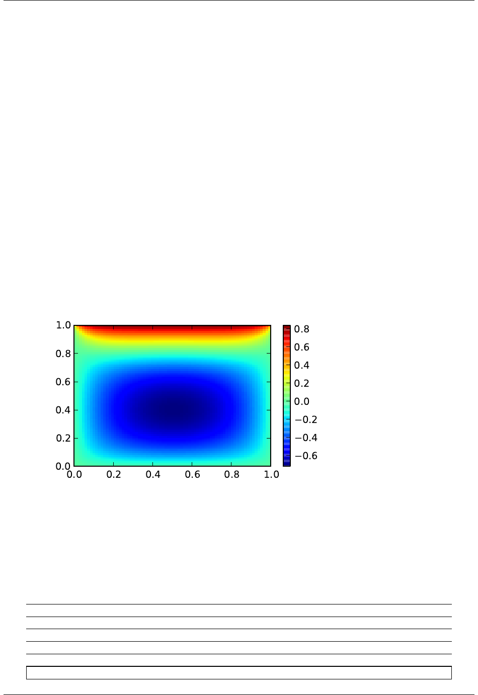
SciPy Reference Guide, Release 0.13.0
d2y =zeros_like(P)
d2x[1:-1]=(P[2:] -2*P[1:-1]+P[:-2]) /hx/hx
d2x[0]=(P[1]-2*P[0]+P_left)/hx/hx
d2x[-1]=(P_right -2*P[-1]+P[-2])/hx/hx
d2y[:,1:-1]=(P[:,2:] -2*P[:,1:-1]+P[:,:-2])/hy/hy
d2y[:,0]=(P[:,1]-2*P[:,0]+P_bottom)/hy/hy
d2y[:,-1]=(P_top -2*P[:,-1]+P[:,-2])/hy/hy
return d2x +d2y -10*cosh(P).mean()**2
# solve
guess =zeros((nx, ny), float)
sol =newton_krylov(residual, guess, method=’lgmres’, verbose=1)
print(’Residual: %g’%abs(residual(sol)).max())
# visualize
import matplotlib.pyplot as plt
x,y=mgrid[0:1:(nx*1j), 0:1:(ny*1j)]
plt.pcolor(x, y, sol)
plt.colorbar()
plt.show()
5.22 Signal processing (scipy.signal)
5.22.1 Convolution
convolve(in1, in2[, mode]) Convolve two N-dimensional arrays.
correlate(in1, in2[, mode]) Cross-correlate two N-dimensional arrays.
fftconvolve(in1, in2[, mode]) Convolve two N-dimensional arrays using FFT.
convolve2d(in1, in2[, mode, boundary, fillvalue]) Convolve two 2-dimensional arrays.
correlate2d(in1, in2[, mode, boundary, ...]) Cross-correlate two 2-dimensional arrays.
Continued on next page
5.22. Signal processing (scipy.signal) 595

SciPy Reference Guide, Release 0.13.0
Table 5.105 – continued from previous page
sepfir2d((input, hrow, hcol) -> output) Description:
scipy.signal.convolve(in1,in2,mode=’full’)
Convolve two N-dimensional arrays.
Convolve in1 and in2, with the output size determined by the mode argument.
Parameters in1 : array_like
First input.
in2 : array_like
Second input. Should have the same number of dimensions as in1; if sizes
of in1 and in2 are not equal then in1 has to be the larger array.
mode : str {‘full’, ‘valid’, ‘same’}, optional
A string indicating the size of the output:
full The output is the full discrete linear convolution of the in-
puts. (Default)
valid The output consists only of those elements that do not rely
on the zero-padding.
same The output is the same size as in1, centered with respect to
the ‘full’ output.
Returns convolve : array
An N-dimensional array containing a subset of the discrete linear convolu-
tion of in1 with in2.
scipy.signal.correlate(in1,in2,mode=’full’)
Cross-correlate two N-dimensional arrays.
Cross-correlate in1 and in2, with the output size determined by the mode argument.
Parameters in1 : array_like
First input.
in2 : array_like
Second input. Should have the same number of dimensions as in1; if sizes
of in1 and in2 are not equal then in1 has to be the larger array.
mode : str {‘full’, ‘valid’, ‘same’}, optional
A string indicating the size of the output:
full The output is the full discrete linear cross-correlation of the
inputs. (Default)
valid The output consists only of those elements that do not rely
on the zero-padding.
same The output is the same size as in1, centered with respect to
the ‘full’ output.
Returns correlate : array
An N-dimensional array containing a subset of the discrete linear cross-
correlation of in1 with in2.
Notes
The correlation z of two arrays x and y of rank d is defined as:
z[...,k,...] = sum[..., i_l, ...]
x[..., i_l,...] * conj(y[..., i_l + k,...])
scipy.signal.fftconvolve(in1,in2,mode=’full’)
Convolve two N-dimensional arrays using FFT.
Convolve in1 and in2 using the fast Fourier transform method, with the output size determined by the mode
argument.
This is generally much faster than convolve for large arrays (n > ~500), but can be slower when only a few
output values are needed, and can only output float arrays (int or object array inputs will be cast to float).
596 Chapter 5. Reference

SciPy Reference Guide, Release 0.13.0
Parameters in1 : array_like
First input.
in2 : array_like
Second input. Should have the same number of dimensions as in1; if sizes
of in1 and in2 are not equal then in1 has to be the larger array.
mode : str {‘full’, ‘valid’, ‘same’}, optional
A string indicating the size of the output:
full The output is the full discrete linear convolution of the in-
puts. (Default)
valid The output consists only of those elements that do not rely
on the zero-padding.
same The output is the same size as in1, centered with respect to
the ‘full’ output.
Returns out : array
An N-dimensional array containing a subset of the discrete linear convolu-
tion of in1 with in2.
scipy.signal.convolve2d(in1,in2,mode=’full’,boundary=’fill’,fillvalue=0)
Convolve two 2-dimensional arrays.
Convolve in1 and in2 with output size determined by mode, and boundary conditions determined by boundary
and fillvalue.
Parameters in1, in2 : array_like
Two-dimensional input arrays to be convolved.
mode : str {‘full’, ‘valid’, ‘same’}, optional
A string indicating the size of the output:
full The output is the full discrete linear convolution of the in-
puts. (Default)
valid The output consists only of those elements that do not rely
on the zero-padding.
same The output is the same size as in1, centered with respect to
the ‘full’ output.
boundary : str {‘fill’, ‘wrap’, ‘symm’}, optional
A flag indicating how to handle boundaries:
fill pad input arrays with fillvalue. (default)
wrap circular boundary conditions.
symm symmetrical boundary conditions.
fillvalue : scalar, optional
Value to fill pad input arrays with. Default is 0.
Returns out : ndarray
A 2-dimensional array containing a subset of the discrete linear convolution
of in1 with in2.
scipy.signal.correlate2d(in1,in2,mode=’full’,boundary=’fill’,fillvalue=0)
Cross-correlate two 2-dimensional arrays.
Cross correlate in1 and in2 with output size determined by mode, and boundary conditions determined by
boundary and fillvalue.
Parameters in1, in2 : array_like
Two-dimensional input arrays to be convolved.
mode : str {‘full’, ‘valid’, ‘same’}, optional
A string indicating the size of the output:
full The output is the full discrete linear cross-correlation of the
inputs. (Default)
valid The output consists only of those elements that do not rely
on the zero-padding.
same The output is the same size as in1, centered with respect to
the ‘full’ output.
boundary : str {‘fill’, ‘wrap’, ‘symm’}, optional
A flag indicating how to handle boundaries:
5.22. Signal processing (scipy.signal) 597

SciPy Reference Guide, Release 0.13.0
fill pad input arrays with fillvalue. (default)
wrap circular boundary conditions.
symm symmetrical boundary conditions.
fillvalue : scalar, optional
Value to fill pad input arrays with. Default is 0.
Returns correlate2d : ndarray
A 2-dimensional array containing a subset of the discrete linear cross-
correlation of in1 with in2.
scipy.signal.sepfir2d(input,hrow,hcol)→output
Description:
Convolve the rank-2 input array with the separable filter defined by the rank-1 arrays hrow, and hcol.
Mirror symmetric boundary conditions are assumed. This function can be used to find an image given its
B-spline representation.
5.22.2 B-splines
bspline(x, n) B-spline basis function of order n.
cubic(x) A cubic B-spline.
quadratic(x) A quadratic B-spline.
gauss_spline(x, n) Gaussian approximation to B-spline basis function of order n.
cspline1d(signal[, lamb]) Compute cubic spline coefficients for rank-1 array.
qspline1d(signal[, lamb]) Compute quadratic spline coefficients for rank-1 array.
cspline2d((input {, lambda, precision}) -> ck) Description:
qspline2d((input {, lambda, precision}) -> qk) Description:
cspline1d_eval(cj, newx[, dx, x0]) Evaluate a spline at the new set of points.
cspline1d_eval(cj, newx[, dx, x0]) Evaluate a spline at the new set of points.
spline_filter(Iin[, lmbda]) Smoothing spline (cubic) filtering of a rank-2 array.
scipy.signal.bspline(x,n)
B-spline basis function of order n.
Notes
Uses numpy.piecewise and automatic function-generator.
scipy.signal.cubic(x)
A cubic B-spline.
This is a special case of bspline, and equivalent to bspline(x, 3).
scipy.signal.quadratic(x)
A quadratic B-spline.
This is a special case of bspline, and equivalent to bspline(x, 2).
scipy.signal.gauss_spline(x,n)
Gaussian approximation to B-spline basis function of order n.
scipy.signal.cspline1d(signal,lamb=0.0)
Compute cubic spline coefficients for rank-1 array.
Find the cubic spline coefficients for a 1-D signal assuming mirror-symmetric boundary conditions. To obtain
the signal back from the spline representation mirror-symmetric-convolve these coefficients with a length 3 FIR
window [1.0, 4.0, 1.0]/ 6.0 .
Parameters signal : ndarray
598 Chapter 5. Reference

SciPy Reference Guide, Release 0.13.0
A rank-1 array representing samples of a signal.
lamb : float, optional
Smoothing coefficient, default is 0.0.
Returns c: ndarray
Cubic spline coefficients.
scipy.signal.qspline1d(signal,lamb=0.0)
Compute quadratic spline coefficients for rank-1 array.
Find the quadratic spline coefficients for a 1-D signal assuming mirror-symmetric boundary conditions. To
obtain the signal back from the spline representation mirror-symmetric-convolve these coefficients with a length
3 FIR window [1.0, 6.0, 1.0]/ 8.0 .
Parameters signal : ndarray
A rank-1 array representing samples of a signal.
lamb : float, optional
Smoothing coefficient (must be zero for now).
Returns c: ndarray
Cubic spline coefficients.
scipy.signal.cspline2d(input {,lambda,precision})→ck
Description:
Return the third-order B-spline coefficients over a regularly spacedi input grid for the two-dimensional
input image. The lambda argument specifies the amount of smoothing. The precision argument allows
specifying the precision used when computing the infinite sum needed to apply mirror- symmetric bound-
ary conditions.
scipy.signal.qspline2d(input {,lambda,precision})→qk
Description:
Return the second-order B-spline coefficients over a regularly spaced input grid for the two-dimensional
input image. The lambda argument specifies the amount of smoothing. The precision argument allows
specifying the precision used when computing the infinite sum needed to apply mirror- symmetric bound-
ary conditions.
scipy.signal.cspline1d_eval(cj,newx,dx=1.0,x0=0)
Evaluate a spline at the new set of points.
dx is the old sample-spacing while x0 was the old origin. In other-words the old-sample points (knot-points) for
which the cj represent spline coefficients were at equally-spaced points of:
oldx = x0 + j*dx j=0...N-1, with N=len(cj)
Edges are handled using mirror-symmetric boundary conditions.
scipy.signal.spline_filter(Iin,lmbda=5.0)
Smoothing spline (cubic) filtering of a rank-2 array.
Filter an input data set, Iin, using a (cubic) smoothing spline of fall-off lmbda.
5.22. Signal processing (scipy.signal) 599

SciPy Reference Guide, Release 0.13.0
5.22.3 Filtering
600 Chapter 5. Reference

SciPy Reference Guide, Release 0.13.0
order_filter(a, domain, rank) Perform an order filter on an N-dimensional array.
medfilt(volume[, kernel_size]) Perform a median filter on an N-dimensional array.
medfilt2d(input[, kernel_size]) Median filter a 2-dimensional array.
wiener(im[, mysize, noise]) Perform a Wiener filter on an N-dimensional array.
symiirorder1((input, c0, z1 {, ...) Implement a smoothing IIR filter with mirror-symmetric boundary conditions
symiirorder2((input, r, omega {, ...) Implement a smoothing IIR filter with mirror-symmetric boundary conditions
lfilter(b, a, x[, axis, zi]) Filter data along one-dimension with an IIR or FIR filter.
lfiltic(b, a, y[, x]) Construct initial conditions for lfilter.
lfilter_zi(b, a) Compute an initial state zi for the lfilter function that corresponds to the steady state of the step response.
filtfilt(b, a, x[, axis, padtype, padlen]) A forward-backward filter.
deconvolve(signal, divisor) Deconvolves divisor out of signal.
hilbert(x[, N, axis]) Compute the analytic signal, using the Hilbert transform.
get_window(window, Nx[, fftbins]) Return a window.
decimate(x, q[, n, ftype, axis]) Downsample the signal by using a filter.
detrend(data[, axis, type, bp]) Remove linear trend along axis from data.
resample(x, num[, t, axis, window]) Resample xto num samples using Fourier method along the given axis.
scipy.signal.order_filter(a,domain,rank)
Perform an order filter on an N-dimensional array.
Perform an order filter on the array in. The domain argument acts as a mask centered over each pixel. The
non-zero elements of domain are used to select elements surrounding each input pixel which are placed in a list.
The list is sorted, and the output for that pixel is the element corresponding to rank in the sorted list.
Parameters a: ndarray
The N-dimensional input array.
domain : array_like
A mask array with the same number of dimensions as in. Each dimension
should have an odd number of elements.
rank : int
A non-negative integer which selects the element from the sorted list (0
corresponds to the smallest element, 1 is the next smallest element, etc.).
Returns out : ndarray
The results of the order filter in an array with the same shape as in.
Examples
>>> from scipy import signal
>>> x=np.arange(25).reshape(5,5)
>>> domain =np.identity(3)
>>> x
array([[ 0, 1, 2, 3, 4],
[ 5, 6, 7, 8, 9],
[10, 11, 12, 13, 14],
[15, 16, 17, 18, 19],
[20, 21, 22, 23, 24]])
>>> signal.order_filter(x, domain, 0)
array([[ 0., 0., 0., 0., 0.],
[ 0., 0., 1., 2., 0.],
[ 0., 5., 6., 7., 0.],
[ 0., 10., 11., 12., 0.],
[ 0., 0., 0., 0., 0.]])
>>> signal.order_filter(x, domain, 2)
array([[ 6., 7., 8., 9., 4.],
[ 11., 12., 13., 14., 9.],
5.22. Signal processing (scipy.signal) 601

SciPy Reference Guide, Release 0.13.0
[ 16., 17., 18., 19., 14.],
[ 21., 22., 23., 24., 19.],
[ 20., 21., 22., 23., 24.]])
scipy.signal.medfilt(volume,kernel_size=None)
Perform a median filter on an N-dimensional array.
Apply a median filter to the input array using a local window-size given by kernel_size.
Parameters volume : array_like
An N-dimensional input array.
kernel_size : array_like, optional
A scalar or an N-length list giving the size of the median filter window in
each dimension. Elements of kernel_size should be odd. If kernel_size is a
scalar, then this scalar is used as the size in each dimension. Default size is
3 for each dimension.
Returns out : ndarray
An array the same size as input containing the median filtered result.
scipy.signal.medfilt2d(input,kernel_size=3)
Median filter a 2-dimensional array.
Apply a median filter to the input array using a local window-size given by kernel_size (must be odd).
Parameters input : array_like
A 2-dimensional input array.
kernel_size : array_like, optional
A scalar or a list of length 2, giving the size of the median filter window in
each dimension. Elements of kernel_size should be odd. If kernel_size is
a scalar, then this scalar is used as the size in each dimension. Default is a
kernel of size (3, 3).
Returns out : ndarray
An array the same size as input containing the median filtered result.
scipy.signal.wiener(im,mysize=None,noise=None)
Perform a Wiener filter on an N-dimensional array.
Apply a Wiener filter to the N-dimensional array im.
Parameters im : ndarray
An N-dimensional array.
mysize : int or arraylike, optional
A scalar or an N-length list giving the size of the Wiener filter window in
each dimension. Elements of mysize should be odd. If mysize is a scalar,
then this scalar is used as the size in each dimension.
noise : float, optional
The noise-power to use. If None, then noise is estimated as the average of
the local variance of the input.
Returns out : ndarray
Wiener filtered result with the same shape as im.
scipy.signal.symiirorder1(input,c0,z1 {,precision})→output
Implement a smoothing IIR filter with mirror-symmetric boundary conditions using a cascade of first-order
sections. The second section uses a reversed sequence. This implements a system with the following transfer
function and mirror-symmetric boundary conditions:
c0
H(z) = ---------------------
(1-z1/z) (1 - z1 z)
602 Chapter 5. Reference

SciPy Reference Guide, Release 0.13.0
The resulting signal will have mirror symmetric boundary conditions as well.
Parameters input : ndarray
The input signal.
c0, z1 : scalar
Parameters in the transfer function.
precision :
Specifies the precision for calculating initial conditions of the recursive fil-
ter based on mirror-symmetric input.
Returns output : ndarray
The filtered signal.
scipy.signal.symiirorder2(input,r,omega {,precision})→output
Implement a smoothing IIR filter with mirror-symmetric boundary conditions using a cascade of second-order
sections. The second section uses a reversed sequence. This implements the following transfer function:
cs^2
H(z) = ---------------------------------------
(1 - a2/z - a3/z^2) (1 - a2 z - a3 z^2 )
where:
a2 = (2 r cos omega)
a3 = - r^2
cs = 1 - 2 r cos omega + r^2
Parameters input : ndarray
The input signal.
r, omega : scalar
Parameters in the transfer function.
precision :
Specifies the precision for calculating initial conditions of the recursive fil-
ter based on mirror-symmetric input.
Returns output : ndarray
The filtered signal.
scipy.signal.lfilter(b,a,x,axis=-1,zi=None)
Filter data along one-dimension with an IIR or FIR filter.
Filter a data sequence, x, using a digital filter. This works for many fundamental data types (including Object
type). The filter is a direct form II transposed implementation of the standard difference equation (see Notes).
Parameters b: array_like
The numerator coefficient vector in a 1-D sequence.
a: array_like
The denominator coefficient vector in a 1-D sequence. If a[0] is not 1,
then both aand bare normalized by a[0].
x: array_like
An N-dimensional input array.
axis : int
The axis of the input data array along which to apply the linear filter. The
filter is applied to each subarray along this axis. Default is -1.
zi : array_like, optional
Initial conditions for the filter delays. It is a vector (or array of vectors for
an N-dimensional input) of length max(len(a),len(b))-1. If zi is
None or is not given then initial rest is assumed. See lfiltic for more
information.
5.22. Signal processing (scipy.signal) 603

SciPy Reference Guide, Release 0.13.0
Returns y: array
The output of the digital filter.
zf : array, optional
If zi is None, this is not returned, otherwise, zf holds the final filter delay
values.
Notes
The filter function is implemented as a direct II transposed structure. This means that the filter implements:
a[0]*y[n] = b[0]*x[n] + b[1]*x[n-1] + ... + b[nb]*x[n-nb]
- a[1]*y[n-1] - ... - a[na]*y[n-na]
using the following difference equations:
y[m] =b[0]*x[m] +z[0,m-1]
z[0,m] =b[1]*x[m] +z[1,m-1]-a[1]*y[m]
...
z[n-3,m] =b[n-2]*x[m] +z[n-2,m-1]-a[n-2]*y[m]
z[n-2,m] =b[n-1]*x[m] -a[n-1]*y[m]
where m is the output sample number and n=max(len(a),len(b)) is the model order.
The rational transfer function describing this filter in the z-transform domain is:
-1 -nb
b[0] + b[1]z + ... + b[nb] z
Y(z) = ---------------------------------- X(z)
-1 -na
a[0] + a[1]z + ... + a[na] z
scipy.signal.lfiltic(b,a,y,x=None)
Construct initial conditions for lfilter.
Given a linear filter (b, a) and initial conditions on the output yand the input x, return the inital conditions on
the state vector zi which is used by lfilter to generate the output given the input.
Parameters b: array_like
Linear filter term.
a: array_like
Linear filter term.
y: array_like
Initial conditions.
If N=len(a) - 1, then y = {y[-1], y[-2], ..., y[-N]}.
If yis too short, it is padded with zeros.
x: array_like, optional
Initial conditions.
If M=len(b) - 1, then x = {x[-1], x[-2], ..., x[-M]}.
If xis not given, its initial conditions are assumed zero.
If xis too short, it is padded with zeros.
Returns zi : ndarray
The state vector zi.zi = {z_0[-1], z_1[-1], ...,
z_K-1[-1]}, where K = max(M,N).
604 Chapter 5. Reference

SciPy Reference Guide, Release 0.13.0
See Also
lfilter
scipy.signal.lfilter_zi(b,a)
Compute an initial state zi for the lfilter function that corresponds to the steady state of the step response.
A typical use of this function is to set the initial state so that the output of the filter starts at the same value as
the first element of the signal to be filtered.
Parameters b, a : array_like (1-D)
The IIR filter coefficients. See lfilter for more information.
Returns zi : 1-D ndarray
The initial state for the filter.
Notes
A linear filter with order m has a state space representation (A, B, C, D), for which the output y of the filter can
be expressed as:
z(n+1)=A*z(n) +B*x(n)
y(n) =C*z(n) +D*x(n)
where z(n) is a vector of length m, A has shape (m, m), B has shape (m, 1), C has shape (1, m) and D has shape
(1, 1) (assuming x(n) is a scalar). lfilter_zi solves:
zi =A*zi +B
In other words, it finds the initial condition for which the response to an input of all ones is a constant.
Given the filter coefficients aand b, the state space matrices for the transposed direct form II implementation of
the linear filter, which is the implementation used by scipy.signal.lfilter, are:
A=scipy.linalg.companion(a).T
B=b[1:] -a[1:]*b[0]
assuming a[0] is 1.0; if a[0] is not 1, aand bare first divided by a[0].
Examples
The following code creates a lowpass Butterworth filter. Then it applies that filter to an array whose values are
all 1.0; the output is also all 1.0, as expected for a lowpass filter. If the zi argument of lfilter had not been
given, the output would have shown the transient signal.
>>> from numpy import array, ones
>>> from scipy.signal import lfilter, lfilter_zi, butter
>>> b,a=butter(5,0.25)
>>> zi =lfilter_zi(b, a)
>>> y, zo =lfilter(b, a, ones(10), zi=zi)
>>> y
array([1., 1., 1., 1., 1., 1., 1., 1., 1., 1.])
Another example:
>>> x=array([0.5,0.5,0.5,0.0,0.0,0.0,0.0])
>>> y, zf =lfilter(b, a, x, zi=zi*x[0])
>>> y
array([ 0.5 , 0.5 , 0.5 , 0.49836039, 0.48610528,
0.44399389, 0.35505241])
5.22. Signal processing (scipy.signal) 605

SciPy Reference Guide, Release 0.13.0
Note that the zi argument to lfilter was computed using lfilter_zi and scaled by x[0]. Then the output
yhas no transient until the input drops from 0.5 to 0.0.
scipy.signal.filtfilt(b,a,x,axis=-1,padtype=’odd’,padlen=None)
A forward-backward filter.
This function applies a linear filter twice, once forward and once backwards. The combined filter has linear
phase.
Before applying the filter, the function can pad the data along the given axis in one of three ways: odd, even or
constant. The odd and even extensions have the corresponding symmetry about the end point of the data. The
constant extension extends the data with the values at end points. On both the forward and backwards passes,
the initial condition of the filter is found by using lfilter_zi and scaling it by the end point of the extended
data.
Parameters b: (N,) array_like
The numerator coefficient vector of the filter.
a: (N,) array_like
The denominator coefficient vector of the filter. If a[0] is not 1, then both a
and b are normalized by a[0].
x: array_like
The array of data to be filtered.
axis : int, optional
The axis of xto which the filter is applied. Default is -1.
padtype : str or None, optional
Must be ‘odd’, ‘even’, ‘constant’, or None. This determines the type of
extension to use for the padded signal to which the filter is applied. If
padtype is None, no padding is used. The default is ‘odd’.
padlen : int or None, optional
The number of elements by which to extend xat both ends of axis before
applying the filter. This value must be less than x.shape[axis]-1.padlen=0
implies no padding. The default value is 3*max(len(a),len(b)).
Returns y: ndarray
The filtered output, an array of type numpy.float64 with the same shape as
x.
See Also
lfilter_zi,lfilter
Examples
First we create a one second signal that is the sum of two pure sine waves, with frequencies 5 Hz and 250 Hz,
sampled at 2000 Hz.
>>> t=np.linspace(0,1.0,2001)
>>> xlow =np.sin(2*np.pi *5*t)
>>> xhigh =np.sin(2*np.pi *250 *t)
>>> x=xlow +xhigh
Now create a lowpass Butterworth filter with a cutoff of 0.125 times the Nyquist rate, or 125 Hz, and apply it to
x with filtfilt. The result should be approximately xlow, with no phase shift.
>>> from scipy import signal
>>> b,a=signal.butter(8,0.125)
>>> y=signal.filtfilt(b, a, x, padlen=150)
>>> np.abs(y -xlow).max()
9.1086182074789912e-06
606 Chapter 5. Reference

SciPy Reference Guide, Release 0.13.0
We get a fairly clean result for this artificial example because the odd extension is exact, and with the moderately
long padding, the filter’s transients have dissipated by the time the actual data is reached. In general, transient
effects at the edges are unavoidable.
scipy.signal.deconvolve(signal,divisor)
Deconvolves divisor out of signal.
Parameters signal : array
Signal input
divisor : array
Divisor input
Returns q: array
Quotient of the division
r: array
Remainder
Examples
>>> from scipy import signal
>>> sig =np.array([0,0,0,0,0,1,1,1,1,])
>>> filter =np.array([1,1,0])
>>> res =signal.convolve(sig, filter)
>>> signal.deconvolve(res, filter)
(array([ 0., 0., 0., 0., 0., 1., 1., 1., 1.]),
array([ 0., 0., 0., 0., 0., 0., 0., 0., 0., 0., 0.]))
scipy.signal.hilbert(x,N=None,axis=-1)
Compute the analytic signal, using the Hilbert transform.
The transformation is done along the last axis by default.
Parameters x: array_like
Signal data. Must be real.
N: int, optional
Number of Fourier components. Default: x.shape[axis]
axis : int, optional
Axis along which to do the transformation. Default: -1.
Returns xa : ndarray
Analytic signal of x, of each 1-D array along axis
Notes
The analytic signal x_a(t) of signal x(t) is:
xa=F−1(F(x)2U) = x+iy
where Fis the Fourier transform, Uthe unit step function, and ythe Hilbert transform of x.[R125]
In other words, the negative half of the frequency spectrum is zeroed out, turning the real-valued signal into
a complex signal. The Hilbert transformed signal can be obtained from np.imag(hilbert(x)), and the
original signal from np.real(hilbert(x)).
References
[R125]
scipy.signal.get_window(window,Nx,fftbins=True)
Return a window.
Parameters window : string, float, or tuple
5.22. Signal processing (scipy.signal) 607

SciPy Reference Guide, Release 0.13.0
The type of window to create. See below for more details.
Nx : int
The number of samples in the window.
fftbins : bool, optional
If True, create a “periodic” window ready to use with ifftshift and be multi-
plied by the result of an fft (SEE ALSO fftfreq).
Returns get_window : ndarray
Returns a window of length Nx and type window
Notes
Window types:
boxcar, triang, blackman, hamming, hann, bartlett, flattop, parzen, bohman, blackmanharris, nuttall,
barthann, kaiser (needs beta), gaussian (needs std), general_gaussian (needs power, width), slepian (needs
width), chebwin (needs attenuation)
If the window requires no parameters, then window can be a string.
If the window requires parameters, then window must be a tuple with the first argument the string name of the
window, and the next arguments the needed parameters.
If window is a floating point number, it is interpreted as the beta parameter of the kaiser window.
Each of the window types listed above is also the name of a function that can be called directly to create a
window of that type.
Examples
>>> from scipy import signal
>>> signal.get_window(’triang’,7)
array([ 0.25, 0.5 , 0.75, 1. , 0.75, 0.5 , 0.25])
>>> signal.get_window((’kaiser’,4.0), 9)
array([ 0.08848053, 0.32578323, 0.63343178, 0.89640418, 1. ,
0.89640418, 0.63343178, 0.32578323, 0.08848053])
>>> signal.get_window(4.0,9)
array([ 0.08848053, 0.32578323, 0.63343178, 0.89640418, 1. ,
0.89640418, 0.63343178, 0.32578323, 0.08848053])
scipy.signal.decimate(x,q,n=None,ftype=’iir’,axis=-1)
Downsample the signal by using a filter.
By default, an order 8 Chebyshev type I filter is used. A 30 point FIR filter with hamming window is used if
ftype is ‘fir’.
Parameters x: ndarray
The signal to be downsampled, as an N-dimensional array.
q: int
The downsampling factor.
n: int, optional
The order of the filter (1 less than the length for ‘fir’).
ftype : str {‘iir’, ‘fir’}, optional
The type of the lowpass filter.
axis : int, optional
The axis along which to decimate.
Returns y: ndarray
The down-sampled signal.
608 Chapter 5. Reference

SciPy Reference Guide, Release 0.13.0
See Also
resample
scipy.signal.detrend(data,axis=-1,type=’linear’,bp=0)
Remove linear trend along axis from data.
Parameters data : array_like
The input data.
axis : int, optional
The axis along which to detrend the data. By default this is the last axis
(-1).
type : {‘linear’, ‘constant’}, optional
The type of detrending. If type == ’linear’ (default), the result
of a linear least-squares fit to data is subtracted from data. If type ==
’constant’, only the mean of data is subtracted.
bp : array_like of ints, optional
A sequence of break points. If given, an individual linear fit is performed
for each part of data between two break points. Break points are specified
as indices into data.
Returns ret : ndarray
The detrended input data.
Examples
>>> from scipy import signal
>>> randgen =np.random.RandomState(9)
>>> npoints =1e3
>>> noise =randgen.randn(npoints)
>>> x=3+2*np.linspace(0,1, npoints) +noise
>>> (signal.detrend(x) -noise).max() <0.01
True
scipy.signal.resample(x,num,t=None,axis=0,window=None)
Resample xto num samples using Fourier method along the given axis.
The resampled signal starts at the same value as xbut is sampled with a spacing of len(x) / num *
(spacing of x). Because a Fourier method is used, the signal is assumed to be periodic.
Parameters x: array_like
The data to be resampled.
num : int
The number of samples in the resampled signal.
t: array_like, optional
If tis given, it is assumed to be the sample positions associated with the
signal data in x.
axis : int, optional
The axis of xthat is resampled. Default is 0.
window : array_like, callable, string, float, or tuple, optional
Specifies the window applied to the signal in the Fourier domain. See below
for details.
Returns resampled_x or (resampled_x, resampled_t)
Either the resampled array, or, if twas given, a tuple containing the resam-
pled array and the corresponding resampled positions.
5.22. Signal processing (scipy.signal) 609

SciPy Reference Guide, Release 0.13.0
Notes
The argument window controls a Fourier-domain window that tapers the Fourier spectrum before zero-padding
to alleviate ringing in the resampled values for sampled signals you didn’t intend to be interpreted as band-
limited.
If window is a function, then it is called with a vector of inputs indicating the frequency bins (i.e. fft-
freq(x.shape[axis]) ).
If window is an array of the same length as x.shape[axis] it is assumed to be the window to be applied directly
in the Fourier domain (with dc and low-frequency first).
For any other type of window, the function scipy.signal.get_window is called to generate the window.
The first sample of the returned vector is the same as the first sample of the input vector. The spacing between
samples is changed from dx to:
dx * len(x) / num
If tis not None, then it represents the old sample positions, and the new sample positions will be returned as
well as the new samples.
5.22.4 Filter design
bilinear(b, a[, fs]) Return a digital filter from an analog one using a bilinear transform.
firwin(numtaps, cutoff[, width, window, ...]) FIR filter design using the window method.
firwin2(numtaps, freq, gain[, nfreqs, ...]) FIR filter design using the window method.
freqs(b, a[, worN, plot]) Compute frequency response of analog filter.
freqz(b[, a, worN, whole, plot]) Compute the frequency response of a digital filter.
iirdesign(wp, ws, gpass, gstop[, analog, ...]) Complete IIR digital and analog filter design.
iirfilter(N, Wn[, rp, rs, btype, analog, ...]) IIR digital and analog filter design given order and critical points.
kaiser_atten(numtaps, width) Compute the attenuation of a Kaiser FIR filter.
kaiser_beta(a) Compute the Kaiser parameter beta, given the attenuation a.
kaiserord(ripple, width) Design a Kaiser window to limit ripple and width of transition region.
remez(numtaps, bands, desired[, weight, Hz, ...]) Calculate the minimax optimal filter using the Remez exchange algorithm.
unique_roots(p[, tol, rtype]) Determine unique roots and their multiplicities from a list of roots.
residue(b, a[, tol, rtype]) Compute partial-fraction expansion of b(s) / a(s).
residuez(b, a[, tol, rtype]) Compute partial-fraction expansion of b(z) / a(z).
invres(r, p, k[, tol, rtype]) Compute b(s) and a(s) from partial fraction expansion: r,p,k
scipy.signal.bilinear(b,a,fs=1.0)
Return a digital filter from an analog one using a bilinear transform.
The bilinear transform substitutes (z-1) / (z+1) for s.
scipy.signal.firwin(numtaps,cutoff,width=None,window=’hamming’,pass_zero=True,scale=True,
nyq=1.0)
FIR filter design using the window method.
This function computes the coefficients of a finite impulse response filter. The filter will have linear phase; it
will be Type I if numtaps is odd and Type II if numtaps is even.
Type II filters always have zero response at the Nyquist rate, so a ValueError exception is raised if firwin is
called with numtaps even and having a passband whose right end is at the Nyquist rate.
Parameters numtaps : int
610 Chapter 5. Reference

SciPy Reference Guide, Release 0.13.0
Length of the filter (number of coefficients, i.e. the filter order + 1). num-
taps must be even if a passband includes the Nyquist frequency.
cutoff : float or 1D array_like
Cutoff frequency of filter (expressed in the same units as nyq) OR an array
of cutoff frequencies (that is, band edges). In the latter case, the frequencies
in cutoff should be positive and monotonically increasing between 0 and
nyq. The values 0 and nyq must not be included in cutoff.
width : float or None
If width is not None, then assume it is the approximate width of the transi-
tion region (expressed in the same units as nyq) for use in Kaiser FIR filter
design. In this case, the window argument is ignored.
window : string or tuple of string and parameter values
Desired window to use. See scipy.signal.get_window for a list of
windows and required parameters.
pass_zero : bool
If True, the gain at the frequency 0 (i.e. the “DC gain”) is 1. Otherwise the
DC gain is 0.
scale : bool
Set to True to scale the coefficients so that the frequency response is exactly
unity at a certain frequency. That frequency is either:
•0 (DC) if the first passband starts at 0 (i.e. pass_zero is True)
•nyq (the Nyquist rate) if the first passband ends at nyq (i.e the
filter is a single band highpass filter); center of first passband
otherwise
nyq : float
Nyquist frequency. Each frequency in cutoff must be between 0 and nyq.
Returns h: (numtaps,) ndarray
Coefficients of length numtaps FIR filter.
Raises ValueError
If any value in cutoff is less than or equal to 0 or greater than or equal to
nyq, if the values in cutoff are not strictly monotonically increasing, or if
numtaps is even but a passband includes the Nyquist frequency.
See Also
scipy.signal.firwin2
Examples
Low-pass from 0 to f:
>>> from scipy import signal
>>> signal.firwin(numtaps, f)
Use a specific window function:
>>> signal.firwin(numtaps, f, window=’nuttall’)
High-pass (‘stop’ from 0 to f):
>>> signal.firwin(numtaps, f, pass_zero=False)
Band-pass:
>>> signal.firwin(numtaps, [f1, f2], pass_zero=False)
Band-stop:
5.22. Signal processing (scipy.signal) 611

SciPy Reference Guide, Release 0.13.0
>>> signal.firwin(numtaps, [f1, f2])
Multi-band (passbands are [0, f1], [f2, f3] and [f4, 1]):
>>> signal.firwin(numtaps, [f1, f2, f3, f4])
Multi-band (passbands are [f1, f2] and [f3,f4]):
>>> signal.firwin(numtaps, [f1, f2, f3, f4], pass_zero=False)
scipy.signal.firwin2(numtaps,freq,gain,nfreqs=None,window=’hamming’,nyq=1.0,antisymmet-
ric=False)
FIR filter design using the window method.
From the given frequencies freq and corresponding gains gain, this function constructs an FIR filter with linear
phase and (approximately) the given frequency response.
Parameters numtaps : int
The number of taps in the FIR filter. numtaps must be less than nfreqs.
freq : array_like, 1D
The frequency sampling points. Typically 0.0 to 1.0 with 1.0 being Nyquist.
The Nyquist frequency can be redefined with the argument nyq. The values
in freq must be nondecreasing. A value can be repeated once to implement
a discontinuity. The first value in freq must be 0, and the last value must be
nyq.
gain : array_like
The filter gains at the frequency sampling points. Certain constraints to gain
values, depending on the filter type, are applied, see Notes for details.
nfreqs : int, optional
The size of the interpolation mesh used to construct the filter. For most
efficient behavior, this should be a power of 2 plus 1 (e.g, 129, 257, etc).
The default is one more than the smallest power of 2 that is not less than
numtaps.nfreqs must be greater than numtaps.
window : string or (string, float) or float, or None, optional
Window function to use. Default is “hamming”. See
scipy.signal.get_window for the complete list of possible
values. If None, no window function is applied.
nyq : float
Nyquist frequency. Each frequency in freq must be between 0 and nyq
(inclusive).
antisymmetric : bool
Whether resulting impulse response is symmetric/antisymmetric. See Notes
for more details.
Returns taps : ndarray
The filter coefficients of the FIR filter, as a 1-D array of length numtaps.
See Also
scipy.signal.firwin
Notes
From the given set of frequencies and gains, the desired response is constructed in the frequency domain. The
inverse FFT is applied to the desired response to create the associated convolution kernel, and the first numtaps
coefficients of this kernel, scaled by window, are returned.
612 Chapter 5. Reference

SciPy Reference Guide, Release 0.13.0
The FIR filter will have linear phase. The type of filter is determined by the value of ‘numtaps‘ and antisymmetric
flag. There are four possible combinations:
•odd numtaps,antisymmetric is False, type I filter is produced
•even numtaps,antisymmetric is False, type II filter is produced
•odd numtaps,antisymmetric is True, type III filter is produced
•even numtaps,antisymmetric is True, type IV filter is produced
Magnitude response of all but type I filters are subjects to following constraints:
•type II – zero at the Nyquist frequency
•type III – zero at zero and Nyquist frequencies
•type IV – zero at zero frequency
New in version 0.9.0.
References
[R115],[R116]
Examples
A lowpass FIR filter with a response that is 1 on [0.0, 0.5], and that decreases linearly on [0.5, 1.0] from 1 to 0:
>>> from scipy import signal
>>> taps =signal.firwin2(150, [0.0,0.5,1.0], [1.0,1.0,0.0])
>>> print(taps[72:78])
[-0.02286961 -0.06362756 0.57310236 0.57310236 -0.06362756 -0.02286961]
scipy.signal.freqs(b,a,worN=None,plot=None)
Compute frequency response of analog filter.
Given the numerator band denominator aof a filter, compute its frequency response:
b[0]*(jw)**(nb-1) + b[1]*(jw)**(nb-2) + ... + b[nb-1]
H(w) = -------------------------------------------------------
a[0]*(jw)**(na-1) + a[1]*(jw)**(na-2) + ... + a[na-1]
Parameters b: ndarray
Numerator of a linear filter.
a: ndarray
Denominator of a linear filter.
worN : {None, int}, optional
If None, then compute at 200 frequencies around the interesting parts of the
response curve (determined by pole-zero locations). If a single integer, then
compute at that many frequencies. Otherwise, compute the response at the
angular frequencies (e.g. rad/s) given in worN.
plot : callable
A callable that takes two arguments. If given, the return parameters wand h
are passed to plot. Useful for plotting the frequency response inside freqs.
Returns w: ndarray
The angular frequencies at which h was computed.
h: ndarray
The frequency response.
See Also
freqz Compute the frequency response of a digital filter.
5.22. Signal processing (scipy.signal) 613
SciPy Reference Guide, Release 0.13.0
Notes
Using Matplotlib’s “plot” function as the callable for plot produces unexpected results, this plots the real part of
the complex transfer function, not the magnitude.
Examples
>>> from scipy.signal import freqs, iirfilter
>>> b,a=iirfilter(4, [1,10], 1,60, analog=True, ftype=’cheby1’)
>>> w,h=freqs(b, a, worN=np.logspace(-1,2,1000))
>>> import matplotlib.pyplot as plt
>>> plt.semilogx(w, abs(h))
>>> plt.xlabel(’Frequency’)
>>> plt.ylabel(’Amplitude response’)
>>> plt.grid()
>>> plt.show()
scipy.signal.freqz(b,a=1,worN=None,whole=0,plot=None)
Compute the frequency response of a digital filter.
Given the numerator band denominator aof a digital filter, compute its frequency response:
jw -jw -jmw
jw B(e) b[0] + b[1]e + .... + b[m]e
H(e) = ---- = ------------------------------------
jw -jw -jnw
A(e) a[0] + a[1]e + .... + a[n]e
Parameters b: ndarray
numerator of a linear filter
a: ndarray
denominator of a linear filter
worN : {None, int, array_like}, optional
614 Chapter 5. Reference

SciPy Reference Guide, Release 0.13.0
If None (default), then compute at 512 frequencies equally spaced around
the unit circle. If a single integer, then compute at that many frequencies.
If an array_like, compute the response at the frequencies given (in radi-
ans/sample).
whole : bool, optional
Normally, frequencies are computed from 0 to the Nyquist frequency, pi
radians/sample (upper-half of unit-circle). If whole is True, compute fre-
quencies from 0 to 2*pi radians/sample.
plot : callable
A callable that takes two arguments. If given, the return parameters wand h
are passed to plot. Useful for plotting the frequency response inside freqz.
Returns w: ndarray
The normalized frequencies at which h was computed, in radians/sample.
h: ndarray
The frequency response.
Notes
Using Matplotlib’s “plot” function as the callable for plot produces unexpected results, this plots the real part of
the complex transfer function, not the magnitude.
Examples
>>> from scipy import signal
>>> b=signal.firwin(80,0.5, window=(’kaiser’,8))
>>> w,h=signal.freqz(b)
>>> import matplotlib.pyplot as plt
>>> fig =plt.figure()
>>> plt.title(’Digital filter frequency response’)
>>> ax1 =fig.add_subplot(111)
>>> plt.semilogy(w, np.abs(h), ’b’)
>>> plt.ylabel(’Amplitude (dB)’, color=’b’)
>>> plt.xlabel(’Frequency (rad/sample)’)
>>> ax2 =ax1.twinx()
>>> angles =np.unwrap(np.angle(h))
>>> plt.plot(w, angles, ’g’)
>>> plt.ylabel(’Angle (radians)’, color=’g’)
>>> plt.grid()
>>> plt.axis(’tight’)
>>> plt.show()
5.22. Signal processing (scipy.signal) 615
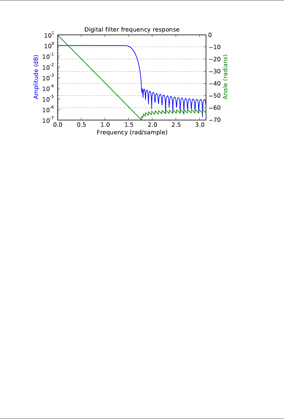
SciPy Reference Guide, Release 0.13.0
scipy.signal.iirdesign(wp,ws,gpass,gstop,analog=False,ftype=’ellip’,output=’ba’)
Complete IIR digital and analog filter design.
Given passband and stopband frequencies and gains, construct an analog or digital IIR filter of minimum order
for a given basic type. Return the output in numerator, denominator (‘ba’) or pole-zero (‘zpk’) form.
Parameters wp, ws : float
Passband and stopband edge frequencies. For digital filters, these are nor-
malized from 0 to 1, where 1 is the Nyquist frequency, pi radians/sample.
(wp and ws are thus in half-cycles / sample.) For example:
•Lowpass: wp = 0.2, ws = 0.3
•Highpass: wp = 0.3, ws = 0.2
•Bandpass: wp = [0.2, 0.5], ws = [0.1, 0.6]
•Bandstop: wp = [0.1, 0.6], ws = [0.2, 0.5]
For analog filters, wp and ws are angular frequencies (e.g. rad/s).
gpass : float
The maximum loss in the passband (dB).
gstop : float
The minimum attenuation in the stopband (dB).
analog : bool, optional
When True, return an analog filter, otherwise a digital filter is returned.
ftype : str, optional
The type of IIR filter to design:
•Butterworth : ‘butter’
•Chebyshev I : ‘cheby1’
•Chebyshev II : ‘cheby2’
•Cauer/elliptic: ‘ellip’
•Bessel/Thomson: ‘bessel’
output : {‘ba’, ‘zpk’}, optional
Type of output: numerator/denominator (‘ba’) or pole-zero (‘zpk’). Default
is ‘ba’.
Returns b, a : ndarray, ndarray
Numerator (b) and denominator (a) polynomials of the IIR filter. Only re-
turned if output=’ba’.
z, p, k : ndarray, ndarray, float
Zeros, poles, and system gain of the IIR filter transfer function. Only re-
turned if output=’zpk’.
scipy.signal.iirfilter(N,Wn,rp=None,rs=None,btype=’band’,analog=False,ftype=’butter’,
output=’ba’)
IIR digital and analog filter design given order and critical points.
616 Chapter 5. Reference

SciPy Reference Guide, Release 0.13.0
Design an Nth order digital or analog filter and return the filter coefficients in (B,A) (numerator, denominator)
or (Z,P,K) form.
Parameters N: int
The order of the filter.
Wn : array_like
A scalar or length-2 sequence giving the critical frequencies. For digital
filters, Wn is normalized from 0 to 1, where 1 is the Nyquist frequency, pi
radians/sample. (Wn is thus in half-cycles / sample.) For analog filters, Wn
is an angular frequency (e.g. rad/s).
rp : float, optional
For Chebyshev and elliptic filters, provides the maximum ripple in the pass-
band. (dB)
rs : float, optional
For Chebyshev and elliptic filters, provides the minimum attenuation in the
stop band. (dB)
btype : {‘bandpass’, ‘lowpass’, ‘highpass’, ‘bandstop’}, optional
The type of filter. Default is ‘bandpass’.
analog : bool, optional
When True, return an analog filter, otherwise a digital filter is returned.
ftype : str, optional
The type of IIR filter to design:
•Butterworth : ‘butter’
•Chebyshev I : ‘cheby1’
•Chebyshev II : ‘cheby2’
•Cauer/elliptic: ‘ellip’
•Bessel/Thomson: ‘bessel’
output : {‘ba’, ‘zpk’}, optional
Type of output: numerator/denominator (‘ba’) or pole-zero (‘zpk’). Default
is ‘ba’.
See Also
buttord,cheb1ord,cheb2ord,ellipord
scipy.signal.kaiser_atten(numtaps,width)
Compute the attenuation of a Kaiser FIR filter.
Given the number of taps Nand the transition width width, compute the attenuation ain dB, given by Kaiser’s
formula:
a = 2.285 * (N - 1) * pi * width + 7.95
Parameters N: int
The number of taps in the FIR filter.
width : float
The desired width of the transition region between passband and stopband
(or, in general, at any discontinuity) for the filter.
Returns a: float
The attenuation of the ripple, in dB.
See Also
kaiserord,kaiser_beta
scipy.signal.kaiser_beta(a)
Compute the Kaiser parameter beta, given the attenuation a.
Parameters a: float
5.22. Signal processing (scipy.signal) 617

SciPy Reference Guide, Release 0.13.0
The desired attenuation in the stopband and maximum ripple in the pass-
band, in dB. This should be a positive number.
Returns beta : float
The beta parameter to be used in the formula for a Kaiser window.
References
Oppenheim, Schafer, “Discrete-Time Signal Processing”, p.475-476.
scipy.signal.kaiserord(ripple,width)
Design a Kaiser window to limit ripple and width of transition region.
Parameters ripple : float
Positive number specifying maximum ripple in passband (dB) and mini-
mum ripple in stopband.
width : float
Width of transition region (normalized so that 1 corresponds to pi radians /
sample).
Returns numtaps : int
The length of the kaiser window.
beta : float
The beta parameter for the kaiser window.
See Also
kaiser_beta,kaiser_atten
Notes
There are several ways to obtain the Kaiser window:
•signal.kaiser(numtaps, beta, sym=0)
•signal.get_window(beta, numtaps)
•signal.get_window((’kaiser’, beta), numtaps)
The empirical equations discovered by Kaiser are used.
References
Oppenheim, Schafer, “Discrete-Time Signal Processing”, p.475-476.
scipy.signal.remez(numtaps,bands,desired,weight=None,Hz=1,type=’bandpass’,maxiter=25,
grid_density=16)
Calculate the minimax optimal filter using the Remez exchange algorithm.
Calculate the filter-coefficients for the finite impulse response (FIR) filter whose transfer function minimizes the
maximum error between the desired gain and the realized gain in the specified frequency bands using the Remez
exchange algorithm.
Parameters numtaps : int
The desired number of taps in the filter. The number of taps is the number
of terms in the filter, or the filter order plus one.
bands : array_like
A monotonic sequence containing the band edges in Hz. All elements must
be non-negative and less than half the sampling frequency as given by Hz.
desired : array_like
A sequence half the size of bands containing the desired gain in each of the
specified bands.
weight : array_like, optional
A relative weighting to give to each band region. The length of weight has
to be half the length of bands.
Hz : scalar, optional
618 Chapter 5. Reference

SciPy Reference Guide, Release 0.13.0
The sampling frequency in Hz. Default is 1.
type : {‘bandpass’, ‘differentiator’, ‘hilbert’}, optional
The type of filter:
‘bandpass’ : flat response in bands. This is the default.
‘differentiator’ : frequency proportional response in bands.
‘hilbert’ [filter with odd symmetry, that is, type III]
(for even order) or type IV (for odd order)
linear phase filters.
maxiter : int, optional
Maximum number of iterations of the algorithm. Default is 25.
grid_density : int, optional
Grid density. The dense grid used in remez is of size (numtaps + 1)
*grid_density. Default is 16.
Returns out : ndarray
A rank-1 array containing the coefficients of the optimal (in a minimax
sense) filter.
See Also
freqz Compute the frequency response of a digital filter.
References
[R132],[R133]
Examples
We want to construct a filter with a passband at 0.2-0.4 Hz, and stop bands at 0-0.1 Hz and 0.45-0.5 Hz. Note
that this means that the behavior in the frequency ranges between those bands is unspecified and may overshoot.
>>> from scipy import signal
>>> bpass =signal.remez(72, [0,0.1,0.2,0.4,0.45,0.5], [0,1,0])
>>> freq, response =signal.freqz(bpass)
>>> ampl =np.abs(response)
>>> import matplotlib.pyplot as plt
>>> fig =plt.figure()
>>> ax1 =fig.add_subplot(111)
>>> ax1.semilogy(freq/(2*np.pi), ampl, ’b-’)# freq in Hz
>>> plt.show()
5.22. Signal processing (scipy.signal) 619
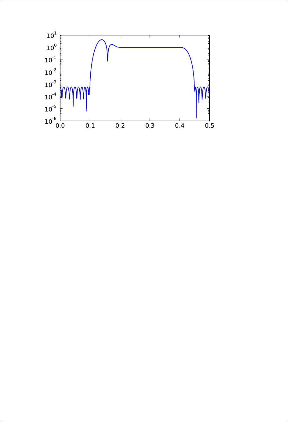
SciPy Reference Guide, Release 0.13.0
scipy.signal.unique_roots(p,tol=0.001,rtype=’min’)
Determine unique roots and their multiplicities from a list of roots.
Parameters p: array_like
The list of roots.
tol : float, optional
The tolerance for two roots to be considered equal. Default is 1e-3.
rtype : {‘max’, ‘min, ‘avg’}, optional
How to determine the returned root if multiple roots are within tol of each
other.
•‘max’: pick the maximum of those roots.
•‘min’: pick the minimum of those roots.
•‘avg’: take the average of those roots.
Returns pout : ndarray
The list of unique roots, sorted from low to high.
mult : ndarray
The multiplicity of each root.
Notes
This utility function is not specific to roots but can be used for any sequence of values for which uniqueness and
multiplicity has to be determined. For a more general routine, see numpy.unique.
Examples
>>> from scipy import signal
>>> vals =[0,1.3,1.31,2.8,1.25,2.2,10.3]
>>> uniq, mult =signal.unique_roots(vals, tol=2e-2, rtype=’avg’)
Check which roots have multiplicity larger than 1:
>>> uniq[mult >1]
array([ 1.305])
scipy.signal.residue(b,a,tol=0.001,rtype=’avg’)
Compute partial-fraction expansion of b(s) / a(s).
If M = len(b) and N = len(a), then the partial-fraction expansion H(s) is defined as:
620 Chapter 5. Reference

SciPy Reference Guide, Release 0.13.0
b(s) b[0] s**(M-1) + b[1] s**(M-2) + ... + b[M-1]
H(s) = ------ = ----------------------------------------------
a(s) a[0] s**(N-1) + a[1] s**(N-2) + ... + a[N-1]
r[0] r[1] r[-1]
= -------- + -------- + ... + --------- + k(s)
(s-p[0]) (s-p[1]) (s-p[-1])
If there are any repeated roots (closer together than tol), then H(s) has terms like:
r[i] r[i+1] r[i+n-1]
-------- + ----------- + ... + -----------
(s-p[i]) (s-p[i])**2 (s-p[i])**n
Returns r: ndarray
Residues.
p: ndarray
Poles.
k: ndarray
Coefficients of the direct polynomial term.
See Also
invres,numpy.poly,unique_roots
scipy.signal.residuez(b,a,tol=0.001,rtype=’avg’)
Compute partial-fraction expansion of b(z) / a(z).
If M = len(b) and N = len(a):
b(z) b[0] + b[1] z**(-1) + ... + b[M-1] z**(-M+1)
H(z) = ------ = ----------------------------------------------
a(z) a[0] + a[1] z**(-1) + ... + a[N-1] z**(-N+1)
r[0] r[-1]
= --------------- + ... + ---------------- + k[0] + k[1]z**(-1) ...
(1-p[0]z**(-1)) (1-p[-1]z**(-1))
If there are any repeated roots (closer than tol), then the partial fraction expansion has terms like:
r[i] r[i+1] r[i+n-1]
-------------- + ------------------ + ... + ------------------
(1-p[i]z**(-1)) (1-p[i]z**(-1))**2 (1-p[i]z**(-1))**n
See Also
invresz,unique_roots
scipy.signal.invres(r,p,k,tol=0.001,rtype=’avg’)
Compute b(s) and a(s) from partial fraction expansion: r,p,k
If M = len(b) and N = len(a):
b(s) b[0] x**(M-1) + b[1] x**(M-2) + ... + b[M-1]
H(s) = ------ = ----------------------------------------------
a(s) a[0] x**(N-1) + a[1] x**(N-2) + ... + a[N-1]
5.22. Signal processing (scipy.signal) 621

SciPy Reference Guide, Release 0.13.0
r[0] r[1] r[-1]
= -------- + -------- + ... + --------- + k(s)
(s-p[0]) (s-p[1]) (s-p[-1])
If there are any repeated roots (closer than tol), then the partial fraction expansion has terms like:
r[i] r[i+1] r[i+n-1]
-------- + ----------- + ... + -----------
(s-p[i]) (s-p[i])**2 (s-p[i])**n
Parameters r: ndarray
Residues.
p: ndarray
Poles.
k: ndarray
Coefficients of the direct polynomial term.
tol : float, optional
The tolerance for two roots to be considered equal. Default is 1e-3.
rtype : {‘max’, ‘min, ‘avg’}, optional
How to determine the returned root if multiple roots are within tol of each
other.
‘max’: pick the maximum of those roots.
‘min’: pick the minimum of those roots.
‘avg’: take the average of those roots.
See Also
residue,unique_roots
5.22.5 Matlab-style IIR filter design
butter(N, Wn[, btype, analog, output]) Butterworth digital and analog filter design.
buttord(wp, ws, gpass, gstop[, analog]) Butterworth filter order selection.
cheby1(N, rp, Wn[, btype, analog, output]) Chebyshev type I digital and analog filter design.
cheb1ord(wp, ws, gpass, gstop[, analog]) Chebyshev type I filter order selection.
cheby2(N, rs, Wn[, btype, analog, output]) Chebyshev type II digital and analog filter design.
cheb2ord(wp, ws, gpass, gstop[, analog]) Chebyshev type II filter order selection.
ellip(N, rp, rs, Wn[, btype, analog, output]) Elliptic (Cauer) digital and analog filter design.
ellipord(wp, ws, gpass, gstop[, analog]) Elliptic (Cauer) filter order selection.
bessel(N, Wn[, btype, analog, output]) Bessel/Thomson digital and analog filter design.
scipy.signal.butter(N,Wn,btype=’low’,analog=False,output=’ba’)
Butterworth digital and analog filter design.
Design an Nth order digital or analog Butterworth filter and return the filter coefficients in (B,A) or (Z,P,K)
form.
Parameters N: int
The order of the filter.
Wn : array_like
A scalar or length-2 sequence giving the critical frequencies. For a Butter-
worth filter, this is the point at which the gain drops to 1/sqrt(2) that of the
passband (the “-3 dB point”). For digital filters, Wn is normalized from 0
622 Chapter 5. Reference

SciPy Reference Guide, Release 0.13.0
to 1, where 1 is the Nyquist frequency, pi radians/sample. (Wn is thus in
half-cycles / sample.) For analog filters, Wn is an angular frequency (e.g.
rad/s).
btype : {‘lowpass’, ‘highpass’, ‘bandpass’, ‘bandstop’}, optional
The type of filter. Default is ‘lowpass’.
analog : bool, optional
When True, return an analog filter, otherwise a digital filter is returned.
output : {‘ba’, ‘zpk’}, optional
Type of output: numerator/denominator (‘ba’) or pole-zero (‘zpk’). Default
is ‘ba’.
Returns b, a : ndarray, ndarray
Numerator (b) and denominator (a) polynomials of the IIR filter. Only re-
turned if output=’ba’.
z, p, k : ndarray, ndarray, float
Zeros, poles, and system gain of the IIR filter transfer function. Only re-
turned if output=’zpk’.
See Also
buttord
Notes
The Butterworth filter has maximally flat frequency response in the passband.
Examples
Plot the filter’s frequency response, showing the critical points:
>>> from scipy import signal
>>> import matplotlib.pyplot as plt
>>> b,a=signal.butter(4,100,’low’, analog=True)
>>> w,h=signal.freqs(b, a)
>>> plt.plot(w, 20 *np.log10(abs(h)))
>>> plt.xscale(’log’)
>>> plt.title(’Butterworth filter frequency response’)
>>> plt.xlabel(’Frequency [radians / second]’)
>>> plt.ylabel(’Amplitude [dB]’)
>>> plt.margins(0,0.1)
>>> plt.grid(which=’both’, axis=’both’)
>>> plt.axvline(100, color=’green’)# cutoff frequency
>>> plt.show()
5.22. Signal processing (scipy.signal) 623
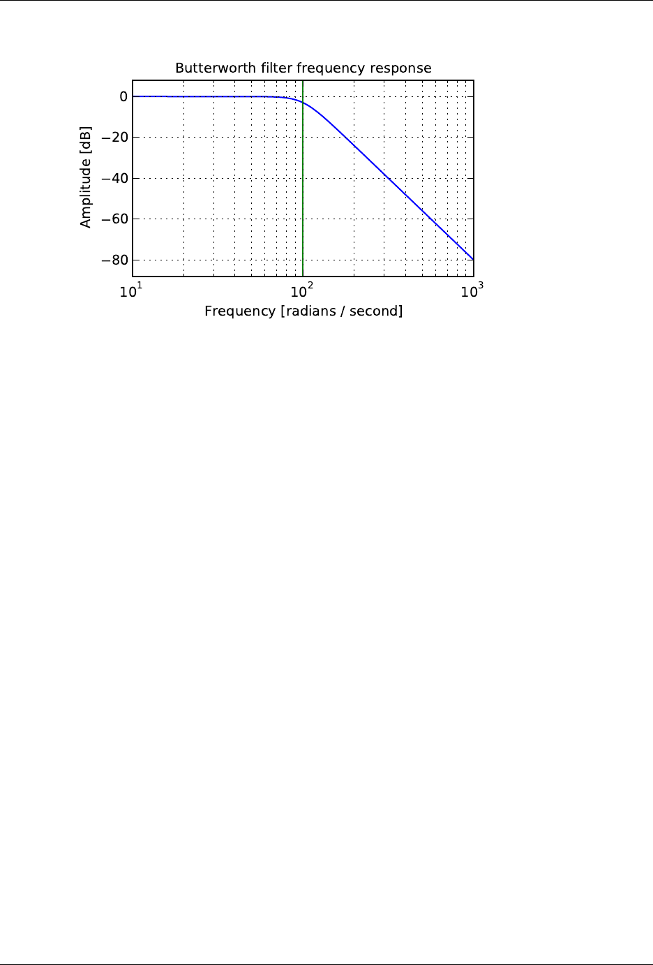
SciPy Reference Guide, Release 0.13.0
scipy.signal.buttord(wp,ws,gpass,gstop,analog=False)
Butterworth filter order selection.
Return the order of the lowest order digital or analog Butterworth filter that loses no more than gpass dB in the
passband and has at least gstop dB attenuation in the stopband.
Parameters wp, ws : float
Passband and stopband edge frequencies. For digital filters, these are nor-
malized from 0 to 1, where 1 is the Nyquist frequency, pi radians/sample.
(wp and ws are thus in half-cycles / sample.) For example:
•Lowpass: wp = 0.2, ws = 0.3
•Highpass: wp = 0.3, ws = 0.2
•Bandpass: wp = [0.2, 0.5], ws = [0.1, 0.6]
•Bandstop: wp = [0.1, 0.6], ws = [0.2, 0.5]
For analog filters, wp and ws are angular frequencies (e.g. rad/s).
gpass : float
The maximum loss in the passband (dB).
gstop : float
The minimum attenuation in the stopband (dB).
analog : bool, optional
When True, return an analog filter, otherwise a digital filter is returned.
Returns ord : int
The lowest order for a Butterworth filter which meets specs.
wn : ndarray or float
The Butterworth natural frequency (i.e. the “3dB frequency”). Should be
used with butter to give filter results.
scipy.signal.cheby1(N,rp,Wn,btype=’low’,analog=False,output=’ba’)
Chebyshev type I digital and analog filter design.
Design an Nth order digital or analog Chebyshev type I filter and return the filter coefficients in (B,A) or (Z,P,K)
form.
Parameters N: int
The order of the filter.
rp : float
The maximum ripple allowed below unity gain in the passband. Specified
in decibels, as a positive number.
Wn : array_like
624 Chapter 5. Reference

SciPy Reference Guide, Release 0.13.0
A scalar or length-2 sequence giving the critical frequencies. For Type I
filters, this is the point in the transition band at which the gain first drops
below -rp. For digital filters, Wn is normalized from 0 to 1, where 1 is the
Nyquist frequency, pi radians/sample. (Wn is thus in half-cycles / sample.)
For analog filters, Wn is an angular frequency (e.g. rad/s).
btype : {‘lowpass’, ‘highpass’, ‘bandpass’, ‘bandstop’}, optional
The type of filter. Default is ‘lowpass’.
analog : bool, optional
When True, return an analog filter, otherwise a digital filter is returned.
output : {‘ba’, ‘zpk’}, optional
Type of output: numerator/denominator (‘ba’) or pole-zero (‘zpk’). Default
is ‘ba’.
Returns b, a : ndarray, ndarray
Numerator (b) and denominator (a) polynomials of the IIR filter. Only re-
turned if output=’ba’.
z, p, k : ndarray, ndarray, float
Zeros, poles, and system gain of the IIR filter transfer function. Only re-
turned if output=’zpk’.
See Also
cheb1ord
Notes
The Chebyshev type I filter maximizes the rate of cutoff between the frequency response’s passband and stop-
band, at the expense of ripple in the passband and increased ringing in the step response.
Type I filters roll off faster than Type II (cheby2), but Type II filters do not have any ripple in the passband.
Examples
Plot the filter’s frequency response, showing the critical points:
>>> from scipy import signal
>>> import matplotlib.pyplot as plt
>>> b,a=signal.cheby1(4,5,100,’low’, analog=True)
>>> w,h=signal.freqs(b, a)
>>> plt.plot(w, 20 *np.log10(abs(h)))
>>> plt.xscale(’log’)
>>> plt.title(’Chebyshev Type I frequency response (rp=5)’)
>>> plt.xlabel(’Frequency [radians / second]’)
>>> plt.ylabel(’Amplitude [dB]’)
>>> plt.margins(0,0.1)
>>> plt.grid(which=’both’, axis=’both’)
>>> plt.axvline(100, color=’green’)# cutoff frequency
>>> plt.axhline(-5, color=’green’)# rp
>>> plt.show()
5.22. Signal processing (scipy.signal) 625
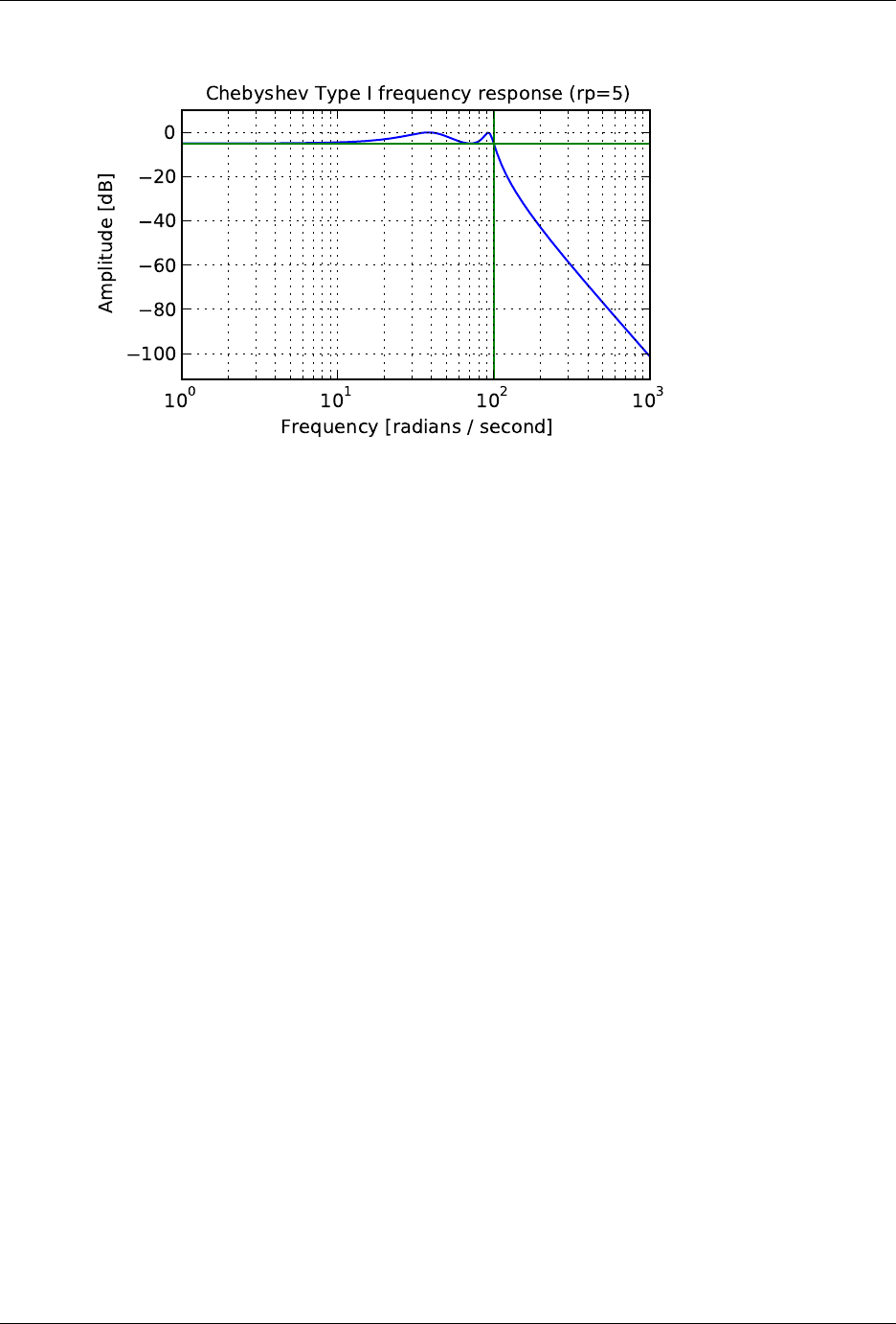
SciPy Reference Guide, Release 0.13.0
scipy.signal.cheb1ord(wp,ws,gpass,gstop,analog=False)
Chebyshev type I filter order selection.
Return the order of the lowest order digital or analog Chebyshev Type I filter that loses no more than gpass dB
in the passband and has at least gstop dB attenuation in the stopband.
Parameters wp, ws : float
Passband and stopband edge frequencies. For digital filters, these are nor-
malized from 0 to 1, where 1 is the Nyquist frequency, pi radians/sample.
(wp and ws are thus in half-cycles / sample.) For example:
•Lowpass: wp = 0.2, ws = 0.3
•Highpass: wp = 0.3, ws = 0.2
•Bandpass: wp = [0.2, 0.5], ws = [0.1, 0.6]
•Bandstop: wp = [0.1, 0.6], ws = [0.2, 0.5]
For analog filters, wp and ws are angular frequencies (e.g. rad/s).
gpass : float
The maximum loss in the passband (dB).
gstop : float
The minimum attenuation in the stopband (dB).
analog : bool, optional
When True, return an analog filter, otherwise a digital filter is returned.
Returns ord : int
The lowest order for a Chebyshev type I filter that meets specs.
wn : ndarray or float
The Chebyshev natural frequency (the “3dB frequency”) for use with
cheby1 to give filter results.
scipy.signal.cheby2(N,rs,Wn,btype=’low’,analog=False,output=’ba’)
Chebyshev type II digital and analog filter design.
Design an Nth order digital or analog Chebyshev type II filter and return the filter coefficients in (B,A) or (Z,P,K)
form.
Parameters N: int
The order of the filter.
rs : float
The minimum attenuation required in the stop band. Specified in decibels,
as a positive number.
Wn : array_like
626 Chapter 5. Reference

SciPy Reference Guide, Release 0.13.0
A scalar or length-2 sequence giving the critical frequencies. For Type II
filters, this is the point in the transition band at which the gain first reaches
-rs. For digital filters, Wn is normalized from 0 to 1, where 1 is the Nyquist
frequency, pi radians/sample. (Wn is thus in half-cycles / sample.) For
analog filters, Wn is an angular frequency (e.g. rad/s).
btype : {‘lowpass’, ‘highpass’, ‘bandpass’, ‘bandstop’}, optional
The type of filter. Default is ‘lowpass’.
analog : bool, optional
When True, return an analog filter, otherwise a digital filter is returned.
output : {‘ba’, ‘zpk’}, optional
Type of output: numerator/denominator (‘ba’) or pole-zero (‘zpk’). Default
is ‘ba’.
Returns b, a : ndarray, ndarray
Numerator (b) and denominator (a) polynomials of the IIR filter. Only re-
turned if output=’ba’.
z, p, k : ndarray, ndarray, float
Zeros, poles, and system gain of the IIR filter transfer function. Only re-
turned if output=’zpk’.
See Also
cheb2ord
Notes
The Chebyshev type II filter maximizes the rate of cutoff between the frequency response’s passband and stop-
band, at the expense of ripple in the stopband and increased ringing in the step response.
Type II filters do not roll off as fast as Type I (cheby1).
Examples
Plot the filter’s frequency response, showing the critical points:
>>> from scipy import signal
>>> import matplotlib.pyplot as plt
>>> b,a=signal.cheby2(4,40,100,’low’, analog=True)
>>> w,h=signal.freqs(b, a)
>>> plt.plot(w, 20 *np.log10(abs(h)))
>>> plt.xscale(’log’)
>>> plt.title(’Chebyshev Type II frequency response (rs=40)’)
>>> plt.xlabel(’Frequency [radians / second]’)
>>> plt.ylabel(’Amplitude [dB]’)
>>> plt.margins(0,0.1)
>>> plt.grid(which=’both’, axis=’both’)
>>> plt.axvline(100, color=’green’)# cutoff frequency
>>> plt.axhline(-40, color=’green’)# rs
>>> plt.show()
5.22. Signal processing (scipy.signal) 627
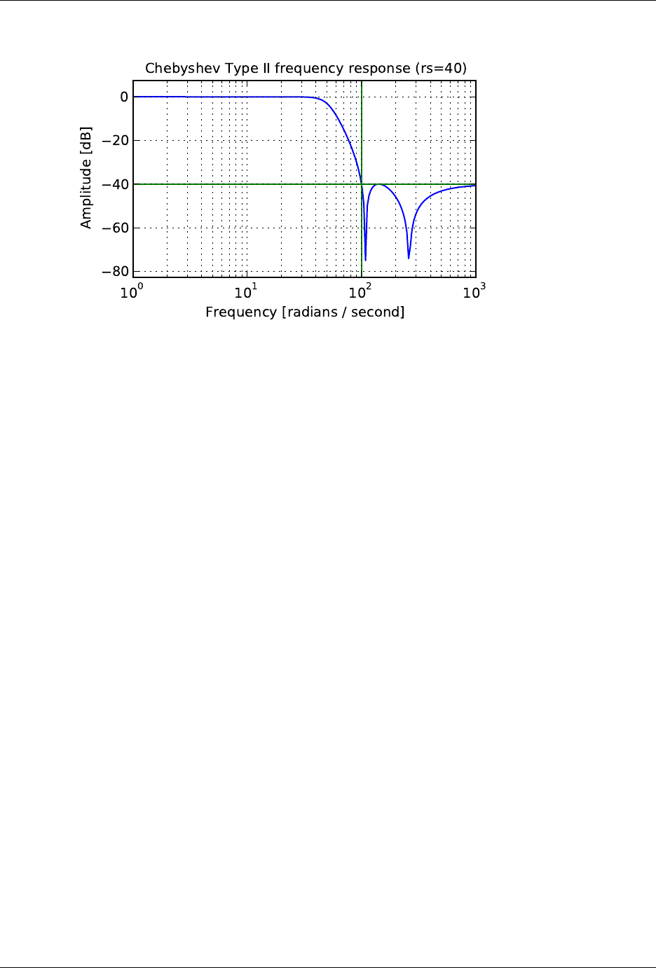
SciPy Reference Guide, Release 0.13.0
scipy.signal.cheb2ord(wp,ws,gpass,gstop,analog=False)
Chebyshev type II filter order selection.
Return the order of the lowest order digital or analog Chebyshev Type II filter that loses no more than gpass dB
in the passband and has at least gstop dB attenuation in the stopband.
Parameters wp, ws : float
Passband and stopband edge frequencies. For digital filters, these are nor-
malized from 0 to 1, where 1 is the Nyquist frequency, pi radians/sample.
(wp and ws are thus in half-cycles / sample.) For example:
•Lowpass: wp = 0.2, ws = 0.3
•Highpass: wp = 0.3, ws = 0.2
•Bandpass: wp = [0.2, 0.5], ws = [0.1, 0.6]
•Bandstop: wp = [0.1, 0.6], ws = [0.2, 0.5]
For analog filters, wp and ws are angular frequencies (e.g. rad/s).
gpass : float
The maximum loss in the passband (dB).
gstop : float
The minimum attenuation in the stopband (dB).
analog : bool, optional
When True, return an analog filter, otherwise a digital filter is returned.
Returns ord : int
The lowest order for a Chebyshev type II filter that meets specs.
wn : ndarray or float
The Chebyshev natural frequency (the “3dB frequency”) for use with
cheby2 to give filter results.
scipy.signal.ellip(N,rp,rs,Wn,btype=’low’,analog=False,output=’ba’)
Elliptic (Cauer) digital and analog filter design.
Design an Nth order digital or analog elliptic filter and return the filter coefficients in (B,A) or (Z,P,K) form.
Parameters N: int
The order of the filter.
rp : float
The maximum ripple allowed below unity gain in the passband. Specified
in decibels, as a positive number.
rs : float
The minimum attenuation required in the stop band. Specified in decibels,
as a positive number.
628 Chapter 5. Reference

SciPy Reference Guide, Release 0.13.0
Wn : array_like
A scalar or length-2 sequence giving the critical frequencies. For elliptic
filters, this is the point in the transition band at which the gain first drops
below -rp. For digital filters, Wn is normalized from 0 to 1, where 1 is the
Nyquist frequency, pi radians/sample. (Wn is thus in half-cycles / sample.)
For analog filters, Wn is an angular frequency (e.g. rad/s).
btype : {‘lowpass’, ‘highpass’, ‘bandpass’, ‘bandstop’}, optional
The type of filter. Default is ‘lowpass’.
analog : bool, optional
When True, return an analog filter, otherwise a digital filter is returned.
output : {‘ba’, ‘zpk’}, optional
Type of output: numerator/denominator (‘ba’) or pole-zero (‘zpk’). Default
is ‘ba’.
Returns b, a : ndarray, ndarray
Numerator (b) and denominator (a) polynomials of the IIR filter. Only re-
turned if output=’ba’.
z, p, k : ndarray, ndarray, float
Zeros, poles, and system gain of the IIR filter transfer function. Only re-
turned if output=’zpk’.
See Also
ellipord
Notes
Also known as Cauer or Zolotarev filters, the elliptical filter maximizes the rate of transition between the fre-
quency response’s passband and stopband, at the expense of ripple in both, and increased ringing in the step
response.
As rp approaches 0, the elliptical filter becomes a Chebyshev type II filter (cheby2). As rs approaches 0, it
becomes a Chebyshev type I filter (cheby1). As both approach 0, it becomes a Butterworth filter (butter).
Examples
Plot the filter’s frequency response, showing the critical points:
>>> from scipy import signal
>>> import matplotlib.pyplot as plt
>>> b,a=signal.ellip(4,5,40,100,’low’, analog=True)
>>> w,h=signal.freqs(b, a)
>>> plt.plot(w, 20 *np.log10(abs(h)))
>>> plt.xscale(’log’)
>>> plt.title(’Elliptic filter frequency response (rp=5, rs=40)’)
>>> plt.xlabel(’Frequency [radians / second]’)
>>> plt.ylabel(’Amplitude [dB]’)
>>> plt.margins(0,0.1)
>>> plt.grid(which=’both’, axis=’both’)
>>> plt.axvline(100, color=’green’)# cutoff frequency
>>> plt.axhline(-40, color=’green’)# rs
>>> plt.axhline(-5, color=’green’)# rp
>>> plt.show()
5.22. Signal processing (scipy.signal) 629
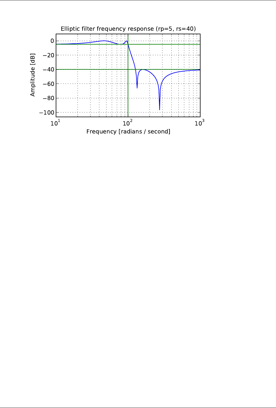
SciPy Reference Guide, Release 0.13.0
scipy.signal.ellipord(wp,ws,gpass,gstop,analog=False)
Elliptic (Cauer) filter order selection.
Return the order of the lowest order digital or analog elliptic filter that loses no more than gpass dB in the
passband and has at least gstop dB attenuation in the stopband.
Parameters wp, ws : float
Passband and stopband edge frequencies. For digital filters, these are nor-
malized from 0 to 1, where 1 is the Nyquist frequency, pi radians/sample.
(wp and ws are thus in half-cycles / sample.) For example:
•Lowpass: wp = 0.2, ws = 0.3
•Highpass: wp = 0.3, ws = 0.2
•Bandpass: wp = [0.2, 0.5], ws = [0.1, 0.6]
•Bandstop: wp = [0.1, 0.6], ws = [0.2, 0.5]
For analog filters, wp and ws are angular frequencies (e.g. rad/s).
gpass : float
The maximum loss in the passband (dB).
gstop : float
The minimum attenuation in the stopband (dB).
analog : bool, optional
When True, return an analog filter, otherwise a digital filter is returned.
Returns ord : int
The lowest order for an Elliptic (Cauer) filter that meets specs.
wn : ndarray or float
The Chebyshev natural frequency (the “3dB frequency”) for use with
ellip to give filter results.
scipy.signal.bessel(N,Wn,btype=’low’,analog=False,output=’ba’)
Bessel/Thomson digital and analog filter design.
Design an Nth order digital or analog Bessel filter and return the filter coefficients in (B,A) or (Z,P,K) form.
Parameters N: int
The order of the filter.
Wn : array_like
A scalar or length-2 sequence giving the critical frequencies. For a Bessel
filter, this is defined as the point at which the asymptotes of the response are
the same as a Butterworth filter of the same order. For digital filters, Wn is
normalized from 0 to 1, where 1 is the Nyquist frequency, pi radians/sample.
630 Chapter 5. Reference

SciPy Reference Guide, Release 0.13.0
(Wn is thus in half-cycles / sample.) For analog filters, Wn is an angular
frequency (e.g. rad/s).
btype : {‘lowpass’, ‘highpass’, ‘bandpass’, ‘bandstop’}, optional
The type of filter. Default is ‘lowpass’.
analog : bool, optional
When True, return an analog filter, otherwise a digital filter is returned.
output : {‘ba’, ‘zpk’}, optional
Type of output: numerator/denominator (‘ba’) or pole-zero (‘zpk’). Default
is ‘ba’.
Returns b, a : ndarray, ndarray
Numerator (b) and denominator (a) polynomials of the IIR filter. Only re-
turned if output=’ba’.
z, p, k : ndarray, ndarray, float
Zeros, poles, and system gain of the IIR filter transfer function. Only re-
turned if output=’zpk’.
Notes
Also known as a Thomson filter, the analog Bessel filter has maximally flat group delay and maximally linear
phase response, with very little ringing in the step response.
As order increases, the Bessel filter approaches a Gaussian filter.
The digital Bessel filter is generated using the bilinear transform, which does not preserve the phase response
of the analog filter. As such, it is only approximately correct at frequencies below about fs/4. To get maximally
flat group delay at higher frequencies, the analog Bessel filter must be transformed using phase-preserving
techniques.
For a given Wn, the lowpass and highpass filter have the same phase vs frequency curves; they are “phase-
matched”.
Examples
Plot the filter’s frequency response, showing the flat group delay and the relationship to the Butterworth’s cutoff
frequency:
>>> from scipy import signal
>>> import matplotlib.pyplot as plt
>>> b,a=signal.butter(4,100,’low’, analog=True)
>>> w,h=signal.freqs(b, a)
>>> plt.plot(w, 20 *np.log10(np.abs(h)), color=’silver’, ls=’dashed’)
>>> b,a=signal.bessel(4,100,’low’, analog=True)
>>> w,h=signal.freqs(b, a)
>>> plt.plot(w, 20 *np.log10(np.abs(h)))
>>> plt.xscale(’log’)
>>> plt.title(’Bessel filter frequency response (with Butterworth)’)
>>> plt.xlabel(’Frequency [radians / second]’)
>>> plt.ylabel(’Amplitude [dB]’)
>>> plt.margins(0,0.1)
>>> plt.grid(which=’both’, axis=’both’)
>>> plt.axvline(100, color=’green’)# cutoff frequency
>>> plt.show()
5.22. Signal processing (scipy.signal) 631
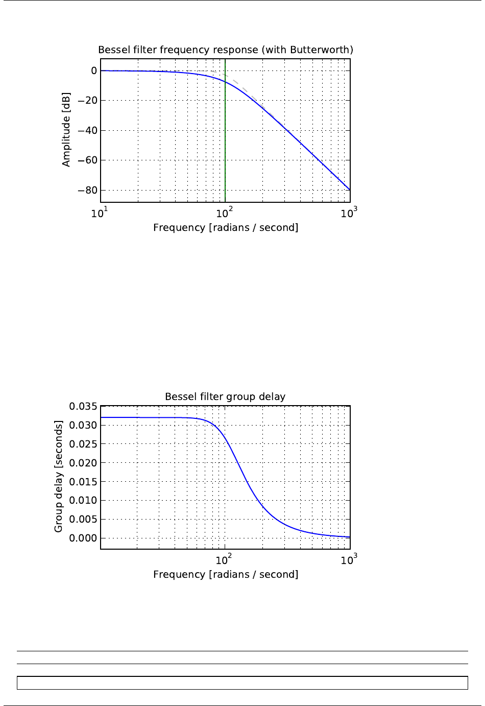
SciPy Reference Guide, Release 0.13.0
>>> plt.figure()
>>> plt.plot(w[1:], -np.diff(np.unwrap(np.angle(h)))/np.diff(w))
>>> plt.xscale(’log’)
>>> plt.title(’Bessel filter group delay’)
>>> plt.xlabel(’Frequency [radians / second]’)
>>> plt.ylabel(’Group delay [seconds]’)
>>> plt.margins(0,0.1)
>>> plt.grid(which=’both’, axis=’both’)
>>> plt.show()
5.22.6 Continuous-Time Linear Systems
freqresp(system[, w, n]) Calculate the frequency response of a continuous-time system.
lti(*args, **kwords) Linear Time Invariant class which simplifies representation.
Continued on next page
632 Chapter 5. Reference

SciPy Reference Guide, Release 0.13.0
Table 5.110 – continued from previous page
lsim(system, U, T[, X0, interp]) Simulate output of a continuous-time linear system.
lsim2(system[, U, T, X0]) Simulate output of a continuous-time linear system, by using
impulse(system[, X0, T, N]) Impulse response of continuous-time system.
impulse2(system[, X0, T, N]) Impulse response of a single-input, continuous-time linear system.
step(system[, X0, T, N]) Step response of continuous-time system.
step2(system[, X0, T, N]) Step response of continuous-time system.
bode(system[, w, n]) Calculate Bode magnitude and phase data of a continuous-time system.
scipy.signal.freqresp(system,w=None,n=10000)
Calculate the frequency response of a continuous-time system.
Parameters system : an instance of the LTI class or a tuple describing the system.
The following gives the number of elements in the tuple and the interpreta-
tion:
•2 (num, den)
•3 (zeros, poles, gain)
•4 (A, B, C, D)
w: array_like, optional
Array of frequencies (in rad/s). Magnitude and phase data is calculated for
every value in this array. If not given a reasonable set will be calculated.
n: int, optional
Number of frequency points to compute if wis not given. The nfrequencies
are logarithmically spaced in an interval chosen to include the influence of
the poles and zeros of the system.
Returns w: 1D ndarray
Frequency array [rad/s]
H: 1D ndarray
Array of complex magnitude values
Examples
# Generating the Nyquist plot of a transfer function
>>> from scipy import signal
>>> import matplotlib.pyplot as plt
>>> s1 =signal.lti([], [1,1,1], [5])
# transfer function: H(s) = 5 / (s-1)^3
>>> w,H=signal.freqresp(s1)
>>> plt.figure()
>>> plt.plot(H.real, H.imag, "b")
>>> plt.plot(H.real, -H.imag, "r")
>>> plt.show()
5.22. Signal processing (scipy.signal) 633

SciPy Reference Guide, Release 0.13.0
class scipy.signal.lti(*args,**kwords)
Linear Time Invariant class which simplifies representation.
Parameters args : arguments
The lti class can be instantiated with either 2, 3 or 4 arguments. The
following gives the number of elements in the tuple and the interpretation:
•2: (numerator, denominator)
•3: (zeros, poles, gain)
•4: (A, B, C, D)
Each argument can be an array or sequence.
Notes
lti instances have all types of representations available; for example after creating an instance s with (zeros,
poles, gain) the transfer function representation (numerator, denominator) can be accessed as s.num and
s.den.
Attributes
A
B
C
D
den
gain
num
poles
zeros
lti.A
lti.B
lti.C
634 Chapter 5. Reference

SciPy Reference Guide, Release 0.13.0
lti.D
lti.den
lti.gain
lti.num
lti.poles
lti.zeros
Methods
bode([w, n]) Calculate Bode magnitude and phase data.
freqresp([w, n]) Calculate the frequency response of a continuous-time system.
impulse([X0, T, N])
output(U, T[, X0])
step([X0, T, N])
lti.bode(w=None,n=100)
Calculate Bode magnitude and phase data.
Returns a 3-tuple containing arrays of frequencies [rad/s], magnitude [dB] and phase [deg]. See
scipy.signal.bode for details. New in version 0.11.0.
Examples
>>> from scipy import signal
>>> import matplotlib.pyplot as plt
>>> s1 =signal.lti([1], [1,1])
>>> w, mag, phase =s1.bode()
>>> plt.figure()
>>> plt.semilogx(w, mag) # Bode magnitude plot
>>> plt.figure()
>>> plt.semilogx(w, phase) # Bode phase plot
>>> plt.show()
5.22. Signal processing (scipy.signal) 635
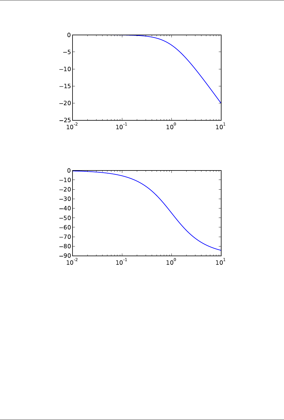
SciPy Reference Guide, Release 0.13.0
lti.freqresp(w=None,n=10000)
Calculate the frequency response of a continuous-time system.
Returns a 2-tuple containing arrays of frequencies [rad/s] and complex magnitude. See
scipy.signal.freqresp for details.
lti.impulse(X0=None,T=None,N=None)
lti.output(U,T,X0=None)
lti.step(X0=None,T=None,N=None)
scipy.signal.lsim(system,U,T,X0=None,interp=1)
Simulate output of a continuous-time linear system.
Parameters system : an instance of the LTI class or a tuple describing the system.
636 Chapter 5. Reference

SciPy Reference Guide, Release 0.13.0
The following gives the number of elements in the tuple and the interpreta-
tion:
•2: (num, den)
•3: (zeros, poles, gain)
•4: (A, B, C, D)
U: array_like
An input array describing the input at each time T(interpolation is assumed
between given times). If there are multiple inputs, then each column of the
rank-2 array represents an input.
T: array_like
The time steps at which the input is defined and at which the output is
desired.
X0 :
The initial conditions on the state vector (zero by default).
interp : {1, 0}
Whether to use linear (1) or zero-order hold (0) interpolation.
Returns T: 1D ndarray
Time values for the output.
yout : 1D ndarray
System response.
xout : ndarray
Time-evolution of the state-vector.
scipy.signal.lsim2(system,U=None,T=None,X0=None,**kwargs)
Simulate output of a continuous-time linear system, by using the ODE solver scipy.integrate.odeint.
Parameters system : an instance of the LTI class or a tuple describing the system.
The following gives the number of elements in the tuple and the interpreta-
tion:
•2: (num, den)
•3: (zeros, poles, gain)
•4: (A, B, C, D)
U: array_like (1D or 2D), optional
An input array describing the input at each time T. Linear interpolation is
used between given times. If there are multiple inputs, then each column of
the rank-2 array represents an input. If U is not given, the input is assumed
to be zero.
T: array_like (1D or 2D), optional
The time steps at which the input is defined and at which the output is
desired. The default is 101 evenly spaced points on the interval [0,10.0].
X0 : array_like (1D), optional
The initial condition of the state vector. If X0 is not given, the initial condi-
tions are assumed to be 0.
kwargs : dict
Additional keyword arguments are passed on to the function odeint. See the
notes below for more details.
Returns T: 1D ndarray
The time values for the output.
yout : ndarray
The response of the system.
xout : ndarray
The time-evolution of the state-vector.
Notes
This function uses scipy.integrate.odeint to solve the system’s differential equations. Ad-
ditional keyword arguments given to lsim2 are passed on to odeint. See the documentation for
scipy.integrate.odeint for the full list of arguments.
5.22. Signal processing (scipy.signal) 637

SciPy Reference Guide, Release 0.13.0
scipy.signal.impulse(system,X0=None,T=None,N=None)
Impulse response of continuous-time system.
Parameters system : an instance of the LTI class or a tuple of array_like
describing the system. The following gives the number of elements in the
tuple and the interpretation:
•2 (num, den)
•3 (zeros, poles, gain)
•4 (A, B, C, D)
X0 : array_like, optional
Initial state-vector. Defaults to zero.
T: array_like, optional
Time points. Computed if not given.
N: int, optional
The number of time points to compute (if Tis not given).
Returns T: ndarray
A 1-D array of time points.
yout : ndarray
A 1-D array containing the impulse response of the system (except for sin-
gularities at zero).
scipy.signal.impulse2(system,X0=None,T=None,N=None,**kwargs)
Impulse response of a single-input, continuous-time linear system.
Parameters system : an instance of the LTI class or a tuple of array_like
describing the system. The following gives the number of elements in the
tuple and the interpretation:
•2 (num, den)
•3 (zeros, poles, gain)
•4 (A, B, C, D)
X0 : 1-D array_like, optional
The initial condition of the state vector. Default: 0 (the zero vector).
T: 1-D array_like, optional
The time steps at which the input is defined and at which the output is
desired. If Tis not given, the function will generate a set of time samples
automatically.
N: int, optional
Number of time points to compute. Default: 100.
kwargs : various types
Additional keyword arguments are passed on to the function
scipy.signal.lsim2, which in turn passes them on to
scipy.integrate.odeint; see the latter’s documentation for
information about these arguments.
Returns T: ndarray
The time values for the output.
yout : ndarray
The output response of the system.
See Also
impulse,lsim2,integrate.odeint
Notes
The solution is generated by calling scipy.signal.lsim2, which uses the differential equation solver
scipy.integrate.odeint. New in version 0.8.0.
Examples
Second order system with a repeated root: x’‘(t) + 2*x(t) + x(t) = u(t)
638 Chapter 5. Reference
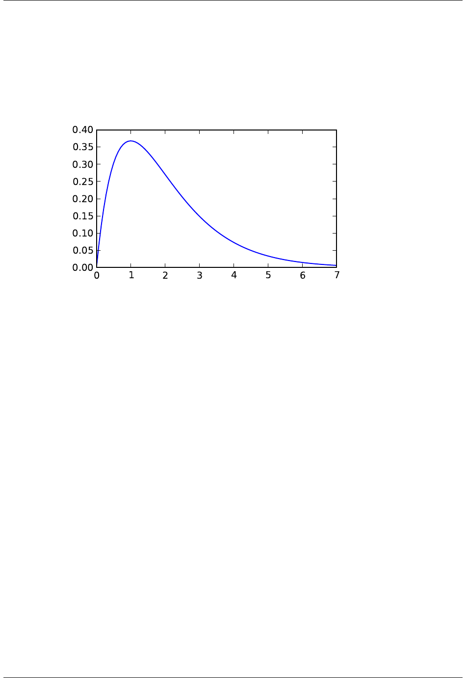
SciPy Reference Guide, Release 0.13.0
>>> from scipy import signal
>>> system =([1.0], [1.0,2.0,1.0])
>>> t,y=signal.impulse2(system)
>>> import matplotlib.pyplot as plt
>>> plt.plot(t, y)
scipy.signal.step(system,X0=None,T=None,N=None)
Step response of continuous-time system.
Parameters system : an instance of the LTI class or a tuple of array_like
describing the system. The following gives the number of elements in the
tuple and the interpretation:
•2 (num, den)
•3 (zeros, poles, gain)
•4 (A, B, C, D)
X0 : array_like, optional
Initial state-vector (default is zero).
T: array_like, optional
Time points (computed if not given).
N: int
Number of time points to compute if Tis not given.
Returns T: 1D ndarray
Output time points.
yout : 1D ndarray
Step response of system.
See Also
scipy.signal.step2
scipy.signal.step2(system,X0=None,T=None,N=None,**kwargs)
Step response of continuous-time system.
This function is functionally the same as scipy.signal.step, but it uses the function
scipy.signal.lsim2 to compute the step response.
Parameters system : an instance of the LTI class or a tuple of array_like
describing the system. The following gives the number of elements in the
tuple and the interpretation:
5.22. Signal processing (scipy.signal) 639

SciPy Reference Guide, Release 0.13.0
•2 (num, den)
•3 (zeros, poles, gain)
•4 (A, B, C, D)
X0 : array_like, optional
Initial state-vector (default is zero).
T: array_like, optional
Time points (computed if not given).
N: int
Number of time points to compute if Tis not given.
kwargs : various types
Additional keyword arguments are passed on the function
scipy.signal.lsim2, which in turn passes them on to
scipy.integrate.odeint. See the documentation for
scipy.integrate.odeint for information about these arguments.
Returns T: 1D ndarray
Output time points.
yout : 1D ndarray
Step response of system.
See Also
scipy.signal.step
Notes
New in version 0.8.0.
scipy.signal.bode(system,w=None,n=100)
Calculate Bode magnitude and phase data of a continuous-time system. New in version 0.11.0.
Parameters system : an instance of the LTI class or a tuple describing the system.
The following gives the number of elements in the tuple and the interpreta-
tion:
•2 (num, den)
•3 (zeros, poles, gain)
•4 (A, B, C, D)
w: array_like, optional
Array of frequencies (in rad/s). Magnitude and phase data is calculated for
every value in this array. If not given a reasonable set will be calculated.
n: int, optional
Number of frequency points to compute if wis not given. The nfrequencies
are logarithmically spaced in an interval chosen to include the influence of
the poles and zeros of the system.
Returns w: 1D ndarray
Frequency array [rad/s]
mag : 1D ndarray
Magnitude array [dB]
phase : 1D ndarray
Phase array [deg]
Examples
>>> from scipy import signal
>>> import matplotlib.pyplot as plt
>>> s1 =signal.lti([1], [1,1])
>>> w, mag, phase =signal.bode(s1)
640 Chapter 5. Reference
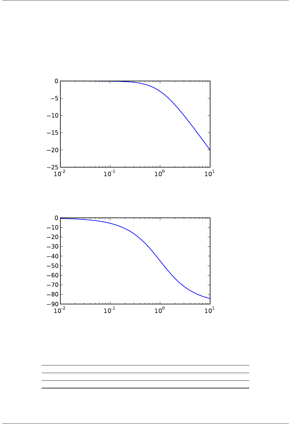
SciPy Reference Guide, Release 0.13.0
>>> plt.figure()
>>> plt.semilogx(w, mag) # Bode magnitude plot
>>> plt.figure()
>>> plt.semilogx(w, phase) # Bode phase plot
>>> plt.show()
5.22.7 Discrete-Time Linear Systems
dlsim(system, u[, t, x0]) Simulate output of a discrete-time linear system.
dimpulse(system[, x0, t, n]) Impulse response of discrete-time system.
dstep(system[, x0, t, n]) Step response of discrete-time system.
scipy.signal.dlsim(system,u,t=None,x0=None)
Simulate output of a discrete-time linear system.
5.22. Signal processing (scipy.signal) 641

SciPy Reference Guide, Release 0.13.0
Parameters system : class instance or tuple
An instance of the LTI class, or a tuple describing the system. The following
gives the number of elements in the tuple and the interpretation:
•3: (num, den, dt)
•4: (zeros, poles, gain, dt)
•5: (A, B, C, D, dt)
u: array_like
An input array describing the input at each time t(interpolation is assumed
between given times). If there are multiple inputs, then each column of the
rank-2 array represents an input.
t: array_like, optional
The time steps at which the input is defined. If tis given, the final value in
tdetermines the number of steps returned in the output.
x0 : arry_like, optional
The initial conditions on the state vector (zero by default).
Returns tout : ndarray
Time values for the output, as a 1-D array.
yout : ndarray
System response, as a 1-D array.
xout : ndarray, optional
Time-evolution of the state-vector. Only generated if the input is a state-
space systems.
See Also
lsim,dstep,dimpulse,cont2discrete
Examples
A simple integrator transfer function with a discrete time step of 1.0 could be implemented as:
>>> from scipy import signal
>>> tf =([1.0,], [1.0,-1.0], 1.0)
>>> t_in =[0.0,1.0,2.0,3.0]
>>> u=np.asarray([0.0,0.0,1.0,1.0])
>>> t_out, y =signal.dlsim(tf, u, t=t_in)
>>> y
array([ 0., 0., 0., 1.])
scipy.signal.dimpulse(system,x0=None,t=None,n=None)
Impulse response of discrete-time system.
Parameters system : tuple
The following gives the number of elements in the tuple and the interpreta-
tion:
•3: (num, den, dt)
•4: (zeros, poles, gain, dt)
•5: (A, B, C, D, dt)
x0 : array_like, optional
Initial state-vector. Defaults to zero.
t: array_like, optional
Time points. Computed if not given.
n: int, optional
The number of time points to compute (if tis not given).
Returns t: ndarray
A 1-D array of time points.
yout : tuple of array_like
Impulse response of system. Each element of the tuple represents the output
of the system based on an impulse in each input.
642 Chapter 5. Reference

SciPy Reference Guide, Release 0.13.0
See Also
impulse,dstep,dlsim,cont2discrete
scipy.signal.dstep(system,x0=None,t=None,n=None)
Step response of discrete-time system.
Parameters system : a tuple describing the system.
The following gives the number of elements in the tuple and the interpreta-
tion:
•3: (num, den, dt)
•4: (zeros, poles, gain, dt)
•5: (A, B, C, D, dt)
x0 : array_like, optional
Initial state-vector (default is zero).
t: array_like, optional
Time points (computed if not given).
n: int, optional
Number of time points to compute if tis not given.
Returns t: ndarray
Output time points, as a 1-D array.
yout : tuple of array_like
Step response of system. Each element of the tuple represents the output of
the system based on a step response to each input.
See Also
step,dimpulse,dlsim,cont2discrete
5.22.8 LTI Representations
tf2zpk(b, a) Return zero, pole, gain (z,p,k) representation from a numerator, denominator representation of a linear filter.
zpk2tf(z, p, k) Return polynomial transfer function representation from zeros
tf2ss(num, den) Transfer function to state-space representation.
ss2tf(A, B, C, D[, input]) State-space to transfer function.
zpk2ss(z, p, k) Zero-pole-gain representation to state-space representation
ss2zpk(A, B, C, D[, input]) State-space representation to zero-pole-gain representation.
cont2discrete(sys, dt[, method, alpha]) Transform a continuous to a discrete state-space system.
scipy.signal.tf2zpk(b,a)
Return zero, pole, gain (z,p,k) representation from a numerator, denominator representation of a linear filter.
Parameters b: ndarray
Numerator polynomial.
a: ndarray
Denominator polynomial.
Returns z: ndarray
Zeros of the transfer function.
p: ndarray
Poles of the transfer function.
k: float
System gain.
Notes
If some values of bare too close to 0, they are removed. In that case, a BadCoefficients warning is emitted.
5.22. Signal processing (scipy.signal) 643

SciPy Reference Guide, Release 0.13.0
scipy.signal.zpk2tf(z,p,k)
Return polynomial transfer function representation from zeros and poles
Parameters z: ndarray
Zeros of the transfer function.
p: ndarray
Poles of the transfer function.
k: float
System gain.
Returns b: ndarray
Numerator polynomial.
a: ndarray
Denominator polynomial.
scipy.signal.tf2ss(num,den)
Transfer function to state-space representation.
Parameters num, den : array_like
Sequences representing the numerator and denominator polynomials. The
denominator needs to be at least as long as the numerator.
Returns A, B, C, D : ndarray
State space representation of the system.
scipy.signal.ss2tf(A,B,C,D,input=0)
State-space to transfer function.
Parameters A, B, C, D : ndarray
State-space representation of linear system.
input : int, optional
For multiple-input systems, the input to use.
Returns num, den : 1D ndarray
Numerator and denominator polynomials (as sequences) respectively.
scipy.signal.zpk2ss(z,p,k)
Zero-pole-gain representation to state-space representation
Parameters z, p : sequence
Zeros and poles.
k: float
System gain.
Returns A, B, C, D : ndarray
State-space matrices.
scipy.signal.ss2zpk(A,B,C,D,input=0)
State-space representation to zero-pole-gain representation.
Parameters A, B, C, D : ndarray
State-space representation of linear system.
input : int, optional
For multiple-input systems, the input to use.
Returns z, p : sequence
Zeros and poles.
k: float
System gain.
scipy.signal.cont2discrete(sys,dt,method=’zoh’,alpha=None)
Transform a continuous to a discrete state-space system.
Parameters sys : a tuple describing the system.
The following gives the number of elements in the tuple and the interpreta-
tion:
•2: (num, den)
644 Chapter 5. Reference

SciPy Reference Guide, Release 0.13.0
•3: (zeros, poles, gain)
•4: (A, B, C, D)
dt : float
The discretization time step.
method : {“gbt”, “bilinear”, “euler”, “backward_diff”, “zoh”}
Which method to use:
•gbt: generalized bilinear transformation
•bilinear: Tustin’s approximation (“gbt” with alpha=0.5)
•euler: Euler (or forward differencing) method (“gbt” with
alpha=0)
•backward_diff: Backwards differencing (“gbt” with al-
pha=1.0)
•zoh: zero-order hold (default)
alpha : float within [0, 1]
The generalized bilinear transformation weighting parameter, which should
only be specified with method=”gbt”, and is ignored otherwise
Returns sysd : tuple containing the discrete system
Based on the input type, the output will be of the form
•(num, den, dt) for transfer function input
•(zeros, poles, gain, dt) for zeros-poles-gain input
•(A, B, C, D, dt) for state-space system input
Notes
By default, the routine uses a Zero-Order Hold (zoh) method to perform the transformation. Alternatively, a
generalized bilinear transformation may be used, which includes the common Tustin’s bilinear approximation,
an Euler’s method technique, or a backwards differencing technique.
The Zero-Order Hold (zoh) method is based on [R111], the generalized bilinear approximation is based on
[R112] and [R113].
References
[R111],[R112],[R113]
5.22.9 Waveforms
chirp(t, f0, t1, f1[, method, phi, vertex_zero]) Frequency-swept cosine generator.
gausspulse(t[, fc, bw, bwr, tpr, retquad, ...]) Return a Gaussian modulated sinusoid:
sawtooth(t[, width]) Return a periodic sawtooth or triangle waveform.
square(t[, duty]) Return a periodic square-wave waveform.
sweep_poly(t, poly[, phi]) Frequency-swept cosine generator, with a time-dependent frequency.
scipy.signal.chirp(t,f0,t1,f1,method=’linear’,phi=0,vertex_zero=True)
Frequency-swept cosine generator.
In the following, ‘Hz’ should be interpreted as ‘cycles per unit’; there is no requirement here that the unit is
one second. The important distinction is that the units of rotation are cycles, not radians. Likewise, tcould be a
measurement of space instead of time.
Parameters t: ndarray
Times at which to evaluate the waveform.
f0 : float
Frequency (e.g. Hz) at time t=0.
t1 : float
Time at which f1 is specified.
f1 : float
Frequency (e.g. Hz) of the waveform at time t1.
5.22. Signal processing (scipy.signal) 645

SciPy Reference Guide, Release 0.13.0
method : {‘linear’, ‘quadratic’, ‘logarithmic’, ‘hyperbolic’}, optional
Kind of frequency sweep. If not given, linear is assumed. See Notes below
for more details.
phi : float, optional
Phase offset, in degrees. Default is 0.
vertex_zero : bool, optional
This parameter is only used when method is ‘quadratic’. It determines
whether the vertex of the parabola that is the graph of the frequency is at
t=0 or t=t1.
Returns y: ndarray
A numpy array containing the signal evaluated at twith the requested
time-varying frequency. More precisely, the function returns cos(phase
+ (pi/180)*phi) where phase is the integral (from 0 to t) of
2*pi*f(t).f(t) is defined below.
See Also
sweep_poly
Notes
There are four options for the method. The following formulas give the instantaneous frequency (in Hz) of the
signal generated by chirp(). For convenience, the shorter names shown below may also be used.
linear, lin, li:
f(t) = f0 + (f1 - f0) *t / t1
quadratic, quad, q:
The graph of the frequency f(t) is a parabola through (0, f0) and (t1, f1). By default, the vertex of the
parabola is at (0, f0). If vertex_zero is False, then the vertex is at (t1, f1). The formula is:
if vertex_zero is True:
f(t) = f0 + (f1 - f0) *t**2 / t1**2
else:
f(t) = f1 - (f1 - f0) *(t1 - t)**2 / t1**2
To use a more general quadratic function, or an arbitrary polynomial, use the function
scipy.signal.waveforms.sweep_poly.
logarithmic, log, lo:
f(t) = f0 *(f1/f0)**(t/t1)
f0 and f1 must be nonzero and have the same sign.
This signal is also known as a geometric or exponential chirp.
hyperbolic, hyp:
f(t) = f0*f1*t1 / ((f0 - f1)*t + f1*t1)
f1 must be positive, and f0 must be greater than f1.
scipy.signal.gausspulse(t,fc=1000,bw=0.5,bwr=-6,tpr=-60,retquad=False,retenv=False)
Return a Gaussian modulated sinusoid:
exp(-a t^2) exp(1j*2*pi*fc*t).
If retquad is True, then return the real and imaginary parts (in-phase and quadrature). If retenv is True, then
return the envelope (unmodulated signal). Otherwise, return the real part of the modulated sinusoid.
Parameters t: ndarray or the string ‘cutoff’
Input array.
fc : int, optional
Center frequency (e.g. Hz). Default is 1000.
646 Chapter 5. Reference
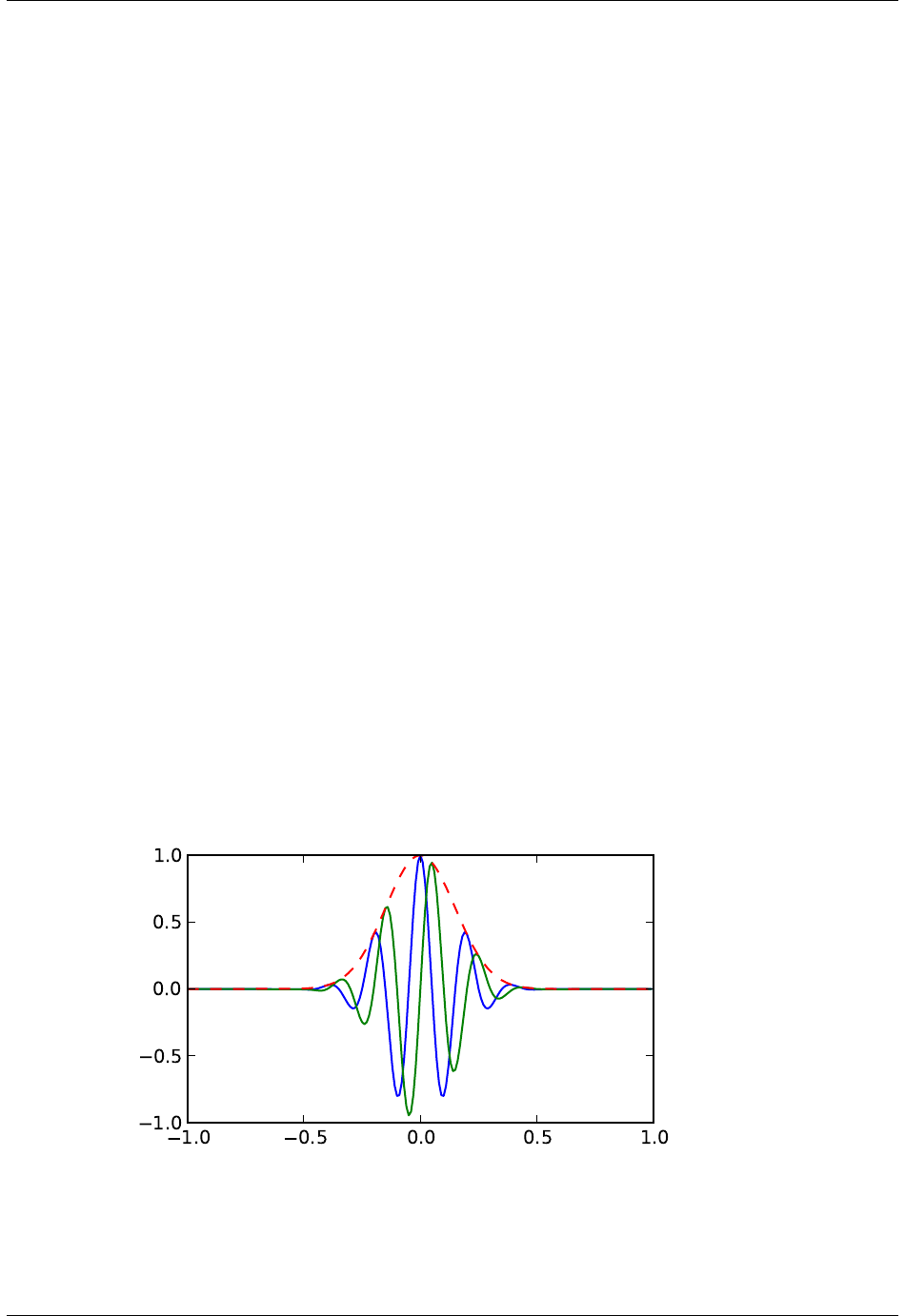
SciPy Reference Guide, Release 0.13.0
bw : float, optional
Fractional bandwidth in frequency domain of pulse (e.g. Hz). Default is
0.5.
bwr : float, optional
Reference level at which fractional bandwidth is calculated (dB). Default is
-6.
tpr : float, optional
If tis ‘cutoff’, then the function returns the cutoff time for when the pulse
amplitude falls below tpr (in dB). Default is -60.
retquad : bool, optional
If True, return the quadrature (imaginary) as well as the real part of the
signal. Default is False.
retenv : bool, optional
If True, return the envelope of the signal. Default is False.
Returns yI : ndarray
Real part of signal. Always returned.
yQ : ndarray
Imaginary part of signal. Only returned if retquad is True.
yenv : ndarray
Envelope of signal. Only returned if retenv is True.
See Also
scipy.signal.morlet
Examples
Plot real component, imaginary component, and envelope for a 5 Hz pulse, sampled at 100 Hz for 2 seconds:
>>> from scipy import signal
>>> import matplotlib.pyplot as plt
>>> t=np.linspace(-1,1,2*100, endpoint=False)
>>> i,q,e=signal.gausspulse(t, fc=5, retquad=True, retenv=True)
>>> plt.plot(t, i, t, q, t, e, ’--’)
scipy.signal.sawtooth(t,width=1)
Return a periodic sawtooth or triangle waveform.
5.22. Signal processing (scipy.signal) 647
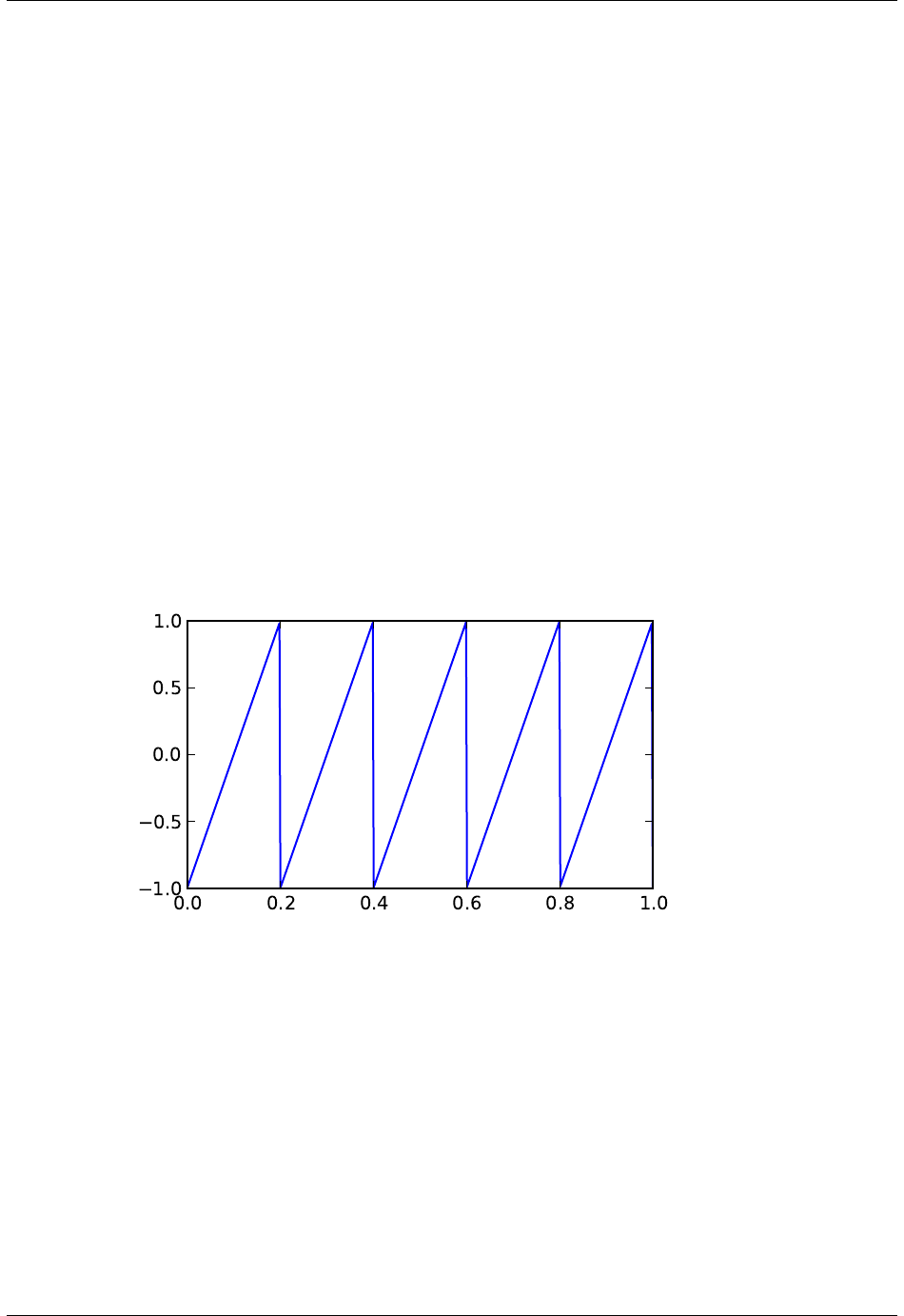
SciPy Reference Guide, Release 0.13.0
The sawtooth waveform has a period 2*pi, rises from -1 to 1 on the interval 0 to width*2*pi, then drops
from 1 to -1 on the interval width*2*pi to 2*pi.width must be in the interval [0, 1].
Note that this is not band-limited. It produces an infinite number of harmonics, which are aliased back and forth
across the frequency spectrum.
Parameters t: array_like
Time.
width : array_like, optional
Width of the rising ramp as a proportion of the total cycle. Default is 1,
producing a rising ramp, while 0 produces a falling ramp. t= 0.5 produces
a triangle wave. If an array, causes wave shape to change over time, and
must be the same length as t.
Returns y: ndarray
Output array containing the sawtooth waveform.
Examples
A 5 Hz waveform sampled at 500 Hz for 1 second:
>>> from scipy import signal
>>> import matplotlib.pyplot as plt
>>> t=np.linspace(0,1,500)
>>> plt.plot(t, signal.sawtooth(2*np.pi *5*t))
scipy.signal.square(t,duty=0.5)
Return a periodic square-wave waveform.
The square wave has a period 2*pi, has value +1 from 0 to 2*pi*duty and -1 from 2*pi*duty to 2*pi.
duty must be in the interval [0,1].
Note that this is not band-limited. It produces an infinite number of harmonics, which are aliased back and forth
across the frequency spectrum.
Parameters t: array_like
The input time array.
duty : array_like, optional
Duty cycle. Default is 0.5 (50% duty cycle). If an array, causes wave shape
to change over time, and must be the same length as t.
Returns y: ndarray
648 Chapter 5. Reference
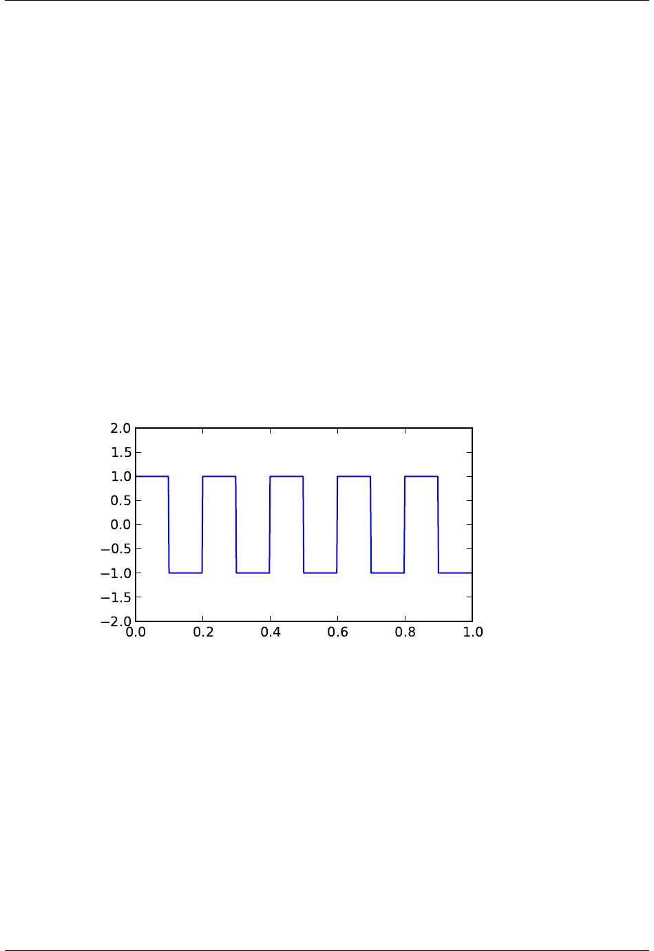
SciPy Reference Guide, Release 0.13.0
Output array containing the square waveform.
Examples
A 5 Hz waveform sampled at 500 Hz for 1 second:
>>> from scipy import signal
>>> import matplotlib.pyplot as plt
>>> t=np.linspace(0,1,500, endpoint=False)
>>> plt.plot(t, signal.square(2*np.pi *5*t))
>>> plt.ylim(-2,2)
A pulse-width modulated sine wave:
>>> plt.figure()
>>> sig =np.sin(2*np.pi *t)
>>> pwm =signal.square(2*np.pi *30 *t, duty=(sig +1)/2)
>>> plt.subplot(2,1,1)
>>> plt.plot(t, sig)
>>> plt.subplot(2,1,2)
>>> plt.plot(t, pwm)
>>> plt.ylim(-1.5,1.5)
5.22. Signal processing (scipy.signal) 649
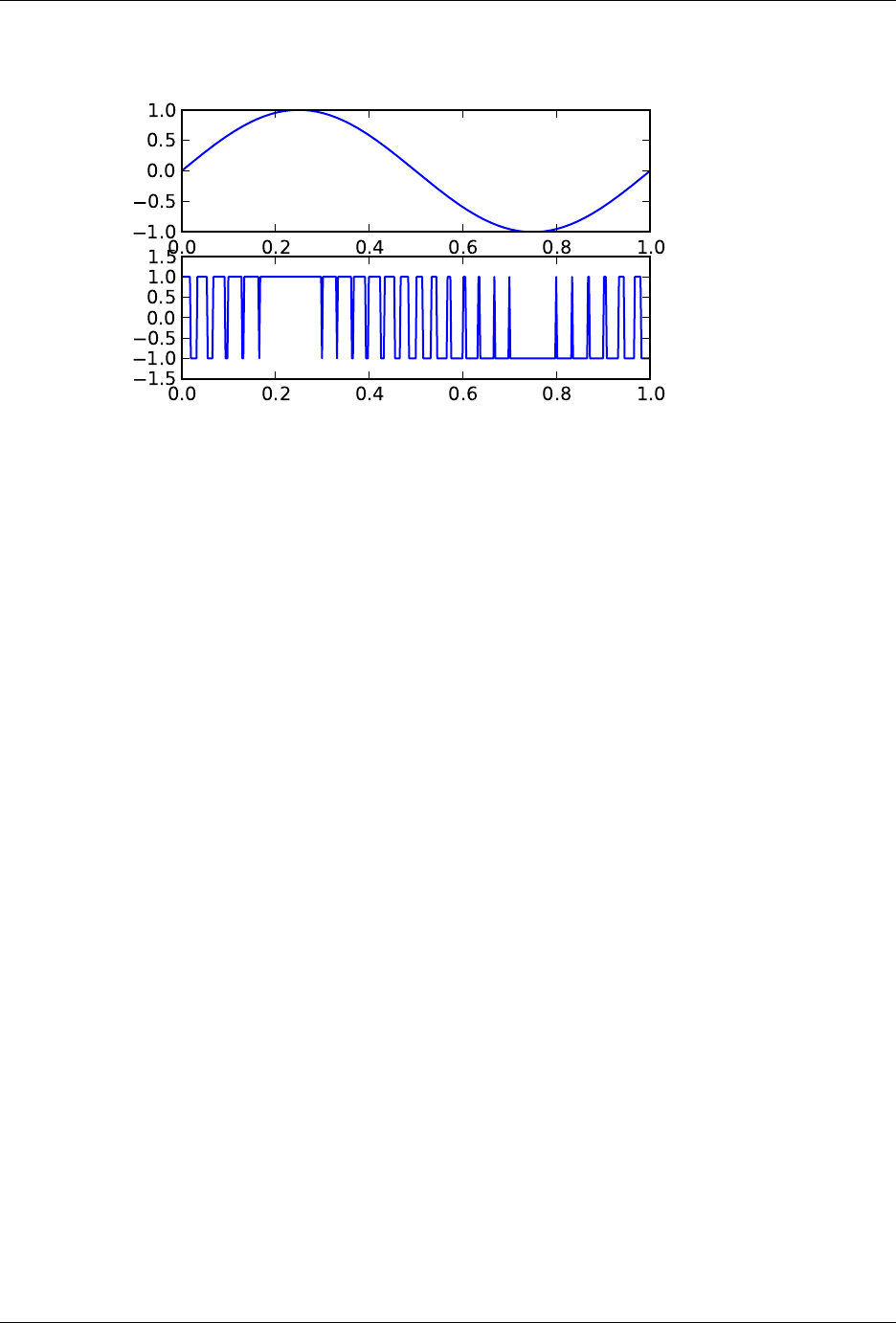
SciPy Reference Guide, Release 0.13.0
scipy.signal.sweep_poly(t,poly,phi=0)
Frequency-swept cosine generator, with a time-dependent frequency.
This function generates a sinusoidal function whose instantaneous frequency varies with time. The frequency at
time tis given by the polynomial poly.
Parameters t: ndarray
Times at which to evaluate the waveform.
poly : 1-D array-like or instance of numpy.poly1d
The desired frequency expressed as a polynomial. If poly is a list or ndarray
of length n, then the elements of poly are the coefficients of the polynomial,
and the instantaneous frequency is
f(t) = poly[0]*t**(n-1) +
poly[1]*t**(n-2) + ... + poly[n-1]
If poly is an instance of numpy.poly1d, then the instantaneous frequency is
f(t) = poly(t)
phi : float, optional
Phase offset, in degrees, Default: 0.
Returns sweep_poly : ndarray
A numpy array containing the signal evaluated at twith the requested time-
varying frequency. More precisely, the function returns cos(phase +
(pi/180)*phi), where phase is the integral (from 0 to t) of 2*pi
*f(t);f(t) is defined above.
See Also
chirp
Notes
New in version 0.8.0. If poly is a list or ndarray of length n, then the elements of poly are the coefficients of the
polynomial, and the instantaneous frequency is:
f(t) = poly[0]*t**(n-1) + poly[1]*t**(n-2) + ... + poly[n-1]
If poly is an instance of numpy.poly1d, then the instantaneous frequency is:
f(t) = poly(t)
Finally, the output sis:
650 Chapter 5. Reference

SciPy Reference Guide, Release 0.13.0
cos(phase + (pi/180)*phi)
where phase is the integral from 0 to tof 2*pi *f(t),f(t) as defined above.
5.22.10 Window functions
get_window(window, Nx[, fftbins]) Return a window.
barthann(M[, sym]) Return a modified Bartlett-Hann window.
bartlett(M[, sym]) Return a Bartlett window.
blackman(M[, sym]) Return a Blackman window.
blackmanharris(M[, sym]) Return a minimum 4-term Blackman-Harris window.
bohman(M[, sym]) Return a Bohman window.
boxcar(M[, sym]) Return a boxcar or rectangular window.
chebwin(M, at[, sym]) Return a Dolph-Chebyshev window.
cosine(M[, sym]) Return a window with a simple cosine shape.
flattop(M[, sym]) Return a flat top window.
gaussian(M, std[, sym]) Return a Gaussian window.
general_gaussian(M, p, sig[, sym]) Return a window with a generalized Gaussian shape.
hamming(M[, sym]) Return a Hamming window.
hann(M[, sym]) Return a Hann window.
kaiser(M, beta[, sym]) Return a Kaiser window.
nuttall(M[, sym]) Return a minimum 4-term Blackman-Harris window according to Nuttall.
parzen(M[, sym]) Return a Parzen window.
slepian(M, width[, sym]) Return a digital Slepian (DPSS) window.
triang(M[, sym]) Return a triangular window.
scipy.signal.get_window(window,Nx,fftbins=True)
Return a window.
Parameters window : string, float, or tuple
The type of window to create. See below for more details.
Nx : int
The number of samples in the window.
fftbins : bool, optional
If True, create a “periodic” window ready to use with ifftshift and be multi-
plied by the result of an fft (SEE ALSO fftfreq).
Returns get_window : ndarray
Returns a window of length Nx and type window
Notes
Window types:
boxcar, triang, blackman, hamming, hann, bartlett, flattop, parzen, bohman, blackmanharris, nuttall,
barthann, kaiser (needs beta), gaussian (needs std), general_gaussian (needs power, width), slepian (needs
width), chebwin (needs attenuation)
If the window requires no parameters, then window can be a string.
If the window requires parameters, then window must be a tuple with the first argument the string name of the
window, and the next arguments the needed parameters.
If window is a floating point number, it is interpreted as the beta parameter of the kaiser window.
Each of the window types listed above is also the name of a function that can be called directly to create a
window of that type.
5.22. Signal processing (scipy.signal) 651

SciPy Reference Guide, Release 0.13.0
Examples
>>> from scipy import signal
>>> signal.get_window(’triang’,7)
array([ 0.25, 0.5 , 0.75, 1. , 0.75, 0.5 , 0.25])
>>> signal.get_window((’kaiser’,4.0), 9)
array([ 0.08848053, 0.32578323, 0.63343178, 0.89640418, 1. ,
0.89640418, 0.63343178, 0.32578323, 0.08848053])
>>> signal.get_window(4.0,9)
array([ 0.08848053, 0.32578323, 0.63343178, 0.89640418, 1. ,
0.89640418, 0.63343178, 0.32578323, 0.08848053])
scipy.signal.barthann(M,sym=True)
Return a modified Bartlett-Hann window.
Parameters M: int
Number of points in the output window. If zero or less, an empty array is
returned.
sym : bool, optional
When True (default), generates a symmetric window, for use in filter design.
When False, generates a periodic window, for use in spectral analysis.
Returns w: ndarray
The window, with the maximum value normalized to 1 (though the value 1
does not appear if the number of samples is even and sym is True).
Examples
Plot the window and its frequency response:
>>> from scipy import signal
>>> from scipy.fftpack import fft, fftshift
>>> import matplotlib.pyplot as plt
>>> window =signal.barthann(51)
>>> plt.plot(window)
>>> plt.title("Bartlett-Hann window")
>>> plt.ylabel("Amplitude")
>>> plt.xlabel("Sample")
>>> plt.figure()
>>> A=fft(window, 2048)/(len(window)/2.0)
>>> freq =np.linspace(-0.5,0.5,len(A))
>>> response =20 *np.log10(np.abs(fftshift(A /abs(A).max())))
>>> plt.plot(freq, response)
>>> plt.axis([-0.5,0.5,-120,0])
>>> plt.title("Frequency response of the Bartlett-Hann window")
>>> plt.ylabel("Normalized magnitude [dB]")
>>> plt.xlabel("Normalized frequency [cycles per sample]")
652 Chapter 5. Reference
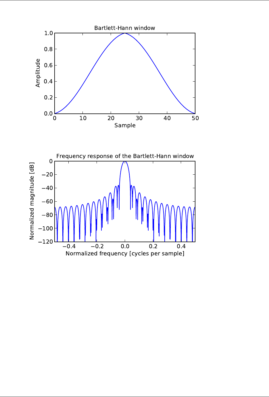
SciPy Reference Guide, Release 0.13.0
scipy.signal.bartlett(M,sym=True)
Return a Bartlett window.
The Bartlett window is very similar to a triangular window, except that the end points are at zero. It is often
used in signal processing for tapering a signal, without generating too much ripple in the frequency domain.
Parameters M: int
Number of points in the output window. If zero or less, an empty array is
returned.
sym : bool, optional
When True (default), generates a symmetric window, for use in filter design.
When False, generates a periodic window, for use in spectral analysis.
Returns w: ndarray
The triangular window, with the maximum value normalized to 1 (though
the value 1 does not appear if the number of samples is even and sym is
True), with the first and last samples equal to zero.
5.22. Signal processing (scipy.signal) 653

SciPy Reference Guide, Release 0.13.0
Notes
The Bartlett window is defined as
w(n) = 2
M−1M−1
2−
n−M−1
2
Most references to the Bartlett window come from the signal processing literature, where it is used as one of
many windowing functions for smoothing values. Note that convolution with this window produces linear in-
terpolation. It is also known as an apodization (which means”removing the foot”, i.e. smoothing discontinuities
at the beginning and end of the sampled signal) or tapering function. The fourier transform of the Bartlett is the
product of two sinc functions. Note the excellent discussion in Kanasewich.
References
[R104],[R105],[R106],[R107],[R108]
Examples
Plot the window and its frequency response:
>>> from scipy import signal
>>> from scipy.fftpack import fft, fftshift
>>> import matplotlib.pyplot as plt
>>> window =signal.bartlett(51)
>>> plt.plot(window)
>>> plt.title("Bartlett window")
>>> plt.ylabel("Amplitude")
>>> plt.xlabel("Sample")
>>> plt.figure()
>>> A=fft(window, 2048)/(len(window)/2.0)
>>> freq =np.linspace(-0.5,0.5,len(A))
>>> response =20 *np.log10(np.abs(fftshift(A /abs(A).max())))
>>> plt.plot(freq, response)
>>> plt.axis([-0.5,0.5,-120,0])
>>> plt.title("Frequency response of the Bartlett window")
>>> plt.ylabel("Normalized magnitude [dB]")
>>> plt.xlabel("Normalized frequency [cycles per sample]")
654 Chapter 5. Reference
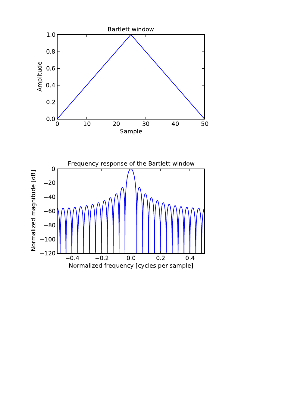
SciPy Reference Guide, Release 0.13.0
scipy.signal.blackman(M,sym=True)
Return a Blackman window.
The Blackman window is a taper formed by using the the first three terms of a summation of cosines. It was
designed to have close to the minimal leakage possible. It is close to optimal, only slightly worse than a Kaiser
window.
Parameters M: int
Number of points in the output window. If zero or less, an empty array is
returned.
sym : bool, optional
When True (default), generates a symmetric window, for use in filter design.
When False, generates a periodic window, for use in spectral analysis.
Returns w: ndarray
The window, with the maximum value normalized to 1 (though the value 1
does not appear if the number of samples is even and sym is True).
5.22. Signal processing (scipy.signal) 655

SciPy Reference Guide, Release 0.13.0
Notes
The Blackman window is defined as
w(n)=0.42 −0.5 cos(2πn/M)+0.08 cos(4πn/M)
Most references to the Blackman window come from the signal processing literature, where it is used as one of
many windowing functions for smoothing values. It is also known as an apodization (which means “removing
the foot”, i.e. smoothing discontinuities at the beginning and end of the sampled signal) or tapering function. It
is known as a “near optimal” tapering function, almost as good (by some measures) as the Kaiser window.
References
[R109],[R110]
Examples
Plot the window and its frequency response:
>>> from scipy import signal
>>> from scipy.fftpack import fft, fftshift
>>> import matplotlib.pyplot as plt
>>> window =signal.blackman(51)
>>> plt.plot(window)
>>> plt.title("Blackman window")
>>> plt.ylabel("Amplitude")
>>> plt.xlabel("Sample")
>>> plt.figure()
>>> A=fft(window, 2048)/(len(window)/2.0)
>>> freq =np.linspace(-0.5,0.5,len(A))
>>> response =20 *np.log10(np.abs(fftshift(A /abs(A).max())))
>>> plt.plot(freq, response)
>>> plt.axis([-0.5,0.5,-120,0])
>>> plt.title("Frequency response of the Blackman window")
>>> plt.ylabel("Normalized magnitude [dB]")
>>> plt.xlabel("Normalized frequency [cycles per sample]")
656 Chapter 5. Reference
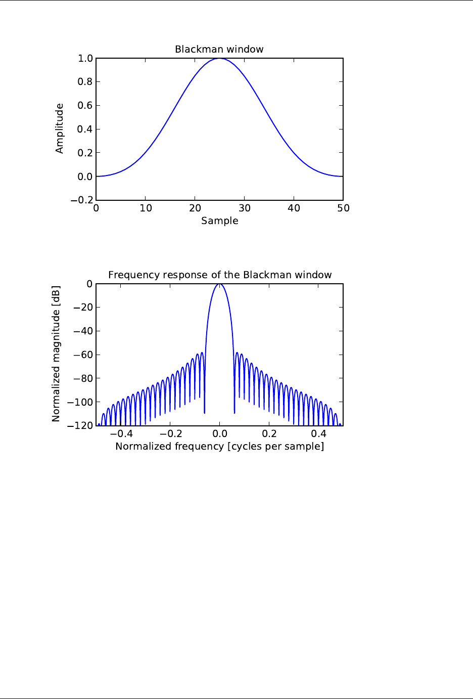
SciPy Reference Guide, Release 0.13.0
scipy.signal.blackmanharris(M,sym=True)
Return a minimum 4-term Blackman-Harris window.
Parameters M: int
Number of points in the output window. If zero or less, an empty array is
returned.
sym : bool, optional
When True (default), generates a symmetric window, for use in filter design.
When False, generates a periodic window, for use in spectral analysis.
Returns w: ndarray
The window, with the maximum value normalized to 1 (though the value 1
does not appear if the number of samples is even and sym is True).
Examples
Plot the window and its frequency response:
5.22. Signal processing (scipy.signal) 657
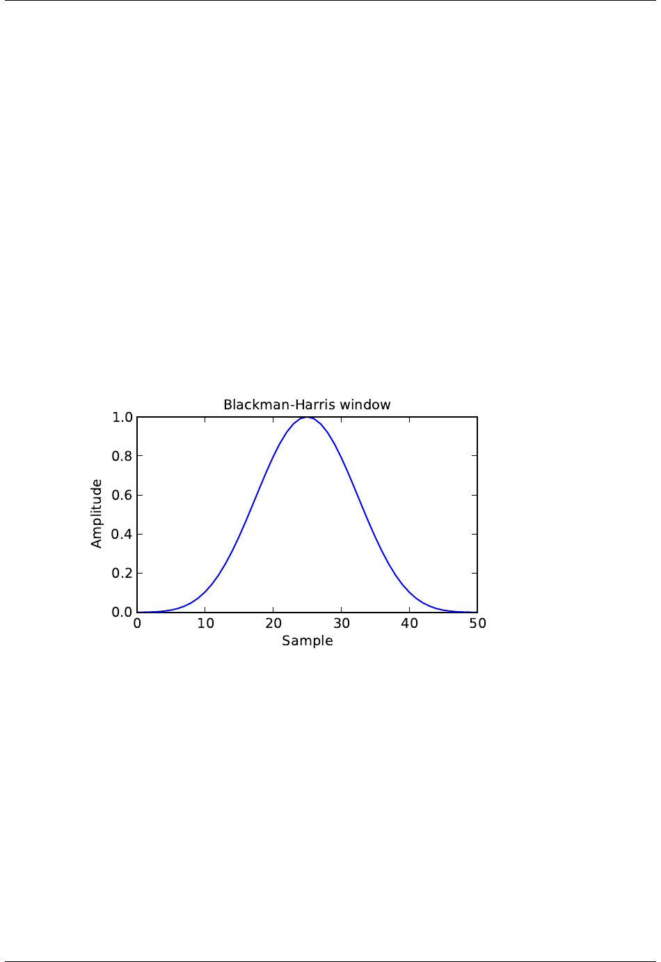
SciPy Reference Guide, Release 0.13.0
>>> from scipy import signal
>>> from scipy.fftpack import fft, fftshift
>>> import matplotlib.pyplot as plt
>>> window =signal.blackmanharris(51)
>>> plt.plot(window)
>>> plt.title("Blackman-Harris window")
>>> plt.ylabel("Amplitude")
>>> plt.xlabel("Sample")
>>> plt.figure()
>>> A=fft(window, 2048)/(len(window)/2.0)
>>> freq =np.linspace(-0.5,0.5,len(A))
>>> response =20 *np.log10(np.abs(fftshift(A /abs(A).max())))
>>> plt.plot(freq, response)
>>> plt.axis([-0.5,0.5,-120,0])
>>> plt.title("Frequency response of the Blackman-Harris window")
>>> plt.ylabel("Normalized magnitude [dB]")
>>> plt.xlabel("Normalized frequency [cycles per sample]")
658 Chapter 5. Reference

SciPy Reference Guide, Release 0.13.0
scipy.signal.bohman(M,sym=True)
Return a Bohman window.
Parameters M: int
Number of points in the output window. If zero or less, an empty array is
returned.
sym : bool, optional
When True (default), generates a symmetric window, for use in filter design.
When False, generates a periodic window, for use in spectral analysis.
Returns w: ndarray
The window, with the maximum value normalized to 1 (though the value 1
does not appear if the number of samples is even and sym is True).
Examples
Plot the window and its frequency response:
>>> from scipy import signal
>>> from scipy.fftpack import fft, fftshift
>>> import matplotlib.pyplot as plt
>>> window =signal.bohman(51)
>>> plt.plot(window)
>>> plt.title("Bohman window")
>>> plt.ylabel("Amplitude")
>>> plt.xlabel("Sample")
>>> plt.figure()
>>> A=fft(window, 2048)/(len(window)/2.0)
>>> freq =np.linspace(-0.5,0.5,len(A))
>>> response =20 *np.log10(np.abs(fftshift(A /abs(A).max())))
>>> plt.plot(freq, response)
>>> plt.axis([-0.5,0.5,-120,0])
>>> plt.title("Frequency response of the Bohman window")
>>> plt.ylabel("Normalized magnitude [dB]")
>>> plt.xlabel("Normalized frequency [cycles per sample]")
5.22. Signal processing (scipy.signal) 659
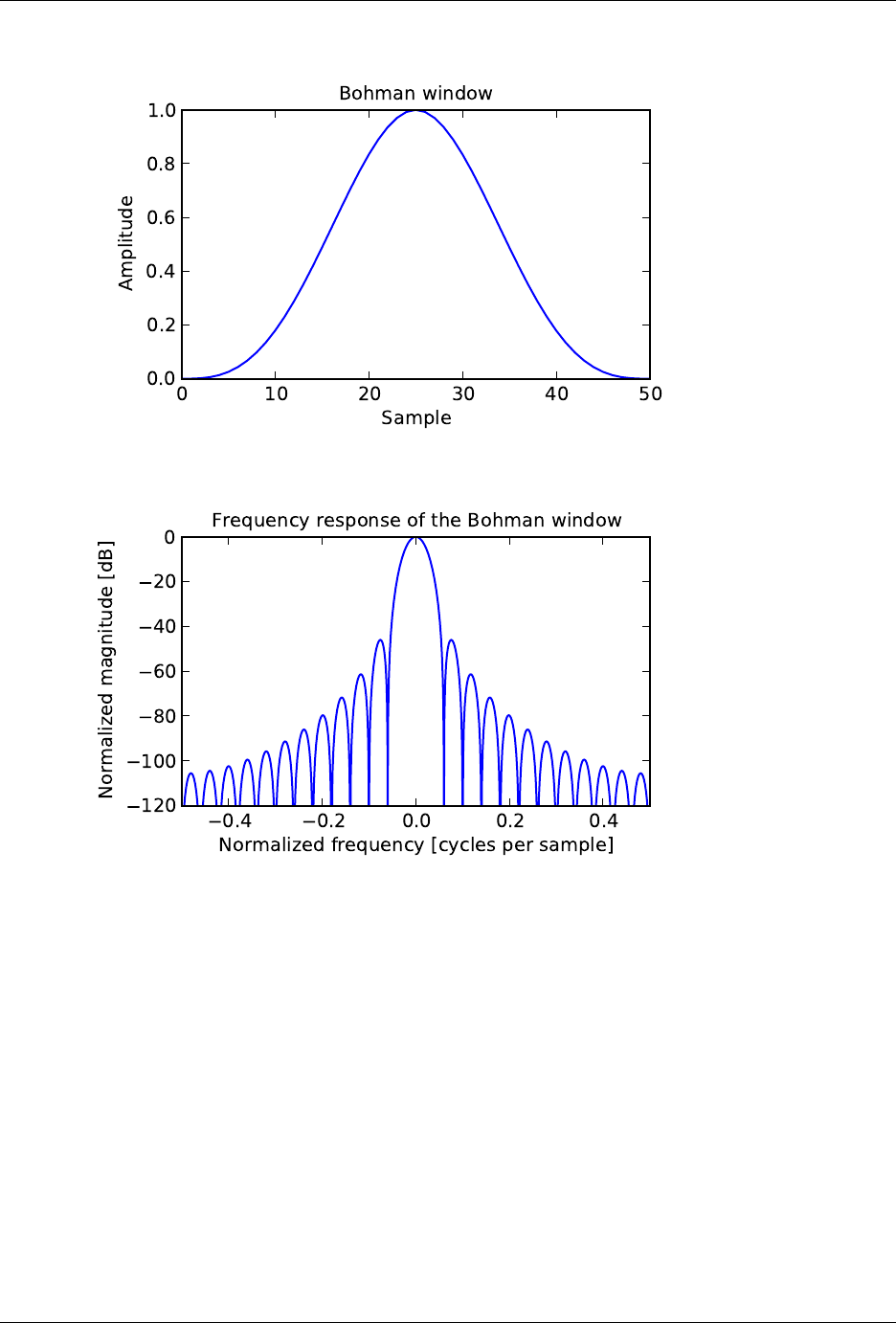
SciPy Reference Guide, Release 0.13.0
scipy.signal.boxcar(M,sym=True)
Return a boxcar or rectangular window.
Included for completeness, this is equivalent to no window at all.
Parameters M: int
Number of points in the output window. If zero or less, an empty array is
returned.
sym : bool, optional
Whether the window is symmetric. (Has no effect for boxcar.)
Returns w: ndarray
The window, with the maximum value normalized to 1
Examples
Plot the window and its frequency response:
660 Chapter 5. Reference
SciPy Reference Guide, Release 0.13.0
>>> from scipy import signal
>>> from scipy.fftpack import fft, fftshift
>>> import matplotlib.pyplot as plt
>>> window =signal.boxcar(51)
>>> plt.plot(window)
>>> plt.title("Boxcar window")
>>> plt.ylabel("Amplitude")
>>> plt.xlabel("Sample")
>>> plt.figure()
>>> A=fft(window, 2048)/(len(window)/2.0)
>>> freq =np.linspace(-0.5,0.5,len(A))
>>> response =20 *np.log10(np.abs(fftshift(A /abs(A).max())))
>>> plt.plot(freq, response)
>>> plt.axis([-0.5,0.5,-120,0])
>>> plt.title("Frequency response of the boxcar window")
>>> plt.ylabel("Normalized magnitude [dB]")
>>> plt.xlabel("Normalized frequency [cycles per sample]")
5.22. Signal processing (scipy.signal) 661
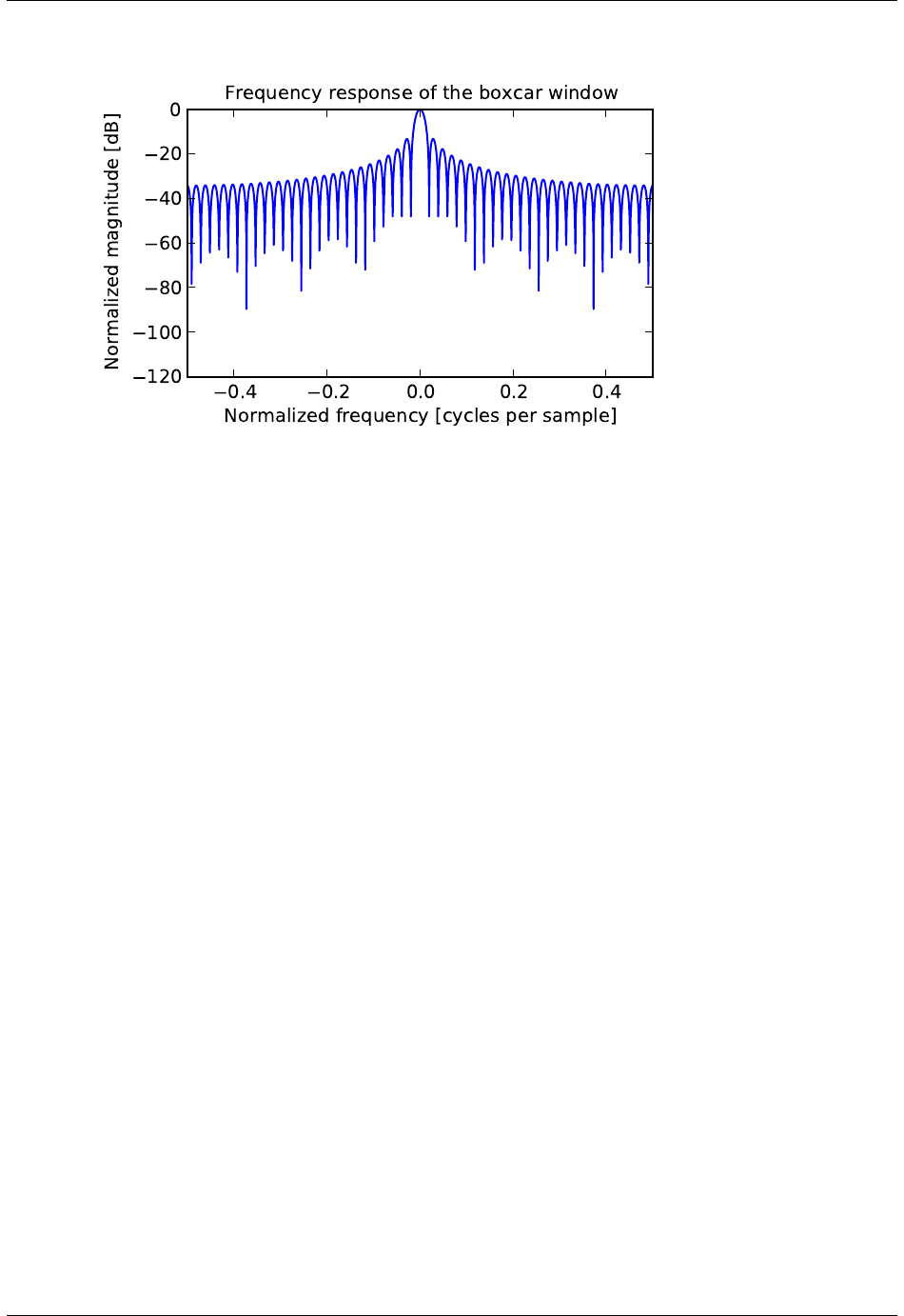
SciPy Reference Guide, Release 0.13.0
scipy.signal.chebwin(M,at,sym=True)
Return a Dolph-Chebyshev window.
Parameters M: int
Number of points in the output window. If zero or less, an empty array is
returned.
at : float
Attenuation (in dB).
sym : bool, optional
When True (default), generates a symmetric window, for use in filter design.
When False, generates a periodic window, for use in spectral analysis.
Returns w: ndarray
The window, with the maximum value always normalized to 1
Examples
Plot the window and its frequency response:
>>> from scipy import signal
>>> from scipy.fftpack import fft, fftshift
>>> import matplotlib.pyplot as plt
>>> window =signal.chebwin(51, at=100)
>>> plt.plot(window)
>>> plt.title("Dolph-Chebyshev window (100 dB)")
>>> plt.ylabel("Amplitude")
>>> plt.xlabel("Sample")
>>> plt.figure()
>>> A=fft(window, 2048)/(len(window)/2.0)
>>> freq =np.linspace(-0.5,0.5,len(A))
>>> response =20 *np.log10(np.abs(fftshift(A /abs(A).max())))
>>> plt.plot(freq, response)
>>> plt.axis([-0.5,0.5,-120,0])
>>> plt.title("Frequency response of the Dolph-Chebyshev window (100 dB)")
>>> plt.ylabel("Normalized magnitude [dB]")
>>> plt.xlabel("Normalized frequency [cycles per sample]")
662 Chapter 5. Reference
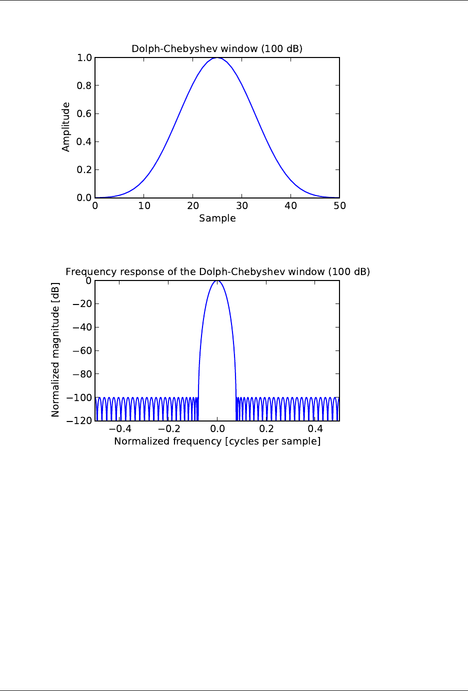
SciPy Reference Guide, Release 0.13.0
scipy.signal.cosine(M,sym=True)
Return a window with a simple cosine shape. New in version 0.13.0.
Parameters M: int
Number of points in the output window. If zero or less, an empty array is
returned.
sym : bool, optional
When True, generates a symmetric window, for use in filter design. When
False, generates a periodic window, for use in spectral analysis.
Returns w: ndarray
The window, with the maximum value normalized to 1.
scipy.signal.flattop(M,sym=True)
Return a flat top window.
Parameters M: int
Number of points in the output window. If zero or less, an empty array is
returned.
5.22. Signal processing (scipy.signal) 663
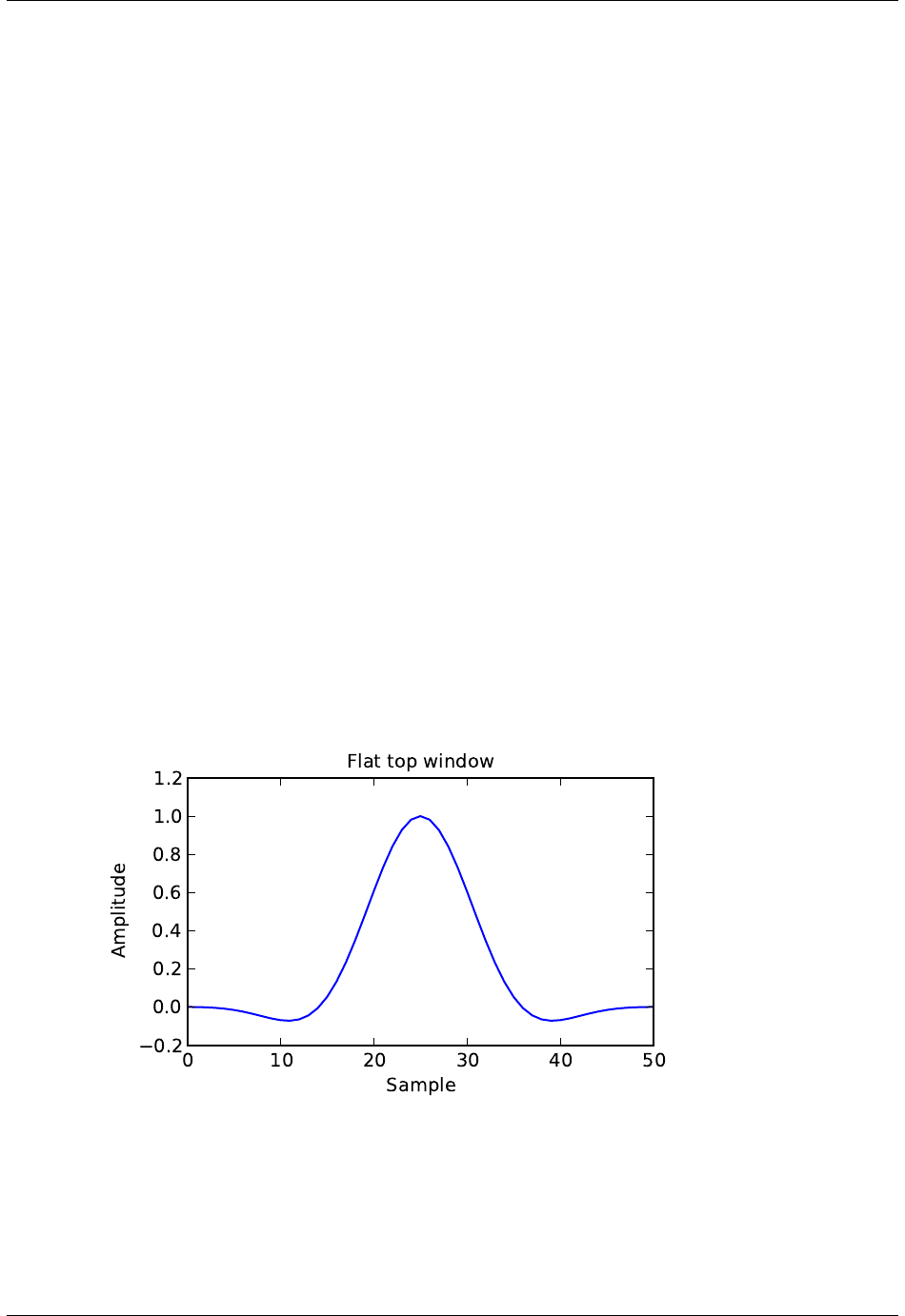
SciPy Reference Guide, Release 0.13.0
sym : bool, optional
When True (default), generates a symmetric window, for use in filter design.
When False, generates a periodic window, for use in spectral analysis.
Returns w: ndarray
The window, with the maximum value normalized to 1 (though the value 1
does not appear if the number of samples is even and sym is True).
Examples
Plot the window and its frequency response:
>>> from scipy import signal
>>> from scipy.fftpack import fft, fftshift
>>> import matplotlib.pyplot as plt
>>> window =signal.flattop(51)
>>> plt.plot(window)
>>> plt.title("Flat top window")
>>> plt.ylabel("Amplitude")
>>> plt.xlabel("Sample")
>>> plt.figure()
>>> A=fft(window, 2048)/(len(window)/2.0)
>>> freq =np.linspace(-0.5,0.5,len(A))
>>> response =20 *np.log10(np.abs(fftshift(A /abs(A).max())))
>>> plt.plot(freq, response)
>>> plt.axis([-0.5,0.5,-120,0])
>>> plt.title("Frequency response of the flat top window")
>>> plt.ylabel("Normalized magnitude [dB]")
>>> plt.xlabel("Normalized frequency [cycles per sample]")
664 Chapter 5. Reference
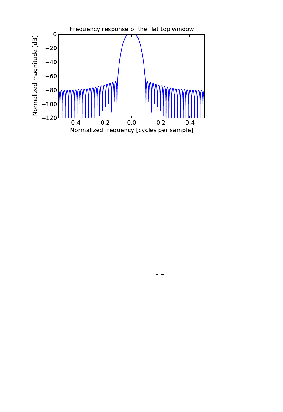
SciPy Reference Guide, Release 0.13.0
scipy.signal.gaussian(M,std,sym=True)
Return a Gaussian window.
Parameters M: int
Number of points in the output window. If zero or less, an empty array is
returned.
std : float
The standard deviation, sigma.
sym : bool, optional
When True (default), generates a symmetric window, for use in filter design.
When False, generates a periodic window, for use in spectral analysis.
Returns w: ndarray
The window, with the maximum value normalized to 1 (though the value 1
does not appear if the number of samples is even and sym is True).
Notes
The Gaussian window is defined as
w(n) = e−1
2(n
σ)2
Examples
Plot the window and its frequency response:
>>> from scipy import signal
>>> from scipy.fftpack import fft, fftshift
>>> import matplotlib.pyplot as plt
>>> window =signal.gaussian(51, std=7)
>>> plt.plot(window)
>>> plt.title(r"Gaussian window ($\sigma$=7)")
>>> plt.ylabel("Amplitude")
>>> plt.xlabel("Sample")
5.22. Signal processing (scipy.signal) 665
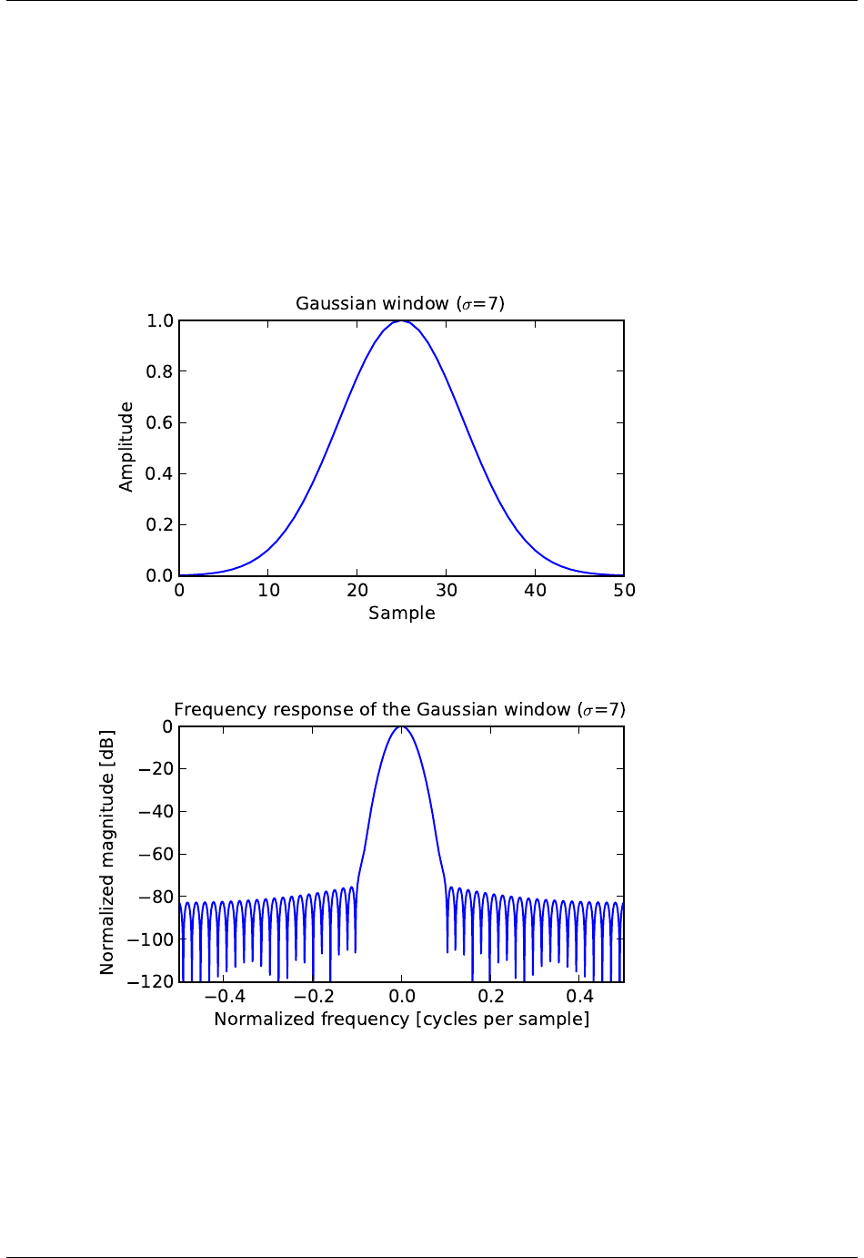
SciPy Reference Guide, Release 0.13.0
>>> plt.figure()
>>> A=fft(window, 2048)/(len(window)/2.0)
>>> freq =np.linspace(-0.5,0.5,len(A))
>>> response =20 *np.log10(np.abs(fftshift(A /abs(A).max())))
>>> plt.plot(freq, response)
>>> plt.axis([-0.5,0.5,-120,0])
>>> plt.title(r"Frequency response of the Gaussian window ($\sigma$=7)")
>>> plt.ylabel("Normalized magnitude [dB]")
>>> plt.xlabel("Normalized frequency [cycles per sample]")
scipy.signal.general_gaussian(M,p,sig,sym=True)
Return a window with a generalized Gaussian shape.
Parameters M: int
Number of points in the output window. If zero or less, an empty array is
returned.
p: float
666 Chapter 5. Reference

SciPy Reference Guide, Release 0.13.0
Shape parameter. p = 1 is identical to gaussian, p = 0.5 is the same shape
as the Laplace distribution.
sig : float
The standard deviation, sigma.
sym : bool, optional
When True (default), generates a symmetric window, for use in filter design.
When False, generates a periodic window, for use in spectral analysis.
Returns w: ndarray
The window, with the maximum value normalized to 1 (though the value 1
does not appear if the number of samples is even and sym is True).
Notes
The generalized Gaussian window is defined as
w(n) = e−1
2|n
σ|2p
the half-power point is at
(2 log(2))1/(2p)σ
Examples
Plot the window and its frequency response:
>>> from scipy import signal
>>> from scipy.fftpack import fft, fftshift
>>> import matplotlib.pyplot as plt
>>> window =signal.general_gaussian(51, p=1.5, sig=7)
>>> plt.plot(window)
>>> plt.title(r"Generalized Gaussian window (p=1.5, $\sigma$=7)")
>>> plt.ylabel("Amplitude")
>>> plt.xlabel("Sample")
>>> plt.figure()
>>> A=fft(window, 2048)/(len(window)/2.0)
>>> freq =np.linspace(-0.5,0.5,len(A))
>>> response =20 *np.log10(np.abs(fftshift(A /abs(A).max())))
>>> plt.plot(freq, response)
>>> plt.axis([-0.5,0.5,-120,0])
>>> plt.title(r"Freq. resp. of the gen. Gaussian window (p=1.5, $\sigma$=7)")
>>> plt.ylabel("Normalized magnitude [dB]")
>>> plt.xlabel("Normalized frequency [cycles per sample]")
5.22. Signal processing (scipy.signal) 667
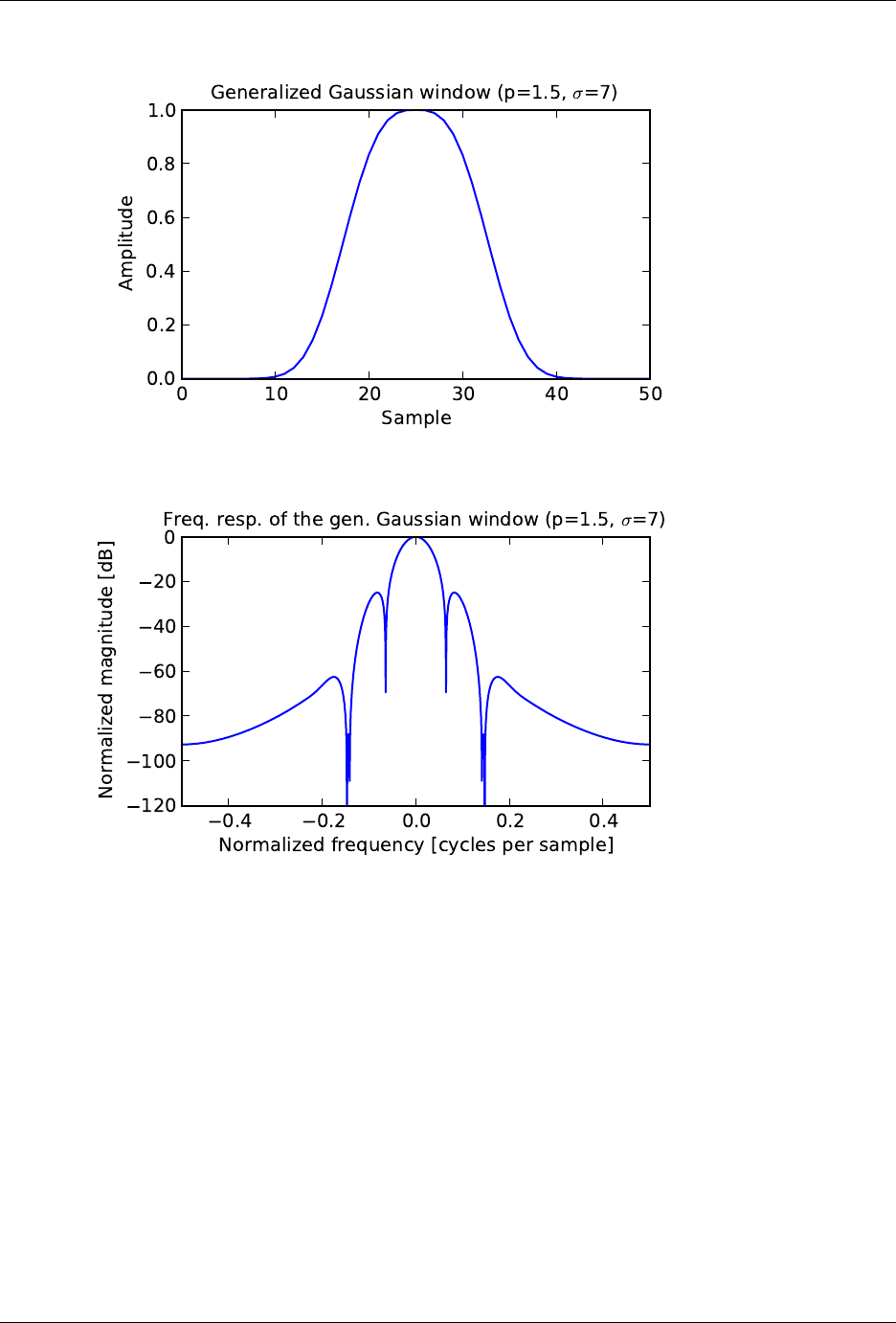
SciPy Reference Guide, Release 0.13.0
scipy.signal.hamming(M,sym=True)
Return a Hamming window.
The Hamming window is a taper formed by using a raised cosine with non-zero endpoints, optimized to mini-
mize the nearest side lobe.
Parameters M: int
Number of points in the output window. If zero or less, an empty array is
returned.
sym : bool, optional
When True (default), generates a symmetric window, for use in filter design.
When False, generates a periodic window, for use in spectral analysis.
Returns w: ndarray
The window, with the maximum value normalized to 1 (though the value 1
does not appear if the number of samples is even and sym is True).
668 Chapter 5. Reference

SciPy Reference Guide, Release 0.13.0
Notes
The Hamming window is defined as
w(n)=0.54 −0.46 cos 2πn
M−10≤n≤M−1
The Hamming was named for R. W. Hamming, an associate of J. W. Tukey and is described in Blackman and
Tukey. It was recommended for smoothing the truncated autocovariance function in the time domain. Most
references to the Hamming window come from the signal processing literature, where it is used as one of many
windowing functions for smoothing values. It is also known as an apodization (which means “removing the
foot”, i.e. smoothing discontinuities at the beginning and end of the sampled signal) or tapering function.
References
[R117],[R118],[R119],[R120]
Examples
Plot the window and its frequency response:
>>> from scipy import signal
>>> from scipy.fftpack import fft, fftshift
>>> import matplotlib.pyplot as plt
>>> window =signal.hamming(51)
>>> plt.plot(window)
>>> plt.title("Hamming window")
>>> plt.ylabel("Amplitude")
>>> plt.xlabel("Sample")
>>> plt.figure()
>>> A=fft(window, 2048)/(len(window)/2.0)
>>> freq =np.linspace(-0.5,0.5,len(A))
>>> response =20 *np.log10(np.abs(fftshift(A /abs(A).max())))
>>> plt.plot(freq, response)
>>> plt.axis([-0.5,0.5,-120,0])
>>> plt.title("Frequency response of the Hamming window")
>>> plt.ylabel("Normalized magnitude [dB]")
>>> plt.xlabel("Normalized frequency [cycles per sample]")
5.22. Signal processing (scipy.signal) 669
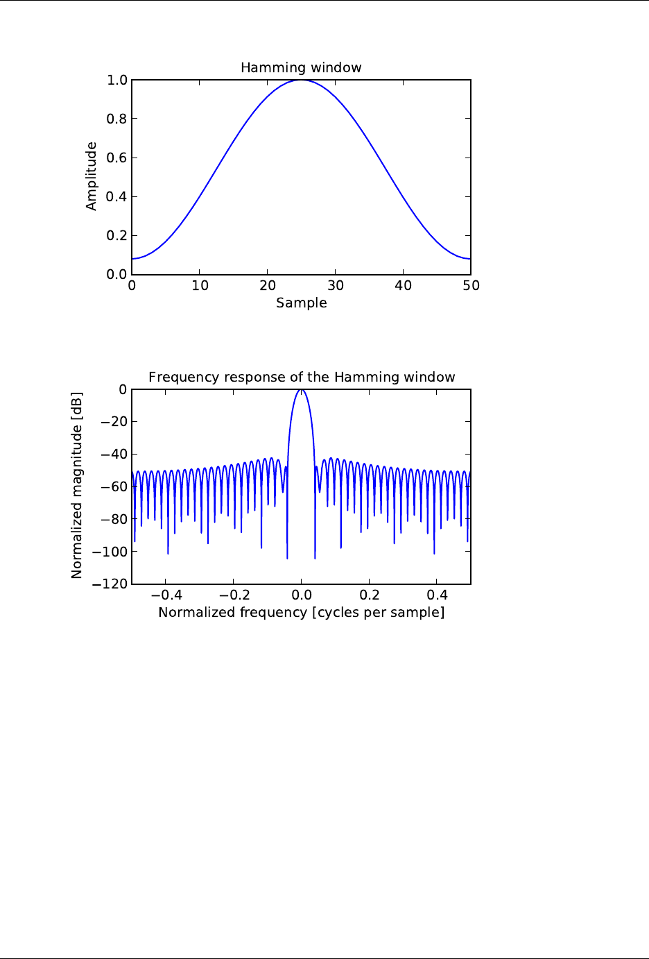
SciPy Reference Guide, Release 0.13.0
scipy.signal.hann(M,sym=True)
Return a Hann window.
The Hann window is a taper formed by using a raised cosine or sine-squared with ends that touch zero.
Parameters M: int
Number of points in the output window. If zero or less, an empty array is
returned.
sym : bool, optional
When True (default), generates a symmetric window, for use in filter design.
When False, generates a periodic window, for use in spectral analysis.
Returns w: ndarray
The window, with the maximum value normalized to 1 (though the value 1
does not appear if Mis even and sym is True).
670 Chapter 5. Reference

SciPy Reference Guide, Release 0.13.0
Notes
The Hann window is defined as
w(n)=0.5−0.5 cos 2πn
M−10≤n≤M−1
The window was named for Julius van Hann, an Austrian meterologist. It is also known as the Cosine Bell. It
is sometimes erroneously referred to as the “Hanning” window, from the use of “hann” as a verb in the original
paper and confusion with the very similar Hamming window.
Most references to the Hann window come from the signal processing literature, where it is used as one of many
windowing functions for smoothing values. It is also known as an apodization (which means “removing the
foot”, i.e. smoothing discontinuities at the beginning and end of the sampled signal) or tapering function.
References
[R121],[R122],[R123],[R124]
Examples
Plot the window and its frequency response:
>>> from scipy import signal
>>> from scipy.fftpack import fft, fftshift
>>> import matplotlib.pyplot as plt
>>> window =signal.hann(51)
>>> plt.plot(window)
>>> plt.title("Hann window")
>>> plt.ylabel("Amplitude")
>>> plt.xlabel("Sample")
>>> plt.figure()
>>> A=fft(window, 2048)/(len(window)/2.0)
>>> freq =np.linspace(-0.5,0.5,len(A))
>>> response =20 *np.log10(np.abs(fftshift(A /abs(A).max())))
>>> plt.plot(freq, response)
>>> plt.axis([-0.5,0.5,-120,0])
>>> plt.title("Frequency response of the Hann window")
>>> plt.ylabel("Normalized magnitude [dB]")
>>> plt.xlabel("Normalized frequency [cycles per sample]")
5.22. Signal processing (scipy.signal) 671
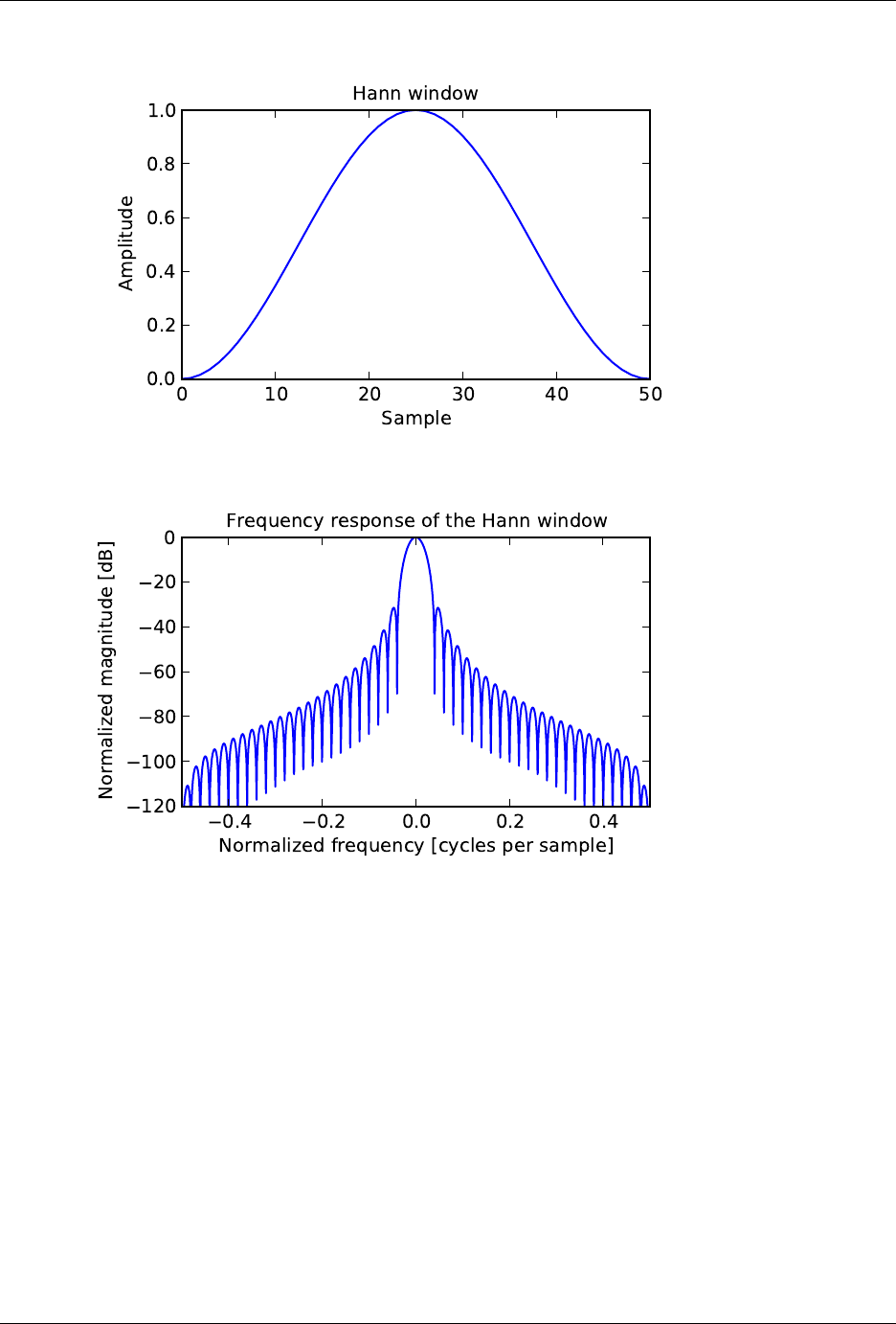
SciPy Reference Guide, Release 0.13.0
scipy.signal.kaiser(M,beta,sym=True)
Return a Kaiser window.
The Kaiser window is a taper formed by using a Bessel function.
Parameters M: int
Number of points in the output window. If zero or less, an empty array is
returned.
beta : float
Shape parameter, determines trade-off between main-lobe width and side
lobe level. As beta gets large, the window narrows.
sym : bool, optional
When True (default), generates a symmetric window, for use in filter design.
When False, generates a periodic window, for use in spectral analysis.
Returns w: ndarray
The window, with the maximum value normalized to 1 (though the value 1
does not appear if the number of samples is even and sym is True).
672 Chapter 5. Reference

SciPy Reference Guide, Release 0.13.0
Notes
The Kaiser window is defined as
w(n) = I0 βs1−4n2
(M−1)2!/I0(β)
with
−M−1
2≤n≤M−1
2,
where I0is the modified zeroth-order Bessel function.
The Kaiser was named for Jim Kaiser, who discovered a simple approximation to the DPSS window based on
Bessel functions. The Kaiser window is a very good approximation to the Digital Prolate Spheroidal Sequence,
or Slepian window, which is the transform which maximizes the energy in the main lobe of the window relative
to total energy.
The Kaiser can approximate many other windows by varying the beta parameter.
beta Window shape
0 Rectangular
5 Similar to a Hamming
6 Similar to a Hann
8.6 Similar to a Blackman
A beta value of 14 is probably a good starting point. Note that as beta gets large, the window narrows, and so
the number of samples needs to be large enough to sample the increasingly narrow spike, otherwise NaNs will
get returned.
Most references to the Kaiser window come from the signal processing literature, where it is used as one of
many windowing functions for smoothing values. It is also known as an apodization (which means “removing
the foot”, i.e. smoothing discontinuities at the beginning and end of the sampled signal) or tapering function.
References
[R126],[R127],[R128]
Examples
Plot the window and its frequency response:
>>> from scipy import signal
>>> from scipy.fftpack import fft, fftshift
>>> import matplotlib.pyplot as plt
>>> window =signal.kaiser(51, beta=14)
>>> plt.plot(window)
>>> plt.title(r"Kaiser window ($\beta$=14)")
>>> plt.ylabel("Amplitude")
>>> plt.xlabel("Sample")
>>> plt.figure()
>>> A=fft(window, 2048)/(len(window)/2.0)
>>> freq =np.linspace(-0.5,0.5,len(A))
5.22. Signal processing (scipy.signal) 673
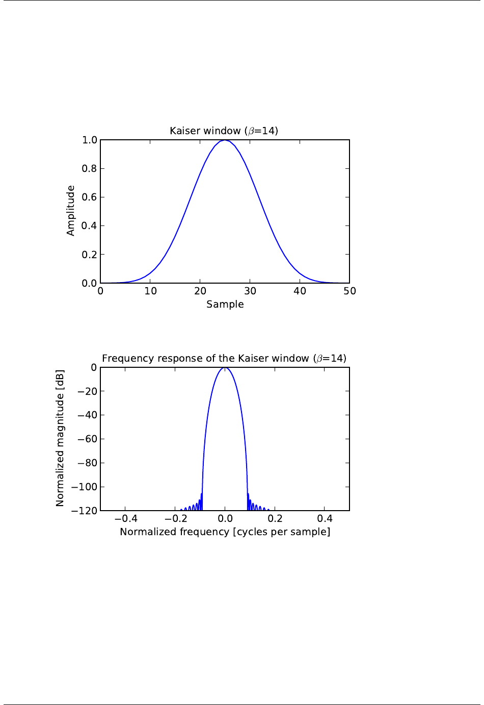
SciPy Reference Guide, Release 0.13.0
>>> response =20 *np.log10(np.abs(fftshift(A /abs(A).max())))
>>> plt.plot(freq, response)
>>> plt.axis([-0.5,0.5,-120,0])
>>> plt.title(r"Frequency response of the Kaiser window ($\beta$=14)")
>>> plt.ylabel("Normalized magnitude [dB]")
>>> plt.xlabel("Normalized frequency [cycles per sample]")
scipy.signal.nuttall(M,sym=True)
Return a minimum 4-term Blackman-Harris window according to Nuttall.
Parameters M: int
Number of points in the output window. If zero or less, an empty array is
returned.
sym : bool, optional
When True (default), generates a symmetric window, for use in filter design.
When False, generates a periodic window, for use in spectral analysis.
Returns w: ndarray
674 Chapter 5. Reference
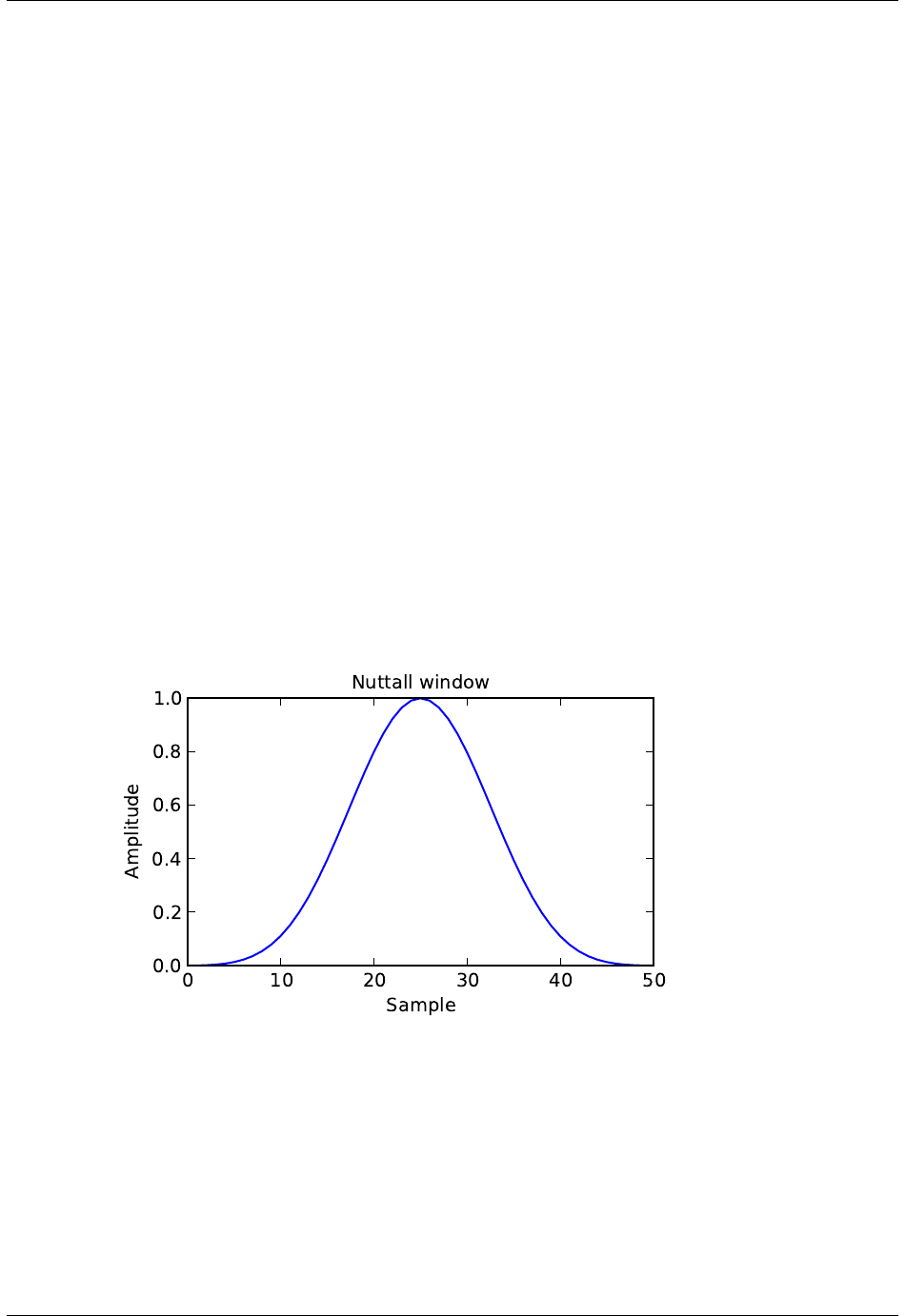
SciPy Reference Guide, Release 0.13.0
The window, with the maximum value normalized to 1 (though the value 1
does not appear if the number of samples is even and sym is True).
Examples
Plot the window and its frequency response:
>>> from scipy import signal
>>> from scipy.fftpack import fft, fftshift
>>> import matplotlib.pyplot as plt
>>> window =signal.nuttall(51)
>>> plt.plot(window)
>>> plt.title("Nuttall window")
>>> plt.ylabel("Amplitude")
>>> plt.xlabel("Sample")
>>> plt.figure()
>>> A=fft(window, 2048)/(len(window)/2.0)
>>> freq =np.linspace(-0.5,0.5,len(A))
>>> response =20 *np.log10(np.abs(fftshift(A /abs(A).max())))
>>> plt.plot(freq, response)
>>> plt.axis([-0.5,0.5,-120,0])
>>> plt.title("Frequency response of the Nuttall window")
>>> plt.ylabel("Normalized magnitude [dB]")
>>> plt.xlabel("Normalized frequency [cycles per sample]")
5.22. Signal processing (scipy.signal) 675
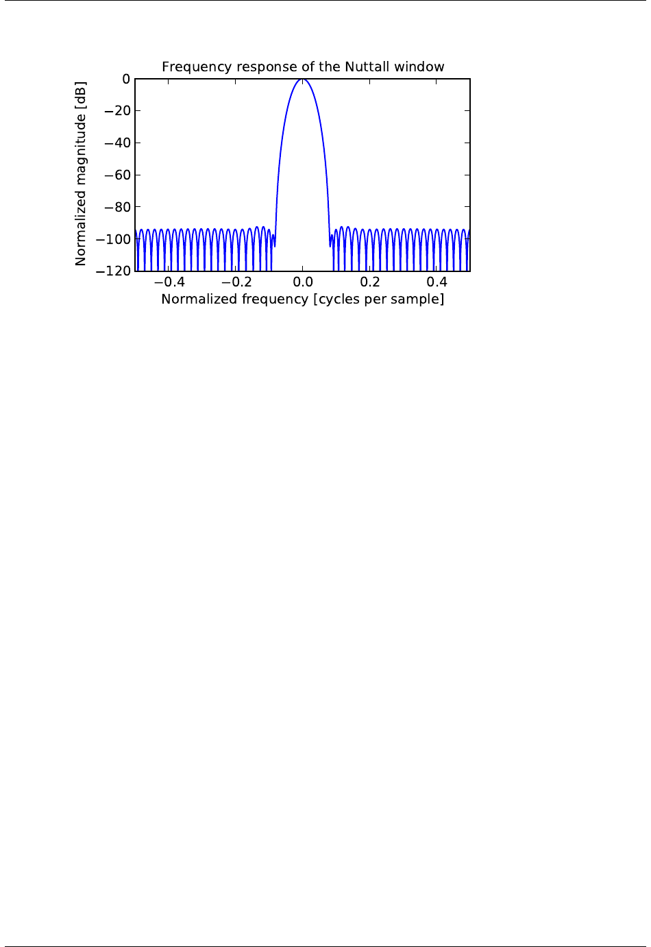
SciPy Reference Guide, Release 0.13.0
scipy.signal.parzen(M,sym=True)
Return a Parzen window.
Parameters M: int
Number of points in the output window. If zero or less, an empty array is
returned.
sym : bool, optional
When True (default), generates a symmetric window, for use in filter design.
When False, generates a periodic window, for use in spectral analysis.
Returns w: ndarray
The window, with the maximum value normalized to 1 (though the value 1
does not appear if the number of samples is even and sym is True).
Examples
Plot the window and its frequency response:
>>> from scipy import signal
>>> from scipy.fftpack import fft, fftshift
>>> import matplotlib.pyplot as plt
>>> window =signal.parzen(51)
>>> plt.plot(window)
>>> plt.title("Parzen window")
>>> plt.ylabel("Amplitude")
>>> plt.xlabel("Sample")
>>> plt.figure()
>>> A=fft(window, 2048)/(len(window)/2.0)
>>> freq =np.linspace(-0.5,0.5,len(A))
>>> response =20 *np.log10(np.abs(fftshift(A /abs(A).max())))
>>> plt.plot(freq, response)
>>> plt.axis([-0.5,0.5,-120,0])
>>> plt.title("Frequency response of the Parzen window")
>>> plt.ylabel("Normalized magnitude [dB]")
>>> plt.xlabel("Normalized frequency [cycles per sample]")
676 Chapter 5. Reference
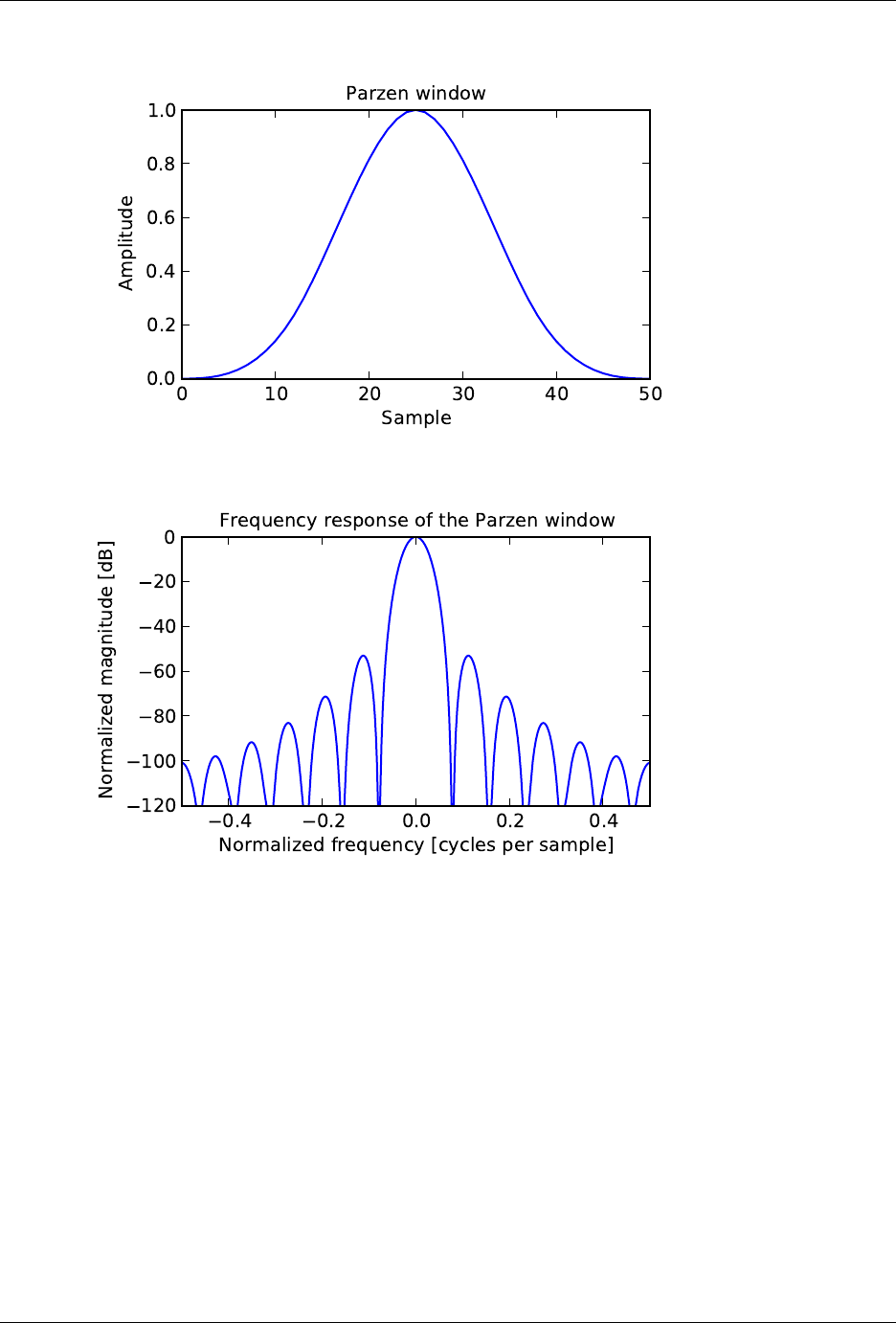
SciPy Reference Guide, Release 0.13.0
scipy.signal.slepian(M,width,sym=True)
Return a digital Slepian (DPSS) window.
Used to maximize the energy concentration in the main lobe. Also called the digital prolate spheroidal sequence
(DPSS).
Parameters M: int
Number of points in the output window. If zero or less, an empty array is
returned.
width : float
Bandwidth
sym : bool, optional
When True (default), generates a symmetric window, for use in filter design.
When False, generates a periodic window, for use in spectral analysis.
Returns w: ndarray
The window, with the maximum value always normalized to 1
5.22. Signal processing (scipy.signal) 677
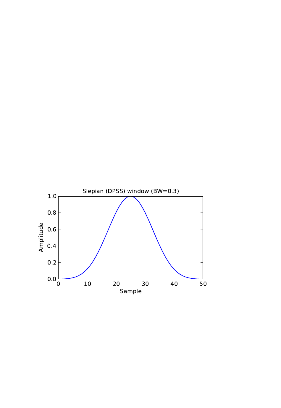
SciPy Reference Guide, Release 0.13.0
Examples
Plot the window and its frequency response:
>>> from scipy import signal
>>> from scipy.fftpack import fft, fftshift
>>> import matplotlib.pyplot as plt
>>> window =signal.slepian(51, width=0.3)
>>> plt.plot(window)
>>> plt.title("Slepian (DPSS) window (BW=0.3)")
>>> plt.ylabel("Amplitude")
>>> plt.xlabel("Sample")
>>> plt.figure()
>>> A=fft(window, 2048)/(len(window)/2.0)
>>> freq =np.linspace(-0.5,0.5,len(A))
>>> response =20 *np.log10(np.abs(fftshift(A /abs(A).max())))
>>> plt.plot(freq, response)
>>> plt.axis([-0.5,0.5,-120,0])
>>> plt.title("Frequency response of the Slepian window (BW=0.3)")
>>> plt.ylabel("Normalized magnitude [dB]")
>>> plt.xlabel("Normalized frequency [cycles per sample]")
678 Chapter 5. Reference
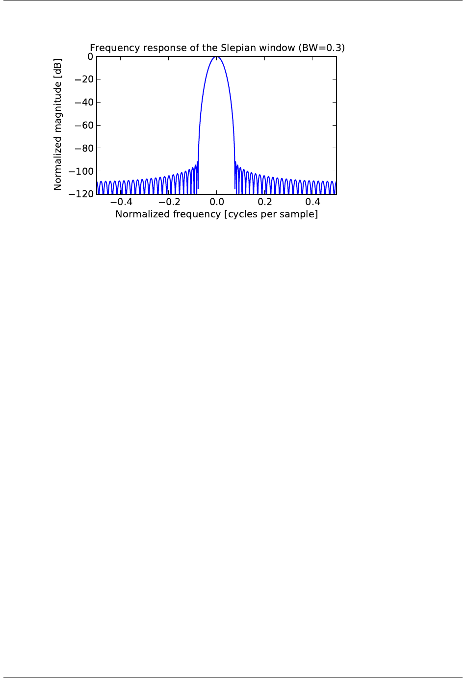
SciPy Reference Guide, Release 0.13.0
scipy.signal.triang(M,sym=True)
Return a triangular window.
Parameters M: int
Number of points in the output window. If zero or less, an empty array is
returned.
sym : bool, optional
When True (default), generates a symmetric window, for use in filter design.
When False, generates a periodic window, for use in spectral analysis.
Returns w: ndarray
The window, with the maximum value normalized to 1 (though the value 1
does not appear if the number of samples is even and sym is True).
Examples
Plot the window and its frequency response:
>>> from scipy import signal
>>> from scipy.fftpack import fft, fftshift
>>> import matplotlib.pyplot as plt
>>> window =signal.triang(51)
>>> plt.plot(window)
>>> plt.title("Triangular window")
>>> plt.ylabel("Amplitude")
>>> plt.xlabel("Sample")
>>> plt.figure()
>>> A=fft(window, 2048)/(len(window)/2.0)
>>> freq =np.linspace(-0.5,0.5,len(A))
>>> response =20 *np.log10(np.abs(fftshift(A /abs(A).max())))
>>> plt.plot(freq, response)
>>> plt.axis([-0.5,0.5,-120,0])
>>> plt.title("Frequency response of the triangular window")
>>> plt.ylabel("Normalized magnitude [dB]")
>>> plt.xlabel("Normalized frequency [cycles per sample]")
5.22. Signal processing (scipy.signal) 679
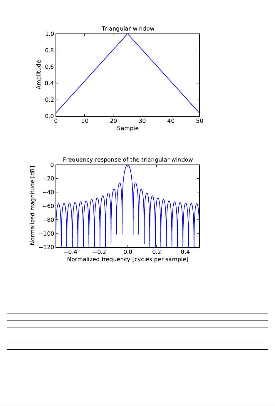
SciPy Reference Guide, Release 0.13.0
5.22.11 Wavelets
cascade(hk[, J]) Return (x, phi, psi) at dyadic points K/2**Jfrom filter coefficients.
daub(p) The coefficients for the FIR low-pass filter producing Daubechies wavelets.
morlet(M[, w, s, complete]) Complex Morlet wavelet.
qmf(hk) Return high-pass qmf filter from low-pass
ricker(points, a) Return a Ricker wavelet, also known as the “Mexican hat wavelet”.
cwt(data, wavelet, widths) Continuous wavelet transform.
scipy.signal.cascade(hk,J=7)
Return (x, phi, psi) at dyadic points K/2**Jfrom filter coefficients.
Parameters hk : array_like
Coefficients of low-pass filter.
680 Chapter 5. Reference

SciPy Reference Guide, Release 0.13.0
J: int, optional
Values will be computed at grid points K/2**J. Default is 7.
Returns x: ndarray
The dyadic points K/2**Jfor K=0...N *(2**J)-1 where
len(hk) = len(gk) = N+1.
phi : ndarray
The scaling function phi(x) at x:phi(x) = sum(hk *
phi(2x-k)), where k is from 0 to N.
psi : ndarray, optional
The wavelet function psi(x) at x:phi(x) = sum(gk *
phi(2x-k)), where k is from 0 to N. psi is only returned if gk is
not None.
Notes
The algorithm uses the vector cascade algorithm described by Strang and Nguyen in “Wavelets and Filter
Banks”. It builds a dictionary of values and slices for quick reuse. Then inserts vectors into final vector at
the end.
scipy.signal.daub(p)
The coefficients for the FIR low-pass filter producing Daubechies wavelets.
p>=1 gives the order of the zero at f=1/2. There are 2p filter coefficients.
Parameters p: int
Order of the zero at f=1/2, can have values from 1 to 34.
Returns daub : ndarray
Return
scipy.signal.morlet(M,w=5.0,s=1.0,complete=True)
Complex Morlet wavelet.
Parameters M: int
Length of the wavelet.
w: float
Omega0. Default is 5
s: float
Scaling factor, windowed from -s*2*pi to +s*2*pi. Default is 1.
complete : bool
Whether to use the complete or the standard version.
Returns morlet : (M,) ndarray
See Also
scipy.signal.gausspulse
Notes
The standard version:
pi**-0.25 *exp(1j*w*x) *exp(-0.5*(x**2))
This commonly used wavelet is often referred to simply as the Morlet wavelet. Note that this simplified version
can cause admissibility problems at low values of w.
The complete version:
pi**-0.25 *(exp(1j*w*x) -exp(-0.5*(w**2))) *exp(-0.5*(x**2))
5.22. Signal processing (scipy.signal) 681

SciPy Reference Guide, Release 0.13.0
The complete version of the Morlet wavelet, with a correction term to improve admissibility. For w greater than
5, the correction term is negligible.
Note that the energy of the return wavelet is not normalised according to s.
The fundamental frequency of this wavelet in Hz is given by f=2*s*w*r/Mwhere r is the sampling rate.
scipy.signal.qmf(hk)
Return high-pass qmf filter from low-pass
Parameters hk : array_like
Coefficients of high-pass filter.
scipy.signal.ricker(points,a)
Return a Ricker wavelet, also known as the “Mexican hat wavelet”.
It models the function:
A (1 - x^2/a^2) exp(-t^2/a^2),
where A = 2/sqrt(3a)pi^1/3.
Parameters points : int
Number of points in vector. Will be centered around 0.
a: scalar
Width parameter of the wavelet.
Returns vector : (N,) ndarray
Array of length points in shape of ricker curve.
Examples
>>> from scipy import signal
>>> import matplotlib.pyplot as plt
>>> points =100
>>> a=4.0
>>> vec2 =signal.ricker(points, a)
>>> print(len(vec2))
100
>>> plt.plot(vec2)
>>> plt.show()
682 Chapter 5. Reference
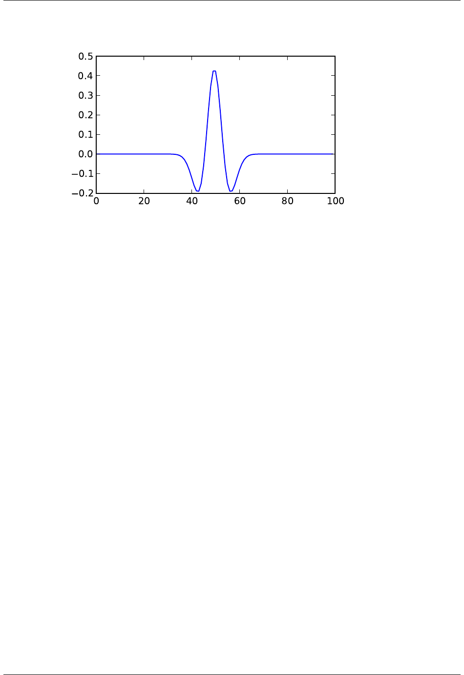
SciPy Reference Guide, Release 0.13.0
scipy.signal.cwt(data,wavelet,widths)
Continuous wavelet transform.
Performs a continuous wavelet transform on data, using the wavelet function. A CWT performs a convolution
with data using the wavelet function, which is characterized by a width parameter and length parameter.
Parameters data : (N,) ndarray
data on which to perform the transform.
wavelet : function
Wavelet function, which should take 2 arguments. The first ar-
gument is the number of points that the returned vector will have
(len(wavelet(width,length)) == length). The second is a width parameter,
defining the size of the wavelet (e.g. standard deviation of a gaussian). See
ricker, which satisfies these requirements.
widths : (M,) sequence
Widths to use for transform.
Returns cwt: (M, N) ndarray
Will have shape of (len(data), len(widths)).
Notes
>>> length =min(10 *width[ii], len(data))
>>> cwt[ii,:] =scipy.signal.convolve(data, wavelet(width[ii],
... length), mode=’same’)
Examples
>>> from scipy import signal
>>> sig =np.random.rand(20)-0.5
>>> wavelet =signal.ricker
>>> widths =np.arange(1,11)
>>> cwtmatr =signal.cwt(sig, wavelet, widths)
5.22.12 Peak finding
5.22. Signal processing (scipy.signal) 683

SciPy Reference Guide, Release 0.13.0
find_peaks_cwt(vector, widths[, wavelet, ...]) Attempt to find the peaks in a 1-D array.
argrelmin(data[, axis, order, mode]) Calculate the relative minima of data.
argrelmax(data[, axis, order, mode]) Calculate the relative maxima of data.
argrelextrema(data, comparator[, axis, ...]) Calculate the relative extrema of data.
scipy.signal.find_peaks_cwt(vector,widths,wavelet=None,max_distances=None,
gap_thresh=None,min_length=None,min_snr=1,noise_perc=10)
Attempt to find the peaks in a 1-D array.
The general approach is to smooth vector by convolving it with wavelet(width) for each width in widths. Relative
maxima which appear at enough length scales, and with sufficiently high SNR, are accepted. New in version
0.11.0.
Parameters vector : ndarray
1-D array in which to find the peaks.
widths : sequence
1-D array of widths to use for calculating the CWT matrix. In general, this
range should cover the expected width of peaks of interest.
wavelet : callable, optional
Should take a single variable and return a 1-D array to convolve with vector.
Should be normalized to unit area. Default is the ricker wavelet.
max_distances : ndarray, optional
At each row, a ridge line is only connected if the relative max at row[n] is
within max_distances[n] from the relative max at row[n+1]. De-
fault value is widths/4.
gap_thresh : float, optional
If a relative maximum is not found within max_distances, there will be a
gap. A ridge line is discontinued if there are more than gap_thresh points
without connecting a new relative maximum. Default is 2.
min_length : int, optional
Minimum length a ridge line needs to be acceptable. Default is
cwt.shape[0] / 4, ie 1/4-th the number of widths.
min_snr : float, optional
Minimum SNR ratio. Default 1. The signal is the value of the cwt matrix
at the shortest length scale (cwt[0, loc]), the noise is the noise_perc‘th
percentile of datapoints contained within a window of ‘window_size around
cwt[0, loc].
noise_perc : float, optional
When calculating the noise floor, percentile of data points examined below
which to consider noise. Calculated using stats.scoreatpercentile. Default
is 10.
See Also
cwt
Notes
This approach was designed for finding sharp peaks among noisy data, however with proper parameter selection
it should function well for different peak shapes.
The algorithm is as follows:
1.Perform a continuous wavelet transform on vector, for the supplied widths. This
is a convolution of vector with wavelet(width) for each width in widths. See cwt
684 Chapter 5. Reference

SciPy Reference Guide, Release 0.13.0
2.Identify “ridge lines” in the cwt matrix. These are relative maxima at each row,
connected across adjacent rows. See identify_ridge_lines
3.Filter the ridge_lines using filter_ridge_lines.
References
[R114]
Examples
>>> from scipy import signal
>>> xs =np.arange(0, np.pi, 0.05)
>>> data =np.sin(xs)
>>> peakind =signal.find_peaks_cwt(data, np.arange(1,10))
>>> peakind, xs[peakind], data[peakind]
([32], array([ 1.6]), array([ 0.9995736]))
scipy.signal.argrelmin(data,axis=0,order=1,mode=’clip’)
Calculate the relative minima of data. New in version 0.11.0.
Parameters data : ndarray
Array in which to find the relative minima.
axis : int, optional
Axis over which to select from data. Default is 0.
order : int, optional
How many points on each side to use for the comparison to consider
comparator(n, n+x) to be True.
mode : str, optional
How the edges of the vector are treated. Available options are ‘wrap’ (wrap
around) or ‘clip’ (treat overflow as the same as the last (or first) element).
Default ‘clip’. See numpy.take
Returns extrema : ndarray
Indices of the minima, as an array of integers.
See Also
argrelextrema,argrelmax
Notes
This function uses argrelextrema with np.less as comparator.
scipy.signal.argrelmax(data,axis=0,order=1,mode=’clip’)
Calculate the relative maxima of data. New in version 0.11.0.
Parameters data : ndarray
Array in which to find the relative maxima.
axis : int, optional
Axis over which to select from data. Default is 0.
order : int, optional
How many points on each side to use for the comparison to consider
comparator(n, n+x) to be True.
mode : str, optional
How the edges of the vector are treated. Available options are ‘wrap’ (wrap
around) or ‘clip’ (treat overflow as the same as the last (or first) element).
Default ‘clip’. See numpy.take.
Returns extrema : ndarray
Indices of the maxima, as an array of integers.
5.22. Signal processing (scipy.signal) 685

SciPy Reference Guide, Release 0.13.0
See Also
argrelextrema,argrelmin
Notes
This function uses argrelextrema with np.greater as comparator.
scipy.signal.argrelextrema(data,comparator,axis=0,order=1,mode=’clip’)
Calculate the relative extrema of data. New in version 0.11.0.
Parameters data : ndarray
Array in which to find the relative extrema.
comparator : callable
Function to use to compare two data points. Should take 2 numbers as
arguments.
axis : int, optional
Axis over which to select from data. Default is 0.
order : int, optional
How many points on each side to use for the comparison to consider
comparator(n, n+x) to be True.
mode : str, optional
How the edges of the vector are treated. ‘wrap’ (wrap around) or ‘clip’
(treat overflow as the same as the last (or first) element). Default is ‘clip’.
See numpy.take.
Returns extrema : ndarray
Indices of the extrema, as an array of integers (same format as np.argmin,
np.argmax).
See Also
argrelmin,argrelmax
5.22.13 Spectral Analysis
periodogram(x[, fs, window, nfft, detrend, ...]) Estimate power spectral density using a periodogram.
welch(x[, fs, window, nperseg, noverlap, ...]) Estimate power spectral density using Welch’s method.
lombscargle(x, y, freqs) Computes the Lomb-Scargle periodogram.
scipy.signal.periodogram(x,fs=1.0,window=None,nfft=None,detrend=’constant’,re-
turn_onesided=True,scaling=’density’,axis=-1)
Estimate power spectral density using a periodogram.
Parameters x: array_like
Time series of measurement values
fs : float, optional
Sampling frequency of the xtime series in units of Hz. Defaults to 1.0.
window : str or tuple or array_like, optional
Desired window to use. See get_window for a list of windows and re-
quired parameters. If window is an array it will be used directly as the
window. Defaults to None; equivalent to ‘boxcar’.
nfft : int, optional
Length of the FFT used. If None the length of xwill be used.
detrend : str or function, optional
686 Chapter 5. Reference

SciPy Reference Guide, Release 0.13.0
Specifies how to detrend xprior to computing the spectrum. If detrend is
a string, it is passed as the type argument to detrend. If it is a function,
it should return a detrended array. Defaults to ‘constant’.
return_onesided : bool, optional
If True, return a one-sided spectrum for real data. If False return a two-
sided spectrum. Note that for complex data, a two-sided spectrum is always
returned.
scaling : { ‘density’, ‘spectrum’ }, optional
Selects between computing the power spectral density (‘density’) where
Pxx has units of V**2/Hz if xis measured in V and computing the power
spectrum (‘spectrum’) where Pxx has units of V**2 if xis measured in V.
Defaults to ‘density’
axis : int, optional
Axis along which the periodogram is computed; the default is over the last
axis (i.e. axis=-1).
Returns f: ndarray
Array of sample frequencies.
Pxx : ndarray
Power spectral density or power spectrum of x.
See Also
welch Estimate power spectral density using Welch’s method
lombscargle
Lomb-Scargle periodogram for unevenly sampled data
Notes
New in version 0.12.0.
Examples
>>> from scipy import signal
>>> import matplotlib.pyplot as plt
Generate a test signal, a 2 Vrms sine wave at 1234 Hz, corrupted by 0.001 V**2/Hz of white noise sampled at
10 kHz.
>>> fs =10e3
>>> N=1e5
>>> amp =2*np.sqrt(2)
>>> freq =1234.0
>>> noise_power =0.001 *fs /2
>>> time =np.arange(N) /fs
>>> x=amp*np.sin(2*np.pi*freq*time)
>>> x+= np.random.normal(scale=np.sqrt(noise_power), size=time.shape)
Compute and plot the power spectral density.
>>> f, Pxx_den =signal.periodogram(x, fs)
>>> plt.semilogy(f, Pxx_den)
>>> plt.xlabel(’frequency [Hz]’)
>>> plt.ylabel(’PSD [V**2/Hz]’)
>>> plt.show()
5.22. Signal processing (scipy.signal) 687
SciPy Reference Guide, Release 0.13.0
If we average the last half of the spectral density, to exclude the peak, we can recover the noise power on the
signal.
>>> np.mean(Pxx_den[256:])
0.0009924865443739191
Now compute and plot the power spectrum.
>>> f, Pxx_spec =signal.periodogram(x, fs, ’flattop’, scaling=’spectrum’)
>>> plt.figure()
>>> plt.semilogy(f, np.sqrt(Pxx_spec))
>>> plt.xlabel(’frequency [Hz]’)
>>> plt.ylabel(’Linear spectrum [V RMS]’)
>>> plt.show()
The peak height in the power spectrum is an estimate of the RMS amplitude.
688 Chapter 5. Reference

SciPy Reference Guide, Release 0.13.0
>>> np.sqrt(Pxx_spec.max())
2.0077340678640727
scipy.signal.welch(x,fs=1.0,window=’hanning’,nperseg=256,noverlap=None,nfft=None,de-
trend=’constant’,return_onesided=True,scaling=’density’,axis=-1)
Estimate power spectral density using Welch’s method.
Welch’s method [R134] computes an estimate of the power spectral density by dividing the data into overlapping
segments, computing a modified periodogram for each segment and averaging the periodograms.
Parameters x: array_like
Time series of measurement values
fs : float, optional
Sampling frequency of the xtime series in units of Hz. Defaults to 1.0.
window : str or tuple or array_like, optional
Desired window to use. See get_window for a list of windows and re-
quired parameters. If window is array_like it will be used directly as the
window and its length will be used for nperseg. Defaults to ‘hanning’.
nperseg : int, optional
Length of each segment. Defaults to 256.
noverlap: int, optional
Number of points to overlap between segments. If None, noverlap =
nperseg / 2. Defaults to None.
nfft : int, optional
Length of the FFT used, if a zero padded FFT is desired. If None, the FFT
length is nperseg. Defaults to None.
detrend : str or function, optional
Specifies how to detrend each segment. If detrend is a string, it is passed
as the type argument to detrend. If it is a function, it takes a segment
and returns a detrended segment. Defaults to ‘constant’.
return_onesided : bool, optional
If True, return a one-sided spectrum for real data. If False return a two-
sided spectrum. Note that for complex data, a two-sided spectrum is always
returned.
scaling : { ‘density’, ‘spectrum’ }, optional
Selects between computing the power spectral density (‘density’) where
Pxx has units of V**2/Hz if x is measured in V and computing the power
spectrum (‘spectrum’) where Pxx has units of V**2 if x is measured in V.
Defaults to ‘density’.
axis : int, optional
Axis along which the periodogram is computed; the default is over the last
axis (i.e. axis=-1).
Returns f: ndarray
Array of sample frequencies.
Pxx : ndarray
Power spectral density or power spectrum of x.
See Also
periodogram
Simple, optionally modified periodogram
lombscargle
Lomb-Scargle periodogram for unevenly sampled data
5.22. Signal processing (scipy.signal) 689

SciPy Reference Guide, Release 0.13.0
Notes
An appropriate amount of overlap will depend on the choice of window and on your requirements. For the
default ‘hanning’ window an overlap of 50% is a reasonable trade off between accurately estimating the signal
power, while not over counting any of the data. Narrower windows may require a larger overlap.
If noverlap is 0, this method is equivalent to Bartlett’s method [R135]. New in version 0.12.0.
References
[R134],[R135]
Examples
>>> from scipy import signal
>>> import matplotlib.pyplot as plt
Generate a test signal, a 2 Vrms sine wave at 1234 Hz, corrupted by 0.001 V**2/Hz of white noise sampled at
10 kHz.
>>> fs =10e3
>>> N=1e5
>>> amp =2*np.sqrt(2)
>>> freq =1234.0
>>> noise_power =0.001 *fs /2
>>> time =np.arange(N) /fs
>>> x=amp*np.sin(2*np.pi*freq*time)
>>> x+= np.random.normal(scale=np.sqrt(noise_power), size=time.shape)
Compute and plot the power spectral density.
>>> f, Pxx_den =signal.welch(x, fs, 1024)
>>> plt.semilogy(f, Pxx_den)
>>> plt.xlabel(’frequency [Hz]’)
>>> plt.ylabel(’PSD [V**2/Hz]’)
>>> plt.show()
If we average the last half of the spectral density, to exclude the peak, we can recover the noise power on the
signal.
>>> np.mean(Pxx_den[256:])
0.0009924865443739191
Now compute and plot the power spectrum.
>>> f, Pxx_spec =signal.welch(x, fs, ’flattop’,1024, scaling=’spectrum’)
>>> plt.figure()
>>> plt.semilogy(f, np.sqrt(Pxx_spec))
>>> plt.xlabel(’frequency [Hz]’)
>>> plt.ylabel(’Linear spectrum [V RMS]’)
>>> plt.show()
The peak height in the power spectrum is an estimate of the RMS amplitude.
>>> np.sqrt(Pxx_spec.max())
2.0077340678640727
690 Chapter 5. Reference

SciPy Reference Guide, Release 0.13.0
scipy.signal.lombscargle(x,y,freqs)
Computes the Lomb-Scargle periodogram.
The Lomb-Scargle periodogram was developed by Lomb [R129] and further extended by Scargle [R130] to
find, and test the significance of weak periodic signals with uneven temporal sampling.
The computed periodogram is unnormalized, it takes the value (A**2) *N/4 for a harmonic signal with
amplitude A for sufficiently large N.
Parameters x: array_like
Sample times.
y: array_like
Measurement values.
freqs : array_like
Angular frequencies for output periodogram.
Returns pgram : array_like
Lomb-Scargle periodogram.
Raises ValueError
If the input arrays xand ydo not have the same shape.
Notes
This subroutine calculates the periodogram using a slightly modified algorithm due to Townsend [R131] which
allows the periodogram to be calculated using only a single pass through the input arrays for each frequency.
The algorithm running time scales roughly as O(x * freqs) or O(N^2) for a large number of samples and fre-
quencies.
References
[R129],[R130],[R131]
Examples
>>> import scipy.signal
First define some input parameters for the signal:
>>> A=2.
>>> w=1.
>>> phi =0.5 *np.pi
>>> nin =1000
>>> nout =100000
>>> frac_points =0.9 # Fraction of points to select
Randomly select a fraction of an array with timesteps:
>>> r=np.random.rand(nin)
>>> x=np.linspace(0.01,10*np.pi, nin)
>>> x=x[r >= frac_points]
>>> normval =x.shape[0]# For normalization of the periodogram
Plot a sine wave for the selected times:
>>> y=A*np.sin(w*x+phi)
Define the array of frequencies for which to compute the periodogram:
>>> f=np.linspace(0.01,10, nout)
5.22. Signal processing (scipy.signal) 691

SciPy Reference Guide, Release 0.13.0
Calculate Lomb-Scargle periodogram:
>>> pgram =sp.signal.lombscargle(x, y, f)
Now make a plot of the input data:
>>> plt.subplot(2,1,1)
<matplotlib.axes.AxesSubplot object at 0x102154f50>
>>> plt.plot(x, y, ’b+’)
[<matplotlib.lines.Line2D object at 0x102154a10>]
Then plot the normalized periodogram:
>>> plt.subplot(2,1,2)
<matplotlib.axes.AxesSubplot object at 0x104b0a990>
>>> plt.plot(f, np.sqrt(4*(pgram/normval)))
[<matplotlib.lines.Line2D object at 0x104b2f910>]
>>> plt.show()
5.23 Sparse matrices (scipy.sparse)
SciPy 2-D sparse matrix package for numeric data.
5.23.1 Contents
Sparse matrix classes
bsr_matrix(arg1[, shape, dtype, copy, blocksize]) Block Sparse Row matrix
coo_matrix(arg1[, shape, dtype, copy]) A sparse matrix in COOrdinate format.
csc_matrix(arg1[, shape, dtype, copy]) Compressed Sparse Column matrix
csr_matrix(arg1[, shape, dtype, copy]) Compressed Sparse Row matrix
dia_matrix(arg1[, shape, dtype, copy]) Sparse matrix with DIAgonal storage
dok_matrix(arg1[, shape, dtype, copy]) Dictionary Of Keys based sparse matrix.
lil_matrix(arg1[, shape, dtype, copy]) Row-based linked list sparse matrix
class scipy.sparse.bsr_matrix(arg1,shape=None,dtype=None,copy=False,blocksize=None)
Block Sparse Row matrix
This can be instantiated in several ways:
bsr_matrix(D, [blocksize=(R,C)])
with a dense matrix or rank-2 ndarray D
bsr_matrix(S, [blocksize=(R,C)])
with another sparse matrix S (equivalent to S.tobsr())
bsr_matrix((M, N), [blocksize=(R,C), dtype])
to construct an empty matrix with shape (M, N) dtype is optional, defaulting to
dtype=’d’.
bsr_matrix((data, ij), [blocksize=(R,C), shape=(M, N)])
where data and ij satisfy a[ij[0, k], ij[1, k]] = data[k]
bsr_matrix((data, indices, indptr), [shape=(M, N)])
is the standard BSR representation where the block column indices for row i
692 Chapter 5. Reference

SciPy Reference Guide, Release 0.13.0
are stored in indices[indptr[i]:indptr[i+1]] and their correspond-
ing block values are stored in data[ indptr[i]: indptr[i+1] ]. If
the shape parameter is not supplied, the matrix dimensions are inferred from the
index arrays.
Notes
Sparse matrices can be used in arithmetic operations: they support addition, subtraction, multiplication, division,
and matrix power.
Summary of BSR format
The Block Compressed Row (BSR) format is very similar to the Compressed Sparse Row (CSR) format. BSR is
appropriate for sparse matrices with dense sub matrices like the last example below. Block matrices often arise
in vector-valued finite element discretizations. In such cases, BSR is considerably more efficient than CSR and
CSC for many sparse arithmetic operations.
Blocksize
The blocksize (R,C) must evenly divide the shape of the matrix (M,N). That is, R and C must satisfy the
relationship M%R=0and N%C=0.
If no blocksize is specified, a simple heuristic is applied to determine an appropriate blocksize.
Examples
>>> from scipy.sparse import bsr_matrix
>>> bsr_matrix((3,4), dtype=np.int8).todense()
matrix([[0, 0, 0, 0],
[0, 0, 0, 0],
[0, 0, 0, 0]], dtype=int8)
>>> row =np.array([0,0,1,2,2,2])
>>> col =np.array([0,2,2,0,1,2])
>>> data =np.array([1,2,3,4,5,6])
>>> bsr_matrix((data, (row,col)), shape=(3,3)).todense()
matrix([[1, 0, 2],
[0, 0, 3],
[4, 5, 6]])
>>> indptr =np.array([0,2,3,6])
>>> indices =np.array([0,2,2,0,1,2])
>>> data =np.array([1,2,3,4,5,6]).repeat(4).reshape(6,2,2)
>>> bsr_matrix((data,indices,indptr), shape=(6,6)).todense()
matrix([[1, 1, 0, 0, 2, 2],
[1, 1, 0, 0, 2, 2],
[0, 0, 0, 0, 3, 3],
[0, 0, 0, 0, 3, 3],
[4, 4, 5, 5, 6, 6],
[4, 4, 5, 5, 6, 6]])
Attributes
has_sorted_indices Determine whether the matrix has sorted indices
bsr_matrix.has_sorted_indices
Determine whether the matrix has sorted indices
5.23. Sparse matrices (scipy.sparse) 693

SciPy Reference Guide, Release 0.13.0
Returns
•True: if the indices of the matrix are in sorted order
•False: otherwise
dtype (dtype) Data type of the matrix
shape (2-tuple) Shape of the matrix
ndim (int) Number of dimensions (this is always 2)
nnz Number of nonzero elements
data Data array of the matrix
indices BSR format index array
indptr BSR format index pointer array
blocksize Block size of the matrix
Methods
arcsin() Element-wise arcsin.
arcsinh() Element-wise arcsinh.
arctan() Element-wise arctan.
arctanh() Element-wise arctanh.
asformat(format) Return this matrix in a given sparse format
asfptype() Upcast matrix to a floating point format (if necessary)
astype(t)
ceil() Element-wise ceil.
check_format([full_check]) check whether the matrix format is valid
conj()
conjugate()
copy()
deg2rad() Element-wise deg2rad.
diagonal() Returns the main diagonal of the matrix
dot(other) Ordinary dot product ..
eliminate_zeros()
expm1() Element-wise expm1.
floor() Element-wise floor.
getH()
get_shape()
getcol(j) Returns a copy of column j of the matrix, as an (m x 1) sparse
getdata(ind)
getformat()
getmaxprint()
getnnz()
getrow(i) Returns a copy of row i of the matrix, as a (1 x n) sparse
log1p() Element-wise log1p.
matmat(other)
matvec(other)
max() Maximum of the elements of this matrix.
mean([axis]) Average the matrix over the given axis.
min() Minimum of the elements of this matrix.
multiply(other) Point-wise multiplication by another matrix, vector, or
nonzero() nonzero indices
prune() Remove empty space after all non-zero elements.
rad2deg() Element-wise rad2deg.
reshape(shape)
Continued on next page
694 Chapter 5. Reference

SciPy Reference Guide, Release 0.13.0
Table 5.122 – continued from previous page
rint() Element-wise rint.
set_shape(shape)
setdiag(values[, k]) Fills the diagonal elements {a_ii} with the values from the given sequence.
sign() Element-wise sign.
sin() Element-wise sin.
sinh() Element-wise sinh.
sort_indices() Sort the indices of this matrix in place
sorted_indices() Return a copy of this matrix with sorted indices
sqrt() Element-wise sqrt.
sum([axis]) Sum the matrix over the given axis.
sum_duplicates()
tan() Element-wise tan.
tanh() Element-wise tanh.
toarray([order, out]) See the docstring for spmatrix.toarray.
tobsr([blocksize, copy])
tocoo([copy]) Convert this matrix to COOrdinate format.
tocsc()
tocsr()
todense([order, out]) Return a dense matrix representation of this matrix.
todia()
todok()
tolil()
transpose()
trunc() Element-wise trunc.
bsr_matrix.arcsin()
Element-wise arcsin.
See numpy.arcsin for more information.
bsr_matrix.arcsinh()
Element-wise arcsinh.
See numpy.arcsinh for more information.
bsr_matrix.arctan()
Element-wise arctan.
See numpy.arctan for more information.
bsr_matrix.arctanh()
Element-wise arctanh.
See numpy.arctanh for more information.
bsr_matrix.asformat(format)
Return this matrix in a given sparse format
Parameters format : {string, None}
desired sparse matrix format
•None for no format conversion
•“csr” for csr_matrix format
•“csc” for csc_matrix format
•“lil” for lil_matrix format
•“dok” for dok_matrix format and so on
5.23. Sparse matrices (scipy.sparse) 695

SciPy Reference Guide, Release 0.13.0
bsr_matrix.asfptype()
Upcast matrix to a floating point format (if necessary)
bsr_matrix.astype(t)
bsr_matrix.ceil()
Element-wise ceil.
See numpy.ceil for more information.
bsr_matrix.check_format(full_check=True)
check whether the matrix format is valid
Parameters:
full_check: True - rigorous check, O(N) operations : default False - basic check, O(1)
operations
bsr_matrix.conj()
bsr_matrix.conjugate()
bsr_matrix.copy()
bsr_matrix.deg2rad()
Element-wise deg2rad.
See numpy.deg2rad for more information.
bsr_matrix.diagonal()
Returns the main diagonal of the matrix
bsr_matrix.dot(other)
Ordinary dot product
Examples
>>> import numpy as np
>>> from scipy.sparse import csr_matrix
>>> A=csr_matrix([[1,2,0], [0,0,3], [4,0,5]])
>>> v=np.array([1,0,-1])
>>> A.dot(v)
array([ 1, -3, -1], dtype=int64)
bsr_matrix.eliminate_zeros()
bsr_matrix.expm1()
Element-wise expm1.
See numpy.expm1 for more information.
bsr_matrix.floor()
Element-wise floor.
See numpy.floor for more information.
bsr_matrix.getH()
696 Chapter 5. Reference

SciPy Reference Guide, Release 0.13.0
bsr_matrix.get_shape()
bsr_matrix.getcol(j)
Returns a copy of column j of the matrix, as an (m x 1) sparse matrix (column vector).
bsr_matrix.getdata(ind)
bsr_matrix.getformat()
bsr_matrix.getmaxprint()
bsr_matrix.getnnz()
bsr_matrix.getrow(i)
Returns a copy of row i of the matrix, as a (1 x n) sparse matrix (row vector).
bsr_matrix.log1p()
Element-wise log1p.
See numpy.log1p for more information.
bsr_matrix.matmat(other)
bsr_matrix.matvec(other)
bsr_matrix.max()
Maximum of the elements of this matrix.
This takes all elements into account, not just the non-zero ones.
Returns amax : self.dtype
Maximum element.
bsr_matrix.mean(axis=None)
Average the matrix over the given axis. If the axis is None, average over both rows and columns, returning
a scalar.
bsr_matrix.min()
Minimum of the elements of this matrix.
This takes all elements into account, not just the non-zero ones.
Returns amin : self.dtype
Minimum element.
bsr_matrix.multiply(other)
Point-wise multiplication by another matrix, vector, or scalar.
bsr_matrix.nonzero()
nonzero indices
Returns a tuple of arrays (row,col) containing the indices of the non-zero elements of the matrix.
Examples
5.23. Sparse matrices (scipy.sparse) 697

SciPy Reference Guide, Release 0.13.0
>>> from scipy.sparse import csr_matrix
>>> A=csr_matrix([[1,2,0],[0,0,3],[4,0,5]])
>>> A.nonzero()
(array([0, 0, 1, 2, 2]), array([0, 1, 2, 0, 2]))
bsr_matrix.prune()
Remove empty space after all non-zero elements.
bsr_matrix.rad2deg()
Element-wise rad2deg.
See numpy.rad2deg for more information.
bsr_matrix.reshape(shape)
bsr_matrix.rint()
Element-wise rint.
See numpy.rint for more information.
bsr_matrix.set_shape(shape)
bsr_matrix.setdiag(values,k=0)
Fills the diagonal elements {a_ii} with the values from the given sequence. If k != 0, fills the off-diagonal
elements {a_{i,i+k}} instead.
values may have any length. If the diagonal is longer than values, then the remaining diagonal entries will
not be set. If values if longer than the diagonal, then the remaining values are ignored.
bsr_matrix.sign()
Element-wise sign.
See numpy.sign for more information.
bsr_matrix.sin()
Element-wise sin.
See numpy.sin for more information.
bsr_matrix.sinh()
Element-wise sinh.
See numpy.sinh for more information.
bsr_matrix.sort_indices()
Sort the indices of this matrix in place
bsr_matrix.sorted_indices()
Return a copy of this matrix with sorted indices
bsr_matrix.sqrt()
Element-wise sqrt.
See numpy.sqrt for more information.
bsr_matrix.sum(axis=None)
Sum the matrix over the given axis. If the axis is None, sum over both rows and columns, returning a
scalar.
bsr_matrix.sum_duplicates()
698 Chapter 5. Reference

SciPy Reference Guide, Release 0.13.0
bsr_matrix.tan()
Element-wise tan.
See numpy.tan for more information.
bsr_matrix.tanh()
Element-wise tanh.
See numpy.tanh for more information.
bsr_matrix.toarray(order=None,out=None)
See the docstring for spmatrix.toarray.
bsr_matrix.tobsr(blocksize=None,copy=False)
bsr_matrix.tocoo(copy=True)
Convert this matrix to COOrdinate format.
When copy=False the data array will be shared between this matrix and the resultant coo_matrix.
bsr_matrix.tocsc()
bsr_matrix.tocsr()
bsr_matrix.todense(order=None,out=None)
Return a dense matrix representation of this matrix.
Parameters order : {‘C’, ‘F’}, optional
Whether to store multi-dimensional data in C (row-major) or Fortran
(column-major) order in memory. The default is ‘None’, indicating
the NumPy default of C-ordered. Cannot be specified in conjunction
with the out argument.
out : ndarray, 2-dimensional, optional
If specified, uses this array (or numpy.matrix) as the output buffer
instead of allocating a new array to return. The provided array must
have the same shape and dtype as the sparse matrix on which you are
calling the method.
Returns arr : numpy.matrix, 2-dimensional
A NumPy matrix object with the same shape and containing the
same data represented by the sparse matrix, with the requested
memory order. If out was passed and was an array (rather than a
numpy.matrix), it will be filled with the appropriate values and
returned wrapped in a numpy.matrix object that shares the same
memory.
bsr_matrix.todia()
bsr_matrix.todok()
bsr_matrix.tolil()
bsr_matrix.transpose()
bsr_matrix.trunc()
Element-wise trunc.
5.23. Sparse matrices (scipy.sparse) 699

SciPy Reference Guide, Release 0.13.0
See numpy.trunc for more information.
class scipy.sparse.coo_matrix(arg1,shape=None,dtype=None,copy=False)
A sparse matrix in COOrdinate format.
Also known as the ‘ijv’ or ‘triplet’ format.
This can be instantiated in several ways:
coo_matrix(D)
with a dense matrix D
coo_matrix(S)with another sparse matrix S (equivalent to S.tocoo())
coo_matrix((M, N), [dtype])
to construct an empty matrix with shape (M, N) dtype is optional, defaulting to
dtype=’d’.
coo_matrix((data, (i, j)), [shape=(M, N)])
to construct from three arrays:
1.data[:] the entries of the matrix, in any order
2.i[:] the row indices of the matrix entries
3.j[:] the column indices of the matrix entries
Where A[i[k], j[k]] = data[k]. When shape is not specified, it is in-
ferred from the index arrays
Notes
Sparse matrices can be used in arithmetic operations: they support addition, subtraction, multiplication, division,
and matrix power.
Advantages of the COO format
•facilitates fast conversion among sparse formats
•permits duplicate entries (see example)
•very fast conversion to and from CSR/CSC formats
Disadvantages of the COO format
•does not directly support:
–arithmetic operations
–slicing
Intended Usage
•COO is a fast format for constructing sparse matrices
•Once a matrix has been constructed, convert to CSR or CSC format for fast arith-
metic and matrix vector operations
•By default when converting to CSR or CSC format, duplicate (i,j) entries will be
summed together. This facilitates efficient construction of finite element matrices
and the like. (see example)
Examples
>>> from scipy.sparse import coo_matrix
>>> coo_matrix((3,4), dtype=np.int8).todense()
matrix([[0, 0, 0, 0],
[0, 0, 0, 0],
[0, 0, 0, 0]], dtype=int8)
700 Chapter 5. Reference

SciPy Reference Guide, Release 0.13.0
>>> row =np.array([0,3,1,0])
>>> col =np.array([0,3,1,2])
>>> data =np.array([4,5,7,9])
>>> coo_matrix((data,(row,col)), shape=(4,4)).todense()
matrix([[4, 0, 9, 0],
[0, 7, 0, 0],
[0, 0, 0, 0],
[0, 0, 0, 5]])
>>> # example with duplicates
>>> row =np.array([0,0,1,3,1,0,0])
>>> col =np.array([0,2,1,3,1,0,0])
>>> data =np.array([1,1,1,1,1,1,1])
>>> coo_matrix((data, (row,col)), shape=(4,4)).todense()
matrix([[3, 0, 1, 0],
[0, 2, 0, 0],
[0, 0, 0, 0],
[0, 0, 0, 1]])
Attributes
dtype (dtype) Data type of the matrix
shape (2-tuple) Shape of the matrix
ndim (int) Number of dimensions (this is always 2)
nnz Number of nonzero elements
data COO format data array of the matrix
row COO format row index array of the matrix
col COO format column index array of the matrix
Methods
arcsin() Element-wise arcsin.
arcsinh() Element-wise arcsinh.
arctan() Element-wise arctan.
arctanh() Element-wise arctanh.
asformat(format) Return this matrix in a given sparse format
asfptype() Upcast matrix to a floating point format (if necessary)
astype(t)
ceil() Element-wise ceil.
conj()
conjugate()
copy()
deg2rad() Element-wise deg2rad.
diagonal() Returns the main diagonal of the matrix
dot(other) Ordinary dot product ..
expm1() Element-wise expm1.
floor() Element-wise floor.
getH()
get_shape()
getcol(j) Returns a copy of column j of the matrix, as an (m x 1) sparse
getformat()
getmaxprint()
Continued on next page
5.23. Sparse matrices (scipy.sparse) 701

SciPy Reference Guide, Release 0.13.0
Table 5.123 – continued from previous page
getnnz()
getrow(i) Returns a copy of row i of the matrix, as a (1 x n) sparse
log1p() Element-wise log1p.
max() Maximum of the elements of this matrix.
mean([axis]) Average the matrix over the given axis.
min() Minimum of the elements of this matrix.
multiply(other) Point-wise multiplication by another matrix
nonzero() nonzero indices
rad2deg() Element-wise rad2deg.
reshape(shape)
rint() Element-wise rint.
set_shape(shape)
setdiag(values[, k]) Fills the diagonal elements {a_ii} with the values from the given sequence.
sign() Element-wise sign.
sin() Element-wise sin.
sinh() Element-wise sinh.
sqrt() Element-wise sqrt.
sum([axis]) Sum the matrix over the given axis.
tan() Element-wise tan.
tanh() Element-wise tanh.
toarray([order, out]) See the docstring for spmatrix.toarray.
tobsr([blocksize])
tocoo([copy])
tocsc() Return a copy of this matrix in Compressed Sparse Column format
tocsr() Return a copy of this matrix in Compressed Sparse Row format
todense([order, out]) Return a dense matrix representation of this matrix.
todia()
todok()
tolil()
transpose([copy])
trunc() Element-wise trunc.
coo_matrix.arcsin()
Element-wise arcsin.
See numpy.arcsin for more information.
coo_matrix.arcsinh()
Element-wise arcsinh.
See numpy.arcsinh for more information.
coo_matrix.arctan()
Element-wise arctan.
See numpy.arctan for more information.
coo_matrix.arctanh()
Element-wise arctanh.
See numpy.arctanh for more information.
coo_matrix.asformat(format)
Return this matrix in a given sparse format
Parameters format : {string, None}
702 Chapter 5. Reference

SciPy Reference Guide, Release 0.13.0
desired sparse matrix format
•None for no format conversion
•“csr” for csr_matrix format
•“csc” for csc_matrix format
•“lil” for lil_matrix format
•“dok” for dok_matrix format and so on
coo_matrix.asfptype()
Upcast matrix to a floating point format (if necessary)
coo_matrix.astype(t)
coo_matrix.ceil()
Element-wise ceil.
See numpy.ceil for more information.
coo_matrix.conj()
coo_matrix.conjugate()
coo_matrix.copy()
coo_matrix.deg2rad()
Element-wise deg2rad.
See numpy.deg2rad for more information.
coo_matrix.diagonal()
Returns the main diagonal of the matrix
coo_matrix.dot(other)
Ordinary dot product
Examples
>>> import numpy as np
>>> from scipy.sparse import csr_matrix
>>> A=csr_matrix([[1,2,0], [0,0,3], [4,0,5]])
>>> v=np.array([1,0,-1])
>>> A.dot(v)
array([ 1, -3, -1], dtype=int64)
coo_matrix.expm1()
Element-wise expm1.
See numpy.expm1 for more information.
coo_matrix.floor()
Element-wise floor.
See numpy.floor for more information.
coo_matrix.getH()
coo_matrix.get_shape()
5.23. Sparse matrices (scipy.sparse) 703

SciPy Reference Guide, Release 0.13.0
coo_matrix.getcol(j)
Returns a copy of column j of the matrix, as an (m x 1) sparse matrix (column vector).
coo_matrix.getformat()
coo_matrix.getmaxprint()
coo_matrix.getnnz()
coo_matrix.getrow(i)
Returns a copy of row i of the matrix, as a (1 x n) sparse matrix (row vector).
coo_matrix.log1p()
Element-wise log1p.
See numpy.log1p for more information.
coo_matrix.max()
Maximum of the elements of this matrix.
This takes all elements into account, not just the non-zero ones.
Returns amax : self.dtype
Maximum element.
coo_matrix.mean(axis=None)
Average the matrix over the given axis. If the axis is None, average over both rows and columns, returning
a scalar.
coo_matrix.min()
Minimum of the elements of this matrix.
This takes all elements into account, not just the non-zero ones.
Returns amin : self.dtype
Minimum element.
coo_matrix.multiply(other)
Point-wise multiplication by another matrix
coo_matrix.nonzero()
nonzero indices
Returns a tuple of arrays (row,col) containing the indices of the non-zero elements of the matrix.
Examples
>>> from scipy.sparse import csr_matrix
>>> A=csr_matrix([[1,2,0],[0,0,3],[4,0,5]])
>>> A.nonzero()
(array([0, 0, 1, 2, 2]), array([0, 1, 2, 0, 2]))
coo_matrix.rad2deg()
Element-wise rad2deg.
See numpy.rad2deg for more information.
coo_matrix.reshape(shape)
704 Chapter 5. Reference

SciPy Reference Guide, Release 0.13.0
coo_matrix.rint()
Element-wise rint.
See numpy.rint for more information.
coo_matrix.set_shape(shape)
coo_matrix.setdiag(values,k=0)
Fills the diagonal elements {a_ii} with the values from the given sequence. If k != 0, fills the off-diagonal
elements {a_{i,i+k}} instead.
values may have any length. If the diagonal is longer than values, then the remaining diagonal entries will
not be set. If values if longer than the diagonal, then the remaining values are ignored.
coo_matrix.sign()
Element-wise sign.
See numpy.sign for more information.
coo_matrix.sin()
Element-wise sin.
See numpy.sin for more information.
coo_matrix.sinh()
Element-wise sinh.
See numpy.sinh for more information.
coo_matrix.sqrt()
Element-wise sqrt.
See numpy.sqrt for more information.
coo_matrix.sum(axis=None)
Sum the matrix over the given axis. If the axis is None, sum over both rows and columns, returning a
scalar.
coo_matrix.tan()
Element-wise tan.
See numpy.tan for more information.
coo_matrix.tanh()
Element-wise tanh.
See numpy.tanh for more information.
coo_matrix.toarray(order=None,out=None)
See the docstring for spmatrix.toarray.
coo_matrix.tobsr(blocksize=None)
coo_matrix.tocoo(copy=False)
coo_matrix.tocsc()
Return a copy of this matrix in Compressed Sparse Column format
Duplicate entries will be summed together.
5.23. Sparse matrices (scipy.sparse) 705

SciPy Reference Guide, Release 0.13.0
Examples
>>> from numpy import array
>>> from scipy.sparse import coo_matrix
>>> row =array([0,0,1,3,1,0,0])
>>> col =array([0,2,1,3,1,0,0])
>>> data =array([1,1,1,1,1,1,1])
>>> A=coo_matrix( (data,(row,col)), shape=(4,4)).tocsc()
>>> A.todense()
matrix([[3, 0, 1, 0],
[0, 2, 0, 0],
[0, 0, 0, 0],
[0, 0, 0, 1]])
coo_matrix.tocsr()
Return a copy of this matrix in Compressed Sparse Row format
Duplicate entries will be summed together.
Examples
>>> from numpy import array
>>> from scipy.sparse import coo_matrix
>>> row =array([0,0,1,3,1,0,0])
>>> col =array([0,2,1,3,1,0,0])
>>> data =array([1,1,1,1,1,1,1])
>>> A=coo_matrix( (data,(row,col)), shape=(4,4)).tocsr()
>>> A.todense()
matrix([[3, 0, 1, 0],
[0, 2, 0, 0],
[0, 0, 0, 0],
[0, 0, 0, 1]])
coo_matrix.todense(order=None,out=None)
Return a dense matrix representation of this matrix.
Parameters order : {‘C’, ‘F’}, optional
Whether to store multi-dimensional data in C (row-major) or Fortran
(column-major) order in memory. The default is ‘None’, indicating
the NumPy default of C-ordered. Cannot be specified in conjunction
with the out argument.
out : ndarray, 2-dimensional, optional
If specified, uses this array (or numpy.matrix) as the output buffer
instead of allocating a new array to return. The provided array must
have the same shape and dtype as the sparse matrix on which you are
calling the method.
Returns arr : numpy.matrix, 2-dimensional
A NumPy matrix object with the same shape and containing the
same data represented by the sparse matrix, with the requested
memory order. If out was passed and was an array (rather than a
numpy.matrix), it will be filled with the appropriate values and
returned wrapped in a numpy.matrix object that shares the same
memory.
coo_matrix.todia()
coo_matrix.todok()
706 Chapter 5. Reference

SciPy Reference Guide, Release 0.13.0
coo_matrix.tolil()
coo_matrix.transpose(copy=False)
coo_matrix.trunc()
Element-wise trunc.
See numpy.trunc for more information.
class scipy.sparse.csc_matrix(arg1,shape=None,dtype=None,copy=False)
Compressed Sparse Column matrix
This can be instantiated in several ways:
csc_matrix(D)with a dense matrix or rank-2 ndarray D
csc_matrix(S) with another sparse matrix S (equivalent to S.tocsc())
csc_matrix((M, N), [dtype])
to construct an empty matrix with shape (M, N) dtype is optional, defaulting to dtype=’d’.
csc_matrix((data, ij), [shape=(M, N)])
where data and ij satisfy the relationship a[ij[0, k], ij[1, k]] = data[k]
csc_matrix((data, indices, indptr), [shape=(M, N)])
is the standard CSC representation where the row indices for column i are stored in
indices[indptr[i]:indptr[i+1]] and their corresponding values are stored in
data[indptr[i]:indptr[i+1]]. If the shape parameter is not supplied, the matrix
dimensions are inferred from the index arrays.
Notes
Sparse matrices can be used in arithmetic operations: they support addition, subtraction, multiplication, division,
and matrix power.
Advantages of the CSC format
•efficient arithmetic operations CSC + CSC, CSC * CSC, etc.
•efficient column slicing
•fast matrix vector products (CSR, BSR may be faster)
Disadvantages of the CSC format
•slow row slicing operations (consider CSR)
•changes to the sparsity structure are expensive (consider LIL or DOK)
Examples
>>> from scipy.sparse import *
>>> from scipy import *
>>> csc_matrix( (3,4), dtype=int8 ).todense()
matrix([[0, 0, 0, 0],
[0, 0, 0, 0],
[0, 0, 0, 0]], dtype=int8)
>>> row =array([0,2,2,0,1,2])
>>> col =array([0,0,1,2,2,2])
>>> data =array([1,2,3,4,5,6])
>>> csc_matrix( (data,(row,col)), shape=(3,3) ).todense()
matrix([[1, 0, 4],
[0, 0, 5],
[2, 3, 6]])
5.23. Sparse matrices (scipy.sparse) 707

SciPy Reference Guide, Release 0.13.0
>>> indptr =array([0,2,3,6])
>>> indices =array([0,2,2,0,1,2])
>>> data =array([1,2,3,4,5,6])
>>> csc_matrix( (data,indices,indptr), shape=(3,3) ).todense()
matrix([[1, 0, 4],
[0, 0, 5],
[2, 3, 6]])
Attributes
has_sorted_indices Determine whether the matrix has sorted indices
csc_matrix.has_sorted_indices
Determine whether the matrix has sorted indices
Returns
•True: if the indices of the matrix are in sorted order
•False: otherwise
dtype (dtype) Data type of the matrix
shape (2-tuple) Shape of the matrix
ndim (int) Number of dimensions (this is always 2)
nnz Number of nonzero elements
data Data array of the matrix
indices CSC format index array
indptr CSC format index pointer array
Methods
arcsin() Element-wise arcsin.
arcsinh() Element-wise arcsinh.
arctan() Element-wise arctan.
arctanh() Element-wise arctanh.
asformat(format) Return this matrix in a given sparse format
asfptype() Upcast matrix to a floating point format (if necessary)
astype(t)
ceil() Element-wise ceil.
check_format([full_check]) check whether the matrix format is valid
conj()
conjugate()
copy()
deg2rad() Element-wise deg2rad.
diagonal() Returns the main diagonal of the matrix
dot(other) Ordinary dot product ..
eliminate_zeros() Remove zero entries from the matrix
expm1() Element-wise expm1.
floor() Element-wise floor.
getH()
get_shape()
getcol(i) Returns a copy of column i of the matrix, as a (m x 1)
getformat()
getmaxprint()
Continued on next page
708 Chapter 5. Reference

SciPy Reference Guide, Release 0.13.0
Table 5.125 – continued from previous page
getnnz()
getrow(i) Returns a copy of row i of the matrix, as a (1 x n)
log1p() Element-wise log1p.
max() Maximum of the elements of this matrix.
mean([axis]) Average the matrix over the given axis.
min() Minimum of the elements of this matrix.
multiply(other) Point-wise multiplication by another matrix, vector, or
nonzero() nonzero indices
prune() Remove empty space after all non-zero elements.
rad2deg() Element-wise rad2deg.
reshape(shape)
rint() Element-wise rint.
set_shape(shape)
setdiag(values[, k]) Fills the diagonal elements {a_ii} with the values from the given sequence.
sign() Element-wise sign.
sin() Element-wise sin.
sinh() Element-wise sinh.
sort_indices() Sort the indices of this matrix in place
sorted_indices() Return a copy of this matrix with sorted indices
sqrt() Element-wise sqrt.
sum([axis]) Sum the matrix over the given axis.
sum_duplicates() Eliminate duplicate matrix entries by adding them together
tan() Element-wise tan.
tanh() Element-wise tanh.
toarray([order, out]) See the docstring for spmatrix.toarray.
tobsr([blocksize])
tocoo([copy]) Return a COOrdinate representation of this matrix
tocsc([copy])
tocsr()
todense([order, out]) Return a dense matrix representation of this matrix.
todia()
todok()
tolil()
transpose([copy])
trunc() Element-wise trunc.
csc_matrix.arcsin()
Element-wise arcsin.
See numpy.arcsin for more information.
csc_matrix.arcsinh()
Element-wise arcsinh.
See numpy.arcsinh for more information.
csc_matrix.arctan()
Element-wise arctan.
See numpy.arctan for more information.
csc_matrix.arctanh()
Element-wise arctanh.
See numpy.arctanh for more information.
5.23. Sparse matrices (scipy.sparse) 709

SciPy Reference Guide, Release 0.13.0
csc_matrix.asformat(format)
Return this matrix in a given sparse format
Parameters format : {string, None}
desired sparse matrix format
•None for no format conversion
•“csr” for csr_matrix format
•“csc” for csc_matrix format
•“lil” for lil_matrix format
•“dok” for dok_matrix format and so on
csc_matrix.asfptype()
Upcast matrix to a floating point format (if necessary)
csc_matrix.astype(t)
csc_matrix.ceil()
Element-wise ceil.
See numpy.ceil for more information.
csc_matrix.check_format(full_check=True)
check whether the matrix format is valid
Parameters - full_check : {bool}
•True - rigorous check, O(N) operations : default
•False - basic check, O(1) operations
csc_matrix.conj()
csc_matrix.conjugate()
csc_matrix.copy()
csc_matrix.deg2rad()
Element-wise deg2rad.
See numpy.deg2rad for more information.
csc_matrix.diagonal()
Returns the main diagonal of the matrix
csc_matrix.dot(other)
Ordinary dot product
Examples
>>> import numpy as np
>>> from scipy.sparse import csr_matrix
>>> A=csr_matrix([[1,2,0], [0,0,3], [4,0,5]])
>>> v=np.array([1,0,-1])
>>> A.dot(v)
array([ 1, -3, -1], dtype=int64)
csc_matrix.eliminate_zeros()
Remove zero entries from the matrix
The is an in place operation
710 Chapter 5. Reference

SciPy Reference Guide, Release 0.13.0
csc_matrix.expm1()
Element-wise expm1.
See numpy.expm1 for more information.
csc_matrix.floor()
Element-wise floor.
See numpy.floor for more information.
csc_matrix.getH()
csc_matrix.get_shape()
csc_matrix.getcol(i)
Returns a copy of column i of the matrix, as a (m x 1) CSC matrix (column vector).
csc_matrix.getformat()
csc_matrix.getmaxprint()
csc_matrix.getnnz()
csc_matrix.getrow(i)
Returns a copy of row i of the matrix, as a (1 x n) CSR matrix (row vector).
csc_matrix.log1p()
Element-wise log1p.
See numpy.log1p for more information.
csc_matrix.max()
Maximum of the elements of this matrix.
This takes all elements into account, not just the non-zero ones.
Returns amax : self.dtype
Maximum element.
csc_matrix.mean(axis=None)
Average the matrix over the given axis. If the axis is None, average over both rows and columns, returning
a scalar.
csc_matrix.min()
Minimum of the elements of this matrix.
This takes all elements into account, not just the non-zero ones.
Returns amin : self.dtype
Minimum element.
csc_matrix.multiply(other)
Point-wise multiplication by another matrix, vector, or scalar.
csc_matrix.nonzero()
nonzero indices
Returns a tuple of arrays (row,col) containing the indices of the non-zero elements of the matrix.
5.23. Sparse matrices (scipy.sparse) 711

SciPy Reference Guide, Release 0.13.0
Examples
>>> from scipy.sparse import csr_matrix
>>> A=csr_matrix([[1,2,0],[0,0,3],[4,0,5]])
>>> A.nonzero()
(array([0, 0, 1, 2, 2]), array([0, 1, 2, 0, 2]))
csc_matrix.prune()
Remove empty space after all non-zero elements.
csc_matrix.rad2deg()
Element-wise rad2deg.
See numpy.rad2deg for more information.
csc_matrix.reshape(shape)
csc_matrix.rint()
Element-wise rint.
See numpy.rint for more information.
csc_matrix.set_shape(shape)
csc_matrix.setdiag(values,k=0)
Fills the diagonal elements {a_ii} with the values from the given sequence. If k != 0, fills the off-diagonal
elements {a_{i,i+k}} instead.
values may have any length. If the diagonal is longer than values, then the remaining diagonal entries will
not be set. If values if longer than the diagonal, then the remaining values are ignored.
csc_matrix.sign()
Element-wise sign.
See numpy.sign for more information.
csc_matrix.sin()
Element-wise sin.
See numpy.sin for more information.
csc_matrix.sinh()
Element-wise sinh.
See numpy.sinh for more information.
csc_matrix.sort_indices()
Sort the indices of this matrix in place
csc_matrix.sorted_indices()
Return a copy of this matrix with sorted indices
csc_matrix.sqrt()
Element-wise sqrt.
See numpy.sqrt for more information.
csc_matrix.sum(axis=None)
Sum the matrix over the given axis. If the axis is None, sum over both rows and columns, returning a
scalar.
712 Chapter 5. Reference

SciPy Reference Guide, Release 0.13.0
csc_matrix.sum_duplicates()
Eliminate duplicate matrix entries by adding them together
The is an in place operation
csc_matrix.tan()
Element-wise tan.
See numpy.tan for more information.
csc_matrix.tanh()
Element-wise tanh.
See numpy.tanh for more information.
csc_matrix.toarray(order=None,out=None)
See the docstring for spmatrix.toarray.
csc_matrix.tobsr(blocksize=None)
csc_matrix.tocoo(copy=True)
Return a COOrdinate representation of this matrix
When copy=False the index and data arrays are not copied.
csc_matrix.tocsc(copy=False)
csc_matrix.tocsr()
csc_matrix.todense(order=None,out=None)
Return a dense matrix representation of this matrix.
Parameters order : {‘C’, ‘F’}, optional
Whether to store multi-dimensional data in C (row-major) or Fortran
(column-major) order in memory. The default is ‘None’, indicating
the NumPy default of C-ordered. Cannot be specified in conjunction
with the out argument.
out : ndarray, 2-dimensional, optional
If specified, uses this array (or numpy.matrix) as the output buffer
instead of allocating a new array to return. The provided array must
have the same shape and dtype as the sparse matrix on which you are
calling the method.
Returns arr : numpy.matrix, 2-dimensional
A NumPy matrix object with the same shape and containing the
same data represented by the sparse matrix, with the requested
memory order. If out was passed and was an array (rather than a
numpy.matrix), it will be filled with the appropriate values and
returned wrapped in a numpy.matrix object that shares the same
memory.
csc_matrix.todia()
csc_matrix.todok()
csc_matrix.tolil()
5.23. Sparse matrices (scipy.sparse) 713

SciPy Reference Guide, Release 0.13.0
csc_matrix.transpose(copy=False)
csc_matrix.trunc()
Element-wise trunc.
See numpy.trunc for more information.
class scipy.sparse.csr_matrix(arg1,shape=None,dtype=None,copy=False)
Compressed Sparse Row matrix
This can be instantiated in several ways:
csr_matrix(D) with a dense matrix or rank-2 ndarray D
csr_matrix(S) with another sparse matrix S (equivalent to S.tocsr())
csr_matrix((M, N), [dtype])
to construct an empty matrix with shape (M, N) dtype is optional, defaulting to
dtype=’d’.
csr_matrix((data, ij), [shape=(M, N)])
where data and ij satisfy the relationship a[ij[0, k], ij[1, k]] =
data[k]
csr_matrix((data, indices, indptr), [shape=(M, N)])
is the standard CSR representation where the column indices for row i are stored in
indices[indptr[i]:indptr[i+1]] and their corresponding values are
stored in data[indptr[i]:indptr[i+1]]. If the shape parameter is not
supplied, the matrix dimensions are inferred from the index arrays.
Notes
Sparse matrices can be used in arithmetic operations: they support addition, subtraction, multiplication, division,
and matrix power.
Advantages of the CSR format
•efficient arithmetic operations CSR + CSR, CSR * CSR, etc.
•efficient row slicing
•fast matrix vector products
Disadvantages of the CSR format
•slow column slicing operations (consider CSC)
•changes to the sparsity structure are expensive (consider LIL or DOK)
Examples
>>> from scipy.sparse import *
>>> from scipy import *
>>> csr_matrix( (3,4), dtype=int8 ).todense()
matrix([[0, 0, 0, 0],
[0, 0, 0, 0],
[0, 0, 0, 0]], dtype=int8)
>>> row =array([0,0,1,2,2,2])
>>> col =array([0,2,2,0,1,2])
>>> data =array([1,2,3,4,5,6])
>>> csr_matrix( (data,(row,col)), shape=(3,3) ).todense()
matrix([[1, 0, 2],
[0, 0, 3],
[4, 5, 6]])
714 Chapter 5. Reference

SciPy Reference Guide, Release 0.13.0
>>> indptr =array([0,2,3,6])
>>> indices =array([0,2,2,0,1,2])
>>> data =array([1,2,3,4,5,6])
>>> csr_matrix( (data,indices,indptr), shape=(3,3) ).todense()
matrix([[1, 0, 2],
[0, 0, 3],
[4, 5, 6]])
Attributes
has_sorted_indices Determine whether the matrix has sorted indices
csr_matrix.has_sorted_indices
Determine whether the matrix has sorted indices
Returns
•True: if the indices of the matrix are in sorted order
•False: otherwise
dtype (dtype) Data type of the matrix
shape (2-tuple) Shape of the matrix
ndim (int) Number of dimensions (this is always 2)
nnz Number of nonzero elements
data CSR format data array of the matrix
indices CSR format index array of the matrix
indptr CSR format index pointer array of the matrix
Methods
arcsin() Element-wise arcsin.
arcsinh() Element-wise arcsinh.
arctan() Element-wise arctan.
arctanh() Element-wise arctanh.
asformat(format) Return this matrix in a given sparse format
asfptype() Upcast matrix to a floating point format (if necessary)
astype(t)
ceil() Element-wise ceil.
check_format([full_check]) check whether the matrix format is valid
conj()
conjugate()
copy()
deg2rad() Element-wise deg2rad.
diagonal() Returns the main diagonal of the matrix
dot(other) Ordinary dot product ..
eliminate_zeros() Remove zero entries from the matrix
expm1() Element-wise expm1.
floor() Element-wise floor.
getH()
get_shape()
getcol(i) Returns a copy of column i of the matrix, as a (m x 1)
getformat()
getmaxprint()
Continued on next page
5.23. Sparse matrices (scipy.sparse) 715

SciPy Reference Guide, Release 0.13.0
Table 5.127 – continued from previous page
getnnz()
getrow(i) Returns a copy of row i of the matrix, as a (1 x n)
log1p() Element-wise log1p.
max() Maximum of the elements of this matrix.
mean([axis]) Average the matrix over the given axis.
min() Minimum of the elements of this matrix.
multiply(other) Point-wise multiplication by another matrix, vector, or
nonzero() nonzero indices
prune() Remove empty space after all non-zero elements.
rad2deg() Element-wise rad2deg.
reshape(shape)
rint() Element-wise rint.
set_shape(shape)
setdiag(values[, k]) Fills the diagonal elements {a_ii} with the values from the given sequence.
sign() Element-wise sign.
sin() Element-wise sin.
sinh() Element-wise sinh.
sort_indices() Sort the indices of this matrix in place
sorted_indices() Return a copy of this matrix with sorted indices
sqrt() Element-wise sqrt.
sum([axis]) Sum the matrix over the given axis.
sum_duplicates() Eliminate duplicate matrix entries by adding them together
tan() Element-wise tan.
tanh() Element-wise tanh.
toarray([order, out]) See the docstring for spmatrix.toarray.
tobsr([blocksize, copy])
tocoo([copy]) Return a COOrdinate representation of this matrix
tocsc()
tocsr([copy])
todense([order, out]) Return a dense matrix representation of this matrix.
todia()
todok()
tolil()
transpose([copy])
trunc() Element-wise trunc.
csr_matrix.arcsin()
Element-wise arcsin.
See numpy.arcsin for more information.
csr_matrix.arcsinh()
Element-wise arcsinh.
See numpy.arcsinh for more information.
csr_matrix.arctan()
Element-wise arctan.
See numpy.arctan for more information.
csr_matrix.arctanh()
Element-wise arctanh.
See numpy.arctanh for more information.
716 Chapter 5. Reference

SciPy Reference Guide, Release 0.13.0
csr_matrix.asformat(format)
Return this matrix in a given sparse format
Parameters format : {string, None}
desired sparse matrix format
•None for no format conversion
•“csr” for csr_matrix format
•“csc” for csc_matrix format
•“lil” for lil_matrix format
•“dok” for dok_matrix format and so on
csr_matrix.asfptype()
Upcast matrix to a floating point format (if necessary)
csr_matrix.astype(t)
csr_matrix.ceil()
Element-wise ceil.
See numpy.ceil for more information.
csr_matrix.check_format(full_check=True)
check whether the matrix format is valid
Parameters - full_check : {bool}
•True - rigorous check, O(N) operations : default
•False - basic check, O(1) operations
csr_matrix.conj()
csr_matrix.conjugate()
csr_matrix.copy()
csr_matrix.deg2rad()
Element-wise deg2rad.
See numpy.deg2rad for more information.
csr_matrix.diagonal()
Returns the main diagonal of the matrix
csr_matrix.dot(other)
Ordinary dot product
Examples
>>> import numpy as np
>>> from scipy.sparse import csr_matrix
>>> A=csr_matrix([[1,2,0], [0,0,3], [4,0,5]])
>>> v=np.array([1,0,-1])
>>> A.dot(v)
array([ 1, -3, -1], dtype=int64)
csr_matrix.eliminate_zeros()
Remove zero entries from the matrix
The is an in place operation
5.23. Sparse matrices (scipy.sparse) 717

SciPy Reference Guide, Release 0.13.0
csr_matrix.expm1()
Element-wise expm1.
See numpy.expm1 for more information.
csr_matrix.floor()
Element-wise floor.
See numpy.floor for more information.
csr_matrix.getH()
csr_matrix.get_shape()
csr_matrix.getcol(i)
Returns a copy of column i of the matrix, as a (m x 1) CSR matrix (column vector).
csr_matrix.getformat()
csr_matrix.getmaxprint()
csr_matrix.getnnz()
csr_matrix.getrow(i)
Returns a copy of row i of the matrix, as a (1 x n) CSR matrix (row vector).
csr_matrix.log1p()
Element-wise log1p.
See numpy.log1p for more information.
csr_matrix.max()
Maximum of the elements of this matrix.
This takes all elements into account, not just the non-zero ones.
Returns amax : self.dtype
Maximum element.
csr_matrix.mean(axis=None)
Average the matrix over the given axis. If the axis is None, average over both rows and columns, returning
a scalar.
csr_matrix.min()
Minimum of the elements of this matrix.
This takes all elements into account, not just the non-zero ones.
Returns amin : self.dtype
Minimum element.
csr_matrix.multiply(other)
Point-wise multiplication by another matrix, vector, or scalar.
csr_matrix.nonzero()
nonzero indices
Returns a tuple of arrays (row,col) containing the indices of the non-zero elements of the matrix.
718 Chapter 5. Reference

SciPy Reference Guide, Release 0.13.0
Examples
>>> from scipy.sparse import csr_matrix
>>> A=csr_matrix([[1,2,0],[0,0,3],[4,0,5]])
>>> A.nonzero()
(array([0, 0, 1, 2, 2]), array([0, 1, 2, 0, 2]))
csr_matrix.prune()
Remove empty space after all non-zero elements.
csr_matrix.rad2deg()
Element-wise rad2deg.
See numpy.rad2deg for more information.
csr_matrix.reshape(shape)
csr_matrix.rint()
Element-wise rint.
See numpy.rint for more information.
csr_matrix.set_shape(shape)
csr_matrix.setdiag(values,k=0)
Fills the diagonal elements {a_ii} with the values from the given sequence. If k != 0, fills the off-diagonal
elements {a_{i,i+k}} instead.
values may have any length. If the diagonal is longer than values, then the remaining diagonal entries will
not be set. If values if longer than the diagonal, then the remaining values are ignored.
csr_matrix.sign()
Element-wise sign.
See numpy.sign for more information.
csr_matrix.sin()
Element-wise sin.
See numpy.sin for more information.
csr_matrix.sinh()
Element-wise sinh.
See numpy.sinh for more information.
csr_matrix.sort_indices()
Sort the indices of this matrix in place
csr_matrix.sorted_indices()
Return a copy of this matrix with sorted indices
csr_matrix.sqrt()
Element-wise sqrt.
See numpy.sqrt for more information.
csr_matrix.sum(axis=None)
Sum the matrix over the given axis. If the axis is None, sum over both rows and columns, returning a
scalar.
5.23. Sparse matrices (scipy.sparse) 719

SciPy Reference Guide, Release 0.13.0
csr_matrix.sum_duplicates()
Eliminate duplicate matrix entries by adding them together
The is an in place operation
csr_matrix.tan()
Element-wise tan.
See numpy.tan for more information.
csr_matrix.tanh()
Element-wise tanh.
See numpy.tanh for more information.
csr_matrix.toarray(order=None,out=None)
See the docstring for spmatrix.toarray.
csr_matrix.tobsr(blocksize=None,copy=True)
csr_matrix.tocoo(copy=True)
Return a COOrdinate representation of this matrix
When copy=False the index and data arrays are not copied.
csr_matrix.tocsc()
csr_matrix.tocsr(copy=False)
csr_matrix.todense(order=None,out=None)
Return a dense matrix representation of this matrix.
Parameters order : {‘C’, ‘F’}, optional
Whether to store multi-dimensional data in C (row-major) or Fortran
(column-major) order in memory. The default is ‘None’, indicating
the NumPy default of C-ordered. Cannot be specified in conjunction
with the out argument.
out : ndarray, 2-dimensional, optional
If specified, uses this array (or numpy.matrix) as the output buffer
instead of allocating a new array to return. The provided array must
have the same shape and dtype as the sparse matrix on which you are
calling the method.
Returns arr : numpy.matrix, 2-dimensional
A NumPy matrix object with the same shape and containing the
same data represented by the sparse matrix, with the requested
memory order. If out was passed and was an array (rather than a
numpy.matrix), it will be filled with the appropriate values and
returned wrapped in a numpy.matrix object that shares the same
memory.
csr_matrix.todia()
csr_matrix.todok()
csr_matrix.tolil()
720 Chapter 5. Reference

SciPy Reference Guide, Release 0.13.0
csr_matrix.transpose(copy=False)
csr_matrix.trunc()
Element-wise trunc.
See numpy.trunc for more information.
class scipy.sparse.dia_matrix(arg1,shape=None,dtype=None,copy=False)
Sparse matrix with DIAgonal storage
This can be instantiated in several ways:
dia_matrix(D)with a dense matrix
dia_matrix(S) with another sparse matrix S (equivalent to S.todia())
dia_matrix((M, N), [dtype])
to construct an empty matrix with shape (M, N), dtype is optional, defaulting to
dtype=’d’.
dia_matrix((data, offsets), shape=(M, N))
where the data[k,:] stores the diagonal entries for diagonal offsets[k]
(See example below)
Notes
Sparse matrices can be used in arithmetic operations: they support addition, subtraction, multiplication, division,
and matrix power.
Examples
>>> from scipy.sparse import *
>>> from scipy import *
>>> dia_matrix( (3,4), dtype=int8).todense()
matrix([[0, 0, 0, 0],
[0, 0, 0, 0],
[0, 0, 0, 0]], dtype=int8)
>>> data =array([[1,2,3,4]]).repeat(3,axis=0)
>>> offsets =array([0,-1,2])
>>> dia_matrix( (data,offsets), shape=(4,4)).todense()
matrix([[1, 0, 3, 0],
[1, 2, 0, 4],
[0, 2, 3, 0],
[0, 0, 3, 4]])
Attributes
nnz number of nonzero values
dia_matrix.nnz
number of nonzero values
explicit zero values are included in this number
5.23. Sparse matrices (scipy.sparse) 721

SciPy Reference Guide, Release 0.13.0
dtype (dtype) Data type of the matrix
shape (2-tuple) Shape of the matrix
ndim (int) Number of dimensions (this is always 2)
data DIA format data array of the matrix
offsets DIA format offset array of the matrix
Methods
arcsin() Element-wise arcsin.
arcsinh() Element-wise arcsinh.
arctan() Element-wise arctan.
arctanh() Element-wise arctanh.
asformat(format) Return this matrix in a given sparse format
asfptype() Upcast matrix to a floating point format (if necessary)
astype(t)
ceil() Element-wise ceil.
conj()
conjugate()
copy()
deg2rad() Element-wise deg2rad.
diagonal() Returns the main diagonal of the matrix
dot(other) Ordinary dot product ..
expm1() Element-wise expm1.
floor() Element-wise floor.
getH()
get_shape()
getcol(j) Returns a copy of column j of the matrix, as an (m x 1) sparse
getformat()
getmaxprint()
getnnz() number of nonzero values
getrow(i) Returns a copy of row i of the matrix, as a (1 x n) sparse
log1p() Element-wise log1p.
mean([axis]) Average the matrix over the given axis.
multiply(other) Point-wise multiplication by another matrix
nonzero() nonzero indices
rad2deg() Element-wise rad2deg.
reshape(shape)
rint() Element-wise rint.
set_shape(shape)
setdiag(values[, k]) Fills the diagonal elements {a_ii} with the values from the given sequence.
sign() Element-wise sign.
sin() Element-wise sin.
sinh() Element-wise sinh.
sqrt() Element-wise sqrt.
sum([axis]) Sum the matrix over the given axis.
tan() Element-wise tan.
tanh() Element-wise tanh.
toarray([order, out]) Return a dense ndarray representation of this matrix.
tobsr([blocksize])
tocoo()
tocsc()
Continued on next page
722 Chapter 5. Reference

SciPy Reference Guide, Release 0.13.0
Table 5.129 – continued from previous page
tocsr()
todense([order, out]) Return a dense matrix representation of this matrix.
todia([copy])
todok()
tolil()
transpose()
trunc() Element-wise trunc.
dia_matrix.arcsin()
Element-wise arcsin.
See numpy.arcsin for more information.
dia_matrix.arcsinh()
Element-wise arcsinh.
See numpy.arcsinh for more information.
dia_matrix.arctan()
Element-wise arctan.
See numpy.arctan for more information.
dia_matrix.arctanh()
Element-wise arctanh.
See numpy.arctanh for more information.
dia_matrix.asformat(format)
Return this matrix in a given sparse format
Parameters format : {string, None}
desired sparse matrix format
•None for no format conversion
•“csr” for csr_matrix format
•“csc” for csc_matrix format
•“lil” for lil_matrix format
•“dok” for dok_matrix format and so on
dia_matrix.asfptype()
Upcast matrix to a floating point format (if necessary)
dia_matrix.astype(t)
dia_matrix.ceil()
Element-wise ceil.
See numpy.ceil for more information.
dia_matrix.conj()
dia_matrix.conjugate()
dia_matrix.copy()
5.23. Sparse matrices (scipy.sparse) 723

SciPy Reference Guide, Release 0.13.0
dia_matrix.deg2rad()
Element-wise deg2rad.
See numpy.deg2rad for more information.
dia_matrix.diagonal()
Returns the main diagonal of the matrix
dia_matrix.dot(other)
Ordinary dot product
Examples
>>> import numpy as np
>>> from scipy.sparse import csr_matrix
>>> A=csr_matrix([[1,2,0], [0,0,3], [4,0,5]])
>>> v=np.array([1,0,-1])
>>> A.dot(v)
array([ 1, -3, -1], dtype=int64)
dia_matrix.expm1()
Element-wise expm1.
See numpy.expm1 for more information.
dia_matrix.floor()
Element-wise floor.
See numpy.floor for more information.
dia_matrix.getH()
dia_matrix.get_shape()
dia_matrix.getcol(j)
Returns a copy of column j of the matrix, as an (m x 1) sparse matrix (column vector).
dia_matrix.getformat()
dia_matrix.getmaxprint()
dia_matrix.getnnz()
number of nonzero values
explicit zero values are included in this number
dia_matrix.getrow(i)
Returns a copy of row i of the matrix, as a (1 x n) sparse matrix (row vector).
dia_matrix.log1p()
Element-wise log1p.
See numpy.log1p for more information.
dia_matrix.mean(axis=None)
Average the matrix over the given axis. If the axis is None, average over both rows and columns, returning
a scalar.
dia_matrix.multiply(other)
Point-wise multiplication by another matrix
724 Chapter 5. Reference

SciPy Reference Guide, Release 0.13.0
dia_matrix.nonzero()
nonzero indices
Returns a tuple of arrays (row,col) containing the indices of the non-zero elements of the matrix.
Examples
>>> from scipy.sparse import csr_matrix
>>> A=csr_matrix([[1,2,0],[0,0,3],[4,0,5]])
>>> A.nonzero()
(array([0, 0, 1, 2, 2]), array([0, 1, 2, 0, 2]))
dia_matrix.rad2deg()
Element-wise rad2deg.
See numpy.rad2deg for more information.
dia_matrix.reshape(shape)
dia_matrix.rint()
Element-wise rint.
See numpy.rint for more information.
dia_matrix.set_shape(shape)
dia_matrix.setdiag(values,k=0)
Fills the diagonal elements {a_ii} with the values from the given sequence. If k != 0, fills the off-diagonal
elements {a_{i,i+k}} instead.
values may have any length. If the diagonal is longer than values, then the remaining diagonal entries will
not be set. If values if longer than the diagonal, then the remaining values are ignored.
dia_matrix.sign()
Element-wise sign.
See numpy.sign for more information.
dia_matrix.sin()
Element-wise sin.
See numpy.sin for more information.
dia_matrix.sinh()
Element-wise sinh.
See numpy.sinh for more information.
dia_matrix.sqrt()
Element-wise sqrt.
See numpy.sqrt for more information.
dia_matrix.sum(axis=None)
Sum the matrix over the given axis. If the axis is None, sum over both rows and columns, returning a
scalar.
dia_matrix.tan()
Element-wise tan.
See numpy.tan for more information.
5.23. Sparse matrices (scipy.sparse) 725

SciPy Reference Guide, Release 0.13.0
dia_matrix.tanh()
Element-wise tanh.
See numpy.tanh for more information.
dia_matrix.toarray(order=None,out=None)
Return a dense ndarray representation of this matrix.
Parameters order : {‘C’, ‘F’}, optional
Whether to store multi-dimensional data in C (row-major) or Fortran
(column-major) order in memory. The default is ‘None’, indicating
the NumPy default of C-ordered. Cannot be specified in conjunction
with the out argument.
out : ndarray, 2-dimensional, optional
If specified, uses this array as the output buffer instead of allocating a
new array to return. The provided array must have the same shape and
dtype as the sparse matrix on which you are calling the method. For
most sparse types, out is required to be memory contiguous (either C
or Fortran ordered).
Returns arr : ndarray, 2-dimensional
An array with the same shape and containing the same data repre-
sented by the sparse matrix, with the requested memory order. If out
was passed, the same object is returned after being modified in-place
to contain the appropriate values.
dia_matrix.tobsr(blocksize=None)
dia_matrix.tocoo()
dia_matrix.tocsc()
dia_matrix.tocsr()
dia_matrix.todense(order=None,out=None)
Return a dense matrix representation of this matrix.
Parameters order : {‘C’, ‘F’}, optional
Whether to store multi-dimensional data in C (row-major) or Fortran
(column-major) order in memory. The default is ‘None’, indicating
the NumPy default of C-ordered. Cannot be specified in conjunction
with the out argument.
out : ndarray, 2-dimensional, optional
If specified, uses this array (or numpy.matrix) as the output buffer
instead of allocating a new array to return. The provided array must
have the same shape and dtype as the sparse matrix on which you are
calling the method.
Returns arr : numpy.matrix, 2-dimensional
A NumPy matrix object with the same shape and containing the
same data represented by the sparse matrix, with the requested
memory order. If out was passed and was an array (rather than a
numpy.matrix), it will be filled with the appropriate values and
returned wrapped in a numpy.matrix object that shares the same
memory.
dia_matrix.todia(copy=False)
726 Chapter 5. Reference

SciPy Reference Guide, Release 0.13.0
dia_matrix.todok()
dia_matrix.tolil()
dia_matrix.transpose()
dia_matrix.trunc()
Element-wise trunc.
See numpy.trunc for more information.
class scipy.sparse.dok_matrix(arg1,shape=None,dtype=None,copy=False)
Dictionary Of Keys based sparse matrix.
This is an efficient structure for constructing sparse matrices incrementally.
This can be instantiated in several ways:
dok_matrix(D)
with a dense matrix, D
dok_matrix(S)with a sparse matrix, S
dok_matrix((M,N), [dtype])
create the matrix with initial shape (M,N) dtype is optional, defaulting to
dtype=’d’
Notes
Sparse matrices can be used in arithmetic operations: they support addition, subtraction, multiplication, division,
and matrix power.
Allows for efficient O(1) access of individual elements. Duplicates are not allowed. Can be efficiently converted
to a coo_matrix once constructed.
Examples
>>> from scipy.sparse import *
>>> from scipy import *
>>> S=dok_matrix((5,5), dtype=float32)
>>> for iin range(5):
>>> for jin range(5):
>>> S[i,j] =i+j# Update element
Attributes
dtype (dtype) Data type of the matrix
shape (2-tuple) Shape of the matrix
ndim (int) Number of dimensions (this is always 2)
nnz Number of nonzero elements
Methods
asformat(format) Return this matrix in a given sparse format
asfptype() Upcast matrix to a floating point format (if necessary)
astype(t)
clear(() -> None. Remove all items from D.)
Continued on next page
5.23. Sparse matrices (scipy.sparse) 727

SciPy Reference Guide, Release 0.13.0
Table 5.130 – continued from previous page
conj()
conjtransp() Return the conjugate transpose
conjugate()
copy()
diagonal() Returns the main diagonal of the matrix
dot(other) Ordinary dot product ..
fromkeys(...) v defaults to None.
get(key[, default]) This overrides the dict.get method, providing type checking
getH()
get_shape()
getcol(j) Returns a copy of column j of the matrix as a (m x 1)
getformat()
getmaxprint()
getnnz()
getrow(i) Returns a copy of row i of the matrix as a (1 x n)
has_key((k) -> True if D has a key k, else False)
items(() -> list of D’s (key, value) pairs, ...)
iteritems(() -> an iterator over the (key, ...)
iterkeys(() -> an iterator over the keys of D)
itervalues(...)
keys(() -> list of D’s keys)
mean([axis]) Average the matrix over the given axis.
multiply(other) Point-wise multiplication by another matrix
nonzero() nonzero indices
pop((k[,d]) -> v, ...) If key is not found, d is returned if given, otherwise KeyError is raised
popitem(() -> (k, v), ...) 2-tuple; but raise KeyError if D is empty.
reshape(shape)
resize(shape) Resize the matrix in-place to dimensions given by ‘shape’.
set_shape(shape)
setdefault((k[,d]) -> D.get(k,d), ...)
setdiag(values[, k]) Fills the diagonal elements {a_ii} with the values from the given sequence.
sum([axis]) Sum the matrix over the given axis.
toarray([order, out]) See the docstring for spmatrix.toarray.
tobsr([blocksize])
tocoo() Return a copy of this matrix in COOrdinate format
tocsc() Return a copy of this matrix in Compressed Sparse Column format
tocsr() Return a copy of this matrix in Compressed Sparse Row format
todense([order, out]) Return a dense matrix representation of this matrix.
todia()
todok([copy])
tolil()
transpose() Return the transpose
update(([E, ...) If E present and has a .keys() method, does: for k in E: D[k] = E[k]
values(() -> list of D’s values)
viewitems(...)
viewkeys(...)
viewvalues(...)
dok_matrix.asformat(format)
Return this matrix in a given sparse format
728 Chapter 5. Reference

SciPy Reference Guide, Release 0.13.0
Parameters format : {string, None}
desired sparse matrix format
•None for no format conversion
•“csr” for csr_matrix format
•“csc” for csc_matrix format
•“lil” for lil_matrix format
•“dok” for dok_matrix format and so on
dok_matrix.asfptype()
Upcast matrix to a floating point format (if necessary)
dok_matrix.astype(t)
dok_matrix.clear() →None. Remove all items from D.
dok_matrix.conj()
dok_matrix.conjtransp()
Return the conjugate transpose
dok_matrix.conjugate()
dok_matrix.copy()
dok_matrix.diagonal()
Returns the main diagonal of the matrix
dok_matrix.dot(other)
Ordinary dot product
Examples
>>> import numpy as np
>>> from scipy.sparse import csr_matrix
>>> A=csr_matrix([[1,2,0], [0,0,3], [4,0,5]])
>>> v=np.array([1,0,-1])
>>> A.dot(v)
array([ 1, -3, -1], dtype=int64)
static dok_matrix.fromkeys(S[,v])→New dict with keys from S and values equal to v.
v defaults to None.
dok_matrix.get(key,default=0.0)
This overrides the dict.get method, providing type checking but otherwise equivalent functionality.
dok_matrix.getH()
dok_matrix.get_shape()
dok_matrix.getcol(j)
Returns a copy of column j of the matrix as a (m x 1) DOK matrix.
dok_matrix.getformat()
5.23. Sparse matrices (scipy.sparse) 729

SciPy Reference Guide, Release 0.13.0
dok_matrix.getmaxprint()
dok_matrix.getnnz()
dok_matrix.getrow(i)
Returns a copy of row i of the matrix as a (1 x n) DOK matrix.
dok_matrix.has_key(k)→True if D has a key k, else False
dok_matrix.items() →list of D’s (key, value) pairs, as 2-tuples
dok_matrix.iteritems() →an iterator over the (key, value) items of D
dok_matrix.iterkeys() →an iterator over the keys of D
dok_matrix.itervalues() →an iterator over the values of D
dok_matrix.keys() →list of D’s keys
dok_matrix.mean(axis=None)
Average the matrix over the given axis. If the axis is None, average over both rows and columns, returning
a scalar.
dok_matrix.multiply(other)
Point-wise multiplication by another matrix
dok_matrix.nonzero()
nonzero indices
Returns a tuple of arrays (row,col) containing the indices of the non-zero elements of the matrix.
Examples
>>> from scipy.sparse import csr_matrix
>>> A=csr_matrix([[1,2,0],[0,0,3],[4,0,5]])
>>> A.nonzero()
(array([0, 0, 1, 2, 2]), array([0, 1, 2, 0, 2]))
dok_matrix.pop(k[,d])→v, remove specified key and return the corresponding value.
If key is not found, d is returned if given, otherwise KeyError is raised
dok_matrix.popitem() →(k, v), remove and return some (key, value) pair as a
2-tuple; but raise KeyError if D is empty.
dok_matrix.reshape(shape)
dok_matrix.resize(shape)
Resize the matrix in-place to dimensions given by ‘shape’.
Any non-zero elements that lie outside the new shape are removed.
dok_matrix.set_shape(shape)
730 Chapter 5. Reference

SciPy Reference Guide, Release 0.13.0
dok_matrix.setdefault(k[,d])→D.get(k,d), also set D[k]=d if k not in D
dok_matrix.setdiag(values,k=0)
Fills the diagonal elements {a_ii} with the values from the given sequence. If k != 0, fills the off-diagonal
elements {a_{i,i+k}} instead.
values may have any length. If the diagonal is longer than values, then the remaining diagonal entries will
not be set. If values if longer than the diagonal, then the remaining values are ignored.
dok_matrix.sum(axis=None)
Sum the matrix over the given axis. If the axis is None, sum over both rows and columns, returning a
scalar.
dok_matrix.toarray(order=None,out=None)
See the docstring for spmatrix.toarray.
dok_matrix.tobsr(blocksize=None)
dok_matrix.tocoo()
Return a copy of this matrix in COOrdinate format
dok_matrix.tocsc()
Return a copy of this matrix in Compressed Sparse Column format
dok_matrix.tocsr()
Return a copy of this matrix in Compressed Sparse Row format
dok_matrix.todense(order=None,out=None)
Return a dense matrix representation of this matrix.
Parameters order : {‘C’, ‘F’}, optional
Whether to store multi-dimensional data in C (row-major) or Fortran
(column-major) order in memory. The default is ‘None’, indicating
the NumPy default of C-ordered. Cannot be specified in conjunction
with the out argument.
out : ndarray, 2-dimensional, optional
If specified, uses this array (or numpy.matrix) as the output buffer
instead of allocating a new array to return. The provided array must
have the same shape and dtype as the sparse matrix on which you are
calling the method.
Returns arr : numpy.matrix, 2-dimensional
A NumPy matrix object with the same shape and containing the
same data represented by the sparse matrix, with the requested
memory order. If out was passed and was an array (rather than a
numpy.matrix), it will be filled with the appropriate values and
returned wrapped in a numpy.matrix object that shares the same
memory.
dok_matrix.todia()
dok_matrix.todok(copy=False)
dok_matrix.tolil()
dok_matrix.transpose()
Return the transpose
5.23. Sparse matrices (scipy.sparse) 731

SciPy Reference Guide, Release 0.13.0
dok_matrix.update([E],**F)→None. Update D from dict/iterable E and F.
If E present and has a .keys() method, does: for k in E: D[k] = E[k] If E present and lacks .keys() method,
does: for (k, v) in E: D[k] = v In either case, this is followed by: for k in F: D[k] = F[k]
dok_matrix.values() →list of D’s values
dok_matrix.viewitems() →a set-like object providing a view on D’s items
dok_matrix.viewkeys() →a set-like object providing a view on D’s keys
dok_matrix.viewvalues() →an object providing a view on D’s values
class scipy.sparse.lil_matrix(arg1,shape=None,dtype=None,copy=False)
Row-based linked list sparse matrix
This is an efficient structure for constructing sparse matrices incrementally.
This can be instantiated in several ways:
lil_matrix(D) with a dense matrix or rank-2 ndarray D
lil_matrix(S) with another sparse matrix S (equivalent to S.tolil())
lil_matrix((M, N), [dtype])
to construct an empty matrix with shape (M, N) dtype is optional, defaulting to
dtype=’d’.
Notes
Sparse matrices can be used in arithmetic operations: they support addition, subtraction, multiplication, division,
and matrix power.
Advantages of the LIL format
•supports flexible slicing
•changes to the matrix sparsity structure are efficient
Disadvantages of the LIL format
•arithmetic operations LIL + LIL are slow (consider CSR or CSC)
•slow column slicing (consider CSC)
•slow matrix vector products (consider CSR or CSC)
Intended Usage
•LIL is a convenient format for constructing sparse matrices
•once a matrix has been constructed, convert to CSR or CSC format for fast arith-
metic and matrix vector operations
•consider using the COO format when constructing large matrices
Data Structure
•An array (self.rows) of rows, each of which is a sorted list of column indices
of non-zero elements.
•The corresponding nonzero values are stored in similar fashion in self.data.
732 Chapter 5. Reference

SciPy Reference Guide, Release 0.13.0
Attributes
dtype (dtype) Data type of the matrix
shape (2-tuple) Shape of the matrix
ndim (int) Number of dimensions (this is always 2)
nnz Number of nonzero elements
data LIL format data array of the matrix
rows LIL format row index array of the matrix
Methods
asformat(format) Return this matrix in a given sparse format
asfptype() Upcast matrix to a floating point format (if necessary)
astype(t)
conj()
conjugate()
copy()
diagonal() Returns the main diagonal of the matrix
dot(other) Ordinary dot product ..
getH()
get_shape()
getcol(j) Returns a copy of column j of the matrix, as an (m x 1) sparse
getformat()
getmaxprint()
getnnz()
getrow(i) Returns a copy of the ‘i’th row.
getrowview(i) Returns a view of the ‘i’th row (without copying).
mean([axis]) Average the matrix over the given axis.
multiply(other) Point-wise multiplication by another matrix
nonzero() nonzero indices
reshape(shape)
set_shape(shape)
setdiag(values[, k]) Fills the diagonal elements {a_ii} with the values from the given sequence.
sum([axis]) Sum the matrix over the given axis.
toarray([order, out]) See the docstring for spmatrix.toarray.
tobsr([blocksize])
tocoo()
tocsc() Return Compressed Sparse Column format arrays for this matrix.
tocsr() Return Compressed Sparse Row format arrays for this matrix.
todense([order, out]) Return a dense matrix representation of this matrix.
todia()
todok()
tolil([copy])
transpose()
lil_matrix.asformat(format)
Return this matrix in a given sparse format
Parameters format : {string, None}
desired sparse matrix format
•None for no format conversion
•“csr” for csr_matrix format
5.23. Sparse matrices (scipy.sparse) 733

SciPy Reference Guide, Release 0.13.0
•“csc” for csc_matrix format
•“lil” for lil_matrix format
•“dok” for dok_matrix format and so on
lil_matrix.asfptype()
Upcast matrix to a floating point format (if necessary)
lil_matrix.astype(t)
lil_matrix.conj()
lil_matrix.conjugate()
lil_matrix.copy()
lil_matrix.diagonal()
Returns the main diagonal of the matrix
lil_matrix.dot(other)
Ordinary dot product
Examples
>>> import numpy as np
>>> from scipy.sparse import csr_matrix
>>> A=csr_matrix([[1,2,0], [0,0,3], [4,0,5]])
>>> v=np.array([1,0,-1])
>>> A.dot(v)
array([ 1, -3, -1], dtype=int64)
lil_matrix.getH()
lil_matrix.get_shape()
lil_matrix.getcol(j)
Returns a copy of column j of the matrix, as an (m x 1) sparse matrix (column vector).
lil_matrix.getformat()
lil_matrix.getmaxprint()
lil_matrix.getnnz()
lil_matrix.getrow(i)
Returns a copy of the ‘i’th row.
lil_matrix.getrowview(i)
Returns a view of the ‘i’th row (without copying).
lil_matrix.mean(axis=None)
Average the matrix over the given axis. If the axis is None, average over both rows and columns, returning
a scalar.
734 Chapter 5. Reference

SciPy Reference Guide, Release 0.13.0
lil_matrix.multiply(other)
Point-wise multiplication by another matrix
lil_matrix.nonzero()
nonzero indices
Returns a tuple of arrays (row,col) containing the indices of the non-zero elements of the matrix.
Examples
>>> from scipy.sparse import csr_matrix
>>> A=csr_matrix([[1,2,0],[0,0,3],[4,0,5]])
>>> A.nonzero()
(array([0, 0, 1, 2, 2]), array([0, 1, 2, 0, 2]))
lil_matrix.reshape(shape)
lil_matrix.set_shape(shape)
lil_matrix.setdiag(values,k=0)
Fills the diagonal elements {a_ii} with the values from the given sequence. If k != 0, fills the off-diagonal
elements {a_{i,i+k}} instead.
values may have any length. If the diagonal is longer than values, then the remaining diagonal entries will
not be set. If values if longer than the diagonal, then the remaining values are ignored.
lil_matrix.sum(axis=None)
Sum the matrix over the given axis. If the axis is None, sum over both rows and columns, returning a
scalar.
lil_matrix.toarray(order=None,out=None)
See the docstring for spmatrix.toarray.
lil_matrix.tobsr(blocksize=None)
lil_matrix.tocoo()
lil_matrix.tocsc()
Return Compressed Sparse Column format arrays for this matrix.
lil_matrix.tocsr()
Return Compressed Sparse Row format arrays for this matrix.
lil_matrix.todense(order=None,out=None)
Return a dense matrix representation of this matrix.
Parameters order : {‘C’, ‘F’}, optional
Whether to store multi-dimensional data in C (row-major) or Fortran
(column-major) order in memory. The default is ‘None’, indicating
the NumPy default of C-ordered. Cannot be specified in conjunction
with the out argument.
out : ndarray, 2-dimensional, optional
If specified, uses this array (or numpy.matrix) as the output buffer
instead of allocating a new array to return. The provided array must
have the same shape and dtype as the sparse matrix on which you are
calling the method.
Returns arr : numpy.matrix, 2-dimensional
5.23. Sparse matrices (scipy.sparse) 735

SciPy Reference Guide, Release 0.13.0
A NumPy matrix object with the same shape and containing the
same data represented by the sparse matrix, with the requested
memory order. If out was passed and was an array (rather than a
numpy.matrix), it will be filled with the appropriate values and
returned wrapped in a numpy.matrix object that shares the same
memory.
lil_matrix.todia()
lil_matrix.todok()
lil_matrix.tolil(copy=False)
lil_matrix.transpose()
Functions
Building sparse matrices:
eye(m[, n, k, dtype, format]) Sparse matrix with ones on diagonal
identity(n[, dtype, format]) Identity matrix in sparse format
kron(A, B[, format]) kronecker product of sparse matrices A and B
kronsum(A, B[, format]) kronecker sum of sparse matrices A and B
diags(diagonals, offsets[, shape, format, dtype]) Construct a sparse matrix from diagonals.
spdiags(data, diags, m, n[, format]) Return a sparse matrix from diagonals.
block_diag(mats[, format, dtype]) Build a block diagonal sparse matrix from provided matrices.
tril(A[, k, format]) Return the lower triangular portion of a matrix in sparse format
triu(A[, k, format]) Return the upper triangular portion of a matrix in sparse format
bmat(blocks[, format, dtype]) Build a sparse matrix from sparse sub-blocks
hstack(blocks[, format, dtype]) Stack sparse matrices horizontally (column wise)
vstack(blocks[, format, dtype]) Stack sparse matrices vertically (row wise)
rand(m, n[, density, format, dtype, ...]) Generate a sparse matrix of the given shape and density with uniformely distributed values.
scipy.sparse.eye(m,n=None,k=0,dtype=<type ‘float’>,format=None)
Sparse matrix with ones on diagonal
Returns a sparse (m x n) matrix where the k-th diagonal is all ones and everything else is zeros.
Parameters n: integer
Number of rows in the matrix.
m: integer, optional
Number of columns. Default: n
k: integer, optional
Diagonal to place ones on. Default: 0 (main diagonal)
dtype :
Data type of the matrix
format : string
Sparse format of the result, e.g. format=”csr”, etc.
736 Chapter 5. Reference

SciPy Reference Guide, Release 0.13.0
Examples
>>> from scipy import sparse
>>> sparse.eye(3).todense()
matrix([[ 1., 0., 0.],
[ 0., 1., 0.],
[ 0., 0., 1.]])
>>> sparse.eye(3, dtype=np.int8)
<3x3 sparse matrix of type ’<type ’numpy.int8’>’
with 3 stored elements (1 diagonals) in DIAgonal format>
scipy.sparse.identity(n,dtype=’d’,format=None)
Identity matrix in sparse format
Returns an identity matrix with shape (n,n) using a given sparse format and dtype.
Parameters n: integer
Shape of the identity matrix.
dtype :
Data type of the matrix
format : string
Sparse format of the result, e.g. format=”csr”, etc.
Examples
>>> identity(3).todense()
matrix([[ 1., 0., 0.],
[ 0., 1., 0.],
[ 0., 0., 1.]])
>>> identity(3, dtype=’int8’, format=’dia’)
<3x3 sparse matrix of type ’<type ’numpy.int8’>’
with 3 stored elements (1 diagonals) in DIAgonal format>
scipy.sparse.kron(A,B,format=None)
kronecker product of sparse matrices A and B
Parameters A: sparse or dense matrix
first matrix of the product
B: sparse or dense matrix
second matrix of the product
format : string
format of the result (e.g. “csr”)
Returns kronecker product in a sparse matrix format
Examples
>>> A=csr_matrix(array([[0,2],[5,0]]))
>>> B=csr_matrix(array([[1,2],[3,4]]))
>>> kron(A,B).todense()
matrix([[ 0, 0, 2, 4],
[ 0, 0, 6, 8],
[ 5, 10, 0, 0],
[15, 20, 0, 0]])
>>> kron(A,[[1,2],[3,4]]).todense()
matrix([[ 0, 0, 2, 4],
[ 0, 0, 6, 8],
5.23. Sparse matrices (scipy.sparse) 737

SciPy Reference Guide, Release 0.13.0
[ 5, 10, 0, 0],
[15, 20, 0, 0]])
scipy.sparse.kronsum(A,B,format=None)
kronecker sum of sparse matrices A and B
Kronecker sum of two sparse matrices is a sum of two Kronecker products kron(I_n,A) + kron(B,I_m) where
A has shape (m,m) and B has shape (n,n) and I_m and I_n are identity matrices of shape (m,m) and (n,n)
respectively.
Parameters A
square matrix
B
square matrix
format : string
format of the result (e.g. “csr”)
Returns kronecker sum in a sparse matrix format
scipy.sparse.diags(diagonals,offsets,shape=None,format=None,dtype=None)
Construct a sparse matrix from diagonals. New in version 0.11.
Parameters diagonals : sequence of array_like
Sequence of arrays containing the matrix diagonals, corresponding to off-
sets.
offsets : sequence of int
Diagonals to set:
•k = 0 the main diagonal
•k > 0 the k-th upper diagonal
•k < 0 the k-th lower diagonal
shape : tuple of int, optional
Shape of the result. If omitted, a square matrix large enough to contain the
diagonals is returned.
format : {“dia”, “csr”, “csc”, “lil”, ...}, optional
Matrix format of the result. By default (format=None) an appropriate sparse
matrix format is returned. This choice is subject to change.
dtype : dtype, optional
Data type of the matrix.
See Also
spdiags construct matrix from diagonals
Notes
This function differs from spdiags in the way it handles off-diagonals.
The result from diags is the sparse equivalent of:
np.diag(diagonals[0], offsets[0])
+ ...
+np.diag(diagonals[k], offsets[k])
Repeated diagonal offsets are disallowed.
Examples
738 Chapter 5. Reference

SciPy Reference Guide, Release 0.13.0
>>> diagonals =[[1,2,3,4], [1,2,3], [1,2]]
>>> diags(diagonals, [0,-1,2]).todense()
matrix([[1, 0, 1, 0],
[1, 2, 0, 2],
[0, 2, 3, 0],
[0, 0, 3, 4]])
Broadcasting of scalars is supported (but shape needs to be specified):
>>> diags([1,-2,1], [-1,0,1], shape=(4,4)).todense()
matrix([[-2., 1., 0., 0.],
[ 1., -2., 1., 0.],
[ 0., 1., -2., 1.],
[ 0., 0., 1., -2.]])
If only one diagonal is wanted (as in numpy.diag), the following works as well:
>>> diags([1,2,3], 1).todense()
matrix([[ 0., 1., 0., 0.],
[ 0., 0., 2., 0.],
[ 0., 0., 0., 3.],
[ 0., 0., 0., 0.]])
scipy.sparse.spdiags(data,diags,m,n,format=None)
Return a sparse matrix from diagonals.
Parameters data : array_like
matrix diagonals stored row-wise
diags : diagonals to set
•k = 0 the main diagonal
•k > 0 the k-th upper diagonal
•k < 0 the k-th lower diagonal
m, n : int
shape of the result
format : format of the result (e.g. “csr”)
By default (format=None) an appropriate sparse matrix format is returned.
This choice is subject to change.
See Also
diags more convenient form of this function
dia_matrixthe sparse DIAgonal format.
Examples
>>> data =array([[1,2,3,4],[1,2,3,4],[1,2,3,4]])
>>> diags =array([0,-1,2])
>>> spdiags(data, diags, 4,4).todense()
matrix([[1, 0, 3, 0],
[1, 2, 0, 4],
[0, 2, 3, 0],
[0, 0, 3, 4]])
scipy.sparse.block_diag(mats,format=None,dtype=None)
Build a block diagonal sparse matrix from provided matrices. New in version 0.11.0.
Parameters A, B, ... : sequence of matrices
Input matrices.
format : str, optional
5.23. Sparse matrices (scipy.sparse) 739

SciPy Reference Guide, Release 0.13.0
The sparse format of the result (e.g. “csr”). If not given, the matrix is
returned in “coo” format.
dtype : dtype specifier, optional
The data-type of the output matrix. If not given, the dtype is determined
from that of blocks.
Returns res : sparse matrix
See Also
bmat,diags
Examples
>>> A=coo_matrix([[1,2], [3,4]])
>>> B=coo_matrix([[5], [6]])
>>> C=coo_matrix([[7]])
>>> block_diag((A, B, C)).todense()
matrix([[1, 2, 0, 0],
[3, 4, 0, 0],
[0, 0, 5, 0],
[0, 0, 6, 0],
[0, 0, 0, 7]])
scipy.sparse.tril(A,k=0,format=None)
Return the lower triangular portion of a matrix in sparse format
Returns the elements on or below the k-th diagonal of the matrix A.
•k = 0 corresponds to the main diagonal
•k > 0 is above the main diagonal
•k < 0 is below the main diagonal
Parameters A: dense or sparse matrix
Matrix whose lower trianglar portion is desired.
k: integer
The top-most diagonal of the lower triangle.
format : string
Sparse format of the result, e.g. format=”csr”, etc.
Returns L: sparse matrix
Lower triangular portion of A in sparse format.
See Also
triu upper triangle in sparse format
Examples
>>> from scipy.sparse import csr_matrix
>>> A=csr_matrix( [[1,2,0,0,3],[4,5,0,6,7],[0,0,8,9,0]], dtype=’int32’ )
>>> A.todense()
matrix([[1, 2, 0, 0, 3],
[4, 5, 0, 6, 7],
[0, 0, 8, 9, 0]])
>>> tril(A).todense()
matrix([[1, 0, 0, 0, 0],
[4, 5, 0, 0, 0],
[0, 0, 8, 0, 0]])
>>> tril(A).nnz
4
740 Chapter 5. Reference

SciPy Reference Guide, Release 0.13.0
>>> tril(A, k=1).todense()
matrix([[1, 2, 0, 0, 0],
[4, 5, 0, 0, 0],
[0, 0, 8, 9, 0]])
>>> tril(A, k=-1).todense()
matrix([[0, 0, 0, 0, 0],
[4, 0, 0, 0, 0],
[0, 0, 0, 0, 0]])
>>> tril(A, format=’csc’)
<3x5 sparse matrix of type ’<type ’numpy.int32’>’
with 4 stored elements in Compressed Sparse Column format>
scipy.sparse.triu(A,k=0,format=None)
Return the upper triangular portion of a matrix in sparse format
Returns the elements on or above the k-th diagonal of the matrix A.
•k = 0 corresponds to the main diagonal
•k > 0 is above the main diagonal
•k < 0 is below the main diagonal
Parameters A: dense or sparse matrix
Matrix whose upper trianglar portion is desired.
k: integer
The bottom-most diagonal of the upper triangle.
format : string
Sparse format of the result, e.g. format=”csr”, etc.
Returns L: sparse matrix
Upper triangular portion of A in sparse format.
See Also
tril lower triangle in sparse format
Examples
>>> from scipy.sparse import csr_matrix
>>> A=csr_matrix( [[1,2,0,0,3],[4,5,0,6,7],[0,0,8,9,0]], dtype=’int32’ )
>>> A.todense()
matrix([[1, 2, 0, 0, 3],
[4, 5, 0, 6, 7],
[0, 0, 8, 9, 0]])
>>> triu(A).todense()
matrix([[1, 2, 0, 0, 3],
[0, 5, 0, 6, 7],
[0, 0, 8, 9, 0]])
>>> triu(A).nnz
8
>>> triu(A, k=1).todense()
matrix([[0, 2, 0, 0, 3],
[0, 0, 0, 6, 7],
[0, 0, 0, 9, 0]])
>>> triu(A, k=-1).todense()
matrix([[1, 2, 0, 0, 3],
[4, 5, 0, 6, 7],
[0, 0, 8, 9, 0]])
>>> triu(A, format=’csc’)
5.23. Sparse matrices (scipy.sparse) 741

SciPy Reference Guide, Release 0.13.0
<3x5 sparse matrix of type ’<type ’numpy.int32’>’
with 8 stored elements in Compressed Sparse Column format>
scipy.sparse.bmat(blocks,format=None,dtype=None)
Build a sparse matrix from sparse sub-blocks
Parameters blocks : array_like
Grid of sparse matrices with compatible shapes. An entry of None implies
an all-zero matrix.
format : {‘bsr’, ‘coo’, ‘csc’, ‘csr’, ‘dia’, ‘dok’, ‘lil’}, optional
The sparse format of the result (e.g. “csr”). If not given, the matrix is
returned in “coo” format.
dtype : dtype specifier, optional
The data-type of the output matrix. If not given, the dtype is determined
from that of blocks.
Returns bmat : sparse matrix
A “coo” sparse matrix or type of sparse matrix identified by format.
See Also
block_diag,diags
Examples
>>> from scipy.sparse import coo_matrix, bmat
>>> A=coo_matrix([[1,2],[3,4]])
>>> B=coo_matrix([[5],[6]])
>>> C=coo_matrix([[7]])
>>> bmat( [[A,B],[None,C]] ).todense()
matrix([[1, 2, 5],
[3, 4, 6],
[0, 0, 7]])
>>> bmat( [[A,None],[None,C]] ).todense()
matrix([[1, 2, 0],
[3, 4, 0],
[0, 0, 7]])
scipy.sparse.hstack(blocks,format=None,dtype=None)
Stack sparse matrices horizontally (column wise)
Parameters blocks
sequence of sparse matrices with compatible shapes
format : string
sparse format of the result (e.g. “csr”) by default an appropriate sparse
matrix format is returned. This choice is subject to change.
See Also
vstack stack sparse matrices vertically (row wise)
Examples
>>> from scipy.sparse import coo_matrix, hstack
>>> A=coo_matrix([[1,2],[3,4]])
>>> B=coo_matrix([[5],[6]])
>>> hstack( [A,B] ).todense()
742 Chapter 5. Reference

SciPy Reference Guide, Release 0.13.0
matrix([[1, 2, 5],
[3, 4, 6]])
scipy.sparse.vstack(blocks,format=None,dtype=None)
Stack sparse matrices vertically (row wise)
Parameters blocks
sequence of sparse matrices with compatible shapes
format : string
sparse format of the result (e.g. “csr”) by default an appropriate sparse
matrix format is returned. This choice is subject to change.
See Also
hstack stack sparse matrices horizontally (column wise)
Examples
>>> from scipy.sparse import coo_matrix, vstack
>>> A=coo_matrix([[1,2],[3,4]])
>>> B=coo_matrix([[5,6]])
>>> vstack( [A,B] ).todense()
matrix([[1, 2],
[3, 4],
[5, 6]])
scipy.sparse.rand(m,n,density=0.01,format=’coo’,dtype=None,random_state=None)
Generate a sparse matrix of the given shape and density with uniformely distributed values.
Parameters m, n : int
shape of the matrix
density : real
density of the generated matrix: density equal to one means a full matrix,
density of 0 means a matrix with no non-zero items.
format : str
sparse matrix format.
dtype : dtype
type of the returned matrix values.
random_state : {numpy.random.RandomState, int}, optional
Random number generator or random seed. If not given, the singleton
numpy.random will be used.
Notes
Only float types are supported for now.
Identifying sparse matrices:
issparse(x)
isspmatrix(x)
isspmatrix_csc(x)
isspmatrix_csr(x)
isspmatrix_bsr(x)
isspmatrix_lil(x)
isspmatrix_dok(x)
isspmatrix_coo(x)
Continued on next page
5.23. Sparse matrices (scipy.sparse) 743

SciPy Reference Guide, Release 0.13.0
Table 5.133 – continued from previous page
isspmatrix_dia(x)
scipy.sparse.issparse(x)
scipy.sparse.isspmatrix(x)
scipy.sparse.isspmatrix_csc(x)
scipy.sparse.isspmatrix_csr(x)
scipy.sparse.isspmatrix_bsr(x)
scipy.sparse.isspmatrix_lil(x)
scipy.sparse.isspmatrix_dok(x)
scipy.sparse.isspmatrix_coo(x)
scipy.sparse.isspmatrix_dia(x)
Submodules
csgraph
linalg
Compressed Sparse Graph Routines (scipy.sparse.csgraph)Fast graph algorithms based on sparse matrix
representations.
connected_components(csgraph[, directed, ...]) Analyze the connected components of a sparse graph ..
laplacian(csgraph[, normed, return_diag]) Return the Laplacian matrix of a directed graph.
shortest_path(csgraph[, method, directed, ...]) Perform a shortest-path graph search on a positive directed or undirected graph.
dijkstra(csgraph[, directed, indices, ...]) Dijkstra algorithm using Fibonacci Heaps
floyd_warshall(csgraph[, directed, ...]) Compute the shortest path lengths using the Floyd-Warshall algorithm
bellman_ford(csgraph[, directed, indices, ...]) Compute the shortest path lengths using the Bellman-Ford algorithm.
johnson(csgraph[, directed, indices, ...]) Compute the shortest path lengths using Johnson’s algorithm.
breadth_first_order(csgraph, i_start[, ...]) Return a breadth-first ordering starting with specified node.
depth_first_order(csgraph, i_start[, ...]) Return a depth-first ordering starting with specified node.
breadth_first_tree(csgraph, i_start[, directed]) Return the tree generated by a breadth-first search
depth_first_tree(csgraph, i_start[, directed]) Return a tree generated by a depth-first search.
minimum_spanning_tree(csgraph[, overwrite]) Return a minimum spanning tree of an undirected graph
Contents
744 Chapter 5. Reference

SciPy Reference Guide, Release 0.13.0
scipy.sparse.csgraph.connected_components(csgraph,directed=True,connection=’weak’,re-
turn_labels=True)
Analyze the connected components of a sparse graph New in version 0.11.0.
Parameters csgraph : array_like or sparse matrix
The N x N matrix representing the compressed sparse graph. The input
csgraph will be converted to csr format for the calculation.
directed : bool, optional
If True (default), then operate on a directed graph: only move from point
i to point j along paths csgraph[i, j]. If False, then find the shortest path
on an undirected graph: the algorithm can progress from point i to j along
csgraph[i, j] or csgraph[j, i].
connection : str, optional
[’weak’|’strong’]. For directed graphs, the type of connection to use. Nodes
i and j are strongly connected if a path exists both from i to j and from j to
i. Nodes i and j are weakly connected if only one of these paths exists. If
directed == False, this keyword is not referenced.
return_labels : str, optional
If True (default), then return the labels for each of the connected compo-
nents.
Returns n_components: int
The number of connected components.
labels: ndarray
The length-N array of labels of the connected components.
References
[R12]
scipy.sparse.csgraph.laplacian(csgraph,normed=False,return_diag=False)
Return the Laplacian matrix of a directed graph.
For non-symmetric graphs the out-degree is used in the computation.
Parameters csgraph : array_like or sparse matrix, 2 dimensions
compressed-sparse graph, with shape (N, N).
normed : bool, optional
If True, then compute normalized Laplacian.
return_diag : bool, optional
If True, then return diagonal as well as laplacian.
Returns lap : ndarray
The N x N laplacian matrix of graph.
diag : ndarray
The length-N diagonal of the laplacian matrix. diag is returned only if re-
turn_diag is True.
Notes
The Laplacian matrix of a graph is sometimes referred to as the “Kirchoff matrix” or the “admittance matrix”,
and is useful in many parts of spectral graph theory. In particular, the eigen-decomposition of the laplacian
matrix can give insight into many properties of the graph.
For non-symmetric directed graphs, the laplacian is computed using the out-degree of each node.
Examples
>>> from scipy.sparse import csgraph
>>> G=np.arange(5)*np.arange(5)[:, np.newaxis]
>>> G
5.23. Sparse matrices (scipy.sparse) 745

SciPy Reference Guide, Release 0.13.0
array([[ 0, 0, 0, 0, 0],
[ 0, 1, 2, 3, 4],
[ 0, 2, 4, 6, 8],
[ 0, 3, 6, 9, 12],
[ 0, 4, 8, 12, 16]])
>>> csgraph.laplacian(G, normed=False)
array([[ 0, 0, 0, 0, 0],
[ 0, 9, -2, -3, -4],
[ 0, -2, 16, -6, -8],
[ 0, -3, -6, 21, -12],
[ 0, -4, -8, -12, 24]])
scipy.sparse.csgraph.shortest_path(csgraph,method=’auto’,directed=True,re-
turn_predecessors=False,unweighted=False,over-
write=False)
Perform a shortest-path graph search on a positive directed or undirected graph. New in version 0.11.0.
Parameters csgraph : array, matrix, or sparse matrix, 2 dimensions
The N x N array of distances representing the input graph.
method : string [’auto’|’FW’|’D’], optional
Algorithm to use for shortest paths. Options are:
‘auto’ – (default) select the best among ‘FW’, ‘D’, ‘BF’, or ‘J’
based on the input data.
‘FW’ – Floyd-Warshall algorithm. Computational cost is
approximately O[N^3]. The input csgraph
will be converted to a dense representation.
‘D’ – Dijkstra’s algorithm with Fibonacci heaps. Computational
cost is approximately O[N(N*k +
N*log(N))], where kis the average
number of connected edges per node. The
input csgraph will be converted to a csr
representation.
‘BF’ – Bellman-Ford algorithm. This algorithm can be used when
weights are negative. If a negative cycle is
encountered, an error will be raised. Com-
putational cost is approximately O[N(N^2
k)], where kis the average number of
connected edges per node. The input csgraph
will be converted to a csr representation.
‘J’ – Johnson’s algorithm. Like the Bellman-Ford algorithm,
Johnson’s algorithm is designed for use
when the weights are negative. It combines
the Bellman-Ford algorithm with Dijkstra’s
algorithm for faster computation.
directed : bool, optional
If True (default), then find the shortest path on a directed graph: only move
from point i to point j along paths csgraph[i, j]. If False, then find the
shortest path on an undirected graph: the algorithm can progress from point
i to j along csgraph[i, j] or csgraph[j, i]
return_predecessors : bool, optional
If True, return the size (N, N) predecesor matrix
746 Chapter 5. Reference

SciPy Reference Guide, Release 0.13.0
unweighted : bool, optional
If True, then find unweighted distances. That is, rather than finding the path
between each point such that the sum of weights is minimized, find the path
such that the number of edges is minimized.
overwrite : bool, optional
If True, overwrite csgraph with the result. This applies only if method ==
‘FW’ and csgraph is a dense, c-ordered array with dtype=float64.
Returns dist_matrix : ndarray
The N x N matrix of distances between graph nodes. dist_matrix[i,j] gives
the shortest distance from point i to point j along the graph.
predecessors : ndarray
Returned only if return_predecessors == True. The N x N matrix of prede-
cessors, which can be used to reconstruct the shortest paths. Row i of the
predecessor matrix contains information on the shortest paths from point
i: each entry predecessors[i, j] gives the index of the previous node in the
path from point i to point j. If no path exists between point i and j, then
predecessors[i, j] = -9999
Raises NegativeCycleError:
if there are negative cycles in the graph
Notes
As currently implemented, Dijkstra’s algorithm and Johnson’s algorithm do not work for graphs with direction-
dependent distances when directed == False. i.e., if csgraph[i,j] and csgraph[j,i] are non-equal edges,
method=’D’ may yield an incorrect result.
scipy.sparse.csgraph.dijkstra(csgraph,directed=True,indices=None,re-
turn_predecessors=False,unweighted=False)
Dijkstra algorithm using Fibonacci Heaps New in version 0.11.0.
Parameters csgraph : array, matrix, or sparse matrix, 2 dimensions
The N x N array of non-negative distances representing the input graph.
directed : bool, optional
If True (default), then find the shortest path on a directed graph: only move
from point i to point j along paths csgraph[i, j]. If False, then find the
shortest path on an undirected graph: the algorithm can progress from point
i to j along csgraph[i, j] or csgraph[j, i]
indices : array_like or int, optional
if specified, only compute the paths for the points at the given indices.
return_predecessors : bool, optional
If True, return the size (N, N) predecesor matrix
unweighted : bool, optional
If True, then find unweighted distances. That is, rather than finding the path
between each point such that the sum of weights is minimized, find the path
such that the number of edges is minimized.
Returns dist_matrix : ndarray
The matrix of distances between graph nodes. dist_matrix[i,j] gives the
shortest distance from point i to point j along the graph.
predecessors : ndarray
Returned only if return_predecessors == True. The matrix of predecessors,
which can be used to reconstruct the shortest paths. Row i of the prede-
cessor matrix contains information on the shortest paths from point i: each
entry predecessors[i, j] gives the index of the previous node in the path from
point i to point j. If no path exists between point i and j, then predecessors[i,
j] = -9999
5.23. Sparse matrices (scipy.sparse) 747

SciPy Reference Guide, Release 0.13.0
Notes
As currently implemented, Dijkstra’s algorithm does not work for graphs with direction-dependent distances
when directed == False. i.e., if csgraph[i,j] and csgraph[j,i] are not equal and both are nonzero, setting di-
rected=False will not yield the correct result.
Also, this routine does not work for graphs with negative distances. Negative distances can lead to infinite cycles
that must be handled by specialized algorithms such as Bellman-Ford’s algorithm or Johnson’s algorithm.
scipy.sparse.csgraph.floyd_warshall(csgraph,directed=True,return_predecessors=False,un-
weighted=False,overwrite=False)
Compute the shortest path lengths using the Floyd-Warshall algorithm New in version 0.11.0.
Parameters csgraph : array, matrix, or sparse matrix, 2 dimensions
The N x N array of distances representing the input graph.
directed : bool, optional
If True (default), then find the shortest path on a directed graph: only move
from point i to point j along paths csgraph[i, j]. If False, then find the
shortest path on an undirected graph: the algorithm can progress from point
i to j along csgraph[i, j] or csgraph[j, i]
return_predecessors : bool, optional
If True, return the size (N, N) predecesor matrix
unweighted : bool, optional
If True, then find unweighted distances. That is, rather than finding the path
between each point such that the sum of weights is minimized, find the path
such that the number of edges is minimized.
overwrite : bool, optional
If True, overwrite csgraph with the result. This applies only if csgraph is a
dense, c-ordered array with dtype=float64.
Returns dist_matrix : ndarray
The N x N matrix of distances between graph nodes. dist_matrix[i,j] gives
the shortest distance from point i to point j along the graph.
predecessors : ndarray
Returned only if return_predecessors == True. The N x N matrix of prede-
cessors, which can be used to reconstruct the shortest paths. Row i of the
predecessor matrix contains information on the shortest paths from point
i: each entry predecessors[i, j] gives the index of the previous node in the
path from point i to point j. If no path exists between point i and j, then
predecessors[i, j] = -9999
Raises NegativeCycleError:
if there are negative cycles in the graph
scipy.sparse.csgraph.bellman_ford(csgraph,directed=True,indices=None,re-
turn_predecessors=False,unweighted=False)
Compute the shortest path lengths using the Bellman-Ford algorithm.
The Bellman-ford algorithm can robustly deal with graphs with negative weights. If a negative cycle is detected,
an error is raised. For graphs without negative edge weights, dijkstra’s algorithm may be faster. New in version
0.11.0.
Parameters csgraph : array, matrix, or sparse matrix, 2 dimensions
The N x N array of distances representing the input graph.
directed : bool, optional
If True (default), then find the shortest path on a directed graph: only move
from point i to point j along paths csgraph[i, j]. If False, then find the
shortest path on an undirected graph: the algorithm can progress from point
i to j along csgraph[i, j] or csgraph[j, i]
indices : array_like or int, optional
if specified, only compute the paths for the points at the given indices.
748 Chapter 5. Reference

SciPy Reference Guide, Release 0.13.0
return_predecessors : bool, optional
If True, return the size (N, N) predecesor matrix
unweighted : bool, optional
If True, then find unweighted distances. That is, rather than finding the path
between each point such that the sum of weights is minimized, find the path
such that the number of edges is minimized.
Returns dist_matrix : ndarray
The N x N matrix of distances between graph nodes. dist_matrix[i,j] gives
the shortest distance from point i to point j along the graph.
predecessors : ndarray
Returned only if return_predecessors == True. The N x N matrix of prede-
cessors, which can be used to reconstruct the shortest paths. Row i of the
predecessor matrix contains information on the shortest paths from point
i: each entry predecessors[i, j] gives the index of the previous node in the
path from point i to point j. If no path exists between point i and j, then
predecessors[i, j] = -9999
Raises NegativeCycleError:
if there are negative cycles in the graph
Notes
This routine is specially designed for graphs with negative edge weights. If all edge weights are positive, then
Dijkstra’s algorithm is a better choice.
scipy.sparse.csgraph.johnson(csgraph,directed=True,indices=None,re-
turn_predecessors=False,unweighted=False)
Compute the shortest path lengths using Johnson’s algorithm.
Johnson’s algorithm combines the Bellman-Ford algorithm and Dijkstra’s algorithm to quickly find shortest
paths in a way that is robust to the presence of negative cycles. If a negative cycle is detected, an error is raised.
For graphs without negative edge weights, dijkstra() may be faster. New in version 0.11.0.
Parameters csgraph : array, matrix, or sparse matrix, 2 dimensions
The N x N array of distances representing the input graph.
directed : bool, optional
If True (default), then find the shortest path on a directed graph: only move
from point i to point j along paths csgraph[i, j]. If False, then find the
shortest path on an undirected graph: the algorithm can progress from point
i to j along csgraph[i, j] or csgraph[j, i]
indices : array_like or int, optional
if specified, only compute the paths for the points at the given indices.
return_predecessors : bool, optional
If True, return the size (N, N) predecesor matrix
unweighted : bool, optional
If True, then find unweighted distances. That is, rather than finding the path
between each point such that the sum of weights is minimized, find the path
such that the number of edges is minimized.
Returns dist_matrix : ndarray
The N x N matrix of distances between graph nodes. dist_matrix[i,j] gives
the shortest distance from point i to point j along the graph.
predecessors : ndarray
Returned only if return_predecessors == True. The N x N matrix of prede-
cessors, which can be used to reconstruct the shortest paths. Row i of the
predecessor matrix contains information on the shortest paths from point
i: each entry predecessors[i, j] gives the index of the previous node in the
path from point i to point j. If no path exists between point i and j, then
predecessors[i, j] = -9999
Raises NegativeCycleError:
5.23. Sparse matrices (scipy.sparse) 749

SciPy Reference Guide, Release 0.13.0
if there are negative cycles in the graph
Notes
This routine is specially designed for graphs with negative edge weights. If all edge weights are positive, then
Dijkstra’s algorithm is a better choice.
scipy.sparse.csgraph.breadth_first_order(csgraph,i_start,directed=True,re-
turn_predecessors=True)
Return a breadth-first ordering starting with specified node.
Note that a breadth-first order is not unique, but the tree which it generates is unique. New in version 0.11.0.
Parameters csgraph : array_like or sparse matrix
The N x N compressed sparse graph. The input csgraph will be converted
to csr format for the calculation.
i_start : int
The index of starting node.
directed : bool, optional
If True (default), then operate on a directed graph: only move from point
i to point j along paths csgraph[i, j]. If False, then find the shortest path
on an undirected graph: the algorithm can progress from point i to j along
csgraph[i, j] or csgraph[j, i].
return_predecessors : bool, optional
If True (default), then return the predecesor array (see below).
Returns node_array : ndarray, one dimension
The breadth-first list of nodes, starting with specified node. The length of
node_array is the number of nodes reachable from the specified node.
predecessors : ndarray, one dimension
Returned only if return_predecessors is True. The length-N list of prede-
cessors of each node in a breadth-first tree. If node i is in the tree, then its
parent is given by predecessors[i]. If node i is not in the tree (and for the
parent node) then predecessors[i] = -9999.
scipy.sparse.csgraph.depth_first_order(csgraph,i_start,directed=True,re-
turn_predecessors=True)
Return a depth-first ordering starting with specified node.
Note that a depth-first order is not unique. Furthermore, for graphs with cycles, the tree generated by a depth-first
search is not unique either. New in version 0.11.0.
Parameters csgraph : array_like or sparse matrix
The N x N compressed sparse graph. The input csgraph will be converted
to csr format for the calculation.
i_start : int
The index of starting node.
directed : bool, optional
If True (default), then operate on a directed graph: only move from point
i to point j along paths csgraph[i, j]. If False, then find the shortest path
on an undirected graph: the algorithm can progress from point i to j along
csgraph[i, j] or csgraph[j, i].
return_predecessors : bool, optional
If True (default), then return the predecesor array (see below).
Returns node_array : ndarray, one dimension
The breadth-first list of nodes, starting with specified node. The length of
node_array is the number of nodes reachable from the specified node.
predecessors : ndarray, one dimension
Returned only if return_predecessors is True. The length-N list of prede-
cessors of each node in a breadth-first tree. If node i is in the tree, then its
750 Chapter 5. Reference

SciPy Reference Guide, Release 0.13.0
parent is given by predecessors[i]. If node i is not in the tree (and for the
parent node) then predecessors[i] = -9999.
scipy.sparse.csgraph.breadth_first_tree(csgraph,i_start,directed=True)
Return the tree generated by a breadth-first search
Note that a breadth-first tree from a specified node is unique. New in version 0.11.0.
Parameters csgraph : array_like or sparse matrix
The N x N matrix representing the compressed sparse graph. The input
csgraph will be converted to csr format for the calculation.
i_start : int
The index of starting node.
directed : bool, optional
If True (default), then operate on a directed graph: only move from point
i to point j along paths csgraph[i, j]. If False, then find the shortest path
on an undirected graph: the algorithm can progress from point i to j along
csgraph[i, j] or csgraph[j, i].
Returns cstree : csr matrix
The N x N directed compressed-sparse representation of the breadth- first
tree drawn from csgraph, starting at the specified node.
Examples
The following example shows the computation of a depth-first tree over a simple four-component graph, starting
at node 0:
input graph breadth first tree from (0)
(0) (0)
/ \ / \
3 8 3 8
/ \ / \
(3)---5---(1) (3) (1)
\ / /
6 2 2
\ / /
(2) (2)
In compressed sparse representation, the solution looks like this:
>>> from scipy.sparse import csr_matrix
>>> from scipy.sparse.csgraph import breadth_first_tree
>>> X=csr_matrix([[0,8,0,3],
... [0,0,2,5],
... [0,0,0,6],
... [0,0,0,0]])
>>> Tcsr =breadth_first_tree(X, 0, directed=False)
>>> Tcsr.toarray().astype(int)
array([[0, 8, 0, 3],
[0, 0, 2, 0],
[0, 0, 0, 0],
[0, 0, 0, 0]])
Note that the resulting graph is a Directed Acyclic Graph which spans the graph. A breadth-first tree from a
given node is unique.
scipy.sparse.csgraph.depth_first_tree(csgraph,i_start,directed=True)
Return a tree generated by a depth-first search.
5.23. Sparse matrices (scipy.sparse) 751

SciPy Reference Guide, Release 0.13.0
Note that a tree generated by a depth-first search is not unique: it depends on the order that the children of each
node are searched. New in version 0.11.0.
Parameters csgraph : array_like or sparse matrix
The N x N matrix representing the compressed sparse graph. The input
csgraph will be converted to csr format for the calculation.
i_start : int
The index of starting node.
directed : bool, optional
If True (default), then operate on a directed graph: only move from point
i to point j along paths csgraph[i, j]. If False, then find the shortest path
on an undirected graph: the algorithm can progress from point i to j along
csgraph[i, j] or csgraph[j, i].
Returns cstree : csr matrix
The N x N directed compressed-sparse representation of the depth- first tree
drawn from csgraph, starting at the specified node.
Examples
The following example shows the computation of a depth-first tree over a simple four-component graph, starting
at node 0:
input graph depth first tree from (0)
(0) (0)
/ \ \
3 8 8
/ \ \
(3)---5---(1) (3) (1)
\ / \ /
6 2 6 2
\ / \ /
(2) (2)
In compressed sparse representation, the solution looks like this:
>>> from scipy.sparse import csr_matrix
>>> from scipy.sparse.csgraph import depth_first_tree
>>> X=csr_matrix([[0,8,0,3],
... [0,0,2,5],
... [0,0,0,6],
... [0,0,0,0]])
>>> Tcsr =depth_first_tree(X, 0, directed=False)
>>> Tcsr.toarray().astype(int)
array([[0, 8, 0, 0],
[0, 0, 2, 0],
[0, 0, 0, 6],
[0, 0, 0, 0]])
Note that the resulting graph is a Directed Acyclic Graph which spans the graph. Unlike a breadth-first tree, a
depth-first tree of a given graph is not unique if the graph contains cycles. If the above solution had begun with
the edge connecting nodes 0 and 3, the result would have been different.
scipy.sparse.csgraph.minimum_spanning_tree(csgraph,overwrite=False)
Return a minimum spanning tree of an undirected graph
A minimum spanning tree is a graph consisting of the subset of edges which together connect all connected
nodes, while minimizing the total sum of weights on the edges. This is computed using the Kruskal algorithm.
New in version 0.11.0.
752 Chapter 5. Reference

SciPy Reference Guide, Release 0.13.0
Parameters csgraph : array_like or sparse matrix, 2 dimensions
The N x N matrix representing an undirected graph over N nodes (see notes
below).
overwrite : bool, optional
if true, then parts of the input graph will be overwritten for efficiency.
Returns span_tree : csr matrix
The N x N compressed-sparse representation of the undirected minimum
spanning tree over the input (see notes below).
Notes
This routine uses undirected graphs as input and output. That is, if graph[i, j] and graph[j, i] are both zero,
then nodes i and j do not have an edge connecting them. If either is nonzero, then the two are connected by the
minimum nonzero value of the two.
Examples
The following example shows the computation of a minimum spanning tree over a simple four-component
graph:
input graph minimum spanning tree
(0) (0)
/ \ /
3 8 3
/ \ /
(3)---5---(1) (3)---5---(1)
\ / /
6 2 2
\ / /
(2) (2)
It is easy to see from inspection that the minimum spanning tree involves removing the edges with weights 8
and 6. In compressed sparse representation, the solution looks like this:
>>> from scipy.sparse import csr_matrix
>>> from scipy.sparse.csgraph import minimum_spanning_tree
>>> X=csr_matrix([[0,8,0,3],
... [0,0,2,5],
... [0,0,0,6],
... [0,0,0,0]])
>>> Tcsr =minimum_spanning_tree(X)
>>> Tcsr.toarray().astype(int)
array([[0, 0, 0, 3],
[0, 0, 2, 5],
[0, 0, 0, 0],
[0, 0, 0, 0]])
Graph Representations This module uses graphs which are stored in a matrix format. A graph with N nodes can
be represented by an (N x N) adjacency matrix G. If there is a connection from node i to node j, then G[i, j] = w, where
w is the weight of the connection. For nodes i and j which are not connected, the value depends on the representation:
• for dense array representations, non-edges are represented by G[i, j] = 0, infinity, or NaN.
• for dense masked representations (of type np.ma.MaskedArray), non-edges are represented by masked values.
This can be useful when graphs with zero-weight edges are desired.
5.23. Sparse matrices (scipy.sparse) 753

SciPy Reference Guide, Release 0.13.0
• for sparse array representations, non-edges are represented by non-entries in the matrix. This sort of sparse
representation also allows for edges with zero weights.
As a concrete example, imagine that you would like to represent the following undirected graph:
G
(0)
/ \
1 2
/ \
(2) (1)
This graph has three nodes, where node 0 and 1 are connected by an edge of weight 2, and nodes 0 and 2 are connected
by an edge of weight 1. We can construct the dense, masked, and sparse representations as follows, keeping in mind
that an undirected graph is represented by a symmetric matrix:
>>> G_dense =np.array([[0,2,1],
... [2,0,0],
... [1,0,0]])
>>> G_masked =np.ma.masked_values(G_dense, 0)
>>> from scipy.sparse import csr_matrix
>>> G_sparse =csr_matrix(G_dense)
This becomes more difficult when zero edges are significant. For example, consider the situation when we slightly
modify the above graph:
G2
(0)
/ \
0 2
/ \
(2) (1)
This is identical to the previous graph, except nodes 0 and 2 are connected by an edge of zero weight. In this case, the
dense representation above leads to ambiguities: how can non-edges be represented if zero is a meaningful value? In
this case, either a masked or sparse representation must be used to eliminate the ambiguity:
>>> G2_data =np.array([[np.inf, 2,0],
... [2, np.inf, np.inf],
... [0, np.inf, np.inf]])
>>> G2_masked =np.ma.masked_invalid(G2_data)
>>> from scipy.sparse.csgraph import csgraph_from_dense
>>> # G2_sparse = csr_matrix(G2_data) would give the wrong result
>>> G2_sparse =csgraph_from_dense(G2_data, null_value=np.inf)
>>> G2_sparse.data
array([ 2., 0., 2., 0.])
Here we have used a utility routine from the csgraph submodule in order to convert the dense representation to a sparse
representation which can be understood by the algorithms in submodule. By viewing the data array, we can see that
the zero values are explicitly encoded in the graph.
Directed vs. Undirected Matrices may represent either directed or undirected graphs. This is specified throughout
the csgraph module by a boolean keyword. Graphs are assumed to be directed by default. In a directed graph, traversal
from node i to node j can be accomplished over the edge G[i, j], but not the edge G[j, i]. In a non-directed graph,
754 Chapter 5. Reference

SciPy Reference Guide, Release 0.13.0
traversal from node i to node j can be accomplished over either G[i, j] or G[j, i]. If both edges are not null, and the two
have unequal weights, then the smaller of the two is used. Note that a symmetric matrix will represent an undirected
graph, regardless of whether the ‘directed’ keyword is set to True or False. In this case, using directed=True
generally leads to more efficient computation.
The routines in this module accept as input either scipy.sparse representations (csr, csc, or lil format), masked repre-
sentations, or dense representations with non-edges indicated by zeros, infinities, and NaN entries.
Functions
bellman_ford(csgraph[, directed, indices, ...]) Compute the shortest path lengths using the Bellman-Ford algorithm.
breadth_first_order(csgraph, i_start[, ...]) Return a breadth-first ordering starting with specified node.
breadth_first_tree(csgraph, i_start[, directed]) Return the tree generated by a breadth-first search
connected_components(csgraph[, directed, ...]) Analyze the connected components of a sparse graph ..
construct_dist_matrix(graph, predecessors[, ...]) Construct distance matrix from a predecessor matrix ..
cs_graph_components(*args, **kwds) cs_graph_components is deprecated!
csgraph_from_dense(graph[, null_value, ...]) Construct a CSR-format sparse graph from a dense matrix.
csgraph_from_masked(graph) Construct a CSR-format graph from a masked array.
csgraph_masked_from_dense(graph[, ...]) Construct a masked array graph representation from a dense matrix.
csgraph_to_dense(csgraph[, null_value]) Convert a sparse graph representation to a dense representation ..
depth_first_order(csgraph, i_start[, ...]) Return a depth-first ordering starting with specified node.
depth_first_tree(csgraph, i_start[, directed]) Return a tree generated by a depth-first search.
dijkstra(csgraph[, directed, indices, ...]) Dijkstra algorithm using Fibonacci Heaps
floyd_warshall(csgraph[, directed, ...]) Compute the shortest path lengths using the Floyd-Warshall algorithm
johnson(csgraph[, directed, indices, ...]) Compute the shortest path lengths using Johnson’s algorithm.
laplacian(csgraph[, normed, return_diag]) Return the Laplacian matrix of a directed graph.
minimum_spanning_tree(csgraph[, overwrite]) Return a minimum spanning tree of an undirected graph
reconstruct_path(csgraph, predecessors[, ...]) Construct a tree from a graph and a predecessor list.
shortest_path(csgraph[, method, directed, ...]) Perform a shortest-path graph search on a positive directed or undirected graph.
Classes
Tester Nose test runner.
Exceptions
NegativeCycleError
Sparse linear algebra (scipy.sparse.linalg)
LinearOperator(shape, matvec[, rmatvec, ...]) Common interface for performing matrix vector products
aslinearoperator(A) Return A as a LinearOperator.
Abstract linear operators
class scipy.sparse.linalg.LinearOperator(shape,matvec,rmatvec=None,matmat=None,
dtype=None)
Common interface for performing matrix vector products
Many iterative methods (e.g. cg, gmres) do not need to know the individual entries of a matrix to solve a linear
system A*x=b. Such solvers only require the computation of matrix vector products, A*v where v is a dense
5.23. Sparse matrices (scipy.sparse) 755

SciPy Reference Guide, Release 0.13.0
vector. This class serves as an abstract interface between iterative solvers and matrix-like objects.
Parameters shape : tuple
Matrix dimensions (M,N)
matvec : callable f(v)
Returns returns A * v.
Other Parameters
rmatvec : callable f(v)
Returns A^H * v, where A^H is the conjugate transpose of A.
matmat : callable f(V)
Returns A * V, where V is a dense matrix with dimensions (N,K).
dtype : dtype
Data type of the matrix.
See Also
aslinearoperator
Construct LinearOperators
Notes
The user-defined matvec() function must properly handle the case where v has shape (N,) as well as the (N,1)
case. The shape of the return type is handled internally by LinearOperator.
LinearOperator instances can also be multiplied, added with each other and exponentiated, to produce a new
linear operator.
Examples
>>> from scipy.sparse.linalg import LinearOperator
>>> from scipy import *
>>> def mv(v):
... return array([ 2*v[0], 3*v[1]])
...
>>> A=LinearOperator( (2,2), matvec=mv )
>>> A
<2x2 LinearOperator with unspecified dtype>
>>> A.matvec( ones(2) )
array([ 2., 3.])
>>> A*ones(2)
array([ 2., 3.])
Attributes
args (tuple) For linear operators describing products etc. of other linear operators, the operands of the
binary operation.
Methods
__call__(x)
dot(other)
matmat(X) Matrix-matrix multiplication
matvec(x) Matrix-vector multiplication
LinearOperator.__call__(x)
756 Chapter 5. Reference

SciPy Reference Guide, Release 0.13.0
LinearOperator.dot(other)
LinearOperator.matmat(X)
Matrix-matrix multiplication
Performs the operation y=A*X where A is an MxN linear operator and X dense N*K matrix or ndarray.
Parameters X: {matrix, ndarray}
An array with shape (N,K).
Returns Y: {matrix, ndarray}
A matrix or ndarray with shape (M,K) depending on the type of the
X argument.
Notes
This matmat wraps any user-specified matmat routine to ensure that y has the correct type.
LinearOperator.matvec(x)
Matrix-vector multiplication
Performs the operation y=A*x where A is an MxN linear operator and x is a column vector or rank-1
array.
Parameters x: {matrix, ndarray}
An array with shape (N,) or (N,1).
Returns y: {matrix, ndarray}
A matrix or ndarray with shape (M,) or (M,1) depending on the type
and shape of the x argument.
Notes
This matvec wraps the user-specified matvec routine to ensure that y has the correct shape and type.
scipy.sparse.linalg.aslinearoperator(A)
Return A as a LinearOperator.
‘A’ may be any of the following types:
•ndarray
•matrix
•sparse matrix (e.g. csr_matrix, lil_matrix, etc.)
•LinearOperator
•An object with .shape and .matvec attributes
See the LinearOperator documentation for additonal information.
Examples
>>> from scipy import matrix
>>> M=matrix( [[1,2,3],[4,5,6]], dtype=’int32’ )
>>> aslinearoperator( M )
<2x3 LinearOperator with dtype=int32>
inv(A) Compute the inverse of a sparse matrix ..
expm(A) Compute the matrix exponential using Pade approximation.
expm_multiply(A, B[, start, stop, num, endpoint]) Compute the action of the matrix exponential of A on B.
Matrix Operations
scipy.sparse.linalg.inv(A)
5.23. Sparse matrices (scipy.sparse) 757

SciPy Reference Guide, Release 0.13.0
Compute the inverse of a sparse matrix New in version 0.12.0.
Parameters A: (M,M) ndarray or sparse matrix
square matrix to be inverted
Returns Ainv : (M,M) ndarray or sparse matrix
inverse of A
Notes
This computes the sparse inverse of A. If the inverse of Ais expected to be non-sparse, it will likely be faster to
convert Ato dense and use scipy.linalg.inv.
scipy.sparse.linalg.expm(A)
Compute the matrix exponential using Pade approximation. New in version 0.12.0.
Parameters A: (M,M) array or sparse matrix
2D Array or Matrix (sparse or dense) to be exponentiated
Returns expA : (M,M) ndarray
Matrix exponential of A
Notes
This is algorithm (6.1) which is a simplification of algorithm (5.1).
References
[R17]
scipy.sparse.linalg.expm_multiply(A,B,start=None,stop=None,num=None,endpoint=None)
Compute the action of the matrix exponential of A on B.
Parameters A: transposable linear operator
The operator whose exponential is of interest.
B: ndarray
The matrix or vector to be multiplied by the matrix exponential of A.
start : scalar, optional
The starting time point of the sequence.
stop : scalar, optional
The end time point of the sequence, unless endpoint is set to False. In that
case, the sequence consists of all but the last of num + 1 evenly spaced
time points, so that stop is excluded. Note that the step size changes when
endpoint is False.
num : int, optional
Number of time points to use.
endpoint : bool, optional
If True, stop is the last time point. Otherwise, it is not included.
Returns expm_A_B : ndarray
The result of the action etkAB.
Notes
The optional arguments defining the sequence of evenly spaced time points are compatible with the arguments
of numpy.linspace.
The output ndarray shape is somewhat complicated so I explain it here. The ndim of the output could be either
1, 2, or 3. It would be 1 if you are computing the expm action on a single vector at a single time point. It would
be 2 if you are computing the expm action on a vector at multiple time points, or if you are computing the expm
action on a matrix at a single time point. It would be 3 if you want the action on a matrix with multiple columns
at multiple time points. If multiple time points are requested, expm_A_B[0] will always be the action of the
expm at the first time point, regardless of whether the action is on a vector or a matrix.
758 Chapter 5. Reference

SciPy Reference Guide, Release 0.13.0
References
[R18],[R19]
onenormest(A[, t, itmax, compute_v, compute_w]) Compute a lower bound of the 1-norm of a sparse matrix.
Matrix norms
scipy.sparse.linalg.onenormest(A,t=2,itmax=5,compute_v=False,compute_w=False)
Compute a lower bound of the 1-norm of a sparse matrix. New in version 0.13.0.
Parameters A: ndarray or other linear operator
A linear operator that can be transposed and that can produce matrix prod-
ucts.
t: int, optional
A positive parameter controlling the tradeoff between accuracy versus time
and memory usage. Larger values take longer and use more memory but
give more accurate output.
itmax : int, optional
Use at most this many iterations.
compute_v : bool, optional
Request a norm-maximizing linear operator input vector if True.
compute_w : bool, optional
Request a norm-maximizing linear operator output vector if True.
Returns est : float
An underestimate of the 1-norm of the sparse matrix.
v: ndarray, optional
The vector such that ||Av||_1 == est*||v||_1. It can be thought of as an input
to the linear operator that gives an output with particularly large norm.
w: ndarray, optional
The vector Av which has relatively large 1-norm. It can be thought of as an
output of the linear operator that is relatively large in norm compared to the
input.
Notes
This is algorithm 2.4 of [1].
In [2] it is described as follows. “This algorithm typically requires the evaluation of about 4t matrix-vector
products and almost invariably produces a norm estimate (which is, in fact, a lower bound on the norm) correct
to within a factor 3.”
References
[R25],[R26]
Solving linear problems Direct methods for linear equation systems:
spsolve(A, b[, permc_spec, use_umfpack]) Solve the sparse linear system Ax=b, where b may be a vector or a matrix.
factorized(A) Return a fuction for solving a sparse linear system, with A pre-factorized.
scipy.sparse.linalg.spsolve(A,b,permc_spec=None,use_umfpack=True)
Solve the sparse linear system Ax=b, where b may be a vector or a matrix.
Parameters A: ndarray or sparse matrix
5.23. Sparse matrices (scipy.sparse) 759

SciPy Reference Guide, Release 0.13.0
The square matrix A will be converted into CSC or CSR form
b: ndarray or sparse matrix
The matrix or vector representing the right hand side of the equation. If a
vector, b.size must
permc_spec : str, optional
How to permute the columns of the matrix for sparsity preservation. (de-
fault: ‘COLAMD’)
•NATURAL: natural ordering.
•MMD_ATA: minimum degree ordering on the structure of
A^T A.
•MMD_AT_PLUS_A: minimum degree ordering on the struc-
ture of A^T+A.
•COLAMD: approximate minimum degree column ordering
use_umfpack : bool (optional)
if True (default) then use umfpack for the solution. This is only referenced
if b is a vector.
Returns x: ndarray or sparse matrix
the solution of the sparse linear equation. If b is a vector, then x is a vector
of size A.shape[1] If b is a matrix, then x is a matrix of size (A.shape[1],
b.shape[1])
Notes
For solving the matrix expression AX = B, this solver assumes the resulting matrix X is sparse, as is often the
case for very sparse inputs. If the resulting X is dense, the construction of this sparse result will be relatively
expensive. In that case, consider converting A to a dense matrix and using scipy.linalg.solve or its variants.
scipy.sparse.linalg.factorized(A)
Return a fuction for solving a sparse linear system, with A pre-factorized.
Parameters A: (N, N) array_like
Input.
Returns solve : callable
To solve the linear system of equations given in A, the solve callable should
be passed an ndarray of shape (N,).
Examples
>>> A=np.array([[ 3. ,2. ,-1. ],
[ 2. , -2. , 4. ],
[-1. , 0.5, -1. ]])
>>> solve =factorized( A ) # Makes LU decomposition.
>>> rhs1 =np.array([1,-2,0])
>>> x1 =solve( rhs1 ) # Uses the LU factors.
array([ 1., -2., -2.])
Iterative methods for linear equation systems:
bicg(A, b[, x0, tol, maxiter, xtype, M, ...]) Use BIConjugate Gradient iteration to solve A x = b
bicgstab(A, b[, x0, tol, maxiter, xtype, M, ...]) Use BIConjugate Gradient STABilized iteration to solve A x = b
cg(A, b[, x0, tol, maxiter, xtype, M, callback]) Use Conjugate Gradient iteration to solve A x = b
cgs(A, b[, x0, tol, maxiter, xtype, M, callback]) Use Conjugate Gradient Squared iteration to solve A x = b
gmres(A, b[, x0, tol, restart, maxiter, ...]) Use Generalized Minimal RESidual iteration to solve A x = b.
lgmres(A, b[, x0, tol, maxiter, M, ...]) Solve a matrix equation using the LGMRES algorithm.
Continued on next page
760 Chapter 5. Reference

SciPy Reference Guide, Release 0.13.0
Table 5.144 – continued from previous page
minres(A, b[, x0, shift, tol, maxiter, ...]) Use MINimum RESidual iteration to solve Ax=b
qmr(A, b[, x0, tol, maxiter, xtype, M1, M2, ...]) Use Quasi-Minimal Residual iteration to solve A x = b
scipy.sparse.linalg.bicg(A,b,x0=None,tol=1e-05,maxiter=None,xtype=None,M=None,call-
back=None)
Use BIConjugate Gradient iteration to solve A x = b
Parameters A: {sparse matrix, dense matrix, LinearOperator}
The real or complex N-by-N matrix of the linear system It is required that
the linear operator can produce Ax and A^T x.
b: {array, matrix}
Right hand side of the linear system. Has shape (N,) or (N,1).
Returns x: {array, matrix}
The converged solution.
info : integer
Provides convergence information:
0 : successful exit >0 : convergence to tolerance not
achieved, number of iterations <0 : illegal input or break-
down
Other Parameters
x0 : {array, matrix}
Starting guess for the solution.
tol : float
Tolerance to achieve. The algorithm terminates when either the relative or
the absolute residual is below tol.
maxiter : integer
Maximum number of iterations. Iteration will stop after maxiter steps even
if the specified tolerance has not been achieved.
M: {sparse matrix, dense matrix, LinearOperator}
Preconditioner for A. The preconditioner should approximate the inverse
of A. Effective preconditioning dramatically improves the rate of conver-
gence, which implies that fewer iterations are needed to reach a given error
tolerance.
callback : function
User-supplied function to call after each iteration. It is called as call-
back(xk), where xk is the current solution vector.
xtype : {‘f’,’d’,’F’,’D’}
This parameter is deprecated – avoid using it.
The type of the result. If None, then it will be determined from A.dtype.char
and b. If A does not have a typecode method then it will compute
A.matvec(x0) to get a typecode. To save the extra computation when A
does not have a typecode attribute use xtype=0 for the same type as b or
use xtype=’f’,’d’,’F’,or ‘D’. This parameter has been superceeded by Lin-
earOperator.
scipy.sparse.linalg.bicgstab(A,b,x0=None,tol=1e-05,maxiter=None,xtype=None,M=None,
callback=None)
Use BIConjugate Gradient STABilized iteration to solve A x = b
Parameters A: {sparse matrix, dense matrix, LinearOperator}
The real or complex N-by-N matrix of the linear system Amust represent a
hermitian, positive definite matrix
b: {array, matrix}
Right hand side of the linear system. Has shape (N,) or (N,1).
Returns x: {array, matrix}
The converged solution.
5.23. Sparse matrices (scipy.sparse) 761

SciPy Reference Guide, Release 0.13.0
info : integer
Provides convergence information:
0 : successful exit >0 : convergence to tolerance not
achieved, number of iterations <0 : illegal input or break-
down
Other Parameters
x0 : {array, matrix}
Starting guess for the solution.
tol : float
Tolerance to achieve. The algorithm terminates when either the relative or
the absolute residual is below tol.
maxiter : integer
Maximum number of iterations. Iteration will stop after maxiter steps even
if the specified tolerance has not been achieved.
M: {sparse matrix, dense matrix, LinearOperator}
Preconditioner for A. The preconditioner should approximate the inverse
of A. Effective preconditioning dramatically improves the rate of conver-
gence, which implies that fewer iterations are needed to reach a given error
tolerance.
callback : function
User-supplied function to call after each iteration. It is called as call-
back(xk), where xk is the current solution vector.
xtype : {‘f’,’d’,’F’,’D’}
This parameter is deprecated – avoid using it.
The type of the result. If None, then it will be determined from A.dtype.char
and b. If A does not have a typecode method then it will compute
A.matvec(x0) to get a typecode. To save the extra computation when A
does not have a typecode attribute use xtype=0 for the same type as b or
use xtype=’f’,’d’,’F’,or ‘D’. This parameter has been superceeded by Lin-
earOperator.
scipy.sparse.linalg.cg(A,b,x0=None,tol=1e-05,maxiter=None,xtype=None,M=None,call-
back=None)
Use Conjugate Gradient iteration to solve A x = b
Parameters A: {sparse matrix, dense matrix, LinearOperator}
The real or complex N-by-N matrix of the linear system Amust represent a
hermitian, positive definite matrix
b: {array, matrix}
Right hand side of the linear system. Has shape (N,) or (N,1).
Returns x: {array, matrix}
The converged solution.
info : integer
Provides convergence information:
0 : successful exit >0 : convergence to tolerance not
achieved, number of iterations <0 : illegal input or break-
down
Other Parameters
x0 : {array, matrix}
Starting guess for the solution.
tol : float
Tolerance to achieve. The algorithm terminates when either the relative or
the absolute residual is below tol.
maxiter : integer
Maximum number of iterations. Iteration will stop after maxiter steps even
if the specified tolerance has not been achieved.
M: {sparse matrix, dense matrix, LinearOperator}
762 Chapter 5. Reference

SciPy Reference Guide, Release 0.13.0
Preconditioner for A. The preconditioner should approximate the inverse
of A. Effective preconditioning dramatically improves the rate of conver-
gence, which implies that fewer iterations are needed to reach a given error
tolerance.
callback : function
User-supplied function to call after each iteration. It is called as call-
back(xk), where xk is the current solution vector.
xtype : {‘f’,’d’,’F’,’D’}
This parameter is deprecated – avoid using it.
The type of the result. If None, then it will be determined from A.dtype.char
and b. If A does not have a typecode method then it will compute
A.matvec(x0) to get a typecode. To save the extra computation when A
does not have a typecode attribute use xtype=0 for the same type as b or
use xtype=’f’,’d’,’F’,or ‘D’. This parameter has been superceeded by Lin-
earOperator.
scipy.sparse.linalg.cgs(A,b,x0=None,tol=1e-05,maxiter=None,xtype=None,M=None,call-
back=None)
Use Conjugate Gradient Squared iteration to solve A x = b
Parameters A: {sparse matrix, dense matrix, LinearOperator}
The real-valued N-by-N matrix of the linear system
b: {array, matrix}
Right hand side of the linear system. Has shape (N,) or (N,1).
Returns x: {array, matrix}
The converged solution.
info : integer
Provides convergence information:
0 : successful exit >0 : convergence to tolerance not
achieved, number of iterations <0 : illegal input or break-
down
Other Parameters
x0 : {array, matrix}
Starting guess for the solution.
tol : float
Tolerance to achieve. The algorithm terminates when either the relative or
the absolute residual is below tol.
maxiter : integer
Maximum number of iterations. Iteration will stop after maxiter steps even
if the specified tolerance has not been achieved.
M: {sparse matrix, dense matrix, LinearOperator}
Preconditioner for A. The preconditioner should approximate the inverse
of A. Effective preconditioning dramatically improves the rate of conver-
gence, which implies that fewer iterations are needed to reach a given error
tolerance.
callback : function
User-supplied function to call after each iteration. It is called as call-
back(xk), where xk is the current solution vector.
xtype : {‘f’,’d’,’F’,’D’}
This parameter is deprecated – avoid using it.
The type of the result. If None, then it will be determined from A.dtype.char
and b. If A does not have a typecode method then it will compute
A.matvec(x0) to get a typecode. To save the extra computation when A
does not have a typecode attribute use xtype=0 for the same type as b or
use xtype=’f’,’d’,’F’,or ‘D’. This parameter has been superceeded by Lin-
earOperator.
5.23. Sparse matrices (scipy.sparse) 763

SciPy Reference Guide, Release 0.13.0
scipy.sparse.linalg.gmres(A,b,x0=None,tol=1e-05,restart=None,maxiter=None,xtype=None,
M=None,callback=None,restrt=None)
Use Generalized Minimal RESidual iteration to solve A x = b.
Parameters A: {sparse matrix, dense matrix, LinearOperator}
The real or complex N-by-N matrix of the linear system.
b: {array, matrix}
Right hand side of the linear system. Has shape (N,) or (N,1).
Returns x: {array, matrix}
The converged solution.
info : int
Provides convergence information:
•0 : successful exit
•>0 : convergence to tolerance not achieved, number of
iterations
•<0 : illegal input or breakdown
Other Parameters
x0 : {array, matrix}
Starting guess for the solution (a vector of zeros by default).
tol : float
Tolerance to achieve. The algorithm terminates when either the relative or
the absolute residual is below tol.
restart : int, optional
Number of iterations between restarts. Larger values increase iteration cost,
but may be necessary for convergence. Default is 20.
maxiter : int, optional
Maximum number of iterations. Iteration will stop after maxiter steps even
if the specified tolerance has not been achieved.
xtype : {‘f’,’d’,’F’,’D’}
This parameter is DEPRECATED — avoid using it.
The type of the result. If None, then it will be determined from A.dtype.char
and b. If A does not have a typecode method then it will compute
A.matvec(x0) to get a typecode. To save the extra computation when A
does not have a typecode attribute use xtype=0 for the same type as b or
use xtype=’f’,’d’,’F’,or ‘D’. This parameter has been superceeded by Lin-
earOperator.
M: {sparse matrix, dense matrix, LinearOperator}
Inverse of the preconditioner of A. M should approximate the inverse of A
and be easy to solve for (see Notes). Effective preconditioning dramatically
improves the rate of convergence, which implies that fewer iterations are
needed to reach a given error tolerance. By default, no preconditioner is
used.
callback : function
User-supplied function to call after each iteration. It is called as call-
back(rk), where rk is the current residual vector.
restrt : int, optional
DEPRECATED - use restart instead.
See Also
LinearOperator
Notes
A preconditioner, P, is chosen such that P is close to A but easy to solve for. The preconditioner parameter
required by this routine is M = P^-1. The inverse should preferably not be calculated explicitly. Rather, use
764 Chapter 5. Reference

SciPy Reference Guide, Release 0.13.0
the following template to produce M:
# Construct a linear operator that computes P^-1 *x.
import scipy.sparse.linalg as spla
M_x =lambda x: spla.spsolve(P, x)
M=spla.LinearOperator((n, n), M_x)
scipy.sparse.linalg.lgmres(A,b,x0=None,tol=1e-05,maxiter=1000,M=None,callback=None,
inner_m=30,outer_k=3,outer_v=None,store_outer_Av=True)
Solve a matrix equation using the LGMRES algorithm.
The LGMRES algorithm [BJM] [BPh] is designed to avoid some problems in the convergence in restarted
GMRES, and often converges in fewer iterations.
Parameters A: {sparse matrix, dense matrix, LinearOperator}
The real or complex N-by-N matrix of the linear system.
b: {array, matrix}
Right hand side of the linear system. Has shape (N,) or (N,1).
x0 : {array, matrix}
Starting guess for the solution.
tol : float
Tolerance to achieve. The algorithm terminates when either the relative or
the absolute residual is below tol.
maxiter : int
Maximum number of iterations. Iteration will stop after maxiter steps even
if the specified tolerance has not been achieved.
M: {sparse matrix, dense matrix, LinearOperator}
Preconditioner for A. The preconditioner should approximate the inverse
of A. Effective preconditioning dramatically improves the rate of conver-
gence, which implies that fewer iterations are needed to reach a given error
tolerance.
callback : function
User-supplied function to call after each iteration. It is called as call-
back(xk), where xk is the current solution vector.
inner_m : int, optional
Number of inner GMRES iterations per each outer iteration.
outer_k : int, optional
Number of vectors to carry between inner GMRES iterations. According to
[BJM], good values are in the range of 1...3. However, note that if you want
to use the additional vectors to accelerate solving multiple similar problems,
larger values may be beneficial.
outer_v : list of tuples, optional
List containing tuples (v, Av) of vectors and corresponding matrix-
vector products, used to augment the Krylov subspace, and carried between
inner GMRES iterations. The element Av can be None if the matrix-vector
product should be re-evaluated. This parameter is modified in-place by
lgmres, and can be used to pass “guess” vectors in and out of the algo-
rithm when solving similar problems.
store_outer_Av : bool, optional
Whether LGMRES should store also A*v in addition to vectors vin the
outer_v list. Default is True.
Returns x: array or matrix
The converged solution.
info : int
Provides convergence information:
•0 : successful exit
5.23. Sparse matrices (scipy.sparse) 765

SciPy Reference Guide, Release 0.13.0
•>0 : convergence to tolerance not achieved, number of iter-
ations
•<0 : illegal input or breakdown
Notes
The LGMRES algorithm [BJM] [BPh] is designed to avoid the slowing of convergence in restarted GMRES, due
to alternating residual vectors. Typically, it often outperforms GMRES(m) of comparable memory requirements
by some measure, or at least is not much worse.
Another advantage in this algorithm is that you can supply it with ‘guess’ vectors in the outer_v argument that
augment the Krylov subspace. If the solution lies close to the span of these vectors, the algorithm converges
faster. This can be useful if several very similar matrices need to be inverted one after another, such as in
Newton-Krylov iteration where the Jacobian matrix often changes little in the nonlinear steps.
References
[BJM],[BPh]
scipy.sparse.linalg.minres(A,b,x0=None,shift=0.0,tol=1e-05,maxiter=None,xtype=None,
M=None,callback=None,show=False,check=False)
Use MINimum RESidual iteration to solve Ax=b
MINRES minimizes norm(A*x - b) for a real symmetric matrix A. Unlike the Conjugate Gradient method, A
can be indefinite or singular.
If shift != 0 then the method solves (A - shift*I)x = b
Parameters A: {sparse matrix, dense matrix, LinearOperator}
The real symmetric N-by-N matrix of the linear system
b: {array, matrix}
Right hand side of the linear system. Has shape (N,) or (N,1).
Returns x: {array, matrix}
The converged solution.
info : integer
Provides convergence information:
0 : successful exit >0 : convergence to tolerance not
achieved, number of iterations <0 : illegal input or break-
down
Other Parameters
x0 : {array, matrix}
Starting guess for the solution.
tol : float
Tolerance to achieve. The algorithm terminates when either the relative or
the absolute residual is below tol.
maxiter : integer
Maximum number of iterations. Iteration will stop after maxiter steps even
if the specified tolerance has not been achieved.
M: {sparse matrix, dense matrix, LinearOperator}
Preconditioner for A. The preconditioner should approximate the inverse
of A. Effective preconditioning dramatically improves the rate of conver-
gence, which implies that fewer iterations are needed to reach a given error
tolerance.
callback : function
User-supplied function to call after each iteration. It is called as call-
back(xk), where xk is the current solution vector.
xtype : {‘f’,’d’,’F’,’D’}
This parameter is deprecated – avoid using it.
766 Chapter 5. Reference

SciPy Reference Guide, Release 0.13.0
The type of the result. If None, then it will be determined from A.dtype.char
and b. If A does not have a typecode method then it will compute
A.matvec(x0) to get a typecode. To save the extra computation when A
does not have a typecode attribute use xtype=0 for the same type as b or
use xtype=’f’,’d’,’F’,or ‘D’. This parameter has been superceeded by Lin-
earOperator.
Notes
THIS FUNCTION IS EXPERIMENTAL AND SUBJECT TO CHANGE!
References
Solution of sparse indefinite systems of linear equations,
C. C. Paige and M. A. Saunders (1975), SIAM J. Numer. Anal. 12(4), pp. 617-629.
http://www.stanford.edu/group/SOL/software/minres.html
This file is a translation of the following MATLAB implementation:
http://www.stanford.edu/group/SOL/software/minres/matlab/
scipy.sparse.linalg.qmr(A,b,x0=None,tol=1e-05,maxiter=None,xtype=None,M1=None,
M2=None,callback=None)
Use Quasi-Minimal Residual iteration to solve A x = b
Parameters A: {sparse matrix, dense matrix, LinearOperator}
The real-valued N-by-N matrix of the linear system. It is required that the
linear operator can produce Ax and A^T x.
b: {array, matrix}
Right hand side of the linear system. Has shape (N,) or (N,1).
Returns x: {array, matrix}
The converged solution.
info : integer
Provides convergence information:
0 : successful exit >0 : convergence to tolerance not
achieved, number of iterations <0 : illegal input or break-
down
Other Parameters
x0 : {array, matrix}
Starting guess for the solution.
tol : float
Tolerance to achieve. The algorithm terminates when either the relative or
the absolute residual is below tol.
maxiter : integer
Maximum number of iterations. Iteration will stop after maxiter steps even
if the specified tolerance has not been achieved.
M1 : {sparse matrix, dense matrix, LinearOperator}
Left preconditioner for A.
M2 : {sparse matrix, dense matrix, LinearOperator}
Right preconditioner for A. Used together with the left preconditioner M1.
The matrix M1*A*M2 should have better conditioned than A alone.
callback : function
User-supplied function to call after each iteration. It is called as call-
back(xk), where xk is the current solution vector.
xtype : {‘f’,’d’,’F’,’D’}
This parameter is DEPRECATED – avoid using it.
The type of the result. If None, then it will be determined from A.dtype.char
and b. If A does not have a typecode method then it will compute
A.matvec(x0) to get a typecode. To save the extra computation when A
5.23. Sparse matrices (scipy.sparse) 767

SciPy Reference Guide, Release 0.13.0
does not have a typecode attribute use xtype=0 for the same type as b or
use xtype=’f’,’d’,’F’,or ‘D’. This parameter has been superceeded by Lin-
earOperator.
See Also
LinearOperator
Iterative methods for least-squares problems:
lsqr(A, b[, damp, atol, btol, conlim, ...]) Find the least-squares solution to a large, sparse, linear system of equations.
lsmr(A, b[, damp, atol, btol, conlim, ...]) Iterative solver for least-squares problems.
scipy.sparse.linalg.lsqr(A,b,damp=0.0,atol=1e-08,btol=1e-08,conlim=100000000.0,
iter_lim=None,show=False,calc_var=False)
Find the least-squares solution to a large, sparse, linear system of equations.
The function solves Ax = b or min ||b - Ax||^2 or min ||Ax - b||^2 + d^2 ||x||^2.
The matrix A may be square or rectangular (over-determined or under-determined), and may have any rank.
1. Unsymmetric equations -- solve A*x=b
2. Linear least squares -- solve A*x=b
in the least-squares sense
3. Damped least squares -- solve ( A )*x=(b)
( damp*I) (0)
in the least-squares sense
Parameters A: {sparse matrix, ndarray, LinearOperatorLinear}
Representation of an m-by-n matrix. It is required that the linear operator
can produce Ax and A^T x.
b: (m,) ndarray
Right-hand side vector b.
damp : float
Damping coefficient.
atol, btol : float
Stopping tolerances. If both are 1.0e-9 (say), the final residual norm should
be accurate to about 9 digits. (The final x will usually have fewer correct
digits, depending on cond(A) and the size of damp.)
conlim : float
Another stopping tolerance. lsqr terminates if an estimate of cond(A)
exceeds conlim. For compatible systems Ax = b,conlim could be as large
as 1.0e+12 (say). For least-squares problems, conlim should be less than
1.0e+8. Maximum precision can be obtained by setting atol = btol =
conlim = zero, but the number of iterations may then be excessive.
iter_lim : int
Explicit limitation on number of iterations (for safety).
show : bool
Display an iteration log.
calc_var : bool
Whether to estimate diagonals of (A’A + damp^2*I)^{-1}.
Returns x: ndarray of float
The final solution.
istop : int
768 Chapter 5. Reference

SciPy Reference Guide, Release 0.13.0
Gives the reason for termination. 1 means x is an approximate solution to
Ax = b. 2 means x approximately solves the least-squares problem.
itn : int
Iteration number upon termination.
r1norm : float
norm(r), where r=b-Ax.
r2norm : float
sqrt( norm(r)^2 + damp^2 *norm(x)^2 ). Equal to r1norm
if damp == 0.
anorm : float
Estimate of Frobenius norm of Abar = [[A]; [damp*I]].
acond : float
Estimate of cond(Abar).
arnorm : float
Estimate of norm(A’*r - damp^2*x).
xnorm : float
norm(x)
var : ndarray of float
If calc_var is True, estimates all diagonals of (A’A)^{-1} (if damp
== 0) or more generally (A’A + damp^2*I)^{-1}. This is well de-
fined if A has full column rank or damp > 0. (Not sure what var means if
rank(A) < n and damp = 0.)
Notes
LSQR uses an iterative method to approximate the solution. The number of iterations required to reach a certain
accuracy depends strongly on the scaling of the problem. Poor scaling of the rows or columns of A should
therefore be avoided where possible.
For example, in problem 1 the solution is unaltered by row-scaling. If a row of A is very small or large compared
to the other rows of A, the corresponding row of ( A b ) should be scaled up or down.
In problems 1 and 2, the solution x is easily recovered following column-scaling. Unless better information is
known, the nonzero columns of A should be scaled so that they all have the same Euclidean norm (e.g., 1.0).
In problem 3, there is no freedom to re-scale if damp is nonzero. However, the value of damp should be assigned
only after attention has been paid to the scaling of A.
The parameter damp is intended to help regularize ill-conditioned systems, by preventing the true solution from
being very large. Another aid to regularization is provided by the parameter acond, which may be used to
terminate iterations before the computed solution becomes very large.
If some initial estimate x0 is known and if damp == 0, one could proceed as follows:
1.Compute a residual vector r0=b-A*x0.
2.Use LSQR to solve the system A*dx = r0.
3.Add the correction dx to obtain a final solution x=x0+dx.
This requires that x0 be available before and after the call to LSQR. To judge the benefits, suppose LSQR
takes k1 iterations to solve A*x = b and k2 iterations to solve A*dx = r0. If x0 is “good”, norm(r0) will be
smaller than norm(b). If the same stopping tolerances atol and btol are used for each system, k1 and k2 will be
similar, but the final solution x0 + dx should be more accurate. The only way to reduce the total work is to use
a larger stopping tolerance for the second system. If some value btol is suitable for A*x = b, the larger value
btol*norm(b)/norm(r0) should be suitable for A*dx = r0.
Preconditioning is another way to reduce the number of iterations. If it is possible to solve a related system M*x
= b efficiently, where M approximates A in some helpful way (e.g. M - A has low rank or its elements are
small relative to those of A), LSQR may converge more rapidly on the system A*M(inverse)*z=b, after
which x can be recovered by solving M*x = z.
5.23. Sparse matrices (scipy.sparse) 769

SciPy Reference Guide, Release 0.13.0
If A is symmetric, LSQR should not be used!
Alternatives are the symmetric conjugate-gradient method (cg) and/or SYMMLQ. SYMMLQ is an implemen-
tation of symmetric cg that applies to any symmetric A and will converge more rapidly than LSQR. If A is
positive definite, there are other implementations of symmetric cg that require slightly less work per iteration
than SYMMLQ (but will take the same number of iterations).
References
[R22],[R23],[R24]
scipy.sparse.linalg.lsmr(A,b,damp=0.0,atol=1e-06,btol=1e-06,conlim=100000000.0,max-
iter=None,show=False)
Iterative solver for least-squares problems.
lsmr solves the system of linear equations Ax = b. If the system is inconsistent, it solves the least-squares
problem min ||b - Ax||_2. A is a rectangular matrix of dimension m-by-n, where all cases are allowed:
m = n, m > n, or m < n. B is a vector of length m. The matrix A may be dense or sparse (usually sparse). New
in version 0.11.0.
Parameters A: {matrix, sparse matrix, ndarray, LinearOperator}
Matrix A in the linear system.
b: (m,) ndarray
Vector b in the linear system.
damp : float
Damping factor for regularized least-squares. lsmr solves the regularized
least-squares problem:
min ||(b) - ( A )x||
||(0) (damp*I) ||_2
where damp is a scalar. If damp is None or 0, the system is solved without
regularization.
atol, btol : float
Stopping tolerances. lsmr continues iterations until a certain backward er-
ror estimate is smaller than some quantity depending on atol and btol. Let
r=b-Axbe the residual vector for the current approximate solution
x. If Ax = b seems to be consistent, lsmr terminates when norm(r)
<= atol *norm(A) *norm(x) + btol *norm(b). Other-
wise, lsmr terminates when norm(A^{T} r) <= atol *norm(A)
*norm(r). If both tolerances are 1.0e-6 (say), the final norm(r)
should be accurate to about 6 digits. (The final x will usually have fewer
correct digits, depending on cond(A) and the size of LAMBDA.) If atol
or btol is None, a default value of 1.0e-6 will be used. Ideally, they should
be estimates of the relative error in the entries of A and B respectively. For
example, if the entries of Ahave 7 correct digits, set atol = 1e-7. This pre-
vents the algorithm from doing unnecessary work beyond the uncertainty
of the input data.
conlim : float
lsmr terminates if an estimate of cond(A) exceeds conlim. For compati-
ble systems Ax = b, conlim could be as large as 1.0e+12 (say). For least-
squares problems, conlim should be less than 1.0e+8. If conlim is None,
the default value is 1e+8. Maximum precision can be obtained by setting
atol = btol = conlim = 0, but the number of iterations may then
be excessive.
maxiter : int
770 Chapter 5. Reference

SciPy Reference Guide, Release 0.13.0
lsmr terminates if the number of iterations reaches maxiter. The default is
maxiter = min(m, n). For ill-conditioned systems, a larger value of
maxiter may be needed.
show : bool
Print iterations logs if show=True.
Returns x: ndarray of float
Least-square solution returned.
istop : int
istop gives the reason for stopping:
istop = 0 means x=0 is a solution.
= 1 means x is an approximate solution to A*x = B,
according to atol and btol.
= 2 means x approximately solves the least-squares problem
according to atol.
= 3 means COND(A) seems to be greater than CONLIM.
= 4 is the same as 1 with atol = btol = eps (machine
precision)
= 5 is the same as 2 with atol = eps.
= 6 is the same as 3 with CONLIM = 1/eps.
= 7 means ITN reached maxiter before the other stopping
conditions were satisfied.
itn : int
Number of iterations used.
normr : float
norm(b-Ax)
normar : float
norm(A^T (b - Ax))
norma : float
norm(A)
conda : float
Condition number of A.
normx : float
norm(x)
References
[R20],[R21]
Matrix factorizations Eigenvalue problems:
eigs(A[, k, M, sigma, which, v0, ncv, ...]) Find k eigenvalues and eigenvectors of the square matrix A.
eigsh(A[, k, M, sigma, which, v0, ncv, ...]) Find k eigenvalues and eigenvectors of the real symmetric square matrix
lobpcg(A, X[, B, M, Y, tol, maxiter, ...]) Solve symmetric partial eigenproblems with optional preconditioning
scipy.sparse.linalg.eigs(A,k=6,M=None,sigma=None,which=’LM’,v0=None,ncv=None,max-
iter=None,tol=0,return_eigenvectors=True,Minv=None,OPinv=None,
OPpart=None)
Find k eigenvalues and eigenvectors of the square matrix A.
Solves A*x[i] = w[i] *x[i], the standard eigenvalue problem for w[i] eigenvalues with correspond-
ing eigenvectors x[i].
If M is specified, solves A*x[i] = w[i] *M*x[i], the generalized eigenvalue problem for w[i]
eigenvalues with corresponding eigenvectors x[i]
5.23. Sparse matrices (scipy.sparse) 771

SciPy Reference Guide, Release 0.13.0
Parameters A: ndarray, sparse matrix or LinearOperator
An array, sparse matrix, or LinearOperator representing the operation A*
x, where A is a real or complex square matrix.
k: int, optional
The number of eigenvalues and eigenvectors desired. kmust be smaller
than N. It is not possible to compute all eigenvectors of a matrix.
M: ndarray, sparse matrix or LinearOperator, optional
An array, sparse matrix, or LinearOperator representing the operation M*x
for the generalized eigenvalue problem
A*x=w*M*x.
M must represent a real, symmetric matrix if A is real, and must represent
a complex, hermitian matrix if A is complex. For best results, the data type
of M should be the same as that of A. Additionally:
If sigma is None, M is positive definite
If sigma is specified, M is positive semi-definite
If sigma is None, eigs requires an operator to compute the solution of the
linear equation M*x=b. This is done internally via a (sparse) LU de-
composition for an explicit matrix M, or via an iterative solver for a general
linear operator. Alternatively, the user can supply the matrix or operator
Minv, which gives x = Minv *b = M^-1 *b.
sigma : real or complex, optional
Find eigenvalues near sigma using shift-invert mode. This requires an op-
erator to compute the solution of the linear system [A - sigma *M]
*x=b, where M is the identity matrix if unspecified. This is computed
internally via a (sparse) LU decomposition for explicit matrices A & M, or
via an iterative solver if either A or M is a general linear operator. Alter-
natively, the user can supply the matrix or operator OPinv, which gives x
= OPinv *b = [A - sigma *M]^-1 *b. For a real matrix A,
shift-invert can either be done in imaginary mode or real mode, specified
by the parameter OPpart (‘r’ or ‘i’). Note that when sigma is specified, the
keyword ‘which’ (below) refers to the shifted eigenvalues w’[i] where:
If A is real and OPpart == ‘r’ (default),
w’[i] = 1/2 *[1/(w[i]-sigma)
+ 1/(w[i]-conj(sigma))].
If A is real and OPpart == ‘i’,
w’[i] = 1/2i *
[1/(w[i]-sigma) -
1/(w[i]-conj(sigma))].
If A is complex, w’[i] = 1/(w[i]-sigma).
v0 : ndarray, optional
Starting vector for iteration.
ncv : int, optional
The number of Lanczos vectors generated ncv must be greater than k; it is
recommended that ncv > 2*k.
which : str, [’LM’ | ‘SM’ | ‘LR’ | ‘SR’ | ‘LI’ | ‘SI’], optional
Which keigenvectors and eigenvalues to find:
‘LM’ : largest magnitude
‘SM’ : smallest magnitude
‘LR’ : largest real part
‘SR’ : smallest real part
‘LI’ : largest imaginary part
‘SI’ : smallest imaginary part
When sigma != None, ‘which’ refers to the shifted eigenvalues w’[i] (see
discussion in ‘sigma’, above). ARPACK is generally better at finding large
772 Chapter 5. Reference

SciPy Reference Guide, Release 0.13.0
values than small values. If small eigenvalues are desired, consider using
shift-invert mode for better performance.
maxiter : int, optional
Maximum number of Arnoldi update iterations allowed
tol : float, optional
Relative accuracy for eigenvalues (stopping criterion) The default value of
0 implies machine precision.
return_eigenvectors : bool, optional
Return eigenvectors (True) in addition to eigenvalues
Minv : ndarray, sparse matrix or LinearOperator, optional
See notes in M, above.
OPinv : ndarray, sparse matrix or LinearOperator, optional
See notes in sigma, above.
OPpart : {‘r’ or ‘i’}, optional
See notes in sigma, above
Returns w: ndarray
Array of k eigenvalues.
v: ndarray
An array of keigenvectors. v[:, i] is the eigenvector corresponding to
the eigenvalue w[i].
Raises ArpackNoConvergence
When the requested convergence is not obtained. The currently con-
verged eigenvalues and eigenvectors can be found as eigenvalues and
eigenvectors attributes of the exception object.
See Also
eigsh eigenvalues and eigenvectors for symmetric matrix A
svds singular value decomposition for a matrix A
Notes
This function is a wrapper to the ARPACK [R13] SNEUPD, DNEUPD, CNEUPD, ZNEUPD, functions which
use the Implicitly Restarted Arnoldi Method to find the eigenvalues and eigenvectors [R14].
References
[R13],[R14]
Examples
Find 6 eigenvectors of the identity matrix:
>>> id =np.eye(13)
>>> vals, vecs =sp.sparse.linalg.eigs(id, k=6)
>>> vals
array([ 1.+0.j, 1.+0.j, 1.+0.j, 1.+0.j, 1.+0.j, 1.+0.j])
>>> vecs.shape
(13, 6)
scipy.sparse.linalg.eigsh(A,k=6,M=None,sigma=None,which=’LM’,v0=None,ncv=None,
maxiter=None,tol=0,return_eigenvectors=True,Minv=None,
OPinv=None,mode=’normal’)
Find k eigenvalues and eigenvectors of the real symmetric square matrix or complex hermitian matrix A.
Solves A*x[i] = w[i] *x[i], the standard eigenvalue problem for w[i] eigenvalues with correspond-
ing eigenvectors x[i].
5.23. Sparse matrices (scipy.sparse) 773

SciPy Reference Guide, Release 0.13.0
If M is specified, solves A*x[i] = w[i] *M*x[i], the generalized eigenvalue problem for w[i]
eigenvalues with corresponding eigenvectors x[i]
Parameters A: An N x N matrix, array, sparse matrix, or LinearOperator representing
the operation A * x, where A is a real symmetric matrix For buckling mode
(see below) A must additionally be positive-definite
k: integer
The number of eigenvalues and eigenvectors desired. kmust be smaller
than N. It is not possible to compute all eigenvectors of a matrix.
Returns w: array
Array of k eigenvalues
v: array
An array of k eigenvectors The v[i] is the eigenvector corresponding to the
eigenvector w[i]
Other Parameters
M: An N x N matrix, array, sparse matrix, or linear operator representing
the operation M * x for the generalized eigenvalue problem
A*x=w*M*x.
M must represent a real, symmetric matrix if A is real, and must represent
a complex, hermitian matrix if A is complex. For best results, the data type
of M should be the same as that of A. Additionally:
If sigma is None, M is symmetric positive definite
If sigma is specified, M is symmetric positive semi-definite
In buckling mode, M is symmetric indefinite.
If sigma is None, eigsh requires an operator to compute the solution of
the linear equation M*x=b. This is done internally via a (sparse)
LU decomposition for an explicit matrix M, or via an iterative solver for
a general linear operator. Alternatively, the user can supply the matrix or
operator Minv, which gives x = Minv *b = M^-1 *b.
sigma : real
Find eigenvalues near sigma using shift-invert mode. This requires an op-
erator to compute the solution of the linear system [A - sigma * M] x = b,
where M is the identity matrix if unspecified. This is computed internally
via a (sparse) LU decomposition for explicit matrices A & M, or via an it-
erative solver if either A or M is a general linear operator. Alternatively, the
user can supply the matrix or operator OPinv, which gives x = OPinv *
b = [A - sigma *M]^-1 *b. Note that when sigma is specified,
the keyword ‘which’ refers to the shifted eigenvalues w’[i] where:
if mode == ‘normal’, w’[i] = 1 / (w[i] -
sigma).
if mode == ‘cayley’, w’[i] = (w[i] + sigma) /
(w[i] - sigma).
if mode == ‘buckling’, w’[i] = w[i] / (w[i] -
sigma).
(see further discussion in ‘mode’ below)
v0 : ndarray
Starting vector for iteration.
ncv : int
The number of Lanczos vectors generated ncv must be greater than k and
smaller than n; it is recommended that ncv > 2*k.
which : str [’LM’ | ‘SM’ | ‘LA’ | ‘SA’ | ‘BE’]
If A is a complex hermitian matrix, ‘BE’ is invalid. Which keigenvectors
and eigenvalues to find:
‘LM’ : Largest (in magnitude) eigenvalues
‘SM’ : Smallest (in magnitude) eigenvalues
774 Chapter 5. Reference

SciPy Reference Guide, Release 0.13.0
‘LA’ : Largest (algebraic) eigenvalues
‘SA’ : Smallest (algebraic) eigenvalues
‘BE’ : Half (k/2) from each end of the spectrum
When k is odd, return one more (k/2+1) from the high end. When sigma !=
None, ‘which’ refers to the shifted eigenvalues w’[i] (see discussion in
‘sigma’, above). ARPACK is generally better at finding large values than
small values. If small eigenvalues are desired, consider using shift-invert
mode for better performance.
maxiter : int
Maximum number of Arnoldi update iterations allowed
tol : float
Relative accuracy for eigenvalues (stopping criterion). The default value of
0 implies machine precision.
Minv : N x N matrix, array, sparse matrix, or LinearOperator
See notes in M, above
OPinv : N x N matrix, array, sparse matrix, or LinearOperator
See notes in sigma, above.
return_eigenvectors : bool
Return eigenvectors (True) in addition to eigenvalues
mode : string [’normal’ | ‘buckling’ | ‘cayley’]
Specify strategy to use for shift-invert mode. This argument applies only
for real-valued A and sigma != None. For shift-invert mode, ARPACK in-
ternally solves the eigenvalue problem OP *x’[i] = w’[i] *B*
x’[i] and transforms the resulting Ritz vectors x’[i] and Ritz values w’[i]
into the desired eigenvectors and eigenvalues of the problem A*x[i]
= w[i] *M*x[i]. The modes are as follows:
‘normal’ : OP = [A - sigma * M]^-1 * M, B = M, w’[i]
= 1 / (w[i] - sigma)
‘buckling’ : OP = [A - sigma * M]^-1 * A, B = A, w’[i] =
w[i] / (w[i] - sigma)
‘cayley’ : OP = [A - sigma * M]^-1 * [A + sigma * M],
B = M, w’[i] = (w[i] + sigma) / (w[i] - sigma)
The choice of mode will affect which eigenvalues are selected by the key-
word ‘which’, and can also impact the stability of convergence (see [2] for
a discussion)
Raises ArpackNoConvergence
When the requested convergence is not obtained.
The currently converged eigenvalues and eigenvectors can be found as
eigenvalues and eigenvectors attributes of the exception object.
See Also
eigs eigenvalues and eigenvectors for a general (nonsymmetric) matrix A
svds singular value decomposition for a matrix A
Notes
This function is a wrapper to the ARPACK [R15] SSEUPD and DSEUPD functions which use the Implicitly
Restarted Lanczos Method to find the eigenvalues and eigenvectors [R16].
References
[R15],[R16]
5.23. Sparse matrices (scipy.sparse) 775

SciPy Reference Guide, Release 0.13.0
Examples
>>> id =np.eye(13)
>>> vals, vecs =sp.sparse.linalg.eigsh(id, k=6)
>>> vals
array([ 1.+0.j, 1.+0.j, 1.+0.j, 1.+0.j, 1.+0.j, 1.+0.j])
>>> vecs.shape
(13, 6)
scipy.sparse.linalg.lobpcg(A,X,B=None,M=None,Y=None,tol=None,maxiter=20,
largest=True,verbosityLevel=0,retLambdaHistory=False,re-
tResidualNormsHistory=False)
Solve symmetric partial eigenproblems with optional preconditioning
This function implements the Locally Optimal Block Preconditioned Conjugate Gradient Method (LOBPCG).
Parameters A: {sparse matrix, dense matrix, LinearOperator}
The symmetric linear operator of the problem, usually a sparse matrix. Of-
ten called the “stiffness matrix”.
X: array_like
Initial approximation to the k eigenvectors. If A has shape=(n,n) then X
should have shape shape=(n,k).
B: {dense matrix, sparse matrix, LinearOperator}, optional
the right hand side operator in a generalized eigenproblem. by default, B =
Identity often called the “mass matrix”
M: {dense matrix, sparse matrix, LinearOperator}, optional
preconditioner to A; by default M = Identity M should approximate the
inverse of A
Y: array_like, optional
n-by-sizeY matrix of constraints, sizeY < n The iterations will be performed
in the B-orthogonal complement of the column-space of Y. Y must be full
rank.
Returns w: array
Array of k eigenvalues
v: array
An array of k eigenvectors. V has the same shape as X.
Other Parameters
tol : scalar, optional
Solver tolerance (stopping criterion) by default: tol=n*sqrt(eps)
maxiter : integer, optional
maximum number of iterations by default: maxiter=min(n,20)
largest : boolean, optional
when True, solve for the largest eigenvalues, otherwise the smallest
verbosityLevel : integer, optional
controls solver output. default: verbosityLevel = 0.
retLambdaHistory : boolean, optional
whether to return eigenvalue history
retResidualNormsHistory : boolean, optional
whether to return history of residual norms
Notes
If both retLambdaHistory and retResidualNormsHistory are True, the return tuple has the following format
(lambda, V, lambda history, residual norms history)
Singular values problems:
776 Chapter 5. Reference

SciPy Reference Guide, Release 0.13.0
svds(A[, k, ncv, tol, which, v0, maxiter, ...]) Compute the largest k singular values/vectors for a sparse matrix.
scipy.sparse.linalg.svds(A,k=6,ncv=None,tol=0,which=’LM’,v0=None,maxiter=None,re-
turn_singular_vectors=True)
Compute the largest k singular values/vectors for a sparse matrix.
Parameters A: sparse matrix
Array to compute the SVD on, of shape (M, N)
k: int, optional
Number of singular values and vectors to compute.
ncv : integer, optional
The number of Lanczos vectors generated ncv must be greater than k+1 and
smaller than n; it is recommended that ncv > 2*k
tol : float, optional
Tolerance for singular values. Zero (default) means machine precision.
which : str, [’LM’ | ‘SM’], optional
Which ksingular values to find:
•‘LM’ : largest singular values
•‘SM’ : smallest singular values
New in version 0.12.0.
v0 : ndarray, optional
Starting vector for iteration, of length min(A.shape). Should be an (approx-
imate) right singular vector if N > M and a right singular vector otherwise.
New in version 0.12.0.
maxiter: integer, optional
Maximum number of iterations. New in version 0.12.0.
return_singular_vectors : bool, optional
Return singular vectors (True) in addition to singular values New in version
0.12.0.
Returns
——-
u: ndarray, shape=(M, k)
Unitary matrix having left singular vectors as columns.
s: ndarray, shape=(k,)
The singular values.
vt : ndarray, shape=(k, N)
Unitary matrix having right singular vectors as rows.
Notes
This is a naive implementation using ARPACK as an eigensolver on A.H * A or A * A.H, depending on which
one is more efficient.
Complete or incomplete LU factorizations
splu(A[, permc_spec, diag_pivot_thresh, ...]) Compute the LU decomposition of a sparse, square matrix.
spilu(A[, drop_tol, fill_factor, drop_rule, ...]) Compute an incomplete LU decomposition for a sparse, square matrix.
scipy.sparse.linalg.splu(A,permc_spec=None,diag_pivot_thresh=None,drop_tol=None,re-
lax=None,panel_size=None,options={})
Compute the LU decomposition of a sparse, square matrix.
Parameters A: sparse matrix
Sparse matrix to factorize. Should be in CSR or CSC format.
permc_spec : str, optional
5.23. Sparse matrices (scipy.sparse) 777

SciPy Reference Guide, Release 0.13.0
How to permute the columns of the matrix for sparsity preservation. (de-
fault: ‘COLAMD’)
•NATURAL: natural ordering.
•MMD_ATA: minimum degree ordering on the structure of
A^T A.
•MMD_AT_PLUS_A: minimum degree ordering on the struc-
ture of A^T+A.
•COLAMD: approximate minimum degree column ordering
diag_pivot_thresh : float, optional
Threshold used for a diagonal entry to be an acceptable pivot. See SuperLU
user’s guide for details [SLU]
drop_tol : float, optional
(deprecated) No effect.
relax : int, optional
Expert option for customizing the degree of relaxing supernodes. See Su-
perLU user’s guide for details [SLU]
panel_size : int, optional
Expert option for customizing the panel size. See SuperLU user’s guide for
details [SLU]
options : dict, optional
Dictionary containing additional expert options to SuperLU. See SuperLU
user guide [SLU] (section 2.4 on the ‘Options’ argument) for more de-
tails. For example, you can specify options=dict(Equil=False,
IterRefine=’SINGLE’)) to turn equilibration off and perform a sin-
gle iterative refinement.
Returns invA : scipy.sparse.linalg.dsolve._superlu.SciPyLUType
Object, which has a solve method.
See Also
spilu incomplete LU decomposition
Notes
This function uses the SuperLU library.
References
[SLU]
scipy.sparse.linalg.spilu(A,drop_tol=None,fill_factor=None,drop_rule=None,
permc_spec=None,diag_pivot_thresh=None,relax=None,
panel_size=None,options=None)
Compute an incomplete LU decomposition for a sparse, square matrix.
The resulting object is an approximation to the inverse of A.
Parameters A: (N, N) array_like
Sparse matrix to factorize
drop_tol : float, optional
Drop tolerance (0 <= tol <= 1) for an incomplete LU decomposition. (de-
fault: 1e-4)
fill_factor : float, optional
Specifies the fill ratio upper bound (>= 1.0) for ILU. (default: 10)
drop_rule : str, optional
Comma-separated string of drop rules to use. Available rules: basic,
prows,column,area,secondary,dynamic,interp. (Default:
basic,area)
See SuperLU documentation for details.
778 Chapter 5. Reference

SciPy Reference Guide, Release 0.13.0
milu : str, optional
Which version of modified ILU to use. (Choices: silu,smilu_1,
smilu_2 (default), smilu_3.)
Remaining other options
Same as for splu
Returns invA_approx : scipy.sparse.linalg.dsolve._superlu.SciPyLUType
Object, which has a solve method.
See Also
splu complete LU decomposition
Notes
To improve the better approximation to the inverse, you may need to increase fill_factor AND decrease drop_tol.
This function uses the SuperLU library.
ArpackNoConvergence(msg, eigenvalues, ...) ARPACK iteration did not converge
ArpackError(info[, infodict]) ARPACK error
Exceptions
exception scipy.sparse.linalg.ArpackNoConvergence(msg,eigenvalues,eigenvectors)
ARPACK iteration did not converge
Attributes
eigenvalues (ndarray) Partial result. Converged eigenvalues.
eigenvectors (ndarray) Partial result. Converged eigenvectors.
5.23. Sparse matrices (scipy.sparse) 779

SciPy Reference Guide, Release 0.13.0
exception scipy.sparse.linalg.ArpackError(info,infodict={‘c’: {0: ‘Normal exit.’,1: ‘Maximum
number of iterations taken. All possible eigenvalues
of OP has been found. IPARAM(5) returns the num-
ber of wanted converged Ritz values.’,2: ‘No longer
an informational error. Deprecated starting with re-
lease 2 of ARPACK.’,3: ‘No shifts could be applied
during a cycle of the Implicitly restarted Arnoldi it-
eration. One possibility is to increase the size of
NCV relative to NEV. ‘,-9999: ‘Could not build an
Arnoldi factorization. IPARAM(5) returns the size
of the current Arnoldi factorization. The user is ad-
vised to check that enough workspace and array stor-
age has been allocated.’,-13: “NEV and WHICH
= ‘BE’ are incompatable.”,-12: ‘IPARAM(1) must
be equal to 0 or 1.’,-1: ‘N must be positive.’,-10:
‘IPARAM(7) must be 1,2,3.’,-9: ‘Starting vec-
tor is zero.’,-8: ‘Error return from LAPACK eigen-
value calculation;’,-7: ‘Length of private work ar-
ray WORKL is not sufficient.’,-6: “BMAT must be
one of ‘I’ or ‘G’.”,-5: ” WHICH must be one of
‘LM’,‘SM’,‘LR’,‘SR’,‘LI’,‘SI”’,-4: ‘The max-
imum number of Arnoldi update iterations allowed
must be greater than zero.’,-3: ‘NCV-NEV >= 2 and
less than or equal to N.’,-2: ‘NEV must be posi-
tive.’,-11: “IPARAM(7) = 1 and BMAT = ‘G’ are in-
compatable.”},‘s’: {0: ‘Normal exit.’,1: ‘Maximum
number of iterations taken. All possible eigenvalues
of OP has been found. IPARAM(5) returns the num-
ber of wanted converged Ritz values.’,2: ‘No longer
an informational error. Deprecated starting with re-
lease 2 of ARPACK.’,3: ‘No shifts could be applied
during a cycle of the Implicitly restarted Arnoldi it-
eration. One possibility is to increase the size of
NCV relative to NEV. ‘,-9999: ‘Could not build an
Arnoldi factorization. IPARAM(5) returns the size
of the current Arnoldi factorization. The user is ad-
vised to check that enough workspace and array stor-
age has been allocated.’,-13: “NEV and WHICH =
‘BE’ are incompatable.”,-12: ‘IPARAM(1) must be
equal to 0 or 1.’,-2: ‘NEV must be positive.’,-10:
‘IPARAM(7) must be 1,2,3,4.’,-9: ‘Starting vec-
tor is zero.’,-8: ‘Error return from LAPACK eigen-
value calculation;’,-7: ‘Length of private work ar-
ray WORKL is not sufficient.’,-6: “BMAT must be
one of ‘I’ or ‘G’.”,-5: ” WHICH must be one of
‘LM’,‘SM’,‘LR’,‘SR’,‘LI’,‘SI”’,-4: ‘The max-
imum number of Arnoldi update iterations allowed
must be greater than zero.’,-3: ‘NCV-NEV >= 2
and less than or equal to N.’,-1: ‘N must be posi-
tive.’,-11: “IPARAM(7) = 1 and BMAT = ‘G’ are in-
compatable.”},‘z’: {0: ‘Normal exit.’,1: ‘Maximum
number of iterations taken. All possible eigenvalues
of OP has been found. IPARAM(5) returns the num-
ber of wanted converged Ritz values.’,2: ‘No longer
an informational error. Deprecated starting with re-
lease 2 of ARPACK.’,3: ‘No shifts could be applied
during a cycle of the Implicitly restarted Arnoldi it-
eration. One possibility is to increase the size of
NCV relative to NEV. ‘,-9999: ‘Could not build an
Arnoldi factorization. IPARAM(5) returns the size
of the current Arnoldi factorization. The user is ad-
vised to check that enough workspace and array stor-
age has been allocated.’,-13: “NEV and WHICH
= ‘BE’ are incompatable.”,-12: ‘IPARAM(1) must
be equal to 0 or 1.’,-1: ‘N must be positive.’,-10:
‘IPARAM(7) must be 1,2,3.’,-9: ‘Starting vec-
tor is zero.’,-8: ‘Error return from LAPACK eigen-
value calculation;’,-7: ‘Length of private work ar-
ray WORKL is not sufficient.’,-6: “BMAT must be
one of ‘I’ or ‘G’.”,-5: ” WHICH must be one of
‘LM’,‘SM’,‘LR’,‘SR’,‘LI’,‘SI”’,-4: ‘The max-
imum number of Arnoldi update iterations allowed
must be greater than zero.’,-3: ‘NCV-NEV >= 2 and
less than or equal to N.’,-2: ‘NEV must be posi-
tive.’,-11: “IPARAM(7) = 1 and BMAT = ‘G’ are in-
compatable.”},‘d’: {0: ‘Normal exit.’,1: ‘Maximum
number of iterations taken. All possible eigenvalues
of OP has been found. IPARAM(5) returns the num-
ber of wanted converged Ritz values.’,2: ‘No longer
an informational error. Deprecated starting with re-
lease 2 of ARPACK.’,3: ‘No shifts could be applied
during a cycle of the Implicitly restarted Arnoldi it-
eration. One possibility is to increase the size of
NCV relative to NEV. ‘,-9999: ‘Could not build an
Arnoldi factorization. IPARAM(5) returns the size
of the current Arnoldi factorization. The user is ad-
vised to check that enough workspace and array stor-
age has been allocated.’,-13: “NEV and WHICH =
‘BE’ are incompatable.”,-12: ‘IPARAM(1) must be
equal to 0 or 1.’,-2: ‘NEV must be positive.’,-10:
‘IPARAM(7) must be 1,2,3,4.’,-9: ‘Starting vec-
tor is zero.’,-8: ‘Error return from LAPACK eigen-
value calculation;’,-7: ‘Length of private work ar-
ray WORKL is not sufficient.’,-6: “BMAT must be
one of ‘I’ or ‘G’.”,-5: ” WHICH must be one of
‘LM’,‘SM’,‘LR’,‘SR’,‘LI’,‘SI”’,-4: ‘The max-
imum number of Arnoldi update iterations allowed
must be greater than zero.’,-3: ‘NCV-NEV >= 2 and
less than or equal to N.’,-1: ‘N must be positive.’,
-11: “IPARAM(7) = 1 and BMAT = ‘G’ are incom-
patable.”}})
780 Chapter 5. Reference

SciPy Reference Guide, Release 0.13.0
ARPACK error
Functions
aslinearoperator(A) Return A as a LinearOperator.
bicg(A, b[, x0, tol, maxiter, xtype, M, ...]) Use BIConjugate Gradient iteration to solve A x = b
bicgstab(A, b[, x0, tol, maxiter, xtype, M, ...]) Use BIConjugate Gradient STABilized iteration to solve A x = b
cg(A, b[, x0, tol, maxiter, xtype, M, callback]) Use Conjugate Gradient iteration to solve A x = b
cgs(A, b[, x0, tol, maxiter, xtype, M, callback]) Use Conjugate Gradient Squared iteration to solve A x = b
eigs(A[, k, M, sigma, which, v0, ncv, ...]) Find k eigenvalues and eigenvectors of the square matrix A.
eigsh(A[, k, M, sigma, which, v0, ncv, ...]) Find k eigenvalues and eigenvectors of the real symmetric square matrix
expm(A) Compute the matrix exponential using Pade approximation.
expm_multiply(A, B[, start, stop, num, endpoint]) Compute the action of the matrix exponential of A on B.
factorized(A) Return a fuction for solving a sparse linear system, with A pre-factorized.
gmres(A, b[, x0, tol, restart, maxiter, ...]) Use Generalized Minimal RESidual iteration to solve A x = b.
inv(A) Compute the inverse of a sparse matrix ..
lgmres(A, b[, x0, tol, maxiter, M, ...]) Solve a matrix equation using the LGMRES algorithm.
lobpcg(A, X[, B, M, Y, tol, maxiter, ...]) Solve symmetric partial eigenproblems with optional preconditioning
lsmr(A, b[, damp, atol, btol, conlim, ...]) Iterative solver for least-squares problems.
lsqr(A, b[, damp, atol, btol, conlim, ...]) Find the least-squares solution to a large, sparse, linear system of equations.
minres(A, b[, x0, shift, tol, maxiter, ...]) Use MINimum RESidual iteration to solve Ax=b
onenormest(A[, t, itmax, compute_v, compute_w]) Compute a lower bound of the 1-norm of a sparse matrix.
qmr(A, b[, x0, tol, maxiter, xtype, M1, M2, ...]) Use Quasi-Minimal Residual iteration to solve A x = b
spilu(A[, drop_tol, fill_factor, drop_rule, ...]) Compute an incomplete LU decomposition for a sparse, square matrix.
splu(A[, permc_spec, diag_pivot_thresh, ...]) Compute the LU decomposition of a sparse, square matrix.
spsolve(A, b[, permc_spec, use_umfpack]) Solve the sparse linear system Ax=b, where b may be a vector or a matrix.
svds(A[, k, ncv, tol, which, v0, maxiter, ...]) Compute the largest k singular values/vectors for a sparse matrix.
use_solver(**kwargs) Valid keyword arguments with defaults (other ignored):
Classes
LinearOperator(shape, matvec[, rmatvec, ...]) Common interface for performing matrix vector products
Tester Nose test runner.
Exceptions
ArpackError(info[, infodict]) ARPACK error
ArpackNoConvergence(msg, eigenvalues, ...) ARPACK iteration did not converge
Exceptions
SparseEfficiencyWarning
SparseWarning
exception scipy.sparse.SparseEfficiencyWarning
exception scipy.sparse.SparseWarning
5.23. Sparse matrices (scipy.sparse) 781

SciPy Reference Guide, Release 0.13.0
5.23.2 Usage information
There are seven available sparse matrix types:
1. csc_matrix: Compressed Sparse Column format
2. csr_matrix: Compressed Sparse Row format
3. bsr_matrix: Block Sparse Row format
4. lil_matrix: List of Lists format
5. dok_matrix: Dictionary of Keys format
6. coo_matrix: COOrdinate format (aka IJV, triplet format)
7. dia_matrix: DIAgonal format
To construct a matrix efficiently, use either lil_matrix (recommended) or dok_matrix. The lil_matrix class supports
basic slicing and fancy indexing with a similar syntax to NumPy arrays. As illustrated below, the COO format may
also be used to efficiently construct matrices.
To perform manipulations such as multiplication or inversion, first convert the matrix to either CSC or CSR format.
The lil_matrix format is row-based, so conversion to CSR is efficient, whereas conversion to CSC is less so.
All conversions among the CSR, CSC, and COO formats are efficient, linear-time operations.
Matrix vector product
To do a vector product between a sparse matrix and a vector simply use the matrix dot method, as described in its
docstring:
>>> import numpy as np
>>> from scipy.sparse import csr_matrix
>>> A=csr_matrix([[1,2,0], [0,0,3], [4,0,5]])
>>> v=np.array([1,0,-1])
>>> A.dot(v)
array([ 1, -3, -1], dtype=int64)
Warning: As of NumPy 1.7, np.dot is not aware of sparse matrices, therefore using it will result on unexpected
results or errors. The corresponding dense matrix should be obtained first instead:
>>> np.dot(A.todense(), v)
matrix([[ 1, -3, -1]], dtype=int64)
but then all the performance advantages would be lost. Notice that it returned a matrix, because todense returns a
matrix.
The CSR format is specially suitable for fast matrix vector products.
Example 1
Construct a 1000x1000 lil_matrix and add some values to it:
>>> from scipy.sparse import lil_matrix
>>> from scipy.sparse.linalg import spsolve
>>> from numpy.linalg import solve, norm
>>> from numpy.random import rand
782 Chapter 5. Reference

SciPy Reference Guide, Release 0.13.0
>>> A=lil_matrix((1000,1000))
>>> A[0, :100]=rand(100)
>>> A[1,100:200]=A[0, :100]
>>> A.setdiag(rand(1000))
Now convert it to CSR format and solve A x = b for x:
>>> A=A.tocsr()
>>> b=rand(1000)
>>> x=spsolve(A, b)
Convert it to a dense matrix and solve, and check that the result is the same:
>>> x_ =solve(A.todense(), b)
Now we can compute norm of the error with:
>>> err =norm(x-x_)
>>> err <1e-10
True
It should be small :)
Example 2
Construct a matrix in COO format:
>>> from scipy import sparse
>>> from numpy import array
>>> I=array([0,3,1,0])
>>> J=array([0,3,1,2])
>>> V=array([4,5,7,9])
>>> A=sparse.coo_matrix((V,(I,J)),shape=(4,4))
Notice that the indices do not need to be sorted.
Duplicate (i,j) entries are summed when converting to CSR or CSC.
>>> I=array([0,0,1,3,1,0,0])
>>> J=array([0,2,1,3,1,0,0])
>>> V=array([1,1,1,1,1,1,1])
>>> B=sparse.coo_matrix((V,(I,J)),shape=(4,4)).tocsr()
This is useful for constructing finite-element stiffness and mass matrices.
Further Details
CSR column indices are not necessarily sorted. Likewise for CSC row indices. Use the .sorted_indices() and
.sort_indices() methods when sorted indices are required (e.g. when passing data to other libraries).
5.23. Sparse matrices (scipy.sparse) 783

SciPy Reference Guide, Release 0.13.0
5.24 Sparse linear algebra (scipy.sparse.linalg)
5.24.1 Abstract linear operators
LinearOperator(shape, matvec[, rmatvec, ...]) Common interface for performing matrix vector products
aslinearoperator(A) Return A as a LinearOperator.
class scipy.sparse.linalg.LinearOperator(shape,matvec,rmatvec=None,matmat=None,
dtype=None)
Common interface for performing matrix vector products
Many iterative methods (e.g. cg, gmres) do not need to know the individual entries of a matrix to solve a linear
system A*x=b. Such solvers only require the computation of matrix vector products, A*v where v is a dense
vector. This class serves as an abstract interface between iterative solvers and matrix-like objects.
Parameters shape : tuple
Matrix dimensions (M,N)
matvec : callable f(v)
Returns returns A * v.
Other Parameters
rmatvec : callable f(v)
Returns A^H * v, where A^H is the conjugate transpose of A.
matmat : callable f(V)
Returns A * V, where V is a dense matrix with dimensions (N,K).
dtype : dtype
Data type of the matrix.
See Also
aslinearoperator
Construct LinearOperators
Notes
The user-defined matvec() function must properly handle the case where v has shape (N,) as well as the (N,1)
case. The shape of the return type is handled internally by LinearOperator.
LinearOperator instances can also be multiplied, added with each other and exponentiated, to produce a new
linear operator.
Examples
>>> from scipy.sparse.linalg import LinearOperator
>>> from scipy import *
>>> def mv(v):
... return array([ 2*v[0], 3*v[1]])
...
>>> A=LinearOperator( (2,2), matvec=mv )
>>> A
<2x2 LinearOperator with unspecified dtype>
>>> A.matvec( ones(2) )
array([ 2., 3.])
>>> A*ones(2)
array([ 2., 3.])
784 Chapter 5. Reference

SciPy Reference Guide, Release 0.13.0
Attributes
args (tuple) For linear operators describing products etc. of other linear operators, the operands of the
binary operation.
Methods
__call__(x)
dot(other)
matmat(X) Matrix-matrix multiplication
matvec(x) Matrix-vector multiplication
LinearOperator.__call__(x)
LinearOperator.dot(other)
LinearOperator.matmat(X)
Matrix-matrix multiplication
Performs the operation y=A*X where A is an MxN linear operator and X dense N*K matrix or ndarray.
Parameters X: {matrix, ndarray}
An array with shape (N,K).
Returns Y: {matrix, ndarray}
A matrix or ndarray with shape (M,K) depending on the type of the
X argument.
Notes
This matmat wraps any user-specified matmat routine to ensure that y has the correct type.
LinearOperator.matvec(x)
Matrix-vector multiplication
Performs the operation y=A*x where A is an MxN linear operator and x is a column vector or rank-1
array.
Parameters x: {matrix, ndarray}
An array with shape (N,) or (N,1).
Returns y: {matrix, ndarray}
A matrix or ndarray with shape (M,) or (M,1) depending on the type
and shape of the x argument.
Notes
This matvec wraps the user-specified matvec routine to ensure that y has the correct shape and type.
scipy.sparse.linalg.aslinearoperator(A)
Return A as a LinearOperator.
‘A’ may be any of the following types:
•ndarray
•matrix
•sparse matrix (e.g. csr_matrix, lil_matrix, etc.)
•LinearOperator
•An object with .shape and .matvec attributes
See the LinearOperator documentation for additonal information.
5.24. Sparse linear algebra (scipy.sparse.linalg) 785

SciPy Reference Guide, Release 0.13.0
Examples
>>> from scipy import matrix
>>> M=matrix( [[1,2,3],[4,5,6]], dtype=’int32’ )
>>> aslinearoperator( M )
<2x3 LinearOperator with dtype=int32>
5.24.2 Matrix Operations
inv(A) Compute the inverse of a sparse matrix ..
expm(A) Compute the matrix exponential using Pade approximation.
expm_multiply(A, B[, start, stop, num, endpoint]) Compute the action of the matrix exponential of A on B.
scipy.sparse.linalg.inv(A)
Compute the inverse of a sparse matrix New in version 0.12.0.
Parameters A: (M,M) ndarray or sparse matrix
square matrix to be inverted
Returns Ainv : (M,M) ndarray or sparse matrix
inverse of A
Notes
This computes the sparse inverse of A. If the inverse of Ais expected to be non-sparse, it will likely be faster to
convert Ato dense and use scipy.linalg.inv.
scipy.sparse.linalg.expm(A)
Compute the matrix exponential using Pade approximation. New in version 0.12.0.
Parameters A: (M,M) array or sparse matrix
2D Array or Matrix (sparse or dense) to be exponentiated
Returns expA : (M,M) ndarray
Matrix exponential of A
Notes
This is algorithm (6.1) which is a simplification of algorithm (5.1).
References
[R173]
scipy.sparse.linalg.expm_multiply(A,B,start=None,stop=None,num=None,endpoint=None)
Compute the action of the matrix exponential of A on B.
Parameters A: transposable linear operator
The operator whose exponential is of interest.
B: ndarray
The matrix or vector to be multiplied by the matrix exponential of A.
start : scalar, optional
The starting time point of the sequence.
stop : scalar, optional
The end time point of the sequence, unless endpoint is set to False. In that
case, the sequence consists of all but the last of num + 1 evenly spaced
time points, so that stop is excluded. Note that the step size changes when
endpoint is False.
num : int, optional
786 Chapter 5. Reference

SciPy Reference Guide, Release 0.13.0
Number of time points to use.
endpoint : bool, optional
If True, stop is the last time point. Otherwise, it is not included.
Returns expm_A_B : ndarray
The result of the action etkAB.
Notes
The optional arguments defining the sequence of evenly spaced time points are compatible with the arguments
of numpy.linspace.
The output ndarray shape is somewhat complicated so I explain it here. The ndim of the output could be either
1, 2, or 3. It would be 1 if you are computing the expm action on a single vector at a single time point. It would
be 2 if you are computing the expm action on a vector at multiple time points, or if you are computing the expm
action on a matrix at a single time point. It would be 3 if you want the action on a matrix with multiple columns
at multiple time points. If multiple time points are requested, expm_A_B[0] will always be the action of the
expm at the first time point, regardless of whether the action is on a vector or a matrix.
References
[R174],[R175]
5.24.3 Matrix norms
onenormest(A[, t, itmax, compute_v, compute_w]) Compute a lower bound of the 1-norm of a sparse matrix.
scipy.sparse.linalg.onenormest(A,t=2,itmax=5,compute_v=False,compute_w=False)
Compute a lower bound of the 1-norm of a sparse matrix. New in version 0.13.0.
Parameters A: ndarray or other linear operator
A linear operator that can be transposed and that can produce matrix prod-
ucts.
t: int, optional
A positive parameter controlling the tradeoff between accuracy versus time
and memory usage. Larger values take longer and use more memory but
give more accurate output.
itmax : int, optional
Use at most this many iterations.
compute_v : bool, optional
Request a norm-maximizing linear operator input vector if True.
compute_w : bool, optional
Request a norm-maximizing linear operator output vector if True.
Returns est : float
An underestimate of the 1-norm of the sparse matrix.
v: ndarray, optional
The vector such that ||Av||_1 == est*||v||_1. It can be thought of as an input
to the linear operator that gives an output with particularly large norm.
w: ndarray, optional
The vector Av which has relatively large 1-norm. It can be thought of as an
output of the linear operator that is relatively large in norm compared to the
input.
Notes
This is algorithm 2.4 of [1].
5.24. Sparse linear algebra (scipy.sparse.linalg) 787

SciPy Reference Guide, Release 0.13.0
In [2] it is described as follows. “This algorithm typically requires the evaluation of about 4t matrix-vector
products and almost invariably produces a norm estimate (which is, in fact, a lower bound on the norm) correct
to within a factor 3.”
References
[R181],[R182]
5.24.4 Solving linear problems
Direct methods for linear equation systems:
spsolve(A, b[, permc_spec, use_umfpack]) Solve the sparse linear system Ax=b, where b may be a vector or a matrix.
factorized(A) Return a fuction for solving a sparse linear system, with A pre-factorized.
scipy.sparse.linalg.spsolve(A,b,permc_spec=None,use_umfpack=True)
Solve the sparse linear system Ax=b, where b may be a vector or a matrix.
Parameters A: ndarray or sparse matrix
The square matrix A will be converted into CSC or CSR form
b: ndarray or sparse matrix
The matrix or vector representing the right hand side of the equation. If a
vector, b.size must
permc_spec : str, optional
How to permute the columns of the matrix for sparsity preservation. (de-
fault: ‘COLAMD’)
•NATURAL: natural ordering.
•MMD_ATA: minimum degree ordering on the structure of
A^T A.
•MMD_AT_PLUS_A: minimum degree ordering on the struc-
ture of A^T+A.
•COLAMD: approximate minimum degree column ordering
use_umfpack : bool (optional)
if True (default) then use umfpack for the solution. This is only referenced
if b is a vector.
Returns x: ndarray or sparse matrix
the solution of the sparse linear equation. If b is a vector, then x is a vector
of size A.shape[1] If b is a matrix, then x is a matrix of size (A.shape[1],
b.shape[1])
Notes
For solving the matrix expression AX = B, this solver assumes the resulting matrix X is sparse, as is often the
case for very sparse inputs. If the resulting X is dense, the construction of this sparse result will be relatively
expensive. In that case, consider converting A to a dense matrix and using scipy.linalg.solve or its variants.
scipy.sparse.linalg.factorized(A)
Return a fuction for solving a sparse linear system, with A pre-factorized.
Parameters A: (N, N) array_like
Input.
Returns solve : callable
To solve the linear system of equations given in A, the solve callable should
be passed an ndarray of shape (N,).
788 Chapter 5. Reference

SciPy Reference Guide, Release 0.13.0
Examples
>>> A=np.array([[ 3. ,2. ,-1. ],
[ 2. , -2. , 4. ],
[-1. , 0.5, -1. ]])
>>> solve =factorized( A ) # Makes LU decomposition.
>>> rhs1 =np.array([1,-2,0])
>>> x1 =solve( rhs1 ) # Uses the LU factors.
array([ 1., -2., -2.])
Iterative methods for linear equation systems:
bicg(A, b[, x0, tol, maxiter, xtype, M, ...]) Use BIConjugate Gradient iteration to solve A x = b
bicgstab(A, b[, x0, tol, maxiter, xtype, M, ...]) Use BIConjugate Gradient STABilized iteration to solve A x = b
cg(A, b[, x0, tol, maxiter, xtype, M, callback]) Use Conjugate Gradient iteration to solve A x = b
cgs(A, b[, x0, tol, maxiter, xtype, M, callback]) Use Conjugate Gradient Squared iteration to solve A x = b
gmres(A, b[, x0, tol, restart, maxiter, ...]) Use Generalized Minimal RESidual iteration to solve A x = b.
lgmres(A, b[, x0, tol, maxiter, M, ...]) Solve a matrix equation using the LGMRES algorithm.
minres(A, b[, x0, shift, tol, maxiter, ...]) Use MINimum RESidual iteration to solve Ax=b
qmr(A, b[, x0, tol, maxiter, xtype, M1, M2, ...]) Use Quasi-Minimal Residual iteration to solve A x = b
scipy.sparse.linalg.bicg(A,b,x0=None,tol=1e-05,maxiter=None,xtype=None,M=None,call-
back=None)
Use BIConjugate Gradient iteration to solve A x = b
Parameters A: {sparse matrix, dense matrix, LinearOperator}
The real or complex N-by-N matrix of the linear system It is required that
the linear operator can produce Ax and A^T x.
b: {array, matrix}
Right hand side of the linear system. Has shape (N,) or (N,1).
Returns x: {array, matrix}
The converged solution.
info : integer
Provides convergence information:
0 : successful exit >0 : convergence to tolerance not
achieved, number of iterations <0 : illegal input or break-
down
Other Parameters
x0 : {array, matrix}
Starting guess for the solution.
tol : float
Tolerance to achieve. The algorithm terminates when either the relative or
the absolute residual is below tol.
maxiter : integer
Maximum number of iterations. Iteration will stop after maxiter steps even
if the specified tolerance has not been achieved.
M: {sparse matrix, dense matrix, LinearOperator}
Preconditioner for A. The preconditioner should approximate the inverse
of A. Effective preconditioning dramatically improves the rate of conver-
gence, which implies that fewer iterations are needed to reach a given error
tolerance.
callback : function
5.24. Sparse linear algebra (scipy.sparse.linalg) 789

SciPy Reference Guide, Release 0.13.0
User-supplied function to call after each iteration. It is called as call-
back(xk), where xk is the current solution vector.
xtype : {‘f’,’d’,’F’,’D’}
This parameter is deprecated – avoid using it.
The type of the result. If None, then it will be determined from A.dtype.char
and b. If A does not have a typecode method then it will compute
A.matvec(x0) to get a typecode. To save the extra computation when A
does not have a typecode attribute use xtype=0 for the same type as b or
use xtype=’f’,’d’,’F’,or ‘D’. This parameter has been superceeded by Lin-
earOperator.
scipy.sparse.linalg.bicgstab(A,b,x0=None,tol=1e-05,maxiter=None,xtype=None,M=None,
callback=None)
Use BIConjugate Gradient STABilized iteration to solve A x = b
Parameters A: {sparse matrix, dense matrix, LinearOperator}
The real or complex N-by-N matrix of the linear system Amust represent a
hermitian, positive definite matrix
b: {array, matrix}
Right hand side of the linear system. Has shape (N,) or (N,1).
Returns x: {array, matrix}
The converged solution.
info : integer
Provides convergence information:
0 : successful exit >0 : convergence to tolerance not
achieved, number of iterations <0 : illegal input or break-
down
Other Parameters
x0 : {array, matrix}
Starting guess for the solution.
tol : float
Tolerance to achieve. The algorithm terminates when either the relative or
the absolute residual is below tol.
maxiter : integer
Maximum number of iterations. Iteration will stop after maxiter steps even
if the specified tolerance has not been achieved.
M: {sparse matrix, dense matrix, LinearOperator}
Preconditioner for A. The preconditioner should approximate the inverse
of A. Effective preconditioning dramatically improves the rate of conver-
gence, which implies that fewer iterations are needed to reach a given error
tolerance.
callback : function
User-supplied function to call after each iteration. It is called as call-
back(xk), where xk is the current solution vector.
xtype : {‘f’,’d’,’F’,’D’}
This parameter is deprecated – avoid using it.
The type of the result. If None, then it will be determined from A.dtype.char
and b. If A does not have a typecode method then it will compute
A.matvec(x0) to get a typecode. To save the extra computation when A
does not have a typecode attribute use xtype=0 for the same type as b or
use xtype=’f’,’d’,’F’,or ‘D’. This parameter has been superceeded by Lin-
earOperator.
scipy.sparse.linalg.cg(A,b,x0=None,tol=1e-05,maxiter=None,xtype=None,M=None,call-
back=None)
Use Conjugate Gradient iteration to solve A x = b
790 Chapter 5. Reference

SciPy Reference Guide, Release 0.13.0
Parameters A: {sparse matrix, dense matrix, LinearOperator}
The real or complex N-by-N matrix of the linear system Amust represent a
hermitian, positive definite matrix
b: {array, matrix}
Right hand side of the linear system. Has shape (N,) or (N,1).
Returns x: {array, matrix}
The converged solution.
info : integer
Provides convergence information:
0 : successful exit >0 : convergence to tolerance not
achieved, number of iterations <0 : illegal input or break-
down
Other Parameters
x0 : {array, matrix}
Starting guess for the solution.
tol : float
Tolerance to achieve. The algorithm terminates when either the relative or
the absolute residual is below tol.
maxiter : integer
Maximum number of iterations. Iteration will stop after maxiter steps even
if the specified tolerance has not been achieved.
M: {sparse matrix, dense matrix, LinearOperator}
Preconditioner for A. The preconditioner should approximate the inverse
of A. Effective preconditioning dramatically improves the rate of conver-
gence, which implies that fewer iterations are needed to reach a given error
tolerance.
callback : function
User-supplied function to call after each iteration. It is called as call-
back(xk), where xk is the current solution vector.
xtype : {‘f’,’d’,’F’,’D’}
This parameter is deprecated – avoid using it.
The type of the result. If None, then it will be determined from A.dtype.char
and b. If A does not have a typecode method then it will compute
A.matvec(x0) to get a typecode. To save the extra computation when A
does not have a typecode attribute use xtype=0 for the same type as b or
use xtype=’f’,’d’,’F’,or ‘D’. This parameter has been superceeded by Lin-
earOperator.
scipy.sparse.linalg.cgs(A,b,x0=None,tol=1e-05,maxiter=None,xtype=None,M=None,call-
back=None)
Use Conjugate Gradient Squared iteration to solve A x = b
Parameters A: {sparse matrix, dense matrix, LinearOperator}
The real-valued N-by-N matrix of the linear system
b: {array, matrix}
Right hand side of the linear system. Has shape (N,) or (N,1).
Returns x: {array, matrix}
The converged solution.
info : integer
Provides convergence information:
0 : successful exit >0 : convergence to tolerance not
achieved, number of iterations <0 : illegal input or break-
down
Other Parameters
x0 : {array, matrix}
Starting guess for the solution.
tol : float
5.24. Sparse linear algebra (scipy.sparse.linalg) 791

SciPy Reference Guide, Release 0.13.0
Tolerance to achieve. The algorithm terminates when either the relative or
the absolute residual is below tol.
maxiter : integer
Maximum number of iterations. Iteration will stop after maxiter steps even
if the specified tolerance has not been achieved.
M: {sparse matrix, dense matrix, LinearOperator}
Preconditioner for A. The preconditioner should approximate the inverse
of A. Effective preconditioning dramatically improves the rate of conver-
gence, which implies that fewer iterations are needed to reach a given error
tolerance.
callback : function
User-supplied function to call after each iteration. It is called as call-
back(xk), where xk is the current solution vector.
xtype : {‘f’,’d’,’F’,’D’}
This parameter is deprecated – avoid using it.
The type of the result. If None, then it will be determined from A.dtype.char
and b. If A does not have a typecode method then it will compute
A.matvec(x0) to get a typecode. To save the extra computation when A
does not have a typecode attribute use xtype=0 for the same type as b or
use xtype=’f’,’d’,’F’,or ‘D’. This parameter has been superceeded by Lin-
earOperator.
scipy.sparse.linalg.gmres(A,b,x0=None,tol=1e-05,restart=None,maxiter=None,xtype=None,
M=None,callback=None,restrt=None)
Use Generalized Minimal RESidual iteration to solve A x = b.
Parameters A: {sparse matrix, dense matrix, LinearOperator}
The real or complex N-by-N matrix of the linear system.
b: {array, matrix}
Right hand side of the linear system. Has shape (N,) or (N,1).
Returns x: {array, matrix}
The converged solution.
info : int
Provides convergence information:
•0 : successful exit
•>0 : convergence to tolerance not achieved, number of
iterations
•<0 : illegal input or breakdown
Other Parameters
x0 : {array, matrix}
Starting guess for the solution (a vector of zeros by default).
tol : float
Tolerance to achieve. The algorithm terminates when either the relative or
the absolute residual is below tol.
restart : int, optional
Number of iterations between restarts. Larger values increase iteration cost,
but may be necessary for convergence. Default is 20.
maxiter : int, optional
Maximum number of iterations. Iteration will stop after maxiter steps even
if the specified tolerance has not been achieved.
xtype : {‘f’,’d’,’F’,’D’}
This parameter is DEPRECATED — avoid using it.
The type of the result. If None, then it will be determined from A.dtype.char
and b. If A does not have a typecode method then it will compute
A.matvec(x0) to get a typecode. To save the extra computation when A
792 Chapter 5. Reference

SciPy Reference Guide, Release 0.13.0
does not have a typecode attribute use xtype=0 for the same type as b or
use xtype=’f’,’d’,’F’,or ‘D’. This parameter has been superceeded by Lin-
earOperator.
M: {sparse matrix, dense matrix, LinearOperator}
Inverse of the preconditioner of A. M should approximate the inverse of A
and be easy to solve for (see Notes). Effective preconditioning dramatically
improves the rate of convergence, which implies that fewer iterations are
needed to reach a given error tolerance. By default, no preconditioner is
used.
callback : function
User-supplied function to call after each iteration. It is called as call-
back(rk), where rk is the current residual vector.
restrt : int, optional
DEPRECATED - use restart instead.
See Also
LinearOperator
Notes
A preconditioner, P, is chosen such that P is close to A but easy to solve for. The preconditioner parameter
required by this routine is M = P^-1. The inverse should preferably not be calculated explicitly. Rather, use
the following template to produce M:
# Construct a linear operator that computes P^-1 *x.
import scipy.sparse.linalg as spla
M_x =lambda x: spla.spsolve(P, x)
M=spla.LinearOperator((n, n), M_x)
scipy.sparse.linalg.lgmres(A,b,x0=None,tol=1e-05,maxiter=1000,M=None,callback=None,
inner_m=30,outer_k=3,outer_v=None,store_outer_Av=True)
Solve a matrix equation using the LGMRES algorithm.
The LGMRES algorithm [BJM] [BPh] is designed to avoid some problems in the convergence in restarted
GMRES, and often converges in fewer iterations.
Parameters A: {sparse matrix, dense matrix, LinearOperator}
The real or complex N-by-N matrix of the linear system.
b: {array, matrix}
Right hand side of the linear system. Has shape (N,) or (N,1).
x0 : {array, matrix}
Starting guess for the solution.
tol : float
Tolerance to achieve. The algorithm terminates when either the relative or
the absolute residual is below tol.
maxiter : int
Maximum number of iterations. Iteration will stop after maxiter steps even
if the specified tolerance has not been achieved.
M: {sparse matrix, dense matrix, LinearOperator}
Preconditioner for A. The preconditioner should approximate the inverse
of A. Effective preconditioning dramatically improves the rate of conver-
gence, which implies that fewer iterations are needed to reach a given error
tolerance.
callback : function
User-supplied function to call after each iteration. It is called as call-
back(xk), where xk is the current solution vector.
5.24. Sparse linear algebra (scipy.sparse.linalg) 793

SciPy Reference Guide, Release 0.13.0
inner_m : int, optional
Number of inner GMRES iterations per each outer iteration.
outer_k : int, optional
Number of vectors to carry between inner GMRES iterations. According to
[BJM], good values are in the range of 1...3. However, note that if you want
to use the additional vectors to accelerate solving multiple similar problems,
larger values may be beneficial.
outer_v : list of tuples, optional
List containing tuples (v, Av) of vectors and corresponding matrix-
vector products, used to augment the Krylov subspace, and carried between
inner GMRES iterations. The element Av can be None if the matrix-vector
product should be re-evaluated. This parameter is modified in-place by
lgmres, and can be used to pass “guess” vectors in and out of the algo-
rithm when solving similar problems.
store_outer_Av : bool, optional
Whether LGMRES should store also A*v in addition to vectors vin the
outer_v list. Default is True.
Returns x: array or matrix
The converged solution.
info : int
Provides convergence information:
•0 : successful exit
•>0 : convergence to tolerance not achieved, number of iter-
ations
•<0 : illegal input or breakdown
Notes
The LGMRES algorithm [BJM] [BPh] is designed to avoid the slowing of convergence in restarted GMRES, due
to alternating residual vectors. Typically, it often outperforms GMRES(m) of comparable memory requirements
by some measure, or at least is not much worse.
Another advantage in this algorithm is that you can supply it with ‘guess’ vectors in the outer_v argument that
augment the Krylov subspace. If the solution lies close to the span of these vectors, the algorithm converges
faster. This can be useful if several very similar matrices need to be inverted one after another, such as in
Newton-Krylov iteration where the Jacobian matrix often changes little in the nonlinear steps.
References
[BJM],[BPh]
scipy.sparse.linalg.minres(A,b,x0=None,shift=0.0,tol=1e-05,maxiter=None,xtype=None,
M=None,callback=None,show=False,check=False)
Use MINimum RESidual iteration to solve Ax=b
MINRES minimizes norm(A*x - b) for a real symmetric matrix A. Unlike the Conjugate Gradient method, A
can be indefinite or singular.
If shift != 0 then the method solves (A - shift*I)x = b
Parameters A: {sparse matrix, dense matrix, LinearOperator}
The real symmetric N-by-N matrix of the linear system
b: {array, matrix}
Right hand side of the linear system. Has shape (N,) or (N,1).
Returns x: {array, matrix}
The converged solution.
info : integer
Provides convergence information:
0 : successful exit >0 : convergence to tolerance not
794 Chapter 5. Reference

SciPy Reference Guide, Release 0.13.0
achieved, number of iterations <0 : illegal input or break-
down
Other Parameters
x0 : {array, matrix}
Starting guess for the solution.
tol : float
Tolerance to achieve. The algorithm terminates when either the relative or
the absolute residual is below tol.
maxiter : integer
Maximum number of iterations. Iteration will stop after maxiter steps even
if the specified tolerance has not been achieved.
M: {sparse matrix, dense matrix, LinearOperator}
Preconditioner for A. The preconditioner should approximate the inverse
of A. Effective preconditioning dramatically improves the rate of conver-
gence, which implies that fewer iterations are needed to reach a given error
tolerance.
callback : function
User-supplied function to call after each iteration. It is called as call-
back(xk), where xk is the current solution vector.
xtype : {‘f’,’d’,’F’,’D’}
This parameter is deprecated – avoid using it.
The type of the result. If None, then it will be determined from A.dtype.char
and b. If A does not have a typecode method then it will compute
A.matvec(x0) to get a typecode. To save the extra computation when A
does not have a typecode attribute use xtype=0 for the same type as b or
use xtype=’f’,’d’,’F’,or ‘D’. This parameter has been superceeded by Lin-
earOperator.
Notes
THIS FUNCTION IS EXPERIMENTAL AND SUBJECT TO CHANGE!
References
Solution of sparse indefinite systems of linear equations,
C. C. Paige and M. A. Saunders (1975), SIAM J. Numer. Anal. 12(4), pp. 617-629.
http://www.stanford.edu/group/SOL/software/minres.html
This file is a translation of the following MATLAB implementation:
http://www.stanford.edu/group/SOL/software/minres/matlab/
scipy.sparse.linalg.qmr(A,b,x0=None,tol=1e-05,maxiter=None,xtype=None,M1=None,
M2=None,callback=None)
Use Quasi-Minimal Residual iteration to solve A x = b
Parameters A: {sparse matrix, dense matrix, LinearOperator}
The real-valued N-by-N matrix of the linear system. It is required that the
linear operator can produce Ax and A^T x.
b: {array, matrix}
Right hand side of the linear system. Has shape (N,) or (N,1).
Returns x: {array, matrix}
The converged solution.
info : integer
Provides convergence information:
0 : successful exit >0 : convergence to tolerance not
achieved, number of iterations <0 : illegal input or break-
down
Other Parameters
x0 : {array, matrix}
5.24. Sparse linear algebra (scipy.sparse.linalg) 795

SciPy Reference Guide, Release 0.13.0
Starting guess for the solution.
tol : float
Tolerance to achieve. The algorithm terminates when either the relative or
the absolute residual is below tol.
maxiter : integer
Maximum number of iterations. Iteration will stop after maxiter steps even
if the specified tolerance has not been achieved.
M1 : {sparse matrix, dense matrix, LinearOperator}
Left preconditioner for A.
M2 : {sparse matrix, dense matrix, LinearOperator}
Right preconditioner for A. Used together with the left preconditioner M1.
The matrix M1*A*M2 should have better conditioned than A alone.
callback : function
User-supplied function to call after each iteration. It is called as call-
back(xk), where xk is the current solution vector.
xtype : {‘f’,’d’,’F’,’D’}
This parameter is DEPRECATED – avoid using it.
The type of the result. If None, then it will be determined from A.dtype.char
and b. If A does not have a typecode method then it will compute
A.matvec(x0) to get a typecode. To save the extra computation when A
does not have a typecode attribute use xtype=0 for the same type as b or
use xtype=’f’,’d’,’F’,or ‘D’. This parameter has been superceeded by Lin-
earOperator.
See Also
LinearOperator
Iterative methods for least-squares problems:
lsqr(A, b[, damp, atol, btol, conlim, ...]) Find the least-squares solution to a large, sparse, linear system of equations.
lsmr(A, b[, damp, atol, btol, conlim, ...]) Iterative solver for least-squares problems.
scipy.sparse.linalg.lsqr(A,b,damp=0.0,atol=1e-08,btol=1e-08,conlim=100000000.0,
iter_lim=None,show=False,calc_var=False)
Find the least-squares solution to a large, sparse, linear system of equations.
The function solves Ax = b or min ||b - Ax||^2 or min ||Ax - b||^2 + d^2 ||x||^2.
The matrix A may be square or rectangular (over-determined or under-determined), and may have any rank.
1. Unsymmetric equations -- solve A*x=b
2. Linear least squares -- solve A*x=b
in the least-squares sense
3. Damped least squares -- solve ( A )*x=(b)
( damp*I) (0)
in the least-squares sense
Parameters A: {sparse matrix, ndarray, LinearOperatorLinear}
Representation of an m-by-n matrix. It is required that the linear operator
can produce Ax and A^T x.
b: (m,) ndarray
Right-hand side vector b.
damp : float
796 Chapter 5. Reference

SciPy Reference Guide, Release 0.13.0
Damping coefficient.
atol, btol : float
Stopping tolerances. If both are 1.0e-9 (say), the final residual norm should
be accurate to about 9 digits. (The final x will usually have fewer correct
digits, depending on cond(A) and the size of damp.)
conlim : float
Another stopping tolerance. lsqr terminates if an estimate of cond(A)
exceeds conlim. For compatible systems Ax = b,conlim could be as large
as 1.0e+12 (say). For least-squares problems, conlim should be less than
1.0e+8. Maximum precision can be obtained by setting atol = btol =
conlim = zero, but the number of iterations may then be excessive.
iter_lim : int
Explicit limitation on number of iterations (for safety).
show : bool
Display an iteration log.
calc_var : bool
Whether to estimate diagonals of (A’A + damp^2*I)^{-1}.
Returns x: ndarray of float
The final solution.
istop : int
Gives the reason for termination. 1 means x is an approximate solution to
Ax = b. 2 means x approximately solves the least-squares problem.
itn : int
Iteration number upon termination.
r1norm : float
norm(r), where r=b-Ax.
r2norm : float
sqrt( norm(r)^2 + damp^2 *norm(x)^2 ). Equal to r1norm
if damp == 0.
anorm : float
Estimate of Frobenius norm of Abar = [[A]; [damp*I]].
acond : float
Estimate of cond(Abar).
arnorm : float
Estimate of norm(A’*r - damp^2*x).
xnorm : float
norm(x)
var : ndarray of float
If calc_var is True, estimates all diagonals of (A’A)^{-1} (if damp
== 0) or more generally (A’A + damp^2*I)^{-1}. This is well de-
fined if A has full column rank or damp > 0. (Not sure what var means if
rank(A) < n and damp = 0.)
Notes
LSQR uses an iterative method to approximate the solution. The number of iterations required to reach a certain
accuracy depends strongly on the scaling of the problem. Poor scaling of the rows or columns of A should
therefore be avoided where possible.
For example, in problem 1 the solution is unaltered by row-scaling. If a row of A is very small or large compared
to the other rows of A, the corresponding row of ( A b ) should be scaled up or down.
In problems 1 and 2, the solution x is easily recovered following column-scaling. Unless better information is
known, the nonzero columns of A should be scaled so that they all have the same Euclidean norm (e.g., 1.0).
5.24. Sparse linear algebra (scipy.sparse.linalg) 797

SciPy Reference Guide, Release 0.13.0
In problem 3, there is no freedom to re-scale if damp is nonzero. However, the value of damp should be assigned
only after attention has been paid to the scaling of A.
The parameter damp is intended to help regularize ill-conditioned systems, by preventing the true solution from
being very large. Another aid to regularization is provided by the parameter acond, which may be used to
terminate iterations before the computed solution becomes very large.
If some initial estimate x0 is known and if damp == 0, one could proceed as follows:
1.Compute a residual vector r0=b-A*x0.
2.Use LSQR to solve the system A*dx = r0.
3.Add the correction dx to obtain a final solution x=x0+dx.
This requires that x0 be available before and after the call to LSQR. To judge the benefits, suppose LSQR
takes k1 iterations to solve A*x = b and k2 iterations to solve A*dx = r0. If x0 is “good”, norm(r0) will be
smaller than norm(b). If the same stopping tolerances atol and btol are used for each system, k1 and k2 will be
similar, but the final solution x0 + dx should be more accurate. The only way to reduce the total work is to use
a larger stopping tolerance for the second system. If some value btol is suitable for A*x = b, the larger value
btol*norm(b)/norm(r0) should be suitable for A*dx = r0.
Preconditioning is another way to reduce the number of iterations. If it is possible to solve a related system M*x
= b efficiently, where M approximates A in some helpful way (e.g. M - A has low rank or its elements are
small relative to those of A), LSQR may converge more rapidly on the system A*M(inverse)*z=b, after
which x can be recovered by solving M*x = z.
If A is symmetric, LSQR should not be used!
Alternatives are the symmetric conjugate-gradient method (cg) and/or SYMMLQ. SYMMLQ is an implemen-
tation of symmetric cg that applies to any symmetric A and will converge more rapidly than LSQR. If A is
positive definite, there are other implementations of symmetric cg that require slightly less work per iteration
than SYMMLQ (but will take the same number of iterations).
References
[R178],[R179],[R180]
scipy.sparse.linalg.lsmr(A,b,damp=0.0,atol=1e-06,btol=1e-06,conlim=100000000.0,max-
iter=None,show=False)
Iterative solver for least-squares problems.
lsmr solves the system of linear equations Ax = b. If the system is inconsistent, it solves the least-squares
problem min ||b - Ax||_2. A is a rectangular matrix of dimension m-by-n, where all cases are allowed:
m = n, m > n, or m < n. B is a vector of length m. The matrix A may be dense or sparse (usually sparse). New
in version 0.11.0.
Parameters A: {matrix, sparse matrix, ndarray, LinearOperator}
Matrix A in the linear system.
b: (m,) ndarray
Vector b in the linear system.
damp : float
Damping factor for regularized least-squares. lsmr solves the regularized
least-squares problem:
min ||(b) - ( A )x||
||(0) (damp*I) ||_2
where damp is a scalar. If damp is None or 0, the system is solved without
regularization.
atol, btol : float
Stopping tolerances. lsmr continues iterations until a certain backward er-
ror estimate is smaller than some quantity depending on atol and btol. Let
798 Chapter 5. Reference

SciPy Reference Guide, Release 0.13.0
r=b-Axbe the residual vector for the current approximate solution
x. If Ax = b seems to be consistent, lsmr terminates when norm(r)
<= atol *norm(A) *norm(x) + btol *norm(b). Other-
wise, lsmr terminates when norm(A^{T} r) <= atol *norm(A)
*norm(r). If both tolerances are 1.0e-6 (say), the final norm(r)
should be accurate to about 6 digits. (The final x will usually have fewer
correct digits, depending on cond(A) and the size of LAMBDA.) If atol
or btol is None, a default value of 1.0e-6 will be used. Ideally, they should
be estimates of the relative error in the entries of A and B respectively. For
example, if the entries of Ahave 7 correct digits, set atol = 1e-7. This pre-
vents the algorithm from doing unnecessary work beyond the uncertainty
of the input data.
conlim : float
lsmr terminates if an estimate of cond(A) exceeds conlim. For compati-
ble systems Ax = b, conlim could be as large as 1.0e+12 (say). For least-
squares problems, conlim should be less than 1.0e+8. If conlim is None,
the default value is 1e+8. Maximum precision can be obtained by setting
atol = btol = conlim = 0, but the number of iterations may then
be excessive.
maxiter : int
lsmr terminates if the number of iterations reaches maxiter. The default is
maxiter = min(m, n). For ill-conditioned systems, a larger value of
maxiter may be needed.
show : bool
Print iterations logs if show=True.
Returns x: ndarray of float
Least-square solution returned.
istop : int
istop gives the reason for stopping:
istop = 0 means x=0 is a solution.
= 1 means x is an approximate solution to A*x = B,
according to atol and btol.
= 2 means x approximately solves the least-squares problem
according to atol.
= 3 means COND(A) seems to be greater than CONLIM.
= 4 is the same as 1 with atol = btol = eps (machine
precision)
= 5 is the same as 2 with atol = eps.
= 6 is the same as 3 with CONLIM = 1/eps.
= 7 means ITN reached maxiter before the other stopping
conditions were satisfied.
itn : int
Number of iterations used.
normr : float
norm(b-Ax)
normar : float
norm(A^T (b - Ax))
norma : float
norm(A)
conda : float
Condition number of A.
normx : float
norm(x)
5.24. Sparse linear algebra (scipy.sparse.linalg) 799

SciPy Reference Guide, Release 0.13.0
References
[R176],[R177]
5.24.5 Matrix factorizations
Eigenvalue problems:
eigs(A[, k, M, sigma, which, v0, ncv, ...]) Find k eigenvalues and eigenvectors of the square matrix A.
eigsh(A[, k, M, sigma, which, v0, ncv, ...]) Find k eigenvalues and eigenvectors of the real symmetric square matrix
lobpcg(A, X[, B, M, Y, tol, maxiter, ...]) Solve symmetric partial eigenproblems with optional preconditioning
scipy.sparse.linalg.eigs(A,k=6,M=None,sigma=None,which=’LM’,v0=None,ncv=None,max-
iter=None,tol=0,return_eigenvectors=True,Minv=None,OPinv=None,
OPpart=None)
Find k eigenvalues and eigenvectors of the square matrix A.
Solves A*x[i] = w[i] *x[i], the standard eigenvalue problem for w[i] eigenvalues with correspond-
ing eigenvectors x[i].
If M is specified, solves A*x[i] = w[i] *M*x[i], the generalized eigenvalue problem for w[i]
eigenvalues with corresponding eigenvectors x[i]
Parameters A: ndarray, sparse matrix or LinearOperator
An array, sparse matrix, or LinearOperator representing the operation A*
x, where A is a real or complex square matrix.
k: int, optional
The number of eigenvalues and eigenvectors desired. kmust be smaller
than N. It is not possible to compute all eigenvectors of a matrix.
M: ndarray, sparse matrix or LinearOperator, optional
An array, sparse matrix, or LinearOperator representing the operation M*x
for the generalized eigenvalue problem
A*x=w*M*x.
M must represent a real, symmetric matrix if A is real, and must represent
a complex, hermitian matrix if A is complex. For best results, the data type
of M should be the same as that of A. Additionally:
If sigma is None, M is positive definite
If sigma is specified, M is positive semi-definite
If sigma is None, eigs requires an operator to compute the solution of the
linear equation M*x=b. This is done internally via a (sparse) LU de-
composition for an explicit matrix M, or via an iterative solver for a general
linear operator. Alternatively, the user can supply the matrix or operator
Minv, which gives x = Minv *b = M^-1 *b.
sigma : real or complex, optional
Find eigenvalues near sigma using shift-invert mode. This requires an op-
erator to compute the solution of the linear system [A - sigma *M]
*x=b, where M is the identity matrix if unspecified. This is computed
internally via a (sparse) LU decomposition for explicit matrices A & M, or
via an iterative solver if either A or M is a general linear operator. Alter-
natively, the user can supply the matrix or operator OPinv, which gives x
= OPinv *b = [A - sigma *M]^-1 *b. For a real matrix A,
shift-invert can either be done in imaginary mode or real mode, specified
by the parameter OPpart (‘r’ or ‘i’). Note that when sigma is specified, the
keyword ‘which’ (below) refers to the shifted eigenvalues w’[i] where:
800 Chapter 5. Reference

SciPy Reference Guide, Release 0.13.0
If A is real and OPpart == ‘r’ (default),
w’[i] = 1/2 *[1/(w[i]-sigma)
+ 1/(w[i]-conj(sigma))].
If A is real and OPpart == ‘i’,
w’[i] = 1/2i *
[1/(w[i]-sigma) -
1/(w[i]-conj(sigma))].
If A is complex, w’[i] = 1/(w[i]-sigma).
v0 : ndarray, optional
Starting vector for iteration.
ncv : int, optional
The number of Lanczos vectors generated ncv must be greater than k; it is
recommended that ncv > 2*k.
which : str, [’LM’ | ‘SM’ | ‘LR’ | ‘SR’ | ‘LI’ | ‘SI’], optional
Which keigenvectors and eigenvalues to find:
‘LM’ : largest magnitude
‘SM’ : smallest magnitude
‘LR’ : largest real part
‘SR’ : smallest real part
‘LI’ : largest imaginary part
‘SI’ : smallest imaginary part
When sigma != None, ‘which’ refers to the shifted eigenvalues w’[i] (see
discussion in ‘sigma’, above). ARPACK is generally better at finding large
values than small values. If small eigenvalues are desired, consider using
shift-invert mode for better performance.
maxiter : int, optional
Maximum number of Arnoldi update iterations allowed
tol : float, optional
Relative accuracy for eigenvalues (stopping criterion) The default value of
0 implies machine precision.
return_eigenvectors : bool, optional
Return eigenvectors (True) in addition to eigenvalues
Minv : ndarray, sparse matrix or LinearOperator, optional
See notes in M, above.
OPinv : ndarray, sparse matrix or LinearOperator, optional
See notes in sigma, above.
OPpart : {‘r’ or ‘i’}, optional
See notes in sigma, above
Returns w: ndarray
Array of k eigenvalues.
v: ndarray
An array of keigenvectors. v[:, i] is the eigenvector corresponding to
the eigenvalue w[i].
Raises ArpackNoConvergence
When the requested convergence is not obtained. The currently con-
verged eigenvalues and eigenvectors can be found as eigenvalues and
eigenvectors attributes of the exception object.
See Also
eigsh eigenvalues and eigenvectors for symmetric matrix A
svds singular value decomposition for a matrix A
5.24. Sparse linear algebra (scipy.sparse.linalg) 801

SciPy Reference Guide, Release 0.13.0
Notes
This function is a wrapper to the ARPACK [R169] SNEUPD, DNEUPD, CNEUPD, ZNEUPD, functions which
use the Implicitly Restarted Arnoldi Method to find the eigenvalues and eigenvectors [R170].
References
[R169],[R170]
Examples
Find 6 eigenvectors of the identity matrix:
>>> id =np.eye(13)
>>> vals, vecs =sp.sparse.linalg.eigs(id, k=6)
>>> vals
array([ 1.+0.j, 1.+0.j, 1.+0.j, 1.+0.j, 1.+0.j, 1.+0.j])
>>> vecs.shape
(13, 6)
scipy.sparse.linalg.eigsh(A,k=6,M=None,sigma=None,which=’LM’,v0=None,ncv=None,
maxiter=None,tol=0,return_eigenvectors=True,Minv=None,
OPinv=None,mode=’normal’)
Find k eigenvalues and eigenvectors of the real symmetric square matrix or complex hermitian matrix A.
Solves A*x[i] = w[i] *x[i], the standard eigenvalue problem for w[i] eigenvalues with correspond-
ing eigenvectors x[i].
If M is specified, solves A*x[i] = w[i] *M*x[i], the generalized eigenvalue problem for w[i]
eigenvalues with corresponding eigenvectors x[i]
Parameters A: An N x N matrix, array, sparse matrix, or LinearOperator representing
the operation A * x, where A is a real symmetric matrix For buckling mode
(see below) A must additionally be positive-definite
k: integer
The number of eigenvalues and eigenvectors desired. kmust be smaller
than N. It is not possible to compute all eigenvectors of a matrix.
Returns w: array
Array of k eigenvalues
v: array
An array of k eigenvectors The v[i] is the eigenvector corresponding to the
eigenvector w[i]
Other Parameters
M: An N x N matrix, array, sparse matrix, or linear operator representing
the operation M * x for the generalized eigenvalue problem
A*x=w*M*x.
M must represent a real, symmetric matrix if A is real, and must represent
a complex, hermitian matrix if A is complex. For best results, the data type
of M should be the same as that of A. Additionally:
If sigma is None, M is symmetric positive definite
If sigma is specified, M is symmetric positive semi-definite
In buckling mode, M is symmetric indefinite.
If sigma is None, eigsh requires an operator to compute the solution of
the linear equation M*x=b. This is done internally via a (sparse)
LU decomposition for an explicit matrix M, or via an iterative solver for
a general linear operator. Alternatively, the user can supply the matrix or
operator Minv, which gives x = Minv *b = M^-1 *b.
sigma : real
802 Chapter 5. Reference

SciPy Reference Guide, Release 0.13.0
Find eigenvalues near sigma using shift-invert mode. This requires an op-
erator to compute the solution of the linear system [A - sigma * M] x = b,
where M is the identity matrix if unspecified. This is computed internally
via a (sparse) LU decomposition for explicit matrices A & M, or via an it-
erative solver if either A or M is a general linear operator. Alternatively, the
user can supply the matrix or operator OPinv, which gives x = OPinv *
b = [A - sigma *M]^-1 *b. Note that when sigma is specified,
the keyword ‘which’ refers to the shifted eigenvalues w’[i] where:
if mode == ‘normal’, w’[i] = 1 / (w[i] -
sigma).
if mode == ‘cayley’, w’[i] = (w[i] + sigma) /
(w[i] - sigma).
if mode == ‘buckling’, w’[i] = w[i] / (w[i] -
sigma).
(see further discussion in ‘mode’ below)
v0 : ndarray
Starting vector for iteration.
ncv : int
The number of Lanczos vectors generated ncv must be greater than k and
smaller than n; it is recommended that ncv > 2*k.
which : str [’LM’ | ‘SM’ | ‘LA’ | ‘SA’ | ‘BE’]
If A is a complex hermitian matrix, ‘BE’ is invalid. Which keigenvectors
and eigenvalues to find:
‘LM’ : Largest (in magnitude) eigenvalues
‘SM’ : Smallest (in magnitude) eigenvalues
‘LA’ : Largest (algebraic) eigenvalues
‘SA’ : Smallest (algebraic) eigenvalues
‘BE’ : Half (k/2) from each end of the spectrum
When k is odd, return one more (k/2+1) from the high end. When sigma !=
None, ‘which’ refers to the shifted eigenvalues w’[i] (see discussion in
‘sigma’, above). ARPACK is generally better at finding large values than
small values. If small eigenvalues are desired, consider using shift-invert
mode for better performance.
maxiter : int
Maximum number of Arnoldi update iterations allowed
tol : float
Relative accuracy for eigenvalues (stopping criterion). The default value of
0 implies machine precision.
Minv : N x N matrix, array, sparse matrix, or LinearOperator
See notes in M, above
OPinv : N x N matrix, array, sparse matrix, or LinearOperator
See notes in sigma, above.
return_eigenvectors : bool
Return eigenvectors (True) in addition to eigenvalues
mode : string [’normal’ | ‘buckling’ | ‘cayley’]
Specify strategy to use for shift-invert mode. This argument applies only
for real-valued A and sigma != None. For shift-invert mode, ARPACK in-
ternally solves the eigenvalue problem OP *x’[i] = w’[i] *B*
x’[i] and transforms the resulting Ritz vectors x’[i] and Ritz values w’[i]
into the desired eigenvectors and eigenvalues of the problem A*x[i]
= w[i] *M*x[i]. The modes are as follows:
‘normal’ : OP = [A - sigma * M]^-1 * M, B = M, w’[i]
= 1 / (w[i] - sigma)
5.24. Sparse linear algebra (scipy.sparse.linalg) 803

SciPy Reference Guide, Release 0.13.0
‘buckling’ : OP = [A - sigma * M]^-1 * A, B = A, w’[i] =
w[i] / (w[i] - sigma)
‘cayley’ : OP = [A - sigma * M]^-1 * [A + sigma * M],
B = M, w’[i] = (w[i] + sigma) / (w[i] - sigma)
The choice of mode will affect which eigenvalues are selected by the key-
word ‘which’, and can also impact the stability of convergence (see [2] for
a discussion)
Raises ArpackNoConvergence
When the requested convergence is not obtained.
The currently converged eigenvalues and eigenvectors can be found as
eigenvalues and eigenvectors attributes of the exception object.
See Also
eigs eigenvalues and eigenvectors for a general (nonsymmetric) matrix A
svds singular value decomposition for a matrix A
Notes
This function is a wrapper to the ARPACK [R171] SSEUPD and DSEUPD functions which use the Implicitly
Restarted Lanczos Method to find the eigenvalues and eigenvectors [R172].
References
[R171],[R172]
Examples
>>> id =np.eye(13)
>>> vals, vecs =sp.sparse.linalg.eigsh(id, k=6)
>>> vals
array([ 1.+0.j, 1.+0.j, 1.+0.j, 1.+0.j, 1.+0.j, 1.+0.j])
>>> vecs.shape
(13, 6)
scipy.sparse.linalg.lobpcg(A,X,B=None,M=None,Y=None,tol=None,maxiter=20,
largest=True,verbosityLevel=0,retLambdaHistory=False,re-
tResidualNormsHistory=False)
Solve symmetric partial eigenproblems with optional preconditioning
This function implements the Locally Optimal Block Preconditioned Conjugate Gradient Method (LOBPCG).
Parameters A: {sparse matrix, dense matrix, LinearOperator}
The symmetric linear operator of the problem, usually a sparse matrix. Of-
ten called the “stiffness matrix”.
X: array_like
Initial approximation to the k eigenvectors. If A has shape=(n,n) then X
should have shape shape=(n,k).
B: {dense matrix, sparse matrix, LinearOperator}, optional
the right hand side operator in a generalized eigenproblem. by default, B =
Identity often called the “mass matrix”
M: {dense matrix, sparse matrix, LinearOperator}, optional
preconditioner to A; by default M = Identity M should approximate the
inverse of A
Y: array_like, optional
n-by-sizeY matrix of constraints, sizeY < n The iterations will be performed
in the B-orthogonal complement of the column-space of Y. Y must be full
rank.
Returns w: array
804 Chapter 5. Reference

SciPy Reference Guide, Release 0.13.0
Array of k eigenvalues
v: array
An array of k eigenvectors. V has the same shape as X.
Other Parameters
tol : scalar, optional
Solver tolerance (stopping criterion) by default: tol=n*sqrt(eps)
maxiter : integer, optional
maximum number of iterations by default: maxiter=min(n,20)
largest : boolean, optional
when True, solve for the largest eigenvalues, otherwise the smallest
verbosityLevel : integer, optional
controls solver output. default: verbosityLevel = 0.
retLambdaHistory : boolean, optional
whether to return eigenvalue history
retResidualNormsHistory : boolean, optional
whether to return history of residual norms
Notes
If both retLambdaHistory and retResidualNormsHistory are True, the return tuple has the following format
(lambda, V, lambda history, residual norms history)
Singular values problems:
svds(A[, k, ncv, tol, which, v0, maxiter, ...]) Compute the largest k singular values/vectors for a sparse matrix.
scipy.sparse.linalg.svds(A,k=6,ncv=None,tol=0,which=’LM’,v0=None,maxiter=None,re-
turn_singular_vectors=True)
Compute the largest k singular values/vectors for a sparse matrix.
Parameters A: sparse matrix
Array to compute the SVD on, of shape (M, N)
k: int, optional
Number of singular values and vectors to compute.
ncv : integer, optional
The number of Lanczos vectors generated ncv must be greater than k+1 and
smaller than n; it is recommended that ncv > 2*k
tol : float, optional
Tolerance for singular values. Zero (default) means machine precision.
which : str, [’LM’ | ‘SM’], optional
Which ksingular values to find:
•‘LM’ : largest singular values
•‘SM’ : smallest singular values
New in version 0.12.0.
v0 : ndarray, optional
Starting vector for iteration, of length min(A.shape). Should be an (approx-
imate) right singular vector if N > M and a right singular vector otherwise.
New in version 0.12.0.
maxiter: integer, optional
Maximum number of iterations. New in version 0.12.0.
return_singular_vectors : bool, optional
Return singular vectors (True) in addition to singular values New in version
0.12.0.
Returns
——-
u: ndarray, shape=(M, k)
5.24. Sparse linear algebra (scipy.sparse.linalg) 805

SciPy Reference Guide, Release 0.13.0
Unitary matrix having left singular vectors as columns.
s: ndarray, shape=(k,)
The singular values.
vt : ndarray, shape=(k, N)
Unitary matrix having right singular vectors as rows.
Notes
This is a naive implementation using ARPACK as an eigensolver on A.H * A or A * A.H, depending on which
one is more efficient.
Complete or incomplete LU factorizations
splu(A[, permc_spec, diag_pivot_thresh, ...]) Compute the LU decomposition of a sparse, square matrix.
spilu(A[, drop_tol, fill_factor, drop_rule, ...]) Compute an incomplete LU decomposition for a sparse, square matrix.
scipy.sparse.linalg.splu(A,permc_spec=None,diag_pivot_thresh=None,drop_tol=None,re-
lax=None,panel_size=None,options={})
Compute the LU decomposition of a sparse, square matrix.
Parameters A: sparse matrix
Sparse matrix to factorize. Should be in CSR or CSC format.
permc_spec : str, optional
How to permute the columns of the matrix for sparsity preservation. (de-
fault: ‘COLAMD’)
•NATURAL: natural ordering.
•MMD_ATA: minimum degree ordering on the structure of
A^T A.
•MMD_AT_PLUS_A: minimum degree ordering on the struc-
ture of A^T+A.
•COLAMD: approximate minimum degree column ordering
diag_pivot_thresh : float, optional
Threshold used for a diagonal entry to be an acceptable pivot. See SuperLU
user’s guide for details [SLU]
drop_tol : float, optional
(deprecated) No effect.
relax : int, optional
Expert option for customizing the degree of relaxing supernodes. See Su-
perLU user’s guide for details [SLU]
panel_size : int, optional
Expert option for customizing the panel size. See SuperLU user’s guide for
details [SLU]
options : dict, optional
Dictionary containing additional expert options to SuperLU. See SuperLU
user guide [SLU] (section 2.4 on the ‘Options’ argument) for more de-
tails. For example, you can specify options=dict(Equil=False,
IterRefine=’SINGLE’)) to turn equilibration off and perform a sin-
gle iterative refinement.
Returns invA : scipy.sparse.linalg.dsolve._superlu.SciPyLUType
Object, which has a solve method.
See Also
spilu incomplete LU decomposition
Notes
This function uses the SuperLU library.
806 Chapter 5. Reference

SciPy Reference Guide, Release 0.13.0
References
[SLU]
scipy.sparse.linalg.spilu(A,drop_tol=None,fill_factor=None,drop_rule=None,
permc_spec=None,diag_pivot_thresh=None,relax=None,
panel_size=None,options=None)
Compute an incomplete LU decomposition for a sparse, square matrix.
The resulting object is an approximation to the inverse of A.
Parameters A: (N, N) array_like
Sparse matrix to factorize
drop_tol : float, optional
Drop tolerance (0 <= tol <= 1) for an incomplete LU decomposition. (de-
fault: 1e-4)
fill_factor : float, optional
Specifies the fill ratio upper bound (>= 1.0) for ILU. (default: 10)
drop_rule : str, optional
Comma-separated string of drop rules to use. Available rules: basic,
prows,column,area,secondary,dynamic,interp. (Default:
basic,area)
See SuperLU documentation for details.
milu : str, optional
Which version of modified ILU to use. (Choices: silu,smilu_1,
smilu_2 (default), smilu_3.)
Remaining other options
Same as for splu
Returns invA_approx : scipy.sparse.linalg.dsolve._superlu.SciPyLUType
Object, which has a solve method.
See Also
splu complete LU decomposition
Notes
To improve the better approximation to the inverse, you may need to increase fill_factor AND decrease drop_tol.
This function uses the SuperLU library.
5.24.6 Exceptions
ArpackNoConvergence(msg, eigenvalues, ...) ARPACK iteration did not converge
ArpackError(info[, infodict]) ARPACK error
exception scipy.sparse.linalg.ArpackNoConvergence(msg,eigenvalues,eigenvectors)
ARPACK iteration did not converge
Attributes
eigenvalues (ndarray) Partial result. Converged eigenvalues.
eigenvectors (ndarray) Partial result. Converged eigenvectors.
5.24. Sparse linear algebra (scipy.sparse.linalg) 807

SciPy Reference Guide, Release 0.13.0
exception scipy.sparse.linalg.ArpackError(info,infodict={‘c’: {0: ‘Normal exit.’,1: ‘Maximum
number of iterations taken. All possible eigenvalues
of OP has been found. IPARAM(5) returns the num-
ber of wanted converged Ritz values.’,2: ‘No longer
an informational error. Deprecated starting with re-
lease 2 of ARPACK.’,3: ‘No shifts could be applied
during a cycle of the Implicitly restarted Arnoldi it-
eration. One possibility is to increase the size of
NCV relative to NEV. ‘,-9999: ‘Could not build an
Arnoldi factorization. IPARAM(5) returns the size
of the current Arnoldi factorization. The user is ad-
vised to check that enough workspace and array stor-
age has been allocated.’,-13: “NEV and WHICH
= ‘BE’ are incompatable.”,-12: ‘IPARAM(1) must
be equal to 0 or 1.’,-1: ‘N must be positive.’,-10:
‘IPARAM(7) must be 1,2,3.’,-9: ‘Starting vec-
tor is zero.’,-8: ‘Error return from LAPACK eigen-
value calculation;’,-7: ‘Length of private work ar-
ray WORKL is not sufficient.’,-6: “BMAT must be
one of ‘I’ or ‘G’.”,-5: ” WHICH must be one of
‘LM’,‘SM’,‘LR’,‘SR’,‘LI’,‘SI”’,-4: ‘The max-
imum number of Arnoldi update iterations allowed
must be greater than zero.’,-3: ‘NCV-NEV >= 2 and
less than or equal to N.’,-2: ‘NEV must be posi-
tive.’,-11: “IPARAM(7) = 1 and BMAT = ‘G’ are in-
compatable.”},‘s’: {0: ‘Normal exit.’,1: ‘Maximum
number of iterations taken. All possible eigenvalues
of OP has been found. IPARAM(5) returns the num-
ber of wanted converged Ritz values.’,2: ‘No longer
an informational error. Deprecated starting with re-
lease 2 of ARPACK.’,3: ‘No shifts could be applied
during a cycle of the Implicitly restarted Arnoldi it-
eration. One possibility is to increase the size of
NCV relative to NEV. ‘,-9999: ‘Could not build an
Arnoldi factorization. IPARAM(5) returns the size
of the current Arnoldi factorization. The user is ad-
vised to check that enough workspace and array stor-
age has been allocated.’,-13: “NEV and WHICH =
‘BE’ are incompatable.”,-12: ‘IPARAM(1) must be
equal to 0 or 1.’,-2: ‘NEV must be positive.’,-10:
‘IPARAM(7) must be 1,2,3,4.’,-9: ‘Starting vec-
tor is zero.’,-8: ‘Error return from LAPACK eigen-
value calculation;’,-7: ‘Length of private work ar-
ray WORKL is not sufficient.’,-6: “BMAT must be
one of ‘I’ or ‘G’.”,-5: ” WHICH must be one of
‘LM’,‘SM’,‘LR’,‘SR’,‘LI’,‘SI”’,-4: ‘The max-
imum number of Arnoldi update iterations allowed
must be greater than zero.’,-3: ‘NCV-NEV >= 2
and less than or equal to N.’,-1: ‘N must be posi-
tive.’,-11: “IPARAM(7) = 1 and BMAT = ‘G’ are in-
compatable.”},‘z’: {0: ‘Normal exit.’,1: ‘Maximum
number of iterations taken. All possible eigenvalues
of OP has been found. IPARAM(5) returns the num-
ber of wanted converged Ritz values.’,2: ‘No longer
an informational error. Deprecated starting with re-
lease 2 of ARPACK.’,3: ‘No shifts could be applied
during a cycle of the Implicitly restarted Arnoldi it-
eration. One possibility is to increase the size of
NCV relative to NEV. ‘,-9999: ‘Could not build an
Arnoldi factorization. IPARAM(5) returns the size
of the current Arnoldi factorization. The user is ad-
vised to check that enough workspace and array stor-
age has been allocated.’,-13: “NEV and WHICH
= ‘BE’ are incompatable.”,-12: ‘IPARAM(1) must
be equal to 0 or 1.’,-1: ‘N must be positive.’,-10:
‘IPARAM(7) must be 1,2,3.’,-9: ‘Starting vec-
tor is zero.’,-8: ‘Error return from LAPACK eigen-
value calculation;’,-7: ‘Length of private work ar-
ray WORKL is not sufficient.’,-6: “BMAT must be
one of ‘I’ or ‘G’.”,-5: ” WHICH must be one of
‘LM’,‘SM’,‘LR’,‘SR’,‘LI’,‘SI”’,-4: ‘The max-
imum number of Arnoldi update iterations allowed
must be greater than zero.’,-3: ‘NCV-NEV >= 2 and
less than or equal to N.’,-2: ‘NEV must be posi-
tive.’,-11: “IPARAM(7) = 1 and BMAT = ‘G’ are in-
compatable.”},‘d’: {0: ‘Normal exit.’,1: ‘Maximum
number of iterations taken. All possible eigenvalues
of OP has been found. IPARAM(5) returns the num-
ber of wanted converged Ritz values.’,2: ‘No longer
an informational error. Deprecated starting with re-
lease 2 of ARPACK.’,3: ‘No shifts could be applied
during a cycle of the Implicitly restarted Arnoldi it-
eration. One possibility is to increase the size of
NCV relative to NEV. ‘,-9999: ‘Could not build an
Arnoldi factorization. IPARAM(5) returns the size
of the current Arnoldi factorization. The user is ad-
vised to check that enough workspace and array stor-
age has been allocated.’,-13: “NEV and WHICH =
‘BE’ are incompatable.”,-12: ‘IPARAM(1) must be
equal to 0 or 1.’,-2: ‘NEV must be positive.’,-10:
‘IPARAM(7) must be 1,2,3,4.’,-9: ‘Starting vec-
tor is zero.’,-8: ‘Error return from LAPACK eigen-
value calculation;’,-7: ‘Length of private work ar-
ray WORKL is not sufficient.’,-6: “BMAT must be
one of ‘I’ or ‘G’.”,-5: ” WHICH must be one of
‘LM’,‘SM’,‘LR’,‘SR’,‘LI’,‘SI”’,-4: ‘The max-
imum number of Arnoldi update iterations allowed
must be greater than zero.’,-3: ‘NCV-NEV >= 2 and
less than or equal to N.’,-1: ‘N must be positive.’,
-11: “IPARAM(7) = 1 and BMAT = ‘G’ are incom-
patable.”}})
808 Chapter 5. Reference

SciPy Reference Guide, Release 0.13.0
ARPACK error
5.25 Compressed Sparse Graph Routines (scipy.sparse.csgraph)
Fast graph algorithms based on sparse matrix representations.
5.25.1 Contents
connected_components(csgraph[, directed, ...]) Analyze the connected components of a sparse graph ..
laplacian(csgraph[, normed, return_diag]) Return the Laplacian matrix of a directed graph.
shortest_path(csgraph[, method, directed, ...]) Perform a shortest-path graph search on a positive directed or undirected graph.
dijkstra(csgraph[, directed, indices, ...]) Dijkstra algorithm using Fibonacci Heaps
floyd_warshall(csgraph[, directed, ...]) Compute the shortest path lengths using the Floyd-Warshall algorithm
bellman_ford(csgraph[, directed, indices, ...]) Compute the shortest path lengths using the Bellman-Ford algorithm.
johnson(csgraph[, directed, indices, ...]) Compute the shortest path lengths using Johnson’s algorithm.
breadth_first_order(csgraph, i_start[, ...]) Return a breadth-first ordering starting with specified node.
depth_first_order(csgraph, i_start[, ...]) Return a depth-first ordering starting with specified node.
breadth_first_tree(csgraph, i_start[, directed]) Return the tree generated by a breadth-first search
depth_first_tree(csgraph, i_start[, directed]) Return a tree generated by a depth-first search.
minimum_spanning_tree(csgraph[, overwrite]) Return a minimum spanning tree of an undirected graph
scipy.sparse.csgraph.connected_components(csgraph,directed=True,connection=’weak’,re-
turn_labels=True)
Analyze the connected components of a sparse graph New in version 0.11.0.
Parameters csgraph : array_like or sparse matrix
The N x N matrix representing the compressed sparse graph. The input
csgraph will be converted to csr format for the calculation.
directed : bool, optional
If True (default), then operate on a directed graph: only move from point
i to point j along paths csgraph[i, j]. If False, then find the shortest path
on an undirected graph: the algorithm can progress from point i to j along
csgraph[i, j] or csgraph[j, i].
connection : str, optional
[’weak’|’strong’]. For directed graphs, the type of connection to use. Nodes
i and j are strongly connected if a path exists both from i to j and from j to
i. Nodes i and j are weakly connected if only one of these paths exists. If
directed == False, this keyword is not referenced.
return_labels : str, optional
If True (default), then return the labels for each of the connected compo-
nents.
Returns n_components: int
The number of connected components.
labels: ndarray
The length-N array of labels of the connected components.
References
[R138]
scipy.sparse.csgraph.laplacian(csgraph,normed=False,return_diag=False)
Return the Laplacian matrix of a directed graph.
5.25. Compressed Sparse Graph Routines (scipy.sparse.csgraph) 809

SciPy Reference Guide, Release 0.13.0
For non-symmetric graphs the out-degree is used in the computation.
Parameters csgraph : array_like or sparse matrix, 2 dimensions
compressed-sparse graph, with shape (N, N).
normed : bool, optional
If True, then compute normalized Laplacian.
return_diag : bool, optional
If True, then return diagonal as well as laplacian.
Returns lap : ndarray
The N x N laplacian matrix of graph.
diag : ndarray
The length-N diagonal of the laplacian matrix. diag is returned only if re-
turn_diag is True.
Notes
The Laplacian matrix of a graph is sometimes referred to as the “Kirchoff matrix” or the “admittance matrix”,
and is useful in many parts of spectral graph theory. In particular, the eigen-decomposition of the laplacian
matrix can give insight into many properties of the graph.
For non-symmetric directed graphs, the laplacian is computed using the out-degree of each node.
Examples
>>> from scipy.sparse import csgraph
>>> G=np.arange(5)*np.arange(5)[:, np.newaxis]
>>> G
array([[ 0, 0, 0, 0, 0],
[ 0, 1, 2, 3, 4],
[ 0, 2, 4, 6, 8],
[ 0, 3, 6, 9, 12],
[ 0, 4, 8, 12, 16]])
>>> csgraph.laplacian(G, normed=False)
array([[ 0, 0, 0, 0, 0],
[ 0, 9, -2, -3, -4],
[ 0, -2, 16, -6, -8],
[ 0, -3, -6, 21, -12],
[ 0, -4, -8, -12, 24]])
scipy.sparse.csgraph.shortest_path(csgraph,method=’auto’,directed=True,re-
turn_predecessors=False,unweighted=False,over-
write=False)
Perform a shortest-path graph search on a positive directed or undirected graph. New in version 0.11.0.
Parameters csgraph : array, matrix, or sparse matrix, 2 dimensions
The N x N array of distances representing the input graph.
method : string [’auto’|’FW’|’D’], optional
Algorithm to use for shortest paths. Options are:
‘auto’ – (default) select the best among ‘FW’, ‘D’, ‘BF’, or ‘J’
based on the input data.
‘FW’ – Floyd-Warshall algorithm. Computational cost is
approximately O[N^3]. The input csgraph
will be converted to a dense representation.
‘D’ – Dijkstra’s algorithm with Fibonacci heaps. Computational
cost is approximately O[N(N*k +
N*log(N))], where kis the average
810 Chapter 5. Reference

SciPy Reference Guide, Release 0.13.0
number of connected edges per node. The
input csgraph will be converted to a csr
representation.
‘BF’ – Bellman-Ford algorithm. This algorithm can be used when
weights are negative. If a negative cycle is
encountered, an error will be raised. Com-
putational cost is approximately O[N(N^2
k)], where kis the average number of
connected edges per node. The input csgraph
will be converted to a csr representation.
‘J’ – Johnson’s algorithm. Like the Bellman-Ford algorithm,
Johnson’s algorithm is designed for use
when the weights are negative. It combines
the Bellman-Ford algorithm with Dijkstra’s
algorithm for faster computation.
directed : bool, optional
If True (default), then find the shortest path on a directed graph: only move
from point i to point j along paths csgraph[i, j]. If False, then find the
shortest path on an undirected graph: the algorithm can progress from point
i to j along csgraph[i, j] or csgraph[j, i]
return_predecessors : bool, optional
If True, return the size (N, N) predecesor matrix
unweighted : bool, optional
If True, then find unweighted distances. That is, rather than finding the path
between each point such that the sum of weights is minimized, find the path
such that the number of edges is minimized.
overwrite : bool, optional
If True, overwrite csgraph with the result. This applies only if method ==
‘FW’ and csgraph is a dense, c-ordered array with dtype=float64.
Returns dist_matrix : ndarray
The N x N matrix of distances between graph nodes. dist_matrix[i,j] gives
the shortest distance from point i to point j along the graph.
predecessors : ndarray
Returned only if return_predecessors == True. The N x N matrix of prede-
cessors, which can be used to reconstruct the shortest paths. Row i of the
predecessor matrix contains information on the shortest paths from point
i: each entry predecessors[i, j] gives the index of the previous node in the
path from point i to point j. If no path exists between point i and j, then
predecessors[i, j] = -9999
Raises NegativeCycleError:
if there are negative cycles in the graph
Notes
As currently implemented, Dijkstra’s algorithm and Johnson’s algorithm do not work for graphs with direction-
dependent distances when directed == False. i.e., if csgraph[i,j] and csgraph[j,i] are non-equal edges,
method=’D’ may yield an incorrect result.
scipy.sparse.csgraph.dijkstra(csgraph,directed=True,indices=None,re-
turn_predecessors=False,unweighted=False)
Dijkstra algorithm using Fibonacci Heaps New in version 0.11.0.
Parameters csgraph : array, matrix, or sparse matrix, 2 dimensions
The N x N array of non-negative distances representing the input graph.
directed : bool, optional
5.25. Compressed Sparse Graph Routines (scipy.sparse.csgraph) 811

SciPy Reference Guide, Release 0.13.0
If True (default), then find the shortest path on a directed graph: only move
from point i to point j along paths csgraph[i, j]. If False, then find the
shortest path on an undirected graph: the algorithm can progress from point
i to j along csgraph[i, j] or csgraph[j, i]
indices : array_like or int, optional
if specified, only compute the paths for the points at the given indices.
return_predecessors : bool, optional
If True, return the size (N, N) predecesor matrix
unweighted : bool, optional
If True, then find unweighted distances. That is, rather than finding the path
between each point such that the sum of weights is minimized, find the path
such that the number of edges is minimized.
Returns dist_matrix : ndarray
The matrix of distances between graph nodes. dist_matrix[i,j] gives the
shortest distance from point i to point j along the graph.
predecessors : ndarray
Returned only if return_predecessors == True. The matrix of predecessors,
which can be used to reconstruct the shortest paths. Row i of the prede-
cessor matrix contains information on the shortest paths from point i: each
entry predecessors[i, j] gives the index of the previous node in the path from
point i to point j. If no path exists between point i and j, then predecessors[i,
j] = -9999
Notes
As currently implemented, Dijkstra’s algorithm does not work for graphs with direction-dependent distances
when directed == False. i.e., if csgraph[i,j] and csgraph[j,i] are not equal and both are nonzero, setting di-
rected=False will not yield the correct result.
Also, this routine does not work for graphs with negative distances. Negative distances can lead to infinite cycles
that must be handled by specialized algorithms such as Bellman-Ford’s algorithm or Johnson’s algorithm.
scipy.sparse.csgraph.floyd_warshall(csgraph,directed=True,return_predecessors=False,un-
weighted=False,overwrite=False)
Compute the shortest path lengths using the Floyd-Warshall algorithm New in version 0.11.0.
Parameters csgraph : array, matrix, or sparse matrix, 2 dimensions
The N x N array of distances representing the input graph.
directed : bool, optional
If True (default), then find the shortest path on a directed graph: only move
from point i to point j along paths csgraph[i, j]. If False, then find the
shortest path on an undirected graph: the algorithm can progress from point
i to j along csgraph[i, j] or csgraph[j, i]
return_predecessors : bool, optional
If True, return the size (N, N) predecesor matrix
unweighted : bool, optional
If True, then find unweighted distances. That is, rather than finding the path
between each point such that the sum of weights is minimized, find the path
such that the number of edges is minimized.
overwrite : bool, optional
If True, overwrite csgraph with the result. This applies only if csgraph is a
dense, c-ordered array with dtype=float64.
Returns dist_matrix : ndarray
The N x N matrix of distances between graph nodes. dist_matrix[i,j] gives
the shortest distance from point i to point j along the graph.
predecessors : ndarray
812 Chapter 5. Reference

SciPy Reference Guide, Release 0.13.0
Returned only if return_predecessors == True. The N x N matrix of prede-
cessors, which can be used to reconstruct the shortest paths. Row i of the
predecessor matrix contains information on the shortest paths from point
i: each entry predecessors[i, j] gives the index of the previous node in the
path from point i to point j. If no path exists between point i and j, then
predecessors[i, j] = -9999
Raises NegativeCycleError:
if there are negative cycles in the graph
scipy.sparse.csgraph.bellman_ford(csgraph,directed=True,indices=None,re-
turn_predecessors=False,unweighted=False)
Compute the shortest path lengths using the Bellman-Ford algorithm.
The Bellman-ford algorithm can robustly deal with graphs with negative weights. If a negative cycle is detected,
an error is raised. For graphs without negative edge weights, dijkstra’s algorithm may be faster. New in version
0.11.0.
Parameters csgraph : array, matrix, or sparse matrix, 2 dimensions
The N x N array of distances representing the input graph.
directed : bool, optional
If True (default), then find the shortest path on a directed graph: only move
from point i to point j along paths csgraph[i, j]. If False, then find the
shortest path on an undirected graph: the algorithm can progress from point
i to j along csgraph[i, j] or csgraph[j, i]
indices : array_like or int, optional
if specified, only compute the paths for the points at the given indices.
return_predecessors : bool, optional
If True, return the size (N, N) predecesor matrix
unweighted : bool, optional
If True, then find unweighted distances. That is, rather than finding the path
between each point such that the sum of weights is minimized, find the path
such that the number of edges is minimized.
Returns dist_matrix : ndarray
The N x N matrix of distances between graph nodes. dist_matrix[i,j] gives
the shortest distance from point i to point j along the graph.
predecessors : ndarray
Returned only if return_predecessors == True. The N x N matrix of prede-
cessors, which can be used to reconstruct the shortest paths. Row i of the
predecessor matrix contains information on the shortest paths from point
i: each entry predecessors[i, j] gives the index of the previous node in the
path from point i to point j. If no path exists between point i and j, then
predecessors[i, j] = -9999
Raises NegativeCycleError:
if there are negative cycles in the graph
Notes
This routine is specially designed for graphs with negative edge weights. If all edge weights are positive, then
Dijkstra’s algorithm is a better choice.
scipy.sparse.csgraph.johnson(csgraph,directed=True,indices=None,re-
turn_predecessors=False,unweighted=False)
Compute the shortest path lengths using Johnson’s algorithm.
Johnson’s algorithm combines the Bellman-Ford algorithm and Dijkstra’s algorithm to quickly find shortest
paths in a way that is robust to the presence of negative cycles. If a negative cycle is detected, an error is raised.
For graphs without negative edge weights, dijkstra() may be faster. New in version 0.11.0.
Parameters csgraph : array, matrix, or sparse matrix, 2 dimensions
5.25. Compressed Sparse Graph Routines (scipy.sparse.csgraph) 813

SciPy Reference Guide, Release 0.13.0
The N x N array of distances representing the input graph.
directed : bool, optional
If True (default), then find the shortest path on a directed graph: only move
from point i to point j along paths csgraph[i, j]. If False, then find the
shortest path on an undirected graph: the algorithm can progress from point
i to j along csgraph[i, j] or csgraph[j, i]
indices : array_like or int, optional
if specified, only compute the paths for the points at the given indices.
return_predecessors : bool, optional
If True, return the size (N, N) predecesor matrix
unweighted : bool, optional
If True, then find unweighted distances. That is, rather than finding the path
between each point such that the sum of weights is minimized, find the path
such that the number of edges is minimized.
Returns dist_matrix : ndarray
The N x N matrix of distances between graph nodes. dist_matrix[i,j] gives
the shortest distance from point i to point j along the graph.
predecessors : ndarray
Returned only if return_predecessors == True. The N x N matrix of prede-
cessors, which can be used to reconstruct the shortest paths. Row i of the
predecessor matrix contains information on the shortest paths from point
i: each entry predecessors[i, j] gives the index of the previous node in the
path from point i to point j. If no path exists between point i and j, then
predecessors[i, j] = -9999
Raises NegativeCycleError:
if there are negative cycles in the graph
Notes
This routine is specially designed for graphs with negative edge weights. If all edge weights are positive, then
Dijkstra’s algorithm is a better choice.
scipy.sparse.csgraph.breadth_first_order(csgraph,i_start,directed=True,re-
turn_predecessors=True)
Return a breadth-first ordering starting with specified node.
Note that a breadth-first order is not unique, but the tree which it generates is unique. New in version 0.11.0.
Parameters csgraph : array_like or sparse matrix
The N x N compressed sparse graph. The input csgraph will be converted
to csr format for the calculation.
i_start : int
The index of starting node.
directed : bool, optional
If True (default), then operate on a directed graph: only move from point
i to point j along paths csgraph[i, j]. If False, then find the shortest path
on an undirected graph: the algorithm can progress from point i to j along
csgraph[i, j] or csgraph[j, i].
return_predecessors : bool, optional
If True (default), then return the predecesor array (see below).
Returns node_array : ndarray, one dimension
The breadth-first list of nodes, starting with specified node. The length of
node_array is the number of nodes reachable from the specified node.
predecessors : ndarray, one dimension
Returned only if return_predecessors is True. The length-N list of prede-
cessors of each node in a breadth-first tree. If node i is in the tree, then its
parent is given by predecessors[i]. If node i is not in the tree (and for the
parent node) then predecessors[i] = -9999.
814 Chapter 5. Reference

SciPy Reference Guide, Release 0.13.0
scipy.sparse.csgraph.depth_first_order(csgraph,i_start,directed=True,re-
turn_predecessors=True)
Return a depth-first ordering starting with specified node.
Note that a depth-first order is not unique. Furthermore, for graphs with cycles, the tree generated by a depth-first
search is not unique either. New in version 0.11.0.
Parameters csgraph : array_like or sparse matrix
The N x N compressed sparse graph. The input csgraph will be converted
to csr format for the calculation.
i_start : int
The index of starting node.
directed : bool, optional
If True (default), then operate on a directed graph: only move from point
i to point j along paths csgraph[i, j]. If False, then find the shortest path
on an undirected graph: the algorithm can progress from point i to j along
csgraph[i, j] or csgraph[j, i].
return_predecessors : bool, optional
If True (default), then return the predecesor array (see below).
Returns node_array : ndarray, one dimension
The breadth-first list of nodes, starting with specified node. The length of
node_array is the number of nodes reachable from the specified node.
predecessors : ndarray, one dimension
Returned only if return_predecessors is True. The length-N list of prede-
cessors of each node in a breadth-first tree. If node i is in the tree, then its
parent is given by predecessors[i]. If node i is not in the tree (and for the
parent node) then predecessors[i] = -9999.
scipy.sparse.csgraph.breadth_first_tree(csgraph,i_start,directed=True)
Return the tree generated by a breadth-first search
Note that a breadth-first tree from a specified node is unique. New in version 0.11.0.
Parameters csgraph : array_like or sparse matrix
The N x N matrix representing the compressed sparse graph. The input
csgraph will be converted to csr format for the calculation.
i_start : int
The index of starting node.
directed : bool, optional
If True (default), then operate on a directed graph: only move from point
i to point j along paths csgraph[i, j]. If False, then find the shortest path
on an undirected graph: the algorithm can progress from point i to j along
csgraph[i, j] or csgraph[j, i].
Returns cstree : csr matrix
The N x N directed compressed-sparse representation of the breadth- first
tree drawn from csgraph, starting at the specified node.
Examples
The following example shows the computation of a depth-first tree over a simple four-component graph, starting
at node 0:
input graph breadth first tree from (0)
(0) (0)
/ \ / \
3 8 3 8
/ \ / \
5.25. Compressed Sparse Graph Routines (scipy.sparse.csgraph) 815

SciPy Reference Guide, Release 0.13.0
(3)---5---(1) (3) (1)
\ / /
6 2 2
\ / /
(2) (2)
In compressed sparse representation, the solution looks like this:
>>> from scipy.sparse import csr_matrix
>>> from scipy.sparse.csgraph import breadth_first_tree
>>> X=csr_matrix([[0,8,0,3],
... [0,0,2,5],
... [0,0,0,6],
... [0,0,0,0]])
>>> Tcsr =breadth_first_tree(X, 0, directed=False)
>>> Tcsr.toarray().astype(int)
array([[0, 8, 0, 3],
[0, 0, 2, 0],
[0, 0, 0, 0],
[0, 0, 0, 0]])
Note that the resulting graph is a Directed Acyclic Graph which spans the graph. A breadth-first tree from a
given node is unique.
scipy.sparse.csgraph.depth_first_tree(csgraph,i_start,directed=True)
Return a tree generated by a depth-first search.
Note that a tree generated by a depth-first search is not unique: it depends on the order that the children of each
node are searched. New in version 0.11.0.
Parameters csgraph : array_like or sparse matrix
The N x N matrix representing the compressed sparse graph. The input
csgraph will be converted to csr format for the calculation.
i_start : int
The index of starting node.
directed : bool, optional
If True (default), then operate on a directed graph: only move from point
i to point j along paths csgraph[i, j]. If False, then find the shortest path
on an undirected graph: the algorithm can progress from point i to j along
csgraph[i, j] or csgraph[j, i].
Returns cstree : csr matrix
The N x N directed compressed-sparse representation of the depth- first tree
drawn from csgraph, starting at the specified node.
Examples
The following example shows the computation of a depth-first tree over a simple four-component graph, starting
at node 0:
input graph depth first tree from (0)
(0) (0)
/ \ \
3 8 8
/ \ \
(3)---5---(1) (3) (1)
\ / \ /
6 2 6 2
816 Chapter 5. Reference

SciPy Reference Guide, Release 0.13.0
\ / \ /
(2) (2)
In compressed sparse representation, the solution looks like this:
>>> from scipy.sparse import csr_matrix
>>> from scipy.sparse.csgraph import depth_first_tree
>>> X=csr_matrix([[0,8,0,3],
... [0,0,2,5],
... [0,0,0,6],
... [0,0,0,0]])
>>> Tcsr =depth_first_tree(X, 0, directed=False)
>>> Tcsr.toarray().astype(int)
array([[0, 8, 0, 0],
[0, 0, 2, 0],
[0, 0, 0, 6],
[0, 0, 0, 0]])
Note that the resulting graph is a Directed Acyclic Graph which spans the graph. Unlike a breadth-first tree, a
depth-first tree of a given graph is not unique if the graph contains cycles. If the above solution had begun with
the edge connecting nodes 0 and 3, the result would have been different.
scipy.sparse.csgraph.minimum_spanning_tree(csgraph,overwrite=False)
Return a minimum spanning tree of an undirected graph
A minimum spanning tree is a graph consisting of the subset of edges which together connect all connected
nodes, while minimizing the total sum of weights on the edges. This is computed using the Kruskal algorithm.
New in version 0.11.0.
Parameters csgraph : array_like or sparse matrix, 2 dimensions
The N x N matrix representing an undirected graph over N nodes (see notes
below).
overwrite : bool, optional
if true, then parts of the input graph will be overwritten for efficiency.
Returns span_tree : csr matrix
The N x N compressed-sparse representation of the undirected minimum
spanning tree over the input (see notes below).
Notes
This routine uses undirected graphs as input and output. That is, if graph[i, j] and graph[j, i] are both zero,
then nodes i and j do not have an edge connecting them. If either is nonzero, then the two are connected by the
minimum nonzero value of the two.
Examples
The following example shows the computation of a minimum spanning tree over a simple four-component
graph:
input graph minimum spanning tree
(0) (0)
/ \ /
3 8 3
/ \ /
(3)---5---(1) (3)---5---(1)
\ / /
6 2 2
5.25. Compressed Sparse Graph Routines (scipy.sparse.csgraph) 817

SciPy Reference Guide, Release 0.13.0
\ / /
(2) (2)
It is easy to see from inspection that the minimum spanning tree involves removing the edges with weights 8
and 6. In compressed sparse representation, the solution looks like this:
>>> from scipy.sparse import csr_matrix
>>> from scipy.sparse.csgraph import minimum_spanning_tree
>>> X=csr_matrix([[0,8,0,3],
... [0,0,2,5],
... [0,0,0,6],
... [0,0,0,0]])
>>> Tcsr =minimum_spanning_tree(X)
>>> Tcsr.toarray().astype(int)
array([[0, 0, 0, 3],
[0, 0, 2, 5],
[0, 0, 0, 0],
[0, 0, 0, 0]])
5.25.2 Graph Representations
This module uses graphs which are stored in a matrix format. A graph with N nodes can be represented by an (N x
N) adjacency matrix G. If there is a connection from node i to node j, then G[i, j] = w, where w is the weight of the
connection. For nodes i and j which are not connected, the value depends on the representation:
• for dense array representations, non-edges are represented by G[i, j] = 0, infinity, or NaN.
• for dense masked representations (of type np.ma.MaskedArray), non-edges are represented by masked values.
This can be useful when graphs with zero-weight edges are desired.
• for sparse array representations, non-edges are represented by non-entries in the matrix. This sort of sparse
representation also allows for edges with zero weights.
As a concrete example, imagine that you would like to represent the following undirected graph:
G
(0)
/ \
1 2
/ \
(2) (1)
This graph has three nodes, where node 0 and 1 are connected by an edge of weight 2, and nodes 0 and 2 are connected
by an edge of weight 1. We can construct the dense, masked, and sparse representations as follows, keeping in mind
that an undirected graph is represented by a symmetric matrix:
>>> G_dense =np.array([[0,2,1],
... [2,0,0],
... [1,0,0]])
>>> G_masked =np.ma.masked_values(G_dense, 0)
>>> from scipy.sparse import csr_matrix
>>> G_sparse =csr_matrix(G_dense)
This becomes more difficult when zero edges are significant. For example, consider the situation when we slightly
modify the above graph:
818 Chapter 5. Reference

SciPy Reference Guide, Release 0.13.0
G2
(0)
/ \
0 2
/ \
(2) (1)
This is identical to the previous graph, except nodes 0 and 2 are connected by an edge of zero weight. In this case, the
dense representation above leads to ambiguities: how can non-edges be represented if zero is a meaningful value? In
this case, either a masked or sparse representation must be used to eliminate the ambiguity:
>>> G2_data =np.array([[np.inf, 2,0],
... [2, np.inf, np.inf],
... [0, np.inf, np.inf]])
>>> G2_masked =np.ma.masked_invalid(G2_data)
>>> from scipy.sparse.csgraph import csgraph_from_dense
>>> # G2_sparse = csr_matrix(G2_data) would give the wrong result
>>> G2_sparse =csgraph_from_dense(G2_data, null_value=np.inf)
>>> G2_sparse.data
array([ 2., 0., 2., 0.])
Here we have used a utility routine from the csgraph submodule in order to convert the dense representation to a sparse
representation which can be understood by the algorithms in submodule. By viewing the data array, we can see that
the zero values are explicitly encoded in the graph.
Directed vs. Undirected
Matrices may represent either directed or undirected graphs. This is specified throughout the csgraph module by a
boolean keyword. Graphs are assumed to be directed by default. In a directed graph, traversal from node i to node j
can be accomplished over the edge G[i, j], but not the edge G[j, i]. In a non-directed graph, traversal from node i to
node j can be accomplished over either G[i, j] or G[j, i]. If both edges are not null, and the two have unequal weights,
then the smaller of the two is used. Note that a symmetric matrix will represent an undirected graph, regardless of
whether the ‘directed’ keyword is set to True or False. In this case, using directed=True generally leads to more
efficient computation.
The routines in this module accept as input either scipy.sparse representations (csr, csc, or lil format), masked repre-
sentations, or dense representations with non-edges indicated by zeros, infinities, and NaN entries.
5.26 Spatial algorithms and data structures (scipy.spatial)
5.26.1 Nearest-neighbor Queries
KDTree(data[, leafsize]) kd-tree for quick nearest-neighbor lookup
cKDTree kd-tree for quick nearest-neighbor lookup
distance
class scipy.spatial.KDTree(data,leafsize=10)
kd-tree for quick nearest-neighbor lookup
This class provides an index into a set of k-dimensional points which can be used to rapidly look up the nearest
5.26. Spatial algorithms and data structures (scipy.spatial) 819

SciPy Reference Guide, Release 0.13.0
neighbors of any point.
Parameters data : (N,K) array_like
The data points to be indexed. This array is not copied, and so modifying
this data will result in bogus results.
leafsize : int, optional
The number of points at which the algorithm switches over to brute-force.
Has to be positive.
Raises RuntimeError
The maximum recursion limit can be exceeded for large data sets. If this
happens, either increase the value for the leafsize parameter or increase the
recursion limit by:
>>> import sys
>>> sys.setrecursionlimit(10000)
Notes
The algorithm used is described in Maneewongvatana and Mount 1999. The general idea is that the kd-tree is
a binary tree, each of whose nodes represents an axis-aligned hyperrectangle. Each node specifies an axis and
splits the set of points based on whether their coordinate along that axis is greater than or less than a particular
value.
During construction, the axis and splitting point are chosen by the “sliding midpoint” rule, which ensures that
the cells do not all become long and thin.
The tree can be queried for the r closest neighbors of any given point (optionally returning only those within
some maximum distance of the point). It can also be queried, with a substantial gain in efficiency, for the r
approximate closest neighbors.
For large dimensions (20 is already large) do not expect this to run significantly faster than brute force. High-
dimensional nearest-neighbor queries are a substantial open problem in computer science.
The tree also supports all-neighbors queries, both with arrays of points and with other kd-trees. These do use a
reasonably efficient algorithm, but the kd-tree is not necessarily the best data structure for this sort of calculation.
Methods
count_neighbors(other, r[, p]) Count how many nearby pairs can be formed.
innernode
leafnode
node
query(x[, k, eps, p, distance_upper_bound]) Query the kd-tree for nearest neighbors
query_ball_point(x, r[, p, eps]) Find all points within distance r of point(s) x.
query_ball_tree(other, r[, p, eps]) Find all pairs of points whose distance is at most r
query_pairs(r[, p, eps]) Find all pairs of points within a distance.
sparse_distance_matrix(other, max_distance) Compute a sparse distance matrix
KDTree.count_neighbors(other,r,p=2.0)
Count how many nearby pairs can be formed.
Count the number of pairs (x1,x2) can be formed, with x1 drawn from self and x2 drawn from other,
and where distance(x1, x2, p) <= r. This is the “two-point correlation” described in Gray and
Moore 2000, “N-body problems in statistical learning”, and the code here is based on their algorithm.
Parameters other : KDTree instance
The other tree to draw points from.
820 Chapter 5. Reference

SciPy Reference Guide, Release 0.13.0
r: float or one-dimensional array of floats
The radius to produce a count for. Multiple radii are searched with a
single tree traversal.
p: float, 1<=p<=infinity
Which Minkowski p-norm to use
Returns result : int or 1-D array of ints
The number of pairs. Note that this is internally stored in a numpy
int, and so may overflow if very large (2e9).
KDTree.query(x,k=1,eps=0,p=2,distance_upper_bound=inf )
Query the kd-tree for nearest neighbors
Parameters x: array_like, last dimension self.m
An array of points to query.
k: integer
The number of nearest neighbors to return.
eps : nonnegative float
Return approximate nearest neighbors; the kth returned value is guar-
anteed to be no further than (1+eps) times the distance to the real kth
nearest neighbor.
p: float, 1<=p<=infinity
Which Minkowski p-norm to use. 1 is the sum-of-absolute-values
“Manhattan” distance 2 is the usual Euclidean distance infinity is the
maximum-coordinate-difference distance
distance_upper_bound : nonnegative float
Return only neighbors within this distance. This is used to prune tree
searches, so if you are doing a series of nearest-neighbor queries, it
may help to supply the distance to the nearest neighbor of the most
recent point.
Returns d: array of floats
The distances to the nearest neighbors. If x has shape tuple+(self.m,),
then d has shape tuple if k is one, or tuple+(k,) if k is larger than one.
Missing neighbors are indicated with infinite distances. If k is None,
then d is an object array of shape tuple, containing lists of distances.
In either case the hits are sorted by distance (nearest first).
i: array of integers
The locations of the neighbors in self.data. i is the same shape as d.
Examples
>>> from scipy import spatial
>>> x,y=np.mgrid[0:5,2:8]
>>> tree =spatial.KDTree(zip(x.ravel(), y.ravel()))
>>> tree.data
array([[0, 2],
[0, 3],
[0, 4],
[0, 5],
[0, 6],
[0, 7],
[1, 2],
[1, 3],
[1, 4],
[1, 5],
[1, 6],
[1, 7],
[2, 2],
5.26. Spatial algorithms and data structures (scipy.spatial) 821

SciPy Reference Guide, Release 0.13.0
[2, 3],
[2, 4],
[2, 5],
[2, 6],
[2, 7],
[3, 2],
[3, 3],
[3, 4],
[3, 5],
[3, 6],
[3, 7],
[4, 2],
[4, 3],
[4, 4],
[4, 5],
[4, 6],
[4, 7]])
>>> pts =np.array([[0,0], [2.1,2.9]])
>>> tree.query(pts)
(array([ 2. , 0.14142136]), array([ 0, 13]))
KDTree.query_ball_point(x,r,p=2.0,eps=0)
Find all points within distance r of point(s) x.
Parameters x: array_like, shape tuple + (self.m,)
The point or points to search for neighbors of.
r: positive float
The radius of points to return.
p: float, optional
Which Minkowski p-norm to use. Should be in the range [1, inf].
eps : nonnegative float, optional
Approximate search. Branches of the tree are not explored if their
nearest points are further than r / (1 + eps), and branches are
added in bulk if their furthest points are nearer than r*(1 +
eps).
Returns results : list or array of lists
If xis a single point, returns a list of the indices of the neighbors of
x. If xis an array of points, returns an object array of shape tuple
containing lists of neighbors.
Notes
If you have many points whose neighbors you want to find, you may save substantial amounts of time by
putting them in a KDTree and using query_ball_tree.
Examples
>>> from scipy import spatial
>>> x,y=np.mgrid[0:4,0:4]
>>> points =zip(x.ravel(), y.ravel())
>>> tree =spatial.KDTree(points)
>>> tree.query_ball_point([2,0], 1)
[4, 8, 9, 12]
KDTree.query_ball_tree(other,r,p=2.0,eps=0)
Find all pairs of points whose distance is at most r
Parameters other : KDTree instance
822 Chapter 5. Reference

SciPy Reference Guide, Release 0.13.0
The tree containing points to search against.
r: float
The maximum distance, has to be positive.
p: float, optional
Which Minkowski norm to use. phas to meet the condition 1 <= p
<= infinity.
eps : float, optional
Approximate search. Branches of the tree are not explored if their
nearest points are further than r/(1+eps), and branches are added
in bulk if their furthest points are nearer than r*(1+eps).eps
has to be non-negative.
Returns results : list of lists
For each element self.data[i] of this tree, results[i] is a
list of the indices of its neighbors in other.data.
KDTree.query_pairs(r,p=2.0,eps=0)
Find all pairs of points within a distance.
Parameters r: positive float
The maximum distance.
p: float, optional
Which Minkowski norm to use. phas to meet the condition 1 <= p
<= infinity.
eps : float, optional
Approximate search. Branches of the tree are not explored if their
nearest points are further than r/(1+eps), and branches are added
in bulk if their furthest points are nearer than r*(1+eps).eps
has to be non-negative.
Returns results : set
Set of pairs (i,j), with i<j, for which the corresponding posi-
tions are close.
KDTree.sparse_distance_matrix(other,max_distance,p=2.0)
Compute a sparse distance matrix
Computes a distance matrix between two KDTrees, leaving as zero any distance greater than
max_distance.
Parameters other : KDTree
max_distance : positive float
p: float, optional
Returns result : dok_matrix
Sparse matrix representing the results in “dictionary of keys” format.
class scipy.spatial.cKDTree
kd-tree for quick nearest-neighbor lookup
This class provides an index into a set of k-dimensional points which can be used to rapidly look up the nearest
neighbors of any point.
The algorithm used is described in Maneewongvatana and Mount 1999. The general idea is that the kd-tree is
a binary trie, each of whose nodes represents an axis-aligned hyperrectangle. Each node specifies an axis and
splits the set of points based on whether their coordinate along that axis is greater than or less than a particular
value.
During construction, the axis and splitting point are chosen by the “sliding midpoint” rule, which ensures that
the cells do not all become long and thin.
The tree can be queried for the r closest neighbors of any given point (optionally returning only those within
some maximum distance of the point). It can also be queried, with a substantial gain in efficiency, for the r
5.26. Spatial algorithms and data structures (scipy.spatial) 823

SciPy Reference Guide, Release 0.13.0
approximate closest neighbors.
For large dimensions (20 is already large) do not expect this to run significantly faster than brute force. High-
dimensional nearest-neighbor queries are a substantial open problem in computer science.
Parameters data : array-like, shape (n,m)
The n data points of dimension mto be indexed. This array is not copied
unless this is necessary to produce a contiguous array of doubles, and so
modifying this data will result in bogus results.
leafsize : positive integer
The number of points at which the algorithm switches over to brute-force.
Attributes
data
leafsize
m
maxes
mins
n
cKDTree.data
cKDTree.leafsize
cKDTree.m
cKDTree.maxes
cKDTree.mins
cKDTree.n
Methods
count_neighbors(self, other, r, p) Count how many nearby pairs can be formed.
query(self, x[, k, eps, p, distance_upper_bound]) Query the kd-tree for nearest neighbors
query_ball_point(self, x, r, p, eps) Find all points within distance r of point(s) x.
query_ball_tree(self, other, r, p, eps) Find all pairs of points whose distance is at most r
query_pairs(self, r, p, eps) Find all pairs of points whose distance is at most r.
sparse_distance_matrix(self, max_distance, p) Compute a sparse distance matrix
cKDTree.count_neighbors(self,other,r,p)
Count how many nearby pairs can be formed.
Count the number of pairs (x1,x2) can be formed, with x1 drawn from self and x2 drawn from other,
and where distance(x1, x2, p) <= r. This is the “two-point correlation” described in Gray and
Moore 2000, “N-body problems in statistical learning”, and the code here is based on their algorithm.
Parameters other : KDTree instance
The other tree to draw points from.
824 Chapter 5. Reference

SciPy Reference Guide, Release 0.13.0
r: float or one-dimensional array of floats
The radius to produce a count for. Multiple radii are searched with a
single tree traversal.
p: float, 1<=p<=infinity
Which Minkowski p-norm to use
Returns result : int or 1-D array of ints
The number of pairs. Note that this is internally stored in a numpy
int, and so may overflow if very large (2e9).
cKDTree.query(self,x,k=1,eps=0,p=2,distance_upper_bound=np.inf )
Query the kd-tree for nearest neighbors
Parameters x: array_like, last dimension self.m
An array of points to query.
k: integer
The number of nearest neighbors to return.
eps : non-negative float
Return approximate nearest neighbors; the kth returned value is guar-
anteed to be no further than (1+eps) times the distance to the real k-th
nearest neighbor.
p: float, 1<=p<=infinity
Which Minkowski p-norm to use. 1 is the sum-of-absolute-values
“Manhattan” distance 2 is the usual Euclidean distance infinity is the
maximum-coordinate-difference distance
distance_upper_bound : nonnegative float
Return only neighbors within this distance. This is used to prune tree
searches, so if you are doing a series of nearest-neighbor queries, it
may help to supply the distance to the nearest neighbor of the most
recent point.
Returns d: array of floats
The distances to the nearest neighbors. If x has shape tuple+(self.m,),
then d has shape tuple+(k,). Missing neighbors are indicated with
infinite distances.
i: ndarray of ints
The locations of the neighbors in self.data. If xhas shape tu-
ple+(self.m,), then ihas shape tuple+(k,). Missing neighbors are in-
dicated with self.n.
cKDTree.query_ball_point(self,x,r,p,eps)
Find all points within distance r of point(s) x.
Parameters x: array_like, shape tuple + (self.m,)
The point or points to search for neighbors of.
r: positive float
The radius of points to return.
p: float, optional
Which Minkowski p-norm to use. Should be in the range [1, inf].
eps : nonnegative float, optional
Approximate search. Branches of the tree are not explored if their
nearest points are further than r / (1 + eps), and branches are
added in bulk if their furthest points are nearer than r*(1 +
eps).
Returns results : list or array of lists
If xis a single point, returns a list of the indices of the neighbors of
x. If xis an array of points, returns an object array of shape tuple
containing lists of neighbors.
5.26. Spatial algorithms and data structures (scipy.spatial) 825

SciPy Reference Guide, Release 0.13.0
Notes
If you have many points whose neighbors you want to find, you may save substantial amounts of time by
putting them in a cKDTree and using query_ball_tree.
Examples
>>> from scipy import spatial
>>> x,y=np.mgrid[0:4,0:4]
>>> points =zip(x.ravel(), y.ravel())
>>> tree =spatial.cKDTree(points)
>>> tree.query_ball_point([2,0], 1)
[4, 8, 9, 12]
cKDTree.query_ball_tree(self,other,r,p,eps)
Find all pairs of points whose distance is at most r
Parameters other : KDTree instance
The tree containing points to search against.
r: float
The maximum distance, has to be positive.
p: float, optional
Which Minkowski norm to use. phas to meet the condition 1 <= p
<= infinity.
eps : float, optional
Approximate search. Branches of the tree are not explored if their
nearest points are further than r/(1+eps), and branches are added
in bulk if their furthest points are nearer than r*(1+eps).eps
has to be non-negative.
Returns results : list of lists
For each element self.data[i] of this tree, results[i] is a
list of the indices of its neighbors in other.data.
cKDTree.query_pairs(self,r,p,eps)
Find all pairs of points whose distance is at most r.
Parameters r: positive float
The maximum distance.
p: float, optional
Which Minkowski norm to use. phas to meet the condition 1 <= p
<= infinity.
eps : float, optional
Approximate search. Branches of the tree are not explored if their
nearest points are further than r/(1+eps), and branches are added
in bulk if their furthest points are nearer than r*(1+eps).eps
has to be non-negative.
Returns results : set
Set of pairs (i,j), with ‘‘i < j‘, for which the corresponding posi-
tions are close.
cKDTree.sparse_distance_matrix(self,max_distance,p)
Compute a sparse distance matrix
Computes a distance matrix between two KDTrees, leaving as zero any distance greater than
max_distance.
Parameters other : cKDTree
max_distance : positive float
Returns result : dok_matrix
826 Chapter 5. Reference

SciPy Reference Guide, Release 0.13.0
Sparse matrix representing the results in “dictionary of keys” format.
FIXME: Internally, built as a COO matrix, it would be more efficient
to return this COO matrix.
Distance computations (scipy.spatial.distance)
Function Reference Distance matrix computation from a collection of raw observation vectors stored in a rectan-
gular array.
pdist(X[, metric, p, w, V, VI]) Pairwise distances between observations in n-dimensional space.
cdist(XA, XB[, metric, p, V, VI, w]) Computes distance between each pair of the two collections of inputs.
squareform(X[, force, checks]) Converts a vector-form distance vector to a square-form distance matrix, and vice-versa.
scipy.spatial.distance.pdist(X,metric=’euclidean’,p=2,w=None,V=None,VI=None)
Pairwise distances between observations in n-dimensional space.
The following are common calling conventions.
1.Y = pdist(X, ’euclidean’)
Computes the distance between m points using Euclidean distance (2-norm) as the distance metric be-
tween the points. The points are arranged as m n-dimensional row vectors in the matrix X.
2.Y = pdist(X, ’minkowski’, p)
Computes the distances using the Minkowski distance ||u−v||p(p-norm) where p≥1.
3.Y = pdist(X, ’cityblock’)
Computes the city block or Manhattan distance between the points.
4.Y = pdist(X, ’seuclidean’, V=None)
Computes the standardized Euclidean distance. The standardized Euclidean distance between two n-
vectors uand vis
qX(ui−vi)2/V [xi]
V is the variance vector; V[i] is the variance computed over all the i’th components of the points. If not
passed, it is automatically computed.
5.Y = pdist(X, ’sqeuclidean’)
Computes the squared Euclidean distance ||u−v||2
2between the vectors.
6.Y = pdist(X, ’cosine’)
Computes the cosine distance between vectors u and v,
1−u·v
||u||2||v||2
where || ∗ ||2is the 2-norm of its argument *, and u·vis the dot product of uand v.
7.Y = pdist(X, ’correlation’)
Computes the correlation distance between vectors u and v. This is
1−(u−¯u)·(v−¯v)
||(u−¯u)||2||(v−¯v)||2
where ¯vis the mean of the elements of vector v, and x·yis the dot product of xand y.
8.Y = pdist(X, ’hamming’)
Computes the normalized Hamming distance, or the proportion of those vector elements between two
n-vectors uand vwhich disagree. To save memory, the matrix Xcan be of type boolean.
5.26. Spatial algorithms and data structures (scipy.spatial) 827

SciPy Reference Guide, Release 0.13.0
9.Y = pdist(X, ’jaccard’)
Computes the Jaccard distance between the points. Given two vectors, uand v, the Jaccard distance is
the proportion of those elements u[i] and v[i] that disagree where at least one of them is non-zero.
10.Y = pdist(X, ’chebyshev’)
Computes the Chebyshev distance between the points. The Chebyshev distance between two n-vectors u
and vis the maximum norm-1 distance between their respective elements. More precisely, the distance is
given by
d(u, v) = max
i|ui−vi|
11.Y = pdist(X, ’canberra’)
Computes the Canberra distance between the points. The Canberra distance between two points uand v
is
d(u, v) = X
i
|ui−vi|
|ui|+|vi|
12.Y = pdist(X, ’braycurtis’)
Computes the Bray-Curtis distance between the points. The Bray-Curtis distance between two points u
and vis
d(u, v) = Piui−vi
Piui+vi
13.Y = pdist(X, ’mahalanobis’, VI=None)
Computes the Mahalanobis distance between the points. The Mahalanobis distance between two points
uand vis (u−v)(1/V )(u−v)Twhere (1/V )(the VI variable) is the inverse covariance. If VI is not
None, VI will be used as the inverse covariance matrix.
14.Y = pdist(X, ’yule’)
Computes the Yule distance between each pair of boolean vectors. (see yule function documentation)
15.Y = pdist(X, ’matching’)
Computes the matching distance between each pair of boolean vectors. (see matching function documen-
tation)
16.Y = pdist(X, ’dice’)
Computes the Dice distance between each pair of boolean vectors. (see dice function documentation)
17.Y = pdist(X, ’kulsinski’)
Computes the Kulsinski distance between each pair of boolean vectors. (see kulsinski function documen-
tation)
18.Y = pdist(X, ’rogerstanimoto’)
Computes the Rogers-Tanimoto distance between each pair of boolean vectors. (see rogerstanimoto func-
tion documentation)
19.Y = pdist(X, ’russellrao’)
828 Chapter 5. Reference

SciPy Reference Guide, Release 0.13.0
Computes the Russell-Rao distance between each pair of boolean vectors. (see russellrao function docu-
mentation)
20.Y = pdist(X, ’sokalmichener’)
Computes the Sokal-Michener distance between each pair of boolean vectors. (see sokalmichener func-
tion documentation)
21.Y = pdist(X, ’sokalsneath’)
Computes the Sokal-Sneath distance between each pair of boolean vectors. (see sokalsneath function
documentation)
22.Y = pdist(X, ’wminkowski’)
Computes the weighted Minkowski distance between each pair of vectors. (see wminkowski function
documentation)
23.Y = pdist(X, f)
Computes the distance between all pairs of vectors in X using the user supplied 2-arity function f. For
example, Euclidean distance between the vectors could be computed as follows:
dm =pdist(X, lambda u, v: np.sqrt(((u-v)**2).sum()))
Note that you should avoid passing a reference to one of the distance functions defined in this library. For
example,:
dm =pdist(X, sokalsneath)
would calculate the pair-wise distances between the vectors in X using the Python function sokalsneath.
This would result in sokalsneath being called n
2times, which is inefficient. Instead, the optimized C
version is more efficient, and we call it using the following syntax.:
dm =pdist(X, ’sokalsneath’)
Parameters X: ndarray
An m by n array of m original observations in an n-dimensional space.
metric : string or function
The distance metric to use. The distance function can be ‘braycurtis’,
‘canberra’, ‘chebyshev’, ‘cityblock’, ‘correlation’, ‘cosine’, ‘dice’, ‘eu-
clidean’, ‘hamming’, ‘jaccard’, ‘kulsinski’, ‘mahalanobis’, ‘matching’,
‘minkowski’, ‘rogerstanimoto’, ‘russellrao’, ‘seuclidean’, ‘sokalmichener’,
‘sokalsneath’, ‘sqeuclidean’, ‘yule’.
w: ndarray
The weight vector (for weighted Minkowski).
p: double
The p-norm to apply (for Minkowski, weighted and unweighted)
V: ndarray
The variance vector (for standardized Euclidean).
VI : ndarray
The inverse of the covariance matrix (for Mahalanobis).
Returns Y: ndarray
Returns a condensed distance matrix Y. For each iand j(where i < j < n),
the metric dist(u=X[i], v=X[j]) is computed and stored in entry
ij.
5.26. Spatial algorithms and data structures (scipy.spatial) 829

SciPy Reference Guide, Release 0.13.0
See Also
squareformconverts between condensed distance matrices and square distance matrices.
Notes
See squareform for information on how to calculate the index of this entry or to convert the condensed
distance matrix to a redundant square matrix.
scipy.spatial.distance.cdist(XA,XB,metric=’euclidean’,p=2,V=None,VI=None,w=None)
Computes distance between each pair of the two collections of inputs.
The following are common calling conventions:
1.Y = cdist(XA, XB, ’euclidean’)
Computes the distance between mpoints using Euclidean distance (2-norm) as the distance metric be-
tween the points. The points are arranged as m n-dimensional row vectors in the matrix X.
2.Y = cdist(XA, XB, ’minkowski’, p)
Computes the distances using the Minkowski distance ||u−v||p(p-norm) where p≥1.
3.Y = cdist(XA, XB, ’cityblock’)
Computes the city block or Manhattan distance between the points.
4.Y = cdist(XA, XB, ’seuclidean’, V=None)
Computes the standardized Euclidean distance. The standardized Euclidean distance between two n-
vectors uand vis
qX(ui−vi)2/V [xi].
V is the variance vector; V[i] is the variance computed over all the i’th components of the points. If not
passed, it is automatically computed.
5.Y = cdist(XA, XB, ’sqeuclidean’)
Computes the squared Euclidean distance ||u−v||2
2between the vectors.
6.Y = cdist(XA, XB, ’cosine’)
Computes the cosine distance between vectors u and v,
1−u·v
||u||2||v||2
where || ∗ ||2is the 2-norm of its argument *, and u·vis the dot product of uand v.
7.Y = cdist(XA, XB, ’correlation’)
Computes the correlation distance between vectors u and v. This is
1−(u−¯u)·(v−¯v)
||(u−¯u)||2||(v−¯v)||2
where ¯vis the mean of the elements of vector v, and x·yis the dot product of xand y.
8.Y = cdist(XA, XB, ’hamming’)
Computes the normalized Hamming distance, or the proportion of those vector elements between two
n-vectors uand vwhich disagree. To save memory, the matrix Xcan be of type boolean.
9.Y = cdist(XA, XB, ’jaccard’)
Computes the Jaccard distance between the points. Given two vectors, uand v, the Jaccard distance is
the proportion of those elements u[i] and v[i] that disagree where at least one of them is non-zero.
10.Y = cdist(XA, XB, ’chebyshev’)
830 Chapter 5. Reference

SciPy Reference Guide, Release 0.13.0
Computes the Chebyshev distance between the points. The Chebyshev distance between two n-vectors u
and vis the maximum norm-1 distance between their respective elements. More precisely, the distance is
given by
d(u, v) = max
i|ui−vi|.
11.Y = cdist(XA, XB, ’canberra’)
Computes the Canberra distance between the points. The Canberra distance between two points uand v
is
d(u, v) = X
i
|ui−vi|
|ui|+|vi|.
12.Y = cdist(XA, XB, ’braycurtis’)
Computes the Bray-Curtis distance between the points. The Bray-Curtis distance between two points u
and vis
d(u, v) = Pi(ui−vi)
Pi(ui+vi)
13.Y = cdist(XA, XB, ’mahalanobis’, VI=None)
Computes the Mahalanobis distance between the points. The Mahalanobis distance between two points
uand vis (u−v)(1/V )(u−v)Twhere (1/V )(the VI variable) is the inverse covariance. If VI is not
None, VI will be used as the inverse covariance matrix.
14.Y = cdist(XA, XB, ’yule’)
Computes the Yule distance between the boolean vectors. (see yule function documentation)
15.Y = cdist(XA, XB, ’matching’)
Computes the matching distance between the boolean vectors. (see matching function documentation)
16.Y = cdist(XA, XB, ’dice’)
Computes the Dice distance between the boolean vectors. (see dice function documentation)
17.Y = cdist(XA, XB, ’kulsinski’)
Computes the Kulsinski distance between the boolean vectors. (see kulsinski function documentation)
18.Y = cdist(XA, XB, ’rogerstanimoto’)
Computes the Rogers-Tanimoto distance between the boolean vectors. (see rogerstanimoto function doc-
umentation)
19.Y = cdist(XA, XB, ’russellrao’)
Computes the Russell-Rao distance between the boolean vectors. (see russellrao function documentation)
20.Y = cdist(XA, XB, ’sokalmichener’)
Computes the Sokal-Michener distance between the boolean vectors. (see sokalmichener function docu-
mentation)
21.Y = cdist(XA, XB, ’sokalsneath’)
5.26. Spatial algorithms and data structures (scipy.spatial) 831

SciPy Reference Guide, Release 0.13.0
Computes the Sokal-Sneath distance between the vectors. (see sokalsneath function documentation)
22.Y = cdist(XA, XB, ’wminkowski’)
Computes the weighted Minkowski distance between the vectors. (see sokalsneath function documenta-
tion)
23.Y = cdist(XA, XB, f)
Computes the distance between all pairs of vectors in X using the user supplied 2-arity function f. For
example, Euclidean distance between the vectors could be computed as follows:
dm =cdist(XA, XB, lambda u, v: np.sqrt(((u-v)**2).sum()))
Note that you should avoid passing a reference to one of the distance functions defined in this library. For
example,:
dm =cdist(XA, XB, sokalsneath)
would calculate the pair-wise distances between the vectors in X using the Python function sokalsneath.
This would result in sokalsneath being called n
2times, which is inefficient. Instead, the optimized C
version is more efficient, and we call it using the following syntax.:
dm =cdist(XA, XB, ’sokalsneath’)
Parameters XA : ndarray
An mAby narray of mAoriginal observations in an n-dimensional space.
XB : ndarray
An mBby narray of mBoriginal observations in an n-dimensional space.
metric : string or function
The distance metric to use. The distance function can be ‘braycurtis’,
‘canberra’, ‘chebyshev’, ‘cityblock’, ‘correlation’, ‘cosine’, ‘dice’, ‘eu-
clidean’, ‘hamming’, ‘jaccard’, ‘kulsinski’, ‘mahalanobis’, ‘matching’,
‘minkowski’, ‘rogerstanimoto’, ‘russellrao’, ‘seuclidean’, ‘sokalmichener’,
‘sokalsneath’, ‘sqeuclidean’, ‘wminkowski’, ‘yule’.
w: ndarray
The weight vector (for weighted Minkowski).
p: double
The p-norm to apply (for Minkowski, weighted and unweighted)
V: ndarray
The variance vector (for standardized Euclidean).
VI : ndarray
The inverse of the covariance matrix (for Mahalanobis).
Returns Y: ndarray
AmAby mBdistance matrix is returned. For each iand j, the metric
dist(u=XA[i], v=XB[j]) is computed and stored in the ij th entry.
Raises An exception is thrown if ‘‘XA‘‘ and ‘‘XB‘‘ do not have
the same number of columns.
scipy.spatial.distance.squareform(X,force=’no’,checks=True)
Converts a vector-form distance vector to a square-form distance matrix, and vice-versa.
Parameters X: ndarray
Either a condensed or redundant distance matrix.
force : str, optional
As with MATLAB(TM), if force is equal to ‘tovector’ or ‘tomatrix’, the
input will be treated as a distance matrix or distance vector respectively.
checks : bool, optional
832 Chapter 5. Reference

SciPy Reference Guide, Release 0.13.0
If checks is set to False, no checks will be made for matrix symmetry nor
zero diagonals. This is useful if it is known that X - X.T1 is small and
diag(X) is close to zero. These values are ignored any way so they do
not disrupt the squareform transformation.
Returns Y: ndarray
If a condensed distance matrix is passed, a redundant one is returned, or if
a redundant one is passed, a condensed distance matrix is returned.
Notes
1.v = squareform(X)
Given a square d-by-d symmetric distance matrix X, v=squareform(X) returns a d*(d-1) / 2
(or ${n choose 2}$) sized vector v.
v[{n choose 2}-{n-i choose 2} + (j-i-1)] is the distance between points i and j. If X is non-square or
asymmetric, an error is returned.
2.X = squareform(v)
Given a d*d(-1)/2 sized v for some integer d>=2 encoding distances as described, X=squareform(v) re-
turns a d by d distance matrix X. The X[i, j] and X[j, i] values are set to v[{n choose 2}-{n-i choose 2} +
(j-u-1)] and all diagonal elements are zero.
Predicates for checking the validity of distance matrices, both condensed and redundant. Also contained in this module
are functions for computing the number of observations in a distance matrix.
is_valid_dm(D[, tol, throw, name, warning]) Returns True if input array is a valid distance matrix.
is_valid_y(y[, warning, throw, name]) Returns True if the input array is a valid condensed distance matrix.
num_obs_dm(d) Returns the number of original observations that correspond to a square, redundant distance matrix.
num_obs_y(Y) Returns the number of original observations that correspond to a condensed distance matrix.
scipy.spatial.distance.is_valid_dm(D,tol=0.0,throw=False,name=’D’,warning=False)
Returns True if input array is a valid distance matrix.
Distance matrices must be 2-dimensional numpy arrays containing doubles. They must have a zero-diagonal,
and they must be symmetric.
Parameters D: ndarray
The candidate object to test for validity.
tol : float, optional
The distance matrix should be symmetric. tol is the maximum difference
between entries ij and ji for the distance metric to be considered sym-
metric.
throw : bool, optional
An exception is thrown if the distance matrix passed is not valid.
name : str, optional
The name of the variable to checked. This is useful if throw is set to True
so the offending variable can be identified in the exception message when
an exception is thrown.
warning : bool, optional
Instead of throwing an exception, a warning message is raised.
Returns valid : bool
True if the variable Dpassed is a valid distance matrix.
5.26. Spatial algorithms and data structures (scipy.spatial) 833

SciPy Reference Guide, Release 0.13.0
Notes
Small numerical differences in Dand D.T and non-zeroness of the diagonal are ignored if they are within the
tolerance specified by tol.
scipy.spatial.distance.is_valid_y(y,warning=False,throw=False,name=None)
Returns True if the input array is a valid condensed distance matrix.
Condensed distance matrices must be 1-dimensional numpy arrays containing doubles. Their length must be a
binomial coefficient n
2for some positive integer n.
Parameters y: ndarray
The condensed distance matrix.
warning : bool, optional
Invokes a warning if the variable passed is not a valid condensed distance
matrix. The warning message explains why the distance matrix is not valid.
name is used when referencing the offending variable.
throws : throw, optional
Throws an exception if the variable passed is not a valid condensed distance
matrix.
name : bool, optional
Used when referencing the offending variable in the warning or exception
message.
scipy.spatial.distance.num_obs_dm(d)
Returns the number of original observations that correspond to a square, redundant distance matrix.
Parameters d: ndarray
The target distance matrix.
Returns num_obs_dm : int
The number of observations in the redundant distance matrix.
scipy.spatial.distance.num_obs_y(Y)
Returns the number of original observations that correspond to a condensed distance matrix.
Parameters Y: ndarray
Condensed distance matrix.
Returns n: int
The number of observations in the condensed distance matrix Y.
Distance functions between two vectors uand v. Computing distances over a large collection of vectors is inefficient
for these functions. Use pdist for this purpose.
braycurtis(u, v) Computes the Bray-Curtis distance between two 1-D arrays.
canberra(u, v) Computes the Canberra distance between two 1-D arrays.
chebyshev(u, v) Computes the Chebyshev distance.
cityblock(u, v) Computes the City Block (Manhattan) distance.
correlation(u, v) Computes the correlation distance between two 1-D arrays.
cosine(u, v) Computes the Cosine distance between 1-D arrays.
dice(u, v) Computes the Dice dissimilarity between two boolean 1-D arrays.
euclidean(u, v) Computes the Euclidean distance between two 1-D arrays.
hamming(u, v) Computes the Hamming distance between two 1-D arrays.
jaccard(u, v) Computes the Jaccard-Needham dissimilarity between two boolean 1-D arrays.
kulsinski(u, v) Computes the Kulsinski dissimilarity between two boolean 1-D arrays.
mahalanobis(u, v, VI) Computes the Mahalanobis distance between two 1-D arrays.
matching(u, v) Computes the Matching dissimilarity between two boolean 1-D arrays.
minkowski(u, v, p) Computes the Minkowski distance between two 1-D arrays.
rogerstanimoto(u, v) Computes the Rogers-Tanimoto dissimilarity between two boolean 1-D arrays.
Continued on next page
834 Chapter 5. Reference

SciPy Reference Guide, Release 0.13.0
Table 5.172 – continued from previous page
russellrao(u, v) Computes the Russell-Rao dissimilarity between two boolean 1-D arrays.
seuclidean(u, v, V) Returns the standardized Euclidean distance between two 1-D arrays.
sokalmichener(u, v) Computes the Sokal-Michener dissimilarity between two boolean 1-D arrays.
sokalsneath(u, v) Computes the Sokal-Sneath dissimilarity between two boolean 1-D arrays.
sqeuclidean(u, v) Computes the squared Euclidean distance between two 1-D arrays.
wminkowski(u, v, p, w) Computes the weighted Minkowski distance between two 1-D arrays.
yule(u, v) Computes the Yule dissimilarity between two boolean 1-D arrays.
scipy.spatial.distance.braycurtis(u,v)
Computes the Bray-Curtis distance between two 1-D arrays.
Bray-Curtis distance is defined as
X|ui−vi|/X|ui+vi|
The Bray-Curtis distance is in the range [0, 1] if all coordinates are positive, and is undefined if the inputs are
of length zero.
Parameters u: (N,) array_like
Input array.
v: (N,) array_like
Input array.
Returns braycurtis : double
The Bray-Curtis distance between 1-D arrays uand v.
scipy.spatial.distance.canberra(u,v)
Computes the Canberra distance between two 1-D arrays.
The Canberra distance is defined as
d(u, v) = X
i
|ui−vi|
|ui|+|vi|.
Parameters u: (N,) array_like
Input array.
v: (N,) array_like
Input array.
Returns canberra : double
The Canberra distance between vectors uand v.
Notes
When u[i] and v[i] are 0 for given i, then the fraction 0/0 = 0 is used in the calculation.
scipy.spatial.distance.chebyshev(u,v)
Computes the Chebyshev distance.
Computes the Chebyshev distance between two 1-D arrays uand v, which is defined as
max
i|ui−vi|.
Parameters u: (N,) array_like
Input vector.
v: (N,) array_like
Input vector.
Returns chebyshev : double
The Chebyshev distance between vectors uand v.
5.26. Spatial algorithms and data structures (scipy.spatial) 835

SciPy Reference Guide, Release 0.13.0
scipy.spatial.distance.cityblock(u,v)
Computes the City Block (Manhattan) distance.
Computes the Manhattan distance between two 1-D arrays uand v, which is defined as
X
i|ui−vi|.
Parameters u: (N,) array_like
Input array.
v: (N,) array_like
Input array.
Returns cityblock : double
The City Block (Manhattan) distance between vectors uand v.
scipy.spatial.distance.correlation(u,v)
Computes the correlation distance between two 1-D arrays.
The correlation distance between uand v, is defined as
1−(u−¯u)·(v−¯v)
||(u−¯u)||2||(v−¯v)||2
where ¯uis the mean of the elements of uand x·yis the dot product of xand y.
Parameters u: (N,) array_like
Input array.
v: (N,) array_like
Input array.
Returns correlation : double
The correlation distance between 1-D array uand v.
scipy.spatial.distance.cosine(u,v)
Computes the Cosine distance between 1-D arrays.
The Cosine distance between uand v, is defined as
1−u·v
||u||2||v||2
.
where u·vis the dot product of uand v.
Parameters u: (N,) array_like
Input array.
v: (N,) array_like
Input array.
Returns cosine : double
The Cosine distance between vectors uand v.
scipy.spatial.distance.dice(u,v)
Computes the Dice dissimilarity between two boolean 1-D arrays.
The Dice dissimilarity between uand v, is
cT F +cF T
2cT T +cF T +cT F
where cij is the number of occurrences of u[k] = iand v[k] = jfor k < n.
Parameters u: (N,) ndarray, bool
Input 1-D array.
v: (N,) ndarray, bool
Input 1-D array.
Returns dice : double
836 Chapter 5. Reference

SciPy Reference Guide, Release 0.13.0
The Dice dissimilarity between 1-D arrays uand v.
scipy.spatial.distance.euclidean(u,v)
Computes the Euclidean distance between two 1-D arrays.
The Euclidean distance between 1-D arrays uand v, is defined as
||u−v||2
Parameters u: (N,) array_like
Input array.
v: (N,) array_like
Input array.
Returns euclidean : double
The Euclidean distance between vectors uand v.
scipy.spatial.distance.hamming(u,v)
Computes the Hamming distance between two 1-D arrays.
The Hamming distance between 1-D arrays uand v, is simply the proportion of disagreeing components in u
and v. If uand vare boolean vectors, the Hamming distance is
c01 +c10
n
where cij is the number of occurrences of u[k] = iand v[k] = jfor k < n.
Parameters u: (N,) array_like
Input array.
v: (N,) array_like
Input array.
Returns hamming : double
The Hamming distance between vectors uand v.
scipy.spatial.distance.jaccard(u,v)
Computes the Jaccard-Needham dissimilarity between two boolean 1-D arrays.
The Jaccard-Needham dissimilarity between 1-D boolean arrays uand v, is defined as
cT F +cF T
cT T +cF T +cT F
where cij is the number of occurrences of u[k] = iand v[k] = jfor k < n.
Parameters u: (N,) array_like, bool
Input array.
v: (N,) array_like, bool
Input array.
Returns jaccard : double
The Jaccard distance between vectors uand v.
scipy.spatial.distance.kulsinski(u,v)
Computes the Kulsinski dissimilarity between two boolean 1-D arrays.
The Kulsinski dissimilarity between two boolean 1-D arrays uand v, is defined as
cT F +cF T −cT T +n
cF T +cT F +n
where cij is the number of occurrences of u[k] = iand v[k] = jfor k < n.
Parameters u: (N,) array_like, bool
Input array.
v: (N,) array_like, bool
5.26. Spatial algorithms and data structures (scipy.spatial) 837

SciPy Reference Guide, Release 0.13.0
Input array.
Returns kulsinski : double
The Kulsinski distance between vectors uand v.
scipy.spatial.distance.mahalanobis(u,v,VI)
Computes the Mahalanobis distance between two 1-D arrays.
The Mahalanobis distance between 1-D arrays uand v, is defined as
q(u−v)V−1(u−v)T
where Vis the covariance matrix. Note that the argument VI is the inverse of V.
Parameters u: (N,) array_like
Input array.
v: (N,) array_like
Input array.
VI : ndarray
The inverse of the covariance matrix.
Returns mahalanobis : double
The Mahalanobis distance between vectors uand v.
scipy.spatial.distance.matching(u,v)
Computes the Matching dissimilarity between two boolean 1-D arrays.
The Matching dissimilarity between two boolean 1-D arrays uand v, is defined as
cT F +cF T
n
where cij is the number of occurrences of u[k] = iand v[k] = jfor k < n.
Parameters u: (N,) array_like, bool
Input array.
v: (N,) array_like, bool
Input array.
Returns matching : double
The Matching dissimilarity between vectors uand v.
scipy.spatial.distance.minkowski(u,v,p)
Computes the Minkowski distance between two 1-D arrays.
The Minkowski distance between 1-D arrays uand v, is defined as
||u−v||p= (X|ui−vi|p)1/p.
Parameters u: (N,) array_like
Input array.
v: (N,) array_like
Input array.
p: int
The order of the norm of the difference ||u−v||p.
Returns d: double
The Minkowski distance between vectors uand v.
scipy.spatial.distance.rogerstanimoto(u,v)
Computes the Rogers-Tanimoto dissimilarity between two boolean 1-D arrays.
The Rogers-Tanimoto dissimilarity between two boolean 1-D arrays uand v, is defined as
R
cT T +cF F +R
where cij is the number of occurrences of u[k] = iand v[k] = jfor k < n and R= 2(cT F +cF T ).
838 Chapter 5. Reference

SciPy Reference Guide, Release 0.13.0
Parameters u: (N,) array_like, bool
Input array.
v: (N,) array_like, bool
Input array.
Returns rogerstanimoto : double
The Rogers-Tanimoto dissimilarity between vectors uand v.
scipy.spatial.distance.russellrao(u,v)
Computes the Russell-Rao dissimilarity between two boolean 1-D arrays.
The Russell-Rao dissimilarity between two boolean 1-D arrays, uand v, is defined as
n−cT T
n
where cij is the number of occurrences of u[k] = iand v[k] = jfor k < n.
Parameters u: (N,) array_like, bool
Input array.
v: (N,) array_like, bool
Input array.
Returns russellrao : double
The Russell-Rao dissimilarity between vectors uand v.
scipy.spatial.distance.seuclidean(u,v,V)
Returns the standardized Euclidean distance between two 1-D arrays.
The standardized Euclidean distance between uand v.
Parameters u: (N,) array_like
Input array.
v: (N,) array_like
Input array.
V: (N,) array_like
Vis an 1-D array of component variances. It is usually computed among a
larger collection vectors.
Returns seuclidean : double
The standardized Euclidean distance between vectors uand v.
scipy.spatial.distance.sokalmichener(u,v)
Computes the Sokal-Michener dissimilarity between two boolean 1-D arrays.
The Sokal-Michener dissimilarity between boolean 1-D arrays uand v, is defined as
R
S+R
where cij is the number of occurrences of u[k] = iand v[k] = jfor k < n,R= 2 ∗(cT F +cF T )and
S=cF F +cT T .
Parameters u: (N,) array_like, bool
Input array.
v: (N,) array_like, bool
Input array.
Returns sokalmichener : double
The Sokal-Michener dissimilarity between vectors uand v.
scipy.spatial.distance.sokalsneath(u,v)
Computes the Sokal-Sneath dissimilarity between two boolean 1-D arrays.
The Sokal-Sneath dissimilarity between uand v,
R
cT T +R
5.26. Spatial algorithms and data structures (scipy.spatial) 839

SciPy Reference Guide, Release 0.13.0
where cij is the number of occurrences of u[k] = iand v[k] = jfor k < n and R= 2(cT F +cF T ).
Parameters u: (N,) array_like, bool
Input array.
v: (N,) array_like, bool
Input array.
Returns sokalsneath : double
The Sokal-Sneath dissimilarity between vectors uand v.
scipy.spatial.distance.sqeuclidean(u,v)
Computes the squared Euclidean distance between two 1-D arrays.
The squared Euclidean distance between uand vis defined as
||u−v||2
2.
Parameters u: (N,) array_like
Input array.
v: (N,) array_like
Input array.
Returns sqeuclidean : double
The squared Euclidean distance between vectors uand v.
scipy.spatial.distance.wminkowski(u,v,p,w)
Computes the weighted Minkowski distance between two 1-D arrays.
The weighted Minkowski distance between uand v, defined as
X(wi|ui−vi|p)1/p .
Parameters u: (N,) array_like
Input array.
v: (N,) array_like
Input array.
p: int
The order of the norm of the difference ||u−v||p.
w: (N,) array_like
The weight vector.
Returns wminkowski : double
The weighted Minkowski distance between vectors uand v.
scipy.spatial.distance.yule(u,v)
Computes the Yule dissimilarity between two boolean 1-D arrays.
The Yule dissimilarity is defined as
R
cT T +cF F +R
2
where cij is the number of occurrences of u[k] = iand v[k] = jfor k < n and R= 2.0∗(cT F +cF T ).
Parameters u: (N,) array_like, bool
Input array.
v: (N,) array_like, bool
Input array.
Returns yule : double
The Yule dissimilarity between vectors uand v.
Functions
840 Chapter 5. Reference

SciPy Reference Guide, Release 0.13.0
braycurtis(u, v) Computes the Bray-Curtis distance between two 1-D arrays.
callable((object) -> bool) Return whether the object is callable (i.e., some kind of function).
canberra(u, v) Computes the Canberra distance between two 1-D arrays.
cdist(XA, XB[, metric, p, V, VI, w]) Computes distance between each pair of the two collections of inputs.
chebyshev(u, v) Computes the Chebyshev distance.
cityblock(u, v) Computes the City Block (Manhattan) distance.
correlation(u, v) Computes the correlation distance between two 1-D arrays.
cosine(u, v) Computes the Cosine distance between 1-D arrays.
dice(u, v) Computes the Dice dissimilarity between two boolean 1-D arrays.
euclidean(u, v) Computes the Euclidean distance between two 1-D arrays.
hamming(u, v) Computes the Hamming distance between two 1-D arrays.
is_valid_dm(D[, tol, throw, name, warning]) Returns True if input array is a valid distance matrix.
is_valid_y(y[, warning, throw, name]) Returns True if the input array is a valid condensed distance matrix.
jaccard(u, v) Computes the Jaccard-Needham dissimilarity between two boolean 1-D arrays.
kulsinski(u, v) Computes the Kulsinski dissimilarity between two boolean 1-D arrays.
mahalanobis(u, v, VI) Computes the Mahalanobis distance between two 1-D arrays.
matching(u, v) Computes the Matching dissimilarity between two boolean 1-D arrays.
minkowski(u, v, p) Computes the Minkowski distance between two 1-D arrays.
norm(x[, ord]) Matrix or vector norm.
num_obs_dm(d) Returns the number of original observations that correspond to a square, redundant distance matrix.
num_obs_y(Y) Returns the number of original observations that correspond to a condensed distance matrix.
pdist(X[, metric, p, w, V, VI]) Pairwise distances between observations in n-dimensional space.
rogerstanimoto(u, v) Computes the Rogers-Tanimoto dissimilarity between two boolean 1-D arrays.
russellrao(u, v) Computes the Russell-Rao dissimilarity between two boolean 1-D arrays.
seuclidean(u, v, V) Returns the standardized Euclidean distance between two 1-D arrays.
sokalmichener(u, v) Computes the Sokal-Michener dissimilarity between two boolean 1-D arrays.
sokalsneath(u, v) Computes the Sokal-Sneath dissimilarity between two boolean 1-D arrays.
sqeuclidean(u, v) Computes the squared Euclidean distance between two 1-D arrays.
squareform(X[, force, checks]) Converts a vector-form distance vector to a square-form distance matrix, and vice-versa.
wminkowski(u, v, p, w) Computes the weighted Minkowski distance between two 1-D arrays.
yule(u, v) Computes the Yule dissimilarity between two boolean 1-D arrays.
Classes
xrange xrange(stop) -> xrange object
5.26.2 Delaunay Triangulation, Convex Hulls and Voronoi Diagrams
Delaunay(points[, furthest_site, ...]) Delaunay tesselation in N dimensions.
ConvexHull(points[, incremental, qhull_options]) Convex hulls in N dimensions.
Voronoi(points[, furthest_site, ...]) Voronoi diagrams in N dimensions.
class scipy.spatial.Delaunay(points,furthest_site=False,incremental=False,qhull_options=None)
Delaunay tesselation in N dimensions. New in version 0.9.
Parameters points : ndarray of floats, shape (npoints, ndim)
Coordinates of points to triangulate
furthest_site : bool, optional
Whether to compute a furthest-site Delaunay triangulation. Default: False
New in version 0.12.0.
5.26. Spatial algorithms and data structures (scipy.spatial) 841

SciPy Reference Guide, Release 0.13.0
incremental : bool, optional
Allow adding new points incrementally. This takes up some additional re-
sources.
qhull_options : str, optional
Additional options to pass to Qhull. See Qhull manual for details. Option
“Qt” is always enabled. Default:”Qbb Qc Qz Qx” for ndim > 4 and “Qbb
Qc Qz” otherwise. Incremental mode omits “Qz”. New in version 0.12.0.
Raises QhullError
Raised when Qhull encounters an error condition, such as geometrical de-
generacy when options to resolve are not enabled.
Notes
The tesselation is computed using the Qhull library [Qhull].
Note: Unless you pass in the Qhull option “QJ”, Qhull does not guarantee that each input point appears as a
vertex in the Delaunay triangulation. Omitted points are listed in the coplanar attribute.
Do not call the add_points method from a __del__ destructor.
References
[Qhull]
Examples
Triangulation of a set of points:
>>> points =np.array([[0,0], [0,1.1], [1,0], [1,1]])
>>> from scipy.spatial import Delaunay
>>> tri =Delaunay(points)
We can plot it:
>>> import matplotlib.pyplot as plt
>>> plt.triplot(points[:,0], points[:,1], tri.simplices.copy())
>>> plt.plot(points[:,0], points[:,1], ’o’)
>>> plt.show()
842 Chapter 5. Reference
SciPy Reference Guide, Release 0.13.0
Point indices and coordinates for the two triangles forming the triangulation:
>>> tri.simplices
array([[3, 2, 0],
[3, 1, 0]], dtype=int32)
>>> points[tri.simplices]
array([[[ 1. , 1. ],
[ 1. , 0. ],
[ 0. , 0. ]],
[[ 1. , 1. ],
[ 0. , 1.1],
[ 0. , 0. ]]])
Triangle 0 is the only neighbor of triangle 1, and it’s opposite to vertex 1 of triangle 1:
>>> tri.neighbors[1]
array([-1, 0, -1], dtype=int32)
>>> points[tri.simplices[1,1]]
array([ 0. , 1.1])
We can find out which triangle points are in:
>>> p=np.array([(0.1,0.2), (1.5,0.5)])
>>> tri.find_simplex(p)
array([ 1, -1], dtype=int32)
We can also compute barycentric coordinates in triangle 1 for these points:
>>> b=tri.transform[1,:2].dot(p -tri.transform[1,2])
>>> np.c_[b, 1-b.sum(axis=1)]
array([[ 0.1 , 0.2 , 0.7 ],
[ 1.27272727, 0.27272727, -0.54545455]])
The coordinates for the first point are all positive, meaning it is indeed inside the triangle.
Attributes
5.26. Spatial algorithms and data structures (scipy.spatial) 843

SciPy Reference Guide, Release 0.13.0
transform Affine transform from xto the barycentric coordinates c.
vertex_to_simplex Lookup array, from a vertex, to some simplex which it is a part of.
convex_hull Vertices of facets forming the convex hull of the point set.
vertex_neighbor_vertices Neighboring vertices of vertices.
Delaunay.transform
Affine transform from xto the barycentric coordinates c.
Type ndarray of double, shape (nsimplex, ndim+1, ndim)
This is defined by:
Tc=x-r
At vertex j,c_j = 1 and the other coordinates zero.
For simplex i,transform[i,:ndim,:ndim] contains inverse of the matrix T, and
transform[i,ndim,:] contains the vector r.
Delaunay.vertex_to_simplex
Lookup array, from a vertex, to some simplex which it is a part of.
Type ndarray of int, shape (npoints,)
Delaunay.convex_hull
Vertices of facets forming the convex hull of the point set.
Type ndarray of int, shape (nfaces, ndim)
The array contains the indices of the points belonging to the (N-1)-dimensional facets that form the convex
hull of the triangulation.
Note: Computing convex hulls via the Delaunay triangulation is inefficient and subject to increased
numerical instability. Use ConvexHull instead.
Delaunay.vertex_neighbor_vertices
Neighboring vertices of vertices.
Tuple of two ndarrays of int: (indices, indptr). The indices of neighboring vertices of vertex kare
indptr[indices[k]:indices[k+1]].
points (ndarray of double, shape (npoints, ndim)) Coordinates of input points.
simplices (ndarray of ints, shape (nsimplex, ndim+1)) Indices of the points forming the simplices
in the triangulation.
neighbors (ndarray of ints, shape (nsimplex, ndim+1)) Indices of neighbor simplices for each
simplex. The kth neighbor is opposite to the kth vertex. For simplices at the boundary,
-1 denotes no neighbor.
equations (ndarray of double, shape (nsimplex, ndim+2)) [normal, offset] forming the hyperplane
equation of the facet on the paraboloid (see [Qhull] documentation for more).
paraboloid_scale,
paraboloid_shift
(float) Scale and shift for the extra paraboloid dimension (see [Qhull] documentation
for more).
coplanar (ndarray of int, shape (ncoplanar, 3)) Indices of coplanar points and the corresponding
indices of the nearest facet and the nearest vertex. Coplanar points are input points
which were not included in the triangulation due to numerical precision issues. If
option “Qc” is not specified, this list is not computed. .. versionadded:: 0.12.0
vertices Same as simplices, but deprecated.
844 Chapter 5. Reference

SciPy Reference Guide, Release 0.13.0
Methods
add_points(points[, restart]) Process a set of additional new points.
close() Finish incremental processing.
find_simplex(self, xi[, bruteforce, tol]) Find the simplices containing the given points.
lift_points(self, x) Lift points to the Qhull paraboloid.
plane_distance(self, xi) Compute hyperplane distances to the point xi from all simplices.
Delaunay.add_points(points,restart=False)
Process a set of additional new points.
Parameters points : ndarray
New points to add. The dimensionality should match that of the initial
points.
restart : bool, optional
Whether to restart processing from scratch, rather than adding points
incrementally.
Raises QhullError
Raised when Qhull encounters an error condition, such as geometri-
cal degeneracy when options to resolve are not enabled.
See Also
close
Notes
You need to specify incremental=True when constructing the object to be able to add points incre-
mentally. Incremental addition of points is also not possible after close has been called.
Delaunay.close()
Finish incremental processing.
Call this to free resources taken up by Qhull, when using the incremental mode. After calling this, adding
more points is no longer possible.
Delaunay.find_simplex(self,xi,bruteforce=False,tol=None)
Find the simplices containing the given points.
Parameters tri : DelaunayInfo
Delaunay triangulation
xi : ndarray of double, shape (..., ndim)
Points to locate
bruteforce : bool, optional
Whether to only perform a brute-force search
tol : float, optional
Tolerance allowed in the inside-triangle check. Default is 100*eps.
Returns i: ndarray of int, same shape as xi
Indices of simplices containing each point. Points outside the trian-
gulation get the value -1.
Notes
This uses an algorithm adapted from Qhull’s qh_findbestfacet, which makes use of the connection
between a convex hull and a Delaunay triangulation. After finding the simplex closest to the point in N+1
dimensions, the algorithm falls back to directed search in N dimensions.
Delaunay.lift_points(self,x)
Lift points to the Qhull paraboloid.
5.26. Spatial algorithms and data structures (scipy.spatial) 845

SciPy Reference Guide, Release 0.13.0
Delaunay.plane_distance(self,xi)
Compute hyperplane distances to the point xi from all simplices.
class scipy.spatial.ConvexHull(points,incremental=False,qhull_options=None)
Convex hulls in N dimensions. New in version 0.12.0.
Parameters points : ndarray of floats, shape (npoints, ndim)
Coordinates of points to construct a convex hull from
incremental : bool, optional
Allow adding new points incrementally. This takes up some additional re-
sources.
qhull_options : str, optional
Additional options to pass to Qhull. See Qhull manual for details. (Default:
“Qx” for ndim > 4 and “” otherwise) Option “Qt” is always enabled.
Raises QhullError
Raised when Qhull encounters an error condition, such as geometrical de-
generacy when options to resolve are not enabled.
Notes
The convex hull is computed using the Qhull libary [Qhull].
Do not call the add_points method from a __del__ destructor.
References
[Qhull]
Examples
Convex hull of a random set of points:
>>> from scipy.spatial import ConvexHull
>>> points =np.random.rand(30,2)# 30 random points in 2-D
>>> hull =ConvexHull(points)
Plot it:
>>> import matplotlib.pyplot as plt
>>> plt.plot(points[:,0], points[:,1], ’o’)
>>> for simplex in hull.simplices:
>>> plt.plot(points[simplex,0], points[simplex,1], ’k-’)
We could also have directly used the vertices of the hull, which for 2-D are guaranteed to be in counterclockwise
order:
>>> plt.plot(points[hull.vertices,0], points[hull.vertices,1], ’r--’, lw=2)
>>> plt.plot(points[hull.vertices[0],0], points[hull.vertices[0],1], ’ro’)
>>> plt.show()
846 Chapter 5. Reference
SciPy Reference Guide, Release 0.13.0
Attributes
points (ndarray of double, shape (npoints, ndim)) Coordinates of input points.
ver-
tices
(ndarray of ints, shape (nvertices,)) Indices of points forming the vertices of the convex hull. For
2-D convex hulls, the vertices are in counterclockwise order. For other dimensions, they are in
input order.
sim-
plices
(ndarray of ints, shape (nfacet, ndim)) Indices of points forming the simplical facets of the convex
hull.
neigh-
bors
(ndarray of ints, shape (nfacet, ndim)) Indices of neighbor facets for each facet. The kth neighbor
is opposite to the kth vertex. -1 denotes no neighbor.
equa-
tions
(ndarray of double, shape (nfacet, ndim+1)) [normal, offset] forming the hyperplane equation of
the facet (see [Qhull] documentation for more).
copla-
nar
(ndarray of int, shape (ncoplanar, 3)) Indices of coplanar points and the corresponding indices of
the nearest facets and nearest vertex indices. Coplanar points are input points which were not
included in the triangulation due to numerical precision issues. If option “Qc” is not specified, this
list is not computed.
Methods
add_points(points[, restart]) Process a set of additional new points.
close() Finish incremental processing.
ConvexHull.add_points(points,restart=False)
Process a set of additional new points.
Parameters points : ndarray
New points to add. The dimensionality should match that of the initial
points.
restart : bool, optional
Whether to restart processing from scratch, rather than adding points
incrementally.
Raises QhullError
Raised when Qhull encounters an error condition, such as geometri-
cal degeneracy when options to resolve are not enabled.
5.26. Spatial algorithms and data structures (scipy.spatial) 847

SciPy Reference Guide, Release 0.13.0
See Also
close
Notes
You need to specify incremental=True when constructing the object to be able to add points incre-
mentally. Incremental addition of points is also not possible after close has been called.
ConvexHull.close()
Finish incremental processing.
Call this to free resources taken up by Qhull, when using the incremental mode. After calling this, adding
more points is no longer possible.
class scipy.spatial.Voronoi(points,furthest_site=False,incremental=False,qhull_options=None)
Voronoi diagrams in N dimensions. New in version 0.12.0.
Parameters points : ndarray of floats, shape (npoints, ndim)
Coordinates of points to construct a convex hull from
furthest_site : bool, optional
Whether to compute a furthest-site Voronoi diagram. Default: False
incremental : bool, optional
Allow adding new points incrementally. This takes up some additional re-
sources.
qhull_options : str, optional
Additional options to pass to Qhull. See Qhull manual for details. (Default:
“Qbb Qc Qz Qx” for ndim > 4 and “Qbb Qc Qz” otherwise. Incremental
mode omits “Qz”.)
Raises QhullError
Raised when Qhull encounters an error condition, such as geometrical de-
generacy when options to resolve are not enabled.
Notes
The Voronoi diagram is computed using the Qhull libary [Qhull].
Do not call the add_points method from a __del__ destructor.
References
[Qhull]
Examples
Voronoi diagram for a set of point:
>>> points =np.array([[0,0], [0,1], [0,2], [1,0], [1,1], [1,2],
... [2,0], [2,1], [2,2]])
>>> from scipy.spatial import Voronoi, voronoi_plot_2d
>>> vor =Voronoi(points)
Plot it:
>>> import matplotlib.pyplot as plt
>>> voronoi_plot_2d(vor)
>>> plt.show()
848 Chapter 5. Reference
SciPy Reference Guide, Release 0.13.0
The Voronoi vertices:
>>> vor.vertices
array([[ 0.5, 0.5],
[ 1.5, 0.5],
[ 0.5, 1.5],
[ 1.5, 1.5]])
There is a single finite Voronoi region, and four finite Voronoi ridges:
>>> vor.regions
[[], [-1, 0], [-1, 1], [1, -1, 0], [3, -1, 2], [-1, 3], [-1, 2], [3, 2, 0, 1], [2, -1, 0], [3, -1, 1]]
>>> vor.ridge_vertices
[[-1, 0], [-1, 0], [-1, 1], [-1, 1], [0, 1], [-1, 3], [-1, 2], [2, 3], [-1, 3], [-1, 2], [0, 2], [1, 3]]
The ridges are perpendicular between lines drawn between the following input points:
>>> vor.ridge_points
array([[0, 1],
[0, 3],
[6, 3],
[6, 7],
[3, 4],
[5, 8],
[5, 2],
[5, 4],
[8, 7],
[2, 1],
[4, 1],
[4, 7]], dtype=int32)
5.26. Spatial algorithms and data structures (scipy.spatial) 849

SciPy Reference Guide, Release 0.13.0
Attributes
points (ndarray of double, shape (npoints, ndim)) Coordinates of input points.
vertices (ndarray of double, shape (nvertices, ndim)) Coordinates of the Voronoi vertices.
ridge_points(ndarray of ints, shape (nridges, 2)) Indices of the points between which each Voronoi ridge lies.
ridge_vertices(list of list of ints, shape (nridges, *)) Indices of the Voronoi vertices forming each Voronoi ridge.
regions (list of list of ints, shape (nregions, *)) Indices of the Voronoi vertices forming each Voronoi
region. -1 indicates vertex outside the Voronoi diagram.
point_region(list of ints, shape (npoints)) Index of the Voronoi region for each input point. If qhull option
“Qc” was not specified, the list will contain -1 for points that are not associated with a Voronoi
region.
Methods
add_points(points[, restart]) Process a set of additional new points.
close() Finish incremental processing.
Voronoi.add_points(points,restart=False)
Process a set of additional new points.
Parameters points : ndarray
New points to add. The dimensionality should match that of the initial
points.
restart : bool, optional
Whether to restart processing from scratch, rather than adding points
incrementally.
Raises QhullError
Raised when Qhull encounters an error condition, such as geometri-
cal degeneracy when options to resolve are not enabled.
See Also
close
Notes
You need to specify incremental=True when constructing the object to be able to add points incre-
mentally. Incremental addition of points is also not possible after close has been called.
Voronoi.close()
Finish incremental processing.
Call this to free resources taken up by Qhull, when using the incremental mode. After calling this, adding
more points is no longer possible.
5.26.3 Plotting Helpers
delaunay_plot_2d(tri[, ax]) Plot the given Delaunay triangulation in 2-D
convex_hull_plot_2d(hull[, ax]) Plot the given convex hull diagram in 2-D
voronoi_plot_2d(vor[, ax]) Plot the given Voronoi diagram in 2-D
scipy.spatial.delaunay_plot_2d(tri,ax=None)
Plot the given Delaunay triangulation in 2-D
Parameters tri : scipy.spatial.Delaunay instance
850 Chapter 5. Reference

SciPy Reference Guide, Release 0.13.0
Triangulation to plot
ax : matplotlib.axes.Axes instance, optional
Axes to plot on
Returns fig : matplotlib.figure.Figure instance
Figure for the plot
See Also
Delaunay,matplotlib.pyplot.triplot
Notes
Requires Matplotlib.
scipy.spatial.convex_hull_plot_2d(hull,ax=None)
Plot the given convex hull diagram in 2-D
Parameters hull : scipy.spatial.ConvexHull instance
Convex hull to plot
ax : matplotlib.axes.Axes instance, optional
Axes to plot on
Returns fig : matplotlib.figure.Figure instance
Figure for the plot
See Also
ConvexHull
Notes
Requires Matplotlib.
scipy.spatial.voronoi_plot_2d(vor,ax=None)
Plot the given Voronoi diagram in 2-D
Parameters vor : scipy.spatial.Voronoi instance
Diagram to plot
ax : matplotlib.axes.Axes instance, optional
Axes to plot on
Returns fig : matplotlib.figure.Figure instance
Figure for the plot
See Also
Voronoi
Notes
Requires Matplotlib.
See Also
Tutorial
5.26.4 Simplex representation
The simplices (triangles, tetrahedra, ...) appearing in the Delaunay tesselation (N-dim simplices), convex hull facets,
and Voronoi ridges (N-1 dim simplices) are represented in the following scheme:
5.26. Spatial algorithms and data structures (scipy.spatial) 851

SciPy Reference Guide, Release 0.13.0
tess =Delaunay(points)
hull =ConvexHull(points)
voro =Voronoi(points)
# coordinates of the j-th vertex of the i-th simplex
tess.points[tess.simplices[i, j], :] # tesselation element
hull.points[hull.simplices[i, j], :] # convex hull facet
voro.vertices[voro.ridge_vertices[i, j], :] # ridge between Voronoi cells
For Delaunay triangulations and convex hulls, the neighborhood structure of the simplices satisfies the condition:
tess.neighbors[i,j] is the neighboring simplex of the i-th simplex, opposite to the j-vertex. It is -1 in
case of no neighbor.
Convex hull facets also define a hyperplane equation:
(hull.equations[i,:-1] * coord).sum() + hull.equations[i,-1] == 0
Similar hyperplane equations for the Delaunay triangulation correspond to the convex hull facets on the corresponding
N+1 dimensional paraboloid.
The Delaunay triangulation objects offer a method for locating the simplex containing a given point, and barycentric
coordinate computations.
Functions
tsearch(tri, xi) Find simplices containing the given points.
distance_matrix(x, y[, p, threshold]) Compute the distance matrix.
minkowski_distance(x, y[, p]) Compute the L**p distance between two arrays.
minkowski_distance_p(x, y[, p]) Compute the p-th power of the L**p distance between two arrays.
scipy.spatial.tsearch(tri,xi)
Find simplices containing the given points. This function does the same thing as Delaunay.find_simplex.
New in version 0.9.
See Also
Delaunay.find_simplex
scipy.spatial.distance_matrix(x,y,p=2,threshold=1000000)
Compute the distance matrix.
Returns the matrix of all pair-wise distances.
Parameters x: (M, K) array_like
TODO: description needed
y: (N, K) array_like
TODO: description needed
p: float, 1 <= p <= infinity
Which Minkowski p-norm to use.
threshold : positive int
If M*N*K>threshold, algorithm uses a Python loop instead of large
temporary arrays.
Returns result : (M, N) ndarray
Distance matrix.
852 Chapter 5. Reference

SciPy Reference Guide, Release 0.13.0
Examples
>>> distance_matrix([[0,0],[0,1]], [[1,0],[1,1]])
array([[ 1. , 1.41421356],
[ 1.41421356, 1. ]])
scipy.spatial.minkowski_distance(x,y,p=2)
Compute the L**p distance between two arrays.
Parameters x: (M, K) array_like
Input array.
y: (N, K) array_like
Input array.
p: float, 1 <= p <= infinity
Which Minkowski p-norm to use.
Examples
>>> minkowski_distance([[0,0],[0,0]], [[1,1],[0,1]])
array([ 1.41421356, 1. ])
scipy.spatial.minkowski_distance_p(x,y,p=2)
Compute the p-th power of the L**p distance between two arrays.
For efficiency, this function computes the L**p distance but does not extract the pth root. If pis 1 or infinity,
this is equal to the actual L**p distance.
Parameters x: (M, K) array_like
Input array.
y: (N, K) array_like
Input array.
p: float, 1 <= p <= infinity
Which Minkowski p-norm to use.
Examples
>>> minkowski_distance_p([[0,0],[0,0]], [[1,1],[0,1]])
array([2, 1])
5.27 Distance computations (scipy.spatial.distance)
5.27.1 Function Reference
Distance matrix computation from a collection of raw observation vectors stored in a rectangular array.
pdist(X[, metric, p, w, V, VI]) Pairwise distances between observations in n-dimensional space.
cdist(XA, XB[, metric, p, V, VI, w]) Computes distance between each pair of the two collections of inputs.
squareform(X[, force, checks]) Converts a vector-form distance vector to a square-form distance matrix, and vice-versa.
scipy.spatial.distance.pdist(X,metric=’euclidean’,p=2,w=None,V=None,VI=None)
Pairwise distances between observations in n-dimensional space.
The following are common calling conventions.
1.Y = pdist(X, ’euclidean’)
5.27. Distance computations (scipy.spatial.distance) 853

SciPy Reference Guide, Release 0.13.0
Computes the distance between m points using Euclidean distance (2-norm) as the distance metric be-
tween the points. The points are arranged as m n-dimensional row vectors in the matrix X.
2.Y = pdist(X, ’minkowski’, p)
Computes the distances using the Minkowski distance ||u−v||p(p-norm) where p≥1.
3.Y = pdist(X, ’cityblock’)
Computes the city block or Manhattan distance between the points.
4.Y = pdist(X, ’seuclidean’, V=None)
Computes the standardized Euclidean distance. The standardized Euclidean distance between two n-
vectors uand vis
qX(ui−vi)2/V [xi]
V is the variance vector; V[i] is the variance computed over all the i’th components of the points. If not
passed, it is automatically computed.
5.Y = pdist(X, ’sqeuclidean’)
Computes the squared Euclidean distance ||u−v||2
2between the vectors.
6.Y = pdist(X, ’cosine’)
Computes the cosine distance between vectors u and v,
1−u·v
||u||2||v||2
where || ∗ ||2is the 2-norm of its argument *, and u·vis the dot product of uand v.
7.Y = pdist(X, ’correlation’)
Computes the correlation distance between vectors u and v. This is
1−(u−¯u)·(v−¯v)
||(u−¯u)||2||(v−¯v)||2
where ¯vis the mean of the elements of vector v, and x·yis the dot product of xand y.
8.Y = pdist(X, ’hamming’)
Computes the normalized Hamming distance, or the proportion of those vector elements between two
n-vectors uand vwhich disagree. To save memory, the matrix Xcan be of type boolean.
9.Y = pdist(X, ’jaccard’)
Computes the Jaccard distance between the points. Given two vectors, uand v, the Jaccard distance is
the proportion of those elements u[i] and v[i] that disagree where at least one of them is non-zero.
10.Y = pdist(X, ’chebyshev’)
Computes the Chebyshev distance between the points. The Chebyshev distance between two n-vectors u
and vis the maximum norm-1 distance between their respective elements. More precisely, the distance is
given by
d(u, v) = max
i|ui−vi|
11.Y = pdist(X, ’canberra’)
Computes the Canberra distance between the points. The Canberra distance between two points uand v
is
d(u, v) = X
i
|ui−vi|
|ui|+|vi|
12.Y = pdist(X, ’braycurtis’)
854 Chapter 5. Reference

SciPy Reference Guide, Release 0.13.0
Computes the Bray-Curtis distance between the points. The Bray-Curtis distance between two points u
and vis
d(u, v) = Piui−vi
Piui+vi
13.Y = pdist(X, ’mahalanobis’, VI=None)
Computes the Mahalanobis distance between the points. The Mahalanobis distance between two points
uand vis (u−v)(1/V )(u−v)Twhere (1/V )(the VI variable) is the inverse covariance. If VI is not
None, VI will be used as the inverse covariance matrix.
14.Y = pdist(X, ’yule’)
Computes the Yule distance between each pair of boolean vectors. (see yule function documentation)
15.Y = pdist(X, ’matching’)
Computes the matching distance between each pair of boolean vectors. (see matching function documen-
tation)
16.Y = pdist(X, ’dice’)
Computes the Dice distance between each pair of boolean vectors. (see dice function documentation)
17.Y = pdist(X, ’kulsinski’)
Computes the Kulsinski distance between each pair of boolean vectors. (see kulsinski function documen-
tation)
18.Y = pdist(X, ’rogerstanimoto’)
Computes the Rogers-Tanimoto distance between each pair of boolean vectors. (see rogerstanimoto func-
tion documentation)
19.Y = pdist(X, ’russellrao’)
Computes the Russell-Rao distance between each pair of boolean vectors. (see russellrao function docu-
mentation)
20.Y = pdist(X, ’sokalmichener’)
Computes the Sokal-Michener distance between each pair of boolean vectors. (see sokalmichener func-
tion documentation)
21.Y = pdist(X, ’sokalsneath’)
Computes the Sokal-Sneath distance between each pair of boolean vectors. (see sokalsneath function
documentation)
22.Y = pdist(X, ’wminkowski’)
Computes the weighted Minkowski distance between each pair of vectors. (see wminkowski function
documentation)
23.Y = pdist(X, f)
Computes the distance between all pairs of vectors in X using the user supplied 2-arity function f. For
example, Euclidean distance between the vectors could be computed as follows:
5.27. Distance computations (scipy.spatial.distance) 855

SciPy Reference Guide, Release 0.13.0
dm =pdist(X, lambda u, v: np.sqrt(((u-v)**2).sum()))
Note that you should avoid passing a reference to one of the distance functions defined in this library. For
example,:
dm =pdist(X, sokalsneath)
would calculate the pair-wise distances between the vectors in X using the Python function sokalsneath.
This would result in sokalsneath being called n
2times, which is inefficient. Instead, the optimized C
version is more efficient, and we call it using the following syntax.:
dm =pdist(X, ’sokalsneath’)
Parameters X: ndarray
An m by n array of m original observations in an n-dimensional space.
metric : string or function
The distance metric to use. The distance function can be ‘braycurtis’,
‘canberra’, ‘chebyshev’, ‘cityblock’, ‘correlation’, ‘cosine’, ‘dice’, ‘eu-
clidean’, ‘hamming’, ‘jaccard’, ‘kulsinski’, ‘mahalanobis’, ‘matching’,
‘minkowski’, ‘rogerstanimoto’, ‘russellrao’, ‘seuclidean’, ‘sokalmichener’,
‘sokalsneath’, ‘sqeuclidean’, ‘yule’.
w: ndarray
The weight vector (for weighted Minkowski).
p: double
The p-norm to apply (for Minkowski, weighted and unweighted)
V: ndarray
The variance vector (for standardized Euclidean).
VI : ndarray
The inverse of the covariance matrix (for Mahalanobis).
Returns Y: ndarray
Returns a condensed distance matrix Y. For each iand j(where i < j < n),
the metric dist(u=X[i], v=X[j]) is computed and stored in entry
ij.
See Also
squareformconverts between condensed distance matrices and square distance matrices.
Notes
See squareform for information on how to calculate the index of this entry or to convert the condensed
distance matrix to a redundant square matrix.
scipy.spatial.distance.cdist(XA,XB,metric=’euclidean’,p=2,V=None,VI=None,w=None)
Computes distance between each pair of the two collections of inputs.
The following are common calling conventions:
1.Y = cdist(XA, XB, ’euclidean’)
Computes the distance between mpoints using Euclidean distance (2-norm) as the distance metric be-
tween the points. The points are arranged as m n-dimensional row vectors in the matrix X.
2.Y = cdist(XA, XB, ’minkowski’, p)
Computes the distances using the Minkowski distance ||u−v||p(p-norm) where p≥1.
3.Y = cdist(XA, XB, ’cityblock’)
Computes the city block or Manhattan distance between the points.
4.Y = cdist(XA, XB, ’seuclidean’, V=None)
856 Chapter 5. Reference

SciPy Reference Guide, Release 0.13.0
Computes the standardized Euclidean distance. The standardized Euclidean distance between two n-
vectors uand vis
qX(ui−vi)2/V [xi].
V is the variance vector; V[i] is the variance computed over all the i’th components of the points. If not
passed, it is automatically computed.
5.Y = cdist(XA, XB, ’sqeuclidean’)
Computes the squared Euclidean distance ||u−v||2
2between the vectors.
6.Y = cdist(XA, XB, ’cosine’)
Computes the cosine distance between vectors u and v,
1−u·v
||u||2||v||2
where || ∗ ||2is the 2-norm of its argument *, and u·vis the dot product of uand v.
7.Y = cdist(XA, XB, ’correlation’)
Computes the correlation distance between vectors u and v. This is
1−(u−¯u)·(v−¯v)
||(u−¯u)||2||(v−¯v)||2
where ¯vis the mean of the elements of vector v, and x·yis the dot product of xand y.
8.Y = cdist(XA, XB, ’hamming’)
Computes the normalized Hamming distance, or the proportion of those vector elements between two
n-vectors uand vwhich disagree. To save memory, the matrix Xcan be of type boolean.
9.Y = cdist(XA, XB, ’jaccard’)
Computes the Jaccard distance between the points. Given two vectors, uand v, the Jaccard distance is
the proportion of those elements u[i] and v[i] that disagree where at least one of them is non-zero.
10.Y = cdist(XA, XB, ’chebyshev’)
Computes the Chebyshev distance between the points. The Chebyshev distance between two n-vectors u
and vis the maximum norm-1 distance between their respective elements. More precisely, the distance is
given by
d(u, v) = max
i|ui−vi|.
11.Y = cdist(XA, XB, ’canberra’)
Computes the Canberra distance between the points. The Canberra distance between two points uand v
is
d(u, v) = X
i
|ui−vi|
|ui|+|vi|.
12.Y = cdist(XA, XB, ’braycurtis’)
Computes the Bray-Curtis distance between the points. The Bray-Curtis distance between two points u
and vis
d(u, v) = Pi(ui−vi)
Pi(ui+vi)
13.Y = cdist(XA, XB, ’mahalanobis’, VI=None)
5.27. Distance computations (scipy.spatial.distance) 857

SciPy Reference Guide, Release 0.13.0
Computes the Mahalanobis distance between the points. The Mahalanobis distance between two points
uand vis (u−v)(1/V )(u−v)Twhere (1/V )(the VI variable) is the inverse covariance. If VI is not
None, VI will be used as the inverse covariance matrix.
14.Y = cdist(XA, XB, ’yule’)
Computes the Yule distance between the boolean vectors. (see yule function documentation)
15.Y = cdist(XA, XB, ’matching’)
Computes the matching distance between the boolean vectors. (see matching function documentation)
16.Y = cdist(XA, XB, ’dice’)
Computes the Dice distance between the boolean vectors. (see dice function documentation)
17.Y = cdist(XA, XB, ’kulsinski’)
Computes the Kulsinski distance between the boolean vectors. (see kulsinski function documentation)
18.Y = cdist(XA, XB, ’rogerstanimoto’)
Computes the Rogers-Tanimoto distance between the boolean vectors. (see rogerstanimoto function doc-
umentation)
19.Y = cdist(XA, XB, ’russellrao’)
Computes the Russell-Rao distance between the boolean vectors. (see russellrao function documentation)
20.Y = cdist(XA, XB, ’sokalmichener’)
Computes the Sokal-Michener distance between the boolean vectors. (see sokalmichener function docu-
mentation)
21.Y = cdist(XA, XB, ’sokalsneath’)
Computes the Sokal-Sneath distance between the vectors. (see sokalsneath function documentation)
22.Y = cdist(XA, XB, ’wminkowski’)
Computes the weighted Minkowski distance between the vectors. (see sokalsneath function documenta-
tion)
23.Y = cdist(XA, XB, f)
Computes the distance between all pairs of vectors in X using the user supplied 2-arity function f. For
example, Euclidean distance between the vectors could be computed as follows:
dm =cdist(XA, XB, lambda u, v: np.sqrt(((u-v)**2).sum()))
Note that you should avoid passing a reference to one of the distance functions defined in this library. For
example,:
dm =cdist(XA, XB, sokalsneath)
would calculate the pair-wise distances between the vectors in X using the Python function sokalsneath.
This would result in sokalsneath being called n
2times, which is inefficient. Instead, the optimized C
version is more efficient, and we call it using the following syntax.:
dm =cdist(XA, XB, ’sokalsneath’)
858 Chapter 5. Reference

SciPy Reference Guide, Release 0.13.0
Parameters XA : ndarray
An mAby narray of mAoriginal observations in an n-dimensional space.
XB : ndarray
An mBby narray of mBoriginal observations in an n-dimensional space.
metric : string or function
The distance metric to use. The distance function can be ‘braycurtis’,
‘canberra’, ‘chebyshev’, ‘cityblock’, ‘correlation’, ‘cosine’, ‘dice’, ‘eu-
clidean’, ‘hamming’, ‘jaccard’, ‘kulsinski’, ‘mahalanobis’, ‘matching’,
‘minkowski’, ‘rogerstanimoto’, ‘russellrao’, ‘seuclidean’, ‘sokalmichener’,
‘sokalsneath’, ‘sqeuclidean’, ‘wminkowski’, ‘yule’.
w: ndarray
The weight vector (for weighted Minkowski).
p: double
The p-norm to apply (for Minkowski, weighted and unweighted)
V: ndarray
The variance vector (for standardized Euclidean).
VI : ndarray
The inverse of the covariance matrix (for Mahalanobis).
Returns Y: ndarray
AmAby mBdistance matrix is returned. For each iand j, the metric
dist(u=XA[i], v=XB[j]) is computed and stored in the ij th entry.
Raises An exception is thrown if ‘‘XA‘‘ and ‘‘XB‘‘ do not have
the same number of columns.
scipy.spatial.distance.squareform(X,force=’no’,checks=True)
Converts a vector-form distance vector to a square-form distance matrix, and vice-versa.
Parameters X: ndarray
Either a condensed or redundant distance matrix.
force : str, optional
As with MATLAB(TM), if force is equal to ‘tovector’ or ‘tomatrix’, the
input will be treated as a distance matrix or distance vector respectively.
checks : bool, optional
If checks is set to False, no checks will be made for matrix symmetry nor
zero diagonals. This is useful if it is known that X - X.T1 is small and
diag(X) is close to zero. These values are ignored any way so they do
not disrupt the squareform transformation.
Returns Y: ndarray
If a condensed distance matrix is passed, a redundant one is returned, or if
a redundant one is passed, a condensed distance matrix is returned.
Notes
1.v = squareform(X)
Given a square d-by-d symmetric distance matrix X, v=squareform(X) returns a d*(d-1) / 2
(or ${n choose 2}$) sized vector v.
v[{n choose 2}-{n-i choose 2} + (j-i-1)] is the distance between points i and j. If X is non-square or
asymmetric, an error is returned.
2.X = squareform(v)
Given a d*d(-1)/2 sized v for some integer d>=2 encoding distances as described, X=squareform(v) re-
turns a d by d distance matrix X. The X[i, j] and X[j, i] values are set to v[{n choose 2}-{n-i choose 2} +
(j-u-1)] and all diagonal elements are zero.
5.27. Distance computations (scipy.spatial.distance) 859

SciPy Reference Guide, Release 0.13.0
Predicates for checking the validity of distance matrices, both condensed and redundant. Also contained in this module
are functions for computing the number of observations in a distance matrix.
is_valid_dm(D[, tol, throw, name, warning]) Returns True if input array is a valid distance matrix.
is_valid_y(y[, warning, throw, name]) Returns True if the input array is a valid condensed distance matrix.
num_obs_dm(d) Returns the number of original observations that correspond to a square, redundant distance matrix.
num_obs_y(Y) Returns the number of original observations that correspond to a condensed distance matrix.
scipy.spatial.distance.is_valid_dm(D,tol=0.0,throw=False,name=’D’,warning=False)
Returns True if input array is a valid distance matrix.
Distance matrices must be 2-dimensional numpy arrays containing doubles. They must have a zero-diagonal,
and they must be symmetric.
Parameters D: ndarray
The candidate object to test for validity.
tol : float, optional
The distance matrix should be symmetric. tol is the maximum difference
between entries ij and ji for the distance metric to be considered sym-
metric.
throw : bool, optional
An exception is thrown if the distance matrix passed is not valid.
name : str, optional
The name of the variable to checked. This is useful if throw is set to True
so the offending variable can be identified in the exception message when
an exception is thrown.
warning : bool, optional
Instead of throwing an exception, a warning message is raised.
Returns valid : bool
True if the variable Dpassed is a valid distance matrix.
Notes
Small numerical differences in Dand D.T and non-zeroness of the diagonal are ignored if they are within the
tolerance specified by tol.
scipy.spatial.distance.is_valid_y(y,warning=False,throw=False,name=None)
Returns True if the input array is a valid condensed distance matrix.
Condensed distance matrices must be 1-dimensional numpy arrays containing doubles. Their length must be a
binomial coefficient n
2for some positive integer n.
Parameters y: ndarray
The condensed distance matrix.
warning : bool, optional
Invokes a warning if the variable passed is not a valid condensed distance
matrix. The warning message explains why the distance matrix is not valid.
name is used when referencing the offending variable.
throws : throw, optional
Throws an exception if the variable passed is not a valid condensed distance
matrix.
name : bool, optional
Used when referencing the offending variable in the warning or exception
message.
scipy.spatial.distance.num_obs_dm(d)
Returns the number of original observations that correspond to a square, redundant distance matrix.
860 Chapter 5. Reference

SciPy Reference Guide, Release 0.13.0
Parameters d: ndarray
The target distance matrix.
Returns num_obs_dm : int
The number of observations in the redundant distance matrix.
scipy.spatial.distance.num_obs_y(Y)
Returns the number of original observations that correspond to a condensed distance matrix.
Parameters Y: ndarray
Condensed distance matrix.
Returns n: int
The number of observations in the condensed distance matrix Y.
Distance functions between two vectors uand v. Computing distances over a large collection of vectors is inefficient
for these functions. Use pdist for this purpose.
braycurtis(u, v) Computes the Bray-Curtis distance between two 1-D arrays.
canberra(u, v) Computes the Canberra distance between two 1-D arrays.
chebyshev(u, v) Computes the Chebyshev distance.
cityblock(u, v) Computes the City Block (Manhattan) distance.
correlation(u, v) Computes the correlation distance between two 1-D arrays.
cosine(u, v) Computes the Cosine distance between 1-D arrays.
dice(u, v) Computes the Dice dissimilarity between two boolean 1-D arrays.
euclidean(u, v) Computes the Euclidean distance between two 1-D arrays.
hamming(u, v) Computes the Hamming distance between two 1-D arrays.
jaccard(u, v) Computes the Jaccard-Needham dissimilarity between two boolean 1-D arrays.
kulsinski(u, v) Computes the Kulsinski dissimilarity between two boolean 1-D arrays.
mahalanobis(u, v, VI) Computes the Mahalanobis distance between two 1-D arrays.
matching(u, v) Computes the Matching dissimilarity between two boolean 1-D arrays.
minkowski(u, v, p) Computes the Minkowski distance between two 1-D arrays.
rogerstanimoto(u, v) Computes the Rogers-Tanimoto dissimilarity between two boolean 1-D arrays.
russellrao(u, v) Computes the Russell-Rao dissimilarity between two boolean 1-D arrays.
seuclidean(u, v, V) Returns the standardized Euclidean distance between two 1-D arrays.
sokalmichener(u, v) Computes the Sokal-Michener dissimilarity between two boolean 1-D arrays.
sokalsneath(u, v) Computes the Sokal-Sneath dissimilarity between two boolean 1-D arrays.
sqeuclidean(u, v) Computes the squared Euclidean distance between two 1-D arrays.
wminkowski(u, v, p, w) Computes the weighted Minkowski distance between two 1-D arrays.
yule(u, v) Computes the Yule dissimilarity between two boolean 1-D arrays.
scipy.spatial.distance.braycurtis(u,v)
Computes the Bray-Curtis distance between two 1-D arrays.
Bray-Curtis distance is defined as
X|ui−vi|/X|ui+vi|
The Bray-Curtis distance is in the range [0, 1] if all coordinates are positive, and is undefined if the inputs are
of length zero.
Parameters u: (N,) array_like
Input array.
v: (N,) array_like
Input array.
Returns braycurtis : double
The Bray-Curtis distance between 1-D arrays uand v.
scipy.spatial.distance.canberra(u,v)
Computes the Canberra distance between two 1-D arrays.
5.27. Distance computations (scipy.spatial.distance) 861

SciPy Reference Guide, Release 0.13.0
The Canberra distance is defined as
d(u, v) = X
i
|ui−vi|
|ui|+|vi|.
Parameters u: (N,) array_like
Input array.
v: (N,) array_like
Input array.
Returns canberra : double
The Canberra distance between vectors uand v.
Notes
When u[i] and v[i] are 0 for given i, then the fraction 0/0 = 0 is used in the calculation.
scipy.spatial.distance.chebyshev(u,v)
Computes the Chebyshev distance.
Computes the Chebyshev distance between two 1-D arrays uand v, which is defined as
max
i|ui−vi|.
Parameters u: (N,) array_like
Input vector.
v: (N,) array_like
Input vector.
Returns chebyshev : double
The Chebyshev distance between vectors uand v.
scipy.spatial.distance.cityblock(u,v)
Computes the City Block (Manhattan) distance.
Computes the Manhattan distance between two 1-D arrays uand v, which is defined as
X
i|ui−vi|.
Parameters u: (N,) array_like
Input array.
v: (N,) array_like
Input array.
Returns cityblock : double
The City Block (Manhattan) distance between vectors uand v.
scipy.spatial.distance.correlation(u,v)
Computes the correlation distance between two 1-D arrays.
The correlation distance between uand v, is defined as
1−(u−¯u)·(v−¯v)
||(u−¯u)||2||(v−¯v)||2
where ¯uis the mean of the elements of uand x·yis the dot product of xand y.
Parameters u: (N,) array_like
Input array.
v: (N,) array_like
Input array.
Returns correlation : double
The correlation distance between 1-D array uand v.
862 Chapter 5. Reference

SciPy Reference Guide, Release 0.13.0
scipy.spatial.distance.cosine(u,v)
Computes the Cosine distance between 1-D arrays.
The Cosine distance between uand v, is defined as
1−u·v
||u||2||v||2
.
where u·vis the dot product of uand v.
Parameters u: (N,) array_like
Input array.
v: (N,) array_like
Input array.
Returns cosine : double
The Cosine distance between vectors uand v.
scipy.spatial.distance.dice(u,v)
Computes the Dice dissimilarity between two boolean 1-D arrays.
The Dice dissimilarity between uand v, is
cT F +cF T
2cT T +cF T +cT F
where cij is the number of occurrences of u[k] = iand v[k] = jfor k < n.
Parameters u: (N,) ndarray, bool
Input 1-D array.
v: (N,) ndarray, bool
Input 1-D array.
Returns dice : double
The Dice dissimilarity between 1-D arrays uand v.
scipy.spatial.distance.euclidean(u,v)
Computes the Euclidean distance between two 1-D arrays.
The Euclidean distance between 1-D arrays uand v, is defined as
||u−v||2
Parameters u: (N,) array_like
Input array.
v: (N,) array_like
Input array.
Returns euclidean : double
The Euclidean distance between vectors uand v.
scipy.spatial.distance.hamming(u,v)
Computes the Hamming distance between two 1-D arrays.
The Hamming distance between 1-D arrays uand v, is simply the proportion of disagreeing components in u
and v. If uand vare boolean vectors, the Hamming distance is
c01 +c10
n
where cij is the number of occurrences of u[k] = iand v[k] = jfor k < n.
Parameters u: (N,) array_like
Input array.
v: (N,) array_like
Input array.
Returns hamming : double
5.27. Distance computations (scipy.spatial.distance) 863

SciPy Reference Guide, Release 0.13.0
The Hamming distance between vectors uand v.
scipy.spatial.distance.jaccard(u,v)
Computes the Jaccard-Needham dissimilarity between two boolean 1-D arrays.
The Jaccard-Needham dissimilarity between 1-D boolean arrays uand v, is defined as
cT F +cF T
cT T +cF T +cT F
where cij is the number of occurrences of u[k] = iand v[k] = jfor k < n.
Parameters u: (N,) array_like, bool
Input array.
v: (N,) array_like, bool
Input array.
Returns jaccard : double
The Jaccard distance between vectors uand v.
scipy.spatial.distance.kulsinski(u,v)
Computes the Kulsinski dissimilarity between two boolean 1-D arrays.
The Kulsinski dissimilarity between two boolean 1-D arrays uand v, is defined as
cT F +cF T −cT T +n
cF T +cT F +n
where cij is the number of occurrences of u[k] = iand v[k] = jfor k < n.
Parameters u: (N,) array_like, bool
Input array.
v: (N,) array_like, bool
Input array.
Returns kulsinski : double
The Kulsinski distance between vectors uand v.
scipy.spatial.distance.mahalanobis(u,v,VI)
Computes the Mahalanobis distance between two 1-D arrays.
The Mahalanobis distance between 1-D arrays uand v, is defined as
q(u−v)V−1(u−v)T
where Vis the covariance matrix. Note that the argument VI is the inverse of V.
Parameters u: (N,) array_like
Input array.
v: (N,) array_like
Input array.
VI : ndarray
The inverse of the covariance matrix.
Returns mahalanobis : double
The Mahalanobis distance between vectors uand v.
scipy.spatial.distance.matching(u,v)
Computes the Matching dissimilarity between two boolean 1-D arrays.
The Matching dissimilarity between two boolean 1-D arrays uand v, is defined as
cT F +cF T
n
where cij is the number of occurrences of u[k] = iand v[k] = jfor k < n.
864 Chapter 5. Reference

SciPy Reference Guide, Release 0.13.0
Parameters u: (N,) array_like, bool
Input array.
v: (N,) array_like, bool
Input array.
Returns matching : double
The Matching dissimilarity between vectors uand v.
scipy.spatial.distance.minkowski(u,v,p)
Computes the Minkowski distance between two 1-D arrays.
The Minkowski distance between 1-D arrays uand v, is defined as
||u−v||p= (X|ui−vi|p)1/p.
Parameters u: (N,) array_like
Input array.
v: (N,) array_like
Input array.
p: int
The order of the norm of the difference ||u−v||p.
Returns d: double
The Minkowski distance between vectors uand v.
scipy.spatial.distance.rogerstanimoto(u,v)
Computes the Rogers-Tanimoto dissimilarity between two boolean 1-D arrays.
The Rogers-Tanimoto dissimilarity between two boolean 1-D arrays uand v, is defined as
R
cT T +cF F +R
where cij is the number of occurrences of u[k] = iand v[k] = jfor k < n and R= 2(cT F +cF T ).
Parameters u: (N,) array_like, bool
Input array.
v: (N,) array_like, bool
Input array.
Returns rogerstanimoto : double
The Rogers-Tanimoto dissimilarity between vectors uand v.
scipy.spatial.distance.russellrao(u,v)
Computes the Russell-Rao dissimilarity between two boolean 1-D arrays.
The Russell-Rao dissimilarity between two boolean 1-D arrays, uand v, is defined as
n−cT T
n
where cij is the number of occurrences of u[k] = iand v[k] = jfor k < n.
Parameters u: (N,) array_like, bool
Input array.
v: (N,) array_like, bool
Input array.
Returns russellrao : double
The Russell-Rao dissimilarity between vectors uand v.
scipy.spatial.distance.seuclidean(u,v,V)
Returns the standardized Euclidean distance between two 1-D arrays.
The standardized Euclidean distance between uand v.
5.27. Distance computations (scipy.spatial.distance) 865

SciPy Reference Guide, Release 0.13.0
Parameters u: (N,) array_like
Input array.
v: (N,) array_like
Input array.
V: (N,) array_like
Vis an 1-D array of component variances. It is usually computed among a
larger collection vectors.
Returns seuclidean : double
The standardized Euclidean distance between vectors uand v.
scipy.spatial.distance.sokalmichener(u,v)
Computes the Sokal-Michener dissimilarity between two boolean 1-D arrays.
The Sokal-Michener dissimilarity between boolean 1-D arrays uand v, is defined as
R
S+R
where cij is the number of occurrences of u[k] = iand v[k] = jfor k < n,R= 2 ∗(cT F +cF T )and
S=cF F +cT T .
Parameters u: (N,) array_like, bool
Input array.
v: (N,) array_like, bool
Input array.
Returns sokalmichener : double
The Sokal-Michener dissimilarity between vectors uand v.
scipy.spatial.distance.sokalsneath(u,v)
Computes the Sokal-Sneath dissimilarity between two boolean 1-D arrays.
The Sokal-Sneath dissimilarity between uand v,
R
cT T +R
where cij is the number of occurrences of u[k] = iand v[k] = jfor k < n and R= 2(cT F +cF T ).
Parameters u: (N,) array_like, bool
Input array.
v: (N,) array_like, bool
Input array.
Returns sokalsneath : double
The Sokal-Sneath dissimilarity between vectors uand v.
scipy.spatial.distance.sqeuclidean(u,v)
Computes the squared Euclidean distance between two 1-D arrays.
The squared Euclidean distance between uand vis defined as
||u−v||2
2.
Parameters u: (N,) array_like
Input array.
v: (N,) array_like
Input array.
Returns sqeuclidean : double
The squared Euclidean distance between vectors uand v.
scipy.spatial.distance.wminkowski(u,v,p,w)
Computes the weighted Minkowski distance between two 1-D arrays.
866 Chapter 5. Reference

SciPy Reference Guide, Release 0.13.0
The weighted Minkowski distance between uand v, defined as
X(wi|ui−vi|p)1/p .
Parameters u: (N,) array_like
Input array.
v: (N,) array_like
Input array.
p: int
The order of the norm of the difference ||u−v||p.
w: (N,) array_like
The weight vector.
Returns wminkowski : double
The weighted Minkowski distance between vectors uand v.
scipy.spatial.distance.yule(u,v)
Computes the Yule dissimilarity between two boolean 1-D arrays.
The Yule dissimilarity is defined as
R
cT T +cF F +R
2
where cij is the number of occurrences of u[k] = iand v[k] = jfor k < n and R= 2.0∗(cT F +cF T ).
Parameters u: (N,) array_like, bool
Input array.
v: (N,) array_like, bool
Input array.
Returns yule : double
The Yule dissimilarity between vectors uand v.
5.28 Special functions (scipy.special)
Nearly all of the functions below are universal functions and follow broadcasting and automatic array-looping rules.
Exceptions are noted.
5.28.1 Error handling
Errors are handled by returning nans, or other appropriate values. Some of the special function routines will emit
warnings when an error occurs. By default this is disabled. To enable such messages use errprint(1), and to
disable such messages use errprint(0).
Example:
>>> print scipy.special.bdtr(-1,10,0.3)
>>> scipy.special.errprint(1)
>>> print scipy.special.bdtr(-1,10,0.3)
errprint([inflag]) Sets or returns the error printing flag for special functions.
scipy.special.errprint(inflag=None)
Sets or returns the error printing flag for special functions.
5.28. Special functions (scipy.special) 867

SciPy Reference Guide, Release 0.13.0
Parameters inflag : bool, optional
Whether warnings concerning evaluation of special functions in
scipy.special are shown. If omitted, no change is made to the current setting.
Returns old_flag
Previous value of the error flag
5.28.2 Available functions
Airy functions
airy(x[, out1, out2, out3, out4]) (Ai,Aip,Bi,Bip)=airy(z) calculates the Airy functions and their derivatives
airye(x[, out1, out2, out3, out4]) (Aie,Aipe,Bie,Bipe)=airye(z) calculates the exponentially scaled Airy functions and
ai_zeros(nt) Compute the zeros of Airy Functions Ai(x) and Ai’(x), a and a’
bi_zeros(nt) Compute the zeros of Airy Functions Bi(x) and Bi’(x), b and b’
scipy.special.airy(x[,out1,out2,out3,out4 ])= <ufunc ‘airy’>
(Ai,Aip,Bi,Bip)=airy(z) calculates the Airy functions and their derivatives evaluated at real or complex number
z. The Airy functions Ai and Bi are two independent solutions of y’‘(x)=xy. Aip and Bip are the first derivatives
evaluated at x of Ai and Bi respectively.
scipy.special.airye(x[,out1,out2,out3,out4 ])= <ufunc ‘airye’>
(Aie,Aipe,Bie,Bipe)=airye(z) calculates the exponentially scaled Airy functions and their derivatives evaluated
at real or complex number z. airye(z)[0:1] = airy(z)[0:1] * exp(2.0/3.0*z*sqrt(z)) airye(z)[2:3] = airy(z)[2:3] *
exp(-abs((2.0/3.0*z*sqrt(z)).real))
scipy.special.ai_zeros(nt)
Compute the zeros of Airy Functions Ai(x) and Ai’(x), a and a’ respectively, and the associated values of Ai(a’)
and Ai’(a).
Returns a[l-1] – the lth zero of Ai(x)
ap[l-1] – the lth zero of Ai’(x)
ai[l-1] – Ai(ap[l-1])
aip[l-1] – Ai’(a[l-1])
scipy.special.bi_zeros(nt)
Compute the zeros of Airy Functions Bi(x) and Bi’(x), b and b’ respectively, and the associated values of Ai(b’)
and Ai’(b).
Returns b[l-1] – the lth zero of Bi(x)
bp[l-1] – the lth zero of Bi’(x)
bi[l-1] – Bi(bp[l-1])
bip[l-1] – Bi’(b[l-1])
Elliptic Functions and Integrals
ellipj(x1, x2[, out1, out2, out3, out4]) (sn,cn,dn,ph)=ellipj(u,m) calculates the Jacobian elliptic functions of
ellipk(m) Computes the complete elliptic integral of the first kind.
ellipkm1(p) The complete elliptic integral of the first kind around m=1.
ellipkinc(...)
ellipe(...)
ellipeinc(...)
868 Chapter 5. Reference

SciPy Reference Guide, Release 0.13.0
scipy.special.ellipj(x1,x2[,out1,out2,out3,out4 ])= <ufunc ‘ellipj’>
(sn,cn,dn,ph)=ellipj(u,m) calculates the Jacobian elliptic functions of parameter m between 0 and 1, and real
u. The returned functions are often written sn(u|m), cn(u|m), and dn(u|m). The value of ph is such that if u =
ellik(ph,m), then sn(u|m) = sin(ph) and cn(u|m) = cos(ph).
scipy.special.ellipk(m)
Computes the complete elliptic integral of the first kind.
This function is defined as
K(m) = Zπ/2
0
[1 −msin(t)2]−1/2dt
Parameters m: array_like
The parameter of the elliptic integral.
Returns K: array_like
Value of the elliptic integral.
Notes
For more precision around point m = 1, use ellipkm1.
scipy.special.ellipkm1(p)= <ufunc ‘ellipkm1’>
The complete elliptic integral of the first kind around m=1.
This function is defined as
K(p) = Zπ/2
0
[1 −msin(t)2]−1/2dt
where m=1-p.
Parameters p: array_like
Defines the parameter of the elliptic integral as m = 1 - p.
Returns K: array_like
Value of the elliptic integral.
See Also
ellipk
scipy.special.ellipkinc(phi,m) returns the incomplete elliptic integral of the first kind:
integral(1/sqrt(1-m*sin(t)**2),t=0..phi)= <ufunc ‘ellipkinc’>
scipy.special.ellipe(m) returns the complete integral of the second kind: integral(sqrt(1-
m*sin(t)**2),t=0..pi/2)= <ufunc ‘ellipe’>
scipy.special.ellipeinc(phi,m) returns the incomplete elliptic integral of the second kind:
integral(sqrt(1-m*sin(t)**2),t=0..phi)= <ufunc ‘ellipeinc’>
Bessel Functions
jn(x1, x2[, out]) y=jv(v,z) returns the Bessel function of real order v at complex z.
jv(x1, x2[, out]) y=jv(v,z) returns the Bessel function of real order v at complex z.
jve(...)
Continued on next page
5.28. Special functions (scipy.special) 869

SciPy Reference Guide, Release 0.13.0
Table 5.188 – continued from previous page
yn(x1, x2[, out]) y=yn(n,x) returns the Bessel function of the second kind of integer
yv(x1, x2[, out]) y=yv(v,z) returns the Bessel function of the second kind of real
yve(...)
kn(x1, x2[, out]) y=kn(n,x) returns the modified Bessel function of the second kind (sometimes called the third kind) for
kv(x1, x2[, out]) y=kv(v,z) returns the modified Bessel function of the second kind (sometimes called the third kind) for
kve(v,z) returns the exponentially scaled, ...)
iv(x1, x2[, out]) y=iv(v,z) returns the modified Bessel function of real order v of
ive(...)
hankel1(x1, x2[, out]) y=hankel1(v,z) returns the Hankel function of the first kind for real order v and complex argument z.
hankel1e(...)
hankel2(x1, x2[, out]) y=hankel2(v,z) returns the Hankel function of the second kind for real order v and complex argument z.
hankel2e(...)
scipy.special.jn(x1,x2[,out ])= <ufunc ‘jv’>
y=jv(v,z) returns the Bessel function of real order v at complex z.
scipy.special.jv(x1,x2[,out ])= <ufunc ‘jv’>
y=jv(v,z) returns the Bessel function of real order v at complex z.
scipy.special.jve(v,z) returns the exponentially scaled Bessel function of real order v at complex z:
jve(v,z) = jv(v,z) * exp(-abs(z.imag))= <ufunc ‘jve’>
scipy.special.yn(x1,x2[,out ])= <ufunc ‘yn’>
y=yn(n,x) returns the Bessel function of the second kind of integer order n at x.
scipy.special.yv(x1,x2[,out ])= <ufunc ‘yv’>
y=yv(v,z) returns the Bessel function of the second kind of real order v at complex z.
scipy.special.yve(v,z) returns the exponentially scaled Bessel function of the second kind of real order
v at complex z: yve(v,z) = yv(v,z) * exp(-abs(z.imag))= <ufunc ‘yve’>
scipy.special.kn(x1,x2[,out ])= <ufunc ‘kn’>
y=kn(n,x) returns the modified Bessel function of the second kind (sometimes called the third kind) for integer
order n at x.
scipy.special.kv(x1,x2[,out ])= <ufunc ‘kv’>
y=kv(v,z) returns the modified Bessel function of the second kind (sometimes called the third kind) for real
order v at complex z.
scipy.special.kve(v,z) returns the exponentially scaled,modified Bessel function of the second kind
(sometimes called the third kind) for real order v at complex z: kve(v,z) = kv(v,z) *
exp(z)= <ufunc ‘kve’>
scipy.special.iv(x1,x2[,out ])= <ufunc ‘iv’>
y=iv(v,z) returns the modified Bessel function of real order v of z. If z is of real type and negative, v must be
integer valued.
scipy.special.ive(v,z) returns the exponentially scaled modified Bessel function of real order v and
complex z: ive(v,z) = iv(v,z) * exp(-abs(z.real))= <ufunc ‘ive’>
scipy.special.hankel1(x1,x2[,out ])= <ufunc ‘hankel1’>
y=hankel1(v,z) returns the Hankel function of the first kind for real order v and complex argument z.
scipy.special.hankel1e(v,z) returns the exponentially scaled Hankel function of the first kind for real
order v and complex argument z: hankel1e(v,z) = hankel1(v,z) * exp(-1j *
z)= <ufunc ‘hankel1e’>
870 Chapter 5. Reference

SciPy Reference Guide, Release 0.13.0
scipy.special.hankel2(x1,x2[,out ])= <ufunc ‘hankel2’>
y=hankel2(v,z) returns the Hankel function of the second kind for real order v and complex argument z.
scipy.special.hankel2e(v,z) returns the exponentially scaled Hankel function of the second kind for
real order v and complex argument z: hankel1e(v,z) = hankel1(v,z) * exp(1j
* z)= <ufunc ‘hankel2e’>
The following is not an universal function:
lmbda(v, x) Compute sequence of lambda functions with arbitrary order v and their derivatives.
scipy.special.lmbda(v,x)
Compute sequence of lambda functions with arbitrary order v and their derivatives. Lv0(x)..Lv(x) are computed
with v0=v-int(v).
Zeros of Bessel Functions
These are not universal functions:
jnjnp_zeros(nt) Compute nt (<=1200) zeros of the Bessel functions Jn and Jn’
jnyn_zeros(n, nt) Compute nt zeros of the Bessel functions Jn(x), Jn’(x), Yn(x), and
jn_zeros(n, nt) Compute nt zeros of the Bessel function Jn(x).
jnp_zeros(n, nt) Compute nt zeros of the Bessel function Jn’(x).
yn_zeros(n, nt) Compute nt zeros of the Bessel function Yn(x).
ynp_zeros(n, nt) Compute nt zeros of the Bessel function Yn’(x).
y0_zeros(nt[, complex]) Returns nt (complex or real) zeros of Y0(z), z0, and the value
y1_zeros(nt[, complex]) Returns nt (complex or real) zeros of Y1(z), z1, and the value
y1p_zeros(nt[, complex]) Returns nt (complex or real) zeros of Y1’(z), z1’, and the value
scipy.special.jnjnp_zeros(nt)
Compute nt (<=1200) zeros of the Bessel functions Jn and Jn’ and arange them in order of their magnitudes.
Returns zo[l-1] : ndarray
Value of the lth zero of of Jn(x) and Jn’(x). Of length nt.
n[l-1] : ndarray
Order of the Jn(x) or Jn’(x) associated with lth zero. Of length nt.
m[l-1] : ndarray
Serial number of the zeros of Jn(x) or Jn’(x) associated with lth zero. Of
length nt.
t[l-1] : ndarray
0 if lth zero in zo is zero of Jn(x), 1 if it is a zero of Jn’(x). Of length nt.
See Also
jn_zeros,jnp_zeros
scipy.special.jnyn_zeros(n,nt)
Compute nt zeros of the Bessel functions Jn(x), Jn’(x), Yn(x), and Yn’(x), respectively. Returns 4 arrays of
length nt.
See jn_zeros, jnp_zeros, yn_zeros, ynp_zeros to get separate arrays.
scipy.special.jn_zeros(n,nt)
Compute nt zeros of the Bessel function Jn(x).
scipy.special.jnp_zeros(n,nt)
Compute nt zeros of the Bessel function Jn’(x).
5.28. Special functions (scipy.special) 871

SciPy Reference Guide, Release 0.13.0
scipy.special.yn_zeros(n,nt)
Compute nt zeros of the Bessel function Yn(x).
scipy.special.ynp_zeros(n,nt)
Compute nt zeros of the Bessel function Yn’(x).
scipy.special.y0_zeros(nt,complex=0)
Returns nt (complex or real) zeros of Y0(z), z0, and the value of Y0’(z0) = -Y1(z0) at each zero.
scipy.special.y1_zeros(nt,complex=0)
Returns nt (complex or real) zeros of Y1(z), z1, and the value of Y1’(z1) = Y0(z1) at each zero.
scipy.special.y1p_zeros(nt,complex=0)
Returns nt (complex or real) zeros of Y1’(z), z1’, and the value of Y1(z1’) at each zero.
Faster versions of common Bessel Functions
j0(x[, out]) y=j0(x) returns the Bessel function of order 0 at x.
j1(x[, out]) y=j1(x) returns the Bessel function of order 1 at x.
y0(x[, out]) y=y0(x) returns the Bessel function of the second kind of order 0 at x.
y1(x[, out]) y=y1(x) returns the Bessel function of the second kind of order 1 at x.
i0(x[, out]) y=i0(x) returns the modified Bessel function of order 0 at x.
i0e(x[, out]) y=i0e(x) returns the exponentially scaled modified Bessel function
i1(x[, out]) y=i1(x) returns the modified Bessel function of order 1 at x.
i1e(x[, out]) y=i1e(x) returns the exponentially scaled modified Bessel function
k0(x[, out]) y=k0(x) returns the modified Bessel function of the second kind (sometimes called the third kind) of
k0e(x[, out]) y=k0e(x) returns the exponentially scaled modified Bessel function
k1(x[, out]) y=i1(x) returns the modified Bessel function of the second kind (sometimes called the third kind) of
k1e(...)
scipy.special.j0(x[,out ])= <ufunc ‘j0’>
y=j0(x) returns the Bessel function of order 0 at x.
scipy.special.j1(x[,out ])= <ufunc ‘j1’>
y=j1(x) returns the Bessel function of order 1 at x.
scipy.special.y0(x[,out ])= <ufunc ‘y0’>
y=y0(x) returns the Bessel function of the second kind of order 0 at x.
scipy.special.y1(x[,out ])= <ufunc ‘y1’>
y=y1(x) returns the Bessel function of the second kind of order 1 at x.
scipy.special.i0(x[,out ])= <ufunc ‘i0’>
y=i0(x) returns the modified Bessel function of order 0 at x.
scipy.special.i0e(x[,out ])= <ufunc ‘i0e’>
y=i0e(x) returns the exponentially scaled modified Bessel function of order 0 at x. i0e(x) = exp(-abs(x)) * i0(x).
scipy.special.i1(x[,out ])= <ufunc ‘i1’>
y=i1(x) returns the modified Bessel function of order 1 at x.
scipy.special.i1e(x[,out ])= <ufunc ‘i1e’>
y=i1e(x) returns the exponentially scaled modified Bessel function of order 0 at x. i1e(x) = exp(-abs(x)) * i1(x).
scipy.special.k0(x[,out ])= <ufunc ‘k0’>
y=k0(x) returns the modified Bessel function of the second kind (sometimes called the third kind) of order 0 at
x.
872 Chapter 5. Reference

SciPy Reference Guide, Release 0.13.0
scipy.special.k0e(x[,out ])= <ufunc ‘k0e’>
y=k0e(x) returns the exponentially scaled modified Bessel function of the second kind (sometimes called the
third kind) of order 0 at x. k0e(x) = exp(x) * k0(x).
scipy.special.k1(x[,out ])= <ufunc ‘k1’>
y=i1(x) returns the modified Bessel function of the second kind (sometimes called the third kind) of order 1 at
x.
scipy.special.k1e(x) returns the exponentially scaled modified Bessel function of the second kind (some-
times called the third kind) of order 1 at x. k1e(x) = exp(x) * k1(x)= <ufunc ‘k1e’>
Integrals of Bessel Functions
itj0y0(x[, out1, out2]) (ij0,iy0)=itj0y0(x) returns simple integrals from 0 to x of the zeroth order
it2j0y0(x[, out1, out2]) (ij0,iy0)=it2j0y0(x) returns the integrals int((1-j0(t))/t,t=0..x) and
iti0k0(x[, out1, out2]) (ii0,ik0)=iti0k0(x) returns simple integrals from 0 to x of the zeroth order
it2i0k0(x[, out1, out2]) (ii0,ik0)=it2i0k0(x) returns the integrals int((i0(t)-1)/t,t=0..x) and
besselpoly(x1, x2, x3[, out]) y=besselpoly(a,lam,nu) returns the value of the integral:
scipy.special.itj0y0(x[,out1,out2 ])= <ufunc ‘itj0y0’>
(ij0,iy0)=itj0y0(x) returns simple integrals from 0 to x of the zeroth order Bessel functions j0 and y0.
scipy.special.it2j0y0(x[,out1,out2 ])= <ufunc ‘it2j0y0’>
(ij0,iy0)=it2j0y0(x) returns the integrals int((1-j0(t))/t,t=0..x) and int(y0(t)/t,t=x..infinitity).
scipy.special.iti0k0(x[,out1,out2 ])= <ufunc ‘iti0k0’>
(ii0,ik0)=iti0k0(x) returns simple integrals from 0 to x of the zeroth order modified Bessel functions i0 and k0.
scipy.special.it2i0k0(x[,out1,out2 ])= <ufunc ‘it2i0k0’>
(ii0,ik0)=it2i0k0(x) returns the integrals int((i0(t)-1)/t,t=0..x) and int(k0(t)/t,t=x..infinitity).
scipy.special.besselpoly(x1,x2,x3[,out ])= <ufunc ‘besselpoly’>
y=besselpoly(a,lam,nu) returns the value of the integral: integral(x**lam * jv(nu,2*a*x),x=0..1).
Derivatives of Bessel Functions
jvp(v, z[, n]) Return the nth derivative of Jv(z) with respect to z.
yvp(v, z[, n]) Return the nth derivative of Yv(z) with respect to z.
kvp(v, z[, n]) Return the nth derivative of Kv(z) with respect to z.
ivp(v, z[, n]) Return the nth derivative of Iv(z) with respect to z.
h1vp(v, z[, n]) Return the nth derivative of H1v(z) with respect to z.
h2vp(v, z[, n]) Return the nth derivative of H2v(z) with respect to z.
scipy.special.jvp(v,z,n=1)
Return the nth derivative of Jv(z) with respect to z.
scipy.special.yvp(v,z,n=1)
Return the nth derivative of Yv(z) with respect to z.
scipy.special.kvp(v,z,n=1)
Return the nth derivative of Kv(z) with respect to z.
scipy.special.ivp(v,z,n=1)
Return the nth derivative of Iv(z) with respect to z.
scipy.special.h1vp(v,z,n=1)
Return the nth derivative of H1v(z) with respect to z.
5.28. Special functions (scipy.special) 873

SciPy Reference Guide, Release 0.13.0
scipy.special.h2vp(v,z,n=1)
Return the nth derivative of H2v(z) with respect to z.
Spherical Bessel Functions
These are not universal functions:
sph_jn(n, z) Compute the spherical Bessel function jn(z) and its derivative for
sph_yn(n, z) Compute the spherical Bessel function yn(z) and its derivative for
sph_jnyn(n, z) Compute the spherical Bessel functions, jn(z) and yn(z) and their
sph_in(n, z) Compute the spherical Bessel function in(z) and its derivative for
sph_kn(n, z) Compute the spherical Bessel function kn(z) and its derivative for
sph_inkn(n, z) Compute the spherical Bessel functions, in(z) and kn(z) and their
scipy.special.sph_jn(n,z)
Compute the spherical Bessel function jn(z) and its derivative for all orders up to and including n.
scipy.special.sph_yn(n,z)
Compute the spherical Bessel function yn(z) and its derivative for all orders up to and including n.
scipy.special.sph_jnyn(n,z)
Compute the spherical Bessel functions, jn(z) and yn(z) and their derivatives for all orders up to and including
n.
scipy.special.sph_in(n,z)
Compute the spherical Bessel function in(z) and its derivative for all orders up to and including n.
scipy.special.sph_kn(n,z)
Compute the spherical Bessel function kn(z) and its derivative for all orders up to and including n.
scipy.special.sph_inkn(n,z)
Compute the spherical Bessel functions, in(z) and kn(z) and their derivatives for all orders up to and including
n.
Riccati-Bessel Functions
These are not universal functions:
riccati_jn(n, x) Compute the Ricatti-Bessel function of the first kind and its
riccati_yn(n, x) Compute the Ricatti-Bessel function of the second kind and its
scipy.special.riccati_jn(n,x)
Compute the Ricatti-Bessel function of the first kind and its derivative for all orders up to and including n.
scipy.special.riccati_yn(n,x)
Compute the Ricatti-Bessel function of the second kind and its derivative for all orders up to and including n.
Struve Functions
struve(x1, x2[, out]) y=struve(v,x) returns the Struve function Hv(x) of order v at x, x
modstruve(x1, x2[, out]) y=modstruve(v,x) returns the modified Struve function Lv(x) of order
itstruve0(x[, out]) y=itstruve0(x) returns the integral of the Struve function of order 0
it2struve0(x[, out]) y=it2struve0(x) returns the integral of the Struve function of order 0
itmodstruve0(x[, out]) y=itmodstruve0(x) returns the integral of the modified Struve function
874 Chapter 5. Reference

SciPy Reference Guide, Release 0.13.0
scipy.special.struve(x1,x2[,out ])= <ufunc ‘struve’>
y=struve(v,x) returns the Struve function Hv(x) of order v at x, x must be positive unless v is an integer.
scipy.special.modstruve(x1,x2[,out ])= <ufunc ‘modstruve’>
y=modstruve(v,x) returns the modified Struve function Lv(x) of order v at x, x must be positive unless v is an
integer and it is recommended that |v| <= 20.
scipy.special.itstruve0(x[,out ])= <ufunc ‘itstruve0’>
y=itstruve0(x) returns the integral of the Struve function of order 0 from 0 to x: integral(H0(t), t=0..x).
scipy.special.it2struve0(x[,out ])= <ufunc ‘it2struve0’>
y=it2struve0(x) returns the integral of the Struve function of order 0 divided by t from x to infinity: inte-
gral(H0(t)/t, t=x..inf).
scipy.special.itmodstruve0(x[,out ])= <ufunc ‘itmodstruve0’>
y=itmodstruve0(x) returns the integral of the modified Struve function of order 0 from 0 to x: integral(L0(t),
t=0..x).
Raw Statistical Functions
See Also
scipy.stats: Friendly versions of these functions.
bdtr(...)
bdtrc(...[, j])
bdtri(x1, x2, x3[, out]) p=bdtri(k,n,y) finds the probability p such that the sum of the
btdtr(x1, x2, x3[, out]) y=btdtr(a,b,x) returns the area from zero to x under the beta
btdtri(x1, x2, x3[, out]) x=btdtri(a,b,p) returns the pth quantile of the beta distribution. It is
fdtr(x1, x2, x3[, out]) y=fdtr(dfn,dfd,x) returns the area from zero to x under the F density
fdtrc(x1, x2, x3[, out]) y=fdtrc(dfn,dfd,x) returns the complemented F distribution function.
fdtri(x1, x2, x3[, out]) x=fdtri(dfn,dfd,p) finds the F density argument x such that
gdtr(x1, x2, x3[, out]) y=gdtr(a,b,x) returns the integral from zero to x of the gamma
gdtrc(x1, x2, x3[, out]) y=gdtrc(a,b,x) returns the integral from x to infinity of the gamma
gdtria(p, b, x[, out]) Inverse with respect to aof gdtr(a, b, x).
gdtrib(a, p, x[, out]) Inverse with respect to bof gdtr(a, b, x).
gdtrix(a, b, p[, out]) Inverse with respect to xof gdtr(a, b, x).
nbdtr(x1, x2, x3[, out]) y=nbdtr(k,n,p) returns the sum of the terms 0 through k of the
nbdtrc(x1, x2, x3[, out]) y=nbdtrc(k,n,p) returns the sum of the terms k+1 to infinity of the
nbdtri(x1, x2, x3[, out]) p=nbdtri(k,n,y) finds the argument p such that nbdtr(k,n,p)=y.
pdtr(x1, x2[, out]) y=pdtr(k,m) returns the sum of the first k terms of the Poisson
pdtrc(x1, x2[, out]) y=pdtrc(k,m) returns the sum of the terms from k+1 to infinity of the
pdtri(x1, x2[, out]) m=pdtri(k,y) returns the Poisson variable m such that the sum
stdtr(...[, x])
stdtridf(x1, x2[, out]) t=stdtridf(p,t) returns the argument df such that stdtr(df,t) is equal to p.
stdtrit(x1, x2[, out]) t=stdtrit(df,p) returns the argument t such that stdtr(df,t) is equal to p.
chdtr(...[, t])
chdtrc(...[, t])
chdtri(x1, x2[, out]) x=chdtri(v,p) returns the argument x such that chdtrc(v,x) is equal
ndtr(...)
ndtri(x[, out]) x=ndtri(y) returns the argument x for which the area udnder the
smirnov(x1, x2[, out]) y=smirnov(n,e) returns the exact Kolmogorov-Smirnov complementary
smirnovi(x1, x2[, out]) e=smirnovi(n,y) returns e such that smirnov(n,e) = y.
kolmogorov(x[, out]) p=kolmogorov(y) returns the complementary cumulative distribution
Continued on next page
5.28. Special functions (scipy.special) 875

SciPy Reference Guide, Release 0.13.0
Table 5.197 – continued from previous page
kolmogi(x[, out]) y=kolmogi(p) returns y such that kolmogorov(y) = p
tklmbda(x1, x2[, out])
logit(x[, out]) Logit ufunc for ndarrays.
expit(x[, out]) Expit ufunc for ndarrays.
scipy.special.bdtr(k,n,p) returns the sum of the terms 0 through k of the Binomial probability density:
sum(nCj p**j (1-p)**(n-j),j=0..k)= <ufunc ‘bdtr’>
scipy.special.bdtrc(k,n,p) returns the sum of the terms k+1 through n of the Binomial probability
density: sum(nCj p**j (1-p)**(n-j),j=k+1..n)= <ufunc ‘bdtrc’>
scipy.special.bdtri(x1,x2,x3[,out ])= <ufunc ‘bdtri’>
p=bdtri(k,n,y) finds the probability p such that the sum of the terms 0 through k of the Binomial probability
density is equal to the given cumulative probability y.
scipy.special.btdtr(x1,x2,x3[,out ])= <ufunc ‘btdtr’>
y=btdtr(a,b,x) returns the area from zero to x under the beta density function:
gamma(a+b)/(gamma(a)*gamma(b)))*integral(t**(a-1) (1-t)**(b-1), t=0..x). SEE ALSO betainc
scipy.special.btdtri(x1,x2,x3[,out ])= <ufunc ‘btdtri’>
x=btdtri(a,b,p) returns the pth quantile of the beta distribution. It is effectively the inverse of btdtr returning the
value of x for which btdtr(a,b,x) = p. SEE ALSO betaincinv
scipy.special.fdtr(x1,x2,x3[,out ])= <ufunc ‘fdtr’>
y=fdtr(dfn,dfd,x) returns the area from zero to x under the F density function (also known as Snedcor’s density
or the variance ratio density). This is the density of X = (unum/dfn)/(uden/dfd), where unum and uden are
random variables having Chi square distributions with dfn and dfd degrees of freedom, respectively.
scipy.special.fdtrc(x1,x2,x3[,out ])= <ufunc ‘fdtrc’>
y=fdtrc(dfn,dfd,x) returns the complemented F distribution function.
scipy.special.fdtri(x1,x2,x3[,out ])= <ufunc ‘fdtri’>
x=fdtri(dfn,dfd,p) finds the F density argument x such that fdtr(dfn,dfd,x)=p.
scipy.special.gdtr(x1,x2,x3[,out ])= <ufunc ‘gdtr’>
y=gdtr(a,b,x) returns the integral from zero to x of the gamma probability density function: a**b / gamma(b) *
integral(t**(b-1) exp(-at),t=0..x). The arguments a and b are used differently here than in other definitions.
scipy.special.gdtrc(x1,x2,x3[,out ])= <ufunc ‘gdtrc’>
y=gdtrc(a,b,x) returns the integral from x to infinity of the gamma probability density function. SEE gdtr, gdtri
scipy.special.gdtria(p,b,x,out=None)= <ufunc ‘gdtria’>
Inverse with respect to aof gdtr(a, b, x).
a = gdtria(p, b, x) returns the inverse with respect to the parameter aof p = gdtr(a, b, x), the cumulative
distribution function of the gamma distribution.
Parameters p: array_like
Probability values.
b: array_like
bparameter values of gdtr(a, b, x).bis the “shape” parameter of the gamma
distribution.
x: array_like
Nonnegative real values, from the domain of the gamma distribution.
out : ndarray, optional
If a fourth argument is given, it must be a numpy.ndarray whose size
matches the broadcast result of a,band x.out is then the array returned
by the function.
876 Chapter 5. Reference

SciPy Reference Guide, Release 0.13.0
Returns a: ndarray
Values of the aparameter such that p = gdtr(a, b, x).1/a is the “scale”
parameter of the gamma distribution.
See Also
gdtr CDF of the gamma distribution.
gdtrib Inverse with respect to bof gdtr(a, b, x).
gdtrix Inverse with respect to xof gdtr(a, b, x).
Examples
First evaluate gdtr.
>>> p=gdtr(1.2,3.4,5.6)
>>> print(p)
0.94378087442
Verify the inverse.
>>> gdtria(p, 3.4,5.6)
1.2
scipy.special.gdtrib(a,p,x,out=None)= <ufunc ‘gdtrib’>
Inverse with respect to bof gdtr(a, b, x).
b = gdtrib(a, p, x) returns the inverse with respect to the parameter bof p = gdtr(a, b, x), the cumulative
distribution function of the gamma distribution.
Parameters a: array_like
aparameter values of gdtr(a, b, x).1/a is the “scale” parameter of the
gamma distribution.
p: array_like
Probability values.
x: array_like
Nonnegative real values, from the domain of the gamma distribution.
out : ndarray, optional
If a fourth argument is given, it must be a numpy.ndarray whose size
matches the broadcast result of a,band x.out is then the array returned
by the function.
Returns b: ndarray
Values of the bparameter such that p = gdtr(a, b, x).bis the “shape”
parameter of the gamma distribution.
See Also
gdtr CDF of the gamma distribution.
gdtria Inverse with respect to aof gdtr(a, b, x).
gdtrix Inverse with respect to xof gdtr(a, b, x).
Examples
First evaluate gdtr.
>>> p=gdtr(1.2,3.4,5.6)
>>> print(p)
0.94378087442
Verify the inverse.
5.28. Special functions (scipy.special) 877

SciPy Reference Guide, Release 0.13.0
>>> gdtrib(1.2,p,5.6)
3.3999999999723882
scipy.special.gdtrix(a,b,p,out=None)= <ufunc ‘gdtrix’>
Inverse with respect to xof gdtr(a, b, x).
x = gdtrix(a, b, p) returns the inverse with respect to the parameter xof p = gdtr(a, b, x), the cumulative
distribution function of the gamma distribution. This is also known as the p’th quantile of the distribution.
Parameters a: array_like
aparameter values of gdtr(a, b, x).1/a is the “scale” parameter of the
gamma distribution.
b: array_like
bparameter values of gdtr(a, b, x).bis the “shape” parameter of the gamma
distribution.
p: array_like
Probability values.
out : ndarray, optional
If a fourth argument is given, it must be a numpy.ndarray whose size
matches the broadcast result of a,band x.out is then the array returned
by the function.
Returns x: ndarray
Values of the xparameter such that p = gdtr(a, b, x).
See Also
gdtr CDF of the gamma distribution.
gdtria Inverse with respect to aof gdtr(a, b, x).
gdtrib Inverse with respect to bof gdtr(a, b, x).
Examples
First evaluate gdtr.
>>> p=gdtr(1.2,3.4,5.6)
>>> print(p)
0.94378087442
Verify the inverse.
>>> gdtrix(1.2,3.4, p)
5.5999999999999996
scipy.special.nbdtr(x1,x2,x3[,out ])= <ufunc ‘nbdtr’>
y=nbdtr(k,n,p) returns the sum of the terms 0 through k of the negative binomial distribution: sum((n+j-1)Cj
p**n (1-p)**j,j=0..k). In a sequence of Bernoulli trials this is the probability that k or fewer failures precede the
nth success.
scipy.special.nbdtrc(x1,x2,x3[,out ])= <ufunc ‘nbdtrc’>
y=nbdtrc(k,n,p) returns the sum of the terms k+1 to infinity of the negative binomial distribution.
scipy.special.nbdtri(x1,x2,x3[,out ])= <ufunc ‘nbdtri’>
p=nbdtri(k,n,y) finds the argument p such that nbdtr(k,n,p)=y.
scipy.special.pdtr(x1,x2[,out ])= <ufunc ‘pdtr’>
y=pdtr(k,m) returns the sum of the first k terms of the Poisson distribution: sum(exp(-m) * m**j / j!, j=0..k) =
gammaincc( k+1, m). Arguments must both be positive and k an integer.
878 Chapter 5. Reference

SciPy Reference Guide, Release 0.13.0
scipy.special.pdtrc(x1,x2[,out ])= <ufunc ‘pdtrc’>
y=pdtrc(k,m) returns the sum of the terms from k+1 to infinity of the Poisson distribution: sum(exp(-m) * m**j
/ j!, j=k+1..inf) = gammainc( k+1, m). Arguments must both be positive and k an integer.
scipy.special.pdtri(x1,x2[,out ])= <ufunc ‘pdtri’>
m=pdtri(k,y) returns the Poisson variable m such that the sum from 0 to k of the Poisson density is equal to the
given probability y: calculated by gammaincinv( k+1, y). k must be a nonnegative integer and y between 0 and
1.
scipy.special.stdtr(df,t) returns the integral from minus infinity to t of the Student t distribution
with df > 0 degrees of freedom: gamma((df+1)/2)/(sqrt(df*pi)*gamma(df/2)) *
integral((1+x**2/df)**(-df/2-1/2),x=-inf..t)= <ufunc ‘stdtr’>
scipy.special.stdtridf(x1,x2[,out ])= <ufunc ‘stdtridf’>
t=stdtridf(p,t) returns the argument df such that stdtr(df,t) is equal to p.
scipy.special.stdtrit(x1,x2[,out ])= <ufunc ‘stdtrit’>
t=stdtrit(df,p) returns the argument t such that stdtr(df,t) is equal to p.
scipy.special.chdtr(v,x) Returns the area under the left hand tail (from 0 to x) of the Chi square
probability density function with v degrees of freedom: 1/(2**(v/2) * gamma(v/2))
* integral(t**(v/2-1) * exp(-t/2),t=0..x)= <ufunc ‘chdtr’>
scipy.special.chdtrc(v,x) returns the area under the right hand tail (from x to infinity) of the Chi
square probability density function with v degrees of freedom: 1/(2**(v/2) *
gamma(v/2)) * integral(t**(v/2-1) * exp(-t/2),t=x..inf )= <ufunc ‘chdtrc’>
scipy.special.chdtri(x1,x2[,out ])= <ufunc ‘chdtri’>
x=chdtri(v,p) returns the argument x such that chdtrc(v,x) is equal to p.
scipy.special.ndtr(x) returns the area under the standard Gaussian probability density function,inte-
grated from minus infinity to x: 1/sqrt(2*pi) * integral(exp(-t**2 / 2),t=-inf..x)=
<ufunc ‘ndtr’>
scipy.special.ndtri(x[,out ])= <ufunc ‘ndtri’>
x=ndtri(y) returns the argument x for which the area udnder the Gaussian probability density function (integrated
from minus infinity to x) is equal to y.
scipy.special.smirnov(x1,x2[,out ])= <ufunc ‘smirnov’>
y=smirnov(n,e) returns the exact Kolmogorov-Smirnov complementary cumulative distribution function (Dn+
or Dn-) for a one-sided test of equality between an empirical and a theoretical distribution. It is equal to the
probability that the maximum difference between a theoretical distribution and an empirical one based on n
samples is greater than e.
scipy.special.smirnovi(x1,x2[,out ])= <ufunc ‘smirnovi’>
e=smirnovi(n,y) returns e such that smirnov(n,e) = y.
scipy.special.kolmogorov(x[,out ])= <ufunc ‘kolmogorov’>
p=kolmogorov(y) returns the complementary cumulative distribution function of Kolmogorov’s limiting distri-
bution (Kn* for large n) of a two-sided test for equality between an empirical and a theoretical distribution. It is
equal to the (limit as n->infinity of the) probability that sqrt(n) * max absolute deviation > y.
scipy.special.kolmogi(x[,out ])= <ufunc ‘kolmogi’>
y=kolmogi(p) returns y such that kolmogorov(y) = p
scipy.special.tklmbda(x1,x2[,out ])= <ufunc ‘tklmbda’>
scipy.special.logit(x[,out ])= <ufunc ‘logit’>
Logit ufunc for ndarrays.
5.28. Special functions (scipy.special) 879

SciPy Reference Guide, Release 0.13.0
The logit function is defined as logit(p) = log(p/(1-p)). Note that logit(0) = -inf, logit(1) = inf, and logit(p) for
p<0 or p>1 yields nan.
Parameters x: ndarray
The ndarray to apply logit to element-wise.
Returns out : ndarray
An ndarray of the same shape as x. Its entries are logit of the corresponding
entry of x.
Notes
As a ufunc logit takes a number of optional keywork arguments. For more information see ufuncs
scipy.special.expit(x[,out ])= <ufunc ‘expit’>
Expit ufunc for ndarrays.
The expit function is defined as expit(x) = 1/(1+exp(-x)). Note that expit is the inverse logit function.
Parameters x: ndarray
The ndarray to apply expit to element-wise.
Returns out : ndarray
An ndarray of the same shape as x. Its entries are expit of the corresponding
entry of x.
Notes
As a ufunc logit takes a number of optional keywork arguments. For more information see ufuncs
Gamma and Related Functions
gamma(x[, out]) y=gamma(z) returns the gamma function of the argument. The gamma
gammaln(...) y=gammaln(z) returns the base e logarithm of the absolute value of the
gammasgn(x[, out]) y=gammasgn(x) returns the sign of the gamma function.
gammainc(x1, x2[, out]) y=gammainc(a,x) returns the incomplete gamma integral defined as
gammaincinv(x1, x2[, out]) gammaincinv(a, y) returns x such that gammainc(a, x) = y.
gammaincc(x1, x2[, out]) y=gammaincc(a,x) returns the complemented incomplete gamma integral
gammainccinv(x1, x2[, out]) x=gammainccinv(a,y) returns x such that gammaincc(a,x) = y.
beta(...)
betaln(x1, x2[, out]) y=betaln(a,b) returns the natural logarithm of the absolute value of
betainc(a, b, x) Compute the incomplete beta integral of the arguments, evaluated from zero to x:: gamma(a+b) / (gamma(a)*gamma(b)) * integral(t**(a-1) (1-t)**(b-1), t=0..x).
betaincinv(a,b,y) Compute x such that betainc(a,b,x) = y.
psi(x[, out]) y=psi(z) is the derivative of the logarithm of the gamma function
rgamma(x[, out]) y=rgamma(z) returns one divided by the gamma function of x.
polygamma(n, x) Polygamma function which is the nth derivative of the digamma (psi) function.
multigammaln(a, d) Returns the log of multivariate gamma, also sometimes called the generalized gamma.
scipy.special.gamma(x[,out ])= <ufunc ‘gamma’>
y=gamma(z) returns the gamma function of the argument. The gamma function is often referred to as the
generalized factorial since z*gamma(z) = gamma(z+1) and gamma(n+1) = n! for natural number n.
scipy.special.gammaln(z) returns the base e logarithm of the absolute value of the gamma function of
z: ln(abs(gamma(z)))= <ufunc ‘gammaln’>
y=gammaln(z) returns the base e logarithm of the absolute value of the gamma function of z: ln(abs(gamma(z)))
See Also
gammasgn
880 Chapter 5. Reference

SciPy Reference Guide, Release 0.13.0
scipy.special.gammasgn(x[,out ])= <ufunc ‘gammasgn’>
y=gammasgn(x) returns the sign of the gamma function.
See Also
gammaln
scipy.special.gammainc(x1,x2[,out ])= <ufunc ‘gammainc’>
y=gammainc(a,x) returns the incomplete gamma integral defined as 1 / gamma(a) * integral(exp(-t) * t**(a-1),
t=0..x). a must be positive and x must be >= 0.
scipy.special.gammaincinv(x1,x2[,out ])= <ufunc ‘gammaincinv’>
gammaincinv(a, y) returns x such that gammainc(a, x) = y.
scipy.special.gammaincc(x1,x2[,out ])= <ufunc ‘gammaincc’>
y=gammaincc(a,x) returns the complemented incomplete gamma integral defined as 1 / gamma(a) *
integral(exp(-t) * t**(a-1), t=x..inf) = 1 - gammainc(a,x). a must be positive and x must be >= 0.
scipy.special.gammainccinv(x1,x2[,out ])= <ufunc ‘gammainccinv’>
x=gammainccinv(a,y) returns x such that gammaincc(a,x) = y.
scipy.special.beta(a,b) returns gamma(a) * gamma(b) / gamma(a+b)= <ufunc ‘beta’>
scipy.special.betaln(x1,x2[,out ])= <ufunc ‘betaln’>
y=betaln(a,b) returns the natural logarithm of the absolute value of beta: ln(abs(beta(x))).
scipy.special.betainc(a,b,x)= <ufunc ‘betainc’>
Compute the incomplete beta integral of the arguments, evaluated from zero to x:
gamma(a+b) / (gamma(a)*gamma(b)) *integral(t**(a-1) (1-t)**(b-1), t=0..x).
Notes
The incomplete beta is also sometimes defined without the terms in gamma, in which case the above definition is
the so-called regularized incomplete beta. Under this definition, you can get the incomplete beta by multiplying
the result of the scipy function by beta(a, b).
scipy.special.betaincinv(a,b,y)= <ufunc ‘betaincinv’>
Compute x such that betainc(a,b,x) = y.
scipy.special.psi(x[,out ])= <ufunc ‘psi’>
y=psi(z) is the derivative of the logarithm of the gamma function evaluated at z (also called the digamma
function).
scipy.special.rgamma(x[,out ])= <ufunc ‘rgamma’>
y=rgamma(z) returns one divided by the gamma function of x.
scipy.special.polygamma(n,x)
Polygamma function which is the nth derivative of the digamma (psi) function.
Parameters n: array_like of int
The order of the derivative of psi.
x: array_like
Where to evaluate the polygamma function.
Returns polygamma : ndarray
The result.
5.28. Special functions (scipy.special) 881

SciPy Reference Guide, Release 0.13.0
Examples
>>> from scipy import special
>>> x=[2,3,25.5]
>>> special.polygamma(1, x)
array([ 0.64493407, 0.39493407, 0.03999467])
>>> special.polygamma(0,x)== special.psi(x)
array([ True, True, True], dtype=bool)
scipy.special.multigammaln(a,d)
Returns the log of multivariate gamma, also sometimes called the generalized gamma.
Parameters a: ndarray
The multivariate gamma is computed for each item of a.
d: int
The dimension of the space of integration.
Returns res : ndarray
The values of the log multivariate gamma at the given points a.
Notes
The formal definition of the multivariate gamma of dimension d for a real a is:
\Gamma_d(a) = \int_{A>0}{e^{-tr(A)\cdot{|A|}^{a - (m+1)/2}dA}}
with the condition a > (d-1)/2, and A>0being the set of all the positive definite matrices of dimension
s. Note that a is a scalar: the integrand only is multivariate, the argument is not (the function is defined over a
subset of the real set).
This can be proven to be equal to the much friendlier equation:
\Gamma_d(a) = \pi^{d(d-1)/4}\prod_{i=1}^{d}{\Gamma(a - (i-1)/2)}.
References
R. J. Muirhead, Aspects of multivariate statistical theory (Wiley Series in probability and mathematical statis-
tics).
Error Function and Fresnel Integrals
erf(z) Returns the error function of complex argument.
erfc(x[, out]) y=erfc(x) returns 1 - erf(x).
erfcx(x[, out]) Scaled complementary error function, exp(x^2) erfc(x) ..
erfi(x[, out]) Imaginary error function, -i erf(i z) ..
erfinv(y)
erfcinv(y)
wofz(...) y=wofz(z) returns the value of the fadeeva function for complex argument
dawsn(x[, out]) y=dawsn(x) returns dawson’s integral: exp(-x**2) *
fresnel(x[, out1, out2]) (ssa,cca)=fresnel(z) returns the Fresnel sin and cos integrals: integral(sin(pi/2
fresnel_zeros(nt) Compute nt complex zeros of the sine and cosine Fresnel integrals
modfresnelp(x[, out1, out2]) (fp,kp)=modfresnelp(x) returns the modified Fresnel integrals F_+(x) and K_+(x)
modfresnelm(x[, out1, out2]) (fm,km)=modfresnelp(x) returns the modified Fresnel integrals F_-(x) and K_-(x)
882 Chapter 5. Reference

SciPy Reference Guide, Release 0.13.0
scipy.special.erf(z)= <ufunc ‘erf’>
Returns the error function of complex argument.
It is defined as 2/sqrt(pi)*integral(exp(-t**2), t=0..z).
Parameters x: ndarray
Input array.
Returns res : ndarray
The values of the error function at the given points x.
See Also
erfc,erfinv,erfcinv
Notes
The cumulative of the unit normal distribution is given by Phi(z) = 1/2[1 + erf(z/sqrt(2))].
References
[R187],[R188],[R189]
scipy.special.erfc(x[,out ])= <ufunc ‘erfc’>
y=erfc(x) returns 1 - erf(x).
References
[R190]
scipy.special.erfcx(x[,out ])= <ufunc ‘erfcx’>
Scaled complementary error function, exp(x^2) erfc(x) New in version 0.12.0.
References
[R191]
scipy.special.erfi(x[,out ])= <ufunc ‘erfi’>
Imaginary error function, -i erf(i z) New in version 0.12.0.
References
[R192]
scipy.special.erfinv(y)
scipy.special.erfcinv(y)
scipy.special.wofz(z) returns the value of the fadeeva function for complex argument z: exp(-
z**2)*erfc(-i*z)= <ufunc ‘wofz’>
y=wofz(z) returns the value of the fadeeva function for complex argument z: exp(-z**2)*erfc(-i*z)
References
[R195]
scipy.special.dawsn(x[,out ])= <ufunc ‘dawsn’>
y=dawsn(x) returns dawson’s integral: exp(-x**2) * integral(exp(t**2),t=0..x).
5.28. Special functions (scipy.special) 883

SciPy Reference Guide, Release 0.13.0
References
[R186]
scipy.special.fresnel(x[,out1,out2 ])= <ufunc ‘fresnel’>
(ssa,cca)=fresnel(z) returns the Fresnel sin and cos integrals: integral(sin(pi/2 * t**2),t=0..z) and inte-
gral(cos(pi/2 * t**2),t=0..z) for real or complex z.
scipy.special.fresnel_zeros(nt)
Compute nt complex zeros of the sine and cosine Fresnel integrals S(z) and C(z).
scipy.special.modfresnelp(x[,out1,out2 ])= <ufunc ‘modfresnelp’>
(fp,kp)=modfresnelp(x) returns the modified Fresnel integrals F_+(x) and K_+(x) as
fp=integral(exp(1j*t*t),t=x..inf) and kp=1/sqrt(pi)*exp(-1j*(x*x+pi/4))*fp
scipy.special.modfresnelm(x[,out1,out2 ])= <ufunc ‘modfresnelm’>
(fm,km)=modfresnelp(x) returns the modified Fresnel integrals F_-(x) and K_-(x) as
fp=integral(exp(-1j*t*t),t=x..inf) and kp=1/sqrt(pi)*exp(1j*(x*x+pi/4))*fp
These are not universal functions:
erf_zeros(nt) Compute nt complex zeros of the error function erf(z).
fresnelc_zeros(nt) Compute nt complex zeros of the cosine Fresnel integral C(z).
fresnels_zeros(nt) Compute nt complex zeros of the sine Fresnel integral S(z).
scipy.special.erf_zeros(nt)
Compute nt complex zeros of the error function erf(z).
scipy.special.fresnelc_zeros(nt)
Compute nt complex zeros of the cosine Fresnel integral C(z).
scipy.special.fresnels_zeros(nt)
Compute nt complex zeros of the sine Fresnel integral S(z).
Legendre Functions
lpmv(x1, x2, x3[, out]) y=lpmv(m,v,x) returns the associated legendre function of integer order
sph_harm Compute spherical harmonics.
scipy.special.lpmv(x1,x2,x3[,out ])= <ufunc ‘lpmv’>
y=lpmv(m,v,x) returns the associated legendre function of integer order m and real degree v (s.t. v>-m-1 or
v<m): |x| <= 1.
scipy.special.sph_harm = <numpy.lib.function_base.vectorize object at 0x4a345d0>
Compute spherical harmonics.
This is a ufunc and may take scalar or array arguments like any other ufunc. The inputs will be broadcasted
against each other.
Parameters m: int
|m| <= n; the order of the harmonic.
n: int
where n>= 0; the degree of the harmonic. This is often called l(lower case
L) in descriptions of spherical harmonics.
theta : float
[0, 2*pi]; the azimuthal (longitudinal) coordinate.
phi : float
884 Chapter 5. Reference

SciPy Reference Guide, Release 0.13.0
[0, pi]; the polar (colatitudinal) coordinate.
Returns y_mn : complex float
The harmonic $Y^m_n$ sampled at theta and phi
Notes
There are different conventions for the meaning of input arguments theta and phi. We take theta to be the
azimuthal angle and phi to be the polar angle. It is common to see the opposite convention - that is theta as the
polar angle and phi as the azimuthal angle.
These are not universal functions:
lpn(n, z) Compute sequence of Legendre functions of the first kind (polynomials),
lqn(n, z) Compute sequence of Legendre functions of the second kind,
lpmn(m, n, z) Associated Legendre functions of the first kind, Pmn(z) and its
lqmn(m, n, z) Associated Legendre functions of the second kind, Qmn(z) and its
scipy.special.lpn(n,z)
Compute sequence of Legendre functions of the first kind (polynomials), Pn(z) and derivatives for all degrees
from 0 to n (inclusive).
See also special.legendre for polynomial class.
scipy.special.lqn(n,z)
Compute sequence of Legendre functions of the second kind, Qn(z) and derivatives for all degrees from 0 to n
(inclusive).
scipy.special.lpmn(m,n,z)
Associated Legendre functions of the first kind, Pmn(z) and its derivative, Pmn’(z) of order m and degree n.
Returns two arrays of size (m+1, n+1) containing Pmn(z) and Pmn’(z) for all orders from 0..m and
degrees from 0..n.
Parameters m: int
|m| <= n; the order of the Legendre function.
n: int
where n >= 0; the degree of the Legendre function. Often called l(lower
case L) in descriptions of the associated Legendre function
z: float or complex
Input value.
Returns Pmn_z : (m+1, n+1) array
Values for all orders 0..m and degrees 0..n
Pmn_d_z : (m+1, n+1) array
Derivatives for all orders 0..m and degrees 0..n
scipy.special.lqmn(m,n,z)
Associated Legendre functions of the second kind, Qmn(z) and its derivative, Qmn’(z) of order m and degree
n. Returns two arrays of size (m+1, n+1) containing Qmn(z) and Qmn’(z) for all orders from 0..m and
degrees from 0..n.
z can be complex.
Orthogonal polynomials
The following functions evaluate values of orthogonal polynomials:
eval_legendre(n, x[, out]) Evaluate Legendre polynomial at a point.
Continued on next page
5.28. Special functions (scipy.special) 885

SciPy Reference Guide, Release 0.13.0
Table 5.203 – continued from previous page
eval_chebyt(n, x[, out]) Evaluate Chebyshev T polynomial at a point.
eval_chebyu(n, x[, out]) Evaluate Chebyshev U polynomial at a point.
eval_chebyc(n, x[, out]) Evaluate Chebyshev C polynomial at a point.
eval_chebys(n, x[, out]) Evaluate Chebyshev S polynomial at a point.
eval_jacobi(n, alpha, beta, x[, out]) Evaluate Jacobi polynomial at a point.
eval_laguerre(n, x[, out]) Evaluate Laguerre polynomial at a point.
eval_genlaguerre(n, alpha, x[, out]) Evaluate generalized Laguerre polynomial at a point.
eval_hermite(n, x[, out]) Evaluate Hermite polynomial at a point.
eval_hermitenorm(n, x[, out]) Evaluate normalized Hermite polynomial at a point.
eval_gegenbauer(n, alpha, x[, out]) Evaluate Gegenbauer polynomial at a point.
eval_sh_legendre(n, x[, out]) Evaluate shifted Legendre polynomial at a point.
eval_sh_chebyt(n, x[, out]) Evaluate shifted Chebyshev T polynomial at a point.
eval_sh_chebyu(n, x[, out]) Evaluate shifted Chebyshev U polynomial at a point.
eval_sh_jacobi(n, p, q, x[, out]) Evaluate shifted Jacobi polynomial at a point.
scipy.special.eval_legendre(n,x,out=None)= <ufunc ‘eval_legendre’>
Evaluate Legendre polynomial at a point.
scipy.special.eval_chebyt(n,x,out=None)= <ufunc ‘eval_chebyt’>
Evaluate Chebyshev T polynomial at a point.
This routine is numerically stable for xin [-1, 1] at least up to order 10000.
scipy.special.eval_chebyu(n,x,out=None)= <ufunc ‘eval_chebyu’>
Evaluate Chebyshev U polynomial at a point.
scipy.special.eval_chebyc(n,x,out=None)= <ufunc ‘eval_chebyc’>
Evaluate Chebyshev C polynomial at a point.
scipy.special.eval_chebys(n,x,out=None)= <ufunc ‘eval_chebys’>
Evaluate Chebyshev S polynomial at a point.
scipy.special.eval_jacobi(n,alpha,beta,x,out=None)= <ufunc ‘eval_jacobi’>
Evaluate Jacobi polynomial at a point.
scipy.special.eval_laguerre(n,x,out=None)= <ufunc ‘eval_laguerre’>
Evaluate Laguerre polynomial at a point.
scipy.special.eval_genlaguerre(n,alpha,x,out=None)= <ufunc ‘eval_genlaguerre’>
Evaluate generalized Laguerre polynomial at a point.
scipy.special.eval_hermite(n,x,out=None)= <ufunc ‘eval_hermite’>
Evaluate Hermite polynomial at a point.
scipy.special.eval_hermitenorm(n,x,out=None)= <ufunc ‘eval_hermitenorm’>
Evaluate normalized Hermite polynomial at a point.
scipy.special.eval_gegenbauer(n,alpha,x,out=None)= <ufunc ‘eval_gegenbauer’>
Evaluate Gegenbauer polynomial at a point.
scipy.special.eval_sh_legendre(n,x,out=None)= <ufunc ‘eval_sh_legendre’>
Evaluate shifted Legendre polynomial at a point.
scipy.special.eval_sh_chebyt(n,x,out=None)= <ufunc ‘eval_sh_chebyt’>
Evaluate shifted Chebyshev T polynomial at a point.
scipy.special.eval_sh_chebyu(n,x,out=None)= <ufunc ‘eval_sh_chebyu’>
Evaluate shifted Chebyshev U polynomial at a point.
886 Chapter 5. Reference

SciPy Reference Guide, Release 0.13.0
scipy.special.eval_sh_jacobi(n,p,q,x,out=None)= <ufunc ‘eval_sh_jacobi’>
Evaluate shifted Jacobi polynomial at a point.
The functions below, in turn, return orthopoly1d objects, which functions similarly as numpy.poly1d. The orthopoly1d
class also has an attribute weights which returns the roots, weights, and total weights for the appropriate form of
Gaussian quadrature. These are returned in an nx3array with roots in the first column, weights in the second
column, and total weights in the final column.
legendre(n[, monic]) Returns the nth order Legendre polynomial, P_n(x), orthogonal over
chebyt(n[, monic]) Return nth order Chebyshev polynomial of first kind, Tn(x). Orthogonal
chebyu(n[, monic]) Return nth order Chebyshev polynomial of second kind, Un(x). Orthogonal
chebyc(n[, monic]) Return nth order Chebyshev polynomial of first kind, Cn(x). Orthogonal
chebys(n[, monic]) Return nth order Chebyshev polynomial of second kind, Sn(x). Orthogonal
jacobi(n, alpha, beta[, monic]) Returns the nth order Jacobi polynomial, P^(alpha,beta)_n(x)
laguerre(n[, monic]) Return the nth order Laguerre polynoimal, L_n(x), orthogonal over
genlaguerre(n, alpha[, monic]) Returns the nth order generalized (associated) Laguerre polynomial,
hermite(n[, monic]) Return the nth order Hermite polynomial, H_n(x), orthogonal over
hermitenorm(n[, monic]) Return the nth order normalized Hermite polynomial, He_n(x), orthogonal
gegenbauer(n, alpha[, monic]) Return the nth order Gegenbauer (ultraspherical) polynomial,
sh_legendre(n[, monic]) Returns the nth order shifted Legendre polynomial, P^*_n(x), orthogonal
sh_chebyt(n[, monic]) Return nth order shifted Chebyshev polynomial of first kind, Tn(x).
sh_chebyu(n[, monic]) Return nth order shifted Chebyshev polynomial of second kind, Un(x).
sh_jacobi(n, p, q[, monic]) Returns the nth order Jacobi polynomial, G_n(p,q,x)
scipy.special.legendre(n,monic=0)
Returns the nth order Legendre polynomial, P_n(x), orthogonal over [-1,1] with weight function 1.
scipy.special.chebyt(n,monic=0)
Return nth order Chebyshev polynomial of first kind, Tn(x). Orthogonal over [-1,1] with weight function
(1-x**2)**(-1/2).
scipy.special.chebyu(n,monic=0)
Return nth order Chebyshev polynomial of second kind, Un(x). Orthogonal over [-1,1] with weight function
(1-x**2)**(1/2).
scipy.special.chebyc(n,monic=0)
Return nth order Chebyshev polynomial of first kind, Cn(x). Orthogonal over [-2,2] with weight function
(1-(x/2)**2)**(-1/2).
scipy.special.chebys(n,monic=0)
Return nth order Chebyshev polynomial of second kind, Sn(x). Orthogonal over [-2,2] with weight function
(1-(x/)**2)**(1/2).
scipy.special.jacobi(n,alpha,beta,monic=0)
Returns the nth order Jacobi polynomial, P^(alpha,beta)_n(x) orthogonal over [-1,1] with weighting function
(1-x)**alpha (1+x)**beta with alpha,beta > -1.
scipy.special.laguerre(n,monic=0)
Return the nth order Laguerre polynoimal, L_n(x), orthogonal over [0,inf) with weighting function exp(-x)
scipy.special.genlaguerre(n,alpha,monic=0)
Returns the nth order generalized (associated) Laguerre polynomial, L^(alpha)_n(x), orthogonal over [0,inf)
with weighting function exp(-x) x**alpha with alpha > -1
scipy.special.hermite(n,monic=0)
Return the nth order Hermite polynomial, H_n(x), orthogonal over (-inf,inf) with weighting function exp(-x**2)
5.28. Special functions (scipy.special) 887

SciPy Reference Guide, Release 0.13.0
scipy.special.hermitenorm(n,monic=0)
Return the nth order normalized Hermite polynomial, He_n(x), orthogonal over (-inf,inf) with weighting func-
tion exp(-(x/2)**2)
scipy.special.gegenbauer(n,alpha,monic=0)
Return the nth order Gegenbauer (ultraspherical) polynomial, C^(alpha)_n(x), orthogonal over [-1,1] with
weighting function (1-x**2)**(alpha-1/2) with alpha > -1/2
scipy.special.sh_legendre(n,monic=0)
Returns the nth order shifted Legendre polynomial, P^*_n(x), orthogonal over [0,1] with weighting function 1.
scipy.special.sh_chebyt(n,monic=0)
Return nth order shifted Chebyshev polynomial of first kind, Tn(x). Orthogonal over [0,1] with weight function
(x-x**2)**(-1/2).
scipy.special.sh_chebyu(n,monic=0)
Return nth order shifted Chebyshev polynomial of second kind, Un(x). Orthogonal over [0,1] with weight
function (x-x**2)**(1/2).
scipy.special.sh_jacobi(n,p,q,monic=0)
Returns the nth order Jacobi polynomial, G_n(p,q,x) orthogonal over [0,1] with weighting function (1-x)**(p-q)
(x)**(q-1) with p>q-1 and q > 0.
Warning: Large-order polynomials obtained from these functions are numerically unstable.
orthopoly1d objects are converted to poly1d, when doing arithmetic. numpy.poly1d works in power basis
and cannot represent high-order polynomials accurately, which can cause significant inaccuracy.
Hypergeometric Functions
hyp2f1(x1, x2, x3, x4[, out]) y=hyp2f1(a,b,c,z) returns the Gauss hypergeometric function
hyp1f1(x1, x2, x3[, out]) y=hyp1f1(a,b,x) returns the confluent hypergeometeric function
hyperu(x1, x2, x3[, out]) y=hyperu(a,b,x) returns the confluent hypergeometric function of the
hyp0f1(v, z) Confluent hypergeometric limit function 0F1.
hyp2f0(x1, x2, x3, x4[, out1, out2]) (y,err)=hyp2f0(a,b,x,type) returns (y,err) with the hypergeometric function 2F0 in y and an error estimate in err. The input type determines a convergence factor and
hyp1f2(x1, x2, x3, x4[, out1, out2]) (y,err)=hyp1f2(a,b,c,x) returns (y,err) with the hypergeometric function 1F2 in y and an error estimate in err.
hyp3f0(x1, x2, x3, x4[, out1, out2]) (y,err)=hyp3f0(a,b,c,x) returns (y,err) with the hypergeometric function 3F0 in y and an error estimate in err.
scipy.special.hyp2f1(x1,x2,x3,x4[,out ])= <ufunc ‘hyp2f1’>
y=hyp2f1(a,b,c,z) returns the Gauss hypergeometric function ( 2F1(a,b;c;z) ).
scipy.special.hyp1f1(x1,x2,x3[,out ])= <ufunc ‘hyp1f1’>
y=hyp1f1(a,b,x) returns the confluent hypergeometeric function ( 1F1(a,b;x) ) evaluated at the values a, b, and
x.
scipy.special.hyperu(x1,x2,x3[,out ])= <ufunc ‘hyperu’>
y=hyperu(a,b,x) returns the confluent hypergeometric function of the second kind U(a,b,x).
scipy.special.hyp0f1(v,z)
Confluent hypergeometric limit function 0F1.
Parameters v, z : array_like
Input values.
Returns hyp0f1 : ndarray
The confluent hypergeometric limit function.
888 Chapter 5. Reference

SciPy Reference Guide, Release 0.13.0
Notes
This function is defined as:
0F1(v, z) =
inf
X
k=0
zk
(v)kk!.
It’s also the limit as q -> infinity of 1F1(q;v;z/q), and satisfies the differential equation :math:‘‘f’‘(z) +
vf’(z) = f(z)‘.
scipy.special.hyp2f0(x1,x2,x3,x4[,out1,out2 ])= <ufunc ‘hyp2f0’>
(y,err)=hyp2f0(a,b,x,type) returns (y,err) with the hypergeometric function 2F0 in y and an error estimate in err.
The input type determines a convergence factor and can be either 1 or 2.
scipy.special.hyp1f2(x1,x2,x3,x4[,out1,out2 ])= <ufunc ‘hyp1f2’>
(y,err)=hyp1f2(a,b,c,x) returns (y,err) with the hypergeometric function 1F2 in y and an error estimate in err.
scipy.special.hyp3f0(x1,x2,x3,x4[,out1,out2 ])= <ufunc ‘hyp3f0’>
(y,err)=hyp3f0(a,b,c,x) returns (y,err) with the hypergeometric function 3F0 in y and an error estimate in err.
Parabolic Cylinder Functions
pbdv(x1, x2[, out1, out2]) (d,dp)=pbdv(v,x) returns (d,dp) with the parabolic cylinder function Dv(x) in
pbvv(x1, x2[, out1, out2]) (v,vp)=pbvv(v,x) returns (v,vp) with the parabolic cylinder function Vv(x) in
pbwa(x1, x2[, out1, out2]) (w,wp)=pbwa(a,x) returns (w,wp) with the parabolic cylinder function W(a,x) in
scipy.special.pbdv(x1,x2[,out1,out2 ])= <ufunc ‘pbdv’>
(d,dp)=pbdv(v,x) returns (d,dp) with the parabolic cylinder function Dv(x) in d and the derivative, Dv’(x) in dp.
scipy.special.pbvv(x1,x2[,out1,out2 ])= <ufunc ‘pbvv’>
(v,vp)=pbvv(v,x) returns (v,vp) with the parabolic cylinder function Vv(x) in v and the derivative, Vv’(x) in vp.
scipy.special.pbwa(x1,x2[,out1,out2 ])= <ufunc ‘pbwa’>
(w,wp)=pbwa(a,x) returns (w,wp) with the parabolic cylinder function W(a,x) in w and the derivative, W’(a,x)
in wp. May not be accurate for large (>5) arguments in a and/or x.
These are not universal functions:
pbdv_seq(v, x) Compute sequence of parabolic cylinder functions Dv(x) and
pbvv_seq(v, x) Compute sequence of parabolic cylinder functions Dv(x) and
pbdn_seq(n, z) Compute sequence of parabolic cylinder functions Dn(z) and
scipy.special.pbdv_seq(v,x)
Compute sequence of parabolic cylinder functions Dv(x) and their derivatives for Dv0(x)..Dv(x) with v0=v-
int(v).
scipy.special.pbvv_seq(v,x)
Compute sequence of parabolic cylinder functions Dv(x) and their derivatives for Dv0(x)..Dv(x) with v0=v-
int(v).
scipy.special.pbdn_seq(n,z)
Compute sequence of parabolic cylinder functions Dn(z) and their derivatives for D0(z)..Dn(z).
5.28. Special functions (scipy.special) 889

SciPy Reference Guide, Release 0.13.0
Mathieu and Related Functions
mathieu_a(x1, x2[, out]) lmbda=mathieu_a(m,q) returns the characteristic value for the even solution,
mathieu_b(x1, x2[, out]) lmbda=mathieu_b(m,q) returns the characteristic value for the odd solution,
scipy.special.mathieu_a(x1,x2[,out ])= <ufunc ‘mathieu_a’>
lmbda=mathieu_a(m,q) returns the characteristic value for the even solution, ce_m(z,q), of Mathieu’s equation
scipy.special.mathieu_b(x1,x2[,out ])= <ufunc ‘mathieu_b’>
lmbda=mathieu_b(m,q) returns the characteristic value for the odd solution, se_m(z,q), of Mathieu’s equation
These are not universal functions:
mathieu_even_coef(m, q) Compute expansion coefficients for even Mathieu functions and
mathieu_odd_coef(m, q) Compute expansion coefficients for even Mathieu functions and
scipy.special.mathieu_even_coef(m,q)
Compute expansion coefficients for even Mathieu functions and modified Mathieu functions.
scipy.special.mathieu_odd_coef(m,q)
Compute expansion coefficients for even Mathieu functions and modified Mathieu functions.
The following return both function and first derivative:
mathieu_cem(x1, x2, x3[, out1, out2]) (y,yp)=mathieu_cem(m,q,x) returns the even Mathieu function, ce_m(x,q),
mathieu_sem(x1, x2, x3[, out1, out2]) (y,yp)=mathieu_sem(m,q,x) returns the odd Mathieu function, se_m(x,q),
mathieu_modcem1(x1, x2, x3[, out1, out2]) (y,yp)=mathieu_modcem1(m,q,x) evaluates the even modified Mathieu function
mathieu_modcem2(x1, x2, x3[, out1, out2]) (y,yp)=mathieu_modcem2(m,q,x) evaluates the even modified Mathieu function
mathieu_modsem1(x1, x2, x3[, out1, out2]) (y,yp)=mathieu_modsem1(m,q,x) evaluates the odd modified Mathieu function
mathieu_modsem2(x1, x2, x3[, out1, out2]) (y,yp)=mathieu_modsem2(m,q,x) evaluates the odd modified Mathieu function
scipy.special.mathieu_cem(x1,x2,x3[,out1,out2 ])= <ufunc ‘mathieu_cem’>
(y,yp)=mathieu_cem(m,q,x) returns the even Mathieu function, ce_m(x,q), of order m and parameter q evaluated
at x (given in degrees). Also returns the derivative with respect to x of ce_m(x,q)
scipy.special.mathieu_sem(x1,x2,x3[,out1,out2 ])= <ufunc ‘mathieu_sem’>
(y,yp)=mathieu_sem(m,q,x) returns the odd Mathieu function, se_m(x,q), of order m and parameter q evaluated
at x (given in degrees). Also returns the derivative with respect to x of se_m(x,q).
scipy.special.mathieu_modcem1(x1,x2,x3[,out1,out2 ])= <ufunc ‘mathieu_modcem1’>
(y,yp)=mathieu_modcem1(m,q,x) evaluates the even modified Mathieu function of the first kind, Mc1m(x,q),
and its derivative at x for order m and parameter q.
scipy.special.mathieu_modcem2(x1,x2,x3[,out1,out2 ])= <ufunc ‘mathieu_modcem2’>
(y,yp)=mathieu_modcem2(m,q,x) evaluates the even modified Mathieu function of the second kind, Mc2m(x,q),
and its derivative at x (given in degrees) for order m and parameter q.
scipy.special.mathieu_modsem1(x1,x2,x3[,out1,out2 ])= <ufunc ‘mathieu_modsem1’>
(y,yp)=mathieu_modsem1(m,q,x) evaluates the odd modified Mathieu function of the first kind, Ms1m(x,q),
and its derivative at x (given in degrees) for order m and parameter q.
scipy.special.mathieu_modsem2(x1,x2,x3[,out1,out2 ])= <ufunc ‘mathieu_modsem2’>
(y,yp)=mathieu_modsem2(m,q,x) evaluates the odd modified Mathieu function of the second kind, Ms2m(x,q),
and its derivative at x (given in degrees) for order m and parameter q.
890 Chapter 5. Reference

SciPy Reference Guide, Release 0.13.0
Spheroidal Wave Functions
pro_ang1(x1, x2, x3, x4[, out1, out2]) (s,sp)=pro_ang1(m,n,c,x) computes the prolate sheroidal angular function
pro_rad1(x1, x2, x3, x4[, out1, out2]) (s,sp)=pro_rad1(m,n,c,x) computes the prolate sheroidal radial function
pro_rad2(x1, x2, x3, x4[, out1, out2]) (s,sp)=pro_rad2(m,n,c,x) computes the prolate sheroidal radial function
obl_ang1(x1, x2, x3, x4[, out1, out2]) (s,sp)=obl_ang1(m,n,c,x) computes the oblate sheroidal angular function
obl_rad1(x1, x2, x3, x4[, out1, out2]) (s,sp)=obl_rad1(m,n,c,x) computes the oblate sheroidal radial function
obl_rad2(x1, x2, x3, x4[, out1, out2]) (s,sp)=obl_rad2(m,n,c,x) computes the oblate sheroidal radial function
pro_cv(x1, x2, x3[, out]) cv=pro_cv(m,n,c) computes the characteristic value of prolate spheroidal
obl_cv(x1, x2, x3[, out]) cv=obl_cv(m,n,c) computes the characteristic value of oblate spheroidal
pro_cv_seq(m, n, c) Compute a sequence of characteristic values for the prolate
obl_cv_seq(m, n, c) Compute a sequence of characteristic values for the oblate
scipy.special.pro_ang1(x1,x2,x3,x4[,out1,out2 ])= <ufunc ‘pro_ang1’>
(s,sp)=pro_ang1(m,n,c,x) computes the prolate sheroidal angular function of the first kind and its derivative
(with respect to x) for mode parameters m>=0 and n>=m, spheroidal parameter c and |x| < 1.0.
scipy.special.pro_rad1(x1,x2,x3,x4[,out1,out2 ])= <ufunc ‘pro_rad1’>
(s,sp)=pro_rad1(m,n,c,x) computes the prolate sheroidal radial function of the first kind and its derivative (with
respect to x) for mode parameters m>=0 and n>=m, spheroidal parameter c and |x| < 1.0.
scipy.special.pro_rad2(x1,x2,x3,x4[,out1,out2 ])= <ufunc ‘pro_rad2’>
(s,sp)=pro_rad2(m,n,c,x) computes the prolate sheroidal radial function of the second kind and its derivative
(with respect to x) for mode parameters m>=0 and n>=m, spheroidal parameter c and |x|<1.0.
scipy.special.obl_ang1(x1,x2,x3,x4[,out1,out2 ])= <ufunc ‘obl_ang1’>
(s,sp)=obl_ang1(m,n,c,x) computes the oblate sheroidal angular function of the first kind and its derivative
(with respect to x) for mode parameters m>=0 and n>=m, spheroidal parameter c and |x| < 1.0.
scipy.special.obl_rad1(x1,x2,x3,x4[,out1,out2 ])= <ufunc ‘obl_rad1’>
(s,sp)=obl_rad1(m,n,c,x) computes the oblate sheroidal radial function of the first kind and its derivative (with
respect to x) for mode parameters m>=0 and n>=m, spheroidal parameter c and |x| < 1.0.
scipy.special.obl_rad2(x1,x2,x3,x4[,out1,out2 ])= <ufunc ‘obl_rad2’>
(s,sp)=obl_rad2(m,n,c,x) computes the oblate sheroidal radial function of the second kind and its derivative
(with respect to x) for mode parameters m>=0 and n>=m, spheroidal parameter c and |x| < 1.0.
scipy.special.pro_cv(x1,x2,x3[,out ])= <ufunc ‘pro_cv’>
cv=pro_cv(m,n,c) computes the characteristic value of prolate spheroidal wave functions of order m,n (n>=m)
and spheroidal parameter c.
scipy.special.obl_cv(x1,x2,x3[,out ])= <ufunc ‘obl_cv’>
cv=obl_cv(m,n,c) computes the characteristic value of oblate spheroidal wave functions of order m,n (n>=m)
and spheroidal parameter c.
scipy.special.pro_cv_seq(m,n,c)
Compute a sequence of characteristic values for the prolate spheroidal wave functions for mode m and n’=m..n
and spheroidal parameter c.
scipy.special.obl_cv_seq(m,n,c)
Compute a sequence of characteristic values for the oblate spheroidal wave functions for mode m and n’=m..n
and spheroidal parameter c.
The following functions require pre-computed characteristic value:
pro_ang1_cv(x1, x2, x3, x4, x5[, out1, out2]) (s,sp)=pro_ang1_cv(m,n,c,cv,x) computes the prolate sheroidal angular function
Continued on next page
5.28. Special functions (scipy.special) 891

SciPy Reference Guide, Release 0.13.0
Table 5.212 – continued from previous page
pro_rad1_cv(x1, x2, x3, x4, x5[, out1, out2]) (s,sp)=pro_rad1_cv(m,n,c,cv,x) computes the prolate sheroidal radial function
pro_rad2_cv(x1, x2, x3, x4, x5[, out1, out2]) (s,sp)=pro_rad2_cv(m,n,c,cv,x) computes the prolate sheroidal radial function
obl_ang1_cv(x1, x2, x3, x4, x5[, out1, out2]) (s,sp)=obl_ang1_cv(m,n,c,cv,x) computes the oblate sheroidal angular function
obl_rad1_cv(x1, x2, x3, x4, x5[, out1, out2]) (s,sp)=obl_rad1_cv(m,n,c,cv,x) computes the oblate sheroidal radial function
obl_rad2_cv(x1, x2, x3, x4, x5[, out1, out2]) (s,sp)=obl_rad2_cv(m,n,c,cv,x) computes the oblate sheroidal radial function
scipy.special.pro_ang1_cv(x1,x2,x3,x4,x5[,out1,out2 ])= <ufunc ‘pro_ang1_cv’>
(s,sp)=pro_ang1_cv(m,n,c,cv,x) computes the prolate sheroidal angular function of the first kind and its deriva-
tive (with respect to x) for mode parameters m>=0 and n>=m, spheroidal parameter c and |x| < 1.0.
Requires pre-computed characteristic value.
scipy.special.pro_rad1_cv(x1,x2,x3,x4,x5[,out1,out2 ])= <ufunc ‘pro_rad1_cv’>
(s,sp)=pro_rad1_cv(m,n,c,cv,x) computes the prolate sheroidal radial function of the first kind and its derivative
(with respect to x) for mode parameters m>=0 and n>=m, spheroidal parameter c and |x| < 1.0. Requires
pre-computed characteristic value.
scipy.special.pro_rad2_cv(x1,x2,x3,x4,x5[,out1,out2 ])= <ufunc ‘pro_rad2_cv’>
(s,sp)=pro_rad2_cv(m,n,c,cv,x) computes the prolate sheroidal radial function of the second kind and its deriva-
tive (with respect to x) for mode parameters m>=0 and n>=m, spheroidal parameter c and |x| < 1.0.
Requires pre-computed characteristic value.
scipy.special.obl_ang1_cv(x1,x2,x3,x4,x5[,out1,out2 ])= <ufunc ‘obl_ang1_cv’>
(s,sp)=obl_ang1_cv(m,n,c,cv,x) computes the oblate sheroidal angular function of the first kind and its deriva-
tive (with respect to x) for mode parameters m>=0 and n>=m, spheroidal parameter c and |x| < 1.0.
Requires pre-computed characteristic value.
scipy.special.obl_rad1_cv(x1,x2,x3,x4,x5[,out1,out2 ])= <ufunc ‘obl_rad1_cv’>
(s,sp)=obl_rad1_cv(m,n,c,cv,x) computes the oblate sheroidal radial function of the first kind and its derivative
(with respect to x) for mode parameters m>=0 and n>=m, spheroidal parameter c and |x| < 1.0. Requires
pre-computed characteristic value.
scipy.special.obl_rad2_cv(x1,x2,x3,x4,x5[,out1,out2 ])= <ufunc ‘obl_rad2_cv’>
(s,sp)=obl_rad2_cv(m,n,c,cv,x) computes the oblate sheroidal radial function of the second kind and its deriva-
tive (with respect to x) for mode parameters m>=0 and n>=m, spheroidal parameter c and |x| < 1.0.
Requires pre-computed characteristic value.
Kelvin Functions
kelvin(x[, out1, out2, out3, out4]) (Be, Ke, Bep, Kep)=kelvin(x) returns the tuple (Be, Ke, Bep, Kep) which contains
kelvin_zeros(nt) Compute nt zeros of all the Kelvin functions returned in a
ber(x[, out]) y=ber(x) returns the Kelvin function ber x
bei(x[, out]) y=bei(x) returns the Kelvin function bei x
berp(x[, out]) y=berp(x) returns the derivative of the Kelvin function ber x
beip(x[, out]) y=beip(x) returns the derivative of the Kelvin function bei x
ker(x[, out]) y=ker(x) returns the Kelvin function ker x
kei(x[, out]) y=kei(x) returns the Kelvin function ker x
kerp(x[, out]) y=kerp(x) returns the derivative of the Kelvin function ker x
keip(x[, out]) y=keip(x) returns the derivative of the Kelvin function kei x
scipy.special.kelvin(x[,out1,out2,out3,out4 ])= <ufunc ‘kelvin’>
(Be, Ke, Bep, Kep)=kelvin(x) returns the tuple (Be, Ke, Bep, Kep) which contains complex numbers represent-
ing the real and imaginary Kelvin functions and their derivatives evaluated at x. For example, kelvin(x)[0].real
892 Chapter 5. Reference

SciPy Reference Guide, Release 0.13.0
= ber x and kelvin(x)[0].imag = bei x with similar relationships for ker and kei.
scipy.special.kelvin_zeros(nt)
Compute nt zeros of all the Kelvin functions returned in a length 8 tuple of arrays of length nt. The tuple
containse the arrays of zeros of (ber, bei, ker, kei, ber’, bei’, ker’, kei’)
scipy.special.ber(x[,out ])= <ufunc ‘ber’>
y=ber(x) returns the Kelvin function ber x
scipy.special.bei(x[,out ])= <ufunc ‘bei’>
y=bei(x) returns the Kelvin function bei x
scipy.special.berp(x[,out ])= <ufunc ‘berp’>
y=berp(x) returns the derivative of the Kelvin function ber x
scipy.special.beip(x[,out ])= <ufunc ‘beip’>
y=beip(x) returns the derivative of the Kelvin function bei x
scipy.special.ker(x[,out ])= <ufunc ‘ker’>
y=ker(x) returns the Kelvin function ker x
scipy.special.kei(x[,out ])= <ufunc ‘kei’>
y=kei(x) returns the Kelvin function ker x
scipy.special.kerp(x[,out ])= <ufunc ‘kerp’>
y=kerp(x) returns the derivative of the Kelvin function ker x
scipy.special.keip(x[,out ])= <ufunc ‘keip’>
y=keip(x) returns the derivative of the Kelvin function kei x
These are not universal functions:
ber_zeros(nt) Compute nt zeros of the Kelvin function ber x
bei_zeros(nt) Compute nt zeros of the Kelvin function bei x
berp_zeros(nt) Compute nt zeros of the Kelvin function ber’ x
beip_zeros(nt) Compute nt zeros of the Kelvin function bei’ x
ker_zeros(nt) Compute nt zeros of the Kelvin function ker x
kei_zeros(nt) Compute nt zeros of the Kelvin function kei x
kerp_zeros(nt) Compute nt zeros of the Kelvin function ker’ x
keip_zeros(nt) Compute nt zeros of the Kelvin function kei’ x
scipy.special.ber_zeros(nt)
Compute nt zeros of the Kelvin function ber x
scipy.special.bei_zeros(nt)
Compute nt zeros of the Kelvin function bei x
scipy.special.berp_zeros(nt)
Compute nt zeros of the Kelvin function ber’ x
scipy.special.beip_zeros(nt)
Compute nt zeros of the Kelvin function bei’ x
scipy.special.ker_zeros(nt)
Compute nt zeros of the Kelvin function ker x
scipy.special.kei_zeros(nt)
Compute nt zeros of the Kelvin function kei x
scipy.special.kerp_zeros(nt)
Compute nt zeros of the Kelvin function ker’ x
5.28. Special functions (scipy.special) 893

SciPy Reference Guide, Release 0.13.0
scipy.special.keip_zeros(nt)
Compute nt zeros of the Kelvin function kei’ x
Other Special Functions
binom(n, k) Binomial coefficient
expn(x1, x2[, out]) y=expn(n,x) returns the exponential integral for integer n and
exp1(x[, out]) y=exp1(z) returns the exponential integral (n=1) of complex argument
expi(x[, out]) y=expi(x) returns an exponential integral of argument x defined as
shichi(x[, out1, out2]) (shi,chi)=shichi(x) returns the hyperbolic sine and cosine integrals:
sici(x[, out1, out2]) (si,ci)=sici(x) returns in si the integral of the sinc function from 0 to x:
spence(...)
lambertw(z[, k, tol]) Lambert W function [R393].
zeta(...)
zetac(...[, k])
scipy.special.binom(n,k)= <ufunc ‘binom’>
Binomial coefficient
scipy.special.expn(x1,x2[,out ])= <ufunc ‘expn’>
y=expn(n,x) returns the exponential integral for integer n and non-negative x and n: integral(exp(-x*t) / t**n,
t=1..inf).
scipy.special.exp1(x[,out ])= <ufunc ‘exp1’>
y=exp1(z) returns the exponential integral (n=1) of complex argument z: integral(exp(-z*t)/t,t=1..inf).
scipy.special.expi(x[,out ])= <ufunc ‘expi’>
y=expi(x) returns an exponential integral of argument x defined as integral(exp(t)/t,t=-inf..x). See expn for a
different exponential integral.
scipy.special.shichi(x[,out1,out2 ])= <ufunc ‘shichi’>
(shi,chi)=shichi(x) returns the hyperbolic sine and cosine integrals: integral(sinh(t)/t,t=0..x) and eul + ln x +
integral((cosh(t)-1)/t,t=0..x) where eul is Euler’s Constant.
scipy.special.sici(x[,out1,out2 ])= <ufunc ‘sici’>
(si,ci)=sici(x) returns in si the integral of the sinc function from 0 to x: integral(sin(t)/t,t=0..x). It returns in ci
the cosine integral: eul + ln x + integral((cos(t) - 1)/t,t=0..x).
scipy.special.spence(x) returns the dilogarithm integral: -integral(log t / (t-1),t=1..x)= <ufunc
‘spence’>
scipy.special.lambertw(z,k=0,tol=1e-8)
Lambert W function [R193].
The Lambert W function W(z) is defined as the inverse function of w*exp(w). In other words, the value of
W(z) is such that z = W(z) *exp(W(z)) for any complex number z.
The Lambert W function is a multivalued function with infinitely many branches. Each branch gives a separate
solution of the equation z = w exp(w). Here, the branches are indexed by the integer k.
Parameters z: array_like
Input argument.
k: int, optional
Branch index.
tol : float, optional
Evaluation tolerance.
Returns w: array
894 Chapter 5. Reference

SciPy Reference Guide, Release 0.13.0
wwill have the same shape as z.
Notes
All branches are supported by lambertw:
•lambertw(z) gives the principal solution (branch 0)
•lambertw(z, k) gives the solution on branch k
The Lambert W function has two partially real branches: the principal branch (k=0) is real for real z >
-1/e, and the k = -1 branch is real for -1/e < z < 0. All branches except k=0have a logarithmic
singularity at z=0.
Possible issues
The evaluation can become inaccurate very close to the branch point at -1/e. In some corner cases, lambertw
might currently fail to converge, or can end up on the wrong branch.
Algorithm
Halley’s iteration is used to invert w*exp(w), using a first-order asymptotic approximation (O(log(w)) or
O(w)) as the initial estimate.
The definition, implementation and choice of branches is based on [R194].
References
[R193],[R194]
Examples
The Lambert W function is the inverse of w exp(w):
>>> from scipy.special import lambertw
>>> w=lambertw(1)
>>> w
(0.56714329040978384+0j)
>>> w*exp(w)
(1.0+0j)
Any branch gives a valid inverse:
>>> w=lambertw(1, k=3)
>>> w
(-2.8535817554090377+17.113535539412148j)
>>> w*np.exp(w)
(1.0000000000000002+1.609823385706477e-15j)
Applications to equation-solving
The Lambert W function may be used to solve various kinds of equations, such as finding the value of the infinite
power tower zzz...
:
>>> def tower(z, n):
... if n== 0:
... return z
... return z** tower(z, n-1)
...
>>> tower(0.5,100)
0.641185744504986
>>> -lambertw(-np.log(0.5)) /np.log(0.5)
(0.64118574450498589+0j)
5.28. Special functions (scipy.special) 895

SciPy Reference Guide, Release 0.13.0
scipy.special.zeta(x,q) returns the Riemann zeta function of two arguments: sum((k+q)**(-x),
k=0..inf )= <ufunc ‘zeta’>
scipy.special.zetac(x) returns 1.0 - the Riemann zeta function: sum(k**(-x),k=2..inf )= <ufunc ‘ze-
tac’>
Convenience Functions
cbrt(x[, out]) y=cbrt(x) returns the real cube root of x.
exp10(x[, out]) y=exp10(x) returns 10 raised to the x power.
exp2(x[, out]) y=exp2(x) returns 2 raised to the x power.
radian(x1, x2, x3[, out]) y=radian(d,m,s) returns the angle given in (d)egrees, (m)inutes, and
cosdg(x[, out]) y=cosdg(x) calculates the cosine of the angle x given in degrees.
sindg(x[, out]) y=sindg(x) calculates the sine of the angle x given in degrees.
tandg(x[, out]) y=tandg(x) calculates the tangent of the angle x given in degrees.
cotdg(x[, out]) y=cotdg(x) calculates the cotangent of the angle x given in degrees.
log1p(x[, out]) y=log1p(x) calculates log(1+x) for use when x is near zero.
expm1(x[, out]) y=expm1(x) calculates exp(x) - 1 for use when x is near zero.
cosm1(x[, out]) y=calculates cos(x) - 1 for use when x is near zero.
round(x[, out]) y=Returns the nearest integer to x as a double precision
xlogy(x, y) Compute x*log(y) so that the result is 0 if x=0.
xlog1py(x, y) Compute x*log1p(y) so that the result is 0 if x=0.
scipy.special.cbrt(x[,out ])= <ufunc ‘cbrt’>
y=cbrt(x) returns the real cube root of x.
scipy.special.exp10(x[,out ])= <ufunc ‘exp10’>
y=exp10(x) returns 10 raised to the x power.
scipy.special.exp2(x[,out ])= <ufunc ‘exp2’>
y=exp2(x) returns 2 raised to the x power.
scipy.special.radian(x1,x2,x3[,out ])= <ufunc ‘radian’>
y=radian(d,m,s) returns the angle given in (d)egrees, (m)inutes, and (s)econds in radians.
scipy.special.cosdg(x[,out ])= <ufunc ‘cosdg’>
y=cosdg(x) calculates the cosine of the angle x given in degrees.
scipy.special.sindg(x[,out ])= <ufunc ‘sindg’>
y=sindg(x) calculates the sine of the angle x given in degrees.
scipy.special.tandg(x[,out ])= <ufunc ‘tandg’>
y=tandg(x) calculates the tangent of the angle x given in degrees.
scipy.special.cotdg(x[,out ])= <ufunc ‘cotdg’>
y=cotdg(x) calculates the cotangent of the angle x given in degrees.
scipy.special.log1p(x[,out ])= <ufunc ‘log1p’>
y=log1p(x) calculates log(1+x) for use when x is near zero.
scipy.special.expm1(x[,out ])= <ufunc ‘expm1’>
y=expm1(x) calculates exp(x) - 1 for use when x is near zero.
scipy.special.cosm1(x[,out ])= <ufunc ‘cosm1’>
y=calculates cos(x) - 1 for use when x is near zero.
896 Chapter 5. Reference

SciPy Reference Guide, Release 0.13.0
scipy.special.round(x[,out ])= <ufunc ‘round’>
y=Returns the nearest integer to x as a double precision floating point result. If x ends in 0.5 exactly, the nearest
even integer is chosen.
scipy.special.xlogy(x,y)= <ufunc ‘xlogy’>
Compute x*log(y) so that the result is 0 if x=0.
Parameters x: array_like
Multiplier
y: array_like
Argument
Returns z: array_like
Computed x*log(y)
scipy.special.xlog1py(x,y)= <ufunc ‘xlog1py’>
Compute x*log1p(y) so that the result is 0 if x=0.
Parameters x: array_like
Multiplier
y: array_like
Argument
Returns z: array_like
Computed x*log1p(y)
5.29 Statistical functions (scipy.stats)
This module contains a large number of probability distributions as well as a growing library of statistical functions.
Each included distribution is an instance of the class rv_continous: For each given name the following methods are
available:
rv_continuous([momtype, a, b, xtol, ...]) A generic continuous random variable class meant for subclassing.
rv_continuous.pdf(x, *args, **kwds) Probability density function at x of the given RV.
rv_continuous.logpdf(x, *args, **kwds) Log of the probability density function at x of the given RV.
rv_continuous.cdf(x, *args, **kwds) Cumulative distribution function of the given RV.
rv_continuous.logcdf(x, *args, **kwds) Log of the cumulative distribution function at x of the given RV.
rv_continuous.sf(x, *args, **kwds) Survival function (1-cdf) at x of the given RV.
rv_continuous.logsf(x, *args, **kwds) Log of the survival function of the given RV.
rv_continuous.ppf(q, *args, **kwds) Percent point function (inverse of cdf) at q of the given RV.
rv_continuous.isf(q, *args, **kwds) Inverse survival function at q of the given RV.
rv_continuous.moment(n, *args, **kwds) n’th order non-central moment of distribution.
rv_continuous.stats(*args, **kwds) Some statistics of the given RV
rv_continuous.entropy(*args, **kwds) Differential entropy of the RV.
rv_continuous.fit(data, *args, **kwds) Return MLEs for shape, location, and scale parameters from data.
rv_continuous.expect([func, args, loc, ...]) Calculate expected value of a function with respect to the distribution
class scipy.stats.rv_continuous(momtype=1,a=None,b=None,xtol=1e-14,badvalue=None,
name=None,longname=None,shapes=None,extradoc=None)
A generic continuous random variable class meant for subclassing.
rv_continuous is a base class to construct specific distribution classes and instances from for continuous
random variables. It cannot be used directly as a distribution.
Parameters momtype : int, optional
The type of generic moment calculation to use: 0 for pdf, 1 (default) for
ppf.
5.29. Statistical functions (scipy.stats) 897

SciPy Reference Guide, Release 0.13.0
a: float, optional
Lower bound of the support of the distribution, default is minus infinity.
b: float, optional
Upper bound of the support of the distribution, default is plus infinity.
xtol : float, optional
The tolerance for fixed point calculation for generic ppf.
badvalue : object, optional
The value in a result arrays that indicates a value that for which some argu-
ment restriction is violated, default is np.nan.
name : str, optional
The name of the instance. This string is used to construct the default exam-
ple for distributions.
longname : str, optional
This string is used as part of the first line of the docstring returned when a
subclass has no docstring of its own. Note: longname exists for backwards
compatibility, do not use for new subclasses.
shapes : str, optional
The shape of the distribution. For example "m, n" for a distribution that
takes two integers as the two shape arguments for all its methods.
extradoc : str, optional, deprecated
This string is used as the last part of the docstring returned when a subclass
has no docstring of its own. Note: extradoc exists for backwards compati-
bility, do not use for new subclasses.
Notes
Methods that can be overwritten by subclasses
_rvs
_pdf
_cdf
_sf
_ppf
_isf
_stats
_munp
_entropy
_argcheck
There are additional (internal and private) generic methods that can be useful for cross-checking and for debug-
ging, but might work in all cases when directly called.
Frozen Distribution
Alternatively, the object may be called (as a function) to fix the shape, location, and scale parameters returning
a “frozen” continuous RV object:
rv = generic(<shape(s)>, loc=0, scale=1)
frozen RV object with the same methods but holding the given shape, location, and scale fixed
Subclassing
New random variables can be defined by subclassing rv_continuous class and re-defining at least the _pdf or
the _cdf method (normalized to location 0 and scale 1) which will be given clean arguments (in between a and
b) and passing the argument check method.
If positive argument checking is not correct for your RV then you will also need to re-define the _argcheck
method.
898 Chapter 5. Reference

SciPy Reference Guide, Release 0.13.0
Correct, but potentially slow defaults exist for the remaining methods but for speed and/or accuracy you can
over-ride:
_logpdf, _cdf, _logcdf, _ppf, _rvs, _isf, _sf, _logsf
Rarely would you override _isf,_sf or _logsf, but you could.
Statistics are computed using numerical integration by default. For speed you can redefine this using _stats:
•take shape parameters and return mu, mu2, g1, g2
•If you can’t compute one of these, return it as None
•Can also be defined with a keyword argument moments=<str>, where <str> is a string composed of
‘m’, ‘v’, ‘s’, and/or ‘k’. Only the components appearing in string should be computed and returned in the
order ‘m’, ‘v’, ‘s’, or ‘k’ with missing values returned as None.
Alternatively, you can override _munp, which takes n and shape parameters and returns the nth non-central
moment of the distribution.
A note on shapes: subclasses need not specify them explicitly. In this case, the shapes will be automatically
deduced from the signatures of the overridden methods. If, for some reason, you prefer to avoid relying on
introspection, you can specify shapes explicitly as an argument to the instance constructor.
Examples
To create a new Gaussian distribution, we would do the following:
class gaussian_gen(rv_continuous):
"Gaussian distribution"
def _pdf(self, x):
...
...
5.29. Statistical functions (scipy.stats) 899

SciPy Reference Guide, Release 0.13.0
900 Chapter 5. Reference

SciPy Reference Guide, Release 0.13.0
Methods
rvs(<shape(s)>, loc=0,
scale=1, size=1)
random variates
pdf(x, <shape(s)>, loc=0,
scale=1)
probability density function
logpdf(x, <shape(s)>, loc=0,
scale=1)
log of the probability density function
cdf(x, <shape(s)>, loc=0,
scale=1)
cumulative density function
logcdf(x, <shape(s)>, loc=0,
scale=1)
log of the cumulative density function
sf(x, <shape(s)>, loc=0,
scale=1)
survival function (1-cdf — sometimes more accurate)
logsf(x, <shape(s)>, loc=0,
scale=1)
log of the survival function
ppf(q, <shape(s)>, loc=0,
scale=1)
percent point function (inverse of cdf — quantiles)
isf(q, <shape(s)>, loc=0,
scale=1)
inverse survival function (inverse of sf)
moment(n, <shape(s)>,
loc=0, scale=1)
non-central n-th moment of the distribution. May not work for array
arguments.
stats(<shape(s)>, loc=0,
scale=1, moments=’mv’)
mean(‘m’), variance(‘v’), skew(‘s’), and/or kurtosis(‘k’)
entropy(<shape(s)>, loc=0,
scale=1)
(differential) entropy of the RV.
fit(data, <shape(s)>, loc=0,
scale=1)
Parameter estimates for generic data
expect(func=None, args=(),
loc=0, scale=1, lb=None,
ub=None,
conditional=False, **kwds) Expected value of a function with respect to the
distribution. Additional kwd arguments passed to integrate.quad
median(<shape(s)>, loc=0,
scale=1)
Median of the distribution.
mean(<shape(s)>, loc=0,
scale=1)
Mean of the distribution.
std(<shape(s)>, loc=0,
scale=1)
Standard deviation of the distribution.
var(<shape(s)>, loc=0,
scale=1)
Variance of the distribution.
interval(alpha, <shape(s)>,
loc=0, scale=1)
Interval that with alpha percent probability contains a random realization
of this distribution.
__call__(<shape(s)>, loc=0,
scale=1)
Calling a distribution instance creates a frozen RV object with the same
methods but holding the given shape, location, and scale fixed. See Notes
section.
Parameters for Methods
x (array_like) quantiles
q (array_like) lower or upper tail probability
<shape(s)> (array_like) shape parameters
loc (array_like, optional) location parameter (default=0)
scale (array_like, optional) scale parameter (default=1)
size (int or tuple of ints, optional) shape of random variates (default computed
from input arguments )
moments (string, optional) composed of letters [’mvsk’] specifying which moments
to compute where ‘m’ = mean, ‘v’ = variance, ‘s’ = (Fisher’s) skew and ‘k’
= (Fisher’s) kurtosis. (default=’mv’)
n (int) order of moment to calculate in method moments
5.29. Statistical functions (scipy.stats) 901

SciPy Reference Guide, Release 0.13.0
rv_continuous.pdf(x,*args,**kwds)
Probability density function at x of the given RV.
Parameters x: array_like
quantiles
arg1, arg2, arg3,... : array_like
The shape parameter(s) for the distribution (see docstring of the instance
object for more information)
loc : array_like, optional
location parameter (default=0)
scale : array_like, optional
scale parameter (default=1)
Returns pdf : ndarray
Probability density function evaluated at x
rv_continuous.logpdf(x,*args,**kwds)
Log of the probability density function at x of the given RV.
This uses a more numerically accurate calculation if available.
Parameters x: array_like
quantiles
arg1, arg2, arg3,... : array_like
The shape parameter(s) for the distribution (see docstring of the instance
object for more information)
loc : array_like, optional
location parameter (default=0)
scale : array_like, optional
scale parameter (default=1)
Returns logpdf : array_like
Log of the probability density function evaluated at x
rv_continuous.cdf(x,*args,**kwds)
Cumulative distribution function of the given RV.
Parameters x: array_like
quantiles
arg1, arg2, arg3,... : array_like
The shape parameter(s) for the distribution (see docstring of the instance
object for more information)
loc : array_like, optional
location parameter (default=0)
scale : array_like, optional
scale parameter (default=1)
Returns cdf : ndarray
Cumulative distribution function evaluated at x
rv_continuous.logcdf(x,*args,**kwds)
Log of the cumulative distribution function at x of the given RV.
Parameters x: array_like
quantiles
arg1, arg2, arg3,... : array_like
The shape parameter(s) for the distribution (see docstring of the instance
object for more information)
loc : array_like, optional
location parameter (default=0)
scale : array_like, optional
scale parameter (default=1)
Returns logcdf : array_like
902 Chapter 5. Reference

SciPy Reference Guide, Release 0.13.0
Log of the cumulative distribution function evaluated at x
rv_continuous.sf(x,*args,**kwds)
Survival function (1-cdf) at x of the given RV.
Parameters x: array_like
quantiles
arg1, arg2, arg3,... : array_like
The shape parameter(s) for the distribution (see docstring of the instance
object for more information)
loc : array_like, optional
location parameter (default=0)
scale : array_like, optional
scale parameter (default=1)
Returns sf : array_like
Survival function evaluated at x
rv_continuous.logsf(x,*args,**kwds)
Log of the survival function of the given RV.
Returns the log of the “survival function,” defined as (1 - cdf), evaluated at x.
Parameters x: array_like
quantiles
arg1, arg2, arg3,... : array_like
The shape parameter(s) for the distribution (see docstring of the instance
object for more information)
loc : array_like, optional
location parameter (default=0)
scale : array_like, optional
scale parameter (default=1)
Returns logsf : ndarray
Log of the survival function evaluated at x.
rv_continuous.ppf(q,*args,**kwds)
Percent point function (inverse of cdf) at q of the given RV.
Parameters q: array_like
lower tail probability
arg1, arg2, arg3,... : array_like
The shape parameter(s) for the distribution (see docstring of the instance
object for more information)
loc : array_like, optional
location parameter (default=0)
scale : array_like, optional
scale parameter (default=1)
Returns x: array_like
quantile corresponding to the lower tail probability q.
rv_continuous.isf(q,*args,**kwds)
Inverse survival function at q of the given RV.
Parameters q: array_like
upper tail probability
arg1, arg2, arg3,... : array_like
The shape parameter(s) for the distribution (see docstring of the instance
object for more information)
loc : array_like, optional
location parameter (default=0)
scale : array_like, optional
5.29. Statistical functions (scipy.stats) 903

SciPy Reference Guide, Release 0.13.0
scale parameter (default=1)
Returns x: ndarray or scalar
Quantile corresponding to the upper tail probability q.
rv_continuous.moment(n,*args,**kwds)
n’th order non-central moment of distribution.
Parameters n: int, n>=1
Order of moment.
arg1, arg2, arg3,... : float
The shape parameter(s) for the distribution (see docstring of the instance
object for more information).
kwds : keyword arguments, optional
These can include “loc” and “scale”, as well as other keyword arguments
relevant for a given distribution.
rv_continuous.stats(*args,**kwds)
Some statistics of the given RV
Parameters arg1, arg2, arg3,... : array_like
The shape parameter(s) for the distribution (see docstring of the instance
object for more information)
loc : array_like, optional
location parameter (default=0)
scale : array_like, optional
scale parameter (default=1)
moments : str, optional
composed of letters [’mvsk’] defining which moments to compute: ‘m’ =
mean, ‘v’ = variance, ‘s’ = (Fisher’s) skew, ‘k’ = (Fisher’s) kurtosis. (de-
fault=’mv’)
Returns stats : sequence
of requested moments.
rv_continuous.entropy(*args,**kwds)
Differential entropy of the RV.
Parameters arg1, arg2, arg3,... : array_like
The shape parameter(s) for the distribution (see docstring of the instance
object for more information).
loc : array_like, optional
Location parameter (default=0).
scale : array_like, optional
Scale parameter (default=1).
rv_continuous.fit(data,*args,**kwds)
Return MLEs for shape, location, and scale parameters from data.
MLE stands for Maximum Likelihood Estimate. Starting estimates for the fit are given by input arguments; for
any arguments not provided with starting estimates, self._fitstart(data) is called to generate such.
One can hold some parameters fixed to specific values by passing in keyword arguments f0,f1, ..., fn (for
shape parameters) and floc and fscale (for location and scale parameters, respectively).
Parameters data : array_like
Data to use in calculating the MLEs.
args : floats, optional
Starting value(s) for any shape-characterizing arguments (those not pro-
vided will be determined by a call to _fitstart(data)). No default
value.
kwds : floats, optional
904 Chapter 5. Reference

SciPy Reference Guide, Release 0.13.0
Starting values for the location and scale parameters; no default. Special
keyword arguments are recognized as holding certain parameters fixed:
f0...fn : hold respective shape parameters fixed.
floc : hold location parameter fixed to specified value.
fscale : hold scale parameter fixed to specified value.
optimizer [The optimizer to use. The optimizer must take func,] and
starting position as the first two arguments, plus args (for
extra arguments to pass to the function to be optimized) and
disp=0 to suppress output as keyword arguments.
Returns shape, loc, scale : tuple of floats
MLEs for any shape statistics, followed by those for location and scale.
Notes
This fit is computed by maximizing a log-likelihood function, with penalty applied for samples outside of range
of the distribution. The returned answer is not guaranteed to be the globally optimal MLE, it may only be locally
optimal, or the optimization may fail altogether.
rv_continuous.expect(func=None,args=(),loc=0,scale=1,lb=None,ub=None,conditional=False,
**kwds)
Calculate expected value of a function with respect to the distribution
The expected value of a function f(x) with respect to a distribution dist is defined as:
ubound
E[x] = Integral(f(x) *dist.pdf(x))
lbound
Parameters func : callable, optional
Function for which integral is calculated. Takes only one argument. The
default is the identity mapping f(x) = x.
args : tuple, optional
Argument (parameters) of the distribution.
lb, ub : scalar, optional
Lower and upper bound for integration. default is set to the support of the
distribution.
conditional : bool, optional
If True, the integral is corrected by the conditional probability of the integra-
tion interval. The return value is the expectation of the function, conditional
on being in the given interval. Default is False.
Additional keyword arguments are passed to the integration routine.
Returns expect : float
The calculated expected value.
Notes
The integration behavior of this function is inherited from integrate.quad.
Calling the instance as a function returns a frozen pdf whose shape, location, and scale parameters are fixed.
Similarly, each discrete distribution is an instance of the class rv_discrete:
rv_discrete([a, b, name, badvalue, ...]) A generic discrete random variable class meant for subclassing.
rv_discrete.rvs(*args, **kwargs) Random variates of given type.
rv_discrete.pmf(k, *args, **kwds) Probability mass function at k of the given RV.
rv_discrete.logpmf(k, *args, **kwds) Log of the probability mass function at k of the given RV.
rv_discrete.cdf(k, *args, **kwds) Cumulative distribution function of the given RV.
Continued on next page
5.29. Statistical functions (scipy.stats) 905

SciPy Reference Guide, Release 0.13.0
Table 5.218 – continued from previous page
rv_discrete.logcdf(k, *args, **kwds) Log of the cumulative distribution function at k of the given RV
rv_discrete.sf(k, *args, **kwds) Survival function (1-cdf) at k of the given RV.
rv_discrete.logsf(k, *args, **kwds) Log of the survival function of the given RV.
rv_discrete.ppf(q, *args, **kwds) Percent point function (inverse of cdf) at q of the given RV
rv_discrete.isf(q, *args, **kwds) Inverse survival function (1-sf) at q of the given RV.
rv_discrete.stats(*args, **kwds) Some statistics of the given discrete RV.
rv_discrete.moment(n, *args, **kwds) n’th non-central moment of the distribution
rv_discrete.entropy(*args, **kwds)
rv_discrete.expect([func, args, loc, lb, ...]) Calculate expected value of a function with respect to the distribution
class scipy.stats.rv_discrete(a=0,b=inf,name=None,badvalue=None,moment_tol=1e-08,val-
ues=None,inc=1,longname=None,shapes=None,extradoc=None)
A generic discrete random variable class meant for subclassing.
rv_discrete is a base class to construct specific distribution classes and instances from for discrete random
variables. rv_discrete can be used to construct an arbitrary distribution with defined by a list of support points
and the corresponding probabilities.
Parameters a: float, optional
Lower bound of the support of the distribution, default: 0
b: float, optional
Upper bound of the support of the distribution, default: plus infinity
moment_tol : float, optional
The tolerance for the generic calculation of moments
values : tuple of two array_like
(xk, pk) where xk are points (integers) with positive probability pk with
sum(pk) = 1
inc : integer
increment for the support of the distribution, default: 1 other values have
not been tested
badvalue : object, optional
The value in (masked) arrays that indicates a value that should be ignored.
name : str, optional
The name of the instance. This string is used to construct the default exam-
ple for distributions.
longname : str, optional
This string is used as part of the first line of the docstring returned when a
subclass has no docstring of its own. Note: longname exists for backwards
compatibility, do not use for new subclasses.
shapes : str, optional
The shape of the distribution. For example "m, n" for a distribution that
takes two integers as the first two arguments for all its methods.
extradoc : str, optional
This string is used as the last part of the docstring returned when a subclass
has no docstring of its own. Note: extradoc exists for backwards compati-
bility, do not use for new subclasses.
Notes
You can construct an arbitrary discrete rv where P{X=xk} = pk by passing to the rv_discrete initialization
method (through the values=keyword) a tuple of sequences (xk, pk) which describes only those values of X (xk)
that occur with nonzero probability (pk).
To create a new discrete distribution, we would do the following:
906 Chapter 5. Reference

SciPy Reference Guide, Release 0.13.0
class poisson_gen(rv_discrete):
#"Poisson distribution"
def _pmf(self, k, mu):
...
and create an instance:
poisson =poisson_gen(name="poisson",
longname=’A Poisson’)
The docstring can be created from a template.
Alternatively, the object may be called (as a function) to fix the shape and location parameters returning a
“frozen” discrete RV object:
myrv = generic(<shape(s)>, loc=0)
- frozen RV object with the same methods but holding the given
shape and location fixed.
A note on shapes: subclasses need not specify them explicitly. In this case, the shapes will be automatically
deduced from the signatures of the overridden methods. If, for some reason, you prefer to avoid relying on
introspection, you can specify shapes explicitly as an argument to the instance constructor.
Examples
Custom made discrete distribution:
>>> import matplotlib.pyplot as plt
>>> from scipy import stats
>>> xk =np.arange(7)
>>> pk =(0.1,0.2,0.3,0.1,0.1,0.1,0.1)
>>> custm =stats.rv_discrete(name=’custm’, values=(xk, pk))
>>> h=plt.plot(xk, custm.pmf(xk))
Random number generation:
>>> R=custm.rvs(size=100)
Display frozen pmf:
>>> numargs =generic.numargs
>>> [<shape(s)>]=[’Replace with resonable value’, ]*numargs
>>> rv =generic(<shape(s)>)
>>> x=np.arange(0, np.min(rv.dist.b, 3)+1)
>>> h=plt.plot(x, rv.pmf(x))
Here, rv.dist.b is the right endpoint of the support of rv.dist.
Check accuracy of cdf and ppf:
>>> prb =generic.cdf(x, <shape(s)>)
>>> h=plt.semilogy(np.abs(x-generic.ppf(prb, <shape(s)>))+1e-20)
5.29. Statistical functions (scipy.stats) 907

SciPy Reference Guide, Release 0.13.0
Methods
generic.rvs(<shape(s)>, loc=0, size=1) random variates
generic.pmf(x, <shape(s)>, loc=0) probability mass function
logpmf(x, <shape(s)>, loc=0) log of the probability density function
generic.cdf(x, <shape(s)>, loc=0) cumulative density function
generic.logcdf(x, <shape(s)>, loc=0) log of the cumulative density function
generic.sf(x, <shape(s)>, loc=0) survival function (1-cdf — sometimes more accurate)
generic.logsf(x, <shape(s)>, loc=0, scale=1) log of the survival function
generic.ppf(q, <shape(s)>, loc=0) percent point function (inverse of cdf — percentiles)
generic.isf(q, <shape(s)>, loc=0) inverse survival function (inverse of sf)
generic.moment(n, <shape(s)>, loc=0) non-central n-th moment of the distribution. May not work
for array arguments.
generic.stats(<shape(s)>, loc=0,
moments=’mv’)
mean(‘m’, axis=0), variance(‘v’), skew(‘s’), and/or
kurtosis(‘k’)
generic.entropy(<shape(s)>, loc=0) entropy of the RV
generic.expect(func=None, args=(), loc=0,
lb=None, ub=None, conditional=False)
Expected value of a function with respect to the distribution.
Additional kwd arguments passed to integrate.quad
generic.median(<shape(s)>, loc=0) Median of the distribution.
generic.mean(<shape(s)>, loc=0) Mean of the distribution.
generic.std(<shape(s)>, loc=0) Standard deviation of the distribution.
generic.var(<shape(s)>, loc=0) Variance of the distribution.
generic.interval(alpha, <shape(s)>, loc=0) Interval that with alpha percent probability contains a
random realization of this distribution.
generic(<shape(s)>, loc=0) calling a distribution instance returns a frozen distribution
rv_discrete.rvs(*args,**kwargs)
Random variates of given type.
Parameters arg1, arg2, arg3,... : array_like
The shape parameter(s) for the distribution (see docstring of the instance
object for more information).
loc : array_like, optional
Location parameter (default=0).
size : int or tuple of ints, optional
Defining number of random variates (default=1). Note that size has to be
given as keyword, not as positional argument.
Returns rvs : ndarray or scalar
Random variates of given size.
rv_discrete.pmf(k,*args,**kwds)
Probability mass function at k of the given RV.
Parameters k: array_like
quantiles
arg1, arg2, arg3,... : array_like
The shape parameter(s) for the distribution (see docstring of the instance
object for more information)
loc : array_like, optional
Location parameter (default=0).
Returns pmf : array_like
Probability mass function evaluated at k
rv_discrete.logpmf(k,*args,**kwds)
Log of the probability mass function at k of the given RV.
Parameters k: array_like
Quantiles.
908 Chapter 5. Reference

SciPy Reference Guide, Release 0.13.0
arg1, arg2, arg3,... : array_like
The shape parameter(s) for the distribution (see docstring of the instance
object for more information).
loc : array_like, optional
Location parameter. Default is 0.
Returns logpmf : array_like
Log of the probability mass function evaluated at k.
rv_discrete.cdf(k,*args,**kwds)
Cumulative distribution function of the given RV.
Parameters k: array_like, int
Quantiles.
arg1, arg2, arg3,... : array_like
The shape parameter(s) for the distribution (see docstring of the instance
object for more information).
loc : array_like, optional
Location parameter (default=0).
Returns cdf : ndarray
Cumulative distribution function evaluated at k.
rv_discrete.logcdf(k,*args,**kwds)
Log of the cumulative distribution function at k of the given RV
Parameters k: array_like, int
Quantiles.
arg1, arg2, arg3,... : array_like
The shape parameter(s) for the distribution (see docstring of the instance
object for more information).
loc : array_like, optional
Location parameter (default=0).
Returns logcdf : array_like
Log of the cumulative distribution function evaluated at k.
rv_discrete.sf(k,*args,**kwds)
Survival function (1-cdf) at k of the given RV.
Parameters k: array_like
Quantiles.
arg1, arg2, arg3,... : array_like
The shape parameter(s) for the distribution (see docstring of the instance
object for more information).
loc : array_like, optional
Location parameter (default=0).
Returns sf : array_like
Survival function evaluated at k.
rv_discrete.logsf(k,*args,**kwds)
Log of the survival function of the given RV.
Returns the log of the “survival function,” defined as 1 - cdf, evaluated at k.
Parameters k: array_like
Quantiles.
arg1, arg2, arg3,... : array_like
The shape parameter(s) for the distribution (see docstring of the instance
object for more information).
loc : array_like, optional
Location parameter (default=0).
Returns sf : ndarray
Survival function evaluated at k.
5.29. Statistical functions (scipy.stats) 909

SciPy Reference Guide, Release 0.13.0
rv_discrete.ppf(q,*args,**kwds)
Percent point function (inverse of cdf) at q of the given RV
Parameters q: array_like
Lower tail probability.
arg1, arg2, arg3,... : array_like
The shape parameter(s) for the distribution (see docstring of the instance
object for more information).
loc : array_like, optional
Location parameter (default=0).
scale : array_like, optional
Scale parameter (default=1).
Returns k: array_like
Quantile corresponding to the lower tail probability, q.
rv_discrete.isf(q,*args,**kwds)
Inverse survival function (1-sf) at q of the given RV.
Parameters q: array_like
Upper tail probability.
arg1, arg2, arg3,... : array_like
The shape parameter(s) for the distribution (see docstring of the instance
object for more information).
loc : array_like, optional
Location parameter (default=0).
Returns k: ndarray or scalar
Quantile corresponding to the upper tail probability, q.
rv_discrete.stats(*args,**kwds)
Some statistics of the given discrete RV.
Parameters arg1, arg2, arg3,... : array_like
The shape parameter(s) for the distribution (see docstring of the instance
object for more information).
loc : array_like, optional
Location parameter (default=0).
moments : string, optional
Composed of letters [’mvsk’] defining which moments to compute:
•‘m’ = mean,
•‘v’ = variance,
•‘s’ = (Fisher’s) skew,
•‘k’ = (Fisher’s) kurtosis.
The default is’mv’.
Returns stats : sequence
of requested moments.
rv_discrete.moment(n,*args,**kwds)
n’th non-central moment of the distribution
Parameters n: int, n>=1
order of moment
arg1, arg2, arg3,... : float
The shape parameter(s) for the distribution (see docstring of the instance
object for more information)
loc : float, optional
location parameter (default=0)
scale : float, optional
scale parameter (default=1)
rv_discrete.entropy(*args,**kwds)
910 Chapter 5. Reference

SciPy Reference Guide, Release 0.13.0
rv_discrete.expect(func=None,args=(),loc=0,lb=None,ub=None,conditional=False)
Calculate expected value of a function with respect to the distribution for discrete distribution
Parameters fn : function (default: identity mapping)
Function for which sum is calculated. Takes only one argument.
args : tuple
argument (parameters) of the distribution
lb, ub : numbers, optional
lower and upper bound for integration, default is set to the support of the
distribution, lb and ub are inclusive (ul<=k<=ub)
conditional : bool, optional
Default is False. If true then the expectation is corrected by the condi-
tional probability of the integration interval. The return value is the expec-
tation of the function, conditional on being in the given interval (k such that
ul<=k<=ub).
Returns expect : float
Expected value.
Notes
•function is not vectorized
•accuracy: uses self.moment_tol as stopping criterium for heavy tailed distribution e.g. zipf(4), accuracy
for mean, variance in example is only 1e-5, increasing precision (moment_tol) makes zipf very slow
•suppnmin=100 internal parameter for minimum number of points to evaluate could be added as keyword
parameter, to evaluate functions with non-monotonic shapes, points include integers in (-suppnmin, sup-
pnmin)
•uses maxcount=1000 limits the number of points that are evaluated to break loop for infinite sums (a
maximum of suppnmin+1000 positive plus suppnmin+1000 negative integers are evaluated)
5.29.1 Continuous distributions
alpha An alpha continuous random variable.
anglit An anglit continuous random variable.
arcsine An arcsine continuous random variable.
beta A beta continuous random variable.
betaprime A beta prime continuous random variable.
bradford A Bradford continuous random variable.
burr A Burr continuous random variable.
cauchy A Cauchy continuous random variable.
chi A chi continuous random variable.
chi2 A chi-squared continuous random variable.
cosine A cosine continuous random variable.
dgamma A double gamma continuous random variable.
dweibull A double Weibull continuous random variable.
erlang An Erlang continuous random variable.
expon An exponential continuous random variable.
exponweib An exponentiated Weibull continuous random variable.
exponpow An exponential power continuous random variable.
fAn F continuous random variable.
fatiguelife A fatigue-life (Birnbaum-Sanders) continuous random variable.
fisk A Fisk continuous random variable.
foldcauchy A folded Cauchy continuous random variable.
Continued on next page
5.29. Statistical functions (scipy.stats) 911

SciPy Reference Guide, Release 0.13.0
Table 5.219 – continued from previous page
foldnorm A folded normal continuous random variable.
frechet_r A Frechet right (or Weibull minimum) continuous random variable.
frechet_l A Frechet left (or Weibull maximum) continuous random variable.
genlogistic A generalized logistic continuous random variable.
genpareto A generalized Pareto continuous random variable.
genexpon A generalized exponential continuous random variable.
genextreme A generalized extreme value continuous random variable.
gausshyper A Gauss hypergeometric continuous random variable.
gamma A gamma continuous random variable.
gengamma A generalized gamma continuous random variable.
genhalflogistic A generalized half-logistic continuous random variable.
gilbrat A Gilbrat continuous random variable.
gompertz A Gompertz (or truncated Gumbel) continuous random variable.
gumbel_r A right-skewed Gumbel continuous random variable.
gumbel_l A left-skewed Gumbel continuous random variable.
halfcauchy A Half-Cauchy continuous random variable.
halflogistic A half-logistic continuous random variable.
halfnorm A half-normal continuous random variable.
hypsecant A hyperbolic secant continuous random variable.
invgamma An inverted gamma continuous random variable.
invgauss An inverse Gaussian continuous random variable.
invweibull An inverted Weibull continuous random variable.
johnsonsb A Johnson SB continuous random variable.
johnsonsu A Johnson SU continuous random variable.
ksone General Kolmogorov-Smirnov one-sided test.
kstwobign Kolmogorov-Smirnov two-sided test for large N.
laplace A Laplace continuous random variable.
logistic A logistic (or Sech-squared) continuous random variable.
loggamma A log gamma continuous random variable.
loglaplace A log-Laplace continuous random variable.
lognorm A lognormal continuous random variable.
lomax A Lomax (Pareto of the second kind) continuous random variable.
maxwell A Maxwell continuous random variable.
mielke A Mielke’s Beta-Kappa continuous random variable.
nakagami A Nakagami continuous random variable.
ncx2 A non-central chi-squared continuous random variable.
ncf A non-central F distribution continuous random variable.
nct A non-central Student’s T continuous random variable.
norm A normal continuous random variable.
pareto A Pareto continuous random variable.
pearson3 A pearson type III continuous random variable.
powerlaw A power-function continuous random variable.
powerlognorm A power log-normal continuous random variable.
powernorm A power normal continuous random variable.
rdist An R-distributed continuous random variable.
reciprocal A reciprocal continuous random variable.
rayleigh A Rayleigh continuous random variable.
rice A Rice continuous random variable.
recipinvgauss A reciprocal inverse Gaussian continuous random variable.
semicircular A semicircular continuous random variable.
Continued on next page
912 Chapter 5. Reference

SciPy Reference Guide, Release 0.13.0
Table 5.219 – continued from previous page
tA Student’s T continuous random variable.
triang A triangular continuous random variable.
truncexpon A truncated exponential continuous random variable.
truncnorm A truncated normal continuous random variable.
tukeylambda A Tukey-Lamdba continuous random variable.
uniform A uniform continuous random variable.
vonmises A Von Mises continuous random variable.
wald A Wald continuous random variable.
weibull_min A Frechet right (or Weibull minimum) continuous random variable.
weibull_max A Frechet left (or Weibull maximum) continuous random variable.
wrapcauchy A wrapped Cauchy continuous random variable.
scipy.stats.alpha = <scipy.stats.distributions.alpha_gen object at 0x4cdc4d0>
An alpha continuous random variable.
Continuous random variables are defined from a standard form and may require some shape parameters to
complete its specification. Any optional keyword parameters can be passed to the methods of the RV object as
given below:
Parameters x: array_like
quantiles
q: array_like
lower or upper tail probability
a: array_like
shape parameters
loc : array_like, optional
location parameter (default=0)
scale : array_like, optional
scale parameter (default=1)
size : int or tuple of ints, optional
shape of random variates (default computed from input arguments )
moments : str, optional
composed of letters [’mvsk’] specifying which moments to compute where
‘m’ = mean, ‘v’ = variance, ‘s’ = (Fisher’s) skew and ‘k’ = (Fisher’s) kurto-
sis. (default=’mv’)
Alternatively, the object may be called (as a function) to fix the shape,
location, and scale parameters returning a “frozen” continuous RV object:
rv = alpha(a, loc=0, scale=1)
•Frozen RV object with the same methods but holding the given shape, loca-
tion, and scale fixed.
Notes
The probability density function for alpha is:
alpha.pdf(x,a) =1/(x**2*Phi(a)*sqrt(2*pi)) *exp(-1/2*(a-1/x)**2),
where Phi(alpha) is the normal CDF, x>0, and a>0.
Examples
>>> from scipy.stats import alpha
>>> numargs =alpha.numargs
5.29. Statistical functions (scipy.stats) 913

SciPy Reference Guide, Release 0.13.0
>>> [a]=[0.9,] *numargs
>>> rv =alpha(a)
Display frozen pdf
>>> x=np.linspace(0, np.minimum(rv.dist.b, 3))
>>> h=plt.plot(x, rv.pdf(x))
Here, rv.dist.b is the right endpoint of the support of rv.dist.
Check accuracy of cdf and ppf
>>> prb =alpha.cdf(x, a)
>>> h=plt.semilogy(np.abs(x -alpha.ppf(prb, a)) +1e-20)
Random number generation
>>> R=alpha.rvs(a, size=100)
Methods
rvs(a, loc=0, scale=1, size=1) Random variates.
pdf(x, a, loc=0, scale=1) Probability density function.
logpdf(x, a, loc=0, scale=1) Log of the probability density function.
cdf(x, a, loc=0, scale=1) Cumulative density function.
logcdf(x, a, loc=0, scale=1) Log of the cumulative density function.
sf(x, a, loc=0, scale=1) Survival function (1-cdf — sometimes more
accurate).
logsf(x, a, loc=0, scale=1) Log of the survival function.
ppf(q, a, loc=0, scale=1) Percent point function (inverse of cdf —
percentiles).
isf(q, a, loc=0, scale=1) Inverse survival function (inverse of sf).
moment(n, a, loc=0, scale=1) Non-central moment of order n
stats(a, loc=0, scale=1, moments=’mv’) Mean(‘m’), variance(‘v’), skew(‘s’), and/or
kurtosis(‘k’).
entropy(a, loc=0, scale=1) (Differential) entropy of the RV.
fit(data, a, loc=0, scale=1) Parameter estimates for generic data.
expect(func, a, loc=0, scale=1, lb=None, ub=None,
conditional=False, **kwds)
Expected value of a function (of one argument) with
respect to the distribution.
median(a, loc=0, scale=1) Median of the distribution.
mean(a, loc=0, scale=1) Mean of the distribution.
var(a, loc=0, scale=1) Variance of the distribution.
std(a, loc=0, scale=1) Standard deviation of the distribution.
interval(alpha, a, loc=0, scale=1) Endpoints of the range that contains alpha percent
of the distribution
scipy.stats.anglit = <scipy.stats.distributions.anglit_gen object at 0x4cdc450>
An anglit continuous random variable.
Continuous random variables are defined from a standard form and may require some shape parameters to
complete its specification. Any optional keyword parameters can be passed to the methods of the RV object as
given below:
Parameters x: array_like
quantiles
q: array_like
914 Chapter 5. Reference

SciPy Reference Guide, Release 0.13.0
lower or upper tail probability
loc : array_like, optional
location parameter (default=0)
scale : array_like, optional
scale parameter (default=1)
size : int or tuple of ints, optional
shape of random variates (default computed from input arguments )
moments : str, optional
composed of letters [’mvsk’] specifying which moments to compute where
‘m’ = mean, ‘v’ = variance, ‘s’ = (Fisher’s) skew and ‘k’ = (Fisher’s) kurto-
sis. (default=’mv’)
Alternatively, the object may be called (as a function) to fix the shape,
location, and scale parameters returning a “frozen” continuous RV object:
rv = anglit(loc=0, scale=1)
•Frozen RV object with the same methods but holding the given shape, loca-
tion, and scale fixed.
Notes
The probability density function for anglit is:
anglit.pdf(x) =sin(2*x+pi/2)=cos(2*x),
for -pi/4 <= x <= pi/4.
Examples
>>> from scipy.stats import anglit
>>> numargs =anglit.numargs
>>> [ ] =[0.9,] *numargs
>>> rv =anglit()
Display frozen pdf
>>> x=np.linspace(0, np.minimum(rv.dist.b, 3))
>>> h=plt.plot(x, rv.pdf(x))
Here, rv.dist.b is the right endpoint of the support of rv.dist.
Check accuracy of cdf and ppf
>>> prb =anglit.cdf(x, )
>>> h=plt.semilogy(np.abs(x -anglit.ppf(prb, )) +1e-20)
Random number generation
>>> R=anglit.rvs(size=100)
5.29. Statistical functions (scipy.stats) 915

SciPy Reference Guide, Release 0.13.0
Methods
rvs(loc=0, scale=1, size=1) Random variates.
pdf(x, loc=0, scale=1) Probability density function.
logpdf(x, loc=0, scale=1) Log of the probability density function.
cdf(x, loc=0, scale=1) Cumulative density function.
logcdf(x, loc=0, scale=1) Log of the cumulative density function.
sf(x, loc=0, scale=1) Survival function (1-cdf — sometimes more
accurate).
logsf(x, loc=0, scale=1) Log of the survival function.
ppf(q, loc=0, scale=1) Percent point function (inverse of cdf — percentiles).
isf(q, loc=0, scale=1) Inverse survival function (inverse of sf).
moment(n, loc=0, scale=1) Non-central moment of order n
stats(loc=0, scale=1, moments=’mv’) Mean(‘m’), variance(‘v’), skew(‘s’), and/or
kurtosis(‘k’).
entropy(loc=0, scale=1) (Differential) entropy of the RV.
fit(data, loc=0, scale=1) Parameter estimates for generic data.
expect(func, loc=0, scale=1, lb=None, ub=None,
conditional=False, **kwds)
Expected value of a function (of one argument) with
respect to the distribution.
median(loc=0, scale=1) Median of the distribution.
mean(loc=0, scale=1) Mean of the distribution.
var(loc=0, scale=1) Variance of the distribution.
std(loc=0, scale=1) Standard deviation of the distribution.
interval(alpha, loc=0, scale=1) Endpoints of the range that contains alpha percent of
the distribution
scipy.stats.arcsine = <scipy.stats.distributions.arcsine_gen object at 0x4cdc7d0>
An arcsine continuous random variable.
Continuous random variables are defined from a standard form and may require some shape parameters to
complete its specification. Any optional keyword parameters can be passed to the methods of the RV object as
given below:
Parameters x: array_like
quantiles
q: array_like
lower or upper tail probability
loc : array_like, optional
location parameter (default=0)
scale : array_like, optional
scale parameter (default=1)
size : int or tuple of ints, optional
shape of random variates (default computed from input arguments )
moments : str, optional
composed of letters [’mvsk’] specifying which moments to compute where
‘m’ = mean, ‘v’ = variance, ‘s’ = (Fisher’s) skew and ‘k’ = (Fisher’s) kurto-
sis. (default=’mv’)
Alternatively, the object may be called (as a function) to fix the shape,
location, and scale parameters returning a “frozen” continuous RV object:
rv = arcsine(loc=0, scale=1)
•Frozen RV object with the same methods but holding the given shape, loca-
tion, and scale fixed.
Notes
The probability density function for arcsine is:
916 Chapter 5. Reference

SciPy Reference Guide, Release 0.13.0
arcsine.pdf(x) = 1/(pi*sqrt(x*(1-x)))
for0<x<1.
Examples
>>> from scipy.stats import arcsine
>>> numargs =arcsine.numargs
>>> [ ] =[0.9,] *numargs
>>> rv =arcsine()
Display frozen pdf
>>> x=np.linspace(0, np.minimum(rv.dist.b, 3))
>>> h=plt.plot(x, rv.pdf(x))
Here, rv.dist.b is the right endpoint of the support of rv.dist.
Check accuracy of cdf and ppf
>>> prb =arcsine.cdf(x, )
>>> h=plt.semilogy(np.abs(x -arcsine.ppf(prb, )) +1e-20)
Random number generation
>>> R=arcsine.rvs(size=100)
Methods
rvs(loc=0, scale=1, size=1) Random variates.
pdf(x, loc=0, scale=1) Probability density function.
logpdf(x, loc=0, scale=1) Log of the probability density function.
cdf(x, loc=0, scale=1) Cumulative density function.
logcdf(x, loc=0, scale=1) Log of the cumulative density function.
sf(x, loc=0, scale=1) Survival function (1-cdf — sometimes more
accurate).
logsf(x, loc=0, scale=1) Log of the survival function.
ppf(q, loc=0, scale=1) Percent point function (inverse of cdf — percentiles).
isf(q, loc=0, scale=1) Inverse survival function (inverse of sf).
moment(n, loc=0, scale=1) Non-central moment of order n
stats(loc=0, scale=1, moments=’mv’) Mean(‘m’), variance(‘v’), skew(‘s’), and/or
kurtosis(‘k’).
entropy(loc=0, scale=1) (Differential) entropy of the RV.
fit(data, loc=0, scale=1) Parameter estimates for generic data.
expect(func, loc=0, scale=1, lb=None, ub=None,
conditional=False, **kwds)
Expected value of a function (of one argument) with
respect to the distribution.
median(loc=0, scale=1) Median of the distribution.
mean(loc=0, scale=1) Mean of the distribution.
var(loc=0, scale=1) Variance of the distribution.
std(loc=0, scale=1) Standard deviation of the distribution.
interval(alpha, loc=0, scale=1) Endpoints of the range that contains alpha percent of
the distribution
scipy.stats.beta = <scipy.stats.distributions.beta_gen object at 0x4cdc710>
A beta continuous random variable.
5.29. Statistical functions (scipy.stats) 917

SciPy Reference Guide, Release 0.13.0
Continuous random variables are defined from a standard form and may require some shape parameters to
complete its specification. Any optional keyword parameters can be passed to the methods of the RV object as
given below:
Parameters x: array_like
quantiles
q: array_like
lower or upper tail probability
a, b : array_like
shape parameters
loc : array_like, optional
location parameter (default=0)
scale : array_like, optional
scale parameter (default=1)
size : int or tuple of ints, optional
shape of random variates (default computed from input arguments )
moments : str, optional
composed of letters [’mvsk’] specifying which moments to compute where
‘m’ = mean, ‘v’ = variance, ‘s’ = (Fisher’s) skew and ‘k’ = (Fisher’s) kurto-
sis. (default=’mv’)
Alternatively, the object may be called (as a function) to fix the shape,
location, and scale parameters returning a “frozen” continuous RV object:
rv = beta(a, b, loc=0, scale=1)
•Frozen RV object with the same methods but holding the given shape, loca-
tion, and scale fixed.
Notes
The probability density function for beta is:
beta.pdf(x, a, b) = gamma(a+b)/(gamma(a)*gamma(b)) *x**(a-1) *
(1-x)**(b-1),
for 0<x<1,a>0,b>0.
Examples
>>> from scipy.stats import beta
>>> numargs =beta.numargs
>>> [a,b]=[0.9,] *numargs
>>> rv =beta(a, b)
Display frozen pdf
>>> x=np.linspace(0, np.minimum(rv.dist.b, 3))
>>> h=plt.plot(x, rv.pdf(x))
Here, rv.dist.b is the right endpoint of the support of rv.dist.
Check accuracy of cdf and ppf
>>> prb =beta.cdf(x, a, b)
>>> h=plt.semilogy(np.abs(x -beta.ppf(prb, a, b)) +1e-20)
Random number generation
918 Chapter 5. Reference

SciPy Reference Guide, Release 0.13.0
>>> R=beta.rvs(a, b, size=100)
Methods
rvs(a, b, loc=0, scale=1, size=1) Random variates.
pdf(x, a, b, loc=0, scale=1) Probability density function.
logpdf(x, a, b, loc=0, scale=1) Log of the probability density function.
cdf(x, a, b, loc=0, scale=1) Cumulative density function.
logcdf(x, a, b, loc=0, scale=1) Log of the cumulative density function.
sf(x, a, b, loc=0, scale=1) Survival function (1-cdf — sometimes more
accurate).
logsf(x, a, b, loc=0, scale=1) Log of the survival function.
ppf(q, a, b, loc=0, scale=1) Percent point function (inverse of cdf —
percentiles).
isf(q, a, b, loc=0, scale=1) Inverse survival function (inverse of sf).
moment(n, a, b, loc=0, scale=1) Non-central moment of order n
stats(a, b, loc=0, scale=1, moments=’mv’) Mean(‘m’), variance(‘v’), skew(‘s’), and/or
kurtosis(‘k’).
entropy(a, b, loc=0, scale=1) (Differential) entropy of the RV.
fit(data, a, b, loc=0, scale=1) Parameter estimates for generic data.
expect(func, a, b, loc=0, scale=1, lb=None,
ub=None, conditional=False, **kwds)
Expected value of a function (of one argument)
with respect to the distribution.
median(a, b, loc=0, scale=1) Median of the distribution.
mean(a, b, loc=0, scale=1) Mean of the distribution.
var(a, b, loc=0, scale=1) Variance of the distribution.
std(a, b, loc=0, scale=1) Standard deviation of the distribution.
interval(alpha, a, b, loc=0, scale=1) Endpoints of the range that contains alpha percent
of the distribution
scipy.stats.betaprime = <scipy.stats.distributions.betaprime_gen object at 0x4cdcbd0>
A beta prime continuous random variable.
Continuous random variables are defined from a standard form and may require some shape parameters to
complete its specification. Any optional keyword parameters can be passed to the methods of the RV object as
given below:
Parameters x: array_like
quantiles
q: array_like
lower or upper tail probability
a, b : array_like
shape parameters
loc : array_like, optional
location parameter (default=0)
scale : array_like, optional
scale parameter (default=1)
size : int or tuple of ints, optional
shape of random variates (default computed from input arguments )
moments : str, optional
composed of letters [’mvsk’] specifying which moments to compute where
‘m’ = mean, ‘v’ = variance, ‘s’ = (Fisher’s) skew and ‘k’ = (Fisher’s) kurto-
sis. (default=’mv’)
Alternatively, the object may be called (as a function) to fix the shape,
location, and scale parameters returning a “frozen” continuous RV object:
5.29. Statistical functions (scipy.stats) 919

SciPy Reference Guide, Release 0.13.0
rv = betaprime(a, b, loc=0, scale=1)
•Frozen RV object with the same methods but holding the given shape, loca-
tion, and scale fixed.
Notes
The probability density function for betaprime is:
betaprime.pdf(x, a, b) =x**(a-1)*(1+x)**(-a-b) /beta(a, b)
for x>0,a>0,b>0, where beta(a, b) is the beta function (see scipy.special.beta).
Examples
>>> from scipy.stats import betaprime
>>> numargs =betaprime.numargs
>>> [a,b]=[0.9,] *numargs
>>> rv =betaprime(a, b)
Display frozen pdf
>>> x=np.linspace(0, np.minimum(rv.dist.b, 3))
>>> h=plt.plot(x, rv.pdf(x))
Here, rv.dist.b is the right endpoint of the support of rv.dist.
Check accuracy of cdf and ppf
>>> prb =betaprime.cdf(x, a, b)
>>> h=plt.semilogy(np.abs(x -betaprime.ppf(prb, a, b)) +1e-20)
Random number generation
>>> R=betaprime.rvs(a, b, size=100)
920 Chapter 5. Reference

SciPy Reference Guide, Release 0.13.0
Methods
rvs(a, b, loc=0, scale=1, size=1) Random variates.
pdf(x, a, b, loc=0, scale=1) Probability density function.
logpdf(x, a, b, loc=0, scale=1) Log of the probability density function.
cdf(x, a, b, loc=0, scale=1) Cumulative density function.
logcdf(x, a, b, loc=0, scale=1) Log of the cumulative density function.
sf(x, a, b, loc=0, scale=1) Survival function (1-cdf — sometimes more
accurate).
logsf(x, a, b, loc=0, scale=1) Log of the survival function.
ppf(q, a, b, loc=0, scale=1) Percent point function (inverse of cdf —
percentiles).
isf(q, a, b, loc=0, scale=1) Inverse survival function (inverse of sf).
moment(n, a, b, loc=0, scale=1) Non-central moment of order n
stats(a, b, loc=0, scale=1, moments=’mv’) Mean(‘m’), variance(‘v’), skew(‘s’), and/or
kurtosis(‘k’).
entropy(a, b, loc=0, scale=1) (Differential) entropy of the RV.
fit(data, a, b, loc=0, scale=1) Parameter estimates for generic data.
expect(func, a, b, loc=0, scale=1, lb=None,
ub=None, conditional=False, **kwds)
Expected value of a function (of one argument)
with respect to the distribution.
median(a, b, loc=0, scale=1) Median of the distribution.
mean(a, b, loc=0, scale=1) Mean of the distribution.
var(a, b, loc=0, scale=1) Variance of the distribution.
std(a, b, loc=0, scale=1) Standard deviation of the distribution.
interval(alpha, a, b, loc=0, scale=1) Endpoints of the range that contains alpha percent
of the distribution
scipy.stats.bradford = <scipy.stats.distributions.bradford_gen object at 0x4cdcd50>
A Bradford continuous random variable.
Continuous random variables are defined from a standard form and may require some shape parameters to
complete its specification. Any optional keyword parameters can be passed to the methods of the RV object as
given below:
Parameters x: array_like
quantiles
q: array_like
lower or upper tail probability
c: array_like
shape parameters
loc : array_like, optional
location parameter (default=0)
scale : array_like, optional
scale parameter (default=1)
size : int or tuple of ints, optional
shape of random variates (default computed from input arguments )
moments : str, optional
composed of letters [’mvsk’] specifying which moments to compute where
‘m’ = mean, ‘v’ = variance, ‘s’ = (Fisher’s) skew and ‘k’ = (Fisher’s) kurto-
sis. (default=’mv’)
Alternatively, the object may be called (as a function) to fix the shape,
location, and scale parameters returning a “frozen” continuous RV object:
rv = bradford(c, loc=0, scale=1)
•Frozen RV object with the same methods but holding the given shape, loca-
tion, and scale fixed.
5.29. Statistical functions (scipy.stats) 921

SciPy Reference Guide, Release 0.13.0
Notes
The probability density function for bradford is:
bradford.pdf(x, c) =c/(k *(1+c*x)),
for 0<x<1,c>0and k = log(1+c).
Examples
>>> from scipy.stats import bradford
>>> numargs =bradford.numargs
>>> [c]=[0.9,] *numargs
>>> rv =bradford(c)
Display frozen pdf
>>> x=np.linspace(0, np.minimum(rv.dist.b, 3))
>>> h=plt.plot(x, rv.pdf(x))
Here, rv.dist.b is the right endpoint of the support of rv.dist.
Check accuracy of cdf and ppf
>>> prb =bradford.cdf(x, c)
>>> h=plt.semilogy(np.abs(x -bradford.ppf(prb, c)) +1e-20)
Random number generation
>>> R=bradford.rvs(c, size=100)
922 Chapter 5. Reference

SciPy Reference Guide, Release 0.13.0
Methods
rvs(c, loc=0, scale=1, size=1) Random variates.
pdf(x, c, loc=0, scale=1) Probability density function.
logpdf(x, c, loc=0, scale=1) Log of the probability density function.
cdf(x, c, loc=0, scale=1) Cumulative density function.
logcdf(x, c, loc=0, scale=1) Log of the cumulative density function.
sf(x, c, loc=0, scale=1) Survival function (1-cdf — sometimes more
accurate).
logsf(x, c, loc=0, scale=1) Log of the survival function.
ppf(q, c, loc=0, scale=1) Percent point function (inverse of cdf —
percentiles).
isf(q, c, loc=0, scale=1) Inverse survival function (inverse of sf).
moment(n, c, loc=0, scale=1) Non-central moment of order n
stats(c, loc=0, scale=1, moments=’mv’) Mean(‘m’), variance(‘v’), skew(‘s’), and/or
kurtosis(‘k’).
entropy(c, loc=0, scale=1) (Differential) entropy of the RV.
fit(data, c, loc=0, scale=1) Parameter estimates for generic data.
expect(func, c, loc=0, scale=1, lb=None, ub=None,
conditional=False, **kwds)
Expected value of a function (of one argument) with
respect to the distribution.
median(c, loc=0, scale=1) Median of the distribution.
mean(c, loc=0, scale=1) Mean of the distribution.
var(c, loc=0, scale=1) Variance of the distribution.
std(c, loc=0, scale=1) Standard deviation of the distribution.
interval(alpha, c, loc=0, scale=1) Endpoints of the range that contains alpha percent
of the distribution
scipy.stats.burr = <scipy.stats.distributions.burr_gen object at 0x4ce8190>
A Burr continuous random variable.
Continuous random variables are defined from a standard form and may require some shape parameters to
complete its specification. Any optional keyword parameters can be passed to the methods of the RV object as
given below:
Parameters x: array_like
quantiles
q: array_like
lower or upper tail probability
c, d : array_like
shape parameters
loc : array_like, optional
location parameter (default=0)
scale : array_like, optional
scale parameter (default=1)
size : int or tuple of ints, optional
shape of random variates (default computed from input arguments )
moments : str, optional
composed of letters [’mvsk’] specifying which moments to compute where
‘m’ = mean, ‘v’ = variance, ‘s’ = (Fisher’s) skew and ‘k’ = (Fisher’s) kurto-
sis. (default=’mv’)
Alternatively, the object may be called (as a function) to fix the shape,
location, and scale parameters returning a “frozen” continuous RV object:
rv = burr(c, d, loc=0, scale=1)
•Frozen RV object with the same methods but holding the given shape, loca-
tion, and scale fixed.
5.29. Statistical functions (scipy.stats) 923

SciPy Reference Guide, Release 0.13.0
See Also
fisk a special case of burr with d=1
Notes
The probability density function for burr is:
burr.pdf(x, c, d) =c*d*x**(-c-1)*(1+x**(-c))**(-d-1)
for x>0.
Examples
>>> from scipy.stats import burr
>>> numargs =burr.numargs
>>> [c,d]=[0.9,] *numargs
>>> rv =burr(c, d)
Display frozen pdf
>>> x=np.linspace(0, np.minimum(rv.dist.b, 3))
>>> h=plt.plot(x, rv.pdf(x))
Here, rv.dist.b is the right endpoint of the support of rv.dist.
Check accuracy of cdf and ppf
>>> prb =burr.cdf(x, c, d)
>>> h=plt.semilogy(np.abs(x -burr.ppf(prb, c, d)) +1e-20)
Random number generation
>>> R=burr.rvs(c, d, size=100)
924 Chapter 5. Reference

SciPy Reference Guide, Release 0.13.0
Methods
rvs(c, d, loc=0, scale=1, size=1) Random variates.
pdf(x, c, d, loc=0, scale=1) Probability density function.
logpdf(x, c, d, loc=0, scale=1) Log of the probability density function.
cdf(x, c, d, loc=0, scale=1) Cumulative density function.
logcdf(x, c, d, loc=0, scale=1) Log of the cumulative density function.
sf(x, c, d, loc=0, scale=1) Survival function (1-cdf — sometimes more
accurate).
logsf(x, c, d, loc=0, scale=1) Log of the survival function.
ppf(q, c, d, loc=0, scale=1) Percent point function (inverse of cdf —
percentiles).
isf(q, c, d, loc=0, scale=1) Inverse survival function (inverse of sf).
moment(n, c, d, loc=0, scale=1) Non-central moment of order n
stats(c, d, loc=0, scale=1, moments=’mv’) Mean(‘m’), variance(‘v’), skew(‘s’), and/or
kurtosis(‘k’).
entropy(c, d, loc=0, scale=1) (Differential) entropy of the RV.
fit(data, c, d, loc=0, scale=1) Parameter estimates for generic data.
expect(func, c, d, loc=0, scale=1, lb=None,
ub=None, conditional=False, **kwds)
Expected value of a function (of one argument)
with respect to the distribution.
median(c, d, loc=0, scale=1) Median of the distribution.
mean(c, d, loc=0, scale=1) Mean of the distribution.
var(c, d, loc=0, scale=1) Variance of the distribution.
std(c, d, loc=0, scale=1) Standard deviation of the distribution.
interval(alpha, c, d, loc=0, scale=1) Endpoints of the range that contains alpha percent
of the distribution
scipy.stats.cauchy = <scipy.stats.distributions.cauchy_gen object at 0x4ce8850>
A Cauchy continuous random variable.
Continuous random variables are defined from a standard form and may require some shape parameters to
complete its specification. Any optional keyword parameters can be passed to the methods of the RV object as
given below:
Parameters x: array_like
quantiles
q: array_like
lower or upper tail probability
loc : array_like, optional
location parameter (default=0)
scale : array_like, optional
scale parameter (default=1)
size : int or tuple of ints, optional
shape of random variates (default computed from input arguments )
moments : str, optional
composed of letters [’mvsk’] specifying which moments to compute where
‘m’ = mean, ‘v’ = variance, ‘s’ = (Fisher’s) skew and ‘k’ = (Fisher’s) kurto-
sis. (default=’mv’)
Alternatively, the object may be called (as a function) to fix the shape,
location, and scale parameters returning a “frozen” continuous RV object:
rv = cauchy(loc=0, scale=1)
•Frozen RV object with the same methods but holding the given shape, loca-
tion, and scale fixed.
5.29. Statistical functions (scipy.stats) 925

SciPy Reference Guide, Release 0.13.0
Notes
The probability density function for cauchy is:
cauchy.pdf(x) =1/(pi *(1+x**2))
Examples
>>> from scipy.stats import cauchy
>>> numargs =cauchy.numargs
>>> [ ] =[0.9,] *numargs
>>> rv =cauchy()
Display frozen pdf
>>> x=np.linspace(0, np.minimum(rv.dist.b, 3))
>>> h=plt.plot(x, rv.pdf(x))
Here, rv.dist.b is the right endpoint of the support of rv.dist.
Check accuracy of cdf and ppf
>>> prb =cauchy.cdf(x, )
>>> h=plt.semilogy(np.abs(x -cauchy.ppf(prb, )) +1e-20)
Random number generation
>>> R=cauchy.rvs(size=100)
Methods
rvs(loc=0, scale=1, size=1) Random variates.
pdf(x, loc=0, scale=1) Probability density function.
logpdf(x, loc=0, scale=1) Log of the probability density function.
cdf(x, loc=0, scale=1) Cumulative density function.
logcdf(x, loc=0, scale=1) Log of the cumulative density function.
sf(x, loc=0, scale=1) Survival function (1-cdf — sometimes more
accurate).
logsf(x, loc=0, scale=1) Log of the survival function.
ppf(q, loc=0, scale=1) Percent point function (inverse of cdf — percentiles).
isf(q, loc=0, scale=1) Inverse survival function (inverse of sf).
moment(n, loc=0, scale=1) Non-central moment of order n
stats(loc=0, scale=1, moments=’mv’) Mean(‘m’), variance(‘v’), skew(‘s’), and/or
kurtosis(‘k’).
entropy(loc=0, scale=1) (Differential) entropy of the RV.
fit(data, loc=0, scale=1) Parameter estimates for generic data.
expect(func, loc=0, scale=1, lb=None, ub=None,
conditional=False, **kwds)
Expected value of a function (of one argument) with
respect to the distribution.
median(loc=0, scale=1) Median of the distribution.
mean(loc=0, scale=1) Mean of the distribution.
var(loc=0, scale=1) Variance of the distribution.
std(loc=0, scale=1) Standard deviation of the distribution.
interval(alpha, loc=0, scale=1) Endpoints of the range that contains alpha percent of
the distribution
926 Chapter 5. Reference

SciPy Reference Guide, Release 0.13.0
scipy.stats.chi = <scipy.stats.distributions.chi_gen object at 0x4ce8a10>
A chi continuous random variable.
Continuous random variables are defined from a standard form and may require some shape parameters to
complete its specification. Any optional keyword parameters can be passed to the methods of the RV object as
given below:
Parameters x: array_like
quantiles
q: array_like
lower or upper tail probability
df : array_like
shape parameters
loc : array_like, optional
location parameter (default=0)
scale : array_like, optional
scale parameter (default=1)
size : int or tuple of ints, optional
shape of random variates (default computed from input arguments )
moments : str, optional
composed of letters [’mvsk’] specifying which moments to compute where
‘m’ = mean, ‘v’ = variance, ‘s’ = (Fisher’s) skew and ‘k’ = (Fisher’s) kurto-
sis. (default=’mv’)
Alternatively, the object may be called (as a function) to fix the shape,
location, and scale parameters returning a “frozen” continuous RV object:
rv = chi(df, loc=0, scale=1)
•Frozen RV object with the same methods but holding the given shape, loca-
tion, and scale fixed.
Notes
The probability density function for chi is:
chi.pdf(x,df) =x**(df-1)*exp(-x**2/2)/(2**(df/2-1)*gamma(df/2))
for x>0.
Special cases of chi are:
•‘‘chi(1, loc, scale) = halfnormal
•‘‘chi(2, 0, scale) = rayleigh
•‘‘chi(3, 0, scale) : maxwell
Examples
>>> from scipy.stats import chi
>>> numargs =chi.numargs
>>> [df]=[0.9,] *numargs
>>> rv =chi(df)
Display frozen pdf
>>> x=np.linspace(0, np.minimum(rv.dist.b, 3))
>>> h=plt.plot(x, rv.pdf(x))
Here, rv.dist.b is the right endpoint of the support of rv.dist.
Check accuracy of cdf and ppf
5.29. Statistical functions (scipy.stats) 927

SciPy Reference Guide, Release 0.13.0
>>> prb =chi.cdf(x, df)
>>> h=plt.semilogy(np.abs(x -chi.ppf(prb, df)) +1e-20)
Random number generation
>>> R=chi.rvs(df, size=100)
Methods
rvs(df, loc=0, scale=1, size=1) Random variates.
pdf(x, df, loc=0, scale=1) Probability density function.
logpdf(x, df, loc=0, scale=1) Log of the probability density function.
cdf(x, df, loc=0, scale=1) Cumulative density function.
logcdf(x, df, loc=0, scale=1) Log of the cumulative density function.
sf(x, df, loc=0, scale=1) Survival function (1-cdf — sometimes more
accurate).
logsf(x, df, loc=0, scale=1) Log of the survival function.
ppf(q, df, loc=0, scale=1) Percent point function (inverse of cdf —
percentiles).
isf(q, df, loc=0, scale=1) Inverse survival function (inverse of sf).
moment(n, df, loc=0, scale=1) Non-central moment of order n
stats(df, loc=0, scale=1, moments=’mv’) Mean(‘m’), variance(‘v’), skew(‘s’), and/or
kurtosis(‘k’).
entropy(df, loc=0, scale=1) (Differential) entropy of the RV.
fit(data, df, loc=0, scale=1) Parameter estimates for generic data.
expect(func, df, loc=0, scale=1, lb=None, ub=None,
conditional=False, **kwds)
Expected value of a function (of one argument)
with respect to the distribution.
median(df, loc=0, scale=1) Median of the distribution.
mean(df, loc=0, scale=1) Mean of the distribution.
var(df, loc=0, scale=1) Variance of the distribution.
std(df, loc=0, scale=1) Standard deviation of the distribution.
interval(alpha, df, loc=0, scale=1) Endpoints of the range that contains alpha percent
of the distribution
scipy.stats.chi2 = <scipy.stats.distributions.chi2_gen object at 0x4ce88d0>
A chi-squared continuous random variable.
Continuous random variables are defined from a standard form and may require some shape parameters to
complete its specification. Any optional keyword parameters can be passed to the methods of the RV object as
given below:
Parameters x: array_like
quantiles
q: array_like
lower or upper tail probability
df : array_like
shape parameters
loc : array_like, optional
location parameter (default=0)
scale : array_like, optional
scale parameter (default=1)
size : int or tuple of ints, optional
shape of random variates (default computed from input arguments )
moments : str, optional
928 Chapter 5. Reference

SciPy Reference Guide, Release 0.13.0
composed of letters [’mvsk’] specifying which moments to compute where
‘m’ = mean, ‘v’ = variance, ‘s’ = (Fisher’s) skew and ‘k’ = (Fisher’s) kurto-
sis. (default=’mv’)
Alternatively, the object may be called (as a function) to fix the shape,
location, and scale parameters returning a “frozen” continuous RV object:
rv = chi2(df, loc=0, scale=1)
•Frozen RV object with the same methods but holding the given shape, loca-
tion, and scale fixed.
Notes
The probability density function for chi2 is:
chi2.pdf(x,df) =1/(2*gamma(df/2)) *(x/2)**(df/2-1)*exp(-x/2)
Examples
>>> from scipy.stats import chi2
>>> numargs =chi2.numargs
>>> [df]=[0.9,] *numargs
>>> rv =chi2(df)
Display frozen pdf
>>> x=np.linspace(0, np.minimum(rv.dist.b, 3))
>>> h=plt.plot(x, rv.pdf(x))
Here, rv.dist.b is the right endpoint of the support of rv.dist.
Check accuracy of cdf and ppf
>>> prb =chi2.cdf(x, df)
>>> h=plt.semilogy(np.abs(x -chi2.ppf(prb, df)) +1e-20)
Random number generation
>>> R=chi2.rvs(df, size=100)
5.29. Statistical functions (scipy.stats) 929

SciPy Reference Guide, Release 0.13.0
Methods
rvs(df, loc=0, scale=1, size=1) Random variates.
pdf(x, df, loc=0, scale=1) Probability density function.
logpdf(x, df, loc=0, scale=1) Log of the probability density function.
cdf(x, df, loc=0, scale=1) Cumulative density function.
logcdf(x, df, loc=0, scale=1) Log of the cumulative density function.
sf(x, df, loc=0, scale=1) Survival function (1-cdf — sometimes more
accurate).
logsf(x, df, loc=0, scale=1) Log of the survival function.
ppf(q, df, loc=0, scale=1) Percent point function (inverse of cdf —
percentiles).
isf(q, df, loc=0, scale=1) Inverse survival function (inverse of sf).
moment(n, df, loc=0, scale=1) Non-central moment of order n
stats(df, loc=0, scale=1, moments=’mv’) Mean(‘m’), variance(‘v’), skew(‘s’), and/or
kurtosis(‘k’).
entropy(df, loc=0, scale=1) (Differential) entropy of the RV.
fit(data, df, loc=0, scale=1) Parameter estimates for generic data.
expect(func, df, loc=0, scale=1, lb=None, ub=None,
conditional=False, **kwds)
Expected value of a function (of one argument)
with respect to the distribution.
median(df, loc=0, scale=1) Median of the distribution.
mean(df, loc=0, scale=1) Mean of the distribution.
var(df, loc=0, scale=1) Variance of the distribution.
std(df, loc=0, scale=1) Standard deviation of the distribution.
interval(alpha, df, loc=0, scale=1) Endpoints of the range that contains alpha percent
of the distribution
scipy.stats.cosine = <scipy.stats.distributions.cosine_gen object at 0x4ce8e90>
A cosine continuous random variable.
Continuous random variables are defined from a standard form and may require some shape parameters to
complete its specification. Any optional keyword parameters can be passed to the methods of the RV object as
given below:
Parameters x: array_like
quantiles
q: array_like
lower or upper tail probability
loc : array_like, optional
location parameter (default=0)
scale : array_like, optional
scale parameter (default=1)
size : int or tuple of ints, optional
shape of random variates (default computed from input arguments )
moments : str, optional
composed of letters [’mvsk’] specifying which moments to compute where
‘m’ = mean, ‘v’ = variance, ‘s’ = (Fisher’s) skew and ‘k’ = (Fisher’s) kurto-
sis. (default=’mv’)
Alternatively, the object may be called (as a function) to fix the shape,
location, and scale parameters returning a “frozen” continuous RV object:
rv = cosine(loc=0, scale=1)
•Frozen RV object with the same methods but holding the given shape, loca-
tion, and scale fixed.
930 Chapter 5. Reference

SciPy Reference Guide, Release 0.13.0
Notes
The cosine distribution is an approximation to the normal distribution. The probability density function for
cosine is:
cosine.pdf(x) =1/(2*pi) *(1+cos(x))
for -pi <= x <= pi.
Examples
>>> from scipy.stats import cosine
>>> numargs =cosine.numargs
>>> [ ] =[0.9,] *numargs
>>> rv =cosine()
Display frozen pdf
>>> x=np.linspace(0, np.minimum(rv.dist.b, 3))
>>> h=plt.plot(x, rv.pdf(x))
Here, rv.dist.b is the right endpoint of the support of rv.dist.
Check accuracy of cdf and ppf
>>> prb =cosine.cdf(x, )
>>> h=plt.semilogy(np.abs(x -cosine.ppf(prb, )) +1e-20)
Random number generation
>>> R=cosine.rvs(size=100)
5.29. Statistical functions (scipy.stats) 931

SciPy Reference Guide, Release 0.13.0
Methods
rvs(loc=0, scale=1, size=1) Random variates.
pdf(x, loc=0, scale=1) Probability density function.
logpdf(x, loc=0, scale=1) Log of the probability density function.
cdf(x, loc=0, scale=1) Cumulative density function.
logcdf(x, loc=0, scale=1) Log of the cumulative density function.
sf(x, loc=0, scale=1) Survival function (1-cdf — sometimes more
accurate).
logsf(x, loc=0, scale=1) Log of the survival function.
ppf(q, loc=0, scale=1) Percent point function (inverse of cdf — percentiles).
isf(q, loc=0, scale=1) Inverse survival function (inverse of sf).
moment(n, loc=0, scale=1) Non-central moment of order n
stats(loc=0, scale=1, moments=’mv’) Mean(‘m’), variance(‘v’), skew(‘s’), and/or
kurtosis(‘k’).
entropy(loc=0, scale=1) (Differential) entropy of the RV.
fit(data, loc=0, scale=1) Parameter estimates for generic data.
expect(func, loc=0, scale=1, lb=None, ub=None,
conditional=False, **kwds)
Expected value of a function (of one argument) with
respect to the distribution.
median(loc=0, scale=1) Median of the distribution.
mean(loc=0, scale=1) Mean of the distribution.
var(loc=0, scale=1) Variance of the distribution.
std(loc=0, scale=1) Standard deviation of the distribution.
interval(alpha, loc=0, scale=1) Endpoints of the range that contains alpha percent of
the distribution
scipy.stats.dgamma = <scipy.stats.distributions.dgamma_gen object at 0x4ce8c90>
A double gamma continuous random variable.
Continuous random variables are defined from a standard form and may require some shape parameters to
complete its specification. Any optional keyword parameters can be passed to the methods of the RV object as
given below:
Parameters x: array_like
quantiles
q: array_like
lower or upper tail probability
a: array_like
shape parameters
loc : array_like, optional
location parameter (default=0)
scale : array_like, optional
scale parameter (default=1)
size : int or tuple of ints, optional
shape of random variates (default computed from input arguments )
moments : str, optional
composed of letters [’mvsk’] specifying which moments to compute where
‘m’ = mean, ‘v’ = variance, ‘s’ = (Fisher’s) skew and ‘k’ = (Fisher’s) kurto-
sis. (default=’mv’)
Alternatively, the object may be called (as a function) to fix the shape,
location, and scale parameters returning a “frozen” continuous RV object:
rv = dgamma(a, loc=0, scale=1)
•Frozen RV object with the same methods but holding the given shape, loca-
tion, and scale fixed.
932 Chapter 5. Reference

SciPy Reference Guide, Release 0.13.0
Notes
The probability density function for dgamma is:
dgamma.pdf(x, a) =1/(2*gamma(a)) *abs(x)**(a-1)*exp(-abs(x))
for a>0.
Examples
>>> from scipy.stats import dgamma
>>> numargs =dgamma.numargs
>>> [a]=[0.9,] *numargs
>>> rv =dgamma(a)
Display frozen pdf
>>> x=np.linspace(0, np.minimum(rv.dist.b, 3))
>>> h=plt.plot(x, rv.pdf(x))
Here, rv.dist.b is the right endpoint of the support of rv.dist.
Check accuracy of cdf and ppf
>>> prb =dgamma.cdf(x, a)
>>> h=plt.semilogy(np.abs(x -dgamma.ppf(prb, a)) +1e-20)
Random number generation
>>> R=dgamma.rvs(a, size=100)
5.29. Statistical functions (scipy.stats) 933

SciPy Reference Guide, Release 0.13.0
Methods
rvs(a, loc=0, scale=1, size=1) Random variates.
pdf(x, a, loc=0, scale=1) Probability density function.
logpdf(x, a, loc=0, scale=1) Log of the probability density function.
cdf(x, a, loc=0, scale=1) Cumulative density function.
logcdf(x, a, loc=0, scale=1) Log of the cumulative density function.
sf(x, a, loc=0, scale=1) Survival function (1-cdf — sometimes more
accurate).
logsf(x, a, loc=0, scale=1) Log of the survival function.
ppf(q, a, loc=0, scale=1) Percent point function (inverse of cdf —
percentiles).
isf(q, a, loc=0, scale=1) Inverse survival function (inverse of sf).
moment(n, a, loc=0, scale=1) Non-central moment of order n
stats(a, loc=0, scale=1, moments=’mv’) Mean(‘m’), variance(‘v’), skew(‘s’), and/or
kurtosis(‘k’).
entropy(a, loc=0, scale=1) (Differential) entropy of the RV.
fit(data, a, loc=0, scale=1) Parameter estimates for generic data.
expect(func, a, loc=0, scale=1, lb=None, ub=None,
conditional=False, **kwds)
Expected value of a function (of one argument) with
respect to the distribution.
median(a, loc=0, scale=1) Median of the distribution.
mean(a, loc=0, scale=1) Mean of the distribution.
var(a, loc=0, scale=1) Variance of the distribution.
std(a, loc=0, scale=1) Standard deviation of the distribution.
interval(alpha, a, loc=0, scale=1) Endpoints of the range that contains alpha percent
of the distribution
scipy.stats.dweibull = <scipy.stats.distributions.dweibull_gen object at 0x4cf3110>
A double Weibull continuous random variable.
Continuous random variables are defined from a standard form and may require some shape parameters to
complete its specification. Any optional keyword parameters can be passed to the methods of the RV object as
given below:
Parameters x: array_like
quantiles
q: array_like
lower or upper tail probability
c: array_like
shape parameters
loc : array_like, optional
location parameter (default=0)
scale : array_like, optional
scale parameter (default=1)
size : int or tuple of ints, optional
shape of random variates (default computed from input arguments )
moments : str, optional
composed of letters [’mvsk’] specifying which moments to compute where
‘m’ = mean, ‘v’ = variance, ‘s’ = (Fisher’s) skew and ‘k’ = (Fisher’s) kurto-
sis. (default=’mv’)
Alternatively, the object may be called (as a function) to fix the shape,
location, and scale parameters returning a “frozen” continuous RV object:
rv = dweibull(c, loc=0, scale=1)
•Frozen RV object with the same methods but holding the given shape, loca-
tion, and scale fixed.
934 Chapter 5. Reference

SciPy Reference Guide, Release 0.13.0
Notes
The probability density function for dweibull is:
dweibull.pdf(x, c) =c/2*abs(x)**(c-1)*exp(-abs(x)**c)
Examples
>>> from scipy.stats import dweibull
>>> numargs =dweibull.numargs
>>> [c]=[0.9,] *numargs
>>> rv =dweibull(c)
Display frozen pdf
>>> x=np.linspace(0, np.minimum(rv.dist.b, 3))
>>> h=plt.plot(x, rv.pdf(x))
Here, rv.dist.b is the right endpoint of the support of rv.dist.
Check accuracy of cdf and ppf
>>> prb =dweibull.cdf(x, c)
>>> h=plt.semilogy(np.abs(x -dweibull.ppf(prb, c)) +1e-20)
Random number generation
>>> R=dweibull.rvs(c, size=100)
Methods
rvs(c, loc=0, scale=1, size=1) Random variates.
pdf(x, c, loc=0, scale=1) Probability density function.
logpdf(x, c, loc=0, scale=1) Log of the probability density function.
cdf(x, c, loc=0, scale=1) Cumulative density function.
logcdf(x, c, loc=0, scale=1) Log of the cumulative density function.
sf(x, c, loc=0, scale=1) Survival function (1-cdf — sometimes more
accurate).
logsf(x, c, loc=0, scale=1) Log of the survival function.
ppf(q, c, loc=0, scale=1) Percent point function (inverse of cdf —
percentiles).
isf(q, c, loc=0, scale=1) Inverse survival function (inverse of sf).
moment(n, c, loc=0, scale=1) Non-central moment of order n
stats(c, loc=0, scale=1, moments=’mv’) Mean(‘m’), variance(‘v’), skew(‘s’), and/or
kurtosis(‘k’).
entropy(c, loc=0, scale=1) (Differential) entropy of the RV.
fit(data, c, loc=0, scale=1) Parameter estimates for generic data.
expect(func, c, loc=0, scale=1, lb=None, ub=None,
conditional=False, **kwds)
Expected value of a function (of one argument) with
respect to the distribution.
median(c, loc=0, scale=1) Median of the distribution.
mean(c, loc=0, scale=1) Mean of the distribution.
var(c, loc=0, scale=1) Variance of the distribution.
std(c, loc=0, scale=1) Standard deviation of the distribution.
interval(alpha, c, loc=0, scale=1) Endpoints of the range that contains alpha percent
of the distribution
5.29. Statistical functions (scipy.stats) 935

SciPy Reference Guide, Release 0.13.0
scipy.stats.erlang = <scipy.stats.distributions.erlang_gen object at 0x4d029d0>
An Erlang continuous random variable.
Continuous random variables are defined from a standard form and may require some shape parameters to
complete its specification. Any optional keyword parameters can be passed to the methods of the RV object as
given below:
Parameters x: array_like
quantiles
q: array_like
lower or upper tail probability
a: array_like
shape parameters
loc : array_like, optional
location parameter (default=0)
scale : array_like, optional
scale parameter (default=1)
size : int or tuple of ints, optional
shape of random variates (default computed from input arguments )
moments : str, optional
composed of letters [’mvsk’] specifying which moments to compute where
‘m’ = mean, ‘v’ = variance, ‘s’ = (Fisher’s) skew and ‘k’ = (Fisher’s) kurto-
sis. (default=’mv’)
Alternatively, the object may be called (as a function) to fix the shape,
location, and scale parameters returning a “frozen” continuous RV object:
rv = erlang(a, loc=0, scale=1)
•Frozen RV object with the same methods but holding the given shape, loca-
tion, and scale fixed.
See Also
gamma
Notes
The Erlang distribution is a special case of the Gamma distribution, with the shape parameter aan integer. Note
that this restriction is not enforced by erlang. It will, however, generate a warning the first time a non-integer
value is used for the shape parameter.
Refer to gamma for examples.
936 Chapter 5. Reference

SciPy Reference Guide, Release 0.13.0
Methods
rvs(a, loc=0, scale=1, size=1) Random variates.
pdf(x, a, loc=0, scale=1) Probability density function.
logpdf(x, a, loc=0, scale=1) Log of the probability density function.
cdf(x, a, loc=0, scale=1) Cumulative density function.
logcdf(x, a, loc=0, scale=1) Log of the cumulative density function.
sf(x, a, loc=0, scale=1) Survival function (1-cdf — sometimes more
accurate).
logsf(x, a, loc=0, scale=1) Log of the survival function.
ppf(q, a, loc=0, scale=1) Percent point function (inverse of cdf —
percentiles).
isf(q, a, loc=0, scale=1) Inverse survival function (inverse of sf).
moment(n, a, loc=0, scale=1) Non-central moment of order n
stats(a, loc=0, scale=1, moments=’mv’) Mean(‘m’), variance(‘v’), skew(‘s’), and/or
kurtosis(‘k’).
entropy(a, loc=0, scale=1) (Differential) entropy of the RV.
fit(data, a, loc=0, scale=1) Parameter estimates for generic data.
expect(func, a, loc=0, scale=1, lb=None, ub=None,
conditional=False, **kwds)
Expected value of a function (of one argument) with
respect to the distribution.
median(a, loc=0, scale=1) Median of the distribution.
mean(a, loc=0, scale=1) Mean of the distribution.
var(a, loc=0, scale=1) Variance of the distribution.
std(a, loc=0, scale=1) Standard deviation of the distribution.
interval(alpha, a, loc=0, scale=1) Endpoints of the range that contains alpha percent
of the distribution
scipy.stats.expon = <scipy.stats.distributions.expon_gen object at 0x4cf34d0>
An exponential continuous random variable.
Continuous random variables are defined from a standard form and may require some shape parameters to
complete its specification. Any optional keyword parameters can be passed to the methods of the RV object as
given below:
Parameters x: array_like
quantiles
q: array_like
lower or upper tail probability
loc : array_like, optional
location parameter (default=0)
scale : array_like, optional
scale parameter (default=1)
size : int or tuple of ints, optional
shape of random variates (default computed from input arguments )
moments : str, optional
composed of letters [’mvsk’] specifying which moments to compute where
‘m’ = mean, ‘v’ = variance, ‘s’ = (Fisher’s) skew and ‘k’ = (Fisher’s) kurto-
sis. (default=’mv’)
Alternatively, the object may be called (as a function) to fix the shape,
location, and scale parameters returning a “frozen” continuous RV object:
rv = expon(loc=0, scale=1)
•Frozen RV object with the same methods but holding the given shape, loca-
tion, and scale fixed.
5.29. Statistical functions (scipy.stats) 937

SciPy Reference Guide, Release 0.13.0
Notes
The probability density function for expon is:
expon.pdf(x) = lambda *exp(- lambda*x)
for x >= 0.
The scale parameter is equal to scale = 1.0 / lambda.
expon does not have shape parameters.
Examples
>>> from scipy.stats import expon
>>> numargs =expon.numargs
>>> [ ] =[0.9,] *numargs
>>> rv =expon()
Display frozen pdf
>>> x=np.linspace(0, np.minimum(rv.dist.b, 3))
>>> h=plt.plot(x, rv.pdf(x))
Here, rv.dist.b is the right endpoint of the support of rv.dist.
Check accuracy of cdf and ppf
>>> prb =expon.cdf(x, )
>>> h=plt.semilogy(np.abs(x -expon.ppf(prb, )) +1e-20)
Random number generation
>>> R=expon.rvs(size=100)
938 Chapter 5. Reference

SciPy Reference Guide, Release 0.13.0
Methods
rvs(loc=0, scale=1, size=1) Random variates.
pdf(x, loc=0, scale=1) Probability density function.
logpdf(x, loc=0, scale=1) Log of the probability density function.
cdf(x, loc=0, scale=1) Cumulative density function.
logcdf(x, loc=0, scale=1) Log of the cumulative density function.
sf(x, loc=0, scale=1) Survival function (1-cdf — sometimes more
accurate).
logsf(x, loc=0, scale=1) Log of the survival function.
ppf(q, loc=0, scale=1) Percent point function (inverse of cdf — percentiles).
isf(q, loc=0, scale=1) Inverse survival function (inverse of sf).
moment(n, loc=0, scale=1) Non-central moment of order n
stats(loc=0, scale=1, moments=’mv’) Mean(‘m’), variance(‘v’), skew(‘s’), and/or
kurtosis(‘k’).
entropy(loc=0, scale=1) (Differential) entropy of the RV.
fit(data, loc=0, scale=1) Parameter estimates for generic data.
expect(func, loc=0, scale=1, lb=None, ub=None,
conditional=False, **kwds)
Expected value of a function (of one argument) with
respect to the distribution.
median(loc=0, scale=1) Median of the distribution.
mean(loc=0, scale=1) Mean of the distribution.
var(loc=0, scale=1) Variance of the distribution.
std(loc=0, scale=1) Standard deviation of the distribution.
interval(alpha, loc=0, scale=1) Endpoints of the range that contains alpha percent of
the distribution
scipy.stats.exponweib = <scipy.stats.distributions.exponweib_gen object at 0x4cf3510>
An exponentiated Weibull continuous random variable.
Continuous random variables are defined from a standard form and may require some shape parameters to
complete its specification. Any optional keyword parameters can be passed to the methods of the RV object as
given below:
Parameters x: array_like
quantiles
q: array_like
lower or upper tail probability
a, c : array_like
shape parameters
loc : array_like, optional
location parameter (default=0)
scale : array_like, optional
scale parameter (default=1)
size : int or tuple of ints, optional
shape of random variates (default computed from input arguments )
moments : str, optional
composed of letters [’mvsk’] specifying which moments to compute where
‘m’ = mean, ‘v’ = variance, ‘s’ = (Fisher’s) skew and ‘k’ = (Fisher’s) kurto-
sis. (default=’mv’)
Alternatively, the object may be called (as a function) to fix the shape,
location, and scale parameters returning a “frozen” continuous RV object:
rv = exponweib(a, c, loc=0, scale=1)
•Frozen RV object with the same methods but holding the given shape, loca-
tion, and scale fixed.
5.29. Statistical functions (scipy.stats) 939

SciPy Reference Guide, Release 0.13.0
Notes
The probability density function for exponweib is:
exponweib.pdf(x, a, c) =
a*c*(1-exp(-x**c))**(a-1) *exp(-x**c)*x**(c-1)
for x>0,a>0,c>0.
Examples
>>> from scipy.stats import exponweib
>>> numargs =exponweib.numargs
>>> [a,c]=[0.9,] *numargs
>>> rv =exponweib(a, c)
Display frozen pdf
>>> x=np.linspace(0, np.minimum(rv.dist.b, 3))
>>> h=plt.plot(x, rv.pdf(x))
Here, rv.dist.b is the right endpoint of the support of rv.dist.
Check accuracy of cdf and ppf
>>> prb =exponweib.cdf(x, a, c)
>>> h=plt.semilogy(np.abs(x -exponweib.ppf(prb, a, c)) +1e-20)
Random number generation
>>> R=exponweib.rvs(a, c, size=100)
940 Chapter 5. Reference

SciPy Reference Guide, Release 0.13.0
Methods
rvs(a, c, loc=0, scale=1, size=1) Random variates.
pdf(x, a, c, loc=0, scale=1) Probability density function.
logpdf(x, a, c, loc=0, scale=1) Log of the probability density function.
cdf(x, a, c, loc=0, scale=1) Cumulative density function.
logcdf(x, a, c, loc=0, scale=1) Log of the cumulative density function.
sf(x, a, c, loc=0, scale=1) Survival function (1-cdf — sometimes more
accurate).
logsf(x, a, c, loc=0, scale=1) Log of the survival function.
ppf(q, a, c, loc=0, scale=1) Percent point function (inverse of cdf —
percentiles).
isf(q, a, c, loc=0, scale=1) Inverse survival function (inverse of sf).
moment(n, a, c, loc=0, scale=1) Non-central moment of order n
stats(a, c, loc=0, scale=1, moments=’mv’) Mean(‘m’), variance(‘v’), skew(‘s’), and/or
kurtosis(‘k’).
entropy(a, c, loc=0, scale=1) (Differential) entropy of the RV.
fit(data, a, c, loc=0, scale=1) Parameter estimates for generic data.
expect(func, a, c, loc=0, scale=1, lb=None,
ub=None, conditional=False, **kwds)
Expected value of a function (of one argument)
with respect to the distribution.
median(a, c, loc=0, scale=1) Median of the distribution.
mean(a, c, loc=0, scale=1) Mean of the distribution.
var(a, c, loc=0, scale=1) Variance of the distribution.
std(a, c, loc=0, scale=1) Standard deviation of the distribution.
interval(alpha, a, c, loc=0, scale=1) Endpoints of the range that contains alpha percent
of the distribution
scipy.stats.exponpow = <scipy.stats.distributions.exponpow_gen object at 0x4cf3290>
An exponential power continuous random variable.
Continuous random variables are defined from a standard form and may require some shape parameters to
complete its specification. Any optional keyword parameters can be passed to the methods of the RV object as
given below:
Parameters x: array_like
quantiles
q: array_like
lower or upper tail probability
b: array_like
shape parameters
loc : array_like, optional
location parameter (default=0)
scale : array_like, optional
scale parameter (default=1)
size : int or tuple of ints, optional
shape of random variates (default computed from input arguments )
moments : str, optional
composed of letters [’mvsk’] specifying which moments to compute where
‘m’ = mean, ‘v’ = variance, ‘s’ = (Fisher’s) skew and ‘k’ = (Fisher’s) kurto-
sis. (default=’mv’)
Alternatively, the object may be called (as a function) to fix the shape,
location, and scale parameters returning a “frozen” continuous RV object:
rv = exponpow(b, loc=0, scale=1)
•Frozen RV object with the same methods but holding the given shape, loca-
tion, and scale fixed.
5.29. Statistical functions (scipy.stats) 941

SciPy Reference Guide, Release 0.13.0
Notes
The probability density function for exponpow is:
exponpow.pdf(x, b) =b*x**(b-1)*exp(1+x**b-exp(x**b))
for x >= 0,b>0.
Examples
>>> from scipy.stats import exponpow
>>> numargs =exponpow.numargs
>>> [b]=[0.9,] *numargs
>>> rv =exponpow(b)
Display frozen pdf
>>> x=np.linspace(0, np.minimum(rv.dist.b, 3))
>>> h=plt.plot(x, rv.pdf(x))
Here, rv.dist.b is the right endpoint of the support of rv.dist.
Check accuracy of cdf and ppf
>>> prb =exponpow.cdf(x, b)
>>> h=plt.semilogy(np.abs(x -exponpow.ppf(prb, b)) +1e-20)
Random number generation
>>> R=exponpow.rvs(b, size=100)
942 Chapter 5. Reference

SciPy Reference Guide, Release 0.13.0
Methods
rvs(b, loc=0, scale=1, size=1) Random variates.
pdf(x, b, loc=0, scale=1) Probability density function.
logpdf(x, b, loc=0, scale=1) Log of the probability density function.
cdf(x, b, loc=0, scale=1) Cumulative density function.
logcdf(x, b, loc=0, scale=1) Log of the cumulative density function.
sf(x, b, loc=0, scale=1) Survival function (1-cdf — sometimes more
accurate).
logsf(x, b, loc=0, scale=1) Log of the survival function.
ppf(q, b, loc=0, scale=1) Percent point function (inverse of cdf —
percentiles).
isf(q, b, loc=0, scale=1) Inverse survival function (inverse of sf).
moment(n, b, loc=0, scale=1) Non-central moment of order n
stats(b, loc=0, scale=1, moments=’mv’) Mean(‘m’), variance(‘v’), skew(‘s’), and/or
kurtosis(‘k’).
entropy(b, loc=0, scale=1) (Differential) entropy of the RV.
fit(data, b, loc=0, scale=1) Parameter estimates for generic data.
expect(func, b, loc=0, scale=1, lb=None, ub=None,
conditional=False, **kwds)
Expected value of a function (of one argument) with
respect to the distribution.
median(b, loc=0, scale=1) Median of the distribution.
mean(b, loc=0, scale=1) Mean of the distribution.
var(b, loc=0, scale=1) Variance of the distribution.
std(b, loc=0, scale=1) Standard deviation of the distribution.
interval(alpha, b, loc=0, scale=1) Endpoints of the range that contains alpha percent
of the distribution
scipy.stats.f= <scipy.stats.distributions.f_gen object at 0x4cf3fd0>
An F continuous random variable.
Continuous random variables are defined from a standard form and may require some shape parameters to
complete its specification. Any optional keyword parameters can be passed to the methods of the RV object as
given below:
Parameters x: array_like
quantiles
q: array_like
lower or upper tail probability
dfn, dfd : array_like
shape parameters
loc : array_like, optional
location parameter (default=0)
scale : array_like, optional
scale parameter (default=1)
size : int or tuple of ints, optional
shape of random variates (default computed from input arguments )
moments : str, optional
composed of letters [’mvsk’] specifying which moments to compute where
‘m’ = mean, ‘v’ = variance, ‘s’ = (Fisher’s) skew and ‘k’ = (Fisher’s) kurto-
sis. (default=’mv’)
Alternatively, the object may be called (as a function) to fix the shape,
location, and scale parameters returning a “frozen” continuous RV object:
rv = f(dfn, dfd, loc=0, scale=1)
•Frozen RV object with the same methods but holding the given shape, loca-
tion, and scale fixed.
5.29. Statistical functions (scipy.stats) 943

SciPy Reference Guide, Release 0.13.0
Notes
The probability density function for fis:
df2**(df2/2) *df1**(df1/2) *x**(df1/2-1)
F.pdf(x, df1, df2) = --------------------------------------------
(df2+df1*x)**((df1+df2)/2) *B(df1/2, df2/2)
for x>0.
Examples
>>> from scipy.stats import f
>>> numargs =f.numargs
>>> [ dfn, dfd ] =[0.9,] *numargs
>>> rv =f(dfn, dfd)
Display frozen pdf
>>> x=np.linspace(0, np.minimum(rv.dist.b, 3))
>>> h=plt.plot(x, rv.pdf(x))
Here, rv.dist.b is the right endpoint of the support of rv.dist.
Check accuracy of cdf and ppf
>>> prb =f.cdf(x, dfn, dfd)
>>> h=plt.semilogy(np.abs(x -f.ppf(prb, dfn, dfd)) +1e-20)
Random number generation
>>> R=f.rvs(dfn, dfd, size=100)
944 Chapter 5. Reference

SciPy Reference Guide, Release 0.13.0
Methods
rvs(dfn, dfd, loc=0, scale=1, size=1) Random variates.
pdf(x, dfn, dfd, loc=0, scale=1) Probability density function.
logpdf(x, dfn, dfd, loc=0, scale=1) Log of the probability density function.
cdf(x, dfn, dfd, loc=0, scale=1) Cumulative density function.
logcdf(x, dfn, dfd, loc=0, scale=1) Log of the cumulative density function.
sf(x, dfn, dfd, loc=0, scale=1) Survival function (1-cdf — sometimes more
accurate).
logsf(x, dfn, dfd, loc=0, scale=1) Log of the survival function.
ppf(q, dfn, dfd, loc=0, scale=1) Percent point function (inverse of cdf —
percentiles).
isf(q, dfn, dfd, loc=0, scale=1) Inverse survival function (inverse of sf).
moment(n, dfn, dfd, loc=0, scale=1) Non-central moment of order n
stats(dfn, dfd, loc=0, scale=1, moments=’mv’) Mean(‘m’), variance(‘v’), skew(‘s’), and/or
kurtosis(‘k’).
entropy(dfn, dfd, loc=0, scale=1) (Differential) entropy of the RV.
fit(data, dfn, dfd, loc=0, scale=1) Parameter estimates for generic data.
expect(func, dfn, dfd, loc=0, scale=1, lb=None,
ub=None, conditional=False, **kwds)
Expected value of a function (of one argument)
with respect to the distribution.
median(dfn, dfd, loc=0, scale=1) Median of the distribution.
mean(dfn, dfd, loc=0, scale=1) Mean of the distribution.
var(dfn, dfd, loc=0, scale=1) Variance of the distribution.
std(dfn, dfd, loc=0, scale=1) Standard deviation of the distribution.
interval(alpha, dfn, dfd, loc=0, scale=1) Endpoints of the range that contains alpha percent
of the distribution
scipy.stats.fatiguelife = <scipy.stats.distributions.fatiguelife_gen object at 0x4cf3b50>
A fatigue-life (Birnbaum-Sanders) continuous random variable.
Continuous random variables are defined from a standard form and may require some shape parameters to
complete its specification. Any optional keyword parameters can be passed to the methods of the RV object as
given below:
Parameters x: array_like
quantiles
q: array_like
lower or upper tail probability
c: array_like
shape parameters
loc : array_like, optional
location parameter (default=0)
scale : array_like, optional
scale parameter (default=1)
size : int or tuple of ints, optional
shape of random variates (default computed from input arguments )
moments : str, optional
composed of letters [’mvsk’] specifying which moments to compute where
‘m’ = mean, ‘v’ = variance, ‘s’ = (Fisher’s) skew and ‘k’ = (Fisher’s) kurto-
sis. (default=’mv’)
Alternatively, the object may be called (as a function) to fix the shape,
location, and scale parameters returning a “frozen” continuous RV object:
rv = fatiguelife(c, loc=0, scale=1)
•Frozen RV object with the same methods but holding the given shape, loca-
tion, and scale fixed.
5.29. Statistical functions (scipy.stats) 945

SciPy Reference Guide, Release 0.13.0
Notes
The probability density function for fatiguelife is:
fatiguelife.pdf(x,c) =
(x+1) / (2*c*sqrt(2*pi*x**3)) *exp(-(x-1)**2/(2*x*c**2))
for x>0.
Examples
>>> from scipy.stats import fatiguelife
>>> numargs =fatiguelife.numargs
>>> [c]=[0.9,] *numargs
>>> rv =fatiguelife(c)
Display frozen pdf
>>> x=np.linspace(0, np.minimum(rv.dist.b, 3))
>>> h=plt.plot(x, rv.pdf(x))
Here, rv.dist.b is the right endpoint of the support of rv.dist.
Check accuracy of cdf and ppf
>>> prb =fatiguelife.cdf(x, c)
>>> h=plt.semilogy(np.abs(x -fatiguelife.ppf(prb, c)) +1e-20)
Random number generation
>>> R=fatiguelife.rvs(c, size=100)
946 Chapter 5. Reference

SciPy Reference Guide, Release 0.13.0
Methods
rvs(c, loc=0, scale=1, size=1) Random variates.
pdf(x, c, loc=0, scale=1) Probability density function.
logpdf(x, c, loc=0, scale=1) Log of the probability density function.
cdf(x, c, loc=0, scale=1) Cumulative density function.
logcdf(x, c, loc=0, scale=1) Log of the cumulative density function.
sf(x, c, loc=0, scale=1) Survival function (1-cdf — sometimes more
accurate).
logsf(x, c, loc=0, scale=1) Log of the survival function.
ppf(q, c, loc=0, scale=1) Percent point function (inverse of cdf —
percentiles).
isf(q, c, loc=0, scale=1) Inverse survival function (inverse of sf).
moment(n, c, loc=0, scale=1) Non-central moment of order n
stats(c, loc=0, scale=1, moments=’mv’) Mean(‘m’), variance(‘v’), skew(‘s’), and/or
kurtosis(‘k’).
entropy(c, loc=0, scale=1) (Differential) entropy of the RV.
fit(data, c, loc=0, scale=1) Parameter estimates for generic data.
expect(func, c, loc=0, scale=1, lb=None, ub=None,
conditional=False, **kwds)
Expected value of a function (of one argument) with
respect to the distribution.
median(c, loc=0, scale=1) Median of the distribution.
mean(c, loc=0, scale=1) Mean of the distribution.
var(c, loc=0, scale=1) Variance of the distribution.
std(c, loc=0, scale=1) Standard deviation of the distribution.
interval(alpha, c, loc=0, scale=1) Endpoints of the range that contains alpha percent
of the distribution
scipy.stats.fisk = <scipy.stats.distributions.fisk_gen object at 0x4ce82d0>
A Fisk continuous random variable.
The Fisk distribution is also known as the log-logistic distribution, and equals the Burr distribution with d ==
1.
Continuous random variables are defined from a standard form and may require some shape parameters to
complete its specification. Any optional keyword parameters can be passed to the methods of the RV object as
given below:
Parameters x: array_like
quantiles
q: array_like
lower or upper tail probability
c: array_like
shape parameters
loc : array_like, optional
location parameter (default=0)
scale : array_like, optional
scale parameter (default=1)
size : int or tuple of ints, optional
shape of random variates (default computed from input arguments )
moments : str, optional
composed of letters [’mvsk’] specifying which moments to compute where
‘m’ = mean, ‘v’ = variance, ‘s’ = (Fisher’s) skew and ‘k’ = (Fisher’s) kurto-
sis. (default=’mv’)
Alternatively, the object may be called (as a function) to fix the shape,
location, and scale parameters returning a “frozen” continuous RV object:
rv = fisk(c, loc=0, scale=1)
5.29. Statistical functions (scipy.stats) 947

SciPy Reference Guide, Release 0.13.0
•Frozen RV object with the same methods but holding the given shape, loca-
tion, and scale fixed.
See Also
burr
Examples
>>> from scipy.stats import fisk
>>> numargs =fisk.numargs
>>> [c]=[0.9,] *numargs
>>> rv =fisk(c)
Display frozen pdf
>>> x=np.linspace(0, np.minimum(rv.dist.b, 3))
>>> h=plt.plot(x, rv.pdf(x))
Here, rv.dist.b is the right endpoint of the support of rv.dist.
Check accuracy of cdf and ppf
>>> prb =fisk.cdf(x, c)
>>> h=plt.semilogy(np.abs(x -fisk.ppf(prb, c)) +1e-20)
Random number generation
>>> R=fisk.rvs(c, size=100)
Methods
rvs(c, loc=0, scale=1, size=1) Random variates.
pdf(x, c, loc=0, scale=1) Probability density function.
logpdf(x, c, loc=0, scale=1) Log of the probability density function.
cdf(x, c, loc=0, scale=1) Cumulative density function.
logcdf(x, c, loc=0, scale=1) Log of the cumulative density function.
sf(x, c, loc=0, scale=1) Survival function (1-cdf — sometimes more
accurate).
logsf(x, c, loc=0, scale=1) Log of the survival function.
ppf(q, c, loc=0, scale=1) Percent point function (inverse of cdf —
percentiles).
isf(q, c, loc=0, scale=1) Inverse survival function (inverse of sf).
moment(n, c, loc=0, scale=1) Non-central moment of order n
stats(c, loc=0, scale=1, moments=’mv’) Mean(‘m’), variance(‘v’), skew(‘s’), and/or
kurtosis(‘k’).
entropy(c, loc=0, scale=1) (Differential) entropy of the RV.
fit(data, c, loc=0, scale=1) Parameter estimates for generic data.
expect(func, c, loc=0, scale=1, lb=None, ub=None,
conditional=False, **kwds)
Expected value of a function (of one argument) with
respect to the distribution.
median(c, loc=0, scale=1) Median of the distribution.
mean(c, loc=0, scale=1) Mean of the distribution.
var(c, loc=0, scale=1) Variance of the distribution.
std(c, loc=0, scale=1) Standard deviation of the distribution.
interval(alpha, c, loc=0, scale=1) Endpoints of the range that contains alpha percent
of the distribution
948 Chapter 5. Reference

SciPy Reference Guide, Release 0.13.0
scipy.stats.foldcauchy = <scipy.stats.distributions.foldcauchy_gen object at 0x4cf3d90>
A folded Cauchy continuous random variable.
Continuous random variables are defined from a standard form and may require some shape parameters to
complete its specification. Any optional keyword parameters can be passed to the methods of the RV object as
given below:
Parameters x: array_like
quantiles
q: array_like
lower or upper tail probability
c: array_like
shape parameters
loc : array_like, optional
location parameter (default=0)
scale : array_like, optional
scale parameter (default=1)
size : int or tuple of ints, optional
shape of random variates (default computed from input arguments )
moments : str, optional
composed of letters [’mvsk’] specifying which moments to compute where
‘m’ = mean, ‘v’ = variance, ‘s’ = (Fisher’s) skew and ‘k’ = (Fisher’s) kurto-
sis. (default=’mv’)
Alternatively, the object may be called (as a function) to fix the shape,
location, and scale parameters returning a “frozen” continuous RV object:
rv = foldcauchy(c, loc=0, scale=1)
•Frozen RV object with the same methods but holding the given shape, loca-
tion, and scale fixed.
Notes
The probability density function for foldcauchy is:
foldcauchy.pdf(x, c) =1/(pi*(1+(x-c)**2)) +1/(pi*(1+(x+c)**2))
for x >= 0.
Examples
>>> from scipy.stats import foldcauchy
>>> numargs =foldcauchy.numargs
>>> [c]=[0.9,] *numargs
>>> rv =foldcauchy(c)
Display frozen pdf
>>> x=np.linspace(0, np.minimum(rv.dist.b, 3))
>>> h=plt.plot(x, rv.pdf(x))
Here, rv.dist.b is the right endpoint of the support of rv.dist.
Check accuracy of cdf and ppf
>>> prb =foldcauchy.cdf(x, c)
>>> h=plt.semilogy(np.abs(x -foldcauchy.ppf(prb, c)) +1e-20)
Random number generation
5.29. Statistical functions (scipy.stats) 949

SciPy Reference Guide, Release 0.13.0
>>> R=foldcauchy.rvs(c, size=100)
Methods
rvs(c, loc=0, scale=1, size=1) Random variates.
pdf(x, c, loc=0, scale=1) Probability density function.
logpdf(x, c, loc=0, scale=1) Log of the probability density function.
cdf(x, c, loc=0, scale=1) Cumulative density function.
logcdf(x, c, loc=0, scale=1) Log of the cumulative density function.
sf(x, c, loc=0, scale=1) Survival function (1-cdf — sometimes more
accurate).
logsf(x, c, loc=0, scale=1) Log of the survival function.
ppf(q, c, loc=0, scale=1) Percent point function (inverse of cdf —
percentiles).
isf(q, c, loc=0, scale=1) Inverse survival function (inverse of sf).
moment(n, c, loc=0, scale=1) Non-central moment of order n
stats(c, loc=0, scale=1, moments=’mv’) Mean(‘m’), variance(‘v’), skew(‘s’), and/or
kurtosis(‘k’).
entropy(c, loc=0, scale=1) (Differential) entropy of the RV.
fit(data, c, loc=0, scale=1) Parameter estimates for generic data.
expect(func, c, loc=0, scale=1, lb=None, ub=None,
conditional=False, **kwds)
Expected value of a function (of one argument) with
respect to the distribution.
median(c, loc=0, scale=1) Median of the distribution.
mean(c, loc=0, scale=1) Mean of the distribution.
var(c, loc=0, scale=1) Variance of the distribution.
std(c, loc=0, scale=1) Standard deviation of the distribution.
interval(alpha, c, loc=0, scale=1) Endpoints of the range that contains alpha percent
of the distribution
scipy.stats.foldnorm = <scipy.stats.distributions.foldnorm_gen object at 0x4cfc150>
A folded normal continuous random variable.
Continuous random variables are defined from a standard form and may require some shape parameters to
complete its specification. Any optional keyword parameters can be passed to the methods of the RV object as
given below:
Parameters x: array_like
quantiles
q: array_like
lower or upper tail probability
c: array_like
shape parameters
loc : array_like, optional
location parameter (default=0)
scale : array_like, optional
scale parameter (default=1)
size : int or tuple of ints, optional
shape of random variates (default computed from input arguments )
moments : str, optional
composed of letters [’mvsk’] specifying which moments to compute where
‘m’ = mean, ‘v’ = variance, ‘s’ = (Fisher’s) skew and ‘k’ = (Fisher’s) kurto-
sis. (default=’mv’)
Alternatively, the object may be called (as a function) to fix the shape,
location, and scale parameters returning a “frozen” continuous RV object:
950 Chapter 5. Reference

SciPy Reference Guide, Release 0.13.0
rv = foldnorm(c, loc=0, scale=1)
•Frozen RV object with the same methods but holding the given shape, loca-
tion, and scale fixed.
Notes
The probability density function for foldnorm is:
foldnormal.pdf(x, c) =sqrt(2/pi) *cosh(c*x) *exp(-(x**2+c**2)/2)
for c >= 0.
Examples
>>> from scipy.stats import foldnorm
>>> numargs =foldnorm.numargs
>>> [c]=[0.9,] *numargs
>>> rv =foldnorm(c)
Display frozen pdf
>>> x=np.linspace(0, np.minimum(rv.dist.b, 3))
>>> h=plt.plot(x, rv.pdf(x))
Here, rv.dist.b is the right endpoint of the support of rv.dist.
Check accuracy of cdf and ppf
>>> prb =foldnorm.cdf(x, c)
>>> h=plt.semilogy(np.abs(x -foldnorm.ppf(prb, c)) +1e-20)
Random number generation
>>> R=foldnorm.rvs(c, size=100)
5.29. Statistical functions (scipy.stats) 951

SciPy Reference Guide, Release 0.13.0
Methods
rvs(c, loc=0, scale=1, size=1) Random variates.
pdf(x, c, loc=0, scale=1) Probability density function.
logpdf(x, c, loc=0, scale=1) Log of the probability density function.
cdf(x, c, loc=0, scale=1) Cumulative density function.
logcdf(x, c, loc=0, scale=1) Log of the cumulative density function.
sf(x, c, loc=0, scale=1) Survival function (1-cdf — sometimes more
accurate).
logsf(x, c, loc=0, scale=1) Log of the survival function.
ppf(q, c, loc=0, scale=1) Percent point function (inverse of cdf —
percentiles).
isf(q, c, loc=0, scale=1) Inverse survival function (inverse of sf).
moment(n, c, loc=0, scale=1) Non-central moment of order n
stats(c, loc=0, scale=1, moments=’mv’) Mean(‘m’), variance(‘v’), skew(‘s’), and/or
kurtosis(‘k’).
entropy(c, loc=0, scale=1) (Differential) entropy of the RV.
fit(data, c, loc=0, scale=1) Parameter estimates for generic data.
expect(func, c, loc=0, scale=1, lb=None, ub=None,
conditional=False, **kwds)
Expected value of a function (of one argument) with
respect to the distribution.
median(c, loc=0, scale=1) Median of the distribution.
mean(c, loc=0, scale=1) Mean of the distribution.
var(c, loc=0, scale=1) Variance of the distribution.
std(c, loc=0, scale=1) Standard deviation of the distribution.
interval(alpha, c, loc=0, scale=1) Endpoints of the range that contains alpha percent
of the distribution
scipy.stats.frechet_r = <scipy.stats.distributions.frechet_r_gen object at 0x4cfc510>
A Frechet right (or Weibull minimum) continuous random variable.
Continuous random variables are defined from a standard form and may require some shape parameters to
complete its specification. Any optional keyword parameters can be passed to the methods of the RV object as
given below:
Parameters x: array_like
quantiles
q: array_like
lower or upper tail probability
c: array_like
shape parameters
loc : array_like, optional
location parameter (default=0)
scale : array_like, optional
scale parameter (default=1)
size : int or tuple of ints, optional
shape of random variates (default computed from input arguments )
moments : str, optional
composed of letters [’mvsk’] specifying which moments to compute where
‘m’ = mean, ‘v’ = variance, ‘s’ = (Fisher’s) skew and ‘k’ = (Fisher’s) kurto-
sis. (default=’mv’)
Alternatively, the object may be called (as a function) to fix the shape,
location, and scale parameters returning a “frozen” continuous RV object:
rv = frechet_r(c, loc=0, scale=1)
•Frozen RV object with the same methods but holding the given shape, loca-
tion, and scale fixed.
952 Chapter 5. Reference

SciPy Reference Guide, Release 0.13.0
See Also
weibull_min
The same distribution as frechet_r.
frechet_l,weibull_max
Notes
The probability density function for frechet_r is:
frechet_r.pdf(x, c) =c*x**(c-1)*exp(-x**c)
for x>0,c>0.
Examples
>>> from scipy.stats import frechet_r
>>> numargs =frechet_r.numargs
>>> [c]=[0.9,] *numargs
>>> rv =frechet_r(c)
Display frozen pdf
>>> x=np.linspace(0, np.minimum(rv.dist.b, 3))
>>> h=plt.plot(x, rv.pdf(x))
Here, rv.dist.b is the right endpoint of the support of rv.dist.
Check accuracy of cdf and ppf
>>> prb =frechet_r.cdf(x, c)
>>> h=plt.semilogy(np.abs(x -frechet_r.ppf(prb, c)) +1e-20)
Random number generation
>>> R=frechet_r.rvs(c, size=100)
5.29. Statistical functions (scipy.stats) 953

SciPy Reference Guide, Release 0.13.0
Methods
rvs(c, loc=0, scale=1, size=1) Random variates.
pdf(x, c, loc=0, scale=1) Probability density function.
logpdf(x, c, loc=0, scale=1) Log of the probability density function.
cdf(x, c, loc=0, scale=1) Cumulative density function.
logcdf(x, c, loc=0, scale=1) Log of the cumulative density function.
sf(x, c, loc=0, scale=1) Survival function (1-cdf — sometimes more
accurate).
logsf(x, c, loc=0, scale=1) Log of the survival function.
ppf(q, c, loc=0, scale=1) Percent point function (inverse of cdf —
percentiles).
isf(q, c, loc=0, scale=1) Inverse survival function (inverse of sf).
moment(n, c, loc=0, scale=1) Non-central moment of order n
stats(c, loc=0, scale=1, moments=’mv’) Mean(‘m’), variance(‘v’), skew(‘s’), and/or
kurtosis(‘k’).
entropy(c, loc=0, scale=1) (Differential) entropy of the RV.
fit(data, c, loc=0, scale=1) Parameter estimates for generic data.
expect(func, c, loc=0, scale=1, lb=None, ub=None,
conditional=False, **kwds)
Expected value of a function (of one argument) with
respect to the distribution.
median(c, loc=0, scale=1) Median of the distribution.
mean(c, loc=0, scale=1) Mean of the distribution.
var(c, loc=0, scale=1) Variance of the distribution.
std(c, loc=0, scale=1) Standard deviation of the distribution.
interval(alpha, c, loc=0, scale=1) Endpoints of the range that contains alpha percent
of the distribution
scipy.stats.frechet_l = <scipy.stats.distributions.frechet_l_gen object at 0x4cfc950>
A Frechet left (or Weibull maximum) continuous random variable.
Continuous random variables are defined from a standard form and may require some shape parameters to
complete its specification. Any optional keyword parameters can be passed to the methods of the RV object as
given below:
Parameters x: array_like
quantiles
q: array_like
lower or upper tail probability
c: array_like
shape parameters
loc : array_like, optional
location parameter (default=0)
scale : array_like, optional
scale parameter (default=1)
size : int or tuple of ints, optional
shape of random variates (default computed from input arguments )
moments : str, optional
composed of letters [’mvsk’] specifying which moments to compute where
‘m’ = mean, ‘v’ = variance, ‘s’ = (Fisher’s) skew and ‘k’ = (Fisher’s) kurto-
sis. (default=’mv’)
Alternatively, the object may be called (as a function) to fix the shape,
location, and scale parameters returning a “frozen” continuous RV object:
rv = frechet_l(c, loc=0, scale=1)
•Frozen RV object with the same methods but holding the given shape, loca-
tion, and scale fixed.
954 Chapter 5. Reference

SciPy Reference Guide, Release 0.13.0
See Also
weibull_max
The same distribution as frechet_l.
frechet_r,weibull_min
Notes
The probability density function for frechet_l is:
frechet_l.pdf(x, c) =c*(-x)**(c-1)*exp(-(-x)**c)
for x<0,c>0.
Examples
>>> from scipy.stats import frechet_l
>>> numargs =frechet_l.numargs
>>> [c]=[0.9,] *numargs
>>> rv =frechet_l(c)
Display frozen pdf
>>> x=np.linspace(0, np.minimum(rv.dist.b, 3))
>>> h=plt.plot(x, rv.pdf(x))
Here, rv.dist.b is the right endpoint of the support of rv.dist.
Check accuracy of cdf and ppf
>>> prb =frechet_l.cdf(x, c)
>>> h=plt.semilogy(np.abs(x -frechet_l.ppf(prb, c)) +1e-20)
Random number generation
>>> R=frechet_l.rvs(c, size=100)
5.29. Statistical functions (scipy.stats) 955

SciPy Reference Guide, Release 0.13.0
Methods
rvs(c, loc=0, scale=1, size=1) Random variates.
pdf(x, c, loc=0, scale=1) Probability density function.
logpdf(x, c, loc=0, scale=1) Log of the probability density function.
cdf(x, c, loc=0, scale=1) Cumulative density function.
logcdf(x, c, loc=0, scale=1) Log of the cumulative density function.
sf(x, c, loc=0, scale=1) Survival function (1-cdf — sometimes more
accurate).
logsf(x, c, loc=0, scale=1) Log of the survival function.
ppf(q, c, loc=0, scale=1) Percent point function (inverse of cdf —
percentiles).
isf(q, c, loc=0, scale=1) Inverse survival function (inverse of sf).
moment(n, c, loc=0, scale=1) Non-central moment of order n
stats(c, loc=0, scale=1, moments=’mv’) Mean(‘m’), variance(‘v’), skew(‘s’), and/or
kurtosis(‘k’).
entropy(c, loc=0, scale=1) (Differential) entropy of the RV.
fit(data, c, loc=0, scale=1) Parameter estimates for generic data.
expect(func, c, loc=0, scale=1, lb=None, ub=None,
conditional=False, **kwds)
Expected value of a function (of one argument) with
respect to the distribution.
median(c, loc=0, scale=1) Median of the distribution.
mean(c, loc=0, scale=1) Mean of the distribution.
var(c, loc=0, scale=1) Variance of the distribution.
std(c, loc=0, scale=1) Standard deviation of the distribution.
interval(alpha, c, loc=0, scale=1) Endpoints of the range that contains alpha percent
of the distribution
scipy.stats.genlogistic = <scipy.stats.distributions.genlogistic_gen object at 0x4cfcd90>
A generalized logistic continuous random variable.
Continuous random variables are defined from a standard form and may require some shape parameters to
complete its specification. Any optional keyword parameters can be passed to the methods of the RV object as
given below:
Parameters x: array_like
quantiles
q: array_like
lower or upper tail probability
c: array_like
shape parameters
loc : array_like, optional
location parameter (default=0)
scale : array_like, optional
scale parameter (default=1)
size : int or tuple of ints, optional
shape of random variates (default computed from input arguments )
moments : str, optional
composed of letters [’mvsk’] specifying which moments to compute where
‘m’ = mean, ‘v’ = variance, ‘s’ = (Fisher’s) skew and ‘k’ = (Fisher’s) kurto-
sis. (default=’mv’)
Alternatively, the object may be called (as a function) to fix the shape,
location, and scale parameters returning a “frozen” continuous RV object:
rv = genlogistic(c, loc=0, scale=1)
•Frozen RV object with the same methods but holding the given shape, loca-
tion, and scale fixed.
956 Chapter 5. Reference

SciPy Reference Guide, Release 0.13.0
Notes
The probability density function for genlogistic is:
genlogistic.pdf(x, c) =c*exp(-x) /(1+exp(-x))**(c+1)
for x>0,c>0.
Examples
>>> from scipy.stats import genlogistic
>>> numargs =genlogistic.numargs
>>> [c]=[0.9,] *numargs
>>> rv =genlogistic(c)
Display frozen pdf
>>> x=np.linspace(0, np.minimum(rv.dist.b, 3))
>>> h=plt.plot(x, rv.pdf(x))
Here, rv.dist.b is the right endpoint of the support of rv.dist.
Check accuracy of cdf and ppf
>>> prb =genlogistic.cdf(x, c)
>>> h=plt.semilogy(np.abs(x -genlogistic.ppf(prb, c)) +1e-20)
Random number generation
>>> R=genlogistic.rvs(c, size=100)
5.29. Statistical functions (scipy.stats) 957

SciPy Reference Guide, Release 0.13.0
Methods
rvs(c, loc=0, scale=1, size=1) Random variates.
pdf(x, c, loc=0, scale=1) Probability density function.
logpdf(x, c, loc=0, scale=1) Log of the probability density function.
cdf(x, c, loc=0, scale=1) Cumulative density function.
logcdf(x, c, loc=0, scale=1) Log of the cumulative density function.
sf(x, c, loc=0, scale=1) Survival function (1-cdf — sometimes more
accurate).
logsf(x, c, loc=0, scale=1) Log of the survival function.
ppf(q, c, loc=0, scale=1) Percent point function (inverse of cdf —
percentiles).
isf(q, c, loc=0, scale=1) Inverse survival function (inverse of sf).
moment(n, c, loc=0, scale=1) Non-central moment of order n
stats(c, loc=0, scale=1, moments=’mv’) Mean(‘m’), variance(‘v’), skew(‘s’), and/or
kurtosis(‘k’).
entropy(c, loc=0, scale=1) (Differential) entropy of the RV.
fit(data, c, loc=0, scale=1) Parameter estimates for generic data.
expect(func, c, loc=0, scale=1, lb=None, ub=None,
conditional=False, **kwds)
Expected value of a function (of one argument) with
respect to the distribution.
median(c, loc=0, scale=1) Median of the distribution.
mean(c, loc=0, scale=1) Mean of the distribution.
var(c, loc=0, scale=1) Variance of the distribution.
std(c, loc=0, scale=1) Standard deviation of the distribution.
interval(alpha, c, loc=0, scale=1) Endpoints of the range that contains alpha percent
of the distribution
scipy.stats.genpareto = <scipy.stats.distributions.genpareto_gen object at 0x4cfcfd0>
A generalized Pareto continuous random variable.
Continuous random variables are defined from a standard form and may require some shape parameters to
complete its specification. Any optional keyword parameters can be passed to the methods of the RV object as
given below:
Parameters x: array_like
quantiles
q: array_like
lower or upper tail probability
c: array_like
shape parameters
loc : array_like, optional
location parameter (default=0)
scale : array_like, optional
scale parameter (default=1)
size : int or tuple of ints, optional
shape of random variates (default computed from input arguments )
moments : str, optional
composed of letters [’mvsk’] specifying which moments to compute where
‘m’ = mean, ‘v’ = variance, ‘s’ = (Fisher’s) skew and ‘k’ = (Fisher’s) kurto-
sis. (default=’mv’)
Alternatively, the object may be called (as a function) to fix the shape,
location, and scale parameters returning a “frozen” continuous RV object:
rv = genpareto(c, loc=0, scale=1)
•Frozen RV object with the same methods but holding the given shape, loca-
tion, and scale fixed.
958 Chapter 5. Reference

SciPy Reference Guide, Release 0.13.0
Notes
The probability density function for genpareto is:
genpareto.pdf(x, c) =(1+c*x)**(-1-1/c)
for c != 0, and for x >= 0 for all c, and x < 1/abs(c) for c<0.
Examples
>>> from scipy.stats import genpareto
>>> numargs =genpareto.numargs
>>> [c]=[0.9,] *numargs
>>> rv =genpareto(c)
Display frozen pdf
>>> x=np.linspace(0, np.minimum(rv.dist.b, 3))
>>> h=plt.plot(x, rv.pdf(x))
Here, rv.dist.b is the right endpoint of the support of rv.dist.
Check accuracy of cdf and ppf
>>> prb =genpareto.cdf(x, c)
>>> h=plt.semilogy(np.abs(x -genpareto.ppf(prb, c)) +1e-20)
Random number generation
>>> R=genpareto.rvs(c, size=100)
5.29. Statistical functions (scipy.stats) 959

SciPy Reference Guide, Release 0.13.0
Methods
rvs(c, loc=0, scale=1, size=1) Random variates.
pdf(x, c, loc=0, scale=1) Probability density function.
logpdf(x, c, loc=0, scale=1) Log of the probability density function.
cdf(x, c, loc=0, scale=1) Cumulative density function.
logcdf(x, c, loc=0, scale=1) Log of the cumulative density function.
sf(x, c, loc=0, scale=1) Survival function (1-cdf — sometimes more
accurate).
logsf(x, c, loc=0, scale=1) Log of the survival function.
ppf(q, c, loc=0, scale=1) Percent point function (inverse of cdf —
percentiles).
isf(q, c, loc=0, scale=1) Inverse survival function (inverse of sf).
moment(n, c, loc=0, scale=1) Non-central moment of order n
stats(c, loc=0, scale=1, moments=’mv’) Mean(‘m’), variance(‘v’), skew(‘s’), and/or
kurtosis(‘k’).
entropy(c, loc=0, scale=1) (Differential) entropy of the RV.
fit(data, c, loc=0, scale=1) Parameter estimates for generic data.
expect(func, c, loc=0, scale=1, lb=None, ub=None,
conditional=False, **kwds)
Expected value of a function (of one argument) with
respect to the distribution.
median(c, loc=0, scale=1) Median of the distribution.
mean(c, loc=0, scale=1) Mean of the distribution.
var(c, loc=0, scale=1) Variance of the distribution.
std(c, loc=0, scale=1) Standard deviation of the distribution.
interval(alpha, c, loc=0, scale=1) Endpoints of the range that contains alpha percent
of the distribution
scipy.stats.genexpon = <scipy.stats.distributions.genexpon_gen object at 0x4d020d0>
A generalized exponential continuous random variable.
Continuous random variables are defined from a standard form and may require some shape parameters to
complete its specification. Any optional keyword parameters can be passed to the methods of the RV object as
given below:
Parameters x: array_like
quantiles
q: array_like
lower or upper tail probability
a, b, c : array_like
shape parameters
loc : array_like, optional
location parameter (default=0)
scale : array_like, optional
scale parameter (default=1)
size : int or tuple of ints, optional
shape of random variates (default computed from input arguments )
moments : str, optional
composed of letters [’mvsk’] specifying which moments to compute where
‘m’ = mean, ‘v’ = variance, ‘s’ = (Fisher’s) skew and ‘k’ = (Fisher’s) kurto-
sis. (default=’mv’)
Alternatively, the object may be called (as a function) to fix the shape,
location, and scale parameters returning a “frozen” continuous RV object:
rv = genexpon(a, b, c, loc=0, scale=1)
•Frozen RV object with the same methods but holding the given shape, loca-
tion, and scale fixed.
960 Chapter 5. Reference

SciPy Reference Guide, Release 0.13.0
Notes
The probability density function for genexpon is:
genexpon.pdf(x, a, b, c) =(a +b*(1-exp(-c*x))) *exp(-a*x-b*x+b/c*(1-exp(-c*x)))
for x >= 0,a,b,c > 0.
References
H.K. Ryu, “An Extension of Marshall and Olkin’s Bivariate Exponential Distribution”, Journal of the American
Statistical Association, 1993.
N. Balakrishnan, “The Exponential Distribution: Theory, Methods and Applications”, Asit P. Basu.
Examples
>>> from scipy.stats import genexpon
>>> numargs =genexpon.numargs
>>> [a,b,c]=[0.9,] *numargs
>>> rv =genexpon(a, b, c)
Display frozen pdf
>>> x=np.linspace(0, np.minimum(rv.dist.b, 3))
>>> h=plt.plot(x, rv.pdf(x))
Here, rv.dist.b is the right endpoint of the support of rv.dist.
Check accuracy of cdf and ppf
>>> prb =genexpon.cdf(x, a, b, c)
>>> h=plt.semilogy(np.abs(x -genexpon.ppf(prb, a, b, c)) +1e-20)
Random number generation
>>> R=genexpon.rvs(a, b, c, size=100)
5.29. Statistical functions (scipy.stats) 961

SciPy Reference Guide, Release 0.13.0
Methods
rvs(a, b, c, loc=0, scale=1, size=1) Random variates.
pdf(x, a, b, c, loc=0, scale=1) Probability density function.
logpdf(x, a, b, c, loc=0, scale=1) Log of the probability density function.
cdf(x, a, b, c, loc=0, scale=1) Cumulative density function.
logcdf(x, a, b, c, loc=0, scale=1) Log of the cumulative density function.
sf(x, a, b, c, loc=0, scale=1) Survival function (1-cdf — sometimes more
accurate).
logsf(x, a, b, c, loc=0, scale=1) Log of the survival function.
ppf(q, a, b, c, loc=0, scale=1) Percent point function (inverse of cdf —
percentiles).
isf(q, a, b, c, loc=0, scale=1) Inverse survival function (inverse of sf).
moment(n, a, b, c, loc=0, scale=1) Non-central moment of order n
stats(a, b, c, loc=0, scale=1, moments=’mv’) Mean(‘m’), variance(‘v’), skew(‘s’), and/or
kurtosis(‘k’).
entropy(a, b, c, loc=0, scale=1) (Differential) entropy of the RV.
fit(data, a, b, c, loc=0, scale=1) Parameter estimates for generic data.
expect(func, a, b, c, loc=0, scale=1, lb=None,
ub=None, conditional=False, **kwds)
Expected value of a function (of one argument)
with respect to the distribution.
median(a, b, c, loc=0, scale=1) Median of the distribution.
mean(a, b, c, loc=0, scale=1) Mean of the distribution.
var(a, b, c, loc=0, scale=1) Variance of the distribution.
std(a, b, c, loc=0, scale=1) Standard deviation of the distribution.
interval(alpha, a, b, c, loc=0, scale=1) Endpoints of the range that contains alpha percent
of the distribution
scipy.stats.genextreme = <scipy.stats.distributions.genextreme_gen object at 0x4d02210>
A generalized extreme value continuous random variable.
Continuous random variables are defined from a standard form and may require some shape parameters to
complete its specification. Any optional keyword parameters can be passed to the methods of the RV object as
given below:
Parameters x: array_like
quantiles
q: array_like
lower or upper tail probability
c: array_like
shape parameters
loc : array_like, optional
location parameter (default=0)
scale : array_like, optional
scale parameter (default=1)
size : int or tuple of ints, optional
shape of random variates (default computed from input arguments )
moments : str, optional
composed of letters [’mvsk’] specifying which moments to compute where
‘m’ = mean, ‘v’ = variance, ‘s’ = (Fisher’s) skew and ‘k’ = (Fisher’s) kurto-
sis. (default=’mv’)
Alternatively, the object may be called (as a function) to fix the shape,
location, and scale parameters returning a “frozen” continuous RV object:
rv = genextreme(c, loc=0, scale=1)
•Frozen RV object with the same methods but holding the given shape, loca-
tion, and scale fixed.
962 Chapter 5. Reference

SciPy Reference Guide, Release 0.13.0
See Also
gumbel_r
Notes
For c=0,genextreme is equal to gumbel_r. The probability density function for genextreme is:
genextreme.pdf(x, c) =
exp(-exp(-x))*exp(-x), for c==0
exp(-(1-c*x)**(1/c))*(1-c*x)**(1/c-1), for x <= 1/c, c > 0
Examples
>>> from scipy.stats import genextreme
>>> numargs =genextreme.numargs
>>> [c]=[0.9,] *numargs
>>> rv =genextreme(c)
Display frozen pdf
>>> x=np.linspace(0, np.minimum(rv.dist.b, 3))
>>> h=plt.plot(x, rv.pdf(x))
Here, rv.dist.b is the right endpoint of the support of rv.dist.
Check accuracy of cdf and ppf
>>> prb =genextreme.cdf(x, c)
>>> h=plt.semilogy(np.abs(x -genextreme.ppf(prb, c)) +1e-20)
Random number generation
>>> R=genextreme.rvs(c, size=100)
5.29. Statistical functions (scipy.stats) 963

SciPy Reference Guide, Release 0.13.0
Methods
rvs(c, loc=0, scale=1, size=1) Random variates.
pdf(x, c, loc=0, scale=1) Probability density function.
logpdf(x, c, loc=0, scale=1) Log of the probability density function.
cdf(x, c, loc=0, scale=1) Cumulative density function.
logcdf(x, c, loc=0, scale=1) Log of the cumulative density function.
sf(x, c, loc=0, scale=1) Survival function (1-cdf — sometimes more
accurate).
logsf(x, c, loc=0, scale=1) Log of the survival function.
ppf(q, c, loc=0, scale=1) Percent point function (inverse of cdf —
percentiles).
isf(q, c, loc=0, scale=1) Inverse survival function (inverse of sf).
moment(n, c, loc=0, scale=1) Non-central moment of order n
stats(c, loc=0, scale=1, moments=’mv’) Mean(‘m’), variance(‘v’), skew(‘s’), and/or
kurtosis(‘k’).
entropy(c, loc=0, scale=1) (Differential) entropy of the RV.
fit(data, c, loc=0, scale=1) Parameter estimates for generic data.
expect(func, c, loc=0, scale=1, lb=None, ub=None,
conditional=False, **kwds)
Expected value of a function (of one argument) with
respect to the distribution.
median(c, loc=0, scale=1) Median of the distribution.
mean(c, loc=0, scale=1) Mean of the distribution.
var(c, loc=0, scale=1) Variance of the distribution.
std(c, loc=0, scale=1) Standard deviation of the distribution.
interval(alpha, c, loc=0, scale=1) Endpoints of the range that contains alpha percent
of the distribution
scipy.stats.gausshyper = <scipy.stats.distributions.gausshyper_gen object at 0x4d03c10>
A Gauss hypergeometric continuous random variable.
Continuous random variables are defined from a standard form and may require some shape parameters to
complete its specification. Any optional keyword parameters can be passed to the methods of the RV object as
given below:
Parameters x: array_like
quantiles
q: array_like
lower or upper tail probability
a, b, c, z : array_like
shape parameters
loc : array_like, optional
location parameter (default=0)
scale : array_like, optional
scale parameter (default=1)
size : int or tuple of ints, optional
shape of random variates (default computed from input arguments )
moments : str, optional
composed of letters [’mvsk’] specifying which moments to compute where
‘m’ = mean, ‘v’ = variance, ‘s’ = (Fisher’s) skew and ‘k’ = (Fisher’s) kurto-
sis. (default=’mv’)
Alternatively, the object may be called (as a function) to fix the shape,
location, and scale parameters returning a “frozen” continuous RV object:
rv = gausshyper(a, b, c, z, loc=0, scale=1)
•Frozen RV object with the same methods but holding the given shape, loca-
tion, and scale fixed.
964 Chapter 5. Reference

SciPy Reference Guide, Release 0.13.0
Notes
The probability density function for gausshyper is:
gausshyper.pdf(x, a, b, c, z) =
C*x**(a-1) *(1-x)**(b-1) *(1+z*x)**(-c)
for 0<=x<=1,a>0,b>0, and C = 1 / (B(a,b) F[2,1](c, a; a+b; -z))
Examples
>>> from scipy.stats import gausshyper
>>> numargs =gausshyper.numargs
>>> [a,b,c,z]=[0.9,] *numargs
>>> rv =gausshyper(a, b, c, z)
Display frozen pdf
>>> x=np.linspace(0, np.minimum(rv.dist.b, 3))
>>> h=plt.plot(x, rv.pdf(x))
Here, rv.dist.b is the right endpoint of the support of rv.dist.
Check accuracy of cdf and ppf
>>> prb =gausshyper.cdf(x, a, b, c, z)
>>> h=plt.semilogy(np.abs(x -gausshyper.ppf(prb, a, b, c, z)) +1e-20)
Random number generation
>>> R=gausshyper.rvs(a, b, c, z, size=100)
5.29. Statistical functions (scipy.stats) 965

SciPy Reference Guide, Release 0.13.0
Methods
rvs(a, b, c, z, loc=0, scale=1, size=1) Random variates.
pdf(x, a, b, c, z, loc=0, scale=1) Probability density function.
logpdf(x, a, b, c, z, loc=0, scale=1) Log of the probability density function.
cdf(x, a, b, c, z, loc=0, scale=1) Cumulative density function.
logcdf(x, a, b, c, z, loc=0, scale=1) Log of the cumulative density function.
sf(x, a, b, c, z, loc=0, scale=1) Survival function (1-cdf — sometimes more
accurate).
logsf(x, a, b, c, z, loc=0, scale=1) Log of the survival function.
ppf(q, a, b, c, z, loc=0, scale=1) Percent point function (inverse of cdf —
percentiles).
isf(q, a, b, c, z, loc=0, scale=1) Inverse survival function (inverse of sf).
moment(n, a, b, c, z, loc=0, scale=1) Non-central moment of order n
stats(a, b, c, z, loc=0, scale=1, moments=’mv’) Mean(‘m’), variance(‘v’), skew(‘s’), and/or
kurtosis(‘k’).
entropy(a, b, c, z, loc=0, scale=1) (Differential) entropy of the RV.
fit(data, a, b, c, z, loc=0, scale=1) Parameter estimates for generic data.
expect(func, a, b, c, z, loc=0, scale=1, lb=None,
ub=None, conditional=False, **kwds)
Expected value of a function (of one argument)
with respect to the distribution.
median(a, b, c, z, loc=0, scale=1) Median of the distribution.
mean(a, b, c, z, loc=0, scale=1) Mean of the distribution.
var(a, b, c, z, loc=0, scale=1) Variance of the distribution.
std(a, b, c, z, loc=0, scale=1) Standard deviation of the distribution.
interval(alpha, a, b, c, z, loc=0, scale=1) Endpoints of the range that contains alpha percent
of the distribution
scipy.stats.gamma = <scipy.stats.distributions.gamma_gen object at 0x4d02790>
A gamma continuous random variable.
Continuous random variables are defined from a standard form and may require some shape parameters to
complete its specification. Any optional keyword parameters can be passed to the methods of the RV object as
given below:
Parameters x: array_like
quantiles
q: array_like
lower or upper tail probability
a: array_like
shape parameters
loc : array_like, optional
location parameter (default=0)
scale : array_like, optional
scale parameter (default=1)
size : int or tuple of ints, optional
shape of random variates (default computed from input arguments )
moments : str, optional
composed of letters [’mvsk’] specifying which moments to compute where
‘m’ = mean, ‘v’ = variance, ‘s’ = (Fisher’s) skew and ‘k’ = (Fisher’s) kurto-
sis. (default=’mv’)
Alternatively, the object may be called (as a function) to fix the shape,
location, and scale parameters returning a “frozen” continuous RV object:
rv = gamma(a, loc=0, scale=1)
•Frozen RV object with the same methods but holding the given shape, loca-
tion, and scale fixed.
966 Chapter 5. Reference

SciPy Reference Guide, Release 0.13.0
See Also
erlang,expon
Notes
The probability density function for gamma is:
gamma.pdf(x, a) = lambda**a*x**(a-1) *exp(-lambda*x) / gamma(a)
for x >= 0,a>0. Here gamma(a) refers to the gamma function.
The scale parameter is equal to scale = 1.0 / lambda.
gamma has a shape parameter awhich needs to be set explicitly. For instance:
>>> from scipy.stats import gamma
>>> rv =gamma(3., loc =0., scale =2.)
produces a frozen form of gamma with shape a = 3.,loc =0. and lambda = 1./scale = 1./2..
When ais an integer, gamma reduces to the Erlang distribution, and when a=1 to the exponential distribution.
Examples
>>> from scipy.stats import gamma
>>> numargs =gamma.numargs
>>> [a]=[0.9,] *numargs
>>> rv =gamma(a)
Display frozen pdf
>>> x=np.linspace(0, np.minimum(rv.dist.b, 3))
>>> h=plt.plot(x, rv.pdf(x))
Here, rv.dist.b is the right endpoint of the support of rv.dist.
Check accuracy of cdf and ppf
>>> prb =gamma.cdf(x, a)
>>> h=plt.semilogy(np.abs(x -gamma.ppf(prb, a)) +1e-20)
Random number generation
>>> R=gamma.rvs(a, size=100)
5.29. Statistical functions (scipy.stats) 967

SciPy Reference Guide, Release 0.13.0
Methods
rvs(a, loc=0, scale=1, size=1) Random variates.
pdf(x, a, loc=0, scale=1) Probability density function.
logpdf(x, a, loc=0, scale=1) Log of the probability density function.
cdf(x, a, loc=0, scale=1) Cumulative density function.
logcdf(x, a, loc=0, scale=1) Log of the cumulative density function.
sf(x, a, loc=0, scale=1) Survival function (1-cdf — sometimes more
accurate).
logsf(x, a, loc=0, scale=1) Log of the survival function.
ppf(q, a, loc=0, scale=1) Percent point function (inverse of cdf —
percentiles).
isf(q, a, loc=0, scale=1) Inverse survival function (inverse of sf).
moment(n, a, loc=0, scale=1) Non-central moment of order n
stats(a, loc=0, scale=1, moments=’mv’) Mean(‘m’), variance(‘v’), skew(‘s’), and/or
kurtosis(‘k’).
entropy(a, loc=0, scale=1) (Differential) entropy of the RV.
fit(data, a, loc=0, scale=1) Parameter estimates for generic data.
expect(func, a, loc=0, scale=1, lb=None, ub=None,
conditional=False, **kwds)
Expected value of a function (of one argument) with
respect to the distribution.
median(a, loc=0, scale=1) Median of the distribution.
mean(a, loc=0, scale=1) Mean of the distribution.
var(a, loc=0, scale=1) Variance of the distribution.
std(a, loc=0, scale=1) Standard deviation of the distribution.
interval(alpha, a, loc=0, scale=1) Endpoints of the range that contains alpha percent
of the distribution
scipy.stats.gengamma = <scipy.stats.distributions.gengamma_gen object at 0x4d02c10>
A generalized gamma continuous random variable.
Continuous random variables are defined from a standard form and may require some shape parameters to
complete its specification. Any optional keyword parameters can be passed to the methods of the RV object as
given below:
Parameters x: array_like
quantiles
q: array_like
lower or upper tail probability
a, c : array_like
shape parameters
loc : array_like, optional
location parameter (default=0)
scale : array_like, optional
scale parameter (default=1)
size : int or tuple of ints, optional
shape of random variates (default computed from input arguments )
moments : str, optional
composed of letters [’mvsk’] specifying which moments to compute where
‘m’ = mean, ‘v’ = variance, ‘s’ = (Fisher’s) skew and ‘k’ = (Fisher’s) kurto-
sis. (default=’mv’)
Alternatively, the object may be called (as a function) to fix the shape,
location, and scale parameters returning a “frozen” continuous RV object:
rv = gengamma(a, c, loc=0, scale=1)
•Frozen RV object with the same methods but holding the given shape, loca-
tion, and scale fixed.
968 Chapter 5. Reference

SciPy Reference Guide, Release 0.13.0
Notes
The probability density function for gengamma is:
gengamma.pdf(x, a, c) =abs(c) *x**(c*a-1)*exp(-x**c) /gamma(a)
for x>0,a>0, and c != 0.
Examples
>>> from scipy.stats import gengamma
>>> numargs =gengamma.numargs
>>> [a,c]=[0.9,] *numargs
>>> rv =gengamma(a, c)
Display frozen pdf
>>> x=np.linspace(0, np.minimum(rv.dist.b, 3))
>>> h=plt.plot(x, rv.pdf(x))
Here, rv.dist.b is the right endpoint of the support of rv.dist.
Check accuracy of cdf and ppf
>>> prb =gengamma.cdf(x, a, c)
>>> h=plt.semilogy(np.abs(x -gengamma.ppf(prb, a, c)) +1e-20)
Random number generation
>>> R=gengamma.rvs(a, c, size=100)
5.29. Statistical functions (scipy.stats) 969

SciPy Reference Guide, Release 0.13.0
Methods
rvs(a, c, loc=0, scale=1, size=1) Random variates.
pdf(x, a, c, loc=0, scale=1) Probability density function.
logpdf(x, a, c, loc=0, scale=1) Log of the probability density function.
cdf(x, a, c, loc=0, scale=1) Cumulative density function.
logcdf(x, a, c, loc=0, scale=1) Log of the cumulative density function.
sf(x, a, c, loc=0, scale=1) Survival function (1-cdf — sometimes more
accurate).
logsf(x, a, c, loc=0, scale=1) Log of the survival function.
ppf(q, a, c, loc=0, scale=1) Percent point function (inverse of cdf —
percentiles).
isf(q, a, c, loc=0, scale=1) Inverse survival function (inverse of sf).
moment(n, a, c, loc=0, scale=1) Non-central moment of order n
stats(a, c, loc=0, scale=1, moments=’mv’) Mean(‘m’), variance(‘v’), skew(‘s’), and/or
kurtosis(‘k’).
entropy(a, c, loc=0, scale=1) (Differential) entropy of the RV.
fit(data, a, c, loc=0, scale=1) Parameter estimates for generic data.
expect(func, a, c, loc=0, scale=1, lb=None,
ub=None, conditional=False, **kwds)
Expected value of a function (of one argument)
with respect to the distribution.
median(a, c, loc=0, scale=1) Median of the distribution.
mean(a, c, loc=0, scale=1) Mean of the distribution.
var(a, c, loc=0, scale=1) Variance of the distribution.
std(a, c, loc=0, scale=1) Standard deviation of the distribution.
interval(alpha, a, c, loc=0, scale=1) Endpoints of the range that contains alpha percent
of the distribution
scipy.stats.genhalflogistic = <scipy.stats.distributions.genhalflogistic_gen object at 0x4d02b10>
A generalized half-logistic continuous random variable.
Continuous random variables are defined from a standard form and may require some shape parameters to
complete its specification. Any optional keyword parameters can be passed to the methods of the RV object as
given below:
Parameters x: array_like
quantiles
q: array_like
lower or upper tail probability
c: array_like
shape parameters
loc : array_like, optional
location parameter (default=0)
scale : array_like, optional
scale parameter (default=1)
size : int or tuple of ints, optional
shape of random variates (default computed from input arguments )
moments : str, optional
composed of letters [’mvsk’] specifying which moments to compute where
‘m’ = mean, ‘v’ = variance, ‘s’ = (Fisher’s) skew and ‘k’ = (Fisher’s) kurto-
sis. (default=’mv’)
Alternatively, the object may be called (as a function) to fix the shape,
location, and scale parameters returning a “frozen” continuous RV object:
rv = genhalflogistic(c, loc=0, scale=1)
•Frozen RV object with the same methods but holding the given shape, loca-
tion, and scale fixed.
970 Chapter 5. Reference

SciPy Reference Guide, Release 0.13.0
Notes
The probability density function for genhalflogistic is:
genhalflogistic.pdf(x, c) =2*(1-c*x)**(1/c-1)/(1+(1-c*x)**(1/c))**2
for 0 <= x <= 1/c, and c>0.
Examples
>>> from scipy.stats import genhalflogistic
>>> numargs =genhalflogistic.numargs
>>> [c]=[0.9,] *numargs
>>> rv =genhalflogistic(c)
Display frozen pdf
>>> x=np.linspace(0, np.minimum(rv.dist.b, 3))
>>> h=plt.plot(x, rv.pdf(x))
Here, rv.dist.b is the right endpoint of the support of rv.dist.
Check accuracy of cdf and ppf
>>> prb =genhalflogistic.cdf(x, c)
>>> h=plt.semilogy(np.abs(x -genhalflogistic.ppf(prb, c)) +1e-20)
Random number generation
>>> R=genhalflogistic.rvs(c, size=100)
5.29. Statistical functions (scipy.stats) 971

SciPy Reference Guide, Release 0.13.0
Methods
rvs(c, loc=0, scale=1, size=1) Random variates.
pdf(x, c, loc=0, scale=1) Probability density function.
logpdf(x, c, loc=0, scale=1) Log of the probability density function.
cdf(x, c, loc=0, scale=1) Cumulative density function.
logcdf(x, c, loc=0, scale=1) Log of the cumulative density function.
sf(x, c, loc=0, scale=1) Survival function (1-cdf — sometimes more
accurate).
logsf(x, c, loc=0, scale=1) Log of the survival function.
ppf(q, c, loc=0, scale=1) Percent point function (inverse of cdf —
percentiles).
isf(q, c, loc=0, scale=1) Inverse survival function (inverse of sf).
moment(n, c, loc=0, scale=1) Non-central moment of order n
stats(c, loc=0, scale=1, moments=’mv’) Mean(‘m’), variance(‘v’), skew(‘s’), and/or
kurtosis(‘k’).
entropy(c, loc=0, scale=1) (Differential) entropy of the RV.
fit(data, c, loc=0, scale=1) Parameter estimates for generic data.
expect(func, c, loc=0, scale=1, lb=None, ub=None,
conditional=False, **kwds)
Expected value of a function (of one argument) with
respect to the distribution.
median(c, loc=0, scale=1) Median of the distribution.
mean(c, loc=0, scale=1) Mean of the distribution.
var(c, loc=0, scale=1) Variance of the distribution.
std(c, loc=0, scale=1) Standard deviation of the distribution.
interval(alpha, c, loc=0, scale=1) Endpoints of the range that contains alpha percent
of the distribution
scipy.stats.gilbrat = <scipy.stats.distributions.gilbrat_gen object at 0x4db0b50>
A Gilbrat continuous random variable.
Continuous random variables are defined from a standard form and may require some shape parameters to
complete its specification. Any optional keyword parameters can be passed to the methods of the RV object as
given below:
Parameters x: array_like
quantiles
q: array_like
lower or upper tail probability
loc : array_like, optional
location parameter (default=0)
scale : array_like, optional
scale parameter (default=1)
size : int or tuple of ints, optional
shape of random variates (default computed from input arguments )
moments : str, optional
composed of letters [’mvsk’] specifying which moments to compute where
‘m’ = mean, ‘v’ = variance, ‘s’ = (Fisher’s) skew and ‘k’ = (Fisher’s) kurto-
sis. (default=’mv’)
Alternatively, the object may be called (as a function) to fix the shape,
location, and scale parameters returning a “frozen” continuous RV object:
rv = gilbrat(loc=0, scale=1)
•Frozen RV object with the same methods but holding the given shape, loca-
tion, and scale fixed.
972 Chapter 5. Reference

SciPy Reference Guide, Release 0.13.0
Notes
The probability density function for gilbrat is:
gilbrat.pdf(x) =1/(x*sqrt(2*pi)) *exp(-1/2*(log(x))**2)
gilbrat is a special case of lognorm with s=1.
Examples
>>> from scipy.stats import gilbrat
>>> numargs =gilbrat.numargs
>>> [ ] =[0.9,] *numargs
>>> rv =gilbrat()
Display frozen pdf
>>> x=np.linspace(0, np.minimum(rv.dist.b, 3))
>>> h=plt.plot(x, rv.pdf(x))
Here, rv.dist.b is the right endpoint of the support of rv.dist.
Check accuracy of cdf and ppf
>>> prb =gilbrat.cdf(x, )
>>> h=plt.semilogy(np.abs(x -gilbrat.ppf(prb, )) +1e-20)
Random number generation
>>> R=gilbrat.rvs(size=100)
Methods
rvs(loc=0, scale=1, size=1) Random variates.
pdf(x, loc=0, scale=1) Probability density function.
logpdf(x, loc=0, scale=1) Log of the probability density function.
cdf(x, loc=0, scale=1) Cumulative density function.
logcdf(x, loc=0, scale=1) Log of the cumulative density function.
sf(x, loc=0, scale=1) Survival function (1-cdf — sometimes more
accurate).
logsf(x, loc=0, scale=1) Log of the survival function.
ppf(q, loc=0, scale=1) Percent point function (inverse of cdf — percentiles).
isf(q, loc=0, scale=1) Inverse survival function (inverse of sf).
moment(n, loc=0, scale=1) Non-central moment of order n
stats(loc=0, scale=1, moments=’mv’) Mean(‘m’), variance(‘v’), skew(‘s’), and/or
kurtosis(‘k’).
entropy(loc=0, scale=1) (Differential) entropy of the RV.
fit(data, loc=0, scale=1) Parameter estimates for generic data.
expect(func, loc=0, scale=1, lb=None, ub=None,
conditional=False, **kwds)
Expected value of a function (of one argument) with
respect to the distribution.
median(loc=0, scale=1) Median of the distribution.
mean(loc=0, scale=1) Mean of the distribution.
var(loc=0, scale=1) Variance of the distribution.
std(loc=0, scale=1) Standard deviation of the distribution.
interval(alpha, loc=0, scale=1) Endpoints of the range that contains alpha percent of
the distribution
5.29. Statistical functions (scipy.stats) 973

SciPy Reference Guide, Release 0.13.0
scipy.stats.gompertz = <scipy.stats.distributions.gompertz_gen object at 0x4d02fd0>
A Gompertz (or truncated Gumbel) continuous random variable.
Continuous random variables are defined from a standard form and may require some shape parameters to
complete its specification. Any optional keyword parameters can be passed to the methods of the RV object as
given below:
Parameters x: array_like
quantiles
q: array_like
lower or upper tail probability
c: array_like
shape parameters
loc : array_like, optional
location parameter (default=0)
scale : array_like, optional
scale parameter (default=1)
size : int or tuple of ints, optional
shape of random variates (default computed from input arguments )
moments : str, optional
composed of letters [’mvsk’] specifying which moments to compute where
‘m’ = mean, ‘v’ = variance, ‘s’ = (Fisher’s) skew and ‘k’ = (Fisher’s) kurto-
sis. (default=’mv’)
Alternatively, the object may be called (as a function) to fix the shape,
location, and scale parameters returning a “frozen” continuous RV object:
rv = gompertz(c, loc=0, scale=1)
•Frozen RV object with the same methods but holding the given shape, loca-
tion, and scale fixed.
Notes
The probability density function for gompertz is:
gompertz.pdf(x, c) =c*exp(x) *exp(-c*(exp(x)-1))
for x >= 0,c>0.
Examples
>>> from scipy.stats import gompertz
>>> numargs =gompertz.numargs
>>> [c]=[0.9,] *numargs
>>> rv =gompertz(c)
Display frozen pdf
>>> x=np.linspace(0, np.minimum(rv.dist.b, 3))
>>> h=plt.plot(x, rv.pdf(x))
Here, rv.dist.b is the right endpoint of the support of rv.dist.
Check accuracy of cdf and ppf
>>> prb =gompertz.cdf(x, c)
>>> h=plt.semilogy(np.abs(x -gompertz.ppf(prb, c)) +1e-20)
Random number generation
974 Chapter 5. Reference

SciPy Reference Guide, Release 0.13.0
>>> R=gompertz.rvs(c, size=100)
Methods
rvs(c, loc=0, scale=1, size=1) Random variates.
pdf(x, c, loc=0, scale=1) Probability density function.
logpdf(x, c, loc=0, scale=1) Log of the probability density function.
cdf(x, c, loc=0, scale=1) Cumulative density function.
logcdf(x, c, loc=0, scale=1) Log of the cumulative density function.
sf(x, c, loc=0, scale=1) Survival function (1-cdf — sometimes more
accurate).
logsf(x, c, loc=0, scale=1) Log of the survival function.
ppf(q, c, loc=0, scale=1) Percent point function (inverse of cdf —
percentiles).
isf(q, c, loc=0, scale=1) Inverse survival function (inverse of sf).
moment(n, c, loc=0, scale=1) Non-central moment of order n
stats(c, loc=0, scale=1, moments=’mv’) Mean(‘m’), variance(‘v’), skew(‘s’), and/or
kurtosis(‘k’).
entropy(c, loc=0, scale=1) (Differential) entropy of the RV.
fit(data, c, loc=0, scale=1) Parameter estimates for generic data.
expect(func, c, loc=0, scale=1, lb=None, ub=None,
conditional=False, **kwds)
Expected value of a function (of one argument) with
respect to the distribution.
median(c, loc=0, scale=1) Median of the distribution.
mean(c, loc=0, scale=1) Mean of the distribution.
var(c, loc=0, scale=1) Variance of the distribution.
std(c, loc=0, scale=1) Standard deviation of the distribution.
interval(alpha, c, loc=0, scale=1) Endpoints of the range that contains alpha percent
of the distribution
scipy.stats.gumbel_r = <scipy.stats.distributions.gumbel_r_gen object at 0x4d03310>
A right-skewed Gumbel continuous random variable.
Continuous random variables are defined from a standard form and may require some shape parameters to
complete its specification. Any optional keyword parameters can be passed to the methods of the RV object as
given below:
Parameters x: array_like
quantiles
q: array_like
lower or upper tail probability
loc : array_like, optional
location parameter (default=0)
scale : array_like, optional
scale parameter (default=1)
size : int or tuple of ints, optional
shape of random variates (default computed from input arguments )
moments : str, optional
composed of letters [’mvsk’] specifying which moments to compute where
‘m’ = mean, ‘v’ = variance, ‘s’ = (Fisher’s) skew and ‘k’ = (Fisher’s) kurto-
sis. (default=’mv’)
Alternatively, the object may be called (as a function) to fix the shape,
location, and scale parameters returning a “frozen” continuous RV object:
rv = gumbel_r(loc=0, scale=1)
5.29. Statistical functions (scipy.stats) 975

SciPy Reference Guide, Release 0.13.0
•Frozen RV object with the same methods but holding the given shape, loca-
tion, and scale fixed.
See Also
gumbel_l,gompertz,genextreme
Notes
The probability density function for gumbel_r is:
gumbel_r.pdf(x) =exp(-(x +exp(-x)))
The Gumbel distribution is sometimes referred to as a type I Fisher-Tippett distribution. It is also related to the
extreme value distribution, log-Weibull and Gompertz distributions.
Examples
>>> from scipy.stats import gumbel_r
>>> numargs =gumbel_r.numargs
>>> [ ] =[0.9,] *numargs
>>> rv =gumbel_r()
Display frozen pdf
>>> x=np.linspace(0, np.minimum(rv.dist.b, 3))
>>> h=plt.plot(x, rv.pdf(x))
Here, rv.dist.b is the right endpoint of the support of rv.dist.
Check accuracy of cdf and ppf
>>> prb =gumbel_r.cdf(x, )
>>> h=plt.semilogy(np.abs(x -gumbel_r.ppf(prb, )) +1e-20)
Random number generation
976 Chapter 5. Reference

SciPy Reference Guide, Release 0.13.0
>>> R=gumbel_r.rvs(size=100)
Methods
rvs(loc=0, scale=1, size=1) Random variates.
pdf(x, loc=0, scale=1) Probability density function.
logpdf(x, loc=0, scale=1) Log of the probability density function.
cdf(x, loc=0, scale=1) Cumulative density function.
logcdf(x, loc=0, scale=1) Log of the cumulative density function.
sf(x, loc=0, scale=1) Survival function (1-cdf — sometimes more
accurate).
logsf(x, loc=0, scale=1) Log of the survival function.
ppf(q, loc=0, scale=1) Percent point function (inverse of cdf — percentiles).
isf(q, loc=0, scale=1) Inverse survival function (inverse of sf).
moment(n, loc=0, scale=1) Non-central moment of order n
stats(loc=0, scale=1, moments=’mv’) Mean(‘m’), variance(‘v’), skew(‘s’), and/or
kurtosis(‘k’).
entropy(loc=0, scale=1) (Differential) entropy of the RV.
fit(data, loc=0, scale=1) Parameter estimates for generic data.
expect(func, loc=0, scale=1, lb=None, ub=None,
conditional=False, **kwds)
Expected value of a function (of one argument) with
respect to the distribution.
median(loc=0, scale=1) Median of the distribution.
mean(loc=0, scale=1) Mean of the distribution.
var(loc=0, scale=1) Variance of the distribution.
std(loc=0, scale=1) Standard deviation of the distribution.
interval(alpha, loc=0, scale=1) Endpoints of the range that contains alpha percent of
the distribution
scipy.stats.gumbel_l = <scipy.stats.distributions.gumbel_l_gen object at 0x4d033d0>
A left-skewed Gumbel continuous random variable.
Continuous random variables are defined from a standard form and may require some shape parameters to
complete its specification. Any optional keyword parameters can be passed to the methods of the RV object as
given below:
Parameters x: array_like
quantiles
q: array_like
lower or upper tail probability
loc : array_like, optional
location parameter (default=0)
scale : array_like, optional
scale parameter (default=1)
size : int or tuple of ints, optional
shape of random variates (default computed from input arguments )
moments : str, optional
composed of letters [’mvsk’] specifying which moments to compute where
‘m’ = mean, ‘v’ = variance, ‘s’ = (Fisher’s) skew and ‘k’ = (Fisher’s) kurto-
sis. (default=’mv’)
Alternatively, the object may be called (as a function) to fix the shape,
location, and scale parameters returning a “frozen” continuous RV object:
rv = gumbel_l(loc=0, scale=1)
•Frozen RV object with the same methods but holding the given shape, loca-
tion, and scale fixed.
5.29. Statistical functions (scipy.stats) 977

SciPy Reference Guide, Release 0.13.0
See Also
gumbel_r,gompertz,genextreme
Notes
The probability density function for gumbel_l is:
gumbel_l.pdf(x) =exp(x -exp(x))
The Gumbel distribution is sometimes referred to as a type I Fisher-Tippett distribution. It is also related to the
extreme value distribution, log-Weibull and Gompertz distributions.
Examples
>>> from scipy.stats import gumbel_l
>>> numargs =gumbel_l.numargs
>>> [ ] =[0.9,] *numargs
>>> rv =gumbel_l()
Display frozen pdf
>>> x=np.linspace(0, np.minimum(rv.dist.b, 3))
>>> h=plt.plot(x, rv.pdf(x))
Here, rv.dist.b is the right endpoint of the support of rv.dist.
Check accuracy of cdf and ppf
>>> prb =gumbel_l.cdf(x, )
>>> h=plt.semilogy(np.abs(x -gumbel_l.ppf(prb, )) +1e-20)
Random number generation
>>> R=gumbel_l.rvs(size=100)
978 Chapter 5. Reference

SciPy Reference Guide, Release 0.13.0
Methods
rvs(loc=0, scale=1, size=1) Random variates.
pdf(x, loc=0, scale=1) Probability density function.
logpdf(x, loc=0, scale=1) Log of the probability density function.
cdf(x, loc=0, scale=1) Cumulative density function.
logcdf(x, loc=0, scale=1) Log of the cumulative density function.
sf(x, loc=0, scale=1) Survival function (1-cdf — sometimes more
accurate).
logsf(x, loc=0, scale=1) Log of the survival function.
ppf(q, loc=0, scale=1) Percent point function (inverse of cdf — percentiles).
isf(q, loc=0, scale=1) Inverse survival function (inverse of sf).
moment(n, loc=0, scale=1) Non-central moment of order n
stats(loc=0, scale=1, moments=’mv’) Mean(‘m’), variance(‘v’), skew(‘s’), and/or
kurtosis(‘k’).
entropy(loc=0, scale=1) (Differential) entropy of the RV.
fit(data, loc=0, scale=1) Parameter estimates for generic data.
expect(func, loc=0, scale=1, lb=None, ub=None,
conditional=False, **kwds)
Expected value of a function (of one argument) with
respect to the distribution.
median(loc=0, scale=1) Median of the distribution.
mean(loc=0, scale=1) Mean of the distribution.
var(loc=0, scale=1) Variance of the distribution.
std(loc=0, scale=1) Standard deviation of the distribution.
interval(alpha, loc=0, scale=1) Endpoints of the range that contains alpha percent of
the distribution
scipy.stats.halfcauchy = <scipy.stats.distributions.halfcauchy_gen object at 0x4d03650>
A Half-Cauchy continuous random variable.
Continuous random variables are defined from a standard form and may require some shape parameters to
complete its specification. Any optional keyword parameters can be passed to the methods of the RV object as
given below:
Parameters x: array_like
quantiles
q: array_like
lower or upper tail probability
loc : array_like, optional
location parameter (default=0)
scale : array_like, optional
scale parameter (default=1)
size : int or tuple of ints, optional
shape of random variates (default computed from input arguments )
moments : str, optional
composed of letters [’mvsk’] specifying which moments to compute where
‘m’ = mean, ‘v’ = variance, ‘s’ = (Fisher’s) skew and ‘k’ = (Fisher’s) kurto-
sis. (default=’mv’)
Alternatively, the object may be called (as a function) to fix the shape,
location, and scale parameters returning a “frozen” continuous RV object:
rv = halfcauchy(loc=0, scale=1)
•Frozen RV object with the same methods but holding the given shape, loca-
tion, and scale fixed.
Notes
The probability density function for halfcauchy is:
5.29. Statistical functions (scipy.stats) 979

SciPy Reference Guide, Release 0.13.0
halfcauchy.pdf(x) =2/(pi *(1+x**2))
for x >= 0.
Examples
>>> from scipy.stats import halfcauchy
>>> numargs =halfcauchy.numargs
>>> [ ] =[0.9,] *numargs
>>> rv =halfcauchy()
Display frozen pdf
>>> x=np.linspace(0, np.minimum(rv.dist.b, 3))
>>> h=plt.plot(x, rv.pdf(x))
Here, rv.dist.b is the right endpoint of the support of rv.dist.
Check accuracy of cdf and ppf
>>> prb =halfcauchy.cdf(x, )
>>> h=plt.semilogy(np.abs(x -halfcauchy.ppf(prb, )) +1e-20)
Random number generation
>>> R=halfcauchy.rvs(size=100)
Methods
rvs(loc=0, scale=1, size=1) Random variates.
pdf(x, loc=0, scale=1) Probability density function.
logpdf(x, loc=0, scale=1) Log of the probability density function.
cdf(x, loc=0, scale=1) Cumulative density function.
logcdf(x, loc=0, scale=1) Log of the cumulative density function.
sf(x, loc=0, scale=1) Survival function (1-cdf — sometimes more
accurate).
logsf(x, loc=0, scale=1) Log of the survival function.
ppf(q, loc=0, scale=1) Percent point function (inverse of cdf — percentiles).
isf(q, loc=0, scale=1) Inverse survival function (inverse of sf).
moment(n, loc=0, scale=1) Non-central moment of order n
stats(loc=0, scale=1, moments=’mv’) Mean(‘m’), variance(‘v’), skew(‘s’), and/or
kurtosis(‘k’).
entropy(loc=0, scale=1) (Differential) entropy of the RV.
fit(data, loc=0, scale=1) Parameter estimates for generic data.
expect(func, loc=0, scale=1, lb=None, ub=None,
conditional=False, **kwds)
Expected value of a function (of one argument) with
respect to the distribution.
median(loc=0, scale=1) Median of the distribution.
mean(loc=0, scale=1) Mean of the distribution.
var(loc=0, scale=1) Variance of the distribution.
std(loc=0, scale=1) Standard deviation of the distribution.
interval(alpha, loc=0, scale=1) Endpoints of the range that contains alpha percent of
the distribution
980 Chapter 5. Reference

SciPy Reference Guide, Release 0.13.0
scipy.stats.halflogistic = <scipy.stats.distributions.halflogistic_gen object at 0x4d03790>
A half-logistic continuous random variable.
Continuous random variables are defined from a standard form and may require some shape parameters to
complete its specification. Any optional keyword parameters can be passed to the methods of the RV object as
given below:
Parameters x: array_like
quantiles
q: array_like
lower or upper tail probability
loc : array_like, optional
location parameter (default=0)
scale : array_like, optional
scale parameter (default=1)
size : int or tuple of ints, optional
shape of random variates (default computed from input arguments )
moments : str, optional
composed of letters [’mvsk’] specifying which moments to compute where
‘m’ = mean, ‘v’ = variance, ‘s’ = (Fisher’s) skew and ‘k’ = (Fisher’s) kurto-
sis. (default=’mv’)
Alternatively, the object may be called (as a function) to fix the shape,
location, and scale parameters returning a “frozen” continuous RV object:
rv = halflogistic(loc=0, scale=1)
•Frozen RV object with the same methods but holding the given shape, loca-
tion, and scale fixed.
Notes
The probability density function for halflogistic is:
halflogistic.pdf(x) =2*exp(-x) /(1+exp(-x))**2=1/2*sech(x/2)**2
for x >= 0.
Examples
>>> from scipy.stats import halflogistic
>>> numargs =halflogistic.numargs
>>> [ ] =[0.9,] *numargs
>>> rv =halflogistic()
Display frozen pdf
>>> x=np.linspace(0, np.minimum(rv.dist.b, 3))
>>> h=plt.plot(x, rv.pdf(x))
Here, rv.dist.b is the right endpoint of the support of rv.dist.
Check accuracy of cdf and ppf
>>> prb =halflogistic.cdf(x, )
>>> h=plt.semilogy(np.abs(x -halflogistic.ppf(prb, )) +1e-20)
Random number generation
5.29. Statistical functions (scipy.stats) 981

SciPy Reference Guide, Release 0.13.0
>>> R=halflogistic.rvs(size=100)
Methods
rvs(loc=0, scale=1, size=1) Random variates.
pdf(x, loc=0, scale=1) Probability density function.
logpdf(x, loc=0, scale=1) Log of the probability density function.
cdf(x, loc=0, scale=1) Cumulative density function.
logcdf(x, loc=0, scale=1) Log of the cumulative density function.
sf(x, loc=0, scale=1) Survival function (1-cdf — sometimes more
accurate).
logsf(x, loc=0, scale=1) Log of the survival function.
ppf(q, loc=0, scale=1) Percent point function (inverse of cdf — percentiles).
isf(q, loc=0, scale=1) Inverse survival function (inverse of sf).
moment(n, loc=0, scale=1) Non-central moment of order n
stats(loc=0, scale=1, moments=’mv’) Mean(‘m’), variance(‘v’), skew(‘s’), and/or
kurtosis(‘k’).
entropy(loc=0, scale=1) (Differential) entropy of the RV.
fit(data, loc=0, scale=1) Parameter estimates for generic data.
expect(func, loc=0, scale=1, lb=None, ub=None,
conditional=False, **kwds)
Expected value of a function (of one argument) with
respect to the distribution.
median(loc=0, scale=1) Median of the distribution.
mean(loc=0, scale=1) Mean of the distribution.
var(loc=0, scale=1) Variance of the distribution.
std(loc=0, scale=1) Standard deviation of the distribution.
interval(alpha, loc=0, scale=1) Endpoints of the range that contains alpha percent of
the distribution
scipy.stats.halfnorm = <scipy.stats.distributions.halfnorm_gen object at 0x4d03910>
A half-normal continuous random variable.
Continuous random variables are defined from a standard form and may require some shape parameters to
complete its specification. Any optional keyword parameters can be passed to the methods of the RV object as
given below:
Parameters x: array_like
quantiles
q: array_like
lower or upper tail probability
loc : array_like, optional
location parameter (default=0)
scale : array_like, optional
scale parameter (default=1)
size : int or tuple of ints, optional
shape of random variates (default computed from input arguments )
moments : str, optional
composed of letters [’mvsk’] specifying which moments to compute where
‘m’ = mean, ‘v’ = variance, ‘s’ = (Fisher’s) skew and ‘k’ = (Fisher’s) kurto-
sis. (default=’mv’)
Alternatively, the object may be called (as a function) to fix the shape,
location, and scale parameters returning a “frozen” continuous RV object:
rv = halfnorm(loc=0, scale=1)
•Frozen RV object with the same methods but holding the given shape, loca-
tion, and scale fixed.
982 Chapter 5. Reference

SciPy Reference Guide, Release 0.13.0
Notes
The probability density function for halfnorm is:
halfnorm.pdf(x) =sqrt(2/pi) *exp(-x**2/2)
for x>0.
halfnorm is a special case of chi with df == 1.
Examples
>>> from scipy.stats import halfnorm
>>> numargs =halfnorm.numargs
>>> [ ] =[0.9,] *numargs
>>> rv =halfnorm()
Display frozen pdf
>>> x=np.linspace(0, np.minimum(rv.dist.b, 3))
>>> h=plt.plot(x, rv.pdf(x))
Here, rv.dist.b is the right endpoint of the support of rv.dist.
Check accuracy of cdf and ppf
>>> prb =halfnorm.cdf(x, )
>>> h=plt.semilogy(np.abs(x -halfnorm.ppf(prb, )) +1e-20)
Random number generation
>>> R=halfnorm.rvs(size=100)
5.29. Statistical functions (scipy.stats) 983

SciPy Reference Guide, Release 0.13.0
Methods
rvs(loc=0, scale=1, size=1) Random variates.
pdf(x, loc=0, scale=1) Probability density function.
logpdf(x, loc=0, scale=1) Log of the probability density function.
cdf(x, loc=0, scale=1) Cumulative density function.
logcdf(x, loc=0, scale=1) Log of the cumulative density function.
sf(x, loc=0, scale=1) Survival function (1-cdf — sometimes more
accurate).
logsf(x, loc=0, scale=1) Log of the survival function.
ppf(q, loc=0, scale=1) Percent point function (inverse of cdf — percentiles).
isf(q, loc=0, scale=1) Inverse survival function (inverse of sf).
moment(n, loc=0, scale=1) Non-central moment of order n
stats(loc=0, scale=1, moments=’mv’) Mean(‘m’), variance(‘v’), skew(‘s’), and/or
kurtosis(‘k’).
entropy(loc=0, scale=1) (Differential) entropy of the RV.
fit(data, loc=0, scale=1) Parameter estimates for generic data.
expect(func, loc=0, scale=1, lb=None, ub=None,
conditional=False, **kwds)
Expected value of a function (of one argument) with
respect to the distribution.
median(loc=0, scale=1) Median of the distribution.
mean(loc=0, scale=1) Mean of the distribution.
var(loc=0, scale=1) Variance of the distribution.
std(loc=0, scale=1) Standard deviation of the distribution.
interval(alpha, loc=0, scale=1) Endpoints of the range that contains alpha percent of
the distribution
scipy.stats.hypsecant = <scipy.stats.distributions.hypsecant_gen object at 0x4d03a90>
A hyperbolic secant continuous random variable.
Continuous random variables are defined from a standard form and may require some shape parameters to
complete its specification. Any optional keyword parameters can be passed to the methods of the RV object as
given below:
Parameters x: array_like
quantiles
q: array_like
lower or upper tail probability
loc : array_like, optional
location parameter (default=0)
scale : array_like, optional
scale parameter (default=1)
size : int or tuple of ints, optional
shape of random variates (default computed from input arguments )
moments : str, optional
composed of letters [’mvsk’] specifying which moments to compute where
‘m’ = mean, ‘v’ = variance, ‘s’ = (Fisher’s) skew and ‘k’ = (Fisher’s) kurto-
sis. (default=’mv’)
Alternatively, the object may be called (as a function) to fix the shape,
location, and scale parameters returning a “frozen” continuous RV object:
rv = hypsecant(loc=0, scale=1)
•Frozen RV object with the same methods but holding the given shape, loca-
tion, and scale fixed.
Notes
The probability density function for hypsecant is:
984 Chapter 5. Reference

SciPy Reference Guide, Release 0.13.0
hypsecant.pdf(x) =1/pi *sech(x)
Examples
>>> from scipy.stats import hypsecant
>>> numargs =hypsecant.numargs
>>> [ ] =[0.9,] *numargs
>>> rv =hypsecant()
Display frozen pdf
>>> x=np.linspace(0, np.minimum(rv.dist.b, 3))
>>> h=plt.plot(x, rv.pdf(x))
Here, rv.dist.b is the right endpoint of the support of rv.dist.
Check accuracy of cdf and ppf
>>> prb =hypsecant.cdf(x, )
>>> h=plt.semilogy(np.abs(x -hypsecant.ppf(prb, )) +1e-20)
Random number generation
>>> R=hypsecant.rvs(size=100)
Methods
rvs(loc=0, scale=1, size=1) Random variates.
pdf(x, loc=0, scale=1) Probability density function.
logpdf(x, loc=0, scale=1) Log of the probability density function.
cdf(x, loc=0, scale=1) Cumulative density function.
logcdf(x, loc=0, scale=1) Log of the cumulative density function.
sf(x, loc=0, scale=1) Survival function (1-cdf — sometimes more
accurate).
logsf(x, loc=0, scale=1) Log of the survival function.
ppf(q, loc=0, scale=1) Percent point function (inverse of cdf — percentiles).
isf(q, loc=0, scale=1) Inverse survival function (inverse of sf).
moment(n, loc=0, scale=1) Non-central moment of order n
stats(loc=0, scale=1, moments=’mv’) Mean(‘m’), variance(‘v’), skew(‘s’), and/or
kurtosis(‘k’).
entropy(loc=0, scale=1) (Differential) entropy of the RV.
fit(data, loc=0, scale=1) Parameter estimates for generic data.
expect(func, loc=0, scale=1, lb=None, ub=None,
conditional=False, **kwds)
Expected value of a function (of one argument) with
respect to the distribution.
median(loc=0, scale=1) Median of the distribution.
mean(loc=0, scale=1) Mean of the distribution.
var(loc=0, scale=1) Variance of the distribution.
std(loc=0, scale=1) Standard deviation of the distribution.
interval(alpha, loc=0, scale=1) Endpoints of the range that contains alpha percent of
the distribution
scipy.stats.invgamma = <scipy.stats.distributions.invgamma_gen object at 0x4d03cd0>
An inverted gamma continuous random variable.
5.29. Statistical functions (scipy.stats) 985

SciPy Reference Guide, Release 0.13.0
Continuous random variables are defined from a standard form and may require some shape parameters to
complete its specification. Any optional keyword parameters can be passed to the methods of the RV object as
given below:
Parameters x: array_like
quantiles
q: array_like
lower or upper tail probability
a: array_like
shape parameters
loc : array_like, optional
location parameter (default=0)
scale : array_like, optional
scale parameter (default=1)
size : int or tuple of ints, optional
shape of random variates (default computed from input arguments )
moments : str, optional
composed of letters [’mvsk’] specifying which moments to compute where
‘m’ = mean, ‘v’ = variance, ‘s’ = (Fisher’s) skew and ‘k’ = (Fisher’s) kurto-
sis. (default=’mv’)
Alternatively, the object may be called (as a function) to fix the shape,
location, and scale parameters returning a “frozen” continuous RV object:
rv = invgamma(a, loc=0, scale=1)
•Frozen RV object with the same methods but holding the given shape, loca-
tion, and scale fixed.
Notes
The probability density function for invgamma is:
invgamma.pdf(x, a) =x**(-a-1)/gamma(a) *exp(-1/x)
forx>0,a>0.
invgamma is a special case of gengamma with c == -1.
Examples
>>> from scipy.stats import invgamma
>>> numargs =invgamma.numargs
>>> [a]=[0.9,] *numargs
>>> rv =invgamma(a)
Display frozen pdf
>>> x=np.linspace(0, np.minimum(rv.dist.b, 3))
>>> h=plt.plot(x, rv.pdf(x))
Here, rv.dist.b is the right endpoint of the support of rv.dist.
Check accuracy of cdf and ppf
>>> prb =invgamma.cdf(x, a)
>>> h=plt.semilogy(np.abs(x -invgamma.ppf(prb, a)) +1e-20)
Random number generation
986 Chapter 5. Reference

SciPy Reference Guide, Release 0.13.0
>>> R=invgamma.rvs(a, size=100)
Methods
rvs(a, loc=0, scale=1, size=1) Random variates.
pdf(x, a, loc=0, scale=1) Probability density function.
logpdf(x, a, loc=0, scale=1) Log of the probability density function.
cdf(x, a, loc=0, scale=1) Cumulative density function.
logcdf(x, a, loc=0, scale=1) Log of the cumulative density function.
sf(x, a, loc=0, scale=1) Survival function (1-cdf — sometimes more
accurate).
logsf(x, a, loc=0, scale=1) Log of the survival function.
ppf(q, a, loc=0, scale=1) Percent point function (inverse of cdf —
percentiles).
isf(q, a, loc=0, scale=1) Inverse survival function (inverse of sf).
moment(n, a, loc=0, scale=1) Non-central moment of order n
stats(a, loc=0, scale=1, moments=’mv’) Mean(‘m’), variance(‘v’), skew(‘s’), and/or
kurtosis(‘k’).
entropy(a, loc=0, scale=1) (Differential) entropy of the RV.
fit(data, a, loc=0, scale=1) Parameter estimates for generic data.
expect(func, a, loc=0, scale=1, lb=None, ub=None,
conditional=False, **kwds)
Expected value of a function (of one argument) with
respect to the distribution.
median(a, loc=0, scale=1) Median of the distribution.
mean(a, loc=0, scale=1) Mean of the distribution.
var(a, loc=0, scale=1) Variance of the distribution.
std(a, loc=0, scale=1) Standard deviation of the distribution.
interval(alpha, a, loc=0, scale=1) Endpoints of the range that contains alpha percent
of the distribution
scipy.stats.invgauss = <scipy.stats.distributions.invgauss_gen object at 0x4d03c90>
An inverse Gaussian continuous random variable.
Continuous random variables are defined from a standard form and may require some shape parameters to
complete its specification. Any optional keyword parameters can be passed to the methods of the RV object as
given below:
Parameters x: array_like
quantiles
q: array_like
lower or upper tail probability
mu : array_like
shape parameters
loc : array_like, optional
location parameter (default=0)
scale : array_like, optional
scale parameter (default=1)
size : int or tuple of ints, optional
shape of random variates (default computed from input arguments )
moments : str, optional
composed of letters [’mvsk’] specifying which moments to compute where
‘m’ = mean, ‘v’ = variance, ‘s’ = (Fisher’s) skew and ‘k’ = (Fisher’s) kurto-
sis. (default=’mv’)
Alternatively, the object may be called (as a function) to fix the shape,
location, and scale parameters returning a “frozen” continuous RV object:
5.29. Statistical functions (scipy.stats) 987

SciPy Reference Guide, Release 0.13.0
rv = invgauss(mu, loc=0, scale=1)
•Frozen RV object with the same methods but holding the given shape, loca-
tion, and scale fixed.
Notes
The probability density function for invgauss is:
invgauss.pdf(x, mu) =1/sqrt(2*pi*x**3)*exp(-(x-mu)**2/(2*x*mu**2))
for x>0.
When mu is too small, evaluating the cumulative density function will be inaccurate due to cdf(mu -> 0)
= inf *0. NaNs are returned for mu <= 0.0028.
Examples
>>> from scipy.stats import invgauss
>>> numargs =invgauss.numargs
>>> [mu]=[0.9,] *numargs
>>> rv =invgauss(mu)
Display frozen pdf
>>> x=np.linspace(0, np.minimum(rv.dist.b, 3))
>>> h=plt.plot(x, rv.pdf(x))
Here, rv.dist.b is the right endpoint of the support of rv.dist.
Check accuracy of cdf and ppf
>>> prb =invgauss.cdf(x, mu)
>>> h=plt.semilogy(np.abs(x -invgauss.ppf(prb, mu)) +1e-20)
Random number generation
>>> R=invgauss.rvs(mu, size=100)
988 Chapter 5. Reference

SciPy Reference Guide, Release 0.13.0
Methods
rvs(mu, loc=0, scale=1, size=1) Random variates.
pdf(x, mu, loc=0, scale=1) Probability density function.
logpdf(x, mu, loc=0, scale=1) Log of the probability density function.
cdf(x, mu, loc=0, scale=1) Cumulative density function.
logcdf(x, mu, loc=0, scale=1) Log of the cumulative density function.
sf(x, mu, loc=0, scale=1) Survival function (1-cdf — sometimes more
accurate).
logsf(x, mu, loc=0, scale=1) Log of the survival function.
ppf(q, mu, loc=0, scale=1) Percent point function (inverse of cdf —
percentiles).
isf(q, mu, loc=0, scale=1) Inverse survival function (inverse of sf).
moment(n, mu, loc=0, scale=1) Non-central moment of order n
stats(mu, loc=0, scale=1, moments=’mv’) Mean(‘m’), variance(‘v’), skew(‘s’), and/or
kurtosis(‘k’).
entropy(mu, loc=0, scale=1) (Differential) entropy of the RV.
fit(data, mu, loc=0, scale=1) Parameter estimates for generic data.
expect(func, mu, loc=0, scale=1, lb=None, ub=None,
conditional=False, **kwds)
Expected value of a function (of one argument)
with respect to the distribution.
median(mu, loc=0, scale=1) Median of the distribution.
mean(mu, loc=0, scale=1) Mean of the distribution.
var(mu, loc=0, scale=1) Variance of the distribution.
std(mu, loc=0, scale=1) Standard deviation of the distribution.
interval(alpha, mu, loc=0, scale=1) Endpoints of the range that contains alpha percent
of the distribution
scipy.stats.invweibull = <scipy.stats.distributions.invweibull_gen object at 0x4d133d0>
An inverted Weibull continuous random variable.
Continuous random variables are defined from a standard form and may require some shape parameters to
complete its specification. Any optional keyword parameters can be passed to the methods of the RV object as
given below:
Parameters x: array_like
quantiles
q: array_like
lower or upper tail probability
c: array_like
shape parameters
loc : array_like, optional
location parameter (default=0)
scale : array_like, optional
scale parameter (default=1)
size : int or tuple of ints, optional
shape of random variates (default computed from input arguments )
moments : str, optional
composed of letters [’mvsk’] specifying which moments to compute where
‘m’ = mean, ‘v’ = variance, ‘s’ = (Fisher’s) skew and ‘k’ = (Fisher’s) kurto-
sis. (default=’mv’)
Alternatively, the object may be called (as a function) to fix the shape,
location, and scale parameters returning a “frozen” continuous RV object:
rv = invweibull(c, loc=0, scale=1)
•Frozen RV object with the same methods but holding the given shape, loca-
tion, and scale fixed.
5.29. Statistical functions (scipy.stats) 989

SciPy Reference Guide, Release 0.13.0
Notes
The probability density function for invweibull is:
invweibull.pdf(x, c) =c*x**(-c-1)*exp(-x**(-c))
for x>0,c>0.
References
F.R.S. de Gusmao, E.M.M Ortega and G.M. Cordeiro, “The generalized inverse Weibull distribution”, Stat.
Papers, vol. 52, pp. 591-619, 2011.
Examples
>>> from scipy.stats import invweibull
>>> numargs =invweibull.numargs
>>> [c]=[0.9,] *numargs
>>> rv =invweibull(c)
Display frozen pdf
>>> x=np.linspace(0, np.minimum(rv.dist.b, 3))
>>> h=plt.plot(x, rv.pdf(x))
Here, rv.dist.b is the right endpoint of the support of rv.dist.
Check accuracy of cdf and ppf
>>> prb =invweibull.cdf(x, c)
>>> h=plt.semilogy(np.abs(x -invweibull.ppf(prb, c)) +1e-20)
Random number generation
>>> R=invweibull.rvs(c, size=100)
990 Chapter 5. Reference

SciPy Reference Guide, Release 0.13.0
Methods
rvs(c, loc=0, scale=1, size=1) Random variates.
pdf(x, c, loc=0, scale=1) Probability density function.
logpdf(x, c, loc=0, scale=1) Log of the probability density function.
cdf(x, c, loc=0, scale=1) Cumulative density function.
logcdf(x, c, loc=0, scale=1) Log of the cumulative density function.
sf(x, c, loc=0, scale=1) Survival function (1-cdf — sometimes more
accurate).
logsf(x, c, loc=0, scale=1) Log of the survival function.
ppf(q, c, loc=0, scale=1) Percent point function (inverse of cdf —
percentiles).
isf(q, c, loc=0, scale=1) Inverse survival function (inverse of sf).
moment(n, c, loc=0, scale=1) Non-central moment of order n
stats(c, loc=0, scale=1, moments=’mv’) Mean(‘m’), variance(‘v’), skew(‘s’), and/or
kurtosis(‘k’).
entropy(c, loc=0, scale=1) (Differential) entropy of the RV.
fit(data, c, loc=0, scale=1) Parameter estimates for generic data.
expect(func, c, loc=0, scale=1, lb=None, ub=None,
conditional=False, **kwds)
Expected value of a function (of one argument) with
respect to the distribution.
median(c, loc=0, scale=1) Median of the distribution.
mean(c, loc=0, scale=1) Mean of the distribution.
var(c, loc=0, scale=1) Variance of the distribution.
std(c, loc=0, scale=1) Standard deviation of the distribution.
interval(alpha, c, loc=0, scale=1) Endpoints of the range that contains alpha percent
of the distribution
scipy.stats.johnsonsb = <scipy.stats.distributions.johnsonsb_gen object at 0x4d13610>
A Johnson SB continuous random variable.
Continuous random variables are defined from a standard form and may require some shape parameters to
complete its specification. Any optional keyword parameters can be passed to the methods of the RV object as
given below:
Parameters x: array_like
quantiles
q: array_like
lower or upper tail probability
a, b : array_like
shape parameters
loc : array_like, optional
location parameter (default=0)
scale : array_like, optional
scale parameter (default=1)
size : int or tuple of ints, optional
shape of random variates (default computed from input arguments )
moments : str, optional
composed of letters [’mvsk’] specifying which moments to compute where
‘m’ = mean, ‘v’ = variance, ‘s’ = (Fisher’s) skew and ‘k’ = (Fisher’s) kurto-
sis. (default=’mv’)
Alternatively, the object may be called (as a function) to fix the shape,
location, and scale parameters returning a “frozen” continuous RV object:
rv = johnsonb(a, b, loc=0, scale=1)
•Frozen RV object with the same methods but holding the given shape, loca-
tion, and scale fixed.
5.29. Statistical functions (scipy.stats) 991

SciPy Reference Guide, Release 0.13.0
See Also
johnsonsu
Notes
The probability density function for johnsonsb is:
johnsonsb.pdf(x, a, b) =b/(x*(1-x)) *phi(a +b*log(x/(1-x)))
for 0<x<1and a,b > 0, and phi is the normal pdf.
Examples
>>> from scipy.stats import johnsonb
>>> numargs =johnsonb.numargs
>>> [a,b]=[0.9,] *numargs
>>> rv =johnsonb(a, b)
Display frozen pdf
>>> x=np.linspace(0, np.minimum(rv.dist.b, 3))
>>> h=plt.plot(x, rv.pdf(x))
Here, rv.dist.b is the right endpoint of the support of rv.dist.
Check accuracy of cdf and ppf
>>> prb =johnsonb.cdf(x, a, b)
>>> h=plt.semilogy(np.abs(x -johnsonb.ppf(prb, a, b)) +1e-20)
Random number generation
>>> R=johnsonb.rvs(a, b, size=100)
992 Chapter 5. Reference

SciPy Reference Guide, Release 0.13.0
Methods
rvs(a, b, loc=0, scale=1, size=1) Random variates.
pdf(x, a, b, loc=0, scale=1) Probability density function.
logpdf(x, a, b, loc=0, scale=1) Log of the probability density function.
cdf(x, a, b, loc=0, scale=1) Cumulative density function.
logcdf(x, a, b, loc=0, scale=1) Log of the cumulative density function.
sf(x, a, b, loc=0, scale=1) Survival function (1-cdf — sometimes more
accurate).
logsf(x, a, b, loc=0, scale=1) Log of the survival function.
ppf(q, a, b, loc=0, scale=1) Percent point function (inverse of cdf —
percentiles).
isf(q, a, b, loc=0, scale=1) Inverse survival function (inverse of sf).
moment(n, a, b, loc=0, scale=1) Non-central moment of order n
stats(a, b, loc=0, scale=1, moments=’mv’) Mean(‘m’), variance(‘v’), skew(‘s’), and/or
kurtosis(‘k’).
entropy(a, b, loc=0, scale=1) (Differential) entropy of the RV.
fit(data, a, b, loc=0, scale=1) Parameter estimates for generic data.
expect(func, a, b, loc=0, scale=1, lb=None,
ub=None, conditional=False, **kwds)
Expected value of a function (of one argument)
with respect to the distribution.
median(a, b, loc=0, scale=1) Median of the distribution.
mean(a, b, loc=0, scale=1) Mean of the distribution.
var(a, b, loc=0, scale=1) Variance of the distribution.
std(a, b, loc=0, scale=1) Standard deviation of the distribution.
interval(alpha, a, b, loc=0, scale=1) Endpoints of the range that contains alpha percent
of the distribution
scipy.stats.johnsonsu = <scipy.stats.distributions.johnsonsu_gen object at 0x4d13510>
A Johnson SU continuous random variable.
Continuous random variables are defined from a standard form and may require some shape parameters to
complete its specification. Any optional keyword parameters can be passed to the methods of the RV object as
given below:
Parameters x: array_like
quantiles
q: array_like
lower or upper tail probability
a, b : array_like
shape parameters
loc : array_like, optional
location parameter (default=0)
scale : array_like, optional
scale parameter (default=1)
size : int or tuple of ints, optional
shape of random variates (default computed from input arguments )
moments : str, optional
composed of letters [’mvsk’] specifying which moments to compute where
‘m’ = mean, ‘v’ = variance, ‘s’ = (Fisher’s) skew and ‘k’ = (Fisher’s) kurto-
sis. (default=’mv’)
Alternatively, the object may be called (as a function) to fix the shape,
location, and scale parameters returning a “frozen” continuous RV object:
rv = johnsonsu(a, b, loc=0, scale=1)
•Frozen RV object with the same methods but holding the given shape, loca-
tion, and scale fixed.
5.29. Statistical functions (scipy.stats) 993

SciPy Reference Guide, Release 0.13.0
See Also
johnsonsb
Notes
The probability density function for johnsonsu is:
johnsonsu.pdf(x, a, b) = b / sqrt(x**2 + 1) *
phi(a + b *log(x + sqrt(x**2 + 1)))
for all x,a,b>0, and phi is the normal pdf.
Examples
>>> from scipy.stats import johnsonsu
>>> numargs =johnsonsu.numargs
>>> [a,b]=[0.9,] *numargs
>>> rv =johnsonsu(a, b)
Display frozen pdf
>>> x=np.linspace(0, np.minimum(rv.dist.b, 3))
>>> h=plt.plot(x, rv.pdf(x))
Here, rv.dist.b is the right endpoint of the support of rv.dist.
Check accuracy of cdf and ppf
>>> prb =johnsonsu.cdf(x, a, b)
>>> h=plt.semilogy(np.abs(x -johnsonsu.ppf(prb, a, b)) +1e-20)
Random number generation
>>> R=johnsonsu.rvs(a, b, size=100)
994 Chapter 5. Reference

SciPy Reference Guide, Release 0.13.0
Methods
rvs(a, b, loc=0, scale=1, size=1) Random variates.
pdf(x, a, b, loc=0, scale=1) Probability density function.
logpdf(x, a, b, loc=0, scale=1) Log of the probability density function.
cdf(x, a, b, loc=0, scale=1) Cumulative density function.
logcdf(x, a, b, loc=0, scale=1) Log of the cumulative density function.
sf(x, a, b, loc=0, scale=1) Survival function (1-cdf — sometimes more
accurate).
logsf(x, a, b, loc=0, scale=1) Log of the survival function.
ppf(q, a, b, loc=0, scale=1) Percent point function (inverse of cdf —
percentiles).
isf(q, a, b, loc=0, scale=1) Inverse survival function (inverse of sf).
moment(n, a, b, loc=0, scale=1) Non-central moment of order n
stats(a, b, loc=0, scale=1, moments=’mv’) Mean(‘m’), variance(‘v’), skew(‘s’), and/or
kurtosis(‘k’).
entropy(a, b, loc=0, scale=1) (Differential) entropy of the RV.
fit(data, a, b, loc=0, scale=1) Parameter estimates for generic data.
expect(func, a, b, loc=0, scale=1, lb=None,
ub=None, conditional=False, **kwds)
Expected value of a function (of one argument)
with respect to the distribution.
median(a, b, loc=0, scale=1) Median of the distribution.
mean(a, b, loc=0, scale=1) Mean of the distribution.
var(a, b, loc=0, scale=1) Variance of the distribution.
std(a, b, loc=0, scale=1) Standard deviation of the distribution.
interval(alpha, a, b, loc=0, scale=1) Endpoints of the range that contains alpha percent
of the distribution
scipy.stats.ksone = <scipy.stats.distributions.ksone_gen object at 0x4cc2d90>
General Kolmogorov-Smirnov one-sided test.
Continuous random variables are defined from a standard form and may require some shape parameters to
complete its specification. Any optional keyword parameters can be passed to the methods of the RV object as
given below:
Parameters x: array_like
quantiles
q: array_like
lower or upper tail probability
n: array_like
shape parameters
loc : array_like, optional
location parameter (default=0)
scale : array_like, optional
scale parameter (default=1)
size : int or tuple of ints, optional
shape of random variates (default computed from input arguments )
moments : str, optional
composed of letters [’mvsk’] specifying which moments to compute where
‘m’ = mean, ‘v’ = variance, ‘s’ = (Fisher’s) skew and ‘k’ = (Fisher’s) kurto-
sis. (default=’mv’)
Alternatively, the object may be called (as a function) to fix the shape,
location, and scale parameters returning a “frozen” continuous RV object:
rv = ksone(n, loc=0, scale=1)
•Frozen RV object with the same methods but holding the given shape, loca-
tion, and scale fixed.
5.29. Statistical functions (scipy.stats) 995

SciPy Reference Guide, Release 0.13.0
Examples
——–
>>> from scipy.stats import ksone
>>> numargs = ksone.numargs
>>> [ n ] = [0.9,] * numargs
>>> rv = ksone(n)
Display frozen pdf
>>> x = np.linspace(0, np.minimum(rv.dist.b, 3))
>>> h = plt.plot(x, rv.pdf(x))
Here, ‘‘rv.dist.b‘‘ is the right endpoint of the support of ‘‘rv.dist‘‘.
Check accuracy of cdf and ppf
>>> prb = ksone.cdf(x, n)
>>> h = plt.semilogy(np.abs(x - ksone.ppf(prb, n)) + 1e-20)
Random number generation
>>> R = ksone.rvs(n, size=100)
Methods
rvs(n, loc=0, scale=1, size=1) Random variates.
pdf(x, n, loc=0, scale=1) Probability density function.
logpdf(x, n, loc=0, scale=1) Log of the probability density function.
cdf(x, n, loc=0, scale=1) Cumulative density function.
logcdf(x, n, loc=0, scale=1) Log of the cumulative density function.
sf(x, n, loc=0, scale=1) Survival function (1-cdf — sometimes more
accurate).
logsf(x, n, loc=0, scale=1) Log of the survival function.
ppf(q, n, loc=0, scale=1) Percent point function (inverse of cdf —
percentiles).
isf(q, n, loc=0, scale=1) Inverse survival function (inverse of sf).
moment(n, n, loc=0, scale=1) Non-central moment of order n
stats(n, loc=0, scale=1, moments=’mv’) Mean(‘m’), variance(‘v’), skew(‘s’), and/or
kurtosis(‘k’).
entropy(n, loc=0, scale=1) (Differential) entropy of the RV.
fit(data, n, loc=0, scale=1) Parameter estimates for generic data.
expect(func, n, loc=0, scale=1, lb=None, ub=None,
conditional=False, **kwds)
Expected value of a function (of one argument) with
respect to the distribution.
median(n, loc=0, scale=1) Median of the distribution.
mean(n, loc=0, scale=1) Mean of the distribution.
var(n, loc=0, scale=1) Variance of the distribution.
std(n, loc=0, scale=1) Standard deviation of the distribution.
interval(alpha, n, loc=0, scale=1) Endpoints of the range that contains alpha percent
of the distribution
scipy.stats.kstwobign = <scipy.stats.distributions.kstwobign_gen object at 0x4cdc090>
Kolmogorov-Smirnov two-sided test for large N.
Continuous random variables are defined from a standard form and may require some shape parameters to
complete its specification. Any optional keyword parameters can be passed to the methods of the RV object as
given below:
Parameters x: array_like
quantiles
q: array_like
lower or upper tail probability
loc : array_like, optional
996 Chapter 5. Reference

SciPy Reference Guide, Release 0.13.0
location parameter (default=0)
scale : array_like, optional
scale parameter (default=1)
size : int or tuple of ints, optional
shape of random variates (default computed from input arguments )
moments : str, optional
composed of letters [’mvsk’] specifying which moments to compute where
‘m’ = mean, ‘v’ = variance, ‘s’ = (Fisher’s) skew and ‘k’ = (Fisher’s) kurto-
sis. (default=’mv’)
Alternatively, the object may be called (as a function) to fix the shape,
location, and scale parameters returning a “frozen” continuous RV object:
rv = kstwobign(loc=0, scale=1)
•Frozen RV object with the same methods but holding the given shape, loca-
tion, and scale fixed.
Examples
——–
>>> from scipy.stats import kstwobign
>>> numargs = kstwobign.numargs
>>> [ ] = [0.9,] * numargs
>>> rv = kstwobign()
Display frozen pdf
>>> x = np.linspace(0, np.minimum(rv.dist.b, 3))
>>> h = plt.plot(x, rv.pdf(x))
Here, ‘‘rv.dist.b‘‘ is the right endpoint of the support of ‘‘rv.dist‘‘.
Check accuracy of cdf and ppf
>>> prb = kstwobign.cdf(x, )
>>> h = plt.semilogy(np.abs(x - kstwobign.ppf(prb, )) + 1e-20)
Random number generation
>>> R = kstwobign.rvs(size=100)
5.29. Statistical functions (scipy.stats) 997

SciPy Reference Guide, Release 0.13.0
Methods
rvs(loc=0, scale=1, size=1) Random variates.
pdf(x, loc=0, scale=1) Probability density function.
logpdf(x, loc=0, scale=1) Log of the probability density function.
cdf(x, loc=0, scale=1) Cumulative density function.
logcdf(x, loc=0, scale=1) Log of the cumulative density function.
sf(x, loc=0, scale=1) Survival function (1-cdf — sometimes more
accurate).
logsf(x, loc=0, scale=1) Log of the survival function.
ppf(q, loc=0, scale=1) Percent point function (inverse of cdf — percentiles).
isf(q, loc=0, scale=1) Inverse survival function (inverse of sf).
moment(n, loc=0, scale=1) Non-central moment of order n
stats(loc=0, scale=1, moments=’mv’) Mean(‘m’), variance(‘v’), skew(‘s’), and/or
kurtosis(‘k’).
entropy(loc=0, scale=1) (Differential) entropy of the RV.
fit(data, loc=0, scale=1) Parameter estimates for generic data.
expect(func, loc=0, scale=1, lb=None, ub=None,
conditional=False, **kwds)
Expected value of a function (of one argument) with
respect to the distribution.
median(loc=0, scale=1) Median of the distribution.
mean(loc=0, scale=1) Mean of the distribution.
var(loc=0, scale=1) Variance of the distribution.
std(loc=0, scale=1) Standard deviation of the distribution.
interval(alpha, loc=0, scale=1) Endpoints of the range that contains alpha percent of
the distribution
scipy.stats.laplace = <scipy.stats.distributions.laplace_gen object at 0x4d13190>
A Laplace continuous random variable.
Continuous random variables are defined from a standard form and may require some shape parameters to
complete its specification. Any optional keyword parameters can be passed to the methods of the RV object as
given below:
Parameters x: array_like
quantiles
q: array_like
lower or upper tail probability
loc : array_like, optional
location parameter (default=0)
scale : array_like, optional
scale parameter (default=1)
size : int or tuple of ints, optional
shape of random variates (default computed from input arguments )
moments : str, optional
composed of letters [’mvsk’] specifying which moments to compute where
‘m’ = mean, ‘v’ = variance, ‘s’ = (Fisher’s) skew and ‘k’ = (Fisher’s) kurto-
sis. (default=’mv’)
Alternatively, the object may be called (as a function) to fix the shape,
location, and scale parameters returning a “frozen” continuous RV object:
rv = laplace(loc=0, scale=1)
•Frozen RV object with the same methods but holding the given shape, loca-
tion, and scale fixed.
Notes
The probability density function for laplace is:
998 Chapter 5. Reference

SciPy Reference Guide, Release 0.13.0
laplace.pdf(x) =1/2*exp(-abs(x))
Examples
>>> from scipy.stats import laplace
>>> numargs =laplace.numargs
>>> [ ] =[0.9,] *numargs
>>> rv =laplace()
Display frozen pdf
>>> x=np.linspace(0, np.minimum(rv.dist.b, 3))
>>> h=plt.plot(x, rv.pdf(x))
Here, rv.dist.b is the right endpoint of the support of rv.dist.
Check accuracy of cdf and ppf
>>> prb =laplace.cdf(x, )
>>> h=plt.semilogy(np.abs(x -laplace.ppf(prb, )) +1e-20)
Random number generation
>>> R=laplace.rvs(size=100)
Methods
rvs(loc=0, scale=1, size=1) Random variates.
pdf(x, loc=0, scale=1) Probability density function.
logpdf(x, loc=0, scale=1) Log of the probability density function.
cdf(x, loc=0, scale=1) Cumulative density function.
logcdf(x, loc=0, scale=1) Log of the cumulative density function.
sf(x, loc=0, scale=1) Survival function (1-cdf — sometimes more
accurate).
logsf(x, loc=0, scale=1) Log of the survival function.
ppf(q, loc=0, scale=1) Percent point function (inverse of cdf — percentiles).
isf(q, loc=0, scale=1) Inverse survival function (inverse of sf).
moment(n, loc=0, scale=1) Non-central moment of order n
stats(loc=0, scale=1, moments=’mv’) Mean(‘m’), variance(‘v’), skew(‘s’), and/or
kurtosis(‘k’).
entropy(loc=0, scale=1) (Differential) entropy of the RV.
fit(data, loc=0, scale=1) Parameter estimates for generic data.
expect(func, loc=0, scale=1, lb=None, ub=None,
conditional=False, **kwds)
Expected value of a function (of one argument) with
respect to the distribution.
median(loc=0, scale=1) Median of the distribution.
mean(loc=0, scale=1) Mean of the distribution.
var(loc=0, scale=1) Variance of the distribution.
std(loc=0, scale=1) Standard deviation of the distribution.
interval(alpha, loc=0, scale=1) Endpoints of the range that contains alpha percent of
the distribution
scipy.stats.logistic = <scipy.stats.distributions.logistic_gen object at 0x4db0190>
A logistic (or Sech-squared) continuous random variable.
5.29. Statistical functions (scipy.stats) 999

SciPy Reference Guide, Release 0.13.0
Continuous random variables are defined from a standard form and may require some shape parameters to
complete its specification. Any optional keyword parameters can be passed to the methods of the RV object as
given below:
Parameters x: array_like
quantiles
q: array_like
lower or upper tail probability
loc : array_like, optional
location parameter (default=0)
scale : array_like, optional
scale parameter (default=1)
size : int or tuple of ints, optional
shape of random variates (default computed from input arguments )
moments : str, optional
composed of letters [’mvsk’] specifying which moments to compute where
‘m’ = mean, ‘v’ = variance, ‘s’ = (Fisher’s) skew and ‘k’ = (Fisher’s) kurto-
sis. (default=’mv’)
Alternatively, the object may be called (as a function) to fix the shape,
location, and scale parameters returning a “frozen” continuous RV object:
rv = logistic(loc=0, scale=1)
•Frozen RV object with the same methods but holding the given shape, loca-
tion, and scale fixed.
Notes
The probability density function for logistic is:
logistic.pdf(x) =exp(-x) /(1+exp(-x))**2
logistic is a special case of genlogistic with c == 1.
Examples
>>> from scipy.stats import logistic
>>> numargs =logistic.numargs
>>> [ ] =[0.9,] *numargs
>>> rv =logistic()
Display frozen pdf
>>> x=np.linspace(0, np.minimum(rv.dist.b, 3))
>>> h=plt.plot(x, rv.pdf(x))
Here, rv.dist.b is the right endpoint of the support of rv.dist.
Check accuracy of cdf and ppf
>>> prb =logistic.cdf(x, )
>>> h=plt.semilogy(np.abs(x -logistic.ppf(prb, )) +1e-20)
Random number generation
>>> R=logistic.rvs(size=100)
1000 Chapter 5. Reference

SciPy Reference Guide, Release 0.13.0
Methods
rvs(loc=0, scale=1, size=1) Random variates.
pdf(x, loc=0, scale=1) Probability density function.
logpdf(x, loc=0, scale=1) Log of the probability density function.
cdf(x, loc=0, scale=1) Cumulative density function.
logcdf(x, loc=0, scale=1) Log of the cumulative density function.
sf(x, loc=0, scale=1) Survival function (1-cdf — sometimes more
accurate).
logsf(x, loc=0, scale=1) Log of the survival function.
ppf(q, loc=0, scale=1) Percent point function (inverse of cdf — percentiles).
isf(q, loc=0, scale=1) Inverse survival function (inverse of sf).
moment(n, loc=0, scale=1) Non-central moment of order n
stats(loc=0, scale=1, moments=’mv’) Mean(‘m’), variance(‘v’), skew(‘s’), and/or
kurtosis(‘k’).
entropy(loc=0, scale=1) (Differential) entropy of the RV.
fit(data, loc=0, scale=1) Parameter estimates for generic data.
expect(func, loc=0, scale=1, lb=None, ub=None,
conditional=False, **kwds)
Expected value of a function (of one argument) with
respect to the distribution.
median(loc=0, scale=1) Median of the distribution.
mean(loc=0, scale=1) Mean of the distribution.
var(loc=0, scale=1) Variance of the distribution.
std(loc=0, scale=1) Standard deviation of the distribution.
interval(alpha, loc=0, scale=1) Endpoints of the range that contains alpha percent of
the distribution
scipy.stats.loggamma = <scipy.stats.distributions.loggamma_gen object at 0x4db0350>
A log gamma continuous random variable.
Continuous random variables are defined from a standard form and may require some shape parameters to
complete its specification. Any optional keyword parameters can be passed to the methods of the RV object as
given below:
Parameters x: array_like
quantiles
q: array_like
lower or upper tail probability
c: array_like
shape parameters
loc : array_like, optional
location parameter (default=0)
scale : array_like, optional
scale parameter (default=1)
size : int or tuple of ints, optional
shape of random variates (default computed from input arguments )
moments : str, optional
composed of letters [’mvsk’] specifying which moments to compute where
‘m’ = mean, ‘v’ = variance, ‘s’ = (Fisher’s) skew and ‘k’ = (Fisher’s) kurto-
sis. (default=’mv’)
Alternatively, the object may be called (as a function) to fix the shape,
location, and scale parameters returning a “frozen” continuous RV object:
rv = loggamma(c, loc=0, scale=1)
•Frozen RV object with the same methods but holding the given shape, loca-
tion, and scale fixed.
5.29. Statistical functions (scipy.stats) 1001

SciPy Reference Guide, Release 0.13.0
Notes
The probability density function for loggamma is:
loggamma.pdf(x, c) =exp(c*x-exp(x)) /gamma(c)
for all x,c>0.
Examples
>>> from scipy.stats import loggamma
>>> numargs =loggamma.numargs
>>> [c]=[0.9,] *numargs
>>> rv =loggamma(c)
Display frozen pdf
>>> x=np.linspace(0, np.minimum(rv.dist.b, 3))
>>> h=plt.plot(x, rv.pdf(x))
Here, rv.dist.b is the right endpoint of the support of rv.dist.
Check accuracy of cdf and ppf
>>> prb =loggamma.cdf(x, c)
>>> h=plt.semilogy(np.abs(x -loggamma.ppf(prb, c)) +1e-20)
Random number generation
>>> R=loggamma.rvs(c, size=100)
1002 Chapter 5. Reference

SciPy Reference Guide, Release 0.13.0
Methods
rvs(c, loc=0, scale=1, size=1) Random variates.
pdf(x, c, loc=0, scale=1) Probability density function.
logpdf(x, c, loc=0, scale=1) Log of the probability density function.
cdf(x, c, loc=0, scale=1) Cumulative density function.
logcdf(x, c, loc=0, scale=1) Log of the cumulative density function.
sf(x, c, loc=0, scale=1) Survival function (1-cdf — sometimes more
accurate).
logsf(x, c, loc=0, scale=1) Log of the survival function.
ppf(q, c, loc=0, scale=1) Percent point function (inverse of cdf —
percentiles).
isf(q, c, loc=0, scale=1) Inverse survival function (inverse of sf).
moment(n, c, loc=0, scale=1) Non-central moment of order n
stats(c, loc=0, scale=1, moments=’mv’) Mean(‘m’), variance(‘v’), skew(‘s’), and/or
kurtosis(‘k’).
entropy(c, loc=0, scale=1) (Differential) entropy of the RV.
fit(data, c, loc=0, scale=1) Parameter estimates for generic data.
expect(func, c, loc=0, scale=1, lb=None, ub=None,
conditional=False, **kwds)
Expected value of a function (of one argument) with
respect to the distribution.
median(c, loc=0, scale=1) Median of the distribution.
mean(c, loc=0, scale=1) Mean of the distribution.
var(c, loc=0, scale=1) Variance of the distribution.
std(c, loc=0, scale=1) Standard deviation of the distribution.
interval(alpha, c, loc=0, scale=1) Endpoints of the range that contains alpha percent
of the distribution
scipy.stats.loglaplace = <scipy.stats.distributions.loglaplace_gen object at 0x4db0550>
A log-Laplace continuous random variable.
Continuous random variables are defined from a standard form and may require some shape parameters to
complete its specification. Any optional keyword parameters can be passed to the methods of the RV object as
given below:
Parameters x: array_like
quantiles
q: array_like
lower or upper tail probability
c: array_like
shape parameters
loc : array_like, optional
location parameter (default=0)
scale : array_like, optional
scale parameter (default=1)
size : int or tuple of ints, optional
shape of random variates (default computed from input arguments )
moments : str, optional
composed of letters [’mvsk’] specifying which moments to compute where
‘m’ = mean, ‘v’ = variance, ‘s’ = (Fisher’s) skew and ‘k’ = (Fisher’s) kurto-
sis. (default=’mv’)
Alternatively, the object may be called (as a function) to fix the shape,
location, and scale parameters returning a “frozen” continuous RV object:
rv = loglaplace(c, loc=0, scale=1)
•Frozen RV object with the same methods but holding the given shape, loca-
tion, and scale fixed.
5.29. Statistical functions (scipy.stats) 1003

SciPy Reference Guide, Release 0.13.0
Notes
The probability density function for loglaplace is:
loglaplace.pdf(x, c) = c / 2 * x**(c-1), for 0 < x < 1
= c / 2 * x**(-c-1), for x >= 1
for c>0.
References
T.J. Kozubowski and K. Podgorski, “A log-Laplace growth rate model”, The Mathematical Scientist, vol. 28,
pp. 49-60, 2003.
Examples
>>> from scipy.stats import loglaplace
>>> numargs =loglaplace.numargs
>>> [c]=[0.9,] *numargs
>>> rv =loglaplace(c)
Display frozen pdf
>>> x=np.linspace(0, np.minimum(rv.dist.b, 3))
>>> h=plt.plot(x, rv.pdf(x))
Here, rv.dist.b is the right endpoint of the support of rv.dist.
Check accuracy of cdf and ppf
>>> prb =loglaplace.cdf(x, c)
>>> h=plt.semilogy(np.abs(x -loglaplace.ppf(prb, c)) +1e-20)
Random number generation
>>> R=loglaplace.rvs(c, size=100)
1004 Chapter 5. Reference

SciPy Reference Guide, Release 0.13.0
Methods
rvs(c, loc=0, scale=1, size=1) Random variates.
pdf(x, c, loc=0, scale=1) Probability density function.
logpdf(x, c, loc=0, scale=1) Log of the probability density function.
cdf(x, c, loc=0, scale=1) Cumulative density function.
logcdf(x, c, loc=0, scale=1) Log of the cumulative density function.
sf(x, c, loc=0, scale=1) Survival function (1-cdf — sometimes more
accurate).
logsf(x, c, loc=0, scale=1) Log of the survival function.
ppf(q, c, loc=0, scale=1) Percent point function (inverse of cdf —
percentiles).
isf(q, c, loc=0, scale=1) Inverse survival function (inverse of sf).
moment(n, c, loc=0, scale=1) Non-central moment of order n
stats(c, loc=0, scale=1, moments=’mv’) Mean(‘m’), variance(‘v’), skew(‘s’), and/or
kurtosis(‘k’).
entropy(c, loc=0, scale=1) (Differential) entropy of the RV.
fit(data, c, loc=0, scale=1) Parameter estimates for generic data.
expect(func, c, loc=0, scale=1, lb=None, ub=None,
conditional=False, **kwds)
Expected value of a function (of one argument) with
respect to the distribution.
median(c, loc=0, scale=1) Median of the distribution.
mean(c, loc=0, scale=1) Mean of the distribution.
var(c, loc=0, scale=1) Variance of the distribution.
std(c, loc=0, scale=1) Standard deviation of the distribution.
interval(alpha, c, loc=0, scale=1) Endpoints of the range that contains alpha percent
of the distribution
scipy.stats.lognorm = <scipy.stats.distributions.lognorm_gen object at 0x4db0910>
A lognormal continuous random variable.
Continuous random variables are defined from a standard form and may require some shape parameters to
complete its specification. Any optional keyword parameters can be passed to the methods of the RV object as
given below:
Parameters x: array_like
quantiles
q: array_like
lower or upper tail probability
s: array_like
shape parameters
loc : array_like, optional
location parameter (default=0)
scale : array_like, optional
scale parameter (default=1)
size : int or tuple of ints, optional
shape of random variates (default computed from input arguments )
moments : str, optional
composed of letters [’mvsk’] specifying which moments to compute where
‘m’ = mean, ‘v’ = variance, ‘s’ = (Fisher’s) skew and ‘k’ = (Fisher’s) kurto-
sis. (default=’mv’)
Alternatively, the object may be called (as a function) to fix the shape,
location, and scale parameters returning a “frozen” continuous RV object:
rv = lognorm(s, loc=0, scale=1)
•Frozen RV object with the same methods but holding the given shape, loca-
tion, and scale fixed.
5.29. Statistical functions (scipy.stats) 1005

SciPy Reference Guide, Release 0.13.0
Notes
The probability density function for lognorm is:
lognorm.pdf(x, s) =1/(s*x*sqrt(2*pi)) *exp(-1/2*(log(x)/s)**2)
for x>0,s>0.
If log(x) is normally distributed with mean mu and variance sigma**2, then xis log-normally distributed
with shape parameter sigma and scale parameter exp(mu).
Examples
>>> from scipy.stats import lognorm
>>> numargs =lognorm.numargs
>>> [s]=[0.9,] *numargs
>>> rv =lognorm(s)
Display frozen pdf
>>> x=np.linspace(0, np.minimum(rv.dist.b, 3))
>>> h=plt.plot(x, rv.pdf(x))
Here, rv.dist.b is the right endpoint of the support of rv.dist.
Check accuracy of cdf and ppf
>>> prb =lognorm.cdf(x, s)
>>> h=plt.semilogy(np.abs(x -lognorm.ppf(prb, s)) +1e-20)
Random number generation
>>> R=lognorm.rvs(s, size=100)
1006 Chapter 5. Reference

SciPy Reference Guide, Release 0.13.0
Methods
rvs(s, loc=0, scale=1, size=1) Random variates.
pdf(x, s, loc=0, scale=1) Probability density function.
logpdf(x, s, loc=0, scale=1) Log of the probability density function.
cdf(x, s, loc=0, scale=1) Cumulative density function.
logcdf(x, s, loc=0, scale=1) Log of the cumulative density function.
sf(x, s, loc=0, scale=1) Survival function (1-cdf — sometimes more
accurate).
logsf(x, s, loc=0, scale=1) Log of the survival function.
ppf(q, s, loc=0, scale=1) Percent point function (inverse of cdf —
percentiles).
isf(q, s, loc=0, scale=1) Inverse survival function (inverse of sf).
moment(n, s, loc=0, scale=1) Non-central moment of order n
stats(s, loc=0, scale=1, moments=’mv’) Mean(‘m’), variance(‘v’), skew(‘s’), and/or
kurtosis(‘k’).
entropy(s, loc=0, scale=1) (Differential) entropy of the RV.
fit(data, s, loc=0, scale=1) Parameter estimates for generic data.
expect(func, s, loc=0, scale=1, lb=None, ub=None,
conditional=False, **kwds)
Expected value of a function (of one argument) with
respect to the distribution.
median(s, loc=0, scale=1) Median of the distribution.
mean(s, loc=0, scale=1) Mean of the distribution.
var(s, loc=0, scale=1) Variance of the distribution.
std(s, loc=0, scale=1) Standard deviation of the distribution.
interval(alpha, s, loc=0, scale=1) Endpoints of the range that contains alpha percent
of the distribution
scipy.stats.lomax = <scipy.stats.distributions.lomax_gen object at 0x4dc0ed0>
A Lomax (Pareto of the second kind) continuous random variable.
Continuous random variables are defined from a standard form and may require some shape parameters to
complete its specification. Any optional keyword parameters can be passed to the methods of the RV object as
given below:
Parameters x: array_like
quantiles
q: array_like
lower or upper tail probability
c: array_like
shape parameters
loc : array_like, optional
location parameter (default=0)
scale : array_like, optional
scale parameter (default=1)
size : int or tuple of ints, optional
shape of random variates (default computed from input arguments )
moments : str, optional
composed of letters [’mvsk’] specifying which moments to compute where
‘m’ = mean, ‘v’ = variance, ‘s’ = (Fisher’s) skew and ‘k’ = (Fisher’s) kurto-
sis. (default=’mv’)
Alternatively, the object may be called (as a function) to fix the shape,
location, and scale parameters returning a “frozen” continuous RV object:
rv = lomax(c, loc=0, scale=1)
•Frozen RV object with the same methods but holding the given shape, loca-
tion, and scale fixed.
5.29. Statistical functions (scipy.stats) 1007

SciPy Reference Guide, Release 0.13.0
Notes
The Lomax distribution is a special case of the Pareto distribution, with (loc=-1.0).
The probability density function for lomax is:
lomax.pdf(x, c) =c/(1+x)**(c+1)
for x >= 0,c>0.
Examples
>>> from scipy.stats import lomax
>>> numargs =lomax.numargs
>>> [c]=[0.9,] *numargs
>>> rv =lomax(c)
Display frozen pdf
>>> x=np.linspace(0, np.minimum(rv.dist.b, 3))
>>> h=plt.plot(x, rv.pdf(x))
Here, rv.dist.b is the right endpoint of the support of rv.dist.
Check accuracy of cdf and ppf
>>> prb =lomax.cdf(x, c)
>>> h=plt.semilogy(np.abs(x -lomax.ppf(prb, c)) +1e-20)
Random number generation
>>> R=lomax.rvs(c, size=100)
1008 Chapter 5. Reference

SciPy Reference Guide, Release 0.13.0
Methods
rvs(c, loc=0, scale=1, size=1) Random variates.
pdf(x, c, loc=0, scale=1) Probability density function.
logpdf(x, c, loc=0, scale=1) Log of the probability density function.
cdf(x, c, loc=0, scale=1) Cumulative density function.
logcdf(x, c, loc=0, scale=1) Log of the cumulative density function.
sf(x, c, loc=0, scale=1) Survival function (1-cdf — sometimes more
accurate).
logsf(x, c, loc=0, scale=1) Log of the survival function.
ppf(q, c, loc=0, scale=1) Percent point function (inverse of cdf —
percentiles).
isf(q, c, loc=0, scale=1) Inverse survival function (inverse of sf).
moment(n, c, loc=0, scale=1) Non-central moment of order n
stats(c, loc=0, scale=1, moments=’mv’) Mean(‘m’), variance(‘v’), skew(‘s’), and/or
kurtosis(‘k’).
entropy(c, loc=0, scale=1) (Differential) entropy of the RV.
fit(data, c, loc=0, scale=1) Parameter estimates for generic data.
expect(func, c, loc=0, scale=1, lb=None, ub=None,
conditional=False, **kwds)
Expected value of a function (of one argument) with
respect to the distribution.
median(c, loc=0, scale=1) Median of the distribution.
mean(c, loc=0, scale=1) Mean of the distribution.
var(c, loc=0, scale=1) Variance of the distribution.
std(c, loc=0, scale=1) Standard deviation of the distribution.
interval(alpha, c, loc=0, scale=1) Endpoints of the range that contains alpha percent
of the distribution
scipy.stats.maxwell = <scipy.stats.distributions.maxwell_gen object at 0x4db0b90>
A Maxwell continuous random variable.
Continuous random variables are defined from a standard form and may require some shape parameters to
complete its specification. Any optional keyword parameters can be passed to the methods of the RV object as
given below:
Parameters x: array_like
quantiles
q: array_like
lower or upper tail probability
loc : array_like, optional
location parameter (default=0)
scale : array_like, optional
scale parameter (default=1)
size : int or tuple of ints, optional
shape of random variates (default computed from input arguments )
moments : str, optional
composed of letters [’mvsk’] specifying which moments to compute where
‘m’ = mean, ‘v’ = variance, ‘s’ = (Fisher’s) skew and ‘k’ = (Fisher’s) kurto-
sis. (default=’mv’)
Alternatively, the object may be called (as a function) to fix the shape,
location, and scale parameters returning a “frozen” continuous RV object:
rv = maxwell(loc=0, scale=1)
•Frozen RV object with the same methods but holding the given shape, loca-
tion, and scale fixed.
5.29. Statistical functions (scipy.stats) 1009

SciPy Reference Guide, Release 0.13.0
Notes
A special case of a chi distribution, with df = 3,loc = 0.0, and given scale = a, where ais the
parameter used in the Mathworld description [R225].
The probability density function for maxwell is:
maxwell.pdf(x) = sqrt(2/pi)x**2*exp(-x**2/2)
for x>0.
References
[R225]
Examples
>>> from scipy.stats import maxwell
>>> numargs =maxwell.numargs
>>> [ ] =[0.9,] *numargs
>>> rv =maxwell()
Display frozen pdf
>>> x=np.linspace(0, np.minimum(rv.dist.b, 3))
>>> h=plt.plot(x, rv.pdf(x))
Here, rv.dist.b is the right endpoint of the support of rv.dist.
Check accuracy of cdf and ppf
>>> prb =maxwell.cdf(x, )
>>> h=plt.semilogy(np.abs(x -maxwell.ppf(prb, )) +1e-20)
Random number generation
>>> R=maxwell.rvs(size=100)
1010 Chapter 5. Reference

SciPy Reference Guide, Release 0.13.0
Methods
rvs(loc=0, scale=1, size=1) Random variates.
pdf(x, loc=0, scale=1) Probability density function.
logpdf(x, loc=0, scale=1) Log of the probability density function.
cdf(x, loc=0, scale=1) Cumulative density function.
logcdf(x, loc=0, scale=1) Log of the cumulative density function.
sf(x, loc=0, scale=1) Survival function (1-cdf — sometimes more
accurate).
logsf(x, loc=0, scale=1) Log of the survival function.
ppf(q, loc=0, scale=1) Percent point function (inverse of cdf — percentiles).
isf(q, loc=0, scale=1) Inverse survival function (inverse of sf).
moment(n, loc=0, scale=1) Non-central moment of order n
stats(loc=0, scale=1, moments=’mv’) Mean(‘m’), variance(‘v’), skew(‘s’), and/or
kurtosis(‘k’).
entropy(loc=0, scale=1) (Differential) entropy of the RV.
fit(data, loc=0, scale=1) Parameter estimates for generic data.
expect(func, loc=0, scale=1, lb=None, ub=None,
conditional=False, **kwds)
Expected value of a function (of one argument) with
respect to the distribution.
median(loc=0, scale=1) Median of the distribution.
mean(loc=0, scale=1) Mean of the distribution.
var(loc=0, scale=1) Variance of the distribution.
std(loc=0, scale=1) Standard deviation of the distribution.
interval(alpha, loc=0, scale=1) Endpoints of the range that contains alpha percent of
the distribution
scipy.stats.mielke = <scipy.stats.distributions.mielke_gen object at 0x4db0e10>
A Mielke’s Beta-Kappa continuous random variable.
Continuous random variables are defined from a standard form and may require some shape parameters to
complete its specification. Any optional keyword parameters can be passed to the methods of the RV object as
given below:
Parameters x: array_like
quantiles
q: array_like
lower or upper tail probability
k, s : array_like
shape parameters
loc : array_like, optional
location parameter (default=0)
scale : array_like, optional
scale parameter (default=1)
size : int or tuple of ints, optional
shape of random variates (default computed from input arguments )
moments : str, optional
composed of letters [’mvsk’] specifying which moments to compute where
‘m’ = mean, ‘v’ = variance, ‘s’ = (Fisher’s) skew and ‘k’ = (Fisher’s) kurto-
sis. (default=’mv’)
Alternatively, the object may be called (as a function) to fix the shape,
location, and scale parameters returning a “frozen” continuous RV object:
rv = mielke(k, s, loc=0, scale=1)
•Frozen RV object with the same methods but holding the given shape, loca-
tion, and scale fixed.
5.29. Statistical functions (scipy.stats) 1011

SciPy Reference Guide, Release 0.13.0
Notes
The probability density function for mielke is:
mielke.pdf(x, k, s) =k*x**(k-1)/(1+x**s)**(1+k/s)
for x>0.
Examples
>>> from scipy.stats import mielke
>>> numargs =mielke.numargs
>>> [k,s]=[0.9,] *numargs
>>> rv =mielke(k, s)
Display frozen pdf
>>> x=np.linspace(0, np.minimum(rv.dist.b, 3))
>>> h=plt.plot(x, rv.pdf(x))
Here, rv.dist.b is the right endpoint of the support of rv.dist.
Check accuracy of cdf and ppf
>>> prb =mielke.cdf(x, k, s)
>>> h=plt.semilogy(np.abs(x -mielke.ppf(prb, k, s)) +1e-20)
Random number generation
>>> R=mielke.rvs(k, s, size=100)
1012 Chapter 5. Reference

SciPy Reference Guide, Release 0.13.0
Methods
rvs(k, s, loc=0, scale=1, size=1) Random variates.
pdf(x, k, s, loc=0, scale=1) Probability density function.
logpdf(x, k, s, loc=0, scale=1) Log of the probability density function.
cdf(x, k, s, loc=0, scale=1) Cumulative density function.
logcdf(x, k, s, loc=0, scale=1) Log of the cumulative density function.
sf(x, k, s, loc=0, scale=1) Survival function (1-cdf — sometimes more
accurate).
logsf(x, k, s, loc=0, scale=1) Log of the survival function.
ppf(q, k, s, loc=0, scale=1) Percent point function (inverse of cdf —
percentiles).
isf(q, k, s, loc=0, scale=1) Inverse survival function (inverse of sf).
moment(n, k, s, loc=0, scale=1) Non-central moment of order n
stats(k, s, loc=0, scale=1, moments=’mv’) Mean(‘m’), variance(‘v’), skew(‘s’), and/or
kurtosis(‘k’).
entropy(k, s, loc=0, scale=1) (Differential) entropy of the RV.
fit(data, k, s, loc=0, scale=1) Parameter estimates for generic data.
expect(func, k, s, loc=0, scale=1, lb=None,
ub=None, conditional=False, **kwds)
Expected value of a function (of one argument)
with respect to the distribution.
median(k, s, loc=0, scale=1) Median of the distribution.
mean(k, s, loc=0, scale=1) Mean of the distribution.
var(k, s, loc=0, scale=1) Variance of the distribution.
std(k, s, loc=0, scale=1) Standard deviation of the distribution.
interval(alpha, k, s, loc=0, scale=1) Endpoints of the range that contains alpha percent
of the distribution
scipy.stats.nakagami = <scipy.stats.distributions.nakagami_gen object at 0x4db0e50>
A Nakagami continuous random variable.
Continuous random variables are defined from a standard form and may require some shape parameters to
complete its specification. Any optional keyword parameters can be passed to the methods of the RV object as
given below:
Parameters x: array_like
quantiles
q: array_like
lower or upper tail probability
nu : array_like
shape parameters
loc : array_like, optional
location parameter (default=0)
scale : array_like, optional
scale parameter (default=1)
size : int or tuple of ints, optional
shape of random variates (default computed from input arguments )
moments : str, optional
composed of letters [’mvsk’] specifying which moments to compute where
‘m’ = mean, ‘v’ = variance, ‘s’ = (Fisher’s) skew and ‘k’ = (Fisher’s) kurto-
sis. (default=’mv’)
Alternatively, the object may be called (as a function) to fix the shape,
location, and scale parameters returning a “frozen” continuous RV object:
rv = nakagami(nu, loc=0, scale=1)
•Frozen RV object with the same methods but holding the given shape, loca-
tion, and scale fixed.
5.29. Statistical functions (scipy.stats) 1013

SciPy Reference Guide, Release 0.13.0
Notes
The probability density function for nakagami is:
nakagami.pdf(x, nu) = 2 *nu**nu / gamma(nu) *
x**(2*nu-1) *exp(-nu*x**2)
for x>0,nu > 0.
Examples
>>> from scipy.stats import nakagami
>>> numargs =nakagami.numargs
>>> [nu]=[0.9,] *numargs
>>> rv =nakagami(nu)
Display frozen pdf
>>> x=np.linspace(0, np.minimum(rv.dist.b, 3))
>>> h=plt.plot(x, rv.pdf(x))
Here, rv.dist.b is the right endpoint of the support of rv.dist.
Check accuracy of cdf and ppf
>>> prb =nakagami.cdf(x, nu)
>>> h=plt.semilogy(np.abs(x -nakagami.ppf(prb, nu)) +1e-20)
Random number generation
>>> R=nakagami.rvs(nu, size=100)
1014 Chapter 5. Reference

SciPy Reference Guide, Release 0.13.0
Methods
rvs(nu, loc=0, scale=1, size=1) Random variates.
pdf(x, nu, loc=0, scale=1) Probability density function.
logpdf(x, nu, loc=0, scale=1) Log of the probability density function.
cdf(x, nu, loc=0, scale=1) Cumulative density function.
logcdf(x, nu, loc=0, scale=1) Log of the cumulative density function.
sf(x, nu, loc=0, scale=1) Survival function (1-cdf — sometimes more
accurate).
logsf(x, nu, loc=0, scale=1) Log of the survival function.
ppf(q, nu, loc=0, scale=1) Percent point function (inverse of cdf —
percentiles).
isf(q, nu, loc=0, scale=1) Inverse survival function (inverse of sf).
moment(n, nu, loc=0, scale=1) Non-central moment of order n
stats(nu, loc=0, scale=1, moments=’mv’) Mean(‘m’), variance(‘v’), skew(‘s’), and/or
kurtosis(‘k’).
entropy(nu, loc=0, scale=1) (Differential) entropy of the RV.
fit(data, nu, loc=0, scale=1) Parameter estimates for generic data.
expect(func, nu, loc=0, scale=1, lb=None, ub=None,
conditional=False, **kwds)
Expected value of a function (of one argument)
with respect to the distribution.
median(nu, loc=0, scale=1) Median of the distribution.
mean(nu, loc=0, scale=1) Mean of the distribution.
var(nu, loc=0, scale=1) Variance of the distribution.
std(nu, loc=0, scale=1) Standard deviation of the distribution.
interval(alpha, nu, loc=0, scale=1) Endpoints of the range that contains alpha percent
of the distribution
scipy.stats.ncx2 = <scipy.stats.distributions.ncx2_gen object at 0x4dc0310>
A non-central chi-squared continuous random variable.
Continuous random variables are defined from a standard form and may require some shape parameters to
complete its specification. Any optional keyword parameters can be passed to the methods of the RV object as
given below:
Parameters x: array_like
quantiles
q: array_like
lower or upper tail probability
df, nc : array_like
shape parameters
loc : array_like, optional
location parameter (default=0)
scale : array_like, optional
scale parameter (default=1)
size : int or tuple of ints, optional
shape of random variates (default computed from input arguments )
moments : str, optional
composed of letters [’mvsk’] specifying which moments to compute where
‘m’ = mean, ‘v’ = variance, ‘s’ = (Fisher’s) skew and ‘k’ = (Fisher’s) kurto-
sis. (default=’mv’)
Alternatively, the object may be called (as a function) to fix the shape,
location, and scale parameters returning a “frozen” continuous RV object:
rv = ncx2(df, nc, loc=0, scale=1)
•Frozen RV object with the same methods but holding the given shape, loca-
tion, and scale fixed.
5.29. Statistical functions (scipy.stats) 1015

SciPy Reference Guide, Release 0.13.0
Notes
The probability density function for ncx2 is:
ncx2.pdf(x, df, nc) = exp(-(nc+df)/2) *1/2 *(x/nc)**((df-2)/4)
*I[(df-2)/2](sqrt(nc*x))
for x>0.
Examples
>>> from scipy.stats import ncx2
>>> numargs =ncx2.numargs
>>> [df,nc]=[0.9,] *numargs
>>> rv =ncx2(df, nc)
Display frozen pdf
>>> x=np.linspace(0, np.minimum(rv.dist.b, 3))
>>> h=plt.plot(x, rv.pdf(x))
Here, rv.dist.b is the right endpoint of the support of rv.dist.
Check accuracy of cdf and ppf
>>> prb =ncx2.cdf(x, df, nc)
>>> h=plt.semilogy(np.abs(x -ncx2.ppf(prb, df, nc)) +1e-20)
Random number generation
>>> R=ncx2.rvs(df, nc, size=100)
1016 Chapter 5. Reference

SciPy Reference Guide, Release 0.13.0
Methods
rvs(df, nc, loc=0, scale=1, size=1) Random variates.
pdf(x, df, nc, loc=0, scale=1) Probability density function.
logpdf(x, df, nc, loc=0, scale=1) Log of the probability density function.
cdf(x, df, nc, loc=0, scale=1) Cumulative density function.
logcdf(x, df, nc, loc=0, scale=1) Log of the cumulative density function.
sf(x, df, nc, loc=0, scale=1) Survival function (1-cdf — sometimes more
accurate).
logsf(x, df, nc, loc=0, scale=1) Log of the survival function.
ppf(q, df, nc, loc=0, scale=1) Percent point function (inverse of cdf —
percentiles).
isf(q, df, nc, loc=0, scale=1) Inverse survival function (inverse of sf).
moment(n, df, nc, loc=0, scale=1) Non-central moment of order n
stats(df, nc, loc=0, scale=1, moments=’mv’) Mean(‘m’), variance(‘v’), skew(‘s’), and/or
kurtosis(‘k’).
entropy(df, nc, loc=0, scale=1) (Differential) entropy of the RV.
fit(data, df, nc, loc=0, scale=1) Parameter estimates for generic data.
expect(func, df, nc, loc=0, scale=1, lb=None,
ub=None, conditional=False, **kwds)
Expected value of a function (of one argument)
with respect to the distribution.
median(df, nc, loc=0, scale=1) Median of the distribution.
mean(df, nc, loc=0, scale=1) Mean of the distribution.
var(df, nc, loc=0, scale=1) Variance of the distribution.
std(df, nc, loc=0, scale=1) Standard deviation of the distribution.
interval(alpha, df, nc, loc=0, scale=1) Endpoints of the range that contains alpha percent
of the distribution
scipy.stats.ncf = <scipy.stats.distributions.ncf_gen object at 0x4dc0110>
A non-central F distribution continuous random variable.
Continuous random variables are defined from a standard form and may require some shape parameters to
complete its specification. Any optional keyword parameters can be passed to the methods of the RV object as
given below:
Parameters x: array_like
quantiles
q: array_like
lower or upper tail probability
dfn, dfd, nc : array_like
shape parameters
loc : array_like, optional
location parameter (default=0)
scale : array_like, optional
scale parameter (default=1)
size : int or tuple of ints, optional
shape of random variates (default computed from input arguments )
moments : str, optional
composed of letters [’mvsk’] specifying which moments to compute where
‘m’ = mean, ‘v’ = variance, ‘s’ = (Fisher’s) skew and ‘k’ = (Fisher’s) kurto-
sis. (default=’mv’)
Alternatively, the object may be called (as a function) to fix the shape,
location, and scale parameters returning a “frozen” continuous RV object:
rv = ncf(dfn, dfd, nc, loc=0, scale=1)
•Frozen RV object with the same methods but holding the given shape, loca-
tion, and scale fixed.
5.29. Statistical functions (scipy.stats) 1017

SciPy Reference Guide, Release 0.13.0
Notes
The probability density function for ncf is:
ncf.pdf(x, df1, df2, nc) = exp(nc/2 + nc*df1*x/(2*(df1*x+df2)))
•df1**(df1/2) * df2**(df2/2) * x**(df1/2-1)
•(df2+df1*x)**(-(df1+df2)/2)
•gamma(df1/2)*gamma(1+df2/2)
•L^{v1/2-1}^{v2/2}(-nc*v1*x/(2*(v1*x+v2)))
/ (B(v1/2, v2/2) * gamma((v1+v2)/2))
for df1, df2, nc > 0.
Examples
>>> from scipy.stats import ncf
>>> numargs =ncf.numargs
>>> [ dfn, dfd, nc ] =[0.9,] *numargs
>>> rv =ncf(dfn, dfd, nc)
Display frozen pdf
>>> x=np.linspace(0, np.minimum(rv.dist.b, 3))
>>> h=plt.plot(x, rv.pdf(x))
Here, rv.dist.b is the right endpoint of the support of rv.dist.
Check accuracy of cdf and ppf
>>> prb =ncf.cdf(x, dfn, dfd, nc)
>>> h=plt.semilogy(np.abs(x -ncf.ppf(prb, dfn, dfd, nc)) +1e-20)
Random number generation
>>> R=ncf.rvs(dfn, dfd, nc, size=100)
1018 Chapter 5. Reference

SciPy Reference Guide, Release 0.13.0
Methods
rvs(dfn, dfd, nc, loc=0, scale=1, size=1) Random variates.
pdf(x, dfn, dfd, nc, loc=0, scale=1) Probability density function.
logpdf(x, dfn, dfd, nc, loc=0, scale=1) Log of the probability density function.
cdf(x, dfn, dfd, nc, loc=0, scale=1) Cumulative density function.
logcdf(x, dfn, dfd, nc, loc=0, scale=1) Log of the cumulative density function.
sf(x, dfn, dfd, nc, loc=0, scale=1) Survival function (1-cdf — sometimes more
accurate).
logsf(x, dfn, dfd, nc, loc=0, scale=1) Log of the survival function.
ppf(q, dfn, dfd, nc, loc=0, scale=1) Percent point function (inverse of cdf —
percentiles).
isf(q, dfn, dfd, nc, loc=0, scale=1) Inverse survival function (inverse of sf).
moment(n, dfn, dfd, nc, loc=0, scale=1) Non-central moment of order n
stats(dfn, dfd, nc, loc=0, scale=1, moments=’mv’) Mean(‘m’), variance(‘v’), skew(‘s’), and/or
kurtosis(‘k’).
entropy(dfn, dfd, nc, loc=0, scale=1) (Differential) entropy of the RV.
fit(data, dfn, dfd, nc, loc=0, scale=1) Parameter estimates for generic data.
expect(func, dfn, dfd, nc, loc=0, scale=1, lb=None,
ub=None, conditional=False, **kwds)
Expected value of a function (of one argument)
with respect to the distribution.
median(dfn, dfd, nc, loc=0, scale=1) Median of the distribution.
mean(dfn, dfd, nc, loc=0, scale=1) Mean of the distribution.
var(dfn, dfd, nc, loc=0, scale=1) Variance of the distribution.
std(dfn, dfd, nc, loc=0, scale=1) Standard deviation of the distribution.
interval(alpha, dfn, dfd, nc, loc=0, scale=1) Endpoints of the range that contains alpha
percent of the distribution
scipy.stats.nct = <scipy.stats.distributions.nct_gen object at 0x4dc0b90>
A non-central Student’s T continuous random variable.
Continuous random variables are defined from a standard form and may require some shape parameters to
complete its specification. Any optional keyword parameters can be passed to the methods of the RV object as
given below:
Parameters x: array_like
quantiles
q: array_like
lower or upper tail probability
df, nc : array_like
shape parameters
loc : array_like, optional
location parameter (default=0)
scale : array_like, optional
scale parameter (default=1)
size : int or tuple of ints, optional
shape of random variates (default computed from input arguments )
moments : str, optional
composed of letters [’mvsk’] specifying which moments to compute where
‘m’ = mean, ‘v’ = variance, ‘s’ = (Fisher’s) skew and ‘k’ = (Fisher’s) kurto-
sis. (default=’mv’)
Alternatively, the object may be called (as a function) to fix the shape,
location, and scale parameters returning a “frozen” continuous RV object:
rv = nct(df, nc, loc=0, scale=1)
•Frozen RV object with the same methods but holding the given shape, loca-
tion, and scale fixed.
5.29. Statistical functions (scipy.stats) 1019

SciPy Reference Guide, Release 0.13.0
Notes
The probability density function for nct is:
df**(df/2) *gamma(df+1)
nct.pdf(x, df, nc) = ----------------------------------------------------
2**df*exp(nc**2/2) *(df+x**2)**(df/2) *gamma(df/2)
for df > 0.
Examples
>>> from scipy.stats import nct
>>> numargs =nct.numargs
>>> [df,nc]=[0.9,] *numargs
>>> rv =nct(df, nc)
Display frozen pdf
>>> x=np.linspace(0, np.minimum(rv.dist.b, 3))
>>> h=plt.plot(x, rv.pdf(x))
Here, rv.dist.b is the right endpoint of the support of rv.dist.
Check accuracy of cdf and ppf
>>> prb =nct.cdf(x, df, nc)
>>> h=plt.semilogy(np.abs(x -nct.ppf(prb, df, nc)) +1e-20)
Random number generation
>>> R=nct.rvs(df, nc, size=100)
1020 Chapter 5. Reference

SciPy Reference Guide, Release 0.13.0
Methods
rvs(df, nc, loc=0, scale=1, size=1) Random variates.
pdf(x, df, nc, loc=0, scale=1) Probability density function.
logpdf(x, df, nc, loc=0, scale=1) Log of the probability density function.
cdf(x, df, nc, loc=0, scale=1) Cumulative density function.
logcdf(x, df, nc, loc=0, scale=1) Log of the cumulative density function.
sf(x, df, nc, loc=0, scale=1) Survival function (1-cdf — sometimes more
accurate).
logsf(x, df, nc, loc=0, scale=1) Log of the survival function.
ppf(q, df, nc, loc=0, scale=1) Percent point function (inverse of cdf —
percentiles).
isf(q, df, nc, loc=0, scale=1) Inverse survival function (inverse of sf).
moment(n, df, nc, loc=0, scale=1) Non-central moment of order n
stats(df, nc, loc=0, scale=1, moments=’mv’) Mean(‘m’), variance(‘v’), skew(‘s’), and/or
kurtosis(‘k’).
entropy(df, nc, loc=0, scale=1) (Differential) entropy of the RV.
fit(data, df, nc, loc=0, scale=1) Parameter estimates for generic data.
expect(func, df, nc, loc=0, scale=1, lb=None,
ub=None, conditional=False, **kwds)
Expected value of a function (of one argument)
with respect to the distribution.
median(df, nc, loc=0, scale=1) Median of the distribution.
mean(df, nc, loc=0, scale=1) Mean of the distribution.
var(df, nc, loc=0, scale=1) Variance of the distribution.
std(df, nc, loc=0, scale=1) Standard deviation of the distribution.
interval(alpha, df, nc, loc=0, scale=1) Endpoints of the range that contains alpha percent
of the distribution
scipy.stats.norm = <scipy.stats.distributions.norm_gen object at 0x4cdc250>
A normal continuous random variable.
The location (loc) keyword specifies the mean. The scale (scale) keyword specifies the standard deviation.
Continuous random variables are defined from a standard form and may require some shape parameters to
complete its specification. Any optional keyword parameters can be passed to the methods of the RV object as
given below:
Parameters x: array_like
quantiles
q: array_like
lower or upper tail probability
loc : array_like, optional
location parameter (default=0)
scale : array_like, optional
scale parameter (default=1)
size : int or tuple of ints, optional
shape of random variates (default computed from input arguments )
moments : str, optional
composed of letters [’mvsk’] specifying which moments to compute where
‘m’ = mean, ‘v’ = variance, ‘s’ = (Fisher’s) skew and ‘k’ = (Fisher’s) kurto-
sis. (default=’mv’)
Alternatively, the object may be called (as a function) to fix the shape,
location, and scale parameters returning a “frozen” continuous RV object:
rv = norm(loc=0, scale=1)
•Frozen RV object with the same methods but holding the given shape, loca-
tion, and scale fixed.
5.29. Statistical functions (scipy.stats) 1021

SciPy Reference Guide, Release 0.13.0
Notes
The probability density function for norm is:
norm.pdf(x) =exp(-x**2/2)/sqrt(2*pi)
Examples
>>> from scipy.stats import norm
>>> numargs =norm.numargs
>>> [ ] =[0.9,] *numargs
>>> rv =norm()
Display frozen pdf
>>> x=np.linspace(0, np.minimum(rv.dist.b, 3))
>>> h=plt.plot(x, rv.pdf(x))
Here, rv.dist.b is the right endpoint of the support of rv.dist.
Check accuracy of cdf and ppf
>>> prb =norm.cdf(x, )
>>> h=plt.semilogy(np.abs(x -norm.ppf(prb, )) +1e-20)
Random number generation
>>> R=norm.rvs(size=100)
Methods
rvs(loc=0, scale=1, size=1) Random variates.
pdf(x, loc=0, scale=1) Probability density function.
logpdf(x, loc=0, scale=1) Log of the probability density function.
cdf(x, loc=0, scale=1) Cumulative density function.
logcdf(x, loc=0, scale=1) Log of the cumulative density function.
sf(x, loc=0, scale=1) Survival function (1-cdf — sometimes more
accurate).
logsf(x, loc=0, scale=1) Log of the survival function.
ppf(q, loc=0, scale=1) Percent point function (inverse of cdf — percentiles).
isf(q, loc=0, scale=1) Inverse survival function (inverse of sf).
moment(n, loc=0, scale=1) Non-central moment of order n
stats(loc=0, scale=1, moments=’mv’) Mean(‘m’), variance(‘v’), skew(‘s’), and/or
kurtosis(‘k’).
entropy(loc=0, scale=1) (Differential) entropy of the RV.
fit(data, loc=0, scale=1) Parameter estimates for generic data.
expect(func, loc=0, scale=1, lb=None, ub=None,
conditional=False, **kwds)
Expected value of a function (of one argument) with
respect to the distribution.
median(loc=0, scale=1) Median of the distribution.
mean(loc=0, scale=1) Mean of the distribution.
var(loc=0, scale=1) Variance of the distribution.
std(loc=0, scale=1) Standard deviation of the distribution.
interval(alpha, loc=0, scale=1) Endpoints of the range that contains alpha percent of
the distribution
1022 Chapter 5. Reference

SciPy Reference Guide, Release 0.13.0
scipy.stats.pareto = <scipy.stats.distributions.pareto_gen object at 0x4dc04d0>
A Pareto continuous random variable.
Continuous random variables are defined from a standard form and may require some shape parameters to
complete its specification. Any optional keyword parameters can be passed to the methods of the RV object as
given below:
Parameters x: array_like
quantiles
q: array_like
lower or upper tail probability
b: array_like
shape parameters
loc : array_like, optional
location parameter (default=0)
scale : array_like, optional
scale parameter (default=1)
size : int or tuple of ints, optional
shape of random variates (default computed from input arguments )
moments : str, optional
composed of letters [’mvsk’] specifying which moments to compute where
‘m’ = mean, ‘v’ = variance, ‘s’ = (Fisher’s) skew and ‘k’ = (Fisher’s) kurto-
sis. (default=’mv’)
Alternatively, the object may be called (as a function) to fix the shape,
location, and scale parameters returning a “frozen” continuous RV object:
rv = pareto(b, loc=0, scale=1)
•Frozen RV object with the same methods but holding the given shape, loca-
tion, and scale fixed.
Notes
The probability density function for pareto is:
pareto.pdf(x, b) =b/x**(b+1)
for x >= 1,b>0.
Examples
>>> from scipy.stats import pareto
>>> numargs =pareto.numargs
>>> [b]=[0.9,] *numargs
>>> rv =pareto(b)
Display frozen pdf
>>> x=np.linspace(0, np.minimum(rv.dist.b, 3))
>>> h=plt.plot(x, rv.pdf(x))
Here, rv.dist.b is the right endpoint of the support of rv.dist.
Check accuracy of cdf and ppf
>>> prb =pareto.cdf(x, b)
>>> h=plt.semilogy(np.abs(x -pareto.ppf(prb, b)) +1e-20)
Random number generation
5.29. Statistical functions (scipy.stats) 1023

SciPy Reference Guide, Release 0.13.0
>>> R=pareto.rvs(b, size=100)
Methods
rvs(b, loc=0, scale=1, size=1) Random variates.
pdf(x, b, loc=0, scale=1) Probability density function.
logpdf(x, b, loc=0, scale=1) Log of the probability density function.
cdf(x, b, loc=0, scale=1) Cumulative density function.
logcdf(x, b, loc=0, scale=1) Log of the cumulative density function.
sf(x, b, loc=0, scale=1) Survival function (1-cdf — sometimes more
accurate).
logsf(x, b, loc=0, scale=1) Log of the survival function.
ppf(q, b, loc=0, scale=1) Percent point function (inverse of cdf —
percentiles).
isf(q, b, loc=0, scale=1) Inverse survival function (inverse of sf).
moment(n, b, loc=0, scale=1) Non-central moment of order n
stats(b, loc=0, scale=1, moments=’mv’) Mean(‘m’), variance(‘v’), skew(‘s’), and/or
kurtosis(‘k’).
entropy(b, loc=0, scale=1) (Differential) entropy of the RV.
fit(data, b, loc=0, scale=1) Parameter estimates for generic data.
expect(func, b, loc=0, scale=1, lb=None, ub=None,
conditional=False, **kwds)
Expected value of a function (of one argument) with
respect to the distribution.
median(b, loc=0, scale=1) Median of the distribution.
mean(b, loc=0, scale=1) Mean of the distribution.
var(b, loc=0, scale=1) Variance of the distribution.
std(b, loc=0, scale=1) Standard deviation of the distribution.
interval(alpha, b, loc=0, scale=1) Endpoints of the range that contains alpha percent
of the distribution
scipy.stats.pearson3 = <scipy.stats.distributions.pearson3_gen object at 0x4dc6210>
A pearson type III continuous random variable.
Continuous random variables are defined from a standard form and may require some shape parameters to
complete its specification. Any optional keyword parameters can be passed to the methods of the RV object as
given below:
Parameters x: array_like
quantiles
q: array_like
lower or upper tail probability
skew : array_like
shape parameters
loc : array_like, optional
location parameter (default=0)
scale : array_like, optional
scale parameter (default=1)
size : int or tuple of ints, optional
shape of random variates (default computed from input arguments )
moments : str, optional
composed of letters [’mvsk’] specifying which moments to compute where
‘m’ = mean, ‘v’ = variance, ‘s’ = (Fisher’s) skew and ‘k’ = (Fisher’s) kurto-
sis. (default=’mv’)
Alternatively, the object may be called (as a function) to fix the shape,
location, and scale parameters returning a “frozen” continuous RV object:
1024 Chapter 5. Reference

SciPy Reference Guide, Release 0.13.0
rv = pearson3(skew, loc=0, scale=1)
•Frozen RV object with the same methods but holding the given shape, loca-
tion, and scale fixed.
Notes
The probability density function for pearson3 is:
pearson3.pdf(x, skew) = abs(beta) / gamma(alpha) *
(beta *(x - zeta))**(alpha - 1) *exp(-beta*(x - zeta))
where:
beta =2/(skew *stddev)
alpha =(stddev *beta)**2
zeta =loc -alpha /beta
References
R.W. Vogel and D.E. McMartin, “Probability Plot Goodness-of-Fit and Skewness Estimation Procedures for the
Pearson Type 3 Distribution”, Water Resources Research, Vol.27, 3149-3158 (1991).
L.R. Salvosa, “Tables of Pearson’s Type III Function”, Ann. Math. Statist., Vol.1, 191-198 (1930).
“Using Modern Computing Tools to Fit the Pearson Type III Distribution to Aviation Loads Data”, Office of
Aviation Research (2003).
Examples
>>> from scipy.stats import pearson3
>>> numargs =pearson3.numargs
>>> [ skew ] =[0.9,] *numargs
>>> rv =pearson3(skew)
Display frozen pdf
>>> x=np.linspace(0, np.minimum(rv.dist.b, 3))
>>> h=plt.plot(x, rv.pdf(x))
Here, rv.dist.b is the right endpoint of the support of rv.dist.
Check accuracy of cdf and ppf
>>> prb =pearson3.cdf(x, skew)
>>> h=plt.semilogy(np.abs(x -pearson3.ppf(prb, skew)) +1e-20)
Random number generation
>>> R=pearson3.rvs(skew, size=100)
5.29. Statistical functions (scipy.stats) 1025

SciPy Reference Guide, Release 0.13.0
Methods
rvs(skew, loc=0, scale=1, size=1) Random variates.
pdf(x, skew, loc=0, scale=1) Probability density function.
logpdf(x, skew, loc=0, scale=1) Log of the probability density function.
cdf(x, skew, loc=0, scale=1) Cumulative density function.
logcdf(x, skew, loc=0, scale=1) Log of the cumulative density function.
sf(x, skew, loc=0, scale=1) Survival function (1-cdf — sometimes more
accurate).
logsf(x, skew, loc=0, scale=1) Log of the survival function.
ppf(q, skew, loc=0, scale=1) Percent point function (inverse of cdf —
percentiles).
isf(q, skew, loc=0, scale=1) Inverse survival function (inverse of sf).
moment(n, skew, loc=0, scale=1) Non-central moment of order n
stats(skew, loc=0, scale=1, moments=’mv’) Mean(‘m’), variance(‘v’), skew(‘s’), and/or
kurtosis(‘k’).
entropy(skew, loc=0, scale=1) (Differential) entropy of the RV.
fit(data, skew, loc=0, scale=1) Parameter estimates for generic data.
expect(func, skew, loc=0, scale=1, lb=None,
ub=None, conditional=False, **kwds)
Expected value of a function (of one argument)
with respect to the distribution.
median(skew, loc=0, scale=1) Median of the distribution.
mean(skew, loc=0, scale=1) Mean of the distribution.
var(skew, loc=0, scale=1) Variance of the distribution.
std(skew, loc=0, scale=1) Standard deviation of the distribution.
interval(alpha, skew, loc=0, scale=1) Endpoints of the range that contains alpha percent
of the distribution
scipy.stats.powerlaw = <scipy.stats.distributions.powerlaw_gen object at 0x4dc65d0>
A power-function continuous random variable.
Continuous random variables are defined from a standard form and may require some shape parameters to
complete its specification. Any optional keyword parameters can be passed to the methods of the RV object as
given below:
Parameters x: array_like
quantiles
q: array_like
lower or upper tail probability
a: array_like
shape parameters
loc : array_like, optional
location parameter (default=0)
scale : array_like, optional
scale parameter (default=1)
size : int or tuple of ints, optional
shape of random variates (default computed from input arguments )
moments : str, optional
composed of letters [’mvsk’] specifying which moments to compute where
‘m’ = mean, ‘v’ = variance, ‘s’ = (Fisher’s) skew and ‘k’ = (Fisher’s) kurto-
sis. (default=’mv’)
Alternatively, the object may be called (as a function) to fix the shape,
location, and scale parameters returning a “frozen” continuous RV object:
rv = powerlaw(a, loc=0, scale=1)
•Frozen RV object with the same methods but holding the given shape, loca-
tion, and scale fixed.
1026 Chapter 5. Reference

SciPy Reference Guide, Release 0.13.0
Notes
The probability density function for powerlaw is:
powerlaw.pdf(x, a) =a*x**(a-1)
for 0<=x<=1,a>0.
powerlaw is a special case of beta with d == 1.
Examples
>>> from scipy.stats import powerlaw
>>> numargs =powerlaw.numargs
>>> [a]=[0.9,] *numargs
>>> rv =powerlaw(a)
Display frozen pdf
>>> x=np.linspace(0, np.minimum(rv.dist.b, 3))
>>> h=plt.plot(x, rv.pdf(x))
Here, rv.dist.b is the right endpoint of the support of rv.dist.
Check accuracy of cdf and ppf
>>> prb =powerlaw.cdf(x, a)
>>> h=plt.semilogy(np.abs(x -powerlaw.ppf(prb, a)) +1e-20)
Random number generation
>>> R=powerlaw.rvs(a, size=100)
5.29. Statistical functions (scipy.stats) 1027

SciPy Reference Guide, Release 0.13.0
Methods
rvs(a, loc=0, scale=1, size=1) Random variates.
pdf(x, a, loc=0, scale=1) Probability density function.
logpdf(x, a, loc=0, scale=1) Log of the probability density function.
cdf(x, a, loc=0, scale=1) Cumulative density function.
logcdf(x, a, loc=0, scale=1) Log of the cumulative density function.
sf(x, a, loc=0, scale=1) Survival function (1-cdf — sometimes more
accurate).
logsf(x, a, loc=0, scale=1) Log of the survival function.
ppf(q, a, loc=0, scale=1) Percent point function (inverse of cdf —
percentiles).
isf(q, a, loc=0, scale=1) Inverse survival function (inverse of sf).
moment(n, a, loc=0, scale=1) Non-central moment of order n
stats(a, loc=0, scale=1, moments=’mv’) Mean(‘m’), variance(‘v’), skew(‘s’), and/or
kurtosis(‘k’).
entropy(a, loc=0, scale=1) (Differential) entropy of the RV.
fit(data, a, loc=0, scale=1) Parameter estimates for generic data.
expect(func, a, loc=0, scale=1, lb=None, ub=None,
conditional=False, **kwds)
Expected value of a function (of one argument) with
respect to the distribution.
median(a, loc=0, scale=1) Median of the distribution.
mean(a, loc=0, scale=1) Mean of the distribution.
var(a, loc=0, scale=1) Variance of the distribution.
std(a, loc=0, scale=1) Standard deviation of the distribution.
interval(alpha, a, loc=0, scale=1) Endpoints of the range that contains alpha percent
of the distribution
scipy.stats.powerlognorm = <scipy.stats.distributions.powerlognorm_gen object at 0x4dc6810>
A power log-normal continuous random variable.
Continuous random variables are defined from a standard form and may require some shape parameters to
complete its specification. Any optional keyword parameters can be passed to the methods of the RV object as
given below:
Parameters x: array_like
quantiles
q: array_like
lower or upper tail probability
c, s : array_like
shape parameters
loc : array_like, optional
location parameter (default=0)
scale : array_like, optional
scale parameter (default=1)
size : int or tuple of ints, optional
shape of random variates (default computed from input arguments )
moments : str, optional
composed of letters [’mvsk’] specifying which moments to compute where
‘m’ = mean, ‘v’ = variance, ‘s’ = (Fisher’s) skew and ‘k’ = (Fisher’s) kurto-
sis. (default=’mv’)
Alternatively, the object may be called (as a function) to fix the shape,
location, and scale parameters returning a “frozen” continuous RV object:
rv = powerlognorm(c, s, loc=0, scale=1)
•Frozen RV object with the same methods but holding the given shape, loca-
tion, and scale fixed.
1028 Chapter 5. Reference

SciPy Reference Guide, Release 0.13.0
Notes
The probability density function for powerlognorm is:
powerlognorm.pdf(x, c, s) = c / (x*s) *phi(log(x)/s) *
(Phi(-log(x)/s))**(c-1),
where phi is the normal pdf, and Phi is the normal cdf, and x>0,s,c>0.
Examples
>>> from scipy.stats import powerlognorm
>>> numargs =powerlognorm.numargs
>>> [c,s]=[0.9,] *numargs
>>> rv =powerlognorm(c, s)
Display frozen pdf
>>> x=np.linspace(0, np.minimum(rv.dist.b, 3))
>>> h=plt.plot(x, rv.pdf(x))
Here, rv.dist.b is the right endpoint of the support of rv.dist.
Check accuracy of cdf and ppf
>>> prb =powerlognorm.cdf(x, c, s)
>>> h=plt.semilogy(np.abs(x -powerlognorm.ppf(prb, c, s)) +1e-20)
Random number generation
>>> R=powerlognorm.rvs(c, s, size=100)
5.29. Statistical functions (scipy.stats) 1029

SciPy Reference Guide, Release 0.13.0
Methods
rvs(c, s, loc=0, scale=1, size=1) Random variates.
pdf(x, c, s, loc=0, scale=1) Probability density function.
logpdf(x, c, s, loc=0, scale=1) Log of the probability density function.
cdf(x, c, s, loc=0, scale=1) Cumulative density function.
logcdf(x, c, s, loc=0, scale=1) Log of the cumulative density function.
sf(x, c, s, loc=0, scale=1) Survival function (1-cdf — sometimes more
accurate).
logsf(x, c, s, loc=0, scale=1) Log of the survival function.
ppf(q, c, s, loc=0, scale=1) Percent point function (inverse of cdf —
percentiles).
isf(q, c, s, loc=0, scale=1) Inverse survival function (inverse of sf).
moment(n, c, s, loc=0, scale=1) Non-central moment of order n
stats(c, s, loc=0, scale=1, moments=’mv’) Mean(‘m’), variance(‘v’), skew(‘s’), and/or
kurtosis(‘k’).
entropy(c, s, loc=0, scale=1) (Differential) entropy of the RV.
fit(data, c, s, loc=0, scale=1) Parameter estimates for generic data.
expect(func, c, s, loc=0, scale=1, lb=None, ub=None,
conditional=False, **kwds)
Expected value of a function (of one argument)
with respect to the distribution.
median(c, s, loc=0, scale=1) Median of the distribution.
mean(c, s, loc=0, scale=1) Mean of the distribution.
var(c, s, loc=0, scale=1) Variance of the distribution.
std(c, s, loc=0, scale=1) Standard deviation of the distribution.
interval(alpha, c, s, loc=0, scale=1) Endpoints of the range that contains alpha percent
of the distribution
scipy.stats.powernorm = <scipy.stats.distributions.powernorm_gen object at 0x4dc66d0>
A power normal continuous random variable.
Continuous random variables are defined from a standard form and may require some shape parameters to
complete its specification. Any optional keyword parameters can be passed to the methods of the RV object as
given below:
Parameters x: array_like
quantiles
q: array_like
lower or upper tail probability
c: array_like
shape parameters
loc : array_like, optional
location parameter (default=0)
scale : array_like, optional
scale parameter (default=1)
size : int or tuple of ints, optional
shape of random variates (default computed from input arguments )
moments : str, optional
composed of letters [’mvsk’] specifying which moments to compute where
‘m’ = mean, ‘v’ = variance, ‘s’ = (Fisher’s) skew and ‘k’ = (Fisher’s) kurto-
sis. (default=’mv’)
Alternatively, the object may be called (as a function) to fix the shape,
location, and scale parameters returning a “frozen” continuous RV object:
rv = powernorm(c, loc=0, scale=1)
•Frozen RV object with the same methods but holding the given shape, loca-
tion, and scale fixed.
1030 Chapter 5. Reference

SciPy Reference Guide, Release 0.13.0
Notes
The probability density function for powernorm is:
powernorm.pdf(x, c) =c*phi(x) *(Phi(-x))**(c-1)
where phi is the normal pdf, and Phi is the normal cdf, and x>0,c>0.
Examples
>>> from scipy.stats import powernorm
>>> numargs =powernorm.numargs
>>> [c]=[0.9,] *numargs
>>> rv =powernorm(c)
Display frozen pdf
>>> x=np.linspace(0, np.minimum(rv.dist.b, 3))
>>> h=plt.plot(x, rv.pdf(x))
Here, rv.dist.b is the right endpoint of the support of rv.dist.
Check accuracy of cdf and ppf
>>> prb =powernorm.cdf(x, c)
>>> h=plt.semilogy(np.abs(x -powernorm.ppf(prb, c)) +1e-20)
Random number generation
>>> R=powernorm.rvs(c, size=100)
5.29. Statistical functions (scipy.stats) 1031

SciPy Reference Guide, Release 0.13.0
Methods
rvs(c, loc=0, scale=1, size=1) Random variates.
pdf(x, c, loc=0, scale=1) Probability density function.
logpdf(x, c, loc=0, scale=1) Log of the probability density function.
cdf(x, c, loc=0, scale=1) Cumulative density function.
logcdf(x, c, loc=0, scale=1) Log of the cumulative density function.
sf(x, c, loc=0, scale=1) Survival function (1-cdf — sometimes more
accurate).
logsf(x, c, loc=0, scale=1) Log of the survival function.
ppf(q, c, loc=0, scale=1) Percent point function (inverse of cdf —
percentiles).
isf(q, c, loc=0, scale=1) Inverse survival function (inverse of sf).
moment(n, c, loc=0, scale=1) Non-central moment of order n
stats(c, loc=0, scale=1, moments=’mv’) Mean(‘m’), variance(‘v’), skew(‘s’), and/or
kurtosis(‘k’).
entropy(c, loc=0, scale=1) (Differential) entropy of the RV.
fit(data, c, loc=0, scale=1) Parameter estimates for generic data.
expect(func, c, loc=0, scale=1, lb=None, ub=None,
conditional=False, **kwds)
Expected value of a function (of one argument) with
respect to the distribution.
median(c, loc=0, scale=1) Median of the distribution.
mean(c, loc=0, scale=1) Mean of the distribution.
var(c, loc=0, scale=1) Variance of the distribution.
std(c, loc=0, scale=1) Standard deviation of the distribution.
interval(alpha, c, loc=0, scale=1) Endpoints of the range that contains alpha percent
of the distribution
scipy.stats.rdist = <scipy.stats.distributions.rdist_gen object at 0x4dc6d10>
An R-distributed continuous random variable.
Continuous random variables are defined from a standard form and may require some shape parameters to
complete its specification. Any optional keyword parameters can be passed to the methods of the RV object as
given below:
Parameters x: array_like
quantiles
q: array_like
lower or upper tail probability
c: array_like
shape parameters
loc : array_like, optional
location parameter (default=0)
scale : array_like, optional
scale parameter (default=1)
size : int or tuple of ints, optional
shape of random variates (default computed from input arguments )
moments : str, optional
composed of letters [’mvsk’] specifying which moments to compute where
‘m’ = mean, ‘v’ = variance, ‘s’ = (Fisher’s) skew and ‘k’ = (Fisher’s) kurto-
sis. (default=’mv’)
Alternatively, the object may be called (as a function) to fix the shape,
location, and scale parameters returning a “frozen” continuous RV object:
rv = rdist(c, loc=0, scale=1)
•Frozen RV object with the same methods but holding the given shape, loca-
tion, and scale fixed.
1032 Chapter 5. Reference

SciPy Reference Guide, Release 0.13.0
Notes
The probability density function for rdist is:
rdist.pdf(x, c) =(1-x**2)**(c/2-1)/B(1/2, c/2)
for -1 <= x <= 1,c>0.
Examples
>>> from scipy.stats import rdist
>>> numargs =rdist.numargs
>>> [c]=[0.9,] *numargs
>>> rv =rdist(c)
Display frozen pdf
>>> x=np.linspace(0, np.minimum(rv.dist.b, 3))
>>> h=plt.plot(x, rv.pdf(x))
Here, rv.dist.b is the right endpoint of the support of rv.dist.
Check accuracy of cdf and ppf
>>> prb =rdist.cdf(x, c)
>>> h=plt.semilogy(np.abs(x -rdist.ppf(prb, c)) +1e-20)
Random number generation
>>> R=rdist.rvs(c, size=100)
5.29. Statistical functions (scipy.stats) 1033

SciPy Reference Guide, Release 0.13.0
Methods
rvs(c, loc=0, scale=1, size=1) Random variates.
pdf(x, c, loc=0, scale=1) Probability density function.
logpdf(x, c, loc=0, scale=1) Log of the probability density function.
cdf(x, c, loc=0, scale=1) Cumulative density function.
logcdf(x, c, loc=0, scale=1) Log of the cumulative density function.
sf(x, c, loc=0, scale=1) Survival function (1-cdf — sometimes more
accurate).
logsf(x, c, loc=0, scale=1) Log of the survival function.
ppf(q, c, loc=0, scale=1) Percent point function (inverse of cdf —
percentiles).
isf(q, c, loc=0, scale=1) Inverse survival function (inverse of sf).
moment(n, c, loc=0, scale=1) Non-central moment of order n
stats(c, loc=0, scale=1, moments=’mv’) Mean(‘m’), variance(‘v’), skew(‘s’), and/or
kurtosis(‘k’).
entropy(c, loc=0, scale=1) (Differential) entropy of the RV.
fit(data, c, loc=0, scale=1) Parameter estimates for generic data.
expect(func, c, loc=0, scale=1, lb=None, ub=None,
conditional=False, **kwds)
Expected value of a function (of one argument) with
respect to the distribution.
median(c, loc=0, scale=1) Median of the distribution.
mean(c, loc=0, scale=1) Mean of the distribution.
var(c, loc=0, scale=1) Variance of the distribution.
std(c, loc=0, scale=1) Standard deviation of the distribution.
interval(alpha, c, loc=0, scale=1) Endpoints of the range that contains alpha percent
of the distribution
scipy.stats.reciprocal = <scipy.stats.distributions.reciprocal_gen object at 0x4dc6ad0>
A reciprocal continuous random variable.
Continuous random variables are defined from a standard form and may require some shape parameters to
complete its specification. Any optional keyword parameters can be passed to the methods of the RV object as
given below:
Parameters x: array_like
quantiles
q: array_like
lower or upper tail probability
a, b : array_like
shape parameters
loc : array_like, optional
location parameter (default=0)
scale : array_like, optional
scale parameter (default=1)
size : int or tuple of ints, optional
shape of random variates (default computed from input arguments )
moments : str, optional
composed of letters [’mvsk’] specifying which moments to compute where
‘m’ = mean, ‘v’ = variance, ‘s’ = (Fisher’s) skew and ‘k’ = (Fisher’s) kurto-
sis. (default=’mv’)
Alternatively, the object may be called (as a function) to fix the shape,
location, and scale parameters returning a “frozen” continuous RV object:
rv = reciprocal(a, b, loc=0, scale=1)
•Frozen RV object with the same methods but holding the given shape, loca-
tion, and scale fixed.
1034 Chapter 5. Reference

SciPy Reference Guide, Release 0.13.0
Notes
The probability density function for reciprocal is:
reciprocal.pdf(x, a, b) =1/(x*log(b/a))
for a<=x<=b,a,b>0.
Examples
>>> from scipy.stats import reciprocal
>>> numargs =reciprocal.numargs
>>> [a,b]=[0.9,] *numargs
>>> rv =reciprocal(a, b)
Display frozen pdf
>>> x=np.linspace(0, np.minimum(rv.dist.b, 3))
>>> h=plt.plot(x, rv.pdf(x))
Here, rv.dist.b is the right endpoint of the support of rv.dist.
Check accuracy of cdf and ppf
>>> prb =reciprocal.cdf(x, a, b)
>>> h=plt.semilogy(np.abs(x -reciprocal.ppf(prb, a, b)) +1e-20)
Random number generation
>>> R=reciprocal.rvs(a, b, size=100)
5.29. Statistical functions (scipy.stats) 1035

SciPy Reference Guide, Release 0.13.0
Methods
rvs(a, b, loc=0, scale=1, size=1) Random variates.
pdf(x, a, b, loc=0, scale=1) Probability density function.
logpdf(x, a, b, loc=0, scale=1) Log of the probability density function.
cdf(x, a, b, loc=0, scale=1) Cumulative density function.
logcdf(x, a, b, loc=0, scale=1) Log of the cumulative density function.
sf(x, a, b, loc=0, scale=1) Survival function (1-cdf — sometimes more
accurate).
logsf(x, a, b, loc=0, scale=1) Log of the survival function.
ppf(q, a, b, loc=0, scale=1) Percent point function (inverse of cdf —
percentiles).
isf(q, a, b, loc=0, scale=1) Inverse survival function (inverse of sf).
moment(n, a, b, loc=0, scale=1) Non-central moment of order n
stats(a, b, loc=0, scale=1, moments=’mv’) Mean(‘m’), variance(‘v’), skew(‘s’), and/or
kurtosis(‘k’).
entropy(a, b, loc=0, scale=1) (Differential) entropy of the RV.
fit(data, a, b, loc=0, scale=1) Parameter estimates for generic data.
expect(func, a, b, loc=0, scale=1, lb=None,
ub=None, conditional=False, **kwds)
Expected value of a function (of one argument)
with respect to the distribution.
median(a, b, loc=0, scale=1) Median of the distribution.
mean(a, b, loc=0, scale=1) Mean of the distribution.
var(a, b, loc=0, scale=1) Variance of the distribution.
std(a, b, loc=0, scale=1) Standard deviation of the distribution.
interval(alpha, a, b, loc=0, scale=1) Endpoints of the range that contains alpha percent
of the distribution
scipy.stats.rayleigh = <scipy.stats.distributions.rayleigh_gen object at 0x4dc6f50>
A Rayleigh continuous random variable.
Continuous random variables are defined from a standard form and may require some shape parameters to
complete its specification. Any optional keyword parameters can be passed to the methods of the RV object as
given below:
Parameters x: array_like
quantiles
q: array_like
lower or upper tail probability
loc : array_like, optional
location parameter (default=0)
scale : array_like, optional
scale parameter (default=1)
size : int or tuple of ints, optional
shape of random variates (default computed from input arguments )
moments : str, optional
composed of letters [’mvsk’] specifying which moments to compute where
‘m’ = mean, ‘v’ = variance, ‘s’ = (Fisher’s) skew and ‘k’ = (Fisher’s) kurto-
sis. (default=’mv’)
Alternatively, the object may be called (as a function) to fix the shape,
location, and scale parameters returning a “frozen” continuous RV object:
rv = rayleigh(loc=0, scale=1)
•Frozen RV object with the same methods but holding the given shape, loca-
tion, and scale fixed.
1036 Chapter 5. Reference

SciPy Reference Guide, Release 0.13.0
Notes
The probability density function for rayleigh is:
rayleigh.pdf(r) =r*exp(-r**2/2)
for x >= 0.
rayleigh is a special case of chi with df == 2.
Examples
>>> from scipy.stats import rayleigh
>>> numargs =rayleigh.numargs
>>> [ ] =[0.9,] *numargs
>>> rv =rayleigh()
Display frozen pdf
>>> x=np.linspace(0, np.minimum(rv.dist.b, 3))
>>> h=plt.plot(x, rv.pdf(x))
Here, rv.dist.b is the right endpoint of the support of rv.dist.
Check accuracy of cdf and ppf
>>> prb =rayleigh.cdf(x, )
>>> h=plt.semilogy(np.abs(x -rayleigh.ppf(prb, )) +1e-20)
Random number generation
>>> R=rayleigh.rvs(size=100)
5.29. Statistical functions (scipy.stats) 1037

SciPy Reference Guide, Release 0.13.0
Methods
rvs(loc=0, scale=1, size=1) Random variates.
pdf(x, loc=0, scale=1) Probability density function.
logpdf(x, loc=0, scale=1) Log of the probability density function.
cdf(x, loc=0, scale=1) Cumulative density function.
logcdf(x, loc=0, scale=1) Log of the cumulative density function.
sf(x, loc=0, scale=1) Survival function (1-cdf — sometimes more
accurate).
logsf(x, loc=0, scale=1) Log of the survival function.
ppf(q, loc=0, scale=1) Percent point function (inverse of cdf — percentiles).
isf(q, loc=0, scale=1) Inverse survival function (inverse of sf).
moment(n, loc=0, scale=1) Non-central moment of order n
stats(loc=0, scale=1, moments=’mv’) Mean(‘m’), variance(‘v’), skew(‘s’), and/or
kurtosis(‘k’).
entropy(loc=0, scale=1) (Differential) entropy of the RV.
fit(data, loc=0, scale=1) Parameter estimates for generic data.
expect(func, loc=0, scale=1, lb=None, ub=None,
conditional=False, **kwds)
Expected value of a function (of one argument) with
respect to the distribution.
median(loc=0, scale=1) Median of the distribution.
mean(loc=0, scale=1) Mean of the distribution.
var(loc=0, scale=1) Variance of the distribution.
std(loc=0, scale=1) Standard deviation of the distribution.
interval(alpha, loc=0, scale=1) Endpoints of the range that contains alpha percent of
the distribution
scipy.stats.rice = <scipy.stats.distributions.rice_gen object at 0x4dcb250>
A Rice continuous random variable.
Continuous random variables are defined from a standard form and may require some shape parameters to
complete its specification. Any optional keyword parameters can be passed to the methods of the RV object as
given below:
Parameters x: array_like
quantiles
q: array_like
lower or upper tail probability
b: array_like
shape parameters
loc : array_like, optional
location parameter (default=0)
scale : array_like, optional
scale parameter (default=1)
size : int or tuple of ints, optional
shape of random variates (default computed from input arguments )
moments : str, optional
composed of letters [’mvsk’] specifying which moments to compute where
‘m’ = mean, ‘v’ = variance, ‘s’ = (Fisher’s) skew and ‘k’ = (Fisher’s) kurto-
sis. (default=’mv’)
Alternatively, the object may be called (as a function) to fix the shape,
location, and scale parameters returning a “frozen” continuous RV object:
rv = rice(b, loc=0, scale=1)
•Frozen RV object with the same methods but holding the given shape, loca-
tion, and scale fixed.
1038 Chapter 5. Reference

SciPy Reference Guide, Release 0.13.0
Notes
The probability density function for rice is:
rice.pdf(x, b) =x*exp(-(x**2+b**2)/2)*I[0](x*b)
for x>0,b>0.
Examples
>>> from scipy.stats import rice
>>> numargs =rice.numargs
>>> [b]=[0.9,] *numargs
>>> rv =rice(b)
Display frozen pdf
>>> x=np.linspace(0, np.minimum(rv.dist.b, 3))
>>> h=plt.plot(x, rv.pdf(x))
Here, rv.dist.b is the right endpoint of the support of rv.dist.
Check accuracy of cdf and ppf
>>> prb =rice.cdf(x, b)
>>> h=plt.semilogy(np.abs(x -rice.ppf(prb, b)) +1e-20)
Random number generation
>>> R=rice.rvs(b, size=100)
5.29. Statistical functions (scipy.stats) 1039

SciPy Reference Guide, Release 0.13.0
Methods
rvs(b, loc=0, scale=1, size=1) Random variates.
pdf(x, b, loc=0, scale=1) Probability density function.
logpdf(x, b, loc=0, scale=1) Log of the probability density function.
cdf(x, b, loc=0, scale=1) Cumulative density function.
logcdf(x, b, loc=0, scale=1) Log of the cumulative density function.
sf(x, b, loc=0, scale=1) Survival function (1-cdf — sometimes more
accurate).
logsf(x, b, loc=0, scale=1) Log of the survival function.
ppf(q, b, loc=0, scale=1) Percent point function (inverse of cdf —
percentiles).
isf(q, b, loc=0, scale=1) Inverse survival function (inverse of sf).
moment(n, b, loc=0, scale=1) Non-central moment of order n
stats(b, loc=0, scale=1, moments=’mv’) Mean(‘m’), variance(‘v’), skew(‘s’), and/or
kurtosis(‘k’).
entropy(b, loc=0, scale=1) (Differential) entropy of the RV.
fit(data, b, loc=0, scale=1) Parameter estimates for generic data.
expect(func, b, loc=0, scale=1, lb=None, ub=None,
conditional=False, **kwds)
Expected value of a function (of one argument) with
respect to the distribution.
median(b, loc=0, scale=1) Median of the distribution.
mean(b, loc=0, scale=1) Mean of the distribution.
var(b, loc=0, scale=1) Variance of the distribution.
std(b, loc=0, scale=1) Standard deviation of the distribution.
interval(alpha, b, loc=0, scale=1) Endpoints of the range that contains alpha percent
of the distribution
scipy.stats.recipinvgauss = <scipy.stats.distributions.recipinvgauss_gen object at 0x4dcb610>
A reciprocal inverse Gaussian continuous random variable.
Continuous random variables are defined from a standard form and may require some shape parameters to
complete its specification. Any optional keyword parameters can be passed to the methods of the RV object as
given below:
Parameters x: array_like
quantiles
q: array_like
lower or upper tail probability
mu : array_like
shape parameters
loc : array_like, optional
location parameter (default=0)
scale : array_like, optional
scale parameter (default=1)
size : int or tuple of ints, optional
shape of random variates (default computed from input arguments )
moments : str, optional
composed of letters [’mvsk’] specifying which moments to compute where
‘m’ = mean, ‘v’ = variance, ‘s’ = (Fisher’s) skew and ‘k’ = (Fisher’s) kurto-
sis. (default=’mv’)
Alternatively, the object may be called (as a function) to fix the shape,
location, and scale parameters returning a “frozen” continuous RV object:
rv = recipinvgauss(mu, loc=0, scale=1)
•Frozen RV object with the same methods but holding the given shape, loca-
tion, and scale fixed.
1040 Chapter 5. Reference

SciPy Reference Guide, Release 0.13.0
Notes
The probability density function for recipinvgauss is:
recipinvgauss.pdf(x, mu) =1/sqrt(2*pi*x) *exp(-(1-mu*x)**2/(2*x*mu**2))
for x >= 0.
Examples
>>> from scipy.stats import recipinvgauss
>>> numargs =recipinvgauss.numargs
>>> [mu]=[0.9,] *numargs
>>> rv =recipinvgauss(mu)
Display frozen pdf
>>> x=np.linspace(0, np.minimum(rv.dist.b, 3))
>>> h=plt.plot(x, rv.pdf(x))
Here, rv.dist.b is the right endpoint of the support of rv.dist.
Check accuracy of cdf and ppf
>>> prb =recipinvgauss.cdf(x, mu)
>>> h=plt.semilogy(np.abs(x -recipinvgauss.ppf(prb, mu)) +1e-20)
Random number generation
>>> R=recipinvgauss.rvs(mu, size=100)
5.29. Statistical functions (scipy.stats) 1041

SciPy Reference Guide, Release 0.13.0
Methods
rvs(mu, loc=0, scale=1, size=1) Random variates.
pdf(x, mu, loc=0, scale=1) Probability density function.
logpdf(x, mu, loc=0, scale=1) Log of the probability density function.
cdf(x, mu, loc=0, scale=1) Cumulative density function.
logcdf(x, mu, loc=0, scale=1) Log of the cumulative density function.
sf(x, mu, loc=0, scale=1) Survival function (1-cdf — sometimes more
accurate).
logsf(x, mu, loc=0, scale=1) Log of the survival function.
ppf(q, mu, loc=0, scale=1) Percent point function (inverse of cdf —
percentiles).
isf(q, mu, loc=0, scale=1) Inverse survival function (inverse of sf).
moment(n, mu, loc=0, scale=1) Non-central moment of order n
stats(mu, loc=0, scale=1, moments=’mv’) Mean(‘m’), variance(‘v’), skew(‘s’), and/or
kurtosis(‘k’).
entropy(mu, loc=0, scale=1) (Differential) entropy of the RV.
fit(data, mu, loc=0, scale=1) Parameter estimates for generic data.
expect(func, mu, loc=0, scale=1, lb=None, ub=None,
conditional=False, **kwds)
Expected value of a function (of one argument)
with respect to the distribution.
median(mu, loc=0, scale=1) Median of the distribution.
mean(mu, loc=0, scale=1) Mean of the distribution.
var(mu, loc=0, scale=1) Variance of the distribution.
std(mu, loc=0, scale=1) Standard deviation of the distribution.
interval(alpha, mu, loc=0, scale=1) Endpoints of the range that contains alpha percent
of the distribution
scipy.stats.semicircular = <scipy.stats.distributions.semicircular_gen object at 0x4dcb850>
A semicircular continuous random variable.
Continuous random variables are defined from a standard form and may require some shape parameters to
complete its specification. Any optional keyword parameters can be passed to the methods of the RV object as
given below:
Parameters x: array_like
quantiles
q: array_like
lower or upper tail probability
loc : array_like, optional
location parameter (default=0)
scale : array_like, optional
scale parameter (default=1)
size : int or tuple of ints, optional
shape of random variates (default computed from input arguments )
moments : str, optional
composed of letters [’mvsk’] specifying which moments to compute where
‘m’ = mean, ‘v’ = variance, ‘s’ = (Fisher’s) skew and ‘k’ = (Fisher’s) kurto-
sis. (default=’mv’)
Alternatively, the object may be called (as a function) to fix the shape,
location, and scale parameters returning a “frozen” continuous RV object:
rv = semicircular(loc=0, scale=1)
•Frozen RV object with the same methods but holding the given shape, loca-
tion, and scale fixed.
1042 Chapter 5. Reference

SciPy Reference Guide, Release 0.13.0
Notes
The probability density function for semicircular is:
semicircular.pdf(x) =2/pi *sqrt(1-x**2)
for -1 <= x <= 1.
Examples
>>> from scipy.stats import semicircular
>>> numargs =semicircular.numargs
>>> [ ] =[0.9,] *numargs
>>> rv =semicircular()
Display frozen pdf
>>> x=np.linspace(0, np.minimum(rv.dist.b, 3))
>>> h=plt.plot(x, rv.pdf(x))
Here, rv.dist.b is the right endpoint of the support of rv.dist.
Check accuracy of cdf and ppf
>>> prb =semicircular.cdf(x, )
>>> h=plt.semilogy(np.abs(x -semicircular.ppf(prb, )) +1e-20)
Random number generation
>>> R=semicircular.rvs(size=100)
Methods
rvs(loc=0, scale=1, size=1) Random variates.
pdf(x, loc=0, scale=1) Probability density function.
logpdf(x, loc=0, scale=1) Log of the probability density function.
cdf(x, loc=0, scale=1) Cumulative density function.
logcdf(x, loc=0, scale=1) Log of the cumulative density function.
sf(x, loc=0, scale=1) Survival function (1-cdf — sometimes more
accurate).
logsf(x, loc=0, scale=1) Log of the survival function.
ppf(q, loc=0, scale=1) Percent point function (inverse of cdf — percentiles).
isf(q, loc=0, scale=1) Inverse survival function (inverse of sf).
moment(n, loc=0, scale=1) Non-central moment of order n
stats(loc=0, scale=1, moments=’mv’) Mean(‘m’), variance(‘v’), skew(‘s’), and/or
kurtosis(‘k’).
entropy(loc=0, scale=1) (Differential) entropy of the RV.
fit(data, loc=0, scale=1) Parameter estimates for generic data.
expect(func, loc=0, scale=1, lb=None, ub=None,
conditional=False, **kwds)
Expected value of a function (of one argument) with
respect to the distribution.
median(loc=0, scale=1) Median of the distribution.
mean(loc=0, scale=1) Mean of the distribution.
var(loc=0, scale=1) Variance of the distribution.
std(loc=0, scale=1) Standard deviation of the distribution.
interval(alpha, loc=0, scale=1) Endpoints of the range that contains alpha percent of
the distribution
5.29. Statistical functions (scipy.stats) 1043

SciPy Reference Guide, Release 0.13.0
scipy.stats.t= <scipy.stats.distributions.t_gen object at 0x4dc0610>
A Student’s T continuous random variable.
Continuous random variables are defined from a standard form and may require some shape parameters to
complete its specification. Any optional keyword parameters can be passed to the methods of the RV object as
given below:
Parameters x: array_like
quantiles
q: array_like
lower or upper tail probability
df : array_like
shape parameters
loc : array_like, optional
location parameter (default=0)
scale : array_like, optional
scale parameter (default=1)
size : int or tuple of ints, optional
shape of random variates (default computed from input arguments )
moments : str, optional
composed of letters [’mvsk’] specifying which moments to compute where
‘m’ = mean, ‘v’ = variance, ‘s’ = (Fisher’s) skew and ‘k’ = (Fisher’s) kurto-
sis. (default=’mv’)
Alternatively, the object may be called (as a function) to fix the shape,
location, and scale parameters returning a “frozen” continuous RV object:
rv = t(df, loc=0, scale=1)
•Frozen RV object with the same methods but holding the given shape, loca-
tion, and scale fixed.
Notes
The probability density function for tis:
gamma((df+1)/2)
t.pdf(x, df) = ---------------------------------------------------
sqrt(pi*df) *gamma(df/2) *(1+x**2/df)**((df+1)/2)
for df > 0.
Examples
>>> from scipy.stats import t
>>> numargs =t.numargs
>>> [df]=[0.9,] *numargs
>>> rv =t(df)
Display frozen pdf
>>> x=np.linspace(0, np.minimum(rv.dist.b, 3))
>>> h=plt.plot(x, rv.pdf(x))
Here, rv.dist.b is the right endpoint of the support of rv.dist.
Check accuracy of cdf and ppf
>>> prb =t.cdf(x, df)
>>> h=plt.semilogy(np.abs(x -t.ppf(prb, df)) +1e-20)
1044 Chapter 5. Reference

SciPy Reference Guide, Release 0.13.0
Random number generation
>>> R=t.rvs(df, size=100)
Methods
rvs(df, loc=0, scale=1, size=1) Random variates.
pdf(x, df, loc=0, scale=1) Probability density function.
logpdf(x, df, loc=0, scale=1) Log of the probability density function.
cdf(x, df, loc=0, scale=1) Cumulative density function.
logcdf(x, df, loc=0, scale=1) Log of the cumulative density function.
sf(x, df, loc=0, scale=1) Survival function (1-cdf — sometimes more
accurate).
logsf(x, df, loc=0, scale=1) Log of the survival function.
ppf(q, df, loc=0, scale=1) Percent point function (inverse of cdf —
percentiles).
isf(q, df, loc=0, scale=1) Inverse survival function (inverse of sf).
moment(n, df, loc=0, scale=1) Non-central moment of order n
stats(df, loc=0, scale=1, moments=’mv’) Mean(‘m’), variance(‘v’), skew(‘s’), and/or
kurtosis(‘k’).
entropy(df, loc=0, scale=1) (Differential) entropy of the RV.
fit(data, df, loc=0, scale=1) Parameter estimates for generic data.
expect(func, df, loc=0, scale=1, lb=None, ub=None,
conditional=False, **kwds)
Expected value of a function (of one argument)
with respect to the distribution.
median(df, loc=0, scale=1) Median of the distribution.
mean(df, loc=0, scale=1) Mean of the distribution.
var(df, loc=0, scale=1) Variance of the distribution.
std(df, loc=0, scale=1) Standard deviation of the distribution.
interval(alpha, df, loc=0, scale=1) Endpoints of the range that contains alpha percent
of the distribution
scipy.stats.triang = <scipy.stats.distributions.triang_gen object at 0x4dcb890>
A triangular continuous random variable.
Continuous random variables are defined from a standard form and may require some shape parameters to
complete its specification. Any optional keyword parameters can be passed to the methods of the RV object as
given below:
Parameters x: array_like
quantiles
q: array_like
lower or upper tail probability
c: array_like
shape parameters
loc : array_like, optional
location parameter (default=0)
scale : array_like, optional
scale parameter (default=1)
size : int or tuple of ints, optional
shape of random variates (default computed from input arguments )
moments : str, optional
composed of letters [’mvsk’] specifying which moments to compute where
‘m’ = mean, ‘v’ = variance, ‘s’ = (Fisher’s) skew and ‘k’ = (Fisher’s) kurto-
sis. (default=’mv’)
5.29. Statistical functions (scipy.stats) 1045

SciPy Reference Guide, Release 0.13.0
Alternatively, the object may be called (as a function) to fix the shape,
location, and scale parameters returning a “frozen” continuous RV object:
rv = triang(c, loc=0, scale=1)
•Frozen RV object with the same methods but holding the given shape, loca-
tion, and scale fixed.
Notes
The triangular distribution can be represented with an up-sloping line from loc to (loc + c*scale) and
then downsloping for (loc + c*scale) to (loc+scale).
The standard form is in the range [0, 1] with c the mode. The location parameter shifts the start to loc. The scale
parameter changes the width from 1 to scale.
Examples
>>> from scipy.stats import triang
>>> numargs =triang.numargs
>>> [c]=[0.9,] *numargs
>>> rv =triang(c)
Display frozen pdf
>>> x=np.linspace(0, np.minimum(rv.dist.b, 3))
>>> h=plt.plot(x, rv.pdf(x))
Here, rv.dist.b is the right endpoint of the support of rv.dist.
Check accuracy of cdf and ppf
>>> prb =triang.cdf(x, c)
>>> h=plt.semilogy(np.abs(x -triang.ppf(prb, c)) +1e-20)
Random number generation
>>> R=triang.rvs(c, size=100)
1046 Chapter 5. Reference

SciPy Reference Guide, Release 0.13.0
Methods
rvs(c, loc=0, scale=1, size=1) Random variates.
pdf(x, c, loc=0, scale=1) Probability density function.
logpdf(x, c, loc=0, scale=1) Log of the probability density function.
cdf(x, c, loc=0, scale=1) Cumulative density function.
logcdf(x, c, loc=0, scale=1) Log of the cumulative density function.
sf(x, c, loc=0, scale=1) Survival function (1-cdf — sometimes more
accurate).
logsf(x, c, loc=0, scale=1) Log of the survival function.
ppf(q, c, loc=0, scale=1) Percent point function (inverse of cdf —
percentiles).
isf(q, c, loc=0, scale=1) Inverse survival function (inverse of sf).
moment(n, c, loc=0, scale=1) Non-central moment of order n
stats(c, loc=0, scale=1, moments=’mv’) Mean(‘m’), variance(‘v’), skew(‘s’), and/or
kurtosis(‘k’).
entropy(c, loc=0, scale=1) (Differential) entropy of the RV.
fit(data, c, loc=0, scale=1) Parameter estimates for generic data.
expect(func, c, loc=0, scale=1, lb=None, ub=None,
conditional=False, **kwds)
Expected value of a function (of one argument) with
respect to the distribution.
median(c, loc=0, scale=1) Median of the distribution.
mean(c, loc=0, scale=1) Mean of the distribution.
var(c, loc=0, scale=1) Variance of the distribution.
std(c, loc=0, scale=1) Standard deviation of the distribution.
interval(alpha, c, loc=0, scale=1) Endpoints of the range that contains alpha percent
of the distribution
scipy.stats.truncexpon = <scipy.stats.distributions.truncexpon_gen object at 0x4dcba50>
A truncated exponential continuous random variable.
Continuous random variables are defined from a standard form and may require some shape parameters to
complete its specification. Any optional keyword parameters can be passed to the methods of the RV object as
given below:
Parameters x: array_like
quantiles
q: array_like
lower or upper tail probability
b: array_like
shape parameters
loc : array_like, optional
location parameter (default=0)
scale : array_like, optional
scale parameter (default=1)
size : int or tuple of ints, optional
shape of random variates (default computed from input arguments )
moments : str, optional
composed of letters [’mvsk’] specifying which moments to compute where
‘m’ = mean, ‘v’ = variance, ‘s’ = (Fisher’s) skew and ‘k’ = (Fisher’s) kurto-
sis. (default=’mv’)
Alternatively, the object may be called (as a function) to fix the shape,
location, and scale parameters returning a “frozen” continuous RV object:
rv = truncexpon(b, loc=0, scale=1)
•Frozen RV object with the same methods but holding the given shape, loca-
tion, and scale fixed.
5.29. Statistical functions (scipy.stats) 1047

SciPy Reference Guide, Release 0.13.0
Notes
The probability density function for truncexpon is:
truncexpon.pdf(x, b) =exp(-x) /(1-exp(-b))
for 0<x<b.
Examples
>>> from scipy.stats import truncexpon
>>> numargs =truncexpon.numargs
>>> [b]=[0.9,] *numargs
>>> rv =truncexpon(b)
Display frozen pdf
>>> x=np.linspace(0, np.minimum(rv.dist.b, 3))
>>> h=plt.plot(x, rv.pdf(x))
Here, rv.dist.b is the right endpoint of the support of rv.dist.
Check accuracy of cdf and ppf
>>> prb =truncexpon.cdf(x, b)
>>> h=plt.semilogy(np.abs(x -truncexpon.ppf(prb, b)) +1e-20)
Random number generation
>>> R=truncexpon.rvs(b, size=100)
1048 Chapter 5. Reference

SciPy Reference Guide, Release 0.13.0
Methods
rvs(b, loc=0, scale=1, size=1) Random variates.
pdf(x, b, loc=0, scale=1) Probability density function.
logpdf(x, b, loc=0, scale=1) Log of the probability density function.
cdf(x, b, loc=0, scale=1) Cumulative density function.
logcdf(x, b, loc=0, scale=1) Log of the cumulative density function.
sf(x, b, loc=0, scale=1) Survival function (1-cdf — sometimes more
accurate).
logsf(x, b, loc=0, scale=1) Log of the survival function.
ppf(q, b, loc=0, scale=1) Percent point function (inverse of cdf —
percentiles).
isf(q, b, loc=0, scale=1) Inverse survival function (inverse of sf).
moment(n, b, loc=0, scale=1) Non-central moment of order n
stats(b, loc=0, scale=1, moments=’mv’) Mean(‘m’), variance(‘v’), skew(‘s’), and/or
kurtosis(‘k’).
entropy(b, loc=0, scale=1) (Differential) entropy of the RV.
fit(data, b, loc=0, scale=1) Parameter estimates for generic data.
expect(func, b, loc=0, scale=1, lb=None, ub=None,
conditional=False, **kwds)
Expected value of a function (of one argument) with
respect to the distribution.
median(b, loc=0, scale=1) Median of the distribution.
mean(b, loc=0, scale=1) Mean of the distribution.
var(b, loc=0, scale=1) Variance of the distribution.
std(b, loc=0, scale=1) Standard deviation of the distribution.
interval(alpha, b, loc=0, scale=1) Endpoints of the range that contains alpha percent
of the distribution
scipy.stats.truncnorm = <scipy.stats.distributions.truncnorm_gen object at 0x4dcbe50>
A truncated normal continuous random variable.
Continuous random variables are defined from a standard form and may require some shape parameters to
complete its specification. Any optional keyword parameters can be passed to the methods of the RV object as
given below:
Parameters x: array_like
quantiles
q: array_like
lower or upper tail probability
a, b : array_like
shape parameters
loc : array_like, optional
location parameter (default=0)
scale : array_like, optional
scale parameter (default=1)
size : int or tuple of ints, optional
shape of random variates (default computed from input arguments )
moments : str, optional
composed of letters [’mvsk’] specifying which moments to compute where
‘m’ = mean, ‘v’ = variance, ‘s’ = (Fisher’s) skew and ‘k’ = (Fisher’s) kurto-
sis. (default=’mv’)
Alternatively, the object may be called (as a function) to fix the shape,
location, and scale parameters returning a “frozen” continuous RV object:
rv = truncnorm(a, b, loc=0, scale=1)
•Frozen RV object with the same methods but holding the given shape, loca-
tion, and scale fixed.
5.29. Statistical functions (scipy.stats) 1049

SciPy Reference Guide, Release 0.13.0
Notes
The standard form of this distribution is a standard normal truncated to the range [a,b] — notice that a and b
are defined over the domain of the standard normal. To convert clip values for a specific mean and standard
deviation, use:
a,b=(myclip_a -my_mean) /my_std, (myclip_b -my_mean) /my_std
Examples
>>> from scipy.stats import truncnorm
>>> numargs =truncnorm.numargs
>>> [a,b]=[0.9,] *numargs
>>> rv =truncnorm(a, b)
Display frozen pdf
>>> x=np.linspace(0, np.minimum(rv.dist.b, 3))
>>> h=plt.plot(x, rv.pdf(x))
Here, rv.dist.b is the right endpoint of the support of rv.dist.
Check accuracy of cdf and ppf
>>> prb =truncnorm.cdf(x, a, b)
>>> h=plt.semilogy(np.abs(x -truncnorm.ppf(prb, a, b)) +1e-20)
Random number generation
>>> R=truncnorm.rvs(a, b, size=100)
1050 Chapter 5. Reference

SciPy Reference Guide, Release 0.13.0
Methods
rvs(a, b, loc=0, scale=1, size=1) Random variates.
pdf(x, a, b, loc=0, scale=1) Probability density function.
logpdf(x, a, b, loc=0, scale=1) Log of the probability density function.
cdf(x, a, b, loc=0, scale=1) Cumulative density function.
logcdf(x, a, b, loc=0, scale=1) Log of the cumulative density function.
sf(x, a, b, loc=0, scale=1) Survival function (1-cdf — sometimes more
accurate).
logsf(x, a, b, loc=0, scale=1) Log of the survival function.
ppf(q, a, b, loc=0, scale=1) Percent point function (inverse of cdf —
percentiles).
isf(q, a, b, loc=0, scale=1) Inverse survival function (inverse of sf).
moment(n, a, b, loc=0, scale=1) Non-central moment of order n
stats(a, b, loc=0, scale=1, moments=’mv’) Mean(‘m’), variance(‘v’), skew(‘s’), and/or
kurtosis(‘k’).
entropy(a, b, loc=0, scale=1) (Differential) entropy of the RV.
fit(data, a, b, loc=0, scale=1) Parameter estimates for generic data.
expect(func, a, b, loc=0, scale=1, lb=None,
ub=None, conditional=False, **kwds)
Expected value of a function (of one argument)
with respect to the distribution.
median(a, b, loc=0, scale=1) Median of the distribution.
mean(a, b, loc=0, scale=1) Mean of the distribution.
var(a, b, loc=0, scale=1) Variance of the distribution.
std(a, b, loc=0, scale=1) Standard deviation of the distribution.
interval(alpha, a, b, loc=0, scale=1) Endpoints of the range that contains alpha percent
of the distribution
scipy.stats.tukeylambda = <scipy.stats.distributions.tukeylambda_gen object at 0x4dcbf50>
A Tukey-Lamdba continuous random variable.
Continuous random variables are defined from a standard form and may require some shape parameters to
complete its specification. Any optional keyword parameters can be passed to the methods of the RV object as
given below:
Parameters x: array_like
quantiles
q: array_like
lower or upper tail probability
lam : array_like
shape parameters
loc : array_like, optional
location parameter (default=0)
scale : array_like, optional
scale parameter (default=1)
size : int or tuple of ints, optional
shape of random variates (default computed from input arguments )
moments : str, optional
composed of letters [’mvsk’] specifying which moments to compute where
‘m’ = mean, ‘v’ = variance, ‘s’ = (Fisher’s) skew and ‘k’ = (Fisher’s) kurto-
sis. (default=’mv’)
Alternatively, the object may be called (as a function) to fix the shape,
location, and scale parameters returning a “frozen” continuous RV object:
rv = tukeylambda(lam, loc=0, scale=1)
•Frozen RV object with the same methods but holding the given shape, loca-
tion, and scale fixed.
5.29. Statistical functions (scipy.stats) 1051

SciPy Reference Guide, Release 0.13.0
Notes
A flexible distribution, able to represent and interpolate between the following distributions:
•Cauchy (lam=-1)
•logistic (lam=0.0)
•approx Normal (lam=0.14)
•u-shape (lam = 0.5)
•uniform from -1 to 1 (lam = 1)
Examples
>>> from scipy.stats import tukeylambda
>>> numargs =tukeylambda.numargs
>>> [lam]=[0.9,] *numargs
>>> rv =tukeylambda(lam)
Display frozen pdf
>>> x=np.linspace(0, np.minimum(rv.dist.b, 3))
>>> h=plt.plot(x, rv.pdf(x))
Here, rv.dist.b is the right endpoint of the support of rv.dist.
Check accuracy of cdf and ppf
>>> prb =tukeylambda.cdf(x, lam)
>>> h=plt.semilogy(np.abs(x -tukeylambda.ppf(prb, lam)) +1e-20)
Random number generation
>>> R=tukeylambda.rvs(lam, size=100)
1052 Chapter 5. Reference

SciPy Reference Guide, Release 0.13.0
Methods
rvs(lam, loc=0, scale=1, size=1) Random variates.
pdf(x, lam, loc=0, scale=1) Probability density function.
logpdf(x, lam, loc=0, scale=1) Log of the probability density function.
cdf(x, lam, loc=0, scale=1) Cumulative density function.
logcdf(x, lam, loc=0, scale=1) Log of the cumulative density function.
sf(x, lam, loc=0, scale=1) Survival function (1-cdf — sometimes more
accurate).
logsf(x, lam, loc=0, scale=1) Log of the survival function.
ppf(q, lam, loc=0, scale=1) Percent point function (inverse of cdf —
percentiles).
isf(q, lam, loc=0, scale=1) Inverse survival function (inverse of sf).
moment(n, lam, loc=0, scale=1) Non-central moment of order n
stats(lam, loc=0, scale=1, moments=’mv’) Mean(‘m’), variance(‘v’), skew(‘s’), and/or
kurtosis(‘k’).
entropy(lam, loc=0, scale=1) (Differential) entropy of the RV.
fit(data, lam, loc=0, scale=1) Parameter estimates for generic data.
expect(func, lam, loc=0, scale=1, lb=None,
ub=None, conditional=False, **kwds)
Expected value of a function (of one argument)
with respect to the distribution.
median(lam, loc=0, scale=1) Median of the distribution.
mean(lam, loc=0, scale=1) Mean of the distribution.
var(lam, loc=0, scale=1) Variance of the distribution.
std(lam, loc=0, scale=1) Standard deviation of the distribution.
interval(alpha, lam, loc=0, scale=1) Endpoints of the range that contains alpha percent
of the distribution
scipy.stats.uniform = <scipy.stats.distributions.uniform_gen object at 0x4dd2210>
A uniform continuous random variable.
This distribution is constant between loc and loc + scale.
Continuous random variables are defined from a standard form and may require some shape parameters to
complete its specification. Any optional keyword parameters can be passed to the methods of the RV object as
given below:
Parameters x: array_like
quantiles
q: array_like
lower or upper tail probability
loc : array_like, optional
location parameter (default=0)
scale : array_like, optional
scale parameter (default=1)
size : int or tuple of ints, optional
shape of random variates (default computed from input arguments )
moments : str, optional
composed of letters [’mvsk’] specifying which moments to compute where
‘m’ = mean, ‘v’ = variance, ‘s’ = (Fisher’s) skew and ‘k’ = (Fisher’s) kurto-
sis. (default=’mv’)
Alternatively, the object may be called (as a function) to fix the shape,
location, and scale parameters returning a “frozen” continuous RV object:
rv = uniform(loc=0, scale=1)
•Frozen RV object with the same methods but holding the given shape, loca-
tion, and scale fixed.
5.29. Statistical functions (scipy.stats) 1053

SciPy Reference Guide, Release 0.13.0
Examples
>>> from scipy.stats import uniform
>>> numargs =uniform.numargs
>>> [ ] =[0.9,] *numargs
>>> rv =uniform()
Display frozen pdf
>>> x=np.linspace(0, np.minimum(rv.dist.b, 3))
>>> h=plt.plot(x, rv.pdf(x))
Here, rv.dist.b is the right endpoint of the support of rv.dist.
Check accuracy of cdf and ppf
>>> prb =uniform.cdf(x, )
>>> h=plt.semilogy(np.abs(x -uniform.ppf(prb, )) +1e-20)
Random number generation
>>> R=uniform.rvs(size=100)
Methods
rvs(loc=0, scale=1, size=1) Random variates.
pdf(x, loc=0, scale=1) Probability density function.
logpdf(x, loc=0, scale=1) Log of the probability density function.
cdf(x, loc=0, scale=1) Cumulative density function.
logcdf(x, loc=0, scale=1) Log of the cumulative density function.
sf(x, loc=0, scale=1) Survival function (1-cdf — sometimes more
accurate).
logsf(x, loc=0, scale=1) Log of the survival function.
ppf(q, loc=0, scale=1) Percent point function (inverse of cdf — percentiles).
isf(q, loc=0, scale=1) Inverse survival function (inverse of sf).
moment(n, loc=0, scale=1) Non-central moment of order n
stats(loc=0, scale=1, moments=’mv’) Mean(‘m’), variance(‘v’), skew(‘s’), and/or
kurtosis(‘k’).
entropy(loc=0, scale=1) (Differential) entropy of the RV.
fit(data, loc=0, scale=1) Parameter estimates for generic data.
expect(func, loc=0, scale=1, lb=None, ub=None,
conditional=False, **kwds)
Expected value of a function (of one argument) with
respect to the distribution.
median(loc=0, scale=1) Median of the distribution.
mean(loc=0, scale=1) Mean of the distribution.
var(loc=0, scale=1) Variance of the distribution.
std(loc=0, scale=1) Standard deviation of the distribution.
interval(alpha, loc=0, scale=1) Endpoints of the range that contains alpha percent of
the distribution
scipy.stats.vonmises = <scipy.stats.distributions.vonmises_gen object at 0x4dd23d0>
A Von Mises continuous random variable.
Continuous random variables are defined from a standard form and may require some shape parameters to
complete its specification. Any optional keyword parameters can be passed to the methods of the RV object as
given below:
1054 Chapter 5. Reference

SciPy Reference Guide, Release 0.13.0
Parameters x: array_like
quantiles
q: array_like
lower or upper tail probability
kappa : array_like
shape parameters
loc : array_like, optional
location parameter (default=0)
scale : array_like, optional
scale parameter (default=1)
size : int or tuple of ints, optional
shape of random variates (default computed from input arguments )
moments : str, optional
composed of letters [’mvsk’] specifying which moments to compute where
‘m’ = mean, ‘v’ = variance, ‘s’ = (Fisher’s) skew and ‘k’ = (Fisher’s) kurto-
sis. (default=’mv’)
Alternatively, the object may be called (as a function) to fix the shape,
location, and scale parameters returning a “frozen” continuous RV object:
rv = vonmises(kappa, loc=0, scale=1)
•Frozen RV object with the same methods but holding the given shape, loca-
tion, and scale fixed.
Notes
If xis not in range or loc is not in range it assumes they are angles and converts them to [-pi, pi] equivalents.
The probability density function for vonmises is:
vonmises.pdf(x, kappa) =exp(kappa *cos(x)) /(2*pi*I[0](kappa))
for -pi <= x <= pi,kappa > 0.
Examples
>>> from scipy.stats import vonmises
>>> numargs =vonmises.numargs
>>> [ kappa ] =[0.9,] *numargs
>>> rv =vonmises(kappa)
Display frozen pdf
>>> x=np.linspace(0, np.minimum(rv.dist.b, 3))
>>> h=plt.plot(x, rv.pdf(x))
Here, rv.dist.b is the right endpoint of the support of rv.dist.
Check accuracy of cdf and ppf
>>> prb =vonmises.cdf(x, kappa)
>>> h=plt.semilogy(np.abs(x -vonmises.ppf(prb, kappa)) +1e-20)
Random number generation
>>> R=vonmises.rvs(kappa, size=100)
5.29. Statistical functions (scipy.stats) 1055

SciPy Reference Guide, Release 0.13.0
Methods
rvs(kappa, loc=0, scale=1, size=1) Random variates.
pdf(x, kappa, loc=0, scale=1) Probability density function.
logpdf(x, kappa, loc=0, scale=1) Log of the probability density function.
cdf(x, kappa, loc=0, scale=1) Cumulative density function.
logcdf(x, kappa, loc=0, scale=1) Log of the cumulative density function.
sf(x, kappa, loc=0, scale=1) Survival function (1-cdf — sometimes more
accurate).
logsf(x, kappa, loc=0, scale=1) Log of the survival function.
ppf(q, kappa, loc=0, scale=1) Percent point function (inverse of cdf —
percentiles).
isf(q, kappa, loc=0, scale=1) Inverse survival function (inverse of sf).
moment(n, kappa, loc=0, scale=1) Non-central moment of order n
stats(kappa, loc=0, scale=1, moments=’mv’) Mean(‘m’), variance(‘v’), skew(‘s’), and/or
kurtosis(‘k’).
entropy(kappa, loc=0, scale=1) (Differential) entropy of the RV.
fit(data, kappa, loc=0, scale=1) Parameter estimates for generic data.
expect(func, kappa, loc=0, scale=1, lb=None,
ub=None, conditional=False, **kwds)
Expected value of a function (of one argument)
with respect to the distribution.
median(kappa, loc=0, scale=1) Median of the distribution.
mean(kappa, loc=0, scale=1) Mean of the distribution.
var(kappa, loc=0, scale=1) Variance of the distribution.
std(kappa, loc=0, scale=1) Standard deviation of the distribution.
interval(alpha, kappa, loc=0, scale=1) Endpoints of the range that contains alpha percent
of the distribution
scipy.stats.wald = <scipy.stats.distributions.wald_gen object at 0x4dd25d0>
A Wald continuous random variable.
Continuous random variables are defined from a standard form and may require some shape parameters to
complete its specification. Any optional keyword parameters can be passed to the methods of the RV object as
given below:
Parameters x: array_like
quantiles
q: array_like
lower or upper tail probability
loc : array_like, optional
location parameter (default=0)
scale : array_like, optional
scale parameter (default=1)
size : int or tuple of ints, optional
shape of random variates (default computed from input arguments )
moments : str, optional
composed of letters [’mvsk’] specifying which moments to compute where
‘m’ = mean, ‘v’ = variance, ‘s’ = (Fisher’s) skew and ‘k’ = (Fisher’s) kurto-
sis. (default=’mv’)
Alternatively, the object may be called (as a function) to fix the shape,
location, and scale parameters returning a “frozen” continuous RV object:
rv = wald(loc=0, scale=1)
•Frozen RV object with the same methods but holding the given shape, loca-
tion, and scale fixed.
1056 Chapter 5. Reference

SciPy Reference Guide, Release 0.13.0
Notes
The probability density function for wald is:
wald.pdf(x, a) =1/sqrt(2*pi*x**3)*exp(-(x-1)**2/(2*x))
for x>0.
wald is a special case of invgauss with mu == 1.
Examples
>>> from scipy.stats import wald
>>> numargs =wald.numargs
>>> [ ] =[0.9,] *numargs
>>> rv =wald()
Display frozen pdf
>>> x=np.linspace(0, np.minimum(rv.dist.b, 3))
>>> h=plt.plot(x, rv.pdf(x))
Here, rv.dist.b is the right endpoint of the support of rv.dist.
Check accuracy of cdf and ppf
>>> prb =wald.cdf(x, )
>>> h=plt.semilogy(np.abs(x -wald.ppf(prb, )) +1e-20)
Random number generation
>>> R=wald.rvs(size=100)
5.29. Statistical functions (scipy.stats) 1057

SciPy Reference Guide, Release 0.13.0
Methods
rvs(loc=0, scale=1, size=1) Random variates.
pdf(x, loc=0, scale=1) Probability density function.
logpdf(x, loc=0, scale=1) Log of the probability density function.
cdf(x, loc=0, scale=1) Cumulative density function.
logcdf(x, loc=0, scale=1) Log of the cumulative density function.
sf(x, loc=0, scale=1) Survival function (1-cdf — sometimes more
accurate).
logsf(x, loc=0, scale=1) Log of the survival function.
ppf(q, loc=0, scale=1) Percent point function (inverse of cdf — percentiles).
isf(q, loc=0, scale=1) Inverse survival function (inverse of sf).
moment(n, loc=0, scale=1) Non-central moment of order n
stats(loc=0, scale=1, moments=’mv’) Mean(‘m’), variance(‘v’), skew(‘s’), and/or
kurtosis(‘k’).
entropy(loc=0, scale=1) (Differential) entropy of the RV.
fit(data, loc=0, scale=1) Parameter estimates for generic data.
expect(func, loc=0, scale=1, lb=None, ub=None,
conditional=False, **kwds)
Expected value of a function (of one argument) with
respect to the distribution.
median(loc=0, scale=1) Median of the distribution.
mean(loc=0, scale=1) Mean of the distribution.
var(loc=0, scale=1) Variance of the distribution.
std(loc=0, scale=1) Standard deviation of the distribution.
interval(alpha, loc=0, scale=1) Endpoints of the range that contains alpha percent of
the distribution
scipy.stats.weibull_min = <scipy.stats.distributions.frechet_r_gen object at 0x4cfc750>
A Frechet right (or Weibull minimum) continuous random variable.
Continuous random variables are defined from a standard form and may require some shape parameters to
complete its specification. Any optional keyword parameters can be passed to the methods of the RV object as
given below:
Parameters x: array_like
quantiles
q: array_like
lower or upper tail probability
c: array_like
shape parameters
loc : array_like, optional
location parameter (default=0)
scale : array_like, optional
scale parameter (default=1)
size : int or tuple of ints, optional
shape of random variates (default computed from input arguments )
moments : str, optional
composed of letters [’mvsk’] specifying which moments to compute where
‘m’ = mean, ‘v’ = variance, ‘s’ = (Fisher’s) skew and ‘k’ = (Fisher’s) kurto-
sis. (default=’mv’)
Alternatively, the object may be called (as a function) to fix the shape,
location, and scale parameters returning a “frozen” continuous RV object:
rv = weibull_min(c, loc=0, scale=1)
•Frozen RV object with the same methods but holding the given shape, loca-
tion, and scale fixed.
1058 Chapter 5. Reference

SciPy Reference Guide, Release 0.13.0
See Also
weibull_min
The same distribution as frechet_r.
frechet_l,weibull_max
Notes
The probability density function for frechet_r is:
frechet_r.pdf(x, c) =c*x**(c-1)*exp(-x**c)
for x>0,c>0.
Examples
>>> from scipy.stats import weibull_min
>>> numargs =weibull_min.numargs
>>> [c]=[0.9,] *numargs
>>> rv =weibull_min(c)
Display frozen pdf
>>> x=np.linspace(0, np.minimum(rv.dist.b, 3))
>>> h=plt.plot(x, rv.pdf(x))
Here, rv.dist.b is the right endpoint of the support of rv.dist.
Check accuracy of cdf and ppf
>>> prb =weibull_min.cdf(x, c)
>>> h=plt.semilogy(np.abs(x -weibull_min.ppf(prb, c)) +1e-20)
Random number generation
>>> R=weibull_min.rvs(c, size=100)
5.29. Statistical functions (scipy.stats) 1059

SciPy Reference Guide, Release 0.13.0
Methods
rvs(c, loc=0, scale=1, size=1) Random variates.
pdf(x, c, loc=0, scale=1) Probability density function.
logpdf(x, c, loc=0, scale=1) Log of the probability density function.
cdf(x, c, loc=0, scale=1) Cumulative density function.
logcdf(x, c, loc=0, scale=1) Log of the cumulative density function.
sf(x, c, loc=0, scale=1) Survival function (1-cdf — sometimes more
accurate).
logsf(x, c, loc=0, scale=1) Log of the survival function.
ppf(q, c, loc=0, scale=1) Percent point function (inverse of cdf —
percentiles).
isf(q, c, loc=0, scale=1) Inverse survival function (inverse of sf).
moment(n, c, loc=0, scale=1) Non-central moment of order n
stats(c, loc=0, scale=1, moments=’mv’) Mean(‘m’), variance(‘v’), skew(‘s’), and/or
kurtosis(‘k’).
entropy(c, loc=0, scale=1) (Differential) entropy of the RV.
fit(data, c, loc=0, scale=1) Parameter estimates for generic data.
expect(func, c, loc=0, scale=1, lb=None, ub=None,
conditional=False, **kwds)
Expected value of a function (of one argument) with
respect to the distribution.
median(c, loc=0, scale=1) Median of the distribution.
mean(c, loc=0, scale=1) Mean of the distribution.
var(c, loc=0, scale=1) Variance of the distribution.
std(c, loc=0, scale=1) Standard deviation of the distribution.
interval(alpha, c, loc=0, scale=1) Endpoints of the range that contains alpha percent
of the distribution
scipy.stats.weibull_max = <scipy.stats.distributions.frechet_l_gen object at 0x4cfcb90>
A Frechet left (or Weibull maximum) continuous random variable.
Continuous random variables are defined from a standard form and may require some shape parameters to
complete its specification. Any optional keyword parameters can be passed to the methods of the RV object as
given below:
Parameters x: array_like
quantiles
q: array_like
lower or upper tail probability
c: array_like
shape parameters
loc : array_like, optional
location parameter (default=0)
scale : array_like, optional
scale parameter (default=1)
size : int or tuple of ints, optional
shape of random variates (default computed from input arguments )
moments : str, optional
composed of letters [’mvsk’] specifying which moments to compute where
‘m’ = mean, ‘v’ = variance, ‘s’ = (Fisher’s) skew and ‘k’ = (Fisher’s) kurto-
sis. (default=’mv’)
Alternatively, the object may be called (as a function) to fix the shape,
location, and scale parameters returning a “frozen” continuous RV object:
rv = weibull_max(c, loc=0, scale=1)
•Frozen RV object with the same methods but holding the given shape, loca-
tion, and scale fixed.
1060 Chapter 5. Reference

SciPy Reference Guide, Release 0.13.0
See Also
weibull_max
The same distribution as frechet_l.
frechet_r,weibull_min
Notes
The probability density function for frechet_l is:
frechet_l.pdf(x, c) =c*(-x)**(c-1)*exp(-(-x)**c)
for x<0,c>0.
Examples
>>> from scipy.stats import weibull_max
>>> numargs =weibull_max.numargs
>>> [c]=[0.9,] *numargs
>>> rv =weibull_max(c)
Display frozen pdf
>>> x=np.linspace(0, np.minimum(rv.dist.b, 3))
>>> h=plt.plot(x, rv.pdf(x))
Here, rv.dist.b is the right endpoint of the support of rv.dist.
Check accuracy of cdf and ppf
>>> prb =weibull_max.cdf(x, c)
>>> h=plt.semilogy(np.abs(x -weibull_max.ppf(prb, c)) +1e-20)
Random number generation
>>> R=weibull_max.rvs(c, size=100)
5.29. Statistical functions (scipy.stats) 1061

SciPy Reference Guide, Release 0.13.0
Methods
rvs(c, loc=0, scale=1, size=1) Random variates.
pdf(x, c, loc=0, scale=1) Probability density function.
logpdf(x, c, loc=0, scale=1) Log of the probability density function.
cdf(x, c, loc=0, scale=1) Cumulative density function.
logcdf(x, c, loc=0, scale=1) Log of the cumulative density function.
sf(x, c, loc=0, scale=1) Survival function (1-cdf — sometimes more
accurate).
logsf(x, c, loc=0, scale=1) Log of the survival function.
ppf(q, c, loc=0, scale=1) Percent point function (inverse of cdf —
percentiles).
isf(q, c, loc=0, scale=1) Inverse survival function (inverse of sf).
moment(n, c, loc=0, scale=1) Non-central moment of order n
stats(c, loc=0, scale=1, moments=’mv’) Mean(‘m’), variance(‘v’), skew(‘s’), and/or
kurtosis(‘k’).
entropy(c, loc=0, scale=1) (Differential) entropy of the RV.
fit(data, c, loc=0, scale=1) Parameter estimates for generic data.
expect(func, c, loc=0, scale=1, lb=None, ub=None,
conditional=False, **kwds)
Expected value of a function (of one argument) with
respect to the distribution.
median(c, loc=0, scale=1) Median of the distribution.
mean(c, loc=0, scale=1) Mean of the distribution.
var(c, loc=0, scale=1) Variance of the distribution.
std(c, loc=0, scale=1) Standard deviation of the distribution.
interval(alpha, c, loc=0, scale=1) Endpoints of the range that contains alpha percent
of the distribution
scipy.stats.wrapcauchy = <scipy.stats.distributions.wrapcauchy_gen object at 0x4dd27d0>
A wrapped Cauchy continuous random variable.
Continuous random variables are defined from a standard form and may require some shape parameters to
complete its specification. Any optional keyword parameters can be passed to the methods of the RV object as
given below:
Parameters x: array_like
quantiles
q: array_like
lower or upper tail probability
c: array_like
shape parameters
loc : array_like, optional
location parameter (default=0)
scale : array_like, optional
scale parameter (default=1)
size : int or tuple of ints, optional
shape of random variates (default computed from input arguments )
moments : str, optional
composed of letters [’mvsk’] specifying which moments to compute where
‘m’ = mean, ‘v’ = variance, ‘s’ = (Fisher’s) skew and ‘k’ = (Fisher’s) kurto-
sis. (default=’mv’)
Alternatively, the object may be called (as a function) to fix the shape,
location, and scale parameters returning a “frozen” continuous RV object:
rv = wrapcauchy(c, loc=0, scale=1)
•Frozen RV object with the same methods but holding the given shape, loca-
tion, and scale fixed.
1062 Chapter 5. Reference

SciPy Reference Guide, Release 0.13.0
Notes
The probability density function for wrapcauchy is:
wrapcauchy.pdf(x, c) =(1-c**2)/(2*pi*(1+c**2-2*c*cos(x)))
for 0<=x<=2*pi,0<c<1.
Examples
>>> from scipy.stats import wrapcauchy
>>> numargs =wrapcauchy.numargs
>>> [c]=[0.9,] *numargs
>>> rv =wrapcauchy(c)
Display frozen pdf
>>> x=np.linspace(0, np.minimum(rv.dist.b, 3))
>>> h=plt.plot(x, rv.pdf(x))
Here, rv.dist.b is the right endpoint of the support of rv.dist.
Check accuracy of cdf and ppf
>>> prb =wrapcauchy.cdf(x, c)
>>> h=plt.semilogy(np.abs(x -wrapcauchy.ppf(prb, c)) +1e-20)
Random number generation
>>> R=wrapcauchy.rvs(c, size=100)
5.29. Statistical functions (scipy.stats) 1063

SciPy Reference Guide, Release 0.13.0
Methods
rvs(c, loc=0, scale=1, size=1) Random variates.
pdf(x, c, loc=0, scale=1) Probability density function.
logpdf(x, c, loc=0, scale=1) Log of the probability density function.
cdf(x, c, loc=0, scale=1) Cumulative density function.
logcdf(x, c, loc=0, scale=1) Log of the cumulative density function.
sf(x, c, loc=0, scale=1) Survival function (1-cdf — sometimes more
accurate).
logsf(x, c, loc=0, scale=1) Log of the survival function.
ppf(q, c, loc=0, scale=1) Percent point function (inverse of cdf —
percentiles).
isf(q, c, loc=0, scale=1) Inverse survival function (inverse of sf).
moment(n, c, loc=0, scale=1) Non-central moment of order n
stats(c, loc=0, scale=1, moments=’mv’) Mean(‘m’), variance(‘v’), skew(‘s’), and/or
kurtosis(‘k’).
entropy(c, loc=0, scale=1) (Differential) entropy of the RV.
fit(data, c, loc=0, scale=1) Parameter estimates for generic data.
expect(func, c, loc=0, scale=1, lb=None, ub=None,
conditional=False, **kwds)
Expected value of a function (of one argument) with
respect to the distribution.
median(c, loc=0, scale=1) Median of the distribution.
mean(c, loc=0, scale=1) Mean of the distribution.
var(c, loc=0, scale=1) Variance of the distribution.
std(c, loc=0, scale=1) Standard deviation of the distribution.
interval(alpha, c, loc=0, scale=1) Endpoints of the range that contains alpha percent
of the distribution
5.29.2 Discrete distributions
bernoulli A Bernoulli discrete random variable.
binom A binomial discrete random variable.
boltzmann A Boltzmann (Truncated Discrete Exponential) random variable.
dlaplace A Laplacian discrete random variable.
geom A geometric discrete random variable.
hypergeom A hypergeometric discrete random variable.
logser A Logarithmic (Log-Series, Series) discrete random variable.
nbinom A negative binomial discrete random variable.
planck A Planck discrete exponential random variable.
poisson A Poisson discrete random variable.
randint A uniform discrete random variable.
skellam A Skellam discrete random variable.
zipf A Zipf discrete random variable.
scipy.stats.bernoulli = <scipy.stats.distributions.bernoulli_gen object at 0x4dd2d50>
A Bernoulli discrete random variable.
Discrete random variables are defined from a standard form and may require some shape parameters to complete
its specification. Any optional keyword parameters can be passed to the methods of the RV object as given
below:
Parameters x: array_like
quantiles
1064 Chapter 5. Reference

SciPy Reference Guide, Release 0.13.0
q: array_like
lower or upper tail probability
p: array_like
shape parameters
loc : array_like, optional
location parameter (default=0)
size : int or tuple of ints, optional
shape of random variates (default computed from input arguments )
moments : str, optional
composed of letters [’mvsk’] specifying which moments to compute where
‘m’ = mean, ‘v’ = variance, ‘s’ = (Fisher’s) skew and ‘k’ = (Fisher’s) kurto-
sis. (default=’mv’)
Alternatively, the object may be called (as a function) to fix the shape and
location parameters returning a “frozen” discrete RV object:
rv = bernoulli(p, loc=0)
•Frozen RV object with the same methods but holding the given shape and
location fixed.
Notes
The probability mass function for bernoulli is:
bernoulli.pmf(k) = 1-p if k = 0
=p ifk=1
for kin {0,1}.
bernoulli takes pas shape parameter.
Examples
>>> from scipy.stats import bernoulli
>>> [p]=[<Replace with reasonable values>]
>>> rv =bernoulli(p)
Display frozen pmf
>>> x=np.arange(0, np.minimum(rv.dist.b, 3))
>>> h=plt.vlines(x, 0, rv.pmf(x), lw=2)
Here, rv.dist.b is the right endpoint of the support of rv.dist.
Check accuracy of cdf and ppf
>>> prb =bernoulli.cdf(x, p)
>>> h=plt.semilogy(np.abs(x -bernoulli.ppf(prb, p)) +1e-20)
Random number generation
>>> R=bernoulli.rvs(p, size=100)
5.29. Statistical functions (scipy.stats) 1065

SciPy Reference Guide, Release 0.13.0
Methods
rvs(p, loc=0, size=1) Random variates.
pmf(x, p, loc=0) Probability mass function.
logpmf(x, p, loc=0) Log of the probability mass function.
cdf(x, p, loc=0) Cumulative density function.
logcdf(x, p, loc=0) Log of the cumulative density function.
sf(x, p, loc=0) Survival function (1-cdf — sometimes more accurate).
logsf(x, p, loc=0) Log of the survival function.
ppf(q, p, loc=0) Percent point function (inverse of cdf — percentiles).
isf(q, p, loc=0) Inverse survival function (inverse of sf).
stats(p, loc=0, moments=’mv’) Mean(‘m’), variance(‘v’), skew(‘s’), and/or kurtosis(‘k’).
entropy(p, loc=0) (Differential) entropy of the RV.
expect(func, p, loc=0, lb=None, ub=None,
conditional=False)
Expected value of a function (of one argument) with
respect to the distribution.
median(p, loc=0) Median of the distribution.
mean(p, loc=0) Mean of the distribution.
var(p, loc=0) Variance of the distribution.
std(p, loc=0) Standard deviation of the distribution.
interval(alpha, p, loc=0) Endpoints of the range that contains alpha percent of the
distribution
scipy.stats.binom = <scipy.stats.distributions.binom_gen object at 0x4dd2990>
A binomial discrete random variable.
Discrete random variables are defined from a standard form and may require some shape parameters to complete
its specification. Any optional keyword parameters can be passed to the methods of the RV object as given
below:
Parameters x: array_like
quantiles
q: array_like
lower or upper tail probability
n, p : array_like
shape parameters
loc : array_like, optional
location parameter (default=0)
size : int or tuple of ints, optional
shape of random variates (default computed from input arguments )
moments : str, optional
composed of letters [’mvsk’] specifying which moments to compute where
‘m’ = mean, ‘v’ = variance, ‘s’ = (Fisher’s) skew and ‘k’ = (Fisher’s) kurto-
sis. (default=’mv’)
Alternatively, the object may be called (as a function) to fix the shape and
location parameters returning a “frozen” discrete RV object:
rv = binom(n, p, loc=0)
•Frozen RV object with the same methods but holding the given shape and
location fixed.
Notes
The probability mass function for binom is:
binom.pmf(k) =choose(n,k) *p**k*(1-p)**(n-k)
1066 Chapter 5. Reference

SciPy Reference Guide, Release 0.13.0
for kin {0,1,...,n}.
binom takes nand pas shape parameters.
Examples
>>> from scipy.stats import binom
>>> [n,p]=[<Replace with reasonable values>]
>>> rv =binom(n, p)
Display frozen pmf
>>> x=np.arange(0, np.minimum(rv.dist.b, 3))
>>> h=plt.vlines(x, 0, rv.pmf(x), lw=2)
Here, rv.dist.b is the right endpoint of the support of rv.dist.
Check accuracy of cdf and ppf
>>> prb =binom.cdf(x, n, p)
>>> h=plt.semilogy(np.abs(x -binom.ppf(prb, n, p)) +1e-20)
Random number generation
>>> R=binom.rvs(n, p, size=100)
Methods
rvs(n, p, loc=0, size=1) Random variates.
pmf(x, n, p, loc=0) Probability mass function.
logpmf(x, n, p, loc=0) Log of the probability mass function.
cdf(x, n, p, loc=0) Cumulative density function.
logcdf(x, n, p, loc=0) Log of the cumulative density function.
sf(x, n, p, loc=0) Survival function (1-cdf — sometimes more accurate).
logsf(x, n, p, loc=0) Log of the survival function.
ppf(q, n, p, loc=0) Percent point function (inverse of cdf — percentiles).
isf(q, n, p, loc=0) Inverse survival function (inverse of sf).
stats(n, p, loc=0, moments=’mv’) Mean(‘m’), variance(‘v’), skew(‘s’), and/or kurtosis(‘k’).
entropy(n, p, loc=0) (Differential) entropy of the RV.
expect(func, n, p, loc=0, lb=None, ub=None,
conditional=False)
Expected value of a function (of one argument) with
respect to the distribution.
median(n, p, loc=0) Median of the distribution.
mean(n, p, loc=0) Mean of the distribution.
var(n, p, loc=0) Variance of the distribution.
std(n, p, loc=0) Standard deviation of the distribution.
interval(alpha, n, p, loc=0) Endpoints of the range that contains alpha percent of the
distribution
scipy.stats.boltzmann = <scipy.stats.distributions.boltzmann_gen object at 0x4ddfe10>
A Boltzmann (Truncated Discrete Exponential) random variable.
Discrete random variables are defined from a standard form and may require some shape parameters to complete
its specification. Any optional keyword parameters can be passed to the methods of the RV object as given
below:
Parameters x: array_like
quantiles
5.29. Statistical functions (scipy.stats) 1067

SciPy Reference Guide, Release 0.13.0
q: array_like
lower or upper tail probability
lambda_, N : array_like
shape parameters
loc : array_like, optional
location parameter (default=0)
size : int or tuple of ints, optional
shape of random variates (default computed from input arguments )
moments : str, optional
composed of letters [’mvsk’] specifying which moments to compute where
‘m’ = mean, ‘v’ = variance, ‘s’ = (Fisher’s) skew and ‘k’ = (Fisher’s) kurto-
sis. (default=’mv’)
Alternatively, the object may be called (as a function) to fix the shape and
location parameters returning a “frozen” discrete RV object:
rv = boltzmann(lambda_, N, loc=0)
•Frozen RV object with the same methods but holding the given shape and
location fixed.
Notes
The probability mass function for boltzmann is:
boltzmann.pmf(k) = (1-exp(-lambda_)*exp(-lambda_*k)/(1-exp(-lambda_*N))
for k = 0,...,N-1.
boltzmann takes lambda_ and Nas shape parameters.
Examples
>>> from scipy.stats import boltzmann
>>> [ lambda_, N ] =[<Replace with reasonable values>]
>>> rv =boltzmann(lambda_, N)
Display frozen pmf
>>> x=np.arange(0, np.minimum(rv.dist.b, 3))
>>> h=plt.vlines(x, 0, rv.pmf(x), lw=2)
Here, rv.dist.b is the right endpoint of the support of rv.dist.
Check accuracy of cdf and ppf
>>> prb =boltzmann.cdf(x, lambda_, N)
>>> h=plt.semilogy(np.abs(x -boltzmann.ppf(prb, lambda_, N)) +1e-20)
Random number generation
>>> R=boltzmann.rvs(lambda_, N, size=100)
1068 Chapter 5. Reference

SciPy Reference Guide, Release 0.13.0
Methods
rvs(lambda_, N, loc=0, size=1) Random variates.
pmf(x, lambda_, N, loc=0) Probability mass function.
logpmf(x, lambda_, N, loc=0) Log of the probability mass function.
cdf(x, lambda_, N, loc=0) Cumulative density function.
logcdf(x, lambda_, N, loc=0) Log of the cumulative density function.
sf(x, lambda_, N, loc=0) Survival function (1-cdf — sometimes more accurate).
logsf(x, lambda_, N, loc=0) Log of the survival function.
ppf(q, lambda_, N, loc=0) Percent point function (inverse of cdf — percentiles).
isf(q, lambda_, N, loc=0) Inverse survival function (inverse of sf).
stats(lambda_, N, loc=0, moments=’mv’) Mean(‘m’), variance(‘v’), skew(‘s’), and/or
kurtosis(‘k’).
entropy(lambda_, N, loc=0) (Differential) entropy of the RV.
expect(func, lambda_, N, loc=0, lb=None,
ub=None, conditional=False)
Expected value of a function (of one argument) with
respect to the distribution.
median(lambda_, N, loc=0) Median of the distribution.
mean(lambda_, N, loc=0) Mean of the distribution.
var(lambda_, N, loc=0) Variance of the distribution.
std(lambda_, N, loc=0) Standard deviation of the distribution.
interval(alpha, lambda_, N, loc=0) Endpoints of the range that contains alpha percent of
the distribution
scipy.stats.dlaplace = <scipy.stats.distributions.dlaplace_gen object at 0x4de8050>
A Laplacian discrete random variable.
Discrete random variables are defined from a standard form and may require some shape parameters to complete
its specification. Any optional keyword parameters can be passed to the methods of the RV object as given
below:
Parameters x: array_like
quantiles
q: array_like
lower or upper tail probability
a: array_like
shape parameters
loc : array_like, optional
location parameter (default=0)
size : int or tuple of ints, optional
shape of random variates (default computed from input arguments )
moments : str, optional
composed of letters [’mvsk’] specifying which moments to compute where
‘m’ = mean, ‘v’ = variance, ‘s’ = (Fisher’s) skew and ‘k’ = (Fisher’s) kurto-
sis. (default=’mv’)
Alternatively, the object may be called (as a function) to fix the shape and
location parameters returning a “frozen” discrete RV object:
rv = dlaplace(a, loc=0)
•Frozen RV object with the same methods but holding the given shape and
location fixed.
Notes
The probability mass function for dlaplace is:
dlaplace.pmf(k) =tanh(a/2)*exp(-a*abs(k))
5.29. Statistical functions (scipy.stats) 1069

SciPy Reference Guide, Release 0.13.0
for a >0.
dlaplace takes aas shape parameter.
Examples
>>> from scipy.stats import dlaplace
>>> [a]=[<Replace with reasonable values>]
>>> rv =dlaplace(a)
Display frozen pmf
>>> x=np.arange(0, np.minimum(rv.dist.b, 3))
>>> h=plt.vlines(x, 0, rv.pmf(x), lw=2)
Here, rv.dist.b is the right endpoint of the support of rv.dist.
Check accuracy of cdf and ppf
>>> prb =dlaplace.cdf(x, a)
>>> h=plt.semilogy(np.abs(x -dlaplace.ppf(prb, a)) +1e-20)
Random number generation
>>> R=dlaplace.rvs(a, size=100)
Methods
rvs(a, loc=0, size=1) Random variates.
pmf(x, a, loc=0) Probability mass function.
logpmf(x, a, loc=0) Log of the probability mass function.
cdf(x, a, loc=0) Cumulative density function.
logcdf(x, a, loc=0) Log of the cumulative density function.
sf(x, a, loc=0) Survival function (1-cdf — sometimes more accurate).
logsf(x, a, loc=0) Log of the survival function.
ppf(q, a, loc=0) Percent point function (inverse of cdf — percentiles).
isf(q, a, loc=0) Inverse survival function (inverse of sf).
stats(a, loc=0, moments=’mv’) Mean(‘m’), variance(‘v’), skew(‘s’), and/or kurtosis(‘k’).
entropy(a, loc=0) (Differential) entropy of the RV.
expect(func, a, loc=0, lb=None, ub=None,
conditional=False)
Expected value of a function (of one argument) with
respect to the distribution.
median(a, loc=0) Median of the distribution.
mean(a, loc=0) Mean of the distribution.
var(a, loc=0) Variance of the distribution.
std(a, loc=0) Standard deviation of the distribution.
interval(alpha, a, loc=0) Endpoints of the range that contains alpha percent of the
distribution
scipy.stats.geom = <scipy.stats.distributions.geom_gen object at 0x4dd2c50>
A geometric discrete random variable.
Discrete random variables are defined from a standard form and may require some shape parameters to complete
its specification. Any optional keyword parameters can be passed to the methods of the RV object as given
below:
Parameters x: array_like
quantiles
1070 Chapter 5. Reference

SciPy Reference Guide, Release 0.13.0
q: array_like
lower or upper tail probability
p: array_like
shape parameters
loc : array_like, optional
location parameter (default=0)
size : int or tuple of ints, optional
shape of random variates (default computed from input arguments )
moments : str, optional
composed of letters [’mvsk’] specifying which moments to compute where
‘m’ = mean, ‘v’ = variance, ‘s’ = (Fisher’s) skew and ‘k’ = (Fisher’s) kurto-
sis. (default=’mv’)
Alternatively, the object may be called (as a function) to fix the shape and
location parameters returning a “frozen” discrete RV object:
rv = geom(p, loc=0)
•Frozen RV object with the same methods but holding the given shape and
location fixed.
Notes
The probability mass function for geom is:
geom.pmf(k) =(1-p)**(k-1)*p
for k >= 1.
geom takes pas shape parameter.
Examples
>>> from scipy.stats import geom
>>> [p]=[<Replace with reasonable values>]
>>> rv =geom(p)
Display frozen pmf
>>> x=np.arange(0, np.minimum(rv.dist.b, 3))
>>> h=plt.vlines(x, 0, rv.pmf(x), lw=2)
Here, rv.dist.b is the right endpoint of the support of rv.dist.
Check accuracy of cdf and ppf
>>> prb =geom.cdf(x, p)
>>> h=plt.semilogy(np.abs(x -geom.ppf(prb, p)) +1e-20)
Random number generation
>>> R=geom.rvs(p, size=100)
5.29. Statistical functions (scipy.stats) 1071

SciPy Reference Guide, Release 0.13.0
Methods
rvs(p, loc=0, size=1) Random variates.
pmf(x, p, loc=0) Probability mass function.
logpmf(x, p, loc=0) Log of the probability mass function.
cdf(x, p, loc=0) Cumulative density function.
logcdf(x, p, loc=0) Log of the cumulative density function.
sf(x, p, loc=0) Survival function (1-cdf — sometimes more accurate).
logsf(x, p, loc=0) Log of the survival function.
ppf(q, p, loc=0) Percent point function (inverse of cdf — percentiles).
isf(q, p, loc=0) Inverse survival function (inverse of sf).
stats(p, loc=0, moments=’mv’) Mean(‘m’), variance(‘v’), skew(‘s’), and/or kurtosis(‘k’).
entropy(p, loc=0) (Differential) entropy of the RV.
expect(func, p, loc=0, lb=None, ub=None,
conditional=False)
Expected value of a function (of one argument) with
respect to the distribution.
median(p, loc=0) Median of the distribution.
mean(p, loc=0) Mean of the distribution.
var(p, loc=0) Variance of the distribution.
std(p, loc=0) Standard deviation of the distribution.
interval(alpha, p, loc=0) Endpoints of the range that contains alpha percent of the
distribution
scipy.stats.hypergeom = <scipy.stats.distributions.hypergeom_gen object at 0x4ddf650>
A hypergeometric discrete random variable.
The hypergeometric distribution models drawing objects from a bin. M is the total number of objects, n is total
number of Type I objects. The random variate represents the number of Type I objects in N drawn without
replacement from the total population.
Discrete random variables are defined from a standard form and may require some shape parameters to complete
its specification. Any optional keyword parameters can be passed to the methods of the RV object as given
below:
Parameters x: array_like
quantiles
q: array_like
lower or upper tail probability
M, n, N : array_like
shape parameters
loc : array_like, optional
location parameter (default=0)
size : int or tuple of ints, optional
shape of random variates (default computed from input arguments )
moments : str, optional
composed of letters [’mvsk’] specifying which moments to compute where
‘m’ = mean, ‘v’ = variance, ‘s’ = (Fisher’s) skew and ‘k’ = (Fisher’s) kurto-
sis. (default=’mv’)
Alternatively, the object may be called (as a function) to fix the shape and
location parameters returning a “frozen” discrete RV object:
rv = hypergeom(M, n, N, loc=0)
•Frozen RV object with the same methods but holding the given shape and
location fixed.
Notes
The probability mass function is defined as:
1072 Chapter 5. Reference

SciPy Reference Guide, Release 0.13.0
pmf(k, M, n, N) = choose(n, k) *choose(M - n, N - k) / choose(M, N),
for N - (M-n) <= k <= min(m,N)
Examples
>>> from scipy.stats import hypergeom
Suppose we have a collection of 20 animals, of which 7 are dogs. Then if we want to know the probability
of finding a given number of dogs if we choose at random 12 of the 20 animals, we can initialize a frozen
distribution and plot the probability mass function:
>>> [M, n, N] =[20,7,12]
>>> rv =hypergeom(M, n, N)
>>> x=np.arange(0, n+1)
>>> pmf_dogs =rv.pmf(x)
>>> fig =plt.figure()
>>> ax =fig.add_subplot(111)
>>> ax.plot(x, pmf_dogs, ’bo’)
>>> ax.vlines(x, 0, pmf_dogs, lw=2)
>>> ax.set_xlabel(’# of dogs in our group of chosen animals’)
>>> ax.set_ylabel(’hypergeom PMF’)
>>> plt.show()
Instead of using a frozen distribution we can also use hypergeom methods directly. To for example obtain the
cumulative distribution function, use:
>>> prb =hypergeom.cdf(x, M, n, N)
And to generate random numbers:
>>> R=hypergeom.rvs(M, n, N, size=10)
5.29. Statistical functions (scipy.stats) 1073

SciPy Reference Guide, Release 0.13.0
Methods
rvs(M, n, N, loc=0, size=1) Random variates.
pmf(x, M, n, N, loc=0) Probability mass function.
logpmf(x, M, n, N, loc=0) Log of the probability mass function.
cdf(x, M, n, N, loc=0) Cumulative density function.
logcdf(x, M, n, N, loc=0) Log of the cumulative density function.
sf(x, M, n, N, loc=0) Survival function (1-cdf — sometimes more accurate).
logsf(x, M, n, N, loc=0) Log of the survival function.
ppf(q, M, n, N, loc=0) Percent point function (inverse of cdf — percentiles).
isf(q, M, n, N, loc=0) Inverse survival function (inverse of sf).
stats(M, n, N, loc=0, moments=’mv’) Mean(‘m’), variance(‘v’), skew(‘s’), and/or
kurtosis(‘k’).
entropy(M, n, N, loc=0) (Differential) entropy of the RV.
expect(func, M, n, N, loc=0, lb=None,
ub=None, conditional=False)
Expected value of a function (of one argument) with
respect to the distribution.
median(M, n, N, loc=0) Median of the distribution.
mean(M, n, N, loc=0) Mean of the distribution.
var(M, n, N, loc=0) Variance of the distribution.
std(M, n, N, loc=0) Standard deviation of the distribution.
interval(alpha, M, n, N, loc=0) Endpoints of the range that contains alpha percent of the
distribution
scipy.stats.logser = <scipy.stats.distributions.logser_gen object at 0x4ddf410>
A Logarithmic (Log-Series, Series) discrete random variable.
Discrete random variables are defined from a standard form and may require some shape parameters to complete
its specification. Any optional keyword parameters can be passed to the methods of the RV object as given
below:
Parameters x: array_like
quantiles
q: array_like
lower or upper tail probability
p: array_like
shape parameters
loc : array_like, optional
location parameter (default=0)
size : int or tuple of ints, optional
shape of random variates (default computed from input arguments )
moments : str, optional
composed of letters [’mvsk’] specifying which moments to compute where
‘m’ = mean, ‘v’ = variance, ‘s’ = (Fisher’s) skew and ‘k’ = (Fisher’s) kurto-
sis. (default=’mv’)
Alternatively, the object may be called (as a function) to fix the shape and
location parameters returning a “frozen” discrete RV object:
rv = logser(p, loc=0)
•Frozen RV object with the same methods but holding the given shape and
location fixed.
Notes
The probability mass function for logser is:
logser.pmf(k) =-p**k/(k*log(1-p))
1074 Chapter 5. Reference

SciPy Reference Guide, Release 0.13.0
for k >= 1.
logser takes pas shape parameter.
Examples
>>> from scipy.stats import logser
>>> [p]=[<Replace with reasonable values>]
>>> rv =logser(p)
Display frozen pmf
>>> x=np.arange(0, np.minimum(rv.dist.b, 3))
>>> h=plt.vlines(x, 0, rv.pmf(x), lw=2)
Here, rv.dist.b is the right endpoint of the support of rv.dist.
Check accuracy of cdf and ppf
>>> prb =logser.cdf(x, p)
>>> h=plt.semilogy(np.abs(x -logser.ppf(prb, p)) +1e-20)
Random number generation
>>> R=logser.rvs(p, size=100)
Methods
rvs(p, loc=0, size=1) Random variates.
pmf(x, p, loc=0) Probability mass function.
logpmf(x, p, loc=0) Log of the probability mass function.
cdf(x, p, loc=0) Cumulative density function.
logcdf(x, p, loc=0) Log of the cumulative density function.
sf(x, p, loc=0) Survival function (1-cdf — sometimes more accurate).
logsf(x, p, loc=0) Log of the survival function.
ppf(q, p, loc=0) Percent point function (inverse of cdf — percentiles).
isf(q, p, loc=0) Inverse survival function (inverse of sf).
stats(p, loc=0, moments=’mv’) Mean(‘m’), variance(‘v’), skew(‘s’), and/or kurtosis(‘k’).
entropy(p, loc=0) (Differential) entropy of the RV.
expect(func, p, loc=0, lb=None, ub=None,
conditional=False)
Expected value of a function (of one argument) with
respect to the distribution.
median(p, loc=0) Median of the distribution.
mean(p, loc=0) Mean of the distribution.
var(p, loc=0) Variance of the distribution.
std(p, loc=0) Standard deviation of the distribution.
interval(alpha, p, loc=0) Endpoints of the range that contains alpha percent of the
distribution
scipy.stats.nbinom = <scipy.stats.distributions.nbinom_gen object at 0x4dd2dd0>
A negative binomial discrete random variable.
Discrete random variables are defined from a standard form and may require some shape parameters to complete
its specification. Any optional keyword parameters can be passed to the methods of the RV object as given
below:
Parameters x: array_like
quantiles
5.29. Statistical functions (scipy.stats) 1075

SciPy Reference Guide, Release 0.13.0
q: array_like
lower or upper tail probability
n, p : array_like
shape parameters
loc : array_like, optional
location parameter (default=0)
size : int or tuple of ints, optional
shape of random variates (default computed from input arguments )
moments : str, optional
composed of letters [’mvsk’] specifying which moments to compute where
‘m’ = mean, ‘v’ = variance, ‘s’ = (Fisher’s) skew and ‘k’ = (Fisher’s) kurto-
sis. (default=’mv’)
Alternatively, the object may be called (as a function) to fix the shape and
location parameters returning a “frozen” discrete RV object:
rv = nbinom(n, p, loc=0)
•Frozen RV object with the same methods but holding the given shape and
location fixed.
Notes
The probability mass function for nbinom is:
nbinom.pmf(k) =choose(k+n-1, n-1)*p**n*(1-p)**k
for k >= 0.
nbinom takes nand pas shape parameters.
Examples
>>> from scipy.stats import nbinom
>>> [n,p]=[<Replace with reasonable values>]
>>> rv =nbinom(n, p)
Display frozen pmf
>>> x=np.arange(0, np.minimum(rv.dist.b, 3))
>>> h=plt.vlines(x, 0, rv.pmf(x), lw=2)
Here, rv.dist.b is the right endpoint of the support of rv.dist.
Check accuracy of cdf and ppf
>>> prb =nbinom.cdf(x, n, p)
>>> h=plt.semilogy(np.abs(x -nbinom.ppf(prb, n, p)) +1e-20)
Random number generation
>>> R=nbinom.rvs(n, p, size=100)
1076 Chapter 5. Reference

SciPy Reference Guide, Release 0.13.0
Methods
rvs(n, p, loc=0, size=1) Random variates.
pmf(x, n, p, loc=0) Probability mass function.
logpmf(x, n, p, loc=0) Log of the probability mass function.
cdf(x, n, p, loc=0) Cumulative density function.
logcdf(x, n, p, loc=0) Log of the cumulative density function.
sf(x, n, p, loc=0) Survival function (1-cdf — sometimes more accurate).
logsf(x, n, p, loc=0) Log of the survival function.
ppf(q, n, p, loc=0) Percent point function (inverse of cdf — percentiles).
isf(q, n, p, loc=0) Inverse survival function (inverse of sf).
stats(n, p, loc=0, moments=’mv’) Mean(‘m’), variance(‘v’), skew(‘s’), and/or kurtosis(‘k’).
entropy(n, p, loc=0) (Differential) entropy of the RV.
expect(func, n, p, loc=0, lb=None, ub=None,
conditional=False)
Expected value of a function (of one argument) with
respect to the distribution.
median(n, p, loc=0) Median of the distribution.
mean(n, p, loc=0) Mean of the distribution.
var(n, p, loc=0) Variance of the distribution.
std(n, p, loc=0) Standard deviation of the distribution.
interval(alpha, n, p, loc=0) Endpoints of the range that contains alpha percent of the
distribution
scipy.stats.planck = <scipy.stats.distributions.planck_gen object at 0x4ddfc50>
A Planck discrete exponential random variable.
Discrete random variables are defined from a standard form and may require some shape parameters to complete
its specification. Any optional keyword parameters can be passed to the methods of the RV object as given
below:
Parameters x: array_like
quantiles
q: array_like
lower or upper tail probability
lambda_ : array_like
shape parameters
loc : array_like, optional
location parameter (default=0)
size : int or tuple of ints, optional
shape of random variates (default computed from input arguments )
moments : str, optional
composed of letters [’mvsk’] specifying which moments to compute where
‘m’ = mean, ‘v’ = variance, ‘s’ = (Fisher’s) skew and ‘k’ = (Fisher’s) kurto-
sis. (default=’mv’)
Alternatively, the object may be called (as a function) to fix the shape and
location parameters returning a “frozen” discrete RV object:
rv = planck(lambda_, loc=0)
•Frozen RV object with the same methods but holding the given shape and
location fixed.
Notes
The probability mass function for planck is:
planck.pmf(k) =(1-exp(-lambda_))*exp(-lambda_*k)
5.29. Statistical functions (scipy.stats) 1077

SciPy Reference Guide, Release 0.13.0
for k*lambda_ >= 0.
planck takes lambda_ as shape parameter.
Examples
>>> from scipy.stats import planck
>>> [ lambda_ ] =[<Replace with reasonable values>]
>>> rv =planck(lambda_)
Display frozen pmf
>>> x=np.arange(0, np.minimum(rv.dist.b, 3))
>>> h=plt.vlines(x, 0, rv.pmf(x), lw=2)
Here, rv.dist.b is the right endpoint of the support of rv.dist.
Check accuracy of cdf and ppf
>>> prb =planck.cdf(x, lambda_)
>>> h=plt.semilogy(np.abs(x -planck.ppf(prb, lambda_)) +1e-20)
Random number generation
>>> R=planck.rvs(lambda_, size=100)
Methods
rvs(lambda_, loc=0, size=1) Random variates.
pmf(x, lambda_, loc=0) Probability mass function.
logpmf(x, lambda_, loc=0) Log of the probability mass function.
cdf(x, lambda_, loc=0) Cumulative density function.
logcdf(x, lambda_, loc=0) Log of the cumulative density function.
sf(x, lambda_, loc=0) Survival function (1-cdf — sometimes more accurate).
logsf(x, lambda_, loc=0) Log of the survival function.
ppf(q, lambda_, loc=0) Percent point function (inverse of cdf — percentiles).
isf(q, lambda_, loc=0) Inverse survival function (inverse of sf).
stats(lambda_, loc=0, moments=’mv’) Mean(‘m’), variance(‘v’), skew(‘s’), and/or
kurtosis(‘k’).
entropy(lambda_, loc=0) (Differential) entropy of the RV.
expect(func, lambda_, loc=0, lb=None,
ub=None, conditional=False)
Expected value of a function (of one argument) with
respect to the distribution.
median(lambda_, loc=0) Median of the distribution.
mean(lambda_, loc=0) Mean of the distribution.
var(lambda_, loc=0) Variance of the distribution.
std(lambda_, loc=0) Standard deviation of the distribution.
interval(alpha, lambda_, loc=0) Endpoints of the range that contains alpha percent of
the distribution
scipy.stats.poisson = <scipy.stats.distributions.poisson_gen object at 0x4ddfa90>
A Poisson discrete random variable.
Discrete random variables are defined from a standard form and may require some shape parameters to complete
its specification. Any optional keyword parameters can be passed to the methods of the RV object as given
below:
Parameters x: array_like
1078 Chapter 5. Reference

SciPy Reference Guide, Release 0.13.0
quantiles
q: array_like
lower or upper tail probability
mu : array_like
shape parameters
loc : array_like, optional
location parameter (default=0)
size : int or tuple of ints, optional
shape of random variates (default computed from input arguments )
moments : str, optional
composed of letters [’mvsk’] specifying which moments to compute where
‘m’ = mean, ‘v’ = variance, ‘s’ = (Fisher’s) skew and ‘k’ = (Fisher’s) kurto-
sis. (default=’mv’)
Alternatively, the object may be called (as a function) to fix the shape and
location parameters returning a “frozen” discrete RV object:
rv = poisson(mu, loc=0)
•Frozen RV object with the same methods but holding the given shape and
location fixed.
Notes
The probability mass function for poisson is:
poisson.pmf(k) = exp(-mu) *mu**k / k!
for k >= 0.
poisson takes mu as shape parameter.
Examples
>>> from scipy.stats import poisson
>>> [mu]=[<Replace with reasonable values>]
>>> rv =poisson(mu)
Display frozen pmf
>>> x=np.arange(0, np.minimum(rv.dist.b, 3))
>>> h=plt.vlines(x, 0, rv.pmf(x), lw=2)
Here, rv.dist.b is the right endpoint of the support of rv.dist.
Check accuracy of cdf and ppf
>>> prb =poisson.cdf(x, mu)
>>> h=plt.semilogy(np.abs(x -poisson.ppf(prb, mu)) +1e-20)
Random number generation
>>> R=poisson.rvs(mu, size=100)
5.29. Statistical functions (scipy.stats) 1079

SciPy Reference Guide, Release 0.13.0
Methods
rvs(mu, loc=0, size=1) Random variates.
pmf(x, mu, loc=0) Probability mass function.
logpmf(x, mu, loc=0) Log of the probability mass function.
cdf(x, mu, loc=0) Cumulative density function.
logcdf(x, mu, loc=0) Log of the cumulative density function.
sf(x, mu, loc=0) Survival function (1-cdf — sometimes more accurate).
logsf(x, mu, loc=0) Log of the survival function.
ppf(q, mu, loc=0) Percent point function (inverse of cdf — percentiles).
isf(q, mu, loc=0) Inverse survival function (inverse of sf).
stats(mu, loc=0, moments=’mv’) Mean(‘m’), variance(‘v’), skew(‘s’), and/or kurtosis(‘k’).
entropy(mu, loc=0) (Differential) entropy of the RV.
expect(func, mu, loc=0, lb=None, ub=None,
conditional=False)
Expected value of a function (of one argument) with
respect to the distribution.
median(mu, loc=0) Median of the distribution.
mean(mu, loc=0) Mean of the distribution.
var(mu, loc=0) Variance of the distribution.
std(mu, loc=0) Standard deviation of the distribution.
interval(alpha, mu, loc=0) Endpoints of the range that contains alpha percent of the
distribution
scipy.stats.randint = <scipy.stats.distributions.randint_gen object at 0x4ddffd0>
A uniform discrete random variable.
Discrete random variables are defined from a standard form and may require some shape parameters to complete
its specification. Any optional keyword parameters can be passed to the methods of the RV object as given
below:
Parameters x: array_like
quantiles
q: array_like
lower or upper tail probability
low, high : array_like
shape parameters
loc : array_like, optional
location parameter (default=0)
size : int or tuple of ints, optional
shape of random variates (default computed from input arguments )
moments : str, optional
composed of letters [’mvsk’] specifying which moments to compute where
‘m’ = mean, ‘v’ = variance, ‘s’ = (Fisher’s) skew and ‘k’ = (Fisher’s) kurto-
sis. (default=’mv’)
Alternatively, the object may be called (as a function) to fix the shape and
location parameters returning a “frozen” discrete RV object:
rv = randint(low, high, loc=0)
•Frozen RV object with the same methods but holding the given shape and
location fixed.
Notes
The probability mass function for randint is:
randint.pmf(k) =1./(high -low)
1080 Chapter 5. Reference

SciPy Reference Guide, Release 0.13.0
for k = low, ..., high - 1.
randint takes low and high as shape parameters.
Note the difference to the numpy random_integers which returns integers on a closed interval [low,
high].
Examples
>>> from scipy.stats import randint
>>> [ low, high ] =[<Replace with reasonable values>]
>>> rv =randint(low, high)
Display frozen pmf
>>> x=np.arange(0, np.minimum(rv.dist.b, 3))
>>> h=plt.vlines(x, 0, rv.pmf(x), lw=2)
Here, rv.dist.b is the right endpoint of the support of rv.dist.
Check accuracy of cdf and ppf
>>> prb =randint.cdf(x, low, high)
>>> h=plt.semilogy(np.abs(x -randint.ppf(prb, low, high)) +1e-20)
Random number generation
>>> R=randint.rvs(low, high, size=100)
Methods
rvs(low, high, loc=0, size=1) Random variates.
pmf(x, low, high, loc=0) Probability mass function.
logpmf(x, low, high, loc=0) Log of the probability mass function.
cdf(x, low, high, loc=0) Cumulative density function.
logcdf(x, low, high, loc=0) Log of the cumulative density function.
sf(x, low, high, loc=0) Survival function (1-cdf — sometimes more accurate).
logsf(x, low, high, loc=0) Log of the survival function.
ppf(q, low, high, loc=0) Percent point function (inverse of cdf — percentiles).
isf(q, low, high, loc=0) Inverse survival function (inverse of sf).
stats(low, high, loc=0, moments=’mv’) Mean(‘m’), variance(‘v’), skew(‘s’), and/or
kurtosis(‘k’).
entropy(low, high, loc=0) (Differential) entropy of the RV.
expect(func, low, high, loc=0, lb=None,
ub=None, conditional=False)
Expected value of a function (of one argument) with
respect to the distribution.
median(low, high, loc=0) Median of the distribution.
mean(low, high, loc=0) Mean of the distribution.
var(low, high, loc=0) Variance of the distribution.
std(low, high, loc=0) Standard deviation of the distribution.
interval(alpha, low, high, loc=0) Endpoints of the range that contains alpha percent of
the distribution
scipy.stats.skellam = <scipy.stats.distributions.skellam_gen object at 0x4de8690>
A Skellam discrete random variable.
5.29. Statistical functions (scipy.stats) 1081

SciPy Reference Guide, Release 0.13.0
Discrete random variables are defined from a standard form and may require some shape parameters to complete
its specification. Any optional keyword parameters can be passed to the methods of the RV object as given
below:
Parameters x: array_like
quantiles
q: array_like
lower or upper tail probability
mu1, mu2 : array_like
shape parameters
loc : array_like, optional
location parameter (default=0)
size : int or tuple of ints, optional
shape of random variates (default computed from input arguments )
moments : str, optional
composed of letters [’mvsk’] specifying which moments to compute where
‘m’ = mean, ‘v’ = variance, ‘s’ = (Fisher’s) skew and ‘k’ = (Fisher’s) kurto-
sis. (default=’mv’)
Alternatively, the object may be called (as a function) to fix the shape and
location parameters returning a “frozen” discrete RV object:
rv = skellam(mu1, mu2, loc=0)
•Frozen RV object with the same methods but holding the given shape and
location fixed.
Notes
Probability distribution of the difference of two correlated or uncorrelated Poisson random variables.
Let k1 and k2 be two Poisson-distributed r.v. with expected values lam1 and lam2. Then, k1 - k2 follows
a Skellam distribution with parameters mu1 = lam1 - rho*sqrt(lam1*lam2) and mu2 = lam2 -
rho*sqrt(lam1*lam2), where rho is the correlation coefficient between k1 and k2. If the two Poisson-
distributed r.v. are independent then rho = 0.
Parameters mu1 and mu2 must be strictly positive.
For details see: http://en.wikipedia.org/wiki/Skellam_distribution
skellam takes mu1 and mu2 as shape parameters.
Examples
>>> from scipy.stats import skellam
>>> [ mu1, mu2 ] =[<Replace with reasonable values>]
>>> rv =skellam(mu1, mu2)
Display frozen pmf
>>> x=np.arange(0, np.minimum(rv.dist.b, 3))
>>> h=plt.vlines(x, 0, rv.pmf(x), lw=2)
Here, rv.dist.b is the right endpoint of the support of rv.dist.
Check accuracy of cdf and ppf
>>> prb =skellam.cdf(x, mu1, mu2)
>>> h=plt.semilogy(np.abs(x -skellam.ppf(prb, mu1, mu2)) +1e-20)
Random number generation
1082 Chapter 5. Reference

SciPy Reference Guide, Release 0.13.0
>>> R=skellam.rvs(mu1, mu2, size=100)
Methods
rvs(mu1, mu2, loc=0, size=1) Random variates.
pmf(x, mu1, mu2, loc=0) Probability mass function.
logpmf(x, mu1, mu2, loc=0) Log of the probability mass function.
cdf(x, mu1, mu2, loc=0) Cumulative density function.
logcdf(x, mu1, mu2, loc=0) Log of the cumulative density function.
sf(x, mu1, mu2, loc=0) Survival function (1-cdf — sometimes more accurate).
logsf(x, mu1, mu2, loc=0) Log of the survival function.
ppf(q, mu1, mu2, loc=0) Percent point function (inverse of cdf — percentiles).
isf(q, mu1, mu2, loc=0) Inverse survival function (inverse of sf).
stats(mu1, mu2, loc=0, moments=’mv’) Mean(‘m’), variance(‘v’), skew(‘s’), and/or
kurtosis(‘k’).
entropy(mu1, mu2, loc=0) (Differential) entropy of the RV.
expect(func, mu1, mu2, loc=0, lb=None,
ub=None, conditional=False)
Expected value of a function (of one argument) with
respect to the distribution.
median(mu1, mu2, loc=0) Median of the distribution.
mean(mu1, mu2, loc=0) Mean of the distribution.
var(mu1, mu2, loc=0) Variance of the distribution.
std(mu1, mu2, loc=0) Standard deviation of the distribution.
interval(alpha, mu1, mu2, loc=0) Endpoints of the range that contains alpha percent of
the distribution
scipy.stats.zipf = <scipy.stats.distributions.zipf_gen object at 0x4ddff90>
A Zipf discrete random variable.
Discrete random variables are defined from a standard form and may require some shape parameters to complete
its specification. Any optional keyword parameters can be passed to the methods of the RV object as given
below:
Parameters x: array_like
quantiles
q: array_like
lower or upper tail probability
a: array_like
shape parameters
loc : array_like, optional
location parameter (default=0)
size : int or tuple of ints, optional
shape of random variates (default computed from input arguments )
moments : str, optional
composed of letters [’mvsk’] specifying which moments to compute where
‘m’ = mean, ‘v’ = variance, ‘s’ = (Fisher’s) skew and ‘k’ = (Fisher’s) kurto-
sis. (default=’mv’)
Alternatively, the object may be called (as a function) to fix the shape and
location parameters returning a “frozen” discrete RV object:
rv = zipf(a, loc=0)
•Frozen RV object with the same methods but holding the given shape and
location fixed.
Notes
The probability mass function for zipf is:
5.29. Statistical functions (scipy.stats) 1083

SciPy Reference Guide, Release 0.13.0
zipf.pmf(k) =1/(zeta(a)*k**a)
for k >= 1.
zipf takes aas shape parameter.
Examples
>>> from scipy.stats import zipf
>>> [a]=[<Replace with reasonable values>]
>>> rv =zipf(a)
Display frozen pmf
>>> x=np.arange(0, np.minimum(rv.dist.b, 3))
>>> h=plt.vlines(x, 0, rv.pmf(x), lw=2)
Here, rv.dist.b is the right endpoint of the support of rv.dist.
Check accuracy of cdf and ppf
>>> prb =zipf.cdf(x, a)
>>> h=plt.semilogy(np.abs(x -zipf.ppf(prb, a)) +1e-20)
Random number generation
>>> R=zipf.rvs(a, size=100)
Methods
rvs(a, loc=0, size=1) Random variates.
pmf(x, a, loc=0) Probability mass function.
logpmf(x, a, loc=0) Log of the probability mass function.
cdf(x, a, loc=0) Cumulative density function.
logcdf(x, a, loc=0) Log of the cumulative density function.
sf(x, a, loc=0) Survival function (1-cdf — sometimes more accurate).
logsf(x, a, loc=0) Log of the survival function.
ppf(q, a, loc=0) Percent point function (inverse of cdf — percentiles).
isf(q, a, loc=0) Inverse survival function (inverse of sf).
stats(a, loc=0, moments=’mv’) Mean(‘m’), variance(‘v’), skew(‘s’), and/or kurtosis(‘k’).
entropy(a, loc=0) (Differential) entropy of the RV.
expect(func, a, loc=0, lb=None, ub=None,
conditional=False)
Expected value of a function (of one argument) with
respect to the distribution.
median(a, loc=0) Median of the distribution.
mean(a, loc=0) Mean of the distribution.
var(a, loc=0) Variance of the distribution.
std(a, loc=0) Standard deviation of the distribution.
interval(alpha, a, loc=0) Endpoints of the range that contains alpha percent of the
distribution
5.29.3 Statistical functions
Several of these functions have a similar version in scipy.stats.mstats which work for masked arrays.
1084 Chapter 5. Reference

SciPy Reference Guide, Release 0.13.0
cmedian(*args, **kwds) cmedian is deprecated!
describe(a[, axis]) Computes several descriptive statistics of the passed array.
gmean(a[, axis, dtype]) Compute the geometric mean along the specified axis.
hmean(a[, axis, dtype]) Calculates the harmonic mean along the specified axis.
kurtosis(a[, axis, fisher, bias]) Computes the kurtosis (Fisher or Pearson) of a dataset.
kurtosistest(a[, axis]) Tests whether a dataset has normal kurtosis
mode(a[, axis]) Returns an array of the modal (most common) value in the passed array.
moment(a[, moment, axis]) Calculates the nth moment about the mean for a sample.
normaltest(a[, axis]) Tests whether a sample differs from a normal distribution.
skew(a[, axis, bias]) Computes the skewness of a data set.
skewtest(a[, axis]) Tests whether the skew is different from the normal distribution.
tmean(a[, limits, inclusive]) Compute the trimmed mean
tvar(a[, limits, inclusive]) Compute the trimmed variance
tmin(a[, lowerlimit, axis, inclusive]) Compute the trimmed minimum
tmax(a, upperlimit[, axis, inclusive]) Compute the trimmed maximum
tstd(a[, limits, inclusive]) Compute the trimmed sample standard deviation
tsem(a[, limits, inclusive]) Compute the trimmed standard error of the mean
nanmean(x[, axis]) Compute the mean over the given axis ignoring nans.
nanstd(x[, axis, bias]) Compute the standard deviation over the given axis, ignoring nans.
nanmedian(x[, axis]) Compute the median along the given axis ignoring nan values.
variation(a[, axis]) Computes the coefficient of variation, the ratio of the biased standard deviation to the mean.
scipy.stats.cmedian(*args,**kwds)
cmedian is deprecated! Deprecated in scipy 0.13.0 - use numpy.median instead.
Returns the computed median value of an array.
All of the values in the input array are used. The input array is first histogrammed using numbins bins. The bin
containing the median is selected by searching for the halfway point in the cumulative histogram. The median
value is then computed by linearly interpolating across that bin.
Parameters a: array_like
Input array.
numbins : int
The number of bins used to histogram the data. More bins give greater
accuracy to the approximation of the median.
Returns cmedian : float
An approximation of the median.
References
[CRCProbStat2000] Section 2.2.6
[CRCProbStat2000]
scipy.stats.describe(a,axis=0)
Computes several descriptive statistics of the passed array.
Parameters a: array_like
data
axis : int or None
axis along which statistics are calculated. If axis is None, then data array is
raveled. The default axis is zero.
Returns size of the data : int
length of data along axis
(min, max): tuple of ndarrays or floats
5.29. Statistical functions (scipy.stats) 1085

SciPy Reference Guide, Release 0.13.0
minimum and maximum value of data array
arithmetic mean : ndarray or float
mean of data along axis
unbiased variance : ndarray or float
variance of the data along axis, denominator is number of observations mi-
nus one.
biased skewness : ndarray or float
skewness, based on moment calculations with denominator equal to the
number of observations, i.e. no degrees of freedom correction
biased kurtosis : ndarray or float
kurtosis (Fisher), the kurtosis is normalized so that it is zero for the normal
distribution. No degrees of freedom or bias correction is used.
See Also
skew,kurtosis
scipy.stats.gmean(a,axis=0,dtype=None)
Compute the geometric mean along the specified axis.
Returns the geometric average of the array elements. That is: n-th root of (x1 * x2 * ... * xn)
Parameters a: array_like
Input array or object that can be converted to an array.
axis : int, optional, default axis=0
Axis along which the geometric mean is computed.
dtype : dtype, optional
Type of the returned array and of the accumulator in which the elements
are summed. If dtype is not specified, it defaults to the dtype of a, unless a
has an integer dtype with a precision less than that of the default platform
integer. In that case, the default platform integer is used.
Returns gmean : ndarray
see dtype parameter above
See Also
numpy.meanArithmetic average
numpy.average
Weighted average
hmean Harmonic mean
Notes
The geometric average is computed over a single dimension of the input array, axis=0 by default, or all values
in the array if axis=None. float64 intermediate and return values are used for integer inputs.
Use masked arrays to ignore any non-finite values in the input or that arise in the calculations such as Not a
Number and infinity because masked arrays automatically mask any non-finite values.
scipy.stats.hmean(a,axis=0,dtype=None)
Calculates the harmonic mean along the specified axis.
That is: n / (1/x1 + 1/x2 + ... + 1/xn)
Parameters a: array_like
Input array, masked array or object that can be converted to an array.
axis : int, optional, default axis=0
Axis along which the harmonic mean is computed.
dtype : dtype, optional
1086 Chapter 5. Reference

SciPy Reference Guide, Release 0.13.0
Type of the returned array and of the accumulator in which the elements
are summed. If dtype is not specified, it defaults to the dtype of a, unless a
has an integer dtype with a precision less than that of the default platform
integer. In that case, the default platform integer is used.
Returns hmean : ndarray
see dtype parameter above
See Also
numpy.meanArithmetic average
numpy.average
Weighted average
gmean Geometric mean
Notes
The harmonic mean is computed over a single dimension of the input array, axis=0 by default, or all values in
the array if axis=None. float64 intermediate and return values are used for integer inputs.
Use masked arrays to ignore any non-finite values in the input or that arise in the calculations such as Not a
Number and infinity.
scipy.stats.kurtosis(a,axis=0,fisher=True,bias=True)
Computes the kurtosis (Fisher or Pearson) of a dataset.
Kurtosis is the fourth central moment divided by the square of the variance. If Fisher’s definition is used, then
3.0 is subtracted from the result to give 0.0 for a normal distribution.
If bias is False then the kurtosis is calculated using k statistics to eliminate bias coming from biased moment
estimators
Use kurtosistest to see if result is close enough to normal.
Parameters a: array
data for which the kurtosis is calculated
axis : int or None
Axis along which the kurtosis is calculated
fisher : bool
If True, Fisher’s definition is used (normal ==> 0.0). If False, Pearson’s
definition is used (normal ==> 3.0).
bias : bool
If False, then the calculations are corrected for statistical bias.
Returns kurtosis : array
The kurtosis of values along an axis. If all values are equal, return -3 for
Fisher’s definition and 0 for Pearson’s definition.
References
[R221]
scipy.stats.kurtosistest(a,axis=0)
Tests whether a dataset has normal kurtosis
This function tests the null hypothesis that the kurtosis of the population from which the sample was drawn is
that of the normal distribution: kurtosis = 3(n-1)/(n+1).
Parameters a: array
array of the sample data
axis : int or None
the axis to operate along, or None to work on the whole array. The default
is the first axis.
Returns z-score : float
5.29. Statistical functions (scipy.stats) 1087

SciPy Reference Guide, Release 0.13.0
The computed z-score for this test.
p-value : float
The 2-sided p-value for the hypothesis test
Notes
Valid only for n>20. The Z-score is set to 0 for bad entries.
scipy.stats.mode(a,axis=0)
Returns an array of the modal (most common) value in the passed array.
If there is more than one such value, only the first is returned. The bin-count for the modal bins is also returned.
Parameters a: array_like
n-dimensional array of which to find mode(s).
axis : int, optional
Axis along which to operate. Default is 0, i.e. the first axis.
Returns vals : ndarray
Array of modal values.
counts : ndarray
Array of counts for each mode.
Examples
>>> a=np.array([[6,8,3,0],
[3, 2, 1, 7],
[8, 1, 8, 4],
[5, 3, 0, 5],
[4, 7, 5, 9]])
>>> from scipy import stats
>>> stats.mode(a)
(array([[ 3., 1., 0., 0.]]), array([[ 1., 1., 1., 1.]]))
To get mode of whole array, specify axis=None:
>>> stats.mode(a, axis=None)
(array([ 3.]), array([ 3.]))
scipy.stats.moment(a,moment=1,axis=0)
Calculates the nth moment about the mean for a sample.
Generally used to calculate coefficients of skewness and kurtosis.
Parameters a: array_like
data
moment : int
order of central moment that is returned
axis : int or None
Axis along which the central moment is computed. If None, then the data
array is raveled. The default axis is zero.
Returns n-th central moment : ndarray or float
The appropriate moment along the given axis or over all values if axis is
None. The denominator for the moment calculation is the number of obser-
vations, no degrees of freedom correction is done.
scipy.stats.normaltest(a,axis=0)
Tests whether a sample differs from a normal distribution.
This function tests the null hypothesis that a sample comes from a normal distribution. It is based on D’Agostino
and Pearson’s [R236],[R237] test that combines skew and kurtosis to produce an omnibus test of normality.
1088 Chapter 5. Reference

SciPy Reference Guide, Release 0.13.0
Parameters a: array_like
The array containing the data to be tested.
axis : int or None
If None, the array is treated as a single data set, regardless of its shape.
Otherwise, each 1-d array along axis axis is tested.
Returns k2 : float or array
s^2 + k^2, where sis the z-score returned by skewtest and kis the z-
score returned by kurtosistest.
p-value : float or array
A 2-sided chi squared probability for the hypothesis test.
References
[R236],[R237]
scipy.stats.skew(a,axis=0,bias=True)
Computes the skewness of a data set.
For normally distributed data, the skewness should be about 0. A skewness value > 0 means that there is more
weight in the left tail of the distribution. The function skewtest can be used to determine if the skewness
value is close enough to 0, statistically speaking.
Parameters a: ndarray
data
axis : int or None
axis along which skewness is calculated
bias : bool
If False, then the calculations are corrected for statistical bias.
Returns skewness : ndarray
The skewness of values along an axis, returning 0 where all values are equal.
References
[CRCProbStat2000] Section 2.2.24.1
[CRCProbStat2000]
scipy.stats.skewtest(a,axis=0)
Tests whether the skew is different from the normal distribution.
This function tests the null hypothesis that the skewness of the population that the sample was drawn from is the
same as that of a corresponding normal distribution.
Parameters a: array
axis : int or None
Returns z-score : float
The computed z-score for this test.
p-value : float
a 2-sided p-value for the hypothesis test
Notes
The sample size must be at least 8.
scipy.stats.tmean(a,limits=None,inclusive=(True,True))
Compute the trimmed mean
This function finds the arithmetic mean of given values, ignoring values outside the given limits.
Parameters a: array_like
array of values
limits : None or (lower limit, upper limit), optional
5.29. Statistical functions (scipy.stats) 1089

SciPy Reference Guide, Release 0.13.0
Values in the input array less than the lower limit or greater than the upper
limit will be ignored. When limits is None, then all values are used. Either
of the limit values in the tuple can also be None representing a half-open
interval. The default value is None.
inclusive : (bool, bool), optional
A tuple consisting of the (lower flag, upper flag). These flags determine
whether values exactly equal to the lower or upper limits are included. The
default value is (True, True).
Returns tmean : float
scipy.stats.tvar(a,limits=None,inclusive=(True,True))
Compute the trimmed variance
This function computes the sample variance of an array of values, while ignoring values which are outside of
given limits.
Parameters a: array_like
array of values
limits : None or (lower limit, upper limit), optional
Values in the input array less than the lower limit or greater than the upper
limit will be ignored. When limits is None, then all values are used. Either
of the limit values in the tuple can also be None representing a half-open
interval. The default value is None.
inclusive : (bool, bool), optional
A tuple consisting of the (lower flag, upper flag). These flags determine
whether values exactly equal to the lower or upper limits are included. The
default value is (True, True).
Returns tvar : float
Trimmed variance.
scipy.stats.tmin(a,lowerlimit=None,axis=0,inclusive=True)
Compute the trimmed minimum
This function finds the miminum value of an array aalong the specified axis, but only considering values greater
than a specified lower limit.
Parameters a: array_like
array of values
lowerlimit : None or float, optional
Values in the input array less than the given limit will be ignored. When
lowerlimit is None, then all values are used. The default value is None.
axis : None or int, optional
Operate along this axis. None means to use the flattened array and the
default is zero
inclusive : {True, False}, optional
This flag determines whether values exactly equal to the lower limit are
included. The default value is True.
Returns tmin : float
scipy.stats.tmax(a,upperlimit,axis=0,inclusive=True)
Compute the trimmed maximum
This function computes the maximum value of an array along a given axis, while ignoring values larger than a
specified upper limit.
Parameters a: array_like
array of values
upperlimit : None or float, optional
Values in the input array greater than the given limit will be ignored. When
upperlimit is None, then all values are used. The default value is None.
1090 Chapter 5. Reference

SciPy Reference Guide, Release 0.13.0
axis : None or int, optional
Operate along this axis. None means to use the flattened array and the
default is zero.
inclusive : {True, False}, optional
This flag determines whether values exactly equal to the upper limit are
included. The default value is True.
Returns tmax : float
scipy.stats.tstd(a,limits=None,inclusive=(True,True))
Compute the trimmed sample standard deviation
This function finds the sample standard deviation of given values, ignoring values outside the given limits.
Parameters a: array_like
array of values
limits : None or (lower limit, upper limit), optional
Values in the input array less than the lower limit or greater than the upper
limit will be ignored. When limits is None, then all values are used. Either
of the limit values in the tuple can also be None representing a half-open
interval. The default value is None.
inclusive : (bool, bool), optional
A tuple consisting of the (lower flag, upper flag). These flags determine
whether values exactly equal to the lower or upper limits are included. The
default value is (True, True).
Returns tstd : float
scipy.stats.tsem(a,limits=None,inclusive=(True,True))
Compute the trimmed standard error of the mean
This function finds the standard error of the mean for given values, ignoring values outside the given limits.
Parameters a: array_like
array of values
limits : None or (lower limit, upper limit), optional
Values in the input array less than the lower limit or greater than the upper
limit will be ignored. When limits is None, then all values are used. Either
of the limit values in the tuple can also be None representing a half-open
interval. The default value is None.
inclusive : (bool, bool), optional
A tuple consisting of the (lower flag, upper flag). These flags determine
whether values exactly equal to the lower or upper limits are included. The
default value is (True, True).
Returns tsem : float
scipy.stats.nanmean(x,axis=0)
Compute the mean over the given axis ignoring nans.
Parameters x: ndarray
Input array.
axis : int, optional
Axis along which the mean is computed. Default is 0, i.e. the first axis.
Returns m: float
The mean of x, ignoring nans.
See Also
nanstd,nanmedian
5.29. Statistical functions (scipy.stats) 1091

SciPy Reference Guide, Release 0.13.0
Examples
>>> from scipy import stats
>>> a=np.linspace(0,4,3)
>>> a
array([ 0., 2., 4.])
>>> a[-1]=np.nan
>>> stats.nanmean(a)
1.0
scipy.stats.nanstd(x,axis=0,bias=False)
Compute the standard deviation over the given axis, ignoring nans.
Parameters x: array_like
Input array.
axis : int or None, optional
Axis along which the standard deviation is computed. Default is 0. If None,
compute over the whole array x.
bias : bool, optional
If True, the biased (normalized by N) definition is used. If False (default),
the unbiased definition is used.
Returns s: float
The standard deviation.
See Also
nanmean,nanmedian
Examples
>>> from scipy import stats
>>> a=np.arange(10, dtype=float)
>>> a[1:3]=np.nan
>>> np.std(a)
nan
>>> stats.nanstd(a)
2.9154759474226504
>>> stats.nanstd(a.reshape(2,5), axis=1)
array([ 2.0817, 1.5811])
>>> stats.nanstd(a.reshape(2,5), axis=None)
2.9154759474226504
scipy.stats.nanmedian(x,axis=0)
Compute the median along the given axis ignoring nan values.
Parameters x: array_like
Input array.
axis : int, optional
Axis along which the median is computed. Default is 0, i.e. the first axis.
Returns m: float
The median of xalong axis.
See Also
nanstd,nanmean
1092 Chapter 5. Reference

SciPy Reference Guide, Release 0.13.0
Examples
>>> from scipy import stats
>>> a=np.array([0,3,1,5,5, np.nan])
>>> stats.nanmedian(a)
array(3.0)
>>> b=np.array([0,3,1,5,5, np.nan, 5])
>>> stats.nanmedian(b)
array(4.0)
Example with axis:
>>> c=np.arange(30.).reshape(5,6)
>>> idx =np.array([False,False,False,True,False]*6).reshape(5,6)
>>> c[idx] =np.nan
>>> c
array([[ 0., 1., 2., nan, 4., 5.],
[ 6., 7., nan, 9., 10., 11.],
[ 12., nan, 14., 15., 16., 17.],
[ nan, 19., 20., 21., 22., nan],
[ 24., 25., 26., 27., nan, 29.]])
>>> stats.nanmedian(c, axis=1)
array([ 2. , 9. , 15. , 20.5, 26. ])
scipy.stats.variation(a,axis=0)
Computes the coefficient of variation, the ratio of the biased standard deviation to the mean.
Parameters a: array_like
Input array.
axis : int or None
Axis along which to calculate the coefficient of variation.
References
[R250]
cumfreq(a[, numbins, defaultreallimits, weights]) Returns a cumulative frequency histogram, using the histogram function.
histogram2(a, bins) Compute histogram using divisions in bins.
histogram(a[, numbins, defaultlimits, ...]) Separates the range into several bins and returns the number of instances in each bin.
itemfreq(a) Returns a 2D array of item frequencies.
percentileofscore(a, score[, kind]) The percentile rank of a score relative to a list of scores.
scoreatpercentile(a, per[, limit, ...]) Calculate the score at a given percentile of the input sequence.
relfreq(a[, numbins, defaultreallimits, weights]) Returns a relative frequency histogram, using the histogram function.
scipy.stats.cumfreq(a,numbins=10,defaultreallimits=None,weights=None)
Returns a cumulative frequency histogram, using the histogram function.
Parameters a: array_like
Input array.
numbins : int, optional
The number of bins to use for the histogram. Default is 10.
defaultlimits : tuple (lower, upper), optional
The lower and upper values for the range of the histogram. If no
value is given, a range slightly larger than the range of the values in a
5.29. Statistical functions (scipy.stats) 1093

SciPy Reference Guide, Release 0.13.0
is used. Specifically (a.min() - s, a.max() + s), where s =
(1/2)(a.max() - a.min()) / (numbins - 1).
weights : array_like, optional
The weights for each value in a. Default is None, which gives each value a
weight of 1.0
Returns cumfreq : ndarray
Binned values of cumulative frequency.
lowerreallimit : float
Lower real limit
binsize : float
Width of each bin.
extrapoints : int
Extra points.
Examples
>>> x=[1,4,2,1,3,1]
>>> cumfreqs, lowlim, binsize, extrapoints =sp.stats.cumfreq(x, numbins=4)
>>> cumfreqs
array([ 3., 4., 5., 6.])
>>> cumfreqs, lowlim, binsize, extrapoints = ... sp.stats.cumfreq(x, numbins=4, defaultreallimits=(1.5,5))
>>> cumfreqs
array([ 1., 2., 3., 3.])
>>> extrapoints
3
scipy.stats.histogram2(a,bins)
Compute histogram using divisions in bins.
Count the number of times values from array afall into numerical ranges defined by bins. Range x is given by
bins[x] <= range_x < bins[x+1] where x =0,N and N is the length of the bins array. The last range is given by
bins[N] <= range_N < infinity. Values less than bins[0] are not included in the histogram.
Parameters a: array_like of rank 1
The array of values to be assigned into bins
bins : array_like of rank 1
Defines the ranges of values to use during histogramming.
Returns histogram2 : ndarray of rank 1
Each value represents the occurrences for a given bin (range) of values.
scipy.stats.histogram(a,numbins=10,defaultlimits=None,weights=None,printextras=False)
Separates the range into several bins and returns the number of instances in each bin.
Parameters a: array_like
Array of scores which will be put into bins.
numbins : int, optional
The number of bins to use for the histogram. Default is 10.
defaultlimits : tuple (lower, upper), optional
The lower and upper values for the range of the histogram. If no value
is given, a range slightly larger then the range of the values in a is used.
Specifically (a.min() - s, a.max() + s),
where s = (1/2)(a.max() - a.min()) /
(numbins - 1).
weights : array_like, optional
The weights for each value in a. Default is None, which gives each value a
weight of 1.0
printextras : bool, optional
1094 Chapter 5. Reference

SciPy Reference Guide, Release 0.13.0
If True, the number of extra points is printed to standard output. Default is
False.
Returns histogram : ndarray
Number of points (or sum of weights) in each bin.
low_range : float
Lowest value of histogram, the lower limit of the first bin.
binsize : float
The size of the bins (all bins have the same size).
extrapoints : int
The number of points outside the range of the histogram.
See Also
numpy.histogram
Notes
This histogram is based on numpy’s histogram but has a larger range by default if default limits is not set.
scipy.stats.itemfreq(a)
Returns a 2D array of item frequencies.
Parameters a: (N,) array_like
Input array.
Returns itemfreq : (2,K) ndarray
A 2D frequency table (col [0:n-1]=scores, col n=frequencies). Column 1
contains sorted, unique values from a, column 2 contains their respective
counts.
Notes
This uses a loop that is only reasonably fast if the number of unique elements is not large. For integers,
numpy.bincount is much faster. This function currently does not support strings or multi-dimensional scores.
Examples
>>> a=np.array([1,1,5,0,1,2,2,0,1,4])
>>> stats.itemfreq(a)
array([[ 0., 2.],
[ 1., 4.],
[ 2., 2.],
[ 4., 1.],
[ 5., 1.]])
>>> np.bincount(a)
array([2, 4, 2, 0, 1, 1])
>>> stats.itemfreq(a/10.)
array([[ 0. , 2. ],
[ 0.1, 4. ],
[ 0.2, 2. ],
[ 0.4, 1. ],
[ 0.5, 1. ]])
scipy.stats.percentileofscore(a,score,kind=’rank’)
The percentile rank of a score relative to a list of scores.
Apercentileofscore of, for example, 80% means that 80% of the scores in aare below the given score.
In the case of gaps or ties, the exact definition depends on the optional keyword, kind.
Parameters a: array_like
5.29. Statistical functions (scipy.stats) 1095

SciPy Reference Guide, Release 0.13.0
Array of scores to which score is compared.
score : int or float
Score that is compared to the elements in a.
kind : {‘rank’, ‘weak’, ‘strict’, ‘mean’}, optional
This optional parameter specifies the interpretation of the resulting score:
•“rank”: Average percentage ranking of score. In case of
multiple matches, average the percentage
rankings of all matching scores.
•“weak”: This kind corresponds to the definition of a cumulative
distribution function. A percentileofscore of
80% means that 80% of values are less than
or equal to the provided score.
•“strict”: Similar to “weak”, except that only values that are
strictly less than the given score are counted.
•“mean”: The average of the “weak” and “strict” scores, often used in
testing. See
http://en.wikipedia.org/wiki/Percentile_rank
Returns pcos : float
Percentile-position of score (0-100) relative to a.
Examples
Three-quarters of the given values lie below a given score:
>>> percentileofscore([1,2,3,4], 3)
75.0
With multiple matches, note how the scores of the two matches, 0.6 and 0.8 respectively, are averaged:
>>> percentileofscore([1,2,3,3,4], 3)
70.0
Only 2/5 values are strictly less than 3:
>>> percentileofscore([1,2,3,3,4], 3, kind=’strict’)
40.0
But 4/5 values are less than or equal to 3:
>>> percentileofscore([1,2,3,3,4], 3, kind=’weak’)
80.0
The average between the weak and the strict scores is
>>> percentileofscore([1,2,3,3,4], 3, kind=’mean’)
60.0
scipy.stats.scoreatpercentile(a,per,limit=(),interpolation_method=’fraction’,axis=None)
Calculate the score at a given percentile of the input sequence.
For example, the score at per=50 is the median. If the desired quantile lies between two data points, we
interpolate between them, according to the value of interpolation. If the parameter limit is provided, it should
be a tuple (lower, upper) of two values.
Parameters a: array_like
A 1-D array of values from which to extract score.
1096 Chapter 5. Reference

SciPy Reference Guide, Release 0.13.0
per : array_like
Percentile(s) at which to extract score. Values should be in range [0,100].
limit : tuple, optional
Tuple of two scalars, the lower and upper limits within which to compute
the percentile. Values of aoutside this (closed) interval will be ignored.
interpolation : {‘fraction’, ‘lower’, ‘higher’}, optional
This optional parameter specifies the interpolation method to use, when the
desired quantile lies between two data points iand j
•fraction: i+(j-i)*fraction where
fraction is the fractional part of the index surrounded by
iand j.
•lower: i.
•higher: j.
axis : int, optional
Axis along which the percentiles are computed. The default (None) is to
compute the median along a flattened version of the array.
Returns score : float (or sequence of floats)
Score at percentile.
See Also
percentileofscore
Examples
>>> from scipy import stats
>>> a=np.arange(100)
>>> stats.scoreatpercentile(a, 50)
49.5
scipy.stats.relfreq(a,numbins=10,defaultreallimits=None,weights=None)
Returns a relative frequency histogram, using the histogram function.
Parameters a: array_like
Input array.
numbins : int, optional
The number of bins to use for the histogram. Default is 10.
defaultreallimits : tuple (lower, upper), optional
The lower and upper values for the range of the histogram. If no value
is given, a range slightly larger then the range of the values in a is used.
Specifically (a.min() - s, a.max() + s),
where s = (1/2)(a.max() - a.min()) /
(numbins - 1).
weights : array_like, optional
The weights for each value in a. Default is None, which gives each value a
weight of 1.0
Returns relfreq : ndarray
Binned values of relative frequency.
lowerreallimit : float
Lower real limit
binsize : float
Width of each bin.
extrapoints : int
Extra points.
5.29. Statistical functions (scipy.stats) 1097

SciPy Reference Guide, Release 0.13.0
Examples
>>> a=np.array([1,4,2,1,3,1])
>>> relfreqs, lowlim, binsize, extrapoints =sp.stats.relfreq(a, numbins=4)
>>> relfreqs
array([ 0.5 , 0.16666667, 0.16666667, 0.16666667])
>>> np.sum(relfreqs) # relative frequencies should add up to 1
0.99999999999999989
binned_statistic(x, values[, statistic, ...]) Compute a binned statistic for a set of data.
binned_statistic_2d(x, y, values[, ...]) Compute a bidimensional binned statistic for a set of data.
binned_statistic_dd(sample, values[, ...]) Compute a multidimensional binned statistic for a set of data.
scipy.stats.binned_statistic(x,values,statistic=’mean’,bins=10,range=None)
Compute a binned statistic for a set of data.
This is a generalization of a histogram function. A histogram divides the space into bins, and returns the count
of the number of points in each bin. This function allows the computation of the sum, mean, median, or other
statistic of the values within each bin. New in version 0.11.0.
Parameters x: array_like
A sequence of values to be binned.
values : array_like
The values on which the statistic will be computed. This must be the same
shape as x.
statistic : string or callable, optional
The statistic to compute (default is ‘mean’). The following statistics are
available:
•‘mean’ : compute the mean of values for points within each
bin. Empty bins will be represented by NaN.
•‘median’ : compute the median of values for points within
each bin. Empty bins will be represented by NaN.
•‘count’ : compute the count of points within each bin. This
is identical to an unweighted histogram. values array is not
referenced.
•‘sum’ : compute the sum of values for points within each
bin. This is identical to a weighted histogram.
•function : a user-defined function which takes a 1D array of
values, and outputs a single numerical statistic. This func-
tion will be called on the values in each bin. Empty bins
will be represented by function([]), or NaN if this returns an
error.
bins : int or sequence of scalars, optional
If bins is an int, it defines the number of equal-width bins in the given range
(10, by default). If bins is a sequence, it defines the bin edges, including the
rightmost edge, allowing for non-uniform bin widths.
range : (float, float), optional
The lower and upper range of the bins. If not provided, range is simply
(x.min(), x.max()). Values outside the range are ignored.
Returns statistic : array
The values of the selected statistic in each bin.
bin_edges : array of dtype float
Return the bin edges (length(statistic)+1).
binnumber : 1-D ndarray of ints
This assigns to each observation an integer that represents the bin in which
this observation falls. Array has the same length as values.
1098 Chapter 5. Reference

SciPy Reference Guide, Release 0.13.0
See Also
numpy.histogram,binned_statistic_2d,binned_statistic_dd
Notes
All but the last (righthand-most) bin is half-open. In other words, if bins is:
[1,2,3,4]
then the first bin is [1, 2) (including 1, but excluding 2) and the second [2, 3). The last bin, however, is
[3, 4], which includes 4.
Examples
>>> stats.binned_statistic([1,2,1,2,4], np.arange(5), statistic=’mean’,
... bins=3)
(array([ 1., 2., 4.]), array([ 1., 2., 3., 4.]), array([1, 2, 1, 2, 3]))
>>> stats.binned_statistic([1,2,1,2,4], np.arange(5), statistic=’mean’, bins=3)
(array([ 1., 2., 4.]), array([ 1., 2., 3., 4.]), array([1, 2, 1, 2, 3]))
scipy.stats.binned_statistic_2d(x,y,values,statistic=’mean’,bins=10,range=None)
Compute a bidimensional binned statistic for a set of data.
This is a generalization of a histogram2d function. A histogram divides the space into bins, and returns the
count of the number of points in each bin. This function allows the computation of the sum, mean, median, or
other statistic of the values within each bin. New in version 0.11.0.
Parameters x: (N,) array_like
A sequence of values to be binned along the first dimension.
y: (M,) array_like
A sequence of values to be binned along the second dimension.
values : (N,) array_like
The values on which the statistic will be computed. This must be the same
shape as x.
statistic : string or callable, optional
The statistic to compute (default is ‘mean’). The following statistics are
available:
•‘mean’ : compute the mean of values for points within each
bin. Empty bins will be represented by NaN.
•‘median’ : compute the median of values for points within
each bin. Empty bins will be represented by NaN.
•‘count’ : compute the count of points within each bin. This
is identical to an unweighted histogram. values array is not
referenced.
•‘sum’ : compute the sum of values for points within each
bin. This is identical to a weighted histogram.
•function : a user-defined function which takes a 1D array of
values, and outputs a single numerical statistic. This func-
tion will be called on the values in each bin. Empty bins
will be represented by function([]), or NaN if this returns an
error.
bins : int or [int, int] or array-like or [array, array], optional
The bin specification:
•the number of bins for the two dimensions (nx=ny=bins),
•the number of bins in each dimension (nx, ny = bins),
•the bin edges for the two dimensions (x_edges = y_edges =
bins),
•the bin edges in each dimension (x_edges, y_edges = bins).
5.29. Statistical functions (scipy.stats) 1099

SciPy Reference Guide, Release 0.13.0
range : (2,2) array_like, optional
The leftmost and rightmost edges of the bins along each dimension (if not
specified explicitly in the bins parameters): [[xmin, xmax], [ymin, ymax]].
All values outside of this range will be considered outliers and not tallied in
the histogram.
Returns statistic : (nx, ny) ndarray
The values of the selected statistic in each two-dimensional bin
xedges : (nx + 1) ndarray
The bin edges along the first dimension.
yedges : (ny + 1) ndarray
The bin edges along the second dimension.
binnumber : 1-D ndarray of ints
This assigns to each observation an integer that represents the bin in which
this observation falls. Array has the same length as values.
See Also
numpy.histogram2d,binned_statistic,binned_statistic_dd
scipy.stats.binned_statistic_dd(sample,values,statistic=’mean’,bins=10,range=None)
Compute a multidimensional binned statistic for a set of data.
This is a generalization of a histogramdd function. A histogram divides the space into bins, and returns the
count of the number of points in each bin. This function allows the computation of the sum, mean, median, or
other statistic of the values within each bin. New in version 0.11.0.
Parameters sample : array_like
Data to histogram passed as a sequence of D arrays of length N, or as an
(N,D) array.
values : array_like
The values on which the statistic will be computed. This must be the same
shape as x.
statistic : string or callable, optional
The statistic to compute (default is ‘mean’). The following statistics are
available:
•‘mean’ : compute the mean of values for points within each
bin. Empty bins will be represented by NaN.
•‘median’ : compute the median of values for points within
each bin. Empty bins will be represented by NaN.
•‘count’ : compute the count of points within each bin. This
is identical to an unweighted histogram. values array is not
referenced.
•‘sum’ : compute the sum of values for points within each
bin. This is identical to a weighted histogram.
•function : a user-defined function which takes a 1D array of
values, and outputs a single numerical statistic. This func-
tion will be called on the values in each bin. Empty bins
will be represented by function([]), or NaN if this returns an
error.
bins : sequence or int, optional
The bin specification:
•A sequence of arrays describing the bin edges along each
dimension.
•The number of bins for each dimension (nx, ny, ... =bins)
•The number of bins for all dimensions (nx=ny=...=bins).
range : sequence, optional
A sequence of lower and upper bin edges to be used if the edges are not
given explicitely in bins. Defaults to the minimum and maximum values
along each dimension.
Returns statistic : ndarray, shape(nx1, nx2, nx3,...)
1100 Chapter 5. Reference

SciPy Reference Guide, Release 0.13.0
The values of the selected statistic in each two-dimensional bin
edges : list of ndarrays
A list of D arrays describing the (nxi + 1) bin edges for each dimension
binnumber : 1-D ndarray of ints
This assigns to each observation an integer that represents the bin in which
this observation falls. Array has the same length as values.
See Also
np.histogramdd,binned_statistic,binned_statistic_2d
obrientransform(*args) Computes the O’Brien transform on input data (any number of arrays).
signaltonoise(a[, axis, ddof]) The signal-to-noise ratio of the input data.
bayes_mvs(data[, alpha]) Bayesian confidence intervals for the mean, var, and std.
sem(a[, axis, ddof]) Calculates the standard error of the mean (or standard error of measurement) of the values in the input array.
zmap(scores, compare[, axis, ddof]) Calculates the relative z-scores.
zscore(a[, axis, ddof]) Calculates the z score of each value in the sample, relative to the sample mean and standard deviation.
scipy.stats.obrientransform(*args)
Computes the O’Brien transform on input data (any number of arrays).
Used to test for homogeneity of variance prior to running one-way stats. Each array in *args is one level of
a factor. If f_oneway is run on the transformed data and found significant, the variances are unequal. From
Maxwell and Delaney [R238], p.112.
Parameters args : tuple of array_like
Any number of arrays.
Returns obrientransform : ndarray
Transformed data for use in an ANOVA. The first dimension of the result
corresponds to the sequence of transformed arrays. If the arrays given are
all 1-D of the same length, the return value is a 2-D array; otherwise it is a
1-D array of type object, with each element being an ndarray.
References
[R238]
Examples
We’ll test the following data sets for differences in their variance.
>>> x=[10,11,13,9,7,12,12,9,10]
>>> y=[13,21,5,10,8,14,10,12,7,15]
Apply the O’Brien transform to the data.
>>> tx, ty =obrientransform(x, y)
Use scipy.stats.f_oneway to apply a one-way ANOVA test to the transformed data.
>>> from scipy.stats import f_oneway
>>> F,p=f_oneway(tx, ty)
>>> p
0.1314139477040335
If we require that p < 0.05 for significance, we cannot conclude that the variances are different.
5.29. Statistical functions (scipy.stats) 1101

SciPy Reference Guide, Release 0.13.0
scipy.stats.signaltonoise(a,axis=0,ddof=0)
The signal-to-noise ratio of the input data.
Returns the signal-to-noise ratio of a, here defined as the mean divided by the standard deviation.
Parameters a: array_like
An array_like object containing the sample data.
axis : int or None, optional
If axis is equal to None, the array is first ravel’d. If axis is an integer, this is
the axis over which to operate. Default is 0.
ddof : int, optional
Degrees of freedom correction for standard deviation. Default is 0.
Returns s2n : ndarray
The mean to standard deviation ratio(s) along axis, or 0 where the standard
deviation is 0.
scipy.stats.bayes_mvs(data,alpha=0.9)
Bayesian confidence intervals for the mean, var, and std.
Parameters data : array_like
Input data, if multi-dimensional it is flattened to 1-D by bayes_mvs. Re-
quires 2 or more data points.
alpha : float, optional
Probability that the returned confidence interval contains the true parameter.
Returns mean_cntr, var_cntr, std_cntr : tuple
The three results are for the mean, variance and standard deviation, respec-
tively. Each result is a tuple of the form:
(center, (lower, upper))
with center the mean of the conditional pdf of the value given the data, and
(lower, upper) a confidence interval, centered on the median, containing the
estimate to a probability alpha.
Notes
Each tuple of mean, variance, and standard deviation estimates represent the (center, (lower, upper)) with center
the mean of the conditional pdf of the value given the data and (lower, upper) is a confidence interval centered
on the median, containing the estimate to a probability alpha.
Converts data to 1-D and assumes all data has the same mean and variance. Uses Jeffrey’s prior for variance and
std.
Equivalent to tuple((x.mean(), x.interval(alpha)) for x in mvsdist(dat))
References
T.E. Oliphant, “A Bayesian perspective on estimating mean, variance, and standard-deviation from data”,
http://hdl.handle.net/1877/438, 2006.
scipy.stats.sem(a,axis=0,ddof=1)
Calculates the standard error of the mean (or standard error of measurement) of the values in the input array.
Parameters a: array_like
An array containing the values for which the standard error is returned.
axis : int or None, optional.
If axis is None, ravel afirst. If axis is an integer, this will be the axis over
which to operate. Defaults to 0.
ddof : int, optional
1102 Chapter 5. Reference

SciPy Reference Guide, Release 0.13.0
Delta degrees-of-freedom. How many degrees of freedom to adjust for bias
in limited samples relative to the population estimate of variance. Defaults
to 1.
Returns s: ndarray or float
The standard error of the mean in the sample(s), along the input axis.
Notes
The default value for ddof is different to the default (0) used by other ddof containing routines, such as np.std
nd stats.nanstd.
Examples
Find standard error along the first axis:
>>> from scipy import stats
>>> a=np.arange(20).reshape(5,4)
>>> stats.sem(a)
array([ 2.8284, 2.8284, 2.8284, 2.8284])
Find standard error across the whole array, using n degrees of freedom:
>>> stats.sem(a, axis=None, ddof=0)
1.2893796958227628
scipy.stats.zmap(scores,compare,axis=0,ddof=0)
Calculates the relative z-scores.
Returns an array of z-scores, i.e., scores that are standardized to zero mean and unit variance, where mean and
variance are calculated from the comparison array.
Parameters scores : array_like
The input for which z-scores are calculated.
compare : array_like
The input from which the mean and standard deviation of the normalization
are taken; assumed to have the same dimension as scores.
axis : int or None, optional
Axis over which mean and variance of compare are calculated. Default is
0.
ddof : int, optional
Degrees of freedom correction in the calculation of the standard deviation.
Default is 0.
Returns zscore : array_like
Z-scores, in the same shape as scores.
Notes
This function preserves ndarray subclasses, and works also with matrices and masked arrays (it uses asanyarray
instead of asarray for parameters).
Examples
>>> a=[0.5,2.0,2.5,3]
>>> b=[0,1,2,3,4]
>>> zmap(a, b)
array([-1.06066017, 0. , 0.35355339, 0.70710678])
scipy.stats.zscore(a,axis=0,ddof=0)
Calculates the z score of each value in the sample, relative to the sample mean and standard deviation.
5.29. Statistical functions (scipy.stats) 1103

SciPy Reference Guide, Release 0.13.0
Parameters a: array_like
An array like object containing the sample data.
axis : int or None, optional
If axis is equal to None, the array is first raveled. If axis is an integer, this
is the axis over which to operate. Default is 0.
ddof : int, optional
Degrees of freedom correction in the calculation of the standard deviation.
Default is 0.
Returns zscore : array_like
The z-scores, standardized by mean and standard deviation of input array a.
Notes
This function preserves ndarray subclasses, and works also with matrices and masked arrays (it uses asanyarray
instead of asarray for parameters).
Examples
>>> a=np.array([ 0.7972,0.0767,0.4383,0.7866,0.8091,0.1954,
0.6307, 0.6599, 0.1065, 0.0508])
>>> from scipy import stats
>>> stats.zscore(a)
array([ 1.1273, -1.247 , -0.0552, 1.0923, 1.1664, -0.8559, 0.5786,
0.6748, -1.1488, -1.3324])
Computing along a specified axis, using n-1 degrees of freedom (ddof=1) to calculate the standard deviation:
>>> b=np.array([[ 0.3148,0.0478,0.6243,0.4608],
[ 0.7149, 0.0775, 0.6072, 0.9656],
[ 0.6341, 0.1403, 0.9759, 0.4064],
[ 0.5918, 0.6948, 0.904 , 0.3721],
[ 0.0921, 0.2481, 0.1188, 0.1366]])
>>> stats.zscore(b, axis=1, ddof=1)
array([[-0.19264823, -1.28415119, 1.07259584, 0.40420358],
[ 0.33048416, -1.37380874, 0.04251374, 1.00081084],
[ 0.26796377, -1.12598418, 1.23283094, -0.37481053],
[-0.22095197, 0.24468594, 1.19042819, -1.21416216],
[-0.82780366, 1.4457416 , -0.43867764, -0.1792603 ]])
threshold(a[, threshmin, threshmax, newval]) Clip array to a given value.
trimboth(a, proportiontocut[, axis]) Slices off a proportion of items from both ends of an array.
trim1(a, proportiontocut[, tail]) Slices off a proportion of items from ONE end of the passed array
scipy.stats.threshold(a,threshmin=None,threshmax=None,newval=0)
Clip array to a given value.
Similar to numpy.clip(), except that values less than threshmin or greater than threshmax are replaced by newval,
instead of by threshmin and threshmax respectively.
Parameters a: array_like
Data to threshold.
threshmin : float, int or None, optional
Minimum threshold, defaults to None.
threshmax : float, int or None, optional
Maximum threshold, defaults to None.
newval : float or int, optional
1104 Chapter 5. Reference

SciPy Reference Guide, Release 0.13.0
Value to put in place of values in aoutside of bounds. Defaults to 0.
Returns out : ndarray
The clipped input array, with values less than threshmin or greater than
threshmax replaced with newval.
Examples
>>> a=np.array([9,9,6,3,1,6,1,0,0,8])
>>> from scipy import stats
>>> stats.threshold(a, threshmin=2, threshmax=8, newval=-1)
array([-1, -1, 6, 3, -1, 6, -1, -1, -1, 8])
scipy.stats.trimboth(a,proportiontocut,axis=0)
Slices off a proportion of items from both ends of an array.
Slices off the passed proportion of items from both ends of the passed array (i.e., with proportiontocut = 0.1,
slices leftmost 10% and rightmost 10% of scores). You must pre-sort the array if you want ‘proper’ trimming.
Slices off less if proportion results in a non-integer slice index (i.e., conservatively slices off proportiontocut).
Parameters a: array_like
Data to trim.
proportiontocut : float
Proportion (in range 0-1) of total data set to trim of each end.
axis : int or None, optional
Axis along which the observations are trimmed. The default is to trim along
axis=0. If axis is None then the array will be flattened before trimming.
Returns out : ndarray
Trimmed version of array a.
See Also
trim_mean
Examples
>>> from scipy import stats
>>> a=np.arange(20)
>>> b=stats.trimboth(a, 0.1)
>>> b.shape
(16,)
scipy.stats.trim1(a,proportiontocut,tail=’right’)
Slices off a proportion of items from ONE end of the passed array distribution.
If proportiontocut = 0.1, slices off ‘leftmost’ or ‘rightmost’ 10% of scores. Slices off LESS if proportion results
in a non-integer slice index (i.e., conservatively slices off proportiontocut ).
Parameters a: array_like
Input array
proportiontocut : float
Fraction to cut off of ‘left’ or ‘right’ of distribution
tail : {‘left’, ‘right’}, optional
Defaults to ‘right’.
Returns trim1 : ndarray
Trimmed version of array a
f_oneway(*args) Performs a 1-way ANOVA.
pearsonr(x, y) Calculates a Pearson correlation coefficient and the p-value for testing
Continued on next page
5.29. Statistical functions (scipy.stats) 1105

SciPy Reference Guide, Release 0.13.0
Table 5.226 – continued from previous page
spearmanr(a[, b, axis]) Calculates a Spearman rank-order correlation coefficient and the p-value
pointbiserialr(x, y) Calculates a point biserial correlation coefficient and the associated p-value.
kendalltau(x, y[, initial_lexsort]) Calculates Kendall’s tau, a correlation measure for ordinal data.
linregress(x[, y]) Calculate a regression line
scipy.stats.f_oneway(*args)
Performs a 1-way ANOVA.
The one-way ANOVA tests the null hypothesis that two or more groups have the same population mean. The
test is applied to samples from two or more groups, possibly with differing sizes.
Parameters sample1, sample2, ... : array_like
The sample measurements for each group.
Returns F-value : float
The computed F-value of the test.
p-value : float
The associated p-value from the F-distribution.
Notes
The ANOVA test has important assumptions that must be satisfied in order for the associated p-value to be valid.
1.The samples are independent.
2.Each sample is from a normally distributed population.
3.The population standard deviations of the groups are all equal. This property is known as homoscedastic-
ity.
If these assumptions are not true for a given set of data, it may still be possible to use the Kruskal-Wallis H-test
(scipy.stats.kruskal) although with some loss of power.
The algorithm is from Heiman[2], pp.394-7.
References
[R211],[R212]
scipy.stats.pearsonr(x,y)
Calculates a Pearson correlation coefficient and the p-value for testing non-correlation.
The Pearson correlation coefficient measures the linear relationship between two datasets. Strictly speaking,
Pearson’s correlation requires that each dataset be normally distributed. Like other correlation coefficients, this
one varies between -1 and +1 with 0 implying no correlation. Correlations of -1 or +1 imply an exact linear
relationship. Positive correlations imply that as x increases, so does y. Negative correlations imply that as x
increases, y decreases.
The p-value roughly indicates the probability of an uncorrelated system producing datasets that have a Pearson
correlation at least as extreme as the one computed from these datasets. The p-values are not entirely reliable
but are probably reasonable for datasets larger than 500 or so.
Parameters x: (N,) array_like
Input
y: (N,) array_like
Input
Returns (Pearson’s correlation coefficient,
2-tailed p-value)
References
http://www.statsoft.com/textbook/glosp.html#Pearson%20Correlation
1106 Chapter 5. Reference

SciPy Reference Guide, Release 0.13.0
scipy.stats.spearmanr(a,b=None,axis=0)
Calculates a Spearman rank-order correlation coefficient and the p-value to test for non-correlation.
The Spearman correlation is a nonparametric measure of the monotonicity of the relationship between two
datasets. Unlike the Pearson correlation, the Spearman correlation does not assume that both datasets are nor-
mally distributed. Like other correlation coefficients, this one varies between -1 and +1 with 0 implying no
correlation. Correlations of -1 or +1 imply an exact monotonic relationship. Positive correlations imply that as
x increases, so does y. Negative correlations imply that as x increases, y decreases.
The p-value roughly indicates the probability of an uncorrelated system producing datasets that have a Spearman
correlation at least as extreme as the one computed from these datasets. The p-values are not entirely reliable
but are probably reasonable for datasets larger than 500 or so.
Parameters a, b : 1D or 2D array_like, b is optional
One or two 1-D or 2-D arrays containing multiple variables and observa-
tions. Each column of aand brepresents a variable, and each row entry a
single observation of those variables. See also axis. Both arrays need to
have the same length in the axis dimension.
axis : int or None, optional
If axis=0 (default), then each column represents a variable, with observa-
tions in the rows. If axis=0, the relationship is transposed: each row rep-
resents a variable, while the columns contain observations. If axis=None,
then both arrays will be raveled.
Returns rho : float or ndarray (2-D square)
Spearman correlation matrix or correlation coefficient (if only 2 variables
are given as parameters. Correlation matrix is square with length equal to
total number of variables (columns or rows) in a and b combined.
p-value : float
The two-sided p-value for a hypothesis test whose null hypothesis is that
two sets of data are uncorrelated, has same dimension as rho.
Notes
Changes in scipy 0.8.0: rewrite to add tie-handling, and axis.
References
[CRCProbStat2000] Section 14.7
[CRCProbStat2000]
Examples
>>> spearmanr([1,2,3,4,5],[5,6,7,8,7])
(0.82078268166812329, 0.088587005313543798)
>>> np.random.seed(1234321)
>>> x2n=np.random.randn(100,2)
>>> y2n=np.random.randn(100,2)
>>> spearmanr(x2n)
(0.059969996999699973, 0.55338590803773591)
>>> spearmanr(x2n[:,0], x2n[:,1])
(0.059969996999699973, 0.55338590803773591)
>>> rho, pval =spearmanr(x2n,y2n)
>>> rho
array([[ 1. , 0.05997 , 0.18569457, 0.06258626],
[ 0.05997 , 1. , 0.110003 , 0.02534653],
[ 0.18569457, 0.110003 , 1. , 0.03488749],
[ 0.06258626, 0.02534653, 0.03488749, 1. ]])
>>> pval
5.29. Statistical functions (scipy.stats) 1107

SciPy Reference Guide, Release 0.13.0
array([[ 0. , 0.55338591, 0.06435364, 0.53617935],
[ 0.55338591, 0. , 0.27592895, 0.80234077],
[ 0.06435364, 0.27592895, 0. , 0.73039992],
[ 0.53617935, 0.80234077, 0.73039992, 0. ]])
>>> rho, pval =spearmanr(x2n.T, y2n.T, axis=1)
>>> rho
array([[ 1. , 0.05997 , 0.18569457, 0.06258626],
[ 0.05997 , 1. , 0.110003 , 0.02534653],
[ 0.18569457, 0.110003 , 1. , 0.03488749],
[ 0.06258626, 0.02534653, 0.03488749, 1. ]])
>>> spearmanr(x2n, y2n, axis=None)
(0.10816770419260482, 0.1273562188027364)
>>> spearmanr(x2n.ravel(), y2n.ravel())
(0.10816770419260482, 0.1273562188027364)
>>> xint =np.random.randint(10,size=(100,2))
>>> spearmanr(xint)
(0.052760927029710199, 0.60213045837062351)
scipy.stats.pointbiserialr(x,y)
Calculates a point biserial correlation coefficient and the associated p-value.
The point biserial correlation is used to measure the relationship between a binary variable, x, and a continuous
variable, y. Like other correlation coefficients, this one varies between -1 and +1 with 0 implying no correlation.
Correlations of -1 or +1 imply a determinative relationship.
This function uses a shortcut formula but produces the same result as pearsonr.
Parameters x: array_like of bools
Input array.
y: array_like
Input array.
Returns r: float
R value
p-value : float
2-tailed p-value
References
http://en.wikipedia.org/wiki/Point-biserial_correlation_coefficient
Examples
>>> from scipy import stats
>>> a=np.array([0,0,0,1,1,1,1])
>>> b=np.arange(7)
>>> stats.pointbiserialr(a, b)
(0.8660254037844386, 0.011724811003954652)
>>> stats.pearsonr(a, b)
(0.86602540378443871, 0.011724811003954626)
>>> np.corrcoef(a, b)
array([[ 1. , 0.8660254],
[ 0.8660254, 1. ]])
scipy.stats.kendalltau(x,y,initial_lexsort=True)
Calculates Kendall’s tau, a correlation measure for ordinal data.
1108 Chapter 5. Reference

SciPy Reference Guide, Release 0.13.0
Kendall’s tau is a measure of the correspondence between two rankings. Values close to 1 indicate strong
agreement, values close to -1 indicate strong disagreement. This is the tau-b version of Kendall’s tau which
accounts for ties.
Parameters x, y : array_like
Arrays of rankings, of the same shape. If arrays are not 1-D, they will be
flattened to 1-D.
initial_lexsort : bool, optional
Whether to use lexsort or quicksort as the sorting method for the initial
sort of the inputs. Default is lexsort (True), for which kendalltau is
of complexity O(n log(n)). If False, the complexity is O(n^2), but with a
smaller pre-factor (so quicksort may be faster for small arrays).
Returns Kendall’s tau : float
The tau statistic.
p-value : float
The two-sided p-value for a hypothesis test whose null hypothesis is an
absence of association, tau = 0.
Notes
The definition of Kendall’s tau that is used is:
tau =(P -Q) /sqrt((P +Q+T) *(P +Q+U))
where P is the number of concordant pairs, Q the number of discordant pairs, T the number of ties only in x, and
U the number of ties only in y. If a tie occurs for the same pair in both xand y, it is not added to either T or U.
References
W.R. Knight, “A Computer Method for Calculating Kendall’s Tau with Ungrouped Data”, Journal of the Amer-
ican Statistical Association, Vol. 61, No. 314, Part 1, pp. 436-439, 1966.
Examples
>>> x1 =[12,2,1,12,2]
>>> x2 =[1,4,7,1,0]
>>> tau, p_value =sp.stats.kendalltau(x1, x2)
>>> tau
-0.47140452079103173
>>> p_value
0.24821309157521476
scipy.stats.linregress(x,y=None)
Calculate a regression line
This computes a least-squares regression for two sets of measurements.
Parameters x, y : array_like
two sets of measurements. Both arrays should have the same length. If only
x is given (and y=None), then it must be a two-dimensional array where one
dimension has length 2. The two sets of measurements are then found by
splitting the array along the length-2 dimension.
Returns slope : float
slope of the regression line
intercept : float
intercept of the regression line
r-value : float
correlation coefficient
p-value : float
5.29. Statistical functions (scipy.stats) 1109

SciPy Reference Guide, Release 0.13.0
two-sided p-value for a hypothesis test whose null hypothesis is that the
slope is zero.
stderr : float
Standard error of the estimate
Examples
>>> from scipy import stats
>>> import numpy as np
>>> x=np.random.random(10)
>>> y=np.random.random(10)
>>> slope, intercept, r_value, p_value, std_err =stats.linregress(x,y)
# To get coefficient of determination (r_squared)
>>> print "r-squared:", r_value**2
r-squared: 0.15286643777
ttest_1samp(a, popmean[, axis]) Calculates the T-test for the mean of ONE group of scores.
ttest_ind(a, b[, axis, equal_var]) Calculates the T-test for the means of TWO INDEPENDENT samples of scores.
ttest_rel(a, b[, axis]) Calculates the T-test on TWO RELATED samples of scores, a and b.
kstest(rvs, cdf[, args, N, alternative, mode]) Perform the Kolmogorov-Smirnov test for goodness of fit.
chisquare(f_obs[, f_exp, ddof, axis]) Calculates a one-way chi square test.
power_divergence(f_obs[, f_exp, ddof, axis, ...]) Cressie-Read power divergence statistic and goodness of fit test.
ks_2samp(data1, data2) Computes the Kolmogorov-Smirnov statistic on 2 samples.
mannwhitneyu(x, y[, use_continuity]) Computes the Mann-Whitney rank test on samples x and y.
tiecorrect(rankvals) Tie correction factor for ties in the Mann-Whitney U and
rankdata(a[, method]) Assign ranks to data, dealing with ties appropriately.
ranksums(x, y) Compute the Wilcoxon rank-sum statistic for two samples.
wilcoxon(x[, y, zero_method, correction]) Calculate the Wilcoxon signed-rank test.
kruskal(*args) Compute the Kruskal-Wallis H-test for independent samples
friedmanchisquare(*args) Computes the Friedman test for repeated measurements
scipy.stats.ttest_1samp(a,popmean,axis=0)
Calculates the T-test for the mean of ONE group of scores.
This is a two-sided test for the null hypothesis that the expected value (mean) of a sample of independent
observations ais equal to the given population mean, popmean.
Parameters a: array_like
sample observation
popmean : float or array_like
expected value in null hypothesis, if array_like than it must have the same
shape as aexcluding the axis dimension
axis : int, optional, (default axis=0)
Axis can equal None (ravel array first), or an integer (the axis over which to
operate on a).
Returns t: float or array
t-statistic
prob : float or array
two-tailed p-value
1110 Chapter 5. Reference

SciPy Reference Guide, Release 0.13.0
Examples
>>> from scipy import stats
>>> np.random.seed(7654567)# fix seed to get the same result
>>> rvs =stats.norm.rvs(loc=5, scale=10, size=(50,2))
Test if mean of random sample is equal to true mean, and different mean. We reject the null hypothesis in the
second case and don’t reject it in the first case.
>>> stats.ttest_1samp(rvs,5.0)
(array([-0.68014479, -0.04323899]), array([ 0.49961383, 0.96568674]))
>>> stats.ttest_1samp(rvs,0.0)
(array([ 2.77025808, 4.11038784]), array([ 0.00789095, 0.00014999]))
Examples using axis and non-scalar dimension for population mean.
>>> stats.ttest_1samp(rvs,[5.0,0.0])
(array([-0.68014479, 4.11038784]), array([ 4.99613833e-01, 1.49986458e-04]))
>>> stats.ttest_1samp(rvs.T,[5.0,0.0],axis=1)
(array([-0.68014479, 4.11038784]), array([ 4.99613833e-01, 1.49986458e-04]))
>>> stats.ttest_1samp(rvs,[[5.0],[0.0]])
(array([[-0.68014479, -0.04323899],
[ 2.77025808, 4.11038784]]), array([[ 4.99613833e-01, 9.65686743e-01],
[ 7.89094663e-03, 1.49986458e-04]]))
scipy.stats.ttest_ind(a,b,axis=0,equal_var=True)
Calculates the T-test for the means of TWO INDEPENDENT samples of scores.
This is a two-sided test for the null hypothesis that 2 independent samples have identical average (expected)
values. This test assumes that the populations have identical variances.
Parameters a, b : array_like
The arrays must have the same shape, except in the dimension correspond-
ing to axis (the first, by default).
axis : int, optional
Axis can equal None (ravel array first), or an integer (the axis over which to
operate on a and b).
equal_var : bool, optional
If True (default), perform a standard independent 2 sample test that assumes
equal population variances [R248]. If False, perform Welch’s t-test, which
does not assume equal population variance [R249]. New in version 0.11.0.
Returns t: float or array
The calculated t-statistic.
prob : float or array
The two-tailed p-value.
Notes
We can use this test, if we observe two independent samples from the same or different population, e.g. exam
scores of boys and girls or of two ethnic groups. The test measures whether the average (expected) value differs
significantly across samples. If we observe a large p-value, for example larger than 0.05 or 0.1, then we cannot
reject the null hypothesis of identical average scores. If the p-value is smaller than the threshold, e.g. 1%, 5%
or 10%, then we reject the null hypothesis of equal averages.
References
[R248],[R249]
5.29. Statistical functions (scipy.stats) 1111

SciPy Reference Guide, Release 0.13.0
Examples
>>> from scipy import stats
>>> np.random.seed(12345678)
Test with sample with identical means:
>>> rvs1 =stats.norm.rvs(loc=5,scale=10,size=500)
>>> rvs2 =stats.norm.rvs(loc=5,scale=10,size=500)
>>> stats.ttest_ind(rvs1,rvs2)
(0.26833823296239279, 0.78849443369564776)
>>> stats.ttest_ind(rvs1,rvs2, equal_var =False)
(0.26833823296239279, 0.78849452749500748)
ttest_ind underestimates p for unequal variances:
>>> rvs3 =stats.norm.rvs(loc=5, scale=20, size=500)
>>> stats.ttest_ind(rvs1, rvs3)
(-0.46580283298287162, 0.64145827413436174)
>>> stats.ttest_ind(rvs1, rvs3, equal_var =False)
(-0.46580283298287162, 0.64149646246569292)
When n1 != n2, the equal variance t-statistic is no longer equal to the unequal variance t-statistic:
>>> rvs4 =stats.norm.rvs(loc=5, scale=20, size=100)
>>> stats.ttest_ind(rvs1, rvs4)
(-0.99882539442782481, 0.3182832709103896)
>>> stats.ttest_ind(rvs1, rvs4, equal_var =False)
(-0.69712570584654099, 0.48716927725402048)
T-test with different means, variance, and n:
>>> rvs5 =stats.norm.rvs(loc=8, scale=20, size=100)
>>> stats.ttest_ind(rvs1, rvs5)
(-1.4679669854490653, 0.14263895620529152)
>>> stats.ttest_ind(rvs1, rvs5, equal_var =False)
(-0.94365973617132992, 0.34744170334794122)
scipy.stats.ttest_rel(a,b,axis=0)
Calculates the T-test on TWO RELATED samples of scores, a and b.
This is a two-sided test for the null hypothesis that 2 related or repeated samples have identical average (ex-
pected) values.
Parameters a, b : array_like
The arrays must have the same shape.
axis : int, optional, (default axis=0)
Axis can equal None (ravel array first), or an integer (the axis over which to
operate on a and b).
Returns t: float or array
t-statistic
prob : float or array
two-tailed p-value
1112 Chapter 5. Reference

SciPy Reference Guide, Release 0.13.0
Notes
Examples for the use are scores of the same set of student in different exams, or repeated sampling from the
same units. The test measures whether the average score differs significantly across samples (e.g. exams). If
we observe a large p-value, for example greater than 0.05 or 0.1 then we cannot reject the null hypothesis of
identical average scores. If the p-value is smaller than the threshold, e.g. 1%, 5% or 10%, then we reject the
null hypothesis of equal averages. Small p-values are associated with large t-statistics.
References
http://en.wikipedia.org/wiki/T-test#Dependent_t-test
Examples
>>> from scipy import stats
>>> np.random.seed(12345678)# fix random seed to get same numbers
>>> rvs1 =stats.norm.rvs(loc=5,scale=10,size=500)
>>> rvs2 =(stats.norm.rvs(loc=5,scale=10,size=500)+
... stats.norm.rvs(scale=0.2,size=500))
>>> stats.ttest_rel(rvs1,rvs2)
(0.24101764965300962, 0.80964043445811562)
>>> rvs3 =(stats.norm.rvs(loc=8,scale=10,size=500)+
... stats.norm.rvs(scale=0.2,size=500))
>>> stats.ttest_rel(rvs1,rvs3)
(-3.9995108708727933, 7.3082402191726459e-005)
scipy.stats.kstest(rvs,cdf,args=(),N=20,alternative=’two-sided’,mode=’approx’)
Perform the Kolmogorov-Smirnov test for goodness of fit.
This performs a test of the distribution G(x) of an observed random variable against a given distribution F(x).
Under the null hypothesis the two distributions are identical, G(x)=F(x). The alternative hypothesis can be either
‘two-sided’ (default), ‘less’ or ‘greater’. The KS test is only valid for continuous distributions.
Parameters rvs : str, array or callable
If a string, it should be the name of a distribution in scipy.stats. If
an array, it should be a 1-D array of observations of random variables. If a
callable, it should be a function to generate random variables; it is required
to have a keyword argument size.
cdf : str or callable
If a string, it should be the name of a distribution in scipy.stats. If
rvs is a string then cdf can be False or the same as rvs. If a callable, that
callable is used to calculate the cdf.
args : tuple, sequence, optional
Distribution parameters, used if rvs or cdf are strings.
N: int, optional
Sample size if rvs is string or callable. Default is 20.
alternative : {‘two-sided’, ‘less’,’greater’}, optional
Defines the alternative hypothesis (see explanation above). Default is ‘two-
sided’.
mode : ‘approx’ (default) or ‘asymp’, optional
Defines the distribution used for calculating the p-value.
•‘approx’ : use approximation to exact distribution of test
statistic
•‘asymp’ : use asymptotic distribution of test statistic
Returns D: float
KS test statistic, either D, D+ or D-.
p-value : float
5.29. Statistical functions (scipy.stats) 1113

SciPy Reference Guide, Release 0.13.0
One-tailed or two-tailed p-value.
Notes
In the one-sided test, the alternative is that the empirical cumulative distribution function of the random variable
is “less” or “greater” than the cumulative distribution function F(x) of the hypothesis, G(x)<=F(x), resp.
G(x)>=F(x).
Examples
>>> from scipy import stats
>>> x=np.linspace(-15,15,9)
>>> stats.kstest(x, ’norm’)
(0.44435602715924361, 0.038850142705171065)
>>> np.random.seed(987654321)# set random seed to get the same result
>>> stats.kstest(’norm’,False, N=100)
(0.058352892479417884, 0.88531190944151261)
The above lines are equivalent to:
>>> np.random.seed(987654321)
>>> stats.kstest(stats.norm.rvs(size=100), ’norm’)
(0.058352892479417884, 0.88531190944151261)
Test against one-sided alternative hypothesis
Shift distribution to larger values, so that cdf_dgp(x) < norm.cdf(x):
>>> np.random.seed(987654321)
>>> x=stats.norm.rvs(loc=0.2, size=100)
>>> stats.kstest(x,’norm’, alternative =’less’)
(0.12464329735846891, 0.040989164077641749)
Reject equal distribution against alternative hypothesis: less
>>> stats.kstest(x,’norm’, alternative =’greater’)
(0.0072115233216311081, 0.98531158590396395)
Don’t reject equal distribution against alternative hypothesis: greater
>>> stats.kstest(x,’norm’, mode=’asymp’)
(0.12464329735846891, 0.08944488871182088)
Testing t distributed random variables against normal distribution
With 100 degrees of freedom the t distribution looks close to the normal distribution, and the K-S test does not
reject the hypothesis that the sample came from the normal distribution:
>>> np.random.seed(987654321)
>>> stats.kstest(stats.t.rvs(100,size=100),’norm’)
(0.072018929165471257, 0.67630062862479168)
With 3 degrees of freedom the t distribution looks sufficiently different from the normal distribution, that we
can reject the hypothesis that the sample came from the normal distribution at the 10% level:
1114 Chapter 5. Reference

SciPy Reference Guide, Release 0.13.0
>>> np.random.seed(987654321)
>>> stats.kstest(stats.t.rvs(3,size=100),’norm’)
(0.131016895759829, 0.058826222555312224)
scipy.stats.chisquare(f_obs,f_exp=None,ddof=0,axis=0)
Calculates a one-way chi square test.
The chi square test tests the null hypothesis that the categorical data has the given frequencies.
Parameters f_obs : array
Observed frequencies in each category.
f_exp : array, optional
Expected frequencies in each category. By default the categories are as-
sumed to be equally likely.
ddof : int, optional
“Delta degrees of freedom”: adjustment to the degrees of freedom for the
p-value. The p-value is computed using a chi-squared distribution with k
- 1 - ddof degrees of freedom, where kis the number of observed fre-
quencies. The default value of ddof is 0.
axis : int or None, optional
The axis of the broadcast result of f_obs and f_exp along which to apply
the test. If axis is None, all values in f_obs are treated as a single data set.
Default is 0.
Returns chisq : float or ndarray
The chi-squared test statistic. The value is a float if axis is None or f_obs
and f_exp are 1-D.
p: float or ndarray
The p-value of the test. The value is a float if ddof and the return value
chisq are scalars.
See Also
power_divergence,mstats.chisquare
Notes
This test is invalid when the observed or expected frequencies in each category are too small. A typical rule is
that all of the observed and expected frequencies should be at least 5.
The default degrees of freedom, k-1, are for the case when no parameters of the distribution are estimated. If
p parameters are estimated by efficient maximum likelihood then the correct degrees of freedom are k-1-p. If
the parameters are estimated in a different way, then the dof can be between k-1-p and k-1. However, it is also
possible that the asymptotic distribution is not a chisquare, in which case this test is not appropriate.
References
[R209],[R210]
Examples
When just f_obs is given, it is assumed that the expected frequencies are uniform and given by the mean of the
observed frequencies.
>>> chisquare([16,18,16,14,12,12])
(2.0, 0.84914503608460956)
With f_exp the expected frequencies can be given.
5.29. Statistical functions (scipy.stats) 1115

SciPy Reference Guide, Release 0.13.0
>>> chisquare([16,18,16,14,12,12], f_exp=[16,16,16,16,16,8])
(3.5, 0.62338762774958223)
When f_obs is 2-D, by default the test is applied to each column.
>>> obs =np.array([[16,18,16,14,12,12], [32,24,16,28,20,24]]).T
>>> obs.shape
(6, 2)
>>> chisquare(obs)
(array([ 2. , 6.66666667]), array([ 0.84914504, 0.24663415]))
By setting axis=None, the test is applied to all data in the array, which is equivalent to applying the test to the
flattened array.
>>> chisquare(obs, axis=None)
(23.31034482758621, 0.015975692534127565)
>>> chisquare(obs.ravel())
(23.31034482758621, 0.015975692534127565)
ddof is the change to make to the default degrees of freedom.
>>> chisquare([16,18,16,14,12,12], ddof=1)
(2.0, 0.73575888234288467)
The calculation of the p-values is done by broadcasting the chi-squared statistic with ddof.
>>> chisquare([16,18,16,14,12,12], ddof=[0,1,2])
(2.0, array([ 0.84914504, 0.73575888, 0.5724067 ]))
f_obs and f_exp are also broadcast. In the following, f_obs has shape (6,) and f_exp has shape (2, 6), so the
result of broadcasting f_obs and f_exp has shape (2, 6). To compute the desired chi-squared statistics, we use
axis=1:
>>> chisquare([16,18,16,14,12,12],
... f_exp=[[16,16,16,16,16,8], [8,20,20,16,12,12]],
... axis=1)
(array([ 3.5 , 9.25]), array([ 0.62338763, 0.09949846]))
scipy.stats.power_divergence(f_obs,f_exp=None,ddof=0,axis=0,lambda_=None)
Cressie-Read power divergence statistic and goodness of fit test.
This function tests the null hypothesis that the categorical data has the given frequencies, using the Cressie-Read
power divergence statistic.
Parameters f_obs : array
Observed frequencies in each category.
f_exp : array, optional
Expected frequencies in each category. By default the categories are as-
sumed to be equally likely.
ddof : int, optional
“Delta degrees of freedom”: adjustment to the degrees of freedom for the
p-value. The p-value is computed using a chi-squared distribution with k
- 1 - ddof degrees of freedom, where kis the number of observed fre-
quencies. The default value of ddof is 0.
axis : int or None, optional
1116 Chapter 5. Reference

SciPy Reference Guide, Release 0.13.0
The axis of the broadcast result of f_obs and f_exp along which to apply
the test. If axis is None, all values in f_obs are treated as a single data set.
Default is 0.
lambda_ : float or str, optional
lambda_ gives the power in the Cressie-Read power divergence statistic.
The default is 1. For convenience, lambda_ may be assigned one of the
following strings, in which case the corresponding numerical value is used:
String Value Description
"pearson" 1 Pearson’s chi-squared statistic.
In this case, the function is
equivalent to ‘stats.chisquare‘.
"log-likelihood" 0 Log-likelihood ratio. Also known as
the G-test [R241]_.
"freeman-tukey" -1/2 Freeman-Tukey statistic.
"mod-log-likelihood" -1 Modified log-likelihood ratio.
"neyman" -2 Neyman’s statistic.
"cressie-read" 2/3 The power recommended in [R243]_.
Returns stat : float or ndarray
The Cressie-Read power divergence test statistic. The value is a float if axis
is None or if‘ f_obs and f_exp are 1-D.
p: float or ndarray
The p-value of the test. The value is a float if ddof and the return value
stat are scalars.
See Also
chisquare
Notes
This test is invalid when the observed or expected frequencies in each category are too small. A typical rule is
that all of the observed and expected frequencies should be at least 5.
When lambda_ is less than zero, the formula for the statistic involves dividing by f_obs, so a warning or error
may be generated if any value in f_obs is 0.
Similarly, a warning or error may be generated if any value in f_exp is zero when lambda_ >= 0.
The default degrees of freedom, k-1, are for the case when no parameters of the distribution are estimated. If
p parameters are estimated by efficient maximum likelihood then the correct degrees of freedom are k-1-p. If
the parameters are estimated in a different way, then the dof can be between k-1-p and k-1. However, it is also
possible that the asymptotic distribution is not a chisquare, in which case this test is not appropriate.
This function handles masked arrays. If an element of f_obs or f_exp is masked, then data at that position is
ignored, and does not count towards the size of the data set. New in version 0.13.0.
References
[R239],[R240],[R241],[R242],[R243]
Examples
(See chisquare for more examples.)
When just f_obs is given, it is assumed that the expected frequencies are uniform and given by the mean of the
observed frequencies. Here we perform a G-test (i.e. use the log-likelihood ratio statistic):
>>> power_divergence([16,18,16,14,12,12], method=’log-likelihood’)
(2.006573162632538, 0.84823476779463769)
5.29. Statistical functions (scipy.stats) 1117

SciPy Reference Guide, Release 0.13.0
The expected frequencies can be given with the f_exp argument:
>>> power_divergence([16,18,16,14,12,12],
... f_exp=[16,16,16,16,16,8],
... lambda_=’log-likelihood’)
(3.5, 0.62338762774958223)
When f_obs is 2-D, by default the test is applied to each column.
>>> obs =np.array([[16,18,16,14,12,12], [32,24,16,28,20,24]]).T
>>> obs.shape
(6, 2)
>>> power_divergence(obs, lambda_="log-likelihood")
(array([ 2.00657316, 6.77634498]), array([ 0.84823477, 0.23781225]))
By setting axis=None, the test is applied to all data in the array, which is equivalent to applying the test to the
flattened array.
>>> power_divergence(obs, axis=None)
(23.31034482758621, 0.015975692534127565)
>>> power_divergence(obs.ravel())
(23.31034482758621, 0.015975692534127565)
ddof is the change to make to the default degrees of freedom.
>>> power_divergence([16,18,16,14,12,12], ddof=1)
(2.0, 0.73575888234288467)
The calculation of the p-values is done by broadcasting the test statistic with ddof.
>>> power_divergence([16,18,16,14,12,12], ddof=[0,1,2])
(2.0, array([ 0.84914504, 0.73575888, 0.5724067 ]))
f_obs and f_exp are also broadcast. In the following, f_obs has shape (6,) and f_exp has shape (2, 6), so the result
of broadcasting f_obs and f_exp has shape (2, 6). To compute the desired chi-squared statistics, we must use
axis=1:
>>> power_divergence([16,18,16,14,12,12],
... f_exp=[[16,16,16,16,16,8],
... [8,20,20,16,12,12]],
... axis=1)
(array([ 3.5 , 9.25]), array([ 0.62338763, 0.09949846]))
scipy.stats.ks_2samp(data1,data2)
Computes the Kolmogorov-Smirnov statistic on 2 samples.
This is a two-sided test for the null hypothesis that 2 independent samples are drawn from the same continuous
distribution.
Parameters a, b : sequence of 1-D ndarrays
two arrays of sample observations assumed to be drawn from a continuous
distribution, sample sizes can be different
Returns D: float
KS statistic
p-value : float
two-tailed p-value
1118 Chapter 5. Reference

SciPy Reference Guide, Release 0.13.0
Notes
This tests whether 2 samples are drawn from the same distribution. Note that, like in the case of the one-sample
K-S test, the distribution is assumed to be continuous.
This is the two-sided test, one-sided tests are not implemented. The test uses the two-sided asymptotic
Kolmogorov-Smirnov distribution.
If the K-S statistic is small or the p-value is high, then we cannot reject the hypothesis that the distributions of
the two samples are the same.
Examples
>>> from scipy import stats
>>> np.random.seed(12345678)#fix random seed to get the same result
>>> n1 =200 # size of first sample
>>> n2 =300 # size of second sample
For a different distribution, we can reject the null hypothesis since the pvalue is below 1%:
>>> rvs1 =stats.norm.rvs(size=n1, loc=0., scale=1)
>>> rvs2 =stats.norm.rvs(size=n2, loc=0.5, scale=1.5)
>>> stats.ks_2samp(rvs1, rvs2)
(0.20833333333333337, 4.6674975515806989e-005)
For a slightly different distribution, we cannot reject the null hypothesis at a 10% or lower alpha since the
p-value at 0.144 is higher than 10%
>>> rvs3 =stats.norm.rvs(size=n2, loc=0.01, scale=1.0)
>>> stats.ks_2samp(rvs1, rvs3)
(0.10333333333333333, 0.14498781825751686)
For an identical distribution, we cannot reject the null hypothesis since the p-value is high, 41%:
>>> rvs4 =stats.norm.rvs(size=n2, loc=0.0, scale=1.0)
>>> stats.ks_2samp(rvs1, rvs4)
(0.07999999999999996, 0.41126949729859719)
scipy.stats.mannwhitneyu(x,y,use_continuity=True)
Computes the Mann-Whitney rank test on samples x and y.
Parameters x, y : array_like
Array of samples, should be one-dimensional.
use_continuity : bool, optional
Whether a continuity correction (1/2.) should be taken into account. Default
is True.
Returns u: float
The Mann-Whitney statistics.
prob : float
One-sided p-value assuming a asymptotic normal distribution.
Notes
Use only when the number of observation in each sample is > 20 and you have 2 independent samples of ranks.
Mann-Whitney U is significant if the u-obtained is LESS THAN or equal to the critical value of U.
This test corrects for ties and by default uses a continuity correction. The reported p-value is for a one-sided
hypothesis, to get the two-sided p-value multiply the returned p-value by 2.
5.29. Statistical functions (scipy.stats) 1119

SciPy Reference Guide, Release 0.13.0
scipy.stats.tiecorrect(rankvals)
Tie correction factor for ties in the Mann-Whitney U and Kruskal-Wallis H tests.
Parameters rankvals : array_like
A 1-D sequence of ranks. Typically this will be the array returned by
stats.rankdata.
Returns factor : float
Correction factor for U or H.
See Also
rankdata Assign ranks to the data
mannwhitneyu
Mann-Whitney rank test
kruskal Kruskal-Wallis H test
References
[R247]
Examples
>>> tiecorrect([1,2.5,2.5,4])
0.9
>>> ranks =rankdata([1,3,2,4,5,7,2,8,4])
>>> ranks
array([ 1. , 4. , 2.5, 5.5, 7. , 8. , 2.5, 9. , 5.5])
>>> tiecorrect(ranks)
0.9833333333333333
scipy.stats.rankdata(a,method=’average’)
Assign ranks to data, dealing with ties appropriately.
Ranks begin at 1. The method argument controls how ranks are assigned to equal values. See [R244] for further
discussion of ranking methods.
Parameters a: array_like
The array of values to be ranked. The array is first flattened.
method : str, optional
The method used to assign ranks to tied elements. The options are ‘aver-
age’, ‘min’, ‘max’, ‘dense’ and ‘ordinal’.
‘average’: The average of the ranks that would have been assigned to
all the tied values is assigned to each value.
‘min’: The minimum of the ranks that would have been assigned
to all the tied values is assigned to each value. (This is also
referred to as “competition” ranking.)
‘max’: The maximum of the ranks that would have been assigned to
all the tied values is assigned to each value.
‘dense’: Like ‘min’, but the rank of the next highest element is as-
signed the rank immediately after those assigned to the tied
elements.
‘ordinal’: All values are given a distinct rank, corresponding to the
order that the values occur in a.
The default is ‘average’.
Returns ranks : ndarray
An array of length equal to the size of a, containing rank scores.
Notes
All floating point types are converted to numpy.float64 before ranking. This may result in spurious ties if an
input array of floats has a wider data type than numpy.float64 (e.g. numpy.float128).
1120 Chapter 5. Reference

SciPy Reference Guide, Release 0.13.0
References
[R244]
Examples
>>> rankdata([0,2,3,2])
array([ 1. , 2.5, 4. , 2.5])
>>> rankdata([0,2,3,2], method=’min’)
array([ 1., 2., 4., 2.])
>>> rankdata([0,2,3,2], method=’max’)
array([ 1., 3., 4., 3.])
>>> rankdata([0,2,3,2], method=’dense’)
array([ 1., 2., 3., 2.])
>>> rankdata([0,2,3,2], method=’ordinal’)
array([ 1., 2., 4., 3.])
scipy.stats.ranksums(x,y)
Compute the Wilcoxon rank-sum statistic for two samples.
The Wilcoxon rank-sum test tests the null hypothesis that two sets of measurements are drawn from the same
distribution. The alternative hypothesis is that values in one sample are more likely to be larger than the values
in the other sample.
This test should be used to compare two samples from continuous distributions. It does not han-
dle ties between measurements in x and y. For tie-handling and an optional continuity correction see
scipy.stats.mannwhitneyu.
Parameters x,y : array_like
The data from the two samples
Returns z-statistic : float
The test statistic under the large-sample approximation that the rank sum
statistic is normally distributed
p-value : float
The two-sided p-value of the test
References
[R245]
scipy.stats.wilcoxon(x,y=None,zero_method=’wilcox’,correction=False)
Calculate the Wilcoxon signed-rank test.
The Wilcoxon signed-rank test tests the null hypothesis that two related paired samples come from the same
distribution. In particular, it tests whether the distribution of the differences x - y is symmetric about zero. It is
a non-parametric version of the paired T-test.
Parameters x: array_like
The first set of measurements.
y: array_like, optional
The second set of measurements. If yis not given, then the xarray is con-
sidered to be the differences between the two sets of measurements.
zero_method : string, {“pratt”, “wilcox”, “zsplit”}, optional
“pratt”: Pratt treatment: includes zero-differences in the ranking pro-
cess (more conservative)
“wilcox”: Wilcox treatment: discards all zero-differences
“zsplit”: Zero rank split: just like Pratt, but spliting the zero rank be-
tween positive and negative ones
correction : bool, optional
5.29. Statistical functions (scipy.stats) 1121

SciPy Reference Guide, Release 0.13.0
If True, apply continuity correction by adjusting the Wilcoxon rank statistic
by 0.5 towards the mean value when computing the z-statistic. Default is
False.
Returns T: float
The sum of the ranks of the differences above or below zero, whichever is
smaller.
p-value : float
The two-sided p-value for the test.
Notes
Because the normal approximation is used for the calculations, the samples used should be large. A typical rule
is to require that n > 20.
References
[R251]
scipy.stats.kruskal(*args)
Compute the Kruskal-Wallis H-test for independent samples
The Kruskal-Wallis H-test tests the null hypothesis that the population median of all of the groups are equal.
It is a non-parametric version of ANOVA. The test works on 2 or more independent samples, which may have
different sizes. Note that rejecting the null hypothesis does not indicate which of the groups differs. Post-hoc
comparisons between groups are required to determine which groups are different.
Parameters sample1, sample2, ... : array_like
Two or more arrays with the sample measurements can be given as argu-
ments.
Returns H-statistic : float
The Kruskal-Wallis H statistic, corrected for ties
p-value : float
The p-value for the test using the assumption that H has a chi square distri-
bution
Notes
Due to the assumption that H has a chi square distribution, the number of samples in each group must not be too
small. A typical rule is that each sample must have at least 5 measurements.
References
[R220]
scipy.stats.friedmanchisquare(*args)
Computes the Friedman test for repeated measurements
The Friedman test tests the null hypothesis that repeated measurements of the same individuals have the same
distribution. It is often used to test for consistency among measurements obtained in different ways. For exam-
ple, if two measurement techniques are used on the same set of individuals, the Friedman test can be used to
determine if the two measurement techniques are consistent.
Parameters measurements1, measurements2, measurements3... : array_like
Arrays of measurements. All of the arrays must have the same number of
elements. At least 3 sets of measurements must be given.
Returns friedman chi-square statistic : float
the test statistic, correcting for ties
p-value : float
the associated p-value assuming that the test statistic has a chi squared dis-
tribution
1122 Chapter 5. Reference

SciPy Reference Guide, Release 0.13.0
Notes
Due to the assumption that the test statistic has a chi squared distribution, the p-value is only reliable for n > 10
and more than 6 repeated measurements.
References
[R215]
ansari(x, y) Perform the Ansari-Bradley test for equal scale parameters
bartlett(*args) Perform Bartlett’s test for equal variances
levene(*args, **kwds) Perform Levene test for equal variances.
shapiro(x[, a, reta]) Perform the Shapiro-Wilk test for normality.
anderson(x[, dist]) Anderson-Darling test for data coming from a particular distribution
binom_test(x[, n, p]) Perform a test that the probability of success is p.
fligner(*args, **kwds) Perform Fligner’s test for equal variances.
mood(x, y[, axis]) Perform Mood’s test for equal scale parameters.
oneway(*args, **kwds) oneway is deprecated!
scipy.stats.ansari(x,y)
Perform the Ansari-Bradley test for equal scale parameters
The Ansari-Bradley test is a non-parametric test for the equality of the scale parameter of the distributions from
which two samples were drawn.
Parameters x, y : array_like
arrays of sample data
Returns AB : float
The Ansari-Bradley test statistic
p-value : float
The p-value of the hypothesis test
See Also
fligner A non-parametric test for the equality of k variances
mood A non-parametric test for the equality of two scale parameters
Notes
The p-value given is exact when the sample sizes are both less than 55 and there are no ties, otherwise a normal
approximation for the p-value is used.
References
[R202]
scipy.stats.bartlett(*args)
Perform Bartlett’s test for equal variances
Bartlett’s test tests the null hypothesis that all input samples are from populations with equal variances. For
samples from significantly non-normal populations, Levene’s test ‘levene‘_ is more robust.
Parameters sample1, sample2,... : array_like
arrays of sample data. May be different lengths.
Returns T: float
The test statistic.
p-value : float
The p-value of the test.
5.29. Statistical functions (scipy.stats) 1123

SciPy Reference Guide, Release 0.13.0
References
[R203],[R204]
scipy.stats.levene(*args,**kwds)
Perform Levene test for equal variances.
The Levene test tests the null hypothesis that all input samples are from populations with equal variances.
Levene’s test is an alternative to Bartlett’s test bartlett in the case where there are significant deviations
from normality.
Parameters sample1, sample2, ... : array_like
The sample data, possibly with different lengths
center : {‘mean’, ‘median’, ‘trimmed’}, optional
Which function of the data to use in the test. The default is ‘median’.
proportiontocut : float, optional
When center is ‘trimmed’, this gives the proportion of data points to cut
from each end. (See scipy.stats.trim_mean.) Default is 0.05.
Returns W: float
The test statistic.
p-value : float
The p-value for the test.
Notes
Three variations of Levene’s test are possible. The possibilities and their recommended usages are:
•‘median’ : Recommended for skewed (non-normal) distributions>
•‘mean’ : Recommended for symmetric, moderate-tailed distributions.
•‘trimmed’ : Recommended for heavy-tailed distributions.
References
[R222],[R223],[R224]
scipy.stats.shapiro(x,a=None,reta=False)
Perform the Shapiro-Wilk test for normality.
The Shapiro-Wilk test tests the null hypothesis that the data was drawn from a normal distribution.
Parameters x: array_like
Array of sample data.
a: array_like, optional
Array of internal parameters used in the calculation. If these are not given,
they will be computed internally. If x has length n, then a must have length
n/2.
reta : bool, optional
Whether or not to return the internally computed a values. The default is
False.
Returns W: float
The test statistic.
p-value : float
The p-value for the hypothesis test.
a: array_like, optional
If reta is True, then these are the internally computed “a” values that may
be passed into this function on future calls.
See Also
anderson The Anderson-Darling test for normality
1124 Chapter 5. Reference

SciPy Reference Guide, Release 0.13.0
References
[R246]
scipy.stats.anderson(x,dist=’norm’)
Anderson-Darling test for data coming from a particular distribution
The Anderson-Darling test is a modification of the Kolmogorov- Smirnov test kstest_ for the null hypothesis
that a sample is drawn from a population that follows a particular distribution. For the Anderson-Darling test, the
critical values depend on which distribution is being tested against. This function works for normal, exponential,
logistic, or Gumbel (Extreme Value Type I) distributions.
Parameters x: array_like
array of sample data
dist : {‘norm’,’expon’,’logistic’,’gumbel’,’extreme1’}, optional
the type of distribution to test against. The default is ‘norm’ and ‘extreme1’
is a synonym for ‘gumbel’
Returns A2 : float
The Anderson-Darling test statistic
critical : list
The critical values for this distribution
sig : list
The significance levels for the corresponding critical values in percents.
The function returns critical values for a differing set of significance levels
depending on the distribution that is being tested against.
Notes
Critical values provided are for the following significance levels:
normal/exponenential
15%, 10%, 5%, 2.5%, 1%
logistic 25%, 10%, 5%, 2.5%, 1%, 0.5%
Gumbel 25%, 10%, 5%, 2.5%, 1%
If A2 is larger than these critical values then for the corresponding significance level, the null hypothesis that
the data come from the chosen distribution can be rejected.
References
[R196],[R197],[R198],[R199],[R200],[R201]
scipy.stats.binom_test(x,n=None,p=0.5)
Perform a test that the probability of success is p.
This is an exact, two-sided test of the null hypothesis that the probability of success in a Bernoulli experiment
is p.
Parameters x: integer or array_like
the number of successes, or if x has length 2, it is the number of successes
and the number of failures.
n: integer
the number of trials. This is ignored if x gives both the number of successes
and failures
p: float, optional
The hypothesized probability of success. 0 <= p <= 1. The default value is
p = 0.5
Returns p-value : float
The p-value of the hypothesis test
5.29. Statistical functions (scipy.stats) 1125

SciPy Reference Guide, Release 0.13.0
References
[R205]
scipy.stats.fligner(*args,**kwds)
Perform Fligner’s test for equal variances.
Fligner’s test tests the null hypothesis that all input samples are from populations with equal variances. Fligner’s
test is non-parametric in contrast to Bartlett’s test bartlett and Levene’s test levene.
Parameters sample1, sample2, ... : array_like
arrays of sample data. Need not be the same length
center : {‘mean’, ‘median’, ‘trimmed’}, optional
keyword argument controlling which function of the data is used in com-
puting the test statistic. The default is ‘median’.
proportiontocut : float, optional
When center is ‘trimmed’, this gives the proportion of data points to cut
from each end. (See scipy.stats.trim_mean.) Default is 0.05.
Returns Xsq : float
the test statistic
p-value : float
the p-value for the hypothesis test
Notes
As with Levene’s test there are three variants of Fligner’s test that differ by the measure of central tendency used
in the test. See levene for more information.
References
[R213],[R214]
scipy.stats.mood(x,y,axis=0)
Perform Mood’s test for equal scale parameters.
Mood’s two-sample test for scale parameters is a non-parametric test for the null hypothesis that two samples
are drawn from the same distribution with the same scale parameter.
Parameters x, y : array_like
Arrays of sample data.
axis: int, optional
The axis along which the samples are tested. xand ycan be of different
length along axis. If axis is None, xand yare flattened and the test is done
on all values in the flattened arrays.
Returns z: scalar or ndarray
The z-score for the hypothesis test. For 1-D inputs a scalar is returned;
p-value : scalar ndarray
The p-value for the hypothesis test.
See Also
fligner A non-parametric test for the equality of k variances
ansari A non-parametric test for the equality of 2 variances
bartlett A parametric test for equality of k variances in normal samples
levene A parametric test for equality of k variances
Notes
The data are assumed to be drawn from probability distributions f(x) and f(x/s) / s respectively, for
some probability density function f. The null hypothesis is that s == 1.
1126 Chapter 5. Reference

SciPy Reference Guide, Release 0.13.0
For multi-dimensional arrays, if the inputs are of shapes (n0, n1, n2, n3) and (n0, m1, n2, n3),
then if axis=1, the resulting z and p values will have shape (n0, n2, n3). Note that n1 and m1 don’t have
to be equal, but the other dimensions do.
Examples
>>> from scipy import stats
>>> x2 =np.random.randn(2,45,6,7)
>>> x1 =np.random.randn(2,30,6,7)
>>> z,p=stats.mood(x1, x2, axis=1)
>>> p.shape
(2, 6, 7)
Find the number of points where the difference in scale is not significant:
>>> (p >0.1).sum()
74
Perform the test with different scales:
>>> x1 =np.random.randn(2,30)
>>> x2 =np.random.randn(2,35)*10.0
>>> stats.mood(x1, x2, axis=1)
(array([-5.84332354, -5.6840814 ]), array([5.11694980e-09, 1.31517628e-08]))
scipy.stats.oneway(*args,**kwds)
oneway is deprecated! oneway was deprecated in scipy 0.13.0 and will be removed in 0.14.0. Use f_oneway
instead.
Test for equal means in two or more samples from the
normal distribution.
If the keyword parameter <equal_var> is true then the variances are assumed to be equal, other-
wise they are not assumed to be equal (default).
Return test statistic and the p-value giving the probability of error if the null hypothesis (equal
means) is rejected at this value.
5.29.4 Contingency table functions
chi2_contingency(observed[, correction, lambda_]) Chi-square test of independence of variables in a contingency table.
contingency.expected_freq(observed) Compute the expected frequencies from a contingency table.
contingency.margins(a) Return a list of the marginal sums of the array a.
fisher_exact(table[, alternative]) Performs a Fisher exact test on a 2x2 contingency table.
scipy.stats.chi2_contingency(observed,correction=True,lambda_=None)
Chi-square test of independence of variables in a contingency table.
This function computes the chi-square statistic and p-value for the hypothesis test of indepen-
dence of the observed frequencies in the contingency table [R206] observed. The expected fre-
quencies are computed based on the marginal sums under the assumption of independence; see
scipy.stats.contingency.expected_freq. The number of degrees of freedom is (expressed us-
ing numpy functions and attributes):
5.29. Statistical functions (scipy.stats) 1127

SciPy Reference Guide, Release 0.13.0
dof =observed.size -sum(observed.shape) +observed.ndim -1
Parameters observed : array_like
The contingency table. The table contains the observed frequencies (i.e.
number of occurrences) in each category. In the two-dimensional case, the
table is often described as an “R x C table”.
correction : bool, optional
If True, and the degrees of freedom is 1, apply Yates’ correction for conti-
nuity. The effect of the correction is to adjust each observed value by 0.5
towards the corresponding expected value.
lambda_ : float or str, optional.
By default, the statistic computed in this test is Pearson’s chi-squared statis-
tic [R207].lambda_ allows a statistic from the Cressie-Read power diver-
gence family [R208] to be used instead. See power_divergence for
details.
Returns chi2 : float
The test statistic.
p: float
The p-value of the test
dof : int
Degrees of freedom
expected : ndarray, same shape as observed
The expected frequencies, based on the marginal sums of the table.
See Also
contingency.expected_freq,fisher_exact,chisquare,power_divergence
Notes
An often quoted guideline for the validity of this calculation is that the test should be used only if the observed
and expected frequency in each cell is at least 5.
This is a test for the independence of different categories of a population. The test is only meaningful when
the dimension of observed is two or more. Applying the test to a one-dimensional table will always result in
expected equal to observed and a chi-square statistic equal to 0.
This function does not handle masked arrays, because the calculation does not make sense with missing values.
Like stats.chisquare, this function computes a chi-square statistic; the convenience this function provides is to
figure out the expected frequencies and degrees of freedom from the given contingency table. If these were
already known, and if the Yates’ correction was not required, one could use stats.chisquare. That is, if one calls:
chi2, p, dof, ex =chi2_contingency(obs, correction=False)
then the following is true:
(chi2, p) == stats.chisquare(obs.ravel(), f_exp=ex.ravel(),
ddof=obs.size -1-dof)
The lambda_ argument was added in version 0.13.0 of scipy.
References
[R206],[R207],[R208]
1128 Chapter 5. Reference

SciPy Reference Guide, Release 0.13.0
Examples
A two-way example (2 x 3):
>>> obs =np.array([[10,10,20], [20,20,20]])
>>> chi2_contingency(obs)
(2.7777777777777777,
0.24935220877729619,
2,
array([[ 12., 12., 16.],
[ 18., 18., 24.]]))
Perform the test using the log-likelihood ratio (i.e. the “G-test”) instead of Pearson’s chi-squared statistic.
>>> g, p, dof, expctd =chi2_contingency(obs, lambda_="log-likelihood")
>>> g, p
(2.7688587616781319, 0.25046668010954165)
A four-way example (2 x 2 x 2 x 2):
>>> obs =np.array(
... [[[[12,17],
... [11,16]],
... [[11,12],
... [15,16]]],
... [[[23,15],
... [30,22]],
... [[14,17],
... [15,16]]]])
>>> chi2_contingency(obs)
(8.7584514426741897,
0.64417725029295503,
11,
array([[[[ 14.15462386, 14.15462386],
[ 16.49423111, 16.49423111]],
[[ 11.2461395 , 11.2461395 ],
[ 13.10500554, 13.10500554]]],
[[[ 19.5591166 , 19.5591166 ],
[ 22.79202844, 22.79202844]],
[[ 15.54012004, 15.54012004],
[ 18.10873492, 18.10873492]]]]))
scipy.stats.contingency.expected_freq(observed)
Compute the expected frequencies from a contingency table.
Given an n-dimensional contingency table of observed frequencies, compute the expected frequencies for the
table based on the marginal sums under the assumption that the groups associated with each dimension are
independent.
Parameters observed : array_like
The table of observed frequencies. (While this function can handle a 1-D
array, that case is trivial. Generally observed is at least 2-D.)
Returns expected : ndarray of float64
The expected frequencies, based on the marginal sums of the table. Same
shape as observed.
5.29. Statistical functions (scipy.stats) 1129

SciPy Reference Guide, Release 0.13.0
Examples
>>> observed =np.array([[10,10,20],[20,20,20]])
>>> expected_freq(observed)
array([[ 12., 12., 16.],
[ 18., 18., 24.]])
scipy.stats.contingency.margins(a)
Return a list of the marginal sums of the array a.
Parameters a: ndarray
The array for which to compute the marginal sums.
Returns margsums : list of ndarrays
A list of length a.ndim.margsums[k] is the result of summing aover all
axes except k; it has the same number of dimensions as a, but the length of
each axis except axis kwill be 1.
Examples
>>> a=np.arange(12).reshape(2,6)
>>> a
array([[ 0, 1, 2, 3, 4, 5],
[ 6, 7, 8, 9, 10, 11]])
>>> m0, m1 =margins(a)
>>> m0
array([[15],
[51]])
>>> m1
array([[ 6, 8, 10, 12, 14, 16]])
>>> b=np.arange(24).reshape(2,3,4)
>>> m0, m1, m2 =margins(b)
>>> m0
array([[[ 66]],
[[210]]])
>>> m1
array([[[ 60],
[ 92],
[124]]])
>>> m2
array([[[60, 66, 72, 78]]])
scipy.stats.fisher_exact(table,alternative=’two-sided’)
Performs a Fisher exact test on a 2x2 contingency table.
Parameters table : array_like of ints
A 2x2 contingency table. Elements should be non-negative integers.
alternative : {‘two-sided’, ‘less’, ‘greater’}, optional
Which alternative hypothesis to the null hypothesis the test uses. Default is
‘two-sided’.
Returns oddsratio : float
This is prior odds ratio and not a posterior estimate.
p_value : float
P-value, the probability of obtaining a distribution at least as extreme as the
one that was actually observed, assuming that the null hypothesis is true.
1130 Chapter 5. Reference

SciPy Reference Guide, Release 0.13.0
See Also
chi2_contingency
Chi-square test of independence of variables in a contingency table.
Notes
The calculated odds ratio is different from the one R uses. In R language, this implementation returns the (more
common) “unconditional Maximum Likelihood Estimate”, while R uses the “conditional Maximum Likelihood
Estimate”.
For tables with large numbers the (inexact) chi-square test implemented in the function chi2_contingency
can also be used.
Examples
Say we spend a few days counting whales and sharks in the Atlantic and Indian oceans. In the Atlantic ocean
we find 8 whales and 1 shark, in the Indian ocean 2 whales and 5 sharks. Then our contingency table is:
Atlantic Indian
whales 8 2
sharks 1 5
We use this table to find the p-value:
>>> oddsratio, pvalue =stats.fisher_exact([[8,2], [1,5]])
>>> pvalue
0.0349...
The probability that we would observe this or an even more imbalanced ratio by chance is about 3.5%. A
commonly used significance level is 5%, if we adopt that we can therefore conclude that our observed imbalance
is statistically significant; whales prefer the Atlantic while sharks prefer the Indian ocean.
5.29.5 General linear model
glm(*args, **kwds) glm is deprecated!
scipy.stats.glm(*args,**kwds)
glm is deprecated! glm is deprecated in scipy 0.13.0 and will be removed in 0.14.0. Use ttest_ind for the
same functionality in scipy.stats, or statsmodels.OLS for a more full-featured general linear model.
Calculates a linear model fit ... anova/ancova/lin-regress/t-test/etc. Taken from:
Returns statistic, p-value ???
5.29.6 Plot-tests
ppcc_max(x[, brack, dist]) Returns the shape parameter that maximizes the probability plot correlation coefficient for the given data to a one-parameter family of distributions.
ppcc_plot(x, a, b[, dist, plot, N]) Returns (shape, ppcc), and optionally plots shape vs.
probplot(x[, sparams, dist, fit, plot]) Calculate quantiles for a probability plot of sample data against a specified theoretical distribution.
scipy.stats.ppcc_max(x,brack=(0.0,1.0),dist=’tukeylambda’)
Returns the shape parameter that maximizes the probability plot correlation coefficient for the given data to a
5.29. Statistical functions (scipy.stats) 1131

SciPy Reference Guide, Release 0.13.0
one-parameter family of distributions.
See also ppcc_plot
scipy.stats.ppcc_plot(x,a,b,dist=’tukeylambda’,plot=None,N=80)
Returns (shape, ppcc), and optionally plots shape vs. ppcc (probability plot correlation coefficient) as a function
of shape parameter for a one-parameter family of distributions from shape value a to b.
See also ppcc_max
scipy.stats.probplot(x,sparams=(),dist=’norm’,fit=True,plot=None)
Calculate quantiles for a probability plot of sample data against a specified theoretical distribution.
probplot optionally calculates a best-fit line for the data and plots the results using Matplotlib or a given plot
function.
Parameters x: array_like
Sample/response data from which probplot creates the plot.
sparams : tuple, optional
Distribution-specific shape parameters (location(s) and scale(s)).
dist : str, optional
Distribution function name. The default is ‘norm’ for a normal probability
plot.
fit : bool, optional
Fit a least-squares regression (best-fit) line to the sample data if True (de-
fault).
plot : object, optional
If given, plots the quantiles and least squares fit. plot is an object with
methods “plot”, “title”, “xlabel”, “ylabel” and “text”. The matplotlib.pyplot
module or a Matplotlib axes object can be used, or a custom object with the
same methods. By default, no plot is created.
Returns (osm, osr) : tuple of ndarrays
Tuple of theoretical quantiles (osm, or order statistic medians) and ordered
responses (osr).
(slope, intercept, r) : tuple of floats, optional
Tuple containing the result of the least-squares fit, if that is performed by
probplot.ris the square root of the coefficient of determination. If
fit=False and plot=None, this tuple is not returned.
Notes
Even if plot is given, the figure is not shown or saved by probplot;plot.show() or
plot.savefig(’figname.png’) should be used after calling probplot.
Examples
>>> import scipy.stats as stats
>>> nsample =100
>>> np.random.seed(7654321)
A t distribution with small degrees of freedom:
>>> ax1 =plt.subplot(221)
>>> x=stats.t.rvs(3, size=nsample)
>>> res =stats.probplot(x, plot=plt)
A t distribution with larger degrees of freedom:
1132 Chapter 5. Reference

SciPy Reference Guide, Release 0.13.0
>>> ax2 =plt.subplot(222)
>>> x=stats.t.rvs(25, size=nsample)
>>> res =stats.probplot(x, plot=plt)
A mixture of 2 normal distributions with broadcasting:
>>> ax3 =plt.subplot(223)
>>> x=stats.norm.rvs(loc=[0,5], scale=[1,1.5],
... size=(nsample/2.,2)).ravel()
>>> res =stats.probplot(x, plot=plt)
A standard normal distribution:
>>> ax4 =plt.subplot(224)
>>> x=stats.norm.rvs(loc=0, scale=1, size=nsample)
>>> res =stats.probplot(x, plot=plt)
5.29.7 Masked statistics functions
Statistical functions for masked arrays (scipy.stats.mstats)
This module contains a large number of statistical functions that can be used with masked arrays.
Most of these functions are similar to those in scipy.stats but might have small differences in the API or in the algorithm
used. Since this is a relatively new package, some API changes are still possible.
argstoarray(*args) Constructs a 2D array from a group of sequences.
betai(a, b, x) Returns the incomplete beta function.
chisquare(f_obs[, f_exp, ddof, axis]) Calculates a one-way chi square test.
count_tied_groups(x[, use_missing]) Counts the number of tied values.
describe(a[, axis]) Computes several descriptive statistics of the passed array.
f_oneway(*args) Performs a 1-way ANOVA, returning an F-value and probability given
f_value_wilks_lambda(ER, EF, dfnum, dfden, a, b) Calculation of Wilks lambda F-statistic for multivarite data, per
find_repeats(arr) Find repeats in arr and return a tuple (repeats, repeat_count).
friedmanchisquare(*args) Friedman Chi-Square is a non-parametric, one-way within-subjects ANOVA.
gmean(a[, axis]) Compute the geometric mean along the specified axis.
hmean(a[, axis]) Calculates the harmonic mean along the specified axis.
kendalltau(x, y[, use_ties, use_missing]) Computes Kendall’s rank correlation tau on two variables xand y.
kendalltau_seasonal(x) Computes a multivariate Kendall’s rank correlation tau, for seasonal data.
kruskalwallis(*args) Compute the Kruskal-Wallis H-test for independent samples
kruskalwallis(*args) Compute the Kruskal-Wallis H-test for independent samples
ks_twosamp(data1, data2[, alternative]) Computes the Kolmogorov-Smirnov test on two samples.
ks_twosamp(data1, data2[, alternative]) Computes the Kolmogorov-Smirnov test on two samples.
kurtosis(a[, axis, fisher, bias]) Computes the kurtosis (Fisher or Pearson) of a dataset.
kurtosistest(a[, axis]) Tests whether a dataset has normal kurtosis
linregress(*args) Calculate a regression line
mannwhitneyu(x, y[, use_continuity]) Computes the Mann-Whitney statistic
plotting_positions(data[, alpha, beta]) Returns plotting positions (or empirical percentile points) for the data.
mode(a[, axis]) Returns an array of the modal (most common) value in the passed array.
moment(a[, moment, axis]) Calculates the nth moment about the mean for a sample.
mquantiles(a[, prob, alphap, betap, axis, limit]) Computes empirical quantiles for a data array.
Continued on next page
5.29. Statistical functions (scipy.stats) 1133

SciPy Reference Guide, Release 0.13.0
Table 5.232 – continued from previous page
msign(x) Returns the sign of x, or 0 if x is masked.
normaltest(a[, axis]) Tests whether a sample differs from a normal distribution.
obrientransform(*args) Computes a transform on input data (any number of columns).
pearsonr(x, y) Calculates a Pearson correlation coefficient and the p-value for testing
plotting_positions(data[, alpha, beta]) Returns plotting positions (or empirical percentile points) for the data.
pointbiserialr(x, y) Calculates a point biserial correlation coefficient and the associated p-value.
rankdata(data[, axis, use_missing]) Returns the rank (also known as order statistics) of each data point along the given axis.
scoreatpercentile(data, per[, limit, ...]) Calculate the score at the given ‘per’ percentile of the sequence a.
sem(a[, axis]) Calculates the standard error of the mean (or standard error of measurement) of the values in the input array.
signaltonoise(data[, axis]) Calculates the signal-to-noise ratio, as the ratio of the mean over standard deviation along the given axis.
skew(a[, axis, bias]) Computes the skewness of a data set.
skewtest(a[, axis]) Tests whether the skew is different from the normal distribution.
spearmanr(x, y[, use_ties]) Calculates a Spearman rank-order correlation coefficient and the p-value
theilslopes(y[, x, alpha]) Computes the Theil slope as the median of all slopes between paired values.
threshold(a[, threshmin, threshmax, newval]) Clip array to a given value.
tmax(a, upperlimit[, axis, inclusive]) Compute the trimmed maximum
tmean(a[, limits, inclusive]) Compute the trimmed mean
tmin(a[, lowerlimit, axis, inclusive]) Compute the trimmed minimum
trim(a[, limits, inclusive, relative, axis]) Trims an array by masking the data outside some given limits.
trima(a[, limits, inclusive]) Trims an array by masking the data outside some given limits.
trimboth(data[, proportiontocut, inclusive, ...]) Trims the smallest and largest data values.
trimmed_stde(a[, limits, inclusive, axis]) Returns the standard error of the trimmed mean along the given axis.
trimr(a[, limits, inclusive, axis]) Trims an array by masking some proportion of the data on each end.
trimtail(data[, proportiontocut, tail, ...]) Trims the data by masking values from one tail.
tsem(a[, limits, inclusive]) Compute the trimmed standard error of the mean
ttest_onesamp(a, popmean) Calculates the T-test for the mean of ONE group of scores.
ttest_ind(a, b[, axis]) Calculates the T-test for the means of TWO INDEPENDENT samples of scores.
ttest_onesamp(a, popmean) Calculates the T-test for the mean of ONE group of scores.
ttest_rel(a, b[, axis]) Calculates the T-test on TWO RELATED samples of scores, a and b.
tvar(a[, limits, inclusive]) Compute the trimmed variance
variation(a[, axis]) Computes the coefficient of variation, the ratio of the biased standard deviation to the mean.
winsorize(a[, limits, inclusive, inplace, axis]) Returns a Winsorized version of the input array.
zmap(scores, compare[, axis, ddof]) Calculates the relative z-scores.
zscore(a[, axis, ddof]) Calculates the z score of each value in the sample, relative to the sample mean and standard deviation.
scipy.stats.mstats.argstoarray(*args)
Constructs a 2D array from a group of sequences.
Sequences are filled with missing values to match the length of the longest sequence.
Parameters args : sequences
Group of sequences.
Returns argstoarray : MaskedArray
A ( mxn) masked array, where mis the number of arguments and nthe
length of the longest argument.
Notes
numpy.ma.row_stack has identical behavior, but is called with a sequence of sequences.
scipy.stats.mstats.betai(a,b,x)
Returns the incomplete beta function.
I_x(a,b) = 1/B(a,b)*(Integral(0,x) of t^(a-1)(1-t)^(b-1) dt)
1134 Chapter 5. Reference

SciPy Reference Guide, Release 0.13.0
where a,b>0 and B(a,b) = G(a)*G(b)/(G(a+b)) where G(a) is the gamma function of a.
The standard broadcasting rules apply to a, b, and x.
Parameters a: array_like or float > 0
b: array_like or float > 0
x: array_like or float
x will be clipped to be no greater than 1.0 .
Returns betai : ndarray
Incomplete beta function.
scipy.stats.mstats.chisquare(f_obs,f_exp=None,ddof=0,axis=0)
Calculates a one-way chi square test.
The chi square test tests the null hypothesis that the categorical data has the given frequencies.
Parameters f_obs : array
Observed frequencies in each category.
f_exp : array, optional
Expected frequencies in each category. By default the categories are as-
sumed to be equally likely.
ddof : int, optional
“Delta degrees of freedom”: adjustment to the degrees of freedom for the
p-value. The p-value is computed using a chi-squared distribution with k
- 1 - ddof degrees of freedom, where kis the number of observed fre-
quencies. The default value of ddof is 0.
axis : int or None, optional
The axis of the broadcast result of f_obs and f_exp along which to apply
the test. If axis is None, all values in f_obs are treated as a single data set.
Default is 0.
Returns chisq : float or ndarray
The chi-squared test statistic. The value is a float if axis is None or f_obs
and f_exp are 1-D.
p: float or ndarray
The p-value of the test. The value is a float if ddof and the return value
chisq are scalars.
See Also
power_divergence,mstats.chisquare
Notes
This test is invalid when the observed or expected frequencies in each category are too small. A typical rule is
that all of the observed and expected frequencies should be at least 5.
The default degrees of freedom, k-1, are for the case when no parameters of the distribution are estimated. If
p parameters are estimated by efficient maximum likelihood then the correct degrees of freedom are k-1-p. If
the parameters are estimated in a different way, then the dof can be between k-1-p and k-1. However, it is also
possible that the asymptotic distribution is not a chisquare, in which case this test is not appropriate.
References
[R226],[R227]
Examples
When just f_obs is given, it is assumed that the expected frequencies are uniform and given by the mean of the
observed frequencies.
5.29. Statistical functions (scipy.stats) 1135

SciPy Reference Guide, Release 0.13.0
>>> chisquare([16,18,16,14,12,12])
(2.0, 0.84914503608460956)
With f_exp the expected frequencies can be given.
>>> chisquare([16,18,16,14,12,12], f_exp=[16,16,16,16,16,8])
(3.5, 0.62338762774958223)
When f_obs is 2-D, by default the test is applied to each column.
>>> obs =np.array([[16,18,16,14,12,12], [32,24,16,28,20,24]]).T
>>> obs.shape
(6, 2)
>>> chisquare(obs)
(array([ 2. , 6.66666667]), array([ 0.84914504, 0.24663415]))
By setting axis=None, the test is applied to all data in the array, which is equivalent to applying the test to the
flattened array.
>>> chisquare(obs, axis=None)
(23.31034482758621, 0.015975692534127565)
>>> chisquare(obs.ravel())
(23.31034482758621, 0.015975692534127565)
ddof is the change to make to the default degrees of freedom.
>>> chisquare([16,18,16,14,12,12], ddof=1)
(2.0, 0.73575888234288467)
The calculation of the p-values is done by broadcasting the chi-squared statistic with ddof.
>>> chisquare([16,18,16,14,12,12], ddof=[0,1,2])
(2.0, array([ 0.84914504, 0.73575888, 0.5724067 ]))
f_obs and f_exp are also broadcast. In the following, f_obs has shape (6,) and f_exp has shape (2, 6), so the
result of broadcasting f_obs and f_exp has shape (2, 6). To compute the desired chi-squared statistics, we use
axis=1:
>>> chisquare([16,18,16,14,12,12],
... f_exp=[[16,16,16,16,16,8], [8,20,20,16,12,12]],
... axis=1)
(array([ 3.5 , 9.25]), array([ 0.62338763, 0.09949846]))
scipy.stats.mstats.count_tied_groups(x,use_missing=False)
Counts the number of tied values.
Parameters x: sequence
Sequence of data on which to counts the ties
use_missing : boolean
Whether to consider missing values as tied.
Returns count_tied_groups : dict
Returns a dictionary (nb of ties: nb of groups).
Examples
1136 Chapter 5. Reference

SciPy Reference Guide, Release 0.13.0
>>> z=[0,0,0,2,2,2,3,3,4,5,6]
>>> count_tied_groups(z)
>>> {2:1,3:2}
>>> # The ties were 0 (3x), 2 (3x) and 3 (2x)
>>> z=ma.array([0,0,1,2,2,2,3,3,4,5,6])
>>> count_tied_groups(z)
>>> {2:2,3:1}
>>> # The ties were 0 (2x), 2 (3x) and 3 (2x)
>>> z[[1,-1]] =masked
>>> count_tied_groups(z, use_missing=True)
>>> {2:2,3:1}
>>> # The ties were 2 (3x), 3 (2x) and masked (2x)
scipy.stats.mstats.describe(a,axis=0)
Computes several descriptive statistics of the passed array.
Parameters a: array
axis : int or None
Returns n: int
(size of the data (discarding missing values)
mm : (int, int)
min, max
arithmetic mean : float
unbiased variance : float
biased skewness : float
biased kurtosis : float
Examples
>>> ma =np.ma.array(range(6), mask=[0,0,0,1,1,1])
>>> describe(ma)
(array(3),
(0, 2),
1.0,
1.0,
masked_array(data = 0.0,
mask = False,
fill_value = 1e+20)
,
-1.5)
scipy.stats.mstats.f_oneway(*args)
Performs a 1-way ANOVA, returning an F-value and probability given any number of groups. From Heiman,
pp.394-7.
Usage: f_oneway (*args) where *args is 2 or more arrays, one per
treatment group
Returns: f-value, probability
scipy.stats.mstats.f_value_wilks_lambda(ER,EF,dfnum,dfden,a,b)
Calculation of Wilks lambda F-statistic for multivarite data, per Maxwell & Delaney p.657.
scipy.stats.mstats.find_repeats(arr)
Find repeats in arr and return a tuple (repeats, repeat_count). Masked values are discarded.
Parameters arr : sequence
Input array. The array is flattened if it is not 1D.
Returns repeats : ndarray
Array of repeated values.
5.29. Statistical functions (scipy.stats) 1137

SciPy Reference Guide, Release 0.13.0
counts [ndarray] Array of counts.
scipy.stats.mstats.friedmanchisquare(*args)
Friedman Chi-Square is a non-parametric, one-way within-subjects ANOVA. This function calculates the Fried-
man Chi-square test for repeated measures and returns the result, along with the associated probability
value.
Each input is considered a given group. Ideally, the number of treatments among each group should be equal.
If this is not the case, only the first n treatments are taken into account, where n is the number of treatments of
the smallest group. If a group has some missing values, the corresponding treatments are masked in the other
groups. The test statistic is corrected for ties.
Masked values in one group are propagated to the other groups.
Returns: chi-square statistic, associated p-value
scipy.stats.mstats.gmean(a,axis=0)
Compute the geometric mean along the specified axis.
Returns the geometric average of the array elements. That is: n-th root of (x1 * x2 * ... * xn)
Parameters a: array_like
Input array or object that can be converted to an array.
axis : int, optional, default axis=0
Axis along which the geometric mean is computed.
dtype : dtype, optional
Type of the returned array and of the accumulator in which the elements
are summed. If dtype is not specified, it defaults to the dtype of a, unless a
has an integer dtype with a precision less than that of the default platform
integer. In that case, the default platform integer is used.
Returns gmean : ndarray
see dtype parameter above
See Also
numpy.meanArithmetic average
numpy.average
Weighted average
hmean Harmonic mean
Notes
The geometric average is computed over a single dimension of the input array, axis=0 by default, or all values
in the array if axis=None. float64 intermediate and return values are used for integer inputs.
Use masked arrays to ignore any non-finite values in the input or that arise in the calculations such as Not a
Number and infinity because masked arrays automatically mask any non-finite values.
scipy.stats.mstats.hmean(a,axis=0)
Calculates the harmonic mean along the specified axis.
That is: n / (1/x1 + 1/x2 + ... + 1/xn)
Parameters a: array_like
Input array, masked array or object that can be converted to an array.
axis : int, optional, default axis=0
Axis along which the harmonic mean is computed.
dtype : dtype, optional
Type of the returned array and of the accumulator in which the elements
are summed. If dtype is not specified, it defaults to the dtype of a, unless a
1138 Chapter 5. Reference

SciPy Reference Guide, Release 0.13.0
has an integer dtype with a precision less than that of the default platform
integer. In that case, the default platform integer is used.
Returns hmean : ndarray
see dtype parameter above
See Also
numpy.meanArithmetic average
numpy.average
Weighted average
gmean Geometric mean
Notes
The harmonic mean is computed over a single dimension of the input array, axis=0 by default, or all values in
the array if axis=None. float64 intermediate and return values are used for integer inputs.
Use masked arrays to ignore any non-finite values in the input or that arise in the calculations such as Not a
Number and infinity.
scipy.stats.mstats.kendalltau(x,y,use_ties=True,use_missing=False)
Computes Kendall’s rank correlation tau on two variables xand y.
Parameters xdata : sequence
First data list (for example, time).
ydata : sequence
Second data list.
use_ties : {True, False}, optional
Whether ties correction should be performed.
use_missing : {False, True}, optional
Whether missing data should be allocated a rank of 0 (False) or the average
rank (True)
Returns tau : float
Kendall tau
prob : float
Approximate 2-side p-value.
scipy.stats.mstats.kendalltau_seasonal(x)
Computes a multivariate Kendall’s rank correlation tau, for seasonal data.
Parameters x: 2-D ndarray
Array of seasonal data, with seasons in columns.
scipy.stats.mstats.kruskalwallis(*args)
Compute the Kruskal-Wallis H-test for independent samples
The Kruskal-Wallis H-test tests the null hypothesis that the population median of all of the groups are equal.
It is a non-parametric version of ANOVA. The test works on 2 or more independent samples, which may have
different sizes. Note that rejecting the null hypothesis does not indicate which of the groups differs. Post-hoc
comparisons between groups are required to determine which groups are different.
Parameters sample1, sample2, ... : array_like
Two or more arrays with the sample measurements can be given as argu-
ments.
Returns H-statistic : float
The Kruskal-Wallis H statistic, corrected for ties
p-value : float
The p-value for the test using the assumption that H has a chi square distri-
bution
5.29. Statistical functions (scipy.stats) 1139

SciPy Reference Guide, Release 0.13.0
Notes
Due to the assumption that H has a chi square distribution, the number of samples in each group must not be too
small. A typical rule is that each sample must have at least 5 measurements.
References
[R228]
scipy.stats.mstats.kruskalwallis(*args)
Compute the Kruskal-Wallis H-test for independent samples
The Kruskal-Wallis H-test tests the null hypothesis that the population median of all of the groups are equal.
It is a non-parametric version of ANOVA. The test works on 2 or more independent samples, which may have
different sizes. Note that rejecting the null hypothesis does not indicate which of the groups differs. Post-hoc
comparisons between groups are required to determine which groups are different.
Parameters sample1, sample2, ... : array_like
Two or more arrays with the sample measurements can be given as argu-
ments.
Returns H-statistic : float
The Kruskal-Wallis H statistic, corrected for ties
p-value : float
The p-value for the test using the assumption that H has a chi square distri-
bution
Notes
Due to the assumption that H has a chi square distribution, the number of samples in each group must not be too
small. A typical rule is that each sample must have at least 5 measurements.
References
[R228]
scipy.stats.mstats.ks_twosamp(data1,data2,alternative=’two-sided’)
Computes the Kolmogorov-Smirnov test on two samples.
Missing values are discarded.
Parameters data1 : array_like
First data set
data2 : array_like
Second data set
alternative : {‘two-sided’, ‘less’, ‘greater’}, optional
Indicates the alternative hypothesis. Default is ‘two-sided’.
Returns d: float
Value of the Kolmogorov Smirnov test
p: float
Corresponding p-value.
scipy.stats.mstats.ks_twosamp(data1,data2,alternative=’two-sided’)
Computes the Kolmogorov-Smirnov test on two samples.
Missing values are discarded.
Parameters data1 : array_like
First data set
data2 : array_like
Second data set
alternative : {‘two-sided’, ‘less’, ‘greater’}, optional
Indicates the alternative hypothesis. Default is ‘two-sided’.
1140 Chapter 5. Reference

SciPy Reference Guide, Release 0.13.0
Returns d: float
Value of the Kolmogorov Smirnov test
p: float
Corresponding p-value.
scipy.stats.mstats.kurtosis(a,axis=0,fisher=True,bias=True)
Computes the kurtosis (Fisher or Pearson) of a dataset.
Kurtosis is the fourth central moment divided by the square of the variance. If Fisher’s definition is used, then
3.0 is subtracted from the result to give 0.0 for a normal distribution.
If bias is False then the kurtosis is calculated using k statistics to eliminate bias coming from biased moment
estimators
Use kurtosistest to see if result is close enough to normal.
Parameters a: array
data for which the kurtosis is calculated
axis : int or None
Axis along which the kurtosis is calculated
fisher : bool
If True, Fisher’s definition is used (normal ==> 0.0). If False, Pearson’s
definition is used (normal ==> 3.0).
bias : bool
If False, then the calculations are corrected for statistical bias.
Returns kurtosis : array
The kurtosis of values along an axis. If all values are equal, return -3 for
Fisher’s definition and 0 for Pearson’s definition.
References
[R229]
scipy.stats.mstats.kurtosistest(a,axis=0)
Tests whether a dataset has normal kurtosis
This function tests the null hypothesis that the kurtosis of the population from which the sample was drawn is
that of the normal distribution: kurtosis = 3(n-1)/(n+1).
Parameters a: array
array of the sample data
axis : int or None
the axis to operate along, or None to work on the whole array. The default
is the first axis.
Returns z-score : float
The computed z-score for this test.
p-value : float
The 2-sided p-value for the hypothesis test
Notes
Valid only for n>20. The Z-score is set to 0 for bad entries.
scipy.stats.mstats.linregress(*args)
Calculate a regression line
This computes a least-squares regression for two sets of measurements.
Parameters x, y : array_like
5.29. Statistical functions (scipy.stats) 1141

SciPy Reference Guide, Release 0.13.0
two sets of measurements. Both arrays should have the same length. If only
x is given (and y=None), then it must be a two-dimensional array where one
dimension has length 2. The two sets of measurements are then found by
splitting the array along the length-2 dimension.
Returns slope : float
slope of the regression line
intercept [float] intercept of the regression line
r-value [float] correlation coefficient
p-value [float] two-sided p-value for a hypothesis test whose null hy-
pothesis is that the slope is zero.
stderr [float] Standard error of the estimate
Notes
Missing values are considered pair-wise: if a value is missing in x, the corresponding value in y is masked.
Examples
>>> from scipy import stats
>>> import numpy as np
>>> x=np.random.random(10)
>>> y=np.random.random(10)
>>> slope, intercept, r_value, p_value, std_err =stats.linregress(x,y)
# To get coefficient of determination (r_squared)
>>> print "r-squared:", r_value**2
r-squared: 0.15286643777
scipy.stats.mstats.mannwhitneyu(x,y,use_continuity=True)
Computes the Mann-Whitney statistic
Missing values in xand/or yare discarded.
Parameters x: sequence
Input
y: sequence
Input
use_continuity : {True, False}, optional
Whether a continuity correction (1/2.) should be taken into account.
Returns u: float
The Mann-Whitney statistics
prob : float
Approximate p-value assuming a normal distribution.
scipy.stats.mstats.plotting_positions(data,alpha=0.4,beta=0.4)
Returns plotting positions (or empirical percentile points) for the data.
Plotting positions are defined as (i-alpha)/(n+1-alpha-beta), where:
•i is the rank order statistics
•n is the number of unmasked values along the given axis
•alpha and beta are two parameters.
Typical values for alpha and beta are:
•(0,1) : p(k) = k/n, linear interpolation of cdf (R, type 4)
•(.5,.5) : p(k) = (k-1/2.)/n, piecewise linear function (R, type 5)
•(0,0) : p(k) = k/(n+1), Weibull (R type 6)
•(1,1) : p(k) = (k-1)/(n-1), in this case, p(k) = mode[F(x[k])].
That’s R default (R type 7)
1142 Chapter 5. Reference

SciPy Reference Guide, Release 0.13.0
•(1/3,1/3): p(k) = (k-1/3)/(n+1/3), then p(k) ~
median[F(x[k])]. The resulting quantile estimates are approximately
median-unbiased regardless of the distribution of x. (R type 8)
•(3/8,3/8): p(k) = (k-3/8)/(n+1/4), Blom. The resulting quantile esti-
mates are approximately unbiased if x is normally distributed (R type 9)
•(.4,.4) : approximately quantile unbiased (Cunnane)
•(.35,.35): APL, used with PWM
•(.3175, .3175): used in scipy.stats.probplot
Parameters data : array_like
Input data, as a sequence or array of dimension at most 2.
alpha : float, optional
Plotting positions parameter. Default is 0.4.
beta : float, optional
Plotting positions parameter. Default is 0.4.
Returns positions : MaskedArray
The calculated plotting positions.
scipy.stats.mstats.mode(a,axis=0)
Returns an array of the modal (most common) value in the passed array.
If there is more than one such value, only the first is returned. The bin-count for the modal bins is also returned.
Parameters a: array_like
n-dimensional array of which to find mode(s).
axis : int, optional
Axis along which to operate. Default is 0, i.e. the first axis.
Returns vals : ndarray
Array of modal values.
counts : ndarray
Array of counts for each mode.
Examples
>>> a=np.array([[6,8,3,0],
[3, 2, 1, 7],
[8, 1, 8, 4],
[5, 3, 0, 5],
[4, 7, 5, 9]])
>>> from scipy import stats
>>> stats.mode(a)
(array([[ 3., 1., 0., 0.]]), array([[ 1., 1., 1., 1.]]))
To get mode of whole array, specify axis=None:
>>> stats.mode(a, axis=None)
(array([ 3.]), array([ 3.]))
scipy.stats.mstats.moment(a,moment=1,axis=0)
Calculates the nth moment about the mean for a sample.
Generally used to calculate coefficients of skewness and kurtosis.
Parameters a: array_like
data
moment : int
order of central moment that is returned
axis : int or None
5.29. Statistical functions (scipy.stats) 1143

SciPy Reference Guide, Release 0.13.0
Axis along which the central moment is computed. If None, then the data
array is raveled. The default axis is zero.
Returns n-th central moment : ndarray or float
The appropriate moment along the given axis or over all values if axis is
None. The denominator for the moment calculation is the number of obser-
vations, no degrees of freedom correction is done.
scipy.stats.mstats.mquantiles(a, prob=[0.25, 0.5, 0.75], alphap=0.4, betap=0.4, axis=None,
limit=())
Computes empirical quantiles for a data array.
Samples quantile are defined by Q(p) = (1-gamma)*x[j] + gamma*x[j+1], where x[j] is the j-th
order statistic, and gamma is a function of j = floor(n*p + m),m = alphap + p*(1 - alphap
- betap) and g=n*p+m-j.
Reinterpreting the above equations to compare to Rlead to the equation: p(k) = (k - alphap)/(n +
1 - alphap - betap)
Typical values of (alphap,betap) are:
•(0,1) : p(k) = k/n : linear interpolation of cdf (Rtype 4)
•(.5,.5) : p(k) = (k - 1/2.)/n : piecewise linear function (Rtype 5)
•(0,0) : p(k) = k/(n+1) : (Rtype 6)
•(1,1) : p(k) = (k-1)/(n-1): p(k) = mode[F(x[k])]. (Rtype 7, Rdefault)
•(1/3,1/3): p(k) = (k-1/3)/(n+1/3): Then p(k) ~ median[F(x[k])]. The
resulting quantile estimates are approximately median-unbiased regardless of the
distribution of x. (Rtype 8)
•(3/8,3/8): p(k) = (k-3/8)/(n+1/4): Blom. The resulting quantile esti-
mates are approximately unbiased if x is normally distributed (Rtype 9)
•(.4,.4) : approximately quantile unbiased (Cunnane)
•(.35,.35): APL, used with PWM
Parameters a: array_like
Input data, as a sequence or array of dimension at most 2.
prob : array_like, optional
List of quantiles to compute.
alphap : float, optional
Plotting positions parameter, default is 0.4.
betap : float, optional
Plotting positions parameter, default is 0.4.
axis : int, optional
Axis along which to perform the trimming. If None (default), the input
array is first flattened.
limit : tuple
Tuple of (lower, upper) values. Values of aoutside this open interval are
ignored.
Returns mquantiles : MaskedArray
An array containing the calculated quantiles.
Notes
This formulation is very similar to Rexcept the calculation of mfrom alphap and betap, where in Rmis
defined with each type.
References
[R230]
1144 Chapter 5. Reference

SciPy Reference Guide, Release 0.13.0
Examples
>>> from scipy.stats.mstats import mquantiles
>>> a=np.array([6.,47.,49.,15.,42.,41.,7.,39.,43.,40.,36.])
>>> mquantiles(a)
array([ 19.2, 40. , 42.8])
Using a 2D array, specifying axis and limit.
>>> data =np.array([[ 6.,7.,1.],
[ 47., 15., 2.],
[ 49., 36., 3.],
[ 15., 39., 4.],
[ 42., 40., -999.],
[ 41., 41., -999.],
[ 7., -999., -999.],
[ 39., -999., -999.],
[ 43., -999., -999.],
[ 40., -999., -999.],
[ 36., -999., -999.]])
>>> mquantiles(data, axis=0, limit=(0,50))
array([[ 19.2 , 14.6 , 1.45],
[ 40. , 37.5 , 2.5 ],
[ 42.8 , 40.05, 3.55]])
>>> data[:, 2]= -999.
>>> mquantiles(data, axis=0, limit=(0,50))
masked_array(data =
[[19.2 14.6 --]
[40.0 37.5 --]
[42.8 40.05 --]],
mask =
[[False False True]
[False False True]
[False False True]],
fill_value = 1e+20)
scipy.stats.mstats.msign(x)
Returns the sign of x, or 0 if x is masked.
scipy.stats.mstats.normaltest(a,axis=0)
Tests whether a sample differs from a normal distribution.
This function tests the null hypothesis that a sample comes from a normal distribution. It is based on D’Agostino
and Pearson’s [R231],[R232] test that combines skew and kurtosis to produce an omnibus test of normality.
Parameters a: array_like
The array containing the data to be tested.
axis : int or None
If None, the array is treated as a single data set, regardless of its shape.
Otherwise, each 1-d array along axis axis is tested.
Returns k2 : float or array
s^2 + k^2, where sis the z-score returned by skewtest and kis the z-score
returned by kurtosistest.
p-value : float or array
A 2-sided chi squared probability for the hypothesis test.
5.29. Statistical functions (scipy.stats) 1145

SciPy Reference Guide, Release 0.13.0
References
[R231],[R232]
scipy.stats.mstats.obrientransform(*args)
Computes a transform on input data (any number of columns). Used to test for homogeneity of variance prior
to running one-way stats. Each array in *args is one level of a factor. If an F_oneway() run on the transformed
data and found significant, variances are unequal. From Maxwell and Delaney, p.112.
Returns: transformed data for use in an ANOVA
scipy.stats.mstats.pearsonr(x,y)
Calculates a Pearson correlation coefficient and the p-value for testing non-correlation.
The Pearson correlation coefficient measures the linear relationship between two datasets. Strictly speaking,
Pearson’s correlation requires that each dataset be normally distributed. Like other correlation coefficients, this
one varies between -1 and +1 with 0 implying no correlation. Correlations of -1 or +1 imply an exact linear
relationship. Positive correlations imply that as xincreases, so does y. Negative correlations imply that as x
increases, ydecreases.
The p-value roughly indicates the probability of an uncorrelated system producing datasets that have a Pearson
correlation at least as extreme as the one computed from these datasets. The p-values are not entirely reliable
but are probably reasonable for datasets larger than 500 or so.
Parameters x: 1-D array_like
Input
y: 1-D array_like
Input
Returns pearsonr : float
Pearson’s correlation coefficient, 2-tailed p-value.
References
http://www.statsoft.com/textbook/glosp.html#Pearson%20Correlation
scipy.stats.mstats.plotting_positions(data,alpha=0.4,beta=0.4)
Returns plotting positions (or empirical percentile points) for the data.
Plotting positions are defined as (i-alpha)/(n+1-alpha-beta), where:
•i is the rank order statistics
•n is the number of unmasked values along the given axis
•alpha and beta are two parameters.
Typical values for alpha and beta are:
•(0,1) : p(k) = k/n, linear interpolation of cdf (R, type 4)
•(.5,.5) : p(k) = (k-1/2.)/n, piecewise linear function (R, type 5)
•(0,0) : p(k) = k/(n+1), Weibull (R type 6)
•(1,1) : p(k) = (k-1)/(n-1), in this case, p(k) = mode[F(x[k])].
That’s R default (R type 7)
•(1/3,1/3): p(k) = (k-1/3)/(n+1/3), then p(k) ~
median[F(x[k])]. The resulting quantile estimates are approximately
median-unbiased regardless of the distribution of x. (R type 8)
•(3/8,3/8): p(k) = (k-3/8)/(n+1/4), Blom. The resulting quantile esti-
mates are approximately unbiased if x is normally distributed (R type 9)
•(.4,.4) : approximately quantile unbiased (Cunnane)
•(.35,.35): APL, used with PWM
•(.3175, .3175): used in scipy.stats.probplot
Parameters data : array_like
1146 Chapter 5. Reference

SciPy Reference Guide, Release 0.13.0
Input data, as a sequence or array of dimension at most 2.
alpha : float, optional
Plotting positions parameter. Default is 0.4.
beta : float, optional
Plotting positions parameter. Default is 0.4.
Returns positions : MaskedArray
The calculated plotting positions.
scipy.stats.mstats.pointbiserialr(x,y)
Calculates a point biserial correlation coefficient and the associated p-value.
The point biserial correlation is used to measure the relationship between a binary variable, x, and a
continuous variable, y. Like other correlation coefficients, this one varies between -1 and +1 with 0
implying no correlation. Correlations of -1 or +1 imply a determinative relationship.
This function uses a shortcut formula but produces the same result as pearsonr.
Parameters x: array_like of bools
Input array.
y[array_like] Input array.
Returns r: float
R value
p-value [float] 2-tailed p-value
Notes
Missing values are considered pair-wise: if a value is missing in x, the corresponding value in y is masked.
Examples
>>> from scipy import stats
>>> a=np.array([0,0,0,1,1,1,1])
>>> b=np.arange(7)
>>> stats.pointbiserialr(a, b)
(0.8660254037844386, 0.011724811003954652)
>>> stats.pearsonr(a, b)
(0.86602540378443871, 0.011724811003954626)
>>> np.corrcoef(a, b)
array([[ 1. , 0.8660254],
[ 0.8660254, 1. ]])
scipy.stats.mstats.rankdata(data,axis=None,use_missing=False)
Returns the rank (also known as order statistics) of each data point along the given axis.
If some values are tied, their rank is averaged. If some values are masked, their rank is set to 0 if use_missing is
False, or set to the average rank of the unmasked values if use_missing is True.
Parameters data : sequence
Input data. The data is transformed to a masked array
axis [{None,int}, optional] Axis along which to perform the
ranking. If None, the array is first flattened. An exception
is raised if the axis is specified for arrays with a dimension
larger than 2
use_missing [{boolean}, optional] Whether the masked values have a
rank of 0 (False) or equal to the average rank of the un-
masked values (True).
5.29. Statistical functions (scipy.stats) 1147

SciPy Reference Guide, Release 0.13.0
scipy.stats.mstats.scoreatpercentile(data,per,limit=(),alphap=0.4,betap=0.4)
Calculate the score at the given ‘per’ percentile of the sequence a. For example, the score at per=50 is the
median.
This function is a shortcut to mquantile
scipy.stats.mstats.sem(a,axis=0)
Calculates the standard error of the mean (or standard error of measurement) of the values in the input array.
Parameters a: array_like
An array containing the values for which the standard error is returned.
axis : int or None, optional.
If axis is None, ravel afirst. If axis is an integer, this will be the axis over
which to operate. Defaults to 0.
ddof : int, optional
Delta degrees-of-freedom. How many degrees of freedom to adjust for bias
in limited samples relative to the population estimate of variance. Defaults
to 1.
Returns s: ndarray or float
The standard error of the mean in the sample(s), along the input axis.
Notes
The default value for ddof is different to the default (0) used by other ddof containing routines, such as np.std
nd stats.nanstd.
Examples
Find standard error along the first axis:
>>> from scipy import stats
>>> a=np.arange(20).reshape(5,4)
>>> stats.sem(a)
array([ 2.8284, 2.8284, 2.8284, 2.8284])
Find standard error across the whole array, using n degrees of freedom:
>>> stats.sem(a, axis=None, ddof=0)
1.2893796958227628
scipy.stats.mstats.signaltonoise(data,axis=0)
Calculates the signal-to-noise ratio, as the ratio of the mean over standard deviation along the given axis.
Parameters data : sequence
Input data
axis [{0, int}, optional] Axis along which to compute. If None,
the computation is performed on a flat version of the array.
scipy.stats.mstats.skew(a,axis=0,bias=True)
Computes the skewness of a data set.
For normally distributed data, the skewness should be about 0. A skewness value > 0 means that there is more
weight in the left tail of the distribution. The function skewtest can be used to determine if the skewness
value is close enough to 0, statistically speaking.
Parameters a: ndarray
data
axis : int or None
axis along which skewness is calculated
1148 Chapter 5. Reference

SciPy Reference Guide, Release 0.13.0
bias : bool
If False, then the calculations are corrected for statistical bias.
Returns skewness : ndarray
The skewness of values along an axis, returning 0 where all values are equal.
References
[CRCProbStat2000] Section 2.2.24.1
[CRCProbStat2000]
scipy.stats.mstats.skewtest(a,axis=0)
Tests whether the skew is different from the normal distribution.
This function tests the null hypothesis that the skewness of the population that the sample was drawn from is the
same as that of a corresponding normal distribution.
Parameters a: array
axis : int or None
Returns z-score : float
The computed z-score for this test.
p-value : float
a 2-sided p-value for the hypothesis test
Notes
The sample size must be at least 8.
scipy.stats.mstats.spearmanr(x,y,use_ties=True)
Calculates a Spearman rank-order correlation coefficient and the p-value to test for non-correlation.
The Spearman correlation is a nonparametric measure of the linear relationship between two datasets. Unlike the
Pearson correlation, the Spearman correlation does not assume that both datasets are normally distributed. Like
other correlation coefficients, this one varies between -1 and +1 with 0 implying no correlation. Correlations of
-1 or +1 imply an exact linear relationship. Positive correlations imply that as xincreases, so does y. Negative
correlations imply that as xincreases, ydecreases.
Missing values are discarded pair-wise: if a value is missing in x, the corresponding value in yis masked.
The p-value roughly indicates the probability of an uncorrelated system producing datasets that have a Spearman
correlation at least as extreme as the one computed from these datasets. The p-values are not entirely reliable
but are probably reasonable for datasets larger than 500 or so.
Parameters x: array_like
The length of xmust be > 2.
y: array_like
The length of ymust be > 2.
use_ties : bool, optional
Whether the correction for ties should be computed.
Returns spearmanr : float
Spearman correlation coefficient, 2-tailed p-value.
References
[CRCProbStat2000] section 14.7
scipy.stats.mstats.theilslopes(y,x=None,alpha=0.05)
Computes the Theil slope as the median of all slopes between paired values.
Parameters y: array_like
Dependent variable.
x: {None, array_like}, optional
Independent variable. If None, use arange(len(y)) instead.
5.29. Statistical functions (scipy.stats) 1149

SciPy Reference Guide, Release 0.13.0
alpha : float
Confidence degree.
Returns medslope : float
Theil slope
medintercept : float
Intercept of the Theil line, as median(y)-medslope*median(x)
lo_slope : float
Lower bound of the confidence interval on medslope
up_slope : float
Upper bound of the confidence interval on medslope
scipy.stats.mstats.threshold(a,threshmin=None,threshmax=None,newval=0)
Clip array to a given value.
Similar to numpy.clip(), except that values less than threshmin or greater than threshmax are replaced by newval,
instead of by threshmin and threshmax respectively.
Parameters a: ndarray
Input data
threshmin : {None, float}, optional
Lower threshold. If None, set to the minimum value.
threshmax : {None, float}, optional
Upper threshold. If None, set to the maximum value.
newval : {0, float}, optional
Value outside the thresholds.
Returns threshold : ndarray
Returns a, with values less then threshmin and values greater threshmax
replaced with newval.
scipy.stats.mstats.tmax(a,upperlimit,axis=0,inclusive=True)
Compute the trimmed maximum
This function computes the maximum value of an array along a given axis, while ignoring values larger than a
specified upper limit.
Parameters a: array_like
array of values
upperlimit : None or float, optional
Values in the input array greater than the given limit will be ignored. When
upperlimit is None, then all values are used. The default value is None.
axis : None or int, optional
Operate along this axis. None means to use the flattened array and the
default is zero.
inclusive : {True, False}, optional
This flag determines whether values exactly equal to the upper limit are
included. The default value is True.
Returns tmax : float
scipy.stats.mstats.tmean(a,limits=None,inclusive=(True,True))
Compute the trimmed mean
This function finds the arithmetic mean of given values, ignoring values outside the given limits.
Parameters a: array_like
array of values
limits : None or (lower limit, upper limit), optional
Values in the input array less than the lower limit or greater than the upper
limit will be ignored. When limits is None, then all values are used. Either
of the limit values in the tuple can also be None representing a half-open
interval. The default value is None.
1150 Chapter 5. Reference

SciPy Reference Guide, Release 0.13.0
inclusive : (bool, bool), optional
A tuple consisting of the (lower flag, upper flag). These flags determine
whether values exactly equal to the lower or upper limits are included. The
default value is (True, True).
Returns tmean : float
scipy.stats.mstats.tmin(a,lowerlimit=None,axis=0,inclusive=True)
Compute the trimmed minimum
This function finds the miminum value of an array aalong the specified axis, but only considering values greater
than a specified lower limit.
Parameters a: array_like
array of values
lowerlimit : None or float, optional
Values in the input array less than the given limit will be ignored. When
lowerlimit is None, then all values are used. The default value is None.
axis : None or int, optional
Operate along this axis. None means to use the flattened array and the
default is zero
inclusive : {True, False}, optional
This flag determines whether values exactly equal to the lower limit are
included. The default value is True.
Returns tmin : float
scipy.stats.mstats.trim(a,limits=None,inclusive=(True,True),relative=False,axis=None)
Trims an array by masking the data outside some given limits.
Returns a masked version of the input array.
Parameters a: sequence
Input array
limits : {None, tuple}, optional
If relative is False, tuple (lower limit, upper limit) in absolute values. Values
of the input array lower (greater) than the lower (upper) limit are masked.
If relative is True, tuple (lower percentage, upper percentage) to cut on each
side of the array, with respect to the number of unmasked data.
Noting n the number of unmasked data before trimming, the (n*limits[0])th
smallest data and the (n*limits[1])th largest data are masked, and the total
number of unmasked data after trimming is n*(1.-sum(limits)) In each case,
the value of one limit can be set to None to indicate an open interval.
If limits is None, no trimming is performed
inclusive : {(bool, bool) tuple}, optional
If relative is False, tuple indicating whether values exactly equal to the ab-
solute limits are allowed. If relative is True, tuple indicating whether the
number of data being masked on each side should be rounded (True) or
truncated (False).
relative : bool, optional
Whether to consider the limits as absolute values (False) or proportions to
cut (True).
axis : int, optional
Axis along which to trim.
Examples
>>> z=[1,2,3,4,5,6,7,8,9,10]
>>> trim(z,(3,8))
[--,--, 3, 4, 5, 6, 7, 8,--,--]
5.29. Statistical functions (scipy.stats) 1151

SciPy Reference Guide, Release 0.13.0
>>> trim(z,(0.1,0.2),relative=True)
[--, 2, 3, 4, 5, 6, 7, 8,--,--]
scipy.stats.mstats.trima(a,limits=None,inclusive=(True,True))
Trims an array by masking the data outside some given limits. Returns a masked version of the input array.
Parameters a: sequence
Input array.
limits : {None, tuple}, optional
Tuple of (lower limit, upper limit) in absolute values. Values of the input
array lower (greater) than the lower (upper) limit will be masked. A limit is
None indicates an open interval.
inclusive : {(True,True) tuple}, optional
Tuple of (lower flag, upper flag), indicating whether values exactly equal to
the lower (upper) limit are allowed.
scipy.stats.mstats.trimboth(data,proportiontocut=0.2,inclusive=(True,True),axis=None)
Trims the smallest and largest data values.
Trims the data by masking the int(proportiontocut *n) smallest and int(proportiontocut
*n) largest values of data along the given axis, where n is the number of unmasked values before trimming.
Parameters data : ndarray
Data to trim.
proportiontocut : float, optional
Percentage of trimming (as a float between 0 and 1). If n is the number of
unmasked values before trimming, the number of values after trimming is
(1 - 2*proportiontocut) *n. Default is 0.2.
inclusive : {(bool, bool) tuple}, optional
Tuple indicating whether the number of data being masked on each side
should be rounded (True) or truncated (False).
axis : int, optional
Axis along which to perform the trimming. If None, the input array is first
flattened.
scipy.stats.mstats.trimmed_stde(a,limits=(0.1,0.1),inclusive=(1,1),axis=None)
Returns the standard error of the trimmed mean along the given axis.
Parameters a: sequence
Input array
limits : {(0.1,0.1), tuple of float}, optional
tuple (lower percentage, upper percentage) to cut on each side of the array,
with respect to the number of unmasked data.
If n is the number of unmasked data before trimming, the values smaller
than n*limits[0] and the values larger than n*‘limits[1]
are masked, and the total number of unmasked data after trimming is n
*(1.-sum(limits)). In each case, the value of one limit can be set
to None to indicate an open interval. If limits is None, no trimming is per-
formed.
inclusive : {(bool, bool) tuple} optional
Tuple indicating whether the number of data being masked on each side
should be rounded (True) or truncated (False).
axis : int, optional
Axis along which to trim.
Returns trimmed_stde : scalar or ndarray
1152 Chapter 5. Reference

SciPy Reference Guide, Release 0.13.0
scipy.stats.mstats.trimr(a,limits=None,inclusive=(True,True),axis=None)
Trims an array by masking some proportion of the data on each end. Returns a masked version of the input
array.
Parameters a: sequence
Input array.
limits : {None, tuple}, optional
Tuple of the percentages to cut on each side of the array, with respect to the
number of unmasked data, as floats between 0. and 1. Noting n the number
of unmasked data before trimming, the (n*limits[0])th smallest data and the
(n*limits[1])th largest data are masked, and the total number of unmasked
data after trimming is n*(1.-sum(limits)). The value of one limit can be set
to None to indicate an open interval.
inclusive : {(True,True) tuple}, optional
Tuple of flags indicating whether the number of data being masked on the
left (right) end should be truncated (True) or rounded (False) to integers.
axis : {None,int}, optional
Axis along which to trim. If None, the whole array is trimmed, but its shape
is maintained.
scipy.stats.mstats.trimtail(data,proportiontocut=0.2,tail=’left’,inclusive=(True,True),
axis=None)
Trims the data by masking values from one tail.
Parameters data : array_like
Data to trim.
proportiontocut : float, optional
Percentage of trimming. If n is the number of unmasked val-
ues before trimming, the number of values after trimming is (1 -
proportiontocut) *n. Default is 0.2.
tail : {‘left’,’right’}, optional
If ‘left’ the proportiontocut lowest values will be masked. If ‘right’ the
proportiontocut highest values will be masked. Default is ‘left’.
inclusive : {(bool, bool) tuple}, optional
Tuple indicating whether the number of data being masked on each side
should be rounded (True) or truncated (False). Default is (True, True).
axis : int, optional
Axis along which to perform the trimming. If None, the input array is first
flattened. Default is None.
Returns trimtail : ndarray
Returned array of same shape as data with masked tail values.
scipy.stats.mstats.tsem(a,limits=None,inclusive=(True,True))
Compute the trimmed standard error of the mean
This function finds the standard error of the mean for given values, ignoring values outside the given limits.
Parameters a: array_like
array of values
limits : None or (lower limit, upper limit), optional
Values in the input array less than the lower limit or greater than the upper
limit will be ignored. When limits is None, then all values are used. Either
of the limit values in the tuple can also be None representing a half-open
interval. The default value is None.
inclusive : (bool, bool), optional
A tuple consisting of the (lower flag, upper flag). These flags determine
whether values exactly equal to the lower or upper limits are included. The
default value is (True, True).
5.29. Statistical functions (scipy.stats) 1153

SciPy Reference Guide, Release 0.13.0
Returns tsem : float
scipy.stats.mstats.ttest_onesamp(a,popmean)
Calculates the T-test for the mean of ONE group of scores.
This is a two-sided test for the null hypothesis that the expected value (mean) of a sample of independent
observations ais equal to the given population mean, popmean.
Parameters a: array_like
sample observation
popmean : float or array_like
expected value in null hypothesis, if array_like than it must have the same
shape as aexcluding the axis dimension
axis : int, optional, (default axis=0)
Axis can equal None (ravel array first), or an integer (the axis over which to
operate on a).
Returns t: float or array
t-statistic
prob : float or array
two-tailed p-value
Examples
>>> from scipy import stats
>>> np.random.seed(7654567)# fix seed to get the same result
>>> rvs =stats.norm.rvs(loc=5, scale=10, size=(50,2))
Test if mean of random sample is equal to true mean, and different mean. We reject the null hypothesis in the
second case and don’t reject it in the first case.
>>> stats.ttest_1samp(rvs,5.0)
(array([-0.68014479, -0.04323899]), array([ 0.49961383, 0.96568674]))
>>> stats.ttest_1samp(rvs,0.0)
(array([ 2.77025808, 4.11038784]), array([ 0.00789095, 0.00014999]))
Examples using axis and non-scalar dimension for population mean.
>>> stats.ttest_1samp(rvs,[5.0,0.0])
(array([-0.68014479, 4.11038784]), array([ 4.99613833e-01, 1.49986458e-04]))
>>> stats.ttest_1samp(rvs.T,[5.0,0.0],axis=1)
(array([-0.68014479, 4.11038784]), array([ 4.99613833e-01, 1.49986458e-04]))
>>> stats.ttest_1samp(rvs,[[5.0],[0.0]])
(array([[-0.68014479, -0.04323899],
[ 2.77025808, 4.11038784]]), array([[ 4.99613833e-01, 9.65686743e-01],
[ 7.89094663e-03, 1.49986458e-04]]))
scipy.stats.mstats.ttest_ind(a,b,axis=0)
Calculates the T-test for the means of TWO INDEPENDENT samples of scores.
This is a two-sided test for the null hypothesis that 2 independent samples have identical average (expected)
values. This test assumes that the populations have identical variances.
Parameters a, b : array_like
The arrays must have the same shape, except in the dimension correspond-
ing to axis (the first, by default).
axis : int, optional
1154 Chapter 5. Reference

SciPy Reference Guide, Release 0.13.0
Axis can equal None (ravel array first), or an integer (the axis over which to
operate on a and b).
equal_var : bool, optional
If True (default), perform a standard independent 2 sample test that assumes
equal population variances [R233]. If False, perform Welch’s t-test, which
does not assume equal population variance [R234]. New in version 0.11.0.
Returns t: float or array
The calculated t-statistic.
prob : float or array
The two-tailed p-value.
Notes
We can use this test, if we observe two independent samples from the same or different population, e.g. exam
scores of boys and girls or of two ethnic groups. The test measures whether the average (expected) value differs
significantly across samples. If we observe a large p-value, for example larger than 0.05 or 0.1, then we cannot
reject the null hypothesis of identical average scores. If the p-value is smaller than the threshold, e.g. 1%, 5%
or 10%, then we reject the null hypothesis of equal averages.
References
[R233],[R234]
Examples
>>> from scipy import stats
>>> np.random.seed(12345678)
Test with sample with identical means:
>>> rvs1 =stats.norm.rvs(loc=5,scale=10,size=500)
>>> rvs2 =stats.norm.rvs(loc=5,scale=10,size=500)
>>> stats.ttest_ind(rvs1,rvs2)
(0.26833823296239279, 0.78849443369564776)
>>> stats.ttest_ind(rvs1,rvs2, equal_var =False)
(0.26833823296239279, 0.78849452749500748)
ttest_ind underestimates p for unequal variances:
>>> rvs3 =stats.norm.rvs(loc=5, scale=20, size=500)
>>> stats.ttest_ind(rvs1, rvs3)
(-0.46580283298287162, 0.64145827413436174)
>>> stats.ttest_ind(rvs1, rvs3, equal_var =False)
(-0.46580283298287162, 0.64149646246569292)
When n1 != n2, the equal variance t-statistic is no longer equal to the unequal variance t-statistic:
>>> rvs4 =stats.norm.rvs(loc=5, scale=20, size=100)
>>> stats.ttest_ind(rvs1, rvs4)
(-0.99882539442782481, 0.3182832709103896)
>>> stats.ttest_ind(rvs1, rvs4, equal_var =False)
(-0.69712570584654099, 0.48716927725402048)
T-test with different means, variance, and n:
5.29. Statistical functions (scipy.stats) 1155

SciPy Reference Guide, Release 0.13.0
>>> rvs5 =stats.norm.rvs(loc=8, scale=20, size=100)
>>> stats.ttest_ind(rvs1, rvs5)
(-1.4679669854490653, 0.14263895620529152)
>>> stats.ttest_ind(rvs1, rvs5, equal_var =False)
(-0.94365973617132992, 0.34744170334794122)
scipy.stats.mstats.ttest_onesamp(a,popmean)
Calculates the T-test for the mean of ONE group of scores.
This is a two-sided test for the null hypothesis that the expected value (mean) of a sample of independent
observations ais equal to the given population mean, popmean.
Parameters a: array_like
sample observation
popmean : float or array_like
expected value in null hypothesis, if array_like than it must have the same
shape as aexcluding the axis dimension
axis : int, optional, (default axis=0)
Axis can equal None (ravel array first), or an integer (the axis over which to
operate on a).
Returns t: float or array
t-statistic
prob : float or array
two-tailed p-value
Examples
>>> from scipy import stats
>>> np.random.seed(7654567)# fix seed to get the same result
>>> rvs =stats.norm.rvs(loc=5, scale=10, size=(50,2))
Test if mean of random sample is equal to true mean, and different mean. We reject the null hypothesis in the
second case and don’t reject it in the first case.
>>> stats.ttest_1samp(rvs,5.0)
(array([-0.68014479, -0.04323899]), array([ 0.49961383, 0.96568674]))
>>> stats.ttest_1samp(rvs,0.0)
(array([ 2.77025808, 4.11038784]), array([ 0.00789095, 0.00014999]))
Examples using axis and non-scalar dimension for population mean.
>>> stats.ttest_1samp(rvs,[5.0,0.0])
(array([-0.68014479, 4.11038784]), array([ 4.99613833e-01, 1.49986458e-04]))
>>> stats.ttest_1samp(rvs.T,[5.0,0.0],axis=1)
(array([-0.68014479, 4.11038784]), array([ 4.99613833e-01, 1.49986458e-04]))
>>> stats.ttest_1samp(rvs,[[5.0],[0.0]])
(array([[-0.68014479, -0.04323899],
[ 2.77025808, 4.11038784]]), array([[ 4.99613833e-01, 9.65686743e-01],
[ 7.89094663e-03, 1.49986458e-04]]))
scipy.stats.mstats.ttest_rel(a,b,axis=None)
Calculates the T-test on TWO RELATED samples of scores, a and b.
This is a two-sided test for the null hypothesis that 2 related or repeated samples have identical average (ex-
pected) values.
Parameters a, b : array_like
1156 Chapter 5. Reference

SciPy Reference Guide, Release 0.13.0
The arrays must have the same shape.
axis : int, optional, (default axis=0)
Axis can equal None (ravel array first), or an integer (the axis over which to
operate on a and b).
Returns t: float or array
t-statistic
prob : float or array
two-tailed p-value
Notes
Examples for the use are scores of the same set of student in different exams, or repeated sampling from the
same units. The test measures whether the average score differs significantly across samples (e.g. exams). If
we observe a large p-value, for example greater than 0.05 or 0.1 then we cannot reject the null hypothesis of
identical average scores. If the p-value is smaller than the threshold, e.g. 1%, 5% or 10%, then we reject the
null hypothesis of equal averages. Small p-values are associated with large t-statistics.
References
http://en.wikipedia.org/wiki/T-test#Dependent_t-test
Examples
>>> from scipy import stats
>>> np.random.seed(12345678)# fix random seed to get same numbers
>>> rvs1 =stats.norm.rvs(loc=5,scale=10,size=500)
>>> rvs2 =(stats.norm.rvs(loc=5,scale=10,size=500)+
... stats.norm.rvs(scale=0.2,size=500))
>>> stats.ttest_rel(rvs1,rvs2)
(0.24101764965300962, 0.80964043445811562)
>>> rvs3 =(stats.norm.rvs(loc=8,scale=10,size=500)+
... stats.norm.rvs(scale=0.2,size=500))
>>> stats.ttest_rel(rvs1,rvs3)
(-3.9995108708727933, 7.3082402191726459e-005)
scipy.stats.mstats.tvar(a,limits=None,inclusive=(True,True))
Compute the trimmed variance
This function computes the sample variance of an array of values, while ignoring values which are outside of
given limits.
Parameters a: array_like
array of values
limits : None or (lower limit, upper limit), optional
Values in the input array less than the lower limit or greater than the upper
limit will be ignored. When limits is None, then all values are used. Either
of the limit values in the tuple can also be None representing a half-open
interval. The default value is None.
inclusive : (bool, bool), optional
A tuple consisting of the (lower flag, upper flag). These flags determine
whether values exactly equal to the lower or upper limits are included. The
default value is (True, True).
Returns tvar : float
Trimmed variance.
scipy.stats.mstats.variation(a,axis=0)
Computes the coefficient of variation, the ratio of the biased standard deviation to the mean.
5.29. Statistical functions (scipy.stats) 1157

SciPy Reference Guide, Release 0.13.0
Parameters a: array_like
Input array.
axis : int or None
Axis along which to calculate the coefficient of variation.
References
[R235]
scipy.stats.mstats.winsorize(a,limits=None,inclusive=(True,True),inplace=False,
axis=None)
Returns a Winsorized version of the input array.
The (limits[0])th lowest values are set to the (limits[0])th percentile, and the (limits[1])th highest values are set
to the (limits[1])th percentile. Masked values are skipped.
Parameters a: sequence
Input array.
limits : {None, tuple of float}, optional
Tuple of the percentages to cut on each side of the array, with respect to the
number of unmasked data, as floats between 0. and 1. Noting n the number
of unmasked data before trimming, the (n*limits[0])th smallest data and the
(n*limits[1])th largest data are masked, and the total number of unmasked
data after trimming is n*(1.-sum(limits)) The value of one limit can be set
to None to indicate an open interval.
inclusive : {(True, True) tuple}, optional
Tuple indicating whether the number of data being masked on each side
should be rounded (True) or truncated (False).
inplace : {False, True}, optional
Whether to winsorize in place (True) or to use a copy (False)
axis : {None, int}, optional
Axis along which to trim. If None, the whole array is trimmed, but its shape
is maintained.
scipy.stats.mstats.zmap(scores,compare,axis=0,ddof=0)
Calculates the relative z-scores.
Returns an array of z-scores, i.e., scores that are standardized to zero mean and unit variance, where mean and
variance are calculated from the comparison array.
Parameters scores : array_like
The input for which z-scores are calculated.
compare : array_like
The input from which the mean and standard deviation of the normalization
are taken; assumed to have the same dimension as scores.
axis : int or None, optional
Axis over which mean and variance of compare are calculated. Default is
0.
ddof : int, optional
Degrees of freedom correction in the calculation of the standard deviation.
Default is 0.
Returns zscore : array_like
Z-scores, in the same shape as scores.
Notes
This function preserves ndarray subclasses, and works also with matrices and masked arrays (it uses asanyarray
instead of asarray for parameters).
1158 Chapter 5. Reference

SciPy Reference Guide, Release 0.13.0
Examples
>>> a=[0.5,2.0,2.5,3]
>>> b=[0,1,2,3,4]
>>> zmap(a, b)
array([-1.06066017, 0. , 0.35355339, 0.70710678])
scipy.stats.mstats.zscore(a,axis=0,ddof=0)
Calculates the z score of each value in the sample, relative to the sample mean and standard deviation.
Parameters a: array_like
An array like object containing the sample data.
axis : int or None, optional
If axis is equal to None, the array is first raveled. If axis is an integer, this
is the axis over which to operate. Default is 0.
ddof : int, optional
Degrees of freedom correction in the calculation of the standard deviation.
Default is 0.
Returns zscore : array_like
The z-scores, standardized by mean and standard deviation of input array a.
Notes
This function preserves ndarray subclasses, and works also with matrices and masked arrays (it uses asanyarray
instead of asarray for parameters).
Examples
>>> a=np.array([ 0.7972,0.0767,0.4383,0.7866,0.8091,0.1954,
0.6307, 0.6599, 0.1065, 0.0508])
>>> from scipy import stats
>>> stats.zscore(a)
array([ 1.1273, -1.247 , -0.0552, 1.0923, 1.1664, -0.8559, 0.5786,
0.6748, -1.1488, -1.3324])
Computing along a specified axis, using n-1 degrees of freedom (ddof=1) to calculate the standard deviation:
>>> b=np.array([[ 0.3148,0.0478,0.6243,0.4608],
[ 0.7149, 0.0775, 0.6072, 0.9656],
[ 0.6341, 0.1403, 0.9759, 0.4064],
[ 0.5918, 0.6948, 0.904 , 0.3721],
[ 0.0921, 0.2481, 0.1188, 0.1366]])
>>> stats.zscore(b, axis=1, ddof=1)
array([[-0.19264823, -1.28415119, 1.07259584, 0.40420358],
[ 0.33048416, -1.37380874, 0.04251374, 1.00081084],
[ 0.26796377, -1.12598418, 1.23283094, -0.37481053],
[-0.22095197, 0.24468594, 1.19042819, -1.21416216],
[-0.82780366, 1.4457416 , -0.43867764, -0.1792603 ]])
5.29.8 Univariate and multivariate kernel density estimation (scipy.stats.kde)
gaussian_kde(dataset[, bw_method]) Representation of a kernel-density estimate using Gaussian kernels.
class scipy.stats.gaussian_kde(dataset,bw_method=None)
Representation of a kernel-density estimate using Gaussian kernels.
5.29. Statistical functions (scipy.stats) 1159

SciPy Reference Guide, Release 0.13.0
Kernel density estimation is a way to estimate the probability density function (PDF) of a random variable in
a non-parametric way. gaussian_kde works for both uni-variate and multi-variate data. It includes auto-
matic bandwidth determination. The estimation works best for a unimodal distribution; bimodal or multi-modal
distributions tend to be oversmoothed.
Parameters dataset : array_like
Datapoints to estimate from. In case of univariate data this is a 1-D array,
otherwise a 2-D array with shape (# of dims, # of data).
bw_method : str, scalar or callable, optional
The method used to calculate the estimator bandwidth. This can be ‘scott’,
‘silverman’, a scalar constant or a callable. If a scalar, this will be used
directly as kde.factor. If a callable, it should take a gaussian_kde in-
stance as only parameter and return a scalar. If None (default), ‘scott’ is
used. See Notes for more details.
Notes
Bandwidth selection strongly influences the estimate obtained from the KDE (much more so than the actual
shape of the kernel). Bandwidth selection can be done by a “rule of thumb”, by cross-validation, by “plug-in
methods” or by other means; see [R218],[R219] for reviews. gaussian_kde uses a rule of thumb, the default
is Scott’s Rule.
Scott’s Rule [R216], implemented as scotts_factor, is:
n**(-1./(d+4)),
with nthe number of data points and dthe number of dimensions. Silverman’s Rule [R217], implemented as
silverman_factor, is:
n*(d + 2) / 4.)**(-1. / (d + 4)).
Good general descriptions of kernel density estimation can be found in [R216] and [R217], the mathematics for
this multi-dimensional implementation can be found in [R216].
References
[R216],[R217],[R218],[R219]
Examples
Generate some random two-dimensional data:
>>> from scipy import stats
>>> def measure(n):
>>> "Measurement model, return two coupled measurements."
>>> m1 =np.random.normal(size=n)
>>> m2 =np.random.normal(scale=0.5, size=n)
>>> return m1+m2, m1-m2
>>> m1, m2 =measure(2000)
>>> xmin =m1.min()
>>> xmax =m1.max()
>>> ymin =m2.min()
>>> ymax =m2.max()
Perform a kernel density estimate on the data:
1160 Chapter 5. Reference
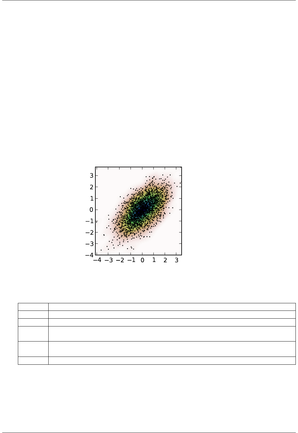
SciPy Reference Guide, Release 0.13.0
>>> X,Y=np.mgrid[xmin:xmax:100j, ymin:ymax:100j]
>>> positions =np.vstack([X.ravel(), Y.ravel()])
>>> values =np.vstack([m1, m2])
>>> kernel =stats.gaussian_kde(values)
>>> Z=np.reshape(kernel(positions).T, X.shape)
Plot the results:
>>> import matplotlib.pyplot as plt
>>> fig =plt.figure()
>>> ax =fig.add_subplot(111)
>>> ax.imshow(np.rot90(Z), cmap=plt.cm.gist_earth_r,
... extent=[xmin, xmax, ymin, ymax])
>>> ax.plot(m1, m2, ’k.’, markersize=2)
>>> ax.set_xlim([xmin, xmax])
>>> ax.set_ylim([ymin, ymax])
>>> plt.show()
Attributes
dataset (ndarray) The dataset with which gaussian_kde was initialized.
d (int) Number of dimensions.
n (int) Number of datapoints.
factor (float) The bandwidth factor, obtained from kde.covariance_factor, with which the covariance
matrix is multiplied.
covari-
ance
(ndarray) The covariance matrix of dataset, scaled by the calculated bandwidth (kde.factor).
inv_cov (ndarray) The inverse of covariance.
5.29. Statistical functions (scipy.stats) 1161

SciPy Reference Guide, Release 0.13.0
Methods
kde.evaluate(points) (ndarray) Evaluate the estimated pdf on a provided set of points.
kde(points) (ndarray) Same as kde.evaluate(points)
kde.integrate_gaussian(mean,
cov)
(float) Multiply pdf with a specified Gaussian and integrate over the whole
domain.
kde.integrate_box_1d(low,
high)
(float) Integrate pdf (1D only) between two bounds.
kde.integrate_box(low_bounds,
high_bounds)
(float) Integrate pdf over a rectangular space between low_bounds and
high_bounds.
kde.integrate_kde(other_kde)(float) Integrate two kernel density estimates multiplied together.
kde.resample(size=None)(ndarray) Randomly sample a dataset from the estimated pdf.
kde.set_bandwidth(bw_method=’scott’)(None) Computes the bandwidth, i.e. the coefficient that multiplies the data
covariance matrix to obtain the kernel covariance matrix. .. versionadded:: 0.11.0
kde.covariance_factor (float) Computes the coefficient (kde.factor) that multiplies the data covariance
matrix to obtain the kernel covariance matrix. The default is scotts_factor.
A subclass can overwrite this method to provide a different method, or set it
through a call to kde.set_bandwidth.
For many more stat related functions install the software R and the interface package rpy.
5.30 Statistical functions for masked arrays (scipy.stats.mstats)
This module contains a large number of statistical functions that can be used with masked arrays.
Most of these functions are similar to those in scipy.stats but might have small differences in the API or in the algorithm
used. Since this is a relatively new package, some API changes are still possible.
argstoarray(*args) Constructs a 2D array from a group of sequences.
betai(a, b, x) Returns the incomplete beta function.
chisquare(f_obs[, f_exp, ddof, axis]) Calculates a one-way chi square test.
count_tied_groups(x[, use_missing]) Counts the number of tied values.
describe(a[, axis]) Computes several descriptive statistics of the passed array.
f_oneway(*args) Performs a 1-way ANOVA, returning an F-value and probability given
f_value_wilks_lambda(ER, EF, dfnum, dfden, a, b) Calculation of Wilks lambda F-statistic for multivarite data, per
find_repeats(arr) Find repeats in arr and return a tuple (repeats, repeat_count).
friedmanchisquare(*args) Friedman Chi-Square is a non-parametric, one-way within-subjects ANOVA.
gmean(a[, axis]) Compute the geometric mean along the specified axis.
hmean(a[, axis]) Calculates the harmonic mean along the specified axis.
kendalltau(x, y[, use_ties, use_missing]) Computes Kendall’s rank correlation tau on two variables xand y.
kendalltau_seasonal(x) Computes a multivariate Kendall’s rank correlation tau, for seasonal data.
kruskalwallis(*args) Compute the Kruskal-Wallis H-test for independent samples
kruskalwallis(*args) Compute the Kruskal-Wallis H-test for independent samples
ks_twosamp(data1, data2[, alternative]) Computes the Kolmogorov-Smirnov test on two samples.
ks_twosamp(data1, data2[, alternative]) Computes the Kolmogorov-Smirnov test on two samples.
kurtosis(a[, axis, fisher, bias]) Computes the kurtosis (Fisher or Pearson) of a dataset.
kurtosistest(a[, axis]) Tests whether a dataset has normal kurtosis
linregress(*args) Calculate a regression line
mannwhitneyu(x, y[, use_continuity]) Computes the Mann-Whitney statistic
plotting_positions(data[, alpha, beta]) Returns plotting positions (or empirical percentile points) for the data.
mode(a[, axis]) Returns an array of the modal (most common) value in the passed array.
Continued on next page
1162 Chapter 5. Reference

SciPy Reference Guide, Release 0.13.0
Table 5.234 – continued from previous page
moment(a[, moment, axis]) Calculates the nth moment about the mean for a sample.
mquantiles(a[, prob, alphap, betap, axis, limit]) Computes empirical quantiles for a data array.
msign(x) Returns the sign of x, or 0 if x is masked.
normaltest(a[, axis]) Tests whether a sample differs from a normal distribution.
obrientransform(*args) Computes a transform on input data (any number of columns).
pearsonr(x, y) Calculates a Pearson correlation coefficient and the p-value for testing
plotting_positions(data[, alpha, beta]) Returns plotting positions (or empirical percentile points) for the data.
pointbiserialr(x, y) Calculates a point biserial correlation coefficient and the associated p-value.
rankdata(data[, axis, use_missing]) Returns the rank (also known as order statistics) of each data point along the given axis.
scoreatpercentile(data, per[, limit, ...]) Calculate the score at the given ‘per’ percentile of the sequence a.
sem(a[, axis]) Calculates the standard error of the mean (or standard error of measurement) of the values in the input array.
signaltonoise(data[, axis]) Calculates the signal-to-noise ratio, as the ratio of the mean over standard deviation along the given axis.
skew(a[, axis, bias]) Computes the skewness of a data set.
skewtest(a[, axis]) Tests whether the skew is different from the normal distribution.
spearmanr(x, y[, use_ties]) Calculates a Spearman rank-order correlation coefficient and the p-value
theilslopes(y[, x, alpha]) Computes the Theil slope as the median of all slopes between paired values.
threshold(a[, threshmin, threshmax, newval]) Clip array to a given value.
tmax(a, upperlimit[, axis, inclusive]) Compute the trimmed maximum
tmean(a[, limits, inclusive]) Compute the trimmed mean
tmin(a[, lowerlimit, axis, inclusive]) Compute the trimmed minimum
trim(a[, limits, inclusive, relative, axis]) Trims an array by masking the data outside some given limits.
trima(a[, limits, inclusive]) Trims an array by masking the data outside some given limits.
trimboth(data[, proportiontocut, inclusive, ...]) Trims the smallest and largest data values.
trimmed_stde(a[, limits, inclusive, axis]) Returns the standard error of the trimmed mean along the given axis.
trimr(a[, limits, inclusive, axis]) Trims an array by masking some proportion of the data on each end.
trimtail(data[, proportiontocut, tail, ...]) Trims the data by masking values from one tail.
tsem(a[, limits, inclusive]) Compute the trimmed standard error of the mean
ttest_onesamp(a, popmean) Calculates the T-test for the mean of ONE group of scores.
ttest_ind(a, b[, axis]) Calculates the T-test for the means of TWO INDEPENDENT samples of scores.
ttest_onesamp(a, popmean) Calculates the T-test for the mean of ONE group of scores.
ttest_rel(a, b[, axis]) Calculates the T-test on TWO RELATED samples of scores, a and b.
tvar(a[, limits, inclusive]) Compute the trimmed variance
variation(a[, axis]) Computes the coefficient of variation, the ratio of the biased standard deviation to the mean.
winsorize(a[, limits, inclusive, inplace, axis]) Returns a Winsorized version of the input array.
zmap(scores, compare[, axis, ddof]) Calculates the relative z-scores.
zscore(a[, axis, ddof]) Calculates the z score of each value in the sample, relative to the sample mean and standard deviation.
scipy.stats.mstats.argstoarray(*args)
Constructs a 2D array from a group of sequences.
Sequences are filled with missing values to match the length of the longest sequence.
Parameters args : sequences
Group of sequences.
Returns argstoarray : MaskedArray
A ( mxn) masked array, where mis the number of arguments and nthe
length of the longest argument.
Notes
numpy.ma.row_stack has identical behavior, but is called with a sequence of sequences.
scipy.stats.mstats.betai(a,b,x)
Returns the incomplete beta function.
5.30. Statistical functions for masked arrays (scipy.stats.mstats) 1163

SciPy Reference Guide, Release 0.13.0
I_x(a,b) = 1/B(a,b)*(Integral(0,x) of t^(a-1)(1-t)^(b-1) dt)
where a,b>0 and B(a,b) = G(a)*G(b)/(G(a+b)) where G(a) is the gamma function of a.
The standard broadcasting rules apply to a, b, and x.
Parameters a: array_like or float > 0
b: array_like or float > 0
x: array_like or float
x will be clipped to be no greater than 1.0 .
Returns betai : ndarray
Incomplete beta function.
scipy.stats.mstats.chisquare(f_obs,f_exp=None,ddof=0,axis=0)
Calculates a one-way chi square test.
The chi square test tests the null hypothesis that the categorical data has the given frequencies.
Parameters f_obs : array
Observed frequencies in each category.
f_exp : array, optional
Expected frequencies in each category. By default the categories are as-
sumed to be equally likely.
ddof : int, optional
“Delta degrees of freedom”: adjustment to the degrees of freedom for the
p-value. The p-value is computed using a chi-squared distribution with k
- 1 - ddof degrees of freedom, where kis the number of observed fre-
quencies. The default value of ddof is 0.
axis : int or None, optional
The axis of the broadcast result of f_obs and f_exp along which to apply
the test. If axis is None, all values in f_obs are treated as a single data set.
Default is 0.
Returns chisq : float or ndarray
The chi-squared test statistic. The value is a float if axis is None or f_obs
and f_exp are 1-D.
p: float or ndarray
The p-value of the test. The value is a float if ddof and the return value
chisq are scalars.
See Also
power_divergence,mstats.chisquare
Notes
This test is invalid when the observed or expected frequencies in each category are too small. A typical rule is
that all of the observed and expected frequencies should be at least 5.
The default degrees of freedom, k-1, are for the case when no parameters of the distribution are estimated. If
p parameters are estimated by efficient maximum likelihood then the correct degrees of freedom are k-1-p. If
the parameters are estimated in a different way, then the dof can be between k-1-p and k-1. However, it is also
possible that the asymptotic distribution is not a chisquare, in which case this test is not appropriate.
References
[R226],[R227]
1164 Chapter 5. Reference

SciPy Reference Guide, Release 0.13.0
Examples
When just f_obs is given, it is assumed that the expected frequencies are uniform and given by the mean of the
observed frequencies.
>>> chisquare([16,18,16,14,12,12])
(2.0, 0.84914503608460956)
With f_exp the expected frequencies can be given.
>>> chisquare([16,18,16,14,12,12], f_exp=[16,16,16,16,16,8])
(3.5, 0.62338762774958223)
When f_obs is 2-D, by default the test is applied to each column.
>>> obs =np.array([[16,18,16,14,12,12], [32,24,16,28,20,24]]).T
>>> obs.shape
(6, 2)
>>> chisquare(obs)
(array([ 2. , 6.66666667]), array([ 0.84914504, 0.24663415]))
By setting axis=None, the test is applied to all data in the array, which is equivalent to applying the test to the
flattened array.
>>> chisquare(obs, axis=None)
(23.31034482758621, 0.015975692534127565)
>>> chisquare(obs.ravel())
(23.31034482758621, 0.015975692534127565)
ddof is the change to make to the default degrees of freedom.
>>> chisquare([16,18,16,14,12,12], ddof=1)
(2.0, 0.73575888234288467)
The calculation of the p-values is done by broadcasting the chi-squared statistic with ddof.
>>> chisquare([16,18,16,14,12,12], ddof=[0,1,2])
(2.0, array([ 0.84914504, 0.73575888, 0.5724067 ]))
f_obs and f_exp are also broadcast. In the following, f_obs has shape (6,) and f_exp has shape (2, 6), so the
result of broadcasting f_obs and f_exp has shape (2, 6). To compute the desired chi-squared statistics, we use
axis=1:
>>> chisquare([16,18,16,14,12,12],
... f_exp=[[16,16,16,16,16,8], [8,20,20,16,12,12]],
... axis=1)
(array([ 3.5 , 9.25]), array([ 0.62338763, 0.09949846]))
scipy.stats.mstats.count_tied_groups(x,use_missing=False)
Counts the number of tied values.
Parameters x: sequence
Sequence of data on which to counts the ties
use_missing : boolean
Whether to consider missing values as tied.
Returns count_tied_groups : dict
Returns a dictionary (nb of ties: nb of groups).
5.30. Statistical functions for masked arrays (scipy.stats.mstats) 1165

SciPy Reference Guide, Release 0.13.0
Examples
>>> z=[0,0,0,2,2,2,3,3,4,5,6]
>>> count_tied_groups(z)
>>> {2:1,3:2}
>>> # The ties were 0 (3x), 2 (3x) and 3 (2x)
>>> z=ma.array([0,0,1,2,2,2,3,3,4,5,6])
>>> count_tied_groups(z)
>>> {2:2,3:1}
>>> # The ties were 0 (2x), 2 (3x) and 3 (2x)
>>> z[[1,-1]] =masked
>>> count_tied_groups(z, use_missing=True)
>>> {2:2,3:1}
>>> # The ties were 2 (3x), 3 (2x) and masked (2x)
scipy.stats.mstats.describe(a,axis=0)
Computes several descriptive statistics of the passed array.
Parameters a: array
axis : int or None
Returns n: int
(size of the data (discarding missing values)
mm : (int, int)
min, max
arithmetic mean : float
unbiased variance : float
biased skewness : float
biased kurtosis : float
Examples
>>> ma =np.ma.array(range(6), mask=[0,0,0,1,1,1])
>>> describe(ma)
(array(3),
(0, 2),
1.0,
1.0,
masked_array(data = 0.0,
mask = False,
fill_value = 1e+20)
,
-1.5)
scipy.stats.mstats.f_oneway(*args)
Performs a 1-way ANOVA, returning an F-value and probability given any number of groups. From Heiman,
pp.394-7.
Usage: f_oneway (*args) where *args is 2 or more arrays, one per
treatment group
Returns: f-value, probability
scipy.stats.mstats.f_value_wilks_lambda(ER,EF,dfnum,dfden,a,b)
Calculation of Wilks lambda F-statistic for multivarite data, per Maxwell & Delaney p.657.
scipy.stats.mstats.find_repeats(arr)
Find repeats in arr and return a tuple (repeats, repeat_count). Masked values are discarded.
Parameters arr : sequence
Input array. The array is flattened if it is not 1D.
Returns repeats : ndarray
1166 Chapter 5. Reference

SciPy Reference Guide, Release 0.13.0
Array of repeated values.
counts [ndarray] Array of counts.
scipy.stats.mstats.friedmanchisquare(*args)
Friedman Chi-Square is a non-parametric, one-way within-subjects ANOVA. This function calculates the Fried-
man Chi-square test for repeated measures and returns the result, along with the associated probability
value.
Each input is considered a given group. Ideally, the number of treatments among each group should be equal.
If this is not the case, only the first n treatments are taken into account, where n is the number of treatments of
the smallest group. If a group has some missing values, the corresponding treatments are masked in the other
groups. The test statistic is corrected for ties.
Masked values in one group are propagated to the other groups.
Returns: chi-square statistic, associated p-value
scipy.stats.mstats.gmean(a,axis=0)
Compute the geometric mean along the specified axis.
Returns the geometric average of the array elements. That is: n-th root of (x1 * x2 * ... * xn)
Parameters a: array_like
Input array or object that can be converted to an array.
axis : int, optional, default axis=0
Axis along which the geometric mean is computed.
dtype : dtype, optional
Type of the returned array and of the accumulator in which the elements
are summed. If dtype is not specified, it defaults to the dtype of a, unless a
has an integer dtype with a precision less than that of the default platform
integer. In that case, the default platform integer is used.
Returns gmean : ndarray
see dtype parameter above
See Also
numpy.meanArithmetic average
numpy.average
Weighted average
hmean Harmonic mean
Notes
The geometric average is computed over a single dimension of the input array, axis=0 by default, or all values
in the array if axis=None. float64 intermediate and return values are used for integer inputs.
Use masked arrays to ignore any non-finite values in the input or that arise in the calculations such as Not a
Number and infinity because masked arrays automatically mask any non-finite values.
scipy.stats.mstats.hmean(a,axis=0)
Calculates the harmonic mean along the specified axis.
That is: n / (1/x1 + 1/x2 + ... + 1/xn)
Parameters a: array_like
Input array, masked array or object that can be converted to an array.
axis : int, optional, default axis=0
Axis along which the harmonic mean is computed.
dtype : dtype, optional
5.30. Statistical functions for masked arrays (scipy.stats.mstats) 1167

SciPy Reference Guide, Release 0.13.0
Type of the returned array and of the accumulator in which the elements
are summed. If dtype is not specified, it defaults to the dtype of a, unless a
has an integer dtype with a precision less than that of the default platform
integer. In that case, the default platform integer is used.
Returns hmean : ndarray
see dtype parameter above
See Also
numpy.meanArithmetic average
numpy.average
Weighted average
gmean Geometric mean
Notes
The harmonic mean is computed over a single dimension of the input array, axis=0 by default, or all values in
the array if axis=None. float64 intermediate and return values are used for integer inputs.
Use masked arrays to ignore any non-finite values in the input or that arise in the calculations such as Not a
Number and infinity.
scipy.stats.mstats.kendalltau(x,y,use_ties=True,use_missing=False)
Computes Kendall’s rank correlation tau on two variables xand y.
Parameters xdata : sequence
First data list (for example, time).
ydata : sequence
Second data list.
use_ties : {True, False}, optional
Whether ties correction should be performed.
use_missing : {False, True}, optional
Whether missing data should be allocated a rank of 0 (False) or the average
rank (True)
Returns tau : float
Kendall tau
prob : float
Approximate 2-side p-value.
scipy.stats.mstats.kendalltau_seasonal(x)
Computes a multivariate Kendall’s rank correlation tau, for seasonal data.
Parameters x: 2-D ndarray
Array of seasonal data, with seasons in columns.
scipy.stats.mstats.kruskalwallis(*args)
Compute the Kruskal-Wallis H-test for independent samples
The Kruskal-Wallis H-test tests the null hypothesis that the population median of all of the groups are equal.
It is a non-parametric version of ANOVA. The test works on 2 or more independent samples, which may have
different sizes. Note that rejecting the null hypothesis does not indicate which of the groups differs. Post-hoc
comparisons between groups are required to determine which groups are different.
Parameters sample1, sample2, ... : array_like
Two or more arrays with the sample measurements can be given as argu-
ments.
Returns H-statistic : float
The Kruskal-Wallis H statistic, corrected for ties
p-value : float
The p-value for the test using the assumption that H has a chi square distri-
bution
1168 Chapter 5. Reference

SciPy Reference Guide, Release 0.13.0
Notes
Due to the assumption that H has a chi square distribution, the number of samples in each group must not be too
small. A typical rule is that each sample must have at least 5 measurements.
References
[R228]
scipy.stats.mstats.kruskalwallis(*args)
Compute the Kruskal-Wallis H-test for independent samples
The Kruskal-Wallis H-test tests the null hypothesis that the population median of all of the groups are equal.
It is a non-parametric version of ANOVA. The test works on 2 or more independent samples, which may have
different sizes. Note that rejecting the null hypothesis does not indicate which of the groups differs. Post-hoc
comparisons between groups are required to determine which groups are different.
Parameters sample1, sample2, ... : array_like
Two or more arrays with the sample measurements can be given as argu-
ments.
Returns H-statistic : float
The Kruskal-Wallis H statistic, corrected for ties
p-value : float
The p-value for the test using the assumption that H has a chi square distri-
bution
Notes
Due to the assumption that H has a chi square distribution, the number of samples in each group must not be too
small. A typical rule is that each sample must have at least 5 measurements.
References
[R228]
scipy.stats.mstats.ks_twosamp(data1,data2,alternative=’two-sided’)
Computes the Kolmogorov-Smirnov test on two samples.
Missing values are discarded.
Parameters data1 : array_like
First data set
data2 : array_like
Second data set
alternative : {‘two-sided’, ‘less’, ‘greater’}, optional
Indicates the alternative hypothesis. Default is ‘two-sided’.
Returns d: float
Value of the Kolmogorov Smirnov test
p: float
Corresponding p-value.
scipy.stats.mstats.ks_twosamp(data1,data2,alternative=’two-sided’)
Computes the Kolmogorov-Smirnov test on two samples.
Missing values are discarded.
Parameters data1 : array_like
First data set
data2 : array_like
Second data set
alternative : {‘two-sided’, ‘less’, ‘greater’}, optional
Indicates the alternative hypothesis. Default is ‘two-sided’.
5.30. Statistical functions for masked arrays (scipy.stats.mstats) 1169

SciPy Reference Guide, Release 0.13.0
Returns d: float
Value of the Kolmogorov Smirnov test
p: float
Corresponding p-value.
scipy.stats.mstats.kurtosis(a,axis=0,fisher=True,bias=True)
Computes the kurtosis (Fisher or Pearson) of a dataset.
Kurtosis is the fourth central moment divided by the square of the variance. If Fisher’s definition is used, then
3.0 is subtracted from the result to give 0.0 for a normal distribution.
If bias is False then the kurtosis is calculated using k statistics to eliminate bias coming from biased moment
estimators
Use kurtosistest to see if result is close enough to normal.
Parameters a: array
data for which the kurtosis is calculated
axis : int or None
Axis along which the kurtosis is calculated
fisher : bool
If True, Fisher’s definition is used (normal ==> 0.0). If False, Pearson’s
definition is used (normal ==> 3.0).
bias : bool
If False, then the calculations are corrected for statistical bias.
Returns kurtosis : array
The kurtosis of values along an axis. If all values are equal, return -3 for
Fisher’s definition and 0 for Pearson’s definition.
References
[R229]
scipy.stats.mstats.kurtosistest(a,axis=0)
Tests whether a dataset has normal kurtosis
This function tests the null hypothesis that the kurtosis of the population from which the sample was drawn is
that of the normal distribution: kurtosis = 3(n-1)/(n+1).
Parameters a: array
array of the sample data
axis : int or None
the axis to operate along, or None to work on the whole array. The default
is the first axis.
Returns z-score : float
The computed z-score for this test.
p-value : float
The 2-sided p-value for the hypothesis test
Notes
Valid only for n>20. The Z-score is set to 0 for bad entries.
scipy.stats.mstats.linregress(*args)
Calculate a regression line
This computes a least-squares regression for two sets of measurements.
Parameters x, y : array_like
1170 Chapter 5. Reference

SciPy Reference Guide, Release 0.13.0
two sets of measurements. Both arrays should have the same length. If only
x is given (and y=None), then it must be a two-dimensional array where one
dimension has length 2. The two sets of measurements are then found by
splitting the array along the length-2 dimension.
Returns slope : float
slope of the regression line
intercept [float] intercept of the regression line
r-value [float] correlation coefficient
p-value [float] two-sided p-value for a hypothesis test whose null hy-
pothesis is that the slope is zero.
stderr [float] Standard error of the estimate
Notes
Missing values are considered pair-wise: if a value is missing in x, the corresponding value in y is masked.
Examples
>>> from scipy import stats
>>> import numpy as np
>>> x=np.random.random(10)
>>> y=np.random.random(10)
>>> slope, intercept, r_value, p_value, std_err =stats.linregress(x,y)
# To get coefficient of determination (r_squared)
>>> print "r-squared:", r_value**2
r-squared: 0.15286643777
scipy.stats.mstats.mannwhitneyu(x,y,use_continuity=True)
Computes the Mann-Whitney statistic
Missing values in xand/or yare discarded.
Parameters x: sequence
Input
y: sequence
Input
use_continuity : {True, False}, optional
Whether a continuity correction (1/2.) should be taken into account.
Returns u: float
The Mann-Whitney statistics
prob : float
Approximate p-value assuming a normal distribution.
scipy.stats.mstats.plotting_positions(data,alpha=0.4,beta=0.4)
Returns plotting positions (or empirical percentile points) for the data.
Plotting positions are defined as (i-alpha)/(n+1-alpha-beta), where:
•i is the rank order statistics
•n is the number of unmasked values along the given axis
•alpha and beta are two parameters.
Typical values for alpha and beta are:
•(0,1) : p(k) = k/n, linear interpolation of cdf (R, type 4)
•(.5,.5) : p(k) = (k-1/2.)/n, piecewise linear function (R, type 5)
•(0,0) : p(k) = k/(n+1), Weibull (R type 6)
•(1,1) : p(k) = (k-1)/(n-1), in this case, p(k) = mode[F(x[k])].
That’s R default (R type 7)
5.30. Statistical functions for masked arrays (scipy.stats.mstats) 1171

SciPy Reference Guide, Release 0.13.0
•(1/3,1/3): p(k) = (k-1/3)/(n+1/3), then p(k) ~
median[F(x[k])]. The resulting quantile estimates are approximately
median-unbiased regardless of the distribution of x. (R type 8)
•(3/8,3/8): p(k) = (k-3/8)/(n+1/4), Blom. The resulting quantile esti-
mates are approximately unbiased if x is normally distributed (R type 9)
•(.4,.4) : approximately quantile unbiased (Cunnane)
•(.35,.35): APL, used with PWM
•(.3175, .3175): used in scipy.stats.probplot
Parameters data : array_like
Input data, as a sequence or array of dimension at most 2.
alpha : float, optional
Plotting positions parameter. Default is 0.4.
beta : float, optional
Plotting positions parameter. Default is 0.4.
Returns positions : MaskedArray
The calculated plotting positions.
scipy.stats.mstats.mode(a,axis=0)
Returns an array of the modal (most common) value in the passed array.
If there is more than one such value, only the first is returned. The bin-count for the modal bins is also returned.
Parameters a: array_like
n-dimensional array of which to find mode(s).
axis : int, optional
Axis along which to operate. Default is 0, i.e. the first axis.
Returns vals : ndarray
Array of modal values.
counts : ndarray
Array of counts for each mode.
Examples
>>> a=np.array([[6,8,3,0],
[3, 2, 1, 7],
[8, 1, 8, 4],
[5, 3, 0, 5],
[4, 7, 5, 9]])
>>> from scipy import stats
>>> stats.mode(a)
(array([[ 3., 1., 0., 0.]]), array([[ 1., 1., 1., 1.]]))
To get mode of whole array, specify axis=None:
>>> stats.mode(a, axis=None)
(array([ 3.]), array([ 3.]))
scipy.stats.mstats.moment(a,moment=1,axis=0)
Calculates the nth moment about the mean for a sample.
Generally used to calculate coefficients of skewness and kurtosis.
Parameters a: array_like
data
moment : int
order of central moment that is returned
axis : int or None
1172 Chapter 5. Reference

SciPy Reference Guide, Release 0.13.0
Axis along which the central moment is computed. If None, then the data
array is raveled. The default axis is zero.
Returns n-th central moment : ndarray or float
The appropriate moment along the given axis or over all values if axis is
None. The denominator for the moment calculation is the number of obser-
vations, no degrees of freedom correction is done.
scipy.stats.mstats.mquantiles(a, prob=[0.25, 0.5, 0.75], alphap=0.4, betap=0.4, axis=None,
limit=())
Computes empirical quantiles for a data array.
Samples quantile are defined by Q(p) = (1-gamma)*x[j] + gamma*x[j+1], where x[j] is the j-th
order statistic, and gamma is a function of j = floor(n*p + m),m = alphap + p*(1 - alphap
- betap) and g=n*p+m-j.
Reinterpreting the above equations to compare to Rlead to the equation: p(k) = (k - alphap)/(n +
1 - alphap - betap)
Typical values of (alphap,betap) are:
•(0,1) : p(k) = k/n : linear interpolation of cdf (Rtype 4)
•(.5,.5) : p(k) = (k - 1/2.)/n : piecewise linear function (Rtype 5)
•(0,0) : p(k) = k/(n+1) : (Rtype 6)
•(1,1) : p(k) = (k-1)/(n-1): p(k) = mode[F(x[k])]. (Rtype 7, Rdefault)
•(1/3,1/3): p(k) = (k-1/3)/(n+1/3): Then p(k) ~ median[F(x[k])]. The
resulting quantile estimates are approximately median-unbiased regardless of the
distribution of x. (Rtype 8)
•(3/8,3/8): p(k) = (k-3/8)/(n+1/4): Blom. The resulting quantile esti-
mates are approximately unbiased if x is normally distributed (Rtype 9)
•(.4,.4) : approximately quantile unbiased (Cunnane)
•(.35,.35): APL, used with PWM
Parameters a: array_like
Input data, as a sequence or array of dimension at most 2.
prob : array_like, optional
List of quantiles to compute.
alphap : float, optional
Plotting positions parameter, default is 0.4.
betap : float, optional
Plotting positions parameter, default is 0.4.
axis : int, optional
Axis along which to perform the trimming. If None (default), the input
array is first flattened.
limit : tuple
Tuple of (lower, upper) values. Values of aoutside this open interval are
ignored.
Returns mquantiles : MaskedArray
An array containing the calculated quantiles.
Notes
This formulation is very similar to Rexcept the calculation of mfrom alphap and betap, where in Rmis
defined with each type.
References
[R230]
5.30. Statistical functions for masked arrays (scipy.stats.mstats) 1173

SciPy Reference Guide, Release 0.13.0
Examples
>>> from scipy.stats.mstats import mquantiles
>>> a=np.array([6.,47.,49.,15.,42.,41.,7.,39.,43.,40.,36.])
>>> mquantiles(a)
array([ 19.2, 40. , 42.8])
Using a 2D array, specifying axis and limit.
>>> data =np.array([[ 6.,7.,1.],
[ 47., 15., 2.],
[ 49., 36., 3.],
[ 15., 39., 4.],
[ 42., 40., -999.],
[ 41., 41., -999.],
[ 7., -999., -999.],
[ 39., -999., -999.],
[ 43., -999., -999.],
[ 40., -999., -999.],
[ 36., -999., -999.]])
>>> mquantiles(data, axis=0, limit=(0,50))
array([[ 19.2 , 14.6 , 1.45],
[ 40. , 37.5 , 2.5 ],
[ 42.8 , 40.05, 3.55]])
>>> data[:, 2]= -999.
>>> mquantiles(data, axis=0, limit=(0,50))
masked_array(data =
[[19.2 14.6 --]
[40.0 37.5 --]
[42.8 40.05 --]],
mask =
[[False False True]
[False False True]
[False False True]],
fill_value = 1e+20)
scipy.stats.mstats.msign(x)
Returns the sign of x, or 0 if x is masked.
scipy.stats.mstats.normaltest(a,axis=0)
Tests whether a sample differs from a normal distribution.
This function tests the null hypothesis that a sample comes from a normal distribution. It is based on D’Agostino
and Pearson’s [R231],[R232] test that combines skew and kurtosis to produce an omnibus test of normality.
Parameters a: array_like
The array containing the data to be tested.
axis : int or None
If None, the array is treated as a single data set, regardless of its shape.
Otherwise, each 1-d array along axis axis is tested.
Returns k2 : float or array
s^2 + k^2, where sis the z-score returned by skewtest and kis the z-score
returned by kurtosistest.
p-value : float or array
A 2-sided chi squared probability for the hypothesis test.
1174 Chapter 5. Reference

SciPy Reference Guide, Release 0.13.0
References
[R231],[R232]
scipy.stats.mstats.obrientransform(*args)
Computes a transform on input data (any number of columns). Used to test for homogeneity of variance prior
to running one-way stats. Each array in *args is one level of a factor. If an F_oneway() run on the transformed
data and found significant, variances are unequal. From Maxwell and Delaney, p.112.
Returns: transformed data for use in an ANOVA
scipy.stats.mstats.pearsonr(x,y)
Calculates a Pearson correlation coefficient and the p-value for testing non-correlation.
The Pearson correlation coefficient measures the linear relationship between two datasets. Strictly speaking,
Pearson’s correlation requires that each dataset be normally distributed. Like other correlation coefficients, this
one varies between -1 and +1 with 0 implying no correlation. Correlations of -1 or +1 imply an exact linear
relationship. Positive correlations imply that as xincreases, so does y. Negative correlations imply that as x
increases, ydecreases.
The p-value roughly indicates the probability of an uncorrelated system producing datasets that have a Pearson
correlation at least as extreme as the one computed from these datasets. The p-values are not entirely reliable
but are probably reasonable for datasets larger than 500 or so.
Parameters x: 1-D array_like
Input
y: 1-D array_like
Input
Returns pearsonr : float
Pearson’s correlation coefficient, 2-tailed p-value.
References
http://www.statsoft.com/textbook/glosp.html#Pearson%20Correlation
scipy.stats.mstats.plotting_positions(data,alpha=0.4,beta=0.4)
Returns plotting positions (or empirical percentile points) for the data.
Plotting positions are defined as (i-alpha)/(n+1-alpha-beta), where:
•i is the rank order statistics
•n is the number of unmasked values along the given axis
•alpha and beta are two parameters.
Typical values for alpha and beta are:
•(0,1) : p(k) = k/n, linear interpolation of cdf (R, type 4)
•(.5,.5) : p(k) = (k-1/2.)/n, piecewise linear function (R, type 5)
•(0,0) : p(k) = k/(n+1), Weibull (R type 6)
•(1,1) : p(k) = (k-1)/(n-1), in this case, p(k) = mode[F(x[k])].
That’s R default (R type 7)
•(1/3,1/3): p(k) = (k-1/3)/(n+1/3), then p(k) ~
median[F(x[k])]. The resulting quantile estimates are approximately
median-unbiased regardless of the distribution of x. (R type 8)
•(3/8,3/8): p(k) = (k-3/8)/(n+1/4), Blom. The resulting quantile esti-
mates are approximately unbiased if x is normally distributed (R type 9)
•(.4,.4) : approximately quantile unbiased (Cunnane)
•(.35,.35): APL, used with PWM
•(.3175, .3175): used in scipy.stats.probplot
Parameters data : array_like
5.30. Statistical functions for masked arrays (scipy.stats.mstats) 1175

SciPy Reference Guide, Release 0.13.0
Input data, as a sequence or array of dimension at most 2.
alpha : float, optional
Plotting positions parameter. Default is 0.4.
beta : float, optional
Plotting positions parameter. Default is 0.4.
Returns positions : MaskedArray
The calculated plotting positions.
scipy.stats.mstats.pointbiserialr(x,y)
Calculates a point biserial correlation coefficient and the associated p-value.
The point biserial correlation is used to measure the relationship between a binary variable, x, and a
continuous variable, y. Like other correlation coefficients, this one varies between -1 and +1 with 0
implying no correlation. Correlations of -1 or +1 imply a determinative relationship.
This function uses a shortcut formula but produces the same result as pearsonr.
Parameters x: array_like of bools
Input array.
y[array_like] Input array.
Returns r: float
R value
p-value [float] 2-tailed p-value
Notes
Missing values are considered pair-wise: if a value is missing in x, the corresponding value in y is masked.
Examples
>>> from scipy import stats
>>> a=np.array([0,0,0,1,1,1,1])
>>> b=np.arange(7)
>>> stats.pointbiserialr(a, b)
(0.8660254037844386, 0.011724811003954652)
>>> stats.pearsonr(a, b)
(0.86602540378443871, 0.011724811003954626)
>>> np.corrcoef(a, b)
array([[ 1. , 0.8660254],
[ 0.8660254, 1. ]])
scipy.stats.mstats.rankdata(data,axis=None,use_missing=False)
Returns the rank (also known as order statistics) of each data point along the given axis.
If some values are tied, their rank is averaged. If some values are masked, their rank is set to 0 if use_missing is
False, or set to the average rank of the unmasked values if use_missing is True.
Parameters data : sequence
Input data. The data is transformed to a masked array
axis [{None,int}, optional] Axis along which to perform the
ranking. If None, the array is first flattened. An exception
is raised if the axis is specified for arrays with a dimension
larger than 2
use_missing [{boolean}, optional] Whether the masked values have a
rank of 0 (False) or equal to the average rank of the un-
masked values (True).
1176 Chapter 5. Reference

SciPy Reference Guide, Release 0.13.0
scipy.stats.mstats.scoreatpercentile(data,per,limit=(),alphap=0.4,betap=0.4)
Calculate the score at the given ‘per’ percentile of the sequence a. For example, the score at per=50 is the
median.
This function is a shortcut to mquantile
scipy.stats.mstats.sem(a,axis=0)
Calculates the standard error of the mean (or standard error of measurement) of the values in the input array.
Parameters a: array_like
An array containing the values for which the standard error is returned.
axis : int or None, optional.
If axis is None, ravel afirst. If axis is an integer, this will be the axis over
which to operate. Defaults to 0.
ddof : int, optional
Delta degrees-of-freedom. How many degrees of freedom to adjust for bias
in limited samples relative to the population estimate of variance. Defaults
to 1.
Returns s: ndarray or float
The standard error of the mean in the sample(s), along the input axis.
Notes
The default value for ddof is different to the default (0) used by other ddof containing routines, such as np.std
nd stats.nanstd.
Examples
Find standard error along the first axis:
>>> from scipy import stats
>>> a=np.arange(20).reshape(5,4)
>>> stats.sem(a)
array([ 2.8284, 2.8284, 2.8284, 2.8284])
Find standard error across the whole array, using n degrees of freedom:
>>> stats.sem(a, axis=None, ddof=0)
1.2893796958227628
scipy.stats.mstats.signaltonoise(data,axis=0)
Calculates the signal-to-noise ratio, as the ratio of the mean over standard deviation along the given axis.
Parameters data : sequence
Input data
axis [{0, int}, optional] Axis along which to compute. If None,
the computation is performed on a flat version of the array.
scipy.stats.mstats.skew(a,axis=0,bias=True)
Computes the skewness of a data set.
For normally distributed data, the skewness should be about 0. A skewness value > 0 means that there is more
weight in the left tail of the distribution. The function skewtest can be used to determine if the skewness
value is close enough to 0, statistically speaking.
Parameters a: ndarray
data
axis : int or None
axis along which skewness is calculated
5.30. Statistical functions for masked arrays (scipy.stats.mstats) 1177

SciPy Reference Guide, Release 0.13.0
bias : bool
If False, then the calculations are corrected for statistical bias.
Returns skewness : ndarray
The skewness of values along an axis, returning 0 where all values are equal.
References
[CRCProbStat2000] Section 2.2.24.1
[CRCProbStat2000]
scipy.stats.mstats.skewtest(a,axis=0)
Tests whether the skew is different from the normal distribution.
This function tests the null hypothesis that the skewness of the population that the sample was drawn from is the
same as that of a corresponding normal distribution.
Parameters a: array
axis : int or None
Returns z-score : float
The computed z-score for this test.
p-value : float
a 2-sided p-value for the hypothesis test
Notes
The sample size must be at least 8.
scipy.stats.mstats.spearmanr(x,y,use_ties=True)
Calculates a Spearman rank-order correlation coefficient and the p-value to test for non-correlation.
The Spearman correlation is a nonparametric measure of the linear relationship between two datasets. Unlike the
Pearson correlation, the Spearman correlation does not assume that both datasets are normally distributed. Like
other correlation coefficients, this one varies between -1 and +1 with 0 implying no correlation. Correlations of
-1 or +1 imply an exact linear relationship. Positive correlations imply that as xincreases, so does y. Negative
correlations imply that as xincreases, ydecreases.
Missing values are discarded pair-wise: if a value is missing in x, the corresponding value in yis masked.
The p-value roughly indicates the probability of an uncorrelated system producing datasets that have a Spearman
correlation at least as extreme as the one computed from these datasets. The p-values are not entirely reliable
but are probably reasonable for datasets larger than 500 or so.
Parameters x: array_like
The length of xmust be > 2.
y: array_like
The length of ymust be > 2.
use_ties : bool, optional
Whether the correction for ties should be computed.
Returns spearmanr : float
Spearman correlation coefficient, 2-tailed p-value.
References
[CRCProbStat2000] section 14.7
scipy.stats.mstats.theilslopes(y,x=None,alpha=0.05)
Computes the Theil slope as the median of all slopes between paired values.
Parameters y: array_like
Dependent variable.
x: {None, array_like}, optional
Independent variable. If None, use arange(len(y)) instead.
1178 Chapter 5. Reference

SciPy Reference Guide, Release 0.13.0
alpha : float
Confidence degree.
Returns medslope : float
Theil slope
medintercept : float
Intercept of the Theil line, as median(y)-medslope*median(x)
lo_slope : float
Lower bound of the confidence interval on medslope
up_slope : float
Upper bound of the confidence interval on medslope
scipy.stats.mstats.threshold(a,threshmin=None,threshmax=None,newval=0)
Clip array to a given value.
Similar to numpy.clip(), except that values less than threshmin or greater than threshmax are replaced by newval,
instead of by threshmin and threshmax respectively.
Parameters a: ndarray
Input data
threshmin : {None, float}, optional
Lower threshold. If None, set to the minimum value.
threshmax : {None, float}, optional
Upper threshold. If None, set to the maximum value.
newval : {0, float}, optional
Value outside the thresholds.
Returns threshold : ndarray
Returns a, with values less then threshmin and values greater threshmax
replaced with newval.
scipy.stats.mstats.tmax(a,upperlimit,axis=0,inclusive=True)
Compute the trimmed maximum
This function computes the maximum value of an array along a given axis, while ignoring values larger than a
specified upper limit.
Parameters a: array_like
array of values
upperlimit : None or float, optional
Values in the input array greater than the given limit will be ignored. When
upperlimit is None, then all values are used. The default value is None.
axis : None or int, optional
Operate along this axis. None means to use the flattened array and the
default is zero.
inclusive : {True, False}, optional
This flag determines whether values exactly equal to the upper limit are
included. The default value is True.
Returns tmax : float
scipy.stats.mstats.tmean(a,limits=None,inclusive=(True,True))
Compute the trimmed mean
This function finds the arithmetic mean of given values, ignoring values outside the given limits.
Parameters a: array_like
array of values
limits : None or (lower limit, upper limit), optional
Values in the input array less than the lower limit or greater than the upper
limit will be ignored. When limits is None, then all values are used. Either
of the limit values in the tuple can also be None representing a half-open
interval. The default value is None.
5.30. Statistical functions for masked arrays (scipy.stats.mstats) 1179

SciPy Reference Guide, Release 0.13.0
inclusive : (bool, bool), optional
A tuple consisting of the (lower flag, upper flag). These flags determine
whether values exactly equal to the lower or upper limits are included. The
default value is (True, True).
Returns tmean : float
scipy.stats.mstats.tmin(a,lowerlimit=None,axis=0,inclusive=True)
Compute the trimmed minimum
This function finds the miminum value of an array aalong the specified axis, but only considering values greater
than a specified lower limit.
Parameters a: array_like
array of values
lowerlimit : None or float, optional
Values in the input array less than the given limit will be ignored. When
lowerlimit is None, then all values are used. The default value is None.
axis : None or int, optional
Operate along this axis. None means to use the flattened array and the
default is zero
inclusive : {True, False}, optional
This flag determines whether values exactly equal to the lower limit are
included. The default value is True.
Returns tmin : float
scipy.stats.mstats.trim(a,limits=None,inclusive=(True,True),relative=False,axis=None)
Trims an array by masking the data outside some given limits.
Returns a masked version of the input array.
Parameters a: sequence
Input array
limits : {None, tuple}, optional
If relative is False, tuple (lower limit, upper limit) in absolute values. Values
of the input array lower (greater) than the lower (upper) limit are masked.
If relative is True, tuple (lower percentage, upper percentage) to cut on each
side of the array, with respect to the number of unmasked data.
Noting n the number of unmasked data before trimming, the (n*limits[0])th
smallest data and the (n*limits[1])th largest data are masked, and the total
number of unmasked data after trimming is n*(1.-sum(limits)) In each case,
the value of one limit can be set to None to indicate an open interval.
If limits is None, no trimming is performed
inclusive : {(bool, bool) tuple}, optional
If relative is False, tuple indicating whether values exactly equal to the ab-
solute limits are allowed. If relative is True, tuple indicating whether the
number of data being masked on each side should be rounded (True) or
truncated (False).
relative : bool, optional
Whether to consider the limits as absolute values (False) or proportions to
cut (True).
axis : int, optional
Axis along which to trim.
Examples
>>> z=[1,2,3,4,5,6,7,8,9,10]
>>> trim(z,(3,8))
[--,--, 3, 4, 5, 6, 7, 8,--,--]
1180 Chapter 5. Reference

SciPy Reference Guide, Release 0.13.0
>>> trim(z,(0.1,0.2),relative=True)
[--, 2, 3, 4, 5, 6, 7, 8,--,--]
scipy.stats.mstats.trima(a,limits=None,inclusive=(True,True))
Trims an array by masking the data outside some given limits. Returns a masked version of the input array.
Parameters a: sequence
Input array.
limits : {None, tuple}, optional
Tuple of (lower limit, upper limit) in absolute values. Values of the input
array lower (greater) than the lower (upper) limit will be masked. A limit is
None indicates an open interval.
inclusive : {(True,True) tuple}, optional
Tuple of (lower flag, upper flag), indicating whether values exactly equal to
the lower (upper) limit are allowed.
scipy.stats.mstats.trimboth(data,proportiontocut=0.2,inclusive=(True,True),axis=None)
Trims the smallest and largest data values.
Trims the data by masking the int(proportiontocut *n) smallest and int(proportiontocut
*n) largest values of data along the given axis, where n is the number of unmasked values before trimming.
Parameters data : ndarray
Data to trim.
proportiontocut : float, optional
Percentage of trimming (as a float between 0 and 1). If n is the number of
unmasked values before trimming, the number of values after trimming is
(1 - 2*proportiontocut) *n. Default is 0.2.
inclusive : {(bool, bool) tuple}, optional
Tuple indicating whether the number of data being masked on each side
should be rounded (True) or truncated (False).
axis : int, optional
Axis along which to perform the trimming. If None, the input array is first
flattened.
scipy.stats.mstats.trimmed_stde(a,limits=(0.1,0.1),inclusive=(1,1),axis=None)
Returns the standard error of the trimmed mean along the given axis.
Parameters a: sequence
Input array
limits : {(0.1,0.1), tuple of float}, optional
tuple (lower percentage, upper percentage) to cut on each side of the array,
with respect to the number of unmasked data.
If n is the number of unmasked data before trimming, the values smaller
than n*limits[0] and the values larger than n*‘limits[1]
are masked, and the total number of unmasked data after trimming is n
*(1.-sum(limits)). In each case, the value of one limit can be set
to None to indicate an open interval. If limits is None, no trimming is per-
formed.
inclusive : {(bool, bool) tuple} optional
Tuple indicating whether the number of data being masked on each side
should be rounded (True) or truncated (False).
axis : int, optional
Axis along which to trim.
Returns trimmed_stde : scalar or ndarray
5.30. Statistical functions for masked arrays (scipy.stats.mstats) 1181

SciPy Reference Guide, Release 0.13.0
scipy.stats.mstats.trimr(a,limits=None,inclusive=(True,True),axis=None)
Trims an array by masking some proportion of the data on each end. Returns a masked version of the input
array.
Parameters a: sequence
Input array.
limits : {None, tuple}, optional
Tuple of the percentages to cut on each side of the array, with respect to the
number of unmasked data, as floats between 0. and 1. Noting n the number
of unmasked data before trimming, the (n*limits[0])th smallest data and the
(n*limits[1])th largest data are masked, and the total number of unmasked
data after trimming is n*(1.-sum(limits)). The value of one limit can be set
to None to indicate an open interval.
inclusive : {(True,True) tuple}, optional
Tuple of flags indicating whether the number of data being masked on the
left (right) end should be truncated (True) or rounded (False) to integers.
axis : {None,int}, optional
Axis along which to trim. If None, the whole array is trimmed, but its shape
is maintained.
scipy.stats.mstats.trimtail(data,proportiontocut=0.2,tail=’left’,inclusive=(True,True),
axis=None)
Trims the data by masking values from one tail.
Parameters data : array_like
Data to trim.
proportiontocut : float, optional
Percentage of trimming. If n is the number of unmasked val-
ues before trimming, the number of values after trimming is (1 -
proportiontocut) *n. Default is 0.2.
tail : {‘left’,’right’}, optional
If ‘left’ the proportiontocut lowest values will be masked. If ‘right’ the
proportiontocut highest values will be masked. Default is ‘left’.
inclusive : {(bool, bool) tuple}, optional
Tuple indicating whether the number of data being masked on each side
should be rounded (True) or truncated (False). Default is (True, True).
axis : int, optional
Axis along which to perform the trimming. If None, the input array is first
flattened. Default is None.
Returns trimtail : ndarray
Returned array of same shape as data with masked tail values.
scipy.stats.mstats.tsem(a,limits=None,inclusive=(True,True))
Compute the trimmed standard error of the mean
This function finds the standard error of the mean for given values, ignoring values outside the given limits.
Parameters a: array_like
array of values
limits : None or (lower limit, upper limit), optional
Values in the input array less than the lower limit or greater than the upper
limit will be ignored. When limits is None, then all values are used. Either
of the limit values in the tuple can also be None representing a half-open
interval. The default value is None.
inclusive : (bool, bool), optional
A tuple consisting of the (lower flag, upper flag). These flags determine
whether values exactly equal to the lower or upper limits are included. The
default value is (True, True).
1182 Chapter 5. Reference

SciPy Reference Guide, Release 0.13.0
Returns tsem : float
scipy.stats.mstats.ttest_onesamp(a,popmean)
Calculates the T-test for the mean of ONE group of scores.
This is a two-sided test for the null hypothesis that the expected value (mean) of a sample of independent
observations ais equal to the given population mean, popmean.
Parameters a: array_like
sample observation
popmean : float or array_like
expected value in null hypothesis, if array_like than it must have the same
shape as aexcluding the axis dimension
axis : int, optional, (default axis=0)
Axis can equal None (ravel array first), or an integer (the axis over which to
operate on a).
Returns t: float or array
t-statistic
prob : float or array
two-tailed p-value
Examples
>>> from scipy import stats
>>> np.random.seed(7654567)# fix seed to get the same result
>>> rvs =stats.norm.rvs(loc=5, scale=10, size=(50,2))
Test if mean of random sample is equal to true mean, and different mean. We reject the null hypothesis in the
second case and don’t reject it in the first case.
>>> stats.ttest_1samp(rvs,5.0)
(array([-0.68014479, -0.04323899]), array([ 0.49961383, 0.96568674]))
>>> stats.ttest_1samp(rvs,0.0)
(array([ 2.77025808, 4.11038784]), array([ 0.00789095, 0.00014999]))
Examples using axis and non-scalar dimension for population mean.
>>> stats.ttest_1samp(rvs,[5.0,0.0])
(array([-0.68014479, 4.11038784]), array([ 4.99613833e-01, 1.49986458e-04]))
>>> stats.ttest_1samp(rvs.T,[5.0,0.0],axis=1)
(array([-0.68014479, 4.11038784]), array([ 4.99613833e-01, 1.49986458e-04]))
>>> stats.ttest_1samp(rvs,[[5.0],[0.0]])
(array([[-0.68014479, -0.04323899],
[ 2.77025808, 4.11038784]]), array([[ 4.99613833e-01, 9.65686743e-01],
[ 7.89094663e-03, 1.49986458e-04]]))
scipy.stats.mstats.ttest_ind(a,b,axis=0)
Calculates the T-test for the means of TWO INDEPENDENT samples of scores.
This is a two-sided test for the null hypothesis that 2 independent samples have identical average (expected)
values. This test assumes that the populations have identical variances.
Parameters a, b : array_like
The arrays must have the same shape, except in the dimension correspond-
ing to axis (the first, by default).
axis : int, optional
5.30. Statistical functions for masked arrays (scipy.stats.mstats) 1183

SciPy Reference Guide, Release 0.13.0
Axis can equal None (ravel array first), or an integer (the axis over which to
operate on a and b).
equal_var : bool, optional
If True (default), perform a standard independent 2 sample test that assumes
equal population variances [R233]. If False, perform Welch’s t-test, which
does not assume equal population variance [R234]. New in version 0.11.0.
Returns t: float or array
The calculated t-statistic.
prob : float or array
The two-tailed p-value.
Notes
We can use this test, if we observe two independent samples from the same or different population, e.g. exam
scores of boys and girls or of two ethnic groups. The test measures whether the average (expected) value differs
significantly across samples. If we observe a large p-value, for example larger than 0.05 or 0.1, then we cannot
reject the null hypothesis of identical average scores. If the p-value is smaller than the threshold, e.g. 1%, 5%
or 10%, then we reject the null hypothesis of equal averages.
References
[R233],[R234]
Examples
>>> from scipy import stats
>>> np.random.seed(12345678)
Test with sample with identical means:
>>> rvs1 =stats.norm.rvs(loc=5,scale=10,size=500)
>>> rvs2 =stats.norm.rvs(loc=5,scale=10,size=500)
>>> stats.ttest_ind(rvs1,rvs2)
(0.26833823296239279, 0.78849443369564776)
>>> stats.ttest_ind(rvs1,rvs2, equal_var =False)
(0.26833823296239279, 0.78849452749500748)
ttest_ind underestimates p for unequal variances:
>>> rvs3 =stats.norm.rvs(loc=5, scale=20, size=500)
>>> stats.ttest_ind(rvs1, rvs3)
(-0.46580283298287162, 0.64145827413436174)
>>> stats.ttest_ind(rvs1, rvs3, equal_var =False)
(-0.46580283298287162, 0.64149646246569292)
When n1 != n2, the equal variance t-statistic is no longer equal to the unequal variance t-statistic:
>>> rvs4 =stats.norm.rvs(loc=5, scale=20, size=100)
>>> stats.ttest_ind(rvs1, rvs4)
(-0.99882539442782481, 0.3182832709103896)
>>> stats.ttest_ind(rvs1, rvs4, equal_var =False)
(-0.69712570584654099, 0.48716927725402048)
T-test with different means, variance, and n:
1184 Chapter 5. Reference

SciPy Reference Guide, Release 0.13.0
>>> rvs5 =stats.norm.rvs(loc=8, scale=20, size=100)
>>> stats.ttest_ind(rvs1, rvs5)
(-1.4679669854490653, 0.14263895620529152)
>>> stats.ttest_ind(rvs1, rvs5, equal_var =False)
(-0.94365973617132992, 0.34744170334794122)
scipy.stats.mstats.ttest_onesamp(a,popmean)
Calculates the T-test for the mean of ONE group of scores.
This is a two-sided test for the null hypothesis that the expected value (mean) of a sample of independent
observations ais equal to the given population mean, popmean.
Parameters a: array_like
sample observation
popmean : float or array_like
expected value in null hypothesis, if array_like than it must have the same
shape as aexcluding the axis dimension
axis : int, optional, (default axis=0)
Axis can equal None (ravel array first), or an integer (the axis over which to
operate on a).
Returns t: float or array
t-statistic
prob : float or array
two-tailed p-value
Examples
>>> from scipy import stats
>>> np.random.seed(7654567)# fix seed to get the same result
>>> rvs =stats.norm.rvs(loc=5, scale=10, size=(50,2))
Test if mean of random sample is equal to true mean, and different mean. We reject the null hypothesis in the
second case and don’t reject it in the first case.
>>> stats.ttest_1samp(rvs,5.0)
(array([-0.68014479, -0.04323899]), array([ 0.49961383, 0.96568674]))
>>> stats.ttest_1samp(rvs,0.0)
(array([ 2.77025808, 4.11038784]), array([ 0.00789095, 0.00014999]))
Examples using axis and non-scalar dimension for population mean.
>>> stats.ttest_1samp(rvs,[5.0,0.0])
(array([-0.68014479, 4.11038784]), array([ 4.99613833e-01, 1.49986458e-04]))
>>> stats.ttest_1samp(rvs.T,[5.0,0.0],axis=1)
(array([-0.68014479, 4.11038784]), array([ 4.99613833e-01, 1.49986458e-04]))
>>> stats.ttest_1samp(rvs,[[5.0],[0.0]])
(array([[-0.68014479, -0.04323899],
[ 2.77025808, 4.11038784]]), array([[ 4.99613833e-01, 9.65686743e-01],
[ 7.89094663e-03, 1.49986458e-04]]))
scipy.stats.mstats.ttest_rel(a,b,axis=None)
Calculates the T-test on TWO RELATED samples of scores, a and b.
This is a two-sided test for the null hypothesis that 2 related or repeated samples have identical average (ex-
pected) values.
Parameters a, b : array_like
5.30. Statistical functions for masked arrays (scipy.stats.mstats) 1185

SciPy Reference Guide, Release 0.13.0
The arrays must have the same shape.
axis : int, optional, (default axis=0)
Axis can equal None (ravel array first), or an integer (the axis over which to
operate on a and b).
Returns t: float or array
t-statistic
prob : float or array
two-tailed p-value
Notes
Examples for the use are scores of the same set of student in different exams, or repeated sampling from the
same units. The test measures whether the average score differs significantly across samples (e.g. exams). If
we observe a large p-value, for example greater than 0.05 or 0.1 then we cannot reject the null hypothesis of
identical average scores. If the p-value is smaller than the threshold, e.g. 1%, 5% or 10%, then we reject the
null hypothesis of equal averages. Small p-values are associated with large t-statistics.
References
http://en.wikipedia.org/wiki/T-test#Dependent_t-test
Examples
>>> from scipy import stats
>>> np.random.seed(12345678)# fix random seed to get same numbers
>>> rvs1 =stats.norm.rvs(loc=5,scale=10,size=500)
>>> rvs2 =(stats.norm.rvs(loc=5,scale=10,size=500)+
... stats.norm.rvs(scale=0.2,size=500))
>>> stats.ttest_rel(rvs1,rvs2)
(0.24101764965300962, 0.80964043445811562)
>>> rvs3 =(stats.norm.rvs(loc=8,scale=10,size=500)+
... stats.norm.rvs(scale=0.2,size=500))
>>> stats.ttest_rel(rvs1,rvs3)
(-3.9995108708727933, 7.3082402191726459e-005)
scipy.stats.mstats.tvar(a,limits=None,inclusive=(True,True))
Compute the trimmed variance
This function computes the sample variance of an array of values, while ignoring values which are outside of
given limits.
Parameters a: array_like
array of values
limits : None or (lower limit, upper limit), optional
Values in the input array less than the lower limit or greater than the upper
limit will be ignored. When limits is None, then all values are used. Either
of the limit values in the tuple can also be None representing a half-open
interval. The default value is None.
inclusive : (bool, bool), optional
A tuple consisting of the (lower flag, upper flag). These flags determine
whether values exactly equal to the lower or upper limits are included. The
default value is (True, True).
Returns tvar : float
Trimmed variance.
scipy.stats.mstats.variation(a,axis=0)
Computes the coefficient of variation, the ratio of the biased standard deviation to the mean.
1186 Chapter 5. Reference

SciPy Reference Guide, Release 0.13.0
Parameters a: array_like
Input array.
axis : int or None
Axis along which to calculate the coefficient of variation.
References
[R235]
scipy.stats.mstats.winsorize(a,limits=None,inclusive=(True,True),inplace=False,
axis=None)
Returns a Winsorized version of the input array.
The (limits[0])th lowest values are set to the (limits[0])th percentile, and the (limits[1])th highest values are set
to the (limits[1])th percentile. Masked values are skipped.
Parameters a: sequence
Input array.
limits : {None, tuple of float}, optional
Tuple of the percentages to cut on each side of the array, with respect to the
number of unmasked data, as floats between 0. and 1. Noting n the number
of unmasked data before trimming, the (n*limits[0])th smallest data and the
(n*limits[1])th largest data are masked, and the total number of unmasked
data after trimming is n*(1.-sum(limits)) The value of one limit can be set
to None to indicate an open interval.
inclusive : {(True, True) tuple}, optional
Tuple indicating whether the number of data being masked on each side
should be rounded (True) or truncated (False).
inplace : {False, True}, optional
Whether to winsorize in place (True) or to use a copy (False)
axis : {None, int}, optional
Axis along which to trim. If None, the whole array is trimmed, but its shape
is maintained.
scipy.stats.mstats.zmap(scores,compare,axis=0,ddof=0)
Calculates the relative z-scores.
Returns an array of z-scores, i.e., scores that are standardized to zero mean and unit variance, where mean and
variance are calculated from the comparison array.
Parameters scores : array_like
The input for which z-scores are calculated.
compare : array_like
The input from which the mean and standard deviation of the normalization
are taken; assumed to have the same dimension as scores.
axis : int or None, optional
Axis over which mean and variance of compare are calculated. Default is
0.
ddof : int, optional
Degrees of freedom correction in the calculation of the standard deviation.
Default is 0.
Returns zscore : array_like
Z-scores, in the same shape as scores.
Notes
This function preserves ndarray subclasses, and works also with matrices and masked arrays (it uses asanyarray
instead of asarray for parameters).
5.30. Statistical functions for masked arrays (scipy.stats.mstats) 1187

SciPy Reference Guide, Release 0.13.0
Examples
>>> a=[0.5,2.0,2.5,3]
>>> b=[0,1,2,3,4]
>>> zmap(a, b)
array([-1.06066017, 0. , 0.35355339, 0.70710678])
scipy.stats.mstats.zscore(a,axis=0,ddof=0)
Calculates the z score of each value in the sample, relative to the sample mean and standard deviation.
Parameters a: array_like
An array like object containing the sample data.
axis : int or None, optional
If axis is equal to None, the array is first raveled. If axis is an integer, this
is the axis over which to operate. Default is 0.
ddof : int, optional
Degrees of freedom correction in the calculation of the standard deviation.
Default is 0.
Returns zscore : array_like
The z-scores, standardized by mean and standard deviation of input array a.
Notes
This function preserves ndarray subclasses, and works also with matrices and masked arrays (it uses asanyarray
instead of asarray for parameters).
Examples
>>> a=np.array([ 0.7972,0.0767,0.4383,0.7866,0.8091,0.1954,
0.6307, 0.6599, 0.1065, 0.0508])
>>> from scipy import stats
>>> stats.zscore(a)
array([ 1.1273, -1.247 , -0.0552, 1.0923, 1.1664, -0.8559, 0.5786,
0.6748, -1.1488, -1.3324])
Computing along a specified axis, using n-1 degrees of freedom (ddof=1) to calculate the standard deviation:
>>> b=np.array([[ 0.3148,0.0478,0.6243,0.4608],
[ 0.7149, 0.0775, 0.6072, 0.9656],
[ 0.6341, 0.1403, 0.9759, 0.4064],
[ 0.5918, 0.6948, 0.904 , 0.3721],
[ 0.0921, 0.2481, 0.1188, 0.1366]])
>>> stats.zscore(b, axis=1, ddof=1)
array([[-0.19264823, -1.28415119, 1.07259584, 0.40420358],
[ 0.33048416, -1.37380874, 0.04251374, 1.00081084],
[ 0.26796377, -1.12598418, 1.23283094, -0.37481053],
[-0.22095197, 0.24468594, 1.19042819, -1.21416216],
[-0.82780366, 1.4457416 , -0.43867764, -0.1792603 ]])
5.31 C/C++ integration (scipy.weave)
Warning: This documentation is work-in-progress and unorganized.
1188 Chapter 5. Reference

SciPy Reference Guide, Release 0.13.0
5.31.1 C/C++ integration
inline – a function for including C/C++ code within Python blitz – a function for compiling Numeric expressions
to C++ ext_tools – a module that helps construct C/C++ extension modules. accelerate – a module that inline
accelerates Python functions
Note: On Linux one needs to have the Python development headers installed in order to be able to compile things
with the weave module. Since this is a runtime dependency these headers (typically in a pythonX.Y-dev package) are
not always installed when installing scipy.
inline(code[, arg_names, local_dict, ...]) Inline C/C++ code within Python scripts.
blitz(expr[, local_dict, global_dict, ...])
ext_tools
accelerate
scipy.weave.inline(code,arg_names=[],local_dict=None,global_dict=None,force=0,com-
piler=’‘,verbose=0,support_code=None,headers=[],customize=None,
type_converters=None,auto_downcast=1,newarr_converter=0,**kw)
Inline C/C++ code within Python scripts.
inline() compiles and executes C/C++ code on the fly. Variables in the local and global Python scope are
also available in the C/C++ code. Values are passed to the C/C++ code by assignment much like variables
passed are passed into a standard Python function. Values are returned from the C/C++ code through a special
argument called return_val. Also, the contents of mutable objects can be changed within the C/C++ code and
the changes remain after the C code exits and returns to Python.
inline has quite a few options as listed below. Also, the keyword arguments for distutils extension modules are
accepted to specify extra information needed for compiling.
Parameters code : string
A string of valid C++ code. It should not specify a return statement. Instead
it should assign results that need to be returned to Python in the return_val.
arg_names : [str], optional
A list of Python variable names that should be transferred from Python into
the C/C++ code. It defaults to an empty string.
local_dict : dict, optional
If specified, it is a dictionary of values that should be used as the local scope
for the C/C++ code. If local_dict is not specified the local dictionary of the
calling function is used.
global_dict : dict, optional
If specified, it is a dictionary of values that should be used as the global
scope for the C/C++ code. If global_dict is not specified, the global dictio-
nary of the calling function is used.
force : {0, 1}, optional
If 1, the C++ code is compiled every time inline is called. This is really only
useful for debugging, and probably only useful if your editing support_code
a lot.
compiler : str, optional
The name of compiler to use when compiling. On windows, it understands
‘msvc’ and ‘gcc’ as well as all the compiler names understood by distutils.
On Unix, it’ll only understand the values understood by distutils. (I should
add ‘gcc’ though to this).
On windows, the compiler defaults to the Microsoft C++ compiler. If this
isn’t available, it looks for mingw32 (the gcc compiler).
5.31. C/C++ integration (scipy.weave) 1189

SciPy Reference Guide, Release 0.13.0
On Unix, it’ll probably use the same compiler that was used when compil-
ing Python. Cygwin’s behavior should be similar.
verbose : {0,1,2}, optional
Speficies how much much information is printed during the compile phase
of inlining code. 0 is silent (except on windows with msvc where it still
prints some garbage). 1 informs you when compiling starts, finishes, and
how long it took. 2 prints out the command lines for the compilation process
and can be useful if your having problems getting code to work. Its handy
for finding the name of the .cpp file if you need to examine it. verbose has
no affect if the compilation isn’t necessary.
support_code : str, optional
A string of valid C++ code declaring extra code that might be needed by
your compiled function. This could be declarations of functions, classes, or
structures.
headers : [str], optional
A list of strings specifying header files to use when compiling the code.
The list might look like ["<vector>","’my_header’"]. Note that
the header strings need to be in a form than can be pasted at the end of a
#include statement in the C++ code.
customize : base_info.custom_info, optional
An alternative way to specify support_code,headers, etc. needed by the
function. See scipy.weave.base_info for more details. (not sure
this’ll be used much).
type_converters : [type converters], optional
These guys are what convert Python data types to C/C++ data types. If
you’d like to use a different set of type conversions than the default, specify
them here. Look in the type conversions section of the main documentation
for examples.
auto_downcast : {1,0}, optional
This only affects functions that have numpy arrays as input variables. Set-
ting this to 1 will cause all floating point values to be cast as float instead of
double if all the Numeric arrays are of type float. If even one of the arrays
has type double or double complex, all variables maintain there standard
types.
newarr_converter : int, optional
Unused.
Other Parameters
Relevant :mod:‘distutils‘ keywords. These are duplicated from Greg Ward’s
:class:‘distutils.extension.Extension‘ class for convenience:
sources : [string]
list of source filenames, relative to the distribution root (where the setup
script lives), in Unix form (slash-separated) for portability. Source files may
be C, C++, SWIG (.i), platform-specific resource files, or whatever else is
recognized by the “build_ext” command as source for a Python extension.
Note: The module_path file is always appended to the front of this list
include_dirs : [string]
list of directories to search for C/C++ header files (in Unix form for porta-
bility)
define_macros : [(name
list of macros to define; each macro is defined using a 2-tuple, where ‘value’
is either the string to define it to or None to define it without a particular
value (equivalent of “#define FOO” in source or -DFOO on Unix C com-
piler command line)
1190 Chapter 5. Reference

SciPy Reference Guide, Release 0.13.0
undef_macros : [string]
list of macros to undefine explicitly
library_dirs : [string]
list of directories to search for C/C++ libraries at link time
libraries : [string]
list of library names (not filenames or paths) to link against
runtime_library_dirs : [string]
list of directories to search for C/C++ libraries at run time (for shared ex-
tensions, this is when the extension is loaded)
extra_objects : [string]
list of extra files to link with (eg. object files not implied by ‘sources’, static
library that must be explicitly specified, binary resource files, etc.)
extra_compile_args : [string]
any extra platform- and compiler-specific information to use when compil-
ing the source files in ‘sources’. For platforms and compilers where “com-
mand line” makes sense, this is typically a list of command-line arguments,
but for other platforms it could be anything.
extra_link_args : [string]
any extra platform- and compiler-specific information to use when linking
object files together to create the extension (or to create a new static Python
interpreter). Similar interpretation as for ‘extra_compile_args’.
export_symbols : [string]
list of symbols to be exported from a shared extension. Not used on all plat-
forms, and not generally necessary for Python extensions, which typically
export exactly one symbol: “init” + extension_name.
swig_opts : [string]
any extra options to pass to SWIG if a source file has the .i extension.
depends : [string]
list of files that the extension depends on
language : string
extension language (i.e. “c”, “c++”, “objc”). Will be detected from the
source extensions if not provided.
See Also
distutils.extension.Extension
Describes additional parameters.
scipy.weave.blitz(expr,local_dict=None,global_dict=None,check_size=1,verbose=0,**kw)
Functions
assign_variable_types(variables[, ...])
downcast(var_specs) Cast python scalars down to most common type of arrays used.
format_error_msg(errors)
generate_file_name(module_name, module_location)
generate_module(module_string, module_file) generate the source code file. Only overwrite
indent(st, spaces)
Classes
ext_function(name, code_block, args[, ...])
Continued on next page
5.31. C/C++ integration (scipy.weave) 1191

SciPy Reference Guide, Release 0.13.0
Table 5.237 – continued from previous page
ext_function_from_specs(name, code_block, ...)
ext_module(name[, compiler])
1192 Chapter 5. Reference

BIBLIOGRAPHY
[WPR] http://en.wikipedia.org/wiki/Romberg’s_method
[NPT] http://docs.scipy.org/doc/numpy/reference/generated/numpy.trapz.html
[KK] D.A. Knoll and D.E. Keyes, “Jacobian-free Newton-Krylov methods”, J. Comp. Phys. 193, 357 (2003).
[PP] PETSc http://www.mcs.anl.gov/petsc/ and its Python bindings http://code.google.com/p/petsc4py/
[AMG] PyAMG (algebraic multigrid preconditioners/solvers) http://code.google.com/p/pyamg/
[CT] Cooley, James W., and John W. Tukey, 1965, “An algorithm for the machine calculation of complex Fourier
series,” Math. Comput. 19: 297-301.
[NR] Press, W., Teukolsky, S., Vetterline, W.T., and Flannery, B.P., 2007, Numerical Recipes: The Art of Scientific
Computing, ch. 12-13. Cambridge Univ. Press, Cambridge, UK.
[Mak] J. Makhoul, 1980, ‘A Fast Cosine Transform in One and Two Dimensions’, IEEE Transactions on acoustics,
speech and signal processing vol. 28(1), pp. 27-34, http://dx.doi.org/10.1109/TASSP.1980.1163351
[WPC] http://en.wikipedia.org/wiki/Discrete_cosine_transform
[WPS] http://en.wikipedia.org/wiki/Discrete_sine_transform
[R1] “Statistics toolbox.” API Reference Documentation. The MathWorks.
http://www.mathworks.com/access/helpdesk/help/toolbox/stats/. Accessed October 1, 2007.
[R2] “Hierarchical clustering.” API Reference Documentation. The Wolfram Research, Inc.
http://reference.wolfram.com/mathematica/HierarchicalClustering/tutorial/ HierarchicalClustering.html. Ac-
cessed October 1, 2007.
[R3] Gower, JC and Ross, GJS. “Minimum Spanning Trees and Single Linkage Cluster Analysis.” Applied Statistics.
18(1): pp. 54–64. 1969.
[R4] Ward Jr, JH. “Hierarchical grouping to optimize an objective function.” Journal of the American Statistical
Association. 58(301): pp. 236–44. 1963.
[R5] Johnson, SC. “Hierarchical clustering schemes.” Psychometrika. 32(2): pp. 241–54. 1966.
[R6] Sneath, PH and Sokal, RR. “Numerical taxonomy.” Nature. 193: pp. 855–60. 1962.
[R7] Batagelj, V. “Comparing resemblance measures.” Journal of Classification. 12: pp. 73–90. 1995.
[R8] Sokal, RR and Michener, CD. “A statistical method for evaluating systematic relationships.” Scientific Bulletins.
38(22): pp. 1409–38. 1958.
[R9] Edelbrock, C. “Mixture model tests of hierarchical clustering algorithms: the problem of classifying everybody.”
Multivariate Behavioral Research. 14: pp. 367–84. 1979.
1193

SciPy Reference Guide, Release 0.13.0
[CODATA2010] CODATA Recommended Values of the Fundamental Physical Constants 2010.
http://physics.nist.gov/cuu/Constants/index.html
[R29] ‘A Fast Cosine Transform in One and Two Dimensions’, by J. Makhoul, IEEE Transactions on acoustics,
speech and signal processing vol. 28(1), pp. 27-34, http://dx.doi.org/10.1109/TASSP.1980.1163351 (1980).
[R30] Wikipedia, “Discrete cosine transform”, http://en.wikipedia.org/wiki/Discrete_cosine_transform
[R31] ‘Romberg’s method’ http://en.wikipedia.org/wiki/Romberg%27s_method
[HNW93] E. Hairer, S.P. Norsett and G. Wanner, Solving Ordinary Differential Equations i. Nonstiff Problems. 2nd
edition. Springer Series in Computational Mathematics, Springer-Verlag (1993)
[R33] Krogh, “Efficient Algorithms for Polynomial Interpolation and Numerical Differentiation”, 1970.
[R34] http://www.qhull.org/
[R32] http://www.qhull.org/
[CT] See, for example, P. Alfeld, ‘’A trivariate Clough-Tocher scheme for tetrahedral data’‘. Computer Aided Ge-
ometric Design, 1, 169 (1984); G. Farin, ‘’Triangular Bernstein-Bezier patches’‘. Computer Aided Geometric
Design, 3, 83 (1986).
[Nielson83] G. Nielson, ‘’A method for interpolating scattered data based upon a minimum norm network’‘. Math.
Comp., 40, 253 (1983).
[Renka84] R. J. Renka and A. K. Cline. ‘’A Triangle-based C1 interpolation method.’‘, Rocky Mountain J. Math.,
14, 223 (1984).
[R52] P. Dierckx, “An algorithm for smoothing, differentiation and integration of experimental data using spline
functions”, J.Comp.Appl.Maths 1 (1975) 165-184.
[R53] P. Dierckx, “A fast algorithm for smoothing data on a rectangular grid while using spline functions”, SIAM
J.Numer.Anal. 19 (1982) 1286-1304.
[R54] P. Dierckx, “An improved algorithm for curve fitting with spline functions”, report tw54, Dept. Computer
Science,K.U. Leuven, 1981.
[R55] P. Dierckx, “Curve and surface fitting with splines”, Monographs on Numerical Analysis, Oxford University
Press, 1993.
[R49] P. Dierckx, “Algorithms for smoothing data with periodic and parametric splines, Computer Graphics and
Image Processing”, 20 (1982) 171-184.
[R50] P. Dierckx, “Algorithms for smoothing data with periodic and parametric splines”, report tw55, Dept. Com-
puter Science, K.U.Leuven, 1981.
[R51] P. Dierckx, “Curve and surface fitting with splines”, Monographs on Numerical Analysis, Oxford University
Press, 1993.
[R44] C. de Boor, “On calculating with b-splines”, J. Approximation Theory, 6, p.50-62, 1972.
[R45] M.G. Cox, “The numerical evaluation of b-splines”, J. Inst. Maths Applics, 10, p.134-149, 1972.
[R46] P. Dierckx, “Curve and surface fitting with splines”, Monographs on Numerical Analysis, Oxford University
Press, 1993.
[R47] P.W. Gaffney, The calculation of indefinite integrals of b-splines”, J. Inst. Maths Applics, 17, p.37-41, 1976.
[R48] P. Dierckx, “Curve and surface fitting with splines”, Monographs on Numerical Analysis, Oxford University
Press, 1993.
[R56] C. de Boor, “On calculating with b-splines”, J. Approximation Theory, 6, p.50-62, 1972.
[R57] M.G. Cox, “The numerical evaluation of b-splines”, J. Inst. Maths Applics, 10, p.134-149, 1972.
1194 Bibliography

SciPy Reference Guide, Release 0.13.0
[R58] P. Dierckx, “Curve and surface fitting with splines”, Monographs on Numerical Analysis, Oxford University
Press, 1993.
[R41] de Boor C : On calculating with b-splines, J. Approximation Theory 6 (1972) 50-62.
[R42] Cox M.G. : The numerical evaluation of b-splines, J. Inst. Maths applics 10 (1972) 134-149.
[R43] Dierckx P. : Curve and surface fitting with splines, Monographs on Numerical Analysis, Oxford University
Press, 1993.
[R38] Dierckx P.:An algorithm for surface fitting with spline functions Ima J. Numer. Anal. 1 (1981) 267-283.
[R39] Dierckx P.:An algorithm for surface fitting with spline functions report tw50, Dept. Computer Sci-
ence,K.U.Leuven, 1980.
[R40] Dierckx P.:Curve and surface fitting with splines, Monographs on Numerical Analysis, Oxford University
Press, 1993.
[R35] Dierckx P. : An algorithm for surface fitting with spline functions Ima J. Numer. Anal. 1 (1981) 267-283.
[R36] Dierckx P. : An algorithm for surface fitting with spline functions report tw50, Dept. Computer Sci-
ence,K.U.Leuven, 1980.
[R37] Dierckx P. : Curve and surface fitting with splines, Monographs on Numerical Analysis, Oxford University
Press, 1993.
[R63] G. H. Golub and C. F. Van Loan, Matrix Computations, Baltimore, MD, Johns Hopkins University Press, 1985,
pg. 15
[R64] R. A. Horn and C. R. Johnson, “Matrix Analysis”, Cambridge University Press, 1985.
[R65] N. J. Higham, “Functions of Matrices: Theory and Computation”, SIAM, 2008.
[R66] Edvin Deadman, Nicholas J. Higham, Rui Ralha (2013) “Blocked Schur Algorithms for Computing the Matrix
Square Root, Lecture Notes in Computer Science, 7782. pp. 171-182.
[R60] Awad H. Al-Mohy and Nicholas J. Higham (2009) Computing the Frechet Derivative of the Matrix Exponen-
tial, with an application to Condition Number Estimation. SIAM Journal On Matrix Analysis and Applications.,
30 (4). pp. 1639-1657. ISSN 1095-7162
[R59] R. A. Horn & C. R. Johnson, Matrix Analysis. Cambridge, UK: Cambridge University Press, 1999, pp. 146-7.
[R61] P. H. Leslie, On the use of matrices in certain population mathematics, Biometrika, Vol. 33, No. 3, 183–212
(Nov. 1945)
[R62] P. H. Leslie, Some further notes on the use of matrices in population mathematics, Biometrika, Vol. 35, No.
3/4, 213–245 (Dec. 1948)
[R294] P.G. Martinsson, V. Rokhlin, Y. Shkolnisky, M. Tygert. “ID: a software package for low-rank approximation
of matrices via interpolative decompositions, version 0.2.” http://cims.nyu.edu/~tygert/id_doc.pdf.
Bibliography 1195

SciPy Reference Guide, Release 0.13.0
[R295] H. Cheng, Z. Gimbutas, P.G. Martinsson, V. Rokhlin. “On the compression of low rank matrices.” SIAM J.
Sci. Comput. 26 (4): 1389–1404, 2005. doi:10.1137/030602678.
[R296] E. Liberty, F. Woolfe, P.G. Martinsson, V. Rokhlin, M. Tygert. “Randomized algorithms for the
low-rank approximation of matrices.” Proc. Natl. Acad. Sci. U.S.A. 104 (51): 20167–20172, 2007.
doi:10.1073/pnas.0709640104.
[R297] P.G. Martinsson, V. Rokhlin, M. Tygert. “A randomized algorithm for the decomposition of matrices.” Appl.
Comput. Harmon. Anal. 30 (1): 47–68, 2011. doi:10.1016/j.acha.2010.02.003.
[R298] F. Woolfe, E. Liberty, V. Rokhlin, M. Tygert. “A fast randomized algorithm for the approximation of matri-
ces.” Appl. Comput. Harmon. Anal. 25 (3): 335–366, 2008. doi:10.1016/j.acha.2007.12.002.
[R67] http://en.wikipedia.org/wiki/Closing_%28morphology%29
[R68] http://en.wikipedia.org/wiki/Mathematical_morphology
[R69] http://en.wikipedia.org/wiki/Dilation_%28morphology%29
[R70] http://en.wikipedia.org/wiki/Mathematical_morphology
[R71] http://en.wikipedia.org/wiki/Erosion_%28morphology%29
[R72] http://en.wikipedia.org/wiki/Mathematical_morphology
[R73] http://en.wikipedia.org/wiki/Mathematical_morphology
[R74] http://en.wikipedia.org/wiki/Hit-or-miss_transform
[R75] http://en.wikipedia.org/wiki/Opening_%28morphology%29
[R76] http://en.wikipedia.org/wiki/Mathematical_morphology
[R77] http://cmm.ensmp.fr/~serra/cours/pdf/en/ch6en.pdf, slide 15.
[R78] http://www.qi.tnw.tudelft.nl/Courses/FIP/noframes/fip-Morpholo.html#Heading102
[R79] http://en.wikipedia.org/wiki/Mathematical_morphology
[R80] http://en.wikipedia.org/wiki/Dilation_%28morphology%29
[R81] http://en.wikipedia.org/wiki/Mathematical_morphology
[R82] http://en.wikipedia.org/wiki/Erosion_%28morphology%29
[R83] http://en.wikipedia.org/wiki/Mathematical_morphology
[R84] http://en.wikipedia.org/wiki/Mathematical_morphology
[R85] http://en.wikipedia.org/wiki/Mathematical_morphology
[R318] P. T. Boggs and J. E. Rogers, “Orthogonal Distance Regression,” in “Statistical analysis of measurement error
models and applications: proceedings of the AMS-IMS-SIAM joint summer research conference held June 10-16,
1989,” Contemporary Mathematics, vol. 112, pg. 186, 1990.
[R93] Nelder, J A, and R Mead. 1965. A Simplex Method for Function Minimization. The Computer Journal 7:
308-13.
[R94] Wright M H. 1996. Direct search methods: Once scorned, now respectable, in Numerical Analysis 1995:
Proceedings of the 1995 Dundee Biennial Conference in Numerical Analysis (Eds. D F Griffiths and G A Watson).
Addison Wesley Longman, Harlow, UK. 191-208.
[R95] Powell, M J D. 1964. An efficient method for finding the minimum of a function of several variables without
calculating derivatives. The Computer Journal 7: 155-162.
[R96] Press W, S A Teukolsky, W T Vetterling and B P Flannery. Numerical Recipes (any edition), Cambridge
University Press.
1196 Bibliography

SciPy Reference Guide, Release 0.13.0
[R97] Nocedal, J, and S J Wright. 2006. Numerical Optimization. Springer New York.
[R98] Byrd, R H and P Lu and J. Nocedal. 1995. A Limited Memory Algorithm for Bound Constrained Optimization.
SIAM Journal on Scientific and Statistical Computing 16 (5): 1190-1208.
[R99] Zhu, C and R H Byrd and J Nocedal. 1997. L-BFGS-B: Algorithm 778: L-BFGS-B, FORTRAN routines for
large scale bound constrained optimization. ACM Transactions on Mathematical Software 23 (4): 550-560.
[R100] Nash, S G. Newton-Type Minimization Via the Lanczos Method. 1984. SIAM Journal of Numerical Analysis
21: 770-778.
[R101] Powell, M J D. A direct search optimization method that models the objective and constraint functions by
linear interpolation. 1994. Advances in Optimization and Numerical Analysis, eds. S. Gomez and J-P Hennart,
Kluwer Academic (Dordrecht), 51-67.
[R90] Nelder, J.A. and Mead, R. (1965), “A simplex method for function minimization”, The Computer Journal, 7,
pp. 308-313
[R91] Wright, M.H. (1996), “Direct Search Methods: Once Scorned, Now Respectable”, in Numerical Analysis
1995, Proceedings of the 1995 Dundee Biennial Conference in Numerical Analysis, D.F. Griffiths and G.A. Wat-
son (Eds.), Addison Wesley Longman, Harlow, UK, pp. 191-208.
[R92] Wright & Nocedal, “Numerical Optimization”, 1999, pp. 120-122.
[R86] Wales, David J. 2003, Energy Landscapes, Cambridge University Press, Cambridge, UK.
[R87] Wales, D J, and Doye J P K, Global Optimization by Basin-Hopping and the Lowest Energy Structures of
Lennard-Jones Clusters Containing up to 110 Atoms. Journal of Physical Chemistry A, 1997, 101, 5111.
[R88] Li, Z. and Scheraga, H. A., Monte Carlo-minimization approach to the multiple-minima problem in protein
folding, Proc. Natl. Acad. Sci. USA, 1987, 84, 6611.
[R89] Wales, D. J. and Scheraga, H. A., Global optimization of clusters, crystals, and biomolecules, Science, 1999,
285, 1368.
[Brent1973] Brent, R. P., Algorithms for Minimization Without Derivatives. Englewood Cliffs, NJ: Prentice-Hall,
1973. Ch. 3-4.
[PressEtal1992] Press, W. H.; Flannery, B. P.; Teukolsky, S. A.; and Vetterling, W. T. Numerical Recipes in FOR-
TRAN: The Art of Scientific Computing, 2nd ed. Cambridge, England: Cambridge University Press, pp. 352-355,
1992. Section 9.3: “Van Wijngaarden-Dekker-Brent Method.”
[Ridders1979] Ridders, C. F. J. “A New Algorithm for Computing a Single Root of a Real Continuous Function.”
IEEE Trans. Circuits Systems 26, 979-980, 1979.
[R102] More, Jorge J., Burton S. Garbow, and Kenneth E. Hillstrom. 1980. User Guide for MINPACK-1.
[R103] C. T. Kelley. 1995. Iterative Methods for Linear and Nonlinear Equations. Society for Industrial and Applied
Mathematics. <http://www.siam.org/books/kelley/>
[vR] B.A. van der Rotten, PhD thesis, “A limited memory Broyden method to solve high-dimensional systems of
nonlinear equations”. Mathematisch Instituut, Universiteit Leiden, The Netherlands (2003).
http://www.math.leidenuniv.nl/scripties/Rotten.pdf
[vR] B.A. van der Rotten, PhD thesis, “A limited memory Broyden method to solve high-dimensional systems of
nonlinear equations”. Mathematisch Instituut, Universiteit Leiden, The Netherlands (2003).
http://www.math.leidenuniv.nl/scripties/Rotten.pdf
[KK] D.A. Knoll and D.E. Keyes, J. Comp. Phys. 193, 357 (2003).
[BJM] A.H. Baker and E.R. Jessup and T. Manteuffel, SIAM J. Matrix Anal. Appl. 26, 962 (2005).
[Ey] 22. Eyert, J. Comp. Phys., 124, 271 (1996).
Bibliography 1197

SciPy Reference Guide, Release 0.13.0
[R125] Wikipedia, “Analytic signal”. http://en.wikipedia.org/wiki/Analytic_signal
[R115] Oppenheim, A. V. and Schafer, R. W., “Discrete-Time Signal Processing”, Prentice-Hall, Englewood Cliffs,
New Jersey (1989). (See, for example, Section 7.4.)
[R116] Smith, Steven W., “The Scientist and Engineer’s Guide to Digital Signal Processing”, Ch. 17.
http://www.dspguide.com/ch17/1.htm
[R132] J. H. McClellan and T. W. Parks, “A unified approach to the design of optimum FIR linear phase digital
filters”, IEEE Trans. Circuit Theory, vol. CT-20, pp. 697-701, 1973.
[R133] J. H. McClellan, T. W. Parks and L. R. Rabiner, “A Computer Program for Designing Optimum FIR Linear
Phase Digital Filters”, IEEE Trans. Audio Electroacoust., vol. AU-21, pp. 506-525, 1973.
[R111] http://en.wikipedia.org/wiki/Discretization#Discretization_of_linear_state_space_models
[R112] http://techteach.no/publications/discretetime_signals_systems/discrete.pdf
[R113] G. Zhang, X. Chen, and T. Chen, Digital redesign via the generalized bilinear transformation, Int. J. Control,
vol. 82, no. 4, pp. 741-754, 2009. (http://www.ece.ualberta.ca/~gfzhang/research/ZCC07_preprint.pdf)
[R104] M.S. Bartlett, “Periodogram Analysis and Continuous Spectra”, Biometrika 37, 1-16, 1950.
[R105] E.R. Kanasewich, “Time Sequence Analysis in Geophysics”, The University of Alberta Press, 1975, pp.
109-110.
[R106] A.V. Oppenheim and R.W. Schafer, “Discrete-Time Signal Processing”, Prentice-Hall, 1999, pp. 468-471.
[R107] Wikipedia, “Window function”, http://en.wikipedia.org/wiki/Window_function
[R108] W.H. Press, B.P. Flannery, S.A. Teukolsky, and W.T. Vetterling, “Numerical Recipes”, Cambridge University
Press, 1986, page 429.
[R109] Blackman, R.B. and Tukey, J.W., (1958) The measurement of power spectra, Dover Publications, New York.
[R110] Oppenheim, A.V., and R.W. Schafer. Discrete-Time Signal Processing. Upper Saddle River, NJ: Prentice-
Hall, 1999, pp. 468-471.
[R117] Blackman, R.B. and Tukey, J.W., (1958) The measurement of power spectra, Dover Publications, New York.
[R118] E.R. Kanasewich, “Time Sequence Analysis in Geophysics”, The University of Alberta Press, 1975, pp.
109-110.
[R119] Wikipedia, “Window function”, http://en.wikipedia.org/wiki/Window_function
[R120] W.H. Press, B.P. Flannery, S.A. Teukolsky, and W.T. Vetterling, “Numerical Recipes”, Cambridge University
Press, 1986, page 425.
[R121] Blackman, R.B. and Tukey, J.W., (1958) The measurement of power spectra, Dover Publications, New York.
[R122] E.R. Kanasewich, “Time Sequence Analysis in Geophysics”, The University of Alberta Press, 1975, pp.
106-108.
[R123] Wikipedia, “Window function”, http://en.wikipedia.org/wiki/Window_function
[R124] W.H. Press, B.P. Flannery, S.A. Teukolsky, and W.T. Vetterling, “Numerical Recipes”, Cambridge University
Press, 1986, page 425.
[R126] J. F. Kaiser, “Digital Filters” - Ch 7 in “Systems analysis by digital computer”, Editors: F.F. Kuo and J.F.
Kaiser, p 218-285. John Wiley and Sons, New York, (1966).
[R127] E.R. Kanasewich, “Time Sequence Analysis in Geophysics”, The University of Alberta Press, 1975, pp.
177-178.
[R128] Wikipedia, “Window function”, http://en.wikipedia.org/wiki/Window_function
1198 Bibliography

SciPy Reference Guide, Release 0.13.0
[R114] Bioinformatics (2006) 22 (17): 2059-2065. doi: 10.1093/bioinformatics/btl355
http://bioinformatics.oxfordjournals.org/content/22/17/2059.long
[R134] P. Welch, “The use of the fast Fourier transform for the estimation of power spectra: A method based on time
averaging over short, modified periodograms”, IEEE Trans. Audio Electroacoust. vol. 15, pp. 70-73, 1967.
[R135] M.S. Bartlett, “Periodogram Analysis and Continuous Spectra”, Biometrika, vol. 37, pp. 1-16, 1950.
[R129] N.R. Lomb “Least-squares frequency analysis of unequally spaced data”, Astrophysics and Space Science,
vol 39, pp. 447-462, 1976
[R130] J.D. Scargle “Studies in astronomical time series analysis. II - Statistical aspects of spectral analysis of un-
evenly spaced data”, The Astrophysical Journal, vol 263, pp. 835-853, 1982
[R131] R.H.D. Townsend, “Fast calculation of the Lomb-Scargle periodogram using graphics processing units.”, The
Astrophysical Journal Supplement Series, vol 191, pp. 247-253, 2010
[R12] D. J. Pearce, “An Improved Algorithm for Finding the Strongly Connected Components of a Directed Graph”,
Technical Report, 2005
[R17] Awad H. Al-Mohy and Nicholas J. Higham (2009) “A New Scaling and Squaring Algorithm for the Matrix
Exponential.” SIAM Journal on Matrix Analysis and Applications. 31 (3). pp. 970-989. ISSN 1095-7162
[R18] Awad H. Al-Mohy and Nicholas J. Higham (2011) “Computing the Action of the Matrix Exponential, with
an Application to Exponential Integrators.” SIAM Journal on Scientific Computing, 33 (2). pp. 488-511. ISSN
1064-8275 http://eprints.ma.man.ac.uk/1591/
[R19] Nicholas J. Higham and Awad H. Al-Mohy (2010) “Computing Matrix Functions.” Acta Numerica, 19. 159-
208. ISSN 0962-4929 http://eprints.ma.man.ac.uk/1451/
[R25] Nicholas J. Higham and Francoise Tisseur (2000), “A Block Algorithm for Matrix 1-Norm Estimation, with
an Application to 1-Norm Pseudospectra.” SIAM J. Matrix Anal. Appl. Vol. 21, No. 4, pp. 1185-1201.
[R26] Awad H. Al-Mohy and Nicholas J. Higham (2009), “A new scaling and squaring algorithm for the matrix
exponential.” SIAM J. Matrix Anal. Appl. Vol. 31, No. 3, pp. 970-989.
[BJM] A.H. Baker and E.R. Jessup and T. Manteuffel, SIAM J. Matrix Anal. Appl. 26, 962 (2005).
[BPh] A.H. Baker, PhD thesis, University of Colorado (2003). http://amath.colorado.edu/activities/thesis/allisonb/Thesis.ps
[R22] C. C. Paige and M. A. Saunders (1982a). “LSQR: An algorithm for sparse linear equations and sparse least
squares”, ACM TOMS 8(1), 43-71.
[R23] C. C. Paige and M. A. Saunders (1982b). “Algorithm 583. LSQR: Sparse linear equations and least squares
problems”, ACM TOMS 8(2), 195-209.
[R24] M. A. Saunders (1995). “Solution of sparse rectangular systems using LSQR and CRAIG”, BIT 35, 588-604.
[R20] D. C.-L. Fong and M. A. Saunders, “LSMR: An iterative algorithm for sparse least-squares problems”, SIAM
J. Sci. Comput., vol. 33, pp. 2950-2971, 2011. http://arxiv.org/abs/1006.0758
[R21] LSMR Software, http://www.stanford.edu/~clfong/lsmr.html
[R13] ARPACK Software, http://www.caam.rice.edu/software/ARPACK/
[R14] R. B. Lehoucq, D. C. Sorensen, and C. Yang, ARPACK USERS GUIDE: Solution of Large Scale Eigenvalue
Problems by Implicitly Restarted Arnoldi Methods. SIAM, Philadelphia, PA, 1998.
[R15] ARPACK Software, http://www.caam.rice.edu/software/ARPACK/
[R16] R. B. Lehoucq, D. C. Sorensen, and C. Yang, ARPACK USERS GUIDE: Solution of Large Scale Eigenvalue
Problems by Implicitly Restarted Arnoldi Methods. SIAM, Philadelphia, PA, 1998.
[SLU] SuperLU http://crd.lbl.gov/~xiaoye/SuperLU/
Bibliography 1199

SciPy Reference Guide, Release 0.13.0
[R173] Awad H. Al-Mohy and Nicholas J. Higham (2009) “A New Scaling and Squaring Algorithm for the Matrix
Exponential.” SIAM Journal on Matrix Analysis and Applications. 31 (3). pp. 970-989. ISSN 1095-7162
[R174] Awad H. Al-Mohy and Nicholas J. Higham (2011) “Computing the Action of the Matrix Exponential, with
an Application to Exponential Integrators.” SIAM Journal on Scientific Computing, 33 (2). pp. 488-511. ISSN
1064-8275 http://eprints.ma.man.ac.uk/1591/
[R175] Nicholas J. Higham and Awad H. Al-Mohy (2010) “Computing Matrix Functions.” Acta Numerica, 19. 159-
208. ISSN 0962-4929 http://eprints.ma.man.ac.uk/1451/
[R181] Nicholas J. Higham and Francoise Tisseur (2000), “A Block Algorithm for Matrix 1-Norm Estimation, with
an Application to 1-Norm Pseudospectra.” SIAM J. Matrix Anal. Appl. Vol. 21, No. 4, pp. 1185-1201.
[R182] Awad H. Al-Mohy and Nicholas J. Higham (2009), “A new scaling and squaring algorithm for the matrix
exponential.” SIAM J. Matrix Anal. Appl. Vol. 31, No. 3, pp. 970-989.
[BJM] A.H. Baker and E.R. Jessup and T. Manteuffel, SIAM J. Matrix Anal. Appl. 26, 962 (2005).
[BPh] A.H. Baker, PhD thesis, University of Colorado (2003). http://amath.colorado.edu/activities/thesis/allisonb/Thesis.ps
[R178] C. C. Paige and M. A. Saunders (1982a). “LSQR: An algorithm for sparse linear equations and sparse least
squares”, ACM TOMS 8(1), 43-71.
[R179] C. C. Paige and M. A. Saunders (1982b). “Algorithm 583. LSQR: Sparse linear equations and least squares
problems”, ACM TOMS 8(2), 195-209.
[R180] M. A. Saunders (1995). “Solution of sparse rectangular systems using LSQR and CRAIG”, BIT 35, 588-604.
[R176] D. C.-L. Fong and M. A. Saunders, “LSMR: An iterative algorithm for sparse least-squares problems”, SIAM
J. Sci. Comput., vol. 33, pp. 2950-2971, 2011. http://arxiv.org/abs/1006.0758
[R177] LSMR Software, http://www.stanford.edu/~clfong/lsmr.html
[R169] ARPACK Software, http://www.caam.rice.edu/software/ARPACK/
[R170] R. B. Lehoucq, D. C. Sorensen, and C. Yang, ARPACK USERS GUIDE: Solution of Large Scale Eigenvalue
Problems by Implicitly Restarted Arnoldi Methods. SIAM, Philadelphia, PA, 1998.
[R171] ARPACK Software, http://www.caam.rice.edu/software/ARPACK/
[R172] R. B. Lehoucq, D. C. Sorensen, and C. Yang, ARPACK USERS GUIDE: Solution of Large Scale Eigenvalue
Problems by Implicitly Restarted Arnoldi Methods. SIAM, Philadelphia, PA, 1998.
[SLU] SuperLU http://crd.lbl.gov/~xiaoye/SuperLU/
[R138] D. J. Pearce, “An Improved Algorithm for Finding the Strongly Connected Components of a Directed Graph”,
Technical Report, 2005
[Qhull] http://www.qhull.org/
[Qhull] http://www.qhull.org/
[Qhull] http://www.qhull.org/
[R187] http://en.wikipedia.org/wiki/Error_function
[R188] Milton Abramowitz and Irene A. Stegun, eds. Handbook of Mathematical Functions with Formulas, Graphs,
and Mathematical Tables. New York: Dover, 1972. http://www.math.sfu.ca/~cbm/aands/page_297.htm
[R189] Steven G. Johnson, Faddeeva W function implementation. http://ab-initio.mit.edu/Faddeeva
[R190] Steven G. Johnson, Faddeeva W function implementation. http://ab-initio.mit.edu/Faddeeva
[R191] Steven G. Johnson, Faddeeva W function implementation. http://ab-initio.mit.edu/Faddeeva
[R192] Steven G. Johnson, Faddeeva W function implementation. http://ab-initio.mit.edu/Faddeeva
1200 Bibliography

SciPy Reference Guide, Release 0.13.0
[R195] Steven G. Johnson, Faddeeva W function implementation. http://ab-initio.mit.edu/Faddeeva
[R186] Steven G. Johnson, Faddeeva W function implementation. http://ab-initio.mit.edu/Faddeeva
[R193] http://en.wikipedia.org/wiki/Lambert_W_function
[R194] Corless et al, “On the Lambert W function”, Adv. Comp. Math. 5 (1996) 329-359.
http://www.apmaths.uwo.ca/~djeffrey/Offprints/W-adv-cm.pdf
[R225] http://mathworld.wolfram.com/MaxwellDistribution.html
[CRCProbStat2000] Zwillinger, D. and Kokoska, S. (2000). CRC Standard Probability and Statistics Tables and
Formulae. Chapman & Hall: New York. 2000.
[R221] Zwillinger, D. and Kokoska, S. (2000). CRC Standard Probability and Statistics Tables and Formulae. Chap-
man & Hall: New York. 2000.
[R236] D’Agostino, R. B. (1971), “An omnibus test of normality for moderate and large sample size,” Biometrika,
58, 341-348
[R237] D’Agostino, R. and Pearson, E. S. (1973), “Testing for departures from normality,” Biometrika, 60, 613-622
[CRCProbStat2000] Zwillinger, D. and Kokoska, S. (2000). CRC Standard Probability and Statistics Tables and
Formulae. Chapman & Hall: New York. 2000.
[R250] Zwillinger, D. and Kokoska, S. (2000). CRC Standard Probability and Statistics Tables and Formulae. Chap-
man & Hall: New York. 2000.
[R238] S. E. Maxwell and H. D. Delaney, “Designing Experiments and Analyzing Data: A Model Comparison
Perspective”, Wadsworth, 1990.
[R211] Lowry, Richard. “Concepts and Applications of Inferential Statistics”. Chapter 14.
http://faculty.vassar.edu/lowry/ch14pt1.html
[R212] Heiman, G.W. Research Methods in Statistics. 2002.
[CRCProbStat2000] Zwillinger, D. and Kokoska, S. (2000). CRC Standard Probability and Statistics Tables and
Formulae. Chapman & Hall: New York. 2000.
[R248] http://en.wikipedia.org/wiki/T-test#Independent_two-sample_t-test
[R249] http://en.wikipedia.org/wiki/Welch%27s_t_test
[R209] Lowry, Richard. “Concepts and Applications of Inferential Statistics”. Chapter 8.
http://faculty.vassar.edu/lowry/ch8pt1.html
[R210] “Chi-squared test”, http://en.wikipedia.org/wiki/Chi-squared_test
[R239] Lowry, Richard. “Concepts and Applications of Inferential Statistics”. Chapter 8.
http://faculty.vassar.edu/lowry/ch8pt1.html
[R240] “Chi-squared test”, http://en.wikipedia.org/wiki/Chi-squared_test
[R241] “G-test”, http://en.wikipedia.org/wiki/G-test
[R242] Sokal, R. R. and Rohlf, F. J. “Biometry: the principles and practice of statistics in biological research”, New
York: Freeman (1981)
[R243] Cressie, N. and Read, T. R. C., “Multinomial Goodness-of-Fit Tests”, J. Royal Stat. Soc. Series B, Vol. 46,
No. 3 (1984), pp. 440-464.
[R247] Siegel, S. (1956) Nonparametric Statistics for the Behavioral Sciences. New York: McGraw-Hill.
[R244] “Ranking”, http://en.wikipedia.org/wiki/Ranking
[R245] http://en.wikipedia.org/wiki/Wilcoxon_rank-sum_test
Bibliography 1201

SciPy Reference Guide, Release 0.13.0
[R251] http://en.wikipedia.org/wiki/Wilcoxon_signed-rank_test
[R220] http://en.wikipedia.org/wiki/Kruskal-Wallis_one-way_analysis_of_variance
[R215] http://en.wikipedia.org/wiki/Friedman_test
[R202] Sprent, Peter and N.C. Smeeton. Applied nonparametric statistical methods. 3rd ed. Chapman and Hall/CRC.
2001. Section 5.8.2.
[R203] http://www.itl.nist.gov/div898/handbook/eda/section3/eda357.htm
[R204] Snedecor, George W. and Cochran, William G. (1989), Statistical Methods, Eighth Edition, Iowa State Uni-
versity Press.
[R222] http://www.itl.nist.gov/div898/handbook/eda/section3/eda35a.htm
[R223] Levene, H. (1960). In Contributions to Probability and Statistics: Essays in Honor of Harold Hotelling, I.
Olkin et al. eds., Stanford University Press, pp. 278-292.
[R224] Brown, M. B. and Forsythe, A. B. (1974), Journal of the American Statistical Association, 69, 364-367
[R246] http://www.itl.nist.gov/div898/handbook/prc/section2/prc213.htm
[R196] http://www.itl.nist.gov/div898/handbook/prc/section2/prc213.htm
[R197] Stephens, M. A. (1974). EDF Statistics for Goodness of Fit and Some Comparisons, Journal of the American
Statistical Association, Vol. 69, pp. 730-737.
[R198] Stephens, M. A. (1976). Asymptotic Results for Goodness-of-Fit Statistics with Unknown Parameters, Annals
of Statistics, Vol. 4, pp. 357-369.
[R199] Stephens, M. A. (1977). Goodness of Fit for the Extreme Value Distribution, Biometrika, Vol. 64, pp. 583-
588.
[R200] Stephens, M. A. (1977). Goodness of Fit with Special Reference to Tests for Exponentiality , Technical
Report No. 262, Department of Statistics, Stanford University, Stanford, CA.
[R201] Stephens, M. A. (1979). Tests of Fit for the Logistic Distribution Based on the Empirical Distribution Func-
tion, Biometrika, Vol. 66, pp. 591-595.
[R205] http://en.wikipedia.org/wiki/Binomial_test
[R213] http://www.stat.psu.edu/~bgl/center/tr/TR993.ps
[R214] Fligner, M.A. and Killeen, T.J. (1976). Distribution-free two-sample tests for scale. ‘Journal of the American
Statistical Association.’ 71(353), 210-213.
[R206] “Contingency table”, http://en.wikipedia.org/wiki/Contingency_table
[R207] “Pearson’s chi-squared test”, http://en.wikipedia.org/wiki/Pearson%27s_chi-squared_test
[R208] Cressie, N. and Read, T. R. C., “Multinomial Goodness-of-Fit Tests”, J. Royal Stat. Soc. Series B, Vol. 46,
No. 3 (1984), pp. 440-464.
[R226] Lowry, Richard. “Concepts and Applications of Inferential Statistics”. Chapter 8.
http://faculty.vassar.edu/lowry/ch8pt1.html
[R227] “Chi-squared test”, http://en.wikipedia.org/wiki/Chi-squared_test
[R228] http://en.wikipedia.org/wiki/Kruskal-Wallis_one-way_analysis_of_variance
[R228] http://en.wikipedia.org/wiki/Kruskal-Wallis_one-way_analysis_of_variance
[R229] Zwillinger, D. and Kokoska, S. (2000). CRC Standard Probability and Statistics Tables and Formulae. Chap-
man & Hall: New York. 2000.
[R230] Rstatistical software at http://www.r-project.org/
1202 Bibliography

SciPy Reference Guide, Release 0.13.0
[R231] D’Agostino, R. B. (1971), “An omnibus test of normality for moderate and large sample size,” Biometrika,
58, 341-348
[R232] D’Agostino, R. and Pearson, E. S. (1973), “Testing for departures from normality,” Biometrika, 60, 613-622
[CRCProbStat2000] Zwillinger, D. and Kokoska, S. (2000). CRC Standard Probability and Statistics Tables and
Formulae. Chapman & Hall: New York. 2000.
[R233] http://en.wikipedia.org/wiki/T-test#Independent_two-sample_t-test
[R234] http://en.wikipedia.org/wiki/Welch%27s_t_test
[R235] Zwillinger, D. and Kokoska, S. (2000). CRC Standard Probability and Statistics Tables and Formulae. Chap-
man & Hall: New York. 2000.
[R216] D.W. Scott, “Multivariate Density Estimation: Theory, Practice, and Visualization”, John Wiley & Sons, New
York, Chicester, 1992.
[R217] B.W. Silverman, “Density Estimation for Statistics and Data Analysis”, Vol. 26, Monographs on Statistics
and Applied Probability, Chapman and Hall, London, 1986.
[R218] B.A. Turlach, “Bandwidth Selection in Kernel Density Estimation: A Review”, CORE and Institut de Statis-
tique, Vol. 19, pp. 1-33, 1993.
[R219] D.M. Bashtannyk and R.J. Hyndman, “Bandwidth selection for kernel conditional density estimation”, Com-
putational Statistics & Data Analysis, Vol. 36, pp. 279-298, 2001.
[R226] Lowry, Richard. “Concepts and Applications of Inferential Statistics”. Chapter 8.
http://faculty.vassar.edu/lowry/ch8pt1.html
[R227] “Chi-squared test”, http://en.wikipedia.org/wiki/Chi-squared_test
[R228] http://en.wikipedia.org/wiki/Kruskal-Wallis_one-way_analysis_of_variance
[R228] http://en.wikipedia.org/wiki/Kruskal-Wallis_one-way_analysis_of_variance
[R229] Zwillinger, D. and Kokoska, S. (2000). CRC Standard Probability and Statistics Tables and Formulae. Chap-
man & Hall: New York. 2000.
[R230] Rstatistical software at http://www.r-project.org/
[R231] D’Agostino, R. B. (1971), “An omnibus test of normality for moderate and large sample size,” Biometrika,
58, 341-348
[R232] D’Agostino, R. and Pearson, E. S. (1973), “Testing for departures from normality,” Biometrika, 60, 613-622
[CRCProbStat2000] Zwillinger, D. and Kokoska, S. (2000). CRC Standard Probability and Statistics Tables and
Formulae. Chapman & Hall: New York. 2000.
[R233] http://en.wikipedia.org/wiki/T-test#Independent_two-sample_t-test
[R234] http://en.wikipedia.org/wiki/Welch%27s_t_test
[R235] Zwillinger, D. and Kokoska, S. (2000). CRC Standard Probability and Statistics Tables and Formulae. Chap-
man & Hall: New York. 2000.
Bibliography 1203

SciPy Reference Guide, Release 0.13.0
1204 Bibliography

INDEX
Symbols
__call__() (scipy.interpolate.BarycentricInterpolator
method), 275
__call__() (scipy.interpolate.BivariateSpline method),
310
__call__() (scipy.interpolate.CloughTocher2DInterpolator
method), 287
__call__() (scipy.interpolate.InterpolatedUnivariateSpline
method), 294
__call__() (scipy.interpolate.KroghInterpolator method),
276
__call__() (scipy.interpolate.LSQBivariateSpline
method), 315
__call__() (scipy.interpolate.LSQSphereBivariateSpline
method), 316
__call__() (scipy.interpolate.LSQUnivariateSpline
method), 296
__call__() (scipy.interpolate.LinearNDInterpolator
method), 286
__call__() (scipy.interpolate.NearestNDInterpolator
method), 286
__call__() (scipy.interpolate.PchipInterpolator method),
280
__call__() (scipy.interpolate.PiecewisePolynomial
method), 278
__call__() (scipy.interpolate.Rbf method), 288
__call__() (scipy.interpolate.RectBivariateSpline
method), 307
__call__() (scipy.interpolate.RectSphereBivariateSpline
method), 309
__call__() (scipy.interpolate.SmoothBivariateSpline
method), 312
__call__() (scipy.interpolate.SmoothSphereBivariateSpline
method), 314
__call__() (scipy.interpolate.UnivariateSpline method),
291
__call__() (scipy.interpolate.interp1d method), 274
__call__() (scipy.interpolate.interp2d method), 289
__call__() (scipy.sparse.linalg.LinearOperator method),
756,785
A
A (scipy.signal.lti attribute), 634
add_points() (scipy.spatial.ConvexHull method), 847
add_points() (scipy.spatial.Delaunay method), 845
add_points() (scipy.spatial.Voronoi method), 850
add_xi() (scipy.interpolate.BarycentricInterpolator
method), 275
affine_transform() (in module
scipy.ndimage.interpolation), 480
ai_zeros() (in module scipy.special), 868
airy (in module scipy.special), 868
airye (in module scipy.special), 868
alpha (in module scipy.stats), 913
anderson() (in module scipy.optimize), 578
anderson() (in module scipy.stats), 1125
anglit (in module scipy.stats), 914
anneal() (in module scipy.optimize), 550
ansari() (in module scipy.stats), 1123
antiderivative() (scipy.interpolate.InterpolatedUnivariateSpline
method), 294
antiderivative() (scipy.interpolate.LSQUnivariateSpline
method), 296
antiderivative() (scipy.interpolate.UnivariateSpline
method), 291
append() (scipy.interpolate.PchipInterpolator method),
280
append() (scipy.interpolate.PiecewisePolynomial
method), 278
approximate_taylor_polynomial() (in module
scipy.interpolate), 319
arcsin() (scipy.sparse.bsr_matrix method), 695
arcsin() (scipy.sparse.coo_matrix method), 702
arcsin() (scipy.sparse.csc_matrix method), 709
arcsin() (scipy.sparse.csr_matrix method), 716
arcsin() (scipy.sparse.dia_matrix method), 723
arcsine (in module scipy.stats), 916
arcsinh() (scipy.sparse.bsr_matrix method), 695
arcsinh() (scipy.sparse.coo_matrix method), 702
arcsinh() (scipy.sparse.csc_matrix method), 709
arcsinh() (scipy.sparse.csr_matrix method), 716
arcsinh() (scipy.sparse.dia_matrix method), 723
1205

SciPy Reference Guide, Release 0.13.0
arctan() (scipy.sparse.bsr_matrix method), 695
arctan() (scipy.sparse.coo_matrix method), 702
arctan() (scipy.sparse.csc_matrix method), 709
arctan() (scipy.sparse.csr_matrix method), 716
arctan() (scipy.sparse.dia_matrix method), 723
arctanh() (scipy.sparse.bsr_matrix method), 695
arctanh() (scipy.sparse.coo_matrix method), 702
arctanh() (scipy.sparse.csc_matrix method), 709
arctanh() (scipy.sparse.csr_matrix method), 716
arctanh() (scipy.sparse.dia_matrix method), 723
argrelextrema() (in module scipy.signal), 686
argrelmax() (in module scipy.signal), 685
argrelmin() (in module scipy.signal), 685
argstoarray() (in module scipy.stats.mstats), 1134,1163
ArpackError, 779,807
ArpackNoConvergence, 779,807
asformat() (scipy.sparse.bsr_matrix method), 695
asformat() (scipy.sparse.coo_matrix method), 702
asformat() (scipy.sparse.csc_matrix method), 710
asformat() (scipy.sparse.csr_matrix method), 717
asformat() (scipy.sparse.dia_matrix method), 723
asformat() (scipy.sparse.dok_matrix method), 728
asformat() (scipy.sparse.lil_matrix method), 733
asfptype() (scipy.sparse.bsr_matrix method), 695
asfptype() (scipy.sparse.coo_matrix method), 703
asfptype() (scipy.sparse.csc_matrix method), 710
asfptype() (scipy.sparse.csr_matrix method), 717
asfptype() (scipy.sparse.dia_matrix method), 723
asfptype() (scipy.sparse.dok_matrix method), 729
asfptype() (scipy.sparse.lil_matrix method), 734
aslinearoperator() (in module scipy.sparse.linalg), 757,
785
assignValue() (scipy.io.netcdf.netcdf_variable method),
330
astype() (scipy.sparse.bsr_matrix method), 696
astype() (scipy.sparse.coo_matrix method), 703
astype() (scipy.sparse.csc_matrix method), 710
astype() (scipy.sparse.csr_matrix method), 717
astype() (scipy.sparse.dia_matrix method), 723
astype() (scipy.sparse.dok_matrix method), 729
astype() (scipy.sparse.lil_matrix method), 734
average() (in module scipy.cluster.hierarchy), 216
B
B (scipy.signal.lti attribute), 634
barthann() (in module scipy.signal), 652
bartlett() (in module scipy.signal), 653
bartlett() (in module scipy.stats), 1123
barycentric_interpolate() (in module scipy.interpolate),
281
BarycentricInterpolator (class in scipy.interpolate), 274
basinhopping() (in module scipy.optimize), 554
bayes_mvs() (in module scipy.stats), 1102
bdtr (in module scipy.special), 876
bdtrc (in module scipy.special), 876
bdtri (in module scipy.special), 876
bei (in module scipy.special), 893
bei_zeros() (in module scipy.special), 893
beip (in module scipy.special), 893
beip_zeros() (in module scipy.special), 893
bellman_ford() (in module scipy.sparse.csgraph), 748,
813
ber (in module scipy.special), 893
ber_zeros() (in module scipy.special), 893
bernoulli (in module scipy.stats), 1064
berp (in module scipy.special), 893
berp_zeros() (in module scipy.special), 893
bessel() (in module scipy.signal), 630
besselpoly (in module scipy.special), 873
beta (in module scipy.special), 881
beta (in module scipy.stats), 917
betai() (in module scipy.stats.mstats), 1134,1163
betainc (in module scipy.special), 881
betaincinv (in module scipy.special), 881
betaln (in module scipy.special), 881
betaprime (in module scipy.stats), 919
bi_zeros() (in module scipy.special), 868
bicg() (in module scipy.sparse.linalg), 761,789
bicgstab() (in module scipy.sparse.linalg), 761,790
bilinear() (in module scipy.signal), 610
binary_closing() (in module scipy.ndimage.morphology),
496
binary_dilation() (in module scipy.ndimage.morphology),
498
binary_erosion() (in module scipy.ndimage.morphology),
500
binary_fill_holes() (in module
scipy.ndimage.morphology), 501
binary_hit_or_miss() (in module
scipy.ndimage.morphology), 502
binary_opening() (in module
scipy.ndimage.morphology), 503
binary_propagation() (in module
scipy.ndimage.morphology), 505
binned_statistic() (in module scipy.stats), 1098
binned_statistic_2d() (in module scipy.stats), 1099
binned_statistic_dd() (in module scipy.stats), 1100
binom (in module scipy.special), 894
binom (in module scipy.stats), 1066
binom_test() (in module scipy.stats), 1125
bisect() (in module scipy.optimize), 569
bisplev() (in module scipy.interpolate), 305,318
bisplrep() (in module scipy.interpolate), 304,317
BivariateSpline (class in scipy.interpolate), 310
black_tophat() (in module scipy.ndimage.morphology),
507
blackman() (in module scipy.signal), 655
blackmanharris() (in module scipy.signal), 657
1206 Index

SciPy Reference Guide, Release 0.13.0
blitz() (in module scipy.weave), 1191
block_diag() (in module scipy.linalg), 365
block_diag() (in module scipy.sparse), 739
bmat() (in module scipy.sparse), 742
bode() (in module scipy.signal), 640
bode() (scipy.signal.lti method), 635
bohman() (in module scipy.signal), 659
boltzmann (in module scipy.stats), 1067
boxcar() (in module scipy.signal), 660
bracket() (in module scipy.optimize), 563
bradford (in module scipy.stats), 921
braycurtis() (in module scipy.spatial.distance), 835,861
breadth_first_order() (in module scipy.sparse.csgraph),
750,814
breadth_first_tree() (in module scipy.sparse.csgraph),
751,815
brent() (in module scipy.optimize), 562
brenth() (in module scipy.optimize), 567
brentq() (in module scipy.optimize), 565
broyden1() (in module scipy.optimize), 574
broyden2() (in module scipy.optimize), 575
brute() (in module scipy.optimize), 557
bspline() (in module scipy.signal), 598
bsr_matrix (class in scipy.sparse), 692
btdtr (in module scipy.special), 876
btdtri (in module scipy.special), 876
burr (in module scipy.stats), 923
butter() (in module scipy.signal), 622
buttord() (in module scipy.signal), 624
bytescale() (in module scipy.misc), 457
C
C (scipy.signal.lti attribute), 634
C2F() (in module scipy.constants), 239
C2K() (in module scipy.constants), 238
canberra() (in module scipy.spatial.distance), 835,861
cascade() (in module scipy.signal), 680
cauchy (in module scipy.stats), 925
caxpy (in module scipy.linalg.blas), 375
cbrt (in module scipy.special), 896
cc_diff() (in module scipy.fftpack), 250
ccopy (in module scipy.linalg.blas), 375
cdf() (scipy.stats.rv_continuous method), 902
cdf() (scipy.stats.rv_discrete method), 909
cdist() (in module scipy.spatial.distance), 830,856
cdotc (in module scipy.linalg.blas), 376
cdotu (in module scipy.linalg.blas), 376
ceil() (scipy.sparse.bsr_matrix method), 696
ceil() (scipy.sparse.coo_matrix method), 703
ceil() (scipy.sparse.csc_matrix method), 710
ceil() (scipy.sparse.csr_matrix method), 717
ceil() (scipy.sparse.dia_matrix method), 723
center_of_mass() (in module
scipy.ndimage.measurements), 485
central_diff_weights() (in module scipy.misc), 458
centroid() (in module scipy.cluster.hierarchy), 216
cg() (in module scipy.sparse.linalg), 762,790
cgbsv (in module scipy.linalg.lapack), 401
cgbtrf (in module scipy.linalg.lapack), 402
cgbtrs (in module scipy.linalg.lapack), 402
cgebal (in module scipy.linalg.lapack), 402
cgees (in module scipy.linalg.lapack), 402
cgeev (in module scipy.linalg.lapack), 403
cgegv (in module scipy.linalg.lapack), 403
cgehrd (in module scipy.linalg.lapack), 403
cgelss (in module scipy.linalg.lapack), 404
cgemm (in module scipy.linalg.blas), 376
cgemv (in module scipy.linalg.blas), 376
cgeqp3 (in module scipy.linalg.lapack), 404
cgeqrf (in module scipy.linalg.lapack), 404
cgerc (in module scipy.linalg.blas), 377
cgerqf (in module scipy.linalg.lapack), 405
cgeru (in module scipy.linalg.blas), 377
cgesdd (in module scipy.linalg.lapack), 405
cgesv (in module scipy.linalg.lapack), 405
cgetrf (in module scipy.linalg.lapack), 405
cgetri (in module scipy.linalg.lapack), 406
cgetrs (in module scipy.linalg.lapack), 406
cgges (in module scipy.linalg.lapack), 406
cggev (in module scipy.linalg.lapack), 407
cgs() (in module scipy.sparse.linalg), 763,791
chbevd (in module scipy.linalg.lapack), 407
chbevx (in module scipy.linalg.lapack), 407
chdtr (in module scipy.special), 879
chdtrc (in module scipy.special), 879
chdtri (in module scipy.special), 879
cheb1ord() (in module scipy.signal), 626
cheb2ord() (in module scipy.signal), 628
chebwin() (in module scipy.signal), 662
cheby1() (in module scipy.signal), 624
cheby2() (in module scipy.signal), 626
chebyc() (in module scipy.special), 887
chebys() (in module scipy.special), 887
chebyshev() (in module scipy.spatial.distance), 835,862
chebyt() (in module scipy.special), 887
chebyu() (in module scipy.special), 887
check_format() (scipy.sparse.bsr_matrix method), 696
check_format() (scipy.sparse.csc_matrix method), 710
check_format() (scipy.sparse.csr_matrix method), 717
check_grad() (in module scipy.optimize), 583
cheev (in module scipy.linalg.lapack), 407
cheevd (in module scipy.linalg.lapack), 408
cheevr (in module scipy.linalg.lapack), 408
chegv (in module scipy.linalg.lapack), 408
chegvd (in module scipy.linalg.lapack), 408
chegvx (in module scipy.linalg.lapack), 409
chemm (in module scipy.linalg.blas), 377
chemv (in module scipy.linalg.blas), 378
Index 1207

SciPy Reference Guide, Release 0.13.0
cher2k (in module scipy.linalg.blas), 378
cherk (in module scipy.linalg.blas), 378
chi (in module scipy.stats), 926
chi2 (in module scipy.stats), 928
chi2_contingency() (in module scipy.stats), 1127
chirp() (in module scipy.signal), 645
chisquare() (in module scipy.stats), 1115
chisquare() (in module scipy.stats.mstats), 1135,1164
cho_factor() (in module scipy.linalg), 351
cho_solve() (in module scipy.linalg), 352
cho_solve_banded() (in module scipy.linalg), 352
cholesky() (in module scipy.linalg), 350
cholesky_banded() (in module scipy.linalg), 350
circulant() (in module scipy.linalg), 366
cityblock() (in module scipy.spatial.distance), 835,862
cKDTree (class in scipy.spatial), 823
claswp (in module scipy.linalg.lapack), 409
clauum (in module scipy.linalg.lapack), 409
clear() (scipy.sparse.dok_matrix method), 729
close() (scipy.io.FortranFile method), 324
close() (scipy.io.netcdf.netcdf_file method), 329
close() (scipy.spatial.ConvexHull method), 848
close() (scipy.spatial.Delaunay method), 845
close() (scipy.spatial.Voronoi method), 850
CloughTocher2DInterpolator (class in scipy.interpolate),
286
ClusterNode (class in scipy.cluster.hierarchy), 222
cmedian() (in module scipy.stats), 1085
comb() (in module scipy.misc), 458
companion() (in module scipy.linalg), 366
complete() (in module scipy.cluster.hierarchy), 215
complex_ode (class in scipy.integrate), 271
conj() (scipy.sparse.bsr_matrix method), 696
conj() (scipy.sparse.coo_matrix method), 703
conj() (scipy.sparse.csc_matrix method), 710
conj() (scipy.sparse.csr_matrix method), 717
conj() (scipy.sparse.dia_matrix method), 723
conj() (scipy.sparse.dok_matrix method), 729
conj() (scipy.sparse.lil_matrix method), 734
conjtransp() (scipy.sparse.dok_matrix method), 729
conjugate() (scipy.sparse.bsr_matrix method), 696
conjugate() (scipy.sparse.coo_matrix method), 703
conjugate() (scipy.sparse.csc_matrix method), 710
conjugate() (scipy.sparse.csr_matrix method), 717
conjugate() (scipy.sparse.dia_matrix method), 723
conjugate() (scipy.sparse.dok_matrix method), 729
conjugate() (scipy.sparse.lil_matrix method), 734
connected_components() (in module
scipy.sparse.csgraph), 744,809
ConstantWarning, 228
cont2discrete() (in module scipy.signal), 644
convex_hull (scipy.spatial.Delaunay attribute), 844
convex_hull_plot_2d() (in module scipy.spatial), 851
ConvexHull (class in scipy.spatial), 846
convolve (in module scipy.fftpack.convolve), 253
convolve() (in module scipy.ndimage.filters), 467
convolve() (in module scipy.signal), 596
convolve1d() (in module scipy.ndimage.filters), 468
convolve2d() (in module scipy.signal), 597
convolve_z (in module scipy.fftpack.convolve), 253
coo_matrix (class in scipy.sparse), 700
cophenet() (in module scipy.cluster.hierarchy), 218
copy() (scipy.sparse.bsr_matrix method), 696
copy() (scipy.sparse.coo_matrix method), 703
copy() (scipy.sparse.csc_matrix method), 710
copy() (scipy.sparse.csr_matrix method), 717
copy() (scipy.sparse.dia_matrix method), 723
copy() (scipy.sparse.dok_matrix method), 729
copy() (scipy.sparse.lil_matrix method), 734
correlate() (in module scipy.ndimage.filters), 469
correlate() (in module scipy.signal), 596
correlate1d() (in module scipy.ndimage.filters), 469
correlate2d() (in module scipy.signal), 597
correlation() (in module scipy.spatial.distance), 836,862
correspond() (in module scipy.cluster.hierarchy), 225
cosdg (in module scipy.special), 896
coshm() (in module scipy.linalg), 360
cosine (in module scipy.stats), 930
cosine() (in module scipy.signal), 663
cosine() (in module scipy.spatial.distance), 836,862
cosm() (in module scipy.linalg), 360
cosm1 (in module scipy.special), 896
cotdg (in module scipy.special), 896
count_neighbors() (scipy.spatial.cKDTree method), 824
count_neighbors() (scipy.spatial.KDTree method), 820
count_tied_groups() (in module scipy.stats.mstats), 1136,
1165
cpbsv (in module scipy.linalg.lapack), 409
cpbtrf (in module scipy.linalg.lapack), 410
cpbtrs (in module scipy.linalg.lapack), 410
cposv (in module scipy.linalg.lapack), 410
cpotrf (in module scipy.linalg.lapack), 411
cpotri (in module scipy.linalg.lapack), 411
cpotrs (in module scipy.linalg.lapack), 411
createDimension() (scipy.io.netcdf.netcdf_file method),
329
createVariable() (scipy.io.netcdf.netcdf_file method), 329
crotg (in module scipy.linalg.blas), 378
cs_diff() (in module scipy.fftpack), 249
csc_matrix (class in scipy.sparse), 707
cscal (in module scipy.linalg.blas), 379
cspline1d() (in module scipy.signal), 598
cspline1d_eval() (in module scipy.signal), 599
cspline2d() (in module scipy.signal), 599
csr_matrix (class in scipy.sparse), 714
csrot (in module scipy.linalg.blas), 379
csscal (in module scipy.linalg.blas), 379
cswap (in module scipy.linalg.blas), 380
1208 Index

SciPy Reference Guide, Release 0.13.0
csymm (in module scipy.linalg.blas), 379
csyr2k (in module scipy.linalg.blas), 380
csyrk (in module scipy.linalg.blas), 380
ctrmv (in module scipy.linalg.blas), 380
ctrsyl (in module scipy.linalg.lapack), 411
ctrtri (in module scipy.linalg.lapack), 412
ctrtrs (in module scipy.linalg.lapack), 412
cubic() (in module scipy.signal), 598
cumfreq() (in module scipy.stats), 1093
cumtrapz() (in module scipy.integrate), 263
cungqr (in module scipy.linalg.lapack), 412
cungrq (in module scipy.linalg.lapack), 412
cunmqr (in module scipy.linalg.lapack), 413
curve_fit() (in module scipy.optimize), 564
cwt() (in module scipy.signal), 683
D
D (scipy.signal.lti attribute), 634
dasum (in module scipy.linalg.blas), 381
Data (class in scipy.odr), 521
data (scipy.spatial.cKDTree attribute), 824
daub() (in module scipy.signal), 681
dawsn (in module scipy.special), 883
daxpy (in module scipy.linalg.blas), 381
dblquad() (in module scipy.integrate), 257
dcopy (in module scipy.linalg.blas), 381
dct() (in module scipy.fftpack), 245
ddot (in module scipy.linalg.blas), 381
decimate() (in module scipy.signal), 608
deconvolve() (in module scipy.signal), 607
deg2rad() (scipy.sparse.bsr_matrix method), 696
deg2rad() (scipy.sparse.coo_matrix method), 703
deg2rad() (scipy.sparse.csc_matrix method), 710
deg2rad() (scipy.sparse.csr_matrix method), 717
deg2rad() (scipy.sparse.dia_matrix method), 723
Delaunay (class in scipy.spatial), 841
delaunay_plot_2d() (in module scipy.spatial), 850
den (scipy.signal.lti attribute), 635
dendrogram() (in module scipy.cluster.hierarchy), 220
depth_first_order() (in module scipy.sparse.csgraph), 750,
815
depth_first_tree() (in module scipy.sparse.csgraph), 751,
816
derivative() (in module scipy.misc), 459
derivative() (scipy.interpolate.InterpolatedUnivariateSpline
method), 294
derivative() (scipy.interpolate.KroghInterpolator method),
276
derivative() (scipy.interpolate.LSQUnivariateSpline
method), 297
derivative() (scipy.interpolate.PchipInterpolator method),
280
derivative() (scipy.interpolate.PiecewisePolynomial
method), 278
derivative() (scipy.interpolate.UnivariateSpline method),
292
derivatives() (scipy.interpolate.InterpolatedUnivariateSpline
method), 295
derivatives() (scipy.interpolate.KroghInterpolator
method), 277
derivatives() (scipy.interpolate.LSQUnivariateSpline
method), 298
derivatives() (scipy.interpolate.PchipInterpolator
method), 280
derivatives() (scipy.interpolate.PiecewisePolynomial
method), 278
derivatives() (scipy.interpolate.UnivariateSpline method),
292
describe() (in module scipy.stats), 1085
describe() (in module scipy.stats.mstats), 1137,1166
destroy_convolve_cache (in module
scipy.fftpack.convolve), 254
destroy_drfft_cache (in module scipy.fftpack._fftpack),
255
destroy_zfft_cache (in module scipy.fftpack._fftpack),
255
destroy_zfftnd_cache (in module scipy.fftpack._fftpack),
255
det() (in module scipy.linalg), 334
detrend() (in module scipy.signal), 609
dgamma (in module scipy.stats), 932
dgbsv (in module scipy.linalg.lapack), 413
dgbtrf (in module scipy.linalg.lapack), 413
dgbtrs (in module scipy.linalg.lapack), 413
dgebal (in module scipy.linalg.lapack), 414
dgees (in module scipy.linalg.lapack), 414
dgeev (in module scipy.linalg.lapack), 414
dgegv (in module scipy.linalg.lapack), 415
dgehrd (in module scipy.linalg.lapack), 415
dgelss (in module scipy.linalg.lapack), 415
dgemm (in module scipy.linalg.blas), 382
dgemv (in module scipy.linalg.blas), 382
dgeqp3 (in module scipy.linalg.lapack), 415
dgeqrf (in module scipy.linalg.lapack), 416
dger (in module scipy.linalg.blas), 382
dgerqf (in module scipy.linalg.lapack), 416
dgesdd (in module scipy.linalg.lapack), 416
dgesv (in module scipy.linalg.lapack), 417
dgetrf (in module scipy.linalg.lapack), 417
dgetri (in module scipy.linalg.lapack), 417
dgetrs (in module scipy.linalg.lapack), 417
dgges (in module scipy.linalg.lapack), 418
dggev (in module scipy.linalg.lapack), 418
dia_matrix (class in scipy.sparse), 721
diagbroyden() (in module scipy.optimize), 581
diagonal() (scipy.sparse.bsr_matrix method), 696
diagonal() (scipy.sparse.coo_matrix method), 703
diagonal() (scipy.sparse.csc_matrix method), 710
Index 1209

SciPy Reference Guide, Release 0.13.0
diagonal() (scipy.sparse.csr_matrix method), 717
diagonal() (scipy.sparse.dia_matrix method), 724
diagonal() (scipy.sparse.dok_matrix method), 729
diagonal() (scipy.sparse.lil_matrix method), 734
diags() (in module scipy.sparse), 738
diagsvd() (in module scipy.linalg), 349
dice() (in module scipy.spatial.distance), 836,863
diff() (in module scipy.fftpack), 247
dijkstra() (in module scipy.sparse.csgraph), 747,811
dimpulse() (in module scipy.signal), 642
distance_matrix() (in module scipy.spatial), 852
distance_transform_bf() (in module
scipy.ndimage.morphology), 507
distance_transform_cdt() (in module
scipy.ndimage.morphology), 508
distance_transform_edt() (in module
scipy.ndimage.morphology), 508
dlamch (in module scipy.linalg.lapack), 418
dlaplace (in module scipy.stats), 1069
dlaswp (in module scipy.linalg.lapack), 418
dlauum (in module scipy.linalg.lapack), 419
dlsim() (in module scipy.signal), 641
dnrm2 (in module scipy.linalg.blas), 382
dok_matrix (class in scipy.sparse), 727
dorgqr (in module scipy.linalg.lapack), 419
dorgrq (in module scipy.linalg.lapack), 419
dormqr (in module scipy.linalg.lapack), 419
dot() (scipy.sparse.bsr_matrix method), 696
dot() (scipy.sparse.coo_matrix method), 703
dot() (scipy.sparse.csc_matrix method), 710
dot() (scipy.sparse.csr_matrix method), 717
dot() (scipy.sparse.dia_matrix method), 724
dot() (scipy.sparse.dok_matrix method), 729
dot() (scipy.sparse.lil_matrix method), 734
dot() (scipy.sparse.linalg.LinearOperator method), 756,
785
dpbsv (in module scipy.linalg.lapack), 420
dpbtrf (in module scipy.linalg.lapack), 420
dpbtrs (in module scipy.linalg.lapack), 420
dposv (in module scipy.linalg.lapack), 421
dpotrf (in module scipy.linalg.lapack), 421
dpotri (in module scipy.linalg.lapack), 421
dpotrs (in module scipy.linalg.lapack), 421
drfft (in module scipy.fftpack._fftpack), 254
drot (in module scipy.linalg.blas), 383
drotg (in module scipy.linalg.blas), 383
drotm (in module scipy.linalg.blas), 383
drotmg (in module scipy.linalg.blas), 383
dsbev (in module scipy.linalg.lapack), 421
dsbevd (in module scipy.linalg.lapack), 422
dsbevx (in module scipy.linalg.lapack), 422
dscal (in module scipy.linalg.blas), 384
dstep() (in module scipy.signal), 643
dswap (in module scipy.linalg.blas), 384
dsyev (in module scipy.linalg.lapack), 422
dsyevd (in module scipy.linalg.lapack), 423
dsyevr (in module scipy.linalg.lapack), 423
dsygv (in module scipy.linalg.lapack), 423
dsygvd (in module scipy.linalg.lapack), 423
dsygvx (in module scipy.linalg.lapack), 424
dsymm (in module scipy.linalg.blas), 384
dsymv (in module scipy.linalg.blas), 384
dsyr2k (in module scipy.linalg.blas), 385
dsyrk (in module scipy.linalg.blas), 385
dtrmv (in module scipy.linalg.blas), 385
dtrsyl (in module scipy.linalg.lapack), 424
dtrtri (in module scipy.linalg.lapack), 424
dtrtrs (in module scipy.linalg.lapack), 424
dweibull (in module scipy.stats), 934
dzasum (in module scipy.linalg.blas), 385
dznrm2 (in module scipy.linalg.blas), 386
E
eig() (in module scipy.linalg), 341
eig_banded() (in module scipy.linalg), 344
eigh() (in module scipy.linalg), 342
eigs() (in module scipy.sparse.linalg), 771,800
eigsh() (in module scipy.sparse.linalg), 773,802
eigvals() (in module scipy.linalg), 341
eigvals_banded() (in module scipy.linalg), 345
eigvalsh() (in module scipy.linalg), 343
eliminate_zeros() (scipy.sparse.bsr_matrix method), 696
eliminate_zeros() (scipy.sparse.csc_matrix method), 710
eliminate_zeros() (scipy.sparse.csr_matrix method), 717
ellip() (in module scipy.signal), 628
ellipe (in module scipy.special), 869
ellipeinc (in module scipy.special), 869
ellipj (in module scipy.special), 869
ellipk() (in module scipy.special), 869
ellipkinc (in module scipy.special), 869
ellipkm1 (in module scipy.special), 869
ellipord() (in module scipy.signal), 630
entropy() (scipy.stats.rv_continuous method), 904
entropy() (scipy.stats.rv_discrete method), 910
erf (in module scipy.special), 883
erf_zeros() (in module scipy.special), 884
erfc (in module scipy.special), 883
erfcinv() (in module scipy.special), 883
erfcx (in module scipy.special), 883
erfi (in module scipy.special), 883
erfinv() (in module scipy.special), 883
erlang (in module scipy.stats), 935
errprint() (in module scipy.special), 867
estimate_rank() (in module scipy.linalg.interpolative),
452
estimate_spectral_norm() (in module
scipy.linalg.interpolative), 451
1210 Index

SciPy Reference Guide, Release 0.13.0
estimate_spectral_norm_diff() (in module
scipy.linalg.interpolative), 452
euclidean() (in module scipy.spatial.distance), 837,863
ev() (scipy.interpolate.BivariateSpline method), 310
ev() (scipy.interpolate.LSQBivariateSpline method), 315
ev() (scipy.interpolate.LSQSphereBivariateSpline
method), 316
ev() (scipy.interpolate.RectBivariateSpline method), 307
ev() (scipy.interpolate.RectSphereBivariateSpline
method), 309
ev() (scipy.interpolate.SmoothBivariateSpline method),
312
ev() (scipy.interpolate.SmoothSphereBivariateSpline
method), 314
eval_chebyc (in module scipy.special), 886
eval_chebys (in module scipy.special), 886
eval_chebyt (in module scipy.special), 886
eval_chebyu (in module scipy.special), 886
eval_gegenbauer (in module scipy.special), 886
eval_genlaguerre (in module scipy.special), 886
eval_hermite (in module scipy.special), 886
eval_hermitenorm (in module scipy.special), 886
eval_jacobi (in module scipy.special), 886
eval_laguerre (in module scipy.special), 886
eval_legendre (in module scipy.special), 886
eval_sh_chebyt (in module scipy.special), 886
eval_sh_chebyu (in module scipy.special), 886
eval_sh_jacobi (in module scipy.special), 886
eval_sh_legendre (in module scipy.special), 886
excitingmixing() (in module scipy.optimize), 579
exp1 (in module scipy.special), 894
exp10 (in module scipy.special), 896
exp2 (in module scipy.special), 896
expect() (scipy.stats.rv_continuous method), 905
expect() (scipy.stats.rv_discrete method), 910
expected_freq() (in module scipy.stats.contingency), 1129
expi (in module scipy.special), 894
expit (in module scipy.special), 880
expm() (in module scipy.linalg), 359
expm() (in module scipy.sparse.linalg), 758,786
expm1 (in module scipy.special), 896
expm1() (scipy.sparse.bsr_matrix method), 696
expm1() (scipy.sparse.coo_matrix method), 703
expm1() (scipy.sparse.csc_matrix method), 711
expm1() (scipy.sparse.csr_matrix method), 718
expm1() (scipy.sparse.dia_matrix method), 724
expm_frechet() (in module scipy.linalg), 362
expm_multiply() (in module scipy.sparse.linalg), 758,
786
expn (in module scipy.special), 894
expon (in module scipy.stats), 937
exponpow (in module scipy.stats), 941
exponweib (in module scipy.stats), 939
extend() (scipy.interpolate.PchipInterpolator method),
281
extend() (scipy.interpolate.PiecewisePolynomial
method), 279
extrema() (in module scipy.ndimage.measurements), 486
eye() (in module scipy.sparse), 736
F
f (in module scipy.stats), 943
F2C() (in module scipy.constants), 239
F2K() (in module scipy.constants), 239
f_oneway() (in module scipy.stats), 1106
f_oneway() (in module scipy.stats.mstats), 1137,1166
f_value_wilks_lambda() (in module scipy.stats.mstats),
1137,1166
factorial() (in module scipy.misc), 459
factorial2() (in module scipy.misc), 460
factorialk() (in module scipy.misc), 460
factorized() (in module scipy.sparse.linalg), 760,788
fatiguelife (in module scipy.stats), 945
fcluster() (in module scipy.cluster.hierarchy), 211
fclusterdata() (in module scipy.cluster.hierarchy), 212
fdtr (in module scipy.special), 876
fdtrc (in module scipy.special), 876
fdtri (in module scipy.special), 876
fft() (in module scipy.fftpack), 242
fft2() (in module scipy.fftpack), 243
fftconvolve() (in module scipy.signal), 596
fftfreq() (in module scipy.fftpack), 252
fftn() (in module scipy.fftpack), 243
fftshift() (in module scipy.fftpack), 251
filtfilt() (in module scipy.signal), 606
find() (in module scipy.constants), 228
find_best_blas_type() (in module scipy.linalg), 373
find_objects() (in module scipy.ndimage.measurements),
486
find_peaks_cwt() (in module scipy.signal), 684
find_repeats() (in module scipy.stats.mstats), 1137,1166
find_simplex() (scipy.spatial.Delaunay method), 845
firwin() (in module scipy.signal), 610
firwin2() (in module scipy.signal), 612
fisher_exact() (in module scipy.stats), 1130
fisk (in module scipy.stats), 947
fit() (scipy.stats.rv_continuous method), 904
fixed_point() (in module scipy.optimize), 570
fixed_quad() (in module scipy.integrate), 260
flattop() (in module scipy.signal), 663
fligner() (in module scipy.stats), 1126
floor() (scipy.sparse.bsr_matrix method), 696
floor() (scipy.sparse.coo_matrix method), 703
floor() (scipy.sparse.csc_matrix method), 711
floor() (scipy.sparse.csr_matrix method), 718
floor() (scipy.sparse.dia_matrix method), 724
Index 1211

SciPy Reference Guide, Release 0.13.0
floyd_warshall() (in module scipy.sparse.csgraph), 748,
812
flush() (scipy.io.netcdf.netcdf_file method), 329
fmin() (in module scipy.optimize), 534
fmin_bfgs() (in module scipy.optimize), 538
fmin_cg() (in module scipy.optimize), 536
fmin_cobyla() (in module scipy.optimize), 546
fmin_l_bfgs_b() (in module scipy.optimize), 542
fmin_ncg() (in module scipy.optimize), 539
fmin_powell() (in module scipy.optimize), 535
fmin_slsqp() (in module scipy.optimize), 547
fmin_tnc() (in module scipy.optimize), 544
fminbound() (in module scipy.optimize), 561
foldcauchy (in module scipy.stats), 949
foldnorm (in module scipy.stats), 950
FortranFile (class in scipy.io), 323
fourier_ellipsoid() (in module scipy.ndimage.fourier),
478
fourier_gaussian() (in module scipy.ndimage.fourier),
478
fourier_shift() (in module scipy.ndimage.fourier), 479
fourier_uniform() (in module scipy.ndimage.fourier), 479
fractional_matrix_power() (in module scipy.linalg), 363
frechet_l (in module scipy.stats), 954
frechet_r (in module scipy.stats), 952
freqresp() (in module scipy.signal), 633
freqresp() (scipy.signal.lti method), 636
freqs() (in module scipy.signal), 613
freqz() (in module scipy.signal), 614
fresnel (in module scipy.special), 884
fresnel_zeros() (in module scipy.special), 884
fresnelc_zeros() (in module scipy.special), 884
fresnels_zeros() (in module scipy.special), 884
friedmanchisquare() (in module scipy.stats), 1122
friedmanchisquare() (in module scipy.stats.mstats), 1138,
1167
from_mlab_linkage() (in module scipy.cluster.hierarchy),
218
fromimage() (in module scipy.misc), 460
fromkeys() (scipy.sparse.dok_matrix static method), 729
fsolve() (in module scipy.optimize), 573
funm() (in module scipy.linalg), 361
G
gain (scipy.signal.lti attribute), 635
gamma (in module scipy.special), 880
gamma (in module scipy.stats), 966
gammainc (in module scipy.special), 881
gammaincc (in module scipy.special), 881
gammainccinv (in module scipy.special), 881
gammaincinv (in module scipy.special), 881
gammaln (in module scipy.special), 880
gammasgn (in module scipy.special), 880
gauss_spline() (in module scipy.signal), 598
gausshyper (in module scipy.stats), 964
gaussian() (in module scipy.signal), 665
gaussian_filter() (in module scipy.ndimage.filters), 469
gaussian_filter1d() (in module scipy.ndimage.filters), 470
gaussian_gradient_magnitude() (in module
scipy.ndimage.filters), 470
gaussian_kde (class in scipy.stats), 1159
gaussian_laplace() (in module scipy.ndimage.filters), 471
gausspulse() (in module scipy.signal), 646
gdtr (in module scipy.special), 876
gdtrc (in module scipy.special), 876
gdtria (in module scipy.special), 876
gdtrib (in module scipy.special), 877
gdtrix (in module scipy.special), 878
gegenbauer() (in module scipy.special), 888
general_gaussian() (in module scipy.signal), 666
generate_binary_structure() (in module
scipy.ndimage.morphology), 510
generic_filter() (in module scipy.ndimage.filters), 471
generic_filter1d() (in module scipy.ndimage.filters), 472
generic_gradient_magnitude() (in module
scipy.ndimage.filters), 472
generic_laplace() (in module scipy.ndimage.filters), 473
genexpon (in module scipy.stats), 960
genextreme (in module scipy.stats), 962
gengamma (in module scipy.stats), 968
genhalflogistic (in module scipy.stats), 970
genlaguerre() (in module scipy.special), 887
genlogistic (in module scipy.stats), 956
genpareto (in module scipy.stats), 958
geom (in module scipy.stats), 1070
geometric_transform() (in module
scipy.ndimage.interpolation), 480
get() (scipy.sparse.dok_matrix method), 729
get_blas_funcs() (in module scipy.linalg), 372
get_coeffs() (scipy.interpolate.BivariateSpline method),
311
get_coeffs() (scipy.interpolate.InterpolatedUnivariateSpline
method), 295
get_coeffs() (scipy.interpolate.LSQBivariateSpline
method), 315
get_coeffs() (scipy.interpolate.LSQSphereBivariateSpline
method), 317
get_coeffs() (scipy.interpolate.LSQUnivariateSpline
method), 298
get_coeffs() (scipy.interpolate.RectBivariateSpline
method), 307
get_coeffs() (scipy.interpolate.RectSphereBivariateSpline
method), 309
get_coeffs() (scipy.interpolate.SmoothBivariateSpline
method), 312
get_coeffs() (scipy.interpolate.SmoothSphereBivariateSpline
method), 314
1212 Index

SciPy Reference Guide, Release 0.13.0
get_coeffs() (scipy.interpolate.UnivariateSpline method),
292
get_count() (scipy.cluster.hierarchy.ClusterNode
method), 223
get_id() (scipy.cluster.hierarchy.ClusterNode method),
223
get_knots() (scipy.interpolate.BivariateSpline method),
311
get_knots() (scipy.interpolate.InterpolatedUnivariateSpline
method), 295
get_knots() (scipy.interpolate.LSQBivariateSpline
method), 315
get_knots() (scipy.interpolate.LSQSphereBivariateSpline
method), 317
get_knots() (scipy.interpolate.LSQUnivariateSpline
method), 298
get_knots() (scipy.interpolate.RectBivariateSpline
method), 307
get_knots() (scipy.interpolate.RectSphereBivariateSpline
method), 310
get_knots() (scipy.interpolate.SmoothBivariateSpline
method), 312
get_knots() (scipy.interpolate.SmoothSphereBivariateSpline
method), 314
get_knots() (scipy.interpolate.UnivariateSpline method),
292
get_lapack_funcs() (in module scipy.linalg), 372
get_left() (scipy.cluster.hierarchy.ClusterNode method),
223
get_residual() (scipy.interpolate.BivariateSpline method),
311
get_residual() (scipy.interpolate.InterpolatedUnivariateSpline
method), 295
get_residual() (scipy.interpolate.LSQBivariateSpline
method), 315
get_residual() (scipy.interpolate.LSQSphereBivariateSpline
method), 317
get_residual() (scipy.interpolate.LSQUnivariateSpline
method), 298
get_residual() (scipy.interpolate.RectBivariateSpline
method), 307
get_residual() (scipy.interpolate.RectSphereBivariateSpline
method), 310
get_residual() (scipy.interpolate.SmoothBivariateSpline
method), 312
get_residual() (scipy.interpolate.SmoothSphereBivariateSpline
method), 314
get_residual() (scipy.interpolate.UnivariateSpline
method), 292
get_right() (scipy.cluster.hierarchy.ClusterNode method),
223
get_shape() (scipy.sparse.bsr_matrix method), 696
get_shape() (scipy.sparse.coo_matrix method), 703
get_shape() (scipy.sparse.csc_matrix method), 711
get_shape() (scipy.sparse.csr_matrix method), 718
get_shape() (scipy.sparse.dia_matrix method), 724
get_shape() (scipy.sparse.dok_matrix method), 729
get_shape() (scipy.sparse.lil_matrix method), 734
get_window() (in module scipy.signal), 607,651
getcol() (scipy.sparse.bsr_matrix method), 697
getcol() (scipy.sparse.coo_matrix method), 703
getcol() (scipy.sparse.csc_matrix method), 711
getcol() (scipy.sparse.csr_matrix method), 718
getcol() (scipy.sparse.dia_matrix method), 724
getcol() (scipy.sparse.dok_matrix method), 729
getcol() (scipy.sparse.lil_matrix method), 734
getdata() (scipy.sparse.bsr_matrix method), 697
getformat() (scipy.sparse.bsr_matrix method), 697
getformat() (scipy.sparse.coo_matrix method), 704
getformat() (scipy.sparse.csc_matrix method), 711
getformat() (scipy.sparse.csr_matrix method), 718
getformat() (scipy.sparse.dia_matrix method), 724
getformat() (scipy.sparse.dok_matrix method), 729
getformat() (scipy.sparse.lil_matrix method), 734
getH() (scipy.sparse.bsr_matrix method), 696
getH() (scipy.sparse.coo_matrix method), 703
getH() (scipy.sparse.csc_matrix method), 711
getH() (scipy.sparse.csr_matrix method), 718
getH() (scipy.sparse.dia_matrix method), 724
getH() (scipy.sparse.dok_matrix method), 729
getH() (scipy.sparse.lil_matrix method), 734
getmaxprint() (scipy.sparse.bsr_matrix method), 697
getmaxprint() (scipy.sparse.coo_matrix method), 704
getmaxprint() (scipy.sparse.csc_matrix method), 711
getmaxprint() (scipy.sparse.csr_matrix method), 718
getmaxprint() (scipy.sparse.dia_matrix method), 724
getmaxprint() (scipy.sparse.dok_matrix method), 729
getmaxprint() (scipy.sparse.lil_matrix method), 734
getnnz() (scipy.sparse.bsr_matrix method), 697
getnnz() (scipy.sparse.coo_matrix method), 704
getnnz() (scipy.sparse.csc_matrix method), 711
getnnz() (scipy.sparse.csr_matrix method), 718
getnnz() (scipy.sparse.dia_matrix method), 724
getnnz() (scipy.sparse.dok_matrix method), 730
getnnz() (scipy.sparse.lil_matrix method), 734
getrow() (scipy.sparse.bsr_matrix method), 697
getrow() (scipy.sparse.coo_matrix method), 704
getrow() (scipy.sparse.csc_matrix method), 711
getrow() (scipy.sparse.csr_matrix method), 718
getrow() (scipy.sparse.dia_matrix method), 724
getrow() (scipy.sparse.dok_matrix method), 730
getrow() (scipy.sparse.lil_matrix method), 734
getrowview() (scipy.sparse.lil_matrix method), 734
getValue() (scipy.io.netcdf.netcdf_variable method), 331
gilbrat (in module scipy.stats), 972
glm() (in module scipy.stats), 1131
gmean() (in module scipy.stats), 1086
gmean() (in module scipy.stats.mstats), 1138,1167
Index 1213

SciPy Reference Guide, Release 0.13.0
gmres() (in module scipy.sparse.linalg), 763,792
golden() (in module scipy.optimize), 562
gompertz (in module scipy.stats), 974
grey_closing() (in module scipy.ndimage.morphology),
511
grey_dilation() (in module scipy.ndimage.morphology),
512
grey_erosion() (in module scipy.ndimage.morphology),
514
grey_opening() (in module scipy.ndimage.morphology),
516
griddata() (in module scipy.interpolate), 283
gumbel_l (in module scipy.stats), 977
gumbel_r (in module scipy.stats), 975
H
h1vp() (in module scipy.special), 873
h2vp() (in module scipy.special), 873
hadamard() (in module scipy.linalg), 367
halfcauchy (in module scipy.stats), 979
halflogistic (in module scipy.stats), 980
halfnorm (in module scipy.stats), 982
hamming() (in module scipy.signal), 668
hamming() (in module scipy.spatial.distance), 837,863
hankel() (in module scipy.linalg), 367
hankel1 (in module scipy.special), 870
hankel1e (in module scipy.special), 870
hankel2 (in module scipy.special), 870
hankel2e (in module scipy.special), 871
hann() (in module scipy.signal), 670
has_key() (scipy.sparse.dok_matrix method), 730
has_sorted_indices (scipy.sparse.bsr_matrix attribute),
693
has_sorted_indices (scipy.sparse.csc_matrix attribute),
708
has_sorted_indices (scipy.sparse.csr_matrix attribute),
715
hermite() (in module scipy.special), 887
hermitenorm() (in module scipy.special), 887
hessenberg() (in module scipy.linalg), 358
hilbert() (in module scipy.fftpack), 248
hilbert() (in module scipy.linalg), 368
hilbert() (in module scipy.signal), 607
histogram() (in module scipy.ndimage.measurements),
487
histogram() (in module scipy.stats), 1094
histogram2() (in module scipy.stats), 1094
hmean() (in module scipy.stats), 1086
hmean() (in module scipy.stats.mstats), 1138,1167
hstack() (in module scipy.sparse), 742
hyp0f1() (in module scipy.special), 888
hyp1f1 (in module scipy.special), 888
hyp1f2 (in module scipy.special), 889
hyp2f0 (in module scipy.special), 889
hyp2f1 (in module scipy.special), 888
hyp3f0 (in module scipy.special), 889
hypergeom (in module scipy.stats), 1072
hyperu (in module scipy.special), 888
hypsecant (in module scipy.stats), 984
I
i0 (in module scipy.special), 872
i0e (in module scipy.special), 872
i1 (in module scipy.special), 872
i1e (in module scipy.special), 872
icamax (in module scipy.linalg.blas), 386
id_to_svd() (in module scipy.linalg.interpolative), 451
idamax (in module scipy.linalg.blas), 386
idct() (in module scipy.fftpack), 246
identity() (in module scipy.sparse), 737
ifft() (in module scipy.fftpack), 242
ifft2() (in module scipy.fftpack), 243
ifftn() (in module scipy.fftpack), 244
ifftshift() (in module scipy.fftpack), 251
ihilbert() (in module scipy.fftpack), 249
iirdesign() (in module scipy.signal), 616
iirfilter() (in module scipy.signal), 616
imfilter() (in module scipy.misc), 461
impulse() (in module scipy.signal), 637
impulse() (scipy.signal.lti method), 636
impulse2() (in module scipy.signal), 638
imread() (in module scipy.misc), 461
imread() (in module scipy.ndimage), 520
imresize() (in module scipy.misc), 461
imrotate() (in module scipy.misc), 461
imsave() (in module scipy.misc), 462
imshow() (in module scipy.misc), 462
inconsistent() (in module scipy.cluster.hierarchy), 218
info() (in module scipy.misc), 462
init_convolution_kernel (in module
scipy.fftpack.convolve), 253
inline() (in module scipy.weave), 1189
integral() (scipy.interpolate.BivariateSpline method), 311
integral() (scipy.interpolate.InterpolatedUnivariateSpline
method), 295
integral() (scipy.interpolate.LSQBivariateSpline method),
315
integral() (scipy.interpolate.LSQUnivariateSpline
method), 298
integral() (scipy.interpolate.RectBivariateSpline method),
307
integral() (scipy.interpolate.SmoothBivariateSpline
method), 312
integral() (scipy.interpolate.UnivariateSpline method),
292
integrate() (scipy.integrate.complex_ode method), 272
integrate() (scipy.integrate.ode method), 271
interp1d (class in scipy.interpolate), 273
1214 Index

SciPy Reference Guide, Release 0.13.0
interp2d (class in scipy.interpolate), 288
interp_decomp() (in module scipy.linalg.interpolative),
449
InterpolatedUnivariateSpline (class in scipy.interpolate),
292
inv() (in module scipy.linalg), 331
inv() (in module scipy.sparse.linalg), 757,786
invgamma (in module scipy.stats), 985
invgauss (in module scipy.stats), 987
invhilbert() (in module scipy.linalg), 368
invres() (in module scipy.signal), 621
invweibull (in module scipy.stats), 989
irfft() (in module scipy.fftpack), 244
is_isomorphic() (in module scipy.cluster.hierarchy), 225
is_leaf() (scipy.cluster.hierarchy.ClusterNode method),
223
is_monotonic() (in module scipy.cluster.hierarchy), 225
is_valid_dm() (in module scipy.spatial.distance), 833,860
is_valid_im() (in module scipy.cluster.hierarchy), 224
is_valid_linkage() (in module scipy.cluster.hierarchy),
225
is_valid_y() (in module scipy.spatial.distance), 834,860
isamax (in module scipy.linalg.blas), 386
isf() (scipy.stats.rv_continuous method), 903
isf() (scipy.stats.rv_discrete method), 910
issparse() (in module scipy.sparse), 744
isspmatrix() (in module scipy.sparse), 744
isspmatrix_bsr() (in module scipy.sparse), 744
isspmatrix_coo() (in module scipy.sparse), 744
isspmatrix_csc() (in module scipy.sparse), 744
isspmatrix_csr() (in module scipy.sparse), 744
isspmatrix_dia() (in module scipy.sparse), 744
isspmatrix_dok() (in module scipy.sparse), 744
isspmatrix_lil() (in module scipy.sparse), 744
it2i0k0 (in module scipy.special), 873
it2j0y0 (in module scipy.special), 873
it2struve0 (in module scipy.special), 875
itemfreq() (in module scipy.stats), 1095
items() (scipy.sparse.dok_matrix method), 730
itemsize() (scipy.io.netcdf.netcdf_variable method), 331
iterate_structure() (in module
scipy.ndimage.morphology), 517
iteritems() (scipy.sparse.dok_matrix method), 730
iterkeys() (scipy.sparse.dok_matrix method), 730
itervalues() (scipy.sparse.dok_matrix method), 730
iti0k0 (in module scipy.special), 873
itilbert() (in module scipy.fftpack), 248
itj0y0 (in module scipy.special), 873
itmodstruve0 (in module scipy.special), 875
itstruve0 (in module scipy.special), 875
iv (in module scipy.special), 870
ive (in module scipy.special), 870
ivp() (in module scipy.special), 873
izamax (in module scipy.linalg.blas), 387
J
j0 (in module scipy.special), 872
j1 (in module scipy.special), 872
jaccard() (in module scipy.spatial.distance), 837,864
jacobi() (in module scipy.special), 887
jn (in module scipy.special), 870
jn_zeros() (in module scipy.special), 871
jnjnp_zeros() (in module scipy.special), 871
jnp_zeros() (in module scipy.special), 871
jnyn_zeros() (in module scipy.special), 871
johnson() (in module scipy.sparse.csgraph), 749,813
johnsonsb (in module scipy.stats), 991
johnsonsu (in module scipy.stats), 993
jv (in module scipy.special), 870
jve (in module scipy.special), 870
jvp() (in module scipy.special), 873
K
k0 (in module scipy.special), 872
k0e (in module scipy.special), 872
k1 (in module scipy.special), 873
k1e (in module scipy.special), 873
K2C() (in module scipy.constants), 238
K2F() (in module scipy.constants), 240
kaiser() (in module scipy.signal), 672
kaiser_atten() (in module scipy.signal), 617
kaiser_beta() (in module scipy.signal), 617
kaiserord() (in module scipy.signal), 618
KDTree (class in scipy.spatial), 819
kei (in module scipy.special), 893
kei_zeros() (in module scipy.special), 893
keip (in module scipy.special), 893
keip_zeros() (in module scipy.special), 893
kelvin (in module scipy.special), 892
kelvin_zeros() (in module scipy.special), 893
kendalltau() (in module scipy.stats), 1108
kendalltau() (in module scipy.stats.mstats), 1139,1168
kendalltau_seasonal() (in module scipy.stats.mstats),
1139,1168
ker (in module scipy.special), 893
ker_zeros() (in module scipy.special), 893
kerp (in module scipy.special), 893
kerp_zeros() (in module scipy.special), 893
keys() (scipy.sparse.dok_matrix method), 730
kmeans() (in module scipy.cluster.vq), 208
kmeans2() (in module scipy.cluster.vq), 210
kn (in module scipy.special), 870
kolmogi (in module scipy.special), 879
kolmogorov (in module scipy.special), 879
krogh_interpolate() (in module scipy.interpolate), 281
KroghInterpolator (class in scipy.interpolate), 275
kron() (in module scipy.linalg), 339
kron() (in module scipy.sparse), 737
kronsum() (in module scipy.sparse), 738
Index 1215

SciPy Reference Guide, Release 0.13.0
kruskal() (in module scipy.stats), 1122
kruskalwallis() (in module scipy.stats.mstats), 1139,
1140,1168,1169
ks_2samp() (in module scipy.stats), 1118
ks_twosamp() (in module scipy.stats.mstats), 1140,1169
ksone (in module scipy.stats), 995
kstest() (in module scipy.stats), 1113
kstwobign (in module scipy.stats), 996
kulsinski() (in module scipy.spatial.distance), 837,864
kurtosis() (in module scipy.stats), 1087
kurtosis() (in module scipy.stats.mstats), 1141,1170
kurtosistest() (in module scipy.stats), 1087
kurtosistest() (in module scipy.stats.mstats), 1141,1170
kv (in module scipy.special), 870
kve (in module scipy.special), 870
kvp() (in module scipy.special), 873
L
label() (in module scipy.ndimage.measurements), 488
labeled_comprehension() (in module
scipy.ndimage.measurements), 489
lagrange() (in module scipy.interpolate), 319
laguerre() (in module scipy.special), 887
lambda2nu() (in module scipy.constants), 241
lambertw() (in module scipy.special), 894
laplace (in module scipy.stats), 998
laplace() (in module scipy.ndimage.filters), 473
laplacian() (in module scipy.sparse.csgraph), 745,809
leaders() (in module scipy.cluster.hierarchy), 213
leafsize (scipy.spatial.cKDTree attribute), 824
leastsq() (in module scipy.optimize), 541
leaves_list() (in module scipy.cluster.hierarchy), 224
legendre() (in module scipy.special), 887
lena() (in module scipy.misc), 463
leslie() (in module scipy.linalg), 369
levene() (in module scipy.stats), 1124
lfilter() (in module scipy.signal), 603
lfilter_zi() (in module scipy.signal), 605
lfiltic() (in module scipy.signal), 604
lgmres() (in module scipy.sparse.linalg), 765,793
lift_points() (scipy.spatial.Delaunay method), 845
lil_matrix (class in scipy.sparse), 732
line_search() (in module scipy.optimize), 582
linearmixing() (in module scipy.optimize), 580
LinearNDInterpolator (class in scipy.interpolate), 285
LinearOperator (class in scipy.sparse.linalg), 755,784
linkage() (in module scipy.cluster.hierarchy), 213
linregress() (in module scipy.stats), 1109
linregress() (in module scipy.stats.mstats), 1141,1170
lmbda() (in module scipy.special), 871
loadarff() (in module scipy.io.arff), 326
loadmat() (in module scipy.io), 320
lobpcg() (in module scipy.sparse.linalg), 776,804
log1p (in module scipy.special), 896
log1p() (scipy.sparse.bsr_matrix method), 697
log1p() (scipy.sparse.coo_matrix method), 704
log1p() (scipy.sparse.csc_matrix method), 711
log1p() (scipy.sparse.csr_matrix method), 718
log1p() (scipy.sparse.dia_matrix method), 724
logcdf() (scipy.stats.rv_continuous method), 902
logcdf() (scipy.stats.rv_discrete method), 909
loggamma (in module scipy.stats), 1001
logistic (in module scipy.stats), 999
logit (in module scipy.special), 879
loglaplace (in module scipy.stats), 1003
logm() (in module scipy.linalg), 359
lognorm (in module scipy.stats), 1005
logpdf() (scipy.stats.rv_continuous method), 902
logpmf() (scipy.stats.rv_discrete method), 908
logser (in module scipy.stats), 1074
logsf() (scipy.stats.rv_continuous method), 903
logsf() (scipy.stats.rv_discrete method), 909
logsumexp() (in module scipy.misc), 464
lomax (in module scipy.stats), 1007
lombscargle() (in module scipy.signal), 690
lpmn() (in module scipy.special), 885
lpmv (in module scipy.special), 884
lpn() (in module scipy.special), 885
lqmn() (in module scipy.special), 885
lqn() (in module scipy.special), 885
lsim() (in module scipy.signal), 636
lsim2() (in module scipy.signal), 637
lsmr() (in module scipy.sparse.linalg), 770,798
LSQBivariateSpline (class in scipy.interpolate), 314
lsqr() (in module scipy.sparse.linalg), 768,796
LSQSphereBivariateSpline (class in scipy.interpolate),
315
LSQUnivariateSpline (class in scipy.interpolate), 295
lstsq() (in module scipy.linalg), 337
lti (class in scipy.signal), 634
lu() (in module scipy.linalg), 347
lu_factor() (in module scipy.linalg), 347
lu_solve() (in module scipy.linalg), 348
M
m (scipy.spatial.cKDTree attribute), 824
mahalanobis() (in module scipy.spatial.distance), 838,
864
mannwhitneyu() (in module scipy.stats), 1119
mannwhitneyu() (in module scipy.stats.mstats), 1142,
1171
map_coordinates() (in module
scipy.ndimage.interpolation), 481
margins() (in module scipy.stats.contingency), 1130
matching() (in module scipy.spatial.distance), 838,864
mathieu_a (in module scipy.special), 890
mathieu_b (in module scipy.special), 890
mathieu_cem (in module scipy.special), 890
1216 Index

SciPy Reference Guide, Release 0.13.0
mathieu_even_coef() (in module scipy.special), 890
mathieu_modcem1 (in module scipy.special), 890
mathieu_modcem2 (in module scipy.special), 890
mathieu_modsem1 (in module scipy.special), 890
mathieu_modsem2 (in module scipy.special), 890
mathieu_odd_coef() (in module scipy.special), 890
mathieu_sem (in module scipy.special), 890
matmat() (scipy.sparse.bsr_matrix method), 697
matmat() (scipy.sparse.linalg.LinearOperator method),
757,785
matvec() (scipy.sparse.bsr_matrix method), 697
matvec() (scipy.sparse.linalg.LinearOperator method),
757,785
max() (scipy.sparse.bsr_matrix method), 697
max() (scipy.sparse.coo_matrix method), 704
max() (scipy.sparse.csc_matrix method), 711
max() (scipy.sparse.csr_matrix method), 718
maxdists() (in module scipy.cluster.hierarchy), 219
maxes (scipy.spatial.cKDTree attribute), 824
maximum() (in module scipy.ndimage.measurements),
490
maximum_filter() (in module scipy.ndimage.filters), 473
maximum_filter1d() (in module scipy.ndimage.filters),
474
maximum_position() (in module
scipy.ndimage.measurements), 491
maxinconsts() (in module scipy.cluster.hierarchy), 219
maxRstat() (in module scipy.cluster.hierarchy), 219
maxwell (in module scipy.stats), 1009
mean() (in module scipy.ndimage.measurements), 492
mean() (scipy.sparse.bsr_matrix method), 697
mean() (scipy.sparse.coo_matrix method), 704
mean() (scipy.sparse.csc_matrix method), 711
mean() (scipy.sparse.csr_matrix method), 718
mean() (scipy.sparse.dia_matrix method), 724
mean() (scipy.sparse.dok_matrix method), 730
mean() (scipy.sparse.lil_matrix method), 734
medfilt() (in module scipy.signal), 602
medfilt2d() (in module scipy.signal), 602
median() (in module scipy.cluster.hierarchy), 217
median_filter() (in module scipy.ndimage.filters), 474
mielke (in module scipy.stats), 1011
min() (scipy.sparse.bsr_matrix method), 697
min() (scipy.sparse.coo_matrix method), 704
min() (scipy.sparse.csc_matrix method), 711
min() (scipy.sparse.csr_matrix method), 718
minimize() (in module scipy.optimize), 530
minimize_scalar() (in module scipy.optimize), 560
minimum() (in module scipy.ndimage.measurements),
493
minimum_filter() (in module scipy.ndimage.filters), 475
minimum_filter1d() (in module scipy.ndimage.filters),
475
minimum_position() (in module
scipy.ndimage.measurements), 493
minimum_spanning_tree() (in module
scipy.sparse.csgraph), 752,817
minkowski() (in module scipy.spatial.distance), 838,865
minkowski_distance() (in module scipy.spatial), 853
minkowski_distance_p() (in module scipy.spatial), 853
minres() (in module scipy.sparse.linalg), 766,794
mins (scipy.spatial.cKDTree attribute), 824
mminfo() (in module scipy.io), 323
mmread() (in module scipy.io), 323
mmwrite() (in module scipy.io), 323
mode() (in module scipy.stats), 1088
mode() (in module scipy.stats.mstats), 1143,1172
Model (class in scipy.odr), 523
modfresnelm (in module scipy.special), 884
modfresnelp (in module scipy.special), 884
modstruve (in module scipy.special), 875
moment() (in module scipy.stats), 1088
moment() (in module scipy.stats.mstats), 1143,1172
moment() (scipy.stats.rv_continuous method), 904
moment() (scipy.stats.rv_discrete method), 910
mood() (in module scipy.stats), 1126
morlet() (in module scipy.signal), 681
morphological_gradient() (in module
scipy.ndimage.morphology), 517
morphological_laplace() (in module
scipy.ndimage.morphology), 519
mquantiles() (in module scipy.stats.mstats), 1144,1173
msign() (in module scipy.stats.mstats), 1145,1174
multigammaln() (in module scipy.special), 882
multiply() (scipy.sparse.bsr_matrix method), 697
multiply() (scipy.sparse.coo_matrix method), 704
multiply() (scipy.sparse.csc_matrix method), 711
multiply() (scipy.sparse.csr_matrix method), 718
multiply() (scipy.sparse.dia_matrix method), 724
multiply() (scipy.sparse.dok_matrix method), 730
multiply() (scipy.sparse.lil_matrix method), 734
N
n (scipy.spatial.cKDTree attribute), 824
nakagami (in module scipy.stats), 1013
nanmean() (in module scipy.stats), 1091
nanmedian() (in module scipy.stats), 1092
nanstd() (in module scipy.stats), 1092
nbdtr (in module scipy.special), 878
nbdtrc (in module scipy.special), 878
nbdtri (in module scipy.special), 878
nbinom (in module scipy.stats), 1075
ncf (in module scipy.stats), 1017
nct (in module scipy.stats), 1019
ncx2 (in module scipy.stats), 1015
ndtr (in module scipy.special), 879
ndtri (in module scipy.special), 879
Index 1217

SciPy Reference Guide, Release 0.13.0
NearestNDInterpolator (class in scipy.interpolate), 286
netcdf_file (class in scipy.io.netcdf), 327
netcdf_variable (class in scipy.io.netcdf), 330
newton() (in module scipy.optimize), 569
newton_krylov() (in module scipy.optimize), 577
nnls() (in module scipy.optimize), 549
nnz (scipy.sparse.dia_matrix attribute), 721
nonzero() (scipy.sparse.bsr_matrix method), 697
nonzero() (scipy.sparse.coo_matrix method), 704
nonzero() (scipy.sparse.csc_matrix method), 711
nonzero() (scipy.sparse.csr_matrix method), 718
nonzero() (scipy.sparse.dia_matrix method), 725
nonzero() (scipy.sparse.dok_matrix method), 730
nonzero() (scipy.sparse.lil_matrix method), 735
norm (in module scipy.stats), 1021
norm() (in module scipy.linalg), 335
normaltest() (in module scipy.stats), 1088
normaltest() (in module scipy.stats.mstats), 1145,1174
nquad() (in module scipy.integrate), 259
nu2lambda() (in module scipy.constants), 241
num (scipy.signal.lti attribute), 635
num_obs_dm() (in module scipy.spatial.distance), 834,
860
num_obs_linkage() (in module scipy.cluster.hierarchy),
226
num_obs_y() (in module scipy.spatial.distance), 834,861
nuttall() (in module scipy.signal), 674
O
obl_ang1 (in module scipy.special), 891
obl_ang1_cv (in module scipy.special), 892
obl_cv (in module scipy.special), 891
obl_cv_seq() (in module scipy.special), 891
obl_rad1 (in module scipy.special), 891
obl_rad1_cv (in module scipy.special), 892
obl_rad2 (in module scipy.special), 891
obl_rad2_cv (in module scipy.special), 892
obrientransform() (in module scipy.stats), 1101
obrientransform() (in module scipy.stats.mstats), 1146,
1175
ode (class in scipy.integrate), 268
odeint() (in module scipy.integrate), 267
ODR (class in scipy.odr), 524
odr() (in module scipy.odr), 529
odr_error, 529
odr_stop, 529
onenormest() (in module scipy.sparse.linalg), 759,787
oneway() (in module scipy.stats), 1127
order_filter() (in module scipy.signal), 601
orth() (in module scipy.linalg), 350
Output (class in scipy.odr), 527
output() (scipy.signal.lti method), 636
P
pade() (in module scipy.misc), 465
pareto (in module scipy.stats), 1022
parzen() (in module scipy.signal), 676
pascal() (in module scipy.linalg), 370
pbdn_seq() (in module scipy.special), 889
pbdv (in module scipy.special), 889
pbdv_seq() (in module scipy.special), 889
pbvv (in module scipy.special), 889
pbvv_seq() (in module scipy.special), 889
pbwa (in module scipy.special), 889
pchip_interpolate() (in module scipy.interpolate), 283
PchipInterpolator (class in scipy.interpolate), 279
pdf() (scipy.stats.rv_continuous method), 902
pdist() (in module scipy.spatial.distance), 827,853
pdtr (in module scipy.special), 878
pdtrc (in module scipy.special), 878
pdtri (in module scipy.special), 879
pearson3 (in module scipy.stats), 1024
pearsonr() (in module scipy.stats), 1106
pearsonr() (in module scipy.stats.mstats), 1146,1175
percentile_filter() (in module scipy.ndimage.filters), 475
percentileofscore() (in module scipy.stats), 1095
periodogram() (in module scipy.signal), 686
physical_constants (in module scipy.constants), 228
piecewise_polynomial_interpolate() (in module
scipy.interpolate), 282
PiecewisePolynomial (class in scipy.interpolate), 277
pinv() (in module scipy.linalg), 337
pinv2() (in module scipy.linalg), 338
pinvh() (in module scipy.linalg), 338
planck (in module scipy.stats), 1077
plane_distance() (scipy.spatial.Delaunay method), 845
plotting_positions() (in module scipy.stats.mstats), 1142,
1146,1171,1175
pmf() (scipy.stats.rv_discrete method), 908
pointbiserialr() (in module scipy.stats), 1108
pointbiserialr() (in module scipy.stats.mstats), 1147,1176
poisson (in module scipy.stats), 1078
polar() (in module scipy.linalg), 352
poles (scipy.signal.lti attribute), 635
polygamma() (in module scipy.special), 881
pop() (scipy.sparse.dok_matrix method), 730
popitem() (scipy.sparse.dok_matrix method), 730
power_divergence() (in module scipy.stats), 1116
powerlaw (in module scipy.stats), 1026
powerlognorm (in module scipy.stats), 1028
powernorm (in module scipy.stats), 1030
ppcc_max() (in module scipy.stats), 1131
ppcc_plot() (in module scipy.stats), 1132
ppf() (scipy.stats.rv_continuous method), 903
ppf() (scipy.stats.rv_discrete method), 909
pprint() (scipy.odr.Output method), 529
1218 Index

SciPy Reference Guide, Release 0.13.0
pre_order() (scipy.cluster.hierarchy.ClusterNode
method), 223
precision() (in module scipy.constants), 228
prewitt() (in module scipy.ndimage.filters), 476
pro_ang1 (in module scipy.special), 891
pro_ang1_cv (in module scipy.special), 892
pro_cv (in module scipy.special), 891
pro_cv_seq() (in module scipy.special), 891
pro_rad1 (in module scipy.special), 891
pro_rad1_cv (in module scipy.special), 892
pro_rad2 (in module scipy.special), 891
pro_rad2_cv (in module scipy.special), 892
probplot() (in module scipy.stats), 1132
prune() (scipy.sparse.bsr_matrix method), 698
prune() (scipy.sparse.csc_matrix method), 712
prune() (scipy.sparse.csr_matrix method), 719
psi (in module scipy.special), 881
Q
qmf() (in module scipy.signal), 682
qmr() (in module scipy.sparse.linalg), 767,795
qr() (in module scipy.linalg), 354
qr_multiply() (in module scipy.linalg), 355
qspline1d() (in module scipy.signal), 599
qspline2d() (in module scipy.signal), 599
quad() (in module scipy.integrate), 255
quadratic() (in module scipy.signal), 598
quadrature() (in module scipy.integrate), 261
query() (scipy.spatial.cKDTree method), 825
query() (scipy.spatial.KDTree method), 821
query_ball_point() (scipy.spatial.cKDTree method), 825
query_ball_point() (scipy.spatial.KDTree method), 822
query_ball_tree() (scipy.spatial.cKDTree method), 826
query_ball_tree() (scipy.spatial.KDTree method), 822
query_pairs() (scipy.spatial.cKDTree method), 826
query_pairs() (scipy.spatial.KDTree method), 823
qz() (in module scipy.linalg), 355
R
rad2deg() (scipy.sparse.bsr_matrix method), 698
rad2deg() (scipy.sparse.coo_matrix method), 704
rad2deg() (scipy.sparse.csc_matrix method), 712
rad2deg() (scipy.sparse.csr_matrix method), 719
rad2deg() (scipy.sparse.dia_matrix method), 725
radian (in module scipy.special), 896
rand() (in module scipy.linalg.interpolative), 452
rand() (in module scipy.sparse), 743
randint (in module scipy.stats), 1080
rank_filter() (in module scipy.ndimage.filters), 476
rankdata() (in module scipy.stats), 1120
rankdata() (in module scipy.stats.mstats), 1147,1176
ranksums() (in module scipy.stats), 1121
rayleigh (in module scipy.stats), 1036
Rbf (class in scipy.interpolate), 287
rdist (in module scipy.stats), 1032
read() (in module scipy.io.wavfile), 326
read_ints() (scipy.io.FortranFile method), 325
read_reals() (scipy.io.FortranFile method), 325
read_record() (scipy.io.FortranFile method), 325
readsav() (in module scipy.io), 322
RealData (class in scipy.odr), 522
recipinvgauss (in module scipy.stats), 1040
reciprocal (in module scipy.stats), 1034
reconstruct_interp_matrix() (in module
scipy.linalg.interpolative), 450
reconstruct_matrix_from_id() (in module
scipy.linalg.interpolative), 450
reconstruct_skel_matrix() (in module
scipy.linalg.interpolative), 450
RectBivariateSpline (class in scipy.interpolate), 306
RectSphereBivariateSpline (class in scipy.interpolate),
307
relfreq() (in module scipy.stats), 1097
remez() (in module scipy.signal), 618
resample() (in module scipy.signal), 609
reshape() (scipy.sparse.bsr_matrix method), 698
reshape() (scipy.sparse.coo_matrix method), 704
reshape() (scipy.sparse.csc_matrix method), 712
reshape() (scipy.sparse.csr_matrix method), 719
reshape() (scipy.sparse.dia_matrix method), 725
reshape() (scipy.sparse.dok_matrix method), 730
reshape() (scipy.sparse.lil_matrix method), 735
residue() (in module scipy.signal), 620
residuez() (in module scipy.signal), 621
resize() (scipy.sparse.dok_matrix method), 730
restart() (scipy.odr.ODR method), 526
rfft() (in module scipy.fftpack), 244
rfftfreq() (in module scipy.fftpack), 252
rgamma (in module scipy.special), 881
riccati_jn() (in module scipy.special), 874
riccati_yn() (in module scipy.special), 874
rice (in module scipy.stats), 1038
ricker() (in module scipy.signal), 682
ridder() (in module scipy.optimize), 568
rint() (scipy.sparse.bsr_matrix method), 698
rint() (scipy.sparse.coo_matrix method), 704
rint() (scipy.sparse.csc_matrix method), 712
rint() (scipy.sparse.csr_matrix method), 719
rint() (scipy.sparse.dia_matrix method), 725
rogerstanimoto() (in module scipy.spatial.distance), 838,
865
romb() (in module scipy.integrate), 266
romberg() (in module scipy.integrate), 262
root() (in module scipy.optimize), 571
roots() (scipy.interpolate.InterpolatedUnivariateSpline
method), 295
roots() (scipy.interpolate.LSQUnivariateSpline method),
298
Index 1219

SciPy Reference Guide, Release 0.13.0
roots() (scipy.interpolate.UnivariateSpline method), 292
rosen() (in module scipy.optimize), 563
rosen_der() (in module scipy.optimize), 564
rosen_hess() (in module scipy.optimize), 564
rosen_hess_prod() (in module scipy.optimize), 564
rotate() (in module scipy.ndimage.interpolation), 482
round (in module scipy.special), 896
rsf2csf() (in module scipy.linalg), 358
run() (scipy.odr.ODR method), 526
russellrao() (in module scipy.spatial.distance), 839,865
rv_continuous (class in scipy.stats), 897
rv_discrete (class in scipy.stats), 906
rvs() (scipy.stats.rv_discrete method), 908
S
sasum (in module scipy.linalg.blas), 387
savemat() (in module scipy.io), 321
sawtooth() (in module scipy.signal), 647
saxpy (in module scipy.linalg.blas), 387
sc_diff() (in module scipy.fftpack), 249
scasum (in module scipy.linalg.blas), 387
schur() (in module scipy.linalg), 357
scipy.cluster (module), 207
scipy.cluster.hierarchy (module), 211
scipy.cluster.vq (module), 207
scipy.constants (module), 226
scipy.fftpack (module), 241
scipy.fftpack._fftpack (module), 254
scipy.fftpack.convolve (module), 253
scipy.integrate (module), 255
scipy.interpolate (module), 272
scipy.io (module), 319
scipy.io.arff (module), 122,326
scipy.io.netcdf (module), 123,327
scipy.io.wavfile (module), 122,325
scipy.linalg (module), 331
scipy.linalg.blas (module), 373
scipy.linalg.interpolative (module), 448
scipy.linalg.lapack (module), 398
scipy.misc (module), 457
scipy.ndimage (module), 466
scipy.ndimage.filters (module), 466
scipy.ndimage.fourier (module), 478
scipy.ndimage.interpolation (module), 480
scipy.ndimage.measurements (module), 485
scipy.ndimage.morphology (module), 496
scipy.odr (module), 520
scipy.optimize (module), 530
scipy.optimize.nonlin (module), 593
scipy.signal (module), 595
scipy.sparse (module), 692
scipy.sparse.csgraph (module), 744,809
scipy.sparse.linalg (module), 755,783
scipy.spatial (module), 819
scipy.spatial.distance (module), 827,853
scipy.special (module), 867
scipy.stats (module), 897
scipy.stats.mstats (module), 1133,1162
scipy.weave (module), 1188
scipy.weave.ext_tools (module), 1191
scnrm2 (in module scipy.linalg.blas), 388
scopy (in module scipy.linalg.blas), 388
scoreatpercentile() (in module scipy.stats), 1096
scoreatpercentile() (in module scipy.stats.mstats), 1147,
1176
sdot (in module scipy.linalg.blas), 388
seed() (in module scipy.linalg.interpolative), 452
sem() (in module scipy.stats), 1102
sem() (in module scipy.stats.mstats), 1148,1177
semicircular (in module scipy.stats), 1042
sepfir2d() (in module scipy.signal), 598
set_f_params() (scipy.integrate.complex_ode method),
272
set_f_params() (scipy.integrate.ode method), 271
set_initial_value() (scipy.integrate.complex_ode method),
272
set_initial_value() (scipy.integrate.ode method), 271
set_integrator() (scipy.integrate.complex_ode method),
272
set_integrator() (scipy.integrate.ode method), 271
set_iprint() (scipy.odr.ODR method), 526
set_jac_params() (scipy.integrate.complex_ode method),
272
set_jac_params() (scipy.integrate.ode method), 271
set_job() (scipy.odr.ODR method), 526
set_link_color_palette() (in module
scipy.cluster.hierarchy), 226
set_meta() (scipy.odr.Data method), 522
set_meta() (scipy.odr.Model method), 524
set_meta() (scipy.odr.RealData method), 523
set_shape() (scipy.sparse.bsr_matrix method), 698
set_shape() (scipy.sparse.coo_matrix method), 705
set_shape() (scipy.sparse.csc_matrix method), 712
set_shape() (scipy.sparse.csr_matrix method), 719
set_shape() (scipy.sparse.dia_matrix method), 725
set_shape() (scipy.sparse.dok_matrix method), 730
set_shape() (scipy.sparse.lil_matrix method), 735
set_smoothing_factor() (scipy.interpolate.InterpolatedUnivariateSpline
method), 295
set_smoothing_factor() (scipy.interpolate.LSQUnivariateSpline
method), 298
set_smoothing_factor() (scipy.interpolate.UnivariateSpline
method), 292
set_solout() (scipy.integrate.complex_ode method), 272
set_solout() (scipy.integrate.ode method), 271
set_yi() (scipy.interpolate.BarycentricInterpolator
method), 275
setdefault() (scipy.sparse.dok_matrix method), 730
1220 Index

SciPy Reference Guide, Release 0.13.0
setdiag() (scipy.sparse.bsr_matrix method), 698
setdiag() (scipy.sparse.coo_matrix method), 705
setdiag() (scipy.sparse.csc_matrix method), 712
setdiag() (scipy.sparse.csr_matrix method), 719
setdiag() (scipy.sparse.dia_matrix method), 725
setdiag() (scipy.sparse.dok_matrix method), 731
setdiag() (scipy.sparse.lil_matrix method), 735
seuclidean() (in module scipy.spatial.distance), 839,865
sf() (scipy.stats.rv_continuous method), 903
sf() (scipy.stats.rv_discrete method), 909
sgbsv (in module scipy.linalg.lapack), 425
sgbtrf (in module scipy.linalg.lapack), 425
sgbtrs (in module scipy.linalg.lapack), 425
sgebal (in module scipy.linalg.lapack), 425
sgees (in module scipy.linalg.lapack), 426
sgeev (in module scipy.linalg.lapack), 426
sgegv (in module scipy.linalg.lapack), 426
sgehrd (in module scipy.linalg.lapack), 427
sgelss (in module scipy.linalg.lapack), 427
sgemm (in module scipy.linalg.blas), 388
sgemv (in module scipy.linalg.blas), 389
sgeqp3 (in module scipy.linalg.lapack), 427
sgeqrf (in module scipy.linalg.lapack), 428
sger (in module scipy.linalg.blas), 389
sgerqf (in module scipy.linalg.lapack), 428
sgesdd (in module scipy.linalg.lapack), 428
sgesv (in module scipy.linalg.lapack), 428
sgetrf (in module scipy.linalg.lapack), 429
sgetri (in module scipy.linalg.lapack), 429
sgetrs (in module scipy.linalg.lapack), 429
sgges (in module scipy.linalg.lapack), 429
sggev (in module scipy.linalg.lapack), 430
sh_chebyt() (in module scipy.special), 888
sh_chebyu() (in module scipy.special), 888
sh_jacobi() (in module scipy.special), 888
sh_legendre() (in module scipy.special), 888
shapiro() (in module scipy.stats), 1124
shichi (in module scipy.special), 894
shift() (in module scipy.fftpack), 250
shift() (in module scipy.ndimage.interpolation), 483
shortest_path() (in module scipy.sparse.csgraph), 746,
810
show_options() (in module scipy.optimize), 583
sici (in module scipy.special), 894
sign() (scipy.sparse.bsr_matrix method), 698
sign() (scipy.sparse.coo_matrix method), 705
sign() (scipy.sparse.csc_matrix method), 712
sign() (scipy.sparse.csr_matrix method), 719
sign() (scipy.sparse.dia_matrix method), 725
signaltonoise() (in module scipy.stats), 1101
signaltonoise() (in module scipy.stats.mstats), 1148,1177
signm() (in module scipy.linalg), 361
simps() (in module scipy.integrate), 265
sin() (scipy.sparse.bsr_matrix method), 698
sin() (scipy.sparse.coo_matrix method), 705
sin() (scipy.sparse.csc_matrix method), 712
sin() (scipy.sparse.csr_matrix method), 719
sin() (scipy.sparse.dia_matrix method), 725
sindg (in module scipy.special), 896
single() (in module scipy.cluster.hierarchy), 215
sinh() (scipy.sparse.bsr_matrix method), 698
sinh() (scipy.sparse.coo_matrix method), 705
sinh() (scipy.sparse.csc_matrix method), 712
sinh() (scipy.sparse.csr_matrix method), 719
sinh() (scipy.sparse.dia_matrix method), 725
sinhm() (in module scipy.linalg), 360
sinm() (in module scipy.linalg), 360
skellam (in module scipy.stats), 1081
skew() (in module scipy.stats), 1089
skew() (in module scipy.stats.mstats), 1148,1177
skewtest() (in module scipy.stats), 1089
skewtest() (in module scipy.stats.mstats), 1149,1178
slamch (in module scipy.linalg.lapack), 430
slaswp (in module scipy.linalg.lapack), 430
slauum (in module scipy.linalg.lapack), 431
slepian() (in module scipy.signal), 677
smirnov (in module scipy.special), 879
smirnovi (in module scipy.special), 879
SmoothBivariateSpline (class in scipy.interpolate), 311
SmoothSphereBivariateSpline (class in scipy.interpolate),
312
snrm2 (in module scipy.linalg.blas), 389
sobel() (in module scipy.ndimage.filters), 477
sokalmichener() (in module scipy.spatial.distance), 839,
866
sokalsneath() (in module scipy.spatial.distance), 839,866
solve() (in module scipy.linalg), 332
solve_banded() (in module scipy.linalg), 333
solve_continuous_are() (in module scipy.linalg), 363
solve_discrete_are() (in module scipy.linalg), 364
solve_discrete_lyapunov() (in module scipy.linalg), 364
solve_lyapunov() (in module scipy.linalg), 365
solve_sylvester() (in module scipy.linalg), 363
solve_triangular() (in module scipy.linalg), 334
solveh_banded() (in module scipy.linalg), 333
sorgqr (in module scipy.linalg.lapack), 431
sorgrq (in module scipy.linalg.lapack), 431
sormqr (in module scipy.linalg.lapack), 431
sort_indices() (scipy.sparse.bsr_matrix method), 698
sort_indices() (scipy.sparse.csc_matrix method), 712
sort_indices() (scipy.sparse.csr_matrix method), 719
sorted_indices() (scipy.sparse.bsr_matrix method), 698
sorted_indices() (scipy.sparse.csc_matrix method), 712
sorted_indices() (scipy.sparse.csr_matrix method), 719
spalde() (in module scipy.interpolate), 303
sparse_distance_matrix() (scipy.spatial.cKDTree
method), 826
Index 1221

SciPy Reference Guide, Release 0.13.0
sparse_distance_matrix() (scipy.spatial.KDTree method),
823
SparseEfficiencyWarning, 781
SparseWarning, 781
spbsv (in module scipy.linalg.lapack), 432
spbtrf (in module scipy.linalg.lapack), 432
spbtrs (in module scipy.linalg.lapack), 432
spdiags() (in module scipy.sparse), 739
spearmanr() (in module scipy.stats), 1106
spearmanr() (in module scipy.stats.mstats), 1149,1178
spence (in module scipy.special), 894
sph_harm (in module scipy.special), 884
sph_in() (in module scipy.special), 874
sph_inkn() (in module scipy.special), 874
sph_jn() (in module scipy.special), 874
sph_jnyn() (in module scipy.special), 874
sph_kn() (in module scipy.special), 874
sph_yn() (in module scipy.special), 874
spilu() (in module scipy.sparse.linalg), 778,807
splantider() (in module scipy.interpolate), 304
splder() (in module scipy.interpolate), 303
splev() (in module scipy.interpolate), 301
spline_filter() (in module scipy.ndimage.interpolation),
484
spline_filter() (in module scipy.signal), 599
spline_filter1d() (in module scipy.ndimage.interpolation),
484
splint() (in module scipy.interpolate), 302
splprep() (in module scipy.interpolate), 300
splrep() (in module scipy.interpolate), 298
splu() (in module scipy.sparse.linalg), 777,806
sposv (in module scipy.linalg.lapack), 432
spotrf (in module scipy.linalg.lapack), 433
spotri (in module scipy.linalg.lapack), 433
spotrs (in module scipy.linalg.lapack), 433
sproot() (in module scipy.interpolate), 302
spsolve() (in module scipy.sparse.linalg), 759,788
sqeuclidean() (in module scipy.spatial.distance), 840,866
sqrt() (scipy.sparse.bsr_matrix method), 698
sqrt() (scipy.sparse.coo_matrix method), 705
sqrt() (scipy.sparse.csc_matrix method), 712
sqrt() (scipy.sparse.csr_matrix method), 719
sqrt() (scipy.sparse.dia_matrix method), 725
sqrtm() (in module scipy.linalg), 361
square() (in module scipy.signal), 648
squareform() (in module scipy.spatial.distance), 832,859
srot (in module scipy.linalg.blas), 389
srotg (in module scipy.linalg.blas), 390
srotm (in module scipy.linalg.blas), 390
srotmg (in module scipy.linalg.blas), 390
ss2tf() (in module scipy.signal), 644
ss2zpk() (in module scipy.signal), 644
ss_diff() (in module scipy.fftpack), 249
ssbev (in module scipy.linalg.lapack), 433
ssbevd (in module scipy.linalg.lapack), 433
ssbevx (in module scipy.linalg.lapack), 434
sscal (in module scipy.linalg.blas), 390
sswap (in module scipy.linalg.blas), 390
ssyev (in module scipy.linalg.lapack), 434
ssyevd (in module scipy.linalg.lapack), 434
ssyevr (in module scipy.linalg.lapack), 435
ssygv (in module scipy.linalg.lapack), 435
ssygvd (in module scipy.linalg.lapack), 435
ssygvx (in module scipy.linalg.lapack), 435
ssymm (in module scipy.linalg.blas), 391
ssymv (in module scipy.linalg.blas), 391
ssyr2k (in module scipy.linalg.blas), 392
ssyrk (in module scipy.linalg.blas), 391
standard_deviation() (in module
scipy.ndimage.measurements), 494
stats() (scipy.stats.rv_continuous method), 904
stats() (scipy.stats.rv_discrete method), 910
stdtr (in module scipy.special), 879
stdtridf (in module scipy.special), 879
stdtrit (in module scipy.special), 879
step() (in module scipy.signal), 639
step() (scipy.signal.lti method), 636
step2() (in module scipy.signal), 639
strmv (in module scipy.linalg.blas), 392
strsyl (in module scipy.linalg.lapack), 436
strtri (in module scipy.linalg.lapack), 436
strtrs (in module scipy.linalg.lapack), 436
struve (in module scipy.special), 875
successful() (scipy.integrate.complex_ode method), 272
successful() (scipy.integrate.ode method), 271
sum() (in module scipy.ndimage.measurements), 494
sum() (scipy.sparse.bsr_matrix method), 698
sum() (scipy.sparse.coo_matrix method), 705
sum() (scipy.sparse.csc_matrix method), 712
sum() (scipy.sparse.csr_matrix method), 719
sum() (scipy.sparse.dia_matrix method), 725
sum() (scipy.sparse.dok_matrix method), 731
sum() (scipy.sparse.lil_matrix method), 735
sum_duplicates() (scipy.sparse.bsr_matrix method), 698
sum_duplicates() (scipy.sparse.csc_matrix method), 712
sum_duplicates() (scipy.sparse.csr_matrix method), 719
svd() (in module scipy.linalg), 348
svd() (in module scipy.linalg.interpolative), 451
svds() (in module scipy.sparse.linalg), 777,805
svdvals() (in module scipy.linalg), 349
sweep_poly() (in module scipy.signal), 650
symiirorder1() (in module scipy.signal), 602
symiirorder2() (in module scipy.signal), 603
sync() (scipy.io.netcdf.netcdf_file method), 329
T
t (in module scipy.stats), 1044
tan() (scipy.sparse.bsr_matrix method), 698
1222 Index

SciPy Reference Guide, Release 0.13.0
tan() (scipy.sparse.coo_matrix method), 705
tan() (scipy.sparse.csc_matrix method), 713
tan() (scipy.sparse.csr_matrix method), 720
tan() (scipy.sparse.dia_matrix method), 725
tandg (in module scipy.special), 896
tanh() (scipy.sparse.bsr_matrix method), 699
tanh() (scipy.sparse.coo_matrix method), 705
tanh() (scipy.sparse.csc_matrix method), 713
tanh() (scipy.sparse.csr_matrix method), 720
tanh() (scipy.sparse.dia_matrix method), 725
tanhm() (in module scipy.linalg), 360
tanm() (in module scipy.linalg), 360
tf2ss() (in module scipy.signal), 644
tf2zpk() (in module scipy.signal), 643
theilslopes() (in module scipy.stats.mstats), 1149,1178
threshold() (in module scipy.stats), 1104
threshold() (in module scipy.stats.mstats), 1150,1179
tiecorrect() (in module scipy.stats), 1119
tilbert() (in module scipy.fftpack), 248
tklmbda (in module scipy.special), 879
tmax() (in module scipy.stats), 1090
tmax() (in module scipy.stats.mstats), 1150,1179
tmean() (in module scipy.stats), 1089
tmean() (in module scipy.stats.mstats), 1150,1179
tmin() (in module scipy.stats), 1090
tmin() (in module scipy.stats.mstats), 1151,1180
to_mlab_linkage() (in module scipy.cluster.hierarchy),
219
to_tree() (in module scipy.cluster.hierarchy), 224
toarray() (scipy.sparse.bsr_matrix method), 699
toarray() (scipy.sparse.coo_matrix method), 705
toarray() (scipy.sparse.csc_matrix method), 713
toarray() (scipy.sparse.csr_matrix method), 720
toarray() (scipy.sparse.dia_matrix method), 726
toarray() (scipy.sparse.dok_matrix method), 731
toarray() (scipy.sparse.lil_matrix method), 735
tobsr() (scipy.sparse.bsr_matrix method), 699
tobsr() (scipy.sparse.coo_matrix method), 705
tobsr() (scipy.sparse.csc_matrix method), 713
tobsr() (scipy.sparse.csr_matrix method), 720
tobsr() (scipy.sparse.dia_matrix method), 726
tobsr() (scipy.sparse.dok_matrix method), 731
tobsr() (scipy.sparse.lil_matrix method), 735
tocoo() (scipy.sparse.bsr_matrix method), 699
tocoo() (scipy.sparse.coo_matrix method), 705
tocoo() (scipy.sparse.csc_matrix method), 713
tocoo() (scipy.sparse.csr_matrix method), 720
tocoo() (scipy.sparse.dia_matrix method), 726
tocoo() (scipy.sparse.dok_matrix method), 731
tocoo() (scipy.sparse.lil_matrix method), 735
tocsc() (scipy.sparse.bsr_matrix method), 699
tocsc() (scipy.sparse.coo_matrix method), 705
tocsc() (scipy.sparse.csc_matrix method), 713
tocsc() (scipy.sparse.csr_matrix method), 720
tocsc() (scipy.sparse.dia_matrix method), 726
tocsc() (scipy.sparse.dok_matrix method), 731
tocsc() (scipy.sparse.lil_matrix method), 735
tocsr() (scipy.sparse.bsr_matrix method), 699
tocsr() (scipy.sparse.coo_matrix method), 706
tocsr() (scipy.sparse.csc_matrix method), 713
tocsr() (scipy.sparse.csr_matrix method), 720
tocsr() (scipy.sparse.dia_matrix method), 726
tocsr() (scipy.sparse.dok_matrix method), 731
tocsr() (scipy.sparse.lil_matrix method), 735
todense() (scipy.sparse.bsr_matrix method), 699
todense() (scipy.sparse.coo_matrix method), 706
todense() (scipy.sparse.csc_matrix method), 713
todense() (scipy.sparse.csr_matrix method), 720
todense() (scipy.sparse.dia_matrix method), 726
todense() (scipy.sparse.dok_matrix method), 731
todense() (scipy.sparse.lil_matrix method), 735
todia() (scipy.sparse.bsr_matrix method), 699
todia() (scipy.sparse.coo_matrix method), 706
todia() (scipy.sparse.csc_matrix method), 713
todia() (scipy.sparse.csr_matrix method), 720
todia() (scipy.sparse.dia_matrix method), 726
todia() (scipy.sparse.dok_matrix method), 731
todia() (scipy.sparse.lil_matrix method), 736
todok() (scipy.sparse.bsr_matrix method), 699
todok() (scipy.sparse.coo_matrix method), 706
todok() (scipy.sparse.csc_matrix method), 713
todok() (scipy.sparse.csr_matrix method), 720
todok() (scipy.sparse.dia_matrix method), 726
todok() (scipy.sparse.dok_matrix method), 731
todok() (scipy.sparse.lil_matrix method), 736
toeplitz() (in module scipy.linalg), 370
toimage() (in module scipy.misc), 465
tolil() (scipy.sparse.bsr_matrix method), 699
tolil() (scipy.sparse.coo_matrix method), 706
tolil() (scipy.sparse.csc_matrix method), 713
tolil() (scipy.sparse.csr_matrix method), 720
tolil() (scipy.sparse.dia_matrix method), 727
tolil() (scipy.sparse.dok_matrix method), 731
tolil() (scipy.sparse.lil_matrix method), 736
tplquad() (in module scipy.integrate), 258
transform (scipy.spatial.Delaunay attribute), 844
transpose() (scipy.sparse.bsr_matrix method), 699
transpose() (scipy.sparse.coo_matrix method), 707
transpose() (scipy.sparse.csc_matrix method), 713
transpose() (scipy.sparse.csr_matrix method), 720
transpose() (scipy.sparse.dia_matrix method), 727
transpose() (scipy.sparse.dok_matrix method), 731
transpose() (scipy.sparse.lil_matrix method), 736
tri() (in module scipy.linalg), 371
triang (in module scipy.stats), 1045
triang() (in module scipy.signal), 679
tril() (in module scipy.linalg), 340
tril() (in module scipy.sparse), 740
Index 1223

SciPy Reference Guide, Release 0.13.0
trim() (in module scipy.stats.mstats), 1151,1180
trim1() (in module scipy.stats), 1105
trima() (in module scipy.stats.mstats), 1152,1181
trimboth() (in module scipy.stats), 1105
trimboth() (in module scipy.stats.mstats), 1152,1181
trimmed_stde() (in module scipy.stats.mstats), 1152,1181
trimr() (in module scipy.stats.mstats), 1152,1181
trimtail() (in module scipy.stats.mstats), 1153,1182
triu() (in module scipy.linalg), 340
triu() (in module scipy.sparse), 741
trunc() (scipy.sparse.bsr_matrix method), 699
trunc() (scipy.sparse.coo_matrix method), 707
trunc() (scipy.sparse.csc_matrix method), 714
trunc() (scipy.sparse.csr_matrix method), 721
trunc() (scipy.sparse.dia_matrix method), 727
truncexpon (in module scipy.stats), 1047
truncnorm (in module scipy.stats), 1049
tsearch() (in module scipy.spatial), 852
tsem() (in module scipy.stats), 1091
tsem() (in module scipy.stats.mstats), 1153,1182
tstd() (in module scipy.stats), 1091
ttest_1samp() (in module scipy.stats), 1110
ttest_ind() (in module scipy.stats), 1111
ttest_ind() (in module scipy.stats.mstats), 1154,1183
ttest_onesamp() (in module scipy.stats.mstats), 1154,
1156,1183,1185
ttest_rel() (in module scipy.stats), 1112
ttest_rel() (in module scipy.stats.mstats), 1156,1185
tukeylambda (in module scipy.stats), 1051
tvar() (in module scipy.stats), 1090
tvar() (in module scipy.stats.mstats), 1157,1186
typecode() (scipy.io.netcdf.netcdf_variable method), 331
U
uniform (in module scipy.stats), 1053
uniform_filter() (in module scipy.ndimage.filters), 477
uniform_filter1d() (in module scipy.ndimage.filters), 477
unique_roots() (in module scipy.signal), 620
unit() (in module scipy.constants), 227
UnivariateSpline (class in scipy.interpolate), 290
update() (scipy.sparse.dok_matrix method), 731
V
value() (in module scipy.constants), 227
values() (scipy.sparse.dok_matrix method), 732
variance() (in module scipy.ndimage.measurements), 495
variation() (in module scipy.stats), 1093
variation() (in module scipy.stats.mstats), 1157,1186
vertex_neighbor_vertices (scipy.spatial.Delaunay at-
tribute), 844
vertex_to_simplex (scipy.spatial.Delaunay attribute), 844
viewitems() (scipy.sparse.dok_matrix method), 732
viewkeys() (scipy.sparse.dok_matrix method), 732
viewvalues() (scipy.sparse.dok_matrix method), 732
vonmises (in module scipy.stats), 1054
Voronoi (class in scipy.spatial), 848
voronoi_plot_2d() (in module scipy.spatial), 851
vq() (in module scipy.cluster.vq), 208
vstack() (in module scipy.sparse), 743
W
wald (in module scipy.stats), 1056
ward() (in module scipy.cluster.hierarchy), 217
watershed_ift() (in module
scipy.ndimage.measurements), 496
weibull_max (in module scipy.stats), 1060
weibull_min (in module scipy.stats), 1058
weighted() (in module scipy.cluster.hierarchy), 216
welch() (in module scipy.signal), 689
white_tophat() (in module scipy.ndimage.morphology),
519
whiten() (in module scipy.cluster.vq), 207
who() (in module scipy.misc), 465
whosmat() (in module scipy.io), 321
wiener() (in module scipy.signal), 602
wilcoxon() (in module scipy.stats), 1121
winsorize() (in module scipy.stats.mstats), 1158,1187
wminkowski() (in module scipy.spatial.distance), 840,
866
wofz (in module scipy.special), 883
wrapcauchy (in module scipy.stats), 1062
write() (in module scipy.io.wavfile), 326
write_record() (scipy.io.FortranFile method), 325
X
xlog1py (in module scipy.special), 897
xlogy (in module scipy.special), 897
Y
y0 (in module scipy.special), 872
y0_zeros() (in module scipy.special), 872
y1 (in module scipy.special), 872
y1_zeros() (in module scipy.special), 872
y1p_zeros() (in module scipy.special), 872
yn (in module scipy.special), 870
yn_zeros() (in module scipy.special), 871
ynp_zeros() (in module scipy.special), 872
yule() (in module scipy.spatial.distance), 840,867
yv (in module scipy.special), 870
yve (in module scipy.special), 870
yvp() (in module scipy.special), 873
Z
zaxpy (in module scipy.linalg.blas), 392
zcopy (in module scipy.linalg.blas), 392
zdotc (in module scipy.linalg.blas), 393
zdotu (in module scipy.linalg.blas), 393
1224 Index

SciPy Reference Guide, Release 0.13.0
zdrot (in module scipy.linalg.blas), 393
zdscal (in module scipy.linalg.blas), 393
zeros (scipy.signal.lti attribute), 635
zeta (in module scipy.special), 895
zetac (in module scipy.special), 896
zfft (in module scipy.fftpack._fftpack), 254
zfftnd (in module scipy.fftpack._fftpack), 255
zgbsv (in module scipy.linalg.lapack), 436
zgbtrf (in module scipy.linalg.lapack), 437
zgbtrs (in module scipy.linalg.lapack), 437
zgebal (in module scipy.linalg.lapack), 437
zgees (in module scipy.linalg.lapack), 437
zgeev (in module scipy.linalg.lapack), 438
zgegv (in module scipy.linalg.lapack), 438
zgehrd (in module scipy.linalg.lapack), 438
zgelss (in module scipy.linalg.lapack), 439
zgemm (in module scipy.linalg.blas), 394
zgemv (in module scipy.linalg.blas), 394
zgeqp3 (in module scipy.linalg.lapack), 439
zgeqrf (in module scipy.linalg.lapack), 439
zgerc (in module scipy.linalg.blas), 394
zgerqf (in module scipy.linalg.lapack), 439
zgeru (in module scipy.linalg.blas), 394
zgesdd (in module scipy.linalg.lapack), 440
zgesv (in module scipy.linalg.lapack), 440
zgetrf (in module scipy.linalg.lapack), 440
zgetri (in module scipy.linalg.lapack), 441
zgetrs (in module scipy.linalg.lapack), 441
zgges (in module scipy.linalg.lapack), 441
zggev (in module scipy.linalg.lapack), 442
zhbevd (in module scipy.linalg.lapack), 442
zhbevx (in module scipy.linalg.lapack), 442
zheev (in module scipy.linalg.lapack), 442
zheevd (in module scipy.linalg.lapack), 443
zheevr (in module scipy.linalg.lapack), 443
zhegv (in module scipy.linalg.lapack), 443
zhegvd (in module scipy.linalg.lapack), 443
zhegvx (in module scipy.linalg.lapack), 444
zhemm (in module scipy.linalg.blas), 395
zhemv (in module scipy.linalg.blas), 395
zher2k (in module scipy.linalg.blas), 396
zherk (in module scipy.linalg.blas), 395
zipf (in module scipy.stats), 1083
zlaswp (in module scipy.linalg.lapack), 444
zlauum (in module scipy.linalg.lapack), 444
zmap() (in module scipy.stats), 1103
zmap() (in module scipy.stats.mstats), 1158,1187
zoom() (in module scipy.ndimage.interpolation), 484
zpbsv (in module scipy.linalg.lapack), 444
zpbtrf (in module scipy.linalg.lapack), 445
zpbtrs (in module scipy.linalg.lapack), 445
zpk2ss() (in module scipy.signal), 644
zpk2tf() (in module scipy.signal), 643
zposv (in module scipy.linalg.lapack), 445
zpotrf (in module scipy.linalg.lapack), 446
zpotri (in module scipy.linalg.lapack), 446
zpotrs (in module scipy.linalg.lapack), 446
zrfft (in module scipy.fftpack._fftpack), 254
zrotg (in module scipy.linalg.blas), 396
zscal (in module scipy.linalg.blas), 396
zscore() (in module scipy.stats), 1103
zscore() (in module scipy.stats.mstats), 1159,1188
zswap (in module scipy.linalg.blas), 397
zsymm (in module scipy.linalg.blas), 396
zsyr2k (in module scipy.linalg.blas), 397
zsyrk (in module scipy.linalg.blas), 397
ztrmv (in module scipy.linalg.blas), 397
ztrsyl (in module scipy.linalg.lapack), 446
ztrtri (in module scipy.linalg.lapack), 447
ztrtrs (in module scipy.linalg.lapack), 447
zungqr (in module scipy.linalg.lapack), 447
zungrq (in module scipy.linalg.lapack), 447
zunmqr (in module scipy.linalg.lapack), 448
Index 1225
