Serpent Manual
User Manual:
Open the PDF directly: View PDF ![]() .
.
Page Count: 164 [warning: Documents this large are best viewed by clicking the View PDF Link!]
- Preface
- Installing and Running Serpent
- Input
- Geometry
- Materials
- Options
- General
- Neutron Population and Criticality Cycles
- Energy grid reconstruction
- Library File Paths
- Unresolved resonance data
- Doppler-Broadening Rejection Correction (DBRC)
- Boundary conditions
- Source rate normalization
- Group constant generation
- Full-core power distributions
- Delta-tracking options
- Cross section data plotter
- Fission source entropy
- Soluble absorber
- Iteration
- Fundamental mode calculation
- Equilibrium xenon calculation
- Miscellaneous parameters
- Output
- Main output file
- Version, title and date
- Run parameters
- File paths
- Delta-tracking parameters
- Run statistics
- Energy grid parameters
- Unresolved resonance data
- Nuclides and reaction channels
- Reaction mode counters
- Slowing-down and thermalization
- Parameters for burnup calculation
- Fission source entropies
- Fission source center
- Soluble absorber
- Iteration
- Equilibrium Xe-135 calculation
- Criticality eigenvalues
- Normalization
- Point-kinetic parameters
- Six-factor formula
- Delayed neutron parameters
- Parameters for group constant generation
- Few-group cross sections
- Fission product poison cross sections
- Fission spectra
- Group-transfer probabilities and cross sections
- Diffusion parameters
- Pn scattering cross sections
- P1 diffusion parameters
- B1 fundamental mode calculation
- Assembly discontinuity factors
- Power distributions in lattices
- History output
- Main output file
- Detectors
- Burnup calculation
- External Source Mode
- Reaction rate mesh plotter
- Complete Input Examples
- Bibliography
Serpent – a Continuous-energy Monte Carlo
Reactor Physics Burnup Calculation Code
June 18, 2015
User’s Manual
Jaakko Leppänen

Preface
This documentation is a User’s Manual for the Serpent continuous-energy Monte Carlo re-
actor physics burnup calculation code.1Code development started at the VTT Technical Re-
search Centre of Finland in 2004, under the working title “Probabilistic Scattering Game”,
or PSG. This name is used in all publications dated before the pre-release of Serpent 1.0.0
in October 2008. The name was changed to due to the various ambiguities related to the
acronym. The code is still under development and this manual covers only the main func-
tionality available in June 18.
The official Serpent website is found at http://montecarlo.vtt.fi. Support and minor updates
in the source code are currently handled via the Serpent mailing list, in which all users are
encouraged to join by sending e-mail to: Jaakko.Leppanen@vtt.fi. Any feedback is appreci-
ated, including comments, bug reports, interesting results and ideas and suggestions for fu-
ture development. A discussion forum for Serpent users is found at http://ttuki.vtt.fi/serpent.
For a quick start, experienced Monte Carlo code users are instructed to view the lattice input
examples in Chapter 11 starting on page 133.
1For referencing the code, use either the website: “http://montecarlo.vtt.fi” or this report: “J. Leppänen. Ser-
pent – a Continuous-energy Monte Carlo Reactor Physics Burnup Calculation Code. VTT Technical Research
Centre of Finland. (June 18, 2015)”
2
Contents
Preface 2
1 Installing and Running Serpent 8
1.1 Compiling Serpent . . . . . . . . . . . . . . . . . . . . . . . . . . . . . . 8
1.2 Running the Code . . . . . . . . . . . . . . . . . . . . . . . . . . . . . . . 9
1.3 Parallel Calculation . . . . . . . . . . . . . . . . . . . . . . . . . . . . . . 10
1.4 Nuclear Data . . . . . . . . . . . . . . . . . . . . . . . . . . . . . . . . . 11
1.4.1 Data Types . . . . . . . . . . . . . . . . . . . . . . . . . . . . . . 11
1.4.2 Directory File . . . . . . . . . . . . . . . . . . . . . . . . . . . . . 12
1.4.3 Radioactive Decay and Fission Yield Data . . . . . . . . . . . . . . 13
2 Input 15
2.1 General . . . . . . . . . . . . . . . . . . . . . . . . . . . . . . . . . . . . 15
2.2 Input format . . . . . . . . . . . . . . . . . . . . . . . . . . . . . . . . . . 15
2.2.1 Input cards . . . . . . . . . . . . . . . . . . . . . . . . . . . . . . 15
2.2.2 Comment lines and sections . . . . . . . . . . . . . . . . . . . . . 16
2.2.3 Dividing the input into several files . . . . . . . . . . . . . . . . . . 16
2.2.4 Input errors . . . . . . . . . . . . . . . . . . . . . . . . . . . . . . 17
2.3 Units . . . . . . . . . . . . . . . . . . . . . . . . . . . . . . . . . . . . . . 18
3 Geometry 19
3.1 The Universe-based Geometry Model in Serpent . . . . . . . . . . . . . . . 19
3.2 Surface Definitions . . . . . . . . . . . . . . . . . . . . . . . . . . . . . . 19
3.2.1 Surface types . . . . . . . . . . . . . . . . . . . . . . . . . . . . . 20
3.2.2 Positive and negative surface sides . . . . . . . . . . . . . . . . . . 21
3.2.3 Surface examples . . . . . . . . . . . . . . . . . . . . . . . . . . . 22
3.3 Cell Definitions . . . . . . . . . . . . . . . . . . . . . . . . . . . . . . . . 24
3

CONTENTS 4
3.3.1 Cell types . . . . . . . . . . . . . . . . . . . . . . . . . . . . . . . 24
3.3.2 Cell examples . . . . . . . . . . . . . . . . . . . . . . . . . . . . . 25
3.4 Fuel pin definitions . . . . . . . . . . . . . . . . . . . . . . . . . . . . . . 27
3.5 Nests . . . . . . . . . . . . . . . . . . . . . . . . . . . . . . . . . . . . . . 27
3.6 Universes and Lattices . . . . . . . . . . . . . . . . . . . . . . . . . . . . 28
3.6.1 Universe transformations and rotations . . . . . . . . . . . . . . . . 28
3.6.2 Lattices . . . . . . . . . . . . . . . . . . . . . . . . . . . . . . . . 29
3.6.3 Universe and lattice examples . . . . . . . . . . . . . . . . . . . . 32
3.7 Repeated Boundary Conditions . . . . . . . . . . . . . . . . . . . . . . . . 36
3.8 HTGR geometry types . . . . . . . . . . . . . . . . . . . . . . . . . . . . 39
3.8.1 Implicit particle fuel model . . . . . . . . . . . . . . . . . . . . . . 39
3.8.2 Explicit particle / pebble bed fuel model . . . . . . . . . . . . . . . 40
3.8.3 HTGR geometry examples . . . . . . . . . . . . . . . . . . . . . . 41
3.9 Geometry plotter . . . . . . . . . . . . . . . . . . . . . . . . . . . . . . . 42
4 Materials 47
4.1 Material definitions . . . . . . . . . . . . . . . . . . . . . . . . . . . . . . 47
4.1.1 Nuclides . . . . . . . . . . . . . . . . . . . . . . . . . . . . . . . . 47
4.1.2 Material cards . . . . . . . . . . . . . . . . . . . . . . . . . . . . . 48
4.2 Thermal scattering libraries . . . . . . . . . . . . . . . . . . . . . . . . . . 49
4.3 Doppler broadening . . . . . . . . . . . . . . . . . . . . . . . . . . . . . . 50
4.4 Material examples . . . . . . . . . . . . . . . . . . . . . . . . . . . . . . . 50
5 Options 53
5.1 General . . . . . . . . . . . . . . . . . . . . . . . . . . . . . . . . . . . . 53
5.2 Neutron Population and Criticality Cycles . . . . . . . . . . . . . . . . . . 53
5.3 Energy grid reconstruction . . . . . . . . . . . . . . . . . . . . . . . . . . 55
5.4 Library File Paths . . . . . . . . . . . . . . . . . . . . . . . . . . . . . . . 57
5.5 Unresolved resonance data . . . . . . . . . . . . . . . . . . . . . . . . . . 57
5.6 Doppler-Broadening Rejection Correction (DBRC) . . . . . . . . . . . . . 59
5.7 Boundary conditions . . . . . . . . . . . . . . . . . . . . . . . . . . . . . 59
5.8 Source rate normalization . . . . . . . . . . . . . . . . . . . . . . . . . . . 61
5.9 Group constant generation . . . . . . . . . . . . . . . . . . . . . . . . . . 64

CONTENTS 5
5.10 Full-core power distributions . . . . . . . . . . . . . . . . . . . . . . . . . 66
5.11 Delta-tracking options . . . . . . . . . . . . . . . . . . . . . . . . . . . . . 66
5.12 Cross section data plotter . . . . . . . . . . . . . . . . . . . . . . . . . . . 68
5.13 Fission source entropy . . . . . . . . . . . . . . . . . . . . . . . . . . . . 68
5.14 Soluble absorber . . . . . . . . . . . . . . . . . . . . . . . . . . . . . . . . 69
5.15 Iteration . . . . . . . . . . . . . . . . . . . . . . . . . . . . . . . . . . . . 70
5.16 Fundamental mode calculation . . . . . . . . . . . . . . . . . . . . . . . . 71
5.17 Equilibrium xenon calculation . . . . . . . . . . . . . . . . . . . . . . . . 72
5.18 Miscellaneous parameters . . . . . . . . . . . . . . . . . . . . . . . . . . . 73
6 Output 77
6.1 Main output file . . . . . . . . . . . . . . . . . . . . . . . . . . . . . . . . 77
6.1.1 Version, title and date . . . . . . . . . . . . . . . . . . . . . . . . . 78
6.1.2 Run parameters . . . . . . . . . . . . . . . . . . . . . . . . . . . . 78
6.1.3 File paths . . . . . . . . . . . . . . . . . . . . . . . . . . . . . . . 79
6.1.4 Delta-tracking parameters . . . . . . . . . . . . . . . . . . . . . . 79
6.1.5 Run statistics . . . . . . . . . . . . . . . . . . . . . . . . . . . . . 80
6.1.6 Energy grid parameters . . . . . . . . . . . . . . . . . . . . . . . . 80
6.1.7 Unresolved resonance data . . . . . . . . . . . . . . . . . . . . . . 81
6.1.8 Nuclides and reaction channels . . . . . . . . . . . . . . . . . . . . 81
6.1.9 Reaction mode counters . . . . . . . . . . . . . . . . . . . . . . . 82
6.1.10 Slowing-down and thermalization . . . . . . . . . . . . . . . . . . 82
6.1.11 Parameters for burnup calculation . . . . . . . . . . . . . . . . . . 83
6.1.12 Fission source entropies . . . . . . . . . . . . . . . . . . . . . . . 83
6.1.13 Fission source center . . . . . . . . . . . . . . . . . . . . . . . . . 84
6.1.14 Soluble absorber . . . . . . . . . . . . . . . . . . . . . . . . . . . 84
6.1.15 Iteration . . . . . . . . . . . . . . . . . . . . . . . . . . . . . . . . 84
6.1.16 Equilibrium Xe-135 calculation . . . . . . . . . . . . . . . . . . . 84
6.1.17 Criticality eigenvalues . . . . . . . . . . . . . . . . . . . . . . . . 85
6.1.18 Normalization . . . . . . . . . . . . . . . . . . . . . . . . . . . . . 86
6.1.19 Point-kinetic parameters . . . . . . . . . . . . . . . . . . . . . . . 87
6.1.20 Six-factor formula . . . . . . . . . . . . . . . . . . . . . . . . . . 87

CONTENTS 6
6.1.21 Delayed neutron parameters . . . . . . . . . . . . . . . . . . . . . 87
6.1.22 Parameters for group constant generation . . . . . . . . . . . . . . 88
6.1.23 Few-group cross sections . . . . . . . . . . . . . . . . . . . . . . . 88
6.1.24 Fission product poison cross sections . . . . . . . . . . . . . . . . . 89
6.1.25 Fission spectra . . . . . . . . . . . . . . . . . . . . . . . . . . . . 90
6.1.26 Group-transfer probabilities and cross sections . . . . . . . . . . . 90
6.1.27 Diffusion parameters . . . . . . . . . . . . . . . . . . . . . . . . . 90
6.1.28 Pnscattering cross sections . . . . . . . . . . . . . . . . . . . . . . 91
6.1.29 P1diffusion parameters . . . . . . . . . . . . . . . . . . . . . . . . 91
6.1.30 B1fundamental mode calculation . . . . . . . . . . . . . . . . . . 92
6.1.31 Assembly discontinuity factors . . . . . . . . . . . . . . . . . . . . 93
6.1.32 Power distributions in lattices . . . . . . . . . . . . . . . . . . . . . 93
6.2 History output . . . . . . . . . . . . . . . . . . . . . . . . . . . . . . . . . 94
7 Detectors 95
7.1 Detector Input . . . . . . . . . . . . . . . . . . . . . . . . . . . . . . . . . 95
7.1.1 Setting the Response Function . . . . . . . . . . . . . . . . . . . . 96
7.1.2 Setting the Energy Domain . . . . . . . . . . . . . . . . . . . . . . 99
7.1.3 Setting the Spatial Domain . . . . . . . . . . . . . . . . . . . . . . 101
7.1.4 Surface Current Detectors . . . . . . . . . . . . . . . . . . . . . . 104
7.2 Detector output . . . . . . . . . . . . . . . . . . . . . . . . . . . . . . . . 105
7.3 Detectors in Burnup Calculation . . . . . . . . . . . . . . . . . . . . . . . 107
8 Burnup calculation 108
8.1 General . . . . . . . . . . . . . . . . . . . . . . . . . . . . . . . . . . . . 108
8.2 Depleted materials . . . . . . . . . . . . . . . . . . . . . . . . . . . . . . . 109
8.3 Irradiation history . . . . . . . . . . . . . . . . . . . . . . . . . . . . . . . 110
8.4 Options for Burnup Calculation . . . . . . . . . . . . . . . . . . . . . . . . 111
8.4.1 Library File Paths . . . . . . . . . . . . . . . . . . . . . . . . . . . 111
8.4.2 Normalization . . . . . . . . . . . . . . . . . . . . . . . . . . . . . 112
8.4.3 Solution of Depletion Equations . . . . . . . . . . . . . . . . . . . 113
8.4.4 Calculation of Transmutation Cross Sections . . . . . . . . . . . . 113

CONTENTS 7
8.4.5 Cut-offs . . . . . . . . . . . . . . . . . . . . . . . . . . . . . . . . 114
8.4.6 Nuclide Inventory . . . . . . . . . . . . . . . . . . . . . . . . . . . 114
8.4.7 Additional Output . . . . . . . . . . . . . . . . . . . . . . . . . . . 115
8.4.8 Decay heat production in multiple precursor groups . . . . . . . . . 115
8.5 Output in independent mode . . . . . . . . . . . . . . . . . . . . . . . . . 116
8.6 Output in coupled mode . . . . . . . . . . . . . . . . . . . . . . . . . . . . 117
8.7 Burnup calculation examples . . . . . . . . . . . . . . . . . . . . . . . . . 117
8.7.1 Material and lattice examples . . . . . . . . . . . . . . . . . . . . . 117
8.7.2 Irradiation history examples . . . . . . . . . . . . . . . . . . . . . 121
9 External Source Mode 125
9.1 General . . . . . . . . . . . . . . . . . . . . . . . . . . . . . . . . . . . . 125
9.2 Source definition . . . . . . . . . . . . . . . . . . . . . . . . . . . . . . . 126
9.2.1 Setting the Spatial Distribution . . . . . . . . . . . . . . . . . . . . 126
9.2.2 Setting the Directional Distribution . . . . . . . . . . . . . . . . . . 128
9.2.3 Setting the Energy Distribution . . . . . . . . . . . . . . . . . . . . 128
9.2.4 Source files . . . . . . . . . . . . . . . . . . . . . . . . . . . . . . 129
9.3 Source Examples . . . . . . . . . . . . . . . . . . . . . . . . . . . . . . . 129
10 Reaction rate mesh plotter 131
10.1 Mesh input . . . . . . . . . . . . . . . . . . . . . . . . . . . . . . . . . . . 131
10.2 Mesh output . . . . . . . . . . . . . . . . . . . . . . . . . . . . . . . . . . 132
11 Complete Input Examples 133
11.1 Quick start . . . . . . . . . . . . . . . . . . . . . . . . . . . . . . . . . . . 133
11.1.1 VVER-440 lattice calculation . . . . . . . . . . . . . . . . . . . . . 134
11.1.2 BWR lattice calculation . . . . . . . . . . . . . . . . . . . . . . . . 137
11.1.3 CANDU lattice calculation . . . . . . . . . . . . . . . . . . . . . . 142
11.1.4 Mixed UOX/MOX PWR lattice calculation . . . . . . . . . . . . . 145
11.2 Burnup calculation examples . . . . . . . . . . . . . . . . . . . . . . . . . 150
11.2.1 Pin-cell burnup calculation . . . . . . . . . . . . . . . . . . . . . . 150
11.2.2 PWR assembly burnup calculation . . . . . . . . . . . . . . . . . . 153
Bibliography 162

Chapter 1
Installing and Running Serpent
1.1 Compiling Serpent
The Serpent code is written in standard ANSI-C language. The code is mainly developed
in the Linux operating system, but it has also been compiled and tested in MAC OS X and
some UNIX machines.1The Monte Carlo method is a computing-intensive calculation tech-
nique and raw computing power has a direct impact on the overall calculation time. It should
be taken into account that the unionized energy grid format used in Serpent requires more
computer memory compared to other continuous-energy Monte Carlo codes. One gigabyte
of RAM should be sufficient for steady-state calculations, but a minimum of 3 Gb is recom-
mended for burnup calculation.
The source code is compiled simply by running the GNU Make utility.2The Makefile pro-
vides for detailed instructions and various options for different platforms. Serpent uses the
GD open source graphics library [1] for producing some graphical output. If this library is
not installed in the system, the source code must be compiled with the “NO_GFX_MODE”
option. The compilation should not result in any errors or warning messages and it should
produce an executable named “sss”. Any problems in installation should be reported by
e-mail to: Jaakko.Leppanen@vtt.fi.
Code updates are provided to registered users by distributing the updated source files by
e-mail. New files replace old ones and the code must be re-compiled for the changes to take
effect.
1The main platforms in PSG/Serpent development have been a 2.6 GHz dual-core AMD Opteron PC with
5 Gb RAM running Fedora Core 4 and an iBook G4 with 1.2 GHz PowerPC processor and 768 Mb RAM
running OS X v10.4.
2For a detailed description of Makefiles, see: http://www.gnu.org/software/make.
8

1.2 Running the Code 9
1.2 Running the Code
All interaction between the code and the user is handled through one or several input files
and various output files, as described in the following chapters. The code is run from the
command line interface. The general syntax is:
sss <inputfile> [<options>]
where <inputfile> is the name of the main input file
<options> are the options
The input file is a standard text file containing the input description. The input can also be
divided into several files which are referred to in the main file.
The available options are:
-version print version information and exit
-replay run the simulation using random number seed from
previous calculation
-plot terminate run after geometry plot
-testgeom <N> test the geometry using <N> randomly sampled
neutron tracks
-checkvolumes <N> calculate Monte Carlo estimates for material
volumes by sampling <N> random points
-mpi <N> run simulation in parallel mode (see Sec. 1.3)
-disperse generate random particle or pebble distribution
files for HTGR calculations
The replay option forces the code to use the same random number seed as in a previous run.
Without this option, the seed is taken from system time and written in a separate seed file
(named <inputfile>.seed) for later use. The seed can also be set manually in the input
using the “set seed” option.3
The geometry test option can be used for debugging the geometry in addition to the geometry
plotter. The code randomly samples neutron tracks across the geometry and checks that the
cells are correctly defined. Some input errors can spotted using this option.
The volume checking option can be used to verify that the volumes used in the calculation
are correct. The code is able to calculate cell volumes for simple lattice geometries, but
some more complicated geometry types require the values to be set by the user. The volumes
3The results of a Monte Carlo calculation depend on the sequence of pseudo random numbers used during
the simulation. This sequence is fixed by the random number seed and the calculation can be repeated using the
same seed. The capability to reproduce the same simulation is important, for example, for debugging purposes.
Some codes, such as MCNP [2], use a fixed seed value, which results in the same results every time the code is
run. The Serpent code uses by default a different seed for each run and hence the results are different as well.
This behavior can be overridden by the replay command line option or by setting the seed manually in the input
file.

1.3 Parallel Calculation 10
are used for normalizing reaction rates for detectors and burnup calculation. The number of
random points should be large (at least 1,000,000) for good statistical accuracy.
The random particle / pebble distribution generator works by prompting the user information
on the volume type and dimensions, particle data and packing fractions. The code then
generates a distribution inside the desired volume without overlapping any particles. The
data is written in a file using format that can be directly read into the explicit HTGR geometry
model (See Sec. 3.8.2 on page 40). The option is available from code version 1.1.5 on.
IMPORTANT NOTES ON RUNNING THE CODE:
1. The seed file is overwritten by a new value each time the code is run without the replay
option and the old seed is lost.
SEE ALSO:
1. Dividing the input into several files (Sec.2.2.3 on page 16)
2. Setting the random number seed manually (Sec. 5.18 on page 73)
3. Geometry plotter (Sec. 3.9 on page 42)
4. Setting material volumes manually (Sec. 4.1.2 on page 49)
1.3 Parallel Calculation
Serpent uses the Message Passing Interface (MPI) [3] for parallel calculation. To activate this
capability the code must be compiled with the “PARALLEL_MPI” option (see the Makefile
for details) and the MPI libraries must be installed on the system.
There are two options for running the code in the parallel calculation mode. The first option
is to use the standard MPI tools, such as mpirun:
[user@host mpitest]$ mpirun -np 10 sss input
This command executes the calculation in 10 hosts as defined in the parallel environment.
The second option is to use the built-in MPI runner and define the number of tasks in the
command line:
[user@host mpitest]$ sss -mpi 10 input
In this calculation mode, the code attempts to run mpirun on its own. This may require small
modifications in the source code or may not work at all in some systems. The file path for
mpirun is defined by the “MPIRUN_PATH” precompiler variable in the “header.h” source
file.

1.4 Nuclear Data 11
IMPORTANT NOTES ON PARALLEL CALCULATION:
1. Parallel calculation is available from version 1.0.3 on.
2. When multiple tasks are sharing the same memory space, the size of allocated memory
is also multiplied. This should be taken into account when setting the memory size in
the compilation.
3. The methodology is still under development. The calculation lacks error tolerance and
load sharing and the mode should be used only in systems consisting of identical hosts.
Most of the MPI routines were directly adopted from PSG and features exclusively
available in Serpent (including burnup calculation) are not thoroughly tested.
SEE ALSO:
1. The MPI standard: http://www-unix.mcs.anl.gov/mpi/
2. The mpirun script:
http://www-unix.mcs.anl.gov/mpi/www/www1/mpirun.html
1.4 Nuclear Data
The Serpent code reads continuous-energy interaction data from ACE format cross section
libraries. The current installation package contains libraries based on JEF-2.2, JEFF-3.1,
ENDF/B-VI.8 and ENDF/B-VII evaluated data files. Since the data format is shared with
MCNP, alternative data for various isotopes should be readily available to most users. There
are also several ACE format data libraries based on different evaluations publicly available
through the OECD/NEA Data Bank [4]. New libraries can be produced from raw ENDF
format data using the NJOY nuclear data processing system [5].
1.4.1 Data Types
Three types of cross sections are available in the data files. Continuous-energy neutron cross
sections (type 1) are used for the actual transport simulation. The data contains all necessary
reaction cross sections, together with energy and angular distributions, fission neutron yields
and delayed neutron parameters.
The second data type is the dosimetry cross section (type 2). Dosimetry cross sections ex-
ist for a large variety of materials and may include derived reaction modes not commonly
encountered in transport calculation. The data may consist of one or several partial cross
sections, but all energy and angular distributions are omitted. The data can be used with
detectors but not in physical materials included in the transport calculation.

1.4 Nuclear Data 12
Thermal scattering cross sections (type 3) are used to replace the low-energy free-gas elastic
scattering reactions for some important bound moderator nuclides, such as hydrogen in water
or carbon in graphite. Thermal systems cannot be modelled using free-atom cross sections
without introducing significant errors in the spectrum and the results.
1.4.2 Directory File
The cross section data is accessed by using a separate directory file, which differs from the
“xsdir” file commonly used with ACE format data. A conversion between the two formats
can be made by running the “xsdirconvert” utility script, included in the installation package:
[user@host xsdata]$ xsdirconvert.pl data.xsdir >> data.xsdata
The Serpent directory file contains the data necessary for the code for locating the cross
section libraries and forming the material compositions. Each line in the directory file has
the following format:
<alias> <zaid> <type> <ZA> <I> <AW> <T> <bin> <path>
where <alias> is the name identifying the nuclide in the input file
<zaid> is the actual nuclide name in the data
<type> is the type of the data
<ZA> is the isotope identifier (1000*Z + A)
<I> is the isomeric state number (0 = ground state)
<AW> is the atomic weight
<T> is the nuclide temperature (in K)
<bin> is the binary format flag (0 = ASCII, 1 = binary)
<path> is the data path for the library
EXAMPLES:
1001.06c 1001.06c 1 1001 0 1.00783 600.0 0 /xs/1001_06.ace
H-1.06c 1001.06c 1 1001 0 1.00783 600.0 0 /xs/1001_06.ace
8016.06c 8016.06c 1 8016 0 15.99492 600.0 0 /xs/8016_06.ace
O-16.06c 8016.06c 1 8016 0 15.99492 600.0 0 /xs/8016_06.ace
40000.06c 40000.06c 1 40000 0 91.21963 600.0 0 /xs/40000_06.ace
Zr-nat.06c 40000.06c 1 40000 0 91.21963 600.0 0 /xs/40000_06.ace
92235.09c 92235.09c 1 92235 0 235.04415 900.0 0 /xs/92235_09.ace
U-235.09c 92235.09c 1 92235 0 235.04415 900.0 0 /xs/92235_09.ace
92238.09c 92238.09c 1 92238 0 238.05078 900.0 0 /xs/92238_09.ace
U-238.09c 92238.09c 1 92238 0 238.05078 900.0 0 /xs/92238_09.ace
95342.09c 95342.09c 1 95242 1 242.05942 900.0 0 /xs/95342_09.ace
Am-242m.09c 95342.09c 1 95242 1 242.05942 900.0 0 /xs/95342_09.ace
lwtr.03t lwtr.03t 3 0 0 0.00000 0.0 0 /xs/tmccs1
Np-237.30y 93237.30y 2 93237 0 239.10201 0.0 0 /xs/llldos1

1.4 Nuclear Data 13
93237.30y 93237.30y 2 93237 0 239.10201 0.0 0 /xs/llldos1
The alias is the nuclide name used in the input file and it may or may not be the same as
the actual isotope name. The xsdirconvert tool writes two entries for each nuclide, one using
the original name and another one using the element symbol and the isotope number. The
data types are: 1 = continuous-energy, 2 = ACE dosimetry. 3 = thermal scattering, The
temperature entry is used with transport data only and the atomic mass with transport and
dosimetry cross sections.
Isomeric states are identified from the state number4(see Am-242m in the example). There
is no standard convention on how to name these isotopes in the ACE format data, but the
xsdirconvert-tool assumes that the mass number of isomeric state nuclides is increased above
300. If another convention is used, the state number must be set manually in the directory
file. It is recommended that the isomeric state entries are always carefully checked after
running xsdirconvert.
1.4.3 Radioactive Decay and Fission Yield Data
Radioactive decay and fission yield data is needed for running the Serpent code in the inde-
pendent burnup calculation mode. It is recommended that the libraries are included in the
coupled mode as well, since it enables the data to be reproduced in the output file, making it
directly available to the coupled calculation.
The decay constants and fission product distributions are read from standardized ENDF for-
mat data files [6]. The format is directly accessible and the data requires no preprocessing.
JEF-2.2, JEFF-3.1, ENDF/B-VI.8 and ENDF/B-VII data libraries are included in the instal-
lation package. More data can be downloaded from various Internet sources:
– OECD/NEA Data Bank: http://www.nea.fr/html/dbdata/
– Los Alamos T2 Nuclear Information Service: http://t2.lanl.gov
– US National Nuclear Data Center: http://www.nndc.bnl.gov
– US Radiation Safety Information Computational Center:
http://www-rsicc.ornl.gov
– IAEA Nuclear Data Centre: http://www-nds.iaea.org
– JAEA Nuclear Data Center: http://wwwndc.tokai-sc.jaea.go.jp
IMPORTANT NOTES ON INTERACTION DATA:
4The information on isomeric states is needed for burnup calculation only. All nuclides are treated similarly
in the transport simulation.

1.4 Nuclear Data 14
1. The weight in the directory file is given as the atomic weight, not the atomic weight
ratio as in MCNP xsdir files.
2. The temperature in the directory file is given in Kelvin, not in MeV as in the MCNP
xsdir files.
3. Binary data is not supported in the current code version.
4. The data path in the directory file must refer to the absolute, not the relative location
of the library file.
5. The code always uses the first matching entry in the directory file. The use of duplicate
isotope names may lead to unexpected results.
SEE ALSO:
1. Setting up the file paths (Sec.5.4 on page 57)
2. Material definitions (Chapter 4 on page 47)
Chapter 2
Input
2.1 General
The Serpent code has no interactive user interface. All communication between the code and
the user is handled through one or several input files and various output files discussed in
Chapter 6. User-defined detectors are discussed as a separate item in Chapter 7 and burnup
calculation in Chapter 8.
2.2 Input format
The format of the input file is unrestricted. The file consists of white-space (space, tab or
newline) separated words, containing alphanumeric characters(’a-z’, ’A-Z’, ’0-9’, ’.’, ’-’).
If special characters or white spaces need to be used within the word (file names, etc.), the
entire string must be enclosed within quotation marks.
2.2.1 Input cards
The input file is divided into separate data blocks, denoted as cards. The file is processed
one card at a time and there are no restrictions in what order the cards should be organized.
The input cards are listed in Table 2.1 and detailed descriptions are provided in the following
chapters. All input cards and special command words are case-insensitive. Each input card is
delimited by the beginning of the next card. It is hence important that none of the parameter
strings used within the card coincide with the card identifiers in Table 2.1.
15

2.2 Input format 16
Table 2.1: List of commands and input cards
Card Description Chapter / Section Page
cell cell definition 3.3 24
dep irradiation history 8.3 110
det detector definition 7.1 95
disp implicit HTGR particle fuel model 3.8.1 39
ene detector energy binning 7.1.2 99
include read a new input file 2.2.3 16
lat lattice definition 3.6.2 30
mat material definition 4.1.2 48
mesh reaction rate mesh plotter 10.1 131
nest nest definition 3.5 27
particle particle definition 3.8 39
pbed explicit HTGR particle / pebble bed fuel model 3.8.2 40
pin pin definition 3.4 27
plot geometry plotter 3.9 42
set misc. parameter definition 5.1 53
src external source definition 9.2 126
surf surface definition 3.2 20
therm thermal scattering data definition 4.2 49
trans universe transformation 3.6.1 29
2.2.2 Comment lines and sections
The Serpent code provides two types of comments for the input files. The percent-sign (%)
or hash (#) are used to define a comment line. Anything from this character to the end of the
line is omitted when the input file is read. The alternative is to use C-style comment sections
beginning with “/*” and ending with “*/”. Everything within these delimiters is omitted,
regardless of the number of newlines or special characters between them.
2.2.3 Dividing the input into several files
Complicated input descriptions can be simplified by dividing the cards into separate files.
This capability may also be useful if different calculation cases share some partial data.
Additional input files are recursively read from the main file using the include-command:
include "<filename>"
where <filename> is the file path for the input file
When this command is encountered, the program will first read the included file before

2.2 Input format 17
continuing with the main file. The number of nested input files is unrestricted. Since file
names and paths often include non-alphanumeric characters, it is good practice to always
enclose the strings within quotation marks.
2.2.4 Input errors
The Serpent code performs some error checking on the input file before proceeding with the
calculation. These checks include:
– Checking that there are an even number of quotation marks.
– Checking the correct number of parameters for some input cards.
– Checking the type (string, integer, real) of some parameters.
– Checking that the values of some parameters are within a reasonable range.
– Checking that all cards that are referred to in other cards are defined.
– Checking that all referred files exist.
– Checking that the input contains sufficient data for running the simulation.
– Various checks related to specific input cards.
Failure in any of the checks results in an error message and the termination of the calculation.
Most common input errors are caused by missing parameters or mistyped command words.
In the former case, the result is often an error message related to parameter type or number.
The program does not recognize card names with typing errors, but rather processes the entire
card as if was a set of parameters belonging to the previous card. Such errors may stop the
calculation later on for entirely different reasons, or in the worst case, run the simulation with
a set of parameters totally different from what the user intended. In case of any unexpected
behavior, the typing of the card names should the first thing to be checked.
IMPORTANT NOTES ON INPUT FORMAT:
1. The input file consists of white-space separated words containing alphanumeric char-
acters. If special characters or white spaces need to be used (file names, etc.), the entire
string must be enclosed within quotation marks.
2. Each card is delimited by the beginning of the next card and it is hence important
that the card names are not used in for other purposes, for example as cell or material
names. If the name of an input card is spelled incorrectly, the previous card is not
delimited, which may result in a completely unexpected behavior.

2.3 Units 18
3. Running the Serpent code should never result in crash or termination without an error
message. In such case, please report the problem by e-mail to
Jaakko.Leppanen@vtt.fi.
2.3 Units
Table 2.2 summaries the most essential units used in the code.
Table 2.2: Units used in the Serpent code.
Quantity Unit Notes
Distance cm
Area cm2
Volume cm3
Time s (depends on the case)
Energy MeV
Microscopic cross section b (barn = 10−24 cm2)
Macroscopic cross section 1/cm
Mass g
Mass density g/cm3
Atomic density 1024/cm3( = 1/barn×cm)
Power W
Power density kW/g
Neutron flux 1/cm2s
Reaction rate 1/cm3s (reaction rate density)
Burnup MWd/kgU (per total initial heavy metal)
Burn time days
IMPORTANT NOTES ON UNITS:
1. Power, neutron flux, reaction rate and all related quantities depend on how the neutron
source rate is normalized.
SEE ALSO:
1. Source rate normalization (Sec. 5.8 on page 61)
Chapter 3
Geometry
3.1 The Universe-based Geometry Model in Serpent
The Serpent code uses a universe-based geometry model for describing complicated struc-
tures, very similar to MCNP. This means that the geometry is divided into separate levels,
which are all constructed independently and nested one inside the other. This approach al-
lows the complexity of the geometry to be divided into smaller parts, which are much easier
to handle. It also enables the use of regular geometry structures, such as square and hexago-
nal lattices, commonly encountered in reactor applications.
Perhaps the best example of a universe-based geometry construction is the reactor core. At
the highest level, the geometry consists of fuel pins, in which the fuel pellets are surrounded
by cladding and coolant. Each pin type is described independently in its own universe. The
next level is the fuel assembly, in which the pin universes are arranged in a regular lattice.
The assembly may also comprise flow channel walls, moderator channels or any support
structures. In the next geometry level these assembly universes are arranged in another lattice
to form the core layout, which can be surrounded by radial and axial reflectors and finally
the reactor pressure vessel wall.
The basic building block of the geometry is the cell, which is a region of space determined
using simple boundary surfaces. Each cell is filled with a homogeneous material composi-
tion, void or another universe.
3.2 Surface Definitions
Serpent provides for various elementary and derived surface types for geometry construc-
tion. A “derived” surface type refers here to a surface comprised of two or more elementary
surfaces, such as a cube constructed of six planes. The input format does not make any dif-
19

3.2 Surface Definitions 20
ference between elementary and derived surfaces and the description below applies to both.
The syntax of the surface card is:
surf <id> <type> <param 1> <param 2> ...
where <id> is the surface identifier
<type> is the surface type (see Table 3.1)
<param 1> <param 2> ... are the surface parameters
The surface identifier is an arbitrarily chosen number identifying the surface in the cell defi-
nitions. Surface types and their use is described in the following subsections.
3.2.1 Surface types
The present code version contains 20 surface types, listed in Table 3.1. The number of
parameters is fixed and depends on the type. Some surface types have parameters that are
optional.
For the three types of planes, the x0, y0and z0coordinates refer to distances from the ori-
gin. For sphere, cube and the cylindrical surfaces these parameters define the coordinates
of the surface center. Sphere, cube and cylinder radii are given by r. The square, hexago-
nal and cruciform cylinders also include an optional parameter r0, which defines the radius
of rounded corners. If this parameter is omitted, it is assumed that the corners are sharp.
The optional parameters z1and z2are bottom and top planes of truncated cylinder. The
cylindrical surfaces are illustrated in Figure 3.1.
The cuboid is defined by the minimum and maximum coordinates in each direction.
The hexagonal prismatic surfaces are similar to the corresponding cylinders, with the differ-
ence that the enclosed space is limited by bottom and top planes at z1and z2.
The “pad” is a cylindrical surface type that was included in the code in order to model the
neutron pad in the VENUS-2 reactor dosimetry benchmark [7]. The surface is defined as a
sector between angles θ1and θ2cut out from a layer between cylinders of radii r1and r2.
The “cone” or “conz” surface type (see Fig. 3.2) is determined by the x0,y0and z0coordi-
nates of the base, the base radius rand the height h. The height of the cone also determines
the orientation: a positive value for a cone pointing in positive direction and a negative value
for a cone pointing in the negative direction of the z-axis. Cones oriented in the x- and y-axes
(“conx” and “cony”, respectively) are defined in a similar manner.
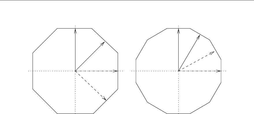
The “dode” and “octa” surface types (see Fig. 3.3) are determined by the x0and y0coor-
dinates of the central axis and two distances r1and r2from the center. If the second value
is omitted, the surface is a regular octa- or dodecagonal cylinder. The octagonal cylinder
basically consists of two intersecting square and the dodecagonal surface of two intersecting

3.2 Surface Definitions 21
Table 3.1: Surface types in the Serpent code.
Type Description Parameters
inf all space -
px plane perpendicular to x-axis x0
py plane perpendicular to y-axis y0
pz plane perpendicular to z-axis z0
sph sphere x0, y0, z0, r
cylx circular cylinder parallel to x-axis y0, z0, r, x1, x2
cyly circular cylinder parallel to y-axis x0, z0, r, y1, y2
cylz or cyl circular cylinder parallel to z-axis x0, y0, r, z1, z2
sqc square cylinder parallel to z-axis x0, y0, r, r0
cube cube x0, y0, z0, r
cuboid cuboid x1, x2, y1, y2, z1, z2
hexxc x-type hexagonal cylinder parallel to z-axis x0, y0, r, r0
hexyc y-type hexagonal cylinder parallel to z-axis x0, y0, r, r0
hexxprism x-type hexagonal prism parallel to z-axis x0, y0, r, z1, z2
hexyprism y-type hexagonal prism parallel to z-axis x0, y0, r, z1, z2
cross cruciform cylinder parallel to z-axis x0, y0, r, d, r0
pad (see description below) x0, y0, r1, r2, θ1, θ2
conx cone oriented in the x-axis x0, y0, z0, r, h
cony cone oriented in the y-axis x0, y0, z0, r, h
conz or cone cone oriented in the z-axis x0, y0, z0, r, h
dode dodecagonal cylinder parallel to z-axis x0, y0, r1, r2
octa octagonal cylinder parallel to z-axis x0, y0, r1, r2
plane general plane A, B, C, D
quadratic general quadratic surface A, B, C, D, E, F, G, H, J, K
regular hexagons.
The general plane is defined by equation
Ax +By +Cz =D
This is a simplified case of the general quadratic surface, defined by
Ax2+By2+Cz2+Dxy +Eyz +F zx +Gx +Hy +Jz +K= 0
3.2.2 Positive and negative surface sides
The surfaces are used for defining the geometry cells as will be described in the following
section. For this purpose, each surface is associated with a positive side and a negative side.
It is defined that a point is inside a surface if it is located on the negative side of the surface.
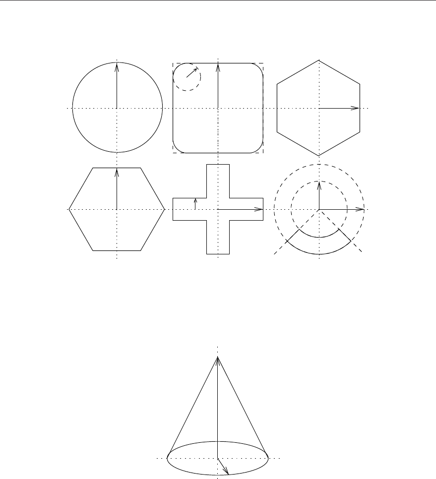
3.2 Surface Definitions 22
x0y0
r
x0y0
r
x0y0
rd
x0y0
r2
r1
x0y0x0y0
r0
hexyc cross pad
hexxcsqccyl
r r
Figure 3.1: Basic cylinder types. The surfaces are infinite in the z-direction. The square
cylinder illustrates the definition of rounded corners.
y0
x0 0 zr
h
cone
Figure 3.2: The cone surface.
For the three types of planes, the positive side is defined in the direction of the positive
coordinate axis. The positive sides of the sphere, cube, cone and the cylindrical surfaces are
defined outside the perimeter of the surface.
3.2.3 Surface examples
A few simple examples of surface definitions are given in the following.
3.2 Surface Definitions 23
x0
r1
x0
r1
r1
r2
r2
r1
r2
0
y
octa
0
y
r2
dode
Figure 3.3: The octagonal and dodecagonal cylinder surfaces.
% --- plane perpendicular to x-axis, located at x = 4.0 cm:
surf 1 px 4.000
% --- sphere centered at (1.0, 0.0, 2.0), radius 5.0:
surf 2 sph 1.000 0.000 2.000 5.000
% --- cylinder centered at origin, radius 10.5 cm:
surf 3 cyl 0.000 0.000 10.500
% --- cube at origin with diameter 5.0 cm:
surf 4 cube 0.000 0.000 0.000 2.500
% --- square cylinder centered at origin, radius 10.0 cm,
% rounded corners with radii 0.2 cm:
surf 5 sqc 0.000 0.000 10.000 0.200
% --- x-type hexagonal cylinder centered at (1.0, 0.0),
% radius 2.0 cm:
surf 6 hexxc 1.000 0.000 2.000
% --- cruciform cylinder centered at origin, radius 20.0 cm,
% half-thickness 5.0 cm:
surf 7 cross 0.000 0.000 20.000 5.000
% --- neutron pad used in the VENUS-2 benchmark:
surf 8 pad 0.000 0.000 11.250 54.750 59.073 65.073
% --- cone at origin, base diameter 2.0 cm, height 5.0 cm
surf 9 cone 0.000 0.000 0.000 1.000 5.000
IMPORTANT NOTES ON SURFACES:

3.3 Cell Definitions 24
1. In code versions earlier than 1.1.8 the cone surface type may only be used with the full
delta-tracking calculation mode (threshold = 1).
2. Reflective and periodic boundary conditions may only be used in geometries where
the outermost boundary is defined by a square or hexagonal cylinder or a cube.
3. The dodecagonal cylinder surface type is available from code version 1.1.4 on.
4. The octagonal cylinder and general plane and quadratic surface are available from code
version 1.1.9 on.
SEE ALSO:
1. Delta-tracking options (Sec. 5.11 on page 66)
2. Boundary conditions (Sec. 5.7 on page 59)
3.3 Cell Definitions
The geometry description in the Serpent code consists of two- or three-dimensional regions,
denoted as cells. Each cell is defined using a set of positive and negative surface numbers,
which correspond to the surface identifiers defined in the surface cards. Unlike MCNP and
other Monte Carlo codes, Serpent can only handle intersections of boundary surfaces. This
means that the neutron is inside the cell, if and only if it is on the same side of each boundary
surface as given in the surface list (see the examples below).
The lack of the union operator restricts the generality of the geometry description to some
extent. This limitation is compensated for by providing a large collection of derived surface
types, which in most cases can be used to replace the unions of the elementary surfaces. The
advantage of this approach is that the geometry description remains relatively simple.1
3.3.1 Cell types
The syntax of the cell card is:
1It is known that the use of derived surface types may slow down the neutron tracking routine in some cases
when the conventional ray-tracing algorithm is used. Neutron transport in Serpent, however, is primarily based
on the delta-tracking method which is not prone to such limitations. The use of derived surface types reduces
the total number of surfaces, which may actually speed up the delta-tracking routine in complicated geometries.

3.3 Cell Definitions 25
cell <name> <u0> <mat> <surf 1> <surf 2> ...
where <name> is the cell name
<u0> is the universe number of the cell
<mat> is the cell material
<surf 1> <surf 2> ... are the boundary surfaces
The cell name is a text string that identifies the cell.2Each cell belongs to a universe, which
is determined by the universe number (lattices and universes are thoroughly described in
Section 3.6 on page 28). Cell material determines the name of the material that fills the cell
(see Chapter 4 for material definitions). There are three exceptions:
1. If the cell is empty, the material name is set to “void”.
2. If the cell describes a region of space that is not part a of the geometry, the material
name is set to “outside”.
3. If the cell is filled by another universe, the material name is replaced by command
“fill” and the number of the filling universe.
The “outside” cells are required for filling the regions of space that are not a part of the actual
geometry. When the neutron streams to such a region, the history is terminated or boundary
conditions are applied.
The cell shape is determined by the list of boundary surfaces. Positive entries refer to positive
(“outside”) surface sides and negative entries to negative (“inside”) surface sides. The cell is
defined as the intersection of all surfaces in the list.
3.3.2 Cell examples
A few simple examples of cell definitions are given in the following.
% --- two half-planes separated by a plane in the z-axis at 5.0 cm:
surf 1 pz 5.000
cell 1 1 water -1 % lower half-plane filled with "water"
cell 2 1 air 1 % upper half-plane filled with "air"
% --- solid uranium sphere ("Godiva") of radius 8.7407 cm:
2When the number of cells in the geometry is large, it is often easier to replace cell names with numerical
constants. This is possible since the code treats cell numbers as any other text strings. This convention is
followed in most example cases in this manual.

3.3 Cell Definitions 26
surf 1 sph 0.0 0.0 0.0 8.7407
cell 1 0 uranium -1 % uranium inside sphere
cell 2 0 outside 1 % outside world
% --- tungsten-reflected plutonium sphere:
surf 1 sph 0.0 0.0 0.0 5.0419
surf 2 sph 0.0 0.0 0.0 9.7409
cell 1 0 plutonium -1 % plutonium inside surface 1
cell 2 0 tungsten 1 -2 % tungsten between surfaces 1 and 2
cell 3 0 outside 2 % outside world
% --- a segment of LWR fuel rod in water:
surf 1 cyl 0.0 0.0 0.40
surf 2 cyl 0.0 0.0 0.45
surf 3 cyl 0.0 0.0 0.60
surf 4 pz -50.0
surf 5 pz 50.0
cell 1 1 UO2 -1 4 -5 % UO2 fuel inside surface 1
cell 2 1 void 1 -2 4 -5 % gap between fuel and cladding
cell 3 1 clad 2 -3 4 -5 % cladding
cell 4 1 water 3 4 -5 % water outside cladding
cell 5 1 water -4 % water below the segment
cell 6 1 water 5 % water above the segment
IMPORTANT NOTES ON CELLS:
1. Material names “void”, “outside” and “fill” are reserved for empty cells, cells
not belonging to the geometry and cells filled by another universe, respectively.
2. Only the intersection operator is available for cell definitions. This means that a point
is inside the cell if and only if it is inside (or outside if defined by a negative surface
number) all the boundary surfaces in the list.
SEE ALSO:
1. Material definitions (Chapter 4 on page 47)
2. Boundary conditions (Sec. 5.7 on page 59)

3.4 Fuel pin definitions 27
3.4 Fuel pin definitions
Since Serpent is primarily a lattice physics code, the geometry has a simplified definition for
fuel pins consisting of nested annular material layers. The syntax of the pin card is:
pin <id>
<mat 1> <r1>
<mat 2> <r2>
...
<mat n>
where <id> is the pin identifier (universe number)
<mat 1> <mat 2> ... are the materials
<r1> <r2> ... are the outer radii of the material regions
The fuel pin is not an actual geometry object, but rather a macro that is used to define a
pin universe. The material regions and their outer radii are given in ascending and the code
constructs the cells using using cylindrical surfaces. If the radius is negative, it is interpreted
as layer thickness instead of absolute radius. The universe number is set by the pin identifier.
Pin materials can also be other universes, which are defined using the fill command (See
filled cells on page 28).
Pin definitions are most commonly used with lattices to define fuel assemblies. Examples
are given in the following section.
IMPORTANT NOTES ON PIN DEFINITIONS:
1. The pin identifier is a universe number, which must not coincide with another universe.
2. The outermost material regions is given without a radius and it fills the rest of the
universe.
3. Layer thickness are available from version 1.1.13 on.
SEE ALSO:
1. Filled cells (Sec. 3.6 on page 28)
2. Lattice examples (Sec. 3.6.3 on page 32)
3.5 Nests
Fuel pin and particle (see Sec. 3.8 on page 39) are special cases of the nest geometry type,
defined as:

3.6 Universes and Lattices 28
nest <id> <type>
<mat 1> <r1>
<mat 2> <r2>
...
<mat n>
where <id> is the nest identifier (universe number)
<type> is the surface type
<mat 1> <mat 2> ... are the materials
<r1> <r2> ... are the surface parameters
Nested objects consist of materials or sub-universes separated by similar surfaces. Nests can
be defined using planar (px,py,pz), cylindrical (cyl,sqc,hexxc,hexyc), spherical
(sph) or cubical (cube) surface types. In each case the parameters <r1>, <r2>, ...
define the main dimension, all other parameters are set to zero.
3.6 Universes and Lattices
As mentioned above, a universe-based geometry allows the geometry to be divided into
separate levels. Each universe is defined independently and must cover all space. Regions of
space not belonging to the geometry must be defined using “outside” cells. The universes are
defined by the cell universe numbers and the geometry is layered by replacing the material
name with the fill command:
cell <name> <u0> fill <u1> <surf 1> <surf 2> ...
where <name> is the cell name
<u0> is the universe number of the cell
<u1> is the universe number of the filling universe
<surf 1> <surf 2> ... are the boundary surfaces
Each universe has its own origin, which can be shifted using the universe transformation
command (see Sec. 3.6.1) The lowest level of the geometry belongs to universe 0, which
must always exist.
3.6.1 Universe transformations and rotations
Each universe is by default centered at the origin, which may sometimes cause difficulties
with filled cells. The origin can be shifted to another location using the universe transforma-
tion card:

3.6 Universes and Lattices 29
trans <u> <x> <y> <z>
where <u> is the universe number
<x> is the x coordinate of the new origin
<y> is the y coordinate of the new origin
<z> is the z coordinate of the new origin
Universe transformations are also convenient, for example, for positioning control rods in a
reactor core. Universes filled in a lattice structure are automatically shifted to the appropriate
position and transformations are not needed.
Universe rotations were implemented in Version 1.1.14. The syntax of the transformation
card with rotations has two alternative formats:
trans <u> <x> <y> <z> <rx> <ry> <rz>
trans <u> <x> <y> <z> <a1> ... <a9>
where <u> is the universe number
<x> is the x coordinate of the new origin
<y> is the y coordinate of the new origin
<z> is the z coordinate of the new origin
<rx> is the rotation angle around x-axis
<ry> is the rotation angle around y-axis
<rz> is the rotation angle around z-axis
<ai> are the coefficients of a rotation matrix
If three values are entered after the coordinates, they are interpreted as rotation angles around
the three coordinate axes. If nine values are entered, they form the rotation matrix, which is
used to multiply the position and direction vectors when the rotation is applied.
The coordinate translation always precedes the rotation.
3.6.2 Lattices
Lattices are special universes, filled with a regular structure of other universes. The Ser-
pent code has eight lattice types: square lattice, two hexagonal lattices, the circular cluster
array, three infinite 3D lattices filled with a single universe and the vertical stack.
Square and hexagonal lattices
The syntax of the lattice card for the square and hexagonal lattices is:

3.6 Universes and Lattices 30
lat <u0> <type> <x0> <y0> <nx> <ny> <p>
where <u0> is the universe number of the lattice
<type> is the lattice type (= 1, 2 or 3)
<x0> is the x coordinate of the lattice origin
<y0> is the y coordinate of the lattice origin
<nx> is the number of lattice elements in the x-direction
<ny> is the number of lattice elements in the y-direction
<p> is the lattice pitch
The lattice card is followed by a list of universe numbers, which determines the layout. The
lattice type numbers are:
1. Square lattice
2. X-type hexagonal lattice (unit cell is the x-type hexagonal cylinder, see Fig. 3.1)
3. Y-type hexagonal lattice (unit cell is the y-type hexagonal cylinder, see Fig. 3.1)
Each lattice defines a universe, which must be embedded inside a cell using the fill com-
mand. If the bounding cell is larger than the lattice, neutrons may stream to undefined lattice
positions, which results in a geometry error. This can be avoided by increasing the lattice
size by defining additional positions in the periphery (see examples below).
Circular cluster array
The circular cluster array (lattice type 4) is defined by:
lat <u0> <type> <x0> <y0> <nr>
where <u0> is the universe number of the lattice
<type> is the lattice type (= 4)
<x0> is the x coordinate of the lattice origin
<y0> is the y coordinate of the lattice origin
<nr> is the number of rings in the array
The lattice card is followed by a list of <nr> rings, which are defined by:
<n> <r> <theta> <u1> <u2> ... <un>
where <n> is the number of sectors in ring
<r> is the central radius of the ring
<theta> is the angle of rotation
<u1> <u2> ... <un> are the universe numbers filling the sectors

3.6 Universes and Lattices 31
The circular array is needed for constructing some cluster-type fuel assemblies, used in
CANDU, MAGNOX, AGR and RBMK reactors. The array is also convenient for deter-
mining the fuel rod layout in some small research reactors, such as the TRIGA.
Infinite 3D lattices
The infinite 3D lattices are used to construct repeated structures of identical cells that fill
the entire universe. This type of construction can be used, for example, for describing the
microscopic fuel particles inside an HTGR fuel pebble or compact. The syntax is:
lat <u0> <type> <x0> <y0> <p>
where <u0> is the universe number of the lattice
<type> is the lattice type (= 6, 7 or 8)
<x0> is the x coordinate of the lattice origin
<y0> is the y coordinate of the lattice origin
<p> is the lattice pitch
<u> is the filler universe
Lattice type 6 is a cubical lattice and types 7 and 8 x- and y-type hexagonal prismatic lattices,
respectively.
Vertical stack
Universes can be vertically stacked, one on top of the other, using lattice type 9:
lat <u0> <type> <x0> <y0> <nl>
where <u0> is the universe number of the lattice
<type> is the lattice type (= 9)
<x0> is the x coordinate of the lattice origin
<y0> is the y coordinate of the lattice origin
<nl> is the number of axial layers
The lattice card is followed by a list of <nl> axial layers, which are defined by:
<z> <u>
where <z> is the axial position (lower boundary of the layer)
<u> is the filler universe
The z-values must be given in ascending order. Space below the lowest z-value is not defined
and the top layer fills the entire space above the highest value.

3.6 Universes and Lattices 32
Cuboidal 3D lattice
The cuboidal lattice is a 3D structure composed of cuboids with different dimensions in the
x-, y- and z-directions. The syntax is:
lat <u0> <type> <x0> <y0> <z0> <nx> <ny> <nz> <px> <py> <pz>
where <u0> is the universe number of the lattice
<type> is the lattice type (= 11)
<x0> is the x coordinate of the lattice origin
<y0> is the y coordinate of the lattice origin
<z0> is the z coordinate of the lattice origin
<nx> is the number of lattice elements in the x-direction
<ny> is the number of lattice elements in the y-direction
<nz> is the number of lattice elements in the z-direction
<px> is the lattice pitch in x-direction
<py> is the lattice pitch in y-direction
<pz> is the lattice pitch in z-direction
The lattice card is followed by a list of universes. This lattice type is available from version
1.1.17 on.
3.6.3 Universe and lattice examples
The universe and lattice definitions are best described using a few examples. The fist example
is a 17×17 PWR MOX fuel assembly containing three types of fuel pins and empty control
rod guide tubes (see Figure 3.4 on page 45).
% --- MOX pin 1:
pin 1
MOX1 4.36250E-01
void 4.43750E-01
clad 4.75000E-01
water
% --- MOX pin 2:
pin 2
MOX2 4.36250E-01
void 4.43750E-01
clad 4.75000E-01
water
% --- MOX pin 3:
pin 3
MOX3 4.36250E-01

3.6 Universes and Lattices 33
void 4.43750E-01
clad 4.75000E-01
water
% --- Empry guide tube:
pin 4
water 5.62500E-01
clad 6.12500E-01
water
% --- Pin lattice (pitch = 1.26 cm):
lat 10 1 0.0 0.0 17 17 1.26
1 1 2 2 2 2 2 2 2 2 2 2 2 2 2 1 1
1 2 3 3 3 2 3 3 2 3 3 2 3 3 3 2 1
2 3 3 3 3 4 3 3 4 3 3 4 3 3 3 3 2
2 3 3 4 3 3 3 3 3 3 3 3 3 4 3 3 2
2 3 3 3 3 3 3 3 3 3 3 3 3 3 3 3 2
2 2 4 3 3 4 3 3 4 3 3 4 3 3 4 2 2
2 3 3 3 3 3 3 3 3 3 3 3 3 3 3 3 2
2 3 3 3 3 3 3 3 3 3 3 3 3 3 3 3 2
2 2 4 3 3 4 3 3 4 3 3 4 3 3 4 2 2
2 3 3 3 3 3 3 3 3 3 3 3 3 3 3 3 2
2 3 3 3 3 3 3 3 3 3 3 3 3 3 3 3 2
2 2 4 3 3 4 3 3 4 3 3 4 3 3 4 2 2
2 3 3 3 3 3 3 3 3 3 3 3 3 3 3 3 2
2 3 3 4 3 3 3 3 3 3 3 3 3 4 3 3 2
2 3 3 3 3 4 3 3 4 3 3 4 3 3 3 3 2
1 2 3 3 3 2 3 3 2 3 3 2 3 3 3 2 1
1 1 2 2 2 2 2 2 2 2 2 2 2 2 2 1 1
The second example is a hexagonal VVER-440 lattice with 126 fuel pins and a central in-
strumentation tube. Empty lattice positions are filled with water (see Figure 3.5 on page 45).
% --- Fuel pin with central hole:
pin 1
void 0.08000
fuel 0.37800
void 0.38800
clad 0.45750
water
% --- Central instrumentation tube:

3.6 Universes and Lattices 34
pin 2
water 0.44000
clad 0.51500
water
% --- Empty lattice position filled with water:
pin 3
water
% --- Pin lattice (x-type hexagonal, pitch = 1.23 cm):
lat 10 2 0.0 0.0 15 15 1.23
3 3 3 3 3 3 3 3 3 3 3 3 3 3 3
3 3 3 3 3 3 3 1 1 1 1 1 1 1 3
3 3 3 3 3 3 1 1 1 1 1 1 1 1 3
3 3 3 3 3 1 1 1 1 1 1 1 1 1 3
3 3 3 3 1 1 1 1 1 1 1 1 1 1 3
3 3 3 1 1 1 1 1 1 1 1 1 1 1 3
3 3 1 1 1 1 1 1 1 1 1 1 1 1 3
3 1 1 1 1 1 1 2 1 1 1 1 1 1 3
3 1 1 1 1 1 1 1 1 1 1 1 1 3 3
3 1 1 1 1 1 1 1 1 1 1 1 3 3 3
3 1 1 1 1 1 1 1 1 1 1 3 3 3 3
3 1 1 1 1 1 1 1 1 1 3 3 3 3 3
3 1 1 1 1 1 1 1 1 3 3 3 3 3 3
3 1 1 1 1 1 1 1 3 3 3 3 3 3 3
3 3 3 3 3 3 3 3 3 3 3 3 3 3 3
The third example is a CANDU cluster consisting of 37 pins in 4 rings. The third ring is
rotated by 15 degrees (see Figure 3.6 on page 46).
% --- Fuel pin:
pin 1
fuel 0.6122
clad 0.6540
coolant
% --- Cluster:
lat 10 4 0.0 0.0 4
1 0.0000 0.0 1
6 1.4885 0.0 1 1 1 1 1 1
12 2.8755 15.0 1 1 1 1 1 1 1 1 1 1 1 1
18 4.3305 0.0 1 1 1 1 1 1 1 1 1 1 1 1 1 1 1 1 1 1

3.6 Universes and Lattices 35
All three examples are illustrated using the geometry plotter in Section 3.9 on page 42. It
should be noted that the plots contain cell structures not included in the above examples.
The following example demonstrates the use of the vertical stack:
% --- Uranium ball:
surf 1 sph 0.0 0.0 2.5 2.5
cell 1 1 uranium -1
cell 2 1 void 1
% --- Stack 5 balls:
lat 2 9 0.0 0.0 5
0.0 1
5.0 1
10.0 1
15.0 1
20.0 1
Notice that the origin of universe 1 is positioned at the bottom of each layer.
IMPORTANT NOTES ON UNIVERSES AND LATTICES:
1. Each universe is defined independently and must cover all space. Regions of space not
belonging to the geometry must be defined using “outside” cells.
2. The lowest level of the geometry belongs to universe 0, which must always exist.
3. Each universe has its own origin, which can be shifted using the universe transforma-
tion command.
4. Cells in higher geometry levels can only be accessed through filled cells or lattices.
5. Each lattice defines a universe, which must be embedded inside a cell using the fill
command. The lattice must fill the container cell completely to avoid neutron stream-
ing to undefined lattice positions.
6. Hexagonal lattices are defined using a square matrix for the universe layout. To posi-
tion the lattice cells correctly, a number of empty cells must be defined for each row.
The definition is best described in the example in Sec. 3.6.3 on page 33.
7. Multi-level hexagonal structures (pin-assembly-core) are defined using both x- and
y-type hexagonal lattices with different type at each level.

3.7 Repeated Boundary Conditions 36
8. If the infinite lattice types are is used in burnup calculation, material volumes must be
set manually (see Sec. 4.1.2 on page 49).
9. The vertical stack lattice type is available from code version 1.1.8 on.
SEE ALSO:
1. Pin definitions (Sec. 3.4 on page 27)
2. Filled cells (Sec. 3.6 on page 28)
3.7 Repeated Boundary Conditions
What happens to neutrons that end up in a region defined as being outside the geometry is
dictated by the boundary conditions. There are three options:
1. Black boundary - the neutron is killed
2. Reflective boundary - the neutron is reflected back into the geometry
3. Periodic boundary - the neutron is moved to the opposite side of the geometry
The condition is set by the “bc” parameter, described in Section 5.7 on page 59.
Reflective and periodic boundary conditions can be used to construct infinite and semi-
infinite lattice structures. The way these boundary conditions are handled in Serpent is
somewhat different from other Monte Carlo codes. Instead of stopping the neutron at the
boundary surface, reflections and translations are handled by coordinate transformations.
This limits the outermost boundary to a few specific surface types that can be used to define
a square or hexagonal lattice structure. There are basically three options:
Infinite 2D geometry: The geometry has no dependence on the z-coordinate. The outer
boundary is defined by a single square or hexagonal cylinder (“sqc”, “hexxc” or
“hexyc”).
Radially infinite, axially finite 3D geometry: The outer boundary is defined by a square
or hexagonal cylinder (“sqc”, “hexxc” or “hexyc”and two axial planes (“pz”).
The boundary condition takes effect in the radial direction only. The axial boundary
conditions are black.
Infinite 3D geometry: The outer boundary is defined by a single cube, cuboid or hexag-
onal prism (“cube”, “cuboid”, “hexxprism”or “hexyprism”). The boundary
condition takes effect in all directions.

3.7 Repeated Boundary Conditions 37
The following examples illustrate the different geometry types. The details of the geometry
are omitted for the sake of simplicity and replaced by a fill command.
An infinite 2D hexagonal geometry can be defined as:
surf 1 hexyc 0.0 0.0 7.350
% --- Cells:
cell 1 0 fill 10 -1
cell 99 0 outside 1
set bc 3
Note that the reflective boundary condition is unphysical in a hexagonal geometry. infinite
2D square geometry can be defined as:
surf 1 sqc -0.233 -0.233 7.68750
cell 1 0 fill 10 -1
cell 99 0 outside 1
set bc 2
In both cases the outer boundary is defined by a single surface.
If the geometry is finite in the axial dimension, the system becomes three-dimensional. A
radially infinite square lattice can be defined as:
surf 1 sqc -0.233 -0.233 7.68750
surf 2 pz -200.0
surf 3 pz 200.0
cell 1 0 fill 10 -1 2 -3
cell 97 0 outside 1 2 -3
cell 98 0 outside -2
cell 99 0 outside 3
set bc 2
It is also possible to define the outside world as:
cell 97 0 outside 1
cell 98 0 outside -1 -2
cell 99 0 outside -1 3

3.7 Repeated Boundary Conditions 38
but the code may run slower because the boundary condition will be handled also for some
neutrons that end up outside the geometry.
As for the infinite 2D geometry, the boundary in an infinite 3D geometry must be defined by
a single surface, such as a cube:
surf 1 cube 0.0 0.0 0.0 3.0
cell 1 0 fill 10 -1
cell 99 0 outside 1
set bc 2
or a hexagonal prism:
surf 1 hexxprism 0.0 0.0 1.880 0.0 4.93
cell 1 0 fill 10 -1
cell 99 0 outside 1
set bc 3
In both cases the boundary conditions are enforced in both radial and axial directions.
IMPORTANT NOTES ON REPEATED BOUNDARY CONDITIONS:
1. The outer boundary must be defined by a single surface in infinite 2D and 3D geome-
tries. The allowed surface types for a 2D geometry are square and hexagonal cylinders.
Infinite 3D geometries can be defined using a cube, cuboid or hexagonal prism.
2. Axially infinite, radially finite geometries are defined by a square or hexagonal cylinder
and two axial planes. The way the outside world is defined may affect the running time.
3. The hexagonal cylinder and prismatic surfaces are physically reasonable only with
periodic boundary conditions (reflective boundary conditions work if the geometry
has a 30 degree symmetry). The use of reflective boundary conditions with these
types was enabled in update 1.1.18. In earlier code versions the boundary condition is
automatically changed into periodic.
SEE ALSO:
1. Surface types (Sec. 3.2.1 on page 20)
2. Defining the outside world (Sec. 3.3.1 on page 25)
3. Setting the boundary condition (Sec. 5.7 on page 59)

3.8 HTGR geometry types 39
3.8 HTGR geometry types
The fuels in high-temperature gas-cooled reactors (HTGR) consist of microscopic TRISO
particles dispersed in a graphite matrix. The multi-layer fuel particles can be defined similar
to fuel pins (see Sec. 3.4 on page 27):
particle <id>
<mat 1> <r1>
<mat 2> <r2>
...
<mat n>
where <id> is the particle identifier (universe number)
<mat 1> <mat 2> ... are the materials
<r1> <r2> ... are the outer radii of the material regions
The simplest approach is to describe the particle distribution as a regular lattice, using lattice
types 6, 7 or 8 (See the infinite 3D lattices in Sec. 3.6.2). However, the regular arrangement
fails to account for the random distribution of the particles and often leads to a distorted
fuel-to-moderator ratio due to cell cut-off at the outer boundary. For this reason the Serpent
code has two geometry models specifically designed for HTGR fuels.
3.8.1 Implicit particle fuel model
The implicit particle fuel model works by sampling new particles on the neutron flight path
during the tracking process. The input syntax is:
disp <u0> <uf> <pf1> <r1> <u1> ... <pfn> <rn> <un>
where <u0> is the universe number of the dispersed medium
<uf> is the universe filling the space between the particles
<pf1> ... <pfn> are the packing fractions of the particle types
<r1> ... <rn> are the radii of the particle types
<u1> ... <un> are the universe numbers of the particle types
The number of particle types is not limited, but the sum of the packing fractions must be less
than 1.0 (physical factors set the upper limit much lower, although this is not checked by the
routine).
The implicit particle fuel model was revised in update 1.1.3. It should be noted that the
model is not exact and there are statistically significant differences compared to the explicit
model described below. The implicit model seems to work best for low packing fractions but
no comprehensive validation has been carried out yet.

3.8 HTGR geometry types 40
3.8.2 Explicit particle / pebble bed fuel model
A better choice for modeling HTGR geometries is the explicit particle fuel model, which
reads the positions of the particles from a separate file. The same model can be used for
setting up reactor-scale pebble-bed geometries. The input syntax is:
pbed <u0> <uf> "<inputfile>" [<options>]
where <u0> is the universe number of the dispersed medium
<uf> is the universe filling the space between the particles / pebbles
<inputfile> is the input file containing the particle / pebble coordinates
<options> are the options
The particle / pebble distribution is handled explicitly, so there are no approximations done
in the modeling. Each line in the input file describes the position of a single particle / pebble.
The format is:
<x> <y> <z> <r> <u>
where <x> is the x coordinate of the particle / pebble
<y> is the y coordinate of the particle / pebble
<z> is the z coordinate of the particle / pebble
<r> is the radius of the particle / pebble
<u> is the universe number of the particle / pebble
The total number of entries is unlimited, although memory or running time may become a
limiting factor if the number exceeds several million.
The options are used to activate the calculation of various particle / pebble-wise parameters.
Currently the only available option is the power distribution, which is requested with op-
tion “pow”. The code writes the output in a separate file “<inputfile>.out”, where
“<inputfile>” is the file where the distribution was read. The input data is included for
convenience. The format of the output is:
<x> <y> <z> <r> <u> <P> <dP>
where <x> is the x coordinate of the particle / pebble
<y> is the y coordinate of the particle / pebble
<z> is the z coordinate of the particle / pebble
<r> is the radius of the particle / pebble
<u> is the universe number of the particle / pebble
<P> is the power produced inside the particle / pebble
<dP> is the associated relative statistical error
All results depend on source normalization (see Sec. 5.8 on page 61).

3.8 HTGR geometry types 41
3.8.3 HTGR geometry examples
The following example shows how the particle distribution inside a single PBMR fuel pebble
can be modeled using a regular 3D array and the two particle fuel models in the Serpent code.
The definition of a fuel particle is very similar to the fuel pin:
% --- Definition of a coated fuel particle:
particle 1
fuel 0.0250
buffer 0.0340
PyC 0.0380
SiC 0.0415
PyC 0.0455
matrix
The first option is to describe the particle distribution as a regular cubical lattice:
% --- Option 1: regular 3D array:
lat 10 6 0.0 0.0 0.16341 1
The implicit particle fuel model is defined using a list of packing fractions and particle types:
% --- Filler universe composed of graphite:
surf 1 inf
cell 1 2 matrix -1
% --- Option 2: implicit particle fuel model:
disp 10 2 0.09043 4.55000E-02 1
The explicit particle fuel model reads particle coordinates from a separate input file (can be
used for pebble distributions at reactor scale as well):
% --- Filler universe composed of graphite:
surf 1 inf
cell 1 2 matrix -1
% --- Option 3: explicit particle fuel model (read coordinates from file):
pbed 10 2 "particles.inp"

3.9 Geometry plotter 42
Finally the pebble description using one of the three options (all assigned with universe
number 10):
% --- Pebble:
surf 10 sph 0.0 0.0 0.0 2.5
surf 20 sph 0.0 0.0 0.0 3.0
surf 30 cube 0.0 0.0 0.0 3.0
cell 10 0 fill 10 -10
cell 20 0 matrix 10 -20
cell 30 0 helium 20 -30
cell 40 0 outside 30
IMPORTANT NOTES ON HTGR GEOMETRY TYPES:
1. The implicit particle fuel model was revised in update 1.1.3. The model is not exact
and should be used with caution. Test calculations show that the model works best for
low packing fractions.
2. If the implicit particle fuel model is used in burnup calculation, material volumes must
be set manually (see Sec. 4.1.2 on page 49).
3. Calculation of particle / pebble-wise power distributions is available from update 1.1.4
on.
SEE ALSO:
1. An earlier version of the implicit particle fuel model in Ref. [8]
3.9 Geometry plotter
The geometry plotter uses the GD open source graphics library [1] for producing png format
output files for visualization. In order to use the plotter, the source code must be compiled
with this library included (see the Makefile for detailed instructions). The syntax of the
plotter command is:

3.9 Geometry plotter 43
plot <or> <nx> <ny> [<p> <min1> <max1> <min2> <max2>]
where <or> is the orientation of the plot plane (1, 2 or 3)
<nx> is the width of the plot in pixels
<ny> is the height of the plot in pixels
<p> is the position on the axis perpendicular to the plot plane
<min1> is the minimum value of the first coordinate
<max1> is the maximum value of the first coordinate
<min2> is the minimum value of the second coordinate
<max2> is the maximum value of the second coordinate
The orientation of the plot plane is defined as:
1. yz-plot (perpendicular to the x-axis)
2. xz-plot (perpendicular to the y-axis)
3. xy-plot (perpendicular to the z-axis)
The plotted area is a rectangle defined by the orientation, the position on the perpendicular
coordinate axis and the coordinates of the two corners. Zero position is assumed if the
position parameter is omitted. If the corner coordinates are not given, the boundary values
of the geometry are used.
Each plotter command produces an output file named “<input>_geom<n>.png”, where
<input> is the name of the input file and <n> is the plot index. The resolution of the figure
is defined by the width and height parameters. Each material is represented by a randomly
selected color (void regions are in black, geometry errors bright green or red). Surfaces are
drawn with black lines, which may overlap cell regions. It should be noted that the plotted
surfaces may not necessarily represent the actual cell boundaries.
Example plots are shown in Figures 3.4–3.7. The lattices in the first three cases are described
in the universe and lattice examples in Sec. 3.6.3. In each case the plotter command was:
plot 3 1000 1000
This generates a 1000 by 1000 pixel plot perpendicular to the z-axis, located at z= 0 and
covering the entire geometry.
IMPORTANT NOTES ON GEOMETRY PLOTTER:
1. The geometry plotter uses the GD open source graphics library [1], which must be
installed in the system.
2. The plotter produces png (portable network graphics) format output files.

3.9 Geometry plotter 44
3. The colors in the plot represent different materials. The color for each material is
selected randomly (void regions are black, geometry errors bright green or red).
4. Surfaces are drawn with black lines, which may overlap cell regions. Plotted surfaces
may not necessarily represent the actual cell boundaries.
SEE ALSO:
1. Compiling Serpent (Sec. 1.1 on page 8)
2. The GD open source graphics library: http://www.libgd.org
3.9 Geometry plotter 45
Figure 3.4: A 17×17 PWR MOX fuel assembly with 3 pin types.
Figure 3.5: A hexagonal VVER-440 fuel assembly with 126 fuel pins and a central instru-
mentation tube in an infinite lattice. The proportions of the assembly are slightly distorted
since the hexagonal assembly is fitted inside a square region.
3.9 Geometry plotter 46
Figure 3.6: A CANDU cluster with 37 fuel pins in 4 rings. The third ring is rotated by 15
degrees.
Figure 3.7: A 10×10 BWR fuel fuel assembly with 7 pin types and an asymmetrically posi-
tioned moderator channel.

Chapter 4
Materials
4.1 Material definitions
The geometry in Monte Carlo codes consists homogeneous material regions, which in Ser-
pent are defined using cells and surfaces (see Chapter 3 for geometry definition).1Each
material consists of a list of nuclides and each nuclide is associated with a cross section
library, as defined in the directory file (see Sec. 1.4.2 on page 12).
Nuclide temperatures are fixed when the cross section data is generated and cannot be
changed afterwards. It is important to use cross section libraries generated at the right tem-
perature to correctly model the Doppler-broadening of resonance peaks. It is equally (or even
more) important to use the appropriate bound-atom thermal scattering libraries for moderator
nuclides.
Soluble absorbers can be defined by mixing two material compositions. This option is in-
troduced in Sec. 5.14 on page 69. The concentration can be used for critical keff iteration.
Serpent also has the option to use a built-in Doppler broadening routine to adjust nuclide
temperatures before the calculation. This method is described in Sec. 4.3 on page 50.
4.1.1 Nuclides
Nuclide names may be arbitrary aliases defined in the directory file. The usual convention,
also used by MCNP, is:
1It is, in principle, possible to model continuously varying material compositions when the delta-tracking
method is used for neutron transport. This option is considered for the future versions of the Serpent code.
47

4.1 Material definitions 48
<Z><A>.<id>
where <Z> is the element Z
<A> is the isotope mass number (three digits)
<id> is the library id
For example, “92235.09c” refers to 235U. Natural element cross sections are denoted by
mass number zero (“40000.06c” for natural zirconium). The library id usually refers to
data evaluation or temperature (“60c” for ENDF/B-VI.0 based data, “09c” for data gener-
ated at 900K, and so on...).
There is no standard convention on how to name isomeric states. The xsdirconvert-utility
used for producing Serpent directory files assumes a form in which the isotope mass number
is simply increased above 300 (“95342.09c” for 242mAm). In any case it is important to
realize that the nuclide names are used for identification only and they do not contain any
information used by the code in the calculation.
4.1.2 Material cards
The basic syntax of the material card is:
mat <name> <dens> [<options>]
<iso 1> <frac 1>
<iso 2> <frac 2>
...
where <name> is the material name
<dens> is the density (mass or atomic)
<options> are the options (depending on case)
<iso 1> <iso 2> ... are the names of the constituent nuclides
<frac 1> <frac 2> ... are the corresponding fractions (mass or atomic)
Material name is used to identify the material in cell cards (see Sec. 3.3.1 on page 25). The
nuclide names correspond to the identifier determined in the directory file. These identifiers
define the cross section data used in the calculation. Densities and fractions can be given
as atomic or mass values. Positive entries refer to atomic densities (in units of 1024/cm3)
and atomic fractions, respectively, and negative entries to mass densities (in units of g/cm3)
and mass fractions. Isotopic compositions are normalized before the calculation and mixed
entries are not allowed.
If the material density is set to zero or “sum”, the value is calculated from the isotopic com-
position. The isotope fractions must then be in absolute density units, not relative fractions.
Material volumes and masses are used for normalizing reaction rates, which is important,
for example, in burnup calculation. The code calculates these automatically for simple pin
structures, but the values must be entered manually for some more complicated geometries.

4.2 Thermal scattering libraries 49
Material volume is set using option:
mat <name> <dens> vol <V>
...
where <V> is the total material volume in cm3
and material mass (alternatively):
mat <name> <dens> mass <M>
...
where <M> is the total material mass in g
Colors for the geometry plotter (see Sec. 3.9 on page 42 can be set using:
mat <name> <dens> rgb <R> <G> <B>
...
where <R> is the value for red channel (between 0 and 255)
<G> is the value for green channel (between 0 and 255)
<B> is the value for blue channel (between 0 and 255)
if the colors are not set, random values are used in the plots.
Other options are used to set up depletion zones in burnup calculation and to determine ther-
mal scattering libraries for moderator materials and temperatures for Doppler broadening.
Material definitions in burnup calculation is a separate topic in Section 8.2 on page 109.
Thermal scattering and Doppler broadening are discussed below.
4.2 Thermal scattering libraries
Thermal scattering cross sections are used to replace the low-energy free-gas elastic scat-
tering reactions for some important bound moderator nuclides, such as hydrogen in water
or carbon in graphite. Thermal systems cannot be modelled using free-atom cross sections
without introducing significant errors in the spectrum and results. Thermal scattering data is
defined using:
therm <thname> <lib>
where <thname> is the name of the data library
<lib> is the library identifier as defined in the directory file
The library identifier is the actual name of the library in the directory file. The library name
is used to associate the data with a material, in which case the material card has an additional
entry:

4.3 Doppler broadening 50
mat <name> <dens> moder <thname> <ZA>
<iso 1> <frac 1>
<iso 2> <frac 2>
...
where <name> is the material name
<dens> is the density (mass or atomic)
<thname> is the name of the thermal scattering data library
<ZA> is the nuclide ZA of the moderator nuclide
<iso 1> <iso 2> ... are the names of the constituent nuclides
<frac 1> <frac 2> ... are the corresponding fractions (mass or atomic)
The nuclide ZA identifies the moderator nuclide (in the form of: 1000*Z + A). The “moder”
entry can be used several times to define thermal scattering libraries for multiple nuclides,
such as hydrogen and deuterium in heavy water (see the example in Sec. 4.4).
4.3 Doppler broadening
The Doppler broadening routine is initiated by adding a “tmp” entry in the material card:
mat <name> <dens> tmp <T>
<iso 1> <frac 1>
<iso 2> <frac 2>
...
where <name> is the material name
<dens> is the density (mass or atomic)
<T> is the Doppler temperature in Kelvin
<iso 1> <iso 2> ... are the names of the constituent nuclides
<frac 1> <frac 2> ... are the corresponding fractions (mass or atomic)
The broadening is performed after the data is read from the ACE format libraries and there
is slight increase in the overall calculation time, depending on the number of nuclides. If the
the same nuclide is broadened to several temperatures in different materials, there is also an
increase in memory usage. The routine works only if the given temperature is above the orig-
inal one. The cross section libraries provided with the Serpent code are generated between
300K intervals and it is recommended that the closest temperature below the broadened value
is used as the basis.
4.4 Material examples
A few simple examples of material definitions are given in the following.

4.4 Material examples 51
% --- Fuel consisting of enriched UO2 and burnable absorber.
% Atomic densities given in units of 1/(barn*cm):
mat UO2Gd sum % Atomic density from composition
92234.09c 4.2940E-06 % Atomic density of U-234
92235.09c 5.6226E-04 % Atomic density of U-235
92238.09c 2.0549E-02 % Atomic density of U-238
64154.09c 4.6173E-05 % Atomic density of Gd-154
64155.09c 2.9711E-04 % Atomic density of Gd-155
64156.09c 4.1355E-04 % Atomic density of Gd-156
64157.09c 3.1518E-04 % Atomic density of Gd-157
64158.09c 4.9786E-04 % Atomic density of Gd-158
64160.09c 4.3764E-04 % Atomic density of Gd-160
8016.09c 4.5243E-02 % Atomic density of O-16
% --- Zircaloy cladding:
mat clad -6.55000 % Mass density given in g/cm3
40000.06c -0.98135 % Mass fraction of natural zirconium
24000.50c -0.00100 % Mass fraction of natural chromium
26000.55c -0.00135 % Mass fraction of natural iron
28000.42c -0.00055 % Mass fraction of natural nickel
50000.42c -0.01450 % Mass fraction of natural tin
8016.06c -0.00125 % Mass fraction of O-16
% --- Boronized light water with thremal scattering data:
mat water -0.7207 moder lwtr 1001
1001.06c -1.1180E-1
8016.06c -8.8755E-1
5010.06c -1.1890E-4
5011.06c -5.3110E-4
therm lwtr lwtr.04t
% --- Heavy water with thermal scattering data (two libraries):
mat D2O -0.812120 moder lwtr1 1001 moder hwtr1 1002
8016.06c -7.99449E-1
1002.06c -1.99768E-1
1001.06c -7.83774E-4
therm lwtr1 lwtr.04t
therm hwtr1 hwtr.04t
% --- Doppler broadening from 900K to 1000K:
mat fuel -10.45700 tmp 1000

4.4 Material examples 52
92235.09c -0.03173
92238.09c -0.84977
8016.09c -0.11850
IMPORTANT NOTES ON MATERIALS:
1. Nuclide names are used for identification only. All information used in the calculation
is read from the directory file and the cross section data.
2. Positive entries in material density and isotopic composition refer to atomic densities
and atomic fractions, respectively, and negative entries to mass densities and mass
fractions. Typical input errors in material compositions are related to confusing the
two definitions.
3. Isotopic compositions can be given as density values, rather than fractions, since the
compositions are normalized before the calculation.
4. The mass fraction of oxygen in UO2fuel is ∼0.1185. Natural boron consists of 20%
10B and 80% 11B (atomic fractions).
5. Thermal scattering data must be used for moderator materials (water, graphite, etc.)
when modelling thermal systems. The use of free-atom cross sections will introduce
significant errors in the results.
6. Doppler broadening is available from code version 1.1.0 on, and completed in version
1.1.2. The broadened temperature must be above the original nuclide temperature.
SEE ALSO:
1. Directory files and the “xsdirconvert” utility (Sec. 1.4.2 on page 12)
2. Soluble absorber definitios (Sec. 5.14 on page 69)
Chapter 5
Options
5.1 General
Serpent has various calculation parameters determined using the “set” command:
set <param> <value 1> <value 2> ...
where <param> is the parameter name
<value 1> <value 2> ... are the parameter values
The available options are listed in Table 5.1 and described in more detail in the following
sections. Parameters used for burnup calculation are described in Section 8.4 of Chapter 8.
Table 8.2 on page 111 summarizes the options in the burnup calculation mode.
5.2 Neutron Population and Criticality Cycles
The default calculation mode in Serpent is the k-eigenvalue criticality source method, in
which the simulation is run in cycles and the source distribution of each cycle is formed by
the fission reaction distribution of the previous cycle. External source simulation is discussed
as a separate topic in Chapter 9. The parameters for criticality source calculation are set
using:
set pop <npop> <cycles> <skip> [<keff0> <int>]
where <npop> is the number of source neutrons per cycle
<cycles> is the number of active cycles run
<skip> is the number of inactive cycles run
<keff0> is the initial guess for keff
<int> is the collection interval
53

5.2 Neutron Population and Criticality Cycles 54
The number of source neutrons per cycle is fixed. Since the number of generated source
points usually differs from this value, the source size is increased (keff <1) or decreased
(keff >1) to match the given source size.
Inactive cycles are cycles that are run in order to allow the initial fission source distribution to
converge before starting to collect the results. In lattice calculations the convergence is typ-
ically reached well within the first 20 cycles. Source convergence in full-core calculations,
however, may take much longer.
The initial source points are randomly selected inside the fissile cells in the geometry and no
source input is needed from the user. The simulation requires an initial guess for keff , which
by default is set to unity. This is usually sufficient, but if the system is far from criticality,
the simulation may die out during the first few cycles. This problem may be overcome by
setting the initial keff guess to a more appropriate value.
If all fissile material is located in a small region compared to the geometry dimensions, initial
source sampling may fail. The default source can be overridden by defining an external
source, as described in Section 9.2 of Chapter 9. If the “nps” parameter is not set, the
user-defined source is used as the initial guess only, and the simulation proceeds in power
iterations.
The statistical accuracy of the results depends on the total number of active neutron histories
run, which is determined by the population size per cycle and the total number of active
cycles. Appropriate values for a typical lattice calculation are 500 active cycles of 5000
source neutrons. If more precision is required or the geometry is larger, it is suggested that
the population size, rather than the number of cycles is increased.
The collection interval defines the number of generations run for each batch of results. By
default this value is set to one, and increasing the number has essentially the same impact as
running more neutrons per generation and fewer generations.1
Serpent uses two buffers to store data for new source points and neutrons produced in multi-
plying scattering reactions and certain special calculation modes. In some cases these buffers
may be overrun, which terminates the simulation. To overcome such problems, the buffer
size may be increased by setting:
set nbuf <f>
where <f> is the buffer factor (criticality mode) or total size (external source mode)
In criticality source mode the buffer size is population size multiplied by the given factor (set
to 2.5 by default). In external source mode neutron histories are run one at a time and the
value of nbuf sets the absolute size of the buffer (set to 1000 by default).
IMPORTANT NOTES ON NEUTRON POPULATION AND CRITICALITY CYCLES:
1The difference is that the correlations between adjacent batches could be weaker, which may have some
impact in the statistics in large geometries (the effects have not yet been studied).

5.3 Energy grid reconstruction 55
1. It is important that a sufficient number of cycles is discarded to allow the initial fis-
sion source to converge before starting to collect the results. This number depends on
the size and the complexity of the geometry. Fission source convergence is a compli-
cated research topic, subject to both theoretical and practical considerations [9–14].
It should be noted, however, that problems with source convergence are practically
never encountered in lattice calculations where the neutron migration distance is long
compared to the dimensions of the geometry.
2. The k-eigenvalue criticality source calculation yields physically consistent results only
in the special case that keff = 1. When the system is far from criticality, the importance
of fission neutrons is either over- (keff <1) or underestimated (keff >1). The result is
that the neutron population becomes biased in energy and space (and time), which may
affect the final results as well. The problem originates from the basic methodology
and the fact that a physically sub- or super-critical chain reaction is simulated as a
steady-state system. Deterministic lattice transport codes use neutron leakage models
to overcome this problem, but the methodology for Monte Carlo calculation is not well
established.
3. All source neutrons are born in fission. Other neutron-multiplying (n,xn) reactions are
treated as scattering within the criticality cycle.
4. External source definitions are available from version 1.1.11 on.
5. Buffer size and collect interval are options available from version 1.1.13 on.
SEE ALSO:
1. Simulating the neutron chain reaction and the k-eigenvalue criticality source calcula-
tion mode in Ref. [15] (Sec. 5.5 on page 112).
2. Discussion on neutron leakage models in Monte Carlo calculation in Ref. [15] (Sec. 9.5
on page 171).
3. External source simulation (Chapter 9).
5.3 Energy grid reconstruction
The continuous-energy reaction cross sections in Serpent are reconstructed using a single
unionized energy grid for all nuclides. The reason for this approach is the major speed-up
in calculation, achieved by minimizing the number of grid search iterations.2The default
2Each nuclide in the continuous-energy ACE format data is associated with its own energy grid. The
calculation of material total cross sections, for example, is carried out by summing over all the constituent
nuclides. This requires an iterative energy grid search to be performed for each nuclide, which may take a
significant fraction of the overall CPU time, especially since the procedure has to be repeated each time the
neutron enters a new material. The advantage of using the same grid for all nuclides is that the grid search has
to be performed only once, each time the neutron scatters to a new energy.

5.3 Energy grid reconstruction 56
method for grid reconstruction is that all grid points of all nuclides in the ACE format data
are included in the master grid. The disadvantage of this method is that computer memory is
wasted for storing a large number of redundant data points. The available memory is usually
not a problem in fresh fuel calculations, but the introduction of actinide and fission product
isotopes in burnup calculation may result in an excessively large master grid. Serpent has
a method for avoiding this problem by combining adjacent grid points. The reconstruction
parameters are given by:
set egrid <tol> [<Emin> <Emax>]
where <tol> is the fractional reconstruction tolerance
<Emin> is the minimum energy in the grid (MeV)
<Emax> is the maximum energy in the grid (MeV)
The fractional reconstruction tolerance is the minimum relative difference between two grid
points, below which the points are combined. All points below the lower limit and above the
upper limit are discarded.
The default value for the fractional reconstruction tolerance is zero in the transport calcula-
tion mode and 5·10−5in the burnup calculation mode. Test calculations have shown that
the results are not significantly affected until the tolerance is raised above 10−3. There is
no absolute guarantee, however, that the results are valid in all imaginable cases when the
grid size is significantly reduced. It is therefore suggested that the grid reduction is not used
unless necessary because of insufficient computer memory.
The lower limit of the energy grid is by default set to 10−9MeV and the upper limit to
15 MeV. Very few neutrons are born or scattered to higher or lower energies in fission reactor
applications.
If a reduction in memory size is necessary, an alternative to grid thinning is the double
indexing method, in which the data is stored in the original ACE format and the unionized
grid used only for accessing the nuclide-wise grids. This method is activated by:
set dix <mode>
where <mode> is 1 if the method is used and 0 if not.
The double indexing method reduces the memory usage, but may lead to an increase in
processing time, which may become significant in burnup calculation. Double indexing is
turned off by default.
IMPORTANT NOTES ON ENERGY GRID:
1. Grid reduction inevitably leads to some loss of data. There is no guarantee that this
reduction does not affect the results.
2. Test calculations have shown that the reduction in grid size does not significantly affect
the overall calculation time.

5.4 Library File Paths 57
SEE ALSO:
1. Cross section data in the PSG code in Ref. [15] (Sec. 8.2 on page 143). NOTE: Some
of the described methods are outdated.
2. A more recent description of the unionized energy grid formats in Serpent is found in
Ref. [16].
5.4 Library File Paths
The Serpent code uses a single directory file for determining the cross sections used in the
transport simulation. The directory file can be generated from an MCNP xsdir file using the
“xsdirconvert” utility (see Sec.1.4 on page 11). The cross section library directory file path
is set using:
set acelib "<file>"
where <file> is the file path for the ACE directory file
A default directory path can be set by defining environment variable SERPENT_DATA. The
code looks for cross section directory files in this path if not found at the absolute location.
IMPORTANT NOTES ON DATA FILES AND FILE PATHS:
1. The cross section library directory file is a text file generated by the “xsdirconvert”
utility.
2. The environment variable feature is available from code version 1.1.8 on.
SEE ALSO:
1. Setting up the directory file (Sec.1.4 on page 11)
2. Setting up file paths for burnup calculation (Sec.8.4 on page 111)
5.5 Unresolved resonance data
The use of unresolved resonance probability tables can be switched on and off using:

5.5 Unresolved resonance data 58
set ures <use> [<mode>] [dilu] [<iso 1> <iso 2> ...]
where <use> is the option (1 = use data, 0 = omit data)
<mode> is the calculation mode
<dilu> is the infinite dilution cut-off
<iso n> are the nuclides for which the data is used or omitted
Since the probability table sampling has to be carried out during tracking, the transport cycle
tends to slow down quite significantly.3There are three options to treat the probability table
data:
1. Sample all cross sections at once, each time the neutron scatters to a new energy, adjust
material totals and majorant.
2. Sample cross sections when the neutron enters a new material. Use a pre-calculated
majorant cross section corresponding to the maximum probability table values.
3. Sample cross sections when the neutron enters a new material. Switch to surface
tracking when neutron is in the unresolved range.
The overall calculation time using the different options depends on the case, in particular the
flux spectrum and the number of nuclides with probability table data. Mode 1 is used by
default. It should also be noted that options 2 and 3 work by sampling the cross sections for
physical materials. If a material is used for detector calculation only, the probability tables
may not be appropriately sampled. This is not a problem for method 1.
Since the overall impact of using unresolved resonance cross sections is a self-shielding
effect, the calculation routine can be optimized by omitting the probability table sampling
for nuclides with low concentration. This limit is given by the infinite dilution cut-off, which
is set to zero by default.
If the options are followed by a list of nuclide names (94239.09c, etc.), the probability table
treatment is used or omitted only for the listed nuclides. If no list is given, the options cover
all nuclides with probability table data.
In order for the methodology to work, the probability table data must be available in the ACE
format cross section libraries. This data is not included, for example, in the default libraries
provided with installation package 1.1.0. The methodology is available from update 1.1.4 on
and is still under development. The mode and infinite dilution cut-off options were added in
update 1.1.5. The treatment is currently switched off by default.
3Serpent pre-calculates certain material-wise total cross sections to avoid having to sum over the constituent
nuclides during the transport cycle. This pre-calculation cannot be combined with probability table sampling,
which has to be carried out on-the-fly.

5.6 Doppler-Broadening Rejection Correction (DBRC) 59
5.6 Doppler-Broadening Rejection Correction (DBRC)
There is a physical flaw in the ENDF reaction laws of the ACE format data, that ignores
the impact of thermal motion on angular distributions of elastic scattering near resonances.
The phenomenon becomes important in heavy nuclides (A > 200) with scattering resonances
at low energy (< 0.2 keV), and ignoring it may result in a noticeable under-prediction of
resonance absorption and over-prediction of keff . To correct this flaw, Serpent can apply a
Doppler-broadening rejection correction (DBRC) in the thermal free-gas model:
set dbrc <Emin> <Emax> [<iso 1> <iso 2> ...]
where <Emin> is the minimum energy for DBRC (MeV)
<Emax> is the maximum energy for DBRC (MeV)
<iso n> are the zero-Kelvin cross section data of the nuclides involved
The method uses zero-Kelvin elastic scattering cross sections in the rejection sampling loop
and the provided data tells the code which nuclides should use the correction. If the correc-
tion is used with U-238, for example, the entry is the nuclide name for U-238 generated at
0K (“92238.00c”). It is usually sufficient to use DBRC for the primary heavy nuclide only.
The energy range should cover the low resonance peaks. Typical range for U-238 is from 0.4
to 210 eV. The method is not used by default.
IMPORTANT NOTES ON DBRC:
1. The correction increases resonance absorption, which may reduce keff by few hundred
pcm.
2. DBRC is not widely used by other Monte Carlo codes, so switching the correction on
may increase differences to any reference results.
3. The method is available from update 1.1.14 on.
4. Zero-Kelvin cross section data is not available in the cross section libraries distributed
with the current base versions.
SEE ALSO:
1. Theory behind DBRC is discussed in reference [17].
5.7 Boundary conditions
Boundary conditions determine the fate of neutrons escaping outside the defined geometry.
The boundary conditions are set using:

5.7 Boundary conditions 60
set bc <c>
where <c> is the boundary condition
The Serpent code has three available boundary condition options: 1 - black, 2 - reflective
and 3 - periodic. Default is the black boundary, which means that all neutrons streaming into
outside cells are killed. Reflective and periodic boundary conditions can be used for setting
up infinite lattices. When the neutron encounters a reflective boundary, it is diverted back
into the geometry. In the case of a periodic boundary, the neutron is moved to the opposite
surface.
Different boundary conditions can be applied in x-, y- and z- surfaces of square cylinder,
cube and cuboidal boundary. The syntax is then:
set bc <cx> <cy> <cz>
where <cx> is the boundary condition in the x-direction
<cy> is the boundary condition in the y-direction
<cz> is the boundary condition in the z-direction
All three entries must be given, even if the geometry is two-dimensional. This capability is
available in code version 1.1.17 on.
Symmetries in finite geometries can be taken into account using the universe symmetry op-
tion:
set usym <uni> <sym> <x> <y>
where <uni> is the universe number
<sym> is symmetry type
<x> is the x-coordinate of symmetry origin
<y> is the y-coordinate of symmetry origin
Present version of Serpent allows only quadrant symmetries (<sym> = 4) in universe 0.
IMPORTANT NOTES ON BOUNDARY CONDITIONS:
1. The reflective and periodic boundary conditions can only be used in geometries where
the outer boundary surface is either a square or a hexagonal cylinder or a cube.
2. Even though the reflective and the periodic boundary conditions produce the same
results in many cases, it should be noted that they are not equivalent when the geometry
is asymmetric. This is the case, for example, for BWR assemblies surrounded by an
asymmetric moderator channel. Infinite BWR lattices must alway be defined using
reflective, instead of periodic boundary conditions.
3. If black boundary conditions are used, the outer geometry boundary must be non re-
entrant or leakage will produce unphysical results.

5.8 Source rate normalization 61
4. The universe symmetry option is available from version 1.1.14 on.
SEE ALSO:
1. Outside cells (Sec. 3.3.1 on page 24)
5.8 Source rate normalization
The integral reaction rate estimates given by a Monte Carlo simulation are more or less
arbitrarily normalized, unless fixed by a given constant. The Serpent code provides for seven
options for source rate normalization.
Normalization to fission neutron generation rate is set using:
set genrate <N>
where <N> is the number of fission neutrons emitted per second
The neutron generation rate includes only prompt and delayed neutrons emitted in fission.
All (n,xn) reactions are treated as neutron-multiplying scattering within the criticality cycle.
Normalization to source rate is set using:
set srcrate <N>
where <N> is the number of neutrons emitted per second
Normalization to source rate is recommended to be used only in external source calculation
mode, in which case the total source rate refers to the rate at which neutrons are emitted from
the user-defined source. In criticality source mode, the normalization is done for the number
of neutron histories started per generation. Normalization to total fission rate is set using:
set fissrate <N>
where <N> is the number of fission reactions per second
Normalization to total absorption rate is set using:
set absrate <N>
where <N> is the number of neutrons absorbed per second
Absorption includes all reactions in which the incident neutron is lost, i.e. all capture reac-
tions and fission. The default normalization is absorption rate set to unity. Normalization to
total loss rate is set using:

5.8 Source rate normalization 62
set lossrate <N>
where <N> is the number of fission neutrons lost per second
Loss rate includes absorption rate and leakage. Normalization to total flux is set using:
set flux <flx>
where <flx> is the total neutron flux
Normalization to total heating power is set using:
set power <P>
where <P> is the total heating power (W)
The total heating power includes all heat generated in the system. If the geometry is two-
dimensional, the value is the linear power in W/cm. The source rate normalization can be
changed during burnup calculation by re-defining the value between burnup intervals. The
first value is used during the first interval, the second during the second interval and so on.
It should be noted that the heating power is not the same thing as the total fission power
(recoverable fission energy production rate), mainly because a significant fraction of heat
is produced in (n,γ) reactions. The direct calculation of this heating power is difficult and
Serpent uses an approximation based on the total fission rate and empirical heating values
directly proportional to fission energy. The heating value for U-235 fission is 202.27 MeV
and the values for other nuclides are scaled according to the ratios of fission Q-values. The
U-235 heating value can also be set manually using:
set U235H <H>
where <H> is the heating value for U-235 (MeV)
Heating values for individual actinides can be overridden using:
set fissh <ZAI1> <H1> <ZAI2> <H2> ...
where <ZAIn> is the actinide ZAI
<Hn> is the heating value
Power density, instead of power can be used for source normalization by setting:
set powdens <pde>
where <pde> is the average power density (kW/g)
The value is the total heating power divided by the total initial mass of fissile isotopes. This
mass is calculated automatically by the code. If the calculation is not possible, the value
must be set manually (see Sec. 8.4.2 on page 112).

5.8 Source rate normalization 63
IMPORTANT NOTES ON SOURCE RATE NORMALIZATION:
1. The source rate normalization affects only integral reaction rates encountered, for ex-
ample, in detector calculation. Homogenized group constants are unaffected since the
normalization cancels out.
2. The default normalization is unit loss rate. It should be noted that the value generally
differs from source and generation rates due to neutron-producing reactions.
3. If the geometry is two-dimensional, the values are divided by unit length. The total
heating power (W), for example, becomes the linear power (W/cm).
4. Power density is given in units of kW/g, not W/g used in several other codes. The
typical order of magnitude for this parameter in LWR calculations is 20E-3 ... 50E-3.
SEE ALSO:
1. Definition of irradiation history (Sec. 8.3 on page 110)
2. Discussion on source normalization in Ref. [15] (Sec. 9.4 on page 169).
3. Additional options for source rate normalization in burnup calculation (Sec. 8.4.2 on
page 112).
<sym> = 0 <sym> = 2 <sym> = 4
<sym> = 6 <sym> = 8 <sym> = 12
Figure 5.1: Symmetry options.

5.9 Group constant generation 64
5.9 Group constant generation
The universes in which the group constants are calculated can be set by:
set gcu <u1> <u2> ...
where <un> are the universe numbers
The homogenization is carried out in the given universes and all higher universes accessed
from lattices and filled cells. The results are printed in the output file (see Sec. 6.1 on page 77)
using a different run index for each universe in the list. The default is <u1> = 0, i.e. a
single universe that covers the entire geometry. It should be noted that the universe options
affect only some of the output parameters, mainly the homogenized group constants. The
methodology was included in code version 1.1.5 and is still under development.
The statistical error in assembly discontinuity factors can be reduced by taking advantage of
the symmetry of the geometry. The symmetry option is set by:
set sym <sym>
where <sym> is the symmetry option
The available symmetries are illustrated in Figure 5.1. Options 2, 4 and 8 are used with
square lattice geometries and options 6 and 12 with hexagonal geometries. Default option is
0 (no symmetry).
All group constants are generated using the same few-energy group structure. The default
structure consists of two energy groups: fast group above 0.625 eV and thermal group below
that. This can be overridden by setting the group boundaries manually:
set nfg <ne> [<E1> <E2> ...]
where <ne> is the number of energy groups
<E1> <E2> ... are the group boundaries (in MeV)
The boundaries are listed in ascending order without the upper and lower limits and the
number must be consistent with the number of given values (<ne> - 1 values for <ne>
groups).
When it comes to multiplying scattering reactions, such as (n,2n), (n,3n) or (n, 2nα), there
is some ambiguity in the way group-to-group scattering matrices and removal cross sections
are defined and used in nodal diffusion codes.
The first option is to reflect only the scattering rate, i.e. to disregard the number of neutrons
produced in each reaction. In this case, the sum of each matrix column equals the group-wise

5.9 Group constant generation 65
total scattering cross section:
G
X
h=1
Σs,g→h= Σs,g = Σela,g + Σinl,g + Σ2n,g + Σ3n,g +··· = Σtot,g −Σcapt,g −Σfiss,g .
The second option is to include neutron production in the cross sections, so that the prod-
uct of group flux and the corresponding group-transfer cross section yields the rate at which
neutrons enter group hfrom scattering reactions in group g, taking into account the mul-
tiplication in (n,xn) reactions. The summation to total scattering cross section no longer
holds.
Serpent versions from 1.1.15 on calculate both matrixes (see Sec. 6.1.23). The definition of
the scattering matrix also affects the removal cross section:
Σrem,g = Σtot,g −Σs,g→g,
and the whether production of secondary neutrons is included or not is selected by:
set remxs <opt>
where <opt> is the scattering matrix option (0 = include only scattering rate,
1 = include also production)
The option is available from version 1.1.15 on. The methods used in previous versions
correspond to option 0. Option 1 is currently used as the default.
IMPORTANT NOTES ON GROUP CONSTANT GENERATION:
1. The methodology has been thoroughly tested only in cases where group constants are
homogenized over the entire geometry. The calculation may produce incorrect results
for diffusion coefficients and assembly discontinuity factors if the homogenization is
restricted to a higher universe.
2. The list of universes given after the gcu option is exclusive. If a collision point is
located in several universes in the list, only the highest universe is scored.
3. The use of the symmetry option will lead to erroneous results if the geometry is not
truly symmetric.
4. The listed energy values cover only the group boundaries between the minimum and
maximum energy of the cross section data. The absolute boundary values are defined
in the reconstruction of the master energy grid.
5. The energy groups are indexed in increasing lethargy (decreasing energy) (1= highest
group, <ne> = lowest group).
SEE ALSO:

5.10 Full-core power distributions 66
1. Setting the master energy grid (Sec. 5.3 on page 55)
2. Group constant output (Sec. 6.1 on page 77)
5.10 Full-core power distributions
Serpent can calculate assembly or pin-wise power distributions in full-core simulations. This
option is set by:
set cpd <depth> [<nz> <zmin> <zmax>]
where <depth> is the number of levels included
<nz> is the number axial bins
<zmin> is the lower axial boundary
<zmax> is the upper axial boundary
The level argument determines whether the calculation is carried out at assembly only (1) or
both assembly and pin-levels (2). The axial variables determine the number and location of
bins in the z-direction.
The code calculates integral fission power inside nested lattice structures (core and assembly
lattices). The output data is printed in a separate file named “<input>_core<n>.png”,
where <input> is the name of the input file and <n> is the burnup step.
IMPORTANT NOTES ON FULL-CORE POWER DISTRIBUTIONS:
1. This is an experimental feature, available from version 1.1.8 on. The routine has not
been thoroughly tested. The results may not be considered reliable, especially when
used in combination with the the track-length estimator option.
2. When used in full 3D mode with axial binning, the routine produces very large output
files.
SEE ALSO:
1. The track-length estimator option (Sec. 5.18 on page 74)
5.11 Delta-tracking options
The Woodcock delta-tracking tracking method used by Serpent loses its efficiency in the
presence of localized heavy absorbers, such as control rods or burnable absorber pins. To
overcome this problem, the code switches to the conventional surface-to-surface ray-tracing

5.11 Delta-tracking options 67
when the probability of sampling a physical collision falls below a user-defined threshold.
The value is set by:
set dt <thresh>
where <thresh> is the delta-tracking threshold value
This parameter determines the probability limit below which the delta-tracking method is
used (0 = never, 1 = always).4
Finding the optimal value for the threshold parameter can only be accomplished by trial and
error. The default value is 0.9, which seems to work well for most cases.
Serpent also has a built-in optimization routine that tries to find the best value for the cut-off
criterion. From version 1.1.9 on the optimization handles each material separately, which has
shown to improve the efficiency at least in some complicated HTGR full-core geometries.
The optimization is switched on by giving a negative threshold value. This value also serves
as the initial guess, so <thresh> = -0.9 is the recommended choice for optimization.
The use of delta-tracking can be blocked in given materials by setting:
set blockdt <mat 1> <mat 2> ...
where <mat 1> <mat 2> ... are the materials where delta-tracking
will not be used
The tracking routine in serpent selects between surface and delta-tracking, based on the cut-
off criterion described above. Some geometries may run faster, however, if surface tracking
is always used in very large material regions comprised of simple cells. A good example of
such region is the outer reflector in a full-core geometry. It should be noted, however, that
this option may also impair the efficiency if not properly used.
IMPORTANT NOTES ON DELTA-TRACKING:
1. The cut-off value is set to 0.9 by default in code version 1.1.1 and later. Earlier versions
use the optimization by default. The optimization routine was changed in update 1.1.9
to handle each material separately.
2. The optimization has not been thoroughly tested and the methodology is not guaran-
teed to result in the optimal threshold value in terms of CPU time.
3. The code should always yield consistent results with and without delta-tracking. If any
discrepancies are observed, please report them by e-mail to Jaakko.Leppanen@vtt.fi
4. The block option is available from version 1.1.8 on.
4The delta-tracking method is essentially a rejection probability sampling technique, and the threshold
parameter determines the highest rejection probability at which the method is used. If the probability is higher
than the threshold value, the code switches to the conventional ray-tracing method.

5.12 Cross section data plotter 68
SEE ALSO:
1. Description of the basic Woodcock delta-tracking method in Ref. [15] (Sec. 5.3.3 on
page 100).
2. Description of the extended delta-tracking method used in PSG in Ref. [15] (Sec. 8.3.1
on page 149). NOTE: The described methods are partially outdated.
3. A more recent description of the method is found in Ref. [18].
5.12 Cross section data plotter
Serpent has the option to plot all cross sections in a matlab m-file format. The cross section
data plotter is activated using:
set xsplot [<ne> <Emin> <Emax> ]
where <ne> is the number of energy points in plot
<Emin> is the lower limit of the energy grid (MeV)
<Emax> is the upper limit of the energy grid (MeV)
The energy grid used for the plot is uniform with respect to the lethargy variable. The plotter
produces a file “<input>_xs<n>.png”, where <input> is the name of the input file
and <n> is the burnup step. The file contains the energy grid vector, isotopic reaction cross
sections, material total cross sections and fission nubars.
5.13 Fission source entropy
The fission source entropy for convergence studies is calculated by default and the total
entropy is divided in x-, y- and z-components. The entropy mesh is set by:
set entr [<nx> <ny> <nz> <x0> <x1> <y0> <y1> <z0> <z1>]
where <nx> is the number of x bins
<ny> is the number of y bins
<nz> is the number of z bins
<x0> is the minimum x-coordinate in mesh
<x1> is the maximum x-coordinate in mesh
<y0> is the minimum y-coordinate in mesh
<y1> is the maximum y-coordinate in mesh
<z0> is the minimum z-coordinate in mesh
<z1> is the maximum z-coordinate in mesh

5.14 Soluble absorber 69
The source entropies are written in the history output file as function of criticality cycle.
SEE ALSO:
1. History output (Sec. 6.2 on page 94)
2. Discussion on fission source entropy in Ref. [14].
5.14 Soluble absorber
Materials with soluble absorber, most commonly boron in light water, can be defined by
mixing two material compositions. This is considerably simpler than explicitly listing the
associated isotopic fractions. The soluble absorber is defined using:
set abs <solu> <conc> <mat 1> <mat 2> ...
where <solu> is the soluble absorber material name
<conc> is the absorber concentration
<mat 1> <mat 2> ... are the materials where the absorber is dissolved
The code mixes material “<abs>” into materials “<mat 1>”, “<mat 2>” ... in concen-
tration defined by “<conc>”. Positive concentrations refer to atomic fractions and negative
concentrations to mass fractions. A simple example is given in the VVER-440 calculation
case in Sec. 11.1.1 on page 134.
The absorber concentration can be changed during burnup calculation by re-defining the
value between burnup intervals. The first value is used during the first interval, the second
during the second interval and so on.
IMPORTANT NOTES ON SOLUBLE ABSORBER:
1. If soluble absorber is used with multiple materials, all must share the same isotopic
composition.
2. Only the total absorption channel of the absorber material is used and fission, scattering
and all the other reaction modes are discarded. This is a good approximation if the
concentration is low and the material is high-absorbing. The maximum concentration
for natural boron in water is around few-thousand ppm per weight. If the concentration
is higher, it is better to determine the isotopic composition explicitly.
3. The methodology is available from code version 1.0.2 on.
SEE ALSO:
1. Definition of irradiation history (Sec. 8.3 on page 110)

5.15 Iteration 70
5.15 Iteration
keff can be iterated to a desired value by allowing the variation in some geometry, material
or physics variable. Iteration is defined by:
set iter <mode> <keff> [<spec> <ne>]
where <mode> is the iteration mode
<keff> is the target keff
<opt> is the leakage spectrum mode (B1-iteration only)
<ne> is number of energy bins in the spectrum (B1-iteration only)
The iteration modes are:
– Iteration of soluble absorber concentration, <mode> = “abs”
–α-eigenvalue calculation, <mode> = “alpha”
– Iteration of albedo boundary condition, <mode> = “albedo”
–B1iteration, <mode> = “B1”
The soluble absorber iteration works by varying the concentration of soluble absorber (see
Sec. 5.14) to yield the desired keff .
The α-eigenvalue mode is a standard transport technique that allows time-absorption or
-multiplication to balance neutron source and loss rates. The “cross section” for the re-
action is equal to the α-eigenvalue divided by neutron speed. The calculation is basically
equivalent with a time-dependent simulation.
The albedo boundary condition iteration is an attempt to simulate the effects of neutron
leakage in an infinite-lattice geometry. The method works by sampling leakage (k > 1) or
multiplication reactions (k < 1) each time a neutron crosses a repeated or periodic bound-
ary. It should be noted that this method is highly experimental, and does not have physical
foundation similar to deterministic leakage models.
The second experimental leakage model is the B1iteration. The method works similar to
the α-eigenvalue simulation: leakage absorption or multiplication reactions are introduced
to balance neutron source and loss rates. The cross section for the reaction is equal to
the B1-factor multiplied by the leakage spectrum, given by the energy-dependence of the
volume-integrated diffusion coefficient. Since the diffusion coefficient cannot be defined
as a continuous-energy parameter, the code calculates a fine-group spectrum using an esti-
mate based on the diffusion area and the removal cross section (<spec> = 1) or the P1-
approximation (<spec> = 2). The energy variable is divided into <ne> equal lethargy-
width bins (default = 500).
IMPORTANT NOTES ON ITERATION:

5.16 Fundamental mode calculation 71
1. When iteration is used in burnup calculation mode, the procedure is repeated indepen-
dently for each burnup step.
2. Soluble absorber must be defined in the absorber iteration mode.
3. The α-eigenvalue calculation, albedo iteration and B1mode are available from update
1.1.5 on.
4. The albedo- and B1-iteration modes are experimental, rather than standard Monte
Carlo techniques. The theory is not on a particularly solid foundation and the results
are generally not satisfactory when compared to deterministic calculations.
5. The B1iteration mode must not be confused with the fundamental mode calculation,
discussed in Section 5.16.
6. The α-eigenvalue simulation is a widely-used method, but the implementation in Ser-
pent has not been validated. The mode does not account for delayed neutron emission.
7. Some of the keff estimates are different from a standard calculation, depending on the
iteration mode used.
SEE ALSO:
1. Definition of soluble absorber (Sec. 5.14 on page 69)
2. Ref. [19] and Sec. 5.5.2 in Ref. [15] for discussion on the α-eigenvalue method.
3. Diffusion coefficients in output (Sec. 6.1.27 and 6.1.29).
4. Discussion on neutron leakage models in Monte Carlo calculation in Sec. 9.5 in Ref. [15]
5.16 Fundamental mode calculation
The fundamental mode calculation can be considered as an intermediate solution to the crit-
icality spectrum problem, until the development of a valid Monte Carlo based leakage cor-
rection. The calculation consists of two stages. First, the Monte Carlo simulation is run to
produce homogenized micro-group cross sections for B1equations. The solution of these
equations yields the criticality spectrum, which is used to re-homogenize the cross sections.
The syntax is:
set fum <egrid>
where <egrid> is the micro-group structure used for the calculation
The energy grid determines the micro-group structure used to form the B1equations and it
is set up using the “ene” parameter (see Sec. 7.1.2). The method produces a separate set of

5.17 Equilibrium xenon calculation 72
output parameters (see Sec. 6.1.30) and does not affect the values of other group constants.
The energy group boundaries in the few-group structure must match the boundaries in the
micro-group structure.
IMPORTANT NOTES ON FUNDAMENTAL MODE CALCULATION:
1. The fundamental mode calculation is available from version 1.1.14 on. The spectrum
correction affects only a set of separately produced few-group constants. Extending
the correction to burnup calculation is under development.
2. The group boundaries in the few-group structure must match the boundaries in the
micro-group structure.
3. Relative statistical errors are not included in the results.
4. The fundamental mode calculation must not be confused with the experimental B1
iteration, discussed in Section 5.15.
SEE ALSO:
1. Definition of energy grids (Sec. 7.1.2 on page 99).
2. Output parameters for fundamental mode calculation (Sec. 6.1.30 on page 92).
3. Definition of the few-group structure (Sec. 5.9 on page 64).
5.17 Equilibrium xenon calculation
Serpent can iterate the concentration of fission product poison Xe-135 to an equilibrium
value in transport or burnup calculation. The equilibrium xenon calculation is set by:
set xenon <mode> [<mat 1> <mat 2> ...]
where <mode> is the calculation mode (0 = off, 1 = on)
<mat 1> <mat 2> ... are the materials involved in the calculation
The mode option is followed by a list of materials for which the calculation is turned on
or off. If no list is given, the option affects all fissile materials. Each material is handled
separately.
The calculation is based on the production rates of Xe-135 and its precursors (I-135, Te-135,
Sb-135 and Sn-135), the absorption rate of Xe-135 and the radioactive decay of the isotopes.
The production and absorption rates are normalized to source rate. The decay and fission
yield data are read from external libraries, similar to a burnup calculation.
IMPORTANT NOTES ON EQUILIBRIUM XENON CALCULATION:

5.18 Miscellaneous parameters 73
1. The equilibrium concentration depends on source rate normalization.
2. When used in the burnup calculation mode, the concentration of Xe-135 is handled
separate from the other nuclides. The equilibrium concentration is copied in the de-
pletion output.
3. The capability was included in code version 1.1.9 and currently it may not work with
unresolved resonance probability table sampling, soluble absorbers or k-eff iteration.
SEE ALSO:
1. Source rate normalization (Sec. 5.8 on page 61)
2. Setting the decay and fission yield library file paths (Sec. 8.4 on page 111)
5.18 Miscellaneous parameters
A title string for the calculation can be set using
set title "<ttl>"
where <ttl> is the title string
This text string is reproduced in the output files together with date and time and version
information.
The Monte Carlo simulation uses a sequence of random numbers, generated from an initial
seed value. This seed is by default taken from system time. The calculation can be repro-
duced using the “replay” command line option, which forces the code to use the same seed
as in the previous run. The seed value can also be set manually using:
set seed <val>
where <val> is the seed value (a large integer)
Temperatures used in the free-gas model for elastic scattering are read from the ACE for-
mat data. The free-gas temperatures in cells can be overridden by defining a list of cell
temperatures:
set ctmp <cell 1> <T1> <cell 2> <T2> ...
where <cell n> are the cell names
<Tn> are the temperatures
User-defined variables can be set up for labeling different runs. The syntax is:

5.18 Miscellaneous parameters 74
set var <name> <value>
where <name> is the variable name
<value> is the value
The variable name and value are printed in the main output (see Sec. 6.1 on page 77). The
type (numeric or string) is identified from the value.
The use of track-length flux estimate can be forced in place of the collision estimator using:
set tle <n>
where <n> is the option (1 = use tle, 0 = use cfe)
If the track-length estimator is used, delta-tracking is switched off.
By default, Serpent uses various pre-calculated summation cross sections for each material
to speed-up the transport simulation. This increases the overall memory demand per mate-
rial, which may become a limiting factor in burnup calculation. To reduce the demand, the
calculation can be switched off using:
set sumxs <use>
where <use> is the option (1 = use pre-calculated cross sections, 0 = calculate
cross sections on-the-fly)
It should be noted that switching off the option results in an increase in the overall calculation
time. The option is available from version 1.1.13 on.
The emission of delayed neutrons can be swithed on and off using:
set delnu <use>
where <use> is the option (1 = emission on, 0 = emission off)
This option was added in version 1.1.16. Delayed neutron emission is on by default in
criticality source problems and off in external source problems.
Calculation of fission product poison cross section (production of I-135, Xe-135, Pm-149
and Sm-149 and absorption of Xe-135 and Sm-149) can be switched on and off by setting:
set poi "<opt>"
where <opt> is the option (0 = off, 1 = on)
Calculation is off by default. Switching the mode on requires setting the file path for fission
yield data (see Sec. 8.4.1). This feature is available from version 1.1.17 on.
SEE ALSO:


5.18 Miscellaneous parameters 76
Table 5.1: List of parameters and options.
Option Description Section Page
pop (3-4) population size and number of cycles 5.2 53
nbuf (1) source buffer 5.2 53
egrid (1-3) energy grid reconstruction 5.3 55
dix (1) double indexing of energy grids 5.3 56
acelib (1) file path for xs library directory file 5.4 57
ures (1-N) probability table treatment for ures data 5.5 58
dbrc (3-N) DBRC correction for scattering kernel 5.6 59
bc (1) boundary conditions 5.7 59
usym (2-4) universe symmetry 5.7 60
genrate (1) source normalisation to generation rate 5.8 61
srcrate (1) source normalisation to source rate 5.8 61
fissrate (1) source normalisation to fission rate 5.8 61
absrate (1) source normalisation to absorption rate 5.8 61
lossrate (1) source normalisation to loss rate 5.8 62
flux (1) source normalisation to total flux 5.8 62
power (1) source normalisation to total heating power 5.8 62
powdens (1) source normalisation to power density 5.8 62
U235H (1) heating value for U-235 fission 5.8 62
fissh (1-N) fission heating values for individual actinides 5.8 62
gcu (1) universe for homogenization 5.9 64
sym (1) symmetry option 5.9 64
nfg (1-N) few-group structure for homogenization 5.9 64
remxs (1) scattering matrix used with removal cross section 5.9 65
cpd (1) full-core power distributions 5.10 66
dt (1) delta-tracking threshold 5.11 67
blockdt (1) delta-tracking block 5.11 67
xsplot (1-4) cross section data plot file 5.12 68
entr (1-9) parameters for source entropy calculation 5.13 68
abs (3-N) soluble absorber 5.14 69
iter (2) keff iterations 5.15 70
fum (2) fundamental mode calculation 5.16 71
xenon (1-N) equilibrium Xe-135 calculation 5.17 72
title (1) case title 5.18 73
seed (1) random number seed value 5.18 73
ctmp (1) override cell temperatures 5.18 73
var (1) user-defined variable 5.18 74
tle (1) track-length estimate of neutron flux 5.18 74
sumxs (1) use pre-calculated summation cross sections 5.18 74
delnu (1) switch delayed neutron emission on and off 5.18 74
poi (1) fission product poison cross sections 5.18 74

Chapter 6
Output
6.1 Main output file
The main output file contains all results calculated by default during the transport cycle.
User-defined detectors produce another file, described in Section 7.2 on Page 105. Inventory
data in burnup calculation is discussed in Section 8.5 on Page 116.
The file is named “<input>_res.m”, where “<input>” is the name of the input file.
The data is written in matlab m-file format to simplify the simultaneous post-processing of
several files. Each parameter is read to a variable (scalar or vector) and a run index “idx”
is assigned to each file. Each time a new file is read, the index is first increased by, 1 so that
the new data is placed on the next line in the result matrix. The following Octave example
illustrates the procedure:1
octave:1> idx = 0
idx = 0
octave:2> run1_res;
octave:3> FISSXS
FISSXS =
0.0160550 0.0005253 0.0033174 0.0006745 0.0863956 0.0005001
octave:4> run2_res;
octave:5> FISSXS
FISSXS =
0.0160550 0.0005253 0.0033174 0.0006745 0.0863956 0.0005001
0.0158454 0.0005277 0.0032059 0.0006817 0.0833996 0.0005078
1GNU Octave is a Matlab-compatible open-source language for numerical computations.
77

6.1 Main output file 78
octave:6> run3_res;
octave:7> FISSXS
FISSXS =
0.0160550 0.0005253 0.0033174 0.0006745 0.0863956 0.0005001
0.0158454 0.0005277 0.0032059 0.0006817 0.0833996 0.0005078
0.0119486 0.0005737 0.0031909 0.0005741 0.0694696 0.0005300
Three input files: “run1_res.m”, “run2_res.m” and “run3_res.m” are read and the data from
each file is placed on a different row in the variables. Variable “FISSXS” is the homoge-
nized fission cross section, calculated in this case using a two-energy group structure. The
first two columns are the total (one-group) value and the associated relative statistical error,
respectively. The following four columns contain the same data for the two energy groups in
ascending order.
Output data in burnup calculation is written in a single file. The run index is updated for each
burnup step. The variables in the main output file are listed in the following.
6.1.1 Version, title and date
Parameter Values Description
VERSION 1 Code version used in calculation
TITLE 1 Case title
DATE 1 Date and time at the beginning
6.1.2 Run parameters
Parameter Values Description
POP 1 Number of source neutrons per cycle
CYCLES 1 Number of active cycles
SKIP 1 Number of inactive cycles
SRC_NORM_MODE 1 Fission source normalization mode (1 = pre-
serve size, 2 = preserve weight)
SEED 1 Random number seed
MPI_TASKS 1 Number of MPI taks in parallel calculation
MPI_MODE 1 Results collection in MPI mode
DEBUG 1 Debug mode flag (1 = yes, 0 = no)
CPU_TYPE 1 CPU type
CPU_MHZ 1 CPU MHz
AVAIL_MEM 1 Available memory in Mb
NOTES:

6.1 Main output file 79
1. In parallel calculation mode, the number of source neutrons per cycle is the number
for each parallel task.
2. CPU type and MHz are read from /proc/cpuinfo and available memory from /proc/meminfo.
6.1.3 File paths
Parameter Values Description
XS_DATA_FILE_PATH 1 Cross section directory file path
DECAY_DATA_FILE_PATH 1 Decay data file path
NFY_DATA_FILE_PATH 1 Fission yield data file path
NOTES:
1. Only the first given xs directory file path is printed
6.1.4 Delta-tracking parameters
Parameter Values Description
DT_THRESH 1 Probability thresold for using delta-tracking
DT_FRAC 1 Fraction of path lengths sampled using delta-
tracking
DT_EFF 1 Efficiency of DT rejection algorithm
MIN_MACROXS 1 Minimum macroscopic cross section for sam-
pling the collision distance

6.1 Main output file 80
6.1.5 Run statistics
Parameter Values Description
TOT_CPU_TIME 1 Total CPU time
RUNNING_TIME 1 Cumulative total running time (wall-clock)
CPU_USAGE 1 CPU usage (ratio of CPU time to wall-clock
time)
INIT_TIME 1 Total initialization time before transport or
burnup cycle
TRANSPORT_CYCLE_TIME 1 Cumulative transport cycle running time
BURNUP_CYCLE_TIME 1 Cumulative time used for solving the deple-
tion equations
PROCESS_TIME 1 Cumulative time used for data processing be-
tween transport cycles
CYCLE_IDX 1 Current cycle index
SOURCE_NEUTRONS 1 Number of simulated source neutrons
MEAN_POP_SIZE 1 Mean population size
MEMSIZE 1 Size of allocated memory block in megabytes
SIMULATION_COMPLETED 1 Flag to idicate that all neutron histories are run
(1 = yes, 0 = no)
NOTES:
1. The total RUNNING_TIME is the sum of INIT_TIME, PROCES_TIME, TRANS-
PORT_CYCLE_TIME and BURNUP_CYCLE_TIME.
6.1.6 Energy grid parameters
Parameter Values Description
ERG_EMIN 1 Minimum energy in unionized grid (MeV)
ERG_EMAX 1 Maximum energy in unionized grid (MeV)
ERG_TOL 1 Fractional grid reconstruction tolerance
ERG_NE 1 Number of grid points
ERG_NE_INI 1 Number of grid points before thinning
ERG_NE_IMP 1 Number of important grid points
ERG_DIX 1 Double indexed energy grids (1 = yes, 0 = no)
USE_DBRC 1 Doppler-broadening rejection correction (1 =
yes, 0 = no)

6.1 Main output file 81
6.1.7 Unresolved resonance data
Parameter Values Description
URES_MODE 1 Probability table sampling mode
URES_DILU_CUT 1 Infinite dilution cut-off
URES_EMIN 1 Minimum energy for unresolved resonance
probability table data (MeV)
URES_EMAX 1 Maximum energy for unresolved resonance
probability table data (MeV)
URES_AVAIL 1 Number of isotopes with ures data available
URES_USED 1 Number of isotopes with ures data used
6.1.8 Nuclides and reaction channels
Parameter Values Description
TOT_ISOTOPES 1 Total number of isotopes
TOT_TRANSPORT_ISOTOPES 1 Total number of isotopes with cross section
data
TOT_DECAY_ISOTOPES 1 Total number of isotopes without cross sec-
tion data
TOT_REA_CHANNELS 1 Total number of reaction channel
TOT_TRANSMU_REA 1 Total number of transmutation reactions
NOTES:
1. TOT_REA_CHANNELS includes neutron reactions only, no decay.

6.1 Main output file 82
6.1.9 Reaction mode counters
Parameter Values Description
COLLISIONS 1 Total number of collisions
FISSION_FRACTION 1 Fraction of fission reactions
CAPTURE_FRACTION 1 Fraction of capture reactions
ELASTIC_FRACTION 1 Fraction of elastic scattering reactions
INELASTIC_FRACTION 1 Fraction of inelastic scattering reactions
ALPHA_FRACTION 1 Fraction of time-absorption or -multiplication
reactions in α-eigenvalue calculation mode
BOUND_SCATTERING_FRACTION 1 Fraction of bound atom scattering reactions
NXN_FRACTION 1 Fraction of (n,xn) reactions
UNKNOWN_FRACTION 1 Fraction of unsampled reactions
VIRTUAL_FRACTION 1 Fraction of virtual collisions
FREEGAS_FRACTION 1 Fraction of free-gas elastic scattering reac-
tions
TOTAL_ELASTIC_FRACTION 1 Fraction of free and bound atom elastic scat-
tering reactions
FISSILE_FISSION_FRACTION 1 Fraction of fission reactions in fissile isotopes
LEAKAGE_REACTIONS 1 Number of leakage reactions
REA_SAMPLING_EFF 1 Reaction mode sampling efficiency
NOTES:
1. Leakage in B1 and albedo iteration modes is counted in LEAKAGE_REACTIONS
6.1.10 Slowing-down and thermalization
Parameter Values Description
COL_SLOW 2 Average number of collisions before thermal-
ization
COL_THERM 2 Average number of collisions after thermal-
ization
COL_TOT 2 Average total number of collisions
SLOW_TIME 2 Average slowing-down time
THERM_TIME 2 Average thermal life time
SLOW_DIST 2 Average slowing-down distance
THERM_DIST 2 Average thermal migration distance
THERM_FRAC 2 Average fraction of neutrons reaching ther-
malization

6.1 Main output file 83
6.1.11 Parameters for burnup calculation
Parameter Values Description
BURN_MODE 1 Burnup mode (1 = TTA, 2 = CRAM)
BURN_STEP 1 Burnup step index
BURN_TOT_STEPS 1 Total number of burnup steps
BURNUP 1 Burnup at current step (in MWd/kgU)
BURN_DAYS 1 Number of burn days at current step
ENERGY_OUTPUT 1 Total cumulative energy output (in J)
DEP_TTA_CUTOFF 1 TTA cut-off value
DEP_STABILITY_CUTOFF 1 Stability cut-off value
DEP_FP_YIELD_CUTOFF 1 Fission product yield cut-off value
DEP_XS_FRAC_CUTOFF 1 Depletion fraction cut-off value
DEP_XS_ENERGY_CUTOFF 1 Depletion reaction energy cut-off value
BURN_MATERIALS 1 Number of depleted materials
FP_NUCLIDES_INCLUDED 1 Total number of fission product nuclides in-
cluded in the calculation
FP_NUCLIDES_AVAILABLE 1 Total number of fission products available be-
fore yield cut-off
TOT_ACTIVITY 1 Total activity at current step
TOT_DECAY_HEAT 1 Total decay heat at current step (in W)
TOT_SF_RATE 1 Total spontaneous fission rate
ACTINIDE_ACTIVITY 1 Actinide activity at current step
ACTINIDE_DECAY_HEAT 1 Actinide decay heat at current step (in W)
FISSION_PRODUCT_ACTIVITY 1 Fission product activity at current step
FISSION_PRODUCT_DECAY_HEAT 1 Fission product decay heat at current step
(in W)
DH_N_PREC 1 Number of decay heat precursor groups
DH_PREC_BOUNDS Jd+ 1 Decay heat precursor group boundaries
DH_PREC_LAMBDA JdDecay heat group-wise decay constants
DH_PREC_HEAT JdDecay heat group-wise heat production (in W)
NOTES:
1. Precursor-group wise decay heat production is available from version 1.1.17 on. The
option for setting the group boundaries is described in Sec. 8.4.8.
6.1.12 Fission source entropies
Parameter Values Description
ENTROPY_X 2 X-component of fission source entropy
ENTROPY_Y 2 Y-component of fission source entropy
ENTROPY_Z 2 Z-component of fission source entropy
ENTROPY_TOT 2 Total fission source entropy

6.1 Main output file 84
6.1.13 Fission source center
Parameter Values Description
SOURCE_X0 2 X-coordinate of fission source center
SOURCE_Y0 2 Y-coordinate of fission source center
SOURCE_Z0 2 Z-coordinate of fission source center
6.1.14 Soluble absorber
Parameter Values Description
SOLU_ABS_AFRAC 1 Atomic fraction of soluble absorber
SOLU_ABS_MFRAC 1 Mass fraction of soluble absorber
NOTES:
1. The values are printed only if soluble absorber defined (see Sec. 5.14 on page 69).
6.1.15 Iteration
Parameter Values Description
ITER_MODE 1 Iteration mode
ITER_KEFF 1 Target keff for iteration
ITER_VAR 2 Iteration variable
B1_MODE 1 Method used for calculating leakage spectrum
in B1 iteration mode
B1_NE 1 Number of equal lethargy-width bins in the
leakage spectrum
B1_ERG B1_NE Energy bin limits for the leakage spectrum
B1_SPECTR B1_NE Cycle-averaged leakage spectrum
NOTES:
1. The values are printed only if iteration is in use (see Sec. 5.15 on page 70).
6.1.16 Equilibrium Xe-135 calculation
Parameter Values Description
XE135_EQUIL_CONC 2 Equilibrium Xe-135 concentration
I135_EQUIL_CONC 2 Equilibrium I-135 concentration
NOTES:

6.1 Main output file 85
1. The values are printed only if xenon iteration is in use (see Sec. 5.17 on page 72).
2. The concentrations are averaged over all regions involved in the iteration
6.1.17 Criticality eigenvalues
Parameter Values Description
ANA_KEFF 2 Analog estimate of keff
IMP_KEFF 2 Implicit estimate of keff
COL_KEFF 2 Collision estimate of keff
ABS_KEFF 2 Absorption estimate of keff
ABS_KINF 2 Absorption estimate of k∞
ABS_GC_KEFF 2 Absorption estimate of keff in group constant
generation universe
ABS_GC_KINF 2 Absorption estimate of k∞in group constant
generation universe
EXT_K 10 External source multiplication factor in 5 gen-
erations
IMPL_ALPHA_EIG 2 Implicit estimate of α-eigenvalue
FIXED_ALPHA_EIG 2 Fixed or iterated value in α-eigenvalue calcu-
lation
GEOM_ALBEDO 2 Fixed or iterated value for albedo
NOTES:
1. The absorption estimate of keff is currently used as the implicit estimate.
2. External source multiplication factor is not printed in criticality source mode.

6.1 Main output file 86
6.1.18 Normalization
Parameter Values Description
TOT_POWER 2 Total power
TOT_GENRATE 2 Total neutron generation rate
TOT_FISSRATE 2 Total fission rate
TOT_ABSRATE 2 Total absorption rate
TOT_LEAKRATE 2 Total leakage rate
TOT_LOSSRATE 2 Total loss rate
TOT_SRCRATE 2 Total source rate
TOT_FLUX 2 Total flux
TOT_RR 2 Total reaction rate
TOT_SOLU_ABSRATE 2 Total absorption rate in soluble absorber
TOT_XE135_ABSRATE 2 Total absorption rate in Xe-135
TOT_FMASS 1 Total fissile mass
TOT_POWDENS 2 Total power density
BURN_POWER 2 Power in burnable materials
BURN_GENRATE 2 Neutron generation rate in burnable materials
BURN_FISSRATE 2 Fission rate in burnable materials
BURN_ABSRATE 2 Absorption rate in burnable materials
BURN_FLUX 2 Flux in burnable materials
BURN_FMASS 1 Fissile mass in burnable materials
BURN_POWDENS 2 Power density in burnable materials
BURN_VOLUME 1 Total combined volume of all burnable mate-
rials
NOTES:
1. Normalization is set by the user (see Sec. 5.8 on page 61).
2. By default, the loss rate is normalized to unity.
3. Total power density is printed only if total fissile mass is calculated or given by the
user.
4. Parameters in burnable materials are printed only in burnup calculation mode.
5. Total (external) source rate is not printed in criticality source mode.
6. Xe-135 absorption rate is printed only in equilibrium xenon mode.
7. All flux values are divided by volume

6.1 Main output file 87
6.1.19 Point-kinetic parameters
Parameter Values Description
ANA_PROMPT_LIFETIME 2 Analog estimate of prompt neutron lifetime
IMPL_PROMPT_LIFETIME 2 Implicit estimate of prompt neutron lifetime
ANA_REPROD_TIME 2 Analog estimate of neutron reproduction time
IMPL_REPROD_TIME 2 Implicit estimate of neutron reproduction time
DELAYED_EMTIME 2 Mean delayed neutron emission time
NOTES:
1. The neutron reproduction time is also commonly known as the “neutron generation
time”.
2. The analog estimates and delayed neutron emission time are calculated for the entire
geometry. The implicit estimates are calculated in the universe set by the user.
6.1.20 Six-factor formula
Parameter Values Description
SIX_FF_ETA 2 Average number of neutrons emitted per ther-
mal neutron absorbed in fuel
SIX_FF_F 2 Thermal utilization factor
SIX_FF_P 2 Resonance escape probability
SIX_FF_EPSILON 2 Fast fission factor
SIX_FF_LF 2 Fast non-leakage probability
SIX_FF_LT 2 Thermal non-leakage probability
SIX_FF_KINF 2 Six-factor k∞(four-factor keff )
SIX_FF_KEFF 2 Six-factor keff
NOTES:
1. The parameters are calculated using simple analog estimates and inteded mainly for
the demonstration of basic reactor physics phenomena.
6.1.21 Delayed neutron parameters
Parameter Values Description
USE_DELNU 1 Delayed neutron emission (0 = off, 1 = on)
PRECURSOR_GROUPS 1 Number of delayed neutron precursor groups
BETA_EFF 2Jd+ 2 Effective delayed neutron fraction
BETA_ZERO 2Jd+ 2 Physical dealyed neutron fraction
DECAY_CONSTANT 2Jd+ 2 Precursor group-wise decay constants

6.1 Main output file 88
NOTES:
1. The number of precursor groups Jddepends on data. The usual number is 6 or 8. The
first two entries refer to the total value and the associated relative statistical error.
2. Since different precursor group structures cannot be combined, the number of groups
is fixed to the value used in the first actinide in the input. Delayed neutron emission is
entirely omitted for nuclides using a different group structure.
6.1.22 Parameters for group constant generation
Parameter Values Description
GC_UNI 1 Universe for group constant generation
GC_SYM 1 Symmetry option
GC_NE 1 Number of energy groups
GC_BOUNDS G+ 1 Group boundaries
6.1.23 Few-group cross sections
Parameter Values Description
FLUX 2G+ 2 Integral flux
LEAK 2G+ 2 Leakage rate
TOTXS 2G+ 2 Total cross section
FISSXS 2G+ 2 Fission cross section
CAPTXS 2G+ 2 Capture cross section
ABSXS 2G+ 2 Absorption cross section
RABSXS 2G+ 2 Reduced absorption cross section
ELAXS 2G+ 2 Elastic scattering cross section
INELAXS 2G+ 2 Inelastic scattering cross section
SCATTXS 2G+ 2 Total scattering cross section
SCATTPRODXS 2G+ 2 Total scattering production cross section
N2NXS 2G+ 2 (n,2n) cross section
REMXS 2G+ 2 Group-removal cross section
NUBAR 2G+ 2 Average number of emitted fission neutrons
NSF 2G+ 2 Fission neutron production cross section
(νΣfissg)
RECIPVEL 2G+ 2 Inverse mean neutron speed
FISSE 2G+ 2 Average fission heating value (in MeV)

6.1 Main output file 89
MAJOR FLAW IN CALCULATION METHODS:
Earlier code versions, including base version 1.1.0, contain a serious flaw in group constant
calculation. The collision flux estimator yields zero values in void regions, resulting in
a systematic over-prediction of the homogenized values. The problem was fixed in code
update 1.1.3.
NOTES:
1. The first two entries are the total (one-group) value and the associated relative statisti-
cal error. The remaining 2Gentries are few-group values.
2. The normalization of group-flux does not work in the pre-release version 1.0.0 of the
Serpent code (corrected in version 1.0.1). The one-group value should be equal to
variable TOT_FLUX (see Sec. 6.1.18).
3. All cross sections are macroscopic.
4. Capture cross section includes all (n,0n) reactions.
5. Absorption cross section includes capture and fission.
6. Elastic scattering includes thermal bound-atom reactions.
7. Group-removal cross section includes absorption and scattering out of the energy
group. Option to include neutron multiplication was added in version 1.1.15 (see Sec.
5.9).
8. Reduced absorption cross section is defined as absorption minus production in (n,xn)
reactions.
6.1.24 Fission product poison cross sections
Parameter Values Description
I135PRODXS 2G+ 2 Production cross section for I-135
XE135PRODXS 2G+ 2 Production cross section for Xe-135
PM149PRODXS 2G+ 2 Production cross section for Pm-149
SM149PRODXS 2G+ 2 Production cross section for Sm-149
XE135ABSXS 2G+ 2 Absorption cross section of Xe-135
SM149ABSXS 2G+ 2 Absorption cross section of Sm-149
NOTES:
1. The option to switch on the calculation of fission product poison cross sections is
described in Sec. 5.18

6.1 Main output file 90
2. All values are microscopic cross sections
3. Available from version 1.1.17 on
6.1.25 Fission spectra
Parameter Values Description
CHI 2GEnergy spectrum of all fission neutrons
CHIP 2GEnergy spectrum of prompt fission neutrons
CHID 2GEnergy spectrum of delayed fission neutrons
6.1.26 Group-transfer probabilities and cross sections
Parameter Values Description
GTRANSFP 2G2Group-transfer probability matrix
GTRANSFXS 2G2Group-transfer cross section matrix
GPRODP 2G2Group-production probability matrix
GPRODXS 2G2Group-production cross section matrix
NOTES:
1. The matrices are given in vector format:
P1→1P2→1... PG→1P1→2P2→2... PG→2...
Each probability and cross section is followed by the associated relative statistical
error. Index for reaction j→iis given by:
n= 2(i−1)G+ 2j−1
2. The production matrixes include neutron multiplication in (n,xn) reactions.
6.1.27 Diffusion parameters
Parameter Values Description
DIFFAREA 2G+ 2 Diffusion area
DIFFCOEF 2G+ 2 Diffusion coefficient
TRANSPXS 2G+ 2 Transport cross section
MUBAR 2G+ 2 Average scattering angle
MAT_BUCKLING 2G+ 2 Material buckling
LEAK_DIFFCOEF 2G+ 2 Diffusion coefficient from leakage mode
NOTES:

6.1 Main output file 91
1. The first two entries are the total (one-group) value and the associated relative statisti-
cal error. The remaining 2Gentries are few-group values.
2. The values are based on the analog estimate of group-wise diffusion area. The results
usually differ from the P1-values below.
3. Leakage diffusion coefficient is defined as buckling divided by leakage, which can be
physical or from a leakage model. The theoretical basis is very questionable.
6.1.28 Pnscattering cross sections
Parameter Values Description
SCATT0 2G+ 2 P0scattering cross section
SCATT1 2G+ 2 P1scattering cross section
SCATT2 2G+ 2 P2scattering cross section
SCATT3 2G+ 2 P3scattering cross section
SCATT4 2G+ 2 P4scattering cross section
SCATT5 2G+ 2 P5scattering cross section
NOTES:
1. The first two entries are the total (one-group) value and the associated relative statisti-
cal error. The remaining 2Gentries are few-group values.
6.1.29 P1diffusion parameters
Parameter Values Description
P1_TRANSPXS 2G+ 2 Transport cross section
P1_DIFFCOEF 2G+ 2 Diffusion coefficient
P1_MUBAR 2G+ 2 Average scattering angle
NOTES:
1. The first two entries are the total (one-group) value and the associated relative statisti-
cal error. The remaining 2Gentries are few-group values.
2. The values are based on the P1approximation. The results usually differ from values
calculated using the analog estimate of diffusion area (see above).

6.1 Main output file 92
6.1.30 B1fundamental mode calculation
Parameter Values Description
B1_KINF 1Iterated multiplication factor
B1_BUCKILNG 1Iterated buckling
B1_FLUX 2G+ 2 B1integral flux
B1_TOTXSXS 2G+ 2 B1total cross section
B1_NSF 2G+ 2 B1fission neutron production cross section
B1_FISSXS 2G+ 2 B1fission cross section
B1_CHI 2G B1fission spectrum
B1_ABSXS 2G+ 2 B1absorption cross section
B1_RABSXS 2G+ 2 B1reduced absorption cross section
B1_REMXS 2G+ 2 B1removal cross section
B1_DIFFCOEF 2G+ 2 B1diffusion coefficient
B1_SCATTXS 4G2B1scattering matrix
B1_SCATTPRODXS 4G2B1scattering production matrix
B1_I135PRODXS 2G+ 2 Production cross section for I-135
B1_XE135PRODXS 2G+ 2 Production cross section for Xe-135
B1_PM149PRODXS 2G+ 2 Production cross section for Pm-149
B1_SM149PRODXS 2G+ 2 Production cross section for Sm-149
B1_XE135ABSXS 2G+ 2 Absorption cross section of Xe-135
B1_SM149ABSXS 2G+ 2 Absorption cross section of Sm-149
NOTES:
1. B1fundamental mode calculation is performed after the transport cycle using homog-
enized multi-group cross sections (see Sec. 5.16).
2. The definition of scattering matrix was changed in version 1.1.15 (see Sec. 5.9).
3. Reduced absorption cross section is defined as absorption minus production in (n,xn)
reactions.
4. Scattering production matrix includes neutron multiplication in (n,xn) reactions.
5. The option to switch on the calculation of fission product poison cross sections is
described in Sec. 5.18
6. The capability is available from version 1.1.14 on. Some parameters were added in
versions 1.1.15 and 1.1.17.

6.1 Main output file 93
6.1.31 Assembly discontinuity factors
Parameter Values Description
ADFS 2GNVSurface discontinuity factors
ADFC 2GNVCorner discontinuity factors
NOTES:
1. The assembly discontinuity factors are calculated only for square and hexagonal cylin-
der boundaries. The ADF surface is the outermost surface in the universe where the
group constants are calculated.
2. The number of vertices NVis 4 for square boundary and 6 for hexagonal boundary.
3. The index for vertice (corner) nand group gis given by:
i= 2(n−1)G+ 2g−1
4. The methodology is tested only group constant generation is extended over the entire
geometry.
5. For square assemblies the numbering of vertices is: 1 - West, 2 - North, 3 - East, 4 -
South and for the corners: 1 - South-West, 2 - South-East, 3 - North-East, 4 - North-
West. Also note that geometry plots are inverted in the north-south direction.
6.1.32 Power distributions in lattices
Parameter Values Description
LAT<nl> 3 Lattice type and size
POWDISTR<nl> 2NLPower distribution in lattice
FG_POWDISTR<nl> 2NL(2G+ 1) Power distribution in lattice divided
into energy groups
PEAKF<nl> 4 Peaking factor in lattice
NOTES:
1. Lattice parameters are calculated for each lattice, regardless of the content. Variable
names include the lattice number “<nl>”.
2. For square and hexagonal lattices the type and number of rows and columns is given.
For cluster-type lattices the entries are type, number of rings and total number of ele-
ments.
3. The values in the power distribution are given as a single vector. The order is deter-
mined by the universe map in the lattice definition.

6.2 History output 94
4. Peaking factor gives the position and the peak value in the lattice.
5. Energy-group wise power distribution is calculated from version 1.1.17 on.
6.2 History output

Chapter 7
Detectors
7.1 Detector Input
Serpent uses the collision estimate of neutron flux for calculating user-defined reaction rates
integrated over space and energy:
R=1
VZVZEi
Ei+1
f(r, E)φ(r, E)d3rdE . (7.1)
The response function f(r, E)and the spatial and energy domains of the integration are set
by the detector parameters.1The syntax is relatively simple:
det <name> <param 1> <param 2> ...
where <name> is the detector name
<param 1> <param 2> ... are the detector parameter sets
The parameters are listed in Table 7.1 and they can be combined in different ways as de-
scribed in the following subsections. Some parameters produce multiple results and some
may be used several times in the definition. In such a case, the results are divided into a
number of separate bins, depending on the combination.
The integral in Eq. (7.1) is divided by detector volume, which is set to unity by default. This
is because in most cases it is the total reaction rate, not the reaction rate density that is
of interest to the user. The volume can be set manually using the “dv” entry. If a negative
number is entered, the code uses a value calculated by the geometry routine (when available).
1To be precise, the integration is also carried over time and space-angle, but user-defined limits can be set
for the spatial and energy variables.
95

7.1 Detector Input 96
Table 7.1: Detector parameters.
Param. Description Comments
dr Reaction multiplier Determines the response function
dv Detector volume Used for normalization
dc Detector cell Defines the cell where the reactions are scored
du Detector universe Defines the universe where the reactions are scored
dm Detector material Defines the material where the reactions are scored
dl Detector lattice Defines the lattice where the reactions are scored
de Detector energy grid Defines the energy bins for the response function
dx Detector mesh Defines the x-mesh where the reactions are scored
dy Detector mesh Defines the y-mesh where the reactions are scored
dz Detector mesh Defines the z-mesh where the reactions are scored
dt Detector type Special detector types
ds Surface current detector Defines surface for current detector
IMPORTANT NOTES ON THE COLLISION FLUX ESTIMATOR:
1. The Serpent code uses the collision estimate of neutron flux, simply because the track-
length estimate is not available when delta-tracking is used for neutron transport. The
two estimates are equally well-suited for typical reactor lattice calculations, in which
the neutron source is distributed over the entire geometry. The efficiency of the colli-
sion estimator becomes poor, however, if reaction rates are calculated inside small or
optically thin volumes located in regions of low collision density. This is why the code
is not the best choice for dosimetry calculations (see Ref. [20]). On the other hand,
the use of the collision estimate requires less computational effort, especially for mesh
detectors, which is directly reflected in the overall calculation time.
7.1.1 Setting the Response Function
The detector response function determines the type of the calculation. In the simplest case,
f= 1, and (7.1) is reduced to the neutron flux integrated over space and energy. If a reaction
cross section is used, the result is the corresponding reaction rate. It should be noted that the
absolute value of the integral depends on source normalization (see Sec. 5.8).
The detector response function is defined by the “dr” entry:
det <name> dr <mt> <mat>
where <name> is the detector name
<mt> is the response function number
<mat> is the material name (or “void” for void material)

7.1 Detector Input 97
Table 7.2: Detector response functions. For a complete list of ENDF reaction MT’s, see
Ref. [6].
MT Reaction mode
Material total reactions 0 None
-1 Total
-2 Total capture
-3 Total elastic
-5 Total (n,2n)
-6 Total fission
-7 Total fission neutron production
-8 Total fission energy deposition
-9 Majorant
ENDF Reaction modes 1 Total
2 Elastic scattering
16 (n,2n)
17 (n,3n)
18 Total fission
19 First-chance fission
20 Second-chance fission
51 Inelastic scattering to 1st excited state
52 Inelastic scattering to 2nd excited state
...
90 Inelastic scattering to 40th excited state
91 Continuum inelastic scattering
102 (n,γ)
103 (n,p)
104 (n,d)
105 (n,t)
106 (n,3He)
107 (n,α)
If multiple responses are defined for a detector, an equal number of bins are created for the
results. The response functions are listed in Table 7.2. Negative entries define total reaction
rates related to materials. The total cross section (mt = -1), for example, is calculated from:
R=1
VZVZEi
Ei+1 X
jΣtot,j (r, E)φ(r, E)d3rdE , (7.2)
where the summation is carried over all nuclides in the material. If the material entry is
set to void, the material at each collision point is used in the calculation. This allows the
integration of reaction rates in volumes extending over several material regions.
Positive response numbers are related to isotopic, rather than material total reaction rates,

7.1 Detector Input 98
and they correspond to the reaction MT’s used in ENDF format data. The list in Table 7.2 is
not complete and a more detailed description is found in Ref. [6]. The detector material for
an isotopic response function must consist of a single nuclide.
Detector values can be multiplied or divided by other values by setting the detector type to 2
or 3, respectively. The type is then followed by the name of the multiplier or divider detector.
The total number of values must be equal for both detectors or the divider / multiplier detector
single-valued.
EXAMPLES:
% Total flux in material "fuel":
det 1 dm fuel
% Detector materials:
mat U235 1.0 92235.09c 1.0
mat U238 1.0 92238.09c 1.0
% Calculate microscopic fission and capture cross sections of
% U-235 and U-238 by dividing the reaction rate by total flux:
det 2 dm fuel dr 18 U235 dt 3 1
det 3 dm fuel dr 102 U235 dt 3 1
det 4 dm fuel dr 18 U238 dt 3 1
det 5 dm fuel dr 102 U238 dt 3 1
IMPORTANT NOTES ON DETECTOR RESPONSE FUNCTIONS:
1. If multiple response functions are defined for a detector, an equal number of bins are
created for the results.
2. Dosimetry cross sections (type 2 or ’y’) can be used with detectors and with detectors
only.
3. The ENDF reaction MT numbers are universal and related to isotopic cross sections.
These reactions may not be used with materials consisting of more than one nuclide.
The result is multiplied by the material atomic density and microscopic reaction rates
can be calculated by setting the density to unity.
4. Some high-energy reaction modes, such as (n,3n), are excluded from the transport sim-
ulation. These modes are not available in the detector calculation either. All reaction
modes are included for dosimetry cross sections.
5. The negative MT numbers are specific to Serpent and not universally defined. The
reaction rates are calculated by summing over all nuclides in the material. MCNP also

7.1 Detector Input 99
uses some code-specific negative reaction MT’s, but the interpretations are slightly
different.
6. The fission energy deposition function defined by mt = -8 yields the total energy ab-
sorbed in the system (in J). This is not equivalent with the fission Q-value (see source
normalization in Sec. 5.8).
7. The mt’s 0, -9 and -10 are not material-specific and the entry must be set to void.
8. If the “dr” entry is omitted entirely, the result is the total flux integrated over space and
energy.
SEE ALSO:
1. Dosimetry cross sections (Sec. 1.4.1 on page 11)
2. Source rate normalization (Sec. 5.8 on page 61)
7.1.2 Setting the Energy Domain
The energy boundaries [Ei+1 Ei]of the integration (7.1) are set by a user-defined energy
grid, linked to the detector by the “dt” entry:
det <name> de <ene>
where <name> is the detector name
<ene> is the grid name
The same energy grid definition is also used with B1fundamental mode calculation (See
Sec. 5.16).
The number of energy bins is defined by the grid size. There are four types of energy grids
1. arbitrarily defined
2. equal energy-width bins
3. equal lethargy-width bins
4. predefined energy group structure
The grid definition has three entry formats:

7.1 Detector Input 100
ene <name> 1 <E1> <E2> ... <En>
ene <name> <type> <N> <Emin> <Emax>
ene <name> 4 <struct>
where <name> is the grid name
<type> is the grid type
<E1> <E2> ... <En> are the bin boundaries in type 1 grid
<N> is the number of bins in type 2 and 3 grids
<Emin> is the minimum energy in type 2 and 3 grids
<Emax> is the maximum energy in type 2 and 3 grids
<struct> is the name of a predefined structure
The predefined energy grid names and descriptions are listed in Table 7.3. Bin boundaries
are not listed here, but the values are easily readable in Serpent source file “egroups.c”.
The detector energy grid is often used for calculating spectral quantities. There are three
special detector types for spectral calculations, determined by the “dt” detector type entry:
1. Cumulative spectrum (“dt -1”)
2. Division by energy width (“dt -2”)
3. Division by lethargy width (“dt -3”)
In the default mode, the bin values are independent and undivided.
EXAMPLES:
% Flux per lethargy using energy grid 1:
det 1 de 1 dt -3
% Differential capture, fission and production spectra:
det 2 de 1 dt -2 dr -2 void
det 3 de 1 dt -2 dr -6 void
det 4 de 1 dt -2 dr -7 void
% Integral capture, fission and production spectra:
det 5 de 1 dt -1 dr -2 void
det 6 de 1 dt -1 dr -6 void
det 7 de 1 dt -1 dr -7 void

7.1 Detector Input 101
Table 7.3: Predefined energy grid types.
Grid name Description
nj2 csewg 239 group structure
nj3 lanl 30 group structure
nj4 anl 27 group structure
nj5 rrd 50 group structure
nj8 laser-thermos 35 group structure
nj9 epri-cpm 69 group structure
nj11 lanl 70 group structure
nj14 eurlib 100-group structure
nj16 vitamin-e 174-group structure
nj17 vitamin-j 175-group structure
nj18 xmas 172-group structure
nj19 ecco 33-group structure
nj20 ecco 1968-group structure
nj21 tripoli 315-group structure
nj22 xmas lwpc 172-group structure
nj23 vit-j lwpc 175-group structure
wms69 WIMS 69-group structure (equivalent with nj9)
wms172 WIMS 172-group structure
cas70 CASMO 70-group structure
cas40 CASMO 40-group structure
cas25 CASMO 25-group structure
cas23 CASMO 23-group structure
cas18 CASMO 18-group structure
cas16 CASMO 16-group structure
cas14 CASMO 14-group structure
cas12 CASMO 12-group structure
cas9 CASMO 9-group structure
cas8 CASMO 8-group structure
cas7 CASMO 7-group structure
cas4 CASMO 4-group structure
cas3 CASMO 3-group structure
cas2 CASMO 2-group structure
mupo43 MUPO 43-group structure
scale44 SCALE 44-group structure
scale238 SCALE 238-group structure
7.1.3 Setting the Spatial Domain
There are five options for setting the spatial domain of the integration:

7.1 Detector Input 102
1. By defining the cell where the reaction rates are scored using the “dc” parameter.
2. By defining the universe where the reaction rates are scored using the “du” parameter.
3. By defining the material where the reaction rates are scored using the “dm” parameter.
4. By defining the lattice where the reaction rates are scored using the “dl” parameter.
5. By setting up a one-, two- or three-dimensional mesh using the “dx”, “dy” and “dz”
parameters.
All these options can be used without restrictions in various combinations. It should be
noted, however, that some combinations may result in physically impossible configurations
and produce zero results.
Detector cells, materials and universes
Detector cell, material and universe parameters all work on the same principle: the collision
is scored if it occurs inside the cell, material or universe, respectively. A separate bin is
created for each entry and the combination of different types creates a combination of bins.
The syntax is:
det <name> dc <cell> dm <mat> du <univ>
where <name> is the detector name
<cell> is the detector cell
<mat> is the detector material
<univ> is the detector universe
Detector cells can be either physical or super-imposed on the geometry. Super-imposed cells
are not used for defining material regions. They must contain void material and the universe
number must be set to a negative value. Universes containing super-imposed cells can be
created for defining complicated geometry regions. These universes are not bound by the
restrictions of physical universes discussed in Section 3.6. Leakage rate can be calculated by
scoring collisions in outside cells.
Fuel pin definitions are geometry macros that are converted into ordinary geometry objects
constructed using cells and surfaces. The cells in fuel pins are named using convention:
nst<np>c<nr>
where <np> is the pin (universe) number
<nr> is the ring index starting from the innermost region (= 1)
Burnable materials in fuel pins are renamed and divided into a user-defined number of annu-
lar depletion zones (see Sec. 8.2 on page 109). The naming convention is:

7.1 Detector Input 103
<mat>p<np>r<nr>
where <mat> is the original material name
<np> is the pin (universe) number
<nr> is the ring index starting from the innermost region (= 1)
EXAMPLES:
% Simple cell, material and universe detectors:
det 1 dc 1 % Score collisions in cell 1
det 2 dm fuel % Score collisions in material "fuel"
det 3 du 2 % Score collisions in universe 2
% Combined detectors:
det 4 dc 1 dc 2 % Two bins: collisions in cells 1 and 2
det 5 du 1 dm H2O % Collisions in material "H2O" in universe 2
% Super-imposed cells:
cell 10 -1 void -1
cell 11 -1 void 1 -2
det 6 dc 10 % Collisions in super-imposed cell 10
det 7 du -1 % Collisions in super-imposed universe -1
Lattice detectors
The input format for the lattice detector is:
det <name> dl <lat>
where <name> is the detector name
<lat> is the detector lattice number
A bin is created for each lattice position. The results can be combined with cell, material and
universe bins. For example, the flux distribution in material “clad” in a fuel pin lattice “10”
can be calculated using:
det 1
dm clad % Score in material "clad"
dl 10 % Lattice bins in lat 10

7.1 Detector Input 104
Mesh detectors
The mesh detector creates a super-imposed uniform square mesh over the geometry. The
mesh structure is given separately in x-, y- and z-directions and the input format for the
x-type is:
det <name> dx <xmin> <xmax> <nx>
where <name> is the detector name
<xmin> is the minimum x-coordinate of the mesh
<xmax> is the maximum x-coordinate of the mesh
<nx> is the number of mesh bins in the x-direction
EXAMPLES:
% One-dimensional mesh (axial power distribution in fuel pin):
det 1
du 1 % Score in universe (pin) 1
dm fuel % Score in material "fuel"
dz 0.0 120.0 50 % 50 axial bins between z = 0 and z = 120 cm
% Two-dimensional mesh (total fission rate distribution):
det 2
dr -6 void % Multiply by total fission rate
dx -225.0 225.0 30 % 30 bins in x-direction
dy -225.0 225.0 30 % 30 bins in y-direction
% Three-dimensional mesh (thermal flux distribution):
ene 1 1 1E-11 0.625E-6 % Detector energy grid (single bin)
det 3
de 1 % Use energy grid 1
dx -225.0 225.0 30 % 30 bins in x-direction
dy -225.0 225.0 30 % 30 bins in y-direction
dz 0.0 400.0 10 % 10 bins in z-direction
7.1.4 Surface Current Detectors
Serpent 1.1.17 and later versions have the capability to calculate neutron current through
surfaces. The syntax for the current detector is:

7.2 Detector output 105
det <name> ds <surf> <dir>
where <name> is the detector name
<surf> is the surface name
<dir> is the direction vector (-1 = inward, 0 = net, 1 = outward)
The surface associated with the detector is assumed to be located relative to the origin of
universe zero, and it may or may not be a part of the geometry definition. The direction
vector determines which surface crossings are included in the result. Inward current has
positive and outward current negative value, respectively. Net current is calculated as the
sum of the two.
The surface current detector was added mainly for the calculation of reflector group con-
stants, and the first implementation had some limitations with respect to boundary condi-
tions (see note below). Reflector geometries typically involve the use of partial boundary
conditions (see Sec. 5.7 on page 59), available from code version 1.1.17 on.
IMPORTANT NOTES ON THE SURFACE CURRENT DETECTOR:
1. The surface current detector in version 1.1.17 cannot cope with some of the coordi-
nate transformations performed when repeated boundary conditions are applied, which
limits its use to geometries with black boundary conditions, or reflected or periodic
boundary condition perpendicular to the detector surface. This limitation was lifted in
update 1.1.18, and the most recent implementation should work in all geometry types.
7.2 Detector output
The output from all detectors is printed in matlab m-file format in a single file named
“<input>_det<n>.m”, where “<input>” is the name of the input file and “<n>” is
the burnup step.
The results for each detector are written in a 13-column table, one bin value per row. The
variable is named “DET<name>.m”, where “<name>” is the detector name. The values in
each column are:
1. Value index (total number in “DET<name>_VALS”)
2. Energy bin index (total number in “DET<name>_EBINS”)
3. Universe bin index (total number in “DET<name>_UBINS”)
4. Cell bin index (total number in “DET<name>_CBINS”)
5. Material bin index (total number in “DET<name>_MBINS”)

7.2 Detector output 106
6. Lattice bin index (total number in “DET<name>_LBINS”)
7. Reaction bin index (total number in “DET<name>_RBINS”)
8. Z-mesh bin index (total number in “DET<name>_ZBINS”)
9. Y-mesh bin index (total number in “DET<name>_YBINS”)
10. X-mesh bin index (total number in “DET<name>_XBINS”)
11. Mean value
12. Relative statistical error
13. Total number of scores
Detector volume is given in variable “DET<name>_VOL”. All results have been divided by
this number.
If an energy bin structure is defined, the corresponding bin boundaries are written in variable
“DET<name>E”. The variable has three columns:
1. Lower energy boundary of bin
2. Upper energy boundary of bin
3. Mean energy of bin
The number of rows is equal to the number of energy bins.
If x-, y- or z-bins are defined, the corresponding bin boundaries are written in variables
“DET<name>X”, “DET<name>Y”, “DET<name>Z”, respectively. The variables have three
columns:
1. Coordinate of the lower bin boundary
2. Coordinate of the upper bin boundary
3. Coordinate of bin center
The number of rows is equal to the number of x-, y- or z-bins.
IMPORTANT NOTES ON DETECTOR OUTPUT:
1. Some variables are missing and the names are in lower-case in the pre-release version
1.0.0 of the Serpent code (corrected in version 1.0.1).
2. Detector volume is printed in version 1.1.13 on.

7.3 Detectors in Burnup Calculation 107
7.3 Detectors in Burnup Calculation
There are a few things that need to be considered when using detectors in the burnup calcu-
lation mode. First, the output is printed in a different file for each burnup step (see previous
section). The file names are separated by the step index, which is set to zero for the initial
composition. Second, when burning materials inside pin and particle structures (see Sec.3.4
and 3.8), the materials are renamed according to pin / particle index and region number if the
material is divided into multiple depletion zones (see Sec. 8.2). The original material names
no longer exist and the new names must be used instead with the “dm” parameter.

Chapter 8
Burnup calculation
8.1 General
Serpent can be run both as a stand-alone burnup calculation code and as a part of a coupled
system. In the first case, the code uses an internal calculation routine for solving the set of
Bateman equations describing the changes in the material compositions caused by neutron-
induced reactions and radioactive decay. In the second case, the code is used as the neutronics
solver in an externally coupled system.
The additional input for burnup calculation consists of identifying the depleted materials
(Sec. 8.2) and setting up the irradiation history (Sec. 8.3). There are also some additional
parameters for determining file paths and options used by the calculation routines (Sec. 8.4).
A few simple examples are given in Sec. 8.7 and complete input listings in Sec. 11.2.
It should be noted that burnup calculations are more sensitive to small changes in the geom-
etry, materials and calculation parameters compared to a steady state simulation. The length
of burnup steps and predictor-corrector calculation (see Sec. 8.3 and Sec. 8.4) may have a
significant impact on the accumulation of certain isotopes, and especially the depletion of
burnable absorbers. In thermal systems, the build-up rate of plutonium is strongly depen-
dent on moderator conditions, such as density and the S(α, β)scattering laws (see Sec. 4.2
on Page 49). As low as a 30K difference in moderator temperature may result in over 1%
discrepancy in Pu-239 concentration at high burnup.1Differences originating from the eval-
uated nuclear data should always be taken into account, especially for older libraries, such
as JEF-2.2 and ENDF/B-VI.
1It should be noted that the thermal scattering data provided with the installation package is generated at
slightly different temperatures for different libraries.
108

8.2 Depleted materials 109
8.2 Depleted materials
Depleted materials are identified by an additional “burn” entry in the material card:
mat <name> <dens> burn <nr>
<iso 1> <frac 1>
<iso 2> <frac 2>
...
where <name> is the material name
<dens> is the density (mass or atomic)
<nr> is the number of annular regions in depleted
fuel pins
<iso 1> <iso 2> ... are the names of the constituent nuclides
<frac 1> <frac 2> ... are the corresponding fractions (mass or atomic)
If the irradiation history is not set up, the “burn” entry activates the coupled calculation mode
and one-group transmutation cross sections, radioactive decay constants and fission yields
are written in a separate output file (see Sec. 8.6) without running the depletion calculation.
The code treats depleted materials in fuel pins different from materials in ordinary cells.
Each pin type is treated separately and further divided into <nr> annular depletion zones of
equal volume. The division is important for accounting for the rim-effects caused by spatial
self-shielding. The code automatically renames the depleted pin materials using convention:
<mat>p<np>r<nr>
where <mat> is the original material name
<np> is the pin (universe) number
<nr> is the ring index starting from the innermost region (= 1)
Depleted materials in ordinary cells are not renamed or divided into sub-regions.
IMPORTANT NOTES ON DEPLETED MATERIALS:
1. Each fuel pin type containing a depleted material is treated separately and divided into
a user-given number of annular depletion zones.
2. The separation of material regions is based on pin type, not lattice position. If similar
pins in different positions need to be treated as different materials, a new (identical)
pin type must be assigned for each position (See examples in Sec. 8.7.1 on page 117).
3. Fuel pins containing burnable absorber should always be divided into ∼10 rings in
order to account for the rim-effects caused by spatial self-shielding.
4. The current code version can only handle burnup calculation in cylindrical or spherical
material regions, such as fuel pins or HTGR micro particles.

8.3 Irradiation history 110
SEE ALSO:
1. Material cards (Sec. 4.1.2 on page 48)
8.3 Irradiation history
The irradiation history in the independent burnup calculation mode consists of one or several
burnup intervals, defined by the “dep” card:
dep <stype>
<step 1>
<step 2>
...
where <stype> is the step type
<step 1> <step 2> ... are the burnup steps
The step types are listed in Table 8.1
Table 8.1: Burnup step types.
<stype> Step values
bustep depletion step, burnup intervals given in MWd/kgU
butot depletion step, cumulative burnup given in MWd/kgU
daystep depletion step, time intervals given in days
daytot depletion step, cumulative time given days
decstep decay step, time intervals given in days
dectot decay step, cumulative time given in days
Source rate normalization and soluble absorber concentration can be changed between in-
tervals by re-defining the values. The first value is used during the first burnup interval, the
second during the second interval and so on. Examples are given in Sec. 8.7.2 on page 121.
The last two options omit the transport cycle and handle only radioactive decay, which makes
the calculation run significantly faster. This mode is intended to be used for calculating
activities and inventories after the irradiation is completed. Downtime between cycles is
better handled by setting the power to zero.
IMPORTANT NOTES ON IRRADIATION HISTORY:
1. If source rate normalization or soluble absorber concentration are changed between
burnup intervals, it is important that the number of definitions is equal to the number
of intervals.

8.4 Options for Burnup Calculation 111
2. The structure of the “dep” card is different in the early code versions (before 1.0.2).
3. The soluble absorber definition is available from version 1.0.2 on.
4. The decay mode is available from code version 1.1.10 on.
SEE ALSO:
1. Source rate normalization options (Sec. 5.8 on page 61)
2. Soluble absorber (Sec. 5.14 on page 69)
8.4 Options for Burnup Calculation
The calculation parameters in the burnup mode are summarized in Table 8.2.
Table 8.2: List of parameters and options in burnup calculation mode.
Option Description Section Page
declib (1) file path for radioactive decay data 8.4.1 112
nfylib (1) file path for fission yield data 8.4.1 112
sfylib (1) file path for spontaneous fission yield data 8.4.1 112
bunorm (1) normalization mode in burnup calculation 8.4.2 112
fmass (1) total fissile mass 8.4.2 112
bumode (1) solution method for Bateman equations 8.4.3 113
pcc (1) flag for predictor-corrector calculation 8.4.3 113
xscalc (1) transmutation cross sections generation 8.4.4 113
fpcut (1) fission product yield cut-off 8.4.5 114
axs (2) actinide mass chains included in calculation 8.4.5 114
stabcut (1) stability cut-off 8.4.5 114
ttacut (1) TTA chain cut-off 8.4.5 114
xsfcut (1) XS fraction cut-off 8.4.5 114
xsecut (1) XS threshold energy cut-off 8.4.5 114
inventory (1-N) nuclide list for burnup calculation output 8.4.6 115
printm (1) flag for printing material compositions 8.4.7 115
dhprec (1) precursor-group wise decay heat production 8.4.8 115
8.4.1 Library File Paths
In addition to the continuous-energy cross section libraries, burnup calculation requires ra-
dioactive decay data and neutron-induced and spontaneous fission product yields. These files
are read in the raw ENDF format. The decay data library file path is set using:

8.4 Options for Burnup Calculation 112
set declib "<file>"
where <file> is the file path for the ENDF format decay data library
the neutron-induced fission yield library using:
set nfylib "<file>"
where <file> is the file path for the ENDF format fission yield library
and the spontaneous fission yield library:
set sfylib "<file>"
where <file> is the file path for the ENDF format fission yield library
The spontaneous fission yield library is optional. If the file path is not set, the code uses
neutron-induced yields for spontaneous fission. The present code version does not model
spontaneous fission.
A default directory path can be set by defining environment variable SERPENT_DATA. The
code looks for data files in this path if not found at the absolute location.
8.4.2 Normalization
The normalization of fission source is described in Sec. 5.8 on page 61. In some burnup
calculation problems, the geometry may contain fissile materials that are not depleted, which
may also affect the source normalization. Serpent offers three options, set using:
set bunorm <mode>
where <mode> is the normalization mode
Mode 1 is the default treatment which normalizes the given reaction rate or power to all
materials. Mode 2 includes only burnable materials and mode 3 only non-burnable materials.
The option is available from update 1.1.5 on and earlier code versions use all materials in the
normalization.
The code automatically calculates the total fissile mass in the system, which is needed for
normalizing the reaction rates. If the calculation fails, the value can be set manually using:
set fmass <m>
where <m> is the total fissile mass in the system (in grams)

8.4 Options for Burnup Calculation 113
8.4.3 Solution of Depletion Equations
The Serpent code has three options and two methods for solving the Bateman equations
describing the changes in the isotopic compositions caused by neutron-induced reactions
and radioactive decay. The calculation mode is set using:
set bumode <mode>
where <mode> is the method used for depletion calculation
The first method (<mode> = 1) is Transmutation Trajectory Analysis (TTA), based on the
analytical solution of linearized transmutation chains. The second method (<mode> = 2),
used by default, is an advanced matrix exponential solution based on the Chebyshev Ratio-
nal Approximation Method (CRAM). The third option (<mode> = 3) is the variation TTA
method, in which cyclic transmutation chains are handled by inducing small variations in the
coefficients instead of solving the extended TTA equations.
Predictor-corrector calculation is activated using:
set pcc <corr>
where <corr> is the flag for running the corrector step (0 = no, 1 = yes)
The method is used by default and results in a more accurate estimation of isotopic changes
during each burnup step. The drawback is that the transport cycle is repeated, which in-
creases the overall calculation time.
8.4.4 Calculation of Transmutation Cross Sections
There are two options for calculating the isotopic one-group transmutation cross sections:
set xscalc <mode>
where <mode> is the method used for cross section calculation
In the default method (<mode> = 2), the code calculates these parameters using a high-
resolution flux spectrum recorded during the transport calculation. This procedure results in
a reduction of calculation time by a factor of 3-4 compared to the direct calculation of the
cross sections during the transport cycle (<mode> = 1). The drawback is that the method is
an approximation and that the information on statistical accuracy is lost.2
2The flux spectrum is calculated using the main energy-grid structure. The resolution is high and the only
approximation is that the continuous-energy cross sections are assumed constant between two grid points. It
is therefore assumed that the difference to the direct calculation are negligible, although the methodology still
requires some thorough validation. The two methods are automatically compared by setting <mode> = 3.

8.4 Options for Burnup Calculation 114
8.4.5 Cut-offs
Burnup calculation uses various cut-offs for reducing the computational effort.
Fission product yield cut-off determines which fission products are included in the calcula-
tion. The selection is based on the cumulative yield of each fp mass chain:
set fpcut <lim>
where <lim> is the limit for fission product yield cut-off
By default, the range of actinide mass chains included in the calculation extends from Amin -
1 to Amax + 7, where Amin and Amax are the minimum and maximum actinide mass numbers
in the initial composition. This range can be set manually by:
set axs <Amin> <Amax>
where <Amin> is the lightest actinide mass chain included in the calculation
<Amax> is the heaviest actinide mass chain included in the calculation
Stability cut-off:
set stabcut <lim>
where <lim> is the limit for stability cut-off
TTA chain cut-off:
set ttacut <lim>
where <lim> is the limit for TTA chain cut-off
Cross section fraction cut-off:
set xsfcut <lim>
where <lim> is the limit for cross section fraction chain cut-off
Threshold energy cut-off:
set xsecut <lim>
where <lim> is the energy boundary
8.4.6 Nuclide Inventory
The standard output in the independent calculation mode consists of material compositions,
transmutation cross sections, activities and decay heating values. The isotopes, elements,

8.4 Options for Burnup Calculation 115
etc. included in the output are set by the inventory option:
set inventory <id1> <id2> ...
where <idn> are the identifiers.
The list consists of numerical values that identify the nuclides (1000*Z + 10*A + I) or ele-
ments (Z). Isotope and and elemental names and symbols (“Pu-239”, “Gd155”, “PM148M”,
“Cs”, “plutonium”, etc.) are also accepted. Elemental values are calculated by summing
over the isotopes. Table 8.3 lists additional options that can be used in the inventory list to
sum over several elements.
Table 8.3: Special entries in the inventory list. The list entry may consist of name or ID.
ID Name Description
201 act Actinides (Z > 89)
202 fp Fission products
204 dp Decay products below thorium in the natural actinide decay series
208 ng Noble gases (in the fission product range, helium and radon excluded)
8.4.7 Additional Output
The code has an option for writing the compositions of depleted materials in a separate output
file after each step:
set printm <mode>
where <mode> is the flag for printing material compositions (0 = no, 1 = yes)
The code produces for each step a file named “<input>.bumat<n>”, where <input>
is the name of the input file and <n> is the burnup step. The material compositions can be
used in another Serpent calculation or converted to MCNP format for validation purposes.
8.4.8 Decay heat production in multiple precursor groups
Decay heat production can be divided into multiple precursor groups based on the nuclide
decay constant. The syntax for the option is:
set dhprec [ <l0> <l1> ... ]
where <ln> are the group boundaries in ascending order
Default values are used if the option is not given. The output is printed in the main output
file (see Sec. 6.1.11). The feature is available from code version 1.1.17 on.

8.5 Output in independent mode 116
IMPORTANT NOTES ON BURNUP CALCULATION PARAMETERS:
1. Decay and fission yield libraries are raw ENDF data files in ASCII format.
2. Symbolical names can be used in the inventory list from version 1.1.3 on. Elemental
and special identifiers are available from version 1.1.10 on. If the list is empty, only
material total values are printed.
3. The code looks for the daughter nuclide cross section data libraries in the ACE direc-
tory file. It is important that the directory file contains as many nuclides as possible.
4. Mode 2 (matrix exponential solution) is available and used by default from version
1.1.0 on.
5. It is important to use the predictor-corrector step in cases involving burnable absorbers.
6. The environment variable feature is available from code version 1.1.8 on.
SEE ALSO:
1. Setting up the cross section library file path (Sec. 5.4 on page 57).
2. Description of the CRAM method in Ref. [21].
8.5 Output in independent mode
The burnup calculation output in the independent calculation mode is written in Matlab m-
file format in file “<input>_dep.m”, where <input> is the name of the input file. The
variables are summarized in Table 8.4. The number of burnup steps is Nand the number of
inventory nuclides I. The material-wise parameters are printed for each depleted material.
IMPORTANT NOTES ON OUTPUT:
1. If the predictor-corrector method is used, the material compositions are given at the
beginning of each step. The transmutation cross sections are not equivalent with the
corrected values used for solving the depletion equations.
2. The variable names are slightly different in the pre-release version 1.0.0 of the Ser-
pent code (corrected in version 1.0.1).
3. The “lost” in the output file refers to data that is lost to undefined nuclides.
SEE ALSO:
1. Setting up burnup inventory list (Sec. 8.4.6 on page 115).

8.6 Output in coupled mode 117
Table 8.4: Variables in the Matlab m-format burnup calculation output file.
Variable Size Contents
BU (1, N) Cumulative burnup in MWd/kgU
DAYS (1, N) Cumulative burn time in days
i<ZAI> 1 Table index for nuclide “<ZAI>”
iTOT 1 Table index for total values
iLOST 1 Table index for lost data
ZAI (I+ 2, 1) Nuclide ZAI’s
NAMES (I+ 2, 8) Nuclide names (character strings)
MAT_<mname>_VOLUME (1, N) Volume of material “<mname>”
MAT_<mname>_FLUX (1, N) Volume-integrated flux in material “<mname>”
MAT_<mname>_ADENS (I+ 2,N) Atomic densities in material “<mname>”
MAT_<mname>_MDENS (I+ 2,N) Mass densities in material “<mname>”
MAT_<mname>_A (I+ 2,N) Activities in material “<mname>”
MAT_<mname>_H (I+ 2,N) Decay heat in material “<mname>”
MAT_<mname>_FISSXS (I+ 2,N) (n,f) cross sections in material “<mname>”
MAT_<mname>_CAPTXS (I+ 2,N) (n,γ) cross sections in material “<mname>”
MAT_<mname>_N2NXS (I+ 2,N) (n,2n) cross sections in material “<mname>”
TOT_VOLUME 1 Total volume of depleted materials
TOT_ADENS (I+ 2,N) Total averaged atomic densities
TOT_MASS (I+ 2,N) Total mass
TOT_A (I+ 2,N) Total activities
TOT_H (I+ 2,N) Total decay heat
8.6 Output in coupled mode
8.7 Burnup calculation examples
8.7.1 Material and lattice examples
A simple assembly burnup calculation consisting of two pin types:
% --- Fuel pin:
pin 1
UO2 0.4025
clad 0.4750
water
% --- Gd-pin:

8.7 Burnup calculation examples 118
pin 3
UO2Gd 0.4025
clad 0.4750
water
% --- Guide tube:
pin 4
water 0.5730
tube 0.6130
water
% --- Pin lattice:
lat 110 1 0.0 0.0 17 17 1.265
1 1 1 1 1 1 1 1 1 1 1 1 1 1 1 1 1
1 1 1 1 1 1 1 1 1 1 1 1 1 1 1 1 1
1 1 1 1 3 4 1 1 4 1 1 4 3 1 1 1 1
1 1 1 4 1 1 1 1 3 1 1 1 1 4 1 1 1
1 1 3 1 1 1 1 1 1 1 1 1 1 1 3 1 1
1 1 4 1 1 4 1 1 4 1 1 4 1 1 4 1 1
1 1 1 1 1 1 3 1 1 1 3 1 1 1 1 1 1
1 1 1 1 1 1 1 1 1 1 1 1 1 1 1 1 1
1 1 4 3 1 4 1 1 4 1 1 4 1 3 4 1 1
1 1 1 1 1 1 1 1 1 1 1 1 1 1 1 1 1
1 1 1 1 1 1 3 1 1 1 3 1 1 1 1 1 1
1 1 4 1 1 4 1 1 4 1 1 4 1 1 4 1 1
1 1 3 1 1 1 1 1 1 1 1 1 1 1 3 1 1
1 1 1 4 1 1 1 1 3 1 1 1 1 4 1 1 1
1 1 1 1 3 4 1 1 4 1 1 4 3 1 1 1 1
1 1 1 1 1 1 1 1 1 1 1 1 1 1 1 1 1
1 1 1 1 1 1 1 1 1 1 1 1 1 1 1 1 1
% --- Fuel in normal pins, no division into rings:
mat UO2 6.7402E-02 burn 1
92234.09c 9.1361E-06
92235.09c 9.3472E-04
92238.09c 2.1523E-02
8016.09c 4.4935E-02
% --- Fuel in Gd pins, division into 10 rings:
mat UO2Gd 6.8366E-02 burn 10
92234.09c 4.2940E-06
92235.09c 5.6226E-04

8.7 Burnup calculation examples 119
92238.09c 2.0549E-02
64154.09c 4.6173E-05
64155.09c 2.9711E-04
64156.09c 4.1355E-04
64157.09c 3.1518E-04
64158.09c 4.9786E-04
64160.09c 4.3764E-04
8016.09c 4.5243E-02
Similar case, but each lattice position treated as a separate depletion zone, taking into account
the 1/12 symmetry of the pin layout:
% --- Fuel pins:
pin 10
UO2 0.4025
clad 0.4750
water
pin 11
UO2 0.4025
clad 0.4750
water
...
(identical definition of pins 12-45 omitted for simpicity)
...
% --- Gd-pins:
pin 50
UO2Gd 0.4025
clad 0.4750
water
pin 51
UO2Gd 0.4025
clad 0.4750
water
pin 52
UO2Gd 0.4025
clad 0.4750
water

8.7 Burnup calculation examples 120
% --- Guide tube:
pin 90
water 0.5730
tube 0.6130
water
% --- Pin lattice:
lat 110 1 0.0 0.0 17 17 1.265
45 44 43 42 41 40 39 38 37 38 39 40 41 42 43 44 45
44 36 35 34 33 32 31 30 29 30 31 32 33 34 35 36 44
43 35 28 27 52 90 26 25 90 25 26 90 52 27 28 35 43
42 34 27 90 24 23 22 21 51 21 22 23 24 90 27 34 42
41 33 52 24 20 19 18 17 16 17 18 19 20 24 52 33 41
40 32 90 23 19 90 15 14 90 14 15 90 19 23 90 32 40
39 31 26 22 18 15 50 13 12 13 50 15 18 22 26 31 39
38 30 25 21 17 14 13 11 10 11 13 14 17 21 25 30 38
37 29 90 51 16 90 12 10 90 10 12 90 16 51 90 29 37
38 30 25 21 17 14 13 11 10 11 13 14 17 21 25 30 38
39 31 26 22 18 15 50 13 12 13 50 15 18 22 26 31 39
40 32 90 23 19 90 15 14 90 14 15 90 19 23 90 32 40
41 33 52 24 20 19 18 17 16 17 18 19 20 24 52 33 41
42 34 27 90 24 23 22 21 51 21 22 23 24 90 27 34 42
43 35 28 27 52 90 26 25 90 25 26 90 52 27 28 35 43
44 36 35 34 33 32 31 30 29 30 31 32 33 34 35 36 44
45 44 43 42 41 40 39 38 37 38 39 40 41 42 43 44 45
% --- Fuel in normal pins, no division into rings:
mat UO2 6.7402E-02 burn 1
92234.09c 9.1361E-06
92235.09c 9.3472E-04
92238.09c 2.1523E-02
8016.09c 4.4935E-02
% --- Fuel in Gd pins, division into 10 rings:
mat UO2Gd 6.8366E-02 burn 10
92234.09c 4.2940E-06
92235.09c 5.6226E-04
92238.09c 2.0549E-02
64154.09c 4.6173E-05
64155.09c 2.9711E-04
64156.09c 4.1355E-04
64157.09c 3.1518E-04
64158.09c 4.9786E-04

8.7 Burnup calculation examples 121
64160.09c 4.3764E-04
8016.09c 4.5243E-02
8.7.2 Irradiation history examples
Irradiation at constant power density, cumulative burnup steps:
set powdens 40.0E-3
dep butot
0.10000
0.50000
1.00000
1.50000
2.00000
2.50000
3.00000
3.50000
4.00000
4.50000
5.00000
5.50000
6.00000
6.50000
7.00000
7.50000
8.00000
8.50000
9.00000
9.50000
10.00000
10.50000
11.00000
11.50000
12.00000
12.50000
13.00000
13.50000
14.00000
14.50000
15.00000
20.00000
25.00000
30.00000
35.00000

8.7 Burnup calculation examples 122
40.00000
Similar case with step size given and history divided into 3 irradiation intervals with cooling
period. Nuclide inventory is traced for 1000 years after the fuel is removed from the reactor:
% --- Cycle 1: 650 ppm boron, final burnup 13.5 MWd/kgU
set powdens 40.0E-3
set abs boron -650E-6 water
dep bustep
0.10000
0.40000
0.50000
0.50000
0.50000
0.50000
0.50000
0.50000
0.50000
0.50000
0.50000
0.50000
0.50000
0.50000
0.50000
0.50000
0.50000
0.50000
0.50000
0.50000
0.50000
0.50000
0.50000
0.50000
0.50000
0.50000
0.50000
0.50000
% --- Downtime for 80 days:
set powdens 0.0
set abs boron -650E-6 water
dep daystep 80

8.7 Burnup calculation examples 123
% --- Cycle 2: 300 ppm boron, final burnup 25.0 MWd/kgU
set powdens 40.0E-3
set abs boron -300E-6 water
dep bustep
0.50000
0.50000
0.50000
5.00000
5.00000
% --- Downtime for 80 days:
set powdens 0.0
set abs boron -300E-6 water
dep daystep 80
% --- Cycle 3: no boron, final burnup 40.0 MWd/kgU
set powdens 40.0E-3
set abs boron 0.0 water
dep bustep
5.00000
5.00000
5.00000
% --- Decay after fuel is removed from the reactor
dep decstep
365 % 1. year
365 % 2. year
365 % 3. year
365 % 4. year
365 % 5. year
365 % 6. year
365 % 7. year
365 % 8. year
365 % 9. year
365 % 10. year
3650 % 20. year
3650 % 30. year

8.7 Burnup calculation examples 124
3650 % 40. year
3650 % 50. year
3650 % 60. year
3650 % 70. year
3650 % 80. year
3650 % 90. year
3650 % 100. year
36500 % 200. year
36500 % 300. year
36500 % 400. year
36500 % 500. year
36500 % 600. year
36500 % 700. year
36500 % 800. year
36500 % 900. year
36500 % 1000. year
Chapter 9
External Source Mode
9.1 General
External source simulation mode, available from version 1.1.11 on, can be used to replace the
k-eigenvalue criticality source method in sub-critical and non-multiplying systems. Instead
of performing power iterations on the fission source, all source neutrons are started from a
user-defined distribution. The calculation mode is activated by replacing the “pop” input
parameter (see Sec. 5.2 on page 53) with:
set nps <Nsrc> [ <Nbatch> ]
where <Nsrc> is the total number of source neutrons run
<Nbatch> is the number of batches run
By default, the simulation is run by dividing the source size into 200 batches. Apart from the
source definition, described in the following section, the external source simulation works
very similar to the criticality source method. All features, including detectors and burnup
calculation are available.
IMPORTANT NOTES ON EXTERNAL SOURCE SIMULATION:
1. The calculation mode is available from version 1.1.11 on, and still very much under
development.
2. External source simulations can only be run in non-multiplying or sub-critical systems.
Geometries with keff ≥1produce infinite multiplication and the simulation diverges.
125

9.2 Source definition 126
9.2 Source definition
The external source simulation requires one or several source definitions. A user-defined
source can also be used as the initial guess for criticality source calculations (see Sec. 5.2).
The syntax for the source definition is:
src <name> <param 1> <param 2> ...
where <name> is the source name
<param 1> <param 2> ... are the source parameter sets
The parameters are listed in Table 9.1 and they can be combined in different ways as de-
scribed in the following subsections. If multiple sources are used, the relative importances
are determined by the weights, set to unity by default.
Table 9.1: Detector parameters.
Param. Description Comments
sw Source weight Determines the relative importance of the source
sc Source cell Defines the cell where the neutrons are started
sm Source material Defines the material where the neutrons are started
sp Source point Defines the coordinates of a point source
sx, sy, sz Source boundaries Defines the boundaries of the source distribution
sd Source direction Defines the source direction vector
se Source energy Multiple uses
sb Source energy bins Defines a bin-wise energy spectrum
sr Source reaction Defines the source reaction
ss Source surface Defines a surface source
9.2.1 Setting the Spatial Distribution
If spatial distribution is not defined, neutrons are started uniformly all over the geometry.
The sampling volume can limited by setting the boundaries in x-, y- and z-directions using:

9.2 Source definition 127
src <name> sx <x0> <x1> sy <y0> <y1> sz <z0> <z1>
where <name> is the source name
<x0> is the minimum boundary in x-direction
<x1> is the maximum boundary in x-direction
<y0> is the minimum boundary in y-direction
<y1> is the maximum boundary in y-direction
<z0> is the minimum boundary in z-direction
<z1> is the maximum boundary in z-direction
The source can be defined by a single cell using:
src <name> sc <cell>
where <name> is the source name
<cell> is the cell where the neutrons are started
or to a single material using:
src <name> sm <mat>
where <name> is the source name
<mat> is the material where the neutrons are started
The cell and material definitions can be used in combination with the boundaries set by “sx”,
“sy” and “sz”.
An alternative to a volume source is the point source, defined as:
src <name> sp <x> <y> <z>
where <name> is the source name
<x> is x-coordinate of the point source
<y> is y-coordinate of the point source
<z> is z-coordinate of the point source
Surface sources can be defined as:
src <name> ss <surf>
where <name> is the source name
<surf> is the source surface
The surface is defined using the “surf” card (see Sec. 3.2 on page 19). Positive and negative
entries refer to neutrons being emitted in the direction of positive and negative surface nor-
mal, respectively. The feature is available from version 1.1.15 on, and the allowed surface
types include sphere (“sph”) and cylinder (“cyl”).

9.2 Source definition 128
9.2.2 Setting the Directional Distribution
By default, all source neutrons in point and volume sources are emitted isotropically. To
define a mono-directional source, the direction vector can be set by the “sd” parameter:
src <name> sd <u> <v> <w>
where <name> is the source name
<u> is direction cosine in the x-direction
<v> is direction cosine in the y-direction
<w> is direction cosine in the z-direction
Directional distributions will be added in future code versions.
9.2.3 Setting the Energy Distribution
A mono-energetic source is defined by setting the “se” parameter:
src <name> se <E>
where <name> is the source name
<E> is neutron energy
By default, the emission energy is set to 1 MeV.
Another option is to take the energy distribution from a nuclear reaction using the “sr” option:
src <name> sr <iso> <mt>
where <iso> is the nuclide identifier
<mt> is the reaction mt
The reaction can be any scattering or fission reaction for which the distribution data exists in
the ACE format data (notice that this is not the case for elastic scattering and inelastic level
scattering). If source energy is defined using the “se” option, the value is used as the energy
of the incoming neutron when the emission energy is sampled. If the value is not set, the
minimum value allowed by the distribution is used.
The third option is to define discrete energy bins as:
src <name> sb <nb> <E0> <w0> <E1> <w1> ... <En> <wn>
where <nb> is the number of source energy bins
<Ei> are the energy bin boundaries
<wi> are the bin weights
The code samples the energy bin according to the probability calculated from the bin weights,

9.3 Source Examples 129
and the energy uniformly between the bin boundaries. The energy entries correspond to the
upper boundaries of each bin, and the weight of the first bin must be set to zero. The feature
is available from version 1.1.15 on.
9.2.4 Source files
Source distribution can be read from a file using:
src <name> sf <file> <type>
where <name> is the source name
<file> is the source file
<type> is the file type (must be 1)
The source file contains coordinates, direction cosines, energy, weight and time for every
source neutron, one entry per line. This feature was added in version 1.1.17, and the format
of the source file may change in later updates.
9.3 Source Examples
Source definition using default parameters – isotropic, mono-energetic 1 MeV source, uni-
formly distributed over the geometry:
src 1
Setting the spatial and directional distribution:
% Uniform source in a cuboid:
src 2 sx -1.0 1.0 sy -1.0 1.0 sz -1.0 1.0
% Source in cell:
src 3 sc 1
% Source in material, bounded in axial direction:
src 4 sm fuel sz -10.0 10.0
% Point source in origin, directed in the positive x-axis:
src 5 sp 0.0 0.0 0.0 sd 1.0 0.0 0.0

9.3 Source Examples 130
Setting the energy distribution:
% Three point sources with different energy and importance
src 6 sw 0.5 sp 0.0 0.0 0.0 se 1.0
src 7 sw 0.3 sp 1.0 0.0 0.0 se 2.0
src 8 sw 0.2 sp 0.0 1.0 0.0 se 3.0
% U-235 fission source in material fuel:
src 9 sc fuel sr 92235.03c 18
% U-238 fission source induced by 14 MeV neutrons:
src 10 sr 92238.03c 18 se 14.0
% Histogram energy distribution defined using 5 bins:
src 6 sb 5
1E-11 0.0 % Energy below 1E-11 MeV (weight must be zero)
1E-6 0.5 % Between 1E-11 and 1E-6 MeV, weight 0.5
1E-3 1.0 % Between 1E-6 and 1E-3 MeV, weight 1.0
1.0 2.0 % Between 1E-3 and 1.0 MeV, weight 2.0
20.0 1.0 % Between 1.0 and 20.0 MeV, weight 1.0
Chapter 10
Reaction rate mesh plotter
10.1 Mesh input
Serpent has a built-in capability to visualize the neutronics in thermal systems by plotting
the fission power and thermal flux distributions in a single png graphics file. The parameters
for a reaction rate mesh plotter are defined as:
mesh <or> <nx> <ny> [ <sym> <x0> <x1> <y0> <y1> <z0> <z1> ]
where <or> is the orientation of the plot plane (1, 2 or 3)
<nx> is the width of the plot in pixels
<ny> is the height of the plot in pixels
<sym> is the symmetry option (0, 2, 4 or 8)
<x0> is the minimum value of the x-coordinate
<x1> is the maximum value of the x-coordinate
<y0> is the minimum value of the y-coordinate
<y1> is the maximum value of the y-coordinate
<z0> is the minimum value of the z-coordinate
<z1> is the maximum value of the z-coordinate
The code calculates reaction rates in an <nx>by <ny> mesh, and projects tha data accord-
ing to the orientation of the plot plane, defined as:
1. yz-plot (perpendicular to the x-axis)
2. xz-plot (perpendicular to the y-axis)
3. xy-plot (perpendicular to the z-axis)
If the optional coordinate boundaries are not given, the code uses the boundaries of the
defined geometry.
131

10.2 Mesh output 132
The symmetry option can be used to attain better statistics. The symmetry types are illus-
trated in Fig. 5.1 on page 63, and only options 0, 2, 4 and 8 are allowed with mesh plots. The
option is set to zero by default (no symmetry).
10.2 Mesh output
Output is written in a png format file “<input>_mesh<n>.png”, where <input> is the
name of the input file and <n> is the plot index. Burnup mode produces new plots for each
depletion step. The files are named “<input>_mesh<n>_bstep<m>.png”, where <m>
is the step index.
The colour scheme consists of “hot” shades of red and yellow, representing relative fission
power, and “cold” shades of blue, representing relative thermal flux (flux below 0.625 eV).
The normalization is fixed after the first burnup step, so changes in flux and power level can
be observed in the color schemes. Examples of reaction rate mesh plots can be found at the
Serpent website: http://montecarlo.vtt.fi/development.htm.
IMPORTANT NOTES ON REACTION RATE MESH PLOTTER:
1. The mesh plots are subject to random noise, and the figures become smoother along
with better statistics.
2. The geometry plotter uses the GD open source graphics library [1], which must be
installed in the system.
3. The plotter produces png (portable network graphics) format output files.
SEE ALSO:
1. Compiling Serpent (Sec. 1.1 on page 8)
2. The GD open source graphics library: http://www.libgd.org
3. Mesh plot gallery at Serpent website:
http://montecarlo.vtt.fi/development.htm.
Chapter 11
Complete Input Examples
11.1 Quick start
For an experienced Monte Carlo code user the easiest way to get started with Serpent is
to look at the lattice input examples in the following subsections. Installation and running
the code is described in Chapter 1 and a general description of the input syntax is given in
Chapter 2. The input cards used in the example cases include:
– Fuel pin definitions (Sec. 3.4 on page 27)
– Lattice definitions (Sec. 3.6 on page 28)
– Surface definitions (Sec. 3.2 on page 19)
– Cell definitions (Sec. 3.3 on page 24)
– Material definitions (Sec. 4.1.2 on page 48, see also Sec. 4.1.1)
– Thermal scattering libraries (Sec. 4.2 on page 49)
– Soluble absorber (Sec. 5.14 on page 69)
– File paths (Sec. 5.4 on page 57)
– Neutron population and criticality cycles (Sec. 5.2 on page 53)
– Boundary conditions (Sec. 5.7 on page 59)
– Parameters for group constant generation (Sec. 5.9 on page 64)
– Detectors (Chapter. 7 on page 95)
133

11.1 Quick start 134
The examples describe the three main lattice types: square and hexagonal lattices and the
circular cluster array. All geometries are two-dimensional and infinite in the axial direction.
The VVER-440 example in Sec. 11.1.1 demonstrates the use of soluble absorber and the
calculation of various spectral quantities using detectors. The BWR case in Sec. 11.1.2
demonstrates the calculation of fast neutron flux (E > 1 MeV) in cladding and flow channel
walls.
A more complicated mixed UOX/MOX lattice example is given in Sec. 11.1.4. The homog-
enization is carried over the central MOX assembly, but the use of a simple infinite MOX
lattice would result in a distroted flux spectrum near the boundary between the two fuel types.
The input format is free and unrestricted. The only limitation is that command words must
be separated by one or more white space characters. Due to the universe-based approach,
similarities to MCNP input files are easy to see. To differentiate from the other examples,
the mixed lattice case in Sec. 11.1.4 is prepared following a “SCALE-style” formulation.
More example cases are available at the Serpent website: http://montecarlo.vtt.fi.
11.1.1 VVER-440 lattice calculation
% --- VVER-440 Assembly --------------------------------------
set title "VVER-440"
% --- Fuel pin with central hole:
pin 1
void 0.08000
fuel 0.37800
void 0.38800
clad 0.45750
water
% --- Central tube:
pin 2
water 0.44000
clad 0.51500
water
% --- Empty lattice position:
pin 3
water

11.1 Quick start 135
% --- Lattice (type = 2, pin pitch = 1.23 cm):
lat 10 2 0.0 0.0 15 15 1.23
3 3 3 3 3 3 3 3 3 3 3 3 3 3 3
3 3 3 3 3 3 3 1 1 1 1 1 1 1 3
3 3 3 3 3 3 1 1 1 1 1 1 1 1 3
3 3 3 3 3 1 1 1 1 1 1 1 1 1 3
3 3 3 3 1 1 1 1 1 1 1 1 1 1 3
3 3 3 1 1 1 1 1 1 1 1 1 1 1 3
3 3 1 1 1 1 1 1 1 1 1 1 1 1 3
3 1 1 1 1 1 1 2 1 1 1 1 1 1 3
3 1 1 1 1 1 1 1 1 1 1 1 1 3 3
3 1 1 1 1 1 1 1 1 1 1 1 3 3 3
3 1 1 1 1 1 1 1 1 1 1 3 3 3 3
3 1 1 1 1 1 1 1 1 1 3 3 3 3 3
3 1 1 1 1 1 1 1 1 3 3 3 3 3 3
3 1 1 1 1 1 1 1 3 3 3 3 3 3 3
3 3 3 3 3 3 3 3 3 3 3 3 3 3 3
% --- Surfaces (assembly pitch = 14.7 cm):
surf 1 hexyc 0.0 0.0 7.100 % Shroud tube inner radius
surf 2 hexyc 0.0 0.0 7.250 % Shroud tube outer radius
surf 3 hexyc 0.0 0.0 7.350 % Outer boundary
% --- Cells:
cell 1 0 fill 10 -1 % Pin lattice
cell 4 0 tube 1 -2 % Shroud tube
cell 5 0 water 2 -3 % Water in channel
cell 99 0 outside 3 % Outside world
% --- UO2 fuel enriched to 3.6 wt-% U-235:
mat fuel -10.45700
92235.09c -0.03173
92238.09c -0.84977
8016.09c -0.11850
% --- Zr-Nb cladding and shroud tube:
mat clad -6.55000
40000.06c -0.99000
41093.06c -0.01000
mat tube -6.58000
40000.06c -0.97500
41093.06c -0.02500

11.1 Quick start 136
% --- Water:
mat water -0.7207 moder lwtr 1001
1001.06c 2.0
8016.06c 1.0
% --- Thermal scattering data for light water:
therm lwtr lwj3.11t
% --- Natural boron (used as soluble absorber):
mat boron 1.0
5010.06c 0.2
5011.06c 0.8
% --- 650 ppm soluble absorber in water:
set abs boron -650E-6 water
% --- Cross section library file path:
set acelib "/xs/sss_jeff31.xsdata"
% --- Periodic boundary condition:
set bc 3
% --- Group constant generation:
% universe = 0 (homogenization over all space)
% symmetry = 12
% 2-group structure (group boundary at 0.625 eV)
set gcu 0
set sym 12
set nfg 2 0.625E-6
% --- Neutron population and criticality cycles:
set pop 2000 500 20
% --- Geometry and mesh plots:
plot 3 500 500
mesh 3 500 500

11.1 Quick start 137
% --- Detector energy grid (uniform lethargy):
ene 1 3 1000 1E-9 12.0
% --- Flux per lethargy:
det 1 de 1 dt -3
% --- Differential capture, fission and production spectra:
det 2 de 1 dt -2 dr -2 void
det 3 de 1 dt -2 dr -6 void
det 4 de 1 dt -2 dr -7 void
% --- Integral capture, fission and production spectra:
det 5 de 1 dt -1 dr -2 void
det 6 de 1 dt -1 dr -6 void
det 7 de 1 dt -1 dr -7 void
% ------------------------------------------------------------
11.1.2 BWR lattice calculation
% --- Asymmetric BWR assembly with Gd-pins -------------------
set title "BWR+Gd"
% --- Fuel Pin definitions:
pin 1
fuel1 4.33500E-01
void 4.42000E-01
clad 5.02500E-01
cool
pin 2
fuel2 4.33500E-01
void 4.42000E-01
clad 5.02500E-01
cool
pin 3
fuel3 4.33500E-01
void 4.42000E-01
clad 5.02500E-01

11.1 Quick start 138
cool
pin 4
fuel4 4.33500E-01
void 4.42000E-01
clad 5.02500E-01
cool
pin 5
fuel5 4.33500E-01
void 4.42000E-01
clad 5.02500E-01
cool
pin 6
fuel6 4.33500E-01
void 4.42000E-01
clad 5.02500E-01
cool
pin 7
fuel7 4.33500E-01
void 4.42000E-01
clad 5.02500E-01
cool
% --- Empty lattice position:
pin 9
cool
% --- Lattice (type = 1, pin pitch = 1.295):
lat 10 1 0.0 0.0 12 12 1.295
9 9 9 9 9 9 9 9 9 9 9 9
9 1 2 3 5 5 5 5 5 3 2 9
9 2 3 5 6 6 6 6 7 5 4 9
9 3 5 7 6 7 6 6 6 6 5 9
9 5 6 6 6 6 6 6 7 6 6 9
9 5 6 7 6 9 9 9 6 7 6 9
9 5 6 6 6 9 9 9 6 6 6 9
9 5 6 6 6 9 9 9 6 6 6 9
9 5 7 6 7 6 6 6 7 6 5 9
9 3 5 6 6 7 6 6 6 6 5 9
9 2 4 5 6 6 6 6 5 5 3 9
9 9 9 9 9 9 9 9 9 9 9 9
% --- Outer channel (assembly pitch = 15.375):

11.1 Quick start 139
surf 1 sqc 0.0 0.0 6.70000
surf 2 sqc 0.0 0.0 6.93000
surf 3 sqc -0.233 -0.233 7.68750
% --- Channel inside assembly:
surf 4 sqc 0.6475 0.6475 1.6742
surf 5 sqc 0.6475 0.6475 1.7445
% --- Cell definitions:
cell 1 0 moder -4 % Water inside moderator channel
cell 2 0 box 4 -5 % Moderator channel walls
cell 3 0 fill 10 -1 5 % Pin lattice
cell 4 0 box 1 -2 % Channel box wall
cell 5 0 moder 2 -3 % Water outside channel box
cell 99 0 outside 3 % Outside world
% --- Fuel materials:
mat fuel1 -10.424
92235.09c -0.015867
92238.09c -0.86563
8016.09c -0.1185
mat fuel2 -10.424
92235.09c -0.018512
92238.09c -0.86299
8016.09c -0.1185
mat fuel3 -10.424
92235.09c -0.022919
92238.09c -0.85858
8016.09c -0.1185
mat fuel4 -10.424
92235.09c -0.026445
92238.09c -0.85505
8016.09c -0.1185
mat fuel5 -10.424
92235.09c -0.029971
92238.09c -0.85153
8016.09c -0.1185
mat fuel6 -10.424
92235.09c -0.032615

11.1 Quick start 140
92238.09c -0.84888
8016.09c -0.1185
% --- Fuel with Gd:
mat fuel7 -10.291
92235.09c -3.13109E-02
92238.09c -8.14929E-01
64152.09c -6.70544E-05
64154.09c -7.13344E-04
64155.09c -5.06012E-03
64156.09c -7.08860E-03
64157.09c -5.43718E-03
64158.09c -8.64341E-03
64160.09c -7.69426E-03
8016.09c -1.19056E-01
% --- Cladding and channel box wall:
mat clad -6.55
40000.06c -0.98135
24000.06c -0.00100
26000.06c -0.00135
28000.06c -0.00055
50000.06c -0.01450
8016.06c -0.00125
mat box -6.55
40000.06c -0.98135
24000.06c -0.00100
26000.06c -0.00135
28000.06c -0.00055
50000.06c -0.01450
8016.06c -0.00125
% --- Coolant (40% void fraction):
mat cool -0.443760 moder lwtr 1001
1001.06c 0.66667
8016.06c 0.33333
% --- Moderator:
mat moder -0.739605 moder lwtr 1001
1001.06c 0.666667
8016.06c 0.333333
% --- Thermal scattering data for light water:

11.1 Quick start 141
therm lwtr lwj3.11t
% --- Cross section data library file path:
set acelib "/xs/sss_jeff31.xsdata"
% --- Reflective boundary condition:
set bc 2
% --- group constant generation:
% universe = 0 (homogenization over all space)
% symmetry = 4
% 4-group structure (3 group boundaries)
set gcu 0
set sym 4
set nfg 4 0.625E-6 5.5E-3 0.821
% --- Neutron population and criticality cycles:
set pop 2000 500 20
% --- Geometry and mesh plots:
plot 3 500 500
mesh 3 500 500
% --- Total power for normalization:
set power 1.96329E+04
% --- Detector energy grid (1 bin, E > 1.0 MeV):
ene 1 1 1.0 20
% --- Average fast flux in cladding:
det 1
de 1 % Use energy grid 1
dm clad % Score in material "clad"
dv 16.3361 % Volume for normalization
% --- Pin-wise fast flux in cladding:
det 2

11.1 Quick start 142
de 1 % Use energy grid 1
dm clad % Score in material "clad"
dl 10 % Lattice bins in lat 10
dv 0.17952 % Volume for normalization
% --- Fast flux in inner moderator channel wall:
det 3
de 1 % Use energy grid 1
dc 2 % Score in cell 2
dv 0.96134 % Volume for normalization
% --- Fast flux in outer channel wall:
det 4
de 1 % Use energy grid 1
dc 4 % Score in cell 4
dv 12.5396 % Volume for normalization
% ------------------------------------------------------------
11.1.3 CANDU lattice calculation
% --- CANDU cluster ------------------------------------------
set title "CANDU"
% --- Fuel pin:
pin 1
fuel 0.6122
clad 0.6540
cool
% --- Lattice (type = 4, 4 rings, 3rd ring rotated 15 deg.):
lat 10 4 0.0 0.0 4
1 0.0000 0.0 1
6 1.4885 0.0 1 1 1 1 1 1
12 2.8755 15.0 1 1 1 1 1 1 1 1 1 1 1 1
18 4.3305 0.0 1 1 1 1 1 1 1 1 1 1 1 1 1 1 1 1 1 1
% --- Surfaces (core pitch = 18.191 cm):
surf 1 cyl 0.0 0.0 5.16890 % Pressure tube inner wall
surf 2 cyl 0.0 0.0 5.60320 % Pressure tube outer wall

11.1 Quick start 143
surf 3 cyl 0.0 0.0 6.44780 % Calandria tube inner wall
surf 4 cyl 0.0 0.0 6.58750 % Calandria tube outer wall
surf 5 sqc 0.0 0.0 9.09570 % Outer boundary
% --- Cells:
cell 1 0 fill 10 -1 % Pin lattice
cell 2 0 tube 1 -2 % Pressure tube
cell 3 0 void 2 -3 % Void between tubes
cell 4 0 caltube 3 -4 % Calandria tube
cell 5 0 moder 4 -5 % Moderator channel
cell 6 0 outside 5 % Outside world
% --- Fuel (UO2, natural uranium, 0.7% U-235):
mat fuel -10.4375010
8016.09c -1.18473E+1
92235.09c -6.27118E-1
92238.09c -8.75256E+1
% --- Cladding:
mat clad -6.44
25055.06c -1.60000E-1
28000.06c -6.00000E-2
24000.06c -1.10000E-1
40000.06c -9.97100E+1
5010.06c -5.7409e-05
5011.06c -2.5259E-04
% --- Pressure tube:
mat tube -6.57
40000.06c -9.75000E+1
5010.06c -3.8889E-05
5011.06c -1.7111E-04
% --- Calandria tube:
mat caltube -6.44
25055.06c -1.60000E-1
28000.06c -6.00000E-2
24000.06c -1.10000E-1
40000.06c -9.97100E+1
5010.06c -5.7409e-05
5011.06c -2.5259E-04
% --- Coolant water:

11.1 Quick start 144
mat cool -0.812120 moder lwtr 1001 moder hwtr 1002
8016.06c -7.99449E-1
1002.06c -1.99768E-1
1001.06c -7.83774E-4
% --- Moderator water:
mat moder -1.082885 moder lwtr 1001 moder hwtr 1002
8016.06c -7.98895E-1
1002.06c -2.01016E-1
1001.06c -8.96000E-5
% --- Thermal scattering data for light and heavy water:
therm lwtr lwj3.11t
therm hwtr hwj3.11t
% --- Cross section data library file path:
set acelib "/xs/sss_jeff31.xsdata"
% --- Periodic boundary condition:
set bc 3
% --- group constant generation:
% universe = 0 (homogenization over all space)
% symmetry = 2
% 4-group structure (3 group boundaries)
set gcu 0
set sym 2
set nfg 4 0.625E-6 5.5E-3 0.821
% --- Neutron population and criticality cycles:
set pop 2000 500 20
% --- Geometry and mesh plots:
plot 3 500 500
mesh 3 500 500
% ------------------------------------------------------------

11.1 Quick start 145
11.1.4 Mixed UOX/MOX PWR lattice calculation
% --- PWR MOX/UOX lattice (SCALE-style input formulation) ----
% --- Problem title:
set title "MOX assembly in UOX lattice"
% --- Cross section library file path:
set acelib "/xs/sss_jeff31.xsdata"
% ------------------------------------------------------------
% --- Material definitions ("comp block"):
% --- UOX fuel, initial enrichment 3.25%, burnup 25 MWd/kgU:
mat UO2 6.585000E-02
92235.09c 3.0000E-04
92236.09c 8.0000E-05
92238.09c 2.0000E-02
93237.09c 7.1000E-06
94238.09c 1.7000E-06
94239.09c 1.2000E-04
94240.09c 3.8000E-05
94241.09c 2.1000E-05
94242.09c 5.3000E-06
95241.09c 4.2000E-07
54131.09c 1.4000E-05
54135.09c 8.0000E-09
63153.09c 2.8000E-06
62149.09c 9.0000E-08
45103.09c 1.8000E-05
60143.09c 2.5000E-05
55133.09c 3.5000E-05
64155.09c 8.4000E-10
43099.09c 3.2000E-05
42095.09c 3.2000E-05
61147.09c 6.4000E-06
62150.09c 7.5000E-06
62151.09c 4.1000E-07
62152.09c 3.2000E-06
8016.09c 4.5100E-02
% --- Low Pu-content (2.9%) MOX fuel:

11.1 Quick start 146
mat MOX1 6.702700E-02
92234.09c 4.3391E-07
92235.09c 4.9682E-05
92236.09c 8.6782E-07
92238.09c 2.1644E-02
94238.09c 5.4861E-06
94239.09c 4.3144E-04
94240.09c 1.3387E-04
94241.09c 4.8185E-05
94242.09c 1.8859E-05
95241.09c 9.1090E-06
8016.09c 4.4685E-02
% --- Medium Pu-content (4.4%) MOX fuel:
mat MOX2 6.702100E-02
92234.09c 4.2718E-07
92235.09c 4.8271E-05
92236.09c 8.5435E-07
92238.09c 2.1309E-02
94238.09c 8.1476E-06
94239.09c 6.5555E-04
94240.09c 2.0151E-04
94241.09c 7.4065E-05
94242.09c 2.7751E-05
95241.09c 1.4626E-05
8016.09c 4.4681E-02
% --- High Pu-content (5.6%) MOX fuel:
mat MOX3 6.701800E-02
92234.09c 4.2175E-07
92235.09c 4.9766E-05
92236.09c 8.4350E-07
92238.09c 2.1037E-02
94238.09c 1.0815E-05
94239.09c 8.3501E-04
94240.09c 2.5798E-04
94241.09c 9.4430E-05
94242.09c 3.6112E-05
95241.09c 1.7374E-05
8016.09c 4.4678E-02
% --- Zircaloy in cladding and guide tube:
mat can 4.004642E-02
40000.06c 3.9550E-02
26000.06c 1.3830E-04

11.1 Quick start 147
24000.06c 7.0720E-05
8016.06c 2.8740E-04
% --- Water with 550 ppm boron:
mat water 7.088200E-02 moder lwtr 1001
1001.06c 4.7240E-02
8016.06c 2.3620E-02
5010.06c 4.3210E-06
5011.06c 1.7390E-05
% --- Thermal scattering data for light water:
therm lwtr lwj3.11t
% ------------------------------------------------------------
% --- Parameters ("param block"):
% --- Periodic boundary condition:
set bc 3
% --- Group constant generation:
% universe = 200 (homogenization over MOX assembly)
% symmetry = 8
% 2-group structure (group boundary at 0.625 eV)
set gcu 200
set sym 8
set nfg 2 0.625E-6
% --- Neutron population and criticality cycles:
set pop 2000 500 20
% ------------------------------------------------------------
% --- Geometry ("geom block"):
% --- UOX Pin ("unit 1"):
pin 1
UO2 0.41260
can 0.47400
water

11.1 Quick start 148
% --- Guide tube ("unit 2"):
pin 2
water 0.57100
can 0.61300
water
% --- MOX Pins ("units 3-5"):
pin 3
MOX1 0.41260
can 0.47400
water
pin 4
MOX2 0.41260
can 0.47400
water
pin 5
MOX3 0.41260
can 0.47400
water
% --- UOX-assembly ("unit 100"):
surf 1000 sqc 0.0 0.0 10.727
cell 100 100 fill 110 -1000
cell 101 100 water 1000
% --- MOX-assembly ("unit 200"):
surf 2000 sqc 0.0 0.0 10.727
cell 200 200 fill 210 -2000
cell 201 200 water 2000
% --- Core lattice ("global unit 0"):
surf 3000 sqc 0.0 0.0 21.612
cell 300 0 fill 300 -3000
cell 301 0 outside 3000
% ------------------------------------------------------------
% --- Lattices ("array block"):

11.1 Quick start 149
% --- UOX pin lattice:
lat 110 1 0.0 0.0 17 17 1.262
1 1 1 1 1 1 1 1 1 1 1 1 1 1 1 1 1
1 1 1 1 1 1 1 1 1 1 1 1 1 1 1 1 1
1 1 1 1 1 2 1 1 2 1 1 2 1 1 1 1 1
1 1 1 2 1 1 1 1 1 1 1 1 1 2 1 1 1
1 1 1 1 1 1 1 1 1 1 1 1 1 1 1 1 1
1 1 2 1 1 2 1 1 2 1 1 2 1 1 2 1 1
1 1 1 1 1 1 1 1 1 1 1 1 1 1 1 1 1
1 1 1 1 1 1 1 1 1 1 1 1 1 1 1 1 1
1 1 2 1 1 2 1 1 2 1 1 2 1 1 2 1 1
1 1 1 1 1 1 1 1 1 1 1 1 1 1 1 1 1
1 1 1 1 1 1 1 1 1 1 1 1 1 1 1 1 1
1 1 2 1 1 2 1 1 2 1 1 2 1 1 2 1 1
1 1 1 1 1 1 1 1 1 1 1 1 1 1 1 1 1
1 1 1 2 1 1 1 1 1 1 1 1 1 2 1 1 1
1 1 1 1 1 2 1 1 2 1 1 2 1 1 1 1 1
1 1 1 1 1 1 1 1 1 1 1 1 1 1 1 1 1
1 1 1 1 1 1 1 1 1 1 1 1 1 1 1 1 1
% --- MOX pin lattice:
lat 210 1 0.0 0.0 17 17 1.262
3 3 3 3 3 3 3 3 3 3 3 3 3 3 3 3 3
3 4 4 4 4 4 4 4 4 4 4 4 4 4 4 4 3
3 4 4 4 4 2 4 4 2 4 4 2 4 4 4 4 3
3 4 4 2 4 5 5 5 5 5 5 5 4 2 4 4 3
3 4 4 4 5 5 5 5 5 5 5 5 5 4 4 4 3
3 4 2 5 5 2 5 5 2 5 5 2 5 5 2 4 3
3 4 4 5 5 5 5 5 5 5 5 5 5 5 4 4 3
3 4 4 5 5 5 5 5 5 5 5 5 5 5 4 4 3
3 4 2 5 5 2 5 5 2 5 5 2 5 5 2 4 3
3 4 4 5 5 5 5 5 5 5 5 5 5 5 4 4 3
3 4 4 5 5 5 5 5 5 5 5 5 5 5 4 4 3
3 4 2 5 5 2 5 5 2 5 5 2 5 5 2 4 3
3 4 4 4 5 5 5 5 5 5 5 5 5 4 4 4 3
3 4 4 2 4 5 5 5 5 5 5 5 4 2 4 4 3
3 4 4 4 4 2 4 4 2 4 4 2 4 4 4 4 3
3 4 4 4 4 4 4 4 4 4 4 4 4 4 4 4 3
3 3 3 3 3 3 3 3 3 3 3 3 3 3 3 3 3
% --- Core lattice:
lat 300 1 0.0 0.0 3 3 21.612

11.2 Burnup calculation examples 150
100 100 100
100 200 100
100 100 100
% ------------------------------------------------------------
% --- Plotters ("plot block"):
% --- Geometry and mesh plots:
plot 3 500 500
mesh 3 500 500
% ------------------------------------------------------------
11.2 Burnup calculation examples
11.2.1 Pin-cell burnup calculation
% --- Pin-cell burnup calculation ----------------------------
set title "Pin-cell burnup calculation"
% --- Pin definition:
pin 1
fuel 0.412
clad 0.475
water
% --- Geometry:
surf 1 sqc 0.0 0.0 0.665
cell 1 0 fill 1 -1
cell 2 0 outside 1
% --- Fuel (composition given in atomic densities):
mat fuel -10.045 burn 1
92234.09c 6.15169E+18
92235.09c 6.89220E+20
92236.09c 3.16265E+18
92238.09c 2.17103E+22

11.2 Burnup calculation examples 151
6012.09c 9.13357E+18
7014.09c 1.04072E+19
8016.09c 4.48178E+22
% --- Zircalloy cladding:
mat clad -6.560
40000.06c -0.9791
50000.06c -0.0159
26000.06c -0.0050
% --- Water (composition given in atomic densities):
mat water -0.7569 moder lwtr 1001
1001.06c 5.06153E+22
8016.06c 2.53076E+22
5010.06c 2.75612E+18
5011.06c 1.11890E+19
% --- Thermal scattering data for light water:
therm lwtr lwj3.11t
% --- Cross section library file path:
set acelib "/xs/sss_jeff31.xsdata"
% --- Periodic boundary condition:
set bc 3
% --- Group constant generation:
% universe = 0 (homogenization over all space)
% symmetry = 12
% 2-group structure (group boundary at 0.625 eV)
set gcu 0
set sym 12
set nfg 2 0.625E-6
% --- Neutron population and criticality cycles:
set pop 2000 500 20
% --- Geometry and mesh plots:
plot 3 500 500

11.2 Burnup calculation examples 152
mesh 3 500 500
% --- Decay and fission yield libraries:
set declib "/xs/JEFF311RDD"
set nfylib "/xs/JEFF31NFY"
% --- Reduce energy grid size:
set egrid 5E-5 1E-9 15.0
% --- Cut-offs:
set fpcut 1E-9
set stabcut 1E-12
set ttacut 1E-18
set xsfcut 1E-6
% --- Options for burnup calculation:
set bumode 1 % TTA method
set pcc 1 % Predictor-corrector calculation on
set xscalc 2 % Cross sections from spectrum
set printm 0 % No material compositions
% --- Depletion steps:
% Power density 40 kW/kgU
% Depletion steps given in units of total burnup
set powdens 40.0E-3
dep butot
0.1
0.5
1
5
10
15
20
25
30
35
40
% --- Isotope list for inventory calculation:

11.2 Burnup calculation examples 153
set inventory
922340
922350
922360
922380
932370
942380
942390
942400
942410
942420
952410
952430
420990
430990
441010
451030
471090
551330
621470
621490
621500
621510
621520
601430
601450
631530
641550
% ------------------------------------------------------------
11.2.2 PWR assembly burnup calculation
set title "PWR Burnup Calculation Based on NEA Benchmark"
% --- Fuel pins:
pin 10
UO2 0.4025
clad 0.4750
water
pin 11
UO2 0.4025
clad 0.4750

11.2 Burnup calculation examples 154
water
pin 12
UO2 0.4025
clad 0.4750
water
pin 13
UO2 0.4025
clad 0.4750
water
pin 14
UO2 0.4025
clad 0.4750
water
pin 15
UO2 0.4025
clad 0.4750
water
pin 16
UO2 0.4025
clad 0.4750
water
pin 17
UO2 0.4025
clad 0.4750
water
pin 18
UO2 0.4025
clad 0.4750
water
pin 19
UO2 0.4025
clad 0.4750
water
pin 20
UO2 0.4025
clad 0.4750
water
pin 21

11.2 Burnup calculation examples 155
UO2 0.4025
clad 0.4750
water
pin 22
UO2 0.4025
clad 0.4750
water
pin 23
UO2 0.4025
clad 0.4750
water
pin 24
UO2 0.4025
clad 0.4750
water
pin 25
UO2 0.4025
clad 0.4750
water
pin 26
UO2 0.4025
clad 0.4750
water
pin 27
UO2 0.4025
clad 0.4750
water
pin 28
UO2 0.4025
clad 0.4750
water
pin 29
UO2 0.4025
clad 0.4750
water
pin 30
UO2 0.4025
clad 0.4750
water

11.2 Burnup calculation examples 156
pin 31
UO2 0.4025
clad 0.4750
water
pin 32
UO2 0.4025
clad 0.4750
water
pin 33
UO2 0.4025
clad 0.4750
water
pin 34
UO2 0.4025
clad 0.4750
water
pin 35
UO2 0.4025
clad 0.4750
water
pin 36
UO2 0.4025
clad 0.4750
water
pin 37
UO2 0.4025
clad 0.4750
water
pin 38
UO2 0.4025
clad 0.4750
water
pin 39
UO2 0.4025
clad 0.4750
water
pin 40
UO2 0.4025

11.2 Burnup calculation examples 157
clad 0.4750
water
pin 41
UO2 0.4025
clad 0.4750
water
pin 42
UO2 0.4025
clad 0.4750
water
pin 43
UO2 0.4025
clad 0.4750
water
pin 44
UO2 0.4025
clad 0.4750
water
pin 45
UO2 0.4025
clad 0.4750
water
% --- Gd-pins:
pin 50
UO2Gd 0.4025
clad 0.4750
water
pin 51
UO2Gd 0.4025
clad 0.4750
water
pin 52
UO2Gd 0.4025
clad 0.4750
water
% --- Guide tube:
pin 90

11.2 Burnup calculation examples 158
water 0.5730
tube 0.6130
water
% --- Pin lattice:
lat 110 1 0.0 0.0 17 17 1.265
45 44 43 42 41 40 39 38 37 38 39 40 41 42 43 44 45
44 36 35 34 33 32 31 30 29 30 31 32 33 34 35 36 44
43 35 28 27 52 90 26 25 90 25 26 90 52 27 28 35 43
42 34 27 90 24 23 22 21 51 21 22 23 24 90 27 34 42
41 33 52 24 20 19 18 17 16 17 18 19 20 24 52 33 41
40 32 90 23 19 90 15 14 90 14 15 90 19 23 90 32 40
39 31 26 22 18 15 50 13 12 13 50 15 18 22 26 31 39
38 30 25 21 17 14 13 11 10 11 13 14 17 21 25 30 38
37 29 90 51 16 90 12 10 90 10 12 90 16 51 90 29 37
38 30 25 21 17 14 13 11 10 11 13 14 17 21 25 30 38
39 31 26 22 18 15 50 13 12 13 50 15 18 22 26 31 39
40 32 90 23 19 90 15 14 90 14 15 90 19 23 90 32 40
41 33 52 24 20 19 18 17 16 17 18 19 20 24 52 33 41
42 34 27 90 24 23 22 21 51 21 22 23 24 90 27 34 42
43 35 28 27 52 90 26 25 90 25 26 90 52 27 28 35 43
44 36 35 34 33 32 31 30 29 30 31 32 33 34 35 36 44
45 44 43 42 41 40 39 38 37 38 39 40 41 42 43 44 45
% --- assembly data:
surf 1000 sqc 0.0 0.0 10.752
surf 1001 sqc 0.0 0.0 10.806
cell 110 0 fill 110 -1000
cell 111 0 water 1000 -1001
cell 112 0 outside 1001
% --- Materials:
mat UO2 6.7402E-02 burn 1
92234.09c 9.1361E-06
92235.09c 9.3472E-04
92238.09c 2.1523E-02
8016.09c 4.4935E-02
mat UO2Gd 6.8366E-02 burn 10
92234.09c 4.2940E-06
92235.09c 5.6226E-04
92238.09c 2.0549E-02
64154.09c 4.6173E-05

11.2 Burnup calculation examples 159
64155.09c 2.9711E-04
64156.09c 4.1355E-04
64157.09c 3.1518E-04
64158.09c 4.9786E-04
64160.09c 4.3764E-04
8016.09c 4.5243E-02
mat clad 3.8510E-02
26000.06c 1.3225E-04
24000.06c 6.7643E-05
40000.06c 3.8310E-02
mat tube 4.3206E-02
26000.06c 1.4838E-04
24000.06c 7.5891E-05
40000.06c 4.2982E-02
mat water 7.2216E-02 moder lwtr 1001
1001.06c 4.8132E-02
8016.06c 2.4066E-02
5010.06c 3.6487E-06
5011.06c 1.4686E-05
therm lwtr lwj3.11t
% --- Cross section library file path:
set acelib "/xs/sss_jeff31.xsdata"
% --- Periodic boundary condition:
set bc 3
% --- Neutron population and criticality cycles:
set pop 5000 500 20
% --- Geometry and mesh plots:
plot 3 500 500
mesh 3 500 500
% --- Decay and fission yield libraries:
set declib "/xs/JEFF311RDD"
set nfylib "/xs/JEFF31NFY"
% --- Reduce energy grid size:

11.2 Burnup calculation examples 160
set egrid 5E-5 1E-9 15.0
% --- Cut-offs:
set fpcut 1E-6
set stabcut 1E-12
% --- Options for burnup calculation:
set bumode 2 % CRAM method
set pcc 1 % Predictor-corrector calculation on
set xscalc 2 % Cross sections from spectrum
% --- Irradiation cycle:
set powdens 38.6E-3
dep butot
0.10000
0.50000
1.00000
1.50000
2.00000
2.50000
3.00000
3.50000
4.00000
4.50000
5.00000
5.50000
6.00000
6.50000
7.00000
7.50000
8.00000
8.50000
9.00000
9.50000
10.00000
10.50000
11.00000
11.50000
12.00000
12.50000
13.00000
13.50000

11.2 Burnup calculation examples 161
14.00000
14.50000
15.00000
17.50000
20.00000
22.50000
25.00000
27.50000
30.00000
32.50000
35.00000
37.50000
40.00000
% --- Nuclide inventory:
set inventory
922340
922350
922360
922370
922380
922390
932360
932370
932380
932390
942360
942380
942390
942400
942410
942420
942430
952410
952420
952430
952440
952421
962420
962430
962440
962450
962460
962470
962480
962490
972490
972500
982490
982500
982510
982520
360830
451030
451050
471090
531350
541310
541350
551330
551340
551350
551370
561400
571400
601430
601450
611470
611480
611490
611481
621470
621490
621500
621510
621520
631530
631540
631550
631560
641520
641540
641550
641560
641570
641600
% ------------------------------------------------------------
162
Bibliography
[1] GD Graphics Library. URL www.libgd.org.
[2] S. M. Girard, editor. MCNP – A General Monte Carlo N-Particle Transport Code,
Version 5 Volume I: Overview and Theory. LA-UR-03-1987. Los Alamos National
Laboratory, 2003.
[3] The Message Passing Interface (MPI) Standard. URL
www-unix.mcs.anl.gov/mpi/, reviewed March 2006.
[4] OECD/NEA Data Bank Home Page. URL www.nea.fr/html/databank/.
[5] R. E. MacFarlane and D. W. Muir. The NJOY Nuclear Data Processing System.
LA-12740-M. Los Alamos National Laboratory, 1994.
[6] V. McLane, editor. ENDF-102, Data Formats and Procedures for the Evaluated
Nuclear Data File ENDF-6. BNL-NCS-44945-01/04-Rev. Brookhaven National
Laboratory, 2001.
[7] N. Messaoudi and B.-C. Na. VENUS-2 MOX-fuelled Reactor Dosimetry Calculations,
Final Report. NEA/NSC/DOC(2005)22. OECD/NEA, 2004.
[8] J. Leppänen. Randomly Dispersed Particle Fuel Model in the PSG Monte Carlo
Neutron Transport Code. In Proc. Joint International Topical Meeting on
Mathematics & Computation and Supercomputing in Nuclear Applications (M&C +
SNA 2007). Monterey, California, April 15–19 2007.
[9] F. Brown et al. MCNP Calculations for the OECD/NEA Source Convergence
Benchmarks for Criticality Safety Analysis. LA-UR-01-5181. Los Alamos National
Laboratory, 2001.
[10] J. Ueki and F. B. Brown. Stationarity and Source Convergence in Monte Carlo
Criticality Calculation. LA-UR-02-6228. Los Alamos National Laboratory, 2002.
[11] T. Yamamoto, T. Nakamura and Y. Miyoshi. Fission Source Convergence of Monte
Carlo Criticality Calculations in Weakly Coupled Fissile Arrays.
J. Nucl. Sci. Technol., 37 (2000) 41–52.
[12] R. N. Blomquist et al. Source Convergence in Criticality Safety Analyses, Phase I:
Results for Four Test Problems. NEA No. 5431. OECD/NEA, 2006.
163
[13] The NEA Expert Group on Source Convergence in Criticality-Safety Analysis. URL
www.nea.fr/html/science/wpncs/convergence/, Reviewed March
2007.
[14] F. B. Brown. On the Use of Shannon Entropy of the Fission Distribution for Assessing
Convergence of Monte Carlo Criticality Calculations. In Proc. PHYSOR-2006
American Nuclear Society’s Topical Meeting on Reactor Physics Organized and
hosted by the Canadian Nuclear Society. Vancouver, BC, Canada, Sept. 10–14 2006.
[15] J. Leppänen. Development of a New Monte Carlo Monte Carlo Reactor Physics Code.
D.Sc. thesis, Helsinki University of Technology, 2007. VTT Publications 640.
[16] J. Leppänen. Two practical methods for unionized energy grid construction in
continuous-energy Monte Carlo neutron transport calculation. Ann. Nucl. Energy, 36
(2009) 878–885.
[17] B. Becker, R. Dagan and G. Lochnert. Proof and implementation of the stochastic
formula for ideal gas, energy dependent scattering kernel. Ann. Nucl. Energy, 36
(2009) 470–474.
[18] J. Leppänen. Performance of Woodcock Delta-Tracking in Lattice Physics
Applications Using the Serpent Monte Carlo Reactor Physics Burnup Calculation
Code. Ann. Nucl. Energy, 37 (2010) 715–722.
[19] D. E. Cullen et al. Static and Dynamic Criticality: Are They Different?
UCRL-TR-201506. Lawrence Livermore National Laboratory, 2003.
[20] J. Leppänen. Current Status of the PSG Monte Carlo Neutron Transport Code. In
Proc. PHYSOR-2006 American Nuclear Society’s Topical Meeting on Reactor Physics
Organized and hosted by the Canadian Nuclear Society. Vancouver, BC, Canada,
Sept. 10–14 2006.
[21] M. Pusa and J. Leppänen. Computing the Matrix Exponential in Burnup Calculations.
Nucl. Sci. Eng., 164 (2010) 140–150.
164
