Sig Tool Users Guide
User Manual:
Open the PDF directly: View PDF ![]() .
.
Page Count: 2

RAWS SIG Selector Tool
Purpose: The RAWS SIG Selector Tool is designed to help users determine which stations should be
grouped together in a Significant Interest Group (SIG) based on the strength of their statistical
correlations.
Data:
Data for each RAWS has been collected from the DRI CEFA website:
https://www.wfas.net/nfdrs2016/maps/
This data was imported into FFP 5.0
ERC-Y values were calculated and imported into the online SIG Selector Tool for years 2005-2017
User Interface Screens:
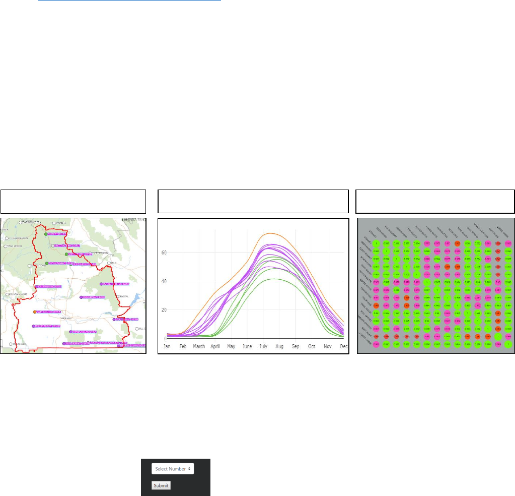
There are three user interface screens: RAWS Map, ERC Climatology Graph and Correlation Matrix. The
correlation matrix is color coded based on the R-squared values between each set of stations. The RAWS
markers on the map are color coded according to their best fit statistical grouping. These color
groupings are also used on the ERC Climatology Graphs. See page 2 for rough details on statistical
methods used.
Step by step instructions:
Using the map display, navigate to the desired dispatch boundary or state
Click inside the dispatch/state boundary
The graph and matrix will populate once the dispatch/state is selected
The number of statistical groupings can be adjusted by using the drop down menu and selecting
the submit button.
Map (RAWS and Dispatch Boundaries)
ERC Climatology Graph
Correlation Matrix

Statistical Methods
Presently, the stations are grouped according to their monthly mean ERC values over the last 10 years utilizing
an algorithm known as hierarchical clustering. We presently force the minimum number of clusters to be "3" for
each dispatch area -- however, the final default grouping methodology will be as follows:
1. Perform dimensionality reduction of each station's 12 reported monthly mean ERC values down to 2 or 3 so
that it will be possible to visualize the potential clustering opportunities in 2D or 3D (pivot charts are difficult to
analyze in many respects). This will be accomplished with Principal Components Analysis. So far, 2 principal
components have managed to explain 90 percent of the variance of the underlying data.
2. Compute the gap-statistic for each dispatch area utilizing the 2 principal components obtained from the
dimensionality reduction performed above. The highest gap-statistic will correspond to our naive estimation of
the default number of clusters "k" to compute for each dispatch. Interpretation of this result will be completely
subjective even though we are utilizing an objectively consistent methodology to obtain it. It's provided merely
to set the defaults.
3. Use a k-Means Clustering algorithm to group / cluster similar stations together within each dispatch area,
where the default "k" value is the max gap-statistic computed previously.
4. For Power-Users Only: To inform / elucidate the user's subsequent decision to either reduce or enlarge the
number of clusters, the Within-Clusters-Sum-of-Squares (WCSS) will be computed for each possible number of
a clusters (minimum of 1 to a maximum of N, where N is the total number of stations under consideration in the
dispatch area) which could be plotted as an elbow graph to help power users discern the trade-off point where
increasing or decreasing the number of clusters occurs. Or, perhaps the more preferable option would be
include plots for conducting silhouette analysis parameterized for different values of k.