Print Preview C:\TEMP\Apdf_2541_3068\home\AppData\Local\PTC\Arbortext\Editor\.aptcache\ae3849j0/tf38450r Signal Processing Toolbox User's Guide

User Manual:

Open the PDF directly: View PDF .
Page Count: 527 [warning: Documents this large are best viewed by clicking the View PDF Link!]

toc
tables

Signal Processing Toolbox™

User’s Guide

R2012b

How to Contact MathWorks

www.mathworks.com Web

comp.soft-sys.matlab Newsgroup

www.mathworks.com/contact_TS.html Technical Support

suggest@mathworks.com Product enhancement suggestions

bugs@mathworks.com Bug reports

doc@mathworks.com Documentation error reports

service@mathworks.com Order status, license renewals, passcodes

info@mathworks.com Sales, pricing, and general information

508-647-7000 (Phone)

508-647-7001 (Fax)

The MathWorks, Inc.

3 Apple Hill Drive

Natick, MA 01760-2098

For contact information about worldwide offices, see the MathWorks Web site.

Signal Processing Toolbox™ User’s Guide

The software described in this document is furnished under a license agreement. The software may be used

or copied only under the terms of the license agreement. No part of this manual may be photocopied or

reproduced in any form without prior written consent from The MathWorks, Inc.

FEDERAL ACQUISITION: This provision applies to all acquisitions of the Program and Documentation

by, for, or through the federal government of the United States. By accepting delivery of the Program

or Documentation, the government hereby agrees that this software or documentation qualifies as

commercial computer software or commercial computer software documentation as such terms are used

or defined in FAR 12.212, DFARS Part 227.72, and DFARS 252.227-7014. Accordingly, the terms and

conditions of this Agreement and only those rights specified in this Agreement, shall pertain to and govern

theuse,modification,reproduction,release,performance,display,anddisclosureoftheProgramand

Documentation by the federal government (or other entity acquiring for or through the federal government)

and shall supersede any conflicting contractual terms or conditions. If this License fails to meet the

government’s needs or is inconsistent in any respect with federal procurement law, the government agrees

to return the Program and Documentation, unused, to The MathWorks, Inc.

Trademarks

MATLAB and Simulink are registered trademarks of The MathWorks, Inc. See

www.mathworks.com/trademarks for a list of additional trademarks. Other product or brand

names may be trademarks or registered trademarks of their respective holders.

Patents

MathWorks products are protected by one or more U.S. patents. Please see

www.mathworks.com/patents for more information.

Revision History

1988 First printing New

November 1997 Second printing Revised

January 1998 Third printing Revised

September 2000 Fourth printing Revised for Version 5.0 (Release 12)

July 2002 Fifth printing Revised for Version 6.0 (Release 13)

December 2002 Online only Revised for Version 6.1 (Release 13+)

June 2004 Online only Revised for Version 6.2 (Release 14)

October 2004 Online only Revised for Version 6.2.1 (Release 14SP1)

March 2005 Online only Revised for Version 6.2.1 (Release 14SP2)

September 2005 Online only Revised for Version 6.4 (Release 14SP3)

March 2006 Sixth printing Revised for Version 6.5 (Release 2006a)

September 2006 Online only Revised for Version 6.6 (Release 2006b)

March 2007 Online only Revised for Version 6.7 (Release 2007a)

September 2007 Online only Revised for Version 6.8 (Release 2007b)

March 2008 Online only Revised for Version 6.9 (Release 2008a)

October 2008 Online only Revised for Version 6.10 (Release 2008b)

March 2009 Online only Revised for Version 6.11 (Release 2009a)

September 2009 Online only Revised for Version 6.12 (Release 2009b)

March 2010 Online only Revised for Version 6.13 (Release 2010a)

September 2010 Online only Revised for Version 6.14 (Release 2010b)

April 2011 Online only Revised for Version 6.15 (Release 2011a)

September 2011 Online only Revised for Version 6.16 (Release 2011b)

March 2012 Online only Revised for Version 6.17 (Release 2012a)

September 2012 Online only Revised for Version 6.18 (Release 2012b)

Contents

Filtering, Linear Systems and Transforms

Overview

Filter Implementation and Analysis ................. 1-2

Filtering Overview ................................ 1-2

Convolution and Filtering ........................... 1-2

Filters and Transfer Functions ...................... 1-3

Filtering with the filter Function ..................... 1-4

The filter Function ................................ 1-6

Other Functions for Filtering ....................... 1-8

Multirate Filter Bank Implementation ................ 1-8

Anti-Causal, Zero-Phase Filter Implementation ......... 1-9

Frequency Domain Filter Implementation ............. 1-10

Impulse Response ................................. 1-12

Frequency Response ............................... 1-14

DigitalDomain ................................... 1-14

Analog Domain ................................... 1-16

Magnitude and Phase .............................. 1-17

Delay ........................................... 1-18

Zero-Pole Analysis ................................. 1-21

Linear System Models .............................. 1-23

Available Models .................................. 1-23

Discrete-Time System Models ....................... 1-23

Continuous-Time System Models ..................... 1-31

Linear System Transformations ..................... 1-32

Discrete Fourier Transform ........................ 1-34

Filter Design and Implementation

Filter Requirements and Specification .............. 2-2

IIR Filter Design .................................. 2-4

IIR vs. FIR Filters ................................. 2-4

Classical IIR Filters ............................... 2-4

Other IIR Filters .................................. 2-5

IIR Filter Method Summary ......................... 2-5

Classical IIR Filter Design Using Analog Prototyping .... 2-6

Comparison of Classical IIR Filter Types .............. 2-9

FIR Filter Design .................................. 2-17

FIR vs. IIR Filters ................................. 2-17

FIR Filter Summary ............................... 2-18

Linear Phase Filters ............................... 2-18

Windowing Method ................................ 2-20

Multiband FIR Filter Design with Transition Bands ..... 2-24

Constrained Least Squares FIR Filter Design .......... 2-31

Arbitrary-Response Filter Design .................... 2-37

Special Topics in IIR Filter Design .................. 2-43

Classic IIR Filter Design ........................... 2-43

Analog Prototype Design ........................... 2-44

Frequency Transformation .......................... 2-44

Filter Discretization ............................... 2-46

Filtering Data With Signal Processing Toolbox

Software ........................................ 2-52

Lowpass FIR Filter — Window Method ................ 2-52

Bandpass Filters — Minimum-Order FIR and IIR

Systems ....................................... 2-56

Zero-Phase Filtering ............................... 2-65

Selected Bibliography .............................. 2-71

vi Contents

Designing a Filter in Fdesign — Process

Overview

Process Flow Diagram and Filter Design

Methodology .................................... 3-2

Exploring the Process Flow Diagram .................. 3-2

Selecting a Response ............................... 3-4

Selecting a Specification ............................ 3-4

Selecting an Algorithm ............................. 3-6

Customizing the Algorithm ......................... 3-8

Designing the Filter ............................... 3-8

Design Analysis ................................... 3-9

RealizeorApplytheFiltertoInputData .............. 3-10

Designing a Filter in the Filterbuilder GUI

Filterbuilder Design Process ....................... 4-2

Introduction to Filterbuilder ........................ 4-2

Design a Filter Using Filterbuilder ................... 4-2

Select a Response ................................. 4-3

Select a Specification .............................. 4-5

Select an Algorithm ................................ 4-5

Customize the Algorithm ........................... 4-6

Analyze the Design ................................ 4-8

RealizeorApplytheFiltertoInputData .............. 4-8

Designing a FIR Filter Using filterbuilder ........... 4-10

FIR Filter Design ................................. 4-10

FDATool: A Filter Design and Analysis GUI

Overview ......................................... 5-2

vii

FDATool ......................................... 5-2

Filter Design Methods ............................. 5-2

Using the Filter Design and Analysis Tool ............. 5-4

Analyzing Filter Responses ......................... 5-4

Filter Design and Analysis Tool Panels ................ 5-4

Getting Help ..................................... 5-5

Using FDATool .................................... 5-6

Choosing a Response Type .......................... 5-7

Choosing a Filter Design Method ..................... 5-8

Setting the Filter Design Specifications ............... 5-8

Computing the Filter Coefficients .................... 5-12

Analyzing the Filter ............................... 5-13

Editing the Filter Using the Pole/Zero Editor ........... 5-19

Converting the Filter Structure ...................... 5-23

Exporting a Filter Design ........................... 5-26

Generating a C Header File ......................... 5-32

Generating MATLAB Code .......................... 5-34

Managing Filters in the Current Session .............. 5-35

Saving and Opening Filter Design Sessions ............ 5-38

Importing a Filter Design .......................... 5-39

Import Filter Panel ................................ 5-39

Filter Structures .................................. 5-40

Statistical Signal Processing

Correlation and Covariance ........................ 6-2

Background Information ............................ 6-2

Using xcorr and xcov Functions ...................... 6-3

Bias and Normalization ............................ 6-3

Multiple Channels ................................. 6-4

Spectral Analysis .................................. 6-5

Background Information ............................ 6-5

Spectral Estimation Method ......................... 6-7

Nonparametric Methods ............................ 6-9

Parametric Methods ............................... 6-32

viii Contents

Selected Bibliography .............................. 6-46

Special Topics

Windows .......................................... 7-2

Why Use Windows? ................................ 7-2

Available Window Functions ........................ 7-2

Graphical User Interface Tools ...................... 7-3

Basic Shapes ..................................... 7-3

Generalized Cosine Windows ........................ 7-6

Kaiser Window ................................... 7-8

Chebyshev Window ................................ 7-12

Parametric Modeling .............................. 7-13

What is Parametric Modeling ........................ 7-13

Available Parametric Modeling Functions ............. 7-13

Time-Domain Based Modeling ....................... 7-14

Frequency-Domain Based Modeling .................. 7-18

Resampling ....................................... 7-21

Available Resampling Functions ..................... 7-21

resample Function ................................. 7-21

decimate and interp Functions ....................... 7-23

upfirdn Function .................................. 7-23

spline Function ................................... 7-23

Cepstrum Analysis ................................. 7-24

What Is a Cepstrum? .............................. 7-24

Inverse Complex Cepstrum ......................... 7-27

FFT-Based Time-Frequency Analysis ................ 7-28

Median Filtering .................................. 7-29

Communications Applications ...................... 7-30

Modulation ....................................... 7-30

Demodulation .................................... 7-31

Voltage Controlled Oscillator ........................ 7-34

Deconvolution ..................................... 7-35

Specialized Transforms ............................ 7-36

Chirp z-Transform ................................. 7-36

Discrete Cosine Transform .......................... 7-37

Hilbert Transform ................................. 7-40

Walsh–Hadamard Transform ........................ 7-41

Selected Bibliography .............................. 7-47

SPTool: A Signal Processing GUI Suite

SPTool: An Interactive Signal Processing

Environment .................................... 8-2

SPTool Overview .................................. 8-2

SPTool Data Structures ............................ 8-3

Opening SPTool ................................... 8-4

Getting Context-Sensitive Help ..................... 8-6

Signal Browser .................................... 8-7

Overview of the Signal Browser ...................... 8-7

Opening the Signal Browser ......................... 8-7

FDATool .......................................... 8-10

Filter Visualization Tool ........................... 8-11

Connection between FVTool and SPTool ............... 8-11

Opening the Filter Visualization Tool ................. 8-11

Analysis Parameters ............................... 8-12

Spectrum Viewer .................................. 8-13

xContents

Spectrum Viewer Overview ......................... 8-13

Opening the Spectrum Viewer ....................... 8-13

Filtering and Analysis of Noise ..................... 8-16

Overview ........................................ 8-16

Importing a Signal into SPTool ...................... 8-16

Designing a Filter ................................. 8-18

Applying a Filter to a Signal ........................ 8-20

Analyzing a Signal ................................ 8-22

Spectral Analysis in the Spectrum Viewer ............. 8-24

Exporting Signals, Filters, and Spectra .............. 8-27

Opening the Export Dialog Box ...................... 8-27

Exporting a Filter to the MATLAB Workspace .......... 8-28

Accessing Filter Parameters ........................ 8-29

Accessing Filter Parameters in a Saved Filter .......... 8-29

Accessing Parameters in a Saved Spectrum ............ 8-30

Importing Filters and Spectra ...................... 8-32

Similarities to Other Procedures ..................... 8-32

Importing Filters .................................. 8-32

Importing Spectra ................................. 8-34

Loading Variables from the Disk .................... 8-36

Saving and Loading Sessions ....................... 8-37

SPTool Sessions ................................... 8-37

Filter Formats .................................... 8-37

Selecting Signals, Filters, and Spectra ............... 8-39

Editing Signals, Filters, or Spectra .................. 8-40

Making Signal Measurements with Markers ......... 8-41

Setting Preferences ................................ 8-43

Overview of Setting Preferences ..................... 8-43

Summary of Settable Preferences .................... 8-44

Setting the Filter Design Tool ....................... 8-45

Using the Filter Designer ........................... 8-47

Filter Designer ................................... 8-47

Filter Types ...................................... 8-47

FIR Filter Methods ................................ 8-48

IIR Filter Methods ................................ 8-48

Pole/Zero Editor ................................... 8-48

Spectral Overlay Feature ........................... 8-48

Opening the Filter Designer ......................... 8-48

Accessing Filter Parameters in a Saved Filter .......... 8-50

Designing a Filter with the Pole/Zero Editor ........... 8-53

Positioning Poles and Zeros ......................... 8-54

Redesigning a Filter Using the Magnitude Plot ......... 8-56

Code Generation from MATLAB Support in

Signal Processing Toolbox

Supported Functions .............................. 9-2

Specifying Inputs in Code Generation from MATLAB

................................................. 9-7

Defining Input Size and Type ........................ 9-7

Inputs must be Constants ........................... 9-8

Code Generation Examples ......................... 9-11

Apply Window to Input Signal ....................... 9-11

Apply Lowpass Filter to Input Signal ................. 9-13

Cross Correlate or Autocorrelate Input Data ........... 9-14

freqz With No Output Arguments ................... 9-15

Zero Phase Filtering ............................... 9-16

xii Contents

Convolution and Correlation

Linear and Circular Convolution ................... 10-2

Confidence Intervals for Sample Autocorrelation ..... 10-5

Residual Analysis with Autocorrelation ............. 10-9

Autocorrelation of Moving Average Process .......... 10-19

Cross-correlation of Two Moving Average Processes .. 10-21

Cross-correlation of Delayed Signal in Noise ......... 10-23

Cross-correlation of Phase-Lagged Sine Wave ........ 10-26

Multirate Signal Processing

Downsampling — Signal Phases .................... 11-2

Downsampling — Aliasing .......................... 11-6

Filtering Before Downsampling ..................... 11-12

Upsampling — Imaging Artifacts .................... 11-14

Filtering After Upsampling — Interpolation ......... 11-16

Changing Signal Sampling Rate ..................... 11-18

xiii

Spectral Analysis

Power Spectral Density Estimates Using FFT ........ 12-2

Bias and Variability in the Periodogram ............. 12-10

Cross Spectrum and Magnitude-Squared Coherence .. 12-20

Amplitude Estimation and Zero Padding ............ 12-24

Significance Testing for Periodic Component ........ 12-27

Frequency Estimation by Subspace Methods ......... 12-29

Frequency-Domain Linear Regression ............... 12-32

Linear Prediction

Prediction Polynomial ............................. 13-2

Formant Estimation with LPC Coefficients .......... 13-5

AR Order Selection with Partial Autocorrelation

Sequence ....................................... 13-9

Transforms

Complex Cepstrum — Fundamental Frequency

Estimation ..................................... 14-2

xiv Contents

Analytic Signal for Cosine .......................... 14-6

Envelope Extraction Using The Analytic Signal ...... 14-9

Signal Generation

Display Time-Domain Data in Signal Browser ........ 15-2

Import and Display Signals ......................... 15-3

Configure the Signal Browser Properties .............. 15-6

Modify the Signal Browser Display ................... 15-9

Inspect Your Data (Scaling the Axes and Zooming) ...... 15-11

Signal Measurement

RMS Value of Periodic Waveforms .................. 16-2

Slew Rate of Triangular Waveform .................. 16-5

Duty Cycle of Rectangular Pulse Waveform .......... 16-9

Estimate State for Digital Clock ..................... 16-12

CalculateSettlingTimewithSignalBrowser ......... 16-16

Find Peak Amplitudes in Signal Browser ............ 16-20

Technical Conventions

Index

xvi Contents

Filtering, Linear Systems

and Transforms Overview

•“Filter Implementation and Analysis” on page 1-2

•“The filter Function” on page 1-6

•“Other Functions for Filtering” on page 1-8

•“Impulse Response” on page 1-12

•“Frequency Response” on page 1-14

•“Zero-Pole Analysis” on page 1-21

•“Linear System Models” on page 1-23

•“Discrete Fourier Transform” on page 1-34

1Filtering, Linear Systems and Transforms Overview

Filter Implementation and Analysis

In this section...

“Filtering Overview” on page 1-2

“Convolution and Filtering” on page 1-2

“Filters and Transfer Functions” on page 1-3

“Filtering with the filter Function” on page 1-4

Filtering Overview

This section describes how to filter discrete signals using the MATLAB®

filter function and other Signal Processing Toolbox™ functions. It also

discusses how to use the toolbox functions to analyze filter characteristics,

including impulse response, magnitude and phase response, group delay,

and zero-pole locations.

Convolution and Filtering

The mathematical foundation of filtering is convolution. The MATLAB conv

function performs standard one-dimensional convolution, convolving one

vector with another:

conv([1 1 1],[1 1 1])

ans =

12321

Note Convolve rectangular matrices for two-dimensional signal processing

using the conv2 function.

A digital filter’s output y(k)isrelatedtoitsinputx(k) by convolution with its

impulse response h(k).

yk hlxk l

() ()( )=−

=−∞

∞

∑

1-2

Filter Implementation and Analysis

If a digital filter’s impulse response h(k) is finite in length, and the input x(k)

is also of finite length, you can implement the filter using conv.Storex(k)ina

vector x,h(k)inavectorh, and convolve the two:

x = randn(5,1); % A random vector of length 5

h = [1 1 1 1]/4; % Length 4 averaging filter

y = conv(h,x);

The length of the output is the sum of the finite-length input vectors minus 1.

Filters and Transfer Functions

In general, the z-transform Y(z) of a discrete-time filter’s output y(n)isrelated

to the z-transform X(z)oftheinputby

Yz HzXz bbz bnz

aaz a

() () () () () ... ( )

() () ...

++++

+++

−−

−

12 1

1(() ()

+−

where H(z)isthefilter’stransfer function. Here, the constants b(i)anda(i)are

the filter coefficients and the order of the filter is the maximum of nand m.

Note The filter coefficients start with subscript 1, rather than 0. This reflects

the standard indexing scheme used for MATLAB vectors.

MATLAB filter functions store the coefficients in two vectors, one for the

numerator and one for the denominator. By convention, it uses row vectors

forfiltercoefficients.

Filter Coefficients and Filter Names

Many standard names for filters reflect the number of aand bcoefficients

present:

•When n=0(thatis,bis a scalar), the filter is an Infinite Impulse Response

(IIR), all-pole, recursive, or autoregressive (AR) filter.

•When m=0(thatis,ais a scalar), the filter is a Finite Impulse Response

(FIR), all-zero, nonrecursive, or moving-average (MA) filter.

1-3

1Filtering, Linear Systems and Transforms Overview

•If both nand mare greater than zero, the filter is an IIR, pole-zero,

recursive, or autoregressive moving-average (ARMA) filter.

The acronyms AR, MA, and ARMA are usually applied to filters associated

with filtered stochastic processes.

Filtering with the filter Function

It is simple to work back to a difference equation from the z-transform relation

shown earlier. Assume that a(1) = 1. Move the denominator to the left-hand

side and take the inverse z-transform.

yk a yk am yk m b xk b xk bn() ()( ) ( )( ) ()() ()( ) (+ − +…+ + − = + − +…+ +21 1 1 21 1))( )xk n−

In terms of current and past inputs, and past outputs, y(k)is

yk a ykb xk b xk bn xk n am() ()( )() () () ( ) ( ) ( ) (=+−+…++−− …−+−−121 1 121 ))( )yk m−

This is the standard time-domain representation of a digital filter, computed

starting with y(1) and assuming a causal system with zero initial conditions.

This representation’s progression is

ybx

ybxbxay

ybx

() () ()

() ()() ()() ()()

() ()()

111

2122121

313

=+−

=+bbx bx ay ay()() ()() ()() ()()22 31 22 31+− −

=

A filter in this form is easy to implement with the filter function. For

example, a simple single-pole filter (lowpass) is

B = 1; % Numerator

A = [1 -0.9]; % Denominator

where the vectors Band Arepresent the coefficients of a filter in transfer

function form. Note that the Acoefficient vectors are written as if the output

and input terms are separated in the difference equation. For the example,

the previous coefficient vectors represent a linear constant-coefficient

difference equation of

1-4

Filter Implementation and Analysis

yn yn xn() . ( ) ()−−=09 1

Changing the sign of the A(2) coefficient, results in the difference equation

yn yn xn() . ( ) ()+−=09 1

The previous coefficients are represented as:

B = 1; %Numerator

A = [1 0.9]; %Denominator

and results in a highpass filter.

Toapplythisfiltertoyourdata,use

y = filter(B,A,x);

filter gives you as many output samples as there are input samples, that

is, the length of yis the same as the length of x.Ifthefirstelementofa

is not 1, filter divides the coefficients by a(1) before implementing the

difference equation.

1-5

1Filtering, Linear Systems and Transforms Overview

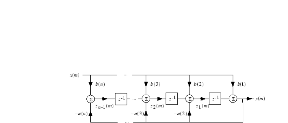
The filter Function

filter is implemented as the transposed direct-form II structure, where n-1

is the filter order. This is a canonical form that has the minimum number of

delay elements.

At sample m,filter computes the difference equations

ym b xm z m

zm b xm zm a ym

() ()() ( )

() ()() ( ) ()()

=+−

=+−−

−

212



221

111() ( )() ( ) ( )()

() ()() ()

mbn xmz m an ym

zmbnxman

=− + −−−

=−

−

−yym()

In its most basic form, filter initializes the delay outputs zi(1), i= 1, ..., n-1

to 0. This is equivalent to assuming both past inputs and outputs are zero.

Set the initial delay outputs using a fourth input parameter to filter,or

access the final delay outputs using a second output parameter:

[y,zf] = filter(b,a,x,zi)

Access to initial and final conditions is useful for filtering data in sections,

especially if memory limitations are a consideration. Suppose you have

collected data in two segments of 5000 points each:

x1 = randn(5000,1); % Generate two random data sequences.

x2 = randn(5000,1);

Perhaps the first sequence, x1, corresponds to the first 10 minutes of data

and the second, x2, to an additional 10 minutes. The whole sequence is

1-6

The filter Function

x=[x1;x2]. If there is not sufficient memory to hold the combined sequence,

filter the subsequences x1 and x2 one at a time. To ensure continuity of

the filtered sequences, use the final conditions from x1 as initial conditions

to filter x2:

[y1,zf] = filter(b,a,x1);

y2 = filter(b,a,x2,zf);

The filtic function generates initial conditions for filter.filtic computes

the delay vector to make the behavior of the filter reflect past inputs and

outputs that you specify. To obtain the same output delay values zf as above

using filtic,use

zf = filtic(b,a,flipud(y1),flipud(x1));

This can be useful when filtering short data sequences, as appropriate initial

conditions help reduce transient startup effects.

1-7

1Filtering, Linear Systems and Transforms Overview

Other Functions for Filtering

In this section...

“Multirate Filter Bank Implementation” on page 1-8

“Anti-Causal, Zero-Phase Filter Implementation” on page 1-9

“Frequency Domain Filter Implementation” on page 1-10

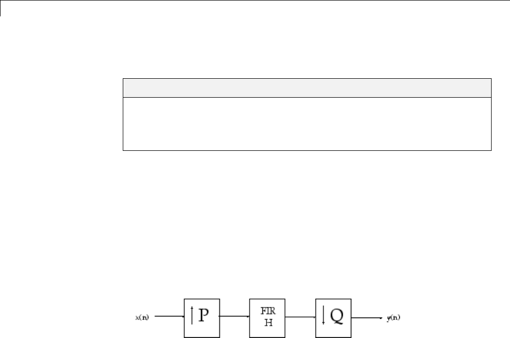
Multirate Filter Bank Implementation

The upfirdn function alters the sampling rate of a signal by an integer ratio

P/Q. It computes the result of a cascade of three systems that performs the

following tasks:

•Upsampling (zero insertion) by integer factor p

•FilteringbyFIRfilterh

•Downsampling by integer factor q

For example, to change the sample rate of a signal from 44.1 kHz to 48 kHz,

we first find the smallest integer conversion ratio p/q.Set

d = gcd(48000,44100);

p = 48000/d;

q = 44100/d;

In this example, p=160 and q=147. Sample rate conversion is then

accomplished by typing

y = upfirdn(x,h,p,q)

This cascade of operations is implemented in an efficient manner using

polyphase filtering techniques, and it is a central concept of multirate

filtering. Note that the quality of the resampling result relies on the quality of

the FIR filter h.

1-8

Other Functions for Filtering

Filter banks may be implemented using upfirdn by allowing the filter h

to be a matrix, with one FIR filter per column. A signal vector is passed

independently through each FIR filter, resulting in a matrix of output signals.

Other functions that perform multirate filtering (with fixed filter) include

resample,interp,anddecimate.

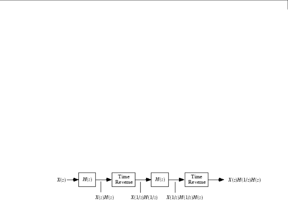
Anti-Causal, Zero-Phase Filter Implementation

In the case of FIR filters, it is possible to design linear phase filters that,

when applied to data (using filter or conv), simply delay the output by a

fixed number of samples. For IIR filters, however, the phase distortion is

usually highly nonlinear. The filtfilt function uses the information in the

signal at points before and after the current point, in essence “looking into the

future,” to eliminate phase distortion.

To see how filtfilt does this, recall that if the z-transform of a real

sequence x(n)isX(z), the z-transform of the time reversed sequence x(n)is

X(1/z). Consider the processing scheme.

Image of Anti Causal Zero Phase Filter

When |z|=1,thatisz=ejω, the output reduces to X(ejω)|H(ejω)|2.Given

all the samples of the sequence x(n), a doubly filtered version of xthat has

zero-phase distortion is possible.

For example, a 1-second duration signal sampled at 100 Hz, composed of two

sinusoidal components at 3 Hz and 40 Hz, is

fs = 100;

t = 0:1/fs:1;

x = sin(2*pi*t*3)+.25*sin(2*pi*t*40);

Now create a 10-point averaging FIR filter, and filter xusing both filter

and filtfilt for comparison:

1-9

1Filtering, Linear Systems and Transforms Overview

b = ones(1,10)/10; % 10 point averaging filter

y = filtfilt(b,1,x); % Noncausal filtering

yy = filter(b,1,x); % Normal filtering

plot(t,x,t,y,'--',t,yy,':')

Both filtered versions eliminate the 40 Hz sinusoid evident in the original,

solid line. The plot also shows how filter and filtfilt differ; the dashed

(filtfilt) line is in phase with the original 3 Hz sinusoid, while the dotted

(filter) line is delayed by about five samples. Also, the amplitude of the

dashed line is smaller due to the magnitude squared effects of filtfilt.

filtfilt reduces filter startup transients by carefully choosing initial

conditions, and by prepending onto the input sequence a short, reflected piece

of the input sequence. For best results, make sure the sequence you are

filtering has length at least three times the filter order and tapers to zero on

both edges.

Frequency Domain Filter Implementation

Dualitybetweenthetimedomainandthefrequencydomainmakesitpossible

to perform any operation in either domain. Usually one domain or the other is

more convenient for a particular operation, but you can always accomplish

a given operation in either domain.

1-10

Other Functions for Filtering

To implement general IIR filtering in the frequency domain, multiply the

discrete Fourier transform (DFT) of the input sequence with the quotient of

the DFT of the filter:

n = length(x);

y = ifft(fft(x).*fft(b,n)./fft(a,n));

This computes results that are identical to filter, but with different startup

transients (edge effects). For long sequences, this computation is very

inefficient because of the large zero-padded FFT operations on the filter

coefficients, and because the FFT algorithm becomes less efficient as the

number of points nincreases.

For FIR filters, however, it is possible to break longer sequences into shorter,

computationally efficient FFT lengths. The function

y = fftfilt(b,x)

uses the overlap add method to filter a long sequence with multiple

medium-length FFTs. Its output is equivalent to filter(b,1,x).

1-11

1Filtering, Linear Systems and Transforms Overview

Impulse Response

The impulse response of a digital filter is the output arising from the unit

impulse sequence defined as



()nn

≠

⎧

⎨

⎩

You can generate an impulse sequence a number of ways; one straightforward

way is

imp = [1; zeros(49,1)];

The impulse response of the simple filter b=1and a=[1 -0.9] is

h = filter(b,a,imp);

Asimplew

ay to display the impulse response is with the Filter Visualization

Tool (fvtool):

fvtool(b,a)

Then click the Impulse Response button on the toolbar or select

Analysis > Impulse Response. This plot shows the exponential decay

h(n) =0.9n ofthesinglepolesystem:

1-12

Impulse Response

1-13

1Filtering, Linear Systems and Transforms Overview

Frequency Response

In this section...

“Digital Domain” on page 1-14

“Analog Domain” on page 1-16

“Magnitude and Phase” on page 1-17

“Delay” on page 1-18

Digital Domain

freqz uses an FFT-based algorithm to calculate the z-transform frequency

response of a digital filter. Specifically, the statement

[h,w] = freqz(b,a,p)

returns the p-point complex frequency response, H(ejω), of the digital filter.

He bbe bne

aae am

jw jw jwn

() ( ) ( ) ... ( )

() () ... (

=++++

++++

−−

−

12 1

12 11)ejwm−

In its simplest form, freqz accepts the filter coefficient vectors band a,andan

integer pspecifying the number of points at which to calculate the frequency

response. freqz returns the complex frequency response in vector h,andthe

actual frequency points in vector win rad/s.

freqz can accept other parameters, such as a sampling frequency or a

vector of arbitrary frequency points. The example below finds the 256-point

frequency response for a 12th-order Chebyshev Type I filter. The call to freqz

specifies a sampling frequency fs of 1000 Hz:

[b,a] = cheby1(12,0.5,200/500);

[h,f] = freqz(b,a,256,1000);

Because the parameter list includes a sampling frequency, freqz returns a

vector fthat contains the 256 frequency points between 0 and fs/2 used in

the frequency response calculation.

1-14

Frequency Response

Note This toolbox uses the convention that unit frequency is the Nyquist

frequency, defined as half the sampling frequency. The cutoff frequency

parameter for all basic filter design functions is normalized by the Nyquist

frequency. For a system with a 1000 Hz sampling frequency, for example,

300 Hz is 300/500 = 0.6. To convert normalized frequency to angular frequency

around the unit circle, multiply by π. To convert normalized frequency back

to hertz, multiply by half the sample frequency.

If you call freqz with no output arguments, it plots both magnitude

versus frequency and phase versus frequency. For example, a ninth-order

Butterworth lowpass filter with a cutoff frequency of 400 Hz, based on a 2000

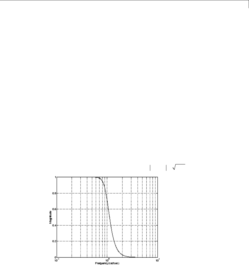
Hz sampling frequency, is

[b,a] = butter(9,400/1000);

To calculate the 256-point complex frequency response for this filter, and plot

the magnitude and phase with freqz,use

freqz(b,a,256,2000)

or to display the magnitude and phase responses in fvtool, which provides

additional analysis tools, use

fvtool(b,a)

and click the Magnitude and Phase Response button on the toolbar or

select Analysis > Magnitude and Phase Response.

1-15

1Filtering, Linear Systems and Transforms Overview

freqz can also accept a vector of arbitrary frequency points for use in the

frequency response calculation. For example,

w = linspace(0,pi);

h = freqz(b,a,w);

calculates the complex frequency response at the frequency points in wfor the

filter defined by vectors band a. The frequency points can range from 0 to

2π. To specify a frequency vector that ranges from zero to your sampling

frequency, include both the frequency vector and the sampling frequency

value in the parameter list.

Analog Domain

freqs evaluates frequency response for an analog filter defined by two input

coefficient vectors, band a. Its operation is similar to that of freqz;youcan

specify a number of frequency points to use, supply a vector of arbitrary

frequency points, and plot the magnitude and phase response of the filter.

1-16

Frequency Response

Magnitude and Phase

MATLAB functions are available to extract magnitude and phase from a

frequency response vector h. The function abs returns the magnitude of the

response; anglereturns the phase angle in radians. To extract the magnitude

and phase of a Butterworth filter:

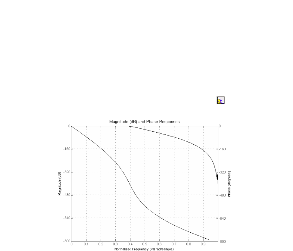
[b,a] = butter(9,400/1000);

fvtool(b,a)

and click the Magnitude and Phase Response button on the toolbar or

select Analysis > Magnitude and Phase Response to display the plot.

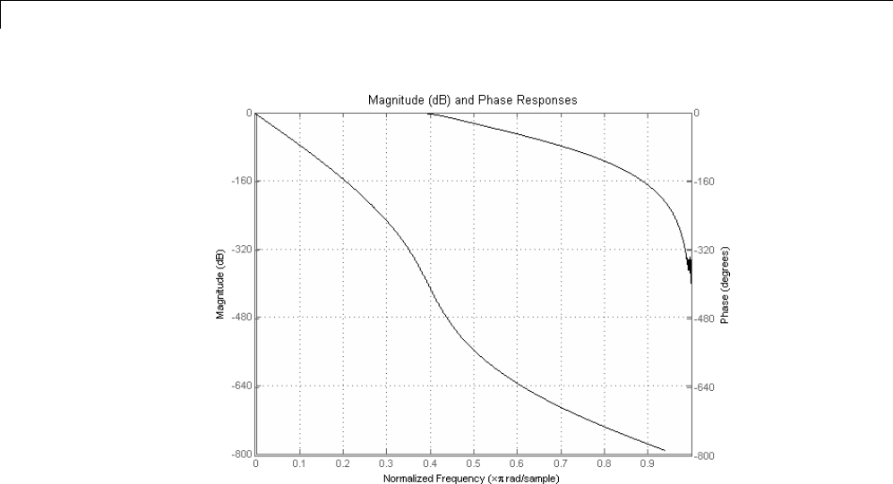
The unwrap function is also useful in frequency analysis. unwrap unwraps

the phase to make it continuous across 360º phase discontinuities by adding

multiples of ±360°, as needed. To see how unwrap is useful, design a

25th-order lowpass FIR filter:

h = fir1(25,0.4);

Obtain the filter’s frequency response with freqz, and plot the phase in

degrees:

1-17

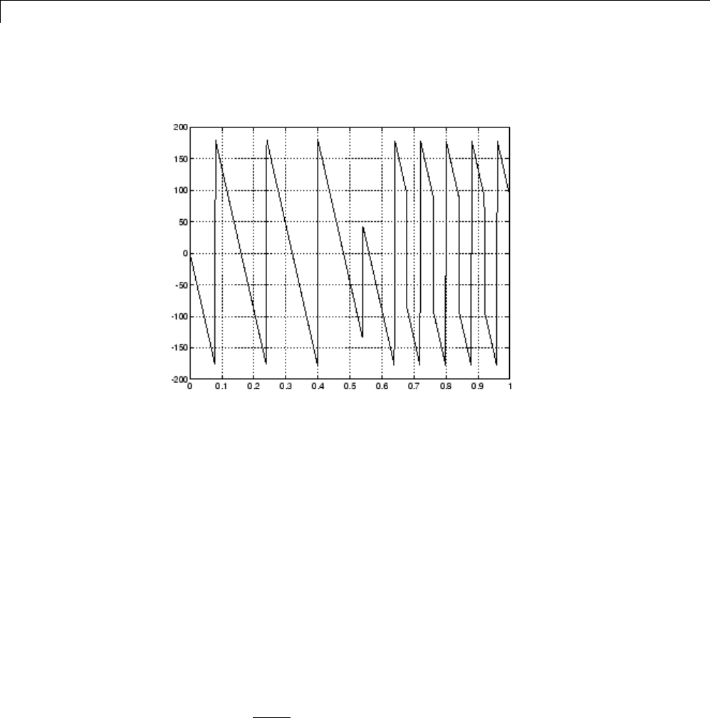
1Filtering, Linear Systems and Transforms Overview

[H,f] = freqz(h,1,512,2);

plot(f,angle(H)*180/pi); grid

It is difficult to distinguish the 360° jumps (an artifact of the arctangent

function inside angle) from the 180° jumps that signify zeros in the frequency

response.

unwrap eliminates the 360° jumps:

plot(f,unwrap(angle(H))*180/pi);

or you can use phasez to see the unwrapped phase.

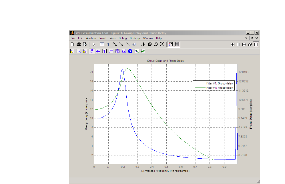
Delay

The group delay ofafilterisameasureoftheaveragetimedelayofthefilter

as a function of frequency. It is defined as the negative first derivative of a

filter’s phase response. If the complex frequency response of a filter is H(ejω),

then the group delay is

 



() ()

=−

1-18

Frequency Response

where θ(ω) is the phase, or argument of H(ejω). Compute group delay with

[gd,w] = grpdelay(b,a,n)

which returns the n-point group delay, ,τg(ω) of the digital filter specified by

band a, evaluated at the frequencies in vector w.

The phase delay of a filter is the negative of phase divided by frequency:

 



p() ()

=−

To plot both the group and phase delays of a system on the same FVTool

graph, type

[b,a] = butter(10,200/1000);

hFVT = fvtool(b,a,'Analysis','grpdelay');

set(hFVT,'NumberofPoints',128,'OverlayedAnalysis','phasedelay');

legend(hFVT)

1-19

1Filtering, Linear Systems and Transforms Overview

1-20

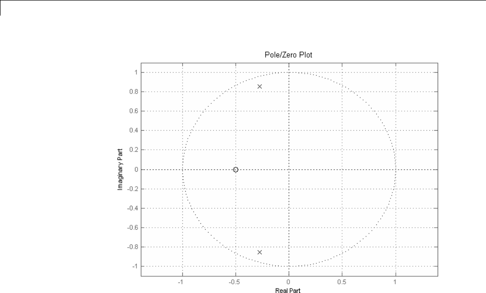
Zero-Pole Analysis

The zplane function plots poles and zeros of alinearsystem. Forexample,

a simple filter with a zero at -1/2 and a complex pole pair at 0.9e–j2π(0.3) and

0.9ej2π(0.3) is

zer = -0.5;

pol = 0.9*exp(j*2*pi*[-0.3 0.3]');

To view the pole-zero plot for this filter you can use

zplane(zer,pol)

or, for access to additional tools, use fvtool. First convert the poles and zeros

to transfer function form, then call fvtool,

[b,a] = zp2tf(zer,pol,1);

fvtool(b,a)

and click the Pole/Zero Plot toolbar button on the toolbar or select

Analysis > Pole/Zero Plot to see the plot.

1-21

1Filtering, Linear Systems and Transforms Overview

For a system in zero-pole form, supply column vector arguments zand pto

zplane:

zplane(z,p)

For a system in transfer function form, supply row vectors band aas

arguments to zplane:

zplane(b,a)

In this case zplane finds the roots of band ausing the roots function and

plots the resulting zeros and poles.

See “Linear System Models” on page 1-23 for details on zero-pole and transfer

function representation of systems.

1-22

Linear System Models

In this section...

“Available Models” on page 1-23

“Discrete-Time System Models” on page 1-23

“Continuous-Time System Models” on page 1-31

“Linear System Transformations” on page 1-32

Available Models

Several Signal Processing Toolbox models are provided for representing linear

time-invariant systems. This flexibility lets you choose the representational

scheme that best suits your application and, within the bounds of numeric

stability, convert freely to and from most other models. This section provides

a brief overview of supported linear system models and describes how to work

with these models in the MATLAB technical computing environment.

Discrete-Time System Models

The discrete-time system models are representational schemes for digital

filters. The MATLAB technical computing environment supports several

discrete-time system models, which are described in the following sections:

•“Transfer Function” on page 1-23

•“Zero-Pole-Gain” on page 1-24

•“State-Space” on page 1-25

•“Partial Fraction Expansion (Residue Form)” on page 1-26

•“Second-Order Sections (SOS)” on page 1-27

•“Lattice Structure” on page 1-28

•“Convolution Matrix” on page 1-30

Transfer Function

The transfer function is a basic z-domain representation of a digital filter,

expressing the filter as a ratio of two polynomials. It is the principal

1-23

1Filtering, Linear Systems and Transforms Overview

discrete-time model for this toolbox. The transfer function model description

for the z-transform of a digital filter’s difference equation is

Yz bbz bnz

aaz amz

() () () ( )

() () ( ) ()=++…++

++…++

−−

12 1

Here, the constants b(i)anda(i) are the filter coefficients, and the order of the

filter is the maximum of nand m. In the MATLAB environment, you store

these coefficients in two vectors (row vectors by convention), one row vector

for the numerator and one for the denominator. See “Filters and Transfer

Functions” on page 1-3 for more details on the transfer function form.

Zero-Pole-Gain

The factored or zero-pole-gain form of a transfer function is

Hz qz

pz kzq zq zqn

zp zp

() ()

()

( ( ))( ( ))...( ( ))

( ( ))( ( ))

−− −

−−

....( ( ))zpn−

By convention, polynomial coefficients are stored in row vectors and

polynomial roots in column vectors. In zero-pole-gain form, therefore, the

zero and pole locations for the numerator and denominator of a transfer

function reside in column vectors. The factored transfer function gain kis a

MATLAB scalar.

The poly and roots functions convert between polynomial and zero-pole-gain

representations. For example, a simple IIR filter is

b=[234];

a=[1331];

The zeros and poles of this filter are

q = roots(b)

p = roots(a)

% Gain factor

k = b(1)/a(1)

Returning to the original polynomials,

1-24

Linear System Models

bb = k*poly(q)

aa = poly(p)

Note that band ain this case represent the transfer function:

Hz zz

zzz

()=++

+++

=++

+++

−−

−−−

23 4

13 3

234

331

123

For b=[2 3 4],theroots function misses the zero for zequal to 0. In fact, it

misses poles and zeros for zequal to 0 whenever the input transfer function

has more poles than zeros, or vice versa. This is acceptable in most cases. To

circumvent the problem, however, simplyappendzerostomakethevectors

the same length before using the roots function; for example, b=[b 0].

State-Space

It is always possible to represent a digital filter, or a system of difference

equations, as a set of first-order difference equations. In matrix or state-space

form, you can write the equations as

xn Axn Bun

yn Cxn Dun

( ) () ()

() () ()

+= +

where uis the input, xis the state vector, and yis the output. For

single-channel systems, Ais an m-by-mmatrix where mis the order of the filter,

Bis a column vector, Cis a row vector, and Dis a scalar. State-space notation

is especially convenient for multichannel systems where input uand output y

become vectors, and B,C,andDbecome matrices.

State-space representation extends easily to the MATLAB environment.A,B,

C,andDare rectangular arrays; MATLAB functions treat them as individual

variables.

Taking the z-transform of the state-space equations and combining them

shows the equivalence of state-space and transfer function forms:

Yz HzUz Hz CzI A B D() () () () ( )==−+

−

, where 1

1-25

1Filtering, Linear Systems and Transforms Overview

Don’t be concerned if you are not familiar with the state-space representation

of linear systems. Some of the filter design algorithms use state-space

form internally but do not require any knowledge of state-space concepts

to use them successfully. If your applications use state-space based signal

processing extensively, however, see the Control System Toolbox™ product

for a comprehensive library of state-space tools.

Partial Fraction Expansion (Residue Form)

Each transfer function also has a corresponding partial fraction expansion or

residue form representation, given by

pnz

kkz

()

() ... ()

() ( ) ( ) ...=−++

−++ ++

−−

−

11 1 12

1kkm n z mn

()

−+ −−

provided H(z) has no repeated poles. Here, nis the degree of the denominator

polynomial of the rational transfer function b(z)/a(z). If ris a pole of

multiplicity sr,thenH(z)hastermsoftheform:

pjz

rj s

pjz

()

(())

... ()

(())1

112 1

−++

−++−

−

−− −

The Signal Processing Toolbox residuez function in converts transfer

functions to and from the partial fraction expansion form. The “z”ontheend

of residuez stands for z-domain, or discrete domain. residuez returns the

poles in a column vector p, the residues corresponding to the poles in a column

vector r, and any improper part of the original transfer function in a row

vector k.residuez determines that two poles are the same if the magnitude of

their difference is smaller than 0.1 percent of either of the poles’ magnitudes.

Partial fraction expansion arises in signal processing as one method of finding

the inverse z-transform of a transfer function. For example, the partial

fraction expansion of

Hz z

()=−+

−

−−

16 8

1-26

Linear System Models

b = [-4 8];

a=[168];

[r,p,k] = residuez(b,a)

which corresponds to

()=−

+++

−−

To find the inverse z-transform of H(z), find the sum of the inverse

z-transforms of the two addends of H(z), giving the causal impulse response:

hn n

() ( ) ( ) ,,,=− − + − = …12 4 8 2 0 1 2

To verify this in the MATLAB environment, type

imp=[10000];

resptf = filter(b,a,imp)

respres = filter(r(1),[1 -p(1)],imp)+...

filter(r(2),[1 -p(2)],imp)

Second-Order Sections (SOS)

Any transfer function H(z) has a second-order sections representation

Hz H z bbzbz

aazaz

Lkk k

kk k

() ()==

−−

∏∏

122

where Lis the number of second-order sections that describe the system.

The MATLAB environment represents the second-order section form of a

discrete-time system as an L-by-6 array sos. Each row of sos contains a

single second-order section, where the row elements are the three numerator

and three denominator coefficients that describe the second-order section.

1-27

1Filtering, Linear Systems and Transforms Overview

sos

bbbaaa

01 11 21 01 11 21

02 12 22 02 12 22

......

bbaaa

LLLL2012

⎛

⎝

⎜

⎞

⎠

⎟

There are many ways to represent a filter in second-order section form.

Through careful pairing of the pole and zero pairs, ordering of the sections

in the cascade, and multiplicative scaling of the sections, it is possible to

reduce quantization noise gain and avoid overflow in some fixed-point filter

implementations. The functions zp2sos and ss2sos, described in “Linear

System Transformations” on page 1-32, perform pole-zero pairing, section

scaling, and section ordering.

Note AllSignalProcessingToolboxsecond-order section transformations

apply only to digital filters.

Lattice Structure

For a discrete Nth order all-pole or all-zero filter described by the polynomial

coefficients a(n),n=1,2,...,N+1, there are Ncorresponding lattice structure

coefficients k(n),n=1,2,...,N. The parameters k(n) are also called the

reflection coefficients of the filter. Given these reflection coefficients, you can

implement a discrete filter as shown below.

1-28

Linear System Models

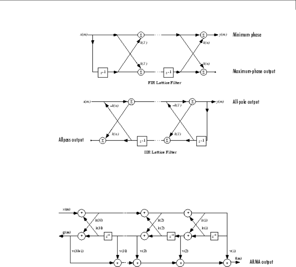
FIRandIIRLatticeFilterstructurediagrams

For a general pole-zero IIR filter described by polynomial coefficients a

and b, there are both lattice coefficients k(n) for the denominator aand

ladder coefficients v(n) for the numerator b. The lattice/ladder filter may be

implemented as

Diagram of lattice/ladder filter

The toolbox function tf2latc accepts an FIR or IIR filter in polynomial form

and returns the corresponding reflection coefficients. An example FIR filter

in polynomial form is

b = [1.0000 0.6149 0.9899 0.0000 0.0031 -0.0082];

1-29

1Filtering, Linear Systems and Transforms Overview

This filter’s lattice (reflection coefficient) representation is

k = tf2latc(b)

For IIR filters, the magnitude of the reflection coefficients provides an easy

stability check. If all the reflection coefficients corresponding to a polynomial

have magnitude less than 1, all of that polynomial’s roots are inside the unit

circle. For example, consider an IIR filter with numerator polynomial bfrom

above and denominator polynomial:

a = [1 1/2 1/3];

The filter’s lattice representation is

[k,v] = tf2latc(b,a);

Because abs(k) <1for all reflection coefficients in k, the filter is stable.

The function latc2tf calculates the polynomial coefficients for a filter from

its lattice (reflection) coefficients. Given the reflection coefficient vector

k(above), the corresponding polynomial form is

b = latc2tf(k);

The lattice or lattice/ladder coefficients can be used to implement the filter

using the function latcfilt.

Convolution Matrix

In signal processing, convolving two vectors or matrices is equivalent to

filtering one of the input operands by the other. This relationship permits the

representation of a digital filter as a convolution matrix.

Given any vector, the toolbox function convmtx generates a matrix whose

inner product with another vector is equivalent to the convolution of the two

vectors. The generated matrix represents a digital filter that you can apply to

any vector of appropriate length; the inner dimension of the operands must

agreetocomputetheinnerproduct.

The convolution matrix for a vector b, representing the numerator coefficients

for a digital filter, is

1-30

Linear System Models

b = [1 2 3]; x = randn(3,1);

C = convmtx(b',3);

Two equivalent ways to convolve bwith xare as follows.

y1 = C*x;

y2 = conv(b,x);

Continuous-Time System Models

The continuous-time system models are representational schemes for analog

filters. Many of the discrete-time system models described earlier are also

appropriate for the representation of continuous-time systems:

•State-space form

•Partial fraction expansion

•Transfer function

•Zero-pole-gain form

It is possible to represent any system of linear time-invariant differential

equations as a set of first-order differential equations. In matrix or state-space

form, you can express the equations as

xAxBu

yCxDu

where uis a vector of nu inputs, xis an nx-element state vector, and yis a

vector of ny outputs. In the MATLAB environment, A,B,C,andDare stored in

separate rectangular arrays.

An equivalent representation of the state-space system is the Laplace

transform transfer function description

Ys HsUs() () ()=

where

1-31

1Filtering, Linear Systems and Transforms Overview

Hs CsI A B D() ( )=− +

−1

For single-input, single-output systems, this form is given by

Hs bs

bs bs bn

as as a

() ()

()

() () ( )

() () (

== ++…++

++…+

−

12 1

1mm +1)

Given the coefficients of a Laplace transform transfer function, residue

determines the partial fraction expansion of the system. See the description

of residue for details.

The factored zero-pole-gain form is

Hs zs

ps ksz sz szn

sp sp

() ()

()

( ( ))( ( )) ( ( ))

( ( ))( ( )) (

==−−…−

−−…

sspm−())

Asinthediscrete-timecase,theMATLABenvironmentstorespolynomial

coefficients in row vectors in descending powers of s.Itstorespolynomial

roots, or zeros and poles, in column vectors.

Linear System Transformations

A number of Signal Processing Toolbox functions are provided to convert

between the various linear system models.. You can use the following chart to

find an appropriate transfer function: find the row of the model to convert

from on the left side of the chart and the column of the model to convert to on

the top of the chart and read the function name(s) at the intersection of the

row and column. Note that some cells of this table are empty.

Transfer

Function

State-

Space

Zero-

Pole-

Gain

Partial

Fraction

Lattice

Filter

Second-

Order

Sections

Convolution

Matrix

Transfer

Function

tf2ss tf2zp

roots

residuez tf2latc none convmtx

State-Space ss2tf ss2zp none none ss2sos none

1-32

Linear System Models

Transfer

Function

State-

Space

Zero-

Pole-

Gain

Partial

Fraction

Lattice

Filter

Second-

Order

Sections

Convolution

Matrix

Zero-Pole-

Gain

zp2tf

poly

zp2ss none none zp2sos none

Partial

Fraction

residuez none none none none none

Lattice

Filter

latc2tf none none none none none

SOS sos2tf sos2ss sos2zp none none none

Note Converting from one filter structure or model to another may produce

a result with different characteristics than the original. This is due to the

computer’s finite-precision arithmetic and the variations in the conversion’s

round-off computations.

Many of the toolbox filter design functions use these functions internally.

For example, the zp2ss function converts the poles and zeros of an analog

prototype into the state-space form required for creation of a Butterworth,

Chebyshev, or elliptic filter. Once in state-space form, the filter design

function performs any required frequency transformation, that is, it

transforms the initial lowpass design into a bandpass, highpass, or bandstop

filter, or a lowpass filter with the desired cutoff frequency.

Note AllSignalProcessingToolboxsecond-order section transformations

apply only to digital filters.

1-33

1Filtering, Linear Systems and Transforms Overview

Discrete Fourier Transform

The discrete Fourier transform, or DFT, is the primary tool of digital signal

processing. The foundation of Signal Processing Toolbox product is the fast

Fourier transform (FFT), a method for computing the DFT with reduced

execution time. Many of the toolbox functions (including z-domain frequency

response, spectrum and cepstrum analysis, and some filter design and

implementation functions) incorporate the FFT.

The MATLAB environment provides the functions fft and ifft to compute

the discrete Fourier transform and its inverse, respectively. For the input

sequence xand its transformed version X(the discrete-time Fourier transform

at equally spaced frequencies around the unit circle), the two functions

implement the relationships

Xk xn W

Nkn

() (),+= +

−

∑

and

xn NXk W

Nkn

() .() 







111

In these equations, the series subscripts begin with 1 instead of 0 because of

the MATLAB vector indexing scheme, and

NjN

=−2



Note TheMATLABconventionistouseanegativejfor the fft function.

This is an engineering convention; physics and pure mathematics typically

use a positive j.

fft, with a single input argument x, computes the DFT of the input vector

or matrix. If xis a vector, fft computes the DFT of the vector; if xis a

rectangular array, fft computes the DFT of each array column.

1-34

Discrete Fourier Transform

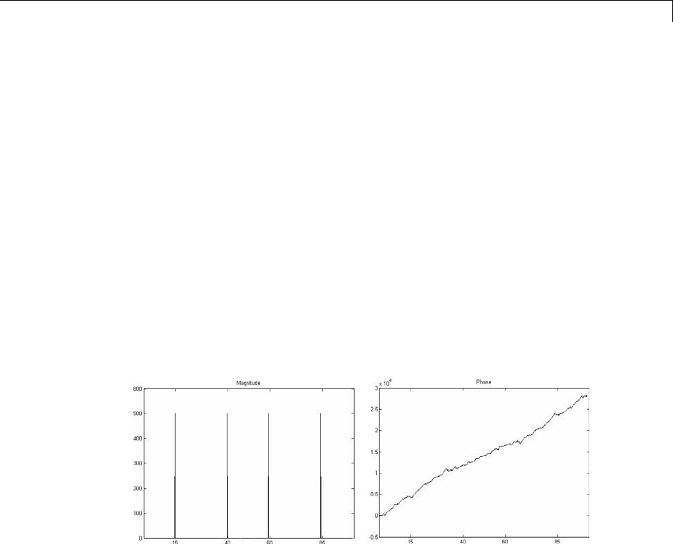
For example, create a time vector and signal:

t = (0:1/100:10-1/100); % Time vector

x = sin(2*pi*15*t) + sin(2*pi*40*t); % Signal

The DFT of the signal, and the magnitude and phase of the transformed

sequence, are then

y = fft(x); % Compute DFT of x

m = abs(y); p = unwrap(angle(y)); % Magnitude and phase

To plot the magnitude and phase, type the following commands:

f = (0:length(y)-1)*99/length(y); % Frequency vector

plot(f,m); title('Magnitude');

set(gca,'XTick',[15 40 60 85]);

figure; plot(f,p*180/pi); title('Phase');

set(gca,'XTick',[15 40 60 85]);

Aseco

nd argument to fft specifies a number of points nfor the transform,

representing DFT length:

y = fft(x,n);

In this case, fft pads the input sequence with zeros if it is shorter than n,or

truncates the sequence if it is longer than n.Ifnisnotspecified,itdefaults

to the length of the input sequence. Execution time for fft depends on the

length, n, of the DFT it performs; see the fft for details about the algorithm.

1-35

1Filtering, Linear Systems and Transforms Overview

Note The resulting FFT amplitude is A*n/2, where A is the original amplitude

and n is the number of FFT points. This is true only if the number of FFT

points is greater than or equal to the number of data samples. If the number

of FFT points is less, the FFT amplitude is lower than the original amplitude

by the above amount.

The inverse discrete Fourier transform function ifft also accepts an input

sequence and, optionally, the number of desired points for the transform. Try

the example below; the original sequence xand the reconstructed sequence

are identical (within rounding error).

t = (0:1/255:1);

x = sin(2*pi*120*t);

y = real(ifft(fft(x)));

This toolbox also includes functions for the two-dimensional FFT and its

inverse, fft2 and ifft2. These functions are useful for two-dimensional

signal or image processing. The goertzel function, which is another

algorithm to compute the DFT, also is included in the toolbox. This function is

efficient for computing the DFTofaportionofalongsignal.

It is sometimes convenient to rearrange the output of the fft or fft2 function

so the zero frequency component is at the center of the sequence. The

MATLAB function fftshift moves the zero frequency component to the

center of a vector or matrix.

1-36

Filter Design and

Implementation

•“Filter Requirements and Specification” on page 2-2

•“IIR Filter Design” on page 2-4

•“FIR Filter Design” on page 2-17

•“Special Topics in IIR Filter Design” on page 2-43

•“Filtering Data With Signal Processing Toolbox Software” on page 2-52

•“Selected Bibliography” on page 2-71

2Filter Design and Implementation

Filter Requirements and Specification

Filter design is the process of creating the filter coefficients to meet specific

filtering requirements. Filter implementation involves choosing and applying

a particular filter structure to those coefficients. Only after both design and

implementation have been performed can data be filtered. The following

chapter describes filter design and implementation in Signal Processing

Toolbox software.

The goal of filter design is to perform frequency dependent alteration of a data

sequence. A possible requirement might be to remove noise above 200 Hz from

a data sequence sampled at 1000 Hz. A more rigorous specification might call

for a specific amount of passband ripple, stopband attenuation, or transition

width. A very precise specification could ask to achieve the performance goals

with the minimum filter order, or it could call for an arbitrary magnitude

shape, or it might require an FIR filter. Filter design methods differ primarily

in how performance is specified.

To design a filter, the Signal Processing Toolbox software offers two

approaches: object-oriented and non-object oriented. The object-oriented

approach first constructs a filter specification object, fdesign,andthen

invokes an appropriate design method. To illustrate the object-oriented

approach, design and implement a 5–th order lowpass Butterworth filter with

a 3–dB frequency of 200 Hz. Assume a sampling frequency of 1 kHz. Apply

thefiltertoinputdata.

Fs=1000; %Sampling Frequency

time = 0:(1/Fs):1; %time vector

% Data vector

x = cos(2*pi*60*time)+sin(2*pi*120*time)+randn(size(time));

d=fdesign.lowpass('N,F3dB',5,200,Fs); %lowpass filter specification object

% Invoke Butterworth design method

Hd=design(d,'butter');

y=filter(Hd,x);

The non-object oriented approach implements the filter using a function such

as butter and firpm. All of the non-object oriented filter design functions

operate with normalized frequencies. Convert frequency specifications in

Hz to normalized frequency to use these functions. The Signal Processing

Toolbox software defines normalized frequency to be in the closed interval

2-2

Filter Requirements and Specification

[0,1] with 1 denoting πradians/sample. For example, to specify a normalized

frequency of π/2 radians/sample, enter 0.5.

To convert from Hz to normalized frequency, multiply the frequency in Hz by

two and divide by the sampling frequency. To design a 5–th order lowpass

Butterworth filter with a 3–dB frequency of 200 Hz using the non-object

oriented approach, use butter:

Wn = (2*200)/1000; %Convert 3-dB frequency

% to normalized frequency: 0.4*pi rad/sample

[B,A] = butter(5,Wn,'low');

y = filter(B,A,x);

2-3

2Filter Design and Implementation

IIR Filter Design

In this section...

“IIR vs. FIR Filters” on page 2-4

“Classical IIR Filters” on page 2-4

“Other IIR Filters” on page 2-5

“IIR Filter Method Summary” on page 2-5

“Classical IIR Filter Design Using Analog Prototyping” on page 2-6

“Comparison of Classical IIR Filter Types” on page 2-9

IIRvs. FIRFilters

TheprimaryadvantageofIIRfiltersoverFIRfiltersisthattheytypically

meet a given set of specifications with a much lower filter order than a

corresponding FIR filter. Although IIR filters have nonlinear phase, data

processing within MATLAB software is commonly performed “offline,” that

is, the entire data sequence is available prior to filtering. This allows for a

noncausal, zero-phase filtering approach (via the filtfilt function), which

eliminates the nonlinear phase distortion of an IIR filter.

Classical IIR Filters

The classical IIR filters, Butterworth, Chebyshev Types I and II, elliptic, and

Bessel, all approximate the ideal “brick wall” filter in different ways.

This toolbox provides functions to create all these types of classical IIR filters

in both the analog and digital domains (except Bessel, for which only the

analog case is supported), and in lowpass, highpass, bandpass, and bandstop

configurations. For most filter types, you can also find the lowest filter

order that fits a given filter specification in terms of passband and stopband

attenuation, and transition width(s).

2-4

IIR Filter Design

Other IIR Filters

The direct filter design function yulewalk finds a filter with magnitude

response approximating a desired function. This is one way to create a

multiband bandpass filter.

You can also use the parametric modeling or system identification functions

to design IIR filters. These functions are discussed in “Parametric Modeling”

on page 7-13.

The generalized Butterworth design function maxflat is discussed in the

section “Generalized Butterworth Filter Design” on page 2-15.

IIR Filter Method Summary

The following table summarizes the various filter methods in the toolbox and

lists the functionsavailabletoimplementthesemethods.

Toolbox Filters Methods and Available Functions

Filter Method Description Filter Functions

Analog

Prototyping

Using the poles and zeros of a

classical lowpass prototype

filter in the continuous

(Laplace) domain, obtain a

digital filter through frequency

transformation and filter

discretization.

Complete design functions:

besself,butter,cheby1,cheby2,ellip

Order estimation functions:

buttord,cheb1ord,cheb2ord,ellipord

Lowpass analog prototype functions:

besselap,buttap,cheb1ap,cheb2ap,

ellipap

Frequency transformation functions:

lp2bp,lp2bs,lp2hp,lp2lp

Filter discretization functions:

bilinear,impinvar

Direct Design Design digital filter directly

in the discrete time-domain

by approximating a piecewise

linear magnitude response.

yulewalk

2-5

2Filter Design and Implementation

Toolbox Filters Methods and Available Functions (Continued)

Filter Method Description Filter Functions

Generalized

Butterworth

Design

Design lowpass Butterworth

filters with more zeros than

poles.

maxflat

Parametric

Modeling

Find a digital filter that

approximates a prescribed time

or frequency domain response.

(See System Identification

Toolbox™ documentation for

an extensive collection of

parametric modeling tools.)

Time-domain modeling functions:

lpc,prony,stmcb

Frequency-domain modeling functions:

invfreqs,invfreqz

Classical IIR Filter Design Using Analog Prototyping

The principal IIR digital filter design technique this toolbox provides is based

on the conversion of classical lowpass analog filters to their digital equivalents.

The following sections describe how to design filters and summarize the

characteristics of the supported filter types. See “Special Topics in IIR Filter

Design” on page 2-43 for detailed steps on the filter design process.

Complete Classical IIR Filter Design

You can easily create a filter of any order with a lowpass, highpass, bandpass,

or bandstop configuration using the filter design functions.

Filter Design Functions

Filter Type Design Function

Bessel (analog only) [b,a] = besself(n,Wn,options)

[z,p,k] = besself(n,Wn,options)

[A,B,C,D] = besself(n,Wn,options)

Butterworth [b,a] = butter(n,Wn,options)

[z,p,k] = butter(n,Wn,options)

[A,B,C,D] = butter(n,Wn,options)

2-6

IIR Filter Design

Filter Design Functions (Continued)

Filter Type Design Function

Chebyshev Type I [b,a] = cheby1(n,Rp,Wn,options)

[z,p,k] = cheby1(n,Rp,Wn,options)

[A,B,C,D] = cheby1(n,Rp,Wn,options)

Chebyshev Type II [b,a] = cheby2(n,Rs,Wn,options)

[z,p,k] = cheby2(n,Rs,Wn,options)

[A,B,C,D] = cheby2(n,Rs,Wn,options)

Elliptic [b,a] = ellip(n,Rp,Rs,Wn,options)

[z,p,k] = ellip(n,Rp,Rs,Wn,options)

[A,B,C,D] = ellip(n,Rp,Rs,Wn,options)

By default, each of these functions returns a lowpass filter; you need only

specify the desired cutoff frequency Wn in normalized frequency (Nyquist

frequency =1 Hz). For a highpass filter, append the string 'high' to the

function’s parameter list. For a bandpass or bandstop filter, specify Wn as a

two-element vector containing the passband edge frequencies, appending the

string 'stop' for the bandstop configuration.

Herearesomeexampledigitalfilters:

[b,a] = butter(5,0.4); % Lowpass Butterworth

[b,a] = cheby1(4,1,[0.4 0.7]); % Bandpass Chebyshev Type I

[b,a] = cheby2(6,60,0.8,'high'); % Highpass Chebyshev Type II

[b,a] = ellip(3,1,60,[0.4 0.7],'stop'); % Bandstop elliptic

To design an analog filter, perhaps for simulation, use a trailing 's' and

specify cutoff frequencies in rad/s:

[b,a] = butter(5,.4,'s'); % Analog Butterworth filter

All filter design functions return a filter in the transfer function,

zero-pole-gain, or state-space linear system model representation, depending

on how many output arguments are present. In general, you should avoid

2-7

2Filter Design and Implementation

using the transfer function form because numerical problems caused by

roundoff errors can occur. Instead, use the zero-pole-gain form which you can

convert to a second-order section (SOS) form using zp2sos and then use the

SOS form with dfilt to analyze or implement your filter.

Note All classical IIR lowpass filters are ill-conditioned for extremely low

cutoff frequencies. Therefore, instead of designing a lowpass IIR filter with

a very narrow passband, it can be better to design a wider passband and

decimate the input signal.

Designing IIR Filters to Frequency Domain Specifications

This toolbox provides order selection functions that calculate the minimum

filter order that meets a given set of requirements.

Filter Type Order Estimation Function

Butterworth [n,Wn] = buttord(Wp,Ws,Rp,Rs)

Chebyshev Type I [n,Wn] = cheb1ord(Wp, Ws, Rp, Rs)

Chebyshev Type II [n,Wn] = cheb2ord(Wp, Ws, Rp, Rs)

Elliptic [n,Wn] = ellipord(Wp, Ws, Rp, Rs)

These are useful in conjunction with the filter design functions. Suppose you

want a bandpass filter with a passband from 1000 to 2000 Hz, stopbands

starting 500 Hz away on either side, a 10 kHz sampling frequency, at most

1 dB of passband ripple, and at least 60 dB of stopband attenuation. You can

meet these specifications by using the butter function as follows.

[n,Wn] = buttord([1000 2000]/5000,[500 2500]/5000,1,60)

Wn =

0.1951 0.4080

[b,a] = butter(n,Wn);

An elliptic filter that meets the same requirements is given by

2-8

IIR Filter Design

[n,Wn] = ellipord([1000 2000]/5000,[500 2500]/5000,1,60)

Wn =

0.2000 0.4000

[b,a] = ellip(n,1,60,Wn);

These functions also work with the other standard band configurations, as

well as for analog filters.

Comparison of Classical IIR Filter Types

The toolbox provides five different types of classical IIR filters, each optimal

in some way. This section shows the basic analog prototype form for each and

summarizes major characteristics.

Butterworth Filter

The Butterworth filter provides the best Taylor Series approximation to the

ideal lowpass filter response at analog frequencies Ω=0andΩ=∞;forany

order N, the magnitude squared response has 2N–1 zero derivatives at these

locations (maximally flat at Ω=0andΩ=∞). Response is monotonic overall,

decreasing smoothly from Ω=0toΩ=∞.Hj() /Ω=12

at Ω=1.

2-9

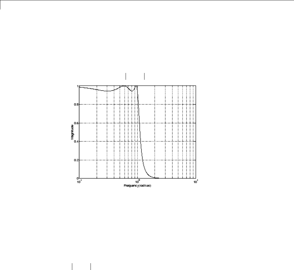
2Filter Design and Implementation

Chebyshev Type I Filter

The Chebyshev Type I filter minimizes the absolute difference between the

ideal and actual frequency response over the entire passband by incorporating

an equal ripple of Rp dB in the passband. Stopband response is maximally

flat. The transition from passband to stopband is more rapid than for the

Butterworth filter. Hj Rp

() /

Ω= −

10 20 at Ω=1.

Chebyshev Type II Filter

The Chebyshev Type II filter minimizes the absolute difference between the

ideal and actual frequency response over the entire stopband by incorporating

an equal ripple of Rs dB in the stopband. Passband response is maximally flat.

The stopband does not approach zero as quickly as the type I filter (and

does not approach zero at all for even-valued filter order n). The absence

of ripple in the passband, however, is often an important advantage.

Hj Rs

() /

Ω= −

10 20 at Ω=1.

2-10

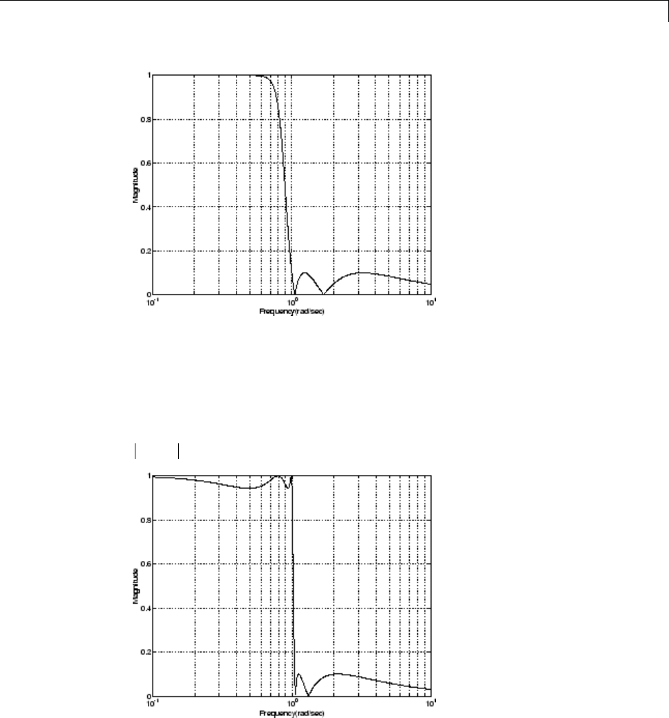
IIR Filter Design

Elliptic Filter

Elliptic filters are equiripple in both the passband and stopband. They

generally meet filter requirements with the lowest order of any supported

filter type. Given a filter order n, passband ripple Rp in decibels, and

stopband ripple Rs in decibels, elliptic filters minimize transition width.

Hj Rp

() /

Ω= −

10 20 at Ω=1.

2-11

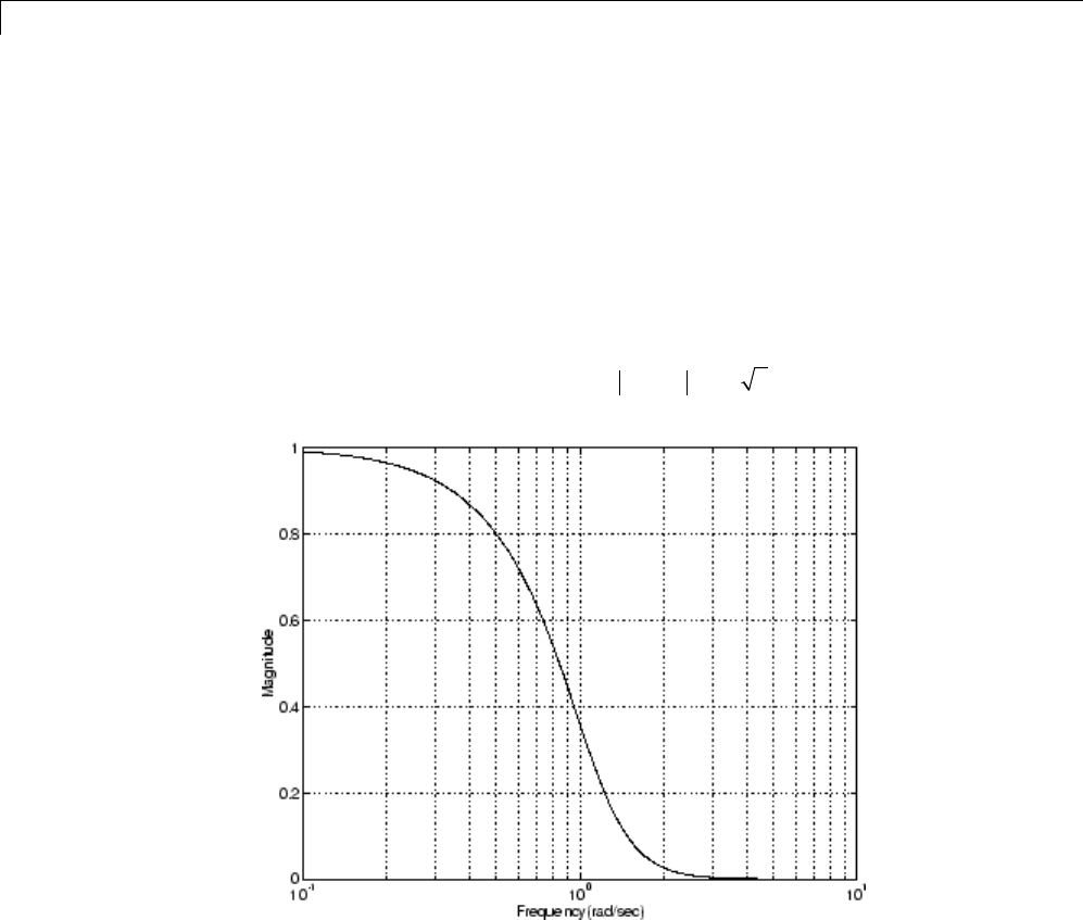
2Filter Design and Implementation

Bessel Filter

Analog Bessel lowpass filters have maximally flat group delay at zero

frequency and retain nearly constant group delay across the entire passband.

Filtered signals therefore maintain their waveshapes in the passband

frequency range. Frequency mapped and digital Bessel filters, however, do

not have this maximally flat property; this toolbox supports only the analog

case for the complete Bessel filter design function.

Bessel filters generally require a higherfilterorderthanotherfiltersfor

satisfactory stopband attenuation. Hj() /Ω<12

at Ω= 1 and decreases as

filter order nincreases.

2-12

IIR Filter Design

Note The lowpass filters shown above were created with the analog prototype

functions besselap,buttap,cheb1ap,cheb2ap,andellipap. These functions

find the zeros, poles, and gain of an order nanalog filter of the appropriate

type with cutoff frequency of 1 rad/s. Thecompletefilterdesignfunctions

(besself,butter,cheby1,cheby2,andellip) call the prototyping functions

as a first step in the design process. See “Special Topics in IIR Filter Design”

on page 2-43 for details.

To create similar plots, use n=5and, as needed, Rp =0.5 and Rs =20.For

example, to create the elliptic filter plot:

[z,p,k] = ellipap(5,0.5,20);

w = logspace(-1,1,1000);

h = freqs(k*poly(z),poly(p),w);

semilogx(w,abs(h)), grid

Direct IIR Filter Design

This toolbox uses the term direct methods to describe techniques for IIR

design that find a filter based on specifications in the discrete domain. Unlike

the analog prototyping method, direct design methods are not constrained

to the standard lowpass, highpass, bandpass, or bandstop configurations.

Rather, these functions design filters with an arbitrary, perhaps multiband,

frequency response. This section discusses the yulewalk function, which

is intended specifically for filter design; “Parametric Modeling” on page

7-13 discusses other methods that may also be considered direct, such as

Prony’s method, Linear Prediction, the Steiglitz-McBride method, and inverse

frequency design.

The yulewalk function designs recursive IIR digital filters by fitting a

specified frequency response. yulewalk’s name reflects its method for

finding the filter’s denominator coefficients: it finds the inverse FFT of

the ideal desired magnitude-squared response and solves the modified

Yule-Walker equations using the resulting autocorrelation function samples.

The statement

[b,a] = yulewalk(n,f,m)

2-13

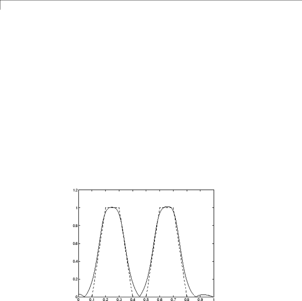
2Filter Design and Implementation

returns row vectors band acontaining the n+1 numerator and denominator

coefficients of the order nIIR filter whose frequency-magnitude characteristics

approximate those given in vectors fand m.fis a vector of frequency points

ranging from 0 to 1, where 1 represents the Nyquist frequency. mis a vector

containing the desired magnitude response at the points in f.fand m

can describe any piecewise linear shape magnitude response, including a

multiband response. The FIR counterpart of this function is fir2,whichalso

designs a filter based on an arbitrary piecewise linear magnitude response.

See “FIR Filter Design” on page 2-17 for details.

Note that yulewalk does not accept phase information, and no statements are

made about the optimality of the resulting filter.

Design a multiband filter with yulewalk, and plot the desired and actual

frequency response:

m=[0011001100];

f = [0 0.1 0.2 0.3 0.4 0.5 0.6 0.7 0.8 1];

[b,a] = yulewalk(10,f,m);

[h,w] = freqz(b,a,128)

plot(f,m,w/pi,abs(h))

2-14

IIR Filter Design

Generalized Butterworth Filter Design

The toolbox function maxflat enables you to design generalized Butterworth

filters, that is, Butterworth filters with differing numbers of zeros and poles.

This is desirable in some implementations where poles are more expensive

computationally than zeros. maxflat is just like the butter function, except

that it you can specify two orders (one for the numerator and one for the

denominator) instead of just one. These filters are maximally flat.This

means that the resulting filter is optimal for any numerator and denominator

orders, with the maximum number of derivatives at 0 and the Nyquist

frequency ω=πboth set to 0.

For example, when the two orders are the same, maxflat is the same as

butter:

[b,a] = maxflat(3,3,0.25)

0.0317 0.0951 0.0951 0.0317

1.0000 -1.4590 0.9104 -0.1978

[b,a] = butter(3,0.25)

0.0317 0.0951 0.0951 0.0317

1.0000 -1.4590 0.9104 -0.1978

However, maxflat is more versatile because it allows you to design a filter

with more zeros than poles:

[b,a] = maxflat(3,1,0.25)

0.0950 0.2849 0.2849 0.0950

1.0000 -0.2402

The third input to maxflat is the half-power frequency, a frequency between

0 and 1 with a desired magnitude response of 12/.

You can also design linear phase filters that have the maximally flat property

using the 'sym' option:

2-15

2Filter Design and Implementation

maxflat(4,'sym',0.3)

ans =

0.0331 0.2500 0.4337 0.2500 0.0331

For complete details of the maxflat algorithm, see Selesnick and Burrus [2].

2-16

FIR Filter Design

In this section...

“FIR vs. IIR Filters” on page 2-17

“FIR Filter Summary” on page 2-18

“Linear Phase Filters” on page 2-18

“Windowing Method” on page 2-20

“Multiband FIR Filter Design with Transition Bands” on page 2-24

“Constrained Least Squares FIR Filter Design” on page 2-31

“Arbitrary-Response Filter Design” on page 2-37

FIRvs. IIRFilters

Digital filters with finite-duration impulse response (all-zero, or FIR filters)

have both advantages and disadvantages compared to infinite-duration

impulseresponse(IIR)filters.

FIR filters have the following primary advantages:

•They can have exactly linear phase.

•They are always stable.

•The design methods are generally linear.

•They can be realized efficiently in hardware.

•The filter startup transients have finite duration.

The primary disadvantage of FIR filters is that they often require a much

higher filter order than IIR filters to achieve a given level of performance.

Correspondingly, the delay of these filters is often much greater than for an

equal performance IIR filter.

2-17

2Filter Design and Implementation

FIR Filter Summary

FIR Filters

Filter Design

Method Description Filter Functions

Windowing Apply window to truncated inverse

Fourier transform of desired “brick

wall” filter

fir1,fir2,

kaiserord

Multiband

with Transition

Bands

Equiripple or least squares approach

over sub-bands of the frequency range

firls,firpm,

firpmord

Constrained

Least Squares

Minimize squared integral error over

entire frequency range subject to

maximum error constraints

fircls,fircls1

Arbitrary

Response

Arbitrary responses, including

nonlinear phase and complex filters

cfirpm

Raised Cosine Lowpass response with smooth,

sinusoidal transition

firrcos

Linear Phase Filters

Except for cfirpm, all of the FIR filter design functions design linear phase

filters only. The filter coefficients, or “taps,” of such filters obey either an even

or odd symmetry relation. Depending on this symmetry, and on whether the

ordernof the filter is even or odd, a linear phase filter (stored in length n+1

vector b) has certain inherent restrictions on its frequency response.

2-18

FIR Filter Design

Linear

Phase

Filter Type

Filter

Order Symmetry of Coefficients

Response

H(f), f =0

Response

H(f), f =1

(Nyquist)

Type I Even even:

bk bn k k n( ) ( ), ,...,=+− = +211

restriction

Type II Odd even:

bk bn k k n( ) ( ), ,...,=+− = +211

restriction

H(1) =0

Type III Even odd:

bk bn k k n( ) ( ), ,...,=− + − = +211

H(0) =0H(1) =0

Type IV Odd odd:

bk bn k k n( ) ( ), ,...,=− + − = +211

H(0) =0No

restriction

The phase delay and group delay of linear phase FIR filters are equal and

constant over the frequency band. For an order nlinear phase FIR filter, the

group delay is n/2, and the filtered signal is simply delayed by n/2 time steps

(and the magnitude of its Fourier transform is scaled by the filter’s magnitude

response). This property preserves the wave shape of signals in the passband;

that is, there is no phase distortion.

The functions fir1,fir2,firls,firpm,fircls,fircls1,andfirrcos all

design type I and II linear phase FIR filters by default. Both firls and

firpm design type III and IV linear phase FIR filters given a 'hilbert' or

'differentiator' flag. cfirpm can design any type of linear phase filter,

and nonlinear phase filters as well.

Note Because the frequency response of a type II filter is zero at the Nyquist

frequency (“high” frequency), fir1 does not design type II highpass and

bandstop filters. For odd-valued nin these cases, fir1 adds 1 to the order

and returns a type I filter.

2-19

2Filter Design and Implementation

Windowing Method

Consider the ideal, or “brick wall,” digital lowpass filter with a cutoff

frequency of ω0rad/s. This filter has magnitude 1 at all frequencies with

magnitude less than ω0, and magnitude 0 at frequencies with magnitude

between ω0and π. Its impulse response sequence h(n)is

hn H e d e d n

jn jn

() ( ) sin( )

===

−−

∫∫

πωω

This filter is not implementable since its impulse response is infinite and

noncausal. To create a finite-duration impulse response, truncate it by

applying a window. By retaining the central section of impulse response in

this truncation, you obtain a linear phase FIR filter. For example, a length 51

filter with a lowpass cutoff frequency ω0of 0.4 πrad/s is

b = 0.4*sinc(0.4*(-25:25));

The window applied here is a simple rectangular window. By Parseval’s

theorem, this is the length 51 filter thatbestapproximatestheideallowpass

filter, in the integrated least squares sense. The following command displays

the filter’s frequency response in FVTool:

fvtool(b,1)

2-20

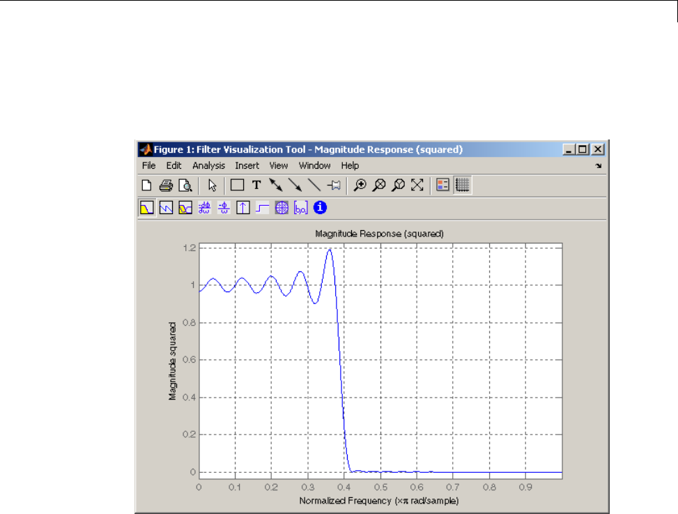
FIR Filter Design

Note that the y-axis shown in the figure below is in Magnitude Squared.

You can set this by right-clicking on the axis label and selecting Magnitude

Squared from the menu.

Ringing and ripples occur in the response, especially near the band edge.

This “Gibbs effect” does not vanish as the filter length increases, but a

nonrectangular window reduces its magnitude. Multiplication by a window in

the time domain causes a convolution or smoothing in the frequency domain.

Apply a length 51 Hamming window to the filter and display the result using

FVTool:

b = 0.4*sinc(0.4*(-25:25));

b = b.*hamming(51)';

fvtool(b,1)

2-21

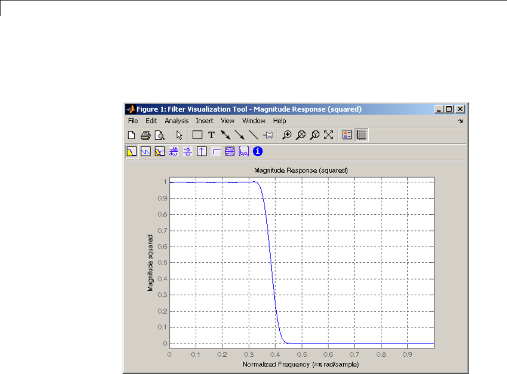
2Filter Design and Implementation

Note that the y-axis shown in the figure below is in Magnitude Squared.

You can set this by right-clicking on the axis label and selecting Magnitude

Squared from the menu.

Using a Hamming window greatly reduces the ringing. This improvement is

at the expense of transition width (the windowed version takes longer to ramp

from passband to stopband) and optimality (the windowed version does not

minimize the integrated squared error).

The functions fir1 and fir2 are based on this windowing process. Given a

filter order and description of an ideal desired filter, these functions return a

windowed inverse Fourier transform of that ideal filter. Both use a Hamming

window by default, but they accept any window function. See “Windows” on

page 7-2 for an overview of windows and their properties.

2-22

FIR Filter Design

Standard Band FIR Filter Design: fir1

fir1 implements the classical method of windowed linear phase FIR

digital filter design. It resembles the IIR filter design functions in that it

is formulated to design filters in standard band configurations: lowpass,

bandpass, highpass, and bandstop.

The statements

n = 50;

Wn = 0.4;

b = fir1(n,Wn);

create row vector bcontaining the coefficients of the order n

Hamming-windowed filter. This is a lowpass, linear phase FIR filter with

cutoff frequency Wn.Wn is a number between 0 and 1, where 1 corresponds to

the Nyquist frequency, half the sampling frequency. (Unlike other methods,

here Wn corresponds to the 6 dB point.) For a highpass filter, simply append

the string 'high' to the function’s parameter list. For a bandpass or bandstop

filter, specify Wn as a two-element vector containing the passband edge

frequencies; append the string 'stop' for the bandstop configuration.

b = fir1(n,Wn,window) uses the window specified in column vector window

for the design. The vector window must be n+1 elements long. If you do not

specify a window, fir1 applies a Hamming window.

Kaiser Window Order Estimation. The kaiserord function estimates the

filter order, cutoff frequency, and Kaiser window beta parameter needed to

meet a given set of specifications. Given a vector of frequency band edges and

a corresponding vector of magnitudes, as well as maximum allowable ripple,

kaiserord returns appropriate input parameters for the fir1 function.

Multiband FIR Filter Design: fir2

The fir2 function also designs windowed FIR filters, but with an arbitrarily

shaped piecewise linear frequency response. This is in contrast to fir1,which

only designs filters in standard lowpass, highpass, bandpass, and bandstop

configurations.

The commands

2-23

2Filter Design and Implementation

n = 50;

f=[0.4.51];

m=[1 1 00];

b = fir2(n,f,m);

return row vector bcontaining the n+1 coefficients of the order nFIR filter

whose frequency-magnitude characteristics match those given by vectors f

and m.fis a vector of frequency points ranging from 0 to 1, where 1 represents

the Nyquist frequency. mis a vector containing the desired magnitude

response at the points specified in f. (The IIR counterpart of this function

is yulewalk, which also designs filters based on arbitrary piecewise linear

magnitude responses. See “IIR Filter Design” on page 2-4 for details.)

Multiband FIR Filter Design with Transition Bands

The firls and firpm functions provide a more general means of specifying

the ideal desired filter than the fir1 and fir2 functions. These functions

design Hilbert transformers, differentiators, and other filters with odd

symmetric coefficients (type III and type IV linear phase). They also let you

include transition or “don’t care” regions in which the error is not minimized,

and perform band dependent weighting of the minimization.

The firls function is an extension of the fir1 and fir2 functions in that

it minimizes the integral of the square of the error between the desired

frequency response and the actual frequency response.

The firpm function implements the Parks-McClellan algorithm, which uses

the Remez exchange algorithm and Chebyshev approximation theory to design

filters with optimal fits between the desired and actual frequency responses.

The filters are optimal in the sense that they minimize the maximum error

between the desired frequency response and the actual frequency response;

they are sometimes called minimax filters. Filters designed in this way

exhibit an equiripple behavior in their frequency response, and hence are also

known as equiripple filters. The Parks-McClellan FIR filter design algorithm

is perhaps the most popular and widely used FIR filter design methodology.

The syntax for firls and firpm isthesame;theonlydifferenceistheir

minimization schemes. The next example shows how filters designed with

firls and firpm reflect these different schemes.

2-24

FIR Filter Design

Basic Configurations

The default mode of operation of firls and firpm is to design type I or type

II linear phase filters, depending on whether the order you desire is even or

odd, respectively. A lowpass example with approximate amplitude 1 from 0 to

0.4 Hz, and approximate amplitude 0 from 0.5 to 1.0 Hz is

n = 20; % Filter order

f = [0 0.4 0.5 1]; % Frequency band edges

a = [1 1 0 0]; % Desired amplitudes

b = firpm(n,f,a);

From 0.4 to 0.5 Hz, firpm performs no error minimization; this is a transition

band or “don’t care” region. A transition band minimizes the error more in

thebandsthatyoudocareabout,attheexpenseofaslowertransitionrate.

In this way, these types of filters have an inherent trade-off similar to FIR

design by windowing.

Tocompareleastsquarestoequiripplefilterdesign,usefirls to create

a similar filter. Type

bb = firls(n,f,a);

and compare their frequency responses using FVTool:

fvtool(b,1,bb,1)

2-25

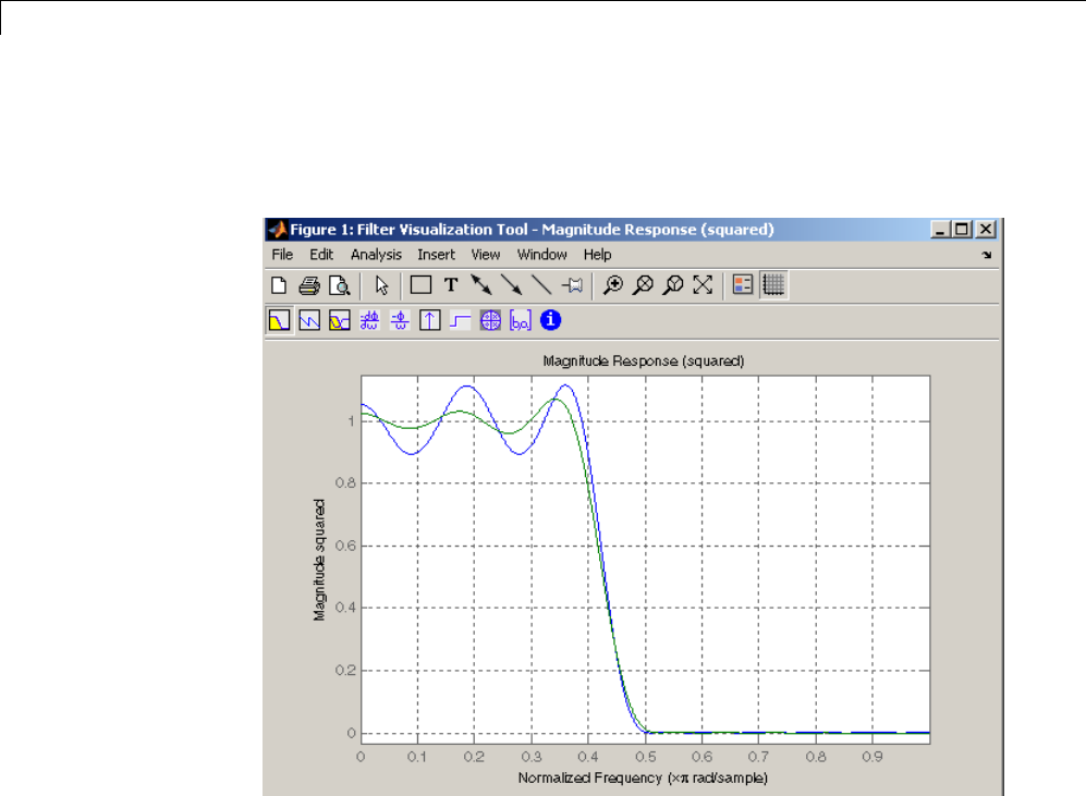
2Filter Design and Implementation

Note that the y-axis shown in the figure below is in Magnitude Squared.

You can set this by right-clicking on the axis label and selecting Magnitude

Squared from the menu.

The filter designed with firpm exhibits equiripple behavior. Also note that

the firls filter has a better response over most of the passband and stopband,

but at the band edges (f=0.4 and f=0.5),theresponseisfurtherawayfrom

the ideal than the firpm filter. This shows that the firpm filter’s maximum

error over the passband and stopband is smaller and, in fact, it is the smallest

possible for this band edge configuration and filter length.

Think of frequency bands as lines over short frequency intervals. firpm and

firls use this scheme to represent any piecewise linear desired function with

any transition bands. firls and firpm design lowpass, highpass, bandpass,

and bandstop filters; a bandpass example is

f = [0 0.3 0.4 0.7 0.8 1]; % Band edges in pairs

2-26

FIR Filter Design

a = [0 0 1 1 0 0]; % Bandpass filter amplitude

Technically, these fand avectors define five bands:

•Two stopbands, from 0.0 to 0.3 and from 0.8 to 1.0

•A passband from 0.4 to 0.7

•Two transition bands, from 0.3 to 0.4 and from 0.7 to 0.8

Example highpass and bandstop filters are

f = [0 0.7 0.8 1]; % Band edges in pairs

a = [0 0 1 1]; % Highpass filter amplitude

f = [0 0.3 0.4 0.5 0.8 1]; % Band edges in pairs

a = [1 1 0 0 1 1]; % Bandstop filter amplitude

An example multiband bandpass filter is

f = [0 0.1 0.15 0.25 0.3 0.4 0.45 0.55 0.6 0.7 0.75 0.85 0.9 1];

a=[11001100110011];

Another possibility is a filter that has as a transition region the line

connecting the passband with the stopband; this can help control “runaway”

magnitude response in wide transition regions:

f = [0 0.4 0.42 0.48 0.5 1];

a = [1 1 0.8 0.2 0 0]; % Passband, linear transition,

% stopband

The Weight Vector

Both firls and firpm allow you to place more or less emphasis on minimizing

the error in certain frequency bands relative to others. To do this, specify a

weight vector following the frequencyandamplitudevectors. Anexample

lowpass equiripple filter with 10 times less ripple in the stopband than the

passband is

n = 20; % Filter order

f = [0 0.4 0.5 1]; % Frequency band edges

a = [1 1 0 0]; % Desired amplitudes

2-27

2Filter Design and Implementation

w = [1 10]; % Weight vector

b = firpm(n,f,a,w);

A legal weight vector is always half the length of the fand avectors; there

must be exactly one weight per band.

Anti-Symmetric Filters / Hilbert Transformers

When called with a trailing 'h' or 'Hilbert' option, firpm and firls design

FIR filters with odd symmetry, that is, type III (for even order) or type IV

(for odd order) linear phase filters. An ideal Hilbert transformer has this

anti-symmetry property and an amplitude of 1 across the entire frequency

range. Try the following approximate Hilbert transformers and plot them

using FVTool:

b = firpm(21,[0.05 1],[1 1],'h'); % Highpass Hilbert

bb = firpm(20,[0.05 0.95],[1 1],'h'); % Bandpass Hilbert

fvtool(b,1,bb,1)

2-28

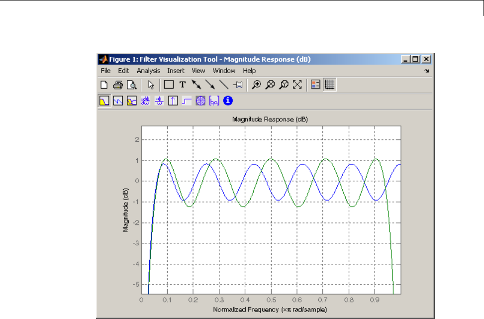
FIR Filter Design

You can find the delayed Hilbert transform of a signal xby passing it through

these filters.

fs = 1000; % Sampling frequency

t = (0:1/fs:2)'; % Two second time vector

x = sin(2*pi*300*t); % 300 Hz sine wave example signal

xh = filter(bb,1,x); % Hilbert transform of x

The analytic signal corresponding to xis the complex signal that has xas its

real part and the Hilbert transform of xas its imaginary part. For this FIR

method (an alternative to the hilbert function), you must delay xby half the

filter order to create the analytic signal:

xd = [zeros(10,1); x(1:length(x)-10)]; % Delay 10 samples

xa = xd + j*xh; % Analytic signal

2-29

2Filter Design and Implementation

This method does not work directly for filters of odd order, which require a

noninteger delay. In this case, the hilbert function, described in “Specialized

Transforms” on page 7-36, estimates the analytic signal. Alternatively, use

the resample function to delay the signal by a noninteger number of samples.

Differentiators

Differentiation of a signal in the time domain is equivalent to multiplication

of the signal’s Fourier transform by an imaginary ramp function. That is, to

differentiate a signal, pass it through a filter that has a response H(ω)=jω.

Approximate the ideal differentiator (with a delay) using firpm or firls with

a'd' or 'differentiator' option:

b = firpm(21,[0 1],[0 pi],'d');

For a type III filter, the differentiation band should stop short of the Nyquist

frequency, and the amplitude vector must reflect that change to ensure the

correct slope:

bb = firpm(20,[0 0.9],[0 0.9*pi],'d');

In the 'd' mode, firpm weights the error by 1/ωin nonzero amplitude bands

to minimize the maximum relative error. firls weights the error by (1/ω)2in

nonzero amplitude bands in the 'd' mode.

2-30

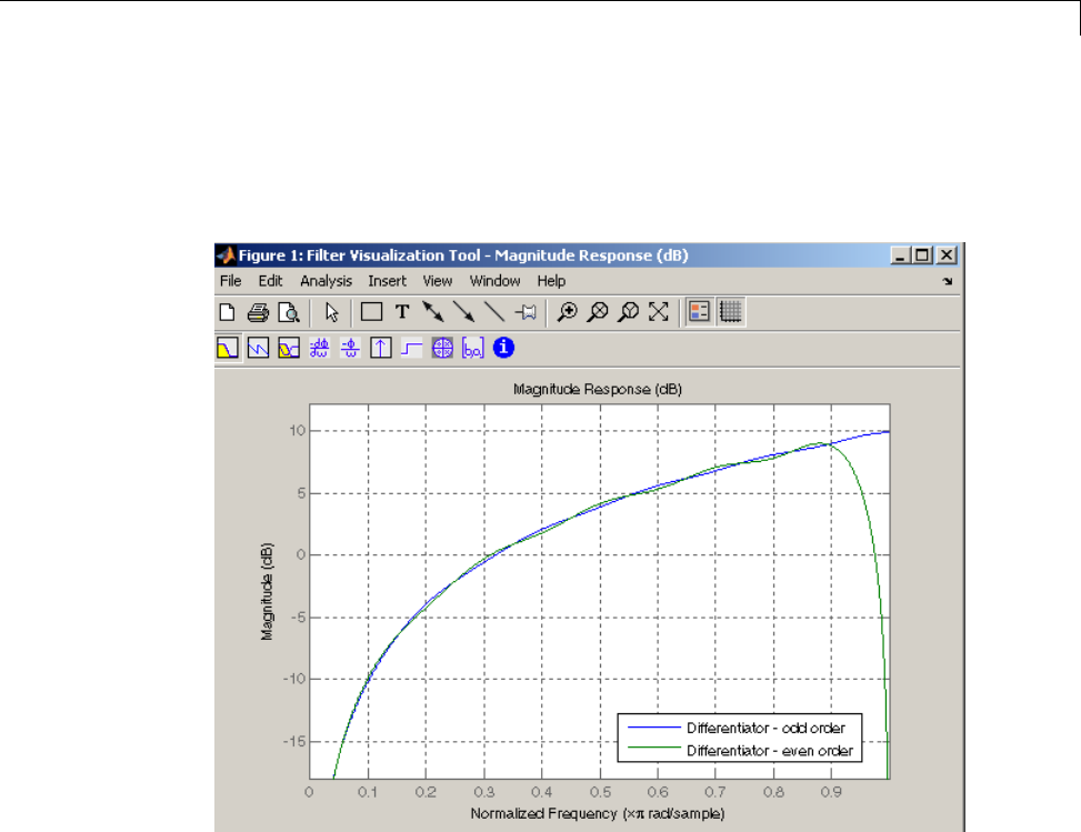
FIR Filter Design

The following plots show the magnitude responses for the differentiators

above.

fvtool(b,1,bb,1)

Constrained Least Squares FIR Filter Design

The Constrained Least Squares (CLS) FIR filter design functions implement

a technique that enables you to design FIR filters without explicitly defining

the transition bands for the magnitude response. The ability to omit the

specification of transition bands is useful in several situations. For example,

it may not be clear where a rigidly defined transition band should appear if

noise and signal information appear together in the same frequency band.

Similarly, it may make sense to omit the specification of transition bands if

they appear only to control the results of Gibbs phenomena that appear in

the filter’s response. See Selesnick, Lang, and Burrus [2] for discussion of

this method.

2-31

2Filter Design and Implementation

Instead of defining passbands, stopbands, and transition regions, the CLS

method accepts a cutoff frequency (for the highpass, lowpass, bandpass, or

bandstop cases), or passband and stopband edges (for multiband cases), for

the desired response. In this way, the CLS method defines transition regions

implicitly, rather than explicitly.

The key feature of the CLS method is that it enables you to define upper

and lower thresholds that contain the maximum allowable ripple in the

magnitude response. Given this constraint, the technique applies the least

square error minimization technique over the frequency range of the filter’s

response, instead of over specific bands. The error minimization includes

any areas of discontinuity in the ideal, “brick wall” response. An additional

benefit is that the technique enables you to specify arbitrarily small peaks

resulting from Gibbs’ phenomena.

There are two toolbox functions that implement this design technique.

Description Function

Constrained least square multiband FIR filter design fircls

Constrained least square filter design for lowpass and

highpass linear phase filters

fircls1

For details on the calling syntax for these functions, see their reference

descriptions in the Function Reference.

Basic Lowpass and Highpass CLS Filter Design

The most basic of the CLS design functions, fircls1, uses this technique to

design lowpass and highpass FIR filters. As an example, consider designing a

filter with order 61 impulse response and cutoff frequency of 0.3 (normalized).

Further, define the upper and lower bounds that constrain the design process

as:

•Maximum passband deviation from 1 (passband ripple) of 0.02.

•Maximum stopband deviation from 0 (stopband ripple) of 0.008.

2-32

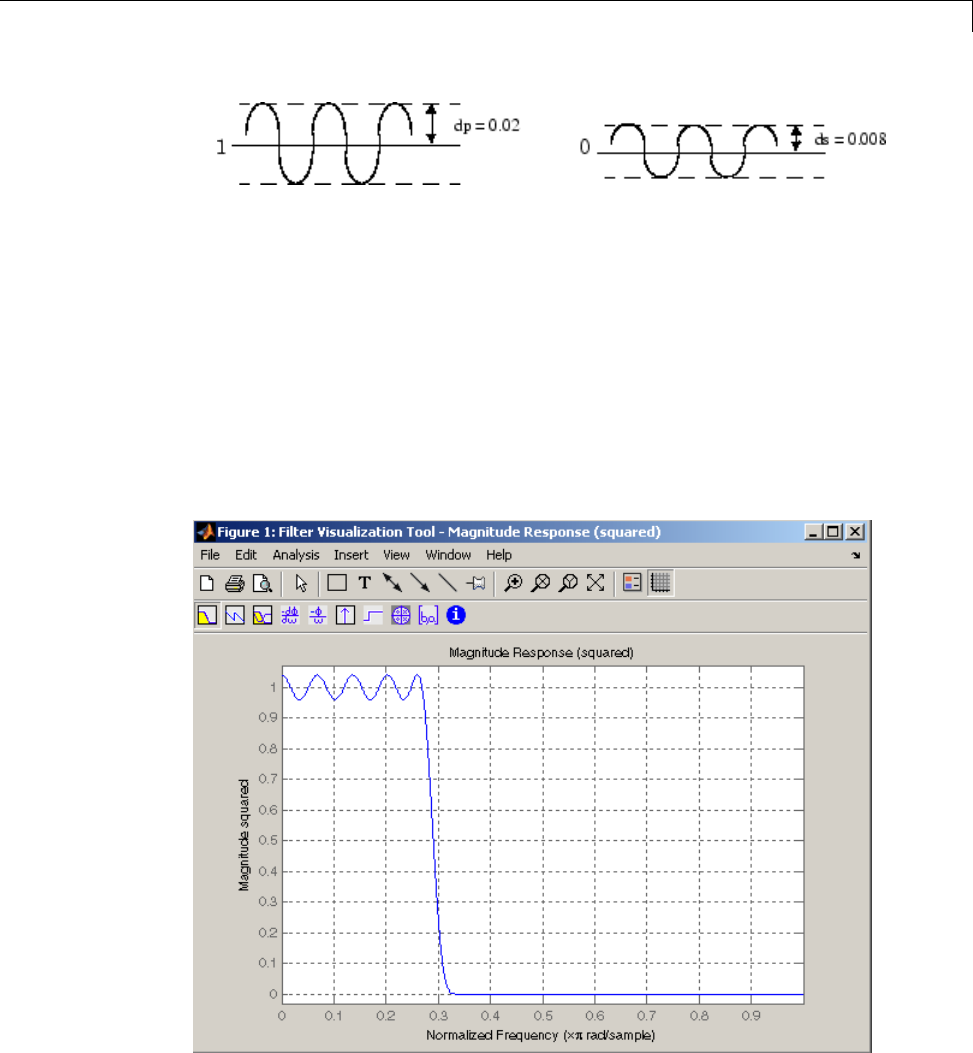
FIR Filter Design

To approach this design problem using fircls1, use the following commands:

n = 61;

wo = 0.3;

dp = 0.02;

ds = 0.008;

h = fircls1(n,wo,dp,ds);

fvtool(h,1)

Note that the y-axisshownbelowisinMagnitude Squared. You can set

this by right-clicking on the axis label and selecting Magnitude Squared

from the menu.

2-33

2Filter Design and Implementation

Multiband CLS Filter Design

fircls uses the same technique to design FIR filters with a desired piecewise

constant magnitude response. In this case, you can specify a vector of band

edges and a corresponding vector of band amplitudes. In addition, you can

specify the maximum amount of ripple for each band.

For example, assume the specifications for a filter call for:

•From 0 to 0.3 (normalized): amplitude 0, upper bound 0.005, lower

bound –0.005

•From 0.3 to 0.5: amplitude 0.5, upper bound 0.51, lower bound 0.49

•From 0.5 to 0.7: amplitude 0, upper bound 0.03, lower bound –0.03

•From 0.7 to 0.9: amplitude 1, upper bound 1.02, lower bound 0.98

•From 0.9 to 1: amplitude 0, upper bound 0.05, lower bound –0.05

Design a CLS filter with impulse response order 129 that meets these

specifications:

n = 129;

f = [0 0.3 0.5 0.7 0.9 1];

a = [0 0.5 0 1 0];

up = [0.005 0.51 0.03 1.02 0.05];

lo = [-0.005 0.49 -0.03 0.98 -0.05];

h = fircls(n,f,a,up,lo);

fvtool(h,1)

2-34

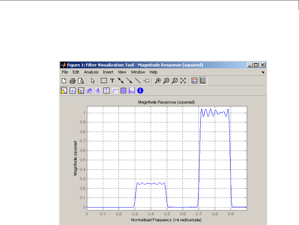
FIR Filter Design

Note that the y-axisshownbelowisinMagnitude Squared. You can set

this by right-clicking on the axis label and selecting Magnitude Squared

from the menu.

Weighted CLS Filter Design

Weighted CLS filter design lets you design lowpass or highpass FIR filters

with relative weighting of the error minimization in each band. The fircls1

function enables you to specify the passband and stopband edges for the least

squares weighting function, as well as a constant kthat specifies the ratio of

the stopband to passband weighting.

Forexample,considerspecificationsthatcallforanFIRfilterwithimpulse

response order of 55 and cutoff frequency of 0.3 (normalized). Also assume

maximum allowable passband ripple of 0.02 and maximum allowable

stopband ripple of 0.004. In addition, add weighting requirements:

2-35

2Filter Design and Implementation

•Passband edge for the weight function of 0.28 (normalized)

•Stopband edge for the weight function of 0.32

•Weight error minimization 10 times as much in the stopband as in the

passband

To approach this using fircls1,type

n = 55;

wo = 0.3;

dp = 0.02;

ds = 0.004;

wp = 0.28;

ws = 0.32;

k = 10;

h = fircls1(n,wo,dp,ds,wp,ws,k);

fvtool(h,1)

2-36

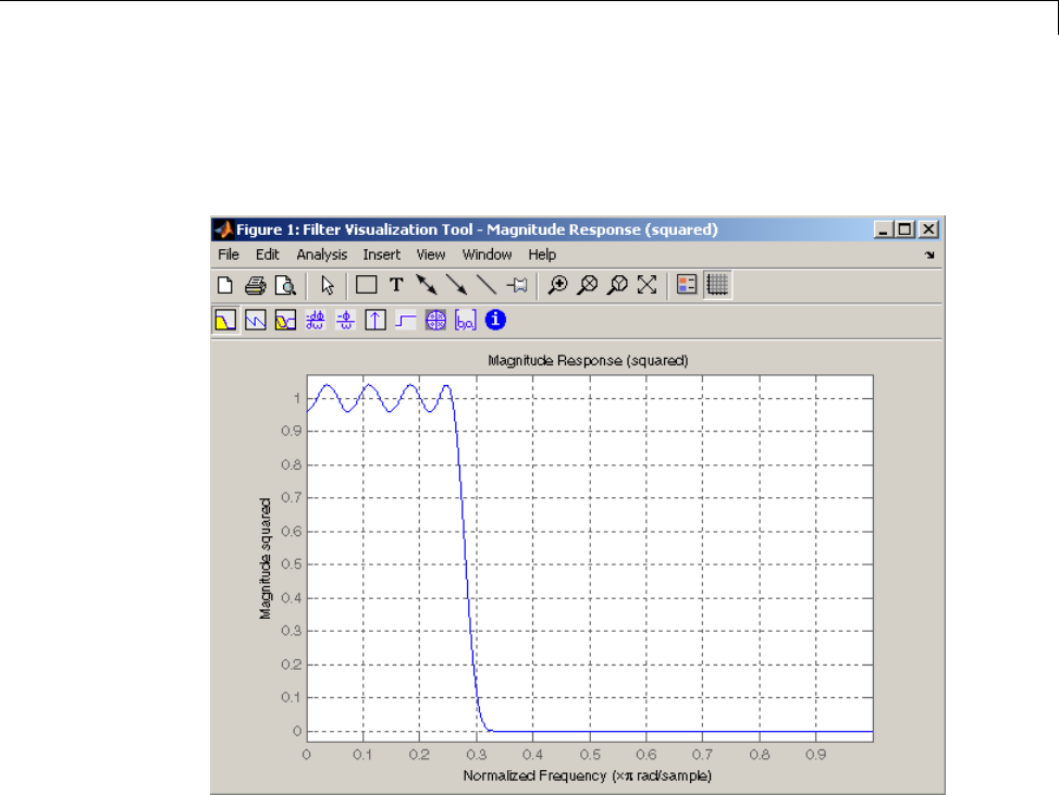
FIR Filter Design

Note that the y-axisshownbelowisinMagnitude Squared. You can set

this by right-clicking on the axis label and selecting Magnitude Squared

from the menu.

Arbitrary-Response Filter Design

The cfirpm filter design function provides a tool for designing FIR filters

with arbitrary complex responses. It differs from the other filter design

functions in how the frequency response of the filter is specified: it accepts the

name of a function which returns the filter response calculated over a grid of

frequencies. This capability makes cfirpm a highly versatile and powerful

technique for filter design.

This design technique may be used to produce nonlinear-phase FIR filters,

asymmetric frequency-response filters (with complex coefficients), or more

symmetric filters with custom frequency responses.

2-37

2Filter Design and Implementation

The design algorithm optimizes the Chebyshev (or minimax) error using

an extended Remez-exchange algorithm for an initial estimate. If this

exchange method fails to obtain the optimal filter, the algorithm switches

to an ascent-descent algorithm that takes over to finish the convergence to

the optimal solution.

Multiband Filter Design

Consider a multiband filter with the following special frequency-domain

characteristics.

Band Amplitude

Optimization

Weighting

[–1 –0.5] [5 1] 1

[–0.4 +0.3] [2 2] 10

[+0.4 +0.8] [2 1] 5

A linear-phase multiband filter may be designed using the predefined

frequency-response function multiband,asfollows:

b = cfirpm(38, [-1 -0.5 -0.4 0.3 0.4 0.8], ...

{'multiband', [5 1 2 2 2 1]}, [1 10 5]);

For the specific case of a multiband filter, we can use a shorthand filter design

notation similar to the syntax for firpm:

b = cfirpm(38,[-1 -0.5 -0.4 0.3 0.4 0.8], ...

[5 1 2 2 2 1], [1 10 5]);

As with firpm, a vector of band edges is passed to cfirpm. This vector defines

the frequency bands over which optimization is performed; note that there are

two transition bands, from –0.5 to –0.4 and from 0.3 to 0.4.

In either case, the frequency response is obtained and plotted using linear

scale in FVTool:

fvtool(b,1)

2-38

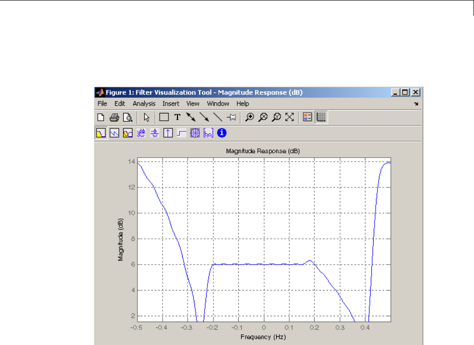
FIR Filter Design

Note that the range of data shown below is (-Fs/2,Fs/2). You can set this

range by changing the x-axis units to Frequency (Fs = 1 Hz).

2-39

2Filter Design and Implementation

The filter response for this multiband filter is complex, which is expected

because of the asymmetry in the frequency domain. The impulse response,

which you can select from the FVTool toolbar, is shown below.

Filter Design with Reduced Delay

Consider the design of a 62-tap lowpass filter with a half-Nyquist cutoff. If

we specify a negative offset value to the lowpass filter design function, the

group delay offset for the design is significantly less than that obtained for a

standard linear-phase design. This filter design may be computed as follows:

b = cfirpm(61,[0 0.5 0.55 1],{'lowpass',-16});

The resulting magnitude response is

fvtool(b,1)

2-40

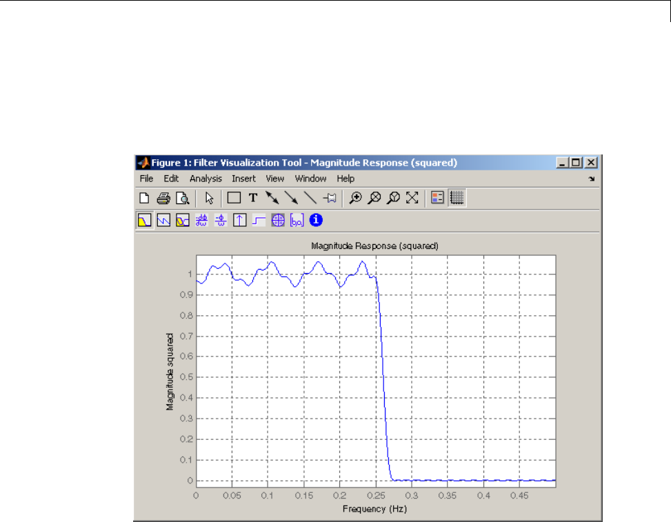
FIR Filter Design

Note that the range of data in this plot is (-Fs/2,Fs/2),whichyoucanset

changing the x-axis units to Frequency.They-axisisinMagnitudeSquared,

which you can set by right-clicking on the axis label and selecting Magnitude

Squared from the menu.

2-41

2Filter Design and Implementation

The group delay of the filter reveals that the offset has been reduced from

N/2 to N/2-16 (i.e., from 30.5 to 14.5). Now, however, the group delay is no

longer flat in the passband region. To create this plot, click the Group Delay

button on the toolbar.

If we compare this nonlinear-phase filter to a linear-phase filter that has

exactly 14.5 samples of group delay, the resulting filter is of order 2*14.5, or

29. Using b = cfirpm(29,[0 0.5 0.55 1],'lowpass'), the passband and

stopband ripple is much greater for the order 29 filter. These comparisons

can assist you in deciding which filter is more appropriate for a specific

application.

2-42

Special Topics in IIR Filter Design

In this section...

“Classic IIR Filter Design” on page 2-43

“Analog Prototype Design” on page 2-44

“Frequency Transformation” on page 2-44

“Filter Discretization” on page 2-46

Classic IIR Filter Design

The classic IIR filter design technique includes the following steps.

1Find an analog lowpass filter with cutoff frequency of 1 and translate this

prototype filter to the desired band configuration

2Transform the filter to the digital domain.

3Discretize the filter.

The toolbox provides functions for each of these steps.

Design Task Available functions

Analog lowpass

prototype

buttap,cheb1ap,besselap,ellipap,cheb2ap

Frequency

transformation

lp2lp,lp2hp,lp2bp,lp2bs

Discretization bilinear,impinvar

Alternatively, the butter,cheby1,cheb2ord,ellip,andbesself functions

perform all steps of the filter design and the buttord,cheb1ord,cheb2ord,

and ellipord functions provide minimum order computation for IIR filters.

These functions are sufficient for many design problems, and the lower level

functions are generally not needed. But if you do have an application where

you need to transform the band edges of an analog filter, or discretize a

rational transfer function, this section describes the tools with which to do so.

2-43

2Filter Design and Implementation

Analog PrototypeDesign

This toolbox provides a number of functions to create lowpass analog

prototype filters with cutoff frequency of 1, the first step in the classical

approach to IIR filter design.

The table below summarizes the analog prototype design functions for each

supported filter type; plots for each type are shown in “IIR Filter Design”

on page 2-4.

Filter Type Analog Prototype Function

Bessel [z,p,k] = besselap(n)

Butterworth [z,p,k] = buttap(n)

Chebyshev Type I [z,p,k] = cheb1ap(n,Rp)

Chebyshev Type II [z,p,k] = cheb2ap(n,Rs)

Elliptic [z,p,k] = ellipap(n,Rp,Rs)

Frequency Transformation

The second step in the analog prototyping design technique is the frequency

transformation of a lowpass prototype. The toolbox provides a set of functions

to transform analog lowpass prototypes (with cutoff frequency of 1 rad/s)

into bandpass, highpass, bandstop, and lowpass filters of the desired cutoff

frequency.

Frequency

Transformation Transformation Function

Lowpass to lowpass

′=ss/

[numt,dent] = lp2lp (num,den,Wo)

[At,Bt,Ct,Dt] =lp2lp (A,B,C,D,Wo)

Lowpass to highpass

′=ss

[numt,dent] = lp2hp (num,den,Wo)

[At,Bt,Ct,Dt] =lp2hp (A,B,C,D,Wo)

2-44

Special Topics in IIR Filter Design

Frequency

Transformation Transformation Function

Lowpass to bandpass

′=+

ωω

1(/ )

[numt,dent] = lp2bp (num,den,Wo,Bw)

[At,Bt,Ct,Dt] =lp2bp (A,B,C,D,Wo,Bw)

Lowpass to bandstop

′=+

sBs

021

(/ )

[numt,dent] = lp2bs (num,den,Wo,Bw)

[At,Bt,Ct,Dt] =lp2bs( A,B,C,D,Wo,Bw)

As shown, all of the frequency transformation functions can accept two linear

system models: transfer function and state-space form. For the bandpass

and bandstop cases

ωωω

012

and

ωω

=−

where ω1is the lower band edge and ω2is the upper band edge.

The frequency transformation functions perform frequency variable

substitution. In the case of lp2bp and lp2bs, this is a second-order

substitution, so the output filter is twice the order of the input. For lp2lp and

lp2hp, the output filter is the same order as the input.

To begin designing an order 10 bandpass Chebyshev Type I filter with a value

of 3 dB for passband ripple, enter

[z,p,k] = cheb1ap(10,3);

Outputs z,p,andkcontain the zeros, poles, and gain of a lowpass analog

filter with cutoff frequency Ωcequal to 1 rad/s. Use the lp2bp function to

transform this lowpass prototype to a bandpass analog filter with band edges

2-45

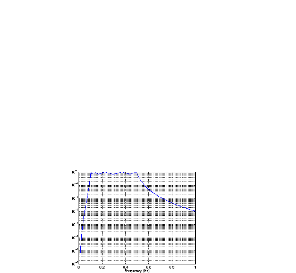
2Filter Design and Implementation

Ω1=π/5 and Ω2=π. First, convert the filter to state-space form so the lp2bp

function can accept it:

[A,B,C,D] = zp2ss(z,p,k); % Convert to state-space form.

Now, find the bandwidth and center frequency, and call lp2bp:

u1 = 0.1*2*pi; u2 = 0.5*2*pi; % In radians per second

Bw = u2-u1;

Wo = sqrt(u1*u2);

[At,Bt,Ct,Dt] = lp2bp(A,B,C,D,Wo,Bw);

Finally, calculate the frequency response and plot its magnitude:

[b,a] = ss2tf(At,Bt,Ct,Dt); % Convert to TF form

w = linspace(0.01,1,500)*2*pi; % Generate frequency vector

h = freqs(b,a,w); % Compute frequency response

semilogy(w/2/pi,abs(h)), grid % Plot log magnitude vs. freq

xlabel('Frequency (Hz)');

Filter Discretization

Thethirdstepintheanalogprototyping technique is the transformation of

thefiltertothediscrete-timedomain. The toolbox provides two methods for

this: the impulse invariant and bilinear transformations. The filter design

2-46

Special Topics in IIR Filter Design

functions butter,cheby1,cheby2,andellip use the bilinear transformation

for discretization in this step.

Analog

to Digital

Transformation Transformation Function

Impulse

invariance

[numd,dend] = impinvar (num,den,fs)

Bilinear

transform

[zd,pd,kd] = bilinear (z,p,k,fs,Fp)

[numd,dend] = bilinear (num,den,fs,Fp)

[Ad,Bd,Cd,Dd] = bilinear (At,Bt,Ct,Dt,fs,Fp)

Impulse Invariance

The toolbox function impinvar creates a digital filter whose impulse response

is the samples of the continuous impulse response of an analog filter. This

function works only on filters in transfer function form. For best results, the

analog filter should have negligible frequency content above half the sampling

frequency, because such high frequency content is aliased into lower bands

upon sampling. Impulse invariance works for some lowpass and bandpass

filters, but is not appropriate for highpass and bandstop filters.

Design a Chebyshev Type I filter and plot its frequency and phase response

using FVTool:

[bz,az] = impinvar(b,a,2);

fvtool(bz,az)

Click the Magnitude and Phase Response toolbar button.

2-47

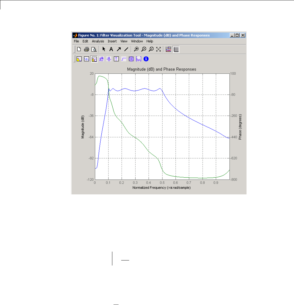
2Filter Design and Implementation

Impulse invariance retains the cutoff frequencies of 0.1 Hz and 0.5 Hz.

Bilinear Transformation

The bilinear transformation is a nonlinear mapping of the continuous domain

to the discrete domain; it maps the s-plane into the z-plane by

Hz Hs sk

() ()==−

Bilinear transformation maps the jΩ-axis of the continuous domain to the

unit circle of the discrete domain according to

=⎛

⎝

⎜⎞

⎠

⎟

−

tan Ω

2-48

Special Topics in IIR Filter Design

The toolbox function bilinear implements this operation, where the

frequency warping constant kis equal to twice the sampling frequency (2*fs)

by default, and equal to 2ππfff

pps

tan

()

if you give bilinear a trailing

argument that represents a “match” frequency Fp. If a match frequency Fp

(in hertz) is present, bilinear maps the frequency Ω=2πfp(in rad/s) to the

same frequency in the discrete domain, normalized to the sampling rate:

ω=2πfp/fs(in rad/sample).

The bilinear function can perform this transformation on three different

linear system representations: zero-pole-gain, transfer function, and

state-space form. Try calling bilinear with the state-space matrices that

describe the Chebyshev Type I filter from the previous section, using a

sampling frequency of 2 Hz, and retaining the lower band edge of 0.1 Hz:

[Ad,Bd,Cd,Dd] = bilinear(At,Bt,Ct,Dt,2,0.1);

The frequency response of the resulting digital filter is

[bz,az] = ss2tf(Ad,Bd,Cd,Dd); % Convert to TF

fvtool(bz,az)

2-49

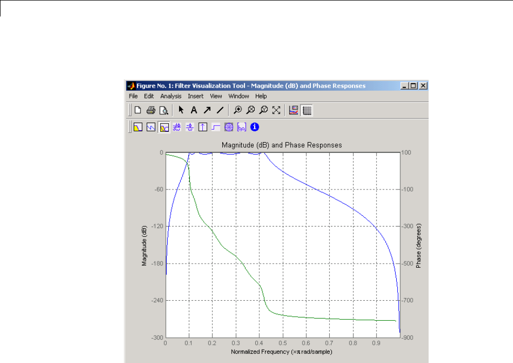
2Filter Design and Implementation

Click the Magnitude and Phase Response toolbar button.

The lower band edge is at 0.1 Hz as expected. Notice, however, that the

upper band edge is slightly less than 0.5 Hz, although in the analog domain

it was exactly 0.5 Hz. This illustrates the nonlinear nature of the bilinear

transformation. To counteract this nonlinearity, it is necessary to create

analog domain filters with “prewarped” band edges, which map to the correct

locations upon bilinear transformation. Here the prewarped frequencies u1

and u2 generate Bw and Wo for the lp2bp function:

fs = 2; % Sampling frequency (hertz)

u1 = 2*fs*tan(0.1*(2*pi/fs)/2); % Lower band edge (rad/s)

u2 = 2*fs*tan(0.5*(2*pi/fs)/2); % Upper band edge (rad/s)

Bw = u2 - u1; % Bandwidth

Wo = sqrt(u1*u2); % Center frequency

[At,Bt,Ct,Dt] = lp2bp(A,B,C,D,Wo,Bw);

2-50

Special Topics in IIR Filter Design

A digital bandpass filter with correct band edges 0.1 and 0.5 times the

Nyquist frequency is

[Ad,Bd,Cd,Dd] = bilinear(At,Bt,Ct,Dt,fs);

The example bandpass filters from the last two sections could also be created

in one statement using the complete IIR design function cheby1.Forinstance,

an analog version of the example Chebyshev filter is

[b,a] = cheby1(5,3,[0.1 0.5]*2*pi,'s');

Note that the band edges are in rad/s for analog filters, whereas for the digital

case, frequency is normalized:

[bz,az] = cheby1(5,3,[0.1 0.5]);

All of the complete design functions call bilinear internally. They prewarp

the band edges as needed to obtain the correct digital filter.

2-51

2Filter Design and Implementation

Filtering Data With Signal Processing Toolbox Software

In this section...

“Lowpass FIR Filter — Window Method” on page 2-52

“Bandpass Filters — Minimum-Order FIR and IIR Systems” on page 2-56

“Zero-Phase Filtering” on page 2-65

Lowpass FIR Filter — Window Method

These examples show you how to design and implement an FIR filter using

the command line functions: fir1 and fdesign.lowpass, and the interactive

tool fdatool.

To filter the input signal, these examples use the filter command. The

examples in “Zero-Phase Filtering” on page 2-65 show you how to implement

zero-phase filtering with filtfilt.

Createasignaltouseintheexamples. Thesignalisa100-Hzsinewavein

additive N(0,1/4) white Gaussian noise. Set the random number generator to

the default state for reproducible results.

rng default;

Fs = 1000;

t = linspace(0,1,Fs);

x = cos(2*pi*100*t)+0.5*randn(size(t));

The filter design is an FIR lowpass filter with order equal to 20 and a cutoff

frequency of 150 Hz. Use a Kasier window with length one sample greater

than the filter order and β=3. See kaiser fordetailsontheKaiserwindow.

Use fir1 to design the filter. fir1 requires normalized frequencies in the

interval [0,1], where 1 is (1)πradians/sample. To use fir1,youmustconvert

all frequency specifications to normalized frequencies.

Design the filter and view the filter’s magnitude response.

fc = 150;

Wn = (2/Fs)*fc;

2-52

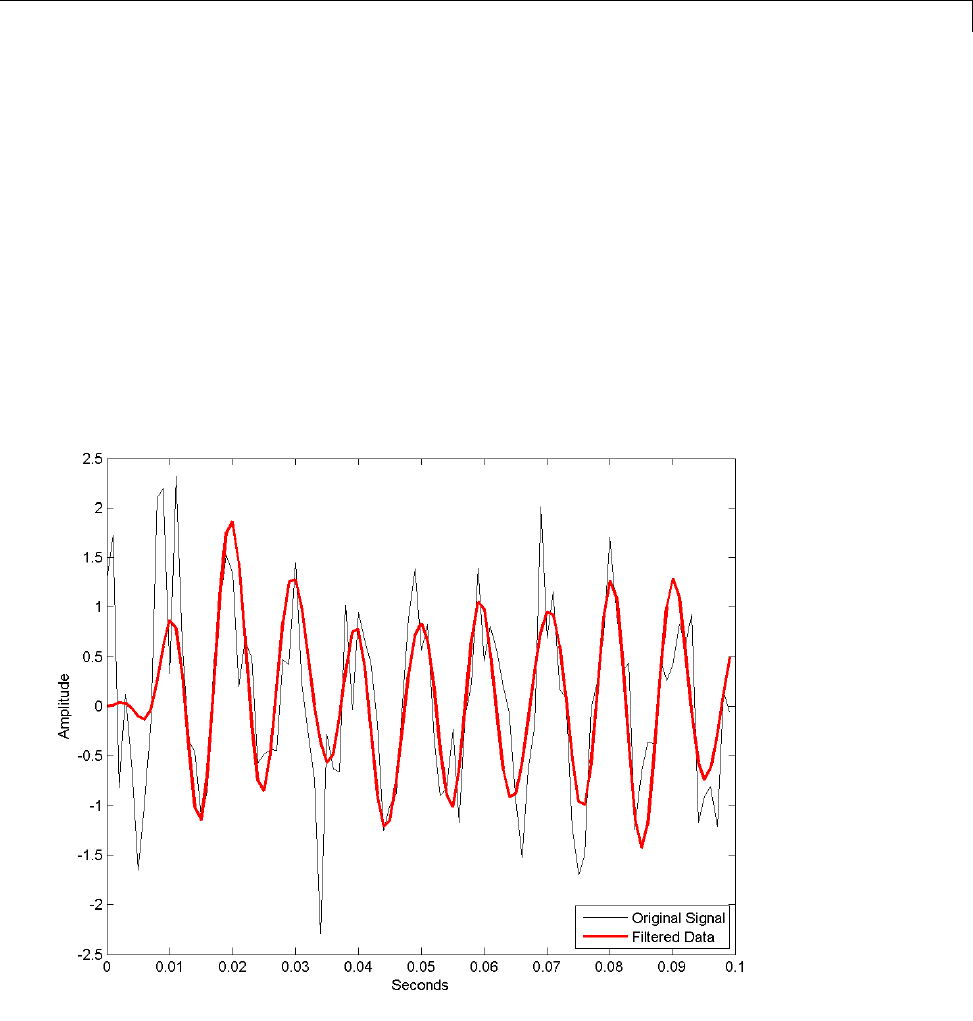
Filtering Data With Signal Processing Toolbox™ Software

b = fir1(20,Wn,'low',kaiser(21,3));

fvtool(b,1,'Fs',Fs);

Apply the filter to the signal and plot the result for the first ten periods of

the 100-Hz sinusoid.

y = filter(b,1,x);

plot(t(1:100),x(1:100),'k');

hold on;

plot(t(1:100),y(1:100),'r','linewidth',2);

legend('Original Signal','Filtered Data','Location','SouthEast');

xlabel('Seconds'); ylabel('Amplitude');

Designthesamefilterusingfdesign.lowpass.

2-53

2Filter Design and Implementation

Set the filter specifications using the 'N,Fc' specification string. With

fdesign.lowpass, you can specify your filter design in Hz.

Fs = 1000;

d = fdesign.lowpass('N,Fc',20,150,Fs);

Hd = design(d,'window','Window',kaiser(21,3));

Filter the data and plot the result.

y1 = filter(Hd,x);

plot(t(1:100),x(1:100),'k');

hold on;

plot(t(1:100),y1(1:100),'r','linewidth',2);

legend('Original Signal','Filtered Data','Location','SouthEast');

xlabel('Seconds'); ylabel('Amplitude');

Design and implement a lowpass FIR filter using the window method with

the interactive tool fdatool.

Start FDATool by entering

fdatool

at the command line.

Set the Response Type to Lowpass.SettheDesign Method to FIR and

select the Window method.

Under Filter Order,selectSpecify order. Set the order to 20.

Under Frequency Specifications.SetUnits to Hz,Fs: to 1000, and Fc: to

150.

2-54

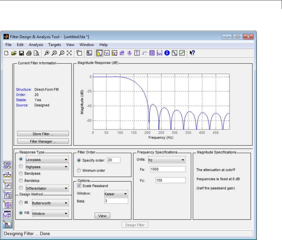
Filtering Data With Signal Processing Toolbox™ Software

Click Design Filter.

Select File —>Export... to export your FIR filter to the MATLAB workspace

as coefficients or a filter object. In this example, export the filter as an object.

Specify the variable name as Hd1.

2-55

2Filter Design and Implementation

Click Export.

Filter the input signal in the command window with the exported filter object.

Plot the result for the first ten periods of the 100-Hz sinusoid.

y2 = filter(Hd1,x);

plot(t(1:100),x(1:100),'k');

hold on;

plot(t(1:100),y1(1:100),'r','linewidth',2);

legend('Original Signal','Filtered Data','Location','SouthEast');

xlabel('Seconds'); ylabel('Amplitude');

Select File —> Generate MATLAB Code to generate a MATLAB function

to create a filter object using your specifications.

You can also use the interactive tool filterbuilder to design your filter.

Bandpass Filters — Minimum-Order FIR and IIR

Systems

This example shows you how to design a bandpass filter and filter data with

minimum-order FIR equiripple and IIR Butterworth filters. The example uses

fdesign.bandpass and the interactive tool fdatool.

You can model many real-world signals as a superposition of oscillating

components, a low-frequency trend, and additive noise. For example,

2-56

Filtering Data With Signal Processing Toolbox™ Software

economic data often contain oscillations, which represent cycles superimposed

on a slowly varying upward or downward trend. In addition, there is an

additive noise component, which is a combination of measurement error and

the inherent random fluctuations in the process.

In these examples, assume you sample some process every day for 1 year.

Assume the process has oscillations on approximately one-week and

one-month scales. In addition, there is a low-frequency upward trend in the

data and additive N(0,1/4) white Gaussian noise.

Create the signal as a superposition of two sine waves with frequencies of 1/7

and 1/30 cycles/day. Add a low-frequency increasing trend term and N(0,1/4)

white Gaussian noise. Set the random number generator to the default state

for reproducible results. The data is sampled at 1 sample/day. Plot the

resulting signal and the power spectral density (PSD) estimate.

rng default;

Fs =1;

n = 1:365;

x = cos(2*pi*(1/7)*n)+cos(2*pi*(1/30)*n-pi/4);

trend = 3*sin(2*pi*(1/1480)*n);

y = x+trend+0.5*randn(size(n));

subplot(211);

plot(n,y); xlabel('Days'); set(gca,'xlim',[1 365]);

grid on;

subplot(212);

psdest = psd(spectrum.periodogram,y,'Fs',Fs);

plot(psdest.Frequencies,10*log10(psdest.Data));

xlabel('Cycles/day'); ylabel('dB'); grid on;

2-57

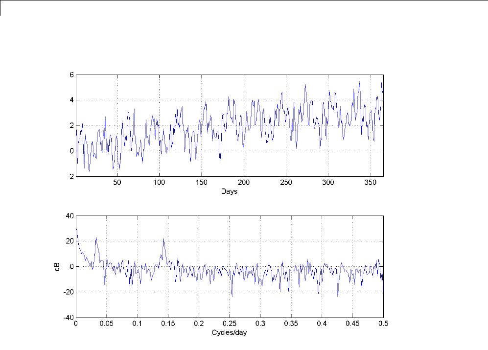
2Filter Design and Implementation

The low-frequency trend appears in the power spectral density estimate

as increased low-frequency power. The low-frequency power appears

approximately 10 dB above the oscillation at 1/30 cycles/day. Use this

information in the specifications for the filter stopbands.

Design minimum-order FIR equiripple and IIR Butterworth filters with the

following specifications: passband from [1/40,1/4] cycles/day and stopbands

from [0,1/60] and [1/4,1/2] cycles/day. Set both stopband attenuations to 10 dB

and the passband ripple tolerance to 1 dB.

d = fdesign.bandpass('Fst1,Fp1,Fp2,Fst2,Ast1,Ap,Ast2',...

1/60,1/40,1/4,1/2,10,1,10,1);

Hd1 = design(d,'equiripple');

Hd2 = design(d,'butter');

2-58

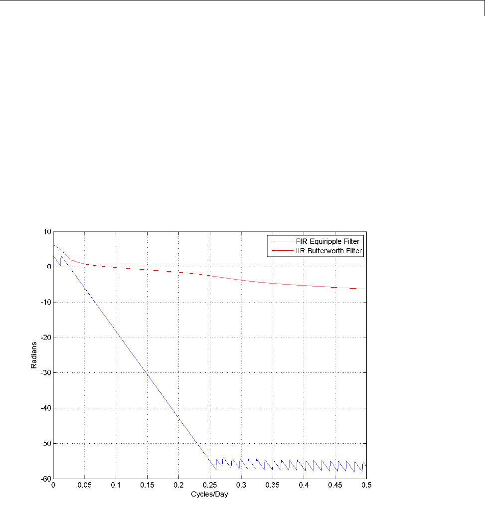
Filtering Data With Signal Processing Toolbox™ Software

Compare the order of the FIR and IIR filters and the unwrapped phase

responses.

fprintf('The order of the FIR filter is %d\n',length(Hd1.Numerator)-1);

[b,a] = sos2tf(Hd2.sosMatrix,Hd2.ScaleValues);

fprintf('The order of the IIR filter is %d\n',length(max(b,a))-1);

[phifir,w] = phasez(Hd1,[],1);

[phiiir,w] = phasez(Hd2,[],1);

plot(w,unwrap(phifir),'b'); hold on;

plot(w,unwrap(phiiir),'r'); grid on;

xlabel('Cycles/Day'); ylabel('Radians');

legend('FIR Equiripple Filter','IIR Butterworth Filter');

2-59

2Filter Design and Implementation

The IIR filter has a much lower order that the FIR filter. However, the FIR

filter has a linear phase response over the passband, while the IIR filter does

not. The FIR filter delays all frequencies in the filter passband equally, while

the IIR filter does not.

Additionally, the rate of change of the phase per unit of frequency is greater

in the FIR filter than in the IIR filter.

Design a lowpass FIR equiripple filter for comparison. The lowpass filter

specifications are: passband [0,1/4] cycles/day, stopband attenuation equal to

10 dB, and the passband ripple tolerance set to 1 dB.

dlow = fdesign.lowpass('Fp,Fst,Ap,Ast',1/4,1/2,1,10,1);

Hdlow = design(dlow,'equiripple');

Filter the data with the bandpass and lowpass filters.

yfir = filter(Hd1,y);

yiir = filter(Hd2,y);

ylow = filter(Hdlow,y);

Plot the PSD estimate of the bandpass IIR filter output. You can replace

yiir with yfir in the following code to view the PSD estimate of the FIR

bandpass filter output.

psdest = psd(spectrum.periodogram,yiir,'Fs',Fs);

plot(psdest.Frequencies,10*log10(psdest.Data));

xlabel('Cycles/day'); ylabel('dB'); grid on;

2-60

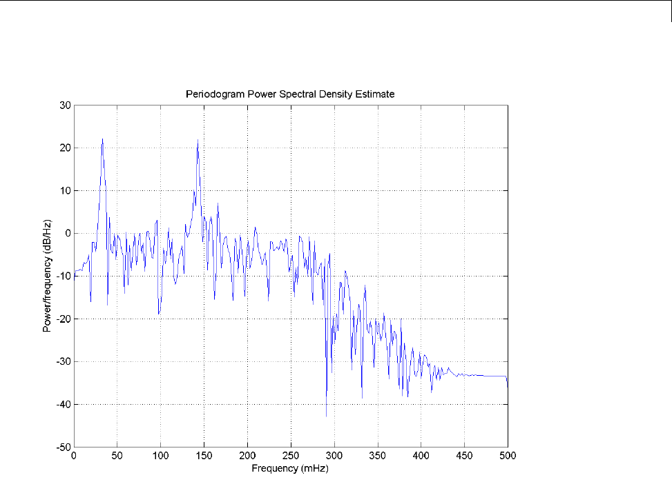
Filtering Data With Signal Processing Toolbox™ Software

The PSD estimate shows the bandpass filter attenuates the low-frequency

trend and high-frequency noise.

Plot the first 120 days of FIR and IIR filter output.

plot(n(1:120),yfir(1:120),'b');

hold on;

plot(n(1:120),yiir(1:120),'r');

xlabel('Days'); axis([1 120 -2.8 2.8]);

legend('FIR bandpass filter output','IIR bandpass filter output',...

'Location','SouthEast');

2-61

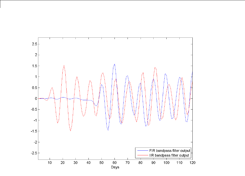
2Filter Design and Implementation

The increased phase delay in the FIR filter is evident in the filter output.

Plot the lowpass FIR filter output superimposed on the superposition of the

7-day and 30-day cycles for comparison.

plot(n,x,'k');

hold on;

plot(n,ylow,'r'); set(gca,'xlim',[1 365]);

legend('7-day and 30-day cycles','FIR lowpass filter output',...

'Location','NorthWest');

xlabel('Days');

2-62

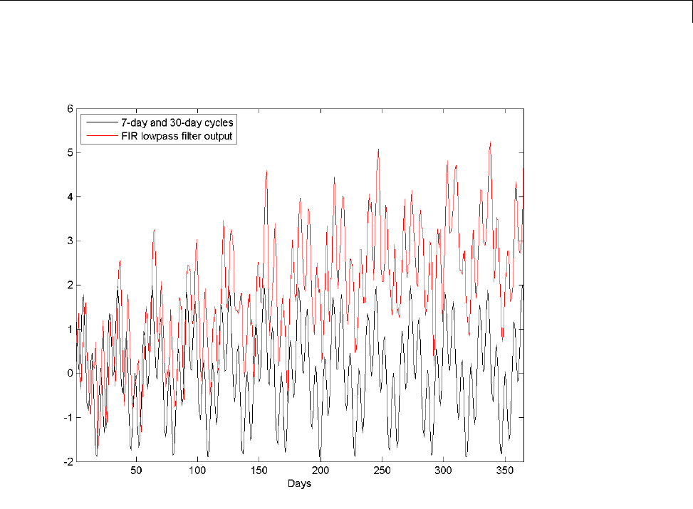
Filtering Data With Signal Processing Toolbox™ Software

You can see in the preceding plot that the low-frequency trend is evident in

the lowpass filter output. While the lowpass filter preserves the 7-day and

30-day cycles, the bandpass filters perform better in this example because the

bandpass filters also remove the low-frequency trend.

Design and implement the bandpass Butterworth (IIR) filter with the

interactive tool fdatool.

Start FDATool by entering

fdatool

at the command line.

2-63

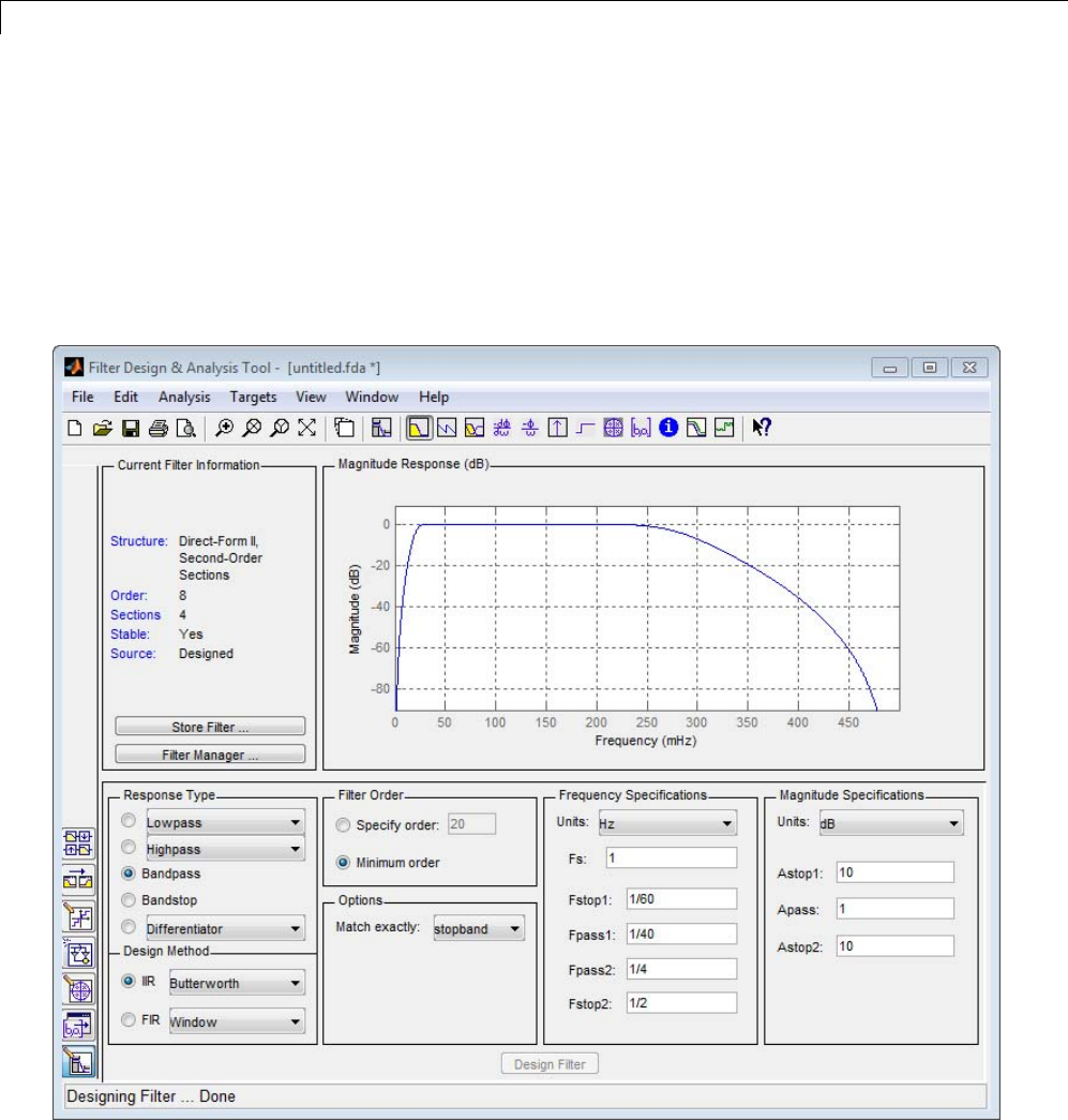
2Filter Design and Implementation

Set the Response Type to Bandpass.SettheDesign Method to IIR and

select the Butterworth design.

Under Filter Order, select Minimum order.

Under Frequency Specifications.SetUnits to Hz,Fs: to 1 , Fstop1: to

1/60, Fpass1: to 1/40, Fpass2: to 1/4, and Fstop2: to 1/2. Under Magnitude

Specifications,setAstop1: and Astop2: to 10 and Apass: to 1.

2-64

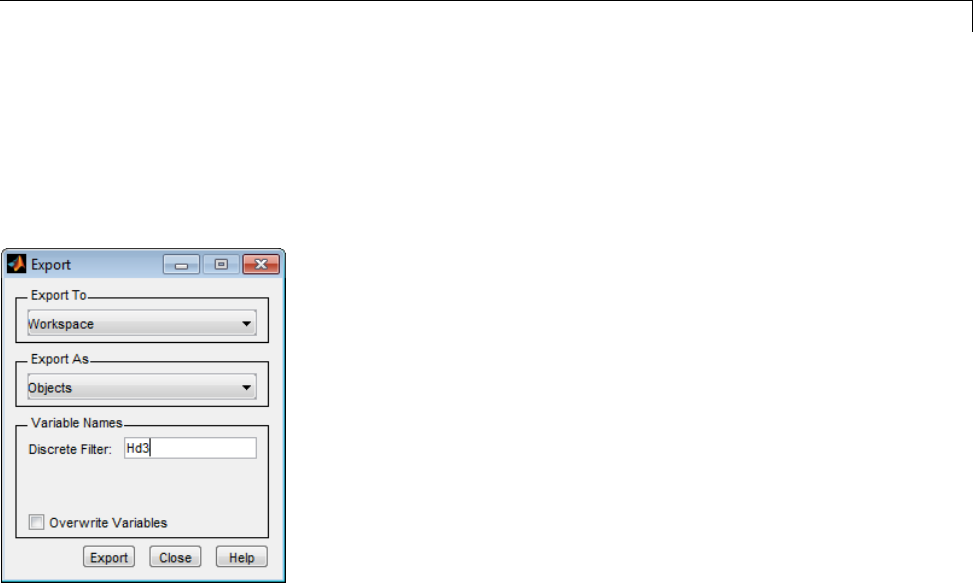
Filtering Data With Signal Processing Toolbox™ Software

Click Design Filter.

Select File —> Export... to export your IIR filter to the MATLAB workspace

as coefficients or a filter object. In this example, export the filter as an object.

Specify the variable name as Hd3.

Click Export.

Filter the input signal in the command window with the exported filter object.

yfilt = filter(Hd3,x);

SelectFile —> Generate MATLAB Code to generate a MATLAB function

to create a filter object using your specifications.

You can also use the interactive tool filterbuilder to design your filter.

Zero-Phase Filtering

These examples show you how to perform zero-phase filtering. The signal and

filters are described in “Lowpass FIR Filter — Window Method” on page 2-52

and “Bandpass Filters — Minimum-Order FIR and IIR Systems” on page 2-56.

2-65

2Filter Design and Implementation

Repeat the signal generation and lowpass filter design with fir1 and

fdesign.lowpass. You do not have to execute the following code if you

already have these variables in your workspace.

rng default;

Fs = 1000;

t = linspace(0,1,Fs);

x = cos(2*pi*100*t)+0.5*randn(size(t));

% Using fir1

fc = 150;

Wn = (2/Fs)*fc;

b = fir1(20,Wn,'low',kaiser(21,3));

% Using fdesign.lowpass

d = fdesign.lowpass('N,Fc',20,150,Fs);

Hd = design(d,'window','Window',kaiser(21,3));

Filter the data using filter. Plot the first 100 points of the filter output

along with a superimposed sinusoid with the same amplitude and initial

phase as the input signal.

yout = filter(Hd,x);

xin = cos(2*pi*100*t);

plot(t(1:100),xin(1:100),'k');

hold on; grid on;

plot(t(1:100),yout(1:100),'r','linewidth',2);

xlabel('Seconds'); ylabel('Amplitude');

legend('Input Sine Wave','Filtered Data',...

'Location','NorthEast');

2-66

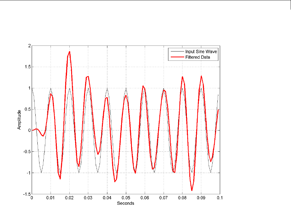
Filtering Data With Signal Processing Toolbox™ Software

Looking at the initial 0.01 seconds of the filtered data, you see that the output

is delayed with respect to the input. The delay appears to be approximately

0.01 seconds, which is almost 1/2 thelengthoftheFIRfilterinsamples

(10*0.001).

This delay is due to the filter’s phase response. The FIR filter in these

examples is a type I linear-phase filter. The group delay of the filter is 10

samples.

Plot the group delay using fvtool.

fvtool(Hd,'analysis','grpdelay');

2-67

2Filter Design and Implementation

In many applications, phase distortion is acceptable. This is particularly true

when phase response is linear. In other applications, it is desirable to have

a filter with a zero-phase response. A zero-phase response is not technically

possibly in a noncausal filter. However, you can implement zero-phase

filtering using a causal filter with filtfilt.filtfilt does not accept filter

objects as input arguments, but you can still use filter objects with filtfilt

by extracting the filter coefficients from the object.

Filter the input signal using the coefficients in the filter object. Plot the

responses to compare the filter outputs obtained with filter and filtfilt.

yzp = filtfilt(Hd.Numerator,1,x);

% or yzp = filtfilt(b,1,x);

plot(t(1:100),xin(1:100),'k');

hold on;

plot(t(1:100),yout(1:100),'r','linewidth',2);

plot(t(1:100),yzp(1:100),'b','linewidth',2);

xlabel('Seconds'); ylabel('Amplitude');

legend('100-Hz Sine Wave','Filtered Signal','Zero-phase Filtering',...

'Location','NorthEast');

2-68

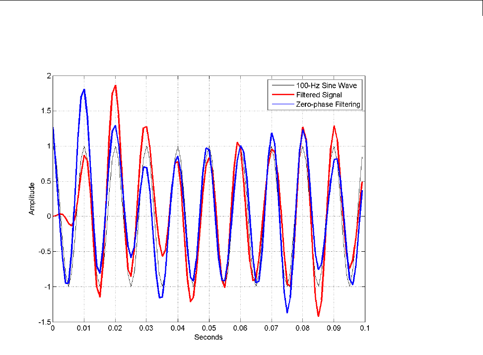
Filtering Data With Signal Processing Toolbox™ Software

In the preceding figure, you can see that the output of filtfilt does not

exhibit the delay due to the phase response of the FIR filter.

The IIR bandpass filter designed in “Bandpass Filters — Minimum-Order

FIR and IIR Systems” on page 2-56 is a biquad filter. Stated equivalently,

the IIR filter is in the form of cascaded second-order sections. To implement

zero-phase filtering with a discrete-time biquad filter, you must input the

matrix of second-order sections and the gain values for each of those sections

into filtfilt.

Zero phase filter the data in “Bandpass Filters — Minimum-Order FIR and

IIR Systems” on page 2-56 with the IIR bandpass filter. For convenience, the

2-69

2Filter Design and Implementation

code to generate the signal and filter is repeated. You do not have to execute

this code if you already have these variables in your workspace.

Generate the data.

rng default;

Fs =1;

n = 1:365;

x = cos(2*pi*(1/7)*n)+cos(2*pi*(1/30)*n-pi/4);

trend = 3*sin(2*pi*(1/1480)*n);

y = x+trend+0.5*randn(size(n));

Specify and design the filter.

d = fdesign.bandpass('Fst1,Fp1,Fp2,Fst2,Ast1,Ap,Ast2',...

1/60,1/40,1/4,1/2,10,1,10,1);

Hd2 = design(d,'butter');

Use filtfilt to zero-phase filter the input. Input the matrix of second-order

sections and gain (scale) values along with your signal.

yzpiir = filtfilt(Hd2.sosMatrix,Hd2.ScaleValues,y);

2-70

Selected Bibliography

[1] Karam, L.J., and J.H. McClellan. “Complex Chebyshev Approximation for

FIR Filter Design.” IEEE Trans. on Circuits and Systems II. March 1995.

[2] Selesnick, I.W., and C.S. Burrus. “Generalized Digital Butterworth

Filter Design.” Proceedings of the IEEE Int. Conf. Acoust., Speech, Signal

Processing. Vol. 3 (May 1996).

[3] Selesnick, I.W., M. Lang, and C.S. Burrus. “Constrained Least Square

Design of FIR Filters without Specified Transition Bands.” Proceedings of

the IEEE Int. Conf. Acoust., Speech, Signal Processing. Vol. 2 (May 1995).

Pgs. 1260-1263.

2-71

2Filter Design and Implementation

2-72

Designing a Filter in

Fdesign — Process

Overview

3Designing a Filter in Fdesign — Process Overview

Process Flow Diagram and Filter Design Methodology

In this section...

“Exploring the Process Flow Diagram” on page 3-2

“Selecting a Response” on page 3-4

“Selecting a Specification” on page 3-4

“Selecting an Algorithm” on page 3-6

“Customizing the Algorithm” on page 3-8

“Designing the Filter” on page 3-8

“Design Analysis” on page 3-9

“Realize or Apply the Filter to Input Data” on page 3-10

Note You must minimally have the Signal Processing Toolbox installed

to use fdesign and design. Some of the features described below may

be unavailable if your installation does not additionally include the DSP

System Toolbox™ license. The DSP System Toolbox significantly expands the

functionality available for the specification, design, and analysis of filters.

You can verify the presence of both toolboxes by typing ver at the command

prompt.

Exploring the Process Flow Diagram

The process flow diagram shown in the following figure lists the steps and

shows the order of the filter design process.

3-2

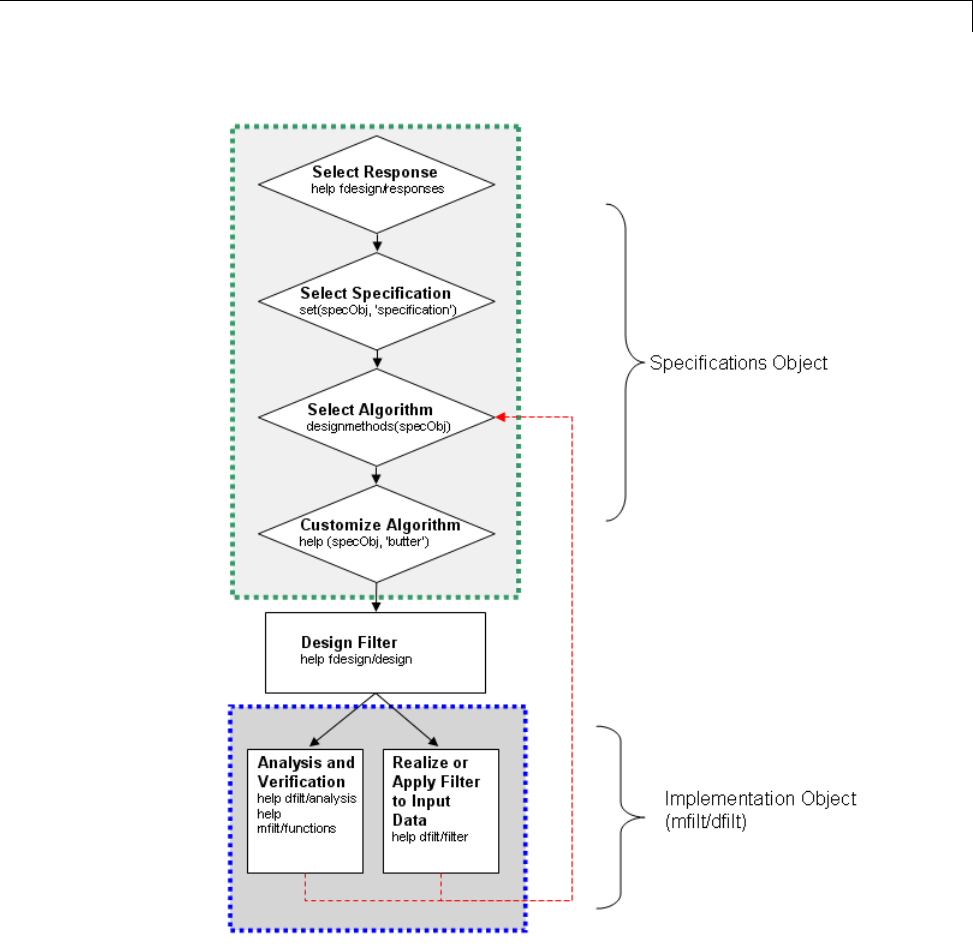
Process Flow Diagram and Filter Design Methodology

The first four steps of the filter design process relate to the filter Specifications

Object, while the last two steps involve the filter Implementation Object. Both

of these objects are discussed in more detail in the following sections. Step 5

- the design of the filter, is the transition step from the filter Specifications

Object to the Implementation object. The analysis and verification step is

3-3

3Designing a Filter in Fdesign — Process Overview

completely optional. It provides methods for the filter designer to ensure that

the filter complies with all design criteria. Depending on the results of this

verification, you can loop back to steps 3 and 4, to either choose a different

algorithm, or to customize the current one. You may also wish to go back to

steps 3 or 4 after you filter the input data with the designed filter (step 7),

andfindthatyouwishtotweakthe filter or change it further.

The diagram shows the help command for each step. Enter the help line at the

MATLAB command prompt to receive instructions and further documentation

links for the particular step. Not all of the steps have to be executed explicitly.

For example, you could go from step 1 directly to step 5, and the interim three

steps are done for you by the software.

The following are the details for each of the steps shown above.

Selecting a Response

If you type:

help fdesign/responses

at the MATLAB command prompt, you see a list of all available filter

responses. The responses marked with an asterisk require the DSP System

Toolbox.

You must select a response to initiate the filter. In this example, a bandpass

filter Specifications Object is created by typing the following:

d = fdesign.bandpass

Selecting a Specification

Aspecification is an array of design parameters for a given filter. The

specification is a property of the Specifications Object.

Note A specification is not the same as the Specifications Object. A

Specifications Object contains a specification as one of its properties.

3-4

Process Flow Diagram and Filter Design Methodology

When you select a filter response, there are a number of different

specifications available. Each one contains a different combination of design

parameters. After you create a filter Specifications Object, you can query the

available specifications for that response. Specifications marked with an

asterisk require the DSP System Toolbox.

>> d = fdesign.bandpass; % step 1 - choose the response

>> set (d, 'specification')

ans =

'Fst1,Fp1,Fp2,Fst2,Ast1,Ap,Ast2'

'N,F3dB1,F3dB2'

'N,F3dB1,F3dB2,Ap'

'N,F3dB1,F3dB2,Ast'

'N,F3dB1,F3dB2,Ast1,Ap,Ast2'

'N,F3dB1,F3dB2,BWp'

'N,F3dB1,F3dB2,BWst'

'N,Fc1,Fc2'

'N,Fp1,Fp2,Ap'

'N,Fp1,Fp2,Ast1,Ap,Ast2'

'N,Fst1,Fp1,Fp2,Fst2'

'N,Fst1,Fp1,Fp2,Fst2,Ap'

'N,Fst1,Fst2,Ast'

'Nb,Na,Fst1,Fp1,Fp2,Fst2'

>> d=fdesign.arbmag;

>> set(d,'specification')

ans =

'N,F,A'

'N,B,F,A'

The set command can be used to select one of theavailablespecificationsas

follows:

>> d = fdesign.lowpass; % step 1

>> % step 2: get a list of available specifications

>> set (d, 'specification')

3-5

3Designing a Filter in Fdesign — Process Overview

ans =

'Fp,Fst,Ap,Ast'

'N,F3dB'

'N,F3dB,Ap'

'N,F3dB,Ap,Ast'

'N,F3dB,Ast'

'N,F3dB,Fst'

'N,Fc'

'N,Fc,Ap,Ast'

'N,Fp,Ap'

'N,Fp,Ap,Ast'

'N,Fp,F3dB'

'N,Fp,Fst'

'N,Fp,Fst,Ap'

'N,Fp,Fst,Ast'

'N,Fst,Ap,Ast'

'N,Fst,Ast'

'Nb,Na,Fp,Fst'

>> %step 2: set the required specification

>> set (d, 'specification', 'N,Fc')

If you do not perform this step explicitly, fdesign returns the default

specification for the response you chose in “Select a Response” on page 4-3, and

provides default values for all design parameters included in the specification.

Selecting an Algorithm

The availability of algorithms depends the chosen filter response, the design

parameters, and the availability of the DSP System Toolbox. In other words,

for the same lowpass filter, changing the specification string also changes the

available algorithms. In the following example, for a lowpass filter and a

specification of 'N, Fc', only one algorithm is available—window.

>> %step 2: set the required specification

>> set (d, 'specification', 'N,Fc')

>> designmethods (d) %step3: get available algorithms

3-6

Process Flow Diagram and Filter Design Methodology

Design Methods for class fdesign.lowpass (N,Fc):

window

However, for a specification of 'Fp,Fst,Ap,Ast',anumberofalgorithmsare

available. If the user has only the Signal Processing Toolbox installed, the

following algorithms are available:

>>set (d, 'specification', 'Fp,Fst,Ap,Ast')

>>designmethods(d)

Design Methods for class fdesign.lowpass (Fp,Fst,Ap,Ast):

butter

cheby1

cheby2

ellip

equiripple

kaiserwin

If the user additionally has the DSP System Toolbox installed, the number of

available algorithms for this response and specification string increases:

>>set(d,'specification','Fp,Fst,Ap,Ast')

>>designmethods(d)

Design Methods for class fdesign.lowpass (Fp,Fst,Ap,Ast):

butter

cheby1

cheby2

ellip

equiripple

ifir

kaiserwin

3-7

3Designing a Filter in Fdesign — Process Overview

multistage

The user chooses a particular algorithm and implements the filter with the

design function.

>>Hd=design(d,'butter');

The preceding code actually creates the filter, where Hd is the filter

Implementation Object. This concept is discussed further in the next step.

If you do not perform this step explicitly, design automatically selects the

optimum algorithm for the chosen response and specification.

Customizing the Algorithm

The customization options available for any given algorithm depend not only

on the algorithm itself, selected in “Selecting an Algorithm” on page 3-6,

but also on the specification selected in “Selecting a Specification” on page

3-4. To explore all the available options, type the following at the MATLAB

command prompt:

help (d, 'algorithm-name')

where dis the Filter Specification Object, and algorithm-name isthenameof

the algorithm in single quotes, such as 'butter' or 'cheby1'.

The application of these customization options takes place while “Designing

the Filter” on page 3-8, because these options are the properties of the filter

Implementation Object, not the Specification Object.

If you do not perform this step explicitly, the optimum algorithm structure is

selected.

Designing the Filter

This next task introduces a new object, the Filter Object, or dfilt. To create

a filter, use the design command:

>> % design filter w/o specifying the algorithm

>> Hd = design(d);

3-8

Process Flow Diagram and Filter Design Methodology

where Hd is the Filter Object and dis the Specifications Object. This code

creates a filter without specifying the algorithm. When the algorithm is not

specified, the software selects the best available one.

Toapplythealgorithmchosenin“SelectinganAlgorithm”onpage3-6,use

the same design command, but specify the Butterworth algorithm as follows:

>> Hd = design(d, 'butter');

where Hd is the new Filter Object, and dis the Specifications Object.

To obtain help and see all the available options, type:

>> help fdesign/design

This help command describes not only the options for the design command

itself, but also options that pertain to the method or the algorithm. If you

are customizing the algorithm, you apply these options in this step. In the

following example, you design a bandpass filter, and then modify the filter

structure:

>> Hd = design(d, 'butter', 'filterstructure', 'df2sos')

FilterStructure: 'Direct-Form II, Second-Order Sections'

Arithmetic: 'double'

sosMatrix: [7x6 double]

ScaleValues: [8x1 double]

PersistentMemory: false

The filter design step, just like the first task of choosing a response, must be

performed explicitly. A Filter Object is created only when design is called.

Design Analysis

After the filter is designed you may wish to analyze it to determine if the filter

satisfies the design criteria. Filter analysis is broken into three main sections:

•Frequency domain analysis — Includes the magnitude response, group

delay, and pole-zero plots.

3-9

3Designing a Filter in Fdesign — Process Overview

•Time domain analysis — Includes impulse and step response

•Implementation analysis — Includes quantization noise and cost

To display help for analysis of a discrete-time filter, type:

>> help dfilt/analysis

To display help for analysis of a multirate filter, type:

>> help mfilt/functions

To display help for analysis of a farrow filter, type:

>> help farrow/functions

To analyze your filter, you must explicitly perform this step.

Realize or Apply the Filter to Input Data

After the filter is designed and optimized, it can be used to filter actual input

data. The basic filter command takes input data x, filters it through the Filter

Object, and produces output y:

>> y = filter (FilterObj, x)

This step is never automatically performed for you. To filter your data, you

must explicitly execute this step. To understand how the filtering commands

work, type:

>> help dfilt/filter

Note If you have Simulink®, you have the option of exporting this filter

to a Simulink block using the realizemdl command. To get help on this

command, type:

>> help realizemdl

3-10

Designing a Filter in the

Filterbuilder GUI

•“Filterbuilder Design Process” on page 4-2

•“Designing a FIR Filter Using filterbuilder” on page 4-10

4Designing a Filter in the Filterbuilder GUI

Filterbuilder Design Process

In this section...

“Introduction to Filterbuilder” on page 4-2

“Design a Filter Using Filterbuilder” on page 4-2

“Select a Response” on page 4-3

“Select a Specification” on page 4-5

“Select an Algorithm” on page 4-5

“Customize the Algorithm” on page 4-6

“Analyze the Design” on page 4-8

“Realize or Apply the Filter to Input Data” on page 4-8

Introduction to Filterbuilder

The filterbuilder function provides a graphical interface to the fdesign

object-object oriented filter design paradigm and is intended to reduce

development time during the filter design process. filterbuilder uses a

specification-centered approach to find the best algorithm for the desired

response.

Note filterbuilder requires the Signal Processing Toolbox. The

functionality of filterbuilder is greatly expanded by the DSP System

Toolbox. Many of the features described or displayed below are only available

if the DSP System Toolbox is installed. You may verify your installation by

typing ver at the command prompt.

Design a Filter Using Filterbuilder

The basic workflow in using filterbuilder is to choose the constraints and

specifications of the filter, and to use those as a starting point in the design.

Postponing the choice of algorithm for the filter allows the best design method

to be determined automatically, based upon the desired performance criteria.

The following are the details of each of the steps for designing a filter with

filterbuilder.

4-2

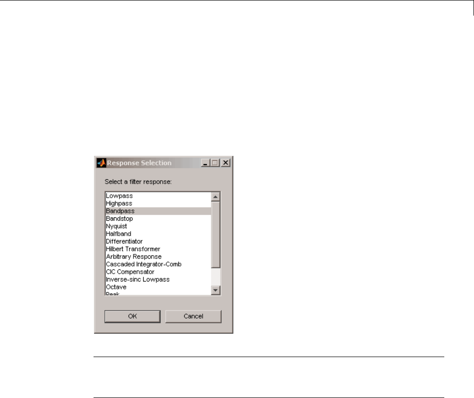
Filterbuilder Design Process

Select a Response

Whenyouopenthefilterbuilder tool by typing:

filterbuilder

at the MATLAB command prompt, the Response Selection dialog box

appears, listing all possible filter responses available in DSP System Toolbox

software.

Note This step cannot be skipped because it is not automatically completed

for you by the software. You must select a response to initiate the filter design

process.

After you choose a response, say bandpass, you start the design of the

Specifications Object, and the Bandpass Design dialog box appears.

This dialog box contains a Main pane, a Data Types pane and a Code

Generation pane. The specifications of your filter are generally set in the

Main pane of the dialog box.

The Data Types pane provides settings for precision and data types, and the

Code Generation pane contains options for various implementations of

the completed filter design.

4-3

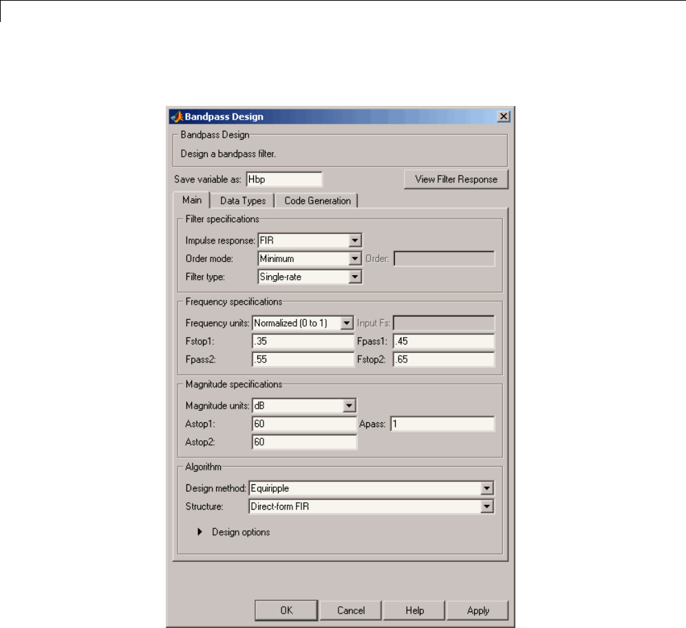
4Designing a Filter in the Filterbuilder GUI

For the initial design of your filter, you will mostly use the Main pane.

The Bandpass Design dialog box contains all the parameters you need to

determine the specifications of a bandpass filter. The parameters listed in

the Main pane depend upon the type of filter you are designing. However,

nomatterwhattypeoffilteryouhavechosenintheResponse Selection

4-4

Filterbuilder Design Process

dialog box, the filter design dialog box contains the Main,Data Types,and

Code Generation panes.

Select a Specification

To choose the specification for the bandpass filter, you can begin by selecting

an Impulse Response,Order Mode,andFilter Type in the Filter

Specifications frame of the Main Pane. You can further specify the

response of your filter by setting frequency and magnitude specifications in

the appropriate frames on the Main Pane.

Note Frequency,Magnitude,andAlgorithm specifications are

interdependent and may change based upon your Filter Specifications

selections. When choosing specifications for your filter, select your Filter

Specifications first and work your way down the dialog box- this approach

ensures that the best settings for dependent specifications display as available

in the dialog box.

Select an Algorithm

The algorithms available for your filter depend upon the filter response and

design parameters you have selected in the previous steps. For example, in the

case of a bandpass filter, if the impulse response selected is IIR and the Order

Mode field is set toMinimum, the design methods available are Butterworth,

Chebyshev type I or II, or Elliptic,whereasiftheOrder Mode field is set

to Specify, the design method available is IIR least p-norm.

4-5

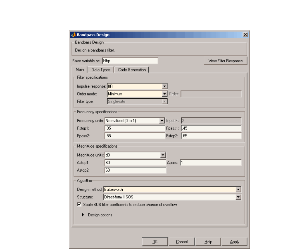
4Designing a Filter in the Filterbuilder GUI

Customize the Algorithm

By expanding the Design options section of the Algorithm frame, you

can further customize the algorithm specified. The options available will

depend upon the algorithm and settings that have already been selected in

the dialog box. In the case of a bandpass IIR filter using the Butterworth

4-6

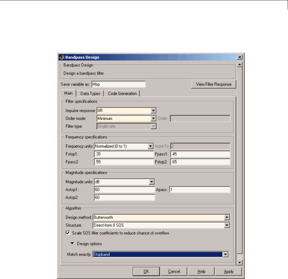
Filterbuilder Design Process

method, design options such as Match Exactly are available, as shown in

the following figure.

4-7

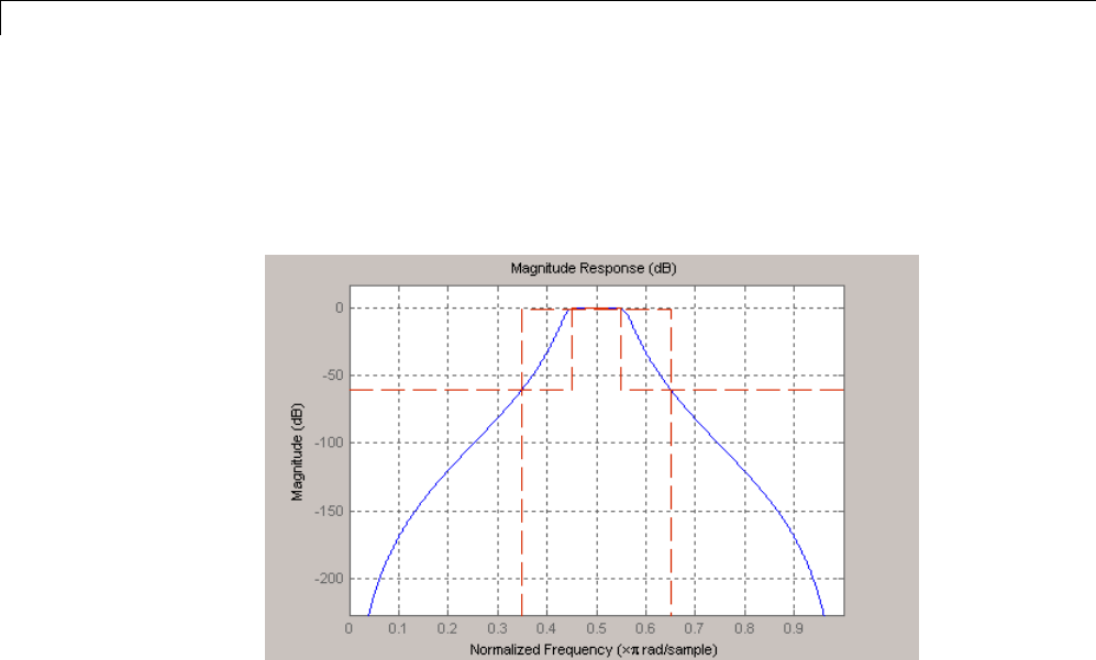
4Designing a Filter in the Filterbuilder GUI

Analyze the Design

To analyze the filter response, click on the View Filter Response button. The

Filter Visualization Tool opens displaying the magnitude plot of the filter

response.

Realize or Apply the Filter to Input Data

When you have achieved the desired filter response through design iterations

and analysis using the Filter Visualization Tool, apply the filter to the

input data. Again, this step is never automatically performed for you by the

software. Tofilteryourdata,youmust explicitly execute this step. In the

Filter Visualization Tool, click OK and DSP System Toolbox software

creates the filter object with the name specified in the Save variable as field

and exports it to the MATLAB workspace.

The filter is then ready to be used to filter actual input data. The basic filter

command takes input data x, filters it through the Filter Object, and produces

output y:

>> y = filter (FilterObj, x)

To understand how the filtering commands work, type:

>> help dfilt/filter

4-8

Filterbuilder Design Process

Tip If you have Simulink, you have the option of exporting this filter to

a Simulink block using the realizemdl command. To get help on this

command, type:

>> help realizemdl

4-9

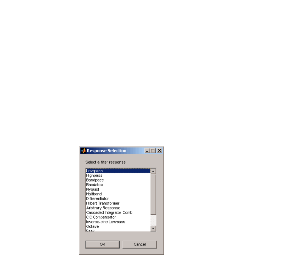
4Designing a Filter in the Filterbuilder GUI

Designing a FIR Filter Using filterbuilder

FIR Filter Design

Example – Using Filterbuilder to Design a Finite Impulse Response

(FIR) Filter

To design a lowpass FIR filter using filterbuilder:

1Open the Filterbuilder GUI by typing the following at the MATLAB prompt:

filterbuilder

The Response Selection dialog box appears. In this dialog box, you can

select from a list of filter response types. Select Lowpass in the list box.

2Hit the OK button. The Lowpass Design dialog box opens. Here you

can specify the writable parameters of the Lowpass filter object. The

components of the Main frame of this dialog box are described in the

section titled Lowpass Filter Design Dialog Box — Main Pane.Inthedialog

box, make the following changes:

•Enter a Fpass value of 0.55.

•Enter a Fstop value of 0.65.

4-10

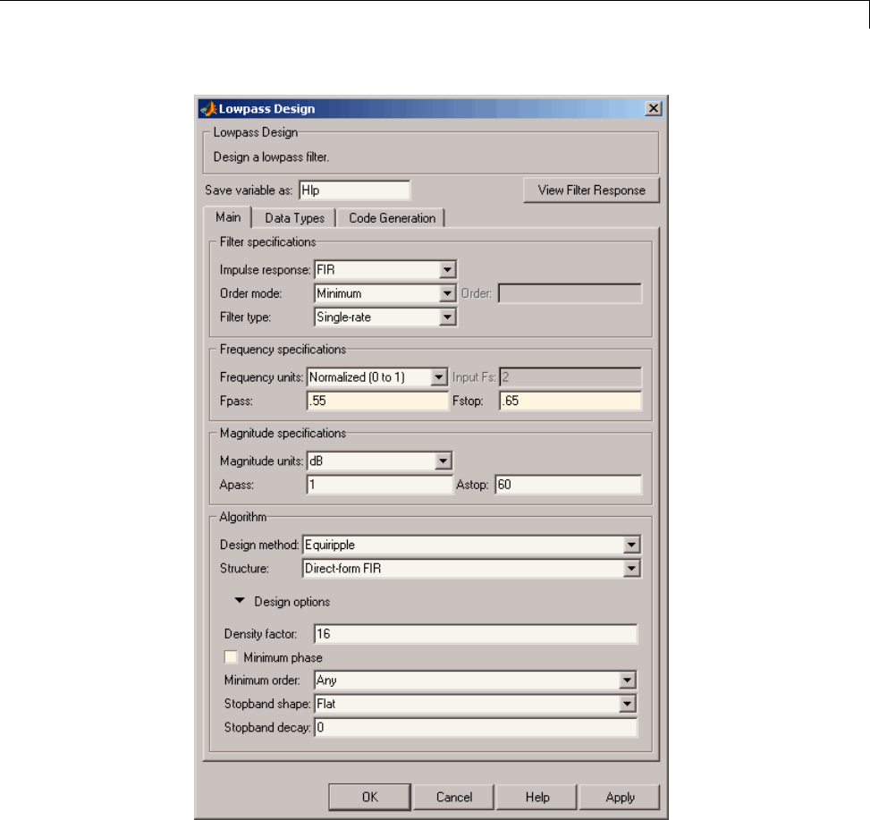
Designing a FIR Filter Using filterbuilder

3Click Apply, and the following message appears at the MATLAB prompt:

The variable 'Hlp' has been exported to the command window.

4-11

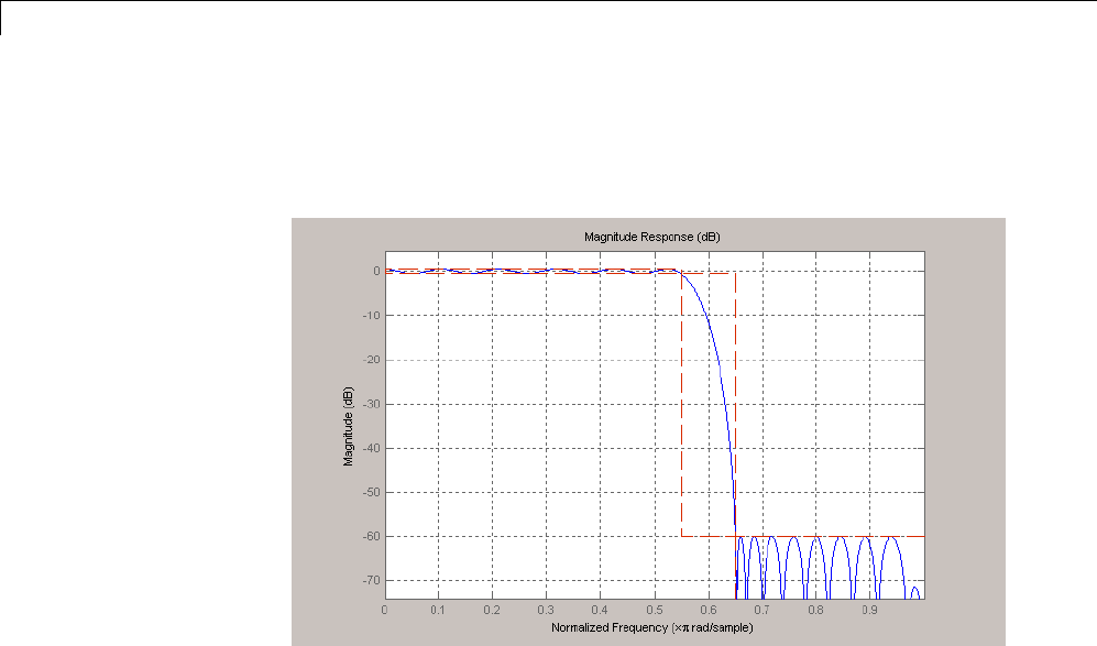
4Designing a Filter in the Filterbuilder GUI

4To check your design, click View Filter Response.TheFilter

Visualization tool appears, showing a plot of the magnitude response of

the filter.

You can change the design and click Apply,followedbyView Filter

Response, as many times as needed until your design specifications are

met.

4-12

FDATool: A Filter Design

and Analysis GUI

•“Overview” on page 5-2

•“Using FDATool” on page 5-6

•“Importing a Filter Design” on page 5-39

5FDATool: A Filter Design and Analysis GUI

Overview

In this section...

“FDATool” on page 5-2

“Filter Design Methods” on page 5-2

“Using the Filter Design and Analysis Tool” on page 5-4

“Analyzing Filter Responses” on page 5-4

“Filter Design and Analysis Tool Panels” on page 5-4

“Getting Help” on page 5-5

FDATool

The Filter Design and Analysis Tool (FDATool) is a user interface for

designing and analyzing filters quickly. FDATool enables you to design digital

FIR or IIR filters by setting filter specifications, by importing filters from

your MATLAB workspace, or by adding, moving or deleting poles and zeros.

FDATool also provides tools for analyzing filters, such as magnitude and

phaseresponseandpole-zeroplots.

Filter Design Methods

FDATool gives you access to the following Signal Processing Toolbox filter

design methods.

Design Method Function

Butterworth butter

Chebyshev Type I cheby1

Chebyshev Type II cheby2

Elliptic ellip

Maximally Flat maxflat

Equiripple firpm

Least-squares firls

5-2

Overview

Design Method Function

Constrained least-squares fircls

Complex equiripple cfirpm

Window fir1

When using the window method in FDATool, all Signal Processing Toolbox

window functions are available, and you can specify a user-defined window by

entering its function name and input parameter.

Advanced Filter Design Methods

The following advanced filter design methods are available if you have DSP

System Toolbox software.

Design Method Function

Constrained equiripple FIR firceqrip

Constrained-band equiripple FIR fircband

Generalized remez FIR firgr

Equripple halfband FIR firhalfband

Least P-norm optimal FIR firlpnorm

Equiripple Nyquist FIR firnyquist

Interpolated FIR ifir

IIR comb notching or peaking iircomb

Allpass filter (given group delay) iirgrpdelay

Least P-norm optimal IIR iirlpnorm

Constrained least P-norm IIR iirlpnormc

Second-order IIR notch iirnotch

Second-order IIR peaking (resonator) iirpeak

5-3

5FDATool: A Filter Design and Analysis GUI

Using the Filter Design and Analysis Tool

There are different ways that you can design filters using the Filter Design

and Analysis Tool. For example:

•You can first choose a response type, such as bandpass, and then choose

from the available FIR or IIR filter design methods.

•You can specify the filter by its type alone, along with certain frequency-

or time-domain specifications such as passband frequencies and stopband

frequencies. The filter you design is then computed using the default filter

design method and filter order.

Analyzing Filter Responses

Once you have designed your filter, you can display the filter coefficients

and detailed filter information, export the coefficients to the MATLAB

workspace, and create a C header file containing the coefficients, and analyze

different filter responses in FDATool or in a separate Filter Visualization Tool

(fvtool). The following filter responses are available:

•Magnituderesponse(

freqz)

•Phase response (phasez)

•Group delay (grpdelay)

•Phase delay (phasedelay)

•Impulseresponse(

impz)

•Step response (stepz)

•Pole-zero plots (zplane)

•Zero-phaseresponse(

zerophase)

Filter Design and Analysis Tool Panels

The Filter Design and Analysis Tool has sidebar buttons that display

particular panels in the lower half of the tool. The panels are

•Design Filter. See “Choosing a Filter Design Method” on page 5-8 for more

information. You use this panel to

-Design filters from scratch.

5-4

Overview

-Modify existing filters designed in FDATool.

-Analyze filters.

•Import filter. You use this panel to

-Import previously saved filters or filter coefficients that you have stored

in the MATLAB workspace.

-Analyze imported filters.

•Pole/Zero Editor. See “Editing the Filter Using the Pole/Zero Editor” on

page 5-19. You use this panel to add, delete, and move poles and zeros

in your filter design.

If you also have DSP System Toolbox product installed, additional panels

are available:

•Set quantization parameters — Use this panel to quantize double-precision

filters that you design in FDATool, quantize double-precision filters that

you import into FDATool, and analyze quantized filters.

•Transform filter — Use this panel to change a filter from one response

type to another.

•Multirate filter design — Use this panel to create a multirate filter

from your existing FIR design, create CIC filters, and linear and hold

interpolators.

If you have Simulink installed, this panel is available:

•Realize Model — Use this panel to create a Simulink block containing the

filter structure.

Getting Help

At any time, you can right-click or click the What’s this? button, ,toget

informationonthedifferentpartsofthetool. YoucanalsousetheHelp

menu to see complete Help information.

5-5

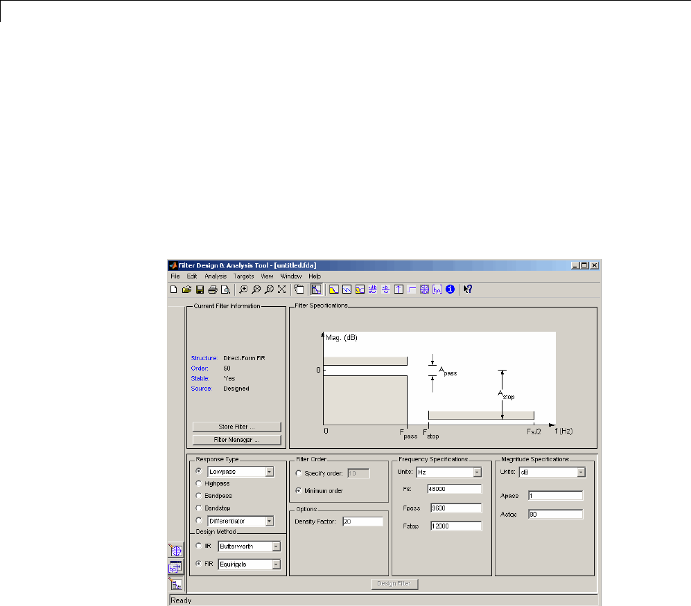
5FDATool: A Filter Design and Analysis GUI

Using FDATool

To open FDATool, type

fdatool

at the MATLAB command prompt.

The Filter Design and Analysis Tool opens with the Design Filter panel

displayed.

Note that when you open FDATool, Design Filter is not enabled. You must

make a change to the default filter design in order to enable Design Filter.

This is true each time you want to change the filter design. Changes to

radio button items or drop down menu items such as those under Response

Type or Filter Order enable Design Filter immediately. Changes to

specifications in text boxes such as Fs,Fpass,andFstop require you to click

outside the text box to enable Design Filter.

5-6

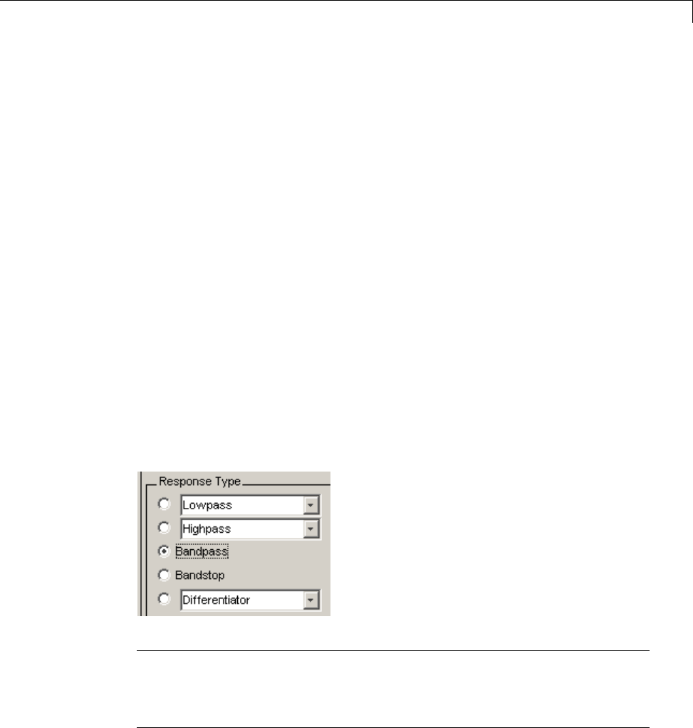
Using FDATool

Choosing a Response Type

You can choose from several response types:

•Lowpass

•Raised cosine

•Highpass

•Bandpass

•Bandstop

•Differentiator

•Multiband

•Hilbert transformer

•Arbitrary magnitude

Additional response types are available if you have DSP System Toolbox

software installed.

To design a bandpass filter, select the radio button next to Bandpass in

the Response Type region of the GUI.

Note Not all filter design methods are available for all response types. Once

you choose your response type, this may restrict the filter design methods

available to you. Filter design methods that are not available for a selected

response type are removed from the Design Method region of the GUI.

5-7

5FDATool: A Filter Design and Analysis GUI

Choosing a Filter Design Method

You can use the default filter design method for the response type that you’ve

selected, or you can select a filter design method from the available FIR and

IIR methods listed in the GUI.

To select the Remez algorithm to compute FIR filter coefficients, select the

FIR radio button and choose Equiripple from the list of methods.

Setting the Filter Design Specifications

•“Viewing Filter Specifications” on page 5-8

•“Filter Order” on page 5-9

•“Options” on page 5-9

•“Bandpass Filter Frequency Specifications” on page 5-10

•“Bandpass Filter Magnitude Specifications” on page 5-12

Viewing Filter Specifications

The filter design specifications that you can set vary according to response

type and design method. The display region illustrates filter specifications

when you select Analysis > Filter Specifications or when you click the

Filter Specifications toolbar button.

You can also view the filter specifications on the Magnitude plot of a designed

filter by selecting View > Specification Mask.

5-8

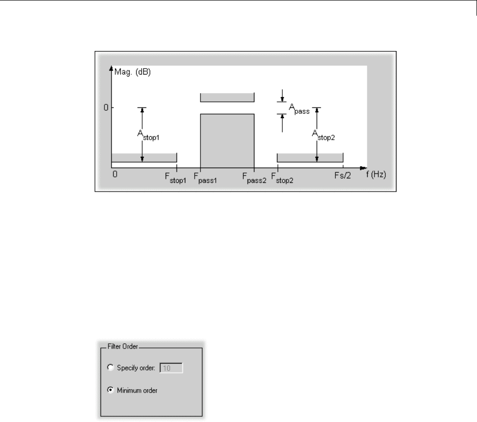
Using FDATool

Filter Order

You have two mutually exclusive options for determining the filter order

when you design an equiripple filter:

•Specify order: You enter the filter order in a text box.

•Minimum order: The filter design method determines the minimum

order filter.

Select the Minimum order radio button for this example.

Note that filter order specification options depend on the filter design method

you choose. Some filter methods may not have both options available.

Options

The available options depend on the selected filter design method. Only

the FIR Equiripple and FIR Window design methods have settable options.

5-9

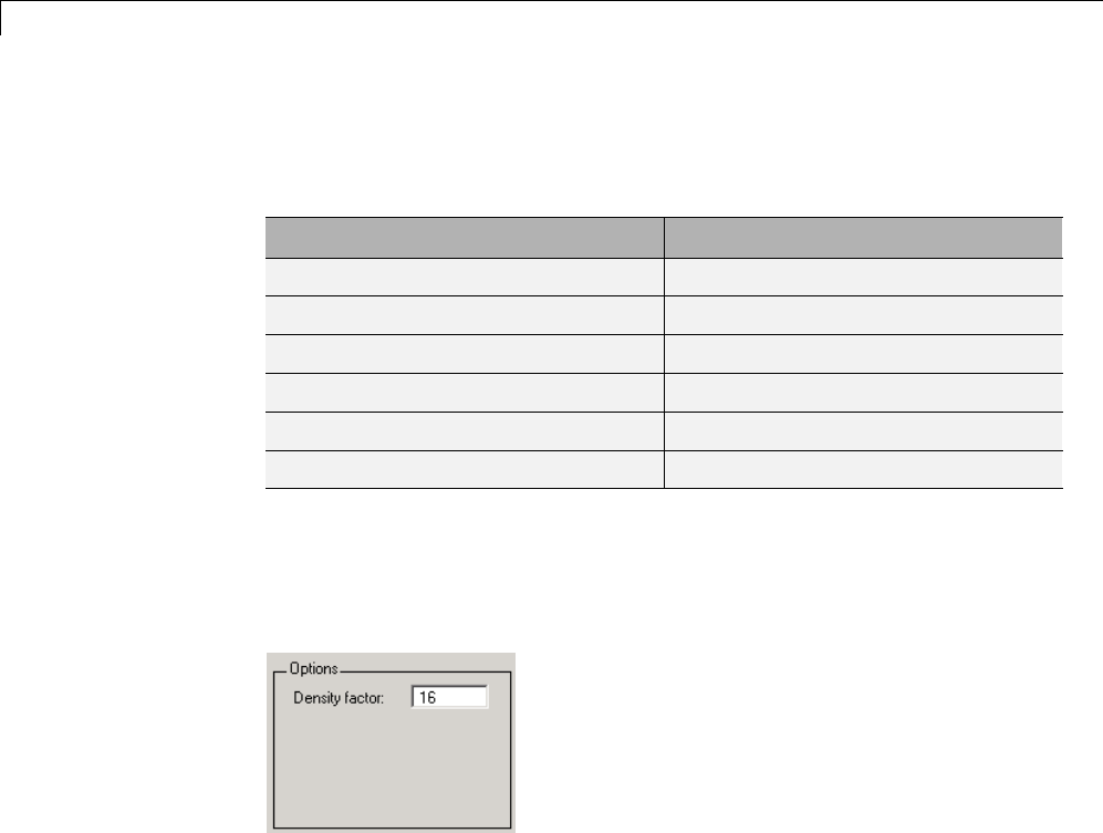
5FDATool: A Filter Design and Analysis GUI

For FIR Equiripple, the option is a Density Factor.Seefirpm for more

information. For FIR Window the options are Scale Passband,Window

selection, and for the following windows, a settable parameter:

Window Parameter

Chebyshev (chebwin) Sidelobe attenuation

Gaussian (gausswin)Alpha

Kaiser (kaiser)Beta

Taylor (taylorwin)NbarandSidelobelevel

Tukey (tukeywin)Alpha

User Defined Function Name, Parameter

You can view the window in the Window Visualization Tool (wvtool)by

clicking the View button.

For this example, set the Density factor to 16.

Bandpass Filter Frequency Specifications

For a bandpass filter, you can set

•Units of frequency:

-Hz

-kHz

-MHz

-Normalized (0 to 1)

5-10

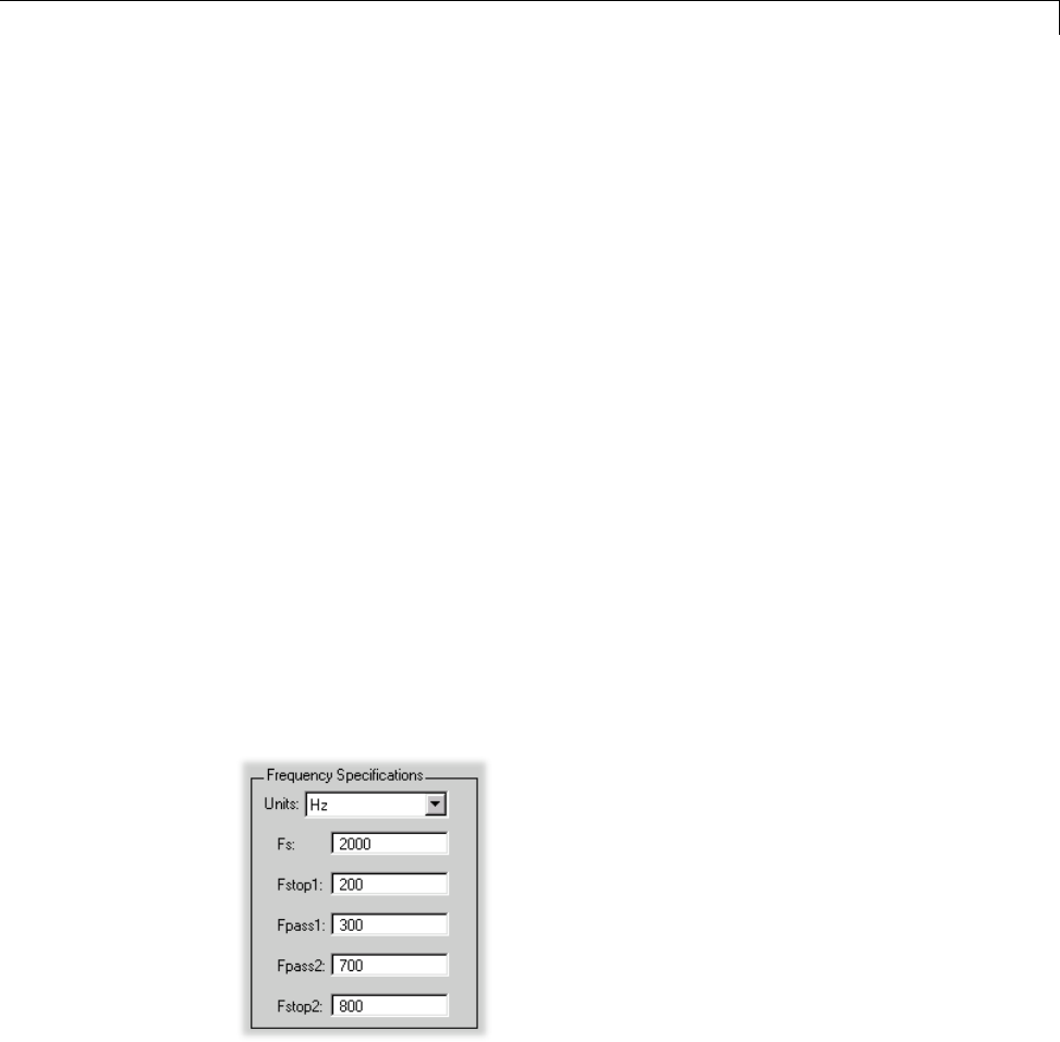
Using FDATool

•Sampling frequency

•Passband frequencies

•Stopband frequencies

You specify the passband with two frequencies. The first frequency

determines the lower edge of the passband, and the second frequency

determines the upper edge of the passband.

Similarly, you specify the stopband with two frequencies. The first frequency

determines the upper edge of the first stopband, and the second frequency

determines the lower edge of the second stopband.

For this example:

•Keep the units in Hz (default).

•Set the sampling frequency (Fs)to2000 Hz.

•Set the end of the first stopband (Fstop1)to200 Hz.

•Set the beginning of the passband (Fpass1)to300 Hz.

•Set the end of the passband (Fpass2)to700 Hz.

•Set the beginning of the second stopband (Fstop2)to800 Hz.

5-11

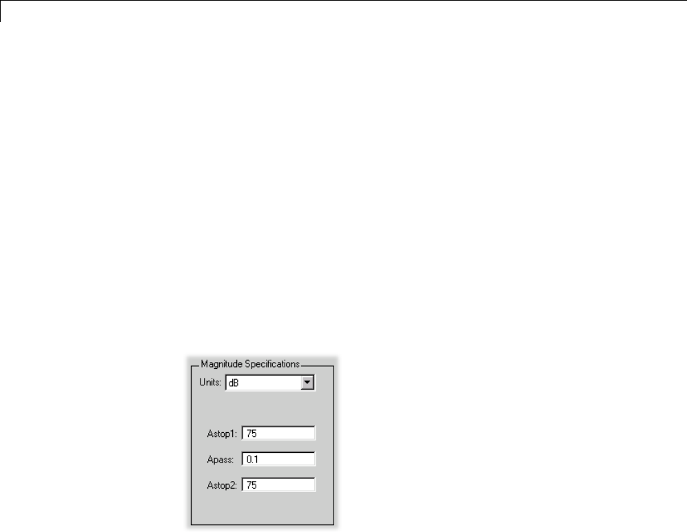
5FDATool: A Filter Design and Analysis GUI

Bandpass Filter Magnitude Specifications

For a bandpass filter, you can specify the following magnitude response

characteristics:

•Units for the magnitude response (dB or linear)

•Passband ripple

•Stopband attenuation

For this example:

•Keep Units in dB (default).

•Set the passband ripple (Apass)to0.1 dB.

•Set the stopband attenuation for both stopbands (Astop1,Astop2)to75

dB.

Computing the Filter Coefficients

Now that you’ve specified the filter design, click the Design Filter button to

compute the filter coefficients.

Notice that the Design Filter button is disabled once you’ve computed the

coefficients for your filter design. This button is enabled again once you make

any changes to the filter specifications.

5-12

Using FDATool

Analyzing the Filter

•“Displaying Filter Responses” on page 5-13

•“Using Data Tips” on page 5-15

•“Drawing Spectral Masks” on page 5-16

•“Changing the Sampling Frequency” on page 5-17

•“Displaying the Response in FVTool” on page 5-18

Displaying Filter Responses

You can view the following filter response characteristics in the display region

or in a separate window.

•Magnitude response

•Phase response

•Magnitude and Phase responses

•Group delay response

•Phase delay response

•Impulse response

•Step response

•Pole-zero plot

•Zero-phase response — available from the y-axis context menu in a

MagnitudeorMagnitudeandPhaseresponseplot.

If you have DSP System Toolbox product installed, two other analyses are

available:magnituderesponseestimateandround-offnoisepower.Thesetwo

analyses are the only ones that use filter internals.

For descriptions of the above responses and their associated toolbar buttons

and other FDATool toolbar buttons, see fvtool.

You can display two responses in the same plot by selecting

Analysis > Overlay Analysis and selecting an available response. A second

5-13

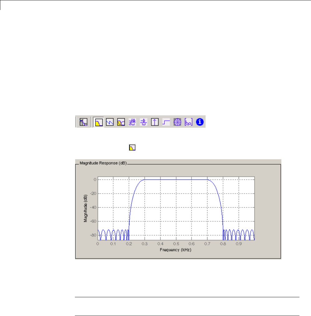
5FDATool: A Filter Design and Analysis GUI

y-axis is added to the right side of theresponseplot. (Notethatnotall

responses can be overlaid on each other.)

You can also display the filter coefficients and detailed filter information in

this region.

For all the analysis methods, except zero-phase response, you can access

them from the Analysis menu, the Analysis Parameters dialog box from the

context menu, or by using the toolbar buttons. For zero-phase, right-click the

y-axis of the plot and select Zero-phase from the context menu.

For example, to look at the filter’s magnitude response, select the Magnitude

Response button on the toolbar.

You can also overlay the filter specifications on the Magnitude plot by

selecting View > Specification Mask.

Note You can use specification masks in FVTool only if FVTool was launched

from FDATool.

5-14

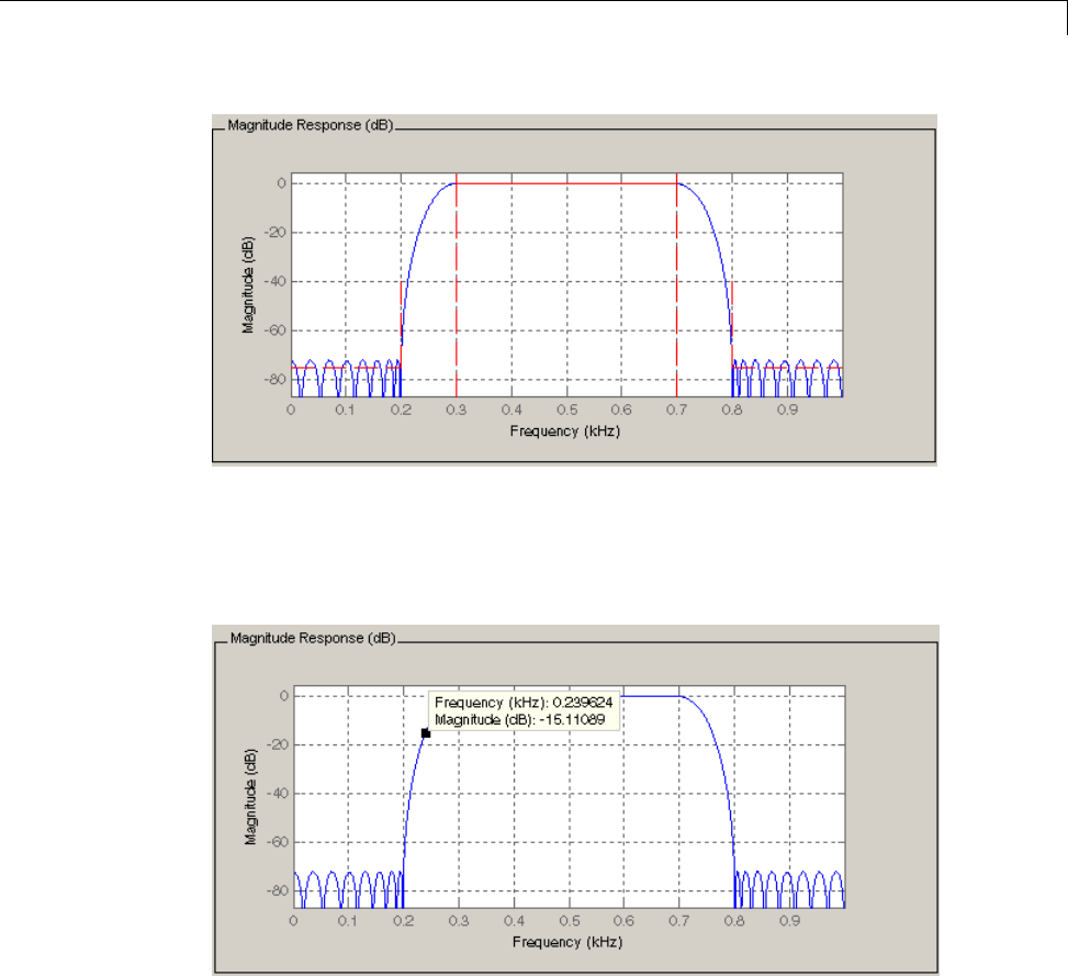
Using FDATool

Using Data Tips

You can click the response to add plot data tips that display information

about particular points on the response.

For information on using data tips, see “Data Cursor — Displaying Data

Values Interactively” in the MATLAB documentation.

5-15

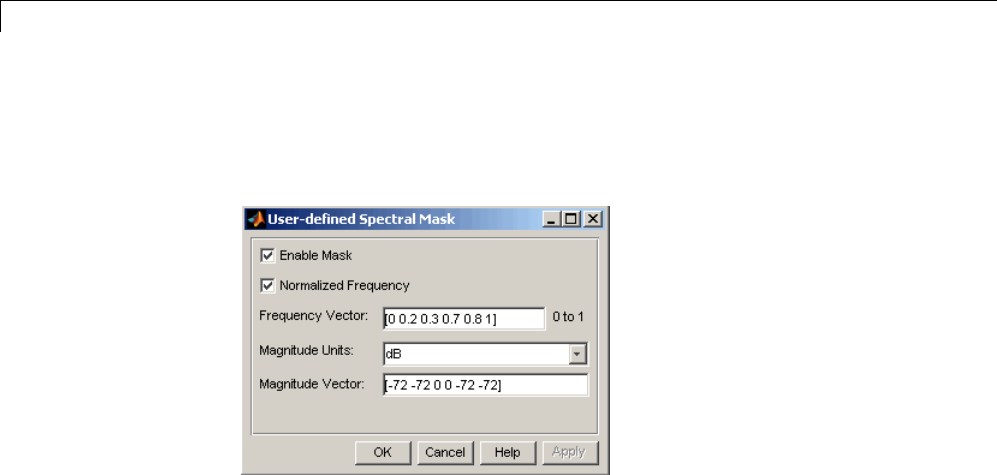
5FDATool: A Filter Design and Analysis GUI

Drawing Spectral Masks

To add spectral masks or rejection area lines to your magnitude plot, click

View > User-defined Spectral Mask.

The mask is defined by a frequency vector and a magnitude vector. These

vectors must be the same length.

•Enable Mask — Select to turn on the mask display.

•Normalized Frequency — Select to normalize the frequency between 0

and 1 across the displayed frequency range.

•Frequency Vector —Enteravectorofx-axis frequency values.

•Magnitude Units — Select the desired magnitude units. These units

should match the units used in the magnitude plot.

•Magnitude Vector — Enter a vector of y-axis magnitude values.

The magnitude response below shows a spectral mask.

5-16

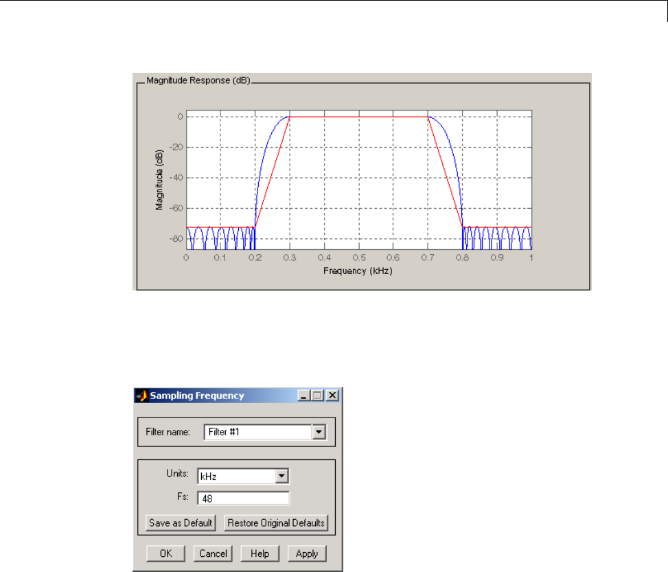
Using FDATool

Changing the Sampling Frequency

To change the sampling frequency of your filter, right-click any filter response

plot and select Sampling Frequency from the context menu.

To change the filter name, type the new name in Filter name.(In

fvtool,

if youhavemultiplefilters,selectthedesired filter and then enter the new

name.)

To change the sampling frequency, selectthedesiredunitfromUnits and

enter the sampling frequency in Fs. (Foreachfilterinfvtool, you can specify

adi

fferent sampling frequency or you can apply the sampling frequency to all

filters.)

5-17

5FDATool: A Filter Design and Analysis GUI

To save the displayed parameters as the default values to use when FDATool

or FVTool is opened, click Save as Default.

To restore the default values, click Restore Original Defaults.

Displaying the Response in FVTool

To display the filter response characteristics in a separate window, select

View > Filter Visualization Tool (available if any analysis, except the

filter specifications, is in the display region) or click the Full View Analysis

button:

This launches the Filter Visualization Tool (fvtool).

Note If Filter Specifications are shown in the display region, clicking the

Full View Analysis toolbar button launches a MATLAB figure window

instead of FVTool. The associated menu item is Print to figure,whichis

enabled only if the filter specifications are displayed.

You can use this tool to annotate your design, view other filter characteristics,

and print your filter response. You can link FDATool and FVTool so that

changes made in FDATool are immediately reflected in FVTool. See fvtool

for more information.

5-18

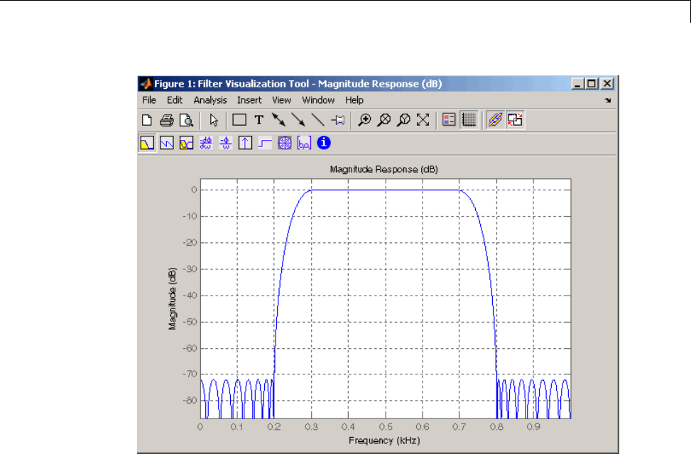
Using FDATool

Editing the Filter Using the Pole/Zero Editor

•“Displaying the Pole-Zero Plot” on page 5-19

•“Changing the Pole-Zero Plot” on page 5-20

Displaying the Pole-Zero Plot

You can edit a designed or imported filter’s coefficients by moving, deleting, or

adding poles and/or zeros using the Pole/Zero Editor panel.

5-19

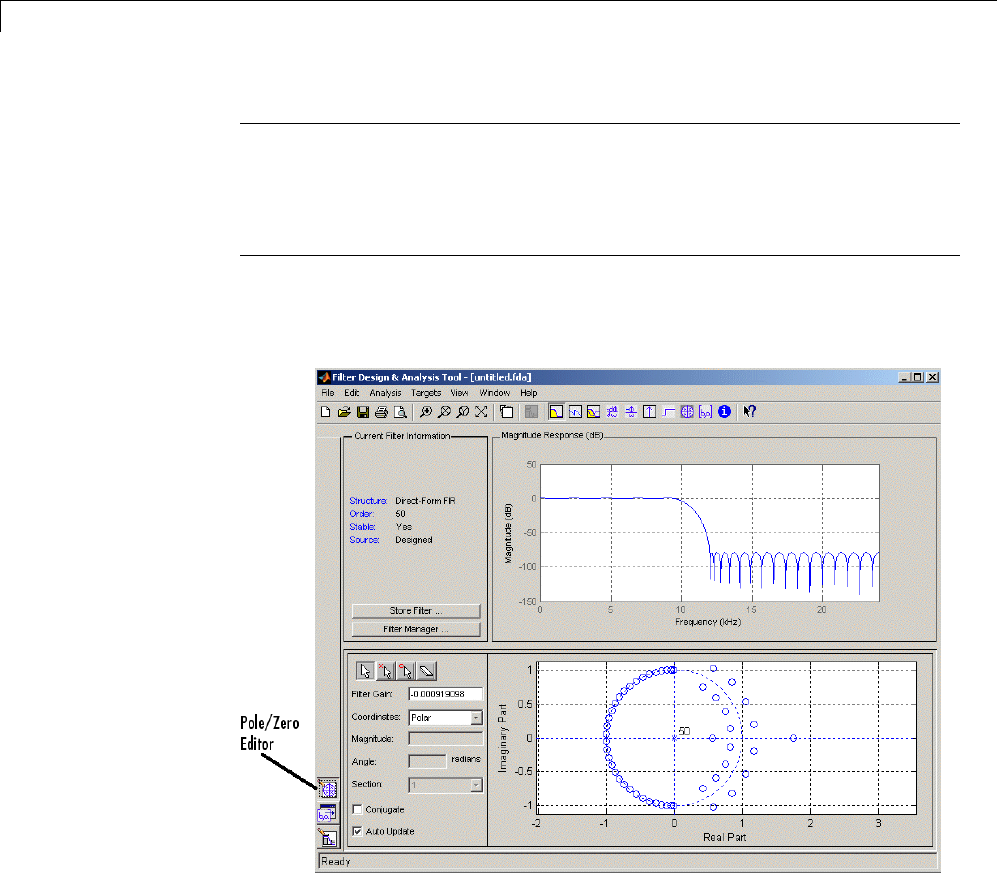
5FDATool: A Filter Design and Analysis GUI

Note You cannot generate MATLAB code (File > Generate MATLAB

code) if your filter was designed or edited with the Pole/Zero Editor.

You cannot move quantized poles and zeros. You can only move the reference

poles and zeros.

Click the Pole/Zero Editor button in the sidebar or select Edit > Pole/Zero

Editor to display this panel.

Poles are shown using x symbols and zeros are shown using o symbols.

Changing the Pole-Zero Plot

Plot mode buttons are located to the left of the pole/zero plot. Select one of the

buttons to change the mode of the pole/zero plot. The Pole/Zero Editor has

5-20

Using FDATool

these buttons from left to right: move pole, add pole, add zero, and delete

pole or zero.

The following plot parameters and controls are located to the left of the

pole/zero plot and below the plot mode buttons.

•Filter gain — factor to compensate for the filter’s pole(s) and zero(s) gains

•Coordinates — units (Polar or Rectangular)oftheselectedpoleorzero

•Magnitude — if polar coordinates is selected, magnitude of the selected

pole or zero

•Angle — if polar coordinates is selected, angle of selected pole(s) or zero(s)

•Real — if rectangular coordinates is selected, real component of selected

pole(s) or zero(s)

•Imaginary — if rectangular coordinates is selected, imaginary component

of selected pole or zero

•Section — for multisection filters, number of the current section

•Conjugate — creates a corresponding conjugate pole or zero or

automatically selects the conjugate pole or zero if it already exists.

•Auto update — immediately updates the displayed magnitude response

when poles or zeros are added, moved, or deleted.

The Edit > Pole/Zero Editor has items for selecting multiple poles/zeros,

for inverting and mirroring poles/zeros, and for deleting, scaling and rotating

poles/zeros.

5-21

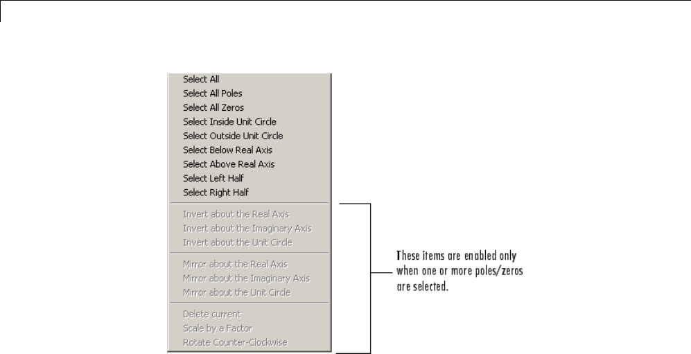
5FDATool: A Filter Design and Analysis GUI

Moving one of the zeros on the vertical axis produces the following result:

5-22

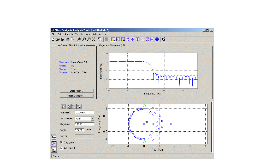
Using FDATool

•The selected zero pair is shown in green.

•When you select one of the zeros from a conjugate pair, the Conjugate check

box and the conjugate are automatically selected.

•The Magnitude Response plot updates immediately because Auto update

is active.

Converting the Filter Structure

•“Converting to a New Structure” on page 5-23

•“Converting to Second-Order Sections” on page 5-25

Converting to a New Structure

You can use Edit > Convert Structure to convert the current filter to a new

structure. All filters can be converted to the following representations:

5-23

5FDATool: A Filter Design and Analysis GUI

•Direct-form I

•Direct-form II

•Direct-form I transposed

•Direct-form II transposed

•Lattice ARMA

Note If you have DSP System Toolbox product installed, you will see

additional structures in the Convert structure dialog box.

In addition, the following conversions are available for particular classes

of filters:

•Minimum phase FIR filters can be converted to Lattice minimum phase

•Maximum phase FIR filters can be converted to Lattice maximum phase

•Allpass filters can be converted to Lattice allpass

•IIR filters can be converted to Lattice ARMA

Note Converting from one filter structure to another may produce a result

with different characteristics than the original. This is due to the computer’s

finite-precision arithmetic and the variations in the conversion’s roundoff

computations.

For example:

•Select Edit > Convert Structure to open the Convert structure dialog box.

•Select Direct-form I in the list of filter structures.

5-24

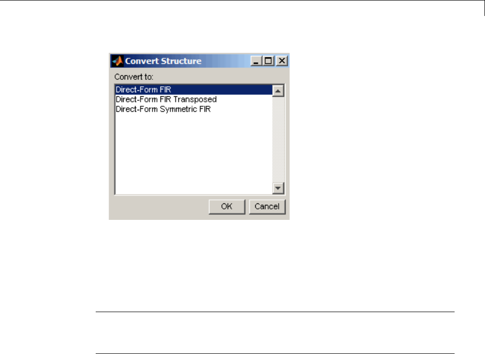
Using FDATool

Converting to Second-Order Sections

You can use Edit > Convert to Second-Order Sections to store the

converted filter structure as a collection of second-order sections rather than

as a monolithic higher-order structure.

Note The following options are also used for Edit > Reorder and Scale

Scale Second-Order Sections,whichyouusetomodifyanSOSfilter

structure.

The following Scale options are available when converting a direct-form II

structure only:

•None (default)

•L-2 (L2norm)

•L-infinity (L∞norm)

The Direction (Up or Down) determines the ordering of the second-order

sections. The optimal ordering changes depending on the Scale option

selected.

For example:

5-25

5FDATool: A Filter Design and Analysis GUI

•Select Edit > Convert to Second-Order Sections to open the Convert to

SOS dialog box.

•Select L-infinity from the Scale menu for L∞norm scaling.

•Leave Up as the Direction option.

Note To convert from second-order sections back to a single section, use

Edit > Convert to Single Section.

Exporting a Filter Design

•“Exporting Coefficients or Objects to the Workspace” on page 5-26

•“Exporting Coefficients to an ASCII File” on page 5-27

•“Exporting Coefficients or Objects to a MAT-File” on page 5-28

•“Exporting to SPTool” on page 5-29

•“Exporting to a Simulink Model” on page 5-29

•“Other Ways to Export a Filter” on page 5-32

Exporting Coefficients or Objects to the Workspace

You can save the filter either as filter coefficients variables or as a dfilt or

mfilt filter object variable. (Note that you must have DSP System Toolbox

product installed to save as an mfilt.) TosavethefiltertotheMATLAB

workspace:

1Select File > Export. The Export dialog box appears.

2Select Workspace from the Export To menu.

3Select Coefficients from the Export As menu to save the filter

coefficients or select Objects to save the filter in a filter object.

4For coefficients, assign variable names using the Numerator (for FIR

filters) or Numerator and Denominator (for IIR filters), or SOS Matrix

and Scale Values (for IIR filters in second-order section form) text boxes

in the Variable Names region.

5-26

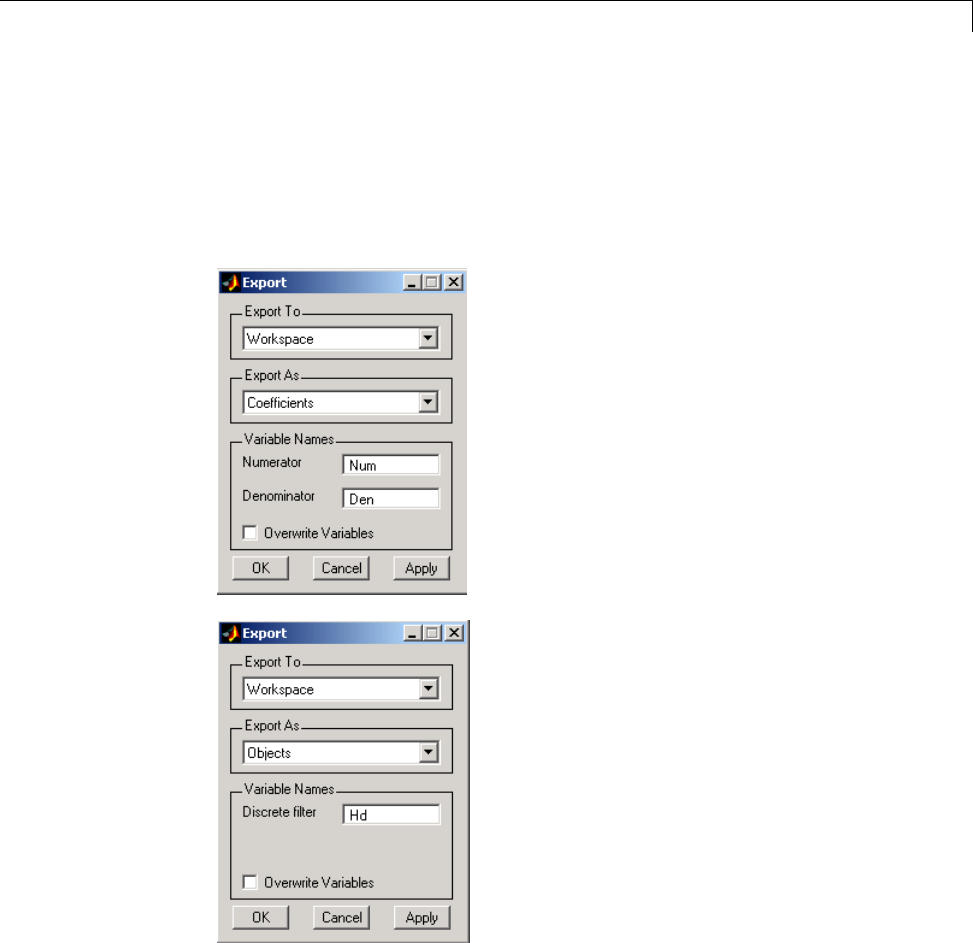
Using FDATool

For objects, assign the variable name in the Discrete Filter (or

Quantized Filter) text box. If you have variables with the same names

in your workspace and you want to overwrite them, select the Overwrite

Variables check box.

5Click the Export button.

Exporting Coefficients to an ASCII File

To save filter coefficients to a text file,

5-27

5FDATool: A Filter Design and Analysis GUI

1Select File > Export. The Export dialog box appears.

2Select Coefficients File (ASCII) from the Export To menu.

3Click the Export button. The Export Filter Coefficients to .FCF File dialog

box appears.

4Choose or enter a filename and click the Save button.

The coefficients are saved in the text file that you specified, and the MATLAB

Editor opens to display the file. The textfilealsocontainscommentswiththe

MATLAB version number, the Signal Processing Toolbox version number,

and filter information.

Exporting Coefficients or Objects to a MAT-File

To save filter coefficients or a filter object as variables in a MAT-file:

1Select File > Export. The Export dialog box appears.

2Select MAT-file from the Export To menu.

3Select Coefficients from the Export As menu to save the filter

coefficients or select Objects to save the filter in a filter object.

4For coefficients, assign variable names using the Numerator (for FIR

filters) or Numerator and Denominator (for IIR filters), or SOS Matrix

and Scale Values (for IIR filters in second-order section form) text boxes

in the Variable Names region.

For objects, assign the variable name in the Discrete Filter (or

Quantized Filter) text box. If you have variables with the same names

in your workspace and you want to overwrite them, select the Overwrite

Variables check box.

5Click the Export button. The Export to a MAT-File dialog box appears.

6Choose or enter a filename and click the Save button.

5-28

Using FDATool

Exporting to SPTool

You may want to use your designed filter in SPTool to do signal processing

and analysis.

1Select File > Export. The Export dialog box appears.

2Select SPTool from the Export To menu.

3AssignthevariablenameintheDiscrete Filter (or Quantized Filter)

text box. If you have variables with the same names in your workspace and

you want to overwrite them, select the Overwrite Variables check box.

4Click the Export button.

SPTool opens and the current FDATool filter appears in the Filter area list

as the specified variable name followed by (Imported).

Note If you are using the DSP System Toolbox software and export a

quantized filter, only the values of its quantized coefficients are exported.

The reference coefficients are not exported. SPTool does not restrict the

coefficient values, so if you edit them in SPTool by moving poles or zeros,

thefilterwillnolongerbeinquantizedform.

Exporting to a Simulink Model

If you have the Simulink product installed, you can export a Simulink block of

your filter design and insert it into a new or existing Simulink model.

You can export a filter designed using any filter design method available

in FDATool.

Note If you have the DSP System Toolbox and Fixed-Point Toolbox™

installed, you can export a CIC filter to a Simulink model.

1After designing your filter, click the Realize Model sidebar button or select

File > Export to Simulink Model. The Realize Model panel is displayed.

5-29

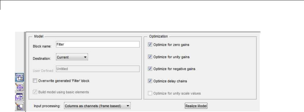
5FDATool: A Filter Design and Analysis GUI

2Specify the name to use for your block in Block name.

3To insert the block into the current (most recently selected) Simulink

model, set the Destination to Current. Toinsettheblockintoanew

model, select New. To insert the block into a user-defined subsystem, select

User defined.

4If you want to overwrite a block previously created from this panel, check

Overwrite generated ‘Filter’ block.

5If you select the Build model using basic elements check box, your filter

is created as a subsystem block, which uses separate sub-elements. In this

mode, the following optimization(s) are available:

•Optimize for zero gains — Removes zero-valued gain paths from

the filter structure.

•Optimize for unity gains — Substitutes a wire (short circuit) for

gains equal to 1 in the filter structure.

•Optimize for negative gains — Substitutes a wire (short circuit) for

gains equal to -1 and changes corresponding additions to subtractions in

the filter structure.

•Optimize delay chains — Substitutes delay chains composed of nunit

delays with a single delay of n.

•Optimize for unity scale values — Removes multiplications for

scale values equal to 1 from the filter structure.

The following illustration shows the effects of some of the optimizations:

5-30

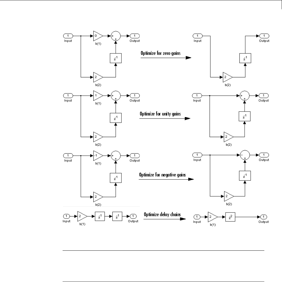
Using FDATool

Optimization Effects

Note The Build model using basic elements check box is enabled

only when you have a DSP System Toolbox license and your filter can be

designed using a Digital Filter block. For more information, see the Filter

Realization Wizard topic in the DSP System Toolbox documentation.

6Set the Input processing parameter to specify whether the generated

filter performs sample- or frame-based processing on the input. Depending

5-31

5FDATool: A Filter Design and Analysis GUI

on the type of filter you design, one or both of the following options may

be available:

•Columns as channels (frame based) — When you select this option,

the block treats each column of the input as a separate channel.

•Elements as channels (sample based) —Whenyouselectthis

option, the block treats each element of the input as a separate channel.

7Click the Realize Model button to create the filter block. When the Build

model using basic elements check box is selected, FDATool implements

the filter as a subsystem block using Sum, Gain, and Delay blocks.

If you double-click the Simulink Filter block, the filter structure is displayed.

Other Ways to Export a Filter

You can also send your filter to a C header file or generate MATLAB code to

construct your filter from the command line. For detailed instructions, see

the following sections:

•“Generating a C Header File” on page 5-32

•“Generating MATLAB Code” on page 5-34

Generating a C Header File

You may want to include filter information in an external C program. To

create a C header file with variables that contain filter parameter data,

follow this procedure:

1Select Targets > Generate C Header. The Generate C Header dialog

box appears.

5-32

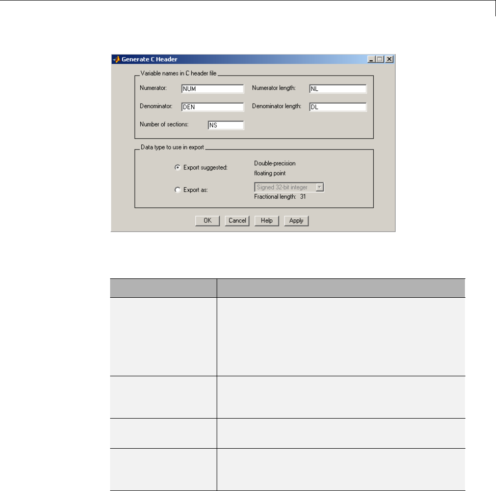
Using FDATool

2EnterthevariablenamestobeusedintheCheaderfile. Theparticular

filter structure determines the variables that are created in the file

Filter Structure Variable Parameter

Direct-form I

Direct-form II

Direct-form I

transposed

Direct-form II

transposed

Numerator, Numerator length*, Denominator,

Denominator length*, and Number of sections

(inactive if filter has only one section)

Lattice ARMA Lattice coeffs, Lattice coeffs length*, Ladder

coeffs, Ladder coeffs length*, Number of sections

(inactive if filter has only one section)

Lattice MA Lattice coeffs, Lattice coeffs length*, and Number

of sections (inactive if filter has only one section)

Direct-form FIR

transposed

Numerator, Numerator length*, and Number of

sections (inactive if filter has only one section)

*length variables contain the total number of coefficients of that type.

5-33

5FDATool: A Filter Design and Analysis GUI

Note Variable names cannot be C language reserved words, such as “for.”

3Select Export Suggested to use the suggested data type or select Export

As and select the desired data type from the pull-down.

Note If you do not have DSP System Toolbox software installed, selecting

any data type other than double-precision floating point results in a filter

that does not exactly match the one you designed in the FDATool. This is

due to rounding and truncating differences.

4Click OK tosavethefileandclosethedialogboxorclickApply to save the

file, but leave the dialog box open for additional C header file definitions.

Generating MATLAB Code

You can generate MATLAB code that constructs the filter you designed

in FDATool from the command line. Select File > Generate MATLAB

Code > Filter Design Function and specify the filename in the Generate

MATLAB code dialog box.

Note You cannot generate MATLAB code (File > Generate MATLAB

Code > Filter Design Function) if your filter was designed or edited with

the Pole/Zero Editor.

The following is generated MATLAB code for the default lowpass filter in

FDATool.

function Hd = ExFilter

%EXFILTER Returns a discrete-time filter object.

% MATLAB Code

% Generated by MATLAB(R) 7.11 and the Signal Processing Toolbox 6.14.

% Generated on: 17-Feb-2010 14:15:37

5-34

Using FDATool

% Equiripple Lowpass filter designed using the FIRPM function.

% All frequency values are in Hz.

Fs = 48000; % Sampling Frequency

Fpass = 9600; % Passband Frequency

Fstop = 12000; % Stopband Frequency

Dpass = 0.057501127785; % Passband Ripple

Dstop = 0.0001; % Stopband Attenuation

dens = 20; % Density Factor

% Calculate the order from the parameters using FIRPMORD.

[N, Fo, Ao, W] = firpmord([Fpass, Fstop]/(Fs/2), [1 0], [Dpass, Dstop]);

% Calculate the coefficients using the FIRPM function.

b = firpm(N, Fo, Ao, W, {dens});

Hd = dfilt.dffir(b);

% [EOF]

Managing Filters in the Current Session

You can store filters designed in the current FDATool session for cascading

together, exporting to FVTool or for recalling later in the same or future

FDATool sessions.

You store and access saved filters with the Store filter and Filter Manager

buttons, respectively, in the Current Filter Information pane.

5-35

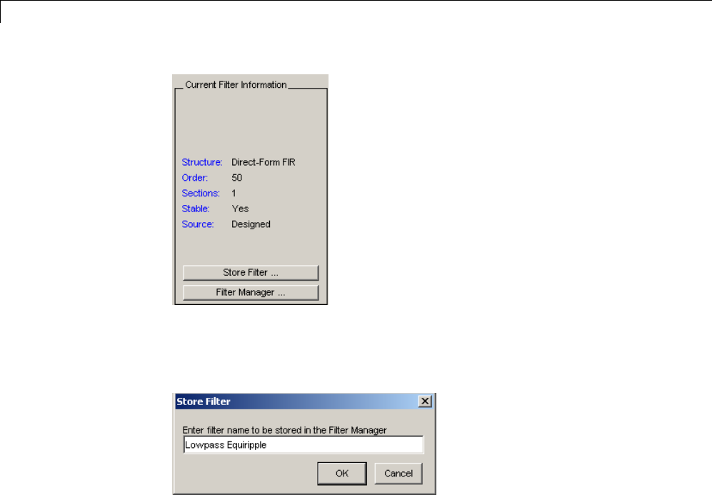
5FDATool: A Filter Design and Analysis GUI

Store Filter — Displays the Store Filter dialog box in which you specify the

filter name to use when storing the filter in the Filter Manager. The default

nameisthetypeofthefilter.

Filter Manager — Opens the Filter Manager.

5-36

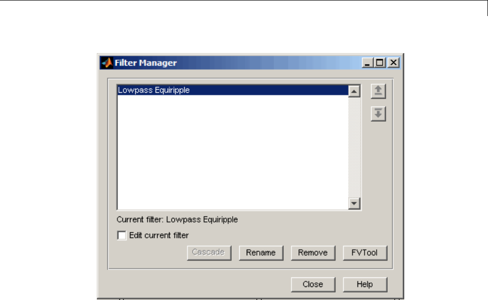
Using FDATool

The current filter is listed below the listbox. To change the current filter,

highlight the desired filter. If you select Edit current filter, FDATool

displays the currently selected filter specifications. If you make any changes

to the specifications, the stored filter is updated immediately.

To cascade two or more filters, highlight the desired filters and press

Cascade. A new cascaded filter is added to the Filter Manager.

To change the name of a stored filter, press Rename. The Rename filter

dialog box is displayed.

To remove a stored filter from the Filter Manager, press Delete.

To export one or more filters to FVTool, highlight the filter(s) and press

FVTool.

5-37

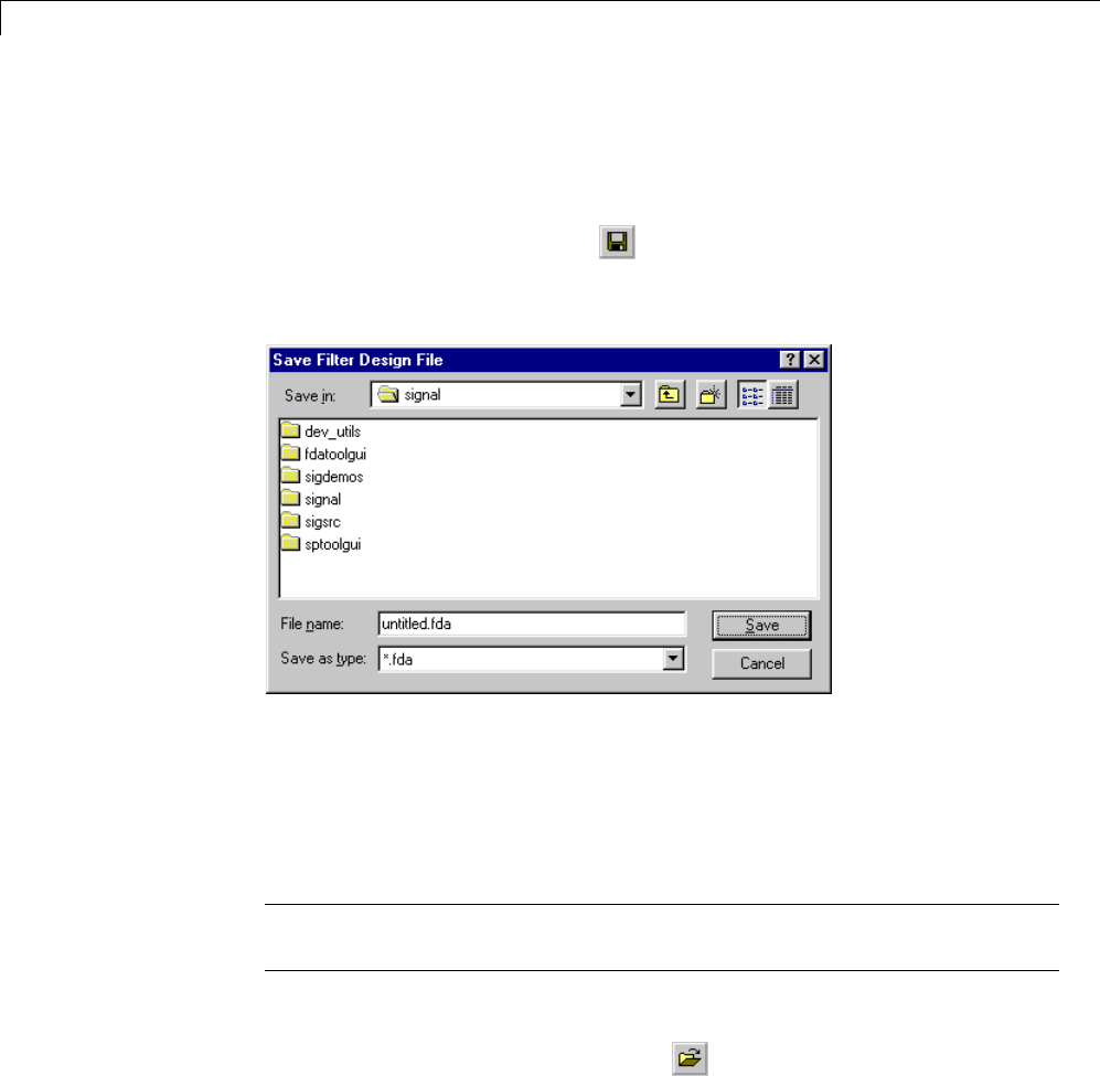
5FDATool: A Filter Design and Analysis GUI

Saving and Opening Filter Design Sessions

You can save your filter design session as a MAT-file and return to the same

session another time.

Select the Save session button to save your session as a MAT-file.

The first time you save a session, a Save Filter Design File browser opens,

prompting you for a session name.

For example, save this design session as TestFilter.fda in your current

working directory by typing TestFilter in the File name field.

The .fda extension is added automatically to all filter design sessions you

save.

Note You can also use the File > Save session and File > Save session

as to save a session.

You can load existing sessions into the Filter Design and Analysis Tool

by selecting the Open session button, or File > Open session .A

Load Filter Design File browser opens that allows you to select from your

previously saved filter design sessions.

5-38

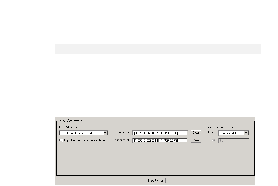
Importing a Filter Design

In this section...

“Import Filter Panel” on page 5-39

“Filter Structures” on page 5-40

Import Filter Panel

The Import Filter panel allows you to import a filter. You can access this

region by clicking the Import Filter buttoninthesidebar.

The imported filter can be in any of the representations listed in the Filter

Structure pull-downmenu.Youcanimportafilter as second-order sections

by selecting the check box.

Specify the filter coefficients in Numerator and Denominator,either

by entering them explicitly or by referring to variables in the MATLAB

workspace.

Select the frequency units from the following options in the Units menu, and

for any frequency unit other than Normalized, specify the value or MATLAB

workspace variable of the sampling frequency in the Fs field.

To import the filter, click the Import Filter button. The display region is

automatically updated when the new filter has been imported.

You can edit the imported filter using the Pole/Zero Editor panel.

5-39

5FDATool: A Filter Design and Analysis GUI

Filter Structures

The available filter structures are:

•Direct Form, which includes direct-form I, direct-form II, direct-form I

transposed, direct-form II transposed, and direct-form FIR

•Lattice, which includes lattice allpass, lattice MA min phase, lattice MA

max phase, and lattice ARMA

•Discrete–time Filter (dfilt object)

The structurethatyouchoosedeterminesthetypeofcoefficientsthatyou

need to specify in the text fields to the right.

Direct-form

For direct-form I, direct-form II, direct-form I transposed, and direct-form II

transposed, specify the filter by its transfer function representation

Hz bbzbz bmz

aazaZ

() () () () ( )

() () ()



 

 



12 3 1

12 3

aan z n

()

•The Numerator field specifies a variable name or value for the numerator

coefficient vector b, which contains m+1 coefficients in descending powers

of z.

•The Denominator field specifies a variable name or value for the

denominator coefficient vector a, which contains n+1 coefficients in

descending powers of z. For FIR filters, the Denominator is 1.

Filters in transfer function form can be produced by all of the Signal

Processing Toolbox filter design functions (such as fir1,fir2,firpm,butter,

yulewalk). See “Transfer Function” on page 1-23 for more information.

Importing as second-order sections. For all direct-form structures,

except direct-form FIR, you can import the filter in its second-order section

representation:

5-40

Importing a Filter Design

Hz G bbzbz

aazaz

kk k

()







01

122

The Gain fieldspecifiesavariablenameoravalueforthegainG,andthe

SOS Matrix fieldspecifiesavariablenameoravaluefortheL-by-6 SOS

matrix

SOS

bbb aa

bbb

LLL



01 11 21 11 22

02 12 22 12 22

012

······

aaa

LL12













whose rows contain the numerator and denominator coefficients bik and aik

of the second-order sections of H(z).

Filters in second-order section form can be produced by functions such as

tf2sos,zp2sos,ss2sos,andsosfilt. See “Second-Order Sections (SOS)”

on page 1-27 for more information.

Lattice

For lattice allpass, lattice minimum and maximum phase, and lattice ARMA

filters, specify the filter by its lattice representation:

•For lattice allpass, the Lattice coeff field specifies the lattice (reflection)

coefficients, k(1) to k(N),whereNis the filter order.

•For lattice MA (minimum or maximum phase), the Lattice coeff field

specifies the lattice (reflection) coefficients, k(1) to k(N),whereNis the

filter order.

•For lattice ARMA, the Lattice coeff field specifies the lattice (reflection)

coefficients, k(1) to k(N),andtheLadder coeff field specifies the ladder

coefficients, v(1) to v(N+1),whereNis the filter order.

Filters in lattice form can be produced by tf2latc. See “Lattice Structure”

on page 1-28 for more information.

5-41

5FDATool: A Filter Design and Analysis GUI

Discrete-time Filter (dfilt object)

For Discrete-time filter, specify the name of the dfilt object. See dfilt for

more information.

Multirate Filter (mfilt object)

For Multirate filter, specify the name of the mfilt object. See mfilt in the

DSP System Toolbox product for more information.

5-42

Statistical Signal

Processing

The following chapter discusses statistical signal processing tools and

applications, including correlations, covariance, and spectral estimation.

•“Correlation and Covariance” on page 6-2

•“Spectral Analysis” on page 6-5

•“Selected Bibliography” on page 6-46

6Statistical Signal Processing

Correlation and Covariance

In this section...

“Background Information” on page 6-2

“Using xcorr and xcov Functions” on page 6-3

“Bias and Normalization” on page 6-3

“Multiple Channels” on page 6-4

Background Information

The cross-correlation sequence for two wide-sense stationary random process,

x(n) and y(n) is:

Rm Exnmyn

xy () {( ) ()}

where *denotes the complex conjugate and the expectation is over the

ensemble of realizations that constitute the random processes.

Note that cross-correlation is not commutative, but a Hermitian (conjugate)

symmetry property holds such that:

Rm R m

xy yx

() ( )

=−

The cross-covariance between x(n) and y(n) is:

Cm Exnm yn Rm

xy x y xy x y

() {(( ) )(() )} ()

=+− −= −

 

For zero-mean wide-sense stationary random processes, the cross-correlation

and cross-covariance are equivalent.

In practice, you must estimate these sequences, because it is possible to

access only a finite segment of the infinite-length random processes. Further,

it is often necessary to estimate ensemble moments based on time averages

because only a single realization of the random processes are available.

A common estimate based on Nsamples of xnand ynis the deterministic

cross-correlation sequence (also called the time-ambiguity function)

6-2

Correlation and Covariance

ˆ() ()()

ˆ()

xn my n m

Rm m

xy n

=+≥

−<

⎧

⎨

⎪

⎩

⎪

−−

∑

where we assume for this discussion that xnand ynare indexed from 0 to

N-1, and ˆ()Rm

xy from -(N-1) to N-1.

Using xcorr and xcov Functions

The functions xcorr and xcov estimate the cross-correlation and

cross-covariance sequences of random processes. They also handle

autocorrelation and autocovariance as special cases. The xcorr function

evaluates the sum shown above with an efficient FFT-based algorithm, given

inputs xnand ynstored in length Nvectors xand y. Its operation is equivalent

to convolution with one of the two subsequences reversed in time.

For example:

x=[11111]';

y=x;

xyc = xcorr(x,y)

Notice that the resulting sequence length is one less than twice the length

of the input sequence. Thus, the Nth element is the correlation at lag 0.

Also notice the triangular pulse of the output that results when convolving

twosquarepulses.

The xcov function estimates autocovariance and cross-covariance sequences.

This function has the same options and evaluates the same sum as xcorr,but

first removes the means of xand y.

Bias and Normalization

An estimate of a quantity is biased if its expected value is not equal to the

quantity it estimates. The expected value of the output of xcorr is

ER m N m R m

xy xy

{()}(||)()=−

6-3

6Statistical Signal Processing

xcorr provides the unbiased estimate, dividing by N-|m|, when you specify

an 'unbiased' flag after the input sequences.

xcorr(x,y,'unbiased')

Although this estimate is unbiased, the end points (near -(N-1) and N-1) suffer

fromlargevariancebecausexcorr computes them using only a few data

points. A possible trade-off is to simply divide by Nusing the 'biased' flag:

xcorr(x,y,'biased')

With this scheme, only the sample of the correlation at zero lag (the Nth

output element) is unbiased. This estimate is often more desirable than the

unbiased one because it avoids random large variations at the end points

of the correlation sequence.

xcorr provides one other normalization scheme. The syntax

xcorr(x,y,'coeff')

divides the output by norm(x)*norm(y) so that, for autocorrelations, the

sample at zero lag is 1.

Multiple Channels

For a multichannel signal, xcorr and xcov estimate the autocorrelation and

cross-correlation and covariance sequences for all of the channels at once. If S

is an M-by-Nsignal matrix representing Nchannels in its columns, xcorr(S)

returns a (2M-1)-by-N2matrix with the autocorrelations and cross-correlations

of the channels of Sin its N2columns. If Sis a three-channel signal

S = [s1 s2 s3]

then the result of xcorr(S) is organized as

R = [Rs1s1 Rs1s2 Rs1s3 Rs2s1 Rs2s2 Rs2s3 Rs3s1 Rs3s2 Rs3s3]

Two related functions, cov and corrcoef, are available in the standard

MATLAB environment. They estimate covariance and normalized covariance

respectively between the different channels at lag 0 and arrange them in

a square matrix.

6-4

Spectral Analysis

In this section...

“Background Information” on page 6-5

“Spectral Estimation Method” on page 6-7

“Nonparametric Methods” on page 6-9

“Parametric Methods” on page 6-32

Background Information

The goal of spectral estimation is to describe the distribution (over frequency)

of the power contained in a signal, based on a finite set of data. Estimation of

power spectra is useful in a variety of applications, including the detection

of signals buried in wideband noise.

The power spectral density (PSD)ofastationaryrandomprocessxnis

mathematically related to the autocorrelation sequence by the discrete-time

Fourier transform. In terms of normalized frequency, this is given by

PRme

xx xx

() ( )ωπ

=−

=−∞

∞

∑

This can be written as a function of physical frequency f(e.g., in hertz) by

using the relation ω=2πf/fs,wherefsis the sampling frequency.

Pf fRme

xx jmff

() ( ) /

=−

=−∞

∞

∑

12π

The correlation sequence can be derivedfromthePSDbyuseoftheinverse

discrete-time Fourier transform:

Rm P e d Pfe df

xx xx jm xx jmf

() () () /

−−

∫∫

ωω

ππ2

6-5

6Statistical Signal Processing

The average power of the sequence xnovertheentireNyquistintervalis

represented by

RPdPfdf

xx xx xx

() () ()

−− ∫∫ ωω

The average power of a signal over a particular frequency band [ω1,ω2],

0≤ω1≤ω2≤π, can be found by integrating the PSD over that band:

PPdPd

xx xx[,] () ()

 



 

12 1

∫∫

−

You can see from the above expression that Pxx(ω) represents the power

content of a signal in an infinitesimal frequency band, which is why it is called

the power spectral density.

The units of the PSD are power (e.g., watts) per unit of frequency. In the case

of Pxx(ω), this is watts/radian/sample or simply watts/radian. In the case

of Pxx(f), the units are watts/hertz. Integration of the PSD with respect to

frequency yields units of watts, as expected for the average power .

For real–valued signals, the PSD is symmetric about DC, and thus Pxx(ω)for

0≤ω≤π is sufficient to completely characterize the PSD. However, to obtain the

average power over the entire Nyquist interval, it is necessary to introduce

the concept of the one-sided PSD.

The one-sided PSD is given by

PPxx

onesided () ()





=−≤ <

≤≤

⎧

⎨

⎩

The average power of a signal over the frequency band, [ω1,ω2]with

0≤ω1≤ω2≤π, can be computed using the one-sided PSD as

PPd

[,] ()

 





12 1

=∫onesided

6-6

Spectral Analysis

Spectral Estimation Method

The various methods of spectrum estimation available in the toolbox are

categorized as follows:

•Nonparametric methods

•Parametric methods

•Subspace methods

Nonparametric methods are those in which the PSD is estimated directly

from the signal itself. The simplest such method is the periodogram.Other

nonparametric techniques such as Welch’s method [8], the multitaper method

(MTM)reduc

e the variance of the periodogram.

Parametric methods are those in which the PSD is estimated from a signal

that is assumed to be output of a linear system driven by white noise.

Examples are the Yule-Walker autoregressive (AR)method and the Burg

method.T

hese methods estimate the PSD by first estimating the parameters

(coefficients) of the linear system that hypothetically generates the signal.

They tend to produce better results than classical nonparametric methods

when the data length of the available signal is relatively short. Parametric

methods also produce smoother estimates of the PSD than nonparametric

methods, but are subject to error from model misspecification.

Subspace methods,alsoknownashigh-resolution methods or super-resolution

methods, generate frequency component estimates for a signal based on an

eigenanalysis or eigendecomposition of the autocorrelation matrix. Examples

are themultiple signal classification (MUSIC)method or the eigenvector (EV)

method. These methods are best suited for line spectra — that is, spectra of

sinusoidal signals — and are effective in the detection of sinusoids buried

in noise, especially when the signal to noise ratios are low. The subspace

methods do not yield true PSD estimates: they do not preserve process power

between the time and frequency domains, and the autocorrelation sequence

cannot be recovered by taking the inverse Fourier transform of the frequency

estimate.

All three categories of methods are listed in the table below with the

corresponding toolbox function and spectrum object names. More information

about each function is on the corresponding function reference page.

6-7

6Statistical Signal Processing

See “Parametric Modeling” on page 7-13 for details about lpc and other

parametric estimation functions.

Spectral Estimation Methods/Functions

Method Description Functions

Periodogram Power spectral density

estimate

spectrum.periodogram,

periodogram

Welch Averaged periodograms

of overlapped, windowed

signal sections

spectrum.welch,pwelch,

cpsd,tfestimate,

mscohere

Multitaper Spectral estimate from

combination of multiple

orthogonal windows (or

“tapers”)

spectrum.mtm,pmtm

Yule-Walker AR Autoregressive (AR)

spectral estimate of

a time-series from its

estimated autocorrelation

function

spectrum.yulear,

pyulear

Burg Autoregressive (AR)

spectral estimation

of a time-series by

minimization of linear

prediction errors

spectrum.burg,pburg

Covariance Autoregressive (AR)

spectral estimation

of a time-series by

minimization of the

forward prediction errors

spectrum.cov,pcov

Modified

Covariance

Autoregressive (AR)

spectral estimation

of a time-series by

minimization of the

forward and backward

prediction errors

spectrum.mcov,pmcov

6-8

Spectral Analysis

Spectral Estimation Methods/Functions (Continued)

Method Description Functions

MUSIC Multiple signal

classification

spectrum.music,pmusic

Eigenvector Pseudospectrum estimate spectrum.eigenvector,

peig

Nonparametric Methods

The following sections discuss the periodogram, modified periodogram, Welch,

and multitaper methods of nonparametric estimation, along with the related

CPSD function, transfer function estimate, and coherence function.

Periodogram

Ingeneralterms,onewayofestimatingthePSDofaprocessistosimplyfind

the discrete-time Fourier transform of the samples of the process (usually

done on a grid with an FFT) and appropriately scale the magnitude squared

of the result. This estimate is called the periodogram.

The periodogram estimate of the PSD of a length-L signal xL[n]is

PLF

fxne

LjfnF

() | () |

−−

∑

122



where Fsis the sampling frequency.

In practice, the actual computation of Pxx(f) can be performed only at a

finite number of frequency points, and usually employs an FFT. Most

implementations of the periodogram method compute the N-point PSD

estimate at the frequencies

fkF

NkN

==…−01 1,, ,

6-9

6Statistical Signal Processing

In some cases, the computation of the periodogram via an FFT algorithm is

more efficient if the number of frequencies is a power of two. Therefore it

is not uncommon to pad the input signal with zeros to extend its length to

a power of two.

As an example of the periodogram, consider the following 1001-element

signal xn, which consists of two sinusoids plus noise:

fs = 1000; % Sampling frequency

t = (0:fs)/fs; % One second worth of samples

A = [1 2]; % Sinusoid amplitudes (row vector)

f = [150;140]; % Sinusoid frequencies (column vector)

xn = A*sin(2*pi*f*t) + 0.1*randn(size(t));

Note The three last lines illustrate a convenient and general way to express

the sum of sinusoids.

Together they are equivalent to xn = sin(2*pi*150*t) +

2*sin(2*pi*140*t) + 0.1*randn(size(t));

The periodogram estimate of the PSD can be computed by creating a

periodogram object. In this case, the data vector is multiplied by a Hamming

window.

Hs = spectrum.periodogram('Hamming');

6-10

Spectral Analysis

and a plot of the PSD estimate can be displayed with the psd method:

psd(Hs,xn,'Fs',fs,'NFFT',1024,'SpectrumType','onesided')

The average power can be computed by approximating the integral with the

following sum:

Hdsp2= psd(Hs,xn,'Fs',fs,'NFFT',1024,'SpectrumType','twosided');

Pow = avgpower(Hdsp2)

You can also compute the average power from the one-sided PSD estimate:

Hdsp3= psd(Hs,xn,'Fs',fs,'NFFT',1024,'SpectrumType','onesided');

Pow = avgpower(Hdsp3)

Algorithm. Spectrum.periodogram computes and scales the output of the

FFT to produce the power vs. frequency plot as follows. For a detailed

example, see “Power Spectral Density Estimates Using FFT” on page 12-2.

1For rapid and efficient processing, make the input signal length (nfft)

equal to a power of 2 by padding it with zeros.

6-11

6Statistical Signal Processing

2If the input signal is real-valued, the magnitude of the resulting FFT is

symmetric with respect to zero frequency (DC). For an even-length FFT,

only the first (1+nfft/2) points are unique. Determine the number of

unique values and keep only those unique points.

3Take the squared magnitudes of the unique FFT values. Scale the squared

magnitudes (except for DC) by 2Fs/N, where Nis the length of signal prior

to any zero padding. Scale the DC value by Fs/N.

4Create a frequency vector from the number of unique points, the nfft and

the sampling frequency.

5Plot the resulting magnitude squared FFT vs. the frequency.

Performance of the Periodogram

The following sections discuss the performance of the periodogram with

regard to the issues of leakage, resolution, bias, and variance.

Spectral Leakage. Consider the PSD of a finite-length (length L)signal

xL[n], as discussed in the “Periodogram” on page 6-9 section. It is frequently

useful to interpret xL[n] as the result of multiplying an infinite signal, x[n], by

a finite-length rectangular window, wR[n]:

xn xnwn

[] [] [].=

Because multiplication in the time domain corresponds to convolution in the

frequency domain, the expected value of the periodogram in the frequency

domain is:

EP f Fs

Lf f Fs

LffFs

xx Fs

{()} sin ( ( ) / )

sin ( ( ) / )

=−′

−′

−

∫



PPfdf

xx () ,

′′

showing that the expected value of the periodogram is the convolution of the

true PSD with the square of the Dirichlet kernel.

The effect of the convolution is best understood for sinusoidal data. Suppose

that x[n]iscomposedofasumofMcomplex sinusoids:

6-12

Spectral Analysis

xn A e

Njn

()=

∑



Its spectrum is

() ( )



=−

∑

which for a finite-length sequence becomes

XAWd

() ( ( )) ( )





=−−

−=

∫∑

==\=

The preceding equation is equal to:

XAW

() ( )



=−

∑

So in the spectrum of the finite-length signal, the Dirac deltas have been

replaced by terms of the form WR(ω-ωk), which corresponds to the frequency

response of a rectangular window centered on the frequency ωk.

6-13

6Statistical Signal Processing

The frequency response of a rectangular window has the shape of a sinc

signal, as shown below.

The plot displays a main lobe and several side lobes, the largest of which is

approximately 13.5 dB below the mainlobe peak. These lobes account for

the effect known as spectral leakage. While the infinite-length signal has its

power concentrated exactly at the discrete frequency points fk, the windowed

(or truncated) signal has a continuum of power “leaked” around the discrete

frequency points fk.

Because the frequency response of a short rectangular window is a much

poorer approximation to the Dirac delta function than that of a longer

window, spectral leakage is especially evident when data records are short.

Consider the following sequence of 100 samples:

fs = 1000; % Sampling frequency

t = (0:fs/10)/fs; % One-tenth second worth of samples

A = [1 2]; % Sinusoid amplitudes

f = [150;140]; % Sinusoid frequencies

xn = A*sin(2*pi*f*t) + 0.1*randn(size(t));

Hs = spectrum.periodogram;

psd(Hs,xn,'Fs',fs,'NFFT',1024)

6-14

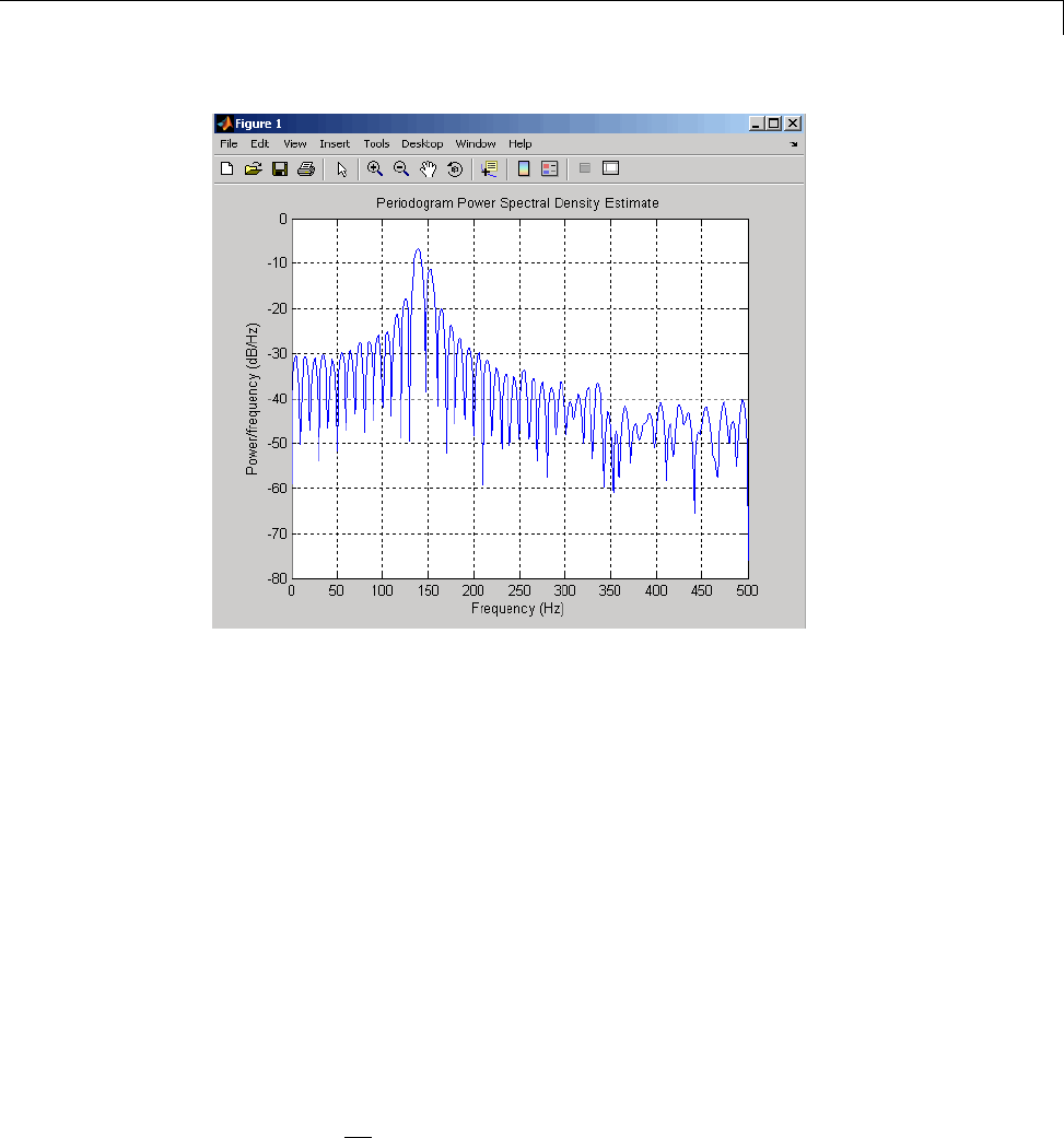
Spectral Analysis

It is important to note that the effect of spectral leakage is contingent solely

on the length of the data record. It is not a consequence of the fact that the

periodogram is computed at a finite number of frequency samples.

Resolution. Resolution refers to the ability to discriminate spectral features,

and is a key concept on the analysis of spectral estimator performance.

In order to resolve two sinusoids that are relatively close together in

frequency, it is necessary for the difference between the two frequencies to

be greater than the width of the mainlobe of the leaked spectra for either

one of these sinusoids. The mainlobe width is defined to be the width of the

mainlobe at the point where the power is half the peak mainlobe power (i.e.,

3 dB width). This width is approximately equal to fs/L.

In other words, for two sinusoids of frequencies f1and f2, the resolvability

condition requires that

()ff Fs

−>

6-15

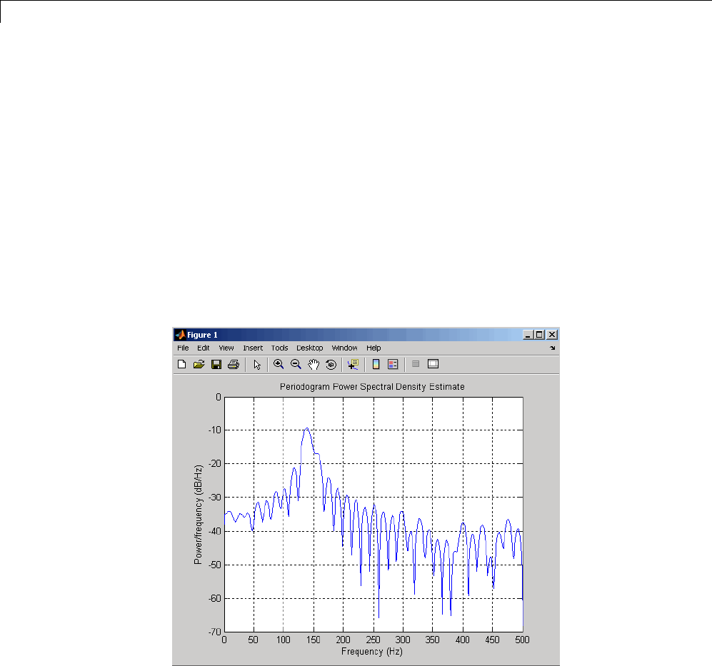
6Statistical Signal Processing

In the example above, where two sinusoids are separated by only 10 Hz, the

data record must be greater than 100 samples to allow resolution of two

distinct sinusoids by a periodogram.

Consider a case where this criterion is not met, as for the sequence of 67

samples below:

fs = 1000; % Sampling frequency

t = (0:fs/15)./fs; % 67 samples

A = [1 2]; % Sinusoid amplitudes

f = [150;140]; % Sinusoid frequencies

xn = A*sin(2*pi*f*t) + 0.1*randn(size(t));

Hs=spectrum.periodogram;

psd(Hs,xn,'Fs',fs,'NFFT',1024)

The above discussion about resolution did not consider the effects of noise

since the signal-to-noise ratio (SNR) has been relatively high thus far. When

the SNR is low, true spectral features are much harder to distinguish, and

6-16

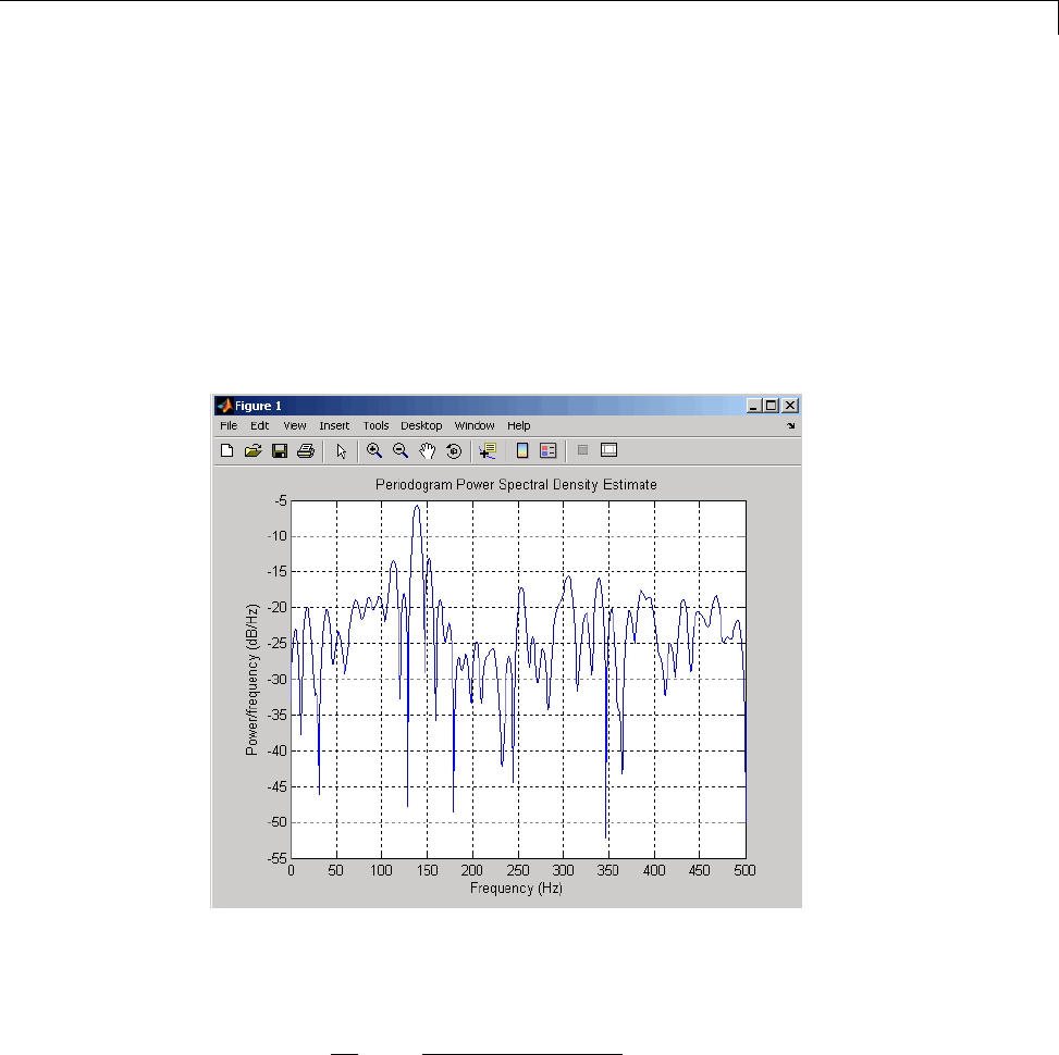
Spectral Analysis

noise artifacts appear in spectral estimates based on the periodogram. The

example below illustrates this:

fs = 1000; % Sampling frequency

t = (0:fs/10)./fs; % One-tenth second worth of samples

A = [1 2]; % Sinusoid amplitudes

f = [150;140]; % Sinusoid frequencies

xn = A*sin(2*pi*f*t) + 2*randn(size(t));

Hs=spectrum.periodogram;

psd(Hs,xn,'Fs',fs,'NFFT',1024)

Bias of the Periodogram. The periodogram is a biased estimator of the

PSD. Its expected value was previously shown to be:

EP f Fs

Lf f Fs

LffFs

xx Fs

{()} sin ( ( ) / )

sin ( ( ) / )

=−′

−′

−

∫



PPfdf

xx () ,

′′

6-17

6Statistical Signal Processing

The periodogram is asymptotically unbiased, which is evident from the earlier

observation that as the data record length tends to infinity, the frequency

response of the rectangular window more closely approximates the Dirac

delta function. However, in some cases the periodogram is a poor estimator

of the PSD even when the data record is long. This is due to the variance of

the periodogram, as explained below.

Variance of the Periodogram. Thevarianceoftheperiodogramcanbe

shown to be:

Var Fs

(()) () /

() /

Pf Pf f

Pf f fFs

xx xx

=<<

⎧

⎨

⎪

⎩

⎪

20 2

whichindicatesthatthevariancedoesnottendtozeroasthedatalengthL

tends to infinity. In statistical terms, the periodogram is not a consistent

estimator of the PSD. Nevertheless, theperiodogramcanbeausefultoolfor

spectral estimation in situations where the SNR is high, and especially if

the data record is long.

The Modified Periodogram

The modified periodogram windows the time-domain signal prior to computing

the DFT in order to smooth the edges of the signal. This has the effect of

reducing the height of the sidelobes or spectral leakage. This phenomenon

gives rise to the interpretation of sidelobesasspuriousfrequenciesintroduced

into the signal by the abrupt truncation that occurs when a rectangular

window is used. For nonrectangular windows, the end points of the truncated

signal are attenuated smoothly, and hence the spurious frequencies

introduced are much less severe. On the other hand, nonrectangular windows

also broaden the mainlobe, which results in a reduction of resolution.

spectrum.periodogram allows you to compute a modified periodogram by

specifyingthewindowtobeusedonthedata.Forexample,compareadefault

rectangular window and a Hamming window:

fs = 1000; % Sampling frequency

t = (0:fs/10)./fs; % One-tenth second worth of samples

A = [1 2]; % Sinusoid amplitudes

6-18

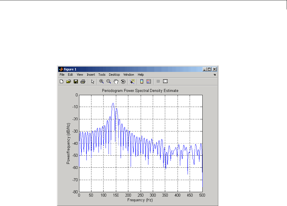
Spectral Analysis

f = [150;140]; % Sinusoid frequencies

xn = A*sin(2*pi*f*t) + 0.1*randn(size(t));

Hrect = spectrum.periodogram;

psd(Hrect,xn,'Fs',fs,'NFFT',1024);

6-19

6Statistical Signal Processing

Hhamm = spectrum.periodogram('Hamming');

psd(Hhamm,xn,'Fs',fs,'NFFT',1024);

You can verify that although the sidelobes are much less evident in the

Hamming-windowed periodogram, the two main peaks are wider. In fact,

the 3 dB width of the mainlobe corresponding to a Hamming window

is approximately twice that of a rectangular window. Hence, for a fixed

data length, the PSD resolution attainable with a Hamming window is

approximately half that attainable with a rectangular window. The competing

interests of mainlobe width and sidelobe height can be resolved to some extent

by using variable windows such as the Kaiser window.

Nonrectangular windowing affects the average power of a signal because

some of the time samples are attenuated when multiplied by the window.

To compensate for this, spectrum.periodogram and spectrum.welch

normalize the window to have an average power of unity. This ensures that

the measured average power is generally independent of window choice. If

the frequency components are not well resolved by the PSD estimators, the

window choice does affect the average power.

6-20

Spectral Analysis

The modified periodogram estimate of the PSD is

ˆ() |()|

Pf Xf

FsLU

xx =2

where Uis the window normalization constant.

ULwn

−

∑

|( )| .

For large values of L,Utends to become independent of window length.

The addition of Uas a normalization constant ensures that the modified

periodogram is asymptotically unbiased.

Welch’s Method

An improved estimator of the PSD is the one proposed by Welch [8]. The

method consists of dividing the time series data into (possibly overlapping)

segments, computing a modified periodogram of each segment, and then

averaging the PSD estimates. The result is Welch’s PSD estimate. Welch’s

method is implemented in the toolbox by the spectrum.welch object or

pwelch function

The averaging of modified periodograms tends to decrease the variance of the

estimate relative to a single periodogram estimate of the entire data record.

Although overlap between segments introduces redundant information, this

effect is diminished by the use of a nonrectangular window, which reduces

the importance or weight given to the end samples of segments (the samples

that overlap).

However, as mentioned above, the combined use of short data records and

nonrectangular windows results in reduced resolution of the estimator. In

summary, there is a trade-off between variance reduction and resolution.

One can manipulate the parameters in Welch’s method to obtain improved

estimates relative to the periodogram, especially when the SNR is low. This is

illustrated in the following example.

Consider an original signal consisting of 301 samples:

6-21

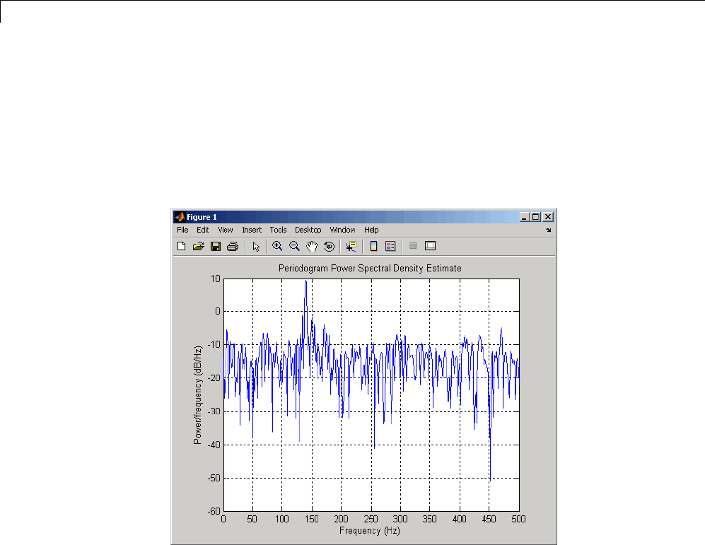
6Statistical Signal Processing

fs = 1000; % Sampling frequency

t = (0:0.3*fs)./fs; % 301 samples

A = [2 8]; % Sinusoid amplitudes (row vector)

f = [150;140]; % Sinusoid frequencies (column vector)

xn = A*sin(2*pi*f*t) + 5*randn(size(t));

Hs = spectrum.periodogram('rectangular');

psd(Hs,xn,'Fs',fs,'NFFT',1024);

We can obtain Welch’s spectral estimate for 3 segments with 50% overlap with

Hs = spectrum.welch('rectangular',150,50);

psd(Hs,xn,'Fs',fs,'NFFT',512);

6-22

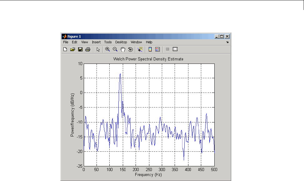
Spectral Analysis

In the periodogram above, noise and the leakage make one of the sinusoids

essentially indistinguishable from the artificial peaks. In contrast, although

the PSD produced by Welch’s method has wider peaks, you can still

distinguish the two sinusoids, which stand out from the “noise floor.”

However, if we try to reduce the variance further, the loss of resolution causes

one of the sinusoids to be lost altogether:

6-23

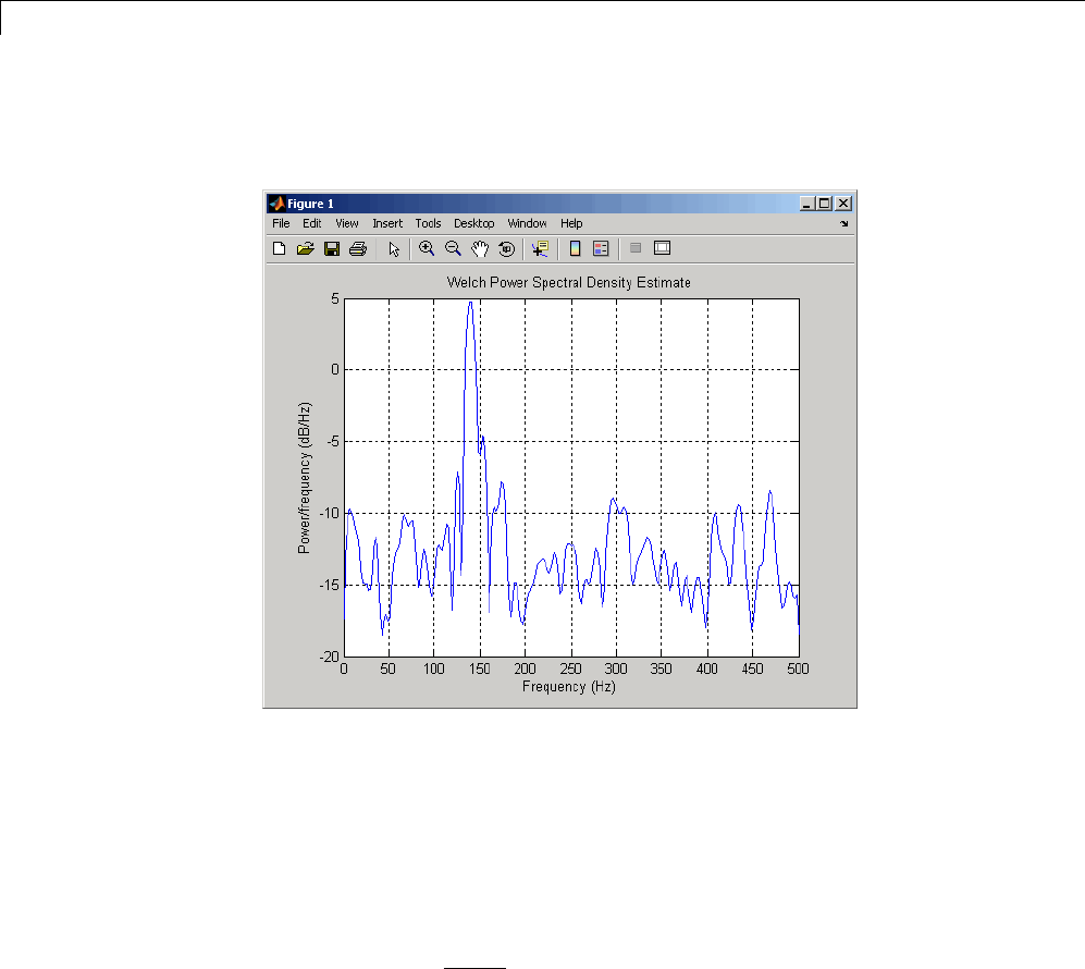
6Statistical Signal Processing

Hs = spectrum.welch('rectangular',100,75);

psd(Hs,xn,'Fs',fs,'NFFT',512);

For a more detailed discussion of Welch’s method of PSD estimation, see

Kay [2] and Welch [8].

Bias and Normalization in Welch’s Method

Welch’s method yields a biased estimator of the PSD. The expected value of

the PSDestimateis:

EP f FsLU Wf f P f df

{()} |()|()

Welch =−

′′′

−

∫

where Lis the length of the data segments, Uisthesamenormalization

constant present in the definition of the modified periodogram, and W(f) is the

Fourier transform of the window function. As is the case for all periodograms,

Welch’s estimator is asymptotically unbiased. For a fixed length data record,

6-24

Spectral Analysis

the bias of Welch’s estimate is larger than that of the periodogram because

the length of the segments is less than the length of the entire data sample.

The variance of Welch’s estimator is difficult to compute because it depends

on both the window used and the amount of overlap between segments.

Basically,thevarianceisinverselyproportional to the number of segments

whose modified periodograms are being averaged.

Multitaper Method

The periodogram can be interpreted as filtering a length Lsignal, xL[n],

through a filter bank (a set of filters in parallel) of LFIR bandpass filters.

The 3 dB bandwidth of each of these bandpass filters can be shown to be

approximately equal to fs/L. The magnitude response of each one of these

bandpass filters resembles that of the rectangular window discussed in

“Spectral Leakage” on page 6-12. The periodogram can thus be viewed as

a computation of the power of each filtered signal (i.e., the output of each

bandpass filter) that uses just one sample of each filtered signal and assumes

that the PSD of xL[n] is constant over the bandwidth of each bandpass filter.

As the length of the signal increases, the bandwidth of each bandpass filter

decreases, making it a more selective filter, and improving the approximation

of constant PSD over the bandwidth of the filter. This provides another

interpretation of why the PSD estimate of the periodogram improves as the

length of the signal increases. However, there are two factors apparent from

this standpoint that compromise the accuracy of the periodogram estimate.

First, the rectangular window yields a poor bandpass filter. Second, the

computation of the power at the output of each bandpass filter relies on a

single sample of the output signal, producing a very crude approximation.

Welch’s method can be given a similar interpretation in terms of a filter bank.

In Welch’s implementation, several samples are used to compute the output

power, resulting in reduced variance of the estimate. On the other hand,

the bandwidth of each bandpass filter is larger than that corresponding to

the periodogram method, which results in a loss of resolution. The filter

bank model thus provides a new interpretation of the compromise between

variance and resolution.

Thompson’s multitaper method (MTM)buildsontheseresultstoprovidean

improved PSD estimate. Instead of using bandpass filters that are essentially

6-25

6Statistical Signal Processing

rectangular windows (as in the periodogram method), the MTM method uses

a bank of optimal bandpass filters to compute the estimate. These optimal

FIR filters are derived from a set of sequences known as discrete prolate

spheroidal sequences (DPSSs, also known as Slepian sequences).

In addition, the MTM method provides a time-bandwidth parameter with

which to balance the variance and resolution. This parameter is given by the

time-bandwidth product, NW and it is directly related to the number of tapers

used to compute the spectrum. There are always 2*NW-1 tapers used to form

the estimate. This means that, as NW increases, there are more estimates of

the power spectrum, and the variance of the estimate decreases. However, the

bandwidth of each taper is also proportional to NW,soasNW increases, each

estimate exhibits more spectral leakage (i.e., wider peaks) and the overall

spectral estimate is more biased. For each data set, there is usually a value

for NW that allows an optimal trade-off between bias and variance.

The Signal Processing Toolbox function that implements the MTM method is

pmtm and the object that implements it is spectrum.mtm.Use spectrum.mtm

to compute the PSD of xn from the previous examples:

fs = 1000; % Sampling frequency

t = (0:fs)/fs; % One second worth of samples

A = [1 2]; % Sinusoid amplitudes

f = [150;140]; % Sinusoid frequencies

xn = A*sin(2*pi*f*t) + 0.1*randn(size(t));

Hs1 = spectrum.mtm(4,'adapt');

psd(Hs1,xn,'Fs',fs,'NFFT',1024)

6-26

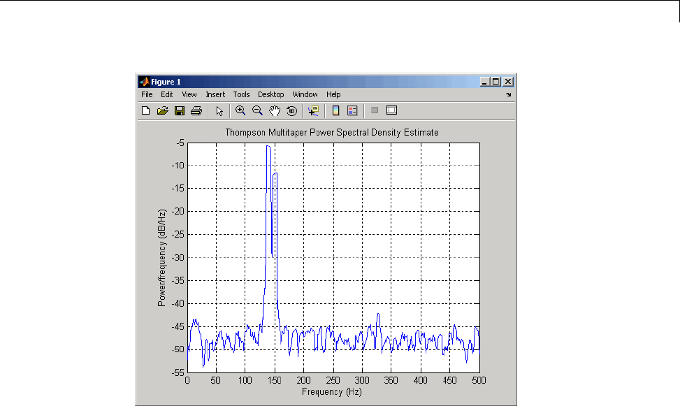
Spectral Analysis

By lowering the time-bandwidth product, you can increase the resolution at

the expense of larger variance:

6-27

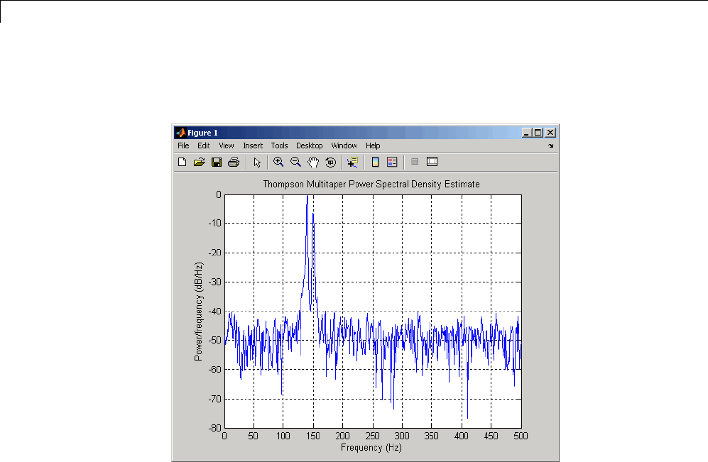
6Statistical Signal Processing

Hs2 = spectrum.mtm(3/2,'adapt');

psd(Hs2,xn,'Fs',fs,'NFFT',1024)

Note that the average power is conserved in both cases:

Hs1p = psd(Hs1,xn,'Fs',fs,'NFFT',1024);

Pow1 = avgpower(Hs1p)

Hs2p = psd(Hs2,xn,'Fs',fs,'NFFT',1024);

Pow2 = avgpower(Hs2p)

This method is more computationally expensive than Welch’s method due to

the cost of computing the discrete prolate spheroidal sequences. For long data

series (10,000 points or more), it is useful to compute the DPSSs once and

save them in a MAT-file. dpsssave,dpssload,dpssdir,anddpssclear are

provided to keep a database of saved DPSSs in the MAT-file dpss.mat.

6-28

Spectral Analysis

Cross-Spectral Density Function

The PSD is a special case of the cross spectral density (CPSD) function,

defined between two signals xnand ynas

PRme

xy xy jm

() ( )ωπ

=−

=−∞

∞

∑

Asisthecaseforthecorrelationandcovariancesequences,thetoolbox

estimates the PSD and CPSD because signal lengths are finite.

To estimate the cross-spectral density of two equal length signals xand y

using Welch’s method, the cpsd function forms the periodogram as the product

of the FFT of xand the conjugate of the FFT of y. Unlike the real-valued PSD,

the CPSD is a complex function. cpsd handles the sectioning and windowing

of xand yin the same way as the pwelch function:

Sxy = cpsd(x,y,nwin,noverlap,nfft,fs)

Transfer Function Estimate

One application of Welch’s method is nonparametric system identification.

Assume that His a linear, time invariant system, and x(n)andy(n)arethe

input to and output of H, respectively. Then the power spectrum of x(n)is

related to the CPSD of x(n)andy(n)by

PHP

yx xx

() () ()ωωω=

An estimate of the transfer function between x(n)andy(n)is



() ()

()

ωω

This method estimates both magnitude and phase information. The

tfestimate function uses Welch’s method to compute the CPSD and power

spectrum, and then forms their quotient for the transfer function estimate.

Use tfestimate the same way that you use the cpsd function.

6-29

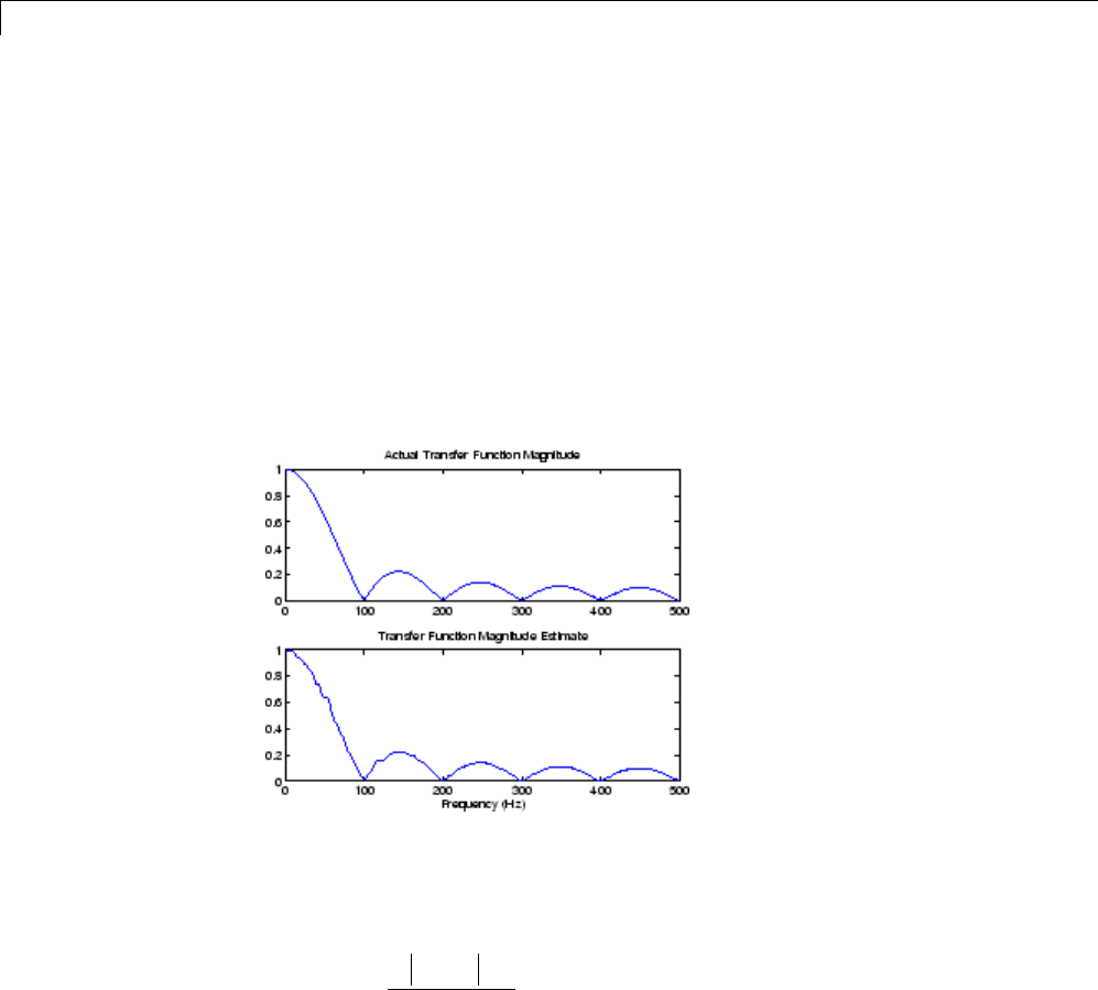
6Statistical Signal Processing

Filter the signal xn with an FIR filter, then plot the actual magnitude

response and the estimated response:

h = ones(1,10)/10; % Moving-average filter

yn = filter(h,1,xn);

[HEST,f] = tfestimate(xn,yn,256,128,256,fs);

H = freqz(h,1,f,fs);

subplot(2,1,1); plot(f,abs(H));

title('Actual Transfer Function Magnitude');

subplot(2,1,2); plot(f,abs(HEST));

title('Transfer Function Magnitude Estimate');

xlabel('Frequency (Hz)');

Coherence Function

The magnitude-squared coherence between two signals x(n)andy(n)is

xx yy

() ()

ωω

This quotient is a real number between 0 and 1 that measures the correlation

between x(n)andy(n) at the frequency ω.

6-30

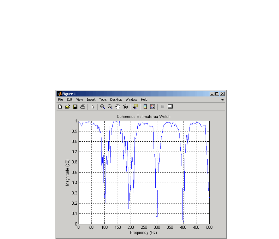
Spectral Analysis

The mscohere function takes sequences xand y, computes their power spectra

and CPSD, and returns the quotient of the magnitude squared of the CPSD

and the product of the power spectra. Its options and operation are similar to

the cpsd and tfestimate functions.

The coherence function of xn and the filter output yn versus frequency is

mscohere(xn,yn,256,128,256,fs)

If the input sequence length nfft,windowlengthwindow, and the number of

overlapping data points in a window numoverlap, are such that mscohere

operates on only a single record, the function returns all ones. This is because

the coherence function for linearly dependent data is one.

6-31

6Statistical Signal Processing

Parametric Methods

Parametric methods can yield higher resolutions than nonparametric methods

in cases when the signal length is short. These methods use a different

approach to spectral estimation; instead of trying to estimate the PSD directly

from the data, they model the data as the output of a linear system driven

by white noise, and then attempt to estimate the parameters of that linear

system.

The most commonly used linear system model is the all-pole model,afilter

with all of its zeroes at the origin in the z-plane. The output of such a filter for

white noise input is an autoregressive (AR) process. For this reason, these

methods are sometimes referred to as AR methods of spectral estimation.

The AR methods tend to adequately describe spectra of data that is “peaky,”

that is, data whose PSD is large at certain frequencies. The data in many

practical applications (such as speech) tends to have “peaky spectra” so that

AR models are often useful. In addition, the AR models lead to a system of

linear equations which is relatively simple to solve.

Signal Processing Toolbox AR methods for spectral estimation include:

•Yule-Walker AR method (autocorrelation method)

•Burg method

•Covariance method

•Modified covariance method

All AR methods yield a PSD estimate given by

ˆ()

|ˆ() |

Pf Fs ake

pjkfFs

−

∑



The different AR methods estimate the parameters slightly differently,

yielding different PSD estimates. The following table provides a summary

of the different AR methods.

6-32

Spectral Analysis

AR Methods

Burg Covariance

Modified

Covariance Yule-Walker

Does not apply

window to data

Does not apply

window to data

Does not apply

window to data

Applies window

to data

Characteristics

Minimizes

the forward

and backward

prediction errors

in the least

squares sense,

with the AR

coefficients

constrained to

satisfy the L-D

recursion

Minimizes

the forward

prediction error

in the least

squares sense

Minimizes

the forward

and backward

prediction errors

in the least

squares sense

Minimizes

the forward

prediction error

in the least

squares sense

(also called

“Autocorrelation

method”)

High resolution

for short data

records

Better resolution

than Y-W

for short

data records

(more accurate

estimates)

High resolution

for short data

records

Performs as well

as other methods

for large data

records

Able to extract

frequencies from

data consisting

of p or more pure

sinusoids

Advantages

Always produces

a stable model

Able to extract

frequencies from

data consisting

of p or more pure

sinusoids

Does not

suffer spectral

line-splitting

Always produces

a stable model

6-33

6Statistical Signal Processing

AR Methods (Continued)

Burg Covariance

Modified

Covariance Yule-Walker

Peak locations

highly dependent

on initial phase

May produce

unstable models

May produce

unstable models

Performs

relatively poorly

for short data

records

May suffer

spectral

line-splitting

for sinusoids in

noise, or when

order is very

large

Peak locations

slightly

dependent on

initial phase

Frequency bias

for estimates of

sinusoids in noise

Disadvantages

Frequency bias

for estimates of

sinusoids in noise

Frequency bias

for estimates of

sinusoids in noise

Minor frequency

bias for estimates

of sinusoids in

noise

Conditions for

Nonsingularity

Order must be

less than or equal

to half the input

frame size

Order must be

less than or equal

to 2/3 the input

frame size

Because of

the biased

estimate, the

autocorrelation

matrix is

guaranteed to

positive-definite,

hence

nonsingular

Yule-Walker AR Method

The Yule-Walker AR method of spectral estimation computes the AR

parameters by solving the following linear system, which give the Yule-Walker

equations in matrix form:

6-34

Spectral Analysis

rr rp

rp rp r

() () ( )

()() ()

01 1

10 2

12 0

…−

−−…

⎛

⎝

⎜

⎞

⎠

⎟⎟

⎟

⎟…

⎛

⎝

⎜

⎞

⎠

⎟

=…

⎛

⎝

⎜

⎞

⎠

⎟

()

In practice, the biased estimate of the autocorrelation is used for the unknown

true autocorrelation.The Yule-Walker AR method produces the same results

as a maximum entropy estimator. For more information, see page 155 of item

[2] in the “Selected Bibliography” on page 6-46.

The use of a biased estimate of the autocorrelation function ensures that

the autocorrelation matrix above is positive definite. Hence, the matrix is

invertible and a solution is guaranteed to exist. Moreover, the AR parameters

thus computed always result in a stable all-pole model. The Yule-Walker

equations can be solved efficiently via Levinson’s algorithm, which takes

advantage of the Hermitian Toeplitz structure of the autocorrelation matrix.

The toolbox object spectrum.yulear and function pyulear implement the

Yule-Walker AR method.

For example, compare the spectrum of a speech signal using Welch’s method

and the Yule-Walker AR method:

load mtlb

Hwelch = spectrum.welch('hamming',256,50);

psd(Hwelch,mtlb,'Fs',Fs,'NFFT',1024)

6-35

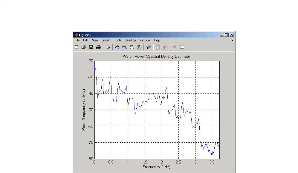
6Statistical Signal Processing

6-36

Spectral Analysis

Hyulear = spectrum.yulear(14);

psd(Hyulear,mtlb,'Fs',Fs,'NFFT',1024)

The Yule-Walker AR spectrum is smoother than the periodogram because of

the simple underlying all-pole model.

Burg Method

The Burg method for AR spectral estimation is based on minimizing the

forward and backward prediction errors while satisfying the Levinson-Durbin

recursion (see Marple [3], Chapter 7, and Proakis [6], Section 12.3.3). In

contrast to other AR estimation methods, the Burg method avoids calculating

the autocorrelation function, and instead estimates the reflection coefficients

directly.

The primary advantages of the Burg method are resolving closely spaced

sinusoids in signals with low noise levels, and estimating short data records,

in which case the AR power spectral density estimates are very close to the

6-37

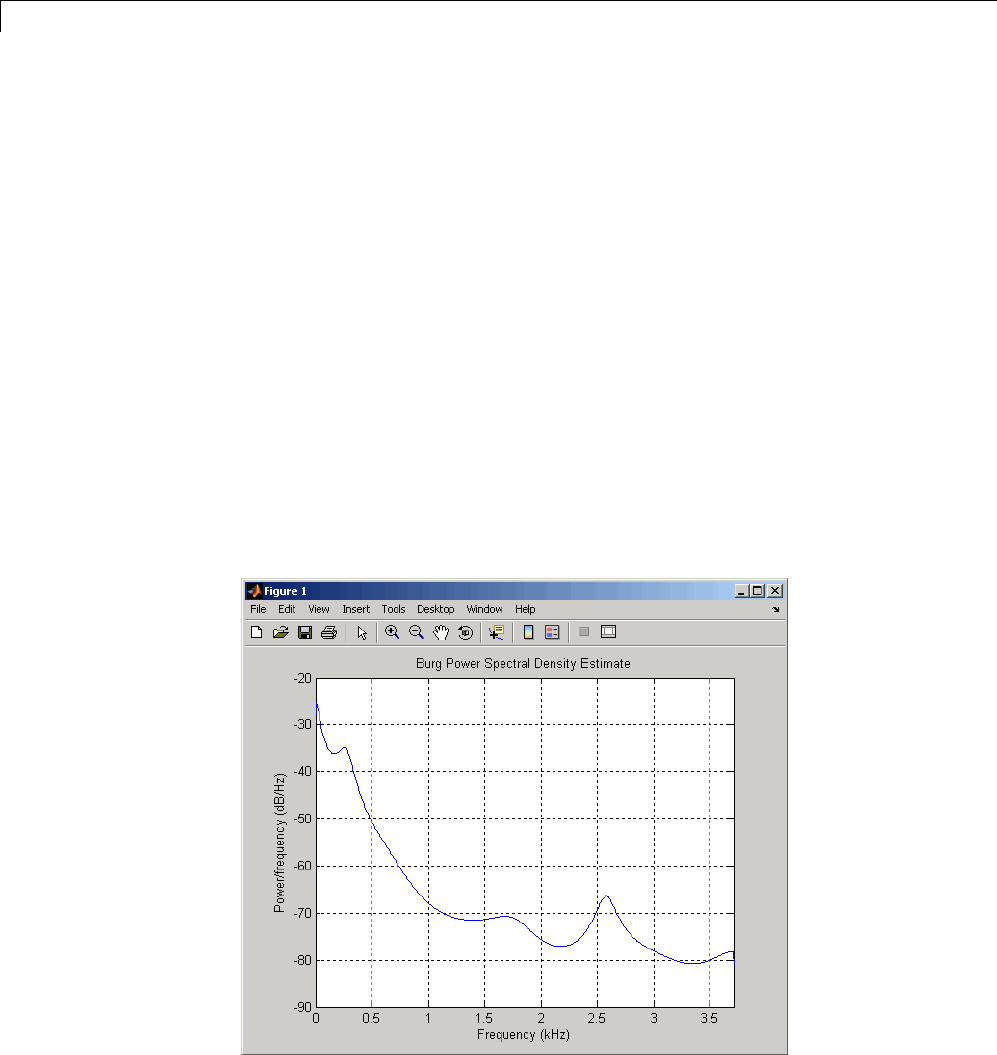
6Statistical Signal Processing

true values. In addition, the Burg method ensures a stable AR model and

is computationally efficient.

The accuracy of the Burg method is lower for high-order models, long data

records, and high signal-to-noise ratios (which can cause line splitting,

or the generation of extraneous peaks in the spectrum estimate). The

spectral density estimate computed by the Burg method is also susceptible

to frequency shifts (relative to the true frequency) resulting from the initial

phase of noisy sinusoidal signals. This effect is magnified when analyzing

short data sequences.

The toolbox object spectrum.burg and function pburg implement the Burg

method. Compare the spectrum of the speech signal generated by both the

Burg method and the Yule-Walker AR method. They are very similar for

large signal lengths:

load mtlb

Hburg = spectrum.burg(14); % 14th order model

psd(Hburg,mtlb(1:512),'Fs',Fs,'NFFT',1024)

6-38

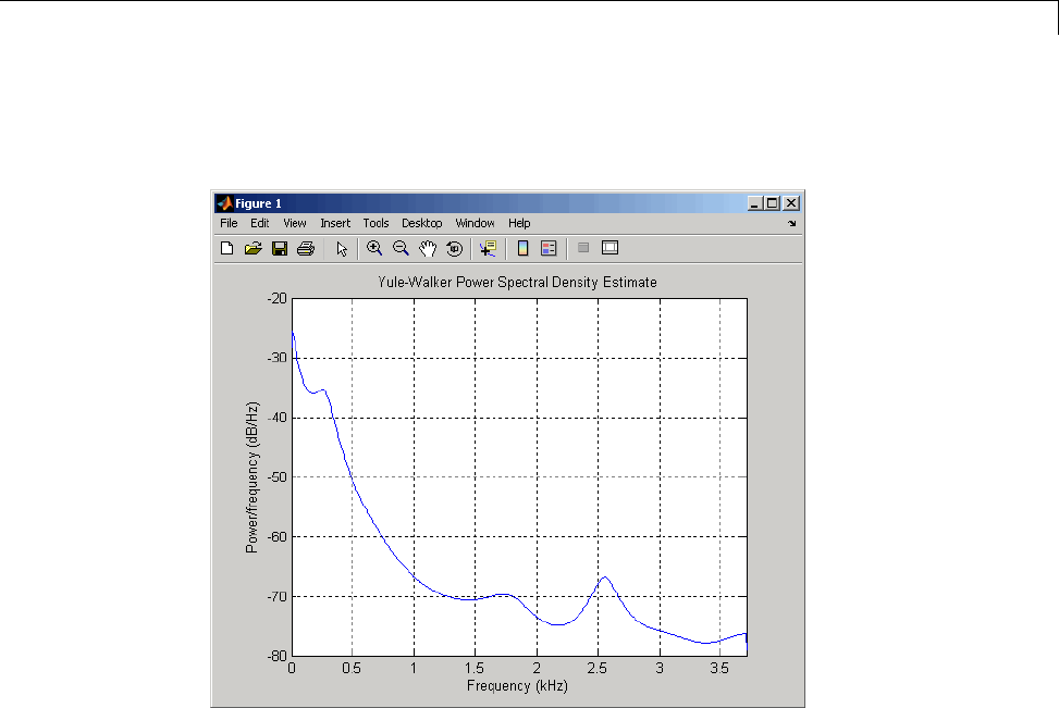
Spectral Analysis

Hyulear = spectrum.yulear(14); % 14th order model

psd(Hyulear,mtlb(1:512),'Fs',Fs,'NFFT',1024)

Compare the spectrum of a noisy signal computed using the Burg method

and the Welch method:

fs = 1000; % Sampling frequency

t = (0:fs)/fs; % One second worth of samples

A = [1 2]; % Sinusoid amplitudes

f = [150;140]; % Sinusoid frequencies

xn = A*sin(2*pi*f*t) + 0.1*randn(size(t));

Hwelch = spectrum.welch('hamming',256,50);

psd(Hwelch,xn,'Fs',fs,'NFFT',1024)

6-39

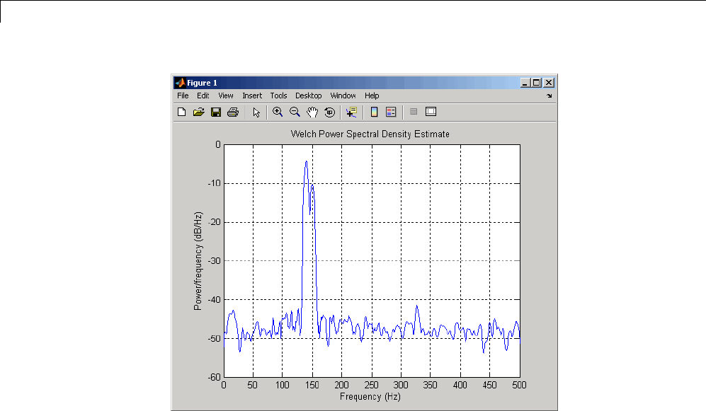
6Statistical Signal Processing

6-40

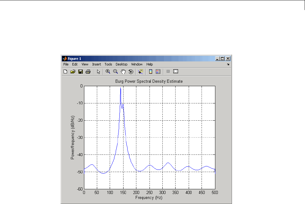
Spectral Analysis

Hburg = spectrum.burg(14);

psd(Hburg,xn,'Fs',fs,'NFFT',1024)

Note that, as the model order for the Burg method is reduced, a frequency

shift due to the initial phase of the sinusoids will become apparent.

Covariance and Modified Covariance Methods

The covariance method for AR spectral estimation is based on minimizing

the forward prediction error. The modified covariance method is based on

minimizing the forward and backward prediction errors. The toolbox object

spectrum.cov and function pcov, and object spectrum.mcov and function

pmcovimplement the respective methods.

Compare the spectrum of the speech signal generated by both the covariance

method and the modified covariance method. They are nearly identical, even

for a short signal length:

6-41

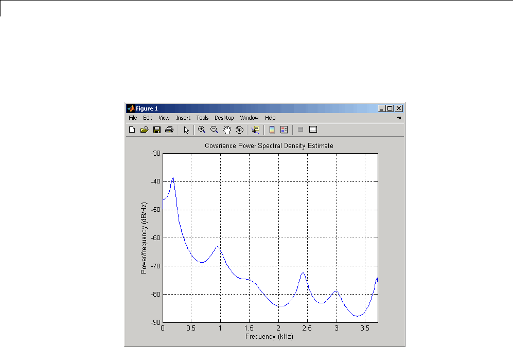
6Statistical Signal Processing

load mtlb

Hcov = spectrum.cov(14); % 14th order model

psd(Hcov,mtlb(1:64),'Fs',Fs,'NFFT',1024)

Hmcov = spectrum.mcov(14); % 14th order model

psd(Hmcov,mtlb(1:64),'Fs',Fs,'NFFT',1024)

6-42

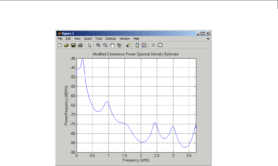
Spectral Analysis

MUSIC and Eigenvector Analysis Methods

The spectrum.music object and pmusic function, and spectrum.eigenvector

object and peig function provide two related spectral analysis methods:

•spectrum.music and pmusic provide the multiple signal classification

(MUSIC) method developed by Schmidt

•spectrum.eigenvector and peig provides the eigenvector (EV) method

developed by Johnson

See Marple [3] (pgs. 373-378) for a summary of these methods.

Both of these methods are frequency estimator techniques based on

eigenanalysis of the autocorrelation matrix. This type of spectral analysis

categorizes the information in a correlation or data matrix, assigning

information to either a signal subspace or a noise subspace.

6-43

6Statistical Signal Processing

Eigenanalysis Overview

Consider a number of complex sinusoids embedded in white noise. You can

write the autocorrelation matrix Rfor this system as the sum of the signal

autocorrelation matrix (S) and the noise autocorrelation matrix (W):

R = S + W. There is a close relationship between the eigenvectors of the signal

autocorrelation matrix and the signal and noise subspaces. The eigenvectors

vof Sspan the same signal subspace as the signal vectors. If the system

contains Mcomplex sinusoids and the order of the autocorrelation matrix is p,

eigenvectors vM+1 through vp+1 span the noise subspace of the autocorrelation

matrix.

Frequency Estimator Functions. To generate their frequency estimates,

eigenanalysis methods calculate functions of the vectors in the signal and

noise subspaces. Both the MUSIC and EV techniques choose a function that

goes to infinity (denominator goes to zero) at one of the sinusoidal frequencies

in the input signal. Using digital technology, the resulting estimate has sharp

peaks at the frequencies of interest; this means that there might not be

infinity values in the vectors.

The MUSIC estimate is given by the formula

|( ) |

()P

ef v

MHk

MUSIC =

∑

wherethev_karetheeigenvectorsofthenoisesubspaceande(f)isavector

of complex sinusoids.

ef e e e

jf jf jM T

() [ ]

()

=…

−

12421

 

vrepresents the eigenvectors of the input signal’s correlation matrix; vkis

the kth eigenvector. His the conjugate transpose operator. The eigenvectors

used in the sum correspond to the smallest eigenvalues and span the noise

subspace (pis the size of the signal subspace).

The expression e(f)Hvkis equivalent to a Fourier transform (the vector

e(f) consists of complex exponentials). This form is useful for numeric

6-44

Spectral Analysis

computation because the FFT can be computed for each vkand then the

squared magnitudes can be summed.

The EV method weights the summation by the eigenvalues of the correlation

matrix:

|()|

()P

efv

MHk

EV =

∑

The pmusic and peig functions in this toolbox interpret their first input

either as a signal matrix or as a correlation matrix (if the 'corr' input flag is

set). In the former case, the singular value decomposition of the signal matrix

is used to determine the signal and noise subspaces. In the latter case, the

eigenvalue decomposition of the correlation matrix is used to determine the

signal and noise subspaces.

6-45

6Statistical Signal Processing

Selected Bibliography

[1] Hayes, M.H. Statistical Digital Signal Processing and Modeling.New

York: John Wiley & Sons, 1996.

[2] Kay, S.M. Modern Spectral Estimation. Englewood Cliffs, NJ: Prentice

Hall, 1988.

[3] Marple, S.L. Digital Spectral Analysis. Englewood Cliffs, NJ: Prentice

Hall, 1987.

[4] Orfanidis, S.J. Introduction to Signal Processing. Upper Saddle River, NJ:

Prentice Hall, 1996.

[5] Percival, D.B., and A.T. Walden. Spectral Analysis for Physical

Applications: Multitaper and Conventional Univariate Techniques.

Cambridge: Cambridge University Press, 1993.

[6] Proakis, J.G., and D.G. Manolakis. Digital Signal Processing: Principles,

Algorithms, and Applications. Englewood Cliffs, NJ: Prentice Hall, 1996.

[7] Stoica, P., and R. Moses. Introduction to Spectral Analysis. Upper Saddle

River, NJ: Prentice Hall, 1997.

[8] Welch, P.D. “The Use of Fast Fourier Transform for the Estimation of

Power Spectra: A Method Based on Time Averaging Over Short, Modified

Periodograms.” IEEE Trans. Audio Electroacoust.Vol.AU-15(June1967).

Pgs. 70-73.

6-46

Special Topics

•“Windows” on page 7-2

•“Parametric Modeling” on page 7-13

•“Resampling” on page 7-21

•“Cepstrum Analysis” on page 7-24

•“FFT-Based Time-Frequency Analysis” on page 7-28

•“Median Filtering” on page 7-29

•“Communications Applications” on page 7-30

•“Deconvolution” on page 7-35

•“Specialized Transforms” on page 7-36

•“Selected Bibliography” on page 7-47

7Special Topics

Windows

In this section...

“Why Use Windows?” on page 7-2

“Available Window Functions” on page 7-2

“Graphical User Interface Tools” on page 7-3

“Basic Shapes” on page 7-3

“Generalized Cosine Windows” on page 7-6

“Kaiser Window” on page 7-8

“Chebyshev Window” on page 7-12

Why Use Windows?

In both digital filter design and spectral estimation, the choice of a windowing

function can play an important role in determining the quality of overall

results. The main role of the window is to damp out the effects of the Gibbs

phenomenon that results from truncation of an infinite series.

Available Window Functions

Window Function

Bartlett-Hann window barthannwin

Bartlett window bartlett

Blackman window blackman

Blackman-Harris window blackmanharris

Bohman window bohmanwin

Chebyshev window chebwin

Flat Top window flattopwin

Gaussian window gausswin

Hamming window hamming

7-2

Windows

Window Function

Hann window hann

Kaiser window kaiser

Nuttall’s Blackman-Harris window nuttallwin

Parzen (de la Valle-Poussin) window parzenwin

Rectangular window rectwin

Tapered cosine window tukeywin

Triangular window triang

Graphical User Interface Tools

Two graphical user interface tools are provided for working with windows in

the Signal Processing Toolbox product:

•Window Design and Analysis Tool (wintool)

•Window Visualization Tool (wvtool)

Refer to the reference pages for these tools for detailed information.

Basic Shapes

The basic window is the rectangular window, a vector of ones of the

appropriate length. A rectangular window of length 50 is

n = 50;

w = rectwin(n);

This toolbox stores windows in column vectors by convention, so an equivalent

expression is

w = ones(50,1);

To use the Window Design and Analysis Tool to create this window, type

wintool

7-3

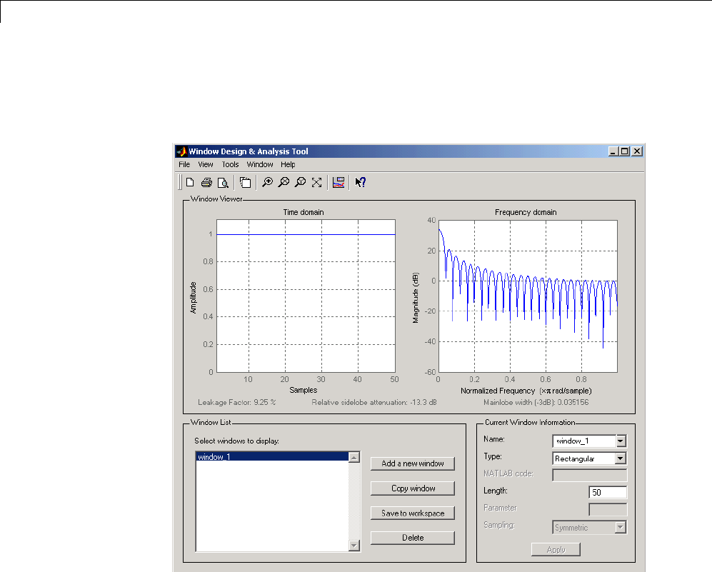
7Special Topics

wintool opens with a default Hamming window. In the Current Window

Information panel, set Type = Rectangular and Length = 50 and then

press Apply.

The Bartlett (or triangular) window is the convolution of two rectangular

windows. The functions bartlett and triang compute similar triangular

windows, with three important differences. The bartlett function always

returns a window with two zeros on the ends of the sequence, so that for n

odd, the center section of bartlett(n+2) is equivalent to triang(n):

Bartlett = bartlett(7);

isequal(Bartlett(2:end-1),triang(5))

% Returns a 1

7-4

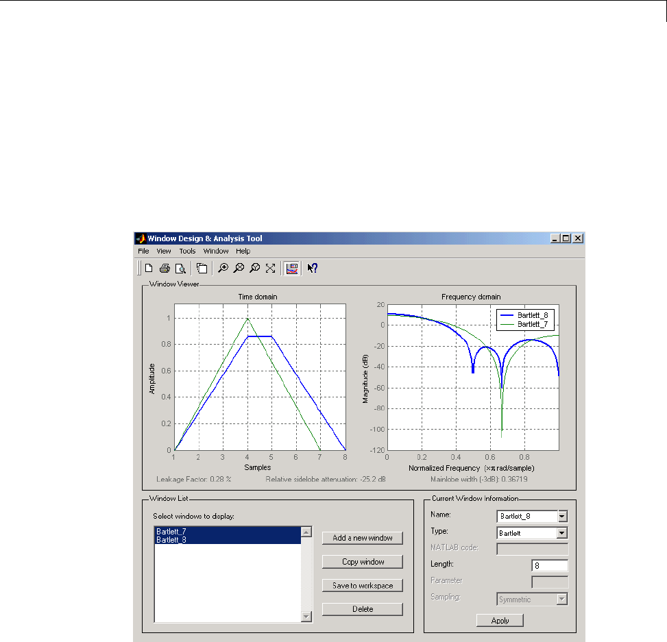
Windows

For neven, bartlett is still the convolution of two rectangular sequences.

There is no standard definition for the triangular window for neven; the

slopes of the line segments of the triang result are slightly steeper than

those of bartlett in this case:

w = bartlett(8);

[w(2:7) triang(6)]

You can see the difference between odd and even Bartlett windows in WinTool.

The final difference between the Bartlett and triangular windows is evident in

the Fourier transforms of these functions. The Fourier transform of a Bartlett

window is negative for neven. The Fourier transform of a triangular window,

however, is always nonnegative.

7-5

7Special Topics

The following figure, which is a zoomed version of the Frequency domain plot

of 8-point Bartlett and Triangular windows with the y-axis set to Zerophase,

illustrates this difference.

This difference can be important when choosing a window for some

spectral estimation techniques, such as the Blackman-Tukey method.

Blackman-Tukey forms the spectral estimate by calculating the Fourier

transform of the autocorrelation sequence. The resulting estimate might be

negative at some frequencies if the window’s Fourier transform is negative

(see Kay [1], pg. 80).

Generalized Cosine Windows

Blackman, flat top, Hamming, Hann, and rectangular windows are all special

cases of the generalized cosine window. These windows are combinations of

sinusoidal sequences with frequencies that are multiples of ,where

Nis the window length. One special case is the Blackman window:

N = 128;

A = 0.42; B = 0.5; C = 0.08;

ind = (0:N-1)'*2*pi/(N-1);

w = A - B*cos(ind) + C*cos(2*ind);

Changing the values of the constants A,B,andCin the previous expression

generates different generalized cosine windows like the Hamming and Hann

7-6

Windows

windows. Adding additional cosine terms of higher frequency generates the

flat top window. The concept behind these windows is that by summing

the individual terms to form the window, the low frequency peaks in the

frequency domain combine in such a way as to decrease sidelobe height. This

has the side effect of increasing the mainlobe width.

The Hamming and Hann windows are two-term generalized cosine windows,

given by A=0.54,B=0.46 for the Hamming and A=0.5,B=0.5 for the Hann.

Note that the definition of the generalized cosine window shown in the earlier

MATLAB code yields zeros at samples 1 and nfor A=0.5 and B=0.5.

This WinTool compares Blackman, Hamming, Hann, and Flat Top windows.

7-7

7Special Topics

Kaiser Window

The Kaiser windowis an approximation to the prolate-spheroidal window, for

which the ratio of the mainlobe energy to the sidelobe energy is maximized.

For a Kaiser window of a particular length, the parameter βcontrols the

sidelobe height. For a given β, the sidelobe height is fixed with respect to

window length.Thestatementkaiser(n,beta) computes a length nKaiser

window with parameter beta.

Examples of Kaiser windows with length 50 and beta parameters of 1, 4, and

9areshowninthis wintool example.

To create these Kaiser windows using the MATLAB command line,

n=50;

7-8

Windows

w1 = kaiser(n,1);

w2 = kaiser(n,4);

w3 = kaiser(n,9);

[W1,f] = freqz(w1/sum(w1),1,512,2);

[W2,f] = freqz(w2/sum(w2),1,512,2);

[W3,f] = freqz(w3/sum(w3),1,512,2);

plot(f,20*log10(abs([W1 W2 W3]))); grid;

legend('beta = 1','beta = 4','beta = 9',3)

As βincreases, the sidelobe height decreases and the mainlobe width

increases. This wintool shows how the sidelobeheightstaysthesamefora

fixed βparameter as the length is varied.

To create these Kaiser windows using the MATLAB command line:

7-9

7Special Topics

w1 = kaiser(50,4);

w2 = kaiser(20,4);

w3 = kaiser(101,4);

[W1,f] = freqz(w1/sum(w1),1,512,2);

[W2,f] = freqz(w2/sum(w2),1,512,2);

[W3,f] = freqz(w3/sum(w3),1,512,2);

plot(f,20*log10(abs([W1 W2 W3]))); grid;

legend('length = 50','length = 20','length = 101')

Kaiser Windows in FIR Design

TherearetwodesignformulasthatcanhelpyoudesignFIRfilterstomeet

a set of filter specifications using a Kaiser window. To achieve a sidelobe

height of -αdB, the beta parameter is

For a transition width of Δω rad/s, use the length

Filters designed using these heuristics will meet the specifications

approximately, but you should verify this. To design a lowpass filter with

cutoff frequency 0.5πrad/s, transition width 0.2πrad/s, and 40 dB of

attenuation in the stopband, try

[n,wn,beta] = kaiserord([0.4 0.6]*pi,[1 0],[0.01 0.01],2*pi);

h = fir1(n,wn,kaiser(n+1,beta),'noscale');

The kaiserord function estimates the filter order, cutoff frequency, and

Kaiser window beta parameter needed to meet a given set of frequency

domain specifications.

7-10

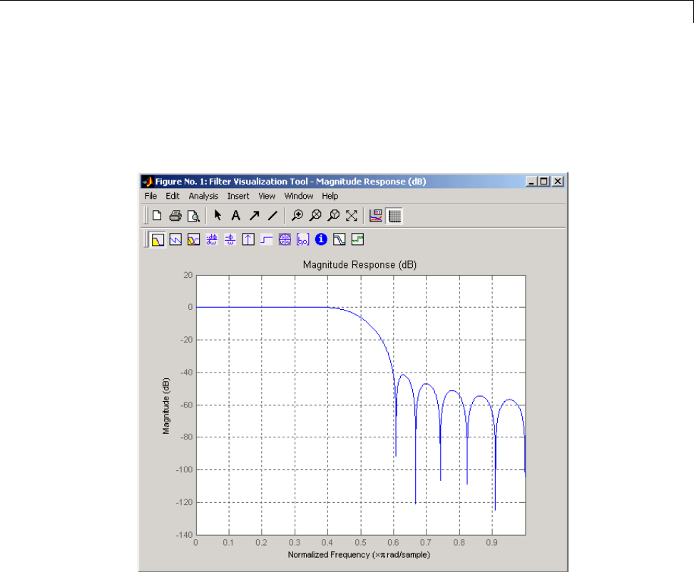
Windows

Therippleinthepassbandisroughlythesameastherippleinthestopband.

As you can see from the frequency response, this filter nearly meets the

specifications:

fvtool(h,1);

7-11

7Special Topics

Chebyshev Window

The Chebyshev window minimizes the mainlobe width, given a particular

sidelobe height. It is characterized by an equiripple behavior, that is, its

sidelobes all have the same height.

As shown in the Time Domain plot, the Chebyshev window has large spikes

at its outer samples.

For a detailed discussion of the characteristics and applications of the various

window types, see Oppenheim and Schafer [3], pgs. 444-462, and Parks and

Burrus [4], pgs. 71-73.

7-12

Parametric Modeling

In this section...

“What is Parametric Modeling” on page 7-13

“Available Parametric Modeling Functions” on page 7-13

“Time-Domain Based Modeling” on page 7-14

“Frequency-Domain Based Modeling” on page 7-18

What is Parametric Modeling

Parametric modeling techniques find the parameters for a mathematical

model describing a signal, system, or process. These techniques use known

information about the system to determine the model. Applications for

parametric modeling include speech and music synthesis, data compression,

high-resolution spectral estimation, communications, manufacturing, and

simulation.

Available Parametric Modeling Functions

The toolbox parametric modeling functions operate with the rational transfer

function model. Given appropriate information about an unknown system

(impulse or frequency response data, or input and output sequences), these

functions find the coefficients of a linear system that models the system.

One important application of the parametric modeling functions is in the

design of filters that have a prescribed time or frequency response.

Here is a summary of the parametric modeling functions in this toolbox.

7-13

7Special Topics

Domain Functions Description

arburg Generate all-pole filter coefficients that

model an input data sequence using the

Levinson-Durbin algorithm.

arcov Generate all-pole filter coefficients

that model an input data sequence by

minimizing the forward prediction error.

armcov Generate all-pole filter coefficients

that model an input data sequence by

minimizing the forward and backward

prediction errors.

aryule Generate all-pole filter coefficients that

model an input data sequence using an

estimate of the autocorrelation function.

lpc,levinson Linear Predictive Coding. Generate

all-pole recursive filter whose impulse

response matches a given sequence.

prony Generate IIR filter whose impulse

response matches a given sequence.

Time

stmcb Find IIR filter whose output, given a

specified input sequence, matches a given

output sequence.

Frequency invfreqz,

invfreqs

Generate digital or analog filter

coefficients given complex frequency

response data.

Time-Domain Based Modeling

The lpc,prony,andstmcb functions find the coefficients of a digital rational

transfer function that approximates a given time-domain impulse response.

The algorithms differ in complexity and accuracy of the resulting model.

Linear Prediction

Linear prediction modeling assumes that each output sample of a signal,

x(k), is a linear combination of the past noutputs (that is, it can be linearly

7-14

Parametric Modeling

predicted from these outputs), and that the coefficients are constant from

sample to sample:

An nth-order all-pole model of a signal xis

a = lpc(x,n)

To illustrate lpc, create a sample signal that is the impulse response of an

all-pole filter with additive white noise:

x = impz(1,[1 0.1 0.1 0.1 0.1],10) + randn(10,1)/10;

The coefficients for a fourth-order all-pole filter that models the system are

a = lpc(x,4)

lpc first calls xcorr to find a biased estimate of the correlation function of x,

and then uses the Levinson-Durbin recursion, implemented in the levinson

function, to find the model coefficients a. The Levinson-Durbin recursion is a

fast algorithm for solving a system of symmetric Toeplitz linear equations.

lpc’s entire algorithm for n=4is

r = xcorr(x);

r(1:length(x)-1) = []; % Remove corr. at negative lags

a = levinson(r,4)

You could form the linear prediction coefficients with other assumptions by

passing a different correlation estimate to levinson, such as the biased

correlation estimate:

r = xcorr(x,'biased');

r(1:length(x)-1) = []; % Remove corr. at negative lags

a = levinson(r,4)

7-15

7Special Topics

Prony’s Method (ARMA Modeling)

The prony function models a signal using a specified number of poles and

zeros. Given a sequence xand numerator and denominator orders nand m,

respectively, the statement

[b,a] = prony(x,n,m)

finds the numerator and denominator coefficients of an IIR filter whose

impulse response approximates the sequence x.

The prony function implements the method described in [4] Parks and Burrus

(pgs. 226-228). This method uses a variation of the covariance method of AR

modeling to find the denominator coefficients a, and then finds the numerator

coefficients bfor which the resulting filter’s impulse response matches exactly

the first n+1samples of x. The filter is not necessarily stable, but it can

potentially recover the coefficients exactly if the data sequence is truly an

autoregressive moving-average (ARMA) process of the correct order.

Note The functions prony and stmcb (described next) are more accurately

described as ARX models in system identification terminology. ARMA

modeling assumes noise only at the inputs, while ARX assumes an external

input. prony and stmcb know the input signal: it is an impulse for prony

and is arbitrary for stmcb.

A model for the test sequence x(from the earlier lpc example) using a

third-order IIR filter is

[b,a] = prony(x,3,3)

The impz command shows how well this filter’s impulse response matches

the original sequence:

format long

[x impz(b,a,10)]

Notice that the first four samples match exactly. For an example of exact

recovery, recover the coefficients of a Butterworth filter from its impulse

response:

7-16

Parametric Modeling

[b,a] = butter(4,.2);

h = impz(b,a,26);

[bb,aa] = prony(h,4,4);

Try this example; you’ll see that bb and aa match the original filter coefficients

to within a tolerance of 10-13.

Steiglitz-McBride Method (ARMA Modeling)

The stmcb function determines the coefficients for the system b(z)/a(z)given

an approximate impulse response x, as well as the desired number of zeros

and poles. This function identifies an unknown system based on both input

and output sequences that describe the system’s behavior, or just the impulse

response of the system. In its default mode, stmcb works like prony.

[b,a] = stmcb(x,3,3)

stmcb also finds systems that match given input and output sequences:

y = filter(1,[1 1],x); % Create an output signal.

[b,a] = stmcb(y,x,0,1)

In this example, stmcb correctly identifies the system used to create yfrom x.

The Steiglitz-McBride method is a fast iterative algorithm that solves for

the numerator and denominator coefficients simultaneously in an attempt

to minimize the signal error between the filter output and the given output

signal. This algorithm usually converges rapidly, but might not converge

if the model order is too large. As for prony,stmcb’s resulting filter is not

necessarily stable due to its exact modeling approach.

stmcb provides control over several important algorithmic parameters; modify

these parameters if you are having trouble modeling the data. To change the

number of iterations from the default of five and provide an initial estimate

for the denominator coefficients:

n = 10; % Number of iterations

a = lpc(x,3); % Initial estimates for denominator

[b,a] = stmcb(x,3,3,n,a);

7-17

7Special Topics

The function uses an all-pole model created with prony as an initial estimate

when you do not provide one of your own.

To compare the functions lpc,prony,andstmcb, compute the signal error

in each case:

a1 = lpc(x,3);

[b2,a2] = prony(x,3,3);

[b3,a3] = stmcb(x,3,3);

[x-impz(1,a1,10) x-impz(b2,a2,10) x-impz(b3,a3,10)]

In comparing modeling capabilities for a given order IIR model, the last result

shows that for this example, stmcb performs best, followed by prony,then

lpc. This relative performance is typical of the modeling functions.

Frequency-Domain Based Modeling

The invfreqs and invfreqz functions implement the inverse operations of

freqs and freqz; they find an analog or digital transfer function of a specified

order that matches a given complex frequency response. Though the following

examples demonstrate invfreqz, the discussion also applies to invfreqs.

To recover the original filter coefficients from the frequency response of a

simple digital filter:

[b,a] = butter(4,0.4) % Design Butterworth lowpass

[h,w] = freqz(b,a,64); % Compute frequency response

[b4,a4] = invfreqz(h,w,4,4) % Model: n = 4, m = 4

The vector of frequencies whas the units in rad/sample, and the frequencies

need not be equally spaced. invfreqz finds a filter of any order to fit the

frequency data; a third-order example is

[b4,a4] = invfreqz(h,w,3,3) % Find third-order IIR

Both invfreqs and invfreqz design filters with real coefficients; for a data

pointatpositivefrequencyf, the functions fit the frequency response at both

fand -f.

7-18

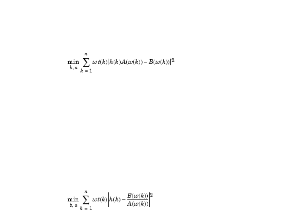
Parametric Modeling

By default invfreqz uses an equation error method to identify the best model

from the data. This finds band ain

by creating a system of linear equations and solving them with the MATLAB

\operator. Here A(w(k)) and B(w(k)) are the Fourier transforms of the

polynomials aand brespectively at the frequency w(k), and nis the number

of frequency points (the length of hand w). wt(k) weights the error relative

to the error at different frequencies. The syntax

invfreqz(h,w,n,m,wt)

includes a weighting vector. In this mode, the filter resulting from invfreqz

is not guaranteed to be stable.

invfreqz provides a superior (“output-error”) algorithm that solves the direct

problem of minimizing the weighted sum of the squared error between the

actual frequency response points and the desired response

To use this algorithm, specify a parameter for the iteration count after the

weight vector parameter:

wt = ones(size(w)); % Create unity weighting vector

[b30,a30] = invfreqz(h,w,3,3,wt,30) % 30 iterations

The resulting filter is always stable.

Graphically compare the results of the first and second algorithms to the

original Butterworth filter with FVTool (and select the Magnitude and Phase

Responses):

fvtool(b,a,b4,a4,b30,a30)

7-19

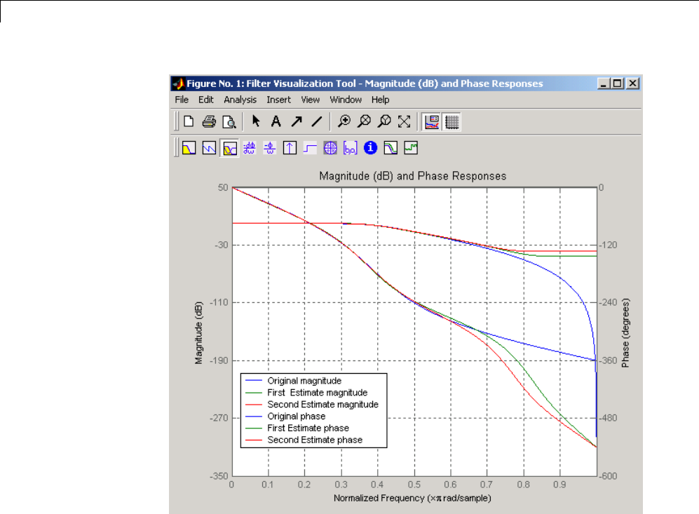
7Special Topics

To verify the superiority of the fit numerically, type

sum(abs(h-freqz(b4,a4,w)).^2) % Total error, algorithm 1

sum(abs(h-freqz(b30,a30,w)).^2) % Total error, algorithm 2

7-20

Resampling

In this section...

“Available Resampling Functions” on page 7-21

“resample Function” on page 7-21

“decimate and interp Functions” on page 7-23

“upfirdn Function” on page 7-23

“spline Function” on page 7-23

Available Resampling Functions

The toolbox provides a number of functions that resample a signal at a higher

or lower rate.

OperationFunction

Apply FIRfilterwith

resampling

upfirdn

Cubic spline interpolation spline

Decimation decimate

Interpolation interp

Other 1-D interpolation interp1

Resample at new rate resample

resample Function

The resample function changes the sampling rate for a sequence to any rate

that is a ratio of two integers. The basic syntax for resample is

y= resample(x,p,q)

where the function resamples the sequence xat p/q times the original

sampling rate. The length of the result yis p/q times the length of x.

7-21

7Special Topics

One resampling application is the conversion of digitized audio signals from

onesamplingratetoanother,suchasfrom48kHz(thedigitalaudiotape

standard) to 44.1 kHz (the compact disc standard).

The example file contains a length 4001 vector of speech sampled at 7418 Hz:

clear

load mtlb

whos

Name Size Bytes Class

Fs 1x1 8 double array

mtlb 4001x1 32008 double array

Grand total is 4002 elements using 32016 bytes

Fs =

7418

To play this speech signal on a workstation that can only play sound at

8192 Hz, use the rat function to find integers pand qthat yield the correct

resampling factor:

[p,q] = rat(8192/Fs,0.0001)

127

115

Since p/q*Fs = 8192.05 Hz, the tolerance of 0.0001 is acceptable; to

resample the signal at very close to 8192 Hz:

y = resample(mtlb,p,q);

resample applies a lowpass filter to the input sequence to prevent aliasing

during resampling. It designs this filter using the firls function with a

Kaiser window. The syntax

resample(x,p,q,l,beta)

7-22

Resampling

controls the filter’s length and the beta parameter of the Kaiser window.

Alternatively, use the function intfilt to design an interpolation filter b

and use it with

resample(x,p,q,b)

decimate and interp Functions

The decimate and interp functions do the same thing as resample with p=1

and q=1, respectively. These functions provide different anti-alias filtering

options, and they incur a slight signal delay due to filtering. The interp

function is significantly less efficient than the resample function with q=1.

upfirdn Function

The toolbox also contains a function, upfirdn,thatappliesanFIRfiltertoan

input sequence and outputs the filtered sequence at a sample rate different

than its original. See “Multirate Filter Bank Implementation” on page 1-8.

spline Function

The standard MATLAB environment contains a function, spline,thatworks

with irregularly spaced data. The MATLAB function interp1 performs

interpolation, or table lookup, using various methods including linear and

cubic interpolation.

7-23

7Special Topics

Cepstrum Analysis

In this section...

“What Is a Cepstrum?” on page 7-24

“Inverse Complex Cepstrum” on page 7-27

What Is a Cepstrum?

Cepstrum analysis is a nonlinear signal processing technique with a variety

of applications in areas such as speech and image processing.

The complex cepstrum for a sequence xis calculated by finding the complex

natural logarithm of the Fourier transform of x, then the inverse Fourier

transform of the resulting sequence.

The toolbox function cceps performs this operation, estimating the complex

cepstrum for an input sequence. It returns a real sequence the same size

as the input sequence:

xhat = cceps(x)

For sequences that have roots on the unit circle, cepstrum analysis has

numerical problems. See Oppenheim and Schafer [2] for information.

The complex cepstrum transformation is central to the theory and application

of homomorphic systems, that is, systems that obey certain general rules

of superposition. See Oppenheim and Schafer [3] for a discussion of the

complex cepstrum and homomorphic transformations, with details on speech

processing applications.

Try using cceps in an echo detection application. First, create a 45 Hz sine

wave sampled at 100 Hz:

t = 0:0.01:1.27;

s1 = sin(2*pi*45*t);

7-24

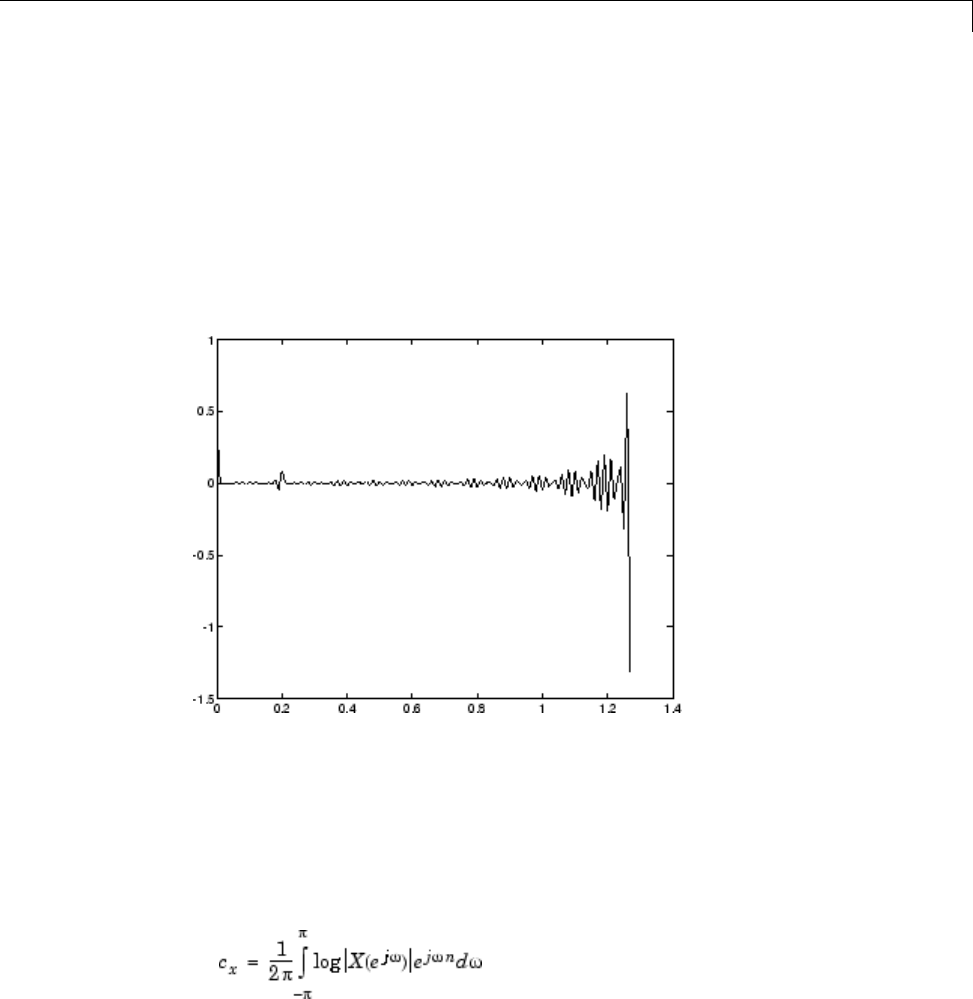
Cepstrum Analysis

Add an echo of the signal, with half the amplitude, 0.2 seconds after the

beginning of the signal.

s2 = s1 + 0.5*[zeros(1,20) s1(1:108)];

The complex cepstrum of this new signal is

c = cceps(s2);

plot(t,c)

Note that the complex cepstrum shows a peak at 0.2 seconds, indicating the

echo.

The real cepstrum of a signal x, sometimes called simply the cepstrum, is

calculated by determining the natural logarithm of magnitude of the Fourier

transform of x, then obtaining the inverse Fourier transform of the resulting

sequence.

7-25

7Special Topics

The toolbox function rceps performs this operation, returning the real

cepstrum for a sequence x. The returned sequence is a real-valued vector the

same size as the input vector:

y = rceps(x)

By definition, you cannot reconstruct the original sequence from its real

cepstrum transformation, as the real cepstrum is based only on the magnitude

of the Fourier transform for the sequence (see Oppenheim and Schafer [3]).

The rceps function also returns a unique minimum-phase sequence that

has the same real cepstrum as x. To obtain both the real cepstrum and the

minimum phase reconstruction for a sequence, use

[y,ym] = rceps(x)

where yis the real cepstrum and ym is the minimum phase reconstruction

of x. The following example shows that one output of rceps is a unique

minimum-phase sequence with the same real cepstrum as x.

y = [4 1 5]; % Non-minimum phase sequence

[xhat,yhat] = rceps(y);

xhat2= rceps(yhat);

[xhat' xhat2']

ans =

1.6225 1.6225

0.3400 0.3400

Summary of Cepstrum Functions

The Signal Processing Toolbox product provides three functions for cepstrum

analysis:

Operation Function

Complex cepstrum cceps

Inverse complex cepstrum icceps

Real cepstrum rceps

7-26

Cepstrum Analysis

Inverse Complex Cepstrum

To invert the complex cepstrum, use the icceps function. Inversion is

complicated by the fact that the cceps function performs a data dependent

phase modification so that the unwrapped phase of its input is continuous at

zero frequency. The phase modification is equivalent to an integer delay. This

delay term is returned by cceps if you ask for a second output. For example:

x = 1:10;

[xhat,delay] = cceps(x)

xhat =

Columns 1 through 4

2.2428 -0.0420 -0.0210 0.0045

Columns 5 through 8

0.0366 0.0788 0.1386 0.2327

Columns 9 through 10

0.4114 0.9249

delay =

To invert the complex cepstrum, use icceps with the original delay parameter:

icc = icceps(xhat,2)

ans =

Columns 1 through 4

2.0000 3.0000 4.0000 5.0000

Columns 5 through 8

6.0000 7.0000 8.0000 9.0000

Columns 9 through 10

10.0000 1.0000

Asshownintheaboveexample,with any modification of the complex

cepstrum, the original delay term may no longer be valid. You will not be able

to invert the complex cepstrum exactly.

7-27

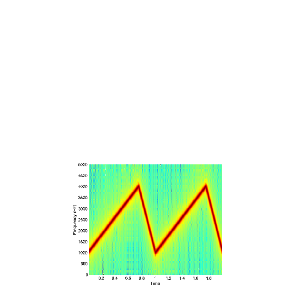
7Special Topics

FFT-Based Time-Frequency Analysis

The Signal Processing Toolbox product provides a function, spectrogram,

that returns the time-dependent Fourier transform for a sequence, or displays

this information as a spectrogram. The time-dependent Fourier transform is

the discrete-time Fourier transform for a sequence, computed using a sliding

window. This form of the Fourier transform, also known as the short-time

Fourier transform (STFT), has numerous applications in speech, sonar, and

radar processing. The spectrogram of a sequence is the magnitude of the

time-dependent Fourier transform versus time.

To display the spectrogramofalinearFMsignal:

fs = 10000;

t = 0:1/fs:2;

x = vco(sawtooth(2*pi*t,.75),[0.1 0.4]*fs,fs);

spectrogram(x,kaiser(256,5),220,512,fs,'yaxis')

7-28

Median Filtering

The function medfilt1 implements one-dimensional median filtering, a

nonlinear technique that applies a sliding window to a sequence. The median

filter replaces the center value in the window with the median value of all the

points within the window [5]. In computing this median, medfilt1 assumes

zeros beyond the input points.

When the number of elements nin the window is even, medfilt1 sorts the

numbers, then takes the average of the n/2 and n/2 +1elements.

Twosimpleexampleswithfourth-and third-order median filters are

medfilt1([4 3 5 2 8 9 1],4)

ans =

1.500 3.500 3.500 4.000 6.500 5.000 4.500

medfilt1([4 3 5 2 8 9 1],3)

ans =

3435881

See the medfilt2 function in the Image Processing Toolbox™ for information

on two-dimensional median filtering.

7-29

7Special Topics

Communications Applications

In this section...

“Modulation” on page 7-30

“Demodulation” on page 7-31

“Voltage Controlled Oscillator” on page 7-34

Modulation

Modulation varies the amplitude, phase, or frequency of a carrier signal with

reference to a message signal.The

modulate function modulates a message

signal with a specified modulation method.

The basic syntax for the modulate function is

y = modulate(x,fc,fs,'method',opt)

where:

•xis the message signal.

•fc is the carrier frequency.

•fs is the sampling frequency.

•method is a flag for the desired modulation method.

•opt is any additional argument that the method requires. (Not all

modulation methods require an option argument.)

The table below summarizes the modulation methods provided; see the

documentation for modulate,demod,andvco for complete details on each.

Method Description

amdsb-sc or am Amplitude modulation, double sideband, suppressed

carrier

amdsb-tc Amplitude modulation, double sideband, transmitted

carrier

7-30

Communications Applications

Method Description

amssb Amplitude modulation, single sideband

fm Frequency modulation

pm Phase modulation

ppm Pulse position modulation

pwm Pulse width modulation

qam Quadrature amplitude modulation

If the input xis an array rather than a vector, modulate modulates each

column of the array.

To obtain the time vector that modulate uses to compute the modulated

signal, specify a second output parameter:

[y,t] = modulate(x,fc,fs,'method',opt)

Demodulation

The demod function performs demodulation, that is, it obtains the original

message signal from the modulated signal:

The syntax for demod is

x = demod(y,fc,fs,'method',opt)

demod uses any of the methods shown for modulate, but the syntax for

quadrature amplitude demodulation requires two output parameters:

[X1,X2] = demod(y,fc,fs,'qam')

If the input yis an array, demod demodulates all columns.

Try modulating and demodulating a signal. A 50 Hz sine wave sampled at

1000 Hz is

t = (0:1/1000:2);

x = sin(2*pi*50*t);

7-31

7Special Topics

With a carrier frequency of 200 Hz, the modulated and demodulated versions

of this signal are

y = modulate(x,200,1000,'am');

z = demod(y,200,1000,'am');

To plot portions of the original, modulated, and demodulated signal:

figure; plot(t(1:150),x(1:150)); title('Original Signal');

figure; plot(t(1:150),y(1:150)); title('Modulated Signal');

figure; plot(t(1:150),z(1:150)); title('Demodulated Signal');

Original Signal

7-32

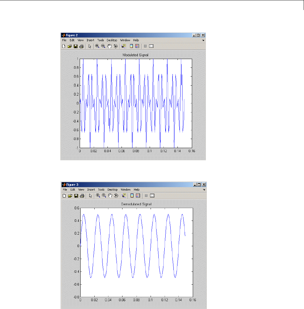
Communications Applications

Modulated Signal

Demodulated Signal

7-33

7Special Topics

Note The demodulated signal is attenuated because demodulation includes

two steps: multiplication and lowpass filtering. The multiplication produces a

component with frequency centered at 0 Hz and a component with frequency

at twice the carrier frequency. The filtering removes the higher frequency

component of the signal, producing the attenuated result.

Voltage Controlled Oscillator

The voltage controlled oscillator function vco creates a signal that oscillates

at a frequency determined by the input vector. The basic syntax for vco is

y = vco(x,fc,fs)

where fc is the carrier frequency and fs is the sampling frequency.

To scale the frequency modulation range, use

y = vco(x,[Fmin Fmax],fs)

In this case, vco scales the frequency modulation range so values of xon the

interval [-1 1] map to oscillations of frequency on [Fmin Fmax].

If the input xis an array, vco produces an array whose columns oscillate

according to the columns of x.

See “FFT-Based Time-Frequency Analysis” on page 7-28 for an example using

the vco function.

7-34

Deconvolution

Deconvolution, or polynomial division, is the inverse operation of convolution.

Deconvolution is useful in recovering the input to a known filter, given the

filtered output. This method is very sensitive to noise in the coefficients,

however, so use caution in applying it.

The syntax for deconv is

[q,r] = deconv(b,a)

where bis the polynomial dividend, ais the divisor, qis the quotient, and r

is the remainder.

To try deconv, first convolve two simple vectors aand b.

a=[123];

b=[456];

c = conv(a,b)

413282718

Now use deconv to deconvolve bfrom c:

[q,r] = deconv(c,a)

456

00000

7-35

7Special Topics

Specialized Transforms

In this section...

“Chirp z-Transform” on page 7-36

“Discrete Cosine Transform” on page 7-37

“Hilbert Transform” on page 7-40

“Walsh–Hadamard Transform” on page 7-41

Chirp z-Transform

The chirp z-transform (CZT), useful in evaluating the z-transform along

contours other than the unit circle. The chirp z-transform is also more efficient

than the DFT algorithm for the computation of prime-length transforms,

and it is useful in computing a subset of the DFT for a sequence. The chirp

z-transform, or CZT, computes the z-transform along spiral contours in the

z-plane for an input sequence. Unlike the DFT, the CZT is not constrained to

operate along the unit circle, but can evaluate the z-transform along contours

described by

where Ais the complex starting point, Wis a complex scalar describing the

complex ratio between points on the contour, and Mis the length of the

transform.

Onepossiblespiralis

A = 0.8*exp(j*pi/6);

W = 0.995*exp(-j*pi*.05);

M = 91;

z = A*(W.^(-(0:M-1)));

zplane([],z.')

7-36

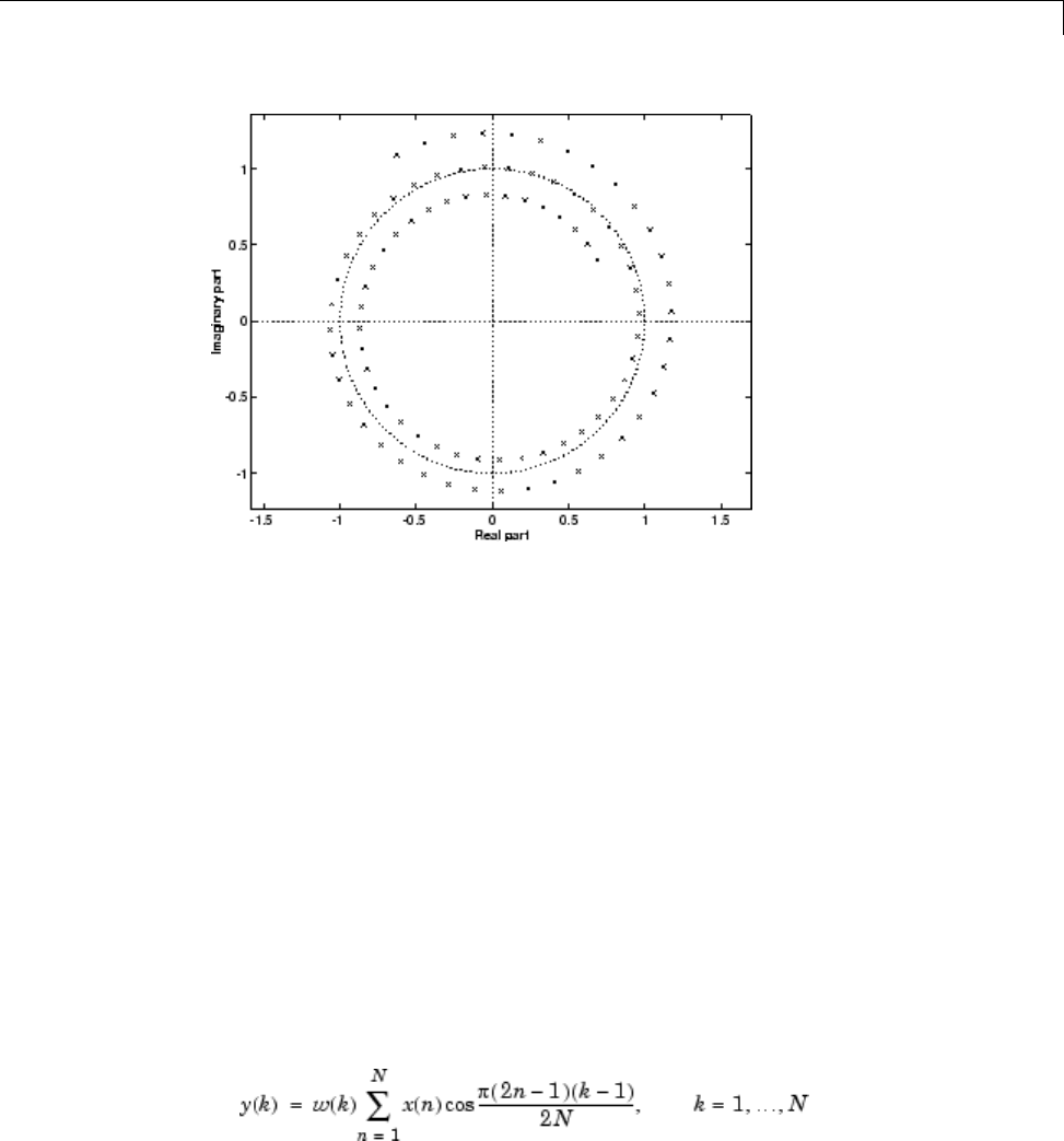
Specialized Transforms

czt(x,M,W,A)computesthez-transform of xon these points.

An interesting and useful spiral set is mevenly spaced samples around the

unit circle, parameterized by A=1and W = exp(-j*pi/M).Thez-transform

on this contour is simply the DFT, obtained by

y = czt(x)

czt may be faster than the fft function for computing the DFT of sequences

with certain odd lengths, particularly long prime-length sequences.

Discrete Cosine Transform

The discrete cosine transform (DCT), closely related to the DFT. The DCT’s

energy compaction properties are useful for applications like signal coding.

The toolbox function dct computes the unitary discrete cosine transform,

or DCT, for an input vector or matrix. Mathematically, the unitary DCT of

an input sequence xis

7-37

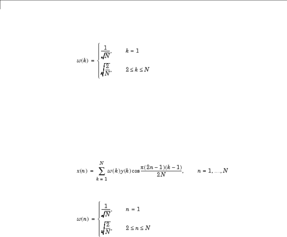
7Special Topics

where

The DCT is closely related to the discrete Fourier transform; the DFT is

actually one step in the computation of the DCT for a sequence. The DCT,

however, has better energy compaction properties, with just a few of the

transform coefficients representing the majority of the energy in the sequence.

The energy compaction properties of the DCT make it useful in applications

such as data communications.

The function idct computes the inverse DCT for an input sequence,

reconstructing a signal from a complete or partial set of DCT coefficients. The

inverse discrete cosine transform is

where

Because of the energy compaction mentioned above, it is possible to

reconstruct a signal from only a fraction of its DCT coefficients. For example,

generate a 25 Hz sinusoidal sequence, sampled at 1000 Hz:

t = (0:1/999:1);

x = sin(2*pi*25*t);

7-38

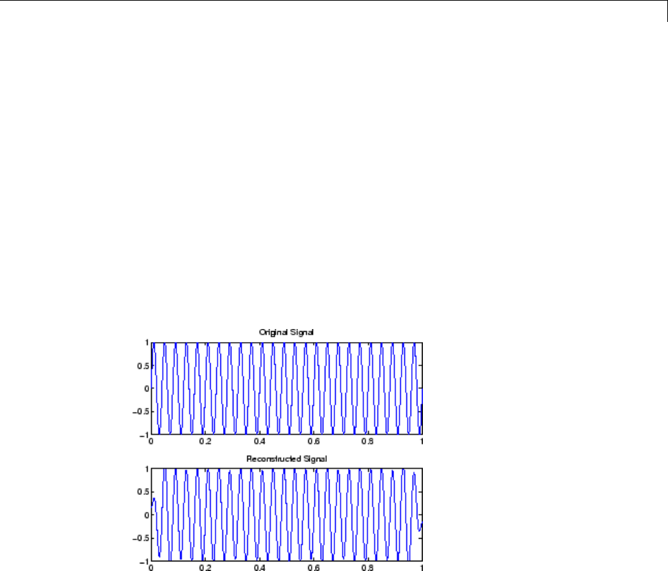
Specialized Transforms

Compute the DCT of this sequence and reconstruct the signal using only

those components with value greater than 0.1 (64 of the original 1000 DCT

coefficients):

y = dct(x) % Compute DCT

y2 = find(abs(y) < 0.9); % Use 17 coefficients

y(y2) = zeros(size(y2)); % Zero out points < 0.9

z = idct(y); % Reconstruct signal w/inverse DCT

Plot the original and reconstructed sequences:

subplot(2,1,1); plot(t,x);

title('Original Signal')

subplot(2,1,2); plot(t,z), axis([0 1 -1 1])

title('Reconstructed Signal')

One measure of the accuracy of the reconstruction is

norm(x-z)/norm(x)

that is, the norm of the difference between the original and reconstructed

signals, divided by the norm of the original signal. In this case, the

relative error of reconstruction is 0.1443. The reconstructed signal retains

approximately 85% of the energy in the original signal.

7-39

7Special Topics

Hilbert Transform

The Hilbert transform facilitates the formation of the analytic signal. The

analytic signal is useful in the area of communications, particularly in

bandpass signal processing. The toolbox function hilbert computes the

Hilbert transform for a real input sequence xand returns a complex result of

thesamelength

y = hilbert(x)

where the real part of yis the original real data and the imaginary part

is the actual Hilbert transform. yis sometimes called the analytic signal,

in reference to the continuous-time analytic signal. A key property of the

discrete-time analytic signal is that its z-transform is 0 on the lower half of

the unit circle. Many applications of the analytic signal are related to this

property; for example, the analytic signal is useful in avoiding aliasing effects

for bandpass sampling operations. The magnitude of the analytic signal is the

complex envelope of the original signal.

The Hilbert transform is related to the actual data by a 90° phase shift; sines

become cosines and vice versa. To plot a portion of data (solid line) and its

Hilbert transform (dotted line):

t = (0:1/1023:1);

x = sin(2*pi*60*t);

y = hilbert(x);

plot(t(1:50),real(y(1:50))), hold on

plot(t(1:50),imag(y(1:50)),':');

axis([0 0.05 -1.1 2]);

legend('Real Part','Imaginary Part','location','northeast');

7-40

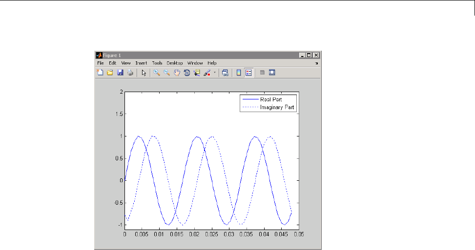
Specialized Transforms

The analytic signal is useful in calculating instantaneous attributes of a time

series, the attributes of the series at any point in time. The instantaneous

amplitude of the input sequence is the amplitude of the analytic signal. The

instantaneous phase angle of the input sequence is the (unwrapped) angle of

the analytic signal; the instantaneous frequency is the time rate of change

of the instantaneous phase angle. You can calculate the instantaneous

frequency using the MATLAB function, diff.

Walsh–Hadamard Transform

The Walsh–Hadamard transform is a non-sinusoidal, orthogonal

transformation technique that decomposes a signal into a set of basis

functions. These basis functions are Walsh functions, which are rectangular

or square waves with values of +1 or –1. Walsh–Hadamard transforms

arealsoknownasHadamard(seethehadamard function in the MATLAB

software), Walsh, or Walsh-Fourier transforms.

The first eight Walsh functions have these values:

7-41

7Special Topics

Index Walsh Function Values

011111111

1 1111-1-1-1-1

21 1 -1 -1 -1 -1 1 1

31 1 -1 -1 1 1 -1 -1

4 1 -1 -1 1 1 -1 -1 1

51-1-11-111-1

61-11-1-11-11

71-11-11-11-1

The Walsh–Hadamard transform returns sequency values. Sequency is a

more generalized notion of frequency and is defined as one half of the average

number of zero-crossings per unit time interval. Each Walsh function has a

unique sequency value. You can use the returned sequency values to estimate

the signal frequencies in the original signal.

Three different ordering schemes are used to store Walsh functions: sequency,

Hadamard, and dyadic. Sequency ordering, which is used in signal processing

applications, has the Walsh functions in the order shown in the table above.

Hadamard ordering, which is used in controls applications, arranges them

as 0, 4, 6, 2, 3, 7, 5, 1. Dyadic or gray code ordering, which is used in

mathematics, arranges them as 0, 1, 3, 2, 6, 7, 5, 4.

The Walsh–Hadamard transform is used in a number of applications, such

as image processing, speech processing, filtering, and power spectrum

analysis. It is very useful for reducing bandwidth storage requirements and

spread-spectrum analysis. Like the FFT, the Walsh–Hadamard transform has

a fast version, the fast Walsh–Hadamard transform (fwht). Compared to the

FFT, the FWHT requires less storage space and is faster to calculate because

it uses only real additions and subtractions, while the FFT requires complex

values. The FWHT is able to represent signals with sharp discontinuities

more accurately using fewer coefficients than the FFT. Both the FWHT and

the inverse FWHT (ifwht) are symmetric and thus, use identical calculation

processes. The FWHT and IFWHT for a signal x(t) of length N are defined as:

7-42

Specialized Transforms

yNxWAL ni

xyWALni

()

−

∑

(,)

where i= 0,1,..., N-1 and WAL(n,i) are Walsh functions. Similar to the

Cooley-Tukey algorithm for the FFT, the Nelements are decomposed into two

sets of N/2 elements, which are then combined using a butterfly structure to

form the FWHT. For images, where the input is typically a 2–D signal, the

FWHT coefficients are calculated by first evaluating across the rows and

then evaluating down the columns.

For the following simple signal, the resulting FWHT shows that xwas created

using Walsh functions with sequency values of 0, 1, 3, and 6, which are the

non-zero indices of the transformed x. The inverse FWHT recreates the

original signal.

x=[422002-20]

y = fwht(x)

11010010

x1 = ifwht(y)

422002-20

Using Walsh-Hadamard Transform for Spectral Analysis and

Compression of ECG Signals

The following example uses an electrocardiogram (ECG) signal to illustrate

working with the Walsh-Hadamard transform. ECG signals typically are

very large and need to be stored for analysis and retrieval at a future time.

Walsh-Hadamard transforms are particularly well-suited to this application

because they provide compression and thus, require less storage space, plus

they also provide rapid signal reconstruction.

Start with an ECG signal. For this example, we replicate it to create a longer

signal and insert some additional random noise. Then, transform the signal

7-43

7Special Topics

using the fast Walsh-Hadamard transform and plot the original signal and

the transformed signal.

xe = ecg(512); % Single ecg wave

xr = repmat(xe,1,8); % Replicate it to create more data

x = xr + 0.1.*randn(1,length(xr)); % Add noise

% Fast Walsh-Hadamard transform. Use default values

% for the number of points to use for the transform and

% for the ordering - sequency -- why???

y = fwht(x);

figure('color','white');

subplot(2,1,1);

plot(x); % Plot original noisy signal

xlabel('Sample index');

ylabel('Amplitude');

title('ECG Signal');

subplot(2,1,2);

plot(abs(y)) % Plot magnitude of transformed signal

xlabel('Sequency index');

ylabel('Magnitude');

title('WHT Coefficients');

7-44

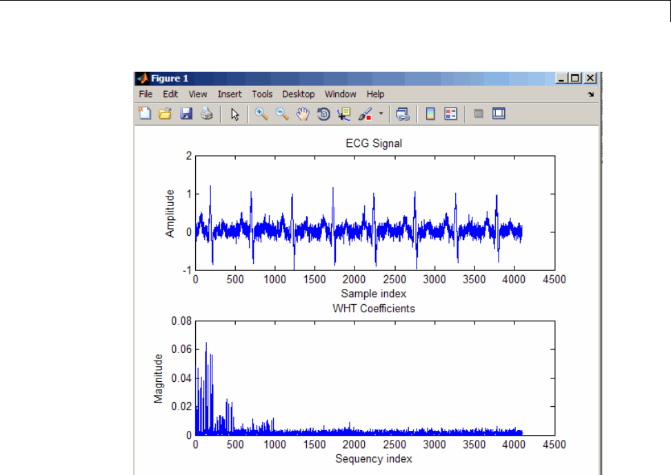
Specialized Transforms

The plot shows that most of the signal energy is in the lower sequency values

below approximately 1100. We will store only the first 1024 coefficients

and see if the signal can be accurately reconstructed from only these stored

coefficients.

y(1025:length(x)) = 0; % Zeroing out the higher coefficients

xHat = ifwht(y); % Signal reconstruction using inverse WHT

figure('color','white');

plot(x);

hold on

plot(xHat,'r');

xlabel('Sample index');

ylabel('ECG signal amplitude');

legend('Original Signal','Reconstructed Signal');

7-45

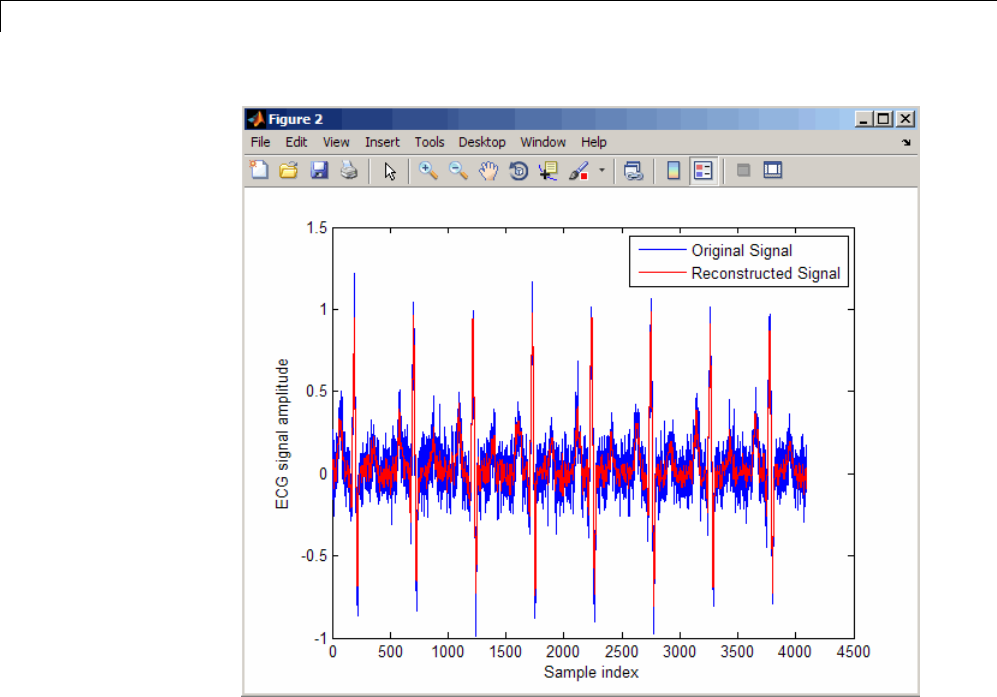
7Special Topics

The reproduced signal is very close to the original signal.

To reconstruct the original signal, we stored only the first 1024 coefficients and

the ECG signal length. This represents a compression ratio of approximately

4:1. Storing more coefficients is a tradeoff between increased resolution and

increased noise, while storing fewer coefficients may cause loss of peaks.

req = [length(x) y(1:1024)];

whos x req

Name Size Bytes Class Attributes

req 1x1025 8200 double

x 1x4096 32768 double

7-46

Selected Bibliography

[1] Kay, S.M. Modern Spectral Estimation. Englewood Cliffs, NJ: Prentice

Hall, 1988.

[2] Oppenheim, A.V., and R.W. Schafer. Discrete-Time Signal Processing.

Englewood Cliffs, NJ: Prentice Hall, 1989.

[3] Oppenheim, A.V., and R.W. Schafer. Discrete-Time Signal Processing.

Englewood Cliffs, NJ: Prentice Hall, 1975, Section 10.5.3.

[4] Parks, T.W., and C.S. Burrus. Digital Filter Design. New York: John

Wiley & Sons, 1987.

[5] Pratt,W.K. Digital Image Processing. New York: John Wiley & Sons, 1991.

7-47

7Special Topics

7-48

SPTool: A Signal Processing

GUI Suite

•“SPTool: An Interactive Signal Processing Environment” on page 8-2

•“Opening SPTool” on page 8-4

•“Getting Context-Sensitive Help” on page 8-6

•“Signal Browser” on page 8-7

•“FDATool” on page 8-10

•“Filter Visualization Tool” on page 8-11

•“Spectrum Viewer” on page 8-13

•“Filtering and Analysis of Noise” on page 8-16

•“Exporting Signals, Filters, and Spectra” on page 8-27

•“Accessing Filter Parameters” on page 8-29

•“Importing Filters and Spectra” on page 8-32

•“Loading Variables from the Disk” on page 8-36

•“Saving and Loading Sessions” on page 8-37

•“Selecting Signals, Filters, and Spectra” on page 8-39

•“Editing Signals, Filters, or Spectra” on page 8-40

•“Making Signal Measurements with Markers” on page 8-41

•“Setting Preferences” on page 8-43

•“Using the Filter Designer” on page 8-47

8SPTool: A Signal Processing GUI Suite

SPTool: An Interactive Signal Processing Environment

In this section...

“SPTool Overview” on page 8-2

“SPTool Data Structures” on page 8-3

SPTool Overview

SPTool is an interactive GUI for digital signal processing used to

•Analyze signals

•Design filters

•Analyze (view) filters

•Filter signals

•Analyze signal spectra

You can accomplish these tasks using four GUIs that you access from within

SPTool:

•The “Signal Browser” on page 8-7 is for analyzing signals. You can also

play signals using your computer’s audio hardware.

•fdatool is available for designing or editing FIR and IIR digital filters.

Most Signal Processing Toolbox filter design methods available at the

command line are also available in FDATool. Additionally, you can use

FDATool to design a filter by using the“Pole/ZeroEditor”onpage8-48to

graphically place poles and zeros on the z-plane.

•The “Filter Visualization Tool” on page 8-11 (FVTool) is for analyzing filter

characteristics.

•The “Spectrum Viewer” on page 8-13 is for spectral analysis. You can use

Signal Processing Toolbox spectral estimation methods to estimate the

power spectral density of a signal.

8-2

SPTool: An Interactive Signal Processing Environment

SPTool Data Structures

You can use SPTool to analyze signals, filters, or spectra that you create at

the MATLAB command line.

You can bring signals, filters, or spectra from the MATLAB workspace into the

SPTool workspace using File > Import. For more information, see “Importing

Filters and Spectra” on page 8-32. Signals, filters, or spectra that you create

in (or import into) the SPTool workspace exist as MATLAB structures. See

the MATLAB documentation for more information on MATLAB structures.

When you use File > Export to save signals, filters, and spectra that you

create or modify in SPTool, these are also saved as MATLAB structures. For

more information on exporting, see “Exporting Signals, Filters, and Spectra”

on page 8-27.

8-3

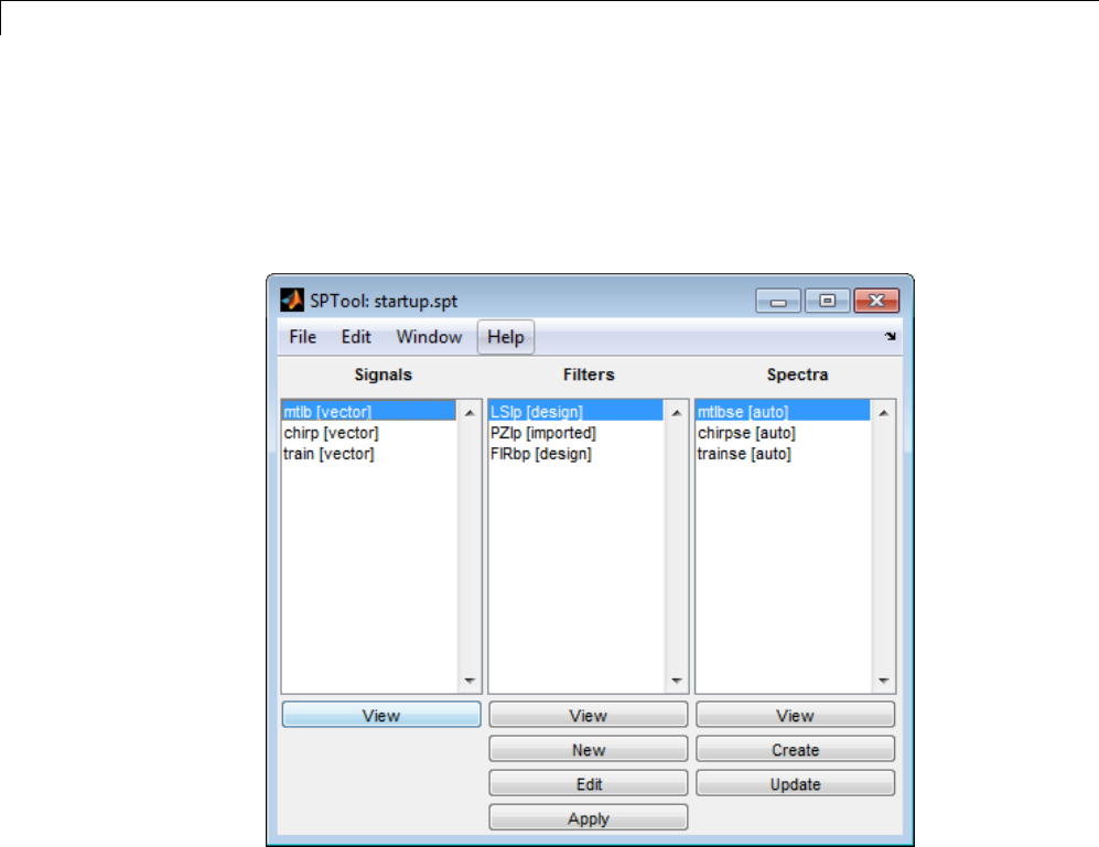
8SPTool: A Signal Processing GUI Suite

Opening SPTool

To open SPTool, type

sptool

When you first open SPTool, it contains a collection of default signals, filters,

and spectra. To specify your own preferences for what signals, filters, and

spectra to see when SPTool opens see “Setting Preferences” on page 8-43.

You can access these three GUIs from SPTool by selecting a signal, filter, or

spectrum and clicking the appropriate View button:

•Signal Browser

•Filter Visualization Tool

•Spectrum Viewer

8-4

Opening SPTool

You can access FDATool by clicking New to create a new filter or Edit to edit

a selected filter. Clicking Apply applies a selected filter to a selected signal.

Create opens the Spectrum Viewer and creates the power spectral density

of the selected signal. Update opens the Spectrum Viewer for the selected

spectrum.

8-5

8SPTool: A Signal Processing GUI Suite

Getting Context-Sensitive Help

To find information on a particular feature or setting of the “Signal Browser”

on page 8-7:

•In any Measurements panel, right-click anywhere on the panel and select

What’s this?.

•In any dialog box where you see the icon in the lower left corner,

right-click on any parameter and select What’s this?.

To find information on a particular region of “FDATool” on page 8-10 or

“Spectrum Viewer” on page 8-13:

1Click What’s this? .

2Click on the region of the GUI you want information on.

You can also use Help > What’s This? to launch context-sensitive help.

8-6

Signal Browser

In this section...

“Overview of the Signal Browser” on page 8-7

“Opening the Signal Browser” on page 8-7

Overview of the Signal Browser

You can use the Signal Browser to display and analyze signals listed in the

Signals list box in SPTool.

Using the Signal Browser, you can:

•Analyze and compare vector or array (matrix) signals.

•Zoom in on portions of signal data.

•Measure a variety of characteristics of signal data.

•Comparemultiplesignals.

•Play portions of signal data on audio hardware.

•Print signal plots.

Opening the Signal Browser

To open the Signal Browser from SPTool:

1Select one or more signals in the Signals list in SPTool.

2Click View under the Signals list.

8-7

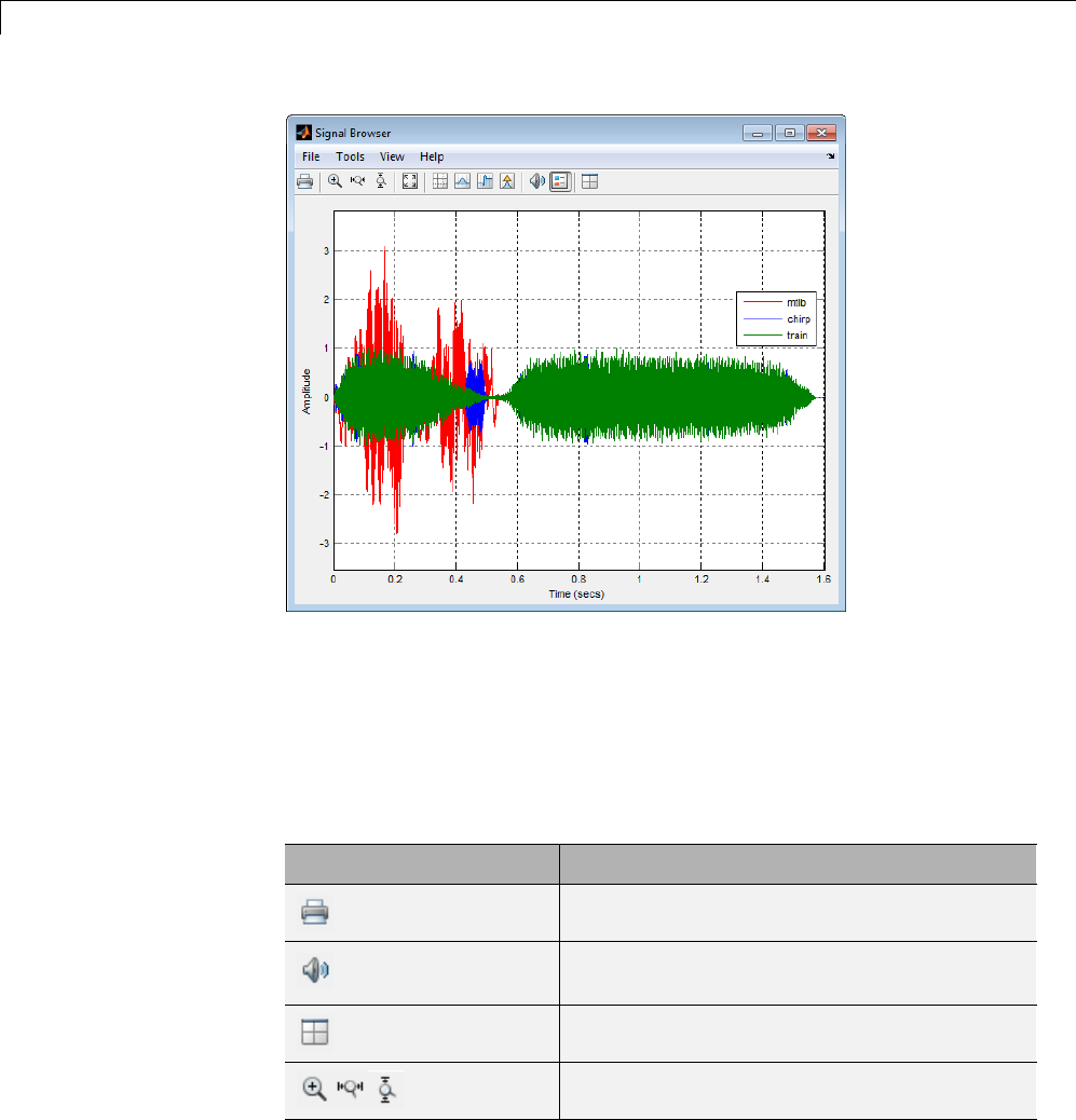
8SPTool: A Signal Processing GUI Suite

The Signal Browser has the following components:

•A display region for analyzing signals

•A panels section on the right side of the scope window, which shows

statistics and information about your signals

•A toolbar with buttons for convenient access to frequently used functions

Icon Description

Print the current scope window.

Play an audio signal. The function soundsc is

used to play the signal.

Show multiple displays of signals.

Zoom the signal in and out.

8-8

Signal Browser

Icon Description

Scale the axes.

Toggle the legends on and off.

Toggle the Cursor Measurements panel. This

panel allows you to see screen cursors and get

measurements of time and amplitude values

at the cursors.

Toggle the Signal Statistics, Bilevel

Measurements, and Peak Finder panels,

which display various measurements about

the selected signal.

For more information on the Signal Browser, see the sptool function

reference page.

8-9

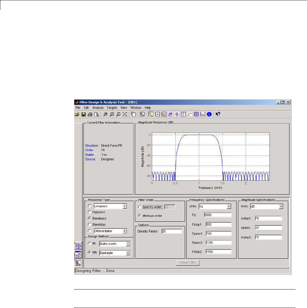
8SPTool: A Signal Processing GUI Suite

FDATool

You can use the Filter Design and Analysis Tool (fdatool)todesignand

edit filters.

To open FDATool from SPTool, click New under the Filters list to create a

new filter or select one of the filters in the Filters list in SPTool and click

Edit to edit that filter.

Note When you open FDATool from SPTool, a reduced version of FDATool

that is compatible with SPTool opens.

8-10

Filter Visualization Tool

In this section...

“Connection between FVTool and SPTool” on page 8-11

“Opening the Filter Visualization Tool” on page 8-11

“Analysis Parameters” on page 8-12

Connection between FVTool and SPTool

You can use the Filter Visualization Tool to analyze response characteristics

of the selected filter(s). See fvtool for detailed information about FVTool.

If you start FVTool by clicking the SPTool Filter View button, that FVTool is

linked to SPTool. Any changes made in SPTool to the filter are immediately

reflected in FVTool. The FVTool title bar includes "SPTool" to indicate the

link.

If you start an FVTool by clicking the New button or by selecting File > New

from within FVTool, that FVTool is a standalone version and is not linked to

SPTool.

Note Every time you click the Filter View button a new, linked FVTool

starts. This allows you to view multiple analyses simultaneously.

Opening the Filter Visualization Tool

YouopenFVToolfromSPToolasfollows.

1Select one or more filters in the Filters list in SPTool.

2Click the View button under the Filters list.

When you first open FVTool, it displays the selected filter’s magnitude plot.

8-11

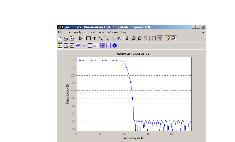
8SPTool: A Signal Processing GUI Suite

Analysis Parameters

In the plot area of any filter response plot, right-click and select Analysis

Parameters to display details about the displayed plot. See “Analysis

Parameters” in the FDATool online help for more information.

You can change any parameter in a linked FVTool, except the sampling

frequency. You can only change the sampling frequency using the SPTool

Edit > Sampling Frequency or the SPTool Filters Edit button.

8-12

Spectrum Viewer

In this section...

“Spectrum Viewer Overview” on page 8-13

“Opening the Spectrum Viewer” on page 8-13

Spectrum Viewer Overview

You can use the Spectrum Viewer for estimating and analyzing a signal’s

power spectral density (PSD). You can use the PSD estimates to understand a

signal’s frequency content.

The Spectrum Viewer provides the following functionality.

•Analyze and compare spectral density plots.

•Use different spectral estimation methods to create spectra:

-Burg (pburg)

-Covariance (pcov)

-FFT (fft)

-Modified covariance (pmcov)

-MTM (multitaper method) (pmtm)

-MUSIC (pmusic)

-Welch (pwelch)

-Yule-Walker AR (pyulear)

•Modify power spectral density parameters such as FFT length, window

type, and sample frequency.

•Print spectral plots.

Opening the Spectrum Viewer

To open the Spectrum Viewer and create a PSD estimate from SPTool:

1Select a signal from the Signal list box in SPTool.

8-13

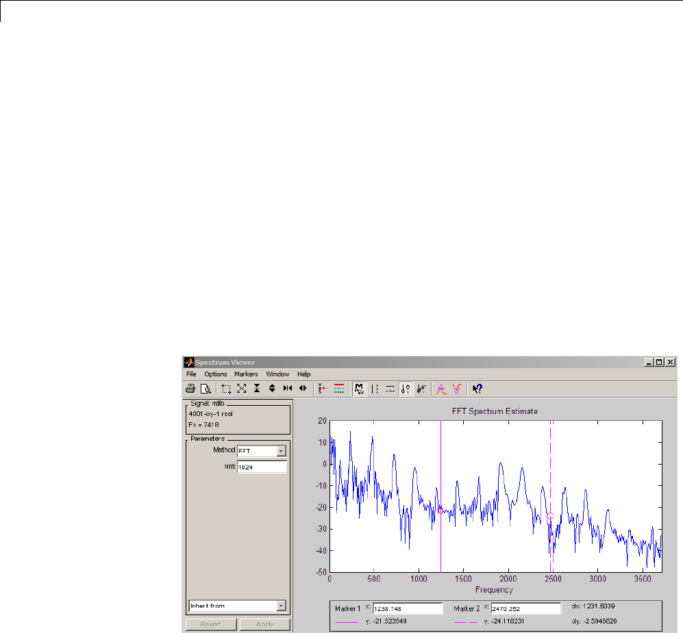
8SPTool: A Signal Processing GUI Suite

2Click Create in the Spectra list.

3Click Apply in the Spectrum Viewer.

To open the Spectrum Viewer with a PSD estimate already listed in SPTool:

1Select a PSD estimate from the Spectra list box in SPTool.

2Click View in the Spectra list.

For example:

1Select mtlb in the default Signals list in SPTool.

2Click Create in SPTool to open the Spectrum Viewer.

3Click Apply in the Spectrum Viewer to plot the spectrum.

The Spectrum Viewer has the following components:

•A signal identification region that provides information about the signal

whose power spectral density estimate is displayed

8-14

Spectrum Viewer

•A Parameters region for modifying the PSD parameters

•A display region for analyzing spectra and an Options menu for modifying

display characteristics

•Spectrum management controls

-Inherit from menu to inherit PSD specifications from another PSD

object listed in the menu

-Revert button to revert to the named PSD’s original specifications

-Apply button for creating or updating PSD estimates

•A toolbar with buttons for convenient access to frequently used functions

Icon Description

Print and print preview

Zoom the signal in and out

Select one of several loaded signals

Set the display color and line style of a

signal

Toggle the markers on and off

Set marker types

Turn on the What’s This help

8-15

8SPTool: A Signal Processing GUI Suite

Filtering and Analysis of Noise

In this section...

“Overview” on page 8-16

“Importing a Signal into SPTool” on page 8-16

“Designing a Filter” on page 8-18

“Applying a Filter to a Signal” on page 8-20

“Analyzing a Signal” on page 8-22

“Spectral Analysis in the Spectrum Viewer” on page 8-24

Overview

The following sections provide an example of using the GUI-based interactive

tools to:

•Design and implement an FIR bandpass digital filter

•Apply the filter to a noisy signal

•Analyze signals and their spectra

The steps include:

1“Importing a Signal into SPTool” on page 8-16

2Designing a bandpass filter using FDATool

3Applyingthefiltertotheoriginalnoisesignaltocreateabandlimited

noise signal

4Comparing the time domain information of the original and filtered signals

using the Signal Browser

5Comparing the spectra of both signals using the Spectrum Viewer

Importing a Signal into SPTool

To import a signal into SPTool from the workspace or disk, the signal must

be either:

8-16

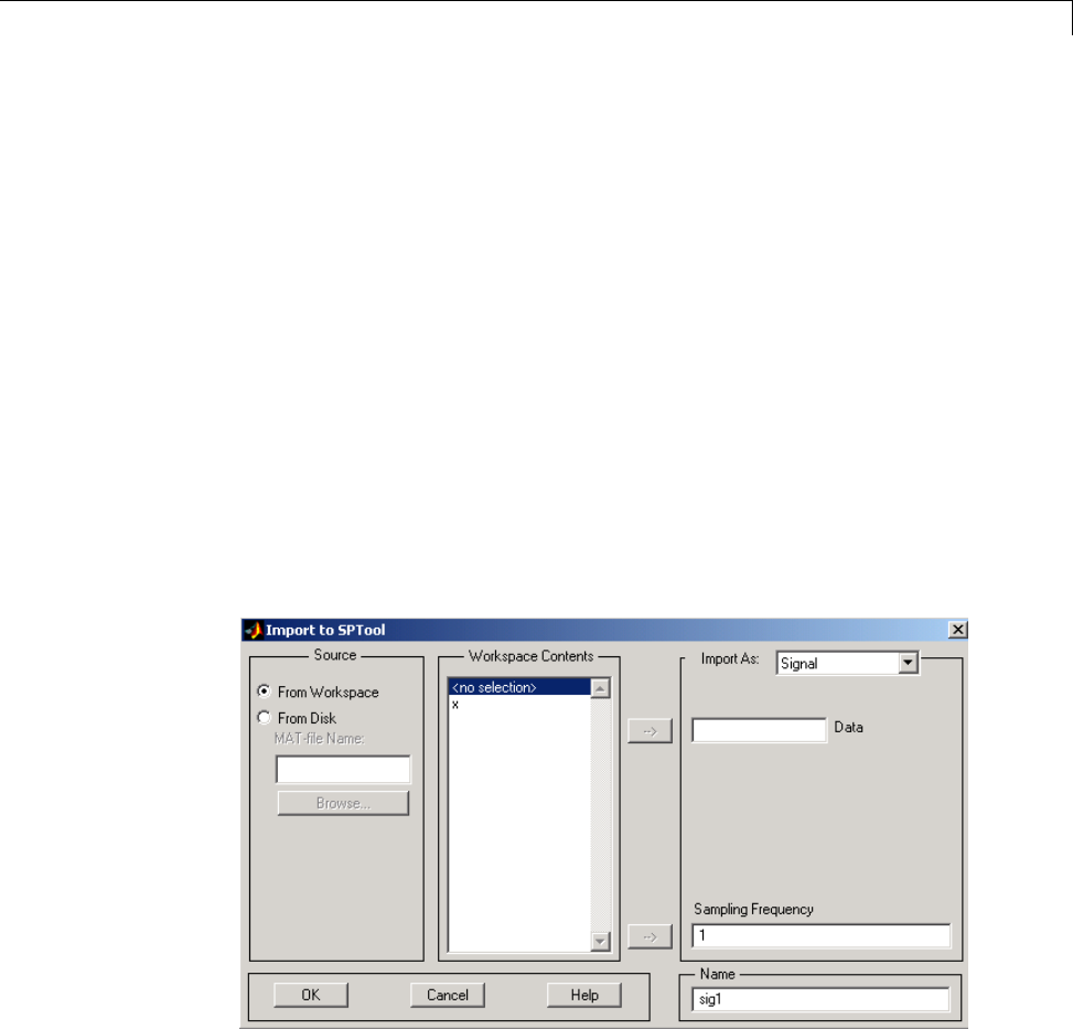
Filtering and Analysis of Noise

•A special MATLAB signal structure, such as that saved from a previous

SPTool session

•A signal created as a variable (vector or matrix) in the MATLAB workspace

For this example, create a new signal at the command line and then import it

as a structure into SPTool:

1Create a random signal in the MATLAB workspace by typing

x = randn(5000,1);

2If SPTool is not already open, open SPTool by typing

sptool

The SPTool window is displayed.

3Select File > Import. The Import to SPTool dialog opens.

The variable xis displayed in the Workspace Contents list. (If it is not,

select the From Workspace radio button todisplaythecontentsofthe

workspace.)

4Select the signal and import it into the Data field:

8-17

8SPTool: A Signal Processing GUI Suite

aSelect the signal variable xin the Workspace Contents list.

bMake sure that Signal is selected in the Import As pull-down menu.

cClick on the arrow to the left of the Data field or type xin the Data field.

dType 5000 in the Sampling Frequency field.

eName the signal by typing noise in the Name field.

fClick OK.

The signal noise[vector] appears and is selected in SPTool’s Signals list.

Note YoucanimportfiltersandspectraintoSPToolinmuchthesameway

as you import signals. See “Importing Filters and Spectra” on page 8-32 for

specific details.

You can also import signals from MAT-files on your disk, rather than from

the workspace. See “Loading Variables from the Disk” on page 8-36 for more

information.

Type help sptool for information about importing from the command line.

Designing a Filter

You can import an existing filter into SPTool, or you can design and edit

a new filter using FDATool.

In this example, you

1Open a default filter in FDATool.

2Specify an equiripple bandpass FIR filter.

Opening FDATool

To open FDATool, click New in SPTool. FDATool opens with a default filter

named filt1.

8-18

Filtering and Analysis of Noise

Specifying the Bandpass Filter

Design an equiripple bandpass FIR filter with the following characteristics:

•Sampling frequency of 5000 Hz

•Stopband frequency ranges of [0 500] Hz and [1500 2500] Hz

•Passband frequency range of [750 1250] Hz

•Ripple in the passband of 0.01 dB

•Stopband attenuation of 75 dB

To modify the filter in FDATool to meet these specifications, you need to

1Select Bandpass from the Response Type list.

2Verify that FIR Equiripple is selected as the Design Method.

3Verify that Minimum order is selected as the Filter Order and that the

Density Factor is set to 20.

4Under Frequency Specifications, set the sampling frequency (Fs)and

the passband (Fpass1,Fpass2) and stopband (Fstop1,Fstop2)edges:

Units Hz

Fs 5000

Fstop1 500

Fpass1 750

Fpass2 1250

Fstop2 1500

5Under Magnitude Specifications, set the stopband attenuation (Astop1,

Astop2) and the maximum passband ripple (Apass):

8-19

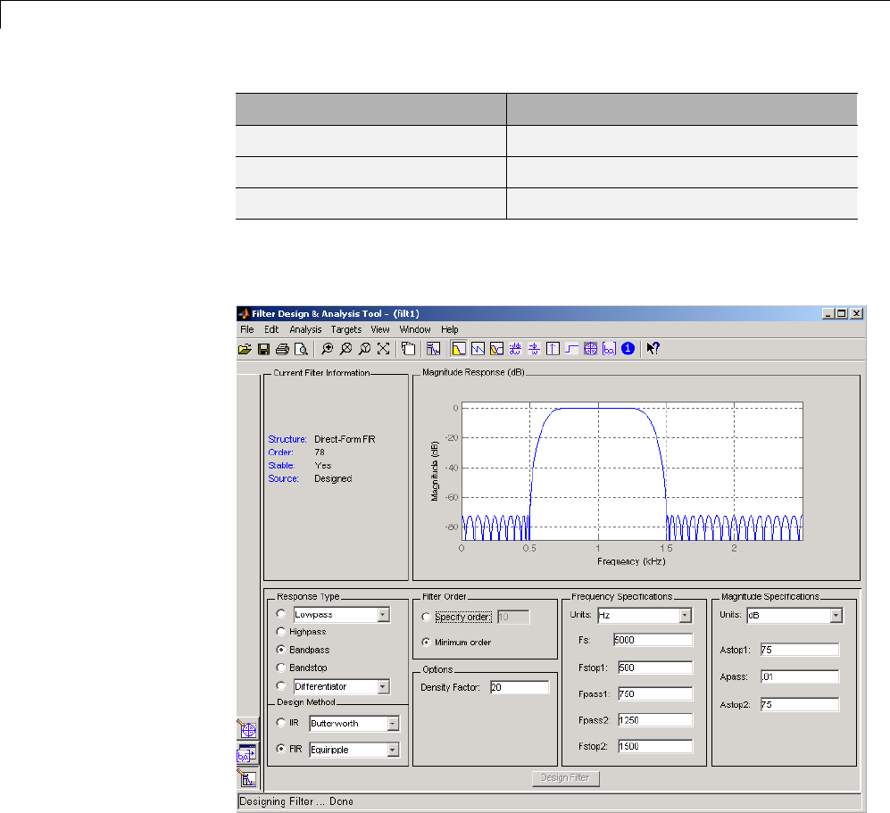
8SPTool: A Signal Processing GUI Suite

Units dB

Astop1 75

Apass 0.01

Astop2 75

6Click Design Filter to design the new filter. When the new filter is

designed, the magnitude response of the filter is displayed.

The resulting filter is an order-78 bandpass equiripple filter.

Applying a Filter to a Signal

When you apply a filter to a signal, you create a new signal in SPTool

representing the filtered signal.

8-20

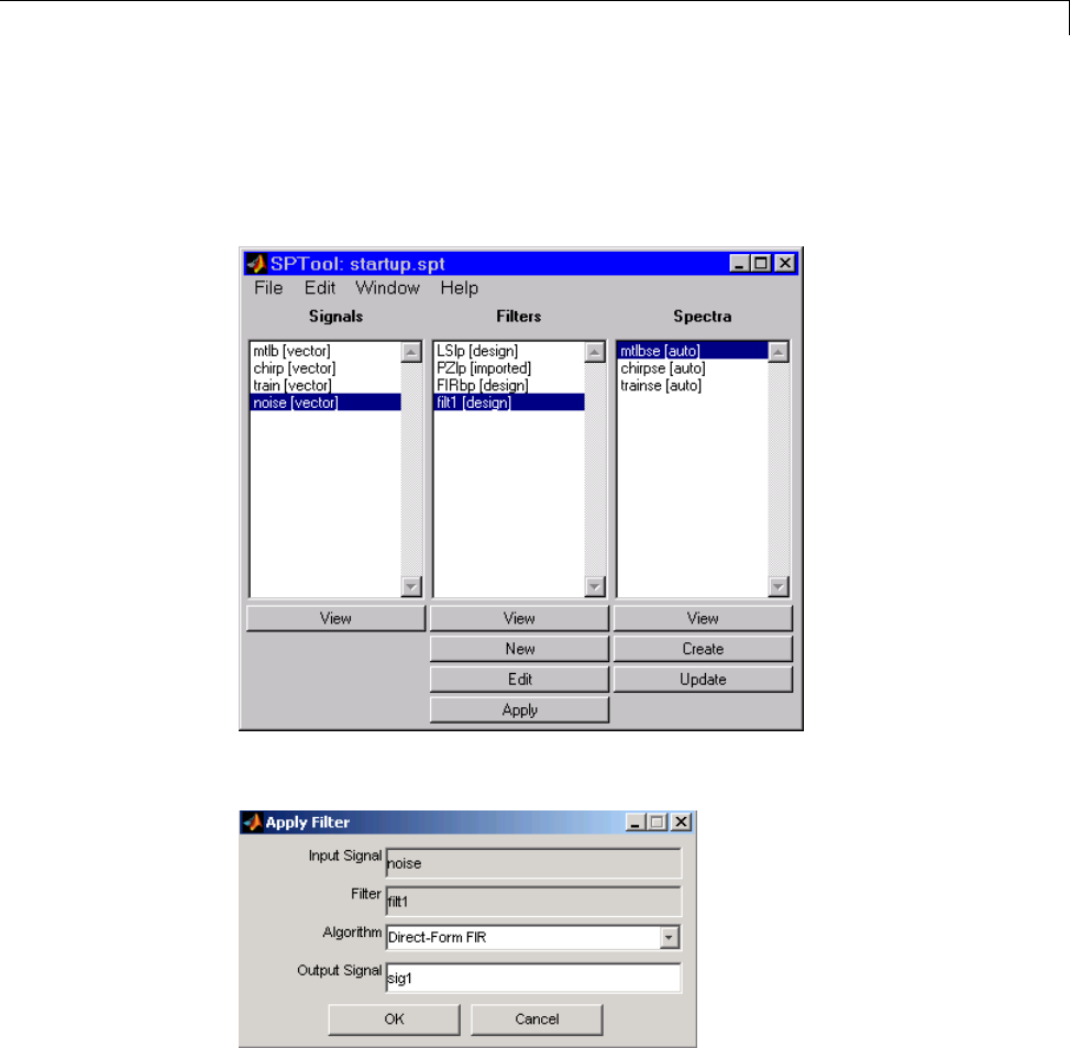
Filtering and Analysis of Noise

To apply the filter filt1 you just created to the signal noise,

1In SPTool, select the signal noise[vector] from the Signals list and select

the filter (named filt1[design])fromtheFilters list.

2Click Apply under the Filters list.

3Leave the Algorithm as Direct-Form FIR.

8-21

8SPTool: A Signal Processing GUI Suite

Note You can apply one of two filtering algorithms to FIR filters. The

default algorithm is specific to the filter structure, which is shown in the

FDATool Current Filter Info frame. Alternately for FIR filters, FFT based

FIR (fftfilt) uses the algorithm described in fftfilt.

For IIR filters, the alternate algorithm is a zero-phase IIR that uses the

algorithm described in filtfilt.

4Enter blnoise as the Output Signal name.

5Click OK to close the Apply Filter dialog box.

The filter is applied to the selected signal, and the filtered signal

blnoise[vector] is listed in the Signals list in SPTool.

Analyzing a Signal

You can analyze and print signals using the Signal Browser. You can also

play the signals if your computer has audio output capabilities.

For example, compare the signal noise to the filtered signal blnoise:

1Shift+click on the noise and blnoise signals in the Signals list of SPTool

to select both signals.

2Click View under the Signals list.

The Signal Browser is activated, and both signals are displayed in the

display region. (The names of both signals are shown above the display

region.) Initially, the original noise signal covers up the bandlimited

blnoise signal.

3Push the selection button on the toolbar to select the blnoise signal.

The display area is updated. Now you can see the blnoise signal

superimposed on top of the noise signal. The signals are displayed in

different colors in both the display region and the panner. You can change

the color of the selected signal using the Line Properties buttononthe

toolbar, .

8-22

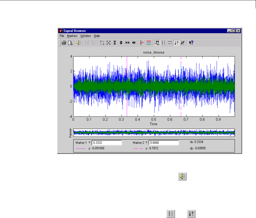
Filtering and Analysis of Noise

Playing a Signal

When you click Play in the Signal Browser toolbar, , the active signal is

played on the computer’s audio hardware:

1To hear a portion of the active (selected) signal

aUse the vertical markers to select a portion of the signal you want to

play. Vertical markers are enabled by the and buttons.

bClick Play.

2To hear the other signal

aSelect the signal as in step above. You can also select the signal directly

in the display region.

bClick Play again.

8-23

8SPTool: A Signal Processing GUI Suite

Printing a Signal

You can print from the Signal Browser using the Print button, .

You can use the line display buttons to maximize the visual contrast between

the signals by setting the line color for noise to gray and the line color for

blnoisetowhite. Dothisbeforeprintingtwosignalstogether.

Note You can follow the same rules to print spectra, but you can’t print filter

responses directly from SPTool.

Use the Signal Browser region in the Preferences dialog box in SPTool to

suppress printing of both the panner and the marker settings.

To print both signals, click Print in the Signal Browser toolbar.

Spectral Analysis in the Spectrum Viewer

You can analyze the frequency content of a signal using the Spectrum Viewer,

which estimates and displays a signal’s power spectral density.

For example, to analyze and compare the spectra of noise and blnoise:

1Create a power spectral density (PSD) object, spect1, that is associated

with the signal noise, and a second PSD object, spect2, that is associated

with the signal blnoise.

2Open the Spectrum Viewer to analyze both of these spectra.

3Print both spectra.

CreatingaPSDObjectFromaSignal

1Click on SPTool, or select Window > SPTool in any active open GUI.

SPTool is now the active window.

2Select the noise[vector] signal in the Signals list of SPTool.

8-24

Filtering and Analysis of Noise

3Click Create in the Spectra list.

The Spectrum Viewer is activated, and a PSD (spect1) corresponding to

the noise signal is created in the Spectra list. The PSD is not computed

or displayed yet.

4Click Apply in the Spectrum Viewer to compute and display the PSD

estimate spect1 using the default parameters.

The PSD of the noise signal is displayed in the display region. The

identifying information for the PSD’s associated signal (noise)isdisplayed

above the Parameters region.

The PSD estimate spect1 is within 2 or 3 dB of 0, so the noise has a fairly

"flat" power spectral density.

5Follow steps 1 through 4 for the bandlimited noise signal blnoise to create a

second PSD estimate spect2.

The PSD estimate spect2 is flat between 750 and 1250 Hz and has 75 dB

less power in the stopband regions of filt1.

Opening the Spectrum Viewer with Two Spectra

1Reactivate SPTool again, as in step 1 above.

2Shift+click on spect1 and spect2 in the Spectra list to select them both.

3Click View in the Spectra list to reactivate the Spectrum Viewer and

display both spectra together.

8-25

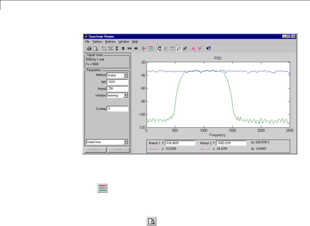
8SPTool: A Signal Processing GUI Suite

Printing the Spectra

Before printing the two spectra together, use the color and line style selection

button, ,todifferentiatethetwoplotsbylinestyle,ratherthanbycolor.

To print both spectra:

1Click Print Preview in the toolbar on the Spectrum Viewer.

2From the Spectrum Viewer Print Preview window, drag the legend out of

the display region so that it doesn’t obscure part of the plot.

3Click Print in the Spectrum Viewer Print Preview window.

8-26

Exporting Signals, Filters, and Spectra

In this section...

“Opening the Export Dialog Box” on page 8-27

“Exporting a Filter to the MATLAB Workspace” on page 8-28

Opening the Export Dialog Box

To save the filter filt1 you just created in this example, open the Export

dialog box with filt1 preselected:

1Select filt1 in the SPTool Filters list.

2Select File > Export.

The Export dialog box opens with filt1 preselected.

8-27

8SPTool: A Signal Processing GUI Suite

Exporting a Filter to the MATLAB Workspace

To export the filter filt1 to the MATLAB workspace:

1Select filt1 from the Export List and deselect all other items using

Ctrl+click.

2Click Export to Workspace.

8-28

Accessing Filter Parameters

In this section...

“Accessing Filter Parameters in a Saved Filter” on page 8-29

“Accessing Parameters in a Saved Spectrum” on page 8-30

Accessing Filter Parameters in a Saved Filter

The MATLAB structures created by SPTool have several associated fields,

many of which are also MATLAB structures. See the MATLAB documentation

for general information about MATLAB structures.

For example, after exporting a filter filt1 to the MATLAB workspace, type

filt1

to display the fields of the MATLAB filter structure. The tf field of the

structure contains information that describes the filter.

The tf Field: Accessing Filter Coefficients

The tf field is a structure containing the transfer function representation of

the filter. Use this field to obtain the filter coefficients;

•filt1.tf.num contains the numerator coefficients.

•filt1.tf.den contains the denominator coefficients.

The vectors contained in these structures represent polynomials in descending

powers of z. The numerator and denominator polynomials are used to specify

the transfer function

Hz Bz

bbz bnbz

aaz ana

() ()

()

() () ( )

() () (

++++

+++

−−

−

12 1



++ −

1)zn

where:

•bis a vector containing the coefficients from the tf.num field.

8-29

8SPTool: A Signal Processing GUI Suite

•ais a vector containing the coefficients from the tf.den field.

•mis the numerator order.

•nis the denominator order.

You can change the filter representation from the default transfer function to

another form by using the tf2ss or tf2zp functions.

Note The FDAspecs field of your filter contains internal information about

FDATool and should not be changed.

Accessing Parameters in a Saved Spectrum

The following structure fields describe the spectra saved by SPTool.

Field Description

PThe spectral power vector.

fThe spectral frequency vector.

confid A structure containing the confidence intervals data

•The confid.level field contains the chosen

confidence level.

•The confid.Pc field contains the spectral power

data for the confidence intervals.

•The confid.enable field contains a 1if confidence

levelsareenabledforthepowerspectraldensity.

signalLabel Thenameofthesignalfromwhichthepower

spectral density was generated.

Fs The associated signal’s sample rate.

You can access the information in these fields as you do with every MATLAB

structure.

For example, if you export an SPTool PSD estimate spect1 to the workspace,

type

8-30

Accessing Filter Parameters

spect1.P

to obtain the vector of associated power values.

8-31

8SPTool: A Signal Processing GUI Suite

Importing Filters and Spectra

In this section...

“Similarities to Other Procedures” on page 8-32

“Importing Filters” on page 8-32

“Importing Spectra” on page 8-34

Similarities to Other Procedures

The procedures are very similar to those explained in

•“Importing a Signal into SPTool” on page 8-16 for loading variables from

the workspace

•“Loading Variables from the Disk” on page 8-36 for loading variables from

your disk

Importing Filters

When you import filters, first select the appropriate filter form from the Form

list. SPTool does not currently support the import of filter objects.

8-32

Importing Filters and Spectra

Foreveryfilteryouspecifyavariablenameoravalueforthefilter’ssampling

frequency in the Sampling Frequency field. Each filter form requires

different variables.

Transfer Function

For Transfer Function, you specify the filter by its transfer function

representation:

Hz Bz

bbz bmz

aaz an

() ()

()

() () ( )

() () (

++++

−−

−

12 1



))zn−

•The Numerator field specifies a variable name or value for the numerator

coefficient vector b, which contains m+1 coefficients in descending powers

of z.

•The Denominator field specifies a variable name or value for the

denominator coefficient vector a, which contains n+1 coefficients in

descending powers of z.

State Space

For State Space, you specify the filter by its state-space representation:



xAxBu

yCxDu

The A-Matrix,B-Matrix,C-Matrix,andD-Matrix fields specifyavariable

name or a value for each matrix in this system.

Zeros, Poles, Gain

For Zeros, Poles, Gain, you specify the filter by its zero-pole-gain

representation:

Hz Zz

Pz kzz zz zzm

zp zp

() ()

()

( ( ))( ( )) ( ( ))

( ( ))( ( )) (

−− −

−−



zzpn−())

8-33

8SPTool: A Signal Processing GUI Suite

•The Zeros field specifies a variable name or value for the zeros vector z,

which contains the locations of mzeros.

•The Poles field specifies a variable name or value for the zeros vector p,

which contains the locations of npoles.

•The Gain field specifies a variable name or value for the gain k.

Second Order Sections

For 2nd Order Sections you specify the filter by its second-order section

representation:

Hz H z bbzbz

az az

kkk k

() ()==

−−

== ∏∏ 01

122

1122

11 1

The SOS Matrix field specifies a variable name or a value for the L-by-6

SOS matrix

sos

bbb aa

LLL L L

01 11 21 11 21

02 12 22 12 22

012 1 2

 

⎡⎡

⎣

⎢

⎤

⎦

⎥

whose rows contain the numerator and denominator coefficients bik and aik

of the second-order sections of H(z).

Note If you import a filter that was not created in SPTool, you can only edit

that filter using the Pole/Zero Editor.

Importing Spectra

When you import a power spectral density (PSD), you specify:

•A variable name or a value for the PSD vector in the PSD field

•AvariablenameoravalueforthefrequencyvectorintheFreq. Vector

field

8-34

Importing Filters and Spectra

The PSD values in the PSD vector correspond to the frequencies contained in

the Freq. Vector vector; the two vectors must have the same length.

8-35

8SPTool: A Signal Processing GUI Suite

Loading Variables from the Disk

To import variables representing signals, filters, or spectra from a MAT-file

on your disk;

1Select the From Disk radio button and do either of the following:

•TypethenameofthefileyouwanttoimportintotheMAT-file Name

field and press either the Tab or the Enter key on your keyboard.

•Select Browse, and then find and select the file you want to import

using Select > File to Open.ClickOK to close that dialog.

In either case, all variables in the MAT-file you selected are displayed

in the File Contents list.

2Select the variables to be imported into SPTool.

You can now import one or more variables from the File Contents list into

SPTool,aslongasthesevariablesare scalars, vectors, or matrices.

8-36

Saving and Loading Sessions

In this section...

“SPTool Sessions” on page 8-37

“Filter Formats” on page 8-37

SPTool Sessions

When you start SPTool, the default startup.spt session is loaded. To save

your work in the startup SPTool session, use File > Save Session or to

specify a session name, use File > Save Session As.

To recall a previously saved session, use File > Open Session.

Filter Formats

When you start SPTool or open a session, the current filter design format

preference is compared to the filter formats in the session. See “Setting

Preferences” on page 8-43.

•If the formats match, the session opens.

•If the filter preference is FDATool, but the session contains Filter Designer

filters, this warning displays:

8-37

8SPTool: A Signal Processing GUI Suite

Click Convert to convert the filters to FDATool format. Click Don’t Use

FDATool to leave the filters in Filter Designer format and change the

preference to Use Filter Designer.

•If the filter preference is Use Filter Designer, but the session contains

FDATool filters, this warning displays:

Click Yes to remove the current filters. Click No to leave the filters in

FDATool.

8-38

Selecting Signals, Filters, and Spectra

All signals, filters, or spectra listed in SPTool exist as special MATLAB

structures. You can bring data representing signals, filters, or spectra into

SPTool from the MATLAB workspace. In general, you can select one or

several items in a given list box. An item is selected when it is highlighted.

The Signals list shows all vector and array signals in the current SPTool

session.

The Filters list shows all designed and imported filters in the current SPTool

session.

The Spectra list shows all spectra in the current SPTool session.

You can select a single data object in a list, a range of data objects in a list,

or multiple separate data objects in a list. You can also have data objects

simultaneously selected in different lists:

•To select a single item, click it. All other items in that list box become

deselected.

•To add or remove a range of items, Shift+click on the items at the top and

bottom of the section of the list that you want to add. You can also drag

your mouse pointer to select these items.

•To add a single data object to a selection or remove a single data object

from a multiple selection, Ctrl+click on the object.

8-39

8SPTool: A Signal Processing GUI Suite

Editing Signals, Filters, or Spectra

You can edit selected items in SPTool by

1Selecting the names of the signals, filters, or spectra you want to edit.

2Selecting the appropriate Edit menu item:

•Duplicate to copy an item in an SPTool list

•Clear to delete an item in an SPTool list

•Name to rename an item in an SPTool list

•Sampling Frequency to modify the sampling frequency associated

with either a signal (and its associated spectra) or filter in an SPTool list

The pull-downmenunexttoeachmenuitemshowsthenamesofall

selected items.

You can also edit the following signal characteristics by right-clicking in the

display region of the Signal Browser, the Filter Visualization Tool, or the

Spectrum Viewer:

•The signal name

•The sampling frequency

•The line style properties

Note If you modify the sampling frequency associated with a signal’s

spectrum using the right-click menu on the Spectrum Viewer display region,

the sampling frequency of the associated signal is automatically updated.

8-40

Making Signal Measurements with Markers

You can use the markers on the Signal Browser or the Spectrum Viewer to

make measurements on either of the following:

•A signal in the Signal Browser

•A power spectral density plotted in the Spectrum Viewer

The following marker buttons are included

Icon Description

Toggle markers on/off

Vertical markers

Horizontal markers

Vertical markers with tracking

Vertical markers with tracking and slope

Display peaks (local maxima)

You can find peaks in a signal from the command line

with findpeaks

Display valleys (local minima)

To make a measurement:

1Select a line to measure (or play, if you are in the Signal Browser).

2Select one of the marker buttons to applyamarkertothedisplayedsignal.

8-41

8SPTool: A Signal Processing GUI Suite

3Position a marker in the main display area by grabbing it with your mouse

and dragging:

aSelect a marker setting. If you choose the Vertical,Track,orSlope

buttons, you can drag a marker to the right or left. If you choose the

Horizontal button, you can drag a marker up or down.

bMove the mouse over the marker (1 or 2) that you want to drag.

The hand cursor with the marker number inside it is displayed when

your mouse passes over a marker.

cDrag the marker to where you want it on the signal

As you drag a marker, the bottom of the Signal Browser shows the current

position of both markers. Depending on which marker setting you select,

some or all of the following fields are displayed — x1,y1,x2,y2,dx,dy,

m. These fields are also displayed when you print from the Signal Browser,

unless you suppress them.

You can also position a marker by typing its x1 and x2 or y1 and y2 values

in the region at the bottom.

8-42

Setting Preferences

In this section...

“Overview of Setting Preferences” on page 8-43

“Summary of Settable Preferences” on page 8-44

“Setting the Filter Design Tool” on page 8-45

Overview of Setting Preferences

Use File > Preferences to customize displays and certain parameters for

SPTool and its four component GUIs. If you change any preferences, a dialog

box displays when you close SPTool askingifyouwanttosavethosechanges.

If you click Yes, the new settings are saved on disk and are used when you

restart SPTool from the MATLAB workspace.

Note You can set MATLAB preferences that affect the Filter Visualization

Tool only from within FVTool by selecting File > Preferences. You can set

FVTool-specific preferences using Analysis > Analysis Parameters.

8-43

8SPTool: A Signal Processing GUI Suite

When you first select Preferences, the Preferences dialog box opens with

Markers selected by default.

Change any marker settings, if desired. To change settings for another

category, click its name in the category list to display its settings. Most

of the fields are self-explanatory. Details of the Filter Design options are

described below.

Summary of Settable Preferences

In the Preferences regions, you can

•Select colors and markers for all displays.

•Select colors and line styles for displayed signals.

•Configure labels, and enable/disable markers, panner, and zoom in the

Signal Browser.

•Configure display parameters, and enable/disable markers and zoom in

the Spectrum Viewer.

•Select whether to use the default FDATool or the Filter Designer to design

filters. FDATool is the recommended designer.

•Enable/disable use of a default session file.

8-44

Setting Preferences

•Export filters for use with Control System Toolbox software.

•Enable/disable search for plug-ins at startup.

Setting the Filter Design Tool

The Filter Designer options include radio buttons to select the filter design

tool.

FDATool is the default and recommended tool. You can use Filter Designer,

but Filter Designer will be removed in a future release. You cannot change

this preference if either FDATool or the Filter Designer is open.

Note Filters in any one SPTool session must be in the same format — either

FDATool format or Filter Designer format. You can convert filters from the

Filter Designer format to FDATool format, but you cannot convert FDATool

filters to Filter Designer format.

If you change the preference from Use FDATool to Use Filter Designer,

a warning message appears. The warning message informs you that filters

created with FDATool are not compatible with Filter Designer and that Filter

Designer will be removed in the future.

8-45

8SPTool: A Signal Processing GUI Suite

See “Saving and Loading Sessions” on page 8-37 for more information.

When you change the preference from Use Filter Designer to Use FDATool,

a confirmation message appears indicating that switching will convert your

filters to FDATool format. See “Saving and Loading Sessions” on page 8-37

for information on this message.

Changes to Filter Designer format are saved only if you save the session.

Exiting the session prompts you to save changes to the sigprefs.mat and

startup.spt files. Starting SPTool with Filter Designer specified as the filter

design tool results in the warning:

The warning appears each time SPTool initializes unless you opt to not show

the warning.

8-46

Using the Filter Designer

In this section...

“Filter Designer” on page 8-47

“Filter Types” on page 8-47

“FIR Filter Methods” on page 8-48

“IIR Filter Methods” on page 8-48

“Pole/Zero Editor” on page 8-48

“Spectral Overlay Feature” on page 8-48

“Opening the Filter Designer” on page 8-48

“Accessing Filter Parameters in a Saved Filter” on page 8-50

“Designing a Filter with the Pole/Zero Editor” on page 8-53

“Positioning Poles and Zeros” on page 8-54

“Redesigning a Filter Using the Magnitude Plot” on page 8-56

Filter Designer

“FDATool” on page 8-10 is the recommended filter design tool. Filter Designer

will be removed in a future release. The following information is provided for

users that choose to use Filter Designer while they transition to FDATool.

Filter Designer, provides an interactive graphical environment for the design

of digital IIR and FIR filters based on specifications that you enter on a

magnitude or pole-zero plot.

Filter Types

You can design filters of the following types using the Filter Designer:

•Bandpass

•Lowpass

•Bandstop

•Highpass

8-47

8SPTool: A Signal Processing GUI Suite

FIR Filter Methods

You can use the following filter methods to design FIR filters:

•Equiripple

•Least squares

•Window

IIR Filter Methods

You can use the following filter methods to design IIR filters:

•Butterworth

•Chebyshev Type I

•Chebyshev Type II

•Elliptic

Pole/ZeroEditor

You can use the Pole/Zero Editor to design arbitrary FIR and IIR filters by

placing and moving poles and zeros on the complex z-plane.

Spectral Overlay Feature

You can also superimpose spectra on a filter’s magnitude response to see if

the filtering requirements are met.

Opening the Filter Designer

Open the Filter Designer from SPTool by either:

•Clicking New in the Filters list in SPTool

•Selecting a filter you want to edit from the Filters list in SPTool, and

then clicking Edit

8-48

Using the Filter Designer

The Filter Designer has the following components:

•Apull-downFilter menu for selecting a filter from the list in SPTool

•ASampling Frequency text box

•Apull-downAlgorithm menu for selecting a filter design method or a

pole-zero plot display

•A Specifications area for viewing or modifying a filter’s design parameters

or pole-zero locations

•A plot display region for graphically adjusting filter magnitude responses

or the pole-zero locations

•A Measurements area for viewing the response characteristics and stability

of the current filter

•A toolbar with the following buttons

8-49

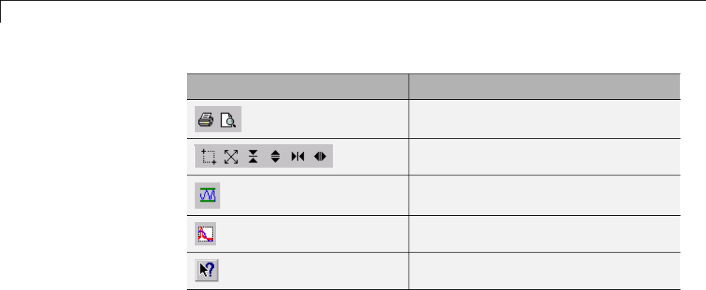
8SPTool: A Signal Processing GUI Suite

Icon Description

Print and print preview

Zoom in and out

Passband view

Overlay spectrum

Turn on the What’s This help

Accessing Filter Parameters in a Saved Filter

The MATLAB structures created by SPTool have several associated fields,

many of which are also MATLAB structures. See the MATLAB documentation

for general information about MATLAB structures.

For example, after exporting a filter filt1 to the MATLAB workspace, type

filt1

to display the fields of the MATLAB filter structure. The tf, Fs,andspecs

fields of the structure contain the information that describes the filter.

The tf Field: Accessing Filter Coefficients

The tf field is a structure containing the transfer function representation of

the filter. Use this field to obtain the filter coefficients;

•filt1.tf.num contains the numerator coefficients.

•filt1.tf.den contains the denominator coefficients.

The vectors contained in these structures represent polynomials in descending

powers of z. The numerator and denominator polynomials are used to specify

the transfer function

8-50

Using the Filter Designer

Hz Bz

bbz bnbz

aaz ana

() ()

()

() () ( )

() () (

++++

+++

−−

−

12 1



++ −

1)zn

where:

•bis a vector containing the coefficients from the tf.num field.

•ais a vector containing the coefficients from the tf.den field.

•mis the numerator order.

•nis the denominator order.

You can change the filter representation from the default transfer function to

another form by using the tf2ss or tf2zp functions.

The Fs Field: Accessing Filter Sample Frequency

The Fs field contains the sampling frequency of the filter in hertz.

The specs Field: Accessing other Filter Parameters

The specs field is a structure containing parameters that you specified

for the filter design. The first field, specs.currentModule,containsa

string representing the most recent design method selected from the Filter

Designer’s Algorithm list before you exported the filter. The possible

contents of the currentModule field and the corresponding design methods

are shown below.

Contents of the currentModule

field Design Method

fdbutter Butterworth IIR

fdcheby1 Chebyshev Type I IIR

fdcheby2 Chebyshev Type II IIR

fdellip Elliptic IIR

fdfirls Least Squares FIR

fdkaiser Kaiser Window FIR

fdremez Equiripple FIR

8-51

8SPTool: A Signal Processing GUI Suite

Following the specs.currentModule field, there may be up to seven

additional fields, with labels such as specs.fdremez,specs.fdfirls,etc.

The design specifications for the most recently exported filter are contained

in the field whose label matches the currentModule string. For example, if

the specs structure is

filt1.specs

ans

currentModule: 'fdremez'

fdremez: [1x1 struct]

the filter specifications are contained in the fdremez field, which is itself

adatastructure.

The specifications include the parameter values from the Specifications region

of the Filter Designer, such as band edges and filter order. For example, the

filter above has the following specifications stored in filt1.specs.fdremez:

filt1.specs.fdremez

ans =

setOrderFlag: 0

type: 3

f: [0 0.2000 0.3000 0.5000 0.6000 1]

m: [6x1 double]

Rp: 0.0100

Rs: 75

wt: [3.2371 1 3.2371]

order: 78

Because certain filter parameters are unique to a particular design, this

structure has a different set of fields for each filter design.

The table below describes the possible fields associated with the filter design

specification field (the specs field) that can appear in the exported structure.

8-52

Using the Filter Designer

Parameter Description

Beta Kaiser window βparameter.

fContains a vector of band-edge frequencies, normalized

so that 1 Hz corresponds to half the sample frequency.

Fpass Passband cutoff frequencies. Scalar for lowpass and

highpass designs, two-element vector for bandpass and

bandstop designs.

Fstop Stopband cutoff frequencies. Scalar for lowpass and

highpass designs, two-element vector for bandpass and

bandstop designs.

mTheresponsemagnitudescorresponding to the band-edge

frequencies in f.

order Filter order.

Rp Passband ripple (dB)

Rs Stopband attenuation (dB)

setOrderFlag Contains 1if the filter order was specified manually (i.e.,

the Minimum Order box in the Specifications region

was not selected). Contains 0if the filter order was

computed automatically.

type Contains 1for lowpass, 2for highpass, 3for bandpass, or

4for bandstop.

w3db -3 dB frequency for Butterworth IIR designs.

wind Vector of Kaiser window coefficients.

Wn Cutoff frequency for the Kaiser window FIR filter when

setOrderFlag = 1.

wt Vector of weights, one weight per frequency band.

Designing a Filter with the Pole/Zero Editor

To design a filter transfer function using the Filter Designer Pole/Zero Editor:

1Select the Pole/Zero Editor option from the Algorithm list to open the

Pole/Zero Editor in the Filter Designer display.

8-53

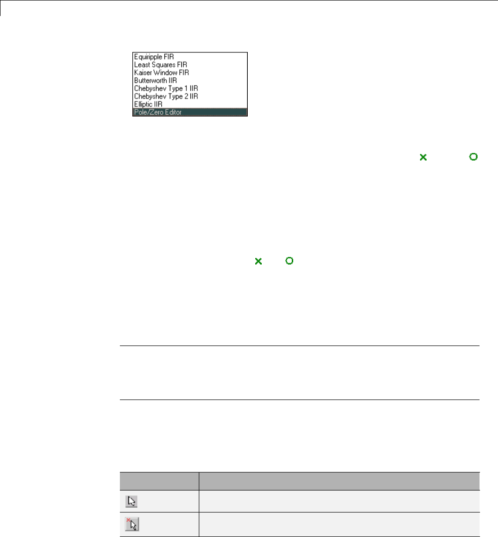
8SPTool: A Signal Processing GUI Suite

2EnterthedesiredfiltergainintheGain edit box.

3Select a pole or zero (or conjugate pair) by selecting one of the (pole) or

(zero) symbols on the plot.

4Choose the coordinates to work in by specifying Polar or Rectangular

from the Coordinates list.

5Specify the new location(s) of the selected pole, zero, or conjugate pair by

typing values into the Mag and Angle fields (for angular coordinates) or X

and Y(for rectangular coordinates) fields. Alternatively, position the poles

and zeros by dragging the and symbols.

6Use the Conjugate pair check box to create a conjugate pair from a lone

pole or zero, or to break a conjugate pair into two individual poles or zeros.

Design a new filter or edit an existing filter in the same way.

Note Keep the Filter Visualization Tool (FVTool) open while designing a

filter with the Pole/Zero Editor. Any changes that you make to the filter

transfer function in the Pole/Zero Editor are then simultaneously reflected in

theresponseplotsofFVTool.

Positioning Poles and Zeros

You can use your mouse to move poles and zeros around the pole/zero plot

and modify your filter design.

Icon Description

Enable moving poles or zeros by dragging on the plot

Add pole

8-54

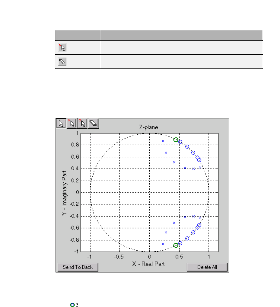
Using the Filter Designer

Icon Description

Add zero

Erase poles or zeros

You can move both members of a conjugate pair simultaneously by

manipulating just one of the poles or zeros.

To ungroup conjugates, select the desired pair and clear Conjugate pair in

the Specifications region on the Filter Designer.

When you place two or more poles (or two or more zeros) directly on top of each

other, a number is displayed next to the symbols (on the left for poles, and on

the right for zeros) indicating the number of poles or zeros at that location

(e.g., for three zeros). This number makes it easy to keep track of all the

8-55

8SPTool: A Signal Processing GUI Suite

poles and zeros in the plot area, even when several are superimposed on each

other and are not visually differentiable. Note, however, that this number

does not indicate the multiplicity of the poles or zeros to which it is attached.

To detect whether or not a set of poles or zeros are truly multiples, use the

zoom tools to magnify the region around the poles or zeros in question.

Because numerical limitations usually prevent any set of poles or zeros from

sharing exactly thesamevalue,atahighenoughzoomleveleventruly

multiple poles or zeros appear distinct from each other.

A common way to assess whether a particular group of poles or zeros contains

multiples is by comparing the mutual proximity of the group members against

a selected threshold value. As an example, the residuez function defines a

pole or zero as being a multiple of another pole or zero if the absolute distance

separating them is less than 0.1% of the larger pole or zero’s magnitude.

Redesigning a Filter Using the Magnitude Plot

After designing a filter in the Filter Designer, you can redesign it by dragging

the specification lines on the magnitude plot. Use the specification lines to

change passband ripple, stopband attenuation, and edge frequencies.

In the following example, create a Chebyshev filter and modify it by dragging

the specification lines:

1Select Chebyshev Type I IIR from the Algorithm menu.

2Select highpass from the Type menu.

3Type 2000 in the Sampling Frequency field.

4Set the following parameters:

•Fp =800

•Fs =700

•Rp =2.5

•Rs =35

5Select Minimum Order so the Filter Designer can calculate the lowest

filter order that produces the desired characteristics.

8-56

Using the Filter Designer

6Click Apply to compute the filter and update the response plot.

7Position the cursor over the horizontal filter specification line for the

stopband. This is the first (leftmost) horizontal specification line you see.

The cursor changes to the up/down drag indicator.

8DragthelineuntiltheRs (stopband attenuation) field reads 100.

Note The Order value in the Measurements region changes because a

higher filter order is needed to meet the new specifications.

8-57

8SPTool: A Signal Processing GUI Suite

8-58

Code Generation from

MATLAB Support in Signal

Processing Toolbox

•“Supported Functions” on page 9-2

•“Specifying Inputs in Code Generation from MATLAB ” on page 9-7

•“Code Generation Examples” on page 9-11

9Code Generation from MATLAB®Support in Signal Processing Toolbox™

Supported Functions

Code generation from MATLAB is a restricted subset of the MATLAB

language that provides optimizations for:

•Generating efficient, production-quality C/C++ code and MEX files for

deployment in desktop and embedded applications. For embedded targets,

the subset restricts MATLAB semantics to meet the memory and data type

requirements of the target environments.

Depending on which feature you wish to use, there are additional required

products. For a comprehensive list, see “Installing Prerequisite Products” in

the Embedded Coder®documentation.

Code generation from MATLAB supports Signal Processing Toolbox functions

listed in the table. You must have the DSP System Toolbox software installed

to use this feature. To generate C code, you must have the MATLAB Coder™

software. If you have the Fixed-Point Toolbox, you can use fiaccel to

generate MEX code for fixed-point applications.

To follow the examples in this documentation:

•To generate C/C++ code and MEX files with codegen, install the MATLAB

Coder software, the Signal Processing Toolbox, the DSP System Toolbox,

and a C compiler. For the Windows®platform, MATLAB supplies a default

Ccompiler. Runmex -setup at the MATLAB command prompt to set up

the C compiler.

•Change to a folder where you have write permission.

Note Many Signal Processing Toolbox functions require constant inputs in

generated code. To specify a constant input for codegen,usecoder.Constant.

9-2

Supported Functions

Function Remarks/Limitations

barthannwin Window length must be a constant. Expressions or variables are

allowed if their values do not change.

bartlett Window length must be a constant. Expressions or variables are

allowed if their values do not change.

besselap Filter order must be a constant. Expressions or variables are allowed if

their values do not change.

bitrevorder —

blackman Window length must be a constant. Expressions or variables are

allowed if their values do not change.

blackmanharris Window length must be a constant. Expressions or variables are

allowed if their values do not change.

bohmanwin Window length must be a constant. Expressions or variables are

allowed if their values do not change.

buttap Filter order must be a constant. Expressions or variables are allowed if

their values do not change.

butter Filter coefficients must be constants. Expressions or variables are

allowed if their values do not change.

buttord All inputs must be constants. Expressions or variables are allowed if

their values do not change.

cfirpm All inputs must be constants. Expressions or variables are allowed if

their values do not change.

cheb1ap All inputs must be constants. Expressions or variables are allowed if

their values do not change.

cheb2ap All inputs must be constants. Expressions or variables are allowed if

their values do not change.

cheb1ord All inputs must be constants. Expressions or variables are allowed if

their values do not change.

cheb2ord All inputs must be constants. Expressions or variables are allowed if

their values do not change.

chebwin All inputs must be constants. Expressions or variables are allowed if

their values do not change.

9-3

9Code Generation from MATLAB®Support in Signal Processing Toolbox™

Function Remarks/Limitations

cheby1 All Inputs must be constants. Expressions or variables are allowed if

their values do not change.

cheby2 All inputs must be constants. Expressions or variables are allowed if

their values do not change.

dct Length of transform dimension must be a power of two. If specified, the

pad or truncation value must be constant. Expressions or variables are

allowed if their values do not change.

downsample —

dpss All inputs must be constants. Expressions or variables are allowed if

their values do not change.

ellip Inputs must be constant. Expressions or variables are allowed if their

values do not change.

ellipap All inputs must be constants. Expressions or variables are allowed if

their values do not change.

ellipord All inputs must be constants. Expressions or variables are allowed if

their values do not change.

filtfilt Filter coefficients must be constants. Expressions or variables are

allowed if their values do not change.

fir1 All inputs must be constants. Expressions or variables are allowed if

their values do not change.

fir2 All inputs must be constants. Expressions or variables are allowed if

their values do not change.

fircls All inputs must be constants. Expressions or variables are allowed if

their values do not change.

fircls1 All inputs must be constants. Expressions or variables are allowed if

their values do not change.

firls All inputs must be constants. Expressions or variables are allowed if

their values do not change.

firpm All inputs must be constants. Expressions or variables are allowed if

their values do not change.

9-4

Supported Functions

Function Remarks/Limitations

firpmord All inputs must be constants. Expressions or variables are allowed if

their values do not change.

firrcos All inputs must be constants. Expressions or variables are allowed if

their values do not change.

flattopwin All inputs must be constants. Expressions or variables are allowed if

their values do not change.

freqz freqz with no output arguments produces a plot only when the function

call terminates in a semicolon. See “freqz With No Output Arguments”

on page 9-15.

gaussfir All inputs must be constant. Expressions or variables are allowed if

their values do not change.

gausswin All inputs must be constant. Expressions or variables are allowed if

their values do not change.

hamming All inputs must be constant. Expressions or variables are allowed if

their values do not change.

hann All inputs must be constant. Expressions or variables are allowed if

their values do not change.

idct Length of transform dimension must be a power of two. If specified, the

pad or truncation value must be constant. Expressions or variables are

allowed if their values do not change.

intfilt All inputs must be constant. Expressions or variables are allowed if

their values do not change.

kaiser All inputs must be constant. Expressions or variables are allowed if

their values do not change.

kaiserord —

levinson If specified, the order of recursion must be a constant. Expressions or

variables are allowed if their values do not change.

maxflat All inputs must be constant. Expressions or variables are allowed if

their values do not change.

nuttallwin All inputs must be constant. Expressions or variables are allowed if

their values do not change.

9-5

9Code Generation from MATLAB®Support in Signal Processing Toolbox™

Function Remarks/Limitations

parzenwin All inputs must be constant. Expressions or variables are allowed if

their values do not change.

rectwin All inputs must be constant. Expressions or variables are allowed if

their values do not change.

resample The upsampling and downsampling factors must be specified as

constants. Expressions or variables are allowed if their values do not

change.

sgolay All inputs must be constant. Expressions or variables are allowed if

their values do not change.

sosfilt —

taylorwin All inputs must be constant. Expressions or variables are allowed if

their values do not change.

triang All inputs must be constant. Expressions or variables are allowed if

their values do not change.

tukeywin All inputs must be constant. Expressions or variables are allowed if

their values do not change.

upfirdn •Filter coefficients, upsampling factor, and downsampling factor must

be constants. Expressions or variables are allowed if their values

do not change.

•Variable-size inputs are not supported.

upsample Either declare input nas constant, or use the assert function in the

calling function to set upper bounds for n. For example,

assert(n<10)

xcorr —

yulewalk If specified, the order of recursion must be a constant. Expressions or

variables are allowed if their values do not change.

9-6

Specifying Inputs in Code Generation from MATLAB®

Specifying Inputs in Code Generation from MATLAB

In this section...

“Defining Input Size and Type” on page 9-7

“Inputs must be Constants” on page 9-8

Defining Input Size and Type

When you use Signal Processing Toolbox functions for code generation, you

must define the size and type of the function inputs. One way to do this is

with the -args compilation option. The size and type of inputs must be

defined because C is a statically typed language. . To illustrate the need to

define input size and type, consider the simplest call to xcorr requiring two

input arguments. The following demonstrates the differences in the use of

xcorr in MATLAB and in Code Generation from MATLAB.

Cross correlate two white noise vectors in MATLAB:

x = randn(512,1); %real valued white noise

y = randn(512,1); %real valued white noise

[C,lags] = xcorr(x,y);

x_circ = randn(256,1)+1j*randn(256,1); %circular white noise

y_circ = randn(256,1)+1j*randn(256,1); %circular white noise

[C1,lags1] = xcorr(x_circ,y_circ);

xcorr does not require any information about the size and type of the

input arguments. xcorr obtains this information at runtime. Contrast this

behavior with a MEX-file created with codegen.Createthefilemyxcorr.m in

a folder where you have read and write permission. Ensure that this folder

is in the MATLAB search path. Copy and paste the following two lines of

code into myxcorr.m and save the file. The compiler tag %#codegen must

be included in the file.

function [C,Lags]=myxcorr(x,y) %#codegen

[C,Lags]=xcorr(x,y);

Enter the following command at the MATLAB command prompt:

codegen myxcorr -args {zeros(512,1),zeros(512,1)} -o myxcorr

9-7

9Code Generation from MATLAB®Support in Signal Processing Toolbox™

Run the MEX-file:

x = randn(512,1); %real valued white noise

y = randn(512,1); %real valued white noise

[C,Lags] = myxcorr(x,y);

Define two new inputs x1 and y1 by transposing xand y.

x1 = x'; %x1 is 1x512

y1 = y'; %y1 is 1x512

Attempt to rerun the MEX-file with the tranposed inputs.

[C,Lags] = myxcorr(x1,y1); %Errors

The preceding program errors with the message ??? MATLAB expression

'x' is not of the correct size: expected [512x1] found [1x512]..

The error results because the inputs are specified to be 512x1 real-valued

column vectors at compilation. For complex-valued inputs, you must specify

that the input is complex valued. For example:

codegen myxcorr -o ComplexXcorr ...

-args {complex(zeros(512,1)),complex(zeros(512,1))}

Run the MEX-file at the MATLAB command prompt with complex-valued

inputs of the correct size:

x_circ = randn(512,1)+1j*randn(512,1); %circular white noise

y_circ = randn(512,1)+1j*randn(512,1); %circular white noise

[C,Lags] = ComplexXcorr(x_circ,y_circ);

Attempting to run ComplexXcorr with real valued inputs results in the error:

??? MATLAB expression 'x' is not of the correct complexness.

Inputs must be Constants

For a number of supported Signal Processing Toolbox functions, the inputs

or a subset of the inputs must be specified as constants at compilation

time. Functions with this behavior are noted in the right column of the

table “Supported Functions” on page 9-2. Use coder.Type with the -args

compilation option, or enter the constants directly in the source code.

9-8

Specifying Inputs in Code Generation from MATLAB®

Specifying inputs as constants at compilation time results in significant

advantages in the speed and efficiency of the generated code. For example,

storing filter coefficients or window function values as vectors in the C source

code improves performance by avoiding costly computation at runtime.

Because a primary purpose of Code Generation from MATLAB is to generate

optimized C code for desktop and embeddedsystems,emphasisisplacedon

providing the user with computational savings at runtime whenever possible.

To illustrate the constant input requirement with butter, create the file

myLowpassFilter.m inafolderwhereyouhavereadandwritepermission.

Ensure that this folder is in the MATLAB search path. Copy and paste the

following lines of code into myLowpassFilter.m and save the file.

function output = myLowpassFilter(input,N,Wn) %#codegen

[B,A] = butter(N,Wn,'low');

output = filter(B,A,input);

If you have the MATLAB Coder software, enter the following command at the

MATLAB command prompt:

codegen myLowpassFilter -o myLowpassFilter ...

-args {zeros(512,1), coder.newtype('constant',5),coder.newtype('constant',

Once the program compiles successfully, the following message appears in the

command window: Code generation successful: View report.

Click on View report.ClickontheC code tab on the top left and open the

target source file myLowpassFilter.c.

Note that the numerator and denominator filter coefficients are included in

the source code.

static real_T dv0[6] = { 5.9795780369978346E-5, 0.00029897890184989173,

static real_T dv1[6] = { 1.0, -3.9845431196123373, 6.4348670902758709, .

Run the MEX-file without entering the constants:

output = myLowpassFilter(randn(512,1));

If you attempt to run the MEX-file by inputting the constants, you receive

the error ??? Error using ==> myLowpassFilter 1 input required for

entry-point 'myLowpassFilter'..

9-9

9Code Generation from MATLAB®Support in Signal Processing Toolbox™

You may also enter the constants in the MATLAB source code directly. Edit

the myLowPassFilter.m file and replace the MATLAB code with the lines:

function output = myLowpassFilter(input) %#codegen

[B,A] = butter(5,0.1,'low');

output = filter(B,A,input);

Enter the following command at the MATLAB command prompt:

codegen myLowpassFilter -args {zeros(512,1)} -o myLowpassFilter

Run the MEX-file by entering the following at the MATLAB command prompt:

output = myLowpassFilter(randn(512,1));

See “Apply Window to Input Signal” on page 9-11 ,“Apply Lowpass Filter

to Input Signal” on page 9-13, and “Zero Phase Filtering” on page 9-16 for

additional examples of the constant input requirement.

9-10

Code Generation Examples

In this section...

“Apply Window to Input Signal” on page 9-11

“Apply Lowpass Filter to Input Signal” on page 9-13

“Cross Correlate or Autocorrelate Input Data” on page 9-14

“freqz With No Output Arguments” on page 9-15

“Zero Phase Filtering” on page 9-16

Apply Window to Input Signal

In this example, apply a Hamming window to an input data vector of size

512x1.

Create a file called window_data.m by typing

>>edit window_data

at the MATLAB command prompt.

Copy and paste the code provided into the editor and save the file.

function output_data=window_data(input_data,N) %#codegen

Win=hamming(N);

output_data=input_data.*Win;

Use codegen to generate a MEX–file window_data.m.

codegen window_data -args {zeros(512,1),coder.newtype('constant',512)} -o

The -args option defines the input specifications for the MEX –file.

input_data is a 512x1 real valued vector. Because the input to hamming

must be a constant, coder.newtype is used to specify the window length. In

a conventional MATLAB program, you can read the input data length at

runtime and construct a Hamming window of the corresponding length.

Alternatively, edit the code for window_data.m as follows:

9-11

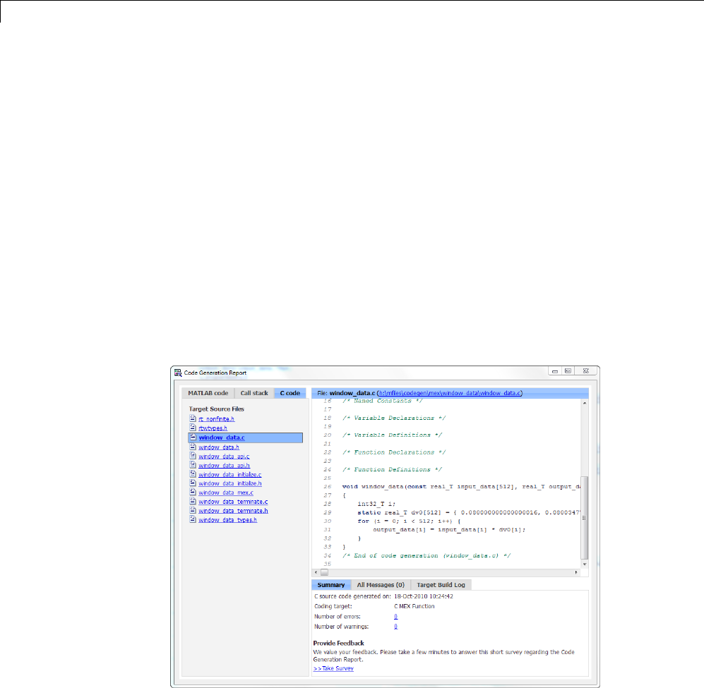
9Code Generation from MATLAB®Support in Signal Processing Toolbox™

function output_data=window_data(input_data) %#codegen

Win=hamming(512);

output_data=input_data.*Win;

The preceding code specifies the length of the Hamming window in the

source code as opposed to using coder.newtype.Usecodegen to generate a

MEX–file and C code:

codegen window_data -args {zeros(512,1)} -o window_data -report

The -report flag generates a compilation report. If the codegen operation is

successful, you obtain: Code generation successful: View report.

Click on View report to view the Code Generation Report.

Select the C-code tab and select window_data.c as the Target Source File.

Note from the location bar that the C source code is in the

codegen/mex/<FUNCTION_NAME> folder. Running codegen creates this folder

9-12

Code Generation Examples

and places the C source code, C header files, and MEX files in the folder. Each

function that you create produces a codegen/mex/<FUNCTION_NAME> folder.

Scroll through the C code to see that the values of the Hamming window are

included directly in the C source code.

Run the MEX-file on a white noise input:

% Window white noise input

output_data=window_data(randn(512,1));

Apply Lowpass Filter to Input Signal

Assuming a sampling frequency of 20 kHz, create a 4–th order Butterworth

filter with a 3–dB frequency of 2.5 kHz. Use the Butterworth filter to lowpass

filter a 10000x1 input data vector.

Create a file called ButterFilt.m. Copy and paste the following code into

the file.

function output_data=ButterFilt(input_data) %#codegen

[b,a]=butter(4,0.25);

output_data=filter(b,a,input_data);

Run the codegen command to obtain the C source code ButterFilt.c and

MEX file:

codegen ButterFilt -args {zeros(10000,1)} -o ButterFilt -report

The C source code includes the five numerator and denominator coefficients

of the 4–th order Butterworth filter as constants.

static real_T dv0[5] = { 0.010209480791203124, 0.040837923164812495, 0.061

static real_T dv1[5] = { 1.0, -1.9684277869385174, 1.7358607092088851, -0.

Apply the filter using the MEX-file:

Fs=20000;

%Create 10000x1 input signal

t=0:(1/Fs):0.5-(1/Fs);

input_data=(cos(2*pi*1000*t)+sin(2*pi*500*t)+0.2*randn(size(t)))';

%Filter data

9-13

9Code Generation from MATLAB®Support in Signal Processing Toolbox™

output_data=ButterFilt(input_data);

Cross Correlate or Autocorrelate Input Data

Estimate the cross correlation or autocorrelation of two real-valued input

vectors to lag 50. Output the estimate at the nonnegative lags.

Create a file called myxcorr.m. Copy and paste the following code into the file:

function [C,Lags]=myxcorr(x,y) %#codegen

[c,lags]=xcorr(x,y,50,'coeff');

C=c(51:end);

Lags=lags(51:end);

Run the codegen command at the MATLAB command prompt:

codegen myxcorr -args {zeros(512,1), zeros(512,1)} -o myxcorr -report

Use the MEX-file to compute and plot the autocorrelation of a white noise

input:

rng(0,'twister')

%White noise input

input_data=randn(512,1);

%Compute autocorrelation with MEX-file

[C,Lags]=myxcorr(input_data,input_data);

% Plot the result

stem(Lags,C); axis([-0.5 51 -1.1 1.1])

xlabel('Lags'); ylabel('Autocorrelation Function');

9-14

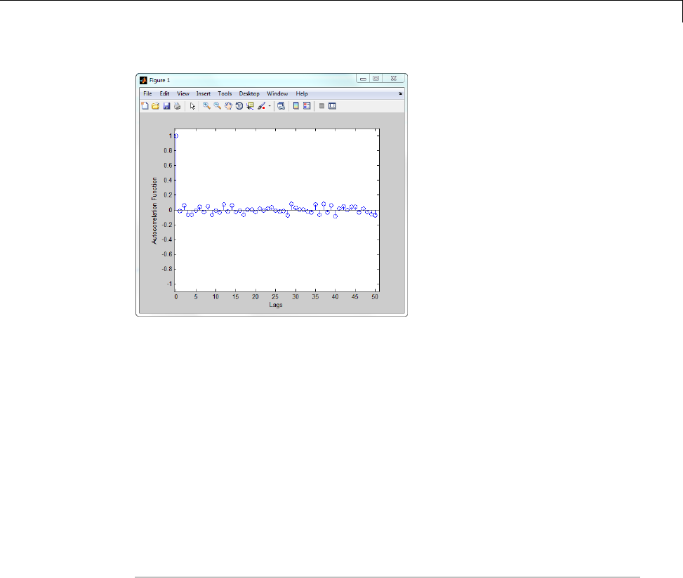
Code Generation Examples

freqz With No Output Arguments

In Code Generation from MATLAB, freqz with no output arguments behaves

differently than in the standard MATLAB language. In standard MATLAB,

freqz with no output arguments produces a plot of the magnitude and phase

response of the input filter. The plot is produced regardless of whether the

call to freqz terminates in a semicolon or not. No frequency response or

phase vectors are returned.

freqz with no output arguments and no terminating semicolon:

B = [0.05 0.9 0.05]; %Numerator coefficients

freqz(B,1) %no semicolon. Plot is produced

freqzwith no output arguments and terminating in a semicolon:

B = [0.05 0.9 0.05]; %Numerator coefficients

freqz(B,1); %semicolon. Plot is produced

The behavior shown in the preceding examples differs from the expected

behavior of a MEX-file using freqz with code generation support. To

illustrate this difference create a program called myfreqz.m.

9-15

9Code Generation from MATLAB®Support in Signal Processing Toolbox™

Copy and paste the following code into the file:

function myfreqz(B,A) %#codegen

freqz(B,A)

Run the following command at the MATLAB command prompt:

codegen myfreqz -args {zeros(1,3), zeros(1,1)} -o myfreqz

Calling the MEX-file writes a 512x1 complex-valued vector to the workspace

and displays the output. The vector is the frequency response. No plot is

produced.

myfreqz([0.05 0.9 0.05],1);

Change the code in myfreqz.m by adding a terminating semicolon:

function myfreqz(B,A) %#codegen

freqz(B,A);

Run the following command at the MATLAB command prompt:

codegen myfreqz -args {zeros(1,3), zeros(1,1)} -o myfreqz

Calling the MEX-file produces a plot of the magnitude and phase response of

the filter. The output of the complex-valued frequency response is suppressed.

myfreqz([0.05 0.9 0.05],1);

Zero Phase Filtering

Design a lowpass Butterworth filter with a 1 kHz 3–dB frequency to

implement zero phase filtering on data with a sampling frequency of 20 kHz.

[B,A] = butter(20,0.314,'low');

Create the program myZerophaseFilt.m.

function output = myZerophaseFilt(input) %#codegen

B=1e-3 *[

0.0000

0.0001

0.0010

0.0060

9-16

Code Generation Examples

0.0254

0.0814

0.2035

0.4071

0.6615

0.8820

0.9702

0.8820

0.6615

0.4071

0.2035

0.0814

0.0254

0.0060

0.0010

0.0001

0.0000];

A=[1.0000

-7.4340

28.2476

-71.6333

134.6222

-197.9575

235.1628

-230.2286

188.0901

-129.1746

74.8284

-36.5623

15.0197

-5.1525

1.4599

-0.3361

0.0613

-0.0085

0.0009

-0.0001

0.0000];

output = filtfilt(B,A,input);

9-17

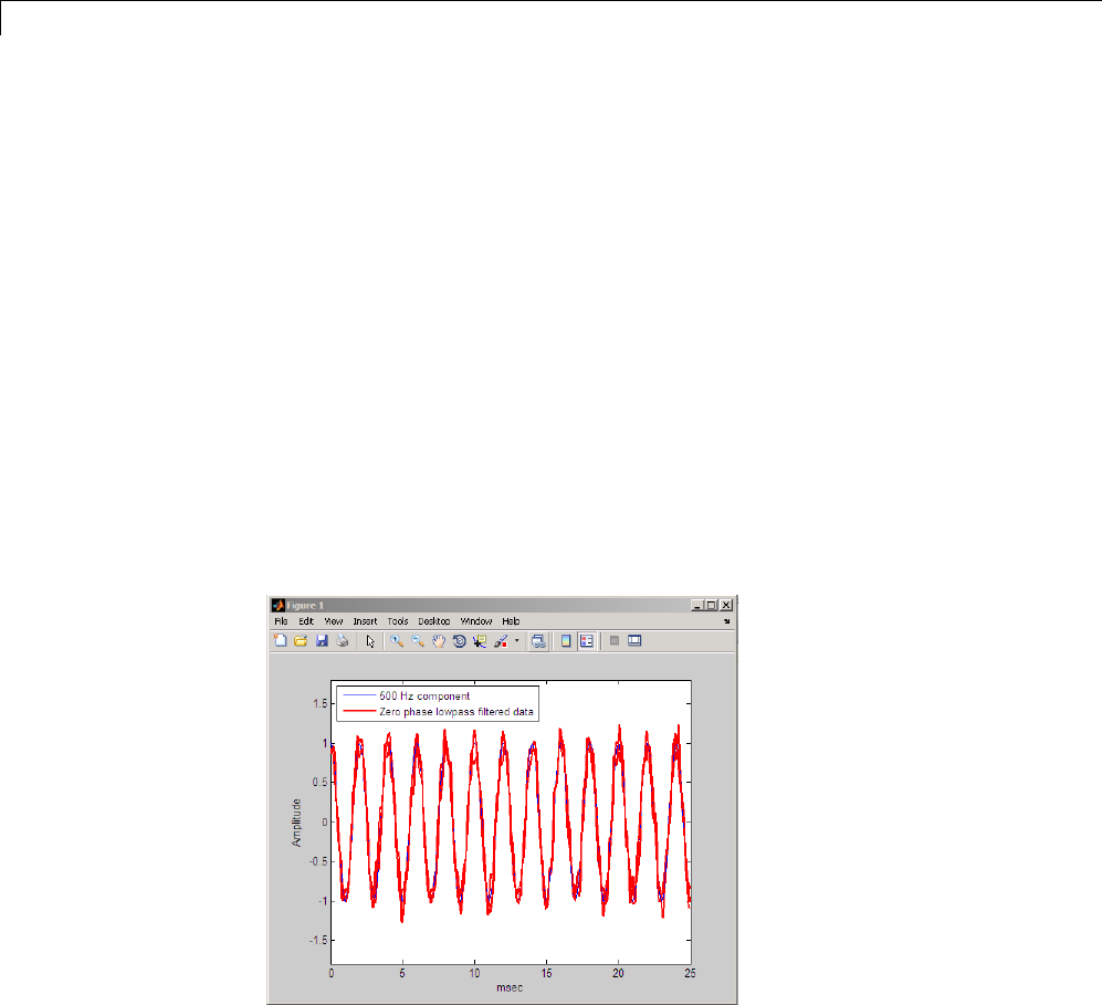
9Code Generation from MATLAB®Support in Signal Processing Toolbox™

Run the following command at the MATLAB command prompt:

codegen myZerophaseFilt -args {zeros(1,20001)} -o myZerophaseFilt

Filter input data with myZerophaseFilt:

Fs = 20000;

t = 0:(1/Fs):1;

Comp500Hz = cos(2*pi*500*t);

Signal = Comp500Hz+sin(2*pi*4000*t)+0.2*randn(size(t));

FilteredData = myZerophaseFilt(Signal);

plot(t(1:500).*1000,Comp500Hz(1:500));

xlabel('msec'); ylabel('Amplitude');

axis([0 25 -1.8 1.8]); hold on;

plot(t(1:500).*1000,FilteredData(1:500),'r','linewidth',2);

legend('500 Hz component','Zero phase lowpass filtered data',...

'Location','NorthWest');

9-18

Convolution and

Correlation

•“LinearandCircularConvolution”onpage10-2

•“Confidence Intervals for Sample Autocorrelation” on page 10-5

•“Residual Analysis with Autocorrelation” on page 10-9

•“Autocorrelation of Moving Average Process” on page 10-19

•“Cross-correlation of Two Moving Average Processes” on page 10-21

•“Cross-correlation of Delayed Signal in Noise” on page 10-23

•“Cross-correlation of Phase-Lagged Sine Wave” on page 10-26

10 Convolution and Correlation

Linear and Circular Convolution

This example shows how to establish an equivalence between linear and

circular convolution.

Linear and circular convolution are fundamentally different operations.

However, there are conditions under which linear and circular convolution

are equivalent. Establishing this equivalence has important implications. For

two vectors, xand y, the circular convolution is equal to the inverse discrete

Fourier transform (DFT) of the product of the vectors’ DFTs. Knowing the

conditions under which linear and circular convolution are equivalent allows

you to use the DFT to efficiently compute linear convolutions.

The linear convolution of an N-point vector, x, and a L-point vector, y,has

length N+L-1.

For the circular convolution of xand yto be equivalent, you must pad the

vectors with zeros to length at least N+L-1 before you take the DFT. After you

invert the product of the DFTs, retain only the first N+L-1 elements.

Create two vectors, xand y, and compute the linear convolution of the two

vectors.

x = [2 1 2 1];

y=[123];

clin = conv(x,y);

The output has length 4+3–1.

Pad both vectors with zeros to length 4+3–1. Obtain the DFT of both vectors,

multiply the DFTs, and obtain the inverse DFT of the product.

xpad = [x zeros(1,6-length(x))];

ypad = [y zeros(1,6-length(y))];

ccirc = ifft(fft(xpad).*fft(ypad));

The circular convolution of the zero-padded vectors, xpad and ypad,is

equivalent to the linear convolution of xand y. You retain all the elements of

ccirc because the output has length 4+3–1.

10-2

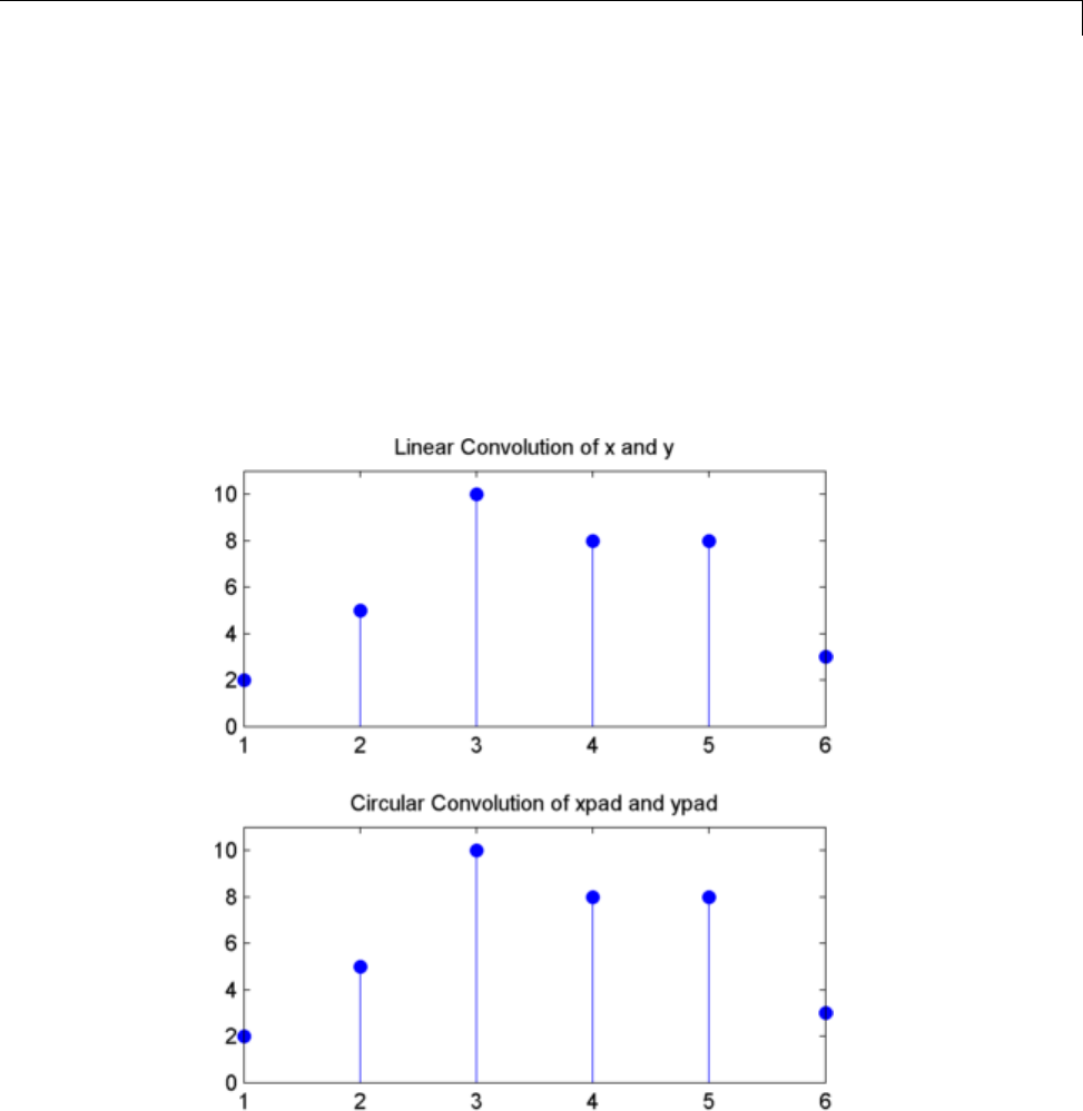
Linear and Circular Convolution

Plot the output of linear convolution and the inverse of the DFT product to

show the equivalence.

subplot(211)

stem(clin,'markerfacecolor',[0 0 1]);

title('Linear Convolution of x and y');

set(gca,'ylim',[0 11]);

subplot(212)

stem(ccirc,'markerfacecolor',[0 0 1]);

set(gca,'ylim',[0 11]);

title('Circular Convolution of xpad and ypad');

10-3

10 Convolution and Correlation

Pad the vectors to length 12 and obtain the circular convolution using the

inverse DFT of the product of the DFTs. Retain only the first 4+3–1 elements

to produce an equivalent result to linear convolution.

N = length(x)+length(y)-1;

xpad = [x zeros(1,12-length(x))];

ypad = [y zeros(1,12-length(y))];

ccirc = ifft(fft(xpad).*fft(ypad));

ccirc = ccirc(1:N);

The Signal Processing Toolbox software has a function, cconv, that returns

the circular convolution of two vectors. You can obtain the linear convolution

of xand yusing circular convolution with the following code.

ccirc2 = cconv(x,y,6);

cconv internallyusesthesameDFT-based procedure illustrated in the

previous example.

10-4

Confidence Intervals for Sample Autocorrelation

This example shows how to construct confidence intervals for the sample

autocorrelation of a white noise process. Having confidence intervals for a

white noise process is important, because many time series procedures aim to

whiten, or decorrelate a random process. To determine the effectiveness of the

whitening procedure, you examine the autocorrelation.

If x(n) is a white noise process, the sample normalized autocorrelation is

approximately normally distributed with mean zero and variance 1/N, where

N is the length of the input vector. In other words, the sample normalized

autocorrelation values follow a N(0,1/N) distribution.

You can form an approximate confidence interval using the mean plus

or minus the appropriate α-level critical value on the standard normal

distribution times the standard deviation. For a symmetric distribution like

the Gaussian (normal), this interval takes the form





z/2

where μis the mean, σis the standard deviation, and zα/2 is the value such

that the interval contains (1–α)% of the probability.

For the N(0,1) distribution, zα/2 = 1.96 gives a 95% probability interval.

10-5

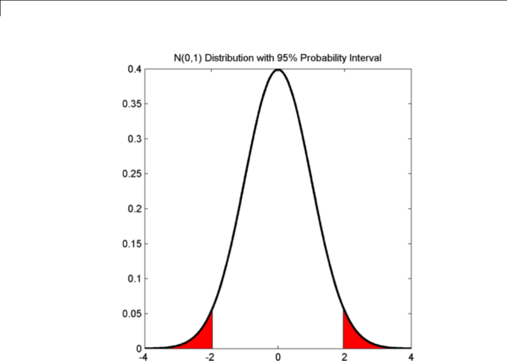
10 Convolution and Correlation

Create a realization of a white noise process 1,000 samples in length. Compute

the sample autocorrelation to lag 20. Plot the sample autocorrelation along

with the approximate 95%-confidence intervals for a white noise process.

Create the white noise random vector. Set the random number generator to

the default settings for reproducible results. Obtain the normalized sampled

autocorrelation to lag 20.

rng default;

x = randn(1e3,1);

[xc,lags] = xcorr(x,20,'coeff');

Create the lower and upper 95% confidence bounds for the N(0,1/N)

distribution. For a 95%-confidence interval, the critical value is 1.96. The

10-6

Confidence Intervals for Sample Autocorrelation

standard deviation is the square root of 1/N, where N is the length of the

input vector.

Theconfidenceintervalis

0196

1000

.

lconf = -1.96/sqrt(length(x));

upconf = 1.96/sqrt(length(x));

Plot the sample autocorrelation along with the 95%-confidence interval.

stem(lags,xc,'markerfacecolor',[0 0 1]);

set(gca,'ylim',[lconf-0.03 1.05]);

hold on;

line(lags,lconf*ones(size(lags)),'color','r','linewidth',2);

line(lags,upconf*ones(size(lags)),'color','r','linewidth',2);

title('Sample Autocorrelation with 95% Confidence Intervals');

10-7

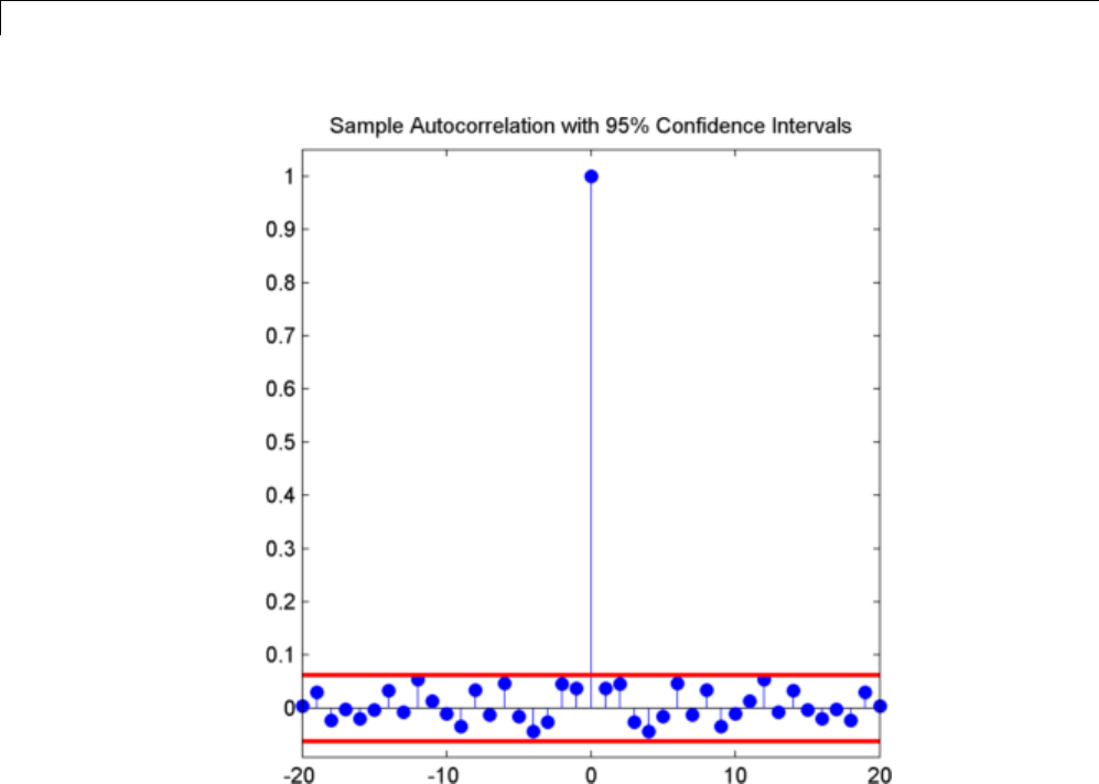
10 Convolution and Correlation

You see in the above figure that the only autocorrelation value outside of the

95%-confidence interval occurs at lag 0 as expected for a white noise process.

Based on this result, you can conclude that the data are a realization of a

white noise process.

10-8

Residual Analysis with Autocorrelation

This example shows you how to use autocorrelation with a confidence interval

to analyze the residuals of a least-squares fit to noisy data. The residuals are

the differences between the fitted model and the data. In a signal+white

noise model, if you have a good fit for the signal, the residuals should be

whitenoise.Theexample“ConfidenceIntervals for Sample Autocorrelation”

on page 10-5 demonstrates the basic technique for forming a confidence

interval for the sample autocorrelation. This example extends the technique

illustrated in that example.

Create a noisy data set consisting of a 1st order polynomial (straight line)

in additive white Gaussian noise. The additive noise is a sequence of

uncorrelated random variables following a N(0,1) distribution. This means

that all the random variables have mean zero and unit variance. Set the

random number generator to the default settings for reproducible results.

x = -3:0.01:3;

rng default

y = 2*x+randn(size(x));

plot(x,y)

10-9

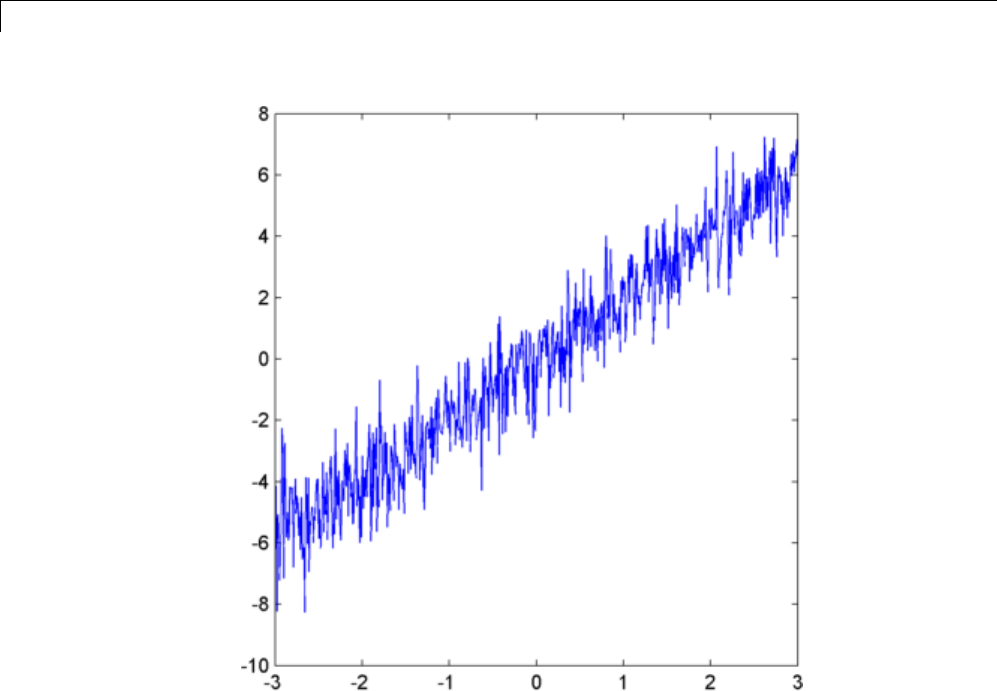
10 Convolution and Correlation

Use polyfit to find the least-squares line for the noisy data. Plot the original

data along with the least-squares fit.

coeffs = polyfit(x,y,1);

yfit = coeffs(2)+coeffs(1)*x;

plot(x,y); hold on;

plot(x,yfit,'r','linewidth',2)

10-10

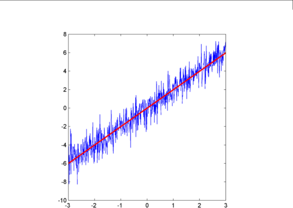
Residual Analysis with Autocorrelation

Find the residuals. Obtain the autocorrelation sequence of the residuals to

lag 50.

residuals = y-yfit;

[xc,lags] = xcorr(residuals,50,'coeff');

When you inspect the autocorrelation sequence, you want to determine

whether or not there is evidence of autocorrelation. In other words, you

want to determine whether the sample autocorrelation sequence looks like

the autocorrelation sequence of white noise. If the autocorrelation sequence

of the residuals looks like the autocorrelation of a white noise process, you

are confident that none of the signal has escaped your fit and ended up in

the residuals. In this example, use a 99%-confidence interval. To construct

the confidence interval, you need to know the distribution of the sample

autocorrelation values. This is described in “Confidence Intervals for Sample

10-11

10 Convolution and Correlation

Autocorrelation” on page 10-5. You also need to find the critical values on the

appropriate distribution between which lie 0.99 of the probability. Because

the distribution in this case is Gaussian, you can use complementary inverse

error function, erfcinv. The relationship between this function and the

inverse of the Gaussian cumulative distribution function is described on the

reference page for erfcinv.

Find the critical value for the 99%-confidence interval.

conf99 = sqrt(2)*erfcinv(2*.01/2)

Ue the critical value to construct the lower and upper confidence bounds.

lconf = -conf99/sqrt(length(x));

upconf = conf99/sqrt(length(x));

Plot the autocorrelation sequence along with the 99%-confidence intervals.

stem(lags,xc,'markerfacecolor',[0 0 1]);

set(gca,'ylim',[lconf-0.03 1.05]);

hold on;

line(lags,lconf*ones(size(lags)),'color','r','linewidth',2);

line(lags,upconf*ones(size(lags)),'color','r','linewidth',2);

title('Sample Autocorrelation with 99% Confidence Intervals');

10-12

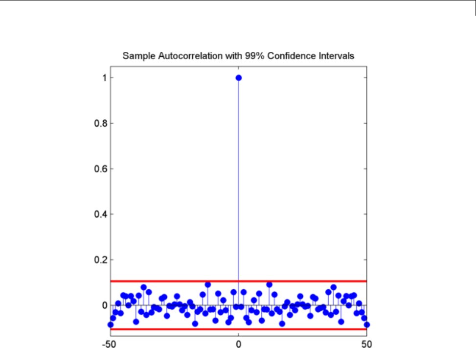
Residual Analysis with Autocorrelation

Except at zero lag, the sample autocorrelation values lie within the

99%-confidence bounds for the autocorrelation of a white noise sequence.

From this, you can conclude that the residuals are white noise. More

specifically, you cannot reject that the residuals are a realization of a white

noise process.

Create a signal consisting of a sine wave plus noise. The data are sampled

at 1 kHz. The frequency of the sine wave is 100 Hz. Set the random number

generator to the default settings for reproducible results.

Fs = 1000;

t = 0:1/Fs:1-1/Fs;

rng default

x = cos(2*pi*100*t)+randn(size(t));

10-13

10 Convolution and Correlation

Use the discrete Fourier transform (DFT) to obtain the least-squares fit to

thesinewaveat100Hz. Theleast-squaresestimateoftheamplitudeis2/N

times the DFT coefficient corresponding to 100 Hz, where N is the length

of the signal. The real part is the ampltiude of a cosine at 100 Hz and the

imaginary part is the amplitude of a sine at 100 Hz. The least-squares fit is

the sum of the cosine and sine with the correct amplitude. In this example,

DFT bin 101 corresponds to 100 Hz.

xdft = fft(x);

ampest = 2/length(x)*xdft(101);

xfit = real(ampest)*cos(2*pi*100*t)+imag(ampest)*sin(2*pi*100*t);

plot(t,x,'r-.','linewidth',2); hold on;

plot(t,xfit,'b','linewidth',2);

axis([0 0.30 -4 4]);

xlabel('Seconds'); ylabel('Amplitude');

10-14

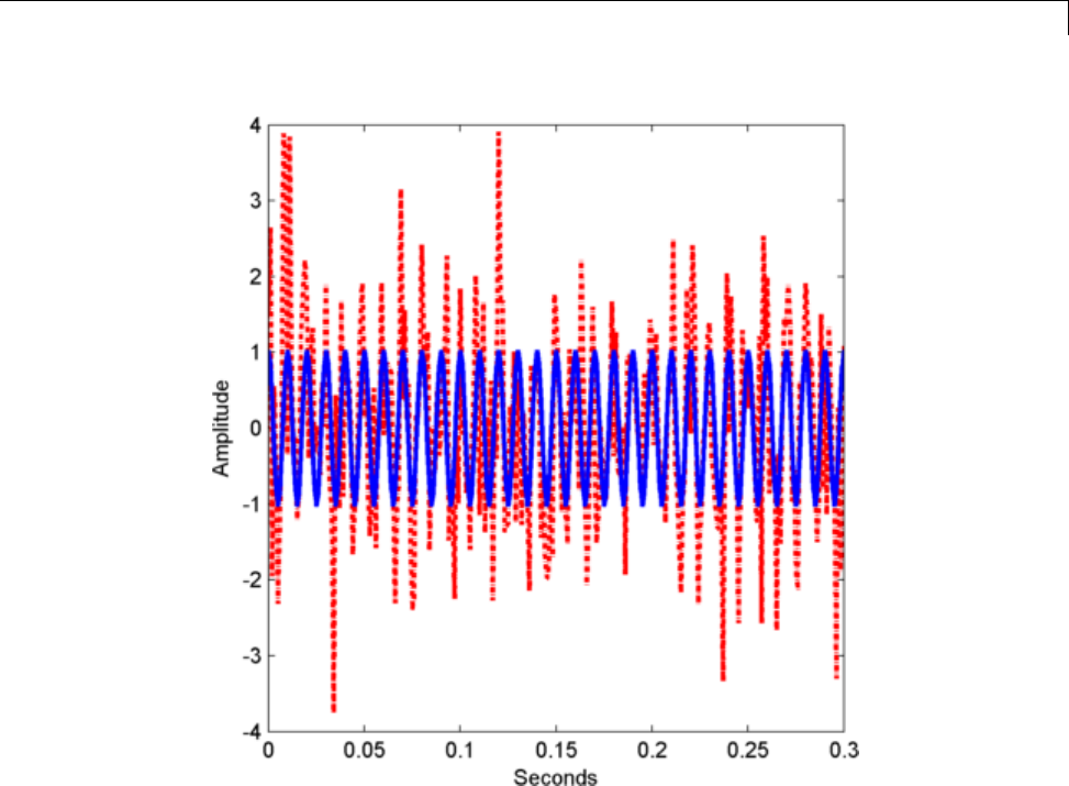
Residual Analysis with Autocorrelation

Find the residuals and determine the sample autocorrelation sequence to

lag 50.

residuals = x-xfit;

[xc,lags] = xcorr(residuals,50,'coeff');

Plot the autocorrelation sequence with the 99%-confidence intervals.

stem(lags,xc,'markerfacecolor',[0 0 1]);

set(gca,'ylim',[lconf-0.03 1.05]);

hold on;

line(lags,lconf*ones(size(lags)),'color','r','linewidth',2);

line(lags,upconf*ones(size(lags)),'color','r','linewidth',2);

title('Sample Autocorrelation with 99% Confidence Intervals');

10-15

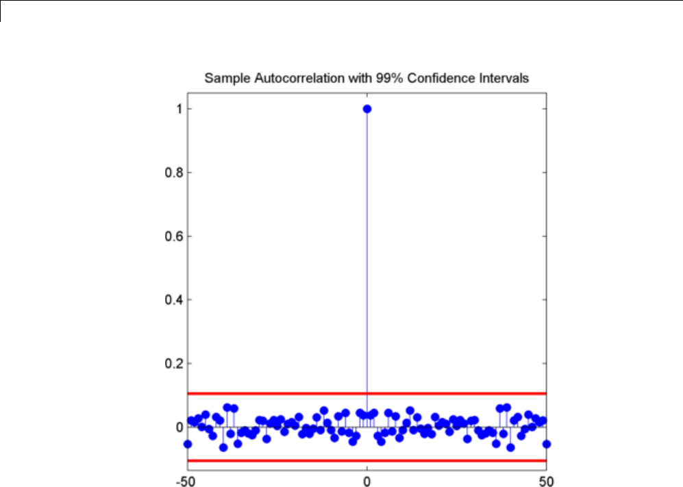
10 Convolution and Correlation

Again, you see that except at zero lag, the sample autocorrelation values lie

within the 99%-confidence bounds for the autocorrelation of a white noise

sequence. From this, you can conclude that the residuals are white noise.

More specifically, you cannot reject that the residuals are a realization of a

white noise process.

Finally, add another sine wave with a frequency of 200 Hz and an amplitude

of 3/4. Fit only the sine wave at 100 Hz and find the sample autocorrelation

of the residuals.

x = x+3/4*sin(2*pi*200*t);

xdft = fft(x);

ampest = 2/length(x)*xdft(101);

xfit = real(ampest)*cos(2*pi*100*t)+imag(ampest)*sin(2*pi*100*t);

10-16

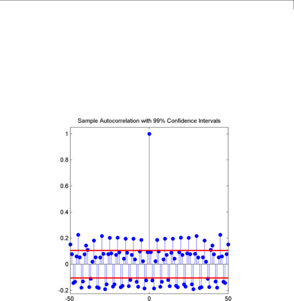
Residual Analysis with Autocorrelation

residuals = x-xfit;

[xc,lags] = xcorr(residuals,50,'coeff');

Plot the sample autocorrelation alongwiththe99%-confidence intervals.

stem(lags,xc,'markerfacecolor',[0 0 1]);

set(gca,'ylim',[lconf-0.12 1.05]);

hold on;

line(lags,lconf*ones(size(lags)),'color','r','linewidth',2);

line(lags,upconf*ones(size(lags)),'color','r','linewidth',2);

title('Sample Autocorrelation with 99% Confidence Intervals');

In this case, the autocorrelation values clearly exceed the 99%-confidence

bounds for a white noise autocorrelation at many lags. Here you can reject the

10-17

10 Convolution and Correlation

hypothesis that the residuals are a white noise sequence. The implication is

that the model has not accounted for all the signal and therefore the residuals

consist of signal+noise.

10-18

Autocorrelation of Moving Average Process

This example shows how filtering a white noise process introduces

autocorrelation. The example also shows how the sample autocorrelation

sequence does not agree perfectly with the known theoretical autocorrelation

sequence. However, the sample autocorrelation sequence accurately

represents the general form of the theoretical autocorrelation.

Simulate a realization of an N(0,1) white noise process. Filter the process

with a 3-point moving average (MA) filter. Plot the sample autocorrelation

along with the known theoretical autocorrelation for comparison.

Create the impulse response for the 3-point MA filter. Filter an N(0,1) white

noise with the filter. Set the random number generator to the default settings

for reproducible results.

h = 1/3*ones(3,1);

rng default;

x = randn(100,1);

y = filter(h,1,x);

Obtain the biased sample autocorrelation out to 20 lags. Plot the sample

autocorrelation along with the theoretical autocorrelation.

[xc,lags] = xcorr(y,20,'biased');

stem(lags,xc,'markerfacecolor',[0 0 1]);

Xc = zeros(size(xc));

Xc([19 23]) = 1/9*var(x);

Xc([20 22]) = 2/9*var(x);

Xc(21) = 3/9*var(x);

hold on;

stem(lags,Xc,'color',[1 0 0],'marker','none','linewidth',2);

legend('Sample Autocorrelation','Theoretical Autocorrelation',...

'Location','NorthEast');

10-19

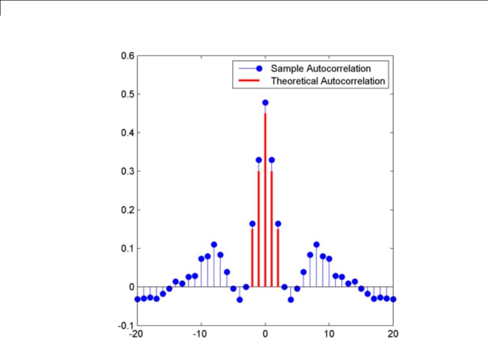
10 Convolution and Correlation

The theoretical autocorrelation is zero outside of lags [-2,2], while the sample

autocorrelation is not. However, the magnitudes (absolute values) of the

sample autocorrelation decay quickly to zero outside of lags [-2,2].

The sample autocorrelation sequence is not in perfect agreement with the

theoretical autocorrelation, but captures that the filter has introduced

significant autocorrelation only over lags [-2,2].

10-20

Cross-correlation of Two Moving Average Processes

This example shows how to find and plot the cross-correlation sequence

between two moving average processes. The example compares the sample

cross-correlation with the theoretical cross-correlation.

Filter an N(0,1) white noise input with two different moving average filters.

Plot the sample and theoretical cross-correlation sequences.

Create an N(0,1) white noise sequence. Set the random number generator

to the default settings for reproducible results. Create two moving average

filters. One filter has impulse response δ(n)+δ(n-1). The other filter has

impulse response, δ(n)-δ(n-1).

rng default;

w = randn(100,1);

x = filter([1 1],1,w);

y = filter([1 -1],1,w);

Obtain the sample cross-correlation sequence up to lag 20. Plot the sample

cross-correlation along with the theoretical cross-correlation.

[xc,lags] = xcorr(x,y,20,'biased');

stem(lags,xc,'markerfacecolor',[0 0 1]);

Xc = zeros(size(xc));

Xc(20) = -1;

Xc(22) = 1;

hold on;

stem(lags,Xc,'color',[1 0 0],'marker','none','linewidth',2);

legend('Sample Cross-correlation','Theoretical Cross-correlation',...

'Location','NorthWest')

10-21

10 Convolution and Correlation

The theoretical cross-correlation is -1 at lag -1, 1 at lag 1, and zero at all other

lags. The sample cross-correlation sequence approximates the theoretical

cross-correlation.

As expected, there is not perfect agreement between the theoretical

cross-correlation and sample cross-correlation. The sample cross-correlation

does accurately represent both the sign and magnitude of the theoretical

cross-correlation sequence values at lag -1 and lag 1.

10-22

Cross-correlation of Delayed Signal in Noise

This example shows how to use the cross-correlation sequence to detect the

time delay in a noise-corrupted sequence. The output sequence is a delayed

version of the input sequence with additive white Gaussian noise.

Create two sequences. One sequence is a delayed version of the other. The

delay is 3 samples. Add an N(0,0.32) white noise sequence to the delayed

signal. Use the sample cross-correlation sequence to detect the lag.

Create and plot the signals. Set the random number generator to the default

settings for reproducible results.

rng default;

x = triang(20);

y = [zeros(3,1); x]+0.3*randn(length(x)+3,1);

subplot(211)

stem(x,'markerfacecolor',[0 0 1]); axis([0 22 -1 2]);

subplot(212)

stem(y,'markerfacecolor',[0 0 1]); axis([0 22 -1 2]);

10-23

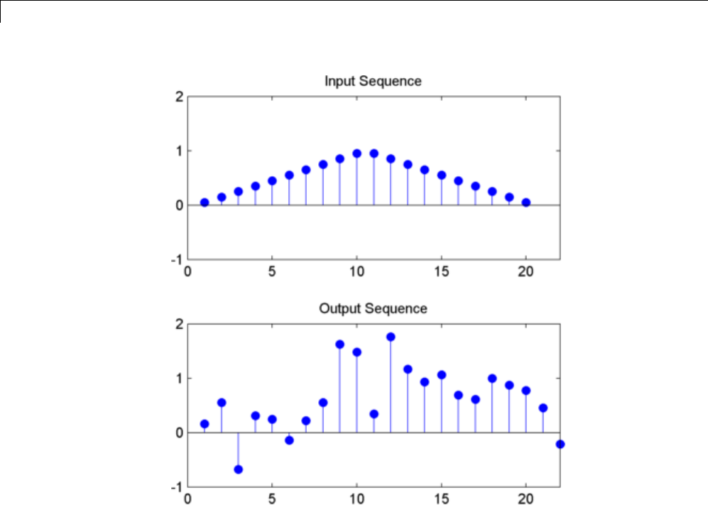
10 Convolution and Correlation

Obtain the sample cross-correlation sequence and use the maximum absolute

valuetoestimatethelag. Plotthesample cross-correlation sequence.

[xc,lags] = xcorr(y,x);

[~,I] = max(abs(xc));

fprintf('Maximum cross correlation sequence value occurs at lag %d\n',lags(

figure;

stem(lags,xc,'markerfacecolor',[0 0 1]);

10-24

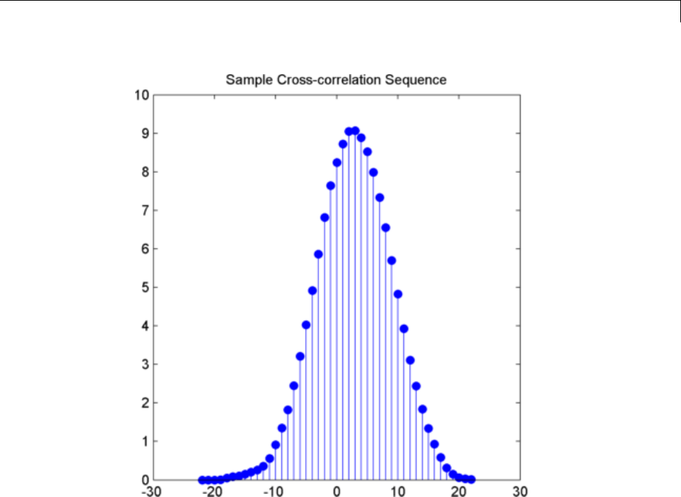
Cross-correlation of Delayed Signal in Noise

The maximum cross correlation sequence value occurs at lag 3 as expected.

10-25

10 Convolution and Correlation

Cross-correlation of Phase-Lagged Sine Wave

This example shows how to use the cross-correlation sequence to estimate the

phase lag between two sine waves. The theoretical cross-correlation sequence

of two sine waves at the same frequency also oscillates at that frequency.

Because the sample cross-correlation sequence uses fewer and fewer samples

at larger lags, the sample cross-correlation sequence also oscillates at the

same frequency, but the amplitude decays as the lag increases.

Use the cross-correlation sequence to detect the phase lag between two sine

waves with a frequency of 2π/10 radians/sample. One sine wave lags the

other in phase by πradians.

Create two sine waves with frequencies of 2π/10 radians/sample. The starting

phase of one sine wave is 0, while the starting phase of the other sine wave is

-πradians. Add N(0,0.252) white noise to the sine wave with the phase lag

of πradians. Set the random number generator to the default settings for

reproducible results.

t = 0:99;

rng default;

x = cos(2*pi*1/10*t);

y = cos(2*pi*1/10*t-pi)+0.25*randn(size(t));

Obtain the sample cross-correlation sequence for two periods of the sine wave

(10 samples). Plot the cross-correlation sequence and mark the known lag

between the two sine waves (5 samples).

[xc,lags] = xcorr(y,x,20,'coeff');

stem(lags(21:end),xc(21:end),'markerfacecolor',[0 0 1]);

set(gca,'xtick',0:5:20);

hold on;

plot([5 5],[-1 1],'r','linewidth',2);

10-26

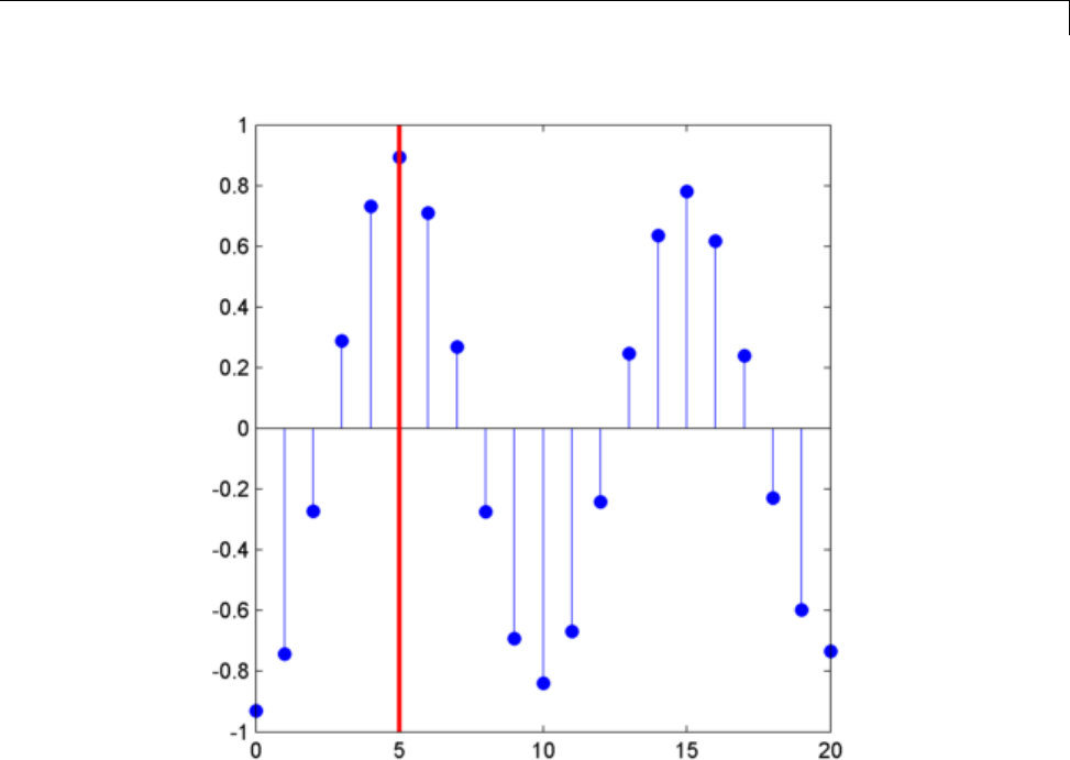
Cross-correlation of Phase-Lagged Sine Wave

You see that the cross-correlation sequence peaks at lag 5 as expected and

oscillates with a period of 10 samples.

10-27

10 Convolution and Correlation

10-28

Multirate Signal Processing

•“Downsampling — Signal Phases” on page 11-2

•“Downsampling — Aliasing” on page 11-6

•“Filtering Before Downsampling” on page 11-12

•“Upsampling — Imaging Artifacts” on page 11-14

•“Filtering After Upsampling — Interpolation” on page 11-16

•“Changing Signal Sampling Rate” on page 11-18

11 Multirate Signal Processing

Downsampling — Signal Phases

These examples show how to use downsample to obtain the phases of a signal.

Downsampling a signal by M can produce M unique phases. For example, if

youhaveadiscrete-timesignal,x, with x(0) x(1) x(2) x(3),...., the M phases

of xare x(nM+λ)withλ=0,1,...M-1.

The M signals are referred to as the polyphase components of x.

Create a white noise vector and obtain the 3 polyphase components associated

with downsampling by 3.

Reset the random number generator to the default settings to produce a

repeatable result. Generate a white noise random vector and obtain the 3

polyphase components associated with downsampling by 3.

rng default;

x = randn(36,1);

x0 = downsample(x,3,0);

x1 = downsample(x,3,1);

x2 = downsample(x,3,2);

The polyphase components have length equal to 1/3 the original signal.

Upsample the polyphase components by 3 using upsample .

y0 = upsample(x0,3,0);

y1 = upsample(x1,3,1);

y2 = upsample(x2,3,2);

Plot the result.

subplot(411)

stem(x,'marker','none');

set(gca,'ylim',[-4 4]); title('Original Signal');

subplot(412)

stem(y0,'marker','none'); ylabel('Phase 0');

set(gca,'ylim',[-4 4]);

subplot(413)

stem(y1,'marker','none'); ylabel('Phase 1');

set(gca,'ylim',[-4 4]);

11-2

Downsampling — Signal Phases

subplot(414)

stem(y2,'marker','none'); ylabel('Phase 2');

set(gca,'ylim',[-4 4]);

If you sum the upsampled polyphase components you obtain the original

signal.

Create a discrete-time sinusoid and obtain the 2 polyphase components

associated with downsampling by 2.

Createadiscrete-timesinewavewithanangularfrequencyofπ/4

radians/sample. AddaDCoffsetof2tothesinewavetohelpwith

visualization of the polyphase components. Downsample the sine wave by 2 to

obtain the even and odd polyphase components.

n = 0:127;

11-3

11 Multirate Signal Processing

x = 2+cos(pi/4*n);

x0 = downsample(x,2,0);

x1 = downsample(x,2,1);

Upsample the two polyphase components.

y0 = upsample(x0,2,0);

y1 = upsample(x1,2,1);

Plot the upsampled polyphase components along with the original signal

for comparison.

subplot(311)

stem(x,'marker','none');

set(gca,'ylim',[0.5 3.5]); title('Original Signal');

subplot(312)

stem(y0,'marker','none'); ylabel('Phase 0');

set(gca,'ylim',[0.5 3.5]);

subplot(313)

stem(y1,'marker','none'); ylabel('Phase 1');

set(gca,'ylim',[0.5 3.5]);

11-4

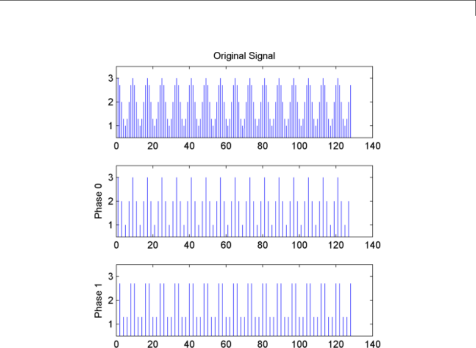
Downsampling — Signal Phases

If you sum the two upsampled polyphase components (Phase 0 and Phase

1), you obtain the original sine wave.

11-5

11 Multirate Signal Processing

Downsampling — Aliasing

These examples show how downsampling can introduce aliasing. If a

discrete-time signal’s baseband spectral support is not limited to an interval

of width 2π/M radians, downsampling by M results in aliasing. Aliasing is

the distortion that occurs when overlapping copies of the signal’s spectrum

are added together. The more the signal’s baseband spectral support exceeds

2π/M radians, the more severe the aliasing.

Demonstrate aliasing in a signal downsampled by two. The signal’s baseband

spectral support exceeds πradians in width.

Create a signal with baseband spectral support equal to 3π/2 radians. Use

fir2 to design the signal. Plot the signal’s spectrum.

F = [0 0.2500 0.5000 0.7500 1.0000];

A = [1.00 0.6667 0.3333 0 0];

Order = 511;

B1 = fir2(Order,F,A);

[Hx,W] = freqz(B1,1,8192,'whole');

Hx = [Hx(4098:end) ; Hx(1:4097)];

omega = -pi+(2*pi/8192):(2*pi)/8192:pi;

plot(omega,abs(Hx));

set(gca,'xlim',[-pi pi]);

set(gca,'xtick',[-pi -pi/2 0 pi/2 pi]);

grid on;

title('Magnitude Spectrum');

xlabel('Radians/Sample'); ylabel('Magnitude');

You see that the signal’s baseband spectral support exceeds [-π/2, π/2].

Downsample the signal by a factor of 2 and plot the downsampled signal’s

spectrum with the spectrum of the original signal.

y = downsample(B1,2,0);

[Hy,W] = freqz(y,1,8192,'whole');

Hy = [Hy(4098:end) ; Hy(1:4097)];

hold on;

plot(omega,abs(Hy),'r','linewidth',2);

set(gca,'xlim',[-pi pi]);

11-6

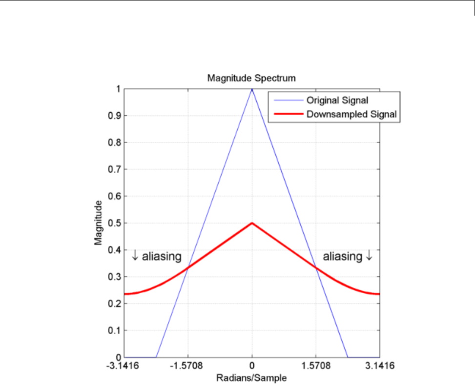
Downsampling — Aliasing

legend('Original Signal','Downsampled Signal');

In addition to an amplitude scaling of the spectrum, the superposition of

overlapping spectral replicas causes distortion of the original spectrum for

|ω|>π/2.

Increase the baseband spectral support of the signal to [-7π/8, 7π/8] and

downsample the signal by 2. Plot the original spectrum along with the

spectrum of the downsampled signal.

F = [0 0.2500 0.5000 0.7500 7/8 1.0000];

A = [1.00 0.7143 0.4286 0.1429 0 0];

Order = 511;

11-7

11 Multirate Signal Processing

B2 = fir2(Order,F,A);

[Hx,W] = freqz(B2,1,8192,'whole');

Hx = [Hx(4098:end) ; Hx(1:4097)];

omega = -pi+(2*pi/8192):(2*pi)/8192:pi;

plot(omega,abs(Hx));

set(gca,'xlim',[-pi pi]);

y = downsample(B2,2,0);

[Hy,W] = freqz(y,1,8192,'whole');

Hy = [Hy(4098:end) ; Hy(1:4097)];

plot(omega,abs(Hx));

hold on;

plot(omega,abs(Hy),'r','linewidth',2);

set(gca,'xlim',[-pi pi]);

grid on;

legend('Original Signal','Downsampled Signal');

xlabel('Radians/Sample'); ylabel('Magnitude');

11-8

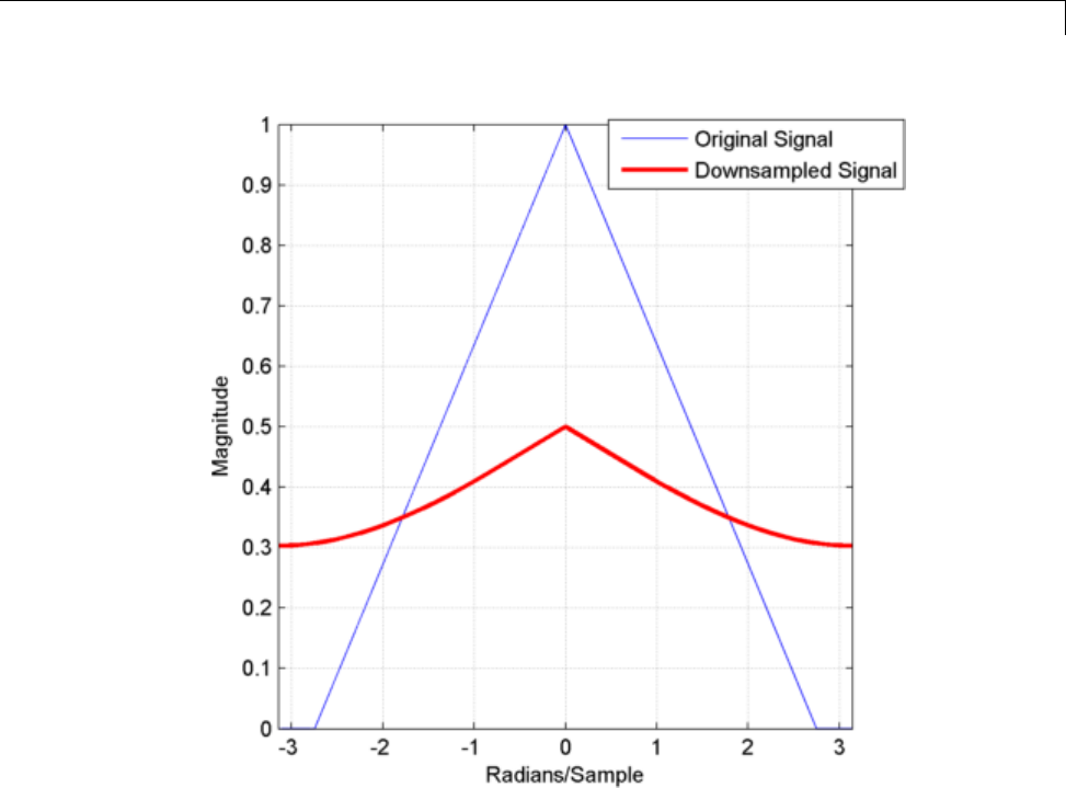
Downsampling — Aliasing

The increased spectral width results in more pronounced aliasing in the

spectrum of the downsampled signal because more signal energy is outside

[-π/2, π/2].

Finally, construct a signal with baseband spectral support limited to [-π/2,

π/2]. Downsample the signal by a factor of 2 and plot the spectrum of the

original and downsampled signals. The downsampled signal is full band, but

the shape of the spectrum is preserved because the spectral copies do not

overlap. There is no aliasing.

F=[

0 0.250 0.500 0.7500 1];

A=[

1.0000 0.5000 0 0 0];

Order = 511;

11-9

11 Multirate Signal Processing

B3 = fir2(Order,F,A);

[Hx,W] = freqz(B3,1,8192,'whole');

Hx = [Hx(4098:end) ; Hx(1:4097)];

omega = -pi+(2*pi/8192):(2*pi)/8192:pi;

plot(omega,abs(Hx));

set(gca,'xlim',[-pi pi]);

y = downsample(B3,2,0);

[Hy,W] = freqz(y,1,8192,'whole');

Hy = [Hy(4098:end) ; Hy(1:4097)];

plot(omega,abs(Hx));

hold on;

plot(omega,abs(Hy),'r','linewidth',2);

set(gca,'xlim',[-pi pi]);

grid on;

legend('Original Signal','Downsampled Signal');

xlabel('Radians/Sample'); ylabel('Magnitude');

11-10

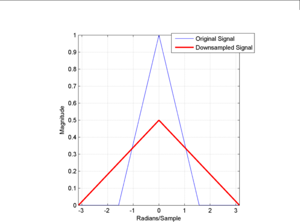
Downsampling — Aliasing

You see in the preceding figure that the shape of the spectrum is preserved.

The spectrum of the downsampled signal is a stretched and scaled version of

the original signal’s spectrum, but there is no aliasing.

11-11

11 Multirate Signal Processing

Filtering Before Downsampling

This example shows how to filter before downsampling to mitigate the

distortion caused by aliasing. You can use decimate or resample to filter

and downsample with one function. Alternatively, you can lowpass filter

your data and then use downsample.

Create a signal with baseband spectral support greater than πradians. Use

decimate to filter the signal with a 10-th order Chebyshev type I lowpass

filter prior to downsampling.

Create the signal and plot the magnitude spectrum.

F = [0 0.2500 0.5000 0.7500 1.0000];

A = [1.00 0.6667 0.3333 0 0];

Order = 511;

B = fir2(Order,F,A);

[Hx,W] = freqz(B,1,8192,'whole');

Hx = [Hx(4098:end) ; Hx(1:4097)];

omega = -pi+(2*pi/8192):(2*pi)/8192:pi;

plot(omega,abs(Hx));

set(gca,'xlim',[-pi pi]);

set(gca,'xtick',[-pi -3*pi/4 -pi/2 0 pi/2 3*pi/4 pi]);

grid on;

title('Magnitude Spectrum');

xlabel('Radians/Sample'); ylabel('Magnitude');

Filter the signal with a 10-th order type I Chebyshev lowpass filter and

downsample by 2. Plot the magnitude spectra of the original signal along with

the filtered and downsampled signal.

y = decimate(B,2,10);

[Hy,W] = freqz(y,1,8192,'whole');

Hy = [Hy(4098:end) ; Hy(1:4097)];

plot(omega,abs(Hx));

hold on;

plot(omega,abs(Hy),'r','linewidth',2);

set(gca,'xlim',[-pi pi]);

grid on;

legend('Original Signal','Downsampled Signal');

11-12

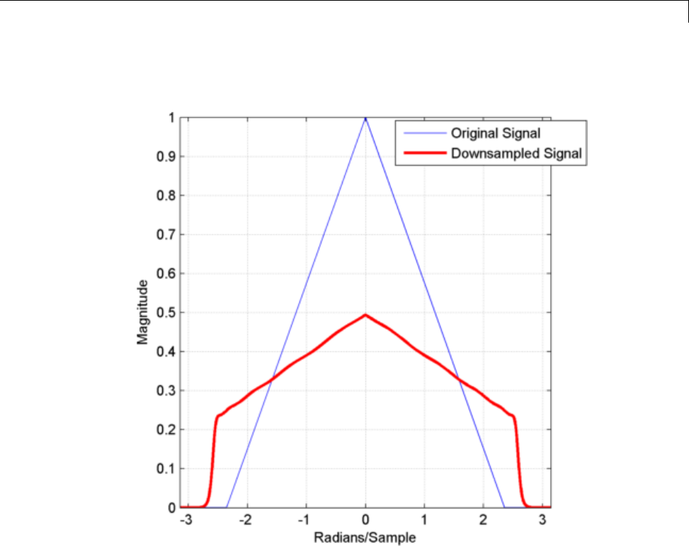
Filtering Before Downsampling

xlabel('Radians/Sample'); ylabel('Magnitude');

The lowpass filter reduces the amount of aliasing distortion outside the

interval [-π/2, π/2].

11-13

11 Multirate Signal Processing

Upsampling — Imaging Artifacts

Thisexampleshowshowtoupsampleasignalandhowupsamplingcan

result in images. Upsampling a signal contracts the spectrum. For example,

upsampling a signal by 2 results in a contraction of the spectrum by a factor

of 2.

Because the spectrum of a discrete-time signal is 2π-periodic, contraction can

cause replicas of the spectrum normally outside of the baseband to appear

inside the interval [-π,π].

Create a signal with baseband spectral support from [-π/2, π/2]. Upsample the

signal by a factor of 2 and demonstrate that upsampling results in images of

the spectrum in [-ππ].

Create a discrete-time signal whose baseband spectral support is [-π/2, π/2].

Plot the magnitude spectrum.

F = [0 0.250 0.500 0.7500 1];

A = [1.0000 0.5000 0 0 0];

Order = 511;

B = fir2(Order,F,A);

[Hx,W] = freqz(B,1,8192,'whole');

Hx = [Hx(4098:end) ; Hx(1:4097)];

omega = -pi+(2*pi/8192):(2*pi)/8192:pi;

plot(omega,abs(Hx));

Upsample the signal by 2. Plot the spectrum of the upsampled signal.

y = upsample(B,2);

[Hy,W] = freqz(y,1,8192,'whole');

Hy = [Hy(4098:end) ; Hy(1:4097)];

plot(omega,abs(Hx));

hold on;

plot(omega,abs(Hy),'r','linewidth',2);

set(gca,'xlim',[-pi pi]);

legend('Original Signal','Upsampled Signal');

xlabel('Radians/Sample'); ylabel('Magnitude');

11-14

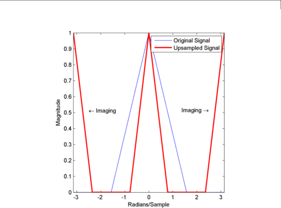
Upsampling — Imaging Artifacts

You can see in the preceding figure that the contraction of the spectrum has

drawn subsequent periods of the spectrum into the interval [-π,π].

11-15

11 Multirate Signal Processing

Filtering After Upsampling — Interpolation

This example shows how to upsample a signal and apply a lowpass

interpolation filter with interp.UpsamplingbyLinserts Lzeros between

every element of the original signal. The example in “Upsampling — Imaging

Artifacts” on page 11-14 shows that upsampling can create imaging artifacts.

Lowpass filtering following upsampling can remove these imaging artifacts.

In the time domain, lowpass filtering interpolates the zeros inserted by

upsampling.

Create a signal with baseband spectral support from [-π/2, π/2]. Upsample

the signal by a factor of 2 and use a lowpass filter to remove the images

resulting fromupsampling.

Create a discrete-time signal whose baseband spectral support is [-π/2 π/2].

Plot the magnitude spectrum.

F = [0 0.250 0.500 0.7500 1];

A = [1.0000 0.5000 0 0 0];

Order = 511;

B = fir2(Order,F,A);

[Hx,W] = freqz(B,1,8192,'whole');

Hx = [Hx(4098:end) ; Hx(1:4097)];

omega = -pi+(2*pi/8192):(2*pi)/8192:pi;

plot(omega,abs(Hx));

set(gca,'xlim',[-pi pi]);

xlabel('Radians/Sample'); ylabel('Magnitude');

Upsample the signal and apply a lowpass filter to remove the imaging

artifacts. Plot the magnitude spectrum.

y = interp(B,2);

[Hy,W] = freqz(y,1,8192,'whole');

Hy = [Hy(4098:end) ; Hy(1:4097)];

hold on;

plot(omega,abs(Hy),'r','linewidth',2);

legend('Original Signal','Upsampled Signal');

11-16

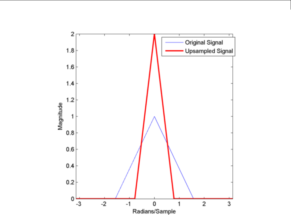
Filtering After Upsampling — Interpolation

Upsampling still contracts the spectrum, but the imaging artifacts are

removed by the lowpass filter.

11-17

11 Multirate Signal Processing

Changing Signal Sampling Rate

This example shows you how to change the sampling rate of a signal. Two

examples are presented here. One example changes the sampling rate of a

sinusoidal input from 44.1 kHz to 48 kHz. This workflow is common to audio

processing. The sampling rate used on compact discs is 44.1 kHz, while the

sampling rate used on digital audio tape is 48 kHz. The other example changes

the sampling rate of a recorded speech sample from 7418 Hz to 8192 Hz.

Create an input signal consisting of a sum of sine waves sampled at 44.1 kHz.

The sine waves have frequencies of 2, 4, and 8 kHz.

Fs = 44.1e3;

t = 0:1/Fs:1-(1/Fs);

x = cos(2*pi*2000*t)+1/2*sin(2*pi*4000*(t-pi/4))+1/4*cos(2*pi*8000*t);

To change the sampling rate from 44.1 to 48 kHz, you have to determine a

rational number (ratio of integers), P/Q, such that P/Qtimes the original

sampling rate, 44100, is equal to 48000 within some specified tolerance.

To determine these factors, use rat. Input the ratio of the new sampling rate,

48000, to the original sampling rate, 44100.

[P,Q] = rat(48e3/Fs);

abs(P/Q*Fs-48000)

You see that P/Q*Fs only differs from the desired sampling rate, 48000, on

the order of 10-12.

Use the numerator and denominator factors obtained with rat as inputs to

resample to output a waveform sampled at 48 kHz.

xnew = resample(x,P,Q);

If your computer can play audio, you can play the two waveforms. Set the

volume to a comfortable level before you play the signals. Execute the play

commands separately so that you can hear the signal with the two different

sampling rates.

P44_1 = audioplayer(x,44100);

P48 = audioplayer(xnew,48000);

11-18

Changing Signal Sampling Rate

play(P44_1)

play(P48)

Change the sampling rate of a speech sample from 7418 Hz to 8192. The

speech signal is a recording of a speaker saying “MATLAB”.

Load the speech sample.

load mtlb

Loading the file mtlb.mat brings the speech signal, mtlb,andthesampling

rate, Fs, into the MATLAB workspace.

Determine a rational approximation to the ratio of the new sample rate, 8192,

to the original sample rate. Use rat to determine the approximation.

[P,Q] = rat(8192/Fs);

Resample the speech sample at the new sampling rate.

mtlb_new = resample(mtlb,P,Q);

If your computer has audio output capability, you can play the two waveforms

at their respective sampling rates for comparison. Set the volume on your

computer to a comfortable listening level before playing the sounds. Execute

the play commands separately to compare the speech samples at the different

sampling rates.

Pmtlb = audioplayer(mtlb,Fs);

Pmtlb_new = audioplayer(mtlb_new,8192);

play(Pmtlb)

play(Pmtlb_new)

11-19

11 Multirate Signal Processing

11-20

Spectral Analysis

•“Power Spectral Density Estimates Using FFT” on page 12-2

•“Bias and Variability in the Periodogram” on page 12-10

•“Cross Spectrum and Magnitude-Squared Coherence” on page 12-20

•“Amplitude Estimation and Zero Padding” on page 12-24

•“Significance Testing for Periodic Component” on page 12-27

•“Frequency Estimation by Subspace Methods” on page 12-29

•“Frequency-Domain Linear Regression” on page 12-32

12 Spectral Analysis

Power Spectral Density Estimates Using FFT

These examples show how to obtain nonparametric power spectral density

(PSD) estimates equivalent to the periodogram using fft. The examples

show you how to properly scale the output of fft for even-length inputs, for

normalized frequency and hertz, and for one- and two-sided PSD estimates.

Obtain the periodogram for an even-length signal sampled at 1 kHz using

both fft and periodogram. Compare the results.

Create a signal consisting of a 100-Hz sine wave in N(0,1) additive noise. The

sampling frequency is 1 kHz. The signal length is 1000 samples. Use the

default settings of the random number generator for reproducible results.

rng default;

Fs = 1000;

t = linspace(0,1,1000);

x = cos(2*pi*100*t)+randn(size(t));

Obtain the periodogram using fft. The signal is real-valued and has even

length. Because the signal is real-valued, you only need power estimates for

thepositiveornegativefrequencies. In order to conserve the total power,

multiply all frequencies that occur inbothsets—thepositiveandnegative

frequencies — by a factor of 2. Zero frequency (DC) and the Nyquist frequency

do not occur twice. Plot the result.

N = length(x);

xdft = fft(x);

xdft = xdft(1:N/2+1);

psdx = (1/(Fs*N)).*abs(xdft).^2;

psdx(2:end-1) = 2*psdx(2:end-1);

freq = 0:Fs/length(x):Fs/2;

plot(freq,10*log10(psdx)); grid on;

title('Periodogram Using FFT');

xlabel('Frequency (Hz)'); ylabel('Power/Frequency (dB/Hz)');

12-2

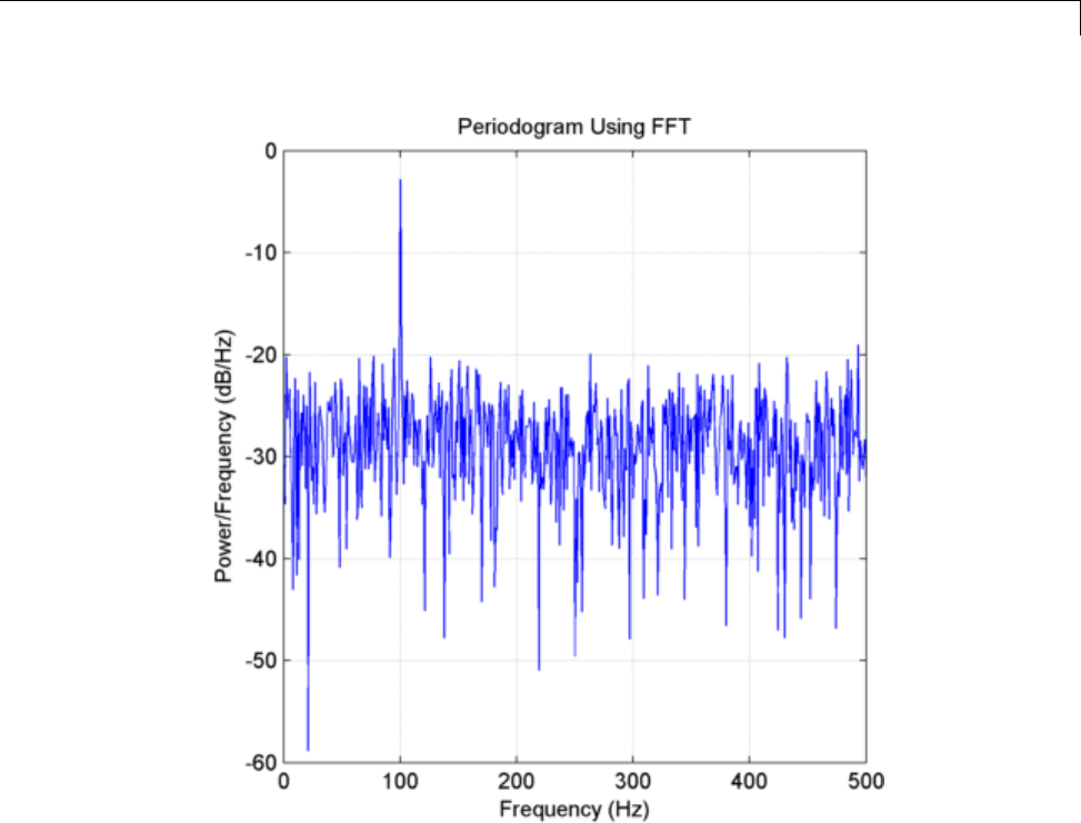
Power Spectral Density Estimates Using FFT

Compute and plot the periodogram using periodogram. Show that the 2

results are identical.

figure;

[psdestx,Fxx] = periodogram(x,rectwin(length(x)),length(x),Fs);

plot(Fxx,10*log10(psdestx)); grid on;

xlabel('Hz'); ylabel('Power/Frequency (dB/Hz)');

title('Periodogram Power Spectral Density Estimate');

max(psdx'-psdestx)

12-3

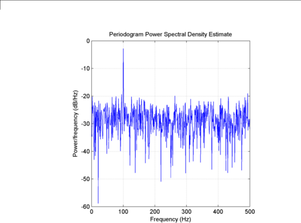
12 Spectral Analysis

Use fft to produce a periodogram for an input using normalized frequency.

Create a signal consisting of a sine wave in N(0,1) additive noise. The sine

wave has an angular frequency of π/4 radians/sample. Use the default

settings of the random number generator for reproducible results.

rng default;

n = 0:999;

x = cos(pi/4*n)+randn(size(n));

Obtain the periodogram using fft. The signal is real-valued and has even

length. Because the signal is real-valued, you only need power estimates for

thepositiveornegativefrequencies. In order to conserve the total power,

12-4

Power Spectral Density Estimates Using FFT

multiply all frequencies that occur inbothsets—thepositiveandnegative

frequencies — by a factor of 2. Zero frequency (DC) and the Nyquist frequency

do not occur twice. Plot the result.

N = length(x);

xdft = fft(x);

xdft = xdft(1:N/2+1);

psdx = (1/(2*pi*N)).*abs(xdft).^2;

psdx(2:end-1) = 2*psdx(2:end-1);

freq = 0:(2*pi)/N:pi;

plot(freq./pi,10*log10(psdx)); grid on;

title('Periodogram Using FFT');

xlabel('Normalized Frequency');

ylabel('Power/Frequency (dB/rad/sample)');

12-5

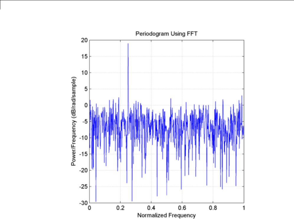
12 Spectral Analysis

Compute and plot the periodogram using periodogram. Show that the 2

results are identical.

figure;

[psdestx,Fxx] = periodogram(x,rectwin(length(x)),length(x));

plot(Fxx./pi,10*log10(psdestx));

xlabel('Hz'); ylabel('Power/Frequency (dB/Hz)');

title('Periodogram Power Spectral Density Estimate');

xlabel('Normalized Frequency'); grid on;

ylabel('Power/Frequency (dB/rad/sample)');

max(psdx'-psdestx)

12-6

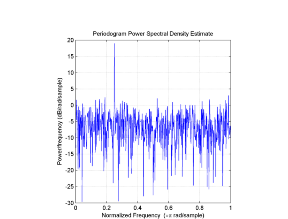
Power Spectral Density Estimates Using FFT

Use fft to produce a periodogram for a complex-valued input with normalized

frequency.

Create the complex-valued signal. The signal is a complex exponential with an

angular frequency of π/4 radians/sample in complex-valued N(0,1) noise. Set

the random number generator to the default settings for reproducible results.

rng default;

n = 0:999;

x = exp(1j*pi/4*n)+1/sqrt(2)*randn(size(n))+1j*1/sqrt(2)*randn(size(n));

Use fft to obtain the periodogram. Because the input is complex-valued,

obtain the periodogram from (-π,π] radians/sample. Plot the result.

12-7

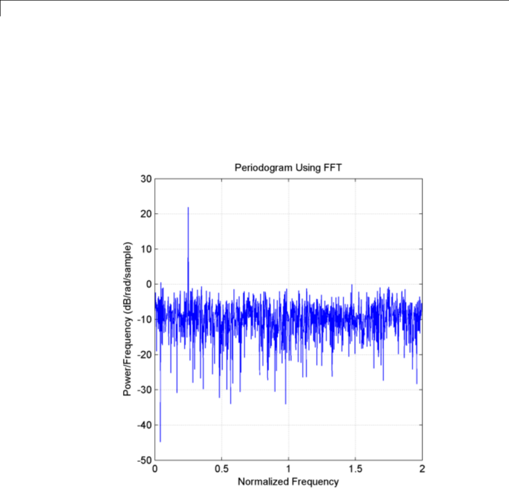
12 Spectral Analysis

N = length(x);

xdft = fft(x);

psdx = (1/(2*pi*N)).*abs(xdft).^2;

freq = 0:(2*pi)/N:2*pi-(2*pi)/N;

plot(freq./pi,10*log10(psdx)); grid on;

title('Periodogram Using FFT');

xlabel('Normalized Frequency');

ylabel('Power/Frequency (dB/rad/sample)');

Use periodogram to obtain and plot the periodogram. Compare the PSD

estimates.

[psdestx,Fxx] = periodogram(x,rectwin(length(x)),length(x),'twosided');

12-8

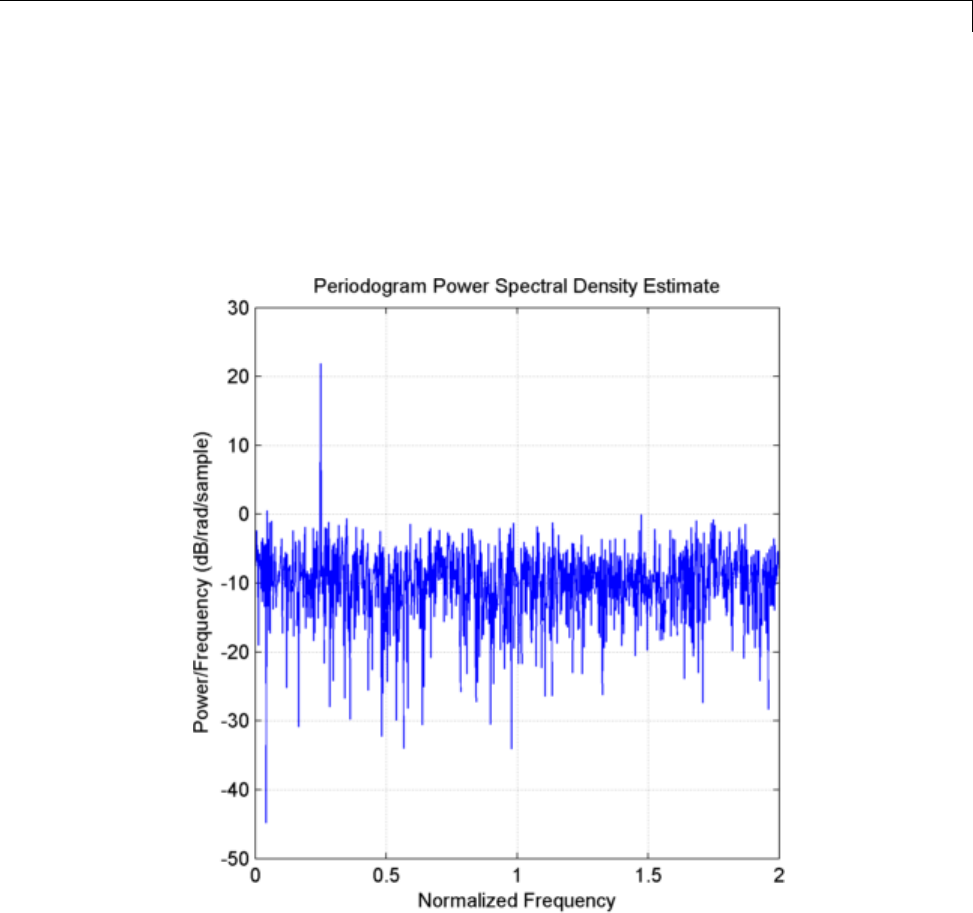
Power Spectral Density Estimates Using FFT

figure;

plot(Fxx./pi,10*log10(psdestx));

grid on; xlabel('Normalized Frequency');

ylabel('Power/Frequency (dB/rad/sample)');

title('Periodogram Power Spectral Density Estimate');

max(psdx'-psdestx)

12-9

12 Spectral Analysis

Bias and Variability in the Periodogram

These examples show how to reduce bias and variability in the periodogram.

Using a window can reduce the bias in the periodogram and using windows

with averaging can reduce variability.

The periodogram suffers from two well-known problems, bias and

inconsistency. Bias is introduced by the convolution of the true spectral

density with Fejer’s kernel. The periodogram is not a consistent estimator of

the true spectral density because the variance of the periodogram does not

decay to zero regardless of the sample size.

The periodogram also exhibits a high degree of variability because of the small

number of degrees of freedom. The periodogram estimates at the Fourier

frequencies are chi-square random variables with two degrees of freedom

except at zero and Nyquist, which only exhibit one degree of freedom.

Bias in the periodogram can be mitigated by tapering,orwindowingthe

time series before computing the PSD estimate. Inconsistency is addressed

by using Welch’s overlapped segment averaging approach, or a multitaper

estimate.

Use wide-sense stationary autoregressive processes (AR) processes to show

the effects of bias and variability in the periodogram. AR processes present a

convenient model because their PSDs have closed-form expressions. Create

an AR(2) model of the following form:

yn yn yn n() . ( ) . ( ) (),075 1 05 2



where ε(n) is a zero mean white noise sequence with some specified variance.

In this example, assume the variance and the sampling period to be 1.

To simulate the preceding AR(2) process, create an all-pole (IIR) filter. View

the filter’s magnitude response.

B2 = 1;

A2 = [1 -0.75 0.5];

fvtool(B2,A2);

12-10

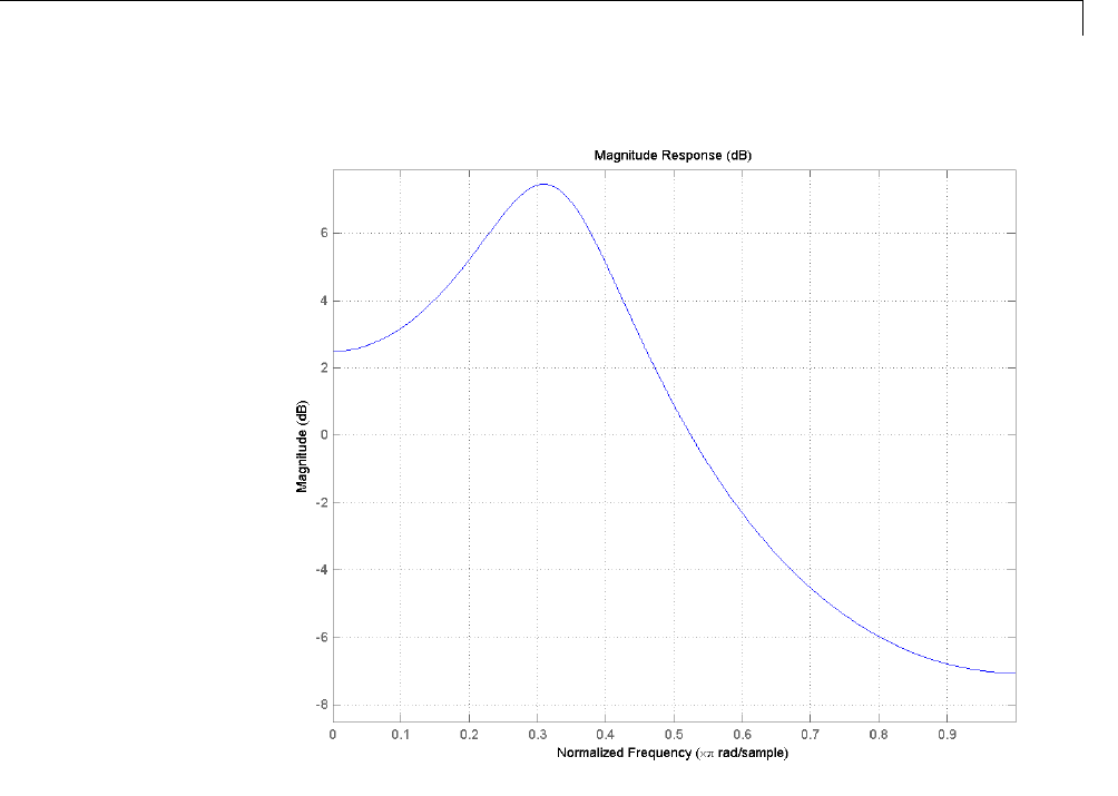
Bias and Variability in the Periodogram

Thisprocessisbandpass. ThedynamicrangeofthePSDisapproximately

14.5 dB, you can determine this with the following code.

[H2,W2] = freqz(B2,A2,1e3,1);

max(20*log10(abs(H2)))-min(20*log10(abs(H2)))

By examining the placement of the poles, you see that this AR(2) process is

stable. The two poles are inside the unit circle.

fvtool(B2,A2,'analysis','polezero');

12-11

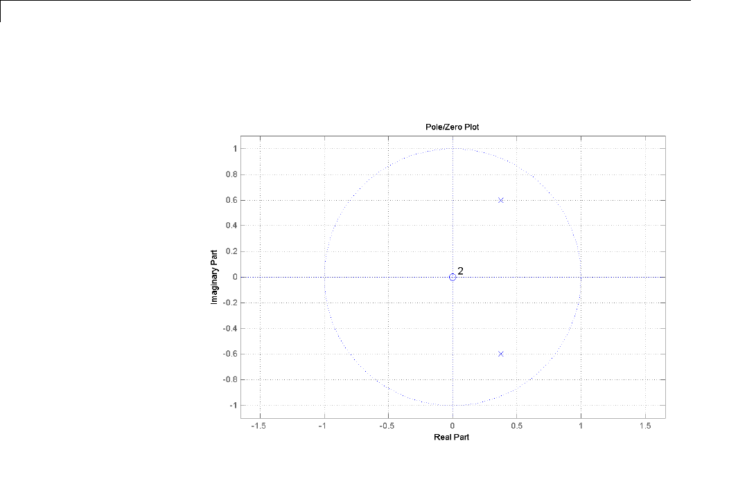
12 Spectral Analysis

Create an AR(4) process described by the following equation:

yn yn yn yn yn().().().().()2 7607 1 3 8106 2 2 6535 3 0 9238 4



(()n

UsethefollowingcodetoviewthemagnituderesponseofthisIIRsystem.

B4 = 1;

A4 = [1 -2.7607 3.8106 -2.6535 0.9238];

fvtool(B4,A4);

12-12

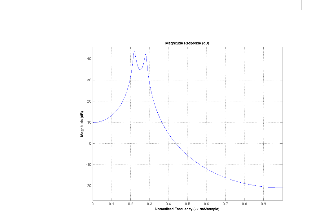
Bias and Variability in the Periodogram

Examining the placement of the poles, you can see this AR(4) process is also

stable. The four poles are inside the unit circle.

fvtool(B4,A4,'analysis','polezero');

12-13

12 Spectral Analysis

The dynamic range of this PSD is approximately 65 dB, much larger than

the AR(2) model.

[H4,W4] = freqz(B4,A4,1e3,1);

max(20*log10(abs(H4)))-min(20*log10(abs(H4)))

To simulate realizations from these AR(p) processes, use randn and filter.

Set the random number generator to the default settings to produce

repeatable results. Plot the realizations.

rng default;

x = randn(1e3,1);

y2 = filter(B2,A2,x);

y4 = filter(B4,A4,x);

12-14

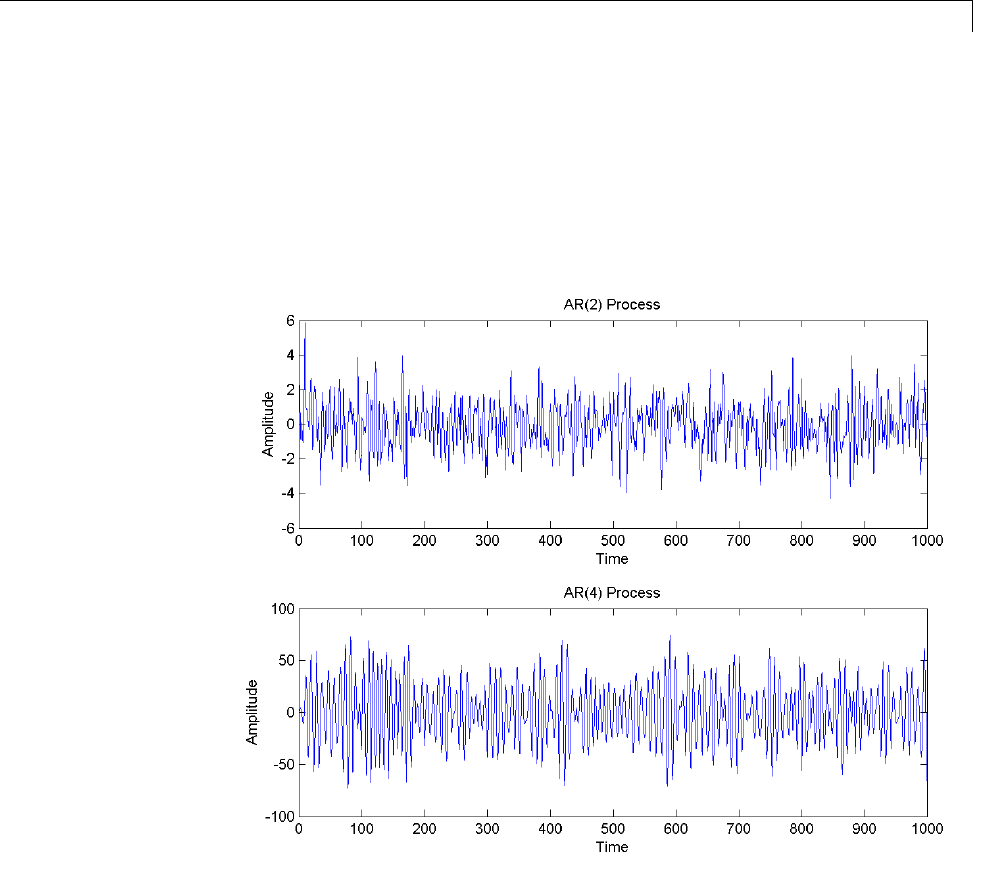
Bias and Variability in the Periodogram

subplot(211)

plot(y2); title('AR(2) Process');

xlabel('Time'); ylabel('Amplitude');

subplot(212);

plot(y4); title('AR(4) Process');

xlabel('Time'); ylabel('Amplitude');

Compute the periodograms of the AR(2) and AR(4) realizations. Plot the

result and compare the periodogram against the true PSD.

Fs = 1;

NFFT = length(y2);

[psdAR2,Fxx] = periodogram(y2,rectwin(length(y2)),length(y2),1);

psdAR4 = periodogram(y4,rectwin(length(y2)),length(y2),1);

12-15

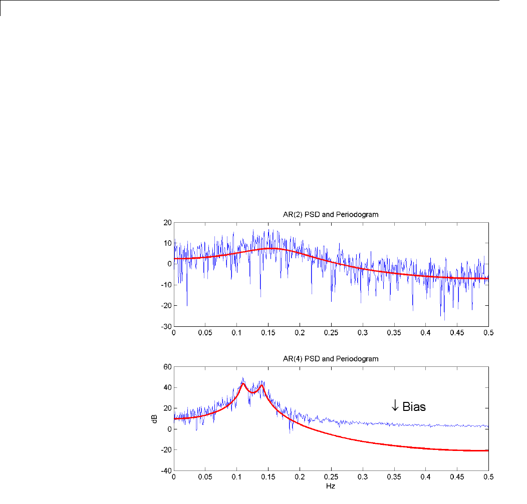
12 Spectral Analysis

subplot(211)

plot(Fxx,10*log10(psdAR2));

hold on;

plot(W2,20*log10(abs(H2)),'r','linewidth',2);

title('AR(2) PSD and Periodogram');

subplot(212)

plot(Fxx,10*log10(psdAR4));

hold on;

plot(W4,20*log10(abs(H4)),'r','linewidth',2);

xlabel('Hz'); ylabel('dB');

title('AR(4) PSD and Periodogram');

12-16

Bias and Variability in the Periodogram

InthecaseoftheAR(2)process,theperiodogram estimate follows the shape

of the true PSD but exhibits considerable variability. This is due to the

low degrees of freedom. The pronounced negative deflections (in dB) in the

periodogram are explained by taking the log of a chi-square random variable

with two degrees of freedom.

InthecaseoftheAR(4)process,theperiodogramfollowstheshapeofthetrue

PSD at low frequencies but deviates from the PSD in the high frequencies.

This is the effect of the convolution with Fejer’s kernel. The large dynamic

range of the AR(4) process compared to the AR(2) process is what makes

thebiasmorepronounced.

Mitigate the bias demonstrated in the AR(4) process by using a taper,

or window. In this example, use a Hamming window to taper the AR(4)

realization before obtaining the periodogram.

[psdAR4H,Fxx] = periodogram(y4,hamming(length(y4)),NFFT,Fs);

plot(Fxx,10*log10(psdAR4H));

hold on;

plot(W4,20*log10(abs(H4)),'r','linewidth',2);

xlabel('Hz'); ylabel('dB');

title('AR(4) PSD and Periodogram with Hamming Window');

legend('Periodogram with Hamming Window','AR(4) PSD',...

'Location','NorthEast');

12-17

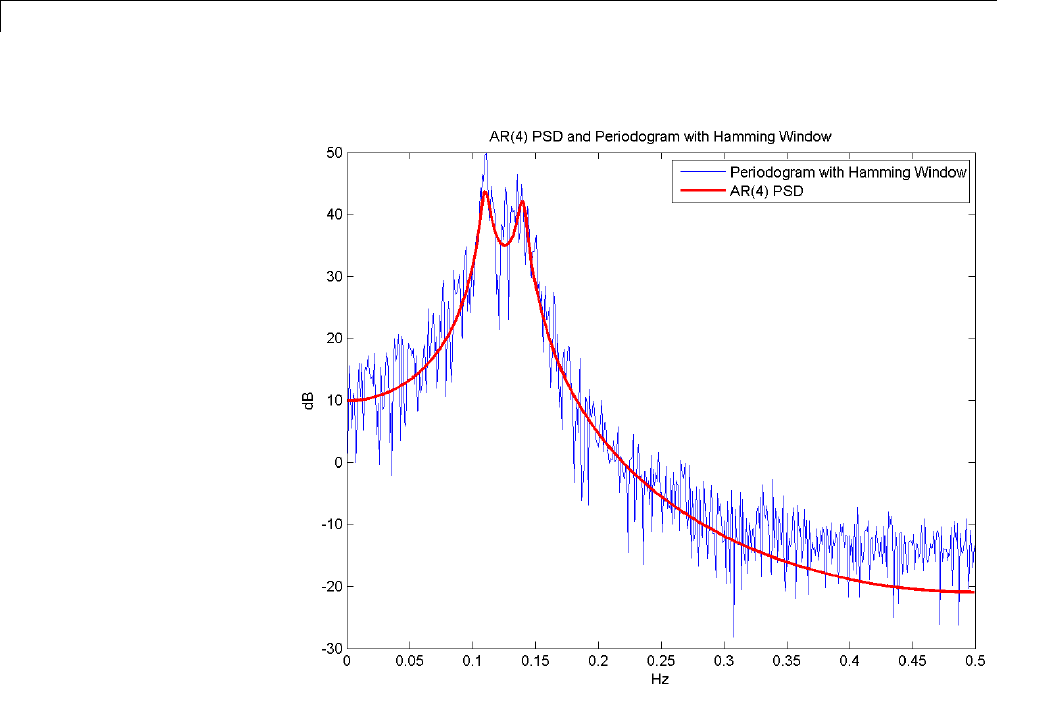
12 Spectral Analysis

Note that the periodogram estimate nowfollowsthetrueAR(4)PSDoverthe

entire [0,Nyquist] frequency range. The periodogram estimates still only have

two degrees of freedom so the use of a window does not reduce the variability

of periodogram, but it does address bias.

In nonparametric spectral estimation, two methods for increasing the degrees

of freedom and reducing the variability of the periodogram are Welch’s

overlapped segment averaging and multitaper spectral estimation.

Obtain a multitaper estimate of the AR(4) time series using a time half

bandwidthproductof3.5. Plottheresult.

NW = 3.5;

[psdmtm,Fxx] = pmtm(y4,NW,NFFT,Fs);

12-18

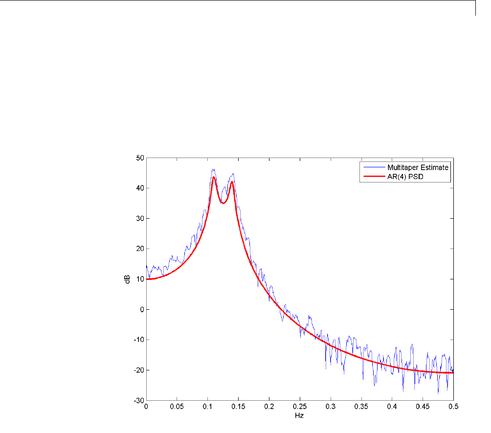
Bias and Variability in the Periodogram

plot(Fxx,10*log10(psdmtm));

hold on;

plot(W4,20*log10(abs(H4)),'r','linewidth',2);

xlabel('Hz'); ylabel('dB');

legend('Multitaper Estimate','AR(4) PSD', ...

'Location','NorthEast');

The multitaper method produces a PSD estimate with significantly less

variability than the periodogram. Because the multitaper method also uses

windows, you see that the bias of the periodogram is also addressed.

12-19

12 Spectral Analysis

Cross Spectrum and Magnitude-Squared Coherence

This example shows how to use the cross spectrum to obtain the phase lag

between sinusoidal components in a bivariate time series. The example

also uses the magnitude-squared coherence (MSC) to identify significant

frequency-domain correlation atthesinewavefrequencies.

Create the bivariate time series. The individual series consist of two sine

waves with frequencies of 100 and 200 Hz in additive white Gaussian noise.

The sine waves in the x-series both have amplitudes equal to 1. The 100-Hz

sine wave in the y-series has amplitude 0.5 and the 200-Hz sine wave in the

y-series has amplitude 0.35. The sine waves in the y-series are phase-lagged

by π/4 radians (100 Hz) and π/2 radians (200 Hz). You can think of y-series as

the noise-corrupted output of a linear system with input x. In the following

code, set the random number generator to the default settings for reproducible

results.

Fs = 1000;

t = 0:1/Fs:1-1/Fs;

rng default;

x = cos(2*pi*100*t)+sin(2*pi*200*t)+0.5*randn(size(t));

y = 0.5*cos(2*pi*100*t-pi/4)+0.35*sin(2*pi*200*t-pi/2)+0.5*randn(size(t));

Obtain the magnitude-squared coherence (MSC) for the bivariate time

series. The magnitude-squared coherence enables you to identify significant

frequency-domain correlation between the two time series. Phase estimates

in the cross spectrum are only useful where significant frequency-domain

correlation exists.

To prevent obtaining a magnitude-squared coherence estimate, which is

identically 1 for all frequencies, you must use an averaged MSC estimator.

Both Welch’s overlapped segment averaging (WOSA) and mulitaper

techniques are appropriate. mscohere implements a WOSA estimator.

Set the window length to 100 samples. This window length contains 10

periods of the 100-Hz sine wave and 20 periods of the 200-Hz sine wave.

Use an overlap of 80 samples with the default Hamming window. Plot the

magnitude-squared coherence.

[Pxy,F] = mscohere(x,y,hamming(100),80,100,Fs);

12-20

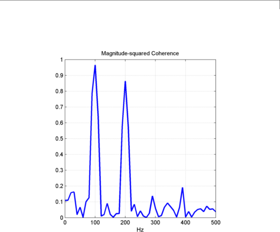
Cross Spectrum and Magnitude-Squared Coherence

plot(F,Pxy,'linewidth',2); title('Magnitude-squared Coherence');

xlabel('Hz'); grid on;

You see that the magnitude-squared coherence is greater than 0.8 at 100

and 200 Hz.

Obtain the cross spectrum of xand yusing cpsd. Use the same parameters

to obtain the cross spectrum that you used in the MSC estimate. Plot the

phase of the cross spectrum and indicate the frequencies with significant

coherencebetweenthetwotimes. Marktheknownphaselagsbetweenthe

sinusoidal components.

[Cxy,F] = cpsd(x,y,hamming(100),80,100,Fs);

12-21

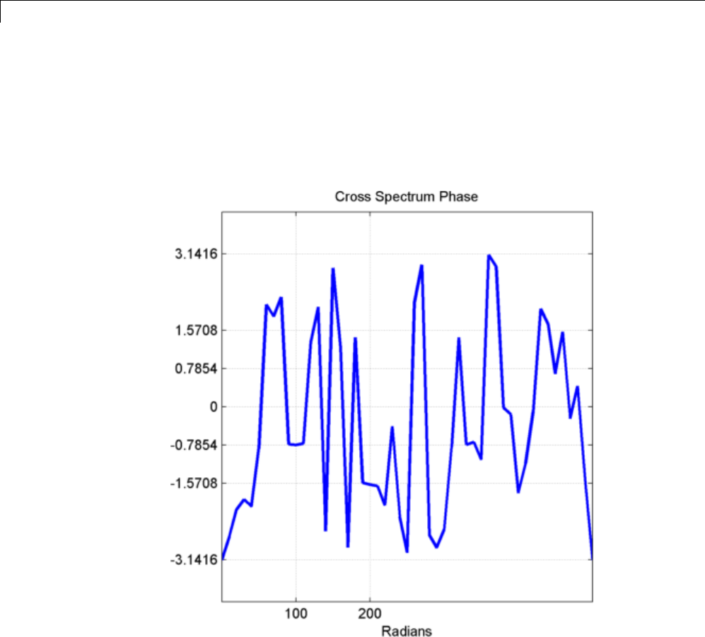
12 Spectral Analysis

figure;

plot(F,-angle(Cxy),'linewidth',2); title('Cross Spectrum Phase');

xlabel('Radians');

set(gca,'xtick',[100 200]);

set(gca,'ytick',[-pi -pi/2 -pi/4 0 pi/4 pi/2 pi]);

grid on;

You see that at 100 Hz and 200 Hz, the phase lags estimated from the cross

spectrumareclosetothetruevalues.

In this example, the cross spectrum estimates are spaced at 1000/100= 10 Hz.

You can return the phase estimates at those frequency bins. Keep in mind

that the first frequency bin corresponds to 0 Hz, or DC.

12-22

Cross Spectrum and Magnitude-Squared Coherence

phi100 = - angle(Cxy(11));

phi200 = - angle(Cxy(21));

You see that phi100 and phi200 are close to –π/4 and –π/2.

12-23

12 Spectral Analysis

Amplitude Estimation and Zero Padding

Thisexampleshowstheeffectoffrequency resolution on amplitude

estimation. Frequencies in the discrete Fourier transform (DFT) are spaced

at intervals of Fs/N where Fs is the sampling frequency and N is the length

of the input time series. Attempting to estimate the amplitude of a sinusoid

with a frequency that does not correspond to a DFT bin canresultinan

inaccurate estimate. Therefore, zero padding the data before you obtain the

DFT can often help to improve the amplitude estimate.

Create a signal consisting of two sine waves. The two sine waves have

frequencies of 100 and 202.5 Hz. The sampling frequency is 1000 Hz and

thesignalis1000samplesinlength.

Fs = 1e3;

t = 0:0.001:1-0.001;

x = cos(2*pi*100*t)+sin(2*pi*202.5*t);

Obtain the DFT of the signal. The DFT bins are spaced at 1 Hz. Accordingly,

the 100-Hz sine wave corresponds to a DFT bin, but the 202.5-Hz sine wave

does not.

Because the signal is real-valued, use only the positive frequencies from the

DFT to estimate the amplitude. Scale the DFT by the length of the input

signal and multiply all frequencies except 0 and the Nyquist by 2.

Plot the result with the known amplitudes for comparison.

freqres = Fs/length(x);

xdft = fft(x);

xdft = xdft(1:length(x)/2+1);

xdft = 1/length(x).*xdft;

xdft(2:end-1) = 2*xdft(2:end-1);

freq = 0:Fs/length(x):Fs/2;

plot(freq,abs(xdft));

xlabel('Hz'); ylabel('Amplitude');

h = line(freq,ones(length(x)/2+1,1));

set(h,'color',[1 0 0],'linewidth',2);

12-24

Amplitude Estimation and Zero Padding

The amplitude estimate at 100 Hz is accurate because that frequency

corresponds to a DFT bin. However, the amplitude estimate at 202.5 Hz is not

accurate because that frequency does not correspond to a DFT bin.

You can interpolate the DFT by zero padding. While zero padding does not

improve the frequency resolution of the DFT, zero padding can allow you to

obtain more accurate amplitude estimates of resolvable signal components.

Pad the DFT out to length 2000. With this length, the spacing between DFT

bins is Fs/2000=0.5 Hz. In this case, the energy from the 202.5-Hz sine wave

falls directly in a DFT bin. Using zero padding out to 2000 samples, obtain

the DFT and plot the amplitude estimates.

xdft = fft(x,2000);

12-25

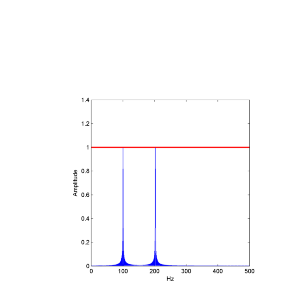
12 Spectral Analysis

xdft = xdft(1:length(xdft)/2+1);

xdft = 1/length(x).*xdft;

xdft(2:end-1) = 2*xdft(2:end-1);

freq = 0:Fs/(2*length(x)):Fs/2;

plot(freq,abs(xdft));

xlabel('Hz'); ylabel('Amplitude');

h = line(freq,ones(2*length(x)/2+1,1));

set(h,'color',[1 0 0],'linewidth',2);

The use of zero padding enables you to estimate the amplitudes of both

frequencies correctly.

12-26

Significance Testing for Periodic Component

This example shows you how to assess the significance of a sinusoidal

component in white noise using Fisher’s g–statistic. Fisher’s g–statistic is

the ratio of the largest periodogram value to the sum of all the periodogram

values over 1/2 of the frequency interval, (0,Fs/2). A detailed description of

the g–statistic and exact distribution can be found in [1] and [2].

Create a signal consisting of a 100-Hz sine wave in white Gaussian noise

with zero mean and variance 1. The amplitude of the sine wave is 0.25. The

sampling rate is 1 kHz. Set the random number generator to the default

settings for reproducible results.

Fs = 1e3;

t = 0:0.001:1-0.001;

rng default;

x = 0.25*cos(2*pi*100*t)+randn(size(t));

Obtain the periodogram of the signal using periodogram.Exclude0and

the Nyquist frequency (Fs/2) .

[Pxx,F] = periodogram(x,rectwin(length(x)),length(x),Fs);

Pxx = Pxx(2:length(x)/2);

Find the maximum value of the periodogram. Fisher’s g–statistic is the ratio

of the maximum perioodgram value to the sum of all periodogram values.

[maxval,index] = max(Pxx);

fisher_g = Pxx(index)/sum(Pxx);

The maximum periodogram value occurs at 100 Hz, which you can verify

by finding the frequency corresponding to the index of the maximum

periodogram value.

F = F(2:end-1);

F(index)

Use the distributional results detailed in [1] and [2] to determine the

significance level, pval,ofFisher’sg–statistic. The following MATLAB code

implements equation 6 on page 7 in [2].

N = length(Pxx);

12-27

12 Spectral Analysis

upper = floor(1/fisher_g);

for nn = 1:3

I(nn) = ...

(-1)^(nn-1)*nchoosek(N,nn)*(1-nn*fisher_g)^(N-1);

end

pval = sum(I);

The p-value is less than 0.00001, which indicates a significant periodic

component at 100 Hz. The interpretation of Fisher’s g–statistic is complicated

by the presence of other periodicities. See [1] for a modification when multiple

periodicities may be present.

References

[1] Percival, D.B. and Walden, A.T. Spectral Analysis for Physical

Applications, Cambridge University Press, 1993, p. 491.

[2] Wichert, S., Fokianos, K., and Strimmer, K. “Identifying periodically

expressed transcripts in microarray time series data”, Bioinformatics, 20,

5-20, 2004.

12-28

Frequency Estimation by Subspace Methods

This example shows you how to resolve closely-spaced sine waves using

subspace methods. Subspace methods assume a harmonic model consisting of

a sum of sine waves, possibly complex, in additive noise. In a complex-valued

harmonic model, the noise is also complex-valued.

Create a complex-valued signal 24 samples in length. The signal consists of

two complex exponentials (sine waves) with frequencies of 0.50 and 0.52 hertz

and additive complex white Gaussian noise. The noise has zero mean and

variance 0.22. In a complex white noise, both the real and imaginary parts

have variance equal to 1/2 the overall variance.

n = 0:23;

rng default

x = exp(1j*2*pi*0.5*n)+exp(1j*2*pi*0.52*n)+ ...

0.2/sqrt(2)*(randn(size(n))+1j*randn(size(n)));

Using periodogram,attempttoresolvethetwosinewaves.

periodogram(x,rectwin(length(x)),128,1);

12-29

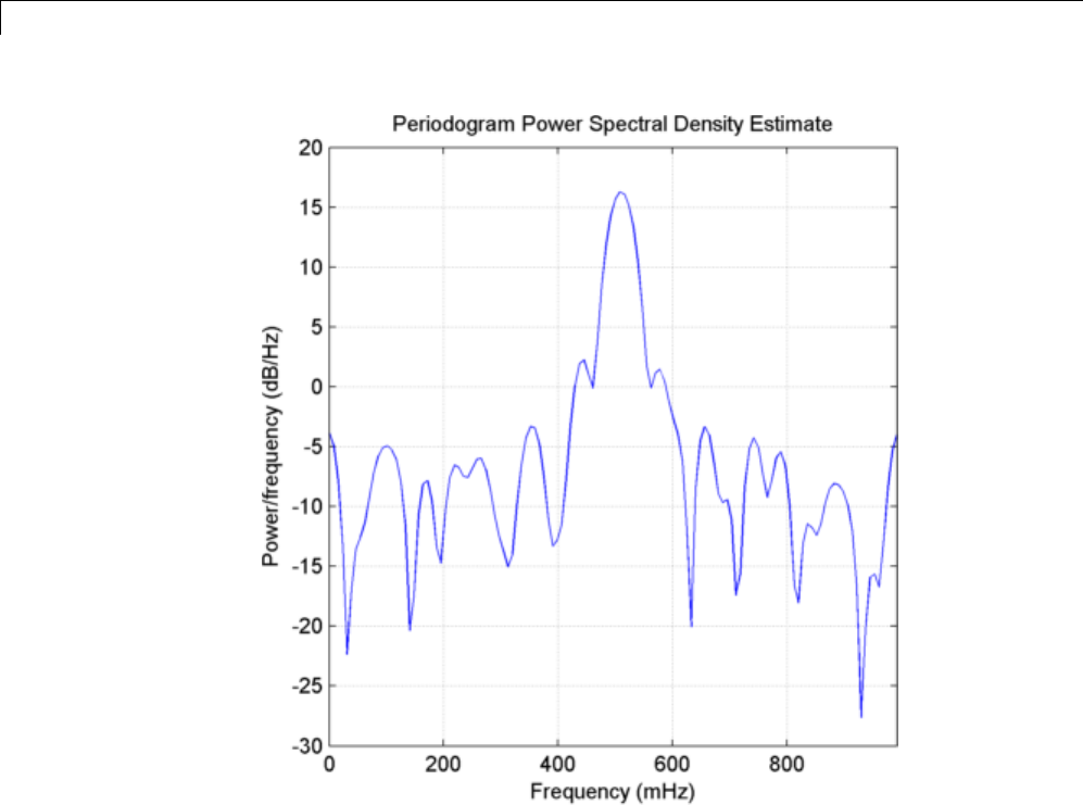
12 Spectral Analysis

The periodogram shows a broad peak near 1/2 Hz. You cannot resolve the two

separate sine waves because the frequency resolution of the periodogram is

1/N, where N is the length of the signal. In this case, 1/N is greater than the

separation of the two sine waves. Zero padding does not help to resolve two

separate peaks.

Use a subspace method to resolve the two closely-spaced peaks. In this

example, use the root-MUSIC method. Estimate the autocorrelation matrix

and input the autocorrelation matrix into pmusic. Specify a model with 2

sinusoidal components. Plot the result.

[X,R] = corrmtx(x,14,'mod');

12-30

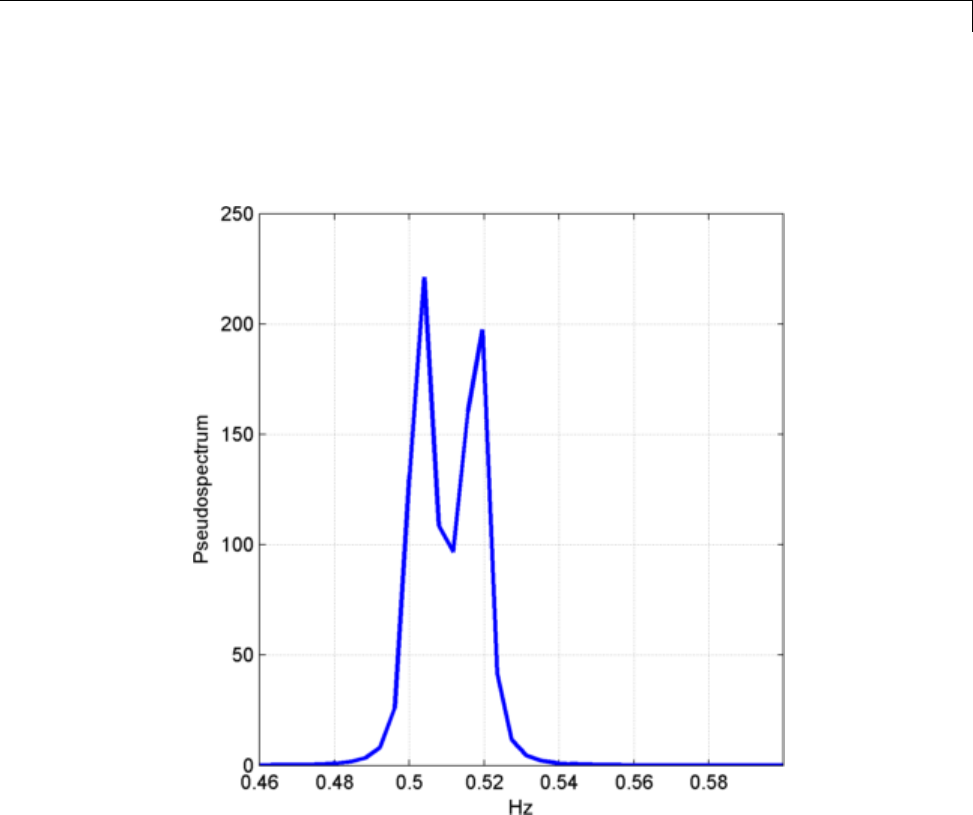
Frequency Estimation by Subspace Methods

[S,F] = pmusic(R,2,[],1,'corr');

plot(F,S,'linewidth',2); set(gca,'xlim',[0.46 0.60]);

grid on; xlabel('Hz'); ylabel('Pseudospectrum');

The root MUSIC method is able to separate the two peaks at 0.5 and 0.52

Hz. However, subspace methods do not produce power estimates like power

spectral density estimates. Subspace methods are most useful for frequency

identification and can be sensitive to model-order misspecification.

12-31

12 Spectral Analysis

Frequency-Domain Linear Regression

This example shows how to use the discrete Fourier transform to construct a

linear regression model for a time series. The time series used in this example

is the monthly number of accidental deaths in the U.S. from 1973 to 1979.

The data are published in [1]. The original source is the U.S. National Safety

Council.

Enter the data. Copy the exdata matrix into the MATLAB workspace.

exdata = [

9007 7750 8162 7717 7792 7836

8106 6981 7306 7461 6957 6892

8928 8038 8124 7776 7726 7791

9137 8422 7870 7925 8106 8129

10017 8714 9387 8634 8890 9115

10826 9512 9556 8945 9299 9434

11317 10120 10093 10078 10625 10484

10744 9823 9620 9179 9302 9827

9713 8743 8285 8037 8314 9110

9938 9129 8433 8488 8850 9070

9161 8710 8160 7874 8265 8633

8927 8680 8034 8647 8796 9240];

exdata is a 12-by-6 matrix. Each column of exdata contains 12 months of

data. The first row of each column contains the number of U.S. accidental

deaths for January of the corresponding year. The last row of each

column contains the number of U.S. accidental deaths for December of the

corresponding year.

Reshape the data matrix into a 72-by-1 time series and plot the data for the

years 1973 to 1978.

ts = reshape(exdata,72,1);

years = linspace(1973,1979,72);

plot(years,ts,'bo-','markerfacecolor',[0 0 1]); xlabel('Year');

ylabel('Number of Accidental Deaths'); grid on;

12-32

Frequency-Domain Linear Regression

A visual inspection of the data indicates that number of accidental deaths

varies in a periodic manner. The period of the oscillation appears to be

roughly 1 year (12 months). The periodic nature of the data suggests that

an appropriate model may be

Xn A B n

Nkkn

() cos( ) sin( ) ()  







where μis the overall mean, N is the length of the time series, and ε(n)

is a white noise sequence of independent and identically-distributed (iid)

Gaussian random variables with zero mean and some variance. The additive

noise term accounts for the randomness inherent in the data. The parameters

12-33

12 Spectral Analysis

of the model are the overall mean and the amplitudes of the cosines and sines.

The model is linear in the parameters.

To construct a linear regression model in the time domain, you have to specify

which frequencies to use for the cosines and sines, form the design matrix,

and solve the normal equations in order to obtain the least-squares estimates

of the model parameters. In this case, it is easier to use the discrete Fourier

transform to detect the periodicities, retain only a subset of the Fourier

coefficients, and invert the transform to obtain the fitted time series.

Perform a spectral analysis of the data to reveal which frequencies contribute

significantly to the variability in the data. Because the overall mean of the

signal is approximately 9,000 and is proportional to the Fourier transform at

0 frequency, subtract the mean prior to the spectral analysis. This reduces the

large magnitude Fourier coefficient at 0 frequency and makes any significant

oscillations easier to detect. The frequencies in the Fourier transform are

spaced at an interval that is the reciprocal of the time series length, 1/72.

Sampling the data monthly, the highest frequency in the spectral analysis is

1 cycle/2 months. In this case, it is convenient to look at the spectral analysis

in terms of cycles/year so scale the frequencies accordingly for visualization.

tsdft = fft(ts-mean(ts));

freq = 0:1/72:1/2;

plot(freq.*12,abs(tsdft(1:length(ts)/2+1)),'bo-','markerfacecolor',[0 0 1]

xlabel('Cycles/Year'); ylabel('Magnitude');

set(gca,'xtick', [1/6 1 2 3 4 5 6])

12-34

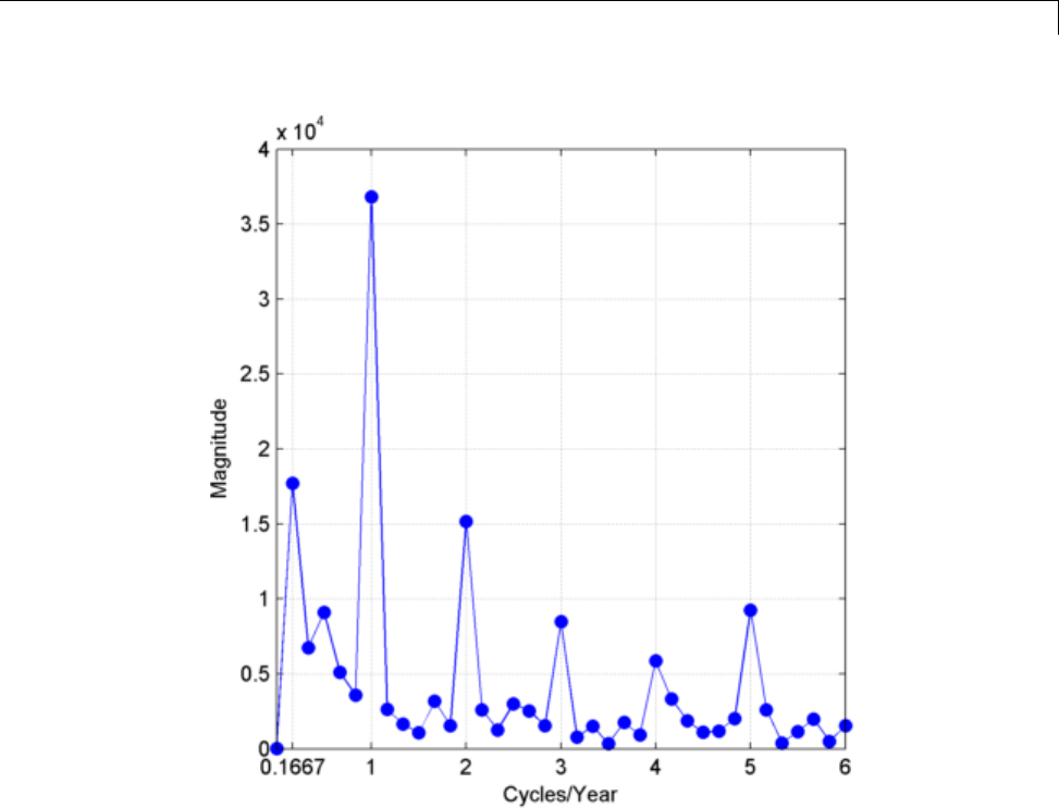
Frequency-Domain Linear Regression

Based on the magnitudes, the frequency of 1 cycle/12 months is the most

significant oscillation in the data. The magnitude at 1 cycle/12 months is

more than twice as large as any other magnitude. However, the spectral

analysis reveals that there are also other periodic components in the data.

For example, there appears to be periodic components at harmonics (integer

multiples) of 1 cycle/12 months. There also appears to be a periodic component

with a period of 1 cycle/72 months.

Based on the spectral analysis of the data, fit a simple linear regression

model using a cosine and sine term with a frequency of the most signficant

component: 1 cycle/year (1 cycle/12 months).

12-35

12 Spectral Analysis

Determine the frequency bin in the discrete Fourier transform that

corresponds to 1 cycle/12 months. Because the frequencies are spaced at 1/72

and the first bin corresponds to 0 frequency, the correct bin is 72/12+1. This

is the frequency bin of the positive frequency. You must also include the

frequency bin corresponding to the negative frequency: –1 cycle/12 months.

With MATLAB indexing, the frequency bin of the negative frequency is

72–72/12+3.

Create a 72-by-1 vector of zeros. Fill the appropriate elements of the vector

with the Fourier coefficients corresponding to a positive and negative

frequency of 1 cycle/12 months. Invert the Fourier transform and add the

overall mean to obtain a fit to the accidental death data.

N=72;

freqbin = N/12+1;

freqbins = [freqbin N-freqbin+2];

tsfit = zeros(72,1);

tsfit(freqbins) = tsdft(freqbins);

tsfit = ifft(tsfit,'symmetric');

mu = mean(ts);

tsfit = mu+tsfit;

Plot the original data along with the fitted series using two Fourier

coefficients.

plot(years,ts,'bo-','markerfacecolor',[0 0 1]); xlabel('Year');

ylabel('Number of Accidental Deaths'); grid on;

hold on;

plot(years,tsfit,'r','linewidth',2);

legend('Data','Fitted Model');

12-36

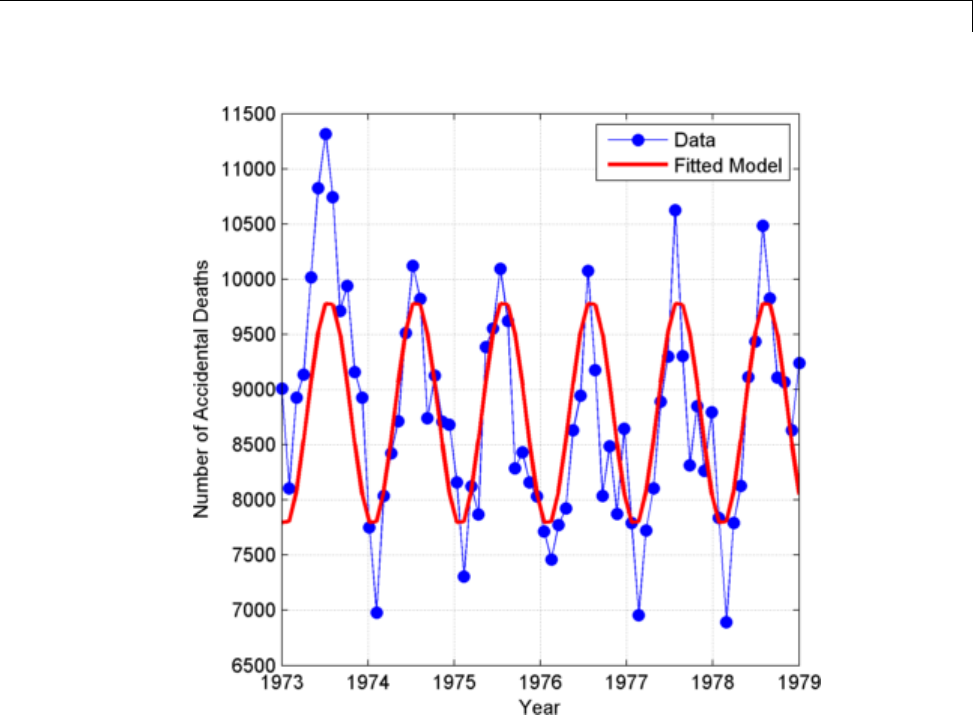
Frequency-Domain Linear Regression

The fitted model appears to capture the general periodic nature of the data

and supports the initial conclusion that data oscillate with a cycle of 1 year.

To assess how adequately the single frequency of 1 cycle/12 months accounts

for the observed time series, form the residuals. If the residuals resemble

a white noise sequence, the simple linear model with one frequency has

adequately modeled the time series.

To assess the residuals, use the autocorrelation sequence with 95%-confidence

intervals for a white noise. See “Confidence Intervals for Sample

Autocorrelation” on page 10-5 for a detailed example on how to form the

95%-confidence intervals.

resid = ts-tsfit;

12-37

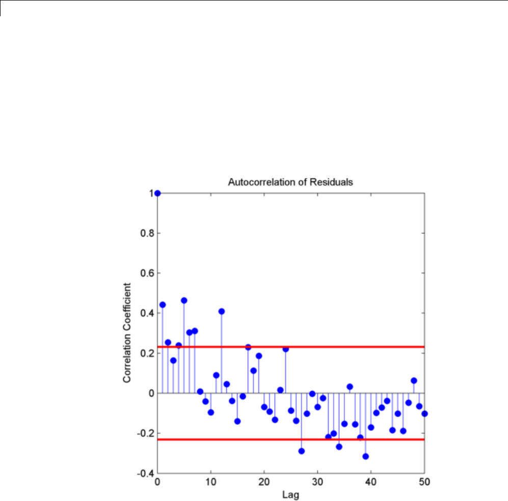
12 Spectral Analysis

[xc,lags] = xcorr(resid,50,'coeff');

stem(lags(51:end),xc(51:end),'markerfacecolor',[0 0 1]);

hold on;

lconf = -1.96*ones(51,1)/sqrt(72);

uconf = 1.96*ones(51,1)/sqrt(72);

plot(lags(51:end),lconf,'r','linewidth',2);

plot(lags(51:end),uconf,'r','linewidth',2);

xlabel('Lag'); ylabel('Correlation Coefficient');

title('Autocorrelation of Residuals');

The autocorrelation values fall outside the 95% confidence bounds at a

number of lags. It does not appear that the residuals are white noise. The

12-38

Frequency-Domain Linear Regression

conclusion is that the simple linear model with one sinusoidal component

does not account for all the oscillations in the number of accidental deaths.

This is expected because the spectral analysis revealed additional periodic

components in addition to the dominant oscillation. Creating a model that

incorporates additional periodic terms indicated by the spectral analysis will

improve the fit and whiten the residuals.

Fit a model which consists of the three largest Fourier coefficient magnitudes.

Because you have to retain the Fourier coefficients corresponding to both

negative and positive frequencies, retain the largest 6 indices.

tsfit2dft = zeros(72,1);

[Y,I] = sort(abs(tsdft),'descend');

indices = I(1:6);

tsfit2dft(indices) = tsdft(indices);

Demonstrate that preserving only 6 of the 72 Fourier coefficients (3

frequencies) retains most of the signal’s energy. First, demonstrate that

retaining all the Fourier coefficients yields energy equivalence between the

original signal and the Fourier transform.

norm(1/sqrt(72)*tsdft,2)/norm(ts-mean(ts),2)

The ratio is 1. Now, examine the energy ratio where only 3 frequencies are

retained.

norm(1/sqrt(72)*tsfit2dft,2)/norm(ts-mean(ts),2)

Almost 90% of the energy is retained. Equivalently, 90% of the variance of the

time series is accounted for by 3 frequency components.

Form an estimate of the data based on 3 frequency components. Compare the

original data, the model with one frequency, and the model with 3 frequencies.

tsfit2 = mu+ifft(tsfit2dft,'symmetric');

plot(years,ts,'bo-','markerfacecolor',[0 0 1]); xlabel('Year');

ylabel('Number of Accidental Deaths'); grid on;

hold on;

plot(years,tsfit,'r','linewidth',2);

plot(years,tsfit2,'k','linewidth',2);

legend('Data','1 Frequency','3 Frequencies');

12-39

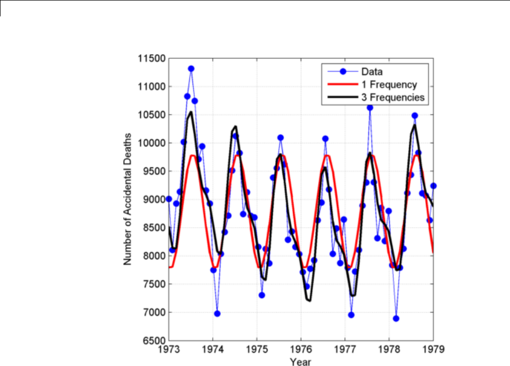
12 Spectral Analysis

Using 3 frequencies has improved the fit to the original signal. You can see

this by examining the autocorrelation of the residuals from the 3-frequency

model.

resid = ts-tsfit2;

[xc,lags] = xcorr(resid,50,'coeff');

stem(lags(51:end),xc(51:end),'markerfacecolor',[0 0 1]);

hold on;

lconf = -1.96*ones(51,1)/sqrt(72);

uconf = 1.96*ones(51,1)/sqrt(72);

plot(lags(51:end),lconf,'r','linewidth',2);

plot(lags(51:end),uconf,'r','linewidth',2);

xlabel('Lag'); ylabel('Correlation Coefficient');

title('Autocorrelation of Residuals');

12-40

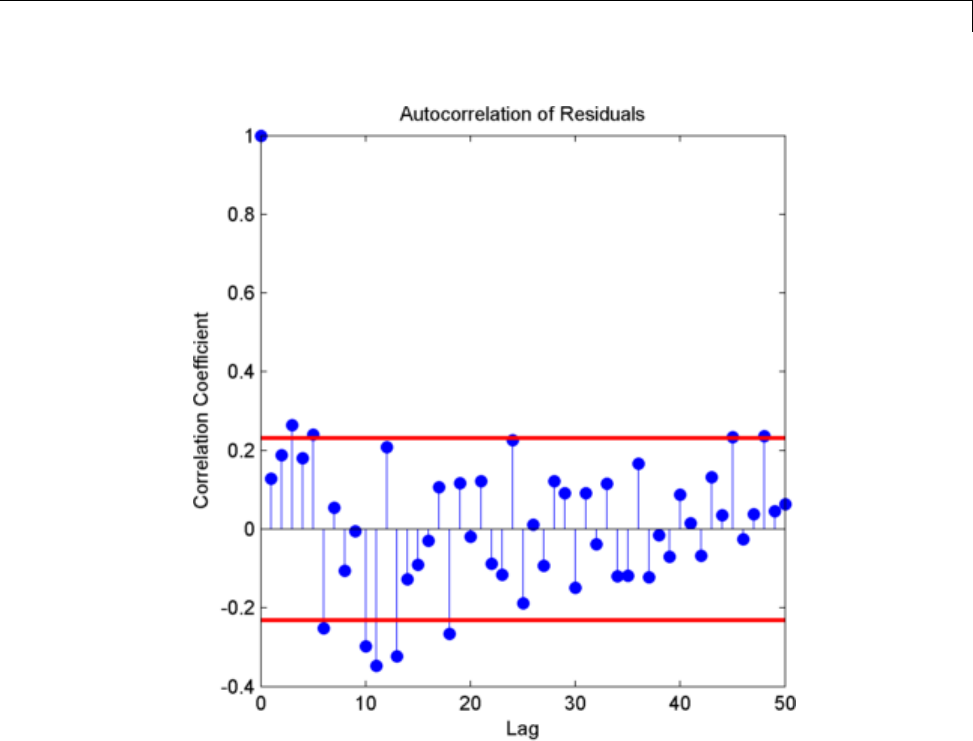
Frequency-Domain Linear Regression

Using 3 frequencies has resulted in residuals that more closely approximate a

white noise process.

Demonstrate that the parameter values obtained from the Fourier

transform are equivalent to a time-domain linear regression model. Find

the least-squares estimates for the overall mean, the cosine amplitudes,

and the sine amplitudes for the 3 frequencies by forming the design matrix

and solving the normal equations. Compare the fitted time series with that

obtained from the Fourier transform.

X = ones(72,7);

X(:,2) = cos(2*pi/72*(0:71))';

12-41

12 Spectral Analysis

X(:,3) = sin(2*pi/72*(0:71))';

X(:,4) = cos(2*pi*6/72*(0:71))';

X(:,5) = sin(2*pi*6/72*(0:71))';

X(:,6) = cos(2*pi*12/72*(0:71))';

X(:,7) = sin(2*pi*12/72*(0:71))';

beta = X\ts;

tsfit_lm = X*beta;

max(abs(tsfit_lm-tsfit2))

The two methods yield identical results. The maximum absolute value of the

difference between the two waveforms is on the order of 10-12.Inthiscase,

the frequency-domain approach was easier than the equivalent time-domain

approach. You naturally use a spectral analysis to visually inspect which

oscillations are present in the data. From that step, it is simple to use the

Fourier coefficients to construct a model for the signal consisting of a sum

cosines and sines.

For more details on spectral analysis in time series and the equivalence with

time-domain regression see [2].

While spectral analysis can answer which periodic components contribute

significantly to the variability of the data, it does not explain why those

components are present. If you examine these data closely, you see that the

minimum values in the 12-month cycle tend to occur in February, while

the maximum values occur in July. A plausible explanation for these data

is that people are naturally more active in summer than in the winter.

Unfortunately, as a result of this increased activity, there is an increased

probability of the occurrence of fatal accidents.

References

[1] Brockwell, P.J and Davis, R.A. Time Series: Theory and Methods,

Springer, 2006.

[2] Shumway, R.H. and Stoffer, D.S. Time Series Analysis and Its Applications

with R Examples, Springer, 2006.

12-42

Linear Prediction

•“Prediction Polynomial” on page 13-2

•“Formant Estimation with LPC Coefficients” on page 13-5

•“AR Order Selection with Partial Autocorrelation Sequence” on page 13-9

13 Linear Prediction

Prediction Polynomial

This example shows how to obtain the prediction polynomial from an

autocorrelation sequence. The examplealsoshowsthattheresulting

prediction polynomial has an inverse that produces a stable all-pole filter.

You can use the all-pole filter to filter a wide-sense stationary white noise

sequence to produce a wide-sense stationary autoregressive process.

Create an autocorrelation sequence defined by

rk k

() ( / ) ( / ) ,,

|| ||

 



24 5 2 27 10 3 0 1 2

k = 0:2;

rk = (24/5)*2.^(-k)-(27/10)*3.^(-k);

Use ac2poly to obtain the prediction polynomial of order 2.

A = ac2poly(rk);

The prediction polynomial of order 2 is

Az z z() / / 



156 16

Examine the pole-zero plot of the FIR filter to see that the zeros are inside

the unit circle.

zplane(A,1)

13-2

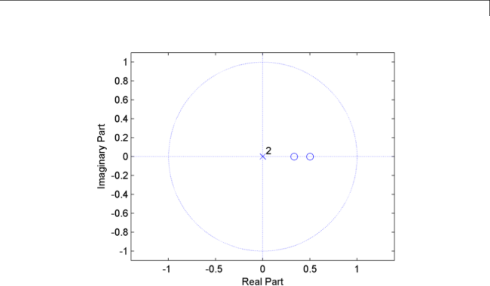
Prediction Polynomial

The inverse all-pole filter is stable with poles inside the unit circle.

zplane(1,A)

13-3

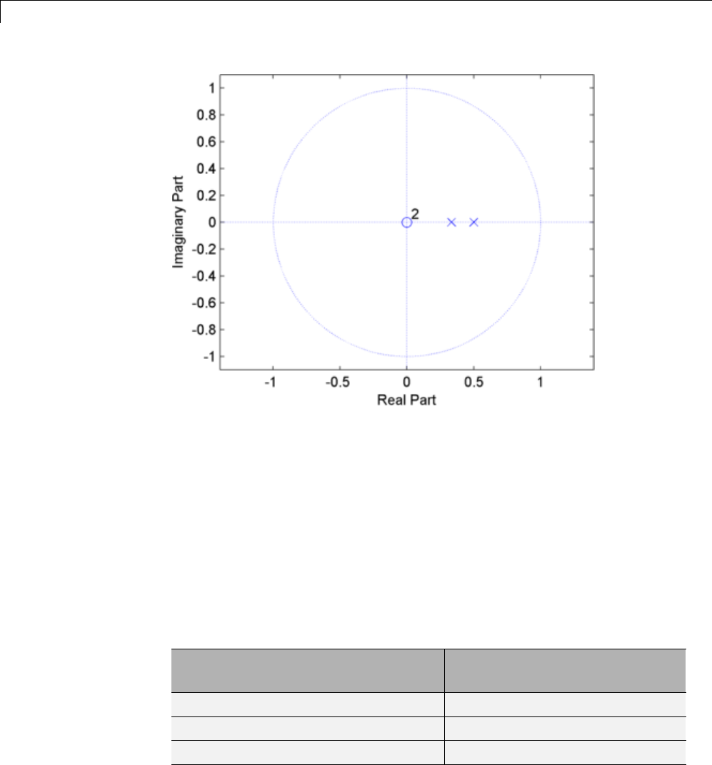
13 Linear Prediction

Use the all-pole filter to produce a realization of a wide-sense stationary AR(2)

process from a white noise sequence. Set the random number generator to the

default settings for reproducible results.

rng default;

x = randn(1000,1);

y = filter(1,A,x);

Compute the sample autocorrelation of the AR(2) realization and show that

the sample autocorrelation is close to the true autocorrelation.

[xc,lags] = xcorr(y,2,'biased');

[xc(3:end) rk']

Estimated Autocorrelation

Sequence Values

True Autocorrelation Sequence

Values

2.24 2.1

1.64 1.5

0.99 0.90

13-4

Formant Estimation with LPC Coefficients

This example shows you how to estimate vowel formant frequencies using

linear predictive coding (LPC). The formant frequencies are obtained by

finding the roots of the prediction polynomial.

The example “Complex Cepstrum — Fundamental Frequency Estimation ” on

page 14-2 uses the same speech signal to estimate the fundamental frequency.

Note This example uses the speech sample mtlb.mat, which is part of

Signal Processing Toolbox. The speech is lowpass-filtered. Because of the

low sampling frequency, this speech sample is not optimal for this example.

The low sampling frequency limits the order of the autoregressive model you

can fit to the data. In spite of this limitation, the example illustrates the

technique for using LPC coefficients to determine vowel formants.

Load the speech signal. The recording is a woman saying “MATLAB”. The

sampling frequency is 7418 Hz.

load mtlb;

The MAT file contains the speech waveform, mtlb,andthesampling

frequency, Fs.

Use the spectrogram to identify a voiced segment for analysis.

segmentlen = 100;

noverlap = 90;

NFFT = 128;

[y,f,t,p] = spectrogram(mtlb,segmentlen,noverlap,NFFT,Fs);

surf(t,f,10*log10(abs(p)),'EdgeColor','none');

axis xy; axis tight; colormap(jet); view(0,90);

xlabel('Time');

ylabel('Frequency (Hz)');

13-5

13 Linear Prediction

Extract the segment from 0.1 to 0.25 seconds for analysis. The extracted

segment corresponds roughly to the first vowel, /ae/, in “MATLAB”.

dt = 1/Fs;

I0 = round(0.1/dt);

Iend = round(0.25/dt);

x = mtlb(I0:Iend);

Two common preprocessing steps applied to speech waveforms before linear

predictive coding are windowing and pre-emphasis (highpass) filtering.

Window the speech segment using a Hamming window.

x1 = x.*hamming(length(x));

13-6

Formant Estimation with LPC Coefficients

Apply a pre-emphasis filter. The pre-emphasis filter is a highpass all-pole

(AR(1)) filter.

preemph = [1 0.63];

x1 = filter(1,preemph,x1);

Obtain the linear prediction coefficients. To specify the model order, use the

general rule that the order is two times the expected number of formants

plus 2. In the frequency range, [0,Fs/2], you expect 3 formants. Therefore,

set the model order equal to 8. Find the roots of the prediction polynomial

returned by lpc.

A = lpc(x1,8);

rts = roots(A);

Because the LPC coefficients are real-valued, the roots occur in complex

conjugate pairs. Retain only the roots with one sign for the imaginary part

and determine the angles corresponding to the roots.

rts = rts(imag(rts)>=0);

angz = atan2(imag(rts),real(rts));

Convert the angular frequencies in radians/sample represented by the angles

to hertz and calculate the bandwidths of the formants [1].

The bandwidths of the formants are represented by the distance of the

prediction polynomial zeros from the unit circle.

[frqs,indices] = sort(angz.*(Fs/(2*pi)));

bw = -1/2*(Fs/(2*pi))*log(abs(rts(indices)));

Use the criteria that formant frequencies should be greater than 90 Hz with

bandwidths less than 400 Hz to determine the formants [2].

nn = 1;

for kk = 1:length(frqs)

if (frqs(kk) > 90 && bw(kk) <400)

formants(nn) = frqs(kk);

nn = nn+1;

end

formants

13-7

13 Linear Prediction

The first three formants are 869.70, 2026.49, and 2737.95 Hz.

References

[1] Snell. R. “Formant location from LPC analysis data”, IEEE®Transactions

on Speech and Audio Processing, 1(2), pp. 129–134, 1993.

[2] Loizou, P. “COLEA: a MATLAB software tool for speech analysis”.

13-8

AR Order Selection with Partial Autocorrelation Sequence

This example shows how to assess the order of an autoregressive model using

the partial autocorrelation sequence. For a moving average process, you

can use the autocorrelation sequence to assess the order. However, for an

autoregressive (AR) or autoregressive moving average (ARMA) process, the

autocorrelation sequence does not help in order selection.

For these processes, you can use the partial autocorrelation sequence to

help with model order selection. For a stationary time series with values

X(1),X(2),X(3),...,X(k+1), the partial autocorrelation sequence at lag kis the

correlation between X(1) and X(k+1) after regressing X(1) and X(k+1) on the

intervening observations X(2),X(3),X(4),...,X(k).

Consider the AR(2) process defined by

Xn Xn Xn n() . ( ) . ( ) () 15 1 075 2



where

(n) is an N(0,1) Gaussian white noise process. The following example

•simulates a realization of the AR(2) process

•graphically explores the correlation between lagged values of the time series

•examines the sample autocorrelation sequence of the time series

•fits an AR(15) model to the time series by solving the Yule-Walker

equations (aryule)

•uses the reflection coefficients returned by aryule to compute the partial

autocorrelation sequence

•examines the partial autocorrelation sequence to select the model order

Simulate a time series 1,000 samples in length from the AR(2) process defined

by the difference equation. Set the random number generator to the default

settings for reproducible results.

A = [1 1.5 0.75];

rng default

x = filter(1,A,randn(1000,1));

View the frequency response of the AR(2) process.

13-9

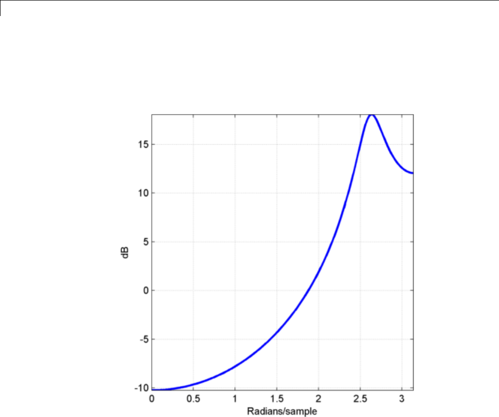
13 Linear Prediction

[H,W] = freqz(1,A);

plot(W,20*log10(abs(H)),'linewidth',2); grid on;

axis tight;

xlabel('Radians/sample'); ylabel('dB');

The AR(2) process acts like a highpass filter in this case.

Graphically examine the correlation in xby producing scatter plots of X(1)

vs X(n) for n=2,3,4,5.

x12 = x(1:end-1);

x21 = x(2:end);

x13 = x(1:end-2);

x31 = x(3:end);

13-10

AR Order Selection with Partial Autocorrelation Sequence

x14 = x(1:end-3);

x41 = x(4:end);

x15 = x(1:end-4);

x51 = x(5:end);

subplot(2,2,1)

plot(x12,x21,'b*');

xlabel('X_1'); ylabel('X_2');

subplot(2,2,2)

plot(x13,x31,'b*');

xlabel('X_1'); ylabel('X_3');

subplot(2,2,3)

plot(x14,x41,'b*');

xlabel('X_1'); ylabel('X_4');

subplot(2,2,4)

plot(x15,x51,'b*');

xlabel('X_1'); ylabel('X_5');

13-11

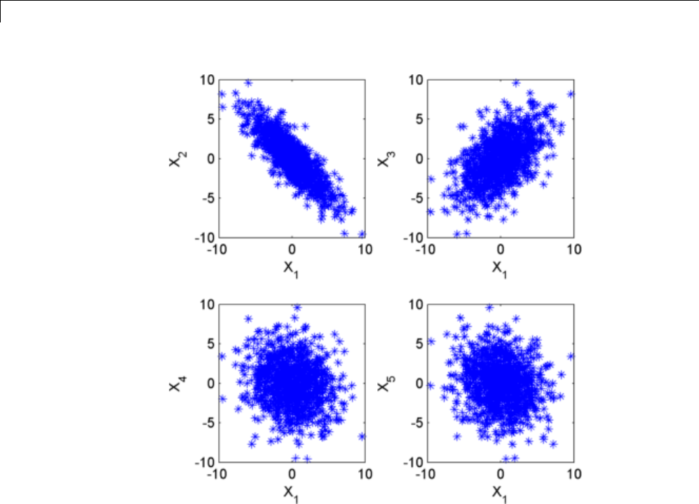
13 Linear Prediction

In the scatter plot, you see there is a linear relationship between X(1),X(2)

and X(1),X(3), but not between X(1) and X(4) or X(5).

The points in the top row scatter plots fall approximately on a line with a

negative slope in the top left panel and positive slope in the top right panel.

The scatter plots in the bottom two panels do not show any apparent linear

relationship.

The negative correlation between X(1) and X(2) and positive correlation

between X(1) and X(3) are explained by the fact that the AR(2) process in this

example acts like a highpass filter.

Find the sample autocorrelation sequence out to lag 50 and plot the result.

13-12

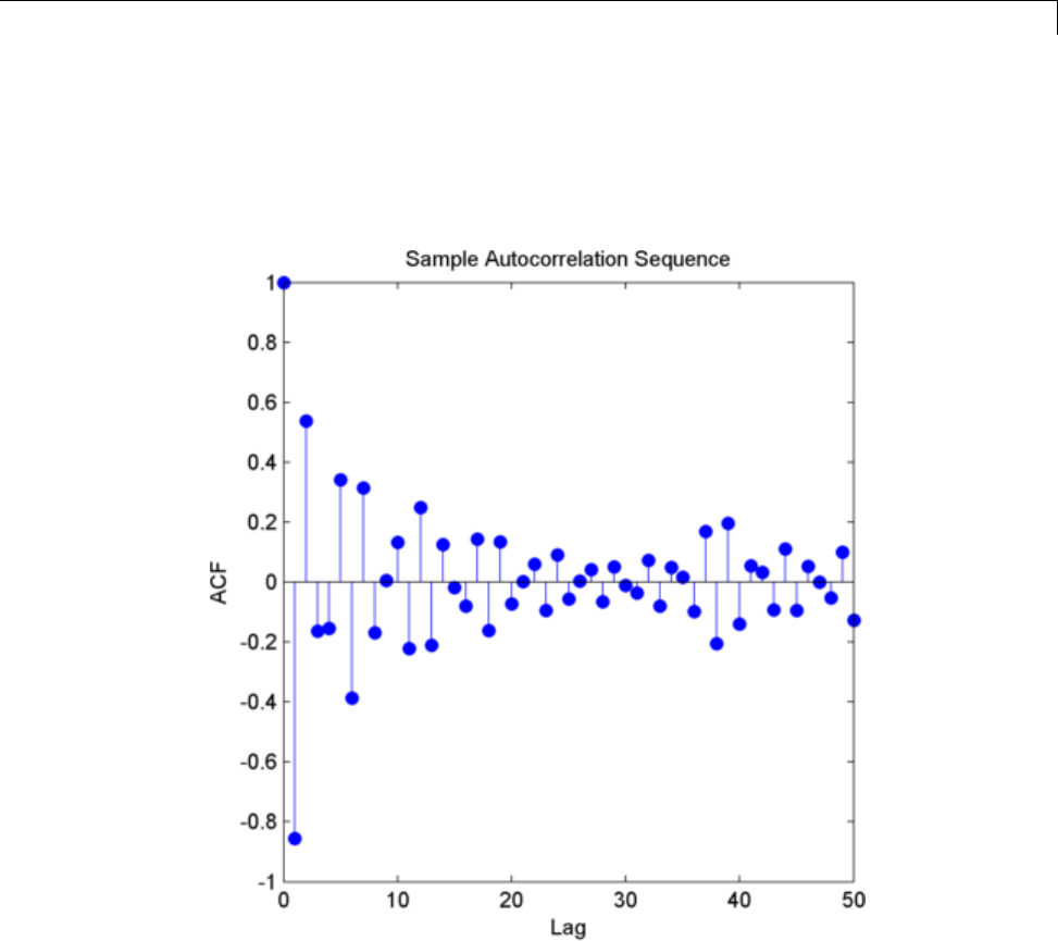
AR Order Selection with Partial Autocorrelation Sequence

[xc,lags] = xcorr(x,50,'coeff');

stem(lags(51:end),xc(51:end),'markerfacecolor',[0 0 1])

xlabel('Lag'); ylabel('ACF');

title('Sample Autocorrelation Sequence');

The sample autocorrelation sequence shows a negative value at lag 1 and

positive value at lag 2. Based on the scatter plot, this is the expected result.

However, you cannot determine from the sample autocorrelation sequence

what order is appropriate for the AR model.

Fit an AR(15) model using aryule. Return the reflection coefficients. The

negative of the reflection coefficients is the partial autocorrelation sequence.

13-13

13 Linear Prediction

[arcoefs,E,K] = aryule(x,15);

Plot the partial autocorrelation sequence along with the large-sample 95%

confidence intervals. If the data are generated by an autoregressive process

of order p, the values of the sample partial autocorrelation sequence for lags

greater than pfollow a N(0,1/N) distribution where N is the length of the

time series. The example “Confidence Intervals for Sample Autocorrelation”

on page 10-5 shows you how to form the 95% confidence intervals for the

N(0,1/N) distributions.

pacf = -K;

lag = 1:15;

stem(lag,pacf,'markerfacecolor',[0 0 1]);

xlabel('Lag'); ylabel('Partial Autocorrelation');

set(gca,'xtick',1:1:15)

lconf = -1.96/sqrt(1000)*ones(length(lag),1);

uconf = 1.96/sqrt(1000)*ones(length(lag),1);

hold on;

line(lag,lconf,'color',[1 0 0]);

line(lag,uconf,'color',[1 0 0]);

13-14

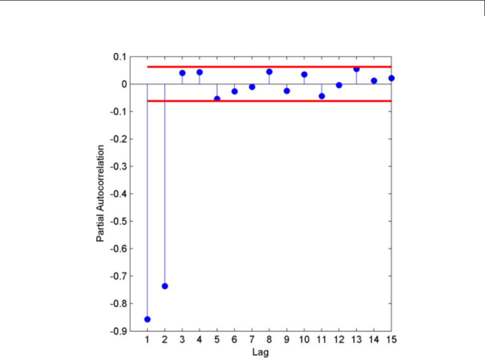
AR Order Selection with Partial Autocorrelation Sequence

The only values of the partial autocorrelation sequence outside the 95%

confidence bounds occur at lags 1 and 2. This indicates that the correct

modelorderfortheARprocessis2.Inthisexample,yougeneratedthetime

series to simulate an AR(2) process, so the partial autocorrelation sequence

only confirms the result. In practice, you have only the observed time series

without any a priori information about model order. In a realistic scenario,

the partial autocorrelation is an important tool for appropriate model order

selection in stationary autoregressive time series.

13-15

13 Linear Prediction

13-16

Transforms

•“Complex Cepstrum — Fundamental Frequency Estimation ” on page 14-2

•“Analytic Signal for Cosine” on page 14-6

•“Envelope Extraction Using The Analytic Signal” on page 14-9

14 Transforms

Complex Cepstrum — Fundamental Frequency Estimation

This example shows you how to estimate a speaker’s fundamental frequency

using the complex cepstrum. The example also estimates the fundamental

frequency using a zero-crossing method and compares the results.

Load the speech signal. The recording is a woman saying “MATLAB”. The

sampling frequency is 7418 Hz.

load mtlb;

The preceding code loads the speech waveform, mtlb,andthesampling

frequency, Fs, in the MATLAB workspace.

Use the spectrogram to identify a voiced segment for analysis.

segmentlen = 100;

noverlap = 90;

NFFT = 128;

[y,f,t,p] = spectrogram(mtlb,segmentlen,noverlap,NFFT,Fs);

surf(t,f,10*log10(abs(p)),'EdgeColor','none');

axis xy; axis tight; colormap(jet); view(0,90);

xlabel('Time');

ylabel('Frequency (Hz)');

14-2

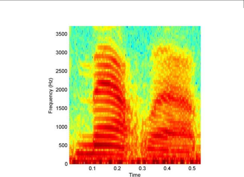
Complex Cepstrum — Fundamental Frequency Estimation

Extract the segment from 0.1 to 0.25 seconds for analysis. The extracted

segment corresponds roughly to the first vowel, /ae/, in “MATLAB”.

dt = 1/Fs;

I0 = round(0.1/dt);

Iend = round(0.25/dt);

x = mtlb(I0:Iend);

Obtain the complex cepstrum.

c = cceps(x);

Plot the cepstrum for times ranging from 2 to 10 msec corresponding to a

frequency range of approximately 100 to 500 Hz. Identify the peak in the

14-3

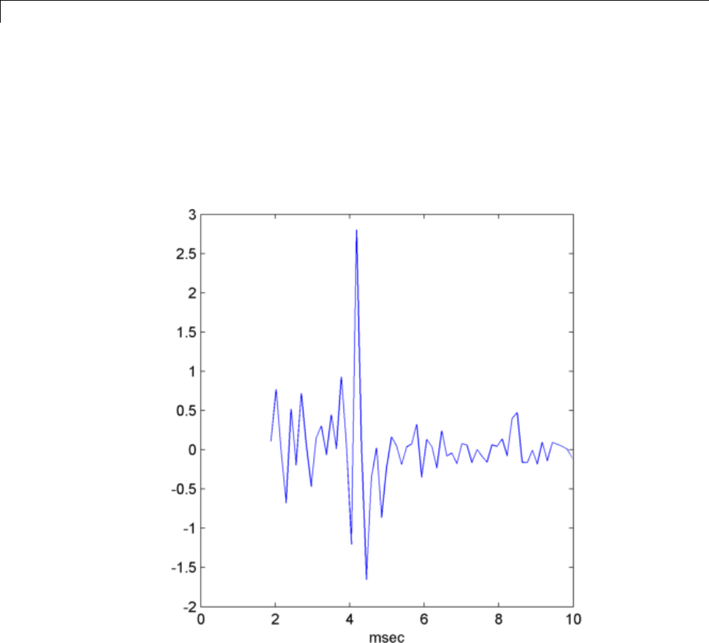
14 Transforms

cepstrum and find the frequency corresponding to the peak. Use the peak as

the estimate of the fundamental frequency.

t = 0:dt:length(x)-dt;

plot(t(15:75).*1e3,c(15:75)); xlabel('msec');

[~,I] = max(c(15:55));

fprintf('Complex cepstrum F0 estimate is %3.2f Hz.\n', 1/(t(I+15)));

Use a zero-crossing detector on a lowpass-filtered and rectified form of the

vowel to estimate the fundamental frequency.

[b0,a0]=butter(2,325/(Fs/2));

xin = abs(x);

xin=filter(b0,a0,xin);

14-4

Complex Cepstrum — Fundamental Frequency Estimation

xin = xin-mean(xin);

x2=zeros(length(xin),1);

x2(1:length(x)-1)=xin(2:length(x));

zc=length(find((xin>0 & x2<0) | (xin<0 & x2>0)));

F0=0.5*Fs*zc/length(x);

fprintf('Zero-crossing F0 estimate is %3.2f Hz.\n',F0);

The estimate of the fundamental frequency obtained with the complex

cepstrum is 231.81 Hz and the estimate with the zero-crossing detector is

233.27 Hz.

14-5

14 Transforms

Analytic Signal for Cosine

This example shows that the imaginary part of the analytic signal

corresponding to a cosine is a sine with the same frequency. If the cosine has

a nonzero mean (DC shift), the real part of the analytic signal is the original

cosine with the same mean, but the imaginary part has zero mean.

Create a cosine with a frequency of 100 Hz. The sampling frequency is 10

kHz. Add a DC offset of 2.5 to the cosine.

t = 0:1e-4:1;

x = 2.5+cos(2*pi*100*t);

Use hilbert to obtain the analytic signal. The real part is equal to the

original signal. The imaginary part is the Hilbert transform of the original

signal. Plot the real and imaginary parts for comparison.

y = hilbert(x);

plot(t,real(y),'b','linewidth',2);

hold on;

plot(t,imag(y),'r','linewidth',2);

set(gca,'xlim',[0 0.1]); grid on;

xlabel('Seconds');

14-6

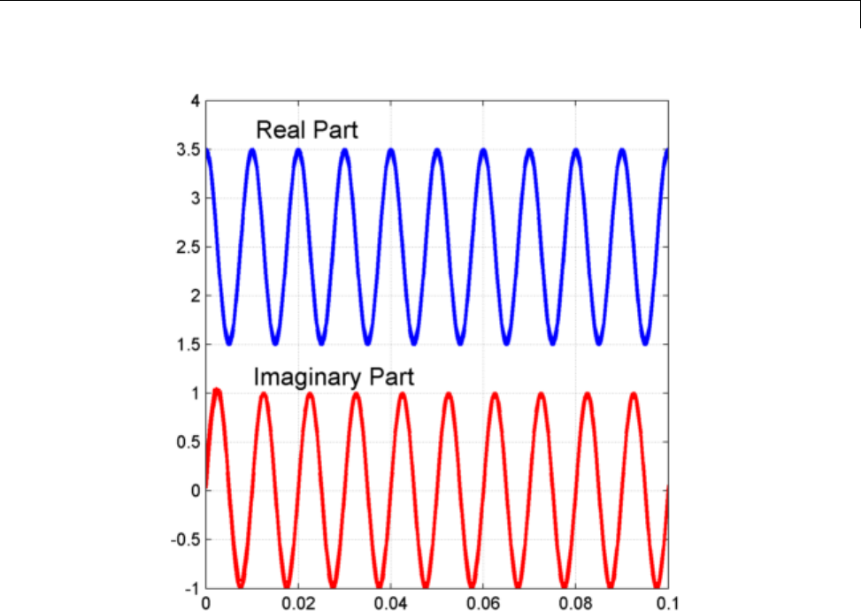
Analytic Signal for Cosine

You see that the imaginary part is a sine with the same frequency as the

cosine real part. However, the imaginary part has a mean of zero, while the

real part has a mean of 2.5.

The original signal is

xt cos t() . ( )2 5 2 1000



The resulting analytic signal is

zt e jt

() . ()

25 2 1000



Plot 10 periods of the complex-valued analytic signal.

14-7

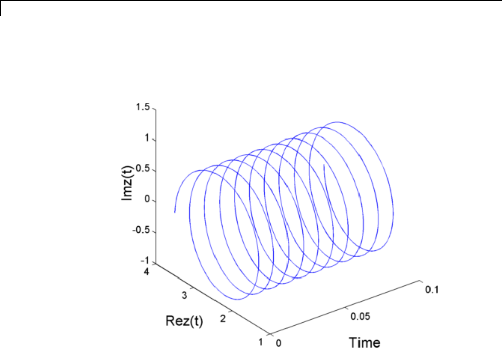
14 Transforms

plot3(t(1:1e3),real(y(1:1e3)),imag(y(1:1e3)));

xlabel('Time','fontsize',14); ylabel('Re{z(t)}','fontsize',14);

zlabel('Im{z(t)}','fontsize',14);

14-8

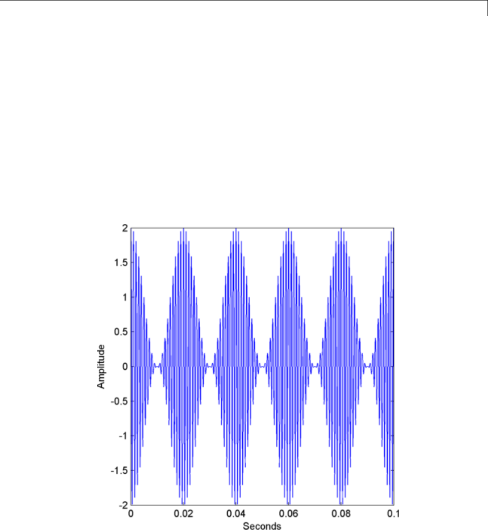
Envelope Extraction Using The Analytic Signal

This example shows how to extract the signal envelope using the analytic

signal.

Create a double sideband amplitude-modulated signal. The carrier frequency

is 1 kHz. The modulation frequency is 50 Hz. The modulation depth is 100%.

The sampling frequency is 10 kHz.

t = 0:1e-4:1;

x = [1+cos(2*pi*50*t)].*cos(2*pi*1000*t);

plot(t,x); set(gca,'xlim',[0 0.1]);

xlabel('Seconds'); ylabel('Amplitude');

14-9

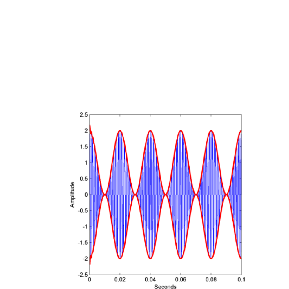
14 Transforms

Obtain the analytic signal. Extract the envelope, which is the magnitude

(modulus) of the analytic signal. Plot the envelope along with the original

signal.

y = hilbert(x);

env = abs(y);

plot(t,x); hold on;

plot(t,abs(y),'r','linewidth',2);

plot(t,-abs(y),'r','linewidth',2);

set(gca,'xlim',[0 0.1]);

xlabel('Seconds'); ylabel('Amplitude');

The magnitude of the analytic signal captures the slowly varying features of

the signal, while the phase contains the high frequency information.

14-10

Signal Generation

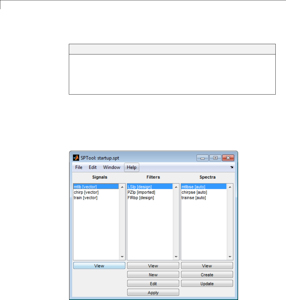
15 Signal Generation

Display Time-Domain Data in Signal Browser

In this section...

“Import and Display Signals” on page 15-3

“Configure the Signal Browser Properties” on page 15-6

“Modify the Signal Browser Display” on page 15-9

“Inspect Your Data (Scaling the Axes and Zooming)” on page 15-11

ThisexampleshowshowtouseandconfiguretheSPToolSignalBrowserto

display time-domain signals. First, open SPTool by typing

sptool

at the MATLAB command line. SPTool opens.

15-2

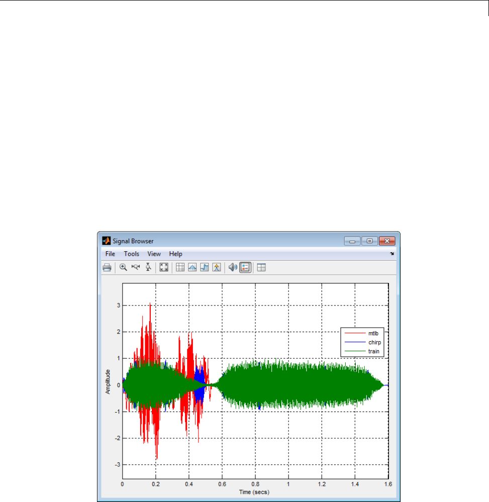
Display Time-Domain Data in Signal Browser

Import and Display Signals

Displaying Multiple Signals

You can display multiple signals in the Signal Browser by selecting more than

one entry in the SPTool Signals list. In the Signals list, first select mtlb

[vector].Nex

t, press the Ctrl key, and select chirp [vector].Finally,

click the View button. The Signal Browser opens, displaying both signals.

Any signals that you select in SPTool are now visible in the Signal Browser.

You can also select multiple entries using the Shift key. In the SPTool

Signals list, first select mtlb [vector]. Next, press the Shift key, and select

train [vector]. The Signal Browser automatically updates to display all

three signals, as shown in the following figure.

15-3

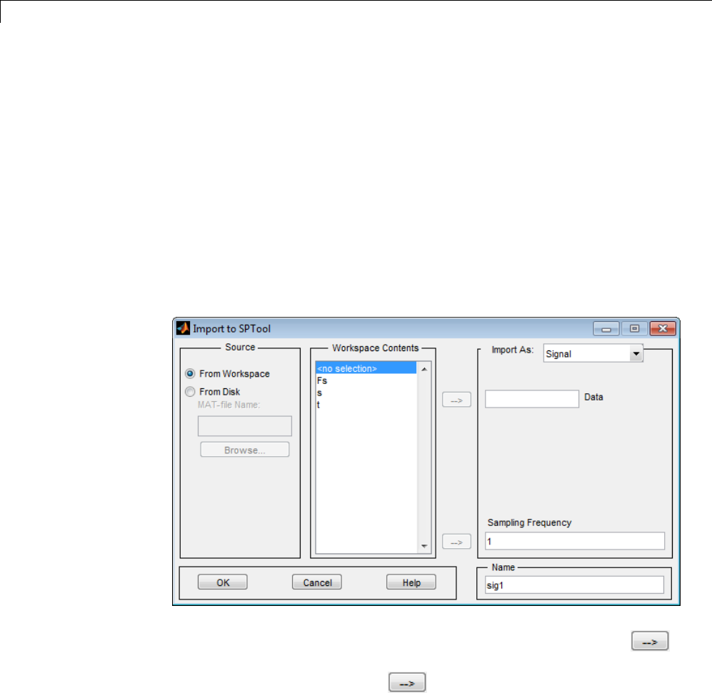
15 Signal Generation

Importing New Signals

Using SPTool, you can import signals from variables in the MATLAB

workspace. First, create a 3-second signal, sampled at 10 kHz, that is the

sum of two sine waves. At the MATLAB command line, enter the following

commands:

Fs = 1e4;

t = 0:1/Fs:3;

s = sum(sin(2*pi*[350;440]*t));

To import the signal from these variables, in the SPTool menu, select

File > Import. Alternatively, you can press the Ctrl+I keyboard shortcut.

TheImporttoSPTooldialogboxopens.

From the Workspace Contents list, select s. Click the right arrow ( )

button to the left of the Data box. Next, from the Workspace Contents list,

select Fs. Click the right arrow ( ) button to the left of the Sampling

Frequency box. You can assign the signal a name in the Name box, but since

you will rename the signal later in this example, leave it as sig1 for now.

15-4

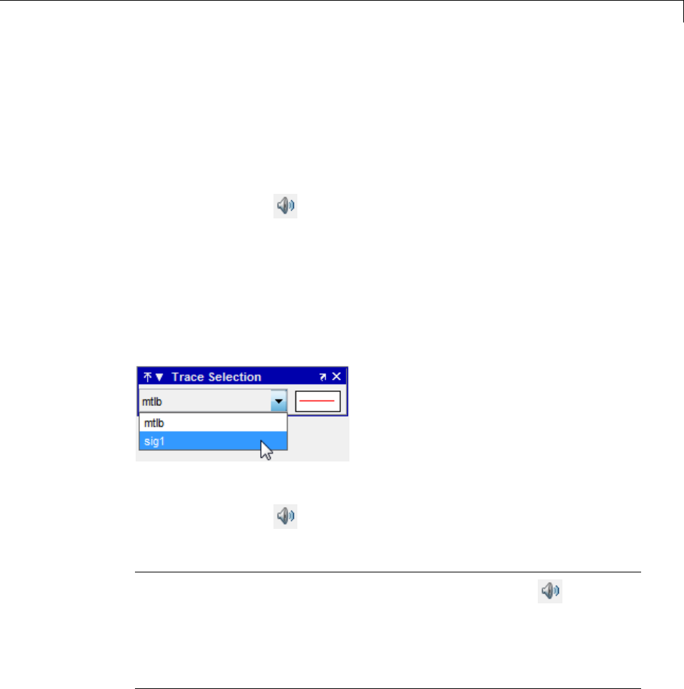
Display Time-Domain Data in Signal Browser

Click OK. The SPTool Signals list now contains a signal named sig1

[vector].

Selecting a Signal and Playing Audio

In the SPTool Signals list, select sig1 [vector], and click the View button.

The Signal Browser reappears in front. To play audio for the signal, click the

Play selected signal ( ) button. Signal Browser sends the audio signal to

the speaker. For more information, see sound in the MATLAB documentation.

If you have multiple signals selected in SPTool, you can use the Trace

Selection panel to choose which signal to make active. In the SPTool

Signals list, press the Ctrl key, and select mtlb [vector].TheSignal

Browser now displays two signals. In the Signal Browser menu, select

Tools > Measurements > Trace Selection.TheTrace Selection panel

appears as showninthefollowingfigure.

In the Trace Selection panel drop-down list, select sig1. Then, click the

Play selected signal ( ) button. Signal Browser sends the audio signal to

the speaker.

Note To hear audio when you click the Play selected signal ( ) button,

your computer sound card must be able to support the sample rate of the

signal. In this example, the sample rate of the signal, sig1 [vector],is10

kHz. If your sound card supports this or a greater sample rate, such as 44.1

kHz, then you can hear the audio on your speaker. For more information, see

sound in the MATLAB documentation.

15-5

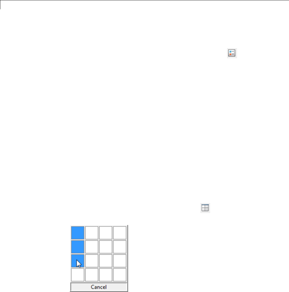
15 Signal Generation

Change Signal Names from the Legend

When multiple signals are displayed, Signal Browser shows a legend by

default. To turn off the legend, click the Show all legends ( ) button. Click

the button again to turn the legend back on. You can modify the names of the

signal directly in the legend. To do so, when the legend is visible, click and

drag it to any location on the display.

You can change the name of any signal directly within the legend. In the

legend, double-click the signal name sig1. A cursor appears, indicating that

you can now change this name. Highlight the text, and type Dial Tone.The

legend now shows Dial Tone asthenameofthatsignal. IntheSPTool

Signals list, the last item is now also named Dial Tone.

Configure the Signal Browser Properties

First, configure the appearance of the Signal Browser window. In the SPTool

Signals list, first select mtlb [vector]. Next, press the Shift key, and select

train [vector]. The Signal Browser automatically updates to display all

three signals.

Multiple Displays

You can display multiple signals on different displays in the Signal Browser

window. In the SPTool Signals list, first ensure all three signals are selected.

In the Signal Browser toolbar, click the Layout ( ) button. Select row 3,

column 1, as shown in the following figure.

15-6

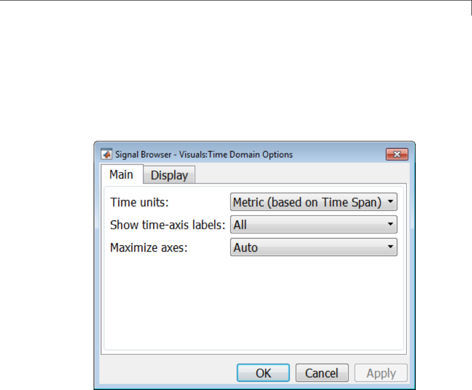
Display Time-Domain Data in Signal Browser

After you make this selection, the Signal Browser is separated into three

displays.

Configure Appearance

In the Signal Browser menu, select View > Properties. The Visuals:Time

Domain Options dialog box opens, as shown in the following figure.

In the Visuals:Time Domain Options dialog box, click the Main tab. Choose

the appropriate parameter settings for the Main tab, as shown in the

following table.

15-7

15 Signal Generation

Parameter Setting

Time units Metric (based on Time Span)

Show time-axis labels Bottom Displays Only

Maximize axes On

When you change the Maximize axes parameter to On, the axes are expanded

to fill the entire display. To conserve space, titles and axis labels are not

shownineachdisplay. ClickApply.

Set Display Properties

In the Visuals:Time Domain Options dialog box, click the Display tab. You

can change the value of the Select display parametertomakedifferent

settings for each display. Set the parameters to the values shown in the

following table.

Parameter Display 1

Setting

Display 2

Setting

Display 3

Setting

Select display 123

Title mtlb chirp train

Show legend Selected Selected Selected

Show grid Selected Selected Selected

Plot signal(s)

as magnitude

and phase

Cleared Cleared Cleared

Minimum

Y-limit

-2.5 -1 -1.5

Maximum

Y-limit

2.5 1 1.5

Y-axis label Amplitude Amplitude Amplitude

15-8

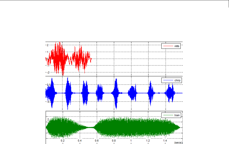
Display Time-Domain Data in Signal Browser

Click OK to save your changes and close the Visuals:Time Domain Options

dialog box. The Signal Browser appears as shown in the following figure.

Modify the Signal Browser Display

UsetheStyledialogboxtomodifytheappearanceoftheaxesandthelinesfor

each of the selected signals in SPTool. In the Signal Browser menu, select

View > Style. The Style dialog box opens, as shown in the following figure.

15-9

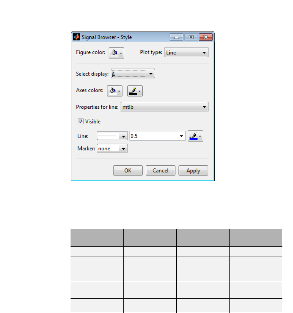
15 Signal Generation

Modify Axes Colors and Line Properties

You can change the value of the Select display parametertomakedifferent

settings for each display. Set the parameters to the values shown in the

following table.

Parameter Display 1

Setting

Display 2

Setting

Display 3

Setting

Select display 123

Axes

background

color

Black Black Black

Ticks, labels,

and grid colors

White White White

Line color Yellow Cyan Magenta

15-10

Display Time-Domain Data in Signal Browser

These settings enable the Signal Browser to display line colors in the same

manner as the Simulink Scope block. Click OK to save your changes and

close the Style dialog box. The Signal Browser now appears as shown in the

following figure.

Show and Hide Toolbar

To hide the toolbar, from the Signal Browser menu, select View > Toolbar.

Doing so removes the toolbar from the Signal Browser window and also

removes the check mark beside the Toolbar option in the View menu. You

can choose to show the toolbar again at any time by selecting View > Toolbar.

Inspect Your Data (Scaling the Axes and Zooming)

So far, you have manually set the y-axis limits. Use one of the following

options to let Signal Browser scale the axes:

•From the Signal Browser menu, select Tools > Scale Axes Limits.

•From the Signal Browser toolbar, click the Scale Axes Limits ( ) button.

15-11

15 Signal Generation

•With the Signal Browser as your active window, press Ctrl + A.

Use the Zoom Tools

The zoom tools allow you to zoom in simultaneously in the directions of both

the x-andy-axes , or in either direction individually. For example, to zoom in

on the signal between 0 and 0.5 seconds, you can use the Zoom X option.

•To activate the Zoom X tool, select Tools > Zoom X,orpressthe

corresponding toolbar button ( ). The Signal Browser indicates that the

Zoom X tool is active by indenting the toolbar button and placing a check

mark next to the Tools > Zoom X menu option.

•Next, zoom in on the region between 0 and 0.5 seconds. In the Signal

Browser window, click on the 0-second mark and drag to the 0.5-second

mark. All three displays reflect this new x-axis setting, as shown in the

following figure.

•To zoom out of the Signal Browser window, right-click inside the window,

andselectZoom Out. Alternatively, you can return to the original view

15-12

Display Time-Domain Data in Signal Browser

of your signal by right-clicking inside the Signal Browser window and

selecting Reset to Original View.

15-13

15 Signal Generation

15-14

Signal Measurement

•“RMS Value of Periodic Waveforms” on page 16-2

•“Slew Rate of Triangular Waveform” on page 16-5

•“Duty Cycle of Rectangular Pulse Waveform” on page 16-9

•“Estimate State for Digital Clock” on page 16-12

•“Calculate Settling Time with Signal Browser” on page 16-16

•“Find Peak Amplitudes in Signal Browser” on page 16-20

16 Signal Measurement

RMS Value of Periodic Waveforms

Thisexampleshowsyouhowtofindtherootmeansquare(RMS)valueof

a sine wave, a square wave, and a rectangular pulse train using rms.The

waveforms in this example are discrete-time versions of their continuous-time

counterparts. The following table gives the RMS values of a continuous-time

sine wave, square wave, and rectangular pulse with duty cycle, D.

Waveform RMS Value

Sine wave with amplitude A A/sqrt(2)

Square wave with values of A and –A A

Rectangular pulse with duty cycle D

and amplitude (on value) A

A*sqrt(D)

Create a discrete-time sine wave. Compute the RMS value and show that it is

a good approximation to the theoretical value for a continuous-time sine wave.

Create a sine wave with a frequency of π/4 radians/sample. The length of the

sine wave is 16 samples, which equals two periods of the sine wave.

n = 0:15;

x = cos(pi/4*n);

Compute the RMS value of the sine wave.

rmsval = rms(x)

The RMS value is equal to 0.7071 as expected.

Create a periodic square wave with a period of 0.1 seconds. The square wave

values oscillate between –2 and 2

t = 0:0.01:1;

x = 2*square(2*pi*10*t);

stem(t,x,'markerfacecolor',[0 0 1]); axis([0 1 -2.5 2.5]);

16-2

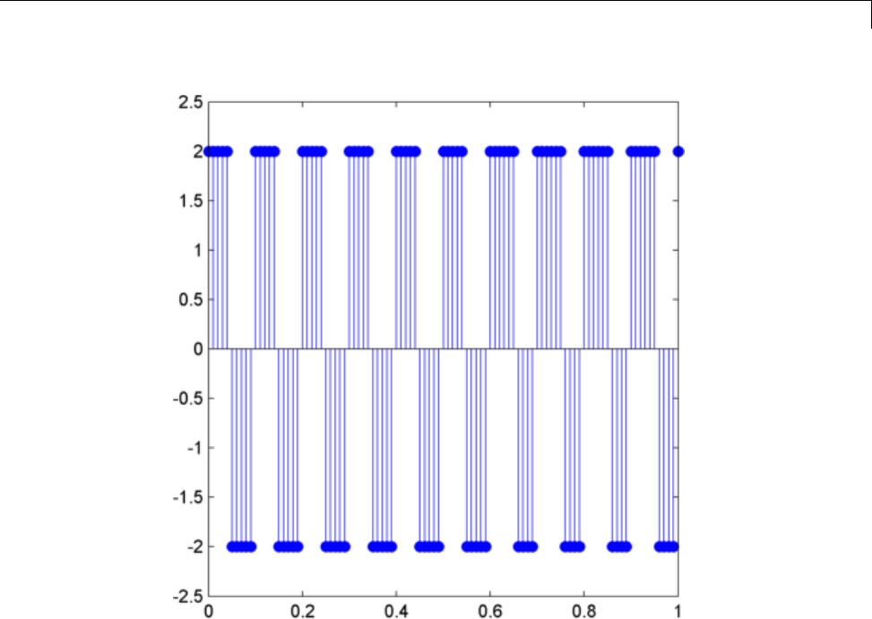
RMS Value of Periodic Waveforms

Find the RMS value.

rmsval = rms(x)

The RMS value agrees with the theoretical value of 2.

Create a rectangular pulse train sampled at 1 kHz with the following

parameters: the pulse is on, or equal to 1, for 0.025 seconds and off, or equal

to 0, for 0.075 seconds in each 0.1 second interval. This means the pulse

period is 0.1 seconds and the pulse is on for 1/4 of that interval. This is

referred to as the duty cycle. See “Duty Cycle of Rectangular Pulse Waveform”

on page 16-9 for a more detailed example of duty cycle. Use pulstran to

create the rectangular pulse train.

t = 0:0.001:(10*0.1);

16-3

16 Signal Measurement

pulsewidth = 0.025;

pulseperiods = [0:10]*0.1;

x = pulstran(t,pulseperiods,@rectpuls,pulsewidth);

plot(t,x); axis([0 1 -0.5 1.5]);

xlabel('Seconds'); ylabel('Amplitude');

Find the RMS value and compare it to the RMS of a continuous-time

rectangular pulse waveform with duty cycle 1/4 and peak amplitude 1.

rmsval = rms(x)

thrms = sqrt(1/4)

The observed RMS value and the RMS value for a continuous-time

rectangular pulse waveform are in good agreement.

16-4

Slew Rate of Triangular Waveform

This example shows you how to use the slew rate as an estimate of the rising

and falling slopes of a triangular waveform.

Create three triangular waveforms. One waveform has rising-falling slopes

of +/- 2, one waveform has rising-falling slopes of +/- 1/2, and one waveform

has a rising slope of +2 and a falling slope of -1/2. Use slewrate to find the

slopes of the waveforms.

Create a triangular waveform with rising-falling slopes of +/- 2. Set the

sampling interval to 0.01 seconds, which corresponds to a sampling frequency

of 100 hertz.

t = 0:0.01:1;

x = 2*t;

x = [x fliplr(x)];

tnew = [t t+1.01];

plot(tnew,x); xlabel('Time');

ylabel('Amplitude');

16-5

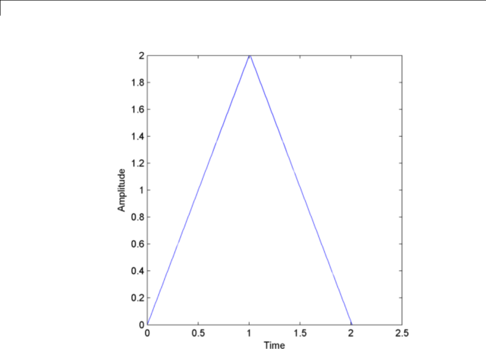
16 Signal Measurement

Calculate the slew rate for the triangular waveform. Input the sampling

frequency (100 Hz) to obtain the correct positive and negative slope values.

s = slewrate(x,100)

Create a triangular waveform with slopes of +/- 1/2. Set the sampling interval

to 0.01 seconds, which corresponds to a sampling frequency of 100 hertz.

t = 0:0.01:1;

x = 1/2*t;

x = [x fliplr(x)];

tnew = [t t+1.01];

plot(tnew,x); xlabel('Time');

ylabel('Amplitude');

16-6

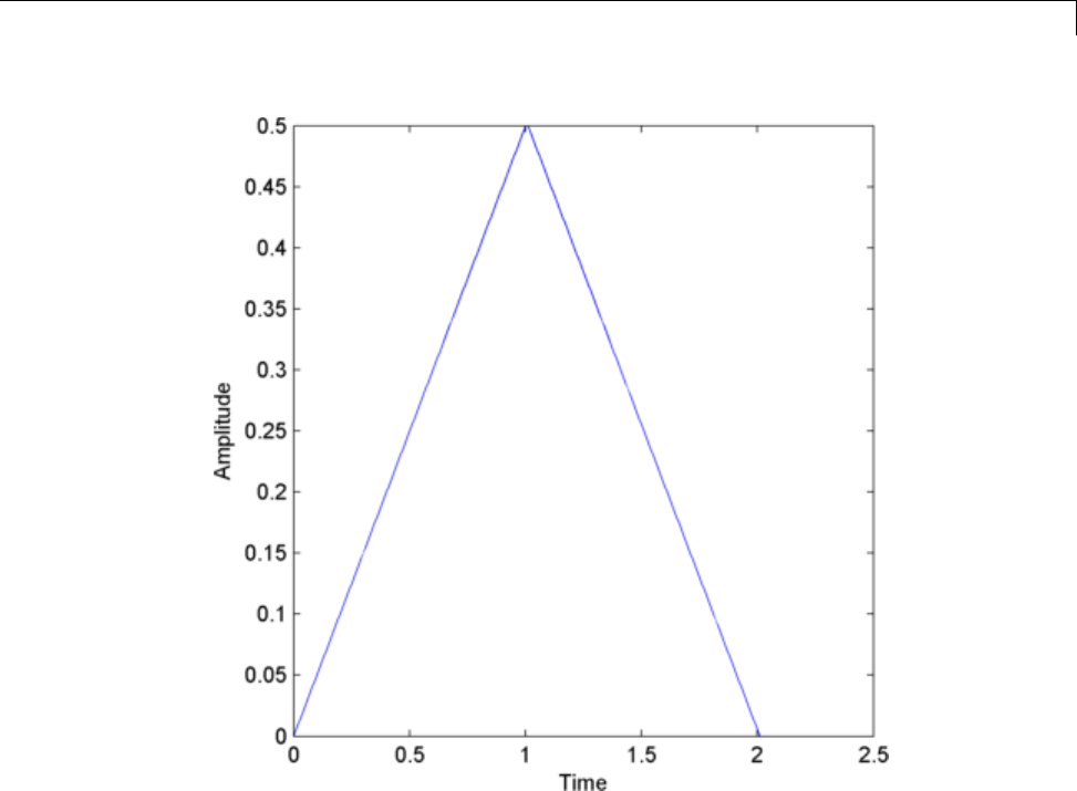
Slew Rate of Triangular Waveform

Calculate the slew rate for the triangular waveform. Input the sampling

frequency (100 Hz) to obtain the correct positive and negative slope values.

s = slewrate(x,100)

Create a triangular waveform with a rising slope of +2 and a falling slope

of -1/2. Set the sampling increment to 0.01 seconds, which corresponds to

a sampling frequency of 100 hertz.

t = 0:0.01:1;

x = 2*t;

t1 = 1:0.01:5;

x1 = -1/2*(t1-1)+2;

y=[xx1];

16-7

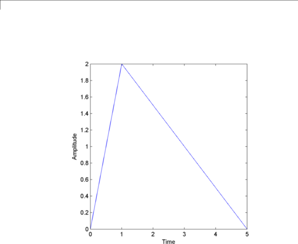
16 Signal Measurement

tnew=[tt1];

plot(tnew,y); xlabel('Time');

ylabel('Amplitude');

Determine the slew rate.

s = slewrate(y,100)

The first element of sis the rising slope and the second element is the falling

slope.

16-8

Duty Cycle of Rectangular Pulse Waveform

This example shows you how to create a rectangular pulse waveform and

measure the duty cycle. You can think of a rectangular pulse waveform as

asequenceofon and off states. One pulse period is the total duration of an

on and off state. The pulse width is the duration of the on state. The duty

cycle is the ratio of the pulse width to the pulse period. The duty cycle for a

rectangular pulse describes the fraction of time that the pulse is on in one

pulse period.

Create a rectangular pulse sampled at 1 gigahertz. The pulse is on, or equal

to 1, for a duration of 1 microsecond. The pulse if off, or equal to 0, for a

duration of 3 microseconds. The pulse period is 4 microseconds. Measure the

duty cycle of the waveform.

Set the sampling frequency equal to 1 gigahertz. Create a vector of times long

enough to accomodate 10 pulses. Define the pulse width to be 1 microsecond.

Space the pulses at intervals of 4 microseconds, which determines the pulse

period. Use pulstran to generate the pulse train and plot the result.

Fs = 1e9;

t = 0:1/Fs:(10*4e-6);

pulsewidth = 1e-6;

pulseperiods = [0:10]*4e-6;

x = pulstran(t,pulseperiods,@rectpuls,pulsewidth);

plot(t.*1e6,x); axis([0 40 -0.5 1.5]);

xlabel('\mus'); ylabel('Amplitude');

16-9

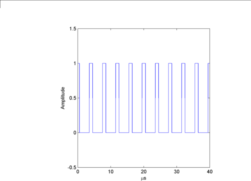
16 Signal Measurement

Determine the duty cycle using dutycycle. Input both the pulse waveform

and the sampling frequency to output the duty cycle. dutycycle outputs a

duty cycle value for each detected pulse.

D = dutycycle(x,Fs)

In this example, the duty cycle for each of the 10 detected pulses is identical

and equal to 0.25. This is the expected duty cycle because the pulse is on

for 1 microsecond and off for 3 microseconds in each 4 microsecond period.

Therefore, the pulse is on for 1/4 of each period. Expressed as a percentage,

this is equal to a duty cycle of 25%.

Calling dutycycle with no output arguments produces a plot with all the

detected pulse widths marked.

16-10

Duty Cycle of Rectangular Pulse Waveform

dutycycle(x,Fs);

Using the same sampling rate and pulse period, vary the pulse on time (pulse

width) from 1 to 3 microseconds in a loop and calculate the duty cycle. Plot

the pulse waveforms and display the duty cycle value in the plot title for each

step through the loop. You see the duty cycle increase from 0.25 (1/4) to 0.75

(3/4) as the pulse width increases.

pulsewidths = 1e-6:1e-6:3e-6;

for nn = 1:length(pulsewidths)

x = pulstran(t,pulseperiods,@rectpuls,pulsewidths(nn));

plot(t.*1e6,x); axis([0 40 -0.5 1.5]);

xlabel('\mus'); ylabel('Amplitude');

D = dutycycle(x,Fs);

title(['Duty cycle is ' num2str(mean(D)) ]);

pause(1);

end

16-11

16 Signal Measurement

Estimate State for Digital Clock

This example shows you how to estimate the high and low state levels for

digital clock data. In contrast to analog voltage signals, signals in digital

circuits have only two states: HIGH and LOW. Information is conveyed by the

pattern of high and low state levels.

Load clockex.mat into the MATLAB workspace. clockex.mat contains a 2.3

volt digital clock waveform sampled at 4 megahertz. Load the clock data

into the variable, x, and the vector of sampling times in the variable, t.Plot

the data.

load('clockex.mat','x','t')

stem(t,x,'markerfacecolor',[0 0 1]); xlabel('Seconds'); ylabel('Volts');

16-12

Estimate State for Digital Clock

Determinethehighandlowstatelevelsfortheclockdatausingstatelevels.

levels = statelevels(x)

The low-state level estimate is 0.0027 volts and the high-state level estimate

is 2.3068volts. Thisistheexpectedresult for the 2.3 volt clock data, where

the noise-free low-state level is 0 volts, and the noise-free high-state level

is 2.3volts.

Use the estimated state levels to convert the voltages into a sequence of 0s and

1s. The sequence of 0s and 1s is a binary waveform representation of the two

states. To make the assignment, use the following decision rule. Assign any

16-13

16 Signal Measurement

voltage within a 3%-tolerance region of the low-state level the value 0, and

any voltage within a 3%-tolerance region of the high-state level the value 1.

Determine the 3%-tolerance region around the low-state level.

lowtol = [levels(1)-3/100*(levels(2)-levels(1)) ...

levels(1)+3/100*(levels(2)-levels(1))];

Determine the 3%-tolerance region around the high-state level.

hightol = [levels(2)-3/100*(levels(2)-levels(1)) ...

levels(2)+3/100*(levels(2)-levels(1))];

Use logical indexing to determine the voltages within a 3%-tolerance region

of the low-state level and the voltages within a 3%-tolerance region of the

high-state level. Assign the value 0 to the voltages within the tolerance region

of the low-state level and 1 to the voltages within the tolerance region of

thehigh-statelevel. Plottheresult.

y = zeros(size(x));

y(x>= lowtol(1) & x<= lowtol(2)) = 0;

y(x>= hightol(1) & x<= hightol(2)) = 1;

subplot(211)

stem(t,x,'markerfacecolor',[0 0 1]); ylabel('Volts');

subplot(212)

stem(t,y,'markerfacecolor',[0 0 1]); ylabel('{0,1}'); xlabel('Seconds');

set(gca,'ytick',[0 1])

16-14

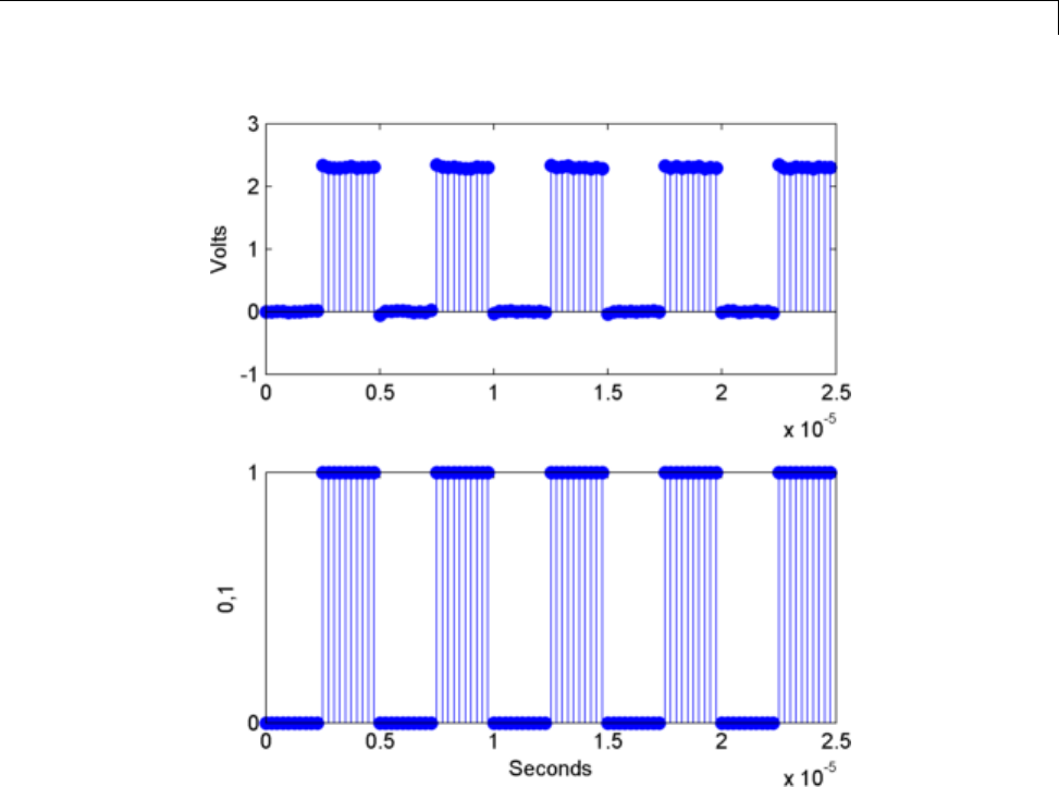
Estimate State for Digital Clock

The decision rule has assigned all the voltages to the correct state.

16-15

16 Signal Measurement

Calculate Settling Time with Signal Browser

This example demonstrates how you can use the SPTool Signal Browser to

find the settling time of a clock signal in the Bilevel Measurements panel.

First, open SPTool by typing

sptool

at the MATLAB command line. SPTool opens.

In this example, you import a clock signal from the MAT-file named

clockex.mat. In the SPTool menu, select File > Import. Alternatively, you

can press the Ctrl+I keyboard shortcut. The Import to SPTool dialog box

opens.

1Under Source,clickFrom Disk.

16-16

Calculate Settling Time with Signal Browser

2In the MAT-file box, type clockex,andpressEnter. The variables x

and tappear under File Contents.

3Under File Contents,clickx. Click the right arrow ( ) button to the

left of the Data box.

4In the Sampling Frequency box, type 4000000.

5In the Name box, type Clock.

6Click OK. The SPTool Signals list now contains a signal named Clock

[vector].

7In SPTool, in the Signals list, select Clock [vector],andclicktheView

button. The Signal Browser appears and displays the clock signal.

Because you selected only one signal, the legend is not needed. Turn off the

legend by clicking the Show All Legends ( ) button. Then, use the Style

dialog box to modify the appearance of the axes and the lines for the signal.

In the Signal Browser menu, select View > Style.

Parameter Display 1

Setting

Axes background color Black

Ticks, labels, and grid colors Dark Gray

Line color Yellow

To show the Bilevel Measurements panel, in the Signal Browser menu,

select Tools > Measurements > Bilevel Measurements.Tocollapsethe

Transitions pane,clickthepanecollapsebutton( )nexttothatlabel. To

expand the Settings pane and the Overshoots / Undershoots pane, click

the pane expand button ( ) next to each label. The Signal Browser appears

as shown in the following figure.

16-17

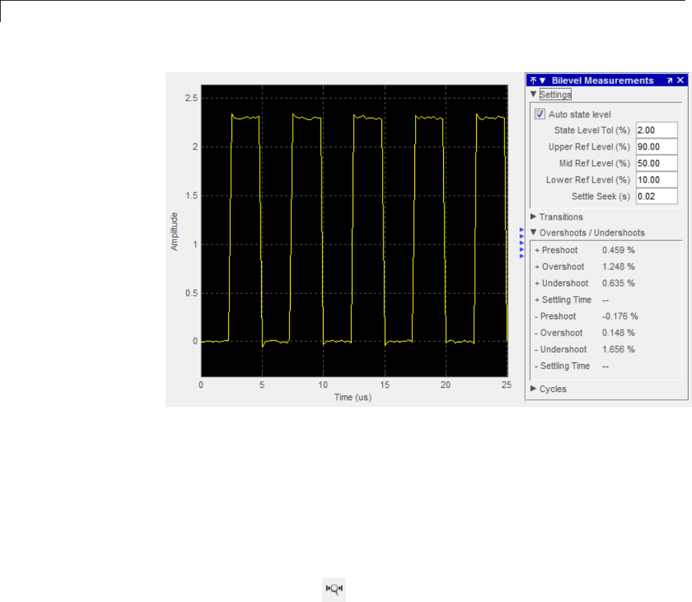
16 Signal Measurement

The value for the rising edge Settling Time parameter does not appear in the

Overshoots / Undershoots pane because the Settle Seek parameter is too

large. The Settle Seek value is longer than the entire simulation duration.

Enter a value for settle seek of 2e-6,andpressEnter.SignalBrowsernow

displays a rising edge settling time value of 118.392 ns.

This settling time value displayed is actually the statistical average of the

settling times for all five rising edges. To display the settling time for only one

rising edge, you can zoom in on that transition. In the Signal Browser toolbar,

click the Zoom X button ( ). Click the display near a value of 2 microseconds

on thetime-axis. Drag to the right, and release near a value of 4 microseconds

on thetime-axis. Signal Browser updates the rising edge Settling Time

value to reflect the new time window, as shown in the following figure.

16-18

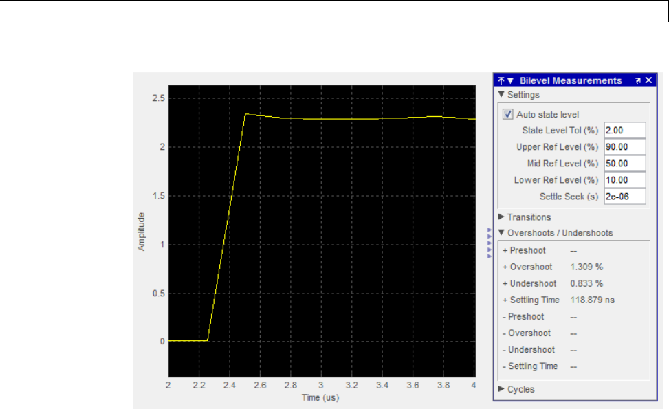
Calculate Settling Time with Signal Browser

16-19

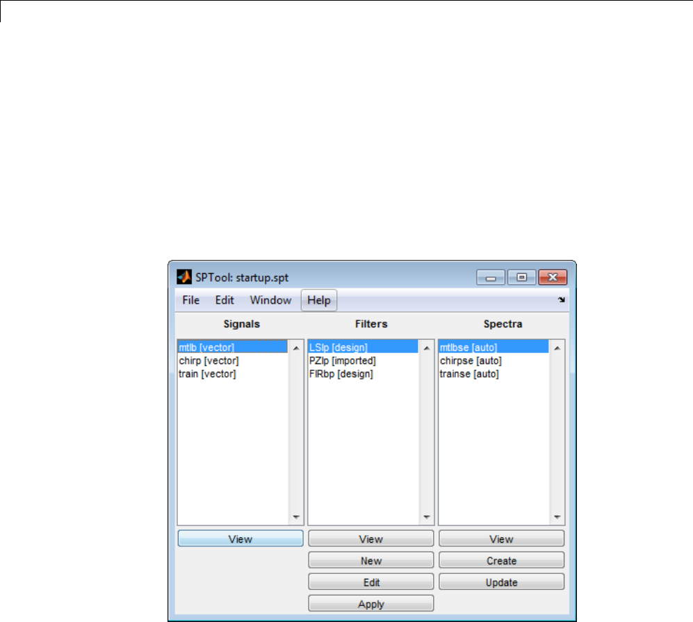
16 Signal Measurement

Find Peak Amplitudes in Signal Browser

The following example demonstrates how you can use the Peak Finder panel

to find heart rate, given an electrocardiogram (ECG) signal.

First, open SPTool by typing

sptool

at the MATLAB command line. SPTool opens.

Using SPTool, you can import signals from variables in the MATLAB

workspace. First, create an electrocardiogram (ECG) signal, sampled at 4

kHz, and apply the Savitzky-Golay filter. At the MATLAB command line,

enter the following commands:

x1 = 3.5*ecg(2700).';

16-20

Find Peak Amplitudes in Signal Browser

y1 = sgolayfilt(kron(ones(1,13),x1),0,21);

n = (1:30000)';

del = round(2700*rand(1));

mhb = y1(n + del);

ts = 0.00025;

Fs = 1/ts;

For more information about the Savitzky-Golay filter, see the sgolayfilt

function reference page or run the sgolaydemo example.

To import the signal from these variables, in the SPTool menu, select

File > Import. Alternatively, you can press the Ctrl+I keyboard shortcut.

The Import to SPTool dialog box appears.

1Under Workspace Contents,clickmhb. Click the right arrow ( )

button to the left of the Data box.

2Under Workspace Contents,clickFs. Click the right arrow ( )

button to the left of the Sampling Frequency box.

3In the Name box, type ECG.

4Click OK. The SPTool Signals list now contains a signal named ECG

[vector].

5In SPTool, in the Signals list, select ECG [vector], and click the View

button. The Signal Browser opens and displays the ECG signal.

Because you only selected one signal, the legend is not needed. Turn off the

legend by clicking the Show All Legends ( ) button. Then, use the Style

dialog box to modify the appearance of the axes and the lines for the signal.

In the Signal Browser menu, select View > Style.

16-21

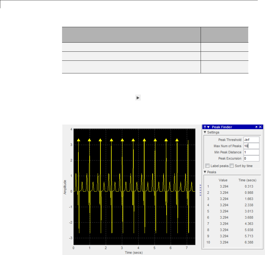
16 Signal Measurement

Parameter Display 1

Setting

Axes background color Black

Ticks, labels, and grid colors Dark Gray

Line color Yellow

To show the Peak Finder panel, in the Signal Browser menu, select

Tools > Measurements > Peak Finder.ToexpandtheSettings pane,

click the pane expand button ( )nexttothatlabel. IntheMax Num of

Peaks box, type 10 and press the Enter key. Signal Browser now displays in

the Peaks pane a list of 10 peak amplitude values, and the times at which

they occur, as shown in the following figure.

16-22

Find Peak Amplitudes in Signal Browser

As you can see from the list of peak values, there is a constant time difference

of 0.675 seconds between each heartbeat. Therefore, the heart rate detected

by the ECG signal is given by the following equation.

0 675

88 89

sec

min

.sec .min ()

beat

beats bpm

16-23

16 Signal Measurement

16-24

Technical Conventions

This manual and all Signal Processing Toolbox functions use the following

technical notations.

Term or Symbol Description

Nyquist frequency One-half the sampling frequency. Some toolbox

functions normalize this value to 1.

x(1) The first element of a data sequence or filter,

corresponding to zero lag.

Ωor w Analog frequency in radians per second.

ωor w Digital frequency in radians per sample.

fDigital frequency in hertz.

[x,y)Theintervalfromxto y,includingxbut not

including y.

... Ellipses in the argument list for a given

syntax on a function reference page indicate

all possible argument lists for that function

appearing prior to the given syntax are valid.

ATechnical Conventions

A-2

Index

IndexA

aliasing

impulse invariance 2-47

preventing 7-22

reducing 7-40

all-pole filters.SeeIIR filters

all-zero filters.SeeFIR filters

AM.Seeamplitude modulation

analog filters 2-9 2-44

Bessel comparison 2-12

bilinear transformation 2-48

Butterworth comparison 2-9

Chebyshev Type I comparison 2-10

Chebyshev Type II comparison 2-10

design 2-7

discretization 2-46

frequency response example 2-13

impulse invariance 2-47

models 1-31

plotting 2-13

Print Preview C:\TEMP\Apdf_2541_3068\home\AppData\Local\PTC\Arbortext\Editor\.aptcache\ae3849j0/tf38450r Signal Processing Toolbox User's Guide

Navigation menu

Versions of this User Manual:

Views

Navigation