Simbody™ Simbody Theory Manual
User Manual:
Open the PDF directly: View PDF ![]() .
.
Page Count: 160 [warning: Documents this large are best viewed by clicking the View PDF Link!]

Simbody™
Theory Manual
Release 3.1
March, 2013
Website: https://simtk.org/home/simbody
SimTK Simbody™ 3.1
Theory Manual
Michael Sherman
Stanford University
March, 2013

ii
Simbody™ is part of SimTK, the open source biosimulation toolkit originating from Simbi-
os, the NIH National Center for Physics-Based Simulation of Biological Structures at Stan-
ford, funded under the NIH Roadmap for Medical Research, grant U54 GM072970. Infor-
mation on the National Centers for Biomedical Computing can be obtained from
http://nihroadmap.nih.gov/bioinformatics.
Simbody home page: https://simtk.org/home/simbody
Simbios home page: http://simbios.stanford.edu
That handsome devil on the cover is my hero, Sir Isaac Newton.
Copyright and Permission Notice
Portions copyright (c) 2005-2013 Stanford University and Michael Sherman.
Permission is hereby granted, free of charge, to any person obtaining a copy of this document (the "Document"), to deal in
the Document without restriction, including without limitation the rights to use, copy, modify, merge, publish, distribute,
sublicense, and/or sell copies of the Document, and to permit persons to whom the Document is furnished to do so, subject
to the following conditions:
This copyright and permission notice shall be included in all copies or substantial portions of the Document.
THE DOCUMENT IS PROVIDED "AS IS", WITHOUT WARRANTY OF ANY KIND, EXPRESS OR IMPLIED,
INCLUDING BUT NOT LIMITED TO THE WARRANTIES OF MERCHANTABILITY, FITNESS FOR A PARTICU-
LAR PURPOSE AND NONINFRINGEMENT. IN NO EVENT SHALL THE AUTHORS, CONTRIBUTORS OR
COPYRIGHT HOLDERS BE LIABLE FOR ANY CLAIM, DAMAGES OR OTHER LIABILITY, WHETHER IN AN
ACTION OF CONTRACT, TORT OR OTHERWISE, ARISING FROM, OUT OF OR IN CONNECTION WITH THE
DOCUMENT OR THE USE OR OTHER DEALINGS IN THE DOCUMENT.

iii
Preface
SimTK Simbody provides a powerful multibody mechanics capability for use in biosimula-
tion. It is designed for use by programmers who are not experts in multibody mechanics.
Simbody provides a sophisticated, robust, high performance, open source option for mechan-
ical simulation, including biomechanical simulation, as well as the additional functionality
and performance needed for effective modeling of large molecular systems in internal
coordinates. It is accessible through a stable C++ API. The full capability of this package,
including bindings for other languages, will be built up in layers over time; this document
covers the current capabilities and discusses future directions.
A complete multibody mechanics simulation (a biomechanical gait simulation or a molecular
dynamics simulation of a protein/RNA interaction, for example) requires many layers. At the
lowest level are hardware-dependent, computationally intense “inner loop” numerical meth-
ods like basic linear algebra and molecular force field computations. Built on those are
numerical mathematics methods like numerical integration, nonlinear root-finding, optimiza-
tion, and higher-level linear algebra. The next layer supports physics and mechanics and
includes Simbody’s multibody dynamics capability, as well as a variety of models for forces
and constraints.
Simbody’s distribution contains multibody dynamics, generally useful force and constraint
models, some crude visualization tools, and the lower-layer software it needs to run efficient-
ly. However, that is still by no means a complete simulation system since it does not include
domain-specific modeling or a GUI. Thus in any complete simulation tool there are typically
two more layers built above Simbody: a modeling layer and a user interface that provides
model building and editing, execution, and visualization of results.
Consequently, Simbody itself is intended for use by primarily by programmers who are
writing domain-specific modeling tools and/or user interfaces and would like to incorporate
high-quality multibody mechanics into their work. Some current examples are: the Open-
Sim™ musculoskeletal modeling layer and GUI https://simtk.org/home/opensim and the
Molmodel™ coarse-grained molecular modeling layer https://simtk.org/home/molmodel.

iv
How to use this document
This Simbody Theory Manual contains background information on simulation in general and
multibody dynamics in particular, as well as detailed mathematical theory discussion and
literature references describing Simbody’s implementation. Generally the equation-dense
parts are kept separate from the overview, so readers who want just one or the other can skim
over large chunks of material.
This is not a programming manual or user guide so you will not find detailed information
here about using Simbody in a program. For that, see the latest Simbody User Guide,
Simbody Advanced Programming Guide, and Doxygen API documentation available from
the Simbody distribution project at https://simtk.org/home/simbody (go to the Documents
tab). Simbody also provides a public forum where you can get help, and bug report and
feature request tools (go to the Advanced tab).
Document conventions
In order to allow myself the pleasure of delivering the occasional opinionated diatribe,
while permitting the easily offended reader to avoid them, I have placed a “pontification
warning” symbol like the one at the left at the beginning of such sections in the text.
The end of these sections is marked with the “off my soapbox” symbol to the right.
The symbol to the left is used to highlight sections which summarize earlier material.
This one is used to mark discussions of capabilities which are planned but not yet
implemented.
v
Table of Contents
1 Background............................................................. 1
1.1 What is “multibody dynamics”? ................................ 1
1.2 Structure of a simulation in Simbody ........................ 2
1.3 Structure of a System ................................................. 4
1.4 Structure of a multibody system ................................ 5
2 Fundamental concepts of multibody mechanics ....... 7
2.1 Coordinate frames ...................................................... 7
2.2 Bodies ......................................................................... 8
2.3 Mobilizers ................................................................. 10
2.3.1 Mobilizers are not joints ........................................... 10
2.3.2 Types of Mobilizers .................................................. 12
2.3.3 Mobility space .......................................................... 13
2.3.4 Parameterization of mobility .................................... 14
2.3.5 A comment on deformable (flexible) bodies ............ 15
2.4 Constraints ................................................................ 16
2.5 Forces........................................................................ 17
2.6 Kinematics ................................................................ 17
2.7 Dynamics .................................................................. 18
3 Basic Simbody numerical types ............................ 19
3.1 Vectors and Matrices ............................................... 19
3.2 Geometry .................................................................. 19
3.2.1 Stations ..................................................................... 19
3.2.2 Directions ................................................................. 20
3.2.3 Rotations ................................................................... 20
3.2.4 Transforms ................................................................ 22
3.3 Mechanics ................................................................. 23
3.3.1 Spatial Notation ........................................................ 24
3.3.2 Cross product matrix ................................................ 26
3.3.3 Spatial mass properties ............................................. 27
3.3.4 Spatial rotation, shifting, and transform ................... 28
4 Constructing a Simbody multibody system ........... 31
4.1 Topology................................................................... 31
4.2 Bodies and their Mobilizers ..................................... 32
4.2.1 The reference configuration ..................................... 33
4.3 Constraints ................................................................ 35
4.4 Forces........................................................................ 37
5 Theory for Mobilizers ........................................... 39
5.1 Reverse mobilizers ................................................... 42
5.2 Mobilizers in body frames ....................................... 44
6 Theory for Constraints .......................................... 47
6.1 Explicit calculation of constraint matrices .............. 51
7 State representation and realization ....................... 53
7.1 Computation – realization of the State .................... 53
7.1.1 Responses, operators, and solvers ............................ 53
7.1.2 Caching of computed results .................................... 54
7.1.3 Computing in stages ................................................. 57
7.2 State variables .......................................................... 58
7.2.1 State partitioning by stage ........................................ 58
7.3 State resources .......................................................... 59
7.4 Allocation of state resources .................................... 60
7.4.1 Mobilized bodies ...................................................... 60
7.4.2 Dynamic variables z ................................................. 61
7.4.3 Structured variables d ............................................... 61
7.4.4 Constraints ................................................................ 61
8 Equations of motion .............................................. 63
8.1 Unconstrained dynamic systems.............................. 64
8.2 Constrained systems ................................................. 67
8.3 Unconstrained systems with prescribed, fast, and
slow variables .....................................................................67
8.4 Constrained systems with prescribed motion ..........69
8.5 Constrained systems as specified to Simbody .........73
8.6 Unilateral constraints ................................................75
8.6.1 Solving for impacts .................................................. 77
8.6.2 Sliding friction forces and impulses ........................ 79
8.6.3 Event detection for unilateral constraints ................ 88
8.7 Dynamic solution method ........................................89
9 Scaling and and accuracy ...................................... 95
9.1 Relative vs. absolute accuracy .................................95
9.2 Weighting and absolute accuracy.............................97
9.3 Scaling of constraint errors ................................... 100
9.4 Scaling at the acceleration level ............................ 102
9.5 Accuracy ................................................................ 103
10 Time Stepping .....................................................105
10.1 Coordinate projection ............................................ 105
10.2 Simplified equations .............................................. 110
10.3 Update rates for state variables ............................. 110
10.3.1 Coupling ................................................................ 113
10.4 How to take a time step ......................................... 115
10.4.1 Setting the values of prescribed variables ............. 118
10.4.2 Relaxation of fast variables ................................... 118
11 Simbody Force Subsystems reference guide.........121
11.1 General Force Subsystem ...................................... 121
11.2 Hertz/Hunt and Crossley contact model subsystem121
11.2.1 Motivation ............................................................. 121
11.2.2 The model .............................................................. 122
11.2.3 Extension to include Friction ................................. 127
11.3 DuMM — Molecular mechanics force field ........ 128
11.3.1 Background ............................................................ 128
11.3.2 Basic concepts ....................................................... 129
11.3.3 Units....................................................................... 131
11.3.4 Defining a force field ............................................. 132
11.3.5 Defining the molecules .......................................... 132
11.3.6 Defining bodies and attaching the molecule to
them 132
11.3.7 Running a simulation ............................................. 132
11.3.8 Theory .................................................................... 132
12 Appendix: derivations ..........................................133
12.1 Notation for multibody theory .............................. 133
12.2 Re-expressing spatial quantities ............................ 136
12.3 Rigid body shifting of spatial quantities ............... 137
12.3.1 Rigid body shift of rigid body spatial inertia ......... 137
12.4 Inversion of rigid body spatial inertia ................... 138
12.5 Articulated body inertia ......................................... 139
12.5.1 Rigid body shift of articulated body inertia ........... 140
12.5.2 Articulated shift of an articulated body inertia ...... 141
12.5.3 Terminal bodies and base bodies ........................... 142
12.6 Modal analysis and implicit integration ................ 143
12.7 Root finding and optimization .............................. 144
12.8 Operator form of Simbody interface ..................... 145
12.9 Misc ........................................................................ 146
13 Acknowledgments ...............................................151
14 References ...........................................................152
1
1 Background
This is general material hopefully providing enough background for the rest of the document
to make sense. Even for those familiar with multibody dynamics, it is probably worth reading
to see how we are characterizing it for the broad uses it will serve for SimTK users.
1.1 What is “multibody dynamics”?
Multibody mechanics (of which multibody dynamics is a component) is the field studying the
classical mechanical properties, especially motion, of systems of bodies interconnected by
joints, influenced by forces, and restricted by constraints. The key feature of a system that
makes it suitable for multibody treatment is the observation that its motion is localized, that
is, it is well-described as a set of independently identifiable parts which undergo large motion
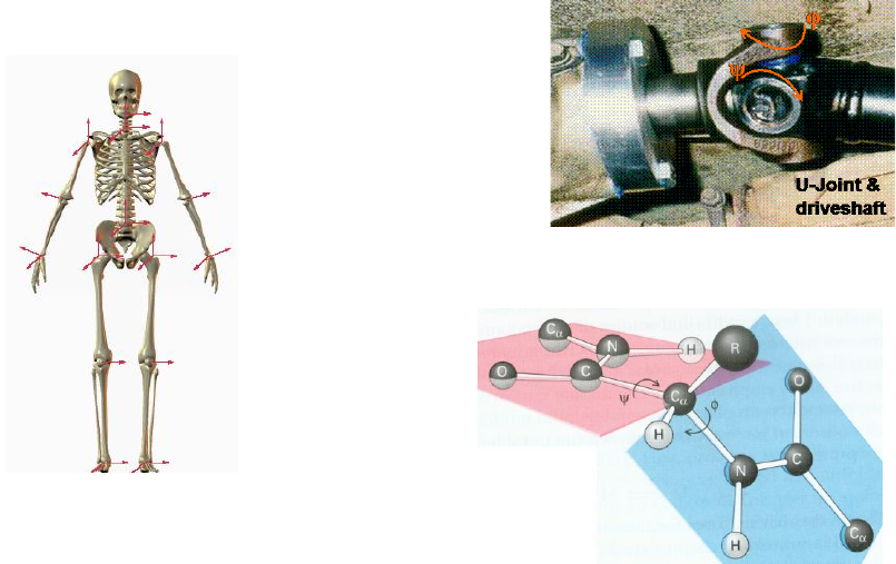
with respect to one another, but are themselves rigid or nearly rigid. Figure 1 shows some
examples of the breadth of applicability of multibody mechanics, which has been used
effectively to model machines, skeletal motion and gait, coarse-grained biopolymers, and
many other systems relevant to a wide variety of scientific and engineering disciplines.
Mechanical U-joint
Articulated
skeleton
Figure 1: Some multibody
systems.
Protein
backbone

2
Multibody mechanics is a generalization of several more-familiar modeling methods. It
includes as special cases, for example, systems of point masses represented in Cartesian
coordinates (e.g. molecular dynamics models) and systems of freely moving extended bodies
(typically, rigid bodies) and these can be intermixed into systems which also contain bodies
whose motion is defined with internal (relative) coordinates, that is, with respect to one
another rather than with respect to the Cartesian frame. Multibody mechanics should be
viewed as a basic numerical capability fundamental to any simulation system. It is in the
same category as, say, a linear algebra library, not an end-user application. Simbody is for
use by modelers and application developers as a basic building block. Computational re-
searchers working to improve multibody simulation methods can use Simbody as a baseline
source of correct answers for debugging and as a performance baseline to demonstrate the
superiority of their new methods. However, Simbody itself is not a research project; it is
intended instead as a reliable, industrial-grade tool on which researchers may depend.
1.2 Structure of a simulation in Simbody
The figure below shows the primary objects involved in computational simulation of a
physical system in SimTK, the infamous “three S’s of simulation”: System, State, and Study.
Here’s our first equation:
Simulation(SimTK) = System + State + Study
A System is a computational embodiment of a mathematical model of the physical world. A
System typically comprises several interacting, separately meaningful subsystems. A System
contains models for physical objects and the forces that act on them and specifies a set of
variables whose values can affect the System’s behavior. However, the System itself is an
unchangeable, state-free (“const”) object. Instead, the values of its variables are stored in a
separate object, called a State, more about which below.
*
Finally, a Study couples a System
and one or more States, and represents a computational experiment intended to reveal some-
*
We will frequently use “state” (lower case) to refer to the values stored within a State object. This isn’t as
confusing as it might seem—even if we get the capitalization wrong the meaning will be obvious from context.
3
thing about the System. By design, the results of any Study can be expressed as a State value
or set of State values which satisfies some pre-specified criteria, along with results which the
System can calculate directly from those State values. Such a set of State values is often
called a trajectory.
It is important to note that our notion of “state” is somewhat more general than the common
use of the term. By state, we mean everything variable about a System. That includes not
only the traditional continuous time, position and velocity variables, but also discrete varia-
bles, memory of past events, modeling choices, and a wide variety of parameters that we call
instance variables. The System’s State has entries for the values of all of these variables.
This design allows the conceptually simple model depicted above to express every kind of
investigation one may wish to perform. Here are some examples. The simplest Study merely
asks the System to evaluate itself using values taken from a particular State. More interest-
ingly, a dynamic Study produces a series of time, position and velocity State values which
result from solving the classical dynamic equations representing Newton’s 2nd law, F=ma.
An energy minimization is a Study which seeks values for the State’s position coordinates at
which an energy calculation yields its minimum value. A Monte Carlo simulation is a Study
yielding a series of states which satisfy an appropriate probability distribution. Design
studies, also used for parameter fitting, are Studies which find values for instance variables
such as lengths, masses, material properties, or coefficients which meet specified criteria.
Modeling Studies select among models or algorithmic choices to improve defined measures
Study
State
System
Results
states
4
of behavior, such as accuracy, stability, or execution speed. And so on. Since we know that
all System variability is contained in the State, we can guarantee that any answers you seek
regarding the System can be expressed in terms of state values, provided that a corresponding
System is available to interpret them.
1.3 Structure of a System
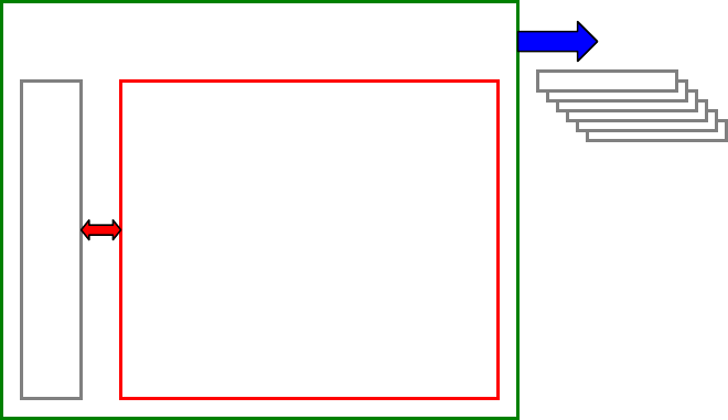
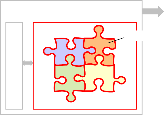
Looking a little closer at a System, you will find that it is composed of a set of interlocking
pieces, which we call subsystems.
In this jigsaw puzzle analogy, you can think of the System as providing the “edge pieces”
which frame the subsystems into a complete whole.
In general any subsystem of a System may have its own state variables, as can the System
itself. The System ensures that its subsystems’ state needs are provided for within the overall
System’s State. The calculations performed by subsystems are interdependent in the sense of
having interlocking computational dependencies. However, these dependencies can always
be untangled by performing computations in “stages” as will be discussed below. It is the
System’s responsibility to properly sequence its subsystems through the stages.
Note that by design this is not a hierarchical structure. It is a flat partitioning of a System into
a small number of Subsystems. In a higher-level modeling layer, one would expect to find
hierarchical models, which are a powerful way to represent the physical world. However,
computational resources are flat, not hierarchical, and the System/Subsystem scheme is a
Study
State
System
subsystem

5
computational device, not a modeling system. The intent is that a modeling layer (or user
program) assembles a System from a small library of Subsystems just at the point when it is
ready to perform resource-intense computations.
1.4 Structure of a multibody system
Simbody provides some computational components (puzzle pieces) of a complete multibody
mechanics System. Simbody’s primary piece, the SimbodyMatterSubsystem, manages the
representation of interconnected massive objects (that is, bodies interconnected by joints).
Simbody can use this representation to perform computations which permit a wide variety of
useful Studies to be performed. For example, given a set of applied forces, Simbody can very
efficiently solve a generalized form of Newton’s 2nd law F=ma. On the other hand, Simbody
is agnostic about the forces F, which come from domain-specific models. That is, Simbody
fully understands the concept of forces, and knows exactly what to do with them, but hasn’t
any idea where they might have come from. Muscle contraction? Molecular electrostatic
interactions? Galactic collisions? Whatever.
A complete System thus consists both of the matter subsystem, and force subsystems that
may be Simbody-provided, user-written, or application-provided. So for a multibody system,
the general System described above is specialized to look something like this:
State
Simbody Multibody System
Matter
Forces #1
Forces #2
Forces #3
6
Although both the Simbody matter subsystem and the force subsystems require state varia-
bles, as discussed above any System (including of course a MultibodySystem) is a stateless
object once constructed. Its subsystems collectively define the System’s parameterization,
but the parameter values themselves are stored externally in a separate State object.
The force and mechanical subsystems are computationally interlocked. For example, a user-
provided force will typically depend on position and velocity information (kinematics)
returned by the Simbody matter subsystem, while accelerations (dynamics) calculated by
Simbody will in turn depend on the values of the forces. Section 7.1 provides details on how
these interlocking computations are performed.
7
2 Fundamental concepts of multibody
mechanics
There are only a few general concepts required to completely specify a multibody system.
These are closely related to physical concepts for which the reader is likely already to have a
good intuition. This is both blessing and curse, since our intuitive understanding of these
concepts is almost, but not quite, general enough or precise enough to serve as a basis for
general simulation. Nevertheless we will plunge ahead using familiar concepts, adding
precise definitions and suitable generalizations where needed.
The concepts we’ll need to define a multibody system are: coordinate frame, body, mobilizer,
constraint, and force. We’ll also discuss the fundamental ideas of kinematics and dynamics
of a multibody system.
2.1 Coordinate frames
We define a coordinate frame (syn: reference frame or just frame) F to be a set of three
mutually orthogonal directions (called axes) and a point (called the frame’s origin). We will
denote the axes as unit vectors Fx, Fy, Fz and follow a right-handed (“dextral”) convention so
that Fz = Fx Fy. We label frame F’s origin point FO.
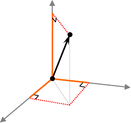
Coordinate frames are used for measuring things. We can express the location of a point P in
frame F, for example, by measuring the vector r from F’s origin to P, that is r=P–FO, and
then expressing it in frame F by writing down the components of r in each of the three axis
directions. These numerical values are called the measure numbers of r in F denoted
( , , ) ( , , )
Fx y z x y z
r r r F F F r r r r
. That is, the measure numbers are the scalars obtained by
taking the dot product of a vector with each of the three axis directions of the expressed-in
frame. Here’s a picture:
8
Note that r is a unique physical quantity (the vector from FO to P) but its measure numbers
would be different if it were expressed in a different frame. In general we will use the
[]
FQ
notation to indicate that some physical quantity Q is being expressed in frame F, whenever
the frame is not already obvious.
I suspect the above has not been much of a stretch for most readers, since this is a perfectly
ordinary example of a conventional coordinate frame. Possibly the notation and the term
“measure number” are new, but everyone is familiar with these concepts. We are just being
excruciatingly precise in distinguishing the physical quantities of direction and location from
their expression in a particular frame of reference.
This next idea may seem a bit odd if you haven’t encountered it before: the concept of a
frame makes perfect sense even if we can’t say where it is or which way its axes are pointing.
Once we have a frame F, for example, like the one defined above, we can start measuring
things in frame F without the slightest idea how F is placed with respect to other things. We
can even measure frame F in itself—the measure numbers of its axes are F[Fx] =(1,0,0),
F[Fy]=(0,1,0), F[Fz]=(0,0,1) and its origin point is F[FO]=(0,0,0). In a sense F defines its own
self-consistent universe without reference to anything else. Note that this universe extends
infinitely in every direction. In multibody mechanics we have another name for such an
independent universe: a body.
2.2 Bodies
Fundamentally, a body B is just a moving reference frame, called the body frame B. You
probably aren’t used to thinking of a body this way! We will shortly connect this back to
FO
Fx
Fz
P
r
rx
ry
rz
Figure 2: Coordinate frame F, and how to
express the location of a point P in F.
Fy
9
more intuitive “body” concepts like mass and geometry; however, it is the frame that is a
body’s most fundamental characteristic. One implication of this is that a body extends
infinitely in all directions. Before you completely reject this idea, answer this question: is the
hole a part of a doughnut?
*
In any case the infinite extent of bodies will turn out to be very
convenient when we start connecting them together.
We call the ordered set of all bodies in a multibody system , with the ith body designated as
[]i
.
[ ]’si
body frame is
[]i
with origin
[]
Oi
. In practice we’ll only have to talk
about a few bodies at a time so we can use different letters for them and avoid subscript
bloat. In particular, body G is the distinguished body Ground representing the inertial (non-
accelerating, non-rotating) reference frame.
†
The ground frame provides a global origin
O
G
(we’ll usually drop the frame in this case and just say O) and fixed orthogonal directions
,,
x y z
G G Gx y z
. By convention, we identify ground with the “0th” body, that is,
[0] G
.
Bodies typically have associated features which can be measured in and expressed in the
body frame. These include other frames, directions (unit vectors) and stations (point loca-
tions). The body frame B origin is the station whose measure numbers when expressed in the
body frame are (0,0,0), and its axes are the directions with measure numbers (1,0,0), (0,1,0),
and (0,0,1). Mass properties include the total mass (a scalar), the center of mass (a station,
represented numerically by a vector), and an inertia tensor (numerically a 33 symmetric
matrix) which expresses rotational inertia about a particular station. When the inertia tensor
is defined about the center of mass it is called the central inertia. For rigid bodies, mass
properties are constant; for deformable bodies (not presently supported by Simbody) the
mass is constant but the center of mass and inertia will be seen to vary when measured in the
body frame.
*
Thanks to Paul Mitiguy for the doughnut analogy.
†
Other names sometimes used for the ground frame are: Cartesian frame, Newtonian frame, world frame,
inertial frame, laboratory frame, and experimenter’s frame.

10
For practical purposes we assign each body a fixed property called that body’s mass struc-
ture. The possible mass structures are: (1) ground, (2) massless, (3) particle (inertialess), (4)
line (inertialess in one direction), (5) rigid body, and (6) flexible body.
2.3 Mobilizers
A mobilizer connects a body to its unique parent body,
*
and provides the relative mobility
(degrees of freedom or “dofs”) allowed between those bodies. Mobility expresses the permit-
ted motion of a body’s frame with respect to its parent’s frame. Don’t confuse this with the
idea of constraining the motion of otherwise free bodies—in Simbody, bodies start out with
no mobility at all, meaning that the body’s frame and its parent’s frame are locked together
and would stay that way forever. Thus there is no motion to be constrained. Instead, Mobi-
lizers are used to grant to a body the ability to move relative to its parent, allowing transla-
tion and/or rotational motion of the body frame and providing a parameterization of that
motion. We call these unrestricted, parent-relative degrees of freedom a body’s mobilities.
The unique Ground body has no parent and no mobility.
2.3.1 Mobilizers are not joints
When describing a multibody system, a joint is a higher-level (more abstract) concept than a
mobilizer, although they are easily confused. We reserve the term “joint” to refer to the
physical-world concept of that name, as illustrated in Figure 3. In general, joints are imple-
mented as a combination of mobilizers and constraints, and may also introduce force ele-
ments (e.g. friction or soft stops). It is possible to create topological loops with joints but not
with mobilizers, as the latter are restricted to connections between bodies and their unique
parents. So a mobilizer can only add degrees of freedom to a system, while a joint may add
or remove them.
*
Recall that Ground is a body.

11
Figure 3: a mechanism with four joints; at most three can be
mobilizers unless you break one of the bodies.
A mobilizer is one way to implement a joint, but not all joints are mobilizers. For example,
when a joint forms a loop as in the figure, it reduces the total mobility, requiring implementa-
tion as a constraint rather than a mobilizer. While the physical system is uniquely described
in terms of its bodies and joints, in general there will be many ways to decompose that
system into mobilizers and constraints for purposes of building a Simbody model. In particu-
lar, for a case like the one illustrated in Figure 3, there is a nice way to make the mobilizers
correspond to the joints—break the loop by cutting one of the bodies instead of the more
intuitive means of breaking one of the joints. The split body’s mass properties should be
divide 50/50 between the two halves (don’t use a massless body – that risks making the tree
part of the system singular which is not allowed in Simbody). Then a Weld constraint is
added to weld the two halves back together into the original body. With this approach all the
joints are mobilizers so are treated uniformly, with the motion of every joint being represent-
ed explicitly by mobilities. The alternative of modeling one of the joints with a 5-constraint
equation Pin constraint can work but is unappealing; one of the joints is then modeled
differently, and there are no coordinates in the system directly corresponding to the motion of
that joint.
One case where it is reasonable to split a loop at the joint is when that joint is a Ball joint
modeled with quaternions – in that case you can use a Ball constraint rather than a Ball
mobilizer and easily obtain the quaternions from the relative orientations of the two con-
12
strained bodies. Other than that, though, we recommend splitting loops by cutting bodies
rather than joints.
2.3.2 Types of Mobilizers
The most common mobilizer types are sliding, torsion, and orientation. A sliding mobilizer
(syn: prismatic) provides a single degree of freedom representing translation along a defined
axis, and adds a single coordinate with units of length to the system’s set of generalized
coordinates. A torsion mobilizer (syn: pin) provides a single degree of freedom representing
rotation about a defined axis and adds a single generalized coordinate with angular units. An
orientation mobilizer (syn: ball, spherical) permits unrestricted relative orientation between
its pair of bodies, that is, three degrees of freedom and at least three corresponding general-
ized coordinates (for dynamics these require a four-element quaternion).
Most other mobilizer types can be viewed as compositions of the three basic types. For
example, a cartesian mobilizer is a composition of three sliding joints with orthogonal axes
and thus permits unrestricted relative translation (three degrees of freedom) between the
bodies it connects. A free mobilizer is a composition of a cartesian and an orientation mobi-
lizer and permits six degrees of freedom (completely unrestricted motion) between its bodies.
A free mobilizer serves to introduce independent rigid bodies into the system and simply
provides a convenient reference frame and corresponding coordinates with which to express
their motion. Note that, like all other mobilizers, a free mobilizer can be placed between any
two bodies—it does not have to connect a body to ground. This allows very convenient
relative coordinates to be used for collections of independent bodies. For example, one can
express a protein domain that carries its local waters and ions along with it when it is moved
kinematically.
Complex joints can be built up from mobilizers and constraints (see below). A “screw joint”
for example could be composed of a coaxial sliding and torsion mobilizer, providing one
translational and one rotational coordinate, plus a constraint enforcing a defined relationship
(the screw’s “pitch”) between the time derivatives of these coordinates. However, the Sim-
body mobilizer concept is extensible in the sense that arbitrarily complicated ones can be
constructed without the use of constraints. There is, in fact, already a screw mobilizer that
has only a single generalized coordinate and no constraints, but can only represent screw
13
motion. A more elaborate, data-driven example is a subject-specific knee joint which can be
built as a 1-dof mobilizer so that a single unconstrained coordinate is used to represent the
complicated coordinated rotational and translational motion of a knee.
2.3.3 Mobility space
A body can have from 0 to 6 relative mobilities (degrees of freedom) with respect to its
parent body. Summing the mobilities of each body in a multibody system, the total of n
mobilities defines an n-dimensional mobility space for the multibody system. The n mobili-
ties are independent by construction and thus form a basis for mobility space. Only configu-
rations in mobility space are representable by the multibody system. Typically there are many
conceivable configurations which simply cannot be expressed. For example, consider a
system composed of Ground and one moving body, a wheel, having a single mobility with
respect to Ground consisting of just a rotation about a fixed axis. One can imagine a configu-
ration in which the wheel is removed from the axis, but the chosen multibody system simply
can’t express that. With just one coordinate, an angle, we can only talk about rotations of the
wheel about an axis. Additional mobilities would have to have been granted to the wheel in
order to express more general configurations.
This ability to limit the mobility space of a multibody system is extremely powerful if you
happen to know something about the space containing the solutions of interest to you. To
continue the above example, if you are a car designer rather than a crash-test engineer, then
you know that correct solutions to your vehicle simulation problems will always exhibit
wheels that are attached to their axles. Solutions in that smaller space are much easier to find
than solutions in the much larger space where wheels may be found anywhere. Similarly, in
molecular mechanics if you know that certain groups of atoms are always observed to move
together as rigid bodies, problems are much easier to solve in a reduced space in which only
those groupings can be expressed, than one in which the atoms could be anywhere. We know
that correct solutions would always “rediscover” the known groupings (at great, and unnec-
essary, expense).

14
2.3.4 Parameterization of mobility
The mobilities of the bodies in a multibody system, taken together, define its mobility space.
However, we must choose a particular parameterization of this space (that is, a basis) in order
to express a particular configuration and motion of the multibody system and this choice is
not unique. Conveniently, body mobilities are mutually independent so we may choose the
parameterization for each body separately. The set containing all these parameters is then the
parameterization of mobility for the multibody system as a whole.
The independence of body mobilities localizes the parameterization issue to the mobilizer for
each body. Each mobilizer must define two sets of scalar parameters to express particular
values for its mobilities, one set to specify the relative positioning (configuration) and the
other to specify the relative velocity (motion) between the parent and child bodies. Parame-
ters used for positioning are conventionally called generalized coordinates; parameters for
velocity are called generalized speeds.
*
The symbol q is used to represent a vector of general-
ized coordinates, and u is a vector of generalized speeds. Generalized coordinates are some-
times referred to as “internal coordinates,” “relative coordinates,” or “torsion coordinates.”
In Simbody, the number of a body’s generalized speeds u is always the same as that body’s
mobility—e.g., if a body has five degrees of freedom with respect to its parent, then it will
also have five u’s. The u’s are thus mutually independent. u’s have interpretations with direct
physical meaning, and the system equations of motion are written in terms of the time
derivatives of u, which we denote
u
and refer to as generalized accelerations. The general-
ized coordinates q, on the other hand, must at times be chosen for convenience or computa-
tional stability and do not always map directly to physical quantities, so in general
qu
. In
fact, for many bodies there will be more q’s than u’s in which case the q’s are not always
independent. However, the interdependence among a body’s q’s is always a localized rela-
tionship among only those q’s, and never involves other bodies. At any particular configura-
*
Generalized here refers to the use of the mobility space basis where the meaning of the coordinates and speeds
depends on the definition of the associated mobility. They can represent translations, rotations, or more general
motions. We similarly use generalized forces to mean both forces, torques, or more general loads which are
applied along or about mobilities.

15
tion, there is always a linear, invertible relationship between
q
and u, and each Mobilizer
provides the necessary conversions. As a specific example, during dynamic calculations
Simbody Mobilizers that permit unrestricted relative orientation between a body and its
parent use four quaternions to stably represent the orientations, while the three generalized
speeds are just the elements of the relative angular velocity vector. The four quaternions must
satisfy a normalization constraint, leaving only the expected three degrees of freedom for the
four coordinates.
For the whole multibody system, the generalized speeds are aggregated in a vector whose
length is the sum of the mobilities of each body. This vector is the set of generalized speeds
for the multibody system and is also designated u. A vector q aggregating the individual
bodies’ generalized coordinates forms the generalized coordinates for the whole multibody
system. Together, q and u constitute the instantaneous state of the matter component of a
multibody system. It will usually be clear from context whether we are referring to the
coordinates of the whole system or just one body, but if we need to be specific we use qB and
uB to indicate the sets of mobilizer parameters for body B.
2.3.5 A comment on deformable (flexible) bodies
In general, the bodies of a multibody system do not have to be rigid. It is sometimes desirable
to allow the bodies themselves to undergo small internal motions, called deformations. These
add a new set of independent coordinates to the overall system coordinates and speeds, but
we distinguish them from the generalized coordinates and generalized speeds introduced by
mobilizers and refer to them instead as deformation coordinates and deformation rates.
Various techniques can be used to determine the appropriate representation of deformable
bodies. Typically, structural mechanic methods are used to aggregate large nearly-rigid
subsystems into deformable bodies with “assumed mode” linear deformations.
We do not provide direct support for deformable bodies yet in Simbody, but it is always
possible to model body flexibility by partitioning the body into Mobilizer-connected rigid
bodies, with internal forces and constraints modeling the deformation behavior. Reference
1
describes how deformable bodies can be incorporated into a computational methodology like
Simbody’s.

16
2.4 Constraints
As discussed above, Simbody’s mobilizers allow construction of a very small mobility space
to represent all possible motion of the bodies of a multibody system. However, we will often
find that even this reduced space is substantially larger than our known solution space. For
example, in a multibody system where the joints form closed loops like the one shown in
Figure 3, mobility space would permit solutions where the loops are not closed. Instead, we
would like to focus on a lower-dimensional subspace of mobility space, called constrained
space. The dimensionality of constrained space is the net number of degrees of freedom
possessed by the multibody system.
*
So a multibody system’s net degrees of freedom (or net
mobility) can be smaller than the sum of its bodies’ individual mobilities.
One might wish simply to redefine the mobility of the bodies so that only constrained space
can be expressed (that is, make mobility space=constrained space), and that is a very good
thing to do if you can. Unfortunately, in general constrained space cannot be parameterized
directly. Instead we create a system with a small but convenient-to-define mobility space,
and then add a set of constraints whose satisfaction implicitly defines the constrained space.
Constraints may represent arbitrary restrictions on the generalized coordinates and general-
ized speeds, and linear restrictions on accelerations. Each Simbody constraint generates one
or more constraint equations. Each independent constraint equation removes one degree of
freedom from the system. In this sense constraints are the complement of mobilizers, whose
generalized speeds each add one degree of freedom to the system. And in fact any n-dof
mobilizer can be represented instead as a free mobilizer plus 6−n constraint equations.
Constraints among the moving bodies of a physical system act by introducing internal forces
and moments. These forces act in the same manner as the applied forces described below—
they can act on bodies or along mobilities (joint axes), and as with applied forces they can
*
When a multibody system represents a mechanism, the net number of degrees of freedom after accounting for
constraints is conventionally called the mechanism’s “mobility.” We use the terms mobility and mobility space
exclusively to mean the number of degrees of freedom in the unconstrained system. We’ll say “net dofs” or
“net mobility” whenever we’re referring to the post-constraint leftovers.

17
always be reduced to a system of forces acting only along the mobilities. The only difference
between constraint forces and externally applied forces is that the constraint forces are
unknown and must be solved for simultaneously with the system accelerations.
2.5 Forces
By forces we mean to include both forces and moments (torques).
*
Force vectors can be
applied to the multibody system at any station on a body and moment vectors can be applied
to any body (or implemented as pairs of forces). Scalar forces or moments can also be
applied to the system’s mobilities, that is, directly along the generalized speeds; these are
called generalized forces or mobility forces. All systems of forces and moments can be
reduced to an equivalent set of generalized forces, and Simbody provides an operator which
efficiently performs this useful conversion.
Forces can be functions of time, position, velocity, and their own internal states. They may
be local effects or result from spatially distributed fields or a constant gravitational field, or
act pairwise between distant stations (e.g. atoms) in the system. Forces which depend only on
configuration are called conservative forces, and are the gradient of some potential energy
function. Non-conservative forces dependent on time and velocity exist as well but may not
contribute to potential energy.
2.6 Kinematics
Kinematics is usually defined as the study of motion without regard to mass or force. In
practice, however, it is entirely concerned with the mapping between the mobility coordi-
nates and spatial positions, velocities, and accelerations of the bodies. The mobility coordi-
nates and speeds uniquely determine the spatial quantities so the mapping in that direction is
fast and direct; this is called forward kinematics. Given a q we can immediately say where all
the bodies are; with q and u we can say how they are moving; and with q, u, and
u
(where
u
is the time derivative of u) we can say how they are reacting (accelerating). The reverse
*
The term loads is often used as an alternative with less ambiguity. However we will continue to use the more
familiar term forces, usually meaning both forces and torques.
18
direction is called inverse kinematics and is more difficult unless all bodies have been given
unrestricted mobility (i.e., they are “free”). Given a set of observed spatial kinematic quanti-
ties, the goal of inverse kinematics is to find the “best fit” mobility coordinates and speeds
that satisfy both the observations and the constraint equations generated by the multibody
systems’ own Constraints. Such problems arise, for example, when fitting a reduced-
coordinate molecular model to a set of atom positions determined with X-ray crystallog-
raphy. Simbody provides an ObservedPointFitter solver that can solve many common inverse
kinematics problems. More generally, there is a broad assortment of useful initial condition
analyses which must be performed prior to the start of a dynamic analysis, and these are
based on kinematic calculations.
2.7 Dynamics
Dynamics is concerned with the relationship between forces and accelerations at a fixed
value of the state variables q and u. This is determined by Newton’s second law, f=ma.
Forward dynamics attempts to calculate accelerations and internal constraint forces, given a
set of applied forces (which is equivalent to some set of generalized forces f). Inverse dynam-
ics (also called prescribed motion) attempts to determine what set of generalized forces
explains a given set of generalized accelerations. In practice it is often useful to specify some
accelerations and some forces and calculate the remaining unknowns.
Given this definition of dynamics, advancing the state through time to produce a trajectory,
or searching through the state to satisfy particular objectives, are higher-level operations
(“Studies”) which are facilitated by the multibody dynamics capabilities described here.
SimTK::TimeStepper and SimTK::Integrator objects are designed to employ Simbody
dynamics calculations to generate a trajectory through time.
19
3 Basic Simbody numerical types
This chapter presents the basic numerical types used repeatedly in the Simbody API and in
theory discussions. We’ll present both the mathematical notation and definitions for these
objects and the C++ classes used to manipulate them programmatically.
3.1 Vectors and Matrices
Simbody makes use of lower-level SimTK toolsets to simplify its interface and internals. The
SimTK general purpose Simmatrix™ package (part of the SimTKcommon library that is part
of Simbody) is used to handle basic vector and matrix objects. We follow the Simmatrix
convention of using names containing “Vector” and “Matrix” to refer to large objects of
variable dimension, and names containing “Vec” and “Mat” to mean small, fixed-size objects
of known dimension. The types we use most are the fixed-size Vec3 and Mat33 types and the
variable length Vector type. We use the basic Simmatrix types to build up a set of special-
ized vectors and matrices of particular use in manipulating physical objects, as described in
the next sections.
3.2 Geometry
We provide a small set of specialized types for dealing with geometric quantities of interest
in multibody dynamics. This is not intended to be a general purpose geometry package. For
example, we happily assume that all geometry of interest is 3D.
Given the fundamental existence of a rigid body frame B, we are primarily interested in
stations, directions, and other frames fixed in B. These are represented by positions, rota-
tions, and transforms (xforms) respectively, which locate these objects with respect to an
existing frame.
3.2.1 Stations
Stations are simply points which are fixed in a particular reference frame (i.e., they are
“stationary” in that frame). They are specified by the position vector which would take the
frame’s origin to the station. A position is represented by a Simmatrix Vec3 type. Simbody
does not provide an explicit Station class; Vec3’s are adequate whenever a station is to
be specified.
20
3.2.2 Directions
Directions are unit vectors, which are Vec3s with the additional property that their lengths are
always 1. We define a class UnitVec3 which behaves identically to Vec3 in most respects but
restricts the ways in which values can be assigned to ensure that the length is always 1. This
has concrete performance benefits because this unit length guarantee means that we can track
length-preserving operations at compile time and avoid unnecessary normalization checks, or
worse, unnecessary normalizations which are very expensive.
3.2.3 Rotations
There are many ways to express 3D rotations. Examples are: pitch-roll-yaw, azimuth-
elevation-twist, axis-angle, and quaternions. Many others are in common use. Each way of
writing orientation has its own quirks and complexities. However, all of these are equivalent
to a 3x3 matrix, called a rotation matrix (synonyms: orientation matrix, direction cosine
matrix). Rotation matrices have a particularly simple definition and straightforward physical
interpretation, and are very easy to work with. At the API level, Simbody uses the rotation
matrix as a least common denominator, embodied in a class Rotation. Rotation provides a
set of methods which can be used to construct a rotation matrix from a wide variety of
commonly-used rotation schemes.
Rotation matrices are simply 3x3 matrices whose three columns are mutually perpendicular
directions (unit vectors) representing the axes of one coordinate frame, expressed in another.
These are represented internally in objects of type Rotation as an ordinary Simmatrix
Mat33, and behave identically except that their construction and assignment is restricted to
ensure that certain properties are maintained. Those properties are: each column and row is a
unit vector, the columns are mutually perpendicular, and the rows are mutually perpendicu-
lar, forming a right-handed set. That means that the third column (row) is the positive cross
product of the first two columns (rows). Such a matrix is orthogonal; hence its transpose is its
inverse. Its determinant is +1, meaning that it is a pure rotation and not a reflection or scaling
operation.
We use the symbol R with left and right superscripts
from to
R
to represent the orientation of the
“to” frame (the right superscript) measured with respect to the “from” frame (the left super-
script), like this:

21
G
GG
GB
xyz
R B B B
(Bx is the x-direction unit vector of frame B, with measure numbers expressed in B’s frame,
while the operator
F
indicates that the measure numbers of some physical quantity are re-
expressed in coordinate frame F.) So the symbol
GB
R
should be read “the axes of frame B
expressed in frame G,” or “the orientation of frame B in G,” or just “B in G.” We never use
“R” alone for a rotation matrix; that is a recipe for certain disaster. Instead, we always
provide the two frames. (When under tight typographical restrictions, as in source code, we
write
GB
R
as R_GB.) Using this notation, one can simply match up superscripts to rotate
vectors or compose rotations. Also, since these are orthogonal, the inverse of a rotation
matrix is just its transpose, which serves simply to swap the superscripts. Using the Simma-
trix “~” operator to indicate matrix transpose:
~G B B G
RR
. As an example, if you have a
rotation
GB
R
and a vector Bv expressed in B, you can re-express that same vector in G like
this:
G G B B
Rvv
. To go the other direction, we can write
~
B B G G G B G
RRv v v
. As a
C++ code fragment, this can be written
Rotation R_GB; //orientation of frame B in G
Vec3 v_G; //a vector expressed in G
…
Vec3 v_B = ~R_GB*v_G; //re-express v_G in frame B
Composition of rotations is similarly accomplished by lining up superscripts (subject to order
reversal with the “~” operator). So given
GB
R
and
GC
R
we can get
BC
R
as
~
B C B G G C G B G C
R R R R R
. Note that the “~” operator has a high precedence like unary
“–” so
~G B G C
RR
is
(~ )
G B G C
RR
, not
~ ( )
G B G C
RR
.
As is typical for Simmatrix operations on small quantities, the transpose operator is actually
just a change in point of view and involves no computation or copying of data. That is, the
operations
B G G
Rv
and
~G B G
Rv
are exactly equivalent in both meaning and performance:
the cost is 15 floating point operations (three inline dot products), with no wasted data
copying or subroutine calls.

22
3.2.4 Transforms
Transforms combine a rotation and a position (translation) and are used to define the configu-
ration of one frame with respect to another. (Recall that we consider a frame to consist of
both a set of axes and an origin point.) We represent a frame B’s configuration with respect
to another frame G by giving the measure numbers in G of each of B’s axes, and the measure
numbers in G of the vector from G’s origin point to B’s origin point, for a total of 4 vectors,
which can be interpreted as a 3x3 Rotation (see above) followed by the origin point location
(a Vec3). Following computer graphics convention, we call this object a transform (abbrevi-
ated xform) and conceptually augment the axes and origin point to create a 4x4 linear opera-
tor which can be applied to augmented vectors (4th element is 0) or points (4th element is 1),
or composed using matrix multiplication. We define a type Transform which conceptually
represents transforms as follows:
[ ] [ ] [ ]
0 0 0 1
G G G GB
x y z
GB B B B p
X
(The notation
OO
GB
GB
pp
, that is, the vector from the origin of the G frame to the origin of
the B frame.) Note that we use the symbol X for transforms, with superscripts
from to
X
so
GB
X
means “the transform from frame G to frame B,” or “frame B measured from and
expressed in frame G.” Another way to interpret
GB
X
is that it represents the operations that
must be performed on G to bring it into alignment with B (a rotation and a translation). Then
as for rotation matrices described above, we can interpret
G B B C
XX
as a composition of
operators yielding
GC
X
, and
~GB
X
is defined to yield the inverse transform
BG
X
.
*
The above transform matrix can be considered a matrix of four columns as shown: three
augmented vectors and an augmented point. An alternate, and entirely equivalent, way to
view this is as a rotation matrix, translation vector, and an extra row:
*
Note that this is actually a different definition for the “~” operator than is normally used in Simmatrix, since
the inverse of a transform is not simply its transpose. However, the analogy with ~R (which is both the trans-
pose and inverse of rotation matrix R), combined with the lack of any practical use for the transpose of a
transform, makes this use of “~” very attractive and natural to use in practice.

23
0 0 0 1
G B G B
G B R p
X
In our implementation, the physical layout of a Simbody Transform is just the three columns
of the rotation matrix followed immediately in memory by the translation vector, that is,
34
G B G B G B
X R p
. There is no need for the fourth row to be stored in memory since it is
always the same.
Given a Transform, you can work with it as though it were a 4x4 matrix, or work directly
with the rotation matrix R and translation vector p individually, without having to make
copies. Although a transform defined this way is not orthogonal, its inverse is easy to apply
with no additional calculation. As described above, we overload the normal matrix transpose
operator “~” to recast a Transform to its inverse so that either the transform or its inverse
can be used conveniently in an expression, for example,
~
B C G B G C
X X X
. As is typical
using Simmatrix objects, this inverse operator is just a change of point of view at zero cost,
so the total cost is the same in either direction. For example, to transform a point measured
and expressed in one frame to the equivalent one re-measured and re-expressed in another
frame costs one 3x3 matrix-vector multiply and one addition of 3-vectors per transformed
point, for a total of 18 floating point operations (flops), and the cost is the same if we trans-
form it back using a Transform inverse. A straightforward implementation of a 4x4 trans-
form (i.e., as an actual 4x4 matrix times a 4-vector) would require 28 floating point opera-
tions per transformed point. Composition of Transforms (using the ‘*’ operator for matrix
multiply) is done in 63 flops but would take 112 using a 4x4 matrix multiply. Thus Trans-
form provides the convenience of a 4x4 transformation matrix at substantially lower cost.
3.3 Mechanics
Some additional specialized quantities arise in mechanics for dealing with mass properties,
which consist of a mass, center of mass, and inertia matrix for each body. Mass is a simple
scalar and center of mass just a point so we do not define special classes for them. Inertia,
however, is a tensor quantity (a 3x3 matrix) which is expected to exhibit certain properties.
24
Among these, it is symmetric, and the values of its elements must satisfy certain relation-
ships. In addition, there are common operations on inertias which can be most efficiently and
conveniently provided with a distinct inertia class. So we provide a class Inertia which is
stored physically as a 3x3 symmetric matrix, i.e., a Simmatrix SymMat33 containing six real-
valued numbers. This behaves like an ordinary matrix for read-only operations but its con-
struction and assignment is restricted to enforce physical relevance, and additional operations
are provided, such as shifting inertia taken about one point to the equivalent inertia about
another point.
For convenience we combine all the mass properties into a MassProperties class, which
contains a mass, a center of mass location, and an inertia matrix. Note that there is implicitly
a reference frame in whose axes the vector and tensor are expressed, and from whose origin
the center of mass location and inertia distribution are measured.
3.3.1 Spatial Notation
We also build on the Simmatrix types to define some specialized vectors and matrices useful
in mechanics. Following Jain and Rodriguez5, we use spatial notation which combines
translational and rotational quantities into a single object. Using Simmatrix we define the
convenient type SpatialVec to mean a stacked vector of two ordinary 3-vectors, and Spa-
tialMat to mean a 2x2 matrix of ordinary 3x3 matrices, that is
typedef Vec<2,Vec3> SpatialVec;
typedef Mat<2,2,Mat33> SpatialMat;
Note that these convenient types have well-defined interpretations as packed arrays of real
numbers, which means they have equivalent descriptions in C and FORTRAN, which we’ll
address later. There is zero overhead in C++ for using the more expressive types.
The first sub-vector of a SpatialVec is always the rotational component, and the second is
the translational one. Some examples of spatial vectors: spatial velocity V, spatial accelera-
tion A, and spatial force F, defined like this:
,,V A F
v a f

25
where ω is an angular velocity vector, v a linear velocity, β an angular acceleration
*
, a is a
linear acceleration, μ a moment (torque), and f is a force. Each of these elements is an ordi-
nary 3-vector (Vec3). Sadly, orientation is not a vector quantity so we can’t use an analogous
SpatialVec
Pp
to represent configuration (orientation and position) of a rigid body
(that is, of a reference frame). However, it can be useful to think of position this way in some
circumstances.
Unless otherwise indicated, all quantities are measured with respect to the ground frame G,
and linear quantities are referred to the body origin. That is, the default symbols above
represent
,,
O O O
G B G B G B
G B G B G B
B B B
G G G
V V A A F F
v a f
For spatial position, instead of the fanciful P we use the Transform class described above,
where
OO
GB
G B G B
X R p
with rotation matrix R playing the role of P’s θ.
The above notation and somewhat atypical use of Greek symbols was chosen so that there
would be an obvious way to represent these using the restrictive typographical capability of a
programming language. For Greek letters we use the correspondence w=ω, b=β, m=μ, q=θ,
so we can represent the above symbols in code with
V=[w,v], A=[b,a], F=[m,f], P=[q,p], X=[R,p]
(Although as mentioned above there is no actual P like this, orientation angles and quaterni-
ons are part of the generalized coordinates q so this notation is conceptually right even if
pragmatically flawed.)
*
We use β rather than the more conventional α for angular acceleration because a and α are too similar in many
fonts, and we can use b in code rather than spelling out alpha.

26
3.3.2 Cross product matrix
For any vector quantity v, we use the notation
v
to indicate a 3x3 skew-symmetric cross
product matrix such that for any vector w,
v w v w
. Spelled out in scalars, the cross
product matrix is
0
0
0
zy
zx
yx
vv
vv
vv
v
(3.1)
Note that the matrix is skew-symmetric, so
vv
T
.
We will occasionally make use of the following identities:
()
v+w v w
(3.2)
3
v w wv w v1
TT
(3.3)
2
3
v v v v v v v1 vv
T T T
(3.4)
(
3
1
is a 3x3 identity matrix.) Note that
vv
T
is a symmetric matrix with non-negative diago-
nal elements. Spelled out in scalars,
22
2 2 2
22
yz
x y x z
x z y z x y
vv
v v v v
v v v v v v
v v v
T
TT
T
(3.5)
where T indicates that the element is the same as the transposed one. This can also be viewed
as the inertia (or gyration) matrix of a unit-mass particle located at v, measured about the
origin.
33
( ) ,
where is orthogonal.
U v U U v
U
T
(3.6)
Since rotation matrices are orthogonal, equation (3.6) is particularly useful when transform-
ing spatial quantities from one frame to another.
()
vv
(3.7)
where the overdot indicates a derivative with respect to time taken in some frame understood
from context.

27
Identity (3.7) is primarily useful to allow us to write
v
unambiguously without concern for
the typographical details of the overdot placement.
3.3.3 Spatial mass properties
The mass properties of a rigid body conventionally consist of the body’s mass m, the mass
center location p, and its inertia tensor J. It is convenient to view the inertia tensor as the
product of the mass and a gyration tensor G, such that J=mG. Then a spatial inertia matrix M
can be written as a spatial gyration matrix (giving the mass distribution) scaled by the total
mass:
3
p
Mmp
1
G
For the spatial inertia matrix
B
M
of a body B about its origin BO we have
OC
BB
pp
so
3
OC
OC
BB
B
BB
BB
p
Mm p
1
G
Note that when the spatial mass properties are given about the center of mass BC we have
0p
so
3
0
0
C
C
B
BB
BB
Mm
1
G
Where the central gyration matrix is
2
3
()
C
B
B B B B
p p p
p p1 ppG G G G
T T T
using the parallel axis theorem and then cross product matrix identities (3.4).
If we have the spatial velocity VC also referred to the center of mass, i.e.
C
C
V
ω
v
, then we
can define another spatial vector quantity, spatial momentum of a body “referred to” its
center of mass:

28
0
0
CC
C C C
CC
P M V m m
ωω
v
1v
GG
In the more general (and typical) case where the body origin BO≠BC we compute spatial
momentum the same way with the result being the spatial momentum referred to BO, which is
not the same quantity:
0
C
C
pp
p
P MV m m P m
pp
ωv
ωv
1vω
v
GG
(Because
Cp
vv ω
and
Cpp
GG T
.) A body’s kinetic energy (a scalar) is calculated
from spatial momentum like this:
1 1 1
2 2 2 ()
( ) 2
KE V MV V P m
p p p
2
ω ω v
ω v v ω ω v
G
T T T
T T T
Note that although the angular momentum must be referred to a specific point, kinetic energy
is independent of that point. That is
1 1 1
2 2 2
2
1 1 1
2 2 2
( 2 )
()
C
C C C C C C
KE V MV V P m p
V M V V P m
2
ω ω v ω v
ω ω v
G
G
T T T T
T T T
These can be shown equivalent by substituting
Cpp
GGT
and
Cp
vv ω
into the last
expression.
3.3.4 Spatial rotation, shifting, and transform
Objects of type Rotation and Transform have equivalent interpretations as spatial matrices:
29
0
spatial rotation 0
AB
AB
AB
R
RR
(3.8)
10
spatial shift 1
PQ
PQ
Sp
(3.9)
0
spatial transform OO
OO
AB
AB
A B A B
AB
A B A B
R
X S R p R R
(3.10)
Then a spatial vector or spatial matrix can be rotated, shifted, or transformed using these
matrices, their inverses, and their duals (inverse transpose). From the definitions above you
can check that swapping the superscripts produces the inverse of each of these matrices:
1
1
1
0( ) ( )
0
1 0 1 0 ()
11
00
()
O O O O
BA
B A A B A B
BA
Q P P Q
Q P P Q
B A B A
B A A B
B A A B
B A B A B A B A
R
R R R
R
SS
pp
RR
XX
p R R R p R
T
(3.11)
The dual operators are given by transposing the inverses, so
* ( ) ( )
1
* ( ) ( ) 01
* ( ) ( ) 0
OO
A B A B B A A B
PQ
P Q P Q Q P
AB
A B A B
A B A B B A
AB
R R R R
p
S S S
R p R
X X X R
TT
TT
TT
(3.12)
Defined this way, operators R, S, and X apply to spatial vectors in the “motion” basis, like
velocities and accelerations. The dual operators R*(=R), S*, and X* apply to spatial vectors
in the “force” basis, like forces and impulses. These definitions follow Featherstone
2
but
have the reverse sense from Jain
3
and Schwieters
4
where the force basis is primary and the
motion basis is dual (their ϕ operator is our S* operator).
Using these definitions you can rotate, shift, or transform a spatial inertia matrix (rigid or
articulated) M like this:
31
4 Constructing a Simbody multibody
system
The Simbody API (application programmer interface) assumes that the caller has made all
modeling decisions and simply wants to perform calculations on the model. The primary
decisions to be made are (1) how the physical model is to be decomposed into a particular set
of rigid bodies, (2) what kinds of mobilizers are to be used to interconnected them in a tree
structure, and (3) what constraints, if any, should be present to restrict the allowable mobility.
A variety of higher-level automated modelers for specific domains can be provided which
can make these decisions and then use the low-level interface.
4.1 Topology
In describing the “matter” side of a multibody system, the most fundamental property is the
system topology. By topology we mean just these properties:
A set of bodies (that is, reference frames). One distinguished body Ground is always
present.
The mass structure of each body. The possible mass structures are: (1) ground, (2)
massless, (3) particle (inertialess), (4) line, (5) rigid body, and (6) flexible body.
For each body except Ground, a unique “parent” body with respect to which the
body’s mobility will be defined. This leads to a tree topology for the system as a
whole, with the ground body at its root.
A set of topological constraints, that is, constraints which are always present and ac-
tive. These can impart a closed-loop topology to the system as a whole.
A body’s mass structure defines the most general form that the body’s mass properties can
take on. Ground and massless bodies have only a single predefined set of mass properties:
infinite and zero respectively. Particles can take only a point mass, and never have inertia
about that point. A line body can be thought of as a linear arrangement of particles, and thus
has mass, a meaningful center of mass along the line, and equal central inertias in two
directions perpendicular to the line, but none about the line. A rigid body (representing a
32
mass distribution on a surface or in a volume) can have a full inertia. A flexible body has a
mass distribution that is not constant in the body’s frame.
4.2 Bodies and their Mobilizers
The primary Simbody representation of matter is a multibody tree, that is, a tree-structured
collection of interconnected bodies, which we call a SimbodyMatterSubsystem. On initial
construction, a SimbodyMatterSubsystem contains just a single body, the inertial frame
Ground (body 0) which is the root of the multibody tree. To add a body B to an existing
SimbodyMatterSubsystem, you will need to be able to specify the following properties:
The parent body P (with body frame P), which must already be in the multibody tree.
A reference frame (axes and origin) for the body (this is implicit, but you need to
have it in mind). We call that the body frame B. (See Figure 2 for an example.)
Mass properties for the body, with the center of mass location measured from BO and
expressed in B, and the inertia (actually the unit inertia or gyration matrix G) meas-
ured about BO and expressed in B.
The mobilizer’s moving frame M attached to B. You must be able to express M’s con-
figuration on B as a transform
BM
X
from B to M.
The mobilizer’s fixed frame F, attached to P, which will be connected to M by the
mobilizer. You must be able to express F’s configuration on P as a transform
PF
X
from P to F.
The kind of mobilizer to be used to connect B to its parent body P, and whether to
reverse the interpretation of the generalized coordinates.
Figure 4 shows a body B being added to a tree already containing its parent P. Not shown are
the body’s mass mB, its inertia JB= mBGB about BO and the transforms
BM
X
and
PF
X
.
When this information is supplied to the appropriate Simbody method, the new body be-
comes part of the growing tree, and a unique, small integer body number is assigned which
can be used to refer to the body later. The specified mobilizer is the unique inboard mobilizer
of body B, that is, the mobilizer which connects it to a body which is closer (in a graph path-
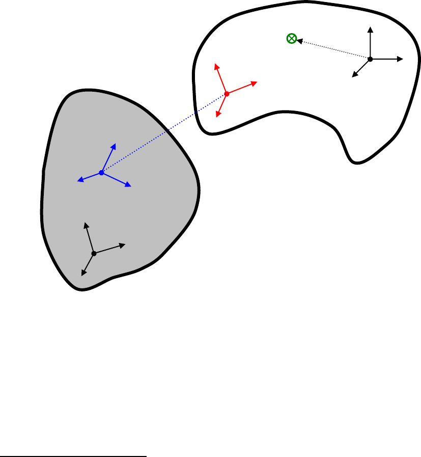
33
length sense) to the Ground body. When defining the sense (sign) of mobilizer coordinates
later we will refer to the frame F on P as the “fixed” frame, and frame M on B as the “mov-
ing” or “mobilized” frame, although these terms are arbitrary and do not imply anything of
physical significance except when P is ground in which case it really is “fixed.”
4.2.1 The reference configuration
The frames M and F are used to define a reference configuration for each body with respect
to its parent. For most mobilizers, that is the configuration in which M and F are overlaid,
and corresponds to a value of zero for the mobilizer’s generalized coordinates
*
. Figure 5
shows the reference configuration for the mobilizer defined in Figure 4. For any mobilizer
type, the values of the generalized coordinates q express a transform
FM
X
which gives the
*
Certain sets of mobilizer coordinates may define their own “zero” which does not necessarily correspond to
numerical values of zero for all coordinates. For example, zero (“no rotation”) for a quaternion is a four-vector
(1,0,0,0).
B
M
BO
BC
P
PO
F
Figure 4: Adding body B to a
multibody tree already containing
parent body P.
FO
MO
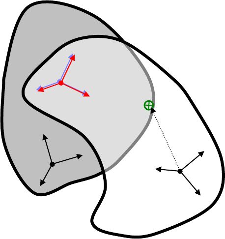
34
current location and orientation of the M frame, measured from and expressed in the F frame.
The definition of each mobilizer type specifies the meaning of each of the q’s for that mobi-
lizer and the kinds of transforms that can be expressed. For example, a Cartesian mobilizer
would permit arbitrary translation of M, but its axes must remain forever aligned with those
of F. A ball (spherical) mobilizer’s coordinates express the complementary motion in which
the origins of the two frames must remain coincident forever, but the orientation of M can be
arbitrary with respect to F. A sliding mobilizer permits translation along one axis only, and a
torsion (pin) mobilizer permits only rotation about a single axis. Other mobilizers permit
various combinations of rotation and translation, with the extremes being the Free mobilizer
which permits all possible motion (six degrees of freedom) and the Weld (im)mobilizer
which permits no motion at all (zero degrees of freedom).
Regardless of the mobilizer type, setting all the coordinates to zero expresses that the M and
F frames are in their reference configuration.
Those users familiar with SD/FAST’s reference configuration should note that the above is a
different method for defining the reference configuration. It is in fact the opposite approach:
SD/FAST requires the bodies to be entered already in the reference configuration, and then
defines the mobilizer (SD/FAST joint) frames from the reference configuration. We think it is
P
PO
F
B
M
BO
BC
Figure 5: The reference
configuration for the
mobilizer added in the
previous figure.
35
much more natural to express the joint frames separately in their bodies’ frames, and then
define the reference configuration from the joint frames. It is always possible to choose
mobilizer frames to reproduce the ones used by SD/FAST if you want, but it is no longer
necessary to calculate them that way.
4.3 Constraints
Constraints in Simbody are the complement of Mobilizers. Mobilizers add mobility to a
multibody system; Constraints reduce mobility by introducing one or more constraint
equations. Mobilizers are local, granting degrees of freedom to a single body, while Con-
straints are global and remove degrees of freedom from the multibody system as a whole by
introducing restrictions on the allowable relationships among the generalized coordinates,
speeds, or accelerations. A simple example is a distance constraint which says that a particu-
lar point fixed on one body must always be at a certain distance d from a point fixed on
another body. If those bodies are far apart in the graph of the multibody topology, this simple
restriction is actually expressing a complicated relationship that must hold among the mobili-
ty coordinates of many bodies. As mentioned earlier, it is much more efficient to define less
mobility in the first place than to grant the bodies their freedom and then take it away later!
However, as with the distance constraint above, that is not always possible or convenient, so
we have Constraints.
In the same way that a single Mobilizer may introduce several mobilities, a single Constraint
may generate multiple constraint equations. Unlike mobilities, which are globally independ-
ent, the constraint equations generated by Constraints may be mutually interdependent
making some of the constraints ineffective, redundant or inconsistent. A trivial example of a
redundant constraint would be adding the same Constraint twice—nothing changes since
mobility coordinates which satisfy the first Constraint also satisfy the second. An example of
an ineffective constraint would be restricting the distance between a point on the outside of a
wheel and the point of the parent at the wheel’s center. If the specified distance is equal to
the wheel’s radius, the single mobility automatically meets this restriction at all times and the
system has the same net mobility with or without the restriction. Changing the required
distance to anything other than the wheel’s radius creates an inconsistent constraint which
can never be satisfied by any setting of the mobility coordinates.
36
Simbody supports a variety of built-in Constraints, and arbitrary user-defined Constraints.
Some examples of built-ins are: Rod (distance) Constraint, Ball (coincident points) Con-
straint, and Weld (coincident frames) Constraint. A Rod constraint generates one constraint
equation which maintains a user-specified constant, non-zero separation distance between a
station on one body (that is, a point fixed on the body) and a station on another body, as
measured along the line between the two stations. Each nonredundant distance constraint
removes one degree of freedom from the system. A Ball or “coincident points” constraint
generates three constraint equations which together hold a station from each of two distinct
bodies together at the same location in space, i.e., at a separation distance of zero, exactly
like a Ball joint. A nonredundant Ball constraint thus removes three translational degrees of
freedom from the system (all translation between the two points), while a Ball mobilizer adds
three rotational degrees of freedom (all rotation about the connected points). A Weld con-
straint maintains frames (both location and orientation) from each of two bodies coincident in
space, generating six constraint equations and thus removing six degrees of freedom from the
system. Weld Constraints are the primary means by which we take a system that has loop
topology and make it a tree—we cut one of the bodies in two to break the loop and then weld
the two halves back together with a Weld constraint.
The information needed for adding one of the above Constraints to a Simbody multibody
system is as follows:
Two distinct bodies A and B. Either one (but not both) may be Ground. Both bodies
must already be part of the multibody tree and are identified by the mobilized body
index that was returned at the time they were added.
(Distance or Coincident Points Constraint) A station point PA fixed on body A and
station point PB fixed on body B. These are measured and expressed in the bodies’ lo-
cal frames, that is, PA is measured from AO and expressed in A while PB is measured
from BO and expressed in B. The measure numbers of these vectors are thus constant
during simulation.
(Weld Constraint) A frame FA fixed on body A and a frame FB fixed on body B.
These are expressed in the bodies’ local frames, that is, FA is given by a transform

37
A
F
AX
while FB is given by transform
B
F
BX
. The measure numbers of the transforms
are thus constant.
For a Rod (constant distance) Constraint you also need to supply a scalar distance.
This is the physical separation
BA
d P P
between the stations that you would like
Simbody to maintain at all times. This separation must be significantly larger than ze-
ro; zero distance between stations is obtained using a Ball Constraint rather than a
Rod Constraint.
Note that nonredundant constraints will not be satisfied by arbitrary values of the mobility
coordinates. Prior to a simulation, you must find an initial set of generalized coordinates q
and speeds u that satisfies all the constraint equations. Occasionally this can be done by
inspection or hand calculation, but in general it is a difficult nonlinear problem to be solved
numerically prior to beginning a simulation (this is called assembly analysis for q and
velocity analysis for u). Given any set of mobility coordinates q and u, Simbody can effi-
ciently calculate the constraint equation violations those entail. Simbody provides a variety
of numerical methods that can be used to drive constraint violations to below a desired
tolerance, at which point the associated constraints will be considered to be satisfied. After
that, valid numerical studies maintain the constraint equations, and thus satisfy the Con-
traints, as they advance from step to step.
4.4 Forces
We can apply forces to bodies, or directly to the mobility coordinates represented by the
generalized speeds u. In general these include both linear and rotational forces (torques).
Forces applied to mobilities are called generalized forces or mobility forces. Forces applied
to the bodies are called spatial forces or body forces. There is always a unique set of mobility
forces equivalent to any set of body forces, in the sense that both sets will produce the same
accelerations. Calculating this equivalent set is an important Simbody capability, since the
equations of motion are written in terms of the mobilities, while forces are typically known in
terms of their effects on the bodies.
It is important to note that calculation of applied forces is not limited to the force types
provided Simbody. Force calculation is a domain-specific modeling issue; Simbody’s job is
38
to provide the information needed by the modeler to calculate the forces, and then to respond
to those forces in accordance with Newton’s laws of motion. For convenience, the Simbody
distribution does include a set of basic force subsystems to use in calculating simple forces
such as gravity, springs, and atomic forces; however, this is by no means an exhaustive set
and it is easily extended.

39
5 Theory for Mobilizers
A Simbody Mobilizer defines the permitted mobility of a body B with respect to a more-
inboard (closer to Ground) body P, called its parent body. A given mobilizer provides n
mobilities (degrees of freedom) for body B with respect to body P, with
0 6n
.
Each body has a unique parent so there is a one-to-one correspondence between bodies and
mobilizers; in Simbody we call the combination of a body with its unique mobilizer a Mobi-
lizedBody. The permitted mobility is described in terms of n scalar velocity coordinates u
(called generalized speeds), and
q
n n
scalar position coordinates q (called generalized
coordinates). The time derivatives of the generalized speeds serve as the generalized accel-
erations
u
. The meanings of these quantities are defined by the following equations, which
express the body’s allowed motion with respect to its parent in terms of q and u. This relative
motion is defined using a pair of coordinate frames associated with the MobilizedBody B at
the time it is added to the multibody tree: the unique mobilizer “moving” frame M attached to
B with constant transform
B M
X
and “fixed” frame F attached to P with constant transform
P F
X
.
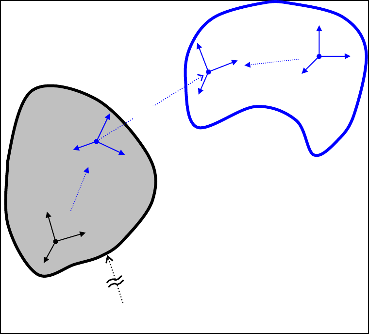
40
These are the equations that define the generalized coordinates and speeds. (The overdot
notation below indicates time derivatives that are taken in the F frame.)
B
mobilizer B
q,u
M
BO
P
PO
F
Figure 6: Coordinate frames for use
in describing the mobility of
MobilizedBody B with respect to its
inboard parent body P. Everything
blue is associated with B. The origin
point O of each frame is labeled.
MO
FO
B M
X
P F
X
( )
F M
X q
body B
Ground
parent body P

41
( ) ( ) ( )
F M F M F M
X q R q p q
(5.1)
( , ) ( ( ))
FM FM
F M F M F M
FM FM
v
V
V q u X q u
Vv
H
(5.2)
( , , )
FM
F M F M F M F M
FM
A q u u V u u
a
HH
(5.3)
()q q uN
(5.4)
n( ) 0q
(5.5)
Note that X and H cannot be chosen arbitrarily, because the time derivative of X is related to
V:
()
F M F M F M
F M F M F M
F M F M F M
v
X R p
Rv
V R V
(5.6)
This implies relationships that must hold among X, H, and N:
()
F M F M F M F M F M
F M F M
R R u R
RR
qu
qq
H
N
(5.7)
( ) ( )
F M F M F M
F M F M
v
p v u
p q p q
qu
qq
H
N
(5.8)
where
H
and
v
H
are the upper and lower 3xn partitions of hinge matrix H. Intuitively, this is
stating the requirement that the spatial velocity produced from u by the action of H is the
time derivative of the spatial position and orientation produced from q by the nonlinear
function X(q), with matrix N serving to mediate between u and
q
. Note from (5.2) that H
depends only on the transform (spatial position) represented by the set of q’s, not on the
definitions of the individual q’s.
Equation (5.5) specifies additional constraints that q must satisfy if there are not enough
equations (5.4) to uniquely specify q. That occurs when there are more q’s than u’s, typically
because q is a quaternion in which case n(q) is the quaternion normalization constraint.

42
5.1 Reverse mobilizers
Because a tree of mobilized bodies must be ordered parentchild along each branch going
away from Ground, the role of parent and child may be reversed from the desired sense for
some mobilizers. When the generalized coordinates and speeds are intended to have a
particular physical meaning, we would like to preserve that meaning even when exchanging
the roles of parent and child. For example, if you make a “knee” mobilizer with the general-
ized coordinate being knee flexion, you would like to preserve that meaning regardless of
whether the femur or tibia is the parent body.
So we will at times be given the mobilizer specification from frame M on body B to frame F
on body P, but a mobilizer specification must go from F to M. That is, we’re given
MF
X
,
MF
H
,
MF
H
, and N for a mobilizer in frame M fixed to the child body B (with time deriva-
tives taken in M), but we want
FM
X
,
FM
H
,
FM
H
, and N describing the mobilizer with
identical generalized coordinates and speeds in frame F fixed on the parent body (and with
time derivatives taken in F).
N is easy enough—since we want q and u to retain their original meanings, N must stay the
same. Almost as easy,
1
()
F M M F F M F M M F
X X R R p
. But we’re going to have to
work to get the other two matrices. First
FM
H
:
From Equation (5.2) (with the frames swapped) we have
MF
MF
MF
MF
MF
v
Vu
v
H
H
(5.9)
We want to find
FM
H
such that
FM
FM
FM
FM
FM
v
Vu
v
H
H
(5.10)
For the moment we are going to leave the expressed-in frame as M and work only with the
physical quantities. We’ll re-express at the end. We know that
F M M F
so it follows that
F M M F
HH
. But the linear velocity cannot simply be negated. We have

43
M F M F M F
Md
v p p
dt
(5.11)
F M F M F M
Fd
v p p
dt
(5.12)
Since
F M M F
pp
we can substitute into (5.12) and get
()
()
()
F M M F
M F F M M F
M F M F M F
M F M F M F
F
v
d
vp
dt
pp
vp
pu
HH
(5.13)
Since
F M F M
v
vuH
we see that
()
F M M F M F M F
vv
Mp
H H H
(5.14)
In the above analysis we left the quantities expressed in the M frame as emphasized in
equation (5.14) (although we took the derivative in F). Re-expressing in the F frame com-
pletes the computation of
FM
H
:
MF
F M F M
M F M F M F
v
Rp
H
HHH
(5.15)
We can differentiate equation (5.15) in F to get
FM
H
:
MF
F M F M F M
M F M F M F
v
MF
FM
M F M F M F M F M F
v
Rp
Rpp
H
HHH
H
HHH
(5.16)
Substituting from (5.12) and (5.15) gives this form for
FM
H
:
MF
F M F M F M F M
M F M F M F M F M F
v
Rpv
H
HHH H H
(5.17)
Algorithmically, we can avoid duplicate computations by separating the two rows of (5.15),
and rearranging to use already-computed terms:

44
F M F M M F
R
HH
(5.18)
()
()
F M F M M F F M M F M F
vv
F M M F F M M F M F F M
v
F M M F F M M F F M
v
F M M F F M F M
v
R R p
R R p R
R R p
Rp
H H H
HH
HH
HH
(5.19)
using identity (3.6) in the second-to-last step.
To create an algorithmic version of (5.17), differentiate equations (5.18) and (5.19) in F to
get
FM
H
in terms of already-computed quantities:
F M F M M F F M F M M F
F M M F F M F M
RR
R
H H H
HH
(5.20)
()
( ( )
)
(
( ) )
F M F M M F F M F M M F F M F M F M F M
v v v
F M M F F M F M F M F M
vv
F M F M F M F M
F M M F F M F M
vv
F M F M F M F M F M F M
R R p v
Rp
pv
R
p v p
H H H H H
H H H
HH
HH
HH
(5.21)
Or, collecting terms
0
()
F M F M M F F M F M
F M F M F M F M F M F M
R
p v p
H H H
HH
(5.22)
Simbody uses equations (5.18), (5.19), (5.20), and (5.22) in that order to perform these
computations.
5.2 Mobilizers in body frames
At times it is more convenient to deal with the mobilizer hinge matrix describing the allowed
motion of the body frame B with respect to the parent body’s frame P, rather than between
the two mobilizer frames. This is related to the hinge matrix H defined above by the constant
transforms
P F
X
and
M B
X
depicted in Figure 6. First, perform a rigid body shift of the
spatial velocity from M’s origin outward to B’s, using the kinematic shift operator
T
:

45
()
FB F
F B M B F M
Vp
u
HH
T
(5.23)
where
FM B F M M B
p R p
1
()
01
AB
AB
v
v
Note that although we are shifting from one point on body B to another, the effect is time
varying since we are expressing the shift vector in the parent body using the cross-mobilizer
rotation matrix
( )
F M
R q
.
Next, re-express the resulting spatial velocity (currently in F) to P:
PB
P B P F F B
VR
u
HH
(5.24)
This transformation involves only a constant rotation matrix, and the translation of the
reference frame from F to P doesn’t affect the velocity.
The time derivative taken in P is then
PP
P B P B P F F B F B
dR
dt
H H H H
(5.25)
where
( ) ( )
F
F B F B M B F M M B F M
FF
dpp
dt
H H H H
TT
(5.26)
and
0
()
00
A
A B B
AB
v
v
(5.27)
These matrices are related to the hinge matrix H* in reference 3 as follows:
46
*
GPB GP B G P P B
VR
u
H H H
(5.28)
**
GG P P B G P P B
GG
G P P B P B
dRR
dt
H H H H
HH
(5.29)
Note that
PB
H
is not shifted to Ground to form H*, but only re-expressed in Ground. That is,
it still represents motion of B with respect to P (not with respect to G), however it has been
re-expressed in the Ground frame. (Time derivatives are taken in the frame indicated by the
expressed-in frame of the differentiated quantity.)

47
6 Theory for Constraints
A Simbody Constraint C is modeled with a set of mC scalar constraint equations which
restrict the allowable values for mobilizer coordinates by enforcing algebraic relationships
among them or their time derivatives. Constraints are usually written to directly affect only a
very small number
b
n
of bodies and nm of mobilizers, typically one, two, or three, which we
call the constrained bodies and constrained mobilizers. For efficient processing, Simbody
must know the complete set
,
C C
k l
B M
of
b
C
n
constrained bodies and
m
C
n
constrained mobi-
lizers for each Constraint C. The set of constrained bodies and mobilizers is considered
topological information and is thus frozen after the Constraint is specified.
The set of mobilities which can appear in the corresponding constraint equations consists of
all the mobilities
m
C
u
associated with the constrained mobilizers, plus all mobilities
b
C
u
which
can affect the relative motions of any the constrained bodies. Note that while the number of
mobilities associated with a mobilizer is very small, the number which may affect a set of
constrained bodies can be much larger, potentially including all the mobilities on the paths
from the constrained bodies back to Ground.
To avoid unnecessarily including a large number of mobilities in the constraint calculations
for a Constraint C, Simbody searches the multibody tree from the constrained bodies in the
inboard direction (towards Ground) to find the outmost common ancestor AC, which is the
most-outboard (highest numbered) body shared by the inboard paths of all the constrained
bodies. Ground can always serve as A if no other common body can be found. We call the
path from the kth constrained body inward to AC the kth branch of the Constraint; these
branches may overlap and may also overlap with constrained mobilizers. We call the set of
all generalized speeds on the kth branch
b,
Ck
u
, with
b b,
k
C Ck
u u
; the complete set of general-
ized speeds which can affect Constraint C is then
m b
,
C C C
u u u
. These are the Constraint’s
C C
n u
participating mobilities. The
q
C
n
participating coordinates are similarly defined as
b b,
k
C Ck
q q
and
m b
,
C C C
q q q
, with
q
C C
n q
and
q
C C
n n
.
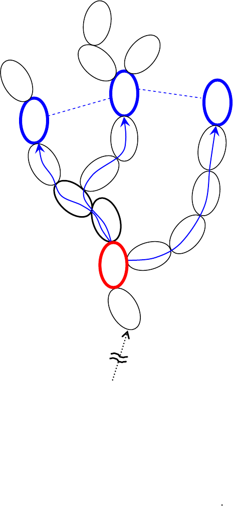
48
Figure 7 depicts these quantities for a single Constraint C with three constrained bodies. The
figure does not show the mC constraint equations that this Constraint generates; mC can’t be
determined just from the number of constrained bodies. However, it does show how the
body-affecting mobilities
b
C
u
are determined. Note that the mobilizers for the two black
highlighted bodies are shared by branches 0 and 1.
For the rest of this section we’ll drop the superscript “C” except when necessary for clarity.
Without the C, our Constraint generates m constraint equations in n mobilities.
The most fundamental constraint equation is a relationship among the accelerations (the n
participating generalized speed derivatives
u
), called an acceleration constraint. Every
0
B
A
branch 0
b,0
u
constrained
bodies
outmost
common
ancestor
Figure 7: Constraint topology. This shows
a single Constraint C with three constrained
bodies
k
B
, the corresponding branches, and
the outmost common ancestor body
A
. The
branches determine the participating
mobilities
b
u
; mobilities of the two black-
outlined bodies are shared between
branches 0 and 1. Additional mobilities
m
u
are introduced explicitly for constrained
mobilizers.
Ground
b b,0 b,1 b,2
b m
u u u u
u u u
1
B
2
B
branch 1
b,1
u
branch 2
b,2
u
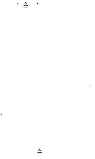
49
Simbody constraint equation ultimately restricts accelerations, and these m acceleration
constraint equations form part of the dynamical equations of motion. The ith acceleration
constraint equation has the following form:
g ( , , , ) ( , , ) 0
i i i
t q u u u b t q u g
(6.1)
Where
i
g
is a scalar function, gi=gi(q) is a row vector of length n, and bi is a scalar function.
Every defined Constraint must provide a method for efficiently evaluating its m scalar
acceleration error functions gi. For constraint equations involving only constrained mobilizers
this can be done directly in terms of the mobilities um. But in the case of participating mobili-
ties ub due to constrained bodies, the constraints are not normally known explicitly as in (6.1)
but rather in terms of some physical consequence of
b
u
, such as body accelerations. The
user-written routine is expected to calculate the error in those terms in constant time, with the
physical consequences of
b
u
having been supplied by Simbody after an O(n) computation.
Similarly, the meaning of the Lagrange multipliers λ is given by
( , ) T
i i i i
f q
- -
g
(6.2)
where fi is a column vector function giving the n generalized forces generated by the scalar
multiplier λi allocated to the ith constraint equation. Every defined Constraint must provide a
method for efficiently calculating its forces given its m multipliers λ. Again, except for
participating coordinates due to constrained mobilizers, this is normally not known explicitly
in generalized forces as in equation (6.2), but in terms of forces and torques applied to
bodies. The user-written routine is written as a constant-time function in those terms, and
then Simbody converts the result to generalized forces with a single O(n) computation.
Constraint equations may differ in the level at which they are first defined: position, velocity,
or acceleration. When a constraint equation is introduced at the position level (such con-
straints are called holonomic and are typically nonlinear), it is differentiated once to yield a
(linear) constraint on velocities, and again to yield a (linear) constraint on accelerations.
When a constraint is first introduced at the velocity level (a nonholonomic constraint, which
can be nonlinear in velocities) it is differentiated once to yield a (linear) constraint on accel-
erations. A constraint which appears only at the acceleration level (an acceleration-only
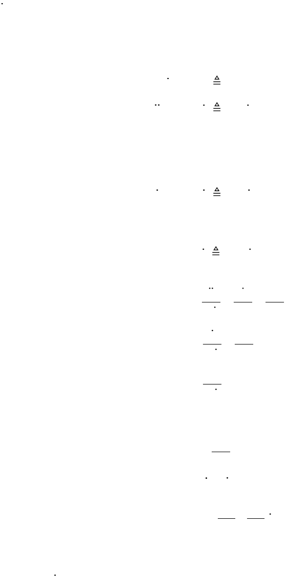
50
constraint; not common) is required by Simbody to be linear in the generalized accelerations
u
. Here are the equations defining each of the three types of constraint equation:
holonomic (position) constraints
p
(0 )j m
p ( , ) 0
jt q
(6.3)
p ( , , ) ( , ) 0
j j j
t q u u c t q p
(6.4)
p,
p ( , , , ) ( , , ) 0
j j j
t q u u u b t q u p
(6.5)
nonholonomic (velocity) constraints
v
(0 )j m
v ( , , ) 0
jt q u
(6.6)
v,
v ( , , , ) ( , , ) 0
j j j
t q u u u b t q u v
(6.7)
acceleration-only constraints
a
(0 )j m
a,
a ( , , , ) ( , , ) 0
j j j
t q u u u b t q u a
(6.8)
where the row vectors are
ppp
() jjj
C
jqu u q
pN
(6.9)
v v
( ) j j
jqu u
v
(6.10)
a
( ) j
jqu
a
(6.11)
and the remainder terms produced by differentiation are
p
( , ) j
j
c t q t
(6.12)
,( , , )
p j j j
b t q u c up
(6.13)
,( , , ) jj
vj
vv
b t q u q
tq
(6.14)
NC is an
q
C C
n n
matrix assembled from a subset of the rows and columns of the global N
such that
C C C
quN
. Note that the equations marked with blue arrows are implied by
differentiation of the modeled constraint equations; they are not independent. These add
another 2mp+mv equations to the mC modeled ones.

51
All mp rows pj stacked together form matrix PC, and all mv rows vi form matrix VC, which
together are used for initial satisfaction of position and velocity constraints, as well as for
constraint projection during numerical integration. All ma rows aj together form matrix AC,
and PC,VC,AC stacked together form the mC rows of constraint matrix
C
C C
C
P
G V
A
as dis-
cussed above. Note that each of the mC rows gi in (6.1) is actually one of the rows pj, vj, or aj.
6.1 Explicit calculation of constraint matrices
For efficient calculation of constraint forces and for performing constraint projections,
Simbody needs to be able to efficiently calculate matrix-vector products involving the
constraint matrices and their transposes. We expect to be able to calculate both Gv and GTw
in O(n+m) time, where G is mXn and v and w are conformant column vectors. (Note that a
straightforward matrix multiply would be O(nm), much more expensive.) Simbody uses the
methods that define the constraint in combination with O(n) operators to perform these
computations efficiently.
With the O(n+m) matrix-vector multiplies available, Simbody can calculate the constraint
matrices P, V, and A (collectively G) explicitly in constant time per element. By making m
calls to the provided routines, mXn matrices can be calculated in O(nm+m2)=O(nm)
*
time
which is within a constant factor of optimal if you have to form these matrices.
Regardless of whether a constraint equation is initially specified at position, velocity, or
acceleration level it will contribute a row g to the acceleration constraint matrix G above,
which will also be a row of P, V, or A. So all the terms we need can be obtained by examin-
ing the constraint equation’s error function once it has been expressed at the acceleration
level, that is, equations (6.5), (6.7), or (6.8). Taken together, these equations are just the
equations (6.1), that is,
g ( , , , ) ( , , ) 0
i i i
t q u u u b t q u g
. So the rows of the explicit matrices
we need are just
g ( , , , )
it q u u u
. An alternative is to use the constraint force functions (6.2)
*
because m≤n, mn+m2≤2mn

52
which can equivalently provide a column of
T
i
g
at O(n) cost per column. Simbody thus
calculates the constraint matrices a row at a time by mC repeated calls to the O(nC) constraint
force function (6.2), yielding an explicit GC matrix to machine precision in O(mC nC) opera-
tions, which is within a constant factor of optimal since the matrix has mC nC elements. The
mC scalars
0
1
C
C
m
b
b
b
from each Constraint form the vector b in equation (6.1), and can if
necessary be determined explicitly in O(n) time using equation (6.1) with all
u
’s set to zero.
As discussed above, it is rare that an acceleration constraint equation will be conveniently
written directly in terms of the generalized accelerations
u
(prescribed motion is an excep-
tion). Instead, it will be written in terms of physically meaningful acceleration-derived
quantities involving the constrained bodies. These may be complicated expressions, but they
are always built from the following fundamental quantities:
the accelerations of points and angular accelerations of vectors fixed on the con-
strained bodies, relative to the ancestor or to other constrained bodies in this Con-
straint, or
the cross-mobilizer accelerations directly in terms of the generalized accelerations
u
of the constrained mobilizers.
Simbody’s Constraint base class provides utilities to efficiently obtain the constrained
bodies’ accelerations relative to the outmost common ancestor A given a set of
u
’s (for fixed
q and u), relative velocities given u’s (for fixed q), and relative positions given q’s. The
user’s constraint equation error functions are written using these utilities.
53
7 State representation and realization
The State concept was presented in Section 1.2. In this section we will take a closer look at
how we represent the state of a Simbody System and how we operate on that state when
performing a Study.
7.1 Computation – realization of the State
This section provides some details about how computations are performed in the System-
State-Study architecture described in Section 1.2.
During a Study, the System is used to realize a State. By realize we mean the process of
taking a new set of values from a State and performing the computations that those new
values enable. A simple example would be to take new position coordinate values from a
State and use them to calculate new spatial locations for the bodies, and then distances
between designated points on different bodies. Realizing a State enables three kinds of
computations: responses, operators, and solvers, defined next.
7.1.1 Responses, operators, and solvers
A response is a numerical result which can be computed knowing only the values in the
State. The above calculation of distance from position coordinates is an example of a re-
sponse. An operator is a computation which requires knowledge of certain State variables,
but then can be applied repeatedly to other input data (i.e., data not from the State) to produce
numerical results. For example, once we know positions and velocities from the State, we
can realize an operator which, when applied to a set of forces, efficiently calculates the
accelerations that would be produced by those forces. Neither responses nor operators make
changes to the State. A solver, on the other hand, both reads from and writes to the State. A
given solver requires certain values from the State, and may make use of those values or
responses and operators calculated from them. It then performs a computation which updates
the State in some well-defined way. The simplest kind of solver is a method which just sets a
particular State variable to a given value. A more elaborate example is a solver which takes
current positions from the State and modifies them to find the nearest set of positions which
satisfies particular constraints.
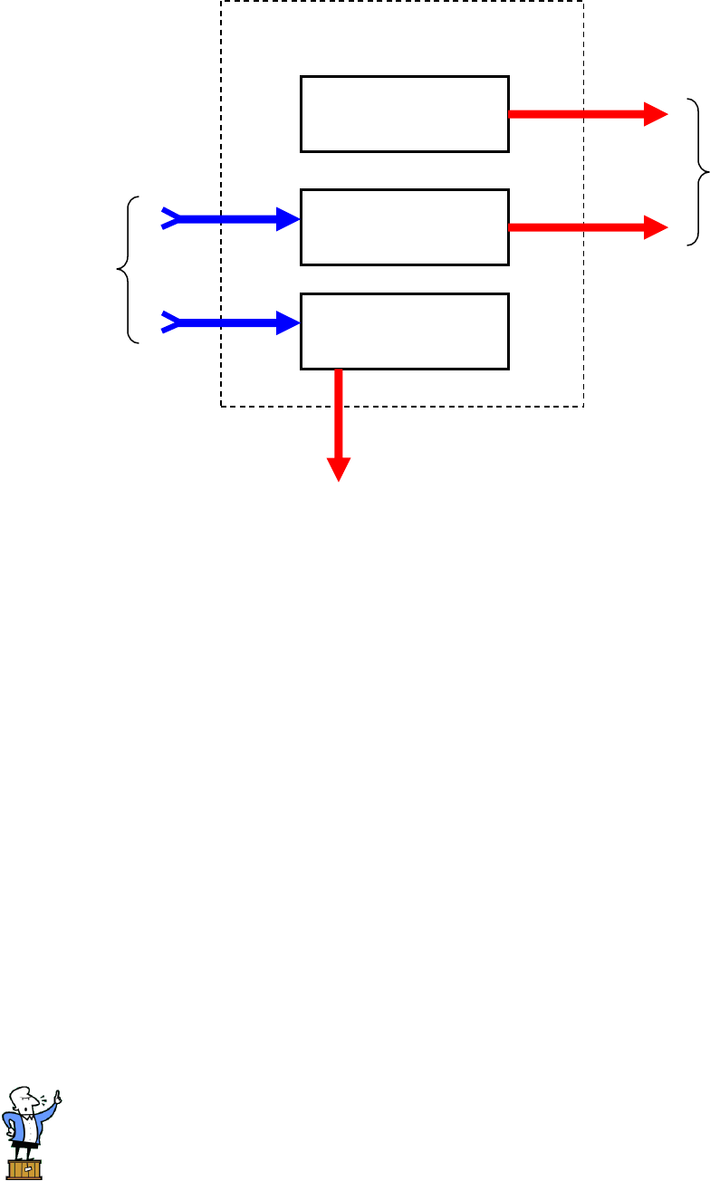
54
7.1.2 Caching of computed results
Realizing a State may require a large amount of expensive computation, and the computed
results are typically used many times in calculation of subsequent results. Consequently it is
crucial that these computations not be re-done once calculated for a particular set of State
values. Given that a System is a read-only object, and that realization results are associated
with a particular State, the obvious place to store these results is in the State object. That way
when a Study provides a State to a System, all previously-calculated results are available as
well, and one may be certain that those results were calculated using the values from the
supplied State. This eliminates the possibility of bugs in which values computed at one state
are incorrectly used as results at a different state. That is an extremely common error in
simulation programs and is very difficult to fix, primarily because it often goes completely
unnoticed. Errors of this type are hidden by the fact that sequentially-produced states tend to
differ very little, making the computed values only a “little bit” wrong.
To take a brief pontification opportunity, I want to emphasize in the strongest possi-
ble terms that “little” bugs in simulation programs do not leave them “nearly” valid the
Subsystem
Responses
Operators
Solvers
Figure 8: After realizing a State, a
subsystem provides responses,
operators, and solvers.
Results
Back to State
Inputs

55
way, say, small measurement errors affect real-world experiments. Simulation software is the
most nonlinear thing in existence—one wrong bit in a billion can completely destroy any
relevance it might have had to the real world. The resulting simulation results, unfortunately,
may still appear plausible, especially where human intuition is of limited use such as with
molecular systems. And statistical reduction methods used to calculate physical properties
from a simulation (e.g., population distributions, free energies, radii of gyration, transi-
tion times, etc.) are almost certain to turn meaningless garbage into “intriguing” results
which “should be researched further.”
Although cached results are stored in the State object, it is important to note that those results
(that is, responses, operators, and solvers) are not logically part of the system state. They are
simply intermediate calculations which have been derived from the state, and can easily be
discarded and re-created when necessary. They are needed only for efficient computation
using the System-State-Study architecture, and so can be viewed as “merely” a hint. They
exist as a kind of shadow behind the actual state variables, whose values do matter. We call
this shadowy construct the realization cache, or more often, just the cache.
56
Figure 9 combines the concepts just described. It shows a subsystem (one of the pieces
making up a System) and how its responses, operators, and solvers make use of the realiza-
tion cache. Note that responses require no input other than the State, while operators and
solvers can have additional inputs (the blue arrows in the figure). Operators and solvers then
differ by the disposition of their outputs (red arrows), with only solvers’ output able to update
the State.
To summarize briefly: A System (or subsystem) by itself is stateless once con-
structed. The values of state variables stored in a particular State object
completely determine the behavior of the System. That behavior is produced
by realizing the State. The results of realization, which are responses, operators,
and solvers, are stored in a hidden cache which is physically contained in the State object, but
is not logically part of the state in the sense that cache values are not permitted to alter the
behavior of the System, except for the speed with which it can perform computations involv-
ing that State.
Figure 9: A subsystem (part of a
System), showing its use of part of the
State to realize responses, operators
and solvers. The realization cache adds
no new information but shadows the
state variables for efficiency.
State
Subsystem
Realization Cache
State Variables
Responses
Operators
Solvers
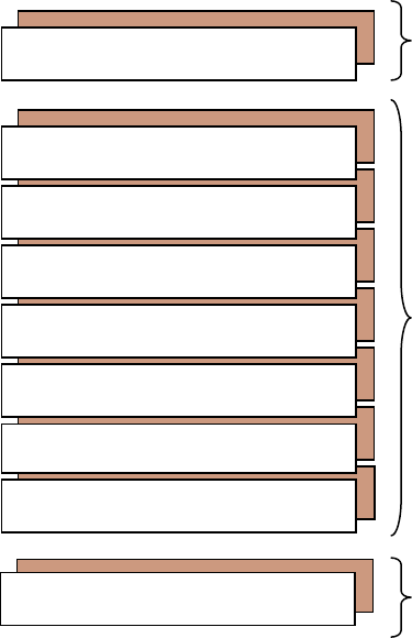
57
7.1.3 Computing in stages
The computations performed by a System in realizing a State are naturally ordered in stages,
and realization is done one stage at a time, in order. For example, one must compute the
positions of the bodies before computing forces that may depend on those positions. This
structure allows for interdependencies among the subsystems in the System, without requir-
ing any subsystem to know any internal details of other subsystems. Of specific relevance for
Simbody, user-supplied forces depend on values provided by the Simbody multibody subsys-
tem (such as positions and velocities), but Simbody dynamic calculations (e.g., accelerations)
likewise depend on the user-supplied forces. Thus complete realization of a State requires
sequences like (1) the SimbodyMatterSubsystem realizes its “Position” stage, then (2) each
force subsystem independently realizes its Position stage to calculate position-dependent
forces (repeat for Velocities), and then (3) SimbodyMatterSubsystem realizes its accelera-
tions (reactions) using computations cached by the force subsystems. This staging approach
allows a composite System computation to be performed efficiently from isolated subsys-
tems, with each subsystem mediating access to its own state variables and cache.
1. Topology
2. Model
3. Instance
4. Time
5. Position
6. Velocity
7. Dynamics
Stages
8. Acceleration
System or
subsystem
State
Figure 10: The conceptual organization
of a computation into ordered stages. A
given stage is fully realized by each
subsystem in a System before the next
stage is realized by any subsystem. For
many purposes, construction of the (read
only) System can be viewed as the initial
stage of computation.
9. Report
Study
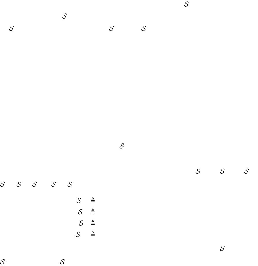
58
7.2 State variables
The complete state of a Simbody System is represented by a set of broadly-defined state
variables. Physically, is stored in a SimTK State object, where it is partitioned into time
t
, and two disjoint subsets
,xy
, so that
{}t x y
. During time stepping, t is
the independent variable; x and y both contain dependent state variables but differ in the
types of variables they can contain. Partition y contains conventional real-valued, “smooth”
state variables q, u, and z representing system kinematic and dynamic quantities, while
partition x contains state variables of arbitrary value types including boolean, integer, and
structured types of any complexity.
7.2.1 State partitioning by stage
State variables may be usefully partitioned by the computation stages they affect; we call the
lowest affected computation stage the state variable’s stage. As shown in Figure 10 stages
that can be affected by state variables in are: model, instance, time, position, velocity,
force, acceleration, and report. (Topology stage is only affected by the contents of the
System, not its State.) We denote state partitions with these effects
model
,
instance
,
time
,
pos
,
vel
,
force
,
acc
,
report
with
time time
pos pos pos pos
vel vel vel vel
force force force force
{}xt
x y x q
x y x u
x y x z
(7.1)
For the other stages, only variables in the x partition can be used, so we have
model model
x
,
instance instance
x
, and
report report
x
,
Partition y consists only of position-, velocity-, and force-stage variables as shown above. For
convenience, we provide more conventional names for those partitions:
pos vel force
,,
with
q y u y z y
y q u z
(7.2)
q and u are the sets of generalized coordinates and speeds associated with the System’s
mobilized bodies. z is a set of generalized dynamic variables typically belonging to force and

59
control elements in the System. z’s can directly affect forces, but not positions or velocities
of bodies.
7.3 State resources
The SimTK::State object manages a collection of resources including state variables and
cache entries needed for realization. Resources are allocated at the request of the various
Subsystems, and the State object keeps them organized by Subsystem. In addition, certain
kinds of state resources are aggregated into global resources pools which represent the
System as a whole. Global pools support efficient numerical manipulation of the System’s
state as a whole in circumstances where the Subsystem composition is irrelevant.
Every State resource has an allocation stage, meaning that that resource is allocated during
realization of that stage, and unallocated if that stage is invalidated later. That means that the
set of resources in a System’s State can vary based on the current stage, and the settings of
state variables that were allocated earlier.
Resources that are always present for a given System are allocated at Topology stage. That
includes the set of state variables which can affect modeling options. Then realizing Model
stage causes more resources to be allocated, reflecting the modeling choices made. Some of
those resources may be state variables representing parameters of the chosen model. Once
those are set, realizing Instance stage allocates the final set of resources needed for further
computation. No state resources may be allocated later than Instance stage; after that only the
values of existing state resources may be changed.
Here are the resources supported by a State object.
Resource
Allocation
Description
Resource notes
Built-in
resources
Topology
Every State has some built-in resources,
allocated at Topology stage. Note that the
System stage can never be higher than
the lowest Subsystem stage.
,prev
tt
System current stage
Per-Subsystem current stages
Low-water mark
Dynamic
variable group
(q,u,z)
Topology
Model
size: Instance
A contiguous array of real-valued
“conventional” state variables. These are
pooled into a global array y, which is
itself partitioned into global q, u, and z
arrays. An additional state variable holds
the size of the group and can be set at
Instance stage.
{ , , },y q u z q
{ , , }
prev prev prev prev
y q u z
sizes
Subsystem-private group Id
Pool slots assignment

60
Structured
variable x
Topology
Model
A private variable belonging to a single
subsystem and able to contain a designat-
ed value type of any kind, from boolean
flag to arbitrary object. Has “invalidates”
stage; must be allocated before that.
Previous value
prev
x
Subsystem-private Id only
Constraint
group (qerr,
uerr, udoterr,
mults)
Topology
Model
Instance
m: Instance
Allocates cache entries which are
contiguous arrays of m scalars for
holding the current constraint errors and
multiplier values. An additional state
variable is allocated to hold the size m of
the group which can be set at Instance
stage.
{ , }
err err err
y q u
err
u
, λ
m
Subsystem-private group Id
Pool slots assignment
Event trigger
group
Topology
Model
Instance
size: Instance
Allocates contiguous array of scalar
cache entries for event trigger function
values, in global pool. The number of
entries can be changed up to Instance
stage.
,prev
ee
# of triggers
Subsystem-private group Id
Pool slots assignment
Event group
Topology
Model
Instance
size: Instance
Allocates a group of event ids for a
subsystem, and a corresponding global
pool of System-unique Ids.
Subsystem-private group Id
# events
Cache entry
Topology
Model
Instance
Private variable belonging to a single
subsystem. Can hold any designated
object type. Has depends-on stage and “is
valid” flag. Must be allocated before
depends-on stage.
Subsystem-private Id only
The State maintains mapping information for the global resources so that one can determine
which particular entity is the owner of an entry in a global pool, for any local entity where in
the global pool it may be found.
7.4 Allocation of state resources
State variables are allocated by the various elements of a System. Here are the System
elements and the kinds of state variables they allocate:
7.4.1 Mobilized bodies
There are nB mobilized bodies
[]j
(including Ground) .
Each
[]j
represents a unique body and its mobilizer providing
0 [ ] 6nj
unconstrained
mobilities (degrees of freedom). The ground body
G [0]
, and n[0]=0. u[j] and
[]uj
are
sets of n[j] scalar generalized speeds and corresponding generalized accelerations defined by
[ ]sj’
mobilizer. q[j] and
[]qj
are the mobilizer’s nq[j] generalized coordinates and their
time derivatives, with
[ ] [ ]
q
n j n j
. q and u are related via an
[ ] [ ]
q
n j n j
kinematic coupling

61
matrix N[j] such that
[ ] [ ] [ ]q j j u jN
. There may be a local quaternion normalization con-
straint n[j] defined, where n[j] depends only on q[j].
For the System as a whole, we define ordered sets
[]
j
u u j
and
[]
j
q q j
, and sets of
their elementwise time derivative variables
u
and
q
. Sizes are
[]
j
n u n j
and
[]
qq
j
n q n j
. We also define block diagonal
q
nn
matrix N=diag(N[j]) so that
quN
.
7.4.2 Dynamic variables z
There are nD scalar dynamic variable sets
[]z i z
.
Any element in the System may allocate one or more sets of nz[i] scalar dynamic variables
z[i] and their corresponding time derivative variables
[]zi
. We collect these into nz-element
aggregate ordered sets z and
z
.
7.4.3 Structured variables d
There are nd structured-value variables
[]d i d
.
These variables can be allocated by any element of the System. Each one holds an object of a
particular type, but that type is arbitrary and is different for each variable. These can be as
simple as boolean flags or integers to arbitrarily complex objects.
7.4.4 Constraints
There are nC constraints
[]i
which can restrict the mobility of the bodies.
Each constraint defines a set of m[i] constraint equations g[i]. These are classified as position
(holonomic), velocity (nonholonomic), and acceleration constraint equations and a single
constraint can generate equations at different levels. g[i] is then partitioned into correspond-
ing subsets
[ ], [ ], [ ] [ ]p i v i a i g i
of cardinality
[ ], [ ], [ ]
p v a
m i m i m i
such that
[ ] [ ] [ ] [ ]
p v a
m i m i m i m i
. We also define aggregate sets
,,
and
with
cardinalities
,,
p v a
m m m
and m, resp.;
p v a
m m m m
.
A position constraint equation
k
p
has the general form
: ( ; ) 0
k k k
q p t q
where
k
qq
,
that is, it defines an implicit algebraic relationship among a subset of the elements of q,
possibly with an explicit dependence on time. If the set qk contains just one element (
1
k
q
),

62
then pk defines qk explicitly as
()
kk
q q t
; this is called a “prescribed position”. Each position
constraint
k
p
requires an entry in the global qerr pool in the State, a corresponding entry in
the uerr pool for the time derivative equation
0
k
p
, an entry in udoterr for
0
k
p
, and a λ
slot in the multiplier pool.
Similarly, a velocity constraint equation
k
v
is
: ( , ; ) 0
k k k k
u v t q u
where
k
uu
, an
implicit relationship among a subset of generalized speeds with explicit dependence on t and
q. Note that there is not necessarily any correspondence between the sets
k
q
and
k
u
in a
velocity constraint;
k
u
can depend on time and any set of q’s. If
1
k
u
then vk defines uk
explicitly as
( , )
k k k
u u t q
, this is called a “prescribed velocity”. Each velocity constraint
k
v
requires an entry in the global uerr pool in the State, an entry in udoterr for
0
k
v
, and a λ
slot in the multiplier pool.
Finally, an acceleration constraint equation
k
a
is
: ( , , ; ) 0
k k k k k
u a t q u u
where
k
uu
,
an implicit relationship among a subset of generalized accelerations with explicit dependence
on t, q, and u. Note that there is not necessarily any correspondence between the sets
k
u
and
k
u
in a velocity constraint;
k
u
can depend on time and any sets of q’s and u’s. If
1
k
u
then
ak defines
k
u
explicitly as
( , , )
k k k k
u u t q u
, this is called a “prescribed acceleration”. Each
acceleration constraint
k
a
requires an entry in the global udoterr pool in the State, and a λ
slot in the multiplier pool.

63
8 Equations of motion
In this chapter we’ll present the equations of motion represented by a Simbody System. By
equations of motion we mean the equations that determine the instantaneous rates of change
for the state variables. Integrating those rates of change into a trajectory through time is a
different topic and will be discussed in Chapter 10.
A few conventions: We use n and subscripted n’s to count quantities related to coordinates
(mobilities or degrees of freedom) and m and subscripted m’s to count constraint equations.
We use overdot to represent differentiation with respect to time, in the Ground frame unless
otherwise specified. We use a right superscript to denote a quantity which applies only to a
particular body or its mobilizer.
As detailed in section 7.4.1, the equations of motion will be written in terms of the set of n
generalized speeds
[]
b
u u b
where b ranges over all the mobilized bodies, and the nq
generalized coordinates
[]
b
q q b
, where u[b] and q[b] are the disjoint sets of n[b] speeds
and nq[b] coordinates for each body
[]b
, which arise from the presence of its mobilizer.
*
Typically there will also be a set of differential equations associated with force models which
must be integrated along with the matter model’s generalized coordinates and speeds; we’ll
call these nz auxiliary state variables z. In general a system will also include discrete-time
equations and associated discrete states (we call those “slow” variables) but we’ll only
consider the continuous system here.
The total number n of mobilities in a multibody system is just the sum of the bodies’ individ-
ual mobilities, that is
[]
b
n n b
. Note that n is the number of unconstrained system
mobilities; the net number of degrees of freedom after constraints will be
net net
n n m
where
net
m m
is the number of independent acceleration-level constraint equations generat-
ed by the system’s constraints.
*
We use n, representing the mobilizer’s of degrees of freedom, rather than nu to count generalized speeds, since
there is necessarily the same number of generalized speeds as degrees of freedom.
64
Generalized speeds u are fundamentally related to the physics of the system, while general-
ized coordinates q are chosen primarily to facilitate good numerical behavior during compu-
tation. Thus the number of generalized speeds introduced by a mobilizer is always the same
as the number of mobilities so that the generalized speeds are always mutually independent.
The number of generalized coordinates
[ ] [ ]
q
n b n b
so the coordinates q[b] may not be
independent. In Simbody, that occurs only when a mobilizer uses a quaternion to represent
unrestricted orientation. For convenience we introduce the symbol
quat[]nb
defined as fol-
lows:
quat
if mobilizer [ ] uses a quaternion
otherwise
1,
[] 0,
b
nb
(8.1)
Then the total number of quaternions in the system is
quat quat[]
b
n n b
.
It should be emphasized that our presentation of the equations of motion below is a formal
description, rather than a computational algorithm. It would be extremely inefficient to set up
and solve the equations in the form they are presented here (although many lesser codes do
that). The techniques of Order(n) multibody dynamics provide the solution of these equations
without ever requiring their explicit formation.
8.1 Unconstrained dynamic systems
In a system with no constraints and where all state variables q, u, and z are defined dynami-
cally by differential equations, the equations of motion are
()q q uN
(8.2)
( ) 0qn
(8.3)
app bias
( ) ( , , , ) ( , )q u t q u z q uM f f
(8.4)
( , , , , )z z t q u z u
(8.5)
Then a time stepper study seeks to find trajectories
( ), ( ), ( )q t u t z t
where

65
0
0
( ) ( ) ( )
t
t
q t q t q d
(8.6)
0
0
( ) ( ) ( )
t
t
u t u t u d
(8.7)
0
0
( ) ( ) ( )
t
t
z t z t z d
(8.8)
Simbody forms equations (8.2)–(8.5) analytically while equations (8.6)–(8.8) must be solved
numerically. Time stepping is discussed in detail in Chapter 10.
Here Mnn is a symmetric, positive definite mass matrix in mobility space (u-space) which
captures all the inertial properties of the system in its current configuration, and fapp (nx1) is
the set of all applied force and torques (including gravity) mapped into an equivalent set of n
generalized forces acting along the mobilities. fbias (nx1) is equivalent to the forces represent-
ing velocity-induced coriolis acceleration and gyroscopic terms. (fbias is quadratic in u, and is
zero if u=0.) We partition the applied forces fapp as follows:
app mob body
Jf f F
T
(8.9)
Here fmob and Fbody are the user-supplied system of forces and torques, while the kinematic
Jacobian J=J(q) is managed internally by Simbody. Fbody is an nBx1 “stacked” vector of
spatial forces consisting of one element per body (that is, the per-body net result of all the
forces and moments applied to each body), where each element is a 6-element spatial vector
combining body forces and moments as described in section 3.3.1. Fbody collects user-applied
forces and moments that act on bodies (such as Cartesian forces on atoms). If gravity has
been specified, then Fbody also includes the spatial forces resulting from the gravitational
model. fmob is an nx1 vector of user-supplied scalar forces applied directly to the mobilities,
such as would be used for bonded forces in a molecular model. JT• is the Cartesian-to-
internal conversion operator, conceptually an nxnB matrix of spatial vectors that maps spatial
forces to their equivalent mobility forces (some authors call J the matrix of “partial veloci-
ties”). In practice the JT• operator is an O(n) algorithm, and J is never formed explicitly in
Simbody (unless you ask for it).
q
nn
N
is a block diagonal, invertible mapping between generalized speeds and generalized
coordinate derivatives. In practice this is mostly used to convert angular velocities to scaled
quaternion derivatives or to Euler angle derivatives. The rectangular system of equations

66
represented by (8.2) has rank only n (≤nq), leaving quaternion lengths undetermined, so we
need nquat additional normalization conditions represented by (8.3) to ensure a unique solu-
tion for trajectory q(t). Note that although equation (8.3) is formally a set of constraints, we
consider this an unconstrained system since these constraints do not affect the physical
solution.
Equation (8.4) is just a version of Newton’s second law F=ma, relating forces to accelera-
tions. The z’s are nz additional state variables whose values can affect the forces, which may
themselves be modeled as differential equations. z’s cannot directly affect positions and
velocities, although of course they do affect accelerations which will ultimately affect
velocities and then positions. Note that z’s time derivatives
z
can depend on
u
but not vice
versa.
Formally, we can solve equation (8.4) for the accelerations
u
with
app bias
()u
1
M f f
(8.10)
By formally we mean, “don’t actually do it that way!” There is always special structure to M
that can be exploited such that the accelerations can be calculated directly in O(n) time, while
a literal matrix inversion would take O(n3) time and be prohibitive for large systems. Even
forming M would take O(n2) time since it has (roughly) n2/2 unique elements, so Simbody
neither forms nor factors M while solving equation (8.10).
As an extreme example, consider the special case of a molecular system modeled with na
point mass atoms and Cartesian coordinates, so that n=3na. M is then a diagonal matrix of
dimension 3na3na with the atomic masses (each repeated three times) arrayed along the
diagonal. The q’s are the Cartesian x,y,z coordinates, and the u’s are the Cartesian velocities
so nq=n (=nu), N is an identity matrix, and
q u
. fbias is always zero for this system. fapp is
simply the Cartesian forces acting on each coordinate of each atom, typically resulting from
taking the gradient of the potential energy function. This represents a set of 3na uncoupled
scalar equations for the Cartesian accelerations of each atom, which can clearly be solved in
O(n)!
In a more general multibody system M will be dense as a result of coupling produced by the
internal coordinates. Use of quaternions for orientation results in there being more q’s than

67
u’s and N is no longer identity and in fact not even square. However, equation (8.10) pro-
vides the solution for the accelerations in this case just as well, and the special structure of
multibody systems permits a solution in O(n) time regardless of the amount of coupling in
M.
8.2 Constrained systems
Constraints introduce unknown forces and moments into the system. Constraints are intro-
duced, for example, if there are topological loops created by the set of bodies and joints. The
constraint forces involve additional unknowns (along with the non-prescribed accelerations).
We call these unknowns Lagrange multipliers and represent them as a vector λ of length m.
These are mapped to mobility forces with a coupling matrix G and thus modify acceleration
equation (8.4) like this:
T
app bias
u
-
M G f f
(8.11)
uG b
(8.12)
where Gmn=G(q) and bm1=b(t,q,u), m is the number of constraint equations and n=nu is the
number of generalized speeds. Equations (8.11) and (8.12) are a system of n+m equations in
n+m unknowns (
and u
-
) so can be solved for the accelerations that satisfy the constraint
equations. The solution of this system makes use of the unconstrained result from equation
(8.10). Note that because we can directly solve for
u
and eliminate λ, this is still just an
ordinary differential equation, with
( , , , )u u t q u z
.
*
8.3 Unconstrained systems with prescribed, fast, and slow varia-
bles
A system may have motion where some or all of the generalized accelerations
u
are known
as functions of time and state, but the corresponding generalized forces are unknown. In this
*
Knocking equations (8.11) and (8.12) around a little, one can verify that
C
uuu 0
, where
1
0 app bias
()u
M f f
,
1 T
C
u
-
M G
, and
1
0
1
( ) ( )u
-
GM G G b
T
. In general the constraint matrix
1
GM GT
can
be singular, so there may be no solution, or an unlimited number of solutions, in which case Simbody will
provide a least squares solution for λ.

68
case we’ll partition the generalized accelerations
u
as
,
pf
u u u
where
p
u
are the
p
n
prescribed accelerations and
f
u
are the
f
n
free accelerations driven by forces. (For notation-
al convenience we’ll treat these as though all prescribed variables follow any dynamic ones,
although that ordering is not required in practice.) We then use
( 1)
p
n
to represent the
unknown generalized forces associated with prescribed generalized accelerations
p
u
. Any
accelerations that are associated with fast or slow variables are prescribed to be zero.
Equation (8.4) is then replaced with equation (8.13) where there are additional unknowns for
the generalized forces that implement the prescribed motions:
app bias
0
( ) ( , , , ) ( , )
ff
p
u
q t q u z q u
u
M f f
(8.13)
[ ]( , , ), upd[ ]
[] 0, upd[ ] or
p pf pf
p
u i t q u i pres
ui i fast slow
(8.14)
[ ] [ ]( , , , , , )z i z i t q u z u
(8.15)
For a subset of the prescribed accelerations
p
u
, we may also know the corresponding
generalized speeds
p
u
analytically as a function of time and position, otherwise the general-
ized speeds will be free variables
f
u
produced by numerical integration of
p
u
. Similarly, for
a subset of the prescribed speeds we will also know prescribed coordinates
p
q
as a function
of time only; otherwise the coordinates will be part of the free position variables
f
q
.
The trajectory equations (8.6) and (8.7) still hold for the free and prescribed dynamic varia-
bles, but only the free variables
,,
ff
q u z
need to be solved via numerical integration:

69
0
0
()
( ) ( )
()
() ()
() () relax( )
()
t
ff
ft
pp
fast fast
k
slow slow
q t q d
qt
qt qt
qt qt q
qt q
(8.16)
0
0
()
( ) ( )
()
() ( , )
() () relax( ; )
()
t
ff
ft
pp pf
fast fast fast
k
slow slow
u t u d
ut
ut u t q
ut ut qu
ut u
(8.17)
0
0
( ) ( ) ( )
t
t
z t z t z d
(8.18)
Note again that the partitioning of q, u, and
u
into free and prescribed variables can differ
because a higher-level coordinate (position or velocity) may need to be produced by integra-
tion even if a lower one (velocity or acceleration) is prescribed.
To solve for the dynamic unknowns
f
u
and
, we view the mass matrix and right hand side
as being composed of partitions corresponding to the free and prescribed variables like this:
bias,
bias,
0
ff fp f f f
f
fp pp p p p
u
u
M M f f
M M f f
T
(8.19)
Multiplying out the blocks and moving the known quantities to the right hand side gives
( , , )
pp
u u t q u
(8.20)
bias,ff f f f fp p
uu M f f M
(8.21)
bias,p p fp f pp p
uu
f f M M
T
(8.22)
These equations can be solved recursively in O(n) time by the method described in reference
5
.
8.4 Constrained systems with prescribed motion
Prescribed motion is similar to a constraint, and in fact one of Simbody’s built-in Constraint
types implements prescribed motion that way. There are two differences between a con-
straint-based prescribed motion and the direct form described here:

70
1. Direct prescribed motion takes priority over any constraints. That is, first prescribed
motion is satisfied, and then constraints are satisfied by modifying only the unpre-
scribed variables.
2. Direct prescribed motion can be implemented much more efficiently. In fact, adding
prescribed motion this way speeds up computation rather than slowing it down, be-
cause inverse dynamics is faster than forward dynamics.
With prescribed motion some of the generalized accelerations are known explicitly as
functions of time, q, and u. As was done in section 8.3, we’ll partition the
u
’s and general-
ized forces into two groups, subscripting those associated with prescribed motion with a p,
and the free (force-driven) ones with an f:
,
fp
u u u
,
,
fp
f f f
with
f
u
,
-
and
being
the unknown dynamic quantities. Substituting into equations (8.11) and (8.12) gives
bias
0
ff
p
u
u
-
M G f f
T
(8.23)
f
p
u
u
Gb
(8.24)
Now we’ll partition M and G into blocks corresponding to the free and prescribed variables
as follows:
,
ff fp
fp
fp pp
MM
M G G G
MM
T
(8.25)
Partitioning the right hand sides analogously, the equations of motion are now
( , , )
pp
u u t q u
(8.26)
bias,
bias,
0
ff fp f f f
ff
fp pp p p p
p
u
u
-
M M f f
G
M M f f
G
T
TT
(8.27)
f
fp
p
u
u
G G b
(8.28)
Multiplying the blocks out and moving the known terms to the right hand side gives
u

71
( , , )
pp
u u t q u
(8.29)
ˆ
ff f f f
u
-
M G f
T
(8.30)
ˆ
ff
uGb
(8.31)
ˆpp
-
fG
T
(8.32)
where
bias,
ˆf f f fp p
u f f f M
(8.33)
ˆpp
ub b G
(8.34)
bias,
ˆp p p fp f pp p
uu f f f M M
T
(8.35)
Equations (8.30) and (8.31) are solved for
f
u
and
-
in the same manner as equations (8.11)
and (8.12), using the known value of
p
u
to evaluate the right hand sides in equations (8.33)
and (8.34). Then the resulting values for
f
u
and
-
are substituted into equations (8.35) and
(8.32), giving the final unknown
.
1
,0
0,0
ˆ
( , ) ˆ()
ff f
f
p
pf
udyn u u
Mf
ff
(8.36)
,0
1
,0 ˆ
() f
f ff f f f
p
u
aerr u
u
-
G M G G b
T
(8.37)
1ˆ
()
( , ) ˆ()
ff f f
f
p
p f p
udyn u u
-
-
-
M f G
fG fG
T
T
T
(8.38)
As before the only matrix we must form and factor explicitly is the mxm possibly-singular
matrix
1
f ff f
G M GT
, which takes worst case
()
f
O m n
time to form and
3
()Om
time to factor,
with the worst case occurring when all the constraints are coupled. All the other matrix-
vector multiplies can be performed with recursive O(n) and O(m) operators and the pre-
scribed constraints do not contribute to this matrix.

72
The operators we have available for performing the above calculations are as follows.
Prescribed motion provides direct calculation of
( , , )
p
u t q u
and applied forces, converted to
equivalent generalized forces
( , , , ) r
p
t q u z
f
ff
are available also.
From the multibody system we have these two O(n) operators:
1
bias,f
bias,
()
( , ) ff r fp p
f
p
p p fp f pp p
u
u
dyn u uu
M f f M
ff f M M
T
(8.39)
10
() 000
ff
ff
pp
u
minv
f
M
ff
(8.40)
From the system of constraints we also have two O(n) operators:
() f
fp
p
u
aerr u u
G G b
(8.41)
cons,
cons,
() ff
pp
frc
--
fG
fG
T
T
(8.42)
These are used to calculate all the above terms efficiently, especially the
mm
matrix
1
f f ff f
W G M GT
which we calculate by noting
1
11
0
where 0 0 0
f f ff f f p
ff f ff fp f
nm
pm pf pp p
W G M G G G X
M G M G
XG
T
TT
T
(8.43)
Our goal is to calculate columns of X one column at a time and then use the aerr() operator
to calculate a column of Wf.
First make one call to the dyn() operator (8.39) to calculate
,0f
u
in equation (8.36). Then
make one call to the aerr() operator (8.41) with a zero argument to calculate the bias term b:
0
0
0
f
p
aerr aerr
b
(8.44)
Then use a call to equation (8.42) to form columns of
GT
explicitly, one at a time:

73
()
ii
ifrc
--
GG
TT
(8.45)
where
i
-
is a unit vector of length m with the ith element 1 and the rest 0.
We then call the minv() operator in equation (8.40), followed by a call to aerr() to calculate a
column
i
X
:
1
()
0
ff i
ii
p
minv
MG
XG
T
T
(8.46)
0
and then ( ) ( )
f f i i
i aerr aerr W G X X
(8.47)
to build up
1
f f ff f
W G M GT
in
()O m n
operations as needed to solve equation (8.37) for a
least squares value for
-
. That is used to calculate constraint forces
-
GT
using the frc()
operator again. These are subtracted from the applied forces for a final call to the dyn()
operator to solve equation (8.38) for
f
u
and
.
8.5 Constrained systems as specified to Simbody
Equations (8.12) and (8.31) are written in terms of linear constraints on the accelerations
u
.
However, in most cases general constraints are known only at the configuration level, that is,
as nonlinear algebraic relationships which must hold among the q’s or among quantities fully
determined by the q’s. A constraint like “these two atoms must be a certain distance apart at
all times” would be an example. In other cases the constraints may be expressed at the
velocity level as restrictions on u. In these cases we time-differentiate the constraints twice or
once, resp., until we have corresponding acceleration constraints, and then use them in
equation (8.12) or (8.31), along with any constraints which may have been defined directly at
the acceleration level. Similarly in the case of prescribed motions given at the position or
velocity level, we differentiate twice or once and then use the result as equation (8.29).
Following this procedure yields correct accelerations, but with approximate numerical
integration of those accelerations the original position or velocity constraints will not remain
satisfied over time. In practice, any constraints that are not actively enforced will gradually
drift apart during a dynamic simulation. To address this, we must keep the original algebraic
constraints in the problem and solve them along with the ODE (8.11), (8.12). That results in
a system of mixed differential and algebraic equations, known as a DAE. Equations (8.48)-

74
(8.54) shows the complete set of equations, including the set of auxiliary, unconstrained
differential equations in z which may be required in the computation of forces.
()q q uN
(8.48)
( ) 0qn
(8.49)
T
bias
( ) ( , , , ) ( , )q u t q u z q u
-
M G f f
(8.50)
( , , ; ) 0t q u u a
(8.51)
( , ; ) 0t q u v
(8.52)
( ; ) 0tqp
(8.53)
(8.54)
Constraint coupling matrix Gmxn is obtained from equations (8.51)-(8.53) as discussed below.
Note also that the constraint equations (8.51)-(8.53) combine both general constraints and
prescribed motion constraints, each subject to different restrictions on the allowable forms
for the constraint functions. We are showing only dynamic variables here; there are also
relaxation conditions for fast variables and discrete conditions for slow variables.
Equations (8.48)-(8.54) show the system as it is defined to Simbody, including all the con-
straints that must be obeyed during a dynamic simulation, starting with initial conditions t0,
q(t0), u(t0), z(t0) such that constraint equations (8.49), (8.52), and (8.53) are satisfied.
The function
a1m
a
in equation (8.51) specifies ma acceleration (index 1) constraints, which
are required to be linear in the accelerations , with maxn coefficient matrix A. These have
application, for example, in some models of Coulomb friction
6
and in producing simulations
which must track measured accelerations or reaction forces. It is common to prescribe an
acceleration to zero to temporarily lock a joint.
The function
v1m
v
in equation (8.52) specifies mv nonholonomic (velocity, index 2) con-
straints (usually, but not necessarily, linear or quadratic in u). These include, for example,
“non slip” constraints like gears and rolling contact, and constraints involving kinetic energy.
The mv time derivatives
v
of the nonholonomic constraints v must also be obeyed since, like
a, they restrict the allowable values of and in general they will be coupled to a. Prescribed
velocity is often used to force a body to rotate at a constant rate.
( , , , )z z t q u z
u
u

75
The function
p1m
p
in equation (8.53) specifies mp holonomic (position, index 3) constraints,
which are arbitrarily nonlinear in t and q. The mp time derivatives
p
, and mp second time
derivatives
p
must also be obeyed since they impose restrictions on u and , respectively,
and in general will be coupled to v and a.
Then a,
v
, and
p
together constitute the acceleration-level constraints, so we have
m=ma+mv+mp as the total number of constraints at the acceleration level.
The system of equations (8.48)-(8.54) contains nq+nu+nz+m equations in the nq+nu+nz+m
unknowns q,u,z and λ, and should thus yield a unique solution for the resulting trajectories
q(t), u(t), z(t) and λ(t), given consistent t0, q(t0), u(t0), and z(t0) to start with. Unfortunately,
obtaining that solution is easier said than done! Numerical analysts describe a system like
this as a Differential Algebraic Equation (DAE) system of index 3, for which few entirely
satisfactory solution methods exist. For a survey of methods, see reference
7
. For Simbody
we advocate and actively support the method known as coordinate projection,
8
which is very
accurate and reliable in practice. It is also possible to use the popular but less robust tech-
nique called Baumgarte stabilization
9
. In the next section we’ll discuss how we go about
solving equations (8.48)-(8.54).
8.6 Unilateral constraints
Normally a constraint generates whatever constraint forces are necessary in order to
satisfy the acceleration-level expression of that constraint. Some constraints are
limited, however, in the forces they can generate. Most commonly this occurs
when constraints are used to represent contact between bodies. In those cases, the constraint
can produce “pushing” forces but not “pulling” forces. Other common examples are joint
stops, ratchets, and ropes. These constraints are capable only of producing forces λ of one
sign, and their characteristic constraint equations are inequalities rather than the equalities
shown in equations (8.51)–(8.53). By convention we’ll require that all the constraint errors
and λ are nonnegative; if they are actually nonpositive we can negate them so that we only
need to consider nonnegativity here. Now when solving for the constraint forces λ we must
first determine which of the unilateral constraints are active. These extra unknowns (that is,
whether each constraint is active) are resolved by a complementarity condition that must hold
u

76
for every acceleration-level unilateral constraint equation: if the force is nonzero then the
constraint error must be zero (constraint is active), or if the constraint error is nonzero then
the force must be zero (constraint is inactive). Thus the product
0
ii
g
-
for every unilateral
constraint equation i, where
i
g
is the acceleration-level constraint error (i.e., it is
i
a
,
i
v
, or
i
p
depending on the kind of constraint). So we have the conditions
0, 0, 0
i i i i
g g i
--
(8.55)
Combined with the always-active acceleration-level equality constraint equations, (8.55) is in
the form of a mixed complementarity problem (MCP). In cases where
i
g
and
i
-
are linear
functions, this is a (mixed) linear complementarity problem (LCP) for which very efficient
solution methods exist. In practice, all our inequality constraints will be linear except for
friction, which can be quadratic.
An enabled, unilateral holonomic constraint will be in one of these seven states:
State
Conditions
Action
violated
p tol
Illegal; must correct.
separated
p tol
Ignore constraint.
separating
,p tol p vtol
inactive
, , 0 and 0p tol p vtol p
-
impacting
,p tol p vtol
Or, impact declared by time stepper.
Perform impulsive MCP; new
p vtol
separating or
candidate.
candidate
, , , p tol p vtol p unknown
-
Perform MCP to determine
,p
-
active
, , 0 and 0p tol p vtol p
-
Obey constraint.
Holonomic unilateral constraints can generate impulses, that is, discontinuous changes to the
velocity state variables due to impacts. The response to an impact requires user specification
of the amount of dissipation that should occur; this results in a coefficient of restitution
01e
that is used to impulsively change the velocities. If the resulting rebound velocity is
small enough, the constraint becomes a candidate to become active; otherwise the surfaces
separate after impact.

77
An enabled, unilateral nonholonomic constraint will be in one of these five states:
State
Conditions
Action
violated
v vtol
Illegal; must correct.
separated
v vtol
Ignore constraint.
inactive
, 0 and 0v vtol v
-
candidate
, , v vtol v unknown
-
Perform MCP to determine
,v
-
active
, 0 and 0v vtol v
-
Obey constraint.
No state variable discontinuity occurs when a unilateral nonholonomic constraint becomes
active, although the acceleration will have a jump.
An enabled, unilateral acceleration-only constraint will be in one of these three states:
State
Conditions
Action
candidate
, a unknown
-
Perform MCP to determine
,a
-
inactive
0 and 0a
-
Ignore constraint.
active
0 and 0a
-
Obey constraint.
Note that a unilateral acceleration-only constraint is always a candidate and can never be
violated.
8.6.1 Solving for impacts
When we have determined that an impact has occurred, we need to make a discontinuous
change to the system’s generalized speeds to avoid violating constraints. These speed chang-
es result from applying an impulse to the system. An impulse is the integral of the forces
applied during the collision, which is considered to be infinitesimally fast for rigid contact so
that the system configuration (value of q) does not change during the impact. Further, during
an impact we assume that all applied forces are insignificant except contact forces, so only
those contribute to the impulse integral. Contact forces result either from the enforcement of
constraints (including unilateral and bilateral constraints and mobilizers), or from the applica-
tion of sliding friction forces.
Impact events have a coefficient of restitution e that determines how much energy is dissipat-
ed during the collision. When e=1, the collision is conservative, and when e=0 it is maximal-
78
ly dissipative. In between some fraction of the energy is lost and there are three common
ways to interpret e: as the ratio of rebound speed to impact speed (Newton’s coefficient); as
the ratio of expansion impulse to compression impulse (Poisson’s coefficient); and as the
square root of the ratio of the final energy to the initial energy (Stronge’s coefficient). These
are all equivalent in simple collisions, but for multibody systems Newton’s interpretation will
often produce non-physical behavior. Poisson’s produces consistent behavior though Stronge
claims that only his interpretation can be guaranteed not to add energy. It is not clear whether
Stronge’s interpretation can be implemented in practice, however, so we use Poisson’s.
The basic procedure for a frictionless impact is as follows:
1. Determine that a contact event has occurred at time
t
that would violate a constraint
c.
2. Determine the collision velocity that must be eliminated to avoid constraint violation,
call it
c
v
(< 0). If
c
v
is below a small “capture velocity” we set coefficient of restitu-
tion e=0, otherwise we use a supplied value or velocity-dependent calculation for e.
3. Compression: calculate the consistent impulse that would just drive vc to zero, call
that I. (By consistent we mean that it satisfies the equations of motion and all con-
straint conditions.)
4. Expansion: Apply the impulse (1+e)I and calculate the resulting change in general-
ized speeds Δu.
5. Update
u u u
and use that to calculate the post-impact velocity
c
v
.
6. If
0
c
v
(to a tolerance), examine its time derivative
c
a
. If
0
c
a
activate constraint
c.
Assume first that only constraint c is unilateral and that all other constraints are active. We
need to integrate the equations of motion over the infinitesimal interval
t
to
t
. Since time
and state don’t change during the impact, only contact force-dependent terms can change
during the integration interval. That leaves us with these impulsive equations of motion:
79
0
p
u
(8.56)
,
,
0
0
ff fp I f
f f f
fp pp pIp
f
IIp
f
u
f
-
MM Gc
MM Gc
TT
TTT
(8.57)
0
0
fp
fp c
f
v
u
GG
cc
(8.58)
where the unknowns are shown in red. These are
f
u
, the change in generalized speeds,
I
-
,
the constraint impulses, and
I
, the prescribed motion impulses. The fI are the sliding friction
impulses applied during the impact. We have added rows to the constraint matrix correspond-
ing to the new constraint c, with right hand side set to the change we want to make in the
constraint violation velocity. For Poisson restitution, we will always want to calculate the
impulse that will make
0
c
v
. Note that the prescribed motions in (8.56), applied and inertial
forces in (8.57), and the right hand side of (8.58) are all zero here, but otherwise these are the
same as the acceleration-level equations of motion with the unknowns relabeled. Thus we
can solve these equations using the same operators and techniques as for the original equa-
tions. Multiplying these out we get
1,
0
f
ff I f
f
Ic
fv
-
G
WM
c
(8.59)
1
,
()
ff I f Ifff
fu
-
M G c
TT
(8.60)
,If
T
I p fp p p I
uf
-
M G c
TT
(8.61)
where
1
f
ff f f
f
G
W M G c
cTT
(8.62)
Note that we do not need to determine the prescribed motion impulses in order to solve for
the constraint impulses and changes to the generalized speeds. As before, W may be singular
so we choose a least squares solution to
I
-
; any choice for
I
-
that solves (8.59) will produce
the same
f
u
.
8.6.2 Sliding friction forces and impulses
Using Coulomb’s friction law results in sliding friction forces or impulses of the form

80
slip
Fe
(8.63)
with sliding friction multiplier σ a nonnegative scalar and e a unit vector in the slip direction
(or impending slip direction). The sliding friction multiplier is defined as
N
(8.64)
where scalar N≥0 is a normal force or impulse magnitude and μ≥0 is a scalar (often velocity-
dependent) representing the coefficient of friction. The dimensionality of slip direction e
determines the dimensionality and meaning of the friction force Fslip – for example, e may be
a scalar (a generalized speed), a translational 2-vector (planar friction), or a rotational 3-
vector such as the angular velocity of a ball joint. These would produce friction forces that
are: a generalized force, a planar force, or a 3d torque, respectively.
8.6.2.1 Coefficient of friction
The coefficient of friction μ in general may be velocity-dependent. Pure Coulomb friction
switches discontinuously between two values, a static coefficient of friction μs used when
sticking, and a dynamic coefficient μd ≤ μs used when sliding. Continuous schemes may
blend these values based on velocity. Coefficients of friction may also change with time and
position, but must not depend on accelerations or constraint forces. A typical form for sliding
friction (where v is the slip velocity vector) is:
dv
v
(8.65)
where μv is a viscous coefficient of friction. For any given pair of contact surfaces, these
coefficients must be calculated via some combination of the two sets of surface properties.
8.6.2.2 Normal force
N may depend nonlinearly (quadratically) on mobilizer or constraint reactions, which are in
turn dependent on the calculated accelerations
u
and Lagrange multipliers λ. Because these
may then depend on friction forces, the equations of motion can become mildly nonlinear
and some iteration may be required to find a compatible set of accelerations, multipliers, and
sliding friction forces for a given set of active constraints. During impact, similar iteration
may be required to find compatible velocity changes, impulse multipliers, and impulsive
sliding friction forces. We expect this iteration usually to converge very rapidly for several
reasons: the nonlinearity is very mild, at most the magnitude of a vector; friction forces are
81
orthogonal to N’s application direction so coupling must be indirect through the multibody
system; and we generally have a very good starting guess from the normal forces at the
previous time step. Nevertheless the coupling can be strong at times and there are circum-
stances in which convergence cannot be obtained without an impulsive change to velocities
(see Painlevé’s paradox).
8.6.2.3 Sliding friction with linear dependence on multipliers
When each sliding friction multiplier
j
is a linear function of a constraint multiplier
j
-
, as is
the case for point contact between surfaces, the equations of motion remain linear, although
with a switching condition (a discrete nonlinearity). There are two cases, depending on
whether the constraint multiplier belongs to a bilateral or a unilateral constraint, as illustrated
below.
Friction force multipliers are required to be nonnegative, but the constraint multipliers they
depend on are signed. This is true even for unilateral constraints here, because we are assum-
ing a given active set (all active constraints are treated as bilateral). If that results in violation
of a unilateral constraint (i.e., a negative constraint multiplier), a higher-level algorithm will
revise the set of active constraints; we do not make that choice here.
The friction force multipliers are given by
0
j
-
λj
σj
0
j
-
λj
{}j bilateral
0
j
-
λj
σj
0
j
-
λj
{}j unilateral
Figure 11: Dependence of sliding force magnitude σ on normal constraint multiplier λ.

82
, { }
max( ,0), { }
jj
j
jj
j bilateral
j unilateral
-
-
(8.66)
where
j
is the index of the constraint multiplier on which sliding friction force j depends.
There are a total of k sliding forces and m multipliers (and n generalized speeds). For conven-
ience we’ll arrange the
jj
mapping in a kxm matrix T, which is all zero except that
element
[ , ] 1jj
T
for j=1..k. Then Tλ selects just the k multipliers for which there are sliding
forces and reorders them if necessary. (T can select the same multiplier more than once if
several sliding forces depend on it, but that is unlikely.)
We can view this as a collection of linear equations, only one of which is active for each j,
depending on the sign of
j
-
:
,0
, 0 and { }
0, 0 and { }
j j j
j j j j
j
j bilateral
j unilateral
- -
- -
-
(8.67)
We don’t know in advance what the signs of the multipliers will be, so we now have k
additional unknowns
sense( ) {1, 1,0}
jj
d
-
giving the sense (“direction”) for each sliding
force equation, defined
sign( ), {}
sense( ) max(sign( ),0), {}
j
jj j
j bilateral
dj unilateral
-
--
(8.68)
where sign(x) is 1 if x≥0, −1 otherwise. Note that d does not represent sliding directions; it is
just the sense of the relationship between the normal constraint multipliers and their sliding
force multipliers. With that definition we have
( 0)
j j j j
d
-
(8.69)
Assemble the sense scalars into a kxk diagonal matrix D=diag(dj). Given the right values for
d, we can write the sliding friction magnitudes as the set of linear equations
( 0)
-
DμT
(8.70)
where σ is a kx1 column vector containing the sliding friction force multipliers and
μ=diag(μj) is a kxk diagonal matrix. Now let ST be the matrix mapping those magnitudes to

83
generalized forces (that is, S=S(t,q,u) is a kxn matrix formed from the slip directions v and
kinematic Jacobian). Then the equations of motion are
sense( ), ( )
TT
uf
ub
dd
-
-
-
M G S
G
DμT
T D diag
(8.71)
Given fixed values for d, the first three equations above define a linear subproblem for the
unknowns
,,u
-
. Substituting the third line of (8.71) into the first eliminates σ:
()
TT
uf
ub
-
M G T DμS
G
(8.72)
Then multiplying through by the inverse mass matrix and substituting eliminates
u
:
1
1
where ( )
TT
fb
-
W GM
W GM G T DμS
(8.73)
This system is likely to be underdetermined, but the least-squares value of λ is the unique
solution we want:
1
()fb
-
W GM
(8.74)
where superscript + indicates pseudoinverse. This is identical to Simbody’s usual calculation
of λ except for the new term
T
TDμS
, which makes W non-symmetric. That doesn’t matter for
us since we can’t easily exploit symmetry anyway here due to the potential for redundancy.
Now we can recalculate d and check whether we used the right set of equations. If so, then
-
DμT
are the correct, nonnegative sliding force multipliers. If not we’ll have to revise d
and re-solve the modified linear system.
In the case where we have chosen d incorrectly, we will have errors in σ due to having
chosen the wrong linear equation from (8.67). For bilateral constraints we will have had d=1
when it should have been −1 or vice versa; for unilateral constraints we will have had d=0
when it should have been 1 or vice versa. That means an incorrect choice leads to twice the
error for bilateral constraints as for unilateral ones. You can see that easily in Figure 12
below.
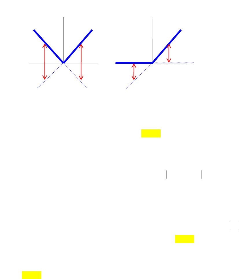
84
We propose the following algorithm to solve this system [TODO: is there a better way?]:
1. Assume we are given an initial set of signs dj (these will typically have been saved
from the previous time step).
2. Solve for λ using (8.74), then define derr such that
sense( ) {0,1,2}
j j j
derr d
-
. This
will be 2 for an incorrect bilateral constraint, 1 for an incorrect unilateral constraint,
and zero if dj was correct.
3. If derr=0 we are done since we used the correct set of linear equations. Go to step 5.
4. Otherwise, from all j for which
0
j
derr
, choose the one for which
j j j j
err derr
-
is largest, then revise dj using (8.68), and repeat from step 2. [TODO: is this the right
way to choose j?] Note that we only revise one sign at a time since all the unknowns
are coupled in general—changing more than one at a time can cause failure to con-
verge. [TODO: what can we say about convergence and uniqueness?]
5. Verify that we have a solution. If not, the system is inconsistent which means there
must be an impulsive velocity change to change a sliding contact into a sticking one;
the impact handler should be invoked.
This same set of equations with relabeling and removing non-impulsive forces can be used
for impact also:
σj
σj
σerrj
σerrj
Figure 12: The error in a sliding friction force multiplier when the wrong linear equation is
chosen for it. The dotted blue lines show the incorrect values of σ. Note that the error is twice
as large for bilateral constraints as for unilateral ones.
Bilateral
Unilateral

85
0
0
sense( ), ( )
TT
u
u
dd
M G S
G
DμT
T D diag
(8.75)
where the unknowns are the set of impulse multipliers π (and σ), the velocity change Δu, and
the signs d.
8.6.2.4 Sliding friction with nonlinear dependence on multipliers
A bilateral constraint implemented with several multipliers may have sliding friction that is
dependent on a normal force that is the magnitude of a vector. Examples are a 2-multiplier
point-on-line constraint (with sliding friction along the line), or joint-like constraints such as
a 3-multiplier ball joint constraint (sliding friction torque vector opposing angular velocity)
or 5-multiplier pin joint constraint (sliding friction generalized torque about rotation axis). In
these cases the normal force scalar of interest is the norm of a vector which is some projec-
tion of the constraint reaction force. Then we can write the magnitude σj≥0 of the jth sliding
friction force as
2
()
where ( )
j j j j
j j j j
N
N
-
--
A
(8.76)
Subscript
j
is now the set of multiplier indices on which σj depends and
j
-
is a vector,
typically with 2 or 3 elements; conceivably it could contain up to 5. Aj=Aj(q) provides
rotation, scaling, and projection as needed. Note that Nj(0)=0; you can’t have a sliding
friction force without a normal force. However, Aj is not necessarily full rank so
jj
-
A
may
be zero even if
0
j
-
.
Now the equations of motion become:
()
TT
uf
ub
N
-
-
M G S
G
μ
(8.77)
where each element of vector function N is one of the Nj and μ=diag(μj). Given an estimate λi
for λ, we can approximate N locally to first order as
86
2
( ) ( )
where
(
( )
)
i
i i i
i
N N N
N
Nk
O
m
-
-
--
- - - -
-
-
(8.78)
From (8.76) we can determine the general form for a block of the derivative:
2
i
j
Ti
j j j
i
jj
N
--
-
--
AA
A
(8.79)
Note that this is undefined when
0
i
j
-
A
, requiring special handling there.
Define
()
ii
N
-
μ
. Assume we have an initial estimate λ0, perhaps saved from the previous
time step, and let
00
()N
-
μ
be our initial estimate of the sliding friction magnitudes. We
can refine this estimate using Newton iteration, terminating when
1ii
tol
(8.80)
for some tol based on user-requested accuracy. Substituting into (8.77) gives
1 1 1
1
1
1
where
i T i T i
i
i i i
ii
uf
ub
N
-
-
-
- - -
M G S
G
μ
(8.81)
The unknowns are
u
and
-
. Rearranging, we get
1
1
()
where
i i T T i
i
i T i T i
u N f
ub
ff
--
-
MGμS
G
GS
(8.82)
We can solve now as for the linear case:
1
1
()
where now ( )
ii
i i T T
fb
N
-
-
W GM
W GM G μS
(8.83)
That gives us λi+1 so we can calculate
11
()
ii
N
-
μ
and check for convergence in (8.80). If
we converged, then the solution is
1 1 1
[ , , ] [ , , ]
i i i
uu
- -
.
Note that the above describes a full Newton iteration, where the Jacobian is recalculated with
each iteration. Because of the mild nonlinearity, we are likely to be able to converge quickly
with a modified Newton, using only
0
N
-
and
0
W
unless one of the λ changes sign. However,
as mentioned above, Jacobian Nλ will be undefined at Aλ=0.

87
8.6.2.5 Stiction to sliding transition
When a contact was sticking but first begins to slide, there is no slip velocity to use to
determine the sliding force direction. Instead we want the sliding force to oppose the (un-
known) impending slip direction. One reasonable approach is to record the last known
stiction force direction and use that as the initial sliding force direction. Provided that the last
stiction force and first sliding force are about the same, this is likely to be a good direction.
However, it is possible that the stiction force exceeded its limit by a lot, and the coefficient of
static friction may be much larger than the coefficient of dynamic friction, so there may be a
large change in magnitude at the stictionsliding transition. This may cause a change in
direction that could make the final stiction force direction differ substantially from the
direction of impending slip.
A single friction element can be viewed as having three distinct “phase”:
1. Stiction. The sliding velocity is zero; the magnitude and direction of the stiction force
that will keep the sliding acceleration at zero are both unknown. This is implemented
as a set of workless constraint equations. If the magnitude exceeds μsN, we transition
to impending slip.
2. Impending slip. The velocity is currently zero but the acceleration is not constrained.
The magnitude is known as a function of the (unknown) normal force (μdN), and the
direction should oppose the (unknown) acceleration.
3. Sliding. The magnitude is known as a function of the (unknown) normal force, and
the direction is known as a function of state (it opposes the sliding velocity).
Here are the equations of motion with an impending slip friction element:
TT
i d i
uf
ub
N
-
M G S
G
e
e a a
(8.84)
where a is the friction-space (usually tangential) acceleration direction which is linearly
dependent on the unknowns
u
. We can get a good initial guess for the direction e using the
last stiction force direction:
/eλλ
88
8.6.3 Event detection for unilateral constraints
Once the set of active constraints has been determined, a Simbody simulation proceeds
continuously with an unchanged active set until a contact event is detected. Then one of two
event handlers is invoked: either the Impact Handler, or the Contact Handler.
The Impact Handler is invoked when a velocity-level unilateral constraint condition would be
violated, requiring a discontinuous change in velocities. There are two ways this can happen.
Most commonly, a holonomic unilateral constraint like contact or a joint stop reaches its
limit with a negative velocity, meaning further simulation would cause violation of the limit.
Alternatively, failure to converge a sliding friction contact force requires an impulsive
transition from sliding to sticking.
The Contact Handler is invoked when an acceleration-level, or equivalently reaction force-
level, unilateral constraint condition would be violated. For example, change of a unilateral
contact’s normal force from positive to negative requires invocation of the Contact Handler.
The solution involves only changes to the active constraint set; no changes to velocity occur
except very small projections of the active velocity constraints to satisfy velocity tolerances.
The Contact Handler is also invoked as the last step of the Impact Handler, to determine the
active set after the instantaneous velocity change has been completed. Figure 13 outlines this
flow of control during a time stepping study.
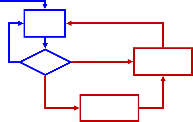
89
Although one or more particular constraint condition violations will trigger an event, the
handlers work with all relevant constraints simultaneously without treating the triggering
event special consideration.
TODO: Impact events: penetration, failure to converge sliding friction normal forces.
TODO: Contact events: liftoff (normal force goes negative), contact (normal acceleration
goes negative), stiction release (force exceeds μsN), slip-to-stick (slip velocity stops or
reverses).
8.7 Dynamic solution method
The previous section glossed over some details of the system formulation that we’ll need to
deal with here. Let’s first revisit the several types of constraint equations. Holonomic con-
straint equations p in equation (8.53) are those that are expressed at the q (position) level and
represent meaningful physical properties of the system. Holonomic constraint equations
involve only state variables at position stage or below, that is, q, t, parameters (instance
Advance time
using current
active set
Determine new
active constraint
set
Apply impulsive
velocity change
Impact
event
Event?
No
Contact event
Impact Handler
Contact
Handler
Figure 13: Flow of control during time stepping with unilateral contact and friction
constraints. Time stepping begins with a feasible active set. Then the normal time stepping
sequence is in blue and does not involve recalculation of the active set.
Start

90
variables), and modeling choices. Holonomic constraint equations can be differentiated once
to produce holonomic velocity constraint equations
p
, and again to produce holonomic
acceleration constraint equations
p
.
The nonholonomic constraint equations v in equation (8.52) are those that are directly
expressed in terms of system velocities, that is, at the u level, and also represent meaningful
physical properties. Typical examples are “non slip” conditions like rolling or gears, but
these can also include more global restrictions such as a conservation of energy constraint.
Nonholonomic constraint equations involve state variables at the velocity stage and below,
which includes the entire list given above for holonomic constraints plus the generalized
speeds u. Nonholonomic constraint equations can be differentiated once to produce nonho-
lonomic acceleration constraint equations
v
.
The acceleration constraint equations a in equation (8.51) are those which are directly
specified in terms of the system accelerations , or quantities which are linearly related to
accelerations such as reaction forces or constraint forces. Like holonomic and nonholonomic
constraints these are physically meaningful constraints.
Also at position level are the quaternion normalization constraints n in equation(8.49), each
of which involves only the coordinates of a single mobilizer and is present for numerical
reasons rather than physical. These are produced by mobilizers which use quaternions to
permit unrestricted orientation. Simbody’s implementation ensures that violation of quaterni-
on normalization constraints has no physical effect on the system. That is, a change to q
which serves only to satisfy a quaternion normalization constraint is not permitted to cause
any change to the system configuration. Quaternion normalization constraints exist only to
reduce the number of degrees of freedom of a mobilizer’s four quaternions down to the three
physical rotational degrees of freedom represented by its three mobilities u.
Unlike the holonomic and nonholonomic constraints, there are no constraints at the velocity
or acceleration level corresponding to the quaternion normalization constraint. Equation
(8.48) constructs the quaternion derivatives in terms of the three independent u’s, ensuring by
construction that the velocity-level constraints are satisfied.
u

91
Note that the system equations include a block diagonal invertible linear mapping between
the u’s and the time derivatives of the q’s, shown in equation (8.48):
()q q uN
. Although N
is a rectangular matrix, it is invertible. Note that when the quaternion normalization con-
straints are not satisfied exactly, the 4x3 blocks Ni on the diagonal of N which correspond to
quaternion qi will be scaled by |qi| so that the resulting
q
is the derivative of the unnormal-
ized quaternion.
Here is the system in the form we actually solve in Simbody, with slow (discrete) variables
not shown:
kinematics
( ) 0
qu
q
N
n
(8.85)
dynamics
bias
0
( , , , )
u
z z t q u z
-
ff
MG
b
G
T
(8.86)
velocity manifold
0
( , ; ) 0
u
t q u
Pc
v
(8.87)
position manifold
( ; ) 0tqp
(8.88)
relax fast variables
( , ; , ) 0
dyn f f
t y d y r
(8.89)
We are given initial condition
0 0 0 0
( ) { , ( ), ( )}t t d t y t
such that equations (8.87)–(8.89) are
satisfied, and are asked in a time stepping study to solve for d(t), y(t) for t0≤t≤tfinal.
Showing prescribed motion and fast variables:
kinematics
( ) 0
qu
q
N
n
(8.90)
dynamics
bias
0
u
-
ff
MG
b
G
T
(8.91)
auxiliary
( , , , , , , )z z t q u z u
-
(8.92)

92
constraint matrix
0
10
10
p
f
ff
pf fp ff
fp ff fp ff
fp ff
u
u
g G b
PP
GGG VV
AA
(8.93)
position manifold
() 0
( , ; )
pp
f p f
qt
t q q
p
pp
(8.94)
velocity manifold
1
0,
( , ) 0
( , , ; )
p
p
qp
qp
fr
pp
f p f
uuq
u
u t q
t q u u
c
pN
Pc
v
vv
acceleration manifold
0
0
( , , ) 0
( , , , ; )
pp
f
pp
f
qq
fq
uu
fu
pp
f p f f f
u
u
u
u
u t q u
t q u u u u
b
pPb
b
vVb
a
aa A b
relax fast variables
time time
pos pos
vel vel
force force
acc acc
( , , ; ) 0
( , , ; , ) 0
( , , , ; , ) 0
( , , , , ; , ) 0
( , , ; , , ) 0
dyn fast
dyn fast fast
dyn fast fast fast
dyn fast fast fast
fast fast
t d y d
t d y d q
t d y q d u
t d y q u d z
t d y d u z
r
r
r
r
r
(8.100)
Relaxation constraints (8.100) should be solved in stage order as shown, so that once fast
variables have been calculated at one stage they can be dependencies in a later stage. Note
that a relaxation solver at any stage may involve repeated state realizations through Accelera-
tion stage; the relaxation stage just determines which of the fast variables may be modified.
(8.95)
(8.96)
(8.97)
(8.98)
(8.99)
93
For compactness, equation (8.100) doesn’t show the always-present dependency on yslow, and
doesn’t show which variables in the state’s d partition can actually serve as dependencies; the
rule is: any d variable is allowed except those in dfast which haven’t yet been computed in the
relaxation sequence. As with the dynamic constraints in (8.94)-(8.99), relaxation constraints
will in general consist of a mix of explicit and implicit equations, but we’re not breaking
them out since there is no special treatment for them outside the relaxation solver itself.
95
9 Scaling and and accuracy
A multibody system is modeled using a set of state variables, and a set of differential and
algebraic equations that those variables must satisfy. There are many mathematically equiva-
lent ways to model the same system, and some of the modeling choices to be made are
arbitrary. Some examples are: choice of units for various quantities; definitions of general-
ized coordinates and speeds; choice of which quantities to treat as independent and which
dependent; and choice of which body is to serve as the base body for a chain. However, the
resulting physically equivalent models are not numerically equivalent so can affect the actual
solutions we obtain when doing computations, which are necessarily approximate. Such
computations involve significant tradeoffs between CPU time and accuracy, so we usually
want to use the loosest accuracy that is adequate for our purposes. The goal of scaling is to
ensure that an accuracy specification (e.g., “1% accuracy”) can be applied in a physically
meaningful way so that the behavior of a study is not dominated by arbitrary modeling
choices. That is, we would like a given accuracy specification to yield the same physical
results for all the physically equivalent models, regardless of any arbitrary choices that may
have been made during construction of those models.
There are two ways in which arbitrary modeling choices interact with accuracy requirements.
These are: (1) scaling of system state variables, and (2) scaling of errors in the algebraic
constraints. Our goal is to be able to determine a physically meaningful “unit change” to each
state variable, and a physically meaningful “unit error” for each algebraic constraint. Then
when solving the system equations we can define “accuracy” to mean calculation of state
variables to some fraction of that unit change, and satisfaction of algebraic equations to some
fraction of that unit error. We deal with multiple variables and equations by defining a scalar
norm representing “overall change” and “overall error” and then requiring our computations
to maintain those norms at or below the requested accuracy.
9.1 Relative vs. absolute accuracy
For some quantities we are satisfied to achieve relative accuracy, e.g. a result that is within
1% of the correct value. In that case absolute errors of larger magnitude are acceptable when
the numerical magnitude of a quantity is larger. However, one must be careful to avoid

96
situations in which a physically-meaningless change in magnitude of a measured quantity
would result in a physically-significant difference in accuracy or behavior. For example,
rotations are cyclical quantities, but the angular variables that define them can grow without
bound, adding 2π with each revolution. There is no configuration change associated with
those factors of 2π and no reason that the absolute angle should be determined less accurately
as the revolution count increases. Less obviously, translational coordinates can also introduce
physically-insignificant numerical changes. Consider a block on a sliding joint that hits a stiff
spring stop at x=1 and a simulation that predicts its behavior as it encounters the stop. If you
now lengthen the block’s travel and put the stop at x=1000, it would be incorrect to calculate
x any less accurately because that could drastically change the calculation of the spring force,
with significant consequences for the block’s predicted behavior. Common sense says a
block should behave the same way in one place as another. Similarly, any change in the
spatial location of a system involves changes to translational variables, yet should not affect
the precision of results. Hence Simbody solves all configuration coordinates q to an absolute
accuracy level independent of their current values. Note that this does mean that there can be
a performance cost for choosing units far from unity; we deem that a more reasonable
consequence than producing bad answers.
Unlike configuration variables, velocity variables u may reasonably be solved to relative
accuracies in most cases
*
. Arbitrary constants in q are eliminated by differentiation, so do not
appear in
q
or u. For auxiliary state variables z relative accuracy may or may not be appro-
priate; Simbody assumes that relative accuracy for z is sufficient unless told otherwise.
When a u or z is near zero, relative accuracy becomes too strict. In that case an absolute
accuracy requirement should be used instead. The absolute accuracy requirement for a
variable represents a “good enough” level that is acceptable no matter what fractional error of
the current value that represents. For example, say accuracy α=0.1% (10−3) has been request-
ed for a forward dynamics study. If the current value of a variable x is 10−6 units, an error
*
This may not be acceptable for u’s that are involved in constraints, since constraint errors generally involve
the differences between velocities.
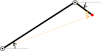
97
estimate no larger than 10−9 units would be required to produce a relative accuracy of 0.1%,
requiring a very small step size. However, if the absolute error requirement for x were 10−5
units, then an error estimate as large as 10−5 units would be acceptable, despite that being
1000% of the current value.
9.2 Weighting and absolute accuracy
An important practical consideration for any multibody formulation is that the state variables
{ , , }y q u z
vary widely in effect, or weight, by which we mean the degree to which a unit
change in the numerical value of a state variable affects a physically meaningful quantity of
interest. There are several causes for the uneven weights of state variables. To begin with,
they are expressed in different units—q’s are typically lengths, angles, or quaternions; u’s are
typically length/time or angle/time; z’s can be anything at all. Weighting differences are even
more pronounced in internal coordinate formulations like Simbody’s, since the effect of a
state variable depends strongly on its position in the multibody tree. A unit change δqi to an
angular coordinate near the system base will have a much larger effect (on almost anything
you might care to measure) than the identical change made to a coordinate which rotates only
a lone terminal body.
Figure 14 depicts this situation. If we hope to achieve a given level of accuracy with regard
to the positioning of the end point P marked with a red square, we need to calculate q1 more
accurately than q2. For example, say d1=10 nm and d2=0.5 nm. Then an error ε=0.1 radians in
q1 induces an error of d1ε=1 nm in P’s location, while that same error in q2 induces only
d2ε=0.05 nm of positioning error. In this situation we say that state q1 has more weight than
q1
q2
d1
Figure 14: Weighting of q1 and q2 are very different
with respect to the position of the end point P.
d2
P
98
q2 with respect to the location of P. If we consider a unit change of P to be 1nm, we can
define a corresponding “unit change” of q1 in this case to be δq1=0.1 radians while δq2=2
radians. Each of those unit changes will move P by 1nm. States which are “more important”
will have a numerically smaller unit change. Note that “unit change” does not mean “small
change.” Rather, this is the quantity to which the requested accuracy α is applied.
Even in the simple example of Figure 14 it is clear that the weights of state variables are not
constant but change as a function of system configuration. Thus weights may need to be
recalculated periodically as a system moves during a study. Fortunately, in practice
weighting does not need to be done perfectly to yield substantial improvements over un-
scaled variables. That permits us to treat weights as constants in the discussion to follow; in
practice they are updated only occasionally. Also, in practice there is no single quantity P
that we can use to neatly define unit changes for each of the generalized coordinates.
This concept of “unit change”
0
i
y
for each state variable yi is used to define the “always
good enough” absolute error requirement
i
y
for use when relative error
i
y
is not
allowed or too stringent. We can then define a diagonal weighting matrix W, where the ith
diagonal element is
1/
ii
wy
, the “unit weight” of state variable yi. For example, referring
again to Figure 14, if we want to scale by the geometric consequences of the state variables
on P’s location we could use
111
1/ dwq
and
222
1/ dwq
. Then we would define W as
follows:
1
2
0
0
dd
W
In the above discussion we have oversimplified the choice of weights for q by choosing a
system in which
qu
. In general, however, we have
()q q uN
(and
()u q q
N
). That
means the effective weights on q contain arbitrary factors due to choice of coordinates in
addition to physical considerations. However, given weights on u (which are physical) we
can easily determine the corresponding
q
weights. So instead of determining weights from
Pq
we instead look at
Pu
. Thus “unit change” estimates are provided for the mobilities
u, which are physical quantities, rather than on the generalized coordinates q which can be
chosen somewhat arbitrarily. So we work only with the nxn diagonal weighting matrix Wu;
there is no separate Wq. Instead, it may be calculated as
99
qu
W NW N
(9.1)
which ensures that the appropriate kinematic relationship holds between the weighted
velocity variables, that is
()
ww
q q uN
where
qw
qqW
and
uw
uuW
. Note that although
Wu is diagonal, positive, and constant, Wq is block-diagonal, signed, and q-dependent since
N=N(q). (Note that although
N N I
,
NN I
.) If there are auxiliary state variables z they
will have independent weights Wz. Then we have
00
00
00
u
u
z
NW N
WW
W
(9.2)
Even when Wu=I, Wq can be significant for orientation coordinates. Some configurations of
quaternions have one or more coordinates with zero weight (because they act only to change
the length of the quaternion and thus produce no rotation). Euler angle coordinates near
singular configurations have one coordinate whose weight approaches infinity; proper
weighting ensures the simulation remains accurate in near-singular configurations, although
possibly with a significant performance penalty.
We can combine relative accuracy requirements with the absolute “unit change” estimates
into a matrix E to form the error norm:
,
,
,
,
min( ,1 ), solved to relative accuracy
where ,otherwise
min( ,1 ), solved to relative accuracy
,otherwise
qu
q
u i i i
uu
ui
z
z i i i
zzi
uu
zz
E NW N
EW
E E E W
E
W
EW
(9.3)
Now let ey represent the vector of ny unweighted error estimates introduced by a step in the
numerical solution for y(t). Then
yy
feE
is the vector giving for each state variable the
unitless fractional error represented by the value in ey. We can define the error 2-norm
yy
E2
ef
and error ∞-norm
yy
E
ef
. We don’t use the 2-norm directly, but instead
use the related RMS norm
yy
ERMS E
1
y
ee
n

100
where ny is the number of state variables, because the RMS norm does not grow with the
problem size. (The ∞-norm is already size-independent.) Now we can provide a precise
meaning for the notion “solve for y(t) to an accuracy α”: either
yERMS
e
or (stricter)
yE
e
at each step during the study. Typically we’ll require that q, u, and z norms
separately meet the required accuracy to avoid mixing dissimilar variables in the RMS case.
9.3 Scaling of constraint errors
The nonlinear algebraic equations defining the system, such as equations (8.52) and (8.53),
cannot be solved exactly by a numerical computation. Instead, they will be met with some
residual error. We would like to keep that error below a specified “tolerance” level during a
study. As with the state variable weighting problem above, we have to deal with the issue
that there are many separate algebraic equations, and the errors they produce will not be
measured in the same units. This is especially important when mixing position (holonomic)
and velocity (nonholonomic) constraints, since velocity constraint errors need to be in units
comparable to the time derivatives of the position constraint errors. Also, if any acceleration-
only constraints are provided their errors must be in units comparable to the 2nd time deriva-
tive of the holonomic constraint errors.
The formulation used by Simbody ensures that the acceleration-level constraints are solved to
machine precision at the same time we solve for the accelerations. So our numerical integra-
tion methods do not need to deal with acceleration constraint tolerances; we’ll just take what
we get from solving system (8.86). However, if you are using your own methods you might
find it useful to scale the acceleration errors. In any case we do need to actively control the
errors in velocity, position, and quaternion normalization constraints. As with state variables,
we want to be able to provide a consistent physical meaning for a statement like “solve the
constraint equations to 1% accuracy.”
To do this we define a set of unit constraint errors
p v a
, , 0t t t
, one for each of the mp position
(holonomic) and mv velocity (nonholonomic) and ma acceleration-only constraint equations.
Each of these has appropriate units for its constraint equation, e.g. angle or length for a
holonomic constraint, speed for a nonholonomic constraint, and accelerations for accelera-
tion-only constraints. Each ti should represent the violation that is to be considered a “unit

101
violation” of the ith constraint (“unit” doesn’t necessarily mean “small”). By default each unit
constraint error is 1, meaning 1 length unit, 1 radian, 1 radian/time unit, etc.
To estimate tolerances for holonomic first and second derivatives, and nonholonomic deriva-
tives, we use a System-defined characteristic time scale parameter tc. This parameter gives a
typical “time of interest” over which we expect to see significant behavior. This should be
roughly the rate at which you could expect interesting reporting data, not necessarily the
highest frequency in the system. For example, given the time scale, we consider an appropri-
ate unit velocity error for a distance constraint derivative to be one unit distance error per tc.
A biomechanical or robotic system might have a timescale of 100ms, a biomolecular system
100fs, and an orbital problem might have a timescale of 10 or 100s. Somewhat counterintui-
tively, a long time scale puts more stringent requirements on velocity constraints since they
have much longer to drift in that case. Our default time scale is 0.1 time units.
Now we can define diagonal constraint weighting matrices Tp, Tpv, Tpva whose diagonal
elements are the weights for the combined constraints at position, velocity, and acceleration
levels (that is, velocity level includes holonomic derivatives, etc.). Note that “unit error” has
the inverse sense to “weight”—while a larger weight means “more important” a larger unit
error means “less important,” so we invert unit errors in T to create weights. Here is how the
constraint weighting matrices are defined:
2
diag(1./ ) , diag(1./ ) , diag(1./ )
p p v v a a
cp
pv
v
cp
c pv
pva c v
aa
t t t
t
t
tt
T T T
T
TT
T
T
TT
TT
. (9.4)
Unlike relative weights of state variables, which can change as the state variable values
change, we expect T to remain fixed once specified since tolerances are absolute quantities.
Now define
,,
p pv pva
as the vectors containing the current, unweighted errors for each
constraint equation at each level. We can now calculate the tolerance norms
T2
p p p
T
and
T
p p p
T
and similarly for pv and pva. These treat all constraint errors uniformly.

102
As in the previous section, in practice we will use the RMS norm
1
TRMS T
p
pp
m
or
∞-norm
T
p
rather than the 2-norm to remove effects due just to problem size, and define
the phrase “meeting tolerance to accuracy α” to mean
max( , )
p p pv pv
norm norm
TT
(9.5)
where norm=RMS or (stricter) norm=∞.
9.4 Scaling at the acceleration level
Acceleration-level constraint weightings Tpva do not matter when using Simbody’s standard
formulation since accelerations are calculated to machine precision. Even when the con-
straints are redundant accelerations are uniquely determined, however in that case the con-
straint forces are not unique. Simbody will calculate a least-squares solution to the constraint
forces which tends to spread the load evenly among the redundant constraints. You can in
theory provide a weighting
-
W
to influence the norm in which that least squares calculation
is performed. However, that is not the same as the acceleration error weighting Tpva. Instead,
-
W
is used to capture the relative stiffness of the compliant elements that are being modeled
rigidly with constraints. This is a rather obscure nuance and is unlikely to be useful in
practice – if you really care about how the forces are distributed you will probably want to
use compliant elements. However, here is a proof that acceleration-level weighting has no
effect except when there are redundant constraints.
Scaling on the constraint forces would be incorporated as follows. First, we want to solve for
the scaled multipliers (using just W here to represent
-
W
):
( ) ( )
WW
Mu G f Mu G f
--
WW
TT
(9.6)
(W is symmetric.) This shows how the scaling transfers to the constraint Jacobian, so the
acceleration constraint equation is scaled like this:
()G u bWW
(9.7)
Note that once we have
W
-
we can unscale this for use with the original constraints via

103
1W
--
W
. (9.8)
Multiplying (9.6) through by M−1 and then WG and substituting from (9.7) gives:
11
( ) ( )
W
GM G GM f b
-
W W W
T
(9.9)
In the underdetermined case we can solve for a least squares
W
-
using the pseudoinverse:
11
( ) ( )
WGM G GM f b
-
W W W
T
(9.10)
But if
1
GM G
T
has full rank then so does the scaled version, and the pseudoinverse is just the
ordinary matrix inverse so we can rewrite (9.10) as
1 1 1
1 1 1 1 1
1 1 1 1
1
( ) ( )
( ) ( )
( ) ( )
W
U
GM G GM f b
GM G GM f b
GM G GM f b
-
-
W W W
W W W
W
W
T
T
T
(9.11)
where
U
-
is just the multiplier we would have calculated without scaling. Unscaling
W
-
using equation (9.8) gives
1
W U U
- - - -
W WW
, that is, the final λ is just the unscaled one.
That proves that weighting the acceleration constraints and multipliers has no effect for
systems with full rank.
9.5 Accuracy
To summarize, we now have a way to define what is meant by solving a multibody
system to a given accuracy, say α=0.1%. We will have defined a locally-constant
weighting matrix W on changes to the state variables u and z (and implying a
weighting on changes to q) and a constant reciprocal tolerance matrix T on the absolute
errors in the constraint equations, appropriately time-scaled. W defines a “unit change” for
each state variable, and T defines a “unit error” for each constraint equation. We also have
information that defines what we consider “full scale” for each state variable, so that we can
interpret accuracy as a request for precision as a fraction of the full scale value. The block
diagonal matrix E combines relative scaling with the absolute unit changes in W to define
the error norm.
Then we have solved a trajectory to an accuracy α =0.1% (for example) when both

104
max( , , ) 0.001
and max( , ) 0.001
q q u u z z
Enorm Enorm
Enorm
p p pv pv
Tnorm Tnorm
e e e
E E E
TT
(9.12)
hold for each step of the solution, where Enorm and Tnorm are RMS or ∞ norms.
Although constraint accuracy is maintained throughout a simulation, it is important to
emphasize that accuracy of the state variables is a local phenomenon. Many multibody
systems are inherently chaotic, meaning that their long term behavior is arbitrarily sensitive
to initial conditions and numerical errors and hence not predictable. Only local measures of
accuracy make sense for such systems. One may think of this as ensuring that the simulation
accurately simulates some system which is very similar to the one under study. Without such
accuracy control there is no guarantee that any such system is being simulated.

105
10 Time Stepping
The system described by equations (8.85)–(8.88) is an overdetermined system since there are
more equations than unknowns. The nq+n+nz+m unknowns are q,u,z and λ. The first line of
equation (8.85) provides only n independent equations, but the second adds nquat more for a
total of nq kinematic equations. Then equation (8.86) provides n+m
*
with the first line and nz
more with the second line. That leaves (8.87) and (8.88) as 2mp+mv “extra” equations. These
equations define the position and velocity constraint manifolds on which the solutions q(t)
and u(t) are expected to lie (that is, the values of q and u should always satisfy those equa-
tions). If equations (8.85) and (8.86) could be integrated perfectly, the solutions would
indeed stay on the manifolds since they start out that way and equations (8.85) and (8.86)
satisfy the constraint derivatives. However, truncation error inherent in methods for approx-
imate numerical integration allows the solution to drift away from the manifolds. The “extra”
equations can be employed rigorously to eliminate this drift, and in fact improve the solution
overall, using the method of coordinate projection8 to be discussed below. We’ll make use
here of the scaling, tolerance, and accuracy theory from Chapter 9.
10.1 Coordinate projection
Given an arbitrary value for the state variables, some or all of the constraint equations may
fail to be satisfied. Since accelerations are computed quantities rather than states, we can
always calculate them to satisfy the acceleration constraint equations. However, since t, q,
and u are independent states we may find position and velocity constraints are not satisfied.
In cases where the equations are expected to be arbitrarily far from being satisfied (typically
prior to the start of a study), we may need special analyses to attempt to find values which
satisfy the constraints. However, during a dynamic simulation it will typically be the case
that the constraints will almost be satisfied, meaning that q and u just need to be “cleaned up”
a little. This cleaning up process can be thought of as taking state variables which have left
*
When G doesn’t have full row rank (meaning some of the constraints are redundant or inconsistent), we
introduce other conditions to select the “best” solution for the underdetermined λ. Specifically, we choose the
value for λ that minimizes |λ|2 in the redundant situation, and the value which minimizes the 2-norm of the
residual error in equation (8.86) if the constraints are (slightly) inconsistent.

106
the required constraint manifold and projecting them back to the manifold via the shortest
path (smallest change in a weighted norm) we can make.
We define
1
n
1
( ) ( )
1
nquat
qq
q
n
q
(10.1)
p( ) (t; )qq
p
(10.2)
pv ( ) (t,q; )uu
p
v
(10.3)
pva ( ) (t,q,u; )uu
p
v
a
(10.4)
where arguments before the semicolon are fixed at their current values. Note that these are
unweighted errors; εp and εpv need to be weighted using the constraint weighting matrices Tp
and Tpv discussed in section 9.3. When some of the q and u values are known due to pre-
scribed motion (see section 8.3), then q={qp, qf} and u={up, uf} and we are only able to
modify the free variables qf and uf to satisfy the violated constraints.
Then we would like to find the smallest change to qf that will drive εp to 0, and the smallest
change to uf that will drive εpv to 0. Those “smallest” changes correspond to a least squares
projection in a weighted direction we call the error norm (E norm), normal to the constraint
manifold, for which a theorem given in reference 8 guarantees that this projection also
improves the solution to the differential equations. See section 9.1 for a discussion of the E
norm. εpva is satisfied exactly when we solve equation (8.86), and εn is always satisfied
simply by normalizing the quaternions
kqn
, which is a 2-norm projection that can be
done separately from everything else, although no projection is done for quaternions that are
contained in qp.
The projection equations are underdetermined, nonlinear equations, but we expect to be close
to a solution so they can be solved efficiently with Newton iteration or similar methods. To
avoid an excess of subscripts we will drop the subscript “f” here, but keep in mind that we

107
are working only with free variables, and matrix columns corresponding to prescribed
variables are removed. All constraint equations remain, however, even as the number of
variables available to solve them is reduced by prescribed motion.
The full Newton steps in projection are
( ) ( )
q p p
( 1) ( )
q
( ) ( ) iterate
ii
ELS
ii
ELS
q q q
q q q
PT
E
(10.5)
( ) final
: | |
last
k k k k
q n n n n
(10.6)
()
final pp
()
vv
( 1) ( ) 1
u
()
() () iterate
i
c
ELS i
ii
ELS
tu
qu u
u u u
T
VT
E
(10.7)
where
q p q q
( ) ( )qq
P T P E
(10.8)
p1
u
v
()
() ()
c
tq
qq
TP
VE
TV
(10.9)
1
q u q u
()
E NW N E NW N
(10.10)
q
and ( ) ( )qq
P P N
. (10.11)
(Columns of
q
P
and
V
corresponding to prescribed variables are removed.)
We iterate (10.5) until we have calculated a final value
( )last
q
that satisfies the holonomic
constraint equations (10.2) to within a specified tolerance, then using equation (10.6) project
the quaternions in
( )last
q
via their normalization constraints (10.1). That gives us
final
q
which
satisfies all the constraints (10.1) and (10.2). We then iterate (10.7) with
V
calculated at
final
q
while solving for the final velocity value
final
u
which satisfies the velocity constraints
(10.3). Note that we must perform a least squares solution to the linear system at each
iteration, and that the diagonal weighting matrices Eu, Tp, and Tv must be constant during the
iteration (although Eq may change a little). Typically, P and V are block-structured matrices
(and weighting preserves that structure). For efficiency, uncoupled blocks should be treated
separately in equations (10.5) and (10.7).

108
Normalizing a quaternion as in equation (10.6) is the least squares projection of the four-
dimensional quaternion onto its constraint manifold, a three-dimensional sphere of unit
radius. However, quaternion projection is done in an unweighted norm since it is a constraint
on the numerical values of the quaternion elements unrelated to the physical effect of those
elements. By construction, the physical effect of a change in the length of a quaternion in
Simbody is zero. Note also that there are no velocity or acceleration constraints correspond-
ing to the quaternion normalization constraint, because those constraints are satisfied exactly
by the quaternion derivatives we calculate from the generalized speeds u.
A very similar problem arises when we have a vector in the q or u basis, and we would like
to remove the component of that vector which is normal to the constraint manifold, in the
weighted norm. For example, when an integrator has computed a pre-projection absolute
error estimate vector
y q u z
,,e e e e
in its computation of integrated state variables
y={q,u,z}, we know that performing the above constraint projection will remove the compo-
nent of the error in the weighted constraint-normal direction (for proof, see ref. 8 and ref.
10
,
§3.8.2), and also the component of error along the length of quaternions. So we can now
reduce that error estimate by subtracting out any component it might have had in the direc-
tions we just fixed, which may allow us to take a bigger step. In that case the projections are
final final
q wq q q q
q q q wq
( ) ( ) no iteration
q e q e
e e e
P P E
E
(10.12)
final final
qˆ
: ( ) quaternions
k k k k kk
e e e e e
q q q q nn
(10.13)
final final
wu u u
1
u u u wu
( ) ( ) no iteration
ˆ
q e q e
e e e
V V E
E
(10.14)
(Here as above we are working only with the error slots corresponding to free variables, not
prescribed ones.)
Again we need to find least-squares solutions to the underdetermined systems (10.12) and
(10.14). Then we set
y q u z
ˆ ˆ ˆ ˆ
,,e e e e
as the new (absolute, unweighted) error estimate. Note
that these use the same (final) iteration matrices as above with a different right hand side.
Equations (10.12) and (10.14) are linear systems so no iteration is needed, and again block

109
structure in P and V should be exploited for efficiency. After this projection the integrator
should use the revised estimate
y
ˆ
e
as its error estimate instead of the original estimate
y
e
(using the W norm).
We can use a pseudoinverse to find the least squares solution at each step. The pseudoinverse
A+ of an mxn matrix A, with m<=n and full row rank (i.e. rank(A)=m) is given by
A+=AT(AAT)–1, although computing A+ that way can be numerically inaccurate. Using an
SVD or faster complete orthogonal factorization (QTZ) we can compute a numerically well-
conditioned pseudoinverse even in the case of redundant constraints, i.e., rank(A)<m.
Looking now at the weighted holonomic position constraint iteration matrix
q
P
in equation
(10.8) we see that the pseudo inverse we need is
1
q p q q p u
( ) ( )
P T P W T PNW N
The corresponding velocity constraint projection from (10.9) is
1
pu
1
vu
c
t
T PW
VT VW
When there are no non-holonomic constraints, we have
VP
the velocity projection is just
1
pu
()
c
t
V P T PW
The constraint projections can be performed sequentially (for proof, see ref. 10, §3.8.3). First,
with t fixed at
ˆ
t
we must find some
()last
qq
that satisfies the holonomic constraint equa-
tions to within a specified tolerance. Then we normalize the quaternions in
()last
q
(which by
construction cannot affect any of the holonomic constraints) and call the result
final
q
. After
that we freeze q at
final
q
and proceed to find u that satisfies the velocity constraint equations
to within a specified tolerance. Note that the holonomic velocity constraint equations (i.e.,
first time derivatives of the holonomic constraint equations) and nonholonomic constraint
equations must be dealt with simultaneously since they can be coupled.
110
10.2 Simplified equations
For use with a generic coordinate projection integrator, the Simbody equations can be viewed
in the following simplified form:
differential eqns.
( , )y f t y
(10.15)
algebraic eqns.
( , ) 0c t y
(10.16)
initial conditions
00
( , ) 0c t y
(10.17)
with the guarantee that equation (10.15) is solved in such a way that any new constraints
introduced by time-differentiating equation (10.16) are satisfied automatically; that is,
( , , ( , )) 0c t y f t y
whenever equations (10.15) and (10.16) are satisfied. There is an nyxny
block-diagonal weighting matrix E and an ncxnc diagonal tolerance matrix T, and corre-
sponding norms as discussed in Chapter 9. To solve this system to accuracy α, the following
two conditions must be satisfied at each integration step:
yERMS
(10.18)
TRMS
( , )c t y
(10.19)
where the
y
are the post-projection local state errors introduced by an integration step.
When conditions (10.18) and (10.19) are met, the integrator can accept the step.
10.3 Update rates for state variables
During a time-stepping study, Simbody supports three distinct update rates for time-varying
variables in : slow (discrete), dynamic, and fast. Slow variables are updated only occasion-
ally upon occurrence of events and never change during a continuous interval. Dynamic
variables follow differential equations, evolve smoothly during continuous intervals, and
have well-defined time derivatives. Fast variables are those whose response may be consid-
ered instantaneous on the scale of the dynamic variables. The dynamic system is thus always
in quasi-static equilibrium with respect to the fast variables, whose values may be determined
by difference equations, equilibrium conditions, or algorithmically. Fast variables change
continuously in response to dynamic ones but can affect dynamic time evolution only indi-
rectly by affecting the dynamic variables’ derivatives.

111
Only variables in the State’s y partition can be dynamic. So we can partition the state by
update rate as follows:
slow slow slow
fast fast fast
dyn dyn
dy
dy
y
(10.20)
where
with
slow slow slow
dyn dyn dyn
fast fast fast
slow dyn fast
y q u
y q u z
y q u
y y y y
(10.21)
There also exists a set of time derivatives
y q u z
, with
0
slow fast
dyn dyn
yy
d
yy
dt
(10.22)
Note that
slow
y
is zero because
slow
y
is constant during a step, while
fast
y
is zero for the
opposite reason:
fast
y
changes so quickly that by the time we look it has already reached
equilibrium and is thus no longer changing. There are no derivatives defined for variables in
x, which are not permitted to be dynamic (although they can be fast or slow).
When we want to denote variables which affect a particular stage and also have a particular
update rate, we combine the sub- and superscripts, for example,
pos pos pos
fast fast fast fast
dq
. Note that a variable’s stage effect is an inherent property of
that variable, while the rate at which it is to be updated is a run time choice that may be
different under different circumstances.
At run time we must choose for every mobilizer:
How motion is driven: forces, acceleration, velocity, or position
The rate at which the driven motion is updated: slow (discrete), dynamic, or fast. A
force-driven mobilizer is always dynamic.
When mobilizer j is updated dynamically, it is driven by differential equations relating
position q[j] and velocity u[j] to acceleration
[]uj
. Normally,
[]uj
is calculated as a re-
112
sponse to forces, with u[j] and then q[j] calculated from
[]uj
by numerical integration. In
that case the dynamic mobilizer j is said to be free. When motion is known analytically, the
mobilizer is said to be prescribed. Both free and prescribed mobilizers are considered dynam-
ic mobilizers since they are both defined by time-varying differential equations. If instead the
driven motion is fast or slow, we have a fast or slow mobilizer, resp. All mobilities of a
multi-dof mobilizer must have the same update rate (that is, slow, prescribed, free, or fast).
Note that for any mobilizer that is driven at acceleration or velocity level, higher levels are
determined by numerical integration and are thus free.
There are some restrictions on the use of “fast” motion, because fast variables may not
directly affect dynamic ones: (1) If a mobilized body is fast, then all its children and de-
scendents in the multibody tree must also be fast. (2) If a constraint involves any fast body or
mobility, that makes it a fast constraint that is not part of the dynamic system. Instead it is
solved taking the dynamic variables as fixed, with only the fast variables varying.
Driven by
Update
rate
u
u
q
forces
dynamic
(free)
, , , ,
fp
u t q u z u
f
u dt
2
f
q dt
acceleration
dynamic
(prescribed)
( , , )
p pr pr
u t q u
f
u dt
2
f
q dt
velocity
dynamic
(prescribed)
p
u d dt
( , )
p pr
u t q
f
q dt
fast
0
p
u
fast
u
: alge-
braic
f
q dt
slow
0
p
u
slow
u
: event-
driven
f
q dt
position
dynamic
(prescribed)
22
p
u d dt
p
u d dt
()
p
qt
fast
0
p
u
0
p
u
fast
q
: alge-
braic
slow
0
p
u
0
p
u
slow
q
: event-
driven

113
Structured variables d that can affect time-varying quantities can be evaluated either continu-
ously (fast) or at discrete times (slow); variables that affect model or instance parameters or
are just used for reporting can’t be continuous. Here the continuous variables cannot be
defined by differential equations; they are always algebraic (or algorithmic).
dmodel,instance,report
dtime,pos,vel,dyn,acc
fast
n/a
fast
d
: algebraic
slow
slow
d
: event-
driven
slow
d
: event-
driven
Also note that “end of step” can be an event, so event-driven (slow) variables can be updated
as frequently as every step. However, they will not be updated during integration stages and
cannot affect integrator step size selection in the current step.
10.3.1 Coupling
Variables which are mutually coupled must be solved simultaneously which can be computa-
tionally expensive. In many cases, modeling considerations dictate that some variables are
“stronger” than others so coupling is only in the direction from driving variables to driven
ones, lending an ordering to the computation that avoids some simultaneity. Simbody sup-
ports four levels of coupling for computations at a given realization stage:
1. Slow (discrete): these variables are event driven so are not updated at all during a
continuous interval. Their values are taken as given at the beginning of a continuous
interval and can affect all subsequent calculations but are themselves unaffected.
2. Dynamic, prescribed: these are q, u, z, or
u
variables defined by differential equa-
tions with explicit analytic solutions based only on already-available values. For ex-
ample: positions as a function of time. This could represent an extremely high-
bandwidth controller, or a locked joint. Prescribed accelerations are not affected by
forces.
3. Dynamic, free: these are q, u, or z variables calculated by numerical integration. Cor-
responding accelerations
u
can additionally be coupled by algebraic constraint equa-
tions, which equations can depend on prescribed accelerations. They can thus be driv-

114
en by prescribed variables at the same level (e.g. prescribed velocity can drive free
velocity) but not vice versa. A dynamic position can affect a prescribed velocity since
that’s a later stage.
z
variables cannot be coupled via constraints.
4. Fast (quasi-static): these variables are calculated from the values of dynamic variables
(free or prescribed). They can affect forces so will change the behavior of free varia-
bles indirectly, through subsequent accelerations or by interaction with the numerical
integration method’s error test.
Free dynamic variables yf are approximated numerically by an integration method, then any
of them that are subject to constraint equations may need to be projected back to the con-
straint manifold via the System’s project() solvers. Prescribed dynamic variables yp are
simply set to their appropriate values via the System’s prescribe() solvers, once their
dependencies are available. Finally, we must solve for the fast variables dfast and yfast using
the System’s relax() solver.
Depending on the operation we are performing, it will be convenient to partition in a
variety of different ways.
Variable type
={d,t,y}
y={q,u,z}
stage(t)=Time
stage(q)=Position
stage(u)=Velocity
stage(z)=Force
stage(x) varies
scalar
variables
y
q
Generalized coordinates
(positions)
u
Generalized speeds (veloci-
ties)
z
Force variables
d
structured variables
t
time
Simulation
={def, t, var, report}
def ={topo, model,
instance}
var ={pos, vel, force,
acc }
def
variables that define the modeled
system: topology, model, instance
t
time
var
variant properties of the modeled
system: position, velocity, forces,
acceleration
report
“output” states for reporting
Time step-
ping
pres ={qp, up}
continuous
variables
pres
prescribed analytically
free
determined by numerical
integration

115
free ={qf, uf, z}
fast ={qfast, ufast, dfast}
slow={qslow, uslow, dslow}
fast
Quasi-static variables
determined algebraically
after pres and free
slow
Discrete “slow” variables (updated
occasionally upon event occurrence)
10.4 How to take a time step
Here we deconstruct a single time step into its constituent parts.
Special handling is required at the start of a time stepping study. Time and all state variables
must be given initial values, and then these must be modified to satisfy all constraints,
starting with prescribed motion. The resulting state must be fully realized using to-be-
updated values for discrete variables, as though we had just completed a zero-length step.
Then we can take the first step as though it were any arbitrary step.
1. Handle events as needed, updating discrete states, realize through Acceleration stage.
2. Take trial step of continuous system (with projection), with success metric.
3. If metric unacceptable, reduce step and return to 2.
4. Check for Time-stage event triggers and handle them; <= Instance stage change is a
restart meaning later event triggers are forgotten.
5. Realize(Positions); check for Position-stage event triggers and handle them; <= In-
stance stage change is a restart.
6. Repeat for Velocity, Force and Acceleration-stage event triggers.
7. If simulation is not done, go to step 1 to begin the next step.
Taking a trial step of the continuous system (we just updated discrete variables). Continuous
system consists of dynamic (prescribed and free), and “fast” variables qfast, ufast, zfast, and dfast.
There are a series of integrator stage evaluations and then a final setting of the state variables
in which differential variables are projected to their constraint manifold.

116
All steps begin like this:
If there are pending triggered events (at
t
):
o Set
tt
. Call time-triggered handlers to change slow variables; re-evaluate
,,y e c
; revise list of pending events
o Repeat for pending position, velocity, dynamics, acceleration-triggered events
If there are any beginning-of-step handlers, call them and re-evaluate. This cannot
cause any other events to occur.
Set t0=t, y0=y; invalidate d0
y
= realize[A](d,t,y)
Set
0
yy
Next step size to attempt is h
Fixed step explicit Euler (DAE step only):
Only stage:
00
free free free
y y h y
Set
0
t t h
; realize[T](t)
pres
q
= prescribeQ(t)
free
q
: projectQ(
,
pres free
qq
)
pres
u
= prescribeU(
,,
pres free
t q q
)
free
u
: projectU(
,
pres free
uu
)
Test convergence of projection. (bad: shrink h goto)
,
fast fast
dy
: relax[TPVFA](
, , ( , ); ,
fast fast fast fast
t y y d y d y
)
Test convergence of relaxation. (bad: shrink h goto)
(Error test OK.) Check for events. If any:
o Localize event(s) to window
( , ]w t t
o Back up the state to
tt
:
()
free
yt
= interpolate(
0
,,
free free
t y y
)
,
pres free
yy
= presAndProjQU(
,free
ty
)
,
fast fast
xy
: relax[TPVFA](
, , ( , ); ,
fast fast fast fast
t y y d y d y
)
o (Projection and relaxation must converge or there is something seriously
wrong.)
Successful, event-free step taken to time t. May be events pending for time
t
.
Explicit trapezoid (w/explicit Euler error estimator):
First stage:
1 0 0
free free free
y y h y

117
0
t t h
; realize[T](
t
)
1
pres
y
= prescribeQU(
1
,free
ty
)
11
,
fast fast
dy
: relax[TPVFA](
1
, , ( , ); ,
fast fast fast fast
t y y d y d y
)
Test convergence of relaxation. (bad: shrink h goto)
Final stage:
1
y
= realize[A](
11
,,t d y
)
0 0 1
2()
h
free free free free
y y y y
1
free free free
yy
,,
pres free free
yy
= presAndProjQU(
,,
pres free free
yy
)
Test
free
and convergence of projection. (bad: shrink h goto)
,
fast fast
dy
: relax[TPVFA](
, , ( , ); ,
fast fast fast fast
t y y d y d y
)
Test convergence of relaxation. (bad: shrink h goto)
(Error test OK.) Check for events. If any:
o Localize event(s) to window
( , ]w t t
o Back up the state to
tt
:
()
free
yt
= interpolate(
0
,,
free free
t y y
)
,
pres free
yy
= presAndProj[PVF](
,free
ty
)
,
fast fast
xy
: relax[TPVFA](
, , ( , ); ,
fast fast fast fast
t y y x y x y
)
o (Projection and relaxation must converge or there is something seriously
wrong.)
Successful, event-free step taken to time t. May be events pending for time
t
.
Verlet
First stage:
2
0 0 0
2
h
free free free free
q q h q q
0
t t h
; realize[T](
t
)
,
pres free
qq
= presAndProjQ(
,free
tq
);
realize[P](
,tq
)
pres
u
= prescribeU(
,,
pres free
t q q
)
1 0 0
free free free
u u h u
;
1 0 0
z z h z
realize[V](
,,t q u
)
1,
fast fast
dq
: relax[TP](
1
, , ( , ); ,
dyn fast fast fast fast
t y y d y d q
)
k=1
Loop until u and z are converged:
,
kk
fast fast
d uz
: relax[VFA](
, , ( , ); ,
k
dyn fast fast fast fast
t y y x y x uz
)

118
,
kk
uz
=realize[VFA](
, , ,
kk
t q u z
) expensive once
++k
0 0 1
2()
kk
h
free free free free
u u u u
;
0 0 1
2()
kk
h
z z z z
11
;
k k k k
uz
u u z z
If δ not converged, continue looping.
;
kk
free free
u u z z
u and z have converged to 2nd order
free free
qu
N
Compute low order estimates:
0 0 1 1
2( ); ;
h
free free free free free free
q q q q u u z z
free free free
yy
error estimate
,free q
= projErrEstQ(
,free q
)
,
,
free free uz
uz
= presAndProjU(
,
,,
pres free free uz
y uz
)
Test
free
and convergence of projection. (bad: shrink h goto)
,
fast fast
d uz
: relax[VFA](
, , ( , ); ,
dyn fast fast fast fast
t y y d y d uz
)
Test convergence of relaxation. (bad: shrink h goto)
Successful continuous step to t. Now check for events.
10.4.1 Setting the values of prescribed variables
Prescribed variables
p
yy
and
p
yy
are defined by analytically-known explicit func-
tions. These include
()
p
qt
,
( , )
p dyn
u t q
,
( , , )
p dyn dyn
u t q u
. (
dyn pres free
q q q
, etc.) Note that
earlier-stage prescribed and dynamic variables can affect later-stage prescribed ones.
A System defines prescribeQ() and prescribeU() solvers which sets the values for
that stage’s prescribed variables, taking values of earlier-stage variables as given. Be sure to
call them in this order: prescribeQ(), projectQ(), prescribeU(), projectU().
10.4.2 Relaxation of fast variables
After the values of time and the differential variables
,
pres free
y y y
have been calculated by
an integrator, the fast variables
fast
yy
and
fast
dd
need to be allowed to respond to the
new values, to attain a new quasi-static equilibrium. We call this process “relaxation” alt-
hough in general a System is permitted to use any method to solve for these variables,
119
provided the correct order of dependencies is followed. A System provides a relax(stage,
tol) solver which will drive a particular stage’s fast variables to their new equilibrium,
solving the associated equations to the given tolerance.
The time-stepping relaxation stages and the variables relaxed at each stage are as follows:
1.
time
fast
d
: relax(Time)
2.
pos
,
fast fast
qd
: relax(Position)
3.
vel
,
fast fast
ud
: relax(Velocity)
4.
force
fast
d
: relax(Force)
5.
acc
fast
d
: relax(Acceleration)
A System may also support relaxation of report-stage variables
report
d
and definition-stage
variables
model
d
and
instance
d
, but these are not relevant for time stepping.

121
11 Simbody Force Subsystems refer-
ence guide
Simbody comes with a predefined set of commonly-used force subsystems. Each of these is
an independent, self-contained set of related features, and users may add their own force
subsystems as well.
11.1 General Force Subsystem
Simbody comes with a force subsystem called GeneralForceSubsystem. It can be used to
add a variety of standard forces to a system, such as linear springs and dampers. It also
provides a mechanism for adding user defined forces.
11.2 Hertz/Hunt and Crossley contact model subsystem
Simbody comes with a force subsystem class called HuntCrossleyContact. This section
describes the theory behind it.
11.2.1 Motivation
Most engineers, physicists and computer scientists are introduced to contact problems using
the concept of coefficient of restitution. The idea presented is that when two objects collide,
they will rebound in a predictable way with the rebound velocity being a known fraction e of
the impact velocity.
Unfortunately, it is rarely mentioned that this concept is only usable in the most
limited cases. Many difficulties arise trying to apply this in a multibody dynamics
context; in particular the presence and motion of the other bodies and the forces
applied to them (which change constantly and are not know in advance) change the rebound
velocity. Also, it is well known in the field of contact mechanics (and to anyone who has
watched closely as a ball bounces) that the coefficient of restitution is very sensitive to the
impact velocity. In fact, in contact mechanics the normal way to approximate the coefficient
of restitution is
1i
e cv
for small impact velocity
i
v
, where c is a material property. An
enormous amount of empirical data supports that—at low velocities, normal materials have a

122
coefficient of restitution that drops linearly with impact velocity. The classic work in this
field is reference 13. Even with this improvement to the functional form of e, the results are
rarely applicable outside the realm of freely falling bodies. In multibody dynamics, the
coefficient of restitution is something to be computed, along with the rest of the system’s
motion, not something that can be known in advance!
To obtain usable results in a multibody context, we need a method that can calculate forces
produced during contact, rather than impulsive velocity changes. That permits contact to be
treated as yet another force among the many that influence the behavior of multibody sys-
tems, ensuring that accurate (or at least reasonable!) behavior will result. Only once you can
obtain physically correct results with some model, should an optimization like “treat
contact as an instantaneous event” be attempted, and even then one might wonder if it is
worth the effort.
11.2.2 The model
This model is based on Hertz theory of elastic contact,
11
and the Hunt and Crossley model for
damping.
12
The idea is to predict contact behavior during a dynamic simulation working only
from material properties and geometry. This is a frictionless model but it can be used as a
starting point for several useful frictional models.
To apply Hertz theory, we need two linearly elastic materials in non-conforming contact,
where the dimensions of the contact patch are small compared to the curvatures, and small
compared to the overall dimensions of the object. Hertz theory can be used for general
curved shapes (including cylinders) provided they can be approximated by paraboloids at the
contact point; however, we will discuss only sphere-sphere and sphere-halfspace contact
here. For Hunt and Crossley, the impact velocities should be small enough not to cause
permanent yielding of the materials. Within these regimes, the model produces a good match
for empirical data, such as that found in reference
13
. Outside these limits, the model can still
produce surprisingly useful results when fit to experimental data, because the form of the
model has a structure which captures the most significant aspects of contact for many pur-
poses. It is especially well-suited for soft contacts such as are common in biology, even
though those are well out of the range that the rigorous theory presented here can support. I
speculate that it works well in most applications because the results of interest don’t usually

123
depend on precise details of contact, only that it behaves in a qualitatively correct manner. As
an example, if you get a stiffness parameter too low, the model will compensate by allowing
more deformation with the result being that you get the same forces (such as are needed to
keep a foot going through the floor) although the precise deformation of the foot and floor
are not obtained. This may be acceptable for researchers who are more interested in studying
some other aspect of the model, knee flexion for example.
For the rest of this section, please refer to Figure 15 which defines the geometry of contact.
We will consider a collision between two bodies, B1 and B2, in which a sphere attached to B1
contacts a sphere or halfspace attached to B2. During the collision (which will occur over an
extended period of time, not impulsively), our goal will be to determine instantaneous values
for the contact force f, the contact patch orientation n and radius a, and a unique contact point
P at which we can apply equal and opposite forces to the two contacting bodies. We will be
given the spatial locations and velocities of the undeformed geometric objects in contact, and
will easily be able to determine the total deformation x that must have occurred because of
the apparent overlap between the undeformed objects. However, in order to find the contact
point P and the compression rates of each body (needed to compute dissipation), we have to
determine the individual deformations
1
x
of B1 and
2
x
of B2, where
1 2
x x x
and
1 2
x x x
.
The thin lines in the figure are intended to show the undeformed shape while the thicker lines
give a (crude) depiction of the deformed shape. Note the assumption that the contact patch is
planar, circular of radius a, centered at P and oriented with normal n pointing towards body
B1. With these conventions, the scalar force f that we will calculate (applied equal and
opposite to the two bodies at P) is always positive, and the vector force fn is applied to body
B1 at P, while we apply −fn to body B2 at P. From the diagram one might think it doesn’t
matter where along the line between the centers we apply the force. However, it is important
to keep in mind that the colliding objects are in general only attached to a larger body—they
do not constitute the whole body. That means the applied force is also generating moments
on the bodies, and those moments depend critically on exactly where the force is applied.
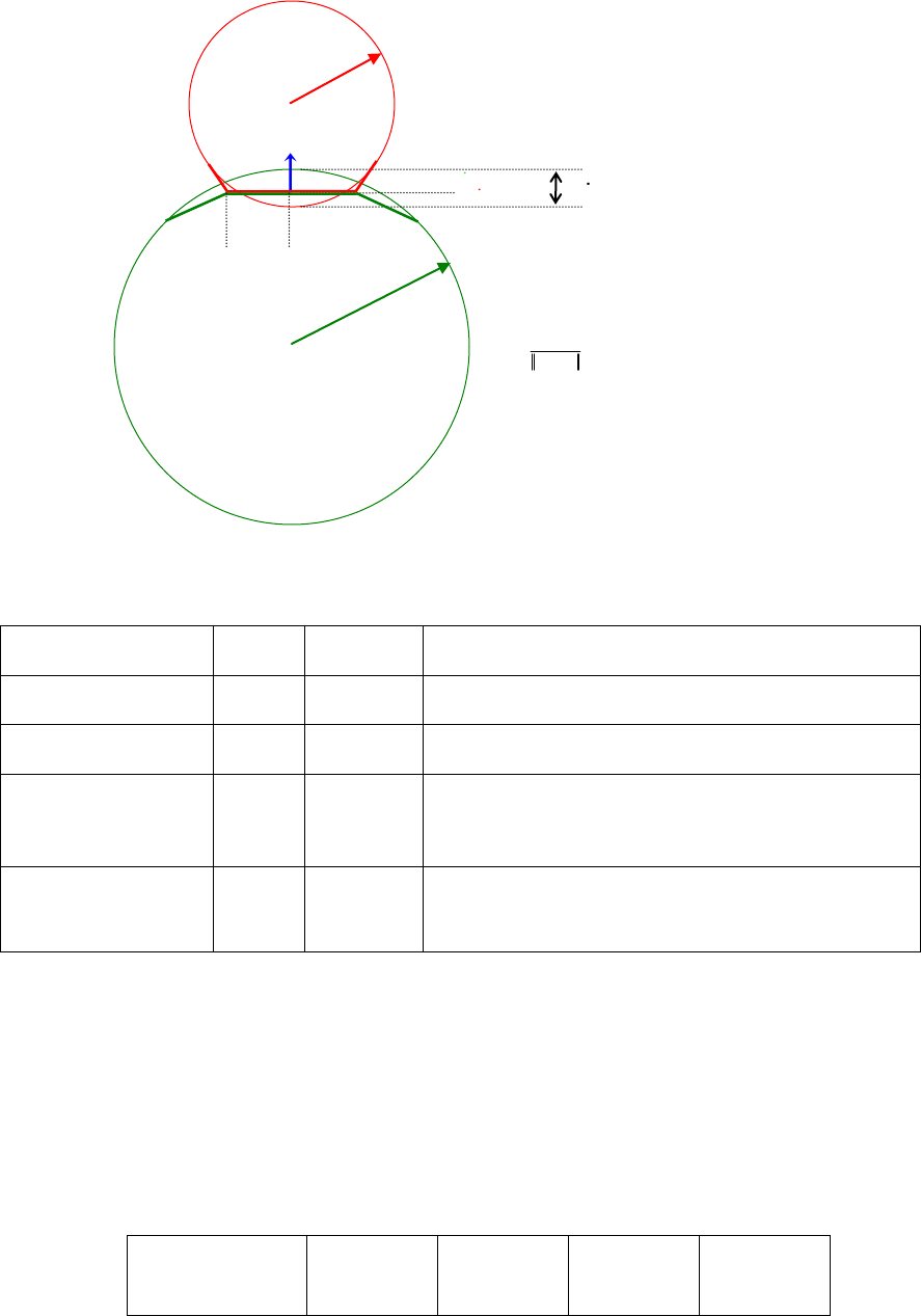
124
We expect to be given the following material properties for each body:
Property
Symbol
Units
Comments
Radius of curvature
R
Length
Measured at the contact point
Young’s modulus
E
Pressure
stress/strain = (force/unit area) / (% deformation)
Poisson’s ratio
ν
Unitless
ratio
ratio of transverse contraction to deformation (0–½ for
normal materials); related to preservation of volume
during strain; rubber has ν=½
Dissipation coefficient
c
1/velocity
−slope of coef. of restitution vs. velocity at low veloci-
ties; i.e., coef. of restitution e=1−cvi for impact velocity
vi
For our purposes, we combine Young’s modulus E and Poisson’s ratio ν into a single “stiff-
ness” property called the plane-strain modulus E*=E/(1−ν2). This is measured as the pressure
per unit area induced by a fractional deformation (strain). The MKS unit is Pascals which are
Newtons/m2. Below are some typical values as ballpark figures only; please don’t rely on
them. (Note that the stiffnesses are given in gigapascals, i.e. 109 N/m2!)
Material
Young’s
modulus E
Poisson’s
ratio ν
Plane-
strain
Dissipation
coefficient
R2
R1
*
1 1
,E c
,x x
2 2
,x x
1
1
1
1 22(1 )
xs x
x s x s xxx
O1•
O2•
n
•
P
1 2
1 2
1 1 1
2 2 2
O O
O O
O (RP)
O (R )
x
x
n
n
n
*
2 2
,E c
1 1
,x x
a
B2
B1
Figure 15: Contact geometry for the
Hertz/Hunt and Crossley model.

125
(GPa)
(unitless)
modulus E*
(GPa)
(s/m)
Rubber
0.01
0.5
.0133
0.05?
Bacteriophage
capsid
2
0.4(?)
2.4
?
Nylon
3
0.4
3.6
?
Lead
14
0.42
17
0.4?
Concrete
25
0.15
25.6
?
Steel
200
0.3
220
0.08?
Diamond
1100
0.2
1150
?
Of these, Young’s modulus and Poisson’s ratio can be obtained easily from handbooks for
most materials, but the dissipation coefficient is harder to get. It would be very useful to
relate this to standard properties such as hardness and yield stress (if that’s possible) but for
now it has to be measured or estimated as the slope of the coefficient of restitution-vs.-
velocity curve at low velocities. References 12 and 13 provide or imply some values for c,
but they should be taken with a grain of salt. Note that this situation is still better than the
standard approach of supplying a coefficient of restitution e directly—at least c is a material
property so can be expected to produce correct behavior over a range of velocities.
Hertz contact theory says the relationship between force fHz and displacement x depends only
on the relative curvature R of the two bodies at the contact point, and on an effective plane
strain modulus E*, and the contact patch radius a is an even simpler function
3 2 1 2*
4
Hz 3,f RE x a R x
Hunt and Crossley start with the above formula for fHz and add a dissipation term:
3
HC Hz 2
(1 )f f cx
where c is an effective dissipation coefficient combining the material properties of the two
contacting materials.

126
Note that although the materials are assumed linear, the force-displacement relationship is
nonlinear because of the changing geometry during contact. This complicates the calculation
of the effective stiffness E*. The literature seems to suggest
* * * * *
1 2 1 2
( )E E E E E
but this
would be inconsistent with the Hertz relationship, by the following reasoning. First, the
relative curvature is a geometric property and is straightforward to calculate:
1 2 1 2
( )R R R R R
. Looking at the figure, note that the contact situation depicted should be
indistinguishable from one in which B1 (the top, red body) had met an infinitely rigid half-
space, with a displacement of instead of x, provided that B1’s radius were R instead of R1.
The effective stiffness in that case would be just the stiffness
*
1
E
of B1. Hertz theory would
then give
3/ 2*
4
1 1 1
3
f RE x
. By the same reasoning, we can view B1 as a rigid half space and
see that the force on B2 (with radius changed to R) would be unchanged at
3/ 2*
4
2 2 2
3
f RE x
.
But the forces must be the same on both bodies and the same as
3 2*
4
3
f RE x
. Recalling
that , we now have enough information to write E* in terms of and
*
2
E
:
3 2
3 2 3 2
2 / 3 2 / 3 2 / 3
3
2
2 / 3 2 / 3
2 / 3 2 / 3
* * *
1 1 2 2 1 2
* * *
1 1 2 2 1 2
* *
*1 2
* *
1 2
E x E x E x x
E x E x E x x
E E
EE E
Note that this combining formula is close, but not identical, to . The
general scheme is that if your force/displacement dependency has an exponent n, as in
n
f kx
, then the combining scheme for the material stiffness is
1/ 1/
1/ 1/
* *
*1 2
* *
1 2
n n
n n
n
E E
EE E
We can now rearrange this for our case where n=3/2 to determine how x is split into and
2
x
given the stiffnesses of the materials, the result we need to determine the contact point
location P:
1
x
12
x x x
*
1
E
* * * * *
1 2 1 2
()E E E E E
1
x

127
2
32 / 3
2 / 3 2 / 3
2
32 / 3
2 / 3 2 / 3
*2
1*
1 1 2
*1
2 1
*
2 1 2
E
E
x x x
E E E
E
E
x x x x x
E E E
By inspection, the time derivatives
1
x
and
2
x
are split in the same ratios, which gives us a
way to define an equivalent dissipation coefficient for
x
:
1 1 2 1
1c c s c s
, where
2 / 3 2 / 3 2 / 3
1 2 1 2
s E E E
. To summarize, here are the combining rules we use:
3
2
2 / 3 2 / 3
2 / 3 2 / 3
2 / 3 2 / 3
2 / 3 2 / 3 2 / 3 2 / 3
* *
*
1 2 1 2
* *
1 2 1 2
2 1
1 2 1
1 2 1 2
1 1 2 2
1 1 2 2 1 1 2 2
,
, 1
,
R R E E
R E
R R E E
E E
s s s
E E E E
x s x x s x
cx c x c x c c s c s
Now we can apply the Hunt and Crossley model, which starts with Hertz contact and adds a
dissipation term:
3 2*3
4
3 2
max( , 0)
max( (1 ), 0)
HC
f f
RE x cx
The max() is needed only when an active force is “yanking” two contacting bodies apart; the
force will never be negative in normal contact/response conditions (see reference
14
for
proof). The “yanking” situation corresponds to pulling the bodies apart faster than they can
undeform.
11.2.3 Extension to include Friction
TBD
Friction models need to know the normal force, and sometimes the contact patch dimensions,
and the Hertz/Hunt and Crossley model provides those.
128
We hope to provide a simple, continuous model with functionality like that described in
reference
15
, which is able to accurately model sticking, pre-sliding, and sliding friction
behavior and exhibit empirically observed Stribeck, Coulomb and viscous friction effects
without adding intermittent constraints to the multibody model and event detection to the
numerical methods.
11.3 DuMM — Molecular mechanics force field
Simbody comes with a force subsystem class called DuMMForceFieldSubsystem,
which we’ll abbreviate “DuMM” below. This is intended to provide a straightforward imple-
mentation of conventional molecular mechanics force fields, for use in experimenting with
rigid-body molecule models, and to serve as sample code for someone who would like to
write or port a good molecular mechanics force field for Simbody. It is not intended for
production work!
11.3.1 Background
Molecular mechanics (MM) uses classical approximations of molecular interactions. It is
thus suited only for circumstances in which quantum effects are not dominant; in practice
that means simulations which do not form or break covalent bonds between atoms. Fortu-
nately this includes a lot of biologically interesting behavior such as binding, aggregation,
protein folding, and other cases where molecules rearrange rather than form or break.
Atomic force models are conventionally divided into two categories: bonded and non-
bonded. Bonded forces act between or among covalently-bound “neighbor” atoms. Since
each atom can form only a small number of bonds, the number of bonded interactions is
O(na) in the number of atoms na. Non-bonded forces, on the other hand, represent interactions
between each atom and all the other atoms. These are electronic in nature and comprise
Coulomb forces and van der Waals forces. Because the number of such forces is O(na2), these
terms dominate the computational cost of the force field for all but the smallest systems.
129
11.3.2 Basic concepts
The primary concepts supported by DuMM are the force field, molecule, and body. The
resulting model permits matter to be coarse-grained (that is, large bodies interconnected by
mobilizers and constraints) while retaining detailed atomic forces and geometry. The same
methods are used to produce systems from ones where atoms are free to move anywhere in
Cartesian space, to systems where all the atoms move together as a rigid body, to anything in
between. Different molecules or pieces of molecules can be modeled at different granularity
in the same simulation.
11.3.2.1 Force field
The force field provides broad atom classes providing van der Waals parameters for particu-
lar elements in particular covalent environments. All bonded terms are specified in terms of
these atom classes. A larger set of charged atom types is defined which combine atom classes
with particular partial charges. Each atom in the molecule is classified as a particular charged
atom type, which implicitly provides the partial charge, van der Waals parameters, and
element. Then the force field provides bonded terms for stretch, bend, and torsion, defined as
a pair, triple, or quad of atom classes.
The force field definition includes a few global parameters as well, such as how to scale
charge and van der Waals forces for closely-bonded atoms, and how to mix van der Waals
parameters for dissimilar atom classes.
11.3.2.2 Molecules
Molecules are built from three concepts: atoms, bonds, and clusters. The only information
required in the definition of an atom is its charged atom type as described above. An integer
atomId is assigned and returned to the caller, so that every atom in the system has a unique
atomId. A bond connects a pair of atoms, with at most one bond allowed between any pair.
A cluster is a rigid grouping of atoms. When a cluster is defined it is assigned a unique
clusterId, which is returned to the caller as a handle for future references to that cluster. Each
cluster has its own reference frame, like a body, and when initially created a cluster consists
only of that reference frame. Whenever an atom is placed in a cluster, it is given a station
(position) with respect to that cluster’s reference frame. Clusters may be placed within larger

130
clusters, in which case a Transform is used to specify the configuration (location and orienta-
tion) of the child cluster’s reference frame with respect to the parent cluster’s frame. An atom
may appear only once within a cluster or any of its subclusters. However, an atom may be
placed in multiple clusters as long as those clusters are independent.
Once a cluster has been populated with atoms, it can calculate its own mass properties which
can then be used in the construction of bodies.
11.3.2.3 Bodies
Once molecules have been constructed by adding atoms and bonds and then partitioning the
atoms into clusters, a mapping of the atoms to SimbodyMatterSubsystem bodies can
be made. Bodies serve as a “top level” cluster, and atoms and clusters can be attached to
bodies. Any time an atom is attached to a body it is given a station in the body’s reference
frame, and a cluster is given a configuration (Transform).
Note that mass properties are not automatically determined by attaching atoms and clusters to
bodies. Rather, bodies must have mass properties assigned at the time they are defined in the
SimbodyMatterSubsystem. Typically, the mass properties as calculated by clusters,
and the masses of individual atoms, will be used in calculating the appropriate mass proper-
ties but that is not required.
Once the bodies are assigned, DuMMForceFieldSubsystem will figure out which of its
atoms are on different bodies, and consequently which of the bonded terms cross bodies.
Bonded and nonbonded terms that act only within a single body are ignored.
There is no automatic mapping of mobilizer coordinates to bonds, and in fact there is not
necessarily any direct mapping possible. Optionally, you may assign particular mobilities to
any of the cross-body bonded terms (such as a sliding mobility to a bond stretch term or a
rotating mobility to a bond torsion angle). Bonded terms which depend directly on mobilities
can be calculated very efficiently, and it can be very convenient to have a coordinate which
corresponds directly to a bonded term. (TODO: bond mapping not implemented yet).

131
11.3.3 Units
There are a number of molecular mechanics unit systems in popular use. DuMM supports a
single “native” unit system but provides conversions to and from the others. The native unit
system is sometimes called “MD units” and is defined by the following units: length in
nanometers (nm, 10-9 m), mass in daltons (Da, g/mol, atomic mass units), and time in pico-
seconds (ps, 10-12 seconds). Angles are measured as unitless radians. In this set of units, a
typical bond has a length of about 0.15 nm, a hydrogen atom has mass about 1 Da, and
substantial motion occurs on a scale of about 1 ps.
This is a particularly appealing set of units because when combined consistently into energy
(mass x length2/time2) we get energy per mole in g-nm2/ps2=103kg-m2/s2 =1kJ. That is, our
energy unit is 1 kilojoule/mol which is one of the energy units popular among molecular
mechanics practitioners. (Our consistent unit of force is then the kJ/nm = 1 Da-nm/ps2.)
The other popular unit system, perhaps somewhat more chemist-friendly than ours, is the
kcal-Ångströms (KA) system. It uses the kilocalorie (kcal) for energy, where 1 kcal = 4.184
kJ, and the Ångström (Å, 0.1 nm) for length (those are both exact conversions), degrees for
angles, and ps for time. However, there is no reasonable consistent set of units in which
energy is measured in kcals, so there is always a conversion involved in this system.
*
The
DuMM subsystem provides alternate methods dealing directly in kcals, Ångstroms, and
degrees so that users who think better in KA units can continue to do so, hopefully resulting
in a smaller chance of errors being made. Whenever we use these nonstandard units we
include “KA” in the method and argument names; any time no unit system is specified you
may assume we are using MD units as described above. And no matter which methods were
called initially, anyone who looks at internal data should be aware that our internal units are
kJ, nm, ps, and radians.
*
Typically, energy is calculated in the consistent unit of decajoules/mol (Da-A2/ps2) and then divided by 418.4
when no one is looking.

132
11.3.4 Defining a force field
TODO
11.3.5 Defining the molecules
TODO
11.3.6 Defining bodies and attaching the molecule to them
TODO
11.3.7 Running a simulation
TODO
11.3.8 Theory
TODO

133
12 Appendix: derivations
This collects detailed derivations for and discussion about some of the results presented
earlier.
12.1 Notation for multibody theory
When discussing physical quantities that arise in multibody dynamics, we must be very
precise. We need to describe exactly what quantity we mean, how it was measured, and in
what coordinate system we have decided to express the result. In the worst case, this can
result in a complicated forest of super- and subscripts, however there are defaults which
cover most cases. Here is the worst-case, fully-decorated symbol:
The type of quantity (the central black symbol) is the only required piece. The right subscript
conveys the particular instance being measured. The superscripts are bodies, frames, or
points. When useful, points are considered to be the origin of a frame that is parallel to the
point’s body frame, but with the origin shifted to the point. That frame is then considered the
“measured in” and “expressed in” frame unless otherwise stated.
Here are the symbols we conventionally use for particular quantities, shown in nice typogra-
phy and then the crude equivalent we have to use in code.
G
G
The unique Ground body, and the inertial (Cartesian) refer-
ence frame fixed to it. Technically this is a MobilizedBody,
although it doesn’t do a lot of moving.
B
Bi
B
Bi
The mobilized body under discussion. The same symbol is
used to mean the body frame associated with that body.
P
PB
P
Pb
The parent (inboard) body of the mobilized body under
discussion, or the parent of a particular body B.
Q
FMi
B
“From” point or
frame
Expressed-in, if
not M
“To” point or
frame
Type of quantity
and which instance

134
M
MB
M
Mb
The mobilizer frame for the mobilized body under discus-
sion, or for a particular mobilized body B. The M frame is
fixed to the body, and is related to the body frame by the
constant transform
B M
X
.
F
FB
F
Fb
The fixed (reference) frame for the mobilized body under
discussion, or for a particular body B. The F frame is fixed to
the parent body P, and is related to the parent’s body frame
by the constant transform
P F
X
.
FO
Fo
The origin point of some frame F.
BC
Bc
The mass center (a point) of some body B. By default this is
the vector from the B origin to the mass center, expressed in
B.
mB
mb
The mass of some body B.
GB
Gb
The gyration matrix of body B. By default this is taken about
the B origin and expressed in the B frame.
JB
Jb
The inertia of body B, where JB=mBGB. By default this is
taken about the B origin and expressed in the B frame.
A B
R
R_AB
The 3x3 rotation matrix whose columns are the B frame’s
axes expressed in the A frame.
R S
p
A B
p
[]
G A B
p
p_RS
p_AB
p_AB_G
The position vector from point R to point S, expressed in the
same frame as R. If R or S are the names of bodies or coordi-
nate frames, the origins of those frames are used as the
points; that is,
OO
AB
AB
pp
. If the position vector is ex-
pressed in a frame other than the “from” point’s frame, we
use the bracket notation shown.
A B
X
X_AB
The spatial transform (rotation and translation) expressing
frame B in frame A.
A B A B A B
X R p
.
A B
V
AQ
V
V_AB
V_AQ
The spatial velocity of frame B in A, expressed in A. This
includes the angular velocity of B in A and the linear velocity
of BO in A as a stacked pair of vectors expressed in A. A
different point Q (fixed in B) can be specified as shown in
which case the linear velocity is of Q in A rather than of BO.
Q can be considered a coordinate frame parallel to B but with
its origin shifted to Q.

135
AB
A
AQ
A
A_AB
A_AQ
The spatial acceleration of frame B in A, expressed in A.
This includes the angular acceleration of B in A and the linear
acceleration of BO in A as a stacked pair of vectors expressed
in A. A different point Q (fixed in B) can be specified as
shown in which case the linear acceleration is of Q in A
rather than of BO. Q can be considered a coordinate frame
parallel to B but with its origin shifted to Q.
MORE
TODO
The right superscript defines the physical quantity by specifying the frame to which a physi-
cal quantity is attached, and optionally a point other than the frame’s origin to which the
physical quantity is referred. The inertia of body B, taken about B’s origin would be JB, but if
the inertia were instead taken about B’s center of mass point
C
B
, the symbol would be
C
B
B
J
.
The left superscript specifies how we are to take the measurement of the physical quantity.
Typically this is just a frame F, so that the measurement is done with respect to that frame’s
coordinate system and from the frame’s origin, and by default the resulting measure numbers
are expressed in F. However, a “measured about” point can be provided which is different
from the origin. As an example, if body B’s center of mass point
C
B
is to be measured in the
local frame of another body A, we would write
AC
B
p
(a vector from body A’s origin to body
B’s center of mass point). If instead we want the vector from A’s center of mass to B’s, the
symbol would be
CC
AB
p
where the expressed-in frame A is inferred from
C
A
. In both cases
the vector would be expressed in A. If instead it was to be expressed in the ground frame G,
we would write
C C C C
GA B A B
GA
p R p
.
Time derivatives with respect to the expressed-in frame are denoted with an overdot. For
example
CC
C
B
C
B
CC
CC
CC
G
GG
A B A B
GG
A A B
C
GG
A A B
CGA
d
pp
dt
pp
pp
136
where for any quantity Q expressed in frame A and an arbitrary frame B:
()
BA B A A
BA B A A B A B A A
B
B A A
A
AA
BB
B B B
A A A A
BB
A B A A
Q R Q
Q R Q R Q
Q
d
QQ
dt
d
Q Q Q Q
dt
QQ
12.2 Re-expressing spatial quantities
For any quantity Q we use the notation
ZQ
to mean “Q re-expressed in frame Z.” Note that
this never changes the physical quantity being represented, just the frame in which the
measure numbers of that quantity are expressed. If v is a vector currently expressed in frame
A, then
ZZA
v R v
. If M is a tensor (matrix) currently expressed in frame A, then
ZZ A Z A Z A A Z
M R M R R M R
T
. We use similar definitions for spatial quantities. If
V is a spatial vector currently expressed in frame A, then we define
0
0
ZA
ZA
ZA
R
R V V
R
. For example,
0
0OO
ZAB
Z A Z A A B
ZA B Z A A B A B
B
Z A Z A A ZB
A
RR
V R V V
R R v v
.
To re-express a spatial inertia matrix M from frame A to frame Z, write
3
3
00
00
()
()
()
Z A A Z
Z A A Z
ZZ A Z A
Z A A Z Z A
ZA
ZZ
Z
RR
RR
M R M R
R R R
Mm
R
m
p
p1
p
p1
T
G
G
137
where we have made use of identity (3.6), the fact that if U is a 3x3 orthogonal matrix, then
U U (U )
v v
T
. (Recall that rotation matrices are orthogonal.)
12.3 Rigid body shifting of spatial quantities
Rigid body shifting is used during processing of the multibody tree to transfer the effect of
inboard kinematic quantities (velocities and accelerations) in an outboard direction, and to
shift applied forces and spatial inertias from outboard bodies in an inward direction. The
rigid body shift matrix
PQ
S
is used to shift a spatial motion vector (e.g., velocity or accelera-
tion) at point Q to the equivalent spatial motion vector acting at point P. The transpose of that
matrix
*
QP PQ
SS
T
is used to shift a spatial force vector (e.g., force or impulse) acting at
point P to the equivalent spatial force acting at point Q, and both forms are used when
shifting inertias. The operators are
10
1
PQ
PQ
Sp
and
1
*01
PQ
QP PQ p
SS
T
so that
PQ
PQ
P Q P Q
V S V
v v p
and
*
P Q P
Q Q P P
QP
pf
F S F
ff
.
12.3.1 Rigid body shift of rigid body spatial inertia
To shift a spatial inertia matrix about a point Q to another point P of the same rigid body, if
stored using a gyration matrix, use

138
3
22
3
2
3
3
10
1
1
01
*
PQ
PQ
Q Q C
QP
P P Q Q
BQC
Q Q C P C P C
BPC
C P C P C
BPC
P P C
BPC
p
p
p
M S M S m p
p p p
mp
pp
mp
p
mp
1
1
1
1
G
G
G
G
where
P C P Q Q C
p p p
.
Note that there is no mention of expressed-in frame; the shifting operators assume that all
quantities are expressed in the same frame. Op counts for the above are
P C P Q Q C
p p p
3
2
QC
p
,
2
PC
p
22 (11 each)
P
G
12 (2 adds)
TOTAL
37 flops
12.4 Inversion of rigid body spatial inertia
In case you find yourself with a need to invert a rigid body spatial inertia, you can do it very
efficiently. We have symmetric, positive definite
3
p
Mm p
1
G
(12.1)
Then its inverse is also a symmetric matrix
1
33
1
*
1
where ( )
Mp p p
m
p
1
T
2
G-
(12.2)
So even though this is a 6x6 matrix, only a symmetric 3x3 need be inverted.
This can be a very useful optimization for lone rigid bodies on free joints to Ground, where
the joint matrix H is a constant identity matrix in Ground. In that case the mobility space

139
mass matrix
D H PHT
(see below) is just the body’s rigid body spatial inertia M re-
expressed in Ground and is itself a rigid body spatial inertia.
Because of the orthogonality of rotation matrices, we also have
11 1 1
( ) ( ) ( )
B F B B B F F B B B F B
FF
M R M R R M R M
(12.3)
which may permit the inverse spatial inertia to be usefully precalculated in some cases.
Note that an articulated body inertia is a general symmetric matrix so there is no “trick” way
to invert it as there is for a rigid body spatial inertia.
12.5 Articulated body inertia
An articulated body inertia (ABI) matrix P(q) contains the spatial inertia properties that a
body appears to have when it is the free base body of an articulated multibody tree in a given
configuration q. Despite the complex relative motion that occurs within a multibody tree, at
any given configuration q there is still a linear relationship between a spatial force F applied
to a point of the base body and the resulting acceleration A of that body and that point:
()F P q A c
, where c is a velocity-dependent inertial bias force. P is thus analogous to a
rigid body spatial inertia (RBI), but for a body which has other bodies connected to it by
joints which are free to move.
An ABI P is a symmetric 6x6 spatial matrix, consisting of 2x2 blocks of 3x3 matrices,
similar to the RBI. However, unlike the RBI which has only 10 independent elements, all 21
non-repeated elements of P are significant. For example, the apparent mass of an articulated
body depends on which way you push on it, and in general there is no well-defined center of
mass. This is a much more expensive matrix to manipulate than an RBI. In Simbody's
formulation, we only work with ABIs in the Ground frame, so there is never a need to rotate
or re-express them. (That is achieved by rotating RBIs prior to using them to construct the
ABIs.) Thus only shifting operations need be performed when transforming ABIs from body
to body. Cheap rigid body shifting is done when moving an ABI within a body or across a
prescribed mobilizer; otherwise we have to perform an articulated shift operation which is
quite expensive. For a full discussion of the properties of articulated body inertias, see

140
Section 7.1 (pp. 119-123) of Roy Featherstone's excellent 2008 book, Rigid Body Dynamics
Algorithms.2
As a spatial matrix, an articulated body inertia is composed these of 3x3 subblocks:
B
P
JF
FM
T
(12.4)
Here
M
is the mass distribution (symmetric),
F
is the first mass moment distribution (full),
and
J
is an inertia (second mass moment, symmetric).
12.5.1 Rigid body shift of articulated body inertia
Rigid body shifting of ABIs is done when an ABI is shifted across a prescribed (or welded)
mobilizer. This is done with a rigid body shift operator
PB
S
as above. Here we’re given an
ABI PB expressed in the Ground frame, taken about the origin BO of body B. We would like
to shift it to the origin PO of its parent body’s frame P, crossing the prescribed mobilizer
connecting B to P.
10
1
1
01
*BP
P P B B p
p
P S P S
T
T
JF
FM
JF
FM
(12.5)
where
p
F F M
(12.6)
pp
J J F F
T
(12.7)
Note that symmetry of
J
is preserved in equation (12.7) because
()
p p p p p p
p p p p
F F F F M
F F M
TT
T T T T
(12.8)
and each of the quantities in {} is symmetric. Therefore we need only calculate the lower
halves of
pFT
and
p
F
which, if done carefully, requires fewer calculations than calculat-
ing the symmetric terms in (12.8) directly would. Flop counts are:
pM
(full)
24
141
p
F F M
9
half of
pp
FF
T
33
J
6
TOTAL
72 flops
This is a little less than twice as expensive as a rigid body shift of a rigid body inertia, which
isn’t bad considering there are more than twice as many meaningful elements in an ABI than
an RBI. Unfortunately, this is the easy case!
12.5.2 Articulated shift of an articulated body inertia
This is the single most expensive operation in the Simbody kernel. We have the articulated
body inertia PB of a child body B which we would like to shift to its parent body A, but
accounting for the movable (free, non-prescribed) mobilizer connecting B to A. That means
that prior to a final rigid body shift from child to parent we have to remove the inertia pro-
jected on the current directions of the mobilities, since the parent can’t “feel” that inertia
through the floppy mobilizer in those directions. The projection of the ABI onto the mobili-
ties is
1BB
P P HD H P
T
and the final result we’re looking for is
* ( )
A A B B B A
P S P P S
.
Here
B
D H P HT
is a symmetric, positive definite nxn mobility-space mass matrix; H is the
6xn hinge matrix associated with the connecting mobilizer.
Pin/slider
joint
Free joint
6
()
B
n
PH
66n
66
396
sym:
()
B
nn
D H P H
T
2
11 11
22
nn
11
231
sym:
1
D
(use Cholesky)
3
5
6n
+n/, / = 10 (?)
10
240
1
6()
B
n
G P H D
12n2–6n
6
396
sym:
66 ()
B
P G P H
T
42n–21
21
231
sym:
B
P P P
21
21
21
sym:
*
A B B A
P S P S
72 (see above)
72
72
sym:
A
PP
21
21
21
total
32
5
617.5 117.5 93n n n
228
1608
n
0
1
2
3
4
5
6
total/per dof
93
228
404/202
625/209
896/224
1222/245
1608/268
142
This is unlikely to be the optimal computation of an articulated shift but it is the best I could
come up with for now. The above is a general-case treatment; there are many special cases
that could be exploited some of which are discussed below.
In addition to PA, several of the intermediate quantities in the above calculation are needed
for subsequent operations, such as calculating accelerations. These are D, D–1, and G.
12.5.3 Terminal bodies and base bodies
In a typical multibody tree, a substantial fraction of the bodies are terminal, meaning they
have no outboard children, or base, meaning their parent body is Ground. For a terminal body
we have
G
BB
PM
, that is, the articulated body inertia is just the rigid body inertia of B,
re-expressed in the Ground frame (and that is still a rigid body inertia matrix). We would like
to use that fact to reduce the op count required for the articulated shift of PB to its parent.
Although PB in the terminal-body case is an ordinary rigid body inertia, from inspecting the
above table it is not obvious how to get much out of that except a modest savings in calculat-
ing PBH because D, D–1, and G still need to be calculated and Pʹ, Pʹʹ, Pʹʹʹ, and PA are all
articulated body inertias. A few possible special cases:
If H is constant when expressed in the body frame B, then
( ) ( )
B B B B
D H P H H M H
TT
is constant. (It doesn’t matter what frame you calcu-
late in since D is in mobility space which is its own coordinate system.) Thus D and
1
D
can be precalculated. Unfortunately it is much more common for H to be con-
stant in the parent body frame than in the child.
For base bodies we don’t need to update the parent’s (Ground’s) articulated body in-
ertia since that is already infinite. Thus Pʹ, Pʹʹ, Pʹʹʹ, and PA calculates are all unneces-
sary.
Particles (lone point masses) and spherical rigid bodies are common special cases that
can be handled extremely efficiently since their spatial inertia matrices are constant
under rotation.
143
A lone, free rigid body is a common case that can be handled efficiently. Here H can
be made an identity matrix in Ground or in the body frame. With H identity in
Ground, D is a rigid body spatial inertia, which can be inverted very efficiently (see
section 12.4). With H identity in the body, D is a constant as discussed above so can
be precalculated.
12.6 Modal analysis and implicit integration
In this section we discuss the related needs of modal analysis (that is, normal modes in
internal coordinates) and implicit integration. Both of these require that the system equations
of motion be differentiated with respect to the generalized coordinates and speeds. That is we
want to calculate the dynamic, internal coordinate Jacobian
qq qu qz
uq uu uz
zq zu zz
q q q u q z
u q u u u z
z q z u z z
J J J
J J J J
J J J
(5)
Modal analysis is typically done with all speeds set to zero, so only the submatrix Juq is of
interest. If q is such that the system is stable (at a local energy minimum), then the eigenval-
ues of this matrix are the normal modes of the system about that equilibrium point and the
corresponding eigenvectors are the modal basis (that is, they represent the coordinated
motion involved in each of the normal modes).
Given the system equations of motion, note that one can easily obtain an approximation to J
by perturbing the state variables (this is called a finite difference approximation to J). Sim-
body 1.0 should, at a minimum, support that method. However, it is both inaccurate and
extremely expensive to compute. Finite differencing loses about half the available precision,
and requires O(n) calculations of the system accelerations to form an nn matrix. In molecu-
lar dynamics straightforward force calculations are typically O(n2), so this can mean the
Jacobian calculation is a prohibitive O(n3). In any case the force calculations are very expen-
sive and doing O(n) of them to get a half-accurate Jacobian is not a very good deal. Analyti-
cal methods exist which allow Juq to be calculated from the spatial force derivatives (energy
Hessian), to full accuracy and in much less time, with the total calculation being O(n2). Note
that this is within a constant factor of optimal for filling in a matrix with n2 elements.
144
If possible, Simbody 1.0 should include a good modern method for calculating J analytically,
but if that can’t be done it should at least provide an interface designed to support such a
calculation in the next release.
For implicit integration the required matrix is the full J (with nonzero velocities) rather than
just Juq. However, that is not much worse. Calculating the Juq submatrix is by far the most
difficult part since it involves the Hessian of the potential energy and (formally) the partial
derivatives of the mass matrix inverse with respect to the q’s.
12.7 Root finding and optimization
The needed computations here depend on the kind of problems being solved. They typically
require Jacobians of various calculations with respect to the generalized coordinates and
speeds. J as defined above can be very useful for minimizations involving search for equilib-
ria. For satisfying constraints, the partial derivatives of the constraint equations (8.52) and
(8.53) are required and Simbody can provide those analytically.
Root finding problems can be difficult when the coordinates are constrained, so it is conven-
ient to define a new set of fully-independent coordinates. It is easy to create a localized 3-
coordinate representation for orientation about a current set of q’s which will remain valid
even for large perturbations, using the N and
1
N
operators provided by Simbody to work
with the kinematic coupling matrix N. Reduced sets of coordinates for more general con-
straints may have limited validity ranges and have to be recalculated periodically during a
root finding or optimization run.

145
12.8 Operator form of Simbody interface
(NOT DONE YET) The Simbody subsystem follows the response/operator/solver scheme
described elsewhere. Arguments in brackets indicate the stage at which the operator is
available; other symbols are the runtime arguments.
Operator
Stage
Method
Description
[]q
quN
Position
void calcQDot(State, Vector
u, Vector& qdot)
Convert generalized
speeds to generalized
coordinate time deriva-
tives.
[ , ] [ ]q u q
q u uNN
Velocity
void calcQDotDot(State,
Vector udot, Vector& qdotdot)
Convert generalized speed
time derivatives to
generalized coordinate 2nd
time derivatives.
a [ ]
c [ ]
bias [ , ]
inv a c bias
q
q
qu
fa
f
f
f f f f
-
M
G
τ
T
Force
void calcMa(State, Vector a,
Vector& f)
Inverse dynamics. Can use
as residual (implicit) form
of equations :
inv applied
[q,u] [t,q,u]
( , ) 0f u f
-
1
[ ]q
a f
M
1
tree [ ] bias
[q,u]
loop tree cons
1
cons a tree
()
λ(ε ( )))
q
u f f
u u u
uu
M
MG
T
Force
void calcMInverseF(State,
Vector f, Vector& a)
void calcTreeUdot(State,
Vector f, Vector& udot)
Forward dynamics.
a [ ] [ , , ]q t q u
a
G b
Force
void calcAccelerationCon-
straintErr(State, Vector a,
Vector& aerr)
Maps accelerations a to
the acceleration constraint
errors they entail.
a
[ , , , ]t q u u
p
v
a
Acceleration
const Vector& getAccelera-
tionConstraintErr(State)
Maps accelerations
u
to
the acceleration constraint
errors they entail.

146
v
[ , , ]t q u
p
v
Velocity
const Vector& getVelocityCon-
straintErr(State)
Given a set of generalized
speeds u, return the
velocity constraint errors
they entail.
p [ , ]t q
p
Position
const Vector& getPositionCon-
straintErr(State)
Given a set of generalized
coordinates q, return the
position constraint errors
they entail.
[ ] a
( ) q
-
1
GM GT
Force
void calcMultipliers(State,
Vector aerr, Vector& lambda)
Given a set of acceleration
constraint violations,
calculate the multipliers
needed to eliminate them.
[ ]q
f FJT
Position
void calcTreeEquivalentForc-
es(State, Vector_<SpatialVec>
bodyForces, Vector& joint-
Forces)
Given a set of body forces
and torques, convert them
to hinge forces ignoring
constraints.
[ ]q
V uJ
Position
Given a set of generalized
speeds, compute the
equivalent spatial
velocities of each body.
ke=ke[q](u)
Position
Real calcKineticEnergy(State,
Vector u)
Given a set of generalized
speeds, calculate the
resulting kinetic energy.
12.9 Misc
This is material that should probably be removed.
147
Quaternion
normalization
position level
only
n = 0
( ) 1
i i i
q q qnT
Prescribed
motion
prescribed
coordinates
qq
uu
holonomic
(index 3)
Local to each
prescribed
mobilizer i.
Given: position
()
ii
qtq
velocity (index 2)
p, ( , )
i i i
u t qu
1
p, ( , ) ( ) ( )
i i i i i
t q q t
u N q
acceleration
(index 1)
p, ( , , )
i i i i
u t q um
p, p,
( , , ) ( , )
i i i i i
t q u t qmu
nonholo-
nomic
(index 2)
Given: velocity
v( , )u t qu
acceleration
(index 1)
v( , , )u t q um
vv
( , , ) ( , )t q u t qmu
acceleration
only (index 1)
Given: acceleration
a( , , )u t q um
General
constraints
free coordi-
nates
ˆ
qq
ˆ
uu
holonomic
(index 3)
Given: position
ˆ
( ) 0qp
ˆ
( , , ) 0t q q p
velocity
ˆ
( ) 0up
(index 2)
ˆˆ( , , ) 0u t q uPc
ˆˆ
ˆˆ
uq
pp
PN
uq
pp
PN
u
t
p
cP
acceleration
ˆ
( ) 0up
(index 1)
p
ˆˆ( , , , ) 0u t q u uPb
pˆˆ
ub c P
Nonholo-
nomic
(index 2)
Given: velocity
ˆ
( ) 0uv
ˆ
( , , , ) 0t q u u v
acceleration
ˆ
( ) 0uv
(index 1)
v
ˆˆ( , , , ) 0u t q u uVb
ˆ
ˆ
u
v
V
u
v
V
vuu
tq
vv
b N V
acceleration
only (index 1)
Given: acceleration
ˆ
( ) 0ua
a
ˆˆ( , , , ) 0u t q u uAb
Note that a must be linear
in
ˆ
u
.
All index 1
constraints
collect contributions from all the
shaded rows above
( , , )
ˆˆ( , , , ) 0
u t q u
u t q u u
m
Gb
ˆ
ˆˆ
ˆ
P
GV
A
p
v
a
b
bb
b
p
v
a
m
mm
m
Table 1: the three classes of constraint equations dealt with by Simbody.

148
An in-progress attempt to include prescribed motion in the above table – please ignore for now.
Quaternion
normalization
position level
only
n = 0
( ) 1
i i i
q q qnT
Prescribed
motion
prescribed
coordinates
qp up
qq
up p
uu
p
uu
holonomic
(index 3)
Local to each
prescribed
mobilizer i.
Given: position
,()
qp i i
qtq
velocity (index 2)
, p, ,
( , )
qp i i qp i
u t qu
1
p, , ,
( , ) ( ) ( )
i qp i i qp i i
t q q t
u N q
acceleration
(index 1)
, p, ,
,
( , ,
)
qp i i qp i
qp i
u t q
u
m
p, , ,
p, ,
( , , )
( , )
i qp i qp i
i qp i
t q u
tq
m
u
nonholo-
nomic
(index 2)
Given: velocity
v( , )
up
u t qu
acceleration
(index 1)
v( , , )
up
u t q um
vv
( , , ) ( , )t q u t qmu
acceleration
only (index 1)
Given: acceleration
a( , , )
p
u t q um
General
constraints
free coordi-
nates
qf qp
q q q
uf up
u u u
fp
u u u
holonomic
(index 3)
Given: position
( ) 0
qf
qp
( , , ) 0
qp qf
t q q p
velocity
( ) 0
qf
up
(index 2)
( , , )
0
qf qp
u t q u
Pc
qf
qf qf
uq
pp
PN
p qp
qp qp
uq
pp
PN
p qp
u
t
p
cP
acceleration
( ) 0
qf
up
(index 1)
p( , , , )
0
qf qp
u t q u u
Pb
pqf
ub c P
Nonholo-
nomic
(index 2)
Given: velocity
( ) 0
uf
uv
( , , , ) 0
up uf
t q u u v
acceleration
( ) 0
uf
uv
(index 1)
v( , , , )
0
uf up
u t q u u
Vb
uf
u
v
V
p
up
u
v
V
vp up
uu
tq
vv
b N V

149
acceleration
only (index 1)
Given: acceleration
( ) 0
f
ua
a( , , , )
0
fp
u t q u u
Ab
Note that a must be linear
in
f
u
.
All index 1
constraints
collect contributions from all the
shaded rows above
( , , )
( , , , )
0
p
fp
u t q u
u t q u u
m
Gb
P
GV
A
p
v
a
b
bb
b
p
v
a
m
mm
m
Table 2: the three classes of constraint equations dealt with by Simbody.

151
13 Acknowledgments
Simbody is built on the proverbial shoulders of giants. It inherits code from the public
domain IVM molecular modeling module written at the NIH and kindly provided by Charles
Schwieters4 and the TAO robotics simulation and control code which was placed into open
source and contributed to SimTK by Arachi Corporation.
16
It inherits ideas from earlier
efforts such as SD/FAST and Imagiro. In turn, these packages were based on fundamental
work in aerospace, robotics, and molecular dynamics by Dan Rosenthal and Michael Sher-
man at Symbolic Dynamics and Protein Mechanics, by Abhi Jain and Guy Rodriguez at JPL
and Cal Tech,3 and in Oussama Khatib’s lab at Stanford. The Simbody effort is intended to
bring the best of these ideas together (and avoid some earlier mistakes) in a form that is
practical for use in physics-based simulation of biological structures over a wide range of
scales.
I thank Charles Schwieters for writing IVM, providing the source code, and helping me
understand the code. I am grateful to Bill Mydlowec for discovering the IVM paper in the
Journal of Magnetic Resonance and pointing it out to me. Thanks also to Oussama Khatib,
James Warren, K.C. Chang, and Diego Ruspini for help in obtaining TAO, and to Michael
Levitt and Vijay Pande for their guidance through the thicket of biomolecular simulation.
The Tinker molecular mechanics code, and in particular its author Jay Ponder, were very
helpful in constructing the DuMM subsystem, whose dummness is not Jay’s fault.
I thank Dan Rosenthal for patiently teaching me everything I know (plus much more which I
promptly forgot) about the fascinating field of multibody dynamics, and Linda Petzold for
inspiring me with her deep knowledge and intense enjoyment of the equally fascinating field
of numerical integration and specifically for helping me learn to solve the system of equa-
tions (8.48)-(8.54).
This work was funded by the National Institutes of Health through the NIH Roadmap for
Medical Research, Grant U54 GM072970. Information on the National Centers for Biomedi-
cal Computing can be obtained from http://nihroadmap.nih.gov/bioinformatics.

152
14 References
1
Jain, A.; Rodriguez, G. Recursive flexible multibody system dynamics using spatial operators. J. Guidance,
Control, and Dynamics 15(6):1453-66 (1992).
2
Featherstone, R. Rigid Body Dynamics Algorithms, Springer (2008).
3
Jain, A.; Vaidehi, N.; Rodriguez, G. A fast recursive algorithm for molecular dynamics simulation. J.
Comput. Phys. 106(2):258-268 (1993).
4
Schwieters, C.D.; Clore, G.M. Internal coordinates for molecular dynamics and minimization in structure
determination and refinement. J. Magnetic Resonance 152:288-302 (2001).
5
Jain, A.; Rodriguez, G. Recursive dynamics algorithm for multibody systems with prescribed motion. J.
Guidance, Control, and Dynamics 16(5):830-837 (1993).
6
Mitiguy, P.C.; Banerjee, A.K. Efficient simulation of motions involving Coulomb friction. J. Guidance,
Control, and Dynamics 22(1):78-86 (1999).
7
Ascher, U.M.; Chin, H.; Petzold, L.R.; Reich, S. Stabilization of constrained mechanical systems with DAEs
and invariant manifolds. Mechanics of Structures and Machines 23(2):135-157 (1995).
8
Eich, E. Convergence results for a coordinate projection method applied to mechanical systems with algebraic
constraints. SIAM J. on Numerical Analysis 30(5):1467-1482 (1993).
9
Baumgarte, J. Stabilization of constraints and integrals of motion in dynamic systems. Computer Methods in
Applied Mechanics and Engineering 1:1–16 (1972).
10
von Schwerin, R. Multibody System Simulation: numerical methods, algorithms, and software. Springer-
Verlag Lecture Notes in Computational Science and Engineering (1999).
11
Johnson, K.L. Contact Mechanics, Cambridge University Press (1985). Chapter 4, especially section 4.2.
12
Hunt, K.H.; Crossley, F.R.E. Coefficient of restitution interpreted as damping in vibroimpact. ASME Journal
of Applied Mechanics, Series E 42:440-445 (1975).
13
Goldsmith, W. Impact, London: Arnold (1960).
14
Marhefka, D.W.; Orin, D.E. Simulation of contact using a nonlinear damping model, Proc. of the 1996 IEEE
Intl. Conf. on Robotics and Automation, Minneapolis, Minnesota (1996).
15
Dupont, P.; Hayward, V.; Armstrong, B.; Altpeter, F. Single state elastoplastic friction models. IEEE Trans.
On Automatic Control, 47(5):787-792 (2002).
16
Chang, K.S.; Khatib, O. Efficient algorithm for extended operational space inertia matrix. Proc. of the 1999
IEEE/RSJ Intl. Conf. on Intelligent Robots and Systems (1999). The TAO source code is available in its original
form under an unrestrictive license on Simtk.org here: https://simtk.org/home/tao_de.
